SNS-3V-YE161838 - Scale Vevor - Free user manual and instructions

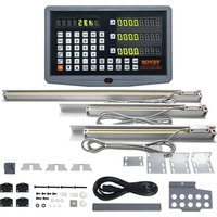
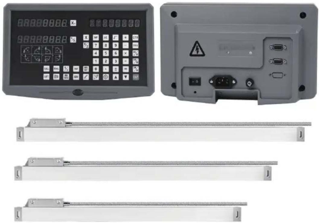
Product Type	Digital Readout (DRO) for machine tools
Brand	Vevor
Model	SNS-3V-YE161838
Power Supply Voltage	85-230 V AC, 50/60 Hz
Resolution	5 µm
Number of Axes	3 (X, Y, Z)
Measurement Range	X: 406 mm, Y: 457 mm, Z: 965 mm (16, 18, 38 inches)
Display	7-segment LED, adjustable brightness (levels 1-3)
Main Functions	Absolute/Incremental coordinates, zero setting, preset, reference search, power-off memory, standby mode, built-in calculator, tool library (200 sets), arc machining (simple and smooth), oblique machining, taper function, radius/diameter conversion, Y+Z addition, EDM function (optional)
Included Accessories	Support rod, knife holder plate, transparent housing, power cord, watch bracket, butterfly pieces, various screws (M4, M5, M8, M10), washers, rubber gaskets, U-shaped pads for scale
Maintenance and Cleaning	Wipe with a dry cloth. Avoid moisture and coolant splashes. Do not open or repair yourself.
Safety	Unplug immediately in case of smoke or abnormal odor. Do not use with linear scales of other brands without technical advice.
Spare parts and repairability	Repairs must be carried out by an authorized technician. Spare parts are available from the manufacturer or dealer.
General Information	Electronic warranty available at www.vevor.com/support. Complies with part 15 of FCC rules.

Frequently Asked Questions - SNS-3V-YE161838 Vevor

How to zero an axis?

In normal display mode, press the X_0 key for X axis, Y_0 for Y axis, Z_0 for Z axis. The display returns to 0.000.

How to switch to absolute (ABS) or incremental (INC) mode?

Press the ABS/INC key to toggle between modes. The active mode is indicated on the display.

How to adjust screen brightness?

Access the LUMI parameter in the configuration menu (press ▲/▼), then use X_0 to change the value (1 to 3, with 3 being the brightest). It is not recommended to change the default value.

What to do in case of power failure?

The DRO has a power-off memory that saves settings and reference values. After power is restored, the data is automatically restored.

How to use the tool library (200 sets)?

In ABS mode, press the ± key 10 times to open the library (TL OPEN). Use TOOL to enter data for each tool. To recall a tool, press CALL and enter the tool number.

How to machine an arc with the ARC function?

Press the ARC key to enter the menu. Select the arc type (simple or smooth), enter the radius (RAD), tool diameter (TLHIM), and feed step (MAX CUT). Move the axes until the display shows 0.000 for each point.

How to calibrate an oblique plane?

Access the OBLIQUE function. Select the plane (XY, XZ or YZ), enter the inclination angle, then move the table until the measuring tool touches the plane and the display returns to zero.

How to use the EDM function?

This function is optional (requires customization). In EDM mode, set the target depth and the fire cutting height. Move the electrode until it contacts the workpiece, zero it, then start machining. The display shows the depth and triggers automatic stop.

How to transfer the calculator result to an axis?

After a calculation, press X_0 to send the value to X axis, Y_0 to Y axis, Z_0 to Z axis. The value will appear on the corresponding axis display.

How to contact Vevor technical support?

Visit www.vevor.com/support for technical assistance, to download the full manual, or to access the electronic warranty certificate.

USER MANUAL SNS-3V-YE161838 Vevor

Technical Support and E-Warranty Certificate

www.vevor.com/support

DRO DISPLAY USER MANUAL

MODEL: SNS-3V-YE102024 / SNS-3V-YE161838

We continue to be committed to provide you tools with competitive price. "Save Half", "Half Price" or any other similar expressions used by us only represents an estimate of savings you might benefit from buying certain tools with us compared to the major top brands and does not necessarily mean to cover all categories of tools offered by us. You are kindly reminded to verify carefully when you are placing an order with us if you are actually saving half in comparison with the top major brands.

MODEL: SNS-3V-YE102024 / SNS-3V-YE161838

NEED HELP? CONTACT US!

Have product questions? Need technical support? Please feel free to contact us:

Technical Support and E-Warranty Certificate www.vevor.com/support

This is the original instruction, please read all manual instructions carefully before operating. VEVOR reserves a clear interpretation of our user manual. The appearance of the product shall be subject to the product you received. Please forgive us that we won't inform you again if there are any technology or software updates on our product.

Dear Users:

Thank you for purchasing multifunction series digital readouts. Digital readouts are used in a wide variety of application. These include machine tools, infeed axes, measuring and inspection equipment, EDM, dividing apparatuses, setting tools, and measuring stations for production control. In order to meet the requirements of these applications, many encoders can be connected to the digital readouts. Read all the instructions in the manual carefully before used and strictly follow them. Keep the manual for future references.

Safety attention:

To prevent electric shock or fire, moisture or directly sprayed cooling liquid must be avoid. In case of any smoke or peculiar smell from the digital readout, please unplug the power plug immediately, otherwise, fire or electric shock may be caused. In such a case, do not try to repair it, please contact the Company or distributors.

✗ Digital readout is a precise measuring device used with an optical Linear Scale. When it is in use, if the connection between the Linear Scale and the digital readout is broken or damaged externally, incorrect measuring values may be resulted. Therefore, the user should be careful.

Do not attempt to repair or modify the digital readout, as this may result in failure, malfunction, or injury. If any abnormal condition occurs, please contact the company or your distributor.

If the optical linear scale used with the digital readout is damaged, do not use a linear scale of another brand. The performance, specifications, and connections of products from different manufacturers may vary, and they cannot be connected without the guidance of specialized technical personnel. Otherwise, it may cause problems with the digital readout.

As products are continuously updated, if there are changes or modifications to the sample parameters, the documents provided with the product shall prevail. The company reserves the right of final interpretation without prior notice.

1. Illustration of Panel and Keyboard 4
2. Keyboard Description 5
3. Parameter Settings 7

3.1 Parameter Setup Routine Entry 7 3.2 Parameter Settings Description 7 3.2.1 Setting the Resolution 7 3.2.2 Setting Positive Direction for Counter 8 3.2.3 Toggle Between R/D Display Mode 8 3.2.4 Setting Z Axis Dial 8 3.2.5 Setting the Rotary Radius of the Workpiece 9 3.2.6 Setting the Angle Display Mode 9 3.2.7 Setting the Baud Rate of RS-232 (Optional) 9 3.2.8 Setting Absolute Zeroing Enable or Disable 10 3.2.9 Setting Absolute from Special Function 10 3.2.10 Setting Calculator Display Mode 10 3.2.11 Display Brightness Setting 10 3.2.12 Linear Scale Counting Frequency Setting 11 3.2.13 Setting QUIT 11 3.2.14 Setting the Type of the DRO 11 3.2.15 Signal Interface Type 11 3.2.16 Restore Factory Settings 12 3.2.17 Shrinkage Ratio Enable or Disable 12 3.2.18 Setting Compensation Type 12 3.2.19 Inch Display: Set the Number of Digits After the Decimal Point 13 3.2.20 Setting EDM (Optional) 13 3.2.21 Setting Linearity Compensation 13 3.2.22 Setting the Shrinkage Ratio 13

4. General Operations 14

4.1 Zeroing 14 4.2 Preset Data to Designated Axis 14 4.3 Toggle Display Unit Between Inch and mm 14 4.4 Absolute/Incremental/200 Groups SDM 15 4.5 1/2 Function 15 4.6 Clear All SDM Datum 16

4.7 Sleeping Mode 16 4.8 Power Interruption Memory 16 4.9 Search the Absolute Reference Point of Scale 17 4.10 Non-Linear Error Compensation 20

5. 200 Groups SDM Coordinate 21 5.1 Zeroing at the Current Point 21 5.2 Preset Datum of SDM Coordinate 22

6. Special Function 24

6.1 Circumference Holes Processing 25

6.2 Linear Holes Processing 28

6.3 ARC Processing 30

6.4 Oblique Processing 39

6.5 Slope Processing 43

6.6 Chamber Processing 44

6.7 The Tool Diameter Compensation Function 45

6.8 Digital Filter of the Grinding Machine 46

6.9 Lathe Function 47

6.9.1 200 sets TOOL Libs 47 6.9.2 Taper Function 48 6.9.3 R/D Function 49 6.9.4 Y + Z Function (only applicable to: 3 axes Lathe) 49

6.10 EDM 50

7. Calculator 56

8. Appendix 57

THREE AXIS PANEL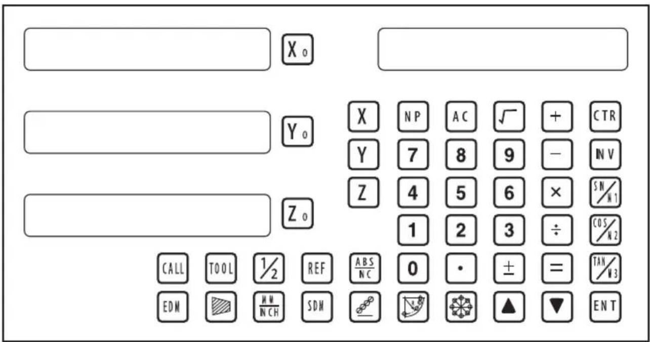

TWO AXIS PANEL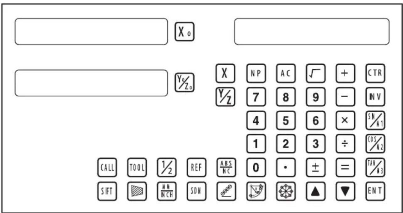

Keyboard Description

	Keys for axis selection
	Zero select axis
	Enter +/- sign
	Enter decimal point
	Entry keys for numbers
	Operation key (in Calculation function key)
	Enter or quit calculating state
	Cancel incorrect operation
	Calculate inverse trigonometric
	Square root
	Confirm operation
	Toggles between inch and millimeter units.
	Press when ready to identify a reference mark.
	Function keys for 200 sub datum
	ARC cutting function
	holes displayed equally on a circle
	holes displayed equally on a line
	Calculate trigonometric or Slope Processing function key
	Calculate trigonometric or rectangular inner chamber processing function key
	Calculate trigonometric or the tool diameter compensation function key
	Toggle between ABS/INC coordinate
	Stroll up or down to select
	Taper measured function key
	Tool library call key
	Opens the tool table.( lathe)
	EDM function key
	Filter display function key
	Half a display value of an axis
	Non Linear Error Compensation function keys

3. Parameters settings

3.1 Parameters setup routine entrance.

Press ☐ to enter the initial system and self-check after the DRO powers on in 1 second. Then, parameter settings are displayed in the Parameters window. Press ▲ ▼ to select the item you want to change.

If you want to quit the initial setting, press ▲ ▼ until “QUIT” appears in the message window and press ENT. You can also press • to quit the initial setting.

3.2 Parameters Settings Description

3.2.1 Setting the Resolution

Press ▲ ▼ until “RESOLUTE” appears in the message window.

When selecting the LINEAR encoder, the resolution will be set as follows:

There are 19 types of resolution:

0.01um; 0.02um; 0.05um; 0.10um; 0.20um; 0.25um; 0.50um; 1.00um; 2.00um; 2.50um; 5.00um; 10.00um; 20.00um; 25.00um; 50.00um; 100.00um; 200.00um; 250.00um; 500.00um.

Press ₀ to change the resolution for the X axis; Press ₀ to change the resolution for the Y axis; Press ₀ to change the resolution for the Z axis.

Set the resolution 5.00um to 1.00um for the X axis:

When selecting the rotary encoder, the resolution will be set as follows:

Input the rotary encoder parameter value.

3.2.2 Setting Positive Direction for Counter

Press ▲ ▼ until “DIRECTE” appears in the message window.

Direction ‘0’ means the display value will increase when the scale moves from right to left and decrease when the scale moves from left to right. Direction ‘1’ means the display value will increase when the scale moves from left to right and decrease when the scale moves from right to left.

Press \(\boxed{X_{0}}\) to change the Direction for X axis; Press \(\boxed{Y_{0}}\) to change the Direction for Y axis; Press \(\boxed{Z_{0}}\) to change the Direction for Z axis; as follow:

3.2.3 Toggle Between R/D Display Mode

Press ▲ ▼ until “R OR D” appears in message window. X window, Y window, Z window displays ‘0’ or ‘1’ separately.

‘0’ is mode R, which means the display value equals the actual measurement. ‘1’ is mode D where the display value equals the double actual measurement. Press \(X_{0}\) to change the R/D for X axis; Press \(Y_{0}\) to change the R/D for Y axis; Press \(Z_{0}\) to change the R/D for Z axis; as follow:

3.2.4 Setting Z axis Dial

Press ▲ ▼ until "Z DIAL" appears in message window.

Z axis dial should be set if Z axis is emulated for 2 axis milling and only install linear scale for X,Y axis. Z axis dial means the distance the Z axis travels when screw runs a revolution.

Set the Z axis Dial 2.5mm as follow;

3.2.5 Setting the Rotary Radius of the Workpiece

Press ▲ ▼ until "RDIUS" appears in message window.

The Rotary radius type is used perimeter to measure angle.

Input the Rotary Radius parameter value 2000mm as follow:

3.2.6 Setting the Angle Display Mode

Press ▲ ▼ until "ANG DISP" appears in message window.

Press \(\boxed{X_{0}}\) to change the angle display mode for X axis; Press \(\boxed{Y_{0}}\) to change the angle display mode for Y axis; Press \(\boxed{Z_{0}}\) to change the angle display mode for Z axis; Example for X axis:

"0.0000" means the angle mode is Circulating DD;

"0000.0000" means the angle mode is Incremental DD;

"0.00.00" means the angle mode is Circulating DMS;

"0000.00.00" means the angle mode is Incremental DMS;

3.2.7 Setting the Baudrate of RS_232 (Special customization function, if you need to buy, please contact the dealer to customize)

Press ▲ ▼ until “BAUDRATE” appears in message window. Set the Baudrate 115200 as follow ;

3.2.8 Setting the Absolute Zeroing enable or disable

Press ▲ ▼ until "ABS_ZERO" appears in the message window.

‘0’ means operation the ABS zeroing and preset data will be enable in the normal display state.

‘1’ means operation the ABS zeroing and preset data will be disable in the normal display state.

Press ₀ to change the absolute zeroing mode for X axis; Press ₀ to change the absolute zeroing mode for Y axis; Press ₀ to change the absolute zeroing mode for Z axis; Example for X axis.

3.2.9 Setting the Absolute form the Special Function

Press ▲ ▼ until "ABS_ASST" appears in message window.

‘0’ means only special function position value is display in the Special Function operation.

‘1’ means special function position value + ABS position value is display in the Special Function operation.

Press X₀ to change the absolute mode for the Special Function will be set as follows:

3.2.10 Setting the Calculator Display Mode

Press ▲ ▼ until "CTR_MODE" appears in the message window.

'0' means the calculator display value at the X window in the display; '1' means the calculator display value at the message window in the display; Press ₀ to change the calculator display mode will be set as follows:

3.2.11 Display Brightness Setting

LED display brightness setting, the factory default setting is only "3", the higher the parameter, the brighter the brightness. Press "X0" to set, it is not recommended that you set the default value yourself.

3.2.12 The Linear Scale Counting Frequency Setting

The factory default setting is only "12", the higher the parameter, the lower the counting frequency, press "X0" to set, it is not recommended that you set the default value yourself.

3.2.13 Setting QUIT: Digital display table parameters quit button. 3.2.14 Setting the type of the DRO.

The type of the DRO will be displayed on the right window. Then press the key ENT to select the correct type. The following system items will be set:

"MILL-3" means the DRO type is 3-axis milling machine table;

"MILL-2" means the DRO type is 2-axis milling machine table;

"LATHE-2" means the DRO type is 2-axis lathe table;

"LATHE-3" means the DRO type is 3-axis lathe table;

"GRIND" means the DRO type is Grind table;

"EDM" means the DRO type is EDM table; (Special customization

function, if you need to buy, please contact the dealer to customize)

3.2.15 Signal Interface Type

Message window displays “SEL AXIS” which indicates the step is to Sensor input signal mode. Press X₀ to change the signal mode for X axis; Press Y₀ to change the signal mode for Y axis; Press Z₀ to change the signal mode for Z axis; Example for X axis:

Press X₀ to scroll through the Rotary encode type, the Linear encode type, the Rotary radius type.

X window displays the Signal type.

“LInER” means the Signal type is linear encode type;

"EnCOdE" means the Signal type is Rotary encode type;

"RdIUS" means the Signal type is Rotary radius type;

Example: currently in the linear encode type, to toggle to the Rotary encode type;

3.2.16 Restore Factory Settings:

Clear all data except DRO type. DRO will load default setup for parameter. After loading default setup, user must search RI once to enable resuming ABS datum function; otherwise to resume the datum by RI is unable;

Message window displays “ALL CLR”, press ENT and message windows display “PASSWORD” indicating the operator to input password; Press 2000 + ENT in turn to load default value;

3.2.17 Shrinkage Ratio enable or disable.

Message window displays “SRK OFF” to disable Shrinkage rate function. Press ☐ to enable Shrinkage rate function in Message window displays “SRK ON”:

3.2.18 Setting Compensation Type

The message window displays “SEL COMP”, indicating this step is for compensation type. Press X₀ to change the compensation type for the X axis; press Y₀ to change the compensation type for the Y axis; press Z₀ to change the compensation type for the Z axis. Example for X axis:

Press X₀ to scroll through the compensation types: no compensation, linear compensation, and non-linear compensation.

“no-CO” means the compensation type is no compensation; “LInE-CO” means the compensation type is linear compensation; “non-LinE” means the compensation type is non-linear compensation.

Example for X axis: currently in the no compensation type, to toggle to the linear compensation type.

3.2.19 Inch Display: Set the Number of Digits After the Decimal Point

In inch display mode, the number of digits after the decimal point is set. The factory default is "4". Press "X0" to set it according to actual needs.

3.2.20 Setting EDM: It is not recommended to change the default value yourself. This function sets the relay off time.

3.2.21 Setting Linearity Compensation.

The message window displays “LIN COMP”, indicating this step is for linearity compensation. Compensate the linear error to make the display value equal to the standard value.

The calculation of the compensation rectifying coefficient:

Coefficient = (Measurement - Standard value) x 1000.000 / Standard value

Example for X axis:

Measurement: 200.020 mm

Standard value: 200.000 mm

Rectifying coefficient = (200.020 - 200) * 1000 / 200 = -0.01 mm/m

Input the compensation rectifying coefficient 0.01 as follows:

3.2.22 Setting the Shrinkage Ratio

Press ▲ ▼ until "SHRINK" appears in the message window.

Shrinkage ratio = (Dimensions of the finished product) / (Dimensions of the working piece)

Set the shrinkage ratio to 1.005 as follows:

4. General Operations

4.1 Zeroing

Zero the designated axis in the normal display state. Zeroing is used to set the current point as the datum point as follows:

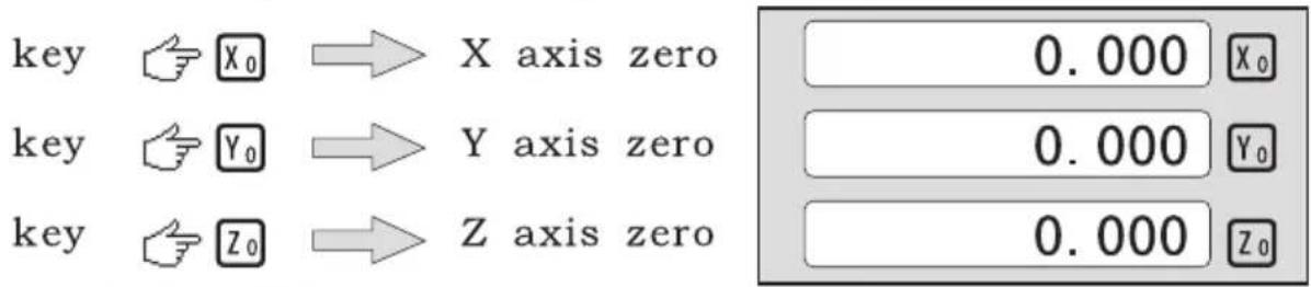
X0, Y0, or Z0 will be returned to the original data before the reset.

4.2 Preset Data to Designated Axis

Preset a value to the current position for a designated axis in the normal display state.

4.3 Toggle Display Unit between inch and mm

Length can be displayed either in "mm" (metric) or "inch" (imperial). The display unit can be toggled between mm and inch.

Example: Display value toggled from mm to inch.

Example: Display value toggle from inch to mm;

4.4 Absolute/Incremental/200 groups SDM

Function: The DRO has 3 coordinate display modes: the absolute mode (ABS); the incremental mode (INC) and 200 groups Second Data Memory (SDM) with the range of 00 to 99. Zero point of work-piece is set at the origin point of ABS coordinate. The relative distance between datum of ABS and SDM remains unchanged when ABS datum is changed.

1. Toggle from ABS to INC coordinate;

1. Toggle from INC to ABS coordinate;

1. Toggle from SDM to ABS coordinate;

4.5 1/2 Function

Function: Set the center of work piece as datum by halving the displayed value.

Example: Set the center of rectangle as datum as the right figure.

Steps:

1. Touch one side of the workpiece with the TOOL, then zero the X axis.

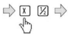
2. Take the TOOL to the opposite side of the workpiece and touch it. Then press + 1/2 in turn to value the X axis display value.

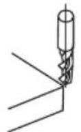
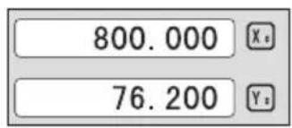
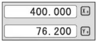
3. Move the machining table until "0.000" is displayed in X axis window. The position is the work-piece's center.

4.6 Clear All SDM datum.

In ABS mode, to continuously press ten times will cause to clear all the datum for 200 sets SDM. Message window displays "SDM CLR".

4.7 Sleeping Mode

In non-ABS mode, pressing the REF key can turn off all displays and the DRO enters Sleeping Mode. Pressing this key again will cause the DRO to return to working mode. In Sleeping Mode, the DRO is still in working state and actually records the tool movement.

Example: In non-ABS mode, press the REF key to access Sleeping Mode. In Sleeping Mode, press the REF key to quit Sleeping Mode.

4.8 Power Interruption Memory

The memory is used to store the settings of the DRO and machine reference values when power is turned off.

4.9 Search the Absolute Reference Point of Scale

During daily machining, it is very common that machining cannot be completed within one work shift, and hence the DRO has to be switched off after work, or power failure happens during machining, leading to loss of the workpiece datum (workpiece zero position). Re-establishing the workpiece datum using an edge finder or other method inevitably induces higher machining inaccuracy because it is not possible to re-establish the workpiece datum exactly at the previous position. To allow recovery of the workpiece datum very accurately without needing to re-establish it using an edge finder or other methods, every linear scale has a reference point location equipped with a reference position to provide datum point memory function.

The working principle of the reference datum memory function is as follows:

Since the reference point of the linear scale is permanent and fixed, it will never change or disappear when the DRO system is switched off. Therefore, we simply need to store the distance between the reference point and the workpiece datum (zero position) in non-volatile memory. Then, in case of power failure or the DRO being switched off, we can recover the workpiece datum (zero position) by presetting the display zero position as the stored distance from the reference point.

An absolute datum should be set when a workpiece is machined. There are three modes of operation (REF, AB, LEF_AB):

Example: to store the X axis work datum.

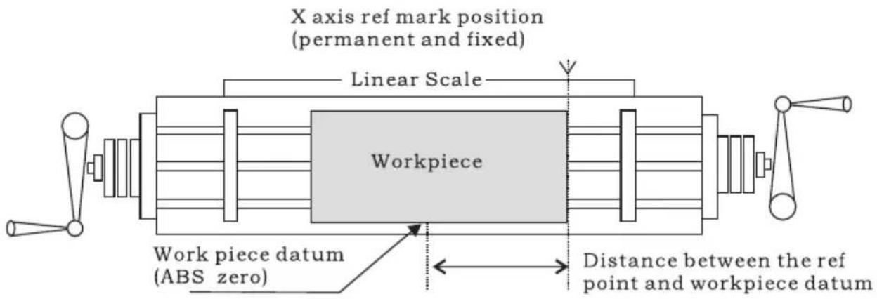
Example for REF mode:

1. DRO is set in ABS coordinate. Press REF, then the message window displays "REF".

2. Message window displays "REF". Press ENT until "FD_REF" appears in message window.

3. Select the axis which needs to search RI. For instance: select X axis, then press ☒. "X_REF" is displayed in message window, and X axis window flashes.

4. Move the machine table. The buzzer sounds when RI is searched, then the X window stops flashing and displays the value of the current position. The DRO returns to normal display state. Then the message window displays "FIND_X".

Example for AB mode:

1. DRO is set in ABS coordinate. Press REF, then the message window displays "REF".

2. Press ▲ ▼, then the message window displays "AB".

3. Message window displays "AB", press ENT until "FIND_AB" appears in the message window.

4. Select the axis which needs to search RI. For instance: select X axis, then press ☒. "X_REF" is displayed in the message window, and the X axis window flashes.

4. Select the axis which needs a reference index (RI) search. For instance: select the X axis, then press ☒. “X_REF” is displayed in the message window, and the X axis window flashes.

5. Move the machine table. The buzzer sounds when RI is searched, displaying the value of the current position for the absolute datum zero. The DRO returns to normal display state. Then the message window displays "FIND_AB".

1. DRO is set in ABS coordinate. Press REF, then the message window displays "REF".

2. Press ▲ ▼, then the message window displays "AB".

3. Message window displays "LEF_AB", press ENT until "ZERO_AB" appears in the message window.

3. The message window displays “LEF_AB”. Press ENT until “ZERO_AB” appears in the message window.

4. Move the machine table to the set zero position point. Then press X, and the X axis will zero. The current position becomes the absolute datum zero. The DRO returns to the normal display state.

NOTE: Linear range without reference point location of the user

4.10 Non Linear Error Compensation

First compensation Type (Linear or Non-Linear) in parameter setting must be set to Non-Linear. Linear scale have a ref point location and find to the Absolute Reference Point will be enable.

Default Non-Linear compensation: 50.

Example for Y axis:

Step 1: Search the Absolute Reference Point of Scale;

Step 2: Press NP, then the message window displays "COMP X".

Step 3: Press ▲ ▼, then the message window displays "COMP Y".

Step 4: Press ☐ENT, then the message window displays "NUMBER". Then input the compensation parameter NUMBER.

Step 5: Press ▲ ▼, then message window displays "Y-MSN-1" which indicates the step is to Non Linear Error Compensation.

Step 6: Input compensation value.

X window displays the value of the measurement value.

Y window displays the value of the standard value.

Example for the first compensation point:

Measurement value: 68.288mm. Standard value: 68.200mm

Step 7: After input all parameters, the DRO automatically exits.

5. 200 Groups SDM coordinate

The DRO has three display modes: the absolute mode (ABS), the incremental mode (INC), and the 200-group second data memory (SDM 1 - SDM200). The ABS datum of the workpiece is set at the beginning, and the 200-group SDM is set relative to the ABS coordinate.

ABS Mode, INC Mode, and SDM Mode are specially designed to provide much more convenience features to the operator to cope with batch machining of relative works and the machining of workpiece dimensions from more than one datum.

Example: The ABS datum is the center point O, and the points sdm1, sdm2, sdm3, sdm4 needed for processing are set as the datums of SDM 1 - SDM 4.

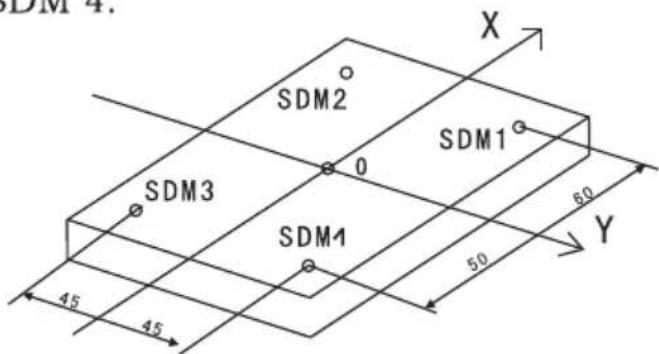
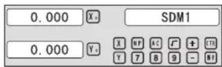
Two ways to set SDM coordinate:

1. Zeroing at the current point. 2. Presetting the datum of the SDM coordinate.

5.1 Zeroing at the Current Point

First, set the center point of the workpiece as the origin of the ABS. Then align the tool with points SDM1, SDM2, SDM3, SDM4 by moving the machine table and zero them. It is the position to process where the “0.000” appears in the X window and Y window by moving the machine table, whether in ABS or in SDM coordinate.

Steps:

1. Move the worktable to place the tool at the center of the workpiece point O as the datum of ABS. Then zero the X axis and Y axis in SDM 1; zero the X axis and Y axis in SDM 2; zero the X axis and Y axis in SDM 3; zero the X axis and Y axis in SDM 4.

2. Set point sdm1 as the datum of SDM 1. Move the machine worktable to x = 60.000, y = 45.000. Then process [X0] [Y0].

2. Set point sdm1 as the datum of SDM 2. Move the machine worktable to x = 60.000, y = -45.000. Then process [X0] [Y0].

3. Set point sdm1 as the datum of SDM 3. Move the machine worktable to x = -60.000, y = -45.000. Then process [X0] [Y0].

4. Set point sdm1 as the datum of SDM 4. Move the machine worktable to x = -60.000, y = 45.000. Then process [X0] [Y0].

5.2 Preset Datum of SDM Coordinate

There are the same examples as in Method 1. First, move the worktable to place the tool exactly at the origin of ABS. Secondly, enter the ABS Mode as follows.

Steps:

1. Move the worktable to place the TOOL at the center of the workpiece point O as the datum of ABS. Then zero the X axis and Y axis in SDM 1; zero the X axis and Y axis in SDM 2; zero the X axis and Y axis in SDM 3; zero the X axis and Y axis in SDM 4.

2. Set point SDM1 as the datum of SDM 1. Press ▲ ▼, then the message window displays “SDM 1”. Input x = 60.000, y = 45.000.

3. Set point SDM1 as the datum of SDM 2. Press ▲ ▼, then the message window displays “SDM 2”. Input x = -60.000, y = 45.000.

4. Set point SDM1 as the datum of SDM 3. Press ▲ ▼, then the message window displays “SDM 3”. Input x = -60.000, y = -45.000.

5. Set point SDM1 as the datum of SDM 4. Press ▲ ▼, then the message window displays “SDM 4”. Input x = -60.000, y = 45.000.

6. Special Function

6.1 Circumference Holes Processing

The Function of PCD Hole positioning on Circumference is used to distribute arc equally, such as boring hole on flange. The right window will show the parameter to be defined when selecting PCD Function.

The Parameters to be defined are:

PCD_XY(XZ,YZ)

Select place

CENTER

Center position

DIA

Diameter of circle

NO_HOLE

Hole number

STANG

Starting angle

ED ANG

Ending angle

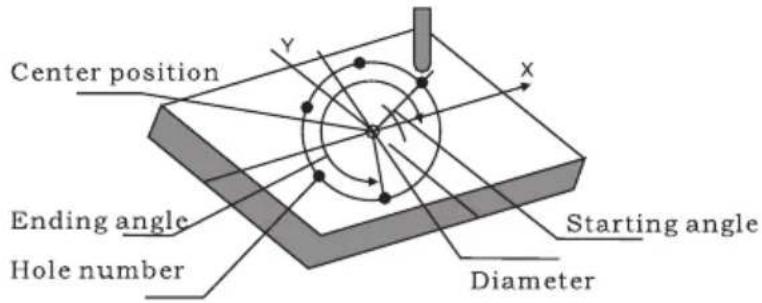
The position of the hole center is calculated automatically after inputting all parameters. Press ▲ or ▼ to choose the hole number and move the machine table until "0.000" appears in the X, Y, and Z windows. This is the position to process the hole.

Example for the XY plane: Machine holes on a circumference as shown in the figure.

PCD_XY(XZ,YZ)	XY
CENTER	X=0,000,Y=0.000
DIA	100,000
NO_HOLE	5
ST ANG	30,000
ED ANG	315,000

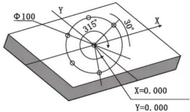
Steps:

1. Set the display unit to metric in normal state; move the machine table until the machine tool is aligned with the center of the circle, then zero the X and Y axes.
2. Select the piece.

Press 🧑️, then the message window displays "PCD_XY" for Circumference Holes Processing. Press ▲ or ▼ to select the XY plane.

1. Input the center position.

Press ENT, then the message window displays "CENTER". The X and Y windows display the previously set center position. Input X = 0, Y = 0 as follows.

1. Input diameter.

Press ▼ until “DIA” appears in the message window. The X window displays the formerly preset diameter. Then input the diameter as 100.000.

1. Input number.

Press ▼ until "NO_HOLE" appears in the message window. The X window displays the formerly preset number. Then press 5 in turn to input the number.

1. Input starting angle.

Press ▼ until “ST ANG” appears in the message window. The X window displays the formerly preset starting angle. Then press 3 0 in turn to input the starting angle.

1. Input ending angle.

Press ▼ until “ED ANG” appears in the message window. The X window displays the formerly preset ending angle. Then press 3 1 5 in turn to input the ending angle.

1. Press ▼ until "NO 1" appears in the message window.

This is the position of the first hole to punch, where “0.000” is displayed in the X window and Y window by moving the machine table. After finishing the first hole, press ▼ or ▲ to change the hole number.

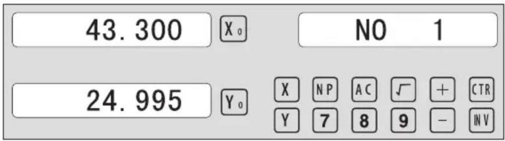
1. After processing all holes, press 📋 to return to normal display.

6.2 Linear Holes Processing

There are two modes to carry out the linear drilling: Length mode and Step mode.

1.LINE S	Step mode
LINE L	Length mode
2.STEP	Step length
LENGTH	Line length
3.ANG	Angle
4.NO.HOLE	Hole number

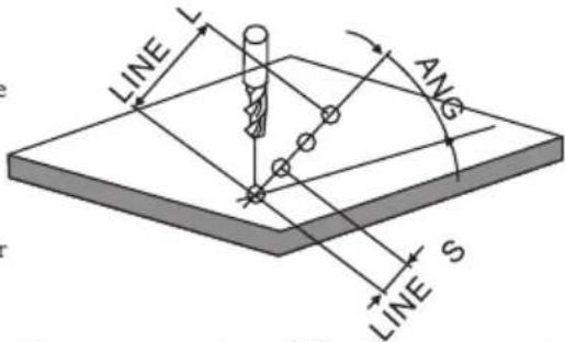
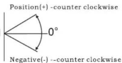
The Linear Holes function can simplify the processing of multiple holes whose centers are equally spaced on one line.

Example:

LINE_L	Length mode
LENGTH	60.000
ANG	30.000
NO.HOLE	4

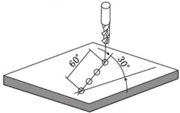
Steps:

1. Select the piece.

Press 📄, then the message window displays "LINE_XY" for Linear Holes Processing. Press ▲ or ▼ to select the XY position.

2. Select Linear Holes mode.

Press ENT, then the message window displays "LINE_S". Press ▲ or ▼ to select "LINE_L".

3. Input linear length.

Press ENT, then the message window displays "LENGTH".

The X window displays the previously preset linear length. Press 6 then 0 to input the linear length.

1. Input angle.

The message window displays "ANG", indicating the step is for angle. The X window displays the previously preset angle. Press 3 then 0 to input the angle.

1. Input number.

The message window displays "NUM", indicating the step is for number. The X window displays the previously preset number. Press 4 to input the number.

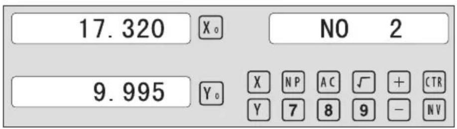
1. Press ▼ until "NO 1" appears in the message window.

This is the position of the first hole to punch, where "0.000" is displayed in the X and Y windows by moving the machine table. After finishing the first hole, press ▲ or ▼ to change the hole number.

1. After processing all holes, press ☐ to return to normal display.

6.3 ARC Processing

Two functions are available for the ARC function: the simple ARC Function and the smooth R function. Press ☑ to enter ARC function, then press ▲ or ▼ for selecting smooth ARC function or Simple ARC Function.

During installation, normally the coordinate of the machine and the direction of X, Y, Z are as per follow. The work plane is shown as the right figure.

(RAD+TL)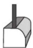

(RAD+TL)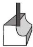

Z(+positive direction)

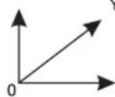
Y(+positive direction)

X(+positive direction)

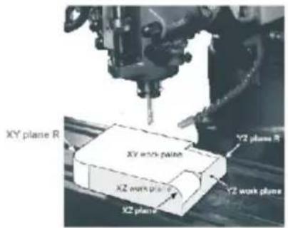
Simple ARC Function:

When the smoothness is not highly demanded, the SIMPLE ARC function is normally used for machining arc. In the SIMPLE function there are only eight type of ARC used to machine. The operator just select the type of R and input the parameters of the radius of Arc, MAX CUT and outer arc or inner arc. In general, an arc may be machined by a planar slot TOOL or arc TOOL, the different between them in different work plane as shown as per follows.

1、SIMPLE Simple processing

2、TYPE 1-8 Mode of the ARC.

3、SEL_XY(XZ,YZ) Select place

4、RAD Arc radius

5、TL DIA Tool diameter

1. MAX CUT Feed step

7. RAD_TL Outer arc and inner arc (only for XY place)

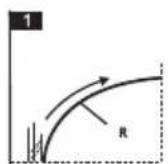
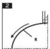
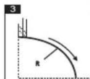
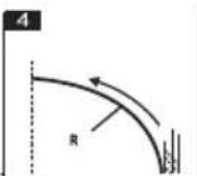
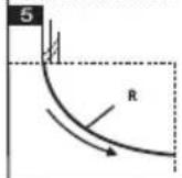
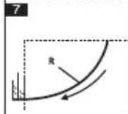
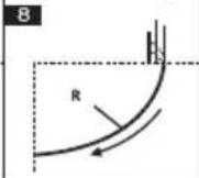
Smooth ARC function:

Provides maximum flexibility in ARC machining, the ARC sector to be machined by the coordinates of ARC. Very flexible, ARC function can machine virtually all kinds of ARC, even the intersected ARC.

Relatively a bit complicated to operate, operator need to calculate and enter the coordinates of ARC centre, start angle and end angle.

Basic parameters as follow:

1. SMOOTH Mode of the Smooth ARC processing;
2. SEL_XY(YZ, XZ) Select place;
3. CENTER Refer to the position of a center.
4. RAD Radius of the ARC
5. TL_DIA Diameter of the TOOL
6. MAX_CUT Feed step
7. ST_ANG Starting angle
8. ED_ANG Ending angle
9. RAD+TL Outer arc. RAD-TL Inner arc.

Example 1 for the Simple ARC Processing:

Parameter settings are as follows:

SIMPLE Simple mode

TYPE 3

SEL_XY XY

RAD 80.000

TL_DIA 6.000

MAX_CUT 0.500

RAD+TL 1

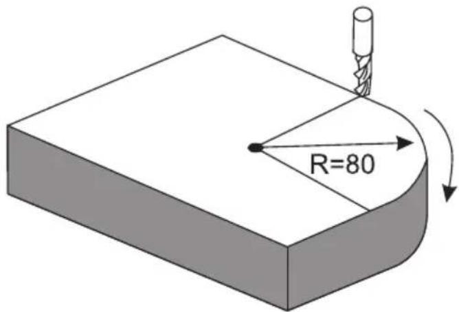
Steps:

1. Select process mode

Press 📋, then the message window displays "SIMPLE" for the ARC Processing. Press ▲ or ▼ to select the simple mode. The message window displays "SIMPLE".

ARC Processing. Press ▲ or ▼ to select the simple mode. The message window displays “SIMPLE”.

Press ☐ENT until "TYPE" appears in the message window. The X-window displays the previously preset type. Press ☐3 in turn.

Press ☐ENT until "TYPE" appears in the message window. The window displays the previously preset type. Press ☐3 in turn

3. Select place

Press ENT until "SEL_XY" appears in the message window. Press ▲ or ▼ to select the place to display "SEL_XY";

4. Input radius:

Press ENT until "RAD" appears in the message window. The X window displays the formerly preset radius of the ARC. Press 8

0 in turn to input the radius.;

5. Input Diameter of the TOOL

Press ▲ or ▼ until "TL DIA" appears in the message window. The X window displays the formerly preset Diameter of the TOOL. Press 6 in turn to input the Diameter value;

6. Input Feed step (MAX_CUT);

Press ▲ or ▼ until "MAX_CUT" appears in the message window. The X window displays the formerly preset MAX_CUT. Press 0 · 5 in turn to input the MAX_CUT value;

1. Select outer arc or inner arc

Press ▲ or ▼ until "RAD-TL" appears in the message window. Press ▲ or ▼ to select the place to display "RAD+TL";

1. After inputting all parameters, press the key ENT for machining.

The DRO will display the position of the first point. Retract the axes until the displays read 0.000. Machine the Arc point by point in accordance with the display. After finishing the position of the first point, press ▲ or ▼ to change position point.

Press ☐ to quit R function at any time.

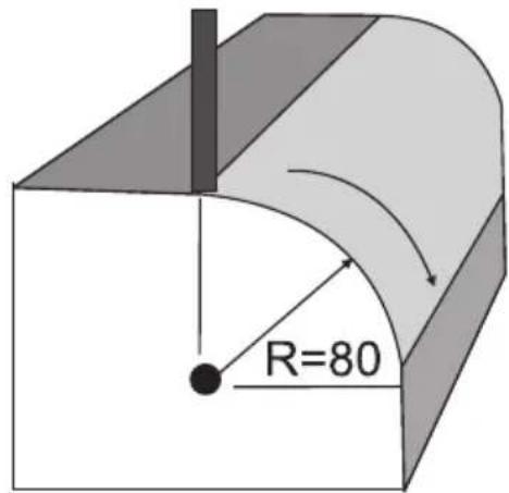
Example 2 for the Simple ARC Processing:

Parameters settings as follow:

SIMPLE Simple mode

TYPE 3

SEL_XY XZ

RAD 80.000

TL_DIA 6.000

MAX_CUT 0.500

Steps:

1. Press ☐, then the message window displays "SIMPLE" for the ARC Processing. Press ▲ or ▼ to select the mode of the simple, the message window displays "SIMPLE"

2. Input the type:

Press ☐ENT until "TYPE" appears in the message window. X-window displays the formerly preset type. Press ☐3 in turn

3. Select place

Press ENT until "SEL_XZ" appears in the message window. Press ▲ or ▼ to select place to display "SEL_XZ";

4. Input radius:

Press ENT until "RAD" appears in the message window. X window displays the formerly preset radius of ARC. Press 8

0 in turn to input the radius.;

5. Input Diameter of the TOOL

Press ▲ or ▼ until “TL DIA” appears in the message window. The X window displays the formerly preset Diameter of the TOOL. Press 6 in turn to input the Diameter value;

6. Input Feed step (MAX_CUT);

Press ▲ or ▼ until "MAX_CUT" appears in the message window. The X window displays the formerly preset MAX_CUT. Press 0 · 5 in turn to input the MAX_CUT value;

1. After inputting all parameters, press the key ENT for machining.

For 2-axis milling machine table, it is not installed with Z-axis, please press ▲ or ▼ to simulate position of Z-axis. Press ▲ to simulate moving to the former process, and press ▼ to simulate moving to the next process point.

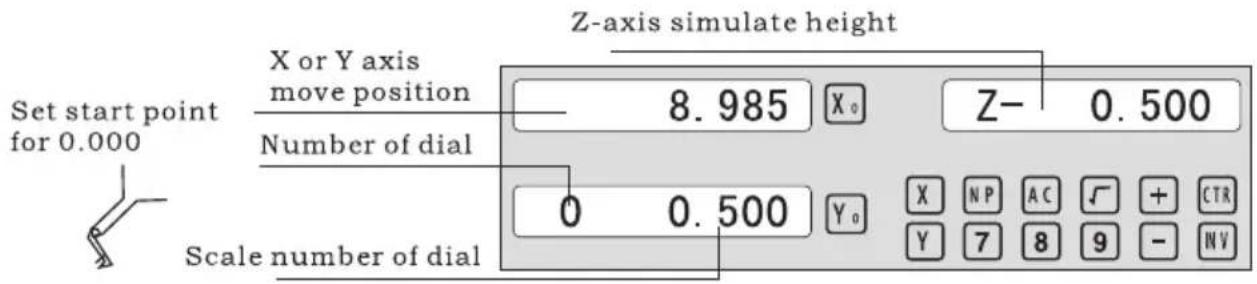
Z-axis simulate height = Number of dial x Z axis Dial + Scale number of dial

Press ☐ to quit R function any time.

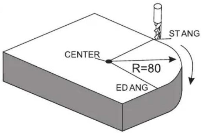
Example 3 for the Smooth ARC function:

Parameters settings as follow:

SMOOTH	Smooth mode
SEL_XY(YZ,XZ)	XY
CENTER	X=0,Y=0
RAD	80.000
TL_DIA	6.000
MAX_CUT	0.500
ST_ANG	0.000
ED_ANG	135.000
RAD+TL	1

Steps:

1. Press 📋, then the message window displays “SIMPLE” for the ARC Processing. Press ▲ or ▼ to select mode of the simple, The

message window displays "SMOOTH"; For 3-axis milling machine table without this step. In second step. Then press ENT.

2. Select place

The message window displays "SEL_XY", which indicates that the select is to be placed. Press ▲ or ▼ to select the place to display "SEL_XY";

3. Input center position.

Press ☐ENT, then the message window displays "CENTER". The X and Y windows display the formerly preset center position. Input X = 0, Y = 0 as follows.

4. Input radius:

Press ENT until "RAD" appears in the message window. The X window displays the formerly preset radius of the ARC. Press 8 0 in turn to input the radius.

5. Input diameter of the tool.

Press ▲ or ▼ until "TL DIA" appears in the message window. The X window displays the formerly preset diameter of the tool. Press 6 in turn to input the diameter value.

1. Input feed step (MAX_CUT).

Press ▲ or ▼ until "MAX_CUT" appears in the message window. The X window displays the formerly preset MAX_CUT. Press

0 · 5 in turn to input the MAX_CUT value.

1. Input starting angle.

Press ▼ until "ST ANG" appears in the message window. The X window displays the formerly preset starting angle. Then press 0 in turn to input the starting angle.

1. Input ending angle.

Press ▼ until "ED ANG" appears in the message window. The X window displays the formerly preset ending angle. Then press 1 3 5 in turn to input the ending angle.

1. Select outer arc or inner arc.

Press ▲ or ▼ until “RAD-TL” appears in the message window. Press ▲ or ▼ to select the place to display “RAD+TL”;

1. After inputting all parameters, machining.

The DRO will display the position of the first point. Retract the axes until the displays read 0.000. Machine the arc point by point in accordance with the display. After finishing the position of the first point, press ▲ or ▼ to change position point.

Press ☐ to quit the ARC function at any time.

6.4 Oblique Processing

There are 2 ways available for machining oblique places:

a). on the place. b). on the place YZ, or XZ;

Only the following parameters need to be inputted:

INCL_XY(XZ,YZ) Set machine place XY, YZ, or XZ place.

ANG The inclination angle of the oblique.

DIA The tool diameter.

ST_POT Starting position;

ED_POT Ending position;

Example 1 for the Oblique XY place:

When the machining plane is on plane XY as the part shown in the figure, the angle of obliquity of the workpiece should be calibrated before the oblique plane is machined. Therefore, at this point the machining of the oblique plane plays the role of calibrating the obliquity.

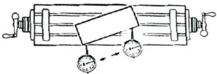
Procedure for calibrating the obliquity

First place the workpiece on the worktable as per the required angle of obliquity.

1) Enter the function of oblique plane.

2) Select the function of plane X Y.

3) Input the angle of obliquity.

4) Move the worktable until the measuring tool (such as a dial gauge) installed on the milling machine touches the obliquity-calibrating plane, adjust it to zero, and move the worktable for any distance in the direction of X-axis.

5) Move the worktable in the distance of Y-Axis until the display turns to zero.

6) Change the angle of the work piece to make the workpiece touch the measuring tool and adjust it to zero.

STEPS:

1. Select place

Press ⚪, then the message window displays “INCL_XY” for the Oblique Processing. Press ▲ or ▼ to select place to display “SEL_XY;

Then press ☐ENT to proceed to the next step;

2. Input the angle of obliquity

The message window displays “ANG”, X window displays the formerly preset angle of obliquity. Press 4 5 in turn to input the angle of obliquity.

1. Move the workpiece along the X-Axis until the measuring tool touches the workpiece, adjust it to zero, and move the worktable for any distance along the X-Axis.

1. Press ☐, display the value of Y-Axis. Move the workpiece along the Y-Axis, change the angle of workpiece to make the obliquity-calibrating plane touch the measuring tool until it turns to zero. Move the worktable until Y-Axis is displayed as zero.

1. Press 5N/_N1 to quit oblique function any time.

Example 2 for the oblique XZ or YZ place:

When the machining plane is on plane XZ or YZ, the function of TOOL inclination can instruct the operator to machine the oblique plane step by step.

Procedures for using the function of cutter inclination:

When the machining plane is on plane XZ or YZ, first please calibrate the obliquity of the primary spindle nose and set the TOOL:

INCL_XY(XZ,YZ)	INCL_XZ
DIA	10.000
ST_POT	20.000
ED_POT	20.000

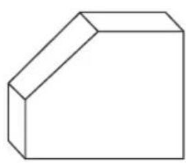
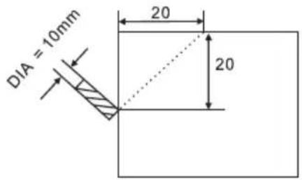
STEPS:

1. Press SNV, then the message window display "INCL_XY" to the oblique Processing. Press ▲ or ▼ to select place to display "SEL_XZ; Then press ENT to in next step;

1. Input The TOOL Diameter

The message window display “DIA”, X window displays the formerly preset the angle of obliquity. Press 10 in turn to input the TOOL Diameter of obliquity. OK, then press ▼ to in next step;

1. Input ST_POT;

The message window display “ST_POT”, X and Y window displays the formerly preset the stating position of obliquity. Input X=0, Y=-20.000. OK, then press ▼ to in next step;

4. Input ED_POT;

The message window display “ED_POT”, X and Y window displays the formerly preset the stating position of obliquity. Input X=20.000, Y=0.000.

5. After input all parameter, press the key ▼ for machining.

For 2-axis milling machine table, it is not installed with Z-axis, please press ▲ or ▼ to simulate position of Z-axis. Press ▲ to simulate moving to the former process, and press ▼ to simulate moving to the next process point.

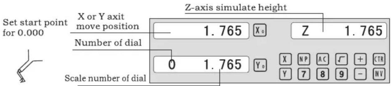
Z-axis simulate height = Number of dial x Z axis Dial + Scale number of dial

Press 5% to quit oblique function any time.

6.5 Slope Processing

This function can calculate the position of every processing point automatically in processing slope. Only the following parameters need to be inputted:

XZ, YZ

Set machine place YZ, or XZ

ANG

The inclination angle

Z_STEP

The slope length

each time processing

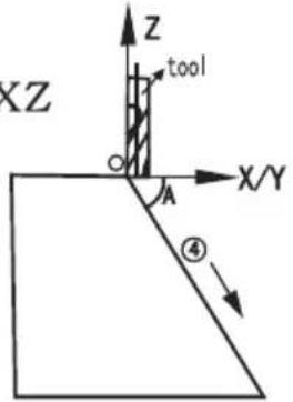
Example 1 for the Slope XZ place;

Step 1. Select place

Press [TAN/W3] , then the message window display "XZ" to the slope Processing. Press ▲ or ▼ to select place to display "SEL_XY; Then press [ENT] to in next step;

Step 2. Input the angle of slope

The message window displays “ANG”, and the X window displays the previously preset angle of slope. Press 4 and 5 in turn.

Step 3. Input Z_step;

The message window displays “Z STEP”, and the X window displays the previously preset starting position of the slope. Input 0.1 in turn.

Step 4: Finishing the ALL processing. Press ☐ to quit the slope function at any time.

6.6 Chambering Processing

1, FLAT_XY: machine position; 2, DIA: diameter of TOOL; 3, CENTER: center of the chambering; 4, SIZE: size of the chambering;

Figure as follows:

STEPS:

1. Press , then the message window displays “FLAT_XY” for the Chambering Processing.

1. Input DIA of the TOOL;

1. Input the center coordinate;

1. Input the size;

1. Process Chambering;

Move the machine until the display of the axis is zero, i.e., the position of the first point. Machine the first point. Display the next machining point by pressing ▲ or ▼. On completion of machining, the right window shows OVER. Press ▲ or ▼, the system will go to the first position for the next workpiece. Press ₂ to quit the Chambering Function.

6.7 The Tool Diameter Compensation Function

Without tool compensation, the operator has to move the tool an additional distance equal to the tool diameter along each side when machining the four 150 and 100 sides of a workpiece to finish machining the entire brim. The digital readouts shall automatically compensate when the tool compensation function is enabled.

Note: The tool compensation is made in the direction of the X and Y axes.

Procedures:

1). Enter the function of compensating the diameter of the tool. 2). Select one of the (four) preset machining modes. 3). Input the diameter of the tool. 4). Enter machining.

Figure A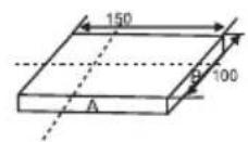

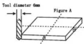
Figure B

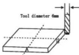
Figure C

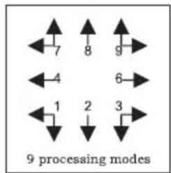
Step 1: Press ☐ to enter the tool compensation function. Then the message window displays "TYPE". Press ☐.

Step 2: Input the diameter of the tool; press 10 in turn.

Step 3: Press ▼ to select the machining mode.

Machining of two side planes can be done by moving the tool until the X-axis is 150.000 and the Y-axis is 100.000. Press the key ☐ to quit the function.

6.8 Digital Filter of the Grinding Machine

When machining a workpiece with a grinder, the display values change quickly due to the vibration of the grinder. The user cannot see the display value clearly. The grinder DRO provides a display value filter function to suppress the quaking changes of the display value.

STEPS:

1. Enter display value filter function.

In normal display state, press SFT to simultaneously enter display value filter function.

1. Exit display value filter function;

Press SIFT, exit display value filter function;

6.9 Lathe Function

6.9.1 200 sets TOOL Libs

It always needs different TOOL when processing different parts. For convenient operation, the Lathe digital readouts has the function of 200 sets TOOL Libs.

Note: Only when the lathe is equipped with the tool setting block, the 200 sets TOOL Libs can be used.

1. Set a datum TOOL. After tool setting, Zero X axis and Z axis, the set zero of absolute coordinate.
2. According to the size of TOOL1 and datumTOOL, determine the position of TOOL relative to zero of absolute coordinate and datum tool. As Figure 6-1. The relative size of TOOL 2 is as follows X axis 25-30=-5, Z axis 20-10=10.
3. Save the TOOL number and the size into digital readout.
4. The number of TOOL can be input at random, the digital readouts will display the position of tool to absolute coordinate zero. Move lathe until X axis and Z axis both display zero.
5. TOOL Libs can save 200 sets of tool data.
6. The TOOL Libs must be used in the opening state. The 200 sets TOOL Libs can be opened by continuously pressing ± ten times until the right window flashes TL - OPEN and a mark “/” displays at the left of the right information window. The mark indicates the operator can set up or revise the 200 sets TOOL Libs. Continuously pressing the key ± ten times will cause the 200 sets TOOL Libs to be closed and the right window flashes TL - CLOSE and the mark disappears. When the mark “/” disappears, the 200 sets TOOL Libs cannot be revised.

The operations for TOOL data and calling TOOL are shown as follows.

Step 1: In ABS state, input the data of the 200 sets TOOL Libs. To open the 200 sets TOOL Libs, continuously press the key ± ten times. A mark “Δ” will appear at the left of the right info window.

Step 2: Press TOOL to access the inputting state. Input TOOL 1 data:

Step 3: Input TOOL 2 data:

Step 4: Press to continue to input the data of the next tool. By pressing number and the key ENT, the operator can directly input the special tool data. Press TOOL to quit.

After TOOL libs are set up, use the TOOL libs according to the following operations: first mount the second tool.

Step 5: To access the using state, press CALL. Then press 2 ENT.

Step 6: Press ▲ or ▼. Select the base TOOL. Then press 1 ENT.

Step 7: Press CALL to quit the function.

Note:

When the base tool is used, the axis cannot be zeroed in ABS state. When the others are used, the axis can only be zeroed in INC state.

6.9.2 Taper Function

For lathing the workpiece with taper, the taper of the workpiece can be measured during processing.

Operations:

As shown in the figure, contact surface A of the workpiece with the lever readout and reset the lever readout to zero.

Step 1: Press 📋, then the message window displays “MEASU” for the paper processing. Move the lever readout to surface B until the lever readout points as follows.

Step 2: Press ☐ENT to calculate.

Step 3: Press ▶ to quit the function.

6.9.3 R/D Function

For 2-axis lathe and 3-axis lathe, press 1/2. The display mode of the X axis is switched between Radius and Diameter. When the X axis is displayed as Diameter, a mark “ ” will appear at the left of the right information window, but when the X axis is displayed as Radius, the mark “ ” disappears. Only the X axis has the diameter/radius transformation function.

6.9.4 Y + Z Function (only applicable to 3-axis lathe)

For 3-axis lathe, the counter of the Y axis and the counter of the Z axis can be added and displayed on the Z axis by pressing the key 🌐. Pressing the key again cancels the Y + Z function.

6.10 EDM (Special customization function; if you need to purchase, please contact the dealer to customize)

1. Description: This function is used for the special machining of Electro Discharge Machining (EDM). When the set target value of the EDM Z-axis equals the present value, the digital readout will output a switch signal to control the EDM to stop the depth machining.

The setting of the Z-axis direction of the Digital Readout is shown in Fig 1, i.e., the deeper the depth, the larger the coordinate value of the Z-axis displays. Since starting machining, the depth will gradually deepen and the Z-axis value will increase.

According to the set Z-axis direction, the machining direction is divided into positive and negative machining. When the electrode descends and machining is carried out from up to down, the digital readout value will increase, which is called positive machining (Positive). This direction setting is the normal setting.

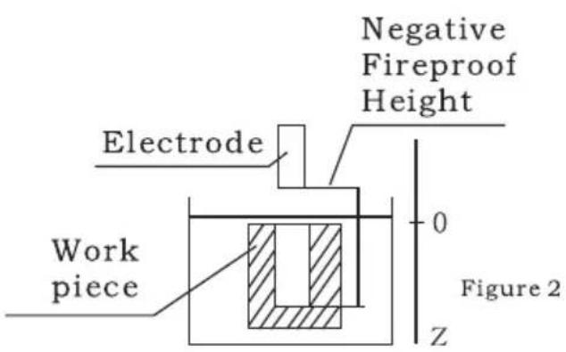
When the electrode ascends and machining is carried out from bottom to top, the digital readout value decreases. The machining direction is negative (negative), which is also called negative machining (as shown in Fig. 1).

The Digital Readout also features other functions, such as negative fireproof height. The negative fireproof height function is a kind of intelligent position-follow check safety protective device. During machining, the electrode surface will generate carbon accumulation. Due to long-time or continuous machining without tending, when carbon accumulation occurs and nobody cleans it, the electrode will slowly move in the negative direction. Once the electrode exceeds the liquid level, it will frequently catch fire and cause losses. This function is designed to address this problem. When setting the negative fireproof height, if the increased height of the electrode exceeds the height between it and the depth of the machined surface (i.e., the negative fireproof height), the digital readout display will blink as a warning; at the same time, the output signal will automatically turn off the EDM to eliminate the risk of fire.

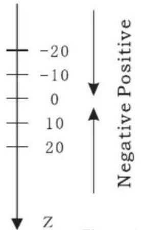
Figure 1

2. Procedure:

See the following example for detailed machining.

1) Before machining, first set each parameter: DEPTH (machining depth), ERRHIGH (negative fireproof height), machining direction (POSITIVE / NEGATIVE), exit mode (AUTO/STOP), and EDM Relay Output Mode.

2) Move the main axis electrode of the Z-axis to make it contact the workpiece reference. Clear the A-axis to zero or set the value.

3) Enter EDM machining by pressing the EDM key.

4) The X-axis will display the machining depth target value. The Y-axis will display the value that has been machined to depth (the value on the Y-axis is the depth that the workpiece has been machined). The Z-axis will display the self-position real-time value (the value on the Z-axis is the position value of the main axis electrode of the Z-axis).

5) Start machining. The Z-axis display value will gradually approach the target value, and the Y-axis display value will also gradually approach the target value. If at this time the electrode moves up and down repeatedly, the Z-axis display value will change accordingly, but the Y-axis display value will not change; it will always display the machined depth value.

6) When the Z-axis display value equals the set target value, the position-reaching switch will be turned off, and the EDM will stop machining. According to the operator's setting, there are two exit modes:

a) Automatic Mode:

It will automatically exit from EDM machining status and recover to the original state before machining.

b) Stop Mode:

It will always stay at the machining interface after finishing machining, and you should press EDM to exit and return to the original state.

Operation steps:

The DEPTH (machining depth), ERRHIGH (negative fireproof height), exit mode, EDM relay output mode, and machining direction should be set.

STEPS:

1. Press EDM to enter the EDM function. Press ▲ to input parameters; press ▼ to enter EDM machining state.
2. Input DEPTH (machining depth). Press the key ▲ to set the next parameter.

1. Input ERRHIGH (negative fireproof height) (undefined). Press the key ▲ to set the next parameter.

1. Set machining direction (positive or negative). Press 1 to select positive direction. Press 0 to select negative direction. Press the key ▲ to set the next parameter.

1. Set exit mode (AUTO mode or STOP mode). Press 0 to select AUTO mode; press 1 to select STOP mode; press the key ▲ to set the next parameter.

1. Set the output mode (Mode 0 or Mode 1) (undefined). Press ☐ to select Mode 0; press ☐ to select Mode 1.

1. Continuously press ▼ to return to EDM for machining. Press EDM to quit the function.

Example 1: positive direction machining.

Machining is shown as the model chamber as follows.

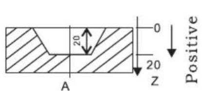
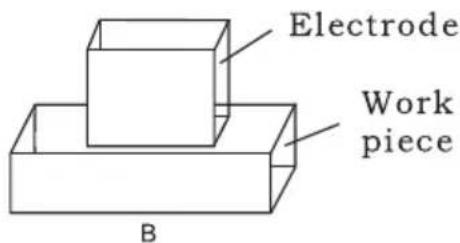
STEPS:

1. Touch one side of the workpiece with the TOOL, then press Z0 to zero the Z axis.

2. Press EDM, set DEPTH to 20.000; press ▼ to start EDM machining.

Example 2: Negative direction machining

Machining is shown as the model chamber as follows:

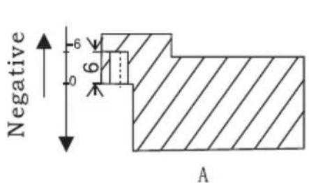
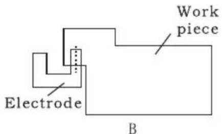
1. Touch one side of the workpiece with the TOOL, then press Z0 to zero the Z axis.

2. Press EDM, set DEPTH to -20.000; press ▼ to start EDM machining.

Example 3: PCD Function for EDM

The PCD Function can access the EDM Function. The operator enters the PCD Function to input parameters for PCD and enter the PCD machining state. At every machining position, press the EDM key to access the EDM Function.

When entering the EDM Function, the operator can input the parameters for EDM.

The operation procedure is as follows:

1) Set PCD parameters (the setting is the same as the common setting of PCD).

After inputting all parameters, enter the PCD machining state. The position of the first hole will be displayed.

2) Press EDM to enter the EDM Function parameters (the setting method is the same as the common setting of EDM parameters); after inputting all parameters, continuously press ▼ to enter the EDM machining state. When machining is done, press EDM to quit the EDM function and enter the PCD machining state.

3) In the PCD machining state, press ▼ for the position of the next hole, move the machine to the displayed value 0, then press EDM to access the EDM function again.

4) Repeat steps 2 and 3 for the following machining points.

7 Calculator

The Calculator not only provides normal mathematical calculations such as +, -, x, /, it also provides trigonometric calculations such as SIN, Arc SIN, COS, Arc COS, TAN, Arc TAN, SQRT, etc.

The operations are the same as commercial calculators, easy to use.

Enter and exit Calculator Function

In normal display state: Press CTR to enter calculator function.

In calculator display state: Press CTR to exit calculator function.

Transferring the Calculator Results to Selected Axis.

After calculation is finished, if the Calculator display Mode is set for mode 1, user can:

Press X0 to transfer the calculated result to X axis; then the X window will display this value;

Press Y0 to transfer the calculated result to Y axis; then the Y window will display this value;

Press Z0 to transfer the calculated result to Z axis; then the Z window will display this value;

Transferring the Current Display Value in window to Calculator. If the Calculator display Mode is set for mode 1, user can:

Press X to transfer the display value in X window to calculator;

Press Y to transfer the display value in Y window to calculator;

Press Z to transfer the display value in Z window to calculator;

8 Appendix

1. Troubleshooting:

The following are the preliminary solvents for troubleshooting.

If there is still trouble, Please contact out company or agents for help.

Troubles	Possible reasons	Solvents
No display	Power isn't connectedPower switch is off.The range of power voltage is not right.The inner power of Linear Scale is short.	Check power wire and connect the powerTurn on the power switch.The range of voltage is in 80--260VUnplug the connector of linear scale
One axis is not counting	Replace the linear scale of the other axis.DRO is in special function	If count is normal, the linear scale has trouble; If abnormal, the DRO readouts has trouble.Quit the special function.
Linear scale is not counting	Reading head is bad for using range exceeds.Aluminum chips is in reading head of linear scale.The span between the reading head and metal part of linear scale is large.The metal parts of linear scale is damage.	Repair the linear scaleRepair the linear scaleRepair the linear scaleRepair the linear scale
Counting is error	Shell is poor grounding.Low precision of machine.Speed of machine is too rapid.Precision of linear scale is low.The resolution of DRO readouts and the linear scale is not match.The unit (mm/inch) is not match.Setting thelinear compensating is not arrest.Reading head of the linear scale is damaged.	Shell is good grounding.Repair the machine.Reduce the speed of machine.Mount the linear scale again.Set the resolution of the DRO again.Cover the unit of display mm/inch.Reset the linear compensation.Repair the linear scale.
The counting of the linear scale is not accurate	The mounting of linear scale does not demand the requirement, and the precision is not adequate.The screw is loosen.Precision of machine is low.The resolution of digital readouts and the linear scale is not match.	Mount the linear scale again and level it.Lock all fixing screws.Repair the machine.Reset the resolution of digital readouts.
Sometimes the linear scale is not counting	The small car and steel ball is separated.The glass of reading head is wearied.The glass of reading head of the linear scale has dirt.The elasticity of the steel wire is not adequate.	Repair the linear scale.Repair the linear scale.Repair the linear scale.Repair the linear scale.

1. Specifications of Digital Readout.

1) Supply Voltage range: AC 85 V \~ 230 V; 50 \~ 60 Hz 2) Power consumption: 15VA 3) Operating temperature: 0°C-- 50°C 4) Storage temperature: - 30°C-- 70°C 5) Relative humidity: < 90 % (25) 6) Max Coordinate number: 3 7) Readout allowable input signal: TTL square wave 8) Allowable input signal frequency: < 5 M Hz 9) Max resolution of digital display length: 0.01 um 10) Max resolution of digital display angle: 0.0001 / PULSE

1. Instructions

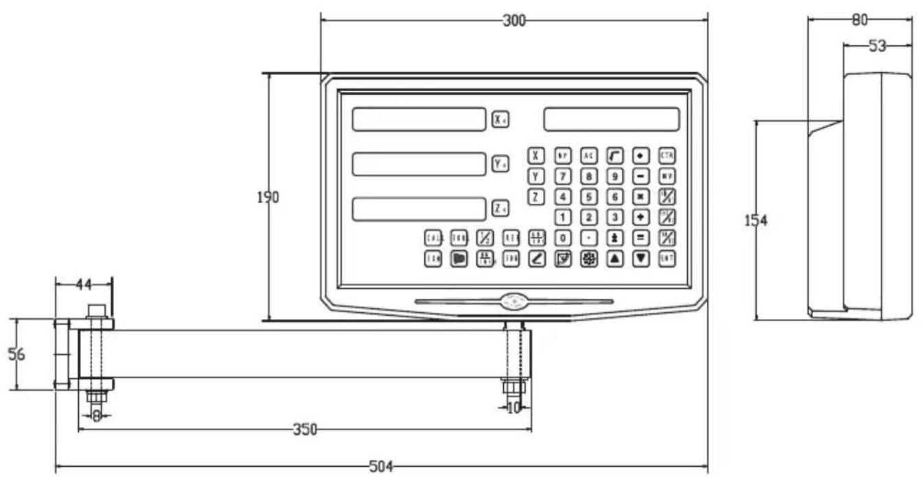
1. Examples of character output at the data interface

1、X,Y,Z Axis

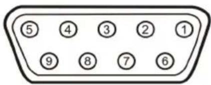
Pin	TTL (Standard)
1
2	OV
3
4
5
6	A+
7	5V
8	B+
9	R+

Pin	TTL (Standard)
1	5V
2	OV
3	A+
4	B+
5	R+
6
7
8
9

For your convenience, If you buy a digital readout,

The wiring definition of your linear scale must be the same as the 2 definitions in the above diagram to be universal!

Installation instructions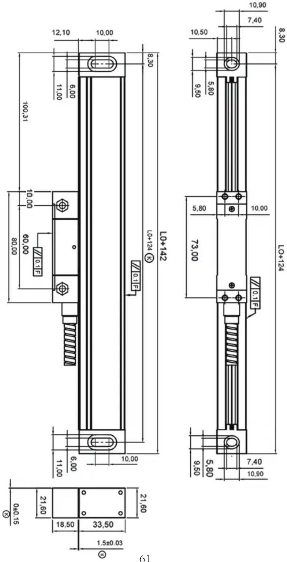

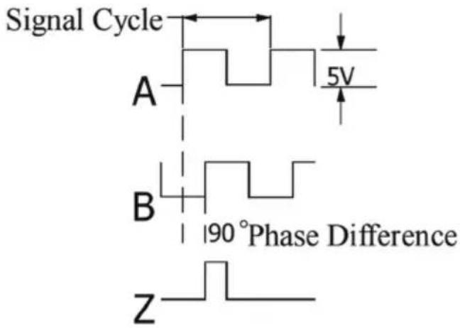
TTL signal Output:

EIA-422-A signal Output:

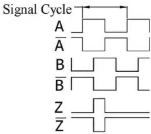
1. TECHNICAL PARAMETER

1.1 Scaling distance: 0.02 mm (50 lines/mm) 1.2 Resolution: 5 μm, 1 μm, 0.5 μm 1.3 Precision: ±3 μm, ±5 μm, ±15 μm/m (at 20±0.1°C) 1.4 Measuring range: 30~3000 mm 1.5 Moving speed: High-speed encoder 120 m/min (to be customized)

Ordinary encoder 60 m/min

1.6 Power supply: +5V±5%, 80 mA 1.7 Cable length: Standard 3 m (special length available according to user's needs) 1.8 Working temperature: 0~45°C 1.9 Pin description: 1) Applicable to: 9-pin socket EIA-422-A signal output.

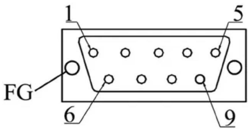
1) Applicable to: 9-pin socket EIA-422-A signal output.

Pin Position	1	2	3	4	5	6	7	8	9
Signal		OV		Empty		A	+5V	B	Z
Color	Green Black	Black	Orange black	FG	White black	Green	Red	White	Orange

FG: Shield connected to metal casing.

1) Applicable to: 9-pin socket TTL signal output.

Pin Position	1	2	3	4	5	6	7	8	9
Signal		OV		Empty		A	+5V	B	Z
Color		Black		FG		Green	Red	Orange	White

FG: Shield connected to metal casing.

Linear scale installation drawings

Installation method: Standard size: (Unit: mm)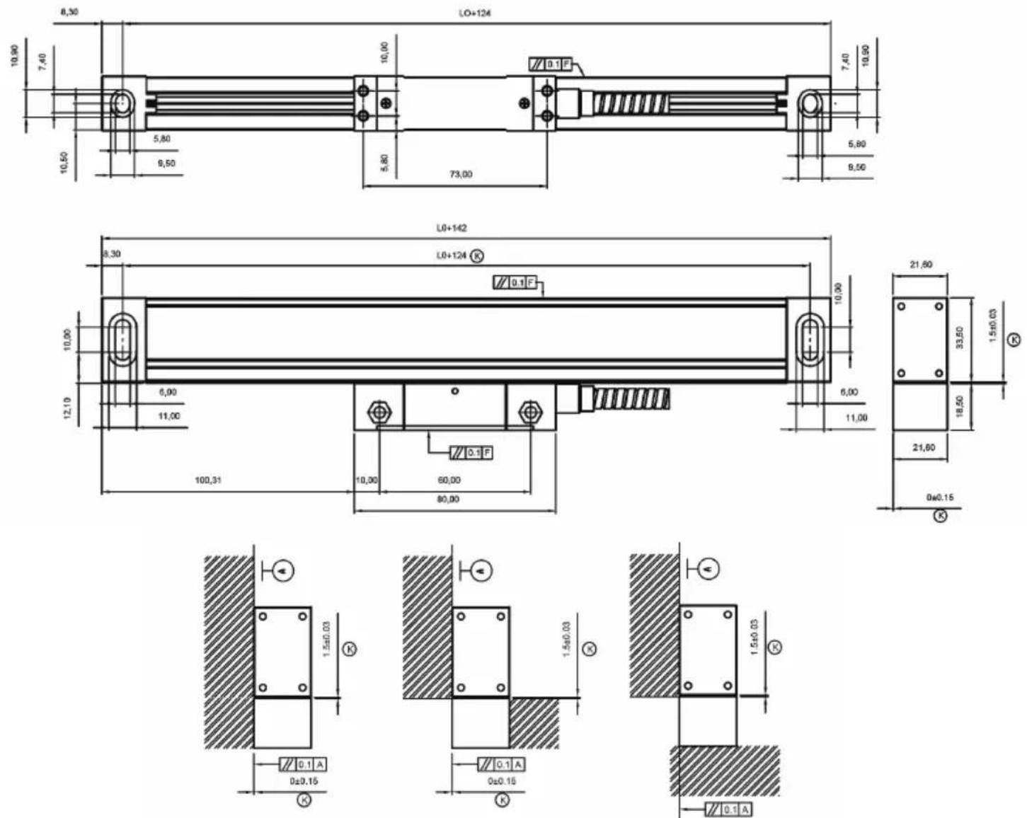

Model	L0 L1	L2 Model	L0 L1 L2
YE-50	50	174	190	YE-550	550	674	690
YE-100	100	224	240	YE-600	600	724	740
YE-150	150	274	290	YE-650	650	774	790
YE-200	200	324	340	YE-700	700	824	840
YE-250	250	374	390	YE-750	750	874	890
YE-300	300	424	440	YE-800	800	924	940
YE-350	350	474	490	YE-850	850	974	990
YE-400	400	524	540	YE-900	900	1024	1040
YE-450	450	574	590	YE-950	950	1074	1090
YE-500	500	624	640	YE-1000	1000	1124	1140

L0: Effective measuring length of the linear encoder; L1: Length of linear encoder mounting holes; L2: Linear encoder overall length

Maintenance:

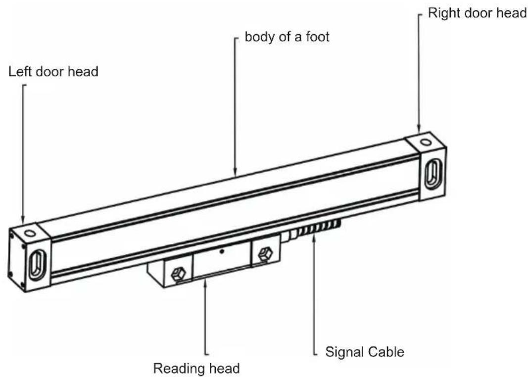
1. The effective travel of the linear encoder should be longer than the maximum travel of the machine tool. If the length is not enough, replace the linear encoder with a larger stroke or add a limit block on the machine. The end position of the reading head from the end of the linear encoder body should be not less than 10 mm space (see the following diagram).

1. For any non-machined surface, a shim must be placed on the back of the linear encoder or a user-made installation shim must be used to ensure the stability and reliability of the connection between the grating ruler and the mounting surface.
2. When using a dial gauge or similar instrument to calibrate the parallelism of the linear encoder, the angle of the side head must be within ±30 degrees, and the smaller the angle, the better.

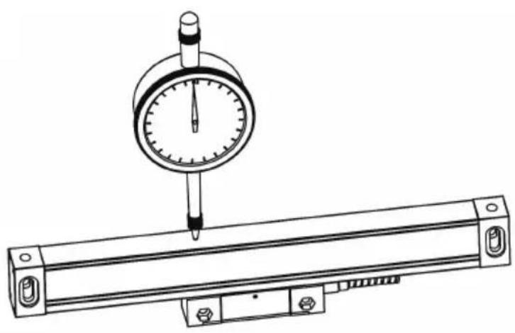
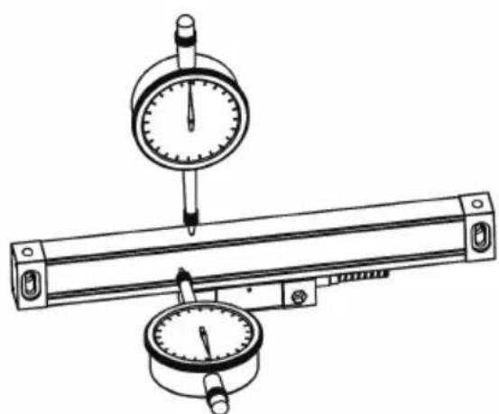
1. The installation position of the linear encoder must avoid direct impact from iron filings, oil, water, and dust (as shown in the figure below). The installation length of the L-plate should be as short as possible under possible circumstances, and the force situation of the mounting surface must be taken into consideration.

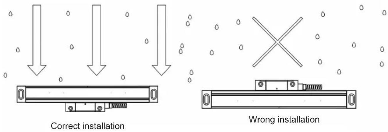
1. There must be a gap of 0.5 mm or more between the dust cover and the ruler body, and avoid contact between the dust cover and the ruler body when moving the reading head (as below).
2. Installation screw thread depth: at least 6 teeth of locking depth; for parts under greater force, such as the fixed plate supporting the digital display meter shelf, at least 8 teeth of locking depth; for YE series scales, the thread depth must be at least 8 teeth of locking depth. After tapping the mounting surface for M4 screws, deburr, remove paint, and clean off stains.

(The following figure)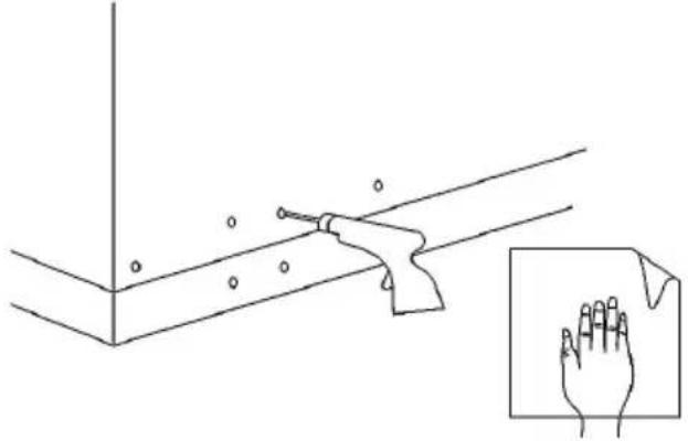

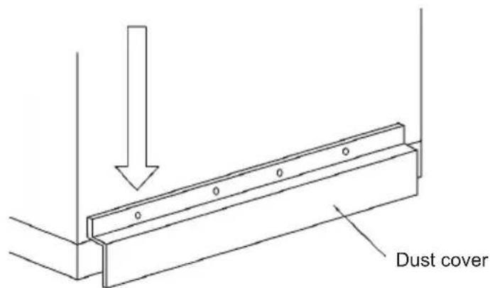
1. The fixing of the signal line must take into account all relevant moving distances. Fixing position as far as possible placed in the very center of the stroke, and the excess signal line is fixed with a wire tie.
2. Adjustment of the scale height level must be the length of the scale center to take the two sides of the symmetry point Do adjust the reference point, any scale regardless of the school level direction or height direction, the Adjustment range: for the scale body, to the head from the scale body at a distance of not more than 20mm from each end shall prevail. For the reading head, between the two quadrilateral reference surfaces (the following figure)

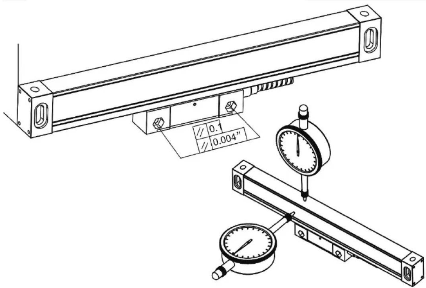
1. The bending radius of the signal line of the scale is greater than 60mm.

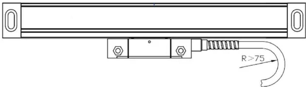
10. Scale installation standard

(1) Installation base surface standard (Figure 4.8a, b, c three installation methods)

1. The installation surface of the ruler body is parallel to the installation surface of the reading head, and the parallelism between the installation surfaces is < 0.1 mm
2. The installation surface of the ruler body is perpendicular to the installation surface of the reading head, and the perpendicularity between the installation surfaces is < 0.1 mm

2) Ruler body installation standards (Figure 4.9, Figure 4.10)

1. Height direction relative to the machine guide parallelism <0.1mm, maximum not more than 0.15mm. In terms of symmetry point, the smaller the better.

3) Standard of reading head installation

1. The clearance between the reading head and the height direction of the ruler body is 0.8mm-1.6mm after installation, and then withdraw the pad block (Figure 4.11)

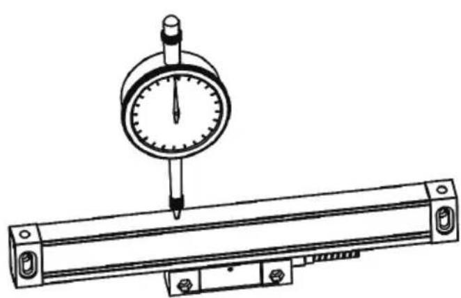
4.9

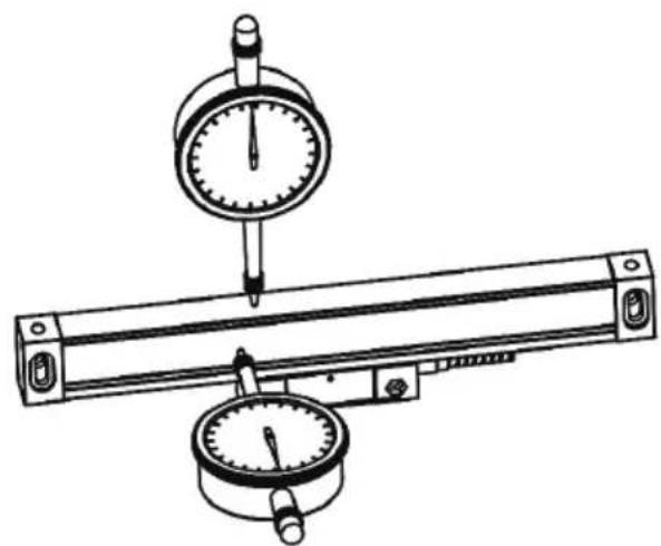
4.10

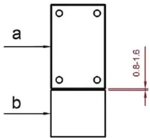
1. Reading head a side and ruler body B side. Misalignment in horizontal direction. 0.25±0.15mm
2. Parallelism of reading head relative to machine tool <0.10mm, maximum cannot exceed 0.30mm

Parameter:

Modle	SNS-3V-YE102024	SNS-3V-YE161838
Rated voltage:	AC85-230V 50Hz/60Hz
Resolution	5 μm
Number of axles	3
Range	10 inches20 inches24 inches	16 inches18 inches38 inches

Standard accessories:

Accessories for digital display meters:

Accessories for grating ruler:

1. Support rod * 12. Knife holder plate * 13. Transparent watch case * 14. Power cord * 15. Watch holder * 16. Butterfly piece * 27. M8 * 70 screw * 18. M10 * 55 screw * 19. Nut M10 * 110. Nut M8 * 111. Nut M5 * 112. Internal hexagonal screw M5 * 20 * 213. Internal hexagonal screw M5 * 25 * 114. M4 * hex socket screw * 415. M5 * 10 machine meter screws * 216. Washer φ 10 * 117. Washer φ 8 * 118. Washer φ 5 * 119. Rubber washer 20 * 10 * 1 * 120. Rubber washer 20 * 10 * 0.5 * 121. Spring washer φ 10 * 122. Spring washer φ 8 * 123. Spring washer φ 5 * 1

1. Ruler cover * 32. L mounting plate * 43. Plug * 64. Screw pack * 3 bagsEach bag contains:Internal hexagonal screw M4 * 30 * 4;Internal hexagonal screw M4 * 12 * 2;Internal hexagonal screw M4 * 8 * 4;U-shaped gasket T=0.2mm * 2;Washer φ 6 * 2;Washer φ 5 * 2;Washer φ 4 * 6;Line card * 2

This device complies with Part 15 of the FCC Rules. Operation is subject to the following two conditions: (1) This device may not cause harmful interference, and (2) this device must accept any interference received, including interference that may cause undesired operation.

Manufacturer: Shanghaimuxinmuyeyouxiangongsi

Address: Shuangchenglu 803nong11hao1602A-1609shi, Baoshan District, Shanghai 200000 CN.

Imported to AUS: SIHAO PTY LTD, 1 ROKEVA STREET, EASTWOOD NSW 2122 Australia

Imported to USA: Sanven Technology Ltd., Suite 250, 9166 Anaheim Place, Rancho Cucamonga, CA 91730

EC

REP

E-CrossStu GmbH

Mainzer Landstr. 69, 60329 Frankfurt am Main

UK

REP

YH CONSULTING LIMITED.

C/O YH Consulting Limited, Office 147, Centurion House

London Road, Staines-upon-Thames, Surrey, TW18 4

VEVOR®

TOUGH TOOLS, HALF PRICE

Technical Support and E-Warranty Certificate

www.vevor.com/support

VEVOR®

TOUGH TOOLS, HALF PRICE

www.vevor.com/support

USER MANUAL FOR THE DRO DISPLAY

MODEL: SNS-3V-YE102024 IS NS-3V-YE161838

NEED HELP? CONTACT US!

1. Illustration of Panel and keyboard 4
2. Caption of the keyboard 5
3. Parameters settings 7

3.1 Parameters setup routine entrance 7 3.2 Parameters Settings Description 7 3.2.1 Setting the Resolution 7 3.2.2 Setting Positive Direction for Counter 8 3.2.3 Toggle Between R/D Display Mode 8 3.2.4 Setting Z axis Dial 8 3.2.5 Setting the Rotary Radius of the Workpiece.... 9 3.2.6 Setting the Angle Display Mode 9 3.2.7 Setting the Baudrate of RS_232(optional) 9 3.2.8 Setting the Absolute Zeroing enable or disable 10 3.2.9 Setting the Absolute form the Special Function 10 3.2.10 Setting the Calculator display Mode 10 3.2.11 display brightness setting 10 3.2.12 The linear scale counting frequency setting 11 3.2.13 Setting QUIT 11 3.2.14 Setting the type of the DRO. 11 3.2.15 Signal Interface Type 11 3.2.16 Restore Factory Settings: 12 3.2.17 Shrinkage Ratio enable or disable....12 3.2.18 Setting Compensation Type 12 3.2.19 Inch display, set the number of digits after the decimal point…13 3.2.20 Setting EDM(optional) 13 3.2.21 Setting Linearity Compensation. 13 3.2.22 Setting the Shrinkage Ratio 13

4. General Operations 14

4.1 Zeroing....14 4.2 Preset Data to Designated Axis 14 4.3 Toggle Display Unit between inch and mm 14 4.4 Absolute/Incremental/200 groups SDM 15 4.5 1/2 Function ...... 15 4.6 Clear All SDM Datum....16

Contents

4.7 Sleeping Mode 16 4.8 Power Interruption Memory 16 4.9 Search the Absolute Reference Point of Scale 17 4.10 Non Linear Error Compensation 20

5. 200 Groups SDM coordinate 21 5.1 Zeroing at the Current Point....21 5.2 Preset datum of SDM coordinate 22

6. Special Function……24

6.1 Circumference Holes Processing 25 6.2 Linear Holes Processing 28 6.3 ARC Processing 30 6.4 Oblique Processing 39 6.5 Slope Processing....43 6.6 Chamber Processing....44 6.7 The Tool Diameter Compensation Function 45 6.8 Digital Filter of the Grinding Machine 46 6.9 Lathe Function 47

6.9.1 200 sets TOOL Libs 47 6.9.2 Taper Function 48 6.9.3 R/D Function 49 6.9.4 Y + Z Function ( only applicable to : 3 axes Lathe)....49

6.10 EDM....50

7. Calculator……56

8. Appendix 57

THREE AXIS PANEL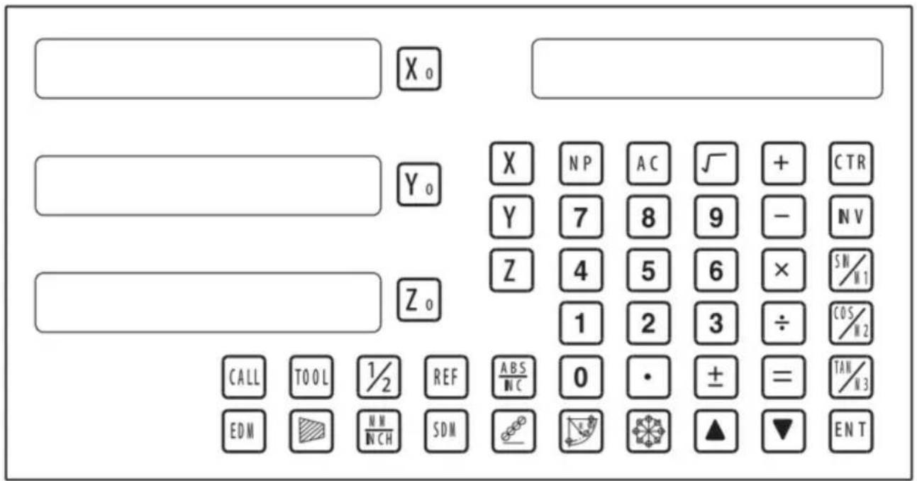

TWO AXIS PANEL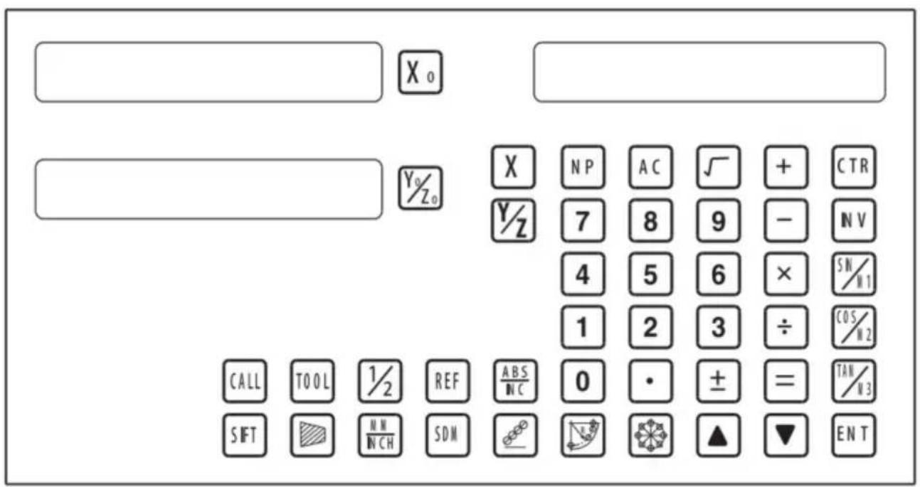

Keyboard Description

	Keys for axis selection
	Zero select axis
	Enter +/- sign
	Enter decimal point
	Entry keys for numbers
	Operation key (in Calculation function key)
	Enter or quit calculating state
	Cancel incorrect operation
	Calculate inverse trigonometric
	Square root
	Confirm operation
	Toggles between inch and millimeter units.
	Press when ready to identify a reference mark.
	Function keys for 200 sub datum
	ARC cutting function
	holes displayed equally on a circle
	holes displayed equally on a line

Caption of the keyboard

	Calculate trigonometric or Slope Processing function key
	Calculate trigonometric or rectangular inner chamber processing function key
	Calculate trigonometric or the tool diameter compensation function key
	Toggle between ABS/INC coordinate
	Stroll up or down to select
	Taper measured function key
	Tool library call key
	Opens the tool table.( lathe)
	EDM function key
	Filter display function key
	Half a display value of an axis
	Non Linear Error Compensation function keys

3. Parameters settings

3.1 Parameters setup routine entrance.

Press ☐ to enter initial system and self-check after DRO powers on in 1 second, then Parameters settings display in the Parameters window. Press ▲ ▼ to select the item you want to change.

If you want to quit initial setting, press ▲ ▼ until “QUIT” appears in message window and press ENTER. You can also press • to quit initial setting.

3.2 Parameters Settings Description

3.2.1 Setting the Resolution

Press ▲ ▼ until “RESOLUTE” appears in message window;

When selecting the LINEAR encoder, the resolution will be set as follows:

There are 19 types of resolution:

0.01um; 0.02um; 0.05um; 0.10um; 0.20um; 0.25um; 0.50um; 1.00um; 2.00um; 2.50um; 5.00um; 10.00um; 20.00um; 25.00um; 50.00um; 100.00um; 200.00um; 250.00um; 500.00um.

Press [X0] to change the resolution for X axis; Press [Y0] to change the resolution for Y axis; Press [Z0] to change the resolution for Z axis;

Set the resolution 5.00um to 1.00um for X axis:

When selecting the rotary encoder, the resolution will be set as follows:

Input the rotary encoder parameter value.

3.2.2 Setting Positive Direction for Counter

Press ▲ ▼ until "DIRECTE" appears in message window.

Direction '0' means the display value will increase when scale moves from right to left and decrease when scale moves from left to right. Direction '1' means the display value will increase when scale moves from left to right and decrease when scale moves from right to left.

Press [X0] to change the Direction for X axis; Press [Y0] to change the Direction for Y axis; Press [Z0] to change the Direction for Z axis; as follows:

3.2.3 Toggle Between R/D Display Mode

Press ▲ ▼ until "R OR D" appears in message window. X window, Y window, Z window display '0' or '1' separately.

'0' is mode R, which means the display value equals the actual measurement. '1' is mode D where the display value equals double the actual measurement. Press [X0] to change the R/D for X axis; Press [Y0] to change the R/D for Y axis; Press [Z0] to change the R/D for Z axis; as follows:

3.2.4 Setting Z axis Dial

Press ▲ ▼ until "Z DIAL" appears in message window.

Z axis dial should be set if Z axis is emulated for 2 axis milling and only install linear scale for X,Y axis. Z axis dial means the distance the Z axis travels when screw runs a revolution.

Set the Z axis Dial 2.5mm as follow ;

3.2.5 Setting the Rotary Radius of the Workpiece

Press ▲ ▼ until "RDIUS" appears in message window.

The Rotary radius type is used perimeter to measure angle.

Input the Rotary Radius parameter value 2000mm as follow:

3.2.6 Setting the Angle Display Mode

Press ▲ ▼ until "ANG DISP" appears in message window.

Press ₀ to change the angle display mode for X axis; Press ₀ to change the angle display mode for Y axis; Press ₀ to change the angle display mode for Z axis; Example for X axis:

"0.0000" means the angle mode is Circulating DD;

"0000.0000" means the angle mode is Incremental DD;

"0.00.00" means the angle mode is Circulating DMS;

"0000.00.00" means the angle mode is Incremental DMS;

3.2.7 Setting the Baudrate of RS_232 (Special customization function, if you need to buy, please contact the dealer to customize)

Press ▲ ▼ until "BAUDRATE" appears in message window. Set the Baudrate 115200 as follow ;

3.2.12 The linear scale counting frequency setting

The factory default setting is only "12". The higher the parameter, the lower the counting frequency. Press "X0" to set. It is not recommended that you change the default value yourself.

3.2.13 Setting QUIT: Digital display table parameters quit button.

3.2.14 Setting the type of the DRO.

The type of the DRO will be displayed on the right window. Then press the key ENT to select the correct type. The following system items will be set:

"MILL-3" means the DRO type is 3-axis milling machine table;

"MILL-2" means the DRO type is 2-axis milling machine table;

"LATHE-2" means the DRO type is 2-axis lathe table;

"LATHE-3" means the DRO type is 3-axis lathe table;

"GRIND" means the DRO type is Grind table;

"EDM" means the DRO type is EDM table; (Special customization

function, if you need to buy, please contact the dealer to customize)

3.2.15 Signal Interface Type

Message window displays "SEL AXIS" which indicates the step is to Sensor input signal mode. Press X₀ to change the signal mode for X axis; Press Y₀ to change the signal mode for Y axis; Press Z₀ to change the signal mode for Z axis. Example for X axis:

Press X₀ to scroll through the Rotary encode type, the Linear encode type, the Rotary radius type.

X window displays the Signal type.

"LINEAR" means the Signal type is linear encode type;

"ENCODE" means the Signal type is Rotary encode type;

"RADIUS" means the Signal type is Rotary radius type;

Example: currently in the linear encode type, to toggle to the Rotary encode type;

3.2.16 Restore Factory Settings:

Clear all data except DRO type. DRO will load default setup for parameters. After loading default setup, user must search RI once to enable resuming ABS datum function; otherwise, to resume the datum by RI is unable;

Message window displays "ALL CLR", press ENT and message window displays "PASSWORD" indicating the operator to input password; Press 2000 + ENT in turn to load default value;

3.2.17 Shrinkage Ratio enable or disable.

Message window displays "SRK OFF" to disable Shrinkage rate function. Press ☐ to enable Shrinkage rate function in Message window displays "SRK ON":

3.2.18 Setting Compensation Type

Message window displays "SEL COMP" which indicates the step is to compensation type. Press X₀ to change the compensation type for X axis; Press Y₀ to change the compensation type for Y axis; Press Z₀ to change the compensation type for Z axis; Example for X axis:

Press X₀ to scroll through the not compensation type, the Linear compensation type, the non-linear compensation type.

"NO-CO" means the compensation type is not compensation type; "LINE-CO" means the compensation type is linear compensation type. "NON-LINE" means the compensation type is non-linear compensation type;

Example for X axis: currently in the not compensation type, to toggle to the linear compensation type;

3.2.19 Inch display, set the number of digits after the decimal point

In the inch display mode, the number of digits after the decimal point is set. The factory default digit is "4". Press "X0" to set it, and it can be adjusted according to actual needs.

3.2.20 Setting EDM: It is not recommended that you set the default value yourself. The EDM function sets the relay off time.

3.2.21 Setting Linearity Compensation.

The message window displays "LIN COMP", which indicates that the step is for linearity compensation. Compensate the linear error to make the display value equal to the standard value.

The calculation of the compensation rectifying coefficient:

Coefficient = (Measurement - Standard value) x 1000.000/ Standard value

Example for X axis:

Measurement: 200.020mm

Standard value: 200.000mm

Rectifying coefficient = (200.020 - 200) * 1000 / 200 = -0.01mm/m

Input compensation rectifying coefficient 0.01 as follows:

3.2.22 Setting the Shrinkage Ratio

Press ▲ ▼ until "SHRINK" appears in the message window.

Shrinkage ratio = Dimensions of the finished product/Dimensions of the working piece

Set the shrinkage radio to 1.005 as follows;

4. General Operations;

4.1 Zeroing

Zero the designated axis in normal display state. Zeroing is used to set the current point as the datum point as follows;

X₀ or Y₀ or Z₀ will be returned to the original data before the reset.

4.2 Preset Data to Designated Axis

Preset a value to the current position for a designated axis in normal display state.

4.3 Toggle Display Unit between inch and mm

Length can be displayed either in "mm" (metric) or "inch" (imperial). The display unit can be toggled between mm and inch.

Example: Display value toggles from mm to inch;

Example: Display value toggles from inch to mm;

4.4 Absolute/Incremental/200 groups SDM

Function: The DRO has 3 coordinate display modes: the absolute mode (ABS); the incremental mode (INC) and 200 groups Second Data Memory (SDM) with the range of 00 to 99. The zero point of the work-piece is set at the origin point of the ABS coordinate. The relative distance between the datum of ABS and SDM remains unchanged when the ABS datum is changed.

1. Toggle from ABS to INC coordinate;

1. Toggle from INC to ABS coordinate;

1. Toggle from SMD to ABS coordinate;

4.5 1/2 Function

Function: Set the center of work piece as datum by halving the displayed value.

Example: Set the center of rectangle as datum as the right figure.

Steps:

1. Touch one side of the workpiece with the TOOL, then zero the X axis.

2. Message window displays “REF”, Press ENT until “FD_REF” appears in message window.

3. Select the axis which need search RI. For instance: select X axis, then press ☒. "X_REF" is displayed in message window, and X axis window flashes.

4. Move the machine table. The buzzer sounds when RI is searched, then X window stops flashing and displays the value of the current position. The DRO returns to normal display state. Then message window displays "FIND_X".

Example for AB mode:

1. DRO is set in ABS coordinate. Press REF, then the message window displays "REF".

2. Press ▲ ▼, then the message window displays “AB”.

3. Message window displays “AB”, Press ENT until “FIND_AB” appears in message window.

4. Select the axis which need search RI. For instance: select X axis, then press ☒. “X_REF” is displayed in message window, and X axis window flashes.

5. Move the machine table. The buzzer sounds when RI is searched, displays the value of the current position for the absolute datum zero. The DRO returns to normal display state. Then message window displays "FIND_AB".

Example for LEF_AB mode:

1. DRO is set in ABS coordinate. Press REF, then the message window displays "REF".

2. Press ▲ ▼, then the message window displays "AB".

3. Message window displays "LEF_AB". Press ENT until "ZERO_AB" appears in the message window.

4. Move the machine table to the position to be set as zero. Then press X, the X axis will be zeroed. The current position becomes the absolute datum zero. The DRO returns to normal display state.

NOTE: Linear range without reference point location of the user

4.10 Non-Linear Error Compensation

First, in parameter setting, the compensation type (Linear or Non-Linear) must be set to Non-Linear. Linear scale has a reference point location, and finding the Absolute Reference Point will be enabled.

Default Non-Linear compensation: 50.

Example for Y axis:

Step 1: Search the Absolute Reference Point of the scale.

Step 2: Press NP, then the message window displays "COMP X".

Step 3: Press ▲ ▼, then the message window displays "COMP Y".

Step 4: Press ENT, then the message window displays "NUMBER". Then input the compensation parameter NUMBER.

Step 5: Press ▲ ▼, then the message window displays "Y-MSN-1", which indicates the step is for Non-Linear Error Compensation.

Step 6: Input compensation value.

X window displays the measurement value.

Y window displays the standard value.

Example for the first compensation point:

Measurement value: 68.288mm. Standard value: 68.200mm

Step 7: After inputting all parameters, the DRO automatically exits.

5. 200 Groups SDM Coordinate

The DRO has three display modes: the absolute mode (ABS), the incremental mode (INC), and the 200 groups second data memory (SDM 1 - SDM200). The ABS datum of the workpiece is set at the beginning, and the 200 groups SDM is set relative to the ABS coordinate.

ABS Mode, INC Mode, and SDM Mode are specially designed to provide much more convenience features to the operator to cope with the batch machining of relative works and the machining of workpiece dimensions from more than one datum.

Example: The ABS datum is the center point O, and the points SDM1, SDM2, SDM3, SDM4 needed for processing are set as the datum of SDM 1 - SDM 4.

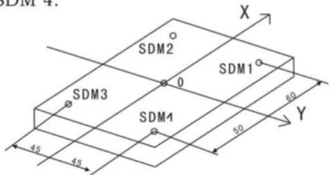
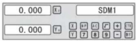
Two ways to set SDM coordinate:

1. Zeroing at the current point. 2. Preset datum of SDM coordinate.

5.1 Zeroing at the Current Point

First, set the center point of the workpiece as the origin of the ABS, then align the tool with points SDM1, SDM2, SDM3, SDM4 by moving the machine table and zero them. It is the position to process where the "0.000" appears in the X window and Y window by moving the machine table, whether in ABS or in SDM coordinate.

Steps:

1. Move the worktable to place the TOOL at the center of the workpiece point O as the datum of ABS. Then zero X axis and Y axis in SDM 1; zero X axis and Y axis in SDM 2; zero X axis and Y axis in SDM 3; zero X axis and Y axis in SDM 4.

2. Set the point sdm1 as the datum of SDM 1. Move the machine worktable to x = 60.000, y = 45.000. Then process _{0 0} .

2. Set the point sdm1 as the datum of SDM 2. Move the machine worktable to x = 60.000, y = -45.000. Then process _{0 0} .

3. Set the point sdm1 as the datum of SDM 3. Move the machine worktable to x = -60.000, y = -45.000. Then process _{0 0} .

4. Set the point sdm1 as the datum of SDM 4. Move the machine worktable to x = -60.000, y = 45.000. Then process _{0 0} .

5.2 Preset datum of SDM coordinate

There are the same sample as Method 1. First move the worktable to place the TOOL exactly at the origin of ABS, secondly enter the ABS Mode as follows.

Steps:

1. Move worktable to place the TOOL at the center of the workpiece point O as the datum of ABS. Then zero X axis and Y axis in SDM 1; zero X axis and Y axis in SDM 2; zero X axis and Y axis in SDM 3; zero X axis and Y axis in SDM 4.

2. Set point sdm1 as the datum of SDM 1. Press ▲ ▼, then the message window displays “SDM 1”. Input x = 60.000, y = 45.000.

3. Set point sdm1 as the datum of SDM 2. Press ▲ ▼, then the message window displays “SDM 2”. Input x = -60.000, y = 45.000.

4. Set point sdm1 as the datum of SDM 3. Press ▲ ▼, then the message window displays “SDM 3”. Input x = -60.000, y = -45.000.

5. Set point sdm1 as the datum of SDM 4. Press ▲ ▼, then the message window displays “SDM 4”. Input x = -60.000, y = 45.000.

The Function of PCD Hole positioning on Circumference is used to distribute arc equally, such as boring hole on flange. The right window will show the parameter to be defined when selecting PCD Function. The parameters to be defined are:

PCD_XY(XZ,YZ)

Select place

CENTER

Center position

DIA

Diameter of circle

NO_HOLE

Hole number

STANG

Starting angle

ED ANG

Ending angle

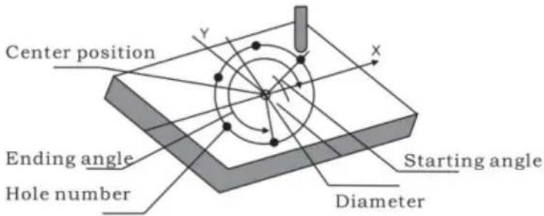
The position of the hole center is calculated automatically after inputting all parameters. Press ▲ or ▼ to choose the hole number and move the machine table until “0.000” appears in the X, Y, and Z windows. That is the position to process a table.

Example for the XY place: Machine hole on circumference as shown in the figure.

PCD_XY(XZ,YZ)	XY
CENTER	X=0,000,Y=0.000
DIA	100,000
NO_HOLE	5
ST ANG	30,000
ED ANG	315,000

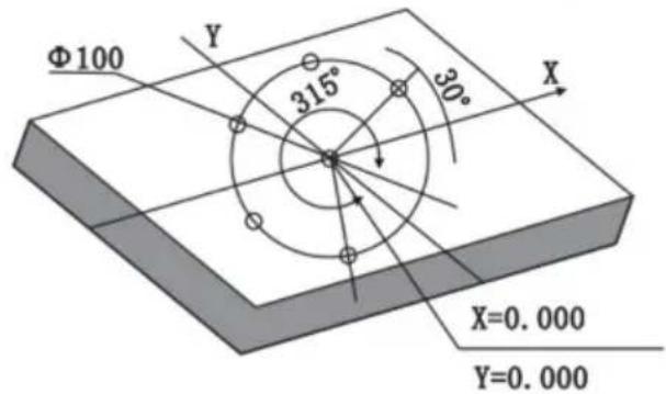
Steps:

1. Set display unit to metric in normal state; move the machine table until the machine tool is aligned with the center of the circle, then zero the X and Y axes.
2. Select piece.

Press 🧑️, then the message window displays "PCD_XY" for the Circumference Holes Processing. Press ▲ or ▼ to select XY place.

2. Input center position.

Press ENT, then the message window displays "CENTER". X and Y windows display the formerly preset center position. Input X = 0, Y = 0 as follows.

4. Input diameter.

Press ▼ until "DIA" appears in the message window. X window displays the formerly preset diameter. Then input the diameter as 100.000.

5. Input number.

Press ▼ until "NO_HOLE" appears in the message window. X window displays the formerly preset number. Then press 5 in turn to input the number.

6. Input starting angle.

Press ▼ until "ST ANG" appears in the message window. X window displays the formerly preset starting angle. Then press 3 0 in turn to input the starting angle.

7. Input ending angle.

Press ▼ until "ED ANG" appears in the message window. X window displays the formerly preset ending angle. Then press 3 1 5 in turn to input the ending angle.

1. Press ▼ until "NO 1" appears in the message window.

It is the position of the first hole to punch where the "0.000" is displayed in X window and Y window by moving the machine table. After finishing the first hole, press ▼ or ▲ to change holes number.

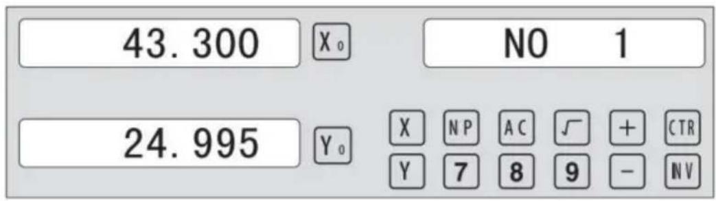
1. After processing all holes, press 📋 to return to normal display.

6.2 Linear Holes Processing

There are two modes to carry out the linear drilling: Length mode and Step mode.

1. LINE S Step mode LINE L Length mode 2.STEP Step length LENGTH Line length
2. ANG Angle
3. NO.HOLE Hole number

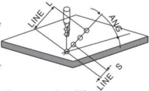
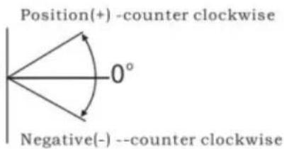
Linear Holes function can simplify the processing of multiple holes whose centers are equally spaced on one line.

Example:

LINE_L	Length mode
LENGTH	60.000
ANG	30.000
NO.HOLE	4

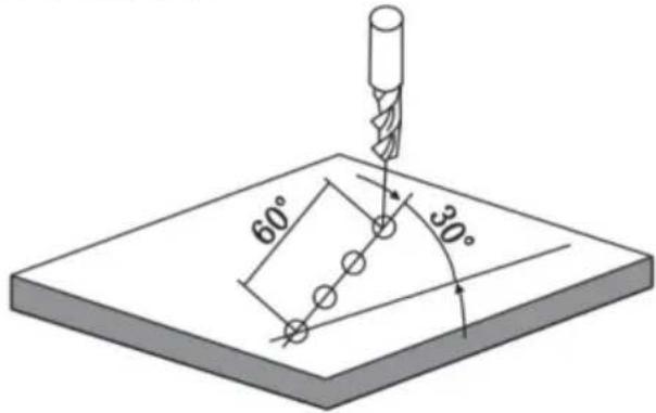
Steps:

1. Select piece.

Press 📄, then the message window displays "LINE_XY" for the Linear Holes Processing. Press ▲ or ▼ to select XY place.

2. Select Linear Holes mode.

Press ENT, then the message window displays "LINE_S". Press ▲ or ▼ to select "LINE_L".

3. Input linear length;

Press ENT, then the message window displays "LENGTH".

X window displays the formerly preset linear length. Press 6 0 in turn to input the linear length.

1. Input angle;

Message window displays “ANG” which indicates the step is to angle. X window displays the formerly preset angle. Press 3 0 in turn to input the angle.

1. Input number;

Message window displays “ANG” which indicates the step is to angle. X window displays the formerly preset number. Press 4 in turn to input the number.

1. Press ▼ until "NO 1" appears in the message window.

It is the position of the first hole to punch where the “0.000” is displayed in X window and Y window by moving the machine table. After finishing the first hole, press ▲ or ▼ to change holes number.

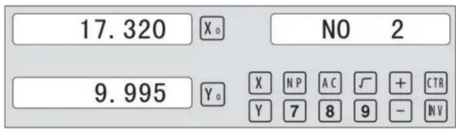
1. After processing all holes, press ☐ to return normal display.

6.3 ARC Processing

X (+ direction positive)

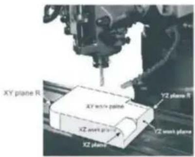
Provides maximum flexibility in ARC machining, the ARC sector to be machined by the coordinates of ARC. Very flexible, ARC function can machine virtually all kinds of ARC, even the intersected ARC.

Relatively a bit complicated to operate, operator need to calculate and enter the coordinates of ARC centre, start angle and end angle.

Basic parameter as follow:

1. SMOOTH Mode of the Smooth ARC processing;
2. SEL_XY(YZ, XZ) Select place;
3. CENTER Refer to the position of a center.
4. RAD Radius of the ARC
5. TL_DIA Diameter of the TOOL
6. MAX_CUT Feed step
7. ST_ANG Starting angle
8. ED_ANG Ending angle
9. RAD+TL Outer arc. RAD-TL Inner arc.

Example 1 for the Simple ARC Processing:

Parameters settings as follow:

SIMPLE Simple mode

TYPE 3

SEL_XY XY

RAD 80.000

TL_DIA 6.000

MAX_CUT 0.500

RAD+TL 1

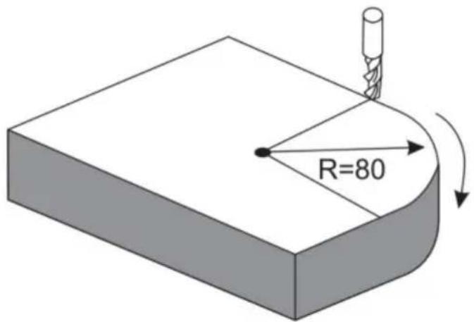
Steps:

1. Select process mode

Press 📋, then the message window displays “SIMPLE” for the ARC Processing. Press ▲ or ▼ to select the mode of the simple, the message window displays “SIMPLE”

2. Input the type:

Press ☐ENT until "TYPE" appears in the message window. X-window displays the formerly preset type. Press ☐3 in turn

3. Select place

Press ENT until "SEL_XY" appears in the message window. Press ▲ or ▼ to select place to display "SEL_XY";

4. Input radius:

Press ENT until "RAD" appears in the message window. X window displays the formerly preset radius of ARC. Press 8

0 in turn to input the radius.;

5. Input Diameter of the TOOL

Press ▲ or ▼ until “TL DIA” appears in the message window. X window displays the formerly preset Diameter of the TOOL. Press 6 in turn to input the Diameter value;

6. Input Feed step (MAX_CUT);

Press ▲ or ▼ until "MAX_CUT" appears in the message window. X window displays the formerly preset MAX_CUT. Press 0 · 5 in turn to input the MAX_CUT value;

7. Select outer arc or inner arc

Press ▲ or ▼ until “RAD-TL” appears in the message window. Press ▲ or ▼ to select place to display “RAD+TL”;

8. After inputting all parameters, press the key ENT for machining.

The DRO will display the position of the first point. Retract the axes until the displays read 0.000, Machine the Arc point by point in accordance with the display. After finishing the position of the first point, press ▲ or ▼ to change position point.

Press ☑ to quit R function any time.

Example 2 for the Simple ARC Processing:

Parameters settings as follow:

SIMPLE Simple mode

TYPE 3

SEL_XY XZ

RAD 80.000

TL_DIA 6.000

MAX_CUT 0.500

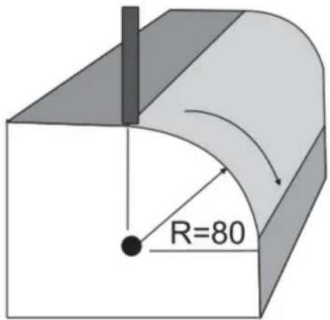
Steps:

1. Press 📋, then the message window display “SIMPLE” to the ARC Processing. Press ▲ or ▼ to select mode of the simple, The message window display “SIMPLE”

ARC Processing

2. Input the type:

Press ENT until "TYPE" appears in the message window. The X window displays the previously set type. Press 3 in turn.

3. Select place

Press ENT until "SEL_XZ" appears in the message window. Press ▲ or ▼ to select the place to display "SEL_XZ".

4. Input radius:

Press ENT until "RAD" appears in the message window. The X window displays the previously set radius of the ARC. Press 8, then 0 in turn to input the radius.

5. Input Diameter of the TOOL

Press ▲ or ▼ until "TL DIA" appears in the message window. The X window displays the previously set diameter of the tool. Press 6 in turn to input the diameter value.

6. Input Feed step (MAX_CUT);

Press ▲ or ▼ until "MAX_CUT" appears in the message window. The X window displays the previously set MAX_CUT. Press 0, then 5 in turn to input the MAX_CUT value.

1. After inputting all parameters, press the ENT key for machining.

For 2-axis milling machine table, it is not installed with Z-axis, please press ▲ or ▼ to simulate position of Z-axis. Press ▲ to simulate moving to the former process, and press ▼ to simulate moving to the next process point.

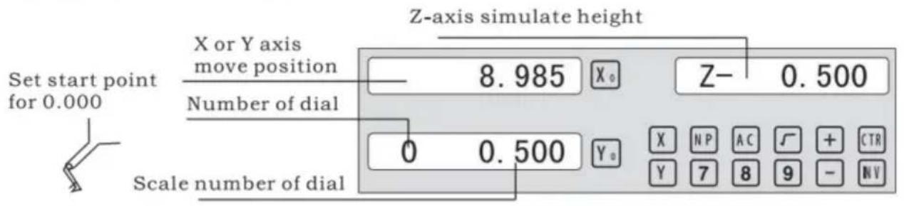
Z-axis simulate height = Number of dial x Z axis Dial + Scale number of dial

Press ☐ to quit R function any time.

Example 3 for the Smooth ARC function:

Parameters settings as follow:

SMOOTH	Smooth mode
SEL_XY(YZ,XZ)	XY
CENTER	X=0,Y=0
RAD	80.000
TL_DIA	6.000
MAX_CUT	0.500
ST_ANG	0.000
ED_ANG	135.000
RAD+TL	1

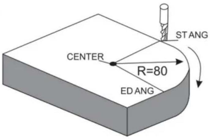
Steps:

1. Press 📋, then the message window displays “SIMPLE” for the ARC Processing. Press ▲ or ▼ to select the mode of the simple. The

message window displays "SMOOTH"; For 3-axis milling machine table without this step. In second step. Then press ENT.

2. Select place

Message window displays “SEL_XY” which indicates the select is to place. Press ▲ or ▼ to select place to display “SEL_XY”;

3. Input center position.

Press ☐ENT, then the message window displays "CENTER". X and Y windows display the formerly preset center position. Input X = 0, Y = 0 as follow.

4. Input radius:

Press ☐ENT until “RAD” appears in the message window. X window displays the formerly preset radius of ARC. Press ☐8 ☐0 in turn to input the radius.;

5. Input Diameter of the TOOL

Press ▲ or ▼ until “TL DIA” appears in the message window. X window displays the formerly preset Diameter of the TOOL. Press 6 in turn to input the Diameter value;

Press ☐ to quit ARC function any time.

6) Change the angle of the work piece to make the workpiece touch the measuring tool and adjust it to zero.

STEPS:

1. Select plane

Press SN/1, then the message window displays "INCL_XY" for oblique processing. Press ▲ or ▼ to select the plane, and the display shows "SEL_XY".

Then press ☐ENT to proceed to the next step.

2. Input the angle of obliquity

The message window displays "ANG", and the X window shows the previously set angle of obliquity. Press 4 and 5 in turn to input the angle of obliquity.

1. Move the workpiece along the X-axis until the measuring tool touches the workpiece, adjust it to zero, and move the worktable for any distance along the X-axis.

1. Press Y, and the value of the Y-axis is displayed. Move the workpiece along the Y-axis, change the angle of the workpiece to make the obliquity-calibrating plane touch the measuring tool until it turns to zero. Move the worktable until the Y-axis is displayed as zero.

1. Press 5W/H1 to quit the oblique function at any time.

Example 2 for the oblique XZ or YZ plane:

When the machining plane is on plane XZ or YZ, the function of tool inclination can instruct the operator to machine the oblique plane step by step.

Procedures for using the function of cutter inclination:

When the machining plane is on plane XZ or YZ, first calibrate the obliquity of the primary spindle nose and set the tool.

INCL_XY(XZ,YZ)	INCL_XZ
DIA	10.000
ST_POT	20.000
ED_POT	20.000

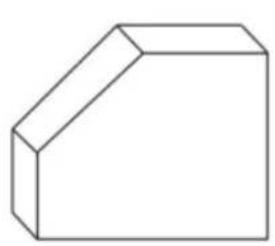
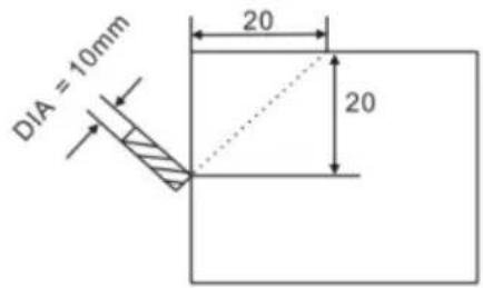
STEPS:

1. Press SN/81, then the message window displays "INCL_XY" for oblique processing. Press ▲ or ▼ to select the plane, and the display shows "SEL_XZ". Then press ENT to proceed to the next step.

1. Input the tool diameter

The message window displays "DIA", and the X window displays the previously preset angle of obliquity. Press 10 in turn to input the TOOL Diameter of obliquity. Press OK, then press ▼ to proceed to the next step;

1. Input ST_POT;

The message window displays "ST_POT", and the X and Y windows display the previously preset starting position of obliquity. Input X=0, Y=-20.000. Press OK, then press ▼ to proceed to the next step;

4. Input ED_POT;

The message window displays "ED_POT", and the X and Y windows display the previously preset starting position of obliquity. Input X=20.000, Y=0.000.

5. After inputting all parameters, press the ▼ key for machining.

For a 2-axis milling machine table, it is not installed with a Z-axis. Please press ▲ or ▼ to simulate the position of the Z-axis. Press ▲ to simulate moving to the former process, and press ▼ to simulate moving to the next process point.

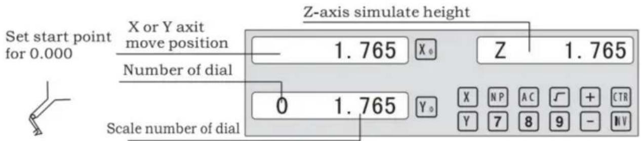
Z-axis simulate height = Number of dial x Z axis Dial + Scale number of dial

Press ☐ to quit the oblique function at any time.

6.5 Slope Processing

This function can calculate the position of every processing point automatically in processing a slope. Only the following parameters need to be inputted:

XZ, YZ

Set machine place YZ, or XZ

ANG

The inclination angle

Z_STEP

The slope length

each time processing

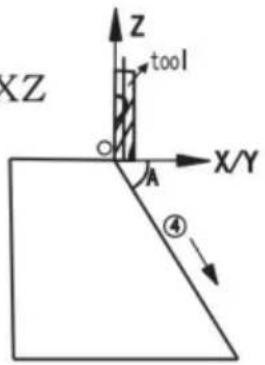
Example 1 for the Slope XZ place;

Step 1. Select place

Press TAN, then the message window displays “XZ” for the slope processing. Press ▲ or ▼ to select place to display “SEL_XY”; then press ENT to proceed to the next step;

Step 2. Input the angle of slope

The message window displays “ANG”, X window displays the formerly preset angle of slope. Press 4 5 in turn.

Step 3. Input Z_step;

The message window displays “Z STEP”, X window displays the formerly preset starting position of slope. Input 0 · 1 in turn.

Step 4: Finishing the ALL processing. Press ☐ to quit slope function any time.

6.6 Chambering Processing

1, FLAT_XY: machine place; 2, DIA: diameter of TOOL; 3, CENTER: center of the chambering; 4, SIZE: size of the chambering;

Figure as follow:

STEPS:

1. Press /W2 , then the message window displays “FLAT_XY” for the Chambering Processing.

1. Input the diameter of the tool;

1. Input the center coordinate;

1. Input the size;

5. Process Chambering;

Move the machine until the display of the axis is zero, i.e., the position of the first point. Machine the first point. Display the next machining point by pressing ▲ or ▼. On completion of machining, the right window shows OVER. Press ▲ or ▼, the system will go to the first position for the next workpiece. Press ⚠/12 to quit the Chambering Function.

6.7 The Tool Diameter Compensation Function

Without tool compensation, the operator has to move the tool for an additional distance equal to the diameter of the tool along each side when machining the four 150 and 100 sides of a workpiece to finish machining the whole brim. The digital readouts shall automatically compensate when the tool compensation function is enabled.

Note: The tool compensation is made in the direction of the X and Y axes.

Procedures:

1). Enter the function of compensating the diameter of the tool. 2). Select one of the (four) preset machining modes. 3). Input the diameter of the tool. 4). Enter machining.

Figure A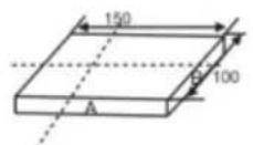

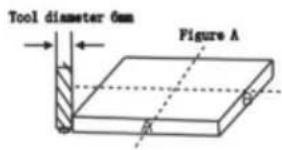
Figure B

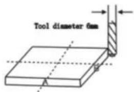
Figure C

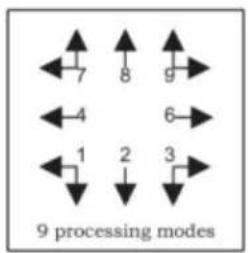
Step 1: Press ☐ to enter the tool compensation function. Then the message window displays “TYPE”. Press ☐.

Step 2: input the diameter of the TOOL; Press 10 in turn.

Step 3: Press ▼ to the machining Mode.

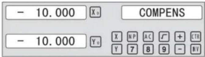
Machining of 2 side planes can be done by moving the TOOL until X-Axis is 150.000 and Y-Axis is 100.000. Press the Key [TAN/V3] to quit the Function.

6.8 Digital Filter of the Grinding Machine

When machining a work-piece by grinder, the display values quickly due to the vibration of grinder. User cannot see display value clearly. Grinder DRO provides display value filter function to disable the quake change of display value.

STEPS:

1. Enter display value filter function.

In normal display state, press SIFT to simultaneously, enter display value filter function.

1. Exit display value filter function;

Press SIFT, exit display value filter function;

6.9 The function

it will automatically exit from EDM machining status and recover to the original state before machining;

b) Stop Mode:

It will always stay at the machining interface after finishing machining, and you should press EDM to exit and back to the original state.

Operation steps:

The DEPTH (machining depth), ERRHIGH (negative fireproof height), exit mode, EDM relay output mode, and machining direction should be set.

STEPS:

1. Press EDM to enter the EDM function. Press ▲ to input parameters; press ▼ to enter EDM machining state.
2. Input DEPTH (machining depth). Press the key ▲ to set the next parameter.

1. Input ERRHIGH (negative fireproof height) (undefined). Press the key ▲ to set the next parameter.

1. Set machining direction (positive or negative). Press 1 to select positive direction. Press 0 to select negative direction. Press the key ▲ to set the next parameter.

EDM

1. Set exit mode (AUTO mode or STOP mode). Press 0 to select AUTO mode; press 1 to select STOP mode; press the key ▲ to set the next parameter.

1. Set the output mode (Mode 0 or Mode 1) (undefined). Press ☐ to select Mode 0; press ☐ to select Mode 1.

1. Continuously press ▼ to return to EDM for machining. Press EDM to quit the function.

Example 1: positive direction machining.

Machining is shown as the model chamber as follows.

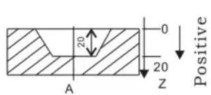
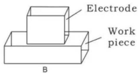
STEPS:

1. Touch one side of the workpiece with the tool, then press ₀ to zero the Z axis.

2. Press EDM, set DEPTH to 20.000; press ▼ to EDM for machining.

Example 2: Negative direction machining

Machining is shown as the model chamber as follows

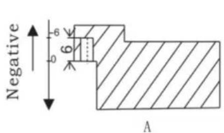
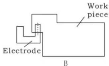
1. Touch one side of the workpiece with the tool, then press Z0 to zero the Z axis.

2. Press EDM, set DEPTH to -20.000; press ▼ to start EDM machining.

Example 3: PCD Function for EDM

The PCD function can access the EDM function. The operator enters the PCD function to input parameters for PCD and enter the PCD machining state. At every position for machining, press the EDM key to access the EDM function.

The following are the preliminary solutions for troubleshooting.

If there is still trouble, please contact our company or agents for help.

Troubles	Possible reasons	Solvents
No display	1. Power isn't connected2. Power switch is off.3. The range of power voltage is not right.4. The inner power of Linear Scale is short.	1. Check power wire and connect the power2. Turn on the power switch.3. The range of voltage is in 80--260V4. Unplug the connector of linear scale
One axis is not counting	1. Replace the linear scale of the other axis.2. DRO is in special function	1. If count is normal, the linear scale has trouble; If abnormal, the DRO readouts has trouble.2. Quit the special function.
Linear scale is not counting	1. Reading head is bad for using range exceeds.2. Aluminum chips is in reading head of linear scale.3. The span between the reading head and metal part of linear scale is large.4. The metal parts of linear scale is damage.	1. Repair the linear scale2. Repair the linear scale3. Repair the linear scale4. Repair the linear scale
Counting is error	1. Shell is poor grounding.2. Low precision of machine.3. Speed of machine is too rapid.4. Precision of linear scale is low.5. The resolution of DRO readouts and the linear scale is not match.6. The unit (mm/inch) is not match.7. Setting the linear compensating is not arrest.8. Reading head of the linear scale is damaged.	1. Shell is good grounding.2. Repair the machine.3. Reduce the speed of machine.4. Mount the linear scale again.5. Set the resolution of the DRO again,6. Cover the unit of display mm/inch.7. Reset the linear compensation.8. Repair the linear scale.
The counting of the linear scale is not accurate	1. The mounting of linear scale does not demand the requirement, and the precision is not adequate.2. The screw is loosen.3. Precision of machine is low.4. The resolution of digital readouts and the linear scale is not match.	1. Mount the linear scale again and level it.2. Lock all fixing screws.3. Repair the machine.4. Reset the resolution of digital readouts.
Sometimes the linear scale is not counting	1. The small car and steel ball is separated.2. The glass of reading head is wearied.3. The glass of reading head of the linear scale has dirt.4. The elasticity of the steel wire is not adequate.	1. Repair the linear scale.2. Repair the linear scale.3. Repair the linear scale.4. Repair the linear scale.

1. Specifications of Digital Readout

1) Supply voltage range: AC 85 V ~ 230 V; 50 ~ 60 Hz 2) Power consumption: 15 VA 3) Operating temperature: 0°C to 50°C 4) Storage temperature: -30°C to 70°C 5) Relative humidity: < 90% (25°C) 6) Max coordinate number: 3 7) Readout allowable input signal: TTL square wave 8) Allowable input signal frequency: < 5 MHz 9) Max resolution of digital display length: 0.01 μm 10) Max resolution of digital display angle: 0.0001° / pulse

1. Instructions

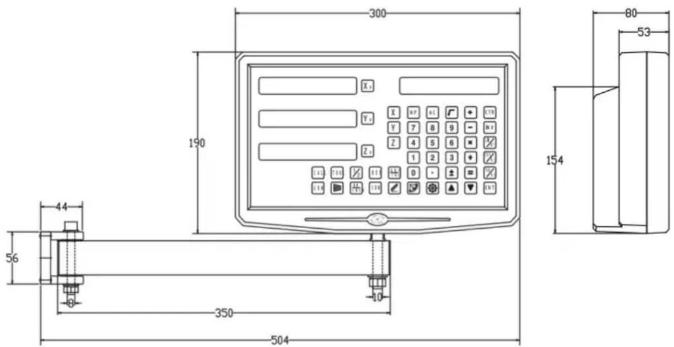
1. X, Y, Z Axis

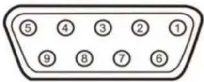
Pin	TTL (Standard)
1
2	OV
3
4
5
6	A+
7	5V
8	B+
9	R+

Pin	TTL (Standard)
1	5V
2	OV
3	A+
4	B+
5	R+
6
7
8
9

For your convenience, if you buy a digital readout,

The wiring definition of your linear scale must be the same as the two definitions in the above diagram to be universal!

Installation instructions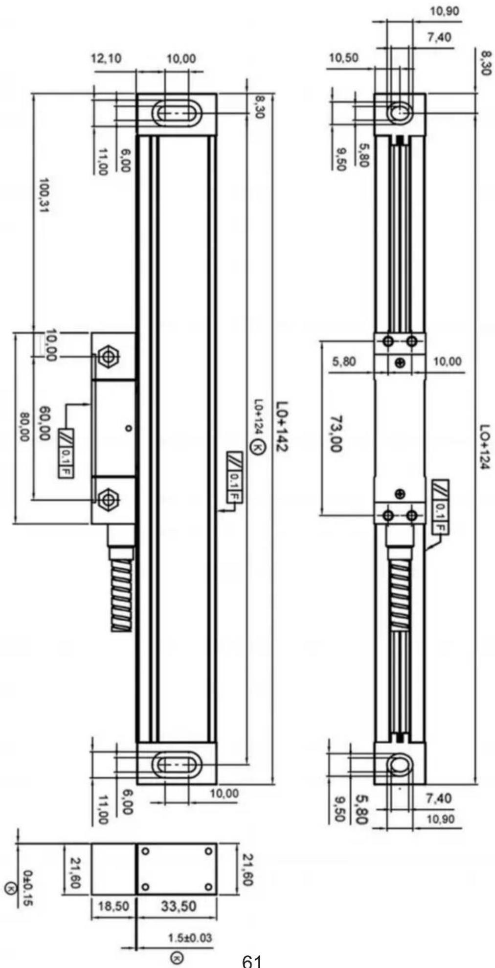

TTL signal Output: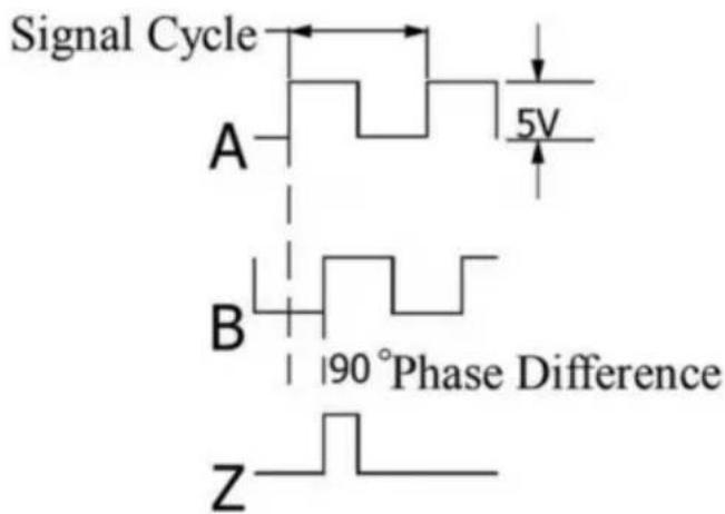

EIA-422-A signal Output: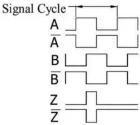

1. TECHNICAL PARAMETER 1.1 SCALING DISTANCE: 0.02 MM (50 LINES /MM) 1.2 RESOLUTION: 5μM, 1μM, 0.5μM 1.3 PRECISION: ±3μM, ±5μM, ±15μM/M (20±0.1℃) 1.4 MEASURING RANGE: 30~3000MM 1.5 MOVING SPEED: HIGH-SPEED ENCODER 120 M/MIN (TO BE CUSTOMIZED)

ORDINARY ENCODER 60M/MIN

1.6 POWER SUPPLY: +5V±5%, 80MA 1.7 CABLE LENGTH: STANDARD 3M (SPECIAL LENGTH AVAILABLE ACCORDING TO THE USER'S NEEDS) 1.8 WORKING TEMPERATURE: 0~45°C 1.9 PIN DESCRIPTION: 1) APPLICABLE TO: 9 PIN SOCKET EIA-422-A SIGNAL OUTPUT.

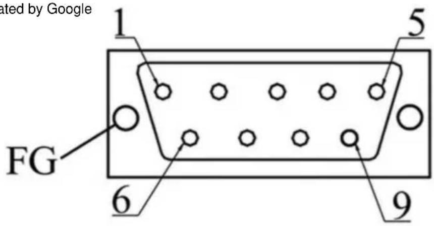
1) Applicable to: 9 pin socket EIA-422-A signal Output.

Pin Position	1	2	3	4	5	6	7	8	9
Signal		OV		Empty		A	+5V	B	Z
Color	Green Black	Black	Orange black	FG	White black	Green	Red	White	Orange

FG: Shield connected to metal casing.

1) Applicable to: 9 pin socket TTL signal Output.

Pin Position	1	2	3	4	5	6	7	8	9
Signal		OV		Empty		A	+5V	B	Z
Color		Black		FG		Green	Red	Orange	White

FG: Shield connected to metal casing.

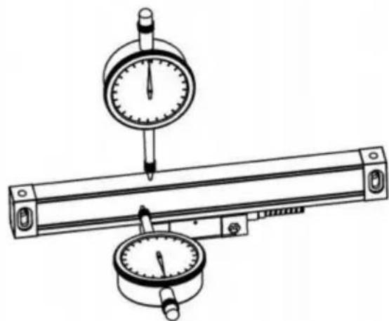
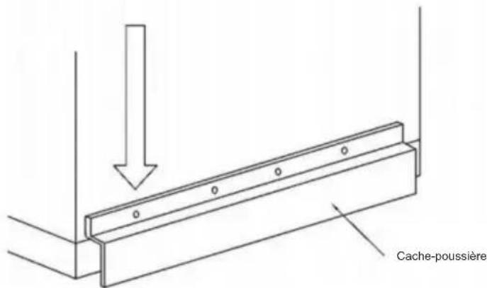
4.9

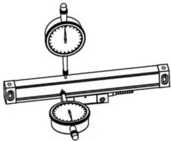
4.10

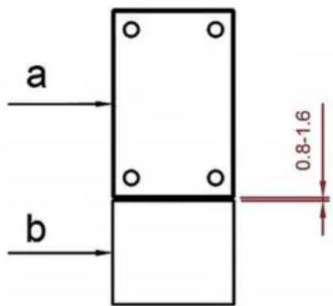
C/O YH Consulting Limited Bureau 147, Centurion House,

Route de Londres, Staines-upon-Thames, Surrey, TW18 4AX

VEVOR®

TOUGH TOOLS, HALF PRICE

www.vevor.com/support

DRO DISPLAY USER MANUAL

MODEL: SNS-3V-YE102024, SNS-3V-YE161838

With the continuous updating of products, if there are changes or

1. Illustration of Panel and keyboard 4
2. Caption of the keyboard 5
3. Parameters settings 7

3.1 Parameters setup routine entrance 7 3.2 Parameters Settings Description 7 3.2.1 Setting the Resolution 7 3.2.2 Setting Positive Direction for Counter 8 3.2.3 Toggle Between R/D Display Mode 8 3.2.4 Setting Z axis Dial 8 3.2.5 Setting the Rotary Radius of the Workpiece 9 3.2.6 Setting the Angle Display Mode 9 3.2.7 Setting the Baudrate of RS_232 (optional) 9 3.2.8 Setting the Absolute Zeroing enable or disable 10 3.2.9 Setting the Absolute form the Special Function 10 3.2.10 Setting the Calculator display Mode 10 3.2.11 Display brightness setting 10 3.2.12 The linear scale counting frequency setting 11 3.2.13 Setting QUIT 11 3.2.14 Setting the type of the DRO 11 3.2.15 Signal Interface Type 11 3.2.16 Restore Factory Settings 12 3.2.17 Shrinkage Ratio enable or disable 12 3.2.18 Setting Compensation Type 12 3.2.19 Inch display, set the number of digits after the decimal point 13 3.2.20 Setting EDM (optional) 13 3.2.21 Setting Linearity Compensation 13 3.2.22 Setting the Shrinkage Ratio 13

4. General Operations 14

4.1 Zeroing 14 4.2 Preset Data to Designated Axis 14 4.3 Toggle Display Unit between inch and mm 14 4.4 Absolute/Incremental/200 groups SDM 15 4.5 1/2 Function 15 4.6 Clear All SDM Datum 16

Contents

4.7 Sleeping Mode 16 4.8 Power Interruption Memory 16 4.9 Search the Absolute Reference Point of Scale 17 4.10 Non Linear Error Compensation 20

5. 200 Groups SDM coordinate 21 5.1 Zeroing at the Current Point....21 5.2 Preset datum of SDM coordinate 22

6. Special Function……24

6.1 Circumference Holes Processing 25 6.2 Linear Holes Processing 28 6.3 ARC Processing 30 6.4 Oblique Processing 39 6.5 Slope Processing....43 6.6 Chamber Processing....44 6.7 The Tool Diameter Compensation Function 45 6.8 Digital Filter of the Grinding Machine 46 6.9 Lathe Function 47

6.9.1 200 sets TOOL Libs 47 6.9.2 Taper Function 48 6.9.3 R/D Function 49 6.9.4 Y + Z Function (only applicable to: 3 axes Lathe)....49

6.10 EDM....50

7. Calculator……56

8. Appendix 57

THREE AXIS PANEL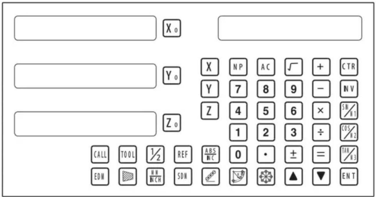

TWO AXIS PANEL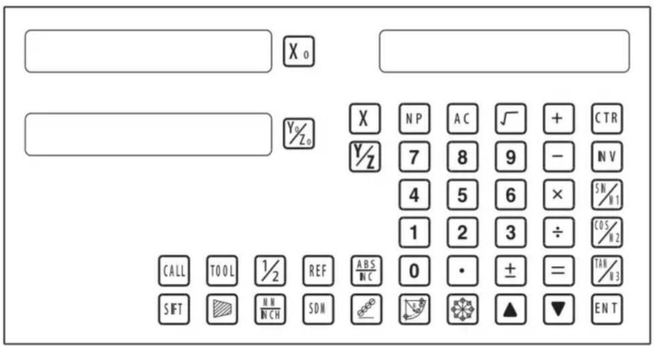

Keyboard Description

	Keys for axis selection
	Zero select axis
	Enter +/- sign
	Enter decimal point
	Entry keys for numbers
	Operation key (in Calculation function key)
[YSKH]	Enter or quit calculating state
	Cancel incorrect operation
	Calculate inverse trigonometric
	Square root
	Confirm operation
	Toggles between inch and millimeter units.
	Press when ready to identify a reference mark.
	Function keys for 200 sub datum
	ARC cutting function
	holes displayed equally on a circle
	holes displayed equally on a line

Caption of the keyboard

	Calculate trigonometric or Slope Processing function key
	Calculate trigonometric or rectangular inner chamber processing function key
	Calculate trigonometric or the tool diameter compensation function key
	Toggle between ABS/INC coordinate
	Stroll up or down to select
	Taper measured function key
	Tool library call key
	Opens the tool table.( lathe)
	EDM function key
	Filter display function key
	Half a display value of an axis
	Non Linear Error Compensation function keys

3. Parameters settings

3.1 Parameters setup routine entrance.

Press ☐ to enter initial system and self-check after DRO powers on in 1 second, then Parameters settings display in the Parameters window. Press ▲ ▼ to select the item you want to change.

If you want to quit initial setting, press ▲ ▼ until “QUIT” appears in message window and press ENTER. You can also press • to quit initial setting.

3.2 Parameters Settings Description

3.2.1 Setting the Resolution

Press ▲ ▼ until “RESOLUTE” appears in message window;

When selecting the LINEAR encoder, the resolution will be set as follows:

There are 19 types of resolution:

0.01um; 0.02um; 0.05um; 0.10um; 0.20um; 0.25um; 0.50um; 1.00um; 2.00um; 2.50um; 5.00um; 10.00um; 20.00um; 25.00um; 50.00um; 100.00um; 200.00um; 250.00um; 500.00um.

Press ₀ to change the resolution for X axis; Press ₀ to change the resolution for Y axis; Press ₀ to change the resolution for Z axis; as follows:

Set the resolution 5.00um to 1.00um for X axis:

When selecting the rotary encoder, the resolution will be set as follows:

Input the rotary encoder parameter value.

3.2.2 Setting Positive Direction for Counter

Press ▲ ▼ until “DIRECTE” appears in message window.

Direction ‘0’ means the display value will increase when scale moves from right to left and decrease when scale moves from left to right. Direction ‘1’ means the display value will increase when scale moves from left to right and decrease when scale moves from right to left.

Press ₀ to change the Direction for X axis; Press ₀ to change the Direction for Y axis; Press ₀ to change the Direction for Z axis; as follows:

3.2.3 Toggle Between R/D Display Mode

Press ▲ ▼ until “R OR D” appears in message window. X window, Y window, Z window displays ‘0’ or ‘1’ separately.

‘0’ is mode R, which means the display value equals the actual measurement. ‘1’ is mode D where the display value equals the double actual measurement. Press X₀ to change the R/D for X axis; Press Y₀ to change the R/D for Y axis; Press Z₀ to change the R/D for Z axis; as follow:

3.2.4 Setting Z axis Dial

Press ▲ ▼ until "Z DIAL" appears in message window.

Z axis dial should be set if Z axis is emulated for 2 axis milling and only install linear scale for X,Y axis. Z axis dial means the distance the Z axis travels when screw runs a revolution.

Set the Z axis Dial 2.5mm as follow ;

3.2.5 Setting the Rotary Radius of the Workpiece

Press ▲ ▼ until "RDIUS" appears in message window.

The Rotary rdius type is used perimeter to measure angle.

Input the Rotary Radius parameter value 2000mm as follow:

3.2.6 Setting the Angle Display Mode

Press ▲ ▼ until "ANG DISP" appears in message window.

Press ₀ to change the angle display mode for X axis; Press ₀ to change the angle display mode for Y axis; Press ₀ to change the angle display mode for Z axis; Example for X axis:

"0.0000" means the angle mode is Circulating DD;

"0000.0000" means the angle mode is Incremental DD;

"0.00.00" means the angle mode is Circulating DMS;

"0000.00.00" means the angle mode is Incremental DMS;

3.2.7 Setting the Baudrate of RS-232 (Special customization function, if you need to buy, please contact the dealer to customize)

Press ▲ ▼ until "BAUDRATE" appears in the message window. Set the Baudrate to 115200 as follows:

3.2.12 The linear scale counting frequency setting

The factory default setting is only "12". The higher the parameter, the lower the counting frequency. Press "X0" to set. It is not recommended that you change the default value yourself.

3.2.13 Setting QUIT: Digital display table parameters quit button.

3.2.14 Setting the type of the DRO.

The type of the DRO will be displayed on the right window. Then press the key ENT to select the correct type. The following system items will be set:

"MILL-3" means the DRO type is 3-axis milling machine table;

"MILL-2" means the DRO type is 2-axis milling machine table;

"LATHE-2" means the DRO type is 2-axis lathe table;

"LATHE-3" means the DRO type is 3-axis lathe table;

"GRIND" means the DRO type is Grind table;

"EDM" means the DRO type is EDM table; (Special customization function, if you need to buy, please contact the dealer to customize)

Function, if you need to buy, please contact the dealer to customize)

3.2.15 Signal Interface Type

Message window displays “SEL AXIS” which indicates the step is to Sensor input signal mode. Press X₀ to change the signal mode for X axis; Press Y₀ to change the signal mode for Y axis; Press Z₀ to change the signal mode for Z axis. Example for X axis:

Press X₀ to scroll through the Rotary encode type, the Linear encode type, the Rotary radius type.

X window displays the Signal type.

“LInER” means the Signal type is linear encode type;

"EnCOdE" means the Signal type is Rotary encode type;

"RdIUS" means the Signal type is Rotary radius type;

Example: currently in the linear encode type, to toggle to the Rotary encode type;

3.2.16 Restore Factory Settings:

Clear all data except DRO type. DRO will load default setup for parameter. After loading default setup, user must search RI once to enable resuming ABS datum function; otherwise to resume the datum by RI is unable;

Message window displays “ALL CLR”, press ENT and message windows display “PASSWORD” indicating the operator to input password; Press 2000 + ENT in turn to load default value;

3.2.17 Shrinkage Ratio enable or disable.

Message window displays “SRK OFF” to disable Shrinkage rate function. Press ☐ to enable Shrinkage rate function in Message window displays “SRK ON”:

3.2.18 Setting Compensation Type

The message window displays “SEL COMP”, which indicates the step is to set the compensation type. Press X0 to change the compensation type for the X axis; press Y0 to change the compensation type for the Y axis; press Z0 to change the compensation type for the Z axis. Example for X axis:

Press X0 to scroll through the compensation types: no compensation, linear compensation, and non-linear compensation.

“no-CO” means the compensation type is no compensation; “LInE-CO” means the compensation type is linear compensation; “non-LinE” means the compensation type is non-linear compensation.

Example for X axis: currently in the no compensation type, to toggle to the linear compensation type.

3.2.19 Inch display, set the number of digits after the decimal point

In the inch display mode, the number of digits after the decimal point is set. The factory default digit is "4". Press "X0" to set it, and it can be set according to actual needs.

3.2.20 Setting EDM: it is not recommended that you set the default value yourself. EDM function sets the relay off time.

3.2.21 Setting Linearity Compensation.

The message window displays “LIN COMP”, which indicates the step is to set linearity compensation. Compensate the linear error to make the display value equal to the standard value.

The calculation of compensation rectifying coefficient:

Coefficient = (Measurement - Standard value) x 1000.000 / Standard value

Example for X axis:

Measurement 200.020mm

Standard value 200.000mm

Rectifying coefficient = (200.020 - 200) * 1000 / 200 = -0.01 mm/m

Input the compensation rectifying coefficient 0.01 as follows:

3.2.22 Setting the Shrinkage Ratio

Press ▲ ▼ until "SHRINK" appears in the message window;

Shrinkage ratio = (Dimensions of the finished product) / (Dimensions of the working piece)

Set the shrinkage ratio to 1.005 as follows;

4. General Operations;

4.1 Zeroing

Zero the designated axis in the normal display state. Zeroing is used to set the current point as the datum point as follows;

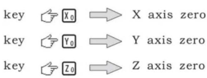
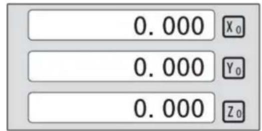
X₀ or Y₀ or Z₀ will be returned to the original data before the reset.

4.2 Preset Data to Designated Axis

Preset a value to the current position for a designated axis in the normal display state.

4.3 Toggle Display Unit between inch and mm

Length can be displayed either in "mm" (metric) or "inch" (imperial). The display unit can be toggled between mm and inch.

Example: Display value toggled from mm to inch;

Example: Display value toggle from inch to mm;

4.4 Absolute/Incremental/200 groups SDM

Function: The DRO has 3 coordinate display modes: the absolute mode (ABS); the incremental mode (INC) and 200 groups Second Data Memory (SDM) with the range of 00 to 99. Zero point of work-piece is set at the origin point of ABS coordinate. The relative distance between datum of ABS and SDM remains unchanged when ABS datum is changed.

1. Toggle from ABS to INC coordinate;

1. Toggle from INC to ABS coordinate;

1. Toggle from SMD to ABS coordinate;

4.5 1/2 Function

Function: Set the center of work piece as datum by halving the displayed value.

Example: Set the center of rectangle as datum as the right figure.

Steps:

1. Touch one side of the workpiece with the TOOL, then zero the X axis.

2. Message window displays “REF”, Press ☐NT until “FD_REF” appears in message window.

3. Select the axis which need search RI. For instance: select X axis, then press ☒. "X_REF" is displayed in message window, and X axis window flashes.

4. Move the machine table. The buzzer sounds when RI is searched, then X window stops flashing and displays the value of the current position. The DRO returns normal display state. Then message window displays "FIND_X".

Example for AB mode:

1. DRO is set in ABS coordinate. Press REF, then the message window displays "REF".

2. Press ▲ ▼, then the message window displays "AB".

3. Message window displays "AB". Press ENT until "FIND_AB" appears in message window.

4. Select the axis which needs to search RI. For instance: select X axis, then press ☒. "X_REF" is displayed in message window, and X axis window flashes.

5. Move the machine table. The buzzer sounds when RI is searched, displays the value of the current position for the absolute datum zero. The DRO returns to normal display state. Then message window displays "FIND_AB".

Example for LEF_AB mode:

1. DRO is set in ABS coordinate. Press REF, then the message window displays "REF".

2. Press ▲ ▼, then the message window displays "AB".

3. Message window displays "LEF_AB". Press ENT until "ZERO_AB" appears in message window.

4. Move the machine table to be set zero position point. Then press X, X axis will be zeroing. The current position for the absolute datum zero. The DRO returns to normal display state.

NOTE: Linear range without reference point location of the user

4.10 Non Linear Error Compensation

First compensation Type (Linear or Non-Linear) in parameter setting must be set Non-Linear. Linear scale have a ref point location and find to the Absolute Reference Point will be enable.

Default Non-Linear compensation: 50.

Example for Y axis:

Step 1: Search the Absolute Reference Point of Scale;

Step 2: Press NP, then the message window displays "COMP X".

Step 3: Press ▲ ▼, then the message window displays "COMP Y".

Step 4: Press ENT, then the message window displays "NUMBER". Then input the compensation parameter NUMBER.

Step 5: Press ▲ ▼, then the message window displays "Y-MSN-1" which indicates the step is for Non Linear Error Compensation.

Step 6: Input compensation value.

X window displays the value of the measurement value.

Y window displays the value of the standard value.

Example for the first compensation point:

Measurement value: 68.288mm. Standard value: 68.200mm

Step 7: After inputting all parameters, the DRO automatically exits.

5. 200 Groups SDM Coordinate

The DRO has three display modes: the absolute mode (ABS), the incremental mode (INC) and the 200 groups second data memory (SDM 1 - SDM200). ABS datum of the work-piece is set at the beginning and the 200 groups SDM is set relative to ABS coordinate.

ABS Mode, INC Mode and SDM Mode are specially designed to provide much more convenience features to the operator to cope with the batch machining of relative works and the machining of the workpiece machining dimensions from more than one datum.

Example: The ABS datum is the center point O, the points sdm1, sdm2, sdm3, sdm4 needed processing are set as datum of SDM 1 - SDM 4.

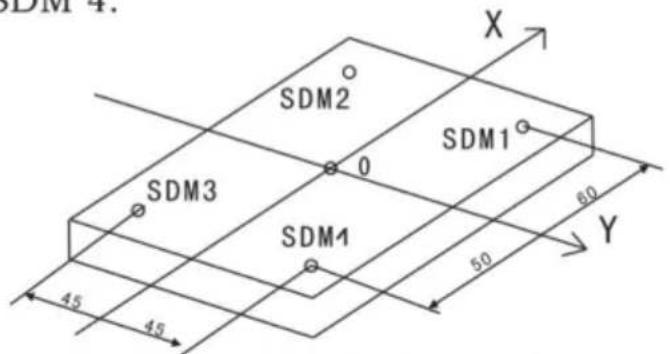
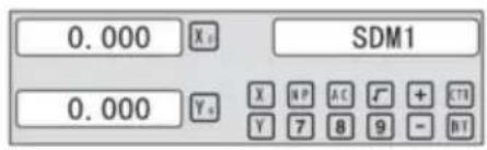
Two ways to set SDM coordinate:

1. Zeroing at the Current Point. 2. Preset datum of SDM coordinate.

5.1 Zeroing at the Current Point

First, set the center point of the workpiece as the origin of the ABS. Then align the TOOL with points SDM1, SDM2, SDM3, SDM4 by moving the machine table and zero them. It is the position to process where the “0.000” appears in the X window and Y window by moving the machine table, whether in ABS or in SDM coordinate.

Steps:

1. Move the worktable to place the TOOL at the center of the workpiece point O as the datum of ABS. Then zero X axis and Y axis in SDM 1; zero X axis and Y axis in SDM 2; zero X axis and Y axis in SDM 3; zero X axis and Y axis in SDM 4.

2. Set the point SDM1 as the datum of SDM 1. Move the machine worktable to x = 60.000, y = 45.000. Then process [X0] [Y0].

2. Set the point SDM1 as the datum of SDM 2. Move the machine worktable to x = 60.000, y = -45.000. Then process [X0] [Y0].

3. Set the point SDM1 as the datum of SDM 3. Move the machine worktable to x = -60.000, y = -45.000. Then process [X0] [Y0].

4. Set the point SDM1 as the datum of SDM 4. Move the machine worktable to x = -60.000, y = 45.000. Then process [X0] [Y0].

5.2 Preset datum of SDM coordinate

There are the same steps as Method 1. First, move the worktable to place the TOOL exactly at the origin of ABS. Secondly, enter the ABS Mode as follows.

Steps:

1. Move the worktable to place the TOOL at the center of the workpiece point O as the datum of ABS. Then zero X axis and Y axis in SDM 1; zero X axis and Y axis in SDM 2; zero X axis and Y axis in SDM 3; zero X axis and Y axis in SDM 4.

2. Set point SDM1 as the datum of SDM 1. Press ▲ ▼, then the message window displays “SDM 1”. Input x = 60.000, y = 45.000.

3. Set point SDM1 as the datum of SDM 2. Press ▲ ▼, then the message window displays “SDM 2”. Input x = -60.000, y = 45.000.

4. Set point SDM1 as the datum of SDM 3. Press ▲ ▼, then the message window displays “SDM 3”. Input x = -60.000, y = -45.000.

5. Set point SDM1 as the datum of SDM 4. Press ▲ ▼, then the message window displays “SDM 4”. Input x = -60.000, y = 45.000.

6. Special Functions

6.1 Circumference Holes Processing

The function of PCD hole positioning on a circumference is used to distribute holes equally, such as boring holes on a flange. The right window will show the parameters to be defined when selecting the PCD function. The parameters to be defined are:

PCD_XY (XZ, YZ)

Select plane

CENTER

Center position

DIA

Diameter of circle

NO_HOLE

Number of holes

STANG

Starting angle

ED ANG

Ending angle

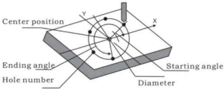
The position of the hole center is calculated automatically after inputting all parameters. Press ▲ or ▼ to choose the hole number and move the machine table until “0.000” appears in the X, Y, and Z windows. That is the position to process the table.

Example for the XY place: Machine holes on a circumference as shown in the figure.

PCD_XY(XZ,YZ)	XY
CENTER	X=0,000,Y=0.000
DIA	100,000
NO_HOLE	5
ST ANG	30,000
ED ANG	315,000

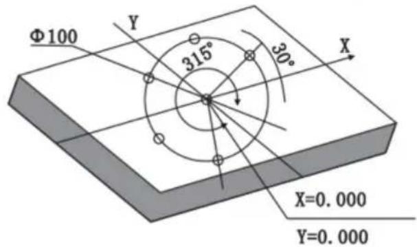
Steps:

1. Set the display unit to metric in the normal state; move the machine table until the machine tool is aligned with the center of the circle, then zero the X and Y axes.
2. Select piece.

Press 🧑️, then the message window displays “PCD_XY” for the Circumference Holes Processing. Press ▲ or ▼ to select XY place.

2. Input center position.

Press ENT, then the message window displays "CENTER". The X and Y windows display the previously preset center position. Input X = 0, Y = 0 as follows.

4. Input diameter.

Press ▼ until “DIA” appears in the message window. The X window displays the previously preset diameter. Then input the diameter as 100.000.

5. Input number.

Press ▼ until "NO_HOLE" appears in the message window. The X window displays the previously preset number. Then press 5 in turn to input the number.

6. Input starting angle.

Press ▼ until “ST ANG” appears in the message window. The X window displays the previously preset starting angle. Then press 3 and 0 in turn to input the starting angle.

7. Input ending angle.

Press ▼ until “ED ANG” appears in the message window. The X window displays the previously preset ending angle. Then press 3, 1, and 5 in turn to input the ending angle.

1. Press ▼ until "NO 1" appears in the message window.

This is the position of the first hole to punch, where “0.000” is displayed in the X and Y windows by moving the machine table. After finishing the first hole, press ▼ or ▲ to change the hole number.

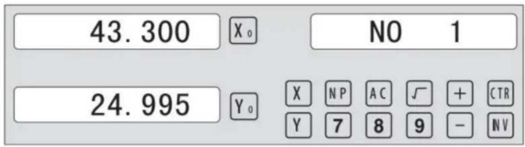
1. After processing all holes, press 📋 to return to normal display.

6.2 Linear Holes Processing

There are two modes to carry out linear drilling: Length mode and Step mode.

1. LINE S Step mode LINE L Length mode 2.STEP Step length LENGTH Line length
2. ANG Angle
3. NO.HOLE Hole number

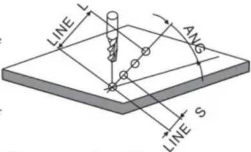
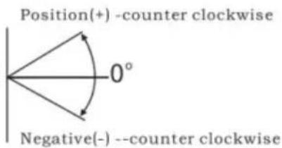
The Linear Holes function can simplify the processing of multiple holes whose centers are equally spaced on one line.

Example:

LINE_L	Length mode
LENGTH	60.000
ANG	30.000
NO.HOLE	4

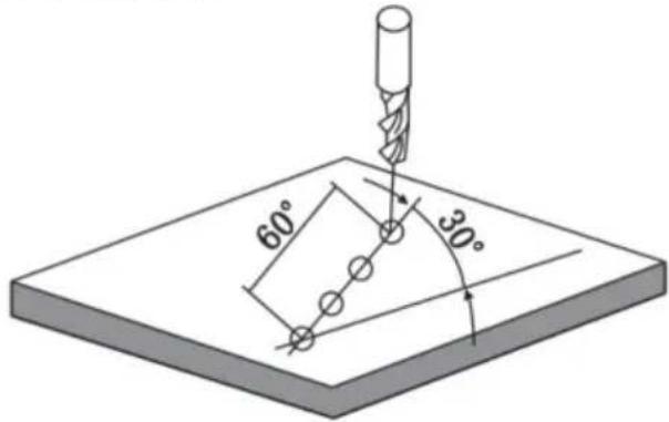
Steps:

1. Select piece.

Press 📄, then the message window displays “LINE_XY” for the Linear Holes Processing. Press ▲ or ▼ to select XY place.

2. Select Linear Holes mode.

Press ENT, then the message window displays "LINE_S". Press ▲ or ▼ to select "LINE_L".

3. Input linear length;

Press ENT, then the message window displays "LENGTH".

X window displays the formerly preset linear length. Press 6 0 in turn to input the linear length.

1. Input angle;

Message window displays “ANG” which indicates the step is to angle. X window displays the formerly preset angle. Press 3 0 in turn to input the angle.

1. Input number;

Message window displays “ANG” which indicates the step is to angle. X window displays the formerly preset number. Press 4 in turn to input the number.

1. Press ▼ until "NO 1" appears in the message window.

It is the position of the first hole to punch where the “0.000” is displayed in X window and Y window by moving the machine table. After finishing the first hole, press ▲ or ▼ to change holes number.

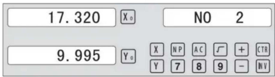
1. After processing all holes, press ☐ to return normal display.

Provides maximum flexibility in ARC machining, the ARC sector to be machined by the coordinates of ARC. Very flexible, ARC function can machine virtually all kinds of ARC, ever the intersected ARC.

Relatively a bit complicated to operate, the operator needs to calculate and enter the coordinates of the ARC center, start angle, and end angle.

Basic parameters are as follows:

1. SMOOTH: Mode of the Smooth ARC processing;
2. SEL_XY (YZ, XZ): Select plane;
3. CENTER: Refers to the position of the center.
4. RAD: Radius of the ARC
5. TL_DIA: Diameter of the TOOL
6. MAX_CUT: Feed step
7. ST_ANG: Starting angle
8. ED_ANG: Ending angle
9. RAD+TL: Outer arc. RAD-TL: Inner arc.

Example 1 for the Simple ARC Processing:

Parameter settings are as follows:

SIMPLE: Simple mode

TYPE: 3

SEL_XY XY

RAD 80.000

TL_DIA 6.000

MAX_CUT 0.500

RAD+TL 1

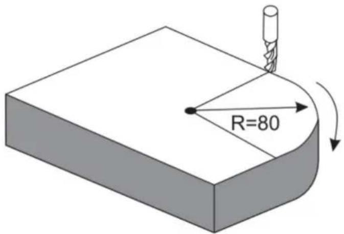
Steps:

1. Select process mode

Press 📋, then the message window displays “SIMPLE” for the ARC Processing. Press ▲ or ▼ to select mode of the simple, the message window displays “SIMPLE”

ARC Processing

2. Input the type:

Press ☐ENT until "TYPE" appears in the message window. X-window displays the formerly preset type. Press ☐3 in turn

3. Select place

Press ENT until "SEL_XY" appears in the message window. Press ▲ or ▼ to select place to display "SEL_XY";

4. Input radius:

Press ENT until "RAD" appears in the message window. X window displays the formerly preset radius of ARC. Press 8

0 in turn to input the radius.;

5. Input Diameter of the TOOL

Press ▲ or ▼ until “TL DIA” appears in the message window. The X window displays the formerly preset Diameter of the TOOL. Press 6 in turn to input the Diameter value;

6. Input Feed step (MAX_CUT);

Press ▲ or ▼ until "MAX_CUT" appears in the message window. The X window displays the formerly preset MAX_CUT. Press 0 · 5 in turn to input the MAX_CUT value;

7. Select outer arc or inner arc

Press ▲ or ▼ until “RAD-TL” appears in the message window. Press ▲ or ▼ to select place to display “RAD+TL”;

8. After inputting all parameters, press the key ENT for machining.

The DRO will display the position of the first point. Retract the axes until the displays read 0.000. Machine the Arc point by point in accordance with the display. After finishing the position of the first point, press ▲ or ▼ to change position point.

Press ☑ to quit R function any time.

Example 2 for the Simple ARC Processing:

Parameters settings as follow:

SIMPLE Simple mode

TYPE 3

SEL_XY XZ

RAD 80.000

TL_DIA 6.000

MAX_CUT 0.500

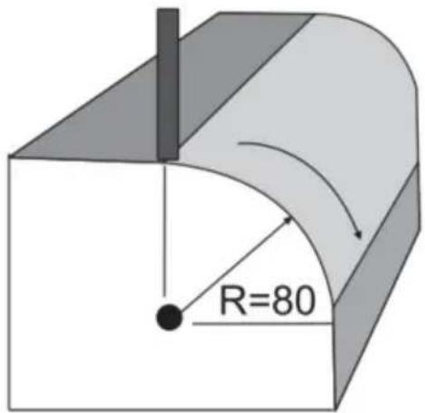
Steps:

1. Press 📋, then the message window displays “SIMPLE” for the ARC Processing. Press ▲ or ▼ to select the mode of the simple; the message window displays “SIMPLE”.

2. Input the type:

Press ☐ENT until "TYPE" appears in the message window. The X-window displays the formerly preset type. Press ☐3 in turn.

3. Select place:

Press ENT until "SEL_XZ" appears in the message window. Press ▲ or ▼ to select the place to display "SEL_XZ";

4. Input radius:

Press ☐ENT until “RAD” appears in the message window. The X-window displays the formerly preset radius of the ARC. Press ☐8 ☐0 in turn to input the radius.

5. Input Diameter of the TOOL:

Press ▲ or ▼ until “TL DIA” appears in the message window. The X-window displays the formerly preset Diameter of the TOOL. Press 6 in turn to input the Diameter value.

6. Input Feed step (MAX_CUT):

Press ▲ or ▼ until “MAX_CUT” appears in the message window. The X-window displays the formerly preset MAX_CUT. Press 0 · 5 in turn to input the MAX_CUT value.

1. After inputting all parameters, press the ENT key for machining.

For a 2-axis milling machine table, it is not installed with a Z-axis. Please press ▲ or ▼ to simulate the position of the Z-axis. Press ▲ to simulate moving to the former process, and press ▼ to simulate moving to the next process point.

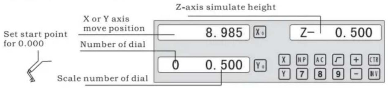
Z-axis simulated height = Number of dial x Z axis Dial + Scale number of dial

Press ☐ to quit the R function at any time.

Example 3 for the Smooth ARC function:

Parameter settings are as follows:

SMOOTH	Smooth mode
SEL_XY(YZ,XZ)	XY
CENTER	X=0,Y=0
RAD	80.000
TL_DIA	6.000
MAX_CUT	0.500
ST_ANG	0.000
ED_ANG	135.000
RAD+TL	1

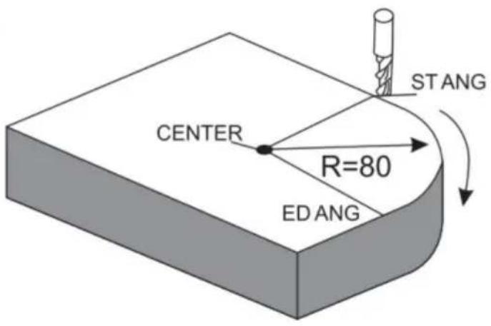
Steps:

1. Press 📋, then the message window displays "SIMPLE" for the ARC processing. Press ▲ or ▼ to select the mode of the simple, The

message window displays "SMOOTH"; For a 3-axis milling machine table, this step is not needed. In the second step, then press ENT.

2. Select place

The message window displays "SEL_XY" which indicates the selection is to place. Press ▲ or ▼ to select place to display "SEL_XY";

3. Input center position.

Press ENT, then the message window displays "CENTER". The X and Y windows display the formerly preset center position. Input X = 0, Y = 0 as follows.

4. Input radius:

Press ENT until "RAD" appears in the message window. The X window displays the formerly preset radius of the ARC. Press 8 and 0 in turn to input the radius.

5. Input Diameter of the TOOL

Press ▲ or ▼ until “TL DIA” appears in the message window. The X window displays the formerly preset diameter of the tool. Press 6 in turn to input the diameter value;

Press ☐ to quit ARC function at any time.

6) Change the angle of the workpiece to make the workpiece touch the measuring tool and adjust it to zero.

STEPS:

1. Select plane

Press SN/1, then the message window displays "INCL_XY" for oblique processing. Press ▲ or ▼ to select plane to display "SEL_XY;

Then press ☐ENT to proceed to the next step;

2. Input the angle of obliquity

The message window displays “ANG”, and the X window displays the formerly preset angle of obliquity. Press 4 5 in turn to input the angle of obliquity.

1. Move the workpiece along the X-Axis until the measuring tool touches the workpiece, adjust it to zero, and move the worktable for any distance along the X-Axis.

1. Press Y, display the value of the Y-Axis. Move the workpiece along the Y-Axis, change the angle of the workpiece to make the obliquity-calibrating plane touch the measuring tool until it turns to zero. Move the worktable until the Y-Axis is displayed as zero.

1. Press 5W/H1 to quit oblique function at any time.

Example 2 for the oblique XZ or YZ plane:

When the machining plane is on plane XZ or YZ, the function of tool inclination can instruct the operator to machine the oblique plane step by step.

Procedures for using the cutter inclination function:

When the machining plane is on the XZ or YZ plane, first calibrate the obliquity of the primary spindle nose and set the tool:

INCL_XY(XZ,YZ)	INCL_XZ
DIA	10.000
ST_POT	20.000
ED_POT	20.000

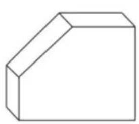
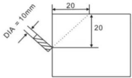
STEPS:

1. Press SN/81, then the message window displays "INCL_XY" for oblique processing. Press ▲ or ▼ to select the display "SEL_XZ"; then press ENT to proceed to the next step.

1. Input the tool diameter.

The message window displays "DIA", and the X window displays the previously preset angle of obliquity. Press 10 in turn to input the tool diameter of obliquity. OK, then press ▼ to proceed to the next step.

1. Input ST_POT.

The message window displays "ST_POT", and the X and Y windows display the previously preset starting position of obliquity. Input X=0, Y=-20.000. OK, then press ▼ to proceed to the next step.

4. Input ED_POT.

The message window displays "ED_POT", and the X and Y windows display the previously preset starting position of obliquity. Input X=20.000, Y=0.000.

5. After inputting all parameters, press the ▼ key for machining.

For a 2-axis milling machine table, which is not installed with a Z-axis, press ▲ or ▼ to simulate the position of the Z-axis. Press ▲ to simulate moving to the previous process, and press ▼ to simulate moving to the next process point.

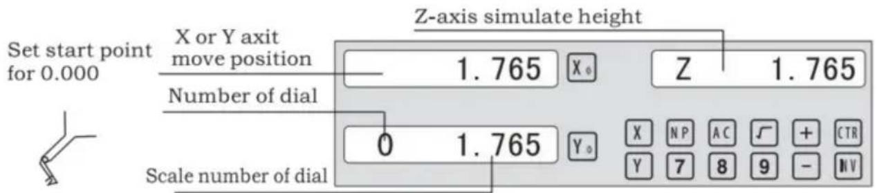
Z-axis simulated height = Number of dial x Z axis Dial + Scale number of dial.

Press ☐ to quit the oblique function at any time.

6.5 Slope Processing

This function can calculate the position of every processing point automatically in processing slope. Only the following parameters need to be inputted:

XZ, YZ

Set machine place YZ, or XZ

ANG

The inclination angle

Z_STEP

The slope length

each time processing

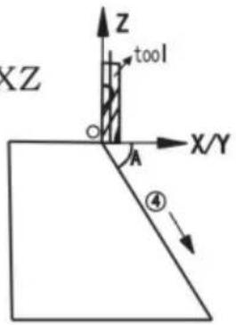
Example 1 for the Slope XZ place;

Step 1. Select place

Press \boxed{\text{TAN}}, then the message window displays "XZ" for the slope processing. Press ▲ or ▼ to select place to display "SEL_XY"; Then press \boxed{\text{ENT}} to go to next step;

Step 2. Input the angle of slope

The message window displays "ANG", X window displays the formerly preset angle of slope. Press 4 5 in turn.

Step 3. Input Z_step;

The message window displays "Z STEP", X window displays the formerly preset starting position of slope. Input 0 · 1 in turn.

Step 4: Finishing the ALL processing. Press ☐ to quit slope function any time.

6.6 Chambering Processing

1, FLAT_XY: machine place; 2, DIA: diameter of TOOL; 3, CENTER: center of the chambering; 4, SIZE: size of the chambering;

Figure as follow:

STEPS:

1. Press /W2 , then the message window displays "FLAT_XY" for the Chambering Processing.

1. Input DIA of the TOOL;

1. Input the center coordinate;

1. Input the size;

5. Process Chambering;

Move the machine until the display of the axis is zero, i.e., the position of the first point. Machine the first point. Display the next machining point by pressing ▲ or ▼. On the completion of machining, the right window shows OVER. Press ▲ or ▼, the system will go to the first position for the next workpiece. Press ⚠/12 to quit the Chambering Function.

6.7 The Tool Diameter Compensation Function

Without TOOL compensation, the operator has to move the TOOL for an additional distance of the diameter of the TOOL along each side when machining the four 150 and 100 sides of a workpiece to finish machining the whole brim. The digital readouts shall automatically compensate when the TOOL compensation function is enabled.

Note: the TOOL compensation is made in the direction of X and Y axis.

Procedures:

1). Enter the function of compensating the diameter of the TOOL. 2). Select one of the (four) preset machining modes. 3). Input the diameter of the TOOL. 4). Enter machining.

Figure A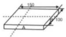

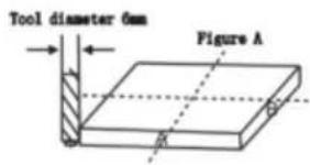
Figure B

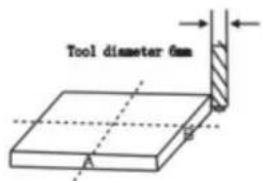
Figure C

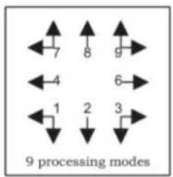
Step 1: press ☐ to enter the TOOL compensation function. Then the message window displays “TYPE”. Press ☐.

Step 2: input the diameter of the TOOL; press 10 in turn.

Step 3: press ▼ to the machining mode.

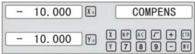
Machining of 2 side planes can be done by moving the TOOL until X-Axis is 150.000 and Y-Axis is 100.000. Press the Key [TAN/V3] to quit the function.

6.8 Digital Filter of the Grinding Machine

When machining a work-piece by grinder, the display values quickly due to the vibration of grinder. User cannot see display value clearly. Grinder DRO provides display value filter function to disable the quake change of display value.

STEPS:

1. Enter display value filter function.

In normal display state, press SIFT to simultaneously, enter display value filter function.

1. Exit display value filter function;

Press SIFT, exit display value filter function;

6.9 EDM Function

It will automatically exit from EDM machining status and recover to the original state before machining;

b) Stop Mode:

It will always stay at the machining interface after finishing machining, and you should press EDM to exit and back to the original state.

Operation steps:

The DEPTH (machining depth), ERRHIGH (negative fireproof height), exit mode, EDM relay output mode, and machining direction should be set.

STEPS:

1. Press EDM to enter the EDM function. Press ▲ to input parameters; press ▼ to enter EDM machining state.
2. Input DEPTH (machining depth). Press the key ▲ to set the next parameter.

1. Input ERRHIGH (negative fireproof height) (undefined). Press the key ▲ to set the next parameter.

1. Set machining direction (positive or negative). Press 1 to select positive direction. Press 0 to select negative direction. Press the key ▲ to set the next parameter.

EDM

1. Set exit mode (AUTO mode or STOP mode). Press 0 to select AUTO mode; press 1 to select STOP mode; press the key ▲ to set the next parameter.

1. Set the output mode (Mode 0 or Mode 1) (undefined). Press ☐ to select Mode 0; press ☐ to select Mode 1.

1. Continuously press ▼ to return to EDM for machining. Press EDM to quit the function.

Example 1: positive direction machining;

Machining is shown as the model chamber as follows

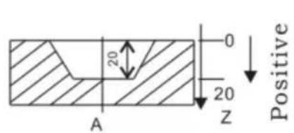
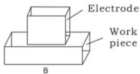
STEPS:

1. Touch one side of the workpiece with the TOOL, then press ₀ , zero the Z axis.

2. Press EDM, Setting DEPTH for 20.000; press ▼ to EDM for machining;

Example 2: Negative direction machining

Machining is shown as the model chamber as follows

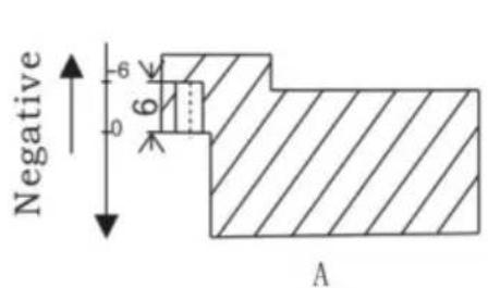
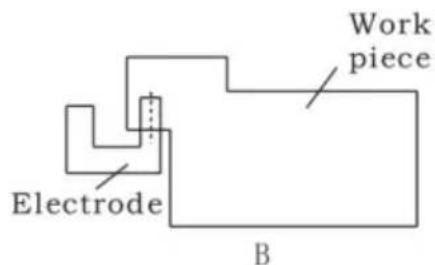
1. Touch one side of the workpiece with the TOOL, then press ₀ , zero the Z axis.

2. Press EDM, Setting DEPTH for -20.000; press ▼ to EDM for machining;

Example 3: PCD Function for EDM

PCD Function can access the EDM Function. The operator enters PCD Function to input parameters for PCD and enter PCD machining state. At every position for machining, press the key EDM to access the EDM Function.

The following are the preliminary solvents for troubleshooting.

If there is still trouble, Please contact out company or agents for help.

Troubles	Possible reasons	Solvents
No display	1. Power isn't connected2. Power switch is off.3. The range of power voltage is not right.4. The inner power of Linear Scale is short.	1. Check power wire and connect the power2. Turn on the power switch.3. The range of voltage is in 80--260V4. Unplug the connector of linear scale
One axis is not counting	1. Replace the linear scale of the other axis.2. DRO is in special function	1. If count is normal, the linear scale has trouble; If abnormal, the DRO readouts has trouble.2. Quit the special function.
Linear scale is not counting	1. Reading head is bad for using range exceeds.2. Aluminum chips is in reading head of linear scale.3. The span between the reading head and metal part of linear scale is large.4. The metal parts of linear scale is damage.	1. Repair the linear scale2. Repair the linear scale3. Repair the linear scale4. Repair the linear scale
Counting is error	1. Shell is poor grounding.2. Low precision of machine.3. Speed of machine is too rapid.4. Precision of linear scale is low.5. The resolution of DRO readouts and the linear scale is not match.6. The unit (mm/inch) is not match.7. Setting the linear compensating is not arrest.8. Reading head of the linear scale is damaged.	1. Shell is good grounding.2. Repair the machine.3. Reduce the speed of machine.4. Mount the linear scale again.5. Set the resolution of the DRO again,6. Cover the unit of display mm/inch.7. Reset the linear compensation.8. Repair the linear scale.
The counting of the linear scale is not accurate	1. The mounting of linear scale does not demand the requirement, and the precision is not adequate.2. The screw is loosen.3. Precision of machine is low.4. The resolution of digital readouts and the linear scale is not match.	1. Mount the linear scale again and level it.2. Lock all fixing screws.3. Repair the machine.4. Reset the resolution of digital readouts.
Sometimes the linear scale is not counting	1. The small car and steel ball is separated.2. The glass of reading head is wearied.3. The glass of reading head of the linear scale has dirt.4. The elasticity of the steel wire is not adequate.	1. Repair the linear scale.2. Repair the linear scale.3. Repair the linear scale.4. Repair the linear scale.

1. Specifications of Digital Readout.

1) Supply Voltage range: AC 85 V \~ 230 V; 50 \~ 60 Hz 2) Power consumption: 15VA 3) Operating temperature: 0°C-- 50°C 4) Storage temperature: - 30°C-- 70°C 5) Relative humidity: < 90 % (25) 6) Max Coordinate number: 3 7) Readout allowable input signal: TTL square wave 8) Allowable input signal frequency: < 5 M Hz 9) Max resolution of digital display length: 0.01 um 10) Max resolution of digital display angle: 0.0001 / PULSE

1. Instructions

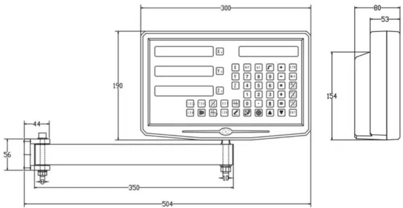
1. X, Y, Z Axis

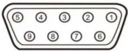
Pin	TTL (Standard)
1
2	OV
3
4
5
6	A+
7	5V
8	B+
9	R+

Pin	TTL (Standard)
1	5V
2	OV
3	A+
4	B+
5	R+
6
7
8
9

For your convenience, if you buy a digital readout,

The wiring definition of your linear scale must be the same as the 2 definitions in the above diagram to be universal!

Installation instructions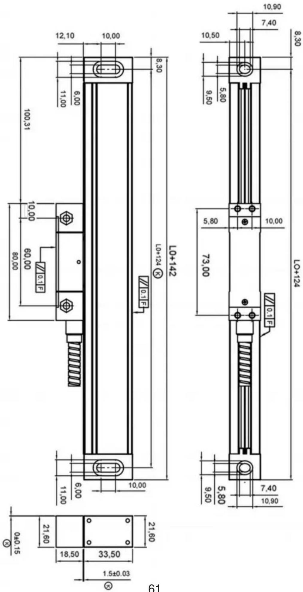

TTL signal Output: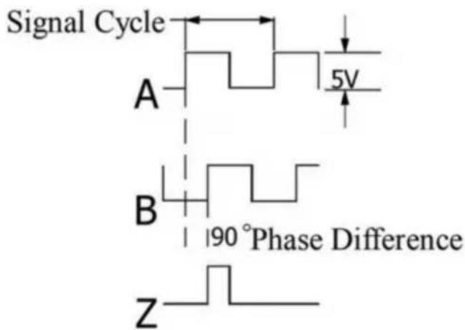

EIA-422-A signal Output: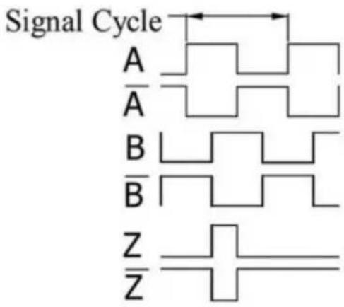

1. TECHNICAL PARAMETER 1.1 SCALING DISTANCE: 0.02 MM (50 LINES /MM) 1.2 RESOLUTION: 5μM, 1μM, 0.5μM 1.3 PRECISION: ±3μM, ±5μM, ±15μM/M (20±0.1℃) 1.4 MEASURING RANGE: 30~3000MM 1.5 MOVING SPEED: HIGH-SPEED ENCODER 120 M/MIN (TO BE CUSTOMIZED)

ORDINARY ENCODER 60M/MIN

1.6 POWER SUPPLY: +5V±5%, 80MA 1.7 CABLE LENGTH: STANDARD 3M (SPECIAL LENGTH AVAILABLE ACCORDING TO THE USER'S NEEDS) 1.8 WORKING TEMPERATURE: 0~45°C 1.9 PIN DESCRIPTION: 1) APPLICABLE TO: 9 PIN SOCKET EIA-422-A SIGNAL OUTPUT.

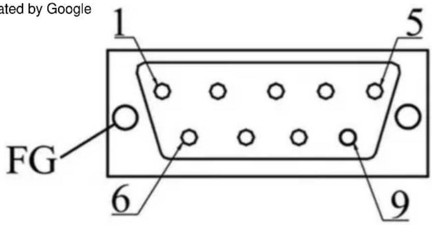
1) Applicable to: 9 pin socket EIA-422-A signal Output.

Pin Position	1	2	3	4	5	6	7	8	9
Signal		OV		Empty		A	+5V	B	Z
Color	Green Black	Black	Orange black	FG	White black	Green	Red	White	Orange

FG: Shield connected to metal casing.

1) Applicable to: 9 pin socket TTL signal Output.

Pin Position	1	2	3	4	5	6	7	8	9
Signal		OV		Empty		A	+5V	B	Z
Color		Black		FG		Green	Red	Orange	White

FG: Shield connected to metal casing.

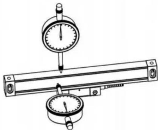
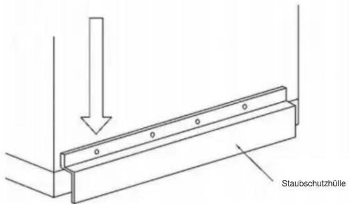
4.9

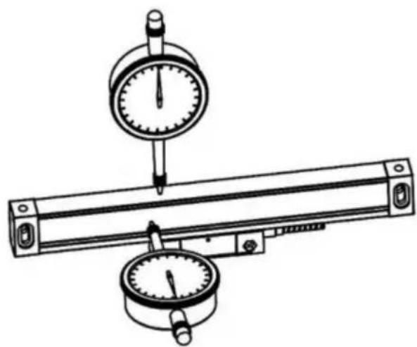
4.10

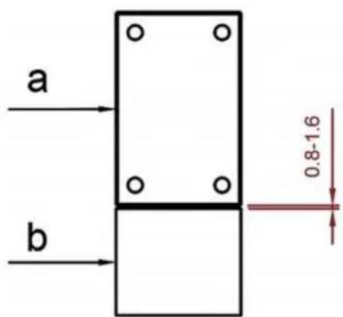
C/O YH Consulting Limited Office 147, Centurion House, London Road, Staines-upon-Thames, Surrey, TW18 4AX

VEVOR®

TOUGH TOOLS, HALF PRICE

www.vevor.com/support

VEVOR®

TOUGH TOOLS, HALF PRICE

www.vevor.com/support

DRO DISPLAY USER MANUAL

1. Illustration of Panel and keyboard 4
2. Caption of the keyboard 5
3. Parameters settings 7

3.1 Parameters setup routine entrance 7 3.2 Parameters Settings Description 7 3.2.1 Setting the Resolution 7 3.2.2 Setting Positive Direction for Counter 8 3.2.3 Toggle Between R/D Display Mode 8 3.2.4 Setting Z axis Dial 8 3.2.5 Setting the Rotary Radius of the Workpiece.... 9 3.2.6 Setting the Angle Display Mode 9 3.2.7 Setting the Baudrate of RS_232(optional) 9 3.2.8 Setting the Absolute Zeroing enable or disable 10 3.2.9 Setting the Absolute form the Special Function 10 3.2.10 Setting the Calculator display Mode 10 3.2.11 display brightness setting 10 3.2.12 The linear scale counting frequency setting 11 3.2.13 Setting QUIT 11 3.2.14 Setting the type of the DRO. 11 3.2.15 Signal Interface Type 11 3.2.16 Restore Factory Settings: 12 3.2.17 Shrinkage Ratio enable or disable....12 3.2.18 Setting Compensation Type 12 3.2.19 Inch display, set the number of digits after the decimal point…13 3.2.20 Setting EDM(optional) 13 3.2.21 Setting Linearity Compensation. 13 3.2.22 Setting the Shrinkage Ratio 13

4. General Operations 14

4.1 Zeroing....14 4.2 Preset Data to Designated Axis 14 4.3 Toggle Display Unit between inch and mm 14 4.4 Absolute/Incremental/200 groups SDM 15 4.5 1/2 Function ...... 15 4.6 Clear All SDM Datum....16

Contents

4.7 Sleeping Mode 16 4.8 Power Interruption Memory 16 4.9 Search the Absolute Reference Point of Scale 17 4.10 Non Linear Error Compensation 20

5. 200 Groups SDM coordinate 21 5.1 Zeroing at the Current Point....21 5.2 Preset datum of SDM coordinate 22

6. Special Function……24

6.1 Circumference Holes Processing 25 6.2 Linear Holes Processing 28 6.3 ARC Processing 30 6.4 Oblique Processing 39 6.5 Slope Processing....43 6.6 Chamber Processing....44 6.7 The Tool Diameter Compensation Function 45 6.8 Digital Filter of the Grinding Machine 46 6.9 Lathe Function 47

6.9.1 200 sets TOOL Libs 47 6.9.2 Taper Function 48 6.9.3 R/D Function 49 6.9.4 Y + Z Function ( only applicable to : 3 axes Lathe)....49

6.10 EDM....50

7. Calculator……56

8. Appendix 57

THREE AXIS PANEL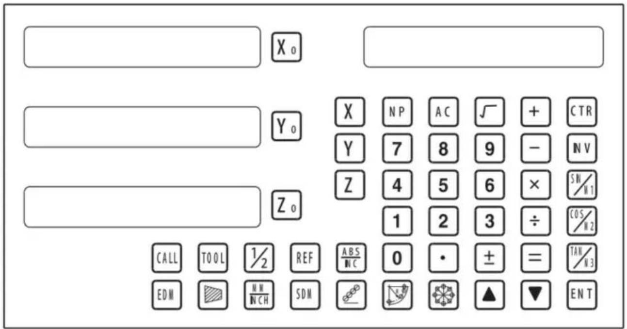

TWO AXIS PANEL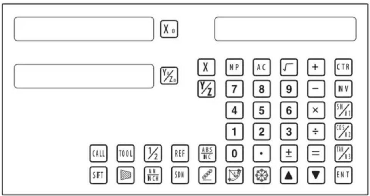

Keyboard Description

	Keys for axis selection
	Zero select axis
	Enter +/- sign
	Enter decimal point
	Entry keys for numbers
	Operation key (in Calculation function key)
	Enter or quit calculating state
	Cancel incorrect operation
	Calculate inverse trigonometric
	Square root
	Confirm operation
	Toggles between inch and millimeter units.
	Press when ready to identify a reference mark.
	Function keys for 200 sub datum
	ARC cutting function
	holes displayed equally on a circle
	holes displayed equally on a line

Caption of the keyboard

	Calculate trigonometric or Slope Processing function key
	Calculate trigonometric or rectangular inner chamber processing function key
	Calculate trigonometric or the tool diameter compensation function key
	Toggle between ABS/INC coordinate
	Stroll up or down to select
	Taper measured function key
	Tool library call key
	Opens the tool table.( lathe)
	EDM function key
	Filter display function key
	Half a display value of an axis
[HXST]	Non Linear Error Compensation function keys

3. Parameter settings

3.1 Parameter setup routine entrance.

Press ☐ to enter the initial system and self-check after the DRO powers on in 1 second, then the parameter settings are displayed in the Parameters window. Press ▲ ▼ to select the item you want to change.

If you want to quit the initial setting, press ▲ ▼ until “QUIT” appears in the message window and press ENTER. You can also press • to quit the initial setting.

3.2 Parameter settings description

3.2.1 Setting the resolution

Press ▲ ▼ until “RESOLUTE” appears in the message window.

When selecting the LINEAR encoder, the resolution will be set as follows:

There are 19 types of resolution:

0.01 µm; 0.02 µm; 0.05 µm; 0.10 µm; 0.20 µm; 0.25 µm; 0.50 µm; 1.00 µm; 2.00 µm; 2.50 µm; 5.00 µm; 10.00 µm; 20.00 µm; 25.00 µm; 50.00 µm; 100.00 µm; 200.00 µm; 250.00 µm; 500.00 µm.

Press ₀ to change the resolution for the X axis; press ₀ to change the resolution for the Y axis; press ₀ to change the resolution for the Z axis.

Set the resolution from 5.00 µm to 1.00 µm for the X axis:

When selecting the rotary encoder, the resolution will be set as follows:

Input the rotary encoder parameter value.

3.2.2 Setting Positive Direction for Counter

Press ▲ ▼ until “ DIRECTE” appears in message window.

Direction ‘0’ means the display value will increase when scale moves from right to left and decrease when scale moves from left to right. Direction ‘1’ means the display value will increase when scale moves from left to right and decrease when scale moves from right to left.

Press ₀ to change the Direction for X axis; Press ₀ to change the Direction for Y axis; Press ₀ to change the Direction for Z axis; as follow:

3.2.3 Toggle Between R/D Display Mode

Press ▲ ▼ until “R OR D” appears in message window. X window, Ywindow, Z window displays ‘0’ or ‘1’ separately.

‘0’ is mode R, which means the display value equals the actual measurement. ‘1’ is mode D where the display value equals the double actual measurement. Press X₀ to change the R/D for X axis;Press Y₀ to change the R/D for Y axis;Press Z₀ to change the R/D for Z axis; as follow:

3.2.4 Setting Z axis Dial

Press ▲ ▼ until "Z DIAL" appears in message window.

Z axis dial should be set if Z axis is emulated for 2 axis milling and only install linear scale for X,Y axis. Z axis dial means the distance the Z axis travels when screw runs a revolution.

Set the Z axis Dial 2.5mm as follow ;

3.2.5 Setting the Rotary Radius of the Workpiece

Press ▲ ▼ until "RDIUS" appears in message window.

The Rotary rdius type is used perimeter to measure angle.

Input the Rotary Radius parameter value 2000mm as follow:

3.2.6 Setting the Angle Display Mode

Press ▲ ▼ until "ANG DISP" appears in message window.

Press ₀ to change the angle display mode for X axis; Press ₀ to change the angle display mode for Y axis; Press ₀ to change the angle display mode for Z axis; Example for X axis:

"0.0000" means the angle mode is Circulating DD;

"0000.0000" means the angle mode is Incremental DD;

"0.00.00" means the angle mode is Circulating DMS;

"0000.00.00" means the angle mode is Incremental DMS;

3.2.7 Setting the Baudrate of RS_232 (Special customization function, if you need to buy, please contact the dealer to customize)

Press ▲ ▼ until “BAUDRATE” appears in message window. Set the Baudrate 115200 as follow ;

3.2.12 The linear scale counting frequency setting

The factory default setting is only "12", the higher the parameter, the lower the counting frequency, press "X0" to set, it is not recommended that you set the default value yourself.

3.2.13 Setting QUIT: Digital display table parameters quit button.

3.2.14 Setting the type of the DRO.

The type of the DRO will be display on the right window. then press the key ENT to select the correct type. the following system item will be set:

"MILL-3" means the DRO type is 3-axis milling machine table;

"MILL-2" means the DRO type is 2-axis milling machine table;

"LATHE-2" means the DRO type is 2-axis lathe table;

"LATHE-3" means the DRO type is 3-axis lathe table;

"GRIND" means the DRO type is Grind table;

"EDM" means the DRO type is EDM table; (Special customization

function, if you need to buy, please contact the dealer to customize)

3.2.15 Signal Interface Type

Message window displays "SEL AXIS" which indicates the step is to Sensor input signal mode. Press X₀ to change the signal mode for X axis; Press Y₀ to change the signal mode for Y axis; Press Z₀ to change the signal mode for Z axis. Example for X axis:

Press X₀ to scroll through the Rotary encode type, the Linear encode type, the Rotary radius type.

X window displays the Signal type.

"LInER" means the Signal type is linear encode type;

"EnCOdE" means the Signal type is Rotary encode type;

"RdIUS" means the Signal type is Rotary radius type;

Example: currently in the linear encode type, to toggle to the Rotary encode type;

3.2.16 Restore Factory Settings:

Clear all data except DRO type. DRO will load default setup for parameters. After loading default setup, the user must search RI once to enable resuming ABS datum function; otherwise, resuming the datum by RI is unable.

Message window displays “ALL CLR”, press ENT and message window displays “PASSWORD” indicating the operator to input password; press 2000 + ENT in turn to load default value.

3.2.17 Shrinkage Ratio enable or disable.

Message window displays “SRK OFF” to disable Shrinkage rate function. Press ☐ to enable Shrinkage rate function, and message window displays “SRK ON”.

3.2.18 Setting Compensation Type

Message window displays “SEL COMP” which indicates the step is to compensation type. Press X₀ to change the compensation type for X axis; press Y₀ to change the compensation type for Y axis; press Z₀ to change the compensation type for Z axis. Example for X axis:

Press X₀ to scroll through the not compensation type, the linear compensation type, the non-linear compensation type.

“no-CO” means the compensation type is not compensation type; “LInE-CO” means the compensation type is linear compensation type; “non-LinE” means the compensation type is non-linear compensation type.

Example for X axis: currently in the not compensation type, to toggle to the linear compensation type.

3.2.19 Inch display, set the number of digits after the decimal point

In the inch display mode, the number of digits after the decimal point is set. The factory default digit is "4", press "X0" to set, can be set according to actual needs.

3.2.20 Setting EDM: it is not recommended that you set the default value yourself. EDM function, set the relay off on time.

3.2.21 Setting Linearity Compensation.

Message window displays “LIN COMP” which indicates the step is to Linearity Compensation. Compensate the linear error to make display value equals to standard value.

The calculation of compensation rectifying coefficient:

Coefficient = (Measurement - Standard value) x 1000.000/ Standard value

Example for X axis:

Measurement 200.020mm

Standard value 200.000mm

Rectifying coefficient= (200.020-200) * 1000 /200 = -0.01mm/m

Input compensation rectifying coefficient 0.01 as follow:

3.2.22 Setting the Shrinkage Ratio

Press ▲ ▼ until “ SHRINK” appears in message window;

Shrinkage radio = Dimensions of the finished product/Dimensions of the working piece

Set the shrinkage radio 1.005 as follow;

4. General Operations;

4.1 Zeroing

Zero the designated axis in normal display state. Zeroing is used to set the current point as datum point as follow;

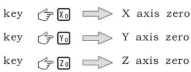
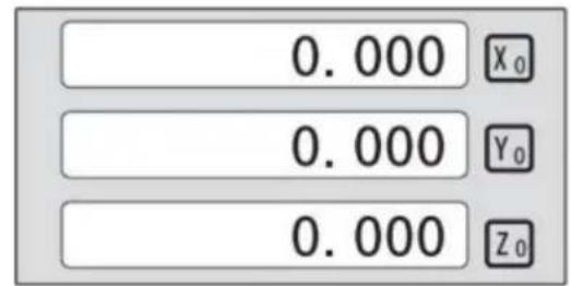
X₀ or Y₀ or Z₀ will be return to the original data before the reset.

4.2 Preset Data to Designated Axis

Preset a value to current position for a designated axis in normal display state.

4.3 Toggle Display Unit between inch and mm

Length can be displayed either in "mm" (metric) or "inch" (imperial). Display unit can be toggled between mm and inch.

Example: Display value toggle from mm to inch;

Example: Display value toggle from inch to mm;

4.4 Absolute/Incremental/200 groups SDM

Function: The DRO has 3 coordinate display modes: the absolute mode (ABS); the incremental mode (INC) and 200 groups Second Data Memory (SDM) with the range of 00 to 99. Zero point of work-piece is set at the origin point of ABS coordinate. The relative distance between datum of ABS and SDM remains unchanged when ABS datum is changed.

1. Toggle from ABS to INC coordinate;

1. Toggle from INC to ABS coordinate;

1. Toggle from SMD to ABS coordinate;

4.5 1/2 Function

Function: Set the center of work piece as datum by halving the displayed value.

Example: Set the center of rectangle as datum as the right figure.

Steps:

1. Touch one side of the workpiece with the TOOL, then zero the X axis.

2. The message window displays “REF”. Press ☐NT until “FD_REF” appears in the message window.

3. Select the axis which needs to search for RI. For instance: select the X axis, then press ☒. "X_REF" is displayed in the message window, and the X axis window flashes.

4. Move the machine table. The buzzer sounds when RI is searched, then the X window stops flashing and displays the value of the current position. The DRO returns to normal display state. Then the message window displays "FIND_X".

Example for AB mode:

1. The DRO is set in ABS coordinate. Press REF, then the message window displays "REF".

2. Press ▲ ▼, then the message window displays “AB”.

3. The message window displays “AB”. Press ENT until “FIND_AB” appears in the message window.

4. Select the axis which needs to search for RI. For instance: select the X axis, then press ☒. “X_REF” is displayed in the message window, and the X axis window flashes.

5. Move the machine table. The buzzer sounds when RI is searched, and the value of the current position for the absolute datum zero is displayed. The DRO returns to normal display state. Then the message window displays "FIND_AB".

Example for LEF_AB mode:

1. The DRO is set in ABS coordinate. Press REF, then the message window displays "REF".

2. Press ▲ ▼, then the message window displays “AB”.

3. The message window displays "LEF_AB". Press ENT until "ZERO_AB" appears in the message window.

4. Move the machine table to the position to be set as zero point. Then press X, and the X axis will be zeroed. The current position for the absolute datum zero is set. The DRO returns to normal display state.

NOTE: Linear range without reference point location of the user

4.10 Non-Linear Error Compensation

First, the compensation type (Linear or Non-Linear) in the parameter setting must be set to Non-Linear. Linear scale has a reference point location, and finding the Absolute Reference Point will be enabled.

Default Non-Linear compensation: 50.

Example for Y axis:

Step 1: Search the Absolute Reference Point of the scale.

Step 2: Press NP, then the message window displays "COMP X".

Step 3: Press ▲ ▼, then the message window displays "COMP Y".

Step 4: Press ENT, then the message window displays "NUMBER". Then input the compensation parameter NUMBER.

Step 5: Press ▲ ▼, then the message window displays "Y-MSN-1", which indicates the step is for Non-Linear Error Compensation.

Step 6: Input compensation value.

X window displays the value of the measurement value.

Y window displays the value of the standard value.

Example for the first compensation point:

Measurement value: 68.288 mm. Standard value: 68.200 mm.

Step 7: After inputting all parameters, the DRO automatically exits.

5. 200 Groups SDM Coordinate

The DRO has three display modes: the absolute mode (ABS), the incremental mode (INC), and the 200 groups second data memory (SDM 1 - SDM200). The ABS datum of the workpiece is set at the beginning, and the 200 groups SDM is set relative to the ABS coordinate.

ABS Mode, INC Mode, and SDM Mode are specially designed to provide much more convenience features to the operator to cope with the batch machining of relative works and the machining of the workpiece machining dimensions from more than one datum.

Example: The ABS datum is the center point O, and the points sdm1, sdm2, sdm3, sdm4 needed for processing are set as the datum of SDM 1 - SDM 4.

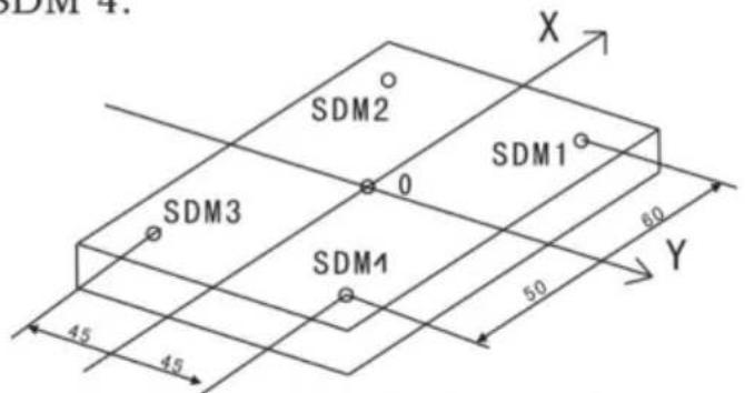
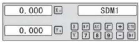
Two ways to set SDM coordinate:

1. Zeroing at the current point. 2. Preset datum of SDM coordinate.

5.1 Zeroing at the Current Point

First, set the center point of the workpiece as the origin of the ABS. Then align the tool with points SDM1, SDM2, SDM3, SDM4 by moving the machine table and zero them. It is the position to process where the “0.000” appears in the X window and Y window by moving the machine table, whether in ABS or in SDM coordinate.

Steps:

1. Move the worktable to place the tool at the center of the workpiece point O as the datum of ABS. Then zero the X axis and Y axis in SDM 1; zero the X axis and Y axis in SDM 2; zero the X axis and Y axis in SDM 3; zero the X axis and Y axis in SDM 4.

2. Set the point sdm1 as the datum of SDM 1. Move the machine worktable to x = 60.000, y = 45.000. Then process X0 Y0.

2. Set the point sdm1 as the datum of SDM 2. Move the machine worktable to x = 60.000, y = -45.000. Then process X0 Y0.

3. Set the point sdm1 as the datum of SDM 3. Move the machine worktable to x = -60.000, y = -45.000. Then process X0 Y0.

4. Set the point sdm1 as the datum of SDM 4. Move the machine worktable to x = -60.000, y = 45.000. Then process X0 Y0.

5.2 Preset Datum of SDM Coordinate

The procedure is the same as Method 1. First, move the worktable to place the tool exactly at the origin of ABS. Then, enter the ABS mode as follows.

Steps:

1. Move the worktable to place the tool at the center of the workpiece point O as the datum of ABS. Then zero the X and Y axes in SDM 1; zero the X and Y axes in SDM 2; zero the X and Y axes in SDM 3; zero the X and Y axes in SDM 4.

2. Set point SDM1 as the datum of SDM 1. Press ▲ ▼, then the message window displays “SDM 1”. Input x = 60.000, y = 45.000.

3. Set point SDM1 as the datum of SDM 2. Press ▲ ▼, then the message window displays “SDM 2”. Input x = -60.000, y = 45.000.

4. Set point SDM1 as the datum of SDM 3. Press ▲ ▼, then the message window displays “SDM 3”. Input x = -60.000, y = -45.000.

5. Set point SDM1 as the datum of SDM 4. Press ▲ ▼, then the message window displays “SDM 4”. Input x = -60.000, y = 45.000.

The PCD (Pitch Circle Diameter) hole positioning function on a circumference is used to distribute holes equally, such as boring holes on a flange. When selecting the PCD function, the right window will show the parameters to be defined. The parameters to be defined are:

PCD_XY (XZ, YZ)

Select place

CENTER

Center position

DIA

Diameter of circle

NO_HOLE

Hole number

STANG

Starting angle

ED ANG

Ending angle

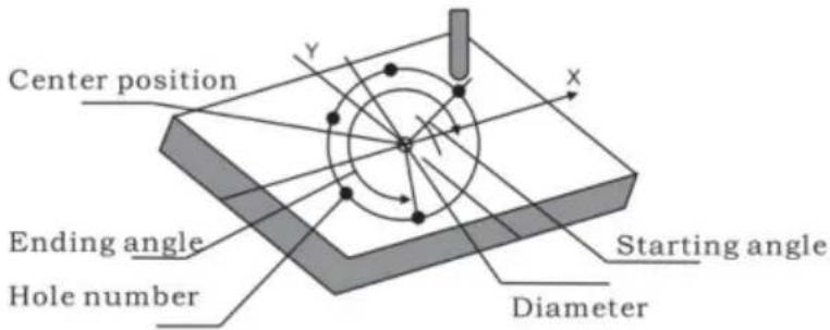
The position of the hole center is calculated automatically after inputting all parameters. Press ▲ or ▼ to choose the hole number and move the machine table until “0.000” appears in the X, Y, and Z windows. That is the position to process a table.

Example for the XY place: Machine holes on a circumference as shown in the figure.

PCD_XY(XZ,YZ)	XY
CENTER	X=0,000,Y=0.000
DIA	100,000
NO_HOLE	5
ST ANG	30,000
ED ANG	315,000

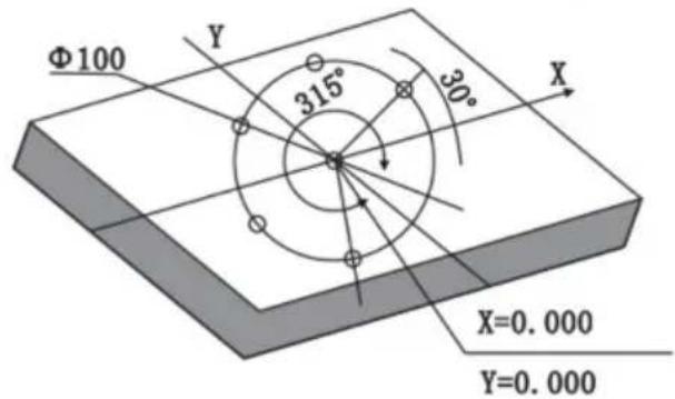
Steps:

1. Set the display unit to metric in normal state; move the machine table until the machine tool is aligned with the center of the circle, then zero the X and Y axes.
2. Select piece.

Press 🧑️, then the message window displays “PCD_XY” for the Circumference Holes Processing. Press ▲ or ▼ to select XY place.

2. Input center position.

Press ENT, then the message window displays "CENTER". The X and Y windows display the formerly preset center position. Input X = 0, Y = 0 as follows.

4. Input diameter.

Press ▼ until “DIA” appears in the message window. The X window displays the formerly preset diameter. Then input the diameter as 100.000.

5. Input number.

Press ▼ until "NO_HOLE" appears in the message window. The X window displays the formerly preset number. Then press 5 in turn to input the number.

6. Input starting angle.

Press ▼ until "ST ANG" appears in the message window. The X window displays the formerly preset starting angle. Then press 3 0 in turn to input the starting angle.

7. Input ending angle.

Press ▼ until "ED ANG" appears in the message window. The X window displays the formerly preset ending angle. Then press 3 1 5 in turn to input the ending angle.

1. Press ▼ until "NO 1" appears in the message window.

It is the position of the first hole to punch where the "0.000" is displayed in the X window and Y window by moving the machine table. After finishing the first hole, press ▼ or ▲ to change the hole number.

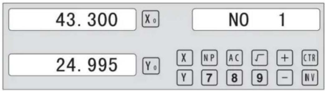
1. After processing all holes, press 📋 to return to normal display.

6.2 Linear Holes Processing

There are two modes to carry out the linear drilling: Length mode and Step mode.

1. LINE S Step mode LINE L Length mode 2. STEP Step length LENGTH Line length
2. ANG Angle
3. NO. HOLE Hole number

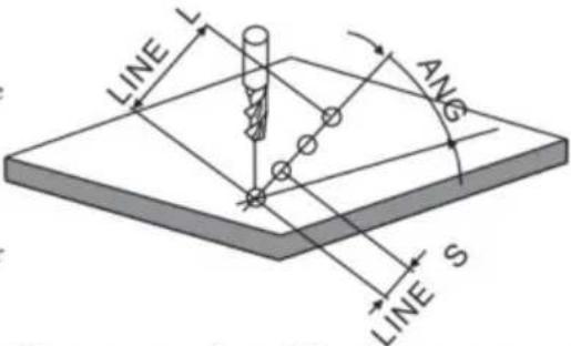
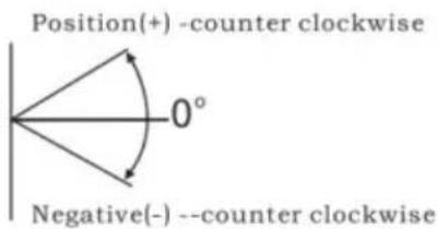
The Linear Holes function can simplify the processing of multiple holes whose centers are equally spaced on one line.

Example:

LINE_L	Length mode
LENGTH	60.000
ANG	30.000
NO.HOLE	4

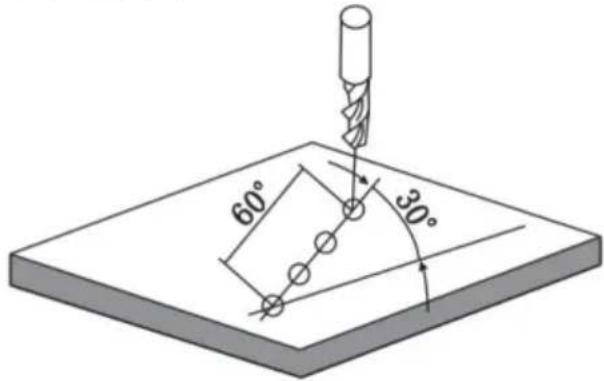
Steps:

1. Select piece.

Press 📄, then the message window displays “LINE_XY” for the Linear Holes Processing. Press ▲ or ▼ to select the XY position.

2. Select Linear Holes mode.

Press ENT, then the message window displays "LINE_S". Press ▲ or ▼ to select "LINE_L".

3. Input linear length;

Press ENT, then the message window displays "LENGTH".

The X window displays the previously preset linear length. Press 6 and 0 in turn to input the linear length.

1. Input angle;

The message window displays “ANG” which indicates the step is to set the angle. The X window displays the previously preset angle. Press 3 and 0 in turn to input the angle.

1. Input number;

The message window displays “NUM” which indicates the step is to set the number. The X window displays the previously preset number. Press 4 in turn to input the number.

1. Press ▼ until "NO 1" appears in the message window.

This is the position of the first hole to punch, where “0.000” is displayed in the X window and Y window by moving the machine table. After finishing the first hole, press ▲ or ▼ to change the hole number.

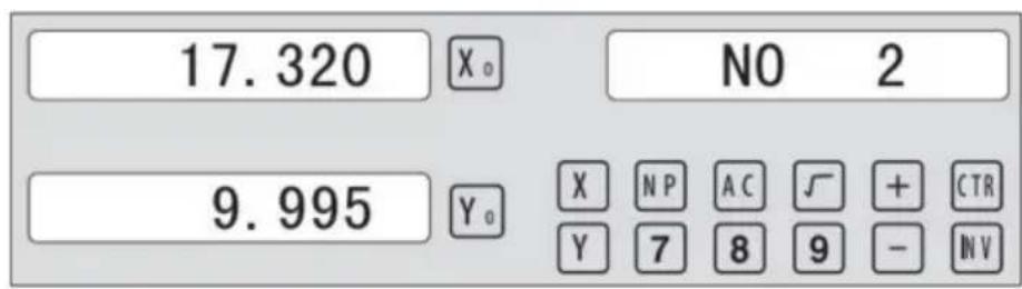
1. After processing all holes, press ☐ to return to normal display.

Provides maximum flexibility in ARC machining; the ARC sector to be machined is defined by the coordinates of the ARC. Very flexible, the ARC function can machine virtually all kinds of arcs, even intersected arcs.

Relatively a bit complicated to operate; the operator needs to calculate and enter the coordinates of the ARC center, start angle, and end angle.

Basic parameters are as follows:

1. SMOOTH: Mode of the Smooth ARC processing;
2. SEL_XY (YZ, XZ): Select plane;
3. CENTER: Position of the center.
4. RAD: Radius of the ARC
5. TL_DIA: Diameter of the tool
6. MAX_CUT: Feed step
7. ST_ANG: Starting angle
8. ED_ANG: Ending angle
9. RAD+TL: Outer arc. RAD-TL: Inner arc.

Example 1 for the Simple ARC Processing:

Parameter settings are as follows:

SIMPLE Simple mode

TYPE 3

SEL_XY XY

RAD 80.000

TL_DIA 6.000

MAX_CUT 0.500

RAD+TL 1

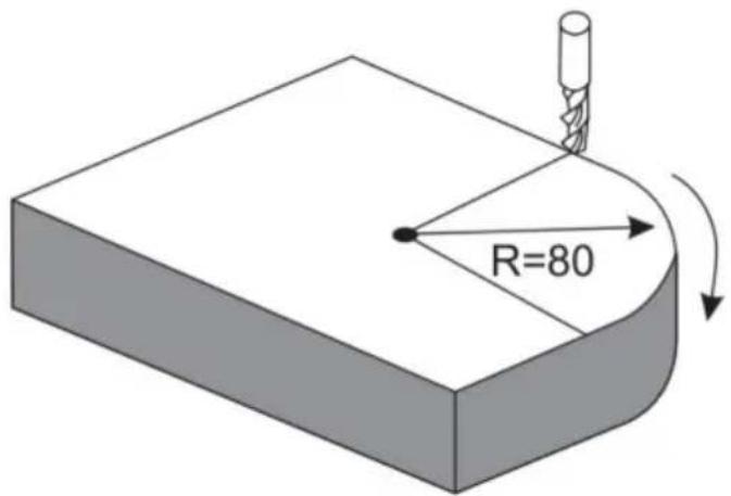
Steps:

1. Select process mode

Press 📋, then the message window displays “SIMPLE” for the ARC Processing. Press ▲ or ▼ to select the mode of the simple, the message window displays “SIMPLE”

ARC Processing

2. Input the type:

Press ☐ENT until "TYPE" appears in the message window. The X-window displays the formerly preset type. Press ☐3 in turn

3. Select place

Press ENT until "SEL_XY" appears in the message window. Press ▲ or ▼ to select the place to display "SEL_XY";

4. Input radius:

Press ENT until "RAD" appears in the message window. The X window displays the previously preset radius of the ARC. Press 8

0 in turn to input the radius.

5. Input Diameter of the TOOL

Press ▲ or ▼ until "TL DIA" appears in the message window. The X window displays the previously preset Diameter of the TOOL. Press 6 in turn to input the Diameter value.

6. Input Feed step (MAX_CUT).

Press ▲ or ▼ until "MAX_CUT" appears in the message window. The X window displays the previously preset MAX_CUT. Press 0 · 5 in turn to input the MAX_CUT value.

7. Select outer arc or inner arc

Press ▲ or ▼ until "RAD-TL" appears in the message window. Press ▲ or ▼ to select the display to show "RAD+TL".

8. After inputting all parameters, press the key ENT for machining.

The DRO will display the position of the first point. Retract the axes until the displays read 0.000. Machine the Arc point by point in accordance with the display. After finishing the position of the first point, press ▲ or ▼ to change position point.

Press ☑ to quit R function at any time.

Example 2 for the Simple ARC Processing:

Parameters settings as follows:

SIMPLE Simple mode

TYPE 3

SEL_XY XZ

RAD 80.000

TL_DIA 6.000

MAX_CUT 0.500

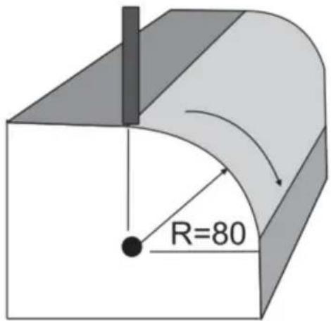
Steps:

1. Press 📋, then the message window displays “SIMPLE” for the ARC Processing. Press ▲ or ▼ to select the mode of the simple. The message window displays “SIMPLE”

ARC Processing

2. Input the type:

Press ☐ENT until "TYPE" appears in the message window. The X-window displays the formerly preset type. Press ☐3 in turn.

3. Select place

Press ENT until "SEL_XZ" appears in the message window. Press ▲ or ▼ to select the place to display "SEL_XZ".

4. Input radius:

Press ☐ENT until “RAD” appears in the message window. The X window displays the formerly preset radius of the ARC. Press ☐8 ☐0 in turn to input the radius.

5. Input Diameter of the TOOL

Press ▲ or ▼ until “TL DIA” appears in the message window. The window displays the formerly preset diameter of the tool. Press 6 in turn to input the diameter value;

6. Input feed step (MAX_CUT);

Press ▲ or ▼ until “MAX_CUT” appears in the message window. The window displays the formerly preset MAX_CUT. Press 0 · 5 in turn to input the MAX_CUT value;

1. After inputting all parameters, press the key ENT for machining.

For 2-axis milling machine table, it is not installed with Z-axis, please press ▲ or ▼ to simulate position of Z-axis. Press ▲ to simulate moving to the former process, and press ▼ to simulate moving to the next process point.

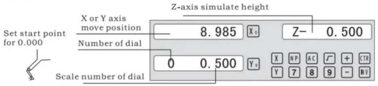
Z-axis simulate height = Number of dial x Z axis Dial + Scale number of dial

Press ☐ to quit R function any time.

Example 3 for the Smooth ARC function:

Parameters settings as follow:

SMOOTH	Smooth mode
SEL_XY(YZ,XZ)	XY
CENTER	X=0,Y=0
RAD	80.000
TL_DIA	6.000
MAX_CUT	0.500
ST_ANG	0.000
ED_ANG	135.000
RAD+TL	1

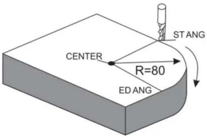
Steps:

1. Press 📋, then the message window displays “SIMPLE” for the ARC Processing. Press ▲ or ▼ to select mode of the simple, The

message window displays "SMOOTH"; For 3-axis milling machine table without this step. In second step. Then press ENT.

2. Select place

Message window displays “SEL_XY” which indicates the select is to place. Press ▲ or ▼ to select place to display “SEL_XY”;

3. Input center position.

Press ENT, then the message window displays "CENTER". The X and Y windows display the previously preset center position. Input X = 0, Y = 0 as follows.

4. Input radius:

Press ENT until "RAD" appears in the message window. The X window displays the previously preset radius of the arc. Press 8, then 0 in turn to input the radius.

5. Input diameter of the tool

Press ▲ or ▼ until "TL DIA" appears in the message window. The X window displays the previously preset diameter of the tool. Press 6 in turn to input the diameter value.

Press to quit the ARC function at any time.

6) Change the angle of the workpiece to make the workpiece touch the measuring tool and adjust it to zero.

STEPS:

1. Select place

Press SN/1, then the message window displays "INCL_XY" for oblique processing. Press ▲ or ▼ to select the place to display "SEL_XY".

Then press ENT to proceed to the next step.

2. Input the angle of obliquity

The message window displays "ANG", and the X window displays the previously preset angle of obliquity. Press 4, then 5 in turn to input the angle of obliquity.

1. Move the workpiece along the X-axis until the measuring tool touches the workpiece, adjust it to zero, and move the worktable for any distance along the X-axis.

1. Press Y to display the value of the Y-axis. Move the workpiece along the Y-axis, change the angle of the workpiece to make the obliquity-calibrating plane touch the measuring tool until it turns to zero. Move the worktable until the Y-axis is displayed as zero.

1. Press 5W/H1 to quit oblique function any time.

Example 2 for the oblique XZ or YZ plane:

When the machining plane is on plane XZ or YZ, the function of TOOL inclination can instruct the operator to machine the oblique plane step by step.

Procedures for using the function of cutter inclination:

When the machining plane is on plane XZ or YZ, first please calibrate the obliquity of the primary spindle nose and set the TOOL:

INCL_XY(XZ,YZ)	INCL_XZ
DIA	10.000
ST_POT	20.000
ED_POT	20.000

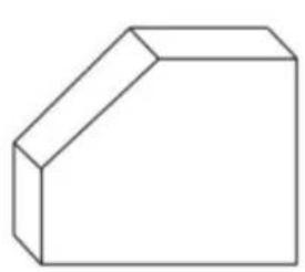
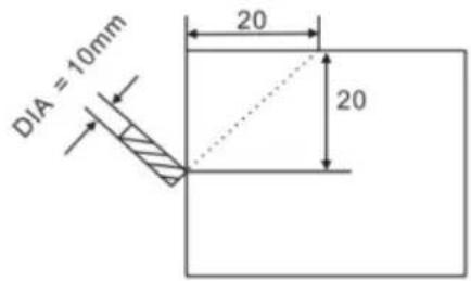
STEPS:

1. Press SN/81, then the message window displays "INCL_XY" for the oblique processing. Press ▲ or ▼ to select the plane to display "SEL_XZ"; then press ENT to go to the next step;

1. Input the TOOL Diameter

The message window displays "DIA", the X window displays the formerly preset angle of obliquity. Press 10 in turn to input the TOOL diameter of obliquity. OK, then press ▼ to go to the next step;

1. Input ST_POT;

The message window displays "ST_POT", the X and Y windows display the formerly preset starting position of obliquity. Input X=0, Y=-20.000. OK, then press ▼ to go to the next step;

4. Input ED_POT;

The message window displays "ED_POT", the X and Y windows display the formerly preset starting position of obliquity. Input X=20.000, Y=0.000.

5. After inputting all parameters, press the key ▼ for machining.

For a 2-axis milling machine table, it is not installed with a Z-axis, please press ▲ or ▼ to simulate the position of the Z-axis. Press ▲ to simulate moving to the former process, and press ▼ to simulate moving to the next process point.

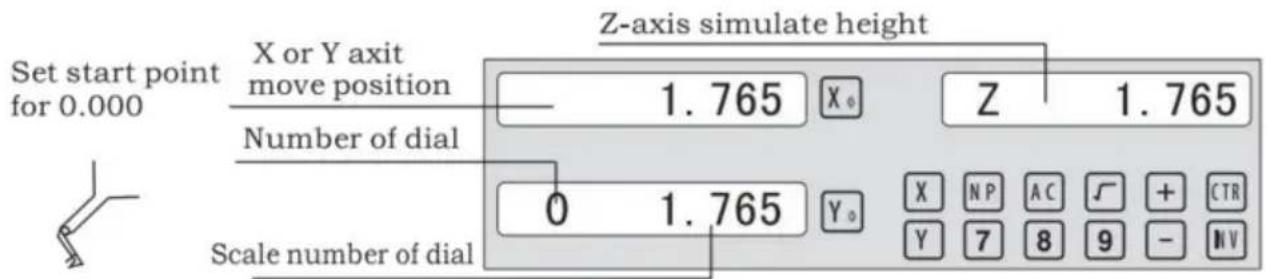
Z-axis simulate height = Number of dial x Z axis Dial + Scale number of dial

Press ☐ to quit oblique function any time.

6.5 Slope Processing

This function can calculate the position of every processing point automatically in processing slope. Only the following parameters need to be inputted:

XZ, YZ

Set machine place YZ, or XZ

ANG

The inclination angle

Z_STEP

The slope length

each time processing

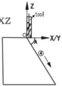
Example 1 for the Slope XZ place;

Step 1. Select place

Press , then the message window display “XZ” to the slope Processing. Press ▲ or ▼ to select place to display “SEL_XY; Then press to in next step;

Step 2. Input the angle of slope

The message window displays "ANG", and the X window displays the previously preset angle of slope. Press 4 and 5 in turn.

Step 3. Input Z_step;

The message window displays "Z STEP", and the X window displays the previously preset starting position of slope. Input 0 and 1 in turn.

Step 4: Finishing the ALL processing. Press ☐ to quit slope function at any time.

6.6 Chambering Processing

1, FLAT_XY: machine place; 2, DIA: diameter of TOOL; 3, CENTER: center of the chambering; 4, SIZE: size of the chambering;

Figure as follows:

STEPS:

1. Press /W2 , then the message window displays "FLAT_XY" for the Chambering Processing.

1. Input DIA of the TOOL;

1. Input the center coordinate;

1. Input the size;

5. Process Chambering;

Move the machine until the display of the axis is zero, i.e., the position of the first point. Machine the first point. Display the next machining point by pressing ▲ or ▼. On completion of machining, the right window shows OVER. Press ▲ or ▼, the system will go to the first position for the next workpiece. Press ⚠/12 to quit the Chambering Function.

6.7 The Tool Diameter Compensation Function

Without TOOL compensation, the operator has to move the TOOL for an additional distance of the diameter of the TOOL along each side when machining the four 150 and 100 sides of a workpiece to finish machining the whole brim. The digital readouts shall automatically compensate when the TOOL compensation function is enabled.

Note: the TOOL compensation is made in the direction of X and Y axis.

Procedures:

1). Enter the function of compensating the diameter of the TOOL. 2). Select one of the (four) preset machining modes. 3). Input the diameter of the TOOL. 4). Enter machining.

Figure A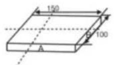

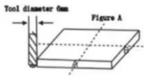
Figure B

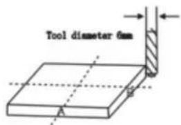
Figure C

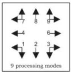
Step 1: press ☐ to enter the TOOL compensation function. Then the message window displays "TYPE". Press ☐.

Step 2: input the diameter of the TOOL; press 10 in turn.

Step 3: press ▼ to the machining mode.

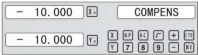
Machining of 2 side planes can be done by moving the TOOL until X-Axis is 150.000 and Y-Axis is 100.000. Press the key [TAN/V3] to quit the function.

6.8 Digital Filter of the Grinding Machine

When machining a workpiece by grinder, the display values change quickly due to the vibration of the grinder. The user cannot see the display value clearly. The grinder DRO provides a display value filter function to disable the quake change of display value.

STEPS:

1. Enter display value filter function.

In normal display state, press SIFT to enter the display value filter function.

1. Exit display value filter function;

Press SIFT to exit display value filter function;

6.9 The function

6.9.1 200 sets of TOOL libraries

It will automatically exit from EDM machining status and recover to the original state before machining;

b) Stop Mode:

It will always stay at the machining interface after finishing machining, and you should press EDM to exit and return to the original state.

Operation steps:

The DEPTH (machining depth), ERRHIGH (negative fireproof height), exit mode, EDM relay output mode, and machining direction should be set.

STEPS:

1. Press EDM to enter the EDM function. Press ▲ to input parameters; press ▼ to enter EDM machining state.
2. Input DEPTH (machining depth). Press the key ▲ to set the next parameter.

1. Input ERRHIGH (negative fireproof height) (undefined). Press the key ▲ to set the next parameter.

1. Set machining direction (positive or negative). Press 1 to select positive direction. Press 0 to select negative direction. Press the key ▲ to set the next parameter.

EDM

1. Set exit Mode (AUTO Mode or STOP Mode). Press 0 to select AUTO Mode; Press 1 to select STOP Mode; Press the key ▲ to set the next parameter.

1. Set the Output Mode (Mode 0 or Mode 1); (undefined). Press ☐ to select Mode 0; Press ☐ to select Mode 1.

1. Continuously press ▼ to return to EDM for machining. Press EDM to quit the function.

Example 1: positive direction machining.

Machining is shown as the model chamber as follows.

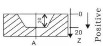
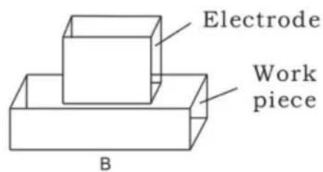
STEPS:

1. Touch one side of the workpiece with the TOOL, then press ₀ to zero the Z axis.

2. Press EDM, set DEPTH to 20.000; press ▼ to EDM for machining.

Example 2: Negative direction machining.

Machining is shown as the model chamber as follows.

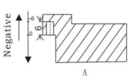
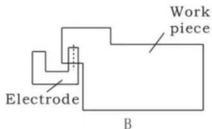
1. Touch one side of the workpiece with the TOOL, then press ₀ to zero the Z axis.

2. Press EDM, set DEPTH to -20.000; press ▼ to EDM for machining.

Example 3: PCD Function for EDM.

The PCD Function can access the EDM Function. The operator enters the PCD Function to input parameters for PCD and enter the PCD machining state. At every position for machining, press the key EDM to access the EDM Function.

The following are the preliminary solvents for troubleshooting.

If there is still trouble, please contact our company or agents for help.

Troubles	Possible reasons	Solvents
No display	1. Power isn't connected2. Power switch is off.3. The range of power voltage is not right.4. The inner power of Linear Scale is short.	1. Check power wire and connect the power2. Turn on the power switch.3. The range of voltage is in 80--260V4. Unplug the connector of linear scale
One axis is not counting	1. Replace the linear scale of the other axis.2. DRO is in special function	1. If count is normal, the linear scale has trouble; If abnormal, the DRO readouts has trouble.2. Quit the special function.
Linear scale is not counting	1. Reading head is bad for using range exceeds.2. Aluminum chips is in reading head of linear scale.3. The span between the reading head and metal part of linear scale is large.4. The metal parts of linear scale is damage.	1. Repair the linear scale2. Repair the linear scale3. Repair the linear scale4. Repair the linear scale
Counting is error	1. Shell is poor grounding.2. Low precision of machine.3. Speed of machine is too rapid.4. Precision of linear scale is low.5. The resolution of DRO readouts and the linear scale is not match.6. The unit (mm/inch) is not match.7. Setting the linear compensating is not arrest.8. Reading head of the linear scale is damaged.	1. Shell is good grounding.2. Repair the machine.3. Reduce the speed of machine.4. Mount the linear scale again.5. Set the resolution of the DRO again,6. Cover the unit of display mm/inch.7. Reset the linear compensation.8. Repair the linear scale.
The counting of the linear scale is not accurate	1. The mounting of linear scale does not demand the requirement, and the precision is not adequate.2. The screw is loosen.3. Precision of machine is low.4. The resolution of digital readouts and the linear scale is not match.	1. Mount the linear scale again and level it.2. Lock all fixing screws.3. Repair the machine.4. Reset the resolution of digital readouts.
Sometimes the linear scale is not counting	1. The small car and steel ball is separated.2. The glass of reading head is wearied.3. The glass of reading head of the linear scale has dirt.4. The elasticity of the steel wire is not adequate.	1. Repair the linear scale.2. Repair the linear scale.3. Repair the linear scale.4. Repair the linear scale.

1. Specifications of Digital Readout.

1) Supply Voltage range: AC 85 V ~ 230 V; 50 ~ 60 Hz 2) Power consumption: 15VA 3) Operating temperature: 0°C-- 50°C 4) Storage temperature: - 30°C-- 70°C 5) Relative humidity: < 90 % (25) 6) Max Coordinate number: 3 7) Readout allowable input signal: TTL square wave 8) Allowable input signal frequency: < 5 M Hz 9) Max resolution of digital display length: 0.01 um 10) Max resolution of digital display angle: 0.0001 / PULSE

1. Instructions

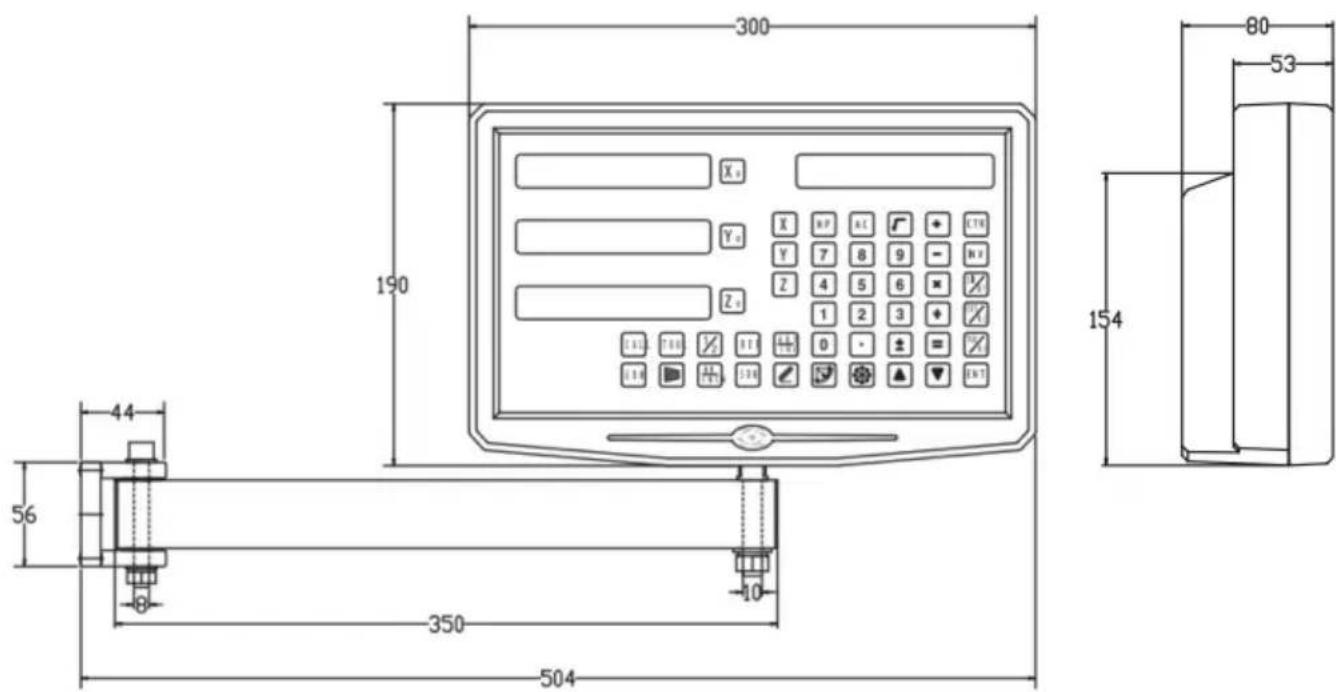
1. X, Y, Z Axis

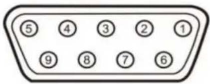
Pin	TTL (Standard)
1
2	OV
3
4
5
6	A+
7	5V
8	B+
9	R+

Pin	TTL (Standard)
1	5V
2	OV
3	A+
4	B+
5	R+
6
7
8
9

For your convenience, if you buy a digital readout,

The wiring definition of your linear scale must be the same as the 2 definitions in the above diagram to be universal!

Installation instructions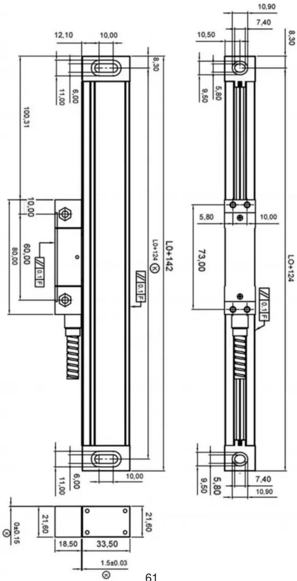

TTL signal Output: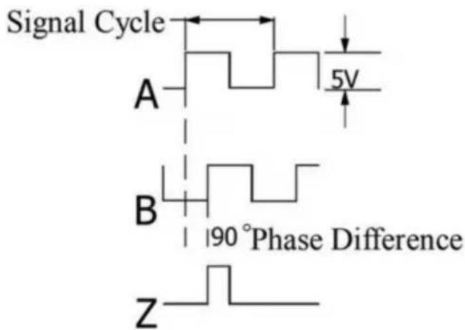

EIA-422-A signal Output:

1. TECHNICAL PARAMETER 1.1 SCALING DISTANCE: 0.02 MM (50 LINES /MM) 1.2 RESOLUTION: 5μM, 1μM, 0.5μM 1.3 PRECISION: ±3μM, ±5μM, ±15μM/M (20±0.1℃) 1.4 MEASURING RANGE: 30~3000MM 1.5 MOVING SPEED: HIGH-SPEED ENCODER 120 M/MIN (TO BE CUSTOMIZED)

ORDINARY ENCODER 60M/MIN

1.6 POWER SUPPLY: +5V±5%, 80MA 1.7 CABLE LENGTH: STANDARD 3M (SPECIAL LENGTH AVAILABLE ACCORDING TO THE USER'S NEEDS) 1.8 WORKING TEMPERATURE: 0~45°C 1.9 PIN DESCRIPTION: 1) APPLICABLE TO: 9 PIN SOCKET EIA-422-A SIGNAL OUTPUT.

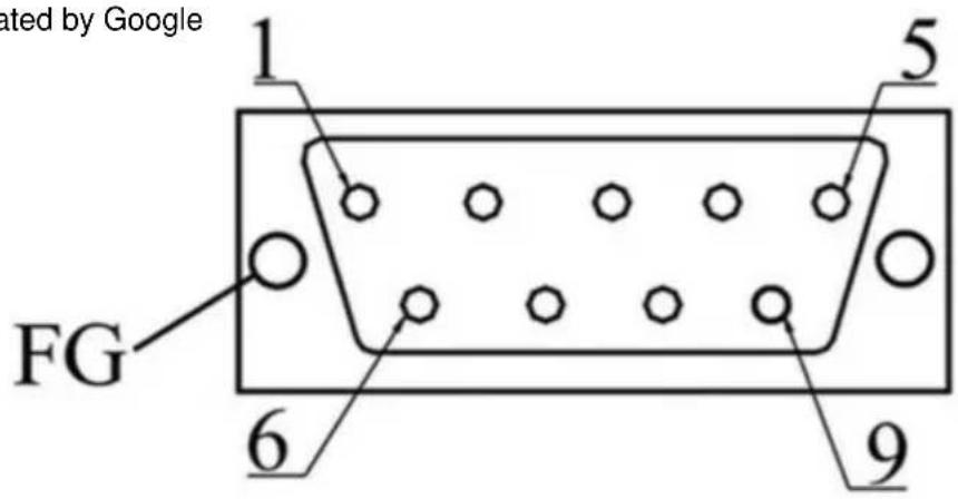
1) Applicable to: 9 pin socket EIA-422-A signal Output.

Pin Position	1	2	3	4	5	6	7	8	9
Signal		OV		Empty		A	+5V	B	Z
Color	Green Black	Black	Orange black	FG	White black	Green	Red	White	Orange

FG: Shield connected to metal casing.

1) Applicable to: 9 pin socket TTL signal Output.

Pin Position	1	2	3	4	5	6	7	8	9
Signal		OV		Empty		A	+5V	B	Z
Color		Black		FG		Green	Red	Orange	White

FG: Shield connected to metal casing.

Linear scale

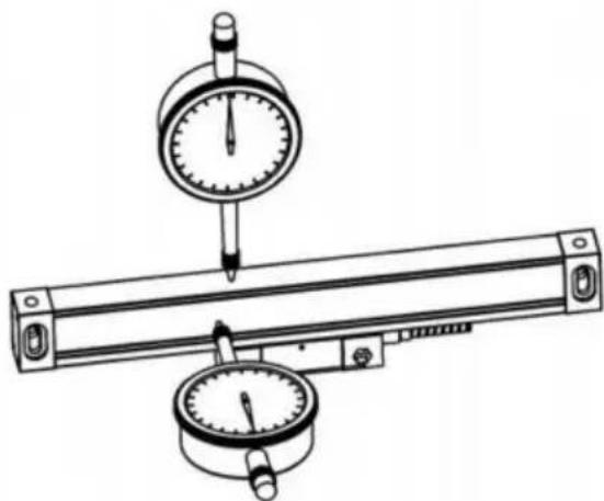
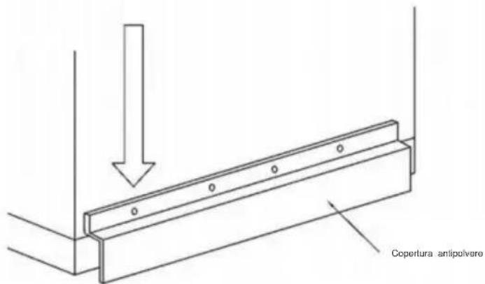
4.9

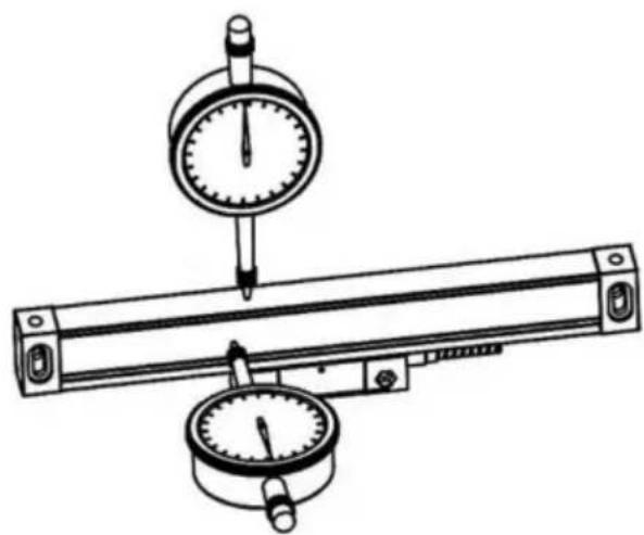
4.10

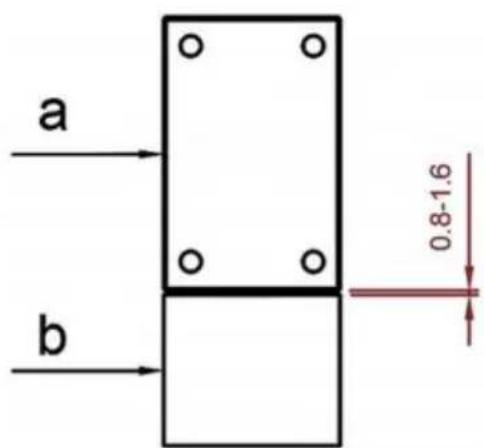
Imported in AUS: SIHAO PTY LTD, 1 ROKEVA STREETEASTWOOD NSW 2122 Australia

Imported in USA: Sanven Technology Ltd., Suite 250, 9166 Anaheim Place, Rancho Cucamonga, CA 91730

www.vevor.com/support

With the continuous updating of products, if there are changes or

1. Illustration of Panel and keyboard 4
2. Caption of the keyboard 5
3. Parameters settings 7

3.1 Parameters setup routine entrance 7 3.2 Parameters Settings Description 7 3.2.1 Setting the Resolution 7 3.2.2 Setting Positive Direction for Counter 8 3.2.3 Toggle Between R/D Display Mode 8 3.2.4 Setting Z axis Dial 8 3.2.5 Setting the Rotary Radius of the Workpiece 9 3.2.6 Setting the Angle Display Mode 9 3.2.7 Setting the Baudrate of RS_232 (optional) 9 3.2.8 Setting the Absolute Zeroing enable or disable 10 3.2.9 Setting the Absolute form the Special Function 10 3.2.10 Setting the Calculator display Mode 10 3.2.11 Display brightness setting 10 3.2.12 The linear scale counting frequency setting 11 3.2.13 Setting QUIT 11 3.2.14 Setting the type of the DRO 11 3.2.15 Signal Interface Type 11 3.2.16 Restore Factory Settings 12 3.2.17 Shrinkage Ratio enable or disable 12 3.2.18 Setting Compensation Type 12 3.2.19 Inch display, set the number of digits after the decimal point 13 3.2.20 Setting EDM (optional) 13 3.2.21 Setting Linearity Compensation 13 3.2.22 Setting the Shrinkage Ratio 13

4. General Operations 14

4.1 Zeroing 14 4.2 Preset Data to Designated Axis 14 4.3 Toggle Display Unit between inch and mm 14 4.4 Absolute/Incremental/200 groups SDM 15 4.5 1/2 Function 15 4.6 Clear All SDM Datum 16

Contents

4.7 Sleeping Mode 16 4.8 Power Interruption Memory 16 4.9 Search the Absolute Reference Point of Scale 17 4.10 Non Linear Error Compensation 20

5. 200 Groups SDM coordinate 21 5.1 Zeroing at the Current Point 21 5.2 Preset datum of SDM coordinate 22

6. Special Function 24

6.1 Circumference Holes Processing 25 6.2 Linear Holes Processing 28 6.3 ARC Processing 30 6.4 Oblique Processing 39 6.5 Slope Processing 43 6.6 Chamber Processing 44 6.7 The Tool Diameter Compensation Function 45 6.8 Digital Filter of the Grinding Machine 46 6.9 Lathe Function 47

6.9.1 200 sets TOOL Libs 47 6.9.2 Taper Function 48 6.9.3 R/D Function 49 6.9.4 Y + Z Function (only applicable to: 3 axes Lathe) 49

6.10 EDM 50

7. Calculator 56

8. Appendix 57

THREE AXIS PANEL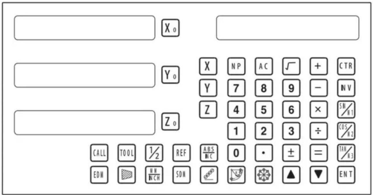

TWO AXIS PANEL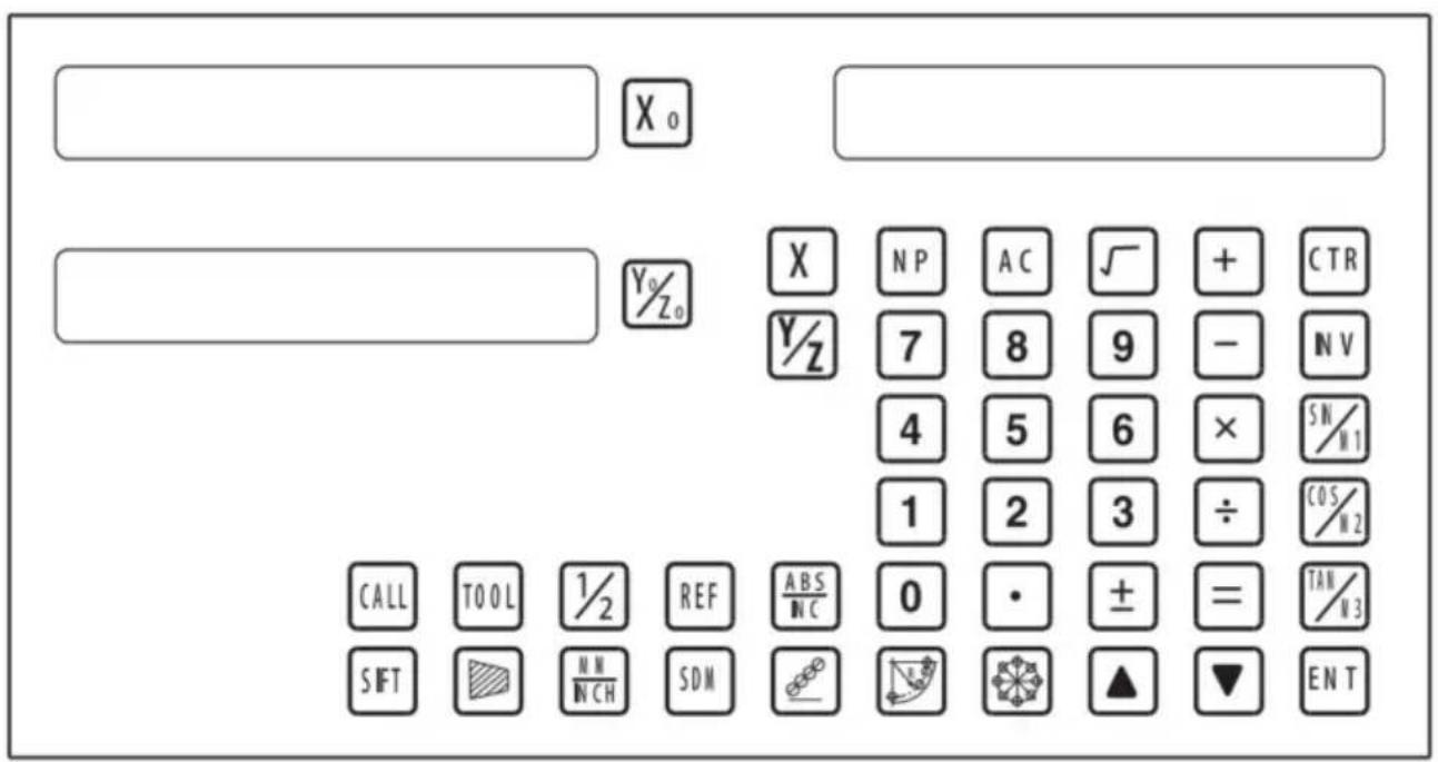

Keyboard Description

	Keys for axis selection
	Zero select axis
	Enter +/- sign
	Enter decimal point
	Entry keys for numbers
	Operation key (in Calculation function key)
	Enter or quit calculating state
	Cancel incorrect operation
	Calculate inverse trigonometric
	Square root
	Confirm operation
	Toggles between inch and millimeter units.
	Press when ready to identify a reference mark.
	Function keys for 200 sub datum
	ARC cutting function
	holes displayed equally on a circle
	holes displayed equally on a line

Caption of the keyboard

	Calculate trigonometric or Slope Processing function key
	Calculate trigonometric or rectangular inner chamber processing function key
	Calculate trigonometric or the tool diameter compensation function key
	Toggle between ABS/INC coordinate
	Stroll up or down to select
	Taper measured function key
	Tool library call key
	Opens the tool table.( lathe)
	EDM function key
	Filter display function key
	Half a display value of an axis
	Non Linear Error Compensation function keys

3. Parameter settings

3.1 Parameters setup routine entrance.

Press ☐ to enter initial system and self-check after DRO powers on in 1 second, then Parameters settings display in the Parameters window. Press ▲ ▼ to select the item you want to change.

If you want to quit initial setting, press ▲ ▼ until “QUIT” appears in message window and press ENT. You can also press • to quit initial setting.

3.2 Parameters Settings Description

3.2.1 Setting the Resolution

Press ▲ ▼ until “RESOLUTE” appears in message window;

When selecting the LINEAR encode, the resolution will be set as follow:

There are 19 types of resolution:

0.01um; 0.02um; 0.05um; 0.10um; 0.20um; 0.25um; 0.50um; 1.00um; 2.00um; 2.50um; 5.00um; 10.00um; 20.00um; 25.00um; 50.00um; 100.00um; 200.00um; 250.00um; 500.00um.

Press ₀ to change the resolution for X axis; Press ₀ to change the resolution for Y axis; Press ₀ to change the resolution for Z axis;

Set the resolution 5.00um to 1.00um for X axis:

When selecting the rotary encoder, the resolution will be set as follows:

Input the rotary encoder parameter value.

3.2.2 Setting Positive Direction for Counter

Press ▲ ▼ until “DIRECTE” appears in the message window.

Direction ‘0’ means the display value will increase when the scale moves from right to left and decrease when the scale moves from left to right. Direction ‘1’ means the display value will increase when the scale moves from left to right and decrease when the scale moves from right to left.

Press ₀ to change the direction for the X axis; press ₀ to change the direction for the Y axis; press ₀ to change the direction for the Z axis, as follows:

3.2.3 Toggle Between R/D Display Mode

Press ▲ ▼ until “R OR D” appears in the message window. The X window, Y window, and Z window display ‘0’ or ‘1’ separately.

‘0’ is mode R, which means the display value equals the actual measurement. ‘1’ is mode D, where the display value equals double the actual measurement. Press X₀ to change the R/D for the X axis; press Y₀ to change the R/D for the Y axis; press Z₀ to change the R/D for the Z axis, as follows:

3.2.4 Setting Z Axis Dial

Press ▲ ▼ until "Z DIAL" appears in the message window.

The Z axis dial should be set if the Z axis is emulated for 2-axis milling and only a linear scale is installed for the X and Y axes. The Z axis dial means the distance the Z axis travels when the screw runs one revolution.

Set the Z axis dial to 2.5mm as follows:

3.2.5 Setting the Rotary Radius of the Workpiece

Press ▲ ▼ until "RDIUS" appears in the message window.

The Rotary Radius type is used to measure angle by perimeter.

Input the Rotary Radius parameter value 2000mm as follows:

3.2.6 Setting the Angle Display Mode

Press ▲ ▼ until "ANG DISP" appears in the message window.

Press X0 to change the angle display mode for the X axis; Press Y0 to change the angle display mode for the Y axis; Press Z0 to change the angle display mode for the Z axis. Example for the X axis:

"0.0000" means the angle mode is Circulating DD;

"0000.0000" means the angle mode is Incremental DD;

"0.00.00" means the angle mode is Circulating DMS;

"0000.00.00" means the angle mode is Incremental DMS;

3.2.7 Setting the Baudrate of RS_232 (Special customization function. If you need to purchase, please contact the dealer to customize.)

Press ▲ ▼ until "BAUDRATE" appears in the message window. Set the Baudrate to 115200 as follows:

3.2.12 The linear scale counting frequency setting

The factory default setting is only "12". The higher the parameter, the lower the counting frequency. Press "X0" to set. It is not recommended that you change the default value yourself.

3.2.13 Setting QUIT: Digital display table parameters quit button.

3.2.14 Setting the type of the DRO.

The type of the DRO will be displayed on the right window. Then press the ENT key to select the correct type. The following system item will be set:

"MILL-3" means the DRO type is 3-axis milling machine table;

"MILL-2" means the DRO type is 2-axis milling machine table;

"LATHE-2" means the DRO type is 2-axis lathe table;

"LATHE-3" means the DRO type is 3-axis lathe table;

"GRIND" means the DRO type is Grind table;

"EDM" means the DRO type is EDM table; (Special customization

function, if you need to buy, please contact the dealer to customize)

3.2.15 Signal Interface Type

Message window displays “SEL AXIS” which indicates the step is to Sensor input signal mode. Press X₀ to change the signal mode for X axis; Press Y₀ to change the signal mode for Y axis; Press Z₀ to change the signal mode for Z axis. Example for X axis:

Press X₀ to scroll through the Rotary encode type, the Linear encode type, the Rotary radius type.

X window displays the Signal type.

“LInER” means the Signal type is linear encode type;

"EnCOdE" means the Signal type is Rotary encode type;

"RdIUS" means the Signal type is Rotary radius type;

Example: currently in the linear encode type, to toggle to the Rotary encode type;

3.2.16 Restore Factory Settings:

Clear all data except DRO type. DRO will load default setup for parameter. After loading default setup, user must search RI once to enable resuming ABS datum function; otherwise, to resume the datum by RI is unable;

Message window displays “ALL CLR”, press ENT and message window displays “PASSWORD” indicating the operator to input password; Press 2000 + ENT in turn to load default value;

3.2.17 Shrinkage Ratio enable or disable.

Message window displays “SRK OFF” to disable Shrinkage rate function. Press ☐ to enable Shrinkage rate function in Message window displays “SRK ON”:

3.2.18 Setting Compensation Type

Message window displays “SEL COMP” which indicates the step is to compensation type. Press X₀ to change the compensation type for X axis; Press Y₀ to change the compensation type for Y axis; Press Z₀ to change the compensation type for Z axis; Example for X axis:

Press X₀ to scroll through the not compensation type, the Linear compensation type, the non-linear compensation type.

“no-CO” means the compensation type is not compensation type; “LInE-CO” means the compensation type is linear compensation type. “non-LinE” means the compensation type is non-linear linear compensation type;

Example for X axis: currently in the not compensation type, to toggle to the linear compensation type;

3.2.19 Inch display, set the number of digits after the decimal point

In the inch display mode, the number of digits after the decimal point is set, the factory default digit is "4", press "X0" to set, can be set according to actual needs.

3.2.20 Setting EDM: it is not recommended that you set the default value yourself, EDM function, Set the relay off on time.

3.2.21 Setting Linearity Compensation.

Message window displays “LIN COMP” which indicates the step is to Linearity Compensation. Compensate the linear error to make display value equals to standard value.

The calculation of compensation rectifying coefficient:

Coefficient = (Measurement - Standard value) x 1000.000/ Standard value

Example for X axis:

Measurement 200.020mm

Standard value 200.000mm

Rectifying coefficient= (200.020-200) * 1000 /200 = -0.01mm/m

Input compensation rectifying coefficient 0.01 as follow:

3.2.22 Setting the Shrinkage Ratio

Press ▲ ▼ until “ SHRINK” appears in message window;

Shrinkage radio = Dimensions of the finished product/Dimensions of the working piece

Set the shrinkage radio 1.005 as follow;

4. General Operations;

4.1 Zeroing

Zero the designated axis in normal display state. Zeroing is used to set the current point as datum point as follow;

X₀ or Y₀ or Z₀ will be returned to the original data before the reset.

4.2 Preset Data to Designated Axis

Preset a value to the current position for a designated axis in normal display state.

4.3 Toggle Display Unit between inch and mm

Length can be displayed either in "mm" (metric) or "inch" (imperial). The display unit can be toggled between mm and inch.

Example: Display value toggles from mm to inch;

Example: Display value toggles from inch to mm;

4.4 Absolute/Incremental/200 groups SDM

Function: The DRO has 3 coordinate display modes: the absolute mode (ABS); the incremental mode (INC) and 200 groups Second Data Memory (SDM) with the range of 00 to 99. The zero point of the work-piece is set at the origin point of the ABS coordinate. The relative distance between the datum of ABS and SDM remains unchanged when the ABS datum is changed.

1. Toggle from ABS to INC coordinate;

1. Toggle from INC to ABS coordinate;

1. Toggle from SMD to ABS coordinate;

4.5 1/2 Function

Function: Set the center of the work piece as datum by halving the displayed value.

Example: Set the center of the rectangle as datum as shown in the right figure.

Steps:

1. Touch one side of the workpiece with the TOOL, then zero the X axis.

2. Message window displays “REF”. Press ENT until “FD_REF” appears in message window.

3. Select the axis which need search RI. For instance: select X axis, then press ☒. "X_REF" is displayed in message window, and X axis window flashes.

4. Move the machine table. The buzzer sounds when RI is searched, then X window stops flashing and displays the value of the current position. The DRO returns to normal display state. Then message window displays "FIND_X".

Example for AB mode:

1. DRO is set in ABS coordinate. Press REF, then the message window displays "REF".

2. Press ▲ ▼, then the message window displays “AB”.

3. Message window displays “AB”. Press ENT until “FIND_AB” appears in message window.

4. Select the axis which need search RI. For instance: select X axis, then press ☒. “X_REF” is displayed in message window, and X axis window flashes.

5. Move the machine table. The buzzer sounds when RI is searched, displays the value of the current position for the absolute datum zero. The DRO returns to normal display state. Then message window displays "FIND_AB".

Example for LEF_AB mode:

1. DRO is set in ABS coordinate. Press REF, then the message window displays "REF".

2. Press ▲ ▼, then the message window displays “AB”.

3. Message window displays "LEF_AB". Press ENT until "ZERO_AB" appears in message window.

4. Move the machine table to the zero position point. Then press X, and the X axis will zero. The current position becomes the absolute datum zero. The DRO returns to normal display state.

NOTE: Linear range without reference point location of the user

4.10 Non-Linear Error Compensation

First, the compensation type (Linear or Non-Linear) in parameter setting must be set to Non-Linear. Linear scales have a reference point location, and finding the Absolute Reference Point will be enabled.

Default Non-Linear compensation: 50.

Example for Y axis:

Step 1: Search the Absolute Reference Point of the scale.

Step 2: Press NP, then the message window displays "COMP X".

Step 3: Press ▲ ▼, then the message window displays "COMP Y".

Step 4: Press ENT, then the message window displays "NUMBER". Then input the compensation parameter NUMBER.

Step 5: Press ▲ ▼, then the message window displays "Y-MSN-1", which indicates the step is for Non-Linear Error Compensation.

Step 6: Input compensation value.

X window displays the value of the measurement value.

Y window displays the value of the standard value.

Example for the first compensation point:

Measurement value: 68.288 mm. Standard value: 68.200 mm.

Step 7: After inputting all parameters, the DRO automatically exits.

5. 200 Groups SDM Coordinate

The DRO has three display modes: the absolute mode (ABS), the incremental mode (INC), and the 200 groups second data memory (SDM 1 - SDM200). The ABS datum of the workpiece is set at the beginning, and the 200 groups SDM is set relative to the ABS coordinate.

ABS Mode, INC Mode, and SDM Mode are specially designed to provide much more convenience features to the operator to cope with the batch machining of relative works and the machining of workpiece dimensions from more than one datum.

Example: The ABS datum is the center point O, and the points sdm1, sdm2, sdm3, sdm4 needed for processing are set as the datum of SDM 1 - SDM 4.

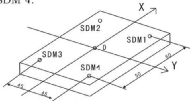
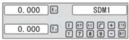
Two ways to set SDM coordinate:

1. Zeroing at the current point. 2. Preset datum of SDM coordinate.

5.1 Zeroing at the Current Point

At first, set the center point of the workpiece as the origin of the ABS, then align the tool with points SDM1, SDM2, SDM3, SDM4 by moving the machine table and zero them. It is the position to process where the “0.000” appears in the X window and Y window by moving the machine table whether in ABS or in SDM coordinate.

Steps:

1. Move the worktable to place the tool at the center of the workpiece point O as the datum of ABS. Then zero the X axis and Y axis in SDM 1; zero the X axis and Y axis in SDM 2; zero the X axis and Y axis in SDM 3; zero the X axis and Y axis in SDM 4.

2. Set the point sdm1 as the datum of SDM 1. Move the machine worktable to x = 60.000, y = 45.000. Then process [X0] [Y0].

2. Set the point sdm1 as the datum of SDM 2. Move the machine worktable to x = 60.000, y = -45.000. Then process [X0] [Y0].

3. Set the point sdm1 as the datum of SDM 3. Move the machine worktable to x = -60.000, y = -45.000. Then process [X0] [Y0].

4. Set the point sdm1 as the datum of SDM 4. Move the machine worktable to x = -60.000, y = 45.000. Then process X0 Y0.

5.2 Preset datum of SDM coordinate

There are the same sample as Method 1. First move the worktable to place the TOOL exactly at the origin of ABS, secondly enter the ABS Mode as follow.

Steps:

1. Move worktable to place the TOOL at the center of the workpiece point O as the datum of ABS. Then zero X axis and Y axis in SDM 1; zero X axis and Y axis in SDM 2; zero X axis and Y axis in SDM 3; zero X axis and Y axis in SDM 4.

2. Set point sdm1 as the datum of SDM 1. Press ▲ ▼, then the message window displays "SDM 1". Input x = 60.000, y = 45.000.

3. Set point sdm1 as the datum of SDM 2. Press ▲ ▼, then the message window displays "SDM 2". Input x = -60.000, y = 45.000.

4. Set point sdm1 as the datum of SDM 3. Press ▲ ▼, then the message window displays "SDM 3". Input x = -60.000, y = -45.000.

5. Set point sdm1 as the datum of SDM 4. Press ▲ ▼, then the message window displays "SDM 4". Input x = -60.000, y = 45.000.

6 Special function

6.1 Circumference Holes Processing

The Function of PCD Hole positioning on Circumference is used to distribute arc equally, such as boring hole on flange. The right window will show the parameter to be defined when selecting PCD Function. The Parameters to be defined are:

PCD_XY(XZ,YZ)

Select place

CENTER

Center position

DIA

Diameter of circle

NO_HOLE

Hole number

STANG

Starting angle

ED ANG

Ending angle

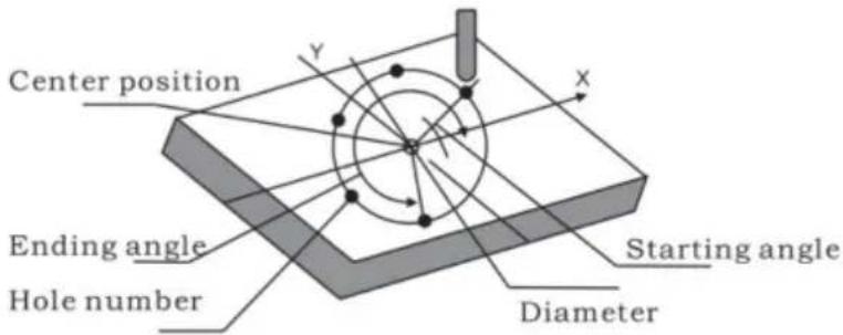
The position of the hole center is calculated automatically after inputting all parameters. Press ▲ or ▼ to choose the hole number and move the machine table until “0.000” appears in the X, Y, and Z windows. That is the position to process the hole.

Example for the XY plane: Machine holes on a circumference as shown in the figure.

PCD_XY(XZ,YZ)	XY
CENTER	X=0,000,Y=0.000
DIA	100,000
NO_HOLE	5
ST ANG	30,000
ED ANG	315,000

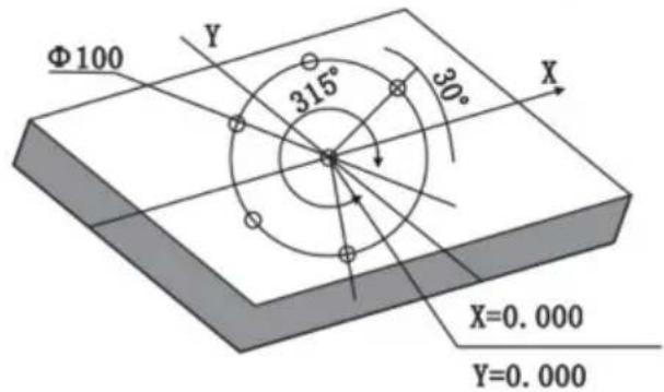
Steps:

1. Set the display unit to metric in the normal state; move the machine table until the machine tool is aligned with the center of the circle, then zero the X and Y axes.
2. Select the piece.

Press 🧑️, then the message window displays “PCD_XY” for the Circumference Holes Processing. Press ▲ or ▼ to select the XY plane.

2. Input center position.

Press ENT, then the message window displays "CENTER". The X and Y windows display the formerly preset center position. Input X = 0, Y = 0 as follows.

4. Input diameter.

Press ▼ until "DIA" appears in the message window. The X window displays the formerly preset diameter. Then input the diameter as 100.000.

5. Input number.

Press ▼ until "NO_HOLE" appears in the message window. The X window displays the formerly preset number. Then press 5 in turn to input the number.

6. Input starting angle.

Press ▼ until "ST ANG" appears in the message window. The X window displays the formerly preset starting angle. Then press 3 and 0 in turn to input the starting angle.

7. Input ending angle.

Press ▼ until "ED ANG" appears in the message window. The X window displays the formerly preset ending angle. Then press 3, 1, and 5 in turn to input the ending angle.

1. Press ▼ until "NO 1" appears in the message window.

It is the position of the first hole to punch where the "0.000" is displayed in the X window and Y window by moving the machine table. After finishing the first hole, press ▼ or ▲ to change the hole number.

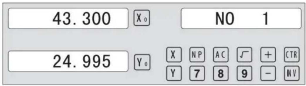
1. After processing all holes, press 📋 to return to normal display.

6.2 Linear Holes Processing

There are two modes to carry out the linear drilling: Length mode and Step mode.

1. LINE S Step mode LINE L Length mode 2.STEP Step length LENGTH Line length
2. ANG Angle
3. NO.HOLE Hole number

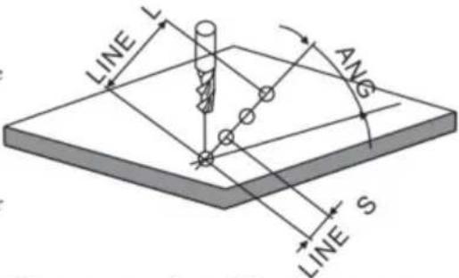
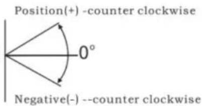
The Linear Holes function simplifies the processing of multiple holes whose centers are equally spaced on a line.

Example:

LINE_L	Length mode
LENGTH	60.000
ANG	30.000
NO.HOLE	4

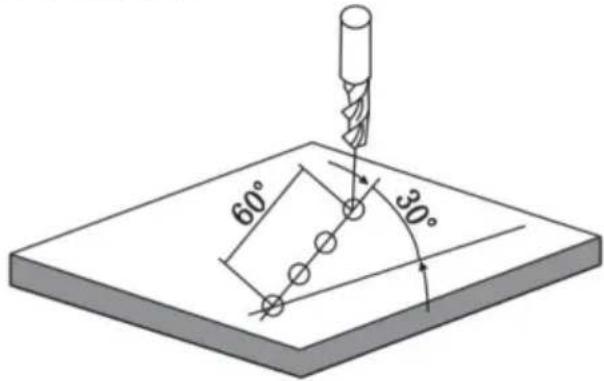
Steps:

1. Select the piece.

Press 📄, then the message window displays “LINE_XY” for Linear Holes Processing. Press ▲ or ▼ to select the XY plane.

2. Select Linear Holes mode.

Press ENT, then the message window displays "LINE_S". Press ▲ or ▼ to select "LINE_L".

3. Input linear length;

Press ENT, then the message window displays "LENGTH".

The X window displays the previously preset linear length. Press 6 0 in turn to input the linear length.

1. Input angle;

The message window displays “ANG” which indicates the step is to angle. The X window displays the previously preset angle. Press 3 0 in turn to input the angle.

1. Input number;

Message window displays “ANG” which indicates the step is to angle. X window displays the formerly preset number. Press 4 in turn to input the number.

1. Press ▼ until "NO 1" appears in the message window.

It is the position of the first hole to punch where the “0.000” is displayed in X window and Y window by moving the machine table. After finishing the first hole, press ▲ or ▼ to change holes number.

1. After processing all holes, press ☐ to return normal display.

Simple ARC function:

Provides maximum flexibility in ARC machining, the ARC sector to be machined by the coordinates of ARC. Very flexible, ARC function can machine virtually all kinds of ARC, even the intersected ARC.

Relatively a bit complicated to operate, operator need to calculate and enter the coordinates of ARC centre, start angle and end angle.

Basic parameter as follow:

1. SMOOTH Mode of the Smooth ARC processing;
2. SEL_XY(YZ, XZ) Select place;
3. CENTER Refer to the position of an center.
4. RAD Radius of the ARC
5. TL_DIA Diameter of the TOOL
6. MAX_CUT Feed step
7. ST_ANG Starting angle
8. ED_ANG Ending angle
9. RAD+TL Outer arc. RAD-TL Inner arc.

Example 1 for the Simple ARC Processing:

Parameters settings as follow:

SIMPLE Simple mode

TYPE 3

SEL_XY XY

RAD 80.000

TL_DIA 6.000

MAX_CUT 0.500

RAD+TL 1

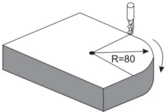
Steps:

1. Select process mode

Press 📋, then the message window displays “SIMPLE” for the ARC Processing. Press ▲ or ▼ to select the simple mode. The message window displays “SIMPLE”

2. Input the type:

Press ENT until "TYPE" appears in the message window. The X window displays the previously preset type. Press 3 in turn.

3. Select place

Press ENT until "SEL_XY" appears in the message window. Press ▲ or ▼ to select the place to display "SEL_XY".

4. Input radius:

Press ENT until "RAD" appears in the message window. The X window displays the previously preset radius of the ARC. Press 8

0 in turn to input the radius.

5. Input Diameter of the TOOL

Press ▲ or ▼ until "TL DIA" appears in the message window. The X window displays the previously preset diameter of the TOOL. Press 6 in turn to input the diameter value.

6. Input Feed step (MAX_CUT)

Press ▲ or ▼ until "MAX_CUT" appears in the message window. The X window displays the previously preset MAX_CUT. Press 0 · 5 in turn to input the MAX_CUT value.

7. Select outer arc or inner arc

Press ▲ or ▼ until "RAD-TL" appears in the message window. Press ▲ or ▼ to select the place to display "RAD+TL".

8. After inputting all parameters, press the ENT key for machining.

The DRO will display the position of the first point. Retract the axes until the displays read 0.000. Machine the arc point by point in accordance with the display. After finishing the position of the first point, press ▲ or ▼ to change the position point.

Press ☑ to quit R function at any time.

Example 2 for the Simple ARC Processing:

Parameter settings are as follows:

SIMPLE Simple mode

TYPE 3

SEL_XY XZ

RAD 80.000

TL_DIA 6.000

MAX_CUT 0.500

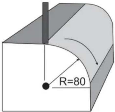
Steps:

1. Press 📋, then the message window displays “SIMPLE” for the ARC Processing. Press ▲ or ▼ to select the mode of the simple, the message window displays “SIMPLE”

ARC Processing

2. Input the type:

Press ☐ENT until "TYPE" appears in the message window. The X-window displays the formerly preset type. Press ☐3 in turn

3. Select place

Press ENT until "SEL_XZ" appears in the message window. Press ▲ or ▼ to select place to display "SEL_XZ";

4. Input radius:

Press ENT until "RAD" appears in the message window. X window displays the formerly preset radius of ARC. Press 8 and 0 in turn to input the radius.

5. Input Diameter of the TOOL

Press ▲ or ▼ until "TL DIA" appears in the message window. X window displays the formerly preset Diameter of the TOOL. Press 6 in turn to input the Diameter value.

6. Input Feed step (MAX_CUT);

Press ▲ or ▼ until "MAX_CUT" appears in the message window. X window displays the formerly preset MAX_CUT. Press 0, ., 5 in turn to input the MAX_CUT value.

1. After inputting all parameters, press the key ENT for machining.

For 2-axis milling machine table, it is not installed with Z-axis, please press ▲ or ▼ to simulate position of Z-axis. Press ▲ simulate moving to the former process, and press ▼ simulate moving to the next process point.

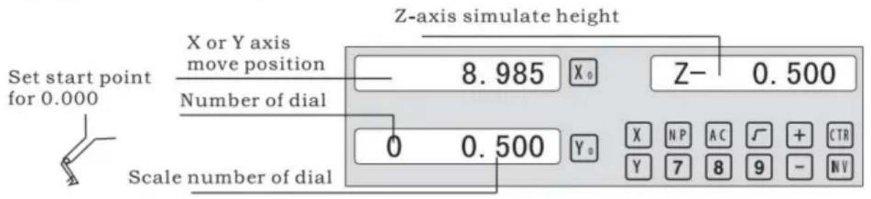
Z-axis simulate height = Number of dial x Z axis Dial + Scale number of dial

Press ☐ to quit R function any time.

Example 3 for the Smooth ARC function:

Parameters settings as follow:

SMOOTH	Smooth mode
SEL_XY(YZ,XZ)	XY
CENTER	X=0,Y=0
RAD	80.000
TL_DIA	6.000
MAX_CUT	0.500
ST_ANG	0.000
ED_ANG	135.000
RAD+TL	1

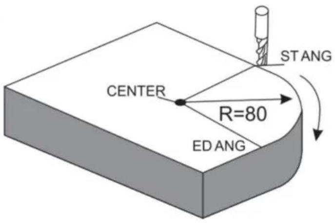
Steps:

1. Press 📋, then the message window displays "SIMPLE" to the ARC Processing. Press ▲ or ▼ to select mode of the simple, The

Message window displays "SMOOTH"; For 3-axis milling machine table without this step. In second step. Then press ENT.

2. Select place

Message window displays "SEL_XY" which indicates the select is to place. Press ▲ or ▼ to select place to display "SEL_XY";

3. Input center position.

Press ENT, then the message window displays "CENTER". X and Y windows display the formerly preset center position. Input X = 0, Y = 0 as follow.

4. Input radius:

Press ENT until "RAD" appears in the message window. X window displays the formerly preset radius of ARC. Press 8 and 0 in turn to input the radius.

5. Input Diameter of the TOOL

Press ▲ or ▼ until "TL DIA" appears in the message window. X window displays the formerly preset diameter of the TOOL. Press 6 in turn to input the diameter value.

Press ENT to quit ARC function any time.

6) Change the angle of the work piece to make the workpiece touch the measuring tool and adjust it to zero.

STEPS:

1. Select place

Press SN/1, then the message window displays "INCL_XY" to the Oblique Processing. Press ▲ or ▼ to select place to display "SEL_XY";

Then press ENT to in next step;

2. Input the angle of obliquity

The message window displays “ANG”, and the X window displays the previously preset angle of obliquity. Press 4 and 5 in turn to input the angle of obliquity.

1. Move the workpiece along the X-axis until the measuring tool touches the workpiece, adjust it to zero, and move the worktable for any distance along the X-axis.

1. Press Y to display the value of the Y-axis. Move the workpiece along the Y-axis, change the angle of the workpiece to make the obliquity-calibrating plane touch the measuring tool until it turns to zero. Move the worktable until the Y-axis is displayed as zero.

1. Press 5W/H1 to quit the oblique function at any time.

Example 2 for the oblique XZ or YZ plane:

When the machining plane is on plane XZ or YZ, the function of tool inclination can instruct the operator to machine the oblique plane step by step.

Procedures for using the function of cutter inclination:

When the machining plane is on plane XZ or YZ, first please calibrate the obliquity of the primary spindle nose and set the tool:

INCL_XY(XZ,YZ)	INCL_XZ
DIA	10.000
ST_POT	20.000
ED_POT	20.000

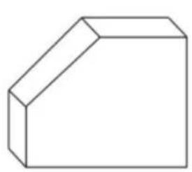
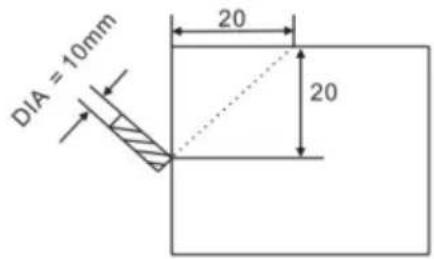
STEPS:

1. Press SN/81, then the message window displays "INCL_XY" for oblique processing. Press ▲ or ▼ to select the plane to display "SEL_XZ"; then press ENT to proceed to the next step.

1. Input the tool diameter

The message window displays “DIA”, and the X window displays the previously preset angle of obliquity. Press 10 in turn to input the tool diameter of obliquity. OK, then press ▼ to proceed to the next step.

1. Input ST_POT;

The message window displays “ST_POT”, and the X and Y windows display the previously preset starting position of obliquity. Input X=0, Y=-20.000. OK, then press ▼ to proceed to the next step.

4. Input ED_POT;

The message window displays “ED_POT”, and the X and Y windows display the previously preset starting position of obliquity. Input X=20.000, Y=0.000.

5. After inputting all parameters, press the ▼ key for machining.

For a 2-axis milling machine table, it is not installed with a Z-axis, so please press ▲ or ▼ to simulate the position of the Z-axis. Press ▲ to simulate moving to the former process, and press ▼ to simulate moving to the next process point.

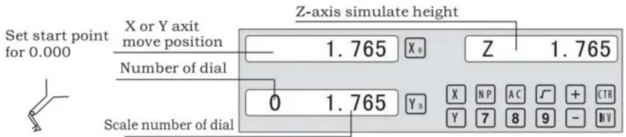
Z-axis simulated height = Number of dial x Z axis Dial + Scale number of dial

Press ☐ to quit the oblique function at any time.

6.5 Slope Processing

This function can calculate the position of every processing point automatically when processing a slope. Only the following parameters need to be inputted:

XZ, YZ

Set machine place YZ, or XZ

ANG

The inclination angle

Z_STEP

The slope length

each time processing

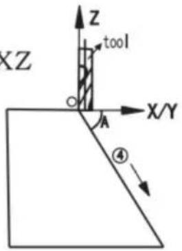
Example 1 for the Slope XZ place;

Step 1. Select place

Press TAN, then the message window displays "XZ" for the slope processing. Press ▲ or ▼ to select place to display "SEL_XY"; Then press ENT to go to the next step;

Step 2. Input the angle of slope

The message window displays "ANG", X window displays the formerly preset angle of slope. Press 4 5 in turn.

Step 3. Input Z_step;

The message window displays "Z STEP", X window displays the formerly preset starting position of slope. Input 0 · 1 in turn.

Step 4: Finishing the ALL processing. Press ☐ to quit slope function any time.

6.6 Chambering Processing

1, FLAT_XY: machine place; 2, DIA: diameter of TOOL; 3, CENTER: center of the chambering; 4, SIZE: size of the chambering;

Figure as follow:

STEPS:

1. Press COS/W2, then the message window displays "FLAT_XY" for the Chambering Processing.

1. Input DIA of the TOOL;

1. Input the center coordinate;

1. Input the size;

5. Process Chambering;

Move the machine until the display of the axis is zero, i.e., the position of the first point. Machine the first point. Display the next machining point by pressing ▲ or ▼. On the completion of machining, the right window shows OVER. Press ▲ or ▼, the system will go to the first position for the next workpiece. Press ⚠/12 to quit the Chambering Function.

6.7 The Tool Diameter Compensation Function

Without tool compensation, the operator has to move the tool for an additional distance of the diameter of the tool along each side when machining the four 150 and 100 sides of a workpiece to finish machining the whole brim. The digital readouts shall automatically compensate when the tool compensation function is enabled.

Note: The tool compensation is made in the direction of X and Y axes.

Procedures:

1). Enter the function of compensating the diameter of the tool. 2). Select one of the (four) preset machining modes. 3). Input the diameter of the tool. 4). Enter machining.

Figure A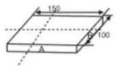

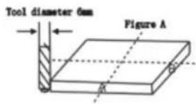
Figure B

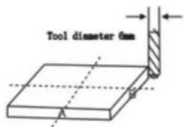
Figure C

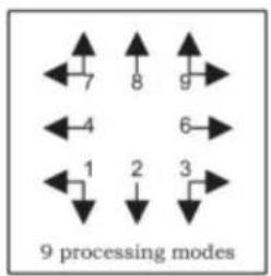
Step 1: Press ☐ to enter the tool compensation function. Then the message window displays “TYPE”. Press ☐.

Step 2: Input the diameter of the tool; press 10 in turn.

Step 3: Press ▼ to the machining mode.

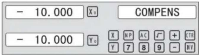
Machining of 2 side planes can be done by moving the tool until X-Axis is 150.000 and Y-Axis is 100.000. Press the Key [TAN/V3] to quit the function.

6.8 Digital Filter of the Grinding Machine

When machining a work-piece by grinder, the display values change quickly due to the vibration of the grinder. The user cannot see the display value clearly. The Grinder DRO provides a display value filter function to disable the quake change of display value.

STEPS:

1. Enter the display value filter function.

In normal display state, press SIFT simultaneously to enter the display value filter function.

1. Exit the display value filter function;

Press SIFT to exit the display value filter function;

6.9 The Function

It will automatically exit from EDM machining status and recover to the original state before machining;

b) Stop Mode:

It will always stay at the machining interface after finishing machining, and you should press EDM to exit and return to the original state.

Operation steps:

The DEPTH (machining depth), ERRHIGH (negative fireproof height), exit mode, EDM relay output mode, and machining direction should be set.

STEPS:

1. Press EDM to enter the EDM function. Press ▲ to input parameters; press ▼ to enter EDM machining state.
2. Input DEPTH (machining depth). Press the ▲ key to set the next parameter.

1. Input ERRHIGH (Negative Fireproof Height) (undefined). Press the ▲ key to set the next parameter.

1. Set machining direction (Positive or Negative). Press 1 to select Positive direction. Press 0 to select Negative direction. Press the ▲ key to set the next parameter.

EDM

1. Set exit Mode (AUTO Mode or STOP Mode). Press 0 to select AUTO Mode; Press 1 to select STOP Mode; Press the ▲ key to set the next parameter.

1. Set the Output Mode (Mode 0 or Mode 1) (undefined). Press ☐ to select Mode 0; Press ☐ to select Mode 1.

1. Continuously press ▼ to return to EDM for machining. Press EDM to quit the function.

Example 1: positive direction machining.

Machining is shown as the model chamber as follows:

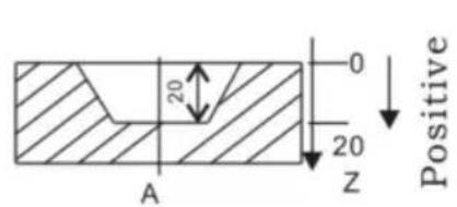
STEPS:

1. Touch one side of the workpiece with the TOOL, then press Z₀ to zero the Z axis.

2. Press EDM, set DEPTH to 20.000; press ▼ to EDM for machining.

Example 2: Negative direction machining.

Machining is shown as the model chamber as follows:

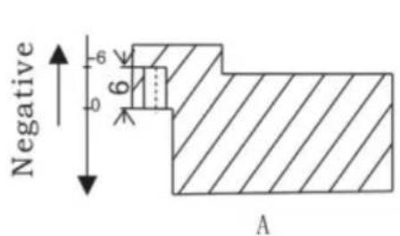
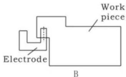
1. Touch one side of the workpiece with the TOOL, then press Z₀ to zero the Z axis.

2. Press EDM, set DEPTH to -20.000; press ▼ to EDM for machining.

Example 3: PCD Function for EDM

The PCD Function can access the EDM Function. The operator enters the PCD Function to input parameters for PCD and enter the PCD machining state. At every position for machining, press the key EDM to access the EDM Function.

The following are the preliminary solutions for troubleshooting.

If there is still trouble, please contact our company or agents for help.

Troubles	Possible reasons	Solvents
No display	1. Power isn't connected2. Power switch is off.3. The range of power voltage is not right.4. The inner power of Linear Scale is short.	1. Check power wire and connect the power2. Turn on the power switch.3. The range of voltage is in 80--260V4. Unplug the connector of linear scale
One axis is not counting	1. Replace the linear scale of the other axis.2. DRO is in special function	1. If count is normal, the linear scale has trouble; If abnormal, the DRO readouts has trouble.2. Quit the special function.
Linear scale is not counting	1. Reading head is bad for using range exceeds.2. Aluminum chips is in reading head of linear scale.3. The span between the reading head and metal part of linear scale is large.4. The metal parts of linear scale is damage.	1. Repair the linear scale2. Repair the linear scale3. Repair the linear scale4. Repair the linear scale
Counting is error	1. Shell is poor grounding.2. Low precision of machine.3. Speed of machine is too rapid.4. Precision of linear scale is low.5. The resolution of DRO readouts and the linear scale is not match.6. The unit (mm/inch) is not match.7. Setting the linear compensating is not arrest.8. Reading head of the linear scale is damaged.	1. Shell is good grounding.2. Repair the machine.3. Reduce the speed of machine.4. Mount the linear scale again.5. Set the resolution of the DRO again,6. Cover the unit of display mm/inch.7. Reset the linear compensation.8. Repair the linear scale.
The counting of the linear scale is not accurate	1. The mounting of linear scale does not demand the requirement, and the precision is not adequate.2. The screw is loosen.3. Precision of machine is low.4. The resolution of digital readouts and the linear scale is not match.	1. Mount the linear scale again and level it.2. Lock all fixing screws.3. Repair the machine.4. Reset the resolution of digital readouts.
Sometimes the linear scale is not counting	1. The small car and steel ball is separated.2. The glass of reading head is wearied.3. The glass of reading head of the linear scale has dirt.4. The elasticity of the steel wire is not adequate.	1. Repair the linear scale.2. Repair the linear scale.3. Repair the linear scale.4. Repair the linear scale.

1. Specifications of Digital Readout.

1) Supply Voltage range: AC 85 V ~ 230 V; 50 ~ 60 Hz 2) Power consumption: 15VA 3) Operating temperature: 0°C - 50°C 4) Storage temperature: -30°C - 70°C 5) Relative humidity: < 90 % (25) 6) Max Coordinate number: 3 7) Readout allowable input signal: TTL square wave 8) Allowable input signal frequency: < 5 MHz 9) Max resolution of digital display length: 0.01 um 10) Max resolution of digital display angle: 0.0001 / PULSE

1. Instructions

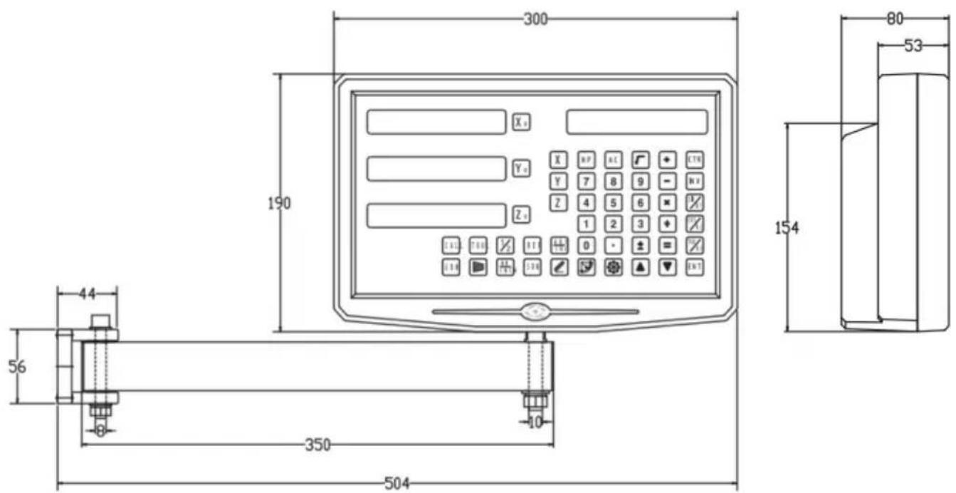
1. X, Y, Z Axis

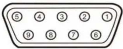
Pin	TTL (Standard)
1
2	OV
3
4
5
6	A+
7	5V
8	B+
9	R+

Pin	TTL (Standard)
1	5V
2	OV
3	A+
4	B+
5	R+
6
7
8
9

For your convenience, if you buy a digital readout,

The wiring definition of your linear scale must be the same as the 2 definitions in the above diagram to be universal!

Installation instructions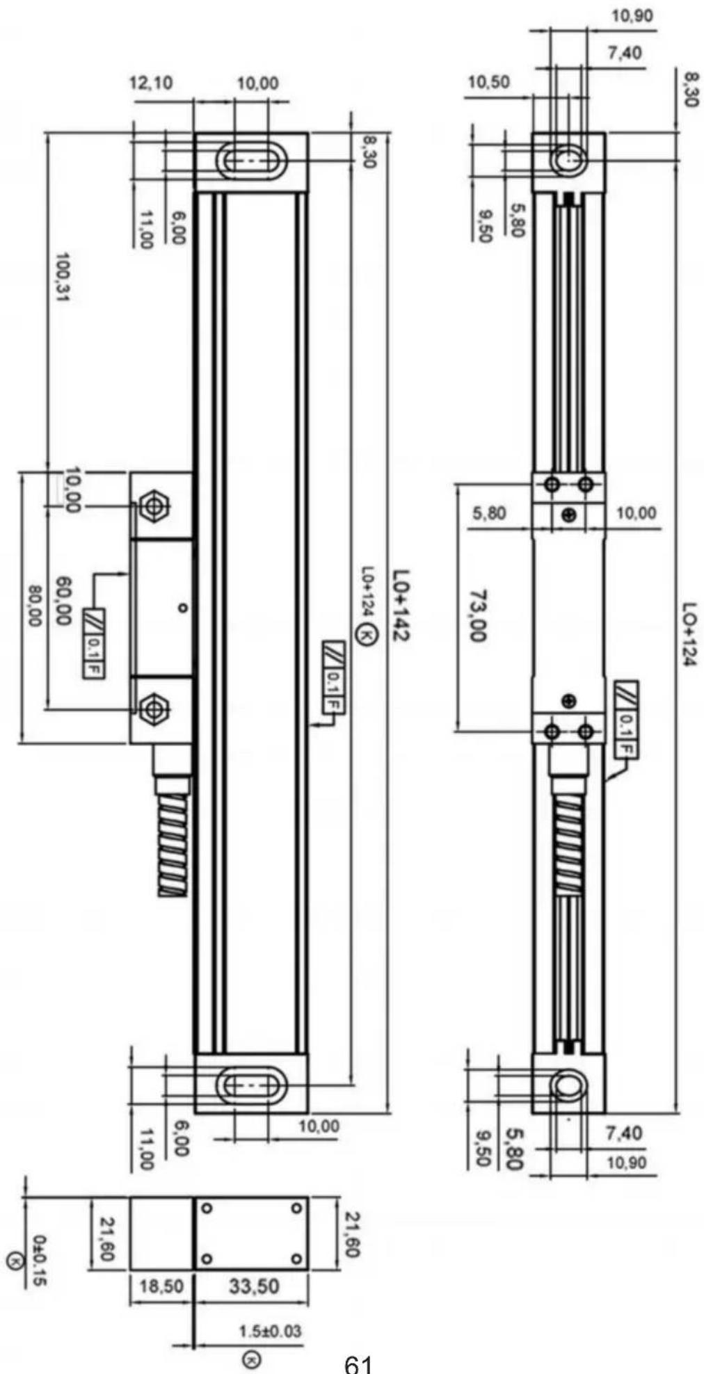

TTL signal Output: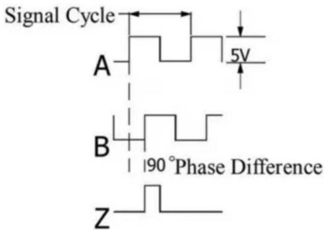

EIA-422-A signal Output: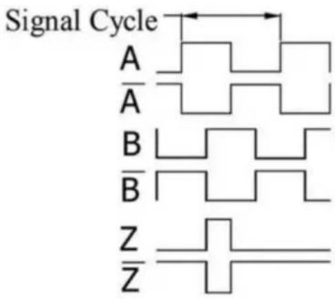

1. TECHNICAL PARAMETER 1.1 SCALING DISTANCE: 0.02 MM (50 LINES /MM) 1.2 RESOLUTION: 5μM, 1μM, 0.5μM 1.3 PRECISION: ±3μM, ±5μM, ±15μM/M (20±0.1℃) 1.4 MEASURING RANGE: 30~3000MM 1.5 MOVING SPEED: HIGH-SPEED ENCODER 120 M/MIN (TO BE CUSTOMIZED)

ORDINARY ENCODER 60M/MIN

1.6 POWER SUPPLY: +5V±5%, 80mA 1.7 CABLE LENGTH: STANDARD 3M (SPECIAL LENGTH AVAILABLE ACCORDING TO THE USER'S NEEDS) 1.8 WORKING TEMPERATURE: 0~45°C 1.9 PIN DESCRIPTION: 1) APPLICABLE TO: 9 PIN SOCKET EIA-422-A SIGNAL OUTPUT.

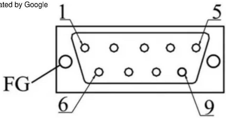
1) Applicable to: 9 pin socket EIA-422-A signal output.

Pin Position	1	2	3	4	5	6	7	8	9
Signal		OV		Empty		A	+5V	B	Z
Color	Green Black	Black	Orange black	FG	White black	Green	Red	White	Orange

FG: Shield connected to metal casing.

1) Applicable to: 9 pin socket TTL signal output.

Pin Position	1	2	3	4	5	6	7	8	9
Signal		OV		Empty		A	+5V	B	Z
Color		Black		FG		Green	Red	Orange	White

FG: Shield connected to metal casing.

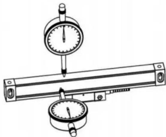
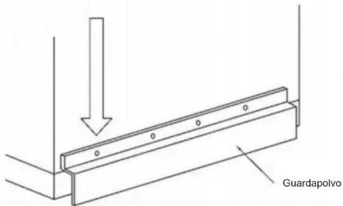
4.9

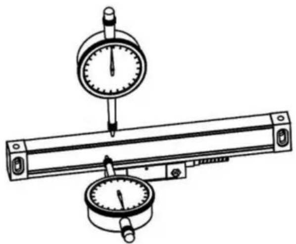
4.10

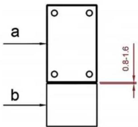
Imported to Australia: SIHAO PTY LTD, 1 ROKEVA STREET EASTWOOD NSW 2122 Australia

Imported to USA: Sanven Technology Ltd., Suite 250, 9166 Anaheim Place, Rancho Cucamonga, CA 91730

E-CrossStu GmbH

NEED HELP? CONTACT US!

www.vevor.com/support

With the continuous updating of products, if there are changes or

1. Illustration of Panel and keyboard 4
2. Caption of the keyboard 5
3. Parameters settings 7

3.1 Parameters setup routine entrance 7 3.2 Parameters Settings Description 7 3.2.1 Setting the Resolution 7 3.2.2 Setting Positive Direction for Counter 8 3.2.3 Toggle Between R/D Display Mode 8 3.2.4 Setting Z axis Dial 8 3.2.5 Setting the Rotary Radius of the Workpiece.... 9 3.2.6 Setting the Angle Display Mode 9 3.2.7 Setting the Baudrate of RS_232(optional) 9 3.2.8 Setting the Absolute Zeroing enable or disable 10 3.2.9 Setting the Absolute form the Special Function 10 3.2.10 Setting the Calculator display Mode 10 3.2.11 display brightness setting 10 3.2.12 The linear scale counting frequency setting 11 3.2.13 Setting QUIT 11 3.2.14 Setting the type of the DRO. 11 3.2.15 Signal Interface Type 11 3.2.16 Restore Factory Settings: 12 3.2.17 Shrinkage Ratio enable or disable....12 3.2.18 Setting Compensation Type 12 3.2.19 Inch display, set the number of digits after the decimal point…13 3.2.20 Setting EDM(optional) 13 3.2.21 Setting Linearity Compensation. 13 3.2.22 Setting the Shrinkage Ratio 13

4. General Operations 14

4.1 Zeroing....14 4.2 Preset Data to Designated Axis 14 4.3 Toggle Display Unit between inch and mm 14 4.4 Absolute/Incremental/200 groups SDM 15 4.5 1/2 Function ...... 15 4.6 Clear All SDM Datum....16

Contents

4.7 Sleeping Mode 16 4.8 Power Interruption Memory 16 4.9 Search the Absolute Reference Point of Scale 17 4.10 Non Linear Error Compensation 20

5. 200 Groups SDM coordinate 21 5.1 Zeroing at the Current Point....21 5.2 Preset datum of SDM coordinate 22

6. Special Function……24

6.1 Circumference Holes Processing 25 6.2 Linear Holes Processing 28 6.3 ARC Processing 30 6.4 Oblique Processing 39 6.5 Slope Processing....43 6.6 Chamber Processing....44 6.7 The Tool Diameter Compensation Function 45 6.8 Digital Filter of the Grinding Machine 46 6.9 Lathe Function 47

6.9.1 200 sets TOOL Libs 47 6.9.2 Taper Function 48 6.9.3 R/D Function 49 6.9.4 Y + Z Function ( only applicable to : 3 axes Lathe)....49

6.10 EDM....50

7. Calculator……56

8. Appendix 57

THREE AXIS PANEL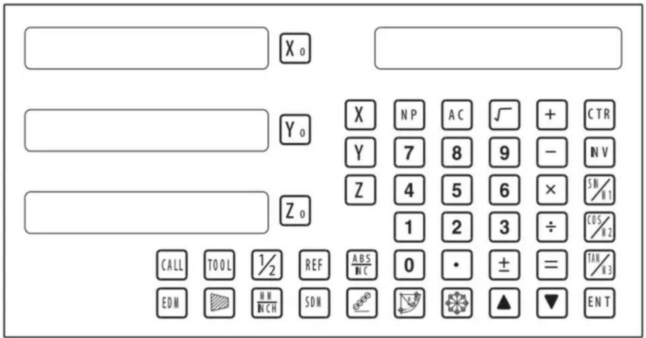

TWO AXIS PANEL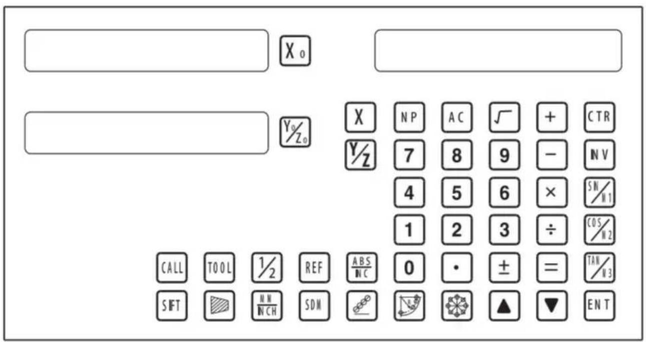

Keyboard Description

	Keys for axis selection
	Zero select axis
	Enter +/- sign
	Enter decimal point
	Entry keys for numbers
	Operation key (in Calculation function key)
	Enter or quit calculating state
	Cancel incorrect operation
	Calculate inverse trigonometric
	Square root
	Confirm operation
	Toggles between inch and millimeter units.
	Press when ready to identify a reference mark.
	Function keys for 200 sub datum
[2TKK]	ARC cutting function
	holes displayed equally on a circle
	holes displayed equally on a line

Caption of the keyboard

	Calculate trigonometric or Slope Processing function key
	Calculate trigonometric or rectangular inner chamber processing function key
	Calculate trigonometric or the tool diameter compensation function key
	Toggle between ABS/INC coordinate
	Stroll up or down to select
	Taper measured function key
	Tool library call key
	Opens the tool table.( lathe)
	EDM function key
	Filter display function key
	Half a display value of an axis
	Non Linear Error Compensation function keys

3. Parameters settings

3.1 Parameters setup routine entrance.

Press ☐ to enter initial system and self-check after DRO powers on in 1 second, then Parameters settings display in the Parameters window. Press ▲ ▼ to select the item you want to change.

If you want to quit initial setting, press ▲ ▼ until “QUIT” appears in message window and press ENTER. You can also press • to quit initial setting.

3.2 Parameters Settings Description

3.2.1 Setting the Resolution

Press ▲ ▼ until “RESOLUTE” appears in message window;

When selecting the LINEAR encode, the resolution will be set as follow:

There are 19 types of resolution:

0.01um;0.02um;0.05um;0.10um;0.20um;0.25um;0.50um;1.00um;2.00um;2.50um;5.00um;10.00um;20.00um;25.00um;50.00um;100.00um;200.00um;250.00um;500.00um.

Press ₀ to change the resolution for X axis; Press ₀ to change the resolution for Y axis; Press ₀ to change the resolution for Z axis;

Set the resolution 5.00um to 1.00um for X axis:

When selecting the rotary encode, the resolution will be set as follow:

Input the rotary encode parameter value.

3.2.2 Setting Positive Direction for Counter

Press ▲ ▼ until “ DIRECTE” appears in message window.

Direction ‘0’ means the display value will increase when scale moves form right to left and decrease when scale moves from left to right. Direction ‘1’ means the display value will increase when scale moves form left to right and decrease when scale moves from right to left.

Press ₀ to change the Direction for X axis; Press ₀ to change the Direction for Y axis; Press ₀ to change the Direction for Z axis; as follow:

3.2.3 Toggle Between R/D Display Mode

Press ▲ ▼ until “R OR D” appears in message window. X window, Ywindow, Z window displays ‘0’ or ‘1’ separately.

‘0’ is mode R, which means the display value equals the actual measurement. ‘1’ is mode D where the display value equals the double actual measurement. Press X₀ to change the R/D for X axis;Press Y₀ to change the R/D for Y axis;Press Z₀ to change the R/D for Z axis; as follow:

3.2.4 Setting Z axis Dial

Press ▲ ▼ until "Z DIAL" appears in message window.

The Z axis dial should be set if the Z axis is emulated for 2-axis milling, and only install the linear scale for the X and Y axes. The Z axis dial refers to the distance the Z axis travels when the screw makes one revolution.

Set the Z axis dial to 2.5mm as follows:

3.2.5 Setting the Rotary Radius of the Workpiece

Press ▲ ▼ until "RDIUS" appears in the message window.

The rotary radius type uses the perimeter to measure the angle.

Input the rotary radius parameter value 2000mm as follows:

3.2.6 Setting the Angle Display Mode

Press ▲ ▼ until "ANG DISP" appears in the message window.

Press ₀ to change the angle display mode for the X axis; press ₀ to change the angle display mode for the Y axis; press ₀ to change the angle display mode for the Z axis. Example for the X axis:

"0.0000" means the angle mode is Circulating DD;

"0000.0000" means the angle mode is Incremental DD;

"0.00.00" means the angle mode is Circulating DMS;

"0000.00.00" means the angle mode is Incremental DMS;

3.2.7 Setting the Baudrate of RS-232 (Special customization function; if you need to purchase, please contact the dealer to customize)

Press ▲ ▼ until "BAUDRATE" appears in the message window. Set the baudrate to 115200 as follows:

3.2.12 The linear scale counting frequency setting

The factory default setting is only "12". The higher the parameter, the lower the counting frequency. Press "X0" to set. It is not recommended that you change the default value yourself.

3.2.13 Setting QUIT: Digital display table parameters quit button.

3.2.14 Setting the type of the DRO.

The type of the DRO will be displayed on the right window. Then press the key ENT to select the correct type. The following system items will be set:

"MILL-3" means the DRO type is 3-axis milling machine table;

"MILL-2" means the DRO type is 2-axis milling machine table;

"LATHE-2" means the DRO type is 2-axis lathe table;

"LATHE-3" means the DRO type is 3-axis lathe table;

"GRIND" means the DRO type is Grind table;

"EDM" means the DRO type is EDM table; (Special customization

function, if you need to buy, please contact the dealer to customize)

3.2.15 Signal Interface Type

Message window displays "SEL AXIS" which indicates the step is to Sensor input signal mode. Press X0 to change the signal mode for X axis; Press Y0 to change the signal mode for Y axis; Press Z0 to change the signal mode for Z axis. Example for X axis:

Press X0 to scroll through the Rotary encode type, the Linear encode type, the Rotary radius type.

X window displays the Signal type.

"LINER" means the Signal type is linear encode type;

"ENCODE" means the Signal type is Rotary encode type;

"RADIUS" means the Signal type is Rotary radius type;

Example: currently in the linear encode type, to toggle to the Rotary encode type;

3.2.16 Restore Factory Settings:

Clear all data except DRO type. DRO will load default setup for parameter. After loading default setup, user must search RI once to enable resuming ABS datum function; otherwise to resume the datum by RI is unable;

Message window displays "ALL CLR", press ENT and message window displays "PASSWORD" indicating the operator to input password; Press 2000 + ENT in turn to load default value;

3.2.17 Shrinkage Ratio enable or disable.

Message window displays "SRK OFF" to disable Shrinkage rate function. Press ☐ to enable Shrinkage rate function in Message window displays "SRK ON":

3.2.18 Setting Compensation Type

Message window displays "SEL COMP" which indicates the step is to compensation type. Press X₀ to change the compensation type for X axis; Press Y₀ to change the compensation type for Y axis; Press Z₀ to change the compensation type for Z axis; Example for X axis:

Press X₀ to scroll through the not compensation type, the Linear compensation type, the non-linear compensation type.

"no-CO" means the compensation type is not compensation type; "LInE-CO" means the compensation type is linear compensation type. "non-LinE" means the compensation type is non-linear compensation type;

Example for X axis: currently in the not compensation type, to toggle to the linear compensation type;

3.2.19 Inch display, set the number of digits after the decimal point

In the inch display mode, the number of digits after the decimal point is set. The factory default digit is "4". Press "X0" to set, and it can be set according to actual needs.

3.2.20 Setting EDM: it is not recommended that you set the default value yourself. EDM function sets the relay off time.

3.2.21 Setting Linearity Compensation.

The message window displays "LIN COMP", which indicates the step is for Linearity Compensation. Compensate the linear error to make the display value equal to the standard value.

The calculation of the compensation rectifying coefficient:

Coefficient = (Measurement - Standard value) x 1000.000/ Standard value

Example for X axis:

Measurement 200.020mm

Standard value 200.000mm

Rectifying coefficient = (200.020-200) * 1000 /200 = -0.01mm/m

Input compensation rectifying coefficient 0.01 as follows:

3.2.22 Setting the Shrinkage Ratio

Press ▲ ▼ until "SHRINK" appears in the message window;

Shrinkage ratio = Dimensions of the finished product/Dimensions of the working piece

Set the shrinkage radio 1.005 as follows;

4. General Operations;

4.1 Zeroing

Zero the designated axis in normal display state. Zeroing is used to set the current point as datum point as follows;

X₀ or Y₀ or Z₀ will be returned to the original data before the reset.

4.2 Preset Data to Designated Axis

Preset a value to current position for a designated axis in normal display state.

4.3 Toggle Display Unit between inch and mm

Length can be displayed either in "mm" (metric) or "inch" (imperial). Display unit can be toggled between mm and inch.

Example: Display value toggle from mm to inch;

Example: Display value toggle from inch to mm;

4.4 Absolute/Incremental/200 groups SDM

Function: The DRO has 3 coordinate display modes: the absolute mode (ABS); the incremental mode (INC) and 200 groups Second Data Memory (SDM) with the range of 00 to 99. Zero point of work-piece is set at the origin point of ABS coordinate. The relative distance between datum of ABS and SDM remains unchanged when ABS datum is changed.

1. Toggle from ABS to INC coordinate;

1. Toggle from INC to ABS coordinate;

1. Toggle from SMD to ABS coordinate;

4.5 1/2 Function

Function: Set the center of work piece as datum by halving the displayed value.

Example: Set the center of rectangle as datum as shown in the right figure.

Steps:

1. Touch one side of the workpiece with the TOOL, then zero the X axis.

2. Message window displays “REF”. Press ENT until “FD_REF” appears in message window.

3. Select the axis which need search RI. For instance: select X axis, then press ☒. "X_REF" is displayed in message window, and X axis window flashes.

4. Move the machine table. The buzzer sounds when RI is searched, then X window stops flashing and displays the value of the current position. The DRO returns to normal display state. Then message window displays "FIND_X".

Example for AB mode:

1. DRO is set in ABS coordinate. Press REF, then the message window displays "REF".

2. Press ▲ ▼, then the message window displays “AB”.

3. Message window displays “AB”. Press ENT until “FIND_AB” appears in message window.

4. Select the axis which need search RI. For instance: select X axis, then press ☒. “X_REF” is displayed in message window, and X axis window flashes.

5. Move the machine table. The buzzer sounds when RI is searched, displays the value of the current position for the absolute datum zero. The DRO returns to normal display state. Then message window displays "FIND_AB".

Example for LEF_AB mode:

1. DRO is set in ABS coordinate. Press REF, then the message window displays "REF".

2. Press ▲ ▼, then the message window displays "AB".

3. Message window displays "LEF_AB". Press ENT until "ZERO_AB" appears in message window.

4. Move the machine table to the position to be set as zero. Then press X, the X axis will be zeroed. The current position becomes the absolute datum zero. The DRO returns to normal display state.

NOTE: Linear range without reference point location of the user

4.10 Non-Linear Error Compensation

First, compensation type (Linear or Non-Linear) in parameter setting must be set to Non-Linear. Linear scale has a reference point location and finding the Absolute Reference Point will be enabled.

Default Non-Linear compensation: 50.

Example for Y axis:

Step 1: Search the Absolute Reference Point of the scale.

Step 2: Press NP, then the message window displays "COMP X".

Step 3: Press ▲ ▼, then the message window displays "COMP Y".

Step 4: Press ENT, then the message window displays "NUMBER". Then input the compensation parameter NUMBER.

Step 5: Press ▲ ▼, then message window displays "Y-MSN-1" which indicates the step is for Non-Linear Error Compensation.

Step 6: Input compensation value.

X window displays the measurement value.

Y window displays the standard value.

Example for the first compensation point:

Measurement value: 68.288mm. Standard value: 68.200mm

Step 7: After inputting all parameters, the DRO automatically exits.

5. 200 Groups SDM Coordinate

The DRO has three display modes: the absolute mode (ABS), the incremental mode (INC), and the 200 groups second data memory (SDM 1 - SDM200). The ABS datum of the workpiece is set at the beginning, and the 200 groups SDM is set relative to the ABS coordinate.

ABS Mode, INC Mode, and SDM Mode are specially designed to provide much more convenience features to the operator to cope with the batch machining of relative works and the machining of workpiece dimensions from more than one datum.

Example: The ABS datum is the center point O, and the points sdm1, sdm2, sdm3, sdm4 needed for processing are set as datums of SDM 1 - SDM 4.

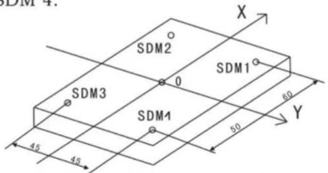
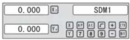
Two ways to set SDM coordinate:

1. Zeroing at the current point. 2. Presetting the datum of SDM coordinate.

5.1 Zeroing at the Current Point

First, set the center point of the workpiece as the origin of the ABS. Then align the tool with points SDM1, SDM2, SDM3, SDM4 by moving the machine table and zero them. It is the position to process where the "0.000" appears in the X window and Y window by moving the machine table, whether in ABS or in SDM coordinate.

Steps:

1. Move the worktable to place the TOOL at the center of the workpiece point O as the datum of ABS. Then zero X axis and Y axis in SDM 1; zero X axis and Y axis in SDM 2; zero X axis and Y axis in SDM 3; zero X axis and Y axis in SDM 4.

2. Set the point sdm1 as the datum of SDM 1. Move the machine worktable to x = 60.000, y = 45.000. Then process X0 Y0.

2. Set the point sdm1 as the datum of SDM 2. Move the machine worktable to x = 60.000, y = -45.000. Then process X0 Y0.

3. Set the point sdm1 as the datum of SDM 3. Move the machine worktable to x = -60.000, y = -45.000. Then process X0 Y0.

4. Set the point sdm1 as the datum of SDM 4. Move the machine worktable to x = -60.000, y = 45.000. Then process X0 Y0.

5.2 Preset datum of SDM coordinate

There are the same sample as Method 1. First move the worktable to place the TOOL exactly at the origin of ABS, secondly enter the ABS Mode as follow.

Steps:

1. Move worktable to place the TOOL at the center of the workpiece point O as the datum of ABS. Then zero X axis and Y axis in SDM 1; zero X axis and Y axis in SDM 2; zero X axis and Y axis in SDM 3; zero X axis and Y axis in SDM 4.

2. Set point sdm1 as the datum of SDM 1. Press ▲ ▼, then the message window displays “SDM 1”. Input x = 60.000, y = 45.000.

3. Set point sdm1 as the datum of SDM 2. Press ▲ ▼, then the message window displays “SDM 2”. Input x = -60.000, y = 45.000.

4. Set point sdm1 as the datum of SDM 3. Press ▲ ▼, then the message window displays “SDM 3”. Input x = -60.000, y = -45.000.

5. Set point sdm1 as the datum of SDM 4. Press ▲ ▼, then the message window displays “SDM 4”. Input x = -60.000, y = 45.000.

The Function of PCD Hole positioning on Circumference is used to distribute arc equally, such as boring hole on flange. The right window will show the parameter to be defined when selecting PCD Function. The Parameters to be defined are:

PCD_XY(XZ,YZ)

Select place

CENTER

Center position

DIA

Diameter of circle

NO_HOLE

Hole number

STANG

Starting angle

ED ANG

Ending angle

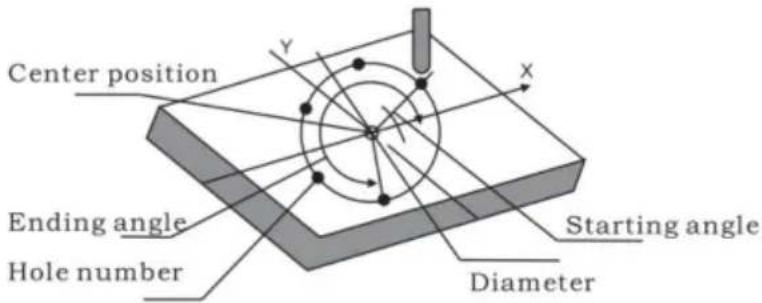
The position of the hole center is calculated automatically after inputting all parameters. Press ▲ or ▼ to choose the hole number and move the machine table until the “0.000” appears in the X window, Y window, and Z window. This is the position to process a table.

Example for the XY place: Machine hole on circumference as shown in the figure.

PCD_XY(XZ,YZ)	XY
CENTER	X=0,000,Y=0.000
DIA	100,000
NO_HOLE	5
ST ANG	30,000
ED ANG	315,000

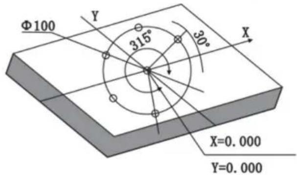
Steps:

1. Set display unit to metric in normal state; move the machine table until the machine tool is aligned with the center of the circle, then zero the X axis and Y axis.
2. Select piece.

Press 🧑️, then the message window displays "PCD_XY" for the Circumference Holes Processing. Press ▲ or ▼ to select XY place.

2. Input center position.

Press ENT, then the message window displays "CENTER". X and Y windows display the formerly preset center position. Input X = 0, Y = 0 as follows.

4. Input diameter.

Press ▼ until "DIA" appears in the message window. X window displays the formerly preset diameter. Then input the diameter as 100.000.

5. Input number.

Press ▼ until "NO_HOLE" appears in the message window. X window displays the formerly preset number. Then press 5 in turn to input the number.

6. Input starting angle.

Press ▼ until "ST ANG" appears in the message window. X window displays the formerly preset starting angle. Then press 3 and 0 in turn to input the starting angle.

7. Input ending angle.

Press ▼ until "ED ANG" appears in the message window. X window displays the formerly preset ending angle. Then press 3, 1, and 5 in turn to input the ending angle.

1. Press ▼ until "NO 1" appears in the message window.

It is the position of the first hole to punch where the "0.000" is displayed in X window and Y window by moving the machine table. After finishing the first hole, press ▼ or ▲ to change the hole number.

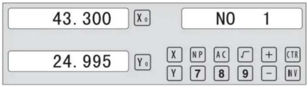
1. After processing all holes, press 📄 to return to normal display.

6.2 Linear Holes Processing

There are two modes to carry out the linear drilling: Length mode and Step mode.

1. LINE S Step mode LINE L Length mode 2.STEP Step length LENGTH Line length
2. ANG Angle
3. NO.HOLE Hole number

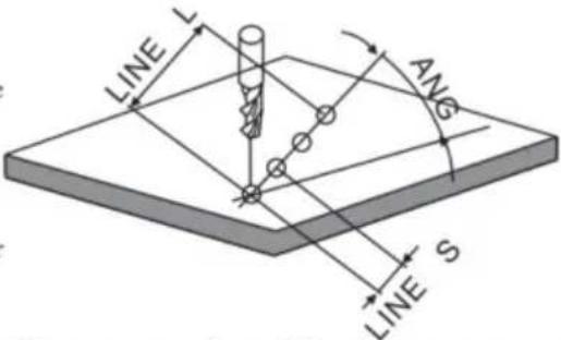
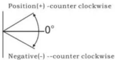
Linear Holes function can simplify the processing of multiple holes whose centers are equally spaced on one line.

Example:

LINE_L	Length mode
LENGTH	60.000
ANG	30.000
NO.HOLE	4

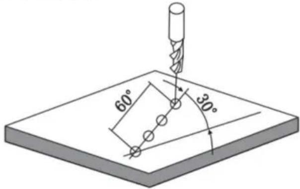
Steps:

1. Select piece.

Press 📄, then the message window displays "LINE_XY" for the Linear Holes Processing. Press ▲ or ▼ to select XY place.

2. Select Linear Holes mode.

Press ENT, then the message window displays "LINE_S". Press ▲ or ▼ to select "LINE_L".

3. Input linear length.

Press ENT, then the message window displays "LENGTH".

X window displays the formerly preset linear length. Press 6 0 in turn to input the linear length.

1. Input angle;

Message window displays “ANG” which indicates the step is to angle. X window displays the formerly preset angle. Press 3 0 in turn to input the angle.

1. Input number;

Message window displays “ANG” which indicates the step is to angle. X window displays the formerly preset number. Press 4 in turn to input the number.

1. Press ▼ until "NO 1" appears in the message window.

It is the position of the first hole to punch where the “0.000” is displayed in X window and Y window by moving the machine table. After finishing the first hole, press ▲ or ▼ to change holes number.

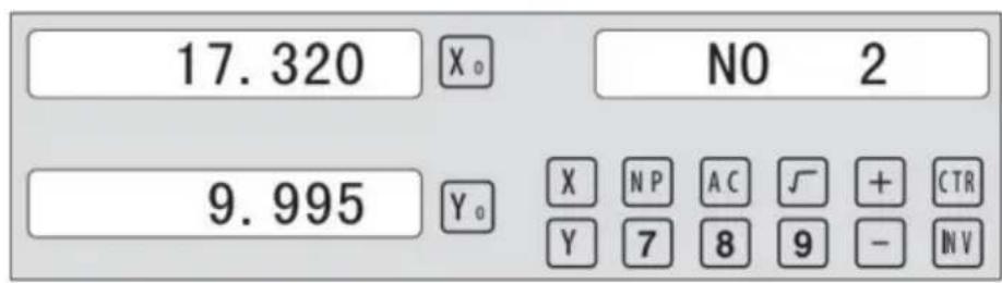
1. After processing all holes, press ☐ to return normal display.

6.3 ARC Processing

Simple ARC function:

Press ☐ENT until "TYPE" appears in the message window. X-window displays the formerly preset type. Press ☐3 in turn

3. Select place

Press ENT until "SEL_XY" appears in the message window. Press ▲ or ▼ to select place to display "SEL_XY";

4. Input radius:

Press ENT until "RAD" appears in the message window. X window displays the formerly preset radius of ARC. Press 8

0 in turn to input the radius.;

5. Input Diameter of the TOOL

Press ▲ or ▼ until “TL DIA” appears in the message window. The X window displays the formerly preset diameter of the tool. Press 6 in turn to input the diameter value;

6. Input Feed step (MAX_CUT);

Press ▲ or ▼ until “MAX_CUT” appears in the message window. The X window displays the formerly preset MAX_CUT. Press 0 · 5 in turn to input the MAX_CUT value;

7. Select outer arc or inner arc

Press ▲ or ▼ until “RAD-TL” appears in the message window. Press ▲ or ▼ to select place to display “RAD+TL”;

8. After inputting all parameters, press the key ENT for machining.

The DRO will display the position of the first point. Retract the axes until the displays read 0.000. Machine the arc point by point in accordance with the display. After finishing the position of the first point, press ▲ or ▼ to change position point.

Press ☑ to quit R function any time.

Example 2 for the Simple ARC Processing:

Parameters settings as follow:

SIMPLE Simple mode

TYPE 3

SEL_XY XZ

RAD 80.000

TL_DIA 6.000

MAX_CUT 0.500

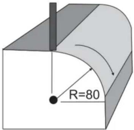
Steps:

1. Press 📋, then the message window displays “SIMPLE” for the ARC Processing. Press ▲ or ▼ to select the mode of the simple, the message window displays “SIMPLE”

ARC Processing

2. Input the type:

Press ☐ENT until "TYPE" appears in the message window. X-window displays the formerly preset type. Press ☐3 in turn

3. Select place

Press ENT until "SEL_XZ" appears in the message window. Press ▲ or ▼ to select place to display "SEL_XZ";

4. Input radius:

Press ☐ENT until “RAD” appears in the message window. X window displays the formerly preset radius of ARC. Press ☐8 ☐0 in turn to input the radius.;

5. Input Diameter of the TOOL

Press ▲ or ▼ until “TL DIA” appears in the message window. X window displays the formerly preset Diameter of the TOOL. Press 6 in turn to input the Diameter value;

6. Input Feed step (MAX_CUT);

Press ▲ or ▼ until “MAX_CUT” appears in the message window. X window displays the formerly preset MAX_CUT. Press 0 · 5 in turn to input the MAX_CUT value;

1. After inputting all parameters, press the ENT key for machining.

For a 2-axis milling machine table, it is not installed with a Z-axis. Please press ▲ or ▼ to simulate the position of the Z-axis. Press ▲ to simulate moving to the former process, and press ▼ to simulate moving to the next process point.

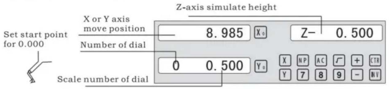
Z-axis simulated height = Number of dial x Z axis Dial + Scale number of dial

Press ☐ to quit the R function at any time.

Example 3 for the Smooth ARC function:

Parameter settings are as follows:

SMOOTH	Smooth mode
SEL_XY(YZ,XZ)	XY
CENTER	X=0,Y=0
RAD	80.000
TL_DIA	6.000
MAX_CUT	0.500
ST_ANG	0.000
ED_ANG	135.000
RAD+TL	1

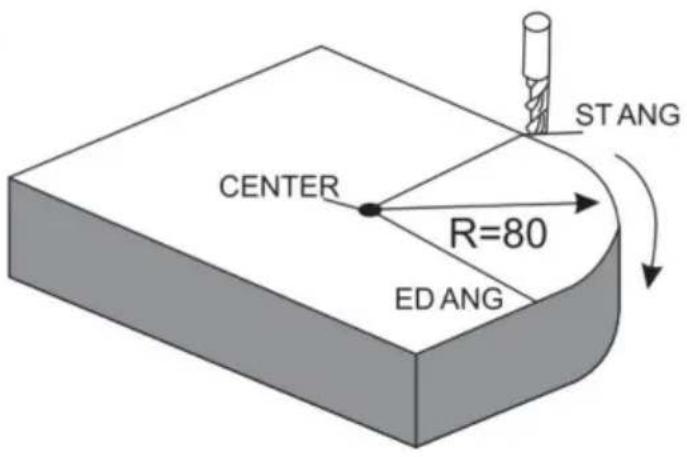
Steps:

1. Press 📋, then the message window displays "SIMPLE" for the ARC Processing. Press ▲ or ▼ to select the mode of the simple, The

message window displays "SMOOTH"; For a 3-axis milling machine table, this step is not needed. In the second step, then press ENT.

2. Select place

The message window displays "SEL_XY" which indicates the selection is to place. Press ▲ or ▼ to select place to display "SEL_XY";

3. Input center position.

Press ENT, then the message window displays "CENTER". The X and Y windows display the formerly preset center position. Input X = 0, Y = 0 as follows.

4. Input radius:

Press ENT until "RAD" appears in the message window. The X window displays the formerly preset radius of the ARC. Press 8 and 0 in turn to input the radius.

5. Input Diameter of the TOOL

Press ▲ or ▼ until “TL DIA” appears in the message window. The X window displays the formerly preset diameter of the tool. Press 6 in turn to input the diameter value;

Press ☐ to quit ARC function at any time.

6) Change the angle of the workpiece to make the workpiece touch the measuring tool and adjust it to zero.

STEPS:

1. Select plane

Press SN/1, then the message window displays "INCL_XY" for the oblique processing. Press ▲ or ▼ to select plane to display "SEL_XY;

Then press ☐ENT to proceed to the next step;

2. Input the angle of obliquity

The message window displays “ANG”, the X window displays the formerly preset angle of obliquity. Press 4 5 in turn to input the angle of obliquity.

1. Move the workpiece along the X-Axis until the measuring tool touches the workpiece, adjust it to zero, and move the worktable for any distance along the X-Axis.

1. Press Y, display the value of Y-Axis. Move the workpiece along the Y-Axis, change the angle of workpiece to make the obliquity-calibrating plane touch the measuring tool until it turns to zero. Move the worktable until Y-Axis is displayed as zero.

1. Press 5W/H1 to quit oblique function at any time.

Example 2 for the oblique XZ or YZ plane:

When the machining plane is on plane XZ or YZ, the function of TOOL inclination can instruct the operator to machine the oblique plane step by step.

Procedures for using the cutter inclination function:

When the machining plane is on plane XZ or YZ, first calibrate the obliquity of the primary spindle nose and set the TOOL:

INCL_XY(XZ,YZ)	INCL_XZ
DIA	10.000
ST_POT	20.000
ED_POT	20.000

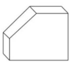
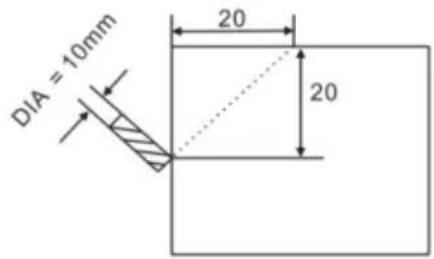
STEPS:

1. Press SN/81, then the message window displays "INCL_XY" for oblique processing. Press ▲ or ▼ to select the display "SEL_XZ"; then press ENT to proceed to the next step.

1. Input the TOOL diameter.

The message window displays "DIA", and the X window displays the previously preset angle of obliquity. Press 10 in turn to input the TOOL diameter of obliquity. OK, then press ▼ to proceed to the next step.

1. Input ST_POT.

The message window displays "ST_POT", and the X and Y windows display the previously preset starting position of obliquity. Input X=0, Y=-20.000. OK, then press ▼ to proceed to the next step.

4. Input ED_POT.

The message window displays "ED_POT", and the X and Y windows display the previously preset starting position of obliquity. Input X=20.000, Y=0.000.

5. After inputting all parameters, press the ▼ key for machining.

For 2-axis milling machine tables that are not installed with a Z-axis, press ▲ or ▼ to simulate the position of the Z-axis. Press ▲ to simulate moving to the previous process, and press ▼ to simulate moving to the next process point.

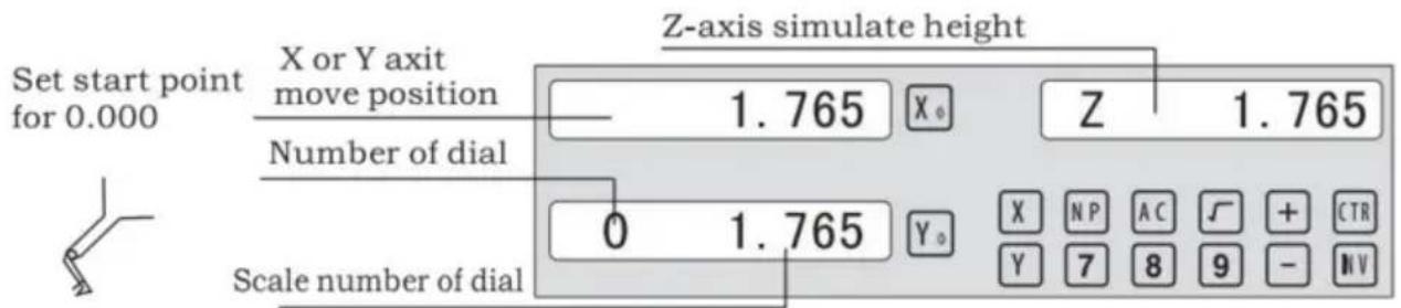
Z-axis simulated height = Number of dial x Z axis Dial + Scale number of dial.

Press ☐ to quit the oblique function at any time.

6.5 Slope Processing

This function can calculate the position of every processing point automatically in processing slope. Only the following parameters need to be inputted:

XZ, YZ

Set machine place YZ, or XZ

ANG

The inclination angle

Z_STEP

The slope length

each time processing

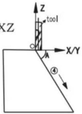
Example 1 for the Slope XZ place;

Step 1. Select place

Press \boxed{\text{TAN}}, then the message window displays "XZ" for the slope processing. Press ▲ or ▼ to select place to display "SEL_XY"; Then press \boxed{\text{ENT}} to go to next step;

Step 2. Input the angle of slope

The message window displays "ANG", X window displays the formerly preset angle of slope. Press 4 5 in turn.

Step 3. Input Z_step;

The message window displays "Z STEP", X window displays the formerly preset starting position of slope. Input 0 · 1 in turn.

Step 4: Finishing the ALL processing. Press ☐ to quit slope function any time.

6.6 Chambering Processing

1, FLAT_XY: machine place; 2, DIA: diameter of TOOL; 3, CENTER: center of the chambering; 4, SIZE: size of the chambering;

Figure as follow:

STEPS:

1. Press /W2 , then the message window displays “FLAT_XY” to the Chambering Processing.

1. Input DIA of the TOOL;

1. Input the center coordinate;

1. Input the size;

5. Process Chambering;

Move the machine until the display of the axis is zero, i.e., the position of the first point. Machine the first point. Display the next machining point by pressing ▲ or ▼. On the completion of machining, the right window shows OVER. Press ▲ or ▼, the system will go to the first position for the next workpiece. Press ⚠/12 to quit the Chambering Function.

6.7 The Tool Diameter Compensation Function

Without TOOL compensation, the operator has to move the TOOL for an additional distance of the diameter of the TOOL along each side when machining the four 150 and 100 sides of a workpiece to finish machining the whole brim. The digital readouts shall automatically compensate when the TOOL compensation function is enabled.

Note: the TOOL compensation is made in the direction of X and Y axis.

Procedures:

1). Enter the function of compensating the diameter of the TOOL. 2). Select one of the (four) preset machining modes. 3). Input the diameter of the TOOL. 4). Enter machining.

Figure A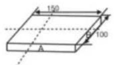

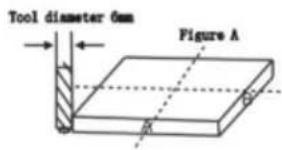
Figure B

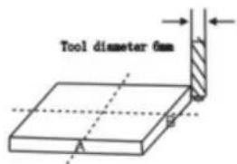
Figure C

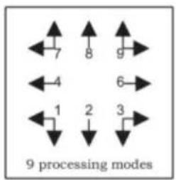
Step 1: press ☐ to enter the TOOL compensation function. Then the message window displays “TYPE”. Press ☐.

Step 2: input the diameter of the TOOL; press 10 in turn.

Step 3: press ▼ to the machining mode.

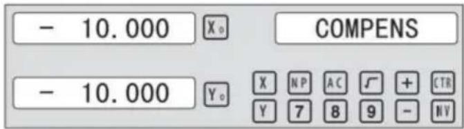
Machining of 2 side planes can be done by moving the TOOL until X-Axis is 150.000 and Y-Axis is 100.000. Press the Key [TAN/V3] to quit the function.

6.8 Digital Filter of the Grinding Machine

When machining a work-piece by grinder, the display values quickly due to the vibration of grinder. User cannot see display value clearly. Grinder DRO provides display value filter function to disable the quake change of display value.

STEPS:

1. Enter display value filter function.

In normal display state, press SIFT to simultaneously, enter display value filter function.

1. Exit display value filter function;

Press SIFT, exit display value filter function;

6.9 The Function

it will automatically exit from EDM machining status and recover to the original state before machining;

b) Stop Mode:

It will always stay at the machining interface after finishing machining, and you should press EDM to exit and back to the original state.

Operation steps:

The DEPTH (machining Depth), ERRHIGH (Negative fireproof height), exit Mode, EDM Relay Output Mode and machining direction should be set.

STEPS:

1. Press EDM to enter the EDM Function. Press ▲ to input parameters; Press ▼ to enter EDM machining state.
2. Input DEPTH (machining depth). Press the key ▲ to set the next parameter.

1. Input ERRHIGH (Negative Fireproof Height) (undefined). Press the key ▲ to set the next parameter.

1. Set machining direction (Positive or Negative). Press 1 to select Positive direction. Press 0 to select Negative direction. Press the key ▲ to set the next parameter.

EDM

1. Set exit Mode (AUTO Mode or STOP Mode). Press 0 to select AUTO Mode; Press 1 to select STOP Mode; Press the key ▲ to set the next parameter.

1. Set the Output Mode (Mode 0 or Mode 1); (undefined). Press ☐ to select Mode 0; Press ☐ to select Mode 1.

1. Continuously press ▼ to return EDM for machining. Press EDM to quit the function;

Example 1: positive direction machining;

Machining is shown as the model chamber as follows

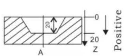
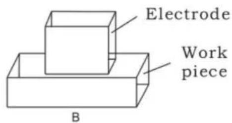
STEPS:

1. Touch one side of the workpiece with the TOOL, then press ₀ , zero the Z axis.

2. Press EDM, Setting DEPTH for 20.000; press ▼ to EDM for machining;

Example 2: Negative direction machining

Machining is shown as the model chamber as follows

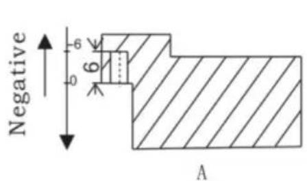
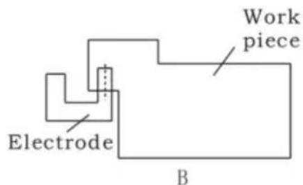
1. Touch one side of the workpiece with the TOOL, then press ₀ , zero the Z axis.

2. Press EDM, Setting DEPTH for -20.000; press ▼ to EDM for machining;

Example 3: PCD Function for EDM

PCD Function can access the EDM Function. The operator enters PCD Function to input parameters for PCD and enter PCD machining state. At every position for machining, press the key EDM to access the EDM Function.

The following are the preliminary solvents for troubleshooting.

If there is still trouble, Please contact out company or agents for help.

Troubles	Possible reasons	Solvents
No display	1. Power isn't connected2. Power switch is off.3. The range of power voltage is not right.4. The inner power of Linear Scale is short.	1. Check power wire and connect the power2. Turn on the power switch.3. The range of voltage is in 80--260V4. Unplug the connector of linear scale
One axis is not counting	1. Replace the linear scale of the other axis.2. DRO is in special function	1. If count is normal, the linear scale has trouble; If abnormal, the DRO readouts has trouble.2. Quit the special function.
Linear scale is not counting	1. Reading head is bad for using range exceeds.2. Aluminum chips is in reading head of linear scale.3. The span between the reading head and metal part of linear scale is large.4. The metal parts of linear scale is damage.	1. Repair the linear scale2. Repair the linear scale3. Repair the linear scale4. Repair the linear scale
Counting is error	1. Shell is poor grounding.2. Low precision of machine.3. Speed of machine is too rapid.4. Precision of linear scale is low.5. The resolution of DRO readouts and the linear scale is not match.6. The unit (mm/inch) is not match.7. Setting the linear compensating is not arrest.8. Reading head of the linear scale is damaged.	1. Shell is good grounding.2. Repair the machine.3. Reduce the speed of machine.4. Mount the linear scale again.5. Set the resolution of the DRO again,6. Cover the unit of display mm/inch.7. Reset the linear compensation.8. Repair the linear scale.
The counting of the linear scale is not accurate	1. The mounting of linear scale does not demand the requirement, and the precision is not adequate.2. The screw is loosen.3. Precision of machine is low.4. The resolution of digital readouts and the linear scale is not match.	1. Mount the linear scale again and level it.2. Lock all fixing screws.3. Repair the machine.4. Reset the resolution of digital readouts.
Sometimes the linear scale is not counting	1. The small car and steel ball is separated.2. The glass of reading head is wearied.3. The glass of reading head of the linear scale has dirt.4. The elasticity of the steel wire is not adequate.	1. Repair the linear scale.2. Repair the linear scale.3. Repair the linear scale.4. Repair the linear scale.

1. Specifications of Digital Readout.

1) Supply Voltage range: AC 85 V \~ 230 V; 50 \~ 60 Hz 2) Power consumption: 15VA 3) Operating temperature: 0°C-- 50°C 4) Storage temperature: - 30°C-- 70°C 5) Relative humidity: < 90 % (25) 6) Max Coordinate number: 3 7) Readout allowable input signal: TTL square wave 8) Allowable input signal frequency: < 5 M Hz 9) Max resolution of digital display length: 0.01 um 10) Max resolution of digital display angle: 0.0001 / PULSE

1. Instructions

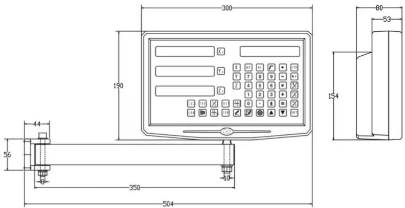
1. X, Y, Z Axis

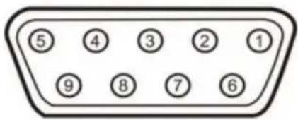
Pin	TTL (Standard)
1
2	OV
3
4
5
6	A+
7	5V
8	B+
9	R+

Pin	TTL (Standard)
1	5V
2	OV
3	A+
4	B+
5	R+
6
7
8
9

For your convenience, if you buy a digital readout,

The wiring definition of your linear scale must be the same as the 2 definitions in the above diagram to be universal!

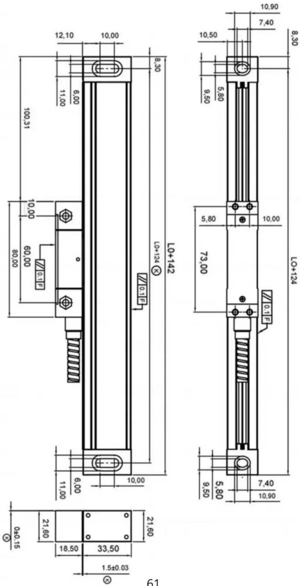
Installation instructions

TTL signal Output: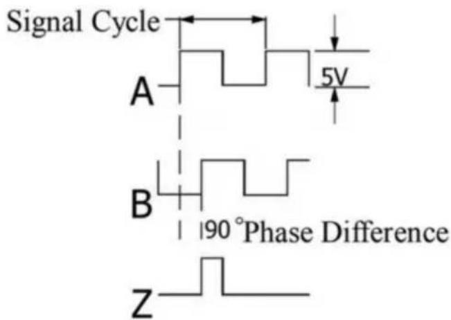

EIA-422-A signal Output: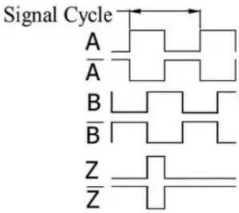

1. TECHNICAL PARAMETER 1.1 SCALING DISTANCE: 0.02 MM (50 LINES /MM) 1.2 RESOLUTION: 5μM, 1μM, 0.5μM 1.3 PRECISION: ±3μM, ±5μM, ±15μM/M (20±0.1℃) 1.4 MEASURING RANGE: 30~3000MM 1.5 MOVING SPEED: HIGH-SPEED ENCODER 120 M/MIN (TO BE CUSTOMIZED)

ORDINARY ENCODER 60M/MIN

1.6 POWER SUPPLY: +5V±5%, 80MA 1.7 CABLE LENGTH: STANDARD 3M (SPECIAL LENGTH AVAILABLE ACCORDING TO THE USER'S NEEDS) 1.8 WORKING TEMPERATURE: 0~45°C 1.9 PIN DESCRIPTION: 1) APPLICABLE TO: 9 PIN SOCKET EIA-422-A SIGNAL OUTPUT.

Machine Translated by Google

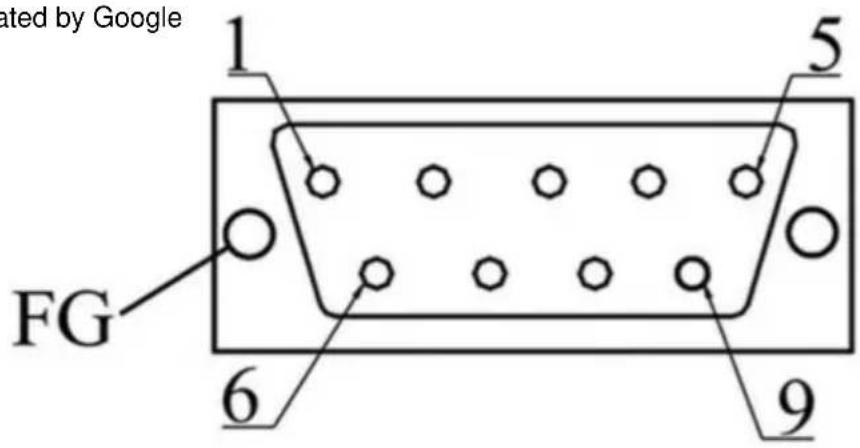
1) Applicable to: 9 pin socket EIA-422-A signal Output.

Pin Position	1	2	3	4	5	6	7	8	9
Signal		OV		Empty		A	+5V	B	Z
Color	Green Black	Black	Orange black	FG	White black	Green	Red	White	Orange

FG: Shield connected to metal casing.

1) Applicable to: 9 pin socket TTL signal Output.

Pin Position	1	2	3	4	5	6	7	8	9
Signal		OV		Empty		A	+5V	B	Z
Color		Black		FG		Green	Red	Orange	White

FG: Shield connected to metal casing.

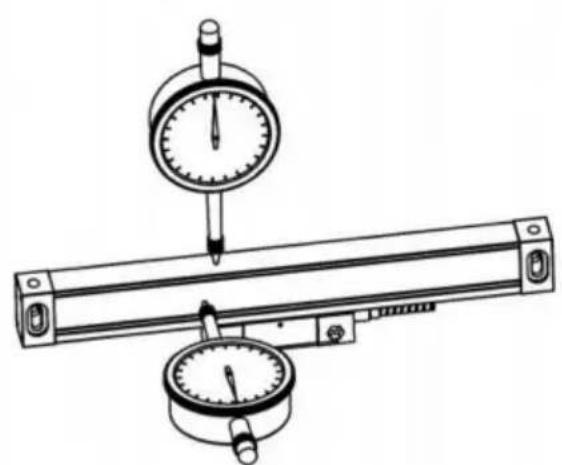
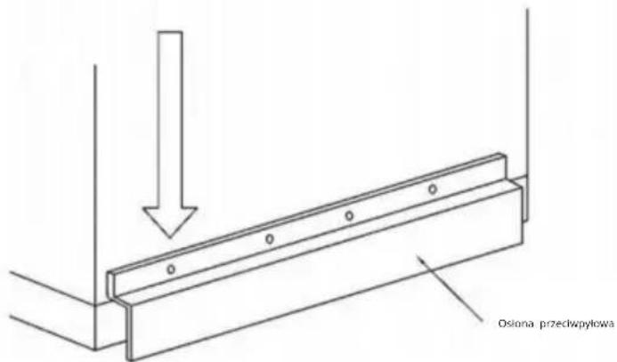
4.9

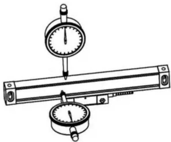
4.10

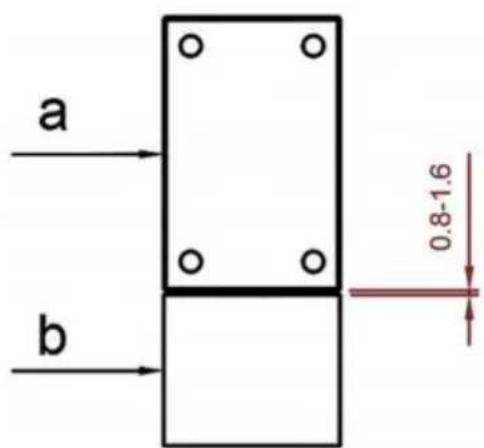
Imported into AUS: SIHAO PTY LTD, 1 ROKEVA STREET EASTWOOD NSW 2122 Australia

Imported into USA: Sanven Technology Ltd., Suite 250, 9166 Anaheim Place, Rancho Cucamonga, CA 91730

C/O YH Consulting Limited Office 147, Centurion House, London Road, Staines-upon-Thames, Surrey, TW18 4AX

VEVOR®

TOUGH TOOLS, HALF PRICE

NEED HELP? CONTACT US!

With the continuous updating of products, if there are changes or

1. Illustration of Panel and keyboard 4
2. Caption of the keyboard 5
3. Parameters settings 7

3.1 Parameters setup routine entrance 7 3.2 Parameters Settings Description 7 3.2.1 Setting the Resolution 7 3.2.2 Setting Positive Direction for Counter 8 3.2.3 Toggle Between R/D Display Mode 8 3.2.4 Setting Z axis Dial 8 3.2.5 Setting the Rotary Radius of the Workpiece 9 3.2.6 Setting the Angle Display Mode 9 3.2.7 Setting the Baudrate of RS_232 (optional) 9 3.2.8 Setting the Absolute Zeroing enable or disable 10 3.2.9 Setting the Absolute form the Special Function 10 3.2.10 Setting the Calculator display Mode 10 3.2.11 Display brightness setting 10 3.2.12 The linear scale counting frequency setting 11 3.2.13 Setting QUIT 11 3.2.14 Setting the type of the DRO 11 3.2.15 Signal Interface Type 11 3.2.16 Restore Factory Settings 12 3.2.17 Shrinkage Ratio enable or disable 12 3.2.18 Setting Compensation Type 12 3.2.19 Inch display, set the number of digits after the decimal point 13 3.2.20 Setting EDM (optional) 13 3.2.21 Setting Linearity Compensation 13 3.2.22 Setting the Shrinkage Ratio 13

4. General Operations 14

4.1 Zeroing 14 4.2 Preset Data to Designated Axis 14 4.3 Toggle Display Unit between inch and mm 14 4.4 Absolute/Incremental/200 groups SDM 15 4.5 1/2 Function 15 4.6 Clear All SDM Datum 16

Contents

4.7 Sleeping Mode 16 4.8 Power Interruption Memory 16 4.9 Search the Absolute Reference Point of Scale 17 4.10 Non Linear Error Compensation 20

5. 200 Groups SDM coordinate 21 5.1 Zeroing at the Current Point 21 5.2 Preset datum of SDM coordinate 22

6. Special Function 24

6.1 Circumference Holes Processing 25 6.2 Linear Holes Processing 28 6.3 ARC Processing 30 6.4 Oblique Processing 39 6.5 Slope Processing 43 6.6 Chamber Processing 44 6.7 The Tool Diameter Compensation Function 45 6.8 Digital Filter of the Grinding Machine 46 6.9 Lathe Function 47

6.9.1 200 sets TOOL Libs 47 6.9.2 Taper Function 48 6.9.3 R/D Function 49 6.9.4 Y + Z Function (only applicable to 3 axes Lathe) 49

6.10 EDM 50

7. Calculator 56

8. Appendix 57

THREE AXIS PANEL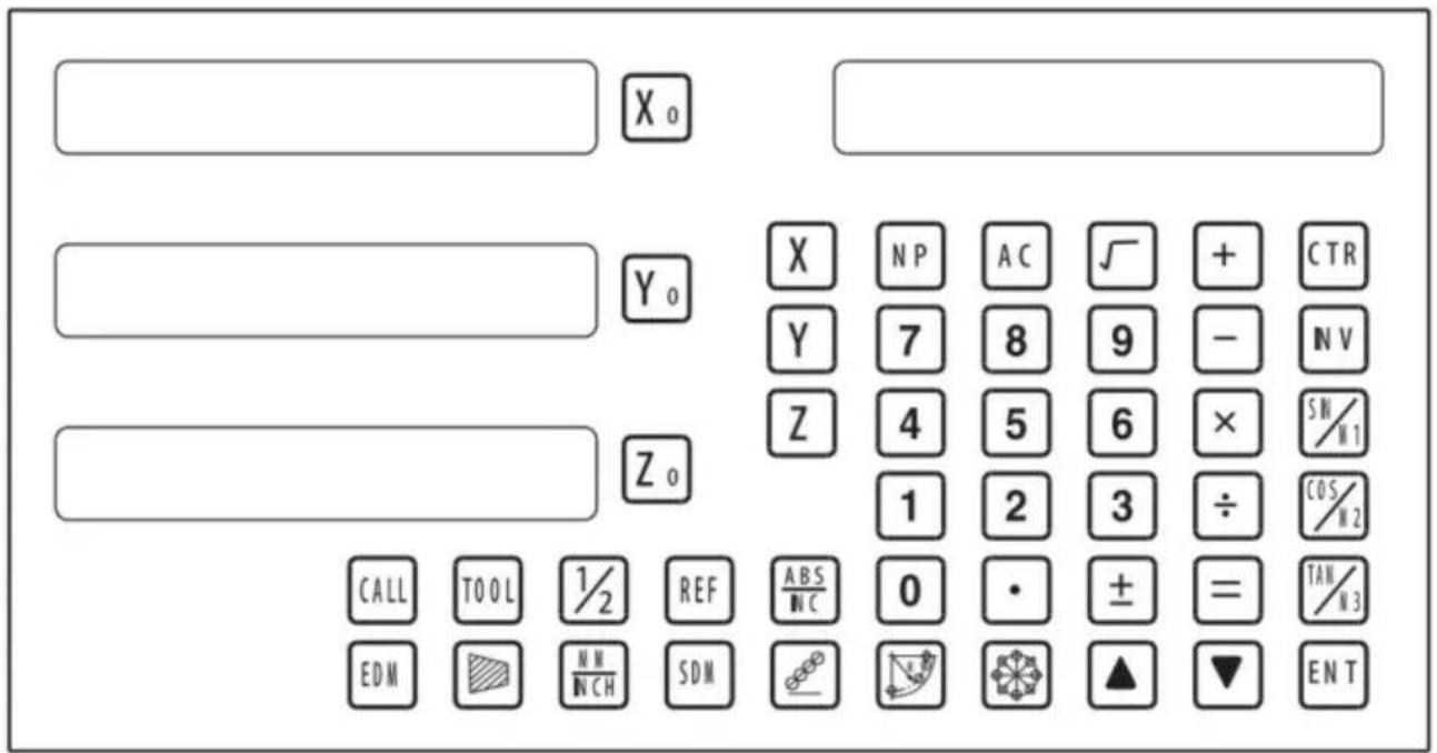

TWO AXIS PANEL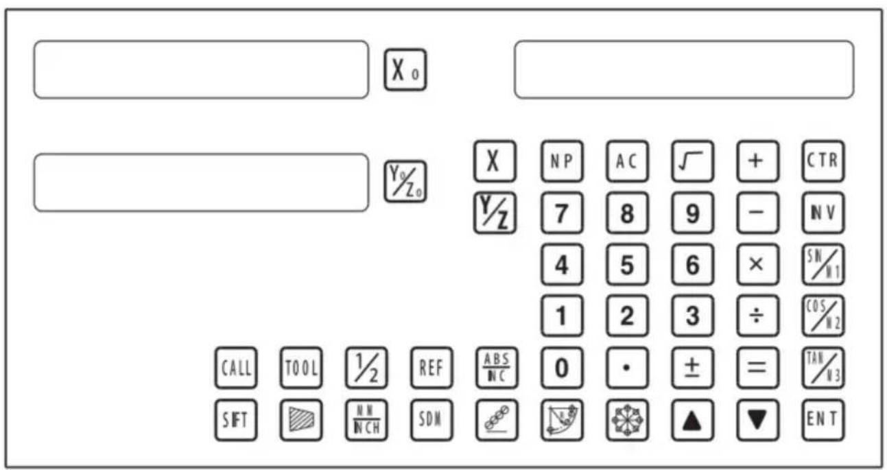

Keyboard Description

	Keys for axis selection
	Zero select axis
	Enter +/- sign
	Enter decimal point
	Entry keys for numbers
	Operation key (in Calculation function key)
	Enter or quit calculating state
	Cancel incorrect operation
	Calculate inverse trigonometric
	Square root
	Confirm operation
	Toggles between inch and millimeter units.
	Press when ready to identify a reference mark.
[STZD]	Function keys for 200 sub datum
	ARC cutting function
	holes displayed equally on a circle
	holes displayed equally on a line

Caption of the keyboard

	Calculate trigonometric or Slope Processing function key
	Calculate trigonometric or rectangular inner chamber processing function key
	Calculate trigonometric or the tool diameter compensation function key
	Toggle between ABS/INC coordinate
	Stroll up or down to select
	Taper measured function key
	Tool library call key
	Opens the tool table.( lathe)
	EDM function key
	Filter display function key
	Half a display value of an axis
	Non Linear Error Compensation function keys

3. Parameters settings

3.1 Parameters setup routine entrance.

Press ☐ to enter initial system and self-check after DRO powers on in 1 second, then Parameters settings display in the Parameters window. Press ▲ ▼ to select the item you want to change.

If you want to quit initial setting, press ▲ ▼ until “QUIT” appears in message window and press ENTER. You can also press • to quit initial setting.

3.2 Parameters Settings Description

3.2.1 Setting the Resolution

Press ▲ ▼ until “RESOLUTE” appears in message window;

When selecting the LINEAR encoder, the resolution will be set as follows:

There are 19 types of resolution:

0.01um; 0.02um; 0.05um; 0.10um; 0.20um; 0.25um; 0.50um; 1.00um; 2.00um; 2.50um; 5.00um; 10.00um; 20.00um; 25.00um; 50.00um; 100.00um; 200.00um; 250.00um; 500.00um.

Press ₀ to change the resolution for X axis; Press ₀ to change the resolution for Y axis; Press ₀ to change the resolution for Z axis;

Set the resolution 5.00um to 1.00um for X axis:

When selecting the rotary encoder, the resolution will be set as follows:

Input the rotary encoder parameter value.

3.2.2 Setting Positive Direction for Counter

Press ▲ ▼ until “DIRECTE” appears in message window.

Direction ‘0’ means the display value will increase when scale moves from right to left and decrease when scale moves from left to right. Direction ‘1’ means the display value will increase when scale moves from left to right and decrease when scale moves from right to left.

Press ₀ to change the Direction for X axis; Press ₀ to change the Direction for Y axis; Press ₀ to change the Direction for Z axis; as follow:

3.2.3 Toggle Between R/D Display Mode

Press ▲ ▼ until “R OR D” appears in message window. X window, Y window, Z window displays ‘0’ or ‘1’ separately.

‘0’ is mode R, which means the display value equals the actual measurement. ‘1’ is mode D where the display value equals the double actual measurement. Press X₀ to change the R/D for X axis; Press Y₀ to change the R/D for Y axis; Press Z₀ to change the R/D for Z axis; as follow:

3.2.4 Setting Z axis Dial

Press ▲ ▼ until "Z DIAL" appears in message window.

Z axis dial should be set if Z axis is emulated for 2 axis milling and only install linear scale for X,Y axis. Z axis dial means the distance the Z axis travels when screw runs a revolution.

Set the Z axis Dial 2.5mm as follow;

3.2.5 Setting the Rotary Radius of the Workpiece

Press ▲ ▼ until "RDIUS" appears in message window.

The Rotary radius type is used perimeter to measure angle.

Input the Rotary Radius parameter value 2000mm as follow:

3.2.6 Setting the Angle Display Mode

Press ▲ ▼ until "ANG DISP" appears in message window.

Press ₀ to change the angle display mode for X axis; Press ₀ to change the angle display mode for Y axis; Press ₀ to change the angle display mode for Z axis; Example for X axis:

"0.0000" means the angle mode is Circulating DD;

"0000.0000" means the angle mode is Incremental DD;

"0.00.00" means the angle mode is Circulating DMS;

"0000.00.00" means the angle mode is Incremental DMS;

3.2.7 Setting the Baudrate of RS_232 (Special customization function, if you need to buy, please contact the dealer to customize)

Press ▲ ▼ until "BAUDRATE" appears in message window. Set the Baudrate 115200 as follow:

3.2.12 The linear scale counting frequency setting

The factory default setting is only "12", the higher the parameter, the lower the counting frequency, press "X0" to set, it is not recommended that you set the default value yourself.

3.2.13 Setting QUIT: Digital display table parameters quit button.

3.2.14 Setting the type of the DRO.

The type of the DRO will be displayed on the right window. Then press the key ENT to select the correct type. The following system items will be set:

"MILL-3" means the DRO type is 3-axis milling machine table;

"MILL-2" means the DRO type is 2-axis milling machine table;

"LATHE-2" means the DRO type is 2-axis lathe table;

"LATHE-3" means the DRO type is 3-axis lathe table;

"GRIND" means the DRO type is Grind table;

"EDM" means the DRO type is EDM table; (Special customization

function, if you need to buy, please contact the dealer to customize)

3.2.15 Signal Interface Type

Message window displays “SEL AXIS” which indicates the step is to Sensor input signal mode. Press X₀ to change the signal mode for X axis; Press Y₀ to change the signal mode for Y axis; Press Z₀ to change the signal mode for Z axis; Example for X axis:

Press X₀ to scroll through the Rotary encode type, the Linear encode type, the Rotary rdius type.

X window displays the Signal type.

“LInER” means the Signal type is linear encode type ;

"EnCOdE " means the Signal type is Rotary encode type;

"RdIUS" means the Signal type is Rotary rdius type ;

Example: currently in the linear encode type, to toggle to the Rotary encode type;

3.2.16 Restore Factory Settings:

Clear all data except DRO type. DRO will load default setup for parameters. After loading default setup, user must search RI once to enable resuming ABS datum function; otherwise, to resume the datum by RI is unable.

Message window displays “ALL CLR”, press ENT and message window displays “PASSWORD” indicating the operator to input password; press 2000 + ENT in turn to load default value.

3.2.17 Shrinkage Ratio enable or disable.

Message window displays “SRK OFF” to disable Shrinkage rate function. Press ☐ to enable Shrinkage rate function, and message window displays “SRK ON”.

3.2.18 Setting Compensation Type

Message window displays “SEL COMP” which indicates the step is to compensation type. Press X₀ to change the compensation type for X axis; press Y₀ to change the compensation type for Y axis; press Z₀ to change the compensation type for Z axis. Example for X axis:

Press X₀ to scroll through the not compensation type, the linear compensation type, the non-linear compensation type.

“no-CO” means the compensation type is not compensation type; “LInE-CO” means the compensation type is linear compensation type; “non-LinE” means the compensation type is non-linear compensation type.

Example for X axis: currently in the not compensation type, to toggle to the linear compensation type.

3.2.19 Inch display, set the number of digits after the decimal point

In the inch display mode, the number of digits after the decimal point is set. The factory default digit is "4". Press "X0" to set, can be set according to actual needs.

3.2.20 Setting EDM: it is not recommended that you set the default value yourself. EDM function, set the relay off on time.

3.2.21 Setting Linearity Compensation.

Message window displays “LIN COMP” which indicates the step is to Linearity Compensation. Compensate the linear error to make display value equals to standard value.

The calculation of compensation rectifying coefficient:

Coefficient = (Measurement - Standard value) x 1000.000/ Standard value

Example for X axis:

Measurement 200.020mm

Standard value 200.000mm

Rectifying coefficient= (200.020-200) * 1000 /200 = -0.01mm/m

Input compensation rectifying coefficient 0.01 as follow:

3.2.22 Setting the Shrinkage Ratio

Press ▲ ▼ until “ SHRINK” appears in message window;

Shrinkage radio = Dimensions of the finished product/Dimensions of the working piece

Set the shrinkage radio 1.005 as follow;

4、General Operations;

4.1 Zeroing

Zero the designated axis in normal display state.Zeroing is used to set the current point as datum point as follow;

X₀ or Y₀ or Z₀ will be return to the original data before the reset.

4.2 Preset Data to Designated Axis

Preset a value to current position for a designated axis in normal display state.

4.3 Toggle Display Unit between inch and mm

Length can be displayed either in “mm” (metric) or “inch” (imperial). Display unit can be toggled between mm and inch.

Example: Display value toggle from mm to inch;

Example: Display value toggle from inch to mm;

4.4 Absolute/Incremental/200 groups SDM

Function: The DRO has 3 coordinate display modes: the absolute mode (ABS); the incremental mode (INC) and 200 groups Second Data Memory (SDM) with the range of 00 to 99. Zero point of work-piece is set at the origin point of ABS coordinate. The relative distance between datum of ABS and SDM remains unchanged when ABS datum is changed.

1. Toggle from ABS to INC coordinate;

1. Toggle from INC to ABS coordinate;

1. Toggle from SMD to ABS coordinate;

4.5 1/2 Function

Function: Set the center of work piece as datum by halving the displayed value.

Example: Set the center of rectangle as datum as the right figure.

Steps:

1. Touch one side of the workpiece with the TOOL, then zero the X axis.

2. The message window displays “REF”. Press ☐NT until “FD_REF” appears in the message window.

3. Select the axis which needs to search for RI. For instance: select the X axis, then press ☒. "X_REF" is displayed in the message window, and the X axis window flashes.

4. Move the machine table. The buzzer sounds when RI is searched, then the X window stops flashing and displays the value of the current position. The DRO returns to normal display state. Then the message window displays "FIND_X".

Example for AB mode:

1. DRO is set in ABS coordinate. Press REF, then the message window displays "REF".

2. Press ▲ ▼, then the message window displays “AB”.

3. The message window displays “AB”. Press ENT until “FIND_AB” appears in the message window.

4. Select the axis which needs to search for RI. For instance: select the X axis, then press ☒. “X_REF” is displayed in the message window, and the X axis window flashes.

5. Move the machine table. The buzzer sounds when RI is searched, and the value of the current position for the absolute datum zero is displayed. The DRO returns to normal display state. Then the message window displays "FIND_AB".

Example for LEF_AB mode:

1. DRO is set in ABS coordinate. Press REF, then the message window displays "REF".

2. Press ▲ ▼, then the message window displays “AB”.

3. The message window displays "LEF_AB". Press ENT until "ZERO_AB" appears in the message window.

4. Move the machine table to the position to be set as zero point. Then press X, the X axis will be zeroed. The current position for the absolute datum zero is set. The DRO returns to normal display state.

NOTE: Linear range without reference point location of the user

4.10 Non Linear Error Compensation

First compensation Type (Linear or Non-Linear) in parameter setting must be set Non-Linear. Linear scale have a ref point location and find to the Absolute Reference Point will be enable.

Default Non-Linear compensation : 50.

Example for Y axis:

Step 1: Search the Absolute Reference Point of Scale;

Step 2: Press NP, then the message window display "COMP X".

Step 3: Press ▲ ▼, then the massage window display "COMP Y"

Step 4: Press ENT, then the message window display "NUMBER". Then input the compensation parameter NUMBER.

Step 5: Press ▲ ▼, then message window displays “Y-MSN-1” which indicates the step is to Non Linear Error Compensation.

Step 6: Input compensation value.

X window display the value of the measurement value.

Y window display the value of the standard value.

Example for the first compensation point:

Measurement value :68.288mm. Standard value: 68.200mm

Step 7: After input all parameter, the DRO automatically exit.

5. 200 Groups SDM Coordinate

The DRO has three display modes: the absolute mode (ABS), the incremental mode (INC), and the 200 groups second data memory (SDM 1 - SDM200). The ABS datum of the workpiece is set at the beginning, and the 200 groups SDM is set relative to the ABS coordinate.

ABS Mode, INC Mode, and SDM Mode are specially designed to provide much more convenience features to the operator to cope with the batch machining of relative works and the machining of the workpiece machining dimensions from more than one datum.

Example: The ABS datum is the center point O, and the points sdm1, sdm2, sdm3, sdm4 needed for processing are set as the datum of SDM 1 - SDM 4.

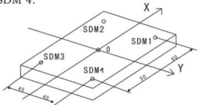
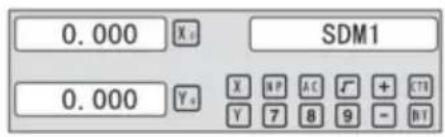
Two ways to set SDM coordinate:

1. Zeroing at the current point. 2. Preset datum of SDM coordinate.

5.1 Zeroing at the Current Point

First, set the center point of the workpiece as the origin of the ABS. Then align the tool with points SDM1, SDM2, SDM3, SDM4 by moving the machine table and zero them. It is the position to process where the “0.000” appears in the X window and Y window by moving the machine table, whether in ABS or in SDM coordinate.

Steps:

1. Move the worktable to place the tool at the center of the workpiece point O as the datum of ABS. Then zero the X axis and Y axis in SDM 1; zero the X axis and Y axis in SDM 2; zero the X axis and Y axis in SDM 3; zero the X axis and Y axis in SDM 4.

2. Set the point sdm1 as the datum of SDM 1. Move the machine worktable to x = 60.000, y = 45.000. Then process X0 Y0.

2. Set the point sdm1 as the datum of SDM 2. Move the machine worktable to x = 60.000, y = -45.000. Then process X0 Y0.

3. Set the point sdm1 as the datum of SDM 3. Move the machine worktable to x = -60.000, y = -45.000. Then process X0 Y0.

4. Set the point sdm1 as the datum of SDM 4. Move the machine worktable to x = -60.000, y = 45.000. Then process X0 Y0.

5.2 Preset Datum of SDM Coordinate

The procedure is the same as Method 1. First, move the worktable to place the tool exactly at the origin of ABS. Then, enter the ABS mode as follows.

Steps:

1. Move the worktable to place the tool at the center of the workpiece point O as the datum of ABS. Then zero the X axis and Y axis in SDM 1; zero the X axis and Y axis in SDM 2; zero the X axis and Y axis in SDM 3; zero the X axis and Y axis in SDM 4.

2. Set point SDM1 as the datum of SDM 1. Press ▲ ▼, then the message window displays “SDM 1”. Input x = 60.000, y = 45.000.

3. Set point SDM1 as the datum of SDM 2. Press ▲ ▼, then the message window displays “SDM 2”. Input x = -60.000, y = 45.000.

4. Set point SDM1 as the datum of SDM 3. Press ▲ ▼, then the message window displays “SDM 3”. Input x = -60.000, y = -45.000.

5. Set point SDM1 as the datum of SDM 4. Press ▲ ▼, then the message window displays “SDM 4”. Input x = -60.000, y = 45.000.

6. Special functions

6.1 Circumference Holes Processing

The function of PCD hole positioning on a circumference is used to distribute arcs equally, such as boring holes on a flange. The right window will show the parameters to be defined when selecting the PCD function. The parameters to be defined are:

PCD_XY (XZ, YZ)

Select place

CENTER

Center position

DIA

Diameter of circle

NO_HOLE

Hole number

STANG

Starting angle

ED ANG

Ending angle

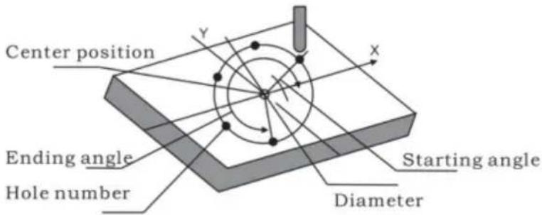
The position of the hole center is calculated automatically after inputting all parameters. Press ▲ or ▼ to choose the hole number and move the machine table until "0.000" appears in the X, Y, and Z windows. That is the position to process the hole.

Example for the XY plane: Machine holes on a circumference as shown in the figure.

PCD_XY(XZ,YZ)	XY
CENTER	X=0,000,Y=0.000
DIA	100,000
NO_HOLE	5
ST ANG	30,000
ED ANG	315,000

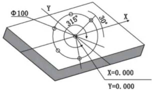
Steps:

1. Set the display unit to metric in the normal state; move the machine table until the machine tool is aligned with the center of the circle, then zero the X and Y axes.
2. Select piece.

Press 🧑️, then the message window displays "PCD_XY" for the Circumference Holes Processing. Press ▲ or ▼ to select XY plane.

2. Input center position.

Press ENT, then the message window displays "CENTER". The X and Y windows display the previously set center position. Input X = 0, Y = 0 as follows.

4. Input diameter.

Press ▼ until “DIA” appears in the message window. The X window displays the formerly preset diameter. Then input the diameter as 100.000.

5. Input number.

Press ▼ until "NO_HOLE" appears in the message window. The X window displays the formerly preset number. Then press 5 in turn to input the number.

6. Input starting angle.

Press ▼ until “ST ANG” appears in the message window. The X window displays the formerly preset starting angle. Then press 3 and 0 in turn to input the starting angle.

7. Input ending angle.

Press ▼ until “ED ANG” appears in the message window. The X window displays the formerly preset ending angle. Then press 3, 1, and 5 in turn to input the ending angle.

1. Press ▼ until "NO 1" appears in the message window.

This is the position of the first hole to punch, where “0.000” is displayed in the X and Y windows by moving the machine table. After finishing the first hole, press ▼ or ▲ to change the hole number.

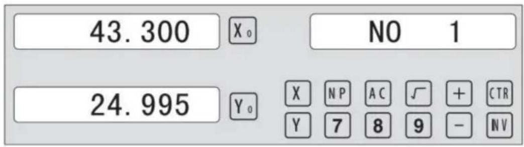
1. After processing all holes, press 📋 to return to normal display.

6.2 Linear Holes Processing

There are two modes to carry out the linear drilling: Length mode and Step mode.

1. LINE S Step mode LINE L Length mode 2. STEP Step length LENGTH Line length
2. ANG Angle
3. NO.HOLE Hole number

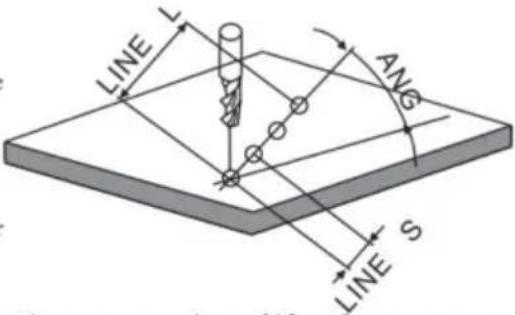
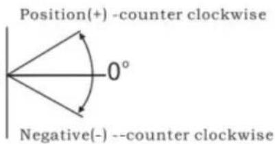
The Linear Holes function can simplify the processing of multiple holes whose centers are equally spaced on one line.

Example:

LINE_L	Length mode
LENGTH	60.000
ANG	30.000
NO.HOLE	4

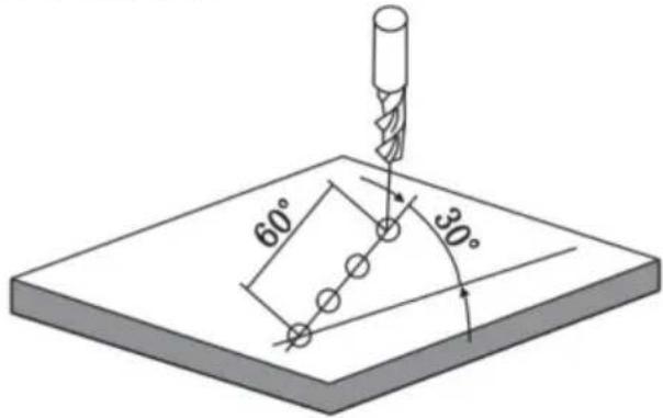
Steps:

1. Select the piece.

Press 📄, then the message window displays “LINE_XY” for the Linear Holes Processing. Press ▲ or ▼ to select the XY plane.

2. Select Linear Holes mode.

Press ENT, then the message window displays "LINE_S". Press ▲ or ▼ to select "LINE_L".

3. Input linear length;

Press ENT, then the message window displays "LENGTH".

The X window displays the previously preset linear length. Press 6 0 in turn to input the linear length.

1. Input angle;

The message window displays “ANG” which indicates the step is to input the angle. The X window displays the previously preset angle. Press 3 0 in turn to input the angle.

1. Input number;

The message window displays “NUMBER” which indicates the step is to input the number. The X window displays the previously preset number. Press 4 in turn to input the number.

1. Press ▼ until "NO 1" appears in the message window.

It is the position of the first hole to punch where the “0.000” is displayed in X window and Y window by moving the machine table. After finishing the first hole, press ▲ or ▼ to change holes number.

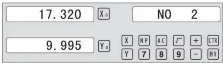
1. After processing all holes, press ☐ to return normal display.

6.3 ARC processing

Provides maximum flexibility in ARC machining, the ARC sector to be machined by the coordinates of ARC. Very flexible, ARC function can machine virtually all kinds of ARC, even the intersected ARC.

Relatively a bit complicated to operate, operator need to calculate and enter the coordinates of ARC centre, start angle and end angle.

Basic parameters as follow:

1. SMOOTH Mode of the Smooth ARC processing;
2. SEL_XY(YZ, XZ) Select place;
3. CENTER Refer to the position of a center.
4. RAD Radius of the ARC
5. TL_DIA Diameter of the TOOL
6. MAX_CUT Feed step
7. ST_ANG Starting angle
8. ED_ANG Ending angle
9. RAD+TL Outer arc. RAD-TL Inner arc.

Example 1 for the Simple ARC Processing:

Parameters settings as follow:

SIMPLE Simple mode

TYPE 3

SEL_XY XY

RAD 80.000

TL_DIA 6.000

MAX_CUT 0.500

RAD+TL 1

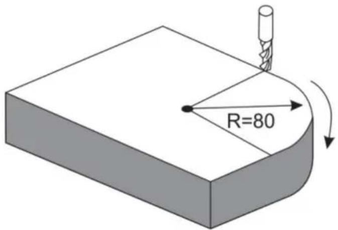
Steps:

1. Select process mode

Press 📋, then the message window displays “SIMPLE” for the ARC Processing. Press ▲ or ▼ to select the mode of the simple, the message window displays “SIMPLE”

ARC Processing

2. Input the type:

Press ENT until "TYPE" appears in the message window. The X window displays the formerly preset type. Press 3 in turn.

3. Select place

Press ENT until "SEL_XY" appears in the message window. Press ▲ or ▼ to select the place to display "SEL_XY".

4. Input radius:

Press ENT until "RAD" appears in the message window. The X window displays the formerly preset radius of ARC. Press 8

0 in turn to input the radius.

5. Input Diameter of the TOOL

Press ▲ or ▼ until "TL DIA" appears in the message window. The X window displays the formerly preset Diameter of the TOOL. Press 6 in turn to input the Diameter value.

6. Input Feed step (MAX_CUT);

Press ▲ or ▼ until "MAX_CUT" appears in the message window. The X window displays the formerly preset MAX_CUT. Press 0 · 5 in turn to input the MAX_CUT value.

7. Select outer arc or inner arc

Press ▲ or ▼ until "RAD-TL" appears in the message window. Press ▲ or ▼ to select the place to display "RAD+TL".

8. After inputting all parameters, press the key ENT for machining.

The DRO will display the position of the first point. Retract the axes until the displays read 0.000. Machine the Arc point by point in accordance with the display. After finishing the position of the first point, press ▲ or ▼ to change position point.

Press ☐ to quit R function any time.

Example 2 for the Simple ARC Processing:

Parameters settings as follow:

SIMPLE Simple mode

TYPE 3

SEL_XY XZ

RAD 80.000

TL_DIA 6.000

MAX_CUT 0.500

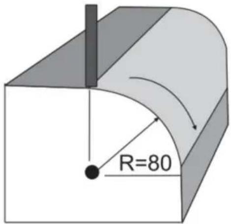
Steps:

1. Press 📋, then the message window displays “SIMPLE” for the ARC Processing. Press ▲ or ▼ to select the mode of the simple, the message window displays “SIMPLE”

ARC Processing

2. Input the type:

Press ☐ENT until "TYPE" appears in the message window. The X-window displays the formerly preset type. Press ☐3 in turn

3. Select place

Press ENT until "SEL_XZ" appears in the message window. Press ▲ or ▼ to select place to display "SEL_XZ";

4. Input radius:

Press ENT until “RAD” appears in the message window. The X window displays the previously preset radius of the ARC. Press 8 and 0 in turn to input the radius.

5. Input Diameter of the TOOL

Press ▲ or ▼ until “TL DIA” appears in the message window. The X window displays the previously preset diameter of the TOOL. Press 6 in turn to input the diameter value.

6. Input Feed step (MAX_CUT);

Press ▲ or ▼ until “MAX_CUT” appears in the message window. The X window displays the previously preset MAX_CUT. Press 0, ., and 5 in turn to input the MAX_CUT value.

1. After inputting all parameters, press the ENT key for machining.

For 2-axis milling machine table, it is not installed with Z-axis, please press ▲ or ▼ to simulate position of Z-axis. Press ▲ to simulate moving to the former process, and press ▼ to simulate moving to the next process point.

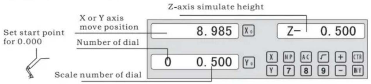
Z-axis simulate height = Number of dial x Z axis Dial + Scale number of dial

Press ☐ to quit R function any time.

Example 3 for the Smooth ARC function:

Parameters settings as follow:

SMOOTH	Smooth mode
SEL_XY(YZ,XZ)	XY
CENTER	X=0,Y=0
RAD	80.000
TL_DIA	6.000
MAX_CUT	0.500
ST_ANG	0.000
ED_ANG	135.000
RAD+TL	1

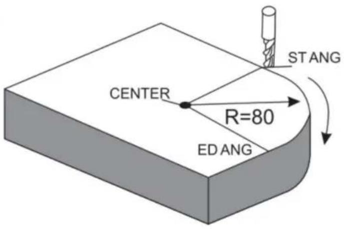
Steps:

1. Press 📋, then the message window displays “SIMPLE” for the ARC Processing. Press ▲ or ▼ to select mode of the simple, the

message window displays "SMOOTH"; For 3-axis milling machine table without this step. In second step. Then press ENT.

2. Select place

Message window displays “SEL_XY” which indicates the select is to place. Press ▲ or ▼ to select place to display “SEL_XY”;

3. Input center position.

Press ☐ENT, then the message window displays "CENTER". X and Y windows display the formerly preset center position. Input X = 0, Y = 0 as follows.

4. Input radius:

Press ☐ENT until “RAD” appears in the message window. X window displays the formerly preset radius of ARC. Press ☐8 ☐0 in turn to input the radius.

5. Input Diameter of the TOOL

Press ▲ or ▼ until “TL DIA” appears in the message window. X window displays the formerly preset Diameter of the TOOL. Press 6 in turn to input the Diameter value.

Press ☐ to quit ARC function at any time.

6) Change the angle of the work piece to make the workpiece touch the measuring tool and adjust it to zero.

STEPS:

1. Select place

Press SN/1, then the message window displays "INCL_XY" for the Oblique Processing. Press ▲ or ▼ to select place to display "SEL_XY";

Then press ☐ENT to proceed to the next step.

2. Input the angle of obliquity

The message window displays "ANG", and the X window displays the previously preset angle of obliquity. Press 4 and 5 in turn to input the angle of obliquity.

1. Move the workpiece along the X-axis until the measuring tool touches the workpiece, adjust it to zero, and move the worktable for any distance along the X-axis.

1. Press Y, display the value of the Y-axis. Move the workpiece along the Y-axis, change the angle of the workpiece to make the obliquity-calibrating plane touch the measuring tool until it turns to zero. Move the worktable until the Y-axis is displayed as zero.

1. Press 5W/H1 to quit the oblique function at any time.

Example 2 for the oblique XZ or YZ plane:

When the machining plane is on plane XZ or YZ, the function of tool inclination can instruct the operator to machine the oblique plane step by step.

Procedures for using the function of cutter inclination:

When the machining plane is on plane XZ or YZ, first please calibrate the obliquity of the primary spindle nose and set the tool:

INCL_XY(XZ,YZ)	INCL_XZ
DIA	10.000
ST_POT	20.000
ED_POT	20.000

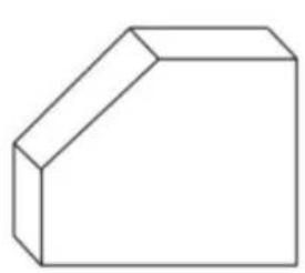
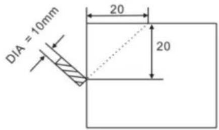
STEPS:

1. Press SN/81, then the message window displays "INCL_XY" for the oblique processing. Press ▲ or ▼ to select the plane to display "SEL_XZ"; then press ENT to go to the next step;

1. Input the tool diameter

The message window displays "DIA", and the X window displays the previously preset angle of obliquity. Press 10 in turn to input the tool diameter of obliquity. OK, then press ▼ to go to the next step;

1. Input ST_POT;

The message window displays "ST_POT", and the X and Y windows display the previously preset starting position of obliquity. Input X=0, Y=-20.000. OK, then press ▼ to go to the next step;

4. Input ED_POT;

The message window displays “ED_POT”, and the X and Y windows display the formerly preset starting position of obliquity. Input X=20.000, Y=0.000.

5. After inputting all parameters, press the ▼ key for machining.

For a 2-axis milling machine table, it is not installed with a Z-axis, please press ▲ or ▼ to simulate the position of the Z-axis. Press ▲ to simulate moving to the former process, and press ▼ to simulate moving to the next process point.

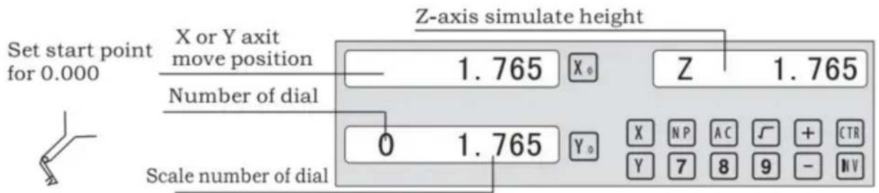
Z-axis simulate height = Number of dial x Z axis Dial + Scale number of dial

Press ☐ to quit oblique function at any time.

6.5 Slope Processing

This function can calculate the position of every processing point automatically in processing slope. Only the following parameters need to be inputted:

XZ, YZ

Set machine place YZ, or XZ

ANG

The inclination angle

Z_STEP

The slope length

each time processing

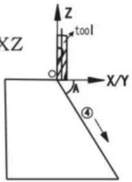
Example 1 for the Slope XZ place;

Step 1. Select place

Press [TAN], then the message window displays "XZ" for slope processing. Press ▲ or ▼ to select place to display "SEL_XY"; then press [ENT] to proceed to the next step.

Step 2. Input the angle of slope

The message window displays "ANG", and the X window displays the previously preset angle of slope. Press 4 and 5 in turn.

Step 3. Input Z_step

The message window displays "Z STEP", and the X window displays the previously preset starting position of slope. Input 0 and 1 in turn.

Step 4: Finishing the ALL processing. Press ☐ to quit slope function at any time.

6.6 Chambering Processing

1, FLAT_XY: machine place; 2, DIA: diameter of TOOL; 3, CENTER: center of the chambering; 4, SIZE: size of the chambering;

Figure as follow:

STEPS:

1. Press [COS/W2], then the message window displays "FLAT_XY" for the Chambering Processing.

1. Input DIA of the TOOL;

1. Input the center coordinate;

1. Input the size;

5. Process Chambering;

Move the machine until the display of the axis is zero, i.e., the position of the first point. Machine the first point. Display the next machining point by pressing ▲ or ▼. On the completion of machining, the right window shows OVER. Press ▲ or ▼, the system will go to the first position for the next workpiece. Press ⚠/12 to quit the Chambering Function.

6.7 The Tool Diameter Compensation Function

Without TOOL compensation, the operator has to move the TOOL for an additional distance of the diameter of the TOOL along each side when machining the four 150 and 100 sides of a workpiece to finish machining the whole brim. The digital readouts shall automatically compensate when the TOOL compensation function is enabled.

Note: the TOOL compensation is made in the direction of X and Y axis.

Procedures:

1). Enter the function of compensating the diameter of the TOOL. 2). Select one of the (four) preset machining modes. 3). Input the diameter of the TOOL. 4). Enter machining.

Figure A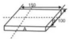

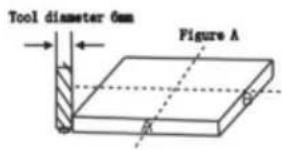
Figure B

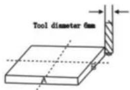
Figure C

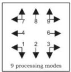
Step 1: press ☐ to enter the TOOL compensation Function. Then the message window displays “TYPE”. Press ☐.

Step 2: input the diameter of the TOOL; Press 10 in turn.

Step 3: Press ▼ to the machining Mode.

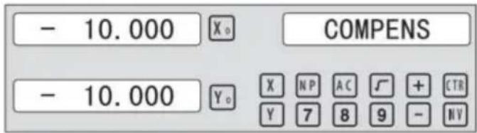
Machining of 2 side planes can be done by moving the TOOL until X-Axis is 150.000 and Y-Axis is 100.000. Press the Key [TAN/V3] to quit the Function.

6.8 Digital Filter of the Grinding Machine

When machining a workpiece with a grinder, the display values change quickly due to the vibration of the grinder. The user cannot see the display value clearly. The grinder DRO provides a display value filter function to suppress the rapid changes in the display value.

STEPS:

1. Enter the display value filter function.

In the normal display state, press SIFT simultaneously to enter the display value filter function.

1. Exit the display value filter function;

Press SIFT to exit the display value filter function;

6.9 The function

6.9.1 200 sets of tool libraries

It will automatically exit from EDM machining status and recover to the original state before machining;

b) Stop Mode:

It will always stay at the machining interface after finishing machining, and you should press EDM to exit and return to the original state.

Operation steps:

The DEPTH (machining depth), ERRHIGH (negative fireproof height), exit mode, EDM relay output mode, and machining direction should be set.

STEPS:

1. Press EDM to enter the EDM function. Press ▲ to input parameters; press ▼ to enter the EDM machining state.
2. Input DEPTH (machining depth). Press the key ▲ to set the next parameter.

1. Input ERRHIGH (Negative Fireproof Height) (undefined). Press the key ▲ to set the next parameter.

1. Set machining direction (Positive or Negative). Press 1 to select Positive direction. Press 0 to select Negative direction. Press the key ▲ to set the next parameter.

EDM

1. Set exit Mode (AUTO Mode or STOP Mode). Press 0 to select AUTO Mode; Press 1 to select STOP Mode; Press the key ▲ to set the next parameter.

1. Set the Output Mode (Mode 0 or Mode 1) (undefined). Press ☐ to select Mode 0; Press ☐ to select Mode 1.

1. Continuously press ▼ to return to EDM for machining. Press EDM to quit the function.

Example 1: positive direction machining.

Machining is shown as the model chamber as follows:

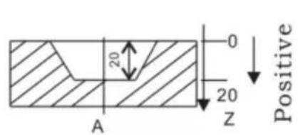
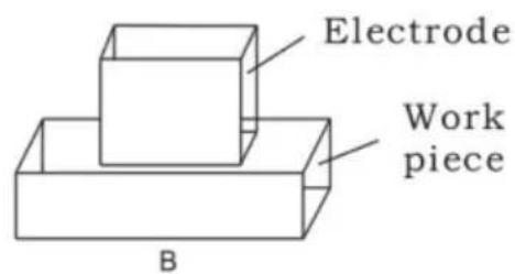
STEPS:

1. Touch one side of the workpiece with the TOOL, then press Z0 to zero the Z axis.

2. Press EDM, set DEPTH to 20.000; press ▼ to EDM for machining.

Example 2: Negative direction machining.

Machining is shown as the model chamber as follows:

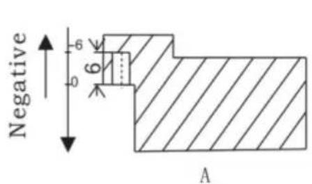
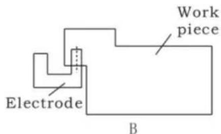
1. Touch one side of the workpiece with the TOOL, then press Z0 to zero the Z axis.

2. Press EDM, set DEPTH to -20.000; press ▼ to EDM for machining.

Example 3: PCD Function for EDM

The PCD Function can access the EDM Function. The operator enters the PCD Function to input parameters for PCD and enter the PCD machining state. At every position for machining, press the EDM key to access the EDM Function.

The following are the preliminary solutions for troubleshooting.

If there is still trouble, please contact our company or agents for help.

Troubles	Possible reasons	Solvents
No display	1. Power isn't connected2. Power switch is off.3. The range of power voltage is not right.4. The inner power of Linear Scale is short.	1. Check power wire and connect the power2. Turn on the power switch.3. The range of voltage is in 80--260V4. Unplug the connector of linear scale
One axis is not counting	1. Replace the linear scale of the other axis.2. DRO is in special function	1. If count is normal, the linear scale has trouble; If abnormal, the DRO readouts has trouble.2. Quit the special function.
Linear scale is not counting	1. Reading head is bad for using range exceeds.2. Aluminum chips is in reading head of linear scale.3. The span between the reading head and metal part of linear scale is large.4. The metal parts of linear scale is damage.	1. Repair the linear scale2. Repair the linear scale3. Repair the linear scale4. Repair the linear scale
Counting is error	1. Shell is poor grounding.2. Low precision of machine.3. Speed of machine is too rapid.4. Precision of linear scale is low.5. The resolution of DRO readouts and the linear scale is not match.6. The unit (mm/inch) is not match.7. Setting the linear compensating is not arrest.8. Reading head of the linear scale is damaged.	1. Shell is good grounding.2. Repair the machine.3. Reduce the speed of machine.4. Mount the linear scale again.5. Set the resolution of the DRO again,6. Cover the unit of display mm/inch.7. Reset the linear compensation.8. Repair the linear scale.
The counting of the linear scale is not accurate	1. The mounting of linear scale does not demand the requirement, and the precision is not adequate.2. The screw is loosen.3. Precision of machine is low.4. The resolution of digital readouts and the linear scale is not match.	1. Mount the linear scale again and level it.2. Lock all fixing screws.3. Repair the machine.4. Reset the resolution of digital readouts.
Sometimes the linear scale is not counting	1. The small car and steel ball is separated.2. The glass of reading head is wearied.3. The glass of reading head of the linear scale has dirt.4. The elasticity of the steel wire is not adequate.	1. Repair the linear scale.2. Repair the linear scale.3. Repair the linear scale.4. Repair the linear scale.

1. Specifications of Digital Readout.

1) Supply Voltage range: AC 85 V ~ 230 V; 50 ~ 60 Hz 2) Power consumption: 15VA 3) Operating temperature: 0°C - 50°C 4) Storage temperature: -30°C - 70°C 5) Relative humidity: < 90 % (25) 6) Max Coordinate number: 3 7) Readout allowable input signal: TTL square wave 8) Allowable input signal frequency: < 5 MHz 9) Max resolution of digital display length: 0.01 um 10) Max resolution of digital display angle: 0.0001 / PULSE

1. Instructions

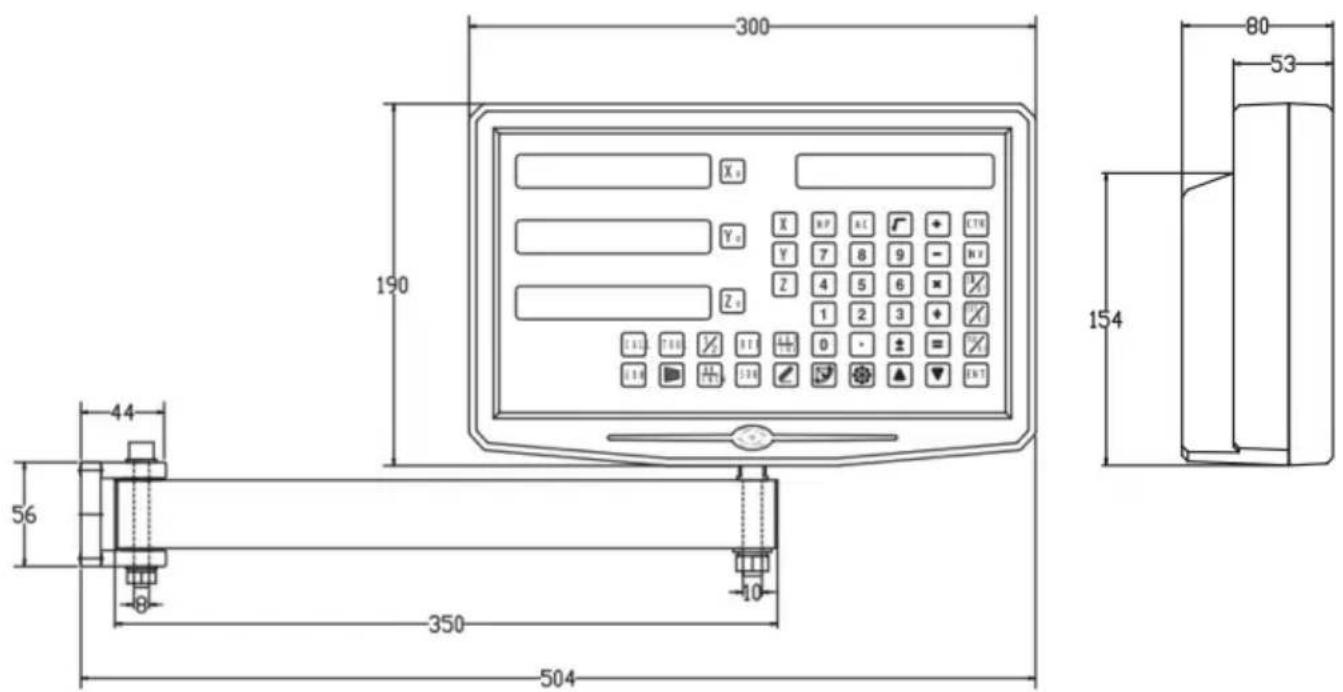
1. X, Y, Z Axis

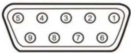
Pin	TTL (Standard)
1
2	OV
3
4
5
6	A+
7	5V
8	B+
9	R+

Pin	TTL (Standard)
1	5V
2	OV
3	A+
4	B+
5	R+
6
7
8
9

For your convenience, if you buy a digital readout,

The wiring definition of your linear scale must be the same as the 2 definitions in the above diagram to be universal!

Installation instructions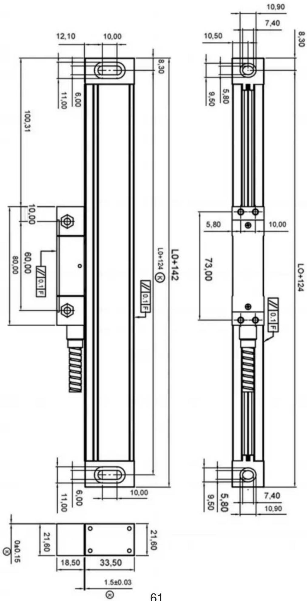

TTL signal Output: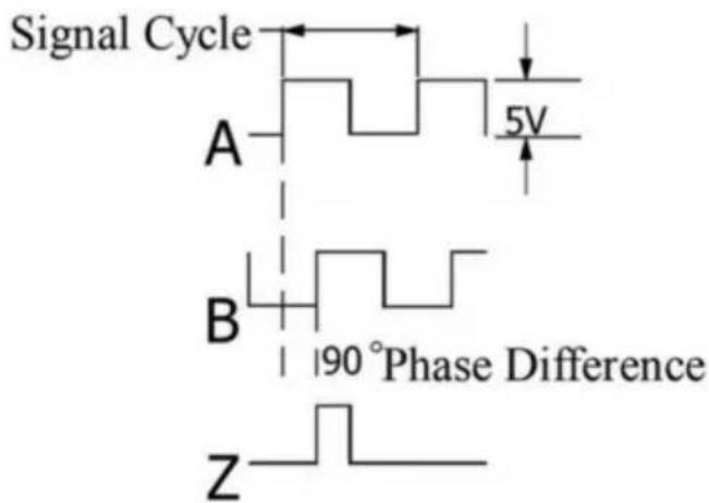

EIA-422-A signal Output:

1. TECHNICAL PARAMETER 1.1 SCALING DISTANCE: 0.02 MM (50 LINES /MM) 1.2 RESOLUTION: 5μM, 1μM, 0.5μM 1.3 PRECISION: ±3μM, ±5μM, ±15μM/M (20±0.1℃) 1.4 MEASURING RANGE: 30~3000MM 1.5 MOVING SPEED: HIGH-SPEED ENCODER 120 M/MIN (TO BE CUSTOMIZED)

ORDINARY ENCODER 60M/MIN

1.6 POWER SUPPLY: +5V±5%, 80MA 1.7 CABLE LENGTH: STANDARD 3M (SPECIAL LENGTH AVAILABLE ACCORDING TO THE USER'S

NEEDS)

1.8 WORKING TEMPERATURE: 0~45°C 1.9 PIN DESCRIPTION: 1) APPLICABLE TO: 9 PIN SOCKET EIA-422-A SIGNAL OUTPUT.

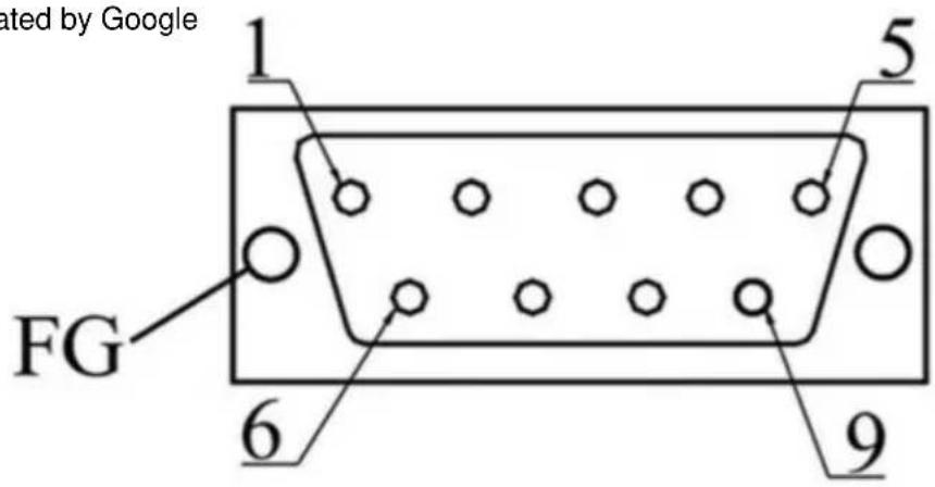
1) Applicable to: 9 pin socket EIA-422-A signal Output.

Pin Position	1	2	3	4	5	6	7	8	9
Signal		OV		Empty		A	+5V	B	Z
Color	Green Black	Black	Orange black	FG	White black	Green	Red	White	Orange

FG: Shield connected to metal casing.

1) Applicable to: 9 pin socket TTL signal Output.

Pin Position	1	2	3	4	5	6	7	8	9
Signal		OV		Empty		A	+5V	B	Z
Color		Black		FG		Green	Red	Orange	White

FG: Shield connected to metal casing.

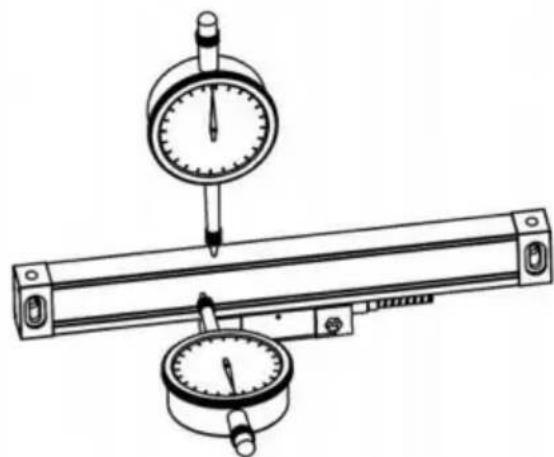
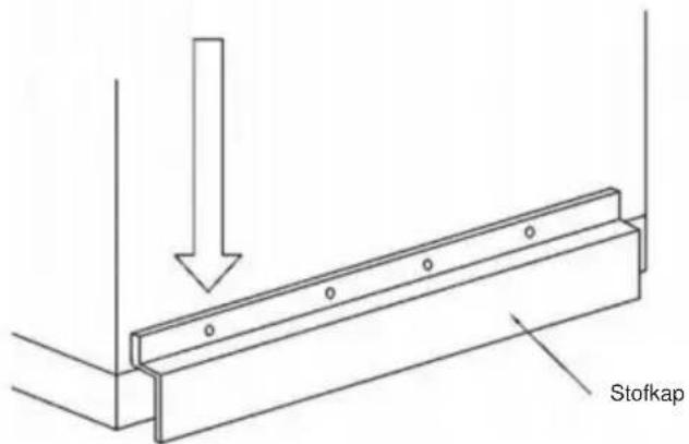
4.9

4.10

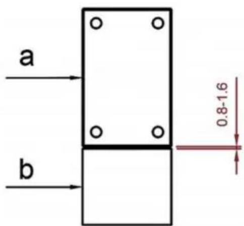
C/O YH Consulting Limited Kantoor 147, Centurion House, Londen Road, Staines-upon-Thames, Surrey, TW18 4AX

VEVOR®

TOUGH TOOLS, HALF PRICE

Technical support and e-warranty certificate www.vevor.com/support

VEVOR®

TOUGH TOOLS, HALF PRICE

www.vevor.se/support

DRO DISPLAY USER MANUAL

MODEL: SNS-3V-YE102024 ÄR NS-3V-YE161838

NEED HELP? CONTACT US!

With the continuous updating of products, if there are changes or

1. Illustration of Panel and keyboard 4
2. Caption of the keyboard 5
3. Parameters settings 7

3.1 Parameters setup routine entrance 7 3.2 Parameters Settings Description 7 3.2.1 Setting the Resolution 7 3.2.2 Setting Positive Direction for Counter 8 3.2.3 Toggle Between R/D Display Mode 8 3.2.4 Setting Z axis Dial 8 3.2.5 Setting the Rotary Radius of the Workpiece.... 9 3.2.6 Setting the Angle Display Mode 9 3.2.7 Setting the Baudrate of RS_232(optional) 9 3.2.8 Setting the Absolute Zeroing enable or disable 10 3.2.9 Setting the Absolute form the Special Function 10 3.2.10 Setting the Calculator display Mode 10 3.2.11 display brightness setting 10 3.2.12 The linear scale counting frequency setting 11 3.2.13 Setting QUIT 11 3.2.14 Setting the type of the DRO. 11 3.2.15 Signal Interface Type 11 3.2.16 Restore Factory Settings: 12 3.2.17 Shrinkage Ratio enable or disable....12 3.2.18 Setting Compensation Type 12 3.2.19 Inch display, set the number of digits after the decimal point…13 3.2.20 Setting EDM(optional) 13 3.2.21 Setting Linearity Compensation. 13 3.2.22 Setting the Shrinkage Ratio 13

4. General Operations 14

4.1 Zeroing....14 4.2 Preset Data to Designated Axis 14 4.3 Toggle Display Unit between inch and mm 14 4.4 Absolute/Incremental/200 groups SDM 15 4.5 1/2 Function ...... 15 4.6 Clear All SDM Datum....16

Contents

4.7 Sleeping Mode 16 4.8 Power Interruption Memory 16 4.9 Search the Absolute Reference Point of Scale 17 4.10 Non Linear Error Compensation 20

5. 200 Groups SDM coordinate 21 5.1 Zeroing at the Current Point 21 5.2 Preset datum of SDM coordinate 22

6. Special Function 24

6.1 Circumference Holes Processing 25 6.2 Linear Holes Processing 28 6.3 ARC Processing 30 6.4 Oblique Processing 39 6.5 Slope Processing 43 6.6 Chamber Processing 44 6.7 The Tool Diameter Compensation Function 45 6.8 Digital Filter of the Grinding Machine 46 6.9 Lathe Function 47

6.9.1 200 sets TOOL Libs 47 6.9.2 Taper Function 48 6.9.3 R/D Function 49 6.9.4 Y + Z Function (only applicable to: 3 axes Lathe) 49

6.10 EDM 50

7. Calculator 56

8. Appendix 57

THREE AXIS PANEL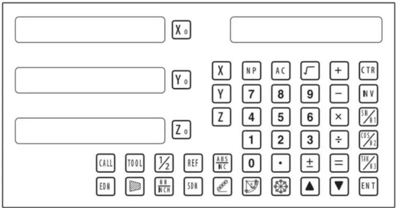

TWO AXIS PANEL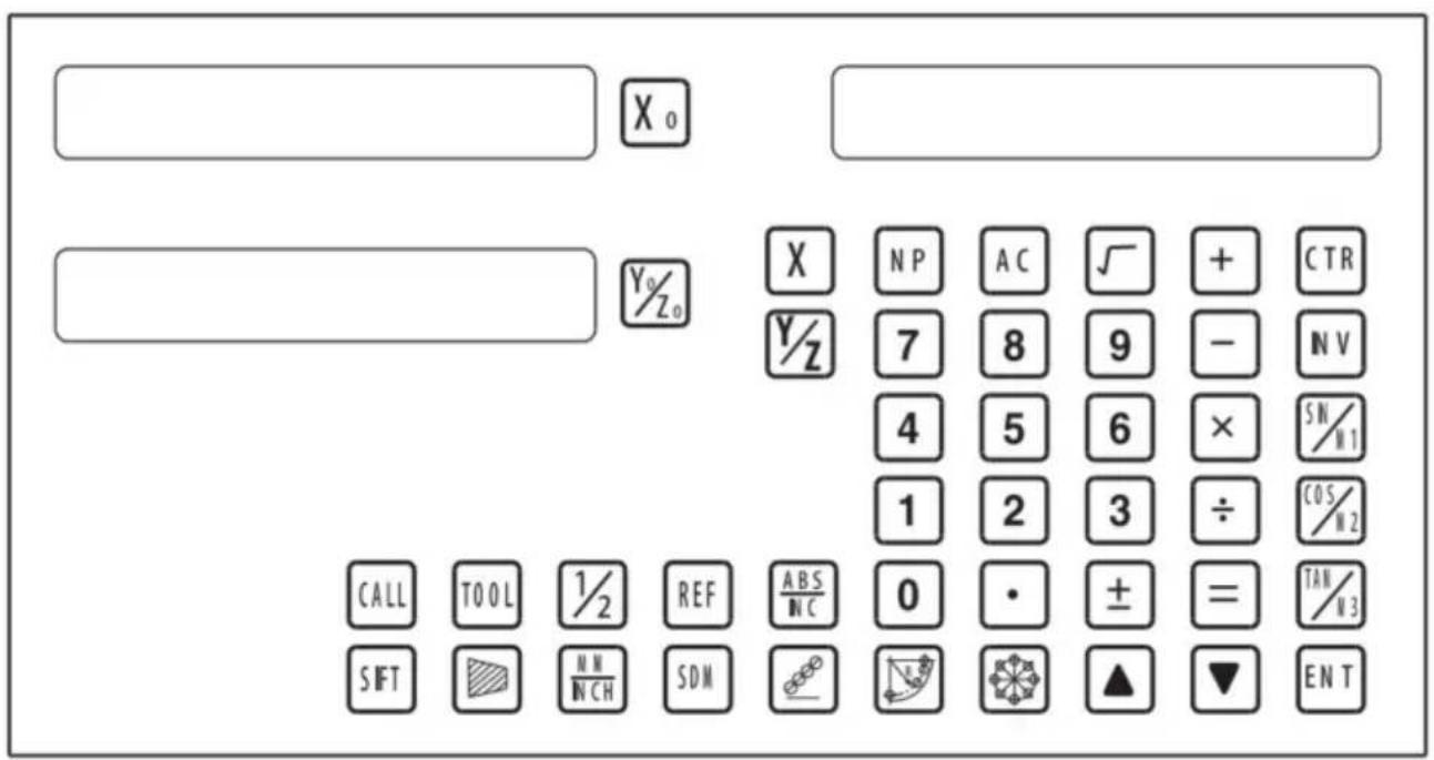

Keyboard Description

	Keys for axis selection
	Zero select axis
	Enter +/- sign
[HK2G]	Enter decimal point
	Entry keys for numbers
	Operation key (in Calculation function key)
	Enter or quit calculating state
	Cancel incorrect operation
	Calculate inverse trigonometric
	Square root
	Confirm operation
	Toggles between inch and millimeter units.
	Press when ready to identify a reference mark.
	Function keys for 200 sub datum
	ARC cutting function
	holes displayed equally on a circle
	holes displayed equally on a line

Caption of the keyboard

	Calculate trigonometric or Slope Processing function key
	Calculate trigonometric or rectangular inner chamber processing function key
	Calculate trigonometric or the tool diameter compensation function key
	Toggle between ABS/INC coordinate
	Stroll up or down to select
	Taper measured function key
	Tool library call key
	Opens the tool table.( lathe)
	EDM function key
	Filter display function key
	Half a display value of an axis
	Non Linear Error Compensation function keys

3. Parameters settings

3.1 Parameters setup routine entrance.

Press ☐ to enter initial system and self-check after DRO powers on in 1 second, then Parameters settings display in the Parameters window. Press ▲ ▼ to select the item you want to change.

If you want to quit initial setting, press ▲ ▼ until “QUIT” appears in message window and press ENTER. You can also press • to quit initial setting.

3.2 Parameters Settings Description

3.2.1 Setting the Resolution

Press ▲ ▼ until “RESOLUTE” appears in message window;

When selecting the LINEAR encoder, the resolution will be set as follows:

There are 19 types of resolution:

0.01um; 0.02um; 0.05um; 0.10um; 0.20um; 0.25um; 0.50um; 1.00um; 2.00um; 2.50um; 5.00um; 10.00um; 20.00um; 25.00um; 50.00um; 100.00um; 200.00um; 250.00um; 500.00um.

Press X0 to change the resolution for X axis; Press Y0 to change the resolution for Y axis; Press Z0 to change the resolution for Z axis;

Set the resolution 5.00um to 1.00um for X axis:

When selecting the rotary encoder, the resolution will be set as follows:

Input the rotary encoder parameter value.

3.2.2 Setting Positive Direction for Counter

Press ▲ ▼ until “DIRECTE” appears in message window.

Direction ‘0’ means the display value will increase when scale moves from right to left and decrease when scale moves from left to right. Direction ‘1’ means the display value will increase when scale moves from left to right and decrease when scale moves from right to left.

Press X0 to change the Direction for X axis; Press Y0 to change the Direction for Y axis; Press Z0 to change the Direction for Z axis; as follows:

3.2.3 Toggle Between R/D Display Mode

Press ▲ ▼ until “R OR D” appears in message window. X window, Y window, Z window displays ‘0’ or ‘1’ separately.

‘0’ is mode R, which means the display value equals the actual measurement. ‘1’ is mode D where the display value equals the double actual measurement. Press X0 to change the R/D for X axis; Press Y0 to change the R/D for Y axis; Press Z0 to change the R/D for Z axis; as follows:

3.2.4 Setting Z axis Dial

Press ▲ ▼ until "Z DIAL" appears in message window.

Z axis dial should be set if Z axis is emulated for 2 axis milling and only install linear scale for X,Y axis. Z axis dial means the distance the Z axis travels when screw runs a revolution.

Set the Z axis Dial 2.5mm as follows:

3.2.5 Setting the Rotary Radius of the Workpiece

Press ▲ ▼ until "RDIUS" appears in message window.

The Rotary radius type is used perimeter to measure angle.

Input the Rotary Radius parameter value 2000mm as follows:

3.2.6 Setting the Angle Display Mode

Press ▲ ▼ until "ANG DISP" appears in message window.

Press X0 to change the angle display mode for X axis; Press Y0 to change the angle display mode for Y axis; Press Z0 to change the angle display mode for Z axis; Example for X axis:

"0.0000" means the angle mode is Circulating DD;

"0000.0000" means the angle mode is Incremental DD;

"0.00.00" means the angle mode is Circulating DMS;

"0000.00.00" means the angle mode is Incremental DMS;

3.2.7 Setting the Baudrate of RS_232 (Special customization function, if you need to buy, please contact the dealer to customize)

Press ▲ ▼ until “BAUDRATE” appears in message window. Set the Baudrate 115200 as follow ;

3.2.12 The linear scale counting frequency setting

The factory default setting is only "12", the higher the parameter, the lower the counting frequency, press "X0" to set, it is not recommended that you set the default value yourself.

3.2.13 Setting QUIT: Digital display table parameters quit button.

3.2.14 Setting the type of the DRO.

The type of the DRO will be display on the right window. then press the key ENT to select the correct type. the following system item will be set:

"MILL-3" means the DRO type is 3-axis milling machine table;

"MILL-2" means the DRO type is 2-axis milling machine table;

“LATHE-2” means the DRO type is 2-axis lathe table;

"LATHE-3" means the DRO type is 3-axis lathe table;

"GRIND" means the DRO type is Grind table;

"EDM" means the DRO type is EDM table; (Special customization

function, if you need to buy, please contact the dealer to customize)

3.2.15 Signal Interface Type

Message window displays "SEL AXIS" which indicates the step is to Sensor input signal mode. Press X₀ to change the signal mode for X axis; Press Y₀ to change the signal mode for Y axis; Press Z₀ to change the signal mode for Z axis. Example for X axis:

Press X₀ to scroll through the Rotary encode type, the Linear encode type, the Rotary radius type.

X window displays the Signal type.

"LInER" means the Signal type is linear encode type;

"EnCOdE" means the Signal type is Rotary encode type;

"RdIUS" means the Signal type is Rotary radius type;

Example: currently in the linear encode type, to toggle to the Rotary encode type;

3.2.16 Restore Factory Settings:

Clear all data except DRO type. DRO will load default setup for parameter. After loading default setup, user must search RI once to enable resuming ABS datum function; otherwise to resume the datum by RI is unable;

Message window displays "ALL CLR", press ENT and message windows display "PASSWORD" indicating the operator to input password; Press 2000 + ENT in turn to load default value;

3.2.17 Shrinkage Ratio enable or disable.

The message window displays “SRK OFF” to disable the Shrinkage Rate function. Press ☐ to enable the Shrinkage Rate function, and the message window will display “SRK ON”.

3.2.18 Setting Compensation Type

The message window displays “SEL COMP”, indicating that this step is for compensation type. Press X₀ to change the compensation type for the X axis; press Y₀ to change the compensation type for the Y axis; press Z₀ to change the compensation type for the Z axis. Example for the X axis:

Press X₀ to scroll through the compensation types: no compensation, linear compensation, and non-linear compensation.

“no-CO” means the compensation type is no compensation; “LInE-CO” means the compensation type is linear compensation; “non-LinE” means the compensation type is non-linear compensation.

Example for the X axis: currently in the no compensation type, to toggle to the linear compensation type.

3.2.19 Inch Display: Set the Number of Digits After the Decimal Point

In inch display mode, the number of digits after the decimal point is set. The factory default is "4". Press "X0" to set it according to actual needs.

3.2.20 Setting EDM: It is not recommended to set the default value yourself. EDM function: Set the relay off time.

3.2.21 Setting Linearity Compensation

The message window displays “LIN COMP”, indicating that this step is for linearity compensation. Compensate the linear error to make the display value equal to the standard value.

The calculation of the compensation rectifying coefficient:

Coefficient = (Measurement - Standard value) x 1000.000/ Standard value

Example for the X axis:

Measurement 200.020mm

Standard value 200.000mm

Rectifying coefficient= (200.020-200) * 1000 /200 = -0.01mm/m

Input compensation rectifying coefficient 0.01 as follow:

3.2.22 Setting the Shrinkage Ratio

Press ▲ ▼ until “ SHRINK” appears in message window;

Shrinkage ratio = (Dimensions of the finished product) / (Dimensions of the working piece)

Set the shrinkage ratio 1.005 as follows;

4. General Operations;

4.1 Zeroing

Zero the designated axis in normal display state. Zeroing is used to set the current point as datum point as follows;

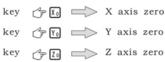
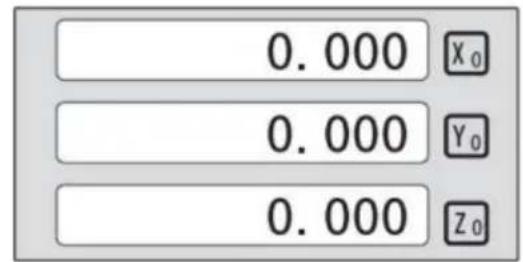
X₀ or Y₀ or Z₀ will be returned to the original data before the reset.

4.2 Preset Data to Designated Axis

Preset a value to current position for a designated axis in normal display state.

4.3 Toggle Display Unit between inch and mm

Length can be displayed either in "mm" (metric) or "inch" (imperial). Display unit can be toggled between mm and inch.

Example: Display value toggle from mm to inch;

Example: Display value toggle from inch to mm;

4.4 Absolute/Incremental/200 groups SDM

Function: The DRO has 3 coordinate display modes: the absolute mode (ABS); the incremental mode (INC) and 200 groups Second Data Memory (SDM) with the range of 00 to 99. Zero point of work-piece is set at the origin point of ABS coordinate. The relative distance between datum of ABS and SDM remains unchanged when ABS datum is changed.

1. Toggle from ABS to INC coordinate;

1. Toggle from INC to ABS coordinate;

1. Toggle from SMD to ABS coordinate;

4.5 1/2 Function

Function: Set the center of work piece as datum by halving the displayed value.

Example: Set the center of rectangle as datum as the right figure.

Steps:

1. Touch one side of the workpiece with the TOOL, then zero the X axis.

2. Message window displays “REF”, Press ☐NT until “FD_REF” appears in message window.

3. Select the axis which need search RI. For instance: select X axis, then press ☒. "X_REF" is displayed in message window, and X axis window flashes.

4. Move the machine table. The buzzer sounds when RI is searched, then X window stops flashing and displays the value of the current position. The DRO returns normal display state. Then message window displays "FIND_X".

Example for AB mode:

1. DRO is set in ABS coordinate. Press REF, then the message window displays "REF".

2. Press ▲ ▼, then the message window displays "AB".

3. Message window displays "AB". Press ENT until "FIND_AB" appears in message window.

4. Select the axis which needs to search RI. For instance: select X axis, then press ☒. "X_REF" is displayed in message window, and X axis window flashes.

5. Move the machine table. The buzzer sounds when RI is searched, displays the value of the current position for the absolute datum zero. The DRO returns to normal display state. Then message window displays "FIND_AB".

Example for LEF_AB mode:

1. DRO is set in ABS coordinate. Press REF, then the message window displays "REF".

2. Press ▲ ▼, then the message window displays "AB".

3. Message window displays "LEF_AB". Press ENT until "ZERO_AB" appears in message window.

4. Move the machine table to be set zero position point. Then press X, X axis will be zeroing. The current position for the absolute datum zero. The DRO returns to normal display state.

NOTE: Linear range without reference point location of the user

4.10 Non Linear Error Compensation

First compensation Type (Linear or Non-Linear) in parameter setting must be set Non-Linear. Linear scale have a ref point location and find to the Absolute Reference Point will be enable.

Default Non-Linear compensation: 50.

Example for Y axis:

Step 1: Search the Absolute Reference Point of Scale;

Step 2: Press NP, then the message window displays "COMP X".

Step 3: Press ▲ ▼, then the message window displays "COMP Y".

Step 4: Press ENT, then the message window displays "NUMBER". Then input the compensation parameter NUMBER.

Step 5: Press ▲ ▼, then message window displays "Y-MSN-1" which indicates the step is to Non Linear Error Compensation.

Step 6: Input compensation value.

X window displays the value of the measurement value.

Y window displays the value of the standard value.

Example for the first compensation point:

Measurement value: 68.288mm. Standard value: 68.200mm

Step 7: After input all parameters, the DRO automatically exits.

5. 200 Groups SDM coordinate

The DRO has three display modes: the absolute mode (ABS), the incremental mode (INC) and the 200 groups second data memory (SDM 1 - SDM200). ABS datum of the work-piece is set at the beginning and the 200 groups SDM is set relative to ABS coordinate.

ABS Mode, INC Mode and SDM Mode are specially designed to provide much more convenience features to the operator to cope with the batch machining of relative works and the machining of the workpiece machining dimensions from more than one datum.

Example: The ABS datum is the center point O, and the points sdm1, sdm2, sdm3, sdm4 that need processing are set as the datums of SDM 1 - SDM 4.

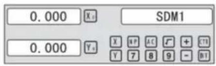
Two ways to set SDM coordinates:

1. Zeroing at the current point. 2. Presetting the datum of the SDM coordinate.

5.1 Zeroing at the Current Point

First, set the center point of the workpiece as the origin of the ABS. Then align the TOOL with points SDM1, SDM2, SDM3, and SDM4 by moving the machine table and zero them. It is the position to process where the "0.000" appears in the X window and Y window by moving the machine table, whether in ABS or in SDM coordinate.

Steps:

1. Move the worktable to place the TOOL at the center of the workpiece point O as the datum of ABS. Then zero the X axis and Y axis in SDM 1; zero the X axis and Y axis in SDM 2; zero the X axis and Y axis in SDM 3; zero the X axis and Y axis in SDM 4.

2. Set the point sdm1 as the datum of SDM 1. Move the machine worktable to x = 60.000, y = 45.000. Then process [X0] [Y0].

2. Set the point sdm1 as the datum of SDM 2. Move the machine worktable to x = 60.000, y = -45.000. Then process [X0] [Y0].

3. Set the point sdm1 as the datum of SDM 3. Move the machine worktable to x = -60.000, y = -45.000. Then process [X0] [Y0].

4. Set the point sdm1 as the datum of SDM 4. Move the machine worktable to x = -60.000, y = 45.000. Then process [X0] [Y0].

5.2 Presetting the datum of SDM coordinate

There are the same examples as in Method 1. First, move the worktable to place the TOOL exactly at the origin of ABS. Secondly, enter the ABS Mode as follows.

Steps:

1. Move the worktable to place the TOOL at the center of the workpiece point O as the datum of ABS. Then zero the X axis and Y axis in SDM 1; zero the X axis and Y axis in SDM 2; zero the X axis and Y axis in SDM 3; zero the X axis and Y axis in SDM 4.

2. Set point SDM1 as the datum of SDM 1. Press ▲ ▼, then the message window displays “SDM 1”. Input x = 60.000, y = 45.000.

3. Set point SDM1 as the datum of SDM 2. Press ▲ ▼, then the message window displays “SDM 2”. Input x = -60.000, y = 45.000.

4. Set point SDM1 as the datum of SDM 3. Press ▲ ▼, then the message window displays “SDM 3”. Input x = -60.000, y = -45.000.

5. Set point SDM1 as the datum of SDM 4. Press ▲ ▼, then the message window displays “SDM 4”. Input x = -60.000, y = 45.000.

6. Special function

6.1 Circumference Holes Processing

The function of PCD hole positioning on a circumference is used to distribute holes equally, such as boring holes on a flange. The right window will show the parameters to be defined when selecting the PCD function. The parameters to be defined are:

PCD_XY (XZ, YZ)

Select plane

CENTER

Center position

DIA

Diameter of circle

NO_HOLE

Number of holes

STANG

Starting angle

ED ANG

Ending angle

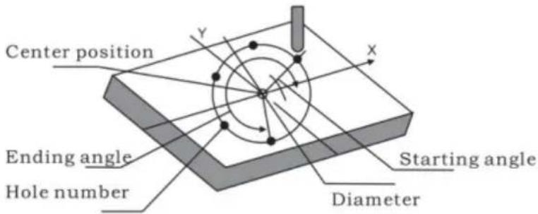
The position of the hole center is calculated automatically after inputting all parameters. Press ▲ or ▼ to choose the hole number and move the machine table until “0.000” appears in the X, Y, and Z windows. That is the position to process a hole.

Example for the XY plane: Machine holes on a circumference as shown in the figure.

PCD_XY(XZ,YZ)	XY
CENTER	X=0,000,Y=0.000
DIA	100,000
NO_HOLE	5
ST ANG	30,000
ED ANG	315,000

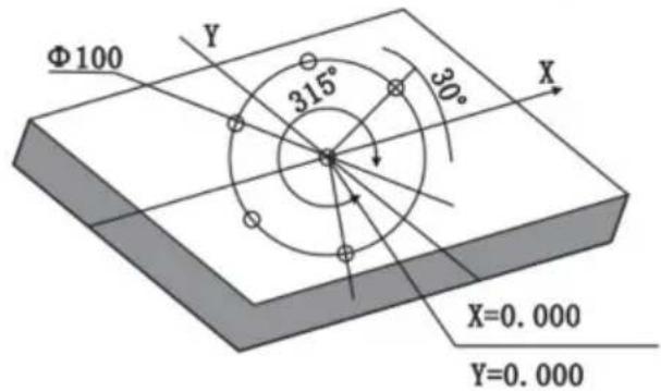
Steps:

1. Set the display unit to metric in the normal state; move the machine table until the machine tool is aligned with the center of the circle, then zero the X and Y axes.
2. Select piece.

Press 🧑️, then the message window displays “PCD_XY” for the Circumference Holes Processing. Press ▲ or ▼ to select XY plane.

2. Input center position.

Press ENT, then the message window displays "CENTER". The X and Y windows display the formerly preset center position. Input X = 0, Y = 0 as follows.

4. Input diameter.

Press ▼ until “DIA” appears in the message window. The X window displays the formerly preset diameter. Then input the diameter as 100.000.

5. Input number.

Press ▼ until "NO_HOLE" appears in the message window. The X window displays the formerly preset number. Then press 5 in turn to input the number.

6. Input starting angle.

Press ▼ until "ST ANG" appears in the message window. The X window displays the formerly preset starting angle. Then press 3 0 in turn to input the starting angle.

7. Input ending angle.

Press ▼ until "ED ANG" appears in the message window. The X window displays the formerly preset ending angle. Then press 3 1 5 in turn to input the ending angle.

1. Press ▼ until "NO 1" appears in the message window.

It is the position of the first hole to punch where the "0.000" is displayed in the X window and Y window by moving the machine table. After finishing the first hole, press ▼ or ▲ to change the hole number.

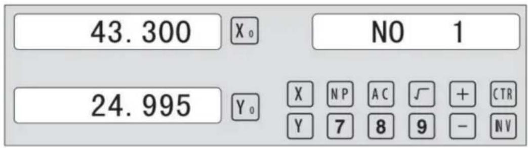
1. After processing all holes, press 📄 to return to normal display.

6.2 Linear Holes Processing

There are two modes to carry out the linear drilling: Length mode and Step mode.

1. LINE S Step mode LINE L Length mode 2.STEP Step length LENGTH Line length
2. ANG Angle
3. NO.HOLE Hole number

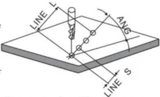
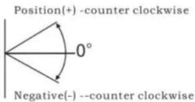
Linear Holes function can simplify the processing of multiple holes whose centers are attributed equally on one line.

Example:

LINE_L	Length mode
LENGTH	60.000
ANG	30.000
NO.HOLE	4

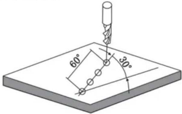
Steps:

1. Select piece.

Press 📄, then the message window displays “LINE_XY” for the Linear Holes Processing. Press ▲ or ▼ to select XY place.

2. Select Linear Holes mode.

Press ENT, then the message window displays "LINE_S". Press ▲ or ▼ to select "LINE_L".

3. Input linear length;

Press ENT, then the message window displays "LENGTH".

X window displays the formerly preset linear length. Press 6 0 in turn to input the linear length.

1. Input angle;

Message window displays “ANG” which indicates the step is to angle. X window displays the formerly preset angle. Press 3 0 in turn to input the angle.

1. Input number;

Message window displays “ANG” which indicates the step is to angle. X window displays the formerly preset number. Press 4 in turn to input the number.

1. Press ▼ until "NO 1" appears in the message window.

It is the position of the first hole to punch where the “0.000” is displayed in X window and Y window by moving the machine table. After finishing the first hole, press ▲ or ▼ to change holes number.

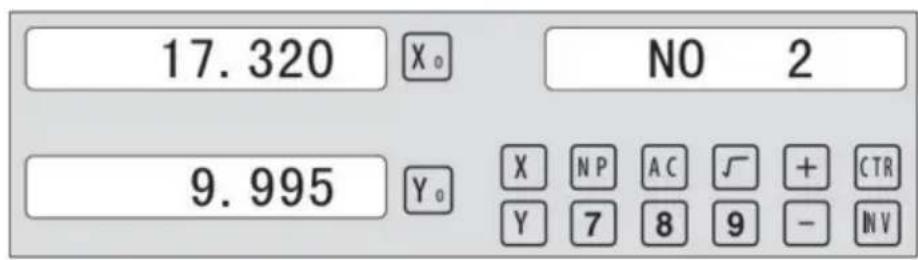
1. After processing all holes, press ☐ to return normal display.

6.3 ARC machining

Simple ARC function:

Provides maximum flexibility in ARC machining, the ARC sector to be machined by the coordinates of ARC. Very flexible, ARC function can machine virtually all kinds of ARC, even the intersected ARC.

Relatively a bit complicated to operate, operator need to calculate and enter the coordinates of ARC centre, start angle and end angle.

Basic parameters as follow:

1. SMOOTH Mode of the Smooth ARC processing;
2. SEL_XY(YZ, XZ) Select plane;
3. CENTER Refer to the position of a center.
4. RAD Radius of the ARC
5. TL_DIA Diameter of the TOOL
6. MAX_CUT Feed step
7. ST_ANG Starting angle
8. ED_ANG Ending angle
9. RAD+TL Outer arc. RAD-TL Inner arc.

Example 1 for the Simple ARC Processing:

Parameters settings as follow:

SIMPLE Simple mode

TYPE 3

SEL_XY XY

RAD 80.000

TL_DIA 6.000

MAX_CUT 0.500

RAD+TL 1

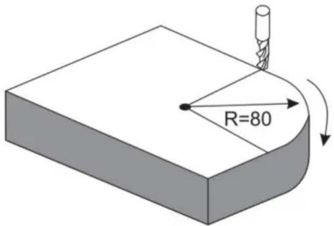
Steps:

1. Select process mode

Press 📋, then the message window displays "SIMPLE" for the ARC Processing. Press ▲ or ▼ to select the mode of the simple, the message window displays "SIMPLE"

ARC Processing

2. Input the type:

Press ☐ENT until "TYPE" appears in the message window. X-window displays the formerly preset type. Press ☐3 in turn

3. Select place

Press ENT until "SEL_XY" appears in the message window. Press ▲ or ▼ to select the place to display "SEL_XY";

4. Input radius:

Press ENT until "RAD" appears in the message window. The X window displays the formerly preset radius of the ARC. Press 8

0 in turn to input the radius.;

5. Input Diameter of the TOOL

Press ▲ or ▼ until "TL DIA" appears in the message window. The X window displays the formerly preset diameter of the TOOL. Press 6 in turn to input the diameter value;

6. Input Feed step (MAX_CUT);

Press ▲ or ▼ until "MAX_CUT" appears in the message window. The X window displays the formerly preset MAX_CUT. Press 0 · 5 in turn to input the MAX_CUT value;

7. Select outer arc or inner arc

Press ▲ or ▼ until "RAD-TL" appears in the message window. Press ▲ or ▼ to select the place to display "RAD+TL";

8. After inputting all parameters, press the key ENT for machining.

The DRO will display the position of the first point. Retract the axes until the displays read 0.000. Machine the arc point by point in accordance with the display. After finishing the position of the first point, press ▲ or ▼ to change position point.

Press ☑ to quit the R function at any time.

Example 2 for the Simple ARC Processing:

Parameters settings as follow:

SIMPLE Simple mode

TYPE 3

SEL_XY XZ

RAD 80.000

TL_DIA 6.000

MAX_CUT 0.500

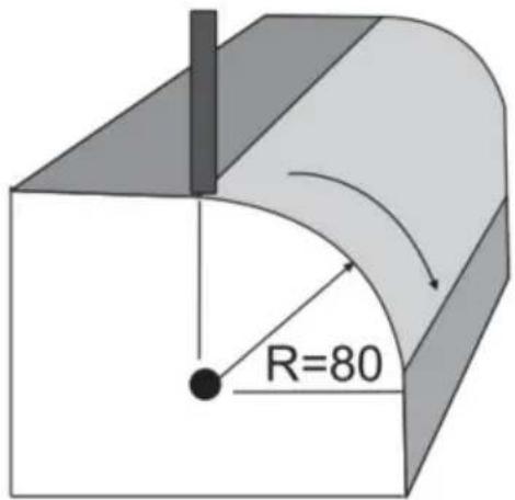
Steps:

1. Press 📋, then the message window displays “SIMPLE” for the ARC Processing. Press ▲ or ▼ to select the mode of the simple. The message window displays “SIMPLE”.

2. Input the type:

Press ☐ENT until "TYPE" appears in the message window. The X-window displays the formerly preset type. Press ☐3 in turn.

3. Select place

Press ENT until "SEL_XZ" appears in the message window. Press ▲ or ▼ to select the place to display "SEL_XZ".

4. Input radius:

Press ☐ENT until “RAD” appears in the message window. The X window displays the formerly preset radius of the ARC. Press ☐8 ☐0 in turn to input the radius.

5. Input Diameter of the TOOL

Press ▲ or ▼ until “TL DIA” appears in the message window. The window displays the formerly preset diameter of the tool. Press 6 in turn to input the diameter value;

6. Input feed step (MAX_CUT);

Press ▲ or ▼ until “MAX_CUT” appears in the message window. The window displays the formerly preset MAX_CUT. Press 0 · 5 in turn to input the MAX_CUT value;

1. After inputting all parameters, press the key ENT for machining.

For 2-axis milling machine table, it is not installed with Z-axis, please press ▲ or ▼ to simulate position of Z-axis. Press ▲ to simulate moving to the former process, and press ▼ to simulate moving to the next process point.

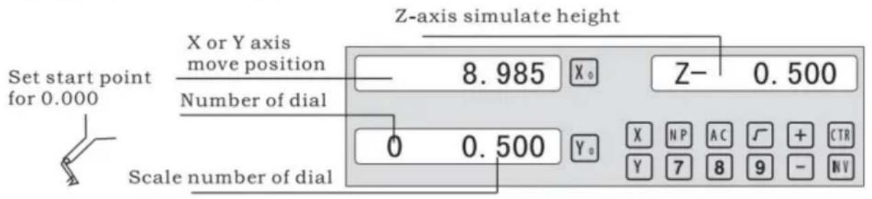
Z-axis simulate height = Number of dial x Z axis Dial + Scale number of dial

Press ☐ to quit R function any time.

Example 3 for the Smooth ARC function:

Parameters settings as follow:

SMOOTH	Smooth mode
SEL_XY(YZ,XZ)	XY
CENTER	X=0,Y=0
RAD	80.000
TL_DIA	6.000
MAX_CUT	0.500
ST_ANG	0.000
ED_ANG	135.000
RAD+TL	1

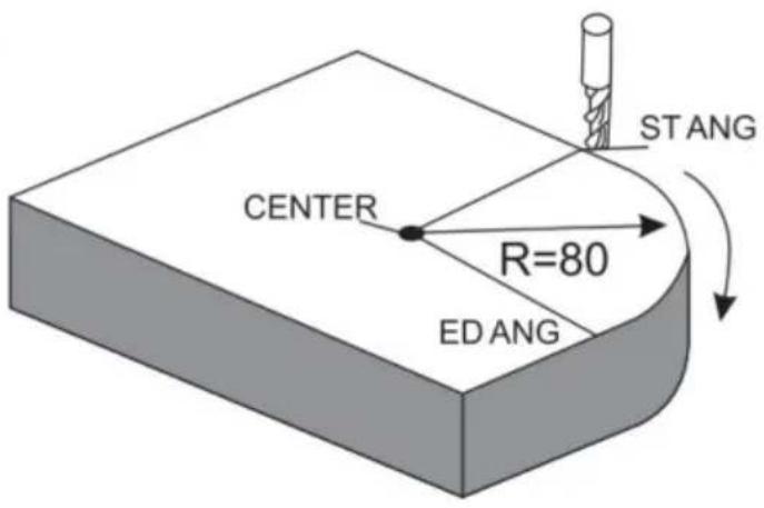
Steps:

1. Press 📋, then the message window displays “SIMPLE” for the ARC Processing. Press ▲ or ▼ to select mode of the simple, The

message window displays "SMOOTH"; For 3-axis milling machine table without this step. In second step. Then press ENT.

2. Select place

Message window displays “SEL_XY” which indicates the select is to place. Press ▲ or ▼ to select place to display “SEL_XY”;

3. Input center position.

Press ENT, then the message window displays "CENTER". The X and Y windows display the previously preset center position. Input X = 0, Y = 0 as follows.

4. Input radius:

Press ENT until "RAD" appears in the message window. The X window displays the previously preset radius of the arc. Press 8 and 0 in turn to input the radius.

5. Input diameter of the tool:

Press ▲ or ▼ until "TL DIA" appears in the message window. The X window displays the previously preset diameter of the tool. Press 6 in turn to input the diameter value.

6. Input step (MAX_CUT):

Press

or

until "MAX CUT" appears in the message window.

Press ENT to quit the ARC function at any time.

6.4 Oblique processing

6) Change the angle of the workpiece to make it touch the measuring tool and adjust it to zero.

STEPS:

1. Select plane:

Press SN/1, then the message window displays "INCL_XY" for oblique processing. Press ▲ or ▼ to select the plane to display "SEL_XY".

Then press ☐ENT to proceed to the next step;

2. Input the angle of obliquity.

The message window displays “ANG”, and the X window displays the previously set angle of obliquity. Press 4 and 5 in sequence to input the angle of obliquity.

1. Move the workpiece along the X-axis until the measuring tool touches it, adjust it to zero, and then move the worktable any distance along the X-axis.

1. Press Y to display the value of the Y-axis. Move the workpiece along the Y-axis, changing the angle of the workpiece so that the obliquity-calibrating plane touches the measuring tool until it reads zero. Move the worktable until the Y-axis displays zero.

1. Press 5W/H1 to exit the oblique function at any time.

Example 2 for the oblique XZ or YZ plane:

When the machining plane is on the XZ or YZ plane, the tool inclination function can guide the operator to machine the oblique plane step by step.

Procedures for using the cutter inclination function:

When the machining plane is on the XZ or YZ plane, first calibrate the obliquity of the primary spindle nose and set the tool:

INCL_XY(XZ,YZ)	INCL_XZ
DIA	10.000
ST_POT	20.000
ED_POT	20.000

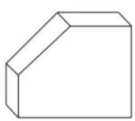
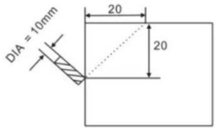
STEPS:

1. Press SN/81, then the message window displays "INCL_XY" for oblique processing. Press ▲ or ▼ to select the plane, and when "SEL_XZ" is displayed, press ENT to proceed to the next step;

1. Input the tool diameter.

The message window displays “DIA”, and the X window displays the previously set angle of obliquity. Press 10 in sequence to input the tool diameter of obliquity. Then press ▼ to proceed to the next step;

1. Input ST_POT;

The message window displays “ST_POT”, and the X and Y windows display the previously preset starting position of obliquity. Input X=0, Y=-20.000. OK, then press ▼ to proceed to the next step;

4. Input ED_POT;

The message window displays “ED_POT”, and the X and Y windows display the previously preset starting position of obliquity. Input X=20.000, Y=0.000.

5. After inputting all parameters, press the ▼ key for machining.

For a 2-axis milling machine table, it is not installed with a Z-axis. Please press ▲ or ▼ to simulate the position of the Z-axis. Press ▲ to simulate moving to the former process, and press ▼ to simulate moving to the next process point.

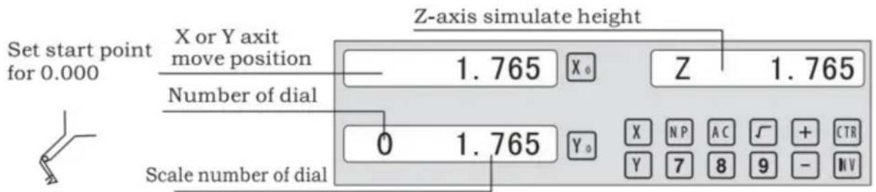
Z-axis simulate height = Number of dial x Z axis Dial + Scale number of dial

Press ☐ to quit the oblique function at any time.

6.5 Slope Processing

This function can calculate the position of every processing point automatically in processing a slope. Only the following parameters need to be inputted:

XZ, YZ

Set machine place YZ, or XZ

ANG

The inclination angle

Z_STEP

The slope length

each time processing

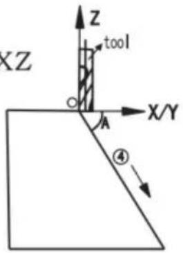
Example 1 for the Slope XZ place;

Step 1. Select place

Press , then the message window displays “XZ” for the slope processing. Press ▲ or ▼ to select the place to display “SEL_XY”; then press to go to the next step;

Step 2. Input the angle of slope

The message window displays “ANG”, and the X window displays the formerly preset angle of slope. Press 4 5 in turn.

Step 3. Input Z_step;

The message window displays “Z STEP”, and the X window displays the formerly preset starting position of slope. Input 0 · 1 in turn.

Step 4: Finishing the ALL processing. Press ☐ to quit the slope function at any time.

6.6 Chambering Processing

1, FLAT_XY: machine place; 2, DIA: diameter of TOOL; 3, CENTER: center of the chambering; 4, SIZE: size of the chambering;

Figure as follows:

STEPS:

1. Press /W2 , then the message window displays “FLAT_XY” for the Chambering Processing.

1. Input DIA of the TOOL;

1. Input the center coordinate;

1. Input the size;

5. Process Chambering;

Move the machine until the display of the axis is zero, i.e., the position of the first point. Machine the first point. Display the next machining point by pressing ▲ or ▼. On completion of machining, the right window shows OVER. Press ▲ or ▼, and the system will go to the first position for the next workpiece. Press ⚠/12 to quit the Chambering Function.

6.7 The Tool Diameter Compensation Function

Without tool compensation, the operator has to move the tool for an additional distance equal to the diameter of the tool along each side when machining the four 150 and 100 sides of a workpiece to finish machining the whole brim. The digital readouts shall automatically compensate when the tool compensation function is enabled.

Note: The tool compensation is made in the direction of the X and Y axes.

Procedures:

1). Enter the function of compensating the diameter of the tool. 2). Select one of the (four) preset machining modes. 3). Input the diameter of the tool. 4). Enter machining.

Figure A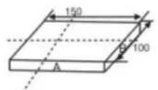

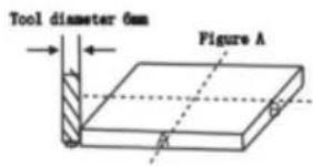
Figure B

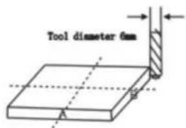
Figure C

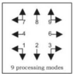
Step 1: Press ☐ to enter the tool compensation function. Then the message window displays “TYPE”. Press ☐.

Step 2: Input the diameter of the tool; press 10 in turn.

Step 3: Press ▼ to the machining mode.

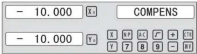
Machining of 2 side planes can be done by moving the TOOL until X-Axis is 150.000 and Y-Axis is 100.000. Press the Key [TAN/V3] to quit the Function.

6.8 Digital Filter of the Grinding Machine

When machining a work-piece by grinder, the display values quickly due to the vibration of grinder. User can not see display value clearly. Grinder DRO provides display value filter function to disable the quake change of display value.

STEPS:

1. Enter display value filter function.

In normal display state, press SIFT to simultaneously, enter display value filter function.

1. Exit display value filter function;

Press SIFT, exit display value filter function;

6.9 Functions

6.9.1 200 set TOOL Libs

Step 3: Enter TOOL 2 data:

It will automatically exit from EDM machining status and recover to the original state before machining;

b) Stop Mode:

It will always stay at the machining interface after finishing machining, and you should press EDM to exit and back to the original state.

Operation steps:

The DEPTH (machining depth), ERRHIGH (negative fireproof height), exit mode, EDM relay output mode, and machining direction should be set.

STEPS:

1. Press EDM to enter the EDM function. Press ▲ to input parameters; press ▼ to enter EDM machining state.
2. Input DEPTH (machining depth). Press the key ▲ to set the next parameter.

1. Input ERRHIGH (negative fireproof height) (undefined). Press the key ▲ to set the next parameter.

1. Set machining direction (positive or negative). Press 1 to select positive direction. Press 0 to select negative direction. Press the key ▲ to set the next parameter.

EDM

1. Set exit mode (AUTO mode or STOP mode). Press 0 to select AUTO mode; press 1 to select STOP mode; press the key ▲ to set the next parameter.

1. Set the output mode (Mode 0 or Mode 1) (undefined). Press ☐ to select Mode 0; press ☐ to select Mode 1.

1. Continuously press ▼ to return to EDM for machining. Press EDM to quit the function.

Example 1: positive direction machining.

Machining is shown as the model chamber as follows.

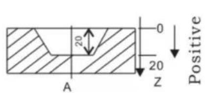
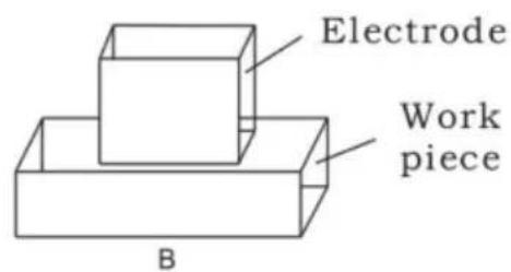
STEPS:

1. Touch one side of the workpiece with the tool, then press ₀ to zero the Z axis.

2. Press EDM, set DEPTH to 20.000; press ▼ to EDM for machining.

Example 2: Negative direction machining

Machining is shown as the model chamber as follows

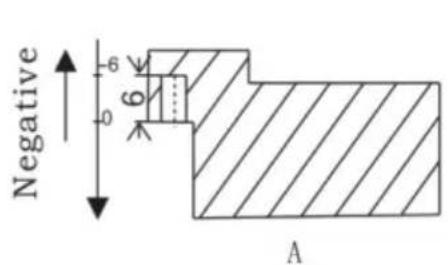
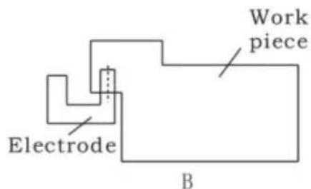
1. Touch one side of the workpiece with the tool, then press Z0 to zero the Z axis.

2. Press EDM, set DEPTH to -20.000; press ▼ to start EDM machining.

Example 3: PCD Function for EDM

The PCD function can access the EDM function. The operator enters the PCD function to input parameters for PCD and enter the PCD machining state. At every position for machining, press the EDM key to access the EDM function.

The following are preliminary solutions for troubleshooting.

If there is still trouble, please contact our company or agents for help.

Troubles	Possible reasons	Solvents
No display	1. Power isn't connected2. Power switch is off.3. The range of power voltage is not right.4. The inner power of Linear Scale is short.	1. Check power wire and connect the power2. Turn on the power switch.3. The range of voltage is in 80--260V4. Unplug the connector of linear scale
One axis is not counting	1. Replace the linear scale of the other axis.2. DRO is in special function	1. If count is normal, the linear scale has trouble; If abnormal, the DRO readouts has trouble.2. Quit the special function.
Linear scale is not counting	1. Reading head is bad for using range exceeds.2. Aluminum chips is in reading head of linear scale.3. The span between the reading head and metal part of linear scale is large.4. The metal parts of linear scale is damage.	1. Repair the linear scale2. Repair the linear scale3. Repair the linear scale4. Repair the linear scale
Counting is error	1. Shell is poor grounding.2. Low precision of machine.3. Speed of machine is too rapid.4. Precision of linear scale is low.5. The resolution of DRO readouts and the linear scale is not match.6. The unit (mm/inch) is not match.7. Setting the linear compensating is not arrest.8. Reading head of the linear scale is damaged.	1. Shell is good grounding.2. Repair the machine.3. Reduce the speed of machine.4. Mount the linear scale again.5. Set the resolution of the DRO again,6. Cover the unit of display mm/inch.7. Reset the linear compensation.8. Repair the linear scale.
The counting of the linear scale is not accurate	1. The mounting of linear scale does not demand the requirement, and the precision is not adequate.2. The screw is loosen.3. Precision of machine is low.4. The resolution of digital readouts and the linear scale is not match.	1. Mount the linear scale again and level it.2. Lock all fixing screws.3. Repair the machine.4. Reset the resolution of digital readouts.
Sometimes the linear scale is not counting	1. The small car and steel ball is separated.2. The glass of reading head is wearied.3. The glass of reading head of the linear scale has dirt.4. The elasticity of the steel wire is not adequate.	1. Repair the linear scale.2. Repair the linear scale.3. Repair the linear scale.4. Repair the linear scale.

1. Specifications of Digital Readout

1) Supply voltage range: AC 85 V ~ 230 V; 50 ~ 60 Hz 2) Power consumption: 15 VA 3) Operating temperature: 0°C to 50°C 4) Storage temperature: -30°C to 70°C 5) Relative humidity: < 90% (25°C) 6) Maximum coordinate number: 3 7) Readout allowable input signal: TTL square wave 8) Allowable input signal frequency: < 5 MHz 9) Maximum resolution of digital display length: 0.01 μm 10) Maximum resolution of digital display angle: 0.0001° / pulse

1. Instructions

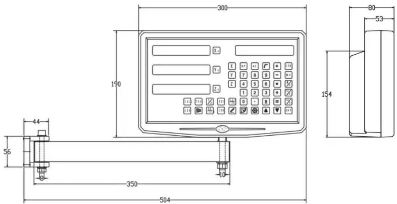
1. X, Y, Z axes

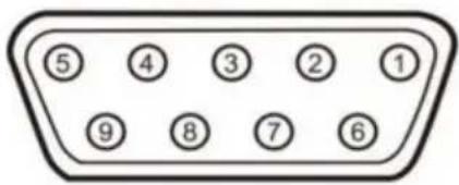
Pin	TTL (Standard)
1
2	OV
3
4
5
6	A+
7	5V
8	B+
9	R+

Pin	TTL (Standard)
1	5V
2	OV
3	A+
4	B+
5	R+
6
7
8
9

For your convenience, if you buy a digital readout,

The wiring definition of your linear scale must be the same as the two definitions in the above diagram to be universal!

Installation instructions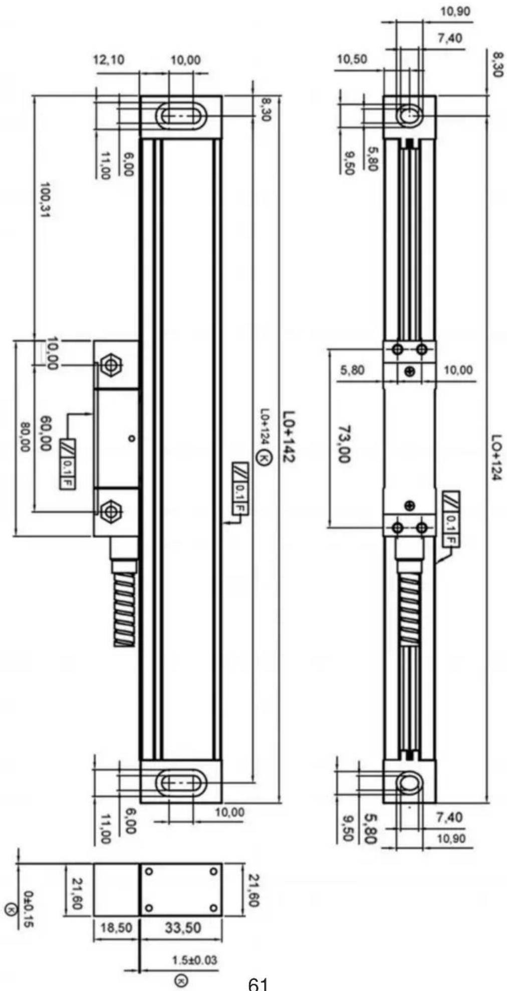

TTL signal Output: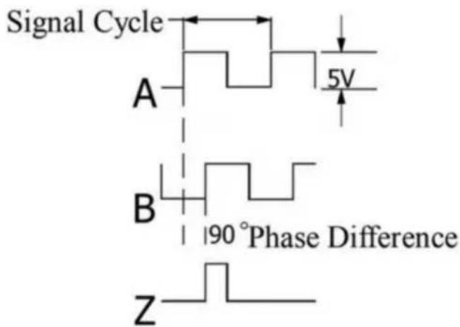

EIA-422-A signal Output: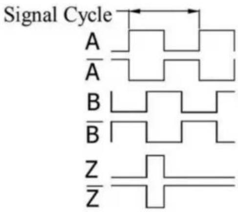

1. TECHNICAL PARAMETER 1.1 SCALING DISTANCE: 0.02 MM (50 LINES/MM) 1.2 RESOLUTION: 5 μM, 1 μM, 0.5 μM 1.3 PRECISION: ±3 μM, ±5 μM, ±15 μM/M (20±0.1℃) 1.4 MEASURING RANGE: 30~3000 MM 1.5 MOVING SPEED: HIGH-SPEED ENCODER 120 M/MIN (TO BE CUSTOMIZED)

ORDINARY ENCODER 60 M/MIN

1.6 POWER SUPPLY: +5V±5%, 80 MA 1.7 CABLE LENGTH: STANDARD 3M (SPECIAL LENGTH AVAILABLE ACCORDING TO THE USER'S NEEDS) 1.8 WORKING TEMPERATURE: 0~45°C 1.9 PIN DESCRIPTION: 1) APPLICABLE TO: 9 PIN SOCKET EIA-422-A SIGNAL OUTPUT.

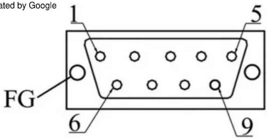
1) Applicable to: 9 pin socket EIA-422-A signal Output.

Pin Position	1	2	3	4	5	6	7	8	9
Signal		OV		Empty		A	+5V	B	Z
Color	Green Black	Black	Orange black	FG	White black	Green	Red	White	Orange

FG: Shield connected to metal casing.

1) Applicable to: 9 pin socket TTL signal Output.

Pin Position	1	2	3	4	5	6	7	8	9
Signal		OV		Empty		A	+5V	B	Z
Color		Black		FG		Green	Red	Orange	White

FG: Shield connected to metal casing.

Linear scale

Installation drawings

Installation method: Standard size: (Unit: mm)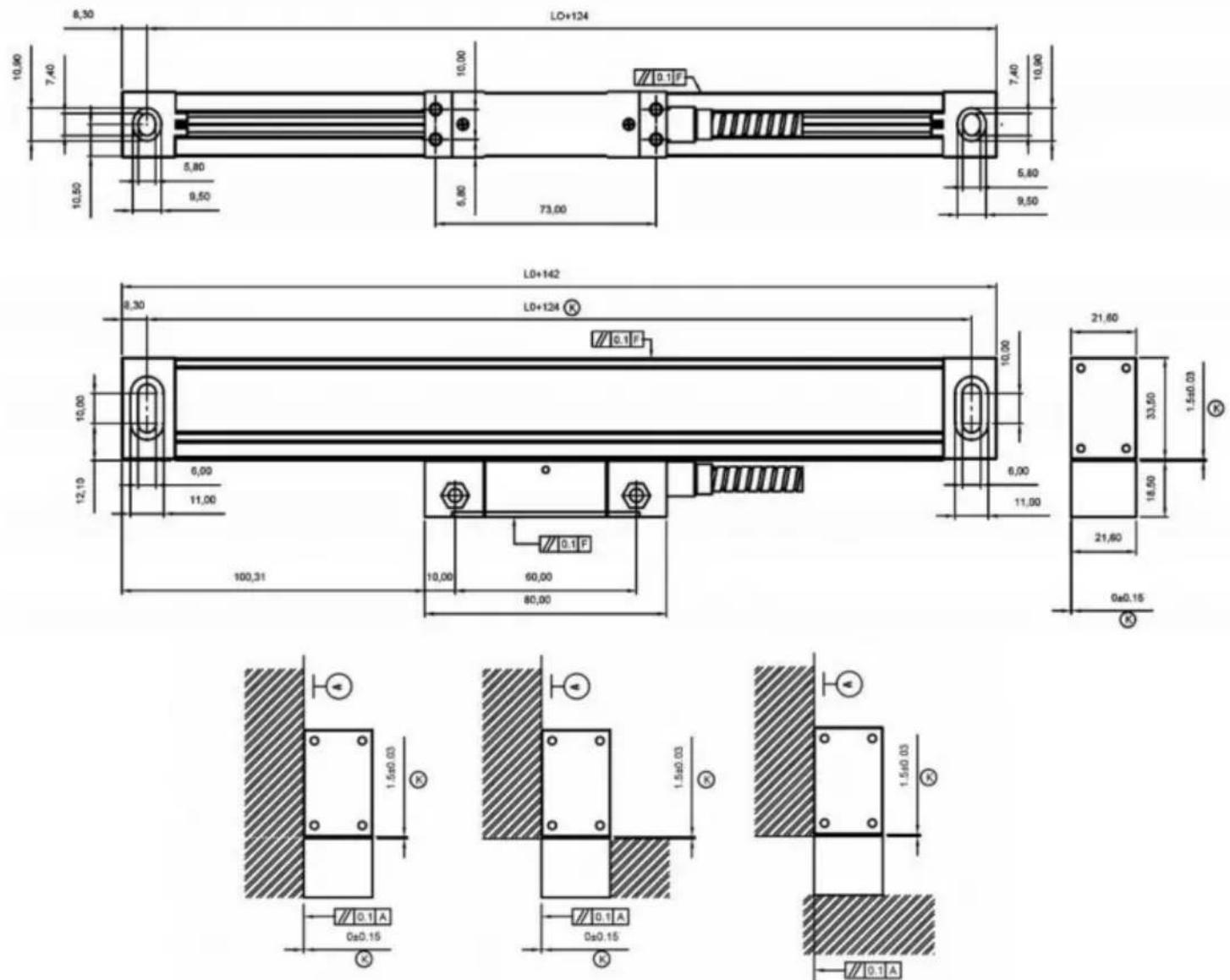

Modell	DET	L1	L2	Modell	L0	L1	L2
YE-50		174	190 YE-550 550			67450	690
	100	224	240 YE-600YE-100	600	724	740
YE-150	150	274	290	YE-650 650		774	790
YE-200 200		324	340 YE-700 700			824	840
YE-250 250		374	390	YE-750	750	874	890
YE-300 300		424	440 YE-800		800	924	940
YE-350 350		474	490 YE-850 850			974	990
YE-400 400		524	540 YE-900		900	1024	1040
YE-450 450		574	590 YE-950 950			1074	1090
YE-500 500		624	640 YE-1000 1000			1124	1140

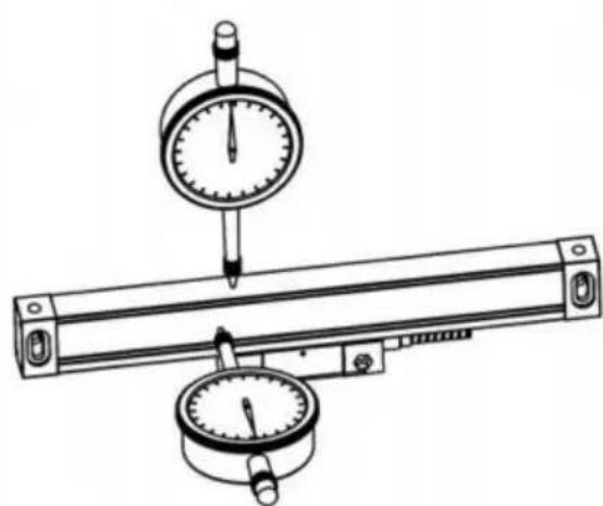
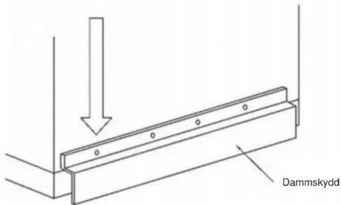
4.9

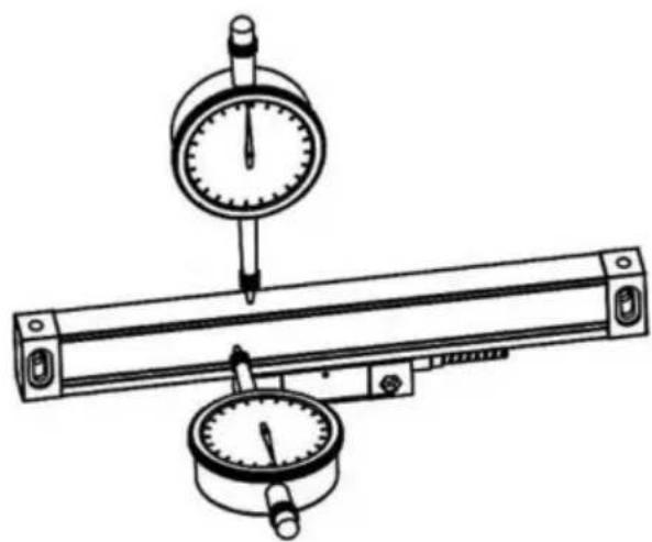
4.10

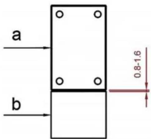
C/O YH Consulting Limited Office 147, Centurion House, London Road, Staines-upon-Thames, Surrey, TW18 4AX

VEVOR®

TOUGH TOOLS, HALF PRICE