PQM-707 - Meter Sonel - Free user manual and instructions
Find the device manual for free PQM-707 Sonel in PDF.


| Product Type | Power Quality Analyzer |
| Brand | Sonel |
| Model | PQM-707 |
| Dimensions (with cover) | 288 x 223 x 75 mm |
| Weight (with cover) | approx. 1.75 kg |
| Display | 7-inch color LCD TFT with touchscreen, 800x480 resolution |
| Power Supply | External 100-240 V AC, 50-60 Hz; internal Li-Ion 11.1 V, 3.4 Ah battery |
| Battery Life | min. 4 hours (full charge, max brightness); typical 6 hours |
| Memory | microSD HC 4 GB (expandable up to 32 GB); internal ~1 GB |
| Voltage Measurement | Up to 760 VAC (L-N), max ±1150 V; supports voltage transducers |
| Current Measurement | Up to 3000 A AC with flexible probes; also supports CT and AC/DC probes |
| Harmonic Analysis | Up to 50th harmonic for voltage and current; THD, TDD |
| Standards Compliance | IEC 61000-4-30 Class S, EN 50160, IEC 61000-4-7, IEC 61000-4-15 |
| Recording Modes | Immediate, threshold-triggered, scheduled; averaging periods 1s to 30min |
| Event Detection | Voltage dips/swells/interruptions; current thresholds; waveform recording |
| Interfaces | USB for PC, USB host for flash drive; microSD slot |
| Safety Rating | CAT IV 600V / CAT III 760V, double insulation, IP51 |
| Operating Temperature | -10°C to +50°C |
| Main Functions | Recording, analysis, compliance reports, inrush current, inverter efficiency, energy loss calculator |
| Accessories | Various flexible and CT current probes, voltage transducers, carrying case |
| Maintenance | Clean with soft damp cloth; no solvents; periodic battery charging for storage |
| Firmware Updates | Via USB flash drive or Sonel Analysis software |
Frequently Asked Questions - PQM-707 Sonel
User questions about PQM-707 Sonel
0 question about this device. Answer the ones you know or ask your own.
Ask a new question about this device
Download the instructions for your Meter in PDF format for free! Find your manual PQM-707 - Sonel and take your electronic device back in hand. On this page are published all the documents necessary for the use of your device. PQM-707 by Sonel.
USER MANUAL PQM-707 Sonel
natural_image
Line drawing of a portable electronic device with control panel and buttons (no text or symbols)USER MANUAL
POWER QUALITY ANALYZER
PQM-707
USER MANUAL
POWER QUALITY ANALYZER PQM-707
CE
SONEL S.A.
Wokulskiego 11
58-100 Świdnica, Poland
Version 1.20.7 30.06.2023
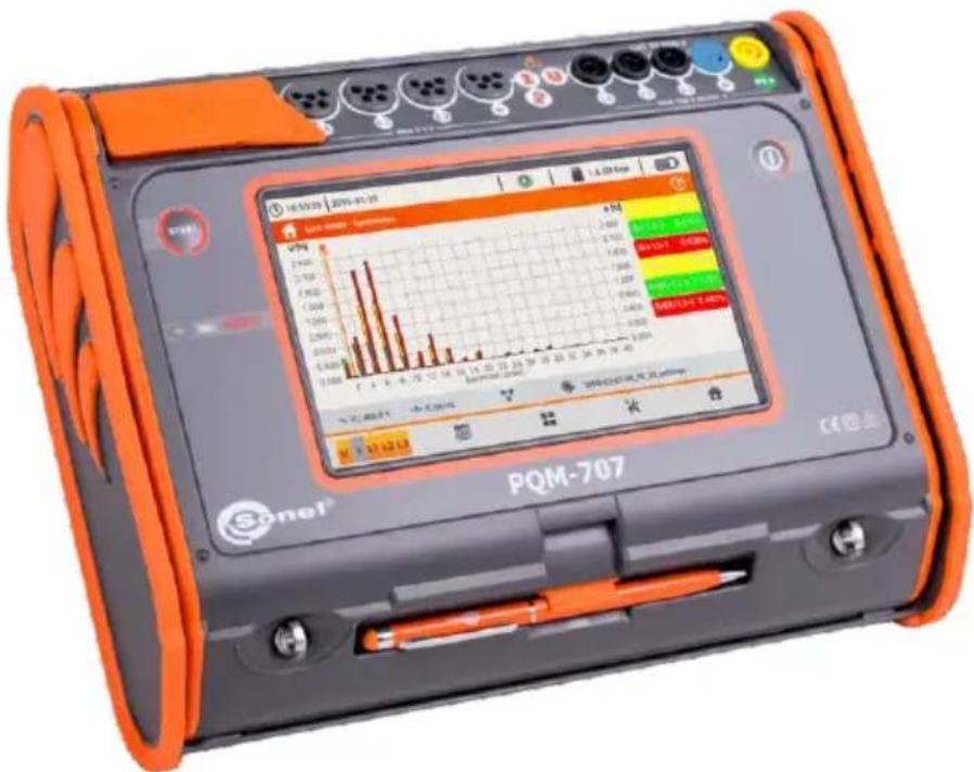
Thank you for purchasing the PQM-707 power quality analyzer. Please acquaint yourself with this manual to avoid measuring errors and prevent possible problems related to the operation of the meter.
CONTENTS
1 General Information....7
1.1 Safety....7
1.2 General characteristics 8
1.3 Power supply of the analyzer 9
1.4 Measured parameters....10
1.5 Compliance with standards 12
2 Operation of the analyzer.... 13
2.1 Switching the analyzer ON/OFF....13
2.2 Emergency restart....13
2.3 Emergency shutdown....13
2.4 Auto-off 14
2.5 LED 14
2.6 MicroSD memory card 14
2.7 USB external memory - pendrive 15
2.8 Main elements of the screen....15
2.8.1 Top bar 16
2.8.2 The title bar and help....16
2.8.3 Main window....16
2.8.4 Information bar on the parameters of the current mains configuration....17
2.8.5 Menu bar 17
2.9 Recording configuration 18
2.9.1 Recording configuration – General settings....21
2.9.2 Recording configuration – General settings II....23
2.9.3 Recording configuration – Voltage parameters 24
2.9.4 Recording configuration – Current parameters....26
2.9.5 Recording configuration – Powers 27
2.9.6 Recording configuration – Energy and power factors....28
2.9.7 Recording configuration – Flicker and unbalance....29
2.9.8 Recording configuration – THD, TDD and harmonics....30
2.9.9 Configuration default settings....31
2.9.10 Start / stop of recording....32
2.9.11 Approximate recording times ....33
2.10 Analyzer settings....34
2.10.1 Analyzer settings – Hardware settings 34
2.10.2 Analyzer settings – Settings....35
2.10.3 Analyzer settings – Managers....37
2.11 Recording analysis....40
2.11.1 List of recordings....40
2.11.2 Recording summary window....41
2.11.3 Timeplots - selecting the time range....42
2.11.4 Timeplots - selecting data 44
2.11.5 Timeplots of parameters - timeplot window 46
2.11.6 Generating report on compliance with standard 48
2.11.7 Report according to standard - description....50
2.11.7.1 Section GENERAL INFORMATION....50
2.11.7.2 Section MEASUREMENT STATISTICS....51
2.11.7.3 Section FREQUENCY 52
2.11.7.4 Section VOLTAGE....53
2.11.7.5 Section PHASE-TO-PHASE VOLTAGE....53
2.11.7.6 Section FLICKER 53
2.11.7.7 Section UNBALANCE....53
2.11.7.8 Section HIGHER ORDER HARMONICS....54
2.11.7.9 Section HIGHER ORDER HARMONICS - ADDITIONAL INFORMATION......54
2.11.7.10 Section ADDITIONAL INFORMATION – EVENTS....54
2.11.7.11 Section ADDITIONAL INFORMATION – STATISTICS OF POLYPHASE EVENTS....54
2.11.7.12 Section ADDITIONAL INFORMATION 55
2.11.8 Harmonics graph 55
2.11.9 Event list....55
2.11.10 Energy cost calculator 59
2.11.10.1 Settings of the energy cost calculator 60
2.11.11 Generating report on compliance with standard NEC220.87....62
2.12 Inrush current....64
2.12.1 Inrush current measurement configuration....64
2.12.2 Inrush current measurement and analysis 66
2.13 Measuring the efficiency of the inverter....70
2.13.1 Measurement configuration....70
2.13.2 Live mode....72
2.14 Energy losses calculator 74
2.14.1 Functional Description 74
2.14.2 Configuration of the loss calculator 75
2.15 About analyzer 77
2.16 LIVE mode of the network 77
2.16.1 Waveforms of voltages and currents 77
2.16.2 Timeplot of RMS values....79
2.16.3 Live mode – tabular view 80
2.16.4 Phasor diagram 82
2.16.5 Harmonics graph/table....83
2.17 Operation with PC 85
2.17.1 "Sonel Analysis" software 85
2.17.2 PC connection and data transmission....85
2.18 Wiring diagrams 86
2.18.1 Verifying the connection....91
2.19 Example of use 93
3 Design and measurement methods 97
3.1 Voltage inputs 97
3.2 Current inputs....97
3.3 Digital integrator 97
3.4 Signal sampling....98
3.5 PLL synchronization....98
3.6 Frequency measurement 99
3.7 Harmonic components measuring method....99
3.8 Event detection 100
3.9 Methods of parameter's averaging....102
4 Calculation formulas.... 103
4.1 Single-phase network....103
4.2 Split-phase network....106
4.3 3-phase 4-wire network....107
4.4 3-phase 4-wire (no U L2) / 2 ½ - element network ..... 109
4.5 3-phase 3-wire networks....110
5 Power Quality - a short guide 111
5.1 Basic Information 111
5.1.1 Current transformer probes (CT) for AC measurements.... 112
5.1.2 AC/DC measurement probes....112
5.1.3 Flexible current probes 113
5.2 Flicker 114
5.3 Power measurement....114
5.3.1 Active power.... 115
5.3.2 Reactive power....115
5.3.3 Reactive power and three-wire systems.... 118
5.3.4 Reactive power and reactive energy meters 119
5.3.5 Apparent power 120
5.3.6 Distortion power D_B and effective nonfundamental apparent power S_eN 121
5.3.7 Power Factor 122
5.4 Harmonics....122
5.4.1 Harmonics characteristics in three-phase systems....124
5.4.2 THD 125
5.5 Unbalance....126
5.6 Detection of voltage dips, swells and interruptions....127
5.7 CBEMA and ANSI curves....129
5.8 Averaging the measurement results....130
6 Technical specification 133
6.1 Inputs....133
6.2 Sampling and real time clock 134
6.3 Measured parameters - accuracy, resolution and ranges 134
6.3.1 Reference conditions....134
6.3.2 Measurement uncertainty within rated temperature range.... 135
6.3.3 Voltage 135
6.3.4 Current 136
6.3.5 Frequency 137
6.3.6 Harmonics 137
6.3.7 Power and energy....137
6.3.8 Estimating the uncertainty of power and energy measurements.... 138
6.3.9 Flicker....140
6.3.10 Unbalance 140
6.4 Event detection – voltage and current RMS....140
6.4.1 Event detection hysteresis.... 140
6.5 Recording....141
6.6 Power supply....142
6.7 Supported mains types 142
6.8 Supported current probes 143
6.9 Communication....143
6.10 Environmental conditions and other technical data.... 143
6.11 Safety and electromagnetic compatibility 144
6.12 Standards....144
7 Optional accessories.... 145
8 Other Information.... 146
8.1 Rechargeable battery....146
8.2 Replacing rechargeable batteries....146
8.3 Positions of the meter's cover 147
8.4 Cleaning and maintenance....147
8.5 Storage 147
8.6 Dismantling and disposal 147
8.7 Manufacturer....148
1 General Information
The following international symbols are used on the analyzer and in this manual:
 | Warning;See explanation in manual |  | Functional earth terminal |  | Alternating voltage/current |
 | Direct voltage/current |  | Double Insulation(Protection Class) |  | Conforms to relevant European Union direc-tives (Conformité Européenne) |
 | Do no dispose of this product as un- sorted municipal waste |  | Recycling information |  | Conforms to relevant Australian standards |
1.1 Safety

Warning
To avoid electric shock or fire, you must observe the following guidelines:
- Before you proceed to operate the analyzer, acquaint yourself thoroughly with the present manual and observe the safety regulations and specifications provided by the producer.
- Any application that differs from those specified in the present manual may result in damage to the device and constitute a source of danger for the user.
- Analyzers must be operated only by appropriately qualified personnel with relevant certificates authorizing the personnel to perform works on electric systems. Operating the analyzer by unauthorized personnel may result in damage to the device and constitute a source of danger for the user.
- The device must not be used for networks and devices in areas with special conditions, e.g. fire-risk and explosive-risk areas.
- Before starting the work, check the analyzer, wires, current probes and other accessories for any sign of mechanical damage. Pay special attention to the connectors.
- It is unacceptable to operate the device when:
⇒ it is damaged and completely or partially out of order,
⇒ its cords and cables have damaged insulation,
⇒ of the device and accessories mechanically damaged. - Do not power the analyzer from sources other than those listed in this manual.
- Do not connect inputs of the analyzer to voltages higher than the rated values.
- PE input of the analyzer is used only for connecting local grounding. Do not connect this input to any voltage.
- Use accessories and probes with a suitable rating and measuring category for the tested circuit.
- Do not use current probes other than those listed in this manual.
- Use only double insulated and certified probes.
- Do not exceed the rated parameters of the lowest measurement category (CAT) of the used measurement set consisting of the analyzer, probes and accessories. The measurement category of the entire set is the same as of the component with the lowest measurement category.
-
If possible, connect the analyzer to the de-energized circuits.
-
Opening the device socket plugs results in the loss of its tightness, leading to a possible damage in adverse weather conditions. It may also expose the user to the risk of electric shock.
- Do not handle or move the device while holding it only by its cables.
- Do not short battery pack terminals together.
- Do not disassembly the pattery pack.
- Repairs may be performed only by an authorized service point.
1.2 General characteristics
PQM-707 (Fig. 1) is a mobile, 3-phase Power Quality Analyzer, providing its users with features for measuring, analysing and recording parameters of 50/60 Hz power networks and power quality in accordance with the European Standard EN 50160 and other standards. The analyzer is made in class S, in accordance with the requirements of IEC 61000-4-30:2015.
Convenient operation is ensured by a 7-inch LCD with a resolution of 800x480 and a multi-point touch panel. It may be also operated using the attached stylus. The display provides the current view of network parameters (including waveforms, vectors, tables). The user interface includes a complete analyzer configuration (selection of parameters for data recording/logging) and an analysis of the recorded data (including time and harmonics diagrams, reports on compliance with standards).
The only two buttons are used to turn on the meter and start the data recording.
The analyzer is equipped with five banana voltage terminals marked as L1, L2, L3, N and PE. The range of voltages measured by four measuring channels is max. ±1150 V. The use of external transducers enables the analyzer to be used in networks with higher voltages.
Four terminals for current probes allow user to connect several types of probes to measure currents. The terminals may be connected to the following probe types: flexible probes [marked as F-1(A), F-2(A)(HD), F-3(A)(HD)] with nominal rating up to 3000 A AC (differing from others only by coil diameter); and CT probes marked as C-4(A) (range up to 1000A AC), C-5A (up to 1000A AC/DC), C-6(A) (up to 10A AC) and C-7(A) (up to 100A AC). Also in case of current, the nominal range may be changed by using additional transformers - for example using the transformer of 10 000 A / 5 A with probes C-6(A), the user can measure currents up to 10 000 A. The analyzer automatically recognizes the type of connected probes (provided that they have letter A in their marking and that automatic probes are set in the recording configuration).
The device has a user-accessible microSD memory card with a capacity of 4 GB. The card is used for storing recorded data files, reports and screenshots. The meter also has an internal memory with a smaller capacity, which is used for storing configuration files, standard settings and other.
Recorded parameters are divided into groups that may be independently turned on/off for recording purposes and this solution facilitates the rational management of the space on the memory card. Parameters that are not recorded, leave more memory space for further measurements.
The meter is compatible with PC software Sonel Analysis, which also supports other analyzers produced by Sonel. In the current version, this software provides the current view of the measured network ("live" mode) and the analysis of recorded data.
The data may be read using the USB port (slot of B type to connect PC) or directly from a microSD card and inserting it to an external memory card reader.
In addition, the analyzer has a second USB port - type A, which may be used to connect an external memory stick. Using the interface of the analyzer, the user may transfer selected files to the memory stick (e.g. files with reports and settings).
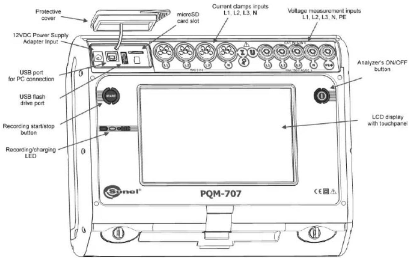
Fig. 1. Power Quality Analyzer PQM-707. General view.
1.3 Power supply of the analyzer
The analyzer is powered from two sources: external power supply adapter (input voltage 100...240 V AC, output 12 V DC) and from a removable Li-Ion battery pack. The fully charged battery pack provides at least 4 hours of uninterrupted operation without an external power supply. After connecting the power supply the battery pack is recharged. Details are described in section 8.1
After the battery pack is discharged the meter stops its current operations (e.g. recording) and switches -off in the emergency mode. When the power supply from mains returns, the analyzer resumes interrupted recording.
Additional option for recharging the meter is connecting it with USB cable to a PC or charger with USB output. The charging current is then reduced accordingly (approx. 15-fold), which means that charging time is longer. This type of charging works only when the analyzer is completely switched off (not in sleep mode).
Additional or new battery pack used for PQM-707 (Li-Ion 11.1 V, 3.4 Ah) may be purchased at our store or in Sonel distribution network.
1.4 Measured parameters
The analyzer is designed to measure and record the following parameters:
• RMS voltages up to 760 VAC referred to PE input (measuring range up to ±1150 V),
- RMS currents:
- up to 3000 A AC (peak currents - up to ±10 kA at 50 Hz) using flexible probes F-1(A), F-2(A)(HD), F-3(A)(HD);
- up to 1000 A (peak values - up to ±3600 A) using CT probes C-4(A) or C-5A;
- up to 10 A (peak values - up to ±36 A) using C-6(A) probes,
-
up to 100 A (peak values - up to ±360 A) using C-7(A) probes,
-
crest factors for current and voltage,
- mains frequency within the range of 40..70 Hz,
• active, reactive and apparent power and energy, distortion power,
• harmonics of voltages and currents (up to 50th),
• active and reactive powers of harmonics, - Total Harmonic Distortion THD _F for current and voltage,
• Total Demand Distortion TDD for current,
• power factor PF, cosφ, tanφ, - unbalance factors for three-phase mains and symmetrical components,
- flicker severity P_ST and P_LT ,
Some of the parameters are aggregated (averaged) according to the time selected by the user (available settings: 1s, 3s, 10s, 30s, 1min, 10min, 15min, 30min) and may be stored on a memory card. In addition to average value, it is also possible to record minimum and maximum values in individual averaging periods.
The analyzer detects the following types of voltage events: dip, swell and interruption. User may define two thresholds for current: exceeding (top value) of the maximum value and dropping below (bottom value) the minimum value. The current in the neutral channel has two independent thresholds. In DC systems, there are two thresholds: exceeding the maximum and minimum voltage value.
Event detection may be accompanied by recording waveforms of voltage and current waveforms and RMS values. These waveforms are recorded at the beginning and end of the event.
Tab. 1 presents a summary of parameters measured by PQM-707, depending on the mains type.
Tab. 1. Measured parameters for different network configurations.
| Mains type, channel Parameter | 1-phase | 2-phase | 3-phase 4-wire, 212 -element | 3-phase 3-wire, 2-element | DC | DC+M | ||||||||||||||
| L1 | N | L1 | L2 | N | Σ | L1 | L2 | L3 | N | Σ | L12 | L23 | L31 | Σ | L1 | L1 | L2 | Σ | ||
| U | RMS voltage | ● | ● | ● | ● | ● | ● | ● | ● | ● | ● | ● | ● | |||||||
| U_DC | DC voltage | ● | ● | ● | ● | ● | ● | ● | ● | ● | ● | ● | ● | ● | ● | ● | ||||
| I | RMS current | ● | ● | ● | ● | ● | ● | ● | ● | ● | ● | ● | ● | |||||||
| I_DC | DC current | ● | ● | ● | ● | ● | ● | ● | ● | ● | ● | ● | ● | ● | ● | ● | ||||
| F | Frequency | ● | ● | ● | ● | |||||||||||||||
| CF U | Voltage crest factor | ● | ● | ● | ● | ● | ● | ● | ● | ● | ● | ● | ● | |||||||
| CF I | Current crest factor | ● | ● | ● | ● | ● | ● | ● | ● | ● | ● | ● | ● | |||||||
| P | Active power | ● | ● | ● | ● | ● | ● | ● | ● | ● | ● | ● | ● | ● | ||||||
| Q_1,Q_B | Reactive power | ● | ● | ● | ● | ● | ● | ● | ● | ●(1) | ||||||||||
| D,SN | Distortion power | ● | ● | ● | ● | ● | ● | ● | ● | |||||||||||
| S | Apparent power | ● | ● | ● | ● | ● | ● | ● | ● | ● | ||||||||||
| PF | Power Factor | ● | ● | ● | ● | ● | ● | ● | ● | ● | ||||||||||
| cosφ | Displacement power factor | ● | ● | ● | ● | ● | ● | ● | ● | |||||||||||
| tanφ | Factor tangent φ | ● | ● | ● | ● | ● | ● | ● | ● | ●(1) | ||||||||||
| THD U | Total harmonic distortion voltage | ● | ● | ● | ● | ● | ● | ● | ● | ● | ● | ● | ● | |||||||
| THD I | Total harmonic distortion current | ● | ● | ● | ● | ● | ● | ● | ● | ● | ● | ● | ● | |||||||
| E_P+,E_P- | Active energy (consumed and supplied) | ● | ● | ● | ● | ● | ● | ● | ● | ● | ●(2) | ●(2) | ●(2) | ●(2) | ||||||
| E_Q1-,E_Q1-E_QB+,E_QB- | Reactive energy (consumed and supplied) | ● | ● | ● | ● | ● | ● | ● | ● | ●(1) | ||||||||||
| E s | Apparent energy | ● | ● | ● | ● | ● | ● | ● | ● | ● | ||||||||||
| U_h1..U_h50 | Voltage harmonic amplitudes | ● | ● | ● | ● | ● | ● | ● | ● | ● | ● | ● | ● | |||||||
| I_h1..I_h50 | Current harmonic amplitudes | ● | ● | ● | ● | ● | ● | ● | ● | ● | ● | ● | ● | |||||||
| P_h1..P_h50 | harmonics active power | ● | ● | ● | ● | ● | ● | |||||||||||||
| Q_h1..Q_h50 | harmonics reactive power | ● | ● | ● | ● | ● | ● | |||||||||||||
| Unbalance U,I | Symmetrical components and unbalance factors | ● | ● | |||||||||||||||||
| P_ST,P_LT | Flicker severity | ● | ● | ● | ● | ● | ● | ● | ● | ● | ||||||||||
| TDD | Total demand distortion | ● | ● | ● | ● | ● | ● | ● | ● | ● | ● | ● | ● | |||||||
Explanations: L1, L2, L3 (L12, L23, L31) indicate subsequent phases,
N is a measurement for voltage channel N-PE or current channel I ter type,
N, depending on the parame-
is the total value for the system.
(1) In 3-wire networks, the total reactive power is calculated as inactive power N = _e^2 - P^2 (see discussion on reactive power in section 5.3)
(2) Only consumed energy E _P+
1.5 Compliance with standards
The analyzer is designed to meet the requirements of the following standards.
Standards valid for measuring network parameters:
- IEC 61000-4-30:2015 – Electromagnetic compatibility (EMC) - Testing and measurement techniques - Power quality measurement methods.
- IEC 61000-4-7:2007 – Electromagnetic compatibility (EMC) – Testing and Measurement Techniques - General Guide on Harmonics and Interharmonics Measurements and Instrumentation for Power Supply Systems and Equipment Connected to them.
- IEC 61000-4-15:2011 – Electromagnetic compatibility (EMC) – Testing and Measurement Techniques - Flickermeter - Functional and Design Specifications.
• IEC 50160:2010 – Voltage characteristics of electricity supplied by public distribution networks.
Safety standards:
- IEC 61010-1 – Safety requirements for electrical equipment for measurement control and laboratory use. Part 1: General requirements.
- IEC 61010-2-030 – Safety requirements for electrical equipment for measurement, control, and laboratory use - Part 2-030: Particular requirements for testing and measuring circuits.
Standards for electromagnetic compatibility:
- IEC 61326 – Electrical equipment for measurement, control and laboratory use. Requirements for electromagnetic compatibility (EMC).
The device meets all the requirements of Class S as defined in IEC 61000-4-30. The summary of the requirements is presented in the table below.
Tab. 2. Summary of selected parameters in terms of their compliance with the standards
| Aggregation of measurements at different intervals | IEC 61000-4-30 Class S:Basic measurement time for parameters (voltage, current, harmonics, unbalance) is a 10-period interval for 50 Hz power supply system and 12-period interval for 60 Hz system,Interval of 3 s (150 periods for the nominal frequency of 50 Hz and 180 periods for 60 Hz),Interval of 10 minutes,Interval of 2 h (basing on 12 intervals of 10 min.) |
| Real-time clock (RTC) uncertainty | IEC 61000-4-30 Class S:Built-in real time clock with accuracy better than ± 5 s / 24 h. |
| Frequency | Compliant with IEC 61000-4-30 Class S of the measurement method and uncertainty |
| Power supply voltage | Compliant with IEC 61000-4-30 Class S of the measurement method and uncertainty |
| Voltage fluctuations (flicker) | The measurement method and uncertainty meets the requirements of IEC 61000-4-15 standard. |
| Dips, interruptions and surges of supply voltage | Compliant with IEC 61000-4-30 Class S of the measurement method and uncertainty |
| Supply voltage unbalance | Compliant with IEC 61000-4-30 Class S of the measurement method and uncertainty |
| Voltage and current harmonics | Compliant with IEC 61000-4-30 Class S of the measurement method and uncertainty (IEC 61000-4-7 class II) |
2 Operation of the analyzer
2.1 Switching the analyzer ON/OFF
The analyzer may be switched-on by pressing button. Starting the meter from the completely inactivated status takes about thirty seconds. The screen displays the version of the software and the boot-up progress is indicated by a bar at the bottom part of the screen. After boot-up, the meter enters normal operation mode and displays the initial screen, which may be specified by the user. The default start-up screen is shown in Fig. 2.
The analyzer may be turned off by pressing button Ⓤ (if recording is not active). A window will be displayed, where the user selects the mode for switching the meter off:
- SHUTDOWN – complete inactivation with minimum power consumption. Selecting this option ends the meter operation and then turns it off. Restarting the meter switched off in this way will take about thirty seconds. The advantage of this mode is the ability a long-term storage of the meter in the off state, without significant discharging of its battery pack.
- SUSPEND – stand-by of the meter. This mode allows user to quickly start the meter, but at the cost of increased power consumption from the battery pack. The battery pack in this state will be completely discharged in approx. 40 hours. After exceeding the critical level of discharging, the meter automatically switches off completely (see the option above).
In some situations, turning off the meter is locked:
- If the analyzer is recording, the user will see a message that recording is in progress. To switch the analyzer off, first stop the recording.
- When the analyzer performs processes that can not be interrupted, e.g. software update. In this case, wait until the meter goes into standby mode.
2.2 Emergency restart
If the analyzer stops to respond, it may be forced to restart. This procedure will not delete any settings or personal information.
If the emergency restart occurs while recording is in progress, the recording will be suspended until the device is restarted.
How to force the analyzer to restart?
- Press and hold button until the device turns off and on again.
- When the startup screen appears (approx. 15 seconds from pressing) release the button.
2.3 Emergency shutdown
If the analyzer stops responding, the user may perform emergency shutdown. Performing this action will not delete any personal information or user settings, but the date and time in the device will reset.
Performing an emergency shutdown during the recording will stop it until the device is restarted. When the device is turned on again, the recording process will continue and its results will be saved to xxx_part2 file, where xxx is the name of the recording that was in progress before the shutdown. For an emergency shutdown, the battery must be removed from the device, as described in sec. 8.2.
It is strongly recommended to avoid an emergency shutdown of the device, as it may damage the file where the recording is in progress or damage the device while updating its firmware.
2.4 Auto-off
The user can enable the option to automatically switching off the meter after 10 or 30-minutes of inactivity (see sec. 2.10.2). If the analyzer during this time is powered from the battery pack and is not in the recording mode and when connection to PC is inactive, it automatically switches when it is not used to save energy.
The analyzer turns off automatically also when the battery is fully discharged. Such emergency shut-down is performed regardless of the mode of the device. In case of active recording, it will be interrupted. When the power supply returns, the recording process is resumed. Emergency shutdown is signalled by an appropriate message.
2.5 LED
Two-colour LED located below (START) button indicates the recording status and charge status of the battery pack.
Red colour indicates the recording process:
• LED flashes red during data recording, with a frequency of 0.5 Hz (once every 2 seconds)
• LED is inactive when recording is off.
Green colour indicates the battery pack:
- LED is continuously green during charging and when recording is off (also when the meter is switched off)
- during charging, but when the recording is on, green LED turns on once every 10 seconds.
- it flashes at 0.5 Hz frequency after charging error is detected (exceeded temperature, no battery pack); at the same time when recording is on red and green LED's flash alternately. When green LED flashes for a long time, even when the ambient temperature is correct and the battery pack temperature is within the range from 0°C to 45°C, it may indicate a faulty battery pack and the need to contact the manufacturer's service.
2.6 MicroSD memory card
Removable microSD HC card is the primary place of data storage for:
- recorded measurement data,
• standard compliance reports, - screenshot files.
The top bar shows the status of the card and its free space available.
To ensure proper operation of the analyzer and prevent data loss:
- do not remove the memory card during recording. Ignoring this recommendation may result in ending the recording process, damage of data recorded, and in some cases, damage to the entire structure of files saved on the card.
- do not modify or delete files stored on the card or store own files on it. If the analyzer after inserting the card detects an error in the file system, the memory format panel is shown to perform formatting of the card. Only after formatting (which removes all files) it will be possible to reuse the card in the analyzer.
- Before removing the card from the meter (e.g. to read the data by Sonel Analysis by using external card reader) it is recommended to turn the meter off, to save all cached data.
MicroSD memory card may be formatted from the user interface level. Enter ANALYZER SETTINGS and select MEMORY, where the user may ability to format the memory (see also sec. 2.10.1).
2.7 USB external memory - pendrive
Connecting an external USB stick allows user to:
- copy selected files with reports on standard compliance from microSD memory card to the memory stick,
- copy selected files with screenshot from microSD memory card to the memory stick,
- save the log file of the meter, in case of an error in the analyzer in order to perform an analysis in the service department of the manufacturer,
- update the firmware of the analyzer. For this purpose, first save in the root folder of the memory stick the update file downloaded from the manufacturer's website http://www.sonel.pl/en/download/firmware.html (after extracting the ZIP archive). After inserting the USB memory to the analyzer, select from the main menu ANALYZER SETTINGS and then UPGRADES. When correct update files are detected, the appropriate window is displayed. The user should follow the on-screen prompts.
Supported file systems are FAT and FAT32. When a memory formatted in a different file system is inserted, the device will display a window informing about detecting unformatted media carrier. From this window, the user may directly enter the formatting screen.
The data on the memory stick are stored in the folder named "PQM-707_DATA".
2.8 Main elements of the screen
Fig. 2 shows the default screen of the analyzer after switching on. There you can distinguish several sections:
- top bar, 1
- the title and help bar , 2
- main window, 3
• information bar on current mains configuration , 4 - menu bar . 5
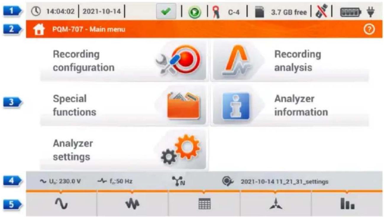
Fig. 2. Main elements of the analyzer screen.
2.8.1 Top bar
Top bar (Fig. 3) includes from left to right:

Fig. 3. Elements of the top bar.
- Current time and date of the analyzer . 1
- Button of HOLD 2 function. Pressing this icon on the screens of LIVE mode (preview of the current network, see sec. 2.16) will stop the refreshing of image displayed in the main window. Press it again to return to normal mode.
- The button signalling the correct connection of the analyzer 3. The icon on this button informs the user about the correctness or potential problem with the configuration or connection of the analyzer. Pressing this icon (it may show symbol √, ? or ✗) will display a window with more detailed information about possible errors in connecting the analyzer to the mains and with the compliance of mains parameters with the measurement configuration. More information can be found in section 2.18.1.
- Recording status icon 4. The icon is green when recording is inactive. After starting the recording of the icon turns red.
- Information on connected or configured current probes. If the measurement configuration has no probes indicated - the field displays dashes "--". When a specific type of probes is selected, their name will be displayed. In the mode of auto detection of probes, the device displays the name of recognized probes (probe must be of the same type used in all measurement channels) or the question mark "?" if no probes are connected (or detected).
- Memory card icon with information about free space 6. If the card is not in the slot, the screen shows the icon crossed out.
- External USB memory icon (USB stick) . If no external memory is connected, the icon is crossed out.
- The icon of battery charge status and external power supply .8
2.8.2 The title bar and help
The title bar (Fig. 2, element) displays the name of the current main window with the name of the section. It allows user to quickly see which part of the interface is displayed. The right side of the screen displays the Help icon. After clicking it, a context help is displayed, which describes interface elements visible on the screen.
2.8.3 Main window
In the central part of the screen, the main window of the analyzer is displayed. The default window (shown in Fig. 2) contains four items:
- RECORDING CONFIGURATION. This part of the interface is used to configure the measurement system and all aspects related to the recording of network parameters such as: mains type (e.g. single-phase, three-phase), probes type, transformers, recorded parameters.
-
RECORDING ANALYSIS – provides an analysis of the recorded data and “live” view of the recording process.
• SPECIAL FUNCTIONS including: -
INRUSH – after selecting this option, the analyzer switches to inrush measurement mode (see section 2.12),
• INVERTER EFFICIENCY (see section 2.13).
• ENERGY LOSSES CALCULATOR (see section 2.14).
- ANALYZER SETTINGS – its includes a range of analyzer configuration options, such as date and time, managing energy saving modes, or standards and files manager.
- ANALYZER INFORMATION – after selecting this option, a window is displayed with the details of the analyzer and manufacturer.
A more detailed description of each section is presented in the following chapters.
2.8.4 Information bar on the parameters of the current mains configuration
Below the main screen a bar is displayed, which shows the main parameters of the active measurement system (Fig. 2, element):
- nominal voltage,
- mains frequency,
- mains type,
- the name of the current recording configuration.
The mains type is symbolized by icons:
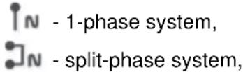


2.8.5 Menu bar
The menu bar is displayed at the bottom of the screen (Fig. 2, element). It usually contains several touch icons which change depending on the current context. The individual icons are described in sections presenting individual screens. In some cases, an additional menu bar is opened above the main menu bar.
Some icons displayed in the menu bar have a permanent effect throughout the interface:

In subsequent sections, the menu bar icons (and their effects), specific for a given view, are described in a separate part of entitled "Menu bar functions".
2.9 Recording configuration
Before any measurement is started it is necessary to properly configure the analyzer in accordance with the requirements of the user. Configuration changes are performed directly in the analyzer and it is (at the moment) the only possible way to configure the device - Sonel Analysis software in its current version (4.3.0) does not support the configuration of PQM-707 analyzer.
To access the configuration module on the main screen, select section RECORDING CONFIGURATION. The list is displayed with measurement configurations saved in the analyzer's memory (Fig. 4).
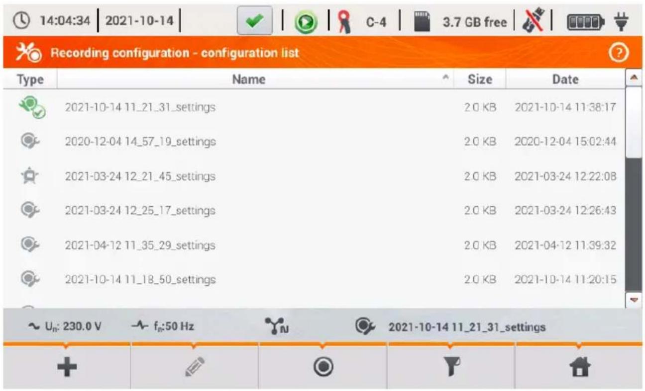
Fig. 4. Recording configuration – Configuration list.
The table has three columns:
- TYPE – displayed icon determines the type of measurement configuration:
- recording acc. to user configuration (inactive - grey)
- recording acc. to user configuration (active - green)
- recording for compliance with the selected standard (inactive)
-
recording for compliance with the selected standard (active)
-
NAME – the name of the configuration given by the user.
- DATE – date and time of creating the configuration.
The list may be scrolled in the window by finger icon or using the bar on the right.
Menu bar functions
To make the desired configuration active, click its line, and then on the bottom bar select icon (activate the configuration).
To modify the indicated configuration, in the bottom bar select icon (editing) or double-click the line of this configuration.
Selecting the filter icon activates an additional menu bar displayed above the main menu bar, where you may indicate which registrations are listed: acc. to user configuration, acc. to a standard,
or both types. Selecting a given type is indicated by orange colour e.g.

To add a new configuration, select icon + (add).
After clicking the icon for adding a new configuration, a window will be displayed as shown in Fig. 5. The title bar will display the default name of the new configuration. It is created from current date and time in the format "YYYY-MM-DD hh_mm_ss_settings", which may be modified. An asterisk after the name indicates that the configuration has been modified but not saved.
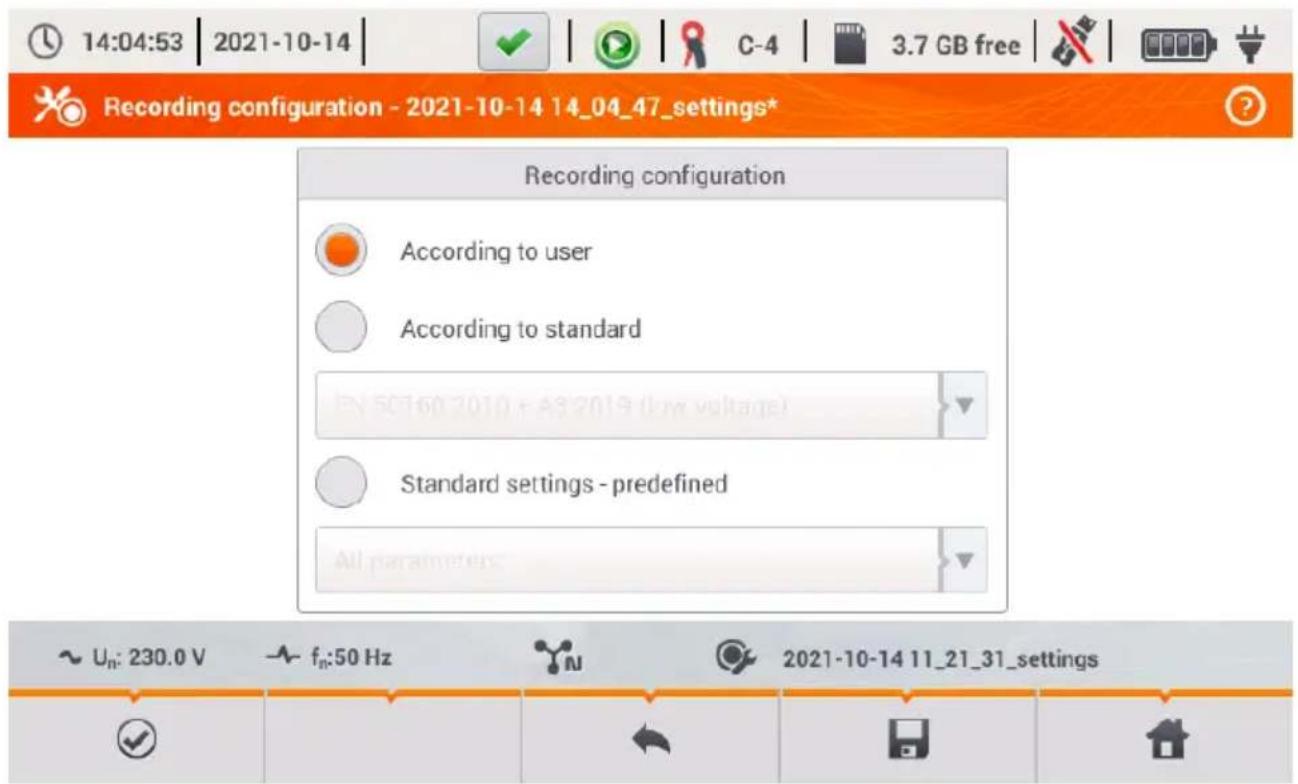
Fig. 5. Recording configuration – selecting the type of a new configuration.
The first step in creating a new configuration is selecting the type of a new configuration. There are two possibilities:
- ACCORDING TO USER – the user decides fully on recording character, averaging time and type of parameters to be recorded.
- ACCORDING TO STANDARD – recording for the compliance of the tested mains with the standard selected from the list; it enables user to generate a compliance report. The user may set only certain recording parameters, e.g. network layout and nominal voltage; other parameters are set automatically in accordance with the requirements of the selected standard (unchangeable). By default the analyzer has the following profiles prepared:
- EN50160: European standard in three variants depending on the nominal voltage value (low, medium and high)
☐ Regulation of the Minister of Economy: provisions valid in Poland in four variants depending on the nominal voltage value (low, medium, high 110 kV and 220 kV, high 400 kV) - Two variants of an Australian Standard (based on EN 50160 and AS 61000.3.100), for low and medium voltage,
○ GOST 32144-2013: Russian standard in four variants depending on the nominal voltage value (low, medium 6-20 kV, medium 35 kV, high), - NEC220.87 – 30-day Load Studies.
- STANDARD SETTINGS – PREDEFINED – list of five predefined settings the user can choose in order to speed up the process of complete setup. User needs to decide on the type of mains and averaging period etc. List of available settings:
- All parameters
○ Logging: V, I, f and THD - Power study & Energy audit
○ Logging: harmonics, V, I - Power Quality
○ Load Study
Menu bar functions
- approving the selected recording type and entering detailed edition.
- saving configuration with default parameters. The user will be asked for the name of the configuration file. You can save the configuration with the default name, created automatically, or change the name as desired.
Detailed configuration settings are divided into eight screens:
• GENERAL SETTINGS,
- GENERAL SETTINGS II,
• VOLTAGE PARAMETERS,
• CURRENT PARAMETERS,
- POWERS,
• ENERGY AND POWER FACTORS,
- FLICKER AND UNBALANCE,
• THD, TDD AND HARMONICS,
• HARMONICS POWER.
Buttons and at the bottom menu bar are used to switch between successive screens.
After editing the configuration you can save it under a certain name in the internal memory of the analyzer
by clicking icon A window will be displayed, in which the user may to give the configuration a name (or leave the proposed one). To edit the name, click its area - a window with on-screen keyboard will appear. Field Set as active will set the saved configuration as active - the analyzer reads all settings and will be ready to start recording. To confirm, click OK, to cancel - CANCEL.
2.9.1 Recording configuration – General settings
Screen of General settings is shown in Fig. 6.
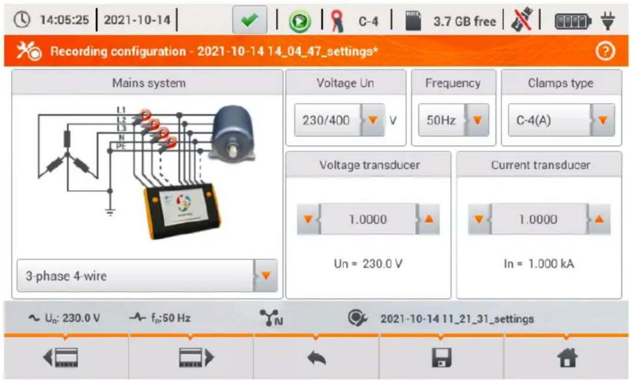
Fig. 6. Recording configuration – General settings
At this point, you may define:
- MAINS TYPE. By clicking the icon from drop-down list, or on the network name, you can select the following types (the names may differ depending on the language selected – US or GB):
o 1-phase,
o Split-phase,
o 3-phase 4-wire (systems with neutral wire, e.g. wye with N),
- 3-phase 3-wire (systems without neutral wire – wye without N and delta),
3-phase 3-wire Aron / 2 element (as standard 3-wire system, but with the current measurement using two probes (I1 and I3), the third current (I2) is calculated according to the calculation method from the formula I2 = -(I1 + I3) )
3-phase 4-wire (no U L2) / 2 ½ element (no V L2/B) (as standard 4-wire system, but with the calculation of U L2 voltage (U L2 voltage is not measured) according to the formula UL2 = -(UL1+UL3)).
- 3-phase open delta,
o Transducers: 3-phase 4-wire,
o Transducers: 3-phase 3-wire,
o Transducers: 3-phase (V system, Aron).
The above types of mains are available for frequencies of 50 and 60 Hz.
In DC systems, there are two systems of networks:
- DC – measuring one DC voltage and one DC current,
- DC+M – measuring two DC voltages in relation to the middle potential (M stands for middle), with the option for measuring two DC currents (probes C-5 or C-5A).
- VOLTAGE UN – the user may select from a list the nominal voltage of the tested network. Each entry in the list contains two values separated by slash, e.g. 230/400. The first of them specifies the nominal phase voltage in systems with neutral conductor (1-phase, split-phase, 3-phase
4-wire). The second value determines the phase-to-phase voltage in such systems and nominal phase-to-phase voltage in systems without neutral conductor (3-phase 3-wire)
- FREQUENCY FN – mains nominal frequency. There are three positions:
○ 50 Hz,
○ 60 Hz,
- DC – selecting this option allows the measurement in DC systems (mains types: DC and DC+M described above).
- PROBES TYPE - here you can enable or disable the measurement of currents and determine the type of probes. If the current measurement is required, indicate probes to be used from the following list:
- F-x – flexible probes (Rogowski coil) with a nominal range of 3000 A, AC measurement,
- C-4 – probes CT (with core) with a range of 1000 A for AC currents measurement,
C-5 – probes with Hall sensor with a range of 1000 A for measuring AC and DC currents (only probes available in DC circuits), - C-6 – probes CT (with core) with a range of 10 A for AC measurement,
- C-7 – probes CT (with core) with a range of 100 A for AC measurement,
- Auto – selecting this item allows you to use any automatic probe (the letter A in the designation, e.g. F-3A). The analyzer displays the type of connected probes on the top bar. Starting the recording is possible only when the analyzer recognized properly connected probes, and when the types of probes in multiphase systems are identical.
- NONE – indicating this option turns off the current measurement and all the parameters that need the current measure (i.e. power).
When from FREQUENCY FN list DC position is selected, then only the following options are available: None, C-5, Auto (in Auto mode only C-5A probes are accepted).
- VOLTAGE TRANSDUCER – allows you to enter a multiplier of the nominal voltage selected from the list. The value of the multiplier may be set in the range from 0.1 to 10000.0 in 0.0001 steps. Multipliers are set in situations when using the external voltage transformers that modify the actual mains voltage to another voltage (usually lower), acceptable to the measuring instrument. Below the multiplier value, the screen displays resulting nominal voltage, which is the product of the multiplier and the nominal voltage indicated on the selection list. For example, when measuring the medium voltage of 15 kV (3-phase, 3-wire system) transformers are used to lower the ratio of 150:1. Voltage of 15 kV is transformed to 100 V, which may be safely provided to the input of the analyzer. In order to ensure that the measuring device indicates the factual voltage in a medium voltage network, it is necessary to set the voltage transformer at 150.0, and choose "58/100" from the list of nominal voltages. Voltage 100 V provided to the analyzer input will be multiplied by 150 and will be shown as 15 kV.
- CURRENT TRANSDUCER - provides the current multiplier measured by the current probes. The value of the multiplier can be set in the range of from 0.1 to 10000.0, in 0.0001 steps. When using external current transformers (usually reducing the current value) this field has to be provided with the same value as the transformer ratio. The currents measured by the probes will be multiplied by the transducer factor to reflect the actual currents flowing on the primary side of the transformer. Below the multiplier value, the resulting new value of the maximum current on the primary side is displayed, which is the product of the multiplier and the nominal range of probes used. For example, using the transformer of 10 000 A / 5 A and a probes C-6(A) (with nominal range of 10 A) you may measure currents up to 10 000 A (the limitation results from abilities of the transducer, not probes - primary current corresponding to the nominal current of the probes is 20 000 A).
2.9.2 Recording configuration – General settings II
Screen of General settings II is shown in Fig. 7. It consists of the following fields:
• TRIGGERING: specifies the method of starting the recording.
o Immediate – starts recording after pressing START,
Threshold – device is ready for recording after pressing START button, but saving data to the memory card begins when the specified threshold of any event is exceeded, e.g. after detecting the first voltage dip. When analyzer waits for the first
event to occur the recording state icon on the top bar changes to

Schedule – start and end times of recording are defined by the user. The user may define only the start time (then the end will be triggered manually using a button), or only the end time (then the recording will be triggered manually by button) or both of the times.
The fields for entering times are on the same screen in section SCHEDULE. Readiness for recording is obtained after pressing START button. When analyzer waits
for the start time the recording state icon on the top bar changes to ⚠ . Proper data recording begins and ends at the set time interval. The scheduled recording process may be interrupted at any time manually by pressing START.
![14:05:42 | 2021-10-14 | C-4 | 3.7 GB free | Recording configuration - 2021-10-14 14_04_47_settings* Triggering Immediate Averaging period 10min Additional measurements N-PE voltage N-conductor current Schedule Configuration name 2021-10-14 14_04_47_settings Hysteresis [%] 2.0 Selected standard Uₙ: 230.0 V fₙ:50 Hz 2021-10-14 11_21_31_settings](/content/2026/05/852541/images/5ca449c2a896ca23d166f6b11c740ac9a50e69e949beb33884ba8af92786278e.jpg)
Fig. 7. Recording configuration – General settings II.
- AVERAGING PERIOD - specifies the averaging time of recorded parameters and also the time between successive recorded data on a memory card (except events). The following settings are available: 1 second, 3 seconds, 10 seconds, 30 seconds, 1 minute, 10 minutes, 15 minutes, 30 minutes.
- HYSTERESIS - percentage value in the range from 0.1 to 10, to be used for detecting events. Higher values allow to limit the number of detected events if the parameter value fluctuates around the threshold. The typical value of the hysteresis is 2%.
- ADDITIONAL MEASUREMENTS - in this section you can enable the measurement of additional channels:
-
N-PE voltage – ticking this box results in recording also parameters of voltage channel N-PE (as for other voltage channels).
○ N-conductor current – ticking this box results in recording the current in the neutral conductor. It is necessary to connect the probes in channel N. -
CONFIGURATION NAME – displays the current name of the edited configuration (read-only).
- SELECTED STANDARD - in case of recording acc. to a standard, this field displays the name of the selected standard, e.g. "EN50160 low voltage". In other cases, the field displays dashes "--".
2.9.3 Recording configuration – Voltage parameters
The screen for setting voltage parameters is shown in Fig. 8.
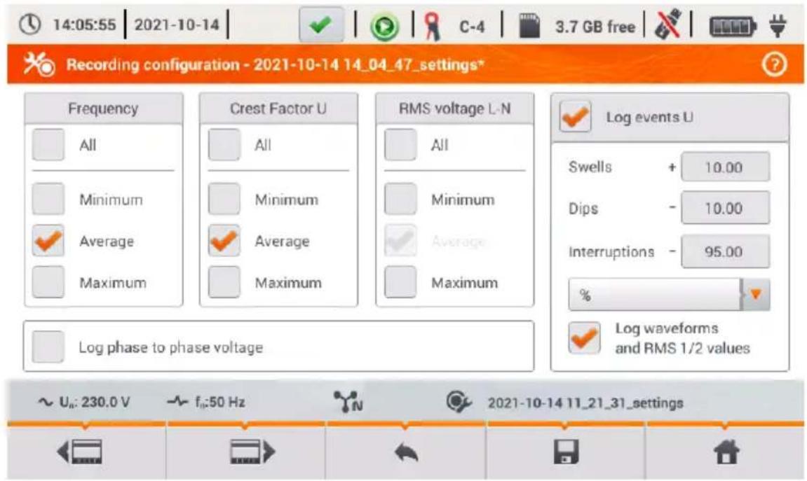
Fig. 8. Recording configuration - Voltage parameters
It contains the following elements:
- FREQUENCY - selection boxes for recording the following parameters:
o Minimum - recording the smallest frequency value registered in averaging period. For example: in 10-minute averaging, this is the minimum value of 10-second frequency out of the 60 measured in that range.
○ Average - the averaged value of the frequency in the averaging period. For example: in case of this parameter and a 10-minute averaging, the value is the arithmetic mean of 60 frequency values measured in this period.
o Maximum - the highest frequency recorded in the averaging period.
- All - ticking this box will automatically select all three parameters (Minimum, Average, Maximum).
- CREST FACTOR U – selection boxes for recording voltage Crest Factor. Similarly to the frequency and most of the other parameters, the following fields are available:
○ Minimum
○ Average
○ Maximum
- RMS VOLTAGE L-N or RMS VOLTAGE L-L (depending on the type of network) - selection boxes for recording RMS voltage phase-to-neutral and phase-to-phase. Minimum and maximum values are searched from RMS _1/2 values (RMS 1-cycle value refreshed every half-cycle). The user may select the following fields:
○ Minimum
○ Maximum
The average value is always recorded and ticked permanently.
- LOG PHASE TO PHASE VOLTAGE – ticking this box enables recording of the average phase-to-phase voltages in 3-phase 4-conductor systems or one phase-to-phase voltage in split-phase system (the box is active only in these two systems).
- LOG EVENTS – ticking this box enables voltage event detection: swells, dips, interruptions. Three field with values allow the user to introduce own thresholds for these three types of events. Thresholds may be entered in volts or as a percentage values referenced to the nominal voltage of the network, e.g. setting the threshold of swell as +10% at nominal voltage of 230 V triggers the detection of swell after exceeding 253 V voltage (RMS 1/2 ). The event ends when the voltage drops to the threshold value reduced by hysteresis. If the hysteresis in the described case is 2%, then the end of the event will occur if when voltage (RMS 1/2 ) is lower than 248.4 V (253 V - 4.6 V).
- LOG WAVEFORMS AND RMS 12 VALUES - ticking this box results in additional recording of waveforms of active measurement channels (also current channels) at the start and end of the voltage event. These waveforms have a standard length of 6 periods (approx. 120 ms), 2 periods of pretrigger (before start time) and 4 periods after.
2.9.4 Recording configuration – Current parameters
The view of this screen is shown in Fig. 9.
![14:06:23 | 2021-10-14 | C-4 | 3.7 GB free | Recording configuration - 2021-10-14 14_04_47_settings* Crest Factor I All Minimum Average Maximum RMS current All Minimum Average Maximum Events Log events I L max [A] N max [A] 100.00 70.00 L min [A] N min [A] 0.00 0.00 Log waveforms and RMS 1/2 values ~ Ua: 230.0 V ~ fa:50 Hz 2021-10-14 11_21_31_settings](/content/2026/05/852541/images/df42e24b5e407f2c0c69b3f6e446bc074611d29643ef5f0f21bdc9c3703ac5c8.jpg)
Fig. 9. Recording configuration - Current parameters
The elements are active (for editing) if the screen of general settings has enabled measurement of currents.
- CREST FACTOR I – recording current Crest Factor. You may record:
○ Minimum
○ Average
○ Maximum
• RMS CURRENT – recording RMS current, Available options:
○ Minimum
○ Average
- Maximum
Minimum and maximum values in the averaging period are searched from all the RMS _1/2 values, as in the case of the RMS voltage.
- LOG EVENTS – ticking this box enables current event detection. Entering "0" disables a given event. The entered values may be from range 0 ... I n (where I n is the current measurement range after taking into account current transformers)
○ L max [A] - maximum value threshold for current L1, L2, L3 (depending on the network). An event is detected when the value of RMS_1/2 current exceeds the specified threshold.
○ L min [A] – minimum value threshold for current L1, L2, L3. An event is detected when the value of RMS_1/2 current drops below the specified threshold.
○ N max [A] – similarly to L max, but it relates to N current channel (neutral current).
- N min [A] – similarly to L min, but it relates to N current channel (neutral current).
- LOG WAVEFORMS AND RMS 12 VALUES - ticking this box results in additional recording of waveforms of active measurement channels (also voltage channels) at the start and end of the current event. These waveforms have a standard length of 6 periods (approx. 120 ms), 2 periods pretrigger time and 4 periods after start.
2.9.5 Recording configuration – Powers
Configuration screen Powers is shown in Fig. 10.
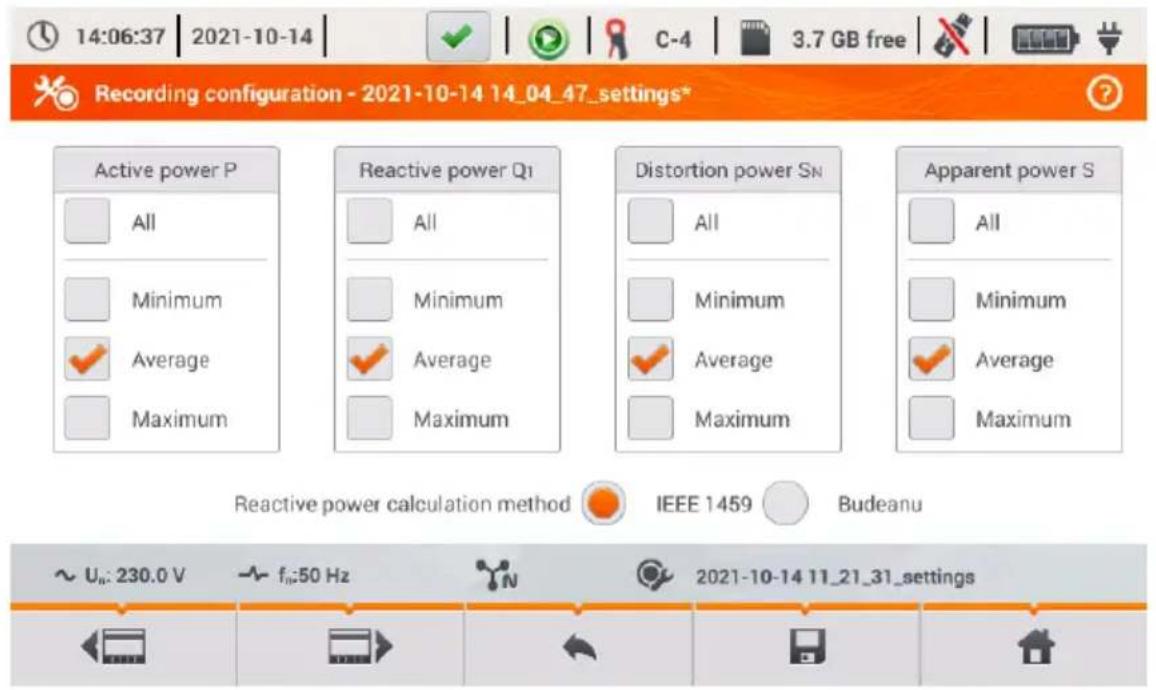
Fig. 10. Recording configuration – Powers.
It is possible to activate the recording of minimum, average and maximum values for the following power types:
• ACTIVE POWER P,
- REACTIVE POWER Q1 (for IEEE 1459) or REACTIVE POWER QB (for Budeanu method),
• DISTORTION POWER S N (for IEEE 1459) or DISTORTION POWER D (for Budeanu method),
• APPARENT POWER S.
In the lower part there is a checkbox "Reactive power calculation method": IEEE 1459 (recommended and set by default) or Budeanu.
2.9.6 Recording configuration – Energy and power factors
Configuration screen Energy and power factors is shown in Fig. 11.
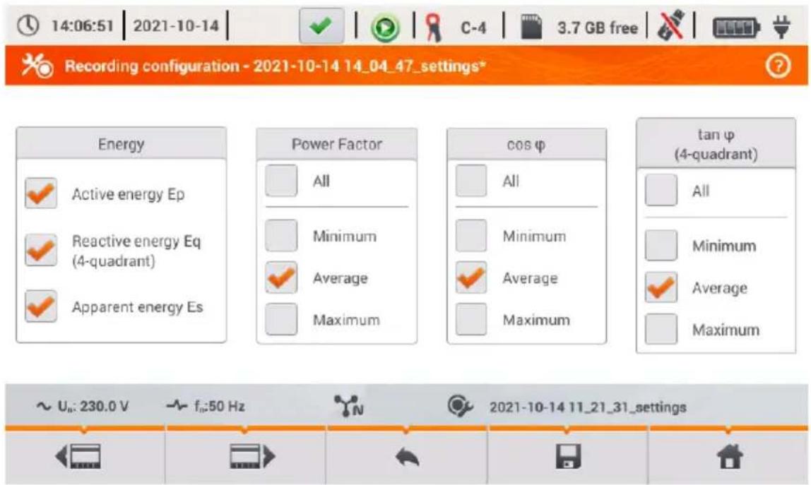
Fig. 11. Recording configuration – Energy and power factors
The following elements are available:
• ENERGY:
Active energy Ep - ticking this box activates recording of active energy. The readout of meters measuring active energy (consumed and supplied) will be saved at every averaging period.
- Reactive energy Eq - ticking this box activates recording of reactive energy. The readout of meters measuring reactive energy (consumed and supplied) will be saved at every averaging period.
- Apparent energy Es - ticking this box activates recording of apparent energy. The readout of the energy meter will be saved at every averaging period.
• POWER FACTOR – user may enable recording of minimum, average and maximum,
- cosφ – recording of Displacement Power Factor (the phase shift between the primary voltage and current components). It is possible to activate the recording of minimum, average and maximum values.
- tanφ - recording tangent φ ratio (the ratio of reactive power to active power). It is possible to activate the recording of minimum, average and maximum values.
2.9.7 Recording configuration – Flicker and unbalance
Configuration screen Flicker and unbalance is shown in Fig. 12.
On this screen the user may enable the following parameters:
- SHORT-TERM FLICKER SEVERITY PST – P _ST factor is calculated every 10 minutes.
- LONG-TERM FLICKER SEVERITY PLT – P_LT is calculated every 2 hours from 12 P_ST values.
- UNBALANCE AND SYMMETRICAL COMPONENTS U - the user may enable recording of minimum, medium and maximum values. This group includes voltage parameters:
○ Positive sequence symmetrical component U 1 [V],
○ Negative sequence symmetrical component U 2 [V],
○ Zero symmetrical component U 0 [V],
○ Negative sequence unbalance factor u_2 [%], which is the ratio of negative sequence U_2 to positive sequence U_1 expressed as a percentage value,
○ Positive sequence unbalance factor u_0 [%], which is the ratio of positive sequence U_0 to positive sequence U_1 expressed as a percentage value,
- UNBALANCE AND SYMMETRICAL COMPONENTS I - the user may enable recording of minimum, medium and maximum values. This group includes current parameters:
○ Positive sequence symmetrical component I 1 [A],
○ Negative sequence symmetrical component I 2 [A],
○ Zero symmetrical component I 0 [A],
○ Negative sequence unbalance factor i 2 [%], which is the ratio of negative sequence I2 to positive sequence I_1 expressed as a percentage value,
○ Positive sequence unbalance factor i 0 [%], which is the ratio of positive sequence I0 to positive sequence I_1 expressed as a percentage value,

14:07:04
2021-10-14


C-4

3.7 GB free


Recording configuration - 2021-10-14 14_04_47_settings*

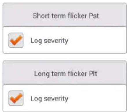
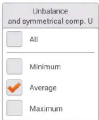
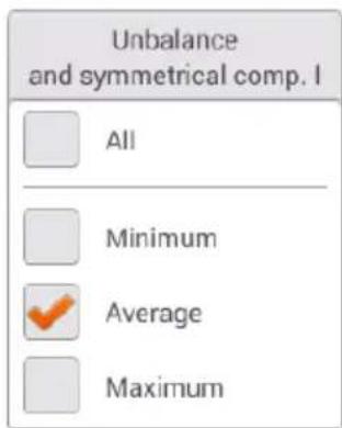

Fig. 12. Recording configuration – Flicker factor and asymmetry.
2.9.8 Recording configuration – THD, TDD and harmonics
The last screen of recording configuration is THD, TDD and harmonics (Fig. 13, Fig. 14). It allows user to activate recording of the following parameters:
- THD U – total harmonic distortion (THD) of voltage; factor THD-F is calculated (referred to the fundamental component). It includes 50 harmonics. You may record:
- minimum,
○ average, - maximum.
- HARMONICS AMplitudes U – activating recording of amplitudes for 50 voltage harmonics. The following elements may be saved:
- minimum values,
- average values,
- maximum values.
• THD I - Total Harmonic Distortion of current, similarly to THD for voltage,
• HARMONICS AMPLITURES I – similarly to voltage harmonics,
• TDD – total demand distortion parameter.
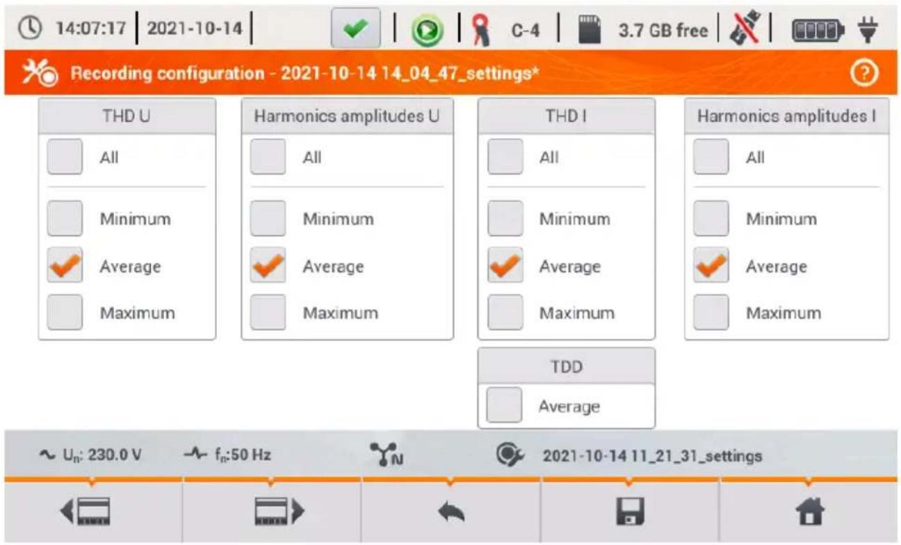
Fig. 13. Recording configuration – THD, TDD and harmonics.
After tapping the or icon the second part of the menu appears (Fig. 14). It allows user to activate recording of the following parameters:
• HARMONICS ACTIVE POWER - activates recording of all harmonic active powers,
• HARMONICS REACTIVE POWER - activates recording of all harmonic reactive powers.
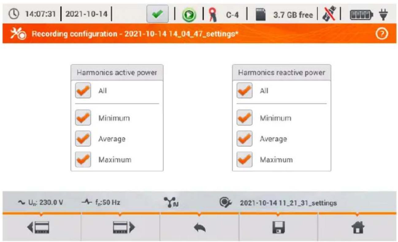
Fig. 14. Recording configuration – harmonic powers.
2.9.9 Configuration default settings
The default configuration settings ac. to the user are as follows:
- Mains type: 3-phase 4-wire,
- Nominal frequency: 230/400 V (phase/phase-to-phase) (120/208 V for US language settings),
- Nominal frequency: 50 Hz (60 Hz for US language settings),
- Current measurements and probes: activated current measurement with automatic probes,
• Voltage and current transducers: disabled, - Triggering: immediate,
• Averaging time: 10 minutes,
• Event detection hysteresis: 2.0%, - N-PE voltage and I _N current measurement: disabled,
- Recorded parameters: average values of the following parameters:
○ frequency,
○ crest factors for voltage and current,
- RMS values of phase voltages and currents,
- active power, reactive power, apparent power, distortion power (measurement method IEEE-1459),
○ active energy, reactive energy, apparent energy,
o power factor PF, cosφ and tanφ factors,
○ flicker factors P ST and P LT ,
- unbalance factors and symmetrical components of voltage and current,
- THD U, THD I, harmonic amplitudes of voltages and currents.
- Event detection:
○ detection of voltage events activated: swell 110% U NOM , dip 90% U NOM , interruption 5% U NOM , recording waveforms and RMS 1/2 activated,
- current events disabled.
The default configuration settings acc. to standard are as follows:
- Selected standard: EN50160 low voltage,
- Mains type: 3-phase 4-wire,
- Nominal frequency: 230/400 V (phase/phase-to-phase),
• Nominal frequency: 50 Hz,
- Current measurements and probes: activated current measurement with automatic probes,
• Voltage and current transducers: disabled,
- Triggering: immediate,
• Event detection hysteresis: 2.0%,
- N-PE voltage and I n current measurement: disabled,
- Recorded parameters:
- in accordance with standard requirements.
- Event detection:
o voltage events in accordance with the requirements of the standard, enabled recording of waveforms and RMS_1/2 values,
- current events disabled.
2.9.10 Start / stop of recording
After correct configuring recording and activating it, measurements can be triggered. To do this, press the START button. Recording in-progress is signalled by red icon in the top bar and flashing red LED.
Before starting the recording, pay attention to the following issues:
- Verify time of the analyzer. If the date or time are incorrect, go to ANALYZER SETTINGS→ DATE AND TIME to enter the correct data.
- Verify connections of the analyzer with the tested network. If the icon for the correct connection of the analyzer on the top bar is or, then before recording parameters, an additional window is displayed warning about a potential problem with the connection. The user must confirm the start of recording ignoring the warning or cancel the start. For more information about the potential problem display the window informing about the correct connection (see sec. 2.18.1). It may be also helpful to check the phasor diagram (vectors of voltages and currents; rotation sequence of phases in 3-phase system should be such that phase UL1 (UL1-2) is at 0°, UL2 (UL2-3) approx. -120°, UL3 (UL3-1) approx. -240°. Both unbalance factors (for voltage and current) shown on this screen should be low (typically less than 10%, especially for voltage). The display of waveforms may be checked for the shape of the waveforms and the RMS values of voltages and currents. The correct connection of current probes may be verified by checking the mark(s) of active power - in most cases of operation of passive loads this sign will be positive.
- If the recording is longer, ensure the continuity of power supply by connecting an external 12V power supply adapter to the socket of the analyzer (the bar in the upper right corner will show an electric plug icon).
- If the user selected the probes of Auto type (automatic probes) in the measurement configuration, the analyzer after pressing START checks whether correct probes are connected. If an error is detected, an adequate message will be displayed; recording will not be triggered. The analyzer requires that all required channels use probes of the same type. The user sees the correct detection of probes on the top bar – when appropriate probes are detected, their type is next to the probes icon. If a question mark is displayed in this place, it means an error of connection. In DC systems, the only permitted probes are C-5 and C-5A.
- The memory card must be inserted into the socket, and have enough free space (which is indicated on the top bar). If the card has not enough free space for the expected records (which
depends e.g. on the averaging time, recording time, mains type and number of measured parameters), you must ensure a free space by deleting previous recordings (go to ANALYZER SETTINGS → FILES).
- Recording takes the name of measurement configuration, which is active at the time of its triggering and there is no possibility to change it later. Therefore, it may be helpful to name the configuration before that, using a name which describes the measurements to facilitate finding it on the list of records (the name of the configuration can be modified before the start, entering the edition of active configuration).
Stopping the recording process:
- To stop recording, press START button and confirm your intention to stop in the pop-up window. Stopping the recording will be confirmed by sounds (one long and three short beeps) and the colour of the recording icon will change into green. Red LED will stop flashing. If the recording is secured by PIN code, you need to enter the correct code and unlock it first.
- Recording ends automatically as scheduled (if the end time is set), in other cases the user stops it by pressing START for recording ends when the memory card is full.
- Recording ends automatically when the memory card is full.
2.9.11 Approximate recording times
The maximum recording time depends on many factors such as the size of the memory card, averaging time, the type of system, number of recorded parameters, waveforms recording, event detection, and event thresholds. A few selected configurations are presented in Tab. 3. The last column specifies the approximate recording times when the memory card is almost completely empty and has approx. 3.6 GB of free space. The typical configurations shown below assumes the measurement of the N-PE voltage and IN current. If the averaging time is different than the one chosen for the sample user configuration of 1 second, the approximate time of recording is proportionally extended, e.g. for 10-second averaging, the recording time will be 10 times the specified recording time at 1-second averaging.
Tab. 3. Approximate recording times for a few typical configurations.
| Configuration type/ recorded parameters | Averaging period | System type (current measurement on) | Events (with waveforms) | Current measurement | Approximate recording time with 3.6GB allocated space |
| according to EN 50160 | 10 minutes | 3-phase4-wire | •(1000 events) | • | >10 years |
| according to EN 50160 | 10 minutes | 1-phase | •(1000 events) | • | >10 years |
| User's recording, all parameters activated | 1 second | 3-phase4-wire | •(1000 events) | • | 17 days |
| User's recording, all parameters activated | 1 second | 3-phase4-wire | •(1000 events) | 39 days | |
| User's recording, all parameters activated | 1 second | 1-phase | •(1000 events) | • | 37 days |
| User's recording, all parameters activated | 1 second | 1-phase | •(1000 events) | 77 days | |
| User's recording, all parameters activated | 1 second | 3-phase3-wire | •(1000 events) | • | 25 days |
| User's recording, all parameters activated | 1 second | 3-phase3-wire | •(1000 events) | 51 days |
2.10 Analyzer settings
After selecting ANALYZER SETTINGS section in the main screen, the screen shown in Fig. 15 will be displayed.
In this part of the meter interface, a series of screens is available for configuring many aspects of the analyzer operation. All settings are divided into the following three sections:
• HARDWARE SETTINGS
- SETTINGS
• MANAGERS
They are described in the following sections.

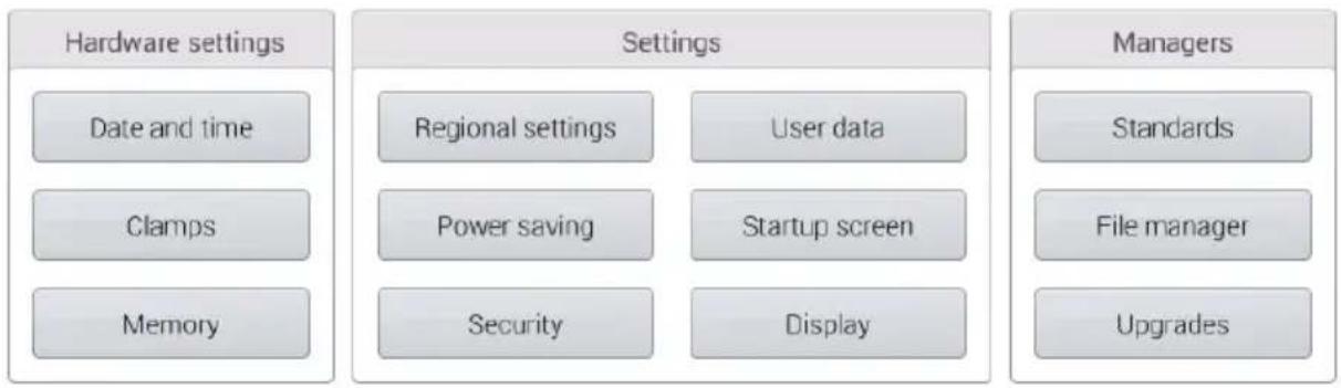
flowchart
graph LR
    A["Hardware settings"] --> B["Date and time"]
    A --> C["Clamps"]
    A --> D["Memory"]
    E["Settings"] --> F["Regional settings"]
    E --> G["User data"]
    E --> H["Power saving"]
    E --> I["Startup screen"]
    E --> J["Security"]
    E --> K["Display"]
    L["Managers"] --> M["Standards"]
    L --> N["File manager"]
    L --> O["Upgrades"]

Fig. 15. Analyzer settings
2.10.1 Analyzer settings – Hardware settings
Section HARDWARE SETTINGS contains the following options:
- DATE AND TIME - to set the date and time of the analyzer. All measured data is determined in accordance with this time. You may also choose one of two ways to display the date:
○ YYYY-MM-DD
○ MM/DD/YYYY
- PROBES - This panel enables user to reverse phases of connected probes in the software. This is useful in situations where the physical reversing of probes is impossible or difficult. To reverse the phase of the selected channel, click on the appropriate icon. The default phase of the probes is marked as DEFAULT. Active reversing (by software) is marked as REVERSED. Phase of probes can not be changed during the recording process.
- MEMORY – displays information on the space on SD memory card, internal memory of the analyzer and possibly on a connected USB storage device (flash drive) (Fig. 16). Each of these three memories may be formatted by clicking FORMAT button. After acknowledging the warning message on deleting all data from the selected memory, the formatting process is started. All files stored on the specified memory will be permanently deleted.
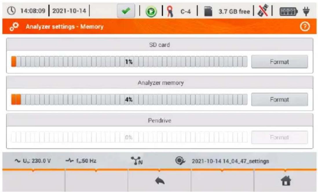
Fig. 16. Analyzer settings - Memory.
2.10.2 Analyzer settings – Settings
Section SETTINGS is divided as follows:
• REGIONAL SETTINGS – on this screen (Fig. 17) you may select:
○ Language,
○ Method for marking subsequent phases (L1, L2, L3, or A, B, C),
The colours assigned to each voltage and current channel in the interface. A few predefined colour profiles have been prepared (EU, Australia, India, China, USA), and two user profiles were marked as U1 and U2. After selecting one user profile from the list, a pop-up window will appear for setting the colour of each channel. First click on the channel to be set and then specify the desired colour.



Fig. 17. Analyzer settings - Regional settings.
- POWER SAVING – the user can activate the Auto-off mode of the analyzer after a specified period of time (if no recording is on), and specify whether the meter is to be turned off completely or enter suspend mode.
○ AUTO-OFF MODE: selecting the method for auto-off: total inactivation (Switch off) or suspend.
- AUTO-OFF TIME – the user may disable the auto-off by selecting Never, or specify the idle time after which the meter turns off (After 10 minutes or After 30 minutes).
- SECURITY – the analyzer may be protected against unauthorized access by 4-digit PIN code. Entering the code will be required every time after turning the meter on, when option LOCK ANALYZER BY PIN CODE is selected. The default PIN is "0000" and may be changed by clicking PIN field. Additionally, you can activate the blocking of the analyzer after 30 seconds from the start of recording. When you select this option, 30 seconds after recording is started (when user does not use the screen interface or buttons during the time), the analyzer displays a window to enter the PIN code. After entering wrong PIN three times in a row, the meter locks for 10 minutes. Only after this time, it will be possible to re-entry PIN.
- In order to reset the PIN code in emergency mode to its default value, hold for 5 seconds
buttons and simultaneously. When the window with the PIN code is displayed, click on the box with blinking cursor. The keyboard screen will be displayed - enter "0000" code and confirm it.
- USER DATA - in this place you can enter your contact information. These data will be also printed in generated reports on compliance with the standard.
- STARTUP SCREEN - you can set the startup screen shown after starting the analyzer:
- DISPLAY – in this place you can adjust the brightness of the LCD. The specified brightness affects the time of the analyzer operation powered from the battery pack. The automatic switching off the display ensures longer life of the battery pack; You can set the time for display switching off at 2 or 5 minutes from the last operation.
2.10.3 Analyzer settings – Managers
Section MANAGERS includes:
- STANDARDS – after selecting this option, a window is displayed, as shown in Fig. 18. This window shows a list of standards profiles stored in the internal memory of the analyzer that are used to generate the compliance reports.
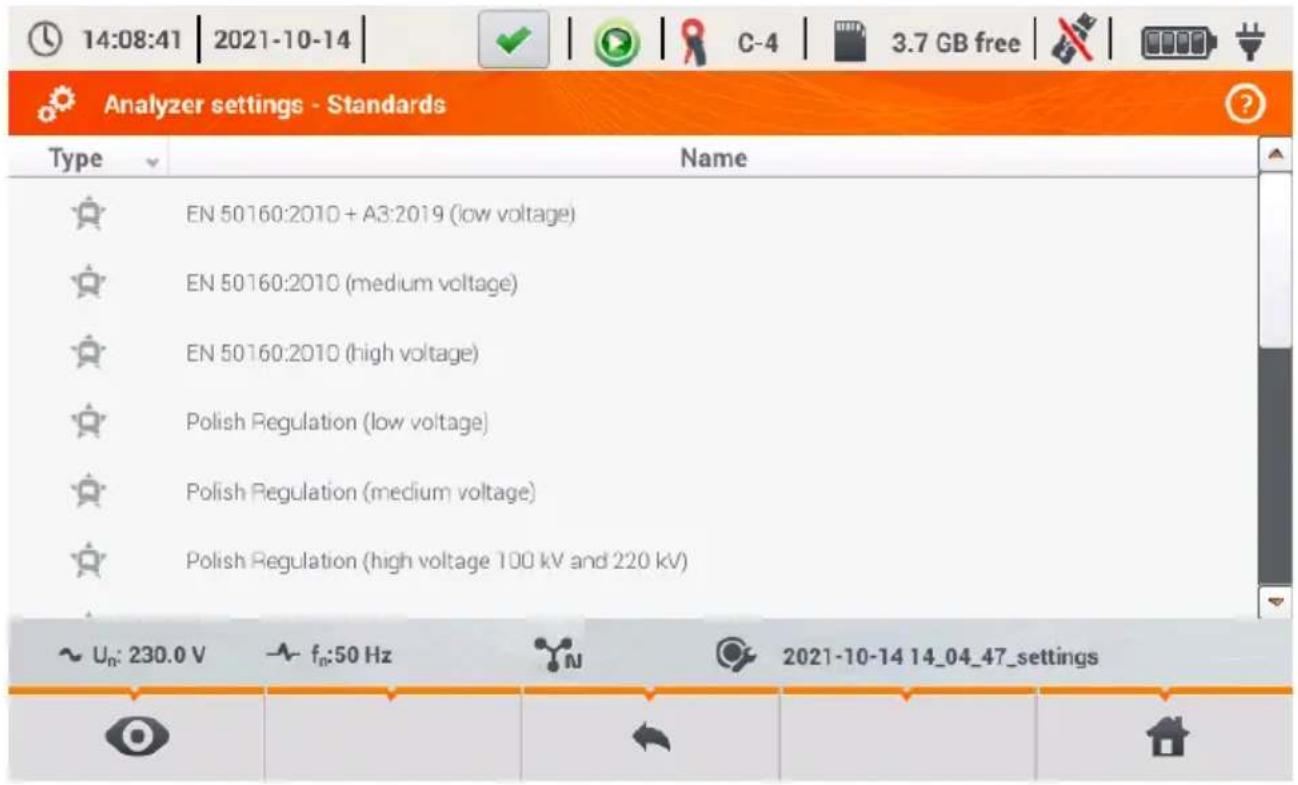
Fig. 18. Analyzer settings - Standards manager.
After clicking the line of selected standard and then preview icon in the bottom menu, the first configuration preview screen will be displayed for a given profile.
Buttons and at the bottom menu bar are used to switch between successive screens.
Button allows you to switch the view to preview standard criteria that are used for generating standard compliance report. Similarly, buttons and allow user to switch between successive windows. Parameters of standards are stored permanently in the analyzer memory and can not be changed. They meet the current standards on power supply quality.
- FILES - This panel allows user to view and manage files saved in the storage media of the analyzer. After selecting it, a window appears with a list of files as shown in Fig. 19.
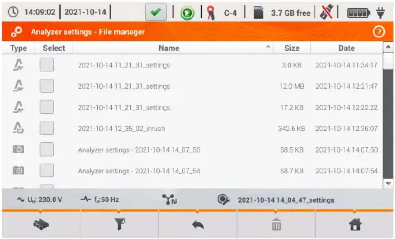
Fig. 19. Analyzer settings - File manager.
The following elements are specified in next table columns:
- TYPE – the icon representing the file type. It consists of the following types:
- recording file acc. to a standard
- recording file acc. to user configuration
- inrush recording file
- screenshot
- configuration file acc. to a standard
- configuration file acc. to user configuration
- configuration file for inrush
- configuration file for inverter efficiency test
-
standard compliance report
-
SELECT – in this column selection boxes are available for a given file (select them to copy or delete)
- NAME – name given to the file
○ SIZE – file size - DATE – date and time of last file modification
Menu bar functions

- displaying an additional menu bar of file manager.

- switching the view to display the data stored in the microSD card.

- switching the view to display the data stored in the internal memory

- copying selected files to external media (USB stick); the icon is active only connecting the storage medium.

- selecting all the files.

- displaying additional menu for filtering files. You may specify what types of files to be displayed in the list by clicking the corresponding icons representing the type; the selected file types are indicated by an icon in orange.

- delete selected files.
- UPGRADES – will be displayed as window shown in Fig. 20. In this mode, a memory stick can be connected to the analyzer with a file containing a new version of firmware. If such a file is detected and you confirm your intention to update firmware, the meter performs automatic upgrade process. The user should follow the on-screen prompts. The second option of updating is the use of Sonel Analysis software.

Please insert pendrive with update files or start update from Sonel Analysis.

natural_image
Pure graphical icons for a document, a house, and a left-pointing arrow on a gray background (no text or symbols)Fig. 20. Analyzer settings - Update manager.
Note!
Before starting the update, connect an external 12V DC power supply, to ensure continuity of supply. During an update, do not remove the USB memory.
2.11 Recording analysis
PQM-707 allows user to perform a simplified analysis of the recorded data, using the device itself, without additional software. The scope of the analysis includes:
- general preview of the recording - start and end time, the number of recorded events, including their type, average values of voltages and currents,
- a detailed overview of all the events with a preview of waveforms and graphs of RMS_1/2 ,
- preview the average value of voltage(s) across the whole recording range on a graph,
- preparing timeplots of any recorded parameters (limited to 1100 points and 4 parameters on a single graph) with zoom-in option and time-point marker.
- Bar-graph preview of harmonics (average value for the whole recording period).
It is possible to analyse recordings completed and saved on the memory card and on-going recordings.
2.11.1 List of recordings
To enter the analysis select RECORDING ANALYSIS in the main screen (the main screen is shown Fig. 2). After selecting this option, a list of recordings saved on the memory card is displayed as shown in Fig. 21.
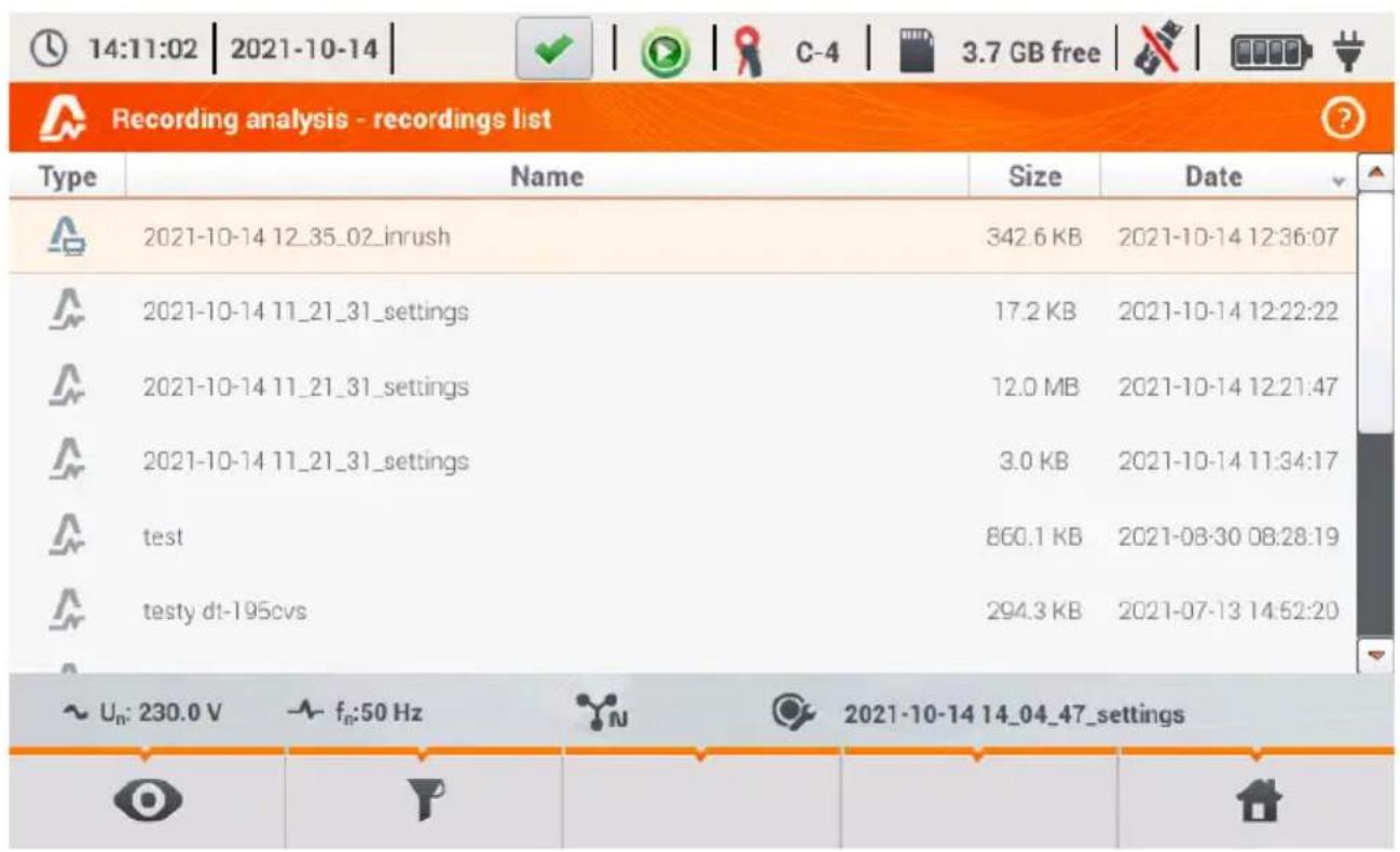
Fig. 21. Recording analysis - recording list.
The table columns present:
- TYPE of recording – the icon indicating recording type:
- recording according to user configuration,
- recording for compliance with the standard,
- inrush recording.
- NAME of the recording, which is the same as the name of the configuration, according to which the recording was made,
• SIZE of the recording,
• DATE of stopping the recording process.
In the case of an active recording, it is always on the top of the list, regardless of the selected sorting, and instead of icon for recording type, the recording icon is displayed
Menu bar functions
- entering the analysis of the selected recording (also by double-clicking its name), - displaying additional menu for filtering files. Specify which types of recording are displayed in the list. Orange icon means that this type was selected.
The maximum number of recordings that can be saved in the recorder (memory card) is 99. After reaching this number, the possibility of making further registrations is blocked. Then you should free up some space in the memory card.
2.11.2 Recording summary window
After selecting a record from the list of registration and clicking icon (or double-clicking record name in the list), a recording summary window is displayed as shown in Fig. 22.
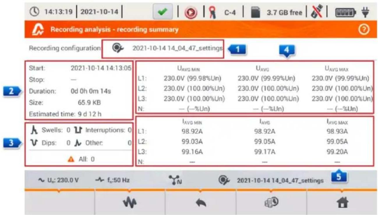
Fig. 22. Recording analysis - Recording summary.
The screen of the recording summary (Fig. 22) shows:
• recording configuration name
- start and end times of recording and its duration (if recording is still in progress - the end time is not shown), the free space on the memory card and the estimated time to fill the space by the recorded data 2
- the number of detected events, divided into several types
- average, minimum average and maximum average voltage values in the whole recording range. Minimum and maximum values are determined from the recorded values of the average voltage (these are not minimum and maximum RMS _1/2 values). In addition to the values in volts, in brackets you can see the percentage value related to the nominal voltage. If a channel has not been measured in a given configuration, dashes are displayed.
- average, minimum average and maximum average current values in the whole recording range. Similarly as for voltages, the minimum and maximum values are determined from average currents. If a channel has not been measured in a given configuration, dashes are displayed.

Menu bar functions

- moving to the list of events.

- diagrams. Click to open an additional menu bar with the following options:
- timeplots. Description in sec. 2.11.3.
- a bar graph with the average values of harmonics. Description in sec. 2.11.8.

- generating a standard compliance report (only for recording acc. to standard). Description c. 2.11.6.

- moving to the energy cost calculator (only for recording acc. to user configuration).
Description in sec. 2.11.10.
2.11.3 Timeplots - selecting the time range
Clicking icon from the recording summary screen, takes you to a part of the interface, that allows you to generate timeplots of recorded parameters. The timeplot may include max. four different parameters.
The screen displays a window with the graph of average voltage RMS or DC (depending on the mains type) from the whole recording period.
This window (Fig. 23) contains the following elements:
- recording start time
- recording duration
- recording end time
- sliders of selected time range (left and right)
• chart of average voltage RMS/DC - buttons for displaying sliders at left/right side of the window,
- start time of the selected time range
- selected time period
• end time of the selected time range


The time range from which the user wants to plot the timeplots of parameters may be determined in two ways:
- using the sliders . Grasp the corresponding slider and drag it, setting individual the beginning and end of the interval;
- writing the desired start and end time, or duration. In case of duration, the user must choose whether the time is to be related to the beginning or end of the range. Introduced range is checked for compliance with the requirements (limited to 1100 points) and if they are not met, the range is automatically modified to the allowable range (corresponding message is displayed).
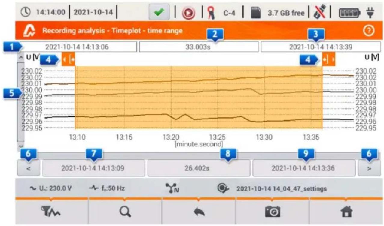
line
| Time (minute) | U [V] | f₀ (Hz) | |---|---|---| | 13:10 | 230.02 | - | | 13:15 | 230.01 | - | | 13:20 | 230.00 | - | | 13:25 | 229.99 | - | | 13:30 | 229.98 | - | | 13:35 | 229.97 | - | | | 229.96 | - | | | 229.95 | - | | 14:13:06 | 33.003s | - | | 14:13:39 | 3 | ? | | 14:13:09 | < 26.402s | - | | 14:13:36 | > 26.402s | - | | 14:14:04 | Uₙ: 230.0 V | ~ f₀:50 Hz | | 14:14:36 | 26.402s | N | | 14:14:47_settings | 2021-10-14 14_04_47_settings | N |Fig. 23. Recording analysis - selecting time range for the chart.
Menu bar functions

- selecting parameters for timeplots,

- graph zoom menu.
2.11.4 Timeplots – selecting data
After selecting desired time range and clicking the icon for parameter selection, a window will appear as shown in Fig. 24.

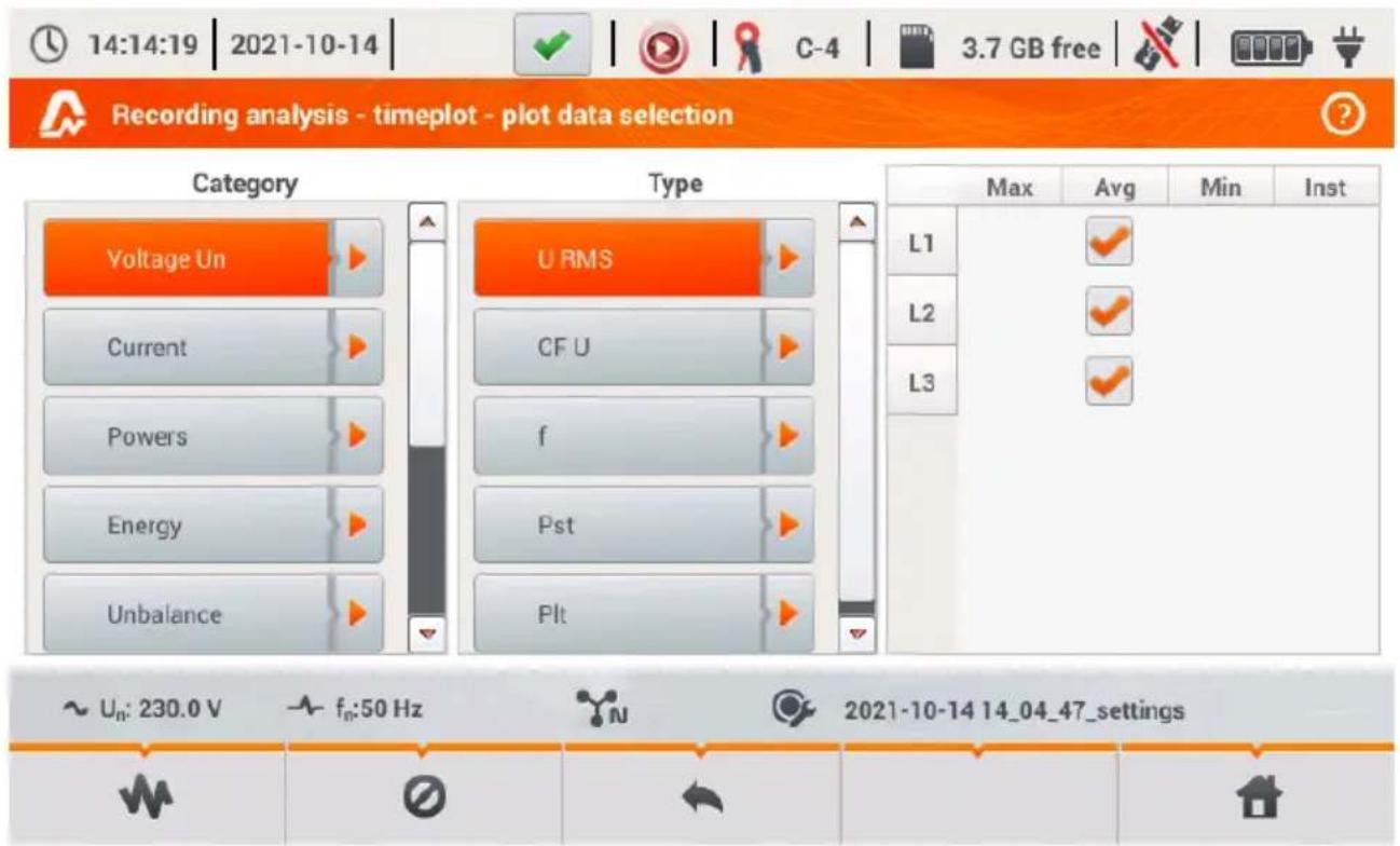
Fig. 24. Recording analysis - selecting parameters for the timeplot.
The specific parameter is selected in 3 steps:
• indicate Category of the parameter,
- it is followed by Type of the parameter within a particular Category,
- in the last step, select a particular parameter from the available channels and the minimum, average, maximum and instantaneous values.
CATEGORY and TYPES are grouped as follows:
• VOLTAGE:
○ U RMS (RMS voltage)
○ U L-L (phase-to-phase RMS voltage)
- CFU (voltage Crest Factor)
○ f (frequency)
○ Pst (short-term flicker severity)
○ PLT (long-term flicker severity)
- CURRENT:
○ I RMS (RMS current)
○ CFI (current Crest Factor)
• POWER:
○ P (active power)
○ Q1/QB (reactive power)
○ Sn/D (distortion power)
○ S (apparent power)
○ cosφ (Displacement Power Factor)
- PF (Power Factor)
○ tanφ
• ENERGY:
o EP+ (active energy consumed)
- EP- (active energy supplied)
o EQ+ (reactive energy consumed)
- EQ- (reactive energy supplied)
- ES (apparent energy)
• HARMONICS U:
○ THD U (voltage Total Harmonic Distortion)
○ UH1...UH50 (voltage harmonics of 1..50)
• HARMONICS I:
- THD I (current Total Harmonic Distortion)
- TDD I (current Total Demand Distortion)
○ IH1...IH50 (current harmonics of 1..50)
• HARMONICS ACTIVE POWER:
○ Ph1...Ph50 (current harmonics of 1...50)
• HARMONICS REACTIVE POWER:
○ QH1...QH50 (current harmonics of 1...50)
After selecting the category and type, tick the box to choose a specific parameter in a particular measurement channel (or a total value).
In the window for selecting the parameters, only those parameters are displayed which were recorded.
For better orientation, the fields with parameters selected for the chart, the fields of category and type are surrounded by orange border, if they contain any selected parameters.
If you have already ticked four parameters, any attempt to select another will result in displaying a message on limited number of parameters in the chart.
Menu bar functions

- display a timeplot of selected parameters.

- removes selection of all the selected parameters.
2.11.5 Timeplots of parameters - timeplot window
After clicking icon in the selection screen data, a timeplot is generated showing changes in time of specified parameters (Fig. 25).
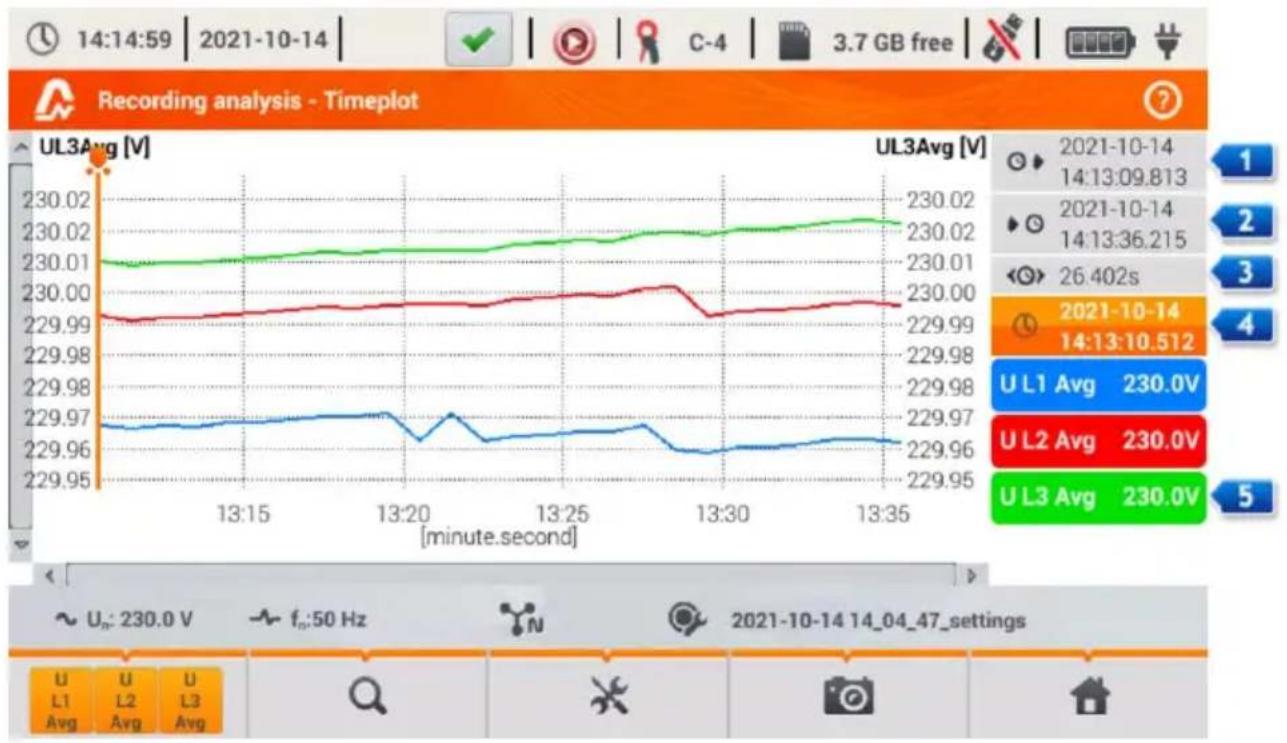
line
| Time | UL3 Avg [V] | | ---------- | ----------- | | 13:15 | 230.01 | | 13:20 | 230.00 | | 13:25 | 230.00 | | 13:30 | 230.00 | | 13:35 | 230.00 |Fig. 25. Recording analysis - timeplot.
On the right side of the chart the following items are shown:
1 - start time of the whole plot,
2 - end time of the whole plot,
3 - time range of the timeplot (total),
4 - date and time marker
5 - buttons for individual waveforms with a value for the time marker.
The area of the chart may be freely enlarged (zoom-in) and moved using the touch panel. Zooming-in the graph does not affect the displayed times of start, end and duration – they are fixed and always apply to the whole plot - not only to the enlarged portion.
Each of the two scales describing the vertical axis may be assigned to one of the plotted parameters or to a few having the same unit.
Menu bar functions
displays additional menu bar for selecting displayed timeplots.

- graph zoom menu.

- displays additional menu for setting scales (Fig. 26). In this menu, you can select the description of the scale on the right and left side of the chart. To do this, click on the icon with name of the parameter. The icon with the unit name is displayed when the graph have at two parameters having the same unit. Click this icon to rescale plots having the same unit common scale (described by one of the common parameters). Remember that when scales not unified, only one waveform with unit assigned to the axis is scaled to the indicated scale
and its plot is adjusted to the size of the window – other waveforms, even having the same unit, are not scaled.

- screenshot of the current window to a graphic file.
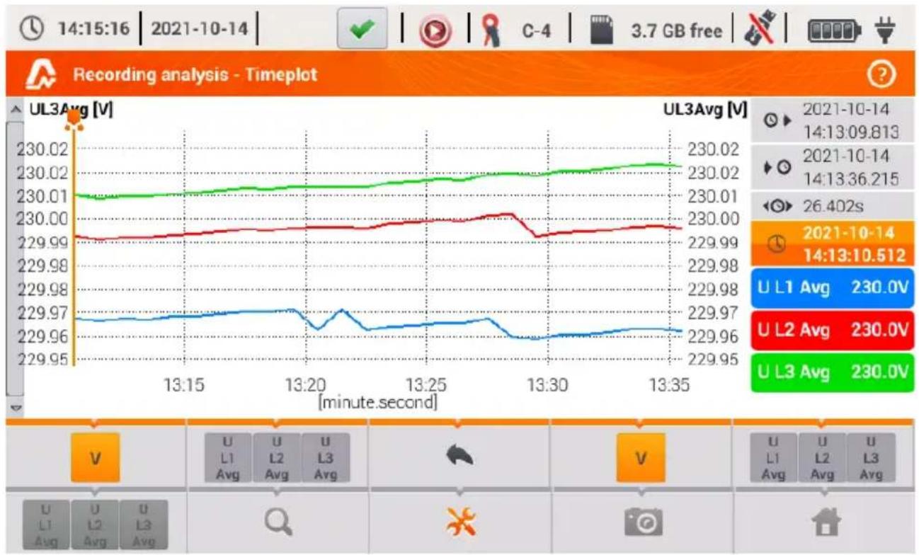
line
Recording analysis - Timeplot | Time | UL3 Avg [V] | | :--- | :--- | | 14:15:16 | 229.97 | | 13:15 | 229.98 | | 13:20 | 229.96 | | 13:25 | 229.97 | | 13:30 | 229.96 | | 13:35 | 229.96 | | 2021-10-14 14:13:09.813 | 230.00 | | 2021-10-14 14:13:36.215 | 230.00 | | 2021-10-14 14:13:10.512 | 230.00 | UL3 Avg 230.0VFig. 26. Recording analysis - timeplot - selecting scale.
2.11.6 Generating report on compliance with standard
Selecting icon on the recording summary screen, results in moving to the screen for generating report on compliance with the standard. If the recording was carried out according to the profile of one of the standards (e.g. EN 50160), then it is possible to verify whether the parameters of the tested network comply with standards requirements and generate a report, including a transcript of the report to a file.
To generate a report, you must first indicate a number of options that affect the way of generating the final report (Fig. 27).
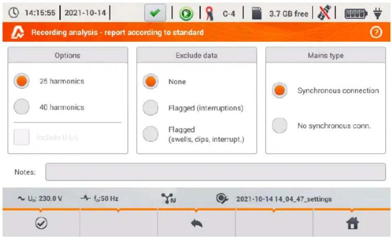
Fig. 27. Recording analysis - options of the report according to standard.
- OPTIONS – 25 HARMONICS / 40 HARMONICS: the user indicates the number of harmonics shown in the report. You can select 25 or 40 harmonics. The criterion to meet the requirements of the standard is in line with the standard guidelines and independent on number of harmonics indicated in this place. This setting affects only the number of harmonics shown in the summary table of the report.
- OPTIONS – INCLUDE U L-L: ticking this option results in including in the report statistics for the phase-to-phase voltages (if recorded). It applies only to split-phase and 3-phase 4-wire systems.
- EXCLUDED DATA: determines data to be excluded from the statistics in the report. There are three options available:
- NONE: report includes all recorded data, including those during which the voltage events occurred,
- FLAGGED (INTERRUPTIONS): statistics of the report are created using data from which the records including interruptions were removed. This is a typical setting, according to which reports should be generated according to the guidelines of EN 50160. Power failures are treated as exceptional situations in the network operation and as abnormal operation are not included in the quality statistics.
The definition of an interruption in polyphase systems is consistent with
standard IEC 61000-4-30, i.e. a power supply interruption in such a system occurs when in all phases of the system an interruption was detected (at the same time).
In the report section describing the event, all interruptions are included.
- FLAGGED (INTERRUPTIONS, DIPS, SWELLS): statistics of the report are created using data from which the records including interruptions, dips and swells were removed. In the report section describing the event, these interruptions are included.
- CONNECTION – SYNCHRONOUS/NO SYNCHRONOUS: Option NO SYNCHRONOUS is selected in island systems, isolated from other networks; otherwise, select option
SYNCHRONOUS. The standards provide a separate quality criteria on frequencies for these two types of connections.
- NOTES: In this field you can type additional text, which will be included in "Note" section of the report.
After setting the parameters of the report, it may be generated by clicking icon in the bottom bar. After a while, it will be displayed on the screen. The report may be scrolled using the finger-pointer or buttons and .
Report may be saved to a file (in pdf format) on the memory card (from the bottom menu select icon, then from the additional menu bar select) or after connecting USB memory stick to the analyzer (from the bottom menu select icon, and then from the additional menu bar
A fragment of a typical report is shown in Fig. 28.
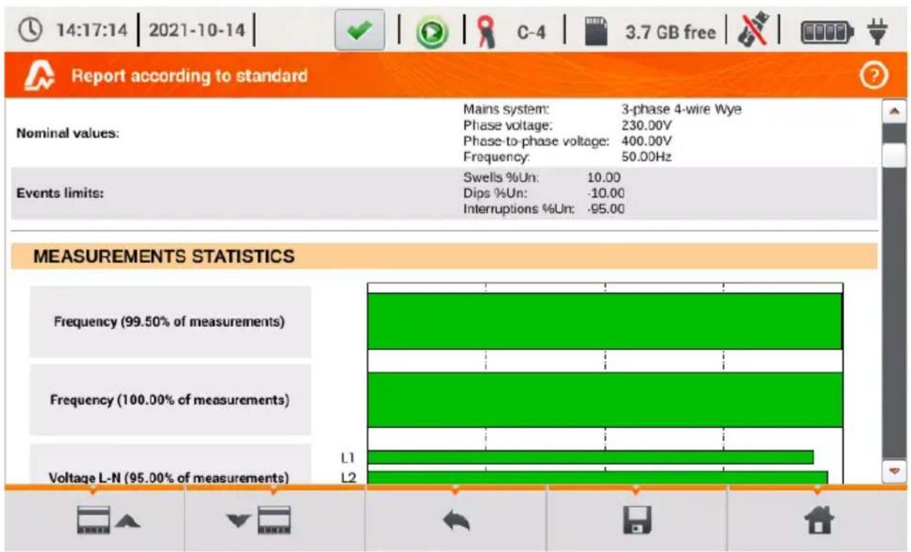
bar
| Measurement Type | Value | | :--- | :--- | | Frequency (99.50% of measurements) | 100.00 | | Voltage L-N (95.00% of measurements) | 95.00 | | Mains system: 3-phase 4-wire Wye | 230.00V | | Phase voltage: 400.00V | 50.00Hz | | Swells %Un: 10.00 | -95.00 | | Dips %Un: -10.00 | -95.00 | L1 L2Fig. 28. Recording analysis - report according to standard.
2.11.7 Report according to standard - description
European standard EN 50160 specifies the characteristics and quality criteria that should be met by the distribution networks of low medium and high voltage. Many countries adopted provisions of this standard, sometimes slightly modifying it, entering own local rules for parameters of the power supply networks.
Standard EN 50160 divides distribution networks, depending on the nominal voltage into three groups:
- Low voltage networks (LV) with voltages U_nom ≤ 1 kV (in PQM-707 the profile for such networks is "EN 50160 (low voltage)"),
- Medium voltage networks (MV): 1kV < U_nom ≤ 36kV (profile "EN 50160 (medium voltage)"),
- High voltage networks (HV): 36kV < U_nom ≤ 150kV (profile "EN 50160 (high voltage)"),
Tab. 4 lists the quality parameters included in standard EN 50160 and the criteria for their evaluation for the low and medium voltage (parameters measured by PQM-707). It should be noted that these criteria relate to the normal operation of the network, excluding periods of power interruptions and other anomalies, e.g. those related to atmospheric phenomena.
2.11.7.1 Section GENERAL INFORMATION
Section GENERAL INFORMATION contains general information about measurement parameters, including additional fields, which may be filled by the user when generating the report:
• Measurement performed by,
- Notes,
- Analyzer type and serial number,
- Software (analyzer software version)
- Time of start, end and duration of the measurement (acc. to local time of the analyzer)
- The number of averaged parameter samples, according to different times - this part specifies the number of time periods for which the parameters were measured:
- 10 s - the number of frequency measurements,
- 10 min - the number of measurement periods for most of other parameters such as RMS voltage, harmonics, THD, symmetrical components,
- 15 min – used in reports on compliance with the Polish Regulation, where additionally 15-minute parameters are measured e.g. active power, reactive power and tanφ,
- 2 h – the number of time periods in which flicker factor P_LT was calculated.
- The number of excluded samples - the total number of excluded time periods due to activated option of excluding flagged data (due to interruptions alone or events such dip, swell, interruptions).
• Nominal values of the network:
○ Mains type,
○ Nominal phase and phase-to-phase voltage,
- Nominal mains frequency.
- Event limits for swells, dips and interruptions.
2.11.7.2 Section MEASUREMENT STATISTICS
Section MEASUREMENT STATISTICS is a graphical summary of the tested network compliance with the standard. Verified parameter type is listed on the left side, while the right side shows the horizontal bars that define percentile of data that meets the quality criteria.
Percentile of a given percentage threshold is the value below which the percentage of all samples is present. Percentile 50% is also called the median; it determines the value for which half of the samples is below the median and the second half is greater or equal to it. In the area of power quality testing, the following percentiles are commonly used: 95%, 99% or 99.5%.
Tab. 4. Power quality criteria according to EN 50160 for the low voltage networks (up to 1kV) and medium voltage networks (36 kV).
| Parameter | Basic parameter measurement time | Criterion | |||
| Slow changes in voltage - RMS voltage | 10 minutes | For LV networks:for 95% of the measurements the deviation from the nominal voltage shall be within the range of ±10% Unomfor 100% of measurements: -15%...+10% UnomFor MV networks:for 99% of the measurements the deviation from the nominal voltage shall be within the range of ±10% Unomfor 100% of measurements: ±15% Unom | |||
| Frequency | 10 seconds | For networks connected synchronously:for 99.5% of the measurements the deviation should be within ±1% fnom (i.e. for 50 Hz it is 49.5...50.5 Hz)for 100% of measurements: -6%...+4% fnom (47...52 Hz)For networks connected asynchronously (e.g. island networks):for 95% of the measurements the deviation should be within ±2% fnom (i.e. for 50Hz it is 49...51 Hz)for 100% of measurements: ±15% fnom (42.5...57.5 Hz) | |||
| Rapid voltage changes (flicker) | 2 hours | for 95% of the measurements the long-term flicker severity is PLT ≤ 1 | |||
| Voltage unbalance | 10 minutes | for 95% of the measurements of the negative-sequence unbalance factor should be ≤ 2% | |||
| Total Harmonic Distortion (THD-F) | 10 minutes | for 95% of measurements, THD-F should be ≤ 8% | |||
| Voltage harmonics | 10 minutes | For 95% of the measurements, the level of each voltage harmonic component related to the fundamental component should be less than: | |||
| Odd order harmonics | Even order harmonics | ||||
| Order | Relative level | Order | Relative level | ||
| 3 | 5.0% | 2 | 2.0% | ||
| 5 | 6.0% | 4 | 1.0% | ||
| 7 | 5.0% | 6 ... 24 | 0.5% | ||
| 9 | 1.5% | ||||
| 11 | 3.5% | ||||
| 13 | 3.0% | ||||
| 15 | 0.5% | ||||
| 17 | 2.0% | ||||
| 19 | 1.5% | ||||
| 21 | 0.5% | ||||
| 23 | 1.5% | ||||
| 25 | 1.5% | ||||
Percentile 0% is the same as the minimum value of the set of samples, whereas percentile 100% is equal to the maximum value of the set (there is no higher value).
For example, standard EN 50160 for the RMS voltage value specifies that 100% of measurements must be within the range of -15%...+10% U_nom , and 95% of measurements must be within the range of ±10% U_nom .
These two requirements may be written as follows:
• percentile of 100% must be between -15% ...+10% U _nom ,
• percentile 95% must be between -10%...+10% U nom.
To check whether the RMS voltage meets the stated requirements, proceed as follows:
- all measured voltage samples are sorted from the lowest [1] the highest [N]
- it is checked whether the maximum value (i.e. percentile 100%, sample with [N] index) is in the range of -15% to +10% U_nom , and if yes then this criterion is met,
- it is checked whether the value of the sorted table with index [N * 0.95] (first integer number greater than or equal to N * 0.95 ) i.e. percentile 95%, is in the range of -10%...+10% U_nem . If yes, this criterion is met.
In case of the report on compliance with the standards and the section on measurement statistics, the length of the bands indicates the percentile of samples (the horizontal axis in the report ranges from 80% to 100%) that meet this criterion. For the RMS voltage, the statistics section provides two separate parameters, for which separate assessment criteria are set:
• Voltage (95.00% of measurements)
• Voltage (100.00% of measurements)
Bands on the right shows the percentage of samples that meet the specified criteria. For example, for 95% of the voltage measurements, if the band has the value 97%, it means that 97% percent of the samples meets this requirement (above the required 95%), and the band will be green (indicating that the criteria are met). If only 90% of the samples meet this criterion, the band will be red, as the standard criterion is not met.
If the percentage of samples that meet the criterion is less than 80%, then the band displays text in red "< 80%", which means that the criterion specified in the standard is not met and the percentile is lower than 80%.
The tested network meets the quality criteria if all percentile bands in section MEASUREMENT STATISTICS are green.
2.11.7.3 Section FREQUENCY
Section FREQUENCY includes detailed statistical information on the network frequency in the tested period.
The first part of the table, provides the percentage values of samples (percentiles), which meet the criteria (Values within tolerance) for both of the defined tolerance ranges (column Tolerance).
The values that meet the criteria are displayed in black. When the criterion is not met, the value is displayed in red with an additional asterisk (*). Column Tolerance specifies the range of frequencies, which must be observed in case of all samples, and which is calculated on the basis of the standard provisions.
The second part of this section contains additional information about the distribution of the samples in the tested set. Individual rows of the table present:
• Maximum (i.e. percentile of 100%) – the maximum recorded frequency,
- 99.50% value - percentile 99.5% (99.5% of frequency samples is lower or equal to a specified voltage in volts); the percentile depends on the specified standard and may be different than the one shown here.
- 0.50% value - percentile 0.5% (0.5% of voltage samples is lower or equal to a specified frequency); this percentile is always selected symmetrically to the previous percentile - to make the distance between two percentiles from the minimum or maximum was the same.
- Minimum (i.e. percentile of 0% ) – the lowest frequency in the tested set of samples.
As in the first part, the frequency range is specified, where the values should fit to meet quality criteria; if a given value does not meet the criterion, it is displayed in red with an additional asterisk (*).
2.11.7.4 Section VOLTAGE
Section VOLTAGE includes detailed statistical information on the criteria for RMS voltage (phase voltage in systems with neutral conductor and phase-to-phase voltage in 3-phase 3-wire systems).
The first part of the table, provides the percentage values of samples (percentiles), which meet the criteria (Values within tolerance) for both of the defined tolerance ranges (column Tolerance). The values that meet the criteria are displayed in black. When the criterion is not met, the value is displayed in red with an additional asterisk (*). Column Tolerance specifies the range of voltages, which must be observed in case of a specified percentage of samples.
The second part of this section contains additional information about the distribution of the samples in the tested set. Individual rows of the table present:
- Maximum (i.e. percentile of 100%) – the maximum voltage value among all samples in the given channel,
- Value 95.00% - percentile of 95% (95% of voltage samples have value lower or equal to a specified voltage in volts),
- Value 5.00% - percentile of 5% (5% of voltage samples have value lower or equal to a specified voltage),
- Minimum (i.e. percentile of 0%) – the lowest voltage value in the tested set of samples.
As in the first part, the voltage range is specified, where the values should fit to meet quality criteria; if a given value does not meet the criterion, it is displayed in red with an additional asterisk (*).
2.11.7.5 Section PHASE-TO-PHASE VOLTAGE
Section PHASE-TO-PHASE VOLTAGE is included in the report only when option INCLUDE UL-L is ticked during report generation and when network layout is split-phase or 3-phase 4-wire. Phase-to-phase voltage is also included in the statistics and influences the overall result of the network quality test. The value of phase-to-phase voltage is determined as:
- In split-phase systems: twice the phase voltage (second voltage (i.e. phase-to-phase) in the list of available nominal voltages in the measurement configuration or exact twice the phase voltage in the case of using voltage transducers)
- In 3-phase 4-wire systems: the second voltage (i.e. phase-to-phase) in the list of available nominal voltages in the measurement configuration or the phase voltage multiplied by 3 in the case of using voltage transducers)
The percentage criteria for the phase-to-phase voltage are the same as for the phase voltage.
2.11.7.6 Section FLICKER
This section provides information about the flicker severity P_LT . The first section provides the percentage of P_LT samples within the range required by the standard (e.g. 0...1).
The second specified the percentile value of 95%. Comparing this value with the limit imposed by the standard allows to assess the margin of parameter in the tested network in terms of standard provisions.
If a given value of P_LT is flagged after enabling the option for excluding flagged data, it is ignored and not reflected in the statistics.
2.11.7.7 Section UNBALANCE
If the tested network is a three-phase network, the report in its UNBALANCE section specifies details of the negative sequence unbalance factor:
- the percentage of samples that meet the criterion of 95% percentile (or another specified in the standard),
- the actual value of the 95% percentile of the unbalance factor.
2.11.7.8 Section HIGHER ORDER HARMONICS
Section HIGHER ORDER HARMONICS includes statistics and measurements for individual harmonics for which the standard defines level limits (usually harmonics of 2..25) and Total Harmonic Distortion factor THD-F. If a value is not within the limits, it is displayed in red with an additional asterisk (*).
2.11.7.9 Section HIGHER ORDER HARMONICS – ADDITIONAL INFORMATION
Section HIGHER ORDER HARMONICS - ADDITIONAL INFORMATION is present in the report after selecting report for 50 harmonics. It is an informational part, presenting values of percentile 95% for 26...50 harmonics, i.e. those for which the standard does not introduce level limits.
2.11.7.10 Section ADDITIONAL INFORMATION – EVENTS
Section ADDITIONAL INFORMATION - EVENTS contains information about detected voltage events such as swell, dip, interruption. For each of these types, the following information is provided:
• Number of events divided into single phases,
- Extreme value (maximum for swell, minimum for dip and interruption),
• Maximum duration of the event.
2.11.7.11 Section ADDITIONAL INFORMATION – STATISTICS OF POLYPHASE EVENTS
This section provides statistics of polyphase events according to the guidelines of EN 50160 (for swells, dips and interruptions). Events are classified basing on their duration and minimum / maximum values. The table presents the number of events meeting the specified couple of the criteria.
Tab. 5. Statistical distribution of swells, according to EN 50160.
| Voltage crest U [% U_nom ] | Duration time t [s] | ||
| 0.01 ≤ t ≤ 0.5 | 0.5 < t ≤ 5 | 5 < t ≤ 60 | |
| U ≥ 120 | S1 | S2 | S3 |
| 110 > U > 120 | T1 | T2 | T3 |
Tab. 6. Statistical distribution of dips, according to EN 50160.
| Residual voltage U [% U_nom ] | Duration time t [s] | ||||
| 0.01 ≤ t ≤ 0.2 | 0.2 < t ≤ 0.5 | 0.5 < t ≤ 1 | 1 < t ≤ 5 | 5 < t ≤ 60 | |
| 90 > U ≥ 80 | A1 | A2 | A3 | A4 | A5 |
| 80 > U ≥ 70 | B1 | B2 | B3 | B4 | B5 |
| 70 > U ≥ 40 | C1 | C2 | C3 | C4 | C5 |
| 40 > U ≥ 5 | D1 | D2 | D3 | D4 | D5 |
| U < 5 | X1 | X2 | X3 | X4 | X5 |
Tab. 7. Statistical distribution of interruptions.
| Residual voltage U [%Unom] | Duration time t | |
| t ≤ 3min | t > 3min | |
| U < 5 | short interruptions | long interruptions |
2.11.7.12 Section ADDITIONAL INFORMATION
Section ADDITIONAL INFORMATION is present in reports generated for compliance with the Polish Regulation of the Minister of Economy, when currents and 15-minute power values were measured. In such cases the following additional parameters are also recorded:
• 15-minute active power,
• 15-minute reactive power,
• 15-minute apparent power,
• total 15-minute tanφ factor
This section of the report presents the maximum 15-minute values recorded for the four parameters.
2.11.8 Harmonics graph
If the user selects option in the recording summary screen, a bar graph will be generated with average harmonics for the whole recording period. Harmonics are averaged using RMS method. Structure of the chart and using the window elements is explained in sec. 2.16.5.

Note
In case of large amounts of measurement data, plotting the harmonics chart may take a long time, which is indicated by a progress bar on the screen.
Plotting a graph of harmonics with the same data will be immediate, thanks to the data buffering.
2.11.9 Event list
Selecting option from the recording summary screen (in the bottom menu) will display a window with a list of recorded events. The analyzer may detect the following types of events:
In 50/60Hz systems:
- voltage dips,
- voltage swells,
• voltage interruptions, - exceeding the maximum current threshold (I > max.), separate thresholds for I_1,2,3 and I_N
- dropping below the minimum current threshold (I < min.), separate thresholds for I 1,2,3 and I N
In DC systems:
- exceeding the absolute maximum DC voltage threshold ( |U_DC| > .)
- exceeding the absolute maximum DC current threshold ( |I_DC| > max. )
If the user selected detection of any of the events listed above in the measurement configuration screen, and if these events have been recorded, the list will include all of them. An example of the event window is shown in Fig. 29.
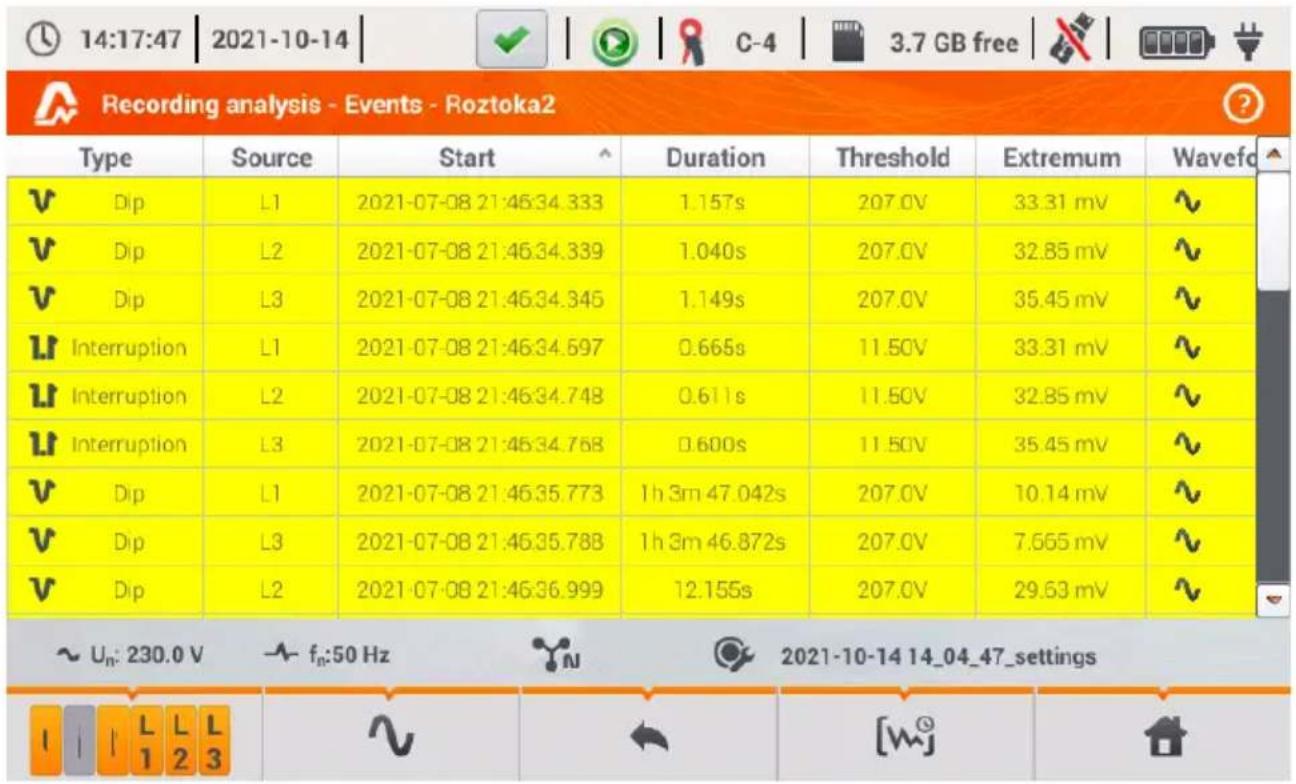
Fig. 29. Recording analysis – list of events.
The table contains the following columns:
- TYPE of event: dip, interruption, swell, I > , I < , U_DC > , I_DC > .
• SOURCE of event: channel where the event occurred,
• START: date and time of beginning of event, - DURATION of the event (if the event was in progress when recording was ended, an additional sign "> " is displayed, which means that the event has not been ended),
- THRESHOLD: threshold value that has been set in the recording configuration,
- EXTREMUM: parameter limit value (maximum or minimum, depending on the event type), which was recorded during the event. For example, in case of voltage dip, it is a residual voltage, which is the lowest U_RMS1/2 value recorded during the dip.
- WAV. (waveform): when recording waveforms and RMS_1/2 values is activated in the configuration, this column will show a sine wave icon indicating available waveforms and RMS values. These waveforms are recorded at the beginning and end of the event.
The table may be sorted by selected column after clicking its header. Next to the column name, a small arrow is present to show the direction of sorting.
Menu bar functions
After selecting a specific event in the table (by clicking its line), you can perform additional operations by selecting the following options from the menu bar:
- opens additional menu of waveforms:
- waveform. After selecting a specific event in the table (by clicking its line) and indicating this option, a waveform of instantaneous voltage and current values (samples) is displayed for the beginning and end of the event. Usually (if activated in the configuration) 6 cycles are stored (120 ms for 50 Hz) for the beginning and 6 cycles for the end of the event (2 cycles before triggering and 4 after triggering). In case of missing data (e.g. when the event was in progress at the end of recording process and data on event end are missing) only the available data are displayed, e.g. chart plotted only for the event start. An
example of window for voltage dip waveform is shown in Fig. 30. The right panel shows the data of the event: start time, end time, duration and the values for the cursor. Similarly as for the other charts, the options are available for zooming in/out the chart area (also by double-click) and selection of displayed channels, etc.
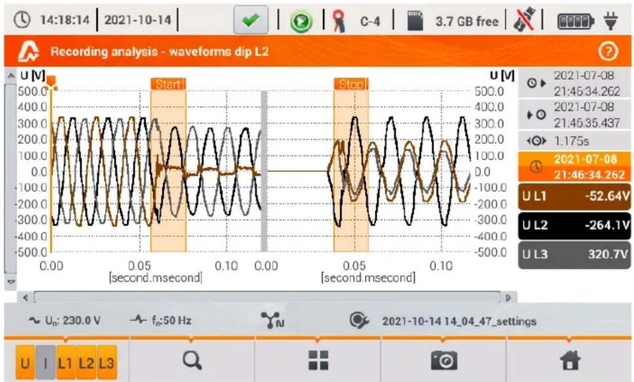
line
| Time (second) | Voltage (V) | | ------------- | ----------- | | 0.00 | 0.0 | | 0.05 | 350.0 | | 0.10 | 350.0 |Fig. 30. Recording analysis - dip waveform.
- RMS 1/2 plot. After selecting a specific event in the table (by clicking its line) and indicating this option, a waveform of RMS 1/2 is displayed. Usually, 15 mains cycles are saved (300 ms for 50 Hz) for the beginning and end of the event (5 cycles before triggering and 10 after triggering). In case of missing data (e.g. when the event was in progress at the end of recording process and data on event end are missing) only the available data are displayed. The functions in the chart window are the same as in case of waveform window.
- ANSI chart. It shows the graph of voltage events according to ANSI criteria. Dots represent individual events and their location indicates the duration (horizontal axis) and peak (extremum in the event table) related to the nominal voltage on the vertical axis. Arrow icons on the right side of the graph may be used to select individual events. By touching the screen in the graph area, the user may move the marker to the indicated place. Information about the specified event (type, duration, extreme value) are shown on the right side of the screen. An example of screen with similar diagram is shown in Fig. 31. More information about ANSI charts are presented in section 5.7.
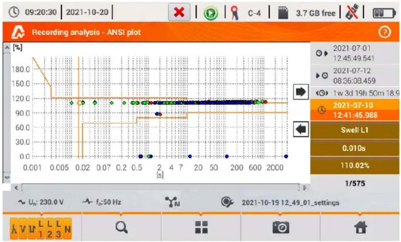
line
| Time [s] | Value [%] | | -------- | --------- | | 0.001 | 180.0 | | 0.005 | 120.0 | | 0.02 | 60.0 | | 0.07 | 120.0 | | 0.2 | 120.0 | | 0.5 | 90.0 | | 2 | 90.0 | | 4 | 90.0 | | 7 | 90.0 | | 20 | 90.0 | | 50 | 90.0 | | 200 | 90.0 | | 600 | 90.0 | | 2000 | 90.0 |Fig. 31. Recording analysis – ANSI graph.

- CBEMA graph. It shows the graph of voltage events according to CBEMA criteria. Description of the graph and its properties are similar to ANSI chart (see above). An exam-f screen with similar diagram is shown in Fig. 32. More information about CBEMA is are presented in section 5.7.
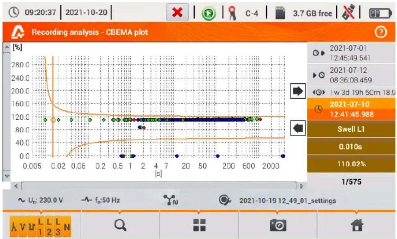
line
| Time (s) | Value (%) | | -------- | --------- | | 0.005 | 280.0 | | 0.02 | 120.0 | | 0.06 | 120.0 | | 0.2 | 120.0 | | 0.5 | 120.0 | | 1 | 120.0 | | 2 | 120.0 | | 4 | 120.0 | | 7 | 120.0 | | 20 | 120.0 | | 50 | 120.0 | | 100 | 120.0 | | 200 | 120.0 | | 600 | 120.0 | | 2000 | 120.0 |Fig. 32. Recording analysis - CBEMA graph.
2.11.10 Energy cost calculator
When the parameters recorded by the analyzer include active energy E_P (see energy recording settings, sec. 2.9.6 and Fig. 11), it is possible to calculate the energy costs acc. to the cost calculator set by the user. To enter the screen of the energy cost calculator, use the bar on the recording
summary window (Fig. 22) and select icon . The screen with energy costs will be displayed as shown in Fig. 33.
The following sections present:
- Recording time – start, end and duration of the recording. The last line shows the duration taken for analysis by the algorithm of the cost calculator (full aggregation periods). The algorithm enables the calculation of the energy costs for the whole recording period and there is no option to select a different time interval.
- Energy – this field displays the total active energy in kilowatt-hours measured in the reporting time interval.
- Single-zone tariff – this section displays the total cost of energy in the selected currency for single-zone variant. The tariff of this type has a single flat rate per kWh, regardless of the time of day and day of the week. Name of the tariff (may be modified by the user) is displayed in the upper part.
- Multi-zone tariff – shows the total cost of energy in the chosen currency in the multi-zone variant. This tariff allows you to define two continuous time intervals in 24 hours, which have different cost rates per kWh, and the third rate for other times of the day. Configuration of rates and zones is carried out in the control panel of the energy cost calculator.
If you have not used or have not changed the settings of the cost calculator, the analyzer will use the default settings. The settings of the cost calculator may be modified by selecting from the
menu bar option ✗
![14:20:39 | 2021-10-14 | C-4 | 3.7 GB free | Energy cost calculator Recording time ▶ 2021-10-14 14:13:05 ▶ 2021-10-14 14:15:34 ◀ 2m 29s ◀ 2m 27s Energy [kWh] 2.791 Single zone tariff C11 [PLN] 0.87 Multi-zone tariff C12 [PLN] 0.71 ~ Uₙ: 230.0 V ~ fₙ:50 Hz 2021-10-14 14_04_47_settings](/content/2026/05/852541/images/c713af1c8deefba634b2fa93d817978a63cde9d07f2c98ac4ae32b190a57e945.jpg)
Fig. 33. Screen with summary of the energy cost calculator.
Menu bar functions

- entering the settings of the energy cost calculator.
2.11.10.1 Settings of the energy cost calculator
The settings of the cost calculator may be easily modified to fit individual needs. The energy cost calculator in the analyzer allows you to calculate costs for two tariffs:
- Single-zone tariff – this is the simplest form of tariffs - a single rate for each kilowatt is taken into account throughout the analysed interval, regardless of time of day or day of the week.
- Multi-zone tariff – a more extensive tariff, which allows you to set three different rates that apply in different time intervals:
○ Zone A billing rate – you may enter the cost of 1 kWh for the first time interval of the day (e.g. daytime rate),
- Zone B billing rate – you may enter the cost of 1 kWh for the second time interval of the day (e.g. night-time rate),
○ Zone C billing rate (not included in zones A and B).
Settings of the cost calculator are divided into two screens shown in Fig. 34 and Fig. 35. The first screen allows you to configure the following parameters:
- Currency - you can choose from a list of several predefined currencies (PLN, EUR, USD, RUB, INR) or set your own (up to four characters), which will be shown on the list as the last position and marked with an asterisk (*).
- For single-zone tariff:
○ Name of the single-zone tariff (C11 as default) - after clicking the name field a panel is displayed for editing.
- Billing rate – the cost of 1 kWh of energy for single-zone tariff - after clicking on the value field a panel is displayed for editing. Rate values may be entered with an accuracy of four decimal places.
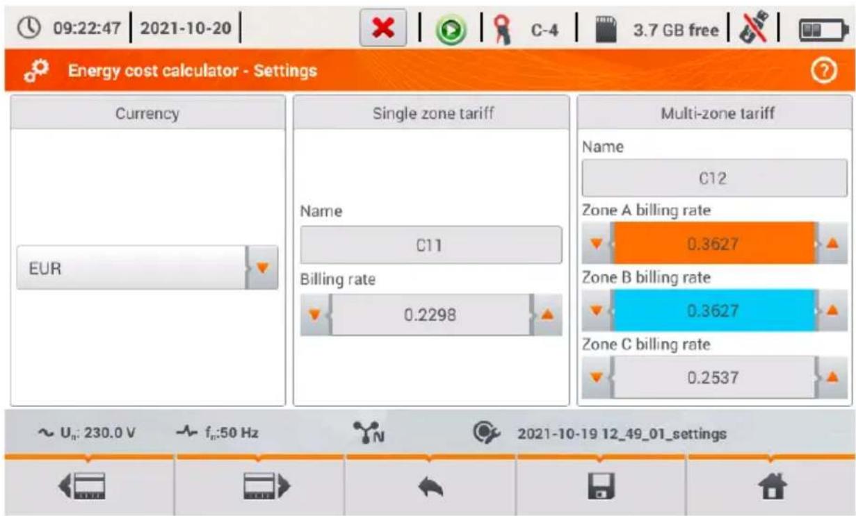
Fig. 34. Energy cost calculator – Settings.
- For Multi-zone tariff:
○ Name of the zone (C12 as default)
○ Zone A billing rate for 1 kWh,
○ Zone B billing rate for 1 kWh,
○ Zone C billing rate for 1 kWh (for other times of the day).
Time intervals of the day corresponding to A, B and C zones are set on the second screen with settings (Fig. 35). Colours of time intervals on the second screen match the colours of billing rates on the first screen. In the simpler variant, the same zone settings are valid for all days of the week (only the set marked with icon ) If you need to configure other time intervals for the selected days (e.g. for Saturdays and Sundays), then click the selection box at the bottom left of the window - the second set of time intervals is unlocked - it is marked with icon 2 Select weekdays for the second set by clicking the selection boxes for desired week days. Both bars displayed on the screen represent the entire day [24 hours] divided into 15-minute blocks.
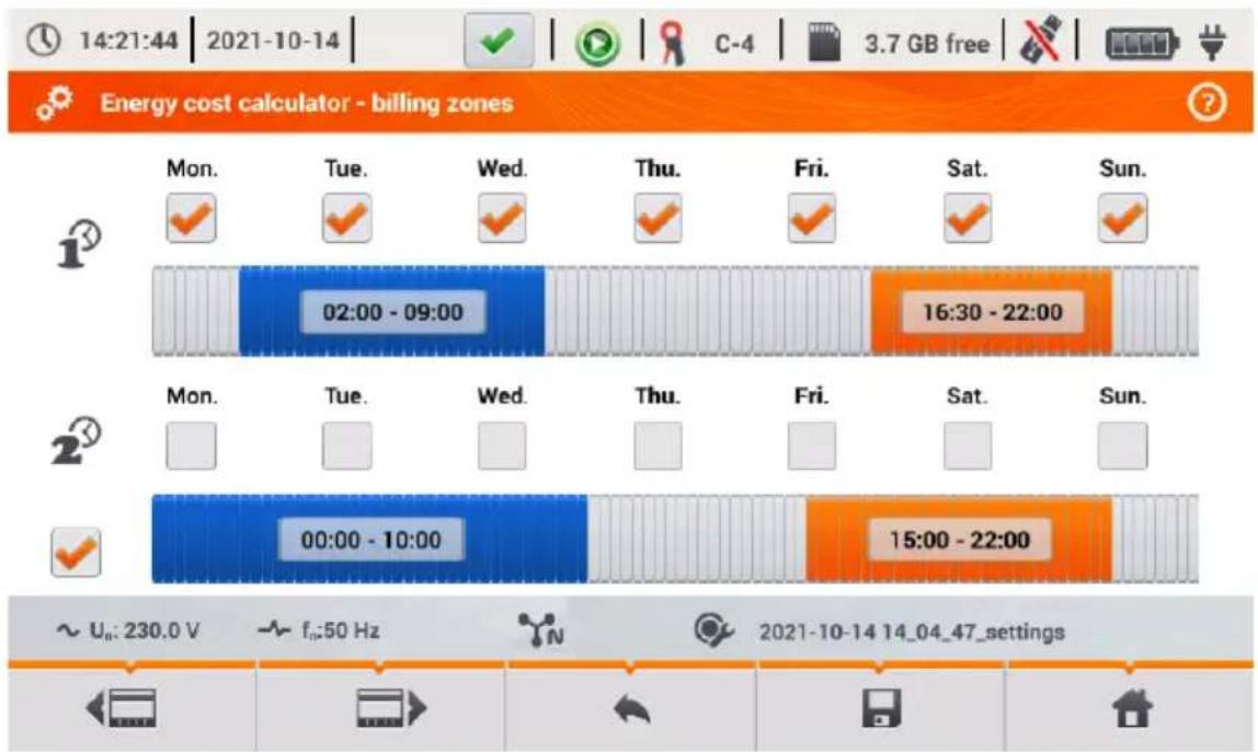
Fig. 35. Energy cost calculator – billing zones
Time intervals for zones A and B may be modified:
- by touching the centre of the time interval and moving it sideways,
- by touching the left or right edge of the interval and changing the start or end of the tariff zone.
Start and end time is displayed in the middle of the time interval. The resolution of time intervals is 15 minutes. The minimum duration of an interval is 2 hours.
To save the changes in the analyzer memory, select option from the menu bar and confirm your intention to save changes. The settings are global for the entire analyzer (not related to a specific recording).
Menu bar functions


switching between the two setting screens of the cost calculator.

- saving the settings in the analyzer memory.
- return to the results indicated by the cost calculator. If the settings have been modified and saved, the energy costs will be automatically calculated and displayed.
2.11.11 Generating report on compliance with standard NEC220.87
Selecting icon on the recording summary screen, results in moving to the screen for generating report on compliance with the standard NEC220.87. This screen is shown in Fig 36.
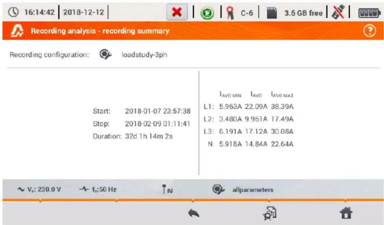
Fig. 36. Recording analysis – recording summary according to standard NEC220.87.
To generate a report, you must first indicate two parameters required by the standard NEC220.87. This screen is shown in Fig 37.

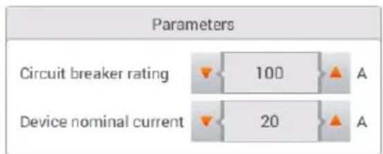

Fig. 37. Recording analysis – parameters of the report according to standard NEC220.87
- CIRCUIT BREAKER RATING IN AMPS: nominal breaker current of circuit breaker for existing installation under test. Could be nominal breaker current of circuit breaker which will be used for this installation..
• DEVICE NOMINAL CURRENT: nominal current of new device in installation
After setting the parameters of the report, it may be generated by clicking icon in the bottom bar. After a while, it will be displayed on the screen. The report may be scrolled using the finger-pointer or buttons and
Report may be saved to a file (in pdf format) on the memory card (from the bottom menu select icon, then from the additional menu bar select) or after connecting USB memory stick to the analyzer (from the bottom menu select icon, and then from the additional menu bar select). An example of a typical report is shown in Fig. 28.
REPORT: NEC 220.87
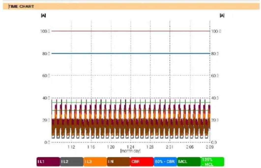
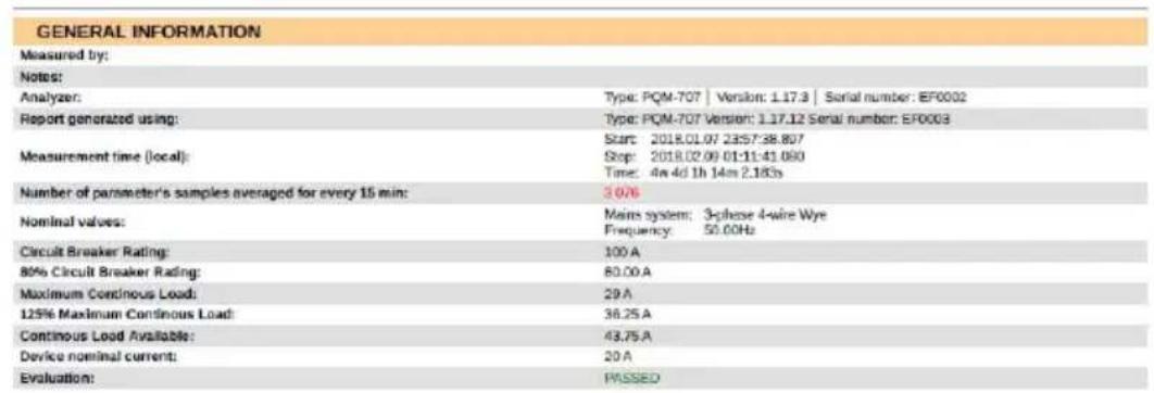
Fig. 38. An example of a typical report.
If the duration of the registration is displayed in red, it means that the registration lasted less than 30 days
2.12 Inrush current
The mode of measuring the inrush current is entered by selecting in the main screen the option of INRUSH CURRENT. This mode is used to measure the inrush currents of various machines, equipment and facilities with sharp increases in current consumption. During a start-up such machines/equipment usually draw instantaneous currents significantly higher than nominal currents, which is caused for example by charging capacitors, mechanical resistance and magnetization of the core (motors and transformers). Knowing the value of inrush currents enables the user to correctly choose the over-current protection parameters for power supply systems supporting such devices (characteristics and nominal current values) in order to protect the system and its users in the event of a failure, but at the same time to prevent accidental tripping of the breaker during the start-up of the devices.
PQM-707 analyzer allows user to quickly and easily measure inrush currents, providing the information about:
- timeplots of instantaneous currents (waveforms),
• timeplots of half-period RMS values - RMS _1/2 , - the maximum recorded values of half-period RMS values and Joule integral values i ^2 t.
Joule integral is a measure of the heat generated during the start-up. To determine i^-2t - a time interval is taken from the moment of exceeding by RMS_1/2 current the threshold value until lowering the value of RMS_1/2 current drops below the threshold minus the hysteresis (by default hysteresis is equal to 2% of the nominal value – I NOM). Knowing the Joule integral is useful when choosing the overcurrent protection of circuits - manufacturers of protection devices usually state in specifications the characteristic value i^2t , which triggers the device and interrupts the current flow in the circuit. Joule integral of the protection devices must be higher than the value measured during the measurement of inrush energy (integral).
Recording time of the waveform may be set in the range of from 5 to 60 seconds. Recording is triggered automatically after exceeding the set current threshold and ends after the set time. Moreover, waveforms before triggering (pretrigger) are recorded (1 second), providing the user with information about the currents before the triggering.
Only current waveforms are recorded; voltage is not recorded, it is also not necessary to connect voltage inputs of the analyzer.
The measuring algorithm implemented in PQM-707 ensures correct measurement of half-period RMS values also in a situation of variable frequency of the power supply current. This is useful in for devices powered from inverters (frequency converters). The permissible range of frequency variations is 30 ... 100 Hz. The algorithm is based on digital filtering of I1 current waveform, which removes all components of frequencies higher than the fundamental, allowing precise determining of points where current waveforms cross zero value, resulting in correct determination of RMS values during variable frequencies.
2.12.1 Inrush current measurement configuration
After selecting in main menu the option of INRUSH CURRENT the screen shown in Fig. 39 is displayed.
Before measuring the inrush current, the user must indicate the measurement parameters:
- MAINS SYSTEM – selection of the type of mains supplying power to the tested device, specifying current channels for connecting the probes: 3-phase 4-wire, 3-phase 3-wire, 3-phase 3-wire with Aron's method measurement of currents, split-phase, single-phase, 3-phase 4-wire (no U L2) / 2 ½ element (no V L2/B), 3-phase open delta.
- FREQUENCY – nominal frequency of power supply to the device (this frequency is used in the absence of current signal; the default algorithm is insensitive to the measured waveform frequency),
- PROBES TYPE – indicate the type of current probes used,
- RECORDING TIME – duration of recording from the triggering (exceeding the current threshold) may be selected from the following times: 5s, 10s, 15s, 20s, 25s, 30s, 60s.
![14:23:09 | 2021-10-14 | C-4 | 3.7 GB free | Inrush current configuration - 2021-10-14 14_22_53_inrush* Mains system Frequency 50Hz Duration 5s Nominal current [A] Clamps type C-4(A) Trigger treshold [A] 3-phase 4-wire Voltage ~ Un: 230.0 V fn:50 Hz 2021-10-14 14_04_47_settings](/content/2026/05/852541/images/d99257f9ea3459ea5a2164671bb9503f586d281eb40b82c3c115f77b7f8f25c2.jpg)
Fig. 39. Inrush current configuration screen.
- NOMINAL CURRENT [A] – enter the nominal value of I_NOM (one phase) of the tested device.
- TRIGGER THRESHOLD [A] – this field is automatically set to 150% of the nominal current during the first edition of NOMINAL CURRENT [A] field (subsequent editions no longer update this field), but the user may enter a different value if necessary. This is the current threshold value – when this value is exceeded the countdown of recording time is triggered. This value is also used for determining the thermal integral i ^2 t – this integral is calculated for the time interval when the measured current value is above the triggering threshold. The threshold value is displayed on graphs as a horizontal line and the field with its value is shown on the right side in the current axis area.
- VOLTAGE CHECKBOX – selection of this checkbox enables recording of the voltage.
The title bar displays the default name of the edited configuration, which is created basing on current date and time, e.g. "2017-01-01 12_10_00_inrush". This name may be modified when you save the configuration.
Menu bar functions
- start of the measurement session for inrush current with specified settings (without saving the configuration).
- saving the configuration of inrush current to a file with an option to start the measurement directly after saving (field Go to measurement in the pop-up window).

- entering the list of saved configurations of inrush current and creating a new configuration. Configurations of the inrush current are presented similarly as the measuring configurations (see Fig. 4), they have their own icon □Double-click on a selected configuration will open it automatically and the inrush current configuration screen (Fig. 39). The button in the menu bar - + is used for adding new configurations starting of the inrush current (a window is displayed, as shown in Fig. 39 with default settings). Icon is used to edit the chosen configuration of the inrush current.
2.12.2 Inrush current measurement and analysis
In the screen of inrush current settings, select the following icon in the menu bar to display a window shown in Fig. 40. Press START to start measurement.
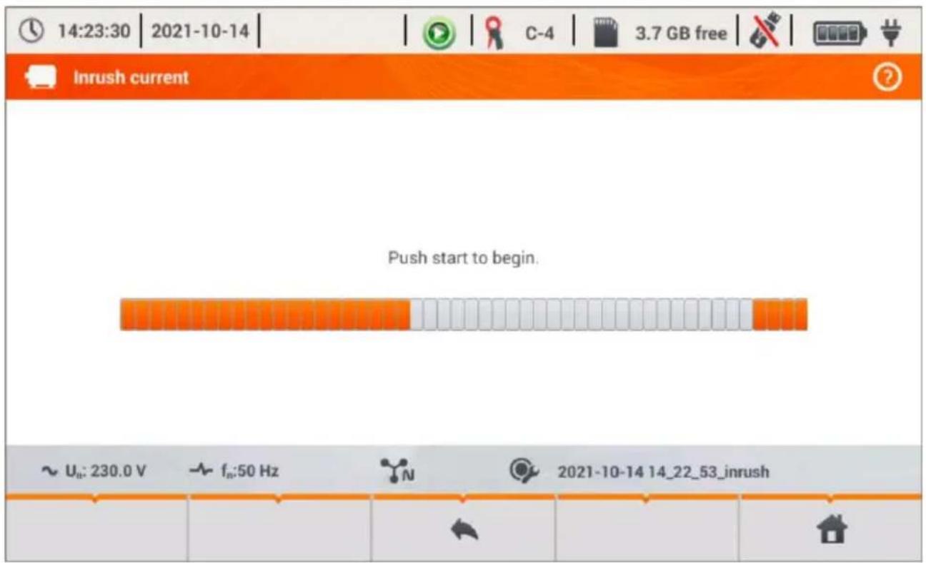
Fig. 40. Inrush current - waiting for start of the measurement.
The analyzer enters the mode of monitoring currents and triggers the measurement if the current value in any of the measured channels exceeds the threshold value. The recording status icon changes to . At this moment you should switch on the tested device. The user may interrupt the process of waiting for a trigger by pressing START button. Exceeding the threshold and correct triggering will be signalled by an audible recording signal (triple tone) and the countdown of recording time will start.
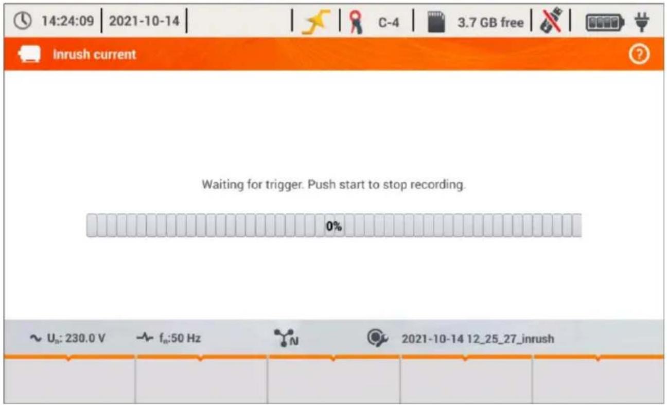
Fig. 41. Inrush current - waiting for triggering the measurement.
After the time elapses, the recording process ends and the analyzer automatically starts the analysis of measured inrush parameters, displaying the timeplot with current waveforms for the entire recording interval.
An example of the screen displayed during the start-up of a 3-phase motor is shown in Fig. 42.
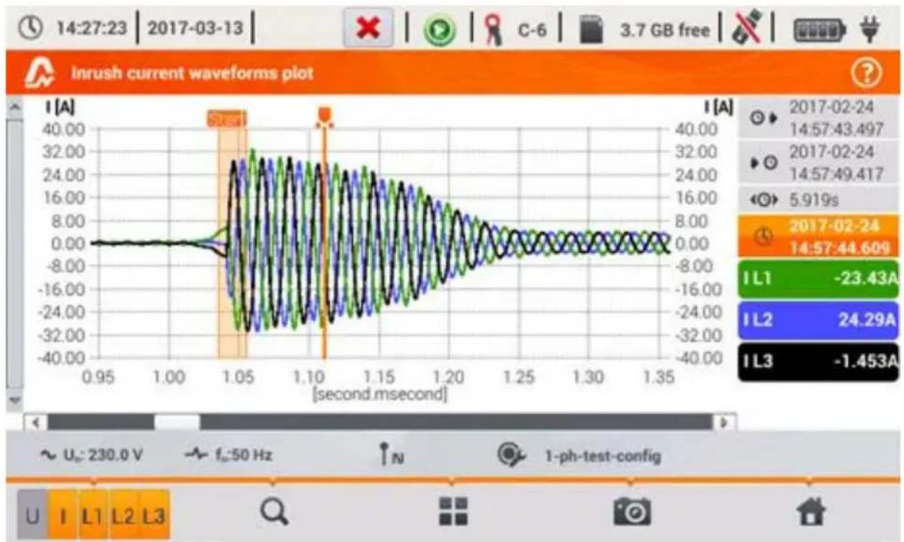
line
| Time (second.msecond) | Current (A) | | --------------------- | ----------- | | 0.95 | 0.00 | | 1.00 | 0.00 | | 1.05 | 32.00 | | 1.10 | -32.00 | | 1.15 | 24.00 | | 1.20 | 8.00 | | 1.25 | 0.00 | | 1.30 | -8.00 | | 1.35 | -40.00 |Fig. 42. Inrush current analysis – waveforms plots.
The window with a waveform of inrush current is similar to windows showing other plots. On the right side you may find the time of starting, ending and duration of the plot, the marker parameters and the buttons of active current channels, which indicate the current value at the marker point and allow user to enable and disable the display of individual channels.
Menu bar function
- switching the view. After clicking it, an additional menu bar is displayed with options (available depending on the current view):
- Inrush RMS plot (Fig. 43; option available in waveforms and table view). Selecting this option displays a plot of RMS_1/2 values of the measured currents.
- plot of inrush waveforms (Fig. 42; option available in the view of a plot for RMS_1/2 and as a table).
- tabular view of inrush characteristic values (Fig. 44). The table displays the maximum RMS_1/2 values and values of Joule integral determined for measured current channels.
Files of recorded inrush current measurement sessions are automatically saved on the memory card and they are available for re-analysis from the main screen after entering RECORDING
ANALYSIS. Recorded sessions are marked on the list by icon 🔒 and their names are the same as the name of the configuration (default or entered by the user).
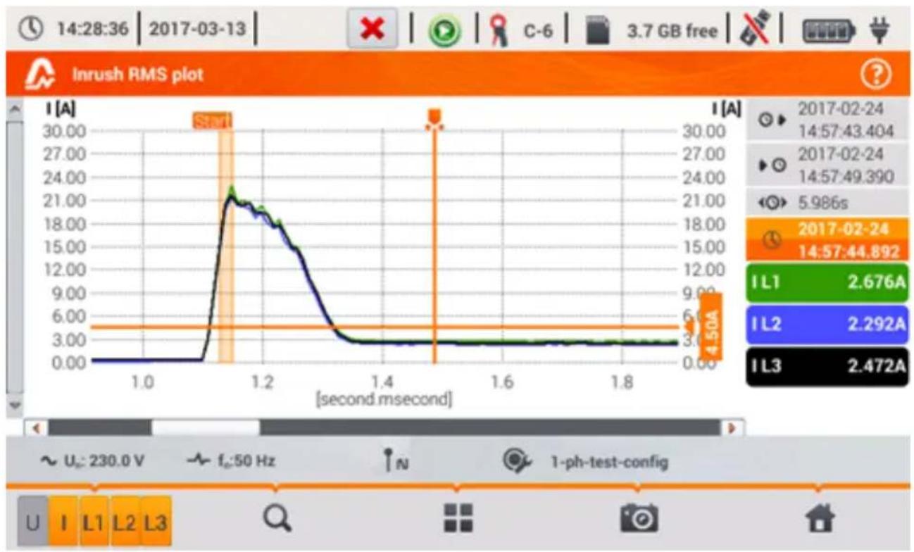
line
| Time [second] | Current (A) | | ------------- | ----------- | | 1.0 | 0.00 | | 1.1 | 21.00 | | 1.2 | 18.00 | | 1.3 | 12.00 | | 1.4 | 3.00 | | 1.5 | 3.00 | | 1.6 | 3.00 | | 1.7 | 3.00 | | 1.8 | 3.00 |Fig. 43. Inrush current analysis – Inrush RMS plot.
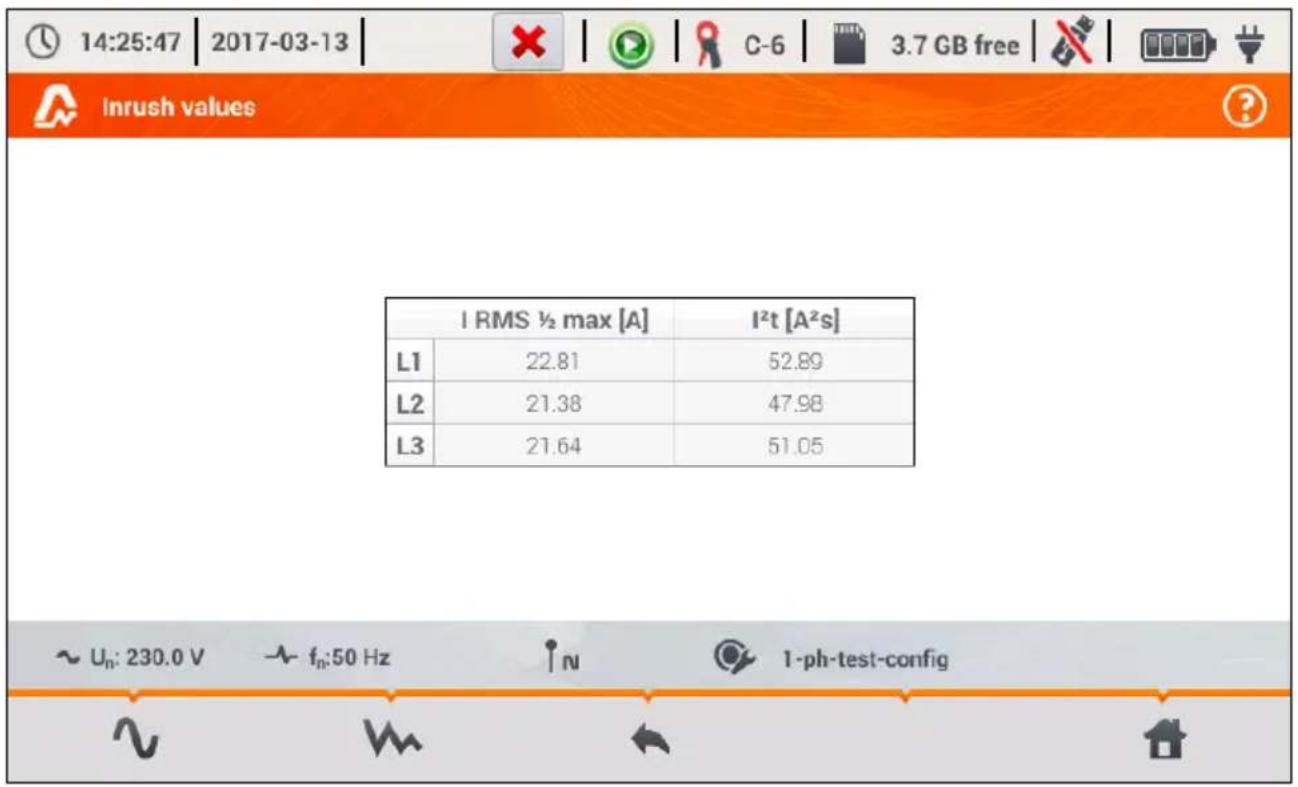
other
| Metric | Value | | :--- | :--- | | L1 | 22.81 | | L2 | 21.38 | | L3 | 21.64 | | I RMS ½ max [A] | 1²t [A²s] | | I²t [A²s] | 52.89 | | I²t [A²s] | 47.98 | | I²t [A²s] | 51.05 |Fig. 44. Inrush current - characteristic parameters.
2.13 Measuring the efficiency of the inverter
2.13.1 Measurement configuration
Inverters are widely used, e.g. in photovoltaic installations or systems of uninterruptible power supply (UPS). The analyzer enables the user to check the efficiency of inverters in electricity processing i.e. converting a DC voltage into single-phase or three-phase AC voltage. To enter this function, select on the main screen of the meter the following: SPECIAL FUNCTIONS and then INVERTER EFFICIENCY.
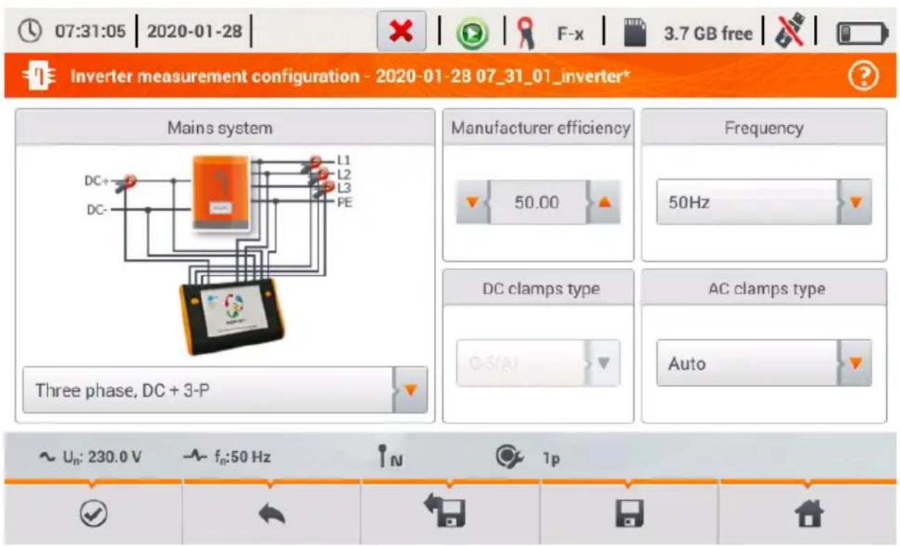
Fig. 45. Configuration screen of inverter efficiency measurement.
Set the parameters of the tested inverter on the displayed configuration screen:
- MAINS SYSTEM – there are two types to choose from:
- SINGLE PHASE, DC + 1-P
Select this system type for inverters with single-phase AC output. The screen will show a simplified diagram of the analyzer connection to the tested circuit:
- DC+ voltage input of the inverter must be connected to 'N' input of the analyzer
- DC- input of the inverter must be connected to L3 input,
- AC voltage side of the inverter must be connected between L1 and PE inputs of the analyzer,
- current of DC side of the inverter is measured with DC clamps connected to N input of the clamps. Note: it is necessary to use clamps for DC measurements; these clamps are C-5A,
- current of AC side of the inverter is measured with clamps connected to L1 input of the analyzer. The user may specify any type of clamps compatible with the analyzer.
○ THREE PHASE, DC + 3-P
It is possible to measure only the efficiency of three-phase, three-wire inverters (delta or star configuration without neutral wire). Please note that due to the limited number of voltage inputs in the analyzer, it is not possible to directly measure all phase-to-phase voltages. Therefore, the measured parameters on AC side are presented as approximate values, with accuracy depending on the symmetry of the output voltages of the inverter. If it works in such systems, verify voltage asymmetry before the efficiency measurement (negative sequence unbalance U2/U1 should be less than 1%). This verification should be carried out by configuring and connecting the meter in a standard way to a three-phase network 3-P (after exiting function INVERTER EFFICIENCY). The asymmetry of currents on AC side is not relevant, as these currents are measured directly.
How to connect the analyzer:
- DC+ voltage input of the inverter must be connected to 'N' input of the analyzer
- DC- input of the inverter must be connected to L3 input,
- AC voltage side of the inverter: L1 and L2 outputs of the inverter must be connected respectively to the L1 and L2 inputs of the analyzer. PE input of the analyzer must be connected to the inverter ground or to a local ground, if the inverter has no grounding connection,
- current of DC side of the inverter is measured with DC clamps connected to N input of the clamps. Note: it is necessary to use clamps for DC measurements; these clamps are C-5A,
-
currents of AC side of the inverter are measured with clamps connected to L1, L2 and L3 inputs of the analyzer. The user may specify any type of clamps compatible with the analyzer.
-
MANUFACTURER EFFICIENCY – efficiency of the inverter declared by the manufacturer. This value is used to compare the measured efficiency with the declared value.
- DC CLAMPS TYPE – this is a read-only field. The type of clamps is set to C-5A.
- AC CLAMPS TYPE - the user may use the list to select the type of clamps used for current measurements on AC side of the inverter.
- FREQUENCY – nominal frequency of the AC output of the inverter.
After setting the required parameters, you can go directly to the required measurements.
Note: Pay attention to the fastening direction of current clamps. After entering relevant measurements, check that the indicated active powers have positive value. Otherwise, the indicated efficiency may have incorrect sign.
Menu bar functions
- entering the measurement screen (live values in a tabular view) with the specified settings (without saving the configuration).
- saving the configuration of inverter efficiency to a file with an option to start the measurement directly after saving (field Go to Live mode in the pop-up window).
- entering the list of saved configurations of inverter efficiency and creating a new configuration. Configurations are presented similarly to the measuring configurations, they have their own icon . Double-click on a selected configuration will open it automatically and entering the
screen with inverter efficiency settings (Fig. 46). The button in the menu bar + is used for adding new configurations starting of the inrush current (a window is displayed, as shown in Fig. 47 with default settings). Icon is used to edit the chosen configuration of the inrush current.
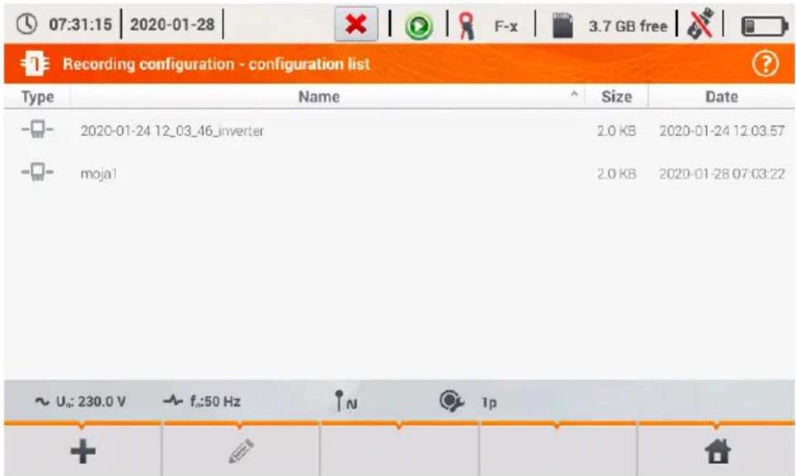
Fig. 46. Menu of recording configuration
2.13.2 Live mode
After entering the live mode screen, all the parameters of the measured inverter circuit are shown in a tabular view.
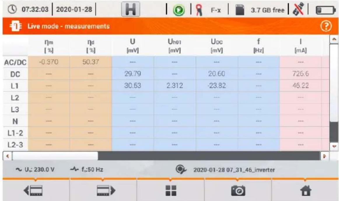
other
| Category | ηm [%] | ηd [%] | U [mV] | Uh01 [mV] | UDC [mV] | f [Hz] | I [mA] | | :--- | :--- | :--- | :--- | :--- | :--- | :--- | :--- | | AC/DC | -0.370 | 50.37 | --- | --- | --- | --- | --- | | DC | --- | --- | 29.79 | --- | 20.60 | --- | 726.6 | | L1 | --- | --- | 30.53 | 2.312 | -23.82 | --- | 46.22 | | L2 | --- | --- | --- | --- | --- | --- | --- | | L3 | --- | --- | --- | --- | --- | --- | --- | | N | --- | --- | --- | --- | --- | --- | --- | | L1-2 | --- | --- | --- | --- | --- | --- | --- | | L2-3 | --- | --- | --- | --- | --- | --- | --- | | ~ Uh: 230.0 V → fn:50 Hz 2020-01-28 07_31_46_inverterFig. 47. Live mode in tabular view for the inverter efficiency measurement mode.
- AC/DC line:
○ column _m displays the efficiency value _m of the inverter as the ratio of the active power of AC side to active power of DC side:
$$ \eta_ {m} [ \% ] = \frac {P _ {A C} [ W ]}{P _ {D C} [ W ]} \cdot 100 \% $$
○ column d shows the difference between the measured and declared efficiency of the inverter:
$$ \eta_ {d} [ \% ] = \eta_ {n o m} [ \% ] - \eta_ {m} [ \% ] $$
where _nom is the declared efficiency of the inverter entered to the configuration screen.
- line DC presents the parameters of DC side of the inverter such as voltage, current, active power, active energy.
- values related to AC side are displayed in lines: L1, L2, L3, N, L1-2, L2-3, L3-1 and .
Menu bar functions
It is possible to display the live values on three screens:

- view of waveforms of currents and voltages

- view of the time diagram,

- view of the table of measurements.
The control is similar to that described in Sec. 2.16 LIVE mode of the network. The differences include the option of displaying additional parameters: I DC, U DC, P AC, P DC on the screens for waveforms and timeplots.
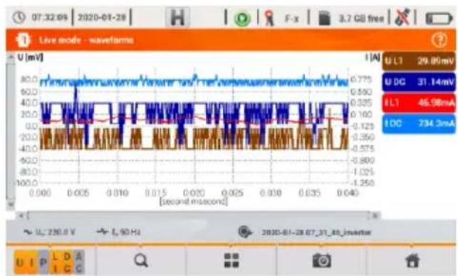
line
| Time [second] | U_L1 [mA] | U_DC [mA] | I_L1 [mA] | I_DC [mA] | | ------------- | --------- | --------- | --------- | --------- | | 0.000 | 0.775 | 31.14 | 46.98 | 734.3 |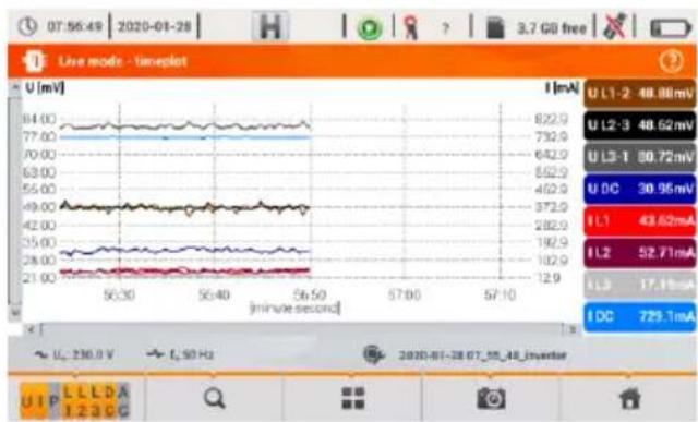
line
| Time (min) | U [mV] | I [mA] | |------------|--------|--------| | 05:30 | 94.00 | 822.9 | | 05:40 | 77.00 | 732.9 | | 05:50 | 70.00 | 642.9 | | 05:60 | 63.00 | 552.9 | | 05:70 | 55.00 | 462.9 | | 05:80 | 49.00 | 372.9 | | 05:90 | 42.00 | 282.9 | | 05:10 | 35.00 | 192.9 | | 05:11 | 28.00 | 102.9 | | 05:12 | 21.00 | 12.9 |Fig. 48. Screens for waveforms and timeplots in the mode of inverter efficiency measurement
2.14 Energy losses calculator
2.14.1 Functional Description
In this mode, you can estimate the loss of active power and associated costs due to poor power supply quality. The loss analysis screen is shown in Fig. 49. Analysis can be performed in terms of the desired time.
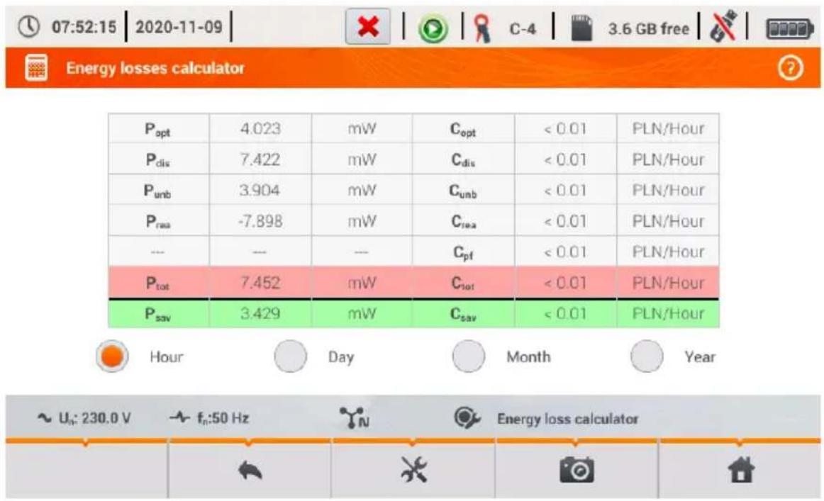
other
| Metric | Value | | :--- | :--- | | P_opt | 4.023 | | P_dis | 7.422 | | P_unb | 3.904 | | P_rea | -7.898 | | --- | --- | | P_tot | 7.452 | | P_sav | 3.429 | | mW | C_opt < 0.01 PLN/Hour | | mW | C_dis < 0.01 PLN/Hour | | mW | C_unb < 0.01 PLN/Hour | | mW | C_rea < 0.01 PLN/Hour | | --- | C_pf < 0.01 PLN/Hour | | mW | C_tot < 0.01 PLN/Hour | | mW | C_sav < 0.01 PLN/Hour | | Hour Day Month Year ~ Uₙ: 230.0 V → fₙ:50 Hz → Energy loss calculatorFig. 49. Energy loss analysis
Parameters to analyse
P_opt power loss due to wire resistance (assuming the absence of higher harmonics, unbalance and reactive power)
P_dis losses due to higher harmonics
P_unb power losses due to network unbalance
P_rea power loss due to the presence of reactive power
P_tot total losses (the sum of the above)
P_sav losses which can be reduced by improving the quality parameters (e.g. compensation of harmonics, elimination of unbalance), arising from the relationship:
$$ P _ {s a v} = P _ {t o t} - P _ {o p t} $$
C_opt cost related to P_opt losses
C_dis cost related to P_dis losses
C_unb cost related to P_unb losses
C_rea cost related to P_rea losses
C_pf cost related to a low power factor (large share of reactive power)
C_tot cost related to P_rea losses
C_sav cost related to P_sav losses
The financial loss can be estimated based on the current readings in terms of:
When one of the above options is activated ( the selection.
), the table will display data relevant to
Description of function icons

going to the configuration panel of the loss calculator (section 2.14.2)
performing the screenshot

returning to the main menu of the recorder mode
2.14.2 Configuration of the loss calculator
After the ✕ icon has been selected, the calculator configuration panel appears, shown in Fig. 50 and Fig. 51. It is possible to switch between screens using the ◀ ➞ icons.
![07:52:24 | 2020-11-09 Energy losses calculator settings Wires parameters Wire Number Section [mm²] Length [m] L 3 16.00 800.00 N 1 16.00 Copper 0.0196 Ømm²/m Aluminium 0.0320 Ømm²/m ~ Uₙ: 230.0 V ~ fₙ:50 Hz Energy loss calculator](/content/2026/05/852541/images/fb99b6ad3ed7cac70f95cf1d2a5b4e7e8c1e1b5bcd7222da53d8d0bcac883cfb.jpg)
Fig. 50. Energy loss analysis – configuration screen 1
On the first screen, set the parameters of the wire, to which the analysis applies, namely:
• for phase conductors L:
o NUMBER OF WIRES in the phase,
o CROSS SECTION of cores in mm ^2 ,
• for neutral conductors N:
O NUMBER OF NEUTRAL WIRES,
o CROSS SECTION of cores in mm ^2 ,
• THE LENGTH of the analysed line in metres,
• LINE MATERIAL – copper or aluminium.
Based on the above parameters, the calculator will calculate the power loss in the analysed line.
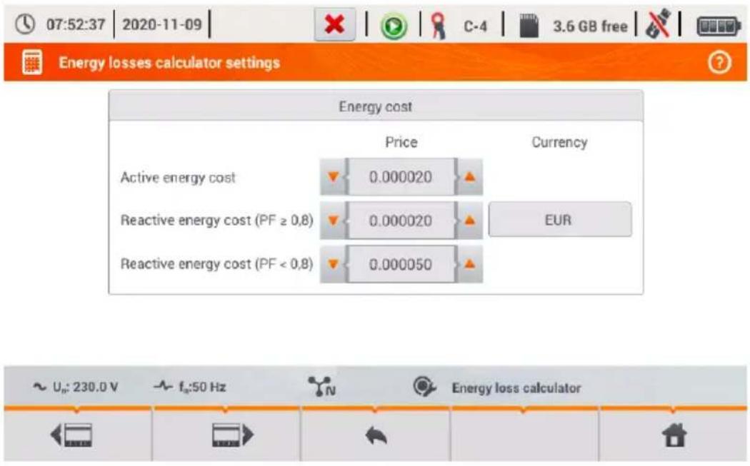
Fig. 51. Energy loss analysis – configuration screen 2
On the second screen, set the parameters defining the financial loss, i.e:
• cost of 1 kWh of active energy,
• cost of 1 kWh reactive energy at power factor PF ≥ 0.8,
- cost of 1 kWh of reactive energy at power factor PF < 0.8,
- currency.
To change the currency:
- tap the field with the current unit,
- enter a new unit using the on-screen keyboard.
Description of function icons

switching between the two setting screens of the calculator.

returning to the results indicated by the calculator. If the settings have been modified and saved, the results will be automatically calculated and displayed.

recording calculator settings

returning to the main menu of the recorder mode
2.15 About analyzer
After selecting this section, a window is displayed with basic information about the software
version of the analyzer and with manufacturer's details. Clicking on icon in the menu bar displays detailed information about the version of the analyzer. On the screen with detailed information, after
connecting an external memory stick (USB flash drive) and clicking icon in the bottom menu, the system log of the meter will be saved. This option is available for diagnostic purposes. The system log can be sent to the company's customer service in case of any problems with the meter.
2.16 LIVE mode of the network
The analyzer allows user to preview network parameters in real time (LIVE mode). Available views include the preview of voltage and current waveforms, timeplots of RMS values of voltages and currents, tabular view of parameters, phasor diagram and the harmonics view. If the default initial screen of the analyzer is the main screen (Fig. 2), then the bottom menu bar displays icons of individual views of LIVE mode:
- view of waveforms of currents and voltages,
- timeplot view,
- view of the table of measurements,
- view of the phasor diagram,
- view of harmonics.
In this mode refreshing of the display can be temporarily blocked by using the function HOLD (see the top bar description in section 2.8.1). Clicking the H button pauses the refreshing (the icon color switches to red). Tapping the button for the second time re-enables refreshing (the icon color switches to black).
2.16.1 Waveforms of voltages and currents
View of waveforms for instantaneous currents and voltages is selected from the main screen
using icon in the bottom bar. They show two cycles of network waveforms for active channels (depending on the measurement configuration). An example of the screen is shown in Fig. 52. Use buttons on the right side of the window to switch on/off individual measuring channels (at least one waveform must be always visible). The buttons include the name of the channel, for example. "U L1" and its RMS value. Waveforms areas can be zoomed-in vertically and horizontally by double-click and scrolled. Waveforms return to their default size after turning on/off any channel (buttons on the right side).
Note: In DC systems (DC and DC+M) this view is not available.
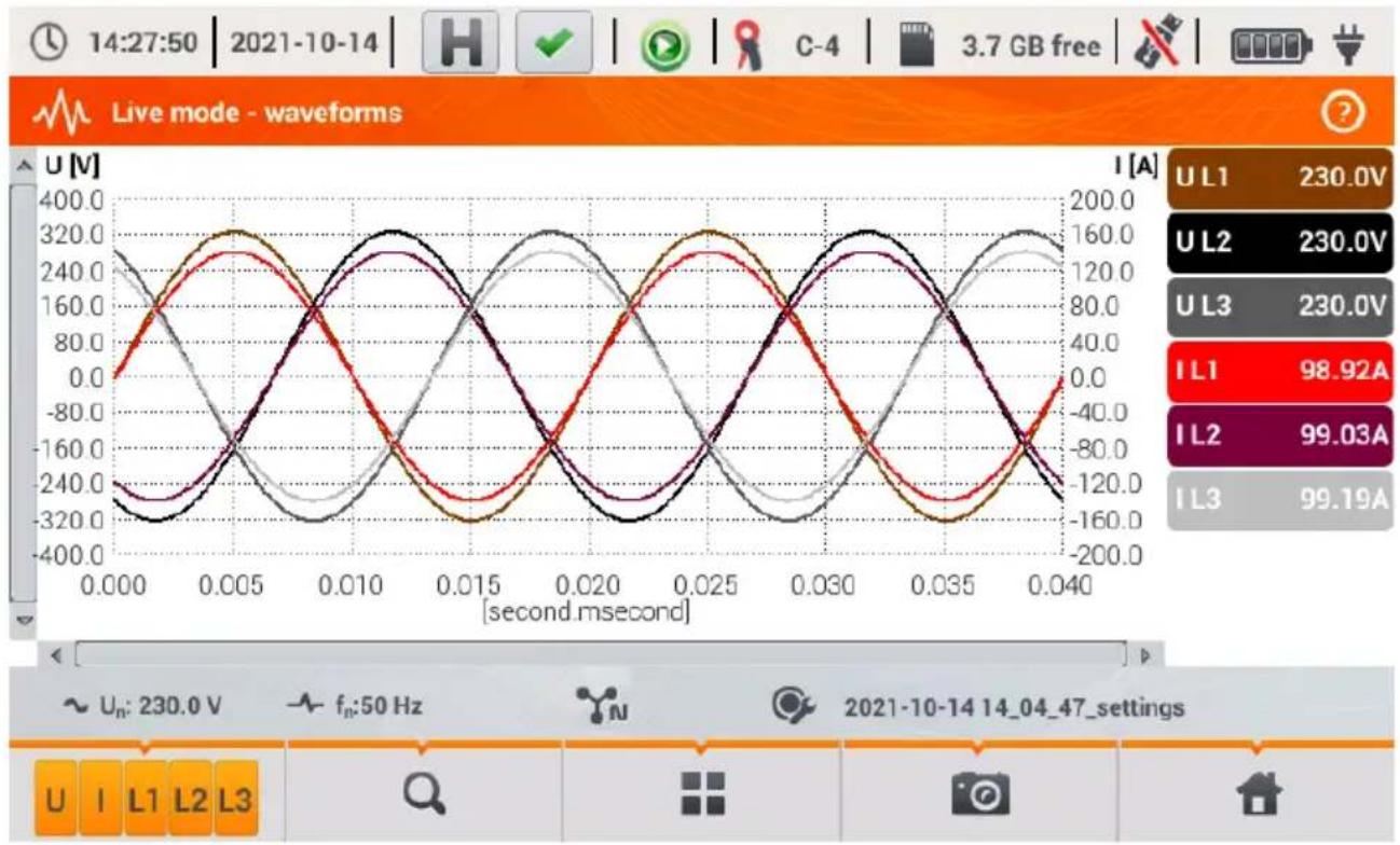
line
| Phase | Voltage (V) | |-------|-------------| | U_L1 | 230.0 | | U_L2 | 230.0 | | U_L3 | 230.0 | | I_L1 | 98.92A | | I_L2 | 99.03A | | I_L3 | 99.19A |Fig. 52. Current readings - waveforms.
Menu bar functions
- icon of active channels. After clicking, an additional menu bar is opened with buttons for enabling or disabling the display of current and voltage channels. The active channel is indicated by orange colour of the button. Remember that the screen must display at least one waveform (you can not turn off all of them). The menu displays only the buttons of channels that exist in the mains system.
- zoom-in icon. Click it to open an additional menu bar with icons for zooming-in the graph horizontally and vertically. Holding the zooming icon for 2 seconds results in the maximum zoom-in/out.
- zoom-in horizontally
- zoom-out horizontally
- zoom-in vertically
- zoom-out vertically
- icon for selecting the view type. It displays the additional menu, where you can change the view type of LIVE mode.
- screenshot icon. Clicking it saves the current contents of the main window to a graphic file. The file name is automatically created basing on the view name and the current date, for example "Live mode - waveforms – 2016-08-01 12_00_00". Files are stored on a microSD card.
2.16.2 Timeplot of RMS values
Timeplot view (Fig. 53) is activated from the main screen using icon v This view displays a graph of the RMS values of voltages and currents in time. In DC and DC+M systems the chart presents DC values of voltages and currents. The whole window covers time of approx. 110 seconds. After filling the entire window, the chart moves to the left by 30 seconds.
Menu bar functions
The same as for waveforms view.
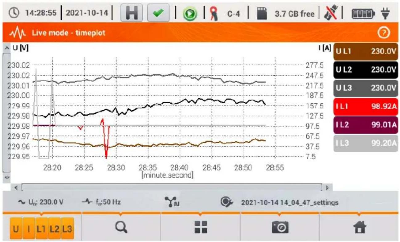
line
| Time (minute.second) | U_L1 (V) | U_L2 (V) | U_L3 (V) | | ------------------- | -------- | -------- | -------- | | 28.20 | 230.0 | 230.0 | 230.0 | | 28.25 | 230.0 | 230.0 | 230.0 | | 28.30 | 98.92 | 99.01 | 99.20 | | 28.40 | 98.92 | 99.01 | 99.20 | | 28.50 | 98.92 | 99.01 | 99.20 | | 28.55 | 98.92 | 99.01 | 99.20 |Fig. 53. Live mode – timeplot.
2.16.3 Live mode – tabular view
To view a table with values of mains parameters, select icon in the main screen. After selecting it, the summary table is displayed with the values of the tested mains, refreshed in real time. An example of the screen is shown in Fig. 54.
![14:29:11 | 2021-10-14 | H C-4 | 3.7 GB free | Live mode - measurements U [M] Uh01 [M] UDC [mV] f [Hz] l [A] Ih01 [A] IDC [A] [L1 230.0 230.0 -11.01 50.00 98.93 98.93 0.000 2 L2 230.0 230.0 6.024 --- 98.99 98.99 0.000 2 L3 230.0 230.0 12.67 --- 99.22 99.22 0.000 2 N --- --- --- --- --- L1-2 398.3 --- --- --- --- --- --- L2-3 398.5 --- --- --- --- --- --- L3-1 398.3 --- --- --- --- --- --- Σ --- --- --- 50.00 --- --- --- 6](/content/2026/05/852541/images/c1c9be538f54920a57789bd7eeddc301f988f26dd482789fc1b774da3fd9e5b0.jpg)
Fig. 54. Live mode – measurements results table.
The next lines were determined as follows:
L1 – phase values L1,
L2 – phase values L2,
L3 – phase values L3,
N – voltage values of channel U_NPE and current channel I_N .
L1-2 - phase-to-phase values L1-2,
L2-3 - phase-to-phase values L2-3,
L3-1 - phase-to-phase values L3-1,
Σ – total values.
The next column show the values of individual parameters:
U [V] - RMS voltage,
Uh01 [V] - RMS of the fundamental voltage component,
UDC [V] - DC voltage,
f [Hz] – mains frequency,
I [A] - RMS current,
Ih01 [A] - RMS of the fundamental current component,
IDC [A] - DC current,
P [W] - active power,
Q1 or QB [var] – reactive power of the fundamental component or reactive power, acc. to Budeanu (depending on the method of calculating reactive power),
S [VA] – apparent power,
SN [VA] or D [var] – apparent distortion power or Budeanu distortion power (depending on the method of calculating the reactive power),
EP+ [Wh] – active energy consumed,
EP- [Wh] – active energy supplied,
EQ1+ or EQB+ [varh] – reactive energy consumed,
EQ1- or EQB- [varh] – reactive energy supplied,
ES [VAh] – apparent energy,
PF – Power Factor,
cosφ – Displacement Power Factor,
tanφ – tangentφ factor,
THDU [%] – Total Harmonic Distortion for voltage (referred to the fundamental component),
THDI [%] – Total Harmonic Distortion for current (referred to the fundamental component),
CFU – voltage Crest Factor,
CFI – current Crest Factor,
PST – short-term flicker severity,
PLT – Long-term flicker severity,
U0 [V] - zero sequence symmetrical component of voltage,
U1 [V] – positive sequence symmetrical component of voltage,
U2 [V] - negative sequence symmetrical component of voltage,
U2/U1 [%] – voltage negative sequence unbalance factor,
U0/U1 [%] – voltage zero sequence unbalance factor,
10 [A] - zero sequence symmetrical component of current,
I1 [A] - positive sequence symmetrical component of current,
I2 [A] - negative sequence symmetrical component of current,
12/11 [%] – current negative sequence unbalance factor,
10/11 [%] – current zero sequence unbalance factor.
Menu bar functions


oving to the next screens with parameters.

- icon for selecting the view type. It displays the additional menu, where you can change view type of LIVE mode.

- screenshot.
2.16.4 Phasor diagram
The view of the phasor diagram is opened when you select icons in the main screen. Phasor graph (e.g. in Fig. 55) shows the basic layout of component vectors of voltages and currents. It may be used to quickly verify the correctness of connecting the analyzer to the network. In addition to the diagram, the tables include information about the values of fundamental components and their angles, as well as two unbalance factors of negative components (factors are displayed only for 3-phase networks). The type of the load is indicated by a coil icon (inductive load) if the angle between the fundamental voltage and current components ( _Uh1,Ih1 ) is greater than zero (voltage ahead of the current), and by a capacitor icon (capacitive load) if this angle is negative (current ahead of voltage).
Note: In DC systems (DC and DC+M) this view is not available.
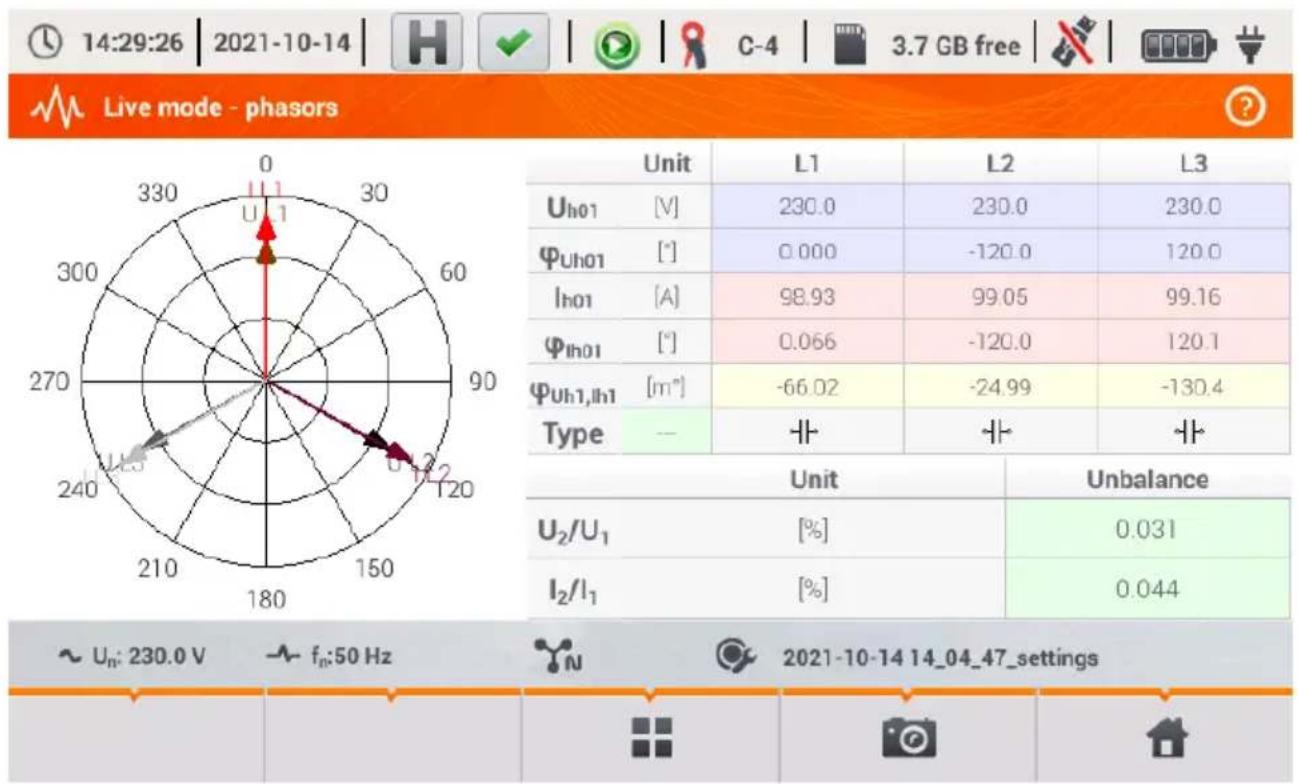
radar
| Unit | L1 | L2 | L3 | |------|------|------|------| | Uh01 | V | 230.0 | 230.0 | | φUh01 | [°] | 0.000 | -120.0 | | Ih01 | [A] | 98.93 | 99.05 | | φIh01 | [°] | 0.066 | -120.0 | | φUh1,Ih1 | [m²] | -66.02 | -24.99 | | Type | — | — | — | | Unit | Unbalance | Unbalance | Unbalance | | U₂/U₁ | [%] | 0.031 | | | I₂/I₁ | [%] | 0.044 | | | ~ Uₙ: 230.0 V ~ fₙ:50 Hz 2021-10-14 14_04_47_settingsFig. 55. Live mode – phasor diagram.
Menu bar functions
- icon for selecting the view type. It displays the additional menu, where you can change the view type of LIVE mode.
- screenshot.
2.16.5 Harmonics graph/table
The last view of the Live mode presents harmonics. This view is selected by clicking icon from the main screen. This screen allows you to view the harmonics of voltages and currents, angles between the current and voltage harmonics, cosφ factors of these currents and THD factors. Harmonics are displayed graphically in a bar graph or in a table. By default, the harmonics are presented in a bar graph. An example is shown in Fig. 56.
Note: In DC systems (DC and DC+M) this view is not available.
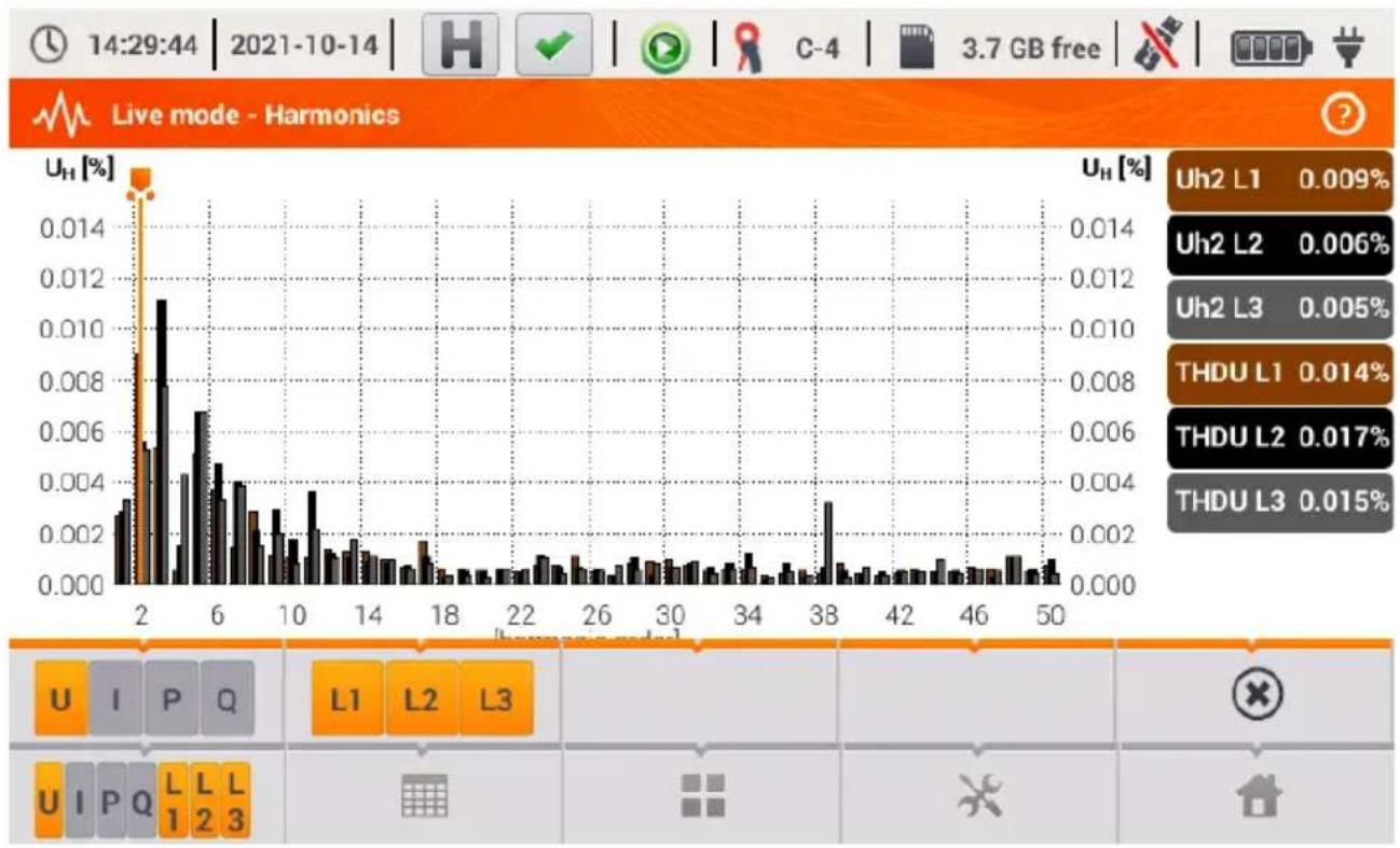
bar
Live mode - Harmonics | Harmonic | U_H [%] | | :--- | :--- | | Uh2 L1 | 0.009 | | Uh2 L2 | 0.006 | | Uh2 L3 | 0.005 | | THDU L1 | 0.014 | | THDU L2 | 0.017 | | THDU L3 | 0.015 |Fig. 56. Live mode - harmonics - bar graph.
Menu bar functions
- menu of active channels. After clicking, an additional menu bar is opened with buttons for enabling or disabling the data and to switch between current and voltage harmonics. Icon (available only in table view) enables preview of angles between voltage and current harmonics, together with the calculated values of cosφ angles. The active channel is indicated by orange colour of the button.
- switching to tabular view of harmonics (Fig. 57). The table in each row displays the harmonic values (from DC component to the harmonic of 50th order) or the angles between the current and voltage harmonics. In case of harmonics, the values may be displayed in absolute units (V/A), or as percentage related to the fundamental harmonic (see below). The angles are given in degrees. The powers of harmonics – in % or W/var. In the tabular view, the buttons on the right side of the window shows the RMS values of voltages and currents.
- switching to the bar graph. The chart includes a marker, which indicates the order of harmonic(s), the value of which is shown on the button on the right side of the window. In addition, THD factor is also displayed at the right side.

- icon for selecting the view type. It displays the additional menu, where you can change view type of LIVE mode.

- options menu for a chart or table. After selecting it, an additional menu bar is displayed, which provides several new options:
- an option of hiding the fundamental harmonic.
- displaying values as percent in relation to the fundamental component.
- screenshot.
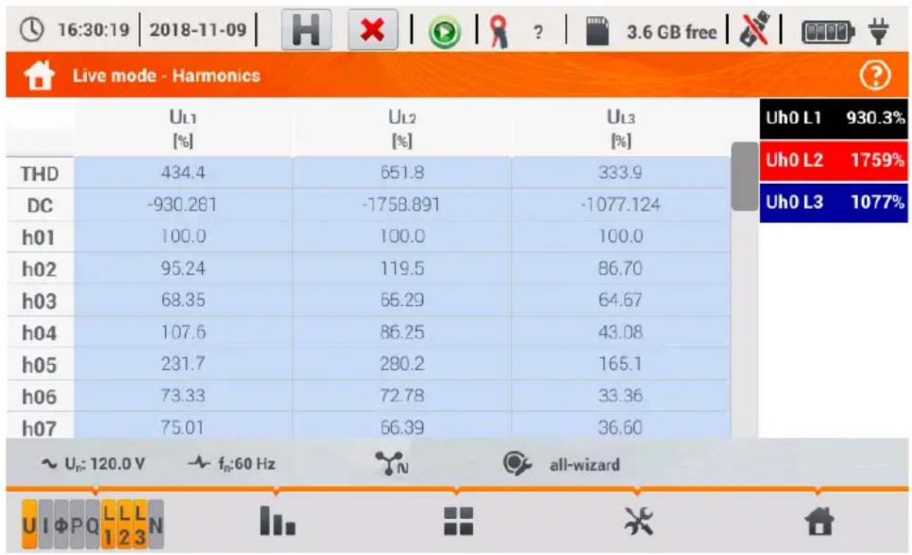
other
| Device | U1 [%] | U2 [%] | U3 [%] | Uh0 L1 (%) | Uh0 L2 (%) | Uh0 L3 (%) | | :--- | :--- | :--- | :--- | :--- | :--- | :--- | | THD | 434.4 | 651.8 | 333.9 | 930.3% | 1759% | 1077% | | DC | -930.281 | -1758.891 | -1077.124 | 930.3% | 1759% | 1077% | | h01 | 100.0 | 100.0 | 100.0 | 930.3% | 1759% | 1077% | | h02 | 95.24 | 119.5 | 86.70 | 930.3% | 1759% | 1077% | | h03 | 68.35 | 65.29 | 64.67 | 930.3% | 1759% | 1077% | | h04 | 107.6 | 86.25 | 43.08 | 930.3% | 1759% | 1077% | | h05 | 231.7 | 280.2 | 165.1 | 930.3% | 1759% | 1077% | | h06 | 73.33 | 72.78 | 33.36 | 930.3% | 1759% | 1077% | | h07 | 75.01 | 66.39 | 36.60 | 930.3% | 1759% | 1077% | ~ Un: 120.0 V → fn:60 Hz → all-wizard UI ΦP Q L L L NFig. 57. Live mode - harmonics - tabular graph.
2.17 Operation with PC
2.17.1 "Sonel Analysis" software
Sonel Analysis is an application used to work with power analyzers of PQM series. When used with PQM-707, it provides the following features:
- read data from the device,
• real-time preview of the mains (live view), - present data in the tabular form,
- present data in the form of graphs,
- analysing data for compliance with EN 50160 standard (reports) and other user-defined conditions,
- updating firmware of analyzer and updating the application itself.
The software operates with Windows 7, Windows 8 and Windows 10.
Detailed manual for "Sonel Analysis" is available in a separate document (also downloadable from the manufacturer's website www.sonel.pl).
2.17.2 PC connection and data transmission
The analyzer allows communication with a PC when connected to it with USB cable.
Connection to a computer (PC mode), ensures:
- transmission of data stored in the recorder memory:
- it is possible to read data from all completed recordings,
• viewing mains parameters on PC:
- instantaneous values of: current, voltage, power and energy, total values for the entire system,
○ harmonics, THD, - unbalance,
- phasor diagrams for voltages and currents,
o current and voltage waveforms drawn in real-time, -
all other measured parameters.
-
When connected to a PC, the display shows message "PC Connection"
- When connected to a PC, all analyzer buttons are locked except button, but when the analyzer operates with key lock mode (e.g. during recording), all the buttons are locked. The icon located in the menu bar, terminates the connection with the PC.
- When within 10 seconds of connecting a PC to the device no data exchange occurs between the analyzer and the computer, the analyzer exits data exchange mode and terminates the connection.
Sonel Analysis software also allows you to read data directly from a microSD card using an external memory card reader. This method allows for the fastest reading of the recorded data. To use this mode, remove the memory card from the meter and insert it into a reader connected to the computer (when removing the card, follow the rules described in sec. 2.6; it is safe to turn off the meter before that).
2.18 Wiring diagrams
The analyzer may be connected directly to the following types of AC networks:
• single-phase (Fig. 58)
• split-phase with split-winding of the transformer (Fig. 59),
• 3-phase 4-wire, 3-phase 4-wire (no U L2) / 2 ½ element (no V L2/B) (Fig. 60),
• 3-phase 3-wire, 3-phase 3-wire Aron / 2-element, 3-phase open delta (Fig. 61, Fig. 62).
Indirect measurement in MV and HV networks is possible:
• in 3-phase 4-wire system (Fig. 63),
• in 3-phase 3-wire system (Fig. 64).
Measurements in DC systems is possible in two configurations:
- DC – one-voltage DC system (Fig. 65)
- DC+M – two-voltage DC system with middle point (Fig. 66) In DC systems, it is possible to measure the current using probes C-5A.
In three-wire AC systems, current may be measured by the Aron method (Fig. 62), which uses only two probes that measure linear currents I_L1 and I_L3 . I_L2 current is then calculated using the following formula:
$$ I _ {L 2} = - I _ {L 1} - I _ {L 3} $$
In systems with neutral conductor, the user may additionally activate current measurement in this conductor, after installing additional probes in I_N channel. This measurement is performed after activating "N conductor current" option in the configuration.
Note
In order to correctly calculate total apparent power S_e and total Power Factor (PF) in a 4-wire 3-phase system, it is necessary to measure the current in the neutral conductor. Then it is necessary to activate option N conductor current and connect 4 probes, as shown in Fig. 60. More information on total apparent power S_e - see sec. 5.3.5.
For systems with available PE and N conductors (earthing and neutral) it is also possible to measure N-PE voltage. To do this, connect PE conductor to PE input of the analyzer. In addition, select option N-PE voltage in measurement point settings.
Pay attention to the direction of current probes. The probes should be installed with the arrow indicating the load direction. It may be verified by conducting an active power measurement – in most types of passive loads active power is positive. When probes are inversely connected, it is possible to change their polarity using in software (ANALYZER SETTINGS → PROBES)
The following figures show schematically how to connect the analyzer to the tested network depending on its type.
Icons used in the drawings with respect for optional connections have the following meanings:
if voltage U_N-PE measurement is required, use this icon to connect as shown in diagram (connect PE input to the protective conductor)

if current I_N measurement is required, use this icon to connect as shown in diagram (connect probes in channel I_N ).
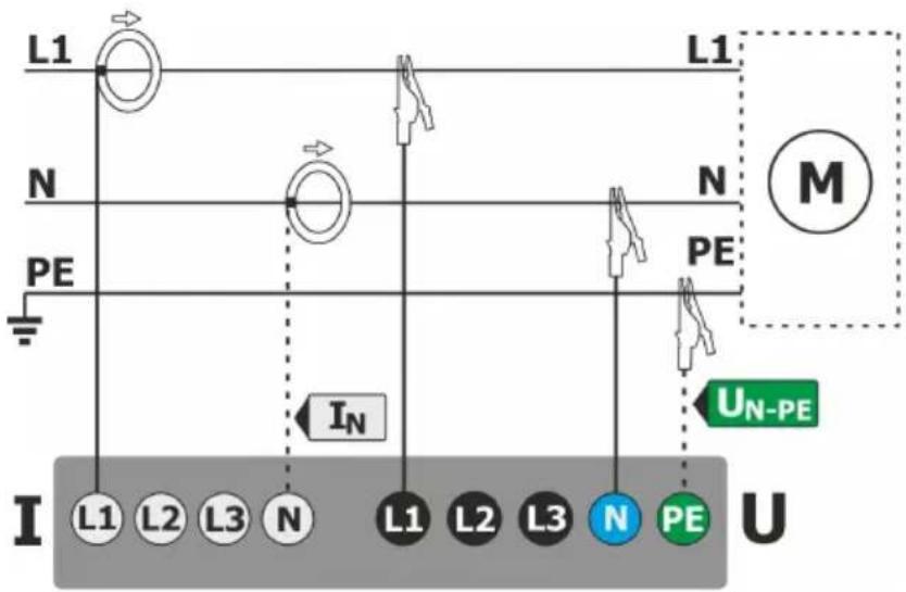
Fig. 58. Wiring diagram – single phase.
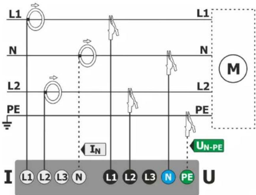
Fig. 59. Wiring diagram – split-phase.
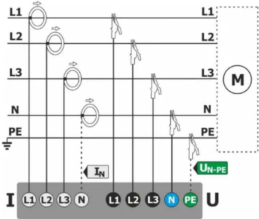
Fig. 60. Wiring diagram – 3-phase 4-wire, 3-phase 4-wire (no U L2) / 2 12 element (no V L2/B) systems.
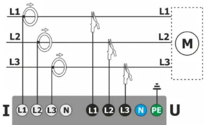
Fig. 61. Wiring diagram – 3-phase 3-wire, 3-phase open delta systems.
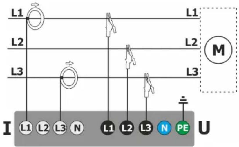
flowchart
graph TD
    L1["Terminal L1"] --> L2["Terminal L2"]
    L1 --> L3["Terminal L3"]
    L2 --> M["Motor M"]
    L3 --> M
    L1 --> U["Power Source U"]
    L2 --> U
    L3 --> U
    style M stroke-dasharray: 5 5
    style U stroke-dasharray: 5 5
    style I stroke-dasharray: 5 5
    style U stroke-dasharray: 5 5
Fig. 62. Wiring diagram – 3-phase 3-wire Aron, 2-element systems (current measurement using Aron method).
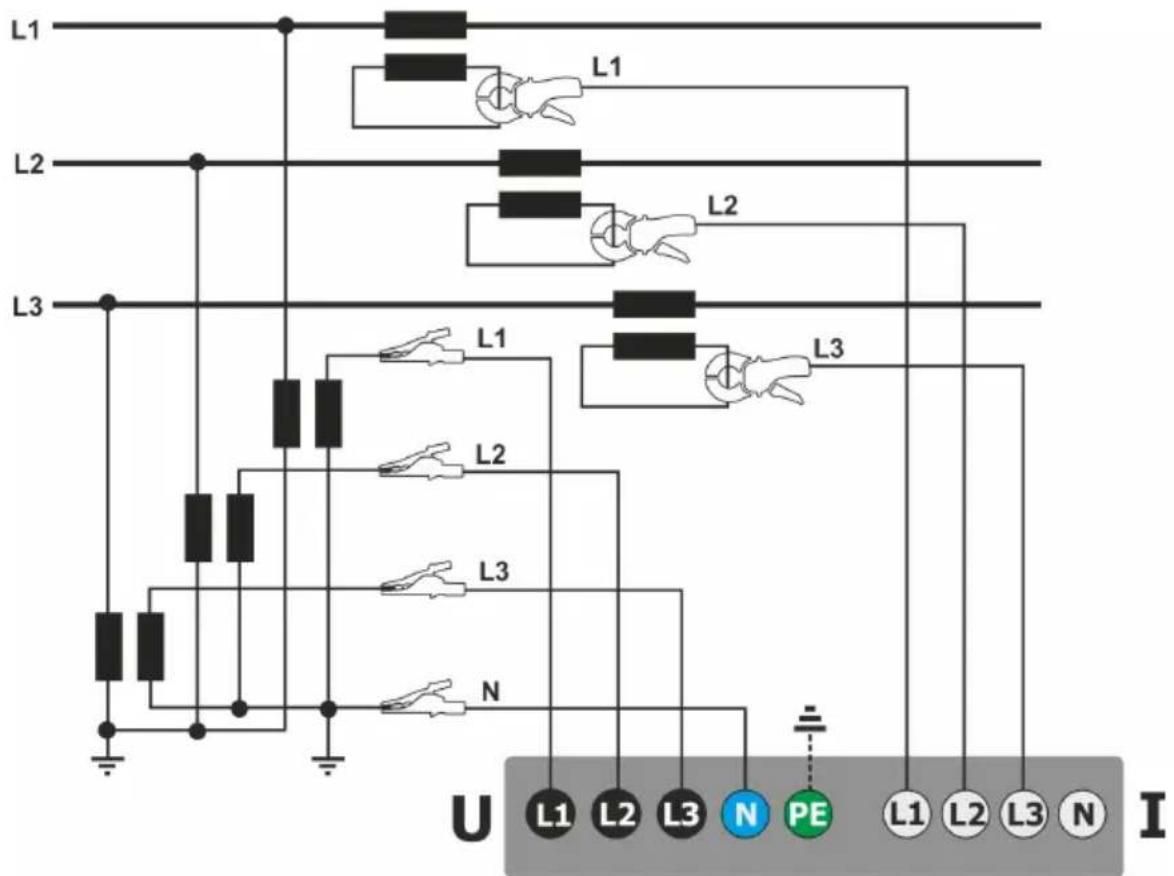
Fig. 63. Wiring diagram – indirect measurement of MV in 3-phase 4-wire system.
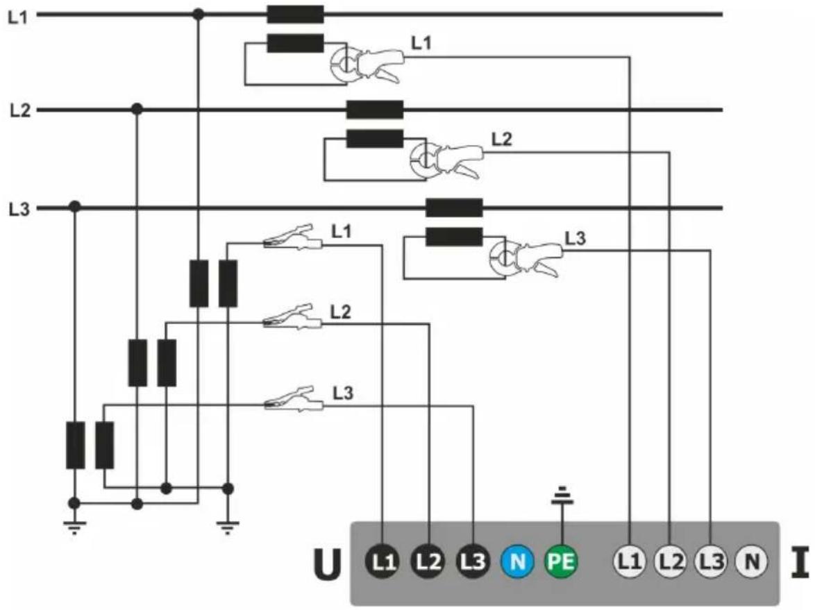
Fig. 64. Wiring diagram – indirect measurement of MV in 3-phase 3-wire system.
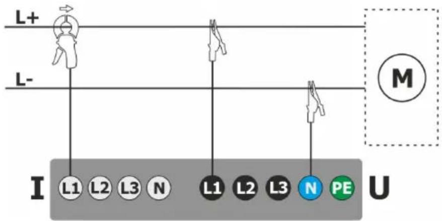
Fig. 65. Wiring diagram – DC system.
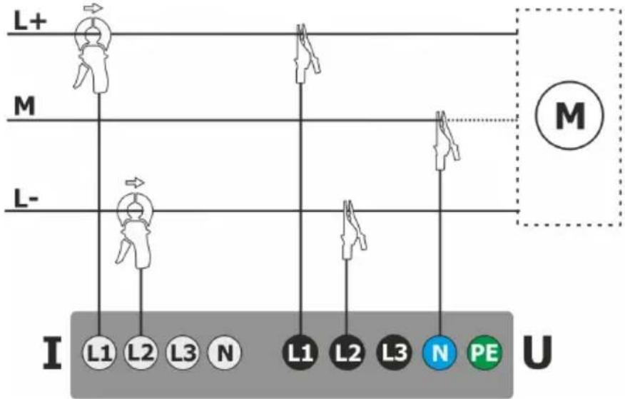
flowchart
graph TD
    L+ --> L1["LM"]
    L+ --> L2["LM"]
    L+ --> L3["LM"]
    L+ --> N["N"]
    M --> L1
    M --> L2
    M --> L3
    M --> N
    L- --> L1
    L- --> L2
    L- --> L3
    L- --> N
    L- --> PE["PE"]
    PE --> U["U"]
Fig. 66. Wiring diagram – DC+M system (bipolar).
2.18.1 Verifying the connection
After clicking the button that is signalling the correct connection of the analyzer (see Fig. 3) a window is displayed showing some important information on the connection of the analyzer to the tested network. This information helps the user to verify the compliance of the current configuration of the analyzer with the parameters of the measured network. The window provides the following information:
• Voltage values - two possible icons:
- RMS voltages are correct, they are within the tolerance range of ± 15% of the nominal voltage,
- RMS values are outside the range of U _NOM ±15%.
- Current values - four options:
- RMS currents are in the range of 0.3% I NOM ...115% I_NOM
- RMS currents are lower than 0.3% I NOM,
• RMS currents are higher than 115% I NOM, - --- dashes are displayed when the current measurement is disabled in the configuration.
In 3-phase 3- and 4-wire systems the analyzer also calculates the sum of all the currents (instantaneous values) and checks if it totals to zero. This helps in determining if all current probes are connected correctly (i.e. arrows on current probes facing to the load). If the calculated current sum RMS value is higher then 0.3% of Inom it is treated as an error and the icon is displayed.
- Voltage vectors - the analyzer verifies the correctness of the fundamental components angles and displays the corresponding icon:
-
- the vectors have correct angles in the range of ± 30^ of the theoretical value for a resistive load and symmetrical circuit (in 3-phase systems),
- the accuracy of angles cannot be verified, because the RMS voltage value is too low (less than 1% of U_NOM ),
- Incorrect angles of vectors. In three-phase systems, this icon is displayed, among others, in case of reversed sequence of voltage phases.
- Current vectors - correctness of vector angles is verified for the fundamental components of main currents in relation to the voltage vectors. The following icons are displayed:
- vectors are within ± 55^ in relation to angles corresponding to the voltage vectors,
- the accuracy of current vector angles cannot be verified, because the RMS current values are too low (below 0.3% of I_NOM ),
- X - vectors are outside the acceptable range of angles ( ±55°),
- --- dashes are displayed when the current measurement is disabled in the configuration.
- Frequency:
- the measured grid frequency is in the range of f_NOM ± 10% ,
- the RMS value of reference voltage phase is lower than 10 V or there is no PLL synchronization.
- the measured frequency is outside of f_NOM ± 10% range.
The icon is displayed in the top control bar in the following way:
- if the table includes is at least one ,
- ? - if the table includes is at least one ?, but there is no error (no ✗),
- if all measured parameters are correct.
2.19 Example of use
The procedure presented below shows how to make a measurement with the analyzer ('step by step'): from connecting the device to generating the measurement report. It provides guidelines how to quickly start to operate the analyzer and Sonel Analysis software. It is assumed that Sonel Analysis software is already installed.
Scenario: 1-phase measurement for compliance with EN 50160.
Measurement scenario is as follows: the user wants to measure voltage parameters of single-phase network 230 V 50 Hz. The goal is to generate a report on compliance with the requirements of standard EN 50160. In accordance with the requirements of the standard, the following parameters should be recorded:
• 10-minute average values of voltage, THD and harmonics,
• frequency of 10 seconds,
- long-term flicker severity P LT ,
- voltage events: 110%U nom for swell, 90%U nom for dip, 5%U nom for interruption. When an event is detected, the waveform and RMS _1/2 graph must be recorded.
After the measurement, generate timelines of measured parameters and a sample report for compliance with the standard. Data should be saved for further analysis.
This above activities shall be done using only the analyzer.
Additionally, read the saved data stored in Sonel Analysis software and generate a report on compliance with the standard.
How to perform the measurements:
Step 1: Turn on the meter. Turn on the analyzer by pressing ⏻ button. After loading the software, a screen should be displayed as shown in Fig. 2 or one of the LIVE mode screens, if the default screen has been changed in the configuration.
Step 2: Connect to the tested network. Connect the analyzer to the tested mains, as shown in Fig. 58. Connect voltage inputs L1, N. Probes do not need to be connected, because the current measurement is not required. Connect an external power supply to the analyzer to avoid supplying from the battery pack that may be interrupted due to the discharged battery.
Step 3: Create a new measurement configuration. Select RECORDING CONFIGURATION in the main screen. In the next few steps a new measurement configuration is created, according to the specified requirements. From the bottom bar menu, select icon (adding a new configuration). Then, in the displayed window select option ACCORDING TO STANDARD on from the drop-down list select standard EN 50160 - LOW VOLTAGE. Confirm your selection by clicking √ icon on the menu bar. The first screen of detailed configuration will be displayed. From the drop-down list of MAINS SYSTEM select 1-phase, voltage Un leave 230/400 V, frequency 50 Hz and from list PROBES TYPE select None. On the other setup screens you do not need to make additional changes, so you can save the configuration by choosing 'Save' icon. A window will be displayed for entering the name for the newly created configuration. By clicking on the box with default name, you can enter your own name, for example „EN50160 1-ph”. After entering the name, tick box Set as active to switch the analyzer immediately to the new configuration and click OK. A window will be displayed to confirm saving of the configuration. The bottom information bar should include the following information: U_n : 230 V, f_n :50 Hz, 1-phase mains icon and the name of the new configuration.
Step 4: Check the correctness of the connection. Go to the main screen (icon 📋), and then display the window with waveforms . The main window should present the instantaneous voltage waveforms (sine wave), and the button on the right side should indicate the value of the RMS voltage, which should be approximately 230 V i.e. the same as the nominal value of the network set. You can also view check the tabular view of instantaneous parameters and harmonics
Step 5: Check the readiness for recording. Before starting recording, make sure that the date and time of the analyzer are correct and that the analyzer has microSD memory card installed with sufficient disk space. If the date is not correct, from the main screen select ANALYZER SETTINGS and then DATE AND TIME, enter correct values and confirm. If the correct memory card is inserted into the analyzer, the top bar will display a memory card icon with information about free space.
Step 6: Data recording. You can start recording by pressing button. After the window for confirming recording start is displayed press YES. Starting the recording will be confirmed by a triple beep and the saving icon in the top bar will turn red, whereas LED will flash in red. The meter should be left in this state for a long period e.g. a few hours to save the appropriate amount of data (in recording according to EN 50160 new records are saved every 10 minutes, and assigning P _LT indicator requires recording that lasts full two hours synchronized with the clock that multiplies the period of two hours). During the recording process, an event of voltage dip may be simulated by disconnecting lead L1 or N from the meter for a while. To meet the regulatory requirements, recording process should be performed at least for the duration of one week.
Step 7: Stop recording. After the required time, stop the recording by pressing 📂 and confirming the intention to stop the recording process.
Step 8: Go to the recording analysis. From the main screen select RECORDING ANALYSIS screen. Find the completed recording in the list of records: its name should be the same as the user's configuration, for example. "EN50160 1-ph" (in step 3), compare the date and time of completion with the current time of the meter. You can also sort the list by date, in order to display the latest recordings at the top of the list. Double-click the found recording or highlight it by single click, and
select from the bottom menu preview icon . You will see the recording summary screen.
Step 9: Generate timeplots. To generate an example of a timeplot with three waveforms: average voltage UL1, 10-second frequency (which are normally stored in all recordings according to standard) and flicker P_LT , perform the following steps. On the recording summary screen, select waveform icon in the bottom menu and then select icon from the additional menu. A graph will be displayed with the average value of the voltage for the entire recording range. This screen is used to indicate the time range, which will be used to generate timeplots of user-selected parameters. Orange rectangle marks the active time range that may be moved to increase (up to the limit of 1,100 samples) or decrease the indicated range. After adjusting the time range, click option in the bottom bar which means the selection of plotted parameters. Select the sample parameters (maximum four) for example average voltage UL1, frequency and voltage THD. After selecting the parameters, go to the bottom bar and click icon to generate chart. The screen will display a window with the timeplot of selected parameters. The marker may indicate a specific time and provide the parameters in this time visible on the right side panel.
Step 10. Generate report on compliance with standard. From the graph window return to the recording summary screen (in the bottom bar select and then, and then twice). After that, to generate a report of compliance with standard EN 50160 (which was used for recording),
click icon in the bottom bar. Window with report options will be displayed (as in Fig. 27). After selecting the desired options, the icon on the menu bar to generate a report. It will be displayed on the screen. Individual sections of the report are presented in sec. 2.11.7.
Step 11. Saving report on the USB memory stick (flash drive). To save the generated report on compliance with the standard in external USB memory, connect the flash drive to the analyzer, wait until the device is recognized, and the top bar should include a not uncrossed icon of USB flash drive. Then, in the menu bar click saving icon and in additional menu that appears, click icon

to save the report. After a successful saving, a window will appear with confirmation. Report (format) will be saved on a removable drive in a folder named "PQM-707_DATA".
Step 12: Connect the meter with Sonel Analysis software. First install this software. Once installed, you must start it and connect the analyzer to the computer using USB cable. If this is the first connection, wait to install the drivers of the analyzer. Select Analyzer →Analysis in the menu, or use the toolbar and select Analysis option. A window will be displayed with a list of available analyzers - the list should include one item with the detected PQM-707. Double click on the name of the analyzer to connect with it. After connecting, the analyzer screen will show window PC connection.
An alternative method to read the data by Sonel Analysis, is transferring the memory card into the card reader connected to a computer (for data safety, first turn off the meter, to save all data on the card). Select (similarly as above) Analyzer→Analysis in the menu, or use the toolbar and select Analysis option. A window will appear with a list of detected memory cards; the list should include item: "PQM-707 [serial number] - Connection with the memory card" of the detected card of the analyzer. Double-click twice on this item and then confirm the connection to continue.
Step 13: Read the recording data from the analyzer. As a result of selecting option Analysis, the software will display a window for choosing data type to be downloaded from the meter. It is possible to download the recording data (measurements) and screenshots. In such case, the recorded data will be downloaded, so you'll need to tick option Recordings. At this point, the program downloads from the meter a list of available recordings. The list includes all recordings that are currently stored on the microSD card of the analyzer. Indicate recording you want to download and click Read data. A window will appear showing data loading progress. After loading all data, a window is displayed for saving downloaded data into the disk. It is recommended to save the data to a desired location on the disk, in order to retrieve it for further analysis. Indicate the location on the disk, name the file and click Save. In the displayed window click on the horizontal bar indicating time of recording placed under text Configuration No... (Standard) (after clicking it turns orange) and then click Data Analysis.
Step 14: Data Analysis. In the main window of data analysis four main buttons are available:
General (default view after loading data), Measurement, Events, Configuration. In General view, on the right side, icons are displayed representing individual measurements, event and recorded waveforms in the timeline. This graph with a large amount of data may be freely enlarged to get more details.
Click Measurements button to display table with the values of all measured parameters, according to selected averaging time. In this scenario, the recording according to standard was selected, where averaging time is always equal to 10 minutes, therefore every 10 minutes the analyzer recorded voltage, THD and harmonics (frequency is always measured every 10 seconds). Each line
contains the data recorded in the subsequent 10-minute interval and each column contains the individual parameters (all 10-second frequency values may be viewed after selecting '10s' from Display data list)
After pressing Events you may view all the recorded events. In this scenario, the following voltage values were recorded: swell, dip and interruption. Each row in the table corresponds to one detected event. When for a given event graphs are available (e.g. waveforms and RMS_1/2 graphs), as in this scenario, the last column contains the icon of saved graphs. After clicking it, the user may display graphs related to a given event.
Step 15: Display the time plot for voltage and THD. To generate the graph, go to Measurement view (click Measurement button), select column headings for voltage L1, THD L1 (columns will be highlighted) and then click Plots and choose Time plot. A window will be displayed with a graph containing two timeplots: L1 voltage and THD U L1. The graph may be freely enlarged, using the three markers mark specific points on the graph and read the parameters of indicated points. The graph may be saved (in selected graphic format) by clicking Save icon on the top toolbar.
Step 16: Displaying graphs with harmonics. Two types of graphs may be displayed for harmonics. The first one is a graph of recorded harmonics in time. To display the graph, select the columns of selected harmonics (e.g. third and fifth order) and click Plots→Time plot.
The second type of the graph is a bar graph of harmonics. It shows all the harmonics in 10-minute interval (in one line). To generate it, first select the desired cell from the time column and the select the column of any L1 voltage harmonic, click Plots and choose from Harmonics list. In the same manner, the user may also select the time interval by dragging time column cells. Then a graph is shown with average values of harmonics in the specified time period.
Step 17: Checking events. If the analyzer, during recording process, detects any event, it will be displayed in a table in Events view. The line describing the specific event displays time of the event (start and end), extreme value (e.g. minimum voltage during the dip), waveform and RMS _1/2 graph when the event was voltage- or current-related. In this scenario, event graphs were activated automatically in settings (due to setting the configuration in accordance with a standard), therefore when the analyzer detects any event, the last column of the table (with Waveform header) should include a graph icon. Click it to display graphs (or press button Plots and select Waveform).
Step 18: Generate report on compliance with standard. To generate a report summarizing the compliance of the tested mains parameters with standard requirements, in view Measurements, click Reports and select Report according to standard. The displayed window will enable you to set parameters of the generated report (e.g. processing of "flagged" data, taking into account phase-to-phase voltage, etc.). Generate button will start data processing and preparing the report. The last step is to provide additional data (optional), which will be added to the report (e.g. report number, description of the measurement, the author's details, graphic logo). To see the report, click icon Preview. Button Save saves data in a format specified by the user (pdf, html, txt, csv).
3 Design and measurement methods
3.1 Voltage inputs
The voltage input block is shown in Fig. 67. The phase inputs L1, L2, L3 can be referred to the neutral input terminal (the measured voltages are then L1-N, L2-N, L3-N), or the protective earth terminal PE (the measured voltages are then L1-PE, L2-PE, L3-PE). The particular reference is selected based on the mains type; the PE reference is used in 3-phase 3-wire systems, while the others use neutral input reference.
The analyzer has one voltage range, with voltage range ±1150V (no ADC saturation).
3.2 Current inputs
The analyzer has four independent current inputs with identical parameters. Current transformer (CT) probes with voltage output in a 1 V standard, or several types of flexible (Rogowski) probes. can be connected to each input.
A typical situation is using flexible probes with built-in electronic integrator. However, the PQM-707 allows connecting the Rogowski coil alone to the input and a digital signal integration.
3.3 Digital integrator
The PQM-707 uses the solution with digital integration of signal coming directly from the Rogowski coil. Such approach has allowed the elimination of the analog integrator problems connected with the necessity to ensure declared long-term accuracy in difficult measuring environments. The analog integrators must also include the systems protecting the inputs from saturation in case DC voltage is present on the input.
A perfect integrator has an infinite amplification for DC signals which falls with the rate of 20 dB/decade of frequency. The phase shift is fixed over the whole frequency range and equals -90^ .
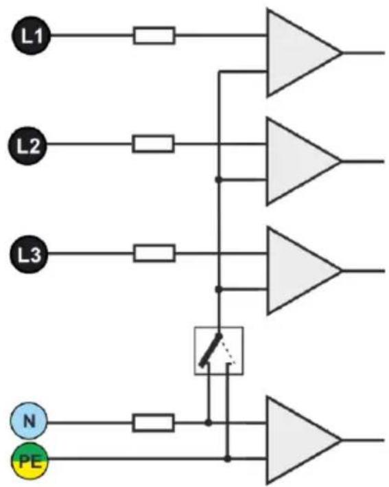
flowchart
graph TD
    L1[" L1 "] --> A[" "] --> B[" "] --> C[" "]
    L2[" L2 "] --> D[" "] --> E[" "] --> F[" "]
    L3[" L3 "] --> G[" "] --> H[" "] --> I[" "]
    N[" N "] --> J[" "] --> K[" "] --> L[" "]
    PE[" PE "] --> K[" "] --> L[" "] --> M[" "]
    style N fill:#000,stroke:#000,color:#fff
    style PE fill:#000,stroke:#000,color:#fff
    style L1 fill:#ccc,stroke:#333
    style L2 fill:#ccc,stroke:#333
    style L3 fill:#ccc,stroke:#333
    style N fill:#99cc,stroke:#333
    style PE fill:#99cc,stroke:#333
Fig. 67. Voltage input terminals
Theoretically infinite amplification for a DC signal, if present on the integrator input, causes the input saturation near the power supply voltage and makes further operation impossible. In practically implemented systems, a solution is applied which limits the amplification for DC to a specified value, and in addition periodically zeroes the output. There are also techniques of active cancellation of DC voltage which involve its measurement and re-applying to the input, but with an opposite sign, which effectively cancels such voltage. There is a term “leaky integrator” which describes an integrator with finite DC gain. An analog leaky integrator is just an integrator featuring a capacitor shunted with a high-value resistor. Such a system is then identical with a low-pass filter of a very low pass frequency.
Digital integrator implementation ensures excellent long-term parameters – the entire procedure is performed by means of calculations, and aging of components, drifts, etc. have been eliminated. However, just like in the analog version, also here we can find the saturation problem and without a suitable counteraction the digital integration may become useless. It should be remembered that both, input amplifiers and analog-to-digital converters, have a given finite and undesirable offset which must be removed prior to integration. The PQM-707 analyzer firmware includes a digital filter which is to remove totally the DC voltage component. The filtered signal is subjected to digital integration. The resultant phase response has excellent properties, and the phase shift for most critical frequencies 50 and 60 Hz is minimal.
Ensuring the least possible phase shift between the voltage and current components is very important for obtaining small power measurement errors. It can be proven that approximate power measurement error can be described with the following relationship ^1 :
$$ \text { Power measurement error } \approx \text { phase error (in radians) } \times \tan (\varphi) \times 100 \% $$
where () is the tangent of the angle between the fundamental voltage and current components. From the formula, it can be concluded that the measurement errors are increasing as the displacement power factor is decreasing; for example, at the phase error of only 0.1^ and = 0.5 , the error is 0.3%. Anyway, for the power measurements to be accurate, the phase coincidence of voltage and current circuits must be the highest possible.
3.4 Signal sampling
The signal is sampled simultaneously in all eight channels at the frequency synchronized with the frequency of power supply voltage in the reference channel. This frequency equals 10.24 kHz for the 50 Hz and 60 Hz mains systems.
Each period includes then about 205 samples for 50 Hz systems, and about 170 samples for 60 Hz systems. A 16-bit analog-to-digital converter has been used which ensures 64-fold oversampling.
3-decibel channels attenuation has been specified for frequency of about 12 kHz, and the amplitude error for the 2.4 kHz maximum usable frequency (i.e. the frequency of 40th harmonics in the 60 Hz system) is about 0.3 dB. The phase shift for this frequency is below 15°. Attenuation in the stop band is above 75 dB.
Please note that for correct measurements of phase shift between the voltage harmonics in relation to current harmonics and power of these harmonics, the important factor is not absolute phase shift in relation to the basic frequency, but the phase coincidence of voltage and current circuits. The highest phase difference error for f = 2.4 kHz is maximum 15^ . Such error is decreasing with the decreasing frequency. Also an additional error caused by used probes are transducers must be considered when estimating the measurement errors for harmonics power measurements.
3.5 PLL synchronization
The sampling frequency synchronization has been implemented by hardware. After passing through the input circuits, the voltage signal is sent to a band-pass filter which is to reduce the harmonics level and pass only the voltage fundamental component. Then, the signal is sent to the phase locked loop circuits as a reference signal. The PLL system generates the frequency which is a multiple of the reference frequency necessary for clocking of the analog-to-digital converter.
The necessity to use the phase locked loop system results directly from the requirements of the IEC 61000-4-7 standard which describes the methodology and admissible errors during the measurements of harmonic components. The standard requires that the measuring window, being the basis for a single measurement and evaluation of harmonics content, is equal to the duration of 10 periods in the 50 Hz mains systems and 12 periods in the 60 Hz systems. In both cases, it corresponds to about 200 ms. Because the mains frequency can be subject to periodical changes and fluctuations, the window duration might not equal exactly 200 ms and for the 51 Hz frequency will be about 196 ms.
The standard also recommends that before the Fourier transform (to separate the spectral components), the data are not subject to windowing operation. Absence of frequency synchronization and allowing the situation in which the FFT is performed on the samples from not the integer number of periods can lead to spectral leakage. This phenomenon causes that the spectral line of a harmonic blurs also to a few neighbouring interharmonic spectral lines which may lead to loss of data about actual level and power of the tested spectral line. The use of Hann weighting window, which reduces the undesirable spectral leakage, has been permitted, but is limited to the situations when
the PLL has lost synchronization.
The IEC 61000-4-7 defines also the required accuracy of the synchronization block: the time between the sampling pulse rising edge and (M+1)-th pulse (where M is the number of samples in the measuring window) should equal the duration of indicated number of periods in the measuring window (10 or 12) with maximum allowed error of ± 0.03% . To explain it in simpler terms, let's use the following example. For nominal frequencies the measuring window duration is exactly 200ms. If the first sampling pulse occurs exactly at time t = 0 , the first sampling pulse of the next measuring window should occur at t = 200 ± 0.06 ms. ± 60 s is allowed deviation of the sampling edge. The standard also defines the recommended minimum frequency range at which the above-mentioned synchronization system accuracy should be maintained and specifies it as ± 5% of rated frequency that is 47.5...52.5 Hz and 57...63 Hz for 50 Hz and 60 Hz mains, respectively.
The input voltage range for which the PLL system will work correctly is quite another matter. The 61000-4-7 standard does not give here any concrete indications or requirements. The PQM-707 PLL circuit needs L1-N voltage above 15 V for proper operation.
3.6 Frequency measurement
The signal for measurement of 10-second frequency values is taken from the L1 voltage channel. It is the same signal which is used for synchronization of the PLL. The L1 signal is sent to the 2^nd order band pass filter which passband has been set to 40...70 Hz. This filter is to reduce the level of harmonic components. Then, a square signal is formed from such filtered waveform. The signal periods number and their duration is counted during the 10-second measuring cycle. 10-second time intervals are determined by the real time clock (every full multiple of 10-second time). The frequency is calculated as a ratio of counted periods to their duration.
3.7 Harmonic components measuring method
The harmonics are measured according to the recommendations given in the IEC 61000-4-7 standard.
The standard specifies the measuring method for individual harmonic components.
The whole process comprises a few stages:
• synchronous sampling (10/12 periods),
- Fast Fourier Transform (FFT),
- grouping.
Fast Fourier Transform is performed on the 10/12-period measuring window (about 200 ms).
As a result of FFT, we receive a set of spectral lines from the 0 Hz frequency (DC) to the 50 ^th harmonics (about 2.5 kHz for 50Hz or 3.0 kHz for 60 Hz). The distance between successive spectral lines depends directly on the determined length of measuring window and is about 5 Hz.
As the PQM-707 analyzer collects 2048 samples per measuring window (for 50 Hz and 60 Hz), this fulfills the requirement of Fast Fourier Transform that the number of samples subjected to transformation equals a power of 2.
A very important thing is to maintain a constant synchronization of sampling with the mains.
FFT can be performed only on the data which include a multiple of the mains period. This condition must be met in order to minimize a so-called spectral leakage which leads to falsified information about actual spectral lines levels. The PQM-707 meets these requirements because the sampling frequency is stabilized by the phase locked loop (PLL).
Because the sampling frequency can fluctuate over time, the standard provides for grouping together with the harmonics main spectral lines also of the spectral lines in their direct vicinity. The reason is that the components energy can pass partially to neighboring interharmonic components. There are two grouping methods:
- harmonic group (includes the main spectral line and five or six neighbouring interharmonic components on each side),
- harmonic subgroup (includes the main spectral line and one neighbouring line on each side).
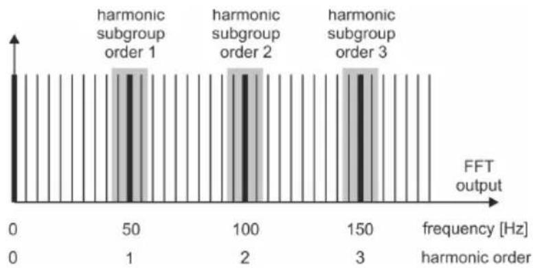
bar
| harmonic order | FFT output | | -------------- | ---------- | | 50 | 1 | | 100 | 2 | | 150 | 3 |Fig. 68. Determination of harmonic subgroups (50 Hz system).
The IEC 61000-4-30 standard recommends that the harmonic subgroup method is used in power quality analyzers.
Example
In order to calculate the 3^rd harmonic component in the 50 Hz system, use the 150 Hz main spectral line and neighbouring 145 Hz and 155 Hz lines. The resultant amplitude is calculated with the RMS method.
3.8 Event detection
The PQM-707 analyzer gives a lot of event detection options in the tested mains system. An event is the situation when the parameter value exceeds the user-defined threshold.
The fact of event occurrence is recorded on the memory card as an entry which includes:
- parameter type,
• channel in which the event occurred,
• times of event beginning and end, - user-defined threshold value,
• parameter extreme value measure during the event,
• parameter average value measure during the event.
Depending on the parameter type, you can set one, two or three thresholds which will be checked by the analyzer. The table below lists all parameters for which the events can be detected, including specification of threshold types.
Tab. 8. Event threshold types for individual parameters
| Parameter | Interruption | Dip | Swell | Minimum | Maximum | |
| U | RMS voltage | ● | ● | ● | ||
| U_DC | DC voltage | ●(1) | ||||
| I | RMS current | ● | ● | |||
| bc | DC current | ●(1)(2) | ||||
(1) only in DC and DC+M system types.
(2) only by using C-5A probes.
Some parameters can take positive and negative values. Examples are DC voltage and current. As the event detection threshold can only be positive, in order to ensure correct detection for above-mentioned parameters, the analyzer compares with the threshold their absolute values.
Example
Event threshold for DC voltage has been set at 100 V. If the measured DC voltage goes below -100V, there will be detected an event of exceeding DC voltage value.
Two parameter types: RMS voltage and RMS current can generate events for which the user can also have the waveforms record.
The analyzer records the waveforms of active channels (voltage and current) at the event start and end. In both cases, six periods are recorded: two before the start (end) of the event and four after start (end) of the event. The waveforms are recorded in an 8-bit format with 10.24 kHz sampling frequency.
The event information is recorded at its end. In some cases it may happen that event is active when the recording is stopped (i.e. the voltage dip continues). Information about such event is also recorded, but with the following changes:
- no event end time,
- extreme value is only for the period until the stop of recording,
• average value is not given, - only the beginning waveform is available for RMS voltage or current related events.
In order to eliminate repeated event detection when the parameter value oscillates around the threshold value, the analyzer has a functionality of user-defined event detection hysteresis. It is defined in percent in the following manner:
- for RMS voltage events, it is the percent of the nominal voltage range (for example 2% of 230 V, that is 4.6 V),
- for RMS current events, it is the percent of the nominal current range (for example for C-4 probes and absence of transducers, the 2% hysteresis equals 0.02 × 1000 A = 20 A),
- for remaining parameters, the hysteresis is specified as a percent of maximum threshold (for example, if the maximum threshold for DC voltage has been set to 100V, the hysteresis will be 0.02 × 100V = 2V .
3.9 Methods of parameter's averaging
| Method of averaging parameter | |
| Parameter | Averaging method |
| RMS Voltage | RMS |
| DC voltage, DC current | arithmetic average |
| Frequency | arithmetic average |
| Crest Factor U, I | arithmetic average |
| Symmetrical components U, I | RMS |
| Unbalance factor U, I | calculated from average values of symmetrical components |
| RMS Current | RMS |
| Active, Reactive, Apparent and Distortion Power | arithmetic average |
| Power Factor | calculated from the averaged power values |
| arithmetic average | |
| calculated from the averaged power values | |
| THD-F U, I | calculated as the ratio of the average RMS value of the higher harmonics to the average RMS value of the fundamental component (for THD-F), or the ratio of the average of RMS value of higher harmonics to the average value of RMS value (for THD-R) |
| Harmonic amplitudes U, I | RMS |
Note:
RMS average value is calculated according to the formula:
$$ R M S = \sqrt {\frac {1}{N} \sum_ {i = 1} ^ {N} X _ {i} ^ {2}} $$
The arithmetic average (AVG) is calculated according to the formula:
$$ A V G = \frac {1}{N} \sum_ {i = 1} ^ {N} X _ {i} $$
where:
- X is subsequent parameter value to be averaged,
- N is the number of values to be averaged.
4 Calculation formulas
4.1 Single-phase network
| Single-phase network | |||
| Parameter | Method of calculation | ||
| Name | Designation | Unit | |
| Voltage (True RMS) | U_A | V | 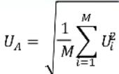 where U_i is a subsequent sample of voltage U_A-N M=2048 for 50Hz and 60 Hz where U_i is a subsequent sample of voltage U_A-N M=2048 for 50Hz and 60 Hz |
| Voltage DC component | U_ADC | V | 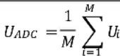 where U_i is a subsequent sample of voltage U_A-N M=2048 for 50Hz and 60 Hz where U_i is a subsequent sample of voltage U_A-N M=2048 for 50Hz and 60 Hz |
| Frequency | F | Hz | number of full voltage periods U_A-N counted during 10-sec period (clock time) divided by the total duration of full periods |
| Current (True RMS) | I_A | A | 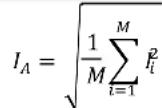 where I_i is subsequent sample of current I_A M=2048 for 50Hz and 60 Hz where I_i is subsequent sample of current I_A M=2048 for 50Hz and 60 Hz |
| Current constant component | I_ADC | A | 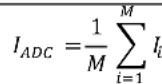 where I_i is a subsequent sample of current I_A M=2048 for 50Hz and 60 Hz where I_i is a subsequent sample of current I_A M=2048 for 50Hz and 60 Hz |
| Active power | P | W | 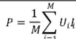 where U_i is a subsequent sample of voltage U_A-N I_i is a subsequent sample of current I_A M=2048 for 50Hz and 60 Hz where U_i is a subsequent sample of voltage U_A-N I_i is a subsequent sample of current I_A M=2048 for 50Hz and 60 Hz |
| Budeanu reactive power | Q_B | var | Q 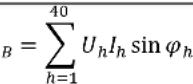 where U_h is h-th harmonic of voltage U_A-N I_h jest h-th harmonic of current I_A _h is h-th angle between harmonic U_h and I_h where U_h is h-th harmonic of voltage U_A-N I_h jest h-th harmonic of current I_A _h is h-th angle between harmonic U_h and I_h |
| Reactive power of fundamental component | Q_i | var |  where U_1 is fundamental component of voltage U_A-N I_h is fundamental component of current I_A _I is angle between fundamental components U_I and I_I where U_1 is fundamental component of voltage U_A-N I_h is fundamental component of current I_A _I is angle between fundamental components U_I and I_I |
| Apparent power | S | VA |  |
| Apparent distortion power | S_N | VA | S_N=^2-(U_1I_1)^2 |
| Budeanu distortion power | D_B | var | D 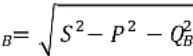 |
| Power Factor | PF | - |  If PF<0, then the load is of a generator typeIf PF>0, then the load is of a receiver type If PF<0, then the load is of a generator typeIf PF>0, then the load is of a receiver type |
| Displacement power factor | - | = DPF = ( U_1 - I_1) where _I1 is an absolute angle of the fundamental component of voltage U_A-N _II1 is an absolute angle of the fundamental component of current I_A | |
| Tangent φ | tanφ | - | tan = where: Q = Q_B when Budeanu method was chosen, Q = Q_I when IEEE 1459 method was chosen, |
| Harmonic components of voltage and current | U_nx I_nx | V A | method of harmonic subgroups according toIEC 61000-4-7x (harmonic) = 1..50 |
| Total Harmonic Distortion for voltage, referred to the fundamental component | THDU_F | - | THDU_F = _h=2^40 U_h^2U_1 × 100% where U_h is h-th harmonic of voltage U_A-N U_i is fundamental component of voltage U_A-N |
| Total Harmonic Distortion for voltage, referred to RMS | THDU_R | - | THDU_R = _h=2^40 U_h^2U_ARMS × 100% where U_h is h-th harmonic of voltage U_A-N |
| Total Harmonic Distortion for current, referred to the fundamental component | THDI_F | - | THDI_F = _h=2^40 I_h^2I_1 × 100% where I_h is h-th harmonic of current I_A I_h is fundamental component of current I_A |
| Total Harmonic Distortion for current, referred to RMS | THDI_R | - | THDI_R = _h=2^40 I_h^2I_ARMS × 100% where I_h is h-th harmonic of current I_A |
| Voltage crest factor | CFU | - | CFU = |U_i|U_ARMS max |U_i| Where the operator expresses the highest absolute value of voltage U_A-N samplesi = 2048 for 50 Hz and 60 Hz |
| Current crest factor | CFI | - | CFI = |I_i|I_ARMS max |I_i| Where the operator expresses the highest absolute value of current I_A samplesi = 2048 for 50 Hz and 60 Hz |
| Short-term flicker | P_st | - | calculated according to IEC 61000-4-15 |
| Long-term flicker | P_it | - | P_LT = [3]_i=1^N P_STi^3N where P_STi is subsequent i-th indicator of short-term flicker |
| Active energy (consumed and supplied) | E_P+ E_P- | Wh | E_P+ = _i=1^m P_+(i)T(i) P_+(i) = P(i) & dla P(i) > 0 \ 0 & dla P(i) ≤ 0 E_P- = _i=1^m P_-(i)T(i) P_-(i) = |P(i)| & dla P(i) < 0 \ 0 & dla P(i) ≥ 0 where:i is subsequent number of the 10/12-period measurement window P(i) represents active power P calculated in i-th measuring window T(i) represents duration of i-th measuring window (in hours) |
| Budeanu reactive energy (consumed and supplied) | E_QB+ E_QB- | varh | E_QB+=_i=1^mQ_B+(i)T(i) Q_B+(i)=\_B(i)dla Q_B(i)>0\\0 dla Q_B(i)≤ 0. E_QB-=_i=1^mQ_B-(i)T(i) Q_B-(i)=\|Q_B(i)|dla Q_B(i)<0\\0 dla Q_B(i)≥ 0. where: i is subsequent number of the 10/12-period measurement window Q_B(i) represents Budeanu active power Q_B calculated in i -th measuring window T(i) represents duration of i -th measuring window (in hours) |
| Reactive energy of fundamental component (consumed and supplied) | E_Q1+ E_Q1- | varh | E_Q1+=_i=1^mQ_1+(i)T(i) Q_1+(i)=\_1(i)dla Q_1(i)>0\\0 dla Q_1(i)≤ 0. E_Q1-=_i=1^mQ_1-(i)T(i) Q_-(i)=\|Q_1(i)|dla Q_1(i)<0\\0 dla Q_1(i)≥ 0. where: i is subsequent number of the 10/12-period measurement window Q_1(i) represents reactive power of fundamental component Q_1 calculated in i -th measuring window T(i) represents duration of i -th measuring window (in hours) |
| Apparent energy | E_S | VAh | E_S=_i=1^mS(i)T(i) where: i is subsequent number of the 10/12-period measurement window S(i) represents apparent power S calculated in i -th measuring window T(i) represents duration of i -th measuring window (in hours) |
4.2 Split-phase network
| Split-phase network(parameters not mentioned are calculated as for single-phase) | |||
| Parameter | Method of calculation | ||
| Name | Designation | Unit | |
| Total active power | P_tot | W | P_tot=P_A+P_B |
| Total Budeanu reactive power | Q_Btot | var | Q_Btot=Q_BA+Q_BB |
| Total reactive power of fundamental component | Q_1tot | var | Q_1tot=Q_1A+Q_1B |
| Total apparent power | S_tot | VA | S_tot=S_A+S_B |
| Total apparent distortion power | S_Ntot | VA | S_Ntot=S_NA+S_NB |
| Total Budeanu distortion power | D_Btot | var | D_Btot=D_BA+D_BB |
| Total Power Factor | PF_tot | - | PF_tot=_totS_tot |
| Total displacement power factor | _tot\_tot | - | _tot=DPF_tot=12(_A+_B) |
| Total tangent φ | _tot | - | _tot=_totP_tot where: Q_tot=Q_Btot , when Budeanu method was chosen, Q_tot=Q_1tot , when IEEE 1459 method was chosen, |
| Total active energy (consumed and supplied) | E_P+tot E_P-tot | Wh | E_P+tot=_i=1^mP_tot+(i)T(i) P_tot+(i)=\_tot(i)dla P_tot(i)>0\\0 dla P_tot(i)≤ 0. E_P-tot=_i=1^mP_tot-(i)T(i) P_tot-(i)=\|P_tot(i)|dla P_tot(i)<0\\0 dla P_tot(i)≥ 0. where: i is subsequent number of the 10/12-period measurement window P_tot(i) represents total active power P_tot calculated in i -th measuring window T(i) represents duration of i -th measuring window (in hours) |
| Total Budeanu reactive energy (consumed and supplied) | E_QB+tot E_QB-tot | varh | E_QB+tot=_i=1^mQ_Btot+(i)T(i) Q_Btot+(i)=\_Btot(i)dla Q_Btot(i)>0\\0 dla Q_Btot(i)≤ 0. E_QB-tot=_i=1^mQ_Btot-(i)T(i) Q_Btot-(i)=\|Q_Btot(i)|dla Q_Btot(i)<0\\0 dla Q_Btot(i)≥ 0. where: i is subsequent number of the 10/12-period measurement window Q_Btot(i) represents total reactive power Q_Btot calculated in i -th measuring window T(i) represents duration of i -th measuring window (in hours) |
| Total reactive energy of fundamental component (consumed and supplied) | E_Q1+tot E_Q1-tot | varh | E_Q1+tot = _i=1^m Q_1tot+(i)T(i) Q_1tot+(i) = Q_1tot+(i) & dla Q_1tot(i) > 0 \ 0 & dla Q_1tot(i) ≤ 0 E_Q1-tot = _i=1^m Q_1tot-(i)T(i) Q_1tot-(i) = |Q_1tot-(i)| & dla Q_1tot(i) < 0 \ 0 & dla Q_1tot(i) ≥ 0 where: i is subsequent number of the 10/12-period measurement window Q_1tot(i) represents total reactive power Q_1tot calculated in i -th measuring window T(i) represents duration of i -th measuring window (in hours) |
| Total apparent energy | E_Stot | VAh | E_Stot = _i=1^m S_tot(i)T(i) where: i is subsequent number of the 10/12-period measurement window S_tot(i) represents total apparent power S_tot calculated in i -th measuring window T(i) represents duration of i -th measuring window (in hours) |
4.3 3-phase 4-wire network
| 3-phase 4-wire network(parameters not mentioned are calculated as for single-phase) | |||
| Parameter | Method of calculation | ||
| Name | Designation | Unit | |
| Total active power | P_tot | W | P_tot=P_A+P_B+P_C |
| Total Budeanu reactive power | Q_Btot | var | Q_Btot=Q_BA+Q_BB+Q_BC |
| Total reactive power acc. to IEEE 1459 | Q_t^+ | var | Q_1^+ = 3U_1^+ I_1^+ _1^+ where:U1+ is the voltage positive sequence component (of the fundamental componentI1+ his the current positive sequence component (of the fundamental component) _1+ is the angle between components U_1+ and I_1+ |
| Effective apparent power | S_e | VA | S_e=3U_eI_e where: U_e=3(U_A^2+U_B^2+U_C^2)+U_AB^2+U_BC^2+U_CA^218 I_e=_A^2+I_B^2+t^2+I_N^23 |
| Effective apparent distortion power | S_eN | VA | S_eN=_e^2+S_e1^2 where: S_e1=3U_e1I_e1 U_e1=3(U_A1^2+U_B1^2+U_C1^2)+U_AB1^2+U_BC1^2+U_CA1^218 I_e1=_A1^2+I_B1^2+I_C1^2+I_N1^23 |
| Total Budeanu distortion power | D_Btot | var | D_Btot=D_BA+D_BB+D_BC |
| Total Power Factor | PF_tot | - | PF_tot=_totS_e |
| Total displacement power factor | _tot\_tot | - | _tot=DPF_tot=13(_A+_B+_C) |
| Total tangent φ | _tot | - | _tot=_totP_tot where: Q_tot=Q_Btot , when Budeanu method was chosen, Q_tot=Q_1tot , when IEEE 1459 method was chosen. |
| Total active energy (consumed and supplied) | E_P+tot E_P-tot | Wh | formula same as in split-phase system |
| Total Budeanu reactive energy (consumed and supplied) | E_QB+tot E_QB-tot | varh | formula same as in split-phase system |
| Total reactive energy of fundamental component (consumed and supplied) | E_Q1+tot E_Q1-tot | varh | formula same as in split-phase system |
| Total apparent energy | E_Stot | VAh | E_Stot=_i=1^mS_e(i)T(i) where:i is subsequent number of the 10/12-period measurement window S_e(i) represents the effective apparent power S_e , calculated in i-th measuring window T(i) represents duration of i-th measuring window (in hours) |
| RMS value of zero voltage sequence | U_0 | V | _0=13(_A1+_B1+_C1) U_0=mag(_0) where _A1,_B1,_C1 are vectors of fundamental components of phase voltages U_A, U_B, U_C Operator mag() indicates vector module |
| RMS value of positive voltage sequence | U_1 | V | _1=13(_A1+_B1+^2U_C1) U_1=mag(_1) where _A1,_B1,_C1 are vectors of fundamental components of phase voltages U_A, U_B, U_C Operator mag() indicates vector module a=1e^j120^=-12+32j a^2=1e^j240^=-12-32j |
| RMS value of negative voltage sequence | U_2 | V | _2=13(_A1+^2_B1+_C1) U_2=mag(U_-2) where _A1,_B1,_C1 are vectors of fundamental components of phase voltages U_A, U_B, U_C Operator mag() indicates vector module a=1e^j120^=-12+32j a^2=1e^j240^=-12-32j |
| Voltage unbalance factor for zero component | u_0 | % | u_0=_0U_1·100% |
| Voltage unbalance factor for negative sequence | u_2 | % | u_2=_2U_1·100% |
| Current zero sequence | I_0 | A | _0=13(_A1+_B1+_C1) I_0=mag(I_-0) where I_A1, I_B1, I_C1 are vectors of fundamental components for phase currents I_A, I_B, I_C Operator mag() indicates vector module |
| RMS value of positive current sequence | I_1 | A | _1=13(_A1+_B1+^2_C1) I_1=mag(I_-1) where I_A1, I_B1, I_C1 are vectors of fundamental current components I_A, I_B, I_C Operator mag() indicates vector module |
| RMS value of negative current sequence | I_2 | A | _2=13(_A1+^2_B1+_C1) I_2=mag(I_-2) where J_A1, J_B1, J_C1 are vectors of fundamental components for phase voltages k, I_B, k Operator mag() indicates vector module |
| Current unbalance factor for zero sequence | i_0 | % | i_0=_0I_1·100% |
| Current unbalance factor for negative sequence | i_2 | % | i_2=_2I_1·100% |
4.4 3-phase 4-wire (no U L2) / 2 12 - element network
| 3-phase 4-wire (no U L2) / 2 1/2 - element networkAll parameters are calculated as in 3-phase 4-wire network expt UB voltage | |||
| Parameter | Method of calculation | ||
| Name | Designation | Unit | |
| UB phase voltage | UB | V | UB=-(UA+UC) |
4.5 3-phase 3-wire networks
| 3-phase 3-wire network3-phase open delta network2-element network(Parameters: RMS voltage and current, DC components of voltage and current, THD, flicker are calculated as for 1-phase circuits; instead of the phase voltages, phase-to-phase voltages are used. Symmetrical components and unbalance factors are calculated as in 3-phase 4-wire systems.) | |||
| Parameter | Method of calculation | ||
| Name | Designation | Unit | |
| Phase-to-phase voltage U_CA | U_CA | V | U_CA=-(U_AB+U_BC) |
| Current I_2 (Aron measuring circuits) | I_2 | A | I_2=-(I_1+I_3) |
| Total active power | P_tot | W | P_tot=1M(_i=1^MU_iACI_iA+_i=1^MU_iBCI_iB) where: U_AC is a subsequent sample of voltage U_A-C U_BC is a subsequent sample of voltage U_B-C I_A is a subsequent sample of current I_A I_iB is a subsequent sample of current I_B M=2048 for 50Hz and 60Hz |
| Total apparent power | S_e | VA | S_e=3U_eI_e where: U_e=_AB^2+U_BC^2+U_CA^29 I_e=_A^2+I_B^2+I_C^23 |
| Total reactive power (Bu-deanu and IEEE 1459) | Q_Btot | var | Q=N=_e^2-P^2 |
| Total Budeanu distortionpower | D_Btot | var | D_Btot=0 |
| Effective apparent distor-tion power | S_eN | VA | S_eN=_e^2+S_e1^2 where: S_e1=3U_e1I_e1 U_e1=_AB1^2+U_BC1^2+U_CA1^29 I_e1=_A1^2+I_B1^2+I_C1^23 |
| Total Power Factor | PF_tot | - | PF_tot=_totS_e |
| Active energy (consumedand supplied) | E_P-tot E_P-tot | Wh | formula same as in split-phase system |
| Total apparent energy | E_Stot | VAh | E_Stot=_i=1^mS_e( T(i)) where:is subsequent number of the 10/12-period measurement window S_i(i) represents the total apparent power S_o calculated in i-th measuring window T(i) represents duration of i-th measuring window (in hours) |
5 Power Quality - a short guide
5.1 Basic Information
The measurement methodology is mostly imposed by the energy quality standards, mainly IEC 61000-4-30. This standard, introducing precise measurement algorithms, ordered analyzers market, allowing customers to easily compare the devices and their results between the analyzers from different manufacturers. Previously, these devices used different algorithms, and often the results from measurements on the same object were completely different when tested with different devices.
The factors behind growing interest in these issues have included wide use of electronic power controllers, DC/DC converters and switched-mode power supplies, energy-saving fluorescent lamps, etc., that is widely understood electrical power conversion. All of these devices had a tendency to significantly deform the supply current waveform.
The design of switched-mode power supplies (widely used in household and industrial applications) is often based on the principle that the mains alternating voltage is first rectified and smoothed with the use of capacitors, meaning that it is converted to direct voltage (DC), and then with a high frequency and efficiency is converted to required output voltage. Such a solution, however, has an undesirable side effect. Smoothing capacitors are recharged by short current pulses at moments when the mains voltage is close to peak value. From power balance rule it is known that if the current is taken only at short intervals, its crest value must be much higher than in case it is taken in a continuous manner. High ratio of current crest value to RMS value (a so-called crest factor) and reduction of power factor (PF) will result in a situation in which in order to obtain a given active power in a receiver (in watts), the power supplier must supply power greater than the receiver active power (this is a so-called apparent power expressed in volt-amperes, VA). Low power factor causes higher load on the transmission cables and higher costs of electricity transfer. Harmonic current components accompanying such parameters cause additional problems. As a result, the electricity suppliers have started to impose financial penalties upon the customers who have not provided sufficiently high power factor.
Among entities that may be potentially interested in power quality analyzers are power utility companies on one hand, (they may use them to control their customers), and on the other hand the power consumers who may use the analyzers to detect and possibly improve the low power factor and solve other problems related to widely understood power quality issues.
The power source quality parameters, as well as the properties of receivers, are described with many various magnitudes and indicators. This section can shed some light on this area.
As already mentioned, the lack of standardization of measurement methods has caused significant differences in values of individual mains parameters calculated with various devices. Efforts of many engineers resulted in IEC 61000-4-30 standard concerning power quality. For the first time, this standard (and related standards) provided very precise methods, mathematical relations and required measurement accuracy for power quality analyzers. Compliance with the standard (in particular, the class A) should be a guarantee of repeatable and almost identical measurement results of the same magnitudes measured with devices from different manufacturers.
5.1.1 Current transformer probes (CT) for AC measurements
CT Current Transformer Probe is just a transformer converting a large current in primary winding to a smaller current in secondary winding. The jaws of typical current probe are made of a ferromagnetic material (such as iron) with the secondary winding wound around. The primary wind-
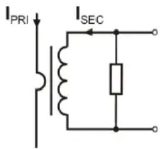
Fig. 69. CT current transformer probe with voltage output.
ing is a conductor around which the probe jaws are closed, hence most often it is one single coil. If the 1000-ampere current flows through the tested conductor, in the secondary winding with 1000 coils the current will be only 1 A (if the circuit is closed). In case of probes with voltage output, a shunt resistor is located in the probes.
Such current transformer has a few characteristic properties. It can be used to measure very large currents, and its power consumption is low. The magnetizing current causes some phase shift (tenth of a degree) which can result in some power measurement error (particularly when the power factor is low). Another disadvantage of this probe type is also the core saturation phenomenon when very large currents are measured (above the rated range). Core saturation as a result of magnetizing hysteresis leads to significant measurement errors which can be eliminated
only by the core demagnetization. The core becomes saturated also when the measured current has a significant DC component. An undeniable disadvantage of such probe is also its considerable weight.
Despite such drawbacks, the CT probes are presently the most widely used non-invasive alternating current (AC) measurement method.
The following CT probes can be used with the PQM-707 analyzers to measure alternating currents:
• C-4(A), rated range 1000 A AC,
• C-6(A), rated range 10 A AC,
• C-7(A), rated range 100 A AC.
5.1.2 AC/DC measurement probes
There are situations when it is necessary to measure the current DC component. In such case, the probes must be based on different principle of operation than a traditional current transformer. The probes in this case use the physical phenomenon known as the Hall effect and include a Hall sensor. In brief: the effect is the production of voltage across an electrical conductor through which the current is flowing and which is placed in a magnetic field. The voltage is transverse to the field induction vector.
The probes based on this phenomenon can measure the DC and AC current component. The conductor with current located inside the probes generates a magnetic field which concentrates in an iron core. In the core slot, where both probe parts are joined, placed is a semiconductor Hall sensor, and its output voltage is amplified by an electronic circuit supplied from a battery.
This probe type usually has the current zero adjustment knob. To adjust the current zero, close the jaws (no conductor inside) and turn the knob until the DC indication is zero.
In the area of AC/DC measurement probes, Sonel S.A. offers the C-5A probe with rated range of 1000 A AC / 1400 A DC. This probe has a voltage output and for 1000 A rated current it gives a 1 V voltage signal (1 mV/A).
5.1.3 Flexible current probes
Flexible Current Probes are based on a totally different physical principle than the current transformer. Their principal part is a so-called Rogowski coil, named after German physicist Walter Rogowski. It is an air-core coil wound around a conductor with current. Special design of the coil allows leading out its both ends on the same side, thus facilitating probe placement around the conductor (the return end is placed inside the coil at its entire length). The current flowing through the measured conductor causes centric magnetic field lines which due to the self-induction phenomenon induce the electromotive force at the end of the coil. This voltage, however, is proportional to the rate of current change in the conductor, and not to the current itself.
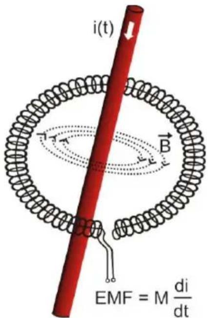
Fig. 70. Rogowski coil.
In comparison with current transformers, the Rogowski coil has a few indisputable advantages. As it does not have a core, the core saturation effect is eliminated; thus being a perfect instrument to measure large currents. Such coil has also an excellent linearity and a wide pass band, much wider than a current transformer, and its weight is much smaller.
However, until recently the wider expansion of flexible probes in the current measurement area was difficult. There are some factors which hinder practical implementation of a measurement system with a Rogowski coil. One of them is a very low voltage level which is induced on the probes (it depends on geometrical dimensions of the coil). For example, the output voltage for the 50 Hz frequency of the F-series flexible probes (to be used with PQM-707) is about 45 V/A. Such low voltages require the use of precise and low-noise amplifiers which of course increase the costs.
Because the output voltage is proportional to the current derivative, it is necessary to use an integrating circuit; generally, the flexible probes comprise a Rogowski coil and an analog integrator circuit (characteristic battery-powered module). On the integrator output available is the voltage signal proportional to measured
current and suitably scaled (for example 1 mV/A).
Another problem connected with the Rogowski coil is its sensitivity to external magnetic fields. A perfect coil should be sensitive only to the fields closed within its area and should totally suppress external magnetic fields. But this is a very difficult task. The only way to obtain such properties is very precise manufacture of the coil, with perfectly homogenous windings and impedance as low as possible. It is the high precision which causes a relatively high price of such probe.
The user may connect the analyzer to the flexible probes offered by Sonel S.A. Clamp types and parameters are described in section 7.
5.2 Flicker
In terms of power quality, flicker means a periodical changes of the luminous intensity as a result of fluctuations of voltage supplied to light bulbs.
The flicker measurement function appeared in the power quality analyzers when it turned out that this phenomenon causes a deteriorated well-being, annoyance, sometimes headache, etc. The luminous intensity fluctuations must have a specified frequency, they may not be to slow as then human iris can adapt to changed lighting, and they may not be too fast because the filament inertia offsets these fluctuations almost totally.
The tests have proved that maximum arduousness occurs at the frequency of about 9 changes per second. The most sensitive light sources are traditional incandescent bulbs with tungsten filament. Halogen bulbs, which filaments have much higher temperature, have also much higher inertia which reduces the perceived brightness changes. Fluorescent lamps have the best flicker “resistance”, as due to their some specific properties they stabilize the current flowing through the lamp during the voltage changes, and thus reduce the fluctuations.
Flicker is measured in so-called perceptibility units, and there are two types of flicker: short-term P_ST which is determined once every 10 minutes, and long-term P_LT which is calculated on the basis of 12 consecutive P_ST values, i.e. every 2 hours. Long measurement time results directly from slow-changing character of this phenomenon – in order to collect a reliable data sample, the measurement must be long. P_ST equal to 1 is considered a value on the border of annoyance – certainly sensitivity to flicker is different in different people; this threshold has been adopted after tests carried out on a representative group of people.
What causes flicker? Most frequently, the reason is the voltage drop as a result of connecting and disconnecting large loads and some level of flicker is present in the majority of mains systems. Disregarding the unfavorable effect on humans described above, flicker does not need to be – and usually is not – a symptom of malfunctioning of our installation. However, if a rather abrupt and unexplainable flicker level increase is observed in the mains (increase of P_ST and P_LT ), this should not be ignored under any circumstances. It may turn out that the flicker is caused by unsure connections in the installation – increased voltage drops on connections in the distribution panel (for example) will result in higher voltage fluctuations on the receivers, such as light bulbs. The voltage drops on connections also cause their heating, and finally sparking and possibly a fire. Periodical mains tests and described symptoms can turn our attention and help find the source of hazard.
5.3 Power measurement
Power is one of the most important parameters defining the properties of electrical circuits. The basic magnitude used for financial settlements between the supplier and the consumer is electric energy which is the power multiplied by time.
A few different power types can be found in electrical engineering:
• active power, designated as P and measured in watts,
- reactive power, designated as Q, unit is var,
- apparent power, S, unit is VA.
These three types of power are the most known, but there are also other types.
At school we are taught that these three power types make up a so-called power triangle which properties are expressed by the following equation:
$$ \mathrm{P} ^ {2} + \mathrm{Q} ^ {2} = \mathrm{S} ^ {2} $$
This equation is however correct only for systems with sinusoidal voltage and current waveforms.
Before a more detailed discussion about the power measurement, individual types of power should be defined.
5.3.1 Active power
Active power P is a magnitude with precise physical meaning and it expresses the ability of a system to perform a given work. It is the power most desired by the energy consumers and it is for this supplied power that the consumer pays the supplier in a given settlement period (the problem of fees for additional reactive power is discussed separately – see below). It is the active power (and consequently, the active energy) which is measured by electric energy meters in each household.
Basic formula to calculate the active power is as follows:
$$ P = \frac {1}{T} \int_ {t} ^ {t + T} u (t) i (t) d t $$
where: u(t) – instantaneous voltage value, i(t) - instantaneous current value, T – period for which the power is calculated.
In sinusoidal systems, the active power can be calculated as:
$$ P = U I \cos \varphi $$
where: U is RMS voltage, I is RMS current, and is the phase shift angle between the voltage and the current.
The PQM-707 analyzer calculates the active power directly from the integral formula, using sampled voltage and current waveforms:
$$ P = \frac {1}{M} \sum_ {i = 1} ^ {M} U _ {i} I _ {i} $$
where M is a number of samples in the 10/12-period measuring window (2048 for the 50 Hz and 60 Hz system), U_i and I_i are successive voltage and current samples.
5.3.2 Reactive power
The most popular formula for reactive power is also correct only for one-phase circuits with sinusoidal voltage and current waveforms:
$$ Q = U I \sin \varphi $$
Interpretation of this power in such systems is as follows: it is an amplitude of AC component of instantaneous power on the source terminals. Existence of a non-zero value of this power indicates a bidirectional and oscillating energy flow between the source and the receiver.
Let us imagine a one-phase system with sinusoidal voltage source which load is a RC circuit. As under such conditions, the elements' behavior is linear, the source current waveform will be sinusoidal, but due to the properties of capacitor it will be shifted in relation to source voltage. In such a system, reactive power Q will be non-zero and can be interpreted as an amplitude of energy oscillation which alternately is collected in the capacitor and returned to the source. Capacitor active power equals zero.
However, it turns out the energy oscillation seems only an effect, and that it appears in particular cases of circuits with sinusoidal current and voltage waveforms, and is not the cause of reactive power. Research in this area has shown that reactive power occurs also in circuits without any energy oscillation. This statement may surprise many engineers. In latest publications on power theory, the only physical phenomenon mentioned which always accompanies appearance of reactive power is phase shift between current and voltage.
The reactive power formula given above is correct only for one-phase sinusoidal circuits. The question thus arises: how do we calculate the reactive power in non-sinusoidal systems? This question opens a proverbial Pandora's box among electrical engineers. It turns out that the reactive power definition in real systems (and not only those idealized) has been subject to controversy and now (2009) we do not have one, generally accepted definition of reactive power in systems with non-sinusoidal voltage and current waveforms, not to mention even unbalanced three-phase systems. The IEEE (Institute of Electrical and Electronics Engineers) 1459-2000 standard (from 2000) does not give a formula for total reactive power for non-sinusoidal three-phase systems – as three basic types of power the standard mentions are active power, apparent power and – attention – nonactive power designated as N. Reactive power has been limited only to the fundamental component and designated Q_1 .
This standard is the last document of this type issued by recognized organization which was to put the power definition issues in order. It was even more necessary as the voices had been appearing in scientific circles for many years that the power definitions used so far may give erroneous results. Most of all, the controversies related to the definition of reactive and apparent power (and also distortion power – see below) in one- and three-phase systems with non-sinusoidal current and voltage waveforms.
In 1987, professor L.S. Czarnecki proved that the widely used definition of reactive power by Budeanu was wrong. This definition is still taught in some technical schools and it was proposed by professor Budeanu in 1927. The formula is as follows:
$$ Q _ {B} = \sum_ {n = 0} ^ {\infty} U _ {n} I _ {n} \sin \varphi_ {n} $$
where U_n and I_n are voltage and current harmonics of order n, and _n are angles between these components.
As, after this magnitude has been introduced, the known power triangle equation was not met for circuits with non-sinusoidal waveforms, Budeanu introduced a new magnitude called the distortion power:
$$ D _ {B} = \sqrt {S ^ {2} - \left(P ^ {2} + Q _ {B} ^ {2}\right)} $$
Distortion power was to represent in the system the power appearing due to distorted voltage and current waveforms.
For years, reactive power had been associated with energy oscillations between the source and the load. The formula indicates that according to Budeanu's definition, the reactive power is a sum of reactive power of individual harmonics. Due to the sinφ factor, such components can be positive or negative, depending on the angle between the harmonics of voltage and current. Hence, a situation is possible when total reactive power Q_B will be zero at non-zero harmonic components. Observation that at non-zero components, total reactive power can – according to this definition – be zero is a key to a deeper analysis which finally allowed proving that in some situations Q_B can give quite surprising results. The research has questioned the general belief that there is a relation between energy oscillations and Budeanu reactive power Q_B . One can give examples of circuits in which despite oscillating character of instantaneous power waveform, reactive power according to Budeanu is zero. Over the years, the scientists have not been able to connect any physical phenomenon to the reactive power according to this definition.
Such doubts about the correctness of this definition of course also cast shadow on the related distortion power D_B . The scientists have started to look for answers to the question whether the distortion power D_B really is the measure of distorted waveforms in non-sinusoidal circuits. The distortion is a situation in which the voltage waveform cannot be “put” on the current waveform with two operations: change of amplitude and shift in time. In other words, if the following condition is met:
$$ u (t) = A i (t - \tau) $$
the voltage is not distorted in relation to the current. In case of sinusoidal voltage and load which is any combination of RLC elements, this condition is always met (for sinusoidal waveforms, these elements maintain linearity). However, when the voltage is distorted, the RLC load does not ensure absence of current distortion in relation to voltage any more, and the load is no longer linear – it is necessary to meet some additional conditions (module and phase of load impedance changing with frequency).
And then, is really D_B a measure of such distortion? Unfortunately, also in this case the Budeanu's power theory fails. It has been proven that the distortion power can be equal to zero in a situation when voltage is distorted in relation to current waveform, and vice versa, the distortion power can be non-zero at total absence of distortion.
Practical aspect of this power theory which relates to improvement of power factor in systems with reactive power was to be the feature to take the most advantage of correct definitions of reactive power. The compensation attempts based on the Budeanu reactive power and related distortion power fell through. These magnitudes did not allow even a correct calculation of correction capacitance which gives the maximum power factor. Sometimes, such attempts ended even with additional deterioration of power factor.
How come, then, that the Budeanu's power theory has become so popular? There may be several reasons. Firstly, engineers got accustomed to old definitions and the curricula in schools have not been changed for years. This factor is often underestimated, though as a form of justification it can be said that this theory had not been refuted for 60 years. Secondly, in the 1920s there were no measuring instruments which could give insight in individual voltage and current harmonic components and it was difficult to verify new theories. Thirdly, distorted voltage and current waveforms (i.e. with high harmonics contents) are a result of revolution in electrical power engineering which did not start before the second part of the last century. Thyristors, controlled rectifiers, converters, etc. began to be widely used. All these caused very large current distortion in the mains, and consequently increased harmonic distortion. Only then, were the deficiencies of the Budeanu's theory felt. Finally, fourthly, the scientific circles related to power utilities were aware of the fact that industrial plants had invested a fortune in the measuring infrastructure (energy meters). Each change is this respect could bring about huge financial consequences.
However, slow changes became visible in the views of electrical engineers. With time, as nonlinear loads were more and more frequent and the waveforms more and more distorted, the limitations of used formulas could no longer be tolerated.
A very significant event was the 2000 publication by IEEE of the standard 1459 called “Definitions for the Measurement of Electric Power Quantities Under Sinusoidal, Non-Sinusoidal, Balanced, or Unbalanced Conditions”. For the first time, Budeanu’s definition of reactive power has been listed as not recommended which should not be used in new reactive power and energy meters. Many magnitudes have been also divided into the part related to the current and voltage fundamental component (first harmonics) and the part related to remaining higher harmonics. In most cases, it is recognized that the usable part of energy is transmitted by the 50/60Hz components, with much smaller (and often harmful) participation of higher harmonics.
The standard also introduced a new magnitude - nonactive power N which represents all nonactive components of power:
$$ N = \sqrt {S ^ {2} - P ^ {2}} $$
Reactive power is one of the components of nonactive power N. In one-phase systems with sinusoidal voltage and current waveforms, N equals Q; hence the nonactive power does not have any other components. In three-phase systems, this is true only for symmetrical sinusoidal systems with a balanced purely resistive load.
Other nonactive power components are related to concrete physical phenomena. According to the professor Czarnecki's theory, which is one of the best in explaining the physical phenomena in
PQM-707 user manual
three-phase systems, the power equation in such systems is as follows:
$$ S ^ {2} = P ^ {2} + D _ {s} ^ {2} + Q ^ {2} + D _ {u} ^ {2} $$
D_s is the scattered power which appears in the system as a result of changing load conductance with frequency. Hence, presence of reactive elements in the system may cause the scattered power. In this equation, reactive power Q appears when there is a phase shift between the voltage and current harmonics.
D_u means the unbalanced power which is a measure of unbalance of a three-phase receiver. This component explains the situation in which an unbalanced three-phase load of a purely resistive character results in the power factor less than one. Such load does not have the reactive power Q, and still the results from the power triangle S, P, Q are totally different (the Budeanu's power theory with its distortion power could not explain this situation either – in a purely resistive load, the distortion power D_B equals zero).
An attempt to connect the IEEE 1459-2000 standard with the Czarnecki's power theory leads to the conclusion that nonactive power conceals at least three separate physical phenomena which influence the reduced effectiveness of energy transmission from the source to the receiver, i.e. reduction of the power factor.
$$ P F = \frac {P}{S _ {e}} = \frac {P}{\sqrt {P ^ {2} + D _ {s} ^ {2} + Q ^ {2} + D _ {u} ^ {2}}} $$
In the IEEE 1459-2000 standard, reactive power known as Q has been limited to the fundamental component, for both one-phase and three-phase systems:
$$ Q _ {1} = U _ {1} I _ {1} \sin \varphi_ {1} $$
In three-phase systems, only the positive sequence component is taken into consideration:
$$ Q _ {1} ^ {+} = 3 U _ {1} ^ {+} I _ {1} ^ {+} \sin \varphi_ {1} ^ {+} $$
Correct measurement of this power requires the same phase rotation sequence (i.e. phase L2 delayed by 120^ in relation to L1, phase L3 delayed by 240^ in relation to L1).
The term of positive sequence component will be discussed in more detail in the section devoted to unbalance.
The value of reactive power of the fundamental component is the main value which allows estimating the size of capacitor to improve the displacement power factor (DPF), that is the displacement of the voltage fundamental components in relation to the current fundamental component (i.e. compensator of the reactive power of the fundamental component).
5.3.3 Reactive power and three-wire systems
Correct reactive power measurement is impossible in unbalanced receivers connected according to the three-wire system (delta and wye systems without the N conductor). Such statement may come as a surprise for many people.
The receiver can be treated as a “black box” with only 3 terminals available. We cannot determine its internal structure. In order to calculate the reactive power, we need to know the phase shift angle between the voltage and the current at each leg of such receiver. Unfortunately, we do not know this angle. In the delta-type receiver we know the voltages on individual impedances, but we do not know the current; in such systems, the phase-to-phase voltages and line currents are measured. Each line current is a sum of two phase currents. In the wye without N-type receivers, we know the currents flowing through impedance, but we do not know the voltages (each phase-to-phase voltage is a sum of two phase-to-neutral voltages.
We need to take account of the fact that at given voltage values at terminals and currents flowing
into such “black box”, there is an infinite number of variants of receiver internal structure which will give us identical measurement results of voltage and current values visible outside the black box.
Then, how is it possible that there are reactive power meters intended for measurements in three-wire systems and the mains analyzers which allow the reactive power measurement under such circumstances?
In both cases, the manufacturers use the trick which involves an artificial creation of a reference point (virtual neutral terminal N). Such point can be created very easily by connecting to the terminals of our black box a wye-connected system of three resistors of the same value.
In no case should a measuring instrument mislead the user, and such approximation can be allowed only after a clear reservation that the indicated value is not a result of actual measurement, but only an approximated value.
5.3.4 Reactive power and reactive energy meters
Reactive energy meters are devices unknown to the household users who for settlements with energy suppliers use the meters of active energy expressed in Wh or kWh. Household users are in a comfortable situation – they pay only for usable energy and do not have to think what the power factor is in their installations.
In contrast to the first group, the industrial consumers are obliged in their contracts and sometimes under pain of financial penalties to keep the power factor at an appropriate level.
The EN 50160 standard gives some guidelines for the power quality requirements, and defines the quality parameters which should be met by energy supplier. Among these parameters are, among others, mains frequency, RMS voltage, total harmonic distortion (THD) and allowed levels of individual voltage harmonics. Besides EN 50160 requirements there is often an additional condition: the supplier does not need to comply with those requirements if an energy consumer does not ensure the factor below some threshold (agreed value which can be changed in the contract between the energy supplier and consumer, i.e. 0.4) and/or exceeds the agreed level of consumed active energy.
The is defined as a ratio of measured reactive energy to the active energy in a settlement period. Going back for a while to the power triangle in sinusoidal systems, we can see that the tangent of the phase shift angle between the voltage and the current is equal to the ratio of reactive power Q to active power P. Consequently, the requirement to maintain the below 0.4 means nothing else but only that maximum level of measured reactive energy may not exceed 0.4 of the measured active energy. Each consumption of reactive energy above this level is subject to additional fees.
Does the knowledge of calculated in this manner give both interested parties an actual view of energy transmission effectiveness? Have we not mentioned before that the reactive power is only one of the nonactive power components which influence the power factor reduction? Indeed, it seems that instead of we should use the power factor PF which takes into account also other issues.
Unfortunately, if the present regulations leave no choice, than the correct reactive power measurement seems a key matter. Now, a question should be asked whether the reactive energy meters ensure correct readings in the light of the controversies described above. And what do such widely used meters really measure?
One can attempt to look for answers to these questions is the standard on such meters - IEC 62053-23. Unfortunately, to our disappointment, we will not find there any reference to measurements in non-sinusoidal conditions – the calculation formulas relate to sinusoidal conditions (we can read in the standard that due to “practical” reasons, non-sinusoidal waveforms have been excluded). The standard does not give any measurement criteria which would allow checking the meter properties at distorted voltage and current waveforms. As a surprise comes also the fact that the older standard IEC 61268 (already withdrawn) defined the test which involved checking the measurement accuracy at 10% of the third current harmonic.
The present situation leaves the choice of measuring method to the meters designers, which unfortunately leads to significant differences in reactive energy indications in the presence of high harmonic distortion level.
Older, electromechanical meters have characteristics similar to that of a low-pass filter – higher harmonics are attenuated in such meters and the reactive power measurement in the presence of harmonics is very close to the value of reactive power of the fundamental component.
Electronic meters which are more and more popular can perform the measurement with various methods. For example, they can measure active and apparent power, and then calculate the reactive power from the power triangle (square root from the sum of both such powers squared). In reality, in the view of the IEEE 1459-2000 standard, they measure the nonactive power, not the reactive power. Another manufacturer may use the method with voltage waveform shift by 90^ , which gives a result close to the reactive power of the fundamental component.
The higher the harmonics content, the higher difference in readings, and of course, as a consequence, other fees for measured energy.
As it has been signaled before, the reactive power measurement in unbalanced three-wire systems with traditional meters is subject to an additional error caused by creation of a virtual zero inside the meter which has little to do with actual zero of the receiver.
On top of that, the manufacturers usually do not give any information about the applied measuring method.
One can only wait impatiently for the next version of the standard, which – let's hope – will define the measuring and testing methods much more precisely, also for non-sinusoidal conditions.
5.3.5 Apparent power
Apparent power S is expressed as the product of RMS voltage and RMS current:
$$ S = U I $$
As such, the apparent power does not have a physical interpretation; it is used during designing of transmission equipment. In terms of value, it is equal to maximum active power which can be supplied to a load at given RMS voltage and current. Thus, the apparent power defines the maximum capacity of the source to supply usable energy to the receiver.
The measure of effective use of supplied power by the receiver is the power factor, which is the ratio of active power to apparent power.
In sinusoidal systems:
$$ P F = \frac {P}{S} = \frac {U I c o s \varphi}{U I} = c o s \varphi $$
In non-sinusoidal systems such simplification is however not allowed, and the power factor is calculated on the basis of actual ratio of active power and apparent power.
$$ P F = \frac {P}{S} $$
In one-phase systems, the apparent power is calculated as shown in the formula above and there are no surprises. However, it turns out that in three-phase systems calculation of this power is equally difficult as calculation of reactive power. Of course, this is related to actual systems with non-sinusoidal waveforms which additionally can be unbalanced.
The tests have shown that the formulas used so far can give erroneous results if the system is unbalanced. As apparent power is a conventional magnitude and does not have a physical interpretation, determination which of proposed apparent power definitions is correct could be difficult. Yet, the attempts have been made based on the observation that the apparent power is closely related to the transmission losses and the power factor. Knowing the transmission losses and the power factor, one can indirectly specify a correct definition of apparent power.
The definitions which have been used so far include arithmetic apparent power and vector apparent power. The test have shown however that neither the arithmetic definition nor the vector
definition give correct value of the power factor. The only definition which did not fail in such a situation, was the definition proposed as early as in 1922 by German physicist F. Buchholz:
$$ S _ {e} = 3 U _ {e} I _ {e} $$
It is based on RMS current and voltage, and the power is called an effective apparent power (hence, the index “e” in designations in three-phase systems). Those effective voltage and current values are such theoretical values which represent voltage and current in an energetically equivalent three-phase balanced system. Consequently, the key issue is to determine the U_e and I_e .
The IEEE 1459 standard gives the following formulas. In three-wire systems:
$$ I _ {e} = \sqrt {\frac {I _ {a} ^ {2} + I _ {b} ^ {2} + I _ {c} ^ {2}}{3}} $$
$$ U _ {e} = \sqrt {\frac {U _ {a b} ^ {2} + U _ {b c} ^ {2} + U _ {c a} ^ {2}}{9}} $$
In four-wire systems:
$$ I _ {e} = \sqrt {\frac {I _ {a} ^ {2} + I _ {b} ^ {2} + I _ {c} ^ {2} + I _ {n} ^ {2}}{3}} $$
$$ U _ {e} = \sqrt {\frac {3 (U _ {a} ^ {2} + U _ {b} ^ {2} + U _ {c} ^ {2}) + U _ {a b} ^ {2} + U _ {b c} ^ {2} + U _ {c a} ^ {2}}{1 8}} $$
where I_a , I_b , I_c , are RMS currents for individual phases (line or phase), lis the RMS current in neutral conductor, U_a , U_b , U_c are RMS phase-to-neutral voltages, and U_ab , U_bc , U_ca are RMS phase-to-phase voltages.
S_e calculated in this manner includes both the power losses in the neutral conductor (in four-wire systems) and the effect of unbalance.
5.3.6 Distortion power D_B and effective nonfundamental apparent power S_eN
During the discussion on reactive power, it was proved that the distortion power according to Budeanu cannot be used at large voltage and current distortions and three-phase systems unbalance (a paradox of distortion power which is not a measure of actual distortion). Despite this fact, however, this power is often used by energy quality specialists and manufacturers of systems for reactive power compensation.
It must be clearly said that this parameter has given relatively good results only in conditions of slight distortion of voltage and current waveforms.
The IEEE 1459-2000 standard lists this definition of power, however just like in case of Budeanu reactive power, it has a non-removable defect and it is recommended to discard it entirely. Instead of D_B , another value has been proposed which is a much better characteristics of total distortion power in a system - nonfundamental apparent power S_eN . The S_eN power allows a quick estimation whether a load works in conditions of small or large harmonic distortion; it is also a basis for estimating the static values and active filters or compensators.
$$ S _ {e N} = \sqrt {S _ {e} ^ {2} - S _ {e 1} ^ {2}} $$
where:
$$ S _ {e 1} = 3 I _ {e 1} U _ {e 1} $$
PQM-707 user manual
Effective current and effective voltage of the fundamental component ( I_ef and U_ef respectively) are calculated similarly to I_e and U_e , but instead of RMS phase-to-neutral or phase-to-phase voltages, the effective voltages of fundamental components are substituted:
$$ S _ {N} = \sqrt {S ^ {2} - (U _ {1} I _ {1}) ^ {2}} $$
where U_1 and I_1 are effective values of fundamental components of phase-to-neutral voltage and current.
5.3.7 Power Factor
True Power Factor or Power Factor (TPF or PF) is the value which takes into account also the presence of higher harmonics. For sinusoidal systems, it is equal to Displacement Power Factor (DPF), popular .
Hence, DPF is a measure of phase shift between the fundamental voltage and current components:
$$ D P F = \frac {P _ {1}}{S _ {1}} = \frac {U _ {1} I _ {1} c o s \varphi_ {U 1 I 1}}{U _ {1} I _ {1}} = c o s \varphi_ {U 1 I 1} $$
The general formula for True Power Factor is:
$$ P F = \frac {P}{S} $$
In case of a purely resistive load (in a one-phase system), the apparent power is equal to active power (in terms of value), and reactive power equals zero, so such load fully uses the energy potential of the source and the power factor is 1. Appearance of reactive component inevitably leads to reduction of energy transmission effectiveness – the active power is then less than apparent power, and the reactive power is increasing.
In three-phase systems, the power factor reduction is also influenced by receiver unbalance (see discussion on reactive power). In such systems, correct power factor value is obtained using the effective apparent power S_e that is the value defined, among others, in the IEEE 1459-2000 standard.
5.4 Harmonics
Decomposition of periodic signal into harmonic components is a very popular mathematical operation based on Fourier's theorem which says that any periodic signal can be represented as a sum of sinusoidal components with frequencies equal to multiples of basic frequency of such signal. Time-domain signal can be subjected to Fast Fourier Transform (FFT) to receive amplitudes and phases of harmonic components in the frequency domain.
In a perfect situation, voltage is generated in a generator which at output gives a pure sinusoidal 50/60 Hz waveform (absence of any higher harmonics). If the receiver is a linear system, then also current in such situation is a pure sinusoidal waveform. In real systems, voltage and current waveforms can be distorted, hence in addition to the fundamental component there must be harmonics of higher orders.
Why is the presence of higher harmonics in the system not desirable?
One of the reasons is the skin effect which involves pushing out the electrons from the center of conductor towards the surface as the current frequency is increasing. As a result, the higher the frequency, the smaller the effective conductor cross section which is available for the electrons, which means that the conductor resistance is increasing. Consequently, the higher the current harmonics, the higher effective cabling resistance for this harmonics, and this inevitably leads to more power losses and heating.
A classic example connected with this effect is related to neutral conductor in three-phase systems. In a system with little distortion, little unbalance and a balanced (or slightly unbalanced) receiver, the current in neutral conductor has the tendency of zeroing (it is much smaller than RMS 122
phase currents). Such observation has tempted many designers to obtain savings by installing the cabling in such systems with neutral conductor of a smaller cross section than in phase conductors. And everything went well until the appearance of odd harmonic orders which are multiples of 3 (third, ninth, etc.). Suddenly, the neutral conductor began overheating and the measurement showed very high RMS current. Explanation of this phenomenon is however rather simple. In this example, the designer did not take into consideration two circumstances: in systems with distorted waveforms, the higher harmonics might not zero in the neutral conductor, and quite to the contrary, they may sum up, and secondly, the skin effect and high harmonic currents additionally contributed to the neutral conductor heating.
Let us try now to answer two basic questions:
What is the cause of harmonic components in voltage?
What is the cause of harmonic components in current?
Seemingly, these two questions are almost identical, but separation of current and voltage is extremely important to understand the essence of this issue.
The answer to the first question is as follows: harmonics in voltage are a result on a non-zero impedance of the distribution system, between the generator (assuming that it generates a pure sinusoid) and the receiver.
Harmonics in current, on the other hand, are a result of non-linear impedance of the receiver. Of course, it must be noted that a linear receiver to which distorted voltage is supplied will also have identically distorted current waveform.
For years, in the literature the following statement has been used “receiver generates harmonics”. It should be remembered that in such case, the receiver is not a physical source of energy (as suggested by the word “generates”). The only source of energy is the distribution system. If the receiver is a passive device, the energy sent from the receiver to the distribution system comes from the same distribution system. What we have here is a disadvantageous and useless bidirectional energy flow. As discussed earlier in the section on power factor, such phenomenon leads to unnecessary energy losses, and the current “generated” in the receiver causes an additional load on the distribution system.
Let us consider the following example. A typical non-linear receiver, such as widely used switched-mode power supplies (i.e. for computers) receives power from a perfect generator of sinusoidal voltage. For the time being, let us assume that the impedance of connections between the generator and the receiver is zero. The voltage measured on the receiver terminals will have sinusoidal waveform (absence of higher harmonics) – this is imply the generator voltage. The receiver current waveform will however include harmonic components – a non-linear receiver often takes current only in specified moments of the total sinusoid period (for example, maximum current can take place at the voltage sinusoid peaks).
However, the receiver does not generate these current harmonics, it simply takes current in a variable or discontinuous way. The whole energy is supplied only by the generator.
In the next step, we can modify the circuit by introducing some impedance between the generator and the receiver. Such impedance represents the resistance of cabling, transformer winding, etc.
Measurements of voltage and current harmonics will give slightly different results. What will change? Small voltage harmonics will appear, and in addition current frequency spectrum will slightly change.
When analyzing the voltage waveform on the receiver, one could notice that original sinusoidal waveform was slightly distorted. If the receiver took current mainly at voltage peaks, it would have visibly flattened tops. Large current taken at such moments results in larger voltage drops on the system impedance. A part of the ideal sinusoidal voltage is now dropped on this impedance. A change in the current spectrum is a result of slightly different waveform of voltage supplied to the receiver.
The example described above and “flattened tops” of the sinusoid are very frequent in typical systems to which switched-mode power supplies are connected.
5.4.1 Harmonics characteristics in three-phase systems
In three-phase systems, the harmonics of given orders have a particular feature which is shown in the table below:
| Order | 1 | 2 | 3 | 4 | 5 | 6 | 7 | 8 | 9 |
| Frequency [Hz] | 50 | 100 | 150 | 200 | 250 | 300 | 350 | 400 | 450 |
| Sequence(+ positive, - negative, 0 zero) | + | - | 0 | + | - | 0 | + | - | 0 |
The row “Sequence” refers to the symmetrical components method which allows the resolution of any 3 vectors to three sets of vectors: positive sequence, negative sequence and zero sequence (more in the part related to unbalance).
Let us use an example. Assuming that a three-phase motor is supplied from a balanced, 4-wire mains (RMS phase-to-neutral voltage values are equal, and angles between the individual fundamental components are 120^ each).
Sign “+” in the row specifying the sequence for the 1 ^st harmonics means the normal direction of the motor shaft rotation. The voltage harmonics, for which the sign is also “+” cause the torque corresponding with the direction of the fundamental component. The harmonics of the 2 ^nd , 5 ^th , 8 ^th and 11 ^th order are the opposite sequence harmonics, meaning that they generate the torque which counteracts normal motor direction of rotation, which can cause heating, unnecessary energy losses, and reduced efficiency. The last group are the zero sequence components, such as the 3 ^rd , 6 ^th and 9 ^th , which do not generate torque but flowing through the motor winding cause additional heating.
Based on the data from the table, it is easy to note that the series +, -, 0 is repeated for all successive harmonic orders. The formula which links the sequence with order is very simple, and for k being any integer:
| Sequence | Harmonic order |
| “+” positive | 3k +1 |
| “-” negative | 3k - 1 |
| “0” zero | 3k |
The even order harmonics do not appear when a given waveform is symmetrical in relation to its average value, and this is the case in majority of power supply systems. In a typical situation, the measured even order harmonics have minimum values. If we consider this property, it turns out that the group of harmonics with the most undesirable properties is the 3^rd , 9^th , 15^th (zero sequence), and the 5^th , 11^th , and 17^th (negative sequence).
The current harmonics which are multiples of 3 cause additional problems in some systems. In 4-wire systems, they have a very undesirable property of summing up in the neutral conductor. It turns out that, contrary to other order harmonics, in which the sum of instantaneous current values is zeroed, the waveforms of these harmonics are in phase with each other which causes adding of the phase currents in the neutral conductor. This can lead to overheating of such conductor (particularly in the distribution systems in which this conductor has a smaller cross section than the phase conductors, and this was widely practiced until recently). Therefore, in systems with non-linear loads and large current distortions, it is now recommended that the cross section of neutral conductor is larger than that of the phased conductors. In the delta systems, the harmonics of these orders are not present in the line currents (provided these are balanced systems), but they circulate in the load branches, also causing unnecessary power losses.
Character of individual harmonics as shown in the table is fully accurate only in three-phase balanced systems. Only in such systems, the fundamental component has the exclusively positive sequence character. In actual systems, with some degree of supply voltage unbalance and the load
unbalance, there are non-zero positive and negative sequence components. The measure of such unbalance is so-called unbalance factors. And this is due to this unbalance of the fundamental component and additionally the differences in amplitudes and phases of the higher harmonics, that also these harmonics will have the positive, negative and zero sequence components. The larger the unbalance, the higher the content of remaining components.
The IEC 61000-4-30 standard recommends using the harmonic subgroup method in network analyzers.
5.4.2 THD
Total Harmonic Distortion (THD) is the most widely used measure of waveform distortion. Two versions of this factor are applied in practical use:
- THD _F (THD-F or simply THD) – total harmonic distortion referred to the fundamental component,
- THD _R (THD-R) – total harmonic distortion referred to the RMS value.
In both cases, THD is expressed in percent. The definitions are given below:
$$ T H D _ {F} = \frac {\sqrt {\sum_ {h = 2} ^ {n} A _ {h} ^ {2}}}{A _ {1}} \times 100 \% $$
$$ T H D _ {R} = \frac {\sqrt {\sum_ {h = 2} ^ {n} A _ {h} ^ {2}}}{A _ {R M S}} \times 100 \% $$
where: A_h – RMS of the hth order harmonics,
A _1 – RMS of the fundamental component,
A RMS - RMS waveform.
Limitation of the number of harmonics used to calculate THD is conventional and is caused mainly by measuring limitations of the device. Because the PQM-707 is capable of measuring the harmonic components up to the 50^th order, the harmonics up to the 50^th order are used to calculate THD.
Please note that when the waveforms are very distorted, the two definitions presented above will give significantly different results. THD R may not exceed 100%, but there is no such limit for THD F and it may go up to 200% or higher. Such case can be seen when measuring very distorted current. The voltage harmonic distortion usually does not exceed a few percent (both THD F and THD R ); for example, the limit according to EN 50160 is 8% (THD _F ).
5.5 Unbalance
Unbalance is term related to three-phase systems and can refer to:
• supply voltage unbalance
- load current unbalance
- receiver unbalance
In three-phase systems, the voltage (current) unbalance occurs when values of three component voltages (currents) are different and/or the angles between individual phases are not equal to 120^ .
The receiver unbalance occurs when impedance values of individual receiver branches are not equal.
These phenomena are particularly dangerous for three-phase motors, in which even a slight voltage unbalance can cause current unbalance that is many times larger. In such situation, the motor torque is reduced, heat losses in windings increase, and mechanical wear is faster. The unbalance also has an unfavorable effect on power supply transformers.
The most frequent reason of unbalance is uneven load on individual phases. A good example is connecting to three-phase systems of large one-phase loads, such as railway traction motors.
The PQM-707 is capable of measuring the voltage and current unbalance with a symmetrical components method. This method is based on the assumption that each set of three unbalanced vectors can be resolved to three groups of vectors: positive sequence, negative sequence and zero sequence.
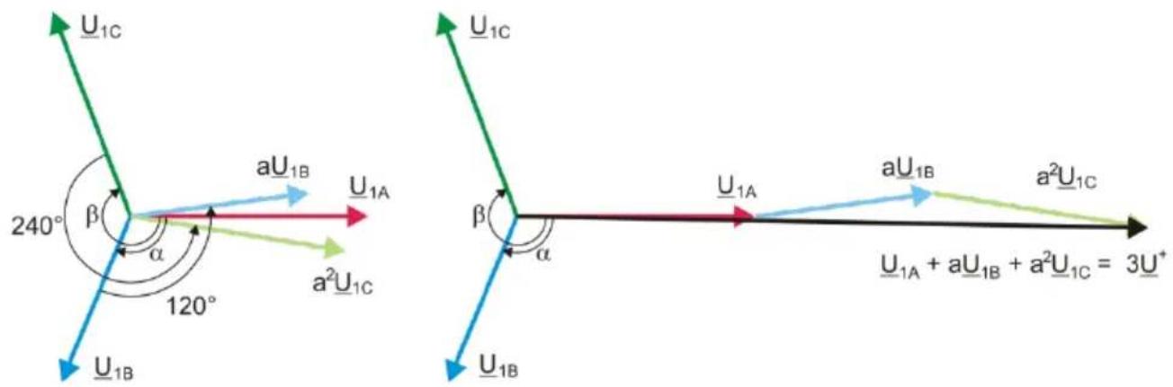
Fig. 71. Example of determination of positive sequence component.
As an example, let us use the calculation of voltage positive sequence component.
$$ \underline {{{{U}}}} ^ {+} = \frac {1}{3} \left(\underline {{{{U}}}} _ {1 A} + a \underline {{{{U}}}} _ {1 B} + a ^ {2} \underline {{{{U}}}} _ {1 C}\right) $$
where: U^+ is the vector of positive sequence component,
U_U_B, U_C — ^1A , U_1B , U_1C are vectors of positive sequence components of phase-to-neutral voltages U_A ,
$$ a = 1 e ^ {j 1 2 0 ^ {\circ}} = - \frac {1}{2} + \frac {\sqrt {3}}{2} j $$
$$ a ^ {2} = 1 e ^ {j 2 4 0 ^ {\circ}} = - \frac {1}{2} - \frac {\sqrt {3}}{2} j $$
Fig. 71 shows a graphical representation of determination of this component. As we can see from the definition, the vector of positive-sequence component equals one third of the sum of the summands U_1A , aU_1B , a^2 U_1C . Operators a and a^2 are unit vectors with angles 120^ and 240^ . The
procedure is as follows: turn the voltage vector U_1B by 120^ counterclockwise (multiply by a) and add to the vector U_1A . Then, turn the vector U_1C by 240^ and add to the previous sum of vectors. As a result, you get the vector 3U^+ . The vector U^+ is the symmetrical positive sequence component. Let us note that in case of a perfect symmetry (equal voltages and angles), the positive sequence component is equal in terms of value to the phase-to-neutral voltages.
The positive sequence component is a measure of similarity of the tested set of three-phase vectors to the symmetrical set of positive sequence vectors.
Analogously, the negative sequence component is a measure of similarity to the symmetrical set of negative sequence vectors.
The zero sequence component exists in the systems in which the sum of three voltages (or currents) is not equal to zero.
A measure of the system unbalance which is widely used in the power generation is the negative sequence and zero sequence unbalance (formulas are for the voltage).
$$ \begin{array}{l} u _ {0} = \frac {U _ {0}}{U _ {1}} \cdot 100 \% \ u _ {2} = \frac {U _ {2}}{U _ {1}} \cdot 100 \% \ \end{array} $$
where: u_0 – zero sequence unbalance,
u 2 – negative sequence unbalance,
U 0 – zero sequence symmetrical component,
U 1 – positive sequence symmetrical component,
U 2 – negative sequence symmetrical component.
The most convenient method to calculate the symmetrical components and unbalance is using the complex number calculus. The vectors parameters are amplitude of the voltage (current) fundamental component and its absolute phase shift angle. Both these values are obtained from FFT.
5.6 Detection of voltage dips, swells and interruptions
Voltage dips, swells and interruptions are the mains system disturbances during which the RMS voltage significantly differs from the nominal value. Each of the three states can be detected by the analyzer when the event detection is activated and when the user defines the threshold values.
Voltage dip is a state during which the RMS voltage is lower than the user-defined voltage dip threshold. The basis for the dip measurement is U_RMS(1/2) , that is the one period RMS value refreshed every half period.
Voltage dip definition (according to the IEC 61000-4-30 standard):
The voltage dip starts at the moment when the U RMS(1/2) voltage decreases below the dip threshold value, and ends at the moment when the U RMS(1/2) voltage is equal to or greater than the dip threshold value plus the voltage hysteresis.
The dip threshold is specified at 90% of U_nom . During the voltage dip, the analyzer remembers the minimum recorded voltage (this is called the residual voltage U_res and is one of the parameters characterizing the dip) and the average voltage value.
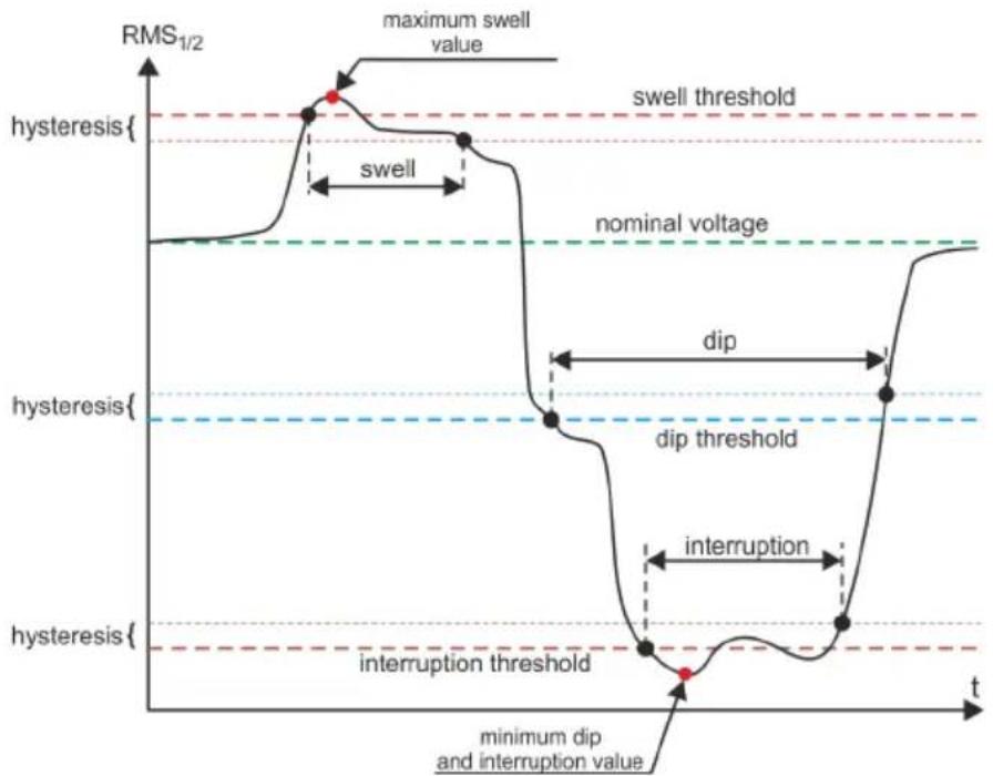
line
| Time (t) | RMS₁/₂ | Event Description | |----------|--------|--------------------------------------| | 0 | High | Maximum swell value | | 1 | Low | Swell | | 2 | High | Maximum swell value | | 3 | Low | Swell | | 4 | High | Maximum swell value | | 5 | Low | Swell | | 6 | High | Maximum swell value | | 7 | Low | Swell | | 8 | High | Maximum swell value | | 9 | Low | Swell | | 10 | High | Maximum swell value | | 11 | Low | Swell | | 12 | High | Maximum swell value | | 13 | Low | Swell | | 14 | High | Maximum swell value | | 15 | Low | Swell | | 16 | High | Maximum swell value | | 17 | Low | Swell | | 18 | High | Maximum swell value | | 19 | Low | Swell | | 20 | High | Maximum swell value | | 21 | Low | Swell | | 22 | High | Maximum swell value | | 23 | Low | Swell | | 24 | High | Maximum swell value | | 25 | Low | Swell | | 26 | High | Maximum swell value | | 27 | Low | Swell | | 28 | High | Maximum swell value | | 29 | Low | Swell | | 30 | High | Maximum swell value | | 31 | Low | Swell | | 32 | High | Maximum swell value | | 33 | Low | Swell | | 34 | High | Maximum swell value | | 35 | Low | Swell | | 36 | High | Maximum swell value | | 37 | Low | Swell | | 38 | High | Maximum swell value | | 39 | Low | Swell | | 40 | High | Maximum swell value | | 41 | Low | Swell | | 42 | High | Maximum swell value | | 43 | Low | Swell | | 44 | High | Maximum swell value | | 45 | Low | Swell | | 46 | High | Maximum swell value | | 47 | Low | Swell | | 48 | High | Maximum swell value | | 49 | Low | Swell | | 50 | High | Maximum swell value | | 51 | Low | Swell | | 52 | High | Maximum swell value | | 53 | Low | Swell | | 54 | High | Maximum swell value | | 55 | Low | Swell | | 56 | High | Maximum swell value | | 57 | Low | Swell | | 58 | High | Maximum swell value | | 59 | Low | Swell | | 60 | High | Maximum swell value | | 61 | Low | Swell | | 62 | High | Maximum swell value | | 63 | Low | Swell | | 64 | High | Maximum swell value | | 65 | Low | Swell | | 66 | High | Maximum swell value | | 67 | Low | Swell | | 68 | High | Maximum swell value | | 69 | Low | Swell | | 70 | High | Maximum swell value | | 71 | Low | Swell | | 72 | High | Maximum swell value | | 73 | Low | Swell | | 74 | High | Maximum swell value | | 75 | Low | Swell | | 76 | High | Maximum swell value | | 77 | Low | Swell | | 78 | High | Maximum swell value | | 79 | Low | Swell | | 80 | High | Maximum swell value | | 81 | Low | Swell | | 82 | High | Maximum swell value | | 83 | Low | Swell | | 84 | High | Maximum swell value | | 85 | Low | Swell | | 86 | High | Maximum swell value | | 87 | Low | Swell | | 88 | High | Maximum swell value | | 89 | Low | Swell | | 90 | High | Maximum swell value | | 91 | Low | Swell | | 92 | High | Maximum swell value | | 93 | Low | Swell | | 94 | High | Maximum swell value | | 95 | Low | Swell | | 96 | High | Maximum swell value | | 97 | Low | Swell | | 98 | High | Maximum swell value | | 99 | Low | Swell | | 100 | High | Maximum swell value | | minimum dip and interruption value at t=0.1 T T T T T T T T T T T T T T T T T T T T T T T T T T T T T T T T T T T T T T T T T T T T T T T T T T T T min min min min min min min min min min min min min min min min min min min min min min min min min min min min min min min min min min min min min min min min min min min min min min min min min min min max max max max max max max max max max max max max max max max max max max max max max max max max max max max max max max max max max max max max max max max max max max max max max max max max max max max max max max max max max max max max max max max max max max max max max max max max max max max max max max max max max max max max max max max max max max max max max max max max max max max max min min min min min min min min min min min min min min min min min min min min min min min min min min min min min min min min min min min min min min min min min max max max max max max max max max max max max max max max max max max max max max max max max max max max max max max max max max max max max max max max max max max max Max Min Min Min Min Min Min Min Min Min Min Min Min Min Min Min Min Min Min Min Min Min Min Min Min Min Min Min Min Min Min Min Min Min Min Min Min Min Min Min Min Min Min Min Min Min Min Min Min Min Min Min Max Max Max Max Max Max Max Max Max Max Max Max Max Max Max Max Max Max Max Max Max Max Max Max Max Max Max Max Max Max Max Max Max Max Max Max Max Max Max Max Max Max Max Max Max Max Max Max Max Max Max Max Min Min Min Min Min Min Min Min Min Min Min Min Min Min Min Min Min Min Min Min Min Min Min Min Min Min Min Min Min Min Min Min Min Min Min Min Min Min Min Min Min Min Min Min Min Min Min Min Min Min M x x x x x x x x x x x x x x x x x x x x x x x x x x x x x x x x x x x x x x x x x x x x x x x x x x x nan (various values estimated from plot)Fig. 72. Voltage swells, dips and interruptions.
Interruption is a state during which the U RMS(1/2) voltage is lower than the specified interruption level. The interruption threshold is usually set much below the voltage dip level, at about 1..10% of U nom .
The interruption starts at the moment when the U RMS(1/2) voltage decreases below the interruption threshold value, and ends at the moment when the U RMS(1/2) voltage is equal to or greater than the interruption threshold value plus the voltage hysteresis.
During the interruption, the analyzer remembers the minimum recorded voltage and the average voltage value.
Swell is a state of increased voltage. The swell threshold is usually set at the level close to 110% of U_nom .
The swell starts at the moment when the U_RMS(1/2) voltage increases above the swell threshold value, and ends at the moment when the U_RMS(1/2) voltage is equal or less than the swell threshold value minus the voltage hysteresis. During the interruption, the analyzer remembers the maximum recorded voltage and the average voltage value.
The hysteresis for all three states is the same, and it is a user-defined percent of nominal voltage U_nom (Events detection h
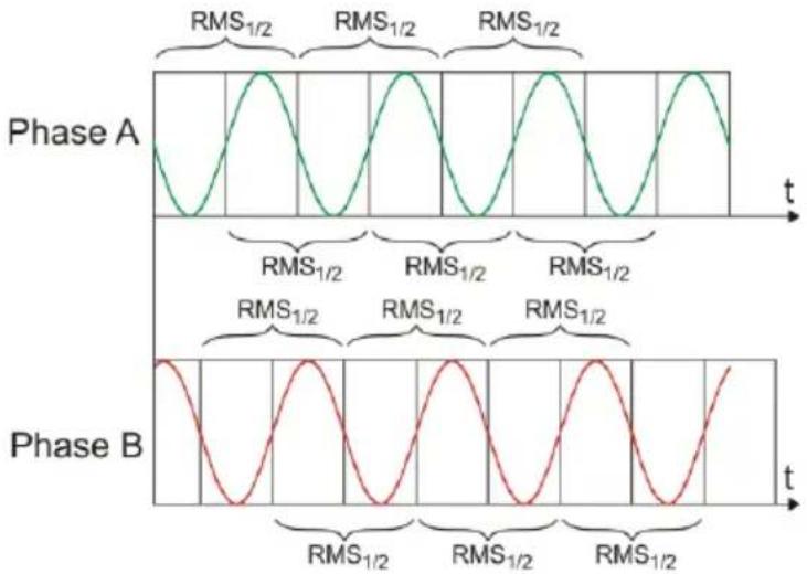
line
| Phase | RMS1/2 | |-------|--------| | Phase A | Green Line | | Phase B | Red Line |Fig. 73. Determination of the U_rms(1/2) value.
The analyzer remembers the event start and end time (with a half a period accuracy).
The minimum voltage dip, interruption and swell duration is half a period.
The U RMS_(1/2) values are determined during 1 period when the fundamental voltage component passes the zero and they are refreshed every half-period, independently for each voltage channel.
This means that these values will be obtained at different times for different channels. Fig. 73 shows the method of the RMS_1/2 determination with two voltage phases. Information about the fundamental component's passing the zero is obtained by FFT.
5.7 CBEMA and ANSI curves
CBEMA curve was first proposed in the 70's of the last century by the organization that gave the curve its name - Computer and Business Equipment Manufacturers Association (now Information Technology Industry), which associated manufacturers of computer and office equipment. The curve was developed as a guide in the construction of power supply adapters and at the beginning it was a graph showing the tolerance of equipment to the size and duration of the disturbances in the power grid. Later, the curve was used to design equipment sensitive to voltage fluctuations as the reference range in which the equipment must operate properly. Finally the curve began to be widely used in the analyses of power-supply quality in terms of disturbances such as swell, dip, interruptions.
The vertical axis of the graph presents voltage in percent of the nominal value, whereas the horizontal axis presents time (in logarithmic scale). The middle part of the graph (between curves) represents the area of the correct operation of the device. The area above represents high voltage conditions that may damage the device or trigger over-voltage protection, while the area under the curves represents a situation of low voltage in mains, which may disconnect the power supply or temporary power shortage resulting in incorrect operation of the equipment.
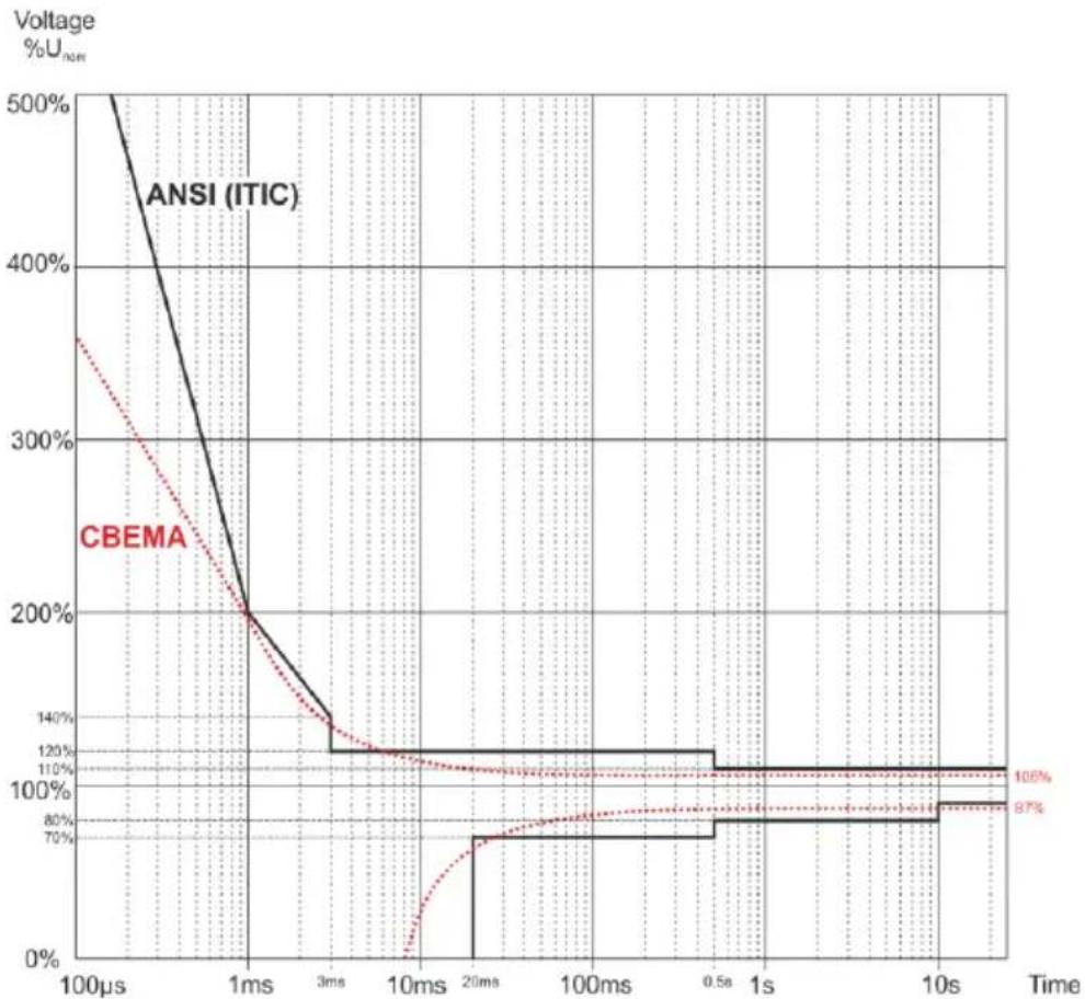
line
| Time | ANSI (ITIC) | CBEMA | | -------- | ----------- | ----- | | 100μs | 500% | 350% | | 1ms | 200% | 200% | | 3ms | 120% | 120% | | 10ms | 120% | 120% | | 20ms | 120% | 120% | | 100ms | 120% | 120% | | 0.5s | 120% | 120% | | 1s | 120% | 120% | | 10s | 120% | 120% | | 10s | 105% | 97% |Fig. 74. Voltage tolerance curves ANSI (ITIC) and CBEMA.
As shown in the graph on Fig. 74, there is a relationship between the voltage value and the duration of the disturbance. For example, voltage swell of 200% U_nom and with duration of 1 ms, in typical cases, does not result in failure or malfunctioning (point between curves), but an interference
of such amplitude, which lasts for half-period of the mains may be have very adverse effects (the point above two curves). Generally it is accepted that in a typical situation, events occurring in the power grid when it comes to the value of the mains voltage, should fit in the middle area of the graph (between curves) and then they should not lead to malfunction or damage to the connected equipment. Equipment manufacturers (especially power adaptors) often use this pattern while designing their products, in order to ensure their reliable operation and maintaining proper output voltage. Note, however, that the curve represents typical cases and cannot be a guarantee of correct operation for each device, as tolerance for interferences is very different.
ITIC curve is the successor of the CBEMA curve developed by ITI in 1994, and later modified to its present form in 2000. This curve has the form of two broken lines and is also known as ANSI curve, as it was adapted by ANSI (American National Standards Institute). Both curves are presented in Fig. 74.
"Sonel Analysis" software provides the ability to modify the characteristic points of the curves allowing user to adjust them to individual requirements.
5.8 Averaging the measurement results
Mains monitoring over a longer period of time means that a huge amount of data needs to be collected. If analysis of such data is to be possible at all, it is necessary to introduce the mechanisms which will reduce the data size to the values acceptable by both, humans and machines.
Lets us take the example of EN 50160 compliant power quality measurements. The basic mains test period is one week. If all 200-millisecond RMS values were to be remembered, we would get 3.024 million measurements. Processing of such amount of data would be time consuming and difficult.
Therefore, the averaging concept has been introduced which involves recording one value per a specified time interval for the analysis purposes. For the EN 50160 standard, such time interval is 10 minutes. In such case, the analyzer calculates an average 10-minute value on the basis of about three thousand 200-millisecond values (approximately, because in reality the conventional 200-millisecond value is a 10/12-period value synchronized with the mains frequency). Each average voltage value is recorded every 10 minutes which gives “only” 1008 measurement results.
Fig. 75 presents the method according to which the PQM-707 analyzer determines the average values at averaging intervals equal to or greater than 10 seconds with the 10-minute averaging time. This method meets the requirements for class S specified in IEC 61000-4-30.
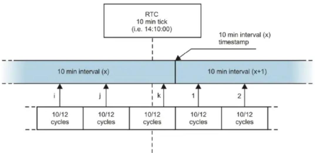
flowchart
graph TD
    A["RTC\n10 min tick\n(i.e. 14:10:00)"] --> B["10 min interval (x)"]
    B --> C["10 min interval (x+1)"]
    C --> D["10/12 cycles"]
    C --> E["10/12 cycles"]
    C --> F["10/12 cycles"]
    C --> G["10/12 cycles"]
    C --> H["10/12 cycles"]
    I["10 min interval (x) \ntimestamp"] --> B
    J["i"] --> C
    K["j"] --> C
    L["k"] --> C
    M["1"] --> C
    N["2"] --> C
Fig. 75. Determining the averaging intervals equal to or longer than 10 seconds (with the 10-minute averaging).
The average values are synchronized with real time clock in the following manner. When the clock measures a successive full multiple of the averaging period, the instantaneous 10/12-period measurement is added as the last to the average value (k-th measurement in Fig. 75). Simultaneously, the ending averaging period is given a time stamp which relates to its end. The next 10/12-period measurement is the first in a consecutive averaging period.
Averaging with times less than 10 seconds is somewhat different. Although, they are all expressed in time units (200 ms, 1 s, 3 s, 5 s), in reality they are measured in multiples of the mains period. For example, selecting of a 3-second averaging period means averaging in the time equal to 150/180 mains periods (fifteen 10/12-period measurements).
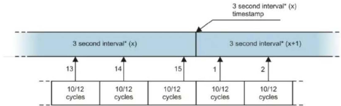
flowchart
graph TD
    A["3 second interval* (x)"] --> B["3 second interval* (x+1)"]
    B --> C["10/12 cycles"]
    B --> D["10/12 cycles"]
    B --> E["10/12 cycles"]
    B --> F["10/12 cycles"]
    B --> G["10/12 cycles"]
    style A fill:#cce5ff,stroke:#333
    style B fill:#cce5ff,stroke:#333
    note right of A: "3 second interval* (x) timestamp"
    note right of B: "3 second interval* (x)"
(*) actually it is a 150/180-cycles interval
Fig. 76. Determining the averaging intervals shorter than 10 seconds (with the 3-second averaging).
The method of average values determination for such periods is shown in Fig. 76. Here, we do not have synchronization with the real time clock. When a defined number of 10/12-period measurement is collected, the instantaneous averaging period is closed and a new one starts. The time stamp corresponds to the end of the interval.
Averaging of measurement results leads to the loss of extreme values (smoothing of results). In cases when the information about a limit value of the measured parameter is essential, the user can take advantage of the option of measuring the minimum, maximum and instantaneous values in the averaging period. If a given parameter is measured in the 10/12-period time, the minimum and maximum value is respectively the smallest and the largest 10/12-period value measured in a given averaging interval. On the other hand, the instantaneous value is the last 10/12-period value in this averaging interval.
In case of RMS current and voltage, the method of searching for minimum and maximum values is different and is based on U_rms(1/2) (RMS values calculated for 1 cycle and refreshed each half-cycle). This gives high sensitivity to instantaneous changes of the measured value.
Selecting the right averaging period is not easy. To a large extent it depends on the type of disturbance in the system and the user's expectations for the final data analysis. A frequent situation is that we know only that there is a problem in the mains, and the measurements with the analyzer will only help us identify the cause. In this situation it is better to use shorter averaging times (e.g. 10 seconds), and activate the recording of minimum and maximum values (for the voltages and currents it is advisable in such situation to set the shortest possible time for determining the maximum and minimum value, i.e. half the period). Short time averaging will give more precise diagrams of changes of parameters over time, and minimums and maximums will be detected and recorded. Recording with short averaging times is performed mostly for limited time, primarily due to rapid growth of data; the air of such recording is identifying the possible cause of a problem, and not a long-term analysis.
Recording with a short averaging time may be sufficient to evaluate the performance of the mains and disturbances in it. However, equally detailed information can probably also be obtained
PQM-707 user manual
with longer times (in minutes) but with activated recording of minimum and maximum values and event detection. An important advantage in this situation is that the volume of recorded data is much smaller which means faster data retrieval and analysis.
On the other hand, the power quality tests are usually made according to the EN 50160. In this case, the analysis is carried out over a longer period of time (e.g. 7 days), and therefore the chosen averaging time is also long - 10 minutes.
Please note that there is no single best setting for both the averaging time and other parameters or event thresholds. Each mains system is different and so are the goals of the mains tests. Therefore, the optimal configuration of the analyzer may require several approaches and will also depend on the experience of the operator.
6 Technical specification
- Technical specification is subject to change without prior notice. The latest revisions of technical documentation are available at www.sonel.pl.
- Basic uncertainty is uncertainty of a measuring instrument in reference conditions given in Table 10.
- Given uncertainty values refer to the PQM-707 analyzer without additional transducers and probes.
- Abbreviations:
• m.v. – measured value,
- U nom – nominal voltage,
- I nom – nominal current range (probe),
- RMS – root mean square value,
- n – harmonic order,
- s.d. – significant digits (or significant figures) – in reference to resolution of measurement result, the value is recorded with the given number of significant digits, e.g. resolution for 230 V with 4 s.d. will be 0.1 V (notation 230.0 V); resolution for 5 A with 4 s.d. will be 0.001 A (notation 5.000 A),
- ph - additional uncertainty caused by the error of phase measurement between the voltage and current harmonics.
6.1 Inputs
| Voltage inputs | |
| Number of inputs | 5 (L1/A, L2/B, L3/C, N, PE - 4 measuring channels) not galvanically isolated between each other |
| Maximum input voltage | L1/A, L2/B, L3/C, N: 760 V RMS 40...70 Hz or DC referred to protective earth terminal (PE) |
| Measurement category | CAT IV 600 VCAT III 760 V |
| Peak input voltage (no ADC saturation) | ±1150 V (L-N, L-PE) |
| Range of measured DC voltages | ±1150 V |
| Analog passband (-3dB) | 12 kHz |
| Transducers | defined by user |
| Impedance of measurement inputs | 13.8 MΩ (L-L, L-N)6.9 MΩ (L-PE) |
| CMRR | >70 dB (50 Hz) |
| Current inputs | |
| Number of inputs | 4 (L1, L2, L3, N) not isolated galvanically between each other |
| Peak input voltage | 5 V referred to protective earth terminal (PE) |
| Nominal input voltage (CT probes) | 1 V_RMS |
| Peak input voltage (CT probes, no ADC saturation) | ±3.6 V |
| Nominal input voltage (flexible clamps) | 0.125 V_RMS |
| Peak input voltage (flexible clamps; without ADC overflow) | ±0.45 V |
| Maximum current probes input voltage referred to earth | 5 V_RMS |
| Analog passband (-3dB) | 12 kHz |
| Input impedance | CT probes: 100 kΩFlexible probes: 12.4 kΩ |
| Measurement range (without transducers) | Flexible probes F-1(A)/F-2(A)/F-3(A): 1..3000 A (±10 kA peak, 50 Hz)Flexible probes F-2AHD/F-3AHD: 1..3000 A (±10 kA peak, 50 Hz)Flexible probes F-1A6/F-2A6/F-3A6: 1...6000 A (±20 kA peak, 50 Hz)Flexible probes F-1A1/F-2A1/F-3A1: 1...1500 A (±5 kA peak, 50 Hz)CT probes C-4(A), C-5A: 1..1000 A (±3600 A peak)CT probes C-6(A): 0.01..10 A (±36 A peak)CT probes C-7(A): 0..100 A (±360 A peak) |
| Transformers | defined by user |
| CMRR | 60 dB (50 Hz) |
6.2 Sampling and real time clock
| Sampling and real time clock | |
| A/D converter | 16-bit |
| Sampling rate | 10.24 kHz for 50 Hz and 60 HzSimultaneous sampling in all channels |
| Samples per period | 204.8 for 50 Hz; 170.67 for 60 Hz |
| PLL synchronization | 40..70Hz |
| Reference channel for PLL | L1-N, L1-L2 (depending on mains type) |
| Real-time clock | ±3.5 ppm max (approx. ± 9 sec./month, ± 0.3 sec./day)in the temperature range of -10°C...+50°C |
6.3 Measured parameters - accuracy, resolution and ranges
6.3.1 Reference conditions
Tab. 9. Reference conditions.
| Reference conditions | |
| Ambient temperature | 23°C ±2°C |
| Relative humidity | 40...60% |
| External supply voltage | 12V ±1% |
| Input voltage | U_nom ±1% |
| Flicker | P_ST< 0.1 |
| Voltage unbalance | ≤ 0.1% for unbalance factor of negative sequence (applies only to 3-phase systems) |
| External continuous magnetic field | ≤ 40 A/m DC≤ 3 A/m AC for 50/60 Hz frequency |
| DC component of voltage and current | none |
| Waveforms | sinusoidal |
| Frequency | 50 ±0.5 Hz lub 60 ±0.5 Hz |
6.3.2 Measurement uncertainty within rated temperature range
The basic uncertainty given in technical data applies to reference conditions only (Tab. 9). Outside of this range an additional multiplier has to be used, as shown in Fig. 77. The multiplier (M) is 2.0 in the ambient temperature range 0^ C...+45°C. Over +45°C up to +55°C it rises in linear manner up to 3.0. Below 0°C down to -25°C it rises in linear manner to 3.0.
For example: the basic uncertainty for RMS voltage measurement is ± 0.5% U_nom .
- At the -10°C measurement uncertainty is ±2.4 × 0.5% U nom that is ±1.2% U nom (multiplier 2.4),
- At the 0^ measurement uncertainty is ± 1% U_nom (multiplier 2.0),
- At the +45^ measurement uncertainty is ± 1% U_nom (multiplier 2.0),
- At the +50°C measurement uncertainty is ±1.25% U _nom (multiplier 2.5).
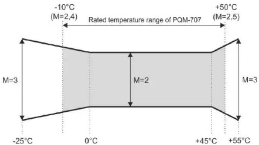
Fig. 77. Basic uncertainty multiplier M as a function of ambient temperature (does not apply to the reference conditions).
6.3.3 Voltage
| Voltage | Ranges and conditions | Resolution | Basic uncertainty |
| U_RMS (AC+DC) | 20% U_nom ≤ U_RMS ≤ 120% U_nom for U_nom ≥ 100 V | 4 s.d. | ±0.5% U_nom |
| Crest Factor | 1..10(1..1.65 for 690 V voltage)for U_RMS ≥ 10% U_nom | 0.01 | ±5% |
6.3.4 Current
| Current | Ranges and conditions | Resolution | Basic uncertainty |
| IRMS (AC+DC) | Input path without clamps | ||
| CT line:0..1 V (±3.6 V max)flexible probes line:0..125 mV (±450 mV max) | 4 s.d. | ±0.2% Inom | |
| Flexible probes F-1(A)/F-2(A)/F-3(A) | |||
| 0..3000 A(±10 kA) | 4 s.d. | Additional uncertainty±1%(±2% taking into account additional error due to the position) | |
| Flexible probes F-2AHD/F-3AHD | |||
| 0..3000 A(±10 kA max) | 4 s.d. | Additional uncertainty±0.5%(±2% taking into account additional error due to the position) | |
| Flexible probes F-1A6/F-2A6/F-3A6 | |||
| 0..6000 A(±20 kA max) | 4 s.d. | Additional uncertainty±1%(±2% taking into account additional error due to the position) | |
| Flexible probes F-1A1/F-2A1/F-3A1 | |||
| 0..1500 A(±5 kA max) | 4 s.d. | Additional uncertainty±1%(±2% taking into account additional error due to the position) | |
| CT probes C-4(A) | |||
| 0..1000 A(±3600 A) | 4 s.d. | Additional uncertainty0.1..10 A: ± (3% + 0.1 A)10 A: ±3%50 A: ±1.5%200 A: ±0.75%1000..1200 A: ±0.5% | |
| CT probes C-5A | |||
| 0..1000 A(±3600 A) | 4 s.d. | Additional uncertainty0.5..100 A: ≤ (1.5% + 1 A)100..800 A: ≤ 2.5%800..1000 A AC: ≤ 4%1000..1400 A DC: ≤ 5% | |
| CT probes C-6(A) | |||
| 0..10 A(±36 A) | 4 s.d. | Additional uncertainty0.01..0.1 A: ± (3% + 1 mA)0.1..1 A: ±2.5%1..12 A: ±1% | |
| CT probes C-7(A) | |||
| 0..100 A(±360 A) | 4 s.d. | Additional uncertainty0..100A: ± (0,5% + 0,02A) (45..65Hz0..100A: ± (1,0% + 0,04A)(40..1000Hz) | |
| Crest Factor | 1..10 (1..3,6 for Inom)for IRMS ≥ 1% Inom | 0.01 | ±5% |
6.3.5 Frequency
| Frequency | Ranges and conditions | Resolution | Basic uncertainty |
| f | 40..70 Hz15% U_nom ≤ U_RMS ≤ 120% U_nom U_nom ≥ 100 V | 0.01 Hz | ±0.05 Hz |
6.3.6 Harmonics
| Harmonics | Ranges and conditions | Resolution | Basic uncertainty |
| Harmonic (n) | DC, 1..50, grouping: harmonics sub-groups acc. to IEC 61000-4-7 | ||
| U_RMS amplitude | 0..200% U_nom | 4 s.d. | ±0.15% U_nom if m.v. <3% U_nom ±5% m.v. if m.v. ≥ 3% U_nom (acc. to IEC 61000-4-7 Class II) |
| I_RMS amplitude | Depending probes used (see specifications for I_RMS ) | 4 s.d. | ±0.5% I_nom if m.v. <10% I_nom ±5% of m.v. if m.v. ≥ 10% I_nom (acc. to IEC 61000-4-7 Class II) |
| Voltage THD-R(n = 2..50) | 0.0...100.0%for U_RMS ≥ 1% U_nom | 0.1% | ±5% |
| Current THD-R(n = 2..50) | 0.0...100.0%for I_RMS ≥ 1% I_nom | 0.1% | ±5% |
| Phase angle (voltage) | -180°...+180° | 0.1° | ±(n × 1°) |
| Phase angle (current) | -180°...+180° | 0.1° | ±(n × 1°) |
6.3.7 Power and energy
| Power and energy | Conditions(for power and energy80% U_nom ≤ U_RMS < 120% U_nom ) | Resolution | Basic uncertainty (1) |
| Active powerActive energy | 2% I_nom ≤ I_RMS < 5% I_nom = 1 | 4 s.d. | 2.5^2 + _ph^2 ± % |
| 5% I_nom ≤ I_RMS ≤ I_nom = 1 | 2.0^2 + _ph^2 ± % | ||
| 5% I_nom ≤ I_RMS < 10% I_nom = 0.5 | 2.5^2 + _ph^2 ± % | ||
| 10% I_nom ≤ I_RMS ≤ I_nom = 0.5 | 2.0^2 + _ph^2 ± % | ||
| Reactive powerReactive energy | 2% I_nom ≤ I_RMS < 5% I_nom = 1 | 4 s.d. | 4.0^2 + _ph^2 ± % |
| 5% I_nom ≤ I_RMS < I_nom = 1 | 3.0^2 + _ph^2 ± % | ||
| 5% I_nom ≤ I_RMS < 10% I_nom = 0.5 | 4.0^2 + _ph^2 ± % | ||
| 10% I_nom ≤ I_RMS < I_nom = 0.5 | 3.0^2 + _ph^2 ± % | ||
| 10% I_nom ≤ I_RMS < I_nom = 0.25 | 4.0^2 + _ph^2 ± % | ||
| Apparent powerApparent energy | 2% I_nom ≤ I_RMS < 5% I_nom | 4 s.d. | ±2.5% |
| 5% I_nom ≤ I_RMS ≤ I_nom | ±2.0% | ||
| Power factor (PF) | 0...150% U_nom ≤ U_RMS < 150% U_nom 10% I_nom ≤ I_RMS < I_nom | 0.01 | ±0.03 |
| Displacement power factor ( / DPF ) | 0...150% U_nom ≤ U_RMS < 150% U_nom 10% I_nom ≤ I_RMS < I_nom | 0.01 | ±0.03 |
(1) See sec. 6.3.8.
6.3.8 Estimating the uncertainty of power and energy measurements
The total uncertainty of active and reactive power and energy measurements and the harmonics power is based on the following relationship (additional time measurement uncertainty is omitted in case of energy as much smaller than other uncertainty types):
$$ \delta_ {P, Q} \cong \sqrt {\delta_ {U h} ^ {2} + \delta_ {I h} ^ {2} + \delta_ {p h} ^ {2}} $$
where: _P,Q – uncertainty of active or reactive power measurement,
_Uh - total uncertainty of voltage harmonic amplitude measurement (analyzer, transducers), _Ih - total uncertainty of current amplitude measurement (analyzer, transducers, probes),
_ph – additional uncertainty caused by the error of phase measurement between the voltage and current harmonics.
The _ph uncertainty can be determined if we know the phase shift angle for a given frequency ranges. Tab. 10 presents the phase difference error between the voltage and current harmonics for the PQM-707 analyzer (without probes and transducers).
Tab. 10. Phase error in the PQM-707 analyzer depending on the frequency
| Frequency range | 0..200 Hz | 200..500 Hz | 500 Hz..1 kHz | 1..2 kHz | 2..3 kHz |
| Phase error | ≤ 1^ | ≤ 2.5^ | ≤ 5^ | ≤ 10^ | ≤ 25^ |
The phase error caused by used transducers and probes can be usually found in their technical documentation. Such being the case, we need to estimate the resultant phase error between the voltage and the current for a given frequency caused by all elements of the measuring circuit: current and voltage transducers, probes, and the analyzer.
The phase uncertainty of the harmonics active power measurements can be calculated according to the following formula:
$$ \Delta_ {p h} = 100 \left(1 - \frac {\cos (\varphi + \Delta \varphi)}{\cos \varphi}\right) [\% ], \cos \varphi \neq 0 $$
On the other hand, the phase uncertainty of the harmonics reactive power measurements can be calculated according to the following formula:
$$ \varDelta_ {p h} = 100 \left(1 - \frac {\sin (\varphi - \Delta \varphi)}{\sin \varphi}\right) [ \% ], \sin \varphi \neq 0 $$
In both formulas, means the actual phase shift angle between the current and voltage components, and means the total phase error for a given frequency. The conclusion which can be drawn from these relationships is that power measurement uncertainty for the same phase error very clearly depends on the displacement power factor between current and voltage. It is shown in Fig. 78.
Example
Calculation of measurement uncertainty of active power fundamental component.
Conditions: = 60^ , U_RMS U_nom , I_RMS = 5% I_nom .
Fundamental uncertainty equals ± 2,5^2 + _ph^2% .
For the 0..200Hz frequency range, the PQM-707 phase error is < 1^ . After substituting to the equation:
$$ \delta_ {p h} = 100 \left(1 - \frac {\cos (\varphi + \Delta \varphi)}{\cos \varphi}\right) = 100 \left(1 - \frac {\cos (61 ^ {\circ})}{\cos (60 ^ {\circ})}\right) = 3,04\% $$
then, the measurement uncertainty is:
$$ \delta = \pm \sqrt {2 , 5 ^ {2} + 3 , 0 4 ^ {2}} = \pm 3, 94 \% $$
Under the same conditions, but with the phase shift = 10^ , we will obtain:
$$ \delta_ {p h} = 100 \left(1 - \frac {\cos (11 ^ {\circ})}{\cos (10 ^ {\circ})}\right) = 0.32 \% $$
and the measurement uncertainty is:
$$ \delta = \pm \sqrt {2, 5 ^ {2} + 0 , 3 2 ^ {2}} = \pm 2, 52 \% $$
The above calculations do not take into account additional errors caused by used probes and transducers.
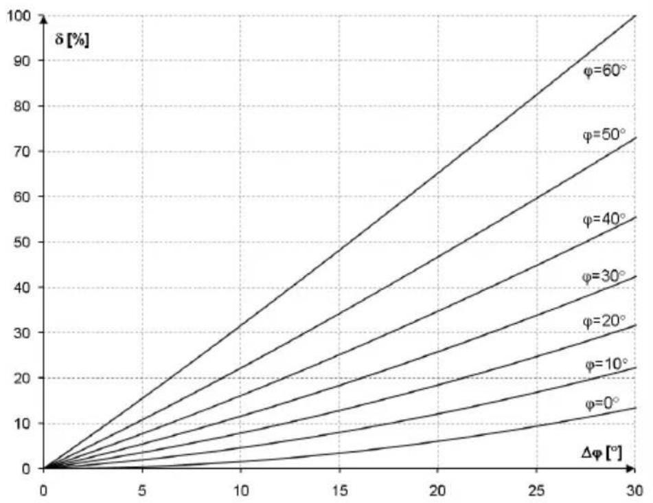
line
| Δφ [°] | φ=0° | φ=10° | φ=20° | φ=30° | φ=40° | φ=50° | φ=60° | | ------ | ---- | ----- | ----- | ----- | ----- | ----- | ----- | | 0 | 0 | 0 | 0 | 0 | 0 | 0 | 0 | | 5 | ~2 | ~4 | ~6 | ~8 | ~10 | ~12 | ~15 | | 10 | ~4 | ~7 | ~10 | ~13 | ~16 | ~19 | ~23 | | 15 | ~6 | ~10 | ~14 | ~18 | ~22 | ~26 | ~31 | | 20 | ~8 | ~13 | ~18 | ~23 | ~28 | ~33 | ~39 | | 25 | ~10 | ~16 | ~22 | ~28 | ~34 | ~40 | ~47 | | 30 | ~12 | ~19 | ~26 | ~33 | ~40 | ~47 | ~55 |Fig. 78. Additional uncertainty from phase error depending on phase shift angle.
6.3.9 Flicker
| Flicker | Ranges and conditions | Resolution | Basic uncertainty |
| P_st(10 min) , P_lt(2 h) | 0.4 ... 10for U_RMS ≥ 80% U_nom | 0.01 | ±10% within the values presented in tables of IEC 61000-4-15 standard |
6.3.10 Unbalance
| Unbalance (voltage and current) | Ranges and conditions | Resolution | Basic uncertainty |
| Unbalance factor for positive, negative and zero sequence | 0.0% ... 10.0%for80% U_nom ≤ U_RMS < 150% U_nom | 0.1% | ±0.15%(absolute uncertainty) |
6.4 Event detection – voltage and current RMS
| U_RMS voltage (dips, interruptions and swells) | Range | Resolution | Basic uncertainty |
| U_RMS(1/2) | 0.0%...120.0% U_nom | 4 s.d. | ±1% U_nom |
| Detection thresholds | Set by the user in percentage or absolute values. Event detection based on the measurement of U_RMS(1/2) (1-period RMS refreshed every 1⁄2 period). | ||
| Duration | hh:mm:ss.ms | 1⁄2 period | One period |
| Waveform record | Two periods before event + 4 periods after the event (total of 6 cycles) 204.8/170.67 (50 Hz/60 Hz) samples per period | ||
| I_RMS current(min, max) | Range | Resolution | Basic uncertainty |
| I_RMS(1/2) | 10% I_nom ≤ I_RMS < 100% I_nom | 4 s.d. | ±0.5% I_nom |
| Detection thresholds | Set by the user in percentage or absolute values. Event detection based on the measurement of I_RMS(1/2) (1-period RMS refreshed every 1⁄2 period). | ||
| Duration | hh:mm:ss.ms | 1⁄2 period | One period |
| Waveform record | Two periods before event + 4 periods after the event (total of 6 cycles)204.8/170.67 (50 Hz/60 Hz) samples per period | ||
6.4.1 Event detection hysteresis
| Event detection hysteresis | Range | Calculation method |
| Hysteresis | 0..10% | For voltage: calculated as a percent of nominal voltage.For current: calculated as a percent of max. threshold. |
6.5 Recording
| Recording | |
| Averaging time (1) | 1 s, 3 s, 10 s, 30 s, 1 min, 10 min, 15 min, 30 min. |
| Averaging min / max for U_RMS (2) | based on U_RMS(1/2) |
| Averaging min / max for I_RMS (2) | based on I_RMS(1/2) |
| Recording activation mode | manual starting at the first detected event scheduled (one defined time period) |
| Measurement configurations | Ability to define an unlimited number of measurement configurations stored in analyzer's internal memory |
| Recording time | Depending on the configuration (e.g. mains type, averaging time, parameters selected, etc.) |
| Memory | User replaceable memory card: microSD HC 4 GB (up to 32 GB supported) |
| Memory model | Linear |
| Security | Analyzer lock to prevent unauthorized access via 4-digit PIN code |
(1) Averaging times shorter than 10 seconds are in fact equal to a multiple of the mains period:
1 s = 50/60 cycles, 3 s = 150/180 cycles.
(2) U_RMS(1/2) and I_RMS(1/2) are RMS values for one period, refreshed every half period..
| Recorded parameters | Average value | Minimum value | Maximum value | Instantaneous value |
| RMS phase/phase-to-phase (depending on the type of system) voltage U_RMS | ● | ● | ● | |
| RMS phase-to-phase voltage U_RMS (only 3-phase wye with N and split-phase systems) | ● | |||
| DC Voltage | ● | ● | ● | |
| RMS current I_RMS | ● | ● | ● | |
| DC current ^(1) | ● | ● | ● | |
| Frequency f | ● | ● | ● | |
| Voltage crest factor CF U | ● | ● | ● | |
| Current crest factor CF I | ● | ● | ● | |
| Unbalance factors for negative and positive sequence, symmetrical components: negative, positive, zero (voltage) U_0 , U_1 , U_2 , u_0 , u_2 | ● | ● | ● | |
| Unbalance factors for negative and positive sequence, symmetrical components: negative, positive, zero (current) b, l1, l2, i0, i | ● | ● | ● | |
| Flicker factor P_st and P_lt , | ● | |||
| Active power (consumed and supplied) P_+, P_- | ● | ● | ● | |
| Reactive power (consumed and supplied) Q_1+, Q_1-/Q_B+, Q_B- | ● | ● | ● | |
| Apparent power S | ● | ● | ● | |
| Distortion power D / Apparent distortion power S_N | ● | ● | ● | |
| Power factor PF | ● | ● | ● | |
| Displacement power factor cos/DPF | ● | ● | ● | |
| Tanφ factor | ● | ● | ● | |
| Active energy (consumed and supplied) E_P+, E_P- | ● | |||
| Reactive energy (consumed and supplied) E_Q+, E_Q- | ● | |||
| Apparent energy E_S | ● | |||
| Total harmonic distortion for Voltage THD-F | ● | ● | ● | |
| Total harmonic distortion for current THD-F | ● | ● | ● | |
| Voltage harmonic amplitudes U_h1...U_h50 | ● | ● | ● | |
| Current harmonic amplitudes I_h1...I_h50 | ● | ● | ● | |
| Harmonics active and rwaactive power P_h1...P_h50, Q_h1...Q_h50 | ● | ● | ● | |
| Total demand distortion TDD | ● |
(1) Only with C-5A probes.
6.6 Power supply
| External power supply | |
| Nominal voltage range | 100-240 V AC, 50-60 Hz |
| Absolute maximum input voltage | 90-264 V AC, 50-60 Hz |
| Overvoltage category | II 300 V |
| Output voltage and current | 12 V DC 2.5 A |
| Output power | 30 W max. |
| Power adapter input ratings | |
| Input voltage range | DC 12 V ±10% |
| Input current | 2.5 A max. |
| Rechargeable battery | |
| Type, nominal voltage, nominal capacity | Li-Ion 11.1 V 3.4 Ah 37.7 Wh |
| Cycle life | 70% of nominal capacity after 500 charge/discharge cycles |
| Minimum operational time on battery (fully charged battery, rated temperature range, maximum LCD brightness) | min. 4 h |
| Typical operational time on battery (fully charged battery, temperature range 0-40°C, LCD brightness 50%) | approx. 6 h |
| Charging time (battery fully discharged, source: external power supply, ambient temperature range 0...40°C) | max. 2 h |
| Charging time via USB port (battery fully discharged, analyzer switcher off, external power supply disconnected, ambient temperature range 0...40°C) | approx. 30 h |
| Current consumption from battery in switched off mode (no external power supply) | < 1 mA |
| Current consumption from battery in sleep mode (no external power supply) | < 75 mA |
| Maximum time in sleep mode to fully discharge battery (fully charged battery, no external power supply) | approx. 45 h |
6.7 Supported mains types
| Types of supported mains (directly and indirectly) | |
| 1-phase | 1-phase with a neutral conductor (terminals: L1, N, PE) |
| 2-phase (split-phase) | Split phase with a neutral conductor (terminals: L1, L2, N, PE) |
| 3-phase 4-wire | 3-phase with a neutral conductor (terminals: L1, L2, L3, N, PE) |
| 3-phase 3-wire | 3-phase Delta (terminals: L1, L2, L3, PE) |
| 3-phase 3-wire Aron / 2-element | 3-phase Delta with Aron current measurement (terminals: L1, L2, L3, PE) |
| 3-phase 4-wire (no U L2) / 2 1/2 element (no V L2/B) | 3-phase 4-wire (terminals L1, L3, N, PE), with U L2 voltage calculated |
| 3-phase open delta | 3-phase Open Leg Delta (terminals: L1, L2, L3, PE) |
| Transducers: 3-phase 4-wire | 3-phase 4-wire with voltage transducers (terminals: L1, L2, L3, N, PE) |
| Transducers: 3-phase 3-wire | 3-phase Delta with voltage transducers (terminals: L1, L2, L3, PE) |
| Transducers: 3-phase 3-wire Aron (2PT's, 2-Elements) | 3-phase Delta with voltage transducers and Aron current measurement (terminals: L1, L2, L3, PE) |
| DC | One channel DC circuit with optional DC current measurement (with C-5A probes) (terminals L1, N) |
| DC+M | Two channels DC circuit with optional DC current measurement (with C-5A probes) (terminals L1, L2, N) |
6.8 Supported current probes
| Types of supported current probes | |
| F-1(A) | Flexible probes (Rogowski coil), perimeter: 120 cm, measuring range 3000 ARMS |
| F-2(A) | Flexible probes (Rogowski coil), perimeter: 80 cm, measuring range 3000 ARMS |
| F-3(A) | Flexible probes (Rogowski coil), perimeter: 45 cm, measuring range 3000 ARMS |
| F-2AHD | Flexible probes (Rogowski coil), perimeter: 91,5 cm, measuring range 3000 ARMS |
| F-3AHD | Flexible probes (Rogowski coil), perimeter: 45 cm, measuring range 3000 ARMS |
| F-1A6 | Flexible probes (Rogowski coil), perimeter: 120 cm, measuring range 6000 ARMS |
| F-2A6 | Flexible probes (Rogowski coil), perimeter: 80 cm, measuring range 6000 ARMS |
| F-3A6 | Flexible probes (Rogowski coil), perimeter: 45 cm, measuring range 6000 ARMS |
| F-1A1 | Flexible probes (Rogowski coil), perimeter: 120 cm, measuring range 1500 ARMS |
| F-2A1 | Flexible probes (Rogowski coil), perimeter: 80 cm, measuring range 1500 ARMS |
| F-3A1 | Flexible probes (Rogowski coil), perimeter: 45 cm, measuring range 1500 ARMS |
| C-4(A) | CT, AC probes, measuring range 1000 ARMS, 1 mV/A |
| C-5A | CT, AC/DC probes with Hall sensor, measuring range 1000 ARMS, 1 mV/A |
| C-6(A) | CT, AC probes for low currents, measuring range 10 ARMS, 1 mV/10 mA |
| C-7(A) | CT, AC probes, measuring range 1000 ARMS, 5 mV/A |
6.9 Communication
| Communication | |
| USB | Double insulated from measured mains (CAT IV 600 V)Compatible with USB 2.0 |
6.10 Environmental conditions and other technical data
| Environmental conditions | |
| Operating temperature range: | -10°C...+50°C |
| Storage temperature range | -20°C...+60°C |
| Humidity | 10...90% no condensation |
| Ingress protection (according to EN 60529) | IP 51 |
| Operating altitude | up to 2000 m(up to 4000 m with derated measurement categoryCAT II 760 V / CAT III 600 V / CAT IV 300 V) |
| Reference conditions | see Tab. 9 |
| Dimensions | 288 x 223 x 75 mm (with cover) |
| Weight | ok. 1,75 kg (with cover) |
| Display | color LCD TFT with polytouch, 800x480 resolution, diagonal 7" |
| Data memory | Removable microSD memory card 4 GB (as standard) for measurement data, screenshots and reports; option of extending up to 32 GB. Internal memory (approx. 1GB) for configuration data. |
6.11 Safety and electromagnetic compatibility
| Safety and EMC | |
| Compliance with | IEC 61010-1 edition 3.0, IEC 61010-2-030 |
| Measurement Category | IV 600V / III 760 V, pollution class 2, according to IEC 61010-2-030 |
| Insulation | Double |
| Electromagnetic compatibility | IEC 61326 |
| Immunity to radio frequency interferences | IEC 61000-4-3 sinusoidal modulation 80% AM, 1 kHz80...1000MHz, 10 V/m1.4...2.0 GHz, 3 V/m2.0 ... 2.7 GHz, 1 V/m |
| Immunity to electrostatic discharge | IEC 61000-4-2 Air discharge: 8 kV Contact discharge: 4 kV |
| Immunity to conducted disturbances, induced by radio-frequency fields | IEC 61000-4-6 sinusoidal modulation 80% AM, 1 kHz0.15...80 MHz, 10V |
| Immunity to a series of electrical fast transients/bursts | IEC 61000-4-4 Amplitude of 2 kV, 5 kHz |
| Surge immunity | IEC 61000-4-5 Amplitude 2 kV (L-L) |
| Emission of radiated RF disturbances | IEC 61000-6-3 30...230 MHz, 40 dB(μV/m) at 10m230...1000 MHz, 47 dB(μV/m) at 10m |
| Emissions of conducted interferences | IEC 61000-6-3 Levels for a quasi-peak detector: 0.15 kHz...0.5 MHz: 66 dBμV...56 dBμV0.5 MHz...5 MHz: 56 dBμV5 MHz...30 MHz: 60 dBμV |
EN 55022 Compliance statement:
PQM-707 is a class A product. In a domestic environment this product may cause radio interference in which case the user may be required to take adequate measures (e.g. increasing the distance between affected products).
6.12 Standards
| Standards | |
| Measurement Methods | IEC 61000-4-30 Class S |
| Measurement Accuracy | IEC 61000-4-30 Class S |
| Power Quality | EN 50160 |
| Flicker | IEC 61000-4-15 |
| Harmonics | IEC 61000-4-7 |
| Safety | IEC 61010-1, IEC 61010-2-030 |
| EMC | IEC 61326 |
| Quality standard | design, construction and manufacturing are ISO 9001 compliant |
7 Optional accessories
The full list of accessories can be found on the manufacturer's website.
 |  |  |  | |
| C-4A | C-5A | C-6A | C-7A | |
| WACEGC4AOKR | WACEGC5AOKR | WACEGC6AOKR | WACEGC7AOKR | |
| Rated current | 1000 A AC | 1000 A AC1400 A DC | 10 A AC | 100 A AC |
| Frequency | 30 Hz...10 kHz | DC...5 kHz | 40 Hz...10 kHz | 40 Hz...1 kHz |
| Max. diameter of measured conductor | 52 mm | 39 mm | 20 mm | 24 mm |
| Minimum accuracy | ≤0.5% | ≤1.5% | ≤1% | 0,5% |
| Battery power | — | √ | — | — |
| Lead length | 2.2 m | 2.2 m | 2.2 m | 3 m |
| Measurement category | IV 300 V | IV 300 V | IV 300 V | III 300 V |
| Ingress protection | IP40 | |||
 |  |  | 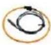 | 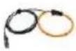 | |
| F-1A1 / F-1A / F-1A6 | F-2A1 / F-2A / F-2A6 | F-3A1 / F-3A / F-3A6 | F-2AHD | F-3AHD | |
| WACEGF1A1OKRWACEGF1AOKRWACEGF1A6OKR | WACEGF2A1OKRWACEGF2AOKRWACEGF2A6OKR | WACEGF3A1OKRWACEGF3AOKRWACEGF3A6OKR | WACEGF2AHDOKR | WACEGF3AHDOKR | |
| Rated current | 1500 / 3000 / 6000 AAC | 1500 / 3000 / 6000 AAC | 1500 / 3000 / 6000 AAC | 3000 AAC | |
| Frequency | 40 Hz...10 kHz | 10 Hz...20 kHz | |||
| Max. diameter of measured conductor | 380 mm | 250 mm | 140 mm | 290 mm | 145 mm |
| Minimum accuracy | 1% | 0.5% | |||
| Battery power | — | — | |||
| Lead length | 2.5 m | 2.5 m | |||
| Measurement category | IV 600 V | IV 600 V | |||
| Ingress protection | IP67 | IP65 | |||
8 Other Information
8.1 Rechargeable battery
PQM-707 is equipped with a Li-Ion battery pack 11.1 V 3.4 Ah. The battery pack includes a circuit monitoring its charge status, which provides precise level of battery pack charge and a temperature sensor.
The charge level of the battery pack is indicated by icon on the top bar of the screen on the right side:
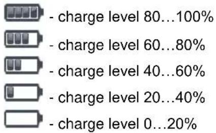
If the device detects the absence of the battery pack or no communication with the pack, the following icon is displayed:
? - a problem with the battery pack (removed or lack of communication)
Charging the battery pack is started automatically after connecting power supply adapter 12 V DC to the analyzer. It is also possible to charge it from the car cigarette lighter socket using a special cable provided with the analyzer. Charging is indicated by animated battery icon on the top bar and LED (see description in sec. 2.5). The temperature of the battery back and the ambient temperature influence the charging process. If the battery temperature is below 0°C or higher than 45°C, the charging process is stopped.
8.2 Replacing rechargeable batteries
The internal real time clock is supplied from the battery pack, therefore to avoid losing the clock settings, the battery pack replacement may be performed with connected power supply of 12 V DC. To replace the battery pack:
- disconnect the meter from the tested network,
- connect the external power supply 12 V DC (to prevent resetting date and time settings)
- Remove the four screws of the rechargeable batteries/batteries compartment (in the lower part of the casing), see Fig. 79,
- Remove the compartment,
- insert a new battery pack into the meter,
- Screw the four screws of the rechargeable batteries/batteries compartment.
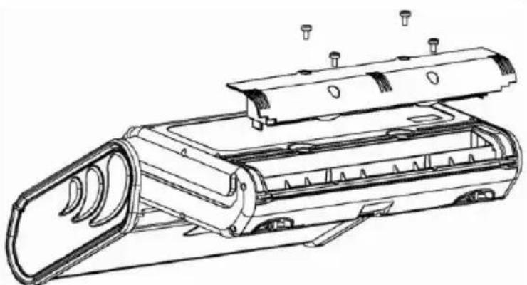
natural_image
Technical line drawing of a mechanical device with multiple ports and mounting holes (no text or symbols)Fig. 79. Replacing the battery pack
8.3 Positions of the meter's cover
The movable cover enables using the meter in various positions.
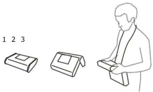
1 - cover as the bottom of the meter,
2 - cover used as a support,
3 – cover in the position that enables convenient use of the meter suspended on the neck by means of hanging straps.
8.4 Cleaning and maintenance
Note Use only the maintenance methods specified by the manufacturer in this manual.
The casing of the analyzer may be cleaned with a soft, damp cloth using all-purpose detergents. Do not use any solvents or cleaning agents which might scratch the casing (powders, pastes, etc.). Cables should be cleaned with water and detergents, and then dried. The analyzer electronic system does not require maintenance.
8.5 Storage
In the case of storage of the device, the following recommendations must be observed:
- Disconnect all the test leads from the meter.
- Clean the meter and all its accessories thoroughly.
- In order to prevent a total discharge of the accumulators in the case of a prolonged storage, charge them from time to time.
8.6 Dismantling and disposal
Worn-out electric and electronic equipment should be gathered selectively, i.e. it must not be placed with waste of another kind.
Worn-out electronic equipment should be sent to a collection point in accordance with the law of waste electrical and electronic equipment.
Before the equipment is sent to a collection point, do not dismantle any elements.
Observe local regulations concerning disposal of packages, waste batteries and accumulators.
8.7 Manufacturer
The manufacturer of the device and provider of guarantee and post-guarantee service:
SONEL S.A.
Wokulskiego 11
58-100 Świdnica
Poland
tel. +48 74 884 10 53 (Customer Service)
e-mail: customerservice@sonel.com
web page: www.sonel.com
Note
Service repairs must be performed only by the manufacturer.
SONEL S.A.
Wokulskiego 11
58-100 Świdnica
Poland
Customer Service
tel. +48 74 884 10 53
e-mail: customerservice@sonel.com
www.sonel.com
- USER MANUAL
- POWER QUALITY ANALYZER
- POWER QUALITY ANALYZER PQM-707
- CONTENTS
- General Information....7
- Operation of the analyzer.... 13
- Design and measurement methods 97
- Calculation formulas.... 103
- Power Quality - a short guide 111
- Technical specification 133
- Optional accessories.... 145
- Other Information.... 146
- General Information
- Safety
- Warning
- General characteristics
- Power supply of the analyzer
- Measured parameters
- Compliance with standards
- Safety standards:
- Operation of the analyzer
- Switching the analyzer ON/OFF
- Emergency restart
- Emergency shutdown
- Auto-off
- LED
- MicroSD memory card
- USB external memory - pendrive
- Main elements of the screen
- Top bar
- The title bar and help
- Main window
- Information bar on the parameters of the current mains configuration
- Menu bar
- Recording configuration
- Menu bar functions
- Recording configuration – General settings
- Recording configuration – General settings II
- Recording configuration – Voltage parameters
- Recording configuration – Current parameters
- Recording configuration – Powers
- Recording configuration – Energy and power factors
- Recording configuration – Flicker and unbalance
- Recording configuration – THD, TDD and harmonics
- Configuration default settings
- Start / stop of recording
- Approximate recording times
- Analyzer settings
- Analyzer settings – Hardware settings
- Analyzer settings – Settings
- Analyzer settings – Managers
- Section MANAGERS includes:
- Note!
- Recording analysis
- List of recordings
- The table columns present:
- Recording summary window
- Timeplots - selecting the time range
- Timeplots – selecting data
- • ENERGY:
- • HARMONICS U:
- • HARMONICS I:
- • HARMONICS ACTIVE POWER:
- • HARMONICS REACTIVE POWER:
- Timeplots of parameters - timeplot window
- Generating report on compliance with standard
- Report according to standard - description
- Section GENERAL INFORMATION
- Section MEASUREMENT STATISTICS
- Section FREQUENCY
- Section VOLTAGE
- Section PHASE-TO-PHASE VOLTAGE
- Section FLICKER
- Section UNBALANCE
- Section HIGHER ORDER HARMONICS
- Section HIGHER ORDER HARMONICS – ADDITIONAL INFORMATION
- Section ADDITIONAL INFORMATION – EVENTS
- Section ADDITIONAL INFORMATION – STATISTICS OF POLYPHASE EVENTS
- Section ADDITIONAL INFORMATION
- Harmonics graph
- Note
- Event list
- Energy cost calculator
- Settings of the energy cost calculator
- Generating report on compliance with standard NEC220.87
- Inrush current
- Inrush current measurement configuration
- Inrush current measurement and analysis
- Menu bar function
- Measuring the efficiency of the inverter
- Measurement configuration
- ○ THREE PHASE, DC + 3-P
- Live mode
- - AC/DC line:
- Energy losses calculator
- Functional Description
- Parameters to analyse
- Configuration of the loss calculator
- Description of function icons
- About analyzer
- LIVE mode of the network
- Waveforms of voltages and currents
- Timeplot of RMS values
- Live mode – tabular view
- Phasor diagram
- Harmonics graph/table
- Operation with PC
- "Sonel Analysis" software
- PC connection and data transmission
- Wiring diagrams
- Verifying the connection
- Example of use
- Scenario: 1-phase measurement for compliance with EN 50160.
- How to perform the measurements:
- Design and measurement methods
- Voltage inputs
- Current inputs
- Digital integrator
- Signal sampling
- PLL synchronization
- Frequency measurement
- Harmonic components measuring method
- Example
- Event detection
- Methods of parameter's averaging
- Note:
- Calculation formulas
- Single-phase network
- 3-phase 4-wire network
- 3-phase 4-wire (no U L2) / 2 12 - element network
- Power Quality - a short guide
- Basic Information
- Current transformer probes (CT) for AC measurements
- AC/DC measurement probes
- Flexible current probes
- Flicker
- Power measurement
- Active power
- Reactive power
- PQM-707 user manual
- Reactive power and three-wire systems
- Reactive power and reactive energy meters
- Apparent power
- Distortion power D_B and effective nonfundamental apparent power S_eN
- Power Factor
- Harmonics
- Harmonics characteristics in three-phase systems
- THD
- Unbalance
- Detection of voltage dips, swells and interruptions
- CBEMA and ANSI curves
- Averaging the measurement results
- Technical specification
- Inputs
- Sampling and real time clock
- Measured parameters - accuracy, resolution and ranges
- Reference conditions
- Measurement uncertainty within rated temperature range
- Voltage
- Estimating the uncertainty of power and energy measurements
- Flicker
- Unbalance
- Event detection – voltage and current RMS
- Event detection hysteresis
- Recording
- Power supply
- Supported mains types
- Supported current probes
- Communication
- Environmental conditions and other technical data
- EN 55022 Compliance statement:
- Optional accessories
- Other Information
- Rechargeable battery
- Replacing rechargeable batteries
- Positions of the meter's cover
- Cleaning and maintenance
- Storage
- Dismantling and disposal
- Manufacturer
- SONEL S.A.
Brand : Sonel
Model : PQM-707
Category : Meter