XDS3000 - Measurement Owon - Free user manual and instructions
Find the device manual for free XDS3000 Owon in PDF.


| Product Type | Digital Storage Oscilloscope |
| Bandwidth | 30 MHz |
| Sample Rate (Real-time) | 250 MS/s |
| Channels | 2 |
| Display | 7-inch TFT LCD, 800x480 pixels |
| Input Impedance | 1 MΩ ± 2%, parallel with 15 pF ± 3 pF |
| Maximum Input Voltage | 400 V (DC + peak AC) for BNC |
| Timebase Range | 2 ns/div to 100 s/div |
| Vertical Sensitivity | 2 mV/div to 10 V/div |
| Trigger Modes | Edge, Video, Pulse, Slope, Over-time |
| Math Functions | Add, Subtract, Multiply, Divide, FFT |
| Auto Measurements | Vpp, Vmax, Vmin, Vavg, Vrms, Frequency, Period, etc. |
| Storage | Internal (waveforms, setups) and USB flash drive |
| Connectivity | USB Host, USB Device, Pass/Fail output |
| Power Supply | 100-240 V AC, 50/60 Hz; or internal rechargeable Li-ion battery (approx. 4 hours) |
| Dimensions (W x D x H) | 270 x 168 x 63 mm |
| Weight | 1.25 kg (including battery) |
| Care and Cleaning | Wipe with a dry cloth; do not use abrasive cleaners or solvents. |
| Safety | Overvoltage Category II, Pollution Degree 2 |
| Spare Parts and Repairability | Probes and power adapter available from authorized distributors; service by qualified personnel only. |
| General Information | Handheld design, 5.6 kg shipping weight, includes user manual, probes, and power cord. |
Frequently Asked Questions - XDS3000 Owon
User questions about XDS3000 Owon
0 question about this device. Answer the ones you know or ask your own.
Ask a new question about this device
Download the instructions for your Measurement in PDF format for free! Find your manual XDS3000 - Owon and take your electronic device back in hand. On this page are published all the documents necessary for the use of your device. XDS3000 by Owon.
USER MANUAL XDS3000 Owon
For product support, visit:www.owon.com.hk/download
※: The illustrations, interface, icons and characters in the user manual may be slightly different from the actual product. Please refer to the actual product.
Oct 2023 edition V1.6.4
Copyright © LILLIPUT Company. All rights reserved.
The LILLIPUT's products are under the protection of the patent rights, including ones which have already obtained the patent rights and those which are applied for. The information in this manual will replace all materials published.
The information in this manual was correct at the time of printing. However, LILLIPUT will continue to improve products and reserves the rights to change specification at any time without notice.
owon ^® is the registered trademark of the LILLIPUT Company.
Fujian LILLIPUT Optoelectronics Technology Co., Ltd.
No. 19, Heming Road
Lantian Industrial Zone, Zhangzhou 363005 P.R. China
Tel: +86-596-2130430 Fax: +86-596-2109272
Web: www.owon.com E-mail: info@owon.com.cn
General Warranty
We warrant that the product will be free from defects in materials and workmanship for a period of 3 years from the date of purchase of the product by the original purchaser from our company. The warranty period for accessories such as probes, battery is 12 months. This warranty only applies to the original purchaser and is not transferable to a third party.
If the product proves defective during the warranty period, we will either repair the defective product without charge for parts and labour, or will provide a replacement in exchange for the defective product. Parts, modules and replacement products used by our company for warranty work may be new or reconditioned like new. All replaced parts, modules and products become the property of our company.
In order to obtain service under this warranty, the customer must notify our company of the defect before the expiration of the warranty period. Customer shall be responsible for packaging and shipping the defective product to the designated service centre, a copy of the customers proof of purchase is also required.
This warranty shall not apply to any defect, failure or damage caused by improper use or improper or inadequate maintenance and care. We shall not be obligated to furnish service under this warranty a) to repair damage resulting from attempts by personnel other than our company representatives to install, repair or service the product; b) to repair damage resulting from improper use or connection to incompatible equipment; c) to repair any damage or malfunction caused by the use of not our supplies; or d) to service a product that has been modified or integrated with other products when the effect of such modification or integration increases the time or difficulty of servicing the product.
Please contact the nearest Sales and Service Offices for services.
Excepting the after-sales services provided in this summary or the applicable warranty statements, we will not offer any guarantee for maintenance definitely declared or hinted, including but not limited to the implied guarantee for marketability and special-purpose acceptability. We should not take any responsibilities for any indirect, special or consequent damages.
Table of Contents
- General Safety Requirements.... 1
- Safety Terms and Symbols.... 2
- Junior User Guidebook....4
Introduction to the Structure of the Oscilloscope.... 5
Front Panel 5
Front Panel Menu Buttons....6
Rear Panel....6
Control Area 7
User Interface Introduction......8
How to Implement the General Inspection.... 10
How to Implement the Function Inspection.... 11
How to Implement the Probe Compensation....12
How to Set the Probe Attenuation Coefficient ....12
How to Use the Probe Safely....13
How to Implement Self-calibration.... 14
Introduction to the Vertical System....14
Introduction to the Horizontal System....15
Introduction to the Trigger System....16
Touchscreen Controls (Touchscreen is optional).... 17
Operate the Menu through Touchscreen 17
Gestures in Normal Mode....17
Gestures in Wave Zoom Mode 21
Other Operations Using Touchscreen 23
Magnifier Function (Only for XDS3102AP/XDS3202A with touchscreen)....23
- Advanced User Guidebook....26
How to Set the Vertical System 27
Use Mathematical Manipulation Function 29
Waveform math 31
User defined function 31
Digital Filter 32
Using FFT function.... 32
Use Vertical Position and Scale Knobs....38
How to Set the Horizontal System....38
Zoom the Waveform 39
How to Set the Trigger/Decoding System....39
Single Trigger 40
Alternate Trigger (Trigger mode: Edge).... 50
Bus Trigger 50
Bus Decoding (Optional)....56
How to Operate the Function Menu....60
How to Implement Sampling Setup....60
How to Set the Display System....62
How to Save and Recall a Waveform....65
How to Record/Playback Waveforms 72
How to Clone and Recall a waveform....75
How to Implement the Auxiliary System Function Setting 80
How to Update your Instrument Firmware 83
How to Measure Automatically....85
Customize an Automatic Measurement....90
How to Measure with Cursors 90
How to Use Autoscale 94
How to Use Built-in Help....95
How to Use Executive Buttons....96
How to Print the Screen Image 97
5. Use theArbitrary Function Generator (Optional) 99
Output Connection....99
To Set Channels....99
To Set Signals....100
To Output Sine Signals....100
To Set the Frequency 100
To Set the Period.... 101
To Set the Start Phase....101
To Set the Amplitude....101
To Set the Offset....102
To Set the High Level....102
To Set the Low Level.... 102
To Output Square Signals....102
To Output Ramp Signals....102
To Set the Symmetry of Ramp 102
To Output Pulse Signals 102
To Set the Pulse Width of Pulse.... 102
To Set the Duty Cycle of Pulse....102
To Output Arbitrary Signals....102
Create a New Waveform....103
File Browse....104
Built-in Waveform....104
Frequency Response Analysis....106
6. Use the Multimeter (Optional)....108
Input Terminals....108
DMM Menu 108
DMM Information Window....109
Making Multimeter Measurements....110
Measuring AC or DC Current 110
Measuring AC or DC Voltage....110
Measuring Resistance....111
Testing Diodes 111
Testing for Continuity 111
Measuring Capacitance....111
Multimeter Features....112
Data Hold Mode....112
Making Relative Measurements....112
Information Display....112
Auto or Manual Range.... 112
Multimeter Recorder 112
7. Communication with PC....115
Using USB Port....115
Using LAN Port....116
Connect directly....116
Connect through a router....117
Using Wi-Fi to Connect with PC (Optional) 119
Connect with PC as Wi-Fi Access Point.... 119
Connect with PC as Wi-Fi Station....120
8. CommunicationwithAndroidDeviceviaWi-Fi(Optional) 123
How to Connect....123
Connect with APP as Wi-Fi Access Point....123
Connect with APP as Wi-Fi Station 125
User Interface 127
Gestures Control....129
9. Demonstration....131
Example 1: Measurement a Simple Signal 131
Example 2: Gain of a Amplifier in a Metering Circuit ....132
Example 3: Capturing a Single Signal....133
Example 4: Analyze the Details of a Signal....134
Example 5: Application of X-Y Function....136
Example 6: Video Signal Trigger....137
10. Troubleshooting.... 139
11. Technical Specifications....140
Oscilloscope....140
Trigger 145
Waveform Generator (Optional)....146
Multimeter (Optional)....147
General Technical Specifications....148
- Appendix.... 149
Appendix A: Enclosure....149
Appendix B: General Care and Cleaning.... 149
Appendix C: Battery Using Guide....150
1. General Safety Requirements
Before use, please read the following safety precautions to avoid any possible bodily injury and to prevent this product or any other connected products from damage. In order to avoid any contingent danger, ensure this product is only used within the range specified.
Only the qualified technicians can implement the maintenance.
To avoid Fire or Personal Injury:
■ Connect the probe correctly. The grounding end of the probe corresponds to the grounding phase. Please don't connect the grounding end to the positive phase.
■ Use Proper Power Cord. Use only the power cord supplied with the product and certified to use in your country.
■ Connect or Disconnect Correctly. When the probe or test lead is connected to a voltage source, please do not connect and disconnect the probe or test lead at random.
■ Product Grounded. This instrument is grounded through the power cord grounding conductor. To avoid electric shock, the grounding conductor must be grounded. The product must be grounded properly before any connection with its input or output terminal.
When powered by AC power, it is not allowed to measure AC power source directly, because the testing ground and power cord ground conductor are connected together, otherwise, it will cause short circuit.
When powered by battery, the product must ground connection. To avoid electric shock, there must be a ground wire connect between ground and the ground port (on the back of product panel).
- Check all Terminal Ratings. To avoid fire or shock hazard, check all ratings and markers of this product. Refer to the user's manual for more information about ratings before connecting to the instrument.
■ Do not operate without covers. Do not operate the instrument with covers or panels removed.
■ Use Proper Fuse. Use only the specified type and rating fuse for this instrument. - Avoid exposed circuit. Do not touch exposed junctions and components when the instrument is powered.
■ Do not operate if in any doubt. If you suspect damage occurs to the instrument, have it inspected by qualified service personnel before further operations.
■ Use your Oscilloscope in a well-ventilated area. Make sure the instrument installed with proper ventilation, refer to the user manual for more details.
■ Do not operate in wet conditions.
■ Do not operate in an explosive atmosphere.
■ Keep product surfaces clean and dry.
2. Safety Terms and Symbols
Safety Terms
Terms in this manual. The following terms may appear in this manual:

Warning: Warning indicates the conditions or practices that could result in injury or loss of life.

Caution: Caution indicates the conditions or practices that could result in damage to this product or other property.
Terms on the product. The following terms may appear on this product:
Danger: It indicates an injury or hazard may immediately happen.
Warning: It indicates an injury or hazard may be accessible potentially.
Caution: It indicates a potential damage to the instrument or other property might occur.
Safety Symbols
Symbols on the product. The following symbol may appear on the product:

Hazardous Voltage

Refer to Manual

Protective Earth Terminal

Chassis Ground

Test Ground
To avoid body damage and prevent product and connected equipment damage, carefully read the following safety information before using the test tool. This product can only be used in the specified applications.

Warning:
The two channels of the oscilloscope are not electrically isolated. The channels should adopt a common ground during measuring. To prevent short circuits, the 2 probe grounds must not be connected to 2 different non-isolated DC levels.

Warning:
Note when measuring the channel to the public base, otherwise may cause short circuit because of the oscilloscope probe ground wire.
The diagram of the oscilloscope ground wire connection:
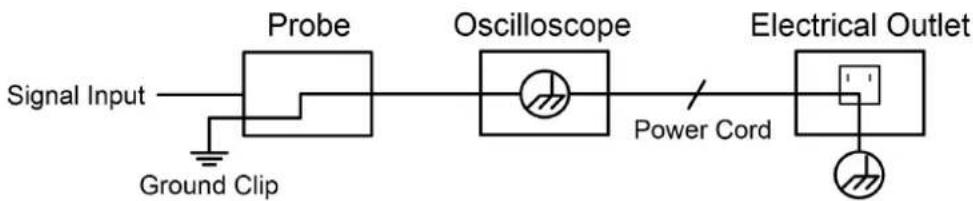
flowchart
graph LR
    A["Signal Input"] --> B["Probe"]
    B --> C["Oscilloscope"]
    C --> D["Power Cord"]
    D --> E["Electrical Outlet"]
    F["Ground Clip"] --> B
The diagram of the ground wire connection when the battery-powered oscilloscope is connected to the AC-powered PC through the ports:

flowchart
graph LR
    A["Signal Input"] --> B["Probe"]
    B --> C["Oscilloscope (Battery-power)"]
    C --> D["PC"]
    D --> E["Electrical Outlet"]
    F["Ground Clip"] --> B
    G["USB/VGA/COM/LAN Cable"] --> D
It is not allowed to measure AC power when the oscilloscope is AC powered, or when the battery-powered oscilloscope is connected to the AC-powered PC through the ports.
Warning:
To avoid fire or electrical shock, when the oscilloscope input signal connected is more than 42V peak (30Vrms) or on circuits of more 4800VA, please take note of below items:
- Only use accessory insulated voltage probes and test lead.
- Check the accessories such as probe before use and replace it there are any damages.
- Remove probes, test leads and other accessories immediately: use.
- Remove USB cable which connects oscilloscope and computer.
- Do not apply input voltages above the rating of the instrume because the probe tip voltage will directly transmit to the oscilloscope. Use with caution when the probe is set as 1:1.
- Do not use exposed metal BNC or banana plug connectors.
- Do not insert metal objects into connectors.
3. Junior User Guidebook
This chapter deals with the following topics mainly:
● Introduction to the structure of the oscilloscope
● Introduction to the user interface
● How to implement the general inspection
● How to implement the function inspection
● How to make a probe compensation
● How to set the probe attenuation coefficient
● How to use the probe safely
● How to implement an auto-calibration
● Introduction to the vertical system
● Introduction to the horizontal system
● Introduction to the trigger system
- Touchscreen Controls (Touchscreen is optional)
Introduction to the Structure of the Oscilloscope
This chapter makes a simple description of the operation and function of the front panel of the oscilloscope, enabling you to be familiar with the use of the oscilloscope in the shortest time.
Front Panel
The front panel has knobs and function buttons. The 5 buttons in the column on the right side of the display screen or in the row under the display screen are menu selection buttons, through which, you can set the different options for the current menu. The other buttons are function buttons, through which, you can enter different function menus or obtain a specific function application directly.
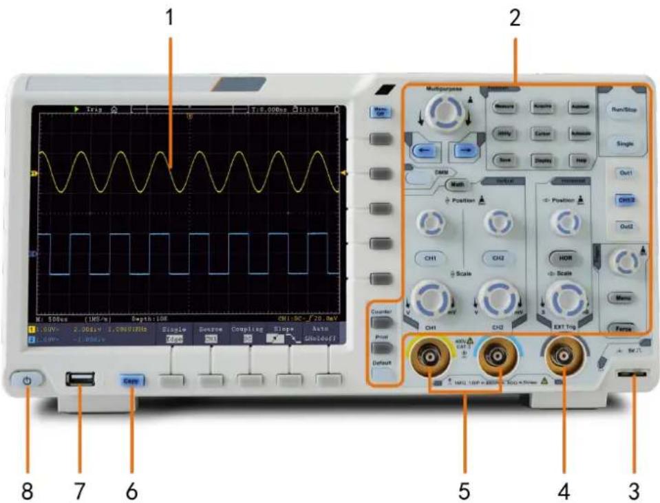
Figure 3-1 Front panel
- Display area.
- Control (button and knob) area.
- Probe Compensation: Measurement signal (5V/1kHz) output.
- EXT Trigger Input.
- Signal Input Channel.
- Copy button: You can save the waveform by just pressing this button in any user interface.
- USB Host port: It is used to transfer data when external USB equipment connects to the oscilloscope regarded as "host device". For example: Saving the waveform to USB flash disk needs to use this port.
- Power on/off
Backlight of this button:
Red light: The oscilloscope is turned off (connects with AC Power or battery);
Green light: The oscilloscope is turned on (powered by AC Power or battery).
Front Panel Menu Buttons
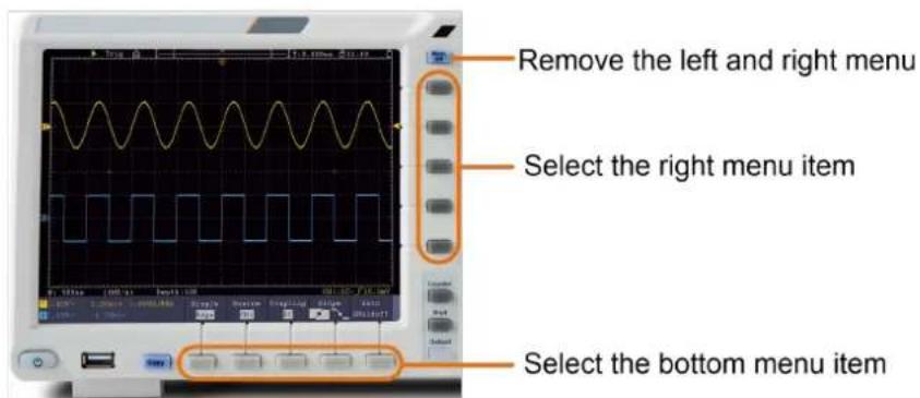
Figure 3-2 Menu Buttons
Rear Panel
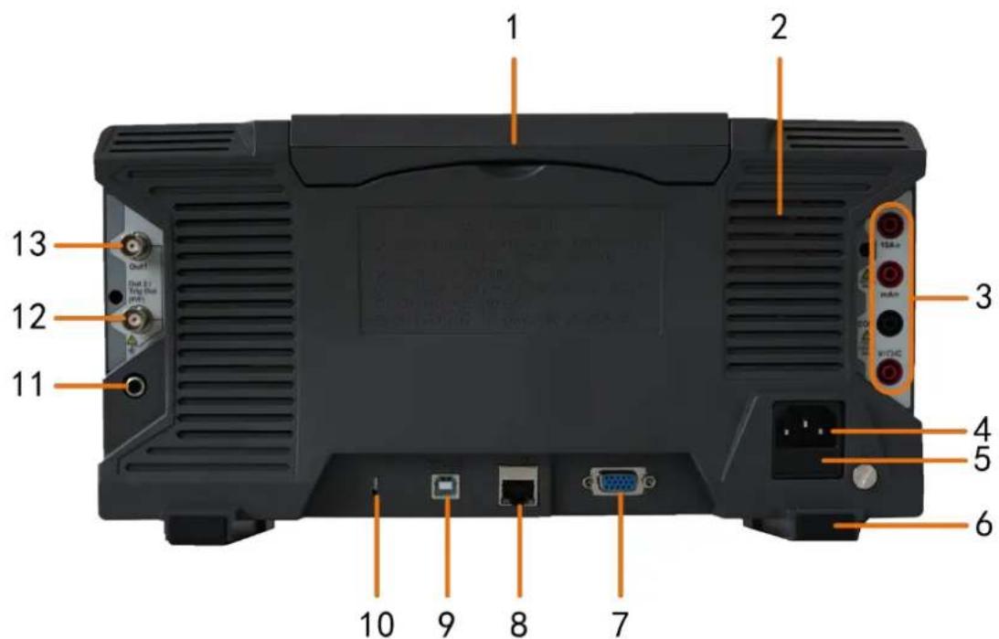
Figure 3-3 Rear Panel
- Handle.
- Air vents.
- Input terminals of multimeter (optional).
- AC power input jack.
- Fuse.
- Foot stool: Adjust the tilt angle of the oscilloscope.
- VGA port: To connect the oscilloscope with a monitor or a projector as VGA output (optional).
-
LAN port: the network port which can be used to connect with PC.
-
USB Device port: It is used to transfer data when external USB equipment connects to the oscilloscope regarded as "slave device". For example: to use this port when connect PC to the oscilloscope by USB.
- Lock Hole: You can lock the oscilloscope to a fixed location using the security lock (please buy it yourself) to secure the oscilloscope.
- AV Port: AV signal output port (optional).
- Trig Out(P/F) port: Trigger signal output or Pass/Fail output, also can be used as the port of CH2 Output of optional dual-channel waveform generator. The output type can be set on the menu (Utility menu→Output→Output).
- Out 1 port: Output (single-channel) or CH1 Output (dual-channel) of optional waveform generator.
Control Area
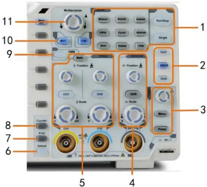
Figure 3-4 Control Area Overview
- Function button area: Total 11 buttons.
- Waveform generator controls (optional)
or
DAQ: Multimeter Recorder (see "Multimeter Recorder" on P112)
P/F: Pass/Fail (see "Pass/Fail" on P81)
W.REC: Waveform Record (see "How to Record/Playback Waveforms" on P72)
- Trigger control area with 2 buttons and 1 knob.
The Trigger Level knob is to adjust trigger voltage. Other 2 buttons refer to trigger system setting.
- Horizontal control area with 1 button and 2 knobs.
"HOR" button refer to horizontal system setting menu, "Horizontal Position" knob control trigger position, "Horizontal Scale" control time base.
- Vertical control area with 3 buttons and 4 knobs.
"CH1" and "CH2" correspond to setting menu in CH1 and CH2. "Math" button provides access to math waveform functions (+, -, ×, /, FFT, user function, digital filter). Two "Vertical Position" knob control the vertical position of CH1/CH2, and two "Scale" knob control voltage scale of CH1, CH2.
- Default: Call out the factory settings.
- Print: Print an image of what appears on the instrument screen.
- Turn on/off the Counter, or turn on/off Decode (optional) function.
- DMM (optional Multimeter) or Snapshot (Shortcut button for measurement snapshot)
- Direction key: Move the cursor of the focused parameter.
- M knob (Multipurpose knob): when M symbol appears on the menu, it indicates you can turn the M knob to select the menu or set the value. You can push it to close the menu on the left and right.
User Interface Introduction
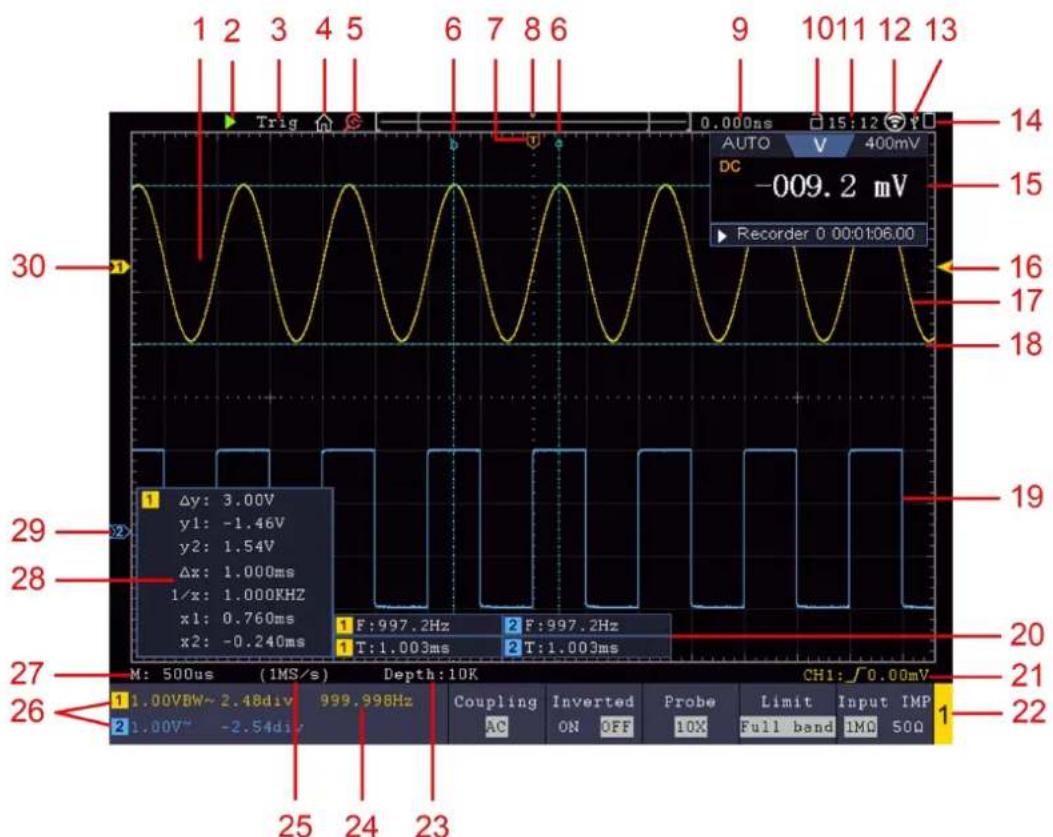
line
| Time (s) | Voltage (mV) | |----------|--------------| | 0 | 3.00 | | 1 | -1.46 | | 2 | 1.54 | | 3 | 1.00 | | 4 | 1.00 | | 5 | 1.00 | | 6 | 1.00 | | 7 | 1.00 | | 8 | 1.00 | | 9 | 1.00 | | 10 | 1.00 | | 11 | 1.00 | | 12 | 1.00 | | 13 | 1.00 | | 14 | -0.092 | | 15 | - | | 16 | - | | 17 | - | | 18 | - | | 19 | - | | 20 | - | | 21 | - | | 22 | - | | 23 | - | | 24 | - | | 25 | - | | 26 | - | | 27 | - | | 28 | - | | 29 | - | | 30 | - |Figure 3-5 Illustrative Drawing of Display Interfaces
- Waveform Display Area.
- Run/Stop (touchable on touchscreen) (see "How to Use Executive Buttons" on P96)
- The state of trigger, including:
Auto: Automatic mode and acquire waveform without triggering.
Trig: Trigger detected and acquire waveform.
Ready: Pre-triggered data captured and ready for a trigger.
Scan: Capture and display the waveform continuously.
Stop: Data acquisition stopped.
-
Click to show/hide the touchable menu pane (only for touchscreen). (see "Operate the Menu through Touchscreen" on P17)
-
Turn on/off the magnifier function(Only for XDS3102AP/XDS3202A with touchscreen)
-
The two blue dotted lines indicates the vertical position of cursor measurement.
-
The T pointer indicates the horizontal position for the trigger.
-
The pointer indicates the trigger position in the record length.
-
It shows present triggering value and displays the site of present window in internal memory.
-
Touchable icon is to enable 📄) or disable ( 📋 the touchscreen controls (only for touchscreen).
-
It shows setting time (see "Config" on P80).
-
Wi-Fi is activated (see "Communication with Android Device via Wi-Fi (Optional)" on P123).
-
It indicates that there is a USB disk connecting with the oscilloscope.
-
Indicating battery power status (see "Display" on P80).
-
Multimeter window.
-
The pointer shows the trigger level position.
-
The waveform of CH1.
-
The two blue dotted lines indicate the horizontal position of cursor measurement.
-
The waveform of CH2.
-
It indicates the measured type and value of the corresponding channel. "T" means period, "F" means frequency, "V" means the average value, "Vp" the peak-peak value, "Vr" the root-mean-square value, "Ma" the maximum amplitude value, "Mi" the minimum amplitude value, "Vt" the Voltage value of the waveform's flat top value, "Vb" the Voltage value of the waveform's flat base, "Va" the amplitude value, "Os" the overshoot value, "Ps" the Preshoot value, "RT" the rise time value, "FT" the fall time value, "PW" the +width value, "NW" the -Width value, "+D" the +Duty value, "-D" the -Duty value, "PD" the Delay A->B ≠ value, "ND" the Delay A->B ≠ value, "TR" the Cycle RMS, "CR" the Cursor RMS, "WP" the Screen Duty, "RP" the Phase, "+PC" the +Pulse count, "FRR" the FRR, "FRF" the FRF, "FFR" the FFR, "FFF" the FFF, "LRR" the, "LRF" the LRF, "LFR" the LFR, "LFF" the LFF, "-PC" the -Pulse count, "+E" the Rise edge count, "-E" the Fall edge count, "AR" the Area, "CA" the Cycle area.
-
The icon shows the selected trigger type, e.g. represents triggering on the rising edge for an Edge trigger. The reading shows the trigger level value of the corresponding channel.
-
Channel identifier of current bottom menu.
-
The readings show the record length.
-
The frequency of the trigger signal.
-
The readings show current sample rate.
-
The readings indicate the corresponding Voltage Division and the Zero Point positions of the channels. "BW" indicates bandwidth limit.
The icon shows the coupling mode of the channel.
"—" indicates direct current coupling;
"\~" indicates AC coupling;
" indicates GND coupling.
-
The reading shows the setting of main time base.
-
It is cursor measure window, showing the absolute values and the readings of the cursors.
-
The blue pointer shows the grounding datum point (zero point position) of the waveform of the CH2 channel. If the pointer is not displayed, it means that this channel is not opened.
-
The yellow pointer indicates the grounding datum point (zero point position) of the waveform of the CH1 channel. If the pointer is not displayed, it means that the channel is not opened.
How to Implement the General Inspection
After you get a new oscilloscope, it is recommended that you should make a check on the instrument according to the following steps:
1. Check whether there is any damage caused by transportation.
If it is found that the packaging carton or the foamed plastic protection cushion has suffered serious damage, do not throw it away first till the complete device and its accessories succeed in the electrical and mechanical property tests.
2. Check the Accessories
The supplied accessories have been already described in the "Appendix A: Enclosure" of this Manual. You can check whether there is any loss of accessories with reference to this description. If it is found that there is any accessory lost or damaged, please get in touch with our distributor responsible for this service or our local offices.
3. Check the Complete Instrument
If it is found that there is damage to the appearance of the instrument, or the instrument can not work normally, or fails in the performance test, please get in touch with our distributor responsible for this business or our local offices. If there is damage to the instrument caused by the transportation, please keep the package. With the transportation department or our distributor responsible for this business informed about it, a repairing or replacement of the instrument will be arranged by us.
How to Implement the Function Inspection
Make a fast function check to verify the normal operation of the instrument, according to the following steps:
- Connect the power cord to a power source. Long press the button on the bottom left of the instrument.
The instrument carries out all self-check items and shows the Boot Logo. Push the Utility button, select Function in the bottom menu. Select Adjust in the left menu, select Default in the bottom menu. The default attenuation coefficient set value of the probe in the menu is 10X.
- Set the Switch in the Oscilloscope Probe as 10X and Connect the Oscilloscope with CH1 Channel.
Align the slot in the probe with the plug in the CH1 connector BNC, and then tighten the probe with rotating it to the right side.
Connect the probe tip and the ground clamp to the connector of the probe compensator.
- Push the Autoset Button on the front panel.
The square wave of 1 KHz frequency and 5V peak-peak value will be displayed in several seconds (see Figure 3-6).
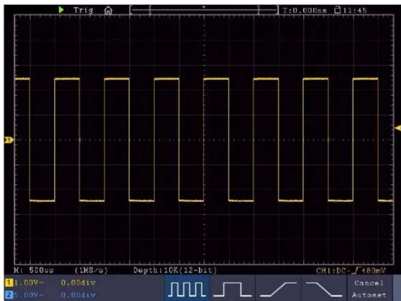
Figure 3-6 Auto set
Check CH2 by repeating Step 2 and Step 3.
How to Implement the Probe Compensation
When connect the probe with any input channel for the first time, make this adjustment to match the probe with the input channel. The probe which is not compensated or presents a compensation deviation will result in the measuring error or mistake. For adjusting the probe compensation, please carry out the following steps:
- Set the attenuation coefficient of the probe in the menu as 10X and that of the switch in the probe as 10X (see "How to Set the Probe Attenuation Coefficient" on P12), and connect the probe with the CH1 channel. If a probe hook tip is used, ensure that it keeps in close touch with the probe. Connect the probe tip with the signal connector of the probe compensator and connect the reference wire clamp with the ground wire connector of the probe connector, and then push the Autoset button on the front panel.
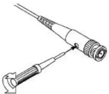
- Check the displayed waveforms and regulate the probe till a correct compensation is achieved (see Figure 3-7 and Figure 3-8).
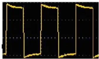
natural_image
Abstract black-and-white pattern with yellow outlines on a dotted grid background (no text or symbols)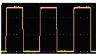
natural_image
Pure electrical circuit lines without any symbols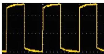
natural_image
Pure electrical circuit lines without any symbolsOvercompensated Compensated correctly Under compensated
Figure 3-7 Displayed Waveforms of the Probe Compensation
- Repeat the steps mentioned if needed.
natural_image
Technical line drawing of two mechanical components with no visible text or symbolsFigure 3-8 Adjust Probe
How to Set the Probe Attenuation Coefficient
The probe has several attenuation coefficients, which will influence the vertical scale factor of the oscilloscope.
To change or check the probe attenuation coefficient in the menu of oscilloscope:
(1) Push the function menu button of the used channels (CH1 or CH2 button).
(2) Select Probe in the bottom menu; select Attenu in the right menu, turn the M knob to
select the proper value corresponding to the probe.
This setting will be valid all the time before it is changed again.

Caution:
The default attenuation coefficient of the probe on the instrument is p 10X.
Make sure that the set value of the attenuation switch in the probe is same as the menu selection of the probe attenuation coefficient in the oscilloscope.
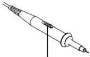
The set values of the probe switch are 1X and 10X (see Figure 3-9).
natural_image
Pure technical line drawing of a mechanical component with no text or symbolsFigure 3-9 Attenuation Switch

Caution:
When the attenuation switch is set to 1X, the probe will limit the ba of the oscilloscope in 5MHz. To use the full bandwidth of the oscillo the switch must be set to 10X.
Identify the Probe Attenuation Coefficient Automatically
The oscilloscope can identify the probe attenuation coefficient of the 100:1 (impedance 5K ± 20% ) or 10:1 (impedance 10K ± 20% ) probe with the identifying pin. When you attach the probe, the oscilloscope set the attenuation automatically on the oscilloscope vertical menu for the channel to match the probe.
For example, if you attach a 10:1 probe with the identifying pin, the screen will prompt "The probe attenuation factor is 10X", and set the attenuation to 10X automatically on the oscilloscope vertical menu for the channel.
How to Use the Probe Safely
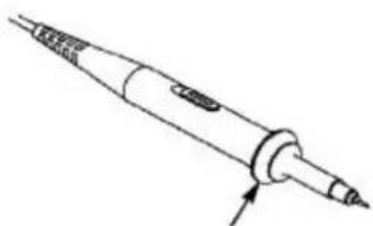
The safety guard ring around the probe body protects your finger against any electric shock, shown as Figure 3-10.
natural_image
Line drawing of a soldering iron with a pointed tip and threaded end (no text or symbols)Figure 3-10 Finger Guard

Warning:
To avoid electric shock, always keep your finger behind the safety gu ring of the probe during the operation.
To protect you from suffering from the electric shock, do not touch a metal part of the probe tip when it is connected to the power supply.
Before making any measurements, always connect the probe to the instrument and connect the ground terminal to the earth.
How to Implement Self-calibration
The self-calibration application can make the oscilloscope reach the optimum condition rapidly to obtain the most accurate measurement value. You can carry out this application program at any time. This program must be executed whenever the change of ambient temperature is 5^ C or over.
Before performing a self-calibration, disconnect all probes or wires from the input connector. Push the Utility button, select Function in the bottom menu, select Adjust. in the left menu, select Self Cal in the bottom menu; run the program after everything is ready.
Introduction to the Vertical System
As shown in Figure 3-11, there are a few of buttons and knobs in Vertical Controls. The following practices will gradually direct you to be familiar with the using of the vertical setting.
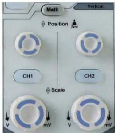
Figure 3-11 Vertical Control Zone
- Use the Vertical Position knob to show the signal in the center of the waveform window. The Vertical Position knob functions the regulating of the vertical display position of the signal. Thus, when the Vertical Position knob is rotated, the pointer of the earth datum point of the channel is directed to move up and down following the waveform.
Measuring Skill
If the channel is under the DC coupling mode, you can rapidly measure the DC component of the signal through the observation of the difference between the wave form and the signal ground.
If the channel is under the AC mode, the DC component would be filtered out. This mode helps you display the AC component of the signal with a higher sensitivity.
Vertical offset back to 0 shortcut key
Turn the Vertical Position knob to change the vertical display position of channel and push the position knob to set the vertical display position back to 0 as a shortcut key, this is especially helpful when the trace position is far out of the screen and want it to get back to the screen center immediately.
- Change the Vertical Setting and Observe the Consequent State Information Change.
With the information displayed in the status bar at the bottom of the waveform window, you can determine any changes in the channel vertical scale factor.
- Turn the Vertical Scale knob and change the "Vertical Scale Factor (Voltage Division)", it can be found that the scale factor of the channel corresponding to the status bar has been changed accordingly.
- Push buttons of CH1, CH2 and Math, the operation menu, symbols, waveforms and scale factor status information of the corresponding channel will be displayed in the screen.
Introduction to the Horizontal System
Shown as Figure 3-12, there are a button and two knobs in the Horizontal Controls. The following practices will gradually direct you to be familiar with the setting of horizontal time base.
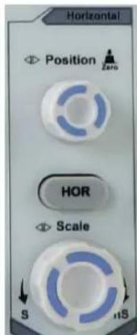
Figure 3-12 Horizontal Control Zone
- Turn the Horizontal Scale knob to change the horizontal time base setting and
observe the consequent status information change. Turn the Horizontal Scale knob to change the horizontal time base, and it can be found that the Horizontal Time Base display in the status bar changes accordingly.
- Use the Horizontal Position knob to adjust the horizontal position of the signal in the waveform window. The Horizontal Position knob is used to control the triggering displacement of the signal or for other special applications. If it is applied to triggering the displacement, it can be observed that the waveform moves horizontally with the knob when you rotate the Horizontal Position knob.
Triggering displacement back to 0 shortcut key
Turn the Horizontal Position knob to change the horizontal position of channel and push the Horizontal Position knob to set the triggering displacement back to 0 as a shortcut key.
- Push the Horizontal HOR button to switch between the normal mode and the wave zoom mode.
Introduction to the Trigger System
As shown in Figure 3-13, there are one knob and three buttons make up Trigger Controls. The following practices will direct you to be familiar with the setting of the trigger system gradually.
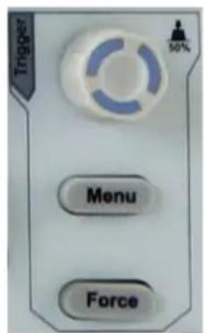
Figure 3-13 Trigger Control Zone
- Push the Trigger Menu button and call out the trigger menu. With the operations of the menu selection buttons, the trigger setting can be changed.
- Use the Trigger Level knob to change the trigger level setting.
By turning the Trigger Level knob, the trigger indicator in the screen will move up and down. With the movement of the trigger indicator, it can be observed that the trigger level value displayed in the screen changes accordingly.
Note: Turning the Trigger Level knob can change trigger level value and it is also the hotkey to set trigger level as the vertical mid point values of the amplitude of the trigger signal.
- Push the Force button to force a trigger signal, which is mainly applied to the "Normal" and "Single" trigger modes.
Touchscreen Controls (Touchscreen is optional)
If the LCD is touchscreen, you can control the oscilloscope by different gestures.
The touchable icon at the top right of the screen is used to enable ( ) or disable ( ) the touchscreen controls.
The instruction of touchscreen controls is as below. You can also use the buttons / knobs enclosed in brackets to do the same thing.
Operate the Menu through Touchscreen
- Select a menu item: Touch the menu items in the bottom menu, or in the right menu, or in the left menu.
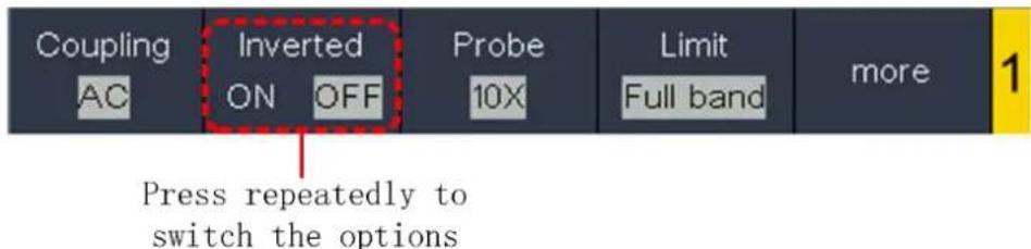
- Switch menu items: If there are options that can be switched in the menu, you can repeatedly touch the area of the menu item to switch, or push the corresponding button to switch. See figure below.
- Scroll the list: If there is a scroll bar in the left menu or in the file system window, you can swipe up and down to scroll the list.
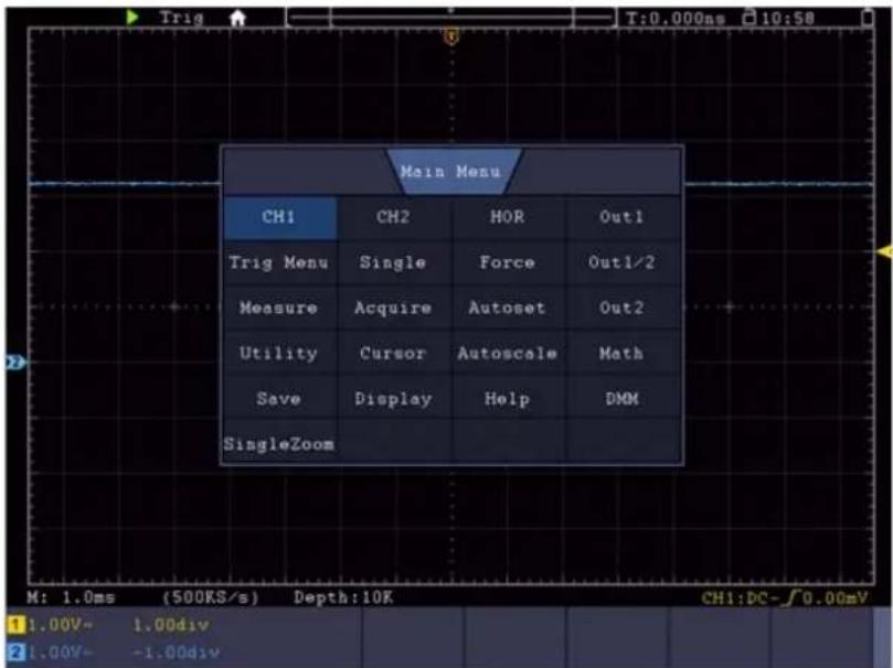
- Touchable menu pane: Click the 📋 icon on the left top of the display area, a menu pane will be shown. Clicking the menu item is same as pushing the corresponding button.
Gestures in Normal Mode
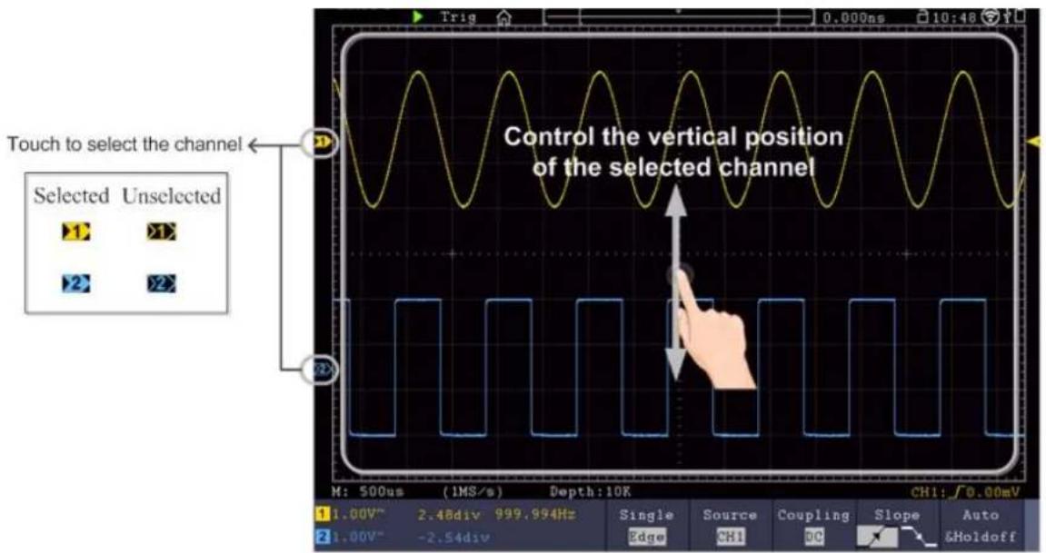
- Select a channel (CH1 or CH2 button): Touch the pointer on the left side of
corresponding channel to make it in selected state.
- Set the vertical position of the selected channel (Vertical Position knob): Swipe up or down on the screen. See figure below.
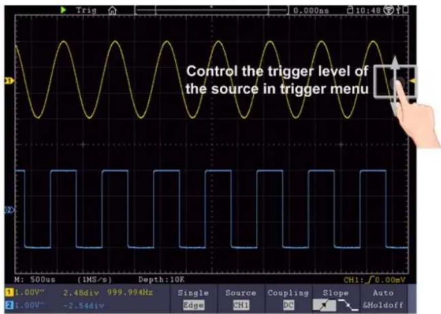
- Set the trigger level of the source in trigger menu (Trigger Level knob): Swipe up or down on the area nearby the trigger pointer on the right. See figure below.
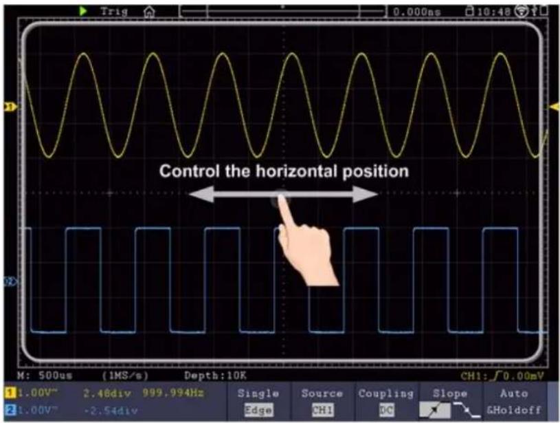
- Set the horizontal position (Horizontal Position knob): Swipe left or right on the display area. See figure below.
Double Zoom and Single Zoom
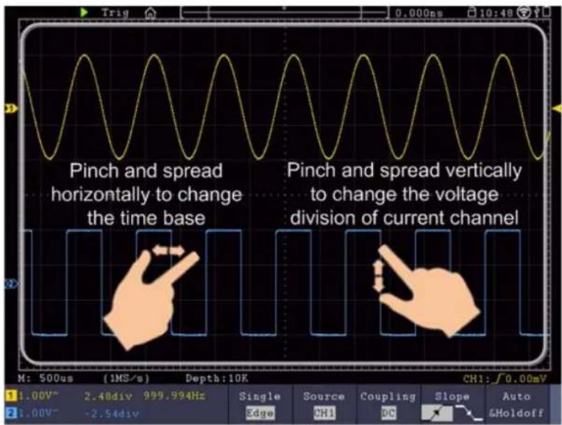
In touchable menu pane, if DoubleZoom is selected, in the display area, pinch and spread horizontally to change the time base; pinch and spread vertically to change the voltage division of current channel. See figure below.
| Main Menu | |||
| CH1 | CH2 | HOR | Out1 |
| Trig Menu | Single | Force | Out1/2 |
| Measure | Acquire | Autoset | Out2 |
| Utility | Cursor | Autoscale | Math |
| Save | Display | Help | DMM |
| DoubleZoom | |||
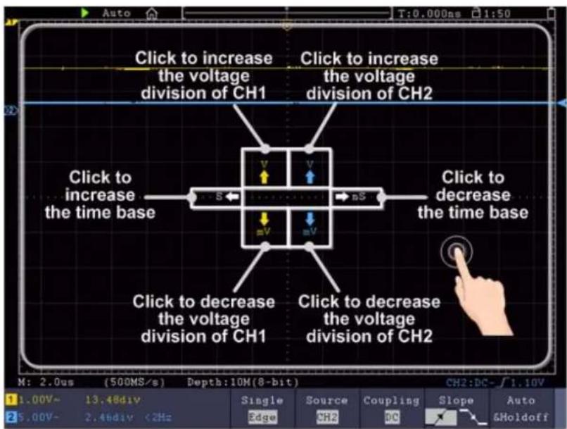
In touchable menu pane, if SingleZoom is selected, click anywhere on the Display area to show the touching control panel. See figure below.
| Main Menu | |||
| CH1 | CH2 | HOR | Out1 |
| Trig Menu | Single | Force | Out1/2 |
| Measure | Acquire | Autoset | Out2 |
| Utility | Cursor | Autoscale | Math |
| Save | Display | Help | DMM |
| SingleZoom | |||
Other Operations Using Touchscreen
● Under cursor measurement, control horizontal or vertical cursor line:  - Run/Stop: Double tap on the display area, or click the ▶ or □ on the left top of the display area to run or stop the waveform sampling. - Touch keyboard: Click to input. - Adjust value in the menu item: . Magnifier Function (Only for XDS3102AP/XDS3202A with touchscreen)
The magnifier window can display the magnified wave of the wave selection, when the magnifier function is enabled. Click the 📄 on the left top of the display area, the magnifier window and menu will be shown. Click the 📄 icon to turn off the magnifier function.  The description of the Magnifier menu is shown as follows:| Function Menu | Setting | Description |
| Horizontal | 1510 | Horizontal magnification factor. The size of the magnifier window is fixed. Therefor, the greater this value, the shorter the horizontal length of the wave selection. |
| Vertical | 12481632 | Vertical magnification factor. The size of t magnifier window is fixed. Therefor, the greater this value, the shorter the vertical height of the wave selection. |
| Transparent | ONOFF | Make the magnifier window transparent or not. |
The Cursor Measurement in Magnifier Window
When the magnifier function is enabled, push Cursor panel key to display the cursor menu. In the bottom menu, select Window as Main or Extension to make the cursors shown in the main window or the magnifier window.  Note: The magnifier function is disabled in wave zoom mode, waveform math, FFT, XY mode, slow-scan mode, stop state, average acquire mode, and persist mode.4. Advanced User Guidebook
Up till now, you have already been familiar with the basic operations of the function areas, buttons and knobs in the front panel of the oscilloscope. Based the introduction of the previous Chapter, the user should have an initial knowledge of the determination of the change of the oscilloscope setting through observing the status bar. If you have not been familiar with the above-mentioned operations and methods yet, we advise you to read the section of Chapter 3 "Junior User Guidebook". This chapter will deal with the following topics mainly: ● How to Set the Vertical System ● How to Set the Horizontal System ● How to Set the Trigger/Decoding System ● How to Implement the Sampling Setup ● How to Set the Display System ● How to Save and Recall Waveform ● How to Record/Playback Waveforms ● How to Clone and Recall a waveform ● How to Implement the Auxiliary System Function Setting ● How to Update your Instrument Firmware ● How to Measure Automatically - Customize an Automatic Measurement ● How to Measure with Cursors ● How to Use Autoscale ● How to Use Built-in Help ● How to Use Executive Buttons ● How to Print the Screen Image It is recommended that you read this chapter carefully to get acquainted the various measurement functions and other operation methods of the oscilloscope.How to Set the Vertical System
The VERTICAL CONTROLS includes three menu buttons such as CH1, CH2 and Math, and four knobs such as Vertical Position, Vertical Scale for each channel.Setting of CH1 and CH2
Each channel has an independent vertical menu and each item is set respectively based on the channel.To turn waveforms on or off (channel, math)
Pushing the CH1, CH2, or Math buttons have the following effect: - If the waveform is off, the waveform is turned on and its menu is displayed. - If the waveform is on and its menu is not displayed, its menu will be displayed. - If the waveform is on and its menu is displayed, the waveform is turned off and its menu goes away. The description of the Channel Menu is shown as the following list:| Function Menu | Setting | Description | ||
| Coupling | DCACGROUND | Pass both AC and DC components of the input signal.Block the DC component of the input signal.Disconnect the input signal. | ||
| Inverted | ONOFF | Display inverted waveform.Display original waveform. | ||
| Probe | Attenu | 0.001X0.002X0.005X0.01X0.02X0.05X0.1X0.2X0.5X | 1X2X5X10X20X50X100X200X500X1000X | Select one of the values based on the probe attenuation factor to keep the vertical gear reading accurate. |
| MeasCurr | YESNO | If you are measuring current by probing the voltage drop across a resistor, choose YES. | ||
| A/V (mA/V)V/A (mV/A)(When selecting the measurement current) | Turn the M knob to set the Amps/Volts ratioThe range is 100 mA/V - 1 KA/V.Amps/Volts ratio = 1/Resistor valueVolts/Amp ratio is automatically calculated. | |||
| AutoDetect | YES | Click to open or close AutoDetect function. | ||
| NO | |||
| Limit | Full band20M | Get full bandwidth.Limit the channel bandwidth to 20MHz to redisplay noise. | |
| Input impedance (Applicable to some models only) | 1MΩ50Ω | The circuit load caused by the interaction between the oscilloscope and the circuit to be measured can be reduced. | |
| more | Tag | ONOFF | Turn channel label on or off. |
| Unit | VAWU | Select the display unit of the parameter. | |
1. To set channel coupling
Taking the Channel 1 for example, the measured signal is a square wave signal containing the direct current bias. The operation steps are shown as below: (1) Push the CH1 button to show the CH1 SETUP menu. (2) Select Coupling in the bottom menu. (3) Select DC in the right menu. Both DC and AC components of the signal are passed. (4) Select AC in the right menu. The direct current component of the signal is blocked.2. To adjust the probe attenuation
For correct measurements, the attenuation coefficient settings in the operating menu of the Channel should always match what is on the probe (see "How to Set the Probe Attenuation Coefficient" on P12). If the attenuation coefficient of the probe is 1:1, the menu setting of the input channel should be set No 1 Take the Channel 1 as an example, the attenuation coefficient of the probe is 10:1, the operation steps are shown as follows: (1) Push the CH1 button to show the CH1 SETUP menu. (2) Select Probe in the bottom menu. Select Attenu in the right menu, turn the M knob to set it as X03. To measure current by probing the voltage drop across a resistor
Take the Channel 1 as an example, if you are measuring current by probing the voltage drop across a 1 resistor, the operation steps are shown as follows: (1) Push the CH1 button to show CH1 SETUP menu. (2) Select Probe in the bottom menu. In the right menu, set MeasCurr as YES, the A/V radio menu will appear below. Select it; turn the M knob to set the Amps/Volts ratio. Amps/Volts ratio = 1/Resistor value. Here the A/V radio should be set to 1.4. To invert a waveform
Waveform inverted: the displayed signal is turned 180 degrees against the phase of the earth potential. Taking the Channel 1 for example, the operation steps are shown as follows: (1) Push the CH1 button to show the CH1 SETUP menu. (2) Select Inverted in the bottom menu, switch to ON. the waveform is inverted. Push again to switch to OFF, the waveform goes back to its original one.5. To set bandwidth limit
When high frequency components of a waveform are not important to its analysis, the bandwidth limit control can be used to reject frequencies above 20 MHz. Taking the Channel 1 for example, the operation steps are shown as below: (1) Push the CH1 button to show CH1 SETUP menu. (2) Select Limit in the bottom menu. (3) Select Full band in the right menu. The high frequency of the signal will be allowed to pass. (4) Select 20M in the right menu. The bandwidth is limited to 20 MHz. The frequencies above 20MHz will be rejected.6. Set the channel label
Set the channel label to see the location of the channel more clearly. Take channel 1 as an example, the operation steps are as follows: (1) Press the CH1 button to call up the CH1 setting menu. (2) In the bottom menu, select More, in the right menu, select label ON, and the channel label function is turned on. Press again to select label to OFF, and the channel label function is turned off.7. Set the display unit
Set the current channel amplitude display unit. The unit can be V, A, W, or U. When you change the unit, the unit in the channel status label changes accordingly. Take channel 1 as an example, the operation steps are as follows: (1) Press the CH1 button to call up the CH1 setting menu. (2) In the bottom menu, select More, in the right menu, select the desired Unit. The default unit is V.Use Mathematical Manipulation Function
The Waveform Calculation function is used to show the results of the addition, multiplication, division and subtraction operations between two channels, the FFT operation for a channel, advanced math feature including Intg, Diff, Sqrt, user defined function, and digital filter. Press the Math button to display the menu on the bottom. The Waveform Calculation menu:| Function Menu | Setting | Description | |
| Dual Wfm Math | Factor1 | CH1CH2 | Select the signal source of the factor1. |
| Sign | + - * / | Select the sign of mathematical manipulation. | |
| Factor2 | CH1CH2 | Select the signal source of the factor2. | |
| Vertical (div) | Turn the M knob to adjust the vertical position of the waveform. | ||
| Vertical (V/div) | Turn the M knob to adjust the vertical division of the waveform. | ||
| FFT | Source | CH1CH2 | Select CH1 as FFT source.Select CH2 as FFT source. |
| Window | HammingRectangleBlackmanHanningKaiserBartlett | Select window for FFT. | |
| Format | V RMSDecibelsRadianDegrees | V RMS and Decibels are amplitude units;Radian and Degrees are phase units. | |
| Hori (Hz) | Position valueTime base value | Switch to select the horizontal position time base of the FFT waveform, turn M knob to adjust it. | |
| Vertical | Position valueDivision value/ | Switch to select the vertical position o vertical division of the FFT waveform, turn the M knob to adjust it. | |
| User Function | Intg, Diff, Sqrt, and user defined function. | ||
| DIR | channel | CH1CH2 | Select channel. |
| type | low-pass | Only the signals whose frequencies are lower than the current cut-off frequency can pass the filter. | |
| high-pass | Only the signals whose frequencies are greater than the current cutoff frequency can pass the filter. | ||
| band-pass | Only the signals whose frequencies are greater than the cutoff frequency down and lower than the current cutoff frequency upper can pass the filter. | ||
| band-reject | Only the signals whose frequencies are lower than the current cutoff frequency down or greater than the current cutoff frequency upper can pass the filter. | ||
| window | rectangular tapered triangular Hanning Hamming Blackman | Select window for digital filter. | |
| cut-off fre or upper down | Turn the M knob to set cut-off freque | ||
| Vertical (div) | Turn the M knob to adjust the vertical position of Math waveform. | ||
| FFT Peak | ON OFF | Enable or disable FFT peak search. Dynamic marker ∇ marks the FFT peak. | |
Waveform math
Taking the additive operation between Channel 1 and Channels 2 for example, the operation steps are as follows: 1. Press the Math button to display the math menu in the bottom. The pink M waveform appears on the screen. 2. Select Dual Wfm Math in the bottom menu. 3. In the right menu, select Factor1 as CH1. 4. Select Sign as + in the right menu. 5. In the right menu, select Factor2 as CH2. 6. Select Vertical (div) in the right menu, turn the M knob to adjust the vertical position of Math waveform. 7. Select Vertical (V/div) in the right menu, turn the M knob to adjust the vertical division of Math waveform.User defined function
1. Press the Math button to display the math menu in the bottom. 2. Select User Function in the bottom menu, an expression input keyboard pops up.  3. Create an expression. When done, choose in the keyboard to confirm The division of Math waveform is displayed at the left bottom of screen. Digital Filter
Digital filter provides 4 types of filters (low pass, high pass, band pass and band reject). The specified frequencies can be filtered by setting the cut-off frequency. 1. Press the Math button to display the math menu in the bottom. 2. Select DIR in the bottom menu. 3. In the right menu, select channel as CH1 or CH2. 4. In the right menu, select type, select the desired filter type. 5. In the right menu, select window, select the desired window. 6. When low-pass or high-pass type is selected, select cut-off fre in the right menu. When band-pass or band-reject type is selected, select upper or down in the right menu. Turn M knob to adjust the frequency. 7. In the right menu, select Vertical (div), turn M knob to adjust the vertical position of Math waveform. The voltage division of Math waveform is the same as the selected channel. Note: On the Low-Scan format, digital filter is disabled.Using FFT function
The FFT (fast Fourier transform) math function mathematically converts a time-domain waveform into its frequency components. It is very useful for analyzing the input signal on Oscilloscope. You can match these frequencies with known system frequencies, such as system clocks, oscillators, or power supplies. FFT function in this oscilloscope transforms 8192 data points of the time-domain signal into its frequency components mathematically (the record length should be 10K or above). The final frequency contains 4096 points ranging from 0Hz to Nyquist frequency. Taking the FFT operation for example, the operation steps are as follows: 1. Press the Math button to display the math menu in the bottom. 2. Select FFT in the bottom menu. 3. In the right menu, select Source as CH1. 4. In the right menu, select Window. In the left menu, turn the M knob to select the proper window type. 5. In the right menu, select Format. In the left menu, turn the M knob to select amplitude unit (V RMS, Decibels) or phase unit (Radian, Degrees). 6. Select Hori (Hz) in the right menu; select repeatedly to make the symbol in front of the horizontal position value (the upper one), turn the M knob to adjust the horizontal position of FFT waveform; then select to make the symbol in front of the time base value below, turn the M knob to adjust the time base of FFT waveform. 7. Select Vertical in the right menu; do the same operations as above to set the vertical position and vertical division.To select the FFT window
■ There are 6 FFT windows. Each one has trade-offs between frequency resolution and magnitude accuracy. What you want to measure and your source signal characteristics help you to determine which window to use. Use the following guidelines to select the best window.| Type | Characteristics | Window |
| Hamming | Better solution for magnitude than Rectangle, an good for frequency as well. It has slightly better frequency resolution than Hanning.Recommend to use for:Sine, periodic and narrow band random noisTransients or bursts where the signal levels before and after the event are significantly different. | 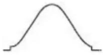 |
| Rectangle | Best solution for frequency, worst for magnitudeBest type for measuring the frequency spectrum nonrepetitive signals and measuring frequency components near DC.Recommend to use for:Transients or bursts, the signal level before a after the event are nearly equal.Equal-amplitude sine waves with frequencies those are very close.Broadband random noise with a relatively sl varying spectrum. | 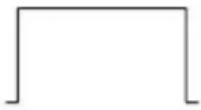 |
| Blackman | Best solution for magnitude, worst for frequencyRecommend to use for:Single frequency waveforms, to find higher order harmonics. | 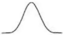 |
| Hanning | Good for magnitude, but poorer frequency resolution than Hamming.Recommend to use for:Sine, periodic and narrow band random noisTransients or bursts where the signal levels before and after the event are significantly different. | 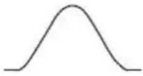 |
| Kaiser | The frequency resolution when using the Kaiser window is fair; the spectral leakage and amplitude accuracy are both good.The Kaiser window is best used when frequencie are very close to the same value but have widely differing amplitudes (the side lobe level and sha factor are closest to the traditional Gaussian RB This window is also good for random signals. | 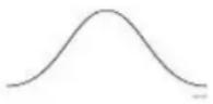 |
| Bartlett | The Bartlett window is a slightly narrower varia of the triangular window, with zero weight at bends. |  |
line
| Metric | Value | | ---------------- | ----------- | | Time (ms) | 100ms | | Duration (Hz) | 250Hz/div | | Width (Hz) | 1.250K | | Format (dB) | 20.0dB/rms/div | | Decibels | 0.00div | | Hori (Hz) | 1.250K | | Vertical (0.00div)| 20.0dB/ | | Channel (DC) | 4.40V | | Power (V) | 5.00V | | Current (V) | 1.00V | | Frequency (Hz) | 999.999Hz | | Frequency (MHz) | 1.250K | | Frequency (MHz) | 250/ | | Frequency (MHz) | Vertical | | Frequency (MHz) | 0.00div | | Frequency (MHz) | 20.0dB/ |line
| Parameter | Value | | --------------- | --------- | | M: 100ms | 5.00V~ | | (5KS/s) | 0.02div | | Depth:10K | 999.999Hz | | Depth:10K | -1.00div | | CH1:DC- ∫ 4.40V | |line
| Hori (Hz) | 1.250K | 250/ | | --------- | ------ | ---- | | Vertical | 0.00div | 20.0dB/ | | Crosshairs | -1.00div | 1.00000KHz | | FFT | 4.40V | 5.00V~ |line
| Hori (Hz) | 1.250K | 250/ | | --------- | ------ | ---- | | 250 | - | - | | 0.00 | - | - |line
| Metric | Value | | ---------------- | --------- | | Time (ms) | 100ms | | Duration (Hz) | 250Hz/div | | Width (Hz) | 1.250K | | Power (MHz) | 1.250K | | Frequency (Hz) | 250/ | | Power (dB) | 0.00div | | Power (dB) | 20.0dB |line
| Metric | Value | | ---------------- | --------- | | Time (ms) | 100ms | | Hori (Hz) | 250Hz/div | | Vertical (dBm) | 20.0dB/rms/div | | Depth (10K) | 1.25K Hz | | Power (MHz) | 1.25K Hz | | Current (W/m) | 1.00000 KHz | | Dual Wfm Math | -1.00 div | | FFT Function | 4.40 V | | FFT Peak ON | OFF |Notes for using FFT
■ Use the default dB scale for details of multiple frequencies, even if they have very different amplitudes. Use the dB scale to compare frequencies. ■ DC component or offset can cause incorrect magnitude values of FFT waveform. To minimize the DC component, choose AC Coupling on the source signal. ■ To reduce random noise and aliased components in repetitive or single-shot events, set the oscilloscope acquisition mode to average.What is Nyquist frequency?
The Nyquist frequency is the highest frequency that any real-time digitizing oscilloscope can acquire without aliasing. This frequency is half of the sample rate. Frequencies above the Nyquist frequency will be under sampled, which causes aliasing. So pay more attention to the relation between the frequency being sampled and measured.Use Vertical Position and Scale Knobs
1. The Vertical Position knob is used to adjust the vertical positions of the waveforms. The analytic resolution of this control knob changes with the vertical division. 2. The Vertical Scale knob is used to regulate the vertical resolution of the wave forms. The sensitivity of the vertical division steps as 1-2-5. The vertical position and vertical resolution is displayed at the left bottom corner of the screen (see Figure 4-7). line
| Parameter | Value | | --------------- | --------- | | M: 500us | 2.48div | | (1MS/s) | 999.99Hz | | Depth: 10K | -2.54div | | CHI: √0.00mV | 999.99Hz |How to Set the Horizontal System
The HORIZONTAL CONTROLS includes the Horizontal HOR button and such knobs as Horizontal Position and Horizontal Scale. 1. Horizontal Position knob: this knob is used to adjust the horizontal positions of all channels (include those obtained from the mathematical manipulation), the analytic resolution of which changes with the time base. 2. Horizontal Scale knob: it is used to set the horizontal scale factor for setting the main time base or the window. 3. Horizontal HOR button: push it to switch between the normal mode and the wave zoom mode. For more detailed operations, see the introductions below.Zoom the Waveform
Push the Horizontal HOR button to enter wave zoom mode. The top half of the display shows the Main window and the bottom half displays the Zoom window. The Zoom window is a magnified portion of the Main window.  In normal mode, the Horizontal Position and Horizontal Scale knobs are used to adjust the horizontal position and time base of the Main window. In wave zoom mode, the Horizontal Position and Horizontal Scale knobs are used to adjust the horizontal position and time base of the Zoom window.Note:
About the gestures for touchscreen, see "Touchscreen Controls (Touchscreen is optional)" on P17.How to Set the Trigger/Decoding System
Trigger determines when DSO starts to acquire data and display waveform. Once trigger is set correctly, it can convert the unstable display to meaningful waveform. When DSO starts to acquire data, it will collect enough data to draw waveform on left of trigger point. DSO continues to acquire data while waiting for trigger condition to occur. Once it detects a trigger it will acquire enough data continuously to draw the waveform on right of trigger point. Trigger control area consists of 1 knob and 2 menu buttons. Trigger Level: The knob that set the trigger level; push the knob and the level will be set as the vertical mid point values of the amplitude of the trigger signal. Force: Force to create a trigger signal and the function is mainly used in "Normal" and "Single" mode. Trigger Menu: The button that activates the trigger control menu.Trigger Control
The oscilloscope provides four trigger types: single trigger, alternate trigger, and bus trigger. Each type of trigger has different sub menus. Two ways to enter trigger mode: Key operation: Press Trigger Menu panel button, then bottom menu Trigger Type, select Single, ALT, Logic or Bus Trigger on the popup right menus, rotate M knob to choose different trigger types. Touch operation (Optional): Click Main menu icon on the left top of the screen, select Trig Menu, click bottom button Trigger Type, choose Single, ALT, Logic or Bus Trigger on the popup right menus, click to choose different trigger types Single trigger: Use a trigger level to capture stable waveforms in two channels simultaneously. Alternate trigger: Trigger on non-synchronized signals. Bus trigger: Set bus timing trigger. The Single Trigger, Alternate Trigger, and Bus Trigger menus are described respectively as follows:Single Trigger
Single trigger has nine types: edge trigger, video trigger, slope trigger, pulse trigger, runt trigger, windows trigger, timeout trigger, Nth edge trigger and logic trigger. Edge Trigger: It occurs when the trigger input passes through a specified voltage level with the specified slope. Video Trigger: Trigger on fields or lines for standard video signal. Slope Trigger: The oscilloscope begins to trigger according to the signal rising or falling speed. Pulse Trigger: Find pulses with certain widths. Runt Trigger: Trigger pulses that pass through one trigger level but fail to pass through the other trigger level. Windows Trigger: Provide a high trigger level and low trigger level, the oscilloscope triggers when the input signal passes through the high trigger level or the low trigger level. Timeout Trigger: The oscilloscope triggers when the time interval from when the rising edge (or the falling edge) passes through the trigger level to when the neighbouring falling edge (or the rising edge) passes through the trigger level is greater than the timeout time set. Nth Edge Trigger: The oscilloscope triggers on the Nth edge that appears on the specified idle time. Logic trigger: Trigger the signal according to the condition of logic relationship. The nine trigger modes in Single Trigger are described respectively as follows:1. Edge Trigger
An edge trigger occurs on trigger level value of the specified edge of input signal. Select Edge trigger mode to trigger on rising edge or falling edge. In Edge Trigger mode, the trigger setting information is displayed on bottom right of the screen, for example, CH1:DC- 0.00mV indicates that trigger type is edge, trigger source is CH1, coupling is DC, and trigger level is 0.00mV. Edge menu list:| Menu | Settings | Instruction | |
| Single Mode | Edge | Set vertical channel trigger type as edge trigger. | |
| Source | CH1CH2EXTEXT/5AC Line | Channel 1 as trigger signal.Channel 2 as trigger signal.External trigger as trigger signal.1/5 of the external trigger signal as trigger signal.AC power line as trigger signal. | |
| Coupling | AC | Block the direct current component. | |
| DC | Allow all component pass. | ||
| HF | Block the high-frequency signal, only low-frequency component pass. | ||
| LF | Block the low-frequency signal, only high-frequency component pass. (LF menu is only for certain mode) | ||
| NoiseReject | On | Click to open or close Noise Reject function. | |
| Off | |||
| Slope |  | Trigger on rising edge.Trigger on falling edge. | |
| Mode&Hold | AutoNormalSingleHoldoff | Acquire waveform even no trigger occurs.Acquire waveform when trigger occurs.When trigger occurs, acquire one waveform then s [SWBH]100 ns - 10 s, turn the M knob or click to set t | |
interval before another trigger occur, press← | |||
2. Video Trigger
Choose video trigger to trigger on fields or lines of NTSC, PAL or SECAM standard video signals. In Video Trigger mode, the trigger setting information is displayed on bottom right of the screen, for example, CH1:ALL, indicates that trigger type is Video, trigger source is CH1, and Sync type is Even. Video Trigger menu list:| MENU | SETTING | INSTRUCTION |
| Single Mode | Video | Set vertical channel trigger type as video trigger. |
| Source | CH1 | Select CH1 as the trigger source. |
| CH2 | Select CH2 as the trigger source. | |
| Modu | NTSC | Select video modulation. |
| PAL | ||
| SECAM | ||
| Sync | Line | Synchronous trigger in video line. |
| Field | Synchronous trigger in video field. | |
| Odd | Synchronous trigger in video odd filed. | |
| Even | Synchronous trigger in video even field. | |
| Line NO. | Synchronous trigger in designed video line, turn the knob or click set the line number. | |
| Mode&Hold | Auto | Acquire waveform even no trigger occurred. |
3. Pulse Width Trigger
Pulse trigger occurs according to the width of pulse. The abnormal signals can be detected through setting up the pulse width condition. In Pulse Width Trigger mode, the trigger setting information is displayed on bottom right of the screen, for example, CH1:DC- 0.00mV ,indicates that trigger type is pulse width, trigger source is CH1, coupling is DC, polarity is positive, and trigger level is 0.00mV. Pulse Width Trigger menu list:| MENU | SETTING | INSTRUCTION | |
| Single Mode | Pulse | Set vertical channel trigger type as pulse trigger. | |
| Source | CH1CH2 | Select CH1 as the trigger source.Select CH2 as the trigger source. | |
| Coupling | AC | Not allow DC portion to pass. | |
| DC | Allow all portion pass. | ||
| NoiseReject | On | Click to open or close Noise Reject function. | |
| Off | |||
| When | Polarity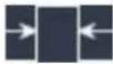  | Choose the polarity. | |
 |  | Select pulse width condition and adjust the M knor click or set time, press panel ← →button or click for move cursor to choose which digit to be set. | |
 |  | ||
 |  | ||
| Mode&Hold | AutoNormalSingleHoldoff | Acquire waveform even no trigger occurred.Acquire waveform when trigger occurred.When trigger occurs, acquire one waveform then stop100 ns - 10 s, adjust M knob or click to set ti interval before another trigger occur, press→ panel button or click to move cursor to choose which digit to be set. | |
4. Slope Trigger
Slope trigger sets the oscilloscope as the positive/negative slope trigger within the specified time. In Slope Trigger mode, the trigger setting information is displayed on bottom right of the screen, for example, CH1: ∫Δ0.00mV, indicates that trigger type is slope, trigger source is CH1, slope is rising, 0.00mV is the differential between up level and low level threshold. Slope trigger menu list:| MENU | SETTING | INSTRUCTION | |
| Single Mode | Slope | Set vertical channel trigger type as slope trigger. | |
| Source | CH1CH2 | Select CH1 as the trigger source.Select CH2 as the trigger source. | |
| When | Slope | Slope selecting. | |
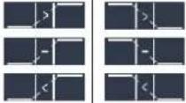 | Set slope condition; turn the M knob or cl to set slope time, press panel button or click  to move cursor to choose which digit to be to move cursor to choose which digit to be | ||
| Slew rate | Slew rate = (High level - Low level) / Settings | ||
| Threshold &SlewRate | High levelLow levelSlew rate | Adjust M knob to set the High level upper limit.Adjust M knob to set Low level lower limit.Slew rate = (High level - Low level) / Settings | |
| Mode&Hold | AutoNormalSingleHoldoff | Acquire waveform even no trigger occurred.Acquire waveform when trigger occurred.When trigger occurs, acquire one waveform then st 100 ns - 10 s, turn the M knob or click to set time interval before another trigger occur, press → panel button or click to move cursor to choose which digit to be set. | |
5.Runt Trigger
Trigger pulses that pass through one trigger level but fail to pass through the other trigger level. Shown as below figure, In Runt Trigger mode, the trigger setting information is displayed on bottom right of the screen, for example, CH1: 0.00mV , indicates that trigger type is runt, trigger source is CH1, polarity is positive, 0.00mV is the differential between up level and low level threshold. See the figure.  Runt Trigger menu list:| MENU | SETTING | INSTRUCTION | |
| Single Mode | Runt | Set vertical channel trigger type as runt trigger. | |
| Source | CH1CH2 | Select CH1 as the trigger source.Select CH2 as the trigger source. | |
| Threshold | Up LevelLow Level |  Adjust the M knob or cl to set the up level threshold. Adjust the M knob or cl to set the up level threshold. Adjust the M knob or cl to set the low level threshold. Adjust the M knob or cl to set the low level threshold. | |
| Condition | Polarity | Positive Polarity, the oscilloscope triggers on the positive runt pulse.Negative Polarity, the oscilloscope triggers on the negative runt pulse. | |
 Adjust the M knob or cl to set pulse width,press panel button or click to Adjust the M knob or cl to set pulse width,press panel button or click to  move cursor to choose which digit to be set.Trigger when runt pulse is greater than the set pulse width.Trigger when runt pulse equals to the set pulse width.Trigger when runt pulse is lower than the set pulse width. move cursor to choose which digit to be set.Trigger when runt pulse is greater than the set pulse width.Trigger when runt pulse equals to the set pulse width.Trigger when runt pulse is lower than the set pulse width. | |||
| Mode&Hold | AutoNormalSingleHoldoff | Acquire waveform even no trigger occurred.Acquire waveform when trigger occurred.When trigger occurs, acquire one waveform then sto 100 ns - 10 s, adjust M knob or k to set timeinterval before another trigger occur press 100 ns - 10 s, adjust M knob or k to set timeinterval before another trigger occur press  panel button or clic panel button or clic  ove cursor to choose which digit to be set. ove cursor to choose which digit to be set. | |
6.Windows Trigger
Provide a high trigger level and low trigger level, the oscilloscope triggers when the input signal passes through the high trigger level or the low trigger level. In Windows Trigger mode, the trigger setting information is displayed on bottom right of the screen, for example, CH1:0.00mVigger type is windows, trigger source is CH1, polarity is positive, 0.00mV the differential between up level and low level threshold. Windows Trigger menu list:| MENU | SETTING | INSTRUCTION | |
| Single Mode | Windows | Set vertical channel trigger type as Windows trigg | |
| Source | CH1CH2 | Select CH1 as the trigger source.Select CH2 as the trigger source. | |
| Threshold | Up LevelLow Level | Adjust the M knob or cl to set the up level threshold. Adjust the M knob or cl to set the low level threshold. Adjust the M knob or cl to set the low level threshold. | |
| Condition | Polarity | Positive Polarity, the oscilloscope triggers on the positive Windows pulse.Negative Polarity, the oscilloscope triggers on the negative Windows pulse. | |
| Enter: Triggers when the trigger signal enters the specified trigger level range.Exit: Triggers when the trigger signal exits the specified trigger level range.Time: Specify the hold time of the input signal after entering the specified trigger level. The oscilloscope triggers when the accumulated hold time is greater than the windows time. Available range is 30ns-10s, default 100ns. | |||
| Mode&Hold | AutoNormalSingleHoldoff | Acquire waveform even no trigger occurred.Acquire waveform when trigger occurred.When trigger occurs, acquire one waveform then s+100 ns - 10 s, adjust M knob or click to set timinterval before another trigger occur, press→panel button or click →to move cursor to choose which digit to be set. | |
7. Timeout Trigger
The oscilloscope triggers when the time interval from when the rising edge (or the falling edge) passes through the trigger level to when the neighbouring falling edge (or the rising edge) passes through the trigger level is greater than the timeout time set. In Timeout Trigger mode, the trigger setting information is displayed on bottom right of the screen, for example, CH1: -F-150V, indicates that trigger type is Timeout, trigger source is CH1, edge is positive, 0.00mV is up level or low level threshold. Timeout Trigger menu list:| MENU | SETTING | INSTRUCTION |
| Single Mode | Timeout | Set vertical channel trigger type as Timeout trigger. |
| Source | CH1CH2 | Select CH1 as the trigger source.Select CH2 as the trigger source. |
| Edge | Edge | Start timing when the rising edge of the input sign passes through the trigger level.Start timing when the falling edge of the input sign passes through the trigger level. |
| Configure | Idle Time | Set idle time. Idle time means the minimum time clock before searching data that can meet trigger conditions. Available range is 30ns-10s, default 100r |
| Mode&Hold | AutoNormalSingleHoldoffNoise Reject | Acquire waveform even no trigger occurred.Acquire waveform when trigger occurred.When trigger occurs, acquire one waveform then stop [x7k5]100 ns - 10 s, adjust M knob or ck to set time interval before another trigger occur, press panel button or clic  cursor to choose which digit to be set.Click to open or close Noise Reject function. cursor to choose which digit to be set.Click to open or close Noise Reject function. |
8.Nth Edge trigger
The oscilloscope triggers on the Nth edge that appears on the specified idle time. As figure shown below, the oscilloscope should trigger on the second falling edge after the specified idle time and the idle time should be set to P1/P2/P3/P4 < Idle Time < M. Wherein, M, P1, P2, P3 and P4 are positive or negative pulse width participating in the counting. In Nth Edge Trigger mode, the trigger setting information is displayed on bottom right of the screen, for example, CH1:Nth0.00mV trigger type is Nth Edge, trigger source is CH1, -150V is up level or low level threshold.  RS232 Trigger menu list:| MENU | SETTING | INSTRUCTION | |
| Bus Type | RS232 | Set vertical channel bus type as RS232 trigger. | |
| Input | Source | CH1 | Select CH1 as the trigger source.Select CH2 as the trigger source. |
| CH2 | |||
| Polarity |  | Select polarity . | |
 | |||
| When | Start | Trigger on the start frame of position. After choosing condition, press Configure to enter detailed settings. | |
| Error | Trigger when error frame is detected. After choosing condition, press Configure to enter detailed settings. | ||
| Chk Error | Trigger when Chk Error is detected. After choosing condition, press Configure to enter detailed settings. | ||
| Data | Trigger on the last bit of the preset data. After cho this condition, press Configure to enter detailed setting | ||
| Configure | Start | Common Baud: adjust M knob to choose common baud.Custom Baud: adjust M knob to choose baud, ranges from 50 to 10,000,000. | |
| Error | Stop Bit Select “1” or ”2”.Parity: “NO”“EVEN”“ODD”.Common Baud: adjust M knob to choose common baud.Custom Baud: adjust M knob to choose baud, ranges from 50 to 10,000,000. | ||
| Chk Error | Parity: Select Even or Odd.Common Baud: adjust M knob to choose common baud.Custom Baud: adjust M knob to choose baud, ranges from 50 to 10,000,000. | ||
| Data | Data Bits: Set as 5、6、7、8 bits.Data: Set data according to data bits, ranges from 0-63, 0-127 or 0-255. | ||
| Common Baud: adjust M knob to choose common baud.Custom Baud: adjust M knob to choose baud, ranges from 50 to 10,000,000. | |||
| Mode | AutoNormalSingle | Acquire waveform even no trigger occurred.Acquire waveform when trigger occurred.When trigger occurs, acquire one waveform then stop | |
2. I2C Trigger
The I2C serial bus consists of SCL and SDA. The transmission rate is determined by SCL, and the transmission data is determined by SDA. As shown in below figure, oscilloscope can trigger on the start, restart, stop, ack lost, specific device address or data value, also device address and data value at the same time. In I2C bus trigger mode, the trigger setting information is displayed on bottom right of the screen, for example, I2C CH1:0.00mV CH2:0.00mV, indicates that trigger type is I2C, CH1 trigger level is 0.00mV, CH2 trigger level is 0.00mV. other
| Signal | Value | |--------|-------| | SCL | 1-7 | | SCL | 8 | | SCL | 9 | | SCL | 1-7 | | SCL | 8 | | SCL | 9 | | SCL | 1-7 | | SCL | 8 | | SCL | 9 | | SDA | 1-7 | | SDA | 8 | | SDA | 9 | | SDA | 1-7 | | SDA | 8 | | SDA | 9 | | SDA | 1-7 | | SDA | 8 | | SDA | 9 | | START condition | 1-7 | | ADDRESS | 8 | | R/W | 9 | | ACK | 1-7 | | DATA | 8 | | ACK | 9 | | DATA | 1-7 | | DATA | 8 | | DATA | 9 | | STOP condition | 1-7 | | STOP condition | 8 | | STOP condition | 9 || MENU | SETTING | INSTRUCTION | |
| Bus Type | I2C | Set vertical channel bus type as I2C trigger. | |
| Source | CH1CH2 | Set CH1 as SCL or SDA.Set CH2 as SCL or SDA. | |
| When | Start | Trigger when SDA data transitions from high to low while SCL is high. | |
| Restart | When another start condition occurs before a stop condition. | ||
| Stop | Trigger when SDA data transitions from low to high while SCL is high. | ||
| Ack Lost | Trigger when SDA data is high during any acknowledgement of SCL clock position. | ||
| Addr | Trigger on the read or write bit when the preset ad is met. | ||
| AdrFo | Addr | Set Address Bits to be “7”8”or“10”. | |
| rmat | Bits | Set address according to the preset address bits, add range is 0-127, 0-255, 0-1023 respectively.Set Data Direction to be Read or Write.Note: The set is not available when Address bits is “8”. | |
| Addr | |||
| Direction | |||
| Data | Search for the preset data value on SDA and trigger the dump edge of SCL of the last bit of the data a | ||
| DatFormat | Byte length | Set data byte length, available range 1-5 bytes. Adjust knob or click set byte length.Select the data bit, ranges from 0 to (byte length*8 Set data to be H, L or X (H or L).Set all the data bits to be the specified value in Da | |
| CurrentBit | |||
| Data | |||
| All Bits | |||
| Addr / Data | Trigger when Address and Data conditions are met; the same time . | ||
| Mode | Auto Normal Single | Acquire waveform even no trigger occurred.Acquire waveform when trigger occurred.When trigger occurs, acquire one waveform then sto | |
3. SPI Trigger
Trigger on the specified data when the timeout condition is meet. When using SPI trigger, you need to specify the SCL and SDA data sources. In SPI bus trigger mode, the trigger setting information is displayed on bottom right of the screen, for example, SPI CH1:0.00mV CH2:0.00mV, indicates that trigger type is SPI, CH1 trigger level is 0.00mV, CH2 trigger level is 0.00mV. SPI Trigger menu list:| MENU | SETTING | INSTRUCTION |
| Bus Type | SPI | Set vertical channel bus type as SPI trigger. |
| Source | CH1CH2 | Set CH1 as SCL or SDA.Set CH2 as SCL or SDA. |
| Time Out | Time out | Set the minimum time that SCL must be idle, that is period of SCL, available range 100ns-10s. Time out m SCL keeps idle for a specified time before oscilloscope starts to search for the data(SDA) on which to trigger.adjust M knob or click to set time out, press←→ panel button or click move cursor to choose which digit to be set. |
| ClockEdge &Data | Clock Edge | Set Edge Clock as Rising edge or Falling edge. Mean sample the SDA data on the rising edge or falling edge the clock.Set the number of bits of the serial data character string can be set to any integer between 4-32. adjust M knoclick set Data Bits. |
  | ||
| Data Bits | ||
| Current Bit | Set the number of the data bits, ranges from 0-31, adjknob or click set Current Bit. | |
| Data | Set the value of the current data bit as H,L or X (H Set all the data bits to be the specified value in Data | |
| All Bits | ||
| Mode | AutoNormalSingle | Acquire waveform even no trigger occurred.Acquire waveform when trigger occurred.When trigger occurs, acquire one waveform then stop. |
4. CAN Trigger (Optional)
CAN (Controller Area Network) is a serial communication protocol of the ISO international standardization. By using the CAN bus trigger, you can trigger on Start of Frame, Type of Frame, Identifier, Data, ID & Data, End of Frame, Missing Ack, or Bit Stuffing Error. You need to specify the signal source, trigger signal type, sample point, and signal rate of the CAN signal. In CAN bus trigger mode, the trigger setting information is displayed on bottom right of the screen, for example, CAN CH1: -126mV type is CAN, CH1 trigger level is -126 mV. CAN Trigger menu list:| MENU | SETTING | INSTRUCTION | ||
| Bus Type | CAN | Set vertical channel bus type as CAN trigger. | ||
| Input | Source | CH1 | Select CH1 as the trigger source. | |
| CH2 | Select CH2 as the trigger source. | |||
| Type | CAN_HCAN_LTXRX | Actual CAN_H bus signal.Actual CAN_L bus signal.Transmission signal on the CAN signal lineReceived signal on the CAN signal line. | ||
| Sample Point |  Turn the M knob (or tap 1 touchscreen) to set the Sample point, which is a point within a bit's time. The oscilloscope samples the bit level at this point. "Sample point" is represented by the percentage of "the time from start of the bit's time to the sample point time" in the time". The range is 5% to 95%. Turn the M knob (or tap 1 touchscreen) to set the Sample point, which is a point within a bit's time. The oscilloscope samples the bit level at this point. "Sample point" is represented by the percentage of "the time from start of the bit's time to the sample point time" in the time". The range is 5% to 95%. | |||
| Common Baud | Turn the M knob to select from the Baud list on the le | |||
| Custom Baud | [7T8S]Turn the M knob (or tap 1 touchscreen) to set the Baud. The range is 10,000 to 1,000,000.Tip: You can select the nearest value in Common Baud, then adjust it in this menu. | |||
| Condition | Start | Trigger on the start frame of the data frame. | ||
| Type | Type(Bottom menu) | Data | Trigger on the selected frame. | |
| Remote | ||||
| Error | ||||
| Overload | ||||
| ID | Configure(Bottom menu) | Format | Select Standard or Extended. | |
| ID | Use the M knob and Direction key on the front panel to set. | |||
| Data | Configure(Bottom menu) | Byte Length | Set the number of bytes with th M knob. The range is 1 to 8. | |
| Data | Set the data with the M knob a Direction key on the front pane | |||
| ID&Data | Configure(Bottom menu) | Format | Select Standard or Extended. | |
| ID | Use the M knob and Direction key on the front panel to set. | |||
| Byte Length | Set the number of bytes with th M knob. The range is 1 to 8. | |||
| Data | Set the data with the M knob a Direction key on the front pane | |||
| End | Trigger on the end frame of the data frame. | |||
| Lost | Trigger on Lost. | |||
| Error | Trigger on Error. | |||
| Mode | AutoNormalSingle | Acquire waveform even no trigger occurred.Acquire waveform when trigger occurred.When trigger occurs, acquire one waveform then stop. | ||
Bus Decoding (Optional)
1. RS232 Decoding
To decode RS232 signal: (1) Connect the RS232 signal to the Signal Input Channel of the oscilloscope. (2) Adjust to the proper time base and voltage division. (3) In trigger menu, select Bus trigger, and select bus type as RS232, set parameters based on the characteristics of the signal, trigger the signal correctly and obtain stable display. Refer to "RS232 Trigger" on page 50. (4) Push the Decode button on the front panel. Select bus type as RS232. set parameters based on the characteristics of the signal. When the parameters are set correctly, the information carried by the signal will be displayed. Tip: If there are repetitive menu items in both trigger menu and decoding menu, you can set anyone of them, the other will be changed synchronously.Note:
- Use the Trigger Level knob to adjust the thresholds of bus trigger and bus decoding. - When decoding, if "Parity" is not set to "None", and the check bit error is detected, two red error marks will be displayed in the corresponding position in the waveform. RS232 Decoding menu list:| MENU | SETTING | INSTRUCTION |
| Bus Type | RS232 | Set bus type of decoding as RS232. |
| Configure | Common Baud | Turn the M knob to select from the Baud list on the le |
| Custom Baud | Turn the M knob (or tap  touchscreen) to set the Baud. The range is 50 to 10,000,000.Tip: You can select the nearest value in Common Baud, then adjust it in this menu. touchscreen) to set the Baud. The range is 50 to 10,000,000.Tip: You can select the nearest value in Common Baud, then adjust it in this menu. | |
| Data Bits | Set the data width of each frame to match the signal. It be set to 5, 6, 7 or 8. | |
| Parity | set the even-odd check mode to match the polarity used the signal. |
| Display | Format | Binary Decimal Hex ASCII | Set the display format of the bus. |
| EventTable | ON OFF | Select "ON" to display the event table. | |
| Save EventTable | If a USB storage device is currently connected to the instrument, save the event table data in a .csv (spreadsh) formatted file on the external USB storage device. | ||
| ASCII Table | ON | Select "ON" to display the ASCII table. | |
| OFF | |||
2. I2C Decoding
To decode I2C signal: (1) Connect the clock line (SCLK) and the data line (SDA) of the I2C signal to the Signal Input Channels of the oscilloscope. (2) Adjust to the proper time base and voltage division. (3) In trigger menu, select Bus trigger, and select bus type as I2C, set parameters based on the characteristics of the signal, trigger the signal correctly and obtain stable display. Refer to "I2C Trigger" on page 52. (4) Push the Decode button on the front panel. Select bus type as I2C. set parameters based on the characteristics of the signal. When the parameters are set correctly, the information carried by the signal will be displayed. Tip: If there are repetitive menu items in both trigger menu and decoding menu, you can set anyone of them, the other will be changed synchronously. Decoded information interpretation:| Information | Abbreviation | Background |
| Read Address | R, Read, or do not display | Green |
| Write Address | W, Write, or do not display | Green |
| Data | D, Data, or do not display | Black |
Note:
- Use the Trigger Level knob to adjust the thresholds of bus trigger and bus decoding. - When the ACK (ACKnowledge Character) is not met, two red error marks will be displayed in the corresponding position in the waveform. I2C Decoding menu list:| MENU | SETTING | INSTRUCTION | |
| Bus Type | I2C | Set bus type of decoding as I2C. | |
| Display | Format | Binary Decimal Hex ASCII | Set the display format of the bus. |
| EventTable | ON OFF | Select "ON" to display the event table. | |
| Save EventTable | If a USB storage device is currently connected to the instrument, save the event table data in a .csv (spreadsh) formatted file on the external USB storage device. | ||
| ASCII Table | ON | Select "ON" to display the ASCII table. | |
| OFF | |||
3. SPI Decoding
To decode SPI signal: (1) Connect the clock line (SCLK) and the data line (SDA) of the SPI signal to the Signal Input Channels of the oscilloscope. (2) Adjust to the proper time base and voltage division. (3) In trigger menu, select Bus trigger, and select bus type as SPI, set parameters based on the characteristics of the signal, trigger the signal correctly and obtain stable display. Refer to "SPI Trigger" on page 53. (4) Push the Decode button on the front panel. Select bus type as SPI. set parameters based on the characteristics of the signal. When the parameters are set correctly, the information carried by the signal will be displayed. Tip: If there are repetitive menu items in both trigger menu and decoding menu, you can set anyone of them, the other will be changed synchronously.Note:
- Use the Trigger Level knob to adjust the thresholds of bus trigger and bus decoding. - LS First in Bit Order menu item (Least Significant Bit First) means that the least significant bit will arrive first: hence e.g. the hexadecimal number 0x12, will arrive as the sequence 01001000 in binary representation, will be decoded as the reversed sequence 00010010. SPI Decoding menu list:| MENU | SETTING | INSTRUCTION | |
| Bus Type | SPI | Set bus type of decoding as SPI. | |
| Configure | SCLK | Select the clock edge to match the signal, sample the SI data on the rising or falling edge of the clock. | |
| Time Out | Set the minimum time that the clock (SCL) signal must idle before the oscilloscope starts to search for the data (SDA) on which to trigger. The range is 30 ns to 10 s. | ||
| Data Bits | Set the data width of each frame to match the signal. It be set to any integer between 4 and 32. | ||
| Bit Order | Select LS First or MS First to match the signal. | ||
| Display | Format | Binary Decimal Hex ASCII | Set the display format of the bus. |
| EventTable | ON OFF | Select "ON" to display the event table. | |
| Save EventTable | If a USB storage device is currently connected to the instrument, save the event table data in a .csv (spreadsh) formatted file on the external USB storage device. | ||
| ASCII Table | ON | Select "ON" to display the ASCII table. | |
| OFF | |||
4. CAN Decoding
To decode CAN signal: (1) Connect the CAN signal to the Signal Input Channel of the oscilloscope. (2) Adjust to the proper time base and voltage division. (3) In trigger menu, select Bus trigger, and select bus type as CAN, set parameters based on the characteristics of the signal, trigger the signal correctly and obtain stable display. Refer to "CAN Trigger" on page 54. (4) Push the Decode button on the front panel. Select bus type as CAN. set parameters based on the characteristics of the signal. When the parameters are set correctly, the information carried by the signal will be displayed. Tip: If there are repetitive menu items in both trigger menu and decoding menu, you can set anyone of them, the other will be changed synchronously. Decoded information interpretation:| Information | Abbreviation | Background |
| Identifier | I, ID, or do not display | Green |
| Overload Frame | OF | Green |
| Error Frame | EF | Green |
| Data Length code | L, DLC, or do not display | Blue |
| Data | D, Data, or do not display | Black |
| Cyclic Redundancy Check | C, CRC, or do not display | Valid: PurpleError: Red |
Note:
- Use the Trigger Level knob to adjust the thresholds of bus trigger and bus decoding. - When the ACK (ACKnowledge Character) of Data Frame or Remote Frame is not met, two red error marks will be displayed in the corresponding position in the waveform. - Error Frame, Remote Frame, and Overload Frame will be identified in the "Data" column in the event table (Data Frame will not be identified). CAN Decoding menu list:| MENU | SETTING | INSTRUCTION | |
| Bus Type | CAN | Set bus type of decoding as CAN. | |
| Display | Format | Binary Decimal Hex ASCII | Set the display format of the bus. |
| EventTable | ON OFF | Select "ON" to display the event table. | |
| Save EventTable | If a USB storage device is currently connected to the instrument, save the event table data in a .csv (spreadsh) formatted file on the external USB storage device. | ||
| ASCII Table | ON | Select "ON" to display the ASCII table. | |
| OFF | |||
How to Operate the Function Menu
The function menu control zone includes 8 function menu buttons: Measure, Acquire, Utility, Cursor, Autoscale, Save, Display, Help and 3 immediate-execution buttons: Autoset, Run/Stop, Single.How to Implement Sampling Setup
Push the Acquire button, Acqu Mode, Length, PERF Mode (only for XDS3000-A series) and Intrpl is shown in the bottom menu. The description of the Acqu Mode menu is shown as follows:| Function Menu | Setting | Description | |
| Acqu | Sample | Normal sampling mode. | |
| Mode | Peak Detect | Use to capture maximal and minimal sampling finding highest and lowest points over adjacent intervals. It is used for the detection of the jamming burr and the possibility of reducing the confusion. | |
| Average | 4, 16, 64, 128 | It is used to reduce the random and don't-do noises, with the optional number of average | |
| Function Menu | Setting | Description |
| Length | 1000 | Choose the record length.(For XDS3102AP/XDS3202A, 40M is available on both single CH and double CH) |
| 10K | ||
| 100K | ||
| 1M | ||
| 10M | ||
| 20M | ||
| 40M (Single CH) |
| Function Menu | Setting | Description |
| PERF Mode | 8-bit | Set the vertical resolution (A/D). |
| 12-bit | ||
| 14-bit (only for XDS3102AP/XDS3202A) |
| Function Menu | Setting | Description |
| Intrpl | Sinx/x | Use sine(x)/x interpolation. |
| x | Use linear interpolation. |
line
| M: 2.0ms | (1GS/s) | Depth: 10M(8-bit) | ACu Mode | Length | Perf Mode | Intrpi | Simox | Others | | -------- | ------- | ----------------- | -------- | ------ | --------- | ------ | ----- | ------ | | 1 | -0.02 | 200.000MHz | 5.00 | 8-bit | 3-bit | - | - | - | | 2 | 0.00 | - | - | - | - | - | - | - | | ... | ... | ... | ... | ... | ... | ... | ... | ... | | CH:DC | - | 0.00mV | - | - | - | - | - | - | | √ 0.00mV | - | - | - | - | - | - | - | - |line
| Time (ms) | Voltage (mV) | | --------- | ------------ | | 0 | 0.02 | | 1 | 0.03 | | 2 | 0.02 | | 3 | 0.03 | | 4 | 0.02 | | 5 | 0.03 | | 6 | 0.02 | | 7 | 0.03 | | 8 | 0.02 | | 9 | 0.03 | | 10 | 0.02 | | 11 | 0.03 | | 12 | 0.02 | | 13 | 0.03 | | 14 | 0.02 | | 15 | 0.03 | | 16 | 0.02 | | 17 | 0.03 | | 18 | 0.02 | | 19 | 0.03 | | 20 | 0.02 | | 21 | 0.03 | | 22 | 0.02 | | 23 | 0.03 | | 24 | 0.02 | | 25 | 0.03 | | 26 | 0.02 | | 27 | 0.03 | | 28 | 0.02 | | 29 | 0.03 | | 30 | 0.02 | | 31 | 0.03 | | 32 | 0.02 | | 33 | 0.03 | | 34 | 0.02 | | 35 | 0.03 | | 36 | 0.02 | | 37 | 0.03 | | 38 | 0.02 | | 39 | 0.03 | | 40 | 0.02 | | 41 | 0.03 | | 42 | 0.02 | | 43 | 0.03 | | 44 | 0.02 | | 45 | 0.03 | | 46 | 0.02 | | 47 | 0.03 | | 48 | 0.02 | | 49 | 0.03 | | 50 | 0.02 | | 51 | 0.03 | | 52 | 0.02 | | 53 | 0.03 | | 54 | 0.02 | | 55 | 0.03 | | 56 | 0.02 | | 57 | 0.03 | | 58 | 0.02 | | 59 | 0.03 | | 60 | 0.02 | | 61 | 0.03 | | 62 | 0.02 | | 63 | 0.03 | | 64 | 0.02 | | 65 | 0.03 | | 66 | 0.02 | | 67 | 0.03 | | 68 | 0.02 | | 69 | 0.03 | | 70 | 0.02 | | 71 | 0.03 | | 72 | 0.02 | | 73 | 0.03 | | 74 | 0.02 | | 75 | 0.03 | | 76 | 0.02 | | 77 | 0.03 | | 78 | 0.02 | | 79 | 0.03 | | 80 | 0.02 | | 81 | 0.03 | | 82 | 0.02 | | 83 | 0.03 | | 84 | 0.02 | | 85 | 0.03 | | 86 | 0.02 | | 87 | 0.03 | | 88 | 0.02 | | 89 | 0.03 | | 90 | 0.02 | | 91 | 0.03 | | 92 | 0.02 | | 93 | 0.03 | | 94 | 0.02 | | 95 | 0.03 | | 96 | 0.02 | | 97 | 0.03 | | 98 | 0.02 | | 99 | 0.03 | |1 | - |How to Set the Display System
Push the Display button and the Display menu is shown as follows:| Function Menu | Setting | Description |
| Type | Dots | Only the sampling points are displayed. |
| Vect | The space between the adjacent sampling point in the display is filled with the vector form. |
| Persist&Color(Color is only for certain models) | Persist | OFF1 Second2 Seconds5 SecondsInfinity | Set the persistence time. |
| Color | ONOFF | Turn on/off the color temperature function. | |
| XY Mode | Enable | ONOFF | Turn on/off XY display function. |
| Full Screen | ONOFF | Turn on/off the full screen view in XY mod | |
| Counter | ONOFF | Turn on/off counter. | |
| Clear | Erase the results of previous acquisitions from the display. The oscilloscope will start to accumulate acquisitions again. | ||
Persist
When the Persist function is used, the persistence display effect of the picture tube oscilloscope can be simulated. The reserved original data is displayed in fade color and the new data is in bright color. (1) Push the Display button. (2) Select Persist or Persist&Color in the bottom menu. (3) For certain models, select Persist in the right menu. (4) In the Time menu, select the persist time, including OFF, 1 Second, 2 Seconds, 5 Seconds and Infinity. When the "Infinity" option is set for Persist Time, the measuring points will be stored till the controlling value is changed. Select OFF to turn off persistence and clear the display. (5) Select Clear in the bottom menu to erase the results of previous acquisitions from the display. The oscilloscope will start to accumulate acquisitions again.Color (Only for certain models)
Color temperature function uses color-grading to indicate frequency of occurrence. The hot colors like red/yellow indicate frequently occurring events, and the colder colors like blue/green indicate rarely occurring events.  (1) Push the Display button. (2) Select Persist&Color in the bottom menu. (3) Select Color in the right menu, choose between ON/OFF. line
| Time (ns) | Amplitude | | --------- | --------- | | 0.000 | 100 | | 500 | 50 | | 1000 | 100 | | 1500 | 50 | | 2000 | 100 | | 2500 | 50 | | 3000 | 100 | | 3500 | 50 | | 4000 | 100 |XY Format
This format is only applicable to Channel 1 and Channel 2. After the XY display format is selected, Channel 1 is displayed in the horizontal axis and Channel 2 in the vertical axis; the oscilloscope is set in the un-triggered sample mode: the data are displayed as bright spots.The operations of all control knobs are as follows:
■ The Vertical Scale and the Vertical Position knobs of Channel 1 are used to set the horizontal scale and position. ■ The Vertical Scale and the Vertical Position knobs of Channel 2 are used to set the vertical scale and position continuously.The following functions can not work in the XY Format:
■ Reference or digital wave form ■ Cursor measurement ■ Trigger control ■ FFTOperation steps:
1. Push the Display button. 2. Select XY Mode in the bottom menu. Select Enable as ON in the right menu. 3. To make the XY view full screen, select Full Screen as ON in the right menu.Counter
It is a 6-digit single-channel counter. The counter can only measure the frequency of the triggering channel. The frequency range is from 2Hz to the full bandwidth. Only if the measured channel is in Edge mode of Single trigger type, the counter can be enabled. The counter is displayed at the bottom of the screen. Operation steps:
1. Push Trigger Menu button, set the trigger type to Single, set the trigger mode to Edge, select the signal source. 2. Push the Display button. 3. Select Counter as ON or OFF in the bottom menu.How to Save and Recall a Waveform
Push the Save button, you can save the waveforms, configures, screen images, record or clone the waveform. The description of the Save Function Menu is shown as the following table:| Function Menu | Setting | Description | |
| Type | WaveConfigureImageRecordClone | Choose the saving type.About the Record type, see "How to Record/Playback Waveforms" on P72.About the Clone type, see “How to Clon and Recall a waveform” on P75. | |
| When the type is Wave, the menu shows as following: | |||
| TypeWave | Format(Right menu) | For internal storage, only BIN can be selected. For external storage, the format be BIN, TXT or CSV. | |
| Source | CH1CH2MathAll | Choose the waveform to be saved. (If cer channel is off, the corresponding menu ite will be disabled.) (Choose All to save all the waveforms tha are turned on. You can save into the curi internal object address, or into USB storag as a single file.) | |
| Object & Show | Object | 0 - 99 | Choose the address which the waveform is saved to or recall from. |
| Show | ONOFF | Recall or close the waveform stored in th current object address. When the show is ON, if the current object address has been used, the stored waveform will be shown, address number and relevant information will be displayed at the top left of the sc if the address is empty, it will prompt "N is saved". | |
| Close All | Close all the waveforms stored in the obj address. | ||
| Save | Save the waveform of the source to the selected address. Whatever the Type of sa menu is set, you can save the waveform just pressing the Copy panel button in an user interface.Select Type in the bottom menu, in the Format menu, you can select the storage format. | ||
| Storage | Internal External | Save to internal storage or USB storage. When External is selected, save the waveform according to the current record length (see "Record Length menu" on P6 the file name is editable. The BIN waveform file could be open by waveform analysis software (on the supplied CD). | |
| When the type is Configure, the menu shows as following: | |||
| Configure | Setting0......Setting19 | The setting address. | |
| Save | Save the current oscilloscope configure to the internal storage. | ||
| Load | Recall the configure from the selected address. | ||
| When the type is Image, the menu shows as following: | |||
| Ink Saver | ON OFF | Turn on/off the toner saving mode. |
| Save | Save the current display screen. The file be only stored in a USB storage, so a U storage must be connected first. The file name is editable. The file is stored in BM format. |
Save and Recall the Waveform
The oscilloscope can store 100 waveforms, which can be displayed with the current waveform at the same time. The stored waveform called out can not be adjusted. In order to save the waveform of CH1, CH2 and Math into the address 1, the operation steps should be followed: 1. Turn on CH1, CH2 and Math channels. 2. Push the Save button. 3. Saving: Select Type in the bottom menu, select Wave in the left menu. 4. Select Storage in the bottom menu, select Internal in the right menu. 5. Select Source in the bottom menu, select All in the right menu for Source. 6. Select Object & Show in the bottom menu, select 1 as object address in the left menu. 7. Select Save in the bottom menu to save the waveform. 8. Recalling: Select Object & Show in the bottom menu, select 1 in the left menu. In the right menu, select Show as ON, the waveform stored in the address will be shown, the address number and relevant information will be displayed at the top left of the screen. In order to save the waveform of CH1 and CH2 into the USB storage as a BIN file, the operation steps should be followed: 1. Turn on CH1 and CH2 channels, turn off the Math channel. 2. Push the Save button. 3. Saving: Select Type in the bottom menu, select Wave in the left menu. 4. Select Storage in the bottom menu, select External in the right menu. 5. Select Type in the bottom menu, select BIN in the right menu as the storage format. 6. Select Source in the bottom menu, select All in the right menu for Source. 7. Select Save in the bottom menu, an input keyboard used to edit the file name will pop up. The default name is current system date and time. Select the key in the keyboard to confirm. 8. Recalling: The BIN waveform file could be open by waveform analysis software (on the supplied CD).Tip:
Whatever the Type of save menu is set, you can save the waveform by just pressing the Copy panel button in any user interface. If the Storage of the save menu is set as "External", you should install the USB disk. Please refer to the contents below to install the USB disk and name the file to be saved.Save the current screen image:
The screen image can only be stored in USB disk, so you should connect a USB disk with the instrument. 1. Install the USB disk: Insert the USB disk into the "USB Host port" of "Figure 3-1 Front panel". If an icon appears on the top right of the screen, the USB disk is installed successfully. If the USB disk cannot be recognized, format the USB disk according to the methods in "USB disk Requirements" on P68. 2. After the USB disk is installed, push the Save panel button, the save menu is displayed at the bottom of the screen. 3. Select Type in the bottom menu, select Image in the left menu. 4. Select Save in the bottom menu, an input keyboard used to edit the file name will pop up. The default name is current system date and time. Select the key in the keyboard to confirm.USB disk Requirements
The supported format of the USB disk: FAT32 file system, the allocation unit size cannot exceed 4K, mass storage USB disk is also supported. If the USB disk doesn't work properly, format it into the supported format and try again. Follow any of the following two methods to format the USB disk: using system-provided function and using the formatting tools. (The USB disk of 8 G or 8 G above can only be formatted using the second method – using the formatting tools.)Use system-provided function to format the USB disk
1. Connect the USB disk to the computer. 2. Right click Computer→Manage to enter Computer Management interface. 3. Click Disk Management menu, and information about the USB disk will display on the right side with red mark 1 and 2.  Figure 4-9: Disk Management of computer 4. Right click 1 or 2 red mark area, choose Format. And system will pop up a warning message, click Yes.  Figure 4-10: Format the USB disk warning 5. Set File System as FAT32, Allocation unit size 4096. Check "Perform a quick format" to execute a quick format. Click OK, and then click Yes on the warning message.  Figure 4-11: Formatting the USB disk setting6. Formatting process.
 Figure 4- 12: Formatting the USB disk 7. Check whether the USB disk is FAT32 with allocation unit size 4096 after formatting.Use Minitool Partition Wizard to format
Download URL: http://www.partitionwizard.com/free-partition-manager.html Tip: There are many tools for the USB disk formatting on the market, just take Minitool Partition Wizard for example here. 1. Connect the USB disk to the computer. 2. Open the software Minitool Partition Wizard. 3. Click Reload Disk on the pull-down menu at the top left or push keyboard F5, and information about the USB disk will display on the right side with red mark 1 and 2.  Figure 4-13: Reload Disk 4. Right click 1 or 2 red mark area, choose Format.  Figure 4-14: Choose format 5. Set File System FAT32, Cluster size 4096. Click OK.  Figure 4-15: Format setting 6. Click Apply at the top left of the menu. Then click Yes on the pop-up warning to begin formatting.   Figure 4-16: Apply setting7. Formatting process
 Figure 4-17: Format process8. Format the USB disk successfully
 Figure 4-18: Format successfullyHow to Record/Playback Waveforms
Wave Record function can record the input current wave. You can set the interval between recorded frames in the range of 10 ms - 10 s. The max frame number reaches 1000, and you can get better analysis effect with playback and storage function. The storage medium contains two kinds: Internal and External. When the storage medium is Internal, Wave Record contains four modes: OFF, Record, Playback and Storage. When storage medium is External, Wave Record contains two modes: OFF, Record. Record: To record wave according to the interval until it reaches the end frame set. Record menu (Internal Storage) shows as follows:| Menu | Setting | Instruction |
| Mode | OFFRecordPlaybackStorage | Close wave record function.Set record menu.Set playback menu.Set storage menu. |
| Record mode FrameSet | End frame | Turn the M knob to select the number of frames to (1 - 1000). |
| Interval | Turn the M knob to select the interval between reco frames (10ms - 10s). | |
| Refresh | ONOFF | Refresh wave during recording.Stop refreshing. |
| Operate | PlayStop | Begin to record.Stop recording. |
Note:
Both of the waveforms of Channel 1 and Channel 2 will be recorded. If a Channel is turned off while recording, the waveform of the channel is invalid in the playback mode. Playback: Play back the wave recorded or saved. Playback menu shows as follows:| Menu | Setting | Instruction |
| Playback Mode FrameSet | Start frameEnd frameCur frameInterval | Turn the M knob to select the number of start to playback (1 - 1000).Turn the M knob to select the number of end f to playback (1 - 1000).Turn the M knob to select the number of curren frame to playback (1 - 1000).Turn the M knob to select the interval between played back frames (10ms - 10s). |
| Playmode | Loop Once | Play back the wave continuously.Play back the wave just one time. |
| Operate | Play Stop | Begin to record.Stop recording. |
| Menu | Setting | Instruction |
| Storage Mode | Start frame | Turn the M knob to select the number of start fram store (1 - 1000). |
| FrameSet | End frame | Turn the M knob to select the number of end frame store (1 - 1000). |
| Save | Save the waveform record file to the internal memor | |
| Load | Load the waveform record file from the memory. |
| Menu | Setting | Instruction |
| Mode | OFFRecord | Close wave record function.Set record menu. |
| Record mode FrameSet | End frame | Turn the M knob to select the number of frames record (1 - 900,000). |
| Interval | Turn the M knob to select the interval between recorded frames (10ms - 10s). | |
| Infinity | Record infinitely until the storage medium is full. | |
| Refresh | ONOFF | Refresh wave during recording.Stop refreshing. |
| Operate | PlayStop | Begin to record.Stop recording. |
Note:
Both of the waveforms of Channel 1 and Channel 2 will be recorded. If a Channel is turned off while recording, the waveform of the channel is invalid in the playback mode. To use wave record to external, do as follows: 1. Push Save button. 2. Select Type in the bottom menu, in the left menu, turn the M knob to select Record. 3. Select Mode in the bottom menu, select OFF in the right menu. 4. In the bottom menu, select Storage as External. 5. Select Mode in the bottom menu, select Record in the right menu. 6. Select FrameSet in the bottom menu, set End frame and Interval in the right menu. If you want to record wave to external infinitely, select Infinity in the right menu, the End frame will display “-”. 7. In the bottom menu, set Refresh. 8. In the bottom menu, select Operate as Play. Connect external device to the computer, and wave\_record\_0.bin is the recorded file. Open the software, and do as follows to play back the waveform. 1. Choose Communications → Auto Player. 2. Transform recording waveform from machine. 3. Add the well transformed files. 4. Set play mode and time delay. 5. Click the green button on the left corner to begin playing back the waveform.   Figure 4-19: Play back waveform by softwareHow to Clone and Recall a waveform
You can clone the waveform of one or both channels between two cursors, and save it in the internal memory or on a USB memory device. You can save four cloned waveforms in the instrument internal memory. The waveform files saved to a USB memory device are saved with the extension "ota". If the optional Arbitrary Function Generator is available in your instrument, you can output the stored waveform from a file in the internal memory or in a USB memory device; and the waveform between two cursors can be output directly without save operation. Clone Wave menu shows as follows:| Menu | Setting | Instruction | |
| Source | CH1CH2CH1&CH2(Only for dual-channel AG) | Clone the waveform of CH1.Clone the waveform of CH2.Clone the waveform of CH1 and CH2. | |
| Line | a | Turn the M knob to move line a. | |
| b | Turn the M knob to move line b. | ||
| ab | Two cursors are linked. Turn the M knob to move pair of cursors. | ||
| x | Set the cursors to select the entire screen automatic | ||
| Clone (Generator is available) | Clone | Clone the waveform between two cursors, and output through the generator. | |
| AG Output(Only for dual-channel AG) | Out1Out2 | If the source is CH1 or CH2, you can se the output channel of the generator.If the source is CH1&CH2, the output channel is not selectable. Out1 outputs CHOut2 outputs CH2. | |
| Save | Save | Save the waveform between two cursors. | |
| Memory | InternalUSB | Select the memory location. | |
| Output | (Generator is available and internal memory is select Output the waveform in the selected object on the | ||
| AG Output(Only for dual-channel AG) | Out1Out2 | (Generator is available and internal memory is selected)For the waveform in the selected object of the left:If the source is CH1 or CH2, you can se the output channel of the generator.If the source is CH1&CH2, the output channel is not selectable. Out1 outputs CHOut2 outputs CH2. | |
Clone.
(3) Select Source in the bottom menu, select one channel (CH1/CH2) or two channels (CH1&CH2) in the right menu for Source. (4) Select Line in the bottom menu. If a or b is selected, turn the M knob to move the cursor. If ab is selected, turn the M knob to move the pair of cursors. If x is selected, the entire screen will be selected automatically. The waveform information is displayed at the left bottom corner of the screen.  Note: If "Out Of Limits" appears in the information or a message "Waveform points beyond the limit." appears on the screen, that means the length of the cloned waveform exceeds the limit. When the source is CH1 or CH2, the maximum length is 2M; When the source is CH1&CH2, the maximum length is 1M. Push the Acquire button, select Length in the bottom menu, and set the record length to a smaller value. (5) Select Save in the bottom menu. - To save the waveform to internal memory, select Storage in the right menu as Internal. Turn the M knob to select an object in the left menu, select Save in the right menu. - To save the waveform onto a USB memory device, insert a USB memory device into the port on the front panel. If the icon appears on the top right of the screen, the USB memory device is installed successfully. If the USB memory device cannot be recognized, format the USB memory device according to the methods in "USB disk Requirements" on P68. Select Storage in the right menu as External. Select Save in the right menu. An input keyboard used to edit the file name will pop up. The name is default as current system date and time. Turn the M knob to select the keys, push the knob to input. Select the ← key in the keyboard to confirm. The cloned waveform will be saved onto the USB memory device as a file with the ota suffix.To output the cloned waveform in the internal memory through the generator:
(The generator is optional.) (1) Push Save button. (2) Select Type in the bottom menu, in the left menu, turn the M knob to select Clone. (3) Select Save in the bottom menu, select Storage in the right menu as Internal. (4) Turn the M knob to select an object in the left menu. If the source of the selected waveform is CH1 or CH2, select AG Output in the right menu and set the output channel of the generator. If the source is CH1&CH2, the output channel is not selectable. (5) Select Output in the right menu. To output the cloned waveform in the USB memory device through the generator: (The generator is optional.) (1) Push (single-channel) or (dual-channel) button. For dual-channel, push button to set the output channel of the generator. (2) Select Arb in the bottom menu, select Others in the right menu, and select File Browse. (3) select Memory in the right menu as USB. The instrument lists a directory of the folders and files on the USB memory device. Select a folder or file using the M knob to scroll up and down the list. To enter the current folder, select Change Dir in the right menu, select it again to return to the upper directory. (4) Select the desired ota file, select Read in the right menu. To output the selected waveform through the generator directly: (The generator is optional.) (1) Push Save button. (2) Select Type in the bottom menu, in the left menu, turn the M knob to select Clone. (3) Select Source in the bottom menu, select one channel (CH1/CH2) or two channels (CH1&CH2) in the right menu for Source. (4) Select Line in the bottom menu. Select the cursor and move it to select the desired waveform. (5) Select Clone in the bottom menu. If the source is CH1 or CH2, select AG Output in the right menu and set the output channel of the generator. If the source is CH1&CH2, the output channel is not selectable. (6) Select Clone in the right menu. The generator will output the waveform between two cursors. Move the cursors by gestures (only for touchscreen) About the gestures for moving cursors, you can refer to "Other Operations Using Touchscreen" on P23.Data format description of OTA waveform file
If the source is CH1 or CH2, OTA file consists of two parts: the file header and the data. If the source is CH1&CH2, OTA file consists of three parts: file header, CH1data, and CH2 data. The file header represents the parameter of file data, which is expressed in "parameter name + value". Each parameter name is a case-sensitive string of 4 bytes. The parameter value is at least 4 bytes.1. Format description of the file header:
1) HEAD
| Parameter name | Meaning | Value | Comment |
| HEAD | Header size | 4 bytes int |
| Parameter name | Meaning | Value | Comment |
| TYPE | Model | 12 bytes char |
| Parameter name | Meaning | Value | Comment |
| BYTE | Data length in bit | 4 bytes int |
| Parameter name | Meaning | Value | Comment |
| SIZE | File size | 4 bytes int | Used to check the file integrity |
| Parameter name | Meaning | Value | Comment |
| VOLT | Voltage division, divided by 400 is ADC resolution. (When the source is CH1&CH2, it is CH1 voltage division.) | 4 bytes float | The value indicates voltage (the unit is mV), such as 200 mV. |
| Parameter name | Meaning | Value | Comment |
| SAMP | Sample rate | 4 bytes float | The unit is Sa/s. |
| Parameter name | Meaning | Value | Comment |
| ADCB | ADC bit, ADC resolution | 4 bytes int | 8-bit or 12-bit |
| Parameter name | Meaning | Value | Comment |
| CHAN | Number of channels | 4 bytes int | 1 or 2 |
| Parameter name | Meaning | Value | Comment |
| VOL2 | Voltage division, divided by 400 is ADC resolution. (When the source is CH1&CH2, it is CH2 voltage division.) | 4 bytes float | The value indicates voltage (the unit is mV), such as 200 mV. |
2.Data
The data type is signed integer. You can determine the data type (char, short int or int) based on the BYTE parameter. The valid range is determined by the ADCB parameter, e.g. the valid range for 8-bit ADC is -127 to +127.How to Implement the Auxiliary System Function Setting
- Config
Push the Utility button, select Function in the bottom menu, select Configure in the left menu. The description of Configure Menu is shown as the follows:| Function Menu | Setting | Description | |
| Language | Choose the display language of the operating system. | ||
| Set Time | Display | ON OFF | On/Off the date display. |
| Hour Min | Setting Hour/Minute. | ||
| Day Month | Setting Date/Month. | ||
| Year | Setting Year. | ||
| KeyLock | Lock all keys. Unlock method: push Trigger Menu button in trigger control area, then pus Force button, repeat 3 times. | ||
| About | Version number and serial number showing. | ||
- Display
Push the Utility button, select Function in the bottom menu, select Display in the left menu. The description of Display Menu is shown as the follows:| Function Menu | Setting | Description |
| BackLight | 0% - 100% | Turn the M knob to adjust the backlight. |
| Graticule | 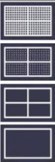 | Select the grid type. |
| Battery | ONOFF | Turn on or off the battery display. |
| Menu Time | OFF, 5s - 30s | Set the disappear time of menu. |
- Adjust
Push the Utility button, select Function in the bottom menu, select Adjust in the left menu. The description of Adjust Menu is shown as the follows:| Function Menu | Description |
| Self Cal | Carry out the self-calibration procedure. |
| Default | Call out the factory settings. |
| ProbeCh. | Check whether probe attenuation is good. |
Do Self Cal (Self-Calibration)
The self-calibration procedure can improve the accuracy of the oscilloscope under the ambient temperature to the greatest extent. If the change of the ambient temperature is up to or exceeds 5^ C, the self-calibration procedure should be executed to obtain the highest level of accuracy. Before executing the self-calibration procedure, disconnect all probes or wires from the input connector. Push the Utility button, select Function in the bottom menu, the function menu will display at the left, select Adjust. If everything is ready, select Self Cal in the bottom menu to enter the self-calibration procedure of the instrument.Probe checking
To check whether probe attenuation is good. The results contain three circumstances: Overflow compensation, Good compensation, Inadequate compensation. According to the checking result, users can adjust probe attenuation to the best. Operation steps are as follows: 1. Connect the probe to CH1, adjust the probe attenuation to the maximum. 2. Push the Utility button, select Function in the bottom menu, select Adjust in the left menu. 3. Select ProbeCh. in the bottom menu, tips about probe checking shows on the screen. 4. Select ProbeCh. again to begin probe checking and the checking result will occur after 3s; push any other key to quit.- Pass/Fail
The Pass/Fail function monitors changes of signals and output pass or fail signals by comparing the input signal that is within the pre-defined mask. Push the Utility button, select Function in the bottom menu, select Pass/fail in the left menu.| Function Menu | Setting | Description |
| operate | Enable | Control enable switch. |
| Operate | Control operate switch. | |
| Output | Pass | Signal tested corresponds with the rule. |
| Fail | Signal tested not correspond with the rule. | |
| Beep | Beep when it satisfies the rule. | |
| Stop | Stop once satisfying the rule. | |
| Info | Control the display status of info frame. | |
| Rule | Source Horizontal Vertical Create | Select source CH1, CH2 or Math. Change the Horizontal tolerance value by turning the M knob. Change the Vertical tolerance value by turning the knob. Use the rule set as testing rule. |
| SaveRule | Number Save Load | Select any one from Rule1 - Rule8 as your rule na Select Save to save the rule. Load some rule as the testing rule. |
Pass/Fail test:
Detect whether the input signal is within the limits of the rule, if it exceeds limits of the rule, it is "Fail"; otherwise it is "Pass". Also it can output fail or pass signal by built-in and configurable output port. To run the test, read the following steps: 1. Push the Utility button, select Function in the bottom menu, select Pass/fail in the left menu. 2. Enable switch on: Select Operate in the bottom menu, select Enable in the right menu as ON. 3. Create rule: Select Rule in the bottom menu. Select Source in the right menu, select the source in the left menu. Set Horizontal tolerance and Vertical tolerance in the right menu. Select Create in the right menu to create the rule. 4. Set output type: Select Output in the bottom menu to enter output option setting. Choose any one or two of the options "Pass", "Fail" or "Beep". "Pass" and "Fail" are mutually exclusive options, which could not be chosen simultaneously. "Stop" means stop once the condition satisfies your setting. 5. Begin to test: Select Operate in the bottom menu, select Operate in the right menu as Start, the test will begin. 6. Save rule: Select SaveRule in the bottom menu. Select the save location in the left menu, and then select Save in the right menu to save the rules, which could be called up at once when need. Select Load to call up the rule saved.Note:
1. When Pass/Fail is ON, if XY or FFT is ready to run, then Pass/Fail will be closed; under the mode of XY or FFT, Pass/Fail is unable. 2. Under the mode of Factory, Auto Scale and Auto Set, Pass/Fail will be closed. 3. When no save setting left in the rule save, tip will be given to show "NO RULE SAVED". 4. Under the status of stop, data comparing will stop, and when it goes on running, the number of Pass/Fail will increase from the former number, not from zero. 5. When the waveform playback mode is on, Pass/Fail is used to test the played-back waveform specially.- Output
Push the Utility button, select Function in the bottom menu, select Output in the left menu. Output menu item in the bottom menu sets the output type of Trig Out(P/F) port in Figure 3-3 Rear Paron P6. In the bottom menu, select Output. The description of Output menu is shown as the follows:| Function Menu | Setting | Description |
| Type | Trig level | Output trig signal synchronously. |
| Pass/fail | Output High Level when Pass, and Low Level when F | |
| AG Output | CH2 Output of dual-channel waveform generator (optiona |
| Function Menu | Setting | Description |
| Video | OFF VGA AV | Turn off video output. Connect the VGA or AV port to an external monitor or projector. Select the port in this menu, the oscilloscope display can be shown on an external monitor or projectc |
• LAN Set
Using the LAN port or Wi-Fi, the oscilloscope can be connected with a computer. The oscilloscope also supports communications with Android based smart device via Wi-Fi. Refer to "Communication with PC" on page 115 and "Communication with Android Device via Wi-Fi (Optional)" on page 123 for the operation steps.- Update
Use the front-panel USB port to update your instrument firmware using a USB memory device. Refer to "How to Update your Instrument Firmware" on page 83.- DAQ
You can use the multimeter data recorder to record the measurements when measuring current/voltage by multimeter (optional). Refer to "Multimeter Recorder" on page 112.• FRA (Frequency Response Analysis)
If there is a built-in arbitrary function generator (optional), you can use the frequency response analysis. Refer to "Frequency Response Analysis" on page 106.How to Update your Instrument Firmware
Use the front-panel USB port to update your instrument firmware using a USB memory device. USB memory device requirements: Insert a USB memory device into the USB port on the front panel. If the i ^n appears on the top right of the screen, the USB memory device is installed successfully. If the USB memory device cannot be detected, format the USB memory device according to the methods in "USB disk Requirements" on P68. Caution: Updating your instrument firmware is a sensitive operation, to prevent damage to the instrument, do not power off the instrument or remove the USB memory device during the update process.To update your instrument firmware, do the following:
1. Push the Utility button, select Function in the bottom menu, select Configure in the left menu, select About in the bottom menu. View the model and the currently installed firmware version. 2. From a PC, visit the website and check if the website offers a newer firmware version. Download the firmware file. The file name must be \*.update. The file name can be up to 15 characters long (including the suffix). Copy the firmware file onto your USB memory device. 3. Insert the USB memory device into the front-panel USB port on your instrument. 4. Push the Utility button, select Function in the bottom menu, select Update in the left menu. 5. Select Open in the bottom menu, the instrument lists a directory of the folders on the USB memory device. Turn the M knob to select a folder, select Open in the bottom menu to enter the folder. Navigate to the folder where the firmware file is, and select the file with the .update suffix. 6. In the bottom menu, select Open, the messages below will be shown.  7. In the bottom menu, select Start again, the interfaces below will be displayed in sequence. The update process will take up to three minutes. After completion, the instrument will be shut down automatically.   8. Long press the button to power on the instrument.How to Measure Automatically
Push the Measure button to display the menu for the settings of the Automatic Measurements. At most 8 types of measurements could be displayed on the bottom left of the screen. The oscilloscopes provide 38 parameters for auto measurement, including Period, Frequency, Mean, PK-PK, RMS, Max, Min, Top, Base, Amplitude, Overshoot, Preshoot, Rise Time, Fall Time, +PulseWidth, -PulseWidth, +Duty Cycle, -Duty Cycle, Delay A→B, Delay A→B, Cycle RMS, Cursor RMS, Screen Duty, FRR, FRF, FFR, FFF, LRR, LRF, LFR, LFF, Phase, +PulseCount, -PulseCount, RiseEdgeCnt, FallEdgeCnt, Area, and Cycle Area. The "Automatic Measurements" menu is described as the following table:| Function Menu | Setting | Description | |
| Add | Meas Type(left menu) | Select the measure types. | |
| Source | CH1 | Select the source. | |
| CH2 | |||
| Add | Add the selected measure types (shown at the left bottom, you co only add 8 types at most). | ||
| Remove | Meas Type(left menu) | Select the types need to be delete | |
| Remove | Remove the chosen measure type. | ||
| Remove All | Remove all the measures. | ||
| Show CH1 | ONOFF | Show all the measures of CH1 on the scre Hide the window of CH1 measures. | |
| Show CH2 | ONOFF | Show all the measures of CH2 on the scre Hide the window of CH2 measures. | |
| Configure | Gating | Screen Cursor | Select "Screen" or "Cursor" to set the cursor nge. |
| Statistics | ON OFF | select "ON" or "OFF" for measurement val statistics. | |
| Statistics Sel | Extremum Difference | When the statistics function is turned on, select "Extreme Value", the current value, average value, maximum value, and minimum value will be displayed at the bottom of the screen; select "Difference", the current value average value, standard deviation, and numb of samples will be displayed at the bottom the screen. | |
| Std Dev Samples | The number of standard deviation samples, number of samples to calculate the standard deviation(Range:0-999). | ||
| Reset | Restart statistics on statistics. | ||
Measure
Only if the waveform channel is in the ON state, the measurement can be performed. The automatic measurement can not be performed in the following situation: 1) On the saved waveform. 2) On the Dual Wfm Math waveform. 3) On the Video trigger mode. On the Scan format, period and frequency can not be measured. Measure the period, the frequency of the CH1, following the steps below: 1. Push the Measure button to show the automatic measurement function menu. 2. Select Add in the bottom menu. 3. In the right menu, select CH1 in the Source menu item. 4. In the left Type menu, turn the M knob to select Period. 5. In the right menu, select Add. The period type is added. 6. In the left Type menu, turn the M knob to select Frequency. 7. In the right menu, select Add. The frequency type is added. The measured value will be displayed at the bottom left of the screen automatically (see Figure 4-20). line
| Frequency | Time (ms) | | --------- | --------- | | F | 997.2 | | T | 1.003 |The automatic measurement of voltage parameters
The oscilloscopes provide automatic voltage measurements including Mean, PK-PK, RMS, Max, Min, Vtop, Vbase, Vamp, OverShoot, PreShoot, Cycle RMS, and Cursor RMS. Figure 4-21 below shows a pulse with some of the voltage measurement points.  Figure 4-21 Mean: The arithmetic mean over the entire waveform. PK-PK: Peak-to-Peak Voltage. RMS: The true Root Mean Square voltage over the entire waveform. Max: The maximum amplitude. The most positive peak voltage measured over the entire waveform. Min: The minimum amplitude. The most negative peak voltage measured over the entire waveform. Top: Voltage of the waveform's flat top, useful for square/pulse waveforms. Base: Voltage of the waveform's flat base, useful for square/pulse waveforms. Amplitude: Voltage between Vtop and Vbase of a waveform. Overshoot: Defined as (Vmax-Vtop)/Vamp, useful for square and pulse waveforms. Preshoot: Defined as (Vmin-Vbase)/Vamp, useful for square and pulse waveforms. Cycle RMS: The true Root Mean Square voltage over the first entire period of the waveform. Cursor RMS: The true Root Mean Square voltage over the range of two cursors.The automatic measurement of time parameters
The oscilloscopes provide time parameters auto-measurements include Period, Frequency, Rise Time, Fall Time, +D width, -D width, +Duty, -Duty, Delay A→B, Delay A→B, and Duty cycle. Figure 4-22 shows a pulse with some of the time measurement points. line
| Time Phase | Value | | -------------- | ----- | | Rise Time | 90% | | Fall Time | 10% |Note for the following delay measurements:
Source A and Source B can be set in the automatic measurement function menu. FRR: Time between Source A first rising edge and Source B first rising edge. FRF: Time between Source A first rising edge and Source B first falling edge. FFR: Time between Source A first falling edge and Source B first rising edge. FFF: Time between Source A first falling edge and Source B first falling edge. LRR: Time between Source A first rising edge and Source B last rising edge. LRF: Time between Source A first rising edge and Source B last falling edge. LFR: Time between Source A first falling edge and Source B last rising edge. LFF: Time between Source A first falling edge and Source B last falling edge.Other measurements
+PulseCount : The number of positive pulses that rise above the mid reference crossing in the waveform. -PulseCount: The number of negative pulses that fall below the mid reference crossing in the waveform. RiseEdgeCnt : The number of positive transitions from the low reference value to the high reference value in the waveform. FallEdgeCnt : The number of negative transitions from the high reference value to the low reference value in the waveform. Area The area of the whole waveform within the screen and the unit is voltage-second. The area measured above the zero reference (namely the vertical offset) is positive; the area measured below the zero reference is negative. The area measured is the algebraic sum of the area of the whole waveform within the screen. Cycle Area. The area of the first period of waveform on the screen and the unit is voltage-second. The area above the zero reference (namely the vertical offset) is positive and the area below the zero reference is negative. The area measured is the algebraic sum of the area of the whole period waveform. Note: When the waveform on the screen is less than a period, the period area measured is 0.Customize an Automatic Measurement
You can customize automatic measurements by using gating and statistics.Gating
- Press the Measure button, and the automatic measurement function menu is displayed at the bottom of the screen; - Press the Set softkey at the bottom of the screen, the setting menu appears on the right side of the screen; - Select the Gating menu. There are two menus: Screen and Cursor under the range. Click the Screen and then click the Cursor, or press the right Screen menu button twice to set the cursor range.Statistics
Select Statistics, you can choose On or Off to enable or disable statistics on the measurement value.Statistical selection
Statistics and display the current value, average value, minimum value (or number of samples) and maximum value (standard deviation) of up to 8 measurement results opened last. When the statistics function is turned on, select "Extreme Value", the current value, average value, maximum value, and minimum value will be displayed at the bottom of the screen; select "Difference", the current value, average value, standard deviation, and number of samples will be displayed at the bottom of the screen. The number of standard deviation samples: The number of standard deviation samples, the number of samples used to calculate the standard deviation. Statistics Reset: Restart statistics on statistics.How to Measure with Cursors
Push the Cursor button to turn cursors on and display the cursor menu. Push it again to turn cursors off.The Cursor Measurement for normal mode:
The description of the cursor menu is shown as the following table:| Function Menu | Setting | Description |
| Type | Voltage Time Time&Voltage AutoCursr | Display the voltage measurement cursor and menu. Display the time measurement cursor and menu. Display the time and voltage measurement cursor and menu. The horizontal cursors are set as the intersections of vertical cursors and the waveform. |
| Line Type (Time&Voltage type) | Time Voltage | Makes the vertical cursors active. Makes the horizontal cursors active. |
| Window(Wave zoom mode) | MainExtension | Measure in the main window.Measure in the extension window. |
| Line | a | Turn the M knob to move line a. |
| b | Turn the M knob to move line b. | |
| ab | Two cursors are linked. Turn the M knob to move pair of cursors. | |
| Source | CH1 | Display the channel to which the cursor measureme will be applied. |
| CH2 |
line
| Parameter | Value | | --------- | --------- | | Δy | 3.00V | | y1 | -1.46V | | y2 | 1.54V | | Δx | 1.000ms | | 1/x | 1.000XHZ | | x1 | 0.760ms | | x2 | -0.240ms | | F | 997.2Hz | | T | 1.003ms | | DC | -294.0 mV |Auto Cursor
For the AutoCursr type, the horizontal cursors are set as the intersections of the vertical cursors and the waveform. Move the cursors by gestures
About the gestures for moving cursors, see "Other Operations Using Touchscreen" on P23.The Cursor Measurement for FFT mode
In FFT mode, push the Cursor button to turn cursors on and display the cursor menu. The description of the cursor menu in FFT mode is shown as the following table:| Function Menu | Setting | Description |
| Type | Vamp (or Phase) | Display the Vamp (or Phase) measurement cursor and menu. |
| Freq | Display the Freq measurement cursor and menu. | |
| Freq&Vamp (or Freq&Phase) | Display the corresponding measurement cursor and menu. | |
| AutoCursr | The horizontal cursors are set as the intersections the vertical cursors and the waveform. | |
| Line Type (Freq&Vamp or Freq&Phase type) | Freq | Makes the vertical cursors active. |
| Vamp (or Phase) | Makes the horizontal cursors active. | |
| Window (Wave zoom mode) | Main Extension | Measure in the main window.Measure in the FFT extension window. |
| Line | a | Turn the M knob to move line a. |
| b | Turn the M knob to move line b. | |
| ab | Two cursors are linked. Turn the M knob to mo the pair of cursors. | |
| Source | Math FFT | Display the channel to which the cursor measurement will be applied. |
How to Use Autoscale
This is a very useful function for first time users to carry out a simple and quick test on the input signal. The function is applied to follow-up signals automatically even if the signals change at any time. Autoscale enables the instrument to set up trigger mode, voltage division and time scale automatically according to the type, amplitude and frequency of the signals. The menu is as follows:| Function Menu | Setting | Instruction |
| Autoscale | ON | Turn on Autoscale. |
| OFF | Turn off Autoscale. | |
| Mode |  | Follow-up and adjust both vertical and horizontal setti |
 | Follow-up and only adjust horizontal scale. | |
 | Follow-up and only adjust vertical scale. | |
| Wave |  | Show Multi-period waveforms. |
 | Only show one or two periods. |
line
| Time (μs) | Amplitude (A) | Amplitude (B) | |-----------|---------------|---------------| | 0 | 1.64 | 2.00 | | 500 | 0.00 | -2.00 | | 1000 | 1.64 | 2.00 | | 1500 | 0.00 | -2.00 | | 2000 | -1.64 | 2.00 | | 2500 | 1.64 | 2.00 | | 3000 | 0.00 | -2.00 | | 3500 | -1.64 | 2.00 | | 4000 | 1.64 | 2.00 | | 4500 | 0.00 | -2.00 | | 5000 | -1.64 | 2.00 | | 5500 | 1.64 | 2.00 | | 6000 | 0.00 | -2.00 | | 6500 | -1.64 | 2.00 | | 7000 | 1.64 | 2.00 | | 7500 | 0.00 | -2.00 | | 8000 | -1.64 | 2.00 | | 8500 | 1.64 | 2.00 | | 9000 | 0.00 | -2.00 | | 9500 | -1.64 | 2.00 | | 10000 | 1.64 | 2.00 | | 10500 | 0.00 | -2.00 | | 11000 | -1.64 | 2.00 | | 11500 | 1.64 | 2.00 | | 12000 | 0.00 | -2.00 | | 12500 | -1.64 | 2.00 | | 13000 | 1.64 | 2.00 | | 13500 | 0.00 | -2.00 | | 14000 | -1.64 | 2.00 | | 14500 | 1.64 | 2.00 | | 15000 | 0.00 | -2.00 | | 15500 | -1.64 | 2.00 | | 16000 | 1.64 | 2.00 | | 16500 | 0.00 | -2.00 | | 17000 | -1.64 | 2.00 | | 17500 | 1.64 | 2.00 | | 18000 | 0.00 | -2.00 | | 18500 | -1.64 | 2.00 | | 19000 | 1.64 | 2.00 | | 19500 | 0.00 | -2.00 | | 20000 | -1.64 | 2.00 | | 20500 | 1.64 | 2.00 | | 21000 | 0.00 | -2.00 | | 21500 | -1.64 | 2.00 | | 22000 | 1.64 | 2.00 | | 22500 | 0.00 | -2.0O | | 23567 | -1.64 | 2.5 | | CH1:DC=√1.64V | Reference | Reference |Note:
1. Entering into Autoscale function and the symbol will be flickering on the top left of the screen. 2. In the mode of Autoscale, the oscilloscope can self-estimate Trigger Mode (Edge, Video). At this point, the trigger menu is not available. 3. At the mode of XY and STOP status, when entering into Autoscale, DSO switches to YT mode and AUTO triggering. 4. At the mode of Autoscale, DSO is always set as DC coupling with AUTO triggering. 5. At the mode of Autoscale, if adjust the vertical position, voltage division, trigger level or time scale of CH1 or CH2, the oscilloscope will turn off Autoscale function. To back to Autoscale, Push Autoset. 6. Turn off the submenu at the Autoscale menu, the Autoscale is off and turn on the submenu still enters into the function. 7. When video triggering, the horizontal time scale is 50us. If one channel is showing edge signal, the other channel is showing video one, the time scale refers to 50us as video one as standard. 8. While the Autoscale is working, the settings below will be made forcibly: The DSO will switch from the wave zoom mode to the normal mode.How to Use Built-in Help
1. Push Help button, the catalog will display in the screen. 2. In the bottom menu, press Prev Page or Next Page to choose help topic, or just turn the M knob to choose. 3. Press OK to view the details about the topic, or just push the M knob. 4. Press Quit to exit the help, or just do other operations.How to Use Executive Buttons
Executive Buttons include Autoset, Run/Stop, Single, Copy.Autoset
It's a very useful and quick way to apply a set of pre-set functions to the incoming signal, and display the best possible viewing waveform of the signal and also works out some measurements for user as well. The details of functions applied to the signal when using Autoset are shown as the following table:| Function Items | Setting |
| Vertical Coupling | Current |
| Channel Coupling | Current |
| Vertical Scale | Adjust to the proper division. |
| Bandwidth | Full |
| Horizontal Level | Middle or ±2 div |
| Horizontal Sale | Adjust to the proper division |
| Trigger Type | Slope or Video |
| Trigger Source | CH1 or CH2 |
| Trigger Coupling | DC |
| Trigger Slope | Current |
| Trigger Level | 3/5 of the waveform |
| Trigger Mode | Auto |
| Display Format | YT |
| Force | Stop |
| Help | Exit |
| Pass/Fail | Off |
| Inverted | Off |
| Zoom Mode | Exit |
Judge waveform type by Autoset
Five kinds of types: Sine, Square, video signal, DC level, Unknown signal. Menu as follow: Sine: (Multi-period, Single-period, FFT, Cancel Autoset)  Square: (Multi-period, Single-period, Rising Edge, Falling Edge, Cancel Autoset)  Video signal:| Type line fiel | Odd | Even | Line NO. 1 | Cancel Autoset |
| Cancel Autoset |
Description for some icons:
Multi-period: To display multiple periods. Single-period: To display single period. FFT: Switch to FFT mode. Rising Edge Display the rising edge of square waveform. Falling Edge Display the falling edge of square waveform. Cancel Autoset Go back to display the upper menu and waveform information. Note: The Autoset function requires that the frequency of signal should be no lower than 20Hz, and the amplitude should be no less than 5mv. Otherwise, the Autoset function may be invalid. Run/Stop: Enable or disable sampling on input signals. Notice: When there is no sampling at STOP state, the vertical division and the horizontal time base of the waveform still can be adjusted within a certain range, in other words, the signal can be expanded in the horizontal or vertical direction. When the horizontal time base is 50ms, the horizontal time base can be expanded for 4 divisions downwards. Single: Push this button you can set the trigger mode as single directly, so when trigger occurs, acquire one waveform then stop. Copy: You can save the waveform by just pushing the Copy panel button in any user interface. The source wave and the storage location are according to the settings of the Save function menu when the Type is Wave. For more details, please see "Save Function Menu" on P65.How to Print the Screen Image
To print an image of what appears on the oscilloscope screen, do as the follows: (1) Connect the printer to the USB Device port on the rear panel of the oscilloscope. Note: The USB Device port supports PictBridge compatible printers. (2) Push the Utility button, select Function in the bottom menu, select Output in the left menu. (3) In the bottom menu, select Device as PICT. (When PC is selected, you can get an image by Oscilloscope software.) (4) In the bottom menu, select Print Setup. In the right menu, set up print parameters. The On selection of Ink Saver will print out a copy with a white background. (5) Once you have connected a printer to your oscilloscope and set up print parameters, you can print current screen images with a single push of the Print button on the front panel.5. Use the Arbitrary Function Generator (Optional)
The oscilloscope contains an integrated arbitrary function generator (25 MHz, dual-channel or single-channel is optional). The function generator provides 4 basic waveforms (sine, square, ramp, and pulse) and 46 built-in arbitrary waveforms (Noise, Exponential rise, Exponential fall, Sin(x)/x, Staircase, etc.). You can create a user-definable waveform and save it to internal storage or USB device.Output Connection
Push the Utility button, select Function in the bottom menu, select Output in the left menu. In the bottom menu, select Output, in the right menu, select AG Output.Single-channel:
Connect the BNC cable to the port marked Out in the back of the oscilloscope.Dual-channel:
Connect the BNC cable to the port marked Out 1 or Out 2 in the back of the oscilloscope. Out 1 is the output of CH1, Out 2 is the output of CH2, also can be used as the port of trigger signal output & Pass/Fail output.  Figure 5-1 Generator Output Ports (Dual-channel) To see the output of the generator, connect the other end of the BNC cable to one of the input channels on the front of the oscilloscope.To Set Channels
Single-channel:
Push Out to turn on/off the channel output. The indicator will be lighted when the corresponding channel is tuned on.Dual-channel:
● To Switch Channels in Menu Settings
Push CH1/2 button to switch between CH1 menu, CH2 menu, and Channel Copy menu.● To Turn On/Off Output of Channels
Push or to turn on/off output of the corresponding channel. The indicator will be lighted when the corresponding channel is tuned on.- Channel Copy menu
Push button to switch to Channel Copy menu.| CH2To CH1 | CH1To CH2 | Freq LockOn | Ampl LockOn | AlignPhase |
Copy Channel
Select CH2 To CH1 in the bottom menu to copy parameters of CH2 to CH1. Select CH1 To CH2 in the bottom menu to copy parameters of CH1 to CH2.Frequency Lock
Select Freq Lock in the bottom menu as On, the frequency of the two channels can be adjusted synchronously.Amplitude Lock
Select Ampl Lock in the bottom menu as On, the amplitude of the two channels can be adjusted synchronously.Align Phase
Select Align Phase in the bottom menu to align the initial phase of two channel signals.To Set Signals
(1) Push AFG (single-channel) or CH1/2 (dual-channel) button to show the bottom menu of generator. (2) Select the desired waveform in the bottom menu, the corresponding menu is displayed on the right. (3) The parameters can be set in the right menu.To Output Sine Signals
The parameters of Sine waveform in the right menu are: Frequency/Period, Start Phase, Amplitude/High Level, Offset/Low Level.To Set the Frequency
Select Frequency in the right menu (if Frequency is not displayed, select Period and push it again to switch to Frequency). Set the parameter in the right menu, see below. Three methods to change the chosen parameter: - Turn the M knob to change the value of cursor position. Press / direction key to move the cursor. - Use the input keyboard: Push the M knob, an input keyboard will pop up. Turn the M knob to move between the keys. Push the M knob to input the chosen key.  \- Use the touchscreen (Touchscreen is optional): To Set the Period
Select Period in the right menu (if Period is not displayed, select Frequency and select it again to switch to Period). Set the parameter in the right menu.To Set the Start Phase
Select StartPhase in the right menu. Set the parameter in the right menu.To Set the Amplitude
Select Amplitude in the right menu (if Amplitude is not displayed, select High Level and select it again to switch to Amplitude). Set the parameter in the right menu.To Set the Offset
Select Offset in the right menu (if Offset is not displayed, select Low Level and select it again to switch to Offset). Set the parameter in the right menu.To Set the High Level
Select High Level in the right menu (if High Level is not displayed, select Amplitude and select it again to switch to High Level). Set the parameter in the right menu.To Set the Low Level
Select Low Level in the right menu (if Low Level is not displayed, select Offset and select it again to switch to Low Level). Set the parameter in the right menu.To Output Square Signals
The parameters of Square waveform are: Frequency/Period, Start Phase, Amplitude/High Level, Offset/Low Level. To set the Frequency/Period, Start Phase, Amplitude/High Level, Offset/Low Level, please refer to To Output Sine Signals on page 100.To Output Ramp Signals
The parameters of Ramp waveform are: Frequency/Period, Start Phase, Amplitude/High Level, Offset/Low Level, Symmetry. To set the Frequency/Period, Start Phase, Amplitude/High Level, Offset/Low Level, please refer to To Output Sine Signals on page 100.To Set the Symmetry of Ramp
Select Symmetry in the right menu of Ramp. Set the parameter in the right menu.To Output Pulse Signals
The parameters of Pulse waveform are: Frequency/Period, Start Phase, Amplitude/High Level, Offset/Low Level, Width/Duty Cycle. To set the Frequency/Period, Start Phase, Amplitude/High Level, Offset/Low Level, please refer to To Output Sine Signals on page 100.To Set the Pulse Width of Pulse
Select Width in the right menu (if Width is not displayed, select Duty Cycle and select it again to switch to Width). Set the parameter in the right menu.To Set the Duty Cycle of Pulse
Select Duty Cycle in the right menu (if Duty Cycle is not displayed, select Width and select it again to switch to Duty Cycle). Set the parameter in the right menu.To Output Arbitrary Signals
The menu items of Arbitrary waveform are: Frequency/Period, Start Phase, Amplitude/High Level, Offset/Low Level, New, File Browse, Built-in. You can operate the menu by using the menu selection buttons on the right. To set the Frequency/Period, Start Phase, Amplitude/High Level, Offset/Low Level, please refer to To Output Sine Signals on page 100. The Arbitrary signal consists of two types: the user-definable waveform and the system built-in waveform.Create a New Waveform
(1) Enter the operation menu: Push (single-channel) or (dual-channel) button. Select Arb in the bottom menu, select Others in the right menu, and select New. (2) Set the number of waveform points: Select Points in the right menu, turn the M knob to change the value, or use the input keyboard (push the M knob to show it) to input the value and choose the unit. X1, X1000, Xle6, Xle9 in the keyboard respectively represent 1, 1000, 1000000, 1000000000. The waveform points range is 2 - 8192. (3) Set the interpolation: Select Intrpl in the right menu, choose between On/Off. If you choose On, the points will be connected with beelines; otherwise, the voltages between two consecutive points will not change, and the waveform looks like a step-up one. (4) Edit the waveform points: Select Edit Points in the right menu. - Select Point, input the number of the point to be edited. - Select Voltage, input the voltage for the current point. - Repeat the step above, set all the points to your needs. - Select Save, enter the file system. If you want to save the waveform to internal memory, select Memory in the right menu as Internal. Turn the M knob to select a file from USER0 through USER31. Select Save in the right menu.  If a USB device is connected, and you want to save the waveform to it, select Memory in the right menu as USB. The instrument lists a directory of the folders and files on the USB memory device. Select a folder or file using the M knob to scroll up and down the list. To enter the current folder, select Change Dir in the right menu, select it again to return to the upper directory.  Enter the desired storage path, select Save in the right menu, an input keyboard pops up, input the file name, choose in the keyboard to confirm The waveform is saved as BIN file in the folder. Note: The input length can have up to 35 characters. File Browse
To read a waveform stored in internal storage or USB device: (1) Push (single-channel) or (dual-channel) button. Select Arb in the bottom menu, select Others in the right menu, and select File Browse. (2) Select the desired waveform file in internal storage (FLASH) or USB device (USBDEVICE). (3) Select Read in the right menu.Built-in Waveform
There are 46 built-in Arbitrary waveforms.Steps for selecting the built-in waveform:
(1) Push AFG (single-channel) or CH1/2 (dual-channel) button to show the bottom menu of generator. (2) Select Arb in the bottom menu, select Others in the right menu, and select Built-in. (3) Select Common, Math, Window or Others in the right menu. E.g. select Others to enter the following interface.| DC | Heart | Round | LFMPulse |
| Rhombus | Cardiac | Noise | |
| Name | Explanation |
| Common | |
| StairD | Stair-down waveform |
| StairU | Stair-up waveform |
| StairUD | Stair-up and stair-down waveform |
| Trapezia | Trapezoid waveform |
| RoundHalf | RoundHalf wave |
| AbsSine | Absolute value of a Sine |
| AbsSineHalf | Absolute value of half a Sine |
| SineTra | Sine transverse cut |
| SineVer | Sine vertical cut |
| NegRamp | Negative ramp |
| AttALT | Gain oscillation curve |
| AmpALT | Attenuation oscillation curve |
| CPulse | Coded pulse |
| PPulse | Positive pulse |
| NPulse | Negative pulse |
| Maths | |
| ExpRise | Exponential rise function |
| ExpFall | Exponential fall function |
| Sinc | Sinc function |
| Tan | Tangent |
| Cot | Cotangent |
| Sqrt | Square root |
| XX | Square function |
| HaverSine | HaverSine function |
| Lorentz | Lorentz function |
| In | Natural logarithm function |
| Cubic | Cubic function |
| Cauchy | Cauchy distribution |
| Besselj | Bessell function |
| Bessely | Besselll function |
| Erf | Error function |
| Airy | Airy function |
| Windows | |
| Rectangle | Rectangle window |
| Gauss | Gauss distribution |
| Hamming | Hamming window |
| Hann | Hanning window |
| Bartlett | Bartlett window |
| Blackman | Blackman window |
| Laylight | Laylight window |
| Triang | Triangle window (Fejer window) |
| Others | |
| DC | DC signal |
| Heart | Heart signal |
| Round | Round signal |
| LFMPulse | Linear FM pulse |
| Rhombus | Rhombus signal |
| Cardiac | Cardiac signal |
| Noise | Noise signal |
Frequency Response Analysis
The Frequency Response Analysis (FRA) feature controls the built-in waveform generator to sweep a sine wave across a range of frequencies while measuring the input to and output from a device under test. At each frequency, gain and phase are measured and plotted on a frequency response Bode chart. When the frequency response analysis completes, you can move a marker across the chart to see the measured gain and phase values at each frequency point. You can also adjust the chart's scale and offset settings for the gain and phase plots. Note: If the signal is disturbed seriously, it is recommended to select Average in Acquire Mode before running the analysis, the averages can only be set as 4 or 16, and then run the analysis. Push the Utility button, select Function in the bottom menu, select FRA in the left menu. The description of FRA Menu is shown as the follows:| Function Menu | Setting | Description |
| ☐FRA | ☐FRA | Check to enable FRA function and show FRA scale and chart. |
| ☐Transparent | When unchecked, FRA information is shown on the FRA window.When checked, FRA information is shown on the waveform display area. | |
| Marker | Turn Multipurpose knob to move the marker, view measured gain and phase values. | |
| Sweep Step ☐Fine | When unchecked, the sweep step is 0.1dB.When checked, the sweep step is 0.01dB. | |
| Save | Click Save function can restore current picture. | |
| Setup | Input VCH1 | Input V is input from CH1.Output V is input from CH2.(Note: The menus are not for selecting menu items, onl showing information.) |
| Output VCH2 | ||
| Min Freq ☐Fine | Turn Multipurpose knob to set frequency sweep mir value. Check to enable fine-tuning. | |
| Max Freq ☐Fine | Turn Multipurpose knob to set frequency sweep ma value. Check to enable fine-tuning. | |
| Amplitude ☐Fine | Turn Multipurpose knob to set waveform generator amplitude. Check to enable fine-tuning.Note: The amplitude range is 2 mVpp to 6 Vpp. | |
| Chart | Gain Scale | Adjust scale of gain plot, range from 5dB to 500dl |
| Gain Offset | Adjust offset of gain plot, range from -250dB to 2: | |
| Phase Scale | Adjust scale of phase plot, range from 5° to 180°. | |
| Phase Offset | Adjust offset of phase plot, range from -180° to 18 | |
| Autoscale | Autoscale gain and phase plots. | |
| ☐Analysis | Run/stop the analysis.F: Frequency; G: Gain; P: Phase. | |
To run the frequency response analysis, do the following:
1. The waveform generator output is connected to a device under test. The input to the device is probed by CH1of the oscilloscope. The output from the device is probed by CH2of the oscilloscope. 2. Push the Utility button, select Function in the bottom menu, select FRA in the left menu 3. In the bottom menu, select □FRA. In the right menu, check □FRA, and set other menu items. 4. In the bottom menu, select Setup or Chart. In the right menu, set the menu items. 5. In the bottom menu, checkAnalysis to run the analysis.6. Use the Multimeter (Optional)
Input Terminals
The input terminals are on the back of the oscilloscope, which marked as 10A, mA, COM, V/Ω/C. natural_image
Back view of a black electronic device with ports and connectors, showing an inset close-up of the rear panel (no text or symbols visible)DMM Menu
Push DMM button on the front panel to enter/exit the multimeter function. The button backlight will be lighted when the multimeter function is enabled.  Figure 6-2 Multimeter Button The bottom menu of multimeter is as below:| Menu | Setting | Description |
| Current | ACA | Measuring AC current. |
| DCA | Measuring DC current. | |
| Voltage | ACV | Measuring AC voltage. |
| DCV | Measuring DC voltage. | |
| R | Measuring resistance. | |
| Testing diode. | ||
| Testing for continuity. | ||
| C | Measuring capacitance. | |
| Hold | ON OFF | Freeze the display during measurement. |
| Configure | Relative | When making relative measurements, reading is the difference between a stored reference value and the input signal. |
| Show Info ON OFF | Show/Hide the information window. | |
| Auto Range | Select auto range mode. | |
| Switch Range | Select manual range mode, press to switch range. | |
| Current mA 10A (Only for current measurement) | Select the current range. |
DMM Information Window
The Multimeter Information Window is displayed on the top right of the screen.  Figure 6-3 Multimeter Information WindowDescription
1. Manual/Auto range indicators, MANUAL refers to the measuring range in manual operation mode and AUTO refers to the measuring range in automatic operation mode. 2. Measurement mode indicators: A ---- Current measurement V ---- Voltage measurement R ---- Resistance measurement Diode measurement Continuity test C ---- Capacitance measurement 3. Range. 4. Measurement display ("OL" is short for overload, indicates the reading exceeds the display range) 5. Data hold mode is enabled. 6. Multimeter recorder (See "Multimeter Recorder" on page 112). 7. The reference value of the relative measurement. 8. Range of measuring current: mA or 10A. 9. AC or DC when measuring current or voltage.Making Multimeter Measurements
Measuring AC or DC Current
To measure a AC or DC current which is less than 400 mA, do the following: (1) Push DMM button on the front panel. Select Current in the bottom menu, select it again to switch between ACA (AC current) or DCA (DC current). (2) Select Configure in the bottom menu, select Current as mA in the right menu. (3) Connect the black test lead to the COM terminal on the back of the oscilloscope. Connect the red test lead to the mA terminal. (4) Turn off the power of the measured circuit. Discharge all high-voltage capacitors. (5) Disconnect the circuit path to be tested. Connect the black test lead to one side of the circuit (with a lower voltage); connect the red test lead to the other side (with a higher voltage). Reversing the leads will produce a negative reading, but will not damage the multimeter. (6) Turn on the power of the measured circuit, and read the display. (7) Turn off the power of the measured circuit and discharge all high-voltage capacitors. Remove the test leads and restore the circuit to the original condition. To measure a AC or DC current which is 400 mA to 10 A, do the following: (1) Push DMM button on the front panel. Select Current in the bottom menu, select it again to switch between ACA (AC current) or DCA (DC current). (2) Select Configure in the bottom menu, select Current as 10A in the right menu. (3) Connect the black test lead to the COM terminal on the back of the oscilloscope. Connect the red test lead to the 10A terminal. (4) Turn off the power of the measured circuit. Discharge all high-voltage capacitors. (5) Disconnect the circuit path to be tested. Connect the black test lead to one side of the circuit (with a lower voltage); connect the red test lead to the other side (with a higher voltage). Reversing the leads will produce a negative reading, but will not damage the multimeter. (6) Turn on the power of the measured circuit, and read the display. (7) Turn off the power of the measured circuit and discharge all high-voltage capacitors. Remove the test leads and restore the circuit to the original condition.Measuring AC or DC Voltage
(1) Push DMM button on the front panel. Select Current in the bottom menu, select it again to switch between ACA (AC current) or DCA (DC current). (2) Connect the black test lead to the COM terminal on the back of the oscilloscope and the red test lead to //C terminal. (3) Probe the test points and read the display.Measuring Resistance
(1) Push DMM button on the front panel. Select in the bottom menu, select R. (2) Connect the black test lead to the COM terminal on the back of the oscilloscope and the red test lead to v/n/c terminal. (3) Probe the test points and read the display.Testing Diodes
(1) Push DMM button on the front panel. Select in the bottom menu, select it until switching to (2) Connect the black test lead to the COM terminal on the back of the oscilloscope and the red test lead to the V/Ω/C terminal. (3) Connect the red test lead to the positive terminal (anode) of the diode and the black test lead to the negative terminal (cathode). The cathode of a diode is indicated with a band. Read the diode forward bias.Testing for Continuity
(1) Push DMM button on the front panel. Select in the bottom menu, select it until switching to (2) Connect the black test lead to the COM terminal on the back of the oscilloscope and the red test lead to //c terminal. (3) Probe the test points to measure the resistance in the circuit. If the reading is below 50 , the multimeter will beep.Measuring Capacitance
(1) Push DMM button on the front panel. Select in the bottom menu, select it until switching to C. (2) Insert the supplied capacitance measurer to the COM terminal and the V/Ω/C terminal on the back of the oscilloscope. (3) Insert the capacitance to the capacitance measurer, then screen shows the capacitance reading. Note: when measuring the capacitance which is less than 5 nF, please use relative value measuring mode to improve measuring precision.Multimeter Features
Data Hold Mode
You can freeze the display for any function. (1) Select Hold in the bottom menu as ON. HOLD will be shown on the display. (2) Select OFF to exit this mode.Making Relative Measurements
When making relative measurements, reading is the difference between a stored reference value and the input signal. (1) Select Configure in the bottom menu, select Relative in the right menu to enter the relative mode. The measurement value at this time is stored as the reference value, and displayed behind . In this mode, current reading = input value - reference value. (2) Press it again to exit the mode. Note: This function is not available when measuring resistance, diodes, and testing for continuity.Information Display
Show/hide the information window on the top right of the display. (1) Select Configure in the bottom menu, select Show Info in the right menu as ON. The information window will be shown on the display. (2) Select OFF to hide.Auto or Manual Range
Auto range is set as default. To switch auto or manual range, do the following steps: (1) Select Configure in the bottom menu. (2) Select Auto Range in the right menu, AUTO will be shown on the display. (3) Select Switch Range in the right menu, MANUAL will be shown on the display. Press this softkey to switch range. Note: When testing diode, testing continuity, and measuring capacitance, manual range is disabled.Multimeter Recorder
You can use the multimeter data recorder to record the measurements when measuring current/voltage by multimeter (optional). Push the Utility button, select Function in the bottom menu, select DAQ in the left menu. The description of DAQ Menu is shown as the follows: 6. Use the Multimeter (Optional)| Function Menu | Setting | Description |
| Set | Interval | Set the record interval (0.5s - 10s, step by 0.5s) |
| Duration | "d h m s" represents day, hour, minute, second.E.g. "1 02:50:30" represents a day and 2 hours, 50 minutes and 30 seconds.Press Duration to switch between the time unit, tu the M knob to set the value. Max duration: 3 days internal storage, 10 days for external storage. | |
| Enable | Turn on or off the recorder. | |
| STRT STOP | Start or stop recording. | |
| Storage | Internal External | Save to internal storage or USB memory device. |
| Export | When internal storage is selected, you can export the internal r file to a USB memory device. | |
How to chart the data
You can open the CSV file using Microsoft Excel, or your favorite spreadsheet application, and create charts based on the data. In the following steps, Microsoft Excel 2010 is used as an example. 1. Open Multimeter Recorder.csv in Excel.  2. Select the data that you want to chart (see Figure 6-4). 3. On the Insert tab, in the Charts group, click Line, and then click Line in 2-D Line (see Figure 6-5). 4. The chart will be displayed (see Figure 6-6). If you want to keep the chart, save the file to XLS format.  Figure 6-4  Figure 6-5 line
| Time | Voltage(mV) | | ---- | ----------- | | 1 | 2.8 | | 2 | 2.8 | | 3 | 2.8 | | 4 | 2.8 | | 5 | 2.7 | | 6 | 2.7 | | 7 | 2.7 | | 8 | 2.7 | | 9 | 2.7 | | 10 | 2.6 | | 11 | 2.6 | | 12 | 2.6 | | 13 | 2.6 | | 14 | 2.6 | | 15 | 2.5 | | 16 | 2.5 | | 17 | 2.5 | | 18 | 2.5 | | 19 | 2.5 | | 20 | 2.5 | | 21 | 2.5 | | 22 | 2.6 |7. Communication with PC
The oscilloscope supports communications with a PC through USB, LAN port or Wi-Fi. You can use the Oscilloscope communication software to store, analyze, display the data and remote control. For the specific operation method of Oscilloscope host software, please download and view the host help document on our download website. Here's how to connect to a computer. Please get the host software installation package on your computer from our official website, double-click it, and click according to the prompts until the installation is complete. Then, there are several connections you can choose from.Using USB Port
(1) Set the USB device protocol type of the instrument: Click Utility → Function → Function → Output → Device, switch to PC. (2) Connection: Use a USB data cable to connect the USB Device port in the right panel of the Oscilloscope to the USB port of a PC. (3) Port setting of the software: Run the Oscilloscope software; click "Communications" on the menu bar, choose "Ports-Settings", in the setting dialog, choose "Connect using" as "USB". After connect successfully, the connection information in the bottom right corner of the software will turn green.  Figure 7-1 Connect with PC through USB portUsing LAN Port
Connect directly
(1) Connection. Plug in the LAN cable to the LAN port in the back of the oscilloscope; plug the other end into the LAN interface of the computer. (2) Set the network parameters of the computer. Since the oscilloscope can not support obtaining an IP address automatically, you should assign a static IP address. Here we set the IP address to 192.168.1.71.  Figure 7-2 Set the network parameters of the computer (3) Set the network parameters of the Oscilloscope Software. Run the software on the computer; choose the "Ports-settings" of the "Communications" menu item. Set "Connect using" to LAN. About the IP, the first three bytes is same as the IP in the step (2), the last byte should be different. Here, we set it to 192.168.1.72. The range of the port value is 0 - 4000, but the port which under 2000 is always used, so it is suggested to set it to the value above 2000. Here, we set it to 3000.  Figure 7-3 Set the network parameters of the Oscilloscope Software (4) Set the network parameters of the oscilloscope. In the oscilloscope, push the Utility button. Select Function in the bottom menu. Select LAN Set in the left menu. In the bottom menu, set the Type item as LAN, and select Set. In the right menu, set IP and Port to the same value as the "Ports-settings" in the software in step (3). Select Save set in the bottom menu, it prompts "Reset to update the config". After resetting the oscilloscope, if you can get data normally in the oscilloscope software, the connection is successful.  Figure 7-4 Set the network parameters of the oscilloscopeConnect through a router
(1) Connection. Use a LAN cable to connect the oscilloscope with a router, the LAN port of the oscilloscope is in the right side panel; the computer should be connected to the router too. (2) Set the network parameters of the computer. Since the oscilloscope can not support obtaining an IP address automatically, you should assign a static IP address. The Default gateway and Subnet mask should be set according to the router. Here we set the IP address to 192.168.1.71, Subnet mask is 255.255.255.0, Default gateway is 192.168.1.1.  Figure 7-5 Set the network parameters of the computer (3) Set the network parameters of the Oscilloscope Software. Run the software on the computer; choose the "Ports-settings" of the "Communications" menu item. Set "Connect using" to LAN. About the IP, the first three bytes is same as the IP in the step (2), the last byte should be different. Here, we set it to 192.168.1.72. The range of the port value is 0 - 4000, but the port which under 2000 is always used, so it is suggested to set it to the value above 2000. Here, we set it to 3000.  Figure 7-6 Set the network parameters of the Oscilloscope Software (4) Set the network parameters of the oscilloscope. In the oscilloscope, push the Utility button. Select Function in the bottom menu. Select LAN Set in the left menu. In the bottom menu, set the Type item as LAN, and select Set. In the right menu, set IP and Port to the same value as the "Ports-settings" in the software in step (3). The Netgate and Net mask should be set according to the router. Select Save set in the bottom menu, it prompts "Reset to update the config". After resetting the oscilloscope, if you can get data normally in the oscilloscope software, the connection is successful.  Figure 7-7 Set the network parameters of the oscilloscopeUsing Wi-Fi to Connect with PC (Optional)
Connect with PC as Wi-Fi Access Point
PC should support Wi-Fi. (1) Set the oscilloscope. In the oscilloscope, push the Utility button. Select Function in the bottom menu. Select LAN Set in the left menu. In the bottom menu, set the Type item as WIFI-AP, and select Set in the bottom menu. (2) In the right menu, select SSID, a keyboard will pop up. You can turn and push the M knob, or touch the keyboard (if the LCD is touchscreen) to set the access point name. (3) In the right menu, select Encryption, push again to set the type. Open type needs no password. WEP or WPA type need to set the password. You can select WPA. In the right menu, select Password, use the keyboard to set the Wi-Fi password (8 to 32 characters). (4) In the right menu, select IP:PORT, IP is fixed by the oscilloscope, and can not be edited. Here IP is 192.168.1.1. Turn the M knob to set the PORT. Here, we set it to 3000. (5) After setting, select ON in the Status menu. The 📞 icon appears on the top right of the screen.  (6) Select Save set in the bottom menu to save current settings. (7) Set Wi-Fi connection on PC. Enter the Wi-Fi settings on PC, select the oscilloscope access point to connect, enter the set password.  (8) Set the network parameters of the Oscilloscope Software. Run the software on the computer; choose the "Ports-settings" of the "Communications" menu item. Set "Connect using" to LAN. Set IP and Port to the same value in the oscilloscope in the step (4). If you can get data normally, the connection is successful.  Figure 7-8 Set the network parameters of the Oscilloscope SoftwareConnect with PC as Wi-Fi Station
The oscilloscope and PC should be on the same network (LAN). (1) In the oscilloscope, push the Utility button. Select Function in the bottom menu. Select LAN Set in the left menu. In the bottom menu, set the Type item as WIFI-STA, and select Set in the bottom menu. (2) In the right menu, select SSID, a keyboard will pop up. Input the name of the Wi-Fi hotspot. You can turn and push the M knob, or touch the keyboard (if the LCD is touchscreen). (3) In the right menu, select Encryption, push to set the Encryption type of the Wi-Fi hotspot. Open type needs no password. WEP or WPA type need to input the password. In the right menu, select Password, use the keyboard to input the Wi-Fi hotspot password. (4) In the right menu, select IP:PORT, Turn the M knob to set the PORT. Here, we set it to 3000. (5) After setting, select ON in the Status menu. The value of IP is displayed in IP:PORT menu. Here IP is 10.1.1.126. A changing icon appears on the top right of the screen.  (6) Select Save set in the bottom menu to save current settings. (7) Set the network parameters of the computer. Set IP in the computer, the first three bytes is same as the IP in the oscilloscope, the last byte should be different. Here, we set it to 10.1.1.123. The Default gateway and Subnet mask should be set according to the router.  Figure 7-9 Set the network parameters of the computer (8) Set the network parameters of the Oscilloscope Software. Run the software on the computer; choose the "Ports-settings" of the "Communications" menu item. Set "Connect using" to LAN. Set IP and Port to the same value in the oscilloscope. If you can get data normally, the connection is successful.  Figure 7-10 Set the network parameters of the Oscilloscope Software8. Communication with Android Device via Wi-Fi (Optional)
The oscilloscope supports communications with Android based smart device via Wi-Fi. You can use the free application software on the Android based smart devices to view the waveform synchronously, perform remote control, The waveform can be saved as image (BMP, PNG) or file (CSV, BIN), or shared via installed sharing apps.System Requirements of Mobile Devices
\- Android Versions: 4.0 and above.How to Connect
In Wi-Fi settings of the oscilloscope, there are two connection types. One is WIFI-AP (Access Point), the oscilloscope is set as Wi-Fi access point, the Android device can be connected to it directly. The other type is WIFI-STA (Station), the oscilloscope is set as Wi-Fi station. The Android device can be connected to it through a Wi-Fi hotspot.Connect with APP as Wi-Fi Access Point
(1) In the oscilloscope, push the Utility button. Select Function in the bottom menu. Select LAN Set in the left menu. In the bottom menu, set the Type item as WIFI-AP, and select Set in the bottom menu. (2) In the right menu, select SSID, a keyboard will pop up. You can turn and push the M knob, or touch the keyboard (if the LCD is touchscreen) to set the access point name. (3) In the right menu, select Encryption, push again to set the type. Open type needs no password. WEP or WPA type need to set the password. You can select WPA. In the right menu, select Password, use the keyboard to set the Wi-Fi password (8 to 32 characters). (4) In the right menu, select IP:PORT, IP is fixed by the oscilloscope, and can not be edited. Turn the M knob to set the PORT. (5) After setting, select ON in the Status menu. The 📞 icon appears on the top right of the screen.  (6) Select Save set in the bottom menu to save current settings. (7) In Android device, enter the Wi-Fi settings, select the oscilloscope access point to connect, enter the set password.  (8) In Android device, launch the application. (9) Click connect on the left.  (10) Set IP and Port to the same value as the setting in the oscilloscope. Click Confirm to connect. Click History to recall the history settings. Connect with APP as Wi-Fi Station
(1) In the oscilloscope, push the Utility button. Select Function in the bottom menu. Select LAN Set in the left menu. In the bottom menu, set the Type item as WIFI-STA, and select Set in the bottom menu. (2) In the right menu, select SSID, a keyboard will pop up. Input the name of the Wi-Fi hotspot. You can turn and push the M knob, or touch the keyboard (if the LCD is touchscreen). (3) In the right menu, select Encryption, push to set the Encryption type of the Wi-Fi hotspot. Open type needs no password. WEP or WPA type need to input the password. In the right menu, select Password, use the keyboard to input the Wi-Fi hotspot password. (4) In the right menu, select IP:PORT, Turn the M knob to set the PORT. (5) After setting, select ON in the Status menu. The value of IP is displayed in IP:PORT menu. A changing icon appears on the top right of the screen.  (6) Select Save set in the bottom menu to save current settings. (7) In Android device, enter the Wi-Fi settings, select the oscilloscope access point to connect, enter the set password.  (8) In Android device, launch the application. (9) Click connect on the left.  (10) Set IP and Port to the same value as the setting in the oscilloscope. Click Confirm to connect. Click History to recall the history settings.  User Interface  flowchart
graph TD
    A["Share"] --> B["Share the image/wave file via the installed sharing apps"]
    C["Save"] --> D["Save into wave file (bmp, png, bin, csv)"]
    E["Feedback"] --> F["Submit feedback"]
    G["Quit"] --> H["Exit APP"]
Control Menu
Display Menu
  9. Demonstration
Example 1: Measurement a Simple Signal
The purpose of this example is to display an unknown signal in the circuit, and measure the frequency and peak-to-peak voltage of the signal. 1. Carry out the following operation steps for the rapid display of this signal: (1) Set the probe menu attenuation coefficient as 10X and that of the switch in the probe switch as 10X (see "How to Set the Probe Attenuation Coefficient" on P12). (2) Connect the probe of Channel 1 to the measured point of the circuit. (3) Push the Autoset button. The oscilloscope will implement the Autoset to make the waveform optimized, based on which, you can further regulate the vertical and horizontal divisions till the waveform meets your requirement.2. Perform Automatic Measurement
The oscilloscope can measure most of the displayed signals automatically. To measure the period, the frequency of the CH1, following the steps below: (1) Push the Measure button to show the Measure menu. (2) Select Add in the bottom menu. (3) In the right menu, select CH1 in the Source menu item. (4) In the left Type menu, turn the M knob to select Period. (5) In the right menu, select Add. The period type is added. (6) In the left Type menu, turn the M knob to select Frequency. (7) In the right menu, select Add. The frequency type is added. The measured value will be displayed at the bottom left of the screen automatically (see Figure 9-1). line
| Time (ms) | Amplitude (dBm) | |-----------|-----------------| | 0 | 0.000 | | 1 | 0.000 | | 2 | 0.000 | | 3 | 0.000 | | 4 | 0.000 | | 5 | 0.000 | | 6 | 0.000 | | 7 | 0.000 | | 8 | 0.000 | | 9 | 0.000 | | 10 | 0.000 | | 11 | 0.000 | | 12 | 0.000 | | 13 | 0.000 | | 14 | 0.000 | | 15 | 0.000 | | 16 | 0.000 | | 17 | 0.000 | | 18 | 0.000 | | 19 | 0.000 | | 20 | 0.000 | | 21 | 0.000 | | 22 | 0.000 | | 23 | 0.000 | | 24 | 0.000 | | 25 | 0.000 | | 26 | 0.000 | | 27 | 0.000 | | 28 | 0.000 | | 29 | 0.000 | | 30 | 0.000 | | 31 | 0.000 | | 32 | 0.000 | | 33 | 0.000 | | 34 | 0.000 | | 35 | 0.000 | | 36 | 0.000 | | 37 | 0.000 | | 38 | 0.000 | | 39 | 0.000 | | 40 | 0.000 | | 41 | 0.000 | | 42 | 0.000 | | 43 | 0.000 | | 44 | 0.000 | | 45 | 0.000 | | 46 | 0.000 | | 47 | 0.000 | | 48 | 0.000 | | 49 | 0.000 | | 50 | 0.000 | | 51 | 0.48div | | 52 | -2.54div | | 53 | Single Edge | | 54 | Source CH1 | | 55 | Coupling DC | | 56 | Slope Auto &Holdoff | | 57 | Auto &Holdoff | | M:5, RMS/s:1, Depth:1, K:1, CH1:√(1.5, √(1.5))Example 2: Gain of a Amplifier in a Metering Circuit
The purpose of this example is to work out the Gain of an Amplifier in a Metering Circuit. First we use Oscilloscope to measure the amplitude of input signal and output signal from the circuit, then to work out the Gain by using given formulas. Set the probe menu attenuation coefficient as 10X and that of the switch in the probe as 10X (see "How to Set the Probe Attenuation Coefficient" on P12). Connect the oscilloscope CH1 channel with the circuit signal input end and the CH2 channel to the output end.Operation Steps:
(1) Push the Autoset button and the oscilloscope will automatically adjust the waveforms of the two channels into the proper display state. (2) Push the Measure button to show the Measure menu. (3) Select Add in the bottom menu. (4) In the right menu, select CH1 in the Source menu item. (5) In the left Type menu, turn the M knob to select PK-PK. (6) In the right menu, select Add. The peak-to-peak type of CH1 is added. (7) In the right menu, select CH2 in the Source menu item. (8) In the left Type menu, turn the M knob to select PK-PK. (9) In the right menu, select Add. The peak-to-peak type of CH2 is added. (10)Read the peak-to-peak voltages of Channel 1 and Channel 2 from the bottom left of the screen (see Figure 9-2). (11)Calculate the amplifier gain with the following formulas. Gain = Output Signal / Input signal Gain (db) = 20×log (gain)  Figure 9-2 Waveform of Gain MeasurementExample 3: Capturing a Single Signal
It's quite easy to use Digital Oscilloscope to capture non-periodic signal, such as a pulse and burr etc. But the common problem is how to set up a trigger if you have no knowledge of the signal? For example, if the pulse is the logic signal of a TTL level, the trigger level should be set to 2 volts and the trigger edge be set as the rising edge trigger. With various functions supported by our Oscilloscope, user can solve this problem by taking an easy approach. First to run your test using auto trigger to find out the closest trigger level and trigger type, this helps user to make few small adjustments to achieve a proper trigger level and mode. Here is how we achieve this.The operation steps are as follows:
(1) Set the probe menu attenuation coefficient to 10X and that of the switch in the probe to 10X (see "How to Set the Probe Attenuation Coefficient" on P12). (2) Adjust the Vertical Scale and Horizontal Scale knobs to set up a proper vertical and horizontal ranges for the signal to be observed. (3) Push the Acquire button to display the Acquire menu. (4) Select Acqu Mode in the bottom menu. Select Peak Detect in the right menu. (5) Push the Trigger Menu button to display the Trigger menu. (6) Select the first menu item in the bottom menu. Select Single in the right menu. (7) In the left menu, select Edge as the mode. (8) Select Source in the bottom menu. Select CH1 in the right menu. (9) Select Coupling in the bottom menu. Select DC in the right menu. (10)In the bottom menu, select Slope as (rising). (11)Turn the Trigger Level knob and adjust the trigger level to the roughly 50% of the signal to be measured. (12)Check the Trigger State Indicator on the top of the screen, if it is not Ready, push down the Run/Stop button and start acquiring, wait for trigger to happen. If a signal reaches to the set trigger level, one sampling will be made and then displayed in the screen. By using this approach, a random pulse can be captured easily. For instance, if we want to find a burst burr of high amplitude, set the trigger level to a slightly higher value of the average signal level, push the Run/Stop button and wait a trigger. Once there is a burr occurring, the instrument will trigger automatically and record the waveform during the period around the trigger time. By turning the Horizontal Position knob in the horizontal control area in the panel, you can change the horizontal triggering position to obtain the negative delay, making an easy observation of the waveform before the burr occurs (see Figure 9-3).  Figure 9-3 Capturing a Single SignalExample 4: Analyze the Details of a Signal
Noise is very common inside most of the electronic signal. To find out what's inside the noise and reduce the level of noise is very important function our oscilloscope is capable to offer. Noise Analysis The level of noise sometime indicates a failure of electronic circuit. The Peak Detect functions acts an important role to help you to find out the details of these noise. Here is how we do it: (1) Push the Acquire button to display the Acquire menu. (2) Select Acqu Mode in the bottom menu. (3) Select Peak Detect in the right menu. The signal displayed on the screen containing some noise, by turning on Peak Detect function and changing time base to slow down the incoming signal, any peaks or burr would be detected by the function (see Figure 9-4).  Figure 9-4 Signal with NoisesSeparate Noises from the Signal
When focusing on signal itself, the important thing is to reduce the noise level as lower as possible, this would enable user to have more details about the signal. The Average function offered by our Oscilloscope can help you to achieve this. Here are the steps for how to enable Average function. (1) Push the Acquire button to display the Acquire menu. (2) Select Acqu Mode in the bottom menu. (3) Select Average in the right menu, turn the M knob and observe the waveform obtained from averaging the waveforms of different average number. User would see a much reduced random noise level and make it easy to see more details of the signal itself. After applying Average, user can easily identify the burrs on the rising and falling edges of some part of the signal (see Figure 9-5).  Figure 9-5 Reduce Noise level by using Average functionExample 5: Application of X-Y Function
Examine the Phase Difference between Signals of two Channels
Example: Test the phase change of the signal after it passes through a circuit network. X-Y mode is a very useful when examining the Phase shift of two related signals. This example takes you step by step to check out the phase change of the signal after it passes a specified circuit. Input signal to the circuit and output signal from circuit are used as source signals. For the examination of the input and output of the circuit in the form of X-Y coordinate graph, please operate according to the following steps: (1) Set the probe menu attenuation coefficient for 10X and that of the switch in the probe for 10X (see "How to Set the Probe Attenuation Coefficient" on P12). (2) Connect the probe of channel 1 to the input of the network and that of Channel 2 to the output of the network. (3) Push the Autoset button, with the oscilloscope turning on the signals of the two channels and displaying them in the screen. (4) Turn the Vertical Scale knob, making the amplitudes of two signals equal in the rough. (5) Push the Display button and recall the Display menu. (6) Select XY Mode in the bottom menu. Select Enable as ON in the right menu. The oscilloscope will display the input and terminal characteristics of the network in the Lissajous graph form. (7) Turn the Vertical Scale and Vertical Position knobs, optimizing the waveform. (8) With the elliptical oscillogram method adopted, observe and calculate the phase difference (see Figure 9-6).  Figure 9-6 Lissajous Graph Based on the expression (q) = A / B or C / D , thereinto, q is the phase difference angle, and the definitions of A, B, C, and D are shown as the graph above. As a result, the phase difference angle can be obtained, namely, q = ± (A / B) or ± (C / D) . If the principal axis of the ellipse is in the I and III quadrants, the determined phase difference angel should be in the I and IV quadrants, that is, in the range of (0 - / 2) or (3 / 2 - 2) . If the principal axis of the ellipse is in the II and IV quadrants, the determined phase difference angle is in the II and III quadrants, that is, within the range of ( / 2 - ) or ( - 3 / 2) .Example 6: Video Signal Trigger
Observe the video circuit of a television, apply the video trigger and obtain the stable video output signal display.Video Field Trigger
For the trigger in the video field, carry out operations according to the following steps: (1) Push the Trigger Menu button to display the trigger menu. (2) Select the first menu item in the bottom menu. Select Single in the right menu. (3) In the left menu, select Video as the mode. (4) Select Source in the bottom menu. Select CH1 in the right menu. (5) Select Modu in the bottom menu. Select NTSC in the right menu. (6) Select Sync in the bottom menu. Select Field in the right menu. (7) Turn the Vertical Scale, Vertical Position and Horizontal Scale knobs to obtain a proper waveform display (see Figure 9-7).  Figure 9-7 Waveform Captured from Video Field Trigger10. Troubleshooting
1. Oscilloscope is powered on but no Display. - Check whether the power connection is connected properly. - Check whether the fuse which is beside the AC power input jack is blew (the cover can be pried open with a straight screwdriver). - Restart the instrument after completing the checks above. - If the problem persists, please contact us and we will be under your service. 2. After acquiring the signal, the waveform of the signal is not displayed in the screen. - Check whether the probe is properly connected to the signal connecting wire. - Check whether the signal connecting wire is correctly connected to the BNC (namely, the channel connector). - Check whether the probe is properly connected with the object to be measured. - Check whether there is any signal generated from the object to be measured (the trouble can be shot by the connection of the channel from which there is a signal generated with the channel in fault). ● Make the signal acquisition operation again. 3. The measured voltage amplitude value is 10 times or 1/10 of the actual value. Look at the attenuation coefficient for the input channel and the attenuation ration of the probe, to make sure they are match (see "How to Set the Probe Attenuation Coefficient" on P12). 4. There is a waveform displayed, but it is not stable. - Check whether the Source item in the TRIG MODE menu is in conformity with the signal channel used in the practical application. - Check on the trigger Type item: The common signal chooses the Edge trigger mode for Type and the video signal the Video. If Alternate trigger is selected, both of the channel 1 and channel 2 trigger levels should be adjusted to the proper position. Only if a proper trigger mode is applied, the waveform can be displayed steadily. - Try to change the trigger coupling into the high frequency suppress and the low frequency suppress to smooth the high frequency or low frequency noise triggered by the interference. (Only for the models that have this function.) 5. No Display Responses to the Push-down of Run/Stop. Check whether Normal or Single is chosen for Polarity in the TRIG MODE menu and the trigger level exceeds the waveform range. If it is, make the trigger level is centered in the screen or set the trigger mode as Auto. In addition, with the Autoset button pressed, the setting above can be completed automatically. 6. The displaying of waveform seems getting slow after increasing AVERAGE value in Acqu Mode (see "How to Implement Sampling Setup" on P60), or a longer duration is set in the Persist in Display (see "Persist" on P63). It's normal as the Oscilloscope is working hard on many more data points.11. Technical Specifications
Unless otherwise specified, the technical specifications applied are for XDS3000 dual-channel series only, and Probes attenuation set as 10X. Only if the oscilloscope fulfills the following two conditions at first, these specification standards can be reached. ■ This instrument should run for at least 30 minutes continuously under the specified operating temperature. ■ If change of the operating temperature is up to or exceeds 5^ C, do a "Self-calibration" procedure (see "How to Implement Self-calibration" on P14). All specification standards can be fulfilled, except one(s) marked with the word "Typical". Oscilloscope| Performance Characteristics | Instruction | ||
| Bandwidth | XDS3062A | 60 MHz | |
| XDS3102(A)XDS3112 | 100 MHz | ||
| XDS3102AP | 8 bits mode12 bits mode | 100 MHz | |
| 14 bits mode | 25 MHz | ||
| XDS3202E | 200 MHz | ||
| XDS3202A | 8 bits mode | 200 MHz | |
| 12 bits mode | 150 MHz | ||
| 14 bits mode | 20 MHz | ||
| XDS3202 | 200 MHz | ||
| XDS3302 | 300 MHz | ||
| Vertical Resolution (A/D) | XDS3062A | 12 bits | |
| XDS3102A | 12 bits | ||
| XDS3102AP | 14 bits | ||
| XDS3102 | 8 bits | ||
| XDS3202E | 8 bits | ||
| XDS3202A | 14 bits | ||
| XDS3112XDS3202 | 8 bits | ||
| XDS3302 | 8 bits | ||
| Channel | 2 + 1 (External) | ||
| Waveform Refresh Rate | XDS3102XDS3102AXDS3202E | 56,000 wfms/s | |
| XDS3112XDS3202XDS3302 | 68,000 wfms/s | ||
| Performance Characteristics | Instruction | ||||
| XDS3062AXDS3102APXDS3202A | 75,000 wfms/s | ||||
| Multi-level Gray Scale Display & Color Temperature Display(Use gray scale to indicate frequency of occurrence, where frequently occurring waveform are bright.) | XDS3062AXDS3102A | Not support | |||
| XDS3102APXDS3102XDS3112XDS3202EXDS3202AXDS3202XDS3302 | Support | ||||
| Magnifier Function(The magnifier window can display the magnified wave of the wave selection.) | XDS3062AXDS3102AXDS3102XDS3112XDS3202EXDS3202XDS3302 | Not support | |||
| XDS3102APXDS3202A | Support (the touchscreen should be configured) | ||||
| Acquisition | Mode | Normal, Peak detect, Averaging | |||
| Sample rate(real time) | XDS3062AXDS3102A | Dual CH | 500 MS/s | ||
| Single CH | 8 bits mode | 1 GS/s | |||
| 12 bits mode | 500 MS/s | ||||
| XDS3102 | Dual CH | 500 MS/s | |||
| Single CH | 1 GS/s | ||||
| XDS3202E | Dual CH | 500 MS/s | |||
| Single CH | 1 GS/s | ||||
| XDS3102APXDS3202A | Dual CH | 8 bits mode | 1 GS/s | ||
| 12 bits mode | 500 MS/s | ||||
| 14 bits mode | 100 MS/s | ||||
| Single CH | 8 bits mode | 1 GS/s | |||
| 12 bits mode | 500 MS/s | ||||
| 14 bits mode | 100 MS/s | ||||
| XDS3112XDS3202 | Dual CH | 1 GS/s | |||
| Single CH | 2 GS/s | ||||
| XDS3302 | Dual CH | 1.25 GS/s | |||
| Single CH | 2.5 GS/s | ||||
| Performance Characteristics | Instruction | ||||
| Input | Input coupling | DC, AC, Ground | |||
| Input impedance | XDS3062AXDS3102(A)XDS3202E | 1 MΩ±2%, in parallel with 15 pF±5 pF | |||
| XDS3102APXDS3112XDS3202(A)XDS3302 | 1 MΩ±2%, in parallel with 15 pF±5 pF; 50Ω ± 2% | ||||
| Probe attenuation factor | 0.001X - 1000X, step by 1 - 2 - 5 | ||||
| Max input voltage | 1MΩ: ≤300 Vrms;50Ω: ≤5 Vrms (For certain models) | ||||
| Bandwidth limit | 20 MHz, full bandwidth | ||||
| Channel to channel isolation | 50Hz: 100 : 110MHz: 40 : 1 | ||||
| Time delay between channel (typical) | 150ps | ||||
| Horizontal System | Sampling rate range | XDS3062AXDS3102A | Dual CH | 0.05 S/s~500 MS/ | |
| Single CH | 8 bits mode | 0.05 S/s~1 GS/s | |||
| 12 bits mode | 0.05 S/s~500 MS/s | ||||
| XDS3102 | Dual CH | 0.05 S/s~500 MS/ | |||
| Single CH | 0.05 S/s~1 GS/s | ||||
| XDS3202E | Dual CH | 0.05 S/s~500 MS/ | |||
| Single CH | 0.05 S/s~1 GS/s | ||||
| XDS3102APXDS3202A | Dual CH | 8 bits mode | 0.05 S/s~1 GS/s | ||
| 12 bits mode | 0.05 S/s~500 MS/s | ||||
| 14 bits mode | 0.05 S/s~100 MS/s | ||||
| Single CH | 8 bits mode | 0.05 S/s~1 GS/s | |||
| 12 bits mode | 0.05 S/s~500 MS/s | ||||
| 14 bits mode | 0.05 S/s~100 MS/s | ||||
| XDS3112XDS3202 | Dual CH | 0.05 S/s~1 GS/s | |||
| Single CH | 0.05 S/s~2 GS/s | ||||
| Performance Characteristics | Instruction | |||
| XDS3302 | Dual CH | 0.05 S/s~1.25 GS/ | ||
| Single CH | 0.05 S/s~2.5 GS/s | |||
| Interpolation | (Sinx)/x, x | |||
| Max Record length | 40M | |||
| Scanning speed (S/div) | XDS3062AXDS3102(A) | 2ns/div - 1000s/div,step by 1 - 2 - 5 | ||
| XDS3102APXDS3112XDS3202EXDS3202(A)XDS3302 | 1ns/div - 1000s/div,step by 1 - 2 - 5 | |||
| Sampling rate / relay time accuracy | ±1ppm (Typical, Ta = +25°C) | |||
| Interval(△T) accuracy(DC - 100MHz) | Single:±(1 interval time+1 ppm×reading+0.6 ns);Average>16:±(1 interval time +1 ppm×reading+0.4 ns) | |||
| Vertical system | Sensitivity | 1 mV/div~10 V/div | ||
| Displacement | XDS3062AXDS3102(A)XDS3102APXDS3202A | ±2 V (1 mV/div - 50 mV/div);±20 V (100 mV/div - 1 V/div);±200 V (2 V/div - 10 V/div) | ||
| XDS3112XDS3202EXDS3202XDS3302 | ±2 V (1 mV/div - 50 mV/div);±20 V (100 mV/div - 500 mV/d)±250 V (1 V/div - 10 V/div) | |||
| Analog bandwidth | 60 MHz, 100 MHz, 200 MHz, 300 MHz | |||
| Single bandwidth | Full bandwidth | |||
| Low Frequency | ≥10 Hz (at input, AC coupling, -3 dB) | |||
| Rise time (at input, Typical) | XDS3062A | ≤ 5.8 ns | ||
| XDS3102AXDS3112 | ≤ 3.5 ns | |||
| XDS3102AP | 8 bits mode12 bits mode | ≤ 3.5 ns | ||
| 14 bits mode | ≤ 14 ns | |||
| XDS3102 | ≤ 3.5 ns | |||
| XDS3202E | ≤ 1.75 ns | |||
| XDS3202A | 8 bits mode | ≤ 1.75 ns | ||
| 12 bits mode | ≤ 2.33 ns | |||
| 14 bits mode | ≤ 17.5 ns | |||
| Performance Characteristics | Instruction | ||||
| XDS3202 | ≤ 1.75 ns | ||||
| XDS3302 | ≤ 1.17 ns | ||||
| DC gain accuracy | XDS3062AXDS3102AXDS3102APXDS3202A | 1 mV | 3% | ||
| 2 mV | 2% | ||||
| ≥ 5 mV | 1.5% | ||||
| XDS3102XDS3112XDS3202EXDS3202XDS3302 | 1 mV | 3% | |||
| ≥ 2 mV | 2% | ||||
| DC accuracy (average) | Delta Volts between any two averages of waveforms acquired with the same scope setup and ambient conditions (△V): ±(3% rdg + 0.05 div) | ||||
| Waveform inverted ON/OFF | |||||
| Measurement | Cursor | △V, △T, △T& △V between cursors, auto cursor | |||
| Automatic | Period, Frequency, Mean, PK-PK, RMS, Min, Top, Base, Amplitude, Overshoot, Preshoot, Rise Time, Fall Time, +Pulse W-Pulse Width, +Duty Cycle, -Duty Cycle, Delay A→B, Delay A→B, Cycle RMS, Cursor RMS, Screen Duty, Phase, +Pulse Count, FRR, FRF, FFR, FFF, LRR, LRF, LFR, LFF, -Pulse Count, Rise Edge Count, Fall Edge Count, Area, and Cycle Area | ||||
| Waveform Math | +, -, *, /, FFT, FFTrms, Intg, Diff, Sqrt, User Defined Function, digital filter (low pass, high pass, band pass, band reject) | ||||
| Decoding Type (optional) | RS232, I2C, SPI, CAN | ||||
| Waveform storage | 100 waveforms | ||||
| Lissajous figure | Bandwidth | Full bandwidth | |||
| Phase difference | ±3 degrees | ||||
| Communication port | Standard | USB, USB Host (USB storage); Trig Out(P/F); LAN po | |||
| Optional | VGA port and AV port | ||||
| Counter | Support | ||||
| Performance Characteristics | Instruction | ||
| Trigger level range | Internal | ±5 div from the screen center | |
| EXT | ±2 V | ||
| EXT/5 | ±10V | ||
| Trigger levelAccuracy (typical) | Internal | ±0.3 div | |
| EXT | ±(10 mV + 6% of Set Value) | ||
| EXT/5 | ±(50 mV +6% of Set Value) | ||
| Trigger displacement | According to Record length and time base | ||
| Trigger Holdoff range | 100 ns - 10 s | ||
| 50% level setting (typical) | Input signal frequency ≥ 50 Hz | ||
| Edge trigger | slope | Rising, Falling | |
| Video Trigger | Modulation | Support standard NTSC, PAL and SECA broadcast systems | |
| Line number range | 1-525 (NTSC) and 1-625 (PAL/SECAM) | ||
| Pulse trigger | Trigger condition | Positive pulse >, <, =Negative pulse >, <, = | |
| Pulse Width range | 30 ns to 10 sFor XDS3102AP/XDS3202A, the range is | ||
| 8 bits mode | 2 ns to 10 s | ||
| 12 bits mode | 4 ns to 10 s | ||
| 14 bits mode | 20 ns to 10 s | ||
| Slope Trigger | Trigger condition | Positive pulse: >, <, =Negative pulse: >, <, = | |
| Time setting | 30 ns to 10 sFor XDS3102AP/XDS3202A, the range is | ||
| 8 bits mode | 2 ns to 10 s | ||
| 12 bits mode | 4 ns to 10 s | ||
| 14 bits mode | 20 ns to 10 s | ||
| Runt Trigger | Polarity | Positive, Negative | |
| Pulse Width Condition | >, =, < | ||
| Pulse Width Range | 30 ns to 10 sFor XDS3102AP/XDS3202A, the range is | ||
| 8 bits mode | 2 ns to 10 s | ||
| 12 bits mode | 4 ns to 10 s | ||
| 14 bits mode | 20 ns to 10 s | ||
| Windows Trigger | Polarity | Positive, Negative | |
| Trigger Position | Enter, Exit, Time | ||
| Windows Time | 30 ns to 10 sFor XDS3102AP/XDS3202A, the range is | ||
| 8 bits mode | 2 ns to 10 s | ||
| 12 bits mode | 4 ns to 10 s | ||
| 14 bits mode | 20 ns to 10 | ||
| Timeout Trigger | Edge Type | Rising, Falling | |
| Idle Time | 30 ns to 10 sFor XDS3102AP/XDS3202A, the range is | ||
| 8 bits mode | 2 ns to 10 s | ||
| 12 bits mode | 4 ns to 10 s | ||
| 14 bits mode | 20 ns to 10 | ||
| Nth Edge Trigger | Edge Type | Rising, Falling | |
| Idle Time | 30 ns to 10 s | ||
| Edge Number | 1 to 128 | ||
| Logic Trigger | Logic Mode | AND, OR, XNOR, XOR | |
| Input Mode | H, L, X, Rising, Falling | ||
| Output Mode | Goes True, Goes False, Is True >,Is True <, Is True = | ||
| RS232 Trigger | Polarity | Normal, Inverted | |
| Trigger Condition | Start, Error, Check Error, Data | ||
| Baud Rate | Common, Custom | ||
| Data Bits | 5 bit, 6 bit, 7 bit, 8 bit | ||
| I2C Trigger | Trigger Condition | Start, Restart, Stop, ACK Lost, Address, Data, Addr/Data | |
| Address Bits | 7 bit, 8 bit, 10 bit | ||
| Address Range | 0 to 127, 0 to 255, 0 to 1023 | ||
| Byte Length | 1 to 5 | ||
| SPI Trigger | Trigger Condition | Timeout | |
| Timeout Value | 30 ns to 10 s | ||
| Data Bits | 4 bit to 32 bit | ||
| Data Line Setting | H, L, X | ||
| CAN Trigger (optional) | Signal Type | CAN_H, CAN_L, TX, RX | |
| Trigger Condition | Start of Frame, Type of Frame, Identifier Data, ID & Data, End of Frame, Missing Ack, Bit Stuffing Error | ||
| Baud Rate | Common, Custom | ||
| Sample Point | 5% to 95% | ||
| Frame Type | Data, Remote, Error, Overload | ||
| Performance Characteristics | Instruction |
| Max Frequency Output | 25 MHz |
| Sample rate | 125 MSa/s |
| Performance Characteristics | Instruction |
| Channel | 1-CH or 2-CH (optional)Note: Only 2-CH optional AG available for XDS3202(A), XDS330 |
| Vertical Resolution | 14 bits |
| Amplitude Range | 2 mVpp - 6 Vpp |
| Waveform length | 8K |
| Standard Waveforms | Sine, Square, Ramp, and Pulse |
| Performance Characteristics | Instruction |
| Full scale reading | 3 34 digits (Max 4000 – count) |
| Diode | 0 V - 1 V |
| Input impedance | 10 MΩ |
| On/Off measurement | <50(±30)Ω beeping |
| Capacitance | 51.2nF - 100uF: ±(3%±3 digit) |
| Voltage | DCV: 400mV, 4V, 40V, 400V, 1000V: ±(1%±1digit)Max. input: DC 1000VACV: 400mV, 4V, 40V, 400V: ±(1%±3digit) 750V: ±(1.5%±3digitFrequency: 40Hz - 400Hz, Max. input: AC 750V (virtual va |
| Current | DCA: 40mA, 400mA: ±(1.5%±1 digit) 4A, 10A: ±(3%±3digit)ACA: 40mA: ±(1.5%±3digit) 400mA: ±(2%±1digit)4A, 10A: ±(3%±3digit) |
| Impedance | 400Ω: ±(1%±3digit) 4KΩ~4MΩ: ±(1%±1digit)40MΩ: ±(1.5%±3digit) |
General Technical Specifications
Display| Display Type | 8" Colored LCD (Liquid Crystal Display) |
| Display Resolution | 800 (Horizontal) × 600 (Vertical) Pixels |
| Display Colors | 65536 colors, TFT screen |
| Output Voltage(Typical) | About 5 V, with the Peak-to-Peak voltage MΩ. |
| Frequency (Typical) | Square wave of 1 KHz |
| Mains Voltage | 100V - 240 VACRMS, 50/60 Hz, CAT II | |
| Power Consumption | XDS3062AXDS3102(A)XDS3102APXDS3112XDS3202EXDS3202(A)XDS3302 | <24 W |
| Fuse | 2 A, T class, 250 V | |
| Battery (optional) | 3.7V, 13200mAh | |
| ● On XDS3062A, XDS3102(A), the battery can last approximately 3.5 hours after charge fully.● On XDS3202(E), XDS3302, the battery can last approximately 2.5 hours after charge fully. | ||
| Temperature | Working temperature: 0°C - 40 °CStorage temperature: -20°C - 60 °C |
| Relative Humidity | ≤ 90% |
| Height | Operating: 3,000 mNon-operating: 15,000 m |
| Cooling Method | Fan cooling |
| Dimension | 340 mm× 177 mm×90 mm (L*H*W) |
| Weight | Approx. 2.6 kg (without accessories) |
Interval Period of Adjustment:
One year is recommended for the calibration interval period.12. Appendix
Appendix A: Enclosure
(The accessories subject to final delivery.)Standard Accessories:
natural_image
Coiled black cable with two connectors, no visible text or symbolsOptions:
 Multimeter Lead  Q9  Capacitance  Battery  Soft Bag Ext ModuleAppendix B: General Care and Cleaning
General Care
Do not store or leave the instrument where the liquid crystal display will be exposed to direct sunlight for long periods of time. Caution: To avoid any damage to the instrument or probe, do not exposed it to any sprays, liquids, or solvents.Cleaning
Inspect the instrument and probes as often as operating conditions require. To clean the instrument exterior, perform the following steps: 1. Wipe the dust from the instrument and probe surface with a soft cloth. Do not make any scuffing on the transparent LCD protection screen when clean the LCD screen. 2. Disconnect power before cleaning your Oscilloscope. Clean the instrument with a wet soft cloth not dripping water. It is recommended to scrub with soft detergent or fresh water. To avoid damage to the instrument or probe, do not use any corrosive chemical cleaning agent.  Warning: Before power on again for operation, it is required to confirm the instrument has already been dried completely, avoiding any electrical short circuit or bodily injury resulting from the moistAppendix C: Battery Using Guide
line
| Time (ms) | Voltage (V) | | --------- | ----------- | | 0 | 2.48 | | 1 | -2.54 | | 2 | 0 | | 3 | 2.48 | | 4 | -2.54 | | 5 | 0 | | 6 | 2.48 | | 7 | -2.54 | | 8 | 0 | | 9 | 2.48 | | 10 | -2.54 | | 11 | 0 | | 12 | 2.48 | | 13 | -2.54 | | 14 | 0 | | 15 | 2.48 | | 16 | -2.54 | | 17 | 0 | | 18 | 2.48 | | 19 | -2.54 | | 20 | 0 | | 21 | 2.48 | | 22 | -2.54 | | 23 | 0 | | 24 | 2.48 | | 25 | -2.54 | | 26 | 0 | | 27 | 2.48 | | 28 | -2.54 | | 29 | 0 | | 30 | 2.48 | | 31 | -2.54 | | 32 | 0 | | 33 | 2.48 | | 34 | -2.54 | | 35 | 0 | | 36 | 2.48 | | 37 | -2.54 | | 38 | 0 | | 39 | 2.48 | | 40 | -2.54 | | 41 | 0 | | 42 | 2.48 | | 43 | -2.54 | | 44 | 0 | | 45 | 2.48 | | 46 | -2.54 | | 47 | 0 | | 48 | 2.48 | | 49 | -2.54 | | 50 | 0 | | 51 | 2.48 | | 52 | -2.54 | | 53 | 0 | | 54 | 2.48 | | 55 | -2.54 | | 56 | 0 | | 57 | 2.48 | | 58 | -2.54 | | 59 | 0 | | 60 | 2.48 | | 61 | -2.54 | | 62 | 0 | | 63 | 2.48 | | 64 | -2.54 | | 65 | 0 | | 66 | 2.48 | | 67 | -2.54 | | 68 | 0 | | 69 | 2.48 | | 70 | -2.54 | | 71 | 0 | | 72 | 2.48 | | 73 | -2.54 | | 74 | 0 | | 75 | 2.48 | | 76 | -2.54 | | 77 | 0 | | 78 | 2.48 | | 79 | -2.54 | | 80 | 0 | | 81 | 2.48 | | 82 | -2.54 | | 83 | 0 | | 84 | 2.48 | | 85 | -2.54 | | 86 | 0 | | 87 | 2.48 | | 88 | -2.54 | | 89 | 0 | | 90 | 2.48 | | 91 | -2.54 | | 92 | 0 | | 93 | 2.48 | | 94 | -2.54 | | 95 | 0 | | 96 | 2.48 | | 97 | -2.54 | | 98 | 0 | | 99 | 2.48 | | Note: The 'Battery level indicator' is not explicitly labeled in the code snippet but is not directly plotted on the chart itself.Charging the oscilloscope
There will have battery power indication show on the top of panel when oscilloscope power supplied by the battery (if no indication has appeared, see "Display" on P80). Indicates the battery is nearly used up.Note:
To avoid overheat of battery during charging, the ambient temperature is not allowed to exceed the permissible value given in technical specification.Replacing the Lithium Battery Unit
It is usually not required to replace the battery unit. But when it is required to replace it, only qualified personnel can carry out this operation, and only use the same specification lithium battery.- Oct 2023 edition V1.6.4
- General Warranty
- Table of Contents
- How to Operate the Function Menu....60
- Use theArbitrary Function Generator (Optional) 99
- Output Connection....99
- To Set Channels....99
- To Set Signals....100
- Frequency Response Analysis....106
- Use the Multimeter (Optional)....108
- Input Terminals....108
- DMM Menu 108
- DMM Information Window....109
- Making Multimeter Measurements....110
- Multimeter Features....112
- Multimeter Recorder 112
- Communication with PC....115
- Using USB Port....115
- Using LAN Port....116
- Using Wi-Fi to Connect with PC (Optional) 119
- CommunicationwithAndroidDeviceviaWi-Fi(Optional) 123
- How to Connect....123
- Demonstration....131
- Example 1: Measurement a Simple Signal 131
- Example 2: Gain of a Amplifier in a Metering Circuit ....132
- Troubleshooting.... 139
- Technical Specifications....140
- Oscilloscope....140
- Waveform Generator (Optional)....146
- General Safety Requirements
- Safety Terms and Symbols
- Safety Terms
- Safety Symbols
- Warning:
- Junior User Guidebook
- This chapter deals with the following topics mainly:
- Introduction to the Structure of the Oscilloscope
- Front Panel
- Front Panel Menu Buttons
- Rear Panel
- Control Area
- User Interface Introduction
- How to Implement the General Inspection
- Check whether there is any damage caused by transportation.
- Check the Accessories
- Check the Complete Instrument
- How to Implement the Function Inspection
- How to Implement the Probe Compensation
- How to Set the Probe Attenuation Coefficient
- Caution:
- Identify the Probe Attenuation Coefficient Automatically
- How to Use the Probe Safely
- How to Implement Self-calibration
- Introduction to the Vertical System
- Measuring Skill
- Vertical offset back to 0 shortcut key
- Introduction to the Horizontal System
- Triggering displacement back to 0 shortcut key
- Introduction to the Trigger System
- Touchscreen Controls (Touchscreen is optional)
- Operate the Menu through Touchscreen
- Gestures in Normal Mode
- Double Zoom and Single Zoom
- Gestures in Wave Zoom Mode
- Other Operations Using Touchscreen
- Magnifier Function (Only for XDS3102AP/XDS3202A with touchscreen)
- The Cursor Measurement in Magnifier Window
- Advanced User Guidebook
- How to Set the Vertical System
- Setting of CH1 and CH2
- To turn waveforms on or off (channel, math)
- To set channel coupling
- To adjust the probe attenuation
- To measure current by probing the voltage drop across a resistor
- To invert a waveform
- To set bandwidth limit
- Set the channel label
- Set the display unit
- Use Mathematical Manipulation Function
- Waveform math
- User defined function
- Digital Filter
- Using FFT function
- To select the FFT window
- Notes for using FFT
- What is Nyquist frequency?
- Use Vertical Position and Scale Knobs
- How to Set the Horizontal System
- Zoom the Waveform
- Note:
- How to Set the Trigger/Decoding System
- Trigger Control
- Single Trigger
- Edge Trigger
- Video Trigger
- Pulse Width Trigger
- Slope Trigger
- 5.Runt Trigger
- 6.Windows Trigger
- Timeout Trigger
- 8.Nth Edge trigger
- Logic Trigger
- Alternate Trigger (Trigger mode: Edge)
- Bus Trigger
- RS232 Trigger
- I2C Trigger
- SPI Trigger
- CAN Trigger (Optional)
- Bus Decoding (Optional)
- RS232 Decoding
- I2C Decoding
- SPI Decoding
- CAN Decoding
- How to Operate the Function Menu
- How to Implement Sampling Setup
- How to Set the Display System
- Persist
- Color (Only for certain models)
- XY Format
- The operations of all control knobs are as follows:
- The following functions can not work in the XY Format:
- Operation steps:
- Counter
- How to Save and Recall a Waveform
- Save and Recall the Waveform
- Tip:
- Save the current screen image:
- USB disk Requirements
- Use system-provided function to format the USB disk
- Formatting process.
- Use Minitool Partition Wizard to format
- Formatting process
- Format the USB disk successfully
- How to Record/Playback Waveforms
- How to Clone and Recall a waveform
- Clone.
- To output the cloned waveform in the internal memory through the generator:
- Data format description of OTA waveform file
- Format description of the file header:
- 1) HEAD
- 2.Data
- How to Implement the Auxiliary System Function Setting
- - Config
- - Display
- - Adjust
- Do Self Cal (Self-Calibration)
- Probe checking
- - Pass/Fail
- Pass/Fail test:
- - Output
- • LAN Set
- - Update
- - DAQ
- • FRA (Frequency Response Analysis)
- How to Update your Instrument Firmware
- To update your instrument firmware, do the following:
- How to Measure Automatically
- Measure
- The automatic measurement of voltage parameters
- The automatic measurement of time parameters
- Note for the following delay measurements:
- Other measurements
- Customize an Automatic Measurement
- Gating
- Statistics
- Statistical selection
- How to Measure with Cursors
- The Cursor Measurement for normal mode:
- Auto Cursor
- Move the cursors by gestures
- The Cursor Measurement for FFT mode
- How to Use Autoscale
- How to Use Built-in Help
- How to Use Executive Buttons
- Autoset
- Judge waveform type by Autoset
- Description for some icons:
- How to Print the Screen Image
- Use the Arbitrary Function Generator (Optional)
- Output Connection
- Single-channel:
- Dual-channel:
- To Set Channels
- ● To Switch Channels in Menu Settings
- ● To Turn On/Off Output of Channels
- - Channel Copy menu
- Copy Channel
- Frequency Lock
- Amplitude Lock
- Align Phase
- To Set Signals
- To Output Sine Signals
- To Set the Frequency
- To Set the Period
- To Set the Start Phase
- To Set the Amplitude
- To Set the Offset
- To Set the High Level
- To Set the Low Level
- To Output Square Signals
- To Output Ramp Signals
- To Set the Symmetry of Ramp
- To Output Pulse Signals
- To Set the Pulse Width of Pulse
- To Set the Duty Cycle of Pulse
- To Output Arbitrary Signals
- Create a New Waveform
- File Browse
- Built-in Waveform
- Steps for selecting the built-in waveform:
- Frequency Response Analysis
- To run the frequency response analysis, do the following:
- Use the Multimeter (Optional)
- Input Terminals
- DMM Menu
- DMM Information Window
- Description
- Making Multimeter Measurements
- Measuring AC or DC Current
- Measuring AC or DC Voltage
- Measuring Resistance
- Testing Diodes
- Testing for Continuity
- Measuring Capacitance
- Multimeter Features
- Data Hold Mode
- Making Relative Measurements
- Information Display
- Auto or Manual Range
- Multimeter Recorder
- How to chart the data
- Communication with PC
- Using USB Port
- Using LAN Port
- Connect directly
- Connect through a router
- Using Wi-Fi to Connect with PC (Optional)
- Connect with PC as Wi-Fi Access Point
- Connect with PC as Wi-Fi Station
- Communication with Android Device via Wi-Fi (Optional)
- System Requirements of Mobile Devices
- How to Connect
- Connect with APP as Wi-Fi Access Point
- Connect with APP as Wi-Fi Station
- Control Menu
- Control Interface of the Generator
- Display Menu
- Demonstration
- Example 1: Measurement a Simple Signal
- Perform Automatic Measurement
- Example 2: Gain of a Amplifier in a Metering Circuit
- Example 3: Capturing a Single Signal
- The operation steps are as follows:
- Example 4: Analyze the Details of a Signal
- Separate Noises from the Signal
- Example 5: Application of X-Y Function
- Examine the Phase Difference between Signals of two Channels
- Example 6: Video Signal Trigger
- Video Field Trigger
- Troubleshooting
- Technical Specifications
- General Technical Specifications
- Interval Period of Adjustment:
- Appendix
- Appendix A: Enclosure
- Standard Accessories:
- Options:
- Appendix B: General Care and Cleaning
- General Care
- Cleaning
- Appendix C: Battery Using Guide
- Charging the oscilloscope
- Replacing the Lithium Battery Unit
Brand : Owon
Model : XDS3000
Category : Measurement