
FX-9860GSD - Graphing calculator CASIO - Free user manual and instructions
Find the device manual for free FX-9860GSD CASIO in PDF.

| Product type | Graphic calculator |
| Brand | CASIO |
| Model | FX-9860GSD |
| Dimensions (L x W x H) | Approximately 175 x 85 x 20 mm |
| Weight | Approx. 250 g (with batteries) |
| Power supply | 4 AAA batteries (LR03) or optional AC adapter |
| Display type | High-contrast LCD, 128 × 64 pixels |
| RAM | 64 KB |
| Flash memory (ROM) | 384 KB |
| Main functions | Graphing, equations, statistics, matrices, complex numbers, programming |
| Connectivity | Serial port for connection to PC or other calculator (cable SB-62 optional) |
| Available languages | Multilingual (French, English, etc.) |
| Care and cleaning | Clean with a soft dry cloth. Do not use solvents or abrasive products. |
| Safety | Avoid exposure to moisture, liquids, and extreme temperatures. |
| Spare parts available | Protective cover, batteries, optional AC adapter |
| Repairability | Moderate difficulty: opening possible with appropriate tools, circuit intervention not recommended without expertise |
| General information | Full manual available for free download on the manufacturer's website or on notice-facile.com |
Frequently Asked Questions - FX-9860GSD CASIO
User questions about FX-9860GSD CASIO
0 question about this device. Answer the ones you know or ask your own.
Ask a new question about this device
Download the instructions for your Graphing calculator in PDF format for free! Find your manual FX-9860GSD - CASIO and take your electronic device back in hand. On this page are published all the documents necessary for the use of your device. FX-9860GSD by CASIO.
USER MANUAL FX-9860GSD CASIO
This equipment has been tested and found to comply with the limits for a Class B digital device, pursuant to Part 15 of the FCC Rules. These limits are designed to provide reasonable protection against harmful interference in a residential installation. This equipment generates, uses and can radiate radio frequency energy and, if not installed and used in accordance with the instructions, may cause harmful interference to radio communications. However, there is no guarantee that interference will not occur in a particular installation. If this equipment does cause harmful interference to radio or television reception, which can be determined by turning the equipment off and on, the user is encouraged to try to correct the interference by one or more of the following measures:
- Reorient or relocate the receiving antenna.
- Increase the separation between the equipment and receiver.
- Connect the equipment into an outlet on a circuit different from that to which the receiver is connected.
- Consult the dealer or an experienced radio/TV technician for help.
FCC WARNING
Changes or modifications not expressly approved by the party responsible for compliance could void the user's authority to operate the equipment.
Proper connectors must be used for connection to host computer and/or peripherals in order to meet FCC emission limits.
Connector SB-62 Power Graphic Unit to Power Graphic Unit
USB connector that comes with the fx-9860G SD/fx-9860G
Power Graphic Unit to PC for IBM Machine
Declaration of Conformity
Model Number: fx-9860G SD/fx-9860G
Trade Name: CASIO COMPUTER CO., LTD.
Responsible party: CASIO, INC.
Address: 570 MT. PLEASANT AVENUE, DOVER, NEW JERSEY 07801
Telephone number: 973-361-5400
This device complies with Part 15 of the FCC Rules. Operation is subject to the following two conditions: (1) This device may not cause harmful interference, and (2) this device must accept any interference received, including interference that may cause undesired operation.
BEFORE USING THE CALCULATOR FOR THE FIRST TIME...
This calculator does not contain any main batteries when you purchase it. Be sure to perform the following procedure to load batteries, reset the calculator, and adjust the contrast before trying to use the calculator for the first time.
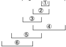
- Making sure that you do not accidentally press the AC/ON key, slide the case onto the calculator and then turn the calculator over. Remove the back cover from the calculator by pulling with your finger at the point marked ①.

natural_image
Illustration of a smartphone with two arrows indicating clockwise rotation (no text or symbols)
natural_image
Line drawing of a pink mobile phone casing against a pink background (no text or symbols)
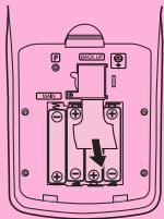
- Load the four batteries that come with the calculator.
- Make sure that the positive (+) and negative (−) ends of the batteries are facing correctly.

natural_image
Pure diagram of a device interior with no text, numbers, or symbols visible- Remove the insulating sheet at the location marked "BACK UP" by pulling in the direction indicated by the arrow.
- Replace the back cover, making sure that its tabs enter the holes marked ② and turn the calculator front side up. The calculator should automatically turn on power and perform the memory reset operation.
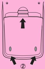
natural_image
Simple line drawing of a container with an upward arrow and two arrows pointing to the bottom (no text or symbols)![MAIN MEMORIES CLEARED! Press [MENU] KEY](/content/2025/01/86785/images/6b646cb7202b54734d472232a0bc9a9a169d3f2dbf32025a5bf4e932012218de.jpg)
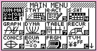
5. Press MENU.
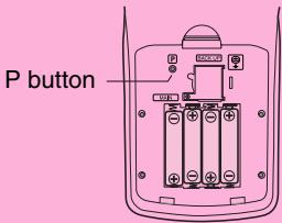
- If the Main Menu shown to the right is not on the display, open the back cover and press the P button located inside of the battery compartment.
- Use the cursor keys (▲, ▼, ◀, ▶) to select the SYSTEM icon and press EXE, then press F1(◀) to display the contrast adjustment screen.
![Contrast [◀]Key [▶]Key Light Dark INIT](/content/2025/01/86785/images/5bbf4207fc0151c8f9b8531b7d22137a968fd886a3af52dc655624cf07cd1dfa.jpg)
-
Adjust the contrast.
-
The ▶ cursor key makes display contrast darker.
-
The ◀ cursor key makes display contrast lighter.
• F1(INIT) returns display contrast to its initial default. -
To exit display contrast adjustment, press MENU.
Quick-Start
TURNING POWER ON AND OFF
USING MODES
BASIC CALCULATIONS
REPLAY FEATURE
FRACTION CALCULATIONS
EXPONENTS
GRAPH FUNCTIONS
DUAL GRAPH
DYNAMIC GRAPH
TABLE FUNCTION
Quick-Start
Welcome to the world of graphing calculators.
Quick-Start is not a complete tutorial, but it takes you through many of the most common functions, from turning the power on, and on to graphing complex equations. When you're done, you'll have mastered the basic operation of this calculator and will be ready to proceed with the rest of this user's guide to learn the entire spectrum of functions available.
Each step of the examples in Quick-Start is shown graphically to help you follow along quickly and easily. When you need to enter the number 57, for example, we've indicated it as follows:
Press 5 7.
Whenever necessary, we've included samples of what your screen should look like. If you find that your screen doesn't match the sample, you can restart from the beginning by pressing the "All Clear" button AC/ON.
TURNING POWER ON AND OFF
To turn power on, press /ON .
To turn power off, press SHIFT OFF AC/ON.
Calculator power turns off automatically if you do not perform any operation within the Auto Power Off trigger time you specify. You can specify either six minutes or 60 minutes as the trigger time.
USING MODES
This calculator makes it easy to perform a wide range of calculations by simply selecting the appropriate mode. Before getting into actual calculations and operation examples, let's take a look at how to navigate around the modes.
To select the RUN·MAT mode
- Press MENU to display the Main Menu.
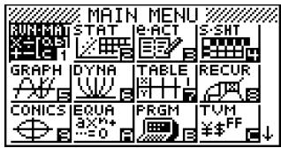
- Use ◀ ▶ ▲ ▼ to highlight RUN · MAT and then press EXE.
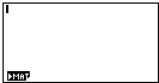
This is the initial screen of the RUN·MAT mode, where you can perform manual calculations, matrix calculations, and run programs.
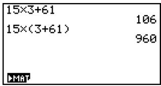
BASIC CALCULATIONS
With manual calculations, you input formulas from left to right, just as they are written on paper. With formulas that include mixed arithmetic operators and parentheses, the calculator automatically applies true algebraic logic to calculate the result.
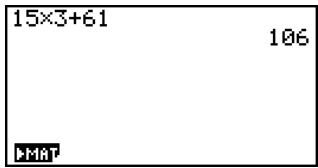
Example: 15 × 3 + 61
- Press /ON to clear the calculator.
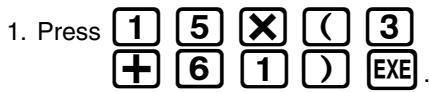
- Press 1 5 × 3 + 6 1 EXE.
Parentheses Calculations
Example: 15 × (3 + 61)
Built-In Functions
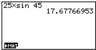
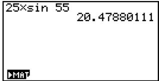
This calculator includes a number of built-in scientific functions, including trigonometric and logarithmic functions.
Example: 25 × 45^
Important!
Be sure that you specify Deg (degrees) as the angle unit before you try this example.
- Press SHIFT MENU to display the Setup screen.
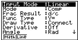
- Press ▼ ▼ ▼ ▼ ▼ ▼ F1 (Deg) to specify degrees as the angle unit.

-
Press EXIT to clear the menu.
-
Press AC/ON to clear the unit.
-
Press 2 5 × sin 4 5 EXE.
REPLAY FEATURE
With the replay feature, simply press ◀ or ▶ to recall the last calculation that was performed so you can make changes or re-execute it as it is.
Example: To change the calculation in the last example from (25 × 45^) to (25 × 55^)
-
Press ◀ to display the last calculation.
-
Press ◀ to move the cursor (I) to the right side of 4.
-
Press DEL to delete 4.
-
Press 5.
-
Press EXE to execute the calculation again.
FRACTION CALCULATIONS
You can use the key to input fractions into calculations. The symbol “」” is used to separate the various parts of a fraction.
Example: ^31/_16 + ^37/_9
-
Press AC/ON.
-
Press 3 1 a_c^b 1 6 + 3 7 a_c^b 9 EXE.
Indicates ^871/_144
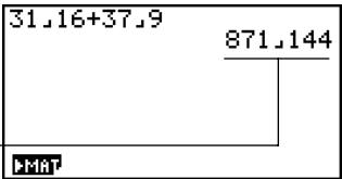
Converting an Improper Fraction to a Mixed Fraction
While an improper fraction is shown on the display, press SHIFT + to convert it to a mixed fraction.
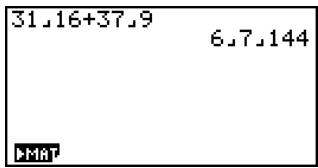
Press SHIFT a + again to convert back to an improper fraction.
Converting a Fraction to Its Decimal Equivalent
While a fraction is shown on the display, press D to convert it to its decimal equivalent.
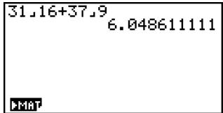
Press D again to convert back to a fraction.
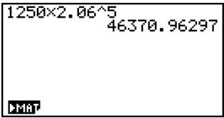
EXPONENTS
Example: 1250 × 2.06^5
- Press /ON .
- Press 1 2 5 0 × 2 · 0 6.
- Press ∧ and the ^ indicator appears on the display.
- Press 5. The ^5 on the display indicates that 5 is an exponent.
- Press EXE.
GRAPH FUNCTIONS
The graphing capabilities of this calculator makes it possible to draw complex graphs using either rectangular coordinates (horizontal axis: x; vertical axis: y) or polar coordinates (angle: ; distance from origin: r).
All of the following graphing examples are performed starting from the calculator setup in effect immediately following a reset operation.
Example 1: To graph Y = X(X + 1)(X - 2)
-
Press MENU .
-
Use ◀▶▶▶▼ to highlight GRAPH, and then press EXE.
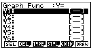
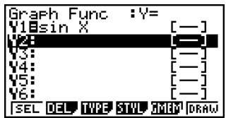
- Input the formula.
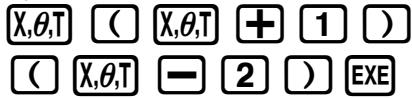
![Graph Func :Y= Y1X(X+1)(X-2) [—] Y2: [—] Y3: [—] Y4: [—] Y5: [—] Y6: [—] SEL DEL TYPE STYLE MEMP DRAW](/content/2025/01/86785/images/69b38ff805249698678423889e214cb7f4265d0bcfeb456103289baee3eba6b9.jpg)
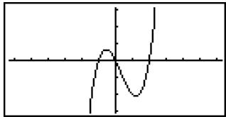
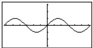
- Press F6 (DRAW) or EXE to draw the graph.
natural_image
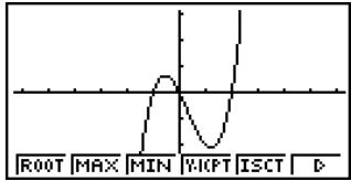
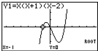
Pure electrical circuit lines without any symbolsExample 2: To determine the roots of Y = X(X + 1)(X - 2)
- Press SHIFT F5 (G-SLV).
line
| X-axis | Value | |--------|-------| | ROOT | 0 | | MAX | 0 | | MIN | 0 | | YKPT | Peak | | ISCT | 0 | | D | 0 |- Press F1 (ROOT).
Press ▶ for other roots.
line
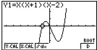
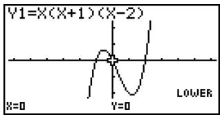
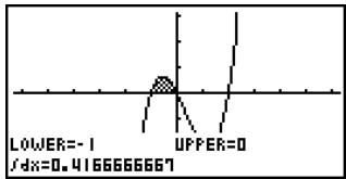
| X | Y | | ---- | ----- | | -1 | 0 | | 0 | 0 |Example 3: Determine the area bounded by the origin and the X = -1 root obtained for Y = X(X + 1)(X - 2)
- Press SHIFT F5 (G-SLV) F6 (▷).
line
| X-axis Label | Y-axis Value | | ------------ | ------------ | | Start | 0 | | Peak | 1 | | End | 0 |- Press 3 ( dx ).
line
| X | Y | | ---- | ----- | | 0 | 0 | | -2 | 0 |- Use ◀ to move the pointer to the location where X = -1, and then press EXE. Next, use ▶ to move the pointer to the location where X = 0, and then press EXE to input the integration range, which becomes shaded on the display.
line
| X | Y | |---|---| | -1 | Lower=-1 | | -1 | Upper=0 | | 0 | Lower=-1 | | 0 | Upper=0 | | dfx=0.415666667 |DUAL GRAPH
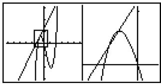
With this function you can split the display between two areas and display two graph windows.
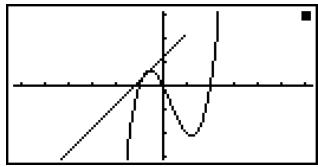
Example: To draw the following two graphs and determine the points of intersection
$$ Y 1 = X (X + 1) (X - 2) $$
$$ Y 2 = X + 1. 2 $$
- Press SHIFT MENU ▼ F1 (G+G)
to specify "G+G" for the Dual Screen setting.
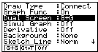
- Press EXIT, and then input the two functions.

![Graph+Graph :Y= Y1X(X+1)(X-2) [—] Y2X+1.2 [—] Y3: [—] Y4: [—] Y5: [—] Y6: [—] SEL DEL TYPE STYLE GMBD DRAW](/content/2025/01/86785/images/2169e3ee21163135b6af6788d0bc153c2ba8d94c9a4f409369fdbc3478e3bf0e.jpg)
- Press F6 (DRAW) or EXE to draw the graphs.
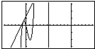
Box Zoom
Use the Box Zoom function to specify areas of a graph for enlargement.
-
Press SHIFT F2 (ZOOM) F1 (BOX).
-
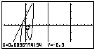
Use ◀▶▶▶▼ to move the pointer to one corner of the area you want to specify and then press EXE.
line
| X | Y | |---|---| | 0.6056774194 | -0.3 |- Use ◀▶▶▶▼ to move the pointer again. As you do, a box appears on the display. Move the pointer so the box encloses the area you want to enlarge.

- Press EXE, and the enlarged area appears in the inactive (right side) screen.
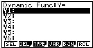
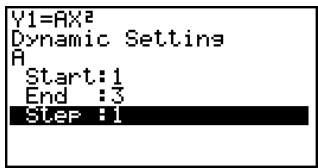
DYNAMIC GRAPH
Dynamic Graph lets you see how the shape of a graph is affected as the value assigned to one of the coefficients of its function changes.
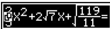
Example: To draw graphs as the value of coefficient A in the following function changes from 1 to 3
$$ Y = A X ^ {2} $$
-
Press MENU.
-
Use ◀ ▶ ▲ ▼ to highlight DYNA, and then press EXE.
-
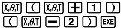
Input the formula.

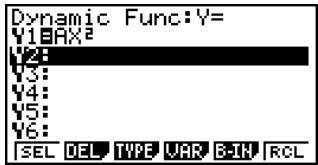
- Press F4 (VAR) 1 EXE to assign an initial value of 1 to coefficient A.
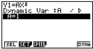
- Press F2 (SET) 1 EXE 3 EXE 1 EXE to specify the range and increment of change in coefficient A.
-
Press EXIT.
-
Press F6 (DYNA) to start Dynamic Graph drawing. The graphs are drawn 10 times.
- To interrupt an ongoing Dynamic Graph drawing operation, press AC/ON.
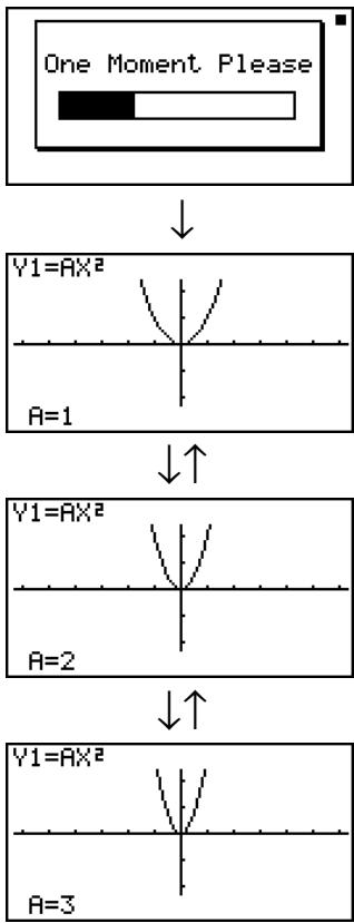
flowchart
graph TD
    A["One Moment Please"] --> B["Y1=AX²\nA=1"]
    B --> C["Y1=AX²\nA=2"]
    C --> D["Y1=AX²\nA=3"]
TABLE FUNCTION
The Table Function makes it possible to generate a table of solutions as different values are assigned to the variables of a function.
Example: To create a number table for the following function
$$ Y = X (X + 1) (X - 2) $$
-
Press MENU.
-
Use ◀▶▶▶▼ to highlight TABLE, and then press EXE.
-
Input the formula.
- Press F6 (TABL) to generate the number table.
![Table Func :Y= V1 V2: [—] V3: [—] V4: [—] V5: [—] V6: [—] SEL DEL TYPE STYLE SET TABL](/content/2025/01/86785/images/68a9930df2c8f2fc38881826663438241fd86bae5144780a48dc1315f9b5396c.jpg)
![Table Func :Y= Y1B(X+1)(X-2) [—] Y2: [—] Y3: [—] Y4: [—] Y5: [—] Y6: [—] SEL DEL TYPE STYL SET TABL](/content/2025/01/86785/images/eba2774b73003c82ccbf90b00c23c9fb5e42084e31196e419af34fd8f3c68a4d.jpg)
![X Y1 [1 -2 2 0 3 12 4 40] FORM DEL ROW EDIT G-CON G-PLT 1](/content/2025/01/86785/images/0c933b94a854b66208829357c1cf5bb7e760b05ee06153d3390b513affb58124.jpg)
To learn all about the many powerful features of this calculator, read on and explore!
Precautions when Using this Product
A progress bar and/or a busy indicator appear on the display whenever the calculator is performing a calculation, writing to memory (including Flash memory), or reading from memory (including Flash memory).
Progress bar
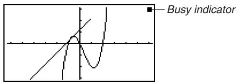
Never press the P button or remove the batteries from the calculator when the progress bar or busy indicator is on the display. Doing so can cause memory contents to be lost and can cause malfunction of the calculator.
This calculator is equipped with Flash memory for data storage. It is recommended that you always backup your data to Flash memory. For details about the backup procedure, see "12-7 MEMORY Mode" in the User's Guide.
You can also transfer data to a computer using the Program-Link software (FA-124) that comes bundled with the calculator. The Program-Link software can also be used to backup data to a computer.
- fx-9860G SD only
If the message “No Card” appears even though an SD card is loaded in the SD card slot, it means that the calculator is not recognizing the card for some reason. Try removing the card and then loading it again. If this does not work, contact the developer of the SD card. Note that some SD cards may not be compatible with this calculator.
Precautions when Connecting to a Computer
A special USB driver must be installed on your computer in order to connect to the calculator. The driver is installed along with the Program-Link software (FA-124) that comes bundled with the calculator. Be sure to install the Program-Link software (FA-124) on your computer before trying to connect the calculator. Attempting to connect the calculator to a computer that does not have the Program-Link software installed can cause malfunction. For information about how to install the Program-Link software, see the User's Guide on the bundled CD-ROM.
Handling Precautions
- Your calculator is made up of precision components. Never try to take it apart.
- Avoid dropping your calculator and subjecting it to strong impact.
- Do not store the calculator or leave it in areas exposed to high temperatures or humidity, or large amounts of dust. When exposed to low temperatures, the calculator may require more time to display results and may even fail to operate. Correct operation will resume once the calculator is brought back to normal temperature.
- The display will go blank and keys will not operate during calculations. When you are operating the keyboard, be sure to watch the display to make sure that all your key operations are being performed correctly.
- Replace the main batteries once every one year regardless of how much the calculator is used during that period. Never leave dead batteries in the battery compartment. They can leak and damage the unit.
- Keep batteries out of the reach of small children. If swallowed, consult a physician immediately.
- Avoid using volatile liquids such as thinner or benzine to clean the unit. Wipe it with a soft, dry cloth, or with a cloth that has been moistened with a solution of water and a neutral detergent and wrung out.
- Always be gentle when wiping dust off the display to avoid scratching it.
- In no event will the manufacturer and its suppliers be liable to you or any other person for any damages, expenses, lost profits, lost savings or any other damages arising out of loss of data and/or formulas arising out of malfunction, repairs, or battery replacement. It is up to you to prepare physical records of data to protect against such data loss.
- Never dispose of batteries, the liquid crystal panel, or other components by burning them.
- Be sure that the power switch is set to OFF when replacing batteries.
- If the calculator is exposed to a strong electrostatic charge, its memory contents may be damaged or the keys may stop working. In such a case, perform the Reset operation to clear the memory and restore normal key operation.
- If the calculator stops operating correctly for some reason, use a thin, pointed object to press the P button on the back of the calculator. Note, however, that this clears all the data in calculator memory.
- Note that strong vibration or impact during program execution can cause execution to stop or can damage the calculator's memory contents.
- Using the calculator near a television or radio can cause interference with TV or radio reception.
- Before assuming malfunction of the unit, be sure to carefully reread this user's guide and ensure that the problem is not due to insufficient battery power, programming or operational errors.
- Battery life can be reduced dramatically by certain operations and by the use of certain types of SD cards.
Be sure to keep physical records of all important data!
Low battery power or incorrect replacement of the batteries that power the unit can cause the data stored in memory to be corrupted or even lost entirely. Stored data can also be affected by strong electrostatic charge or strong impact. It is up to you to keep back up copies of data to protect against its loss.
In no event shall CASIO Computer Co., Ltd. be liable to anyone for special, collateral, incidental, or consequential damages in connection with or arising out of the purchase or use of these materials. Moreover, CASIO Computer Co., Ltd. shall not be liable for any claim of any kind whatsoever against the use of these materials by any other party.
- The contents of this user's guide are subject to change without notice.
- No part of this user's guide may be reproduced in any form without the express written consent of the manufacturer.
- The options described in Chapter 12 of this user's guide may not be available in certain geographic areas. For full details on availability in your area, contact your nearest CASIO dealer or distributor.
Contents
Getting Acquainted — Read This First!
Chapter 1 Basic Operation
1-1 Keys 1-1-1
1-2 Display 1-2-1
1-3 Inputting and Editing Calculations 1-3-1
1-4 Option (OPTN) Menu 1-4-1
1-5 Variable Data (VARS) Menu 1-5-1
1-6 Program (PRGM) Menu 1-6-1
1-7 Using the Setup Screen 1-7-1
1-8 Using Screen Capture 1-8-1
1-9 When you keep having problems... 1-9-1
Chapter 2 Manual Calculations
2-1 Basic Calculations 2-1-1
2-2 Special Functions 2-2-1
2-3 Specifying the Angle Unit and Display Format 2-3-1
2-4 Function Calculations 2-4-1
2-5 Numerical Calculations 2-5-1
2-6 Complex Number Calculations 2-6-1
2-7 Binary, Octal, Decimal, and Hexadecimal Calculations with Integers 2-7-1
2-8 Matrix Calculations 2-8-1
Chapter 3 List Function
3-1 Inputting and Editing a List 3-1-1
3-2 Manipulating List Data 3-2-1
3-3 Arithmetic Calculations Using Lists 3-3-1
3-4 Switching Between List Files 3-4-1
Chapter 4 Equation Calculations
4-1 Simultaneous Linear Equations 4-1-1
4-2 Quadratic and Cubic Equations 4-2-1
4-3 Solve Calculations 4-3-1
4-4 What to Do When an Error Occurs 4-4-1
Chapter 5 Graphing
5-1 Sample Graphs 5-1-1
5-2 Controlling What Appears on a Graph Screen 5-2-1
5-3 Drawing a Graph 5-3-1
5-4 Storing a Graph in Picture Memory 5-4-1
5-5 Drawing Two Graphs on the Same Screen 5-5-1
5-6 Manual Graphing 5-6-1
5-7 Using Tables 5-7-1
5-8 Dynamic Graphing 5-8-1
5-9 Graphing a Recursion Formula 5-9-1
5-10 Changing the Appearance of a Graph 5-10-1
5-11 Function Analysis 5-11-1
Chapter 6 Statistical Graphs and Calculations
6-1 Before Performing Statistical Calculations 6-1-1
6-2 Calculating and Graphing Single-Variable Statistical Data 6-2-1
6-3 Calculating and Graphing Paired-Variable Statistical Data 6-3-1
6-4 Performing Statistical Calculations 6-4-1
6-5 Tests 6-5-1
6-6 Confidence Interval 6-6-1
6-7 Distribution 6-7-1
Chapter 7 Financial Calculation (TVM)
7-1 Before Performing Financial Calculations 7-1-1
7-2 Simple Interest 7-2-1
7-3 Compound Interest 7-3-1
7-4 Cash Flow (Investment Appraisal) 7-4-1
7-5 Amortization 7-5-1
7-6 Interest Rate Conversion.... 7-6-1
7-7 Cost, Selling Price, Margin 7-7-1
7-8 Day/Date Calculations 7-8-1
Chapter 8 Programming
8-1 Basic Programming Steps 8-1-1
8-2 PRGM Mode Function Keys 8-2-1
8-3 Editing Program Contents 8-3-1
8-4 File Management 8-4-1
8-5 Command Reference 8-5-1
8-6 Using Calculator Functions in Programs 8-6-1
8-7 PRGM Mode Command List 8-7-1
8-8 Program Library 8-8-1
Chapter 9 Spreadsheet
9-1 Spreadsheet Overview 9-1-1
9-2 File Operations and Re-calculation 9-2-1
9-3 Basic Spreadsheet Screen Operations 9-3-1
9-4 Inputting and Editing Cell Data 9-4-1
9-5 S·SHT Mode Commands 9-5-1
9-6 Statistical Graphs 9-6-1
9-7 Using the CALC Function 9-7-1
9-8 Using Memory in the S • SHT Mode 9-8-1
Chapter 10 eActivity
10-1 eActivity Overview 10-1-1
10-2 Working with eActivity Files 10-2-1
10-3 Inputting and Editing eActivity File Data 10-3-1
10-4 Using Matrix Editor and List Editor 10-4-1
10-5 eActivity File Memory Usage Screen 10-5-1
Chapter 11 System Settings Menu
11-1 Using the System Settings Menu 11-1-1
11-2 System Settings 11-2-1
11-3 Version/ID Number List 11-3-1
11-4 Reset 11-4-1
Chapter 12 Data Communications
12-1 Connecting Two Units 12-1-1
12-2 Connecting the Unit to a Personal Computer 12-2-1
12-3 Performing a Data Communication Operation 12-3-1
12-4 Data Communications Precautions 12-4-1
12-5 Image Transfer 12-5-1
12-6 Add-ins 12-6-1
12-7 MEMORY Mode 12-7-1
Chapter 13 Using SD Cards (fx-9860G SD only)
13-1 Using an SD Card 13-1-1
13-2 Formatting an SD Card 13-2-1
13-3 SD Card Precautions during Use 13-3-1
Appendix
1 Error Message Table ....... α-1-1
2 Input Ranges ....α-2-1
3 Specifications....α-3-1
4 Key Index ....α-4-1
5 P Button (In case of hang up) ....α-5-1
6 Power Supply....α-6-1
Getting Acquainted
— Read This First!
About this User's Guide
- SHIFT ^2 (√)
The above indicates you should press SHIFT and then x^2 , which will input a symbol. All multiple-key input operations are indicated like this. Key cap markings are shown, followed by the input character or command in parentheses.
- MENU EQUA
This indicates you should first press MENU, use the cursor keys (▲, ▼, ◀, ▶) to select the EQUA mode, and then press EXE. Operations you need to perform to enter a mode from the Main Menu are indicated like this.
- Function Keys and Menus
- Many of the operations performed by this calculator can be executed by pressing function keys F1 through F6. The operation assigned to each function key changes according to the mode the calculator is in, and current operation assignments are indicated by function menus that appear at the bottom of the display.
- This user's guide shows the current operation assigned to a function key in parentheses following the key cap for that key. [F1] (Comp), for example, indicates that pressing [F1] selects {Comp}, which is also indicated in the function menu.
- When (▷) is indicated in the function menu for key F6, it means that pressing F6 displays the next page or previous page of menu options.
- Menu Titles
- Menu titles in this user's guide include the key operation required to display the menu being explained. The key operation for a menu that is displayed by pressing OPTN and then {MAT} would be shown as: [OPTN]-[MAT].
- F6 (▷) key operations to change to another menu page are not shown in menu title key operations.
•Graphs
As a general rule, graph operations are shown on facing pages, with actual graph examples on the right hand page. You can produce the same graph on your calculator by performing the steps under the Procedure above the graph.
Look for the type of graph you want on the right hand page, and then go to the page indicated for that graph. The steps under “Procedure” always use initial RESET settings.
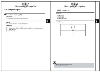
The step numbers in the “Set Up” and “Execution” sections on the left hand page correspond to the “Procedure” step numbers on the right hand page.
Example:
Left hand page
Right hand page
- Draw the graph.
③ F5 (DRAW)(or EXE)
- Command List
The PRGM Mode Command List (page 8-7) provides a graphic flowchart of the various function key menus and shows how to maneuver to the menu of commands you need.
Example: The following operation displays Xfct: [VARS]-[FACT]-[Xfct]
- Page Contents
Three-part page numbers are centered at the top of each page. The page number “1-2-3”, for example, indicates Chapter 1, Section 2, page 3.
●Supplementary Information
Supplementary information is shown at the bottom of each page in a “(Notes)” block.
* indicates a note about a term that appears in the same page as the note.
# indicates a note that provides general information about topic covered in the same section as the note.
Chapter
1
Basic Operation
1-1 Keys
1-2 Display
1-3 Inputting and Editing Calculations
1-4 Option (OPTN) Menu
1-5 Variable Data (VARS) Menu
1-6 Program (PRGM) Menu
1-7 Using the Setup Screen
1-8 Using Screen Capture
1-9 When you keep having problems...
1-1 Keys
![Trace Zoom V-Window Sketch G-Solv G↔T F1 F2 F3 F4 F5 F6 SHIFT OPTN VARS SET UP A-LOCK r x̄ θ QUIT REPLAY ALPHA x² ∧ EXIT ∠ A 10° B e* C sin⁻¹ D cos⁻¹ E tan⁻¹ F X,θ,T log In sin cos tan ≡ G a‡→‡ H I x⁻¹ J K L a b/c F↔D ( ) , → CAPTURE M CLIP N PASTE O INS OFF 7 8 9 DEL AC/ON CATALOG P Q R { S } T 4 5 6 × ÷ List U Mat V W [ X ] Y 1 2 3 + - i Z = SPACE π " Ans ↓ 0 • EXP (-) EXE](/content/2025/01/86785/images/f1c42225329d1d9973535fb219805249707d7ba25bfa09c229be1ffe5b048f32.jpg)

Key Table
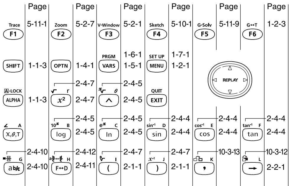
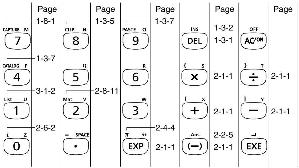

■ Key Markings
Many of the calculator's keys are used to perform more than one function. The functions marked on the keyboard are color coded to help you find the one you need quickly and easily.
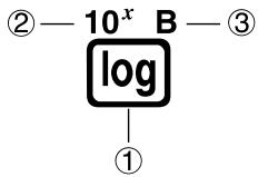
| Function | Key Operation | |
| 1 | log | log |
| 2 | 10^x | SHIFT log |
| 3 | B | ALPHA log |
The following describes the color coding used for key markings.
| Color | Key Operation |
| Orange | Press SHIFT and then the key to perform the marked function. |
| Red | Press ALPHA and then the key to perform the marked function. |

A-LOCK
# ALPHA Alpha Lock
Normally, once you press ALPHA and then a key to input an alphabetic character, the keyboard reverts to its primary functions immediately.
If you press SHIFT and then ALPHA, the keyboard locks in alpha input until you press ALPHA again.
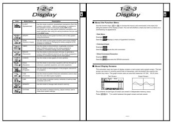
1-2 Display
■ Selecting Icons
This section describes how to select an icon in the Main Menu to enter the mode you want.
- To select an icon
- Press MENU to display the Main Menu.
- Use the cursor keys (◀, ▶, ▲, ▼) to move the highlighting to the icon you want.
Currently selected icon
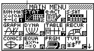
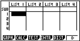
- Press EXE to display the initial screen of the mode whose icon you selected. Here we will enter the STAT mode.
- You can also enter a mode without highlighting an icon in the Main Menu by inputting the number or letter marked in the lower right corner of the icon.
The following explains the meaning of each icon.
| Icon | Mode Name | Description |
 | RUN·MAT(Run·Matrix) | Use this mode for arithmetic calculations and function calculations, and for calculations involving binary, octal, decimal, and hexadecimal values and matrices. |
 | STAT(Statistics) | Use this mode to perform single-variable (standard deviation) and paired-variable (regression) statistical calculations, to perform tests, to analyze data and to draw statistical graphs. |
 | e·ACT(eActivity) | eActivity lets you input text, math expressions, and other data in a notebook-like interface. Use this mode when you want to store text or formulas, or built-in application data in a file. |

| Icon | Mode Name | Description |
 | S·SHT(Spreadsheet) | Use this mode to perform spreadsheet calculations. Each file contains a 26-column × 999-line spreadsheet. In addition to the calculator's built-in commands and S·SHT mode commands, you can also perform statistical calculations and graph statistical data using the same procedures that you use in the STAT mode. |
 | GRAPH | Use this mode to store graph functions and to draw graphs using the functions. |
 | DYNA(Dynamic Graph) | Use this mode to store graph functions and to draw multiple versions of a graph by changing the values assigned to the variables in a function. |
 | TABLE | Use this mode to store functions, to generate a numeric table of different solutions as the values assigned to variables in a function change, and to draw graphs. |
 | RECUR(Recursion) | Use this mode to store recursion formulas, to generate a numeric table of different solutions as the values assigned to variables in a function change, and to draw graphs. |
 | CONICS | Use this mode to draw graphs of conic sections. |
 | EQUA(Equation) | Use this mode to solve linear equations with two through six unknowns, quadratic equations, and cubic equations. |
 | PRGM(Program) | Use this mode to store programs in the program area and to run programs. |
 | TVM(Financial) | Use this mode to perform financial calculations and to draw cash flow and other types of graphs. |
 | LINK | Use this mode to transfer memory contents or back-up data to another unit or PC. |
 | MEMORY | Use this mode to manage data stored in memory. |
 | SYSTEM | Use this mode to initialize memory, adjust contrast, and to make other system settings. |

■ About the Function Menu
Use the function keys (F1 to F6) to access the menus and commands in the menu bar along the bottom of the display screen. You can tell whether a menu bar item is a menu or a command by its appearance.
- Next Menu
Example: HYP
Selecting HYP displays a menu of hyperbolic functions.
- Command Input
Example: sinh
Selecting sinh inputs the sinh command.
- Direct Command Execution
Example: DRAW
Selecting DRAW executes the DRAW command.
■ About Display Screens
This calculator uses two types of display screens: a text screen and a graph screen. The text screen can show 21 columns and 8 lines of characters, with the bottom line used for the function key menu. The graph screen uses an area that measures 127 (W) × 63 (H) dots.
Text Screen
Graph Screen
natural_image
Pure waveform diagram with no text, numbers, or symbolsThe contents of each type of screen are stored in independent memory areas.
Press SHIFT F6(G↔T) to switch between the graph screen and text screen.

Normal Display
The calculator normally displays values up to 10 digits long. Values that exceed this limit are automatically converted to and displayed in exponential format.
- How to interpret exponential format
$$ \boxed { \begin{array}{c c} 1. 2 \mathrm{E} 1 2 & \ & 1. 2 \mathrm{E} + 1 2 \end{array} } $$
1.2_E+12 indicates that the result is equivalent to 1.2 × 10^12 . This means that you should move the decimal point in 1.2 twelve places to the right, because the exponent is positive. This results in the value 1,200,000,000,000.
$$ \boxed { \begin{array}{c c} 1. 2 \mathrm{E} - 3 & \ & 1. 2 \mathrm{E} - 0 3 \end{array} } $$
1.2_E - 03 indicates that the result is equivalent to 1.2 × 10^-3 . This means that you should move the decimal point in 1.2 three places to the left, because the exponent is negative. This results in the value 0.0012.
You can specify one of two different ranges for automatic changeover to normal display.
Norm 1 ...... 10^-2(0.01) > |x| , |x| ≥ 10^10
Norm 2 ...... 10^-9 (0.000000001) > |x|, |x| ≥ 10^10
All of the examples in this manual show calculation results using Norm 1. See page 2-3-2 for details on switching between Norm 1 and Norm 2.

■ Special Display Formats
This calculator uses special display formats to indicate fractions, hexadecimal values, and degrees/minutes/seconds values.
- Fractions
$$ \boxed { \begin{array}{c c} 4 5 6, 1 2, 2 3 & \ & 4 5 6, 1 2, 2 3 \end{array} } \dots\dotsIndicates: 4 5 6 \frac {1 2}{2 3} $$
- Hexadecimal Values
$$ \boxed { \begin{array}{c c} \text {ABCDEF1} & \ & 0 \text {ABCDEF1} \end{array} } \dots\dots\text {Indicates: 0ABCDEF1_{(16)}, which} \ & \text {equals 180150001_{(10)}} $$
• Degrees/Minutes/Seconds
$$ \boxed { \begin{array}{c c} 1 2. 5 8 2 4 4 & \ & 1 2 ^ {\circ} 3 4 ^ {\prime} 5 6. 7 8 ^ {\prime \prime} \end{array} } \dots\dotsIndicates: 1 2 ^ {\circ} 3 4 ^ {\prime} 5 6. 7 8 ^ {\prime \prime} $$
- In addition to the above, this calculator also uses other indicators or symbols, which are described in each applicable section of this manual as they come up.
■ Calculation Execution Indicator
Whenever the calculator is busy drawing a graph or executing a long, complex calculation or program, a black box “■” flashes in the upper right corner of the display. This black box tells you that the calculator is performing an internal operation.

1-3 Inputting and Editing Calculations
Note
- Unless specifically noted otherwise, all of the operations in this section are explained using the Linear input mode.
■ Inputting Calculations
When you are ready to input a calculation, first press AC to clear the display. Next, input your calculation formulas exactly as they are written, from left to right, and press EXE to obtain the result.

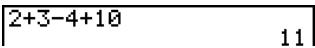
Example 1 2 + 3 - 4 + 10 =


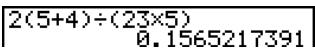
Example 2 2(5 + 4) ÷ (23 × 5) =


■ Editing Calculations
Use the ◀ and ▶ keys to move the cursor to the position you want to change, and then perform one of the operations described below. After you edit the calculation, you can execute it by pressing EXE. Or you can use ▶ to move to the end of the calculation and input more.
- To change a step

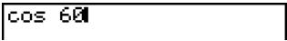
Example To change cos60 to sin60


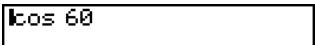


In the Linear input mode, pressing SHIFT DEL (INS) changes the cursor to “_”.
The next function or value you input is overwritten at the location of “_”.


To abort this operation, press SHIFT DEL (INS) again.
- To delete a step

Example To change 369 × × 2 to 369 × 2


In the insert mode, the DEL key operates as a backspace key.

The cursor is a vertical flashing line (I) when the insert mode is selected. The cursor is a horizontal flashing line (—) when the overwrite mode is selected.
# The initial default for Linear input mode is the insert mode. You can switch to the overwrite mode by pressing SHIFT DEL (INS).

- To insert a step

Example
To change 2.36^2 to 2.36^2
2.3621

2.36 ^2

sin 2.36 ^2
- To change the last step you input

Example
To change 369 × 3 to 369 × 2
369×3

369×1

369×2

■ Using Replay Memory
The last calculation performed is always stored into replay memory. You can recall the contents of the replay memory by pressing ◀ or ▶.
If you press ▶, the calculation appears with the cursor at the beginning. Pressing ◀ causes the calculation to appear with the cursor at the end. You can make changes in the calculation as you wish and then execute it again.

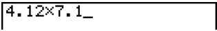
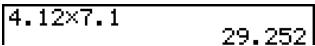
Example 1 To perform the following two calculations
$$ 4. 1 2 \times \underline {{6 . 4}} = 2 6. 3 6 8 $$
$$ 4. 1 2 \times \underline {{7 . 1}} = 2 9. 2 5 2 $$

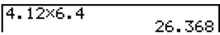

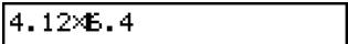

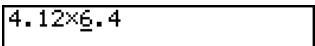


After you press AC, you can press ▲ or ▼ to recall previous calculations, in sequence from the newest to the oldest (Multi-Replay Function). Once you recall a calculation, you can use ▶ and ◀ to move the cursor around the calculation and make changes in it to create a new calculation.

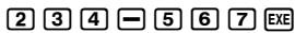
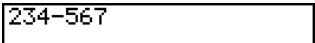
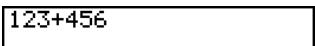
Example 2

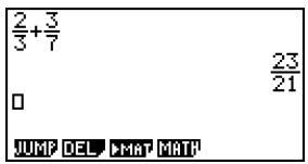
| 123+456 | 579 |
| 234-567 | -333 |


# A calculation remains stored in replay memory until you perform another calculation.
# The contents of replay memory are not cleared when you press the AC key, so you can recall a calculation and execute it even after pressing the AC key.
# Replay memory is enabled in the Linear input mode only. In the Math input mode, the history function is used in place of the replay memory. For details, see “History Function” (page 2-2-6).
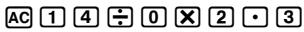
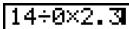
■ Making Corrections in the Original Calculation

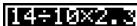
Example 14 ÷ 0 × 2.3 entered by mistake for 14 ÷ 10 × 2.3

![1d:\My3 Ma ERROR Press:[EXIT]](/content/2025/01/86785/images/a718a977f5964ee836d47eba8642426713fa54fba813884d48f9eb688437d736.jpg)
Press EXIT.
Cursor is positioned automatically at the location of the cause of the error.
Make necessary changes.

Execute again.

3.22
■ Using the Clipboard for Copy and Paste
You can copy (or cut) a function, command, or other input to the clipboard, and then paste the clipboard contents at another location.
- To specify the copy range
Linear input mode
- Move the cursor (I) to the beginning or end of the range of text you want to copy and then press SHIFT 8 (CLIP). This changes the cursor to "F".
- Use the cursor keys to move the cursor and highlight the range of text you want to copy.

# The copy range of text you can specify depends on the current "Input Mode" setting.
Linear input mode: 1 character 1 line Multiple lines Math input mode: 1 line only
- Press F1(COPY) to copy the highlighted text to the clipboard, and exit the copy range specification mode.
$$ \boxed {1 4 \div 1 0 \times 2. 3} $$
The selected characters are not changed when you copy them.
To cancel text highlighting without performing a copy operation, press EXIT.
Math input mode
- Use the cursor keys to move the cursor to the line you want to copy.
- Press SHIFT 8 (CLIP). The cursor will change to "☐".
CPY-L
- Press F1(CPY·L) to copy the highlighted text to the clipboard.
- To cut the text
- Move the cursor (I) to the beginning or end of the range of text you want to cut and then press SHIFT 8 (CLIP). This changes the cursor to "☐".
$$ 1 4 \div 9 0 \times 2. 3 $$
- Use the cursor keys to move the cursor and highlight the range of text you want to cut.
$$ 1 4 \div [ 2. 3 $$
- Press F2 (CUT) to cut the highlighted text to the clipboard.
$$ \boxed {1 4 \div 2. 3} $$
Cutting causes the original characters to be deleted.
The CUT operation is supported for the Linear input mode only. It is not supported for the Math input mode.

- Pasting Text
Move the cursor to the location where you want to paste the text, and then press SHIFT ⑨ (PASTE). The contents of the clipboard are pasted at the cursor position.
AC
SHIFT 9 (PASTE)
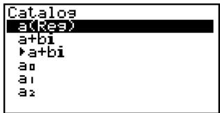
■ Catalog Function
The Catalog is an alphabetic list of all the commands available on this calculator. You can input a command by calling up the Catalog and then selecting the command you want.
- To use the Catalog to input a command
- Press SHIFT 4 (CATALOG) to display an alphabetic Catalog list of commands.
- Input the first letter of the command you want to input. This will display the first command that starts with that letter.
- Use the cursor keys (▲, ▼) to highlight the command you want to input, and then press EXE.
● ● ● ● ●
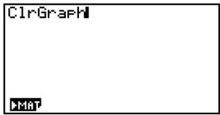
Example To use the Catalog to input the ClrGraph command
AC SHIFT 4 (CATALOG) In (C) ▼ \~ ▼ EXE
Pressing EXIT or SHIFT EXIT (QUIT) closes the Catalog.

■ Input Operations in the Math Input Mode
Selecting “Math” for the “Input Mode” setting on the Setup screen (page 1-7-1) turns on the Math input mode, which allows natural input and display of certain functions, just as they appear in your textbook.
Note
- The initial default “Input Mode” setting is “Linear” (Linear input mode). Before trying to perform any of the operations explained in this section, be sure to change the “Input Mode” setting to “Math”.
- In the Math input mode, all input is insert mode (not overwrite mode) input. Note that the SHIFT DEL (INS) operation (page 1-3-2) you use in the Linear input mode to switch to insert mode input performs a completely different function in the Math input mode. For more information, see “Inserting a Function into an Existing Expression” (page 1-3-13).
- Unless specifically stated otherwise, all operations in this section are performed in the RUN·MAT mode.

- Math Input Mode Functions and Symbols
The functions and symbols listed below can be used for natural input in the Math input mode. The “Bytes” column shows the number of bytes of memory that are used up by input in the Math input mode.
| Function/Symbol | Key Operation | Bytes |
| Fraction (Improper) | _2 | 9 |
| Mixed Fraction^*1 | _2 (■■) | 14 |
| Power | 4 | |
| Square | ^2 | 4 |
| Negative Power (Reciprocal) | ( x^-1 ) | 5 |
| ^2 ( ) | 6 | |
| Cube Root | ( ^3 ) | 9 |
| Power Root | ( x ) | 9 |
| e^x | ( e^x ) | 6 |
| 10^x | ( 10^x ) | 6 |
| log(a,b) | (Input from MATH menu*2) | 7 |
| Abs (Absolute Value) | (Input from MATH menu*2) | 6 |
| Linear Differential*3 | (Input from MATH menu*2) | 7 |
| Quadratic Differential*3 | (Input from MATH menu*2) | 7 |
| Integral*3 | (Input from MATH menu*2) | 8 |
| Calculation*4 | (Input from MATH menu*2) | 11 |
| Matrix | (Input from MATH menu*2) | 14^*5 |
| Parentheses | and | 1 |
| Braces (Used during list input.) | × ( { } and ± ( { }) | 1 |
| Brackets (Used during matrix input.) | ( [ ) and ( ] ) | 1 |

*1 Mixed fraction is supported in the Math input mode only.
*2 For information about function input from the MATH function menu, see "Using the MATH Menu" on page 1-3-10.
*3 Tolerance cannot be specified in the Math input mode. If you want to specify tolerance, use the Linear input mode.
*4 For calculation in the Math input mode, the pitch is always 1. If you want to specify a different pitch, use the Linear input mode.
*5 This is the number of bytes for a 2 × 2 matrix.

• Using the MATH Menu
In the RUN·MAT mode, pressing F4(MATH) displays the MATH menu.
You can use this menu for natural input of matrices, differentials, integrals, etc.
- {MAT} ... {displays the MAT submenu, for natural input of matrices}
- 2× 2 ... {inputs a 2× 2 matrix}
- 3 × 3 ... {inputs a 3 × 3 matrix}
- m × n ... {inputs a matrix with m lines and n columns (up to 6 × 6 )}
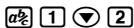
- _ab ... {starts natural input of logarithm log ab}
- {Abs} ... {starts natural input of absolute value |X|}
- d / dx ... {starts natural input of linear differential f(x)_x = a }
- d^2 / dx^2 ... {starts natural input of quadratic differential ^2dx^2 f(x)_x=a
- dx {starts natural input of integral _a^b f(x) dx }
- ( starts natural input of calculation _x=^ f(x)
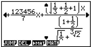
- Math Input Mode Input Examples
This section provides a number of different examples showing how the MATH function menu and other keys can be used during Math input mode natural input. Be sure to pay attention to the input cursor position as you input values and data.

Example 1 To input 2^3 + 1
| AC 2 ∧ | 2 |
| 3 | 23 |
| 231 | |
| + 1 | 23+11 |
| EXE | 23+1 9 |


Example 2
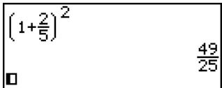
To input (1 + 25)^2

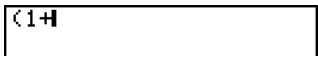

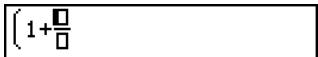

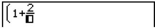

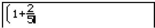

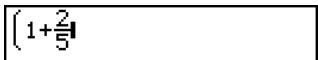

$$ \boxed{\left(1 + \frac{2}{5}\right)^2\mathbf{I}} $$


Example 3
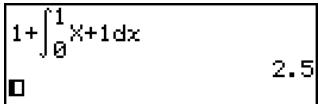
To input 1 + _0^1 x + 1dx

$$ \boxed{1 + \int_{\square}^{\square}\square \mathrm{d}x} $$

$$ \boxed{1 + \int_{0}^{0}X + 1\mathrm{d}x} $$

$$ 1 + \int_{\mathbb{R}}^{\mathbb{Q}}X + 1\mathrm{d}x $$

$$ \boxed{1 + \int_{0}^{11}\times + 1dx} $$

$$ \boxed{1 + \int_{0}^{1}\times + 1\mathrm{d}\times \mathbf{l}} $$


Example 4
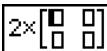
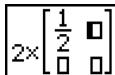
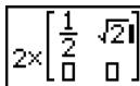
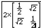
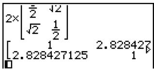
To input 2 × 12 & 2 2 & 12
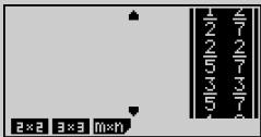
AC 2 ✗ F4 (MATH) F1 (MAT) F1 (2×2)


- When the calculation does not fit within the display window
Arrows appear at the left, right, top, or bottom edge of the display to let you know when there is more of the calculation off the screen in the corresponding direction.
When you see an arrow, you can use the cursor keys to scroll the screen contents and view the part you want.

- Inserting a Function into an Existing Expression
In the Math input mode, you can make insert a natural input function into an existing expression. Doing so will cause the value or parenthetical expression to the right of the cursor to become the argument of the inserted function. Use SHIFT DEL (INS) to insert a function into an existing expression.
- To insert a function into an existing expression
● ● ● ● ●
Example To insert the function into the expression 1 + (2 + 3) + 4 so the parenthetical expression becomes the argument of the function
- Move the cursor so it is located directly to the left of the part of the expression that you want to become the argument of the function you will insert.
$$ 1 + (2 + 3) + 4 $$
- Press SHIFT DEL (INS).
- This changes the cursor to an insert cursor (▶).
$$ \boxed {1 + \text { 2 } + 3) + 4} $$
- Press SHIFT ^2() to insert the function.
- This inserts the function and makes the parenthetical expression its argument.
$$ 1 + \sqrt {(2 + 3)} + 4 $$
• Function Insert Rules
The following are the basic rules that govern how a value or expressions becomes the argument of an inserted function.
- If the insert cursor is located immediately to the left of an open parenthesis, everything from the open parenthesis to the following closing parenthesis will be the argument of the inserted function.
- If the input cursor is located immediately to the left of a value or fraction, that value or fraction will be the argument of the inserted function.

# In the Linear input mode, pressing SHIFT DEL (INS) will change to the insert mode. See page 1-3-2 for more information.

- Functions that Support Insertion
The following lists the functions that can be inserted using the procedure under “To insert a function into an existing expression” (page 1-3-13). It also provides information about how insertion affects the existing calculation.
| Function | Key Operation | Original Expression | Expression After Insertion |
| Improper Fraction | _2^2 | 1+K(2+3)+4 | 1+K(2+3)/0+4 |
| Power | 1+2K(2+3)+4 | 1+2K(2+3)+4 | |
| SHIFT x^2 ( ) | 1+K(2+3)+4 | 1+K(2+3)+4 | |
| Cube Root | SHIFT ( ^3 ) | 1+3√K(2+3)+4 | |
| Power Root | SHIFT ( ^x ) | 1+0√(2+3)+4 | |
| e^x | SHIFT ( e^x ) | 1+eK(2+3)+4 | |
| 10^x | SHIFT ( 10^x ) | 1+10K(2+3)+4 | |
| log(a,b) | F4(MATH)F2(logab) | 1+log((2+3))+4 | |
| Absolute Value | F4(MATH)F3(Abs) | 1+|K(2+3)|+4 | |
| Linear Differential | F4(MATH)F4(d/dx) | 1+K(X+3)+4 | 1+ (K(X+3))|x=0+4 |
| Quadratic Differential | F4(MATH)F5( d^2/dx^2 ) | 1+ ^2dx^2 (K(X+3))|x=0+4 | |
| Integral | F4(MATH)F6(>) F1 ( dx ) | 1+ _0^0 K(X+3)dx+4 | |
| Σ Calculation | F4(MATH)F6(>) F2 ( ( ) | 1+ (K(X+3))+4 =0 |
- Editing Calculations in the Math Input Mode
The procedures for editing calculations in the Math input mode are basically the same as those for the Linear input mode. For more information, see “Editing Calculations” (page 1-3-1).
Note however, that the following points are different between the Math input mode and the Linear input mode.
- Overwrite mode input that is available in the Linear input mode is not supported by the Math input mode. In the Math input mode, input is always inserted at the current cursor location.
- In the Math input mode, pressing the DEL key always performs a backspace operation.
- Math Input Mode Calculation Result Display
Fractions, matrices, and lists produced by Math input mode calculations are displayed in natural format, just as they appear in your textbook.
![[1 2]×2 [2 4] 3 4 [6 8] □ DELLE DELA](/content/2025/01/86785/images/acfa5fd5fd30995dfeb64dc210c6f6bba54762c736d215ea2357b7398d583d50.jpg)
Sample Calculation Result Displays
- Math Input Mode Input Restrictions
Note the following restrictions that apply during input of the Math input mode.
- Certain types of expressions can cause the vertical width of a calculation formula to be greater than one display line. The maximum allowable vertical width of a calculation formula is about two display screens (120 dots). You cannot input any expression that exceeds this limitation.

Fractions are displayed either as improper fractions or mixed fractions, depending on the "Frac Result" setting on the Setup screen. For details, see "1-7 Using the Setup Screen".
Matrices are displayed in natural format, up to 6 × 6 . A matrix that has more than six rows or columns will be displayed on a MatAns screen, which is the same screen used in the Linear input mode.
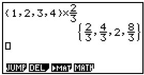
Lists are displayed in natural format for up to 20 elements. A list that has more than 20 elements will be displayed on a ListAns screen, which is the same screen used in the Linear input mode.
Arrows appear at the left, right, top, or bottom edge of the display to let you know when there is more data off the screen in the corresponding direction.
![(√2,√3) [414213562,1.7320508] JUMP DEL ►MAT MATH](/content/2025/01/86785/images/bba621af47a04276484d2992ab5a842211993d40539620a1f24985a065d1e0e1.jpg)
You can use the cursor keys to scroll the screen and view the data you want.
Pressing F2(DEL)F1(DEL·L) while a calculation result is selected will delete both the result and the calculation that produced it.
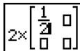
The multiplication sign cannot be omitted immediately before an improper fraction or mixed fraction. Be sure to always input a multiplication sign in this case.
Example : 2 × 25
2 × a 2 ▼ 5
# A , ^2 , or (x^-1) key operation cannot be followed immediately by another , ^2 , or (x^-1) key operation. In this case, use parentheses to keep the key operations separate.
Example: (3^2)^-1
( 3 x^2 ) SHIFT ( x^-1 )
1-4 Option (OPTN) Menu
The option menu gives you access to scientific functions and features that are not marked on the calculator's keyboard. The contents of the option menu differ according to the mode you are in when you press the OPTN key.
See "8-7 PRGM Mode Command List" for details on the option (OPTN) menu.
- Option menu in the RUN·MAT or PRGM mode
- {LIST} ... {list function menu}
- {MAT} ... {matrix operation menu}
- {CPLX} ... {complex number calculation menu}
- {CALC} ... {functional analysis menu}
- {STAT} ... {paired-variable statistical estimated value menu}
- {HYP} ... {hyperbolic calculation menu}
- {PROB} ... {probability/distribution calculation menu}
- {NUM} ... {numeric calculation menu}
- {ANGL} ... {menu for angle/coordinate conversion, DMS input/conversion}
- {ESYM} ... {engineering symbol menu}
- {PICT} ... {picture memory menu} ^*1
- {FMEM} ... {function memory menu} ^*1
- {LOGIC} ... {logic operator menu}
- {CAPT} ... {screen capture menu}

# The option (OPTN) menu does not appear during binary, octal, decimal, and hexadecimal calculations.
*1 The PICT, FMEM and CAPT items are not displayed when “Math” is selected as the Input Mode.

- Option menu during numeric data input in the STAT, TABLE, RECUR, EQUA and S·SHT modes
- {LIST}/{CPLX}/{CALC}/{HYP}/{PROB}/{NUM}/{ANGL}/{ESYM}/{FMEM}/{LOGIC}
- Option menu during formula input in the GRAPH, DYNA, TABLE, RECUR and EQUA modes
- {List}/{CALC}/{HYP}/{PROB}/{NUM}/{FMEM}/{LOGIC}
The following shows the function menus that appear under other conditions.
- Option menu when a number table value is displayed in the TABLE or RECUR mode
- {LMEM} ... {list memory menu}
• {∘, „}/{ENG}/{ENG}
The meanings of the option menu items are described in the sections that cover each mode.

1-5 Variable Data (VARS) Menu
To recall variable data, press VARS to display the variable data menu.
{V-WIN}/{FACT}/{STAT}/{GRPH}/{DYNA}/
{TABL}/{RECR}/{EQUA*1}/{TVM*1}
See "8-7 PRGM Mode Command List" for details on the variable data (VARS) menu.
• V-WIN — Recalling V-Window values
• {X}/{Y}/{T,θ}
... {x-axis menu}/{y-axis menu}/{T, θ menu}
• {R-X}/{R-Y}/{R-T,θ}
...{x-axis menu}/{y-axis menu}/{T,θ menu} for right side of Dual Graph
- {min}/{max}/{scal}/{dot}/{ptch}
... {minimum value}/{maximum value}/{scale}/{dot value*2}/{pitch}
• FACT — Recalling zoom factors
- {Xfact}/{Yfact} ... {x-axis factor}/{y-axis factor}

*1 The EQUA and TVM items appear only when you access the variable data menu from the RUN·MAT, PRGM or e·ACT mode.
# The variable data menu does not appear if you press VARS while binary, octal, decimal, or hexadecimal is set as the default number system.
*2The dot value indicates the display range (Xmax value – Xmin value) divided by the screen dot pitch (126).
The dot value is normally calculated automatically from the minimum and maximum values. Changing the dot value causes the maximum to be calculated automatically.

• STAT — Recalling statistical data
- X ... {single-variable, paired-variable x -data}
- n// x/ x^2/x_ n/x_ n-1/ X/ X ... number of data/mean/sum/sum of squares/population standard deviation/sample standard deviation/minimum value/maximum value
• {Y} ... {paired-variable y-data} - / y/ y^2/ xy/on/on-1/ Y/ Y ... mean/sum/sum of squares/sum of products of x-data and y-data/population standard deviation/sample standard deviation/minimum value/maximum value
- {GRPH} ... {graph data menu}
- a / b / c / d / e ... {regression coefficient and polynomial coefficients}
- r/r^2 ... {correlation coefficient}/{coefficient of determination}
- {MSe} ... {mean square error}
• {Q1}/{Q3} ... {first quartile}/{third quartile} - {Med}/{Mod} ... {median}/{mode} of input data
- {Strt}/{Pitch} ... histogram {start division}/{pitch}
- {PTS} ... {summary point data menu}
- x_1 / y_1 / x_2 / y_2 / x_3 / y_3 ... {coordinates of summary points}

• GRPH — Recalling Graph Functions
- Y / ... {rectangular coordinate or inequality function}/ polar coordinate function
• {Xt}/{Yt}
... parametric graph function {Xt}/{Yt} - {X} ... {X=constant graph function}
(Press these keys before inputting a value to specify a storage memory.)
• DYNA — Recalling Dynamic Graph Set Up Data
- {Strt}/{End}/{Pitch} ... {coefficient range start value}/{coefficient range end value}/{coefficient value increment}
- TABL — Recalling Table Set Up and Content Data
- {Strt}/{End}/{Pitch}
... {table range start value}/{table range end value}/{table value increment} - ResIt^*1
... {matrix of table contents}

*1 The Reslt item appears only when the TABL menu is displayed in the RUN•MAT, PRGM or e•ACT mode.

- RECR — Recalling Recursion Formula ^*1 , Table Range, and Table Content Data
- {FORM} ... {recursion formula data menu}
- a_n / a_n+1 / a_n+2 / b_n / b_n+1 / b_n+2 / c_n / c_n+1 / c_n+2 ... a_n / a_n+1 / a_n+2 / b_n / b_n+1 / b_n+2 / c_n / c_n+1 / c_n+2 expressions
- {RANG} ... {table range data menu}
- {Strt}/{End}
    ... table range {start value}/{end value}
- {a0}/{a1}/{a2}/{b0}/{b1}/{b2}/{c0}/{c1}/{c2}
    ... {a0}/{a1}/{a2}/{b0}/{b1}/{b2}/{c0}/{c1}/{c2} value
- {anSt}/{bnSt}/{cnSt}
    ... origin of {an}/{bn}/{cn} recursion formula con graph)
- Reslt^2 ... matrix of table contents^3
- EQUA — Recalling Equation Coefficients and Solutions ^*4 \*5
- {S-Rlt}/{S-Cof}
    ... matrix of {solutions}/{coefficients} for linear equations with two through six unknowns*6
- {P-Rlt}/{P-Cof}
    ... matrix of {solution}/{coefficients} for a quadratic or cubic equation
• TVM — Recalling Financial Calculation Data
- n/I%/PV/PMT/FV ... {payment periods (installments)}/{ interest (%) / principal / payment amount / account balance or principal plus interest following the final installment - P/Y/C/Y ... {number of installment periods per year}/ number of compounding periods per year

*1 An error occurs when there is no function or recursion formula numeric table in memory.
*2 "Reslt" is available only in the RUN·MAT, PRGM and e·ACT modes.
*3 Table contents are stored automatically in Matrix Answer Memory (MatAns).
*4 Coefficients and solutions are stored automatically in Matrix Answer Memory (MatAns).
*5 The following conditions cause an error.
- When there are no coefficients input for the equation
- When there are no solutions obtained for the equation
*6 Coefficient and solution memory data for a linear equation cannot be recalled at the same time.

1-6 Program (PRGM) Menu
To display the program (PRGM) menu, first enter the RUN·MAT or PRGM mode from the Main Menu and then press SHIFT VARS (PRGM). The following are the selections available in the program (PRGM) menu.
- {COM} ..... {program command menu}
- {CTL}......{program control command menu}
- {JUMP} .... {jump command menu}
- {?} ...... {input prompt}
• {▲}...... {output command} - {CLR} ...... {clear command menu}
- {DISP} ..... {display command menu}
- {REL} ...... {conditional jump relational operator menu}
- {I/O}...... {I/O control/transfer command menu}
- {:} ....{multistatement connector}
The following function key menu appears if you press SHIFT VARS (PRGM) in the RUN·MAT mode or the PRGM mode while binary, octal, decimal, or hexadecimal is set as the default number system.
- {Prog} ..... {program recall}
- {JUMP}/{?}/{▲}/{REL}/{:}
The functions assigned to the function keys are the same as those in the Comp mode.
For details on the commands that are available in the various menus you can access from the program menu, see “8. Programming”.

1-7 Using the Setup Screen
The mode's Setup screen shows the current status of mode settings and lets you make any changes you want. The following procedure shows how to change a setup.
- To change a mode setup
- Select the icon you want and press EXE to enter a mode and display its initial screen. Here we will enter the RUN·MAT mode.
- Press SHIFT MENU (SET UP) to display the mode's Setup screen.
- This Setup screen is just one possible example. Actual Setup screen contents will differ according to the mode you are in and that mode's current settings.
■ ■ ■
- Use the ▲ and ▼ cursor keys to move the highlighting to the item whose setting you want to change.
- Press the function key (F1 to F6) that is marked with the setting you want to make.
- After you are finished making any changes you want, press EXIT to exit the Setup screen.
■ Setup Screen Function Key Menus
This section details the settings you can make using the function keys in the Setup screen. \~\~ \~ indicates default setting.
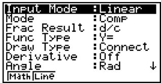
- Input Mode
- {Math}/{Line}... {Math}/{Linear} input mode
- Mode (calculation/binary, octal, decimal, hexadecimal mode)
- {Comp} ... {arithmetic calculation mode}
- {Dec}/{Hex}/{Bin}/{Oct} ... {decimal}/{hexadecimal}/{binary}/{octal}
- Frac Result (fraction result display format)
- {d/c}/{ab/c}... {improper}/{mixed} fraction
- Func Type (graph function type)
Pressing one of the following function keys also switches the function of the ,,T key.
- Y = / r = / Parm / X = c ... {rectangular coordinate}/{polar coordinate}/{parametric coordinate}/{X = constant} graph
- Y > / Y < / Y ≥ / Y ≤ ... y > f(x) / y < f(x) / y ≥ f(x) / y ≤ f(x) inequality graph
- Draw Type (graph drawing method)
- {Con}/{Plot} ... {connected points}/{unconnected points}
• Derivative (derivative value display)
- {On}/{Off} ... {display on}/{display off} while Graph-to-Table, Table & Graph, and Trace are being used
- Angle (default angle unit)
- {Deg}/{Rad}/{Gra} ... {degrees}/{radians}/{grads}
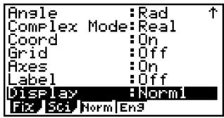
- Complex Mode
• {Real} ... {calculation in real number range only}
- a + bi /r ... {rectangular format}/{polar format} display of a complex calculation
- Coord (graph pointer coordinate display)
- {On}/{Off} ... {display on}/{display off}
- Grid (graph gridline display)
- {On}/{Off} ... {display on}/{display off}
- Axes (graph axis display)
- {On}/{Off} ... {display on}/{display off}
- Label (graph axis label display)
- {On}/{Off} ... {display on}/{display off}
- Display (display format)
- {Fix}/{Sci}/{Norm}/{Eng} ... {fixed number of decimal places specification}/{number of significant digits specification}/{normal display setting}/{engineering mode}
- Stat Wind (statistical graph V-Window setting method)
• {Auto}/{Man} ... {automatic}/{manual}
- Resid List (residual calculation)
- {None}/{LIST} ... {no calculation}/{list specification for the calculated residual data}
- List File (list file display settings)
- {FILE} ... {settings of list file on the display}
- Sub Name (list naming)
- {On}/{Off} ... {display on}/{display off}
- Graph Func (function display during graph drawing and trace)
- {On}/{Off} ... {display on}/{display off}
- Dual Screen (dual screen mode status)
- {G+G}/{GtoT}/{Off} ... {graphing on both sides of dual screen}/{graph on one side and numeric table on the other side of dual screen}/{dual screen off}
- Simul Graph (simultaneous graphing mode)
- {On}/{Off} ... {simultaneous graphing on (all graphs drawn simultaneously)}/{simultaneous graphing off (graphs drawn in area numeric sequence)}

- Background (graph display background)
- {None}/{PICT} ... {no background}/{graph background picture specification}
- Sketch Line (overlaid line type)
• {—}/{—}{……}/{……} ... {normal}/{thick}/{broken}/{dot}
• Dynamic Type (dynamic graph type)
- {Cnt}/{Stop} ... {non-stop (continuous)}/{automatic stop after 10 draws}
- Locus (dynamic graph locus mode)
- {On}/{Off} ... {locus drawn}/{locus not drawn}
- Y=Draw Speed (dynamic graph draw speed)
- {Norm}/{High} ... {normal}/{high-speed}
- Variable (table generation and graph draw settings)
- {RANG}/{LIST} ... {use table range}/{use list data}
- Display ( value display in recursion table)
- {On}/{Off} ... {display on}/{display off}
- Slope (display of derivative at current pointer location in conic section graph)
- {On}/{Off} ... {display on}/{display off}
- Payment (payment period setting)
- {BGN}/{END} ... {beginning}/{end} setting of payment period

- Date Mode (number of days per year setting)
- {365}/{360} ... interest calculations using {365}*1/{360} days per year
• Auto Calc (spreadsheet auto calc)
- {On}/{Off} ... {execute}/{not execute} the formulas automatically
• Show Cell (spreadsheet cell display mode)
- {Form}/{Val} ... {formula}*2/{value}
- Move (spreadsheet cell cursor direction) ^*3
- {Low}/{Right} ... {move down}/{move right}

*1 The 365-day year must be used for date calculations in the TVM mode. Otherwise, an error occurs.
*2 Selecting “Form” (formula) causes a formula in the cell to be displayed as a formula. The “Form” does not affect any non-formula data in the cell.
*3 Specifies the direction the cell cursor moves when you press the EXE key to register cell input, when the Sequence command generates a number table, and when you recall data from List memory.

1-8 Using Screen Capture
Any time while operating the calculator, you can capture an image of the current screen and save it in capture memory.
- To capture a screen image
- Operate the calculator and display the screen you want to capture.
- Press SHIFT 7 (CAPTURE).
- This displays a memory area selection dialog box.
![Store In Capture Memory Capture[1~20]:1 GRAPH CALC TEST INTU DIST D>](/content/2025/01/86785/images/b0d18deb954de18c01a7ed9c8b704d6707e4e92e1d7c44031f80a20165048457.jpg)
- Input a value from 1 to 20 and then press EXE.
- This will capture the screen image and save it in capture memory area named "Capt n" (n = the value you input).
- You cannot capture the screen image of a message indicating that an operation or data communication is in progress.
- A memory error will occur if there is not enough room in main memory to store the screen capture.
- To recall a screen image from capture memory
- In the RUN·MAT mode (Linear input mode), press OPTN F6 (▷) F6 (▷) F5 (CAPT) F1 (RCL).
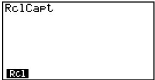
- Enter a capture memory number in the range of 1 to 20, and then press EXE.
- You can also use the RclCapt command in a program to recall a screen image from capture memory.

1-9 When you keep having problems...
If you keep having problems when you are trying to perform operations, try the following before assuming that there is something wrong with the calculator.
■ Getting the Calculator Back to its Original Mode Settings
- From the Main Menu, enter the SYSTEM mode.
- Press F5 (RSET).
- Press F1(STUP), and then press F1(Yes).
- Press EXIT MENU to return to the Main Menu.
Now enter the correct mode and perform your calculation again, monitoring the results on the display.
In Case of Hang Up
- Should the unit hang up and stop responding to input from the keyboard, press the P button on the back of the calculator to reset the calculator to its initial defaults (see page -5-1). Note, however, that this may clear all the data in calculator memory.
■ Low Battery Message
If either of the following messages appears on the display, immediately turn off the calculator and replace main batteries as instructed.
Low
Main Batteries!
Please Replace
If you continue using the calculator without replacing main batteries, power will automatically turn off to protect memory contents. Once this happens, you will not be able to turn power back on, and there is the danger that memory contents will be corrupted or lost entirely.

# You will not be able to perform data communications operations after the low battery message appears.

Chapter
2
2
Manual Calculations
2-1 Basic Calculations
2-2 Special Functions
2-3 Specifying the Angle Unit and Display Format
2-4 Function Calculations
2-5 Numerical Calculations
2-6 Complex Number Calculations
2-7 Binary, Octal, Decimal, and Hexadecimal Calculations with Integers
2-8 Matrix Calculations
Linear/Math input mode (page 1-3-8)
- Unless specifically noted otherwise, all of the operations in this chapter are explained using the Linear input mode.
- When necessary, the input mode is indicated by the following symbols.
(Math>.... Math input mode
2-1 Basic Calculations
Arithmetic Calculations
- Enter arithmetic calculations as they are written, from left to right.
- Use the (-) key to input the minus sign before a negative value.
- Calculations are performed internally with a 15-digit mantissa. The result is rounded to a 10-digit mantissa before it is displayed.
- For mixed arithmetic calculations, multiplication and division are given priority over addition and subtraction.
| Example | Operation |
| 23 + 4.5 - 53 = -25.5 | 23 + 4.5 - 53 |
| 56 × (-12) ÷ (-2.5) = 268.8 | 56 × (-) 12 ÷ (-) 2.5 |
| (2 + 3) × 10^2 = 500 | (2 + 3) × 1 2 ^*1 |
| 1 + 2 - 3 × 4 ÷ 5 + 6 = 6.6 | 1 + 2 - 3 × 4 ÷ 5 + 6 |
| 100 - (2 + 3) × 4 = 80 | 100 - (2 + 3) × 4 |
| 2 + 3 × (4 + 5) = 29 | 2 + 3 × (4 + 5) ^*2 |
| (7 - 2) × (8 + 5) = 65 | (7 - 2) (8 + 5) ^*3 |
| 64 × 5 = 0.3 ( 310 ) | |
| 6 ÷ (4 × 5) ^*4 | |
| 6 4 × 5 | |
| (1 + 2i) + (2 + 3i) = 3 + 5i | (1 + 2) 0(i) × + (2 + 3) 0(i) × |
| (2 + i) × (2 - i) = 5 | (2 + SHIFT) 0(i) × (2 - SHIFT) 0(i) × |

*1 2 + 3 EXP 2 does not produce the correct result. Be sure to enter this calculation as shown.
*2 Final closed parentheses (immediately before operation of the EXE key) may be omitted, no matter how many are required.
*3 A multiplication sign immediately before an open parenthesis may be omitted.
*4 This is identical to 6 ☐ 4 ☐ 5 EXE.

■ Number of Decimal Places, Number of Significant Digits, Normal Display Range [SET UP]-[Display] -[Fix]/[Sci]/
[SET UP]- [Display] -[Fix]/[Sci]/[Norm]
- Even after you specify the number of decimal places or the number of significant digits, internal calculations are still performed using a 15-digit mantissa, and displayed values are stored with a 10-digit mantissa. Use Rnd of the Numeric Calculation Menu (NUM) (page 2-4-1) to round the displayed value off to the number of decimal place and significant digit settings.
- Number of decimal place (Fix) and significant digit (Sci) settings normally remain in effect until you change them or until you change the normal display range (Norm) setting.
![CASIO FX-9860GSD - ■ Number of Decimal Places, Number of Significant Digits, Normal Display Range [SET UP]-[Display] -[Fix]/[Sci]/ - 1](/content/2025/01/86785/images/87edaed938b1f098f06e660da5f08477837bf75d828704fa5ab42f105362add4.jpg)
*1 Displayed values are rounded off to the place you specify.
![CASIO FX-9860GSD - ■ Number of Decimal Places, Number of Significant Digits, Normal Display Range [SET UP]-[Display] -[Fix]/[Sci]/ - 2](/content/2025/01/86785/images/5e150bcb9ee2532e3eb9da32b1810010eb266a974fdc80f34698f23d790bfa08.jpg)
![CASIO FX-9860GSD - ■ Number of Decimal Places, Number of Significant Digits, Normal Display Range [SET UP]-[Display] -[Fix]/[Sci]/ - 3](/content/2025/01/86785/images/1121a2708db80c47c0efaff3cb400ef774989a37881220d7903afde4f49d874e.jpg)
Example
200 ÷ 7 × 14 = 400
| Condition | Operation | Display |
| 3 decimal places | 200 ÷ 7 × 14EXE | 400 |
| SHIFTMENU (SET UP)▲(or▼12 times)F1(Fix)3EXEEXITEXE | 400.000 | |
| Calculation continues using display capacity of 10 digits | 200 ÷ 7EXE | 28.571 |
| 14EXE | Ans × I400.000 |
- If the same calculation is performed using the specified number of digits:
| 200 7 EXE | 28.571 | |
| The value stored internally is rounded off to the number of decimal places specified on the Setup screen. | OPTN F6 (▷) F4 (NUM) F4 (Rnd) EXE | 28.571 |
| 14 EXE | 399.994 | |
| 200 7 EXE | 28.571 | |
| You can also specify the number of decimal places for rounding of internal values for a specific calculation.*1(Example: To specify rounding to two decimal places) | F6 (RndFi) SHIFT (→) (Ans) ▶ 2 ) | RndFix(Ans,2) |
| EXE | 28.570 | |
| 14 EXE | 399.980 |
■ Calculation Priority Sequence
This calculator employs true algebraic logic to calculate the parts of a formula in the following order:
① Coordinate transformation Pol (x, y), Rec (r, θ)
Derivatives, second derivatives, integrations, calculations
d / dx, d^2 /dx^2, dx, ,Mat,Solve,FMin,FMax,List Mat,Seq,Min,Max,Median,Mean,
Augment, Mat→List, P(, Q(, R(, t(, List, RndFix, log ab
Composite functions ^*2 fn, Yn, rn, Xtn, Ytn, Xn

*1 To turn off rounding, specify 10 for the significant number of digits.
^*2 You can combine the contents of multiple function memory (fn) locations or graph memory (Yn, rn, Xtn, Ytn, Xn) locations into composite functions. Specifying fn1(fn2), for example, results in the composite function fn1°fn2 (see page 5-3-3).
A composite function can consist of up to five functions.
# You cannot use a differential, quadratic differential, integration, , maximum/minimum value, Solve, RndFix or log ab calculation expression inside of a RndFix calculation term.

② Type A functions
With these functions, the value is entered and then the function key is pressed.
x^2, x^-1, x!, , '', ENG symbols, angle unit ^ , ^r , ^g
③ Power/root (x^y), x
④ Fractions a^b/_c
⑤ Abbreviated multiplication format in front of , memory name, or variable name.
2π, 5A, Xmin, F Start, etc.
⑥ Type B functions
With these functions, the function key is pressed and then the value is entered.
, ^3 , log, In, e^x , 10^x , sin, cos, tan, ^-1 , ^-1 , ^-1 , sinh, cosh, tanh, ^-1 , ^-1 , ^-1 , (−), d, h, b, o, Neg, Not, Det, Trn, Dim, Identity, Sum, Prod, Cuml, Percent, List, Abs, Int, Frac, Intg, Arg, Conjg, ReP, ImP
⑦ Abbreviated multiplication format in front of Type B functions
23 , A log2, etc.
⑧ Permutation, combination nPr, nCr, ∠
⑨ ×, ÷
⑩ +, -
⑪ Relational operators =, ≠, >, <, ≥, ≤
⑫ And (logical operator), and (bitwise operator)
⑬ Or (logical operator), or, xor, xnor (bitwise operator)
● ● ● ● ●
Example 2 + 3 × ( 2^2 + 6.8) = 22.07101691 (angle unit = Rad)
flowchart
graph TD
    A["①"] --> B["②"]
    B --> C["③"]
    C --> D["④"]
    D --> E["⑤"]
    E --> F["⑥"]

# When functions with the same priority are used in series, execution is performed from right to left.
$$ e ^ {x} \ln \sqrt {1 2 0} \rightarrow e ^ {x} {\ln (\sqrt {1 2 0}) } $$
Otherwise, execution is from left to right.
Compound functions are executed from right to left.
Anything contained within parentheses receives highest priority.

■ Multiplication Operations without a Multiplication Sign
You can omit the multiplication sign (×) in any of the following operations.
- Before coordinate transformation and Type B functions (① on page 2-1-3 and ⑥ on page 2-1-4), except for negative signs
● ● ● ● ●
Example 2sin30, 10log1.2, 2 , 2Pol(5, 12), etc.
- Before constants, variable names, memory names
● ● ● ● ●
Example 2, 2AB, 3Ans, 3Y_1, etc.
• Before an open parenthesis
● ● ● ● ●
Example 3(5 + 6) , (A + 1)(B - 1) , etc.
■ Overflow and Errors
Exceeding a specified input or calculation range, or attempting an illegal input causes an error message to appear on the display. Further operation of the calculator is impossible while an error message is displayed. The following events cause an error message to appear on the display.
- When any result, whether intermediate or final, or any value in memory exceeds ± 9.999999999 × 10^99 (Ma ERROR).
- When an attempt is made to perform a function calculation that exceeds the input range (Ma ERROR).
- When an illegal operation is attempted during statistical calculations (Ma ERROR). For example, attempting to obtain 1VAR without data input.
- When an improper data type is specified for the argument of a function calculation (Ma ERROR).
- When the capacity of the numeric value stack or command stack is exceeded (Stack ERROR). For example, entering 25 successive ☐ followed by 2 + 3 × 4 EXE.
- When an attempt is made to perform a calculation using an illegal formula (Syntax ERROR). For example, 5 ✗ ✗ 3 EXE.

# Other errors can occur during program execution. Most of the calculator's keys are inoperative while an error message is displayed.
Press EXIT to clear the error and display the error position (see page 1-3-5).
# See the "Error Message Table" on page -1-1 for information on other errors.

- When you try to perform a calculation that causes memory capacity to be exceeded (Memory ERROR).
- When you use a command that requires an argument, without providing a valid argument (Argument ERROR).
- When an attempt is made to use an illegal dimension during matrix calculations (Dimension ERROR).
- When you are in the real mode and an attempt is made to perform a calculation that produces a complex number solution. Note that “Real” is selected for the Complex Mode setting on the Setup screen (Non-Real ERROR).
■ Memory Capacity
In the Linear input mode, each time you press a key, either one byte or two bytes is used. Some of the functions that require one byte are: 1, 2, 3, sin, cos, tan, log, ln, , and . Some of the functions that take up two bytes are d/dx (, Mat, Xmin, If, For, Return, DrawGraph, SortA(, PxION, Sum, and a_n+1 ).
For details about the number of bytes required for each function in the Math input mode, see page 1-3-9.

# As you input numeric values or commands, they appear flush left on the display. Calculation results, on the other hand, are displayed flush right.
# The allowable range for both input and output values is 15 digits for the mantissa and two digits for the exponent. Internal calculations are also performed using a 15-digit mantissa and two-digit exponent.

2-2 Special Functions
■ Calculations Using Variables
| Example | Operation | Display |
| 193.2 ALPHA X, ,T (A)EXE | 193.2 | |
| 193.2 ÷ 23 = 8.4 | ALPHA X, ,T (A) 23EXE | 8.4 |
| 193.2 ÷ 28 = 6.9 | ALPHA X, ,T (A) 28EXE | 6.9 |
■ Memory
- Variables (Alpha Memory)
This calculator comes with 28 variables as standard. You can use variables to store values you want to use inside of calculations. Variables are identified by single-letter names, which are made up of the 26 letters of the alphabet, plus r and . The maximum size of values that you can assign to variables is 15 digits for the mantissa and 2 digits for the exponent.
- To assign a value to a variable
[value] → [variable name] EXE

Example
To assign 123 to variable A


Example
To add 456 to variable A and store the result in variable B
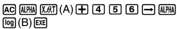
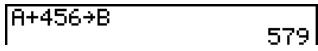

# Variable contents are retained even when you turn power off.

- To display the contents of a variable

Example
To display the contents of variable A

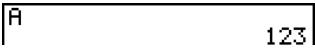
- To clear a variable

Example
To clear variable A

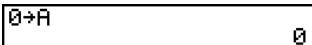
- To assign the same value to more than one variable
[value]→ [first variable name*1] ALPHA F3 (\~) [last variable name*1] EXE

Example
To assign a value of 10 to variables A through F
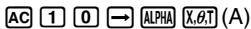
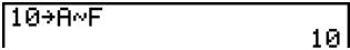

- Function Memory
[OPTN]-[FMEM]
Function memory ( f_1 f_20 ) is convenient for temporary storage of often-used expressions. For longer term storage, we recommend that you use the GRAPH mode for expressions and the PRGM mode for programs.
- {STO}/{RCL}/{fn}/{SEE} ... {function store}/{function recall}/{function area specification as a variable name inside an expression}/{function list}

*1 You cannot use "r" or "θ" as a variable name.

- To store a function

Example To store the function (A+B) (A-B) as function memory number 1

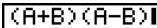

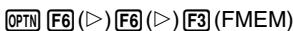
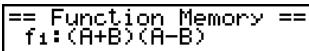


- To recall a function

Example To recall the contents of function memory number 1

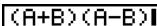
- To recall a function as a variable
| 3→A | 3 |
| 1→B | 1 |
| fn1+2 | 10 |


- To display a list of available functions
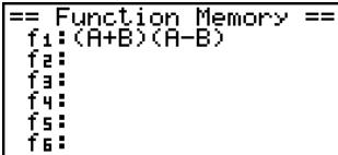


# If the function memory number to which you store a function already contains a function, the previous function is replaced with the new one.
# The recalled function appears at the current location of the cursor on the display.

- To delete a function
● ● ● ● ●
Example To delete the contents of function memory number 1
AC OPTN F6 (▷) F6 (▷) F3 (FMEM)
F1(STO) 1 EXE
== Function Memory == f1:
- Executing the store operation while the display is blank deletes the function in the function memory you specify.
• To use stored functions
● ● ● ● ●
Example To store x^3 + 1 , x^2 + x into function memory, and then graph:
$$ y = x ^ {3} + x ^ {2} + x + 1 $$
Use the following V-Window settings.
- For full details about graphing, see “5. Graphing”.

# You can also use → to store a function in function memory in a program.
In this case, you must enclose the function inside of double quotation marks.
"(A+B)(A-B)"→fn11

Answer Function
The Answer Function automatically stores the last result you calculated by pressing EXE (unless the EXE key operation results in an error). The result is stored in the answer memory.
- To use the contents of the answer memory in a calculation

Example
$$ 1 2 3 + 4 5 6 = \underline {{5 7 9}} $$
$$ 7 8 9 - \underline {{5 7 9}} = 2 1 0 $$


| 123+456 | 579 |
| 789-Ans | 210 |
In the Math input mode, the answer memory is refreshed with each calculation. Note, however, that the answer memory content recall operation is different from that used in the Linear input mode. For details, see “History Function” (page 2-2-6).
■ Performing Continuous Calculations
Answer memory also lets you use the result of one calculation as one of the arguments in the next calculation.

Example 1 1 ÷ 3 =
$$ \mathbf {1} \div \mathbf {3} \times \mathbf {3} = $$

(Continuing) ✗ 3 EXE
Continuous calculations can also be used with Type A functions (x^2, x^-1, x! , page 2-1-4), +, -, (x^y), x- , °', " , etc.

# The largest value that the answer memory can hold is 15 digits for the mantissa and 2 digits for the exponent.
# Only numeric values and calculation results can be stored in answer memory.
# Answer memory contents are not cleared when you press the AC key or when you switch power off.
# When “Linear” is selected as the Input Mode, answer memory contents are not changed by an operation that assigns values to Alpha memory (such as: 5 → ALPHA X,0,T(A) EXE).

■ History Function
The history function maintains a history of calculation expressions and results in the Math input mode. Up to 30 sets of calculation expressions and results are maintained.
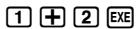

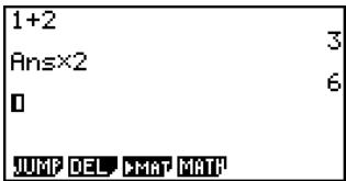
You can also edit the calculation expressions that are maintained by the history function and recalculate. This will recalculate all of the expressions starting from the edited expression.

Example To change “1+2” to “1+3” and recalculate
Perform the following operation following the sample shown above.

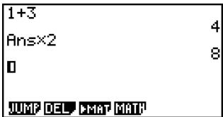

# The value stored in the answer memory is always dependent on the result produced by the last calculation performed. If history contents include operations that use the answer memory, editing a calculation may affect the answer memory value used in subsequent calculations.
- If you have a series of calculations that use the answer memory to include the result of the previous calculation in the next calculation, editing a calculation will affect the results of all the other calculations that come after it.
- When the first calculation of the history includes the answer memory contents, the answer memory value is "0" because there is no calculation before the first one in history.

■ Stacks
The unit employs memory blocks, called stacks, for storage of low priority values and commands. There is a 10-level numeric value stack, a 26-level command stack, and a 10-level program subroutine stack. An error occurs if you perform a calculation so complex that it exceeds the capacity of available numeric value stack or command stack space, or if execution of a program subroutine exceeds the capacity of the subroutine stack.

Example
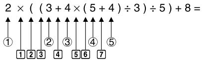
Numeric Value Stack
| 1 | 2 |
| 2 | 3 |
| 3 | 4 |
| 4 | 5 |
| 5 | 4 |
Command Stack
| 1 | × |
| 2 | ( |
| 3 | ( |
| 4 | + |
| 5 | × |
| 6 | ( |
| 7 | + |
| ⋮ |

# Calculations are performed according to the priority sequence. Once a calculation is executed, it is cleared from the stack.
- # Storing a complex number takes up two numeric value stack levels. - # Storing a two-byte function takes up two command stack levels.

■ Using Multistatements
Multistatements are formed by connecting a number of individual statements for sequential execution. You can use multistatements in manual calculations and in programmed calculations. There are two different ways that you can use to connect statements to form multistatements.
- Colon (:)
Statements that are connected with colons are executed from left to right, without stopping.
- Display Result Command (▲)
When execution reaches the end of a statement followed by a display result command, execution stops and the result up to that point appears on the display. You can resume execution by pressing the EXE key.
● ● ● ● ●
Example
$$ 6. 9 \times 1 2 3 = 8 4 8. 7 $$
$$ \underline {{1 2 3}} \div 3. 2 = 3 8. 4 3 7 5 $$
AC 1 2 3 → ALPHA X,θ,T (A)
SHIFT VARS (PRGM) F6 (▷) F5 (:) 6 • 9
✗ ALPHA X,θ,T (A) SHIFT VARS (PRGM) F5 (▲)
ALPHA X,θ,T (A) ÷ 3 • 2 EXE
EXE
123→A:6.9×A. A÷3.2 848.7 - Disp -
123→A:6.9×A. A÷3.2 848.7 38.4375

# You cannot construct a multistatement in which one statement directly uses the result of the previous statement.
Example: 123 × 456: × 5 Invalid

2-3 Specifying the Angle Unit and Display Format
Before performing a calculation for the first time, you should use the Setup screen to specify the angle unit and display format.
■ Setting the Angle Unit
[SET UP]- [Angle]
- On the Setup screen, highlight "Angle".
- Press the function key for the angle unit you want to specify, then press EXIT.
- {Deg}/{Rad}/{Gra} ... {degrees}/{radians}/{grads}
- The relationship between degrees, grads, and radians is shown below.
$$ 3 6 0 ^ {\circ} = 2 \pi \text { radians } = 4 0 0 \text { grads } $$
$$ 9 0 ^ {\circ} = \pi / 2 \text { radians } = 1 0 0 \text { grads } $$
■ Setting the Display Format
[SET UP]- [Display]
- On the Setup screen, highlight "Display".
- Press the function key for the item you want to set, then press EXIT.
- {Fix}/{Sci}/{Norm}/{Eng} ... {fixed number of decimal places specification}/{number of significant digits specification}/{normal display}/{Engineering mode}
- To specify the number of decimal places (Fix)
● ● ● ● ●
Example To specify two decimal places
F1 (Fix) 2 EXE
Press the number key that corresponds to the number of decimal places you want to specify (n = 0 to 9) .
Display :Fix2

# Displayed values are rounded off to the number of decimal places you specify.

- To specify the number of significant digits (Sci)

Example To specify three significant digits
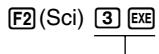
Press the number key that corresponds
to the number of significant digits you
want to specify (n = 0 to 9).
Specifying 0 makes the number of
significant digits 10.

- To specify the normal display (Norm 1/Norm 2)
Press F3 (Norm) to switch between Norm 1 and Norm 2.
Norm 1: 10^-2(0.01) > |x| , |x| ≥ 10^10
Norm 2: 10^-9(0.000000001) > |x|, |x| ≥ 10^10
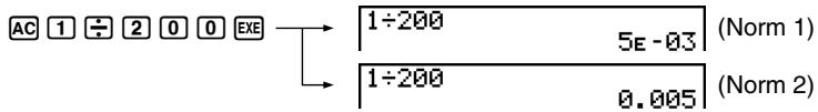
- To specify the engineering notation display (Eng mode)
Press F4 (Eng) to switch between engineering notation and standard notation. The indicator "/E" is on the display while engineering notation is in effect.
You can use the following symbols to convert values to engineering notation, such as 2,000 (= 2 × 10^3) 2k .
| E (Exa) | × 10^18 | m (milli) | × 10^-3 | |
| P (Peta) | × 10^15 | (micro) | × 10^-6 | |
| T (Tera) | × 10^12 | n (nano) | × 10^-9 | |
| G (Giga) | × 10^9 | p (pico) | × 10^-12 | |
| M (Mega) | × 10^6 | f (femto) | × 10^-15 | |
| k (kilo) | × 10^3 |

# Displayed values are rounded off to the number of significant digits you specify.
# The engineering symbol that makes the mantissa a value from 1 to 1000 is automatically selected by the calculator when engineering notation is in effect.

2-4 Function Calculations
■ Function Menus
This calculator includes five function menus that give you access to scientific functions not printed on the key panel.
- The contents of the function menu differ according to the mode you entered from the Main Menu before you pressed the OPTN key. The following examples show function menus that appear in the RUN·MAT mode.
• Hyperbolic Calculations (HYP)
[OPTN]-[HYP]
- {sinh}/{cosh}/{tanh} ... hyperbolic {sine}/{cosine}/{tangent}
- ^-1 / ^-1 / ^-1 ... inverse hyperbolic sine / cosine / tangent
● Probability/Distribution Calculations (PROB)
[OPTN]-[PROB]
- x! ... {press after inputting a value to obtain the factorial of the value.}
- nPr / nCr permutation / combination
- {Ran#}... {pseudo random number generation (0 to 1)}
- P(·) / Q(·) / R(·) normal distribution probability P(t) / Q(t) / R(t)
- t(·) value of normalized variate t(x)
- Numeric Calculations (NUM)
[OPTN]-[NUM]
- {Abs} ... {select this item and input a value to obtain the absolute value of the value.}
- {Int}/{Frac} ... select the item and input a value to extract the {integer}/{fraction} part.
- {Rnd} ... {rounds off the value used for internal calculations to 10 significant digits (to match the value in the Answer Memory), or to the number of decimal places (Fix) and number of significant digits (Sci) specified by you.}
- {Intg} ... {select this item and input a value to obtain the largest integer that is not greater than the value.}
- {RndFi} ... {rounds off the value used for internal calculations to specified digits (0\~9) (see page 2-1-3).}

- Angle Units, Coordinate Conversion, Sexagesimal Operations (ANGL)
[OPTN]-[ANGL]
- /r/g ... {degrees}/{radians}/{grads} for a specific input value
- {°, "}"} ... {specifies degrees (hours), minutes, seconds when inputting a degrees/minutes/seconds value}
- , ... {converts decimal value to degrees/minutes/seconds value} *1
- {Pol()/{Rec()} ... {rectangular-to-polar}/{polar-to-rectangular} coordinate conversion
- DMS} ... {converts decimal value to sexagesimal value}
• Engineering Symbol (ESYM)
[OPTN]-[ESYM]
• m//n/p/f ... milli (10^-3)/micro (10^-6)/nano (10^-9)/pico (10^-12)/femto (10^-15)
• {k}/{M}/{G}/{T}/{P}/{E} ... {kilo (10³)}/{mega (10⁶)}/{giga (10⁹)}/{tera (10¹²)}/{peta (10¹⁵)}/{exa (10¹⁸)}
- {ENG}/{ENG} ... shifts the decimal place of the displayed value three digits to the {left}/{right} and {decreases}/{increases} the exponent by three. ^*2 When you are using engineering notation, the engineering symbol is also changed accordingly.

*1 The {∘, "} menu operation is available only when there is a calculation result on the display.
*2The {ENG} and {ENG} menu operations are available only when there is a calculation result on the display.
# ENG/ENG switching is disabled for the following types of calculation results.
- Result of matrix calculation input in the Math input mode
- Result of list calculation input in the Math input mode

Angle Units
To change the angle unit of an input value, first press OPTN F6 (▷) F5 (ANGL). On the function key menu that appears, select "o", "r", or "g".
- Be sure to specify Comp for Mode in the Setup screen.
| Example | Operation |
| To convert 4.25 rad to degrees:243.5070629 | SHIFT MENU (SET UP) ▼ ▼ ▼ ▼ ▼ ▼ F1 (Deg) EXIT4.25 OPTN F6 (▷) F5 (ANGL) F2 (r) EXE |
| 47.3^ + 82.5 rad = 4774.20181^ | 47.3 82.5 OPTN F6 () F5 (ANGL) F2 (r) EXE |
| 2^20'30'' + 39'30'' = 3^00'00'' | 2 OPTN F6 () F5 (ANGL) F4 (^,") 20 F4 (^,") 30 F4 (^,") 0 F4 (^,") 39 F4 (^,") 30 F4 (^,") EXE F5 (^,") |
| 2.255^ = 2^15'18'' | 2.255 OPTN F6 () F5 (ANGL) F6 () F3 ( DMS) EXE |

# Once you specify an angle unit, it remains in effect until you specify a different one. The specification is retained even if you turn power off.

■ Trigonometric and Inverse Trigonometric Functions
- Be sure to set the angle unit before performing trigonometric function and inverse trigonometric function calculations.
$$ (9 0 ^ {\circ} = \frac {\pi}{2} \text { radians } = 1 0 0 \text { grads }) $$
- Be sure to specify Comp for Mode in the Setup screen.
| Example | Operation |
| 63^ = 0.8910065242 | SHIFT MENU (SET UP)▽▽▽▽▽▽F1 (Deg) EXITsin 63 EXE |
| (3 rad) = 0.5 | SHIFT MENU (SET UP)▽▽▽▽▽▽F2 (Rad) EXIT<Line>cos ( SHIFT EXP (π) ÷ 3 ) EXE<Math>cos α2 SHIFT EXP (π) ▼ 3 EXE |
| (-35gra) = -0.6128007881 | SHIFT MENU (SET UP)▽▽▽▽▽▽F3 (Gra) EXITtan (→ 35 EXE |
| 2 · 45^ × 65^ = 0.5976724775 | SHIFT MENU (SET UP)▽▽▽▽▽▽F1 (Deg) EXIT2 × sin 45 × cos 65 EXE *1 |
| cosec 30^ = 1 30^ = 2 | SHIFT MENU (SET UP)▽▽▽▽▽▽F1 (Deg) EXIT1 ÷ sin 30 EXE<Math>α2 1 ▼ sin 30 EXE |
| ^-10.5 = 30^ (x when x = 0.5 ) | SHIFT MENU (SET UP)▽▽▽▽▽▽F1 (Deg) EXITSHIFT sin (sin−1)0.5*2 EXE |

*1 ☒ can be omitted.
*2 Input of leading zero is not necessary.

■ Logarithmic and Exponential Functions
- Be sure to specify Comp for Mode in the Setup screen.
| Example | Operation |
| 1.23 (_101.23) = 0.08990511144 _28 = 3 | |
| OPTN F4 (CALC) F6 (▷) F4 (logab)2 ▶ 8 ▷ EXE | |
| F4 (MATH) F2 (logab) 2 ▶ 8 EXE | |
| In 90 ( _e90 ) = 4.49980967 | In 90 EXE |
| 10^1.23 = 16.98243652 (To obtain the antilogarithm of common logarithm 1.23) | SHIFT log ( 10^x )1.23 EXE |
| e^4.5 = 90.0171313 (To obtain the antilogarithm of natural logarithm 4.5) | SHIFT In ( e^x )4.5 EXE |
| (-3)^4 = (-3) × (-3) × (-3) × (-3) = 81 | ☐ ☐ 3 □ △ 4 EXE |
| -3^4 = -(3 × 3 × 3 × 3) = -81 | ☐ 3 △ 4 EXE |
| [7]123 (= 123^17) = 1.988647795 | |
| 7 SHIFT △ ( ^x )123 EXE | |
| SHIFT △ ( ^x )7 ▶ 123 EXE | |
| 2 + 3 × [3]64 - 4 = 10 | 2 ⊕ 3 ✗ 3 SHIFT △ ( ^x )64 — 4 EXE *1 |
| 2 ⊕ 3 ✗ SHIFT △ ( ^x )3 ▶ 64 ▶ — 4 EXE |

^*1(x^y) and x take precedence over multiplication and division.
# You cannot use a differential, quadratic differential, integration, , maximum/minimum value, Solve, RndFix or log ab calculation expression inside of a log ab calculation term.
# The Linear input mode and Math input mode produce different results when two or more powers are input in series, like: 2 3 2.
Linear input mode: 2^32 = 64
Math input mode: 2^3^2 = 512
This is because the Math input mode internally treats the above input as: 2^(3^(2)) .

■ Hyperbolic and Inverse Hyperbolic Functions
- Be sure to specify Comp for Mode in the Setup screen.
| Example | Operation |
| 3.6 = 18.28545536 | OPTN F6 (▷) F2 (HYP) F1 (sinh)3.6 EXE |
| 1.5 - 1.5 = 0.2231301601 = e^-1.5 (Display: -1.5 )(Proof of x ± x = e^± x ) | OPTN F6 (▷) F2 (HYP) F2 (cosh)1.5 —F1 (sinh)1.5 EXEIn SHIFT (-) (Ans) EXE |
| ^-1(2015)=0.7953654612 | |
| OPTN F6 (▷) F2 (HYP) F5 ( ^-1 ) [20 ÷ 15] EXE | |
| OPTN F6 (▷) F2 (HYP) F5 ( ^-1 ) a% 20 ▼ 15 EXE | |
| Determine the value of x when 4x=0.88 | |
| x=^-10.884 = 0.3439419141 | OPTN F6 (▷) F2 (HYP) F6 ( ^-1 )0.88 ÷ 4 EXE |
| a% OPTN F6 (▷) F2 (HYP) F6 ( ^-1 )0.88 ▼ 4 EXE |

■ Other Functions
- Be sure to specify Comp for Mode in the Setup screen.
| Example | Operation |
| 2 + 5 = 3.65028154 | SHIFT x^2( )2 + SHIFT x^2( )5 EXE |
| (3+i) = 1.755317302 +0.2848487846i | |
| SHIFT x^2( ) (3 + SHIFT 0(i)) EXE | |
| SHIFT x^2( ) 3 + SHIFT 0(i) EXE | |
| (-3)^2 = (-3) × (-3) = 9 | (-3) 3 x^2 EXE |
| -3^2 = -(3 × 3) = -9 | (-3) 3 EXE |
| 113 - 14 = 12 | |
| (3 SHIFT ) (x^-1) = 4 SHIFT ) (x^-1) SHIFT ) (x^-1) EXE | |
| α_2^2 1 α_2^2 1 3 -α_2^2 1 4 EXE | |
| 8! (= 1 × 2 × 3 × .... × 8) = 40320 | 8 OPTN F6 ( ) F3 (PROB) F1 ( x! ) EXE |
| ^336 × 42 × 49 = 42 | |
| SHIFT (3 ) (36 × 42 × 49) EXE | |
| SHIFT (3 ) 36 × 42 × 49 EXE | |
| What is the absolute value of the common logarithm of 34 ? | |
| | 34 | = 0.1249387366 | |
| OPTN F6 ( ) F4 (NUM) F1 (Abs) log (3 ÷ 4) EXE | |
| F4 (MATH) F3 (Abs) log α_2^2 3 4 EXE | |
| What is the integer part of -3.5? -3 | OPTN F6 ( ) F4 (NUM) F2 (Int) ( -3.5 EXE |
| What is the decimal part of -3.5? -0.5 | OPTN F6 ( ) F4 (NUM) F3 (Frac) ( -3.5 EXE |
| What is the nearest integer not exceeding -3.5? -4 | OPTN F6 ( ) F4 (NUM) F5 (Intg) ( -3.5 EXE |

■ Random Number Generation (Ran#)
This function generates a 10-digit truly random or sequentially random number that is greater than zero and less than 1.
- A truly random number is generated if you do not specify anything for the argument.
| Example | Operation |
| Ran# (Generates a random number.) | 6 (▷) 3 (PROB) 4 (Ran#) |
| (Each press of generates a new random number.) |
- Specifying an argument from 1 to 9 generates random numbers based on that sequence.
- Specifying an argument of 0 initializes the sequence.*1
| Example | Operation |
| Ran# 1 (Generates the first random number in sequence 1.) | OPTN F6(▷)F3(PROB) |
| F4(Ran#)1 EXE | |
| (Generates the second random number in sequence 1.) | EXE |
| Ran# 0 (Initializes the sequence.) | F4(Ran#)0 EXE |
| Ran# 1 (Generates the first random number in sequence 1.) | F4(Ran#)1 EXE |

*1 Changing to a different sequence or generating a totally random number (without an argument) initializes the sequence.

■ Coordinate Conversion
- Rectangular Coordinates
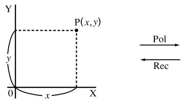
- Polar Coordinates
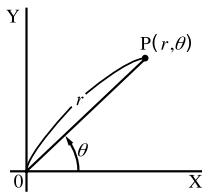
- With polar coordinates, can be calculated and displayed within a range of -180^ < ≤ 180^ (radians and grads have same range).
- Be sure to specify Comp for Mode in the Setup screen.
| Example | Operation |
| Calculate r and ^ when x = 14 and y = 20.7 |  |
| 1 [ 24.989 \ 55.928 ] 24.98979792 (r) |  |
 | |
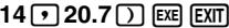 | |
| Calculate x and y when r = 25 and = 56^ |  |
| 1 [ 13.979 \ 20.725 ] 13.97982259 (x) | |
| 2 [ 20.725 \ 20.72593931 (y) ] 20.72593931 (y) |

■ Permutation and Combination
- Permutation
$$ n \mathsf {P r} = \frac {n !}{(n - r) !} $$
- Combination
$$ n \mathsf {C} r = \frac {n !}{r ! (n - r) !} $$
- Be sure to specify Comp for Mode in the Setup screen.

Example
To calculate the possible number of different arrangements using 4 items selected from among 10 items
| Formula | Operation |
| _10P_4 = 5040 | 10^OPTN F6 (▷) F3 (PROB) F2 (,,P_r) 4^EXE |

Example
To calculate the possible number of different combinations of 4 items that can be selected from among 10 items
| Formula | Operation |
| _10C_4 = 210 | 10^OPTN F6 (▷) F3 (PROB) F3 (,,C_r)4^EXE |
Fractions
How you should input fractions depends on the input mode that is currently selected.
| Improper Fraction | Mixed Fraction | |
| Math input mode |  (a7 7 ▼ 3) (a7 7 ▼ 3) | [BXTX](SHIFT a3(■□)2 ▶ 1 ▼ 3) |
| Linear input mode | 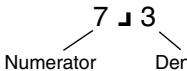 iominator(7 a3 3) iominator(7 a3 3) | Integer 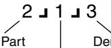 nominatorNumerator(2 a2 1 a3 3) nominatorNumerator(2 a2 1 a3 3) |
- For information about the Math input mode, see “Input Operations in the Math Input Mode” on page 1-3-8.
- Fraction calculation results are always reduced before being displayed.

- Be sure to specify Comp for Mode in the Setup screen.
| Example | Operation |
| 25 + 314 = 7320 | 25 5 + 25 (= =) 3 >1 >4 |
| 12578 + 14572 = 6.066202547 × 10^-4*1 | 2 55 + 3 55 1 55 4 |
| 12 × 0.5 = 0.25^*2 | 12 2578 + + 12 1 >4572 |
| 1.5 + 2.3i = 32 + 2310 i ( Display: \ 3 2 \ +23 10i ) | 1 25 2 ×.5 |
| 113 + 14 = 127 | 1.5 + 2.3 0 (i) -D -D ^*3 |
| 12 1 12 1 >3 > + 12 1 >4 | |
| 1 12 (1 12 3 + 1 12 4) |

*1 When the total number of characters, including integer, numerator, denominator and delimiter marks exceeds 10, the fraction is automatically displayed in decimal format.
*2 Calculations containing both fractions and decimals are calculated in decimal format.
*3 Pressing F-D once when converting the decimal part of a complex number to a fraction first displays the real part and imaginary part on separate lines.

Switching between improper fraction and mixed fraction format
Pressing the F-D ( a ) key toggles the display fraction between mixed fraction and improper fraction format.
Switching between fraction and decimal format

- If the calculation result includes a fraction, the display format (improper fraction or mixed fraction) is in accordance with the “Frac Result” setting of the Setup screen. For details, see “1-7 Using the Setup Screen”.
- You cannot switch from decimal format to mixed fraction format if the total number of digits used in the mixed fraction (including integer, numerator, denominator, and separator symbols) is greater than 10.
■ Engineering Notation Calculations
Input engineering symbols using the engineering notation menu.
- Be sure to specify Comp for Mode in the Setup screen.
| Example | Operation |
| 999k (kilo) + 25k (kilo)= 1.024M (mega) | SHIFT MENU (SET UP) ▲ (or ▼ 12 times)F4 (Eng) EXIT999 OPTN F6 (▷) F6 (▷) F1 (EYSM) F6 (▷) F1 (k) +25 F1 (k) EXE |
| 9 ÷ 10 = 0.9 = 900m (milli)= 0.9= 0.0009k (kilo)= 0.9= 900m | 9 ÷ 10 EXEOPTN F6 (▷) F6 (▷) F1 (EYSM) F6 (▷) F6 (▷) F3 (ENG)*1F3 (ENG)*1F2 (ENG)*2F2 (ENG)*2 |

*1 Converts the displayed value to the next higher engineering unit, by shifting the decimal point three places to the right.
*2 Converts the displayed value to the next lower engineering unit, by shifting the decimal point three places to the left.

2-5 Numerical Calculations
The following describes the items that are available in the menus you use when performing differential/quadratic differential, integration, , maximum/minimum value, and Solve calculations.
When the option menu is on the display, press F4 (CALC) to display the function analysis menu. The items of this menu are used when performing specific types of calculations.
- {Solve}/{d/dx}/{d²/dx²}/{∫dx}/{FMin}/{FMax}/{Σ{} ... {solve}/{differential}/{quadratic differential}/{integration}/{minimum value}/{maximum value}/{Σ (sigma)} calculations
■ Solve Calculations
The following is the syntax for using the Solve function in a program.
Solve( f(x),n,a,b)
(a: lower limit, b: upper limit, n: initial estimated value)
There are two different input methods that can be used for Solve calculations: direct assignment and variable table input.
With the direct assignment method (the one described here), you assign values directly to variables. This type of input is identical to that used with the Solve command used in the PRGM mode.
Variable table input is used with the Solve function in the EQUA mode. This input method is recommended for most normal Solve function input.
An error (Time Out) occurs when there is no convergence of the solution.
For information about Solve calculations, see page 4-3-1.

■ Differential Calculations
[OPTN]-[CALC]-[d/dx]
To perform differential calculations, first display the function analysis menu, and then input the values using the syntax below.
OPTN F4 (CALC) F2 (d/dx) f(x) a tol
(a: point for which you want to determine the derivative, tol: tolerance)
$$ d / d x (f (x), a) \Rightarrow \frac {d}{d x} f (a) $$
The differentiation for this type of calculation is defined as:
$$ f ^ {\prime} (a) = \lim _ {\Delta x \rightarrow 0} \frac {f (a + \Delta x) - f (a)}{\Delta x} $$
In this definition, infinitesimal is replaced by a sufficiently small x , with the value in the neighborhood of f'(a) calculated as:
$$ f ^ {\prime} (a) \doteq \frac {f (a + \Delta x) - f (a)}{\Delta x} $$
In order to provide the best precision possible, this unit employs central difference to perform differential calculations.
Using Differential Calculation in a Graph Function
- Omitting the tolerance (tol) value when using the differential command inside of a graph function simplifies the calculation for drawing the graph. In such a case, precision is sacrificed for the sake of faster drawing. The tolerance value is specified, the graph is drawn with the same precision obtained when you normally perform a differential calculation.
- You can also omit input of the derivative point by using the following format for the differential graph: Y2 = d / dx(Y1) . In this case, the value of the X variable is used as the derivative point.


Example
To determine the derivative at point x = 3 for the function
$$ y = x ^ {3} + 4 x ^ {2} + x - 6, \text { with a tolerance of ``tol'' } = 1 _ {\mathrm{E}} - 5 $$
Input the function f(x) .
$$ \boxed {\mathrm{AC}} \boxed {\mathrm{OPTN}} \boxed {\mathrm{F4}} (\text {CALC}) \boxed {\mathrm{F2}} (d / d x) \boxed {\mathrm{X}, \theta , \mathrm{T}} \wedge \boxed {3} + \boxed {4} \boxed {\mathrm{X}, \theta , \mathrm{T}} \boxed {\mathrm{x} ^ {2}} + \boxed {\mathrm{X}, \theta , \mathrm{T}} - \boxed {6}, $$
Input point x = a for which you want to determine the derivative.

Input the tolerance value.


$$ \boxed { \begin{array}{c} \mathrm{d} / \mathrm{dx} (X ^ {\wedge} 3 + 4 X ^ {2} + X - 6, 3, 1 \varepsilon \ - 5) \ 5 2 \end{array} } $$
(Math>


$$ \boxed {\frac {d}{d x} (x ^ {3} + 4 x ^ {2} + x - 6) | _ {x = 3}} \quad 5 2 $$

In the function f(x) , only X can be used as a variable in expressions. Other variables (A through Z excluding X, r, ) are treated as constants, and the value currently assigned to that variable is applied during the calculation.
Input of the tolerance (tol) value and the closing parenthesis can be omitted. If you omit tolerance (tol) value, the calculator automatically uses a value for tol as 1E-10.
Specify tolerance (tol) value of 1E-14 or less. An error (Time Out) occurs whenever no solution that satisfies the tolerance value can be obtained.
In the Math input mode, the tolerance value is fixed at 1E-10 and cannot be changed.
Inaccurate results and errors can be caused by the following:
- discontinuous points in x values
- extreme changes in x values
- inclusion of the local maximum point and local minimum point in x values
- inclusion of the inflection point in x values
- inclusion of undifferentiable points in x values
- differential calculation results approaching zero

- Applications of Differential Calculations
- Differentials can be added, subtracted, multiplied or divided with each other.
$$ \frac {d}{d x} f (a) = f ^ {\prime} (a), \frac {d}{d x} g (a) = g ^ {\prime} (a) $$
Therefore:
$$ f ^ {\prime} (a) + g ^ {\prime} (a), f ^ {\prime} (a) \times g ^ {\prime} (a), \text { etc. } $$
- Differential results can be used in addition, subtraction, multiplication, and division, and in functions.
$$ 2 \times f ^ {\prime} (a), \log (f ^ {\prime} (a)), \text { etc. } $$
- Functions can be used in any of the terms (f(x), a, tol) of a differential.
$$ \frac {d}{d x} (\sin x + \cos x, \sin 0. 5, 1 \mathrm{E} - 8), \text { etc. } $$

# You cannot use a differential, quadratic differential, integration, , maximum/minimum value, Solve, RndFix or log ab calculation expression inside a differential calculation term.
# Pressing AC during calculation of a differential (while the cursor is not shown on the display) interrupts the calculation.
# Always use radians (Rad mode) as the angle unit when performing trigonometric differentials.

■ Quadratic Differential Calculations
[OPTN]-[CALC]- [d^2 /dx^2 ]
After displaying the function analysis menu, you can input quadratic differentials using the following syntax.
$$ \boxed {\text {OPTN}} \boxed {\mathsf {F 4}} (\text {CALC}) \boxed {\mathsf {F 3}} (d ^ {2} / d x ^ {2}) f (x) \boxed {\bullet} a \boxed {\bullet} t o l \boxed {\bullet} $$
(a: differential coefficient point, tol: tolerance)
$$ \frac {d ^ {2}}{d x ^ {2}} (f (x), a) \Rightarrow \frac {d ^ {2}}{d x ^ {2}} f (a) $$
Quadratic differential calculations produce an approximate differential value using the following second order differential formula, which is based on Newton's polynomial interpretation.
$$ f ^ {\prime \prime} (a) = \frac {2 f (a + 3 h) - 2 7 f (a + 2 h) + 2 7 0 f (a + h) - 4 9 0 f (a) + 2 7 0 f (a - h) - 2 7 f (a - 2 h) + 2 f (a - 3 h)}{1 8 0 h ^ {2}} $$
In this expression, values for “sufficiently small increments of h” are used to obtain a value that approximates f''(a) .
● ● ● ● ●
Example To determine the quadratic differential coefficient at the point where x = 3 for the function y = x^3 + 4x^2 + x - 6 Here we will use a tolerance tol = 1E - 5
Input the function f(x) .
$$ \boxed {\mathrm{AC}} \boxed {\mathrm{OPTN}} \boxed {\mathrm{F4}} (\text {CALC}) \boxed {\mathrm{F3}} (d ^ {2} / d x ^ {2}) \boxed {\mathrm{X}, \theta , \mathrm{T}} \boxed {\wedge} \boxed {3} + $$
$$ Ⓥ 4 \boxed {X, \theta , T} \boxed {x ^ {2}} + \boxed {X, \theta , T} - \boxed {6}, $$
Input 3 as point a, which is the differential coefficient point.
3,
Input the tolerance value.
1 EXP (-) 5 )
EXE
$$ \left| \begin{array}{c c} d ^ {2} / d x ^ {2} (X ^ {\wedge} 3 + 4 X ^ {2} + X - 6, 3, \ 1 e - 5) & 2 6 \end{array} \right. $$

# In the function f(x) , only X can be used as a variable in expressions. Other variables (A through Z excluding X, r, ) are treated as constants, and the value currently assigned to that variable is applied during the calculation.
# Input of the tolerance (tol) value and the closing parenthesis can be omitted.
# Specify tolerance (tol) value of 1E-14 or less. An error (Time Out) occurs whenever no solution that satisfies the tolerance value can be obtained.

(Math>
AC F4 (MATH) F5 (d^2 /dx^2) X,θ,T ∧ 3
+ 4 X,θ,T x² + X,θ,T - 6 ▶ 3 EXE
$$ \boxed {\frac {d ^ {2}}{d x ^ {2}} (x ^ {3} + 4 x ^ {2} + x - 6) | _ {x = 3}} \tag {26} $$
• Quadratic Differential Applications
- Arithmetic operations can be performed using two quadratic differentials.
$$ \frac {d ^ {2}}{d x ^ {2}} f (a) = f ^ {\prime \prime} (a), \frac {d ^ {2}}{d x ^ {2}} g (a) = g ^ {\prime \prime} (a) $$
Therefore:
$$ f ^ {\prime \prime} (a) + g ^ {\prime \prime} (a), f ^ {\prime \prime} (a) \times g ^ {\prime \prime} (a), \text { etc. } $$
- The result of a quadratic differential calculation can be used in a subsequent arithmetic or function calculation.
$$ 2 \times f ^ {\prime \prime} (a), \log \left(f ^ {\prime \prime} (a)\right), \text { etc. } $$
- Functions can be used within the terms (f(x), a, tol) of a quadratic differential expression.
$$ \frac {d ^ {2}}{d x ^ {2}} (\sin x + \cos x, \sin 0. 5, 1 _ {\mathrm{E}} - 8), \text { etc. } $$

In the Math input mode, the tolerance value is fixed at 1E-10 and cannot be changed.
Using Quadratic Differential Calculation in a Graph Function (see page 2-5-2)
Inaccurate results and errors can be caused by the following:
- discontinuous points in x values
- extreme changes in x values
- inclusion of the local maximum point and local minimum point in x values
- inclusion of the inflection point in x values
- inclusion of undifferentiable points in x values
- differential calculation results approaching zero
You can interrupt an ongoing quadratic differential calculation by pressing the AC key.
Always use radians (Rad mode) as the angle unit when performing trigonometric quadratic differentials.
You cannot use a differential, quadratic differential, integration, , maximum/minimum value, Solve, RndFix or log ab calculation expression inside of a quadratic differential calculation term.
With quadratic differential calculation, calculation precision is up to five digits for the mantissa.

■ Integration Calculations
[OPTN]-[CALC]-[∫dx]
To perform integration calculations, first display the function analysis menu and then input the values using the syntax below.
$$ \boxed {\text {OPTN}} \boxed {\mathsf {F 4}} (\text {CALC}) \boxed {\mathsf {F 4}} (\int d x) f (x) \boxed {\text {,}} a \boxed {\text {,}} b \boxed {\text {,}} t o l \boxed {\text {)}} $$
(a: start point, b: end point, tol: tolerance)
$$ \int (f (x), a, b, t o l) \Rightarrow \int_ {a} ^ {b} f (x) d x $$
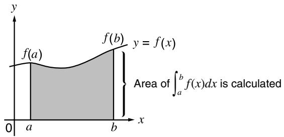
As shown in the illustration above, integration calculations are performed by calculating integral values from a through b for the function y = f(x) where a ≤ x ≤ b , and f(x) ≥ 0 . This in effect calculates the surface area of the shaded area in the illustration.
● ● ● ● ●
Example To perform the integration calculation for the function shown below, with a tolerance of “tol” = 1_E - 4
$$ \int_ {1} ^ {5} (2 x ^ {2} + 3 x + 4) d x $$
Input the function f(x) .
AC OPTN F4 (CALC) F4 (∫dx) 2 X,θ,T x² + 3 X,θ,T + 4 ,
Input the start point and end point.
1,5,
Input the tolerance value.
1 EXP (-) 4 )
EXE
(2X^2 + 3X + 4, 1, 5, 1E - 4) 134.6666667

# If f(x) < 0 where a ≤ x ≤ b , the surface area calculation produces negative values (surface area × -1 ).

(Math>
F4 (MATH) F6 (▷) F1 (∫dx) 2 X,θ,T x² +
3 X,θ,T + 4 ▶ 1 ▲ 5 EXE
$$ \left[ \begin{array}{c} \int_ {1} ^ {5} 2 x ^ {2} + 3 x + 4 d x \ 1 3 4. 6 6 6 6 6 6 7 \end{array} \right] $$
- Application of Integration Calculation
- Integrals can be used in addition, subtraction, multiplication or division.
$$ \int_ {a} ^ {b} f (x) d x + \int_ {c} ^ {d} g (x) d x, \text { etc. } $$
- Integration results can be used in addition, subtraction, multiplication or division, in functions.
$$ 2 \times \int_ {a} ^ {b} f (x) d x, \text { etc. } \log \left(\int_ {a} ^ {b} f (x) d x\right), \text { etc. } $$
- Functions can be used in any of the terms (f(x), a, b, tol) of an integral.
$$ \int_ {\sin 0. 5} ^ {\cos 0. 5} (\sin x + \cos x) d x = \int (\sin x + \cos x, \sin 0. 5, \cos 0. 5, 1 \mathrm{E} - 4) $$

# In the Math input mode, the tolerance value is fixed at 1_E-5 and cannot be changed.
# In the function f(x) , only X can be used as a variable in expressions. Other variables (A through Z excluding X, r, ) are treated as constants, and the value currently assigned to that variable is applied during the calculation.
# Input of “tol” and closing parenthesis can be omitted. If you omit “tol,” the calculator automatically uses a default value of 1_E-5 .
# Integration calculations can take a long time to complete.
# You cannot use a differential, quadratic differential, integration, , maximum/minimum value, Solve, RndFix or log ab calculation expression inside of an integration calculation term.

Note the following points to ensure correct integration values.
(1) When cyclical functions for integration values become positive or negative for different divisions, perform the calculation for single cycles, or divide between negative and positive, and then add the results together.
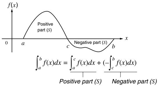
line
| Point | Value | |-------|-------| | a | Positive part (S) | | b | Negative part (S) | | c | Positive part (S) | | d | Negative part (S) | | e | Positive part (S) | | f | Negative part (S) |(2) When minute fluctuations in integration divisions produce large fluctuations in integration values, calculate the integration divisions separately (divide the large fluctuation areas into smaller divisions), and then add the results together.
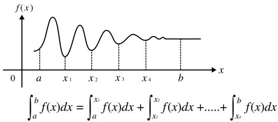
line
| x | f(x) | | ---- | ---- | | a | ∞ | | x₁ | Peak | | x₂ | Low | | x₃ | Medium | | x₄ | Low | | b | Stable |
# Pressing AC during calculation of an integral (while the cursor is not shown on the display) interrupts the calculation.
# Always use radians (Rad mode) as the angle unit when performing trigonometric integrations.
# An error (Time Out) occurs whenever no solution that satisfies the tolerance value can be obtained.

Σ Calculations
[OPTN]-[CALC]-[Σ]
To perform calculations, first display the function analysis menu, and then input the values using the syntax below.
$$ \boxed {\text {OPTN}} \boxed {\mathsf {F 4}} (\text {CALC}) \boxed {\mathsf {F 6}} (\triangleright) \boxed {\mathsf {F 3}} (\Sigma ( ) a _ {k} \boxed {\bullet}, k \boxed {\bullet}, \alpha \boxed {\bullet}, \beta \boxed {\bullet}, n \boxed {\bullet}) $$
$$ \sum \left(a _ {k}, k, \alpha , \beta , n\right) = \sum_ {k = \alpha} ^ {\beta} a _ {k} = a _ {\alpha} + a _ {\alpha + 1} + \dots \dots + a _ {\beta} $$
(n: distance between partitions)

Example To calculate the following:
$$ \sum_ {k = 2} ^ {6} (k ^ {2} - 3 k + 5) $$
Use n = 1 as the distance between partitions.
$$ \begin{array}{c} \boxed {A C} \boxed {O P T N} \boxed {F 4} (C A L C) \boxed {F 6} (\triangleright) \boxed {F 3} (\Sigma () \boxed {A L P H A} \boxed {\cdot} (K) \boxed {\Sigma (K ^ {2} - 3 K + 5, K, 2, 6, 1)} \ \boxed {x ^ {2}} \boxed {-} \boxed {3} \boxed {A L P H A} \boxed {\cdot} (K) \boxed {+} \boxed {5} \boxed {\cdot} \end{array} \tag {55} $$
$$ \boxed {\mathrm{ALPHA}} \boxed {,} (\mathrm{K}) \boxed {,} \boxed {2}, \boxed {6}, \boxed {1}) \boxed {\mathrm{EXE}} $$
(Math>
$$ \boxed {A C} \boxed {F 4} (M A T H) \boxed {F 6} (\triangleright) \boxed {F 2} (\Sigma () \boxed {A L P H A} \boxed {\cdot}, (K) $$
$$ \boxed {x ^ {2}} \boxed {-} \boxed {3} \boxed {\text { ALPHA }} \boxed {,} (\mathrm{K}) \boxed {+} \boxed {5} \boxed {\triangleright} $$
$$ \boxed {\mathrm{ALPHA}} \boxed {,} (\mathrm{K}) \boxed {\triangleright} \boxed {2} \boxed {\triangle} \boxed {6} \boxed {\mathrm{EXE}} $$
$$ \boxed {\sum_ {K = 2} ^ {6} (K ^ {2} - 3 K + 5)} \tag {55} $$

# You can use only one variable in the function for input sequence a_k .
# Input integers only for the initial term ( ) of sequence a_k and last term ( ) of sequence a_k .
# Input of n and the closing parentheses can be omitted. If you omit n, the calculator automatically uses n = 1.
# In the Math input mode, the distance between partitions (n) is fixed at 1 and cannot be changed.

- Calculation Applications
- Arithmetic operations using calculation expressions
Expressions:
$$ \mathrm{S} _ {n} = \sum_ {k = 1} ^ {n} a _ {k}, \mathrm{T} _ {n} = \sum_ {k = 1} ^ {n} b _ {k} $$
Possible operations:
$$ \mathrm{S} _ {n} + \mathrm{T} _ {n}, \mathrm{S} _ {n} - \mathrm{T} _ {n}, \text { etc. } $$
- Arithmetic and function operations using calculation results
$$ 2 \times \mathrm{S} _ {n}, \log (\mathrm{S} _ {n}), \text { etc. } $$
- Function operations using calculation terms ( a_k, k )
(sink, k, 1, 5), etc.

# You cannot use a differential, quadratic differential, integration, , maximum/minimum value, Solve, RndFix or log ab calculation expression inside of a calculation term.
# Make sure that the value used as the final term is greater than the value used as the initial term . Otherwise, an error will occur.
# To interrupt an ongoing calculation (indicated when the cursor is not on the display), press the AC key.

Maximum/Minimum Value Calculations
[OPTN]-[CALC]-[FMin]/[FMax]
After displaying the function analysis menu, you can input maximum/minimum calculations using the formats below, and solve for the maximum and minimum of a function within interval a ≤ x ≤ b .
●Minimum Value
OPTN F4 (CALC) F6 (▷) F1 (FMin) f(x) a b n
(a: start point of interval, b: end point of interval, n: precision (n = 1 to 9))
●Maximum Value
OPTN F4 (CALC) F6 (▷) F2 (FMax) f(x) a b n
(a: start point of interval, b: end point of interval, n: precision (n = 1 to 9))
● ● ● ● ●
Example 1 To determine the minimum value for the interval defined by start point a = 0 and end point b = 3, with a precision of n = 6 for the function y = x^2 - 4x + 9
Input f(x) .
AC OPTN F4 (CALC) F6 (▷) F1 (FMin) X,θ,T x² - 4 X,θ,T + 9 ,
Input the interval a = 0, b = 3.
0,3,
Input the precision n = 6.
6)
EXE
![AnS 1 [ ] 2 2 [ ] 5](/content/2025/01/86785/images/58ac401d27096eb84301028431255d6b9abcf979f67891fee1dd387145789004.jpg)


Example 2 To determine the maximum value for the interval defined by start point a = 0 and end point b = 3, with a precision of n = 6 for the function y = -x^2 + 2x + 2
Input f(x) .

Input the interval a = 0, b = 3.
Input the precision n = 6.


![AnS 1 [ ] 1 2 [ ] 3](/content/2025/01/86785/images/1c1f72cf8826052a39e66348cab8db42e8b226543b7e6e81a702961100dafc4d.jpg)

In the function f(x) , only X can be used as a variable in expressions. Other variables (A through Z excluding X, r, ) are treated as constants, and the value currently assigned to that variable is applied during the calculation.
Input of n and the closing parenthesis can be omitted.
Discontinuous points or sections with drastic fluctuation can adversely affect precision or even cause an error.
You cannot use a differential, quadratic differential, integration, , maximum/minimum value, Solve, RndFix or log ab calculation expression inside of a maximum/minimum calculation term.
Inputting a larger value for n increases the precision of the calculation, but it also increases the amount of time required to perform the calculation.
The value you input for the end point of the interval (b) must be greater than the value you input for the start point (a). Otherwise an error occurs.
You can interrupt an ongoing maximum/minimum calculation by pressing the AC key.
You can input an integer in the range of 1 to 9 for the value of n. Using any value outside this range causes an error.

2-6 Complex Number Calculations
You can perform addition, subtraction, multiplication, division, parentheses calculations, function calculations, and memory calculations with complex numbers just as you do with the manual calculations described on pages 2-1-1 and 2-4-7.
You can select the complex number calculation mode by changing the Complex Mode item on the Setup screen to one of the following settings.
- {Real} ... Calculation in the real number range only ^*1
- a + bi ... Performs complex number calculation and displays results in rectangular form
- ... Performs complex number calculation and displays results in polar form*2
Press OPTN F3 (CPLX) to display the complex calculation number menu, which contains the following items.
- i ... {imaginary unit i input}
- {Abs}/{Arg} ... obtains {absolute value}/{argument}
- {Conj} ... {obtains conjugate}
- {ReP}/{ImP} ... {real}/{imaginary} part extraction
- r/ a+bi ... converts the result to polar/rectangular form

*1 When there is an imaginary number in the argument, however, complex number calculation is performed and the result is displayed using rectangular form.
Examples:
$$ \ln 2 i = 0. 6 9 3 1 4 7 1 8 0 6 + 1. 5 7 0 7 9 6 3 2 7 i $$
$$ \ln 2 i + \ln (- 2) = (\text { Non - Real ERROR }) $$
*2 The display range of depends on the angle unit set for the Angle item on the Setup screen.
- Deg ... -180 < ≤ 180
- Rad ... - < ≤
• Gra ... -200 < θ ≦ 200
# Solutions obtained by the Real, a+bi and r modes are different for power root ( x^y ) calculations when x<0 and y=m/n when n is an odd number.
Example:
$$ \begin{array}{l} 3 ^ {x} \sqrt {- (- 8)} = - 2 (\text { Real }) \ = 1 + 1. 7 3 2 0 5 0 8 0 8 i (a + b i) \ = 2 \angle 6 0 (r \angle \theta) \ \end{array} $$
# To input the “∠” operator into the polar coordinate expression (r∠θ), press SHIFT X,θ,T.

Arithmetic Operations
[OPTN]-[CPLX]-[i]
Arithmetic operations are the same as those you use for manual calculations. You can even use parentheses and memory.

Example 1 (1 + 2i) + (2 + 3i)
AC OPTN F3 (CPLX)
$$ \boxed {(1 + 2 \mathbf {i}) + (2 + 3 \mathbf {i})} \quad 3 + 5 \mathbf {i} $$
(1+2F1(i))
+ ( 2 + 3 F1(i) ) EXE

Example 2 (2 + i)× (2 - i)
AC OPTN F3 (CPLX)
$$ \boxed {(2 + \mathbf {i}) \times (2 - \mathbf {i})} \quad 5 $$
(2 + F1(i) )
× (2 - F1(i) ) EXE
■ Reciprocals, Square Roots, and Squares

Example (3+i)
AC OPTN F3 (CPLX)
$$ \begin{array}{c} \hline \sqrt {(3 + \mathbf {i})} \ 1. 7 5 5 3 1 7 3 0 2 \ + 0. 2 8 4 8 4 8 7 8 4 6 \mathbf {i} \end{array} $$
SHIFT x^2() (3 + F1(i)) EXE
■ Complex Number Format Using Polar Form

Example 230 × 345 = 675
SHIFT MENU (SET UP) ▼ ▼ ▼ ▼ ▼ ▼
$$ \begin{array}{c c} \hline 2 \angle 3 0 \times 3 \angle 4 5 & \ & 6 \angle 7 5 \ \hline \end{array} $$
F1 (Deg) ▼ F3 (r∠θ) EXIT
AC 2 SHIFT X,θ,T (∠) 3 0 X 3
SHIFT X,θ,T (∠) 4 5 EXE

# You can also use SHIFT 0 (i) in place of OPTN F3 (CPLX) F1 (i).

■ Absolute Value and Argument
[OPTN]-[CPLX]-[Abs]/[Arg]
The unit regards a complex number in the form a + bi as a coordinate on a Gaussian plane, and calculates absolute value |Z| and argument (arg).

Example
To calculate absolute value (r) and argument () for the complex number 3 + 4i , with the angle unit set for degrees
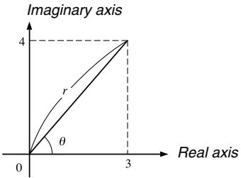
AC OPTN F3 (CPLX) F2 (Abs)
Abs (3+4i) 5
(3+4F1(i)EXE
(Calculation of absolute value)
AC OPTN F3 (CPLX) F3 (Arg)
Ar·a (3+4i) 53.13010235
( 3 + 4 F1(i) ) EXE
(Calculation of argument)
■ Conjugate Complex Numbers
[OPTN]-[CPLX]-[Conj]
A complex number of the form a + bi becomes a conjugate complex number of the form a - bi.

Example
To calculate the conjugate complex number for the complex number 2 + 4i
AC OPTN F3 (CPLX) F4 (Conj)
Conja (2+4i) 2-4i
(2 + 4 F1(i) ) EXE

# The result of the argument calculation differs in accordance with the current angle unit setting (degrees, radians, grads).

■ Extraction of Real and Imaginary Parts
[OPTN]-[CPLX]-[ReP]/[ImP]
Use the following procedure to extract the real part a and the imaginary part b from a complex number of the form a + bi .

Example To extract the real and imaginary parts of the complex number 2 + 5i
AC OPTN F3 (CPLX) F6 (▷) F1 (ReP)
ReP (2+5i) 2
(2 + 5 F6 (▷) F1 (i) ) EXE
(Real part extraction)
AC OPTN F3 (CPLX) F6 (▷) F2 (ImP)
ImP (2+5i) 5
(2 + 5 F6 (▷) F1 (i) ) EXE
(Imaginary part extraction)

# The input/output range of complex numbers is normally 10 digits for the mantissa and two digits for the exponent.
# When a complex number has more than 21 digits, the real part and imaginary part are displayed on separate lines.
# When either the real part or imaginary part of a complex number equals zero, that part is not displayed in rectangular form.
# The following functions can be used with complex numbers.
,x^2,x^-1,(x^),^3,^x, , In, ,_ab,10^x,e^x , Int, Frac, Rnd, Intg, RndFix(, Fix, Sci, ENG, ,^,^,^,a^b/c,d/c

■ Polar and Rectangular Form Transformation
[OPTN]-[CPLX]-[▶r∠θ]/[▶a+bi]
Use the following procedure to transform a complex number displayed in rectangular form to polar form, and vice versa.

Example
To transform the rectangular form of complex number 1 + 3i to its polar form
SHIFT MENU (SET UP) ▼ ▼ ▼ ▼ ▼ ▼
F1 (Deg) ▼ F2 (a+bi) EXIT
AC 1 + (SHIFT x^2 (√) 3 )
OPTN F3 (CPLX) F1 (i) F6 (▷) F3 (▶r∠θ) EXE
1+(√3)i-r∠8 2∠60
AC 2 SHIFT X,θ,T (∠) 6 0
OPTN F3 (CPLX) F6 (▷) F4 (▶a+bi) EXE
2460a+bi 1+1.732050808i

2-7 Binary, Octal, Decimal, and Hexadecimal Calculations with Integers
You can use the RUN·MAT mode and binary, octal, decimal, and hexadecimal settings to perform calculations that involve binary, octal, decimal and hexadecimal values. You can also convert between number systems and perform bitwise operations.
- You cannot use scientific functions in binary, octal, decimal, and hexadecimal calculations.
- You can use only integers in binary, octal, decimal, and hexadecimal calculations, which means that fractional values are not allowed. If you input a value that includes a decimal part, the calculator automatically cuts off the decimal part.
- If you attempt to enter a value that is invalid for the number system (binary, octal, decimal, hexadecimal) you are using, the calculator displays an error message. The following shows the numerals that can be used in each number system.
Binary: 0, 1
Octal: 0, 1, 2, 3, 4, 5, 6, 7
Decimal: 0, 1, 2, 3, 4, 5, 6, 7, 8, 9
Hexadecimal: 0, 1, 2, 3, 4, 5, 6, 7, 8, 9, A, B, C, D, E, F
- Negative binary, octal, and hexadecimal values are produced using the two's complement of the original value.
- The following are the display capacities for each of the number systems.
| Number System | Display Capacity |
| Binary | 16 digits |
| Octal | 11 digits |
| Decimal | 10 digits |
| Hexadecimal | 8 digits |

# The alphabetic characters used in the hexadecimal number appear differently on the display to distinguish them from text characters.
| Normal Text | A | B | C | D | E | F |
| Hexadecimal Values | ||||||
| Keys | ,, |

- The following are the calculation ranges for each of the number systems.
Binary Values
Positive: 0 ≤ x ≤ 1111111111111111
Negative: 1000000000000000 ≤ x ≤ 1111111111111111
Octal Values
Positive: 0 ≤ x ≤ 17777777777
Negative: 20000000000 ≤ x ≤ 37777777777
Decimal Values
Positive: 0 ≤ x ≤ 2147483647
Negative: -2147483648 ≤ x ≤ -1
Hexadecimal Values
Positive: 0 ≤ x ≤ 7FFFFFFF
Negative: 80000000 ≤ x ≤ FFFFFFFF
- To perform a binary, octal, decimal, or hexadecimal calculation
[SET UP]-[Mode]-[Dec]/[Hex]/[Bin]/[Oct]
- In the main menu, select RUN·MAT.
- Press SHIFT MENU (SET UP) ▼ and then specify the default number system by pressing F2 (Dec), F3 (Hex), F4 (Bin), or F5 (Oct) for the Mode setting.
- Press EXIT to change to the screen for calculation input. This causes a function menu with the following items to appear.
- {d\~o}/{LOG}/{DISP} ... {number system specification}/{bitwise operation}/{decimal/hexadecimal/binary/octal conversion} menu

■ Selecting a Number System
You can specify decimal, hexadecimal, binary, or octal as the default number system using the Setup screen.
- To specify a number system for an input value
You can specify a number system for each individual value you input. Press F1(d\~o) to display a menu of number system symbols. Press the function key that corresponds to the symbol you want to select and then input the value.
- {d}/{h}/{b}/{o} ... {decimal}/{hexadecimal}/{binary}/{octal}
- To input values of mixed number systems
● ● ● ● ●
Example
To input 123_10 or 1010_2 , when the default number system is hexadecimal
SHIFT MENU (SET UP) ▼ F3 (Hex) EXIT
d123 0000007B
■ Arithmetic Operations
● ● ● ● ●
Example 1 To calculate 10111_2 + 11010_2
SHIFT MENU (SET UP) ▼ F4 (Bin) EXIT
10111+11010 00000000000110001
AC 1 0 1 1 1 +
1 1 0 1 0 EXE


Example 2 To input and execute 123_8 × ABC_16 , when the default number system is decimal or hexadecimal
SHIFT MENU (SET UP) ▼ F2 (Dec) EXIT
o123×hABC 228084
AC F1(d\~o) F4(o) 1 2 3 ✗
F2 (h) A B C *1 EXE
EXIT F3 (DISP) F2 (▶Hex) EXE
Ans▶Hex 00037AF4
■ Negative Values and Bitwise Operations
Press F2(LOG) to display a menu of negation and bitwise operators.
- Neg negation^*2
- {Not}/{and}/{or}/{xor}/{xnor} ... {NOT}*3/{AND}/{OR}/{XOR}/{XNOR}*4
- Negative Values

Example To determine the negative of 110010_2
SHIFT MENU (SET UP) ▼ F4 (Bin) EXIT
Neg 110010 11111111111001110
- Bitwise Operations

Example 1 To input and execute “ 120_16 and AD_16 ”
SHIFT MENU (SET UP) ▼ F3 (Hex) EXIT
120andAD 00000020
AC 1 2 0 F2(LOG)
F3 (and) A D *1 EXE

*1 See page 2-7-1.
*2 two's complement
*3 one's complement (bitwise complement)
*4 bitwise AND, bitwise OR, bitwise XOR, bitwise XNOR
# Negative binary, octal, and hexadecimal values are produced by taking the binary two's complement and then returning the result to the original number base. With the decimal number base, negative values are displayed with a minus sign.


Example 2 To display the result of “368 or 11102” as an octal value
SHIFT MENU (SET UP) ▼ F5 (Oct) EXIT
36orb1110 00000000036
AC 3 6 F2(LOG)
F4 (or) EXIT F1 (d\~o) F3 (b)
1 1 1 0 EXE

Example 3 To negate 2FFFED _16
SHIFT MENU (SET UP) ▼ F3 (Hex) EXIT
Not 2FFFED FFD00012
AC F2 (LOG) F2 (Not)
2 F F F E D *1 EXE
• Number System Transformation
Press F3 (DISP) to display a menu of number system transformation functions.
- {▶Dec}/{▶Hex}/{▶Bin}/{▶Oct} ... transformation of displayed value to its {decimal}/{hexadecimal}/{binary}/{octal} equivalent
- To convert a displayed value from one number system to another

Example To convert 22_10 (default number system) to its binary or octal value
AC SHIFT MENU (SET UP) ▼ F2 (Dec) EXIT
d22 22
2-8 Matrix Calculations
From the Main Menu, enter the RUN·MAT mode, and press F1(▶MAT) to perform Matrix calculations.
26 matrix memories (Mat A through Mat Z) plus a Matrix Answer Memory (MatAns), make it possible to perform the following matrix operations.
- Addition, subtraction, multiplication
- Scalar multiplication calculations
• Determinant calculations - Matrix transposition
- Matrix inversion
- Matrix squaring
- Raising a matrix to a specific power
- Matrix modification using matrix commands
- Absolute value, integer part extraction, fractional part extraction, maximum integer calculations
The maximum number of rows that can be specified for a matrix is 255, and the maximum number of columns is 255.

# About Matrix Answer Memory (MatAns) The calculator automatically stores matrix calculation results in Matrix Answer Memory. Note the following points about Matrix Answer Memory.
- Whenever you perform a matrix calculation, the current Matrix Answer Memory contents are replaced by the new result. The previous contents are deleted and cannot be recovered.
- Inputting values into a matrix does not affect Matrix Answer Memory contents.

■ Inputting and Editing Matrices
Pressing F1(▶MAT) displays the Matrix Editor screen. Use the Matrix Editor to input and edit matrices.
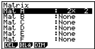
m × n m (row) × n (column) matrix
None... no matrix preset
- {DEL}/{DEL·A} ... deletes {a specific matrix}/{all matrices}
- {DIM} ... {specifies the matrix dimensions (number of cells)}
- Creating a Matrix
To create a matrix, you must first define its dimensions (size) in the Matrix Editor. Then you can input values into the matrix.
- To specify the dimensions (size) of a matrix
● ● ● ● ●
Example To create a 2-row × 3-column matrix in the area named Mat B
Highlight Mat B.

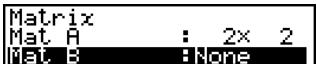
F3 (DIM) (This step can be omitted.)
Specify the number of rows.
2 EXE
Specify the number of columns.
3 EXE
EXE
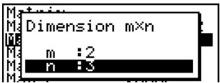
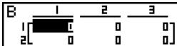
- All of the cells of a new matrix contain the value 0.

# If "Memory ERROR" remains next to the matrix area name after you input the dimensions, it
means there is not enough free memory to create the matrix you want.

- To input cell values

Example To input the following data into Matrix B :
$$ \left[ \begin{array}{c c c} 1 & 2 & 3 \ 4 & 5 & 6 \end{array} \right] $$
The following operation is a continuation of the example calculation on the previous page.
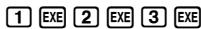

(Data is input into the highlighted cell. Each time you press EXE, the highlighting moves to the next cell to the right.)
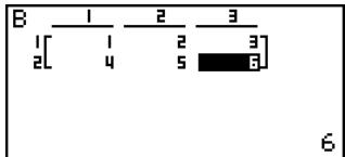
To exit the Matrix input screen, press EXIT.
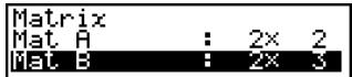

You cannot input complex numbers into the cell of a matrix.
Displayed cell values show positive integers up to six digits, and negative integers up to five digits (one digit used for the negative sign). Exponential values are shown with up to two digits for the exponent. Fractional values are not displayed.
You can see the entire value assigned to a cell by using the cursor keys to move the highlighting to the cell whose value you want to view.
The amount of memory required for a matrix is 9 bytes per cell. This means that a 3 × 3 matrix requires 81 bytes of memory ( 3 × 3 × 9 = 81 ).

- Deleting Matrices
You can delete either a specific matrix or all matrices in memory.
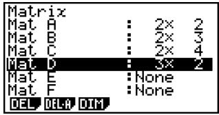
- To delete a specific matrix
- While the Matrix Editor is on the display, use ▲ and ▼ to highlight the matrix you want to delete.
- Press F1(DEL).
- Press F1 (Yes) to delete the matrix or F6 (No) to abort the operation without deleting anything.
- To delete all matrices
- While the Matrix Editor is on the display, press F2 (DEL·A).
- Press F1(Yes) to delete all matrices in memory or F6(No) to abort the operation without deleting anything.

# The indicator “None” replaces the dimensions of the matrix you delete.
# Inputting the format or changing the dimensions of a matrix deletes its current contents.

■ Matrix Cell Operations
Use the following procedure to prepare a matrix for cell operations.
-
While the Matrix Editor is on the display, use ▲ and ▼ to highlight the name of the matrix you want to use.
You can jump to a specific matrix by inputting the letter that corresponds to the matrix name. Inputting ALPHA 8 (N), for example, jumps to Mat N.
Pressing SHIFT (Ans) jumps to the Matrix current Memory. -
Press EXE and the function menu with the following items appears.
-
{R-OP} ... {row operation menu}
• {ROW} - {DEL}/{INS}/{ADD} ... row {delete}/{insert}/{add}
• {COL} - {DEL}/{INS}/{ADD} ... column {delete}/{insert}/{add}
- {EDIT} ... {cell editing screen}
All of the following examples use Matrix A.
- Row Calculations
The following menu appears whenever you press [F1] (R-OP) while a recalled matrix is on the display.
- {Swap} ... {row swap}
- × Rw ... {product of specified row and scalar}
- × Rw + ... {addition of one row and the product of a specified row with a scalar}
- Rw + ... {addition of specified row to another row}
- To swap two rows
● ● ● ● ●
Example To swap rows two and three of the following matrix :
$$ \text { Matrix } \mathbf {A} = \left[ \begin{array}{c c} 1 & 2 \ 3 & 4 \ 5 & 6 \end{array} \right] $$
F1(R-OP) F1(Swap)
Input the number of the rows you want to swap.
2 EXE 3 EXE
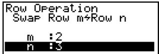
F6(EXE) (or EXE)
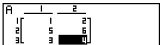

- To calculate the scalar multiplication of a row

Example To calculate the product of row 2 of the following matrix and the scalar 4 :
$$ \text { Matrix } \mathbf {A} = \left[ \begin{array}{c c} 1 & 2 \ 3 & 4 \ 5 & 6 \end{array} \right] $$
F1 (R-OP) F2 (×Rw)
Input multiplier value.
4 EXE
Specify row number.
2 EXE
F6(EXE) (or EXE)
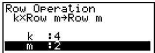
![A 1 2 1 [ 1 2 ] 2 [ 12 16 ] 3 [ 5 ■ E ]](/content/2025/01/86785/images/0b40ba029bbe7f4f2797572353b8787786ed875cff9bc255d5748f83f7deb947.jpg)
- To calculate the scalar multiplication of a row and add the result to another row

Example To calculate the product of row 2 of the following matrix and the scalar 4, then add the result to row 3 :
$$ \text { Matrix } \mathbf {A} = \left[ \begin{array}{l l} 1 & 2 \ 3 & 4 \ 5 & 6 \end{array} \right] $$
F1 (R-OP) F3 (×Rw+)
Input multiplier value.
4 EXE
Specify number of row whose product should be calculated.
2 EXE
Specify number of row where result should be added.
3 EXE
F6(EXE) (or EXE)
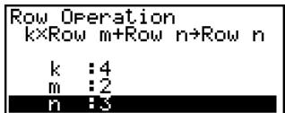
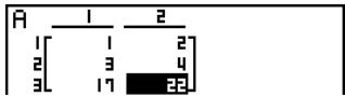

• To add two rows together

Example To add row 2 to row 3 of the following matrix :
$$ \text { Matrix } \mathbf {A} = \left[ \begin{array}{c c} 1 & 2 \ 3 & 4 \ 5 & 6 \end{array} \right] $$
F1 (R-OP) F4 (Rw+)
Specify number of row to be added.
2 EXE
Specify number of row to be added to.
3 EXE
F6(EXE) (or EXE)
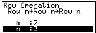
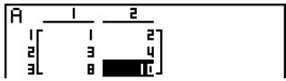
- Row Operations
- {DEL} ... {delete row}
- {INS} ... {insert row}
- {ADD} ... {add row}
- To delete a row

Example To delete row 2 of the following matrix :
$$ \text { Matrix } \mathbf {A} = \left[ \begin{array}{c c} 1 & 2 \ 3 & 4 \ 5 & 6 \end{array} \right] $$

F2 (ROW) F1 (DEL)
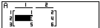
![A 1 2 1 [ E ] 2 2 [ E ] 6 ]](/content/2025/01/86785/images/04acc184e6a54f0126bff32988bf7f388667720a0e8b8c7b72a08873401d43b7.jpg)

- To insert a row

Example
To insert a new row between rows one and two of the following matrix :
$$ \text { Matrix } \mathbf {A} = \left[ \begin{array}{c c} 1 & 2 \ 3 & 4 \ 5 & 6 \end{array} \right] $$

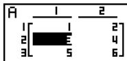
F2 (ROW) F2 (INS)
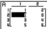
- To add a row

Example
To add a new row below row 3 of the following matrix :
$$ \text { Matrix } \mathbf {A} = \left[ \begin{array}{c c} 1 & 2 \ 3 & 4 \ 5 & 6 \end{array} \right] $$

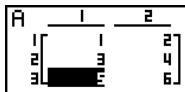
F2 (ROW) F3 (ADD)
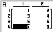

- Column Operations
- {DEL} ... {delete column}
- {INS} ... {insert column}
- {ADD} ... {add column}
- To delete a column

Example To delete column 2 of the following matrix :
$$ \text { Matrix } \mathbf {A} = \left[ \begin{array}{c c} 1 & 2 \ 3 & 4 \ 5 & 6 \end{array} \right] $$

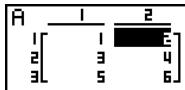
F3 (COL) F1 (DEL)
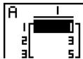
- To insert a column

Example To insert a new column between columns 1 and 2 of the following matrix :
$$ \text { Matrix } \mathbf {A} = \left[ \begin{array}{c c} 1 & 2 \ 3 & 4 \ 5 & 6 \end{array} \right] $$

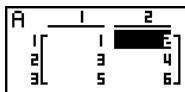
F3 (COL) F2 (INS)
![A 1 2 3 1 [ 1 ] 2 2 [ 3 ] 0 4 3 [ 5 ] 0 6](/content/2025/01/86785/images/04a3d0313b06ce874e5c42e245b62c7dfd2449bebb1ab7dfdf855403b1c96c85.jpg)

- To add a column

Example To add a new column to the right of column 2 of the following matrix :
$$ \text { Matrix } \mathbf {A} = \left[ \begin{array}{c c} 1 & 2 \ 3 & 4 \ 5 & 6 \end{array} \right] $$

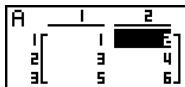
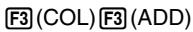
![A 1 2 3 1 [ 1 2 ] 1 2 [ 3 4 0 3 [ 5 6 0]](/content/2025/01/86785/images/b1ce84e23ea4077932fde013d8fe8587a0f098f694c543a1e047129d47a154bb.jpg)
■ Modifying Matrices Using Matrix Commands
[OPTN]-[MAT]
- To display the matrix commands
- From the Main Menu, enter the RUN • MAT mode.
- Press OPTN to display the option menu.
- Press F2 (MAT) to display the matrix command menu.
The following describes only the matrix command menu items that are used for creating matrices and inputting matrix data.
- {Mat} ... {Mat command (matrix specification)}
- M L ... Mat List command (assign contents of selected column to list file)
- {Det} ... {Det command (determinant command)}
- {Trn} ... {Trn command (transpose matrix command)}
- {Aug} ... {Augment command (link two matrices)}
- {lden} ... {Identity command (identity matrix input)}
- {Dim} ... {Dim command (dimension check)}
- {Fill} ... {Fill command (identical cell values)}

- Matrix Data Input Format
[OPTN]-[MAT]-[Mat]
The following shows the format you should use when inputting data to create a matrix using the Mat command.
$$ \left[ \begin{array}{c c c c} \mathsf {a} _ {1 1} & \mathsf {a} _ {1 2} & ... & \mathsf {a} _ {1 n} \ \mathsf {a} _ {2 1} & \mathsf {a} _ {2 2} & ... & \mathsf {a} _ {2 n} \ \vdots & \vdots & & \vdots \ \mathsf {a} _ {m 1} & \mathsf {a} _ {m 2} & ... & \mathsf {a} _ {m n} \end{array} \right] $$
$$ = \left[ \left[ a _ {1 1}, a _ {1 2}, \dots , a _ {1 n} \right] \left[ a _ {2 1}, a _ {2 2}, \dots , a _ {2 n} \right] \dots \left[ a _ {m 1}, a _ {m 2}, \dots , a _ {m n} \right] \right] $$
$$ \rightarrow \text { Mat [letter A through Z] } $$

Example 1 To input the following data as Matrix A :
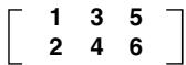
SHIFT + ( [ ) SHIFT + ( [ ) 1 , 3 , 5
[[1,3,5][2,4,6]]→Mat AI
SHIFT — ( ) SHIFT + ( [ ) 2 , 4 , 6
SHIFT — ( ) SHIFT — ( ) → OPTN F2 (MAT)
F1 (Mat) ALPHA X,θ,T (A)

Matrix name
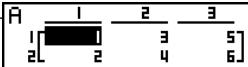

# You can also use SHIFT 2 (Mat) in place of OPTN F2 (MAT) F1 (Mat).
# The maximum value of both m and n is 255.
# An error occurs if memory becomes full as you are inputting data.
# You can also use the above format inside a program that inputs matrix data.

- To input an identity matrix
[OPTN]-[MAT]-[Iden]
Use the Identity command to create an identity matrix.

Example 2 To create a 3 × 3 identity matrix as Matrix A
![A 1 2 3 1 [ ] 0 0 2 [ ] 0 1 0 3 [ ] 0 0 1](/content/2025/01/86785/images/ca52f303a55839cc49a745f0fdf9904d610f724bfa8b49f357b4e475007751c9.jpg)
- To check the dimensions of a matrix
[OPTN]-[MAT]-[Dim]
Use the Dim command to check the dimensions of an existing matrix.

Example 3 To check the dimensions of Matrix A, which was input in Example 1
![AnS 1[ ]E 2[ ]3](/content/2025/01/86785/images/21514bbac4ae479c6a8df95af6d1935bab5e6c732c874cb11a48614db192004c.jpg)
The display shows that Matrix A consists of two rows and three columns.
Since the result of the Dim command is list type data, it is stored in ListAns memory.
You can also use Dim to specify the dimensions of the matrix.

Example 4 To specify dimensions of 2 rows and 3 columns for Matrix B
![B 1 2 3 1 [ ] 0 0 2 [ ] 0 0](/content/2025/01/86785/images/fe9b197f874b6af98bddfa70299ad0acd13faccf1c2f7a550379e52da855625b.jpg)

- Modifying Matrices Using Matrix Commands
You can also use matrix commands to assign values to and recall values from an existing matrix, to fill in all cells of an existing matrix with the same value, to combine two matrices into a single matrix, and to assign the contents of a matrix column to a list file.
- To assign values to and recall values from an existing matrix
[OPTN]-[MAT]-[Mat]
Use the following format with the Mat command to specify a cell for value assignment and recall.
Mat X [m, n]
X ...... matrix name (A through Z, or Ans)
m..... row number
n ...... column number
● ● ● ● ●
Example 1 Assign 10 to the cell at row 1, column 2 of the following matrix :
$$ \text { Matrix } \mathbf {A} = \left[ \begin{array}{c c} 1 & 2 \ 3 & 4 \ 5 & 6 \end{array} \right] $$
1 0 → OPTN F2 (MAT) F1 (Mat)
10→Mat A[1,2] 10
ALPHA X,θ,T (A) SHIFT + ( [ ) 1 , 2
SHIFT - ( ) EXE
EXIT EXIT F1 (▶ MAT) EXE
![A 1 1 2 1 [ ] 10 2 3 4 3 [ ] 5 6](/content/2025/01/86785/images/cef4aa26a4a634d4ea5f1d165e7adf1c98471b1164ad0fc2d57bc4ac645ced14.jpg)
● ● ● ● ●
Example 2 Multiply the value in the cell at row 2, column 2 of the above matrix by 5
OPTN F2 (MAT) F1 (Mat)
Mat A[2,2]×5 20
ALPHA X,θ,T (A) SHIFT + ( [ ) 2 , 2
SHIFT - ( ) ✗ 5 EXE

- To fill a matrix with identical values and to combine two matrices into a single matrix [OPTN]-[MAT]-[Fill]/[A
[OPTN]-[MAT]-[Fill]/[Aug]
Use the Fill command to fill all the cells of an existing matrix with an identical value and the Augment command to combine two existing matrices into a single matrix.

Example 1 To fill all of the cells of Matrix A with the value 3
OPTN F2 (MAT) F6 (▷) F3 (Fill)
3 F6 (▷) F1 (Mat) ALPHA X,θ,T (A) EXE
F1 (Mat) ALPHA X,θ,T (A) EXE
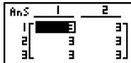

Example 2 To combine the following two matrices :
$$ \mathbf {A} = \left[ \begin{array}{l} 1 \ 2 \end{array} \right] \quad \mathbf {B} = \left[ \begin{array}{l} 3 \ 4 \end{array} \right] $$
OPTN F2 (MAT) F5 (Aug)
F1(Mat) ALPHA X,θ,T (A),
F1(Mat) ALPHA log(B) EXE
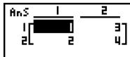

# The two matrices you combine must have the same number of rows. An error occurs if you try to combine two matrices that have different number of rows.
# You can use Matrix Answer Memory to assign the results of the above matrix input and edit operations to a matrix variable. To do so, use the following syntax.
- Fill (n, Mat ) Mat
• Augment (Mat α, Mat β) → Mat γ
In the above, , , and are any variable names A through Z, and n is any value.
The above does not affect the contents of Matrix Answer Memory.

- To assign the contents of a matrix column to a list
[OPTN]-[MAT]-[M→L]
Use the following format with the Mat→List command to specify a column and a list.
Mat → List (Mat X, m) → List n
X = matrix name (A through Z, or Ans)
m = column number
n = list number

Example To assign the contents of column 2 of the following matrix to list 1 :
$$ \text { Matrix } \mathbf {A} = \left[ \begin{array}{c c} 1 & 2 \ 3 & 4 \ 5 & 6 \end{array} \right] $$
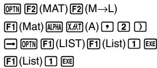
![AnS 1 [2] 2 [4] 3 [6]](/content/2025/01/86785/images/1c0c84543874a188205c7f1b83c11c08069777bd1ea5ab8e48214907a27e9783.jpg)

# You can also use SHIFT 1 (List) in place of OPTN F1 (LIST) F1 (List).

■ Matrix Calculations
[OPTN]-[MAT]
Use the matrix command menu to perform matrix calculation operations.
- To display the matrix commands
- From the Main Menu, enter the RUN • MAT mode.
- Press ☐OPTN to display the option menu.
- Press F2 (MAT) to display the matrix command menu.
The following describes only the matrix commands that are used for matrix arithmetic operations.
- {Mat} ... {Mat command (matrix specification)}
- {Det} ... {Det command (determinant command)}
- {Trn} ... {Trn command (transpose matrix command)}
- {lden} ... {Identity command (identity matrix input)}
All of the following examples assume that matrix data is already stored in memory.

- Matrix Arithmetic Operations
[OPTN]-[MAT]-[Mat]/[Iden]

Example 1 To add the following two matrices (Matrix A + Matrix B):
$$ \mathbf {A} = \left[ \begin{array}{c c} 1 & 1 \ 2 & 1 \end{array} \right] $$
$$ \mathbf {B} = \left[ \begin{array}{c c} 2 & 3 \ 2 & 1 \end{array} \right] $$
$$ \boxed {A C} \boxed {O P T N} \boxed {F 2} (M A T) \boxed {F 1} (M a t) \boxed {A L P H A} \boxed {X, \theta , T} (A) \boxed {+} $$
$$ \boxed {F 1} (\text { Mat }) \boxed {\text { ALPHA }} \boxed {\log} (B) \boxed {\text { EXE }} $$
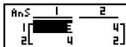

Example 2 Calculate the product to the following matrix using a multiplier value of 5 :
$$ \text { Matrix } \mathbf {A} = \left[ \begin{array}{c c} 1 & 2 \ 3 & 4 \end{array} \right] $$
$$ \boxed {A C} \boxed {5} \boxed {O P T N} \boxed {F 2} (M A T) \boxed {F 1} (M a t) $$
$$ \boxed {\text { ALPHA }} \boxed {X, \theta , T} (A) \boxed {\text { EXE }} $$
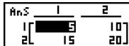
Example 3 To multiply the two matrices in Example 1 (Matrix A × Matrix B)
$$ \boxed {A C} \boxed {O P T N} \boxed {F 2} (M A T) \boxed {F 1} (M a t) \boxed {A L P H A} \boxed {X, \theta , T} (A) \boxed {\times} $$
$$ \boxed {\mathsf {F 1}} (\text { Mat }) \boxed {\text { ALPHA }} \boxed {\log} (\text { B }) \boxed {\text { EXE }} $$
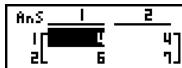

Example 4 To multiply Matrix A (from Example 1) by a 2 × 2 identity matrix
$$ \boxed {A C} \boxed {O P T N} \boxed {F 2} (M A T) \boxed {F 1} (M a t) \boxed {A L P H A} \boxed {X, \theta , T} (A) \boxed {\times} $$
$$ \boxed {F 6} (\triangleright) \boxed {F 1} (I d e n) \boxed {2} \boxed {E X E} $$
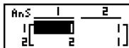
Number of rows and columns

# The two matrices must have the same dimensions in order to be added or subtracted. An error occurs if you try to add or subtract matrices of different dimensions.
# For multiplication (Matrix 1 × Matrix 2), the number of columns in Matrix 1 must match the number of rows in Matrix 2. Otherwise, an error occurs.
# When performing matrix arithmetic operations, inputting the Identity command at the location of a matrix command (such as Mat A) makes it possible to perform identity matrix calculations.

- Determinant
[OPTN]-[MAT]-[Det]

Example Obtain the determinant for the following matrix :
$$ \text { Matrix } \mathbf {A} = \left[ \begin{array}{r r r} 1 & 2 & 3 \ 4 & 5 & 6 \ - 1 & - 2 & 0 \end{array} \right] $$
OPTN F2 (MAT) F3 (Det) F1 (Mat)
ALPHA X,θ,T (A) EXE
Det Mat A -9
- Matrix Transposition
[OPTN]-[MAT]-[Trn]
A matrix is transposed when its rows become columns and its columns become rows.

Example To transpose the following matrix :
$$ \text { Matrix } \mathbf {A} = \left[ \begin{array}{c c} 1 & 2 \ 3 & 4 \ 5 & 6 \end{array} \right] $$
OPTN F2 (MAT) F4 (Trn) F1 (Mat)
ALPHA X,θ,T (A) EXE
![AnS 1 2 3 1 [ ] 3 5 2 [ ] 2 4 6](/content/2025/01/86785/images/1c6ba5acc0512293aefc62ca58e54add7979db12e0fa86e093ee6468a4749c4a.jpg)

# Determinants can be obtained only for square matrices (same number of rows and columns). Trying to obtain a determinant for a matrix that is not square produces an error.
# The determinant of a 2 × 2 matrix is calculated as shown below.
$$ | \mathsf {A} | = \left[ \begin{array}{l l} \mathsf {a} _ {1 1} & \mathsf {a} _ {1 2} \ \mathsf {a} _ {2 1} & \mathsf {a} _ {2 2} \end{array} \right] = \mathsf {a} _ {1 1} \mathsf {a} _ {2 2} - \mathsf {a} _ {1 2} \mathsf {a} _ {2 1} $$
# The determinant of a 3 × 3 matrix is calculated as shown below.
$$ \begin{array}{l} | \mathsf {A} | = \left[ \begin{array}{l l l} \mathsf {a} _ {1 1} & \mathsf {a} _ {1 2} & \mathsf {a} _ {1 3} \ \mathsf {a} _ {2 1} & \mathsf {a} _ {2 2} & \mathsf {a} _ {2 3} \ \mathsf {a} _ {3 1} & \mathsf {a} _ {3 2} & \mathsf {a} _ {3 3} \end{array} \right] \ = a _ {1 1} a _ {2 2} a _ {3 3} + a _ {1 2} a _ {2 3} a _ {3 1} + a _ {1 3} a _ {2 1} a _ {3 2} \ - a _ {1 1} a _ {2 3} a _ {3 2} - a _ {1 2} a _ {2 1} a _ {3 3} - a _ {1 3} a _ {2 2} a _ {3 1} \ \end{array} $$

- Matrix Inversion
[OPTN]-[MAT]- [x^-1]

Example To invert the following matrix :
$$ \text { Matrix } \mathbf {A} = \left[ \begin{array}{c c} 1 & 2 \ 3 & 4 \end{array} \right] $$
OPTN F2 (MAT) F1 (Mat)
ALPHA X,θ,T (A) SHIFT ) (x⁻¹) EXE
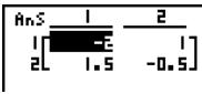
- Squaring a Matrix
[OPTN]-[MAT]- [x^2]

Example To square the following matrix :
$$ \text { Matrix } \mathbf {A} = \left[ \begin{array}{c c} 1 & 2 \ 3 & 4 \end{array} \right] $$
OPTN F2 (MAT) F1 (Mat) ALPHA X,θ,T (A) x^2 EXE
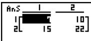

Only square matrices (same number of rows and columns) can be inverted. Trying to invert a matrix that is not square produces an error.
A matrix with a determinant of zero cannot be inverted. Trying to invert a matrix with determinant of zero produces an error.
Calculation precision is affected for matrices whose determinant is near zero.
# A matrix being inverted must satisfy the conditions shown below.
$$ \mathbf {A} \mathbf {A} ^ {- 1} = \mathbf {A} ^ {- 1} \mathbf {A} = \mathbf {E} = \left[ \begin{array}{c c c} 1 & 0 \ 0 & 1 \end{array} \right] $$
The following shows the formula used to invert Matrix A into inverse matrix A^-1 .
$$ \mathbf {A} = \left[ \begin{array}{c c c} \mathbf {a} & \mathbf {b} \ \mathbf {c} & \mathbf {d} \end{array} \right] $$
$$ \mathbf {A} ^ {- 1} = \frac {1}{a d - b c} \left[ \begin{array}{c c} d & - b \ - c & a \end{array} \right] $$
Note that ad - bc ≠ 0.

• Raising a Matrix to a Power
[OPTN]-[MAT]-[^]

Example To raise the following matrix to the third power :
$$ \text { Matrix } \mathbf {A} = \left[ \begin{array}{c c} 1 & 2 \ 3 & 4 \end{array} \right] $$
OPTN F2 (MAT) F1 (Mat) ALPHA X,θ,T (A)
^ 3 EXE
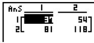
- Determining the Absolute Value, Integer Part, Fraction Part, and Maximum Integer of a Matrix [OPTN]-[NUM]-[Abs]/[Frac]/[Int]/[Intg]

Example To determine the absolute value of the following matrix :
$$ \text { Matrix } \mathbf {A} = \left[ \begin{array}{c c} 1 & - 2 \ - 3 & 4 \end{array} \right] $$
OPTN F6 (▷) F4 (NUM) F1 (Abs)
OPTN F2 (MAT) F1 (Mat) ALPHA X,θ,T (A) EXE
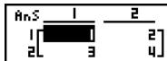

# Determinants and inverse matrices are subject to error due to dropped digits.
# Matrix operations are performed individually on each cell, so calculations may require considerable time to complete.
# The calculation precision of displayed results for matrix calculations is ± 1 at the least significant digit.
# If a matrix calculation result is too large to fit into Matrix Answer Memory, an error occurs.
# You can use the following operation to transfer Matrix Answer Memory contents to another matrix (or when Matrix Answer Memory contains a determinant to a variable).
$$ \text { MatAns } \rightarrow \text { Mat } \alpha $$
In the above, is any variable name A through Z. The above does not affect the contents of Matrix Answer Memory.
# For matrix power calculations, calculation is possible up to a power of 32766.

■ Performing Matrix Calculations Using Natural Input
- To specify the dimensions (size) of a matrix
- In the RUN • MAT mode, press SHIFT MENU (SET UP) F1 (Math) EXIT.
- Press F4 (MATH) to display the MATH menu.
- Press F1(MAT) to display the following menu.
- 2 × 2 {inputs a 2 × 2 matrix}
- 3 × 3 ... {inputs a 3 × 3 matrix}
- m × n {inputs an m -row × n -column matrix (up to 6 × 6 )}

Example To create a 2-row × 3-column matrix
F3(m×n)
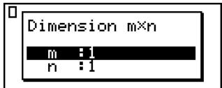
Specify the number of rows.
2 EXE
Specify the number of columns.
3 EXE
EXE
![[0 0 0] [0 0 0] 2×2 3×3 M×1](/content/2025/01/86785/images/d627c758873a99445847f95df1573aeb69f1a295d8ec1ed0756f5b67c7631964.jpg)

- To input cell values

Example To perform the calculation shown below
$$ \left[ \begin{array}{c c c} 1 & \frac {1}{2} & 3 3 \ \frac {1 3}{4} & \sqrt {5} & 6 \end{array} \right] \times \mathbf {8} $$
The following operation is a continuation of the example calculation on the previous page.
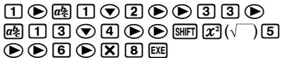
- To assign a matrix created using natural input to a MAT mode matrix

Example To assign the calculation result to Mat J
![L 4 J [8 4 264] [26 17.88854382 48] Mat Ans→Mat J [8 4 264] [26 17.88854382 48] □ 2×2 3×3 M×1](/content/2025/01/86785/images/30a8099d6046e8ee2995b1dc0f243c8c58add5bfc2267abf917689ee10d559fa.jpg)

# Pressing the DEL key while the cursor is located at the top (upper left) of the matrix will delete the entire matrix.
![2×[12 0 0] [34 0 0] 2×2 3×3 m×h DEL ⇒ 2×1 2×2 3×3 m×h](/content/2025/01/86785/images/53b34846b5ad1d1d92232c359ed157dc0e72f18ff2938123519eece16397d996.jpg)

Chapter
3
3
List Function
A list is a storage place for multiple data items.
This calculator lets you store up to 26 lists in a single file, and you can store up to six files in memory. Stored lists can be used in arithmetic and statistical calculations, and for graphing.
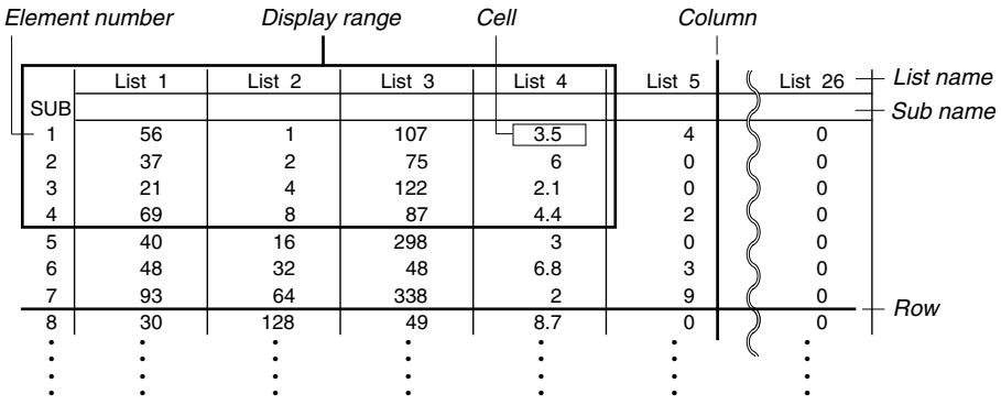
3-1 Inputting and Editing a List
3-2 Manipulating List Data
3-3 Arithmetic Calculations Using Lists
3-4 Switching Between List Files
3-1 Inputting and Editing a List
When you enter the STAT mode, the "List Editor" will appear first. You can use the List Editor to input data into a list and to perform a variety of other list data operations.
- To input values one-by-one
Use the cursor keys to move the highlighting to the list name, sub name or cell you want to select.
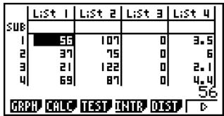
The screen automatically scrolls when the highlighting is located at either edge of the screen.
The following example is performed starting with the highlighting located at Cell 1 of List 1.
- Input a value and press EXE to store it in the list.
3 EXE
- The highlighting automatically moves down to the next cell for input.
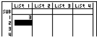
- Input the value 4 in the second cell, and then input the result of 2 + 3 in the next cell.
4 EXE 2 + 3 EXE
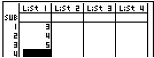
other
| SUB | List 1 | List 2 | List 3 | List 4 | |---|---|---|---|---| | 1 | 3 | | | | | 2 | 4 | | | | | 3 | 5 | | | | | 4 | | | | |
# You can also input the result of an expression or a complex number into a cell.
# You can input values up to 999 cells in a single list.

- To batch input a series of values
- Use the cursor keys to move the highlighting to another list.
| Li:St 1 | Li:St 2 | Li:St 3 | Li:St 4 | |
| SUB | ||||
| I | 3 |
- Press SHIFT ( ), and then input the values you want, pressing , between each one. Press SHIFT ( ) after inputting the final value.

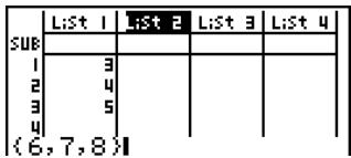
- Press EXE to store all of the values in your list.

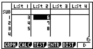
You can also use list names inside of a mathematical expression to input values into another cell. The following example shows how to add the values in each row in List 1 and List 2, and input the result into List 3.
- Use the cursor keys to move the highlighting to the name of the list where you want the calculation results to be input.
| Li:St 1 | Li:St 2 | Li:St 3 | Li:St 4 | |
| SUB | ||||
| I | 3 | 6 |
- Press OPTN and input the expression.

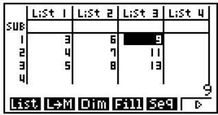
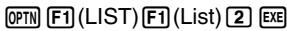

# You can also use SHIFT 1 (List) in place of OPTN F1 (LIST) F1 (List).
# Remember that a comma separates values, so you should not input a comma after the final value of the set you are inputting.
Right: {34, 53, 78}
Wrong: {34, 53, 78,}

■ Editing List Values
- To change a cell value
Use the cursor keys to move the highlighting to the cell whose value you want to change. Input the new value and press EXE to replace the old data with the new one.
- To edit the contents of a cell
- Use the cursor keys to move the highlighting to the cell whose contents you want to edit.
- Press F6 (▷) F2 (EDIT).
- Make any changes in the data you want.
- To delete a cell
- Use the cursor keys to move the highlighting to the cell you want to delete.
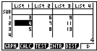
- Press F6(▷)F3(DEL) to delete the selected cell and cause everything below it to be shifted up.


# The cell delete operation does not affect cells in other lists. If the data in the list whose cell you delete is somehow related to the data in
neighboring lists, deleting a cell can cause related values to become misaligned.

- To delete all cells in a list
Use the following procedure to delete all the data in a list.
- Use the cursor key to move the highlighting to any cell of the list whose data you want to delete.
- Pressing F6(▷)F4(DEL•A) causes a confirmation message to appear.
- Press F1 (Yes) to delete all the cells in the selected list or F6 (No) to abort the delete operation without deleting anything.
- To insert a new cell
- Use the cursor keys to move the highlighting to the location where you want to insert the new cell.
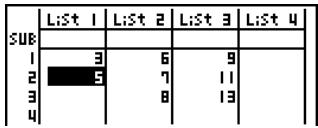
- Press 6 (▷) 5 (INS) to insert a new cell, which contains a value of 0, causing everything below it to be shifted down.
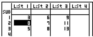
other
| | List 1 | List 2 | List 3 | List 4 | |---|---|---|---|---| | SUB | | | | | | 1 | 3 | 6 | 9 | | | 2 | 0 | 7 | 11 | | | 3 | 5 | 8 | 13 | | | 4 | | | | |
# The cell insert operation does not affect cells in other lists. If the data in the list where you insert a cell is somehow related to the data in
neighboring lists, inserting a cell can cause related values to become misaligned.

■ Naming a List
You can assign List 1 through List 26 "sub names" of up to eight bytes each.
- To name a list
- On the Setup screen, highlight "Sub Name" and then press F1 (On) EXIT.
- Use the cursor keys to move the highlighting to the SUB cell of the list you want to name.
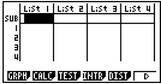
- Type in the name and then press EXE.
- To type in a name using alpha characters, press SHIFT ALPHA to enter the ALPHA-LOCK mode.
Example: YEAR

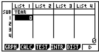
- The following operation displays a sub name in the RUN•MAT mode.

(n = list number from 1 to 26)
![List 1[0] YEAR MMT](/content/2025/01/86785/images/a429d06e7a73661048661898545c3d601b2dbd56e3fcb604fb5a88129758ec3a.jpg)

# Though you can input up to 8 bytes for the sub name, only the characters that can fit within the List Editor cell will be displayed.
# The List Editor SUB cell is not displayed when "Off" is selected for "Sub Name" on the Setup screen.

■ Sorting List Values
You can sort lists into either ascending or descending order. The highlighting can be located in any cell of the list.
- To sort a single list
Ascending order
- While the lists are on the screen, press F6(▷)F1(TOOL)F1(SRT•A).
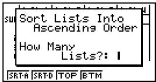
- The prompt "How Many Lists?:" appears to ask how many lists you want to sort. Here we will input 1 to indicate we want to sort only one list.
1 EXE
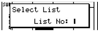
- In response to the "Select List List No." prompt, input the number of the list you want to sort.
1 EXE
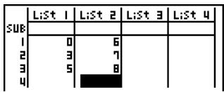
Descending order
Use the same procedure as that for the ascending order sort. The only difference is that you should press F2(SRT•D) in place of F1(SRT•A).

- To sort multiple lists
You can link multiple lists together for a sort so that all of their cells are rearranged in accordance with the sorting of a base list. The base list is sorted into either ascending order or descending order, while the cells of the linked lists are arranged so that the relative relationship of all the rows is maintained.
Ascending order
- While the lists are on the screen, press F6 (▷) F1 (TOOL) F1 (SRT•A).

- The prompt "How Many Lists?:" appears to ask how many lists you want to sort. Here we will sort one base list linked to one other list, so we should input 2.
2 EXE
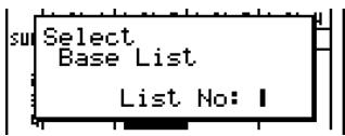
- In response to the "Select Base List List No:" prompt, input the number of the list you want to sort into ascending order. Here we will specify List 1.
1 EXE
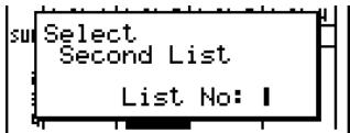
- In response to the "Select Second List List No:" prompt, input the number of the list you want to link to the base list. Here we will specify List 2.
2 EXE
| SUB | Li:St 1 | Li:St 2 | Li:St 3 | Li:St 4 |
| 1 | 0 | 7 | ||
| 2 | 3 | 6 | ||
| 3 | 5 | 8 | ||
| 4 |

Descending order
Use the same procedure as that for the ascending order sort. The only difference is that you should press F2(SRT•D) in place of F1(SRT•A).

# You can specify a value from 1 to 6 as the number of lists for sorting.
# If you specify a list more than once for a single sort operation, an error occurs.
An error also occurs if lists specified for sorting do not have the same number of values (rows).

3-2 Manipulating List Data
List data can be used in arithmetic and function calculations. In addition, various list data manipulation functions make manipulation of list data quick and easy.
You can use list data manipulation functions in the RUN·MAT, STAT, TABLE, EQUA and PRGM modes.
■ Accessing the List Data Manipulation Function Menu
All of the following examples are performed after entering the RUN·MAT mode.
Press OPTN and then F1(LIST) to display the list data manipulation menu, which contains the following items.
- {List}/{L→M}/{Dim}/{Fill}/{Seq}/{Min}/{Max}/{Mean}/{Med}/{Aug}/{Sum}/{Prod}/{Cuml}/{%}/{∆}
Note that all closing parentheses at the end of the following operations can be omitted.
- To transfer list contents to Matrix Answer Memory
[OPTN]-[LIST]-[L→M]
OPTN F1 (LIST) F2 (L→M) F1 (List)
F1(List) ... F1(List)
EXE
- You can skip input F1(List) in the part of the above operation.
- All the lists must contain the same number of data items. If they don't, an error occurs.
Example: List → Mat (1, 2) EXE
● ● ● ● ●
Example
To transfer the contents of List 1 (2, 3, 6, 5, 4) to column 1, and the contents of List 2 (11, 12, 13, 14, 15) to column 2 of Matrix Answer Memory
AC OPTN F1 (LIST) F2 (L→M)
F1 (List) 1 ,
F1 (List) 2 ) EXE
![AnS 1 2 1 [2 11] 2 3 12 3 6 13 4 5 14 5 4 15](/content/2025/01/86785/images/df9146214f356bca01ccf1183ac079733ba66221d11b4525de0943d4847ef6a0.jpg)
- To count the number of data items in a list
[OPTN]-[LIST]-[Dim]
OPTN F1 (LIST) F3 (Dim) F1 (List) EXE
- The number of cells a list contains its “dimension.”
● ● ● ● ●
Example To count the number of values in List 1 (36, 16, 58, 46, 56)
AC OPTN F1 (LIST) F3 (Dim)
F1 (List) 1 EXE
Dim List 1 5
- To create a list or matrix by specifying the number of data items
[OPTN]-[LIST]-[Dim]
Use the following procedure to specify the number of data in the assignment statement and create a list.
EXE
$$ n = 1 - 9 9 9 $$
● ● ● ● ●
Example To create five data items (each of which contains 0) in List 1
AC 5 → OPTN F1 (LIST) F3 (Dim)
F1 (List) 1 EXE
You can view the newly created list by entering the STAT mode.
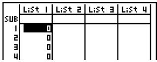
Use the following procedure to specify the number of data rows and columns, and the matrix name in the assignment statement and create a matrix.
SHIFT ✗ ( { )
OPTN F1 (LIST) F3 (Dim) OPTN F2 (MAT) F1 (Mat) ALPHA
m, n = 1 - 255, matrix name: A - Z


Example
To create a 2-row × 3-column matrix (each cell of which contains 0) in Matrix A


The following shows the new contents of Mat A.
![A 1 2 3 1 [0 0 0] 2 [0 0 0]](/content/2025/01/86785/images/8fd1e95d42dc14bf01f7dee3374dad6aabc1ccaa4ad8d133d6fba31e322691c4.jpg)
- To replace all data items with the same value
[OPTN]-[LIST]-[Fill]
OPTN F1 (LIST) F4 (Fill) EXE

Example
To replace all data items in List 1 with the number 3
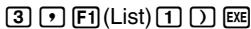
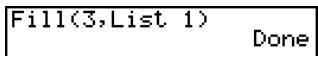
The following shows the new contents of List 1.

- To generate a sequence of numbers
[OPTN]-[LIST]-[Seq]
OPTN F1 (LIST) F5 (Seq)

- The result of this operation is stored in ListAns Memory.

Example
To input the number sequence 1^2 , 6^2 , 11^2 , into a list, using the function f(x) = X^2 . Use a starting value of 1, an ending value of 11, and an increment of 5


![AnS 1 [ ] 1 2 [ ] 36 3 [ ] 121](/content/2025/01/86785/images/7bce96418ef8ef6d226cc967f1b9e2b632ec65b25b7fcad69133ad65d716da86.jpg)
Specifying an ending value of 12, 13, 14, or 15 produces the same result as shown above, because all of them are less than the value produced by the next increment (16).

- To find the minimum value in a list
[OPTN]-[LIST]-[Min]
OPTN F1 (LIST) F6 (▷) F1 (Min) F6 (▷) F6 (▷) F1 (List) ☐ EXE

Example To find the minimum value in List 1 (36, 16, 58, 46, 56)
AC OPTN F1 (LIST) F6 (▷) F1 (Min)
Min(List 1) 16
F6 (▷) F6 (▷) F1 (List) 1 ) EXE
- To find the maximum value in a list
[OPTN]-[LIST]-[Max]
Use the same procedure as when finding the minimum value (Min), except press F6(▷)F2(Max) in place of F6(▷)F1(Min).
- To find which of two lists contains the smallest value
[OPTN]-[LIST]-[Min]
OPTN F1 (LIST) F6 (▷) F1 (Min) F6 (▷) F6 (▷) F1 (List)
F1 (List) EXE
- The two lists must contain the same number of data items. If they don't, an error occurs.
- The result of this operation is stored in ListAns Memory.

Example To find whether List 1 (75, 16, 98, 46, 56) or List 2 (35, 59, 58, 72, 67) contains the smallest value
OPTN F1 (LIST) F6 (▷) F1 (Min)
F6 (▷) F6 (▷) F1 (List) 1
F1 (List) 2 ) EXE
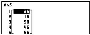
- To find which of two lists contains the greatest value
[OPTN]-[LIST]-[Max]
Use the same procedure as that for the smallest value, except press F6(▷)F2(Max) in place of F6(▷)F1(Min).
- The two lists must contain the same number of data items. If they don't, an error occurs.
- The result of this operation is stored in ListAns Memory.

- To calculate the mean of data items
[OPTN]-[LIST]-[Mean]
OPTN F1 (LIST) F6 (▷) F3 (Mean) F6 (▷) F6 (▷) F1 (List) ) EXE

Example To calculate the mean of data items in List 1 (36, 16, 58, 46, 56)
AC OPTN F1 (LIST) F6 (▷) F3 (Mean)
F6 (▷) F6 (▷) F1 (List) 1 ) EXE
Mean(List 1) 42.4
- To calculate the mean of data items of specified frequency
[OPTN]-[LIST]-[Mean]
This procedure uses two lists: one that contains values and one that indicates the frequency (number of occurrences) of each value. The frequency of the data in Cell 1 of the first list is indicated by the value in Cell 1 of the second list, etc.
- The two lists must contain the same number of data items. If they don't, an error occurs.
OPTN F1 (LIST) F6 (▷) F3 (Mean) F6 (▷) F6 (▷) F1 (List)
F1 (List) EXE

Example To calculate the mean of data items in List 1 (36, 16, 58, 46, 56), whose frequency is indicated by List 2 (75, 89, 98, 72, 67)
AC OPTN F1 (LIST) F6 (▷) F3 (Mean)
F6 (▷) F6 (▷) F1 (List) 1
F1 (List) 2 ) EXE
Mean(List 1, List 2) 42.07481297
- To calculate the median of data items in a list
[OPTN]-[LIST]-[Med]
OPTN F1 (LIST) F6 (▷) F4 (Med) F6 (▷) F6 (▷) F1 (List)
) EXE

Example To calculate the median of data items in List 1 (36, 16, 58, 46, 56)
AC OPTN F1 (LIST) F6 (▷) F4 (Med)
F6 (▷) F6 (▷) F1 (List) 1 ) EXE
Median(List 1) 46

- To calculate the median of data items of specified frequency
[OPTN]-[LIST]-[Med]
This procedure uses two lists: one that contains values and one that indicates the frequency (number of occurrences) of each value. The frequency of the data in Cell 1 of the first list is indicated by the value in Cell 1 of the second list, etc.
- The two lists must contain the same number of data items. If they don't, an error occurs.
OPTN F1 (LIST) F6 (▷) F4 (Med) F6 (▷) F6 (▷) F1 (List)
F1 (List) EXE

Example
To calculate the median of values in List 1 (36, 16, 58, 46, 56), whose frequency is indicated by List 2 (75, 89, 98, 72, 67)
AC OPTN F1 (LIST) F6 (▷) F4 (Med)
F6 (▷) F6 (▷) F1 (List) 1
F1 (List) 2 ) EXE
Median(List 1, List 2) 46
- To combine lists
[OPTN]-[LIST]-[Aug]
- You can combine two different lists into a single list. The result of a list combination operation is stored in ListAns memory.
OPTN F1 (LIST) F6 (▷) F5 (Aug) F6 (▷) F6 (▷) F1 (List)
F1 (List) EXE

Example To combine the List 1 (-3, -2) and List 2 (1, 9, 10)
AC OPTN F1 (LIST) F6 (▷) F5 (Aug)
F6 (▷) F6 (▷) F1 (List) 1
F1 (List) 2 ) EXE
![AnS 1 [3] 2 -2 3 1 4 9 5 10](/content/2025/01/86785/images/878abecb479c06efdffb887484886a33e6223028f59e0042aced4a9c53ce3608.jpg)
- To calculate the sum of data items in a list
[OPTN]-[LIST]-[Sum]
OPTN F1 (LIST) F6 (▷) F6 (▷) F1 (Sum) F6 (▷) F1 (List) EXE

Example To calculate the sum of data items in List 1 (36, 16, 58, 46, 56)
AC OPTN F1 (LIST) F6 (▷) F6 (▷) F1 (Sum)
F6 (▷) F1 (List) 1 EXE
Sum List 1 212

- To calculate the product of values in a list
[OPTN]-[LIST]-[Prod]
OPTN F1 (LIST) F6 (▷) F6 (▷) F2 (Prod) F6 (▷) F1 (List) EXE

Example To calculate the product of values in List 1 (2, 3, 6, 5, 4)
AC OPTN F1 (LIST) F6 (▷) F6 (▷) F2 (Prod)
Prod List 1 720
F6 (▷) F1 (List) 1 EXE
- To calculate the cumulative frequency of each data item
[OPTN]-[LIST]-[Cuml]
OPTN F1 (LIST) F6 (▷) F6 (▷) F3 (Cuml) F6 (▷) F1 (List) EXE
- The result of this operation is stored in ListAns Memory.

Example To calculate the cumulative frequency of each data item in List 1 (2, 3, 6, 5, 4)
AC OPTN F1 (LIST) F6 (▷) F6 (▷) F3 (Cuml)
F6 (▷) F1 (List) 1 EXE
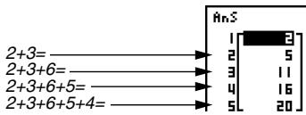
- To calculate the percentage represented by each data item
[OPTN]-[LIST]-[%]
OPTN F1 (LIST) F6 (▷) F6 (▷) F4 (%) F6 (▷) F1 (List) EXE
- The above operation calculates what percentage of the list total is represented by each data item.
- The result of this operation is stored in ListAns Memory.


Example
To calculate the percentage represented by each data item in List 1 (2, 3, 6, 5, 4)
AC OPTN F1 (LIST) F6 (▷) F6 (▷) F4 (%)
F6 (▷) F1 (List) 1 EXE
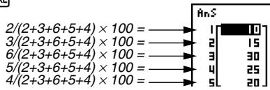
- To calculate the differences between neighboring data inside a list
[OPTN]-[LIST]-[Δ]
OPTN F1 (LIST) F6 (▷) F6 (▷) F5 (△) EXE
- The result of this operation is stored in ListAns memory.

Example To calculate the difference between the data items in List 1 (1, 3, 8, 5, 4)
AC OPTN F1 (LIST) F6 (▷) F6 (▷) F5 (△)
1 EXE
![(2) 3 - 1 = ————→ 8 - 3 = ————→ 5 - 8 = ————→ 4 - 5 = ————→ AnS 1 [■] 2 2 [■] 5 3 [■] -3 4 [■] -1](/content/2025/01/86785/images/aa76b0a6de6e64a2223509b6c15c313bfcf1669a79672519572dc689942cdb46.jpg)

# You can specify the storage location in list memory for a calculation result produced by a list calculation whose result is stored in ListAns memory. For example, specifying “ List 1 → List 2” will store the result of List 1 in List 2.
# The number of cells in the new List is one less than the number of cells in the original list.
# An error occurs if you execute List for a list that has no data or only one data item.

3-3 Arithmetic Calculations Using Lists
You can perform arithmetic calculations using two lists or one list and a numeric value.
flowchart
graph LR
    A["List Numeric Value"] --> B["+/-"]
    B --> C["List Numeric Value"]
    C --> D["="]
    D --> E["List Ans Memory"]
    E --> F["Calculation results are stored in ListAns Memory"]
■ Error Messages
- A calculation involving two lists performs the operation between corresponding cells. Because of this, an error occurs if the two lists do not have the same number of values (which means they have different “dimensions”).
- An error occurs whenever an operation involving any two cells generates a mathematical error.
■ Inputting a List into a Calculation
There are two methods you can use to input a list into a calculation.
- To input a specific list by name
- Press OPTN to display the first Operation Menu.
- This is the function key menu that appears in the RUN·MAT mode when you press OPTN.
- Press F1(LIST) to display the List Data Manipulation Menu.
- Press F1(List) to display the "List" command and input the number of the list you want to specify.

- To directly input a list of values
You can also directly input a list of values using {,}, and ☐.

Example 1 To input the list: 56, 82, 64

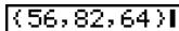
Example 2 To multiply List 3 ( = 41 65 22 ) by the list [ 6 0 4 ]

The resulting list 246 0 88 is stored in ListAns Memory.
- To assign the contents of one list to another list
Use to assign the contents of one list to another list.

Example 1 To assign the contents of List 3 to List 1

In place of OPTN F1 (LIST) F1 (List) 3 operation in the above procedure, you could input SHIFT X ( { } 4 1 6 5 2 2 SHIFT ÷ ( }).

Example 2 To assign the list in ListAns Memory to List 1


- To recall the value in a specific list cell
You can recall the value in a specific list cell and use it in a calculation. Specify the cell number by enclosing it inside square brackets.

Example
To calculate the sine of the value stored in Cell 3 of List 2
sin OPTN F1 (LIST) F1 (List) 2 SHIFT + ( ) 3 SHIFT - ( ) EXE
- To input a value into a specific list cell
You can input a value into a specific list cell inside a list. When you do, the value that was previously stored in the cell is replaced with the new value you input.

Example
To input the value 25 into Cell 2 of List 3
2 5 → OPTN F1 (LIST) F1 (List) 3 SHIFT + ( [ ) 2 SHIFT - ( ) EXE
■ Recalling List Contents

Example
To recall the contents of List 1
OPTN F1 (LIST) F1 (List) 1 EXE
- The above operation displays the contents of the list you specify and also stores them in ListAns Memory. You can then use the ListAns Memory contents in a calculation.
- To use list contents in ListAns Memory in a calculation

Example
To multiply the list contents in ListAns Memory by 36
OPTN F1 (LIST) F1 (List) SHIFT (-) (Ans) ✗ 3 6 EXE
- The operation OPTN F1(LIST) F1(List) SHIFT (-)(Ans) recalls ListAns Memory contents.
- This operation replaces current ListAns Memory contents with the result of the above calculation.

■ Graphing a Function Using a List
When using the graphing functions of this calculator, you can input a function such as Y1 = List 1 X. If List 1 contains the values 1, 2, 3, this function will produce three graphs: Y = X, Y = 2X, Y = 3X.
There are certain limitations on using lists with graphing functions.

Example To input the data 1, 2, 3 into List 1, and then graph the data in the GRAPH mode
- In the STAT mode, input 1, 2, 3 into List 1.
- In the GRAPH mode, input the formula Y1=List 1X.
OPTN F1 (List) 1 X,θ,T EXE
- Graph the data, which will produce three graphs.
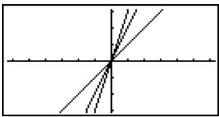
natural_image
Pure geometric lines intersecting at the origin (no text or symbols)■ Inputting Scientific Calculations into a List
You can use the numeric table generation functions in the TABLE mode to input values that result from certain scientific function calculations into a list. To do this, first generate a table and then use the list copy function to copy the values from the table to the list.

Example To use the TABLE mode to create a number table for the formula (Y1 = x^2-1 ), and then copy the table to List 1 in the STAT mode
- In the TABLE mode, input the formula Y1 = x^2 - 1 .
-
Create the number table.
-
Use ▶ to move the highlighting to the Y1 column.
-
Press OPTN F1 (LMEM).
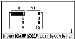
![Store In List Memory List[1~26]: 1 0 MEN ENG ENG](/content/2025/01/86785/images/256c016c4e356e28d30561e61e5484e783b12487cdeab36c2a7088964cf15ea2.jpg)

- Press 1 EXE.
- Enter the STAT mode to confirm that TABLE mode column Y1 has been copied to List 1.
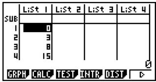
■ Performing Scientific Function Calculations Using a List
Lists can be used just as numeric values are in scientific function calculations. When the calculation produces a list as a result, the list is stored in ListAns Memory.
Example To use List 3 [ 41 65 22 ] to perform sin (List 3)
Use radians as the angle unit.
sin OPTN F1 (LIST) F1 (List) 3 EXE
The resulting list [ -0.158 0.8268 -8E - 3 ] is stored in ListAns Memory.
In place of the OPTN F1 (LIST) F1 (List) 3 operation in the above procedure, you could input SHIFT X ( { ) 4 1 , 6 5 , 2 2 SHIFT ÷ ( } ).
Example To use List 1 [ 1 2 3 ] and List 2 [ 4 5 6 ] to perform List 1^List 2
This creates a list with the results of 1^4 , 2^5 , 3^6 .
OPTN F1 (LIST) F1 (List) 1 ∧ F1 (List) 2 EXE
The resulting list 1 32 729 is stored in ListAns Memory.

3-4 Switching Between List Files
You can store up to 26 lists (List 1 to List 26) in each file (File 1 to File 6). A simple operation lets you switch between list files.
- To switch between list files
- From the Main Menu, enter the STAT mode.
Press SHIFT MENU (SET UP) to display the STAT mode Setup screen.
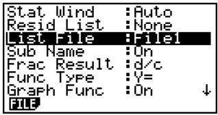
- Use ▼ to highlight "List File".
- Press F1(FILE) and then input the number of the list file you want to use.

Example To select File 3
F1(FILE)3
![Rg Select List News Select File No. File[1~6]: 31](/content/2025/01/86785/images/2010071a1e1a1610db9b9a9352864d6b6458926196beaf6a1fe6e506634d9180.jpg)


All subsequent list operations are applied to the lists contained in the file you select (List File 3 in the above example).

Chapter
4
4
Equation Calculations
Your graphic calculator can perform the following three types of calculations:
- Simultaneous linear equations
• Quadratic and cubic equations - Solve calculations
From the Main Menu, enter the EQUA mode.
- {SIML} ... {linear equation with 2 to 6 unknowns}
• {POLY} ... {degree 2 or 3 equation} - {SOLV} ... {solve calculation}
Equation
Select Type
F1: Simultaneous
F2:Polynomial
F3: Solver
SIML POLY SOLU
4-1 Simultaneous Linear Equations
4-2 Quadratic and Cubic Equations
4-3 Solve Calculations
4-4 What to Do When an Error Occurs
4-1 Simultaneous Linear Equations
Description
You can solve simultaneous linear equations with two to six unknowns.
- Simultaneous Linear Equation with Two Unknowns:
$$ a _ {1} x _ {1} + b _ {1} x _ {2} = c _ {1} $$
$$ a _ {2} x _ {1} + b _ {2} x _ {2} = c _ {2} $$
- Simultaneous Linear Equation with Three Unknowns:
$$ a _ {1} x _ {1} + b _ {1} x _ {2} + c _ {1} x _ {3} = d _ {1} $$
$$ a _ {2} x _ {1} + b _ {2} x _ {2} + c _ {2} x _ {3} = d _ {2} $$
$$ \begin{array}{c} a _ {3} x _ {1} + b _ {3} x _ {2} + c _ {3} x _ {3} = d _ {3} \ \vdots \end{array} $$
Set Up
- From the Main Menu, enter the EQUA mode.
Execution
- Select the SIML (simultaneous equation) mode, and specify the number of unknowns (variables).
You can specify from 2 to 6 unknowns.
- Sequentially input the coefficients.
The cell that is currently selected for input is highlighted. Each time you input a coefficient, the highlighting shifts in the sequence:
$$ a _ {1} \rightarrow b _ {1} \rightarrow c _ {1} \rightarrow \dots a n \rightarrow b n \rightarrow c n \rightarrow (n = 2 \text { to } 6) $$
You can also input fractions and values assigned to variables as coefficients.
You can cancel the value you are inputting for the current coefficient by pressing EXIT at any time before you press EXE to store the coefficient value. This returns to the coefficient to what it was before you input anything. You can then input another value if you want.
To change the value of a coefficient that you already stored by pressing EXE, move the cursor to the coefficient you want to edit. Next, input the value you want to change to.
Pressing F3 (CLR) clears all coefficients to zero.
- Solve the equations.


Example To solve the following simultaneous linear equations for x, y , and z
$$ 4 x + y - 2 z = - 1 $$
$$ x + 6 y + 3 z = 1 $$
$$ - 5 x + 4 y + z = - 7 $$
Procedure
① MENU EQUA
② F1(SIML)
F2 (3)
Internal calculations are performed using a 15-digit mantissa, but results are displayed using a 10-digit mantissa and a 2-digit exponent.
Simultaneous linear equations are solved by inverting the matrix containing the coefficients of the equations. For example, the following shows the solution (x_1, x_2, x_3) of a simultaneous linear equation with three unknowns.
$$ \left[ \begin{array}{c} x _ {1} \ x _ {2} \ x _ {3} \end{array} \right] = \left[ \begin{array}{c c c} a _ {1} & b _ {1} & c _ {1} \ a _ {2} & b _ {2} & c _ {2} \ a _ {3} & b _ {3} & c _ {3} \end{array} \right] ^ {- 1} \left[ \begin{array}{c} d _ {1} \ d _ {2} \ d _ {3} \end{array} \right] $$
Because of this, precision is reduced as the value of the determinant approaches zero. Also, simultaneous equations with three or more unknowns may take a very long time to solve.
An error occurs if the calculator is unable to find a solution.
After calculation is complete, you can press F1 (REPT), change coefficient values, and then re-calculate.

4-2 Quadratic and Cubic Equations
Description
You can use this calculator to solve quadratic equations and cubic equations.
- Quadratic Equation:
$$ a x ^ {2} + b x + c = 0 (a \neq 0) $$
- Cubic Equation:
$$ a x ^ {3} + b x ^ {2} + c x + d = 0 (a \neq 0) $$
Set Up
- From the Main Menu, enter the EQUA mode.
Execution
-
Select the POLY (higher degree equation) mode, and specify the degree of the equation.
You can specify a degree 2 or 3. -
Sequentially input the coefficients.
The cell that is currently selected for input is highlighted. Each time you input a coefficient, the highlighting shifts in the sequence:
$$ a \rightarrow b \rightarrow c \rightarrow \dots $$
You can also input fractions and values assigned to variables as coefficients.
You can cancel the value you are inputting for the current coefficient by pressing EXIT at any time before you press EXE to store the coefficient value. This returns to the coefficient to what it was before you input anything. You can then input another value if you want.
To change the value of a coefficient that you already stored by pressing EXE, move the cursor to the coefficient you want to edit. Next, input the value you want to change to.
Pressing F3 (CLR) clears all coefficients to zero.
- Solve the equations.

# Internal calculations are performed using a 15-digit mantissa, but results are displayed using a 10-digit mantissa and a 2-digit exponent.
# It may take considerable time for the calculation result of cubic equations to appear on the display.
# An error occurs if the calculator is unable to find a solution.
# After calculation is complete, you can press F1(REPT), change coefficient values, and then re-calculate.
# An error occurs if the calculator is unable to find a solution.
After calculation is complete, you can press F1(REPT), change coefficient values, and then re-calculate.


Example To solve the cubic equation (Angle unit = Rad)
$$ x ^ {3} - 2 x ^ {2} - x + 2 = 0 $$
Procedure
① MENU EQUA
② F2(POLY)
F2 (3)
Complex Mode: Real (page 1-7-2)
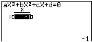
Complex Mode: a + bi
![aX³+bX²+cX+d=0 X 1[-0.5+1.3228i] 2[-0.5-1.3228i] 3[-1] -1,2+1.322875656i](/content/2025/01/86785/images/33ff4de4cfaf6af6e1b5452578c3bd0f4c5d0750881b26241eae174a7d394f87.jpg)
Complex Mode: r
![aX³+bX²+cX+d=0 x 1[1.4142-1.932] 2[1.4142-1.932] 3[1.43.1415] 1.414213562 ∠1.932163451](/content/2025/01/86785/images/d46cee968957437e0f44145b5258698e811c427475a19c797fff06a6a6fbbd7d.jpg)

4-3 Solve Calculations
Description
The Solve Calculation mode lets you determine the value of any variable in a formula without having to solve the equation.
Set Up
- From the Main Menu, enter the EQUA mode.
Execution
- Select the Solve Calculation mode, and input the equation as it is written. If you do not input an equals sign, the calculator assumes that the expression is to the left of the equals sign, and there is a zero to the right. *^1
- In the table of variables that appears on the display, input values for each variable. You can also specify values for Upper and Lower to define the upper and lower limits of the range of solutions. *^2
- Select the variable for which you want to solve to obtain the solution. “Lft” and “Rgt” indicate the left and right sides that are calculated using the solution. ^*3

*1 An error occurs if you input more than one equals sign.
*2 An error occurs if the solution falls outside the range you specify.
*3 Solutions are approximated using Newton's method. Lft and Rgt values are displayed for confirmation, because Newton's method may produce results that are the real solution.
The closer the difference between the Lft and Rgt values is to zero, the lower degree of error in the result.
# The message “Retry” appears on the display when the calculator judges that convergence is not sufficient for the displayed results.


Example
An object thrown into the air at initial velocity V takes time T to reach height H. Use the following formula to solve for initial velocity V when H = 14 (meters), T = 2 (seconds) and gravitational acceleration is G = 9.8 (m/s ^2 ).
$$ \mathrm{H} = \mathrm{VT} - 1 / 2 \mathrm{GT} ^ {2} $$
Procedure
① MENU EQUA
② F3(SOLV)
ALPHA F→D (H) SHIFT (=) ALPHA 2 (V) ALPHA ÷ (T) — (1 ÷ 2 )
ALPHA a^b/_c(G) ALPHA ÷(T)x^2 EXE
③ 1 4 EXE (H = 14)
0 EXE (V = 0)
2 EXE (T = 2)
9 • 8 EXE (G = 9.8)
④ Press ▲▲▲ to highlight V = 0, and then press F6(SOLV).
Result Screen
Eq:H=VT-(1÷2)GT ^2 V=16.8 Lft=14 Rst=14 REPT

4-4 What to Do When an Error Occurs
- Error during coefficient value input
Press the EXIT key to clear the error and return to the value that was registered for the coefficient before you input the value that generated the error. Try inputting a new value again.
- Error during calculation
Press the EXIT key to clear the error and display the coefficient. Try inputting values for the coefficients again.
■ Clearing Equation Memories
-
Enter the equation calculation mode (SIML or POLY) you want to use and perform the function key operation required for that mode.
-
In the case of the SIML mode (F1), use the function keys to specify the number of unknowns.
- In the case of the POLY mode (F2), use the function keys to specify the degree of the polynomial.
-
If you pressed F3(SOLV), advance directly to step 2.
-
Press F2 (DEL).
-
Press F1 (Yes) to delete the applicable equation memories or F6 (No) to abort the operation without deleting anything.

Chapter 5
5
Graphing
Sections 5-1 and 5-2 of this chapter provide basic information you need to know in order to draw a graph. The remaining sections describe more advanced graphing features and functions.
Select the icon in the Main Menu that suits the type of graph you want to draw or the type of table you want to generate.
• GRAPH ... General function graphing
- CONICS ... Conic section graphing (5-1-5 \~ 5-1-6, 5-11-17\~5-11-22)
- RUN·MAT ... Manual graphing (5-6-1 \~ 5-6-4)
- TABLE ... Number table generation (5-7-1 \~ 5-7-16)
• DYNA ... Dynamic Graph (5-8-1 \~ 5-8-8)
- RECUR ... Recursion graphing or number table generation (5-9-1 \~ 5-9-10)
5-1 Sample Graphs
5-2 Controlling What Appears on a Graph Screen
5-3 Drawing a Graph
5-4 Storing a Graph in Picture Memory
5-5 Drawing Two Graphs on the Same Screen
5-6 Manual Graphing
5-7 Using Tables
5-8 Dynamic Graphing
5-9 Graphing a Recursion Formula
5-10 Changing the Appearance of a Graph
5-11 Function Analysis
5-1 Sample Graphs
■ How to draw a simple graph (1)
Description
To draw a graph, simply input the applicable function.
Set Up
- From the Main Menu, enter the GRAPH mode.
Execution
- Input the function you want to graph.
Here you would use the V-Window to specify the range and other parameters of the graph. See 5-2-1. - Draw the graph.


Example
To graph y = 3x^2
Procedure
① MENU GRAPH
② 3 X,θ,T x^2 EXE
③ F6 (DRAW) (or EXE)
Result Screen
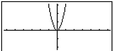
natural_image
Simple geometric diagram showing a vertical line intersecting a horizontal axis, with two curved lines forming a V-shape (no text or labels)
# Pressing AC while a graph is on the display will return to the screen in step 2.

■ How to draw a simple graph (2)
Description
You can store up to 20 functions in memory and then select the one you want for graphing.
Set Up
- From the Main Menu, enter the GRAPH mode.
Execution
- Specify the function type and input the function whose graph you want to draw.
You can use the GRAPH mode to draw a graph for the following types of expressions: rectangular coordinate expression, polar coordinate expression, parametric function, X = constant expression, inequality.
F3(TYPE) F1(Y=)... rectangular coordinates
F2 (r=) ... polar coordinates
F3(Parm) ... parametric function
F4 (X=c) ... X = constant function
F5(CONV) F1(▶Y=)\~ F5(▶Y≤) ... changes the function type
F6 (▷) F1 (Y>)\~ F4 (Y≤) ... inequality
Repeat this step as many times as required to input all of the functions you want.
Next you should specify which of the functions among those that are stored in memory you want to graph (see 5-3-6). If you do not select specific functions here, the graph operation will draw graphs of all the functions currently stored in memory.
- Draw the graph.


Example
Input the functions shown below and draw their graphs
$$ \mathbf {Y} 1 = 2 x ^ {2} - 3, r 2 = 3 \sin 2 \theta $$
Procedure
① MENU GRAPH
② F3 (TYPE) F1 (Y=) 2 X,θ,T x² - 3 EXE
$$ \boxed {\mathsf {F 3}} (\text { TYPE }) \boxed {\mathsf {F 2}} (r =) \boxed {3} \boxed {\sin} \boxed {2} \boxed {\mathsf {X}, \theta , \mathsf {T}} \boxed {\mathsf {E X E}} $$
③ F6 (DRAW)
Result Screen
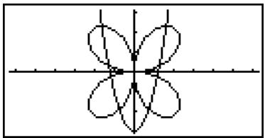
natural_image
Symmetrical abstract line drawing with four petal-like lobes and intersecting axes (no text or symbols)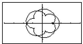
natural_image
Pure geometric diagram with intersecting lines and a central circle (no text or symbols)(Parametric)
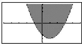
natural_image
Simple geometric diagram showing a shaded semicircle with a vertical axis and horizontal line (no text or symbols)(Inequality)

■ How to draw a simple graph (3)
Description
Use the following procedure to graph the function of a parabola, circle, ellipse, or hyperbola.
Set Up
- From the Main Menu, enter the CONICS mode.
Execution
- Use the cursor ▲▼ keys to specify one of the function type as follows.
| Graph Type | Function |
| Parabola | X = A (Y - K)^2 + H X = A Y^2 + B Y + C Y = A (X - H)^2 + K Y = A X^2 + B X + C |
| Circle | (X - H)^2 + (Y - K)^2 = R^2 A X^2 + A Y^2 + B X + C Y + D = 0 |
| Ellipse | (X - H)^2A^2 + (Y - K)^2B^2 = 1 |
| Hyperbola | (X - H)^2A^2 - (Y - K)^2B^2 = 1 (Y - K)^2A^2 - (X - H)^2B^2 = 1 |
- Input values for the required variables.
- Graph the function.


Example
Graph the circle (X - 1)^2 + (Y - 1)^2 = 2^2
Procedure
① MENU CONICS
② ▼ ▼ ▼ ▼ EXE
③ 1 EXE 1 EXE 2 EXE
④ F6 (DRAW)
Result Screen
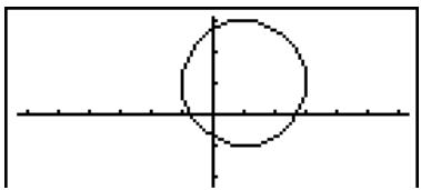
natural_image
Simple geometric diagram with a circle intersected by perpendicular lines (no text or labels)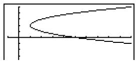
natural_image
Pure mathematical curve diagram without any text, numbers, or symbols(Parabola)
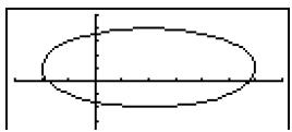
natural_image
Pure geometric diagram showing an ellipse with intersecting lines and a vertical axis (no text or symbols)(Ellipse)
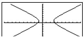
natural_image
Pure geometric line drawing of a hyperbola with intersecting curves and vertical dashed lines (no text or symbols)(Hyperbola)

■ How to draw a simple graph (4)
Description
You can specify the graph line style, if you want.
Set Up
- From the Main Menu, enter the GRAPH mode.
Execution
-
Input the function you want to graph. Here you would use the V-Window to specify the range and other parameters of the graph. See 5-2-1.
-
Select the line style. F4(STYL) F1(—) ... Normal (initial default) F2(—) ... Thick (twice the thickness of Normal) F3(……) ... Broken (thick broken) F4(……) ... Dot (dotted)
-
Draw the graph.
The line style selection is valid only when “Connect” is selected for “Draw Type” on the Setup screen.

# The initial default line setting for an inequality (Y>, Y<) is dot plot type.
# You can change the graph line style while in the GRAPH, TABLE or RECUR mode.


Example
To graph y = 3x^2
Procedure
① MENU GRAPH
② F3 (TYPE) F1 (Y=) 3 X,θ,T x² EXE
③ ▲ F4 (STYL) F3 (……) EXIT
④ F6 (DRAW) (or EXE)
Result Screen
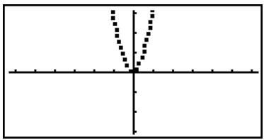
line
| X | Y | |---|---| | -3.0 | 1.0 | | -2.5 | 0.8 | | -2.0 | 0.6 | | -1.5 | 0.4 | | -1.0 | 0.2 | | -0.5 | 0.1 | | 0.0 | 0.0 | | 0.5 | 0.1 | | 1.0 | 0.2 | | 1.5 | 0.4 | | 2.0 | 0.6 | | 2.5 | 0.8 | | 3.0 | 1.0 |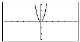
natural_image
Simple geometric diagram showing a vertical line intersecting a horizontal axis, with no text or symbols present.(Normal)
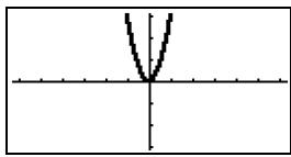
(Thick)
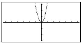
natural_image
Pure Cartesian coordinate system with dashed lines forming a V-shape (no labels or text)(Dotted)

5-2 Controlling What Appears on a Graph Screen
■ V-Window (View Window) Settings
Use the View Window to specify the range of the x- and y-axes, and to set the spacing between the increments on each axis. You should always set the V-Window parameters you want to use before graphing.
- To make V-Window settings
- From the Main Menu, enter the GRAPH mode.
- Press SHIFT F3 (V-WIN) to display the V-Window setting screen.
Rectangular coordinate parameter
Xmin ... Minimum x-axis value
Xmax ... Maximum x-axis value
Xscale ... Spacing of x-axis increments
Xdot ... Value that corresponds to one x
Ymin ... Minimum y-axis value
Ymax ... Maximum y-axis value
Yscale ... Spacing of y-axis increments
Polar coordinate parameter
Tθ min ... T, θ minimum values
Tθ max ... T, θ maximum values
Tθ pitch ... T, θ pitch
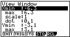
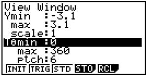
-
Press ▼ to move the highlighting and input an appropriate value for each parameter, pressing EXE after each.
-
{INIT}/{TRIG}/{STD} ... V-Window {initial settings}/{initial settings using specified angle unit}/{standardized settings}
- {STO}/{RCL} ... V-Window setting {store}/{recall}
After settings are the way you want them, press EXIT or SHIFT EXIT (QUIT) to exit the V-Window setting screen.*1

*1 Pressing EXE without inputting anything while
■ is displayed exits the V-Window setting screen.

• V-Window Setting Precautions
- Inputting zero for Tθ ptch causes an error.
- Any illegal input (out of range value, negative sign without a value, etc.) causes an error.
- When T max is less than T min, T ptch becomes negative.
- You can input expressions (such as 2 ) as V-Window parameters.
- When the V-Window setting produces an axis that does not fit on the display, the scale of the axis is indicated on the edge of the display closest to the origin.
- Changing the V-Window settings clears the graph currently on the display and replaces it with the new axes only.
- Changing the Xmin or Xmax value causes the Xdot value to be adjusted automatically. Changing the Xdot value causes the Xmax value to be adjusted automatically.
- A polar coordinate (r =) or parametric graph will appear coarse if the settings you make in the V-Window cause the T ptch value to be too large, relative to the differential between the T min and T max settings. If the settings you make cause the T ptch value to be too small relative to the differential between the T min and T max settings, on the other hand, the graph will take a very long time to draw.
- The following is the input range for V-Window parameters.
-9.9999999999E 97 to 9.9999999999E 97

■ Initializing and Standardizing the V-Window
- To initialize the V-Window
- From the Main Menu, enter the GRAPH mode.
- Press SHIFT F3 (V-WIN).
This displays the V-Window setting screen.
- Press F1(INIT) to initialize the V-Window.
$$ \mathrm{Xmin} = - 6. 3, \quad \mathrm{Xmax} = 6. 3, \quad \mathrm{Xscale} = 1, \quad \mathrm{Xdot} = 0. 1 $$
$$ \mathrm{Ymin} = - 3. 1, \quad \mathrm{Ymax} = 3. 1, \quad \text { Yscale } = 1 $$
$$ T \theta \min = 0, \quad T \theta \max = 2 \pi (\text { rad }), \quad T \theta \operatorname{ptch} = 2 \pi / 1 0 0 (\text { rad }) $$
- To initialize the V-Window in accordance with an angle unit
In step 3 of the procedure under “To initialize the V-Window” above, press F2 (TRIG) to initialize the V-Window in accordance with an angle unit.
$$ \text { Xmin } = - 3 \pi (\text { rad }), \quad \text { Xmax } = 3 \pi (\text { rad }), \quad \text { Xscale } = \pi / 2 (\text { rad }), \quad \text { Xdot } = \pi / 2 1 (\text { rad }), $$
$$ \mathrm{Ymin} = - 1. 6, \quad \mathrm{Ymax} = 1. 6, \quad \mathrm{Yscale} = 0. 5 $$
- To standardize the V-Window
The following are the standard V-Window settings of this calculator.
$$ \mathrm{Xmin} = - 1 0, \quad \mathrm{Xmax} = 1 0, \quad \mathrm{Xscale} = 1, \quad \mathrm{Xdot} = 0. 1 5 8 7 3 0 1 5 $$
$$ \mathrm{Ymin} = - 1 0, \quad \mathrm{Ymax} = 1 0, \quad \text { Yscale } = 1 $$
$$ T \theta \min = 0, \quad T \theta \max = 2 \pi (\text { rad }), \quad T \theta \operatorname{ptch} = 2 \pi / 1 0 0 (\text { rad }) $$
In step 3 of the procedure under “To initialize the V-Window” above, press F3(STD) to standardize V-Window settings in accordance with the above.

# Initialization and standardization cause T min, T max, T ptch values to change automatically in accordance with the current angle unit setting as shown below.
Deg mode:
$$ T \theta \min = 0, T \theta \max = 3 6 0, T \theta \operatorname{ptch} = 3. 6 $$
Gra mode:
$$ T \theta \min = 0, T \theta \max = 4 0 0, T \theta \text { ptch } = 4 $$

■ V-Window Memory
You can store up to six sets of V-Window settings in V-Window memory for recall when you need them.
- To store V-Window settings
- From the Main Menu, enter the GRAPH mode.
- Press SHIFT F3 (V-WIN) to display the V-Window setting screen, and input the values you want.
- Press F4 (STO) to display the pop-up window.
- Press a number key to specify the V-Window memory where you want to save the settings, and then press EXE. Pressing 1 EXE stores the settings in V-Window Memory 1 (V-Win1).
- To recall V-Window memory settings
- From the Main Menu, enter the GRAPH mode.
- Press SHIFT F3 (V-WIN) to display the V-Window setting screen.
- Press F5(RCL) to display the pop-up window.
- Press a number key to specify the V-Window memory number for the settings you want to recall, and then press EXE. Pressing 1 EXE recalls the settings in V-Window Memory 1 (V-Win1).

# Storing V-Window settings to a memory that already contains setting data replaces the previous data with the new settings.
# Recalling settings causes the current V-Window settings to be replaced with those recalled from memory.

■ Specifying the Graph Range
Description
You can define a range (start point, end point) for a function before graphing it.
Set Up
- From the Main Menu, enter the GRAPH mode.
- Make V-Window settings.
Execution
- Specify the function type and input the function. The following is the syntax for function input.
Function ⚙ SHIFT ⊕ ( [ ) Start Point ⚙ End Point SHIFT — ( ]) - Draw the graph.


Example
Graph y = x^2 + 3x - 2 within the range -2 ≤ x ≤ 4
Use the following V-Window settings.
Xmin = -3, Xmax = 5, Xscale = 1
Ymin = -10, Ymax = 30, Yscale = 5
Procedure
① MENU GRAPH
② SHIFT F3 (V-WIN) (-) 3 EXE 5 EXE 1 EXE ▼
(一) 1 0 EXE 3 0 EXE 5 EXE EXIT
③ F3 (TYPE) F1 (Y=) X,θ,T x² + 3 X,θ,T - 2 ,
SHIFT + ( ) (-) 2 , 4 SHIFT - ( ) EXE
④ F6 (DRAW)
Result Screen
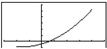

# You can specify a range when graphing rectangular expressions, polar expressions, parametric functions, and inequalities.

Zoom
Description
This function lets you enlarge and reduce the graph on the screen.
Set Up
- Draw the graph.
Execution
- Specify the zoom type.
SHIFT F2 (ZOOM) F1 (BOX) ... Box zoom
Draw a box around a display area, and that area is enlarged to fill the entire screen.
F2 (FACT)
F3 (IN)/F4 (OUT) ... Factor zoom
The graph is enlarged or reduced in accordance with the factor you specify, centered on the current pointer location.
F5 (AUTO) ... Auto zoom
V-Window y-axis settings are automatically adjusted so the graph fills the screen along the y-axis.
F6 (▷) F1 (ORIG) ... Original size
Returns the graph to its original size following a zoom operation.
F6 (▷) F2 (SQR) ... Graph correction
V-Window x-axis values are corrected so they are identical to the y-axis values.
F6 (▷) F3 (RND) ... Coordinate rounding
Rounds the coordinate values at the current pointer location.
F6 (▷) F4 (INTG) ... Integer
Each dot is given a width of 1, which makes coordinate values integers.
F6 (▷) F5 (PRE) ... Previous
V-Window parameters are returned to what they were prior to the last zoom operation.
Box zoom range specification
-
Use the cursor keys to move the pointer (⊕) in the center of the screen to the location where you want one corner of the box to be, and then press EXE.
-
Use the cursor keys to move the pointer. This causes a box to appear on the screen. Move the cursor until the area you want to enlarge is enclosed in the box, and then press EXE to enlarge it.


Example
Graph y = (x + 5)(x + 4)(x + 3) , and then perform a box zoom.
Use the following V-Window settings.
$$ \mathrm{Xmin} = - 8, $$
$$ \mathrm{Xmax} = 8, $$
$$ \mathrm{Xscale} = 2 $$
$$ \mathbf {Y} \min = - 4, $$
$$ \mathbf {Y} \max = 2, $$
$$ \text { Yscale } = 1 $$
Procedure
① MENU GRAPH


F6 (DRAW)
② SHIFT F2 (ZOOM) F1 (BOX)
③ ◀️ \~ ◀️ EXE
④ ◀️ \~ ◀️, ▲️ \~ ▲️ EXE
Result Screen
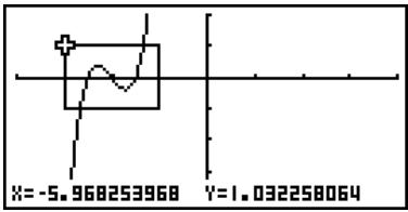
line
| X Value | Y Value | | ------- | ------- | | -5.968253968 | 1.032258064 |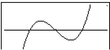
natural_image
Simple line drawing of a wave with a horizontal axis and a vertical axis (no text or symbols)
# You must specify two different points for box zoom, and the two points cannot be on a straight line vertically or horizontally from each other.

Factor Zoom
Description
With factor zoom, you can zoom in or out, centered on the current cursor position.
Set Up
- Draw the graph.
Execution
- Press SHIFT F2 (ZOOM) F2 (FACT) to open a pop-up window for specifying the x-axis and y-axis zoom factor. Input the values you want and then press EXIT.
- Press SHIFT F2 (ZOOM) F3 (IN) to enlarge the graph, or SHIFT F2 (ZOOM) F4 (OUT) to reduce it. The graph is enlarged or reduced centered on the current pointer location.
- Use the cursor keys to move the cursor to the point upon which you want the zoom operation to be centered, and then press EXIT to zoom.


Example
Enlarge the graphs of the two expressions shown below five times on both the x - and y -axis to see if they are tangent.
$$ \mathrm{Y} 1 = (x + 4) (x + 1) (x - 3), \quad \mathrm{Y} 2 = 3 x + 2 2 $$
Use the following V-Window settings.
$$ \mathrm{Xmin} = - 8, \quad \mathrm{Xmax} = 8, \quad \mathrm{Xscale} = 1 $$
$$ \mathrm{Ymin} = - 3 0, \quad \mathrm{Ymax} = 3 0, \quad \text { Yscale } = 5 $$
Procedure
① MENU GRAPH
SHIFT F3 (V-WIN) (-) 8 EXE 8 EXE 1 EXE ▼
natural_image
Simple geometric diagram with a diagonal line and a semicircle (no text or symbols)
# You can repeat factor zoom to enlarge or reduce a graph even further.

5-3 Drawing a Graph
You can store up to 20 functions in memory. Functions in memory can be edited, recalled, and graphed.
■ Specifying the Graph Type
Before you can store a graph function in memory, you must first specify its graph type.
- While the Graph relation list is on the display, press F3(TYPE) to display the graph type menu, which contains the following items.
- Y = / r = / Parm / X = c rectangular coordinate / polar coordinate / parametric / X = constant^*1 graph
- Y > /Y < /Y≥ /Y≤ ... Y > f(x) /Y < f(x) /Y f(x) /Y≤ f(x) inequality graph
• {CONV}
... {changes the function type of the selected expression}
$$ \bullet {\blacktriangleright Y = } / {\blacktriangleright Y > } / {\blacktriangleright Y < } / {\blacktriangleright Y \geq } / {\blacktriangleright Y \leq } $$
- Press the function key that corresponds to the graph type you want to specify.
■ Storing Graph Functions
- To store a rectangular coordinate function (Y=) *2
● ● ● ● ●
Example To store the following expression in memory area Y1: y = 2x^2 - 5
F3(TYPE) F1(Y=)(Specifies rectangular coordinate expression.)
2 X,θ,T x^2 — 5 (Inputs expression.)
EXE (Stores expression.)
$$ \boxed { \begin{array}{l l} \text {Graph Func} & : Y = \ Y 1 0 2 X ^ {2} - 5 & [ - ] \end{array} } $$

*1 Attempting to draw a graph for an expression in which X is input for an X = constant expression results in an error.
*2 A function cannot be stored into a memory area that already contains a function of a different type from the one you are trying to store. Select a memory area that contains a function that is the same type as the one you are storing, or delete the function in the memory area to which you are trying to store.

- To store a polar coordinate function (r = )^*1
● ● ● ● ●
Example To store the following expression in memory area r2 : r = 5 3
F3(TYPE) F2(r=)(Specifies polar coordinate expression.)
5 sin 3 X,θ,T (Inputs expression.)
EXE (Stores expression.)
- To store a parametric function \*2
● ● ● ● ●
Example To store the following functions in memory areas Xt3 and Yt3 :
$$ x = 3 \sin T $$
$$ y = 3 \cos T $$
F3(TYPE) F3(Parm) (Specifies parametric expression.)
3 sin X,θ,T EXE (Inputs and stores x expression.)
3 cos X,θ,T EXE (Inputs and stores y expression.)

^*1 A function cannot be stored into a memory area that already contains a function of a different type from the one you are trying to store. Select a memory area that contains a function that is the same type as the one you are storing, or delete the function in the memory area to which you are trying to store.
*2 You will not be able to store the expression in an area that already contains a rectangular coordinate expression, polar coordinate expression, X = constant expression or inequality. Select another area to store your expression or delete the existing expression first.

- To store an X = constant expression *1
● ● ● ● ●
Example To store the following expression in memory area X4 : X = 3
F3(TYPE) F4(X=c) (Specifies X = constant expression.)
③ (Inputs expression.)
EXE (Stores expression.)
- Inputting X, Y, T, r , or for the constant in the above procedures causes an error.
- To store an inequality *1
● ● ● ● ●
Example To store the following inequality in memory area Y5 : y > x^2 - 2x - 6
F3(TYPE) F6(▷) F1(Y>) (Specifies an inequality.)
X,,T x^2 — 2 X,,T — 6 (Inputs expression.)
EXE (Stores expression.)
- To create a composite function
● ● ● ● ●
Example To use relations in Y1 and Y2 to create composite functions for Y3 and Y4
$$ \mathbf {Y} 1 = \sqrt {(\mathbf {X} + 1)}, \mathbf {Y} 2 = \mathbf {X} ^ {2} + 3 $$
Assign Y1°Y2 to Y3, and Y2°Y1 to Y4.
$$ \left(\mathrm{Y} 1 \circ \mathrm{Y} 2 = \sqrt {\left(\left(\mathrm{x} ^ {2} + 3\right) + 1\right)} = \sqrt {\left(\mathrm{x} ^ {2} + 4\right)} \quad \mathrm{Y} 2 \circ \mathrm{Y} 1 = \left(\sqrt {(\mathrm{X} + 1)}\right) ^ {2} + 3 = \mathrm{X} + 4 (\mathrm{X} \geq - 1)\right) $$
Input relations into Y3 and Y4.
F3 (TYPE) F1 (Y=) VARS F4 (GRPH)
F1(Y) 1 ( F1(Y) 2 ) EXE
VARS F4 (GRPH) F1 (Y) 2
( F1(Y) 1 ) EXE
![Graph Func :Y= Y1Bf(X+1) [—] Y2BfX2+3 [—] Y3BfV1(V2) [—] Y4BfV2(V1) [—] Y5: Y6: SEL DEL TYPE STYLE SMEM DRAW](/content/2025/01/86785/images/458a0899500b11e9ba75509e95f529f7d0b9548c9e50145433c8e2d74e91b457.jpg)
- A composite function can consist of up to five functions.

*1A function cannot be stored into a memory area that already contains a function of a different type from the one you are trying to store. Select a memory area that contains a
function that is the same type as the one you are storing, or delete the function in the memory area to which you are trying to store.

- To assign values to the coefficients and variables of a graph function

Example
To assign the values -1, 0 , and 1 to variable A in Y = AX^2 - 1 , and draw a graph for each value
F3(TYPE) F1(Y=)
ALPHA X,θ,T (A) X,θ,T x^2 — 1 EXE
VARS F4 (GRPH) F1 (Y) 1 C ALPHA X,θ,T (A)
SHIFT • (=) (-) 1 ) EXE
VARS F4 (GRPH) F1 (Y) 1 ( ALPHA X,θ,T (A)
SHIFT □ (=) 0 ) EXE
VARS F4 (GRPH) F1 (Y) 1 ( ALPHA X,θ,T (A)
SHIFT • (=) 1 ) EXE
▲ ▲ ▲ ▲ F1 (SEL)
F6 (DRAW)
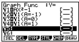
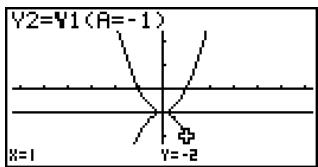
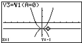
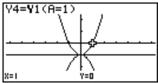
The above three screens are produced using the Trace function.
See "5-11 Function Analysis" for more information.

- If you do not specify a variable name (variable A in the above key operation), the calculator automatically uses one of the default variables listed below. Note that the default variable used depends on the memory area type where you are storing the graph function.
| Memory Area Type | Default Variable |
| Yn | X |
| rn | θ |
| Xtn | T |
| Ytn | T |
| fn | X |

Example Y1 (3) and Y1 (X = 3) are identical values.
- You can also use Dynamic Graph for a look at how changes in coefficients alter the appearance of a graph. See “5-8 Dynamic Graphing” for more information.

■ Editing and Deleting Functions
• To edit a function in memory

Example To change the expression in memory area Y1 from y = 2x^2 - 5 to y = 2x^2 - 3
(Displays cursor.)
▶▶▶▶▶DEL 3 (Changes contents.)
EXE (Stores new graph function.)
- To change the line style of a graph function
- On the Graph relation list screen, use ▲ and ▼ to highlight the relation whose line style you want to change.
- Press F4(STYL).
- Select the line style.

Example To change the line style of y = 2x^2 - 3 , which is stored in area Y1, to “Broken”.
F4(STYL) F3(……) (Selects "Broken".)
![Graph Func :Y= W1=2X1-3 Y2: [—] Y3: [—] Y4: [—] Y5: [—] Y6: [—] SEL DEL TYPE STYL GMB Draw](/content/2025/01/86785/images/4576457ccb8df107365e1f27a5bab4d11b0e5b0fadda6495dbb00cd0c4a8cba3.jpg)
![Graph Func :Y= V1=2X1-3 V2: [—] V3: [—] V4: [—] V5: [—] V6: [—]](/content/2025/01/86785/images/d22057e747d2d2271148393a85c288760a0609f74caf8c6b18325434453df1dc.jpg)

- To change the type of a function ^*1
- While the Graph relation list is on the display, press ▲ or ▼ to move the highlighting to the area that contains the function whose type you want to change.
- Press F3(TYPE)F5(CONV).
- Select the function type you want to change to.

Example To change the function in memory area Y1 from y = 2x^2 - 3 to y < 2x^2 - 3 F3(TYPE)(F5(CONV)(F3(▶Y<) (Changes the function type to “Y<”).
- To delete a function
- While the Graph relation list is on the display, press ▲ or ▼ to move the highlighting to the area that contains the function you want to delete.
- Press F2 (DEL) or DEL.
- Press [F1] (Yes) to delete the function or [F6] (No) to abort the procedure without deleting anything.

*1 The function type can be changed for rectangular coordinate functions and inequalities only.
# Parametric functions come in pairs (Xt and Yt).

■ Selecting Functions for Graphing
- To specify the draw/non-draw status of a graph
- On the graph relation list, use ⬆ and ⬇ to highlight the relation you do not want to graph.
- Press F1(SEL).
• Each press of F1(SEL) toggles graphing on and off. - Press F6 (DRAW).

Example To select the following functions for drawing :
$$ \mathbf {Y} 1 = 2 x ^ {2} - 5, r 2 = 5 \sin 3 \theta $$
Use the following V-Window settings.
$$ \mathrm{Xmin} = - 5, \quad \mathrm{Xmax} = 5, \quad \mathrm{Xscale} = 1 $$
$$ \mathrm{Ymin} = - 5, \quad \mathrm{Ymax} = 5, \quad \text { Yscale } = 1 $$
$$ \mathbf {T} \theta \min = 0, \quad \mathbf {T} \theta \max = \pi , \quad \mathbf {T} \theta \operatorname{ptch} = 2 \pi / 6 0 $$
▼ (Select a memory area that contains a function for which you want to specify non-draw.)
F1(SEL) (Specifies non-draw.)
F6 (DRAW) or EXE (Draws the graphs.)
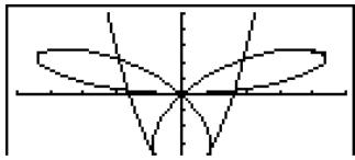
natural_image
Symmetrical geometric line drawing with intersecting curves and a horizontal axis (no text or symbols)- You can use the Setup screen settings to alter the appearance of the graph screen as shown below.
- Grid: On (Axes: On Label: Off)
This setting causes dots to appear at the grid intersects on the display.
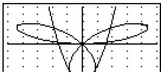
natural_image
Symmetrical geometric line drawing with intersecting curves and a central axis (no text or symbols)- Axes: Off (Label: Off Grid: Off)
This setting clears the axis lines from the display.
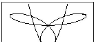
natural_image
Abstract geometric line drawing with intersecting curves and loops (no text or symbols)- Label: On (Axes: On Grid: Off)
This setting displays labels for the x- and y-axes.
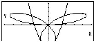

■ Graph Memory
Graph memory lets you store up to 20 sets of graph function data and recall it later when you need it.
A single save operation saves the following data in graph memory.
- All graph functions in the currently displayed Graph relation list (up to 20)
- Graph types
• Function graph line information - Draw/non-draw status
• V-Window settings (1 set)
- To store graph functions in graph memory
- Press F5 (GMEM) F1 (STO) to display the pop-up window.
- Press a number key to specify the Graph memory where you want to save the graph function, and then press EXE. Pressing 1 EXE stores the graph function to Graph Memory 1 (G-Mem1).
- There are 20 graph memories numbered G-Mem1 to G-Mem20.
• To recall a graph function
- Press F5 (GMEM) F2 (RCL) to display the pop-up window.
- Press a number key to specify the Graph memory for the function you want to recall, and then press EXE. Pressing 1 EXE recalls the graph function in Graph Memory 1 (G-Mem1).

# Storing a function in a memory area that already contains a function replaces the existing function with the new one.
# If the data exceeds the calculator's remaining memory capacity, an error occurs.
# Recalling data from graph memory causes any data currently on the Graph relation list to be deleted.

5-4 Storing a Graph in Picture Memory
You can save up to 20 graphic images in picture memory for later recall. You can overdraw the graph on the screen with another graph stored in picture memory.
- To store a graph in picture memory
- After graphing in GRAPH mode, press OPTN F1 (PICT) F1 (STO) to display the pop-up window.
- Press a number key to specify the Picture memory where you want to save the picture, and then press EXE. Pressing 1 EXE stores the picture function to Picture Memory 1 (Pict 1).
- There are 20 picture memories numbered Pict 1 to Pict 20.
- To recall a stored graph
- After graphing in GRAPH mode, press OPTN F1 (PICT) F2 (RCL) to display the pop-up window.
- Press a number key to specify the Picture memory for the picture you want to recall, and then press EXE. Pressing 1 EXE recalls the picture function in Picture Memory 1 (Pict 1).
- Recalling picture memory contents causes the currently displayed graph to be overwritten.
- Use the sketch CIs function (page 5-10-1) to clear a graph that was recalled from picture memory.

# Storing a graphic image in a memory area that already contains a graphic image replaces the existing graphic image with the new one.
# A dual graph screen or any other type of graph that uses a split screen cannot be saved in picture memory.

5-5 Drawing Two Graphs on the Same Screen
■ Copying the Graph to the Sub-screen
Description
Dual Graph lets you split the screen into two parts. Then you can graph two different functions in each for comparison, or draw a normal size graph on one side and its enlarged version on the other side. This makes Dual Graph a powerful graph analysis tool.
With Dual Graph, the left side of the screen is called the “main screen,” while the right side is called the “sub-screen.”
- Main Screen
The graph in the main screen is actually drawn from a function.
- Sub-screen
The graph on the sub-screen is produced by copying or zooming the main screen graph. You can even make different V-Window settings for the sub-screen and main screen.
Set Up
- From the Main Menu, enter the GRAPH mode.
- On the Setup screen, select G+G for Dual Screen.
- Make V-Window settings for the main screen.
Press F6 (RIGHT) to display the sub-graph settings screen. Pressing F6 (LEFT) returns to the main screen setting screen.
Execution
- Store the function, and draw the graph in the main screen.
- Perform the Dual Graph operation you want.
OPTN F1 (COPY) ... Duplicates the main screen graph in the sub-screen
OPTN F2(SWAP) ... Swaps the main screen contents and sub-screen contents


Example
Graph y = x(x + 1)(x - 1) in the main screen and sub-screen.
Use the following V-Window settings.
(Main Screen)
$$ \mathrm{Xmin} = - 2, \quad \mathrm{Xmax} = 2, \quad \mathrm{Xscale} = 0. 5 $$
$$ \mathrm{Ymin} = - 2, \quad \mathrm{Ymax} = 2, \quad \text { Yscale } = 1 $$
(Sub-screen)
$$ \mathrm{Xmin} = - 4, \quad \mathrm{Xmax} = 4, \quad \mathrm{Xscale} = 1 $$
$$ \mathrm{Ymin} = - 3, \quad \mathrm{Ymax} = 3, \quad \text { Yscale } = 1 $$
Procedure
① MENU GRAPH
② SHIFT MENU (SET UP) ▼ ▼ F1 (G+G) EXIT
③ SHIFT F3 (V-WIN) (-) 2 EXE 2 EXE 0 • 5 EXE ▼
$$ ① (-) ② \text { EXE } ② \text { EXE } ① \text { EXE } $$
$$ \boxed {F 6} (\text {RIGHT}) (-) \boxed {4} \boxed {\text {EXE}} \boxed {4} \boxed {\text {EXE}} \boxed {1} \boxed {\text {EXE}} \boxed {\triangledown} $$
$$ (-) \boxed {3} \boxed {\mathrm{EXE}} \boxed {3} \boxed {\mathrm{EXE}} \boxed {1} \boxed {\mathrm{EXE}} \boxed {\mathrm{EXIT}} $$
④ F3 (TYPE) F1 (Y=) X,θ,T (X,θ,T + 1 ) (X,θ,T - 1 ) EXE
$$ \boxed {F 6} (\text { DRAW }) $$
⑤ OPTN F1 (COPY)
Result Screen
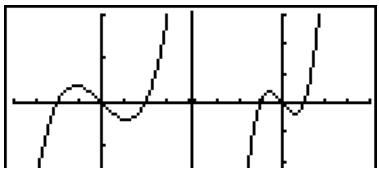
natural_image
Pure electrical circuit lines without any symbols
# Pressing AC while a graph is on the display will return to the screen in step 4.

■ Graphing Two Different Functions
Description
Use the following procedure to graph different functions in the main screen and sub-screen.
Set Up
- From the Main Menu, enter the GRAPH mode.
- On the Setup screen, select G+G for Dual Screen.
- Make V-Window settings for the main screen.
Press F6 (RIGHT) to display the sub-graph settings screen. Pressing F6 (LEFT) returns to the main screen setting screen.
Execution
- Store the functions for the main screen and sub-screen.
- Select the function of the graph that you want to eventually have in the sub-screen.
- Draw the graph in the main screen.
- Swap the main screen and sub-screen contents.
- Return to the function screen.
- Select the function of the next graph you want in the main screen.
- Draw the graph in the main screen.


Example
Graph y = x(x + 1)(x - 1) in the main screen, and y = 2x^2 - 3 in the sub-screen.
Use the following V-Window settings.
(Main Screen)
natural_image
Pure electrical circuit lines without any symbols
■ Using Zoom to Enlarge the Sub-screen
Description
Use the following procedure to enlarge the main screen graph and then move it to the sub-screen.
Set Up
- From the Main Menu, enter the GRAPH mode.
- On the Setup screen, select G+G for Dual Screen.
- Make V-Window settings for the main screen.
Execution
- Input the function and draw the graph in the main screen.
- Use Zoom to enlarge the graph, and then move it to the sub-screen.


Example
Draw the graph y = x(x + 1)(x - 1) in the main screen, and then use Box Zoom to enlarge it.
Use the following V-Window settings.
(Main Screen)
Xmin = -2, Xmax = 2, Xscale = 0.5
Ymin = -2, Ymax = 2, Yscale = 1
Procedure
① MENU GRAPH
② SHIFT MENU (SET UP) ▼ F1 (G+G) EXIT
③ SHIFT F3 (V-WIN) (-) 2 EXE 2 EXE 0 • 5 EXE ▼
(一) 2 EXE 2 EXE 1 EXE EXIT
④ F3(TYPE)F1(Y=) ,,T ( ,,T + 1 ) ( ,,T - 1 ) EXE
F6 (DRAW)
⑤ SHIFT F2 (ZOOM) F1 (BOX)
▼ \~ ▼ ▶ \~ ▶ EXE
▲ \~ ▲ ◀ \~ ◀ EXE
Result Screen
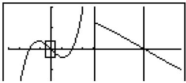
natural_image
Pure geometric diagram with intersecting lines and a square marker, no text or symbols present
5-6 Manual Graphing
■ Rectangular Coordinate Graph
Description
Inputting the Graph command in the RUN·MAT mode enables drawing of rectangular coordinate graphs.
Set Up
- From the Main Menu, enter the RUN·MAT mode.
- Make V-Window settings.
Execution
- Input the commands for drawing the rectangular coordinate graph.
- Input the function.

# You can draw graphs of the following built-in scientific functions.
- Rectangular Coordinate Graph
- x
- x
- tan x
- ^-1 x
• ^-1x
- ^-1 x
- x
- x
- x
- ^-1 x
- ^-1 x
- ^-1 x
•
• x^2
- x
- x
• 10^x
• e^x
• x^-1
• 3√x
- Polar Coordinate Graph
• sin θ
• cos θ
• tan θ
• ^-1
• ^-1
• ^-1
• sinh θ
-
• tanh θ
- ^-1
- ^-1
- ^-1
• √θ
• ^2
• log θ
-
• 10^
• e^
• θ-1
• 3√θ
# V-Window settings are made automatically for built-in graphs.


Example
Use the following V-Window settings.
natural_image
Simple parabolic curve drawn on a Cartesian coordinate system (no labels or text)
■ Integration Graph
Description
Inputting the Graph command in the RUN·MAT mode enables graphing of functions produced by an integration calculation.
The calculation result is shown in the lower left corner of the display, and the calculation range is cross plot type.
Set Up
- From the Main Menu, enter the RUN·MAT mode.
- Make V-Window settings.
Execution
- Input graph commands for the integration graph.
- Input the function.


Example
Graph the integration _-2^1(x + 2)(x - 1)(x - 3)dx .
Use the following V-Window settings.
F5 (GRPH) F5 (G·∫dx)
④ (X,θ,T + 2) (X,θ,T - 1) (X,θ,T - 3),
(-) 2 , 1 EXE
Result Screen
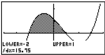
area
| Category | Value | | -------- | ----- | | LOWER | -2 | | dx | 15.75 |
■ Drawing Multiple Graphs on the Same Screen
Description
Use the following procedure to assign various values to a variable contained in an expression and overwrite the resulting graphs on the screen.
Set Up
- From the Main Menu, enter the GRAPH mode.
- On the Setup screen, change the "Dual Screen" setting to "Off".
- Make V-Window settings.
Execution
- Specify the function type and input the function. The following is the syntax for function input.
Expression containing one variable ⚡ SHIFT ⊕ ( [ ) variable SHIFT ● (=) value □ value □ ... □ value SHIFT — ( ] ) - Draw the graph.


Example
To graph y = Ax^2 - 3 as the value of A changes in the sequence 3, 1, -1.
Use the following V-Window settings.
$$ \mathrm{Xmin} = - 5, \quad \mathrm{Xmax} = 5, \quad \mathrm{Xscale} = 1 $$
$$ \mathrm{Ymin} = - 1 0, \quad \mathrm{Ymax} = 1 0, \quad \mathrm{Yscale} = 2 $$
Procedure
① MENU GRAPH
② SHIFT MENU (SET UP) ▼ ▼ F3 (Off) EXIT
③ SHIFT F3 (V-WIN) (-) 5 EXE 5 EXE 1 EXE ▼
$$ ① 1 0 \text { EXE } 1 0 \text { EXE } 2 \text { EXE } \text { EXIT } $$
④ F3 (TYPE) F1 (Y=) ALPHA X,θ,T (A) X,θ,T x² - 3 ,
$$ \boxed {\text {SHIFT}} \boxed {+} ([) \boxed {\text {ALPHA}} \boxed {X, \theta , T} (A) \boxed {\text {SHIFT}} \boxed {\cdot} (=) \boxed {3}, \boxed {1}, \boxed {(-)} \boxed {1} \boxed {\text {SHIFT}} \boxed {-} (]) \boxed {\text {EXE}} $$
⑤ F6 (DRAW)
Result Screen
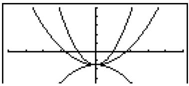

The value of only one of the variables in the expression can change.
Any of the following cannot be used for the variable name: X, Y, r, θ, T.
You cannot assign a variable to the variable inside the function.
When Simul Graph is turned on, all of the graphs for the specified variable values are drawn simultaneously.
Overwrite can be used when graphing rectangular expressions, polar expressions, parametric functions, X = constant functions, and inequalities.

■ Using Copy and Paste to Graph a Function
Description
You can graph a function by copying it to the clipboard, and then pasting it into the graph screen.
There are two types of functions you can paste into the graph screen.
Type 1 (Y= expression)
A function with the Y variable to the left of the equal sign is graphed as Y= expression.
Example: To paste Y=X and graph it
- Any spaces to the left of Y are ignored.
Type 2 (expression)
Pasting this type of expression graphs Y= expression.
Example: To paste X and graph Y=X
- Any spaces to the left of the expression are ignored.
Set Up
- Copy the function you want to graph to the clipboard.
- From the Main Menu, enter the GRAPH mode.
- On the Setup screen, change the "Dual Screen" setting to "Off".
- Make V-Window settings.
- Draw the graph.
Execution
- Paste the expression.

Paste is supported only when "Off" is selected for the "Dual Screen" setting on the Setup screen.
Though there is no limit per se on the number of graphs you can draw by pasting a function, the total number of graphs supported by trace and other functions is 30 (number of graphs drawn using expression number 1 to 20, plus graphs drawn using pasted functions).
For the graph of a pasted function, the graph expression that appears when using trace or other functions is displayed in the format: Y= expression.
Re-executing a draw without clearing graph screen memory will redraw all the graphs, including those produced by pasting functions.


Example
While the graph of y = 2x^2 + 3x - 4 is currently displayed, to paste the previously copied function Y=X from the clipboard
Use the following V-Window settings.
$$ \mathrm{Xmin} = - 5, \quad \mathrm{Xmax} = 5, \quad \mathrm{Xscale} = 2 $$
$$ \mathrm{Ymin} = - 1 0, \quad \mathrm{Ymax} = 1 0, \quad \text { Yscale } = 5 $$
Procedure
① MENU RUN·MAT


② MENU GRAPH
③ SHIFT MENU (SET UP) ▼ ▼ F3 (Off) EXIT
④ SHIFT F3 (V-WIN) (-) 5 EXE 5 EXE 2 EXE ▼

⑤ F3 (TYPE) F1 (Y=) 2 X,θ,T x² + 3 X,θ,T - 4 EXE
F6 (DRAW)
⑥ SHIFT 9 (PASTE)
Result Screen
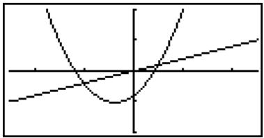

5-7 Using Tables
To enter the TABLE mode, select the TABLE icon on the Main Menu.
■ Storing a Function and Generating a Number Table
- To store a function

Example To store the function y = 3x^2 - 2 in memory area Y1
Use ▲ and ▼ to move the highlighting in the Table relation list to the memory area where you want to store the function. Next, input the function and press EXE to store it.
- Variable Specifications
There are two methods you can use to specify value for the variable x when generating a numeric table.
- Table range method
With this method, you specify the conditions for the change in value of the variable.
- List
With this method, the data in the list you specify is substituted for the x-variable to generate a number table.
- To generate a table using a table range

Example To generate a table as the value of variable x changes from -3 to 3, in increments of 1
MENU TABLE
F5 (SET)
The numeric table range defines the conditions under which the value of variable x changes during function calculation.
Start ...... Variable x start value
End ...... Variable x end value
Step ...... Variable x value change (interval)
After specifying the table range, press EXIT to return to the Table relation list.

- To generate a table using a list
- While the Table relation list is on the screen, display the Setup screen.
- Highlight Variable and then press F2 (LIST) to display the pop-up window.
- Select the list whose values you want to assign for the x-variable.
- To select List 6, for example, press 6 EXE. This causes the setting of the Variable item of the Setup screen to change to List 6.
- After specifying the list you want to use, press EXIT to return to the previous screen.
- Generating a Table

Example To generate a table of values for the functions stored in memory areas Y1 and Y3 of the Table relation list
Use ▲ and ▼ to move the highlighting to the function you want to select for table generation and press F1(SEL) to select it.
The “=” sign of selected functions is highlighted on the screen. To deselect a function, move the cursor to it and press F1(SEL) again.
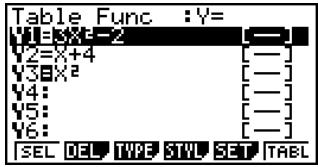
Press F6 (TABL) to generate a number table using the functions you selected. The value of variable x changes according to the range or the contents of the list you specified.
The example screen shown here shows the results based on the contents of List 6 (-3, -2, -1, 0, 1, 2, 3).
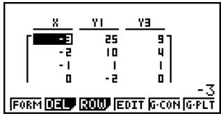
Each cell can contain up to six digits, including negative sign.

You can use cursor keys to move the highlighting around the table for the following purposes.
- To display the selected cell's value at the bottom of the screen, using the calculator's current number of decimal place, number of significant digit, and exponential display range settings
- To scroll the display and view parts of the table that do not fit in the display
- To display at the top of the screen the scientific function that produced the value in the selected cell (in columns Y1, Y2, etc.)
- To change x variable values by replacing values in column X
Press F1(FORM) or EXIT to return to the Table relation list.
- To generate a differential number table \*1
Changing the setting of Setup screen's Derivative item to On causes a number table that includes the derivative to be displayed whenever you generate a number table.
Locating the cursor at a differential —— coefficient displays “dy/dx” in the top line, which indicates differential.
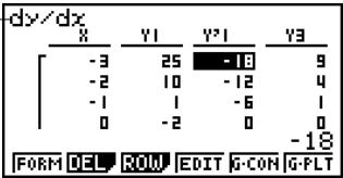
- Specifying the function type
You can specify a function as being one of three types. ^2
- Rectangular coordinate (Y=)
- Polar coordinate (r=)
-
Parametric (Parm)
-
Press F3(TYPE) while the relation list is on the screen.
- Press the number key that corresponds to the function type you want to specify.

*1 An error occurs if a graph for which a range is specified or an overwrite graph is included among the graph expressions.
*2 The number table is generated only for the function type specified on the relation list (Table Func). You cannot generate a number table for a mixture of different function types.
The function type specified in the GRAPH mode is not one of these three, entering the TABLE mode causes the function type to change to rectangular coordinate (Y=).

■ Editing and Deleting Functions
- To edit a function

Example
To change the function in memory area Y1 from y = 3x^2 - 2 to y = 3x^2 - 5
Use ▲ and ▼ to move the highlighting to the function you want to edit.

Use ▶ to move the cursor to the beginning of the expression.
Use ◀ and ▶ to move the cursor to the location of the change.

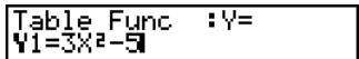

![Table Func :Y= Y1B3X²-5 [—] Y2=8+4 [—] Y3B3X² [—]](/content/2025/01/86785/images/775ff7ccbb64f30657a760c8036450a7eb4f9ccc63820cb212b244fb0b326369.jpg)

- You can specify the graph line style when graphing a connect type graph (G·CON). The line style specification also applies to the GRAPH mode.
- The Function Link Feature automatically reflects any changes you make to functions in the GRAPH mode list, and DYNA mode list.
- To delete a function
- Use ▲ and ▼ to move the highlighting to the function you want to delete and then press F2(DEL) or DEL.
- Press F1(Yes) to delete the function or F6(No) to abort the operation without deleting anything.

■ Editing Tables
You can use the table menu to perform any of the following operations once you generate a table.
- Change the values of variable x
- Edit (delete, insert, and append) rows
- Delete a table
- Draw a connect type graph
-
Draw a plot type graph
-
{FORM} ... {return to Table relation list}
- {DEL} ... {delete table}
- {ROW}
-
{DEL}/{INS}/{ADD} ... {delete}/{insert}/{add} row
-
{EDIT} ... {edit value of x -variable}
- {G·CON}/{G·PLT} ... {connected type}/{draw plot type} graph draw
- To change variable values in a table

Example
To change the value in Column x, Row 3 of the table generated on page 5-7-2 from -1 to -2.5

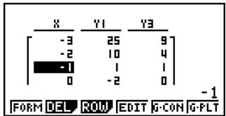

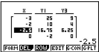
- When you change a variable value in Column x , all values in the columns to the right are recalculated and displayed.

# If you try to replace a value with an illegal operation (such as division by zero), an error occurs and the original value remains unchanged.
# You cannot directly change any values in the other (non-x) columns of the table.

- Row Operations
- To delete a row

Example To delete Row 2 of the table generated on page 5-7-2

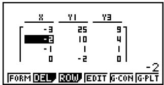
F3(ROW) F1(DEL)
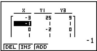
- To insert a row

Example To insert a new row between Rows 1 and 2 in the table generated on page 5-7-2

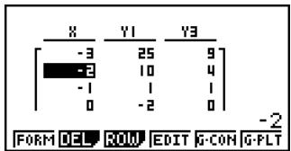
F3 (ROW) F2 (INS)
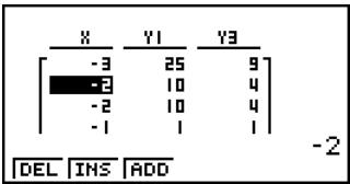

- To add a row

Example
To add a new row below Row 7 in the table generated on page 5-7-2
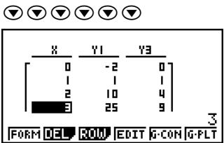
F3 (ROW) F3 (ADD)
![X Y1 Y3 [1 1 1 2 10 4 3 25 9 [3 25 9] DEL INS ADD 3](/content/2025/01/86785/images/a0e452154f7d639eff4ca348ad0e791d641e48421851fcc88409a8cf24882880.jpg)
- Deleting a Table
- Display the table and then press F2 (DEL).
- Press F1(Yes) to delete the table or F6(No) to abort the operation without deleting anything.

■ Copying a Table Column to a List
A simple operation lets you copy the contents of a numeric table column into a list.
Use ◀ and ▶ to move the cursor to the column you want to copy. The cursor can be in any row.
• To copy a table to a list

Example To copy the contents of Column x into List 1
OPTN F1 (LMEM)
![Store In List Memory List[1~26]: 1 LHP ENG ENG](/content/2025/01/86785/images/9335b23caa9dbf01aee6cb7f48384ae94b0b1bd1a362d1ce7719ba9a63723d36.jpg)
Input the number of the list you want to copy and then press EXE.
1 EXE
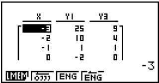

■ Drawing a Graph from a Number Table
Description
Use the following procedure to generate a number table and then draw a graph based on the values in the table.
Set Up
- From the Main Menu, enter the TABLE mode.
- Make V-Window settings.
Execution
- Store the functions.
- Specify the table range.
- Generate the table.
- Select the graph type and draw it.
F5 (G·CON) ... line graph*1
F6 (G • PLT) ... plot type graph*1
- Selecting F6(G·PLT) draws a 1-dot broken line plot type graph, regardless of the currently selected line style (page 5-3-6).

*1 After drawing the graph, pressing SHIFT F6 (G ↔ T) or AC returns to the number table screen.


Example
Store the two functions below, generate a number table, and then draw a line graph. Specify a range of -3 to 3, and an increment of 1.
$$ \mathbf {Y} 1 = 3 x ^ {2} - 2, \mathbf {Y} 2 = x ^ {2} $$
Use the following V-Window settings.
$$ \mathrm{Xmin} = 0, \quad \mathrm{Xmax} = 6, \quad \mathrm{Xscale} = 1 $$
$$ \mathrm{Ymin} = - 2, \quad \mathrm{Ymax} = 1 0, \quad \text { Yscale } = 2 $$
Procedure
$$ ① \boxed {2} \boxed {\mathrm{EXE}} \boxed {1} \boxed {0} \boxed {\mathrm{EXE}} \boxed {2} \boxed {\mathrm{EXE}} \boxed {\mathrm{EXIT}} $$
$$ \boxed {X, \theta , T} \boxed {\boldsymbol {x} ^ {2}} \boxed {E X E} $$
① MENU TABLE
② SHIFT F3 (V-WIN) 0 EXE 6 EXE 1 EXE ▼
③ F3 (TYPE) F1 (Y=) 3 X,θ,T x² - 2 EXE
④ F5 (SET) (-) 3 EXE 3 EXE 1 EXE EXIT
⑤ F6 (TABL)
⑥ F5(G·CON)
Result Screen
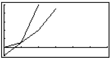
natural_image
Pure geometric lines and curves without any text, numbers, or symbols
# You can use Trace, Zoom, or Sketch after drawing a graph.

■ Specifying a Range for Number Table Generation
Description
Use the following procedure to specify a number table range when calculating scatter data from a function.
Set Up
- From the Main Menu, enter the TABLE mode.
Execution
- Store the functions.
- Specify the table range.
- Select the functions for which you want to generate a table.
The “=” sign of selected functions is highlighted on the screen. - Generate the table.


Example
Store the three functions shown below, and then generate a table for functions Y1 and Y3. Specify a range of -3 to 3, and an increment of 1.
$$ \mathbf {Y} 1 = 3 x ^ {2} - 2, \mathbf {Y} 2 = x + 4, \mathbf {Y} 3 = x ^ {2} $$
Procedure
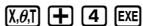
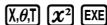
① MENU TABLE
② F3 (TYPE) F1 (Y=) 3 X,θ,T x² - 2 EXE
③ F5 (SET) (-) 3 EXE 3 EXE 1 EXE EXIT
④ ▲ ▲ F1 (SEL)
⑤ F6 (TABL)
Result Screen
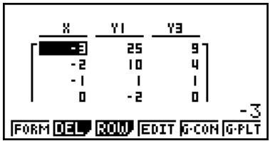

# You can generate number tables from rectangular coordinate, polar coordinate, and parametric functions.
# You can include derivatives in generated number tables by specifying On for the Derivative item on the Setup screen.

■ Simultaneously Displaying a Number Table and Graph
Description
Specifying T+G for Dual Screen on the Setup screen makes it possible to display a number table and graph at the same time.
Set Up
- From the Main Menu, enter the TABLE mode.
- Make V-Window settings.
- On the Setup screen, select T+G for Dual Screen.
Execution
- Input the function.
- Specify the table range.
- The number table is displayed in the sub-screen on the right.
- Specify the graph type and draw the graph.
F5 (G·CON) ... line graph
F6 (G • PLT) ... plot type graph

# The Setup screen's "Dual Screen" setting is applied in the TABLE mode and the RECUR mode.


Example
Store the function Y1 = 3x^2 - 2 and simultaneously display its number table and line graph. Use a table range of -3 to 3 with an increment of 1.
Use the following V-Window settings.
$$ \mathrm{Xmin} = 0, \quad \mathrm{Xmax} = 6, \quad \mathrm{Xscale} = 1 $$
$$ \mathrm{Ymin} = - 2, \quad \mathrm{Ymax} = 1 0, \quad \text { Yscale } = 2 $$
Procedure
① MENU TABLE
② SHIFT F3 (V-WIN) 0 EXE 6 EXE 1 EXE ▼
$$ ① \boxed {2} \boxed {\mathrm{EXE}} \boxed {1} \boxed {0} \boxed {\mathrm{EXE}} \boxed {2} \boxed {\mathrm{EXE}} \boxed {\mathrm{EXIT}} $$
③ SHIFT MENU (SET UP) ▼ ▼ F1 (T+G) EXIT
④ F3 (TYPE) F1 (Y=) 3 X,θ,T x² - 2 EXE
⑤ F5 (SET)
$$ (-) \boxed {3} \boxed {\text {EXE}} \boxed {3} \boxed {\text {EXE}} \boxed {1} \boxed {\text {EXE}} \boxed {\text {EXIT}} $$
⑥ F6 (TABL)
⑦ F5(G·CON)
Result Screen
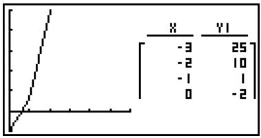
line
| X | Y1 | |---|---| | -3 | 25 | | -2 | 10 | | -1 | 1 | | 0 | -2 |
# You can make the number table active by pressing OPTN F1 (CHNG) or AC.
# After drawing a graph, you can return to the number table screen by pressing SHIFT F6(G↔T) or AC.

■ Using Graph-Table Linking
Description
With Dual Graph, you can use the following procedure to link the graph and table screens so the pointer on the graph screen jumps to the location of the currently selected table value.
Set Up
- From the Main Menu, enter the TABLE mode.
- Make the required V-Window settings.
Display the Setup screen, select the Dual Screen item, and change its setting to "T+G".
Execution
- Input the function of the graph and make the required table range settings.
- With the number table on the right side of the display, draw the graph on the left side.
F5 (G·CON) ... connect type graph
F6 (G • PLT) ... plot type graph
- Press OPTN F2 (GLINK) to enter the Graph-Table Linking mode.
- Now when you use ▼ and ▲ to move the highlighting among the cells in the table, the pointer jumps to the corresponding point on the graph screen.
If there are multiple graphs, pressing ◀ and ▶ causes the pointer to jump between them.
To exit the Graph-Table Linking mode, press EXIT or SHIFT EXIT (QUIT).


Example
Store the function Y1 = 3 x and simultaneously display its number table and plot-type graph. Use a table range of 2 through 9, with an increment of 1.
Use the following V-Window settings.
$$ \mathrm{Xmin} = - 1, \quad \mathrm{Xmax} = 1 0, \quad \mathrm{Xscale} = 1 $$
$$ \mathrm{Ymin} = - 1, \quad \mathrm{Ymax} = 4, \quad \text { Yscale } = 1 $$
Procedure
① MENU TABLE
② SHIFT F3 (V-WIN) (-) 1 EXE 1 0 EXE 1 EXE ▼
$$ ① (-) \boxed {1} \boxed {\mathrm{EXE}} \boxed {4} \boxed {\mathrm{EXE}} \boxed {1} \boxed {\mathrm{EXE}} \boxed {\mathrm{EXIT}} $$
$$ \boxed {\text {SHIFT}} \boxed {\text {MENU}} (\text {SET UP}) \boxed {\blacktriangledown} \boxed {\blacktriangledown} \boxed {\text {F1}} (\text {T+G}) \boxed {\text {EXIT}} $$
③ F3 (TYPE) F1 (Y=) 3 log X,θ,T EXE
$$ \boxed {F 5} (S E T) $$
$$ 2 \text { EXE } 9 \text { EXE } 1 \text { EXE } \text { EXIT } $$
④ F6 (TABL)
$$ \boxed {F 6} (G \cdot P L T) $$
⑤ OPTN F2 (GLINK)
⑥ ▼ \~ ▼, ▲ \~ ▲
Result Screen
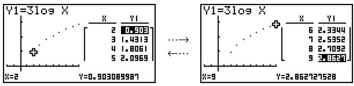
scatter
| X | Y | |------|-------| | 2 | 0.903 | | 3 | 1.4313| | 4 | 1.8061| | 5 | 2.0969| | 6 | 2.3344| | 7 | 2.5352| | 8 | 2.7092| | 9 | 3.0874|
5-8 Dynamic Graphing
■ Using Dynamic Graph
Description
Dynamic Graph lets you define a range of values for the coefficients in a function, and then observe how a graph is affected by changes in the value of a coefficient. It helps to see how the coefficients and terms that make up a function influence the shape and position of a graph.
Set Up
- From the Main Menu, enter the DYNA mode.
- Make V-Window settings.
Execution
- On the Setup screen, specify the Dynamic Type.
F1(Cnt) ... Continuous
F2 (Stop) ... Automatic stop after 10 draws
- Use the cursor keys to select the function type on the built-in function type list.*1
- Input values for coefficients, and specify which coefficient will be the dynamic variable. ^*2
- Specify the start value, end value, and increment.
- Specify the drawing speed.
F3 (SPEED) F1 (IID) ..... Pause after each draw (Stop&Go)
F2(>) ...... Half normal speed (Slow)
F3(▶) ...... Normal speed (Normal)
F4(≫) ..... Twice normal speed (Fast)
- Draw the Dynamic Graph.

*1 The following are the seven built-in function types.
•Y=AX+B
- Y = A(X - B)^2 + C
- Y = AX^2 + BX + C
- Y = AX^3 + BX^2 + CX + D
•Y=Asin(BX+C)
•Y=Acos(BX+C)
•Y=Atan(BX+C)
After you press F3(TYPE) and select the function type you want, you can then input the actual function.
F1(Y=) ... rectangular coordinate expression
F2(r=) ... polar coordinate expression
F3 (Parm) ... parametric function
Entering the DYNA mode when a Function Type that is not one of the three types listed above is selected in the GRAPH mode causes the Function Type to change automatically to "rectangular coordinate expression (Y=)".
*2 You could also press EXE here and display the parameter setting menu.
The message “Too Many Functions” appears when more than one function is selected for Dynamic Graphing.


Example
Use Dynamic Graph to graph y = A(x - 1)^2 - 1 , in which the value of coefficient A changes from 2 through 5 in increments of 1. The Graph is drawn 10 times.
Use the following V-Window settings.
Xmin = -6.3, Xmax = 6.3, Xscale = 1
Ymin = -3.1, Ymax = 3.1, Yscale = 1 (initial defaults)
Procedure
① MENU DYNA
② SHIFT F3 (V-WIN) F1 (INIT) EXIT
③ SHIFT MENU (SET UP) F2 (Stop) EXIT
④ F5 (B-IN) ▼ F1 (SEL)
⑤ F4 (VAR) 2 EXE 1 EXE (-) 1 EXE
⑥ F2 (SET) 2 EXE 5 EXE 1 EXE EXIT
⑦ F3 (SPEED) F3 (▶) EXIT
⑧ F6(DYNA)
Result Screen

↓
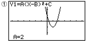
Repeats from ① through ④.
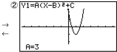
line
| X-Axis Label | Y-Axis Value | |--------------|--------------| | A | 3 | | B | 2 | | C | 1 |↓↑
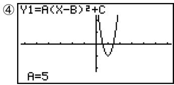
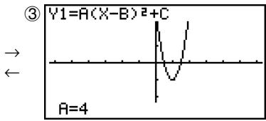

■ Drawing a Dynamic Graph Locus
Description
Turning on the Dynamic Graph locus setting on the Setup screen lets you overlay a graph drawn by changing the coefficient values.
Set Up
- From the Main Menu, enter the DYNA mode.
- Make V-Window settings.
Execution
- On the Setup screen, select "On" for "Locus".
- Use the cursor keys to select the function type on the built-in function type list.
- Input values for coefficients, and specify which coefficient will be the dynamic variable.
- Specify the start value, end value, and increment.
- Specify Normal for the draw speed.
- Draw the Dynamic Graph.


Example
Use Dynamic Graph to graph y = Ax , in which the value of coefficient A changes from 1 through 4 in increments of 1. The Graph is drawn 10 times.
Use the following V-Window settings.
Xmin = -6.3, Xmax = 6.3, Xscale = 1
Ymin = -3.1, Ymax = 3.1, Yscale = 1 (initial defaults)
Procedure
① MENU DYNA
② SHIFT F3 (V-WIN) F1 (INIT) EXIT
③ SHIFT MENU (SET UP) ▼ F1 (On) EXIT
④ F5(B-IN) F1(SEL)
⑤ F4 (VAR) 1 EXE 0 EXE
⑥ F2 (SET) 1 EXE 4 EXE 1 EXE EXIT
⑦ F3 (SPEED) F3 (▶) EXIT
⑧ F6(DYNA)
Result Screen
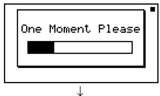
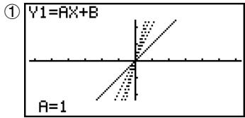
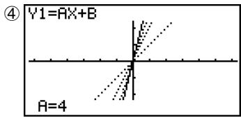
Repeats from ① through ④.
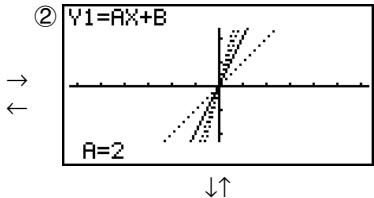
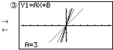

■ Dynamic Graph Application Examples
Description
You can also use Dynamic Graph to simulate simple physical phenomena.
Set Up
- From the Main Menu, enter the DYNA mode.
- Make V-Window settings.
Execution
- On the Setup screen, specify Stop for Dynamic Type and Deg for Angle.
- Specify Parm (parametric function) as the function type, and input a function that contains a dynamic variable.
- Specify the dynamic coefficient.
- Specify the start value, end value, and increment.
- Specify Normal for the draw speed.
- Start the Dynamic Graph operation.


Example
The path over time T of a ball thrown in the air at initial velocity V and an angle of degrees from horizontal can be calculated as follows.
$$ \mathbf {X} = (\mathrm{Vcos} \theta) \mathbf {T}, \quad \mathbf {Y} = (\mathrm{Vsin} \theta) \mathbf {T} - (1 / 2) \mathrm{gT} ^ {2} (\mathrm{g} = 9. 8 \mathrm{m} / \mathrm{s} ^ {2}) $$
Use Dynamic Graph to plot the path of a ball thrown at an initial velocity of 20 meters per second, at horizontal angles of 30, 45, and 60 degrees (Angle: Deg).
Use the following V-Window settings.
$$ \mathrm{Xmin} = - 1, \quad \mathrm{Xmax} = 4 2, \quad \mathrm{Xscale} = 5 $$
$$ \mathrm{Ymin} = - 1, \quad \mathrm{Ymax} = 1 6, \quad \text { Yscale } = 2 $$
$$ \mathbf {T} \theta \min = 0, \quad \mathbf {T} \theta \max = 6, \quad \mathbf {T} \theta \operatorname{ptch} = 0. 1 $$
Procedure
① MENU DYNA
② SHIFT F3 (V-WIN) (-) 1 EXE 4 2 EXE 5 EXE ▼
$$ (-) \boxed {1} \text {EXE} \boxed {1} \boxed {6} \text {EXE} \boxed {2} \text {EXE} $$
$$ ⓠ \quad \boxed {E X E} \quad \boxed {6} \quad \boxed {E X E} \quad \boxed {0} \quad \bullet \quad \boxed {1} \quad \boxed {E X E} \quad \boxed {E X I T} $$
③ SHIFT MENU (SET UP) F2 (Stop)
$$ ⓥ Ⓦ Ⓦ Ⓦ Ⓦ Ⓦ Ⓦ ⓕ F 1 (D e g) \boxed {E X I T} $$
④ F3(TYPE)F3(Parm)
$$ \boxed {(2 0} \cos \text { ALPHA } (X, \theta , T) (A) \boxed {)} X, \theta , T \text { EXE } $$
$$ \boxed {(2 0} \sin \text { ALPHA } (A) \boxed {X, \theta , T} - \boxed {4} \cdot \boxed {9} X, \theta , T x ^ {2} E X E $$
⑤ F4 (VAR)
⑥ F2 (SET) 3 0 EXE 6 0 EXE 1 5 EXE EXIT
⑦ F3 (SPEED) F3 (F) EXIT
⑧ F6 (DYNA)
Result Screen
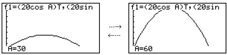
line
| A | f1=(20cos A)T, (20sin) | | --- | ---------------------- | | 30 | (various values) |
■ Adjusting the Dynamic Graph Speed
You can use the following procedure to adjust the Dynamic Graph speed while the draw operation is taking place.
- While a Dynamic Graph draw operation is being performed, press AC to change to the speed adjustment menu.
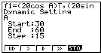
- {III} ... {Each step of the Dynamic Graph draw operation is performed each time you press EXE.}
- {>}/{▶}/{▶} ... {slow (1/2 speed)}/{normal (default speed)}/{fast (double speed)}
-
{STO} ... {stores graph conditions and screen data in Dynamic Graph memory}
-
Press the function key (F1 to F4) that corresponds to the speed you want to change to.
■ Graph Calculation DOT Switching Function
Use this function to specify drawing of all the dots on the Dynamic Graph X-axis, or every other dot. This setting is value for Dynamic Func Y= graphic only.
- Press SHIFT MENU (SET UP) to display the Setup screen.
- Press ▼▼ to select Y=Draw Speed.
- Select the graphing method.
F1(Norm) ... Draws all X-axis dots. (initial default)
F2 (High) ... Draws every other X-axis dot. (faster drawing than Normal) - Press EXIT.

# To clear the speed adjustment menu without changing anything, press EXE.
# Press SHIFT F6(G↔T) to return to the graph screen.

■ Using Dynamic Graph Memory
You can store Dynamic Graph conditions and screen data in Dynamic Graph memory for later recall when you need it. This lets you save time, because you can recall the data and immediately begin a Dynamic Graph draw operation. Note that you can store one set of data in memory at any one time.
The following is all of the data that makes up a set.
• Graph functions (up to 20)
• Dynamic Graph conditions
- Setup screen settings
• V-Window contents
• Dynamic Graph screen
- To save data in Dynamic Graph memory
- While a Dynamic Graph draw operation is being performed, press AC to change to the speed adjustment menu.
- Press F5 (STO). In response to the confirmation dialog that appears, press F1 (Yes) to save the data.
- To recall data from Dynamic Graph memory
- Display the Dynamic Graph relation list.
- Pressing F6(RCL) recalls Dynamic Graph memory contents and draws the graph.

# If there is already data stored in Dynamic Graph memory, the data save operation replaces it with the new data.
# Data recalled from Dynamic Graph memory replaces the calculator's current graph functions, draw conditions, and screen data. The previous data is lost when it is replaced.

5-9 Graphing a Recursion Formula
■ Generating a Number Table from a Recursion Formula
Description
You can input up to three of the following types of recursion formulas and generate a number table.
- General term of sequence a_n , composed of a_n, n
- Linear two-term recursion composed of a_n+1, a_n, n
- Linear three-term recursion composed of a_n+2, a_n+1, a_n, n
Set Up
- From the Main Menu, enter the RECUR mode.
Execution
- Specify the recursion type.
F3(TYPE) F1( a_n ) ... {general term of sequence a_n } F2( a_n+1 ) ... {linear two-term recursion} F3( a_n+2 ) ... {linear three-term recursion}
Select Type
F1: an=An+B
F2: an+1=An+Bn+C
F3: an+z=An+1+Ban+...
an |an+i |an+z
- Input the recursion formula.
- Specify the table range. Specify a start point and end point for n. If necessary, specify a value for the initial term, and a pointer start point value if you plan to graph the formula.
- Display the recursion formula number table.


Example
Generate a number table from recursion between three terms as expressed by a_n+2=a_n+1+a_n , with initial terms of a_1=1 , a_2=1 (Fibonacci sequence), as n changes in value from 1 to 6.
Procedure
① MENU RECUR
② F3(TYPE)F3( a_n+2 )
③ F4(n. a_n ..) F3( a_n+1 ) + F2( a_n ) EXE
④ F5 (SET) F2 (a1) 1 EXE 6 EXE 1 EXE 1 EXE EXIT
⑤ F6 (TABL)
Result Screen
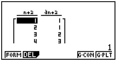
* The first two values correspond to a_1 = 1 and a_2 = 1 .

# Pressing F1(FORM) will return to the screen for storing recursion formulas.
# Specifying On for the Display of the Setup screen causes the sum of each term to be included in the table.

■ Graphing a Recursion Formula (1)
Description
After generating a number table from a recursion formula, you can graph the values on a line graph or plot type graph.
Set Up
- From the Main Menu, enter the RECUR mode.
- Make V-Window settings.
Execution
- Specify the recursion formula type and input the formula.
- Specify the table range, and start and ending values for n. If necessary, specify the initial term value and pointer start point.
- Select the line style for the graph.
- Display the recursion formula number table.
- Specify the graph type and draw the graph.
F5(G·CON) ... line graph
F6 (G • PLT) ... plot type graph
- Selecting F6(G·PLT) draws a 1-dot broken line plot type graph, regardless of the currently selected line style (page 5-3-6).


Example
Generate a number table from recursion between two terms as expressed by a_n+1=2a_n+1 , with an initial term of a_1=1 , as n changes in value from 1 to 6. Use the table values to draw a line graph.
Use the following V-Window settings.
$$ \mathrm{Xmin} = 0, \quad \mathrm{Xmax} = 6, \quad \mathrm{Xscale} = 1 $$
$$ \mathrm{Ymin} = - 1 5, \quad \mathrm{Ymax} = 6 5, \quad \mathrm{Yscale} = 5 $$
Procedure
① MENU RECUR
② SHIFT F3 (V-WIN) 0 EXE 6 EXE 1 EXE ▼
$$ ① 1 5 E X E 6 5 E X E 5 E X E E X I T $$
③ F3 (TYPE) F2 (an+1) 2 F2 (an) + 1 EXE
④ F5 (SET) F2 (a1) 1 EXE 6 EXE 1 EXE EXIT
⑤ F1(SEL+S) ▲ F2(—) EXIT
⑥ F6 (TABL)
⑦ F5(G·CON)
Result Screen
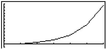
line
| X | Y | |---|---| | 0 | 0 | | 1 | 0.25 | | 2 | 0.5 | | 3 | 0.75 | | 4 | 1.0 | | 5 | 1.25 | | 6 | 1.5 | | 7 | 1.75 | | 8 | 2.0 | | 9 | 2.25 | | 10 | 2.5 | | 11 | 2.75 | | 12 | 3.0 | | 13 | 3.25 | | 14 | 3.5 | | 15 | 3.75 | | 16 | 4.0 | | 17 | 4.25 | | 18 | 4.5 | | 19 | 4.75 | | 20 | 5.0 | | 21 | 5.25 | | 22 | 5.5 | | 23 | 5.75 | | 24 | 6.0 | | 25 | 6.25 | | 26 | 6.5 | | 27 | 6.75 | | 28 | 7.0 | | 29 | 7.25 | | 30 | 7.5 | | 31 | 7.75 | | 32 | 8.0 | | 33 | 8.25 | | 34 | 8.5 | | 35 | 8.75 | | 36 | 9.0 | | 37 | 9.25 | | 38 | 9.5 | | 39 | 9.75 | | 40 | 10.0 | | 41 | 10.25 | | 42 | 10.5 | | 43 | 10.75 | | 44 | 11.0 | | 45 | 11.25 | | 46 | 11.5 | | 47 | 11.75 | | 48 | 12.0 | | 49 | 12.25 | | 50 | 12.5 | | 51 | 12.75 | | 52 | 13.0 | | 53 | 13.25 | | 54 | 13.5 | | 55 | 13.75 | | 56 | 14.0 | | 57 | 14.25 | | 58 | 14.5 | | 59 | 14.75 | | 60 | 15.0 | | 61 | 15.25 | | 62 | 15.5 | | 63 | 15.75 | | 64 | 16.0 | | 65 | 16.25 | | 66 | 16.5 | | 67 | 16.75 | | 68 | 17.0 | | 69 | 17.25 | | 70 | 17.5 | | 71 | 17.75 | | 72 | 18.0 | | 73 | 18.25 | | 74 | 18.5 | | 75 | 18.75 | | 76 | 19.0 | | 77 | 19.25 | | 78 | 19.5 | | 79 | 19.75 | | 80 | 20.0 | | 81 | 20.25 | | 82 | 20.5 | | 83 | 20.75 | | 84 | 21.0 | | 85 | 21.25 | | 86 | 21.5 | | 87 | 21.75 | | 88 | 22.0 | | 89 | 22.25 | | 90 | 22.5 | | 91 | 22.75 | | 92 | 23.0 | | 93 | 23.25 | | 94 | 23.5 | | 95 | 23.75 | | 96 | 24.0 | | 97 | 24.25 | | 98 | 24.5 | | 99 | 24.75 | | Note: The actual values in the 'Y' column are not provided in the code and are not explicitly labeled in the original text 'A'. The 'F' label is not present in the image.
# After drawing a graph, you can use Trace, Zoom, and Sketch.
# After drawing a graph, you can return to the number table screen by pressing SHIFT F6 (G↔T) or AC.

■ Graphing a Recursion Formula (2)
Description
The following describes how to generate a number table from a recursion formula and graph the values while Display is On.
Set Up
- From the Main Menu, enter the RECUR mode.
- On the Setup screen, specify On for Display.
- Make V-Window settings.
Execution
- Specify the recursion formula type and input the recursion formula.
- Specify the table range, and start and ending values for n . If necessary, specify the initial term value and pointer start point.
- Select the line style for the graph.
- Display the recursion formula number table.
- Specify the graph type and draw the graph.
F5 (G·CON) F1 (an) ... Line graph with ordinate an, abscissa n
F6 ( a_n) ... Line graph with ordinate a_n , abscissa n
F6 (G·PLT) F1( a_n ) ... Plot type graph with ordinate a_n , abscissa n
F6(Σan) ... Plot type graph with ordinate Σan, abscissa n
- Selecting F6(G·PLT) draws a 1-dot broken line plot type graph, regardless of the currently selected line style (page 5-3-6).


Example
Generate a number table from recursion between two terms as expressed by a_n+1=2a_n+1 , with an initial term of a_1=1 , as n changes in value from 1 to 6. Use the table values to draw a plot line graph with ordinate a_n , abscissa n.
Use the following V-Window settings.
Xmin = 0, Xmax = 6, Xscale = 1
Ymin = -15, Ymax = 65, Yscale = 5
Procedure
① MENU RECUR
② SHIFT MENU (SET UP) F1 (On) EXIT
③ SHIFT F3 (V-WIN) 0 EXE 6 EXE 1 EXE ▼
(一) 1 5 EXE 6 5 EXE 5 EXE EXIT
④ F3 (TYPE) F2 (an+1) 2 F2 (an) + 1 EXE
⑤ F5 (SET) F2 (a1) 1 EXE 6 EXE 1 EXE EXIT
⑥ F1 (SEL+S) ▲ F2 (—) EXIT
⑦ F6 (TABL)
⑧ F6(G·PLT) F6(Σan)
Result Screen
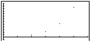
scatter
| X | Y | |---|---| | 0.1 | 0.1 | | 0.2 | 0.2 | | 0.3 | 0.3 | | 0.4 | 0.4 | | 0.5 | 0.5 | | 0.6 | 0.6 | | 0.7 | 0.7 | | 0.8 | 0.8 | | 0.9 | 0.9 | | 1.0 | 1.0 |
■ WEB Graph (Convergence, Divergence)
Description
y = f(x) is graphed by presuming a_n+1 = y , a_n = x for linear two-term regression a_n+1 = f(a_n) composed of a_n+1, a_n . Next, it can be determined whether the function is convergent or divergent.
Set Up
- From the Main Menu, enter the RECUR mode.
- Make V-Window settings.
Execution
- Select 2-term recursion as the recursion formula type, and input the formula.
- Specify the table range, n start and end points, initial term value, and pointer start point.
- Display the recursion formula number table.
- Draw the graph.
- Press EXE, and the pointer appears at the start point you specified. Press EXE several times.
If convergence exists, lines that resemble a spider web are drawn on the display. Failure of the web lines to appear indicates either divergence or that the graph is outside the boundaries of the display screen. When this happens, change to larger V-Window values and try again.
You can use ▲▼ to select the graph.

# To change the graph line style, press F1(SEL+S) after step 4.
# With WEB Graph, you can specify the line type for a y = f(x) graph. The line type setting is valid only when “Connect” is selected for “Draw Type” on the Setup screen.


Example
To draw the WEB graph for the recursion formula a_n+1 = -3(a_n)^2 + 3a_n , b_n+1 = 3b_n + 0.2 , and check for divergence or convergence. Use the following table range and V-Window Settings.
Table Range
Start = 0, End = 6, a_0 = 0.01 , a_n Str = 0.01 , b_0 = 0.11 , b_n Str = 0.11
V-Window Settings
Xmin = 0,
Xmax = 1,
Xscale = 1
Ymin = 0,
Ymax = 1,
Yscale = 1
Procedure
① MENU RECUR
② SHIFT F3 (V-WIN) 0 EXE 1 EXE 1 EXE ▼
0 EXE 1 EXE 1 EXE EXIT
③ F3 (TYPE) F2 (an+1) (-) 3 F2 (an) x² + 3 F2 (an) EXE
3 F3 (bn) + 0 · 2 EXE
④ F5 (SET) F1 (a0)
⑤ F6 (TABL)
⑥ F4 (WEB)
⑦ EXE \~ EXE (an is convergence)
☑ EXE \~ EXE ( b_n is divergence)
Result Screen
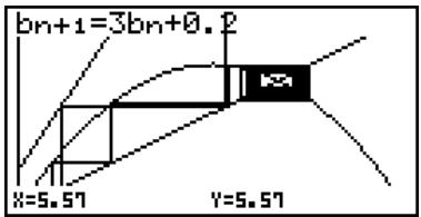

■ Graphing a Recursion Formula on Dual Screen
Description
When “T+G” is specified for the Dual Screen setting, you can view the number table and graph at the same time.
Set Up
- From the Main Menu, enter the RECUR mode.
- Make V-Window settings.
- On the Setup screen, select T+G for Dual Screen.
Execution
- Specify the recursion formula type and input the formula.
- Specify the table range, and start and ending values for n . If necessary, specify the initial term value and pointer start point.
- Select the line style for the graph.
- Display the recursion formula number table.
- Specify the graph type and draw the graph.
F5 (G·CON) ... line graph
F6(G·PLT) ... plot type graph

# The Setup screen's "Dual Screen" setting is applied in the TABLE mode and the RECUR mode.


Example
Generate a number table from recursion between two terms as expressed by a_n+1=2a_n+1 , with an initial term of a_1=1 , as n changes in value from 1 to 6. Use the table values to draw a line graph.
Use the following V-Window settings.
$$ \mathrm{Xmin} = 0, \quad \mathrm{Xmax} = 6, \quad \mathrm{Xscale} = 1 $$
$$ \mathrm{Ymin} = - 1 5, \quad \mathrm{Ymax} = 6 5, \quad \text { Yscale } = 5 $$
Procedure
① MENU RECUR
② SHIFT F3 (V-WIN) 0 EXE 6 EXE 1 EXE ▼
$$ ① 1 5 E X E 6 5 E X E 5 E X E E X I T $$
③ SHIFT MENU (SET UP) ▼ ▼ ▼ F1 (T+G) EXIT
④ F3 (TYPE) F2 (an+1) 2 F2 (an) + 1 EXE
⑤ F5 (SET) F2 (a1) 1 EXE 6 EXE 1 EXE EXIT
⑥ F1 (SEL+S) ▲ F2 (—) EXIT
⑦ F6 (TABL)
⑧ F5(G·CON)
Result Screen
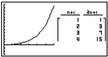
line
| x | n+1 | 3n+1 | |---|---|---| | 0 | 0 | 0 | | 1 | 0.5 | 0.5 | | 2 | 1 | 1 | | 3 | 2 | 2 | | 4 | 3 | 3 | | 5 | 4 | 4 | | 6 | 5 | 5 | | 7 | 6 | 6 | | 8 | 7 | 7 | | 9 | 8 | 8 | | 10 | 9 | 9 | | 11 | 10 | 10 | | 12 | 11 | 11 | | 13 | 12 | 12 | | 14 | 13 | 13 | | 15 | 14 | 14 | | 16 | 15 | 15 | | 17 | 16 | 16 | | 18 | 17 | 17 | | 19 | 18 | 18 | | 20 | 19 | 19 | | 21 | 20 | 20 | | 22 | 21 | 21 | | 23 | 22 | 22 | | 24 | 23 | 23 | | 25 | 24 | 24 | | 26 | 25 | 25 | | 27 | 26 | 26 | | 28 | 27 | 27 | | 29 | 28 | 28 | | 30 | 29 | 29 | | 31 | 30 | 30 | | 32 | 31 | 31 | | 33 | 32 | 32 | | 34 | 33 | 33 | | 35 | 34 | 34 | | 36 | 35 | 35 | | 37 | 36 | 36 | | 38 | 37 | 37 | | 39 | 38 | 38 | | 40 | 39 | 39 | | 41 | 40 | 40 | | 42 | 41 | 41 | | 43 | 42 | 42 | | 44 | 43 | 43 | | 45 | 44 | 44 | | 46 | 45 | 45 | | 47 | 46 | 46 | | 48 | 47 | 47 | | 49 | 48 | 48 | | 50 | 49 | 49 | | 51 | 50 | 50 | | 52 | - | - | | 53 | - | - | | 54 | - | - | | 55 | - | - | | 56 | - | - | | 57 | - | - | | 58 | - | - | | 59 | - | - | | 60 | - | - | | 61 | - | - | | 62 | - | - | | 63 | - | - | | 64 | - | - | | 65 | - | - | | 66 | - | - | | 67 | - | - | | 68 | - | - | | 69 | - | - | | 70 | - | - | | 71 | - | - | | 72 | - | - | | 73 | - | - | | 74 | - | - | | 75 | - | - | | 76 | - | - | | 77 | - | - | | 78 | - | - | | 79 | - | - | | 80 | - | - | | 81 | - | - | | 82 | - | - | | 83 | - | - | | 84 | - | - | | 85 | - | - | | 86 | - | - | | 87 | - | - | | 88 | - | - | | 89 | - | - | | 90 | - | - | | 91 | - | - | | 92 | - | - | | 93 | - | - | | 94 | - | - | | 95 | - | - | | 96 | - | - | | 97 | - | - | | 98 | - | - | | 99 | - | - | | Note: The values in the chart are estimated based on the provided code (e.g., 'n+1' and '3n+1') and are not explicitly provided in the code.
# You can make the number table active by pressing OPTN F1 (CHNG) or AC.
# After drawing a graph, you can return to the number table screen by pressing SHIFT F6(G↔T) or AC.

5-10 Changing the Appearance of a Graph
■ Drawing a Line
Description
The sketch function lets you draw points and lines inside of graphs.
You can select one of four different line styles for drawing with the sketch function.
Set Up
- From the Main Menu, enter the GRAPH mode.
- Make V-Window settings.
- On the Setup screen, use the "Sketch Line" setting to specify the line style you want.
F1(—) ... Normal (initial default)
F2(一) ... Thick (twice the thickness of Normal)
F3(……) ... Broken (thick broken)
F4(……) ... Dot (dotted) - Input the function of the graph.
- Draw the graph.
Execution
- Select the sketch function you want to use.*1
SHIFT F4 (SKTCH) F1 (Cls) ... Screen clear
F2 (Tang) ... Tangent line
F3(Norm) ... Line normal to a curve
F4 (Inv) ... Inverse function ^*2
F6 (▷) F1 (PLOT)
{Plot}/{PI·On}/{PI·Off}/{PI·Chg}
... Point {Plot}/{On}/{Off}/{Change}
F6 (▷) F2 (LINE)
{Line}/{F·Line} ... {connects 2 points plotted by F6(▷) F1(PLOT)
with a line}/{for drawing a line between any 2 points}
F6 (▷) F3 (Crcl) ... Circle
F6 (▷) F4 (Vert) ... Vertical line
F6 (▷) F5 (Hztl) ... Horizontal line
F6 (▷) F6 (▷) F1 (PEN) ... Freehand
F6 (▷) F6 (▷) F2 (Text) ... Text input
- Use the cursor keys to move the pointer (⊕) to the location where you want to draw, and press EXE.*3

*1 The above shows the function menu that appears in the GRAPH mode. Menu items may differ somewhat in other modes.
*2 In the case of an inverse function graph, drawing starts immediately after you select this option.
*3 Some sketch functions require specification of two points. After you press EXE to specify the first point, use the cursor keys to move the pointer to the location of the second point and press EXE.
# You can specify line type for the following sketch functions: Tangent, Normal, Inverse, Line, F • Line, Circle, Vertical, Horizontal, Pen


Example
Draw a line that is tangent to point (2, 0) on the graph for y = x ( x + 2 ) ( x - 2 ).
Use the following V-Window settings.
$$ \mathrm{Xmin} = - 6. 3, \quad \mathrm{Xmax} = 6. 3, \quad \mathrm{Xscale} = 1 $$
$$ \text { Ymin } = - 3. 1, \quad \text { Ymax } = 3. 1, \quad \text { Yscale } = 1 (\text { initial defaults }) $$
Procedure
① MENU GRAPH
② SHIFT F3 (V-WIN) F1 (INIT) EXIT
③ SHIFT MENU (SET UP) ▼ ▼ ▼ ▼ ▼ ▼ F1 (—) EXIT
④ F3 (TYPE) F1 (Y=) X,θ,T (X,θ,T + 2 ) (X,θ,T - 2 ) EXE
⑤ F6 (DRAW)
⑥ SHIFT F4 (SKTCH) F2 (Tang)
⑦ ▶ \~ ▶ EXE *1
Result Screen
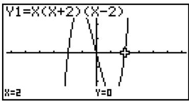

*1 You can draw a tangent line in succession by moving the “+” pointer and pressing EXE.

■ Inserting Comments
Description
You can insert comments anywhere you want in a graph.
Set Up
- Draw the graph.
Execution
- Press SHIFT F4 (SKTCH) F6 (▷) F6 (▷) F2 (Text), and a pointer appears in the center of the display.
- Use the cursor keys to move the pointer to the location where you want the text to be, and input the text.

# You can input any of the following characters as comment text: A\~Z, r, θ, space, 0\~9, ., +, -, ×, ÷, (-), EXP, π, Ans, (, ), [, ], {}, comma, →,
x^2, , , , , x, 10^x, e^x, ^3, x^-1, , , , ^-1, ^-1, ^-1, i, List, Mat,


Example
Insert text into the graph y = x (x + 2)(x - 2) .
Use the following V-Window settings.
You can use the pen option for freehand drawing in a graph.
Set Up
- Draw the graph.
Execution
- Press SHIFT F4 (SKTCH) F6 (▷) F6 (▷) F1 (PEN), and a pointer appears in the center of the screen.
- Use the cursor keys to move the pointer to the point from which you want to start drawing, and then press EXE.
- Use the cursor keys to move the pointer. A line is drawn wherever you move the pointer. To stop the line, press EXE.
Repeat step 3 and 4 to draw other lines.


Example
Use the pen to draw on the graph y = x (x + 2)(x - 2) .
Use the following V-Window settings.
line
| X | Y | |---|---| | -1.904761905 | 4.35483871 |
■ Changing the Graph Background
You can use the Setup screen to specify the memory contents of any picture memory area (Pict 1 through Pict 20) as the Background item. When you do, the contents of the corresponding memory area is used as the background of the graph screen.

Example 1 With the circle graph X^2 + Y^2 = 1 as the background, use Dynamic Graph to graph Y = X^2 + A as variable A changes value from -1 to 1 in increments of 1.
Recall the background graph.
$$ \left(X ^ {2} + Y ^ {2} = 1\right) $$
SHIFT MENU (SET UP) ▼ ▼ ▼ ▼ ▼
F2 (PICT) 1 EXE EXIT
(When the graph for X^2 + Y^2 = 1 is stored in Pict 1)
natural_image
Simple geometric diagram with a circle centered at the intersection of two perpendicular lines (no text or labels)
Draw the dynamic graph.
$$ (Y = X ^ {2} - 1) $$
$$ (Y = X ^ {2}) $$
$$ (Y = X ^ {2} + 1) $$
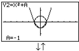
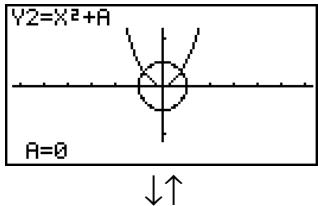
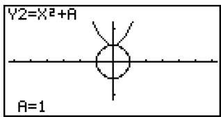
- See “5-8 Dynamic Graphing” for details on using the Dynamic Graph feature.

5-11 Function Analysis
■ Reading Coordinates on a Graph Line
Description
Trace lets you move a pointer along a graph and read out coordinates on the display.
Set Up
- From the Main Menu, enter the GRAPH mode.
- Draw the graph.
Execution
- Press SHIFT F1 (TRCE), and a pointer appears in the center of the graph.*1
- Use ◀ and ▶ to move the pointer along the graph to the point at which you want to display the derivative.
When there are multiple graphs on the display, press ▲ and ▼ to move between them along the x-axis of the current pointer location. - You can also move the pointer by pressing ,,T to display the pop-up window, and then inputting coordinates.
The pop-up window appears even when you input coordinates directly.
To exit a trace operation, press SHIFT F1 (TRCE).

^*1 The pointer is not visible on the graph when it is located at a point outside the graph display area or when an error of no value occurs.
# You can turn off display of the coordinates at the pointer location by specifying "Off" for the "Coord" item on the Setup screen.


Example
Read coordinates along the graph of the function shown below.
$$ \mathbf {Y 1} = x ^ {2} - 3 $$
Use the following V-Window settings.
$$ \mathrm{Xmin} = - 5, \quad \mathrm{Xmax} = 5, \quad \mathrm{Xscale} = 1 $$
$$ \mathrm{Ymin} = - 1 0, \quad \mathrm{Ymax} = 1 0, \quad \text { Yscale } = 2 $$
Procedure
① MENU GRAPH
② SHIFT F3 (V-WIN) (-) 5 EXE 5 EXE 1 EXE ▼
$$ (-) \boxed {1} \boxed {0} \boxed {\mathrm{EXE}} \boxed {1} \boxed {0} \boxed {\mathrm{EXE}} \boxed {2} \boxed {\mathrm{EXE}} \boxed {\mathrm{EXIT}} $$
$$ \boxed {F 3} (\text { TYPE }) \boxed {F 1} (Y =) \boxed {X, \theta , T} \boxed {x ^ {2}} - \boxed {3} \boxed {\text { EXE }} $$
$$ \boxed {F 6} (\text { DRAW }) $$
③ SHIFT F1 (TRCE)
④ ◀\~◀
⑤ (-) 1 EXE
Result Screen
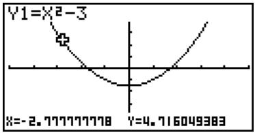
line
| X | Y | |---|---| | -2 | -2 | | 4 | 4 |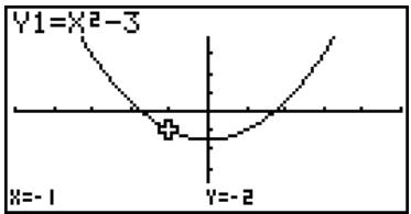
line
| x | y | |---|---| | -1 | -2 | | 0 | 0 | | 1 | -2 |
# The following shows how coordinates are displayed for each function type.
- Polar Coordinate Graph
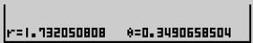
- Parametric Graph
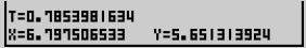
- Inequality Graph
# The pointer will not move if you press the ◀ and ▶ keys during trace of an "X=c" type graph.

■ Displaying the Derivative
Description
In addition to using Trace to display coordinates, you can also display the derivative at the current pointer location.
Set Up
- From the Main Menu, enter the GRAPH mode.
- On the Setup screen, specify On for Derivative.
- Draw the graph.
Execution
- Press SHIFT F1(TRCE), and the pointer appears at the center of the graph. The current coordinates and the derivative also appear on the display at this time.
- Use ◀ and ▶ to move the pointer along the graph to the point at which you want to display the derivative.
When there are multiple graphs on the display, press ▲ and ▼ to move between them along the x-axis of the current pointer location. - You can also move the pointer by pressing ,, to display the pop-up window, and then inputting coordinates.
The pop-up window appears even when you input coordinates directly.


Example
Read coordinates and derivatives along the graph of the function shown below.
$$ \mathbf {Y 1} = x ^ {2} - 3 $$
Use the following V-Window settings.
$$ \mathrm{Xmin} = - 5, \quad \mathrm{Xmax} = 5, \quad \mathrm{Xscale} = 1 $$
$$ \mathrm{Ymin} = - 1 0, \quad \mathrm{Ymax} = 1 0, \quad \text { Yscale } = 2 $$
Procedure
① MENU GRAPH
② SHIFT MENU (SET UP) ▼ ▼ ▼ ▼ F1 (On) EXIT
③ SHIFT F3 (V-WIN) (-) 5 EXE 5 EXE 1 EXE ▼
$$ (-) \boxed {1} \boxed {0} \boxed {\text { EXE }} \boxed {1} \boxed {0} \boxed {\text { EXE }} \boxed {2} \boxed {\text { EXE }} \boxed {\text { EXIT }} $$
$$ \boxed {F 3} (\text { TYPE }) \boxed {F 1} (Y =) \boxed {X, \theta , T} \boxed {x ^ {2}} - \boxed {3} \boxed {\text { EXE }} $$
$$ \boxed {F 6} (\text { DRAW }) $$
④ SHIFT F1 (TRCE)
⑤ ◀\~◀
⑥ (-) 1 EXE
Result Screen
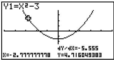
line
| Point | Value | |---|---| | X | -2.77777778 | | Y | 4.716049383 | | dY/dX | -5.555 |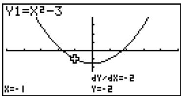
line
| Point | X | Y | |---|---|---| | Point 1 | -1 | 0 | | Point 2 | 0 | 0 | | Point 3 | 0 | 0 | | Point 4 | 0 | 0 | | Point 5 | 0 | 0 | | Point 6 | 0 | 0 | | Point 7 | 0 | 0 | | Point 8 | 0 | 0 | | Point 9 | 0 | 0 | | Point 10 | 0 | 0 | | Point 11 | 0 | 0 | | Point 12 | 0 | 0 | | Point 13 | 0 | 0 | | Point 14 | 0 | 0 | | Point 15 | 0 | 0 | | Point 16 | 0 | 0 | | Point 17 | 0 | 0 | | Point 18 | 0 | 0 | | Point 19 | 0 | 0 | | Point 20 | 0 | 0 | | Point 21 | 0 | 0 | | Point 22 | 0 | 0 | | Point 23 | 0 | 0 | | Point 24 | 0 | 0 | | Point 25 | 0 | 0 | | Point 26 | 0 | 0 | | Point 27 | 0 | 0 | | Point 28 | 0 | 0 | | Point 29 | 0 | 0 | | Point 30 | 0 | 0 | | Point 31 | 0 | 0 | | Point 32 | 0 | 0 | | Point 33 | 0 | 0 | | Point 34 | 0 | 0 | | Point 35 | 0 | 0 | | Point 36 | 0 | 0 | | Point 37 | 0 | 0 | | Point 38 | 0 | 0 | | Point 39 | 0 | 0 | | Point 40 | 0 | 0 | | Point 41 | -1 | -1 | | Point 42 | -1 | -2 | | Point 43 | -1 | -2 | | Point 44 | -1 | -2 | | Point 45 | -1 | -2 | | Point 46 | -1 | -2 | | Point 47 | -1 | -2 | | Point 48 | -1 | -2 | | Point 49 | -1 | -2 | | Point 50 | -1 | -2 | | Point 51 | -1 | -2 | | Point 52 | -1 | -2 | | Point 53 | -1 | -2 | | Point 54 | -1 | -2 | | Point 55 | -1 | -2 | | Point 56 | -1 | -2 | | Point 57 | -1 | -2 | | Point 58 | -1 | -2 | | Point 59 | -1 | -2 | | Point 60 | -1 | -2 | | Point 61 | -1 | -2 | | Point 62 | -1 | -2 | | Point 63 | -1 | -2 | | Point 64 | -1 | -2 | | Point 65 | -1 | -2 | | Point 66 | -1 | -2 | | Point 67 | -1 | -2 | | Point 68 | -1 | -2 | | Point 69 | -1 | -2 | | Point 70 | -1 | -2 | | Point 71 | -1 | -2 | | Point 72 | -1 | -2 | | Point 73 | -1 | -2 | | Point 74 | -1 | -2 | | Point 75 | -1 | -2 | | Point 76 | -1 | -2 | | Point 77 | -1 | -2 | | Point 78 | -1 | -2 | | Point 79 | -1 | -2 | | Point 80 | -1 | -2 | | Point 81 | -1 | -2 | | Point 82 | -1 | -2 | | Point 83 | -1 | -2 | | Point 84 | -1 | -2 | | Point 85 | -1 | -2 | | Point 86 | -1 | -2 | | Point 87 | -1 | -2 | | Point 88 | -1 | -2 | | Point 89 | -1 | -2 | | Point 90 | -1 | -2 | | Point 91 | -1 | -2 | | Point 92 | -1 | -2 | | Point 93 | -1 | -2 | | Point 94 | -1 | -2 | | Point 95 | -1 | -2 | | Point 96 | -1 | -2 | | Point 97 | -1 | -2 | | Point 98 | -1 | -2 | | Point 99 | -1 | -2 | | Point100 Point1 = X²-3 Point2 = X²-3 Point3 = X²-3 Point4 = X²-3 Point5 = X²-3 Point6 = X²-3 Point7 = X²-3 Point8 = X²-3 Point9 = X²-3 Point10 = X²-3 Point11 = X²-3 Point12 = X²-3 Point13 = X²-3 Point14 = X²-3 Point15 = X²-3 Point16 = X²-3 Point17 = X²-3 Point18 = X²-3 Point19 = X²-3 Point20 = X²-3 Point21 = X²-3 Point22 = X²-3 Point23 = X²-3 Point24 = X²-3 Point25 = X²-3 Point26 = X²-3 Point27 = X²-3 Point28 = X²-3 Point29 = X²-3 Point30 = X²-3 Point31 = X²-3 Point32 = X²-3 Point33 = X²-3 Point34 = X²-3 Point35 = X²-3 Point36 = X²-3 Point37 = X²-3 Point38 = X²-3 Point39 = X²-3 Point40 = X²-3 Point41 = X²-3 Point42 = X²-3 Point43 = X²-3 Point44 = X²-3 Point45 = X²-3 Point46 = X²-3 Point47 = X²-3 Point48 = X²-3 Point49 = X²-3 Point50 = X²-3 Point51 = X²-3 Point52 = X²-3 Point53 = X²-3 Point54 = X²-3 Point55 = X²-3 Point56 = X²-3 Point57 = X²-3 Point58 = X²-3 Point59 = X²-3 Point60 = X²-3 Point61 = X²-3 Point62 = X²-3 Point63 = X²-3 Point64 = X²-3 Point65 = X²-3 Point66 = X²-3 Point67 = X²-3 Point68 = X²-3 Point69 = X²-3 Point70 = X²-3 Point71 = X²-3 Point72 = X²-3 Point73 = X²-3 Point74 = X²-3 Point75 = X²-3 Point76 = X²-3 Point77 = X²-3 Point78 = X²-3 Point79 = X²-3 Point80 = X²-3 Point81 = X²-3 Point82 = X²-3 Point83 = X²-3 Point84 = X²-3 Point85 = X²-3 Point86 = X²-3 Point87 = X²-3 Point88 = X²-3 Point89 = X²-3 Point90 = X²-3 Point91 = X²-3 Point92 = X²-3 Point93 = X²-3 Point94 = X²-3 Point95 = X²-3 Point96 = X²-3 Point97 = X²-3 Point98 = X²-3 Point99 = X²-3
■ Graph to Table
Description
You can use trace to read the coordinates of a graph and store them in a number table. You can also use Dual Graph to simultaneously store the graph and number table, making this an important graph analysis tool.
Set Up
- From the Main Menu, enter the GRAPH mode.
- On the Setup screen, specify GtoT for Dual Screen.
- Make V-Window settings.
Execution
- Save the function and draw the graph on the active (left) screen.
- Activate Trace. When there are multiple graphs on the display, press ▲ and ▼ to select the graph you want.
- Use ◀ and ▶ to move the pointer and press EXE to store coordinates into the number table. Repeat this step to store as many values as you want.
- Press OPTN F1(CHNG) to make the number table active.
- From the pop-up window, input the list number you want to save.


Example
Save, in a table, the coordinates in the vicinity of the points of intersection at X = 0 for the two graphs shown below, and store the table contents in List 1.
$$ \mathbf {Y} 1 = x ^ {2} - 3, \mathbf {Y} 2 = - x + 2 $$
Use the following V-Window settings.
$$ \mathrm{Xmin} = - 5, \quad \mathrm{Xmax} = 5, \quad \mathrm{Xscale} = 1 $$
$$ \mathrm{Ymin} = - 1 0, \quad \mathrm{Ymax} = 1 0, \quad \text { Yscale } = 2 $$
Procedure
① MENU GRAPH
② SHIFT MENU (SET UP) ▼ F2 (GtoT) EXIT
③ SHIFT F3 (V-WIN) (-) 5 EXE 5 EXE 1 EXE ▼
$$ ① 1 0 \text { EXE } 1 0 \text { EXE } 2 \text { EXE } \text { EXIT } $$
④ F3 (TYPE) F1 (Y=) X,θ,T x² - 3 EXE
$$ ⓜ (-) ⓧ X, \theta , T + 2 ⓐ E X E $$
F6 (DRAW)
⑤ SHIFT F1 (TRCE)
⑥ ◀️ \~ ◀️ EXE ▶️ \~ ▶️ EXE
⑦ OPTN F1 (CHNG)
⑧ OPTN F2 (LMEM) 1 EXE
Result Screen
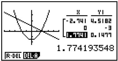
line
| X | Y1 | Y2 | |---|---|---| | -2.741 | 4.5182 | | | 0 | -3 | | | 0.7741 | 0.1477 | | | 1.774193548 | | |
# Instead of pressing OPTN F1(CHNG) in step 7, you could press AC to make the number table active.

■ Coordinate Rounding
Description
This function rounds off coordinate values displayed by Trace.
Set Up
- From the Main Menu, enter the GRAPH mode.
- Draw the graph.
Execution
- Press SHIFT F2 (ZOOM) F6 (▷) F3 (RND). This causes the V-Window settings to be changed automatically in accordance with the Rnd value.
- Press SHIFT F1(TRCE), and then use the cursor keys to move the pointer along the graph. The coordinates that now appear are rounded.


Example
Use coordinate rounding and display the coordinates in the vicinity of the points of intersection for the two graphs produced by the functions shown below.
$$ \mathbf {Y} 1 = x ^ {2} - 3, \mathbf {Y} 2 = - x + 2 $$
Use the following V-Window settings.
$$ \mathrm{Xmin} = - 5, \quad \mathrm{Xmax} = 5, \quad \mathrm{Xscale} = 1 $$
$$ \mathrm{Ymin} = - 1 0, \quad \mathrm{Ymax} = 1 0, \quad \text { Yscale } = 2 $$
Procedure
① MENU GRAPH
② SHIFT F3 (V-WIN) (-) 5 EXE 5 EXE 1 EXE ▼
$$ (-) \boxed {1} \boxed {0} \boxed {\text {EXE}} \boxed {1} \boxed {0} \boxed {\text {EXE}} \boxed {2} \boxed {\text {EXE}} \boxed {\text {EXIT}} $$
$$ \boxed {F 3} (\text { TYPE }) \boxed {F 1} (Y =) \boxed {X, \theta , T} \boxed {x ^ {2}} - \boxed {3} \boxed {\text { EXE }} $$
$$ ⓜ (-) ⓧ X, \theta , T + 2 Ⓔ E X E $$
$$ \boxed {F 6} (\text { DRAW }) $$
③ SHIFT F2 (ZOOM) F6 (▷) F3 (RND)
④ SHIFT F1 (TRCE)
$$ ⓛ \sim Ⓟ $$
Result Screen
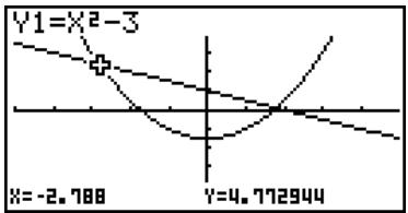
line
| x | y1 | y2 | | ------- | ------ | ------ | | -2.788 | -3.000 | -3.000 | | 4.712944| -3.000 | -3.000 |
■ Calculating the Root
Description
This feature provides a number of different methods for analyzing graphs.
Set Up
- From the Main Menu, enter the GRAPH mode.
- Draw the graphs.
Execution
- Select the analysis function.
SHIFT F5 (G-SLV) F1 (ROOT) ... Calculation of root
F2(MAX) ... Local maximum value
F3 (MIN) ... Local minimum value
F4 (Y-ICPT) ... y-intercept
F5(ISCT) ... Intersection of two graphs
F6 (▷) F1 (Y-CAL) ... y-coordinate for given x-coordinate
F6 (▷) F2 (X-CAL) ... x-coordinate for given y-coordinate
F6 (▷) F3 (∫dx) ... Integral value for a given range
- When there are multiple graphs on the screen, the selection cursor (■) is located at the lowest numbered graph. Press ▲ and ▼ to move the cursor to the graph you want to select.
- Press EXE to select the graph where the cursor is located and display the value produced by the analysis.
When an analysis produces multiple values, press ▶ to calculate the next value.
Pressing ◀ returns to the previous value.


Example
Draw the graph shown below and calculate the root for Y1.
$$ \mathbf {Y} 1 = x (x + 2) (x - 2) $$
Use the following V-Window settings.
$$ \mathrm{Xmin} = - 6. 3, \quad \mathrm{Xmax} = 6. 3, \quad \mathrm{Xscale} = 1 $$
$$ \text { Ymin } = - 3. 1, \quad \text { Ymax } = 3. 1, \quad \text { Yscale } = 1 (\text { initial defaults }) $$
Procedure
① MENU GRAPH
② SHIFT F3 (V-WIN) F1 (INIT) EXIT
$$ \boxed {\mathsf {F 3}} (\text { TYPE }) \boxed {\mathsf {F 1}} (Y =) \boxed {X, \theta , T} (\boxed {X, \theta , T} + \boxed {2}) (\boxed {X, \theta , T} - \boxed {2}) \boxed {\text { EXE }} $$
$$ \boxed {F 6} (\text { DRAW }) $$
③ SHIFT F5 (G-SLV) F1 (ROOT)

Result Screen
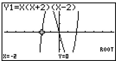
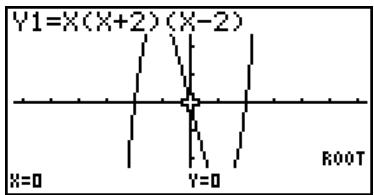
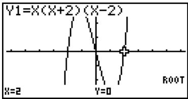

When analyzing a single graph, results appear as soon as you select an analysis function in step 3, so step 4 is not necessary.
Root, local maximum value, local minimum value, and y-intercept can be calculated for rectangular coordinate graphs and inequality graphs only.
Graph analysis is not possible for the graph whose function is the format X = constant.
The y-intercept is the point where the graph crosses the y-axis.

■ Calculating the Point of Intersection of Two Graphs
Description
Use the following procedure to calculate the point of intersection of two graphs.
Set Up
- Draw the graphs.
Execution
- Press SHIFT F5 (G-SLV) F5 (ISCT). When there are three or more graphs, the selection cursor (■) appears at the lowest numbered graph.
- Press ▲ and ▼ to move the cursor to the graph you want to select.
- Press EXE to select the first graph, which changes the shape of the cursor from ■ to ◆.
- Press ▲ and ▼ to move the cursor to the second graph.
- Press EXE to calculate the point of intersection for the two graphs. When an analysis produces multiple values, press ▶ to calculate the next value. Pressing ◀ returns to the previous value.


Example
Graph the two functions shown below, and determine the point of intersection between Y1 and Y2.
$$ \mathbf {Y} 1 = x + 1, \mathbf {Y} 2 = x ^ {2} $$
Use the following V-Window settings.
$$ \mathrm{Xmin} = - 5, \quad \mathrm{Xmax} = 5, \quad \mathrm{Xscale} = 1 $$
$$ \mathrm{Ymin} = - 5, \quad \mathrm{Ymax} = 5, \quad \text { Yscale } = 1 $$
Procedure
① MENU GRAPH

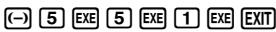

F6 (DRAW)
② SHIFT F5 (G-SLV) F5 (ISCT)

Result Screen
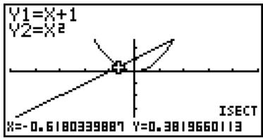
line
| Point | Y1=X+1 | Y2=X² | |---|---|---| | (X=-0.6180339887) | | | | (Y=0.3819660113) | | |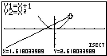
line
| X | Y1=X+1 | Y2=X² | |---|---|---| | 1.618033989 | | | | 2.618033989 | | |
# In the case of two graphs, the point of intersection is calculated immediately after you press SHIFT F5 F5 in step 2.
# You can calculate the point of intersection for rectangular coordinate graphs and inequality graphs only.

■ Determining the Coordinates for Given Points
Description
The following procedure describes how to determine the y-coordinate for a given x, and the x-coordinate for a given y.
Set Up
- Draw the graph.
Execution
- Select the function you want to perform. When there are multiple graphs, the selection cursor (■) appears at the lowest numbered graph.
SHIFT F5 (G-SLV) F6 (▷) F1 (Y-CAL) ... y-coordinate for given x
F6 (▷) F2 (X-CAL) ... x-coordinate for given y
-
Use ⚠️ ▼ to move the cursor (■) to the graph you want, and then press EXE to select it.
-
Input the given x-coordinate value or y-coordinate value. Press EXE to calculate the corresponding y-coordinate value or x-coordinate value.


Example
Graph the two functions shown below and then determine the y-coordinate for x = 0.5 and the x-coordinate for y = 2.2 on graph Y2.
$$ \mathsf {Y 1} = x + 1, \mathsf {Y 2} = x (x + 2) (x - 2) $$
Use the following V-Window settings.
$$ \mathrm{Xmin} = - 6. 3, \quad \mathrm{Xmax} = 6. 3, \quad \mathrm{Xscale} = 1 $$
Ymin = -3.1, Ymax = 3.1, Yscale = 1 (initial defaults)
Procedure
① MENU GRAPH
SHIFT F3 (V-WIN) F1 (INIT) EXIT
F3 (TYPE) F1 (Y=) X,θ,T + 1 EXE
X,θ,T (X,θ,T + 2 ) (X,θ,T - 2 ) EXE
F6 (DRAW)
② SHIFT F5 (G-SLV) F6 (▷) F1 (Y-CAL)
② SHIFT F5 (G-SLV) F6 (▷) F2 (X-CAL)
③ ▼ EXE
③ ▼ EXE
④ 0 · 5 EXE
④ 2 · 2 EXE
Result Screen
line
| X | Y | |---|---| | 0.5 | -1.875 | | 2 | -1.875 | | 3 | -1.875 | | 4 | -1.875 | | 5 | -1.875 | | 6 | -1.875 | | 7 | -1.875 | | 8 | -1.875 | | 9 | -1.875 | | 10 | -1.875 | | 11 | -1.875 | | 12 | -1.875 | | 13 | -1.875 | | 14 | -1.875 | | 15 | -1.875 | | 16 | -1.875 | | 17 | -1.875 | | 18 | -1.875 | | 19 | -1.875 | | 20 | -1.875 | | 21 | -1.875 | | 22 | -1.875 | | 23 | -1.875 | | 24 | -1.875 | | 25 | -1.875 | | 26 | -1.875 | | 27 | -1.875 | | 28 | -1.875 | | 29 | -1.875 | | 30 | -1.875 | | 31 | -1.875 | | 32 | -1.875 | | 33 | -1.875 | | 34 | -1.875 | | 35 | -1.875 | | 36 | -1.875 | | 37 | -1.875 | | 38 | -1.875 | | 39 | -1.875 | | 40 | -1.875 | | 41 | -1.875 | | 42 | -1.875 | | 43 | -1.875 | | 44 | -1.875 | | 45 | -1.875 | | 46 | -1.875 | | 47 | -1.875 | | 48 | -1.875 | | 49 | -1.875 | | 50 | -1.875 | | 51 | -1.875 | | 52 | -1.875 | | 53 | -1.875 | | 54 | -1.875 | | 55 | -1.875 | | 56 | -1.875 | | 57 | -1.875 | | 58 | -1.875 | | 59 | -1.875 | | 60 | -1.875 | | 61 | -1.875 | | 62 | -1.875 | | 63 | -1.875 | | 64 | -1.875 | | 65 | -1.875 | | 66 | -1.875 | | 67 | -1.875 | | 68 | -1.875 | | 69 | -1.875 | | 70 | -1.875 | | 71 | -1.875 | | 72 | -1.875 | | 73 | -1.875 | | 74 | -1.875 | | 75 | -1.875 | | 76 | -1.875 | | 77 | -1.875 | | 78 | -1.875 | | 79 | -1.875 | | 80 | -1.875 | | 81 | -1.875 | | 82 | -1.875 | | 83 | -1.875 | | 84 | -1.875 | | 85 | -1.875 | | 86 | -1.875 | | 87 | -1.875 | | 88 | -1.875 | | 89 | -1.875 | | 90 | -1.875 | | 91 | -1.875 | | 92 | -1.875 | | 93 | -1.875 | | 94 | -1.875 | | 95 | -1.875 | | 96 | -1.875 | | 97 | -1.875 | | 98 | -1.875 | | 99 | -1.875 | | 100 | -1.875 |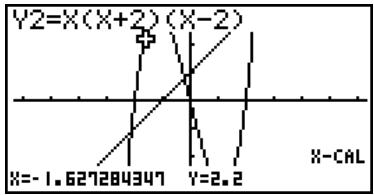
line
| X-CAL | Y2 | |---|---| | -1.627284347 | 2.2 |
# When there are multiple results for the above procedure, press ▶ to calculate the next value. Pressing ◀ returns to the previous value.
# Step 3 of the above procedure is skipped when there is only one graph on the display.
# The X-CAL value cannot be obtained for a parametric function graph.
# After obtaining coordinates with the above procedure, you can input different coordinates by first pressing [X,,T] .

■ Calculating the Integral Value for a Given Range
Description
Use the following procedure to obtain integration values for a given range.
Set Up
- Draw the graph.
Execution
- Press SHIFT F5 (G-SLV) F6 (▷) F3 (∫dx). When there are multiple graphs, this causes the selection cursor (■) to appear at the lowest numbered graph.
- Use ⚠️ ▼ to move the cursor (■) to the graph you want, and then press EXE to select it.
- Use ◄ to move the lower limit pointer to the location you want, and then press EXE. You can also move the pointer by pressing X,θ,T to display the pop-up window, and then inputting coordinates.
- Use ▶ to move the upper limit pointer to the location you want. You can also move the pointer by pressing ,,T to display the pop-up window, and then inputting the upper limit and lower limit values for the integration range.
- Press EXE to calculate the integral value.

# You can also specify the lower limit and upper limit by inputting them on the 10-key pad.
# When setting the range, make sure that the lower limit is less than the upper limit.
# Integral values can be calculated for rectangular coordinate graphs only.


Example
Graph the function shown below, and then determine the integral value at (-2, 0) .
$$ \mathbf {Y} 1 = x (x + 2) (x - 2) $$
Use the following V-Window settings.
$$ \mathrm{Xmin} = - 6. 3, \quad \mathrm{Xmax} = 6. 3, \quad \mathrm{Xscale} = 1 $$
$$ \mathrm{Ymin} = - 4, \quad \mathrm{Ymax} = 4, \quad \text { Yscale } = 1 $$
Procedure
① MENU GRAPH

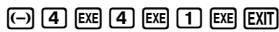

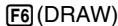
② SHIFT F5 (G-SLV) F6 (▷) F3 (∫dx)
:
④ ◀\~◀ (Lower limit: x = -2) EXE
⑤ ▶\~▶ (Upper limit: x = 0)
⑥ EXE
Result Screen
line
| Parameter | Value | | :--- | :--- | | LOWER=-2 /dx=4 | -2 | | UPPER=0 | 0 |
■ Conic Section Graph Analysis
You can determine approximations of the following analytical results using conic section graphs.
- Focus/vertex/eccentricity
• Length of latus rectum - Center/radius
- x -/y-intercept
- Directrix/axis of symmetry drawing and analysis
-
Asymptote drawing and analysis
-
From the Main Menu, enter the CONICS mode.
- Use ▲ and ▼ to select the conic section you want to analyze.
- Input the conic section constants.
- Draw the Graph.
After graphing a conic section, press SHIFT F5 (G-SLV) to display the following graph analysis menus.
• Parabolic Graph Analysis
- {FOCS}/{VTX}/{LEN}/{e} ... {focus}/{vertex}/{length of latus rectum}/{eccentricity}
- {DIR}/{SYM} ... {directrix}/{axis of symmetry}
- {X-IN}/{Y-IN} ... {x-intercept}/{y-intercept}
• Circular Graph Analysis
- {CNTR}/{RADS} ... {center}/{radius}
- {X-IN}/{Y-IN} ... {x-intercept}/{y-intercept}
• Elliptical Graph Analysis
- {FOCS}/{VTX}/{CNTR}/{e} ... {focus}/{vertex}/{center}/{eccentricity}
- {X-IN}/{Y-IN} ... {x-intercept}/{y-intercept}
• Hyperbolic Graph Analysis
- {FOCS}/{VTX}/{CNTR}/{e} ... {focus}/{vertex}/{center}/{eccentricity}
- {ASYM} ... {asymptote}
- {X-IN}/{Y-IN} ... {x-intercept}/{y-intercept}
The following examples show how to use the above menus with various types of conic section graphs.
- To calculate the focus, vertex and length of latus rectum
[G-SLV]-[FOCS]/[VTX]/[LEN]

Example
To determine the focus, vertex and length of latus rectum for the parabola X = (Y - 2)^2 + 3
Use the following V-Window settings.
Xmin = -1, Xmax = 10, Xscale = 1
Ymin = -5, Ymax = 5, Yscale = 1
MENU CONICS
EXE
1 EXE 2 EXE 3 EXE F6 (DRAW)
SHIFT F5 (G-SLV)
F1(FOCS)
(Calculates the focus.)
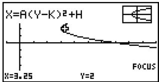
line
| X | Y | |---|---| | 3.25 | 2 | | 2 | 1 |SHIFT F5 (G-SLV)
F4(VTX)
(Calculates the vertex.)
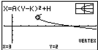
SHIFT F5 (G-SLV)
F5 (LEN)
(Calculates the length of latus rectum.)
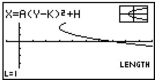
- When calculating two foci for an ellipse or hyperbolic graph, press ▶ to calculate the second focus. Pressing ◀ returns to the first focus.
- When calculating two vertexes for a hyperbolic graph, press to calculate the second vertex. Pressing returns to the first vertex.
- Pressing ▶ when calculating the vertices of an ellipse will calculate the next value. Pressing ◀ will scroll back through previous values. An ellipse has four vertices.

• To calculate the center and radius
[G-SLV]-[CNTR]/[RADS]

Example
To determine the center and radius for the circle
$$ (X + 2) ^ {2} + (Y + 1) ^ {2} = 2 ^ {2} $$
Use the following V-Window settings.
Xmin = -6.3, Xmax = 6.3, Xscale = 1
Ymin = -3.1, Ymax = 3.1, Yscale = 1 (initial defaults)
MENU CONICS
▼ ▼ ▼ ▼ EXE
(-) 2 EXE (-) 1 EXE 2 EXE F6 (DRAW)
SHIFT F5 (G-SLV)
F1(CNTR)
(Calculates the center.)
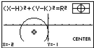
SHIFT F5 (G-SLV)
F2 (RADS)
(Calculates the radius.)
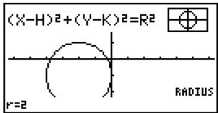

- To calculate the x - and y -intercepts
[G-SLV]-[X-IN]/[Y-IN]

Example To determine the x- and y-intercepts for the hyperbola
$$ \frac {(X - 3) ^ {2}}{2 ^ {2}} - \frac {(Y - 1) ^ {2}}{2 ^ {2}} = 1 $$
Use the following V-Window settings.
Xmin = -4, Xmax = 8, Xscale = 1
Ymin = -5, Ymax = 5, Yscale = 1
MENU CONICS
EXE
2 EXE 2 EXE 3 EXE 1 EXE F6 (DRAW)
SHIFT F5 (G-SLV)
F2 (X-IN)
(Calculates the x-intercept.)
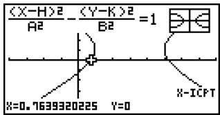
SHIFT F5 (G-SLV)
F3 (Y-IN)
(Calculates the y-intercept.)
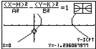
- Press ▶ to calculate the second set of x-/y-intercepts. Pressing ◀ returns to the first set of intercepts.

- To draw and analyze the axis of symmetry and directrix
[G-SLV]-[SYM]/[DIR]

Example To draw the axis of symmetry and directrix for the parabola
$$ \mathbf {X} = 2 (\mathbf {Y} - 1) ^ {2} + 1 $$
Use the following V-Window settings.
$$ \mathrm{Xmin} = - 6. 3, \quad \mathrm{Xmax} = 6. 3, \quad \mathrm{Xscale} = 1 $$
Ymin = -3.1, Ymax = 3.1, Yscale = 1 (initial defaults)
MENU CONICS
EXE
2 EXE 1 EXE 1 EXE F6 (DRAW)
SHIFT F5 (G-SLV)
F2 (SYM)
(Draws the axis of symmetry.)
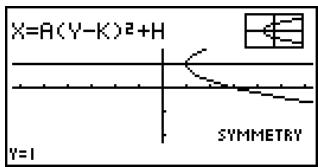
SHIFT F5 (G-SLV)
F3 (DIR)
(Draws the directrix.)
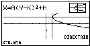

- To draw and analyze the asymptotes
[G-SLV]-[ASYM]

Example
To draw the asymptotes for the hyperbola
$$ \frac {(X - 1) ^ {2}}{2 ^ {2}} - \frac {(Y - 1) ^ {2}}{2 ^ {2}} = 1 $$
Use the following V-Window settings.
Xmin = -6.3, Xmax = 6.3, Xscale = 1
Ymin = -5, Ymax = 5, Yscale = 1
MENU CONICS
EXE
2 EXE 2 EXE 1 EXE 1 EXE F6 (DRAW)
SHIFT F5 (G-SLV)
F5 (ASYM)
(Draws the asymptotes.)
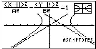
• To calculate eccentricity
[G-SLV]-[e]

Example
To determine the eccentricity of the graph for ellipse
$$ \frac {(X - 2) ^ {2}}{4 ^ {2}} + \frac {(Y - 2) ^ {2}}{2 ^ {2}} = 1 $$
Use the following V-Window settings.
Xmin = -3, Xmax = 7, Xscale = 1
Ymin = -1, Ymax = 5, Yscale = 1
MENU CONICS
EXE
4 EXE 2 EXE 2 EXE 2 EXE F6 (DRAW)
SHIFT F5 (G-SLV)
F6 (▷) F1 (e)
(Calculates eccentricity.)
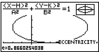
scatter
| X-Axis Label | Y-Axis Label | Value | |---|---|---| | (X-H)² / A² | (Y-K)² | 1 | | 0.8660254038 | ECCENTRICITY | 0.0000 | The chart displays a single data point for (X-H)² / A² = 1 and (Y-K)² / B² = 1. The vertical axis represents the same label 'ECCENTRICITY' and the horizontal axis represents the same label 'e=0.8660254038'.
# Certain V-Window parameters can produce errors in values produced as graph analysis results.
# The message "Not Found" appears on the display when graph analysis is unable to produce a result.
# The following can result in inaccurate analysis results or may even make it impossible to obtain a solution at all.
- When the solution is tangent to the x-axis.
- When the solution is a point of tangency between two graphs.

Chapter
6
6
Statistical Graphs and Calculations
This chapter describes how to input statistical data into lists, how to calculate the mean, maximum and other statistical values, how to perform various statistical tests, how to determine the confidence interval, and how to produce a distribution of statistical data. It also tells you how to perform regression calculations.
6-1 Before Performing Statistical Calculations
6-2 Calculating and Graphing Single-Variable Statistical Data
6-3 Calculating and Graphing Paired-Variable Statistical Data
6-4 Performing Statistical Calculations
6-5 Tests
6-6 Confidence Interval
6-7 Distribution
Important!
- This chapter contains a number of graph screen shots. In each case, new data values were input in order to highlight the particular characteristics of the graph being drawn. Note that when you try to draw a similar graph, the unit uses data values that you have input using the List function. Because of this, the graphs that appear on the screen when you perform a graphing operation will probably differ somewhat from those shown in this manual.
6-1 Before Performing Statistical Calculations
Entering the STAT mode from the Main Menu displays the List Editor screen.
You can use the List Editor screen to input statistical data and perform statistical calculations.
Use ▲, ▼, ◀ and ▶ to move the highlighting around the lists.
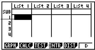
Once you input data, you can use it to produce a graph and check for tendencies. You can also use a variety of different regression calculations to analyze the data.
- For information about using the statistical data lists, see “3. List Function”.
■ Inputting Data into Lists

Example
To input the following two data groups
0.5, 1.2, 2.4, 4.0, 5.2
-2.1, 0.3, 1.5, 2.0, 2.4


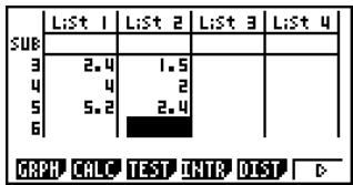
Once data is input, you can use it for graphing and statistical calculations.

# Except for complex numbers, calculation results can be input as statistical data.
# You can use the ▲, ▼, ◀ and ▶ keys to move the highlighting to any cell in the lists for data input.

■ Changing Graph Parameters
Use the following procedures to specify the graph draw/non-draw status, the graph type, and other general settings for each of the graphs in the graph menu (GPH1, GPH2, GPH3).
While the statistical data list is on the display, press [F1] (GRPH) to display the graph menu, which contains the following items.
- {GPH1}/{GPH2}/{GPH3} ... graph {1}/{2}/{3} drawing ^*1
- {SEL} ... {simultaneous graph (GPH1, GPH2, GPH3) selection} You can specify the multiple graphs.
- {SET} ... {graph settings (graph type, list assignments)}
1. General graph settings
[GRPH]-[SET]
This section describes how to use the general graph settings screen to make the following settings for each graph (GPH1, GPH2, GPH3).
- Graph Type
The initial default graph type setting for all the graphs is scatter graph. You can select one of a variety of other statistical graph types for each graph.
- List
The initial default statistical data is List 1 for single-variable data, and List 1 and List 2 for paired-variable data. You can specify which statistical data list you want to use for x-data and y-data.
- Frequency
Normally, each data item or data pair in the statistical data list is represented on a graph as a point. When you are working with a large number of data items however, this can cause problems because of the number of plot points on the graph. When this happens, you can specify a frequency list that contains values indicating the number of instances (the frequency) of the data items in the corresponding cells of the lists you are using for x-data and y-data. Once you do this, only one point is plotted for the multiple data items, which makes the graph easier to read.

*1 The initial default graph type setting for all the graphs (Graph 1 through Graph 3) is scatter diagram, but you can change to one of a number of other graph types.
# You can specify the graph draw/non-draw status, the graph type, and other general settings for each of the graphs in the graph menu (GPH1, GPH2, GPH3).

- Mark Type
This setting lets you specify the shape of the plot points on the graph.
- To display the general graph settings screen
[GRPH]-[SET]
Pressing F1(GRPH)F6(SET) displays the general graph settings screen.
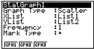
- The settings shown here are examples only. The settings on your general graph settings screen may differ.
• StatGraph (statistical graph specification)
• {GPH1}/{GPH2}/{GPH3} ... graph {1}/{2}/{3}
• Graph Type (graph type specification)
- {Scat}/{xy}/{NPP} ... {scatter diagram}/{xy line graph}/{normal probability plot}
- {Hist}/{Box}/{N·Dis}/{Brkn} ... {histogram}/{med-box graph}/{normal distribution curve}/{broken line graph}
- {X}/{Med}/{X^2}/{X^3}/{X^4} ... {linear regression graph}/{Med-Med graph}/{quadratic regression graph}/{cubic regression graph}/{quartic regression graph}
- {Log}/{Exp}/{Pwr}/{Sin}/{Lgst} ... {logarithmic regression graph}/{exponential regression graph}/{power regression graph}/{sinusoidal regression graph}/{logistic regression graph}
- XList (x-axis data list)
- {LIST} ... {List 1 to 26}
- YList (y-axis data list)
- {LIST} ... {List 1 to 26}
• Frequency (number of times a value occurs)
• {1} ... {1-to-1 plot}
- {LIST} ... frequency data in {List 1 to 26}
• Mark Type (plot mark type)
- /×/ ... scatter diagram plot points
- Outliers (outliers specification)
- {On}/{Off} ... {display}/{do not display} Med-Box outliers

2. Graph draw/non-draw status
[GRPH]-[SEL]
The following procedure can be used to specify the draw (On)/non-draw (Off) status of each of the graphs in the graph menu.
- To specify the draw/non-draw status of a graph
- Pressing F1(GRPH) F4(SEL) displays the graph On/Off screen.
| StatGraph1 | :DrawUn |
| StatGraph2 | :DrawOff |
| StatGraph3 | :DrawOff |
- Note that the StatGraph1 setting is for Graph 1 (GPH1 of the graph menu), StatGraph2 is for Graph 2, and StatGraph3 is for Graph 3.
-
Use the cursor keys to move the highlighting to the graph whose status you want to change, and press the applicable function key to change the status.
-
{On}/{Off} ... {On (draw)}/{Off (non-draw)}
-
{DRAW} ... {draws all On graphs}
-
To return to the graph menu, press EXIT.

# V-Window parameters are normally set automatically for statistical graphing. If you want to set V-Window parameters manually, you must change the Stat Wind item to "Manual".
While the statistical data list is on the display, perform the following procedure.
SHIFT MENU (SET UP) F2 (Man)
EXIT (Returns to previous menu.)
Note that V-Window parameters are set automatically for the following types of graphs regardless of whether or not the Stat Wind item is set to "Manual".
1-Sample Z Test, 2-Sample Z Test, 1-Prop Z Test, 2-Prop Z Test, 1-Sample t Test, 2-Sample t Test, ^2 Test, 2-Sample F Test (x-axis only disregarded).
# The default setting automatically uses List 1 data as x-axis (horizontal) values and List 2 data as y-axis (vertical) values. Each set of x/y data is a point on the scatter diagram.

6-2 Calculating and Graphing Single-Variable Statistical Data
Single-variable data is data with only a single variable. If you are calculating the average height of the members of a class for example, there is only one variable (height).
Single-variable statistics include distribution and sum. The following types of graphs are available for single-variable statistics.
You can also use the procedures under “Changing Graph Parameters” on page 6-1-2 to make the settings you want before drawing each graph.
■ Normal Probability Plot (NPP)
This plot compares the data accumulated ratio with a normal distribution accumulated ratio. XList specifies the list where data is input, and Mark Type is used to select from among the marks / × / you want to plot.
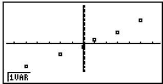
scatter
| x | y | | ---- | ---- | | 1.0 | 0.5 | | 2.0 | 0.3 | | 3.0 | 0.7 | | 4.0 | 0.9 | | 5.0 | 1.1 | | 6.0 | 1.3 | | 7.0 | 1.5 | | 8.0 | 1.7 | | 9.0 | 1.9 | | 10.0 | 2.1 |Press AC, EXIT or SHIFT EXIT (QUIT) to return to the statistical data list.
■ Histogram (Bar Graph) (Hist)
XList specifies the list where the data is input, while Freq specifies the list where the data frequency is input. 1 is specified for Freq when frequency is not specified.
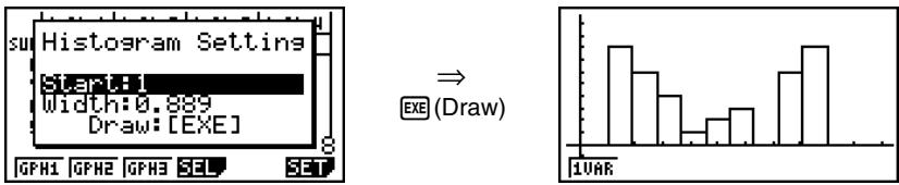
The display screen appears as shown above before the graph is drawn. At this point, you can change the Start and Width values.

■ Med-box Graph (MedBox)
This type of graph lets you see how a large number of data items are grouped within specific ranges. A box encloses all the data in an area from the first quartile (Q1) to the third quartile (Q3), with a line drawn at the median (Med). Lines (called whiskers) extend from either end of the box up to the minimum (minX) and maximum (maxX) of the data.
From the statistical data list, press F1(GRPH) to display the graph menu, press F6(SET), and then change the graph type of the graph you want to use (GPH1, GPH2, GPH3) to med-box graph.
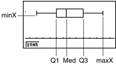
To plot the data that falls outside the box, first specify “MedBox” as the Graph Type. Then, on the same screen you use to specify the graph type, turn the Outliers item “On”, and draw the graph.
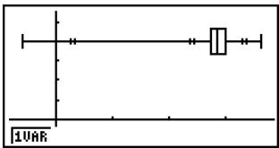

■ Normal Distribution Curve (N·Dis)
The normal distribution curve is graphed using the following normal distribution function.
$$ y = \frac {1}{\sqrt {(2 \pi)} x \sigma_ {n}} e ^ {- \frac {(x - \bar {x}) ^ {2}}{2 x \sigma_ {n} ^ {2}}} $$
XList specifies the list where the data is input, while Freq specifies the list where the data frequency is input. 1 is specified for Freq when frequency is not specified.
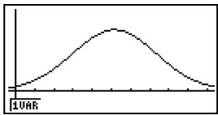
line
| X-Axis Label | Y-Axis Value | |---|---| | 10AR | 0 | | Peak | 100 | | End | 0 |■ Broken Line Graph (Brkn)
Lines connect center points of a histogram bar.
XList specifies the list where the data is input, while Freq specifies the list where the data frequency is input. 1 is specified for Freq when frequency is not specified.
![Histogram Setting Start:1 Width:0.889 Draw:[EXE] GPH1 GPH2 GPH3 SEL SET](/content/2025/01/86785/images/ddd9c3404b89f407d54945925b7301b66cd88fbfd561c5e869df225ebbe55ecc.jpg)
⇒ EXE (Draw)
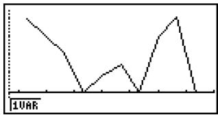
line
| X-Axis Label | Y-Axis Value | | :--- | :--- | | 1 | 0 | | 2 | 1 | | 3 | 0 | | 4 | 1 | | 5 | 0 | | 6 | 1 | | 7 | 2 | | 8 | 3 | | 9 | 4 | | 10 | 5 | | 11 | 6 | | 12 | 7 | | 13 | 8 | | 14 | 9 | | 15 | 10 | | 16 | 11 | | 17 | 12 | | 18 | 13 | | 19 | 14 | | 20 | 15 | | 21 | 16 | | 22 | 17 | | 23 | 18 | | 24 | 19 | | 25 | 20 | | 26 | 21 | | 27 | 22 | | 28 | 23 | | 29 | 24 | | 30 | 25 | | 31 | 26 | | 32 | 27 | | 33 | 28 | | 34 | 29 | | 35 | 30 | | 36 | 31 | | 37 | 32 | | 38 | 33 | | 39 | 34 | | 40 | 35 | | 41 | 36 | | 42 | 37 | | 43 | 38 | | 44 | 39 | | 45 | 40 | | 46 | 41 | | 47 | 42 | | 48 | 43 | | 49 | 44 | | 50 | 45 | | 51 | 46 | | 52 | 47 | | 53 | 48 | | 54 | 49 | | 55 | 50 | | 56 | 51 | | 57 | 52 | | 58 | 53 | | 59 | 54 | | 60 | 55 | | 61 | 56 | | 62 | 57 | | 63 | 58 | | 64 | 59 | | 65 | 60 | | 66 | 61 | | 67 | 62 | | 68 | 63 | | 69 | 64 | | 70 | 65 | | 71 | 66 | | 72 | 67 | | 73 | 68 | | 74 | 69 | | 75 | 70 | | 76 | 71 | | 77 | 72 | | 78 | 73 | | 79 | 74 | | 80 | 75 | | 81 | 76 | | 82 | 77 | | 83 | 78 | | 84 | 79 | | 85 | 80 | | 86 | 81 | | 87 | 82 | | 88 | 83 | | 89 | 84 | | 90 | 85 | | 91 | 86 | | 92 | 87 | | 93 | 88 | | 94 | 89 | | 95 | 90 | | 96 | 91 | | 97 | 92 | | 98 | 93 | | 99 | 94 | | Note: The data is in a format format (e.g., bar, line, or pie chart) but not explicitly provided in the image. The text labels are '1UAR' at the top left. The chart type is a line chart.The display screen appears as shown above before the graph is drawn. At this point, you can change the Start and Width values.

■ Displaying the Calculation Results of a Drawn Single-Variable Graph
Single-variable statistics can be expressed as both graphs and parameter values. When these graphs are displayed, the single-variable calculation results appear as shown below when you press F1(1VAR).
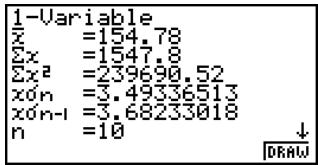
- Use ▼ to scroll the list so you can view the items that run off the bottom of the screen.
The following describes the meaning of each of the parameters.
.... mean x .... sum x^2 .... sum of squares x_n .... population standard deviation x_n-1 .... sample standard deviation n .... number of data items minX .... minimum Q1 .... first quartile Med .... median Q3 .... third quartile maxX .... maximum Mod .... mode Mod : n ... number of data mode items Mod : F ... data mode frequency
- Press F6(DRAW) to return to the original single-variable statistical graph.

# When Mod has multiple solutions, they are all displayed.

6-3 Calculating and Graphing Paired-Variable Statistical Data
■ Drawing a Scatter Diagram and xy Line Graph
Description
The following procedure plots a scatter diagram and connects the dots to produce an xy line graph.
Set Up
- From the Main Menu, enter the STAT mode.
Execution
- Input the data into a list.
- Specify Scat (scatter diagram) or xy (xy line graph) as the graph type, and then execute the graph operation.
Press AC, EXIT or SHIFT EXIT (QUIT) to return to the statistical data list.


Example
Input the two sets of data shown below. Next, plot the data on a scatter diagram and connect the dots to produce an xy line graph.
0.5, 1.2, 2.4, 4.0, 5.2 (xList)
-2.1, 0.3, 1.5, 2.0, 2.4 (yList)
Procedure
① MENU STAT
③ (xy line graph) F1 (GRPH) F6 (SET) ▼ F2 (xy) EXIT
F1 (GPH1)
Result Screen

scatter
| x | y | |---|---| | 1 | 0.5 | | 2 | 0.6 | | 3 | 0.7 | | 4 | 0.8 | | 5 | 0.9 |(Scatter diagram)
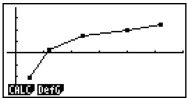
line
| Category | Value | |---|---| | CALC | 10 | | Det0 | 25 | | | 30 | | | 35 | | | 40 | | | 45 | | | 50 | | | 55 | | | 60 | | | 65 | | | 70 | | | 75 | | | 80 | | | 85 | | | 90 | | | 95 | | | 100 | The chart displays a single data series labeled 'CALC' and 'Det0'. The x-axis is labeled 'CALC' and the y-axis is labeled 'Det0'. The values for 'CALC' are explicitly labeled on the graph.(xy line graph)

■ Drawing a Regression Graph
Description
Use the following procedure to input paired-variable statistical data, perform a regression calculation using the data, and then graph the results.
Set Up
- From the Main Menu, enter the STAT mode.
Execution
- Input the data into a list, and plot the scatter diagram.
- Select the regression type, execute the calculation, and display the regression parameters.
- Draw the regression graph.


Example
Input the two sets of data shown below and plot the data on a scatter diagram. Next, perform logarithmic regression on the data to display the regression parameters, and then draw the corresponding regression graph.
0.5, 1.2, 2.4, 4.0, 5.2 (xList)
-2.1, 0.3, 1.5, 2.0, 2.4 (yList)
Procedure
① MENU STAT
③ F1 (CALC) F6 (▷) F2 (Log)
④ F6 (DRAW)
Result Screen
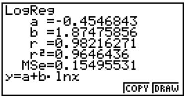
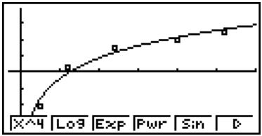
line
| X | Y | |---|---| | 4 | 0 | | Log9 | 1 | | Exp | 2 | | Pwr | 3 | | Sin | 4 | | D | 5 |
■ Selecting the Regression Type
After you graph paired-variable statistical data, press F1(CALC). Then you can use the function menu at the bottom of the display to select from a variety of different types of regression.
- {2VAR} ... {paired-variable statistical results}
- {X}/{Med}/{X^2}/{X^3}/{X^4}/{Log}/{Exp}/{Pwr}/{Sin}/{Lgst} ... {linear regression}/{Med-Med}/{quadratic regression}/{cubic regression}/{quartic regression}/{logarithmic regression}/{exponential regression}/{power regression}/{sinusoidal regression}/{logistic regression} calculation and graphing
■ Displaying Regression Calculation Results
Whenever you perform a regression calculation, the regression formula parameter (such as a and b in the linear regression y = ax + b ) calculation results appear on the display. You can use these to obtain statistical calculation results.
Regression parameters are calculated as soon as you press a function key to select a regression type, while a graph is on the display.
■ Graphing Statistical Calculation Results
While the parameter calculation result is on the display, you can graph the displayed regression formula by pressing F6 (DRAW).

■ Linear Regression Graph
Linear regression uses the method of least squares to plot a straight line that passes close to as many data points as possible, and returns values for the slope and y-intercept (y-coordinate when x = 0) of the line.
The graphic representation of this relationship is a linear regression graph.
F1(CALC) F2(X)
F6 (DRAW)
The following is the linear regression model formula.
$$ y = a x + b $$
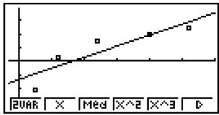
scatter
| X | Y | |---|---| | 2UAR | 0.1 | | X | 0.3 | | Med | 0.5 | | X^2 | 0.6 | | X^3 | 0.7 | | D | 0.8 |a ...... regression coefficient (slope)
b ...... regression constant term (y-intercept)
r ...... correlation coefficient
r^2 ...... coefficient of determination
MSe ...... mean square error
■ Med-Med Graph
When it is suspected that there are a number of extreme values, a Med-Med graph can be used in place of the least squares method. This is similar to linear regression, but it minimizes the effects of extreme values.
F1 (CALC) F3 (Med)
F6 (DRAW)
The following is the Med-Med graph model formula.
$$ y = a x + b $$
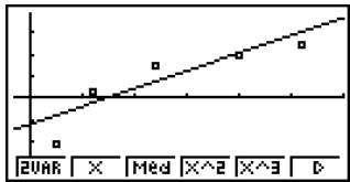
scatter
| X | Y | |---|---| | 2UAR | 0.5 | | Med | 1.0 | | X^2 | 1.5 | | X^3 | 2.0 | | D | 2.5 |a ...... Med-Med graph slope
b ...... Med-Med graph y-intercept

# Input a positive integer for frequency data. Other types of values (decimals, etc.) cause an error.

■ Quadratic/Cubic/Quartic Regression Graph
A quadratic/cubic/quartic regression graph represents connection of the data points of a scatter diagram. It uses the method of least squares to draw a curve that passes close to as many data points as possible. The formula that represents this is quadratic/cubic/quartic regression.
Ex. Quadratic regression
F1(CALC) F4(X^2)
F6 (DRAW)
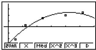
line
| X-Axis | Y-Axis | |---|---| | 2UAR | 0 | | Med | 1 | | X^2 | 2 | | X^3 | 3 | | D | 4 |Quadratic regression
Model formula ..... y = ax^2 + bx + c
a ...... regression second coefficient
b ...... regression first coefficient
c ...... regression constant term (y-intercept)
r^2 ...... coefficient of determination
MSe ...... mean square error
Cubic regression
Model formula ..... y = ax^3 + bx^2 + cx + d
a ...... regression third coefficient
b ...... regression second coefficient
c ...... regression first coefficient
d ...... regression constant term (y-intercept)
r^2 ...... coefficient of determination
MSe ...... mean square error
Quartic regression
Model formula ..... y = ax^4 + bx^3 + cx^2 + dx + e
a ...... regression fourth coefficient
b ...... regression third coefficient
c ...... regression second coefficient
d ...... regression first coefficient
e ...... regression constant term (y-intercept)
r^2 ...... coefficient of determination
MSe ...... mean square error

■ Logarithmic Regression Graph
Logarithmic regression expresses y as a logarithmic function of x. The standard logarithmic regression formula is y = a + b × x , so if we say that X = x , the formula corresponds to linear regression formula y = a + bX .
F1 (CALC) F6 (▷) F2 (Log)
F6 (DRAW)
The following is the logarithmic regression model formula.
$$ y = a + b \cdot \ln x $$
a ...... regression constant term
b ...... regression coefficient
r...... correlation coefficient
r^2 ...... coefficient of determination
MSe ...... mean square error
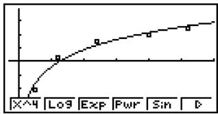
line
| X | Log9 | Exp | FwR | Sin | D | |---|---|---|---|---|---| | 4 | 0 | 0 | 0 | 0 | 0 | | 5 | 1 | 1 | 1 | 1 | 1 | | 6 | 2 | 2 | 2 | 2 | 2 | | 7 | 3 | 3 | 3 | 3 | 3 | | 8 | 4 | 4 | 4 | 4 | 4 | | 9 | 5 | 5 | 5 | 5 | 5 | | 10 | 6 | 6 | 6 | 6 | 6 | | 11 | 7 | 7 | 7 | 7 | 7 | | 12 | 8 | 8 | 8 | 8 | 8 | | 13 | 9 | 9 | 9 | 9 | 9 | | 14 | 10 | 10 | 10 | 10 | 10 | | 15 | 11 | 11 | 11 | 11 | 11 | | 16 | 12 | 12 | 12 | 12 | 12 | | 17 | 13 | 13 | 13 | 13 | 13 | | 18 | 14 | 14 | 14 | 14 | 14 | | 19 | 15 | 15 | 15 | 15 | 15 | | 20 | 16 | 16 | 16 | 16 | 16 | | 21 | 17 | 17 | 17 | 17 | 17 | | 22 | 18 | 18 | 18 | 18 | 18 | | 23 | 19 | 19 | 19 | 19 | 19 | | 24 | 20 | 20 | 20 | 20 | 20 | | 25 | 21 | 21 | 21 | 21 | 21 | | 26 | 22 | 22 | 22 | 22 | 22 | | 27 | 23 | 23 | 23 | 23 | 23 | | 28 | 24 | 24 | 24 | 24 | 24 | | 29 | 25 | 25 | 25 | 25 | 25 | | 30 | 26 | 26 | 26 | 26 | 26 | | ... (repeated) for all values of X to D are missing in the chart. The y-axis is labeled as 'x'. The x-axis is labeled as 'Log9' (logarithmic scale). The y-axis is labeled as 'Exp' (expansion scale). The x-axis is labeled as 'FwR' (further expansion scale). The y-axis is labeled as 'Sin' (sin phase), and the x-axis is labeled as 'D' (duration).■ Exponential Regression Graph
Exponential regression expresses y as a proportion of the exponential function of x. The standard exponential regression formula is y = a × e^bx , so if we take the logarithms of both sides we get y = a + bx . Next, if we say Y = y , and A = a , the formula corresponds to linear regression formula Y = A + bx .
F1 (CALC) F6 (▷) F3 (Exp)
F6 (DRAW)
The following is the exponential regression model formula.
$$ y = a \cdot e ^ {b x} $$
a ...... regression coefficient
b ...... regression constant term
r...... correlation coefficient
r^2 ...... coefficient of determination
MSe ...... mean square error
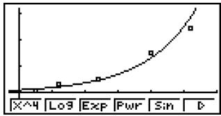
line
| X | Lo9 | Exp | Fwr | Sin | D | |---|---|---|---|---|---| | 0 | 0 | 0 | 0 | 0 | 0 | | 1 | 0.5 | 0.3 | 0.2 | 0.1 | 0.1 | | 2 | 1.0 | 0.6 | 0.4 | 0.2 | 0.2 | | 3 | 1.5 | 0.9 | 0.6 | 0.3 | 0.3 | | 4 | 2.0 | 1.2 | 0.8 | 0.4 | 0.4 | | 5 | 2.5 | 1.5 | 1.0 | 0.5 | 0.5 | | 6 | 3.0 | 1.8 | 1.2 | 0.6 | 0.6 | | 7 | 3.5 | 2.1 | 1.4 | 0.7 | 0.7 | | 8 | 4.0 | 2.4 | 1.6 | 0.8 | 0.8 | | 9 | 4.5 | 2.7 | 1.8 | 0.9 | 0.9 | | 10 | 5.0 | 3.0 | 2.0 | 1.0 | 1.0 | | 11 | 5.5 | 3.3 | 2.2 | 1.1 | 1.1 | | 12 | 6.0 | 3.6 | 2.4 | 1.2 | 1.2 | | 13 | 6.5 | 3.9 | 2.6 | 1.3 | 1.3 | | 14 | 7.0 | 4.2 | 2.8 | 1.4 | 1.4 | | 15 | 7.5 | 4.5 | 3.0 | 1.5 | 1.5 | | 16 | 8.0 | 4.8 | 3.2 | 1.6 | 1.6 | | 17 | 8.5 | 5.1 | 3.4 | 1.7 | 1.7 | | 18 | 9.0 | 5.4 | 3.6 | 1.8 | 1.8 | | 19 | 9.5 | 5.7 | 3.8 | 1.9 | 1.9 | | 20 | 10.0 | 6.0 | 4.0 | 2.0 | 2.0 | | ... (repeated) for all values of X to D are missing in the image.
■ Power Regression Graph
Power regression expresses y as a proportion of the power of x. The standard power regression formula is y = a × x^b , so if we take the logarithm of both sides we get y = a + b × x . Next, if we say X = x , Y = y , and A = a , the formula corresponds to linear regression formula Y = A + bX .
F1 (CALC) F6 (▷) F4 (Pwr)
F6 (DRAW)
The following is the power regression model formula.
$$ y = a \cdot x ^ {b} $$
a ...... regression coefficient
b ...... regression power
r...... correlation coefficient
r^2 ...... coefficient of determination
MSe ...... mean square error
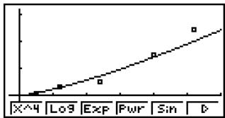
line
| Variable | Value | |---|---| | X^4 | 0 | | Lo9 | 1 | | Exp | 2 | | Fwr | 3 | | Sin | 4 | | D | 5 |■ Sinusoidal Regression Graph
Sinusoidal regression is best applied for cyclical data.
The following is the sinusoidal regression model formula.
$$ y = a \cdot \sin (b x + c) + d $$
While the statistical data list is on the display, perform the following key operation.
F1 (CALC) F6 (▷) F5 (Sin)
F6 (DRAW)
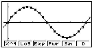
Drawing a sinusoidal regression graph causes the angle unit setting of the calculator to automatically change to Rad (radians). The angle unit does not change when you perform a sinusoidal regression calculation without drawing a graph.
- Certain types of data may take a long time to calculate. This does not indicate malfunction.

■ Logistic Regression Graph
Logistic regression is best applied for time-based phenomena in which there is a continual increase until a saturation point is reached.
The following is the logistic regression model formula.
$$ y = \frac {c}{1 + a e ^ {- b x}} $$
F1 (CALC) F6 (▷) F6 (▷) F1 (Lgst)
F6 (DRAW)
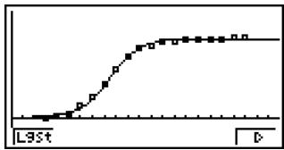
line
| X | Y | | --- | --- | | 0 | 0 | | 1 | 0.5 | | 2 | 1.0 | | 3 | 1.5 | | 4 | 2.0 | | 5 | 2.5 | | 6 | 3.0 | | 7 | 3.5 | | 8 | 4.0 | | 9 | 4.5 | | 10 | 5.0 | | 11 | 5.5 | | 12 | 6.0 | | 13 | 6.5 | | 14 | 7.0 | | 15 | 7.5 | | 16 | 8.0 | | 17 | 8.5 | | 18 | 9.0 | | 19 | 9.5 | | 20 | 10.0 |- Certain types of data may take a long time to calculate. This does not indicate malfunction.
■ Residual Calculation
Actual plot points (y-coordinates) and regression model distance can be calculated during regression calculations.
While the statistical data list is on the display, recall the Setup screen to specify a LIST ("List 1" through "List 26") for "Resid List". Calculated residual data is stored in the specified list.
The vertical distance from the plots to the regression model will be stored in the list.
Plots that are higher than the regression model are positive, while those that are lower are negative.
Residual calculation can be performed and saved for all regression models.

# Any data already existing in the selected list is cleared. The residual of each plot is stored in the same precedence as the data used as the model.

■ Displaying the Calculation Results of a Drawn Paired-Variable Graph
Paired-variable statistics can be expressed as both graphs and parameter values. When these graphs are displayed, the paired-variable calculation results appear as shown below when you press F1(CALC)F1(2VAR).
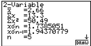
- Use ▼ to scroll the list so you can view the items that run off the bottom of the screen.
| ...... | mean of data stored in xList |
| x ...... | sum of data stored in xList |
| x^2 ...... | sum of squares of data stored in xList |
| x_n ...... | population standard deviation of data stored in xList |
| x_n-1 ...... | sample standard deviation of data stored in xList |
| n ...... | number of data |
| ...... | mean of data stored in yList |
| y ...... | sum of data stored in yList |
| y^2 ...... sum of squares of data stored in yList |
| y_n ...... population standard deviation of data stored in yList |
| y_n-1 .... sample standard deviation of data stored in yList |
| xy ...... sum of the product of data stored in xList and yList |
| minX ... minimum of data stored in xList |
| maxX .. maximum of data stored in xList |
| minY ... minimum of data stored in yList |
| maxY .. maximum of data stored in yList |
■ Copying a Regression Graph Formula to the GRAPH Mode
You can copy regression formula calculation results to the GRAPH mode graph relation list, and store and compare.
- While a regression calculation result is on the display (see "Displaying Regression Calculation Results" on page 6-3-5), press F5(COPY).
- This will display the GRAPH mode graph relation list.*1
- Use ▲ and ▼ to highlight the area to which you want to copy the regression formula of the displayed result.
- Press EXE to save the copied graph formula and return to the previous regression calculation result display.

*1 You cannot edit regression formulas for graph formulas in the GRAPH mode.

■ Multiple Graphs
You can draw more than one graph on the same display by using the procedure under “Changing Graph Parameters” to set the graph draw (On)/non-draw (Off) status of two or all three of the graphs to draw On, and then pressing F6(DRAW)(see page 6-1-4). After drawing the graphs, you can select which graph formula to use when performing single-variable statistic or regression calculations.

F1(CALC)
F2(X)
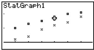
scatter
| X | Y | |---|---| | 1 | 0.5 | | 2 | 0.6 | | 3 | 0.7 | | 4 | 0.8 | | 5 | 0.9 | | 6 | 1.0 | | 7 | 0.9 | | 8 | 0.8 | | 9 | 0.7 | | 10 | 0.6 | | 11 | 0.5 | | 12 | 0.4 | | 13 | 0.3 | | 14 | 0.2 | | 15 | 0.1 | | 16 | 0.0 | | 17 | -0.1 | | 18 | -0.2 | | 19 | -0.3 | | 20 | -0.4 | | 21 | -0.5 | | 22 | -0.6 | | 23 | -0.7 | | 24 | -0.8 | | 25 | -0.9 | | 26 | -1.0 | | 27 | -0.9 | | 28 | -0.8 | | 29 | -0.7 | | 30 | -0.6 | | 31 | -0.5 | | 32 | -0.4 | | 33 | -0.3 | | 34 | -0.2 | | 35 | -0.1 | | 36 | 0.0 | | 37 | 0.1 | | 38 | 0.2 | | 39 | 0.3 | | 40 | 0.4 | | 41 | 0.5 | | 42 | 0.6 | | 43 | 0.7 | | 44 | 0.8 | | 45 | 0.9 | | 46 | 1.0 | | 47 | 0.9 | | 48 | 0.8 | | 49 | 0.7 | | 50 | 0.6 | | 51 | 0.5 | | 52 | 0.4 | | 53 | 0.3 | | 54 | 0.2 | | 55 | 0.1 | | 56 | 0.0 | | 57 | -0.1 | | 58 | -0.2 | | 59 | -0.3 | | 60 | -0.4 | | 61 | -0.5 | | 62 | -0.6 | | 63 | -0.7 | | 64 | -0.8 | | 65 | -0.9 | | 66 | -1.0 | | 67 | -0.9 | | 68 | -0.8 | | 69 | -0.7 | | 70 | -0.6 | | 71 | -0.5 | | 72 | -0.4 | | 73 | -0.3 | | 74 | -0.2 | | 75 | -0.1 | | 76 | 0.0 | | 77 | 0.1 | | 78 | 0.2 | | 79 | 0.3 | | 80 | 0.4 | | 81 | 0.5 | | 82 | 0.6 | | 83 | 0.7 | | 84 | 0.8 | | 85 | 0.9 | | 86 | 1.0 | | 87 | 0.9 | | 88 | 0.8 | | 89 | 0.7 | | 90 | 0.6 | | 91 | 0.5 | | 92 | 0.4 | | 93 | 0.3 | | 94 | 0.2 | | 95 | 0.1 | | 96 | 0.0 | | 97 | -0.1 | | 98 | -0.2 | | 99 | -0.3 | | Note: The actual values in the CSV data are not provided in the code image, so they are left blank in the image.- The text at the top of the screen indicates the currently selected graph (StatGraph1 = Graph 1, StatGraph2 = Graph 2, StatGraph3 = Graph 3).
- Press ▼. The graph name at the top of the screen changes when you do.
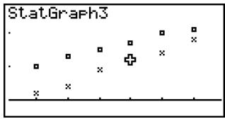
- When the graph you want to use is selected, press EXE.
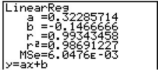

■ Overlaying a Function Graph on a Statistical Graph
Description
You can overlay a paired-variable statistical graph with any type of function graph you want.
Set Up
- From the Main Menu, enter the STAT mode.
Execution
- Input the data into a list, and draw the statistical graph.
- Display the Graph Function menu, and input the function you want to overlay on the statistical graph.
- Graph the function.


Example
Input the two sets of data shown below. Next, plot the data on a scatter diagram and overlay a function graph y = 2 x .
0.5, 1.2, 2.4, 4.0, 5.2
-2.1, 0.3, 1.5, 2.0, 2.4
Procedure
① MENU STAT
You can also perform trace, etc. for drawn function graphs.
Graphs of types other than rectangular coordinate graphs cannot be drawn.
# Pressing EXIT while inputting a function returns the expression to what it was prior to input. Pressing SHIFT EXIT (QUIT) clears the input expression and returns to the statistical data list.

6-4 Performing Statistical Calculations
All of the statistical calculations up to this point were performed after displaying a graph. The following procedures can be used to perform statistical calculations alone.
- To specify statistical calculation data lists
You have to input the statistical data for the calculation you want to perform and specify where it is located before you start a calculation. Display the statistical data and then press F2 (CALC) F6 (SET).
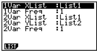
The following is the meaning for each item.
1Var XList .... location of single-variable statistic x values (XList)
1Var Freq ...... location of single-variable frequency values (Frequency)
2Var XList .... location of paired-variable statistic x values (XList)
2Var YList ...... location of paired-variable statistic y values (YList)
2Var Freq .... location of paired-variable frequency values (Frequency)
- Calculations in this section are performed based on the above specifications.

■ Single-Variable Statistical Calculations
In the previous example under “Displaying the Calculation Results of a Drawn Single-Variable Graph”, statistical calculation results were displayed after the graph was drawn. These were numeric expressions of the characteristics of variables used in the graphic display.
These values can also be directly obtained by displaying the statistical data list and pressing F2 (CALC) F1 (1VAR).
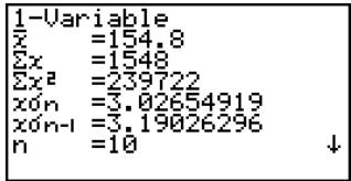
After this, pressing ▲ or ▼ scrolls the statistical calculation result display so you can view variable characteristics.
For details on the meanings of these statistical values, see “Displaying the Calculation Results of a Drawn Single-Variable Graph” (page 6-2-4).
■ Paired-Variable Statistical Calculations
In the previous example under “Displaying the Calculation Results of a Drawn Paired-Variable Graph”, statistical calculation results were displayed after the graph was drawn. These were numeric expressions of the characteristics of variables used in the graphic display.
These values can also be directly obtained by displaying the statistical data list and pressing F2 (CALC) F2 (2VAR).
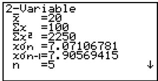
After this, pressing ▲ or ▼ scrolls the statistical calculation result display so you can view variable characteristics.
For details on the meanings of these statistical values, see “Displaying the Calculation Results of a Drawn Paired-Variable Graph” (page 6-3-11).

■ Regression Calculation
In the explanations from “Linear Regression Graph” to “Logistic Regression Graph,” regression calculation results were displayed after the graph was drawn. Here, each coefficient value of the regression line or regression curve is expressed as a number.
You can directly determine the same expression from the data input screen.
Pressing F2(CALC)F3(REG) displays a function menu, which contains the following items.
• {X}/{Med}/{X^2}/{X^3}/{X^4}/{Log}/{Exp}/{Pwr}/{Sin}/{Lgst} ... {linear regression}/{Med-Med}/{quadratic regression}/{cubic regression}/{quartic regression}/{logarithmic regression}/{exponential regression}/{power regression}/{sinusoidal regression}/{logistic regression} parameters
● ● ● ● ●
Example To display single-variable regression parameters
F2 (CALC) F3 (REG) F1 (X)
LinearReg a =0.51164637 b =-0.1009793 r =0.97377522 r^2=0.94823819 MSe=0.07198341 y=ax+b COPY
The meanings of the parameters that appear on this screen are the same as those for “Linear Regression Graph” to “Logistic Regression Graph”.
- Calculation of the Coefficient of Determination (r^2) and MSe
You can use the STAT mode to calculate the coefficient of determination ( r^2 ) for quadratic regression, cubic regression, and quartic regression. The following types of MSe calculations are also available for each type of regression.
QuadReg a =0.31765306 b =-0.1133673 c =0.11530612 r^2=0.99991584 MSe=4.8149E-03 y=ax²+bx+c COPY

- Linear Regression ... MSe = 1n - 2_i=1^n(y_i - (ax_i + b))^2
- Quadratic Regression ... MSe = 1n - 3_i=1^n(y_i - (ax_i^2 + bx_i + c))^2
- Cubic Regression ... MSe = 1n - 4_i = 1^n(y_i - (ax_i^3 + bx_i^2 + cx_i + d))^2
- Quartic Regression ... MSe = 1n - 5_i = 1^n(y_i - (ax_i^4 + bx_i^3 + cx_i^2 + dx_i + e))^2
- Logarithmic Regression ... MSe = 1n - 2 _i=1^n (y_i - (a + b x_i))^2
- Exponential Repression ... MSe = 1n - 2 _i=1^n ( y_i - ( a + bx_i) )^2
- Power Regression ... MSe = 1n - 2_i=1^n( y_i - ( a + b x_i))^2
- Sin Regression ... MSe = 1n - 2_i=1^n(y_i - (a (bx_i + c) + d))^2
- Logistic Regression ... MSe = 1n - 2_i = 1^n(y_i - 1 + ae^-bx_i)^2
- Estimated Value Calculation for Regression Graphs
The STAT mode also includes a Y-CAL function that uses regression to calculate the estimated y-value for a particular x-value after graphing a paired-variable statistical regression.
The following is the general procedure for using the Y-CAL function.
- After drawing a regression graph, press SHIFT F5 (G-SLV) F1 (Y-CAL) to enter the graph selection mode, and then press EXE.
If there are multiple graphs on the display, use ▲ and ▼ to select the graph you want, and then press EXE.
- This causes an x -value input dialog box to appear.
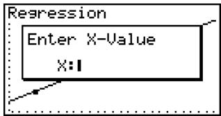

- Input the value you want for x and then press EXE.
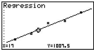
scatter
Regression | X | Y | |---|---| | 17 | 100.5 |- This causes the coordinates for x and y to appear at the bottom of the display, and moves the pointer to the corresponding point on the graph.
- Pressing ,,T or a number key at this time causes the x-value input dialog box to reappear so you can perform another estimated value calculation if you want.
-
After you are finished, press EXIT to clear the coordinate values and the pointer from the display.
-
The pointer does not appear if the calculated coordinates are not within the display range.
- The coordinates do not appear if "Off" is specified for the "Coord" item of the Setup screen.
- The Y-CAL function can also be used with a graph drawn by using DefG feature.
- Regression Formula Copy Function from a Regression Calculation Result Screen
In addition to the normal regression formula copy function that lets you copy the regression calculation result screen after drawing a statistical graph (such as Scatter Plot), the STAT mode also has a function that lets you copy the regression formula obtained as the result of a regression calculation. To copy a resulting regression formula, press F6 (COPY).
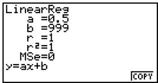

■ Estimated Value Calculation ( , )
After drawing a regression graph with the STAT mode, you can use the RUN·MAT mode to calculate estimated values for the regression graph's x and y parameters.

Example
To perform a linear regression using the nearby data and estimate the values of and when xi = 20 and yi = 1000
| xi | yi |
| 10 | 1003 |
| 15 | 1005 |
| 20 | 1010 |
| 25 | 1011 |
| 30 | 1014 |
- From the Main Menu, enter the STAT mode.
- Input data into the list and draw the linear regression graph.
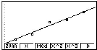
-
From the Main Menu, enter the RUN·MAT mode.
-
Press the keys as follows.
20(value of xi)
OPTN F5 (STAT) F2 ( ) EXE
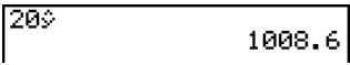
The estimated value is displayed for xi = 20.
1 0 0 0 (value of yi)
F1( ) EXE
| 20% | 1008.6 |
| 1000% | 4.642857143 |
The estimated value is displayed for yi = 1000.

# You cannot obtain estimated values for a MedMed, quadratic regression, cubic regression,
quartic regression, sinusoidal regression, or logistic regression graph.

■ Normal Probability Distribution Calculation
You can calculate normal probability distributions for single-variable statistics with the RUN·MAT mode.
Press OPTN F6 (▷) F3 (PROB) F6 (▷) to display a function menu, which contains the following items.
- P( / Q( / R( ... obtains normal probability P(t) /Q(t) /R(t) value
- t(·) obtains normalized variate t(x) value
- Normal probability P(t) , Q(t) , and R(t) , and normalized variate t(x) are calculated using the following formulas.
Standard Normal Distribution
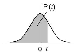
$$ \frac {1}{\sqrt {2 \pi}} \int_ {- \infty} ^ {t} e ^ {- \frac {u ^ {2}}{2}} d u $$
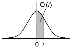
$$ \frac {1}{\sqrt {2 \pi}} \int_ {0} ^ {t} e ^ {- \frac {u ^ {2}}{2}} d u $$
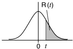
line
| t | R(t) | | ---- | ---- | | 0 | Peak |$$ \frac {1}{\sqrt {2 \pi}} \int_ {t} ^ {+ \infty} e ^ {- \frac {u ^ {2}}{2}} d u $$
$$ t (x) = \frac {x - \bar {x}}{x \sigma_ {n}} $$

Example
The following table shows the results of measurements of the height of 20 college students. Determine what percentage of the students fall in the range 160.5 cm to 175.5 cm. Also, in what percentile does the 175.5 cm tall student fall?
| Class no. | Height (cm) | Frequency |
| 1 | 158.5 | 1 |
| 2 | 160.5 | 1 |
| 3 | 163.3 | 2 |
| 4 | 167.5 | 2 |
| 5 | 170.2 | 3 |
| 6 | 173.3 | 4 |
| 7 | 175.5 | 2 |
| 8 | 178.6 | 2 |
| 9 | 180.4 | 2 |
| 10 | 186.7 | 1 |

- From the Main Menu, enter the STAT mode.
- Input the height data into List 1 and the frequency data into List 2.
- Perform the single-variable statistical calculations.*1
F2 (CALC) F6 (SET)
F1 (LIST) 1 EXE
F2 (LIST) 2 EXE SHIFT EXIT (QUIT)
F2 (CALC) F1 (1VAR)
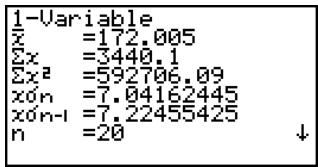
- Press MENU, select the RUN·MAT mode, press OPTN F6 (▷) F3 (PROB) to recall the probability calculation (PROB) menu.
F3 (PROB) F6 (▷) F4 (t() 1 6 0 • 5 ) EXE
(Normalized variate t for 160.5cm)
Result: -1.633855948
$$ (\doteq - 1. 6 3 4) $$
F4(t() 1 7 5 • 5 ) EXE
(Normalized variate t for 175.5cm)
Result: 0.4963343361
$$ (\doteq 0. 4 9 6) $$
F1(P()0·496)—
F1(P)(-) 1 • 6 3 4 ) EXE
(Percentage of total)
Result: 0.638921
(63.9% of total)
F3 (R() 0 • 4 9 6 ) EXE
(Percentile)
Result: 0.30995
(31.0 percentile)

*1 You can obtain the normalized variate immediately after performing single-variable statistical calculations only.

■ Drawing a Normal Probability Distribution Graph
Description
You can draw a normal probability distribution graph using manual graphing with the RUN·MAT mode.
Set Up
- From the Main Menu, enter the RUN·MAT mode.
Execution
- Input the commands to draw a rectangular coordinate graph.
- Input the probability value.


Example
To draw a normal probability P (0.5) graph.
Procedure
① MENU RUN·MAT
② SHIFT F4 (SKTCH) F1 (Cls) EXE
F5 (GRPH) F1 (Y=)
③ OPTN F6 (▷) F3 (PROB) F6 (▷) F1 (P() 0 • 5 EXE
Result Screen
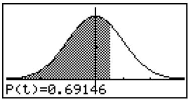
histogram
| Statistic | Value | | --------- | --------- | | P(t) | 0.69146 |
6-5 Tests
The Z Test provides a variety of different standardization-based tests. They make it possible to test whether or not a sample accurately represents the population when the standard deviation of a population (such as the entire population of a country) is known from previous tests. Z testing is used for market research and public opinion research, that need to be performed repeatedly.
1-Sample Z Test tests for the unknown population mean when the population standard deviation is known.
2-Sample Z Test tests the equality of the means of two populations based on independent samples when both population standard deviations are known.
1-Prop Z Test tests for an unknown proportion of successes.
2-Prop Z Test tests to compare the proportion of successes from two populations.
The t Test tests the hypothesis when the population standard deviation is unknown. The hypothesis that is the opposite of the hypothesis being proven is called the null hypothesis, while the hypothesis being proved is called the alternative hypothesis. The t-test is normally applied to test the null hypothesis. Then a determination is made whether the null hypothesis or alternative hypothesis will be adopted.
1-Sample t Test tests the hypothesis for a single unknown population mean when the population standard deviation is unknown.
2-Sample t Test compares the population means when the population standard deviations are unknown.
LinearReg t Test calculates the strength of the linear association of paired data.
^2 Test tests hypothesis concerning the proportion of samples included in each of a number of independent groups. Mainly, it generates cross-tabulation of two categorical variables (such as yes, no) and evaluates the independence of these variables. It could be used, for example, to evaluate the relationship between whether or not a driver has ever been involved in a traffic accident and that person's knowledge of traffic regulations.
2-Sample F Test tests the hypothesis for the ratio of sample variances. It could be used, for example, to test the carcinogenic effects of multiple suspected factors such as tobacco use, alcohol, vitamin deficiency, high coffee intake, inactivity, poor living habits, etc.
ANOVA tests the hypothesis that the population means of the samples are equal when there are multiple samples. It could be used, for example, to test whether or not different combinations of materials have an effect on the quality and life of a final product.
One-Way ANOVA is used when there is one independent variable and one dependent variable.
Two-Way ANOVA is used when there are two independent variables and one dependent variable.

The following pages explain various statistical calculation methods based on the principles described above. Details concerning statistical principles and terminology can be found in any standard statistics textbook.
On the initial STAT mode screen, press F3 (TEST) to display the test menu, which contains the following items.
- F3 (TEST) F1(Z) ... Z Tests (page 6-5-2)
F2(t) ... t Tests (page 6-5-10)
F3 (CHI) ... ^2 Test (page 6-5-18)
F4(F) ... 2-Sample F Test (page 6-5-20)
F5 (ANOV) ... ANOVA (page 6-5-22)
■ Z Tests
• Z Test Common Functions
You can use the following graph analysis functions after drawing a Z Test result output graph.
• F1(Z) ... Displays z score.
Pressing 1(Z) displays the z score at the bottom of the display, and displays the pointer at the corresponding location in the graph (unless the location is off the graph screen).
Two points are displayed in the case of a two-tail test. Use ◀ and ▶ to move the pointer. Press EXIT to clear the z score.
- F2(P) ... Displays p-value.
Pressing F2(P) displays the p-value at the bottom of the display without displaying the pointer.
Press EXIT to clear the p-value.
- 1-Sample Z Test
This test is used when the population standard deviation is known to test the hypothesis. The 1-Sample Z Test is applied to the normal distribution.
$$ Z = \frac {\bar {x} - \mu_ {0}}{\frac {\sigma}{\sqrt {n}}} $$
: mean of sample
_0 : assumed population mean
σ : population standard deviation
n : size of sample

# The following V-Window settings are used for drawing the graph.
$$ X m i n = - 3. 2, X m a x = 3. 2, X s c a l e = 1, $$
$$ Y \min = - 0. 1, Y \max = 0. 4 5, Y \text { scale } = 0. 1 $$
# Executing an analysis function automatically stores the z and p values in alpha variables Z and P, respectively.

Perform the following key operations from the statistical data list.
F3 (TEST)
F1(Z)
F1(1-S)
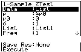
The following shows the meaning of each item in the case of list data specification.
Data ...... data type
...... population mean value test conditions (“ _0 ” specifies two-tail test, “< _0 ” specifies lower one-tail test, “> _0 ” specifies upper one-tail test.)
_0 ...... assumed population mean
σ.... population standard deviation ( > 0 )
List ...... list whose contents you want to use as data (List 1 to 26)
Freq..... frequency (1 or List 1 to 26)
Save Res ...... list for storage of calculation results (None or List 1 to 26)
Execute ...... executes a calculation or draws a graph
The following shows the meaning of parameter data specification items that are different from list data specification.
$$ \left| \begin{array}{c c c} \bar {x} & : \bar {0} \ \underline {{n}} & : \bar {0} \end{array} \right| $$
...... mean of sample
n ...... size of sample (positive integer)
After setting all the parameters, use ▼ to move the highlighting to “Execute” and then press one of the function keys shown below to perform the calculation or draw the graph.
• F1 (CALC) ... Performs the calculation.
• F6 (DRAW) ... Draws the graph.

Calculation Result Output Example
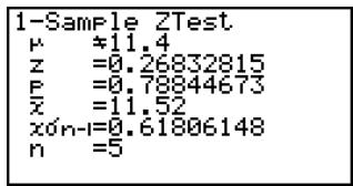
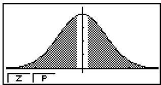
area
| Category | Value | | -------- | ----- | | Z | Low | | P | High |11.4 direction of test
z ...... z score
p ...... p-value
...... mean of sample
x_n-1 ...... sample standard deviation (Displayed only for Data: List setting.)
n ...... size of sample
- For details about graph screen function keys F1(Z) and F2(P), see “Z Test Common Functions” on page 6-5-2.

# [Save Res] does not save the condition in line 2.

- 2-Sample Z Test
This test is used when the standard deviations for two populations are known to test the hypothesis. The 2-Sample Z Test is applied to the normal distribution.
$$ Z = \frac {\bar {x} _ {1} - \bar {x} _ {2}}{\sqrt {\frac {\sigma_ {1} ^ {2}}{n _ {1}} + \frac {\sigma_ {2} ^ {2}}{n _ {2}}}} $$
_1 : mean of sample 1
_2 : mean of sample 2
_1 : population standard deviation of sample 1
_2 : population standard deviation of sample 2
n_1 : size of sample 1
n_2 : size of sample 2
Perform the following key operations from the statistical data list.
F3 (TEST)
F1(Z)
F2(2-S)
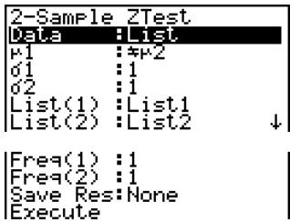
The following shows the meaning of each item in the case of list data specification.
Data ...... data type
_1 population mean value test conditions (“ _2 ” specifies two-tail test, “< _2 ” specifies one-tail test where sample 1 is smaller than sample 2, “> _2 ” specifies one-tail test where sample 1 is greater than sample 2.)
_1 population standard deviation of sample 1 ( _1 > 0 )
_2 population standard deviation of sample 2 ( _2 > 0 )
List(1) ...... list whose contents you want to use as sample 1 data (List 1 to 26)
List(2) .... list whose contents you want to use as sample 2 data (List 1 to 26)
Freq(1) ...... frequency of sample 1 (1 or List 1 to 26)
Freq(2) ...... frequency of sample 2 (1 or List 1 to 26)
Save Res ...... list for storage of calculation results (None or List 1 to 26)
Execute ...... executes a calculation or draws a graph

The following shows the meaning of parameter data specification items that are different from list data specification.
| 1 | :0 |
| n1 | :0 |
| 2 | :0 |
| n2 | :0 |
_1 mean of sample 1
n_1 ...... size (positive integer) of sample 1
_2 mean of sample 2
n_2 ...... size (positive integer) of sample 2
After setting all the parameters, use ▼ to move the highlighting to “Execute” and then press one of the function keys shown below to perform the calculation or draw the graph.
• F1 (CALC) ... Performs the calculation.
- F6 (DRAW) ... Draws the graph.
Calculation Result Output Example
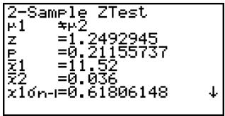
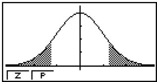
area
| Category | Value | | -------- | ----- | | Z | 0 | | P | 1 |_1_2 direction of test
z ...... z score
p ...... p-value
_1 mean of sample 1
_2 mean of sample 2
x_1_n-1 standard deviation of sample 1
(Displayed only for Data: List setting.)
x_2_n-1 standard deviation of sample 2
(Displayed only for Data: List setting.)
n_1 ...... size of sample 1
n_2 ...... size of sample 2
- For details about graph screen function keys F1(Z) and F2(P), see “Z Test Common Functions” on page 6-5-2.

# [Save Res] does not save the _1 condition in line 2.

- 1-Prop Z Test
This test is used to test for an unknown proportion of successes. The 1-Prop Z Test is applied to the normal distribution.
$$ Z = \frac {\frac {x}{n} - p _ {0}}{\sqrt {\frac {p _ {0} (1 - p _ {0})}{n}}} $$
p_0 : expected sample proportion
n : size of sample
Perform the following key operations from the statistical data list.
F3 (TEST)
F1(Z)
F3(1-P)
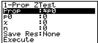
Prop ...... sample proportion test conditions (“≠ p₀” specifies two-tail test, “< p₀” specifies lower one-tail test, “> p₀” specifies upper one-tail test.)
p_0 ...... expected sample proportion ( 0 < p_0 < 1 )
x ...... sample value (x ≧ 0 integer)
n ...... size of sample (positive integer)
Save Res .... list for storage of calculation results (None or List 1 to 26)
Execute ...... executes a calculation or draws a graph
After setting all the parameters, use ▼ to move the highlighting to “Execute” and then press one of the function keys shown below to perform the calculation or draw the graph.
• F1(CALC) ... Performs the calculation.
• F6(DRAW) ... Draws the graph.
Calculation Result Output Example
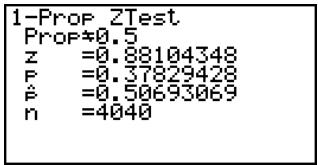
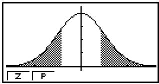
area
| Category | Value | | -------- | ----- | | Z | 0 | | P | 1 |Prop≠0.5 ..... direction of test
z ...... z score
p ...... p-value
...... estimated sample proportion
n ...... size of sample
- For details about graph screen function keys F1(Z) and F2(P), see “Z Test Common Functions” on page 6-5-2.

# [Save Res] does not save the Prop condition in line 2.
- 2-Prop Z Test
This test is used to compare the proportion of successes. The 2-Prop Z Test is applied to the normal distribution.
$$ Z = \frac {\frac {x _ {1}}{n _ {1}} - \frac {x _ {2}}{n _ {2}}}{\sqrt {\hat {p} (1 - \hat {p}) \left(\frac {1}{n _ {1}} + \frac {1}{n _ {2}}\right)}} $$
x_1 : data value of sample 1
x_2 : data value of sample 2
n_1 : size of sample 1
n_2 : size of sample 2
: estimated sample proportion
Perform the following key operation from the statistical data list.
F3 (TEST)
F1(Z)
F4(2-P)
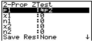
IExecute
p_1 ...... sample proportion test conditions (“ p_2 ” specifies two-tail test, “
p _2 ” specifies one-tail test where sample 1 is greater than sample 2.)
x_1 ...... data value ( x_1 ≥ 0 integer) of sample 1
n_1 ...... size (positive integer) of sample 1
x_2 ...... data value ( x_2 ≥ 0 integer) of sample 2
n_2 ...... size (positive integer) of sample 2
Save Res ...... list for storage of calculation results (None or List 1 to 26)
Execute ...... executes a calculation or draws a graph
After setting all the parameters, use ▼ to move the highlighting to "Execute" and then press one of the function keys shown below to perform the calculation or draw the graph.
• F1 (CALC) ... Performs the calculation.
• F6 (DRAW) ... Draws the graph.

Calculation Result Output Example
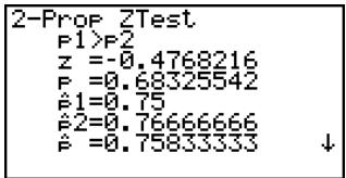
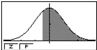
area
| Z | P | | --- | --- | | 0 | 0 | | Peak | High | | 1 | Low |p_1 > p_2 direction of test
z ...... z score
p ...... p-value
_1 ...... estimated proportion of sample 1
_2 ...... estimated proportion of sample 2
...... estimated sample proportion
n_1 ...... size of sample 1
n_2 ...... size of sample 2
- For details about graph screen function keys F1(Z) and F2(P), see “Z Test Common Functions” on page 6-5-2.

# [Save Res] does not save the p_1 condition in line 2.

■ t Tests
- t Test Common Functions
You can use the following graph analysis functions after drawing a t Test result output graph.
• F1(T) ... Displays t score.
Pressing F1(T) displays the t score at the bottom of the display, and displays the pointer at the corresponding location in the graph (unless the location is off the graph screen).
Two points are displayed in the case of a two-tail test. Use ◀ and ▶ to move the pointer.
Press EXIT to clear the t score.
• F2(P) ... Displays p-value.
Pressing F2(P) displays the p-value at the bottom of the display without displaying the pointer.
Press EXIT to clear the p-value.

# The following V-Window settings are used for drawing the graph.
$$ X m i n = - 3. 2, X m a x = 3. 2, X s c a l e = 1, $$
$$ Y m i n = - 0. 1, Y m a x = 0. 4 5, Y s c a l e = 0. 1 $$
# Executing an analysis function automatically stores the t and p values in alpha variables T and P, respectively.

• 1-Sample t Test
This test uses the hypothesis test for a single unknown population mean when the population standard deviation is unknown. The 1-Sample t Test is applied to t-distribution.
$$ t = \frac {\bar {x} - \mu_ {0}}{\frac {x \sigma_ {n - 1}}{\sqrt {n}}} $$
: mean of sample
_0 : assumed population mean
x_n-1 : sample standard deviation
n : size of sample
Perform the following key operations from the statistical data list.
F3 (TEST)
F2(t)
F1(1-S)
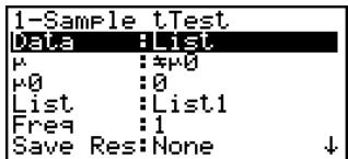
|Execute |
The following shows the meaning of each item in the case of list data specification.
Data ...... data type
...... population mean value test conditions (“ _0 ” specifies two-tail test, “< _0 ” specifies lower one-tail test, “> _0 ” specifies upper one-tail test.)
_0 ...... assumed population mean
List ...... list whose contents you want to use as data (List 1 to 26)
Freq..... frequency (1 or List 1 to 26)
Save Res ...... list for storage of calculation results (None or List 1 to 26)
Execute ...... executes a calculation or draws a graph
The following shows the meaning of parameter data specification items that are different from list data specification.
$$ \left|\begin{array}{ll} \overline{x} & :0 \ x \acute{o} n - 1 & :0 \ n & :0 \end{array}\right| $$
...... mean of sample
x_n-1 ...... sample standard deviation (x_n-1 > 0)
n ...... size of sample (positive integer)
After setting all the parameters, use ▼ to move the highlighting to “Execute” and then press one of the function keys shown below to perform the calculation or draw the graph.
• F1 (CALC) ... Performs the calculation.
• F6 (DRAW) ... Draws the graph.

Calculation Result Output Example
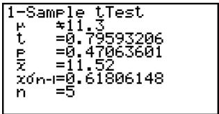
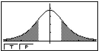
histogram
| Category | Value | | -------- | ----- | | T | 0 | | P | 0 |11.3 direction of test
t ...... t score
p ...... p-value
...... mean of sample
x_n-1 sample standard deviation
n ...... size of sample
- For details about graph screen function keys F1(T) and F2(P), see “t Test Common Functions” on page 6-5-10.

# [Save Res] does not save the condition in line 2.

- 2-Sample t Test
2-Sample t Test compares the population means when the population standard deviations are unknown. The 2-Sample t Test is applied to t-distribution.
The following applies when pooling is in effect.
$$ t = \frac {\bar {x} _ {1} - \bar {x} _ {2}}{\sqrt {x _ {p} \sigma_ {n - 1} ^ {2} \left(\frac {1}{n _ {1}} + \frac {1}{n _ {2}}\right)}} $$
$$ x _ {p} \sigma_ {n - 1} = \sqrt {\frac {(n _ {1} - 1) x _ {1} \sigma_ {n - 1} ^ {2} + (n _ {2} - 1) x _ {2} \sigma_ {n - 1} ^ {2}}{n _ {1} + n _ {2} - 2}} $$
$$ d f = n _ {1} + n _ {2} - 2 $$
_1 : mean of sample 1
_2 : mean of sample 2
x_1_n-1 : standard deviation of sample 1
x_2_n-1 : standard deviation of sample 2
n_1 : size of sample 1
n_2 : size of sample 2
x_p_n-1 : pooled sample standard deviation
df: degrees of freedom
The following applies when pooling is not in effect.
$$ t = \frac {\bar {x} _ {1} - \bar {x} _ {2}}{\sqrt {\frac {x _ {1} \sigma_ {n - 1} ^ {2}}{n _ {1}} + \frac {x _ {2} \sigma_ {n - 1} ^ {2}}{n _ {2}}}} $$
$$ d f = \frac {1}{\frac {C ^ {2}}{n _ {1} - 1} + \frac {(1 - C) ^ {2}}{n _ {2} - 1}} $$
$$ C = \frac {\frac {x _ {1} \sigma_ {n - 1} ^ {2}}{n _ {1}}}{\left(\frac {x _ {1} \sigma_ {n - 1} ^ {2}}{n _ {1}} + \frac {x _ {2} \sigma_ {n - 1} ^ {2}}{n _ {2}}\right)} $$
_1 : mean of sample 1
_2 : mean of sample 2
x_1_n-1 : standard deviation of sample 1
x_2_n-1 : standard deviation of sample 2
n_1 : size of sample 1
n_2 : size of sample 2
df: degrees of freedom
Perform the following key operations from the statistical data list.
F3 (TEST)
F2(t)
F2(2-S)
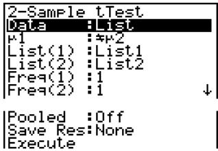

The following shows the meaning of each item in the case of list data specification.
Data ...... data type
_1 ...... sample mean value test conditions (“ _2 ” specifies two-tail test, “< _2 ” specifies one-tail test where sample 1 is smaller than sample 2, “> _2 ” specifies one-tail test where sample 1 is greater than sample 2.)
List(1) ...... list whose contents you want to use as data of sample 1 (List 1 to 26)
List(2) ...... list whose contents you want to use as data of sample 2 (List 1 to 26)
Freq(1) ...... frequency of sample 1 (1 or List 1 to 26)
Freq(2) ...... frequency of sample 2 (1 or List 1 to 26)
Pooled .... pooling On (in effect) or Off (not in effect)
Save Res ...... list for storage of calculation results (None or List 1 to 26)
Execute ...... executes a calculation or draws a graph
The following shows the meaning of parameter data specification items that are different from list data specification.
$$ \left| \begin{array}{c c} \overline {{x}} 1 & : 0 \ x 1 \acute {o} n - 1 & : 0 \ n 1 & : 0 \ \overline {{x}} 2 & : 0 \ \hline x 2 \acute {o} n - 1 & : 0 \ n 2 & : 0 \end{array} \right| $$
_1 mean of sample 1
x_1_n - 1 standard deviation (x_1_n - 1 > 0) of sample 1
n_1 ...... size (positive integer) of sample 1
_2 mean of sample 2
x_2_n-1 standard deviation (x_2_n-1 > 0) of sample 2
n_2 ...... size (positive integer) of sample 2
After setting all the parameters, use ▼ to move the highlighting to “Execute” and then press one of the function keys shown below to perform the calculation or draw the graph.
- F1 (CALC) ... Performs the calculation.
- F6 (DRAW) ... Draws the graph.

Calculation Result Output Example
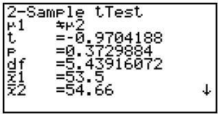
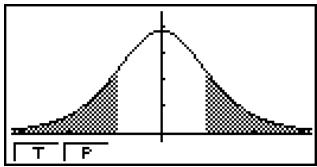
area
| Category | Value | | -------- | ----- | | T | Low | | P | High |_1_2 direction of test
t ...... t score
p ...... p-value
df ...... degrees of freedom
_1 mean of sample 1
_2 mean of sample 2
x_1_n-1 standard deviation of sample 1
x_2_n - 1 standard deviation of sample 2
x_p_n-1 pooled sample standard deviation (Displayed only when Pooled: On setting.)
n_1 ...... size of sample 1
n_2 ...... size of sample 2
- For details about graph screen function keys F1(T) and F2(P), see “t Test Common Functions” on page 6-5-10.

# [Save Res] does not save the _1 condition in line 2.

- LinearReg t Test
LinearReg t Test treats paired-variable data sets as (x, y) pairs, and uses the method of least squares to determine the most appropriate a, b coefficients of the data for the regression formula y = a + bx . It also determines the correlation coefficient and t value, and calculates the extent of the relationship between x and y.
$$ b = \frac {\sum_ {i = 1} ^ {n} (x - \bar {x}) (y - \bar {y})}{\sum_ {i = 1} ^ {n} (x - \bar {x}) ^ {2}} \qquad a = \bar {y} - b \bar {x} \qquad t = r \sqrt {\frac {n - 2}{1 - r ^ {2}}} \begin{array}{l l} a & : \text {intercept} \ b & : \text {slope of the line} \ n & : \text {size of sample (n\geq 3)} \ r & : \text {correlation coefficient} \ r ^ {2} & : \text {coefficient of} \ & \text {determination} \end{array} $$
Perform the following key operations from the statistical data list.
F3 (TEST)
F2(t)
F3 (REG)
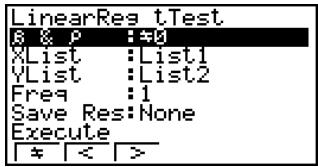
The following shows the meaning of each item in the case of list data specification.
β & ρ ...... p-value test conditions (“≠ 0” specifies two-tail test, “< 0” specifies lower one-tail test, “> 0” specifies upper one-tail test.)
XList ...... list for x-axis data (List 1 to 26)
YList .... list for y-axis data (List 1 to 26)
Freq..... frequency (1 or List 1 to 26)
Save Res ...... list for storage of calculation results (None or List 1 to 26)
Execute ...... executes a calculation
After setting all the parameters, use ▼ to move the highlighting to "Execute" and then press the function key shown below to perform the calculation.
- F1(CALC) ... Performs the calculation.

# You cannot draw a graph for LinearReg t Test.

Calculation Result Output Example
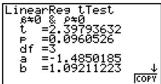
0 \& 0 ..... direction of test
t ...... t score
p ...... p-value
df ...... degrees of freedom
a ...... constant term
b .... coefficient
s ...... standard error
r correlation coefficient
r^2 coefficient of determination
Pressing F6 (COPY) while a calculation result is on the display copies the regression formula to the graph relation list.
![Graph Func V1: V2: [—] V3: [—] V4: [—] V5: [—] V6: [—]](/content/2025/01/86785/images/408456416e0e6b4c37e3983951de6496b5d33b8d626a92a2ef58c6bf1607412a.jpg)
When there is a list specified for the [Resid List] item on the Setup screen, regression formula residual data is automatically saved to the specified list after the calculation is finished.

# [Save Res] does not save the & conditions in line 2.
# When the list specified by [Save Res] is the same list specified by the [Resid List] item on the Setup screen, only [Resid List] data is saved in the list.

^2 Test
^2 Test sets up a number of independent groups and tests hypothesis related to the proportion of the sample included in each group. The ^2 Test is applied to dichotomous variables (variable with two possible values, such as yes/no).
Expected counts
$$ F _ {i j} = \frac {\sum_ {i = 1} ^ {k} x _ {i j} \times \sum_ {j = 1} ^ {\ell} x _ {i j}}{\sum_ {i = 1} ^ {k} \sum_ {j = 1} ^ {\ell} x _ {i j}} $$
$$ \chi^ {2} = \sum_ {i = 1} ^ {k} \sum_ {j = 1} ^ {\ell} \frac {(x _ {i j} - F _ {i j}) ^ {2}}{F _ {i j}} $$
Perform the following key operations from the statistical data list.
F3 (TEST)
F3 (CHI)
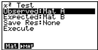
Next, specify the matrix that contains the data. The following shows the meaning of the above item.
Observed .... name of matrix (A to Z) that contains observed counts (all cells positive integers)
Expected ...... name of matrix (A to Z) that is for saving expected frequency
Save Res ...... list for storage of calculation results (None or List 1 to 26)
Execute ...... executes a calculation or draws a graph

# The matrix must be at least two lines by two columns. An error occurs if the matrix has only one line or one column.
# Pressing F1(Mat) while the "Observed" and "Expected" parameter settings are highlighted will display the Matrix (A to Z) setting screen.
# Pressing F2 (▶MAT) while setting parameters enters the Matrix Editor, which you can use to edit and view the contents of matrices.

After setting all the parameters, use ▼ to move the highlighting to “Execute” and then press one of the function keys shown below to perform the calculation or draw the graph.
• F1 (CALC) ... Performs the calculation.
- F6 (DRAW) ... Draws the graph.
Calculation Result Output Example
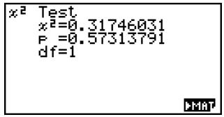
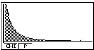
area
| Category | Value | |---|---| | CHI | 100 | | P | 50 |^2 ...... ^2 value
p ...... p-value
df ...... degrees of freedom
You can use the following graph analysis functions after drawing a graph.
- F1(CHI) ... Displays ^2 value.
Pressing F1 (CHI) displays the ^2 value at the bottom of the display, and displays the pointer at the corresponding location in the graph (unless the location is off the graph screen).
Press EXIT to clear the ^2 value.
- F2(P) ... Displays p-value.
Pressing F2(P) displays the p-value at the bottom of the display without displaying the pointer.
Press EXIT to clear the p-value.

# Pressing F6 (▶MAT) while a calculation result is displayed enters the Matrix Editor, which you can use to edit and view the contents of matrices.
# The following V-Window settings are used for drawing the graph.
$$ X m i n = 0, X m a x = 1 1. 5, X s c a l e = 2, $$
$$ Y m i n = - 0. 1, Y m a x = 0. 5, Y s c a l e = 0. 1 $$
# Executing an analysis function automatically stores the ^2 and p values in alpha variables C and P, respectively.

■ 2-Sample F Test
2-Sample F Test tests the hypothesis for the ratio of sample variances. The F Test is applied to the F distribution.
$$ F = \frac {x _ {1} \sigma_ {n - 1} ^ {2}}{x _ {2} \sigma_ {n - 1} ^ {2}} $$
Perform the following key operations from the statistical data list.
F3 (TEST)
F4(F)
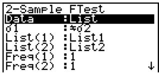
|Save Res: None |Execute
The following is the meaning of each item in the case of list data specification.
Data ...... data type
_1 population standard deviation test conditions ("≠ _2 " specifies two-tail test, "< _2 " specifies one-tail test where sample 1 is smaller than sample 2, "> _2 " specifies one-tail test where sample 1 is greater than sample 2.)
List(1) ...... list whose contents you want to use as data of sample 1 (List 1 to 26)
List(2) ...... list whose contents you want to use as data of sample 2 (List 1 to 26)
Freq(1) ...... frequency of sample 1 (1 or List 1 to 26)
Freq(2) ...... frequency of sample 2 (1 or List 1 to 26)
Save Res ...... list for storage of calculation results (None or List 1 to 26)
Execute ...... executes a calculation or draws a graph
The following shows the meaning of parameter data specification items that are different from list data specification.
$$ \left| \begin{array}{l l} x 1 \text { ón - i } & : 0 \ n 1 & : 0 \ x 2 \text { ón - i } & : 0 \ n 2 & : 0 \end{array} \right. $$
x_1_n-1 standard deviation ( x_1_n-1>0 ) of sample 1
n_1 ...... size (positive integer) of sample 1
x_2_n-1 standard deviation ( x_2_n-1 > 0 ) of sample 2
n_2 ...... size (positive integer) of sample 2

After setting all the parameters, use ▼ to move the highlighting to “Execute” and then press one of the function keys shown below to perform the calculation or draw the graph.
- F1 (CALC) ... Performs the calculation.
- F6 (DRAW) ... Draws the graph.
Calculation Result Output Example
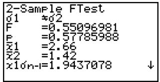
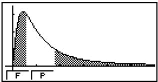
area
| Category | Value | | -------- | ----- | | F | Peak | | P | Low |_1_2 direction of test
F...... F value
p ...... p-value
_1 ...... mean of sample 1 (Displayed only for Data: List setting.)
_2 ...... mean of sample 2 (Displayed only for Data: List setting.)
x_1_n-1 standard deviation of sample 1
x_2_n-1 standard deviation of sample 2
n_1 ...... size of sample 1
n_2 ...... size of sample 2
You can use the following graph analysis functions after drawing a graph.
- F1(F) ... Displays F value.
Pressing 1(F) displays the F value at the bottom of the display, and displays the pointer at the corresponding location in the graph (unless the location is off the graph screen).
Two points are displayed in the case of a two-tail test. Use ◀ and ▶ to move the pointer. Press EXIT to clear the F value.
- F2(P) ... Displays p-value.
Pressing F2(P) displays the p-value at the bottom of the display without displaying the pointer. Press EXIT to clear the p-value.

# [Save Res] does not save the _1 condition in line 2.
# V-Window settings are automatically optimized for drawing the graph.
# Executing an analysis function automatically stores the F and p values in alpha variables F and P, respectively.

ANOVA
ANOVA tests the hypothesis that the population means of the samples are equal when there are multiple samples.
One-Way ANOVA is used when there is one independent variable and one dependent variable.
Two-Way ANOVA is used when there are two independent variables and one dependent variable.
Perform the following key operations from the statistical data list.
F3 (TEST)
F5 (ANOV)
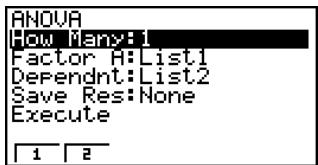
The following is the meaning of each item in the case of list data specification.
How Many ...... selects One-Way ANOVA or Two-Way ANOVA (number of levels)
Factor A...... category list (List 1 to 26)
Dependnt .... list to be used for sample data (List 1 to 26)
Save Res ....first list for storage of calculation results (None or List 1 to 22) ^*1
Execute ...... executes a calculation or draws a graph (Two-Way ANOVA only)
The following item appears in the case of Two-Way ANOVA only.
Factor B ...... category list (List 1 to 26)
After setting all the parameters, use ▼ to move the highlighting to "Execute" and then press one of the function keys shown below to perform the calculation or draw the graph.
- F1 (CALC) ... Performs the calculation.
- F6 (DRAW) ... Draws the graph (Two-Way ANOVA only).
Calculation results are displayed in table form, just as they appear in science books.

*1 [Save Res] saves each vertical column of the table into its own list. The leftmost column is saved in the specified list, and each subsequent column to the right is saved in
the next sequentially numbered list. Up to five lists can be used for storing columns. You can specify an first list number in the range of 1 to 22.

Calculation Result Output Example
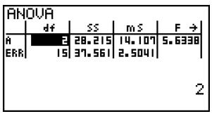
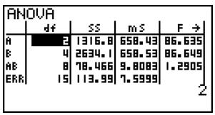
One-Way ANOVA
Line 1 (A) ...... Factor A df value, SS value, MS value, F value, p-value
Line 2 (ERR) ...... Error df value, SS value, MS value
Two-Way ANOVA
Line 1 (A) ...... Factor A df value, SS value, MS value, F value, p-value
Line 2 (B) ...... Factor B df value, SS value, MS value, F value, p-value
Line 3 (AB) ...... Factor A × Factor B df value, SS value, MS value, F value, p-value
*Line 3 does not appear when there is only one observation in each cell.
Line 4 (ERR) ...... Error df value, SS value, MS value
F...... F value
p ...... p-value
df ...... degrees of freedom
SS ...... sum of squares
MS...... mean squares
With Two-Way ANOVA, you can draw Interaction Plot graphs. The number of graphs depends on Factor B, while the number of X-axis data depends on the Factor A. The Y-axis is the average value of each category.
You can use the following graph analysis function after drawing a graph.
- F1(Trace) or SHIFT F1(TRCE) ... Trace function
Pressing ◀ or ▶ moves the pointer on the graph in the corresponding direction. When there are multiple graphs, you can move between graphs by pressing ▲ and ▼.
Press EXIT to clear the pointer from the display.

# Graphing is available with Two-Way ANOVA only. V-Window settings are performed automatically, regardless of Setup screen settings.
# Using the Trace function automatically stores the number of conditions to alpha variable A and the mean value to variable M, respectively.

■ ANOVA (Two-Way)
- Description
The nearby table shows measurement results for a metal product produced by a heat treatment process based on two treatment levels: time (A) and temperature (B). The experiments were repeated twice each under identical conditions.
| B (Heat Treatment Temperature)A (Time) | B1 | B2 |
| A1 | 113 , 116 | 139 , 132 |
| A2 | 133 , 131 | 126 , 122 |
Perform analysis of variance on the following null hypothesis, using a significance level of 5%.
H_0 : No change in strength due to time
H_0 : No change in strength due to heat treatment temperature
H_0 : No change in strength due to interaction of time and heat treatment temperature
- Solution
Use two-way ANOVA to test the above hypothesis. Input the above data as shown below.
$$ \text { List1 } = {1, 1, 1, 1, 2, 2, 2, 2 } $$
$$ \text { List2 } = {1, 1, 2, 2, 1, 1, 2, 2 } $$
$$ \text { List3 } = {1 1 3, 1 1 6, 1 3 9, 1 3 2, 1 3 3, 1 3 1, 1 2 6, 1 2 2 } $$
Define List 3 (the data for each group) as Dependent. Define List 1 and List 2 (the factor numbers for each data item in List 3) as Factor A and Factor B respectively.
Executing the test produces the following results.
• Time differential (A) level of significance P = 0.2458019517
The level of significance p = 0.2458019517 is greater than the significance level (0.05), so the hypothesis is not rejected.
• Temperature differential (B) level of significance P = 0.04222398836
The level of significance p = 0.04222398836 is less than the significance level 0.05 , so the hypothesis is rejected.
- Interaction (A × B) level of significance P = 2.78169946e-3
The level of significance (p = 2.78169946e-3) is less than the significance level (0.05), so the hypothesis is rejected.
The above test indicates that the time differential is not significant, the temperature differential is significant, and interaction is highly significant.
- Input Example
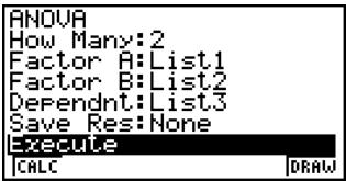
- Results
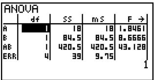
other
ANOVA | | df | SS | mS | F → | |---|---|---|---|---| | A | 1 | 18 | 18 | 1.8461 | | B | 1 | 84.5 | 84.5 | 8.6666 | | AB | 1 | 420.5 | 420.5 | 43.128 | | ERR | 4 | 39 | 9.75 | | 1| ANOVA | ||||
| +ss | mS | F | P | |
| A | 18 | 18 | 1.0461 | 1.2458 |
| B | 84.5 | 84.5 | 8.6666 | 0.0422 |
| AB | 420.5 | 420.5 | 43.128 | 2.7E-3 |
| ERR | 39 | 9.75 | ||
| 0.2458019517 | ||||
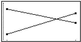
natural_image
Simple line diagram with two intersecting lines and one dashed, no text or symbols present
6-6 Confidence Interval
A confidence interval is a range (interval) that includes a statistical value, usually the population mean.
A confidence interval that is too broad makes it difficult to get an idea of where the population value (true value) is located. A narrow confidence interval, on the other hand, limits the population value and makes it difficult to obtain reliable results. The most commonly used confidence levels are 95% and 99%. Raising the confidence level broadens the confidence interval, while lowering the confidence level narrows the confidence level, but it also increases the chance of accidentally overlooking the population value. With a 95% confidence interval, for example, the population value is not included within the resulting intervals 5% of the time.
When you plan to conduct a survey and then t test and Z test the data, you must also consider the sample size, confidence interval width, and confidence level. The confidence level changes in accordance with the application.
1-Sample Z Interval calculates the confidence interval for an unknown population mean when the population standard deviation is known.
2-Sample Z Interval calculates the confidence interval for the difference between two population means when the population standard deviations of two samples are known.
1-Prop Z Interval calculates the confidence interval for an unknown proportion of successes.
2-Prop Z Interval calculates the confidence interval for the difference between the proposition of successes in two populations.
1-Sample t Interval calculates the confidence interval for an unknown population mean when the population standard deviation is unknown.
2-Sample t Interval calculates the confidence interval for the difference between two population means when both population standard deviations are unknown.
On the initial STAT mode screen, press F4 (INTR) to display the confidence interval menu, which contains the following items.
- F4 (INTR) F1 (Z) ... Z intervals (page 6-6-3)
F2(t) ... t intervals (page 6-6-8)

# There is no graphing for confidence interval functions.

- General Confidence Interval Precautions
Inputting a value in the range of 0 ≤ C -Level < 1 for the C-Level setting sets you value you input. Inputting a value in the range of 1 ≤ C -Level < 100 sets a value equivalent to your input divided by 100.

# Inputting a value of 100 or greater, or a negative value causes an error (Ma ERROR).

Z Interval
• 1-Sample Z Interval
1-Sample Z Interval calculates the confidence interval for an unknown population mean when the population standard deviation is known.
The following is the confidence interval.
$$ L e f t = \bar {x} - Z \left(\frac {\alpha}{2}\right) \frac {\sigma}{\sqrt {n}} $$
$$ R i g h t = \bar {x} + Z \left(\frac {\alpha}{2}\right) \frac {\sigma}{\sqrt {n}} $$
However, is the level of significance. The value 100(1-)% is the confidence level.
When the confidence level is 95%, for example, inputting 0.95 produces 1 - 0.95 = 0.05 = .
Perform the following key operations from the statistical data list.
F4 (INTR)
F1(Z)
F1(1-S)
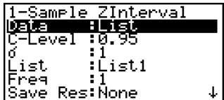
|Execute |
The following shows the meaning of each item in the case of list data specification.
Data ...... data type
C-Level ...... confidence level (0 ≤ C-Level < 1)
σ.... population standard deviation (σ > 0)
List .... list whose contents you want to use as sample data (List 1 to 26)
Freq..... sample frequency (1 or List 1 to 26)
Save Res ...... list for storage of calculation results (None or List 1 to 26)
Execute ...... executes a calculation
The following shows the meaning of parameter data specification items that are different from list data specification.
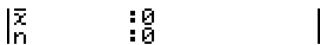
...... mean of sample
n ...... size of sample (positive integer)

After setting all the parameters, use ▼ to move the highlighting to “Execute” and then press the function key shown below to perform the calculation.
• F1(CALC) ... Performs the calculation.
Calculation Result Output Example
1-Sample ZInterval
Left =57.7260809
Right=70.8739191
x =64.3
n =20
Left ...... confidence interval lower limit (left edge)
Right.... confidence interval upper limit (right edge)
...... mean of sample
x_n-1 ...... sample standard deviation
(Displayed only for Data: List setting.)
n ...... size of sample
• 2-Sample Z Interval
2-Sample Z Interval calculates the confidence interval for the difference between two population means when the population standard deviations of two samples are known.
The following is the confidence interval. is the level of significance. The value 100 (1 - ) % is the confidence level.
$$ L e f t = (\bar {x} _ {1} - \bar {x} _ {2}) - Z \left(\frac {\alpha}{2}\right) \sqrt {\frac {\sigma_ {1} ^ {2}}{n _ {1}} + \frac {\sigma_ {2} ^ {2}}{n _ {2}}} $$
$$ R i g h t = (\bar {x} _ {1} - \bar {x} _ {2}) + Z \bigg (\frac {\alpha}{2} \bigg) \sqrt {\frac {\sigma_ {1} ^ {2}}{n _ {1}} + \frac {\sigma_ {2} ^ {2}}{n _ {2}}} $$
_1 : mean of sample 1
_2 : mean of sample 2
_1 : population standard deviation of sample 1
_2 : population standard deviation of sample 2
n_1 : size of sample 1
n_2 : size of sample 2
Perform the following key operations from the statistical data list.
F4 (INTR)
F1(Z)
F2(2-S)
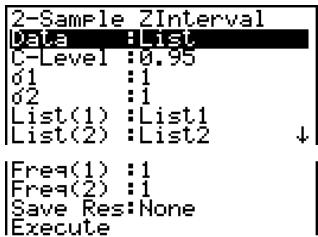

The following shows the meaning of each item in the case of list data specification.
Data ...... data type
C-Level..... confidence level (0 ≤ C-Level < 1)
_1 population standard deviation of sample 1 ( _1 > 0 )
_2 ...... population standard deviation of sample 2 ( _2 > 0 )
List(1) ...... list whose contents you want to use as data of sample 1 (List 1 to 26)
List(2) ...... list whose contents you want to use as data of sample 2 (List 1 to 26)
Freq(1) ...... frequency of sample 1 (1 or List 1 to 26)
Freq(2) ...... frequency of sample 2 (1 or List 1 to 26)
Save Res ...... list for storage of calculation results (None or List 1 to 26)
Execute ...... executes a calculation
The following shows the meaning of parameter data specification items that are different from list data specification.


_1 mean of sample 1
n_1 ...... size (positive integer) of sample 1
_2 mean of sample 2
n_2 ...... size (positive integer) of sample 2
After setting all the parameters, use ▼ to move the highlighting to “Execute” and then press the function key shown below to perform the calculation.
- F1(CALC) ... Performs the calculation.
Calculation Result Output Example
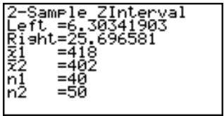
Left ...... confidence interval lower limit (left edge)
Right..... confidence interval upper limit (right edge)
_1 mean of sample 1
_2 mean of sample 2
x_1_n - 1 standard deviation of sample 1
(Displayed only for Data: List setting.)
x_2_n - 1 standard deviation of sample 2
(Displayed only for Data: List setting.)
n_1 ...... size of sample 1
n_2 ...... size of sample 2

• 1-Prop Z Interval
1-Prop Z Interval uses the number of data to calculate the confidence interval for an unknown proportion of successes.
The following is the confidence interval. is the level of significance. The value 100(1-)% is the confidence level.
$$ L e f t = \frac {x}{n} - Z \left(\frac {\alpha}{2}\right) \sqrt {\frac {1}{n} \left(\frac {x}{n} \left(1 - \frac {x}{n}\right)\right)} \qquad \qquad \begin{array}{l l} n: & \text {size of sample} \ x: & \text {data} \end{array} $$
$$ \text { Right } = \frac {x}{n} + Z \left(\frac {\alpha}{2}\right) \sqrt {\frac {1}{n} \left(\frac {x}{n} \left(1 - \frac {x}{n}\right)\right)} $$
Perform the following key operations from the statistical data list.
F4 (INTR)
F1(Z)
F3(1-P)
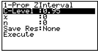
Data is specified using parameter specification. The following shows the meaning of each item.
C-Level ...... confidence level (0 ≤ C-Level < 1)
x ...... data (0 or positive integer)
n ...... size of sample (positive integer)
Save Res .... list for storage of calculation results (None or List 1 to 26)
Execute ...... executes a calculation
After setting all the parameters, use ▼ to move the highlighting to “Execute” and then press the function key shown below to perform the calculation.
• F1(CALC) ... Performs the calculation.
Calculation Result Output Example
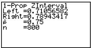
Left ...... confidence interval lower limit (left edge)
Right.... confidence interval upper limit (right edge)
...... estimated sample proportion
n ...... size of sample

- 2-Prop Z Interval
2-Prop Z Interval uses the number of data items to calculate the confidence interval for the difference between the proportion of successes in two populations.
The following is the confidence interval. is the level of significance. The value 100 (1 - ) % is the confidence level.
$$ L e f t = \frac {x _ {1}}{n _ {1}} - \frac {x _ {2}}{n _ {2}} - Z \left(\frac {\alpha}{2}\right) \sqrt {\frac {\frac {x _ {1}}{n _ {1}} \left(1 - \frac {x _ {1}}{n _ {1}}\right)}{n _ {1}} + \frac {\frac {x _ {2}}{n _ {2}} \left(1 - \frac {x _ {2}}{n _ {2}}\right)}{n _ {2}}} $$
n_1, n_2 : size of sample
x_1, x_2 : data
$$ R i g h t = \frac {x _ {1}}{n _ {1}} - \frac {x _ {2}}{n _ {2}} + Z \left(\frac {\alpha}{2}\right) \sqrt {\frac {\frac {x _ {1}}{n _ {1}} \left(1 - \frac {x _ {1}}{n _ {1}}\right)}{n _ {1}} + \frac {\frac {x _ {2}}{n _ {2}} \left(1 - \frac {x _ {2}}{n _ {2}}\right)}{n _ {2}}} $$
Perform the following key operations from the statistical data list.
F4 (INTR)
F1(Z)
F4(2-P)
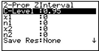
|Execute |
Data is specified using parameter specification. The following shows the meaning of each item.
C-Level ...... confidence level (0 ≤ C-Level < 1)
x_1 ...... data value ( x_1 ≥ 0 ) of sample 1
n_1 ...... size (positive integer) of sample 1
x_2 ...... data value ( x_2 ≥ 0 ) of sample 2
n_2 ...... size (positive integer) of sample 2
Save Res .... list for storage of calculation results (None or List 1 to 26)
Execute ...... executes a calculation
After setting all the parameters, use ▼ to move the highlighting to “Execute” and then press the function key shown below to perform the calculation.
• F1 (CALC) ... Performs the calculation.
Calculation Result Output Example
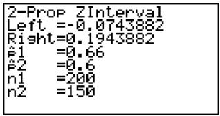

Left ...... confidence interval lower limit (left edge)
Right.... confidence interval upper limit (right edge)
_1 ...... estimated sample proportion for sample 1
_2 ...... estimated sample propotion for sample 2
n_1 ...... size of sample 1
n_2 ...... size of sample 2
■ t Interval
• 1-Sample t Interval
1-Sample t Interval calculates the confidence interval for an unknown population mean when the population standard deviation is unknown.
The following is the confidence interval. is the level of significance. The value 100(1-)% is the confidence level.
$$ L e f t = \bar {x} - t _ {n - 1} \left(\frac {\alpha}{2}\right) \frac {x \sigma_ {n - 1}}{\sqrt {n}} $$
$$ R i g h t = \bar {x} + t _ {n - 1} \left(\frac {\alpha}{2}\right) \frac {x \sigma_ {n - 1}}{\sqrt {n}} $$
Perform the following key operations from the statistical data list.
F4 (INTR)
F2(t)
F1(1-S)
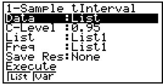
The following shows the meaning of each item in the case of list data specification.
Data ...... data type
C-Level ...... confidence level (0 ≤ C-Level < 1)
List .... list whose contents you want to use as sample data (List 1 to 26)
Freq..... sample frequency (1 or List 1 to 26)
Save Res .... list for storage of calculation results (None or List 1 to 26)
Execute ...... executes a calculation
The following shows the meaning of parameter data specification items that are different from list data specification.
$$ \left| \begin{array}{l l} \overline {{x}} & : 0 \ x \acute {o} n - 1 & : 0 \ n & : 0 \end{array} \right. $$

...... mean of sample
x_n-1 ...... sample standard deviation (x_n-1 ≥ 0)
n ...... size of sample (positive integer)
After setting all the parameters, use ▼ to move the highlighting to “Execute” and then press the function key shown below to perform the calculation.
- F1(CALC) ... Performs the calculation.
Calculation Result Output Example
1-Sample tInterval
Left =60.9628946
Right=71.6371054
x =66.3
xón-l =8.4
n =12
Left ...... confidence interval lower limit (left edge)
Right..... confidence interval upper limit (right edge)
...... mean of sample
x_n-1 sample standard deviation
n ...... size of sample
• 2-Sample t Interval
2-Sample t Interval calculates the confidence interval for the difference between two population means when both population standard deviations are unknown. The t interval is applied to t distribution.
The following confidence interval applies when pooling is in effect. is the level of significance. The value 100 (1 - ) % is the confidence level.
$$ L e f t = \left(\bar {x} _ {1} - \bar {x} _ {2}\right) - t _ {n _ {1} + n _ {2} - 2} \left(\frac {\alpha}{2}\right) \sqrt {x _ {p} \sigma_ {n - 1} {} ^ {2} \left(\frac {1}{n _ {1}} + \frac {1}{n _ {2}}\right)} $$
$$ R i g h t = (\bar {x} _ {1} - \bar {x} _ {2}) + t _ {n _ {1} + n _ {2} - 2} \left(\frac {\alpha}{2}\right) \sqrt {x _ {p} \sigma_ {n - 1} {} ^ {2} \left(\frac {1}{n _ {1}} + \frac {1}{n _ {2}}\right)} $$
$$ x _ {p} \sigma_ {n - 1} = \sqrt {\frac {(n _ {1} - 1) x _ {1} \sigma_ {n - 1} ^ {2} + (n _ {2} - 1) x _ {2} \sigma_ {n - 1} ^ {2}}{n _ {1} + n _ {2} - 2}} $$

The following confidence interval applies when pooling is not in effect. is the level of significance. The value 100(1-)% is the confidence level.
$$ L e f t = (\bar {x} _ {1} - \bar {x} _ {2}) - t _ {d f} \left(\frac {\alpha}{2}\right) \sqrt {\left(\frac {x _ {1} \sigma_ {n - 1} {} ^ {2}}{n _ {1}} + \frac {x _ {2} \sigma_ {n - 1} {} ^ {2}}{n _ {2}}\right)} $$
$$ R i g h t = (\bar {x} _ {1} - \bar {x} _ {2}) + t _ {d f} \left(\frac {\alpha}{2}\right) \sqrt {\left(\frac {x _ {1} \sigma_ {n - 1} ^ {2}}{n _ {1}} + \frac {x _ {2} \sigma_ {n - 1} ^ {2}}{n _ {2}}\right)} $$
$$ d f = \frac {1}{\frac {C ^ {2}}{n _ {1} - 1} + \frac {(1 - C) ^ {2}}{n _ {2} - 1}} $$
$$ C = \frac {\frac {x _ {1} \sigma_ {n - 1} ^ {2}}{n _ {1}}}{\left(\frac {x _ {1} \sigma_ {n - 1} ^ {2}}{n _ {1}} + \frac {x _ {2} \sigma_ {n - 1} ^ {2}}{n _ {2}}\right)} $$
Perform the following key operations from the statistical data list.
F4 (INTR)
F2(t)
F2(2-S)
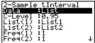
$$ \begin{array}{l} \text {Pooled : Off} \ \text {Save Res: None} \ \text {Execute} \end{array} $$
The following shows the meaning of each item in the case of list data specification.
Data ...... data type
C-Level ...... confidence level (0 ≤ C-Level < 1)
List(1) ...... list whose contents you want to use as data of sample 1 (List 1 to 26)
List(2) ...... list whose contents you want to use as data of sample 2 (List 1 to 26)
Freq(1) ...... frequency of sample 1 (1 or List 1 to 26)
Freq(2) ...... frequency of sample 2 (1 or List 1 to 26)
Pooled .... pooling On (in effect) or Off (not in effect)
Save Res ...... list for storage of calculation results (None or List 1 to 26)
Execute ...... executes a calculation
The following shows the meaning of parameter data specification items that are different from list data specification.
$$ \left| \begin{array}{l l} \overline {{x}} 1 & : 0 \ x 1 \acute {o} n - 1 & : 0 \ n 1 & : 0 \ \overline {{x}} 2 & : 0 \ x 2 \acute {o} n - 1 & : 0 \ n 2 & : 0 \end{array} \right. $$

_1 mean of sample 1
x_1_n - 1 standard deviation (x_1_n - 1≥ 0) of sample 1
n_1 ...... size (positive integer) of sample 1
_2 mean of sample 2
x_2_n-1 standard deviation ( x_2_n-1 ≥ 0 ) of sample 2
n_2 ...... size (positive integer) of sample 2
After setting all the parameters, use ▼ to move the highlighting to “Execute” and then press the function key shown below to perform the calculation.
• F1 (CALC) ... Performs the calculation.
Calculation Result Output Example
2-Sample tInterval
Left = -7.5088264
Right = -0.0911735
df = 7.29033011
x1 = 88.4
x2 = 84.2
x16n-1 = 2.07364414 ↓
Left ...... confidence interval lower limit (left edge)
Right..... confidence interval upper limit (right edge)
df ...... degrees of freedom
_1 mean of sample 1
_2 mean of sample 2
x_1_n-1 standard deviation of sample 1
x_2_n-1 standard deviation of sample 2
x_p_n-1 pooled sample standard deviation
(Displayed only when Pooled: On setting.)
n_1 ...... size of sample 1
n_2 ...... size of sample 2

6-7 Distribution
There is a variety of different types of distribution, but the most well-known is “normal distribution,” which is essential for performing statistical calculations. Normal distribution is a symmetrical distribution centered on the greatest occurrences of mean data (highest frequency), with the frequency decreasing as you move away from the center. Poisson distribution, geometric distribution, and various other distribution shapes are also used, depending on the data type.
Certain trends can be determined once the distribution shape is determined. You can calculate the probability of data taken from a distribution being less than a specific value.
For example, distribution can be used to calculate the yield rate when manufacturing some product. Once a value is established as the criteria, you can calculate normal probability when estimating what percent of the products meet the criteria. Conversely, a success rate target (80% for example) is set up as the hypothesis, and normal distribution is used to estimate the proportion of the products will reach this value.
Normal probability density calculates the probability density of normal distribution from a specified x value.
Normal distribution probability calculates the probability of normal distribution data falling between two specific values.
Inverse cumulative normal distribution calculates a value that represents the location within a normal distribution for a specific cumulative probability.
Student- t probability density calculates t probability density from a specified x value.
Student- t distribution probability calculates the probability of t distribution data falling between two specific values.
Like t distribution, distribution probability can also be calculated for ^2 , F, Binomial, Poisson, and Geometric distributions.
On the initial STAT mode screen, press F5 (DIST) to display the distribution menu, which contains the following items.
- F5 (DIST) F1 (NORM) ... Normal distribution (page 6-7-3)
F2(t) ... Student-t distribution (page 6-7-7)
F3 (CHI) ... ^2 distribution (page 6-7-9)
F4(F) ... F distribution (page 6-7-12)
F5 (BINM) ... Binomial distribution (page 6-7-16)
F6(▷) F1(POISN) ... Poisson distribution (page 6-7-19)
F6(▷) F2(GEO) ... Geometric distribution (page 6-7-21)

- Common Distribution Functions
After drawing a graph, you can use the P-CAL function to calculate an estimated p-value for a particular x value.
The following is the general procedure for using the P-CAL function.
- After drawing a distribution graph, press SHIFT F5(G-SLV) F1(P-CAL) to display the x value input dialog box.
- Input the value you want for x and then press EXE.
- This causes the x and p values to appear at the bottom of the display, and moves the pointer to the corresponding point on the graph.
- Pressing ,,T or a number key at this time causes the x value input dialog box to reappear so you can perform another estimated value calculation if you want.
- After you are finished, press EXIT to clear the coordinate values and the pointer from the display.

# Executing an analysis function automatically stores the x and p values in alpha variables X and P, respectively.

Normal Distribution
- Normal Probability Density
Normal probability density calculates the probability density of normal distribution from a specified x value. Normal probability density is applied to standard normal distribution.
$$ f (x) = \frac {1}{\sqrt {2 \pi} \sigma} e ^ {- \frac {(x - \mu) ^ {2}}{2 \sigma^ {2}}} \quad (\sigma > 0) $$
Perform the following key operations from the statistical data list.
F5 (DIST)
F1(NORM)
F1(Npd)
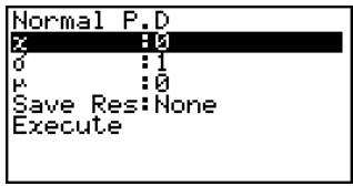
Data is specified using parameter specification. The following shows the meaning of each item.
x ...... data
σ...... standard deviation ( > 0 )
μ .... mean
Save Res ...... list for storage of calculation results (None or List 1 to 26)
Execute ...... executes a calculation or draws a graph
- Specifying = 1 and = 0 specifies standard normal distribution.
After setting all the parameters, use ▼ to move the highlighting to “Execute” and then press one of the function keys shown below to perform the calculation or draw the graph.
• F1(CALC) ... Performs the calculation.
- F6 (DRAW) ... Draws the graph.
Calculation Result Output Example
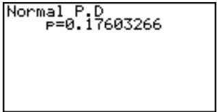
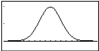
p ...... normal probability density

# V-Window settings for graph drawing are set automatically when the Setup screen's [Stat Wind] setting is [Auto]. Current V-Window
settings are used for graph drawing when the [Stat Wind] setting is [Manual].

- Normal Distribution Probability
Normal distribution probability calculates the probability of normal distribution data falling between two specific values.
$$ p = \frac {1}{\sqrt {2 \pi} \sigma} \int_ {a} ^ {b} e ^ {- \frac {(x - \mu) ^ {2}}{2 \sigma^ {2}}} d x $$
a : lower boundary
b : upper boundary
Perform the following key operations from the statistical data list.
F5 (DIST)
F1(NORM)
F2 (Ncd)
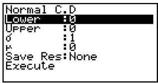
Data is specified using parameter specification. The following shows the meaning of each item.
Lower ...... lower boundary
Upper .... upper boundary
σ...... standard deviation ( > 0 )
μ .... mean
Save Res .... list for storage of calculation results (None or List 1 to 26)
Execute ...... executes a calculation
After setting all the parameters, use ▼ to move the highlighting to “Execute” and then press the function key shown below to perform the calculation.
• F1 (CALC) ... Performs the calculation.

# There is no graphing for normal distribution probability.

Calculation Result Output Example
Normal C.D
P =0.09184805
z:Low=1
z:UP =1.5
p ...... normal distribution probability
z:Low .... z:Low value (converted to standardize z score for lower value)
z:Up ...... z:Up value (converted to standardize z score for upper value)
- Inverse Cumulative Normal Distribution
Inverse cumulative normal distribution calculates a value that represents the location within a normal distribution for a specific cumulative probability.
| _-^ f(x) dx = p | _^+ f(x) dx = p | _^ f(x) dx = p | ||
| Tail: Left | Tail: Right | Tail: Central | ||
| upper | lower | upper and | ||
| boundary of | boundary of | lower | ||
| integration | integration | boundaries | ||
| interval | interval | of integration | ||
| = ? | = ? | interval | ||
| = ? | = ? | |||
Specify the probability and use this formula to obtain the integration interval.
Perform the following key operations from the statistical data list.
F5 (DIST)
F1(NORM)
F3 (InvN)
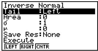
Data is specified using parameter specification. The following shows the meaning of each item.
Tail ...... probability value tail specification (Left, Right, Central)
Area ...... probability value (0 ≤ Area ≤ 1)
σ...... standard deviation ( > 0 )
μ .... mean
Save Res ...... list for storage of calculation results (None or List 1 to 26)
Execute ...... executes a calculation

After setting all the parameters, use ▼ to move the highlighting to “Execute” and then press the function key shown below to perform the calculation.
• F1 (CALC) ... Performs the calculation.
Calculation Result Output Examples
Inverse Normal
x=1.64485363
Inverse Normal
x:Low=-0.0627067
x:Up=0.06270677
x...... inverse cumulative normal distribution
- When [Left] is selected for [Tail]: upper boundary of integration interval.
- When [Right] is selected for [Tail]: lower boundary of integration interval.
- When [Central] is selected for [Tail]: upper and lower boundaries of integration interval.

# There is no graphing for inverse cumulative normal distribution.

■ Student-t Distribution
- Student- t Probability Density
Student-t probability density calculates t probability density from a specified x value.
$$ f (x) = \frac {\Gamma \left(\frac {d f + 1}{2}\right)}{\Gamma \left(\frac {d f}{2}\right)} \frac {\left(1 + \frac {x ^ {2}}{d f}\right) ^ {- \frac {d f + 1}{2}}}{\sqrt {\pi d f}} $$
Perform the following key operations from the statistical data list.
F5 (DIST)
F2(t)
F1(tpd)
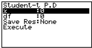
Data is specified using parameter specification. The following shows the meaning of each item.
x ...... data
df ...... degrees of freedom (df > 0)
Save Res ...... list for storage of calculation results (None or List 1 to 26)
Execute ...... executes a calculation or draws a graph
After setting all the parameters, use ▼ to move the highlighting to “Execute” and then press one of the function keys shown below to perform the calculation or draw the graph.
• F1(CALC) ... Performs the calculation.
- F6 (DRAW) ... Draws the graph.
Calculation Result Output Example
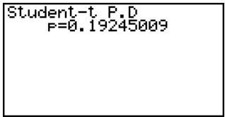
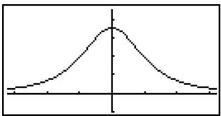
line
| x | y | | ---- | ----- | | 0.0 | 0.0 | | 0.2 | 0.1 | | 0.4 | 0.3 | | 0.6 | 0.5 | | 0.8 | 0.7 | | 1.0 | 0.9 | | 1.2 | 0.7 | | 1.4 | 0.5 | | 1.6 | 0.3 | | 1.8 | 0.1 | | 2.0 | 0.0 |p ...... Student-t probability density

# Current V-Window settings are used for graph drawing when the Setup screen's [Stat Wind] setting is [Manual]. The V-Window settings below are set automatically
when the [Stat Wind] setting is [Auto].
$$ X m i n = - 3. 2, X m a x = 3. 2, X s c a l e = 1, $$
$$ Y m i n = - 0. 1, Y m a x = 0. 4 5, Y s c a l e = 0. 1 $$

- Student- t Distribution Probability
Student-t distribution probability calculates the probability of t distribution data falling between two specific values.
$$ p = \frac {\Gamma \left(\frac {d f + 1}{2}\right)}{\Gamma \left(\frac {d f}{2}\right) \sqrt {\pi d f}} \int_ {a} ^ {b} \left(1 + \frac {x ^ {2}}{d f}\right) ^ {- \frac {d f + 1}{2}} d x $$
a : lower boundary
b : upper boundary
Perform the following key operations from the statistical data list.
F5 (DIST)
F2(t)
F2 (tcd)
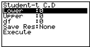
Data is specified using parameter specification. The following shows the meaning of each item.
Lower ...... lower boundary
Upper .... upper boundary
df ...... degrees of freedom (df > 0)
Save Res .... list for storage of calculation results (None or List 1 to 26)
Execute ...... executes a calculation
After setting all the parameters, use ▼ to move the highlighting to “Execute” and then press the function key shown below to perform the calculation.
- F1 (CALC) ... Performs the calculation.

# There is no graphing for Student-t distribution probability.

Calculation Result Output Example
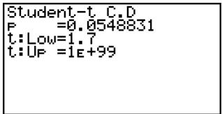
p ...... Student-t distribution probability
t:Low ...... t:Low value (input lower value)
t:Up ...... t:Up value (input upper value)
■ ^2 Distribution
- ^2 Probability Density
^2 probability density calculates the probability density function for the ^2 distribution at a specified x value.
$$ f (x) = \frac {1}{\Gamma \left(\frac {d f}{2}\right)} \left(\frac {1}{2}\right) ^ {\frac {d f}{2}} x ^ {\frac {d f}{2} - 1} e ^ {- \frac {x}{2}} $$
Perform the following key operations from the statistical data list.
F5 (DIST)
F3 (CHI)
F1(Cpd)
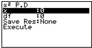
Data is specified using parameter specification. The following shows the meaning of each item.
x ...... data
df ...... degrees of freedom (positive integer)
Save Res ...... list for storage of calculation results (None or List 1 to 26)
Execute ...... executes a calculation or draws a graph
After setting all the parameters, use ▼ to move the highlighting to “Execute” and then press one of the function keys shown below to perform the calculation or draw the graph.
• F1(CALC) ... Performs the calculation.
• F6 (DRAW) ... Draws the graph.

Calculation Result Output Example
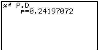
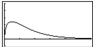
line
| x | y | | --- | --- | | 0 | 0 | | 1 | 1 | | 2 | 2 | | 3 | 3 | | 4 | 4 | | 5 | 5 | | 6 | 6 | | 7 | 7 | | 8 | 8 | | 9 | 9 | | 10 | 10 | | 11 | 11 | | 12 | 12 | | 13 | 13 | | 14 | 14 | | 15 | 15 | | 16 | 16 | | 17 | 17 | | 18 | 18 | | 19 | 19 | | 20 | 20 | | 21 | 21 | | 22 | 22 | | 23 | 23 | | 24 | 24 | | 25 | 25 | | 26 | 26 | | 27 | 27 | | 28 | 28 | | 29 | 29 | | 30 | 30 | | 31 | 31 | | 32 | 32 | | 33 | 33 | | 34 | 34 | | 35 | 35 | | 36 | 36 | | 37 | 37 | | 38 | 38 | | 39 | 39 | | 40 | 40 | | 41 | 41 | | 42 | 42 | | 43 | 43 | | 44 | 44 | | 45 | 45 | | 46 | 46 | | 47 | 47 | | 48 | 48 | | 49 | 49 | | 50 | 50 | | 51 | 51 | | 52 | 52 | | 53 | 53 | | 54 | 54 | | 55 | 55 | | 56 | 56 | | 57 | 57 | | 58 | 58 | | 59 | 59 | | 60 | 60 | | 61 | 61 | | 62 | 62 | | 63 | 63 | | 64 | 64 | | 65 | 65 | | 66 | 66 | | 67 | 67 | | 68 | 68 | | 69 | 69 | | 70 | 70 | | 71 | 71 | | 72 | 72 | | 73 | 73 | | 74 | 74 | | 75 | 75 | | 76 | 76 | | 77 | 77 | | 78 | 78 | | 79 | 79 | | 80 | 80 | | 81 | 81 | | 82 | 82 | | 83 | 83 | | 84 | 84 | | 85 | 85 | | 86 | 86 | | 87 | 87 | | 88 | 88 | | 89 | 89 | | 90 | 90 | | 91 | 91 | | 92 | 92 | | 93 | 93 | | 94 | 94 | | 95 | 95 | | 96 | 96 | | 97 | 97 | | 98 | 98 | | 99 | 99 | |100 |100 |p .... ^2 probability density

# Current V-Window settings are used for graph drawing when the Setup screen's [Stat Wind] setting is [Manual]. The V-Window settings below are set automatically
when the [Stat Wind] setting is [Auto].
$$ X m i n = 0, X m a x = 1 1. 5, X s c a l e = 2, $$
$$ Y \min = - 0. 1, Y \max = 0. 5, Y \text { scale } = 0. 1 $$

- ^2 Distribution Probability
^2 distribution probability calculates the probability of ^2 distribution data falling between two specific values.
$$ p = \frac {1}{\Gamma \left(\frac {d f}{2}\right)} \left(\frac {1}{2}\right) ^ {\frac {d f}{2}} \int_ {a} ^ {b} x ^ {\frac {d f}{2} - 1} e ^ {- \frac {x}{2}} d x $$
a : lower boundary
b : upper boundary
Perform the following key operations from the statistical data list.
F5 (DIST)
F3 (CHI)
F2(Ccd)
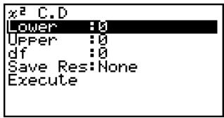
Data is specified using parameter specification. The following shows the meaning of each item.
Lower ...... lower boundary
Upper .... upper boundary
df ...... degrees of freedom (positive integer)
Save Res ...... list for storage of calculation results (None or List 1 to 26)
Execute ...... executes a calculation
After setting all the parameters, use ▼ to move the highlighting to “Execute” and then press the function key shown below to perform the calculation.
• F1 (CALC) ... Performs the calculation.

# There is no graphing for ^2 distribution probability.

Calculation Result Output Example
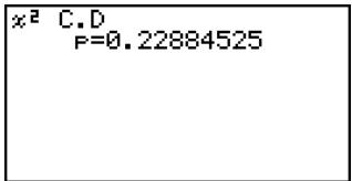
p .... ^2 distribution probability
F Distribution
- F Probability Density
F probability density calculates the probability density function for the F distribution at a specified x value.
$$ f (x) = \frac {\Gamma \left(\frac {n + d}{2}\right)}{\Gamma \left(\frac {n}{2}\right) \Gamma \left(\frac {d}{2}\right)} \left(\frac {n}{d}\right) ^ {\frac {n}{2}} x ^ {\frac {n}{2} - 1} \left(1 + \frac {n x}{d}\right) ^ {- \frac {n + d}{2}} $$
Perform the following key operations from the statistical data list.
F5 (DIST)
F4(F)
F1(Fpd)
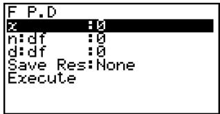
Data is specified using parameter specification. The following shows the meaning of each item.
x ...... data
n:df ...... numerator degrees of freedom (positive integer)
d:df...... denominator degrees of freedom (positive integer)
Save Res ...... list for storage of calculation results (None or List 1 to 26)
Execute ...... executes a calculation or draws a graph
After setting all the parameters, use ▼ to move the highlighting to “Execute” and then press one of the function keys shown below to perform the calculation or draw the graph.
• F1(CALC) ... Performs the calculation.
• F6(DRAW) ... Draws the graph.

Calculation Result Output Example
F P.D P=0.90782683
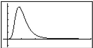
line
| x | y | | ---- | ----- | | 0 | 0 | | 1 | 1 | | 2 | 3 | | 3 | 5 | | 4 | 7 | | 5 | 8 | | 6 | 9 | | 7 | 10 | | 8 | 11 | | 9 | 12 | | 10 | 13 | | 11 | 14 | | 12 | 15 | | 13 | 16 | | 14 | 17 | | 15 | 18 | | 16 | 19 | | 17 | 20 | | 18 | 21 | | 19 | 22 | | 20 | 23 | | 21 | 24 | | 22 | 25 | | 23 | 26 | | 24 | 27 | | 25 | 28 | | 26 | 29 | | 27 | 30 | | 28 | 31 | | 29 | 32 | | 30 | 33 | | 31 | 34 | | 32 | 35 | | 33 | 36 | | 34 | 37 | | 35 | 38 | | 36 | 39 | | 37 | 40 | | 38 | 41 | | 39 | 42 | | 40 | 43 | | 41 | 44 | | 42 | 45 | | 43 | 46 | | 44 | 47 | | 45 | 48 | | 46 | 49 | | 47 | 50 | | 48 | 51 | | 49 | 52 | | 50 | 53 | | 51 | 54 | | 52 | 55 | | 53 | 56 | | 54 | 57 | | 55 | 58 | | 56 | 59 | | 57 | 60 | | 58 | 61 | | 59 | 62 | | 60 | 63 | | 61 | 64 | | 62 | 65 | | 63 | 66 | | 64 | 67 | | 65 | 68 | | 66 | 69 | | 67 | 70 | | 68 | 71 | | 69 | 72 | | 70 | 73 | | 71 | 74 | | 72 | 75 | | 73 | 76 | | 74 | 77 | | 75 | 78 | | 76 | 79 | | 77 | 80 | | 78 | 81 | | 79 | 82 | | 80 | 83 | | 81 | 84 | | 82 | 85 | | 83 | 86 | | 84 | 87 | | 85 | 88 | | 86 | 89 | | 87 | 90 | | 88 | 91 | | 89 | 92 | | 90 | 93 | | 91 | 94 | | 92 | 95 | | 93 | 96 | | 94 | 97 | | 95 | 98 | | 96 | 99 | | 97 | 100 | | 98 | | | | |p ...... F probability density

# V-Window settings for graph drawing are set automatically when the Setup screen's [Stat Wind] setting is [Auto]. Current V-Window
settings are used for graph drawing when the [Stat Wind] setting is [Manual].

- F Distribution Probability
F distribution probability calculates the probability of F distribution data falling between two specific values.
$$ p = \frac {\Gamma \left(\frac {n + d}{2}\right)}{\Gamma \left(\frac {n}{2}\right) \Gamma \left(\frac {d}{2}\right)} \left(\frac {n}{d}\right) ^ {\frac {n}{2}} \int_ {a} ^ {b} x ^ {\frac {n}{2} - 1} \left(1 + \frac {n x}{d}\right) ^ {- \frac {n + d}{2}} d x $$
a : lower boundary
b : upper boundary
Perform the following key operations from the statistical data list.
F5 (DIST)
F4(F)
F2 (Fcd)
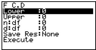
Data is specified using parameter specification. The following shows the meaning of each item.
Lower ...... lower boundary
Upper ...... upper boundary
n:df ...... numerator degrees of freedom (positive integer)
d:df ...... denominator degrees of freedom (positive integer)
Save Res .... list for storage of calculation results (None or List 1 to 26)
Execute ...... executes a calculation
After setting all the parameters, use ▼ to move the highlighting to “Execute” and then press the function key shown below to perform the calculation.
• F1 (CALC) ... Performs the calculation.

# There is no graphing for F distribution probability.

Calculation Result Output Example
F C.D
P=0.91400535
p ...... F distribution probability

Binomial Distribution
- Binomial Probability
Binomial probability calculates a probability at a specified value for the discrete binomial distribution with the specified number of trials and probability of success on each trial.
$$ f (x) = _ {n} C _ {x} p ^ {x} (1 - p) ^ {n - x} \quad \left(x = 0, 1, \dots \dots , n\right) \quad p: \text { success probability } \quad (0 \leq p \leq 1) $$
$$ n: \text {number of trials} $$
Perform the following key operations from the statistical data list.
F5 (DIST)
F5 (BINM)
F1 (Bpd)
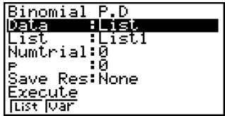
The following shows the meaning of each item when data is specified using list specification.
Data ...... data type
List .... list whose contents you want to use as specified data (List 1 to 26)
Numtrial ...... number of trials
p ...... success probability (0 ≤ p ≤ 1)
Save Res .... list for storage of calculation results (None or List 1 to 26)
Execute ...... executes a calculation
The following shows the meaning of a parameter data specification item that is different from list data specification.
|x :0 |
x ...... integer from 0 to n
After setting all the parameters, use ▼ to move the highlighting to “Execute” and then press the function key shown below to perform the calculation.
- F1(CALC) ... Performs the calculation.

# There is no graphing for binomial distribution.

Calculation Result Output Example
![Binomial P.D 1 [0.3599] 2 [0.4799] 3 [0.1599] 0.36](/content/2025/01/86785/images/967292d4495d2c60fd7c923abd4864d9a96b59255041fbef6ec21a0b9114f005.jpg)
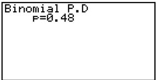
- Binomial Cumulative Density
Binomial cumulative density calculates a cumulative probability at a specified value for the discrete binomial distribution with the specified number of trials and probability of success on each trial.
Perform the following key operations from the statistical data list.
F5 (DIST)
F5 (BINM)
F2 (Bcd)
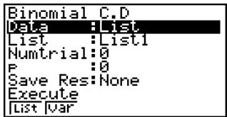
The following shows the meaning of each item when data is specified using list specification.
Data ...... data type
List .... list whose contents you want to use as specified data (List 1 to 26)
Numtrial...... number of trials
p ...... success probability (0 ≤ p ≤ 1)
Save Res ...... list for storage of calculation results (None or List 1 to 26)
Execute ...... executes a calculation
The following shows the meaning of a parameter data specification item that is different from list data specification.
|x :0 |
x ...... integer from 0 to n

After setting all the parameters, use ▼ to move the highlighting to “Execute” and then press the function key shown below to perform the calculation.
• F1(CALC) ... Performs the calculation.
Calculation Result Output Example
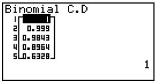
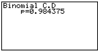
p ...... probability of success

■ Poisson Distribution
- Poisson Probability
Poisson probability calculates a probability at a specified value for the discrete Poisson distribution with the specified mean.
$$ f (x) = \frac {e ^ {- \mu} \mu^ {x}}{x !} $$
$$ (x = 0, 1, 2, \dots) $$
$$ \mu : \text { mean } (\mu > 0) $$
Perform the following key operations from the statistical data list.
F5 (DIST)
F6 (▷) F1 (POISN)
F1(Ppd)
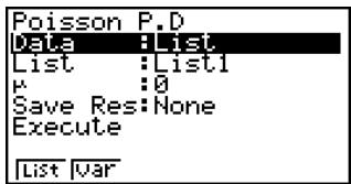
The following shows the meaning of each item when data is specified using list specification.
Data ...... data type
List .... list whose contents you want to use as specified data (List 1 to 26)
...... mean ( > 0 )
Save Res .... list for storage of calculation results (None or List 1 to 26)
Execute ...... executes a calculation
The following shows the meaning of a parameter data specification item that is different from list data specification.
|x
:0
x ( x ≥ 0 )
After setting all the parameters, use ▼ to move the highlighting to “Execute” and then press the function key shown below to perform the calculation.
- F1(CALC) ... Performs the calculation.
Calculation Result Output Example
![Poisson P.D 1 [0.238] 2 [0.3346] 3 [0.251] 0.2231301601](/content/2025/01/86785/images/47d8bbc478e3e2d1f0fd5c1fa41546ccc1b15f749f4b49949d263fa6d69ea148.jpg)
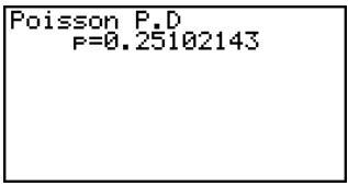
p Poisson probability

# There is no graphing for Poisson distribution.

- Poisson Cumulative Density
Poisson cumulative density calculates a cumulative probability at specified value for the discrete Poisson distribution with the specified mean.
Perform the following key operations from the statistical data list.
F5 (DIST)
F6 (▷) F1 (POISN)
F2 (Pcd)
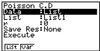
The following shows the meaning of each item when data is specified using list specification.
Data ...... data type
List .... list whose contents you want to use as specified data (List 1 to 26)
...... mean ( > 0 )
Save Res .... list for storage of calculation results (None or List 1 to 26)
Execute ...... executes a calculation
The following shows the meaning of a parameter data specification item that is different from list data specification.
|x :0 |
x ( x ≥ 0 )
After setting all the parameters, use ▼ to move the highlighting to “Execute” and then press the function key shown below to perform the calculation.
- F1 (CALC) ... Performs the calculation.
Calculation Result Output Example
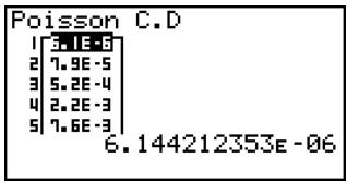
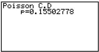
p ...... Poisson cumulative probability

■ Geometric Distribution
- Geometric Probability
Geometric probability calculates the probability at a specified value, and the number of the trial on which the first success occurs, for the geometric distribution with a specified probability of success.
$$ f (x) = p (1 - p) ^ {x - 1} \quad (x = 1, 2, 3, \dots) $$
Perform the following key operations from the statistical data list.
F5 (DIST)
F6 (▷) F2 (GEO)
F1 (Gpd)
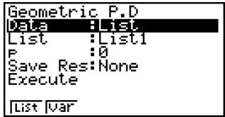
The following shows the meaning of each item when data is specified using list specification.
Data ...... data type
List .... list whose contents you want to use as specified data (List 1 to 26)
p ...... success probability (0 ≤ p ≤ 1)
Save Res ...... list for storage of calculation results (None or List 1 to 26)
Execute ...... executes a calculation
The following shows the meaning of a parameter data specification item that is different from list data specification.
|x :0 |
x ...... positive integer (x ≧ 1)
After setting all the parameters, use ▼ to move the highlighting to “Execute” and then press the function key shown below to perform the calculation.
• F1 (CALC) ... Performs the calculation.
Calculation Result Output Example
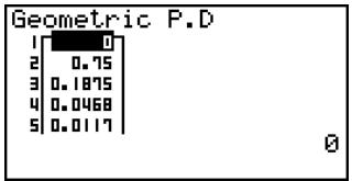
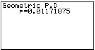
p geometric probability

# There is no graphing for geometric distribution.
# Positive integer number is calculated whether list data (Data:List) or x value (Data:variable) is specified.

- Geometric Cumulative Density
Geometric cumulative density calculates a cumulative probability at specified value, the number of the trial on which the first success occurs, for the discrete geometric distribution with the specified probability of success.
Perform the following key operations from the statistical data list.
F5 (DIST)
F6 (▷) F2 (GEO)
F2 (Gcd)
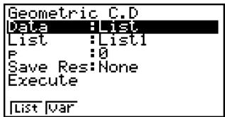
The following shows the meaning of each item when data is specified using list specification.
Data ...... data type
List .... list whose contents you want to use as specified data (List 1 to 26)
p ...... success probability (0 ≤ p ≤ 1)
Save Res ...... list for storage of calculation results (None or List 1 to 26)
Execute ...... executes a calculation
The following shows the meaning of a parameter data specification item that is different from list data specification.
|x :0 |
x ...... positive integer (x ≧ 1)
After setting all the parameters, use ▼ to move the highlighting to “Execute” and then press the function key shown below to perform the calculation.
- F1(CALC) ... Performs the calculation.
Calculation Result Output Example
![Geometric C.D 1 [0.45] 2 [0.8749] 3 [0.9315] 0.75](/content/2025/01/86785/images/5632508e3a0ef2ec9292f0ac93857960add3bd622161a2e8ccc5e0289374d18c.jpg)
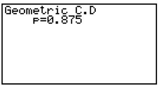
p geometric cumulative probability

# Positive integer number is calculated whether list data (Data:List) or x value (Data:variable) is specified.

Chapter
Financial Calculation (TVM)
The TVM mode provides you with the tools to perform the following types of financial calculations.
- Simple interest
- Compound interest
• Cash Flow (Investment appraisal) - Amortization
- Interest rate conversion (annual percentage rate and effective interest rate)
- Cost, selling price, margin
• Day/date calculations
7-1 Before Performing Financial Calculations
7-2 Simple Interest
7-3 Compound Interest
7-4 Cash Flow (Investment Appraisal)
7-5 Amortization
7-6 Interest Rate Conversion
7-7 Cost, Selling Price, Margin
7-8 Day/Date Calculations
7-1 Before Performing Financial Calculations
From the Main Menu, enter the TVM mode and display the Financial screen like the one shown below.
Financial 1 screen
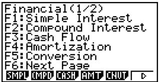
Financial 2 screen
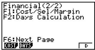
- {SMPL} ... {simple interest}
- {CMPD} ... {compound interest}
- {CASH} ... {cash flow (investment appraisal)}
- {AMT} ... {amortization}
- {CNVT} ... {interest rate conversion}
- {COST} ... {cost, selling price, margin}
- {DAYS} ... {day/date calculations}
Setup Items
- Payment
- {BGN}/{END} ... Specifies {beginning of the period}/{end of the period} payment
- Date Mode
- {365}/{360} ... Specifies calculation according to a {365-day}/{360-day} year
Note the following points regarding Setup screen settings whenever using the TVM mode.
- Drawing a financial graph while the Label item is turned on, displays the label CASH for the vertical axis (deposits, withdrawals), and TIME for the horizontal axis (frequency).
- The number of display digits applied in the TVM mode is different from the number of digits used in other modes. The calculators automatically reverts to Norm 1 whenever you enter the TVM mode, which cancels a Sci (number of significant digits) or Eng (engineering notation) setting made in another mode.
■ Graphing in the TVM Mode
After performing a financial calculation, you can use F6 (GRPH) to graph the results as shown below.
natural_image
Simple geometric shape composed of two rectangles (no text or symbols)- Pressing F1 (Trace) or SHIFT F1 (TRCE) while a graph is on the display activates Trace, which can be used to look up other financial values. In the case of simple interest, for example, pressing ▶ displays PV, SI, and SFV. Pressing ◀ displays the same values in reverse sequence.
- Zoom, Scroll, and Sketch cannot be used in the TVM mode.
- Whether you should use a positive or a negative value for the present value (PV) or the purchase price (PRC) depends on the type of calculation you are trying to perform.
- Note that graphs should be used only for reference purposes when viewing TVM mode calculation results.
- Note that calculation results produced in this mode should be regarded as reference values only.
- Whenever performing an actual financial transaction, be sure to check any calculation results obtained using this calculator with against the figures calculated by your financial institution.
7-2 Simple Interest
This calculator uses the following formulas to calculate simple interest.
- Formula
| 365-day Mode | SI' = 365 × PV × i | ( i = %100 ) | SI : interest |
| n : number of interest | |||
| 360-day Mode | SI' = 360 × PV × i | ( i = %100 ) | periods |
| PV : principal | |||
| I% : annual interest | |||
| SFV : principal plus interest | |||
| SI = -SI' | |||
| SFV = -(PV + SI') |
Press F1(SMPL) from the Financial 1 screen to display the following input screen for simple interest.
F1(SMPL)
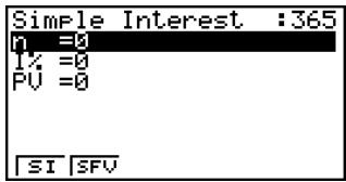
n ...... number of interest periods (days)
I% ...... annual interest rate
PV...... principal
After configuring the parameters, use one of the function menus noted below to perform the corresponding calculation.
- {SI} ... {simple interest}
- {SFV} ... {simple future value}
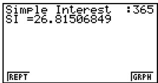
- An error (Ma ERROR) occurs if parameters are not configured correctly.
Use the following function menus to maneuver between calculation result screens.
- {REPT} ... {parameter input screen}
- {GRPH} ... {draws graph}
natural_image
Simple geometric shape composed of two adjacent rectangles (no text or symbols)After drawing a graph, you can press SHIFT F1(TRCE) to turn on trace and read calculation results along the graph.
Each press of ▶ while trace is turned on cycles the displayed value in the sequence: present value (PV) simple interest (SI) simple future value (SFV) . Pressing ◀ cycles in the reverse direction.
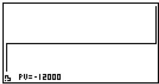
Press EXIT to return to the parameter input screen.
7-3 Compound Interest
This calculator uses the following standard formulas to calculate compound interest.
- Formula I
$$ P V + P M T \times \frac {(1 + i \times S) [ (1 + i) ^ {n} - 1 ]}{i (1 + i) ^ {n}} + F V \frac {1}{(1 + i) ^ {n}} = 0 \quad \left(i = \frac {I \%}{1 0 0}\right) $$
Here:
$$ P V = - (P M T \times \alpha + F V \times \beta) $$
$$ F V = - \frac {P M T \times \alpha + P V}{\beta} $$
$$ P M T = - \frac {P V + F V \times \beta}{\alpha} $$
$$ n = \frac {\log \left{\frac {(1 + i \times S) P M T - F V i}{(1 + i \times S) P M T + P V i} \right}}{\log (1 + i)} $$
$$ \alpha = \frac {(1 + i \times S) [ (1 + i) ^ {n} - 1 ]}{i (1 + i) ^ {n}} $$
$$ \beta = \frac {1}{(1 + i) ^ {n}} $$
$$ F (i) = \text { Formula I } $$
$$ F (i) ^ {\prime} = \frac {P M T}{i} \left[ - \frac {(1 + i \times S) [ 1 - (1 + i) ^ {- n} ]}{i} + (1 + i \times S) [ n (1 + i) ^ {- n - 1} ] \right. $$
$$ \left. + S \left[ 1 - (1 + i) ^ {- n} \right] \right] - n F V (1 + i) ^ {- n - 1} $$
- Formula II (I% = 0)
$$ P V + P M T \times n + F V = 0 $$
Here:
$$ P V = - (P M T \times n + F V) $$
$$ P V \quad : \text { present value } $$
$$ F V \quad : \text { future value } $$
$$ P M T: \text { payment } $$
$$ n \quad : \text { number of compound periods } $$
$$ I \% \quad : \text { annual interest rate } $$
i is calculated using Newton's Method.
$$ S = 0 \text { assumed for end of term } $$
$$ S = 1 \text { assumed for beginning of term } $$
$$ F V = - (P M T \times n + P V) $$
$$ P M T = - \frac {P V + F V}{n} $$
$$ n = - \frac {P V + F V}{P M T} $$
- A deposit is indicated by a plus sign (+), while a withdrawal is indicated by a minus sign (−).
- Converting between the nominal interest rate and effective interest rate
The nominal interest rate (I% value input by user) is converted to an effective interest rate (I%') when the number of installments per year (P/Y) is different from the number of compound interest calculation periods (C/Y). This conversion is required for installment savings accounts, loan repayments, etc.
$$ I \% ^ {\prime} = \left{\left(1 + \frac {I \%}{1 0 0 \times [ C / Y ]}\right) ^ {\frac {[ C / Y ]}{[ P / Y ]}} - 1 \right} \times 1 0 0 $$
P/Y: installment periods per year
C/Y: compounding periods per year
When calculating n, PV, PMT, FV
The following calculation is performed after conversion from the nominal interest rate to the effective interest rate, and the result is used for all subsequent calculations.
$$ i = I \% ^ {\prime} \div 100 $$
When calculating I%
After I% is obtained, the following calculation is performed to convert to I%^1 .
$$ I \% ^ {\prime} = \left{\left(1 + \frac {I \%}{1 0 0}\right) ^ {\frac {[ P / Y ]}{[ C / Y ]}} - 1 \right} \times [ C / Y ] \times 1 0 0 $$
P/Y: installment periods per year
C/Y: compounding periods per year
The value of I%' is returned as the result of the I% calculation.
Press F2 (CMPD) from the Financial 1 screen to display the following input screen for compound interest.
F2 (CMPD)
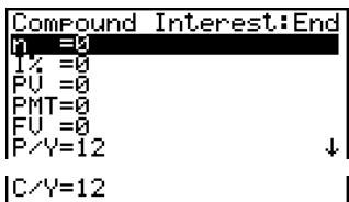
n ...... number of compound periods
I% ...... annual interest rate
PV ...... present value (loan amount in case of loan; principal in case of savings)
PMT ...... payment for each installment (payment in case of loan; deposit in case of savings)
FV ...... future value (unpaid balance in case of loan; principal plus interest in case of savings)
P/Y ...... installment periods per year
C/Y .... compounding periods per year
Important!
Inputting Values
A period (n) is expressed as a positive value. Either the present value (PV) or future value (FV) is positive, while the other (PV or FV) is negative.
Precision
This calculator performs interest calculations using Newton's Method, which produces approximate values whose precision can be affected by various calculation conditions. Because of this, interest calculation results produced by this calculator should be used keeping the above limitation in mind or the results should be verified.
After configuring the parameters, use one of the function menus noted below to perform the corresponding calculation.
- n ... {number of compound periods}
- {I%} ... {annual interest rate}
- {PV} ... {present value} (Loan: loan amount; Savings: balance)
- {PMT} ... {payment} (Loan: installment; Savings: deposit)
- {FV} ... {future value} (Loan: unpaid balance; Savings: principal plus interest)
- {AMT} ... {amortization screen}
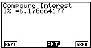
- An error (Ma ERROR) occurs if parameters are not configured correctly.
Use the following function menus to maneuver between calculation result screens.
- {REPT} ... {parameter input screen}
- {AMT} ... {amortization screen}
- {GRPH} ... {draws graph}
natural_image
Simple geometric shape with two horizontal lines inside a rectangle (no text or symbols)After drawing a graph, you can press SHIFT F1(TRCE) to turn on trace and read calculation results along the graph.
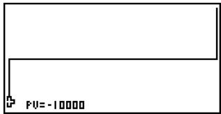
Press EXIT to return to the parameter input screen.
7-4 Cash Flow (Investment Appraisal)
This calculator uses the discounted cash flow (DCF) method to perform investment appraisal by totalling cash flow for a fixed period. This calculator can perform the following four types of investment appraisal.
- Net present value (NPV)
- Net future value (NFV)
- Internal rate of return (IRR)
- Payback period* (PBP)
* The payback period (PBP) can also be called the “discounted payback period” (DPP). When the annual interest rate (I%) is zero, the PBP is called the “simple payback period” (SPP).
A cash flow diagram like the one shown below helps to visualize the movement of funds.
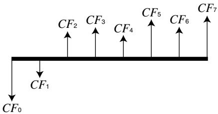
With this graph, the initial investment amount is represented by CF_0 . The cash flow one year later is shown by CF_1 , two years later by CF_2 , and so on.
Investment appraisal can be used to clearly determine whether an investment is realizing profits that were originally targeted.
• NPV
$$ N P V = C F _ {0} + \frac {C F _ {1}}{(1 + i)} + \frac {C F _ {2}}{(1 + i) ^ {2}} + \frac {C F _ {3}}{(1 + i) ^ {3}} + \dots + \frac {C F _ {n}}{(1 + i) ^ {n}} \quad \left(i = \frac {I \%}{1 0 0}\right) $$
n: natural number up to 254
• NFV
$$ N F V = N P V \times (1 + i) ^ {n} $$
- IRR
$$ 0 = C F _ {0} + \frac {C F _ {1}}{(1 + i)} + \frac {C F _ {2}}{(1 + i) ^ {2}} + \frac {C F _ {3}}{(1 + i) ^ {3}} + \dots + \frac {C F _ {n}}{(1 + i) ^ {n}} $$
In this formula, NPV = 0, and the value of IRR is equivalent to i × 100 . It should be noted, however, that minute fractional values tend to accumulate during the subsequent calculations performed automatically by the calculator, so NPV never actually reaches exactly zero. IRR becomes more accurate the closer than NPV approaches to zero.
• PBP
$$ P B P = \left{ \begin{array}{l} 0 \dots \dots (C F _ {0} \geq 0) \ n - \frac {N P V _ {n}}{N P V _ {n + 1} - N P V _ {n}} \dots (\text { Other than those above }) \end{array} \right. $$
$$ N P V _ {n} = \sum_ {k = 0} ^ {n} \frac {C F _ {k}}{(1 + i) ^ {k}} $$
n: Smallest positive integer that satisfies the conditions NPV_n ≤ 0 , NPV_n+1 ≥ 0 , or 0.
- Press F3 (CASH) from the Financial 1 screen to display the following input screen for Cash Flow.
F3 (CASH)
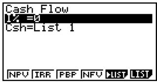
I% ...... interest rate (%)
Csh ...... list for cash flow
If you have not yet input data into a list, press F5(▶LIST) and input data into a list.
After configuring the parameters, use one of the function menus noted below to perform the corresponding calculation.
- {NPV} ... {net present value}
- {IRR} ... {internal rate of return}
- {PBP} ... {payback period}
- {NFV} ... {net future value}
- {▶LIST} ... {inputs data into a list}
- {LIST} ... {specifies a list for data input}
Cash Flow NPV=9610.156175
REPT
GRAPH
- An error (Ma ERROR) occurs if parameters are not configured correctly.
Use the following function menus to maneuver between calculation result screens.
- {REPT} ... {parameter input screen}
- {GRPH} ... {draws graph}
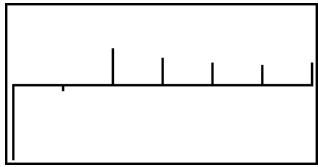
natural_image
Simple line drawing of a rectangular shape with vertical lines and a horizontal base (no text or symbols)After drawing a graph, you can press SHIFT F1(TRCE) to turn on trace and read calculation results along the graph.
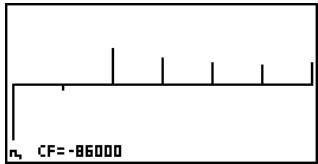
Press EXIT to return to the parameter input screen.
7-5 Amortization
This calculator can be used to calculate the principal and interest portion of a monthly installment, the remaining principal, and amount of principal and interest repaid up to any point.
- Formula
Amount of single payment
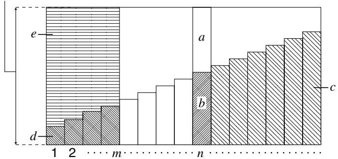
bar
| Category | Value | |---|---| | a | 100 | | b | 80 | | c | 95 | | d | 60 | | e | 120 |(Number of payments)
a: interest portion of installment PM1 (INT)
b: principal portion of installment PM1 (PRN)
c: balance of principal after installment PM2 (BAL)
d: total principal from installment PM1 to payment of installment PM2 ( PRN )
e: total interest from installment PM1 to payment of installment PM2 (ΣINT)
$$ ^ {*} a + b = \text { one repayment } (P M T) $$
$$ a: I N T _ {\mathrm{PM} 1} = \left| B A L _ {\mathrm{PM} 1 - 1} \times i \right| \times (P M T \text { sign }) $$
$$ b: P R N _ {\mathrm{PM} 1} = P M T + B A L _ {\mathrm{PM} 1 - 1} \times i $$
$$ c: B A L _ {\mathrm{PM2}} = B A L _ {\mathrm{PM2-1}} + P R N _ {\mathrm{PM2}} $$
$$ d: \sum_ {\mathrm{PM1}} ^ {\mathrm{PM2}} P R N = P R N _ {\mathrm{PM1}} + P R N _ {\mathrm{PM1+1}} + \dots + P R N _ {\mathrm{PM2}} $$
$$ e: \sum_ {\mathrm{PM1}} ^ {\mathrm{PM2}} I N T = I N T _ {\mathrm{PM1}} + I N T _ {\mathrm{PM1+1}} + \dots + I N T _ {\mathrm{PM2}} $$
$$ B A L _ {0} = P V \left(I N T _ {1} = 0 \text { and } P R N _ {1} = P M T \text { at beginning of installment term }\right) $$
- Converting between the nominal interest rate and effective interest rate
The nominal interest rate (I% value input by user) is converted to an effective interest rate (I%') for installment loans where the number of installments per year is different from the number of compound interest calculation periods.
$$ I \% ^ {\prime} = \left{\left(1 + \frac {I \%}{1 0 0 \times [ C / Y ]}\right) ^ {\frac {[ C / Y ]}{[ P / Y ]}} - 1 \right} \times 1 0 0 $$
The following calculation is performed after conversion from the nominal interest rate to the effective interest rate, and the result is used for all subsequent calculations.
$$ i = I \% ^ {\prime} \div 100 $$
Press F4 (AMT) from the Financial 1 screen to display the following input screen for amortization.
F4 (AMT)
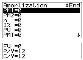
PM1 ...... first installment of installments 1 through n
PM2 ...... second installment of installments 1 through n
n ...... installments
I% ...... interest rate
PV ....... principal
PMT ...... payment for each installment
FV ...... balance following final installment
P/Y ...... installments per year
C/Y ...... compounds per year
After configuring the parameters, use one of the function menus noted below to perform the corresponding calculation.
- {BAL} ... {balance of principal after installment PM2}
- {INT} ... {interest portion of installment PM1}
- {PRN} ... {principal portion of installment PM1}
- ... {total interest paid from installment PM1 to installment PM2}
- PRN ... {total principal paid from installment PM1 to installment PM2}
- {CMPD} ... {compound interest screen}
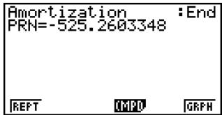
- An error (Ma ERROR) occurs if parameters are not configured correctly.
Use the following function menus to maneuver between calculation result screens.
- {REPT} ... {parameter input screen}
- {CMPD} ... {compound interest screen}
- {GRPH} ... {draws graph}
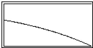
natural_image
Simple downward-sloping dashed line on white background (no text or symbols)After drawing a graph, you can press SHIFT F1(TRCE) to turn on trace and read calculation results along the graph.
The first press of SHIFT F1 (TRCE) displays INT and PRN when n = 1. Each press of ▶ shows INT and PRN when n = 2, n = 3, and so on.
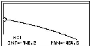
line
| x | y | |---|---| | 1 | 1 | | INT | -748.2 | | PRN | -464.6 |Press EXIT to return to the parameter input screen.
7-6 Interest Rate Conversion
The procedures in this section describe how to convert between the annual percentage rate and effective interest rate.
- Formula
$$ E F F = \left[ \left(1 + \frac {A P R / 1 0 0}{n}\right) ^ {n} - 1 \right] \times 1 0 0 $$
APR : annual percentage rate (%)
EFF : effective interest rate (%)
n : number of compoundings
$$ A P R = \left[ \left(1 + \frac {E F F}{1 0 0}\right) ^ {\frac {1}{n}} - 1 \right] \times n \times 1 0 0 $$
Press F5 (CNVT) from the Financial 1 screen to display the following input screen for interest rate conversion.
F5(CNVT)
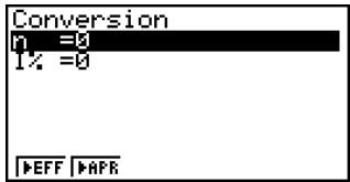
n...... number of compoundings
I% ...... interest rate
After configuring the parameters, use one of the function menus noted below to perform the corresponding calculation.
- ... {converts annual percentage rate to effective interest rate}
- ... {converts effective interest rate to annual percent rate}
Conversion EFF=12.550881
REPT
- An error (Ma ERROR) occurs if parameters are not configured correctly.
Use the following function menu to maneuver between calculation result screens.
- {REPT} ... {parameter input screen}
7-7 Cost, Selling Price, Margin
Cost, selling price, or margin can be calculated by inputting the other two values.
- Formula
$$ C S T = S E L \left(1 - \frac {M R G}{1 0 0}\right) $$
CST : cost
$$ S E L = \frac {C S T}{1 - \frac {M R G}{1 0 0}} $$
SEL : selling price
$$ M R G (\%) = \left(1 - \frac {C S T}{S E L}\right) \times 100 $$
MRG : margin
Press F1(COST) from the Financial 2 screen to display the following input screen.
F6(▷) F1(COST)
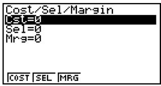
Cst...... cost
Sel ...... selling price
Mrg .... margin
After configuring the parameters, use one of the function menus noted below to perform the corresponding calculation.
- {COST} ... {cost}
- {SEL} ... {selling price}
- {MRG} ... {margin}
Cost/Sel/Margin Cst=1700
REPT
- An error (Ma ERROR) occurs if parameters are not configured correctly.
Use the following function menu to maneuver between calculation result screens.
- {REPT} ... {parameter input screen}
7-8 Day/Date Calculations
You can calculate the number of days between two dates, or you can determine what date comes a specific number of days before or after another date.
Press F2 (DAYS) from the Financial 2 screen to display the following input screen for day/date calculation.
F6 (▷) F2 (DAYS)
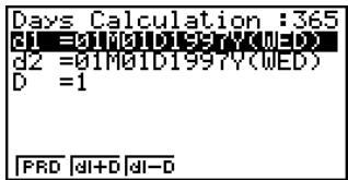
d1 ...... date 1
d2 ...... date 2
D ...... number of days
To input a date, first highlight d1 or d2. Pressing a number key to input the month causes an input screen like the one shown below to appear on the display.
![Input a Date ...Month M[1~12]: 8 PRD dI+D dI-D](/content/2025/01/86785/images/ec93bd5a0154586677730d7103e27b8537510bca74647a4ac34edd37d9f0d452.jpg)

# The Setup screen can be used to specify either a 365-day or 360-day year for financial calculations. Day/date calculations are also performed in accordance with the current setting for number of days in the year, but the following calculations cannot be performed
when the 360-day year is set. Attempting to do so causes an error.
(Date) + (Number of Days)
(Date) – (Number of Days)
# The allowable calculation range is January 1, 1901 to December 31, 2099.
Input the month, day, and year, pressing EXE after each.
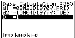
After configuring the parameters, use one of the function menus noted below to perform the corresponding calculation.
- {PRD} ... {number of days from d1 to d2 (d2 - d1)}
- d1 + D d1 plus a number of days (d1 + D)
- {d1-D} ... {d1 minus a number of days (d1 - D)}
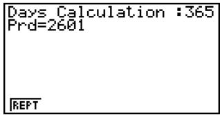
- An error (Ma ERROR) occurs if parameters are not configured correctly.
Use the following function menu to maneuver between calculation result screens. - {REPT} ... {parameter input screen}
360-day Date Mode Calculations
The following describes how calculations are processed when 360 is specified for the Date Mode item in the Setup screen.
- If d1 is day 31 of a month, d1 is treated as day 30 of that month is used.
- If d2 is day 31 of a month, d2 is treated as day 1 of the following month, unless d1 is day 30.
Chapter
8
Programming
8-1 Basic Programming Steps
8-2 PRGM Mode Function Keys
8-3 Editing Program Contents
8-4 File Management
8-5 Command Reference
8-6 Using Calculator Functions in Programs
8-7 PRGM Mode Command List
8-8 Program Library
This unit comes with approximately 64 Kbytes of memory.
- You can check how much memory has been used and how much remains by entering the MEMORY mode from the Main Menu, and then pressing [F1] (MAIN). See “12-7 MEMORY Mode” for details.
8-1 Basic Programming Steps
Description
Commands and calculations are executed sequentially, just like manual calculation multistatements.
Set Up
- From the Main Menu, enter the PRGM mode. When you do, a program list appears on the display.
Selected program area — (use ▲ and ▼ to move)
Files are listed in the alphabetic sequence of their names.
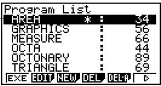
Execution
- Register a file name.
- Input the program.
- Run the program.

# If there are no programs stored in memory when you enter the PRGM mode, the message “No Programs” appears on the display and only the NEW item (F3) is shown in the function menu.
# The values to the right of the program list indicate the number of bytes used by each program.
# A file name can be up to eight characters long.
# The following are the characters you can use in a file name:
A through Z, r, θ, spaces, [, ], {, }, ' ,, \~, 0 through 9, ., +, -, ×, ÷
# Registering a file name uses 32 bytes of memory.
# The file name input screen remains on the display if you press EXE without inputting a file name.
# To exit the file name input screen and return to the program list without registering a file name, press EXIT.


Example 1 To calculate the surface area (cm ^2 ) and volume (cm ^3 ) of three regular octahedrons when the length of one side is 7, 10, and 15 cm, respectively
Store the calculation formula under the file name OCTA.
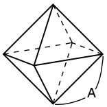
natural_image
Geometric diagram of a polyhedron with labeled point A and dashed lines indicating hidden edges (no text or symbols beyond label)The following are the formulas used for calculating surface area S and volume V of a regular octahedron for which the length of one side A is known.
$$ S = 2 \sqrt {3} A ^ {2}, \quad V = \frac {\sqrt {2}}{3} A ^ {3} $$
Procedure
① MENU PRGM
② F3 (NEW) O C T A EXE *1
③ SHIFT VARS (PRGM) F4 (?) → ALPHA X,θ,T (A) F6 (▷) F5 (:) *2
2 ✗ SHIFT x^2() 3 ✗ ALPHA X,θ,T (A) x^2 F6 (▷) F5 (▲)
SHIFT x^2() 2 ÷ 3 ✗ ALPHA X,θ,T (A) ∧ 3
EXIT EXIT
④ F1(EXE) or EXE
7 EXE (Value of A)
EXE
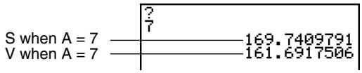
EXE
EXE 1 0 EXE
EXE
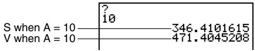
EXE
EXE 1 5 EXE
EXE *3
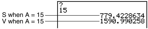

*1 Press F3 (NEW) and the cursor changes form to indicate alpha character input.
*2 The following shows how the calculation of the surface area and volume of a regular octahedron would be calculated using a manual calculation.
Surface Area S ... 2 ✗ SHIFT x² (√) 3 ✗
Volume V ........ SHIFT x^2() 2 ÷ 3 ✗
*3 Pressing EXE while the final result of a program is on the display changes to the program list.
You can also run a program while in the RUN•MAT mode by inputting: Prog "" EXE.
Pressing EXE while the final result of a program executed using this method is on the display re-executes the program.
An error occurs if the program specified by Prog "" cannot be found.

8-2 PRGM Mode Function Keys
- {NEW} ... {new program}
- When you are registering a file name
- {RUN}/{BASE} ... {general calculation}/{number base} program input
- {m0} ... {password registration}
- {SYBL} ... {symbol menu}
- When you are inputting a program — F1(RUN) ... default
- {TOP}/{BTM} ... {top}/{bottom} of program
- {SRC} ... {search}
- {MENU} ... {mode menu}
- {STAT}/{MAT}/{LIST}/{GRPH}/{DYNA}/{TABL}/{RECR} ... {statistic}/{matrix}/{list}/{graph}/{Dynamic Graph}/{Table}/{recursion} menu
- A a ... {toggles between upper-case and lower-case input}
- {CHAR} ... {displays a screen for selecting various mathematical symbols, special symbols, and accented characters}
- Pressing SHIFT VARS (PRGM) displays the following PRGM (PROGRAM) menu.
- {COM} ... {program command menu}
- {CTL} ... {program control command menu}
- {JUMP} ... {jump command menu}
- {?}/{▲} ... {input}/{output} command
- {CLR}/{DISP} ... {clear}/{display} command menu
- {REL} ... {conditional jump relational operator menu}
- {I/O} ... {I/O control/transfer command menu}
- {:} ... {separator for expressions and commands}
See “8-5 Command Reference” for full details on each of these commands.
- Pressing SHIFT MENU (SET UP) displays the mode command menu shown below.
• {ANGL}/{COOR}/{GRID}/{AXES}/{LABL}/{DISP}/{S/L}/{DRAW}/{DERV}/{BACK}/{FUNC}/{SIML}/{S-WIN}/{LIST}/{LOCS}/{T-VAR}/{Σ DSP}/{RESID}/{CPLX}/{FRAC}/{Y·SPD}
See “Setup Screen Function Key Menus” on page 1-7-1 for details about each of these commands.

- When you are inputting a program — F2(BASE) ^*1
- {TOP}/{BTM}/{SRC}
• {MENU} - {d\~o} ... {decimal}/{hexadecimal}/{binary}/{octal} value input
- {LOG} ... {logical operators}
- {DISP} ... conversion of displayed value to {decimal}/{hexadecimal}/{binary}/{octal}
• {A↔a}/{CHAR}
- Pressing SHIFT VARS (PRGM) displays the following PRGM (PROGRAM) menu.
- {Prog} ... {program recall}
- {JUMP}/{?}/{▲}
- {REL} ... {logical operator menu}
- {:} ... {separator for expressions and commands}
- Pressing SHIFT MENU (SET UP) displays the mode command menu shown below.
- {Dec}/{Hex}/{Bin}/{Oct}
- {EXE}/{EDIT}
... program {execute}/{edit} - {NEW} ... {new program}
• {DEL}/{DEL·A}
... {specific program}/{all program} delete - {SRC}/{REN}
... file name {search}/{change}

*1 Programs input after pressing F2 (BASE) are indicated by B to the right of the file name.

8-3 Editing Program Contents
■ Debugging a Program
A problem in a program that keeps the program from running correctly is called a “bug,” and the process of eliminating such problems is called “debugging.” Either of the following symptoms indicates that your program contains bugs that require debugging.
- Error messages appearing when the program is run
• Results that are not within your expectations
- To eliminate bugs that cause error messages
An error message, like the one shown below, appears whenever something illegal occurs during program execution.
Ma ERROR
Press: [EXIT]
When such a message appears, press EXIT to display the place in the program where the error was caused. The cursor will be flashing at the location of the problem. Check the “Error Message Table” (page -1-1) for steps you should take to correct the situation.
- Note that pressing EXIT does not display the location of the error if the program is password protected. Instead, it returns to the program list screen.
- To eliminate bugs that cause bad results
If your program produces results that are not what you normally expect, check the contents of the program and make necessary changes.
F1(TOP) ..... Moves the cursor to the top of the program
= = = = = = OCTA = = = = = = A:2× 3× A^2, 2÷ 3× A^3
F2(BTM) ..... Moves the cursor to the bottom of the program
= = = = = = OCTA = = = = = = ?→A:2×Γ3×A², √2÷3×A^3

■ Using an Existing Program to Create a New Program
Sometimes you can input a new program by using a program already in memory as a base.
Simply recall the existing program, make the changes you need, and then execute it.

Example 2 To use the OCTA program (page 8-1-2) to create a program that calculates the surface area (cm ^2 ) and volume (cm ^3 ) of regular tetrahedrons when the length of one side is 7, 10, and 15 cm Use TETRA as the file name.
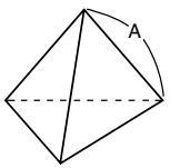
natural_image
Geometric diagram of a triangular pyramid with labeled point A (no text or symbols beyond label)The following are the formulas used for calculating surface area S and volume V of a regular tetrahedron for which the length of one side A is known.
$$ \mathsf {S} = \sqrt {3} \mathsf {A} ^ {2}, \quad \mathsf {V} = \frac {\sqrt {2}}{1 2} \mathsf {A} ^ {3} $$
Use the following key operations when inputting the program.
Length of One Side A .. SHIFT VARS (PRGM) F4 (?) → ALPHA X,θ,T (A) F6 (▷) F5 (:)
Surface Area S ........ SHIFT x^2() 3 X ALPHA X,θ,T (A) x^2 F6 (▷) F5 (▲)
Volume V .... SHIFT x^2() 2 ÷ 1 2 ✗ ALPHA X,θ,T (A) ∧ 3
Compare this with the program for calculating the surface area and volume of a regular octahedron.
Length of One Side A .. SHIFT VARS (PRGM) F4 (?) → ALPHA X,θ,T (A) F6 (▷) F5 (:)
Surface Area S ..... 2 X SHIFT x^2 (√) 3 X ALPHA X,θ,T (A) x^2 F6 (▷) F5 (▲)
Volume V .... SHIFT x^2 (√) 2 ÷ 3 X ALPHA X,θ,T (A) ∧ 3
As you can see, you can produce the TETRA program by making the following changes in the OCTA program.
- Deleting 2 ✗ (underlined using a wavy line above)
- Changing 3 to 1 2 (underlined using a solid line above)

Now edit OCTA to produce the TETRA program.
- Edit the program name.

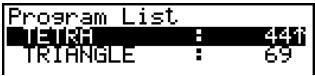
- Edit the program contents.
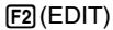
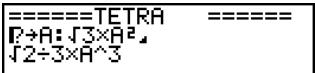

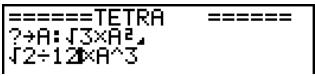


- Try running the program.

| ? | |
| ? | 84.87048957 |
| 40.42293766 |
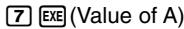


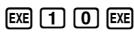
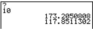


| ? 15 | 389.7114317 397.7475644 |


■ Searching for Data Inside a Program

Example To search for the letter "A" inside the program named OCTA
- Recall the program.
- Press F3(SRC) and input the data you want to find.
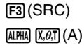
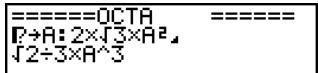
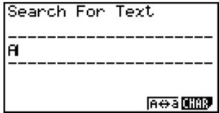
- Press EXE to begin the search. The contents of the program appear on the screen with the cursor located at the first instance of the data you specified.*1
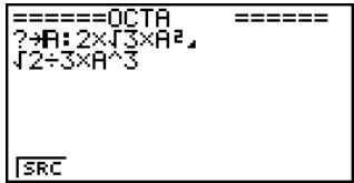
- Each press of EXE or F1(SRC) causes the cursor to jump to the next instance of the data you specified.*2
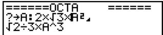

*1 The message "Not Found" appears when the search data you specify cannot be found in the program.
*2 If there are no more instances of the data you specified, the search operation ends and the cursor returns to the point from which you started your search.
You cannot specify the newline symbol (←) or display command (▲) for the search data.
# Once the contents of the program are on the screen, you can use the cursor keys to move the cursor to another location before searching for the next instance of the data. Only the part of the program starting from the current cursor location is searched when you press EXE.
# Once the search finds an instance of your data, inputting characters or moving the cursor causes the search operation to be cancelled.
# If you make a mistake while inputting characters to search for, press AC to clear your input and re-input from the beginning.

8-4 File Management
■ Searching for a File
- To find a file using initial character search

Example To use initial character search to recall the program named OCTA
- While the program list is on the display, press F6(▷)F1(SRC) and input the initial characters of the file you want to find.
F6 (▷) F1 (SRC)
O C T
Search For Program [OCTA]
- Press EXE to search.
Program List OCTA : 441 OCTONARY : 89 TRIANGLE : 69
- The name that starts with the characters you input highlights.

# If there is no program whose file name starts with the characters you input, the message
"Not Found" appears on the display. If this happens, press EXIT to clear the error message.

■ Editing a file name

Example To change the name of a file from TRIANGLE to ANGLE
- While the program list is on the display, use ⚠ and ⬇ to move the highlighting to the file whose name you want to edit and then press F6(▷)F2(REN).
Rename [&RIANGLE]
- Make any changes you want.

Rename [ANGLE ]
- Press EXE to register the new name and return to the program list.
The program list is resorted according to the changes you made in the file name.
■ Deleting a Program
- To delete a specific program
- While the program list is on the display, use ⚠ and ⬇ to move the highlighting to the name of the program you want to delete.
- Press F4 (DEL).
- Press F1(Yes) to delete the selected program or F6(No) to abort the operation without deleting anything.

# If the modifications you make result in a file name that is identical to the name of a program already stored in memory, the message “Already Exists” appears. When this happens, you can perform either of the following two operations to correct the situation.
- Press EXIT to clear the error and return to the file name editing screen.
- Press AC to clear the input file name and input a new one.

- To delete all programs
- While the program list is on the display, press F5 (DEL·A).
- Press F1(Yes) to delete all the programs in the list or F6(No) to abort the operation without deleting anything.
- You also can delete all programs by entering the MEMORY mode from the Main Menu, and then pressing [F1] (MAIN) to display the memory information screen.
See "12-7 MEMORY Mode" for details.
■ Registering a password
When inputting a program, you can protect it with a password that limits access to the program contents to those who know the password.
- You do not need to input the password to run a program.
● ● ● ● ●
Example To create a program file under the name AREA and protect it with the password CASIO
- While the program list is on the display, press F3 (NEW) and input the file name of the new program file.
F3 (NEW)
A R E A
Program Name [AREA]
- Press F5(π0) and then input the password.
F5 (π0)
C A S I O
Program Name [AREA] Password? [CASIOA]

# The password input procedure is identical to that used for file name input.

- Press EXE to register the file name and password. Now you can input the contents of the program file.
- After inputting the program, press SHIFT EXIT (QUIT) to exit the program file and return to the program list. Files that are password protected are indicated by an asterisk to the right of the file name.

■ Recalling a Password Protected Program

Example To recall the file named AREA which is protected by the password CASIO
- In the program list, use ▲ and ▼ to move the highlighting to the name of the program you want to recall.
- Press F2 (EDIT).
- Input the password and press EXE to recall the program.
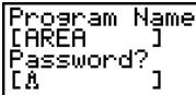

# Pressing EXE without inputting a password while saving a new program causes the file to be saved without a password. Pressing EXE without inputting a password registers the file name only, without a password.
# Inputting the wrong password when recalling a password protected program causes the message "Mismatch" to appear. Press EXIT to return to the password input screen.

8-5 Command Reference
Command Index
Break 8-5-6
ClrGraph 8-5-12
ClrList 8-5-12
ClrMat 8-5-12
ClrText 8-5-12
DispF-Tbl, DispR-Tbl 8-5-13
Do\~LpWhile 8-5-5
DrawDyna 8-5-13
DrawFTG-Con, DrawFTG-Plt 8-5-13
DrawGraph 8-5-13
DrawR-Con, DrawR-Plt 8-5-13
DrawRΣ-Con, DrawRΣ-Plt 8-5-14
DrawStat 8-5-14
DrawWeb 8-5-14
Dsz 8-5-9
For\~To\~(Step\~)Next 8-5-4
Getkey 8-5-15
Goto\~Lbl 8-5-10
If\~Then\~(Else\~)IfEnd 8-5-4
lsz 8-5-11
Locate 8-5-16
OpenComport38k/CloseComport38k 8-5-17
Prog 8-5-7
RclCapt 8-5-18
Receive (/ Send (....8-5-17
Receive38k/Send38k 8-5-17
Return 8-5-8
Stop 8-5-8
While\~WhileEnd 8-5-6
? (Input Command) 8-5-2
▲ (Output Command) 8-5-3
: (Multi-statement Command) 8-5-3
← (Carriage Return) 8-5-3
' (Comment Text Delimiter) 8-5-3
(Jump Code) 8-5-11
=, ≠, >, <, ≥, ≤ (Relational Operators) 8-5-18

The following are conventions that are used in this section when describing the various commands.
Boldface Text ...... Actual commands and other items that always must be input are shown in boldface.
{Curly Brackets} ....... Curly brackets are used to enclose a number of items, one of which must be selected when using a command. Do not input the curly brackets when inputting a command.
[Square Brackets] ...... Square brackets are used to enclose items that are optional. Do not input the square brackets when inputting a command.
Numeric Expressions... Numeric expressions (such as 10, 10 + 20, A) indicate constants, calculations, numeric constants, etc.
Alpha Characters ...... Alpha characters indicate literal strings (such as AB).
■ Basic Operation Commands
? (Input Command)
Function: Prompts for input of values for assignment to variables during program execution.
Syntax: ? →
Example: ? → A
Description:
- This command momentarily interrupts program execution and prompts for input of a value or expression for assignment to a variable. If you do not specify a prompt, execution of this command causes “?” to appear indicating the calculator is standing by for input. If a prompt is specified, “
?” appears to prompt input. Up to 255 bytes of text can be used for a prompt. - Input in response to the input command must be a value or an expression, and the expression cannot be a multi-statement.
- You can specify a list name, matrix name, function memory (fn), graph (Yn), etc. as a variable name.

▲ (Output Command)
Function: Displays an intermediate result during program execution.
Description:
- This command momentarily interrupts program execution and displays alpha character text or the result of the calculation immediately before the command.
- The output command should be used at locations where you would normally press the EXE key during a manual calculation.
: (Multi-statement Command)
Function: Connects two statements for sequential execution without stopping.
Description:
- Unlike the output command (▲), statements connected with the multi-statement command are executed non-stop.
- The multi-statement command can be used to link two calculation expressions or two commands.
- You can also use a carriage return indicated by in place of the multi-statement command.
← (Carriage Return)
Function: Connects two statements for sequential execution without stopping.
Description:
- Operation of the carriage return is identical to that of the multi-statement command.
- You can create a blank line in a program by inputting a carriage return only. Using a carriage return in place of the multi-statement command makes the displayed program easier to read.
' (Comment Text Delimiter)
Function: Indicates comment text inserted inside a program.
Description: Anything following the apostrophe is treated as non-executable comment text.

■ Program Commands (COM)
If\~Then\~(Else\~)IfEnd
Function: The Then-statement is executed only when the If-condition is true (non-zero). The Else-statement is executed when the If-condition is false (0). The IfEnd-statement is always executed following either the Then-statement or Else-statement.
Syntax:
![If numeric expression {←} : ▲ } Then [ {←} : ▲ ] {←} : ▲ } (Else [ {←} : ▲ ] ] {←} : ▲ ) IfEnd](/content/2025/01/86785/images/1d6822c27aaed0628d811e6f022d3bf6530909fe1abb603710288562a45fd947.jpg)
Parameters: condition, numeric expression
Description:
(1) If \~ Then \~ IfEnd
- When the condition is true, execution proceeds with the Then-statement and then continues with the statement following IfEnd.
- When the condition is false, execution jumps to the statement following IfEnd.
(2) If \~ Then \~ Else \~ IfEnd
- When the condition is true, execution proceeds with the Then-statement and then jumps to the statement following IfEnd.
- When the condition is false, execution jumps to the Else-statement and then continues with the statement following IfEnd.
For\~To\~(Step\~)Next
Function: This command repeats everything between the For-statement and the Next-statement. The starting value is assigned to the control variable with the first execution, and the value of the control variable is changed according to the step value with each execution. Execution continues until the value of the control variable exceeds the ending value.
Syntax:
For
$$ \left(\text{Step} < \text{step value}\right)\left{\begin{array}{c}\leftarrow \ :\ \blacktriangle \end{array}\right} \text{Next} $$
Parameters:
• control variable name: A to Z
- starting value: value or expression that produces a value (i.e. x , A, etc.)
• ending value: value or expression that produces a value (i.e. sin x, A, etc.)
- step value: numeric value (default: 1)

Description:
- The default step value is 1.
- Making the starting value less than the ending value and specifying a positive step value causes the control variable to be incremented with each execution. Making the starting value greater than the ending value and specifying a negative step value causes the control variable to be decremented with each execution.
Do\~LpWhile
Function: This command repeats specific commands as long as its condition is true (non-zero).
Syntax:
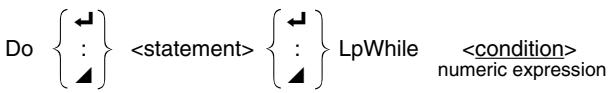
Parameters: expression
Description:
- This command repeats the commands contained in the loop as long as its condition is true (non-zero). When the condition becomes false (0), execution proceeds from the statement following the LpWhile-statement.
- Since the condition comes after the LpWhile-statement, the condition is tested (checked) after all of the commands inside the loop are executed.

While\~WhileEnd
Function: This command repeats specific commands as long as its condition is true (non-zero).
Syntax:
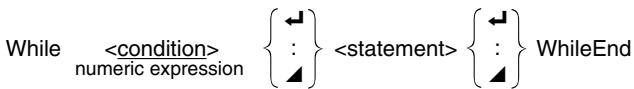
Parameters: expression
Description:
- This command repeats the commands contained in the loop as long as its condition is true (non-zero). When the condition becomes false (0), execution proceeds from the statement following the WhileEnd-statement.
- Since the condition comes after the While-statement, the condition is tested (checked) before the commands inside the loop are executed.
■ Program Control Commands (CTL)
Break
Function: This command breaks execution of a loop and continues from the next command following the loop.
Syntax: Break
Description:
- This command breaks execution of a loop and continues from the next command following the loop.
- This command can be used to break execution of a For-statement, Do-statement, and While-statement.

Prog
Function: This command specifies execution of another program as a subroutine. In the RUN·MAT mode, this command executes a new program.
Syntax: Prog "file name"
Example: Prog "ABC"
Description:
- Even when this command is located inside of a loop, its execution immediately breaks the loop and launches the subroutine.
- This command can be used as many times as necessary inside of a main routine to call up independent subroutines to perform specific tasks.
- A subroutine can be used in multiple locations in the same main routine, or it can be called up by any number of main routines.
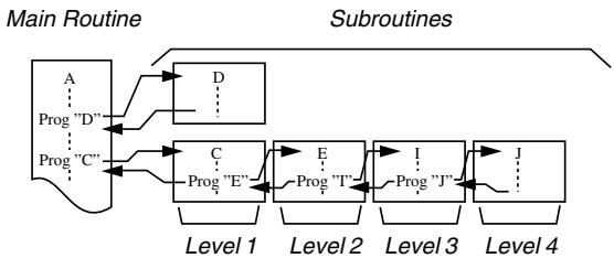
flowchart
graph TD
    A["Main Routine"] --> B["Subroutines"]
    subgraph Level 1
        C["A"] --> D["D"]
        E["Prog "D""] --> C
        F["Prog "C""] --> C
        G["C"] --> H["E"]
        I["Prog "E""] --> H
        J["Prog "T""] --> H
        K["I"] --> L["J"]
        M["Prog "J""] --> L
    end
    subgraph Level 2
        N["Level 1"] --> O["Level 2"]
        P["Level 2"] --> Q["Level 3"]
        R["Level 2"] --> S["Level 3"]
        T["Level 2"] --> U["Level 4"]
    end
    subgraph Level 3
        V["Level 1"] --> W["Level 2"]
        X["Level 2"] --> Y["Level 3"]
        Z["Level 3"] --> AA["Level 4"]
    end
    subgraph Level 4
        AB["Level 1"] --> AC["Level 2"]
        AD["Level 2"] --> AE["Level 3"]
        AF["Level 3"] --> AG["Level 4"]
    end
- Calling up a subroutine causes it to be executed from the beginning. After execution of the subroutine is complete, execution returns to the main routine, continuing from the statement following the Prog command.
- A Goto\~Lbl command inside of a subroutine is valid inside of that subroutine only. It cannot be used to jump to a label outside of the subroutine.
- If a subroutine with the file name specified by the Prog command does not exist, an error occurs.
- In the RUN·MAT mode, inputting the Prog command and pressing EXE launches the program specified by the command.

Return
Function: This command returns from a subroutine.
Syntax: Return
Description:
Execution of the Return command inside a main routine causes execution of the program to stop. Execution of the Return command within a subroutine terminates the subroutine and returns to the program from which the subroutine was jumped to.
Stop
Function: This command terminates execution of a program.
Syntax: Stop
Description:
- This command terminates program execution.
- Execution of this command inside of a loop terminates program execution without an error being generated.

■ Jump Commands (JUMP)
Dsz
Function: This command is a count jump that decrements the value of a control variable by 1, and then jumps if the current value of the variable is zero.
Syntax:
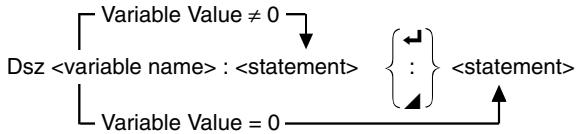
flowchart
graph TD
    A["Variable Value ≠ 0"] --> B["Dsz <variable name>: <statement>"]
    C["Variable Value = 0"] --> D["..."]
    B --> E["{←}"]
    D --> F["{:}"]
    E --> G["<statement>"]
    F --> G
Parameters: variable name: A to Z, r, θ
[Example] Dsz B : Decrements the value assigned to variable B by 1.
Description:
This command decrements the value of a control variable by 1, and then tests (checks) it. If the current value is non-zero, execution continues with the next statement. If the current value is zero, execution jumps to the statement following the multi-statement command (:), display command (▲), or carriage return (◀).

Goto\~Lbl
Function: This command performs an unconditional jump to a specified location.
Syntax: Goto
Parameters: label name: value (0 to 9), variable (A to Z, r, θ)
Description:
- This command consists of two parts: Goto n (where n is a parameter as described above) and Lbl n (where n is the parameter referenced by Goto n ). This command causes program execution to jump to the Lbl-statement whose n parameter matches that specified by the Goto-statement.
- This command can be used to loop back to the beginning of a program or to jump to any location within the program.
- This command can be used in combination with conditional jumps and count jumps.
- If there is no Lbl-statement whose value matches that specified by the Goto-statement, an error occurs.

lsz
Function: This command is a count jump that increments the value of a control variable by 1, and then jumps if the current value of the variable is zero.
Syntax:
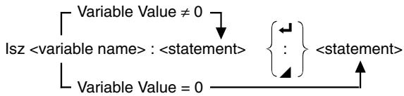
flowchart
graph TD
    A["Isz <variable name>: <statement>"] --> B{<statement>}
    C["Variable Value = 0"] --> B
    B --> D["Variable Value ≠ 0"]
    D --> A
Parameters: variable name: A to Z, r, θ
[Example] Isz A : Increments the value assigned to variable A by 1.
Description:
This command increments the value of a control variable by 1, and then tests (checks) it. If the current value is non-zero, execution continues with the next statement. If the current value is zero, execution jumps to the statement following the multi-statement command (:), display command (▲), or carriage return (◀).
(Jump Code)
Function: This code is used to set up conditions for a conditional jump. The jump is executed whenever the conditions are false.
Syntax:
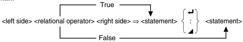
flowchart
graph TD
    A["<left side>"] --> B["<relational operator>"]
    B --> C["<right side>"]
    C --> D["<statement>"]
    D --> E{}
    E --> F["<statement>"]
    G["False"] --> D
    H["True"] --> C
    I["↓"] --> C
Parameters:
left side/right side: variable (A to Z, r, ), numeric constant, variable expression (such as: A × 2)
relational operator: =, ≠, >, <, ≥, ≤ (page 8-5-18)
Description:
- The conditional jump compares the contents of two variables or the results of two expressions, and a decision is made whether or not to execute the jump based on the results of the comparison.
- If the comparison returns a true result, execution continues with the statement following the command. If the comparison returns a false result, execution jumps to the statements following the multi-statement command (:), display command (▲), or carriage return (◀).
With this program, inputting a value of zero or greater calculates and displays the square root of the input value. Inputting a value less than zero returns to the input prompt without calculating anything.

■ Clear Commands (CLR)
ClrGraph
Function: This command clears the graph screen and returns View Window settings to their INIT values.
Syntax: ClrGraph
Description: This command clears the graph screen during program execution.
ClrList
Function: This command deletes list data.
Syntax: ClrList
ClrList
Parameters: list name: 1 to 26, Ans
Description: This command deletes the data in the list specified by "list name". All list data is deleted if nothing is specified for "list name".
ClrMat
Function: This command deletes matrix data.
Syntax: ClrMat
ClrMat
Parameters: matrix name: A to Z, Ans
Description: This command deletes the data in the matrix specified by "matrix name". All matrix data is deleted if nothing is specified for "matrix name".
ClrText
Function: This command clears the text screen.
Syntax: ClrText
Description: This command clears text from the screen during program execution.

■ Display Commands (DISP)
DispF-Tbl, DispR-Tbl
No parameters
Function: These commands display numeric tables.
Description:
- These commands generate numeric tables during program execution in accordance with conditions defined within the program.
- DispF-Tbl generates a function table, while DispR-Tbl generates a recursion table.
DrawDyna
No parameters
Function: This command executes a Dynamic Graph draw operation.
Description: This command draws a Dynamic Graph during program execution in accordance with current Dynamic Graph parameters.
DrawFTG-Con, DrawFTG-Plt
No parameters
Function: This command uses values in a generated table to graph a function.
Description:
- This command draws a function graph in accordance with current conditions.
- DrawFTG-Con produces a connect type graph, while DrawFTG-Plt produces a plot type graph.
DrawGraph
No parameters
Function: This command draws a graph.
Description: This command draws a graph in accordance with current conditions.
DrawR-Con, DrawR-Plt
No parameters
Function: These commands use values in a generated table to graph a recursion expression with a_n(b_n or c_n) as the vertical axis and n as the horizontal axis.
Description:
- These commands graph recursion expressions in accordance with current conditions, with a_n(b_n or c_n) as the vertical axis and n as the horizontal axis.
- DrawR-Con produces a connect type graph, while DrawR-Plt produces a plot type graph.

DrawRΣ-Con, DrawRΣ-Plt
No parameters
Function: These commands use values in a generated table to graph a recursion expression with a_n( b_n or c_n) as the vertical axis and n as the horizontal axis.
Description:
- These commands graph recursion expressions in accordance with current conditions, with a_n( b_n or c_n) as the vertical axis and n as the horizontal axis.
- DrawRΣ-Con produces a connect type graph, while DrawRΣ-Plt produces a plot type graph.
DrawStat
Function: This draws a statistical graph.
Syntax: See "Using Statistical Calculations and Graphs in a Program" on page 8-6-9.
Description:
This command draws a statistical graph in accordance with current statistical graph conditions.
DrawWeb
Function: This command graphs convergence/divergence of a recursion expression (WEB graph).
Syntax: DrawWeb
Example: DrawWeb a_n+1 ( b_n+1 or c_n+1 ), 5
Description:
- This command graphs convergence/divergence of a recursion expression (WEB graph).
- Omitting the number of lines specification automatically specifies the default value 30.

■ Input/Output Commands (I/O)
Getkey
Function: This command returns the code that corresponds to the last key pressed.
Syntax: Getkey
Description:
- This command returns the code that corresponds to the last key pressed.
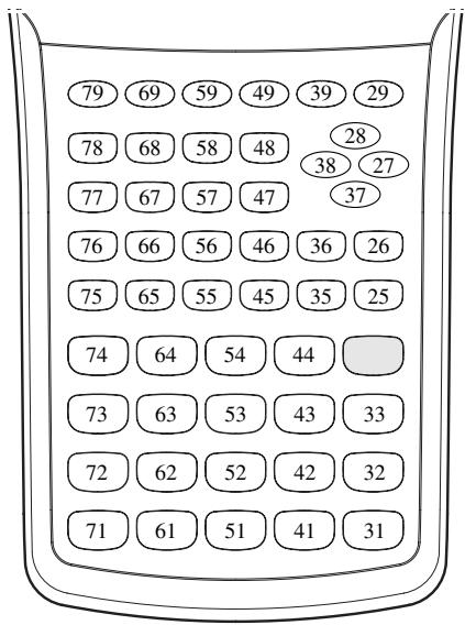
- A value of zero is returned if no key was pressed previous to executing this command.
- This command can be used inside of a loop.

Locate
Function: This command displays alpha-numeric characters at a specific location on the text screen.
Syntax: Locate
Locate
Locate
[Example] Locate 1, 1, "AB"
Parameters:
• line number: number from 1 to 7
• column number: number from 1 to 21
• value and numeric expression
• string: character string
Description:
- This command displays values (including variable contents) or text at a specific location on the text screen. If there is a calculation input, that calculation result is displayed.
- The line is designated by a value from 1 to 7, while the column is designated by a value from 1 to 21.
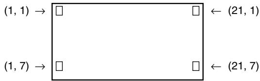
flowchart
graph TD
    A["(1, 1)"] --> B[" "]
    B --> C[" "]
    C --> D["(21, 1)"]
    E["(1, 7)"] --> F[" "]
    F --> G[" "]
    G --> H["(21, 7)"]
Example: Cls
Locate 7, 1, "CASIO FX"
This program displays the text "CASIO FX" in the center of the screen.
- In some cases, the CIrText command should be executed before running the above program.

Receive (/ Send (
Function: This command receives data from and sends data to a connected device.
Syntax: Receive () / Send ()
Description:
- This command receives data from and sends data to a connected device.
- The following types of data can be received (sent) by this command.
- Individual values assigned to variables
- Matrix data (all values - individual values cannot be specified)
- List data (all values - individual values cannot be specified)
OpenComport38k/CloseComport38k
Function: Opens and closes the 3-pin COM port (serial).
Description: See the Receive38k/Send38k command below.
Receive38k/Send38k
Function: Executes data send and receive at a data rate of 38 kbps.
Syntax: Send38k
Receive38k
Description:
- The OpenComport38k command must be executed before this command is executed.
- The CloseComport38k command must be executed after this command is executed.
- If this command is executed when the communication cable is not connected, program execution will continue without generating an error.

■ Conditional Jump Relational Operators (REL)
$$ = , \neq , >, < , \geq , \leq $$
Function: These relational operators are used in combination with the conditional jump command.
Syntax:
Parameters:
left side/right side: variable (A to Z, r, ), numeric constant, variable expression (such as: A × 2)
relational operator: =, ≠, >, <, ≥, ≤
Other
RclCapt
Function: Displayed the contents specified by the capture memory number.
Syntax: RclCapt

8-6 Using Calculator Functions in Programs
■ Text Display
You can include text in a program by simply enclosing it between double quotation marks. Such text appears on the display during program execution, which means you can add labels to input prompts and results.
| Program | Display |
| "CASIO" | CASIO |
| ? → X | ? |
| "X = " ? → X | X = ? |
- If the text is followed by a calculation formula, be sure to insert a display command (▲) between the text and calculation.
- Inputting more than 21 characters causes the text to move down to the next line. The screen scrolls automatically if the text exceeds 21 characters.
- You can specify up to 255 bytes of text for a comment.
■ Using Matrix Row Operations in a Program
These commands let you manipulate the rows of a matrix in a program.
- For this program, enter the RUN • MAT mode and then use the Matrix Editor to input the matrix, and then enter the PRGM mode to input the program.
- To swap the contents of two rows (Swap)
● ● ● ● ●
Example 1 To swap the values of Row 2 and Row 3 in the following matrix:
$$ \text { Matrix } \mathbf {A} = \left[ \begin{array}{c c} 1 & 2 \ 3 & 4 \ 5 & 6 \end{array} \right] $$
The following is the syntax to use for this program.
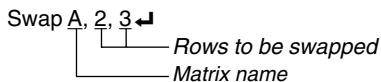
Mat A
Executing this program produces the following result.
![AnS 1 2 1 [ ] 2 2 [ ] 5 6 3 [ ] 3 4](/content/2025/01/86785/images/62ee424aa58da610d31aa5548906602386c4ca6049a016d6e84d736fbfe3f286.jpg)

- To calculate a scalar multiplication (\*Row)

Example 2 To calculate the product of Row 2 of the matrix in Example 1 and the scalar 4
The following is the syntax to use for this program.
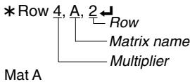
Executing this program produces the following result.
![AnS 1 2 1 [ ] 2 2 [ ] 12 16 3 [ ] 5 6](/content/2025/01/86785/images/f4de8f6147643554fd55378f6a0dff6d73f77c3fb0a3d77881cdfc5093d5d78a.jpg)
- To calculate a scalar multiplication and add the results to another row (\*Row+)

Example 3 To calculate the product of Row 2 of the matrix in Example 1 and the scalar 4, then add the result to row 3
The following is the syntax to use for this program.
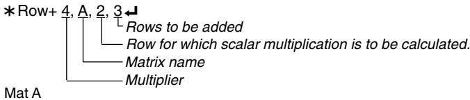
Executing this program produces the following result.
![AnS 1 2 1 [ ] 2 2 [ ] 3 4 3 [ ] 17 22](/content/2025/01/86785/images/b830abdb8d7bb5d664548161fb9652a72028e427c80a1a94be6116ef27d17b27.jpg)

• To add two rows (Row+)

Example 4 To add Row 2 to Row 3 of the matrix in Example 1
The following is the syntax to use for this program.
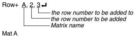
Executing this program produces the following result.
![AnS 1 2 1 [ ] 2 2 [ ] 3 4 3 [ ] 8 10](/content/2025/01/86785/images/6ad1bc21930678810b183454238b1d8e996bddbe488935b6c3695beed7e04c9f.jpg)
■ Using Graph Functions in a Program
You can incorporate graph functions into a program to draw complex graphs and to overlay graphs on top of each other. The following shows various types of syntax you need to use when programming with graph functions.
- View Window
View Window -5, 5, 1, -5, 5, 1
- Graph function input
Y = Type ← .... Specifies graph type.
$$ " X ^ {2} - 3" \rightarrow Y 1 \leftarrow $$
- Graph draw operation
DrawGraph
Example Program
①ClrGraph
②View Window -10, 10, 2, -120, 150, 50
③Y = Type
$$ " X ^ {\wedge} 4 - X ^ {\wedge} 3 - 2 4 X ^ {2} + 4 X + 8 0" \Rightarrow \underset {④} {Y 1} \leftarrow $$
⑤G SelOn 1
⑥ BrokenThickG 1
⑦DrawGraph
① SHIFT VARS F6 F1 F2 EXIT
② SHIFT F3 F1 EXIT
③ F4 F4 F3 F1
④ VARS F4 F1 EXIT EXIT
⑤ F4 F4 F1 F1 EXIT
⑥ F4 F3
⑦ SHIFT VARS F6 F2 F2
Executing this program produces the result shown here.
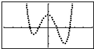
line
| X | Y | |---|---| | 0.0 | 100 | | 0.2 | 50 | | 0.4 | 75 | | 0.6 | 100 | | 0.8 | 75 | | 1.0 | 50 | | 1.2 | 25 | | 1.4 | 0 | | 1.6 | -25 | | 1.8 | -50 | | 2.0 | -75 | | 2.2 | -100 | | 2.4 | -75 | | 2.6 | -50 | | 2.8 | -25 | | 3.0 | 0 | | 3.2 | 25 | | 3.4 | 50 | | 3.6 | 75 | | 3.8 | 100 | | 4.0 | 75 | | 4.2 | 50 | | 4.4 | 25 | | 4.6 | 0 | | 4.8 | -25 | | 5.0 | -50 | | 5.2 | -75 | | 5.4 | -100 | | 5.6 | -75 | | 5.8 | -50 | | 6.0 | -25 | | 6.2 | 0 | | 6.4 | 25 | | 6.6 | 50 | | 6.8 | 75 | | 7.0 | 100 | | 7.2 | 75 | | 7.4 | 50 | | 7.6 | 25 | | 7.8 | 0 | | 8.0 | -25 | | 8.2 | -50 | | 8.4 | -75 | | 8.6 | -100 | | 8.8 | -75 | | 9.0 | -50 | | 9.2 | -25 | | 9.4 | 0 | | 9.6 | 25 | | 9.8 | 50 | | 10.0 | 75 | | 10.2 | 100 | | 10.4 | 75 | | 10.6 | 50 | | 10.8 | 25 | | 11.0 | 0 | | 11.2 | -25 | | 11.4 | -50 | | 11.6 | -75 | | 11.8 | -100 | | 12.0 | -75 | | 12.2 | -50 | | 12.4 | -25 | | 12.6 | 0 | | 12.8 | 25 | | 13.0 | 50 | | 13.2 | 75 | | 13.4 | 100 | | 13.6 | 75 | | 13.8 | 50 | | 14.0 | 25 | | 14.2 | 0 | | 14.4 | -25 | | 14.6 | -50 | | 14.8 | -75 | | 15.0 | -100 | | 15.2 | -75 | | 15.4 | -50 | | 15.6 | -25 | | 15.8 | 0 | | 16.0 | 25 | | 16.2 | 50 | | 16.4 | 75 | | 16.6 | 100 | | 16.8 | 75 | | 17.0 | 50 | | 17.2 | 25 | | 17.4 | 0 | | 17.6 | -25 | | 17.8 | -50 | | 18.0 | -75 | | 18.2 | -100 | | 18.4 | -75 | | 18.6 | -50 | | 18.8 | -25 | | 19.0 | 0 | | 19.2 | 25 | | 19.4 | 50 | | 19.6 | 75 | | 19.8 | 100 | | 20.0 | -75 | | 20.2 | -100 | | 20.4 | -75 | | 20.6 | -50 | | 20.8 | -25 | | 21.0 | +25 | | 21.2 | +50 | | 21.4 | +75 | | 21.6 | +100 | | 21.8 | +75 | | 22.0 | +50 | | 22.2 | +25 | | 22.4 | +0 | | 22.6 | -25 | | 22.8 | -50 | | 23.0 | -75 | | 23.2 | -100 | | 23.4 | -75 | | 23.6 | -50 | | 23.8 | -25 | | 24.0 | +25 | | 24.2 | +50 | | 24.4 | +75 | | 24.6 | +100 | | 24.8 | -75 | | 25.0 | -100 | | 25.2 | -75 | | 25.4 | -50 | | 25.6 | -25 | | 25.8 | +25 | | 26.0 | +50 | | 26.2 | +75 | | 26.4 | +100 | | 26.6 | -75 | | 26.8 | -100 | | 27.0 | -75 | | 27.2 | -50 | | 27.4 | -25 | | 27.6 | +25 | | 27.8 | +50 | | 28.0 | +75 | | 28.2 | +100 | | 28.4 | -75 | | 28.6 | -100 | | 28.8 | -75 | | 29.0 | -50 | | 29.2 | -25 | | 39.4 | +33 (approx) for the x-axis from x = x_3 to x_3 (approx) versus x = x_3 (approx) on the y-axis (approx). The chart displays a single data series with values ranging from approximately -33 to +33 (approx). The y-axis label is 'X' (likely a typo or placeholder), and the x-axis label is 'Y' (likely a typo or placeholder). The chart is divided into four quadrants: bottom-left, top-left, bottom-right, and top-right, with each quadrant labeled by its corresponding value.
- Syntax of other graphing functions
• V-Window
View Window <Xmin>, <Xmax>, <Xscale>, <Ymin>, <Ymax>, <Yscale>, <Tθmin>, <Tθmax>, <Tθpitch>
StoV-Win <area of V-Win>...... area: 1 to 6
RclV-Win <area of V-Win> ...... area: 1 to 6
- Zoom
Factor <X factor>, <Y factor>
ZoomAuto ...... Non-parameter
- Pict
StoPict <area of picture> .... area: 1 to 20
numeric expression
RclPict <area of picture> .... area: 1 to 20
numeric expression
- Sketch
PlotOn <X-coordinate>, <Y-coordinate>
PlotOff <X-coordinate>, <Y-coordinate>
PlotChg <X-coordinate>, <Y-coordinate>
PxlOn<line number>, <column number>
PxlOff<line number>, <column number>
PxlChg<line number>, <column number>
PxlTest(<line number>, <column number>[])
Text <line number>, <column number>, "<text>"
Text <line number>, <column number>, <expression>
SketchThick, SketchBroken, SketchDot, SketchNormal
Tangent <function>, <X-coordinate>
Normal <function>, <X-coordinate>
Inverse <function>
Line <X-coordinate 1>, <Y-coordinte 1>, <X-coordinate 2>, <Y-coordinte 2>
F-Line <X-coordinate 1>, <Y-coordinate 1>, <X-coordinate 2>, <Y-coordinate 2>
Circle <center point X-coordinate>, <center point Y-coordinate>, <radius R value>
Vertical <X-coordinate>
Horizontal <Y-coordinate>

■ Using Dynamic Graph Functions in a Program
Using Dynamic Graph functions in a program makes it possible to perform repeated Dynamic Graph operations. The following shows how to specify the Dynamic Graph range inside a program.
• Dynamic Graph range
$$ 1 \rightarrow D \text { Start } ↳ $$
$$ 5 \rightarrow D E n d \leftarrow $$
$$ 1 \rightarrow D \text { pitch } \leftarrow $$
Example Program
$$ \mathrm{ClrGraph} \leftarrow $$
$$ \text { View Window } - 5, 5, 1, - 5, 5, 1 \leftarrow $$
$$ Y = \text { Type } \leftarrow $$
$$ " A X + 1" \rightarrow \underset {①} {Y} 1 \leftarrow $$
$$ ② D \text { SelOn } 1 \leftarrow $$
$$ ③ D \text { Var } A \leftarrow $$
$$ 1 \rightarrow^ {④} D S t a r t \leftarrow $$
$$ 5 \rightarrow^ {⑤} D E n d \leftarrow $$
$$ 1 \rightarrow^ {⑥} D p i t c h \leftarrow $$
$$ ⑦ \text { DrawDyna } $$
① VARS F4 F1 EXIT EXIT
② F4 F5 F1
③ F3
④ VARS F5 F1
⑤ F2
⑥ F3
⑦ SHIFT VARS F6 F2 F3
Executing this program produces the result shown here.
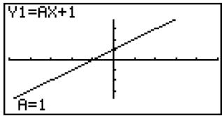
: ↑ ↓ :

■ Using Table & Graph Functions in a Program
Table & Graph functions in a program can generate numeric tables and perform graphing operations. The following shows various types of syntax you need to use when programming with Table & Graph functions.
- Table range setting
$$ 1 \rightarrow F \text { Start } ↳ $$
$$ 5 \rightarrow F E n d \leftarrow $$
$$ 1 \rightarrow F \text { pitch } ↳ $$
- Numeric table generation
$$ \text { DispF - Tbl } \leftarrow $$
- Graph draw operation
$$ \text { Connect type: DrawFTG - Con } \leftarrow $$
$$ \text { Plot type: DrawFTG - Plt } \leftarrow $$
Example Program
$$ \mathrm{ClrGraph} \leftarrow $$
$$ \mathrm{ClrText} \leftarrow $$
$$ \text { View Window } 0, 6, 1, - 2 0, 1 0 6, 1 0 \leftarrow $$
$$ Y = \text { Type } \leftarrow $$
$$ " 3 X ^ {2} - 2" \rightarrow Y 1 \leftarrow $$
$$ ① T \text { SelOn } 1 \leftarrow $$
$$ 0 \rightarrow ② F S t a r t \leftarrow $$
$$ 6 \rightarrow^ {③} F E n d \leftarrow $$
$$ 1 \rightarrow ④ F p i t c h \leftarrow $$
$$ ⑤ D i s p F - T b l ↳ $$
$$ ⑥ \text { DrawFTG - Con } $$
$$ ① \boxed {F 4} \boxed {F 6} \boxed {F 1} \boxed {F 1} $$
$$ ② \boxed {\text { VARS }} \boxed {\text { F6 }} \boxed {\text { F1 }} \boxed {\text { F1 }} $$
$$ ③ \boxed {F 2} $$
$$ ④ \boxed {F 3} $$
$$ ⑤ \boxed {S H I F T} \boxed {V A R S} \boxed {F 6} \boxed {F 2} \boxed {F 4} \boxed {F 1} $$
$$ ⑥ \boxed {S H I F T} \boxed {V A R S} \boxed {F 6} \boxed {F 2} \boxed {F 4} \boxed {F 2} $$
Executing this program produces the results shown here.
Numeric Table
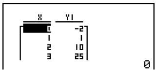
Graph
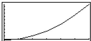
line
| X | Y | |---|---| | 0 | 0 | | 1 | 0.5 | | 2 | 1 | | 3 | 1.5 | | 4 | 2.5 | | 5 | 3.5 | | 6 | 4.5 | | 7 | 5.5 | | 8 | 6.5 | | 9 | 7.5 | | 10 | 8.5 | | 11 | 9.5 | | 12 | 10.5 | | 13 | 11.5 | | 14 | 12.5 | | 15 | 13.5 | | 16 | 14.5 | | 17 | 15.5 | | 18 | 16.5 | | 19 | 17.5 | | 20 | 18.5 | | 21 | 19.5 | | 22 | 20.5 | | 23 | 21.5 | | 24 | 22.5 | | 25 | 23.5 | | 26 | 24.5 | | 27 | 25.5 | | 28 | 26.5 | | 29 | 27.5 | | 30 | 28.5 | | 31 | 29.5 | | 32 | 30.5 | | 33 | 31.5 | | 34 | 32.5 | | 35 | 33.5 | | 36 | 34.5 | | 37 | 35.5 | | 38 | 36.5 | | 39 | 37.5 | | 40 | 38.5 | | 41 | 39.5 | | 42 | 40.5 | | 43 | 41.5 | | 44 | 42.5 | | 45 | 43.5 | | 46 | 44.5 | | 47 | 45.5 | | 48 | 46.5 | | 49 | 47.5 | | 50 | 48.5 | | 51 | 49.5 | | 52 | 50.5 | | 53 | 51.5 | | 54 | 52.5 | | 55 | 53.5 | | 56 | 54.5 | | 57 | 55.5 | | 58 | 56.5 | | 59 | 57.5 | | 60 | 58.5 | | 61 | 59.5 | | 62 | 60.5 | | 63 | 61.5 | | 64 | 62.5 | | 65 | 63.5 | | 66 | 64.5 | | 67 | 65.5 | | 68 | 66.5 | | 69 | 67.5 | | 70 | 68.5 | | 71 | 69.5 | | 72 | 70.5 | | 73 | 71.5 | | 74 | 72.5 | | 75 | 73.5 | | 76 | 74.5 | | 77 | 75.5 | | 78 | 76.5 | | 79 | 77.5 | | 80 | 78.5 | | 81 | 79.5 | | 82 | 80.5 | | 83 | 81.5 | | 84 | 82.5 | | 85 | 83.5 | | 86 | 84.5 | | 87 | 85.5 | | 88 | 86.5 | | 89 | 87.5 | | 90 | 88.5 | | 91 | 89.5 | | 92 | 90.5 | | 93 | 91.5 | | 94 | 92.5 | | 95 | 93.5 | | 96 | 94.5 | | 97 | 95.5 | | 98 | 96.5 | | 99 | 97.5 | | Note: The data is extracted from the image and presented in CSV format as requested by the code.
■ Using Recursion Table & Graph Functions in a Program
Incorporating Recursion Table & Graph functions in a program lets you generate numeric tables and perform graphing operations. The following shows various types of syntax you need to use when programming with Recursion Table & Graph functions.
- Recursion formula input
a_n+1 Type ← .... Specifies recursion type.
$$ " 3 a _ {n} + 2" \rightarrow a _ {n + 1} \leftarrow $$
$$ " 4 b _ {n} + 6" \rightarrow b _ {n + 1} \leftarrow $$
- Table range setting
1 → R Start
5 → R End ←
1 a_0
2 b_0
1 a_n Start
3 b_n Start
- Numeric table generation
DispR-Tbl
• Graph draw operation
Connect type: DrawR-Con←, DrawRΣ-Con←
Plot type: DrawR-Plt←, DrawRΣ-Plt←
• Statistical convergence/divergence graph (WEB graph)
DrawWeb a_n+1 , 10

Example Program
View Window 0, 1, 1, -0.2, 1, 1
① a_n+1 Type
$$ " - 3 ^ {②} a _ {n} ^ {2} + 3 a _ {n}" \rightarrow a _ {n + 1} ^ {③} \leftarrow $$
$$ 0 \rightarrow \stackrel {{\text { ④ }}} {{R}} \text { Start } \leftarrow $$
$$ 6 \rightarrow^ {⑤} R E n d \leftarrow $$
$$ 0. 0 1 \rightarrow a _ {0} ^ {\textcircled {6}} \leftarrow $$
$$ 0. 0 1 \rightarrow a _ {n} ^ {\textcircled {7}} \text { Start } ↳ $$
⑧ DispR-Tbl
⑨ DrawWeb a_n+1 , 30
① F4 F6 F2 F3 F2 EXIT
② F4 F2
③ F3
④ VARS F6 F2 F2 F1
⑤ F2
⑥ F3
⑦ F6 F6 F6 F1
⑧ SHIFT VARS F6 F2 F5 F1
⑨ SHIFT VARS F6 F2 F5 F2 EXIT EXIT EXIT
⑩ F4 F6 F2 F4 F3
Executing this program produces the results shown here.
Numeric Table

Recursion graph
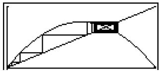
natural_image
Abstract geometric diagram with curved lines and a central square (no text or symbols)■ Using List Sort Functions in a Program
These functions let you sort data in lists into ascending or descending order.
- Ascending order
① SortA (List 1, List 2, List 3) Lists to be sorted (up to six can be specified)
① F4 F3 F1 ② OPTN F1 F1
- Descending order
③ SortD (List 1, List 2, List 3) Lists to be sorted (up to six can be specified)
③ F4 F3 F2

■ Using Solve Calculation Function in a Program
The following is the syntax for using the Solve function in a program.
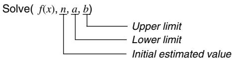
Example Program
$$ ① \text { Solve } (2 X ^ {2} + 7 X - 9, 1, 0, 1) $$
$$ ① \boxed {O P T N} \boxed {F 4} \boxed {F 1} $$
- In the function f(x) , only X can be used as a variable in the expression. Other variables (A through Z, r, ) are treated as constants, and the value currently assigned to that variable is applied during the calculation.
- Input of the closing parenthesis, lower limit a and upper limit b can be omitted.
■ Using Statistical Calculations and Graphs in a Program
Including statistical calculations and graphing operations in a program lets you calculate and graph statistical data.
- To set conditions and draw a statistical graph
Following "StatGraph", you must specify the following graph conditions:
- Graph Type
- x -axis data location (list name)
- y-axis data location (list name)
• Frequency data location (list name) - Mark Type
- Graph draw/non-draw status (DrawOn/DrawOff)

# Solutions obtained using Solve may include errors.
# You cannot use a differential, quadratic differential, integration, , maximum/minimum value or Solve calculation expressions inside of a Solve calculation term.

The graph conditions that are required depends on the graph type. See “Changing Graph Parameters” (page 6-1-2).
- The following is a typical graph condition specification for a scatter diagram or xy Line graph.
S-Gph1 DrawOn, Scatter, List 1, List 2, 1, Square
In the case of an xy line graph, replace "Scatter" in the above specification with "xyLine".
- The following is a typical graph condition specification for a normal probability plot.
S-Gph1 DrawOn, NPPlot, List 1, Square
- The following is a typical graph condition specification for a single-variable graph.
S-Gph1 DrawOn, Hist, List 1, List 2
The same format can be used for the following types of graphs, by simply replacing "Hist" in the above specification with the applicable graph type.
Histogram: ...... Hist
Median Box: ...... MedBox*1
Normal Distribution: N-Dist
Broken Line: ...... Broken
- The following is a typical graph condition specification for a regression graph.
S-Gph1 DrawOn, Linear, List 1, List 2, List 3
The same format can be used for the following types of graphs, by simply replacing “Linear” in the above specification with the applicable graph type.
Linear Regression: .... Linear
Med-Med: ...... Med-Med
Quadratic Regression: .... Quad
Cubic Regression: .... Cubic
Quartic Regression: .... Quart
Logarithmic Regression: ...... Log
Exponential Regression: .... Exp
Power Regression: ...... Power

*1 Outliers: On
S-Gph1 DrawOn, MedBox, List 1, 1, 1
Outliers:Off
S-Gph1 DrawOn, MedBox, List 1, 1, 0

- The following is a typical graph condition specification for a sinusoidal regression graph. S-Gph1 DrawOn, Sinusoidal, List 1, List 2
- The following is a typical graph condition specification for a logistic regression graph. S-Gph1 DrawOn, Logistic, List 1, List 2
Example Program
ClrGraph
①
S-Wind Auto
{1, 2, 3} → List 1
{1, 2, 3} → List 2
② ③ ④ ⑤
S-Gph1 DrawOn, Scatter, List 1, List 2, 1, Square
⑥
DrawStat
① SHIFT MENU F6 F6 F3 F1
② F4 F1 F2 F1 EXIT
③ F1 F1 EXIT
④ F2 F4 EXIT
⑤ EXIT F4 F1 F4 F1
⑥ SHIFT VARS F6 F2 F1
Executing this program produces the scatter diagram shown here.
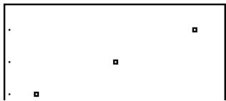
natural_image
Simple diagram with a rectangle containing scattered black squares on white background (no text or symbols)■ Performing Statistical Calculations
- Single-variable statistical calculation
①1-Variable List 1, List 2
Frequency data (Frequency)
x-axis data (XList)
①F4 F1 F6 F1
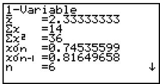

- Paired-variable statistical calculation
flowchart
graph TD
    A["①2-Variable List 1, List 2, List 3"] --> B["Frequency data (Frequency)"]
    A --> C["y-axis data (YList)"]
    A --> D["x-axis data (XList)"]
①F4 F1 F6 F2
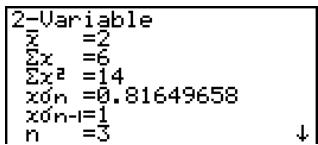
- Regression statistical calculation
flowchart
graph TD
    A["LinearReg"] --> B["Calculation type*"]
    B --> C["List 1, List 2, List 3"]
    C --> D["Frequency data (Frequency)"]
    C --> E["y-axis data (YList)"]
    C --> F["x-axis data (XList)"]
①F4 F1 F6 F6 F1
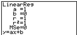
* Any one of the following can be specified as the calculation type.
LinearReg ...... linear regression
Med-MedLine .... Med-Med calculation
QuadReg ...... quadratic regression
CubicReg...... cubic regression
QuartReg ...... quartic regression
LogReg ...... logarithmic regression
ExpReg ...... exponential regression
PowerReg ...... power regression
- Sinusoidal regression statistical calculation
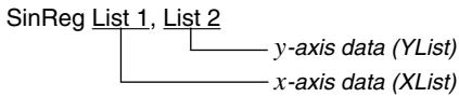
flowchart
graph TD
    A["SinReg List 1, List 2"] --> B["y-axis data (YList)"]
    A --> C["x-axis data (XList)"]
- Logistic regression statistical calculation
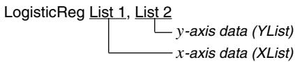
flowchart
graph TD
    A["LogisticReg List 1, List 2"] --> B["y-axis data (YList)"]
    A --> C["x-axis data (XList)"]

8-7 PRGM Mode Command List
RUN Program
| [F4](MENU) key | |||
| Level 1 | Level 2 | Level 3 | Command |
| STAT | DRAW | On | DrawOn |
| Off | DrawOff | ||
| GRPH | GPH1 | S-Gph1_ | |
| GPH2 | S-Gph2_ | ||
| GPH3 | S-Gph3_ | ||
| Scat | Scatter | ||
| xy | xyLine | ||
| Hist | Hist | ||
| Box | MedBox | ||
| N-Dis | N-Dist | ||
| Brkn | Broken | ||
| X | Linear | ||
| Med | Med-Med | ||
| X^2 | Quad | ||
| X^3 | Cubic | ||
| X^4 | Quart | ||
| Log | Log | ||
| Exp | Exp | ||
| Pwr | Power | ||
| Sin | Sinusoidal | ||
| NPP | NPPlot | ||
| Lgst | Logistic | ||
| List | List_ | ||
| MARK | Square | ||
| × | Cross | ||
| Dot | |||
| CALC | 1VAR | 1-Variable_ | |
| 2VAR | 2-Variable_ | ||
| X | LinearReg_ | ||
| Med | Med-MedLine_ | ||
| X^2 | QuadReg_ | ||
| X^3 | CubicReg_ | ||
| X^4 | QuartReg_ | ||
| Log | LogReg_ | ||
| Exp | ExpReg_ | ||
| Pwr | PowerReg_ | ||
| Sin | SinReg_ | ||
| Lgst | LogisticReg_ | ||
| MAT | Swap | Swap_ | |
| ×Rw | *Row_ | ||
| ×Rw+ | *Row+_ | ||
| Rw+ | Row+_ | ||
| LIST | Srt-A | SortA( | |
| Srt-D | SortD( | ||
| GRPH | SEL | On | G_SelOn_ |
| Off | G_SelOff_ | ||
| TYPE | Y= | Y-Type | |
| r= | r-Type | ||
| Parm | ParamType | ||
| X=c | X=cType | ||
| Y> | Y>Type | ||
| Y< | Y | ||
| Y≥ | Y≥Type | ||
| Y≤ | Y≤Type | ||
| STYL | — | NormalG_ | |
| — | ThickG_ | ||
| ...... | BrokenThickG_ | ||
| ...... | DotG_ | ||
| GMEM | Sto | StoGMEM_ | |
| Rcl | RclGMEM_ | ||
| DYNA | On | D_SelOn_ | |
| Off | D_SelOff_ | ||
| Var | D_Var_ | ||
| TYPE | Y= | Y=Type | |
| r= | r=Type | ||
| Parm | ParamType | ||
| TABL | On | T_SelOn_ | |
| Off | T_SelOff_ | ||
| TYPE | Y= | Y=Type | |
| r= | r=Type | ||
| Parm | ParamType | ||
| STYL | — | NormalG_ | |
| — | ThickG_ | ||
| ...... | BrokenThickG_ | ||
| ...... | DotG_ | ||
| RECR | SEL+S | On | R_SelOn_ |
| Off | R_SelOff_ | ||
| — | NormalG_ | ||
| — | ThickG_ | ||
| ...... | BrokenThickG_ | ||
| ...... | DotG_ | ||
| TYPE | an | anType | |
| an+1 | an+1Type | ||
| an+2 | an+2Type | ||
| n.an- | n | n | |
| an | an | ||
| an+1 | an+1 | ||
| bn | bn | ||
| bn+1 | bn+1 | ||
| cn | cn | ||
| cn+1 | cn+1 | ||
| RANG | ao | Sel_a0 | |
| a1 | Sel_a1 |
| [OPTN] key | |||
| Level 1 | Level 2 | Level 3 | Command |
| LIST | List | List_ | |
| L→M | List→Mat( | ||
| Dim | Dim_ | ||
| Fill | Fill( | ||
| Seq | Seq( | ||
| Min | Min( | ||
| Max | Max( | ||
| Mean | Mean( | ||
| Med | Median( | ||
| Aug | Augment( | ||
| Sum | Sum_ | ||
| Prod | Prod_ | ||
| Cuml | Cuml_ | ||
| % | Percent_ | ||
| List_ | |||
| MAT | Mat | Mat_ | |
| M→L | Mat→List( | ||
| Det | Det_ | ||
| Trn | Trn_ | ||
| Aug | Augment( | ||
| Iden | Identity_ | ||
| Dim | Dim_ | ||
| Fill | Fill( | ||
| CPLX | i | i | |
| Abs | Abs_ | ||
| Arg | Arg_ | ||
| Conj | Conjg_ | ||
| ReP | ReP_ | ||
| ImP | ImP_ | ||
| r | r | ||
| a+bi | a+bi | ||
| CALC | Solve | Solve( | |
| d/dx | d/dx( | ||
| d^2/dx^2 | d^2/dx^2 ( | ||
| f/dx | f/ | ||
| FMin | FMin( | ||
| FMax | FMax( | ||
| ( | ( | ||
| logab | logab( | ||
| STAT | |||
| HYP | sinh | sinh_ | |
| cosh | cosh_ | ||
| tanh | tanh_ | ||
| sinh^-1 | sinh^-1 _ | ||
| cosh^-1 | cosh^-1 _ | ||
| tanh^-1 | tanh^-1 _ | ||
| PROB | X! | ! | |
| nPr | P | ||
| nCr | C | ||
| Ran# | Ran#_ | ||
| P( | P( | ||
| Q( | Q( | ||
| R( | R( | ||
| t( | t( | ||
| NUM | Abs | Abs_ | |
| Int | Int_ | ||
| Frac | Frac_ | ||
| Rnd | Rnd | ||
| Intg | Intg_ | ||
| RndFi | RndFix( | ||
| ANGL | ° | ° | |
| r | r | ||
| g | g | ||
| °,” | ° | ||
| Pol( | Pol( | ||
| Rec( | Rec( | ||
| ►DMS | ►DMS | ||
| ESYM | m | m | |
| μ | μ | ||
| n | n | ||
| p | p | ||
| f | f | ||
| k | k | ||
| M | M | ||
| G | G | ||
| T | T | ||
| P | P | ||
| E | E | ||
| PICT | Sto | StoPict_ | |
| Rcl | RclPict_ | ||
| FMEM | fn | fn | |
| LOGIC | And | _And_ | |
| Or | _Or_ | ||
| Not | Not_ | ||
| CAPT | Rcl | RclCapt_ |

| [VARS] key | |||
| Level 1 | Level 2 | Level 3 | Command |
| V-WIN | X | min | Xmin |
| max | Xmax | ||
| scal | Xscl | ||
| dot | Xdot | ||
| Y | min | Ymin | |
| max | Ymax | ||
| scal | Yscl | ||
| T,θ | min | Tθ min | |
| max | Tθ max | ||
| ptch | Tθ ptch | ||
| R-X | min | RightXmin | |
| max | RightXmax | ||
| scal | RightXscl | ||
| dot | RightXdot | ||
| R-Y | min | RightYmin | |
| max | RightYmax | ||
| scal | RightYscl | ||
| R-T,θ | min | RightTθ min | |
| max | RightTθ max | ||
| ptch | RightTθ ptch | ||
| FACT | Xfct | Xfct | |
| Yfct | Yfct | ||
| STAT | X | n | n |
| Σx | Σx | ||
| Σx2 | Σx2 | ||
| xσn | xσn | ||
| xσn-1 | xσn-1 | ||
| minX | minX | ||
| maxX | maxX | ||
| Y | |||
| Σy | Σy | ||
| Σy2 | Σy2 | ||
| Σxy | Σxy | ||
| yσn | yσn | ||
| yσn-1 | yσn-1 | ||
| minY | minY | ||
| maxY | maxY | ||
| GRPH | a | a | |
| b | b | ||
| c | c | ||
| d | d | ||
| e | e | ||
| r | r | ||
| r2 | r2 | ||
| MSe | MSe | ||
| Q1 | Q1 | ||
| Med | Med | ||
| Q3 | Q3 | ||
| Mod | Mod | ||
| Strt | H_Start | ||
| Pitch | H_pitch | ||
| PTS | x1 | x1 | |
| y1 | y1 | ||
| x2 | x2 | ||
| y2 | y2 | ||
| x3 | x3 | ||
| y3 | y3 | ||
| GRPH | Y | Y | |
| r | r | ||
| Xt | Xt | ||
| Yt | Yt | ||
| X | X | ||
| DYNA | Strt | D_Start | |
| End | D_End | ||
| Pitch | D_pitch | ||
| TABL | Strt | F_Start | |
| End | F_End | ||
| Pitch | F_pitch | ||
| Reslt | F_Result | ||
| RECR | FORM | an | an |
| an+1 | an+1 | ||
| an+2 | an+2 | ||
| bn | bn | ||
| bn+1 | bn+1 | ||
| bn+2 | bn+2 | ||
| cn | cn | ||
| cn+1 | cn+1 | ||
| cn+2 | cn+2 | ||
| RANG | Strt | R_Start | |
| End | R_End | ||
| a0 | a0 | ||
| a1 | a1 | ||
| a2 | a2 | ||
| b0 | b0 | ||
| b1 | b1 | ||
| b2 | b2 | ||
| c0 | c0 | ||
| c1 | c1 | ||
| c2 | c2 | ||
| anSt | anStart | ||
| bnSt | bnStart | ||
| cnSt | cnStart | ||
| Reslt | R_Result | ||
| EQUA | S-Rlt | Sim_Result | |
| S-Cof | Sim_Coef | ||
| P-Rlt | Ply_Result | ||
| P-Cof | Ply_Coef | ||
| TVM | n | n | |
| I% | I% | ||
| PV | PV | ||
| PMT | PMT | ||
| FV | FV | ||
| P/Y | P/Y | ||
| C/Y | C/Y |
| [SHIFT] [VARS] (PRGM) key | |||
| Level 1 | Level 2 | Level 3 | Command |
| COM | If | If_ | |
| Then | Then_ | ||
| Else | Else_ | ||
| I-End | IfEnd | ||
| For | For_ | ||
| To | _To_ | ||
| Step | _Step_ | ||
| Next | Next | ||
| While | While_ | ||
| WEnd | WhileEnd | ||
| Do | Do | ||
| Lp-W | LpWhile_ | ||
| CTL | Prog | Prog_ | |
| Rtrn | Return | ||
| Brk | Break | ||
| Stop | Stop | ||
| JUMP | Lbl | Lbl | |
| Goto | Goto_ | ||
| ⇒ | ⇒ | ||
| Isz | Isz_ | ||
| Dsz | Dsz_ | ||
| ? | ? | ||
| ▲ | ▲ | ||
| CLR | Text | ClrText | |
| Grph | ClrGraph | ||
| List | ClrList_ | ||
| Mat | ClrMat_ | ||
| DISP | Stat | DrawStat | |
| Grph | DrawGraph | ||
| Dyna | DrawDyna | ||
| F-Tbl | Tabl | DispF-Tbl | |
| G-Con | DrawFTG-Con | ||
| G-Plt | DrawFTG-Plt | ||
| R-Tbl | Tabl | DispR-Tbl | |
| Web | DrawWeb_ | ||
| an-Cn | DrawR-Con | ||
| Σa-Cn | DrawR Σ-Con | ||
| an-Pl | DrawR-Plt | ||
| Σa-Pl | DrawR Σ -Plt | ||
| REL | = | = | |
| ≠ | ≠ | ||
| > | > | ||
| < | < | ||
| ≥ | ≥ | ||
| ≤ | ≤ | ||
| I/O | Lcte | Locate_ | |
| Gtky | Getkey | ||
| Send | Send( | ||
| Recv | Receive( | ||
| S38k | Send38k_ | ||
| R38k | Receive38k_ | ||
| Open | OpenComport38k | ||
| Close | CloseComport38k | ||
| : | : | ||
| [SHIFT] [MENU] (SET UP) key | |||
| Level 1 | Level 2 | Level 3 | Command |
| ANGL | Deg | Deg | |
| Rad | Rad | ||
| Gra | Gra | ||
| COOR | On | CoordOn | |
| Off | CoordOff | ||
| GRID | On | GridOn | |
| Off | GridOff | ||
| AXES | On | AxesOn | |
| Off | AxesOff | ||
| LABL | On | LabelOn | |
| Off | LabelOff | ||
| DISP | Fix | Fix_ | |
| Sci | Sci_ | ||
| Norm | Norm_ | ||
| ENG | On | EngOn | |
| Off | EngOff | ||
| Eng | Eng | ||
| S/L | — | S-L-Normal | |
| — | S-L-Thick | ||
| ...... | S-L-Broken | ||
| ...... | S-L-Dot | ||
| DRAW | Con | G-Connect | |
| Plot | G-Plot | ||
| DERV | On | DerivOn | |
| Off | DerivOff | ||
| BACK | None | BG-None | |
| Pict | BG-Pict_ | ||
| FUNC | On | FuncOn | |
| Off | FuncOff | ||
| SIML | On | SimulOn | |
| Off | SimulOff | ||
| S-WIN | Auto | S-WindAuto | |
| Man | S-WindMan | ||
| LIST | File | File_ | |
| LOCS | On | LocusOn | |
| Off | LocusOff | ||
| T-VAR | Rang | VarRange | |
| List | VarCharList_ | ||
| Σ DSP | On | Σ dispOn | |
| Off | Σ dispOff | ||
| RESID | None | Resid-None | |
| List | Resid-List_ | ||
| CPLX | Real | Real | |
| a+bi | a+bi | ||
| r∠θ | r∠θ | ||
| FRAC | d/c | d/c | |
| ab/c | ab/c | ||
| Y-SPD | Norm | Y=DrawSpeedNorm | |
| High | Y=DrawSpeedHigh | ||

BASE Program
| [SHIFT] key | |||
| Level 1 | Level 2 | Level 3 | Command |
| ZOOM | Fact | Factor_ | |
| Auto | ZoomAuto | ||
| V-WIN | V-Win | ViewWindow_ | |
| Sto | StoV-Win_ | ||
| Rcl | RclV-Win_ | ||
| SKTCH | Cls | Cls | |
| Tang | Tangent_ | ||
| Norm | Normal_ | ||
| Inv | Inverse_ | ||
| GRPH | Y= | Graph_Y= | |
| r= | Graph_r= | ||
| Parm | Graph(X,Y)=( | ||
| X=c | Graph_X= | ||
| G-/dx | Graph_/ | ||
| Y> | Graph_Y> | ||
| Y< | Graph_Y< | ||
| Y≥ | Graph_Y≥ | ||
| Y≤ | Graph_Y≤ | ||
| PLOT | Plot | Plot_ | |
| PI-On | PlotOn_ | ||
| PI-Off | PlotOff_ | ||
| PI-Chg | PlotChg_ | ||
| LINE | Line | Line | |
| F-Line | F-Line_ | ||
| Crcl | Circle_ | ||
| Vert | Vertical_ | ||
| Hztl | Horizontal_ | ||
| Text | Text_ | ||
| PIXL | On | PxlOn_ | |
| Off | PxlOff_ | ||
| Chg | PxlChg_ | ||
| Test | PxlTest( | ||
| STYL | — | SketchNormal_ | |
| — | SketchThick_ | ||
| ...... | SketchBroken_ | ||
| ...... | SketchDot_ | ||
| [F4](MENU) key | |||
| Level 1 | Level 2 | Level 3 | Command |
| d~o | d | d | |
| h | h | ||
| b | b | ||
| o | o | ||
| LOG | Neg | Neg_ | |
| Not | Not_ | ||
| and | and | ||
| or | or | ||
| xor | xor | ||
| xnor | xnor | ||
| DISP | ►Dec | ►Dec | |
| ►Hex | ►Hex | ||
| ►Bin | ►Bin | ||
| ►Oct | ►Oct | ||
| [SHIFT][MENU](SET UP) key | |||
| Level 1 | Level 2 | Level 3 | Command |
| Dec | Dec | ||
| Hex | Hex | ||
| Bin | Bin | ||
| Oct | Oct | ||
| [SHIFT][VARS](PRGM) key | |||
| Level 1 | Level 2 | Level 3 | Command |
| Prog | Prog_ | ||
| JUMP | Lbl | Lbl_ | |
| Goto | Goto_ | ||
| ⇒ | ⇒ | ||
| Isz | Isz_ | ||
| Dsz | Dsz_ | ||
| ? | ? | ||
| ▲ | ▲ | ||
| REL | = | = | |
| ≠ | ≠ | ||
| > | > | ||
| < | < | ||
| ≥ | ≥ | ||
| ≤ | ≤ | ||
| : | : | ||

8-8 Program Library
- Be sure to check how many bytes of unused memory are remaining before attempting to perform any programming.
Program Name
Prime Factorization
Description
This program continually divides a natural number by factors until all its prime factors are produced.
Purpose
This program accepts input of natural number A, and divides it by B (2, 3, 5, 7....) to find the prime factors of A.
- If a division operation does not produce a remainder, the result of the operation is assigned to A.
- The above procedure is repeated until B > A .

Example
$$ 4 4 0 7 3 0 = 2 \times 3 \times 3 \times 5 \times 5 9 \times 8 3 $$
ClrText
"INPUT NUMBER"?→A
2→B
Do
While Frac (A÷B)=0
B
A÷B→A
WhileEnd
If B=2
Then 3→B
Else B+2→B
IfEnd
LpWhile B≤A
"END"

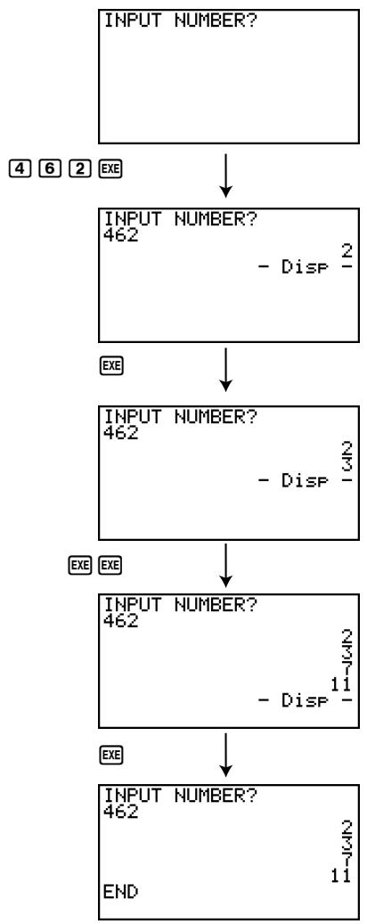
flowchart
graph TD
    A["INPUT NUMBER?"] --> B["INPUT NUMBER? 462 - Disp 2"]
    B --> C["INPUT NUMBER? 462 - Disp 13"]
    C --> D["INPUT NUMBER? 462 - Disp 11"]
    D --> E["INPUT NUMBER? 462 END"]

Program Name Arithmetic-Geometric Sequence Differentiation
Description
After inputting sequence terms 1, 2, and 3, this program determines whether it is an arithmetic sequence or geometric sequence based on the differences and ratios of the terms.
Purpose
This program determines whether a specific sequence is an arithmetic sequence or geometric sequence.
● ● ● ● ●
Example 1 5, 10, 15, ... Arithmetic sequence
● ● ● ● ●
Example 2 5, 10, 20, ... Geometric sequence
ClrText
"A1"?→A
"A2"?→B
"A3"?→C
B-A→D
C-B→E
If D=E
Then ClrText
"AN = A1 + (N-1)D"
" "←
"A1 ="
"D ="
Locate 6,3,A
Locate 6,4,D
IfEnd
B÷A→F
C÷B→G
If F=G
Then ClrText
"AN = A1×r^(N-1)"
" "←
"A1 ="
"r ="
Locate 6,3,A
Locate 6,4,F
IfEnd
"END"

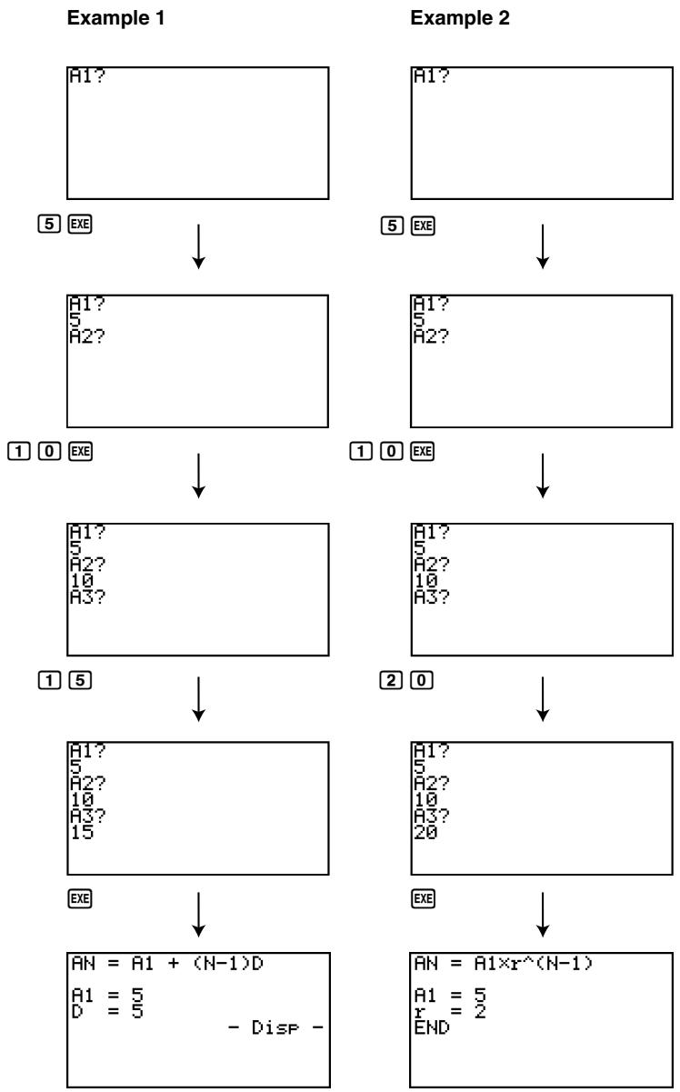
flowchart
graph TD
    A["Example 1"] --> B{A1?}
    B --> C["5 EXE"]
    C --> D["A1?"]
    D --> E["4"]
    D --> F["A2?"]
    F --> G["1 0 EXE"]
    G --> H["A1?"]
    H --> I["5"]
    H --> J["A2?"]
    J --> K["10"]
    J --> L["A3?"]
    L --> M["1 5"]
    M --> N["A1?"]
    N --> O["5"]
    N --> P["A2?"]
    P --> Q["10"]
    P --> R["A3?"]
    R --> S["15"]
    S --> T["EXE"]
    T --> U["AN = A1 + (N-1)D"]
    U --> V["A1 = 5"]
    V --> W["D = 5"]
    W --> X["- Disp -"]
    X --> Y["EXE"]

Program Name
Ellipse
Description
This program displays a number table of the following values based on input of the foci of an ellipse, the sum of the distance between the loci and foci, and the pitch (step size) of X.
Y1: Coordinate values of upper half of ellipse
Y2: Coordinate values of lower half of ellipse
Y3: Distances between right focus and loci
Y4: Distances between left focus and loci
Y5: Sum of Y3 and Y4
Next, the program plots the foci and values in Y1 and Y2.
Purpose
This program shows that the sums of the distances between the loci and two foci of an ellipse are equal.
Do
ClrText
"FOCUS (C,0),(-C,0)"
"C="?→C
"SUM DISTANCE"?→D
LpWhile 2Abs C≥D Or D≤0
D÷2→A
√(A²-C²)→B
Y=Type
"B√(1-X²÷A²)"→Y1
"-Y1"→Y2
"√((X-C)²+Y1²)"→Y3
"√((X+C)²+Y1²)"→Y4
"Y3+Y4"→Y5
For 1→E To 20
If E≤5
Then T SelOn E
Else T SelOff E
IfEnd
Next
-Int A→F Start
Int A→F End
"F pitch"?→F pitch
DispF-Tbl
ClrGraph
1.2A→Xmax
-1.2A→Xmin
1.2B→Ymax
-1.2B→Ymin
T SelOff 3
T SelOff 4
T SelOff 5
DispF-Tbl
DrawFTG-Plt
PlotOn C,0
PlotOn -C,0
"END"

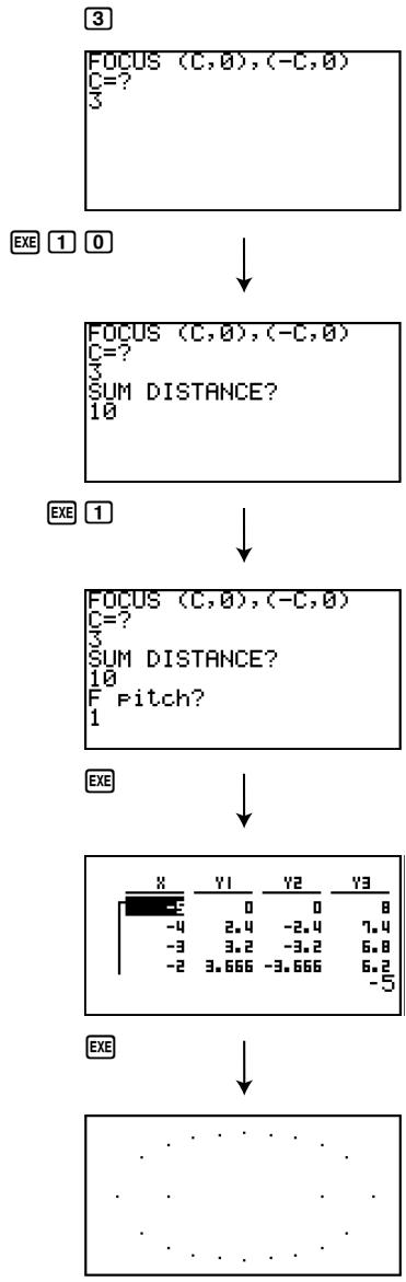
flowchart
graph TD
    A["FOCUS (C,0), (-C,0)\nC=?"] --> B["FOCUS (C,0), (-C,0)\nC=?\nSUM DISTANCE?\n10"]
    B --> C["FOCUS (C,0), (-C,0)\nC=?\nSUM DISTANCE?\n10\nF pitch?\n1"]
    C --> D["X Y1 Y2 Y3\n-5 0 0 8\n-4 2.4 -2.4 7.4\n-3 3.2 -3.2 6.8\n-2 3.666 -3.666 6.2\n-5"]
    D --> E["EXE"]

Program Name
Rotation
Description
This program draws an angle at the coordinate defined by an input vertex, and then rotates it to a specified angle around the vertex.
Purpose
This program demonstrates coordinate transformation using a matrix.
Important!
Deg must be set as the angle unit for this program.
AxesOff
Deg
Do
ClrText
"VERTEX NUMBER"?→A
LpWhile A≤0 Or Frac A≠0
{2,A}→Dim Mat A
ClrGraph
For 1→B To A
Text 1,1,"VERTEX"
Text 1,30,B
If B=1
Then Plot
PlotOn X,Y
X→Mat A[1,B]
Y→Mat A[2,B]
Else Plot C,D
F-Line C,D,X,Y
X→Mat A[1,B]
Y→Mat A[2,B]
IfEnd
Mat A[1,B]→C
Mat A[2,B]→D
Next
Mat A[1,1]→E
Mat A[2,1]→F
F-Line C,D,E,F
Text 1,1,"--AXIS--"
Plot
PlotOn X,Y
X→C
Y→D
A→Dim List 1
A→Dim List 2
Fill(C,List 1)
Fill(D,List 2)
List→Mat(List 1,List 2)
Trn Mat Ans→Mat C
Mat A-Mat C→Mat A
ClrText
"ANGLE"?→E
[[cos E,-sin E][sin E,cos E]]→Mat B
Mat B×Mat A→Mat D
Mat D+Mat C→Mat D
If A=1
Then PlotOn Mat D[1,1],Mat D[2,1]
Else For 1→B To A-1
Mat D[1,B]→F
Mat D[2,B]→G
Mat D[1,B+1]→H
Mat D[2,B+1]→I
F-Line F,G,H,I
Next
If A>2
Then Mat D[1,1]→F
Mat D[2,1]→G
F-Line H, I, F, G
IfEnd
IfEnd
Text 1, 1, "--END--"

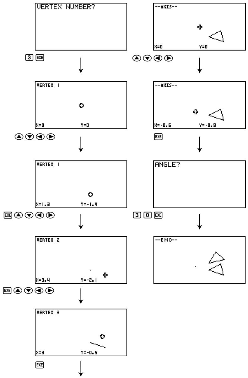
flowchart
graph TD
    A["VERTEX NUMBER?"] --> B["3 EXE"]
    C["--AXIS--"] --> D["→"]
    E["VEY=0"] --> F["→"]
    G["VEY=0"] --> H["→"]
    I["--AXIS--"] --> J["→"]
    K["VEY=-0.6"] --> L["→"]
    M["VEY=-0.9"] --> N["→"]
    O["VEY=1.3"] --> P["→"]
    Q["VEY=-1.4"] --> R["→"]
    S["VEY=3.4"] --> T["→"]
    U["VEY=-2.1"] --> V["→"]
    W["VEY=3"] --> X["→"]
    Y["VEY=-0.5"] --> Z["→"]
    AA["EXE"] --> AB["3 0 EXE"]
    AC["--END--"] --> AD["→"]

Program Name Interior Angles and Surface Area of a Triangle
Description
This program calculates the interior angles and surface area of a triangle defined by input coordinates for angles A, B, and C.
Purpose
This program calculates the interior angles and surface area of a triangle defined by coordinates for angles A, B, and C.
Important!
Inputting the same coordinates for any two angles (A, B, C) causes an error.
C1rText↓
"WHICH ANGLE?"↓
" 1.Deg"↓
" 2.Rad"↓
" 3.Gra"↓
Do↓
Getkey↓
LpWhile ((Ans=72) Or (Ans=62) Or (Ans=52))=0↓
If Ans=72↓
Then 1→θ↓
Deg↓
" "↓
"-Deg-Deg-Deg-Deg-Deg-"↓
IfEnd↓
If Ans=62↓
Then 2→θ↓
Rad↓
" "↓
"-Rad-Rad-Rad-Rad-Rad-Rad-"↓
IfEnd↓
If Ans=52↓
Then 3→θ↓
Gra↓
" "↓
"-Gra-Gra-Gra-Gra-Gra-"↓
IfEnd↓
"AX"?→A↓
"AY"?→B↓
"BX"?→C↓
"BY"?→D↓
"CX"?→E↓
"CY"?→F↓
A-C→G↓
B-D→H↓
C-E→I↓
D-F→J↓
E-A→K↓
F-B→L↓
-GI-HJ→M↓
-IK-JL→N↓
-KG-LH→O↓
φ'(G²+H²)→P↓
φ'(I²+J²)→Q↓
φ'(K²+L²)→R↓
M÷PQ→S↓
N÷QR→T↓
O÷PR→U↓
cos⁻¹ S→V↓
cos⁻¹ T→W↓
cos⁻¹ U→X↓
PQφ'(1-S²)→Y↓
ClrText↓
" <ABC=" ↓
Locate 9.1.V ↓
" <ACB = "↓
Locate 9,2,W↓
" <BAC = "↓
Locate 9,3,X↓
If θ=1↓
Then " (Deg)"↓
IfEnd↓
If θ=2↓
Then " (Rad)"↓
IfEnd↓
If θ=3↓
Then " (Gra)"↓
IfEnd↓
" AREA = "↓
Locate 9,5,Y÷2↓
" "↓
"END"

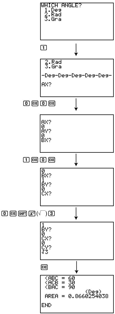
flowchart
graph TD
    A["WHICH ANGLE?\n1. Deg\n2. Rad\n3. Gra"] --> B["1"]
    B --> C["2. Rad\n3. Gra\n-Des-Des-Des-Des-Des-AX?"]
    C --> D["0 EXE 0 EXE"]
    D --> E["AX?\n0\nAY?\n0\nBX?"]
    E --> F["1 EXE 0 EXE"]
    F --> G["0\nBX?\n1\nBY?\n0\nCX?"]
    G --> H["0 EXE SHIFT x²(√) 3"]
    H --> I["1\nBY?\n0\nCX?\n0\nCY?\n√3"]
    I --> J["EXE"]
    J --> K["\(ABCB = 60\)\(ACB = 30\)\(BAC = 90\)(Deg)\nAREA = 0.8660254038\END"]

Chapter
9
Spreadsheet
The Spreadsheet application provides you with powerful, take-along-anywhere spreadsheet capabilities.
9-1 Spreadsheet Overview
9-2 File Operations and Re-calculation
9-3 Basic Spreadsheet Screen Operations
9-4 Inputting and Editing Cell Data
9-5 S·SHT Mode Commands
9-6 Statistical Graphs
9-7 Using the CALC Function
9-8 Using Memory in the S·SHT Mode
9-1 Spreadsheet Overview
This section describes the Spreadsheet application screen, and provides basic information about its menus and commands.
■ Using the S·SHT Mode
On the Main Menu, select the S·SHT icon.
- This will enter the S·SHT mode and display a spreadsheet.
- The first time you enter the S·SHT mode, the calculator will automatically create a file named "SHEET" for the displayed spreadsheet.
■ Spreadsheet Screen Configuration
A spreadsheet consists of a “cells” and their contents as shown below.
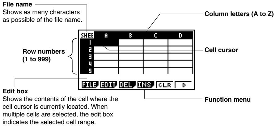
• Each cell can contain a value, expression, text, or a formula. Formulas can contain a reference to a specific cell or a range of cells.
- Each cell has a unique name, consisting of its column letter and row number. The name of the cell where the cell cursor is located in the above example is “A1”.

■ S·SHT Mode Function Menu
- {FILE} ... {displays the FILE submenu}
- {NEW} ... {creates a new spreadsheet file}
- {OPEN} ... {displays a list of previously saved spreadsheet files} You can select a file on this list and open it or delete it.
- {SV·AS} ... {saves the displayed spreadsheet under a new name (Save As)}
- {RECAL} ... {recalculates the formulas included in the displayed spreadsheet}
- {EDIT} ... {displays the EDIT submenu}
- {CUT}/{PASTE} ... F1(CUT) specifies you want to cut the currently selected cell(s). This causes the F1 function key function to change to (PASTE), so you can move the cell cursor to another location and press F1(PASTE) to paste the cells you cut. Performing the paste operation causes the original cells to be cleared.
- {COPY} ... F2 (COPY) specifies you want to copy the currently selected cell(s). This causes the F1 function key function to change to (PASTE), so you can move the cell cursor to another location and press F1 (PASTE) to paste the cells you copied. Performing the paste operation does not affect the original cells.
- {CELL} ... {recalls the contents of the currently selected cell (one only) for editing}
-
{JUMP} ... {displays a JUMP submenu}
-
{GO} ... {displays a dialog box for making the cell cursor jump to a particular cell}
- TOP ... {causes the cell cursor to jump to line 1 of the column where the cell cursor is located}
- TOP ... {causes the cell cursor to jump to column A of the line where the cell cursor is located}
- BOT ... {causes the cell cursor to jump to last line of the column where the cell cursor is located}
- BOT ... {causes the cell cursor to jump to column Z of the line where the cell cursor is located}

- {SEQ} ... {generates a numeric sequence the same way as the "Seq(" command (page 3-2-3))}
The sequence starts from a specified cell, and can be configured to proceed in a line-wise or column-wise direction. The direction is the one specified by the "Move" setting on the Setup screen (page 1-7-5). - {FILL} ... {displays a screen for entering a formula, expression, value, or text, which is then filled into the all of the currently selected cells}
- {SRT • A} ... {sorts ascending (A, B, C...) the currently selected row or column of cells}
- {SRT·D} ... {sorts descending (Z, Y, X...) the currently selected row or column of cells}
- {DEL} ... {displays the DEL submenu}
- {ROW} ... {deletes the entire row(s) of the currently selected cell(s), and shifts anything below upwards}
- {COL} ... {deletes the entire column(s) of the currently selected cell(s), and shifts anything to the right leftwards}
- {ALL} ... {deletes the contents of all of the cells in the currently displayed spreadsheet}
- {INS} ... {displays the INS submenu}
- {ROW} ... {inserts the same number of rows as the currently selected rows, above the selected rows}
- {COL} ... {inserts the same number of columns as the currently selected columns, to the right of the selected columns}
- {CLR} ... {clears the contents of the currently selected cell(s)}
- {GRPH} ... {displays a graph menu that is identical to the one used in the STAT mode} {GPH1}/{GPH2}/{GPH3}/{SEL}/{SET}
Some of the functions on the menu that appears when you press F6 (SET) here are different from those that appear when you press F6 (SET) in the STAT mode.
- {CALC} ... {displays a CALC (statistical calculation) menu that is identical to the one used in the STAT mode}
{1VAR}/{2VAR}/{REG}/{SET}
Some of the functions on the menu that appears when you press F6 (SET) here are different from those that appear when you press F6 (SET) in the STAT mode. See "9-7 Using the CALC Function" for more information.

- {STO} ... {displays the STO submenu}
- {VAR} ... {assigns the contents of a cell to a variable}
- {LIST} ... {saves the contents of a range of cells as a list}
- {FILE} ... {saves the contents of a range of cells as a file}
- {MAT} ... {saves the contents of a range of cells as a matrix}
- {RCL} ... {displays the RCL submenu}
- {LIST} ... {imports data from a list into the spreadsheet}
- {FILE} ... {imports data from a file into the spreadsheet}
- {MAT} ... {imports data from a matrix into the spreadsheet}
- Data Input Function Menu
- {GRAB} ... {enters the Grab mode for inputting sell references} For details, see “To reference a particular cell” (page 9-4-6).
- ... {inputs the absolute reference command ( ) into a cell }
- ... {inputs the cell range command (:) into a cell}
- {If} ... {inputs the "CellIf(" S • SHT mode command}}
- {CEL} ... {displays a submenu for inputting the following S·SHT mode commands} "CellMin(", "CellMax(", "CellMean(", "CellMedian(", "CellSum(", "CellProd("
- {REL} ... {displays a submenu for inputting the following relational operators} "=", "≠", ">", "<", "≥", "≤"

# For details about the S • SHT mode commands you can access with F4 (If) and F5 (CEL), see "9-5 S • SHT Mode Commands".

9-2 File Operations and Re-calculation
This section explains the various operations you can perform with S·SHT mode files. It also tells you how to re-calculate the formulas in a spreadsheet.
■ Spreadsheet File Operations
- To create a new file
- In the S·SHT mode, press F1(FILE)F1(NEW).
- This displays a dialog box for inputting a file name.
- Enter up to eight characters for the Spreadsheet file name, and then press EXE.
- This will display a blank spreadsheet.
![Spread Sheet Name [& ]](/content/2025/01/86785/images/c4f427e5a7c50641816829d0c9c969b00ebba707ffc12c4c9151e3a4e7e392c5.jpg)
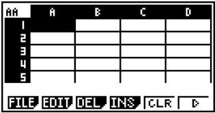

# If the file name you enter in step 2 is the name of a spreadsheet file already stored in memory, the calculator will open that file instead of creating a new one.

- To open a file
- In the S·SHT mode, press F1(FILE)F2(OPEN).
- This will display a list of existing spreadsheet files.
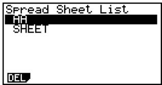
-
Use ▲ and ▼ to highlight the name of the file you want to open.
-
Press EXE.
- This will open the spreadsheet you selected in step 2.
- To delete a file
- In the S·SHT mode, press F1(FILE)F2(OPEN).
- This will display a list of existing spreadsheet files.
-
Use ▲ and ▼ to highlight the name of the file you want to delete.
-
Press F1 (DEL).
![Delete Sheet? Yes: [F1] No : [F6]](/content/2025/01/86785/images/c89ffb99bc7f95c0e0e3e0d5f2b95e8bb3e7d4147c04e54626f2f46ed688761f.jpg)
-
In response to the confirmation message that appears, press F1(Yes) to delete the file, or F6(No) to cancel the delete operation without doing anything.
-
To return to the spreadsheet from the file list, press EXIT.

# If you delete the currently open file, the calculator will automatically close its screen
and then automatically generate a new file named "SHEET", and display its blank spreadsheet.

- To save a file under a new name (Save As)
-
In the S·SHT mode, press F1(FILE)F3(SV·AS).
-
This will display a dialog box for entering a file name.
- Enter up to eight characters for the file name, and then press EXE.
About Auto Save
The S·SHT mode has an Auto Save feature that automatically saves any changes to make to a spreadsheet file as you edit it. This means you do not need to perform any manual save operation.
Recalculating a Formula
Use the following procedure to recalculate the formulas in a spreadsheet.
- To re-execute all of the formulas in a spreadsheet
While the spreadsheet is on the display, press F1(FILE)F4(RECAL).
- This will re-execute all of the formulas and display the updated results in the applicable cells.

# If a file already exists with the same file name you input in step 2, a message will appear asking if you want to replace the existing file with the new one.
![[A [AA ] Already Exists Overwrite OK? Yes: [F1] No : [F6]](/content/2025/01/86785/images/6c35ef68ecf11bd533eb072a16700496956c656b3847a76d1941d68343141714.jpg)
Press F1(Yes) to replace the existing file with the new one, or F6(No) to return to the spreadsheet without saving.
# Using Auto Calc
When “On” is selected for the “Auto Calc” setting on the Setup screen (page 1-7-5), all of the formulas in a spreadsheet are executed and cell values are update automatically whenever the spreadsheet file is opened, whenever the spreadsheet is edited, etc. The initial default setting for “Auto Calc” is “On”.
Formulas in a spreadsheet are not executed automatically if "Off" is selected for "Auto Calc". In this case, you need to press F1 (FILE) F4 (RECAL) to re-execute formulas and update cell values when you want.
# The expressions in all cells are re-calculated when “Auto Calc” is “On”. This can cause the calculation to take longer.

9-3 Basic Spreadsheet Screen Operations
This section explains basic procedures for selecting cells and moving the cell cursor on a spreadsheet.
Cell Cursor
The cell cursor is the highlighting showing the cell or cells that are currently selected on a spreadsheet.
- While a single cell is selected with the cell cursor, the edit box (the line above the function menu at the bottom of the spreadsheet screen) shows the contents (value, formula, etc.) of that cell. While multiple cells are selected with the cell cursor, the edit box shows the range of selected cells.
- For details about selecting cells, see “Selecting Cells” (page 9-3-2).
■ Moving the Cell Cursor
You can move the cell cursor with the cursor key, or by using the JUMP command.
- To move the cell cursor using the cursor key
When a single cell is selected, you can use the cursor key to move the cell cursor up, down, left, or right.

- To move the cell cursor using the JUMP command
| To move the cell cursor to here: | Do this: |
| A particular cell | 1. Press F2(EDIT)F4(JUMP)F1(GO).2. On the “Go To Cell” dialog box that appears, enter the name of the destination cell (A1 to Z999).3. Press EXE. |
| Line 1 of current column | Press F2(EDIT)F4(JUMP)F2(TOP↑). |
| Column A of current line | Press F2(EDIT)F4(JUMP)F3(TOP←). |
| Bottom line of current column | Press F2(EDIT)F4(JUMP)F4(BOT↓). |
| Column Z of current line | Press F2(EDIT)F4(JUMP)F5(BOT→). |
- Specifying Cell Cursor Movement when Inputting Cell Data
Under the initial default setup, the cell cursor moves down to the next line when you press the EXE to finalize input into a spreadsheet cell. You can use the "Move" setting on the Setup screen to change this to rightward movement if you want. For details, see "1-7 Using the Setup Screen".
■ Selecting Cells
Before performing any operation in a cell, you must first select it. You can select a single cell, a range of cells, all the cells in a row or column, or all of the cells in the spreadsheet.
- To select a single cell
Use the cursor keys or the JUMP command to move the cell cursor to the cell you want.
- See “Moving the Cell Cursor” (page 9-3-1) for more information.

# The EDIT function key menu will remain on the display after the cell cursor jumps to the destination cell. To return to page 1 of the function menu, press EXIT.

- To select an entire line
While the cell cursor is located in any cell of Column A, press the ⬆ key. This will select the entire line where the cell cursor is located.
If the cell cursor is located at cell A1, for example, pressing ⬇ will select all of line 1 (A1 to Z1). The edit box will show "A1:Z1".
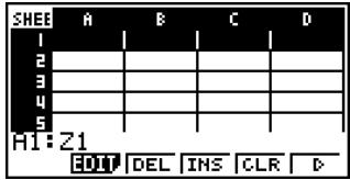
- To select an entire column
While the cell cursor is located in any cell of Line 1, press the ⬆ key. This will select the entire column where the cell cursor is located.
If the cell cursor is located at cell A1, for example, pressing ⬆ will select all of column 1 (A1 to A999). The edit box will show "A1:A999".
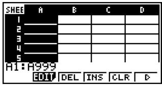
- To select all of the cells in a spreadsheet
Perform either of the following two operations.
- While all of the cells of Column A are selected, press ◀.
- While all of the cells of Line 1 are selected, press ▲.
When all cells are selected, the edit box will show the file name of the currently open spreadsheet.
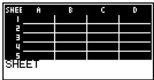
- For this example, the file name of the spreadsheet is "SHEET".

• To select a range of cells
- Move the cell cursor to the start cell of the range you want to select.
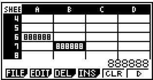
-
Press SHIFT 8 (CLIP).
-
This will cause the cell cursor to change from highlighting to a thick-line boundary.
- As you move the cell cursor, the edit box will show the range of cells that are currently selected.
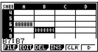
- Use the cursor keys to move the cell cursor to the end cell of the range you want to select.
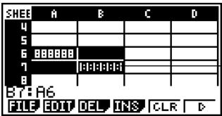
Selected cells are highlighted.
- To cancel cell selection, press EXIT. If you do, the cell cursor will be located at the end cell of the range you selected.

# Pressing SHIFT 8 (CLIP) while an entire line is selected, that line will be the selection range start point. You can use the ▲ and ▼ cursor keys to select additional lines.
# Pressing SHIFT 8 (CLIP) while an entire column is selected, that column will be the selection range start point. You can use the ◀ and ▶ cursor keys to select additional columns.

9-4 Inputting and Editing Cell Data
This section explains how to input and edit formulas, text, and other spreadsheet cell data. It covers how to copy, insert, and delete cells.
Note that the S·SHT mode does not support complex number data.
■ Basic Cell Data Input
You need to enter the edit mode in order to input data into a cell. There are two different methods you can use to enter the edit mode, and the method you should use depends on whether you want to input new data or edit the cell's existing data.
| When you want to do this: | Use this method: |
| Replace the cell’s current contents with your new input. | Select the cell and then start inputting. |
| Retain the cell’s current contents to edit or add to it. | Select the cell and then press F2 (EDIT) F3 (CELL). Next, edit the cell contents as desired. |
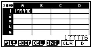
Normally, the contents of the cell where the cell cursor is located are displayed flush right in the edit box (input and editing disabled).

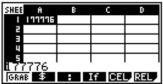
In the edit mode, the cell's contents change to flush left, to indicate that input and editing are enabled.

- To replace a cell's current contents with new input
- Move the cell cursor to the cell where you want to input data.
- Input the desired data.
Use the calculator's keys to input values, math expressions, or text, and the function menus to input commands.
- The calculator enters the edit mode as soon as you start input, so your input appears flush left in the edit box.
- The input cursor is located at the current input position. You can move the input cursor using the left and right cursor keys.
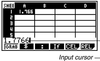
-
After everything is the way you want, press EXE.
-
Pressing EXE will cause the cell cursor to move to the next cell. You can specify movement to the next line or to the next column using the "Move" setting on the Setup screen (page 1-7-5).
- If "Auto Calc" is turned on (page 1-7-5), all of the formulas in the spreadsheet will be re-calculated when you press EXE.
- To cancel data input, press EXIT. This will return the cell contents to what they were before you started inputting data.
- To edit the current contents of a cell
- Move the cell cursor to the cell where you want to edit data.
- This will display the contents of the cell, flush right, in the edit box.
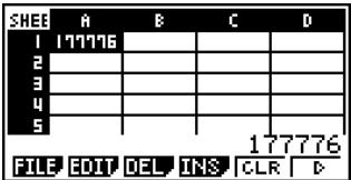

2. Press F2 (EDIT) F3 (CELL).
- This will enter the edit mode, which is indicated by the cell contents in the edit box changing to flush left. The input cursor also will appear to the left of the first character of the edit box.
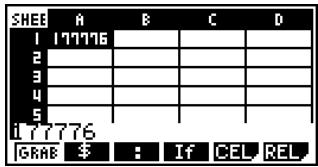
3. Edit the data in the edit box.
4. After everything is the way you want, press EXE.
- If "Auto Calc" is turned on (page 1-7-5), all of the formulas in the spreadsheet will be re-calculated when you press EXE.
- To cancel data input, press EXIT. This will return the cell contents to what they were before you started editing them.
■ Inputting a Formula
A formula is an expression that the S·SHT mode calculates and evaluates when you input it, when data related to the formula is changed, etc.
A formula always starts with an equal sign (=), and can contain any one of the following.
- Values
• Mathematical expressions - Cell references
- Calculator built-in function commands (page 2-4-1)
- S·SHT mode commands (page 9-5-1)
If “Auto Calc” is turned on (page 1-7-5), formulas are calculated dynamically whenever related values are changed, and the latest result is always displayed in the spreadsheet.
The following shows a simple example where a formula in cell B5 calculates the average of the values in cells B1 through B3.
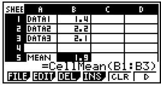

- Formula Input Example
In this example, we will input the 60 into cell A1, and then input the following formulas into the indicated cells: B1: =sin(A1), B2: =cos(A1), B3: =tan(A1), B4: =B1/B2
We will also show that the values produced by B3 and B4 are the same even if we change the value of A1, so (x) ÷ (x) = (x) holds true.
Note
- This example assumes that the calculator is configured as follows.
The "Move" setting on the Setup screen (page 1-7-5) is "Low" (initial default). The "Angle" setting on the Setup screen is "Deg".
- This example also uses cell referencing. For more information about cell referencing, see page 9-4-5.
- To input formulas
- Move the cell cursor to cell A1, and then input 6 0 EXE.
- Move the cell cursor to cell B1, and then input the following.
SHIFT • (=) sin ALPHA X,θ,T (A) 1 EXE
- Pressing EXE will cause the cell cursor to move to cell B2.
- Perform the following procedures to input the formulas for cells B2 through B4.
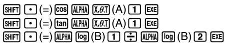
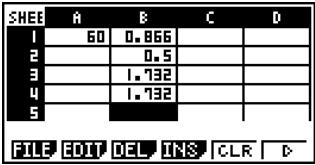
- Move the cell cursor to cell A1, and then input 3 0 EXE.
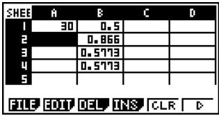
- This will cause the updated values to appear in cells B1 through B4, based on re-calculation using the new value you input in cell A1. Since the values produced by B3 and B4 are the same even if we change the value of A1, (x) ÷ (x) = (x) holds true.

■ Using Cell References
A cell reference is a symbol that references the value of one cell for use by another cell. If you input “=A1+B1” into cell C2, for example, the Spreadsheet will add the current value of cell A1 to the current value of cell B1, and display the result in cell C2.
There are two types of cell references: relative and absolute. It is very important that you understand the difference between relative and absolute cell references. Otherwise, your spreadsheet may not produce the results you expect.
Relative Cell References
A relative cell reference is one that changes according to its location on the spreadsheet. The cell reference “=A1” in cell C2, for example, is a reference to the cell located “two columns to the left and one cell up” from the current cell (C2, in this case). If we copy the contents of cell C2 and paste them into cell D12, for example, the cell reference will change automatically to “=B11”, because B11 is two columns to the left and one cell up from cell D12.
Be sure to remember that relative cell references always change dynamically in this way whenever you move them using copy and paste.
Important!
When you copy a relative cell reference from the edit box, it is copied to the clipboard as text and pasted "as-is" without changing. If "=A1" is in cell C2 and you copy "=A1" from the edit box and paste it into cell D12, for example, D12 will also be "=A1".
Absolute Cell References
An absolute cell reference is the one that does not change, regardless of where it is located or where it is copied to or moved to. You can make both the row and column of a cell reference absolute, or you can make only the row or only the column of a cell reference absolute, as described below.
| This cell reference: | Does this: |
| A1 | Always refers to column A, row 1 |
| A1 | Always refers to column A, but the row changes dynamically when moved, as with a relative cell reference |
| A1 | Always refers to row 1, but the column changes dynamically when moved, as with a relative cell reference |
Let's say, for example, that a reference to cell A1 is in cell C1. The following shows what each of the above cell references would become if the contents of cell C1 were copied to cell D12.
$$ \A\ 1 \rightarrow \A\ 1 $$
$$ \begin{array}{l}\text {A1} \rightarrow \text {A12}\end{array} $$
$$ \mathrm{A} 1 \rightarrow \mathrm{B} 1 $$

■ Referencing a Particular Cell
The following procedure shows how to reference A1 (which contains the value 3) and perform the calculation A1 × 2 .
• To reference a particular cell
- Move the cell cursor to cell A2, and then input SHIFT ☐ (=).
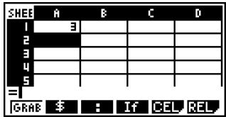
- Press F1 (GRAB).
- This enters the Grab mode, which changes the function menu to the function described below. The Grab mode function menu makes it easier to move the cursor around the spreadsheet.

| To move the cell cursor to here: | Press this key: |
| A specific cell | F2 (GO) |
| Line 1 of current column | F3 (TOP↑) |
| Column A of current line | F4 (TOP←) |
| Bottom line of current column | F5 (BOT↓) |
| Column Z of current line | F6 (BOT→) |
-
Press ⬆ to move the cell cursor to cell A1.
-
Press F1 (SET).
- This inputs the reference to cell A1.
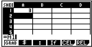

Instead of using the GRAB command (F1(GRAB) in step 2), you could also type in the necessary letter and number manually, if you want. In place of steps 2 through 4 in the
above procedure, you could input ALPHA ,,T (A) 1 to type “A1” if you want. For more information, see “Formula Input Example” (page 9-4-4).

- Next, input ☒ 2.
- Press EXE to store the formula.
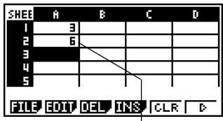
Result of A1 × 2
■ Referencing a Range of Cells
You can reference a range of cells to obtain their sum, mean, etc.
The following procedure input a formula to determine the sum of cells A6 through B7, and inputs the result in cell A4. This procedure assumes that cells A6 through B7 already contain the values shown below.
| A | B | |
| 6 | 1 | 2 |
| 7 | 3 | 4 |
• To reference a range of cells
- Move the cell cursor to cell A4, and then input SHIFT □ (=).
- Perform the following key operation to input the sum command.
F5 (CEL) F5 (Sum)
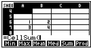
- "CellSum(" is a S·SHT mode command. See "9-5 S·SHT Mode Commands" for more information.
- Press EXIT F1 (GRAB).
• This enters the Grab mode.
- Use the cursor keys to move the cell cursor to the first cell of the range you want to select (A6 in this example).
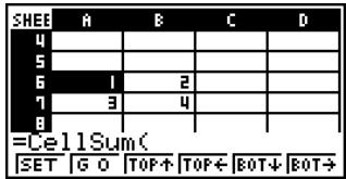

- Press SHIFT 8 (CLIP).
- This will cause the cell cursor to change from highlighting to a thick-line boundary.
- Use the cursor keys to move the cell cursor to the last cell of the range you want to select (B7 in this example).
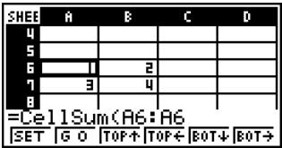
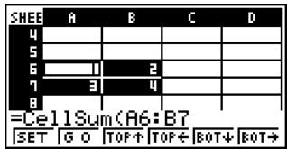
- You can use the function menu keys F2 through F6 for cell cursor movement. Available functions are those described in step 2 under “To reference a particular cell” (page 9-4-6).
- To register the range of cells, press F1 (SET).
- This will input the cell range (A6:B7).
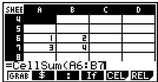
- Press EXE to store the formula.
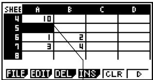
Indicates the sum of the values in cells A6 through B7.

# Instead of using the "CLIP" command (SHIFT 8 (CLIP) in step 5) to select a range of cells, you could also use the "GRAB" command and the ":" command. To use this method perform the following steps in place of steps 3 through 7 in the above procedure.
-
Press F1(GRAB) to enter the Grab mode.
-
Move the cell cursor to the first cell of the range (A6), and then press F1 (SET).
- This will exit the Grab mode and input a reference to cell A6.
-
Press F3(:).
-
Press F1(GRAB) to re-enter the Grab mode.
-
Move the cell cursor to the last cell of the range (B7), and then press F1(SET).
- This will input the cell range (A6:B7).

■ Inputting the Absolute Reference Symbol (\$)
You can input the absolute reference symbol at the current cursor position by pressing the F2 (\$) key of the edit mode function menu. See “Absolute Cell References” (page 9-4-5) for more information.
- To input the absolute reference symbol
● ● ● ● ●
Example To input =\A\1 into cell C1
- Move the cell cursor to cell C1, and then input SHIFT □ (=).
- Press F2 (\$).
- Press F1(GRAB) to enter the Grab mode, and move the cell cursor to cell A1.
- Press F1(SET).
- Press the ◀ key to move the cursor to the left of "1".
- Press F2 (\$).
- To register the formula, press EXE.


■ Inputting a Constant
An expression or value that you input without an equal (=) in front of it is called a “constant”, because the value is not affected by anything outside of the cell where it is located.
If you input a math expression as a constant, the cell shows its result. A “Syntax ERROR” will occur if an expression uses an incomplete or illegal syntax, or if its result is a list or matrix.
The following table shows various types of constants and the results they display.
| Constant | Displayed Result |
| 2005 | 2005 |
| 7+3 | 10 |
| sin 30 | 0.5 |
| X+1^*1 | 1.5 |
| AX * ^1*2 | 60 |
| dim {1,2,3} | 3 |
| 1=0 | 0 |
| 1>0 | 1 |
| sin | Syntax ERROR |
| {1,2,3} | Syntax ERROR |

*1 When 30 is assigned to variable X and 2 is assigned to variable A.
*2 A character string like AX is treated as a series of variables (page 2-2-1).
To have a character string treated as text, start it with a quote mark (").

■ Inputting Text
A text string starting with a quote mark (") is treated as text, and displayed as-is. The quote mark (") is not displayed as part of the text.
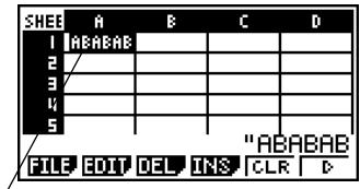
Up to six characters can be displayed by the cell.
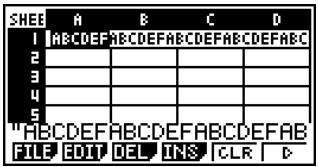
If the text cannot fit into a single cell, it extends into the next cell to the right, when the cell to the right is empty.
■ Generating a Numeric Sequence in a Spreadsheet
The following shows how to generate a numeric sequence (same procedure as the Seq command on page 3-2-3) and input the result automatically into a series of cells, starting from the cell you specify.
- To generate a numeric sequence in a spreadsheet
● ● ● ● ●
Example
To generate a numeric sequence starting from cell A1 using the following parameters
Function: f(x) = X^2
Variable: X
Starting Value: 1
Ending Value: 15
Increment: 7
-
Move the cell cursor to the cell from which you want the generated sequence to be input.
-
Press F2 (EDIT) F5 (SEQ).
- This will display a dialog box like the one shown to the right.
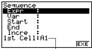
This is the cell you selected in step 1.
You can input a total of 249 bytes into the Expr, Var, Start, End, and Incre items of the Sequence dialog box.

3. Enter the required items to generate the sequence.
- The following describes the required input items.
| Item | Description |
| Expr | Function f(x) for generating the sequence |
| Var | Name of the variable in the function f(x) Even if a function has only one variable, its name must be defined here. |
| Start | The starting value (Start), ending value (End) and pitch (Incre) of the values assigned to the variable specified by Var |
| End | Specifying Start: 1, End: 15, and Incre: 7, for example, will generate a sequence by assigning the following values to the variable: 1, 8, 15. |
| Incre |
- Use the ⚠️ and ⬇ cursor keys to move between items, and input the required data for each one. The following shows how the screen should appear after your input the data required for this example.
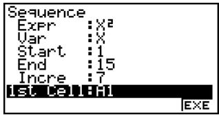
4. After inputting data for all the items, press F6(EXE) or the EXE key.
- This will cause the values of the generated sequence to be input into the spreadsheet starting from the cell you selected in step 1.
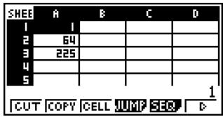

# If any cell that is within the range of cells where sequence values are input already contains data, the existing data is replaced with the sequence values.
# Sequence values are input into cells either line-wise or column-wise, depending on the "Move" setting on the Setup screen. The initial default setting is line-wise (top to bottom). For details, see "1-7 Using the Setup Screen".

■ Filling a Range of Cells with the Same Content
You can use the following procedure to fill a range of cells with the same formula, expression, value, or text.
- To fill a range of cells with the same content

Example
To use the "FILL" command to fill cells A2 through B3 with the formula = A1 + 1
The A1 cell name of the formula is a relative reference. This means the formula is = A1+1 in cell A2, = A2+1 in cell A3, etc.
In this example, it is assumed that 1 is already input into cell A1, and 2 is input into cell B1.
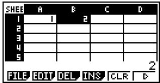
- Select the range of cells from A2 through B3.
- See “To select a range of cells” (page 9-3-4) for more information.
- Press F2 (EDIT) F6 (▷) F1 (FILL).
- This displays the Fill dialog box.
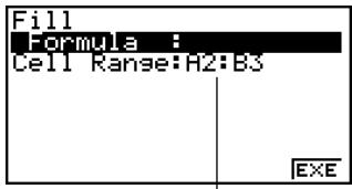
This is the range of cells you selected in step 1.
- While the "Formula" line is highlighted, enter the content you want to be filled into each of the cells in the selected range.
- Here we will enter “=A1+1”.

4. Press EXE.
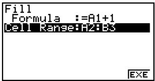
5. Press F6 (EXE) or the EXE key.
- This executes the "FILL" command and fills the specified content into the specified range of cells.

The A1 cell reference is a relative reference. The following shows the formulas that are actually input into each cell.
| A | B | |
| 2 | =A1+1 | =B1+1 |
| 3 | =A2+1 | =B2+1 |

# If any cell within the range of selected cells already contains data, the new fill data will replace the existing data.

■ Cut and Paste
You can use the procedures in this section to cut the data in one location of a spreadsheet and paste in another location. You can cut the contents of a single cell or a range of cells.
- How cut and paste affects cell references
The cut and paste operation has special rules that govern how cell references (page 9-4-5) within the cells being cut and pasted are handled. There are actually two different sets of rules to cover the following two conditions.
- When cells within the cut area are referencing cells that are outside the cut area
- When cells within the cut area are referencing cells that are also within the cut area
- When a cell within the cut area is referencing a cell that is outside the cut area
In this case all cell references are treated as absolute cell references, no matter what type they actually are (absolute or relative).

Example
Let's say we have a spreadsheet that contains the following data: A1: 4, B1: =A1+1, C1: =B1+2.
Cut B1:C1 (left screen) and paste the data in B2:C2 (right screen).
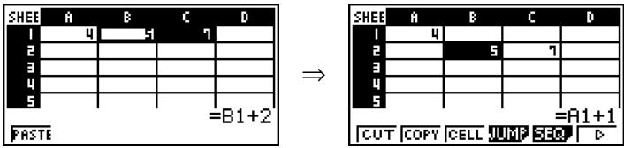
Since the expression in cell B1 references cell A1, which is outside the cut area (B1:C1), the A1 reference is pasted unchanged (like an absolute cell reference) into cell C2.

- When a cell within the cut area is referencing a cell that also is within the cut area
In this case all cell references are treated as relative cell references, no matter what type they actually are (absolute or relative).

Example
Let's say we have a spreadsheet that contains the following data:
A1: 4, B1: =A1+1, C1: = \B\1+2.
Cut B1:C1 (left screen) and paste the data in B2:C2 (right screen).
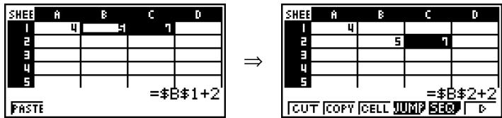
Since the expression in cell C1 references cell B1, which is also inside the cut area (B1:C1), the \B\1 reference changes to \B\2 (like a relative cell reference) when pasted into cell C2, even though it is an absolute cell reference.
- To cut and paste spreadsheet data
- Select the cell(s) you want to cut.
- See “To select a single cell” (page 9-3-2) and “To select a range of cells” (page 9-3-4) for more information.
-
Press F2 (EDIT) F1 (CUT).
-
This selects the data and enters the paste mode, which causes the F1 function key menu to change to (PASTE).
- You can exit the paste mode at any time during the following steps by pressing EXIT.

# For more information about absolute and relative cell references, see “Using Cell References” on page 9-4-5.

- Use the cursor keys to move the cell cursor to the cell from which you want to paste the data.
- If you selected a range of cells in step 1, the cell you select with the cell cursor will be the upper left cell of the paste range. If you cut the A1:B2 range of cells, locating the cell cursor at cell C1 will paste the cells at C1:D2.
- Press F1 (PASTE).
- This will clear the data from the cell(s) you selected in step 1 and paste it at the location you selected in step 3.
Copy and Paste
You can use the procedures in this section to copy the data in one location of a spreadsheet and paste in another location. You can copy the contents of a single cell or of a range of cells. Once you copy data, you can paste it multiple times in different locations.
- To copy and paste spreadsheet data
- Select the cell(s) you want to copy.
- See “To select a single cell” (page 9-3-2) and “To select a range of cells” (page 9-3-4) for more information.
- Press F2 (EDIT) F2 (COPY).
- This selects the data and enters the paste mode, which causes the F1 function key menu to change to (PASTE).
- You can exit the paste mode at any time during the following steps by pressing EXIT.

# If any cell in the paste area already contains data, the existing data is replaced by the pasted data.
# If pasted data includes a formula, the formula is always re-executed when you paste it. This is true regardless of whether the "Auto Calc" feature on the Setup screen (page 1-7-5) is on or off.
# If there are any relative cell references contained in the data you are pasting, they are handled in accordance with standard relative cell reference rules. See “Relative Cell References” (page 9-4-5) for more information.

- Use the cursor keys to move the cell cursor to the cell from which you want to paste the data.
- If you selected a range of cells in step 1, the cell you select with the cell cursor will be the upper left cell of the paste range. If you copy the A1:B2 range of cells, locating the cell cursor at cell C1 will paste the cells at C1:D2.
- Press F1 (PASTE).
- This will paste the data in the cells you selected in step 1 at the location you selected in step 3.
- The calculator will remain in the paste mode, so you could repeat steps 3 and 4 to paste the same data at other locations, if you want.
- After you are finish pasting the data where you want, press EXIT to exit the paste mode.

If any cell in the paste area already contains data, the existing data is replaced by the pasted data.
If a copy and paste operation causes a relative cell reference to become an illegal reference, the illegal reference will be replaced by “?” in the cell where it is pasted. Let’s say, for example, that you copy the contents of cell A3 (=A1+A2) and paste it in cell B2.
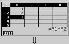
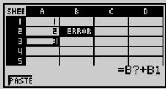
When the A1 relative cell reference in A3 (which effectively means “two cells up”) is pasted into cell B2, it becomes an illegal reference because there is no cell located two cells up from cell B2. This will cause the cell reference to change to “B?” when it is pasted in cell B2, and “ERROR” will be displayed in place of the cell B2 contents.
# If “On” is selected for the “Auto Calc” setting on the Setup screen (page 1-7-5), “ERROR” will appear as soon as the data is pasted. If “Auto Calc” is turned off, the contents of the cell will not be performed when they are pasted, so the destination cell (B2) will display the same data as the original source cell (A3) until the contents of the spreadsheet are re-calculated and updated.

■ Sorting Spreadsheet Data
Spreadsheet data can be sorted column-wise or line-wise. You can select either ascending sort or descending sort.
Important!
- Sorting can be performed only when the selected range of cells contains all constants.
- To sort spreadsheet data
- Select the series of cells in a single row or a single column that you want to sort.
- See “To select a range of cells” (page 9-3-4) for more information.
- Use the function menu to select the type of sort you want to perform.
Ascending: F2 (EDIT) F6 (▷) F2 (SRT•A)
Descending: F2 (EDIT) F6 (▷) F3 (SRT·D) - Selecting a sort type will sort the data.
■ Deleting and Inserting Cells
You can delete an individual cell, or an entire line or column of cells. You can also insert a line or column of blank cells when you need to.
- To delete an entire line or column of cells
- Select one or more cells inside the line(s) or column(s) you want to delete.
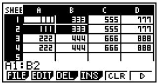
This cell selection can be used to delete lines 1 and 2 or columns A and B.
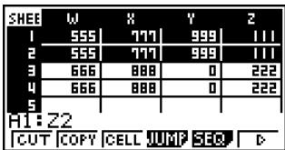
You could also select the entire line or column to be deleted. In this case, pressing F3 (DEL) in step 2 below will instantly delete the entire line or column, without displaying the DEL submenu.
- Press F3 (DEL) to display the DEL submenu.

# Data sorting is supported only for a single line or a single column of data. Attempting to perform a sort operation when multiple lines or multiples columns are selected will cause a "Range ERROR".
# A "Syntax ERROR" will occur if the data you are trying to sort contains a formula or text.

- Use the DEL submenu to perform the operation you want.
| When you want to do this: | Press this key: |
Delete the entire row(s) of the currently selected cell(s), and shift anything below upwards.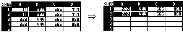 | F1(ROW) |
Delete the entire column(s) of the currently selected cell(s), and shift anything to the right leftwards.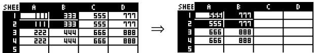 | F2(COL) |
- To exit the DEL submenu without deleting anything, press EXIT instead of a function key.
- To delete the contents of all the cells in a spreadsheet
- Press F3 (DEL) F3 (ALL).
![Delete All? Yes: [F1] No : [F6]](/content/2025/01/86785/images/c241cd35222df8f5f4bfe9be8e2fde215d120e7bfcb2875c67f4899a3c556cbd.jpg)
- In response to the confirmation message that appears, press F1(Yes) to delete the data, or F6(No) to cancel the delete operation without deleting anything.
- After deleting all data, the blank spreadsheet screen will appear with the cell cursor located at cell A1.

- To insert lines or columns of blank cells
- Select one or more cells to specify how many lines or columns you want to insert.
- Selection rules are the same as those for line and column deletion. See step 1 under "To delete an entire line or column of cells" (page 9-4-19) for more information.
- Press F4 (INS) to display the INS submenu.
- Use the INS submenu to perform the operation you want.
| When you want to do this: | Press this key: |
Insert the same number of rows as the currently selected rows, above the selected rows.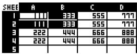 ⇒ ⇒ 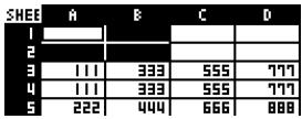 | F1(ROW) |
Insert the same number of columns as the currently selected columns, above the selected columns.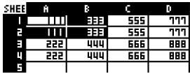 ⇒ ⇒ 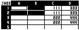 | F2(COL) |
- To exit the INS submenu without inserting anything, press EXIT instead of a function key.
- A Range ERROR occurs if a line or column insert operation causes the current cells to exceed the range of A1:Z999.
■ Clearing Cell Contents
Perform the following procedure when you want to clear the contents of specific cells.
• To clear cell contents
- Select the cell(s) whose contents you want to clear.
- Press F5 (CLR).
- This will clear the contents of the currently selected cells.

9-5 S·SHT Mode Commands
This section explains how to use the S·SHT mode commands.
- To input a S·SHT mode command
- Select the cells where you want to input the formula that contains the S·SHT mode command.
- Press F2 (EDIT) F3 (CELL) or SHIFT □ (=) to enter the edit mode.
- F2 (EDIT) F3 (CELL) can be used if the selected cell already contains data.
- Press the function menu key for the command you want to input.
| To input this command: | Press this key: | For details: | |
| CellIf( | (Condition) | F4 (If) | Page 9-5-2 |
| CellMin( | (Minimum of Cells) | F5 (CEL) F1 (Min) | Page 9-5-2 |
| CellMax( | (Maximum of Cells) | F5 (CEL) F2 (Max) | Page 9-5-3 |
| CellMean( | (Mean of Cells) | F5 (CEL) F3 (Mean) | Page 9-5-3 |
| CellMedian( | (Median of Cells) | F5 (CEL) F4 (Med) | Page 9-5-3 |
| CellSum( | (Sum of Cells) | F5 (CEL) F5 (Sum) | Page 9-5-4 |
| CellProd( | (Product of Cells) | F5 (CEL) F6 (Prod) | Page 9-5-4 |
- Input the other parameters.
- The additional parameters you need to input depend on the command you are using. For details, see “S • SHT Mode Command Reference” on page 9-5-2.

■ S·SHT Mode Command Reference
This section provides details about the function and syntax of each command, as well as practical examples of how to use them. Note that you can omit anything enclosed in brackets ([ ]) in the Syntax of each command.
- CellIf(
Function: Returns expression 1 when the equation or inequality is true, and expression 2 when it is false.
Syntax: CellIf( equation, expression 1, expression 2 [ ) ]
CellIf( inequality, expression 1, expression 2 [ ) ]
Example: If the value in cell A1 is greater than the value in cell B1, input the value of cell A1 into cell A2. Otherwise, input the value of cell B1 into cell A2.
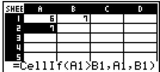
- CellMin(
Function: Returns the lowest value contained in the range of specified cells.
Syntax: CellMin( start cell : end cell [ ) ]
Example: To determine the lowest value in the block whose upper left corner is located at A3 and whose lower right corner is located at C5, and input the result in cell A1:
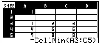

- CellMax(
Function: Returns the greatest value contained in the range of specified cells.
Syntax: CellMax( start cell : end cell [ ) ]
Example: To determine the greatest value in the block whose upper left corner is located at A3 and whose lower right corner is located at C5, and input the result in cell A1:
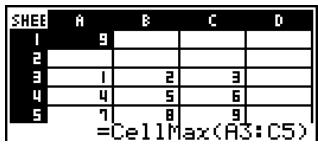
- CellMean(
Function: Returns the mean of the values contained in the range of specified cells.
Syntax: CellMean( start cell : end cell [ ) ]
Example: To determine the mean of the values in the block whose upper left corner is located at A3 and whose lower right corner is located at C5, and input the result in cell A1:
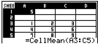
- CellMedian(
Function: Returns the median of the values contained in the range of specified cells.
Syntax: CellMedian( start cell : end cell [ ) ]
Example: To determine the median of the values in the block whose upper left corner is located at A3 and whose lower right corner is located at C5, and input the result in cell A1:
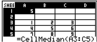

- CellSum(
Function: Returns the sum of the values contained in the range of specified cells.
Syntax: CellSum( start cell : end cell [ ) ]
Example: To determine the sum of the values in the block whose upper left corner is located at A3 and whose lower right corner is located at C5, and input the result in cell A1:
| SHEE | A | B | C | D |
| 1 | 45 | |||
| 2 | ||||
| 3 | 1 | 2 | 3 | |
| 4 | 4 | 5 | 6 | |
| 5 | 7 | 8 | 9 |
- CellProd(
Function: Returns the product of the values contained in the range of specified cells.
Syntax: CellProd( start cell : end cell [ ) ]
Example: To determine the product of the values in cells B3 through B5, and input the result in cell A1:
| SHEE | A | B | C | D |
| 1 | 80 | |||
| 2 | ||||
| 3 | 1 | 2 | 3 | |
| 4 | 4 | 5 | 6 | |
| 5 | 7 | 8 | 9 |

9-6 Statistical Graphs
This section explains how to graph the data in a spreadsheet.
Overview
Except for selection of the data to be graphed, the graph operations you can use in the S·SHT mode are basically the same as those in the STAT mode. This section explains the differences between the S·SHT mode graph functions and the STAT mode graph functions.
■ Using the Graph Menu
Press F6(▷)F1(GRPH) to display the GRPH submenu.
The functions on the GRPH submenu are the same as those that appear when you press F1 (GRPH) in the STAT mode List Editor. The following explains each function and where you need to go to find out more for them.
| Key | Description | Go here for more details: |
| F1(GPH1) | Draws a graph in accordance with StatGraph1 settings (see F6 (SET) below). | “Changing Graph Parameters” (page 6-1-2) |
| F2(GPH2) | Draws a graph in accordance with StatGraph2 settings (see F6 (SET) below). | |
| F3(GPH3) | Draws a graph in accordance with StatGraph3 settings (see F6 (SET) below). | |
| F4(SEL) | Displays a screen for selecting the graph parameter setup (StatGraph1, StatGraph2, or StatGraph3). You can also use the screen to specify simultaneous drawing of multiple graphs. | “2. Graph draw/non-draw status” (page 6-1-4) |
| F6(SET) | Displays a screen for configuring graph parameter settings (data to be graphed, graph type, etc.) The setting screen lets you configure separate settings for StatGraph1, StatGraph2, and StatGraph3. | “1. General graph settings” (page 6-1-2)“Configuring Graph Parameter Settings” (page 9-6-2) |
The functions of function menu keys F1 through F4 are basically the same as the STAT mode function menu. Some of the functions on the menu that appears when you press F6 (SET) here are different from those that appear when you press F6 (SET) in the STAT mode. For details about the differences, see “Configuring Graph Parameter Settings” on page 9-6-2.

■ Configuring Graph Parameter Settings
Pressing F6 (SET) on the GRPH submenu displays a graph settings screen like the one shown below.
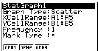
In the STAT mode, you can graph data input with the List Editor. In the S·SHT mode, you can graph the data input into the spreadsheet cells. Because of this, the purpose of S·SHT mode graph settings is to select the range of cells that contain the data to be graphed. The purpose of STAT mode settings, on the other hand, is to specify the number of the list (List 1 through List 26) where the data to be graphed is located.
The following describes the Spreadsheet graph settings you can configure on the graph settings screen.
- XCellRange (range x -axis data cells)
- {Cell} ... {the specified cell range data corresponds to x -axis data}
- YCellRange (range y-axis data cells)
- {Cell} ... {the specified cell range data corresponds to y-axis data}
- Frequency (number of times a value occurs)
- {1} ... {specifies 1 as the frequency of the values in the cell ranges specified by XCellRange and YCellRange}
- {Cell} ... {range of cells that specify the frequency for each cell specified by XCellRange and YCellRange}
For example, if XCellRange = A3:A5, YCellRange = B3:B5, and Frequency = C3:C5, the frequency of A3 and B3 will be the value in C3, the frequency of A4 and B4 will be C4, and so on.
For information on other settings, see “1. General graph settings” on page 6-1-2.

■ Graphing Statistical Data
The following shows an actual example of how to graph statistical data in the S·SHT mode. It also explains various methods you can use to specify the range of cells that contains the graph data.
• To graph statistical data

Example: Input the following data into a spreadsheet, and then draw a scatter diagram.
| Height | Shoe Size | |
| A | 155 | 23 |
| B | 165 | 25.5 |
| C | 180 | 27 |
| D | 185 | 28 |
| E | 170 | 25 |
- Input the statistical data into a spreadsheet.
- Here, we will input the above data into the cell range A1:B5.
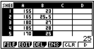
- Select the cell ranges you want to graph.
• Here we will select the range A1:B5.
-
Press F6(▷)F1(GRPH) to display the GRPH submenu.
-
Press F6 (SET).
- This displays the StatGraph1 settings screen. The first column of cells you selected in step 2 will be displayed for XCellRange, while the second column will be displayed for YCellRange.
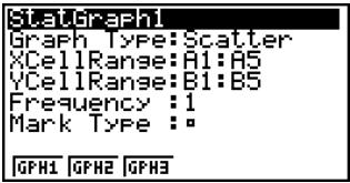
- You can change the XCellRange and YCellRange settings manually, if you want. For details, see “Configuring Range Settings for Graph Data Cells” (page 9-6-5).

-
Configure the graph setup settings.
-
For information about configuring the Graph Type and Mark Type settings, see "1. General graph settings" on page 6-1-2, "6-2 Calculating and Graphing Single-Variable Statistical Data", and "6-3 Calculating and Graphing Paired-Variable Statistical Data".
-
For information about configuring the Frequency setting, see “Configuring the Frequency Setting” (page 9-6-6).
-
After all of the settings are the way you want, press EXIT to exit the graph settings screen.
-
Press F1(GPH1).
- This will draw a graph in accordance with the StatGraph1 settings.
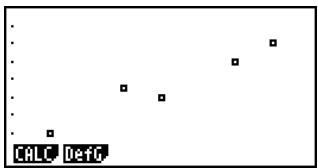
scatter
| x | y | |---|---| | 1 | 0.5 | | 2 | 0.7 | | 3 | 0.6 | | 4 | 0.8 | | 5 | 0.9 | | 6 | 1.0 | | 7 | 1.1 | | 8 | 1.2 | | 9 | 1.3 | | 10 | 1.4 | | 11 | 1.5 | | 12 | 1.6 | | 13 | 1.7 | | 14 | 1.8 | | 15 | 1.9 | | 16 | 2.0 | | 17 | 2.1 | | 18 | 2.2 | | 19 | 2.3 | | 20 | 2.4 | | 21 | 2.5 | | 22 | 2.6 | | 23 | 2.7 | | 24 | 2.8 | | 25 | 2.9 | | 26 | 3.0 | | 27 | 3.1 | | 28 | 3.2 | | 29 | 3.3 | | 30 | 3.4 | | 31 | 3.5 | | 32 | 3.6 | | 33 | 3.7 | | 34 | 3.8 | | 35 | 3.9 | | 36 | 4.0 | | 37 | 4.1 | | 38 | 4.2 | | 39 | 4.3 | | 40 | 4.4 | | 41 | 4.5 | | 42 | 4.6 | | 43 | 4.7 | | 44 | 4.8 | | 45 | 4.9 | | 46 | 5.0 | | 47 | 5.1 | | 48 | 5.2 | | 49 | 5.3 | | 50 | 5.4 | | 51 | 5.5 | | 52 | 5.6 | | 53 | 5.7 | | 54 | 5.8 | | 55 | 5.9 | | 56 | 6.0 | | 57 | 6.1 | | 58 | 6.2 | | 59 | 6.3 | | 60 | 6.4 | | 61 | 6.5 | | 62 | 6.6 | | 63 | 6.7 | | 64 | 6.8 | | 65 | 6.9 | | 66 | 7.0 | | 67 | 7.1 | | 68 | 7.2 | | 69 | 7.3 | | 70 | 7.4 | | 71 | 7.5 | | 72 | 7.6 | | 73 | 7.7 | | 74 | 7.8 | | 75 | 7.9 | | 76 | 8.0 | | 77 | 8.1 | | 78 | 8.2 | | 79 | 8.3 | | 80 | 8.4 | | 81 | 8.5 | | 82 | 8.6 | | 83 | 8.7 | | 84 | 8.8 | | 85 | 8.9 | | 86 | 9.0 | | 87 | 9.1 | | 88 | 9.2 | | 89 | 9.3 | | 90 | 9.4 | | 91 | 9.5 | | 92 | 9.6 | | 93 | 9.7 | | 94 | 9.8 | | 95 | 9.9 | | 96 | 10.0 | | Note: The actual values may vary due to the random nature of the data generation.
■ Configuring Range Settings for Graph Data Cells
The XCellRange and YCellRange settings on the graph settings screen are configured automatically in accordance with the cells you select on the spreadsheet. You can use the procedure below to change these settings manually, if you want.
Note that the automatic XCellRange and YCellRange settings always specify a series of lines in a specific column. With manual settings, you can specify a series of lines in a specific column, or a series of columns in a specific line.
- To change the XCellRange and YCellRange settings manually
- Press F6 (SET) on the GRPH submenu to display the graph settings screen.
- Use the ▲ and ▼ cursor keys to move the highlighting to XCellRange.
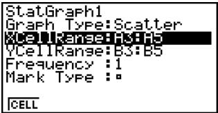
-
Press F1 (CELL) or simply input something.
-
Pressing F1 (CELL) will display the current XCellRange setting (A3:A5 in this example) with an input cursor, so you can edit it.
- If you simply input something, the current cell range setting will be replaced by what you input.
-
The function menu will change to the colon (:).
-
Input or edit the cell range.
- To input the colon, press F1(:).
- After the XCellRange setting is the way you want, press EXIT ▼ to move to the YCellRange setting, and then perform steps 3 through 4 to configure its setting.
- After all the settings are the way you want, press EXIT.

■ Configuring the Frequency Setting
The frequency is a value that specifies how many times each of the statistical data items is repeated. A value of 1 is the initial default for this setting. With this setting, each data item (x) or data pair (x, y) is represented as one point on the graph.
In cases where there is a large amount of data, however, plotting one point per data item (x) or data pair (x, y) can cause the graph to become cluttered and difficult to read. If this happens, you can specify a frequency value for each data item, which will reduce the number of plots of very frequent data items and make the graph easier to read.
- To specify the frequency of each data item
- Input the frequency values on the spreadsheet.
- For this example, input the frequency values for the example data on page 9-6-3.
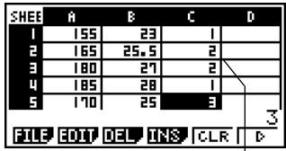
Frequency column (C)
- Press F6 (SET) on the GRPH submenu to display the graph settings screen.
- Use the ▲ and ▼ cursor keys to move the highlighting to Frequency.
- Press F2 (CELL).
- This enables cell range input for the Frequency setting. The function menu will change to the colon (:).
- Input the range of the cells that specify the frequencies (C1:C5 in this example).
- To input the colon (:), press F1(:).
- After the setting is the way you want, press EXIT.

9-7 Using the CALC Function
This section explains how to use the CALC function to perform statistical calculations on spreadsheet data.
Overview
Except for selection of the data, the statistical calculation operations you can use in the S·SHT mode are basically the same as those in the STAT mode. This section explains the differences between the S·SHT mode statistical calculation functions and the STAT mode statistical calculation functions.
- Displaying the CALC Submenu
Press F6(▷)F2(CALC) to display the CALC submenu.
The functions on the CALC submenu are the same as those that appear when you press F2(CALC) in the STAT mode List Editor. The following explains each function and where you need to go to find out more for them.
| Key | Description | Go here for more details: |
| F1(1VAR) | Press to perform single-variable statistical calculations. | “Single-Variable Statistical Calculations” (page 6-4-2) |
| F2(2VAR) | Press to perform paired-variable statistical calculations. | “Paired-Variable Statistical Calculations” (page 6-4-2) |
| F3(REG) | Press to perform regression calculations. | “Regression Calculation” (page 6-4-3) |
| F6(SET) | Displays a screen for specifying data to be used for the statistical calculations performed by pressing F1(1VAR), F2(2VAR), and F3(REG). | “Configuring Statistical Calculation Data Settings” (page 9-7-2) |
The functions of function menu keys F1 through F3 are basically the same as the STAT mode function menu. The settings you can configure with F6 (SET) are different from those in the STAT mode.

■ Configuring Statistical Calculation Data Settings
To execute a statistical calculation in the S·SHT mode, you need to input the data on the spreadsheet and define the range of cells where the data is located as statistical calculation cells. To define statistical calculation cells, press F6 (SET) on the CALC submenu and settings screen shown below.
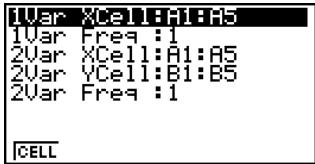
The following explains the each of the items on this screen.
- 1Var XCell (x-variable cell range for single-variable statistical calculations)
- {Cell} ... {specifies the cell range of x -variable values for single-variable statistical calculations}
• 1Var Freq (value frequency)
- {1} ... {specifies 1 as the frequency of the values in the cell range specified 1Var XCell}
- {Cell} ... {range of cells that specify the frequency for each cell specified by 1Var XCell}
- 2Var XCell (x-variable cell range for paired-variable statistical calculations)
- {Cell} ... {specifies the cell range of x -variable values for paired-variable statistical calculations}
- 2Var YCell (y-variable cell range for paired-variable statistical calculations)
- {Cell} ... {specifies the cell range of y-variable values for paired-variable statistical calculations}
- 2Var Freq (value frequency)
- {1} ... {specifies 1 as the frequency of the values in the cell range specified 2Var XCell and 2Var YCell}
- {Cell} ... {range of cells that specify the frequency for each cell specified by 2Var XCell and 2Var YCell}

■ Executing a Statistical Calculation
The following shows an actual example of how to perform a statistical calculation in the S·SHT mode.
- To execute a statistical calculation
● ● ● ● ●
Example
To input the data shown below into a spreadsheet, and then to perform paired-variable statistical calculations and regression calculations
| Height | Shoe Size | Frequency | |
| A | 155 | 23 | 1 |
| B | 165 | 25.5 | 2 |
| C | 180 | 27 | 2 |
| D | 185 | 28 | 1 |
| E | 170 | 25 | 3 |
- Input the statistical data into a spreadsheet.
- Here, we will input data in the A1:B5 range, and the frequency values in the C1:C5 range.
- Select the range of cells where you input the data (A1:B5).
- Press F6 (▷) F2 (CALC) to display the CALC submenu.
-
Press F6 (SET) to display the statistical calculation settings screen.
-
The first column of cells you selected in step 2 will be displayed for 1Var XCell, while the second column will be displayed for 2Var YCell.
-
You can change the cell ranges manually using the same procedures as those for the graphing cell range settings. See “To change the XCellRange and YCellRange settings manually” (page 9-6-5) for more information.
-
Use the ▲ and ▼ cursor keys to move the highlighting to 2Var Freq.
- Press F2 (CELL).
- This enables cell range input for the Frequency setting. The function menu will change to the colon (:).
- Input the range of cells for the frequency values (C1:C5).
- To input the colon (:), press F1(:).
- After the settings are the way you want, press EXE.

9. Press EXIT F2 (2VAR).
- This will display the paired-variable statistical calculation result list. You can use the up and down cursor keys to scroll the result screen.
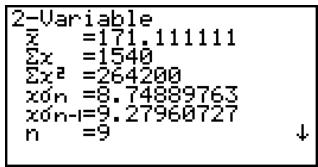
- For information about the meaning of each of the values on the result screen, see “Displaying the Calculation Results of a Drawn Paired-Variable Graph” on page 6-3-11.
10. Press EXIT F3 (REG) F1 (X).
- This will display the linear regression coefficients for the original data.
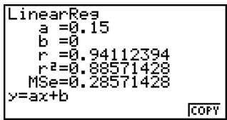
- For information about the meaning of each of the coefficient values on this screen, see “Linear Regression Graph” on page 6-3-6.
11. Press EXIT to return to the spreadsheet screen.

9-8 Using Memory in the S·SHT Mode
This section explains how to save spreadsheet data to memory, and how to import memory data into a spreadsheet.
■ Saving Spreadsheet Data
You can assign spreadsheet data to a variable, or save it to List Memory, File Memory, or Mat Memory.
■ Assigning Spreadsheet Data to a Variable
You can use the following procedure to assign the contents of a single cell to a variable (A to Z, r, or ).
- To assign the contents of a cell to a variable
- Move the cell cursor to the cell whose data you want to assign to a variable.
- Press F6 (▷) F3 (STO) F1 (VAR).
- The “Cell” setting will show the name of the cell you selected in step 1.
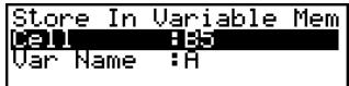
- Press ▼ to move the highlighting to "Var Name".
- Input the variable name (A to Z, r, or ), and then press EXE.
- Press F6(EXE) or the EXE key to assign the data to the variable.
- If the variable you select already has data assigned to it, the new data will replace the existing data.

# With all types of memory, saving a cell that includes a formula will save the calculation result.
# If the cell you select is empty, contains text, or has ERROR displayed for it, an error will occur when you perform step 5 of the above procedure.

■ Saving Spreadsheet Data to List Memory
You can use the following procedure to select a series of cells in a particular column or row and save their data to List Memory (List 1 through List 26).
- To save the contents of a range of cells to List Memory
- Select the range of cells whose data you want to save in List Memory.
- You can select a series of cells in a column or a series of cells in a line. Selecting any other configuration of cells will cause an error.
- Press F6 (▷) F3 (STO) F2 (LIST).
- The “Cell Range” setting will show the range of cells you selected in step 1.
![Store In List Memory Cell Range: H1H01 List[1~26]:1](/content/2025/01/86785/images/7f309077ff63eae48cb58773cb40e0e5cefe11a6b0ec31e46156266585f84f2d.jpg)
- Press ▼ to move the highlighting to "List [1\~26]".
- Enter a list number in the range of 1 to 26, and then press EXE.
- Press F6(EXE) or the EXE key to save the data in the List Memory.
- If the List Memory you select already has data assigned to it, the new data will replace the existing data.
■ Saving Spreadsheet Data to File Memory
You can use the following procedure to select a range of cells and save their data to File Memory (File 1 through File 6). Data is saved sequentially from left to right, line by line, and each column is saved as a File Memory list (List 1 through List 26).
The following shows how spreadsheet data in the range of A1:C3 is saved to File 6.
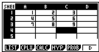
Spreadsheet

| File6 | ||
| List1 | List2 | List3 |
| 1 | 2 | 3 |
| 4 | 5 | 6 |
| 7 | 8 | 9 |
File Memory

# The value in any cell that is empty, contains text, or has ERROR displayed is changed to 0 when you perform step 5 of the above procedure.

- To save the contents of a range of cells to File Memory
- Select the range of cells whose data you want to save in File Memory.
- Press F6 (▷) F3 (STO) F3 (FILE).
- The “Cell Range” setting will show the range of cells you selected in step 1.
![Store In File Memory Cell Range: H1H01 File[1~6] :1](/content/2025/01/86785/images/55a649485ae2afa9d8a3ca7732d3b4af33ae9b84a6189f2b8c67527892d11341.jpg)
- Press ▼ to move the highlighting to "File [1\~6]".
- Enter a file number in the range of 1 to 6, and then press EXE.
- Press F6(EXE) or the EXE key to save the data in the File Memory.
- If the File Memory you select already has data assigned to it, the new data will replace the existing data.
■ Saving Spreadsheet Data to Mat Memory
You can use the following procedure to save the contents of a range of cells to Mat Memory (A to Z).
- To save the contents of a range of cells to Mat Memory
- Select the range of cells whose data you want to save in Mat Memory.
- Press F6 (▷) F3 (STO) F4 (MAT).
- The “Cell Range” setting will show the range of cells you selected in step 1.

- Press ▼ to move the highlighting to "Mat Name".
- Input the Mat Memory name (A to Z) where you want to save the date.
- Press F6(EXE) or the EXE key to save the data in the Mat Memory.
- If the Mat Memory you select already has data assigned to it, the new data will replace the existing data.

# The value in any cell that is empty, contains text, or has ERROR displayed is changed to 0 when you perform step 5 of the above procedure.

■ Recalling Data from Memory
The procedures in this section explain how to recall data from List Memory, File Memory, and Mat Memory, and input it into a spreadsheet starting from a specific cell. It also explains how to use variables in spreadsheet constants and formulas.
Note
When recalling List Memory, File Memory, or Mat Memory data, an error will occur if the recalled data runs outside the allowable range of the spreadsheet (A1:Z999).
Recalling a 2-line by 4-column matrix from Mat Memory starting from spreadsheet cell X2, for example, will cause the matrix to run outside the range of the spreadsheet as shown below, which will cause an error.
The above also applies when pasting data into a spreadsheet.
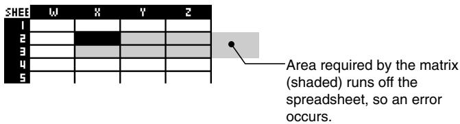
■ Recalling Data from List Memory
Use the procedure in this section to select a List Memory (List 1 through List 26) and input it into a spreadsheet. The data is input into the spreadsheet either line-wise or column-wise, depending on the current “Move” setting on the Setup screen.
Note
The initial default “Move” setting is line-wise (top to bottom) data input. If you want to perform column-wise (left to right) input, change the “Move” setting. For details, see “1-7 Using the Setup Screen”.
- To recall data from a List Memory to a spreadsheet
- On the spreadsheet, select the first cell of the range where you want the recalled data to be input.
- Press F6(▷)F4(RCL)F1(LIST) to display a data recall screen like the one shown below.
- The “1st Cell” setting will show the name of the cell you selected in step 1.
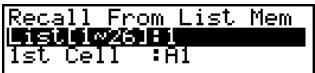
- Input the List number (1 to 26) of the List Memory whose data you want to recall, and then press EXE.
- Press F6(EXE) or the EXE key to recall the data.

- To recall data from a File Memory to a spreadsheet
- On the spreadsheet, select the upper left cell of the range where you want the recalled data to be input.
- Press F6(▷)F4(RCL)F2(FILE) to display a data recall screen like the one shown below.
- The “1st Cell” setting will show the name of the cell you selected in step 1.
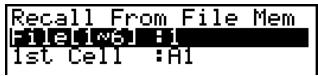
-
Input the File number (1 to 6) of the File Memory whose data you want to recall, and then press EXE.
-
Press F6(EXE) or the EXE key to recall the data.
- To recall data from a Mat Memory to a spreadsheet
- On the spreadsheet, select the upper left cell of the range where you want the recalled data to be input.
- Press F6(▷)F4(RCL)F3(MAT) to display a data recall screen like the one shown below.
- The “1st Cell” setting will show the name of the cell you selected in step 1.
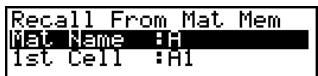
-
Input the name (A to Z) of the Mat Memory whose data you want to recall, and then press EXE.
-
Press F6(EXE) or the EXE key to recall the data.
- To use a variable in a spreadsheet
You can include variable names (A to Z) in constants or formulas you input into spreadsheet cells. When you do, the value currently assigned to the applicable variable to be recalled.
If 1 is assigned to variable A and 2 is assigned to variable B, for example, inputting =A+B into cell A1 will cause 3 to be displayed for cell A1.
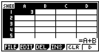

Chapter 10
eActivity
An eActivity is both a documentation tool and a student notebook. As a documentation tool, a teacher can create electronic examples and practice problems with accompanying text, mathematical expressions, graphs, and tables.
eActivities also provide the student the means to explore problems, document their learning and problem solving by entering notes, and share their learning by saving their work to a file.
10-1 eActivity Overview
10-2 Working with eActivity Files
10-3 Inputting and Editing eActivity File Data
10-4 Using Matrix Editor and List Editor
10-5 eActivity File Memory Usage Screen
10-1 eActivity Overview
eActivity lets you input and edit text, mathematical expressions, and application data, and save your input in a file called an “eActivity”.
■ Using the e·ACT Mode
On the Main Menu, select the e·ACT icon.
- This displays a file list screen like the ones shown below.
![eAct List [ ] No Files NEW SD](/content/2025/01/86785/images/0d5acf86fdd52bfd75b8a9562c7c6060d8faff571c885d30a7fabfb91554bc21.jpg)
When there are no files stored in the e·ACT mode
![[FOLDER2] CONICS : 740 GEO : 260 GRAPH : 600 INTEG : 640↓ OPEN NEW DEL SRC SD](/content/2025/01/86785/images/f113a30ce0167c829b211c6a3d6b4bfc950a57e2c8f5ffdd224511fcd6c3aaff.jpg)
When there are files stored in the e·ACT mode
■ File List Function Menu
The following describes the functions of the file list function menu.
- {OPEN} ... {opens the eActivity file or folder that is currently selected on the file list}
- {NEW} ... {creates a new eActivity file}
- {DEL} ... {deletes the eActivity file that is currently selected on the file list}
- {SRC} ... {starts a file search operation}
- {SD}/{SMEM} ... {changes the memory area} (fx-9860G SD only)
When the file list currently shows Storage Memory contents, the menu for this function key is “SD” (for switching to SD card contents). When SD card contents are displayed, the function key menu is “SMEM” (for switching to Storage Memory contents).

# When there are no eActivity files, only the F2 (NEW) and F6 (SD/SMEM) function keys are displayed.
# 128 Kbytes or more of free storage memory is required to enter the e·ACT mode the first time. A Memory ERROR will occur if there is not enough free memory available.

■ Workspace Screen Function Menu
Opening an eActivity file displays a workspace screen that shows the current contents of the eActivity.
The sample below shows the parts that make up the eActivity workspace. Note that not all of the eActivity can be displayed in a single screen. The heavy line in the example shows what is currently on the display, while the lighter line shows the part of the eActivity that is not displayed. You can view all of the parts of the eActivity by scrolling the screen contents upwards and downwards.
You can use the workspace screen in insert text, formulas, application data strips, and other data into an eActivity.
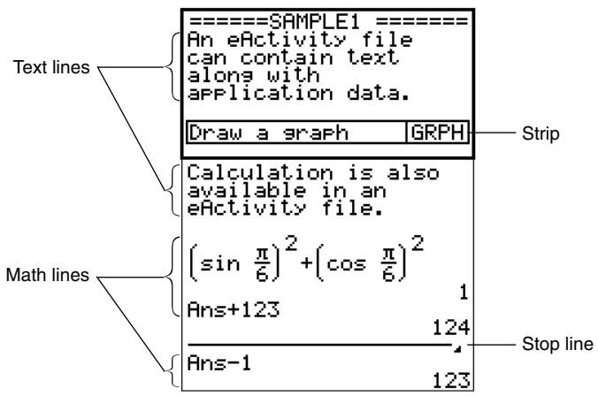
The content of the workspace function menu depends on the line (or strip) that is currently selected.

■ Text Line Function Menu
- {FILE} ... {displays the FILE submenu}
- {SAVE} ... {saves the file you are editing, overwriting the previous (unedited) version}
- {SV • AS} ... {saves the file you are editing under a new name (Save As)}
- {OPT} ... {performs Storage Memory or SD card garbage collection} For more information, see “Optimizing the Storage Memory or SD Card Memory” (page 12-7-17).
-
{CAPA} ... {displays the size of the currently open eActivity file and how much memory is available for use by the current file}
-
{STRP} ... {inserts a strip}
- {TEXT} ... {changes the current line from a text line to a math line}
- {CHAR} ... {displays a screen for selecting various mathematical symbols, special symbols, and accented characters}
- A a ... {toggles between upper-case and lower-case input} This function is available only during alpha input (page 1-1-3)
-
{JUMP} ... {displays the JUMP submenu}
-
{TOP} ... {moves the cursor to the top of the file}
-
{BTM} ... {moves the cursor to the bottom of the file}
-
{DEL • L} ... {deletes the line that is currently selected or where the cursor is located}
-
{INS} ... {displays an insert submenu for inserting a new line above the line that is currently selected or where the cursor is located}
-
{TEXT} ... {inserts a text line}
• {CALC} ... {inserts a math line} - {STOP} ... {inserts a stop line}
- {MATH} ... {displays a MATH menu for natural input of matrices and mathematical functions}
For more information, see “Using the MATH Menu” (page 1-3-10).
- ... {displays the Matrix Editor (page 2-8-2)}
- {▶LIST} ... {displays the List Editor (page 6-1-1)}

■ Math Line and Stop Line Function Menu
- {FILE} ... Same as {FILE} under "Text Line Function Menu" (page 10-1-3).
- {STRP} ... Same as {STRP} under "Text Line Function Menu" (page 10-1-3).
- {CALC} ... {changes the current line from a math line to a text line}
- {MATH} ... {displays a MATH menu for natural input of matrices and mathematical functions}
For more information, see “Using the MATH Menu” (page 1-3-10). - {INS} ... Same as {INS} under "Text Line Function Menu" (page 10-1-3).
- {JUMP} ... Same as {JUMP} under "Text Line Function Menu" (page 10-1-3).
- {DEL·L} ... {deletes the line that is currently selected or where the cursor is located} Note that deleting a math line deletes both the input expression and the result.
- {▶MAT} ... {displays the Matrix Editor (page 2-8-2)}
- {▶LIST} ... {displays the List Editor (page 6-1-1)}

■ Strip Function Menu
- {FILE} ... Same as {FILE} under "Text Line Function Menu" (page 10-1-3) except for {SIZE}.
- {SIZE} ... {displays the size of the strip that is currently selected or where the cursor is currently located}
- {STRP} ... Same as {STRP} under "Text Line Function Menu" (page 10-1-3).
- {INS} ... {inserts a new line above the currently selected strip}
- {TEXT} ... {inserts a text line}
- {CALC} ... {inserts a math line}
- {STOP} ... {inserts a stop line}
- {CHAR} ... Same as {CHAR} under "Text Line Function Menu" (page 10-1-3).
- A a ... Same as A a under "Text Line Function Menu" (page 10-1-3).
- {JUMP} ... Same as {JUMP} under "Text Line Function Menu" (page 10-1-3).
- {DEL • L} ... {deletes the strip that is currently selected or where the cursor is located}
- ... {displays the Matrix Editor (page 2-8-2)}
- {▶LIST} ... {displays the List Editor (page 6-1-1)}
■ Basic eActivity File Operations
This section provides an overview of the following eActivity operations.
- Creating a new eActivity file
- Inputting text, numeric expressions, strips, and other data
- Accessing applications from a strip and using the application's screen
- Saving an eActivity file
This overview is explained using the following example problem:
- Solve 2x^2 + x - 3 = 0 (extract the roots of y = 2x^2 + x - 3 ).
- Graph y = 2x^2 + x - 3 and confirm the above solution.
- Use G-SLV to extract the roots on the graph screen.

- From the main menu, enter the e·ACT mode.
-
Create a new eActivity file.
-
Press F2 (NEW).
-
On the dialog box that appears, enter up to eight characters for the eActivity file name, and then press EXE.
- This will display a blank workspace screen with a text line cursor (for text line input).
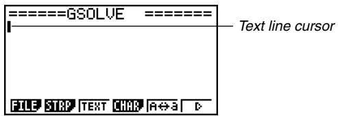
-
Use the text line to input to type in comments, information about the eActivity problem, etc.
-
Here we will input the text shown below.
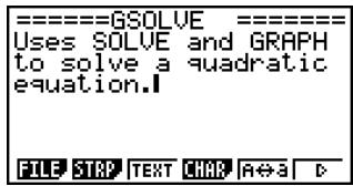
- Note that a text line does not perform auto word wrapping, so you need to insert carriage returns manually where you want them by pressing EXE.
- After inputting all of the text you want, press EXE.
-
This will cause the cursor to move from the end of the text to the beginning of the next line.
-
Use math lines to enter the expression (2x^2 + x - 3 = 0) and solve it.
For this example, we will use the Solve function, configuring it with the following settings.
Initial Estimated Value: 0
Lower Limit: 0
Upper Limit: 10
For details about using the Solve function, see page 8-6-9.
- First, press F3(TEXT) to change to a math line.
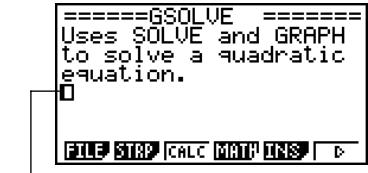
Math line cursor

- Specify the Solve calculation, and then enter the function.
AC OPTN F4 (CALC) F1 (Solve)
2 X,θ,T x² + X,θ,T - 3 ,
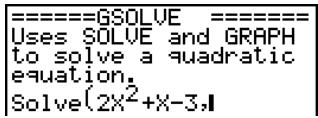
- Input the initial estimate value, the lower limit, and the upper limit.
0,0,10)
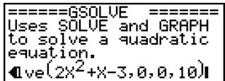
- Press EXE to solve for x.
- This will display the solution (x = 1) and move the cursor to the beginning of the next line.
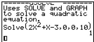
- Press EXIT twice to close the option (OPTN) menu.
5. Now to draw a graph, insert a Graph strip into the eActivity.
- Press F2 (STRP).
- This will display a dialog box with a list of insertable strips.
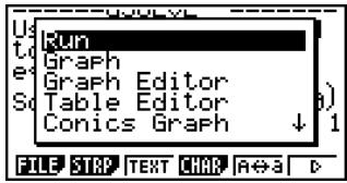
- On the list, select "Graph", and then press EXE.
- This will insert a Graph strip, ready for you to input a title.
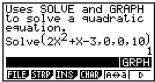
- Type a title for the list ("Graph draw" for this example), and then press EXE.
- This will register the title and highlight the strip.
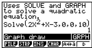

6. Graph the expression using the Graph strip.
- While the "Graph draw" Graph strip you created in step 5 is selected, press EXE.
- This will display a graph screen.
- Press SHIFT F6 (G↔T) to display the Graph Editor screen.
- In line Y1, input the function (y = 2x^2 + x - 3) you want to graph.
- Press F6 (DRAW) to graph the function.
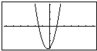
natural_image
Simple V-shaped curve drawn on a Cartesian coordinate system (no labels or text)- This will display a graph screen. Since the graph intersects the x -axis at -1.5 and 1 , we can conclude that the solution (x = 1) obtained in step 4 is valid. The -1.5 value was not included as a solution because we specified a lower limit of 0 .
-
The graph drawn here is stored in the strip we created in step 5.
-
To return to the eActivity workspace screen, press SHIFT → (💡).
7. Use G-SLV to extract the roots on the graph screen.
- Select the Graph strip we created in step 5, and then press EXE.
- This will display the graph screen and draw the graph we drew in step 6.
- Use G-SLV to extract the roots of y = 2x^2 + x - 3 .
SHIFT F5 (G-SLV) F1 (ROOT) .. (Extracts first root.)
▶ (Extracts next root.)
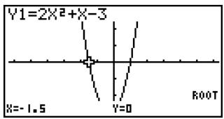
line
| Point | Value | |---|---| | Y1 | 2X² + X - 3 | | X | -1.5 | | Y | 0 | | ROOT | (labeled point) |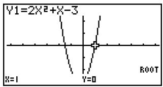
- For details about using G-SLV, see page 5-11-9.
- To return to the eActivity workspace screen, press SHIFT → (💡).
8. Save the eActivity file.
- Press F1(FILE)F1(SAVE) to save the file. This will save the file you are editing by replacing the currently stored version (if any).

10-2 Working with eActivity Files
This section explains the different file operations you can perform from the eActivity file list screen.
■ Selecting a Memory Area to Display its Files
Pressing the F6 function key toggles the eActivity list between Storage Memory and the SD card loaded in the card slot.
When the F6 function key menu is “SD”, it means that Storage Memory files are currently listed. When the menu is “SMEM”, it means that SD card files are listed.
![eAct List [ ] HCT1 : 372 ACT2 : 344 CONICS : 740 GEO : 260 GRAPH : 600 INTEG : 640↓ OPEN NEW DEL SRC SD](/content/2025/01/86785/images/d2f323c727510b4678f83bddf75f92d0e59a3f7a2f68feacab0712ae5ec29063.jpg)
Storage Memory file list
![eAct List [ ] HCT1 : 216 HCT2 : 248 CONICS : 644 GEO : 164 GRAPH : 504 INTEG : 544↓ OPEN NEW DEL SRC $MBM](/content/2025/01/86785/images/3b60608bfb62c84b8b8c2d023e8b9e34389a7753b004abea912e68d1d947544d.jpg)
SD card file list
■ eActivity File Operations
- To create a new file
- While the file list screen is displayed, use the F6 function key to select the memory area (Storage Memory or SD card) where you want to create the new file.
- If the eActivity workspace screen is displayed, press the EXIT key to display the file list. Then perform step 1.
- If you want to create the file in a specific folder, use ▲ and ▼ to highlight the folder you want, and then press F1 (OPEN) or EXE.
![eAct List [FOLDER1] HCT1 : 372 HCT2 : 344 CONICS : 740 GEO : 260 GRAPH : 600 INTEG : 640↓ OPEN NEW DEL SRC S.D.](/content/2025/01/86785/images/f6ad743a3d5b8708f83971cb3a36cd86da5ec57d7785d5501b7a4c4f546b1adf.jpg)

- You do not need to open a folder if you want to create the new file in the Storage Memory or SD card root directory.
-
For information about creating a new folder, see “Creating a Folder in Storage Memory or on an SD Card” (page 12-7-5).
-
Press F2 (NEW).
- This displays a dialog box for inputting a file name.
-
Enter up to eight characters for the eActivity file name, and then press EXE.
-
This displays a blank workspace screen.
- The following are the characters you can use in a file name: A through Z, {, }, ', \~, 0 through 9
eActivity Name [A]
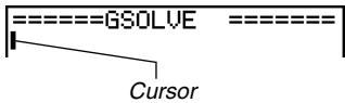
- To open a file
- While the file list screen is displayed, use the F6 function key to select the memory area (Storage Memory or SD card) that contains the file you want to open.
- If the file you want to open is in a folder, use ▲ and ▼ to highlight the folder, and then press F1 (OPEN) or EXE.
- Use ▲ and ▼ to highlight the file you want to open, and then press F1(OPEN) or EXE *1.
- This will open the file.

*1 If a memory error occurs in step 3, delete capture memory contents and clipboard data, or try moving the data to your computer's hard disk or an SD card.

- To delete a file
- While the file list screen is displayed, use the F6 function key to select the memory area (Storage Memory or SD card) that contains the file you want to delete.
-
If the file you want to delete is in a folder, use ▲ and ▼ to highlight the folder, and then press F1 (OPEN) or EXE.
-
Use ▲ and ▼ to highlight the file you want to delete, and then press F3 (DEL).
![Delete eActivity? Yes: [F1] No : [F6]](/content/2025/01/86785/images/3d3321cc7ecc6b8637ff30dce552c5f3eb5e8269a4d451f79bb5b81cf5fc3099.jpg)
- In response to the confirmation message that appears, press F1(Yes) to delete the file, or F6(No) to cancel the delete operation without doing anything.
- To search for a file
- While the file list screen is displayed, press F4 (SRC).
- This displays a file search dialog box.
Search [A]
- Enter part or all of the name of the file you want to find.
- Note that file name characters are searched from left to right. This means that if you enter “IT” here, names such as ITXX, ITABC, and IT123 will be hits, but names like XXIT and ABITC will not be hits.
- Press EXE.
- If a file name that corresponds to the text you input in step 2 is found, the name will appear highlighted on the file list.
![eAct List [ ] E10 : 2381 SAMPLE1 : 740 OPEN NEW DEL SRC SD](/content/2025/01/86785/images/5b602d651bcc818a3876923022dbb995abb232840342598c7512cfb8163f65a2.jpg)
- The message “Not Found” will appear if a match cannot be found. Press the EXIT key to close the message dialog box.

10-3 Inputting and Editing eActivity File Data
The following shows the type of eActivity file data you can input and edit.
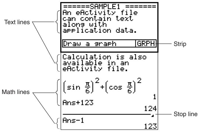
Text line
A text line can be used to input characters, numbers, and expressions as non-executable text.
Math lines
Math lines let you perform calculations in an eActivity. When you input a mathematical expression, the result appears, right justified, in the next line. You can perform the same operations as the ones you use in the RUN·MAT mode while “Math” is selected as the Input Mode.
Stop line
A stop line can be used to stop calculation at a particular point.
Strip
A strip can be used to embed data from Graph, Conics Graph, Spreadsheet, and other applications into an eActivity. There is also a Notes strip, which can be used to insert data from Notes, which is the eActivity text editor.

■ Navigating around the eActivity Workspace Screen
- To scroll the eActivity workspace screen vertically
The workspace screen can be scrolled line-by-line, or screen-by-screen.
- Pressing ⬆ while the cursor is in the top line of the workspace screen will scroll one line upwards. Pressing ⬇ while the cursor is in the bottom line will scroll one line downwards.
- To scroll screen-by-screen, press SHIFT ▲ or SHIFT ▼.
- To jump to the top or the bottom of the eActivity workspace screen
- To jump to the top of the screen, press F6 (▷) F1 (JUMP) F1 (TOP).
- To jump to the bottom of the screen, press F6 (▷) F1 (JUMP) F2 (BTM).
■ Using a Text Line
A text line can be used to input characters, numbers, and expressions as non-executable text.
- To input into a text line
-
On the eActivity workspace screen, change the line where the cursor is currently located into a text line, or insert a new text line.
-
“To change the current line into a text line” (page 10-3-3)
-
“To insert a text line” (page 10-3-3)
-
Input the text or expression you want into the text line.
- "Inputting and Editing Text Line Contents" (page 10-3-4)

- To change the current line into a text line
-
On the eActivity workspace screen, check the menu of the F3 function key.
-
If the F3 key menu is "TEXT", it means that the current line is already a text line. In this case, you can input text in the line without performing step 2, below.
-
If the F3 key menu is "CALC", it means that the current line is a math line. Perform step 2, below, to change it to a text line.
-
Press F3 (CALC) to change the math line to a text line.
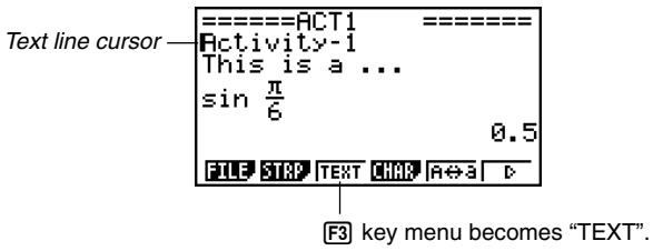
- You cannot use the above procedure to change to a text line while a strip is selected. In this case, you need to perform the procedure under “To insert a text line” or move the cursor to a line that is not a strip.
- To insert a text line
| To insert a text line while the cursor is located here: | Perform this key operation: |
| In a text line | F6 (▷) F3 (INS) F1 (TEXT) |
| In a math line | F5 (INS) F1 (TEXT) |
| In a strip | F3 (INS) F1 (TEXT) |
The text line is inserted above the line or the strip where the cursor is currently located.

- Inputting and Editing Text Line Contents
- You can input up to 255 bytes of text into a text line. Scroll arrows (◀▶) will appear on the left and right sides of the text line to let you know there is additional text that does not fit within the text line display area. In this case, you can use the left and right cursor keys to scroll the text.
- The F5 (A↔a) function key toggles between upper-case and lower-case input. This function is available only during alpha input (page 1-1-3). The text line cursor is “!” while upper-case input is selected, and “?” during lower-case input.
- You can input a carriage return into a text line by pressing EXE. Note that there is no return display symbol.
- To clear all of the text in the text line where the cursor is located, press the AC key.
■ Using Math Lines
A math line lets you input a calculation into an eActivity file, and then perform the same calculations you use in the RUN·MAT mode while "Math" is selected as the Input Mode. Math lines always have two parts: an input expression and a result.
eActivity calculations are different from RUN·MAT mode calculations as described below.
- When you input a mathematical expression into an eActivity, the Input Mode (page 1-3-8) always changes to “Math”, regardless of the calculator’s current input mode setting.
- You can input stop lines in an eActivity.

# When you input a mathematical expression into a text line, the Input Mode (page 1-3-8) always changes to “Math”, regardless of the calculator’s current input mode setting.
# Pressing F6 (▷) F4 (MATH) displays the MATH submenu. You can use this menu for natural input of matrices, differentials, integrals, etc. For details about input using the MATH menu, see "Using the MATH Menu" (page 1-3-10).
# Any mathematical expression you input into a text line is non-executable.

- To input a calculation formula into an eActivity
- On the eActivity workspace screen, change the line where the cursor is currently located into a math line, or insert a new math line.
- “To change the current line into a math line” below
-
“To insert a math line” (page 10-3-6)
-
Input the expression.
Example: sin a_c^b SHIFT EXP ( ) ▼ 6
- "Inputting and Editing Math Line Contents" (page10-3-6)
Math line cursor
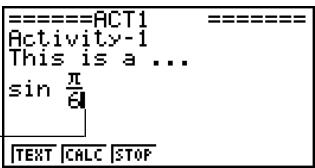
- To obtain the result of the calculation and display it, press EXE.
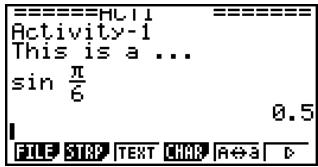
- To change the current line into a math line
-
On the eActivity workspace screen, check the menu of the F3 function key.
-
If the F3 key menu is "CALC", it means that the current line is already a math line. In this case, you can input an expression in the line without performing step 2, below.
-
If the F3 key menu is "TEXT", it means that the current line is a text line. Perform step 2, below, to change it to a math line.
-
Press F3(TEXT) to change the text line to a math line.
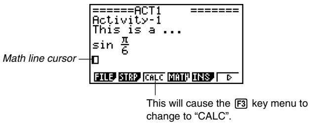

# You cannot use the above procedure to change to a math line while a strip is selected. In this case, you need to perform the
procedure under "To insert a math line" or move the cursor to a line that is not a strip.

- To insert a math line
| To insert a math line while the cursor is located here: | Perform this key operation: |
| In a math line | F5 (INS) F2 (CALC) |
| In a text line | F6 (▷) F3 (INS) F2 (CALC) |
| In a strip | F3 (INS) F2 (CALC) |
The math line is inserted above the line or the strip where the cursor is currently located.
- Inputting and Editing Math Line Contents
Math line content input and editing can be performed using the same procedures you use in the RUN·MAT mode while “Math” is selected as the Input Mode (on the Setup screen).
■ Using Stop Lines
Any time you change the expression in any math line of an eActivity that contains more than one math line, pressing EXE will cause all of the math lines to be recalculated.
Recalculation can take some time if there is a large number of math lines or if the math lines include complex calculations.
To avoid having to wait for all the expressions to be recalculated each time you make a change, you can insert a stop line below the math line(s) you are editing. Then when you press EXE the calculator will re-calculate the math lines up to the stop line and then stop automatically.
- To insert a stop line
| To insert a stop line while the cursor is located here: | Perform this key operation: |
| In a math line | F5 (INS) F3 (STOP) |
| In a text line | F6 (▷) F3 (INS) F3 (STOP) |
| In a strip | F3 (INS) F3 (STOP) |
The stop line is inserted above the line or the strip where the cursor is currently located.

- Stop Line Example
The following screen shows how you can use stop lines to group calculation steps.
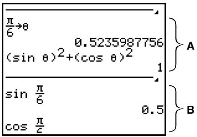
A: Substituting a value (6 here) for in the expression in line 1 executes ( )^2 + ( )^2 in line 3, and displays the result in line 4 (1). In this example, substituting any value in line 1 and pressing will produce a result of 1.
If we wanted to test various values for without recalculating all of the math lines underneath it, we could insert a stop line at the location shown above. Then, each time we change the value of and press EXE, the calculator will re-calculate ()^2 + ()^2 and then stop.
B: These math lines are not required to test various values for .

■ Inserting a Strip
A strip can be used to embed data from Graph, Conics Graph, Spreadsheet, and other applications into an eActivity. Note that only one application screen (either the Graph screen or Graph Editor screen in the case of GRAPH mode data, for example) can be used in each strip.
A strip consists of a title field on the left, and a screen name field on the right.
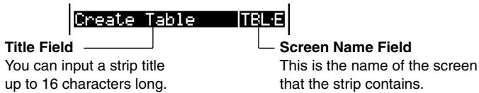
Using the ▲ and ▼ keys to move the highlighting to a strip and then pressing EXE will display the applicable application screen.
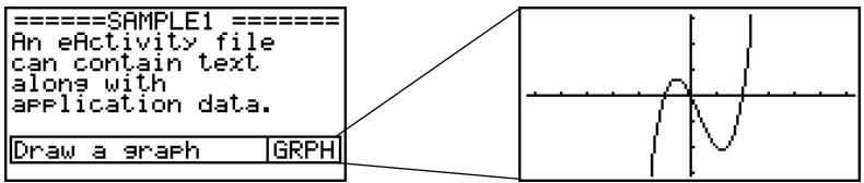
The data used to perform operations on an application screen called up from a strip (functions used for graphing, etc.) is stored in the strip's data memory. Because of this, any data stored in the strip is available whenever you call up the application from there or even if you switch the strip to another application.

# Though the applicable application screen fills the display when you call up an application from a strip, eActivity continues running in the background. It is important to keep in mind that any operation you perform within the application is an eActivity operation.
# Any data you input on an application screen called up from a data strip is stored in the data strip's data memory, not in an application data file.
# Separate data is stored in each strip's data memory, so if you create multiple strips that are associated with the same application screen, the application screen for each strip will produce its own unique results.

- To insert a strip
- Move the cursor to the location where you want to insert the strip.
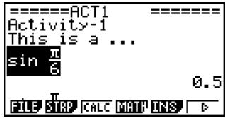
- Press F2 (STRP).
- This will display a dialog box with a list of insertable strips.
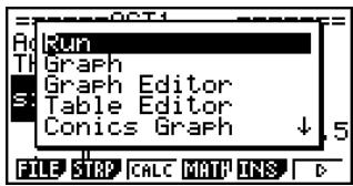
- Use ▲ and ▼ to highlight the name of the strip for the type of data you want to embed.
| When you want to embed this type of data: | Select this type of strip: |
| RUN·MAT mode calculation screen | Run (Math)*1 |
| GRAPH mode Graph screen | Graph |
| GRAPH mode Graph Editor screen(Graph relation list) | Graph Editor |
| TABLE mode Table Editor screen(Table relation list) | Table Editor |
| CONICS mode Conics Graph screen | Conics Graph |
| CONICS mode Conics Editor screen | Conics Editor |
| STAT mode Stat Graph screen | Stat Graph |
| STAT mode List Editor screen | List Editor |
| EQUA mode Solver screen | Solver |
| RECUR mode Recur Editor screen | Recur Editor |
| Notes screen*2 | Notes |
| RUN·MAT mode Matrix Editor screen | Matrix Editor |
| EQUA mode Simul Equation screen | Simul Equation |
| EQUA mode Poly Equation screen | Poly Equation |

*1Run starts up in the Math input mode.
*2 Notes is an application that can be called up from eActivity only. See “Using Notes” (page 10-3-18) for more information.

| When you want to embed this type of data: | Select this type of strip: |
| DYNA mode Dynamic Graph screen | Dynamic Graph |
| TVM mode Financial screen | Financial |
| S·SHT mode Spreadsheet screen | SpreadSheet |
4. Press EXE.
- The strip is inserted above the line or the strip where the cursor is currently located.
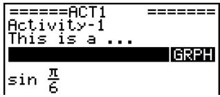
- Press ◀ or ▶ to display the text input cursor, and then enter up to 16 characters for the strip title.
- The text cursor will also appear if you start to input text without pressing ◀ or ▶ first.
- Press EXE to assign the title to the strip.

# Pressing the EXE key while a strip is highlighted (selected) as shown in steps 4 and 6 above will display the applicable application screen. For details, see “To call up an application from a strip” (page 10-3-12).

• To change the title of a strip
- Use ▲ and ▼ to highlight the strip whose title you want to change.

- Input the new title.
- Press ◀ or ▶ to display the text input cursor, and then edit the current title.
- If you press a character key without pressing the ◀ or ▶ key first, the current title will be cleared and the character will be input.
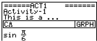
- After making sure the title is the way you want, press EXE.
- Pressing EXIT will cancel title input without changing the current title.

- To call up an application from a strip
- Use the ⬆ and ⬇ cursor keys to move the highlighting to the strip whose associated application you want to call up.
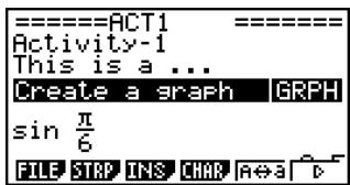
2. Press EXE.
- The application screen will be blank the first time you call it up after inserting a strip.
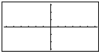
natural_image
Simple Cartesian coordinate system with x and y axes (no labels or data points)-
Input data, graph, and perform any other operations you want on the application screen.
-
Operations you can perform on an application screen that you call up from an eActivity strip are the same as those you can normally perform while the application is running. For details about using each application, see the section of this User's Guide that explains that application's mode.
- Also see “Practical Strip Examples” (page 10-3-13) for more information.
- To toggle between the eActivity workspace screen and the application screen called up from a strip
Press SHIFT → ( ).
- This will toggle between the two screens, displaying one in the front and sending the other to the back.

# If you select a Conics Graph strip and press EXE without inputting any graph data, the Conics Editor screen appears in place of the Conics Graph screen.

- To switch from an application screen called up from a strip to another application screen
Press SHIFT (☐☐).
- On the application list that appears, use ▲ and ▼ to highlight the name of the screen to which you want to switch, and then press EXE.
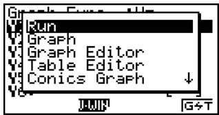
■ Practical Strip Examples
This section provides real-life examples of how to insert strips into the eActivity workspace screen, how to call up an application screen from a strip, and how to input data.
- Graph Strip Example
This example shows how to create a Graph strip to graph the function y = x^2 .
Things to remember...
- Though the graph screen is called up from the Graph strip, you need to switch to the Graph Editor screen to input the function.
- To create a Graph strip
- On the eActivity workspace screen, press F2 (STRP), select "Graph" from the strip list that appears, and then press EXE.
- This will insert a Graph strip.
- Input the strip title, and then press EXE.
- Here we will input "Graph draw".


# For an actual example about how to switch applications, see “Table Editor Strip Example” (page 10-3-15).
# Even after using SHIFT (☐) to switch a strip to another application, you can still use SHIFT (☐) to toggle between the eActivity workspace screen and the application screen.

- Press EXE to call up the graph screen.
- Since you have not input any data yet, the graph screen that appears will be blank.
- Press SHIFT F6 (G↔T) to display the Graph Editor screen.
- This will display the current Graph strip's Graph relation list. Since this list is independent of the GRAPH mode Graph relation list, it will be blank because this is a new Graph strip.
- Input the function you want to graph (Y1 = X² in this example).
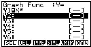
- Press F6 (DRAW) to graph the function.
- This will display the graph screen with a graph of the function you input on the Graph Editor screen.
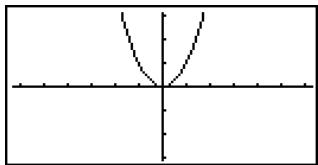
natural_image
Simple geometric diagram showing a parabola and a horizontal line intersecting at the origin (no text or labels)- To return to the eActivity workspace screen, press SHIFT → ( ).
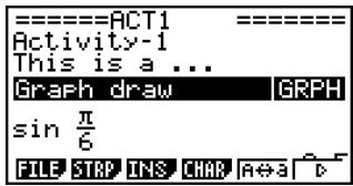
- Press EXE again to call up the graph screen.
- This will re-graph the function you input in step 5.

# You can also paste a previously copied function from the clipboard into a graph screen called up from a Graph strip. Note, however, that a graph produced by pasting the function
is not stored in the memory of the Graph strip. For more information, see “Using Copy and Paste to Draw a Graph” (page 10-3-16).

- Table Editor Strip Example
In this example, we use a Table Editor strip to input the function y = x^2 , and reference “List 1” of the List Editor for the x-variable range to generate a number table.
Things to remember...
- Use the Table Editor to input the function y = x^2 .
- Setup Table Editor (using the Setup screen) to reference “List 1” for the x -variable and generate the numeric table.
- Call up the List Editor to input the data to be used as the range of the x -variable into List 1.
- To create a Table Editor strip
- On the eActivity workspace screen, press F2 (STRP), select "Table Editor" from the strip list that appears, and then press EXE.
- This will insert a Table Editor strip.
- Input the strip title, and then press EXE.
-
Here we will input "Table create".
-
Press EXE to call up the Table Editor screen.
-
This will display a blank Table Editor screen.
- Input the function you want to use to generate the table ( Y1 = X^2 in this example).
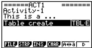
![Table Func :Y= V1=X2 V2: [—] V3: [—] V4: [—] V5: [—] V6: [—] SEL DEL TYPE STYLE SET TABL](/content/2025/01/86785/images/5328cccc62d29f1269d4795eb40b5fc286a636df8d110eddd4671ff3aed08d2e.jpg)
-
Press SHIFT MENU (SET UP) to display the Setup screen.
-
This will display the Table Editor Setup screen, with the “Variable” item highlighted.
- Press F2 (LIST). On the dialog box that appears, input "1" and then press EXE.
- Specify List 1 as the variable for generating the number table.
- Press EXIT to close the Setup screen.

- Call up the List Editor screen (page 6-1-1).
- Press SHIFT (☐) to display the application list, select List Editor, and then press EXE.
- Input the values into List 1.
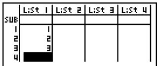
- Return to the Table Editor screen.
- Press SHIFT (☐) to display the application list, select Table Editor, and then press EXE.
- When the Table Editor screen appears, press EXE.
- This generates the number table for the function y = x^2 using the values in List 1 as the x -variable range.
![X Y1 [1 1 2 4 3 9] FORM DEL ROW EDIT G-CON G-PLT 1](/content/2025/01/86785/images/1fc1d4a0b8e9b623c149749fb4cfced25e3aac57131e9d41afeb743c526c9580.jpg)
- To return to the eActivity workspace screen, press SHIFT → (☐).
■ Using Copy and Paste to Draw a Graph
You can paste a previously copied function from the clipboard into a graph screen called up from a Graph strip. If you do, however, the pasted data will not be reflected in the function stored in the memory of the Graph strip. Use copy and paste when you need a quick, temporary look at the graph produced by a function.

# After returning to the eActivity workspace screen in step 12, you can press EXE to display the Table Editor screen, which will contain the function you input. Pressing EXE while the Table Editor screen is on the display will return to the number table in step 11.
# As you can see in this example all data and settings related to the application screen called up from a strip are stored in strip memory.

- To use copy and paste to draw a graph
- Perform steps 1 through 7 under "To create a Graph strip" (page 10-3-13) to create a Graph strip with the title "Graph draw".
- After completing step 7, check to make sure the Graph strip is highlighted on the eActivity workspace screen. If it isn't, use the ▲ and ▼ cursor keys to move the highlighting to the Graph strip.
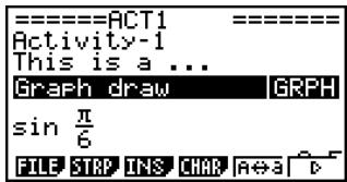
- Press F3(INS)F1(TEXT) to input a text line.
- Enter the following expression into the text line: Y = X^2 - 1 .
- Use the ▲ and ▼ cursor keys to move the cursor to the expression you just input Y = X^2 - 1 , and copy it to the clipboard.
- See “To specify the copy range” (page 1-3-5) for details about how to copy text to the clipboard.
- Use the ▲ and ▼ cursor keys to move the highlighting to the Graph strip, and then press EXE.
- This will graph the function currently stored in "Graph draw" strip memory.
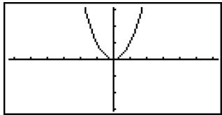
natural_image
Pure mathematical graph with a parabola and horizontal axis, no text or symbols present- Press SHIFT 9 (PASTE).
- This will graph the function that is on the clipboard ( Y = X^2 - 1 ).
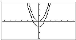
natural_image
Simple V-shaped curve graph with no text or labels- To return to the eActivity workspace screen, press SHIFT → (☐).
- Press EXE again to call up the graph screen.
- This will re-graph the function currently stored in “Graph draw” strip memory.

# Though the above example uses an expression that was copied from the eActivity workspace screen, you can also copy an
expression from another application and then paste it into eActivity.

■ Using Notes
Notes is a text editor that can be used only in eActivity. You can call up the Notes screen from a Notes strip on the eActivity workspace screen.
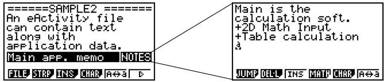
You can perform the following operations on a Notes screen.
- Input and edit text
Text is input at the current cursor position on the Notes screen. Input, editing, cursor movement, and vertical screen scrolling operations are all identical to those you can perform in an eActivity text line. For details about these operations, see “Inputting and Editing Text Line Contents” (page 10-3-4) and “To scroll the eActivity workspace screen vertically” (page 10-3-2). Note, however, that function menu assignments for Notes are different from those used for text lines. See “Notes Screen Function Menu” below for more information.
- Copy and paste text
Use SHIFT 8 (CLIP) to copy text and SHIFT 9 (PASTE) to paste it. For more information, see "Using the Clipboard for Copy and Paste" (page 1-3-5).
- Notes Screen Function Menu
The following describes the function menu of the Notes screen.
- {JUMP} ... {displays a JUMP menu that you can use to jump to the top (F1(TOP)) or the bottom (F2(BTM)) of the data}
- {DEL·L} ... {deletes the line where the cursor is located}
- {INS} ... {inserts one new line above the line where the cursor is currently located}
- {MATH} ... {displays a MATH menu for natural input of matrices and mathematical functions}
For more information, see “Using the MATH Menu” (page 1-3-10). - {CHAR} ... {displays a screen for selecting various mathematical symbols, special symbols, and accented characters}
- A a ... {toggles between upper-case and lower-case input}

■ Deleting an eActivity Line or Strip
Use the following procedure to delete a line or strip from the eActivity workspace screen.
Remember that deleting a math line deletes both the expression line and the result line.
- To delete a line or strip
- Use the ▲ and ▼ cursor keys to move the highlighting to the strip you want to delete.
- Press F6 (▷) F2 (DEL·L).
- In response to the confirmation message that appears, press F1 (Yes) to delete the line or strip, or F6 (No) to cancel the delete operation without doing anything.
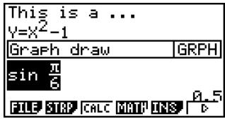
![Delete Line? Yes: [F1] No : [F6]](/content/2025/01/86785/images/4d5ceb8b50bd16cf232602b435bfa0f2ea7e8162dbc7235416f08589119769d7.jpg)
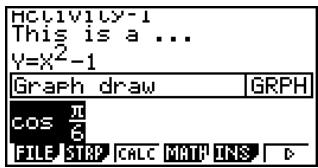

■ Saving an eActivity File
After inputting or editing data on the eActivity workspace screen, you can save it to a file under a new name (Save As) or you can replace the previously saved version of the file you are working on (Save). In the case of Save As, both the previous version and the new version of the file are saved.
- To replace the existing file with the new version
On the eActivity workspace screen, press F1(FILE)F1(SAVE).
- To save a file under a new name (Save As)
- Press F1(FILE)F2(SV·AS).
- This displays a dialog box for inputting a file name.
- Enter up to eight characters for the eActivity file name, and then press EXE.
- This will create a new file with the name you input in the same memory area (Storage Memory or SD card) where the original file is located.

# If you press EXIT to quit eActivity while there are unsaved edits on the screen, a message will appear asking you if you want to save first. When this message appears, you can any one of the following.
- Press F1 (Yes) key to save your edits and replace the previously saved version of the file.
- Press F6(No) to exit without saving.
- Press AC to return to the eActivity workspace screen.
# If a file already exists with the same file name you input in step 2, a message will appear asking if you want to replace the existing file with the new one. Press F1(Yes) to replace the existing file, or F6(No) to cancel the save operation and return to the file name input dialog box in step 1.

10-4 Using Matrix Editor and List Editor
In addition to the strip operation for calling up application screens within eActivity (page 10-3-12), you can also use the eActivity function menu to call up Matrix Editor and List Editor.
■ Calling Up Matrix Editor
You can call up Matrix Editor to input a matrix into a math line on the eActivity workspace screen.
Note
The data you create by calling up the Matrix Editor using the procedure below can be used in the calculation line on the eActivity workspace screen only. It is different from and independent of data you create by calling up the Matrix Editor from a strip or from the RUN·MAT mode.
• To call up Matrix Editor
Perform one of the following operations on the eActivity workspace screen.
| To call up Matrix Editor while the cursor is located here: | Perform this key operation: |
| In a text line | F6 (▷) F6 (▷) F1 (▶MAT) |
| In a math line | F6 (▷) F3 (▶MAT) |
| In a strip | F6 (▷) F3 (▶MAT) |
- To return to the eActivity workspace screen from Matrix Editor
Press EXIT.
- To use Matrix Editor
Matrix Editor operations are identical to those you perform when you call it up from the RUN·MAT mode. For more information, see "2-8 Matrix Calculations".
- To perform matrix calculations using a matrix stored with Matrix Editor
Use the same procedures as those you use in the RUN·MAT mode to use an existing Matrix Editor matrix on the eActivity workspace screen. For details see “Inputting and Editing Matrices” (page 2-8-2), “Matrix Cell Operations” (page 2-8-5), and “Modifying Matrices Using Matrix Commands” (page 2-8-10).

■ Calling Up List Editor
You can call up List Editor to input a list into a math line on the eActivity workspace screen.
Note
The data you create by calling up the List Editor using the procedure below can be used in the calculation line on the eActivity workspace screen only. It is different from and independent of data you create by calling up the List Editor from a strip or from the RUN·MAT mode.
- To call up List Editor
Perform one of the following operations on the eActivity workspace screen.
| To call up List Editor while the cursor is located here: | Perform this key operation: |
| In a text line | F6 (▷) F6 (▷) F2 (▶LIST) |
| In a math line | F6 (▷) F4 (▶LIST) |
| In a strip | F6 (▷) F4 (▶LIST) |
- To return to the eActivity workspace screen from List Editor
Press EXIT.
- To use List Editor
List Editor operations are identical to those you perform when you call it up from the STAT mode.
See “3. List Function” and “Inputting Data into Lists” (page 6-1-1) for information about inputting data to List Editor and performing List Editor calculations.

# The function menu arrangement when you call up List Editor from the eActivity workspace screen is slightly different from the function menu arrangement when you call it up from the STAT mode. The functions, however, are identical.
Initial Function Menu

F1(TOOL) Function Submenu
SRTA SRTD TOP BTM

10-5 eActivity File Memory Usage Screen
The size of an eActivity file is limited. You can use the eActivity file memory usage screen to check the current size and how much more memory is available for the eActivity file you are working on. You can also display the size of the strip that is currently highlighted or where the cursor is currently located.
- To display the eActivity memory usage screen
- On the eActivity workspace screen, press F1(FILE)F4(CAPA).
- This will display a screen like the one shown to the right, which shows the current size of the eActivity file (Total Data Size) and how much main memory is available for storage of additional data (Free Bytes).
- To exit the memory usage screen, press EXIT.
![Total Data Size 1760 Bytes Free Bytes 28624 Bytes Press:[EXIT]](/content/2025/01/86785/images/1ee34df99dfd01327ac1d5e814f4c15498c96806849200de3db49fa5d571d4ed.jpg)
- The maximum allowable size for a single eActivity file is approximately 30,000 bytes. The actual maximum size depends on capture memory and clipboard use. The actual maximum file size may be less than 30,000 bytes may be less, depending on how capture memory and the clipboard are used.
- To display the strip memory usage screen
- Use ▲ and ▼ to move the highlighting to the strip whose memory usage you want to view.
- Press F1(FILE)F5(SIZE).
- This will display the memory usage screen for the currently selected strip.
![Ad Strip Data Size TH 376 Bytes Y- Press: [EXIT] G π SAVE SUMS OPT CAPS SIZE](/content/2025/01/86785/images/d949e4c28530c8b86df187cba2be6681b73a2b77d5df96feec5ddc1686f40fb7.jpg)
- To exit the memory usage screen, press EXIT.

Chapter 11
System Settings Menu
Use the system settings menu to view system information and make system settings. The system settings menu lets you do the following.
- Make contrast settings
- Make Auto Power Off settings
- Specify the system language
- View the operating system and application versions, and the product ID
- Reset the calculator
11-1 Using the System Settings Menu
11-2 System Settings
11-3 Version/ID Number List
11-4 Reset
11-1 Using the System Settings Menu
From the Main Menu, enter the SYSTEM mode and display the following menu items.
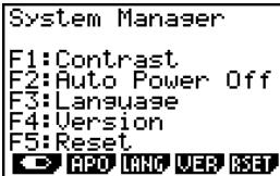
- F1(◀) ... {display contrast adjustment}
- F2 (APO) ... {Auto Power Off time setting}
• F3 (LANG) ... {system language}
• F4 (VER) ... {version, ID} - F5 (RSET) ... {system reset operations}

11-2 System Settings
■ Contrast Adjustment
Use the ◆ (Contrast) item to adjust display contrast.
While the initial SYSTEM mode screen is displayed, press F1(◀) to display the Contrast Adjustment screen.
![Contrast [◀]Key [▶]Key Light Dark INIT](/content/2025/01/86785/images/93e7cc2426343e0d1edb916e0498f9a11d709023bfc96dc1abd31c04b05a82d2.jpg)
- The ▶ cursor key makes display contrast darker.
- The ◀ cursor key makes display contrast lighter.
- F1(INIT) returns display contrast to its initial default.
Pressing EXIT or SHIFT EXIT (QUIT) returns to the initial SYSTEM mode screen.
You can adjust contrast while any screen besides the Main Menu is on the display by pressing SHIFT and then ▶ or ◀. To exit contrast adjustment, press SHIFT again.
■ APO Settings
You can specify either six minutes or 60 minutes as the Auto Power Off trigger time. The initial default setting is six minutes.
While the initial SYSTEM mode screen is displayed, press F2(APO) to display the Auto Power Off Setting screen.
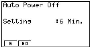
• F1(6) ... 6 minutes
• F2(60) ... 60 minutes
Pressing EXIT or SHIFT EXIT (QUIT) returns to the initial SYSTEM mode screen.

■ System Language Setting
Use LANG to specify the display language for built-in applications. You can also use add-ins to install various other languages.
- To select the Mssage Language
- From the initial SYSTEM mode screen, press F3 (LANG) to display the Message Language selection screen.
![Message Language [English] English Español Deutsch Français Portusuês SEL MENU](/content/2025/01/86785/images/8b4eb87551b16d5f55f46c362a25a71e5af7b5d486304bab1b111182a6aad9c4.jpg)
- Use the ▲ and ▼ cursor keys to select the language you want, and then press F1(SEL).
- The pop up window appears using the language you selected. Check the contents and then press EXIT.
Press EXIT or SHIFT EXIT (QUIT) to return to the initial SYSTEM mode screen.
- To select the Menu Language
- From the initial SYSTEM mode screen, press F3 (LANG) to display the Message Language selection screen.
- Press F6 (MENU).
![Menu Language [English] English SEL MSG](/content/2025/01/86785/images/3caecc86ff4cafb01ecdb2d1bdba27894e125ad2d3f32a70bf00dabbb2cd4fd6.jpg)
- Use the ▲ and ▼ cursor keys to select the language you want, and then press F1(SEL).
- The pop up window appears using the language you selected. Check the contents and then press EXIT.
- Press F6 (MSG) to return to the Message Language selection screen.
Press EXIT or SHIFT EXIT (QUIT) to return to the initial SYSTEM mode screen.

11-3 Version/ID Number List
The Version/ID Number list shows the following items.
- Operating system version
- Add-in application versions
- Add-in message data versions
- Add-in menu data versions
- Product ID
- User name
You can register the user name you want.
- To display version information
- On the initial SYSTEM mode screen, press F4(VER) to display the Version/ID Number List.
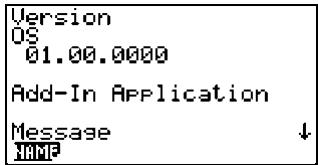
- Use ▲ and ▼ to scroll the screen. The contents of the list are shown below.
Operating system version
Add-in application names and versions ^*1
Message languages and versions
Menu languages and versions
User name
Press EXIT or SHIFT EXIT (QUIT) to return to the initial SYSTEM mode screen.

*1 Only installed add-ins are displayed.
# The operating system version that actually appears depends on the calculator mode.

• To register a user name
- While the Version/ID Number list is displayed, press F1(NAME) to display the user name input screen.
![User Name [& ]](/content/2025/01/86785/images/92a4ae2fc5e81fa995bd446617cdcabe0e5b128231c9f16c949e588ac5042b85.jpg)
- Input up to eight characters for the user name you want.
- After inputting the name, press EXE to register it, and return to the Version/ID Number list.
- If you want to cancel user name input and return to the Version/ID Number list without registering a name, press EXIT.

11-4 Reset
- While the initial SYSTEM mode screen is displayed, press F5(RSET) to display the Reset Screen 1.
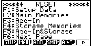
- F1(STUP) ... {setup initialization}
- F2 (MAIN) ... {main memory data clear}
- F3(ADD) ... {add-in application clear}
- F4(SMEM) ... {storage memory data clear}
- F5(A&S) ... {add-in application and storage memory data clear}
Pressing F6(▷) on the above screen displays the Reset Screen 2 shown below.
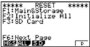
- F1(M&S) ... {main memory data and storage memory data clear}
• F2 (ALL) ... {all memory clear}
• F3(SD) ... {SD card format}
The following table shows the functions of the function keys. You can use the function keys to delete the specific data you want.
Function Key Functions
| Initialize Setup Information | Delete Main Memory Data | Delete Add-in Applications | Delete Storage Memory Data (Excluding Add-in Applications) | Format SD Card | |
| F1(STUP) | ○ | ||||
| F2(MAIN) | ○ | ○ | |||
| F3(ADD) | ○ | ||||
| F4(SMEM) | ○ | ||||
| F5(A&S) | ○ | ○ | |||
| F6(▷)F1(M&S) | ○ | ○ | ○ | ||
| F6(▷)F2(ALL) | ○ | ○ | ○ | ○ | |
| F6(▷)F3(SD) | ○ |

- Press the function key that corresponds to the reset operation you want to perform.
- In response to the confirmation message that appears, press F1 (Yes) to perform the reset operation you specified, or F6 (No) to cancel.
![Reset OK? Main Memories Yes: [F1] No: [F6]](/content/2025/01/86785/images/aa9e1fa63a8fdcebc9d42a9f654254fee59122ea3607cae75a265cdbae2410c1.jpg)
Screen produced when
F2 (MAIN) is pressed in step 2.
-
A message appears to let you know when the reset operation is complete.
-
For all memory clear: Press EXIT to restart the calculator and return to the Main Menu.
- Other: Press EXIT to clear the message.
![Reset! Main Memories Press:[EXIT]](/content/2025/01/86785/images/5a6ea0a831cafecdc735b3115bbea8674d3a24ed0a4876c6405986dd824571af.jpg)
Screen produced when
F2 (MAIN) is pressed in step 2.

Chapter 12
Data Communications
This chapter tells you everything you need to know to transfer programs between two CASIO Power Graphic calculators connected using the cable that is equipped as a standard accessory.
You can use the USB cable that comes with the calculator to connect it to a computer to exchange images and other data.
12-1 Connecting Two Units
12-2 Connecting the Unit to a Personal Computer
12-3 Performing a Data Communication Operation
12-4 Data Communications Precautions
12-5 Image Transfer
12-6 Add-ins
12-7 MEMORY Mode
Important!
All of the references to SD card storage in this chapter apply only to the fx-9860G SD, which is equipped with an SD card slot.
12-1 Connecting Two Units
The following procedure describes how to connect two units with the connecting cable that comes equipped as a standard accessory.
- To connect two units
- Check to make sure that the power of both units is off.
- Remove the covers from the connectors of the two units.
- Connect the two units using the cable.
- Perform the following steps on both units to specify 3PIN as the cable type.
(1) From the Main Menu, enter the LINK mode.
(2) Press F4(CABL). This displays the cable type selection screen.
(3) Press F2 (3PIN).
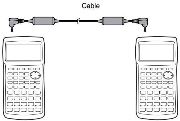

# Models that are supported for this configuration are shown below.
fx-9860G SD
fx-9860G
# Be sure you keep the connector covers in a safe place so you can replace them after you finish your data communications.
# Keep the connectors covered when you are not using them.

12-2 Connecting the Unit to a Personal Computer
You can use the USB cable that comes with the calculator to connect it to a computer to exchange images and other data.
For details on operation, the types of computer that can be connected, and hardware limitations, see the user's documentation for the FA-124 software that comes with the calculator.
Some types of data may not be able to be exchanged with a personal computer.
- To connect the unit to a personal computer
- Check to make sure that the power of the unit and the personal computer is off.
- Connect the USB cable to your computer.
- Remove the cover from the connector of the unit.
- Connect the other end of the USB cable to the calculator.
- Turn on the power of the unit, followed by the personal computer.
- Perform the following procedure on the calculator to specify USB as the cable type.
(1) From the Main Menu, enter the LINK mode.
(2) Press F4 (CABL). This displays the cable type selection screen.
(3) Press F1 (USB).

natural_image
Line drawing of a vintage remote control device connected to a desktop computer via cable (no text or symbols)- After you finish data communications, turn off power in the sequence: the unit first, and then the personal computer. Finally, disconnect the equipment.

# The fx-9860G SD/fx-9860G also supports to PC transfer of programs created with a CASIO CFX-9850 series calculator.
# Data communication is supported with Windows computers (98 or later).

12-3 Performing a Data Communication Operation
From the Main Menu, enter the LINK mode. The following data communication main menu appears on the display.
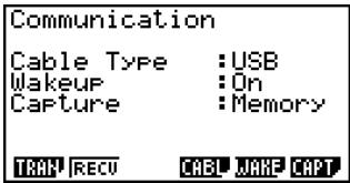
- {TRAN} ... {displays the data send screen}
- {RECV} ... {displays the data receive screen}
- {CABL} ... {displays the cable type selection screen}
- {WAKE} ... {displays the wakeup setting screen}
- {CAPT} ... {displays the image transfer setting screen}
Communication parameters are fixed at the following settings.
- 3-pin serial port
- Speed (BPS): 9600 bps max. (Connected with CFX-9850 series) 115200 bps max. (Connected with another fx-9860G SD/fx-9860G)
- Parity (PARITY): NONE
- USB port
- Communication speed is in accordance with USB standards.

■ Performing a Data Transfer Operation
Connect the two units and then perform the following procedures.
Receiving unit
To set up the calculator to receive data, press F2(RECV) while the data communication main menu is displayed.
Receiving...
AC : Cancel
The calculator enters a data receive standby mode and waits for data to arrive. Actual data receive starts as soon as data is sent from the sending unit.
Sending unit
To set up the calculator to send data, press F1(TRAN) while the data communication main menu is displayed.
This displays the send data type selection screen.
Select Data Type
F1: Main Memory
F2: Storage Memory
MAIN SEM
- {MAIN} ... {main memory data}
- {SMEM} ... {storage memory data}

Pressing F1(MAIN) or F2(SMEM) displays a screen for specifying the data selection method.
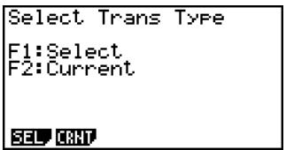
When F1(MAIN) is pressed
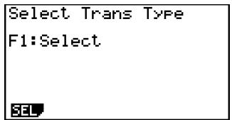
When F2(SMEM) is pressed
- {SEL} ... {selects new data}
- {CRNT} ... {automatically selects previously selected data*1}
- To send selected data items (Example: To send user data)
Press F1(SEL) or F2(CRNT) to display a data item selection screen.
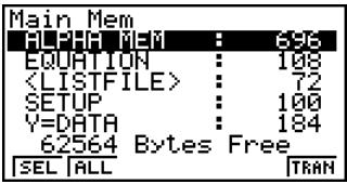
- {SEL} ... {selects data item where cursor is located}
- {ALL} ... {selects all data}
- {TRAN} ... {sends selected data items}
Use the ⬆ and ⬇ cursor keys to move the cursor to the data item you want to select and press F1 (SEL) to select it. Currently selected data items are marked with “▶”. Pressing F6 (TRAN) sends all the selected data items.
- To deselect a data item, move the cursor to it and press F1(SEL) again.
Only items that contain data appear on the data item selection screen. If there are too many data items to fit on a single screen, the list scrolls when you move the cursor to the bottom line of the items on the screen.

*1The previously selected data memory is cleared whenever you perform either of the following operations.
- Change the type of transfer data
- Change to another mode

•To execute a send operation
After selecting the data items to send, press F6 (TRAN). A message appears to confirm that you want to execute the send operation.
![Transmit OK? Yes: [F1] No : [F6]](/content/2025/01/86785/images/ea045bbfbd5ba872f3b509f7705f1fbcebe0ae7fd2d6d0faadf20208293f425c.jpg)
- F1(Yes) ... sends data
• F6 (No) ... returns to data selection screen
Press F1(Yes) to send the data.
Transmitting... AC : Cancel
- You can interrupt a data operation at any time by pressing AC.
The following shows what the displays of the sending and receiving units look like after the data communication operation is complete.
Sending Unit
![Tr A0 Complete! Press:[EXIT]](/content/2025/01/86785/images/7748cda005be7b8c3cb1258a78a17350bb06bf87dbbc76a3edd55c8a8296f239.jpg)
Receiving Unit
![Receiving A0 Complete! Press:[EXIT]](/content/2025/01/86785/images/a8de22c55bd969fa3c6c7403c615956545f8010e7a414d5799c17e56d44915bc.jpg)
Press EXIT to return to the data communication main menu.

# Add-in applications, add-in languages, and add-in menus are stored in the receiver's storage memory.
# A commercial add-in application cannot be transferred.

■ Specifying the Cable Type
Use the following procedure to specify the cable type for data communication.
- On the data communication main menu, press F4 (CABL).
This displays the cable type selection screen.
Select Cable Type
F1:USB cable
F2:3Pin cable
USB3PIN
- {USB} ... {USB cable}
- {3PIN} ... {3-pin cable}
- Press F1(USB) or F2(3PIN) to select the cable type and return to the data communication main menu.
- Configuring the Receiver’s Wakeup Feature
When Wakeup is turned on the receiver, the receiver turns on automatically when data transfer starts.
When communicating between two calculators (3PIN selected as the cable type), the receiver enters the receive mode automatically after it wakes up. When communication is with a computer (USB selected as the cable type), connecting the USB cable to a computer and then to the calculator (while the calculator is turned off) will cause the calculator to turn on and enter the receive mode.
- On the receiver's data communication main menu, press F5 (WAKE).
This displays the Wakeup setting screen.
Wakeup Enable
F1:On
F2:0ff
On Off
- {On} ... {turns Wakeup on}
- {Off} ... {turns Wakeup off}
- Press F1(On).
This turns on Wakeup and returns of the data communication main menu.
-
Turn off the receiver.
-
Connect the receiver to the sender.
-
Starting a send operation on the sender causes the receiver to turn on automatically and performs the data transfer operation.

12-4 Data Communications Precautions
The following are the types of data items that can be sent.
| Data Item | Contents | Overwrite Check*1 |
| Program group | ||
| Program names | Program contents (All programs are listed.) | Yes |
| Matrix group | ||
| MAT n | Matrix memory (A to Z, and Ans) contents | Yes |
| List file group | ||
| LIST n | List memory (1 to 26, and Ans) contents | Yes |
| LIST FILE n | List file memory (1 to 6) contents | Yes |
| Y=DATA | Graph expressions, graph draw/non-draw status, V-Window contents, zoom factors | No |
| Graph memory group | ||
| G-MEM n | Graph memory (1 to 20) contents | Yes |
| V-Window memory group | ||
| V-WIN n | V-Window memory contents | No |
| Picture memory group | ||
| PICT n | Picture (graph) memory (1 to 20) data | No |
| DYNA MEM | Dynamic Graph functions | Yes |
| EQUATION | Equation calculation coefficient values | No |
| ALPHA MEM | Alpha memory contents | No |
| Function memory group | ||
| F-MEM n | Function memory contents | No |
| STAT | Stat result data | No |
| TABLE | Table data | No |
| FINANCIAL | Financial data | No |
| Spreadsheet group | ||
| Spreadsheet data names | Spreadsheet data(All spreadsheet data are listed.) | Yes |
| RECURSION | Recursion data | No |

| Data Item | Contents | Overwrite Check*1 |
| Capture memory group | ||
| CAPT n | Capture memory (1 to 20) data | No |
| SETUP | Setup data | No |
| SYSTEM | OS and data shared by applications (clipboard, replay, history, etc.), which is not included in the above | No |
| Add-in application names | Add-in application data(All add-in applications are listed.) | No |
*1 No overwrite check: If the receiving unit already contains the same type of data, the existing data is overwritten with the new data.
With overwrite check: If the receiving unit already contains the same type of data, a message appears to ask if the existing data should be overwritten with the new data.
Data item name
![[MAT A ] Already Exists Overwrite OK? F1 :Yes F6 :No AC :Cancel \YES](/content/2025/01/86785/images/7a971f90a3056ac49f3c0a5fe1e747b1c23fd793b00d5df75ba92259b0dd499e.jpg)
- F1(YES) ... {replaces the receiving unit's existing data with the new data}
• F6(NO) ... {skips to next data item}
Note the following precautions whenever you perform data communications.
- An error occurs whenever you try to send data to a receiving unit that is not yet standing by to receive data. When this happens, press EXIT to clear the error and try again, after setting up the receiving unit to receive data.
- An error occurs whenever the receiving unit does not receive any data approximately six minutes after it is set up to receive data. When this happens, press EXIT to clear the error.
- An error occurs during data communications if the cable becomes disconnected, if the parameters of the two units do not match, or if any other communications problem occurs. When this happens, press EXIT to clear the error, then correct the problem before trying data communications again. If data communications are interrupted by the EXIT key operation or an error, any data successfully received up to the interruption will be in the memory of the receiving unit.
- An error occurs if the receiving unit memory becomes full during data communications. When this happens, press EXIT to clear the error and delete unneeded data from the receiving unit to make room for the new data, and then try again.
■ Exchanging Data with another Model Calculator
- The graph line style data of this calculator is interchangeable with the line color data of the CFX-9850.
- Sending the following type of data to a CFX-9850 will cause an error.
✗ Any List, G-Mem, Pict, or F-Mem data other than the first seven data items CFX-9850 supports up to six List, G-Mem, Pict, and F-Mem data items only.
✗ More than 255 cells of List data CFX-9850 supports up to 255 List cells only.
✗ Any List data that contains a complex number CFX-9850 does not support complex number input.
- Attempting to send any of the following types of data to a CFX-9850 will not cause an error, but the data will not be stored in CFX-9850 memory.
Table setting data
Recursion data
Financial data
Spreadsheet data
Add-in application data
Hard copy memory
Setup data
- Sending V-Window x -dot data to the CFX-9850 will cause the data to become corrupted.

12-5 Image Transfer
■ Transferring Images to a Computer
Use the following procedure to capture calculator screen images to a computer. Perform this procedure using FA-124 software running on the computer.
- Use the USB cable to connect the calculator to the computer.
- On the calculator, press F6 (CAPT).
This displays the image transfer setting screen.
Capture Set Mode
F1:Memory
F2:PC
F3:OHP
Mem PC OHP
- {Mem} ... {turns off image transfer}
- {PC} ... {turns on manual image transfer}
-
{OHP} ... {turns on auto image transfer}
-
Press F2 (PC).
This turns on manual image transfer and returns to the data communication main menu.
- On the calculator, display the screen you want to transfer.
- Use FA-124 to perform the transfer operation.
- On the calculator, press SHIFT 7 (CAPTURE).
- The screen data is sent to the computer.

# Selecting "PC" (turns on manual image transfer) automatically disables screen capture.
# The following types of screen images cannot be transferred to another calculator or computer using auto image transfer.
- The screen displayed during data transfer
- The screen displayed during a calculation
- The screen displayed after reset is performed
- The low battery screen

■ Auto Image Transfer to an OHP Unit
The following procedure sends the screen of this calculator to an OHP unit at fixed intervals.
- Use the USB cable to connect the calculator to the OHP unit.
- On the calculator's data communication main menu, press F6 (CAPT).
- Press F3(OHP).
This turns on auto image transfer and returns of the data communication main menu. - Display the image you want to send.
- The displayed image is sent automatically to the OHP unit.
- To continue with auto image transfer, return to step 4.
- To stop auto image transfer, press F6(CAPT)F1(Mem) on the data communication main menu.
See the User's Guide that comes with the OHP unit for information about connecting the OHP unit and how to use the calculator while the OHP unit is attached.

12-6 Add-ins
Add-in capabilities let you install separately available applications and other software to tailor the calculator to suit your particular needs.
Add-ins are installed from a computer using the data communication described on page 12-3-1.
The following are the types of software that can be installed as add-ins.
- Add-in Application
After you install an application, its icon appears in the Main Menu, and you can run it just as you would a built-in application.
• Built-in Application Upgrades
These are upgrades for the applications that are pre-programmed in the calculator's ROM.
- On-screen Message Language Data
This data is required to display on-screen messages in other languages. Installing this data causes all on-screen messages to appear in the corresponding language.
- Function Menu Language Data
This data is required to display function menus in other languages. Installing this data causes function menus to appear in the corresponding language.

12-7 MEMORY Mode
This calculator has two separate memory areas: a “main memory” and a “storage memory.” The main memory is a work area where you can perform input data, perform calculations and run programs. Data in the main memory is relatively safe, but it can be deleted when batteries go dead or when you perform a full reset.
The storage memory uses “flash memory,” so data is safe even when power is interrupted. Normally, you would use the storage memory for data you need to store securely for long periods and load it into the main memory only when you need it.
Use the MEMORY mode to transfer data between the main memory, storage memory and SD card, and to perform other memory management operations.
From the Main Menu, select the MEMORY icon to enter the MEMORY mode and display its initial screen.
Memory Manager
F1: Main Memory
F2: Storage Memory
F3: SD Card
F4: Backup
F5: Optimization
MAIN SMEM SD GROUP OPT
- {MAIN} ... {displays main memory information}
- {SMEM} ... {displays storage memory information}
- {SD} ... {displays SD card memory information} (fx-9860G SD only)
- {BKUP} ... {main memory backup}
- {OPT} ... {storage memory, SD card optimization}

■ Memory Information Screen
Press F1(MAIN) to display current main memory use information.
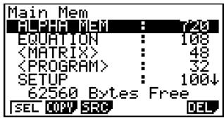
Press F2 (SMEM) to display current storage memory use information.
![Storage Mem[ ] [FOLDER2] DATA1.s1m : 824 DATA2.s1m : 982 391346 Bytes Free SEL COPY SRC MHF RHF DEL](/content/2025/01/86785/images/d5bc43afeb94914e1b0fc496b5a9b92aa066cb20673055eb9340ad87c324abb7.jpg)
Press F3 (SD) to display current SD card memory use information.
![SD Card [ ] [FOLDER2] DATA1.sim : 776 DATA2.sim : 934 248760 KBytes Free SEL COPY SRC MKF RHF DEL](/content/2025/01/86785/images/6b76292fee0029b46116efb58050bebe6fd3f341060c5cc1fbd08dcf883f5c9b.jpg)
- Use the cursor ⚠️ and ⬇ keys to move the highlighting and check the number of bytes used by each type of data.
- Line 7 shows how many bytes of memory are currently unused in the currently selected memory (main, storage, or SD card).
- The first time you store data to the storage memory, the calculator will reserve a management memory area automatically, which will reduce the “Free” value by 65535 bytes.
- On the main memory screen, < > indicates a data group. On the storage memory and SD card screens, [ ] indicates folders.

Moving the highlighting to a data group or folder and pressing EXE will display the data group or folder contents. Pressing EXIT will return to the previous screen.
When the contents of a storage memory or SD card folder are displayed, the first line of the screen shows the name of the folder.
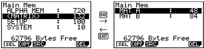
Folder name
(Blank when the root folder is displayed.)
![Storage Mem[FOLDER1] D:\H1.s1m : 824 DATA2.s1m : 982 391346 Bytes Free SEL COPY SRC DEL](/content/2025/01/86785/images/59380e5b5a9b595ad3c0d475fd7c60b60185304b17365172cf028568d1004677.jpg)
- The following data can be checked.
Main Memory
| Data Name | Contents |
| ALPHA MEM | Alpha letter variables |
| Matrix group | |
| MAT n (n = A to Z, and Ans) | Matrix |
| List file group | |
| LIST n (n = 1 to 26, and Ans) | List memory contents |
| LIST FILE n (n = 1 to 6) | List File |
| STAT | Stat result data |
| Y=DATA | Graph expression |
| Graph memory group | |
| G-MEM n (n = 1 to 20) | Graph memory |
| V-Window memory group | |
| V-WIN n (n = 1 to 6) | V-Window memory |
| Picture memory group | |
| PICT n (n = 1 to 20) | Picture memory |
| DYNA MEM | Dynamic Graph memory |
| TABLE | Table data |
| EQUATION | Equation data |
| FINANCIAL | Financial data |

| Data Name | Contents |
| Capture memory group | |
| CAPT n (n = 1 to 20) | Capture memory |
| CONICS | Conics setting data |
| Program group | |
| Each program name | Programs |
| Spreadsheet group | |
| Each spreadsheet name | Spreadsheet data |
| Each add-in application name | Application-specific data |
| Function memory group | |
| F-MEM n (n = 1 to 20) | Function memory |
| SETUP | Setup data |
| SYSTEM | OS and data shared by applications (clipboard, replay, history, etc.), which is not included in the above |
Storage Memory, SD Card ^*1
| Data Name | Contents |
| *.g1m file names | Data items listed in the Main Memory table that has been copied to storage memory or an SD card.The names of these files have the extension “.g1m”. |
| eActivity data names | eActivity data stored in storage memory or on an SD card. |
| Add-in software names (Applications, languages, menus) | Add-in applications, add-in languages, and add-in menus stored in storage memory or on an SD card. |
| Folder names | Enclosed in square brackets ([ ]). |
| Unknown | Area that is unusable due to writing error, etc. |

*1 "No Data" is displayed when there is no data in storage memory or on the SD card. The message "No Card" indicates there is no SD card loaded in the calculator.

■ Creating a Folder in Storage Memory or on an SD Card
Use the following procedure to create and rename folders in storage memory and on an SD card.
- To create a new folder
- While storage memory or SD card memory data is on the display, press F4(MK·F) to display the folder name input screen.
- Input up to eight characters for the name you want to give to the folder.
![Folder Name [A ]](/content/2025/01/86785/images/dc8b990aab995eaf86ba259fc2131bfa52551969df52166982a2b88346c0b685.jpg)
- Only the following characters are supported: A through Z, {}, ', \~, 0 through 9 Inputting any invalid character will cause an "Invalid Name" error.
- An "Invalid Name" also occurs if the name you input is already being used by an existing file.
-
To cancel folder creation, press EXIT.
-
Press EXE to create the folder and return to the storage memory or SD card memory information screen.
![Storage Mem[ ] [FOLDER] 393184 Bytes Free SEL COPY SRC MMF RNF DEL](/content/2025/01/86785/images/c57bb4104976a62c0139a6a1f6c141eb0d038c5788725eb83d61660c4ae58e2c.jpg)

- To rename a folder
- On the storage memory or SD card memory information screen, select the folder you want to rename.
- Press F5(RN·F) to display the rename folder screen.
- Input up to eight characters for the name you want to give to the folder.
![Rename [A] 1 2](/content/2025/01/86785/images/3db7cda99d51b2c1f083c4e2ef00ab2ba4b632b1f36fadef6c1b2b607c13d955.jpg)
- Only the following characters are supported: A through Z, {}, ', \~, 0 through 9 Inputting any invalid character will cause an "Invalid Name" error.
- An “Invalid Name” also occurs if the name you input is already being used by an existing file.
-
To cancel folder creation, press EXIT.
-
Press EXE to rename the folder and return to the storage memory or SD card memory information screen.
![Storage Mem[ ] [MYDATA] 393184 Bytes Free SEL COPY SRC MIFF RHF DEL](/content/2025/01/86785/images/3ed89fdda251aaa52508debdd0fc9b3281baa525f8f634087a39a58bdcaad2b7.jpg)
■ Selecting Data
You can use the following procedures to select data for copy and deletion.
- Press F1(SEL) to select the currently highlighted item, which is indicated by the black selection pointer (▶) appearing next to it. Pressing F1(SEL) again will deselect the item, causing the selection pointer to disappear.
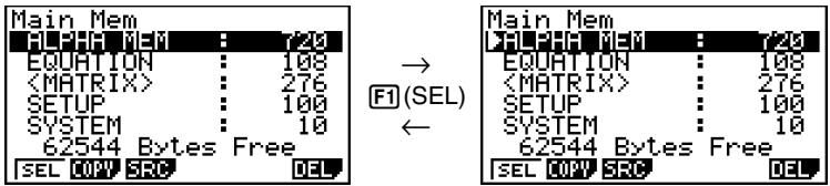

- You can select multiple files, if you want.
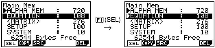
- Selecting a group or folder also selects everything inside of it. Deselecting a group or folder deselects all of its contents.
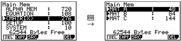
- If you select one or more individual items inside of a data group or folder, the black selection pointer (▶) appears next to each item, while a white selection pointer (▷) appears next to the group or folder name.
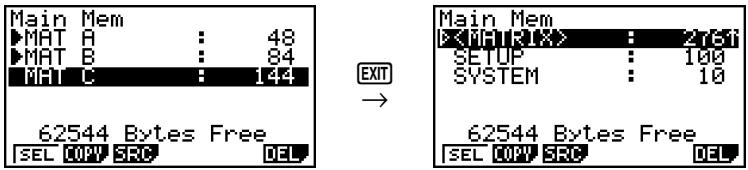
- The current data selection is maintained when any of the following operations is performed.
Save/load execution
Search execution
- Returning to the MEMORY mode initial screen deselects all currently selected items.

■ Copying Data
You can copy data between main memory, storage memory, and the SD card.
- To copy from main memory to storage memory
Note
- The following procedure saves the selected data into a single file. You assign a name to the file, which is stored in storage memory.
- On the main memory data information screen, select the data you want to copy.
- Press F2 (COPY).
- This displays the storage memory/SD card selection screen (fx-9860G SD only).*1
![Copy to Storage Mem:[1] SD Card :[2] 62544 Bytes Free SEL COPY SRC DEL](/content/2025/01/86785/images/32afd853f893b34ad0b3ee441a72bc59c8282dbf73d9fd7159dcfcfe74ddc9dc.jpg)
- Press ① to select storage memory (fx-9860G SD only).*2
- This displays the folder selection screen.

- Select the folder to which you want to copy the data.
- This displays the file name input screen.
- Input the file name you want to give to the file.
- To cancel the copy operation, press EXIT.
- Press EXE.
- This copies the data.
- The message "Complete!" appears when the copy operation is complete. Pressing EXIT will return to the MEMORY mode initial screen.

*1 Copying data from the storage memory or an SD card causes one of the screens shown below to appear (fx-9860G SD only).
![Copy to Main Mem :[1] SD Card :[2] 257420 Bytes Free SEL COPY SRC MINF RNF DEL Copy to Main Mem :[1] Storage Mem:[2] 248736 KBytes Free SEL COPY SRC MINF RNF DEL](/content/2025/01/86785/images/703b2ccb592bbda9cc3d16e6a665f49a50357f9d64b717082bdb5de280c15f96.jpg)
Pressing ① selects main memory and copies the data, without displaying the folder selection screen.
![File Name [A]](/content/2025/01/86785/images/424c2941d8581cc48a880c84b37ce6ac2aeffbf71aa8077b4958ab6b75b26584.jpg)
The file name input screen does not appear when you copy data from storage memory or/and SD card to main memory.
*2 To copy to the SD card, press ②. The "No Card" error message will appear if there is no SD card loaded in the calculator.

Copying a *.g1m file to main memory restores the file to its original (non-g1m) type. Copying a *.g1m file to an SD card copies it as a *.g1m file.
Performing a copy operation while data group (
■ Error Checks During Data Copy
The following error checks are performed while a data copy operation is being executed.
Low battery check
The calculator performs low battery check before starting the data copy operation. If the battery is at Level 1, a low battery error occurs and the copy operation is not performed.
Available memory check
The calculator checks to see if there is enough free memory available to store the copied data.
A “Memory Full” error occurs if there is not enough memory available.
A “Too Many Data” error occurs when the number of data items is too great.
A “Fragmentation ERROR” occurs when there is enough free memory available, but a garbage collection operation is required.
If a “Fragmentation ERROR” occurs, perform the optimization procedure (page 12-7-17).
Overwrite check
The calculator checks to see if there is any existing data at the copy destination with the same name as the data being copied.
An overwrite confirmation message appears if there is data with the same name.
![[[DATA1.aim ] Already Exists Overwrite OK? Yes:[F1] No :[F6]](/content/2025/01/86785/images/66f56232affe5cc50de85b8a6c419f0fd73c1f5ddf338c3cc8a1bdbe93ceeafd.jpg)
- F1(Yes) ... overwrites the existing data with the new data
- F6 (No) ... advances to the next data item without copying the data with the same name
- Pressing AC will cancel the copy operation and return to the MEMORY mode initial screen.
Overwrite check is performed for the following types of data only. All other types of data are copied, without checking for data files with the same name.
- Programs
- Matrices
- List files
- Graph memories
• Dynamic Graph memories - Spreadsheet data
Overwrite check is performed for data of the same type only. If different types of data have the same name, the copy operation is performed without regard to the data with the same name.
Overwrite check applies only to the destination of the copy operation.
Type mismatch error check
eActivity data, add-in applications, add-in languages, add-in menus, and backup data cannot be copied to main memory. Attempting to do so will cause a type mismatch error.

■ Deleting Files
Use the procedures in this section to delete main memory, storage memory, and SD card data.
- To delete a main memory file
- On the initial MEMORY mode screen press F1(MAIN).
- This displays a list of files that are in the main memory.
- Select the file(s) you want to delete. You can select multiple files, if you want.
- Press F6 (DEL).
![Delete All The Selected Data? Yes: [F1] No: [F6]](/content/2025/01/86785/images/e523f788bcedcde03b69cb6c71c7e95b8ba989c2fa2307f3c40162016eb313dd.jpg)
- Press F1 (Yes) to delete the file.
- Press F6 (No) to cancel the delete operation.
- To delete a storage memory file
- On the initial MEMORY mode screen press F2 (SMEM).
- This displays a list of files that are in the storage memory.
- Select the file(s) you want to delete. You can select multiple files, if you want.
-
Press F6 (DEL).
-
Press F1 (Yes) to delete the file.
- Press F6 (No) to cancel the delete operation.
- To delete SD card files (fx-9860G SD only)
- On the initial MEMORY mode screen press F3 (SD).
- This displays a list of files that are in the SD card.
- Select the file(s) you want to delete. You can select multiple files, if you want.
-
Press F6 (DEL).
-
Press F1 (Yes) to delete the file.
- Press F6 (No) to cancel the delete operation.

■ Searching for a File
Use the following procedures to search for a specific file in the main memory or storage memory or on the SD card.
- To search for a file in the main memory \*1

Example To search for all files in the main memory whose names begin with the letter "R"
- On the initial MEMORY mode screen press F1 (MAIN).
- This displays a list of files that are in the main memory.
- Press F3(SRC).
- Input the letter "R" for the keyword.
| Search [RA] |
- The first file name that begins with the letter "R" appears highlighted on display.
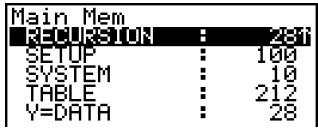

*1 You can input up to eight characters for the keyword.
# The message "Not Found" appears if there are no file names that match your keyword.

- To search for a file in the storage memory

Example To search for all files in the storage memory whose names begin with the letter "S"
- On the initial MEMORY mode screen press F2 (SMEM).
- This displays a list of files that are in the storage memory.
-
Press F3 (SRC).
-
Input the letter "S" for the keyword.
- The first file name that begins with the letter "S" appears highlighted on display.
![Storage Mem[ ] SHADE.sim : 4001 TRIG.sim : 348 VENN.sim : 236](/content/2025/01/86785/images/db6b7726fdb544d7a509c945eb44534d69aed531d26039bc32f2a662a419213e.jpg)
- To search for a file in the SD card (fx-9860G SD only)

Example To search for all files in the SD card whose names begin with the letter "R"
- On the initial MEMORY mode screen press F3 (SD).
- This displays a list of files that are in the SD card.
-
Press F3(SRC).
-
Input the letter "R" for the keyword.
- The first file name that begins with the letter "R" appears highlighted on display.
![SD Card [ ] REF.g1m : 372t SHADE.g1m : 336 TRIG.g1m : 284](/content/2025/01/86785/images/b9bca123310956013595cd0df8800285a74a467e92ec67142f814b4d0eca4404.jpg)

# The message "Not Found" appears if there are no file names that match your keyword.

■ Backing Up Main Memory Data
You can back up all the data in the main memory and store it in the storage memory or on the SD card. Later you can restore the backed up data to the main memory when necessary.
- To back up main memory data
- On the initial MEMORY mode screen press F4 (BKUP).
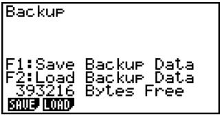
- Press F1(SAVE). This displays the save location selection screen (fx-9860G SD only).
![Save to Storage Mem:[1] SD Card :[2] 393216 Bytes Free SAVE LOAD](/content/2025/01/86785/images/65f68203e51bceac700c6b1afb47092709b517b29ffdf063ec51555c34e47be2.jpg)
- 1 ... storage memory
-
2 ... SD card
-
Press ① or ② (fx-9860G SD only). This displays a folder selection screen.
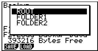
- Use ▲ and ▼ to select the folder where you want to save the data.
- Press EXE to start the backup.

# Backup data is saved in a file named BACKUP.g1m.

The message “Complete!” appears when the backup operation is finished.
Press EXIT to return to the screen displayed in step 1.
The following message appears if there is already backup data in the storage memory.
![[BACKUP.g1m ] Already Exists Overwrite OK? Yes: [F1] No : [F6]](/content/2025/01/86785/images/99dea0601d602cf04e044f24ab7a1dc4b0f8c9b2975754ae94c23096bf378f28.jpg)
Press F1 (Yes) to back up the data, or F6 (No) to cancel the backup operation.
A “Memory Full” occurs when there is not enough space available in the storage memory to complete the backup operation.
- To restore backup data to the main memory
- On the initial MEMORY mode screen press F4(BKUP).
- On the screen that appears, you can confirm whether or not there is backup data in the storage memory.
- Press F2 (LOAD).
This displays the restore source data selection screen (fx-9860G SD only).
![Load from Storage Mem:[1] SD Card :[2] 393216 Bytes Free SAVE LOAD](/content/2025/01/86785/images/9bc3f119d2689d8e9880bc6c093eeb1a019bf60e53480748841cb5e2e5d7042c.jpg)
- ① ... Restore from storage memory
-
② ... Restore from SD card
-
Press ① or ② (fx-9860G SD only).
This displays the folder selection screen.
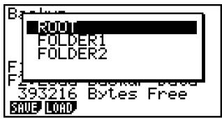
- Use ▲ and ▼ to select a folder.

5. Press EXE.\*1
- A message appears to confirm whether or not you really want to restore the backed up data.
![Overwrite OK? Yes: [F1] No : [F6] 391688 Bytes Free SAVE LOAD](/content/2025/01/86785/images/d4473ce9b24aa3420ba25aa49e32bc29a37c605c3e4347fedfa1a7f7d496356a.jpg)
Press F1(Yes) to restore the data and delete any data currently in the area.
Press F6 (No) to cancel the data backup operation.
The message “Complete!” appears when the restore operation is finished.
Press EXIT to return to the screen displayed in step 1.

*1 The message "No Data" will appear if there is no backup data stored in memory. Pressing EXIT will return the screen in step 1.

■ Optimizing the Storage Memory or SD Card Memory
Storage memory or SD card memory can become fragmented after many store and load operations. Fragmentation can cause blocks of memory to become unavailable for data storage. Because of this, you should periodically perform the storage memory or SD card optimization procedure, which rearranges the data in the storage memory or SD card and makes memory usage more economical.
- To optimize the storage memory
- On the initial MEMORY mode screen press F5(OPT) to optimize the storage memory.
- Select the memory you want to optimize (fx-9860G SD only).
![Optimize F1 Storage Mem:[1] F2 SD Card :[2] F3 Optimization MAIN SMART SD GROUP OPT](/content/2025/01/86785/images/1a07f2dda1cf55a26a5e13b5fdb0bbb9287b1233e7085ae1dbd7f003395b22a4.jpg)
-
1 ... storage memory
• 2 ... SD card -
Press ① or ② to start optimization.
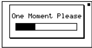
The message “Complete!” appears when the optimize operation is complete.
Press EXIT to return to the initial MEMORY mode screen.

# In some cases, the amount of free memory capacity may be unchanged when you check it after performing the optimization procedure. This does not indicate any problem with the calculator.

Chapter 13
Using SD Cards
(fx-9860G SD only)
You can use SD cards to store calculator data. You can copy main memory and storage memory data to and from an SD card.
13-1 Using an SD Card
13-2 Formatting an SD Card
13-3 SD Card Precautions during Use

Important!
- Always use an SD memory card. Operation is not guaranteed when another type of memory card is used.
- Be sure to read the user documentation that comes with an SD card before using it.
- Certain types of SD cards can slow down processing speeds.
- Certain types of SD cards and operating conditions can shorten battery life.
- SD cards have a write protect switch, which protects against accidental erasure of data. Note, however, that you need to remove write protection before you can copy data to or delete data from, or format a disk that is write-protected.
- Static electric charge, electric noise, and other phenomena can delete or corrupt card data unexpectedly. Because of this you should always backup valuable data to other media (CD-R, CD-RW, MO disk, hard disk, etc.)
13-1 Using an SD Card
Important!
- Always turn off the calculator before inserting or removing an SD card.
- Note that a card needs to be oriented correctly (proper side must be facing upwards, the proper end must be inserted) when inserting it into the calculator. Trying to force card into the slot while it is oriented incorrectly can damage the card and slot.
- Removing the Dummy Card
- Your calculator is shipped from the factory with a dummy card inserted in the SD card slot. Before using an SD card, first use the procedure under “To remove the SD card” on page 13-1-2 to remove the dummy card.
- To insert an SD card
- Orient the SD card so its back is facing upwards (in the same direction as the calculator keyboard).
- Carefully insert the SD card into the calculator's SD card slot.
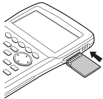
natural_image
Line drawing of a mobile phone with a scroll and control panel, showing a close-up of the right-hand side of the device (no text or symbols present)
Front
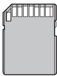
Back
Important!
- Never insert anything other an SD cards into the SD card slot. Doing so can damage the calculator.
- Should water or any foreign matter ever get into the SD card slot, immediately turn off the calculator, remove its batteries, and contact your original retailer or nearest CASIO authorized service center.

- To remove the SD card
- Press in on the SD card and then release it.
- This will cause the card to pop part way out of the slot.
- Grasp the SD card with your fingers and pull it out of the slot.

natural_image
Line drawing of a mobile phone control panel with a scroll wheel and keypad (no text or symbols)Important!
- Never remove the SD card while data is being transferred to it. Doing so not only stops the data you are transferring to the card from being saved, it can also corrupt SD card contents.
- Exerting undue force when removing an SD card can damage the card slot or the card.

13-2 Formatting an SD Card
- Use the procedure under "11-4 Reset" to format an SD card.

13-3 SD Card Precautions during Use
- SD card problems can normally be corrected by reformatting the card. However, it is always a good idea to take along more than one SD card to avoid data storage problems.
- Card formatting (initialization) is recommended before using a new SD card for the first time.
- If an SD card has been formatted on a computer or other device, you can use it as-is without reformatting. A computer or other device also will be able to use an SD card that has been formatted with the calculator.
-
Never perform any of the following operations while the SD card is being accessed.
-
Removing the SD card
- Connecting or disconnecting a USB cable
- Turning off the calculator
- When connected to a computer, exiting the FA-124 software or shutting down the computer
- Note that an SD card needs to be oriented correctly (proper side must be facing upwards, the proper end must be inserted) when inserting it into the calculator. Trying to force an SD card into the slot when it is oriented incorrectly can damage the card and slot.
- Use of certain SD cards while calculator battery power is low can cause the display to go blank without displaying the low battery warning message. If this happens, replace the batteries.
■ Recommended SD Card Types
Toshiba
SD-NA032MT
SD-NA064MT
SD-NA128MT
SD-NA256MT
SD-NA512MT
SD-FA128MT
SD-FA256MT
SanDisk
SDSDB-64-J60
SDSDB-128-J60
SDSDB-256-J60
SDSDB-512-J60
SDSDH-256-903
SDSDH-512-903
For detailed information (specifications, features, etc.) about the SD card, contact the SD card manufacturer.
Appendix
1 Error Message Table
2 Input Ranges
3 Specifications
4 Key Index
5 P Button (In case of hang up)
6 Power Supply
α
1 Error Message Table
| Message | Meaning | Countermeasure |
| Syntax ERROR | Illegal syntaxAttempt to input an illegal command | PressEXITto display the error and make necessary corrections. |
| Ma ERROR | Calculation result exceeds the display range.Calculation is outside the input range of a function.Mathematical error (division by zero, etc.)Sufficient precision could not be obtained for Σ calculation, differential calculation, etc.Solution could not be obtained for equation calculation, etc. | Check input values and make corrections to ensure that values are within allowable limits. |
| Go ERROR | 1 No corresponding Lbl n for Goto n.2 No program stored in program area Prog "file name". | 1 Correctly input a Lbl n to correspond to the Goto n , or delete the Goto n if not required.2 Store a program in program area Prog "file name", or delete the Prog "file name" if not required. |
| Nesting ERROR | Nesting of subroutines by Prog "file name" exceeds 10 levels. | Ensure that Prog "file name" is not used to return from subroutines to main routine. If used, delete any unnecessary Prog "file name".Trace the subroutine jump destinations and ensure that no jumps are made back to the original program area. Ensure that returns are made correctly. |
| Stack ERROR | Execution of calculations that exceed the capacity of the stack for numeric values or stack for commands. | Simplify the formulas to keep stacks within 10 levels for the numeric values and 26 levels for the commands.Divide the formula into two or more parts. |

| Message | Meaning | Countermeasure |
| MemoryERROR | Operation or memory storage operation exceeds remaining memory capacity. | Keep the number of memories you use within the currently specified number of memories.Simplify the data you are trying to store to keep it within the available memory capacity.Delete no longer needed data to make room for the new data. |
| ArgumentERROR | Incorrect argument specification for a command that requires an argument. | Correct the argument. |
| DimensionERROR | Illegal dimension used during matrix or list calculations. | Check the matrix or list dimension. |
| Range ERROR | 1 Input of an improper V-Window value.2 V-Window range settings exceeded when a graph is redrawn.3 Input of an improper value on the range screen and use of that value for execution.4 The spreadsheet cell range was exceeded by paste, recall, or other cell operation. | 1 Change the V-Window value so it is within range.2 Redraw using the proper settings.3 Input a proper range value.4 Repeat the procedure taking care that the cell range is not exceeded. |
| ConditionERROR | Execution of a calculation or function before all conditions required for execution are met. | Check the conditions and make any necessary corrections. |
| Non-RealERROR | Calculation that produces a complex number when Real is specified for the Complex Mode setting on the Setup screen, even though the argument is a real number. | Change the Complex Mode setting to something other than Real. |
| Complex Number In List | List containing complex number used in a calculation or operation for which complex number data is invalid. | Change all data in the list to real numbers. |
| Can’t Solve! Adjust initial value or bounds. Then try again | A Solve calculation could not obtain a solution within the specified range. | Change the specified range.Correct the input expression. |

| Message | Meaning | Countermeasure |
| No Variable | No variable specified within a graph function being used for Dynamic Graph.No variable within a Solve equation. | Specify a variable for the graph function.Input a Solve equation that includes a variable. |
| Com ERROR | Problem with cable connection or parameter setting during program data communications. | Check to make sure there is nothing wrong with the cable connection, and that parameters are configured correctly. |
| Transmit ERROR | Problem with cable connection or parameter setting during data communications. | Check to make sure there is nothing wrong with the cable connection, and that parameters are configured correctly. |
| Receive ERROR | Problem with cable connection or parameter setting during data communications. | Check to make sure there is nothing wrong with the cable connection, and that parameters are configured correctly. |
| Memory Full | Memory of receiving unit became full during program data communications. | Delete some data stored in the receiving unit and try again. |
| Time Out | A Solve calculation or integration calculation was unable to satisfy convergence conditions. | If you are performing a Solve calculation, try changing to the initial default estimated value.If you are performing an integration calculation, try changing to a larger tol value. |
| Circular ERROR | There is a circular reference (such as “=A1” in cell A1) in the spreadsheet. | Change cell contents to remove the circular references. |
| Please Reconnect | The connection was dropped for some reason while updating the operating system. | Reconnect and try again. |
| Too Many Data | The number of data items is too large. | Delete unneeded data. |
| Fragmentation ERROR | Memory must be optimized before any more data can be stored. | Optimize memory. |
| Invalid Name | The file name you input includes invalid characters. | Use the correct characters to input a valid file name. |

| Message | Meaning | Countermeasure |
| Invalid Type | An illegal data type is specified. | Specify valid data. |
| Storage Memory Full | The storage memory is full. | Delete unneeded data. |
| No Card* | There is no SD card loaded in the calculator. | Load an SD card. |
| SD Card Full* | The SD card is full. | Delete unneeded data. |
| Invalid file name or folder name.* | Data or folders that are supported by this calculator cannot be found on the SD card. | Replace the card with one that contains data/folders that are supported by this calculator. |
| Invalid Card* | A card that is not compatible with the calculator is loaded. | Replace the card with a compatible card. |
| Card is protected* | The SD card is write protected. | Remove write protection. |
| Data ERROR | A data error occurred. | Check to make sure you are writing correct type of data and try again. |
| Card ERROR* | An SD card error occurred. | Remove and correctly insert the SD card and try again. If this error occurs again, re-format the SD card. |
| Data is protected* | The Read Only attribute of the SD card loaded in the calculator has been turned on using a computer, etc. | Turn off the SD card's Read Only attribute. |
*fx-9860G SD only

2 Input Ranges
| Function | Input range for real number solutions | Internal digits | Precision | Notes |
| x x x | (DEG) |x| < 9 × (10^9)^ (RAD) |x| < 5 × 10^7 rad (GRA) |x| < 1 × 10^10grad | 15 digits | As a rule,precision is ±1 at the 10th digit.* | However, for x : |x| 90(2n+1) : DEG |x| /2(2n+1) : RAD |x| 100(2n+1) : GRA |
| ^-1x ^-1x ^-1x | |x| ≤ 1 | " | " | |
| |x| < 1 × 10^100 | ||||
| x x x | |x| ≤ 230.9516564 | " | " | |
| |x| < 1 × 10^100 | ||||
| ^-1x ^-1x ^-1x | |x| < 1 × 10^100 | " | " | |
| 1 ≤ x < 1 × 10^100 | ||||
| |x| < 1 | ||||
| x x | 1 × 10^-99 ≤ x < 1 × 10^100 | " | " | • Complex numbers can be used as arguments. |
| 10^x e^x | -1 × 10^100 < x < 100 | " | " | • Complex numbers can be used as arguments. |
| -1 × 10^100 < x ≤ 230.2585092 | ||||
| x^2 | 0 ≤ x < 1 × 10^100 | " | " | • Complex numbers can be used as arguments. |
| |x| < 1 × 10^50 | ||||
| 1/x ^3 | |x| < 1 × 10^100, x 0 | " | " | • Complex numbers can be used as arguments. |
| |x| < 1 × 10^100 | ||||
| x! | 0 ≤ x ≤ 69 ( x is an integer) | " | " | |
| nPr nCr | Result < 1 × 10^100 n, r ( n and r are integers) 0 ≤ r ≤ n, n < 1 × 10^10 | " | " |

| Function | Input range for real number solutions | Internal digits | Precision | Notes |
| Pol (x, y) | ^2 + y^2 < 1 × 10^100 | 15 digits | As a rule, precision is ±1 at the 10th digit.* | |
| Rec (r, θ) | |r| < 1 × 10100(DEG) |θ| < 9 × (109)°(RAD) |θ| < 5 × 10⁷π rad(GRA) |θ| < 1 × 10¹⁰grad | " | " | However, for tanθ: |θ| ≠ 90(2n+1): DEG |θ| ≠ π/2(2n+1): RAD |θ| ≠ 100(2n+1): GRA |
| ○, „ | |a|, b, c < 1 × 101000 ≤ b, c | " | " | |
| |x| < 1 × 10100Sexagesimal display: |x| < 1 × 10⁷ | ||||
| ^(x^y) | x > 0:-1 × 10100 < y log x < 100x = 0 : y > 0x < 0 : y = n, 2n+1 (m, n are integers)However;-1 × 10100 < y log |x| < 100 | " | " | Complex numbers can be used as arguments. |
| ^x | y > 0 : x ≠ 0-1 × 10100 < 1x log y < 100y = 0 : x > 0y < 0 : x = 2n+1, 2n+1m (m ≠ 0; m, n are integers)However;-1 × 10100 < 1x log |y| < 100 | " | " | Complex numbers can be used as arguments. |
| a^b/c | Total of integer, numerator and denominator must be within 10 digits (includes division marks). | " | " |
* For a single calculation, calculation error is ±1 at the 10th digit. (In the case of exponential display, calculation error is ±1 at the last significant digit.) Errors are cumulative in the case of consecutive calculations, which can also cause them to become large. (This is also true of internal consecutive calculations that are performed in the case of (x^y), x^y, x!, x', [3]x, nPr, nCr , etc.)
In the vicinity of a function's singular point and point of inflection, errors are cumulative and may become large.

| Function | Input range |
| Binary, octal, decimal, hexadecimal calculation | Values fall within following ranges after conversion:DEC: -2147483648 ≤ x ≤ 2147483647BIN: 1000000000000000 ≤ x ≤ 111111111111111 (negative)0 ≤ x ≤ 111111111111111 (0, positive)OCT: 20000000000 ≤ x ≤ 37777777777 (negative)0 ≤ x ≤ 17777777777 (0, positive)HEX: 80000000 ≤ x ≤ FFFFFFFF (negative)0 ≤ x ≤ 7FFFFFFF (0, positive) |

3 Specifications
Variables: 28
Calculation range:
±1×10^-99 to ±9.999999999×10^99 and 0. Internal operations use 15-digit mantissa.
Exponential display range: Norm 1: 10^-2 > |x|, |x| ≥ 10^10
Norm 2: 10^-9 > |x| , |x| ≥ 10^10
Program capacity: 64000 bytes (max.)
Storage memory capacity: 1.5MB (max.)
Power supply:
Main: Four AAA-size batteries (LR03 (AM4))
Back-up: One CR2032 lithium battery
Power consumption: 0.7 W
Approximate battery life
Main:
LR03 (AM4): 300 hours (continuous display of main menu) 220 hours continuous operation (5 minutes calculation, 55 minutes display) 90 hours when an SD card is used (fx-9860G SD only) 1 year (unused with power off)
- Any of the following can shorten battery life.
- Certain SD card types or frequent SD card access
- Sequential program calculation execution
- Certain battery types
Back-up: 5 years
Auto power off:
Power is automatically turned off approximately six minutes or 60 minutes after last operation.
Ambient temperature range: 0 °C to 40 °C
Dimensions: 24 mm (H) × 92.5 mm (W) × 184.5 mm (D)
$$ 1 ^ {\prime \prime} (H) \times 3 ^ {5 / 8 ^ {\prime \prime}} (W) \times 7 ^ {1 / 4 ^ {\prime \prime}} (D) $$
Weight: fx-9860G SD
Approx. 265 g (including batteries)
fx-9860G
Approx. 260 g (including batteries)
Data Communications
3-pin serial port
Method: Start-stop (asynchronous), half-duplex
Transmission speed (BPS):
115200 bits/second (normal)
9600 bits/second (When connected to CFX-9850/fx-7400 series; Send/Receive commands)
38400 bits/second (Send38k/Receive38k commands)
<115200 bits/second>
Parity: EVEN
Bit length: 8 bits
Stop bit:
Send: 1 bit
Receive: 1 bit
Includes parity (None) 1-bit
X ON/X OFF Control: None
<9600, 38400 bits/second>
Parity: None
Bit length: 8 bits
Stop bit:
Send: 3 bits
Receive: 2 bits
Includes parity (None) 1-bit
X ON/X OFF Control: None
USB port
In accordance with USB 1.1 standards
4 Key Index
| Key | Primary Function | Combined withSHIFT | Combined withALPHA |
| TraceF1 | Selects 1st function menu item. | Performs trace operation. | |
| ZoomF2 | Selects 2nd function menu item. | Performs zoom operation. | |
| V-WindowF3 | Selects 3rd function menu item. | Displays V-Window parameter input screen. | |
| SketchF4 | Selects 4th function menu item. | Performs sketch operation. | |
| G-SolvF5 | Selects 5th function menu item. | Performs G-Solve operation. | |
| G↔TF6 | Selects 6th function menu item. | Switches display between graph and text screens. | |
| Key | Primary Function | Combined withSHIFT | Combined withALPHA |
| SHIFT | Activates shift functions of other keys and function menus. | ||
| OPTN | Displays option menu. | ||
| PRGMVARS | Displays the variable data menu. | Displays program command menu. | |
| SET UPMENU | Returns to the Main Menu. | Shows the Setup screen. | |
| A-LOCKALPHA | Allows entry of alphanumeric characters shown in red. | Locks entry of alpha-numeric characters. | |
| √r x^2 | Press after entering value to calculate square. | Press before entering value to calculate square root. | Enters character r. |
| x-θ | Press between two values to make second value exponent of first. | Linear Input Mode:Press between entering values for X & Y to show xth root of y.Math Input Mode:Enters ( ) in natural input format. | Enters character θ. |
| QUITEXIT | Back steps to the previous screen without making any changes. | Returns directly to initial screen of the mode. | |
| ▲ | Moves cursor upward. Scrolls screen.Switches to previous function in trace mode. | Scrolls one screen up in the e·ACT or RUN·MAT (Math input mode) mode. | |

| Key | Primary Function | Combined withSHIFT | Combined withALPHA |
| Moves cursor downward. Scrolls screen. Switches to next function in trace mode. | Scrolls one screen down in the e·ACT or RUN·MAT (Math input mode) mode. | ||
| Moves cursor to left. Scrolls screen. Press after EXE to display calculation from end. | Makes contrast lighter. | ||
| Moves cursor to right. Scrolls screen. Press after EXE to display calculation from beginning. | Makes contrast darker. | ||
| ∠A ,,T | Allows input of variable X, θ, and T. | Enters the operator (∠) for complex number polar format input. | Enters letter A. |
| 10^x B | Press before entering value to calculate common logarithm. | Press before entering exponent value of 10. | Enters letter B. |
| e^x C | Press before entering value to calculate natural logarithm. | Press before entering exponent value of e. | Enters letter C. |
| ^-1 D | Press before entering value to calculate sine. | Press before entering value to calculate inverse sine. | Enters letter D. |
| ^-1 E | Press before entering value to calculate cosine. | Press before entering value to calculate inverse cosine. | Enters letter E. |
| ^-1 F | Press before entering value to calculate tangent. | Press before entering value to calculate inverse tangent. | Enters letter F. |
| ■ 吕 G 23 | Linear input mode:Press between entering fraction values.Math input mode:Enters an improper fraction (吕) in natural input format. | Inputs a mixed fraction.(Enabled only for the Math input mode.) | Enters letter G. |
| a_c^b,d,c H D | Converts fraction to decimal. | Converts between an improper fraction and mixed fraction. | Enters letter H. |
| [3]I (☐) | Enters open parenthesis in formula. | Press before entering value to calculate cube root. | Enters letter I. |
| x^-1 J☐) | Enters close parenthesis in formula. | Press after entering value to calculate reciprocal. | Enters letter J. |
| ☐K☐ | Enters comma. | Transitions from an application launched from an eActivity to another application. (Enabled only in an eActivity.) | Enters letter K. |
| ☐L☐ | Assigns value to an Alpha memory name. | Toggles between an eActivity and the screen of an application launched from the eActivity.(Enabled only in an eActivity.) | Enters letter L. |
| CAPTURE M7 | Enters number 7. | Captures the current screen to Capture memory. | Enters letter M. |

| Key | Primary Function | Combined withSHIFT | Combined withALPHA |
| CLIP N8 | Enters number 8. | Changes the shape of the cursor to indicate that the clipboard function is enabled. | Enters letter N. |
| PASTE O9 | Enters number 9. | Pastes the character string that is on the clipboard. | Enters letter O. |
| INSDEL | Insert mode:Backspace function.Overwrite mode:Deletes the character at the cursor position. | Linear input mode:Toggles between the insert mode and overwrite mode.Math input mode:With natural input, inserts a function into an existing expression (see page 1-3-13). | |
| OFFAC/ON | Turns power on.Clears the display. | Turns power off. | |
| CATALOG P4 | Enters number 4. | Displays the catalog function list. | Enters letter P. |
| Q5 | Enters number 5. | Enters letter Q. | |
| R6 | Enters number 6. | Enters letter R. | |
| { S× | Multiplication function. | Enters open curly bracket. | Enters letter S. |
| } T÷ | Division function. | Enters close curly bracket. | Enters letter T. |
| List U1 | Enters number 1. | Inputs List command. | Enters letter U. |
| Mat V2 | Enters number 2. | Inputs Mat command. | Enters letter V. |
| W3 | Enters number 3. | Enters letter W. | |
| [ X+ | Addition function.Specifies positive value. | Enters open bracket. | Enters letter X. |
| ] Y- | Subtraction function.Specifies negative value. | Enters close bracket. | Enters letter Y. |
| i Z0 | Enters number 0. | Inputs imaginary number unit. | Enters letter Z. |
| = SPACE· | Enters decimal point. | Enters character =. | Enters a blank space. |
| π "EXP | Enables entry of exponent. | Inputs value of pi.Enters pi symbol. | Enters double quotation mark. |
| Ans(→) | Enter before value to specify as negative. | Recalls most recent calculation result. | |
| ←EXE | Displays result of calculation. | Inputs a new line. |

5 P Button (In case of hang up)
Pressing the P button resets the calculator to its initial defaults.
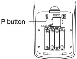
Warning!
Never perform this operation unless you want to totally clear the memory of the calculator. If you need the data currently stored in memory, be sure to write it down somewhere before performing the P button operation.
- Pressing the P button while a calculation operation is being performed (while the calculator is performing a calculation internally) deletes all data in memory.
- You can also reset the calculator using front panel key operations (see 11-4 Reset). Use the P button to reset only while the front panel keys are disabled for some reason.

6 Power Supply
This calculator is powered by four AAA-size (LR03 (AM4)) batteries. In addition, it uses a single CR2032 lithium battery as a back up power supply for the memory.
If the following message appears on the display, immediately turn off the calculator and replace main batteries as instructed.
Low Main Batteries!
Please Replace
If you try to continue using the calculator, it will automatically turn off in order to protect memory contents. You will not be able to turn power back on until you replace batteries.
Be sure to replace the main batteries at least once every one year, no matter how much you use the calculator during that time.
The batteries that come with this calculator discharge slightly during shipment and storage. Because of this, they may require replacement sooner than the normal expected battery life.
Warning!
Main memory contents will be deleted if you remove both the main power supply and the memory back up batteries at the same time. If you ever remove both batteries, correctly reload them and then perform the reset operation.

■ Replacing Batteries
Precautions:
Incorrectly using batteries can cause them to burst or leak, possibly damaging the interior of the calculator. Note the following precautions:
- Be sure that the positive (+) and negative (−) poles of each battery are facing in the proper directions.
- Never mix batteries of different types.
- Never mix old batteries and new ones.
- Never leave dead batteries in the battery compartment.
- Remove the batteries if you do not plan to use the calculator for long periods.
- Never try to recharge the batteries supplied with the calculator.
- Do not expose batteries to direct heat, let them become shorted, or try to take them apart.

natural_image
Cartoon illustration of a character with spiky hair and expressive eyes (no text or symbols)

natural_image
Simple line drawing of a hand holding a cylindrical object with four arms (no text or symbols)
(Should a battery leak, clean out the battery compartment of the calculator immediately, taking care to avoid letting the battery fluid come into direct contact with your skin.)
Keep batteries out of the reach of small children. If swallowed, consult with a physician immediately.
- To replace the main power supply batteries
- Never remove the main power supply and the memory back up batteries from the calculator at the same time.
- Never turn on the calculator while the main power supply batteries are removed or not loaded correctly. Doing so can cause memory data to be deleted and malfunction of the calculator. If mishandling of batteries causes such problems, correctly load batteries and then perform the RESET operation to resume normal operation.
- Be sure to replace all four batteries with new ones.

- Press SHIFT AC/ON (OFF) to turn off the calculator.
Warning!
- Be sure to turn the calculator off before replacing batteries. Replacing batteries with power on will cause data in memory to be deleted.
- Making sure that you do not accidentally press the AC/ON key, slide the case onto the calculator and then turn it over.
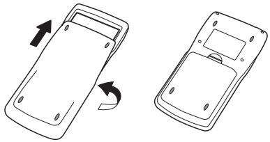
natural_image
Two line drawings of a mobile phone casing with arrows indicating rotation (no text or symbols)-
Remove the back cover from the calculator by pulling with your finger at the point marked ①.
-
Remove the four old batteries.
-
Load a new set of four batteries, making sure that their positive (+) and negative (−) ends are facing in the proper directions.
-
Replace the back cover.
-
Turn the calculator front side up and slide off its case. Next, press AC/ON to turn on power.
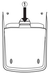
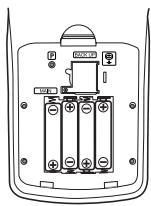
natural_image
Diagram of a device rear panel showing battery pack and socket (no text or symbols)
# Power supplied by memory back up battery while the main power supply batteries are removed for replacement retains memory contents.
# Do not leave the calculator without main power supply batteries loaded for long periods. Doing so can cause deletion of data stored in memory.
# If the figures on the display appear too light and hard to see after you turn on power, adjust the contrast.

- To replace the memory back up battery
- Before replacing the memory back up battery, check to make sure the main batteries are not dead.
- Never remove the main power supply and the memory back up batteries from the calculator at the same time.
-
Be sure to replace the back up power supply battery at least once 5 years, regardless of how much you use the calculator during that time. Failure to do so can cause data in memory to be deleted.
-
Press SHIFT AC/ON (OFF) to turn off the calculator.
Warning!
- Be sure to turn the calculator off before replacing battery. Replacing battery with power on will cause data in memory to be deleted.
- Making sure that you do not accidentally press the AC/ON key, slide the case onto the calculator and then turn it over.

natural_image
Two line drawings of a mobile phone casing with arrows indicating rotation (no text or symbols)- Remove the back cover from the calculator by pulling with your finger at the point marked ①.
- Remove screw Ⓐ on the back of the calculator, and remove the back up battery compartment cover.
- Insert a thin, pointed non-metal object (such as a toothpick) into the hole made ⑧ and remove the old battery.
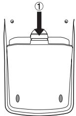
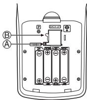

- Wipe off the surfaces of a new battery with a soft, dry cloth. Load it into the calculator so that its positive (+) side is facing up.
- Install the back up battery compartment cover onto the calculator and secure it in place with the screw. Next, replace the back cover.
- Turn the calculator front side up and slide off its case. Next, press AC/ON to turn on power.
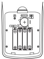
Calculator power turns off automatically if you do not perform any operation within the Auto Power Off trigger time you specify. You can specify either six minutes or 60 minutes as the trigger time (see "APO Settings" on page 11-2-1). To restore power, press AC.ON.


Please keep your manual and all information handy for future reference.

CASIO®
CASIO COMPUTER CO., LTD.
6-2, Hon-machi 1-chome Shibuya-ku, Tokyo 151-8543, Japan
One or more of the following patents may be used in the product. U.S.Pats. 4,794,553 4,794,554 5,166,897 5,210,708 5,535,317 5,539,867
- FCC WARNING
- Declaration of Conformity
- BEFORE USING THE CALCULATOR FOR THE FIRST TIME...
- Press MENU.
- Quick-Start
- TURNING POWER ON AND OFF
- USING MODES
- To select the RUN·MAT mode
- BASIC CALCULATIONS
- Parentheses Calculations
- Built-In Functions
- REPLAY FEATURE
- FRACTION CALCULATIONS
- Example: 31/_16 + 37/_9
- Converting an Improper Fraction to a Mixed Fraction
- Converting a Fraction to Its Decimal Equivalent
- EXPONENTS
- GRAPH FUNCTIONS
- Example 1: To graph Y = X(X + 1)(X - 2)
- Example 2: To determine the roots of Y = X(X + 1)(X - 2)
- DUAL GRAPH
- Box Zoom
- DYNAMIC GRAPH
- TABLE FUNCTION
- Precautions when Using this Product
- - fx-9860G SD only
- Precautions when Connecting to a Computer
- Handling Precautions
- Be sure to keep physical records of all important data!
- Contents
- Getting Acquainted — Read This First!
- Chapter 1 Basic Operation
- Chapter 2 Manual Calculations
- Chapter 3 List Function
- Chapter 4 Equation Calculations
- Chapter 5 Graphing
- Chapter 6 Statistical Graphs and Calculations
- Chapter 7 Financial Calculation (TVM)
- Chapter 8 Programming
- Chapter 9 Spreadsheet
- Chapter 10 eActivity
- Chapter 11 System Settings Menu
- Chapter 12 Data Communications
- Chapter 13 Using SD Cards (fx-9860G SD only)
- Appendix
- Getting Acquainted
- — Read This First!
- About this User's Guide
- - SHIFT 2 (√)
- - MENU EQUA
- - Function Keys and Menus
- - Menu Titles
- •Graphs
- - Command List
- - Page Contents
- ●Supplementary Information
- Chapter
- Basic Operation
- 1-1 Keys
- Key Table
- ■ Key Markings
- # ALPHA Alpha Lock
- 1-2 Display
- ■ Selecting Icons
- - To select an icon
- ■ About the Function Menu
- ■ About Display Screens
- Normal Display
- - How to interpret exponential format
- ■ Special Display Formats
- ■ Calculation Execution Indicator
- 1-3 Inputting and Editing Calculations
- Note
- ■ Inputting Calculations
- ■ Editing Calculations
- - To change a step
- - To delete a step
- The cursor is a vertical flashing line (I) when the insert mode is selected. The cursor is a horizontal flashing line (—) when the overwrite mode is selected.
- - To insert a step
- - To change the last step you input
- ■ Using Replay Memory
- Example 1 To perform the following two calculations
- Example 2
- ■ Making Corrections in the Original Calculation
- ■ Using the Clipboard for Copy and Paste
- - To specify the copy range
- Linear input mode
- Math input mode
- - To cut the text
- - Pasting Text
- ■ Catalog Function
- - To use the Catalog to input a command
- ■ Input Operations in the Math Input Mode
- - Math Input Mode Functions and Symbols
- • Using the MATH Menu
- - Math Input Mode Input Examples
- Example 3
- Example 4
- - When the calculation does not fit within the display window
- - Inserting a Function into an Existing Expression
- - To insert a function into an existing expression
- Example To insert the function into the expression 1 + (2 + 3) + 4 so the parenthetical expression becomes the argument of the function
- • Function Insert Rules
- - Functions that Support Insertion
- - Editing Calculations in the Math Input Mode
- - Math Input Mode Calculation Result Display
- - Math Input Mode Input Restrictions
- Fractions are displayed either as improper fractions or mixed fractions, depending on the "Frac Result" setting on the Setup screen. For details, see "1-7 Using the Setup Screen".
- Matrices are displayed in natural format, up to 6 × 6 . A matrix that has more than six rows or columns will be displayed on a MatAns screen, which is the same screen used in the Linear input mode.
- Lists are displayed in natural format for up to 20 elements. A list that has more than 20 elements will be displayed on a ListAns screen, which is the same screen used in the Linear input mode.
- Arrows appear at the left, right, top, or bottom edge of the display to let you know when there is more data off the screen in the corresponding direction.
- Pressing F2(DEL)F1(DEL·L) while a calculation result is selected will delete both the result and the calculation that produced it.
- The multiplication sign cannot be omitted immediately before an improper fraction or mixed fraction. Be sure to always input a multiplication sign in this case.
- 1-4 Option (OPTN) Menu
- - Option menu in the RUN·MAT or PRGM mode
- 1-5 Variable Data (VARS) Menu
- • V-WIN — Recalling V-Window values
- • FACT — Recalling zoom factors
- • STAT — Recalling statistical data
- • GRPH — Recalling Graph Functions
- • DYNA — Recalling Dynamic Graph Set Up Data
- - TABL — Recalling Table Set Up and Content Data
- - RECR — Recalling Recursion Formula *1 , Table Range, and Table Content Data
- - EQUA — Recalling Equation Coefficients and Solutions *4 \*5
- • TVM — Recalling Financial Calculation Data
- 1-6 Program (PRGM) Menu
- 1-7 Using the Setup Screen
- - To change a mode setup
- ■ Setup Screen Function Key Menus
- - Input Mode
- 1-8 Using Screen Capture
- - To capture a screen image
- - To recall a screen image from capture memory
- 1-9 When you keep having problems...
- ■ Getting the Calculator Back to its Original Mode Settings
- In Case of Hang Up
- ■ Low Battery Message
- 2
- Manual Calculations
- Linear/Math input mode (page 1-3-8)
- 2-1 Basic Calculations
- Arithmetic Calculations
- ■ Number of Decimal Places, Number of Significant Digits, Normal Display Range [SET UP]-[Display] -[Fix]/[Sci]/
- ■ Calculation Priority Sequence
- Compound functions are executed from right to left.
- Anything contained within parentheses receives highest priority.
- ■ Multiplication Operations without a Multiplication Sign
- ■ Overflow and Errors
- ■ Memory Capacity
- 2-2 Special Functions
- ■ Memory
- - Variables (Alpha Memory)
- - To assign a value to a variable
- - To display the contents of a variable
- - To clear a variable
- - To assign the same value to more than one variable
- - Function Memory
- - To store a function
- - To recall a function
- - To recall a function as a variable
- - To display a list of available functions
- - To delete a function
- • To use stored functions
- Answer Function
- - To use the contents of the answer memory in a calculation
- ■ Performing Continuous Calculations
- ■ History Function
- Example To change “1+2” to “1+3” and recalculate
- ■ Stacks
- ■ Using Multistatements
- - Colon (:)
- - Display Result Command (▲)
- 2-3 Specifying the Angle Unit and Display Format
- ■ Setting the Angle Unit
- ■ Setting the Display Format
- - To specify the number of decimal places (Fix)
- - To specify the number of significant digits (Sci)
- Example To specify three significant digits
- - To specify the normal display (Norm 1/Norm 2)
- - To specify the engineering notation display (Eng mode)
- 2-4 Function Calculations
- ■ Function Menus
- • Hyperbolic Calculations (HYP)
- ● Probability/Distribution Calculations (PROB)
- - Numeric Calculations (NUM)
- - Angle Units, Coordinate Conversion, Sexagesimal Operations (ANGL)
- • Engineering Symbol (ESYM)
- Angle Units
- ■ Trigonometric and Inverse Trigonometric Functions
- ■ Logarithmic and Exponential Functions
- ■ Hyperbolic and Inverse Hyperbolic Functions
- ■ Other Functions
- ■ Random Number Generation (Ran#)
- ■ Coordinate Conversion
- ■ Permutation and Combination
- Example
- Fractions
- Switching between improper fraction and mixed fraction format
- Switching between fraction and decimal format
- ■ Engineering Notation Calculations
- 2-5 Numerical Calculations
- ■ Solve Calculations
- ■ Differential Calculations
- Using Differential Calculation in a Graph Function
- (Math>
- In the function f(x) , only X can be used as a variable in expressions. Other variables (A through Z excluding X, r, ) are treated as constants, and the value currently assigned to that variable is applied during the calculation.
- Input of the tolerance (tol) value and the closing parenthesis can be omitted. If you omit tolerance (tol) value, the calculator automatically uses a value for tol as 1E-10.
- Specify tolerance (tol) value of 1E-14 or less. An error (Time Out) occurs whenever no solution that satisfies the tolerance value can be obtained.
- In the Math input mode, the tolerance value is fixed at 1E-10 and cannot be changed.
- Inaccurate results and errors can be caused by the following:
- - Applications of Differential Calculations
- ■ Quadratic Differential Calculations
- • Quadratic Differential Applications
- Using Quadratic Differential Calculation in a Graph Function (see page 2-5-2)
- You can interrupt an ongoing quadratic differential calculation by pressing the AC key.
- Always use radians (Rad mode) as the angle unit when performing trigonometric quadratic differentials.
- You cannot use a differential, quadratic differential, integration, , maximum/minimum value, Solve, RndFix or log ab calculation expression inside of a quadratic differential calculation term.
- With quadratic differential calculation, calculation precision is up to five digits for the mantissa.
- ■ Integration Calculations
- - Application of Integration Calculation
- Σ Calculations
- - Calculation Applications
- Maximum/Minimum Value Calculations
- ●Minimum Value
- ●Maximum Value
- Example 2 To determine the maximum value for the interval defined by start point a = 0 and end point b = 3, with a precision of n = 6 for the function y = -x2 + 2x + 2
- Input of n and the closing parenthesis can be omitted.
- Discontinuous points or sections with drastic fluctuation can adversely affect precision or even cause an error.
- You cannot use a differential, quadratic differential, integration, , maximum/minimum value, Solve, RndFix or log ab calculation expression inside of a maximum/minimum calculation term.
- Inputting a larger value for n increases the precision of the calculation, but it also increases the amount of time required to perform the calculation.
- The value you input for the end point of the interval (b) must be greater than the value you input for the start point (a). Otherwise an error occurs.
- You can interrupt an ongoing maximum/minimum calculation by pressing the AC key.
- You can input an integer in the range of 1 to 9 for the value of n. Using any value outside this range causes an error.
- 2-6 Complex Number Calculations
- Arithmetic Operations
- ■ Reciprocals, Square Roots, and Squares
- ■ Complex Number Format Using Polar Form
- ■ Absolute Value and Argument
- ■ Conjugate Complex Numbers
- ■ Extraction of Real and Imaginary Parts
- ■ Polar and Rectangular Form Transformation
- 2-7 Binary, Octal, Decimal, and Hexadecimal Calculations with Integers
- ■ Selecting a Number System
- - To specify a number system for an input value
- - To input values of mixed number systems
- ■ Arithmetic Operations
- ■ Negative Values and Bitwise Operations
- - Negative Values
- - Bitwise Operations
- Example 2 To display the result of “368 or 11102” as an octal value
- Example 3 To negate 2FFFED _16
- • Number System Transformation
- - To convert a displayed value from one number system to another
- Example To convert 22_10 (default number system) to its binary or octal value
- 2-8 Matrix Calculations
- ■ Inputting and Editing Matrices
- - Creating a Matrix
- - To specify the dimensions (size) of a matrix
- - To input cell values
- You cannot input complex numbers into the cell of a matrix.
- Displayed cell values show positive integers up to six digits, and negative integers up to five digits (one digit used for the negative sign). Exponential values are shown with up to two digits for the exponent. Fractional values are not displayed.
- You can see the entire value assigned to a cell by using the cursor keys to move the highlighting to the cell whose value you want to view.
- The amount of memory required for a matrix is 9 bytes per cell. This means that a 3 × 3 matrix requires 81 bytes of memory ( 3 × 3 × 9 = 81 ).
- - Deleting Matrices
- - To delete a specific matrix
- - To delete all matrices
- ■ Matrix Cell Operations
- - Row Calculations
- - To swap two rows
- - To calculate the scalar multiplication of a row
- - To calculate the scalar multiplication of a row and add the result to another row
- • To add two rows together
- - Row Operations
- - To delete a row
- - To insert a row
- - To add a row
- - Column Operations
- - To delete a column
- - To insert a column
- - To add a column
- ■ Modifying Matrices Using Matrix Commands
- - To display the matrix commands
- - Matrix Data Input Format
- Example 1 To input the following data as Matrix A :
- - To input an identity matrix
- Example 2 To create a 3 × 3 identity matrix as Matrix A
- - To check the dimensions of a matrix
- Example 3 To check the dimensions of Matrix A, which was input in Example 1
- Example 4 To specify dimensions of 2 rows and 3 columns for Matrix B
- - Modifying Matrices Using Matrix Commands
- - To assign values to and recall values from an existing matrix
- - To assign the contents of a matrix column to a list
- ■ Matrix Calculations
- - Matrix Arithmetic Operations
- - Determinant
- - Matrix Transposition
- - Matrix Inversion
- - Squaring a Matrix
- Only square matrices (same number of rows and columns) can be inverted. Trying to invert a matrix that is not square produces an error.
- A matrix with a determinant of zero cannot be inverted. Trying to invert a matrix with determinant of zero produces an error.
- Calculation precision is affected for matrices whose determinant is near zero.
- • Raising a Matrix to a Power
- ■ Performing Matrix Calculations Using Natural Input
- - To assign a matrix created using natural input to a MAT mode matrix
- 3
- List Function
- 3-1 Inputting and Editing a List
- - To input values one-by-one
- - To batch input a series of values
- ■ Editing List Values
- - To change a cell value
- - To edit the contents of a cell
- - To delete a cell
- - To delete all cells in a list
- - To insert a new cell
- ■ Naming a List
- - To name a list
- ■ Sorting List Values
- - To sort a single list
- Ascending order
- Descending order
- - To sort multiple lists
- 3-2 Manipulating List Data
- ■ Accessing the List Data Manipulation Function Menu
- - To count the number of data items in a list
- - To create a list or matrix by specifying the number of data items
- - To replace all data items with the same value
- - To generate a sequence of numbers
- - To find the minimum value in a list
- - To find the maximum value in a list
- - To find which of two lists contains the smallest value
- - To find which of two lists contains the greatest value
- - To calculate the mean of data items
- - To calculate the mean of data items of specified frequency
- - To calculate the median of data items in a list
- - To calculate the median of data items of specified frequency
- - To combine lists
- - To calculate the sum of data items in a list
- 3-3 Arithmetic Calculations Using Lists
- ■ Error Messages
- ■ Inputting a List into a Calculation
- - To input a specific list by name
- - To directly input a list of values
- - To assign the contents of one list to another list
- - To recall the value in a specific list cell
- - To input a value into a specific list cell
- ■ Recalling List Contents
- - To use list contents in ListAns Memory in a calculation
- ■ Graphing a Function Using a List
- ■ Inputting Scientific Calculations into a List
- ■ Performing Scientific Function Calculations Using a List
- 3-4 Switching Between List Files
- - To switch between list files
- 4
- Equation Calculations
- 4-1 Simultaneous Linear Equations
- Description
- Set Up
- Execution
- Procedure
- Internal calculations are performed using a 15-digit mantissa, but results are displayed using a 10-digit mantissa and a 2-digit exponent.
- Simultaneous linear equations are solved by inverting the matrix containing the coefficients of the equations. For example, the following shows the solution (x_1, x_2, x_3) of a simultaneous linear equation with three unknowns.
- An error occurs if the calculator is unable to find a solution.
- After calculation is complete, you can press F1 (REPT), change coefficient values, and then re-calculate.
- 4-2 Quadratic and Cubic Equations
- After calculation is complete, you can press F1(REPT), change coefficient values, and then re-calculate.
- 4-3 Solve Calculations
- Result Screen
- 4-4 What to Do When an Error Occurs
- - Error during coefficient value input
- - Error during calculation
- ■ Clearing Equation Memories
- Chapter 5
- 5
- Graphing
- 5-1 Sample Graphs
- ■ How to draw a simple graph (1)
- ■ How to draw a simple graph (2)
- ■ How to draw a simple graph (3)
- ■ How to draw a simple graph (4)
- 5-2 Controlling What Appears on a Graph Screen
- ■ V-Window (View Window) Settings
- - To make V-Window settings
- Rectangular coordinate parameter
- Polar coordinate parameter
- • V-Window Setting Precautions
- ■ Initializing and Standardizing the V-Window
- - To initialize the V-Window
- - To initialize the V-Window in accordance with an angle unit
- - To standardize the V-Window
- ■ V-Window Memory
- - To store V-Window settings
- - To recall V-Window memory settings
- ■ Specifying the Graph Range
- Zoom
- Factor Zoom
- 5-3 Drawing a Graph
- ■ Specifying the Graph Type
- ■ Storing Graph Functions
- - To store a polar coordinate function (r = )*1
- - To store a parametric function \*2
- - To assign values to the coefficients and variables of a graph function
- ■ Editing and Deleting Functions
- • To edit a function in memory
- - To change the line style of a graph function
- - To change the type of a function *1
- ■ Selecting Functions for Graphing
- - To specify the draw/non-draw status of a graph
- ■ Graph Memory
- - To store graph functions in graph memory
- • To recall a graph function
- 5-4 Storing a Graph in Picture Memory
- - To store a graph in picture memory
- - To recall a stored graph
- 5-5 Drawing Two Graphs on the Same Screen
- ■ Copying the Graph to the Sub-screen
- - Main Screen
- - Sub-screen
- ■ Graphing Two Different Functions
- ■ Using Zoom to Enlarge the Sub-screen
- 5-6 Manual Graphing
- ■ Rectangular Coordinate Graph
- ■ Integration Graph
- ■ Drawing Multiple Graphs on the Same Screen
- The value of only one of the variables in the expression can change.
- Any of the following cannot be used for the variable name: X, Y, r, θ, T.
- You cannot assign a variable to the variable inside the function.
- When Simul Graph is turned on, all of the graphs for the specified variable values are drawn simultaneously.
- Overwrite can be used when graphing rectangular expressions, polar expressions, parametric functions, X = constant functions, and inequalities.
- ■ Using Copy and Paste to Graph a Function
- Type 1 (Y= expression)
- Type 2 (expression)
- Paste is supported only when "Off" is selected for the "Dual Screen" setting on the Setup screen.
- Though there is no limit per se on the number of graphs you can draw by pasting a function, the total number of graphs supported by trace and other functions is 30 (number of graphs drawn using expression number 1 to 20, plus graphs drawn using pasted functions).
- For the graph of a pasted function, the graph expression that appears when using trace or other functions is displayed in the format: Y= expression.
- Re-executing a draw without clearing graph screen memory will redraw all the graphs, including those produced by pasting functions.
- 5-7 Using Tables
- ■ Storing a Function and Generating a Number Table
- - Variable Specifications
- - Table range method
- - List
- - To generate a table using a table range
- - To generate a table using a list
- - Generating a Table
- Example To generate a table of values for the functions stored in memory areas Y1 and Y3 of the Table relation list
- - To generate a differential number table \*1
- - Specifying the function type
- - To edit a function
- ■ Editing Tables
- - To change variable values in a table
- - Deleting a Table
- ■ Copying a Table Column to a List
- • To copy a table to a list
- ■ Drawing a Graph from a Number Table
- ■ Specifying a Range for Number Table Generation
- ■ Simultaneously Displaying a Number Table and Graph
- ■ Using Graph-Table Linking
- 5-8 Dynamic Graphing
- ■ Using Dynamic Graph
- The message “Too Many Functions” appears when more than one function is selected for Dynamic Graphing.
- ■ Drawing a Dynamic Graph Locus
- ■ Dynamic Graph Application Examples
- ■ Adjusting the Dynamic Graph Speed
- ■ Graph Calculation DOT Switching Function
- ■ Using Dynamic Graph Memory
- - To save data in Dynamic Graph memory
- - To recall data from Dynamic Graph memory
- 5-9 Graphing a Recursion Formula
- ■ Generating a Number Table from a Recursion Formula
- ■ Graphing a Recursion Formula (1)
- ■ Graphing a Recursion Formula (2)
- ■ WEB Graph (Convergence, Divergence)
- ■ Graphing a Recursion Formula on Dual Screen
- 5-10 Changing the Appearance of a Graph
- ■ Drawing a Line
- ■ Inserting Comments
- ■ Changing the Graph Background
- 5-11 Function Analysis
- ■ Reading Coordinates on a Graph Line
- ■ Displaying the Derivative
- ■ Graph to Table
- ■ Coordinate Rounding
- ■ Calculating the Root
- When analyzing a single graph, results appear as soon as you select an analysis function in step 3, so step 4 is not necessary.
- Root, local maximum value, local minimum value, and y-intercept can be calculated for rectangular coordinate graphs and inequality graphs only.
- Graph analysis is not possible for the graph whose function is the format X = constant.
- The y-intercept is the point where the graph crosses the y-axis.
- ■ Calculating the Point of Intersection of Two Graphs
- ■ Determining the Coordinates for Given Points
- ■ Calculating the Integral Value for a Given Range
- ■ Conic Section Graph Analysis
- - To calculate the focus, vertex and length of latus rectum
- • To calculate the center and radius
- - To calculate the x - and y -intercepts
- - To draw and analyze the axis of symmetry and directrix
- - To draw and analyze the asymptotes
- • To calculate eccentricity
- 6
- Statistical Graphs and Calculations
- Important!
- 6-1 Before Performing Statistical Calculations
- ■ Inputting Data into Lists
- ■ Changing Graph Parameters
- General graph settings
- - Graph Type
- - Frequency
- - Mark Type
- - To display the general graph settings screen
- • StatGraph (statistical graph specification)
- • Graph Type (graph type specification)
- - XList (x-axis data list)
- - YList (y-axis data list)
- • Frequency (number of times a value occurs)
- • Mark Type (plot mark type)
- - Outliers (outliers specification)
- Graph draw/non-draw status
- 6-2 Calculating and Graphing Single-Variable Statistical Data
- ■ Normal Probability Plot (NPP)
- ■ Histogram (Bar Graph) (Hist)
- ■ Med-box Graph (MedBox)
- ■ Normal Distribution Curve (N·Dis)
- ■ Broken Line Graph (Brkn)
- ■ Displaying the Calculation Results of a Drawn Single-Variable Graph
- 6-3 Calculating and Graphing Paired-Variable Statistical Data
- ■ Drawing a Scatter Diagram and xy Line Graph
- ■ Drawing a Regression Graph
- ■ Selecting the Regression Type
- ■ Displaying Regression Calculation Results
- ■ Graphing Statistical Calculation Results
- ■ Linear Regression Graph
- ■ Med-Med Graph
- ■ Quadratic/Cubic/Quartic Regression Graph
- Quadratic regression
- Cubic regression
- Quartic regression
- ■ Logarithmic Regression Graph
- ■ Exponential Regression Graph
- ■ Power Regression Graph
- ■ Sinusoidal Regression Graph
- ■ Logistic Regression Graph
- ■ Residual Calculation
- ■ Displaying the Calculation Results of a Drawn Paired-Variable Graph
- ■ Copying a Regression Graph Formula to the GRAPH Mode
- ■ Multiple Graphs
- ■ Overlaying a Function Graph on a Statistical Graph
- You can also perform trace, etc. for drawn function graphs.
- Graphs of types other than rectangular coordinate graphs cannot be drawn.
- 6-4 Performing Statistical Calculations
- - To specify statistical calculation data lists
- ■ Single-Variable Statistical Calculations
- ■ Paired-Variable Statistical Calculations
- ■ Regression Calculation
- - Calculation of the Coefficient of Determination (r2) and MSe
- - Estimated Value Calculation for Regression Graphs
- - Regression Formula Copy Function from a Regression Calculation Result Screen
- ■ Estimated Value Calculation ( x , y )
- ■ Normal Probability Distribution Calculation
- ■ Drawing a Normal Probability Distribution Graph
- To draw a normal probability P (0.5) graph.
- 6-5 Tests
- ■ Z Tests
- • Z Test Common Functions
- - 1-Sample Z Test
- Calculation Result Output Example
- - 2-Sample Z Test
- - 1-Prop Z Test
- - 2-Prop Z Test
- ■ t Tests
- - t Test Common Functions
- • 1-Sample t Test
- - 2-Sample t Test
- - LinearReg t Test
- < >
- Test
- ■ 2-Sample F Test
- ANOVA
- One-Way ANOVA
- Two-Way ANOVA
- ■ ANOVA (Two-Way)
- - Description
- - Solution
- - Input Example
- - Results
- 6-6 Confidence Interval
- - General Confidence Interval Precautions
- Z Interval
- • 1-Sample Z Interval
- • 2-Sample Z Interval
- • 1-Prop Z Interval
- - 2-Prop Z Interval
- ■ t Interval
- • 1-Sample t Interval
- • 2-Sample t Interval
- 6-7 Distribution
- - Common Distribution Functions
- Normal Distribution
- - Normal Probability Density
- - Normal Distribution Probability
- - Inverse Cumulative Normal Distribution
- Calculation Result Output Examples
- ■ Student-t Distribution
- - Student- t Probability Density
- - Student- t Distribution Probability
- ■ 2 Distribution
- - 2 Probability Density
- - 2 Distribution Probability
- F Distribution
- - F Probability Density
- - F Distribution Probability
- Binomial Distribution
- - Binomial Probability
- - Binomial Cumulative Density
- ■ Poisson Distribution
- - Poisson Probability
- - Poisson Cumulative Density
- ■ Geometric Distribution
- - Geometric Probability
- - Geometric Cumulative Density
- Financial Calculation (TVM)
- 7-1 Before Performing Financial Calculations
- Setup Items
- - Payment
- - Date Mode
- ■ Graphing in the TVM Mode
- 7-2 Simple Interest
- - Formula
- 7-3 Compound Interest
- - Formula I
- - Formula II (I% = 0)
- - Converting between the nominal interest rate and effective interest rate
- When calculating n, PV, PMT, FV
- When calculating I%
- Inputting Values
- Precision
- 7-4 Cash Flow (Investment Appraisal)
- • PBP
- 7-5 Amortization
- 7-6 Interest Rate Conversion
- 7-7 Cost, Selling Price, Margin
- 7-8 Day/Date Calculations
- 360-day Date Mode Calculations
- 8
- Programming
- 8-1 Basic Programming Steps
- Example 1 To calculate the surface area (cm 2 ) and volume (cm 3 ) of three regular octahedrons when the length of one side is 7, 10, and 15 cm, respectively
- You can also run a program while in the RUN•MAT mode by inputting: Prog "" EXE.
- Pressing EXE while the final result of a program executed using this method is on the display re-executes the program.
- An error occurs if the program specified by Prog "" cannot be found.
- 8-2 PRGM Mode Function Keys
- - When you are registering a file name
- - When you are inputting a program — F1(RUN) ... default
- - When you are inputting a program — F2(BASE) *1
- 8-3 Editing Program Contents
- ■ Debugging a Program
- - To eliminate bugs that cause error messages
- - To eliminate bugs that cause bad results
- ■ Using an Existing Program to Create a New Program
- ■ Searching for Data Inside a Program
- Example To search for the letter "A" inside the program named OCTA
- You cannot specify the newline symbol (←) or display command (▲) for the search data.
- 8-4 File Management
- ■ Searching for a File
- - To find a file using initial character search
- ■ Editing a file name
- Example To change the name of a file from TRIANGLE to ANGLE
- ■ Deleting a Program
- - To delete a specific program
- - To delete all programs
- ■ Registering a password
- Example To create a program file under the name AREA and protect it with the password CASIO
- ■ Recalling a Password Protected Program
- Example To recall the file named AREA which is protected by the password CASIO
- 8-5 Command Reference
- Command Index
- ■ Basic Operation Commands
- ? (Input Command)
- Description:
- ▲ (Output Command)
- : (Multi-statement Command)
- ← (Carriage Return)
- ' (Comment Text Delimiter)
- ■ Program Commands (COM)
- If\~Then\~(Else\~)IfEnd
- Syntax:
- For\~To\~(Step\~)Next
- Parameters:
- Do\~LpWhile
- Parameters: expression
- While\~WhileEnd
- ■ Program Control Commands (CTL)
- Break
- Prog
- Return
- Stop
- ■ Jump Commands (JUMP)
- Dsz
- Goto\~Lbl
- lsz
- (Jump Code)
- ■ Clear Commands (CLR)
- ClrGraph
- ClrList
- ClrMat
- ClrText
- ■ Display Commands (DISP)
- DispF-Tbl, DispR-Tbl
- No parameters
- DrawDyna
- DrawFTG-Con, DrawFTG-Plt
- DrawGraph
- DrawR-Con, DrawR-Plt
- DrawRΣ-Con, DrawRΣ-Plt
- DrawStat
- DrawWeb
- ■ Input/Output Commands (I/O)
- Getkey
- Locate
- Example: Cls
- Receive (/ Send (
- OpenComport38k/CloseComport38k
- Receive38k/Send38k
- ■ Conditional Jump Relational Operators (REL)
- Other
- RclCapt
- 8-6 Using Calculator Functions in Programs
- ■ Text Display
- ■ Using Matrix Row Operations in a Program
- - To calculate a scalar multiplication (\*Row)
- Example 2 To calculate the product of Row 2 of the matrix in Example 1 and the scalar 4
- - To calculate a scalar multiplication and add the results to another row (\*Row+)
- Example 3 To calculate the product of Row 2 of the matrix in Example 1 and the scalar 4, then add the result to row 3
- • To add two rows (Row+)
- Example 4 To add Row 2 to Row 3 of the matrix in Example 1
- ■ Using Graph Functions in a Program
- Example Program
- - Syntax of other graphing functions
- • V-Window
- - Zoom
- - Pict
- - Sketch
- ■ Using Dynamic Graph Functions in a Program
- • Dynamic Graph range
- ■ Using Table & Graph Functions in a Program
- ■ Using Recursion Table & Graph Functions in a Program
- ■ Using List Sort Functions in a Program
- ■ Using Solve Calculation Function in a Program
- ■ Using Statistical Calculations and Graphs in a Program
- - To set conditions and draw a statistical graph
- ■ Performing Statistical Calculations
- 8-7 PRGM Mode Command List
- 8-8 Program Library
- Program Name
- Prime Factorization
- Purpose
- Program Name Arithmetic-Geometric Sequence Differentiation
- Ellipse
- Rotation
- Program Name Interior Angles and Surface Area of a Triangle
- 9
- Spreadsheet
- 9-1 Spreadsheet Overview
- ■ Using the S·SHT Mode
- ■ Spreadsheet Screen Configuration
- ■ S·SHT Mode Function Menu
- - Data Input Function Menu
- 9-2 File Operations and Re-calculation
- ■ Spreadsheet File Operations
- - To create a new file
- - To open a file
- - To delete a file
- - To save a file under a new name (Save As)
- About Auto Save
- Recalculating a Formula
- - To re-execute all of the formulas in a spreadsheet
- # Using Auto Calc
- 9-3 Basic Spreadsheet Screen Operations
- Cell Cursor
- ■ Moving the Cell Cursor
- - To move the cell cursor using the cursor key
- - To move the cell cursor using the JUMP command
- - Specifying Cell Cursor Movement when Inputting Cell Data
- ■ Selecting Cells
- - To select a single cell
- - To select an entire line
- - To select an entire column
- - To select all of the cells in a spreadsheet
- • To select a range of cells
- 9-4 Inputting and Editing Cell Data
- ■ Basic Cell Data Input
- - To replace a cell's current contents with new input
- - To edit the current contents of a cell
- Press F2 (EDIT) F3 (CELL).
- Edit the data in the edit box.
- After everything is the way you want, press EXE.
- ■ Inputting a Formula
- - Formula Input Example
- - To input formulas
- ■ Using Cell References
- Relative Cell References
- Absolute Cell References
- ■ Referencing a Particular Cell
- • To reference a particular cell
- ■ Referencing a Range of Cells
- • To reference a range of cells
- ■ Inputting the Absolute Reference Symbol (\$)
- - To input the absolute reference symbol
- Example To input =\A\1 into cell C1
- ■ Inputting a Constant
- ■ Inputting Text
- ■ Generating a Numeric Sequence in a Spreadsheet
- - To generate a numeric sequence in a spreadsheet
- Enter the required items to generate the sequence.
- After inputting data for all the items, press F6(EXE) or the EXE key.
- ■ Filling a Range of Cells with the Same Content
- - To fill a range of cells with the same content
- Press EXE.
- Press F6 (EXE) or the EXE key.
- ■ Cut and Paste
- - How cut and paste affects cell references
- - To cut and paste spreadsheet data
- Copy and Paste
- - To copy and paste spreadsheet data
- If any cell in the paste area already contains data, the existing data is replaced by the pasted data.
- If a copy and paste operation causes a relative cell reference to become an illegal reference, the illegal reference will be replaced by “?” in the cell where it is pasted. Let’s say, for example, that you copy the contents of cell A3 (=A1+A2) and paste it in cell B2.
- ■ Sorting Spreadsheet Data
- - To sort spreadsheet data
- ■ Deleting and Inserting Cells
- - To delete an entire line or column of cells
- - To delete the contents of all the cells in a spreadsheet
- - To insert lines or columns of blank cells
- ■ Clearing Cell Contents
- • To clear cell contents
- 9-5 S·SHT Mode Commands
- - To input a S·SHT mode command
- ■ S·SHT Mode Command Reference
- - CellIf(
- - CellMin(
- - CellMax(
- - CellMean(
- - CellMedian(
- - CellSum(
- - CellProd(
- 9-6 Statistical Graphs
- Overview
- ■ Using the Graph Menu
- ■ Configuring Graph Parameter Settings
- ■ Graphing Statistical Data
- • To graph statistical data
- ■ Configuring Range Settings for Graph Data Cells
- - To change the XCellRange and YCellRange settings manually
- ■ Configuring the Frequency Setting
- - To specify the frequency of each data item
- 9-7 Using the CALC Function
- - Displaying the CALC Submenu
- ■ Configuring Statistical Calculation Data Settings
- ■ Executing a Statistical Calculation
- - To execute a statistical calculation
- Press EXIT F2 (2VAR).
- Press EXIT F3 (REG) F1 (X).
- Press EXIT to return to the spreadsheet screen.
- 9-8 Using Memory in the S·SHT Mode
- ■ Saving Spreadsheet Data
- ■ Assigning Spreadsheet Data to a Variable
- - To assign the contents of a cell to a variable
- ■ Saving Spreadsheet Data to List Memory
- - To save the contents of a range of cells to List Memory
- ■ Saving Spreadsheet Data to File Memory
- - To save the contents of a range of cells to File Memory
- ■ Saving Spreadsheet Data to Mat Memory
- - To save the contents of a range of cells to Mat Memory
- ■ Recalling Data from Memory
- ■ Recalling Data from List Memory
- - To recall data from a List Memory to a spreadsheet
- - To recall data from a File Memory to a spreadsheet
- - To recall data from a Mat Memory to a spreadsheet
- - To use a variable in a spreadsheet
- Chapter 10
- eActivity
- 10-1 eActivity Overview
- ■ Using the e·ACT Mode
- ■ File List Function Menu
- ■ Workspace Screen Function Menu
- ■ Text Line Function Menu
- ■ Math Line and Stop Line Function Menu
- ■ Strip Function Menu
- ■ Basic eActivity File Operations
- Now to draw a graph, insert a Graph strip into the eActivity.
- Graph the expression using the Graph strip.
- Use G-SLV to extract the roots on the graph screen.
- Save the eActivity file.
- 10-2 Working with eActivity Files
- ■ Selecting a Memory Area to Display its Files
- ■ eActivity File Operations
- - To search for a file
- 10-3 Inputting and Editing eActivity File Data
- Text line
- Math lines
- Stop line
- Strip
- ■ Navigating around the eActivity Workspace Screen
- - To scroll the eActivity workspace screen vertically
- - To jump to the top or the bottom of the eActivity workspace screen
- ■ Using a Text Line
- - To input into a text line
- - To change the current line into a text line
- - To insert a text line
- - Inputting and Editing Text Line Contents
- ■ Using Math Lines
- - To input a calculation formula into an eActivity
- - To change the current line into a math line
- - To insert a math line
- - Inputting and Editing Math Line Contents
- ■ Using Stop Lines
- - To insert a stop line
- - Stop Line Example
- ■ Inserting a Strip
- - To insert a strip
- • To change the title of a strip
- - To call up an application from a strip
- Press EXE.
- - To toggle between the eActivity workspace screen and the application screen called up from a strip
- ■ Practical Strip Examples
- - Table Editor Strip Example
- Things to remember...
- - To create a Table Editor strip
- ■ Using Copy and Paste to Draw a Graph
- - To use copy and paste to draw a graph
- ■ Using Notes
- - Input and edit text
- - Copy and paste text
- - Notes Screen Function Menu
- ■ Deleting an eActivity Line or Strip
- - To delete a line or strip
- ■ Saving an eActivity File
- - To replace the existing file with the new version
- 10-4 Using Matrix Editor and List Editor
- ■ Calling Up Matrix Editor
- • To call up Matrix Editor
- - To return to the eActivity workspace screen from Matrix Editor
- - To use Matrix Editor
- - To perform matrix calculations using a matrix stored with Matrix Editor
- ■ Calling Up List Editor
- - To call up List Editor
- - To use List Editor
- 10-5 eActivity File Memory Usage Screen
- - To display the eActivity memory usage screen
- - To display the strip memory usage screen
- Chapter 11
- System Settings Menu
- 11-1 Using the System Settings Menu
- 11-2 System Settings
- ■ Contrast Adjustment
- ■ APO Settings
- ■ System Language Setting
- - To select the Mssage Language
- - To select the Menu Language
- 11-3 Version/ID Number List
- - To display version information
- • To register a user name
- 11-4 Reset
- Chapter 12
- Data Communications
- 12-1 Connecting Two Units
- - To connect two units
- 12-2 Connecting the Unit to a Personal Computer
- - To connect the unit to a personal computer
- 12-3 Performing a Data Communication Operation
- ■ Performing a Data Transfer Operation
- Receiving unit
- Sending unit
- •To execute a send operation
- ■ Specifying the Cable Type
- - Configuring the Receiver’s Wakeup Feature
- 12-4 Data Communications Precautions
- ■ Exchanging Data with another Model Calculator
- 12-5 Image Transfer
- ■ Transferring Images to a Computer
- ■ Auto Image Transfer to an OHP Unit
- 12-6 Add-ins
- - Add-in Application
- • Built-in Application Upgrades
- - On-screen Message Language Data
- - Function Menu Language Data
- 12-7 MEMORY Mode
- ■ Memory Information Screen
- ■ Creating a Folder in Storage Memory or on an SD Card
- - To create a new folder
- - To rename a folder
- ■ Selecting Data
- ■ Copying Data
- - To copy from main memory to storage memory
- ■ Error Checks During Data Copy
- Low battery check
- Available memory check
- Overwrite check
- Type mismatch error check
- ■ Deleting Files
- - To delete a main memory file
- - To delete a storage memory file
- - To delete SD card files (fx-9860G SD only)
- - To search for a file in the main memory \*1
- - To search for a file in the storage memory
- Example To search for all files in the storage memory whose names begin with the letter "S"
- - To search for a file in the SD card (fx-9860G SD only)
- Example To search for all files in the SD card whose names begin with the letter "R"
- ■ Backing Up Main Memory Data
- - To back up main memory data
- - To restore backup data to the main memory
- Press EXE.\*1
- ■ Optimizing the Storage Memory or SD Card Memory
- - To optimize the storage memory
- Chapter 13
- Using SD Cards
- 13-1 Using an SD Card
- - Removing the Dummy Card
- - To insert an SD card
- - To remove the SD card
- 13-2 Formatting an SD Card
- 13-3 SD Card Precautions during Use
- ■ Recommended SD Card Types
- Error Message Table
- Specifications
- Variables: 28
- Calculation range:
- Power supply:
- Approximate battery life
- Main:
- Auto power off:
- 3-pin serial port
- Transmission speed (BPS):
- USB port
- P Button (In case of hang up)
- Warning!
- Power Supply
- ■ Replacing Batteries
- Precautions:
- - To replace the main power supply batteries
- - To replace the memory back up battery
- CASIO®
- CASIO COMPUTER CO., LTD.
Brand : CASIO
Model : FX-9860GSD
Category : Graphing calculator