
GRAPH 25+ PRO - Graphing calculator CASIO - Free user manual and instructions
Find the device manual for free GRAPH 25+ PRO CASIO in PDF.

| Product type | Graphing calculator |
| Brand | CASIO |
| Model | GRAPH 25+ PRO |
| Dimensions (approx.) | 17.5 x 8.5 x 1.8 cm |
| Weight (approx.) | 190 g (with batteries) |
| Power supply | 4 AAA (LR03) batteries |
| Battery life | Approximately 200 hours of continuous use (constant display) |
| Display | LCD screen 96 × 64 pixels, 8 lines × 21 characters (text) |
| Main functions | Arithmetic calculations, trigonometric functions, logarithms, single and two-variable statistics, regressions, tests, confidence intervals, probability distributions, financial calculations (interest, amortization), programming (PRGM), spreadsheet (S·SHT), function graphs (Cartesian, polar, parametric, conic), value tables, equation solving, matrices, complex numbers, metric conversions, binary/octal/decimal/hexadecimal calculations. |
| Memory | Approximately 64 KB of user memory (variables, programs, graphs, lists) |
| Connectivity | USB port (mini-B) for connection to PC/projector (via included USB cable), serial port for connection between calculators (SB-62) |
| Operating system | OS 2.00 (upgradeable) |
| Available languages | French, English, German, Spanish, Italian, Portuguese, Dutch, etc. (depending on version) |
| Maintenance and cleaning | Wipe with a soft dry cloth. Do not use solvents or household cleaners. Protect from moisture and shocks. |
| Safety | Use only recommended batteries. Do not short-circuit. Remove batteries if not used for extended periods. Keep out of reach of children under 3 years (risk of ingestion of small parts). |
| Spare parts and repairability | Batteries are user-replaceable. No other official spare parts. For repairs, contact a CASIO authorized service center. Repairability index not provided. |
| General information | Full manual available for free download. Manual covers several models (GRAPH 25+ Pro, GRAPH 35+, GRAPH 75, GRAPH 85, GRAPH 95). Some functions (eActivity, E-CON2) not available on GRAPH 25+ Pro. |
Frequently Asked Questions - GRAPH 25+ PRO CASIO
User questions about GRAPH 25+ PRO CASIO
0 question about this device. Answer the ones you know or ask your own.
Ask a new question about this device
Download the instructions for your Graphing calculator in PDF format for free! Find your manual GRAPH 25+ PRO - CASIO and take your electronic device back in hand. On this page are published all the documents necessary for the use of your device. GRAPH 25+ PRO by CASIO.
USER MANUAL GRAPH 25+ PRO CASIO
E-CON2 Application (English)
1 E-CON2 Overview
2 Using the Setup Wizard
3 Using Advanced Setup
4 Using a Custom Probe
5 Using the MULTIMETER Mode
6 Using Setup Memory
7 Using Program Converter
8 Starting a Sampling Operation
9 Using Sample Data Memory
10 Using the Graph Analysis Tools to Graph Data
11 Graph Analysis Tool Graph Screen Operations
12 Calling E-CON2 Functions from an eActivity
(GRAPH 95/GRAPH 75/GRAPH 35+subsection)
"ABC" Str 1 Done Str 1 ABC
Ran# [a] 1≤ a≤ 9
RanList# (n [,a]) 1 ≤ n ≤ 999
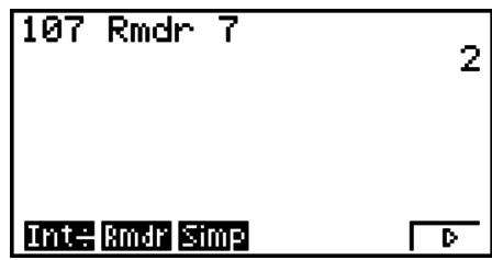
[OPTN]-[CALC]-[Int÷]
AC 1 0 7 OPTN F4 (CALC)* F6 (>)
F6( )F2(Rmdr)7
EXE
- GRAPH 25+ Pro : F3(CALC)
■ Simplification
[OPTN]-[CALC]-[Simp]
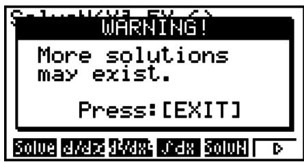
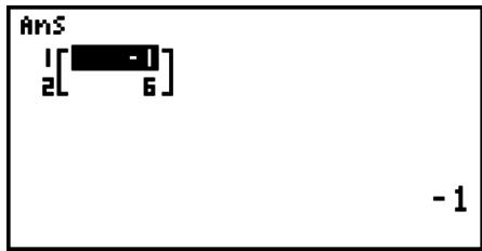
OPTN F4(CALC)*F5(SolvN)
X,0,T X² = 5 X,0,T = 6 EXE
- GRAPH 25+ Pro: [F3(CALC)
EXIT
AC OPTN F3 (CPLX)* F2 (Abs)
Abs(3+4i) 5
3+4F1(i) E
[OPTN]-[CPLX]-[Conj]
[OPTN]-[CPLX]-[ReP]/[ImP]
Négative: -2147483648 ≤ x ≤ -1
[SET UP]-[Mode]-[Dec]/[Hex]/[Bin]/[Oct]
OPTN F2 (MAT) F5 (Aug)
F1 (Mat) ALPHA X, ,T A
F1 (Mat) ALPHA log (B) EXE
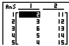
AnS 1 2 3
→OPTN F1(List)F1(List)1 EXE
F1(List) 1 EXE
Calculus matriciels
[OPTN]-[MAT]
Source: NIST Special Publication 811 (1995)
SHIFT 1(List) n SHIFT + ([ ] 0 SHIFT - ([ ]) EXE
OPTN F1(List) F2(L→M) F1(List)
F1(List) 1 F1(List) 2 EXE
OPTN F1(List) F3 (Dim) F1(List)
AC OPTN F1(List) F3 (Dim)
F1(List) 1 EXE
Dim List 1 5
OPTN F1(List) F4(Fill)
OPTN F1(List) F6 (D) F2 (Max) F6 (D) F6 (D) F1(List)
OPTN F1(List) F6(>) F2(Max)
F6(>)F6(>)F1(List)1
F1(List) 2 EXE
[OPTN]-[LIST]-[Mean]
OPTN F1(List) F6(>) F3(Mean) F6(>) F6(>) F1(List)
F6(>)F6(>)F1(List) 1 EXE
OPTN F1(List) F6 () F4 (Med) F6 () F6 () F1(List)
F6(>)F6(>)F1(List) 1
F1(List) 2 EXE
Pour combiner des listed
[OPTN]-[LIST]-[Aug]
OPTN F1(List) F6(>) F5(Aug) F6(>) F6(>) F1(List)
AC OPTN F1 (LIST) F6 () F5 (Aug)
F6(>)F6(>)F1(List) 1
F1(List) 2 EXE
OPTN F1(List) F6(>) F6(>) F1(Sum) F6(>) F1(List)
OPTN F1(List) F6(>) F6(>) F3(Cuml) F6(>) F1(List)
OPTN F1(List) F6(>) F6(>) F4(%) F6(>) F1(List)
OPTN F1(List) F1(List) 3 → F1(List) 1 EXE
À la place de l'opération F1(List)F1(List) 3 précédente, vous pouvez entrer SHIFT ()41··65··22··SHIFT (·)
sin OPTN F1(List) F1(List) 2 SHIFT + ([ ) 3 SHIFT - ([ ]) EXE
2 5 → OPTN F1(List) F1(List) 3 SHIFT + ([ ) 2 SHIFT - ([ ]) EXE
OPTN F1(List) F1(List) 1 EXE
OPTN F1(List) F1(List) SHIFT (-)(Ans) X 3 6 EXE
sin OPTN F1(List) F1(List) 3 EXE
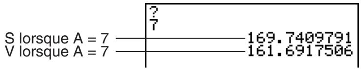
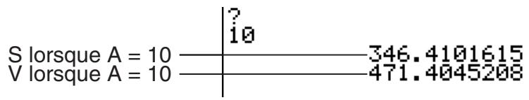
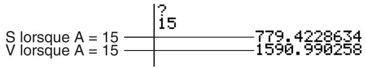
ALPHA F-D (H) SHIFT = (A) ALPHA 2 (V) ALPHA T
1 2 ALPHA *G) ALPHA T) xEXE
- GRAPH 25+ Pro: [a+%]
③ 1 4 EXE(H=14)
0 EXE(V=0)
2 EXE(T=2)
9 8 EXE (G = 9,8)
F3 (TYPE) F1 (Y=) VARS F4 (GRPH)
F1(Y) F1 F1(Y) 2 EXE
VARS F4 (GRPH) F1 (Y) 2
F1(Y) 1 EXE
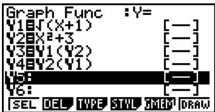
Type 1 (Y= expression)
SHIFT 8 (CLIP) F1 (COPY)
② MENU GRAPH
③ SHIFT MENU (SET UP) F3 (Off) EXIT
- GRAPH 25+ Pro: ⋒ ⋒ ⋒
④ SHIFT F3 (V-WIN) 5 EXE 5 EXE 2 EXE
() 1 0 EXE 1 0 EXE 5 EXE EXIT
⑤ F3(TYPE) F1(Y=)2 X,0,T x² + 3 X,0,T - 4 EXE
F6 (DRAW)
⑥ SHIFT 9 (PASTE)
① MENU GRAPH
② SHIFT F3 (V-WIN) F1 (INIT) EXIT
③ SHIFT MENU (SET UP) ^* F1 (一) EXIT
- GRAPH 25+ Pro : Ⓞ Ⓞ Ⓞ Ⓞ Ⓞ Ⓞ
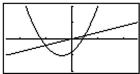
④ F3(TYPE)F1(Y=)X,0,T C X,0,T + 2 )C X,0,T

⑤ F6(DRAW)
⑥ SHIFT F4 (SKTCH) F2 (Tang)
⑦ D\~EXE*1
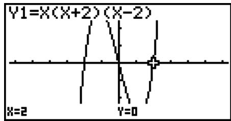
$$ \Upsilon 1 = x (x + 2) (x - 2) $$
■ Graph type camembert
F1(CALC) F6(>) F2(Log)
F6 (DRAW)
F2(List) 2 EXE SHIFT EXIT (QUIT)
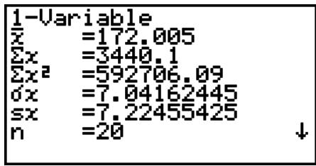
F2(CALC) F1(1VAR)
F1(List) F1(List) 1 F1(List) 2 EXE
- GRAPH 25+ Pro : F4 (STAT) F3 (S • Dev)
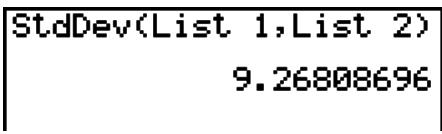
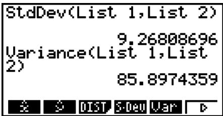
EXIT F5 (STAT) F5 (Var)* EXIT
F1(List) F1(List) 1 F1(List) 2 EXE
- GRAPH 25+ Pro : F4 (STAT) F4 (Var)
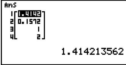
F1(List) F1(List) SHIFT (Ans) EXE
Save Res:None Execute
_1 _2 ...hypothesé alternative
p_1 > p_2 ....hypothesé alternative
Save Res:None Execute
F5 (DIST) F5 (BINM) F2 (BCd)
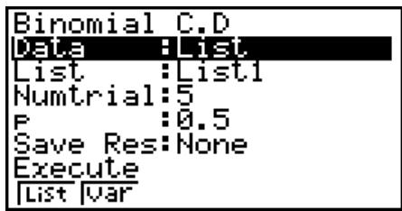
Freq.......effectif(1ou listed 1a26)
$$ P V = - (P M T \times n + F V) $$
$$ F V = - (P M T \times n + P V) $$
$$ P M T = - \frac {P V + \beta \times F V}{\alpha} $$
$$ n = \frac {\log \left{\frac {(1 + i S) \times P M T - F V \times i}{(1 + i S) \times P M T + P V \times i} \right}}{\log (1 + i)} $$
$$ P M T = - \frac {P V + F V}{n} $$
$$ n = - \frac {P V + F V}{P M T} $$
$$ \alpha = (1 + i \times S) \times \frac {1 - \beta}{i}, \beta = (1 + i) ^ {- n} $$
$$ S = \left{ \begin{array}{l} 0 \quad \dots \dots \dots \text {P a y m e n t : E n d} \ \text {(E c r a n d e c o n f i g u r a t i o n)} \ 1 \quad \dots \dots \dots \text {P a y m e n t : B e g i n} \ \text {(E c r a n d e c o n f i g u r a t i o n)} \end{array} \right. $$
$$ i = \left{ \begin{array}{l} \frac {I \%}{100} \ (1 + \frac {I \%}{100 \times [C / Y]})^{\frac {C / Y}{P / Y}} - 1 \dots \dots \dots \dots \dots \dots \dots \dots \dots \dots \dots \dots \dots \dots \dots \dots \dots \dots \dots \dots \dots \dots \dots \dots \dots \dots \dots \dots \dots \dots \dots \dots \dots \dots \dots \dots \dots \dots \dots \dots \dots \dots \dots \dots \dots \dots \dots \dots \dots \dots \tag{P/Y=C/Y=1} \ (\text{Autres que ci-dessus}) \end{array} \right. $$
- I %
$$ P V + \alpha \times P M T + \beta \times F V = 0 $$
$$ N F V = N P V \times (1 + i) ^ {n} $$
- IRR
$$ 0 = C F _ {0} + \frac {C F _ {1}}{(1 + i)} + \frac {C F _ {2}}{(1 + i) ^ {2}} + \frac {C F _ {3}}{(1 + i) ^ {3}} + \dots + \frac {C F _ {n}}{(1 + i) ^ {n}} $$
$$ i = I \% \prime \div 100 $$
$$ I N T = - \frac {A}{D} \times \frac {C P N}{M} \quad C S T = P R C + I N T $$
- Rendement annuel (YLD)
Bond Calculation CPD=01M01D2012Y(SUN)
① MENU PRGM
(2) F3 (NEW) 9 (O) In (C) T (A)
③ SHIFT VARS (PRGM) F4 (?) → ALPHA X,θ,T (A) F6 (▷) F5 (:
2XSHIFTx²(√)3XALPHAx,0T(A)x²F6(>)F6(>)F5(A
SHIFT ^2 (-) 2÷3x [ALPHA]A)A
EXIT EXIT
(4) F1(EXE) ou exe
EXE(Valeur de A)
EXE


a_n, b_n, c_n, a_n+1, b_n+1, c_n+1, a_n+2, b_n+2, c_n+2, a_n, b_n, c_n, a_n+1, b_n+1, c_n+1, a_n+2, b_n+2, c_n+2
Locate 7, 1, "CASIO FX"
Receive38k / Send38k
| Programme | Affichage |
| "CASIO" | CASIO |
| ? → X | ? |
| "X =" ? → X | X = ? |
S-Gph1 DrawOn, Scatter, List 1, List 2, 1, Square
S-Gph1 DrawOn, NPPlot, List 1, Square
S-Gph1 DrawOn, Hist, List 1, List 2
S-Gph1 DrawOn, Linear, List 1, List 2, List 3
S-Gph1 DrawOn, Logistic, List 1, List 2
S-Gph1 DrawOn, Bar, List 1, None, None, StickLength
S-Gph1 DrawOn, Scatter, List 1, List 2, 1, Square
DrawStat
Syntaxe:ChiCD(Lower,Upper,df[])
Syntaxe: TwoSampleTTest "condition _1^ , ^1 , s x1 n1, x2, s x2 n2[,condition Pooled ] TwoSampleTTest "condition _1^ , List1, List2, [, Freq1[, Freq2[ condition Pooled ]]
Syntax: Cash_PBP(1%, Csh)
Syntax: Cash_NFV(1%, Csh)
- Amortissement
* RESET ** F1: Setup Data F2: Main Memories F3:Add-In F4: Storage Memories F5:Add-In&Storage F6: Next Page STOP RANK ADD STRF HSS
Receivins... AC :Cancel
E-CON2 Application (English)
All of the explanations provided here assume that you are already familiar with the operating precautions, terminology, and operational procedures of the calculator and the EA-200.
1 E-CON2 Overview
- From the Main Menu, select E-CON2 to enter the E-CON2 Mode.
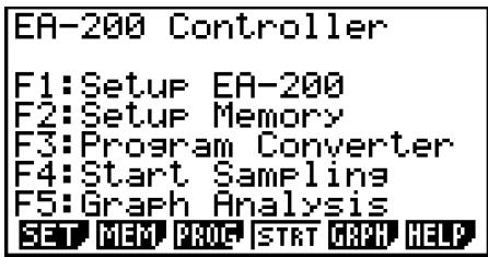
E-CON2 Main Menu
-
The "E-CON2 Mode" provides the functions listed below for simple and more efficient data sampling using the CASIO EA-200.
-
F1 (SET) ....... Displays a screen for setting up the EA-200.
- F2(MEM) ....... Displays a screen for saving EA-200 setup data under a file name.
-
F3(PROG) .... Perform program conversion.
-
This function can be used to convert EA-200 setup data configured using E-CON2 to an EA-200 control program (or EA-100 control program) that can run on the fx-9860G SD/fx-9860G.
-
It also can be used to convert data to a program that can be run on a CFX-9850 Series/fx-7400 Series calculator.
-
F4(START) ....... Starts data collection.
- F5 (GRPH) .... Graphs data sampled by the EA-200, and provides tools for analyzing graphs. Graph Analysis tools include calculation of periodic frequency, various types of regression, Fourier series calculation, and more.
-
[F6] (HELP) ....... Displays E-CON2 help.
-
Pressing the [OPTN] key (Setup Preview) or a cursor key while the E-CON2 main menu is on the screen displays a preview dialog box that shows the contents of the setup in the current setup memory area.
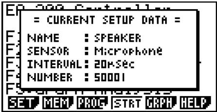
To close the preview dialog box, press EXIT.
Note
For details about setup data and the current setup memory area, see “6 Using Setup Memory” (page 6-1).
About online help
Pressing the F6(HELP) key displays online help about the E-CON2 Mode.
2 Using the Setup Wizard
This section explains how to use the Setup Wizard to configure the EA-200 setup quickly and easily simply by replying to questions as they appear. If you need more control over specific sampling parameters, you should consider using the Advanced Setup procedure on page 3-1.
■ Setup Wizard Parameters
Setup Wizard lets you make changes to the following three EA-200 basic sampling parameters using an interactive wizard format.
- Sensor (Select Sensor):
Specify a CASIO or VERNIER sensor from a menu of choices.
Vernier Software & Technology
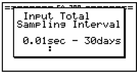
Total Sampling Time:
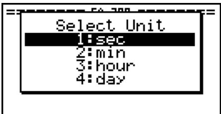
Specify a value within the range of 0.01 second to 30 days. - Sampling Time Unit (Select Unit):
Specify seconds (sec), minutes (min), hours (hour), or days (day) as the time unit of the value you input for the total sampling time (Total Sampling Time).
Note
For some sensors (EA-200 built-in microphone, Vernier PhotoGate, etc.), sampling parameters are different from those shown above. The differences between sampling parameters and setup procedures for each sensor are described in this section.
Setup Wizard Rules
Note the following rules whenever you use the Setup Wizard.
- The EA-200 sampling channel is CH1 or SONIC.
- The trigger for a Setup Wizard setup is always the key.
- To configure an EA-200 setup using Setup Wizard
Before getting started...
- Before starting the procedure below, make sure you first decide if you want to start sampling immediately using the setup you configure with Setup Wizard, or if you want to store the setup for later sampling.
- See sections 6-1, 7-1, and 8-1 of this manual for information about procedures required to start sampling and to store a setup. We recommend that you read through the entire procedure first, referencing the other sections and pages as noted, before actually trying to perform it.
-
To terminate Setup Wizard part way through and cancel the setup, press SHIFT (QUIT).
-
Display the E-CON2 main menu (page 1-1).
-
Press F1 (SET) and then F1 (WIZ).
-
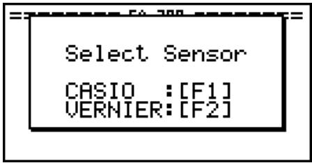
This launches the Setup Wizard and displays the "Select Sensor" screen.
-
Press F1 to specify a CASIO sensor or F2 to specify a Vernier sensor.
-
Pressing either key will display the corresponding sensor list. The following shows the sensor list that appears when you press F1.
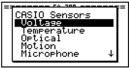
- Specify the sensor you want to use.
Use the and cursor keys to move the highlighting to the sensor you want to use, and then press .
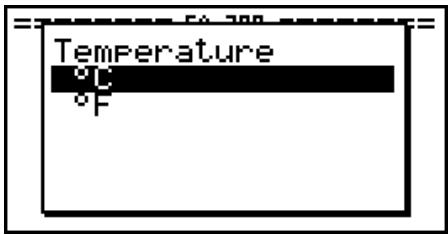
- If the sensor you specified has more than one option (more detailed specifications, such as sampling unit, mode, etc.), an option list will appear on the display at this time. If this happens, advance to step 5 (where you will see an example of the screen that appears when you select F1 - [Temperature] in step 4).
- If the "Input Total Sampling Interval" screen appears, skip to step 6.
- Select the options for the sensor you specified in step 4.
Use the and cursor keys to move the highlighting to the option you want to select, and then press .
- If the "Input Total Sampling Interval" screen appears, advance to step 6.
Important!
When special settings are required by the sensor and/or option you select, other screens other than the "Input Total Sampling Interval" screen will appear on the display. The following shows where you should go to find information about the operations you need to perform for each sensor/option selection.
| If you select this sensor/option: | Go here for more information: |
| [CASIO] - [Microphone] - [Sound wave & FFT] | “Using Setup Wizard to Configure Settings for FFT (Frequency Characteristics) Data Sampling” on page 2-5 |
| [CASIO] - [Microphone] - [FFT only] | |
| [VERNIER] - [Photogate] - [Gate] | “To configure a setup for PhotoGate alone” on page 2-6 |
| [VERNIER] - [Photogate] - [Pulley] | “To configure a setup for PhotoGate and Smart Pulley” on page 2-7 |
| [CASIO] - [Speaker] - [y=f(x)] | “Outputting the Waveform of a Function through the Speaker” on page 2-8 |
- Use the number input keys to input the total sampling time. Just input a value.
In step 8 of this procedure, you will be able to specify the unit (seconds, minutes, hours, days) of the value you input here.
Note
- With some sensors ([CASIO] - [Microphone] - [Sound wave], etc.) sampling time is limited to a few seconds. The unit for such a sensor is always seconds, and so the "Select Unit" screen does not appear.
-
If you specify a total sampling time value in the range of 10 seconds to 23 hours, 59 minutes, 59 seconds, real-time graphing will be performed during sampling. This is the same as selecting the Realtime Mode on the “Advanced Setup” screen.
-
After inputting total sampling time value you want, press . This displays the "Select Unit" screen.
-
Use number keys 1 through 4 to specify the unit for the value you specified in step 6.
-
This displays a confirmation screen like the one shown below.
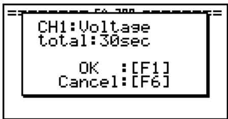
- If there is not problem with the contents of the confirmation screen, press F1.
If you need to change the setup, press F6 or EXIT. This will return to the screen in step 4 (for setting the total sampling interval), where you can change the setting.
- Pressing F1 will take you to the final Setup Wizard screen.
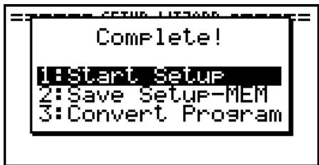
- Press number keys described below to specify what you want to do with the setup you have configured.
1(Start Setup) ........ Starts sampling using the setup (page 8-1)
2 (Save Setup-MEM) .... Saves the setup (page 6-1)
(Convert Program) ....... Converts the setup to a program (page 7-1)
Using Setup Wizard to Configure Settings for FFT (Frequency Characteristics) Data Sampling
When you perform sound sampling executed the EA-200's built-in microphone (by specifying [CASIO] - [Microphone] as the sensor), Setup Wizard will provide you with three options: [Sound wave], [Sound wave & FFT], and [FFT only]. "Sound wave" records the following two dimensions for the sampled sound data: elapsed time (horizontal axis) and volume (vertical axis). "FFT" records the following two dimensions: frequency (horizontal axis) and volume (vertical axis).
The following shows the settings for recording FFT data.
- Perform the first two steps of the procedure under "To configure an EA-200 setup using Setup Wizard" on page 2-2.
-
On the "Select Sensor" screen, select [CASIO] - [Microphone] - [Sound wave & FFT] on [CASIO] - [Microphone] - [FFT only].
-
This causes a "Select FFT Range" screen to appear.
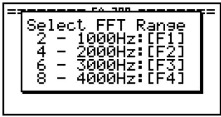
- You can select one of four settings for FFT Range. The setting you select will automatically apply the applicable fixed parameters shown below.
| Setting Parameter | 2 - 1000 Hz: F1 | 4 - 2000 Hz: F2 | 6 - 3000 Hz: F3 | 8 - 4000 Hz: F4 |
| Frequency pitch | 2 Hz | 4 Hz | 6 Hz | 8 Hz |
| Frequency max | 1000 Hz | 2000 Hz | 3000 Hz | 4000 Hz |
| Sampling interval | 61 μsec | 31 μsec | 20 μsec | 31 μsec |
| Number of samples | 8192 | 8192 | 8192 | 4096 |
The following explains the meaning of each parameter.
Frequency pitch: Pitch in Hz at which sampling is performed
Frequency max: Upper limit of sampling frequency (lower limit is fixed at 0 Hz)
Sampling interval: Interval in seconds at which sampling is performed
Number of samples: Number of times sampling is performed
-
Use function keys F1 through F4 to select an FFT Range setting.
-
Selecting an FFT Range causes the final Setup Wizard screen to appear.
-
Perform step 10 under "To configure an EA-200 setup using Setup Wizard" on page 2-2 to finalize the procedure.
Using Setup Wizard to Configure a PhotoGate Setup
Connection of a Vernier PhotoGate requires configuration of setup parameters that are slightly different from parameters for other types of sensors.
- To configure a setup for PhotoGate alone
- Perform the first two steps of the procedure under "To configure an EA-200 setup using Setup Wizard" on page 2-2.
-
On the "Select Sensor" screen, select [VERNIER] - [Photogate] - [Gate].
-
This displays a screen where you specify whether PhotoGate is connected to the CH1 or SONIC channel.
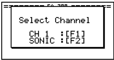
-
Press F1 to specify CH1 or F2 to specify SONIC.
-
This causes a "Gate Status" screen to appear.
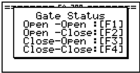
- "Open" means the photo path is not blocked, while "Close" means the photo path is blocked.
- The gate status defines what PhotoGate status should cause timing to start, and what status should cause timing to stop.
Open-Open ....... Timing starts when the gate opens, and continues until it closes and then opens again.
Open-Close .... ... Timing starts when the gate opens, and continues until it closes.
Close-Open ....... Timing starts when the gate closes, and continues until it opens.
Close-Close ....... Timing starts when the gate closes, and continues until it opens and then closes again.
-
Use function keys F1 through F4 to select a Gate Status setting.
-
Selecting a gate status causes a screen for specifying the number of samples to appear.
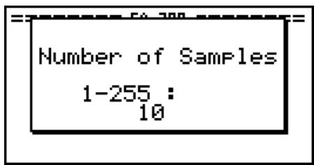
- Input an integer in the range of 1 to 255 to specify the number of samples.
- Perform step 10 under "To configure an EA-200 setup using Setup Wizard" on page 2-2 to finalize the procedure.
- To configure a setup for PhotoGate and Smart Pulley
- Perform the first two steps of the procedure under "To configure an EA-200 setup using Setup Wizard" on page 2-2.
-
On the "Select Sensor" screen, select [VERNIER] - [Photogate] - [Pulley].
-
This causes an "Input Distance(m)" screen to appear.

- The distance you specify here is the distance the weight travels after it is released.
-
Input a value in the range of 0.1 to 4 to specify the distance in meters.
-
Perform step 10 under "To configure an EA-200 setup using Setup Wizard" on page 2-2 to finalize the procedure.
■ Outputting the Waveform of a Function through the Speaker
Normally, the Setup Wizard helps you configure setups for sensors connected to the EA-200. If you select [CASIO] - [Speaker] - [y=f(x)] on the "Select Sensor" screen, however, it configures the EA-200 to output the sound that corresponds to a function that you input and graph on the calculator.
- To configure a setup for speaker output
- Connect the data communication cable (SB-62) to the communication port of the calculator and the MASTER port of the EA-200.
- Perform the first two steps of the procedure under "To configure an EA-200 setup using Setup Wizard" on page 2-2.
- On the "Select Sensor" screen, select [CASIO] - [Speaker] - [y=f(x)]. This displays a screen like the one shown below.
-
Press EXE to advance to the View Window setting screen.
-
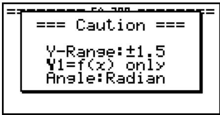
The following settings are configured automatically: Ymin = -1.5 and Ymax = 1.5. Do not change these settings.
-
Press EXE or EXIT to advance to the graph function list.
- In line "Y1", input the function of the waveform for the sound you want to input.
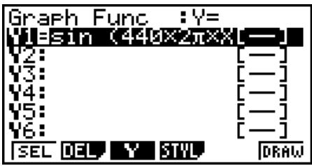
- Note that the angle unit is always radians.
-
Input a function where the value of "Y" is within the range of -1.5 to +1.5.
-
Press F6 (DRAW) to graph the function.
-
This graphs the function and displays a vertical cursor line as shown below. Use the graph to specify the range that you want to output to the speaker.
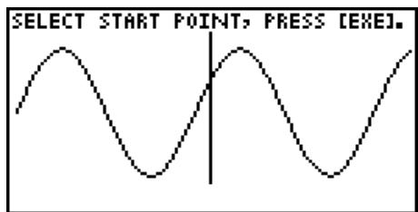
- Use the and cursor keys to move the cursor to the start point of the output, and then press to register it.
-
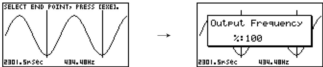
Use the and cursor keys to move the cursor to the end point of the output, and then press to register it.
-
After you specify the start point and end point, an output frequency dialog box shown below appears on the display.
-
Input a percent value for the output frequency value you want.
-
To output the original sound as-is, specify 100% . To raise the original sound by one octave, input a value of 200% . To lower the original sound by one octave, input a value of 50% .
-
After inputting an output frequency value, press .
-
This outputs the waveform between the start point and end point from the EA-200 speaker.
-
If the sound you configured cannot be output for some reason, the message “Range Error” will appear. If this happens, press [EXIT] to scroll back through the previous setting screens and change the setup as required.
-
To terminate sound output, press the EA-200 [START/STOP] key.
-
Press EXE.
-
This displays a screen like the one shown below.
- Perform one of the following operations, depending on what you want to do.
To change the output frequency and try again:
Press F1 (Yes) to return to the "Output Frequency" dialog box. Next, repeat the above steps from step 10.
To change the output range of the waveform graph and try again:
Press F6 (No) to return to the graph screen in step 7. Next, repeat the above steps from step 8.
To change the function:
Press F6 (No) and then EXIT to return to the graph function list in step 6. Next, repeat the above steps from step 6.
To exit the procedure and return to the E-CON2 main menu:
Press F6 (No) and then press EXIT twice.
3 Using Advanced Setup
Advanced Setup provides you with total control over a number of parameters that you can adjust to configure the EA-200 setup that suits your particular needs.
The procedures in this section provide the general steps you should perform when using Advanced Setup to configure an EA-200 setup, and to returns setup settings to their initial default values. You can find details about individual settings and the options that are available with each setting are provided by the explanations that start on page 3-3.
■ Advanced Setup Operations
- To configure an EA-200 setup using Advanced Setup
The following procedure describes the general steps for using Advanced Setup. Refer to the pages as noted for more information.
- Display the E-CON2 main menu (page 1-1).
- Press F1 (SET). This displays the "Setup EA-200" submenu.
- Press F2 (ADV). This displays the Advanced Setup menu.
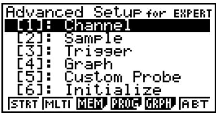
Advanced Setup Menu
-
If you want to configure a custom probe at this point, press ⑤ (Custom Probe). Next, follow the steps under “To configure a custom probe setup” on page 4-1.
-
You can also configure a custom probe during the procedure under "To configure Channel Setup settings" on page 3-3.
-
Custom probe configurations you have stored in memory can be selected using Channel in step 5, below.
-
Use the Advanced Setup function keys described below to set other parameters.
-
(Channel) .... Displays a screen that shows the sensors that are currently assigned to each channel (CH1, CH2, CH3, SONIC, Mic). You can also use this dialog to change sensor assignments. See "Channel Setup" on page 3-3 for more information.
-
(Sample) .... Displays a screen for selecting the sampling mode, and for specifying the sampling interval, the number of samples, and the warm-up mode. When "Fast" is selected for "Mode", this dialog box also displays a setting for turning FFT (frequency characteristics) graphing on and off. See "Sample Setup" on page 3-5 for more information.
-
3 (Trigger) ....... Displays a screen for configuring sampling start (trigger) conditions. See "Trigger Setup" on page 3-8 for more information.
-
4 (Graph) ....... Displays a screen for configuring graph settings. See “Graph Setup” on page 3-13 for more information.
-
You can return the settings on the above setup screens (1 through 4) using the procedure described under "To return setup parameters to their initial defaults".
-
After you configure a setup, you can use the function key operations described below to start sampling or perform other operations.
-
F1(STRT) ....... Starts sampling using the setup (page 8-1).
- F2 (MLTI) ....... Starts MULTIMETER Mode sampling using the setup (page 5-1).
- F3(MEM) ....... Saves the setup (page 6-1).
- F4 .... Converts the setup to a program (page 7-1).
- F5 (GRPH) .... Graphs data sampled by the EA-200, and provides tools for analyzing graphs (page 10-1).
- F6(ABT) ....... Displays version information about the EA-200 unit that is currently connected to the calculator.
- To return setup parameters to their initial defaults
Perform the following procedure when you want to return the parameters of the setup in the current setup memory area to their initial defaults.
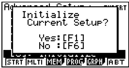
- While the Advanced Setup menu (page 3-1) is on the display, press 6 (Initialize).
-
In response to the confirmation message that appears, press F1 (Yes) to initialize the setup.
-
To clear the confirmation message without initializing the setup, press F6 (No).
■ Channel Setup
The Channel Setup screen shows the sensors that are currently assigned to each channel (CH1, CH2, CH3, SONIC, Mic).
- To configure Channel Setup settings
-
While the Advanced Setup menu (page 3-1) is on the display, press 1 (Channel).
-
This displays the Channel Setup screen.
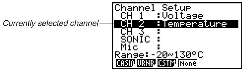
Channel Setup Screen
- Use the and cursor keys to move the highlighting to the channel whose setting you want to change.
-
What you need to do next depends on the currently selected channel.
-
CH1, CH2, or CH3
Press a function key to display a menu of sensors that can be assigned to the selected channel.
F1 (CASIO) ....... Displays a menu of CASIO sensors.
F2 (VRNR) ....... Displays a menu of Vernier sensors.
F3 (CSTM) ....... Displays a menu of custom probes.
F4(None) ....... Press this key when you want leave the channel without any sensor assigned to it.
- SONIC Channel
Press a function key to display a menu of sensors that can be assigned to this channel.
F1(CASIO) ....... Displays a menu of CASIO sensors, but only "Motion" can be selected.
F2 (VRNR) ....... Displays a menu of Vernier sensors. You can select "Motion" or "Photogate".
Note
- On the menu that appears after you select "Motion" from either the CASIO or Vernier sensor menu, select either "meters" or "feet" as the sampling unit.
-
After selecting "Motion" from either the CASIO or Vernier sensor menu, you can press the OPTN key to toggle "smoothing (correction of measurement error)" on ("-Smooth" displayed) and off ("-Smooth" not displayed).
-
From the menu that appears after you select "Photogate" as the sensor, select [Gate] or [Pulley].
[Gate] Select this option when using the PhotoGate sensor alone.
[Pulley] Select this option when using the PhotoGate sensor along with a smart pulley.
(F4) (None) ....... Select this option to disable the SONIC channel.
- Mic Channel
For this channel, the sensor is automatically set to Built-in (External) Microphone. However, you need to configure the settings described below.
F1(Snd) .... Select this option to record elapsed time and volume 2-dimensional sampled sound data (elapsed time on the horizontal axis, volume on the vertical axis).
F2 (FFT) .... Select this option to record frequency and volume 2-dimensional sampled sound data (frequency on the horizontal axis, volume on the vertical axis).
F4(None) ....... Select this option to disable the Mic channel.
- Repeat steps 2 and 3 as many times as necessary to configure all the channels you want.
-
After all the settings are the way you want, press .
-
This returns to the Advanced Setup menu.
Note
- When you select a channel on the Channel Setup screen, the sampling range of the selected channel appears in the bottom line of the screen.
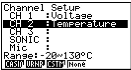
In the above example, the range of the temperature sensor assigned to CH2 appears on the display.
If the sampling range value is too long to fit on the display, only the part of the value that fits on the display will be shown.
- Whenever the current Sample Setup (page 3-5) and Trigger Setup (page 3-8) settings become incompatible due to a change in Channel Setup settings, these settings revert automatically to their initial defaults. Selecting the Mic channel with Channel Setup while the Sample Setup has "Extended" selected for the sampling mode, for example, will cause the sampling mode to change automatically to "Fast" (which is the initial default setting when the Mic channel is selected). For information about the channels that can be selected for each sampling mode, see "Sample Setup" (page 3-5).
Sample Setup
The Sample Setup screen lets you configure a number of settings that control sampling.
- To configure Sample Setup settings
-
While the Advanced Setup menu (page 3-1) is on the display, press 2(Sample).
-
This displays the Sample Setup screen, with the "Mode" line highlighted, which indicates that you can select the sampling mode.
| Sample Setup | |
| Mode | Real-Time |
| Interval | 1sec |
| Number | 101 |
| Warm-up | [0h01m40s] |
| R-T | Fast Norm Extd Help D |
- Select the sampling mode that suits the type of sampling you want to perform.
| To do this: | Press this key: | To select this mode: |
| Graph data in real-time as it is sampled | F1(R-T) | Realtime |
| Perform sampling of high-speed phenomena (sound, etc.) | F2(Fast) | Fast |
| Perform sampling over a long time (weather, etc.) • The EA-200 enters a power off sleep state while standing by. | F4(Extd) | Extended |
| Sample sound using the EA-200's built-in microphone | F6(▷) F1(Snd) | Sound |
| Record the time of the occurrence of a particular trigger event as an absolute value starting from 0, which is the sampling start time | F6(▷) F2(Clck) | Clock |
| Perform periodic sampling, from a start trigger event to an end trigger event | F6(▷) F3(Priod) | Period |
| Perform sampling other than that described above | F3(Norm) | Normal |
- Note that the mode you select also determines the channel(s) you can use.
| Sampling mode: | Selectable Channel(s) |
| Realtime, Extended, Normal | CH1, CH2, CH3, SONIC |
| Fast | CH1, Mic |
| Sound | Mic |
| Clock, Period | CH1 |
-
To change the sampling interval setting, move the highlighting to "Interval". Next, press F1 to display a dialog box for specifying the sampling interval.
-
The range of values you can select depends on the current sampling mode setting.
| If this sampling mode is selected: | This is the allowable setting range: |
| Realtime | 0.2 to 299 sec |
| Fast | 20 to 500 μsec |
| Extended | 5 to 240 min |
| Period | “=Trigger” only (no value input required) |
| Sound | 20 to 27 μsec |
| Clock | “=Trigger” only (no value input required) |
| Normal | 0.0005 to 299 sec |
-
To change the number of samples setting, move the highlighting to "Number". Next, press F1 to display a dialog box for specifying the number of samples.
-
You can specify a value in the range of 10 to 30,000.
- The total sampling time shown at the bottom of the dialog box is calculated by multiplying the "Sampling Interval" value you specified in step 3 by the number of samples you specify here.
Important!
-
When all of the following conditions exist, a "Distance" setting appears in place of the "Number" setting. See "To configure the Distance setting" (page 3-7) for information about configuring the "Distance" setting.
-
Channel Setup (page 3-3): F2 (VRNR) - [Photogate] - [Pulley]
-
Sampling Mode (page 3-5): Clock
-
To change the warm-up time setting, move the highlighting to "Warm-up". Next, perform one of the function key operations described below.
Note
- The "Warm-up" setting will not be displayed on the Sample Setup screen if "Fast", "Sound" or "Extended" is currently selected as the sampling mode.
| To do this: | Press this key: |
| Have the warm-up time for each sensor set automatically | F1 (Auto) |
| Input a warm-up time, in seconds, manually | F2 (Man) |
| Disable the warm-up time | F3 (None) |
Important!
-
When the following condition exists, an "FFT Graph" setting appears in place of the "Warm-up" setting. See "To configure the FFT Graph setting" (page 3-7) for information about configuring the "FFT Graph" setting.
-
Sampling Mode (page 3-5): Fast
-
After all the settings are the way you want, press EXE.
-
This returns to the Advanced Setup menu.
Note
- Whenever the current Channel Setup (page 3-3) and Trigger Setup (page 3-8) settings become incompatible due to a change in Sample Setup settings, these settings revert automatically to their initial defaults. Selecting "Realtime" as the sampling mode with Sample Setup while the Mic channel is selected with Channel Setup and the Trigger Setup has "Mic" selected for "Source", for example, will cancel the Channel Setup Mic channel selection and change the Trigger Setup "Source" setting to "[EXE] key". For information about the channels that can be selected for each sampling mode, see step 2 of "To configure Sample Setup settings". For information about the trigger sources that can be selected for each sampling mode, see "Trigger Setup" (page 3-8).
- To configure the Distance setting
In place of step 3 of the procedure under "To configure Sample Setup settings", press F1 to display a dialog box for specifying the distance the weight travels in meters.
- Specify a value in the range of 0.1 to 4 meters.
- To configure the FFT Graph setting
In place of step 5 of the procedure under “To configure Sample Setup settings”, press F1 to display a dialog box for turning frequency characteristic graphing (FFT Graph) on and off.
| To do this: | Press this key: |
| Turn on graphing of frequency characteristics after sampling | F1(On) |
| Turn off graphing of frequency characteristics after sampling | F2(Off) |
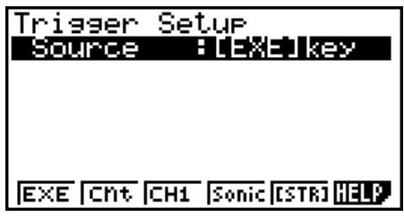
Trigger Setup
You can use the Trigger Setup screen to specify the event that causes sampling to start (key operation, etc.) The event that causes sampling to start is called the "trigger source", which is indicated as "Source" on the Trigger Setup screen.
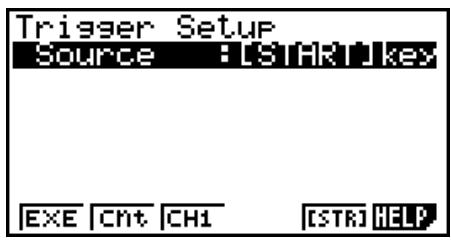
The following table describes each of the six available trigger sources.
| To start sampling when this happens: | Select this trigger source: |
| When the EXE key is pressed | [EXE] key |
| After the specified number of seconds are counted down | Count Down |
| When input at CH1 reaches a specified value | CH1 |
| When input at the SONIC channel reaches a specified value | SONIC |
| When the EA-200's built-in microphone detects sound | Mic |
| When the EA-200's [START/STOP] key is pressed | [START] key |
Note
The trigger sources you can select depends on the sampling mode selected with the Sample Setup (page 3-5).
| For this sampling mode: | The following trigger source(s) can be selected: |
| Realtime | [EXE] key, Count Down |
| Fast | [EXE] key, Count Down, CH1, Mic |
| Normal | [EXE] key, Count Down, CH1, SONIC, [START] key |
| Extended | [EXE] key |
| Sound | [EXE] key, Count Down, Mic |
| Clock | CH1 |
| Period | CH1 |
- To configure Trigger Setup settings
-
While the Advanced Setup menu (page 3-1) is on the display, press ③(Trigger).
-
This displays the Trigger Setup screen with the "Source" line highlighted.
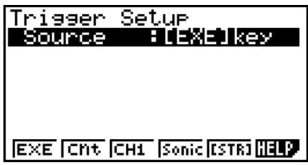
-
The function menu items that appears in the menu bar depend on the sampling mode selected with Sample Setup (page 3-5). The above screen shows the function menu when "Normal" is selected as the sample sampling mode.
-
Use the function keys to select the trigger source you want.
-
The following shows the trigger sources that can be selected for each sampling mode.
| Sampling Mode | Trigger Source |
| Realtime | F1(EXE) : [EXE] key, F2(Cnt) : Count Down |
| Fast | F1(EXE) : [EXE] key, F2(Cnt) : Count Down, F3(CH1), F5(Mic) |
| Normal | F1(EXE) : [EXE] key, F2(Cnt) : Count Down, F3(CH1), F4(Sonic), F5(STR) : [START] key |
| Sound | F1(EXE) : [EXE] key, F2(Cnt) : Count Down, F5(Mic) |
-
The trigger source is always “[EXE] key” when the sampling mode is “Extended”, and “CH1” when the sampling mode is “Clock” or “Period”.
-
Perform one of the following operations, in accordance with the trigger source that was selected in step 2.
| If this is the trigger source: | Do this next: |
| [EXE] key | Press [EXE] to finalize Trigger Setup and return to the Advanced Setup menu. |
| Count Down | Specify the countdown start time. See “To specify the countdown start time” below. |
| CH1 | Specify the trigger threshold value and trigger edge direction. See “To specify the trigger threshold value and trigger edge type”, “To configure trigger threshold, trigger start edge, and trigger end edge settings” on page 3-11 or “To configure PhotoGate trigger start and end settings” on page 3-12. |
| SONIC | Specify the trigger threshold value and motion sensor level. See “To specify the trigger threshold value and motion sensor level” on page 3-12. |
| Mic | Specify microphone sensitivity. See “To specify microphone sensitivity” below. |
| [START] key | Press [EXE] to finalize Trigger Setup and return to the Advanced Setup menu. |
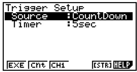
- To specify the countdown start time
- Move the highlighting to "Timer".
- Press F1(Time) to display a dialog box for specifying the countdown start time.
- Input a value in seconds from 1 to 10.
- Press ExE to finalize Trigger Setup and return to the Advanced Setup menu.
- To specify microphone sensitivity
- Move the highlighting to "Sense" and then press one of the function keys describe below.
| To select this level of microphone sensitivity: | Press this key: |
| Low | F1 (Low) |
| Medium | F2 (Mid) |
| High | F3 (High) |
- Press to finalize Trigger Setup and return to the Advanced Setup menu (page 3-1).
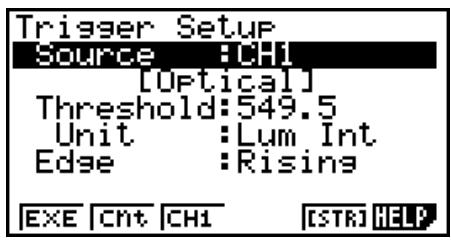
- To specify the trigger threshold value and trigger edge type
Perform the following steps when "Fast", "Normal", or "Clock" is specified as the sampling mode (page 3-5).
- Move the highlighting to "Threshold".
- Press F1 (EDIT) to display a dialog box for specifying the trigger threshold value, which is value that data needs to attain before sampling starts.
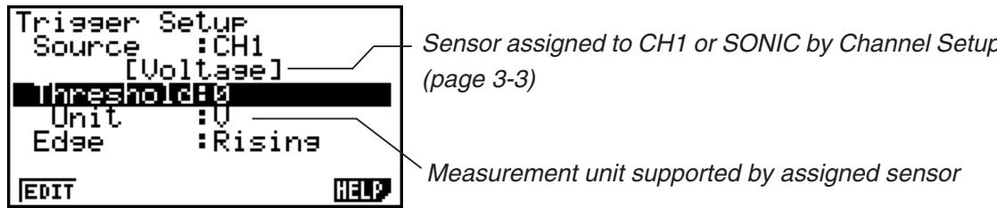
- Input the value you want, and then press .
- Move the highlighting to "Edge".
- Press one of the function keys described below.
| To select this type of edge: | Press this key: |
| Falling | F1(Fall) |
| Rising | F2(Rise) |
- Press to finalize Trigger Setup and return to the Advanced Setup menu (page 3-1).
- To configure trigger threshold, trigger start edge, and trigger end edge settings
Perform the following steps when "Period" is specified as the sampling mode (page 3-5).
- Move the highlighting to "Threshold".
- Press F1 (EDIT) to display a dialog box for specifying the trigger threshold value, which is value that data needs to attain before sampling starts.
- Input the value you want.
- Move the highlighting to "Start to".
- Press one of the function keys described below.
| To select this type of edge: | Press this key: |
| Falling | F1(Fall) |
| Rising | F2(Rise) |
- Move the highlighting to "End Edge".
- Press one of the function keys described below.
| To select this type of edge: | Press this key: |
| Falling | F1(Fall) |
| Rising | F2(Rise) |
- Press to finalize Trigger Setup and return to the Advanced Setup menu (page 3-1).
- To configure PhotoGate trigger start and end settings
Perform the following steps when CH1 is selected as a Photogate trigger source.
- Move the highlighting to "Start to".
- Press one of the function keys described below.
| To specify this PhotoGate status: | Press this key: |
| PhotoGate closed | F1(Close) |
| PhotoGate open | F2(Open) |
- Move the highlighting to "End Gate".
- Press one of the function keys described below.
| To specify this PhotoGate status: | Press this key: |
| PhotoGate closed | F1(Close) |
| PhotoGate open | F2(Open) |
- Press to finalize Trigger Setup and return to the Advanced Setup menu (page 3-1).
- To specify the trigger threshold value and motion sensor level
- Move the highlighting to "Threshold".
- Press F1(EDIT) to display a dialog box for specifying the trigger threshold value, which is value that data needs to attain before sampling starts.
- Input the value you want, and then press .
- Move the highlighting to "Level".
- Press one of the function keys described below.
| To select this type of level: | Press this key: |
| Below | F1(Blw) |
| Above | F2(Abv) |
- Press to finalize Trigger Setup and return to the Advanced Setup menu (page 3-1).
Graph Setup
Use the Graph Setup screen to configure settings for the graph produced after sampling is complete. You use the Sample Setup settings (page 3-5) to turn graphing on or off.
- To configure Graph Setup settings
-
While the Advanced Setup menu (page 3-1) is on the display, press 4 (Graph).
-
This displays the Graph Setup screen.
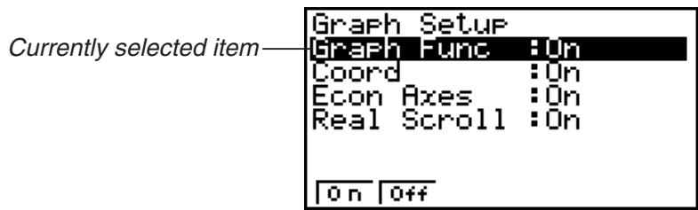
Graph Setup Screen
- To change the graph source data name display setting, use the and cursor keys to move the highlighting to "Graph Func". Next, press one of the function keys described below.
| To specify this graph source data name display setting: | Press this key: |
| Display source data name | F1(On) |
| Hide source data name | F2(Off) |
- When the graph data is stored in a sample data memory file, the file name appears as the source data name. When the graph data is stored in current data area, the channel name appears.
Note
-
For details about sample data memory and current data area, see "9 Using Sample Data Memory".
-
To change the trace operation coordinate display setting, use the and cursor keys to move the highlighting to "Coord". Next, press one of the function keys described below.
| To specify this coordinate display setting for the trace operation: | Press this key: |
| Display trace coordinates | F1(On) |
| Hide trace coordinates | F2(Off) |
- To change the numeric axes display setting, use the and cursor keys to move the highlighting to "Econ Axes". Next, press one of the function keys described below.
| To specify this axes display setting: | Press this key: |
| Display axes | F1(On) |
| Hide axes | F2(Off) |
- To change the real-time scroll setting, use the and cursor keys to move the highlighting to "RealScroll". Next, press one of the function keys described below.
| To specify this real-time scrolling setting: | Press this key: |
| Real-time scrolling on | F1(On) |
| Real-time scrolling off | F2(Off) |
- Press to finalize Graph Setup and return to the Advanced Setup menu.
4 Using a Custom Probe
You can use the procedures in this section to configure a custom probe for use with the EA-200. The term "custom probe" means any sensor other than the CASIO or Vernier sensors specified as standard for the E-CON2 Mode.
■ Configuring a Custom Probe Setup
To configure a custom probe setup, you must input values for the constants of the fixed linear interpolation formula (ax + b) . The required constants are slope (a) and intercept (b) . x in the above expression (ax + b) is the sampled voltage value (sampling range: 0 to 5 volts).
- To configure a custom probe setup
-
From the E-CON2 main menu (page 1-1), press F1 (SET) and then 2 (ADV) to display the Advanced Setup menu.
-
See "3 Using Advanced Setup" for more information.
-
On the Advanced Setup menu (page 3-1), press ⑤ (Custom Probe) to display the Custom Probe List.
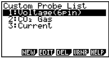
-
The message "No Custom Probe" appears if the Custom Probe List is empty.
-
Press F2 (NEW).
-
This displays a custom probe setup screen like the one shown below.
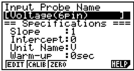
-
The initial default setting for the probe name is "Voltage(6pin)". The first step for configuring custom probe settings is to change this name to another one. If you want to leave the default name the way it is, skip steps 4 and 5.
-
Press F1(EDIT).
-
This enters the probe name editing mode.
-
Input up to 18 characters for the custom probe name, and then press .
-
This will cause the highlighting to move to "Slope".
-
Use the function keys described below to configure the custom probe setup.
-
To change the setting of an item, first use the and cursor keys to move the highlighting to the item. Next, use the function keys to select the setting you want.
(1) Slope
Press F1 to input the slope for the linear interpolation formula.
(2) Intercept
Press F1(EDIT) to input the intercept for the linear interpolation formula.
(3) Unit Name
Press F1(EDIT) to input up to eight characters for the unit name.
(4) Warm-up
Press F1(EDIT) to input the warm-up time.
-
Press and then input a memory number (1 to 99).
-
This saves the custom probe setup and returns to the Custom Probe List, which should now contain the new custom probe setup you configured.
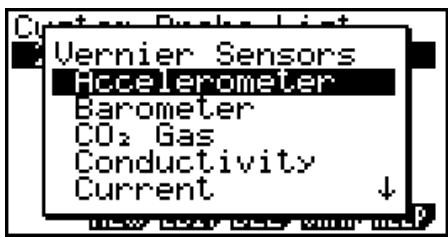
- To recall the specifications of a Vernier sensor and configure custom probe settings
- Perform the first two steps of the procedure under "To configure a custom probe setup" on page 4-1.
-
Press F5(VRNR).
-
This displays a Vernier sensor list.
-
Use the and keys to move the highlighting to the Vernier sensor whose setting you want to use as the basis of the custom probe settings, and then press .
-
The name and specifications of the Vernier sensor you select will appear on the custom probe setup screen.
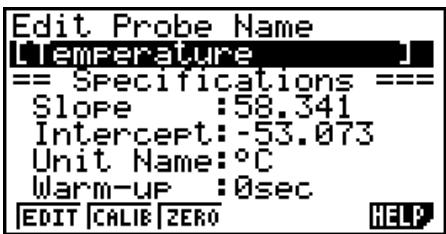
- To complete this procedure, perform steps 4 through 7 under "To configure a custom probe setup" (page 4-1).
Auto Calibrating a Custom Probe
Auto calibration automatically corrects the slope and intercept values of a custom probe setup based on two actual samples.
Important!
- Before performing the procedure below, you should prepare two conditions whose measurement values are known.
- When inputting reference value in step 5 of the procedure below, input the exact known measurement value of the condition you will sample in step 4. When inputting reference value in step 7 of the procedure below, input the exact known measurement value of the condition you will sample in step 6.
- To auto calibrate a custom probe
- Connect the calculator and EA-200, and connect the custom probe you want to auto calibrate to CH1 of the EA-200.
- What you should do first depends on whether you are configuring a new custom probe for calibration, or editing the configuration of an existing custom probe.
If you are configuring a new custom probe:
- Perform steps 1 through 6 of the procedure under "To configure a custom probe setup" on page 4-1.
- Auto calibrate will automatically set the slope and intercept, so you do not need to specify them in step 6 of the above procedure.
If you are editing the configuration of an existing custom probe:
-
Perform steps 1 through 3 of the procedure under "To edit a custom probe setup" on page 4-6.
-
Press F2(CALIB).
-
This will start the first sampling operation with the sensor connected to EA-200's CH1, and then display a screen like the one shown below.
-
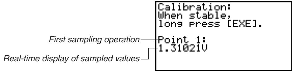
After the sampled value stabilizes, hold down for a few seconds.
-
This will register the first sampled value and display it on the screen. At this time the cursor will appear at the bottom of the display, ready for input of a reference value.
Calibration: When stable, long Press [EXE].
Point 1: 1.31021U Input Value(U)?
-
Use the key pad to input the reference value for the first sampled value, and then press EXE.
-
This cause sampling of the second value to be performed automatically, and display the same type of screen that appeared in step 3.
Second sampling operation
Point 2: 4.38035U
-
After the sampled value stabilizes, hold down for a few seconds.
-
This will register the second sampled value and display it on the screen. The cursor will appear at the bottom of the display, ready for input of a reference value.
Calibration: When stable, long Press [EXE].
Point 2: 4.38035U Input Value(U)?
-
Use the key pad to input the reference value for the second sampled value, and then press .
-
This will return to the custom probe setup screen.
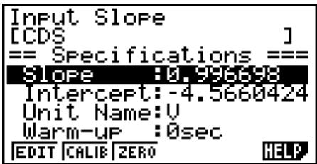
- The E-CON2 will calculate the slope and intercept value based on the two reference values that you input, and configure the settings automatically. The automatically configured values will appear on the custom probe setup screen, where you can view them.
Input Slope
[CST] = = Specifications = = = Slope:1.93751Intercept:1.4267E-03Unit Name:UWarm-upF:0secEDIT CALIB ZERO HELP
-
Press , and then input a memory number from 1 to 99.
-
This saves the custom probe setup and returns to the custom probe list.
Zero Adjusting a Custom Probe
This procedure zero adjusts a custom probe and sets its intercept value based on an actual sample using the applicable custom probe.
- To zero adjust a custom probe
- Connect the calculator and EA-200, and connect the custom probe you want to zero adjust to CH1 of the EA-200.
- What you should do first depends on whether you are configuring a new custom probe for zero adjusting, or editing the configuration of an existing custom probe.
If you are configuring a new custom probe:
- Perform steps 1 through 6 of the procedure under "To configure a custom probe setup" on page 4-1.
- Auto calibrate will automatically set the intercept, so you do not need to specify it in step 6 of the above procedure.
If you are editing the configuration of an existing custom probe:
-
Perform steps 1 through 3 of the procedure under "To edit a custom probe setup" on page 4-6.
-
Press F3 (ZERO).
- This will start the sampling operation with the sensor connected to EA-200's CH1, and then display a screen like the one shown below.
Zero Adjust:
When stable,
lona Press [EXE].
Point 1:0.99682U
-
At the point your want to perform zero adjustment (the point that the displayed value is the appropriate zero adjust value), press .
-
This will return to the custom probe setup screen.
- The E-CON2 will set the intercept value automatically based on the sampled value. The automatically configured value will appear on the custom probe setup screen, where you can view it.
-
Press , and then input a memory number from 1 to 99.
-
This saves the custom probe setup and returns to the custom probe list.
■ Managing Custom Probe Setups
Use the procedures in this section to edit and delete existing custom probe setups.
- To edit a custom probe setup
- Display the Custom Probe List.
-
Select the custom probe setup whose configuration you want to edit.
-
Use the and cursor keys to highlight the name of the custom probe you want.
-
Press F3(EDIT).
-
This displays the screen for configuring a custom probe setup.
- To edit the custom probe setup, perform the procedure starting from step 6 under "To configure a custom probe setup" on page 4-1.
- To delete a custom probe setup
- Display the Custom Probe List.
-
Select the custom probe setup you want to delete.
-
Use the and cursor keys to highlight the name of the custom probe setup you want.
-
Press F4 (DEL).
- In response to the confirmation message that appears, press F1 (Yes) to delete the custom probe setup.
- To clear the confirmation message without deleting anything, press F6 (No).
5 Using the MULTIMETER Mode
You can use the Channel Setup screen (page 3-3) to configure a channel so that EA-200 MULTIMETER Mode sampling is triggered by a calculator operation.
To use the MULTIMETER Mode
- Connect the calculator and EA-200, and connect the sensors you want to the applicable EA-200 channels.
- From the Advanced Setup menu (page 3-1), use the Channel Setup screen (page 3-3) to configure sensor setups for each channel you will be using.
-
After configuring the sensor setups, press [EXE] to return to the Advanced Setup menu (page 3-1), and then press F2.
-
This starts sampling in the EA-200 MULTIMETER mode and displays a list of sample values for each channel.
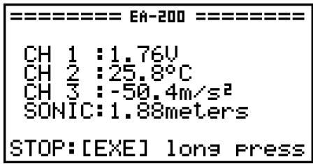
- Displayed sample data is refreshed at 0.5-second intervals.
- Do not connect sensors to any other channels except for those you specified in step 2.
-
Data sampled in the MULTIMETER mode is not saved in memory.
-
To end MULTIMETER mode sampling, press the key.
6 Using Setup Memory
Creating EA-200 setup data using the Setup Wizard or Advanced Setup causes the data to be stored in the "current setup memory area". The current contents of the current setup memory area are overwritten whenever you create other setup data.
You can use setup memory to save the current setup memory area contents to calculator memory to keep it from being overwritten, if you want.
Saving a Setup
A setup can be saved when any one of the following conditions exist.
- After configuring a new setup with Setup Wizard
See step 8 under "To configure an EA-200 setup using Setup Wizard" on page 2-2.
After configuring a new setup with Advanced Setup
See step 6 under "To configure an EA-200 setup using Advanced Setup" on page 3-1 for more information.
- While the E-CON2 main menu (page 1-1) is on the display
Performing the setup save operation while the E-CON2 main menu is on the display saves the contents of the current setup memory area (which were configured using Setup Wizard or Advanced Setup).
Details on saving a setup are listed below.
- To save a setup
- If the final Setup Wizard screen (page 2-4) is on the display, advance to step 2. If it isn't, start the save operation by performing one of the function key operations described below.
If the Advanced Setup menu (page 3-1) is on the display, press F3(MEM).
If the E-CON2 main menu (page 1-1) is on the display, press F2(MEM).
- Performing any one of the above operations causes the setup memory list to appear.
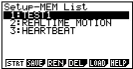
-
The message "No Setup-MEM" appears if setup memory is empty.
-
If you are starting from the final Setup Wizard screen, press 2 (Save Setup-MEM). If you are starting from another screen, press F2 (SAVE).
-
This displays the screen for inputting the setup name.
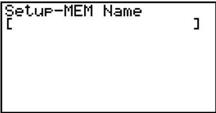
- Input up to 18 characters for the setup name.
-
Press and then input a memory number (1 to 99).
-
If you start from the final Setup Wizard screen (page 2-4), this saves the setup and the message "Complete!" appears. Press to return to the final Setup Wizard screen (page 2-4).
- If you start from the Advanced Setup menu (page 3-1) or the E-CON2 main menu (page 1-1), this saves the setup and returns to the setup memory list which includes the name you assigned it.
Important!
- Since you assign both a setup name and a file number to each setup, you can assign the same name to multiple setups, if you want.
Using and Managing Setups in Setup Memory
All of the setups you save are shown in the setup memory list. After selecting a setup in the list, you can use it to sample data or you can edit it.
- To preview saved setup data
You can use the following procedure to check the contents of a setup before you use it for sampling.
- On the E-CON2 main menu (page 1-1), press F2(MEM) to display the setup memory list.
- Use the and cursor keys to highlight the name of the setup you want.
-
Press OPTN (Setup Preview).
-
This displays the preview dialog box.
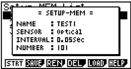
- To close the preview dialog box, press EXIT
- To recall a setup and use it for sampling
Be sure to perform the following steps before starting sampling with the EA-200.
- Connect the calculator to the EA-200.
- Turn on EA-200 power.
- In accordance with the setup you plan to use, connect the proper sensor to the appropriate EA-200 channel.
- Prepare the item whose data is to be sampled.
- On the E-CON2 main menu (page 1-1), press F2(MEM) to display the setup memory list.
- Use the and cursor keys to highlight the name of the setup you want.
- Press F1 (STRT).
-
In response to the confirmation message that appears, press F1.
-
Pressing sets up the EA-200 and then starts sampling.
To clear the confirmation message without sampling, press F6.
Note
- See "Operations during a sampling operation" on page 8-2 for information about operations you can perform while a sampling operation is in progress.
- To change the name of setup data
- On the E-CON2 main menu (page 1-1), press F2(MEM) to display the setup memory list.
- Use the and cursor keys to highlight the name of the setup you want.
-
Press F3(REN).
-
This displays the screen for inputting the setup name.
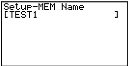
-
Input up to 18 characters for the setup name, and then press .
-
This changes the setup name and returns to the setup memory list.
- To delete setup data
- On the E-CON2 main menu (page 1-1), press F2(MEM) to display the setup memory list.
- Use the and cursor keys to highlight the name of the setup you want.
- Press F4 (DEL).
-
In response to the confirmation message that appears, press F1 (Yes) to delete the setup.
-
To clear the confirmation message without deleting anything, press F6 (No).
- To recall setup data
Recalling setup data stores it in the current setup memory area. You can then use Advanced Setup to edit the setup. This capability comes in handy when you need to perform a setup that is slightly different from one you have stored in memory.
- On the E-CON2 main menu (page 1-1), press F2(MEM) to display the setup memory list.
- Use the and cursor keys to highlight the name of the setup you want.
- Press F5 (LOAD).
-
In response to the confirmation message that appears, press F1 (Yes) to recall the setup.
-
To clear the confirmation message without recalling the setup, press F6 (No).
Note
- Recalling setup data replaces any other data currently in the current setup memory area.
7 Using Program Converter
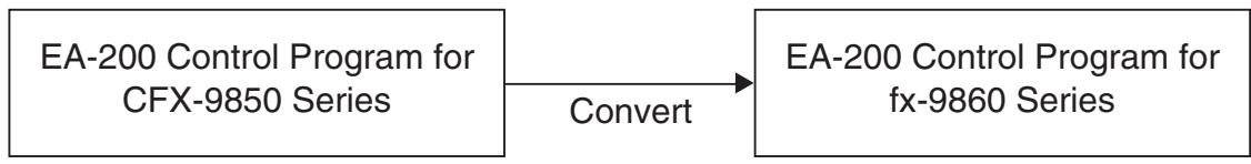
Program Converter converts an EA-200 setup you configured using Setup Wizard or Advanced Setup to a program that can run on the calculator. You can also use Program Converter to convert a setup to a CFX-9850 Series/fx-7400 Series-compatible program. ^1 ^2
1 See the documentation that came with your scientific calculator or EA-200 for information about how to use a converted program.
2 See online help (PROGRAM CONVERTER HELP) for information about supported CFX-9850 Series and fx-7400 Series models.
Converting a Setup to a Program
A setup can be converted to a program when any one of the following conditions exists.
- After configuring a new setup with Setup Wizard
See step 8 under "To configure an EA-200 setup using Setup Wizard" on page 2-2.
- After configuring a new setup with Advanced Setup
See step 6 under "To configure an EA-200 setup using Advanced Setup" on page 3-1 for more information.
- While the E-CON2 main menu (page 1-1) is on the display
Performing the program converter operation while the E-CON2 main menu is on the display converts the contents of the current setup memory area (which were configured using Setup Wizard or Advanced Setup).
The program converter procedure is identical in all of the above cases.
- To convert a setup to a program
- Start the converter operation by performing one of the key operations described below.
If the final Setup Wizard screen (page 2-4) is on the display, press 3 (Convert Program).
If the Advanced Setup menu (page 3-1) is on the display, press F4 PROG.
If the E-CON2 main menu (page 1-1) is on the display, press F3 (PROG).
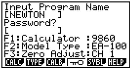
- After you perform any one of the above operations, the program converter screen will appear on the display.
Input Program Name [ ]
F1: Calculator :9860
F2:Model Type :EA-200
F3:Calibration:None
CALC TYPE CALF 30 SVEB HELP
- Enter up to eight characters for the program name.
Note
Using the program converter initial default settings will create a program like the one below.
- Associated Scientific Calculator: fx-9860 Series
- Associated Data Analyzer: EA-200
- Calibration: None
- Password: None
If you want to use these settings the way they are without changing them, skip steps 3 through 7 and go directly to step 8. If you want to change any of the settings, perform the applicable operations in steps 3 through 7.
- Specify the scientific calculator model to be associated with the program. Perform one of the following key operations to associate the program with a scientific calculator.
| To associate the program with this calculator: | Perform this key operation: |
| fx-9860 Series | F1(CALC) F1(9860) |
| CFX-9850 Series | F1(CALC) F2(9850) |
| fx-7400 Series | F1(CALC) F3(7400) |
- The number part of the scientific calculator model number you specify will appear in line "F1:" of the program converter screen.
Note
For information about 1 (CALC) 4 ( 38K), see “Converting a CFX-9850 Series Program to a fx-9860 Series Compatible Program” (page 7-4).
- Specify the Data Analyzer model (EA-100 or EA-200) to be associated with the program. Perform one of the following key operations to associate the program with a Data Analyzer.
| To associate the program with this Data Analyzer: | Perform this key operation: |
| EA-200 | F2 (TYPE) F1 (200) |
| EA-100 | F2 (TYPE) F2 (100) |
- The number part of the Data Analyzer model number you specify will appear in line "F2:" of the program converter screen.
Important!
-
Note that the capabilities of the EA-100 and EA-200 are different. Because of this, you should keep in mind that an EA-200 program converted to an EA-100 program and used to perform sampling with an EA-100 setup may not produce the desired results.
-
If you plan to use a custom probe connected to CH1 of the Data Analyzer, specify whether calibration or zero adjust should be performed. Perform one of the following key operations to configure the desired setting.
| To perform this operation: | Perform this key operation: |
| Calibration of the CH1 custom probe | F3(CALB) F1(CALIB) |
| Zero adjust of the CH1 custom probe | F3(CALB) F2(ZERO) |
| No calibration | F3(CALB) F3(None) |
-
The operation you specify will appear in line "F3:" of the program converter screen.
-
To password protect the program, press F4 (m).
-
This will cause the "Password?" prompt and password input field to appear under the program name input field.
-
Enter up to eight characters for the password.
-
If you change your mind about assigning a password, press EXIT here. This will cause the password input field to disappear and cancel password input.
-
After everything is the way you want, press [EXE] to convert the program in accordance with the setup.
-
The message "Complete!" appears when conversion is complete. To clear the message and return to the screen that was on the display in step 1, press or .
Converting a CFX-9850 Series Program to a fx-9860 Series Compatible Program
To use an EA-200 control program created on the CFX-9850 Series calculator (for use on the CFX-9850) on the E-CON2, you need to convert the program to an fx-9860 program. Conversion can be performed using the program converter.
- To convert a program
- Transfer the EA-200 control program created for the CFX-9850 Series to the fx-9860 main memory.
- Use the cable that comes bundled with the fx-9860 to connect its 3-pin serial port to the 3-pin serial port of the CFX-9850. For details, see the chapter titled "Data Communications" in the manuals that come with each unit.
- Perform step 1 under "To convert a setup to a program" on page 7-1, which displays the program converter screen.
-
Press F1(CALC) and then press F4 ( 38K) .
-
This displays a list of programs currently in main memory.
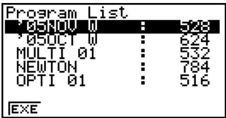
-
Use and to move the highlighting of the program you want to convert, and then press F1(EXE) or EXE.
-
A program name input screen will appear after conversion is complete.
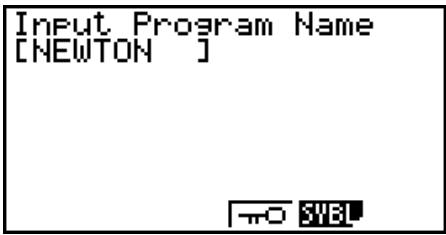
-
Enter up to eight characters for the program name.
-
If you want to password protect the program, perform steps 6 and 7 under "To convert a setup to a program" after inputting the program name.
-
Press to start conversion of the program.
-
The message "Complete!" appears when conversion is complete. To clear the message, press or .
8 Starting a Sampling Operation
The section describes how to use a setup configured using the E-CON2 Mode to start an EA-200 sampling operation.
Before getting started...
Be sure to perform the following steps before starting sampling with the EA-200.
- Connect the calculator to the EA-200.
- Turn on EA-200 power.
- In accordance with the setup you plan to use, connect the proper sensor to the appropriate EA-200 channel.
- Prepare the item whose data is to be sampled.
Starting a Sampling Operation
A sampling operation can be started when any one of the following conditions exist.
- After configuring a new setup with Setup Wizard
See step 8 under "To configure an EA-200 setup using Setup Wizard" on page 2-2.
After configuring a new setup with Advanced Setup
See step 6 under "To configure an EA-200 setup using Advanced Setup" on page 3-1. - While the E-CON2 main menu (page 1-1) is on the display
Starting a sampling operation while the E-CON2 main menu is on the display performs sampling using the contents of the current setup memory area (which were configured using Setup Wizard or Advanced Setup).
While the setup memory list is on the display
You can select the setup you want on the setup memory list and then start sampling.
The following procedures explain the first three conditions described above. See "To recall a setup and use it for sampling" on page 6-3 for information about starting sampling from the setup memory list.
- To start sampling
- Start the sampling operation by performing one of the function key operations described below.
If the final Setup Wizard screen (page 2-4) is on the display, press 1 (Start Setup).
If the Advanced Setup menu (page 3-1) is on the display, press F1(STRT).
If the E-CON2 main menu (page 1-1) is on the display, press F4(STRT).
- After you perform any one of the above operations, a sampling start confirmation screen like the one shown below will appear on the display.
=EN-200 ==
\*IS THE SENSOR CONNECTED?
\*CONNECT LINK-CABLE FIRMLY?
\*IS SAMPLING DONE? Press:[EXE]
-
Press [EXE].
-
This sets up the EA-200 using the setup data in the current setup memory area.
- The message "Setting EA-200..." remains on the display while EA-200 setup is in progress. You can cancel the setup operation any time this message is displayed by pressing AC.
- The screen shown below appears after EA-200 setup is complete.
-
Press EXE to start sampling.
-
The screens that appear while sampling is in progress and after sampling is complete depend on setup details (sampling mode, trigger setup, etc.). For details, see "Operations during a sampling operation" below.
- Operations during a sampling operation
Sending a sample start command from the calculator to the EA-200 causes the following sequence to be performed.
Setup Data Transfer Sampling Start Sampling End Transfer of Sample Data from the EA-200 to the Calculator
The table on the next page shows how the trigger conditions and sensor type specified in the setup data affects the above sequence.
Starts Sampling
| Mode | 1. EA-200 Setup | 2. Start Standby | 3. Sampling | 4. Graphing |
| Real-time | Setting EA-200...Cancel:[AC] | Start Sampling?Press:[EXE] | → | Sampled values are saved asCurrent Sample Data. |
| Fast | → | ·When Mode = SoundGraph screen does not show all sampled values,but only a partial preview. | ||
| Normal | The screen shown below appears when CH1,SONIC, or Mic is used as the trigger. | MICSound US pSec | ||
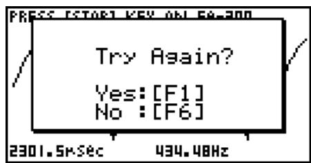
| Sound | When sampling is done, Press [EXE] key. | MICSound US pSecOutput Frequency%: | ||
| Extended | Press [F1] advances to“4. Graphing”.Press [EXE] there returns to“3. Sampling”. | Input values.EXE PRESS [STOP] KEY ON EA-200Output throughspeaker | ||
| Period | When sampling is done, Press [EXE] key. | ·When Number of Samples = 1The following three graph typescan be produced when Photo-Gate-Pulley is being used.1. Time and distance graph2. Time and velocity graph3. Time and acceleration graph | ||
| Clock | ·When Number of Samples >1Sample values is stored as Listdata only. |
9 Using Sample Data Memory
Performing an EA-200 sampling operation from the E-CON2 Mode causes sampled results to be stored in the "current data area" of E-CON2 memory. Separate data is saved for each channel, and the data for a particular channel in the current data area is called that channel's "current data".
Any time you perform a sampling operation, the current data of the channel(s) you use is replaced by the newly sampled data. If you want to save a set of current data and keep it from being replaced by a new sampling operation, save the data in sample data memory under a different file name.
Managing Sample Data Files
- To save current sample data to a file
-
On the E-CON2 main menu (page 1-1), press F5(GRPH).
-
This displays the Graph Mode screen.
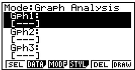
Graph Mode Screen
-
For details about the Graph Mode screen, see "10 Using the Graph Analysis Tools to Graph Data".
-
Press F2 (DATA).
-
This displays the Sampling Data List screen.
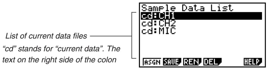
Sampling Data List Screen
-
Use the and cursor keys to move the highlighting to the current data file you want to save, and then press F2 (SAVE).
-
This displays the screen for inputting a data name.
Sample Data Name
[ ] = = Specifications = = = Sensor:Optical Interval:0.2sec Number:101 Max:317Lum Int Min:0.66667Lum Int
- Enter up to 18 characters for the data file name, and then press
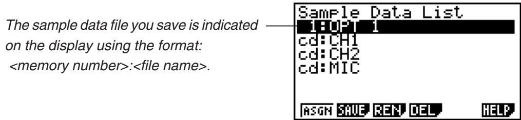
- This displays a dialog box for inputting a memory number.
- Enter a memory number in the range of 1 to 99, and then press .
- This saves the sample data at the location specified by the memory number you input.
-
If you specify a memory number that is already being used to store a data file, a confirmation message appears asking if you want to replace the existing file with the new data file. Press F1 to replace the existing data file, or F6 to return to the memory number input dialog box in Step 4.
-
To return to the E-CON2 main menu (page 1-1), press EXIT twice.
Note
- You could select another data file besides a current data file in step 3 of the above procedure and save it under a different memory number. You do not need to change the file's name as long as you use a different file number.
- To rename an existing sample data file
Note
-
You cannot use this procedure to rename a current data file name.
-
On the E-CON2 main menu (page 1-1), press F5(GRPH).
- This displays the Graph Mode screen.
- Press F2 (DATA).
This displays the Sampling Data List screen. - Use the and cursor keys to move the highlighting to the data file you want to rename, and then press F3 (REN).
- This displays the screen for inputting a file name.
- Enter up to 18 characters for the new data file name, and then tap .
- This returns to the Sampling Data List screen.
- To return to the E-CON2 main menu (page 1-1), press EXIT twice.
- To delete a sample data file
-
On the E-CON2 main menu (page 1-1), press F5(GRPH).
-
This displays the Graph Mode screen.
-
Press F2 (DATA).
-
This displays the Sampling Data List screen.
-
Use the and cursor keys to move the highlighting to the data file you want to delete, and then press F4 (DEL).
-
In response to the confirmation message that appears, press F1 (Yes) to delete the data file.
-
To clear the confirmation message without deleting the data file, press F6 (No).
-
This returns to the Sampling Data List screen.
-
To return to the E-CON2 main menu (page 1-1), press EXIT twice.
10 Using the Graph Analysis Tools to Graph Data
Graph Analysis tools make it possible to analyze graphs drawn from sampled data.
■ Accessing Graph Analysis Tools
You can access Graph Analysis tools using either of the two methods described below.
- Accessing Graph Analysis tools from the Graph Mode screen, which is displayed by pressing F5(GRPH) on the E-CON2 main menu (page 1-1)
Graph Mode Screen
- The main menu appears after you perform a sampling operation. Press F5 (GRPH) at that time.
-
When you access Graph Analysis tools using this method, you can select from among a variety of other Analysis modes. See "Selecting an Analysis Mode and Drawing a Graph" (page 10-2) for more information about the other Analysis modes.
-
Accessing Graph Analysis tools from the screen of a graph drawn after a sampling operation is executed from the Setup Wizard or from Advanced Setup (Realtime Mode)
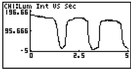
Graph Screen
- In this case, data is graphed after the sampling operation is complete, and the calculator accesses Graph Analysis tools automatically. See "Graph Screen Key Operations" on page 11-1.
■ Selecting an Analysis Mode and Drawing a Graph
This section contains a detailed procedure that covers all steps from selecting an analysis mode to drawing a graph.
Note
- Step 4 through step 6 are not essential and may be skipped, if you want. Skipping any step automatically applies the initial default values for its settings.
- If you skip step 2, the default analysis mode is the one whose name is displayed in the top line of the Graph Mode screen.
- To select an analysis mode and draw a graph
-
On the E-CON2 main menu (page 1-1), press F5(GRPH).
-
This displays the Graph Mode screen.
-
Press F3 (MODE), and then select the analysis mode you want from the menu that appears.
| To do this: | Perform this menu operation: | To select this mode: |
| Graph three sets of sampled data simultaneously | [Norm] | Graph Analysis |
| Graph sampled data along with its first and second derivative graph | [diff] | d/dt & d²/dt² |
| Display the graphs of different sampled data in upper and lower windows for comparison | [CMPR]→[GRPH] | Compare Graph |
| Output sampled data from the speaker, displaying graph of the raw data in the upper window and the output waveform in the lower window | [CMPR]→[Snd] | Compare Sound |
| Display the graph of sampled data in the upper window and its first derivative graph in the lower window | [CMPR]→[d/dt] | Compare d/dt |
| Display the graph of sampled data in the upper window and its second derivative graph in the lower window | [CMPR]→[d²/dt²] | Compare d²/dt² |
- The name of the currently selected mode appears in the top line of the Graph Modescreen.
Analysis mode name

- Press F2 (DATA).
This displays the Sampling Data List screen.
- Specify the sampled data for graphing.
a. Use the and cursor keys to move the highlighting to the name of the sampled data file you want to select, and then press F1(ASGN) or EXE.
- This returns to the Graph Mode screen, which shows the name of the sample data file you selected.
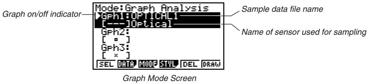
b. Repeat step a above to specify sample data files for other graphs, if there are any.
- If you select "Graph Analysis" as the analysis mode in step 2, you must specify sample data files for three graphs. If you select "Compare Graph" as the analysis mode in step 2, you must specify sample data files for two graphs. With other modes, you need to specify only one sample data file.
-
For details about Sampling Data List screen operations, see "9 Using Sample Data Memory".
-
Turn on graphing for each of the graphs listed on the Graph Mode screen.
a. On the Graph Mode screen, use the and cursor keys to select a graph, and then press F1 (SEL) to toggle graphing on or off.
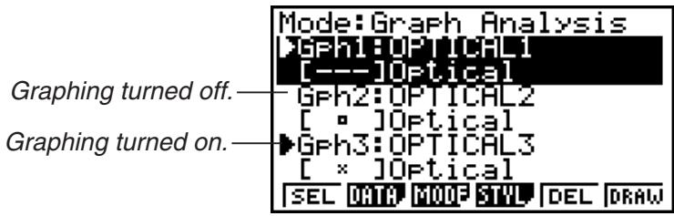
b. Repeat step a to turn each of the graphs listed on the Graph Mode screen on or off.
- Select the graph style you want to use.
a. On the Graph Mode screen, use the and cursor keys to move the highlighting to the graph (Gph1, Gph2, etc.) whose style you want to specify, and then press F4(STYL). This will cause the function menu to change as shown below.
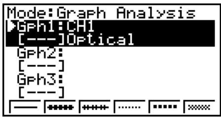
b. Use the function keys to specify the graph style you want.
| To specify this graph style: | Press this key: |
| Line graph with dot ( • ) data markers | F1( — —) |
| Line graph with square ( □ ) data markers | F2( *****) |
| Line graph with X (× ) data markers | F3( ++++ ) |
| Scatter graph with dot ( • ) data markers | F4( …… ) |
| Scatter graph with square ( □ ) data markers | F5( …… ) |
| Scatter graph with X (× ) data markers | F6( …… ) |
c. Repeat a and b to specify the style for each of the graphs on the Graph Mode screen.
-
On the Graph Mode screen, press F6 (DRAW) or EXE.
-
This draws the graph(s) in accordance with the settings you configured in step 2 through step 6.
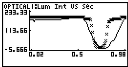
Graph Screen
- When a Graph screen is on the display, the function keys provide you with zooming and other capabilities to aid in graph analysis.
For details about Graph screen function key operations, see the following section.
- To deselect sampled data assigned for graphing on the Graph Modescreen
-
On the Graph Mode screen, use the and cursor keys to move the highlighting to the graph (Gph1, Gph2, etc.) whose sampled data you want to deselect.
-
Press F5 (DEL).
-
This will deselect sample data assigned to the highlighted graph.
11 Graph Analysis Tool Graph Screen Operations
This section explains the various operations you can perform on the graph screen after drawing a graph.
You can perform these operations on a graph screen produced by a sampling operation, or by the operation described under “Selecting an Analysis Mode and Drawing a Graph” on page 10-2.
Graph Screen Key Operations
On the graph screen, you can use the keys described in the table below to analyze (CALC) graphs by reading data points along the graph (Trace) and enlarging specific parts of the graph (Zoom).
| Key Operation | Description |
| SHIFT F1(TRCE) | Displays a trace pointer on the graph along with the coordinates of the current cursor location. Trace can also be used to obtain the periodic frequency of a specific range on the graph and assign it to a variable. See “Using Trace” on page 11-3. |
| SHIFT F2(ZOOM) | Starts a zoom operation, which you can use to enlarge or reduce the size of the graph along the x-axis or the y-axis. See “Using Zoom” on page 11-4. |
| SHIFT F3(V-WIN) | Displays a function menu of special View Window commands for the E-CON2 Mode graph screen. For details about each command, see “Configuring View Window Parameters” on page 11-14. |
| SHIFT F4(SKTCH) | Displays a menu that contains the following commands: CIs, Plot, F-Line, Text, PEN, Vert, and Hztl. For details about each command, see “5-10 Changing the Appearance of a Graph” in the manual that comes with the fx-9860G SD/fx-9860G calculator. |
| OPTN F1(PICT) | Saves the currently displayed graph as a graphic image. You can recall a saved graph image and overlay it on another graph to compare them. For details about these procedures, see “5-4 Storing a Graph in Picture Memory” in the manual that comes with the fx-9860G SD/fx-9860G calculator. |
| OPTN F2(LMEM) | Displays a menu of functions for saving the sample values in a specific range of a graph to a list. See “Transforming Sampled Data to List Data” on page 11-5. |
| OPTN F3(EDIT) | Displays a menu of functions for zooming and editing a particular graph when the graph screen contains multiple graphs. See “Working with Multiple Graphs” on page 11-10. |
| OPTN F4(CALC) | Displays a menu that lets you transform a sample result graph to a function using Fourier series expansion, and to perform regression to determine the tendency of a graph. See “Using Fourier Series Expansion to Transform a Waveform to a Function” on page 11-6, and “Performing Regression” on page 11-8. |
| OPTN F5(Y=fx) | Displays the graph function list, which lets you select a Y=f(x) graph to overlay on the sampled result graph. See “Overlaying a Y=f(x) Graph on a Sampled Result Graph” on page 11-9. |
| OPTN F6(SPKR) | Starts an operation for outputting a specific range of a sound data waveform graph from the speaker. See “Outputting a Specific Range of a Graph from the Speaker” on page 11-12. |
■ Scrolling the Graph Screen
Press the cursor keys while the graph screen is on the display scrolls the graph left, right, up, or down.
Note
- The cursor keys perform different operations besides scrolling while a trace or graph operation is in progress. To perform a graph screen scroll operation in this case, press EXIT to cancel the trace or graph operation, and then press the cursor keys.
Using Trace
Trace displays a crosshair pointer on the displayed graph along with the coordinates of the current cursor position. You can use the cursor keys to move the pointer along the graph. You can also use trace to obtain the periodic frequency value for a particular range, and assign the range (time) and periodic frequency values in separate Alpha-Memory values.
To use trace
-
On the graph screen, press SHIFT F1(TRCE).
-
This causes a trace pointer to appear on the graph. The coordinates of the current trace pointer location are also shown on the display.
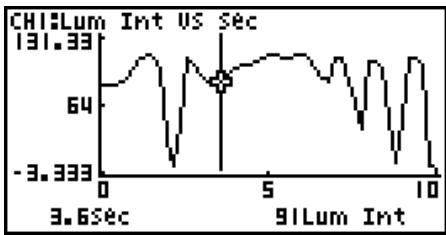
-
Use the and cursor keys to move the trace pointer along the graph to the location you want.
-
The coordinate values change in accordance with the trace pointer movement.
- You can exit the trace pointer at any time by pressing .
To obtain the periodic frequency value
- Use the procedure under "To use trace" above to start a trace operation.
- Move the trace pointer to the start point of the range whose periodic frequency you want to obtain, and then press .
-
Move the trace pointer to the end point of the range whose periodic frequency you want to obtain.
-
This causes the period and periodic frequency value at the start point you selected in step 2 to appear along the bottom of the screen.
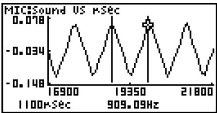
-
Press to assign the period and periodic frequency values to Alpha-Memory variables.
-
This displays a dialog box for specifying variable names for [Period] and [Frequency] values.
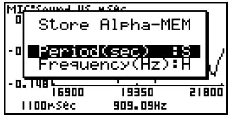
-
The initial default variable name settings are "S" for the period and "H" for the periodic frequency. To change to another variable name, use the up and down cursor keys to move the highlighting to the item you want to change, and then press the applicable letter key.
-
After everything is the way you want, press .
-
This stores the values and exits the trace operation.
- For details about using Alpha-Memory, see the manual that comes with the fx-9860G SD/fx-9860G calculator.
Using Zoom
Zoom lets you enlarge or reduce the size of the graph along the x -axis or the y -axis.
Note
- When there are multiple graphs on the screen, the procedure below zooms all of them. For information about zooming a particular graph when there are multiple graphs on the screen, see "Working with Multiple Graphs" on page 11-10.
- To zoom the graph screen
-
On the graph screen, press SHIFT F2 (ZOOM).
-
This causes a magnifying glass cursor ( _k ) to appear in the center of the screen.
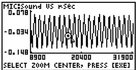
- Use the cursor keys to move the magnifying glass cursor to the location on the screen that you want at the center of the enlarged or reduced screen.
3. Press [EXE].
- This causes the magnifying glass to disappear and enters the zoom mode.
- The cursor keys perform the following operations in the zoom mode.
| To do this: | Press this cursor key: |
| Enlarge the graph image horizontally | ◎ |
| Reduce the size of the graph image horizontally | ◎ |
| Enlarge the graph image vertically | ▲ |
| Reduce the size of the graph image vertically | ◎ |
4. To exit the zoom mode, press EXIT.
Transforming Sampled Data to List Data
Use the following procedure to transform the sampled data in a specific range of a graph into list data.
To transform sampled data to list data
- On the graph screen, press OPTN, and then F2(LMEM).
- This displays the [LMEM] menu.
- Press F2 (SEL).
- This displays the trace pointer for selecting the range on the graph.
- Move the trace pointer to the start point of the range you want to convert to list data, and then press .
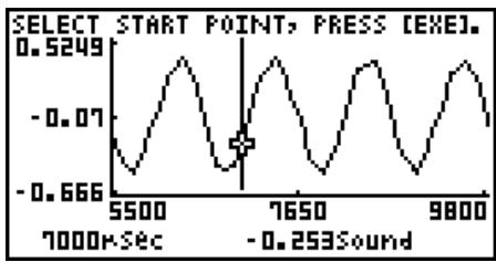
-
Move the trace pointer to the end point of the range you want to convert to list data, and then press .
-
This displays a dialog box for specifying the lists where you want to store the time data and the sampled data.
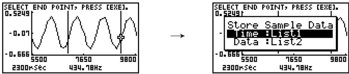
-
The initial default lists are List 1 for the time and List 2 for sample data. To change to another list (List 1 to List 26), use the up and down cursor keys to move the highlighting to the list you want to change, and then input the applicable list number.
-
After everything is the way you want, press .
-
This saves the lists and the message "Complete!" appears. Press to return to the graph screen.
- For details about using list data, see the manual that comes with the fx-9860G SD/fx-9860G calculator.
Note
- Pressing F1 (All) in place of F2 (SEL) in step 2 converts the entire graph to list data. In this case, the "Store Sample Data" dialog box appears as soon as you press F1 (All).
Using Fourier Series Expansion to Transform a Waveform to a Function
Fourier series expansion is effective for studying sounds by expressing them as functions. The procedure below assumes that there is a graph of sampled sound data already on the graph screen.
To perform Fourier series expansion
-
On the graph screen, press OPTN, and then F4(CALC).
-
The [CALC] menu appears at the bottom of the display.
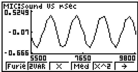
-
Press F1(Furie).
-
This displays the trace pointer for selecting the graph range.
-
Move the trace pointer to the start point of the range for which you want to perform Fourier series expansion, and then press .
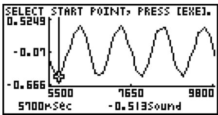
-
Move the trace pointer to the end point of the range for which you want to perform Fourier series expansion, and then press .
-
This displays a dialog box for specifying the start degree of the Fourier series.
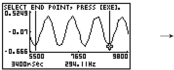
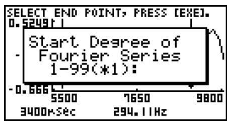
-
Input a value in the range of 1 to 99, and then press .
-
This displays a dialog box for inputting the degree of the Fourier series.
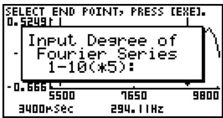
-
Input a value in the range of 1 to 10, and then press .
-
The graph function list appears with the calculation result.

- Pressing F6(DRAW) here graphs the function.
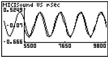
- This lets you compare the expanded function graph and the original graph to see if they are the same.
Note
When you press F6 (DRAW) in step 7, the graph of the result of the Fourier series expansion may not align correctly with the original graph on which it is overlaid. If this happens, shift the position the original graph to align it with the overlaid graph.
For information about how to move the original graph, see "To move a particular graph on a multi-graph display" (page 11-12).
Performing Regression
You can use the procedure below to perform regression for a range specified using the trace pointer. All of the following regression types are supported: Linear, Med-Med, Quadratic, Cubic, Quartic, Logarithmic, Exponential, Power, Sine, and Logistic.
For details about these regression types, see page 6-3-5 through 6-3-10 of the manual that comes with the fx-9860G SD/fx-9860G calculator.
The following procedure shows how to perform quadratic regression. The same general steps can also be used to perform the other types of regression.
To perform quadratic regression
- On the graph screen, press OPTN, and then F4(CALC).
- The [CALC] menu appears at the bottom of the display.
- Press F5(X^2).
- This displays the trace pointer for selecting the range on the graph.
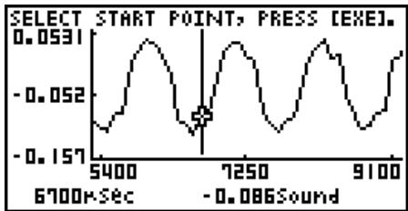
- Move the trace pointer to the start point of the range for which you want to perform quadratic regression, and then press .
-
Move the trace pointer to the end point of the range for which you want to perform quadratic regression, and then press .
-
This displays the quadratic regression calculation result screen.
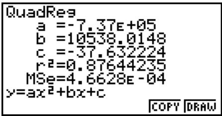
5. Press F6 (DRAW).
- This draws a quadratic regression graph and overlays it over the original graph.
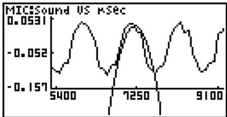
- To delete the overlaid quadratic regression graph, press SHIFT F4 (SKTCH) and then F1 (Cls).
■ Overlaying a Y=f(x) Graph on a Sampled Result Graph
Use the following procedure when you want to overlay a Y = f(x) graph on the sampled result graph.
- To overlay a Y = f(x) graph on an existing graph
-
On the graph screen, press OPTN, and then F5(Y=fx).
-
This displays the graph function list. Any functions you have previously input on the graph function list appear at this time.
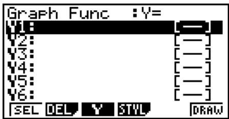
-
Input the function you want to graph.
-
To input a function, use the and cursor keys to move the highlighting to the line where you want to input it, and then use the calculator keys for input. Press X E to store the function.
-
On the graph function list, specify which functions you want to graph.
-
Graphing is turned on for any function whose “=” symbol is highlighted. To toggle graphing of a function on or off, use the and cursor keys to move the highlighting to the function, and then press F1 (SEL).
-
After the graph function list settings are configured the way you want, press F6(DRAW).
-
This overlays graphs of all the functions for which graphing is turned on, over the graph that was originally on the graph screen.
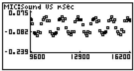
Original Graph


Overlaid with Y = f(x) Graph
- To delete the overlaid graph, press SHIFT F4 (SKTCH) and then F1 (Cls).
Important!
- The screenshot shown in step 4 above is of a function that was calculated and stored by performing regression on a graph that was drawn using sampled data. Note that overlaying a Y = f(x) graph on a sampled data graph does not automatically draw a regression graph based on sampled data.
■ Working with Multiple Graphs
The procedures in this section explain how you can zoom or move a particular graph when there are multiple graphs on the display.
- To zoom a particular graph on a multi-graph display
-
When the graph screen contains multiple graphs, press OPTN , and then F3(EDIT).
-
The [EDIT] menu appears at the bottom of the display.
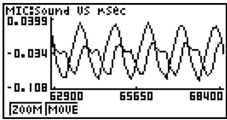
2. Press [F1] (ZOOM).
- This displays only one of the graphs that were originally on the graph screen.
![CASIO GRAPH 25+ PRO - Press [F1] (ZOOM). - 1](/content/2019/11/195600/images/c5331015232f40f1242b327a2d02b2224885601048f68025790eee3a28b2054c.jpg)
-
Use the and cursor keys to cycle through the graphs until the one you want is displayed, and then press X E .
-
This enters the zoom mode and causes all of the graphs to reappear, along with a magnifying glass cursor (O) in the center of the screen.
![CASIO GRAPH 25+ PRO - Press [F1] (ZOOM). - 2](/content/2019/11/195600/images/8d8daf1c1ec4809ed08746030ea2187badd643a739ef6bdedf781e4093fb6471.jpg)
-
Use the cursor keys to move the magnifying glass cursor to the location on the screen that you want at the center of the enlarged or reduced screen.
-
Press [EXE].
-
This causes the magnifying glass to disappear and enters the zoom mode.
- The cursor keys perform the following operations in the zoom mode.
| To do this: | Press this cursor key: |
| Enlarge the graph image horizontally | ◎ |
| Reduce the size of the graph image horizontally | ◎ |
| Enlarge the graph image vertically | ▲ |
| Reduce the size of the graph image vertically | ◎ |
![CASIO GRAPH 25+ PRO - Press [F1] (ZOOM). - 3](/content/2019/11/195600/images/dbe18bc13d49d52a6704770f729fbe0fe1975ca4231f4dbabc2874b833bb87f5.jpg)
![CASIO GRAPH 25+ PRO - Press [F1] (ZOOM). - 4](/content/2019/11/195600/images/9a76fc8bd8668449a87f388fc589da414626fe14110199619e5f074e1669579e.jpg)
![CASIO GRAPH 25+ PRO - Press [F1] (ZOOM). - 5](/content/2019/11/195600/images/d6c29e027f6d4ded0294dfe02d8a1bf82ab397e59873e7f8e856d310992a34b3.jpg)
- To exit the zoom mode, press EXIT
- To move a particular graph on a multi-graph display
- When the graph screen contains multiple graphs, press OPTN, and then F3 (EDIT).
- This displays the [EDIT] menu.
- Press F2 (MOVE).
-
This displays only one of the graphs that were originally on the graph screen.
-
Use the and cursor keys to cycle through the graphs until the one you want is displayed, and then press .
- This enters the move mode and causes all of the graphs to reappear.
- Use the and cursor keys to move the graph left and right, or the and cursor keys to move the graph up and down.
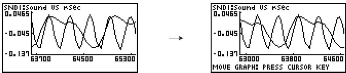
- To exit the move mode, press EXIT
■ Outputting a Specific Range of a Graph from the Speaker
Use the following procedure to output a specific range of a sound data waveform graph from the speaker.
- To output a graph from the speaker
-
On the graph screen, press OPTN, and then F4 (SPKR).
-
This displays the trace pointer for selecting the range on the graph.
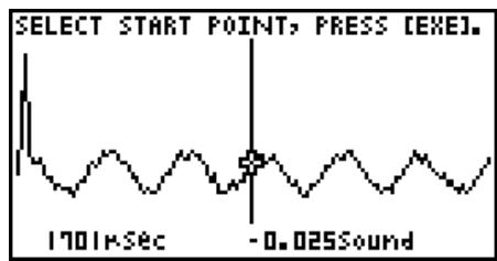
-
Move the trace pointer to the start point of the range you want to output from the speaker, and then press .
-
Move the trace pointer to the end point of the range you want to output from the speaker, and then press .
-
After you specify the start point and end point, an output frequency dialog box shown below appears on the display.
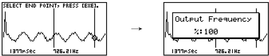
-
Input a percent value for the output frequency value you want.
-
The output frequency specification is a percent value. To output the original sound as-is, specify 100% . To raise the original sound by one octave, input a value of 200% . To lower the original sound by one octave, input a value of 50% .
-
After inputting an output frequency value, press EXE.
-
This outputs the waveform between the start point and end point from the EA-200 speaker.
-
If the sound you configured cannot be output for some reason, the message “Range Error” will appear. If this happens, press [EXIT] to scroll back through the previous setting screens and change the setup as required.
-
To terminate sound output, press the EA-200 [START/STOP] key.
-
Press [EXE].
-
This displays a screen like the one shown below.
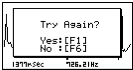
-
If you want to retry output from the speaker, press F1 (Yes). To exit the procedure and return to the graph screen, press F6 (No).
-
Pressing F1 (Yes) returns to the "Output Frequency" dialog box. From there, repeat the above steps from step 4.
■ Configuring View Window Parameters
Pressing SHIFT F3 (V-Window) while the graph screen is on the display displays a View Window function key menu along the bottom of the display.
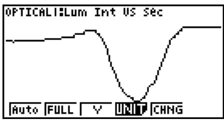
Press the function key that corresponds to the View Window parameter you want to configure.
| Function Key | Description |
| F1(Auto) | Automatically applies the following View Window parameters. Y-axis Elements: In accordance with screen size X-axis Elements: In accordance with screen size when 1 data item equals 1 dot; 1 data equals 1 dot in other cases |
| F2(FULL) | Resizes the graph so all of it fits in the screen. |
| F3(Y) | Resizes the graph so all of it fits in the screen along the Y-axis, without changing the X-axis dimensions. |
| F4(UNIT) | Specifies the unit of the numeric axis grid displayed by the Econ Axes setting of the graph setup screen (page 3-13). F1(μ sec): microseconds F2(msec): milliseconds F3(sec): seconds F4(DHMS):days, hours, minutes, seconds (1 day, 2 hours, 30 minutes, 5 seconds = 1d2h30m5s) F5(Auto):Auto selection |
| F5(CHNG) | Toggles display of the source data on the graph screen on and off. |
To exit the View Window function key menu and return to the standard function key menu, press EXIT.
12 Calling E-CON2 Functions from an eActivity
You can call E-CON2 functions from an eActivity by including an "Econ strip" in the eActivity file. The following describes each of the four available Econ strips.
- Econ SetupWizard strip
This strip calls the E-CON2 Setup Wizard. The Econ Setup Wizard strip makes it possible to perform the following series of operations from the eActivity: EA-200 setup using the Setup Wizard Sampling Graphing.
- Econ AdvancedSetup strip
This strip calls the E-CON2 Advanced Setup screen. The Advanced Setup provides access to almost all executable functions (except for the program converter), including detailed EA-200 setup and sampling execution; graphing and Graph Analysis Tools; simultaneous sampling with multiple sensors using the MULTIMETER Mode, etc.
Econ Sampling strip
This strip records on set of EA-200 setup information configured using Advanced Setup, and performs sampling. Once setup information is recorded to this type of strip, sampling starts immediately based on the recorded setup information the next time the strip is executed.
Econ Graph strip
This strip graphs sampled data that is recorded in the strip. The sampled data is recorded to the strip the first time the strip is executed.
This section explains how to insert each type of Econ strip into an eActivity file, and how to use inserted Econ strips. For details about eActivity operations, see "Chapter 10 eActivity" in the manual that comes with the fx-9860G SD or fx-9860G.
Inserting an Econ Strip into an eActivity File
The following procedure assumes that the eActivity file into which you want to insert the Econ strip is already open. For information about creating a new file and other basic eActivity operations, see "Basic eActivity File Operation" (page 10-1-5) in the manual that comes with the fx-9860G SD or fx-9860G.
- To insert an Econ Strip into an eActivity file
- On the eActivity workspace screen, move the cursor the location where you want to insert the Econ strip.
-
Press F2 (STRP).
-
This will display a dialog box with a list of insertable strips.
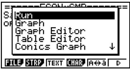
- Use and to move the highlighting to the type of Econ strip you want to insert.
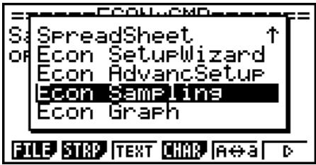
-
See the beginning of this section (page 12-1) for details about each Econ strip type.
-
Press .
- The strip is inserted above the line or the strip where the cursor is currently located.
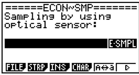
-
Enter up to 16 characters for the strip title.
-
Press EXE to assign the title to the strip.
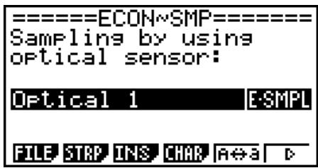
- This will highlight the strip.
- You can execute the strip here by pressing . For details about operations that are required when you execute a strip, see "Calling an E-CON2 Function from an Econ Strip" below.
■ Calling an E-CON2 Function from an Econ Strip
This section explains operations for each type of Econ strip that can be inserted into an eActivity file. The following procedure assumes that the applicable Econ strip has already been inserted into an eActivity that is currently open.
- To access the Setup Wizard from an Econ SetupWizard strip
- On the eActivity workspace screen, use the and keys to move the highlighting to the Econ SetupWizard strip.
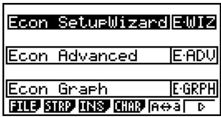
-
Press [EXE].
-
This launches the Setup Wizard and displays the "Select Sensor" screen.
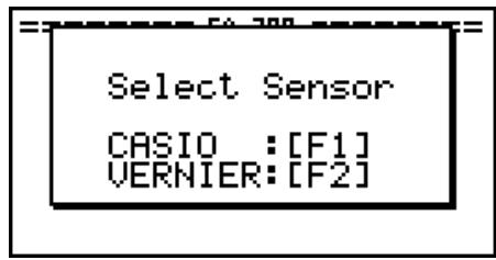
- Perform the procedure under "To configure an EA-200 setup using Setup Wizard" (page 2-2) from step 3 to set up the EA-200 and execute sampling.
Note
- In the case of the Econ SetupWizard strip, only the "1: Start Setup" is available on the "Complete!" dialog box. Other options are not available.
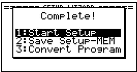
- To return to the eActivity workspace screen, press SHIFT (E) EXIT.
- To access Advanced Setup from an Econ Advanced Setup strip
- On the eActivity workspace screen, use the and keys to move the highlighting to the Econ Advanced Setup strip.
-
Press [EXE].
-
This displays the Advanced Setup screen.
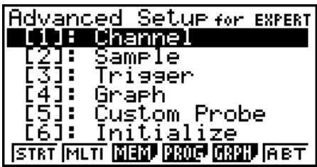
- From here, perform the procedure under "To configure an EA-200 setup using Advanced Setup" (page 3-1) from step 4.
- To return to the eActivity workspace screen after you finished the procedure or at any point during the procedure, press SHIFT (Shift).
Note
- Using an Econ Advanced Setup strip to configure a setup causes the setup information to be registered in the applicable strip. This means that the next time you open the strip, sampling can be performed in accordance with the previously configured setup information.
- To execute sampling from an Econ Sampling strip
- On the eActivity workspace screen, use the and keys to move the highlighting to the Econ Sampling strip.

2. Press [EXE].
- This displays a sampling start confirmation screen.
![CASIO GRAPH 25+ PRO - Press [EXE]. - 1](/content/2019/11/195600/images/0111b16f9d365468549688c27919fc6cc2a4bb5158f58a2103447d75d88602c3.jpg)
- If this is the first time you are using this Econ Sampling strip for sampling, continue on to step 3.
-
If this is an Econ Sampling strip that you have used for sampling in the paste and want to re-execute with the same setup, jump to step 8.
-
Press SHIFT (O) to display the application list.
![CASIO GRAPH 25+ PRO - Press [EXE]. - 2](/content/2019/11/195600/images/7e719af662fc66760c6b183f4d70a5895485df43c9614f445ae8875c18a20ada.jpg)
- Use the and cursor keys to move the highlighting to "Econ AdvancSetup", and then press EXE.
- This displays the Advanced Setup screen.
- Perform steps 4 and 5 under "To configure an EA-200 setup using Advanced Setup (page 3-1) to configure the setup for sampling.
- Press SHIFT (O) to display the application list.
- Use the and cursor keys to move the highlighting to "Econ Sampling", and then press .
-
This will return to the sampling start confirmation screen in step 2 of this procedure.
-
Press [EXE].
-
This will set up the EA-200 in accordance with the setup data registered in the Econ Sampling strip. The message "Start sampling?" appears on the screen after EA-200 set up is complete.
-
Press EXE to start sampling.
-
The screens that appear while sampling is in progress and after sampling is complete depend on setup details. For more information, see "Starting a Sampling Operation" (page 8-1).
-
After sampling is complete, the data will be graphed in accordance with the setup settings.
-
To return to the eActivity workspace screen from the graph screen, press SHIFT (Shift).
- To graph sampled data from an Econ Graph strip
- On the eActivity workspace screen, use the and keys to move the highlighting to the Econ Graph strip.
-
Press [EXE].
-
If this Econ Graph strip already has sampled data registered to it because of a previous execution, a graph of the existing data will appear on the display. In this case, jump to step 5 of this procedure.
-
If this is the first time you are executing this Econ Graph strip, the Advanced Setup screen will appear on the display. If this happens, proceed with step 3 of this procedure.
-
Perform steps 4 and 5 under "To configure an EA-200 setup using Advanced Setup (page 3-1) to configure the setup for sampling.
-
Press F1(STRT).
-
As instructed by the message that appears on the display, press the key to perform sampling.
-
After sampling is complete, the data will be graphed in accordance with the setup settings.
-
To return to the eActivity workspace screen from the graph screen, press SHIFT (Shift).
- Econ Strip Memory Capacity Precautions
- The memory capacity of each Econ strip is 25KB . An error will occur if you perform an operation that causes this capacity to be exceeded. Particular care is required when handling a large number of samples, which can cause memory capacity to be exceeded.
- Always make sure that FFT Graph is turned off whenever performing sampling with the microphone. Leaving FFT Graph turned on cause memory capacity to be exceeded.
- If an error occurs, press SHIFT (Shift) to return to the eActivity workspace screen and perform the procedure again.
- For information about checking the memory usage of each strip, see "10-5 eActivity File Memory Usage Screen" in the manual that comes with the fx-9860G SD or fx-9860G.

Manufacturer:
CASIO COMPUTER CO., LTD.
6-2, Hon-machi 1-chome, Shibuya-ku, Tokyo 151-8543, Japan
Responsible within the European Union:
CASIO EUROPE GmbH
- E-CON2 Application (English)
- ■ Simplification
- Calculus matriciels
- Type 1 (Y= expression)
- ■ Graph type camembert
- - Rendement annuel (YLD)
- Receive38k / Send38k
- - Amortissement
- E-CON2 Overview
- Note
- About online help
- Using the Setup Wizard
- ■ Setup Wizard Parameters
- Setup Wizard Rules
- - To configure an EA-200 setup using Setup Wizard
- Before getting started...
- Important!
- Using Setup Wizard to Configure Settings for FFT (Frequency Characteristics) Data Sampling
- Using Setup Wizard to Configure a PhotoGate Setup
- - To configure a setup for PhotoGate alone
- - To configure a setup for PhotoGate and Smart Pulley
- ■ Outputting the Waveform of a Function through the Speaker
- - To configure a setup for speaker output
- To change the output frequency and try again:
- To change the output range of the waveform graph and try again:
- To change the function:
- To exit the procedure and return to the E-CON2 main menu:
- Using Advanced Setup
- ■ Advanced Setup Operations
- - To configure an EA-200 setup using Advanced Setup
- - To return setup parameters to their initial defaults
- ■ Channel Setup
- - To configure Channel Setup settings
- Sample Setup
- - To configure Sample Setup settings
- - To configure the Distance setting
- - To configure the FFT Graph setting
- Trigger Setup
- - To configure Trigger Setup settings
- - To specify the countdown start time
- - To specify microphone sensitivity
- - To specify the trigger threshold value and trigger edge type
- - To configure trigger threshold, trigger start edge, and trigger end edge settings
- - To configure PhotoGate trigger start and end settings
- - To specify the trigger threshold value and motion sensor level
- Graph Setup
- - To configure Graph Setup settings
- Using a Custom Probe
- ■ Configuring a Custom Probe Setup
- - To configure a custom probe setup
- - To recall the specifications of a Vernier sensor and configure custom probe settings
- Auto Calibrating a Custom Probe
- - To auto calibrate a custom probe
- If you are configuring a new custom probe:
- If you are editing the configuration of an existing custom probe:
- Zero Adjusting a Custom Probe
- - To zero adjust a custom probe
- ■ Managing Custom Probe Setups
- - To edit a custom probe setup
- - To delete a custom probe setup
- Using the MULTIMETER Mode
- To use the MULTIMETER Mode
- Using Setup Memory
- Saving a Setup
- - To save a setup
- Using and Managing Setups in Setup Memory
- - To preview saved setup data
- - To recall a setup and use it for sampling
- - To change the name of setup data
- - To delete setup data
- - To recall setup data
- Using Program Converter
- Converting a Setup to a Program
- - To convert a setup to a program
- Converting a CFX-9850 Series Program to a fx-9860 Series Compatible Program
- - To convert a program
- Starting a Sampling Operation
- Starting a Sampling Operation
- - To start sampling
- - Operations during a sampling operation
- Using Sample Data Memory
- Managing Sample Data Files
- - To save current sample data to a file
- - To rename an existing sample data file
- - To delete a sample data file
- Using the Graph Analysis Tools to Graph Data
- ■ Accessing Graph Analysis Tools
- ■ Selecting an Analysis Mode and Drawing a Graph
- - To select an analysis mode and draw a graph
- - To deselect sampled data assigned for graphing on the Graph Modescreen
- Graph Analysis Tool Graph Screen Operations
- Graph Screen Key Operations
- ■ Scrolling the Graph Screen
- Using Trace
- To use trace
- To obtain the periodic frequency value
- Using Zoom
- - To zoom the graph screen
- Press [EXE].
- To exit the zoom mode, press EXIT.
- Transforming Sampled Data to List Data
- To transform sampled data to list data
- Using Fourier Series Expansion to Transform a Waveform to a Function
- To perform Fourier series expansion
- Performing Regression
- To perform quadratic regression
- Press F6 (DRAW).
- ■ Overlaying a Y=f(x) Graph on a Sampled Result Graph
- - To overlay a Y = f(x) graph on an existing graph
- ■ Working with Multiple Graphs
- - To zoom a particular graph on a multi-graph display
- Press [F1] (ZOOM).
- - To move a particular graph on a multi-graph display
- ■ Outputting a Specific Range of a Graph from the Speaker
- - To output a graph from the speaker
- ■ Configuring View Window Parameters
- Calling E-CON2 Functions from an eActivity
- - Econ SetupWizard strip
- - Econ AdvancedSetup strip
- Econ Sampling strip
- Econ Graph strip
- Inserting an Econ Strip into an eActivity File
- - To insert an Econ Strip into an eActivity file
- ■ Calling an E-CON2 Function from an Econ Strip
- - To access the Setup Wizard from an Econ SetupWizard strip
- - To access Advanced Setup from an Econ Advanced Setup strip
- - To execute sampling from an Econ Sampling strip
- Press [EXE].
- - To graph sampled data from an Econ Graph strip
- - Econ Strip Memory Capacity Precautions
Brand : CASIO
Model : GRAPH 25+ PRO
Category : Graphing calculator