
ICMflex - Meter Megger - Free user manual and instructions
Find the device manual for free ICMflex Megger in PDF.


| Product Type | Partial discharge and loss factor measurement system (meter) |
| Brand | Megger |
| Model | ICMflex |
| Rated Voltage (Standard Versions) | 30 kV, 50 kV, 100 kV, 150 kV (RMS) |
| Frequency Range | 20–510 Hz (normal); 0.02–0.1 Hz (VLF) |
| Weight (ICMflex 30 kV) | 22 kg |
| Dimensions (ICMflex 30 kV) | 600 x 350 x 350 mm (H x W x L) |
| Power Supply | Battery operated (Lithium-ion, up to 6 hours); approx. 20 VA |
| Main Functions | Partial discharge detection, PD fault location on cables, tan delta (loss factor) measurement, capacitance measurement, voltage and frequency measurement |
| PD Input Sensitivity | < 150 µV (0.2 pC) without preamplifier; < 15 µV (0.02 pC) with built-in preamplifier (ICMflex2 only) |
| PD Frequency Range | Lower cut-off: 40, 80, or 100 kHz; Upper cut-off: 250, 600, or 800 kHz (software-controlled) |
| Cable Fault Location Precision | 1 m + 0.1 % of cable length |
| Tan Delta Resolution | 5 x 10⁻⁵ |
| Communication Interfaces | Bluetooth (921 kBit/s), fibre optic serial link (921 kBit/s) |
| Operating Temperature | 0–55 °C (non-condensing) |
| Maintenance | No regular maintenance required; annual voltage calibration recommended; keep instrument clean |
| Safety Features | Solid grounding required; use supplied HV cables; fibre optic or Bluetooth communication for operator safety; built-in gating for noise rejection |
| Spare Parts / Repairability | Contact Power Diagnostix for spare parts; battery module replaceable; firmware updates available online |
| General Information | Designed for on-site testing of motors, generators, HV cables, and other high voltage equipment; operates with any fixed or portable HV power supply |
Frequently Asked Questions - ICMflex Megger
User questions about ICMflex Megger
0 question about this device. Answer the ones you know or ask your own.
Ask a new question about this device
Download the instructions for your Meter in PDF format for free! Find your manual ICMflex - Megger and take your electronic device back in hand. On this page are published all the documents necessary for the use of your device. ICMflex by Megger.
USER MANUAL ICMflex Megger
natural_image
Two industrial testing devices with cylindrical wheels and wiring, no visible text or symbolsPartial discharge and loss factor measurement system
LANGUAGE | EN
USER GUIDE
Power Diagnostix
NOTICE OF COPYRIGHT and PROPRIETARY RIGHTS
© Copyright 2024 by Power Diagnostix Instruments GmbH. All rights reserved.
The contents of this manual are the property of Power Diagnostix Instruments GmbH. No part of this work may be reproduced or transmitted in any form or by any means without the written permission of the publisher. Product and company names herein may be the trademarks of their respective owners.
Power Diagnostix reserves the right to alter the specification of its products from time to time without notice. Although every effort is made to ensure the completeness and accuracy of the information contained within this document, it is not warranted or represented by Power Diagnostix to be a complete and up-to-date description.
This manual supersedes all previous issues of this manual. Please ensure that you are using the most recent issue of this document.
ICMflex
Partial discharge and loss factor measurement system
LANGUAGE | EN
USER GUIDE
Contents
1 General 7
1.1 About this user guide 7
1.2 Instrument safety 7
1.3 Health and safety recommendations....8
1.3.1 General safety procedures prior to testing....8
1.3.2 Health and safety risks 9
1.3.3 Environmental conditions....9
1.3.4 Lithium-ion battery module warnings....9
2 Principle of operation....10
3 Measurement set-up ....13
3.1 Verifying the part list.... 13
3.2 High voltage cabling.... 13
3.3 Location 14
3.4 Parts of the ICMflex under high voltage potential.... 14
3.5 Connecting the ICMflex 14
4 Software and driver installation ....17
4.1 Installing the ICMflex software.... 17
4.2 Setting up a Bluetooth COM port.... 18
4.3 Setting up a fibre optic communication port (USB serial COM).... 19
5 ICMflex software....21
5.1 First steps 21
5.2 Connecting to the instrument 22
5.3 Firmware updates and configuration files 23
5.4 Principle of operation 24
5.4.1 PD display mode 24
5.4.2 LOC display mode....26
5.4.3 REC display mode....28
5.5 Display mode settings.... 30
5.5.1 Settings for partial discharge measurement 30
5.5.2 Settings for PD fault location 31
5.5.3 Settings for the record mode....32
Contents
5.6 Functions and menus.... 34
5.6.1 Menu items....34
5.6.2 Function keys 37
5.7 ICMflex and PD calibration 39
5.7.1 Calibrators 39
5.8 Gating....41
5.8.1 Principle of operation....41
5.8.2 Analogue gating 41
6 Application notes....43
6.1 Medium and high voltage cables.... 43
6.1.1 Measurement set-up 43
6.1.2 Calibration....43
6.1.3 Standard PD measurement....46
6.1.4 PD measurements on cables with high capacitance....47
6.1.5 PD fault location 48
6.1.6 Test voltage recommendations and criteria....50
6.1.7 Typical PD patterns and tan delta levels 52
6.1.8 Normative references 53
6.2 Rotating machines....54
6.2.1 Test set-up....54
6.2.2 Calibration....54
6.2.3 PD measurements....55
6.2.4 Step-by-step guide 57
6.2.5 Typical PD patterns and tan delta levels on rotating machines....64
6.2.6 Normative references 66
6.3 Stator bars 66
6.3.1 General 66
6.3.2 Test set-up....67
6.3.3 PD calibration 67
6.3.4 PD and tan delta measurement 67
6.3.5 Typical patterns and tan delta levels on single stator bars....68
6.3.6 Normative References....68
Contents
7 Options 69
7.1 Guard Ring Control (GRC) 69
7.2 Additional PD input for noise cancellation (ICMflex2) 69
7.3 Gating via fibre optic link (FO gating).... 75
7.4 Bypass 78
7.5 Built-in RPA1L....78
7.6 External battery adapter....78
8 Miscellaneous....79
8.1 Maintenance 79
8.2 Product marks 79
8.3 Transport and shipment instructions....79
8.3.1 Instrument....79
8.3.2 Batteries....79
8.4 Declaration of Conformity 80
8.5 UK Declaration of Conformity 81
9 Technical data (standard version) 82
9.1 Cable fault location....82
9.2 Loss factor measurement....82
9.3 Weight and Dimensions 83
10 Appendix....84
10.1 What is the loss factor (or dissipation factor) tan delta? 84
10.2 Troubleshooting 85
10.3 National Instruments hardening guide 87
10.3.1 Introduction....87
10.3.2 Step-by-step guide 87
10.3.3 Service description 88
11 Index....89
1 General
1.1 About this user guide
This user guide describes the hardware, software, and usage of the ICMflex in its current version including all available configurations. Some of the hardware features of the most recent versions are not available with earlier versions of the instrument. It is possible to upgrade most of the previous instruments to the features of the current instruments. Please contact Power Diagnostix for details (support@pdix.com).
Software updates are available through Power Diagnostix's website (www.pdix.com). Access to the download area of the website is password protected and requires a valid software maintenance contract. Please contact Power Diagnostix for details. Current brochures and revisions of this manual are also available for download (PDF format) on this website.
1.2 Instrument safety
Before using the ICMflex, read the following safety information in this manual carefully. In particular, read and follow the information, which is marked with the words 'Warning' and 'Caution'. The word 'Warning' is reserved for conditions and actions that pose hazards to the user, while the word 'Caution' is reserved for conditions and actions that may damage the instrument, or its accessories, or that may lead to malfunction.
Always obey the safety rules given by warnings on the instrument and in this guide. Be particularly aware of the safety issues that can arise while performing field measurements. Never disregard safety considerations, even under the time constraints often found with on-line and off-line tests on site.

Warning
● Always ensure solid grounding of the instrument. Use the wing nut terminal for ground connection on the ground plate or the multi-contact connectors beside it. Never operate the instrument without protective grounding.
- Do not work alone.
- Do not allow the instrument to be used if it is damaged or its safety is impaired.
- Inspect the ground leads and signal cables for continuity.
- Select the proper coupling circuit and connection for your application.
- Do not use the instrument in an environment where there is risk of condensation or risk of explosion.
- Use the fibre optic link or the Bluetooth communication to operate the instrument.
- Only use cables supplied by Power Diagnostix.
ICMflex
Partial discharge and loss factor measurement system
1.3 Health and safety recommendations
1.3.1 General safety procedures prior to testing
When working with high voltages, these topics need to be considered carefully prior to the measurement setup and testing.
- The operators must have read the safety instructions and met the local site safety requirements relating to health and possible hazards.
- The sample to be tested must be offline, de-energised, and grounded.
- Each operator has to check the safety conditions together with the person responsible on the site and pass the tagout/lockout procedure for the specimen to be tested.
- After the tagout/lockout procedure, the specimen must be checked for the presence of voltage in conjunction with the person responsible on site by using a suitable HV tester.
- The operator has to check for solid grounding together in conjunction with the person responsible on site.
- After completing steps 1) to 5), the specimen is in a safe condition and may be connected to the test equipment.
- Find a safe area as close as possible to the specimen terminals to install the equipment.
- Apply demarcation around the whole measurement set-up and make use of a safety guard, if necessary.
- Do not work alone.
- Only authorised personnel are allowed to enter the demarcated test area.
- Warn other people working close to the hazardous area before energising the test specimen.
- Check the insulation resistance prior to applying external HV potential.
- Remove the calibrator before applying any external high voltage.
- When applying external high voltage, carefully increase the voltage while checking that the voltage and current stay within predefined limits.
- Make sure that the sample is discharged after the external high voltage has been switched off.
- Discharge and ground the test specimen with a grounding stick before changing or touching any HV connection.
- The specimen is now in safe condition, and necessary changes to the set-up can be made safely.
Please check the detailed Power Diagnostix "Health and Safety Instructions and Recommendations" guidelines in the case of any ambiguities regarding safety.
1.3.2 Health and safety risks
Incautious actions during testing can result in life-threatening hazards such as electrocution. Please be aware that this risk applies not only to the operators but also to other people working close to the area under high voltage. Please follow the necessary personal protection recommendations as mentioned above and in the detailed Power Diagnostix "Health and Safety Instructions and Recommendations" guidelines so that testing can be performed safely.
A specimen under high voltage can produce Ozone due to the presence of partial discharge activity. The maximum permissible ozone concentration in the open air is fixed on 0.1 ppm (parts per million) in accordance with the European Health Commission. Inhalation of too much ozone can lead to severe lung problems in the short and/or long term. Please make sure that the test area is sufficiently ventilated. When necessary, make use of personal protection equipment, and be aware of this health recommendation during testing.
1.3.3 Environmental conditions
Care must be taken to ensure that the area surrounding the test specimen is in sufficiently clean and dry condition before installing the equipment and starting the tests. We recommend considering particularly the temperature and relative humidity. Temperatures above 45 °C can directly affect the performance of the battery. Working in conditions of high humidity can lead to additional stray capacitances influencing the tan delta and capacitance values, as well as the partial discharge measurement. Always make sure that the equipment is clean and leave sufficient space between the parts under high voltage and any other objects nearby.
1.3.4 Lithium-ion battery module warnings
- This instrument may be provided with a Lithium-ion high energy battery module.
- Do not pierce, damage, disassemble, or modify the battery module. The battery module contains safety and protection devices which, if tampered with, may cause the battery to generate heat, to rupture, or to ignite.
- If a battery is suspected to be faulty, replace it with a Power Diagnostix approved battery module.
- If an instrument is suspected to contain a faulty battery module, the module must be removed before the instrument is shipped.
- Do not ship a faulty battery module, either separately or connected to an instrument.
ICMflex
Partial discharge and loss factor measurement system
2 Principle of operation
The ICMflex is a unique measurement system that covers PD detection, PD fault location on cables, and tan delta measurements (standard ICMflex, only). It has been designed to simplify the operation and to combine different measuring tasks with one instrument. This new principle minimises testing and operation time, increases operator's safety, and guarantees the highest sensitivity and precision. Main users of these systems are:
● Service groups testing motors, generators, and associated accessories
● Service groups testing high voltage cables, termination, and joints
• Maintenance and repair shops
• High voltage laboratories
• Research and development departments
The system is mainly used for on-site testing but can also be used in laboratories and workshops. It operates with any fixed or portable high voltage power supply, such as transformers, hi-pots, resonant test systems, motor generator sets, and VLF systems (cos/square and sine waves). Power Diagnostix offers complete sys-
tems as well as modular components.
A complete acquisition system is shown in Figure 1. It consists of a reference capacitor C_n , two shunt capacitors C_sn and C_sx , a decoupling circuit for PD measurement, and an acquisition box with battery module. If PD measurement is not wanted, the decoupling circuit will not be present. For systems above 30 kV, the main box is surrounded by an aluminium electrode to smooth the electrical field. Communication between a computer and the instrument can be established via Bluetooth or via fibre optic serial bus. All measurement values are displayed by the ICMflex remote control software on the computer.
Two voltages can be measured with this system. U_x is taken from the capacitive divider between the external capacitance of the test object C_x and the internal shunt capacitor C_sx . The reference voltage U_n is provided by the capacitive divider C_n/C_sn . The waveform of both voltages is displayed together with the absolute values of U_peak , U RMS, and U_peak/sqrt2 . The correlation of both signals gives further results, including the tan delta value, the power factor, and the capacitance C_x of the sample under test. Due to the high sampling rate of 100 kS/s and 16-bit A/D conversion, precision and accuracy can be guaranteed.

Figure 1: Design of the ICMflex
The high frequency PD signal is used for PD pattern acquisition as well as for PD fault location on cables, if needed. The PD scope has 8-bit resolution for phase and amplitude. The pulse count is up to 65536 (16 bits) per phase-amplitude position. The sensitivity of PD measurements depends strongly on the quality of the power supply. Power Diagnostix offers various modular filter units to block noise generated by the source (see section 3.5). Furthermore, the instrument comes with a built-in gating input to trigger on HF pulses from the input side. External noise signals do not interfere with the measurements as all signals are directly taken at high voltage potential so there are no critical ground loops.
Partial discharge and loss factor measurement system
The following table shows the most common combinations and configurations of the ICMflex. Instruments for higher voltages and other configurations are available on request. Adaptable high voltage filters are available for all systems.
| TYPE RATED VOLTAGE U_R (RMS) | FREQUENCY RANGE F | REFERENCE CAPACITOR C_N | SHUNT CAPACITOR C_SN | SHUNT CAPACITOR C_sx |
| 30 kV | 20–510 Hz (norm.) 0.02–0.1 Hz(VLF) | 1000 pF 3 μF 10 μF/100 μF | ||
| 30 kV | 20–510 Hz (norm.) 0.02–0.1 Hz(VLF) | 1000 pF 3 μF 40 μF/400 μF | ||
| 50 kV | 20–510 Hz (norm.) 0.02–0.1 Hz(VLF) | 666 pF 2.5 μF 10 μF/100 μF | ||
| 50 kV | 20–510 Hz (norm.) 0.02–0.1 Hz(VLF) | 666 pF 4 μF 40 μF/400 μF | ||
| 100 kV | 20–510 Hz (norm.) 0.02–0.1 Hz(VLF) | 500 pF 10 μF 10 μF/100 μF | ||
| 100vkV | 20–510 Hz (norm.) 0.02–0.1 Hz(VLF) | 500 pF 10 μF 40 μF/400 μF | ||
| 150 kV | 20–510 Hz (norm.) 0.02–0.1 Hz(VLF) | 1000 pF 15μF 10 μF/100 μF | ||
| 150 kV | 20–510 Hz (norm.) 0.02–0.1 Hz(VLF) | 1000 pF 15 μF 40 μF/400 μF |
Typical filter units are listed in the table below. Please contact Power Diagnostix if modified versions are needed.
| TYPE RATED VOLTAGE U_R (RMS) | RATED CURRENT I_R (RMS) | FREQUENCY RANGE F | FILTER CONFIGURATION | BLOCKING CAPACITOR C_B | DAMPING FACTOR @100 KHZ | |
| T30/1 30 kV | 1 A DC-300 Hz | L-C-L 6.7 nF | >100 | |||
| T50/1 50 kV | 1 A DC-300 Hz | L-C-L 10 nF | >100 | |||
| T100/1 | 100vkV | 1 A | DC-300 Hz | L-C-L | 10 nF | >100 |
| T100/70 | 100 kV | 70 A | DC-300 Hz | L-C-L | 10 nF | >100 |
| T150/1 | 150 kV | 1 A | DC-300 Hz | L-C-L | 10 nF | >100 |
ICMflex
Partial discharge and loss factor measurement system
Figure 2 shows a 50 kV set consisting of a T-filter T50/1 (left) and the ICMflex model for 50 kV (right).

natural_image
Two industrial equipment cylindrical platforms with metal frame and wheels, no visible text or symbolsBased on application requirements, it is possible to order the ICMflex acquisition system in various configurations. The following table illustrates this modularity. Please contact Power Diagnostix to specify your required configuration.
| TYPE COMMENT | |
| ICMflexBasic system | The basic system offers voltage measurement, frequency measurement, together with Bluetooth and fibre optic serial transmission ports. The black acquisition box is placed in the head of the grey case. The system is not usable without one of the following options. |
| ICMflexOption TD | This option enables all features for loss factor measurements. The system is supplied with customised shunt and reference capacitors. The software calculates the following values: C_x : Capacitance of the test objecttan delta: Loss factor of the sample under testcos phi: Power factor of the sample under testOptionally, the system can be fitted with a C_x bypass to avoid overstressing the shunt capacitor if the test object's capacitance is too high. |
| ICMflexOption PD | This option is needed if PD measurements are to be made for the test object. The system comes with a built-in measuring impedance on HV potential. The software displays all PD activities in a PD scope graph, allows PD pattern acquisition, and indicates the precise PD magnitude Q_p . |
| ICMflexOption LOC | This option can be chosen in addition to the PD option. A special high-speed sampling board with 16-bit 100 MS A/D converter enables pulse measurement vs. time. This option is mandatory for PD fault location on cables. The software offers a special TDR (Time Domain Reflectometry) graph and other evaluation tools. |
3 Measurement set-up
3.1 Verifying the part list
Before commencing installation, check that all parts are available. The standard package consists of the these items:
• Acquisition unit ICMflex,
• HV filter (optional),
- Battery pack type BAT2A,
- Battery charger,
• Fibre optic cable (10 m); USB to Sub-D
• Computer including ICMflex software,
- PD calibrator CAL1B or similar including connection set (optional),
- Set of cables:
- 0.6 m HV cable (grey) with multi-contact connectors (male/female),
- 1.5 m HV extension cable (grey) with multi-contact connectors (male/female)
- 1.0 m HV cable (grey) with multi-contact connector (female) at one end and clamp connector at the other end,
- 1.0 m grounding lead (yellow/green) with multi-contact connectors (male/female),
- 1.5 m grounding lead (yellow/green) with multi-contact connector (male) at one end and clamp connector at the other end,
74 cm RG58 cable
- Set of spare connectors; type multi-contact (male),
- User guide.
Please contact Power Diagnostix for spare parts or updates.
3.2 High voltage cabling
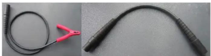
A set of high voltage cables is shown in Figure 3. Please be aware that the high voltage cables supplied are non-shielded cables which must not touch or be close to ground potential. The insulation of the high voltage cables supplied by Power Diagnostix can withstand a maximum voltage of 13.8 kV with direct contact to ground. Nevertheless, the cable must be installed at a safe distance from any grounded objects. If the cables are in direct contact with ground, surface discharge activity will start from 3 kV. Please check the detailed Power Diagnostix “Health and Safety Instructions and Recommendations”. The minimum distances which are to be observed in open air conditions, in relation to the applied voltage, are specified in Appendix 3.
natural_image
Two black cable connectors with red clamps, shown side by side against a plain gray background (no text or symbols visible)Figure 3: High voltage cables
ICMflex
Partial discharge and loss factor measurement system
3.3 Location
As mentioned above in the general procedure prior to installation, find a safe location close to the specimen to install the equipment. Ask for a fenced, delineated, or enclosed area, if required, as shown in Figure 4, and avoid environmental conditions with high relative humidity and extreme temperatures.

natural_image
Outdoor installation site with modular shipping container and warning signs, no visible text or symbolsFigure 4: MV cable testing on-site
3.4 Parts of the ICMflex under high voltage potential
The ICMflex has a unique design concept. The entire acquisition unit is at high voltage potential right where the necessary signals are. This offers the advantage that no additional signal cables are needed. The filter units are constructed on the same principle. The parts that are at high voltage potential are marked with warning signs to prevent confusion during set-up (see Figure 5 in section 3.5).
The complete head box, including the corona cage surrounding the top of the reference capacitor and both MC connectors on the in- and output, is at high voltage potential. The bottom plate of the ICMflex and corresponding filter unit are at ground potential.
3.5 Connecting the ICMflex
Please read the application notes for testing of medium and high voltage cables and rotating machines for specific set-up information. In general, the main connections are explained below.
The appropriate connection of the HV source (HV transformer, resonance test set, VLF high potential) to the filter and/or ICMflex is sown on the top covers of both the filtering unit and the ICMflex. Please follow the connection arrangements shown.
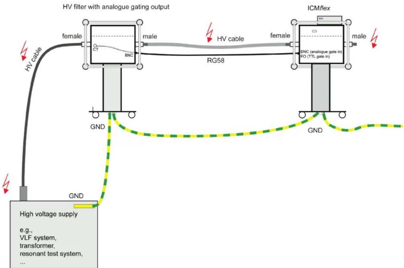
The HV cable of the power supply has to be connected to the female input connector of the filter (at the left-hand side of Figure 5) or, if a filter is not needed, directly to the input of the ICMflex. A connection needs to be provided from the male output connector of the filter (at the right-hand side of Figure 5) to the female connector of the ICMflex. Finally, the male connector of the ICMflex needs to be connected to the specimen. This can be a motor terminal, the conductor of a shielded high voltage cable or a stator bar. The interconnection between the filter and ICMflex is, of course, not needed if no filter is used.
Partial discharge and loss factor measurement system

Figure 5: Filter connectors
The coaxial output from the filter (left picture in Figure 6) is used for analogue noise gating. A noise decoupling circuit is directly built into the filter to capture any noise originating from the high voltage supply. A coaxial connection between the filter output and the ICMf/ex input (right picture in Figure 6) has to be established to use the gating option. Please prevent direct contact between the coax cable and the high voltage cable connecting the filter and the ICMf/ex.

natural_image
Two industrial control panels with warning symbols, one showing a blue box and metallic frame, the other showing a gray device with yellow warning labels (no readable text or symbols)Figure 6: Coaxial gating connector for filter (left) and ICMflex (right)
The ground loop of the measuring set-up is very important. Poor grounding has a big influence on the sensitivity because of background noise. The main ground of the power supply has to be connected to the ground terminal of the filter unit or, if no filter is used, directly to the ICMflex. Connection points are provided on the metallic grounding plates, as shown in Figure 7. Connections can be made by using a cable lug or a multi-contact. Use the short cables supplied to interconnect the grounding of the filter and the grounding of the ICMflex. Avoid loops since these will act as an antennas and influence the noise behaviour. Finally, a connection, which should be as short as possible, must be established between the ICMflex and the main grounding of the test specimen. Please choose a solid grounding connection and ensure good contact. Interconnection between the grounding of the filter and the ICMflex is not necessary if no filter is used. A typical test set-up is shown in Figure 10.

natural_image
Two-panel image showing a metallic mechanical component with blue arrows pointing to features, and a close-up of a mechanical assembly with no visible text or symbols.Figure 7: Ground connection points
ICMflex
Partial discharge and loss factor measurement system
The most convenient way to communicate with the instrument is via the Bluetooth interface as this requires no additional cabling. However, if a Bluetooth connection cannot be established, it is possible to use the fibre optic serial link instead. The D-Sub female connector of the cable has to be connected to the male connector on the upper side of the ICMflex (as shown in Figure 9). The cable USB connector of the cable can be connected to any free USB port on the computer. As the fibre optic cable provides a galvanic separation from the high voltage potential, there is no risk to the operator.
Caution and Warning: Never use a standard D-Sub cable that does not galvanic separation. This can result in damage to components and serious injury or death.

natural_image
Exterior view of a gray industrial control box mounted on a metal frame (no visible text or symbols)Figure 9: SUB-D input connector
flowchart
graph TD
    A["HV cable"] --> B["HV filter with analogue gating output"]
    B --> C["ICMflex"]
    C --> D["High voltage supply"]
    D --> E["GND"]
    E --> F["High voltage supply e.g., VLF system, transformer, resonant test system, ..."]
    B --> G["CT"]
    B --> H["BNC"]
    B --> I["male"]
    B --> J["male"]
    B --> K["RG58"]
    B --> L["GND"]
    L --> M["HV cable"]
    M --> N["Female"]
    N --> O["ICMflex"]
    O --> P["BNC (analogue gate in) FO (TTL gate in)"]
    P --> Q["male"]
    Q --> R["GND"]
Figure 10: General connection diagram for ICMflex
Partial discharge and loss factor measurement system
4 Software and driver installation
The ICMflex is supplied with a Windows based software package on a USB stick or CD. The software can be installed on Windows operating systems versions 7, 8, and 10 with 32-bit or 64-bit architecture. If a computer is provided by Power Diagnostix, the software and the instrument drivers are pre-installed and ready configured. In this case, no further action is needed but, in all other cases, the following preparations must be made.
4.1 Installing the ICMflex software
Start the setup.exe file that can be found within the ICMflex directory on the USB stick. If a new software version has been downloaded from the internet, unzip all files to a local directory on the target system first. After starting the setup.exe file, a window like the one shown in Figure 11 below will pop up.
Please choose custom installation directories, if wanted, and click "Next". The installation kit automatically detects earlier versions and updates only these with newer files provided by this release. This software has been developed under National Instruments LabWindows/CVI. Therefore, additional DLLs and libraries will be installed automatically within the Windows system directory. Administrator rights are necessary to complete the installation of this software product. Please contact your system administrator if you have insufficient rights on this machine.
After finalising the software installation procedure, the system restarts automatically.

Figure 11: Software installation setup

The ICMflex software can be started directly by clicking on the appropriate icon (as shown in Figure 12) on the desktop. Before starting to communicate with the instrument, however, further preparations must be completed.
Figure 12: Desktop icon
ICMflex
Partial discharge and loss factor measurement system
4.2 Setting up a Bluetooth COM port
All Bluetooth devices on computer systems can provide so-called virtual COM ports. These COM ports are used to establish a connection with the ICMflex. Standard laptops usually come with built-in Bluetooth interfaces. If such an interface is not available, it is possible to use external USB-Bluetooth devices. Power Diagnostix can provide these devices for USB, PCI, and other interfaces. The Bluetooth interface on any computer provides an automatic scanning function. Please start this function to find the ICMflex Bluetooth device.

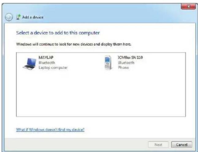
Figure 13: Bluetooth connection wizard Figure 14: Adding a Bluetooth device
The express mode will guide you through this set-up (Figure 13). Click "Next". The search routine can take a few minutes. A pop-up window will display all devices found in range (Figure 14). Select the "ICMflex" entry and continue the installation procedure (Figure 15).
It is mandatory to set the device code (Figure 16) for the ICMflex connection to "0000".


Figure 15: Bluetooth device successfully added Figure 16: Entering pairing code
Partial discharge and loss factor measurement system

Figure 17: Windows Device Manager
If, successful, the Windows hardware manager will automatically install a virtual COM port for the new device. Typically, two COM ports will be installed for the ICMflex as shown in Figure 17. Enable both with the ICMflex software interface settings as described in section 5.2.
4.3 Setting up a fibre optic communication port (USB serial COM)
A special fibre optic cable is supplied with the ICMflex. The D-Sub male connector has to be connected to the COM TTL female connector of the instrument box. The case of the D-sub plug contains the hard wired connection to the fibre optic converter. The default length of this cable is 10 meters. Individual lengths can be supplied on demand. The side with the USB-A connector contains a fibre optic to USB converter. This end can be connected to any free USB port of the laptop or PC. The driver for the fibre optic cable will be installed with the software. Please do not connect the cable to the computer before the software is installed! If the driver is not installed correctly, Windows will start the hardware installation wizard (as shown in Figure 18) when connecting the USB connector to the computer for the first time.
To guarantee correct installation, it is recommended to perform the installation procedure while being connected to the internet. The Windows hardware manager searches the Windows driver library on the internet to find a suitable driver for this new device. Please contact Power Diagnostix in case of problems.
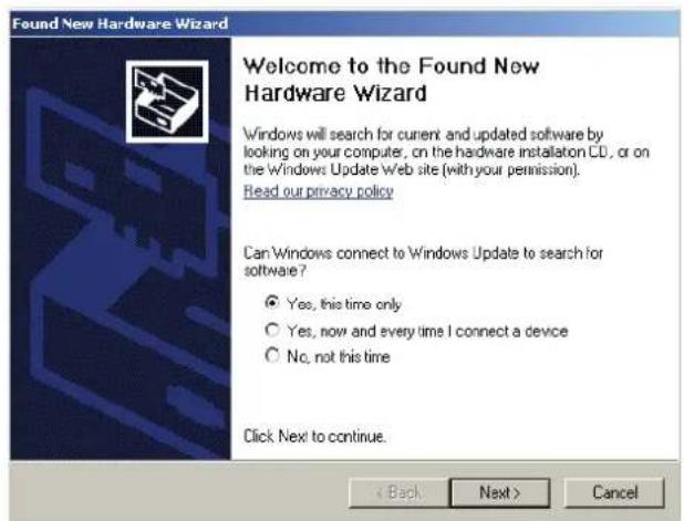
Figure 18: Driver installation wizard

ICMflex
Partial discharge and loss factor measurement system
If the computer does not recognise the cable, the drivers need to be installed manually. Go to the device manager and select the related COM port. After a right mouse click, select "Update driver". A window similar to that in Figure 18 will pop up. Find the driver in a subfolder named "USB Driver\CP210x" in your ICMflex software installation directory, e.g.,
C:\pdix\Software\ICMflex\ICMflex.186]\USB Driver\CP210x.

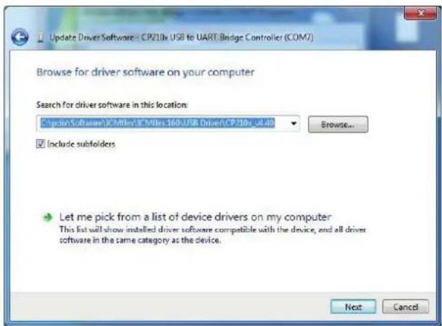
Figure 19: Driver installation
This procedure must be performed twice: the first time for the USB cable itself and the second time for the cable converter.
The setup routine will automatically install the USB serial COM port, if found, and a new COM port (e.g., COM7) will be displayed by the device manager.
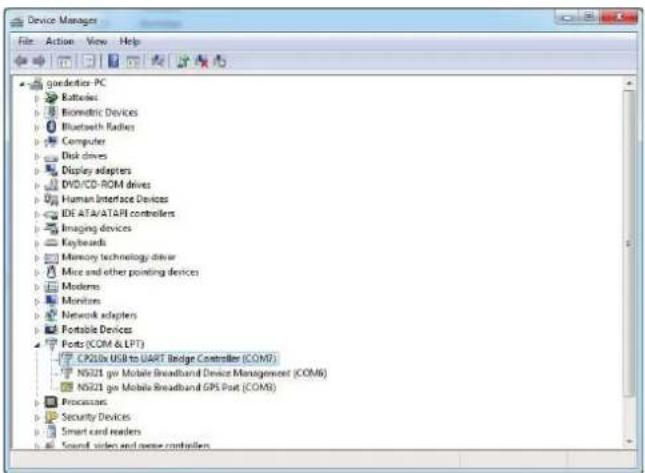
Figure 20: Device Manager
Note that the COM port number has to be enabled within the interface settings of the ICMflex software (see section 5.2). After restarting computer, the software will automatically search for the COM port in use. If the software can't find the COM port, check manually in the device manager as shown in Figure 20.
Partial discharge and loss factor measurement system
5 ICMflex software
5.1 First steps
The ICMflex software has a default factory settings at start-up. All settings will be saved when closing the application. When they are changed, settings affecting the acquisition circuit are sent to the ICMflex acquisition box. The instrument acts as slave, and the software acts as master.
Note: If the application window appears very small when started on a PC with Windows 10, please refer to section "10.2 Troubleshooting" on page 85.
If not yet connected to an instrument the software displays all data for the last measurement. This data is saved in an .flx file into a specified storage directory, e.g.,
c:\pdix\software\ICMflex\ICMflex.154\icmflex.flx
All optional program preferences like colours, interface settings, etc. are stored in a file called
c:\pdix\software\ICMflex\ICMflex.154\icmflex.ini
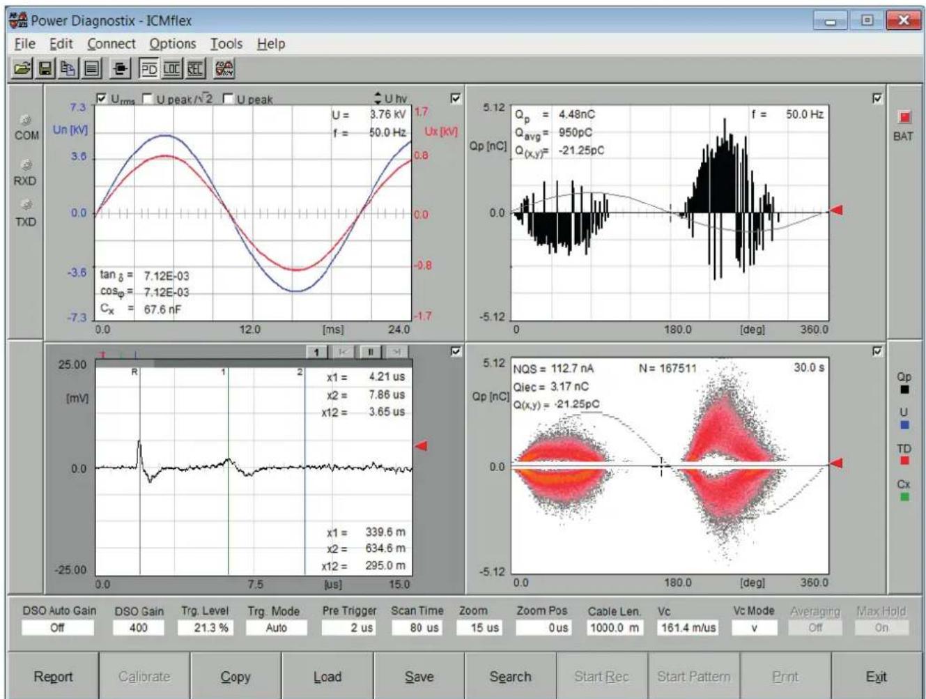
The main program appears as a shortcut link on the desktop, in the "Start"->"Programs" folder, and can be started directly from the installation directory. A screenshot of the main program with an ICMflex connected is shown in Figure 21.
c:\pdix\software\ICMflex\ICMflex.154\icmflex.exe
line
| Parameter | Value | | --------- | --------- | | Qp | 4.48nC | | Avg | 950pC | | Q(x,y) | -21.25pC | | NQS | 112.7 nA | | Qiec | 3.17 nC | | Q(x,y) | -21.25pC | | x1 | 4.21 us | | x2 | 7.86 us | | x12 | 3.65 us | | x1 | 339.6 m | | x2 | 634.6 m | | x12 | 295.0 m |Figure 21: Main screen of the ICMflex software
ICMflex
Partial discharge and loss factor measurement system
5.2 Connecting to the instrument
Before connecting to the instrument, it is recommended to check the COM port settings in the menu "Options"->"Interface Settings" as shown in Figure 22. Enable the port number specified for Bluetooth or fibre optic communication (see sections 4.2 and 4.3). Normally, the software automatically searches the instrument when the check box "Search Device at Startup" is selected. The COM port in use will be indicated by the * symbol. If this is not the case, the correct settings can be found with the Windows device manager.
Make sure that only one COM port is enabled. First, disable all ports by pressing the "Disable All" button. Then select the COM port from the list by clicking the corresponding checkbox. All other settings remain unchanged and do not need to be modified during standard operation.
All changes will become active after closing this panel by pressing the "OK" button. The "Cancel" function closes this window without any changes to the values. Pressing the "Standard" button enables the default COM ports and sets all timeouts back to these default values:
![Interface Settings Search for Device at: COM3 (Generic Serial/Bluetooth Connection) COM4 (Generic Serial/Bluetooth Connection) COM5 (Generic Serial/Bluetooth Connection) Search Device at Startup General COM Port Settings: Search Timeout [s] 1.0 Run Timeout [s] 5.0 Baudrate 921600 Cancel Disable All Auto Search Standard OK](/content/2026/05/853729/images/f4235f9cf92491dd8372b86b5ac1bbefe36783e8fd87ec2dc428f416bbf67026.jpg)
Figure 22: Interface settings
Search Timeout: 2 s
Run Timeout: 5 s
Baud rate: 921600 kBit/s
To connect with an instrument, press the "Search" button on the front panel. This function can be started by using the command button at the bottom of the window, or by selecting the "Search" function from the function keys at the bottom of the window. Important functions can also be activated by shortcuts. For the search routine, press the function key F5.
The search pop-up window shows if an instrument was found and successfully connected. If new firmware for the acquisition unit is available with the software, it is possible to flash the instrument's program memory directly. A pop-up window (see Figure 23) will appear and can be confirmed by the user. Do not interrupt the flashing procedure and contact Power Diagnostix in case of problems. Usually, the latest firmware will be stored into a new instrument.

Figure 23: Searching for ICMflex COM ports
Partial discharge and loss factor measurement system
5.3 Firmware updates and configuration files
After a software upgrade, a pop-up window may appear indicating the availability of a new firmware version (see Figure 24). Do not hesitate to install the update, as it will include important enhancements for the unit.

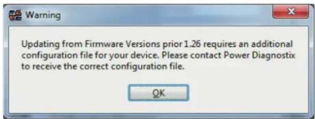
Figure 24: New firmware pop-up Figure 25: Configuration file pop-up
Updates of firmware version ≥ 1.26 require a configuration file after the first launch. Normally, the latest ICMflex units are configured at the factory. If you update from an older version, a pop-up will appear as shown in Figure 25. To receive a configuration file for your device, please contact the Power Diagnostix software department (software@pdix.com) and quote the instrument's serial number.
Once stored in the device, this configuration does not need to be repeated. The configuration file contains all important information about the instrument, such as the capacitor values according to the voltage calibration, Cn and Csn and the shunt capacitor Csx high and low. These settings can be cross checked via the menu "Edit" -> "Advanced Settings" (see Figure 26).
Firmware and configuration files can be uploaded using the device update function, available via the menu "Tools"->"Device Information". A screenshot of the update tool is shown in Figure 27. A firmware file is identified by the extension .bin, a configuration file by the extension .cfg.

Figure 26: Advanced settings
After a successful upload, the communication with the instrument will be briefly interrupted and then automatically re-established after rebooting the acquisition box.
![Update Firmware Interface Settings COM Port: COM 5 Baudrate: 921600 Timeout [s]: 3.0 File Selection Firmware Filename c:\Users\goedertier\Desktop\cmflex1.27.bin Configuration Filename c:\Users\goedertier\Desktop\SN062.cfg Upd. PLD Browse Upd. CFG Upd. FW Exit](/content/2026/05/853729/images/ccb56a0d82920deb7574394a6f00a84588c9bc041f75e435d38c5595606a1dcd.jpg)
Figure 27: Firmware update window
ICMflex
Partial discharge and loss factor measurement system
The device configuration panel shows detailed information about the instrument, e.g., the serial number and installed firmware version. To access this information, connect to the instrument and open the device configuration panel. A screenshot of the device configuration is shown in Figure 28. Since the instrument can be ordered in different configurations, check that all features are available as expected, e.g.,
• Partial discharge measurement
• Partial discharge fault location for cables
- Tan delta and loss factor measurements including voltage and frequency acquisition
Besides the instrument options, the information panel also shows the battery monitoring parameters such as the battery voltage, current, charge, and battery lifetime.

Figure 28: Device configuration panel
5.4 Principle of operation
The ICMflex software has a typical front-panel system that gives access to all main functions, graphs, and settings. This panel, as shown on the next page, is divided into four main areas. These areas vary depending on the display mode that is chosen. Available display modes are PD, LOC, and REC.
5.4.1 PD display mode
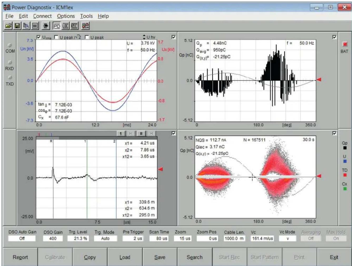
The PD display mode shown in Figure 29 is mainly used for PD measurements and is required for calibration of the apparent charge's amplitude. For cable testing, the cable length and pulse velocity can also be calibrated in this screen.
The upper left area of the window shows the voltage waveforms (12-bit resolution) for the voltage dividers U_sn (reference path) and U_sx (specimen path), the voltage and frequency values, and, if supported by the system, the loss factor and capacitance values. The graph in the upper right-hand part of the screen continuously displays a two-dimensional representation of PD activity vs. phase, accumulated over multiple refresh cycles.
Partial discharge and loss factor measurement system
line
| Parameter | Value | | --------- | ------------ | | U | 3.76 kV | | f | 50.0 Hz | | tan δ | 7.12E-03 | | cos φ | 7.12E-03 | | Cₓ | 67.6 nF | | Qp [nC] | 4.48 nC | | Q_avg | 950 pC | | Q(x,y) | -21.25 pC | | x1 | 4.21 us | | x2 | 7.86 us | | x12 | 3.65 us | | x1 | 339.6 m | | x2 | 634.6 m | | x12 | 295.0 m | | NQS | 112.7 nA | | Qiec | 3.17 nC | | Q(x,y) | -21.25 pC | | N = 167511 | 30.0 s | | Q = 167511 | 167511 | | Q = 167511 | 30.0 s | | Q = 167511 | 30.0 s | | Q = 167511 | 30.0 s | | Q = 167511 | 30.0 s | | Q = 167511 | 30.0 s | | Q = 167511 | 30.0 s | | Q < Td | -21.25 pC | | Q < Td | -21.25 pC | | Q < Td | -21.25 pC | | Q < Td | -21.25 pC | | Q < Td | -21.25 pC | | Q < Td | -21.25 pC | | Q < Td | -21.25 P/C | | Q < Td | -21.25 P/C | | Q < Td | -21.25 P/C | | Q < Td | -21.25 P/C | | Q < Td | -21.25 P/C | | Q < Td | -21.25 P/C | | Q < Td | -21.25 S/P | | Q < Td | -21.25 S/P | | Q < Td | -21.25 S/P | | Q < Td | -21.25 S/P | | Q < Td | -21.25 S/P | | Q < Td | -21.25 S/P | | Q < Td | -21.26 S/P | | Q < Td | -21.26 S/P | | Q < Td | -21.26 S/P | | Q < Td | -21.26 S/P | | Q < Td | -21.26 S/P | | Q < Td | -21.26 S/P | | Q < Td | -21.S/P | | Q < Td | -21.S/P | | Q < Td | -21.S/P | | Q < Td | -21.S/P | | Q < Td | -21.S/P | | Q < Td | -21.S/P | | Q < Td | -21.S/P | | Q < Td | -21.S/P | | | Q < Td | -21.S/P | | Q < Td | -21.S/P | | Q < Td | -21.S/P | | Q < Td | -21.S/P | | Q < Td | -21.S/P | | Q < Td | -21.S/P | | Q < Td | -21.S/P | | q < Td | -21.S/P | | q < Td | -21.S/P | | q < Td | -21.S/P | | q < Td | -21.S/P | | q < Td | -21.S/P | | q < Td | -21.S/P | | q < Td | -21.S/P | | qFigure 29: PD display mode
Additionally, the current PD peak magnitude is shown in the upper left corner of this graph. The magnitude must be calibrated (see applications notes in section 5.7). The time domain graph in the lower left area can be used to evaluate single PD events and the reflections of pulses, as detected on medium and high voltage cable insulation systems, on a time-based curve (resolution of 100 Msamples/second). The different cursors help determine the exact fault position and to get precise results. In the lower right area of the windows, a three-dimensional PD pattern acquisition can be initiated and visualised. The phase-resolved PD pattern has a resolution of 8 bits x 8 bits with a 16-bit colour depth and allows further interpretation of failures within the insulation system. As well as the pattern itself, the related discharge levels, set time, and the number of events are shown.
ICMflex
Partial discharge and loss factor measurement system
5.4.2 LOC display mode
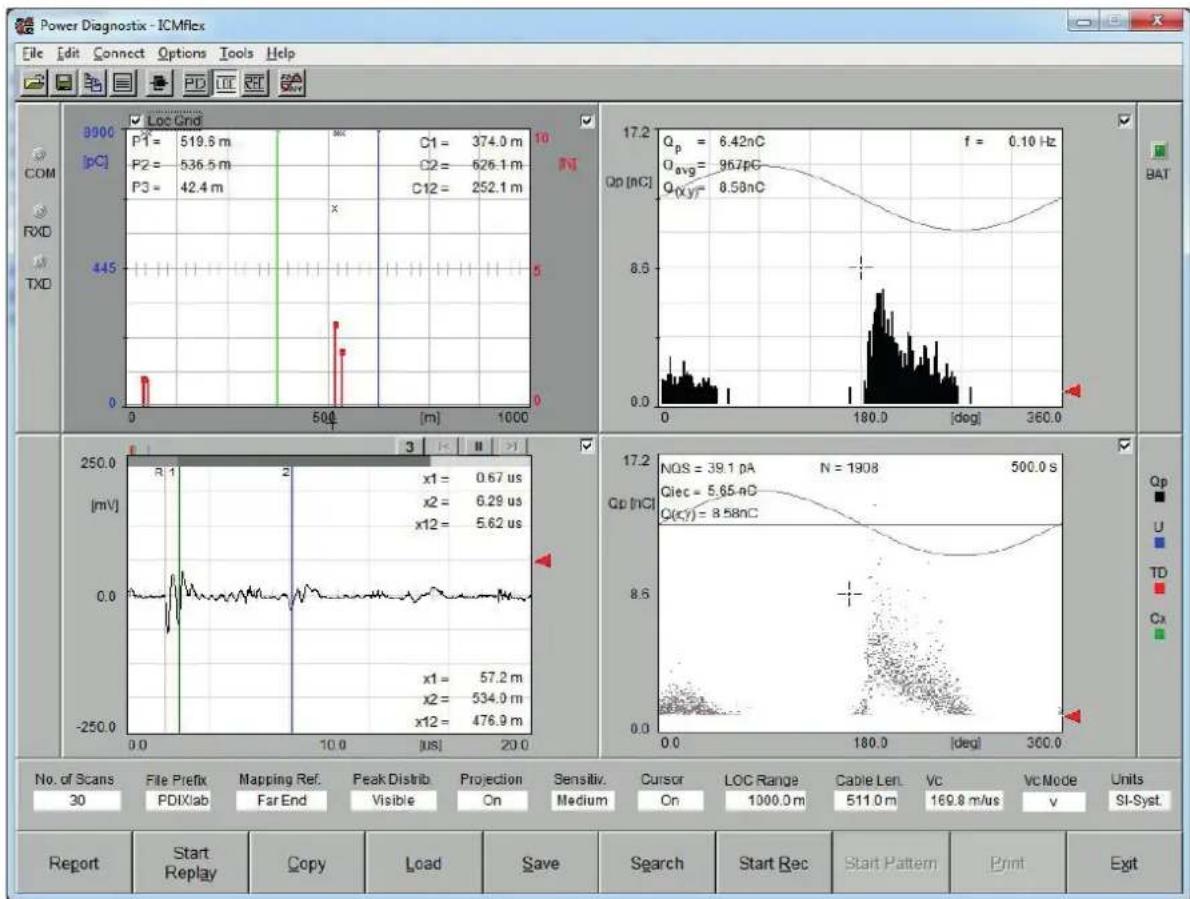
The LOC display mode is used to perform PD fault location measurements on medium and high voltage cables. An ICMflex with the LOC option for cable fault location incorporates a digital storage oscilloscope (DSO) to display partial discharge signals on a time-based curve. Single PD pulses can be triggered with a time resolution of 10 ns (100 Msamples/s) and a maximum display range of 320 s (firmware version ≥ 1.25) which corresponds to a theoretical maximum cable length of approximately 22 km for a cable with a pulse velocity of 140 m/ s. The DSO panel is at the lower left in PD and LOC mode (see Figure 30). As well as the DSO display, both PD representation charts remain available in upper and lower areas on the right-hand side. In the upper left screen, a summary of the measured reflections versus the position of occurrence along the cable length can be shown.
To perform cable fault location (LOC), the length of the cable and/or the pulse velocity of the cable must be known in advance. Time domain reflectometry (TDR) is based on the travel time of pulses. Since a cable behaves as a wave conductor, the TDR principle can be used to locate sources of partial discharges along the full cable length.
A partial discharge pulse that is caused by an insulation imperfection travels to both ends of the cable. For an open end (no load attached, or high impedance load compared to the cable's characteristic impedance), a partial discharge pulse occurring somewhere in the cable will, when it reaches the end of the cable, be reflected toward the opposite end. The distance of the PD source to the near and/or far end of the cable can be calculated using the time difference between the arrival times of pulses at the measuring impedance (coupling capacitor).
line
| Panel | Value | |-------|-------------| | Top | 374.0 m | | Middle| 6.42 nC | | Bottom| 8.58 nC |Figure 30: LOC display mode
Partial discharge and loss factor measurement system
The principle of the time domain reflectometry is illustrated in Figure 31. The travel paths of the first three reflections of the original partial discharge pulse that enter the coupling unit of the ICMflex are displayed in different colours.
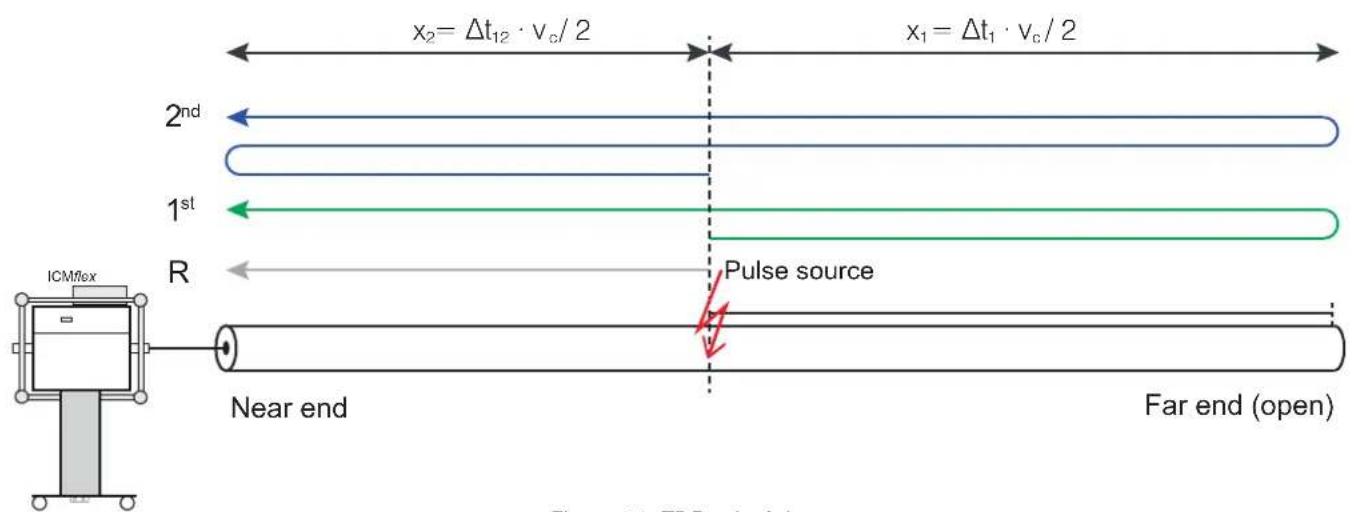
Figure 31: TDR principle
In Figure 32, the three impulses are shown as they would appear on the ICMflex DSO screen. The reference pulse (R, black cursor) travelled directly from the pulse source to the coupling unit. The first reflection ( 1^st , green cursor) travelled first in the opposite direction, away from the coupler and was reflected at the open end of the cable. This resulted in a time delay t_i that indicates the distance of the PD source from the far end of the cable. Finally, the second reflection ( 2^nd , blue cursor) shows the time delay between the reference pulse and its reflection at the far end. The time difference between the first and the second reflection is a time delay t_12 representing the distance of the pulse source from the near end of the cable. See the application notes in section 6.1 for a detailed example.

line
| Time (μs) | Voltage (mV) | | --------- | ------------ | | 0.0 | -5000 | | 9.5 | 0.0 | | 19.0 | 5000 |Figure 32: ICMflex DSO screen
ICMflex
Partial discharge and loss factor measurement system
5.4.3 REC display mode
The REC display mode is used to show results in a summarising table or graph. The collected data can be displayed vs. time or vs. voltage. The voltage graph in the upper left area remains unchanged. The strip chart at the upper right-hand side always shows the actual measurement readings, while the lower left chart shows the values from the data table at the lower right. Figure 33 shows the data plotted against voltage. By changing the setting of the X-axis to "vs. Time", the values will be shown as a function of time. The table gives an overview of voltage, tan delta, and tan delta tip-up (see also section 6.1), the specimen capacitance, and the peak discharge level at the moment of triggering.

line
| Parameter | U [kV] | tanD | D(tanD) | Cx [nF] | Cp [pC] | |-----------|--------|------|---------|---------|---------| | 1 | 2.04 | 1.27E-03 | N/A | 119.509 | 0.00 | | 2 | 2.04 | 1.27E-03 | 0.00E+00 | 119.509 | 0.00 | | 3 | 4.07 | 1.06E-03 | -2.10E-04 | 119.485 | 578 | | 4 | 6.11 | 1.35E-03 | 2.95E-04 | 119.537 | 1432 | | 5 | 8.15 | 1.77E-03 | 4.19E-04 | 119.574 | 5076 | | 6 | 10.18 | 2.30E-03 | 5.20E-04 | 119.646 | 7973 | | 7 | 12.22 | 3.48E-03 | 1.18E-03 | 119.691 | 11892 | | 8 | 14.26 | 5.39E-03 | 1.90E-03 | 119.652 | 10473 | | 9 | 16.29 | 8.39E-03 | 3.00E-03 | 119.650 | 12297 | | 10 | 18.32 | 1.22E-02 | 3.86E-03 | 119.525 | 11486 |Figure 33: REC display mode
The strip charts in the corner on the upper right and lower left sides show:
- Green: Capacitance of the sample under test (Cx)
Blue: Supplied voltage level (U), as RMS, peak, or peak/√2 - Black: PD magnitude in pC (Qp)
Red: Loss factor (TD)
With each data refresh from the instrument, the latest values are shown in the two upper charts. A full measurement can be recorded manually or automatically by defining a measurement sequence.
Partial discharge and loss factor measurement system
When using manual mode, the measurement is started by pressing the "Start Rec" button. To store readings, the "Trigger" button is used, when the required voltage step is reached. Relevant data, such as the applied voltage, tan delta, tan delta tip-up value, capacitance, and apparent charge levels, will be registered and show as graph versus voltage or time in the lower left of the screen.
An automatic trigger mode is included and is selected by setting the record mode to "Sequence". The "Trigger" button changes to "Sequence" and allows the measurement sequence to be defined. The desired voltage steps can be entered manually via the panel for the manual sequence or can be calculated for the automatic sequence after entering the specimen's ratings.
Additional settings needed are the voltage tolerance between the measured and the desired voltage levels, the number of values to be triggered at each voltage step, the time to stabilise before conducting any readings, and the period between consecutive values (capture interval) at a fixed voltage step. Once a sequence is defined, it can be saved and reloaded for future measurements.
Besides recording with a manually defined sequence, the software also offers an automatic sequence mode, which can be edited, as shown in Figure 34. Here, the required voltage steps are calculated automatically according to the specimen voltage, which can be set as the phase-to-phase or the phase-to-ground voltage, and the number of voltage steps.

Figure 34: Automatic sequence wizard
Depending on the high voltage source and frequency, we recommend selecting appropriate values for stabilisation time and capture interval. At power frequencies, a period refresh takes 16–20 milliseconds, while at very low frequencies a period refresh takes more than 100 seconds. Allow the instrument to complete at least three refreshes to ensure that accurate and useful data is entered into the table.
ICMflex
Partial discharge and loss factor measurement system
5.5 Display mode settings
Settings affecting individual graphs or measurements can be found in the lower area of the window above the functional keys. Depending on the graph or area activated (indicated by a dark grey area in the background, e.g., the graph on the lower left-hand side in Figure 35), different settings will be displayed. To toggle between the different set-ups, click once with the left mouse button on the area or graph that you intend to modify.
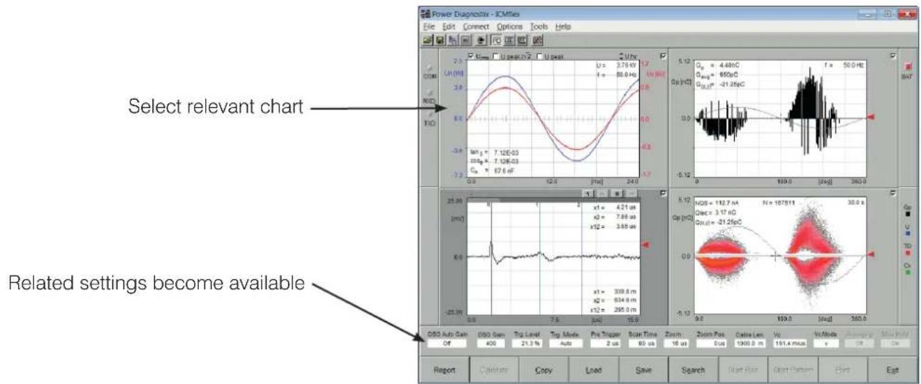
Figure 35: Chart settings
5.5.1 Settings for partial discharge measurement
| PD Auto GainOff | PD Gain4 | Cal Gain4 | Cal Value [pC]5000.0 | Highpass40 kHz | Lowpass800 kHz | LLD [%]8.6 | CodingUnipolar | GatingOff | Gate Level [%]7.8 | Sync ModeVLF 0.1Hz |
| SETTING VALUES / RANGE EXPLANATION | ||
| PD Auto Gain | On/Off | The automatic gain adjustment can help to find the best gain setting for the PD measurement path. If the PD signal reaches 95% of the Y-scale, the software automatically decreases the gain. If the level drops below 10 %, the gain is increased.If the PD level is fluctuating widely, it may be useful to disable automatic mode. |
| PD Gain 1, 2, 4, 8, 10 | 20,40, 80, 100, 200,400, 800, 1024,2048, 4096 | The signal amplification can be set manually by selecting a suitable factor from the list. The optimum setting is when the highest peaks are between 60 and 90 % of full scale. |
| Cal Gain 1, 2, 4, 8, 10 | 20,40, 80, 100, 200,400, 800, 1024,2048, 4096 | This entry indicates the gain value set during calibration. This value is modified automatically during calibration and cannot be set manually. |
| Cal Value 1pC–10000 pC This value has to be set according to the PD level used during calibration. | ||
| Highpass 40 kHz, 80 kHz,100 kHz | Depends on the lower cut-off frequency of the PD bandpass filter. | |
Partial discharge and loss factor measurement system
| Lowpass 250 kHz, 600 kHz,800 kHz | Depends on the upper cut-off frequency of the PD bandpass filter. |
| LLD 0–100 % LLD stands for Low Level Discriminator. This is the minimum trigger level for PD pulse acquisition. A level of at least 2 % should be set to eliminate small noise pulses. The level refers to the 100 % full scale of the Y-axis of the PD scope and PD pattern graphs. | |
| Coding Unipolar / Bipolar PD pulses can be separated by their polarity. “Bipolar” shows positive and negative pulses separately, whereas “Unipolar” does not consider the polarity. | |
| Gating On / Off If gating is enabled (On) it is possible to eliminate external noise pulses. This function is available with all instruments offering an external “Gate In” connector on the acquisition box. The noise signal is taken directly from the HV line input on the HV filter. A special high frequency current transformer must be used. | |
| Gate Level 0–100 % This trigger level determines the sensitivity of the gate input of the acquisition system. The higher this level is set, the fewer external pulses will be triggered. | |
| Sync Mode Normal, VLF 0.1 Hz, VLF 0.05 Hz, VLF 0.02 Hz | Normal: The frequency of the applied voltage is calculated automatically in a range between 20 Hz and 510 Hz.VLF: The frequency is set manually to match the frequency setting on the VLF power supply. |
| Set Time 0..100000 s Pre-set set time for a PD pattern acquisition. The pattern (map) is stopped automatically after expiration of this time. | |
5.5.2 Settings for PD fault location
| PD Auto GainOff | PD Gain4 | Cal Gain4 | Cal Value [pC]5000.0 | Highpass40 kHz | Lowpass800 kHz | LLD [%]8.6 | CodingUnipolar | GatingOff | Gate Level [%]7.8 | Sync ModeVLF 0.1Hz |
| SETTING VALUES / RANGE EXPLANATION | ||
| DSO Auto Gain | On / Off | The automatic gain adjustment can help find the best gain setting for the LOC or DSO graph. If the PD signal rises above 95 % of the Y-scale, the software automatically decreases the gain. If the level drops down below 10 %, the gain is increased. Automatic voltage adjustment is recommended the normal sync mode only. |
| DSO Gain | 1, 2, 4, 8, 10, 20, 40, 80, 100, 200, 400, 800 | Amplification factor for the PD signal in time domain. |
| Trg. level | 0–100 % | Trigger level for high resolution PD pulses in the time domain graph. |
ICMflex
Partial discharge and loss factor measurement system
| Trg. Mode Auto | NormalSingle Shot | Auto: This mode continuously displays a signal on the DSO graph (triggered or non-triggered signals).Normal: This mode continuously displays triggered signals only.Single Shot: This mode displays a single triggered PD event and subsequently stops the refresh. |
| Pre Trigger | 1–10 μs | Time on the DSO graph from zero position to the first trigger. |
| Scan time | 2–320 μs | Total measurement time for PD signals plotted against time (DSO graph). |
| Zoom 2–320 μs Zoomed area within the DSO graph. Zooming allows more precise positioning of the cursors. | ||
| Zoom Pos 2–320 μs Zero position of the zoomed area. | ||
| Cable Len. 10–25000 m Length of the cable under test. This length can be calculated during calibration or can be pre-set if the exact value is known. | ||
| vc [m/μs] | 100–200 m/μs | Pulse velocity for PD signals on the MV cable. |
| vc/2 [m/μs] | 50–100 m/μs | |
| U Auto Gain | Gain Usn | Gain Usx | Cn | Csn | Csx | Scaling | Record Mode | X-Axis | Sync Mode |
| Off | 1 | 7 | 513.0 pF | 4000.0 nF | 40.00 uF | Auto | Sequence | vs. Time | Normal |
5.5.3 Settings for the record mode
| SETTING VALUES | / RANGE EXPLANATION | |
| U Auto Gain | On / Off | The automatic gain adjustment can help to find the best gain setting for the voltage measurement path. If the voltage signal rises 95 % of the Y-scale, the software automatically decreases the gain. If the level drops down below 10 %, the gain is increased. Automatic voltage adjustment is recommended the normal sync mode only. |
| Gain Usn | 1, 2, 3, 4, 5, 6, 7, 8, 9, 10, 11, 12, 13, 14, 15, 16 | Amplification factor for the voltage signal from the shunt capacitor on the reference path; U_max = 20 V_peak |
| Gain Usx | 1, 2, 3, 4, 5, 6, 7, 8, 9, 10, 11, 12, 13, 14, 15, 16 | Amplification factor for the voltage signal from the shunt capacitor on the test pat; U_max = 200 V_peak |
| Cn | Stored into device via configuration file firmware version ≥ 1.26 | Capacitance value of the reference capacitor. Please check your system's data sheet or read the value as written on the grey acquisition box. |
| Csn | Stored into device via configuration file firmware version ≥ 1.26 | Capacitance value of the shunt capacitor of the reference path. Please check your system's data sheet or read the value as written on the grey acquisition box. |
Partial discharge and loss factor measurement system
| Csx (see remark below) | No limit; to be calculated before high voltage is applied | Capacitance value of the shunt capacitor of the test path. Please check your system's data sheet or read the value as written on the grey acquisition box. With most systems this value is switchable (ext. jumper) between two ranges, e. g. 40 μF/400 μF |
| Scaling Auto / Full Range Y-axis scaling mode for the voltage graph (left upper corner). The voltage waveform is scaled to a maximum in "Auto" mode. The "Full Range" mode sets the maximum of the Y-axis to the maximum value corresponding to the gain chosen. | ||
| Record Mode Manual / Sequence | This mode is important for the record function. In "Manual" mode, the values in the record table are filled for each manual trigger event. The "Sequence" mode fills the values into the table if a pre-set voltage level is reached. The voltage level must be defined in advance. | |
| X-Axis vs. Time / vs. Voltage | The record graph in the left lower corner can show values versus time or versus voltage. | |
| Sync Mode Normal, VLF 0.1 Hz, VLF 0.05 Hz, VLF 0.02 Hz | Normal: The frequency of the applied voltage is calculated automatically in a range between 20 Hz and 510 Hz. VLF: The frequency is set manually to match the frequency setting on the VLF power supply. | |
Note:
The setting of the shunt capacitance value for the test circuit C_sx depends on the maximum test voltage. The voltage at the shunt capacitor C_sx must not exceed 200 V _peak or 140 V RMS.
$$ U _ {x (\max)} = U _ {\max} \cdot C _ {x, (\max)} / C _ {s x} < 1 4 0 \mathrm{V} (!) $$
Please select values for C_sx according to the test specimen capacitance and the required maximum test voltage ( U_max ). The shunt capacitor values are stored into the device settings via the configuration file provided by Power Diagnostix. The actual voltages given by dividers U_n and U_x can be shown in the voltage display by selecting U_acq . Incorrect selection of the shunt capacitor will result in clipping of the sine wave. Please be aware that U_n,max must not exceed 20 V_peak (14 V RMS) and Ux,max must not exceed 200 V_peak (140 V RMS). Both values are displayed in the top right-hand corner of the voltage measurement chart (see Figure 36).

line
| Parameter | Value | | --------- | --------- | | Un | 1.59 V | | Ux | 1.60 V | | f | 50.0 Hz | | tan δ | 2.32E-02 | | cos φ | 2.32E-02 | | Cₓ | 69.0 nF |Figure 36: Voltage measurement chart
ICMflex
Partial discharge and loss factor measurement system
5.6 Functions and menus
The ICMflex software offers multiple functions directly from the front panel or via the menu bar at the top of the screen. These functions vary, depending on the display mode chosen and the hardware options available with the instrument.
5.6.1 Menu items
5.6.1.1 File
Standard file functions, such as loading and saving files and setting the default directory, can be selected directly from the "File" menu, as shown in Figure 37. Waveform and/or record exports to an .xls, .xlsx or .html file can also be selected here. After loading the .flx file, the export will be made automatically.

Figure 37: File menu
5.6.1.2 Edit
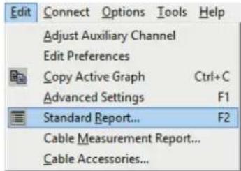
Figure 38: Edit menu
The "Edit" menu contains the options for copying the active graph to the Windows clipboard. It also offers access to preferences, advanced settings for the device (see Figure 38), report functions, and options for cable accessories (see Figure 39).
If the cable is equipped with accessories at a fixed position that is known, such as joints, terminations, and cross-link boxes, these can be shown as a symbol in the summarising LOC graph. The exact position along the cable length and the desired symbol and colour can be set using the "Cable Accessories" option.
![Cable Accessory Distance [m] Accessory Symbol Color 1 250.0 Joint B GY 2 788.0 Termination B BL 3 325.7 Cross Link Box C GF 4 -1.0 B GY 5 -1.0 B GY 6 -1.0 B GY 7 -1.0 B GY 8 -1.0 B GY Symbol / Character Assignment A B C D Color / Character Assignment RD YL BL GY GR Distances of the cable accessories always refer to the near end! Set Distance to -1.0 to disable this entry! Cancel Clear Ok](/content/2026/05/853729/images/de9ce7688e23d31608cc29df0d94b193e2e39beae2ad498ca0ab0ca4e73f40d1.jpg)
Figure 39: Cable accessory window
Partial discharge and loss factor measurement system
The software can generate a standard report as explained in section 5.6.2.1 and/or a detailed cable measurement report. The editable options for the detailed report are shown in the screenshot in Figure 40. In general, the measured data included in the reports is similar. The differences are mainly various details concerning the specimen under test, which can be entered, and the cable accessories at known positions along the cable length.
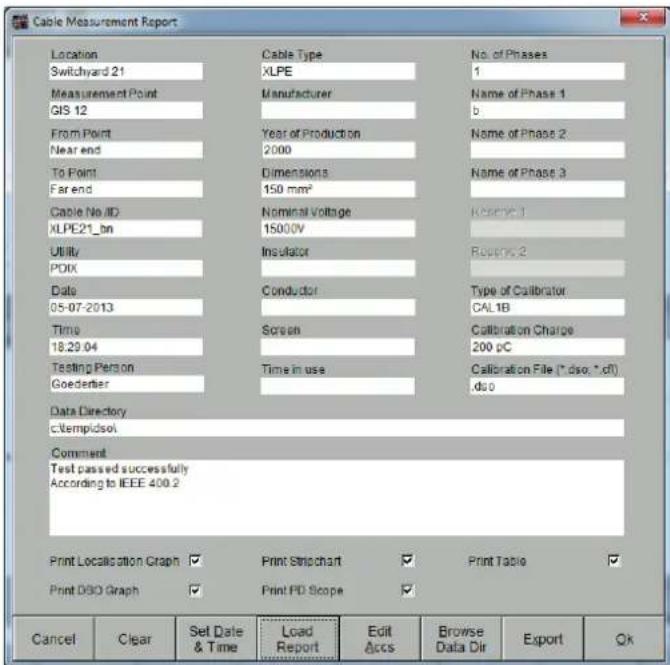
Figure 40: Cable measurement report window
General settings, such as interface and report language, display resolution, or the type of window labelling can be made in the “Preferences” window.
"Record Charge Weighting" determines whether the charge weighting follows IEC 60270 (Qiec) or IEC 60034-27-1 (Qm).
"Record PD/inc/ext voltage" enables/disables recording of the inception/extinction voltage.
"Activate TCP Server" enables/disables the ICMflex control software's built-in TCP server, which allows third-party programs to access measured values. Connection to the TCP server can be established using the computer's IP address and the port specified in the preferences.
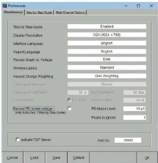
Figure 41: General preferences windows
ICMflex
Partial discharge and loss factor measurement system
5.6.1.3 Connect
Connection of the software to the ICMflex can be established by using the F6 function key, with the menu option as shown in Figure 42, or by pressing the "Search" button in the key bar.
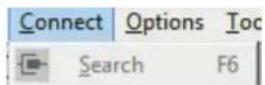
Figure 42: Connect menu
5.6.1.4 Options
The "Options" menu (Figure 43) mostly offers settings for the various charts. In addition, the language, display resolution, and the interface settings, as explained in section 5.2, can be selected.

Figure 43: Options menu
5.6.1.5 Tools
The "Tools" menu (see Figure 44) shows the device information (see Figure 28).
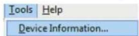
Figure 44: Tools menu
Help
The "About" item of the "Help" menu (Figure 45) gives information about the installed software release as shown in Figure 46. For further questions regarding the device, the Power Diagnostix contact details are given.

Figure 45: Help menu

Figure 46: 'About' window
Partial discharge and loss factor measurement system
5.6.2 Function keys
All main functions are shown at the bottom of the window (see figure below). Some buttons cover multiple functions depending on the display mode of the software.
| Report | Calibrate | Copy | Load | Save | Search | Start Rec | Start Map | Exit |
Figure 47: Function keys at the bottom of the application window
5.6.2.1 Report [F1]
Pressing this button will open the pop-up window shown in Figure 48. Here, it is possible to fill out a standard report with brief information regarding the measurements made. This set of information is saved with each ICMf/ex file (*.flx) and is available after loading files from the hard drive or SSD. It will appear on most printouts and with all exported data, like .html or .xls(x) files. The live charts required for the report can be selected with the tick boxes at the bottom of the panel. Note that the charts used in the reports are always the current charts.
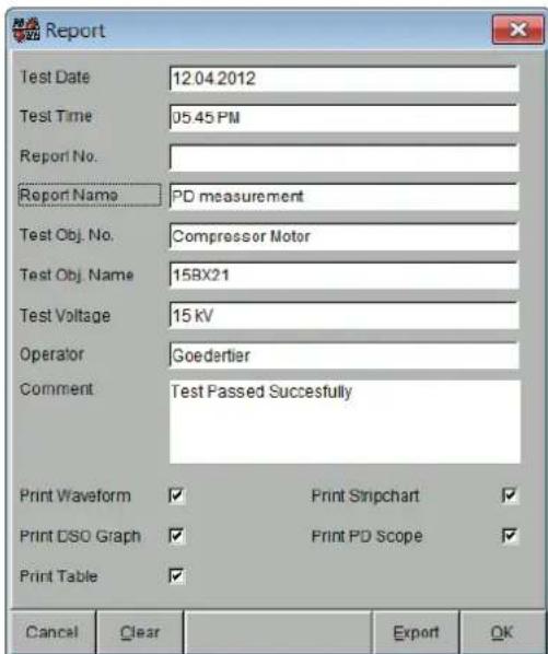
Figure 48: Standard report
5.6.2.2 Calibrate [F2]
The "Calibrate" function can be used to calibrate either the PD amplitude or the cable length of an MV cable under test. To calibrate the PD amplitude, it is necessary to activate the PD scope display (graph on the upper right) or the PD pattern display (graph on the lower right). Pressing the "Calibrate" [F2] button in this mode will open a pop-up window where the exact PD calibration value must be entered. This value is equal to the value displayed on the PD calibrator (CAL1A or CAL1B). Please check the correct connection of the PD calibrator, the correct gain setting, and the PD pulse on the PD scope display before calibrating. Further explanation is given in the application notes in sections 6.1.2 and 6.2.2. The length of an MV cable can be calibrated by first activating the DSO display (lower left graph). Check the reflections of PD pulses on the graph and set cursor R and cursor 2 to the first and the second pulse. After pressing the button "Calibrate" the software automatically calculates the pulse velocity of the PD pulses.
5.6.2.3 Copy [F3]
This helpful tool copies graphs to the Windows clipboard. Pressing this button will place a copy of the activated graph (panel with dark grey background) into the clipboard, from where it can be pasted into documents in other applications.
ICMflex
Partial discharge and loss factor measurement system
5.6.2.4 Load [F4]
This function is available only when the software is not connected to an instrument. It allows old measurements to be loaded from a hard disc or other memory. Files saved with the ICMflex software have the file suffix *.flx. This file comprises all measurement data, settings, and reports. To restore typical settings, it is helpful to save some default files for standard set-ups for cables and rotating machines.
5.6.2.5 Save [F5]
In all modes, it is possible to save *.flx files. Old files can be loaded, modified, and saved again. Running measurements can be saved at any time. The saved file consists of all measurement data, settings, and reports.
5.6.2.6 Search/Offline [F6]
To connect the ICMflex software to an instrument, press the "Search" button. If the COM port settings and the cabling are correct and the instrument is turned on, a pop-up window will show the message "ICMflex found at COM xy". This message will disappear automatically after a few seconds. To disconnect the communication line, press the same button again. While online, this button is labelled "Offline". While offline, the button is labelled "Search".
5.6.2.7 Start Rec / Stop Rec [F7]
This button is used to start a recording of values vs. time. Switch to the TD display mode to see all values recorded in the corresponding graph and in the table. This function has to be started and stopped manually by pressing the F7 button.
5.6.2.8 Start Map/Stop Map [F8]
Use this button to start PD pattern acquisition. The pattern is shown in the graph on the lower. The measurement is stopped automatically at the end of the pre-set "Set Time". It can also be stopped by pressing the F8 button again.
5.6.2.9 Print [F9]
This button sends the active graph to the default printer.
5.6.2.10 Exit
Close the program by pressing this button.
5.7 ICMflex and PD calibration
5.7.1 Calibrators
There is a broad range of impulse generators offered by Power Diagnostix for different purposes. The table below gives an overview of these. All allow the calibration of PD measurements according to IEC 60270/2000, except the CAL2B/C/D, since these models are not equipped with an injection capacitor to enable calibration on GIS. For the ICMflex's applications, the most common calibrators used are the CAL1B for on-site testing and CAL1A for laboratory purposes.
| CALIBRATOR RANGE OUTPUT FREQUENCY | |||
| CAL1A 1, 2, 5, 10, 20, 50, 100 pC Injection capacitor <1 pF | 50 Hz (60 Hz) | ||
| CAL1B 100, 200, 500 pC, 1, 2, 5, 10 nC Injection capacitor | <100 pF 50 Hz (60 Hz) | ||
| CAL1C 1, 2, 5, 10, 20, 50, 100 pC* at 100 pF Voltage output (50 Ω) 50 Hz (60 Hz) | |||
| CAL1D | 10, 20, 50, 100, 200, 500, 1000 pC | Injection capacitor <10 pF | 50 Hz (60 Hz) |
| CAL1E 0.5, 1, 2, 5, 10, 20, 50 nC Injection capacitor <500 pF 50 Hz (60 Hz) | |||
| CAL1F | 0.2, 0.5, 1, 2, 5, 10, 20 nC | Injection capacitor <200 pF | 50 Hz (60 Hz) |
| CAL1G | 0.02, 0.05, 0.1, 0.2, 0.5, 1, 2 nC | Injection capacitor <20 pF | 50 Hz (60 Hz) |
| CAL1H | 0.5, 1, 2, 5, 10, 20, 50 pC* at **pF | Voltage output (50 Ω) | 50 Hz (60 Hz) |
| CAL1J | 10, 20, 50, 100, 200, 500, 1000 pC* at 100 pF100, 200, 500, 1000, 2000, 5000, 10000 pC* at 1 nF | Voltage output (50 Ω) 50 Hz (60 Hz) | |
| CAL2B | 2, 5, 10, 20, 30, 40, 50 V (into RL=50 Ω) | Voltage output (50 Ω) | 50 Hz (60 Hz) |
| CAL2C | 1, 2, 5, 7, 10, 12, 15, 17, 20 V (into RL=50 Ω) | Voltage output (50 Ω) | 50 Hz (60 Hz) |
| CAL2D | 5, 7.5, 10, 15, 20, 30, 40 V (into RL=50 Ω) | Voltage output (50 Ω) | 50 Hz (60 Hz) |
*with external high voltage capacitor, ** value to be specified by customer
Table 1: Calibrator overview
As an example, a type CAL1A calibrator is shown in Figure 49. All calibrators are switched on with the "On/Off" button. Both amplitude (Range) and polarity (Pos/Neg) of the single charge pulse per cycle are displayed and can be adjusted by pressing the two buttons. The instrument is synchronised to line frequency by a photodiode. In case of insufficient pick-up of power frequency light, it will automatically select the internal quartz oscillator (50 Hz and 60 Hz versions available). The "On/Off" button must be pressed for more than one second to switch the pulse generator off, while automatic switch-off occurs after approximately 15 min. Operation time of up to 200 hours is possible with the 9 V lithium battery as the average supply current is approximately 5 mA (quiescent current is negligible). An alkaline battery may be used in place of the lithium battery and will give around 90 hours of continuous operation may replace the lithium battery. A weak battery is indicated by the "LO BAT" sign of the LC display.

Warning: While changing the battery, be aware of internal parts carrying up to 125 V DC!
Figure 49: CAL1A
ICMflex
Partial discharge and loss factor measurement system
Power Diagnostix delivers its standard calibrators with a fully traceable DAkkS calibration certificate (DK150680100). This calibration certificate documents traceability according to national standards, which fulfil the units of measurement according to the International System of Units SI. The DAkkS (Deutsche Akkreditierungsstelle) is a signatory to the multilateral agreement of the European co-operation for Accreditation (EA) for the mutual recognition of calibration certificates.
Before attaching the calibrator, make sure that the object under test is de-energised. The inner conductor of the BNC/banana adapter must be connected to the test specimen's conductor. The outer (ground) connector has to be connected with the solid grounding of the test object. Ensure that ground leads between the calibrator and the ground shield are as short as possible. Care must be taken that the calibrator is isolated from the HV part of the ICMflex.

Calibration pulse Noise level
Figure 50: Calibration pulse scope display Figure 51: Calibration pulse PD pattern
The charge level to be injected into the measurement circuit depends on the cable length, stator winding or bar capacitance (attenuation), and background noise conditions. It's important to have a good signal-to-noise ratio to ensure a sufficient sensitivity. Choose a value approximately five to ten times higher than the present background noise. Typical values used for on-site testing vary from 200 pC to 5 nC, even 10 nC in the case of very long cable lengths or large turbo generators.
Once the injection value is selected, the calibration pulse can be observed with the ICMflex software. Calibration of the apparent charge is supported by the two charts on the right of the PD mode display. The upper left chart represents the calibration pulse as scope like pulse pattern (two-dimensional, compare Figure 50) while the upper right one plots the pulse into an -q-n related pattern (three-dimensional as shown in Figure 51). Adjust the PD gain settings so that the calibration pulse fills 60 - 90% of the maximum current amplitude. Also, select the appropriate SYNC setting during calibration, CAL50Hz or CAL60Hz, even if VLF is used. Using the same settings for VLF, speeds up the screen refresh. Select a value for the low level discriminator such that the background noise can still be observed. Don't forget to switch off the gating function during calibration.
Calibration can be performed by a double click on the highest pulse shown in the scope-like display or by a double click on the corresponding upper line in the phase resolved PD pattern. Thereafter, the calibration pop-up (Figure 52) will ask for the value of calibration charge. Once this is entered, compensation of the attenuation of the complete circuit will be done automatically. Please bear in mind that the calibration is valid for one bandwidth and one specific test set-up only. Hardware and/or software changes require a new calibration. Don't forget to save the calibration file!
![Edit... Calibration Charge 500 Cancel Ok [nC] Ok [pC]](/content/2026/05/853729/images/6a157e85aa1a84992febd768ec6968fee836453f7330eb88c4bd832d8c228802.jpg)
Figure 52: Calibration charge pop-up
Partial discharge and loss factor measurement system
Ensure that the selected unit [pC/nC] and amplitude are suitable for the injected charge. For further information about calibration, please see sections 6.1.2 and 6.2.2.

Warning
● Always provide solid grounding of the instrument and the filter units
- Make sure that the cable/machine is de-energised before calibration.
5.8 Gating
5.8.1 Principle of operation
Effective noise reduction is required when the ICMflex is used for measurements in an environment where high frequency (HF) electrical noise is present. HF disturbances that hamper partial discharge detection but can be mitigated by the gating function include frequency converter switching pulses, corona discharge, and thyristor firing, provided those signals from the noise source are picked up by an antenna or another sensor. Using the analogue gating function cuts out this impulse noise. With some applications, a current transformer (CT) is used to acquire the disturbance signal from a ground conductor or from the screen of a signal cable. Some electronically controlled resonant test sets provide a TTL signal for switching purposes.
5.8.2 Analogue gating
The standard ICMflex comes with a “GATE IN” terminal for a BNC cable that transmits a gating signal from an HV filter with a built-in current transformer. The gate level is set by using the ICMflex software (see section 5.5.1). This option is mainly used for VLF cable testing.
Caution: The analogue gating input of the ICMflex is intended exclusively for connection to an HV filter! Never connect another device to this input as this may cause serious damage to the equipment.
When using the gating function in the ICMflex, disturbance signals from the HV line are detected by the high frequency current transformer (HFCT) embedded in the high voltage filter (T50/1 or equivalent). The output

Figure 53: Gating Inputs
of the HFCT should be connected to the "GATE IN" BNC terminal of the ICMflex shown in Figure 53. In the instrument, a built-in preamplifier takes care of signal conditioning. The bandwidth for the gating signal is internally set from 2 to 20MHz . Analogue gating can be activated in the software in the PD Mode (gating on). The gating threshold in percent (gating sensitivity) must be set according to the level of the disturbance puls
ICMflex
Partial discharge and loss factor measurement system
es. The gate level in percent refers to the maximum scale of the PD pattern or PD scope view at the particular gain. To adjust the gate level to blind out the switching pulses of the VLF for instance, the general background noise must be investigated; the low level discriminator (LLD) level should be set to the peak value of the overall ambient noise. As soon as the LLD level (peak value of the ambient noise) is known, the gate level can be selected at a level above the LLD level to avoid excessive gating times. As soon as the instrument is gating effectively, the corresponding gating time is shown in the PD scope graph (upper graph on the right in PD mode). The gate time in percent refers to the time the instrument gates during one full cycle.
Example:
With 0.1 Hz, one cycle is 10 s, if the gate time is 30 %, gating has been active for 3 s.

bar_line
| Angle (deg) | Op (nC) | |-------------|---------| | 0 | 0.0 | | 180.0 | 1.22 | | 360.0 | 0.0 |Figure 54: PD and VLF switching pulses

line
| Parameter | Value | | --------- | --------- | | Op | 692pC | | Avg | 72.0pC | | X,Y | 481pC |Figure 55: Switching pulses effectively gated
In the example shown in Figure 54 and Figure 55, the LLD level was 5% and the gating threshold was set to 8% , resulting in a gating time of 7% , i.e., 0.7 s with a sine wave of 0.1 Hz.
Try to reduce the gate time below 30% so as not to lose significant PD pulses. In other words, don't set the gating sensitivity too low so that the gate time exceeds 30 to 50% . Ambient noise other than the switching pulses of the VLF, transformer, or rack transfer switch is not blocked using analogue gating. To deal with other kinds of disturbances, fibre optic gating using the GST1 and a current transformer is available (see section 7.3).
Partial discharge and loss factor measurement system
6 Application notes
The application notes for medium and high voltage cables, rotating machines, and single stator bars describe the measurement set-up, calibration, step by step procedure for performing the measurement, software usage, and evaluation criteria according to the relevant standards.
6.1 Medium and high voltage cables
6.1.1 Measurement set-up
A general description of the measurement set-up is given in section 3, but here, the focus is on medium voltage (MV) and high voltage (HV) voltage cable applications. The order of connecting the various links is shown in Figure 56. Most important is the interconnection between the main grounding of the high voltage supply and the cable ground shield (1–3). The final link from the grounded baseplate of the ICMflex to the ground shield must be as short as possible (3). The HV output cable of the ICMflex must be connected to the inner conductor or termination (6).
6.1.2 Calibration
Performing HV tests including partial discharge (PD) measurements and PD fault location on cables, requires calibration of both the apparent charge and the cable length. When the safety procedure detailed in section 1.3 has been completed and the set-up has been carried out as described above, calibration can be performed. General procedures are described in the Power Diagnostix's user manual for calibration impulse generators. However, the detailed calibration procedure for cable fault location is explained below.
Since a test specimen has a capacitance against the ground shield, which for medium and high voltage cables ranges from 200 pF/m to 425 pF/m, the cable capacitance will strongly attenuate of the injected pulse. The difference between the injected and measured Qp level is the k factor, the overall attenuation factor of the complete test circuit. The k factor has to be compensated for by the calibration.
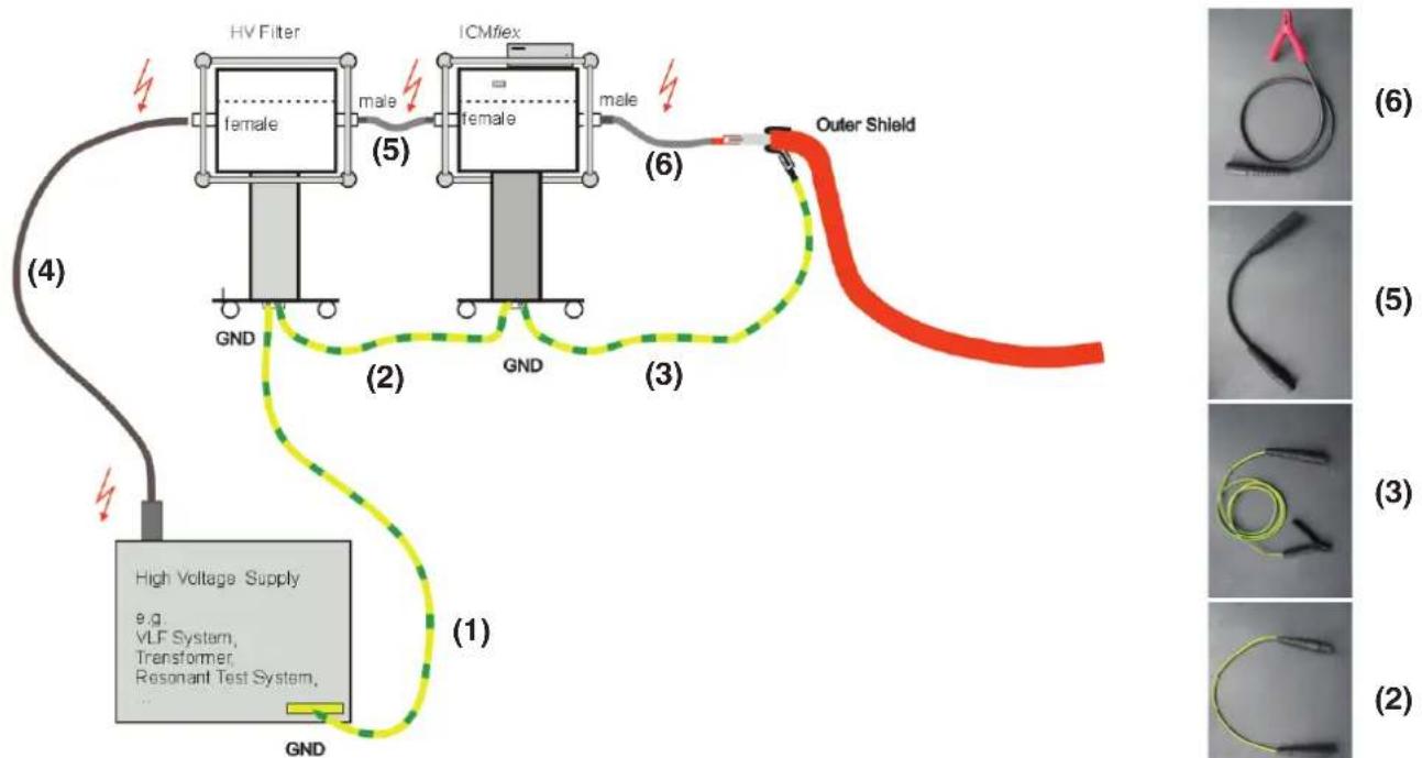
flowchart
graph TD
    A["High Voltage Supply<br>e.g. VLF System, Transformer, Resonant Test System"] --> B["GND"]
    B --> C["HV Filter<br>female"]
    C --> D["Outer Shield"]
    D --> E["ICMflex<br>female"]
    E --> F["Male"]
    style A fill:#f9f,stroke:#333
    style B fill:#ccf,stroke:#333
    style C fill:#cfc,stroke:#333
    style D fill:#fcc,stroke:#333
    style E fill:#cff,stroke:#333
    style F fill:#ffc,stroke:#333
Figure 56: MV cable measurement set-up
ICMflex
Partial discharge and loss factor measurement system
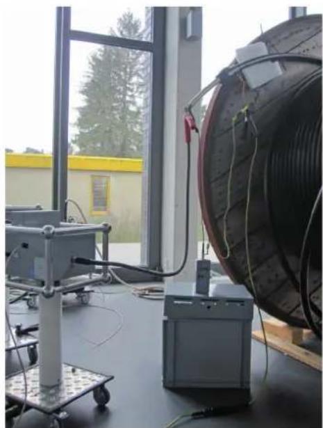
natural_image
Laboratory setup with a large coiled cable and control equipment near a window, no visible text or symbolsFigure 57: CAL1B connected to MV cable (lab)

Figure 58: CAL1B connected to MV cable (on-site)
Common calibration levels for laboratory acceptance tests are in the range 2 to 10 pC (CAL1A). However, for on-site testing, it is often not possible to use calibration as sensitive as in the laboratory. Due to this, calibration is often made with injection levels from 100 pC to 2 nC (CAL1B).
In additional to the calibration of the apparent charge in accordance with IEC 60270, the cable length or pulse velocity has to be calibrated for performing PD fault location (time domain reflectometry (TDR)). At least one of the two values must be known in advance. Table 2 lists some typical values for the velocity of propagation in relation to the cable insulation type. Note that these values can vary, depending on the nominal voltage and dielectric strength. The cable supplier usually provides the exact values with the cable data.
| INSULATION TYPE VC (M/μS) VC/2 (M/μS) | ||
| XLPE 147-168 73-84 | ||
| PILC 147 73 | ||
| EPR 165 82 | ||
| Vacuum 300 150 | ||
Table 2: Pulse velocity factors
The injection principle is the same as for the calibration of the apparent charge. A higher charge level may be required to see the necessary reflections for the TDR. Often a pulse magnitude of 5 or even 10 nC is required. If the injected calibration pulse is not visible in the digital storage oscilloscope (DSO) screen, increase the value of "DSO Gain", until the pulse becomes visible. It is also important to choose a sufficiently high trigger value to avoid triggering on disturbance levels. Along with the DSO gain and trigger level, adjust the timebase (X-axis) to ensure that the reflections are visible.
For calibration of the cable length, the cable terminations must be disconnected on both sides for a full reflection of the signal at an infinite impedance. Check the cable set-up carefully before calibrating.
Partial discharge and loss factor measurement system
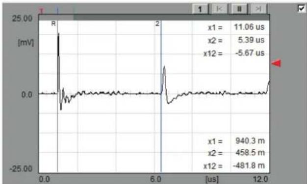
line
| Time (us) | Voltage (mV) | | --------- | ------------ | | 0.0 | 0.0 | | 6.0 | 0.0 | | 12.0 | 0.0 |Figure 59: Cable with shorted end

line
| Time (us) | Voltage (mV) | | --------- | ------------ | | 0.0 | 0.0 | | 6.0 | 0.0 | | 12.0 | 0.0 |Figure 60: Cable with open end
The DSO screen in Figure 59 shows the first two reflections arriving at the measuring impedance. Since the cable has an open end, the time difference between the reference pulse and its first reflection represents twice the cable length. The factor of 2 is automatically computed and must not be taken into account separately. The DSO screen in Figure 60 shows the result with a shorted cable. Here, the second reflection shows a polarity change due to the negative reflection factor. Check both ends in such a case.
For the calibration of the cable length as shown in Figure 61 it is important to consider the following parameters:
- DSO gain : The reference pulse must fill 60–90 % of the maximum scale
- Trigger level : Must be set sufficiently high not to trigger on disturbance pulses
- Scan time : Adjust according to the cable length to achieve the best sensitivity (0–320 μs)
- Zoom : Use the zoom function to position the cursors more accurately
- Zoom position : Sets the start position of the zoom function with reference to the X-axis
The black cursor (R) must be placed at the beginning of the reference pulse; the blue cursor (2) must be placed at the beginning of the first reflection. If the cable length is known, the "Calibrate" button at the bottom of the window can be pressed. The software will for the cable length to be entered. In cases where the pulse velocity is known, the value must be set for pulse velocity Vc. When the pulse velocity is known and both cursors are set correctly, x2 will show the cable length. The more accurate the cursor positions are, the more accurate the distances calculated will be. We recommend saving the file.
![Power Diagnostics - XOMex File Edit Connect Options Tools Help COM RIO TND 0 P1 = 0.0 m P2 = 0.0 m P3 = 0.0 m C1 = 132.5m C2 = 132.5m C12 = 132.5m 1.22 Op (Hz) Dg = -0.00pC Davg = -0.00pC Dp,p,p' = -6.07pC f = 50.9 Hz BAT Satz... Cable Length [m] 450.00 OK 1.2 pA N = 1979 30.0 s 7 pC Dccu = -0.07pC z1 = 982.5 m x2 = 490.0 m x12 = -582.5 m -1.22 -25.00 6.5 6.0 5.5 5.0 6.0 5.5 5.0 -25.00 DRO Auto Gain CSO Gain Tsp Lenter Tsp Mode Ptn Trigger Scan Time Devn Camer Pres Cable Lat Vc Vc Mode Avg Off 460 49.2 % Auth 1 us 80 us 12 us 2 us 460.6 m 166.5 ms u v Off Report Calibrate Copy Load Save Offline Start Sec Start Pattern Cns Eqt](/content/2026/05/853729/images/a5c98181149deff29d004d5b434196bb2fc2e600195b391384d85f6710d09ee4.jpg)
Figure 61: Cable length calibration
ICMflex
Partial discharge and loss factor measurement system
6.1.3 Standard PD measurement
Once the calibration procedure is completed and the calibrator has been removed from the test specimen, the voltage may be switched on. Pay attention to the correct setting for the shunt capacitor Csx (low or high) as explained in section 5.5.3.
Before switching on the voltage, it is important to observe the background noise level. Adjust the PD gain and LLD level so that the maximum of the background noise is still visible. Do not set the LLD level down to 0 %, as this will mean that the A/D converter is occupied converting background noise pulses. Masking the background noise up to 80 % of its maximum amplitude is acceptable.
After switching on the voltage, additional noise cancellation may be required to get rid of disturbances caused by the power supply itself or by external sources. This can be done by using the gating option, either with analogue gating or gating via a fibre optic gating transmitter. See sections 5.8 and 7.3 for more information.
The next step is finding the partial discharge inception voltage level. Clearly, before reaching the partial discharge inception voltage (PDIV), no root cause analysis or PD location investigation using time domain reflectometry can be performed. According to IEEE 400-3, for instance, a healthy cable will not show any sign of partial discharge activity at voltage levels lower than 2 Un.
Once the inception voltage is reached, the PD pattern can be mapped and compared with typical phase resolved pattern from known PD origins (see section 6.1.7). Besides the pattern, the related discharge levels (Qp, QIEC) and the average discharge current (NQS) are given. Pay attention to the correct settings of PD gain and LLD level. Adjust the gain value until the PD pulse amplitude is between 50–90 % of the maximum scale as shown in Figure 62 and Figure 63. The first line analysis of the nature, cause, or PD origin can be made using the pattern. The location along the cable length must be determined using time domain reflectometry. Typical times for mapping the phase resolved pattern are 30 to 60 seconds for power frequency and about 500 to 1000 seconds for VLF at 0.1 Hz.

bar_line
| Time (dec) | Qp (nC) | Qx (nC) | |------------|---------|---------| | 0 | 0.0 | 0.0 | | 180.0 | 17.7 | 0.0 | | 360.0 | 0.0 | 0.0 |
scatter
| Parameter | Value | | --------- | --------- | | NQS | 16.9 nA | | Qlec | 9.26 nC | | Q(x,y) | -34.60 μC |Partial discharge and loss factor measurement system
6.1.4 PD measurements on cables with high capacitance
For PD measurements on specimens with high capacitance, Power Diagnostix provides the CSX900 extension box (Figure 64) which extends the Csx value of the ICMflex to 900 F . The box is mounted onto an isolator of predefined height according to the maximum voltage level of the VLF source.
The following figure shows the set-up when using the CSX900 box.
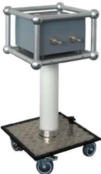
natural_image
Exterior view of a gray industrial control box mounted on a wheeled cart (no visible text or symbols)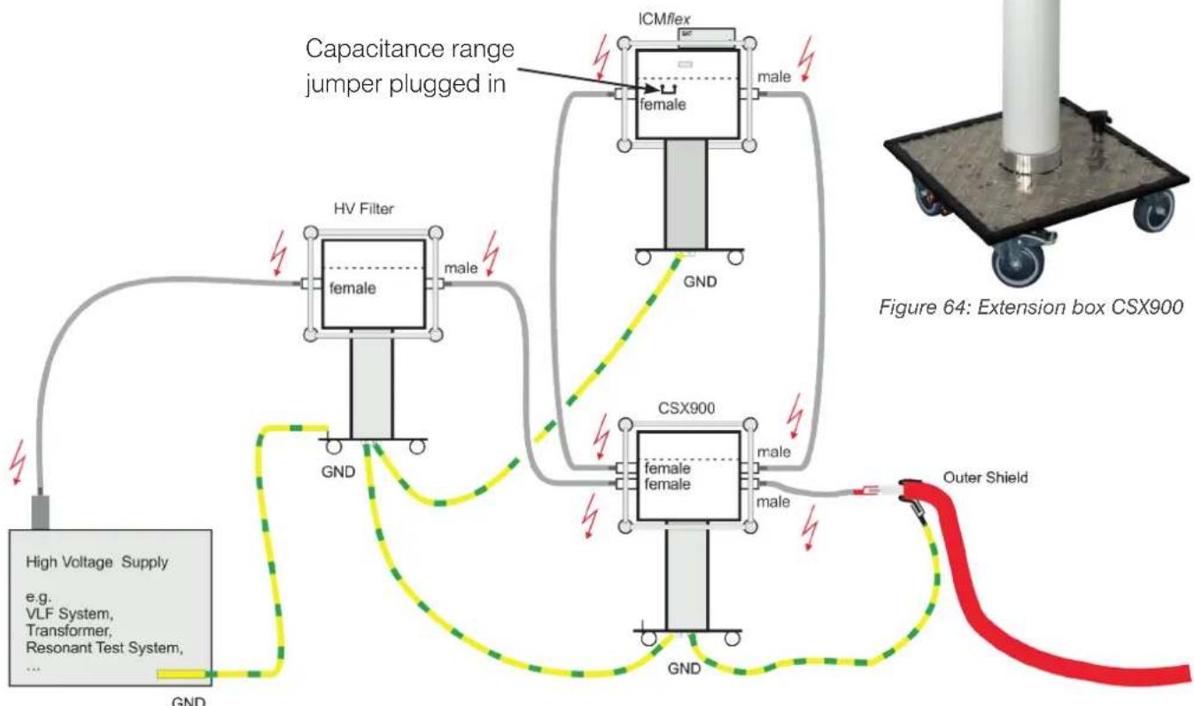
flowchart
graph TD
    A["High Voltage Supply e.g. VLF System, Transformer, Resonant Test System, ..."] --> B["HV Filter"]
    B --> C["Capacitance range jumper plugged in"]
    C --> D["ICMflex"]
    D --> E["CSX900"]
    E --> F["Outer Shield"]
    F --> G["GND"]
    G --> H["GS"]
    H --> I["GS"]
    I --> J["GS"]
    J --> K["GS"]
    K --> L["GS"]
    L --> M["GS"]
    M --> N["GS"]
    N --> O["GS"]
    O --> P["GS"]
    P --> Q["GS"]
    Q --> R["GS"]
    R --> S["GS"]
    S --> T["GS"]
    T --> U["GS"]
    U --> V["GS"]
    V --> W["GS"]
    W --> X["GS"]
    X --> Y["GS"]
    Y --> Z["GS"]
    Z --> AA["GS"]
    AA --> AB["GS"]
    AB --> AC["GS"]
    AC --> AD["GS"]
    AD --> AE["GS"]
    AE --> AF["GS"]
    AF --> AG["GS"]
    AG --> AH["GS"]
    AH --> AI["GS"]
    AI --> AJ["GS"]
    AJ --> AK["GS"]
    AK --> AL["GS"]
    AL --> AM["GS"]
    AM --> AN["GS"]
    AN --> AO["GS"]
    AO --> AP["GS"]
    AP --> AQ["GS"]
    AQ --> AR["GS"]
    AR --> AS["GS"]
    AS --> AT["GS"]
    AT --> AU["GS"]
    AU --> AV["GS"]
    AV --> AW["GS"]
    AW --> AX["GS"]
    AX --> AY["GS"]
Figure 65: Measurement set-up with CSX900 extension box for specimen with high capacitances
Warning: The ICMflex contains a shunt capacitor Csx, located between the two MC connectors, which can retain charge that is potentially harmful or fatal to users. To fully discharge Csx, the ICMflex must be grounded at both the input and output sides. Grounding the voltage source is not sufficient to ground the test object. If only the test object is grounded and the voltage source does not provide a permanent grounding connection, the potential of the ICMflex input connector will only be shifted such that the charge remains and poses a hazard to users.
ICMflex
Partial discharge and loss factor measurement system
6.1.5 PD fault location
When the PD pattern has been mapped and saved and the required notes are made, attention should be given to the DSO. Here, each partial discharge pulse is represented on a time-based curve. First, the settings must be adjusted so that the reference pulse and the two first reflections arriving at the coupling unit are visible on the screen, as explained in section 5.4.2.
Once partial discharge activity has initiated, the DSO can be used for estimating the PD location.
When the DSO settings (such as the DSO gain, trigger level, scan time, zoom, and zoom position) are optimised so that the reference pulse and the first as well as the second reflection are clearly visible on the DSO screen, the scan procedure may be started. While scanning, snapshots will be taken of pulses that exceed the trigger level. It is important to select a trigger level that avoids triggering on disturbance signals. After pressing the "Scan" button in the DSO menu, the pop-up screen for scan settings will appear (Figure 66).
- Select the required data directory for saving scan files
- Enter the maximum number of scan files (up to 1000)
- Select phase (1, 2, or 3)
- Enter the name of the phase under test
- Enter the file prefix, useful for later analysis
- If non-triggered snapshots are also needed, select the corresponding option
• To start the scan, press "OK"

After the scan is finished, the PD location can be pinpointed. Go off-line with the software and run the "Start Replay" function from the function keys at the bottom of the window. Here, you can evaluate the scan files manually. First, the software asks you to select the folder where the scan files are stored.
Once you have chosen the relevant folder, you can select the .tdr files to be evaluated. After selecting the files and pressing the "Add" button, the files you have chosen will be shown in the selection box (see Figure 67). To confirm that these are the correct files, click "OK". The software will automatically open the replay function.

Partial discharge and loss factor measurement system
The main task when using the replay function is the correct positioning of the cursor for the reference pulse (grey cursor in Figure 68) and the cursor for the first reflection arriving at the coupling capacitor (green cursor). The file name of the current .tdr file is displayed above the diagram.
Below the diagram are text boxes indicating the distance between the cursors, the time delay between the two pulses, the voltage level at which the files were recorded, and the related Qp level for the file.

line
| Parameter | Value | | --------- | --------- | | ΔI | 460.1 m | | ΔI | 5.48 us | | U/V2 | 0.0 kV | | Qp | 127.4 pC |Figure 68: Replay screen
In the bottom part of the replay screen (Figure 68), you will find these buttons:
- Cancel: For stopping the current replay
- Save File As: For storing the current file
- Delete File: For removing the file from the selection
- Back: For returning to the previous file
- Skip: For switching to the next file
- Select All: For adding all files into the LOC screen
- Select: For adding the current file into the LOC screen
After you have positioned the cursors for the reference pulse and first reflection, you can use "Select" to add the position of the PD activity along the cable to the summarising LOC diagram. When scan files are validated and result in identical positions along the cable, the result of each single event will be added and shown as the total amplitude in the red bar, as shown in Figure 69. The PD amplitude refers to the peak discharge level at the time of scanning and does not indicate the PD amplitude at the position of occurrence.
With the check box "Loc Grid", it is possible to switch on grid lines within the LOC chart. With the option "Projections", you can enable cursors in the LOC chart. The mapping reference, i.e., near or far end, is indicated by the coupler symbol on the X-axis.

bar
| Position (m) | Value (pC) | | :--- | :--- | | 0 | 0 | | 350 | 120 | | 700 | 240 | | C1 | 0.0 | | C2 | 0.0 | | C12 | 0.0 |ICMflex
Partial discharge and loss factor measurement system
6.1.6 Test voltage recommendations and criteria
The relevant standards for medium and high voltage cable testing describe test voltages, sequences, and PD evaluation criteria in relation to the cable's voltage class. Select the test type to be performed, i.e., acceptance testing or on-site testing. On-site testing is mostly performed after installation tests and is recommended to verify the performance of cable accessories, such as joints and end terminations, which are often installed on-site. Table 3 shows the recommendations given in the relevant IEC standards.
| ACCEPTANCE TESTING ON-SITE TESTING | ||||||
| Standard Frequency Voltage PD Criteria Frequency Voltage PD Criteria | ||||||
| 1 kV < U < 40 kV | ||||||
| IEC 60502 49–61 Hz 3.5 U | _0/5 min 1.73 U _0 < 10 pC | 49–61 Hz49–61 HzDC | 1.73 U _0 /5 minU0/24h4 U _0 /15 min | None | ||
| 40 kV < U < 150 kV | ||||||
| IEC 60840 49–61 Hz 2.5 U | _0/30 min No PDup to 1.5 U0 | 20–300 Hz49–61 Hz | 1.73–2 U _0 /1 hU _0 /24 h | None | ||
| 150 kV < U < 500 kV | ||||||
| IEC 62067 49–61 Hz 2.5 U | _0/30 min2.5 U _0 /60 min | 1.5 U _0 < 10 pC 20–300 Hz49–61 Hz | 1.1–1.73 U _0 /1 hU _0 /24 h | None | ||
Table 3: MV cable test voltages
As can be seen from Table 3, no PD criteria are given for on-site testing. Shielded test room conditions cannot be compared with on-site conditions. The main reason is the set-up sensitivity which is often critical because of the background noise. In shielded test rooms background noise levels of less than 2 pC can be achieved and in these cases, specifying criteria makes sense. With on-site testing, background noise from a few tens up to hundred pC is not unusual. In this case, it is important to build a well-considered partial discharge free test set-up and to perform sufficient sensitivity checks at all available positions in order to gain a better understanding of the partial discharge's high frequency signal transfer within a certain bandwidth.
Partial discharge and loss factor measurement system
As well as the IEC standards, there are applicable IEEE publications. The general procedures and criteria do not differ much from those prescribed by the IEC. However, of interest in the IEEE standards are the test voltage criteria for testing at very low frequency (VLF). The IEEE splits cable testing into three different groups: installation test, acceptance test and maintenance test, each with related test voltages.
| VLF OUTPUT WAVE-FORM | CABLE RATING PHASE-TO-PHASE | INSTALLATION TEST PHASE-TO-GROUND - U_0 | ACCEPTANCE TEST PHASE-TO-GROUND - U_0 | MAINTENANCE TEST PHASE-TO-GROUND - U_0 | |||
| Sinusoidal | kV RMS kV RMS kV peak kV RMS kV peak kV RMS kV peak | ||||||
| 5 9 13 10 14 7 10 | |||||||
| 8 11 16 13 18 | 10 | 14 | |||||
| 15 | 19 27 21 30 | 16 | 22 | ||||
| 20 | 24 34 26 37 | 20 | 28 | ||||
| 25 | 29 41 32 45 | 24 | 34 | ||||
| 28 | 32 45 36 51 | 27 | 38 | ||||
| 30 | 34 48 38 54 | 29 | 41 | ||||
| 35 | 29 55 44 62 | 33 | 47 | ||||
| 46 | 51 72 57 81 | 43 | 61 | ||||
| 69 | 75 | 106 | 84 | 119 | 63 | 89 | |
Table 4: MV cable VLF test voltage recommendations
In general, the recommended testing time according to IEEE 400.2, varies between 15 and 60 minutes. 30 minutes is suggested. For maintenance testing, 15 minutes is recommended.
ICMflex
Partial discharge and loss factor measurement system
6.1.7 Typical PD patterns and tan delta levels
MV class cables are tested in the factory in accordance with common IEC standards. The acceptance level for new cable systems is < 2 pC. Therefore, all PD detected on MV cables under applied voltage up to 1.5 x rated voltage should be considered as a problem within the cable or its accessories. Further analysis should clarify the cause of this PD activity.
| PD PHENOMENA TYPICAL RANGE | FURTHER ANALYSIS RECOMMENDED | PD PATTERN EXAMPLE | |
| Void discharge with low availability of starting electrons | <2 pC >20 pC |  | |
| Surface discharge <2 pC >20 pC |  | ||
| Internal discharges in a prefabricated EPR cable joint | <2 pC >20 pC | [CCCCK] | |
| Several flat cavities in silicon fat due to improper mounting procedure | <2 pC >20 pC |  | |
Table 5: Typical PD patterns for MV cables
Partial discharge and loss factor measurement system
The loss factor values measured on MV cables are usually specified in relation to the cable insulation system and voltage level U_0 , 2 U_0 or the tip-up between 2 U_0 and U_0 . Pay attention to the environmental conditions as they strongly influence loss factor and capacitance measurements. Indicative TD values are given in Table 6.
| TYPE OF CABLE SYSTEM NEW SERVICE AGED CRITICAL LEVELS | |||
| XLPE < 0.1 x 10 | -3 | ~ 1.2 x 10⁻³ | >2.2 x 10⁻³ |
| EPR < 3.5 x 10 | -3 | >3.5 x 10⁻³ | - |
| PVC < 6 x 10 | -2 (50 Hz)< 8 x 10⁻²(0.1 Hz) | >6 x 10⁻²(50 Hz)>8 x 10⁻²(0.1 Hz) | - |
Table 6: Tan delta levels versus insulation system
6.1.8 Normative references
IEC 60502: Power cables with extruded insulation and their accessories for rated voltages from 1 kV ( U_m = 1.2 kV) up to 30 kV ( U_m = 36 kV)
IEC 60840: Power cables with extruded insulation and their accessories for rated voltages above 30 kV ( U_m = 36 kV) up to 150 kV ( U_m = 170 kV) – Test methods and requirements
IEC 62067: Power cables with extruded insulation and their accessories for rated voltages above 150 kV ( U_m = 170 kV) up to 500 kV ( U_m = 550 kV) – Test methods and requirements
IEEE 400: IEEE Guide for Field Testing and Evaluation of the Insulation of Shielded Power Cable Systems Rated 5 kV and Above
IEEE 400.2: IEEE Guide for Field Testing of Shielded Power Cable Systems Using Very Low Frequency (VLF) (less than 1 Hz)
IEEE 400.3: IEEE Guide for Partial Discharge Testing of Shielded Power Cable Systems in a Field Environment
ICMflex
Partial discharge and loss factor measurement system
6.2 Rotating machines
6.2.1 Test set-up
A general description of the measurement set-up is given in section 3, but here, the focus is on rotating machines applications. Most important is the interconnection between the main grounding of the high voltage power supply, i.e., a transformer or resonance test set, and the main grounding of the machine frame. The final link from the grounded baseplate of the ICMflex to the ground shield must be as short as possible. The high voltage output cable of the ICMflex has to be connected to the phase terminals of the motor or generator. Figure 70 shows the connections for a typical set-up.
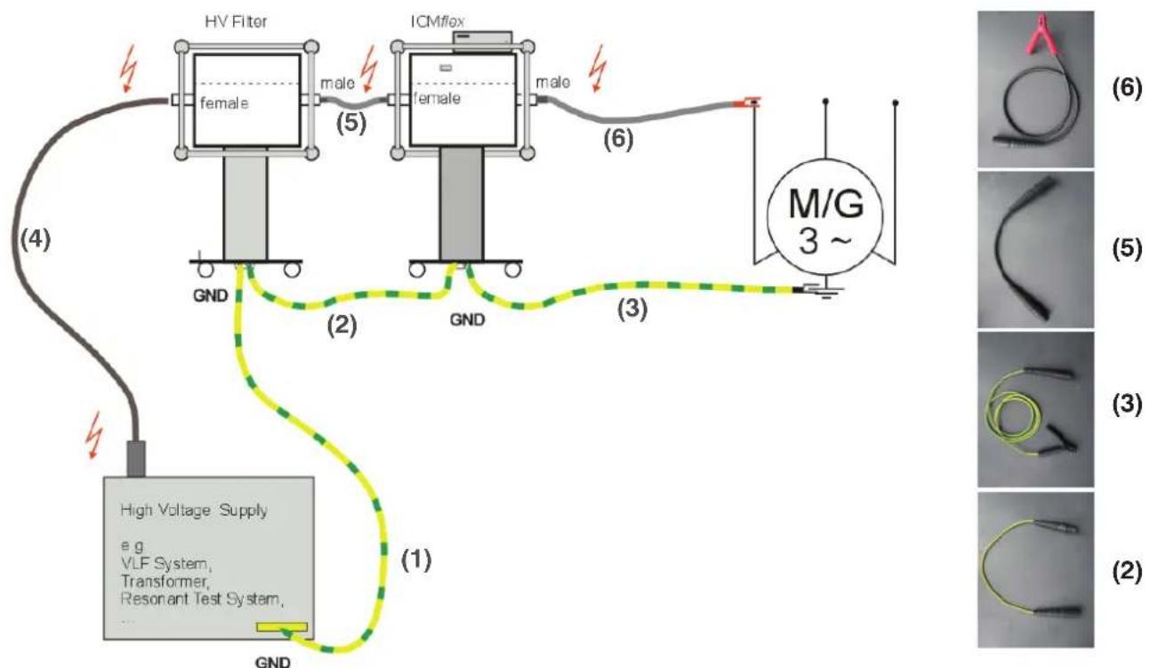
flowchart
graph TD
    A["High Voltage Supply e.g. VLF System, Transformer, Resonant Test System"] --> B["HV Filter"]
    B --> C["ICM/lox"]
    C --> D["M/G 3 ~"]
    style A fill:#f9f,stroke:#333
    style B fill:#ccf,stroke:#333
    style C fill:#ccf,stroke:#333
    style D fill:#cfc,stroke:#333
    subgraph Inputs
        E["1: GND"]
        F["2: GND"]
        G["3: GND"]
        H["4: GND"]
        I["5: male"]
        J["6: male"]
    end
    subgraph Outputs
        K["7: (1) High Voltage Supply"]
        L["8: (2) High Voltage Supply"]
        M["9: (3) High Voltage Supply"]
        N["10: (4) High Voltage Supply"]
        O["11: (5) High Voltage Supply"]
        P["12: (6) High Voltage Supply"]
Figure 70: Rotating machines measurement set-up
6.2.2 Calibration
Performing high voltage tests, including partial discharge measurements on rotating machines insulation systems in accordance with IEC 60270, requires calibration of the apparent charge. When the complete safety procedure as detailed in section 1.3 has been completed and when the set-up has been arranged as described above, calibration can be performed. General procedures are described in the Power Diagnostix user manual for calibration impulse generators. The detailed calibration procedure for generators and motors is explained below.
A calibrator is connected to the phase terminal that is connected to the ICMflex as shown in Figure 71. The selection of the charge level to be injected into the measurement circuit depends on the machine's ratings. The main parameter influencing the required charge is the stator winding capacitance. In general, the capacitance depends on the nominal voltage, number of poles, and the core length. It is important to have a reasonable signal-to-noise ratio to ensure sufficient sensitivity. Select a value that is approximately 5 to 10 times higher than the background noise present. Typical values used for on-site testing range from 1 nC to 5 nC, and even 10 nC for hydro or turbo generators.
Partial discharge and loss factor measurement system
It is recommended also to make a calibration using the PD attenuator. Due to the properties of the insulation materials and the winding manufacturing techniques in an epoxy mica insulation system, partial discharge pulses can reach large amplitudes. In regular mode, the amplifier may not be able to handle these unusually large pulses. For this reason, the ICMflex has an on-board 10 dB attenuator, which can be activated in the advanced settings. It is possible to activate the attenuator and upload the relevant calibration file without interrupting the measurement session. The PD attenuator can be switched on using the menu item “Edit”->“Advanced Settings” of the ICMflex software.
If access to the neutral connection (star point) is possible, the phases can also be tested separately. In this case, it is necessary to carry out additional calibration as the capacitance to ground will be different. Furthermore, injecting a pulse at the neutral terminal and measuring the response at the line terminal gives a good idea of measurement sensitivity.

natural_image
Industrial machine setup with green cylindrical component and connected test equipment (no visible text or symbols)Figure 71: Calibration on a small asynchronous motor

natural_image
Industrial machine setup with a worker operating a digital testing device (no visible text or symbols)Figure 72: Calibration on a synchronous generator
6.2.3 PD measurements
After the calibration procedure has been completed and the calibrator (CAL1) has been removed from the test specimen, the voltage may be switched on. Pay attention to the correct setting of the shunt capacitor C_sx (low or high) as mentioned in section 5.5.3.
Before applying voltage, it is important to check the level of background noise present. Adjust the PD gain and LLD level so that the PD amplitude is 50–90 % of the maximum scale and the maximum of the background noise is still visible. Do not set the LLD level down to 0 %, as this will mean that the A/D converter is occupied converting background noise pulses. Masking the background noise up to 80 % of its maximum amplitude is acceptable.
After switching on the voltage, additional noise cancellation might be required to get rid of disturbances caused by the power supply itself or by external sources. Use the gating option for this purpose. Analogue gating and gating via a fibre optic gating transmitter are possible. Please see sections 5.8 and 7.3 for more information.
ICMflex
Partial discharge and loss factor measurement system
The next step of the measurement process is identification of the partial discharge inception voltage ( P_DIV ). A sensitive abd slow ramp up of the test voltage is important for determining the P_DIV . A typical test sequence used for partial discharge measurements is, for instance, the same as that for tan delta measurements. An example is shown in Figure 73. In this case, the test voltage must be increased in five equal steps, each 20 % of U_MAX up to a maximum of U_MAX . The maximum voltage level ( U_MAX ) applied to ground is the operating line-to-line voltage as stated on the machines rating plate. Testing up to the line-to-line voltage not only covers the insulation to ground but also the performance of the interphase insulation, and is strongly recommended for acceptance testing of new stator windings. Other common U_MAX levels are up to the operating line-to-ground voltage ( U_MAX/3 ) or up to 120 % of the operating line-to-ground voltage ( 1.2 U_MAX/3 ). The maximum test voltage is often agreed between the owner and service group and is chosen according to the kind of test, e.g., a periodical test or a test after repair.

line
| U [kV] | Qp [nC] | TD [E-3] | | :--- | :--- | :--- | | 0.0 | 0.00 | 0.00 | | 4.0 | 1.00 | 2.00 | | 8.0 | 2.00 | 4.00 | | 16.0 | 21.00 | 6.00 |Figure 73: Test sequence of a 15 kV winding, PD and TD vs. voltage
After the inception voltage is found, phase resolved patterns can be mapped and compared with typical phase resolved pattern from known PD origins (see section 6.2.5). The recommended value for the PD pattern test time is between 30 s and 60 s when working at power frequency (50 Hz–60 Hz) and about 1000 s to 1500 s when using very low frequency (VLF) power supplies.
As well as the pattern, the related discharge levels (Qp, Q_IEC ) and the average discharge current (NQS) are given. Relevant data for test reports relating to rotating machines are: Summary table of all test results versus voltage, partial discharge inception and extinction voltage, and the phase-resolved patterns at each voltage step. The ICMflex software supports export of this data as a file for MS Excel.
Partial discharge and loss factor measurement system
6.2.4 Step-by-step guide
To simplify measurements, a step-by-step guide has been implemented in the ICMflex standard software. This guides users through the required steps prior to and during the measurement. The step-by-step guide option is enabled via "Edit"->"Edit Preferences" in the "Miscellaneous" tab. The settings related to the step-by-step measurement are found on the "Step by Step Guide" tab, shown in Figure 74.
- Voltage Cycles to Stabilize: The system recognises the applied voltage after having detected the selected number of stable cycles between the fixed voltage tolerance levels.
- Cycles per Measurement Interval: This setting determines the number of averages taken for the tan delta measurement at a certain voltage level after detection of a stable voltage level between the fixed voltage tolerances
- Voltage Tolerance: Selectable in volts [V] or percentage [%]. Tolerance on the accepted difference between the theoretical value calculated for each voltage step and the applied voltage during test procedure.
![Preferences Miscellaneous | Step by Step Guide | Multi Channel Options | General Settings Device Under Test Rotating Machines Voltage Cycles to Stabilize 5 cycles Cycles per Measurement Interval 5 cycles Acquisition Mode Tan Delta Report Selection Show Selection Popup Report Logo Path c:\projects\reportlogo.png Voltage Tolerance 200.0 V ▼ TanD Cycles 5 Sync Mode Normal Set Time 30.0 s Time To Stabilize Voltage 0.00 s Interval 100.00 s Show Preferences ✓ Report Logo Preview Stretch Logo [max. 280px *80px] Logo Cancel Load Save Default OK](/content/2026/05/853729/images/b44baa4d12ba7d68725a4b8ea4b4dc3a743589ae8fc9003d8a4f18e4320fe538.jpg)
Figure 74: Preferences window
- Time To Stabilize Voltage: Waiting time until measured values are recorded at the set test voltage, to ensure stable voltage values when pattern recording starts.
Step 1: Figure 75 shows the screen for step 1. The user has to enter the general information such as:
Work number
- Machine type
- Serial number
Nominal voltage
- Phase to be tested
• Maximum voltage
- Measured by
• Approved by
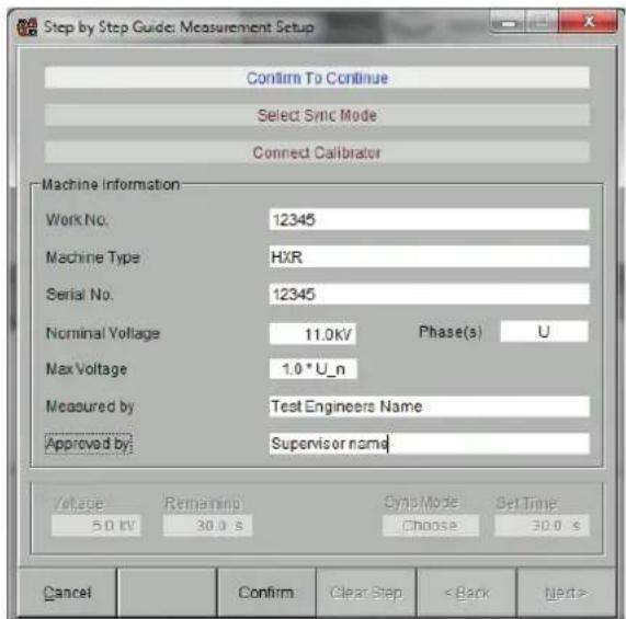
Figure 75: Measurement Setup Guide screen
ICMflex
Partial discharge and loss factor measurement system
After filling in individual fields, the background colour of the text box changes from red to black when the entry is confirmed by pressing the enter button. The nominal voltage to be entered is the operating phase-to-phase voltage of the stator winding. The user can choose to record data for each phase separately or all three phases together (star point connected). The maximum voltage for the record file is adjustable, varying from 0.8 × U_N to 1.4 × U_N in steps of 0.2 U_N . Once all the required fields are filled in, the upper guide bar will indicate "Confirm to Continue". The settings are saved by pressing the "Confirm" button below in the guidance screen. Pressing the "Cancel" button stops the step-by-step procedure.
If the user confirms the entered data, the upper guidance bar will indicate "Completed" in a green font, and the software continues to the next step (Figure 76). If an error is detected, the step can be fully deleted by pushing the "Clear step" button.
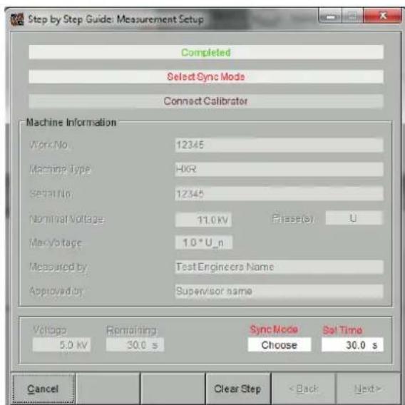
Figure 76: Completed first step
Step 2: Selection of synchronisation frequency (Figure 77)
In step 2 the user selects the synchronisation frequency for the measurement from the "Sync Mode" drop-down list. Available options are:
Normal: 50–60 Hz, power frequency
VLF 0.1 Hz
VLF 0.05 Hz
VLF 0.02 Hz
Depending on the synchronisation frequency, the appropriate set time must be chosen. Power Diagnostix has predefined recommended set times for each frequency. The user can choose between selecting the recommended set time or entering a custom set time based on their own test procedure. The predefined set times are:
Normal: 60 seconds
• VLF 0.1 Hz : 1500 seconds
• VLF 0.05 Hz : 1500 seconds
• VLF 0.02 Hz: 3000 seconds

Figure 77: Synchronisation frequency selection
Partial discharge and loss factor measurement system
After entering and confirming the set time, the user prompted to enter a file name (Figure 78). This can be done by pushing the button "Filename" at the bottom of the guidance menu. All measured data at each voltage interval will be stored under the entered file name into in the relevant folder on the computer's hard drive.
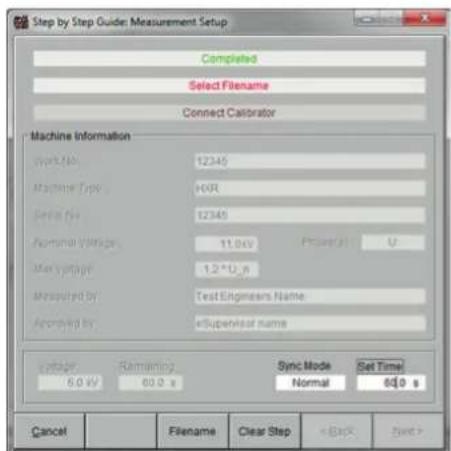
![Save Description: [0] User geodesat Developer:\MSM\msw36 Save in: workshop Name: Date modified Type: Size win_lnc_w27495.0x 10.0.0001/14.43 14.3 fps 3.886 KB File name: .com_rsc_12345 Save Asigns: (F) No OK Cancel](/content/2026/05/853729/images/c3513521ca95eb0c34d49ce26c8436db2182bd77eb833cbeba5a9cc66b35800b.jpg)
Figure 78: File name selection
After the file name and desired location on the computer's hard drive have been selected, the second guidance bar in the upper guidance screen will show "Completed" in a green font and will ask the operator to continue with step 3. If an error is detected, the step can be deleted by pushing the "Clear step" button and the data entry can be repeated.
Step 3: Partial Discharge Calibration (IEC 60270)
The third step of the measurement guidance asks the user to perform calibration of the apparent charge for the partial discharge measurement. Therefore, they must connect the calibrator to the winding that is going to be measured. The calibrator must be connected, as shown in Figure 71.
It is important to consider the signal-to-noise ratio (SNR). The user should inject a calibration pulse of sufficiently large amplitude, so that it is possible to clearly distinguish it from the level of background noise present (see Figure 79). Common charge levels injected for rotating machines are 500 pC, 1 nC, 2 nC, and 5 nC. In general, the charge to be injected will be determined by the complex impedance of the stator winding and by the measurement set-up. Performing the calibration, provides a reference to compensate for changes to the injected signal (especially attenuation), such that the pulse amplitude reaching the ICMf/ex via the phase terminal under test can be scaled to a known amplitude level. By double clicking on the upper calibrator line, the injected value can be entered in a dialogue box (Figure 79) which will appear on the screen.
ICMflex
Partial discharge and loss factor measurement system
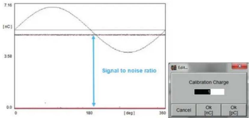
line
| Angle (deg) | Signal to noise ratio (nC) | |-------------|-----------------------------| | 0 | 7.16 | | 180 | 3.58 | | 360 | 7.16 |Figure 79: PD calibration
The steps that have to be performed to complete the calibration sequence are shown in Figure 80. They are:
- Connect the calibrator
- Start pattern: wait for 10 s (standard acquisition time for calibration)
• Double click on the calibrator pulse

Figure 80: Calibration sequence
After the injected calibration pulse is entered, the calibration file will be stored into the .flx file with the chosen file name in the selected location on the computer. The third guidance bar in the upper guidance screen will now indicate "Calibration done" in a green font and ask the user to continue with the next step by pressing the "Next >" button in the lower right corner of the guidance screen.
Partial discharge and loss factor measurement system
Step 4: Apply voltage
The next step in the measurement process is to apply voltage. In the upper guidance bar, the required voltage level will be indicated (see Figure 81). It is shown as a phase-to-ground or phase-to-phase voltage.
From this point in the sequence, the user can go back to the previous step by pushing the "< Back" button or go to the next step by pushing the "> Next" button. Note that "> Next" only becomes available when a step has been completed.
The instrument will recognise the voltage level automatically.
Until the desired voltage within the fixed tolerance is reached, the second guidance bar will indicate "Waiting". Once the required voltage level is reached, the first guidance bar will change into "Voltage reached" in a green font, and the second guidance bar will show now "Acquire Tan Delta Values" as shown in Figure 82.

Figure 81: Guidance screen while waiting for the voltage level to be reached
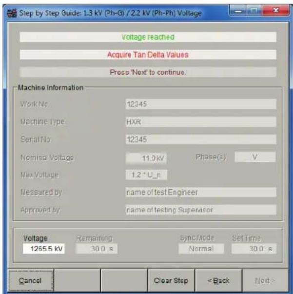
Figure 82: Guidance screen after reaching the test voltage
The tan delta measurement will now be performed automatically according to the settings in the preferences. When the number of averages is reached and values are stored for a particular voltage step, the second guidance bar will show “Start Pattern Acquisition” for performing the partial discharge measurement (Figure 83). The voltage level and remaining acquisition time will always be shown on the left-hand side in the lower part of the guidance window.
ICMflex
Partial discharge and loss factor measurement system
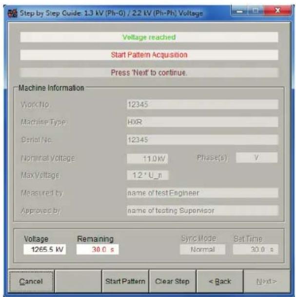

Figure 83: Guidance screen for starting the PD pattern Figure 84: Guidance screen after completing pattern acquisition
Pattern acquisition is started by pressing the "Start Pattern" button at the bottom of the guidance screen (see Figure 83). The pattern will be collected over the set time. Once the pattern is acquired, the second guidance bar will indicate "Pattern Acquisition finished" in a green font. The user has to confirm this message by pressing the "Next >" button. The pattern will then be stored under the selected file name, per voltage step, in a .flx file. If necessary, the pattern can be mapped again should some of the settings need to be adjusted. The previously stored pattern will then be over-written by the new pattern. To map a new pattern, use the "< Back" button.
After having confirmed a successful pattern acquisition by pressing "Next >", the guide will show the next voltage step. When ramping-up the voltage, the user must cross check the gain settings for U_n and U_x to ensure that the capacitive voltage dividers are not over-ranged. Should this happen, a warning will be generated in the second guidance bar "U_sn (or _sx) Overrange - Decrease U_sn (or _sx) Gain" (Figure 85). The corrective action required will also be indicated. The maximum voltage for U_sn is 14 V RMS, and for U_sn it is 140 V RMS. The actual voltage drop on the capacitive dividers can be observed in the upper left chart by selecting U_acc , located in the upper right-hand corner of the chart. After adjusting the gain settings properly and detecting that the applied voltage is within the fixed tolerance, the message "Voltage Reached" will appear in a green font in the first guidance bar. The tan delta records will be made, and afterwards, the pattern can be acquired again. This procedure must be repeated until the last voltage step is reached.

Figure 85: Voltage over-ranging
Partial discharge and loss factor measurement system
As well as the gain settings for both voltage dividers, the gain for the partial discharge measurement must also be monitored. At each voltage step, check if the PD activity present is within the maximum scale of the pattern. If not, increase or decrease the PD gain accordingly.
When pattern acquisition for the last voltage step is finished, the entire table will have been filled automatically by the software. The upper guidance bar will show the message "Measurement finalized", and the second guidance bar will prompt the operator "Print measurement or start new measurement" (see Figure 86). The test report can be printed by pressing the "Print" button located in the lower right-hand corner of the guidance screen. The report will be printed and shown on the computer screen.

Figure 86: Printing/new test guidance screen
After having printed the report or started a new test, the button "Keep Infos" appears in the lower area of the guidance screen. This option is implemented to keep the machine details, etc., for consecutive measurements on the same machine. For instance, phase V after finishing phase U. In this case, it is only necessary to re-select the phase name, the file name and to do the PD calibration for the relevant phase. When performing consecutive measurements for the next phase or all three phases together, for instance, the principle of measuring stays the same – that is, the operator will be guided through the complete sequence again, step by step. If the "Clear all" button is pressed, all of the machine information will be deleted.
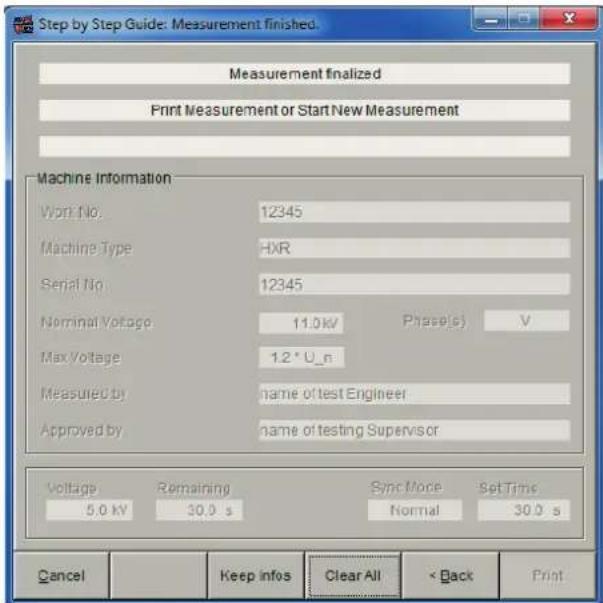
Figure 87: Final guidance screen
ICMflex
Partial discharge and loss factor measurement system
6.2.5 Typical PD patterns and tan delta levels on rotating machines
To simplify the evaluation of measurement results, you can find here some common partial discharge patterns versus PD origin and tan delta evaluation criteria, based on rotating machines standards and other related literature. Power Diagnostix has more than 25 years' experience in PD diagnostics on rotating machines. The following table gives an overview regarding regular PD levels and miscellaneous PD phenomena.
In general, partial discharge activity is inherent to epoxy-mica insulation systems. Compared with other insulation systems where the PD level criteria are specified in the lower pC ranges, such as XLPE for medium and high voltage cables or oil-paper insulation systems for power transformers, the common PD levels for stator winding insulation systems are higher. Epoxy-mica insulation systems also widely tolerate partial discharge activity since these systems are developed to be partial discharge resistant for many years. Performing PD tests on new machines provides a baseline for further trending over time, and, if design faults are present, it will reveal them. Basically, every significant deviation from regular internal PD can be considered as a potential problem with insulation quality, and the root cause must be investigated.
As the measured apparent charge levels depend on many different parameters such as measurement setup, measurement frequency, location of the coupler, test voltage, insulation system, and PD location within the winding, there are currently no specified no-go criteria. The levels given below are indicative values.
| PD PHENOMENA TYPICAL | RANGE | FURTHER ANALYSIS RECOMMENDED | PD PATTERN EXAMPLE |
| Spherical void discharge with low availability of starting electrons | 0 nC >500 pC |  | |
| Surface discharge at the slot exit the first stage of field grading problem | 0–2 nC >2 nC |  |
Partial discharge and loss factor measurement system
| PD PHENOMENA TYPICAL | RANGE | FURTHER ANALYSIS RECOMMENDED | PD PATTERN EXAMPLE |
| Thermally aged main insulationsymmetrical in both half-cycles | <5 nC >5 nC |  | |
| Slot discharges with machine barsnon-symmetricalpredominantly in the negative half-cycle | 0 nC >5 nC | 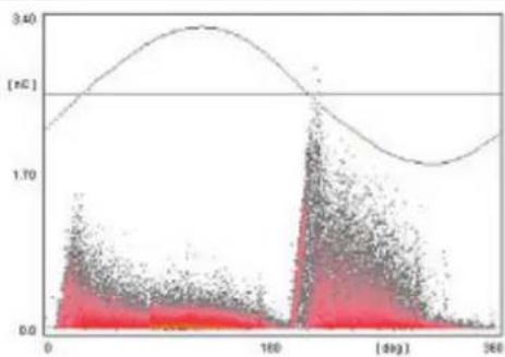 | |
| Surface discharges at the end winding | 0–2 nC >20 nC |  |
Table 7: Typical rotating machine patterns
| SPECIMEN VOLTAGE LEVEL | NEW SERVICE AGED | COMMENTS | ||
| Stator winding 0.2 UNUNTip-up per 0.2 UN | <30 x 100-3<60 x 100-3<5 x 100-3at 50 Hz | >30 x 100-3>80 x 100-3>5 x 100-3at 50 Hz | Relevant standard: IEC 60894Often, different tan delta levels are found between various insulation types such as global VPI and resin rich. | |
| Single bar 0.2 UNUNTip-up per 0.2 UN | <30 x 100-3<60 x 100-32-7 x 100-3at 50 Hz | Relevant standard: IEEE 286-2000Please be aware that it is only reasonable to test fully cured coils.10 % of the complete set needs to be examined. | ||
Table 8: Common TD evaluation criteria for rotating machines
ICMflex
Partial discharge and loss factor measurement system
6.2.6 Normative references
| TS IEC 600034-27: | Off-line partial discharge measurements on the stator winding insulation of rotating electrical machines |
| IEC 600034-27-3: | Dielectric dissipation factor measurement on stator winding insulation of rotating electrical machines |
| IEC 60894: | Guide for test procedure for the measurement of loss tangent of coils and bars for machine windings |
| IEEE 286-2000: | Practice for Measurement of Power Factor Tip-Up of Electric Machinery Stator Coil Insulation |
6.3 Stator bars
6.3.1 General
The principle for PD and tan delta testing on separate stator bars using the ICMf/ex is very similar to testing complete assembled stator windings. In this case, the coils are not assembled into the magnetic stator core, so, an artificial core should be provided to ground the straight part of the coils. Common materials used for applying grounding electrodes (as simulated slots) are conductive adhesive tapes or copper/aluminium bars. It is important that the ground electrode has a similar length as the real stator core. It is even more important to achieve optimal contact between the ground electrode material and the slot's semi-conductive outer layer. When copper/aluminium bars are used, pincers can be used to ensure good contact, as shown in Figure 88. Coils can be tested completely by bridging the grounded straight parts of both coil ends or tested partially by grounding the straight part of one coil end only. The main purpose of tan delta and tan delta tip-up testing is to determine the general condition of the coil's ground wall insulation (see section 10.1). The test results mainly show the performance of the slot's conductive outer layer, acting as the ground electrode to the magnetic core.
Generally, stator bars with rated voltage of 6 kV or more are provided with a field grading junction, consisting of a semi-conductive material, e.g., silicon carbide, at the slot-exit area. The function of the grading junction is to control the surface field at the coil's slot exit in proportion to the distance from the core. Depending on the rated voltage, this high resistance material with non-linear resistive characteristic has a specific length and overlaps with the slot's linear resistive outer layer. Usually, the overlap between these two layers is outside the magnetic core.
These semi-conductive materials can influence the overall tan delta level, as they show a resistive loss under influence of high voltage potential. Therefore, standards such as the IEEE 286-2000 and the IEC 60034-27-3 require the use of guard rings during the tan delta test to eliminate the influence of these resistive losses. When using guard rings, the aim of the tan delta measurement, i.e., checking the performance of the slot corona prevention layer, is achieved without the results being influenced by the semi-conductive materials used for the field grading. For this reason, Power Diagnostix designed the ICMflex GRC, with guard ring control. For complete windings the contribution of the resistive losses produced by the semi-conductive material in the overall tan delta level can be ignored, and hence, the standard ICMflex can still be used.
Partial discharge and loss factor measurement system
6.3.2 Test set-up
The PD and tan delta measurement set-up using the standard ICMflex is very similar to the testing of complete windings (see section 6.2.1). Instead of connecting the grounding to the motor or generator frame, it is connected to the simulated slot on the straight part of the stator bar. If the entire coil needs to be tested, both straight parts are interconnected. The high voltage output of the ICMflex must be connected to the coil's HV conductor circuit.

Figure 88: PD and TD testing of resin rich bar for a small hydro generator
Figure 89: Testing of resin rich bar for an asynchronous motor
6.3.3 PD calibration
In general, the calibration procedure for the PD measurement is similar that is described in section 6.2.2. Since the test circuit for a single bar has a fairly low capacitance, a lower calibration charge can be selected than for fully assembled stator windings. Common charge levels are in the range of 100 pC to 500 pC. The PD calibrator should be connected between the HV conductor circuit of the coil and the simulated slot (GND clamp).
6.3.4 PD and tan delta measurement
The measurement procedure is similar as described in section 6.2.3 for testing complete windings. Depending on the applicable standard (see section 6.3.6), the procedure and levels of applied voltage might be different. In the examples below, tan delta measurement results are shown for a 10 kV resin-rich bar without guard rings (Figure 90) and with guard rings applied (Figure 91). As well as the results in strip charts, the slope of the tan delta graph versus voltage clearly shows the effect of the resistive losses of the semi-conductive layer.

line
| U [kV] | TD [E-3] | Cx [nF] | | ------ | -------- | ------- | | 0.0 | 10.0 | 0.0 | | 2.5 | 12.5 | 0.0 | | 5.0 | 15.0 | 0.0 | | 7.5 | 17.5 | 0.0 | | 10.0 | 20.0 | 0.0 |Figure 90: Tan delta measurement without guard rings
| U [kV] | tanD | D(tanD) | Cx [nF] | Qp [pC] | |
| 1 | 2.02 | 1.25E-02 | N/A | 1.116 | 10.8 |
| 2 | 4.03 | 1.39E-02 | 1.38E-03 | 1.119 | 29.0 |
| 3 | 6.01 | 1.54E-02 | 1.49E-03 | 1.121 | 581 |
| 4 | 8.28 | 1.76E-02 | 2.20E-03 | 1.124 | 667 |
| 5 | 9.90 | 1.91E-02 | 1.48E-03 | 1.126 | 720 |
ICMflex
Partial discharge and loss factor measurement system

line
| U [kV] | TD [E-3] | Cx [nF] | | ------ | -------- | ------- | | 0.0 | 10.0 | 0.0 | | 2.5 | 10.0 | 0.0 | | 5.0 | 10.0 | 0.0 | | 7.5 | 10.0 | 0.0 | | 10.0 | 10.0 | 0.0 || U [kV] | tanD | D(tanD) | Cx [nF] | Qp [pC] | |
| 1 | 2.07 | 9.86E-03 | N/A | 1.085 | 0.00 |
| 2 | 2.08 | 9.84E-03 | -2.33E-05 | 1.085 | 0.00 |
| 3 | 4.05 | 1.00E-02 | 1.96E-04 | 1.086 | 38.7 |
| 4 | 6.08 | 1.02E-02 | 1.80E-04 | 1.085 | 403 |
| 5 | 7.98 | 1.04E-02 | 1.36E-04 | 1.085 | 516 |
| 6 | 9.90 | 1.05E-02 | 1.54E-04 | 1.085 | 731 |
Figure 91: Tan delta measurement with guard rings
6.3.5 Typical patterns and tan delta levels on single stator bars
The partial discharge patterns are very similar to those given for rotating machines in section 6.2.5. However, for the tan delta measurement, different criteria are applicable. Common levels are specified in Table 9 below. In contrast to the testing of complete windings, both IEC and IEEE have specified evaluation criteria for the tan delta measurements on single stator bars.
According to IEC 60034-27-3 these criteria are valid for resin rich insulation systems as well as for vacuum pressure impregnated (VPI) systems.
For the partial discharge measurement, no criteria are given. Based on past measurement experience, regular levels for internal PD in well made new bars range from <100 pC up to 500 pC. When testing a batch of coils, it is specified that 10 % of the complete set must be tested. The intention is to compare the results and check conformity. This procedure allows defining average levels per coil type, and, hence, any deviations in the sample testing can point to problems with a particular bar.
| SPECIMEN VOLTAGE LEVEL | NEW SERVICE AGED COMMENTS | ||
| Single bar 0.2 | UN | < 20 x 10-3/ < 30 x 10-3 | |
| UN | < 60 x 10-3 | ||
| Tip-up per 0.2 UN | 5 x 10⁻³/ 2-7 x 10⁻³ | ||
| at 50 Hz | |||
Table 9: Common TD evaluation criteria for stator bars
6.3.6 Normative References
| IEEE 286-2000: | IEEE Recommended Practice for Measurement of Power Factor Tip-Up of Electric Machinery Stator Coil Insulation |
| IEC 600034-27-3: | Dielectric dissipation factor measurement on stator winding insulation of rotating electrical machines |
| IEC 60894: | Guide for test procedure for the measurement of loss tangent of coils and bars for machine windings |
7 Options
7.1 Guard Ring Control (GRC)
In order to meet the requirements of the IEEE 286-2000 and IEC 60034-27-3 standards for dielectric dissipation factor testing (also known as tan delta testing) on rotating machine stator bars, Power Diagnostix upgraded the design of the existing ICMflex to produce the ICMflex GRC (Guard Ring Control). Both standards require that tan delta testing on stator bars is performed using guard rings to negate the resistive losses of the semi-conductive layer.
The guard ring control option provides two driven guard inputs on the ICMflex acquisition unit. An internal voltage follower circuit keeps the surface potential of the semi-conductive layer equal to the surface potential of the simulated slot. This means that leakage currents created in the semi-conductive layer flowing from this layer to the straight part of the stator bar are intercepted, and therefore do not influence the dissipation-factor measurement.
The ICMflex GRC is optimised for the capacitances of stator bars ranging from small asynchronous induction motors up to the Roebel bars in large synchronous turbogenerators. The embedded voltage divider for up to 30 kV RMS comes with a DAkkS calibration certificate.

natural_image
Exterior view of a metallic industrial sensor or measurement device with a cylindrical top and base (no visible text or symbols)Figure 92: ICMflex GRC
The general principle of operation is similar to that of the regular ICMflex. It still supports simultaneous PD and tan delta measurement, and hence, the operational software for the ICMflex GRC is the same as that for the ICMflex. The main difference with the standard unit is that the acquisition unit is at low voltage potential allowing the incorporation of guard rings. Additionally, the battery is now internal. The instrument can operate either from the battery or from the line supply.
7.2 Additional PD input for noise cancellation (ICMflex2)
The ICMflex2 makes it possible to separate pulses from the test object and pulses from the test voltage source by their polarity. The instrument offers a second PD input, as shown in Figure 93, for PD pulses separated from a quadrupole that is built into the HV filter. Another quadrupole is in the path of the coupling capacitor, in the same position as in the standard ICMflex. With this configuration, pulses from the test object and pulses from the test voltage source have opposite polarities (see Figure 95). The acquisition unit looks at the polarity of each pulse and sorts it into either a PD pattern or into a disturbance pattern.

natural_image
Close-up of a white electronic device front panel with two labeled buttons (CATE IN and PIN IN) and a central metallic knob (no additional text or symbols visible)Figure 93: Additional input for noise cancellation 'PD2 IN'
ICMflex
Partial discharge and loss factor measurement system
With an additional PD input there are some additional options selectable in the preferences panel of the ICMflex software. These are shown in Figure 94. The user can determine if different filter configurations should be used for the main and the auxiliary channel (not recommended) and whether or not these two channels should use the same configuration. "DSO & Scope View" determines the behaviour of the software when changing the channel during acquisition, while "Pattern Acquisition" shows, which channel is used for the acquisition of a PD pattern. It is also possible to change the gating time or use the default value of 10 s . The "Circuit attenuation" setting determines the attenuation difference between the acquisition channel and the disturbance channel so that the gains of the two channels can be matched.
The "DSO Bandwidth" can be switched to "IEC 60270" for optimised time resolution during fault location. The DSO normally operates with an extended bandwidth of 20 MHz.
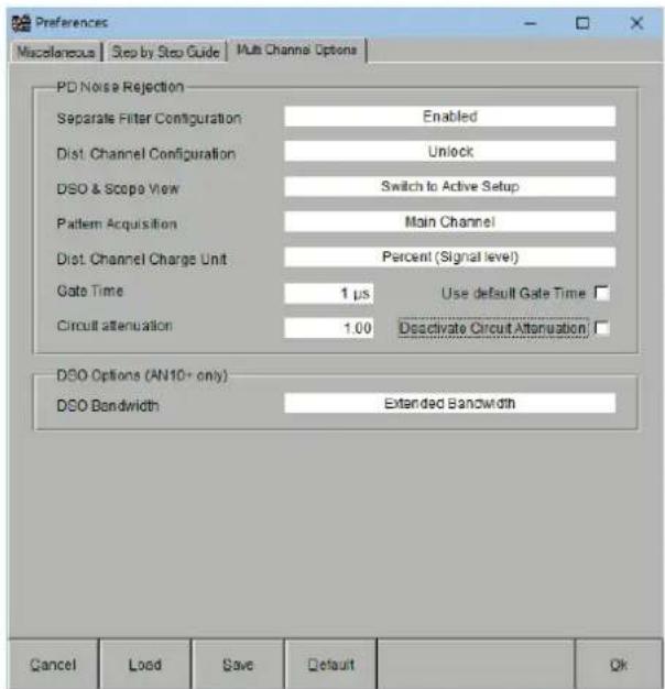
Figure 94: Multi-channel options
To determine the polarity, each pulse must be acquired separately. Acquisition is triggered when one of both channels exceeds the low level discriminator (LLD) setting. At this instant, the dead time starts, and at its end, the positive and negative peak amplitudes of both channels are digitised. To achieve t a good pulse separation, both values must be set very carefully. It would be ideal to set the LLD higher than the noise floor, but in order to see the noise floor in the acquisition pattern, it is recommended to set the LLD to a value which allows triggering only on the highest noise pulses. If the LLD is set too low, the acquisition is triggered too often on noise pulses rather than PD pulses. The dead time must be set to the length of the pulse oscillation. If it is set too short, the pulse will not be finished and double triggering can result. If it is set too long, a second pulse may arrive within the dead time, and the smaller pulse will be ignored.
Depending on the ICMflex2 configuration, the two quadrupoles may have different sensitivities. In this case, the PD gain must be set separately for the two channels. To compare the sensitivities, the user can switch to the auxiliary channel during calibration and set the gain so that the calibrator pulse amplitude is similar to that of the main channel. The LLD can also be set individually for each channel. To get equal pulse properties on both channels, their high-pass and low-pass settings should be equal. To achieve this, the separate filter configuration can be disabled in the multi-channel options of the preferences (see Figure 94).
The ICMflex2 functions can be used with the two right-hand screens in the PD and LOC display of the ICMflex software. Three additional settings are available with these displays:
Channel: For toggling between the main and auxiliary channel in the screen on the upper right-hand side.
Rejection: Offers three different modes of noise cancellation ("First Pol.", "Peak Pol.", and "F&P Pol.")
Dead Time: Time during which a signal is converted, and which is reserved for a single pulse. The A/D converter will not convert or accept another signal during this time, so additional pulses occurring within the dead time are lost.
In general, there are two different methods of pulse polarity detection. The first is to decide at what polarity the LLD is exceeded first ("First Pol."). The second is to compare the peak amplitude of both polarities at the end of the dead time ("Peak Pol."). Additionally, the ICMf/ex2 offers an AND combination of both methods
Partial discharge and loss factor measurement system
("F&P Pol.). The effectiveness of these methods depends on the repetition rate and the amplitude ratio of the two pulse sources. If there is a high repetition rate, the "First Pol." method has a problem when a large disturbance pulse follows a smaller PD pulse. If the amplitude of the pulse sources is very different, the "Peak Pol." method has a problem; if one pulse is over-ranged in both polarities, the peak amplitudes cannot be compared. Examples of pulse polarity detection are shown in Figure 97 to Figure 100.
Calibration and PD measurement is usually done with the main channel. If “Switch to Active Setup” is selected for “DSO & Scope View” within the preferences (see Figure 94), the corresponding screens of the PD and LOC display can also show the auxiliary channel, but no calibration is possible, as the amplitude is shown in percent. For the upper right-hand screen, it is possible to choose, whether the scope view displays the acquisition pattern or the disturbance pattern. The lower right-hand screen always shows the acquisition pattern.
To view the shape of the pulses used for the pattern choose "IEC 60270" for "DSO Bandwidth" in the multi-channel options of the preferences (see Figure 94). In IEC 60270 mode, the DSO shows the filtered signal used for the pattern and the polarity decision. In this mode, only the PD gain is relevant.
ICMflex
Partial discharge and loss factor measurement system

flowchart
graph TD
    A["Resonant test set with variable frequency and high disbursements"] --> B["Resonant test"]
    B --> C["Ground"]
    C --> D["CH1"]
    C --> E["CH2"]
    C --> F["Ch3"]
    C --> G["Ch4"]
    C --> H["Ch5"]
    C --> I["Ch6"]
    C --> J["Ch7"]
    C --> K["Ch8"]
    C --> L["Ch9"]
    C --> M["Ch10"]
    C --> N["Ch11"]
    C --> O["Ch12"]
    C --> P["Ch13"]
    C --> Q["Ch14"]
    C --> R["Ch15"]
    C --> S["Ch16"]
    C --> T["Ch17"]
    C --> U["Ch18"]
    C --> V["Ch19"]
    C --> W["Ch20"]
    C --> X["Ch21"]
    C --> Y["Ch22"]
    C --> Z["Ch23"]
    C --> AA["Ch24"]
    C --> AB["Ch25"]
    C --> AC["Ch26"]
    C --> AD["Ch27"]
    C --> AE["Ch28"]
    C --> AF["Ch29"]
    C --> AG["Ch30"]
    C --> AH["Ch31"]
    C --> AI["Ch32"]
    C --> AJ["Ch33"]
    C --> AK["Ch34"]
    C --> AL["Ch35"]
    C --> AM["Ch36"]
    C --> AN["Ch37"]
    C --> AO["Ch38"]
    C --> AP["Ch39"]
    C --> AQ["Ch40"]
    C --> AR["Ch41"]
    C --> AS["Ch42"]
    C --> AT["Ch43"]
    C --> AU["Ch44"]
    C --> AV["Ch45"]
    C --> AW["Ch46"]
    C --> AX["Ch47"]
    C --> AY["Ch48"]
    C --> AZ["Ch49"]
    C --> BA["Ch50"]
    C --> BB["Max: 450A"]
    B --> BC["I max: 450A"]
    BC --> BD["L line filter LF450"]
    BD --> BE["P02 + GATE"]
    BE --> BF[Cn + GATE / Sn / Sn / Sn / Sn / Sn / Sn / Sn / Sn / Sn / Sn / Sn / Sn / Sn / Sn / Sn / Sn / Sn / Sn / Sn / Sn / Sn / Sn / Sn / Sn / Sn / Sn / Sn / Sn / Sn / Sn / Sn / Sn / Sn / Sn / Sn / Sn / Sn / Sn / Sn / Sn / Sn / Sn / Sn / Sn / Sn / Sn / Sn / Sn / Sn / Sn / Agg
    subgraph Test
        B
        B
        B
        B
        B
        B
        B
        B
        B
        B
        B
        B
        B
        B
        B
        B
        B
        B
        B
        B
        B
        B
        B
        B
        B
        B
        B
        B
        B
        B
        B
        B
        B
        B
Figure 95: General connection diagram for ICMflex2
Partial discharge and loss factor measurement system

Figure 96: ICMflex2 and line filter LF450 installed on an external coupling capacitor
ICMflex
Partial discharge and loss factor measurement system
- Polarity of first pulse exceeding the LLD Sampled peak values
- Polarity of maximum pulse amplitude Peak hold
Pulse from test object Pulse from test voltage source
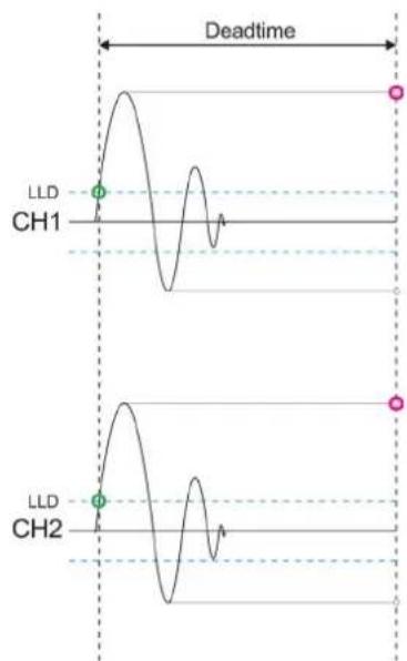
Figure 97: o and have positive polarity on channels => 'First Pol.' and 'Peak Pol.' have the same result.

both Figure 98: ○ positive polarity on channel 1, negative polarity on channel 2; ○ positive polarity on channel 1, negative polarity on channel 2 => 'First Pol.' and 'Peak Pol.' have the same result.
Pulse from test object followed by larger pulse from test voltage source within deadtime

Figure 99: ○ Positive polarity on both channels; ○ positive polarity on channel 1, negative polarity on channel 2 => Only 'Peak Pol.' result is correct: Pulse gets sorted into disturbance pattern.
Pulse from test object with too high amplitude (clipping on both polarities)

line
| Signal | Time Segment | Label | |--------|--------------|-------| | LLD | 0 | LLD | | CH1 | 0 | CH1 | | CH2 | 0 | CH2 |Figure 100: ○ Positive polarity on both channels; ○ no decision possible, => only 'First Pol.' result is correct: Pulse gets sorted into disturbance pattern.
Partial discharge and loss factor measurement system
7.3 Gating via fibre optic link (FO gating)
An ICMflex with an FO gating function has an additional terminal (“FO GATE IN” for a fibre optic (FO) cable, which sends the signal from the gating signal transmitter (GST1) to HV potential. The transmitter is included in the scope of delivery if FO gating is ordered. An external signal sensor (e.g., CT1) is connected via a BNC cable to the “GATE IN” terminal of the GST1.
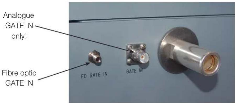
Figure 109: Gating inputs
If disturbances like relay switching or thyristor firing have a known source, it might be possible to create a TTL signal relating to the disturbance. This signal can be used to gate the PD measurement path. If a TTL signal is available, it can be connected via a BNC cable to the "TTL IN" terminal of the GST1.
Caution: Never connect the GST1's BNC TTL output to the analogue gating input of the ICMflex. This will result in serious damage of the instruments!
FO gating and analogue gating can be used simultaneously.
ICMflex
Partial discharge and loss factor measurement system
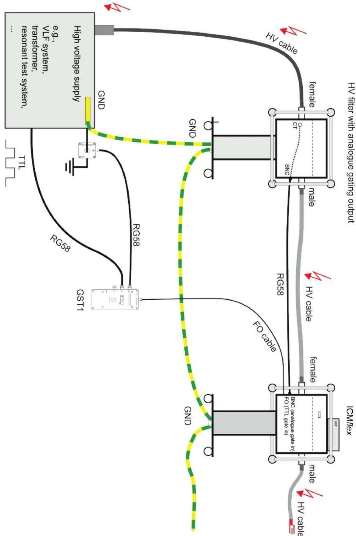
flowchart
graph TD
    A["ICMflex"] --> B["BNC (analogouge gate in)"]
    B --> C["GO (TTL gate in)"]
    C --> D["GO"]
    D --> E["FGS8"]
    E --> F["GT"]
    F --> G["female"]
    G --> H["HV cable"]
    H --> I["HV cable with analogouge gating output"]
    I --> J["High voltage supply"]
    J --> K["e.g., VLF system, transformer, resonant test system..."]
    K --> L["FGS8"]
    L --> M["GT"]
    M --> N["female"]
    N --> O["HV cable"]
    O --> P["HV cable with analogouge gating output"]
Figure 101: Gating connection diagram
Partial discharge and loss factor measurement system
The gating signal transmitter GST1 is shown in Figure 102. It offers logarithmic amplification and can be set to three different frequency ranges (40–800 kHz, 2–20 MHz, or 200–600 MHz), which can be selected with a push-button. The active bandwidth mode is shown by a green LED. The gate level can be adjusted with the GST1 rotary switch and is indicated by the orange LED. The level of the analogue signal incoming via “GATE IN” is indicated by the green LED bar. If it exceeds the selected gate level, the bar changes to red. The gate level should be set to the maximum when using a TTL gating signal as the only signal source.

Figure 102: Gating signal transmitter (GST1)

flowchart
graph LR
    A["Analog Gate In (RG58 cable)"] --> B["Gate level"]
    B --> C["Peak detection"]
    C --> D["Peak > Gate level"]
    D --> E["OR"]
    E --> F["TTL Gate Out (FO cable)"]
    E --> G["TTL Gate Out (RG58 cable)"]
    H["TTL Gate In (RG58 cable)"] --> I["Waveform"]
    I --> J["Waveform"]
    J --> K["Waveform"]
    K --> L["Waveform"]
    L --> M["Waveform"]
    M --> N["Waveform"]
    N --> O["Waveform"]
    O --> P["Waveform"]
    P --> Q["Waveform"]
    Q --> R["Waveform"]
    R --> S["Waveform"]
    S --> T["Waveform"]
    T --> U["Waveform"]
    U --> V["Waveform"]
    V --> W["Waveform"]
    W --> X["Waveform"]
    X --> Y["Waveform"]
    Y --> Z["Waveform"]
    Z --> AA["Waveform"]
    AA --> AB["Waveform"]
    AB --> AC["Waveform"]
    AC --> AD["Waveform"]
    AD --> AE["Waveform"]
    AE --> AF["Waveform"]
    AF --> AG["Waveform"]
    AG --> AH["Waveform"]
    AH --> AI["Waveform"]
    AI --> AJ["Waveform"]
    AJ --> AK["Waveform"]
    AK --> AL["Waveform"]
    AL --> AM["Waveform"]
    AM --> AN["Waveform"]
    AN --> AO["Waveform"]
    AO --> AP["Waveform"]
    AP --> AQ["Waveform"]
    AQ --> AR["Waveform"]
    AR --> AS["Waveform"]
    AS --> AT["Waveform"]
    AT --> AU["Waveform"]
    AU --> AV["Waveform"]
    AV --> AW["Waveform"]
    AW --> AX["Waveform"]
    AX --> AY["Waveform"]
    AY --> AZ["Waveform"]
    AZ --> BA["Waveform"]
    BA --> BB["Waveform"]
    BB --> BC["Waveform"]
    BC --> BD["Waveform"]
    BD --> BE["Waveform"]
    BE --> BF["Waveform"]
    BF --> BG["Waveform"]
    BG --> BH["Waveform"]
    BH --> BI["Waveform"]
    BI --> BJ["Waveform"]
    BJ --> BK["Waveform"]
    BK --> BL["Waveform"]
    BL --> BM["Waveform"]
    BM --> BN["Waveform"]
    BN --> BO["Waveform"]
    BO --> BP["Waveform"]
    BP --> BQ["Waveform"]
    BQ --> BR["Waveform"]
    BR --> BS["Waveform"]
    BS --> BT["Waveform"]
    BT --> BU["Waveform"]
    BU --> BV["Waveform"]
    BV --> BW["Waveform"]
Figure 103: Disjunction of gating signals when simultaneously using analogue and TTL gating
ICMflex
Partial discharge and loss factor measurement system
7.4 Bypass
If the capacitance of the test object is too high, the ICMflex for tan delta measurements can be fitted with a C_x bypass to avoid overstressing of the shunt capacitor. With the bypass active, loss factor measurements are disabled but PD diagnostics are still possible.
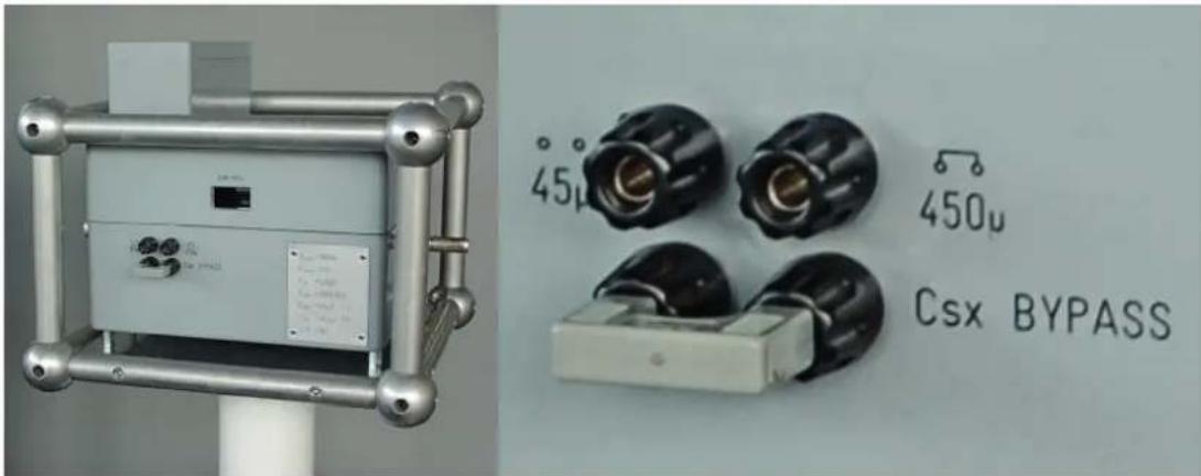
Figure 104: Jumper in bypass mode
7.5 Built-in RPA1L
For applications requiring high sensitivity, the ICMflex can be fitted with a built-in preamplifier (RPA1L), which reduces the instruments input sensitivity to 15 V . It has switchable pre-gain of 1, 10, and 100. The ICMflex with preamplifier has an extended gain list (4 to 80000, see Figure 105). From 4 to 100 the pre-gain is 1, from 200 to 1000 the pre-gain is 10, and from 2000 to 80000 the pre-gain is 100. The range of DSO gain is also influenced by the pre-gain, and the total DSO gain cannot be lower than the pre-gain.
If there is an incorrect connection or a short circuit in the cable from the ICMflex to the RPA1L, the software shows a warning by changing the background colour of the "PD Gain" setting to red.
If an ICMflex2 is equipped with a built-in preamplifier, a second RPA1L must to be installed as close as possible to the quadrupole in the HV filter.
Figure 105: Extended gain list
| 4 |
| 8 |
| 10 |
| 20 |
| 40 |
| 80 |
| √ 100 |
| 200 |
| 400 |
| 800 |
| 1000 |
| 2000 |
| 4000 |
| 8000 |
| 10000 |
| 20000 |
| 40000 |
| 80000 |
7.6 External battery adapter
Power Diagnostix offers an external battery adapter for connecting larger batteries to the instrument, instead of using the standard ICMflex battery BAT2A.
Partial discharge and loss factor measurement system
8 Miscellaneous
8.1 Maintenance
The ICMflex does not require any maintenance on a regular basis, neither is regular fine adjustment needed, as partial discharge measurement is a relative measurement that is calibrated with a reference source (charge calibrator, CAL series) prior to a measurement. The instrument receives high frequency PD signals and assigns them with a pC level based on the calibration made prior to testing. In case of daily usage, it is recommended to calibrate the impulse generator annually to ensure that its output signal remains within the recommended limits. The only part of the instrument that requires calibration is voltage measurement. Voltage calibration should also be calibrated annually, unless the customer's calibration policy defines a different time interval.
Please take care that the instrument stays clean. Any conductive contamination might result into leakage current, which can influence the tan delta measurement results.
8.2 Product marks
This symbol indicates that the marked product should not be disposed of as normal household waste. As it is a B2B product, it may also not be disposed of at civic disposal centres. If you wish to dispose of this product, please do so properly by taking it to an organisation specialising in the disposal of old electrical equipment near you.

natural_image
Simple line drawing of a trash bin with no text or symbolsAny batteries installed must be disposed of separately from the unit.
As a responsible manufacturer, certified according to ISO 14001, Power Diagnostix offers to take back old instruments from its customers. Please contact Power Diagnostix at support@pdix.com to discuss the procedure for this.
8.3 Transport and shipment instructions
8.3.1 Instrument
Generally, we recommend transporting the high voltage filter and the ICMflex in a vertical position to prevent problems with the HV and GND connections of the ICMflex reference capacitor and the T-filter damping capacitor.
If a unit needs to be returned to the factory, make sure the acquisition unit is packed safely. Please use the boxes provided for the shipment. As the units are relatively large, shipment by a forwarding agent is the recommended mode of transportation. If possible, declare the instrument as 'used instruments for evaluation' at a relatively low value. Consult Power Diagnostix for further details. Power Diagnostix may provide you with a temporary replacement unit in urgent cases.
8.3.2 Batteries
If an instrument is suspected to contain a faulty battery module, the module must be removed before the instrument is shipped. Never ship a faulty battery module, either separately or connected to an instrument.
ICMflex
Partial discharge and loss factor measurement system
8.4 Declaration of Conformity
The manufacturer
Power Diagnostix Instruments GmbH
Vaalser Strasse 250
52074 Aachen
Germany

declares that the product
ICMflex
Partial discharge detector for use in high voltage areas
provided it is installed, maintained, and used for which it was made, in accordance with relevant installation standards and manufacturer's instruction, meets the requirements of the following directive(s):
Low Voltage Directive 2014/35/EU
EMC Directive 2004/108/EG
RoHS Directive 2011/65/EU
It complies with the following standards and/or normative documents:
EN 61010-1:2020
EN 61326-1:2013
EN IEC 63000:2018
Aachen, 13/03/2024
Dr. Mihai Huzmezan
(CEO, Power Diagnostix Instruments GmbH)
Note: Since the measurement of partial discharge pulses is done in frequency bands partly occupied by radio transmission, and since test leads may act as antennas, disturbance-free measurements may require well-shielded environments and/or additional filter techniques.
8.5 UK Declaration of Conformity
The manufacturer
Power Diagnostix Instruments GmbH
Vaalser Strasse 250
52074 Aachen
Germany

declares that the product
ICMflex
Partial discharge detector for use in high voltage areas
provided it is installed, maintained, and used for which it was made, in accordance with relevant installation standards and manufacturer's instruction, meets the requirements of the following Statutory Instruments:
SI 2016 no. 1101 The Electrical Equipment (Safety) Regulations 2016
SI 2016 no. 1091 The Electromagnetic Compatibility Regulations 2016
SI 2012 no. 3032 The Restriction of the Use of Certain Hazardous Substances in Electrical and Electronic Equipment Regulations 2012
It complies with the following standards and/or normative documents:
EN 61010-1:2020
EN 61326-1:2013
EN IEC 63000:2018
Aachen, 13/03/2024
Dr. Mihai Huzmezan
(CEO, Power Diagnostix Instruments GmbH)
Note: Since the measurement of partial discharge pulses is done in frequency bands partly occupied by radio transmission, and since test leads may act as antennas, disturbance-free measurements may require well-shielded environments and/or additional filter techniques.
ICMflex
Partial discharge and loss factor measurement system
9 Technical data (standard version)
Mains supply: Battery operated (up to 6 hours)
Power requirements: Approx. 20 VA
Operation: Remote controlled via ICMflex software
PD input impedance: 1 kΩ // 50 pF
PD input sensitivity: < 150 μV, corresponds to 0.2 pC (without built-in preamplifier)
(without test object) < 15 μV, corresponds to 0.02 pC (with built-in preamplifier; ICMflex2 only)
PD lower cut-off (-6 dB): 40, 80, or 100 kHz (software-controlled)
PD upper cut-off (-6 dB): 250, 600, or 800 kHz (software-controlled)
PD A/D converter: 8 bits ( ± 7 bits)
Voltage measurement: 16 bits, 100 kSamples
Voltage values displayed: U RMS value, /2 value, crest factor
Synchronisation: External on reference voltage
Synchronisation range: 20–510 Hz (normal mode) 0.1 Hz, 0.05 Hz, 0.02 Hz (VLF)
Operation temperature: 0–55 °C (non-condensing)
Interfaces: Bluetooth (921 kBit/s)
Fibre optic serial link (921 kBit/s)
9.1 Cable fault location
A/D converter: 8 bits
Samples: 100 MSamples
Specimen cable length: 10 to 5000 m, for a sample rate of 320 s and v_c = 160 m/ s
(Localisation on cables longer than 5000 m is not possible because of pulse attenuation)
Localisation precision: 1 m + 0.1 % of the cable length
9.2 Loss factor measurement
Tan delta resolution: 5 × 10^-5
Tan delta precision: 1 x 10 -4
Partial discharge and loss factor measurement system
9.3 Weight and Dimensions
| TYPE RATED | VOLTAGE U_r (RMS) | MAX. WEIGHTkg | HEIGHTmm | WIDTHmm | LENGTHmm | COMMENT |
| Measurement system | ||||||
| ICMflex 30 kV | 22 600 350 | 350 | ||||
| ICMflex 50 kV | 23 800 350 | 350 | ||||
| ICMflex 100 kV | 24 800 350 | 350 | ||||
| ICMflex 150 kV | 60 1600 450 | 450 | ||||
| ICMflex | >200 kV | - | - | - | To be installed on separate HV reference capacitor of min. 1 nF. | |
| ICMflex2 | >200 kV | 220 | 365 | 350 | To be installed on separate HV reference capacitor of min. 1 nF. | |
| Filter unit | ||||||
| T30 | 30 kV 35 610 350 350 | |||||
| T50 | 50 kV 40 800 350 350 | |||||
| T100 | 100 kV 46/58 985 350 350 | |||||
| T150 | 150 kV 65 1200 350 350 | |||||
| LF450 | - | 130 | 512 | 450 | 450 | To be installed on separate HV blocking capacitors of min. 10 nF. |
ICMflex
Partial discharge and loss factor measurement system
10 Appendix
10.1 What is loss factor (or dissipation factor) tan delta?
Building high voltage equipment requires the use of insulating material. Commonly used insulating materials show losses due to resistive currents and polarisation currents of dipoles. Often, the magnitude of these losses can be used as an indicator for the quality of the insulation. In particular, when assessing the quality of aged insulation, increased dissipation indicates oil or paper decomposition (transformers), humidity, electro-chemical processes (water-trees in polymeric cables), or heavy partial discharge.
With an ideal capacitor (C), the resistance of the insulating material (dielectric) is infinite. When an AC voltage (V) is applied, the current (Ic) leads the voltage by exactly phi = 90°. A component close to this ideal capacitor with negligible resistance should be used as standard (or reference) capacitor for the reference branch of a dielectric loss analyser.
Practical insulation systems are usually built of less than perfect insulating material, resulting in a small current ( I_R ) in phase with the applied voltage (V). This current can be considered as flowing in a resistor (R) in parallel with an ideal capacitor (C). The phase difference between the actual current (I) and the ideal current ( I_C ) can be described as phase angle: delta.
Because P = Q · , where P is resistive power and Q is reactive power, the losses, which are proportional to tan delta, will usually be given as a value of tan delta to express the quality of an insulating material. The angle delta is described as loss angle and tan delta as loss factor.
With the good insulation of low-loss capacitors (delta 0^ and phi 90^ ), the actual current (Ic) is approximately equal to the real

line
| Time | Red Line Value | Black Line Value | |------|----------------|------------------| | 0 | 0 | 1 | | 1 | 0.5 | 0.75 | | 2 | 1 | 0.5 | | 3 | 0.5 | 0.25 | | 4 | 0 | 0 | | 5 | -0.5 | -0.25 | | 6 | -1 | -0.5 | | 7 | -0.5 | -0.75 | | 8 | 0 | -1 | | 9 | 0.5 | -0.75 | | 10 | 1 | -0.5 | | 11 | 0.5 | -0.25 | | 12 | 0 | 0 | | 13 | -0.5 | 0.25 | | 14 | -1 | 0.5 | | 15 | -0.5 | 0.75 | | 16 | 0 | 1 | | 17 | 0.5 | 0.75 | | 18 | 1 | 0.5 | | 19 | 0.5 | 0.25 | | 20 | 0 | 0 |
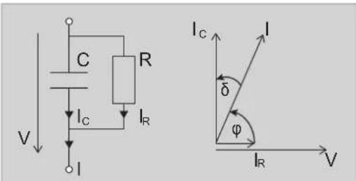
Loss factor (dissipation factor)
$$ \tan \delta = \frac {I _ {R}}{I _ {C}} = \frac {P}{Q} = \frac {1}{\omega \cdot C \cdot R} $$
Quality factor
$$ Q F = \frac {1}{\tan \delta} = \frac {I _ {R}}{I _ {C}} = \frac {P}{Q} = \omega \cdot C \cdot R $$
Power factor
$$ P F = \cos \varphi = \frac {I _ {R}}{1} $$
current (I); resulting in a negligible deviation of the values tan delta and cos phi. In Europe, the dissipation factor tan delta is the most usual figure used to describe dielectric losses, while in North America power factor (PF = ) is commonly used. The ICMflex software displays both values, together with the calculated capacitance, the voltages, and the frequency.
Partial discharge and loss factor measurement system
10.2 Troubleshooting
The personal computer cannot find the ICMflex
If no communication between the ICMflex and the software can be established, please reboot the control computer and check:
- that all necessary drivers are properly installed (see sections 4.2 and 4.3)
• that the battery is charged.
To do this, measure the DC voltage when trying to establish a connection to the ICMflex. Connect the battery to the ICMflex as shown in Figure 106 (check the polarity first!). If the voltage is 10.5 V or less, the battery has to be recharged. If the voltage drops even after charging for at least six hours, the battery is faulty.

natural_image
Industrial testing setup with digital multimeter and control panel (no visible text or symbols)Figure 106: Testing the voltage of the battery
ICMflex
Partial discharge and loss factor measurement system
The ICMflex application window appears very small on high resolution monitors in Windows 10.
On PCs running Windows 10 with the Creator's Update of 2017 the ICMflex application window may appear very small on high resolution monitors. To increase the size of the window, take the following steps:
- Right-click on the application shortcut on the desktop.
- Choose "Properties" from the context menu, which will open the "Properties" window (Figure 107).
- Enable "Override high DPI scaling behaviour" and set "Scaling performed by" to "System" on the "Compatibility" tab.
- If you have administrator rights, you can change the settings for all users by clicking the corresponding button.
- Approve the change by clicking "OK".

Figure 107: Properties window

Figure 108: Desktop before and after changing scaling behaviour

Partial discharge and loss factor measurement system
10.3 National Instruments hardening guide
10.3.1 Introduction
These instructions will guide you through the Power Diagnostix proposed cyber security operation system hardening after the installation of a National Instruments based software product. The configuration refers only to the Power Diagnostix software products. If any other third-party National Instruments-based software products are installed or required, the proposed configuration should be adjusted in line with the configuration of the responsible manufacturer.
This configuration guide will close three unnecessary National Instruments services. The local ports 3848 UDP and TCP opened by these services will also be closed.
| nidmsrv.exe | 3848 | TCPV6 | [0:0:0:0:0:0:0:1] | 49672 | [0:0:0:0:0:0:0:1] | 49673 | ESTABLISHED |
| nidmsrv.exe | 3848 | TCPV6 | [0:0:0:0:0:0:0:1] | 49673 | [0:0:0:0:0:0:0:1] | 49672 | ESTABLISHED |
| nidmsrv.exe | 3848 | TCP | DESKTOP-Q5NEF6E | 59111 | DESKTOP-Q5NE... | 0 | LISTENING |
| nidmsrv.exe | 3848 | UDP | DESKTOP-Q5NEF6E | 5000 | * | * | |
| nidmsrv.exe | 3848 | UDP | DESKTOP-Q5NEF6E | 6000 | * | * |
10.3.2 Step-by-step guide
1.) Open the Windows start menu and type "services.msc".
2.) Click on the search result named "Services". The "Services" window will open.
3.) Locate the following in the service list:
NI Domain Service
NI PSP Service Locator
• NI Time Synchronization
| NI Domain Service | Provides a domain server for NI Shared Variable se... | Running | Automatic | Local Syste... |
| NI PSP Service Locator | Locates servers at the request of network variable c... | Running | Automatic | Network S... |
| NI Time Synchronization | Allows this machine to keep its time synchronized ... | Running | Automatic | Local Syste... |
4.) Open the configuration popup by double clicking each service and change the "Startup type" to "Disabled".
5.) Save the changes with the button "OK".

ICMflex
Partial discharge and loss factor measurement system
10.3.3 Service description
http://www.ni.com/product-documentation/14487/en
| NI Domain Service |
| Service: NIDomainServiceProcess: nidmsrv.exe |
| Description: Provides a domain server for NI Shared Variable security. |
| If Disabled: If this service is stopped or disabled, this machine will be unable to act as a domain when configuring shared variable security. |
| NI PSP Service Locator |
| Service: IkClassAdsProcess: Ikads.exe |
| Description: Locates servers at the request of network variable clients and other proprietary NI network protocols. |
| If Disabled: If this service is stopped or disabled, network variables and network streams will stop working. |
| NI Time Synchronization |
| Service: IkTimeSyncProcess: Iktsrv.exe |
| Description: Allows this machine to keep its time synchronized with a master time server, or to act as a time server for other machines. This feature is configured with the Shared Variable Engine settings in LabVIEW. |
| If Disabled: If this service is stopped or disabled, this form of time synchronization will not be available. |
Partial discharge and loss factor measurement system
11 Index
A
Acquisition box.... 10
Analogue gating.... 41, 42, 46, 55, 75, 77
B
BAT2A.... 13,78
Battery 9, 10, 24, 39, 69, 78, 79, 85
Battery charger.... 13
Bluetooth 7, 10, 12, 16, 18, 22, 82
Bypass 78
C
Calibration .. 23, 24, 30, 32, 37, 39, 40, 41, 43, 44, 45, 46, 54, 55, 59, 60, 63, 67, 69, 70, 71, 79
Calibrator. 8, 13, 37, 39, 40, 46, 54, 55, 59, 60, 67, 70, 79
COM port.... 18, 20, 22, 38
Current transformer 31, 41, 42
D
Digital storage oscilloscope.... 26, 48
Display modes 24, 25, 26, 28, 34, 37, 38, 40
Driver 17, 19, 20, 85
DSO display 37
DSO screen.... 27, 44, 45, 48
F
Fibre optic connection ..... 7, 10, 12, 16, 19, 22, 42, 46
Fibre optic gating 55,75
Filters.... 10, 11, 13, 14, 31, 41, 69, 78, 79
Firmware update 23
G
Grounding 7, 8, 13, 15, 40, 41, 43, 54, 66, 67
GST1 42,75,77
Guard ring control 69
H
Hardening guide 87
High frequency current transformer.... 41
High voltage cables 10, 13, 14, 26, 43, 64
|
ICMflex2.... 69, 70, 71, 72, 73, 78, 82, 83
L
Lithium-ion battery.... 9
LOC display.... 26, 70, 71
Loss factor measurement 1, 3, 12
Low level discriminator.... 31, 42, 46, 55, 70, 74
M
Maintenance.... 79
Multi-contact connector 7, 13, 15
Multi-contact connectors 14
N
Noise cancellation 46, 55, 69, 70
Noise gating 15
Noise reduction 41
P
Pattern acquisition.... 10, 12, 25, 31, 38, 62, 63
PD fault location 10, 12, 24, 26, 43, 44, 48
PD measurement 10, 12, 24, 39, 47, 55
PD pattern .. 10, 12, 25, 31, 37, 40, 42, 46, 48, 52, 56, 62, 64, 65, 69, 70
PD scope.... 10, 12, 31, 37, 42
Preferences 21, 34, 35, 57, 61, 70, 71
R
Reference capacitor.... 10, 14, 32, 79, 83
Report.... 34, 35, 37, 63
Rotating machines 54
S
Safety 7,8,9,10,43,54
Settings 20, 21, 22, 23, 24, 29, 30, 31, 32, 33, 34, 35, 36, 38, 40, 46, 48, 55, 57, 58, 61, 62, 63, 70, 86
Shipment 79
Shunt capacitor 10
Software. 7, 10, 12, 13, 17, 19, 20, 21, 22, 23, 24, 26, 29, 30, 31, 32, 34, 35, 36, 37, 38, 40, 41, 43, 45, 48, 55, 56, 57, 58, 63, 69, 70, 78, 82, 84, 85, 86, 87
Stator bars.... 43, 66, 68, 69
Step-by-step guide.... 57, 87
Synchronisation frequency.... 58
T
Tan delta measurement 10, 57, 61, 66, 67, 68
Technical data 82
T-filter.... 12,79
Time domain reflectometry 12, 26, 27, 44, 46
V
Voltage measurement chart.... 33
ICMflex
Partial discharge and loss factor measurement system
LANGUAGE | EN
USER GUIDE
Power Diagnostix Systems GmbH · Vaalser Strasse 250 · 52074 Aachen Germany · Telephone +49 241 74927 · Fax +49 241 79521 · www.pdix.com
ICMflex_UG_e1.10 March 2024
© Power Diagnostix Systems GmbH 2024


- Power Diagnostix
- NOTICE OF COPYRIGHT and PROPRIETARY RIGHTS
- ICMflex
- Contents
- Functions and menus.... 34
- ICMflex and PD calibration 39
- Gating....41
- Application notes....43
- Medium and high voltage cables.... 43
- Rotating machines....54
- Stator bars 66
- General
- About this user guide
- Instrument safety
- Warning
- Partial discharge and loss factor measurement system
- Health and safety recommendations
- General safety procedures prior to testing
- Health and safety risks
- Environmental conditions
- Lithium-ion battery module warnings
- Principle of operation
- Measurement set-up
- Verifying the part list
- High voltage cabling
- Location
- Parts of the ICMflex under high voltage potential
- Connecting the ICMflex
- Software and driver installation
- Installing the ICMflex software
- Setting up a Bluetooth COM port
- Setting up a fibre optic communication port (USB serial COM)
- ICMflex software
- First steps
- Connecting to the instrument
- Firmware updates and configuration files
- Principle of operation
- PD display mode
- LOC display mode
- REC display mode
- Display mode settings
- Settings for partial discharge measurement
- Settings for PD fault location
- Settings for the record mode
- Note:
- Functions and menus
- Menu items
- File
- Edit
- Connect
- Options
- Tools
- Help
- Function keys
- Report [F1]
- Calibrate [F2]
- Copy [F3]
- Load [F4]
- Save [F5]
- Search/Offline [F6]
- Start Rec / Stop Rec [F7]
- Start Map/Stop Map [F8]
- Print [F9]
- Exit
- ICMflex and PD calibration
- Calibrators
- Gating
- Principle of operation
- Analogue gating
- Example:
- Application notes
- Medium and high voltage cables
- Measurement set-up
- Calibration
- Standard PD measurement
- PD measurements on cables with high capacitance
- PD fault location
- Test voltage recommendations and criteria
- Typical PD patterns and tan delta levels
- Normative references
- Rotating machines
- Test set-up
- Calibration
- PD measurements
- Step-by-step guide
- Step 2: Selection of synchronisation frequency (Figure 77)
- Step 3: Partial Discharge Calibration (IEC 60270)
- Step 4: Apply voltage
- Typical PD patterns and tan delta levels on rotating machines
- Normative references
- Stator bars
- General
- Test set-up
- PD calibration
- PD and tan delta measurement
- Typical patterns and tan delta levels on single stator bars
- Normative References
- Options
- Guard Ring Control (GRC)
- Additional PD input for noise cancellation (ICMflex2)
- Gating via fibre optic link (FO gating)
- Bypass
- Built-in RPA1L
- External battery adapter
- Miscellaneous
- Maintenance
- Product marks
- Transport and shipment instructions
- Instrument
- Batteries
- Declaration of Conformity
- UK Declaration of Conformity
- Technical data (standard version)
- Cable fault location
- Loss factor measurement
- Appendix
- What is loss factor (or dissipation factor) tan delta?
- Troubleshooting
- The personal computer cannot find the ICMflex
- The ICMflex application window appears very small on high resolution monitors in Windows 10.
- National Instruments hardening guide
- Introduction
- Step-by-step guide
- Service description
- Index
- A
- B
- C
- D
- F
- G
- H
- |
- L
- M
- N
- P
- R
- S
- T
- V
Brand : Megger
Model : ICMflex
Category : Meter