EL-9900 - Calculator SHARP - Free user manual and instructions

USER MANUAL EL-9900 SHARP

Declaration of Conformity

Graphing Calculator: EL-9900

This device complies with Part 15 of the FCC Rules. Operation is subject to the following two conditions: (1) This device may not cause harmful interference, and (2) this device must accept any interference received, including interference that may cause undesired operation.

Responsible Party:

SHARP ELECTRONICS CORPORATION

Sharp Plaza, Mahwah, New Jersey 07430-1163

TEL: 1-800-BE-SHARP

Tested To Comply With FCC Standards

FOR HOME OR OFFICE USE

WARNING — FCC Regulations state that any unauthorized changes or modifications to this equipment not expressly approved by the manufacturer could void the user's authority to operate this equipment.

Note: This equipment has been tested and found to comply with the limits for a Class B digital device, pursuant to Part 15 of the FCC Rules.

These limits are designed to provide reasonable protection against harmful interference in a residential installation. This equipment generates, uses, and can radiate radio frequency energy and, if not installed and used in accordance with the instructions, may cause harmful interference to radio communications.

However, there is no guarantee that interference will not occur in a particular installation. If this equipment does cause harmful interference to radio or television reception, which can be determined by turning the equipment off and on, the user is encouraged to try to correct the interference by one or more of the following measures:

— Reorient or relocate the receiving antenna.
— Increase the separation between the equipment and receiver.
- Connect the equipment into an outlet on a circuit different from that to which the receiver is connected.
— Consult the dealer or an experienced radio/TV technician for help.

Note: A shielded interface cable is required to ensure compliance with FCC regulations for Class B certification.

FOR YOUR RECORDS...

For your assistance in reporting this product in case of loss or theft, please record the model number and serial number which are located on the bottom of the unit.

Please retain this information.

Model Number

Serial Number

Date of Purchase

Place of Purchase

Introduction

This graphing calculator can handle many types of mathematical formulas and expressions for you. It is powerful enough to process very complex formulas used in rocket science, but yet so compact that it fits in your coat pocket. The main features of this graphing calculator are as follows:

• Reversible Keyboard to suit the needs of students' levels, ranging from middle-school level arithmetic to high-school calculus, and beyond,
• Graphing Capability to help you visualize what you are working on,
• Slide Show Function to help you understand common formulas, prepare for presentations,
  Large memory capacity, with fast processing speed, and more.

We strongly recommend you read this manual thoroughly. If not, then browse through the very first chapter "Getting Started", at least. Last, but not least, congratulations on purchasing the Graphing Calculator!

NOTICE

• The material in this manual is supplied without representation or warranty of any kind. SHARP assumes no responsibility and shall have no liability of any kind, consequential or otherwise, from the use of this material.
• SHARP strongly recommends that separate permanent written records be kept of all important data. Data may be lost or altered in virtually any electronic memory product under certain circumstances. Therefore, SHARP assumes no responsibility for data lost or otherwise rendered unusable whether as a result of improper use, repairs, defects, battery replacement, use after the specified battery life has expired, or any other cause.
• SHARP assumes no responsibility, directly or indirectly, for financial losses or claims from third persons resulting from the use of this product and any of its functions, the loss of or alteration of stored data, etc.
• The information provided in this manual is subject to change without notice.
• Screens and keys shown in this manual may differ from the actual ones on the calculator.
• Some of the accessories and optional parts described in this manual may not be available at the time you purchase this product.
• Some of the accessories and optional parts described in this manual may be unavailable in some countries.
• All company and/or product names are trademarks and/or registered trademarks of their respective holders.

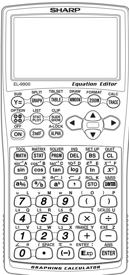
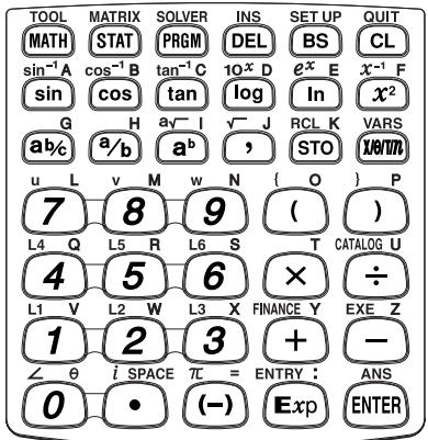
Reversible Keyboard

This calculator comes equipped with a reversible keyboard. Reverse the keyboard to select Basic Mode or Advanced Mode.

Basic Mode

A green background color keyboard with basic mathematical functions. This mode is suitable for learning mathematics in lower grades.

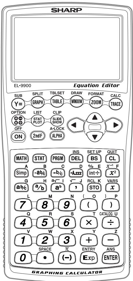
Advanced Mode (Default mode)

A blue background color keyboard with advanced mathematical functions. This mode is suitable for learning or studying mathematics in higher grades.

Contents

Caring for Your Calculator 1

Chapter 1

Getting Started 2

Before Use 2

Using the Hard Cover 3

Part Names and Functions 4

Main Unit 4

Reversible Keyboard 6

Basic Key Operations 8

Changing the Keyboard 9

Quick Run-through: Basic Mode 10

Chapter 2

Operating the Graphing Calculator 13

Basic/AdvancedKeyboard 13

Basic Key Operations - Standard Calculation Keys 13

1. Entering numbers 14
2. Performing standard math calculations 15

Cursor Basics 15

Editing Entries 17

Second Function Key 18

ALPHA Key 19

Math Function Keys 20

MATH, STAT, and PRGM Menu Keys 23

SETUP Menu 24

SETUP Menu Items 25

Precedence of Calculations 27

Error Messages 28

Resetting the Calculator 29

1. Using the reset switch 29
2. Selecting the RESET within the OPTION menu 30

Chapter 3

Basic Calculations - Basic Keyboard 31

1. Try it! 31
2. Arithmetic Keys 33
3. Calculations Using Various Function Keys 35
4. Calculations Using MATH Menu Items 42

Chapter 4

Basic Graphing Features — Basic Keyboard 50

1. Try it! 50
2. Explanations of Various Graphing Keys 52
3. Other Useful Graphing Features 58

Substitution feature 63

Chapter 5

Advanced Calculations - Advanced Keyboard 66

1. Try it! 66
2. Various Calculation Keys 67
3. Calculations Using MATH Menu 70
4. More Variables: Single Value Variables and LIST Variables 80
   5.TOOL Menu. 81
5. SETUP Menu 83

Chapter 6

Advanced Graphing Features - Advanced Keyboard 84

1. Try it! 84
2. Graphing Parametric Equations 87
3. Polar Graphing 88
4. Graphing Sequences 89
5. The CALC Function 93
6. Format Setting 95
7. Zoom Functions 96
8. Setting a Window 98
9. Tables 99
10. The DRAW Function 102
11. Substitution Feature 114

Chapter 7

SLIDE SHOW Feature 115

1. Try it! 115
2. The SLIDE SHOW menu 118

Chapter 8

Matrix Features 120

1. Try it! 120
2. Entering and Viewing a Matrix 122

Editing keys and functions 123

1. Normal Matrix Operations 124
2. Special Matrix Operations 125

Calculations using OPE menus 125

Calculations using MATH menus 129

Use of [] menus 130

Chapter 9

List Features 131

1. Try it! 131
   2.Creating a list 133
2. Normal List Operations 133
3. Special List Operations 135

Calculations using the OPE menu functions 135
Calculations using MATH Menus 139

1. Drawing multiple graphs using the list function 141
2. Using L_DATA functions 142
3. Using List Table to Enter or Edit Lists 143

How to enter the list 143
How to edit the list 144

Chapter 10

Statistics & Regression Calculations 145

1. Try it! 145

2. Statistics Features 149

3. STAT menus 149

4. Statistical evaluations available under the C CALC menu 150

5. Graphing the statistical data 153

6. Graph Types 153

7. Specifying statistical graph and graph functions 157
8. Statistical plotting on/off function 157
9. Trace function of statistical graphs 158

4.Data list operations 159
5. Regression Calculations 160
6. Statistical Hypothesis Testing 165
7. Distribution functions 177

Chapter 11

Financial Features 183

1. Try it! 1 183
   Try it! 2. 187
   2.CALC functions 189
2. VARS Menu 193

Chapter 12

The SOLVER Feature 194

1. Three Analysis Methods: Equation, Newton, and Graphic 194
2. Saving/Renaming Equations for Later Use 200
3. Recalling a Previously Saved Equation 201

Chapter 13

Programming Features 202

1. Try it! 202
2. Programming Hints 204
3. Variables 206
   Setting a variable 206
4. Operands 206
   Comparison operands 206
5. Programming commands 207

APRGM menu 207
B BRNCH menu 209
C SCRN menu 209
D I/O menu 209
E SETUP menu 210
F FORMAT menu 211
G S_PLOT menu 213

1. Flow control tools 214
2. Other menus convenient for programming 216

H COPY menu 216
VARS menu 217

1. Debugging 219
2. Sample programs 220

Chapter 14

OPTION Menu 222

Accessing the OPTION Menu 222

1. Adjusting the screen contrast 222
2. Checking the memory usage 222
3. Deleting files 224
4. Linking to another EL-9900 or PC 224
5. Reset function 227

Appendix 228

1. Replacing Batteries 228
2. Troubleshooting Guide 231
3. Specifications 233
4. Error Codes and Error Messages 235

5. Error Conditions Relating to Specific Tasks 237

6. Financial 237

7. Error conditions during financial calculations 239

8. Distribution function 239

9. Calculation Range 241

10. Arithmetic calculation 241

11. Function calculation 241

Contents

1. Complex number calculation 245

7.CATALOG Feature 246
8. List of Menu/Sub-menu Items 247

1. MATH menus 247
2. LIST menus 249
3. STAT menus 251
4. STAT PLOT menus 253
5. DRAW menus 254
   6.ZOOM menus 255
   7.CALC menus 257
6. SLIDE SHOW menus 258
7. PRGM menus 258
   10.MATRIMXmenus 261
8. FINANCE menus 262
   12.TOOL menus 263
   13.SOLVER menus 264

INDEX 265

Caring for Your Calculator

• Do not carry the calculator around in your back pocket, as it may break when you sit down. The display is made of glass and is particularly fragile.
• Keep the calculator away from extreme heat such as on a car dashboard or near a heater, and avoid exposing it to excessively humid or dusty environments.
• Since this product is not waterproof, do not use it or store it where fluids, for example water, can splash onto it. Raindrops, water spray, juice, coffee, steam, perspiration, etc. will also cause malfunction.
• Clean with a soft, dry cloth. Do not use solvents.
• Do not use a sharp pointed object or exert too much force when pressing keys.
• Avoid excessive physical stress.

Chapter 1 Getting Started

Before Use

Inserting batteries - resetting the memory

1. Open the battery cover located on the back of the calculator. Pull down the notch, then lift the battery cover up to remove it.

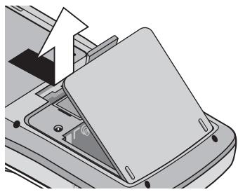
1. Insert the batteries, as indicated. Make sure that the batteries are inserted in the correct directions.

1. Pull off the insulation sheet from the memory backup battery.
2. Place the battery cover back, and make sure that the notch is snapped on.
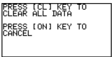
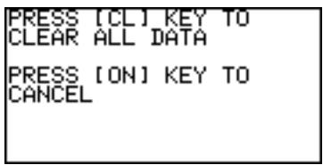
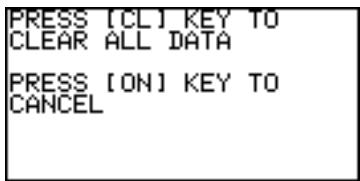
3. Press ON and you will see the following message on the display:

PRESS [CL] KEY TO CLEAR ALL DATA
PRESS [ON] KEY TO CANCEL

Note: If the above message does not appear, check the direction of the batteries and close the cover again. If this does not solve the problem, follow the instruction described in "Resetting the Calculator - 1. Using the reset switch" on page 29.

1. Press CL to reset the calculator's memory. The memory will be initialized. Press any key to set the calculator ready for normal calculation mode.

Adjusting display contrast

Since the display contrast may vary with the ambient temperature and/or remaining battery power, you may want to adjust the contrast accordingly. Here's how:

1. Press 2ndF , then OPTION.

1. Adjust the contrast by using the + and - keys.

2. :increases the contrast - :decreases the contrast

3. When done, press CL to exit the mode.

Turning the calculator OFF

Press 2ndF OFF to turn the calculator off.

Automatic power off function

• The calculator is automatically turned off when there is no key operation for approximately 10 minutes (The power-off time depends on the conditions.)
• The calculator will not automatically power off while it is executing calculations ("I" flashes on the upper right corner of the display.)

Using the Hard Cover

To open the cover:

When in use:

When not in use:

Part Names and Functions

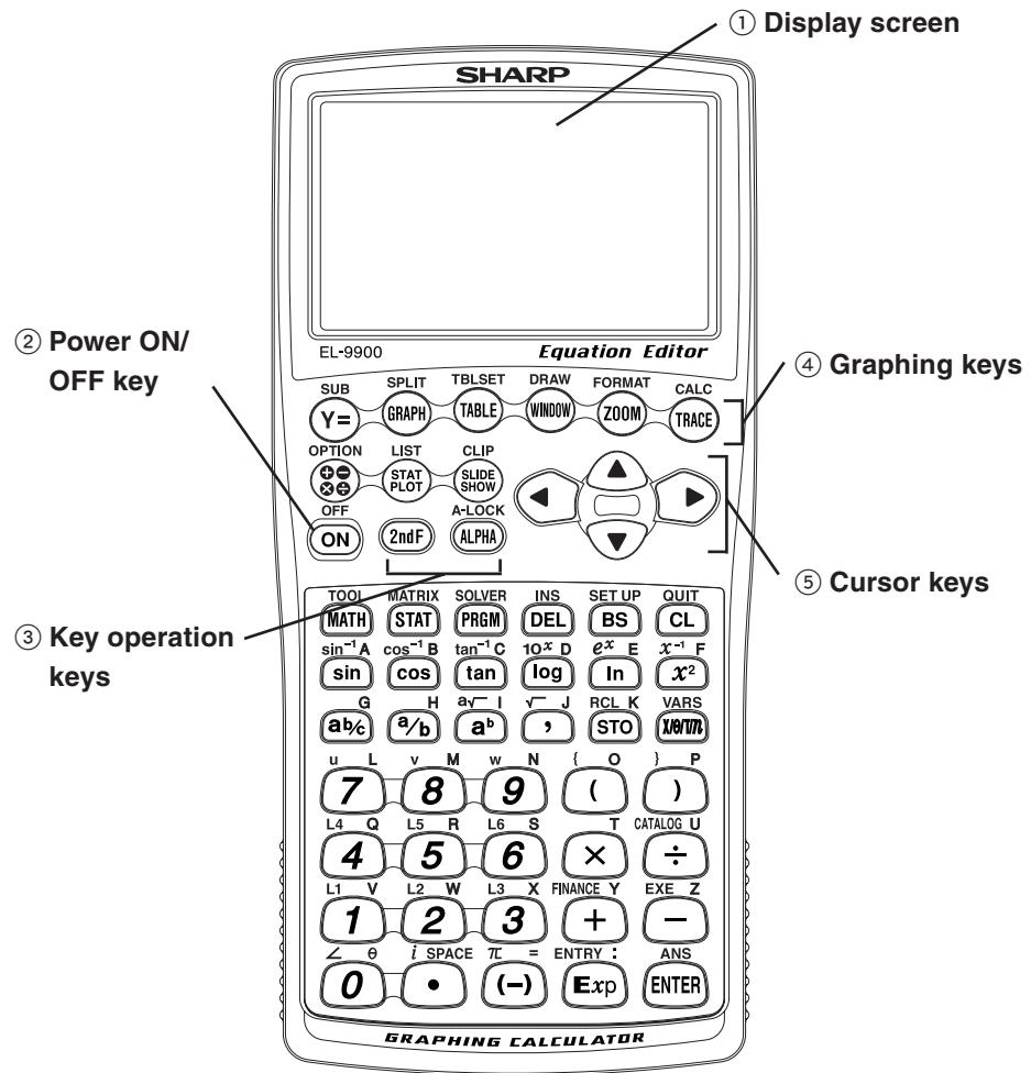
Main Unit

① Display screen:

Displays up to 132 pixels wide by 64 pixels tall of graphs and texts.

② Power ON/OFF key:

Turns calculator ON. To turn off the calculator, press 2ndF, then OFF.

③ Key operation keys:

These keys are used to change the key functions.

2ndF: Changes the cursor to "2", and the next keystroke enters the function or mode printed above each key in yellow.

ALPHA: Changes the cursor to "A", and the next keystroke enters the alphabetical letter printed above each key in purple.

Note: Press 2ndF A-LOCK to lock the specific keys in the alphabet entering mode. (ALPHA-LOCK)

④ Graphing keys:

These keys specify settings for the graphing-related mode.

= : Opens the formula input screen for drawing graphs.

GRAPH: Draws a graph based on the formulas programmed in the Y = window.

TABLE: Opens a Table based on the formulas programmed in =

WINDOW: Sets the display ranges for the graph screen.

ZOOM: Changes the display range of the graph screen.

TRACE: Places the cursor pointer on the graph for tracing, and displays the coordinates.

SUB: Displays the substitution feature.

SPLIT: Displays both a graph and a table at the same time.

TABSET: Opens the table setup screen.

Draw: Draws items on the graph. Use this key also to save or recall the graph/pixel data.

FORMAT: Sets the operations of the graph screen.

CALC:Calculates specific values based on formulas programmed in Y=

⑤ Cursor keys:

Enables you to move the cursor (appears as _, etc. on the screen) in four directions. Use these keys also to select items in the menu.

Reset switch (in the battery compartment):

Used when replacing batteries or clear the calculator memory.

key: Returns calculator to calculation screen.
OPTION key: Sets or resets the calculator settings, such as LCD contrast and memory usage.
CLIP key: Obtains the screen for the slide show.
LIST key:Accesses list features.
SLIDE key: Creates your own slide shows.
STAT key: Sets the statistical plotting. PLOT

Reversible Keyboard

Basic keyboard

Advanced keyboard

Basic Operation keys

ENTER: Used when executing calculations or specifying commands.

CL/ [QUIT]: Clear/Quit key

BS: Backspace delete key

DEL: Delete key

INS: Toggle input mode between insert and overwrite (in one-line edit mode).

SETUP: Allows you to set up the basic behavior of this calculator, such as to set answers in scientific or normal notation.

Menu keys (Function of these keys may vary between basic and advanced mode.)

MATH: Enter the Math menu with additional mathematical functions.
STAT: Enter the statistics menu.
PRGM: Enter the programming menu.
VARS: Enter the menu for calculator specific variables.

Advanced Mode specific keys

TOOL: Converts hexadecimal, decimal, octal and binary numbers or solves systems of linear equations, finds roots for quadratic and cubic equations.
MATRIX: Enter menu for matrix functions
SOLVER: Enter screen and menu for Solver features
FINANCE: Enter menu for financial solver and functions

Scientific Calculation keys (See each chapter for details.)

Basic Mode specific keys

[ \boxed{\mathrm{Simp}} / \boxed{\rightarrow a b \%} / \boxed{\rightarrow b \%} / \boxed{\rightarrow A.x x x} ]

Fraction calculation keys

int ÷ ：Integer division and remainder calculation keys

% : Percentage calculation key

• In Advanced mode, you can access above functions from CATALOG menu.

Advanced Mode specific keys

sin /cos tan / sin-1 / cos-1 / tan-1:

Trigonometric function keys

log /In 10x /e

Logarithm and exponential functions.

Basic Key Operations

Since this calculator has more than one function assigned to each key, you will need to follow a few steps to get the function you need.

Example

• Press "as is" to get the function and number printed on each key.
• To access secondary function printed above each key in yellow, press 2ndF first, then press the key. Press CL to cancel.
• To press the key printed above each key in purple, press ALPHA first, then press the key. When in Menu selection screen however, you do not have to press ALPHA to access the characters. Press CL to cancel.
• If you want enter alphabetical letters (purple) sequentially, use 2ndF A-LOCK. Press ALPHA to return to the normal mode.
• In this manual, alphanumeric characters to be entered are indicated as they are (without using the key symbols). Use of the key symbol indicates that it is for selecting the menu specified by the character or number. The above example also indicates the key notation rules of this manual.

Changing the Keyboard

This calculator is designed with a reversible keyboard, which by utilizing it will not only change the appearance, but will also change the internal functions and configurations of the calculator as well.

To change the keyboard:

1. Press 2ndF OFF to turn off the calculator's power.
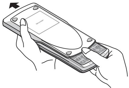
2. Open the battery compartment cover. Hold the calculator as illustrated.
3. Slide the keyboard eject tab (KEYBOARD EJECT) down. The keyboard will be ejected.

Be careful not to drop the keyboard on the floor, as this may damage it.

1. Turn the keyboard over, and replace in the calculator as illustrated. Secure by gently pressing the keyboard until you hear the notch click.

Note: Clean the edges and contact points of the keyboard and the keyboard tap before reattaching the keyboard to the main unit. DO NOT touch the pad portion in the keyboard tap.

1. Replace the battery compartment cover.
2. Press ON

3. Make sure that the message shown on the right appears.

4. Press ON

When you reverse the keyboard, the following settings are automatically changed.

Basic Advanced

• Simplifying: Auto (Auto at SIMPLE in SETUP menu)

Advanced Basic

• Coordinate system: Rectangular coordinates (Rect at COORD in SETUP menu.)
• Answer mode: Displays a mixed number if ANSWER is set to complex numbers.
• Angle unit: Set to Deg if DRG is set to Grad.
• Decimal format: Set to FloatPt if FSE is set to Eng.

Quick Run-through: Basic Mode

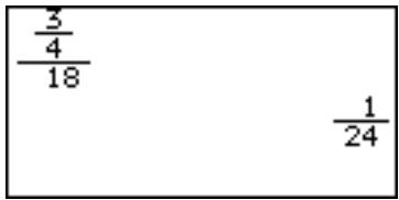
Here are the major ingredients for 18 doughnuts:

14 cup warm water 34 cup warm milk 13 cup sugar
4 cups all-purpose flour
2 eggs
3 tablespoons butter

Based on these values, solve the following problems using the calculator.

Question If you make 60 doughnuts according to the above recipe, how many cups of warm milk are required?

At first, you may calculate how many cups of warm milk are required for 1 doughnut =

$$ \frac {3}{4} \div 1 8 $$

As for the ordinary calculator, the answer is 0.041666666. But how much is 0.04166666 of a cup of warm milk? The Basic mode of this graphing calculator is initially set to the fraction answer mode instead of the decimal answer mode. You may easily obtain the answer in fraction.

Set up the calculator before calculation

1. Press [ ] to enter the calculation screen.
2. Press CL to clear the display.

Enter fractions

1. Press 3 a b 4
2. Press _b 18
3. Press ENTER.

Now we have found 124 of a cup of warm milk is required per one doughnut, how many cups are required for 60 doughnuts?

If you want to use the answer of the previous calculation, press ANS and you do not have to reenter the value.

1. Press 2ndF ANS X, or directly (multiplication).

"Ans×" is displayed. ANS is a calculator specific variable which indicates the answer of calculations just before.

• When you enter + (addition), - (subtraction), × (multiplication), ÷ (division), it is not required to press ANS.

• Press 60.

• Press ENTER.

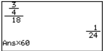
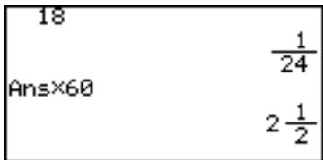
Answer: 212 cups of warm milk are required for making 60 doughnuts.

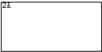
On the Basic Mode, you can toggle between decimal values, mixed values, and improper fractions using A.x x x , a , and b% , respectively.

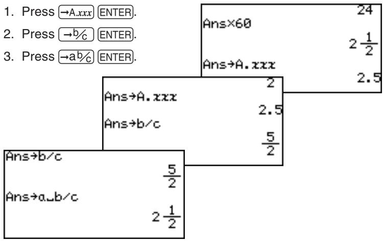
Change answer mode from fractions to decimals

1. Press 2ndF SETUP.

1. Select F ANSWER and press 1.

1. Press CL

Now the answer mode is set to the decimal answer mode and 2.5 is displayed.

Chapter 2 Operating the Graphing Calculator

Basic / Advanced Keyboard

This calculator comes equipped with a reversible keyboard to support two different keyboard configurations: Basic and Advanced keyboard. By reversing the keyboard, the calculator switches its set of functions and behaviors as well as its visual aspect.

The Basic keyboard, with its key frame colored in dark green, is designed to be used by students at lower grades of math classes. Functions associated with complex calculations, such as matrix functions and various trigonometric functions, are not included in this layout to avoid confusing students. Menu items are also carefully chosen to meet the educational needs of the students at lower grades.

With the Advanced keyboard however, all functions and features are accessible for higher grade math students and various professionals in the fields of architecture, finance, mathematics, and physics.

How to switch the keyboard

See page 9.

Basic Key Operations - Standard Calculation Keys

The standard calculation keys, located at the bottom four rows of the keyboard, enable you to access the basic functions of the calculator.

1. Entering numbers

Use the number keys (0 9) , decimal point key (·) , and negative number key (-) to enter numbers into the calculator. To clear the screen entry, press CL.

Number entry

Example

Type 10.23456789 onto the Calculation screen.

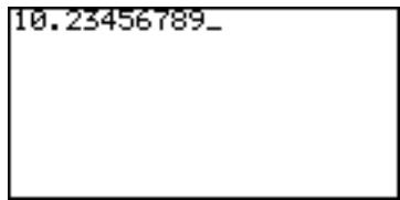
1. Enter the Calculation screen, then clear the screen entry:

1. Enter numbers with the number keys and decimal point key, as follows:

10 23456789

Note: Exp can be used to enter a value in scientific notation.

Example

$$ 6. 3 \times 1 0 ^ {8} + 4. 9 \times 1 0 ^ {7} $$

Entering a negative value

The negative number key (-) can be used to enter numbers, lists, and functions with negative values. Press (-) before entering the value.

Note: Do not use the -key to specify a negative value. Doing so will result in an error.

Example

Type -9460.827513 into the Calculation screen.

2. Performing standard math calculations

By utilizing the + - × and ÷ keys, you can perform the standard arithmetic calculations of addition, subtraction, multiplication, and division. Press ENTER to perform each calculation.

Perform an arithmetic calculation

Example

Obtain the answer to 6 × 5 + 3 - 2 .

Using parentheses

With the ( and keys, parentheses (round brackets) can be added to group sections of expressions. Sections within the parentheses will be calculated first. Parentheses can also be used to close the passings of values in various functions, such as "round(1.2459,2)".

Example

Obtain the answer to (9 + 7)× (5 - 3)

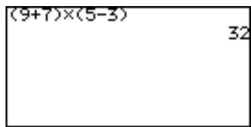
Note: The multiplication sign “ × ”, as the one in the above example, can be abbreviated if it proceeds a math function, a parenthesis “ (·) , or a variable. Abbreviating “ (1 + 2) × 3 ” to “ (1 + 2) 3 ” will result in an error.

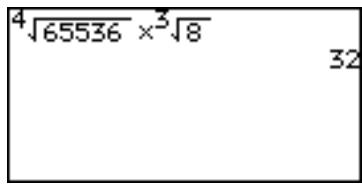
Cursor Basics

The cursor indicates where the next entry will be placed. The cursor may be placed automatically to different areas by various functions and tools, or can be moved around by using the keys. Use the cursor keys to select a menu item, select a cell item in a matrix, and trace along a graph.

Example

Enter [4]65536 × [3]8 in the Calculation screen. Jump the cursor to the beginning of the expression (just for this exercise), then press ENTER to calculate.

1. Press 日 , then to clear the display.
2. Enter 4 for the root's depth, then press 2ndF a√

The root figure is entered, with the cursor automatically placed below the figure.

For detailed instructions of how to use the 2ndF key, refer to "Second Function Key" and "ALPHA Key" in this chapter.

1. Enter 65536.

At this moment, the cursor is still placed under the root figure.

1. Press to move the cursor out of the area, then enter at the cursor.

2. Press 2ndF a√ again. Notice that the cursor is automatically placed so that you can specify the depth of this root figure. Type 3, ▼, and 8.

3. Press ENTER to obtain the answer.

Cursor appearance and input method

The cursor also displays information regarding the calculator's input method. See the following diagram.

Mode	Symbol	Remarks
Normal mode	... | | |	The appearance of the cursor pointer may vary according to the mode or position. The major shapes and the definitions are as follows:
When ALPHA is pressed	... | |
When 2ndF is pressed	... | |	: Insert mode | : Overwrite mode

• , and ^ appear at the insertion point within the functions such as a/b and [n]n .

Editing Entries

Editing modes

The calculator has the following two editing modes: equation mode, and one line mode.

You can select one from the G EDITOR menu of the SETUP menu.

Equation editor

One line editor

* See page 26 for details.

Cursor navigation

Use to move the cursor around, and use the DEL BS CL keys to edit entries.

• DEL key deletes an entry AT THE CURSOR.
• BS key erases one BEFORE THE CURSOR.
• Use CL to clear the entire entry line.

About the Insert mode

When the editing mode is set to one-line, insert mode needs to be manually specified. Press and release 2ndF, then INS to set the insert mode. Press 2ndF INS again to return to the overwrite mode.

The CL key clears all screen entries in the Calculation screen, as well as clearing error messages. It also clears a single line equation in the Y = screen. For more information on the Y = key, refer to Chapters 4 and 6 of the manual.

Example

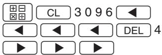
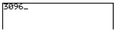
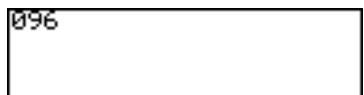
Type 3096, then change 3 to 4. When done, jump the cursor to

the very end of the numbers.

Example

Type 4500000, then remove 500.

Tips: You can jump the cursor to the beginning or the end of line by using the 2ndF and keys. Likewise, press 2ndF to jump the cursor all the way to the bottom. Press 2ndF to jump the cursor to the top. To learn about how to use the 2ndF key and its functions, refer to the section "Second Function Key" of this chapter.

Second Function Key

Use 2ndF to call up the calculator's extended key functions, math functions and figures.

All functions associated with 2ndF are color coded light yellow, and are printed above each key.

Note: Available Second function keys differ between the Basic keyboard and the Advanced keyboard. For example, a second function “ e^x ” is not accessible within the Basic keyboard.

Example

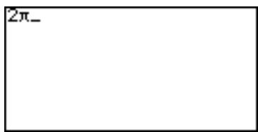
Enter "2π" on the screen.

1. Press CL to clear the screen, then enter "2" by pressing 2.
2. Press 2ndF. When the key is released, the cursor on the screen changes, indicating that a second function is now ready to be called up.
3. Press . The entry appears on the screen.

ALPHA Key

Use ALPHA to enter an alphabet character. With the Basic keyboard, all 26 alphabet characters from "A" up to "Z", and space can be typed; the Advanced keyboard has all 26 characters accessible, as well as "θ", "=", " : ", and space.

All functions associated with ALPHA are color coded purple, and are printed above each key.

Note: Do not type out math figures (sin, log, etc.), graph equation names (Y1, Y2, etc.), list names (L1, L2, etc.), or matrix names (mat A, mat B, etc.), etc. with ALPHA keys. If “SIN” is entered from ALPHA mode, then each alphabet character — “S”, “I” and “N” — will be entered as a variable. Call up the figure and equation names from within the second functions and various menus instead. If a colon (:) is used, data may continue to be entered in more than one term.

Entering one Alphabet character

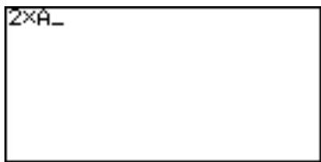
Example

Enter 2× A on the screen.

1. Press CL to clear the screen. Enter "2 x" by pressing 2 x.

1. To enter "A", press ALPHA; the cursor pattern changes to "A" upon releasing the key.

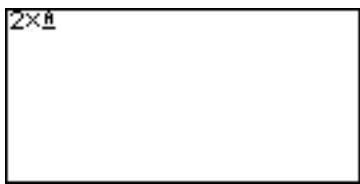
1. Press A to call "A" at the cursor. After the entry, the cursor pattern changes back to normal.

Entering 1 or More Alphabet characters

To type more than one alphabet character, use 2ndF then ALPHA to apply the "ALPHA-LOCK". When done, press ALPHA to escape from the mode.

Math Function Keys

Basic keyboard

Advanced keyboard

Mathematical functions can be called up quickly with the Math Function keys. The Math Function key sets for both the Basic and Advanced Keyboards are designed to suit the needs of calculations at each level.

Math Function keys for the

Basic keyboard:

Simp Reduces a fraction
ab% Converts a number to a mixed fraction, if possible
2% Converts a number to an improper fraction
A.xxx Converts a number to decimal form
int- Gives an answer in quotient and remainder
% Specifies a percentage number
Enters an variable "x" at the cursor

Math Function keys for the

Advanced keyboard:

sin Enters a sine function at the cursor
^-1 Enters an arc sine function at the cursor
cos Enters a cosine function at the cursor

^-1 Enters an arc cosine function at the cursor
tan Enters a tangent function at the cursor
tan-1 Enters an arctangent function at the cursor
log Enters a logarithm function at the cursor
10x Enters "10 to the x th power", then sets the cursor at the "x"
In Enters a natural logarithm function at the cursor
^x Enters "e-constant to the power of x ", then sets the cursor at the "x"
/ /T / n Enters a variable x , "0, T", or "n". The variable is automatically determined according to the calculator's coordinate setup: "x" for rectangular, "0" for polar, "T" for parametric, "n" for sequential.

Common Math Function keys for both keyboards:

^2 Enters " ^ 2 " at the cursor, to raise a number to the second power
^-1 Enters“-1”at the cursor,to raise a number to the negative first power
%b% Enters a mixed number.
a b Enters a fraction.
a b Enters an exponent.
a√ By itself enters a "root" figure; the cursor will be set at "a", the depth.

Note: If a number precedes % / b ^b and , then the number will be set as the first entry of the figure. Else, the first entry is blank and the cursor flashes.

Examples

2ab 3
4

ab%

4 2 3 4

Enters a "root" figure at the cursor
Enters“，”(a comma)at the cursor
STO Stores a number or a formula into a variable
RCL Recalls an item stored in a variable
VARS Brings up the VARS menu.

MATH, STAT, and PRGM Menu Keys

By using the MATH, STAT, and PRGM keys, you can access many menu items for complex calculation tasks. The appendix "List of Menu/Sub-menu Items" shows the contents of each, with detailed descriptions of each sub-menu item.

Note that the contents of menu items differ drastically between the Basic keyboard and the Advanced keyboard. For example, the PRGM menu for the Basic mode contains only one item (A EXEC), while in the Advanced mode there are three menu items (A EXEC, B EDIT, and C NEW).

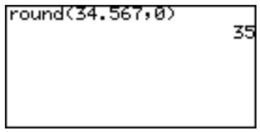
Example

Round the following number beyond the decimal point: 34.567

1. Press CL, then MATH.The MATH menu takes over the screen, as shown to the right.MATH menu items are displayed on the left side of the screen.

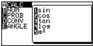
Note: The example above is simulated on the Basic mode. There are more menu items available with the Advanced mode.

1. Use the and keys to move the cursor up and down the menu. As you scroll, you will see the corresponding sub-menu contents (shown on the right side of the screen) change.
2. Set the cursor at B NUM.

Menu items can also be selected by using shortcut keys (A through H); in this example, simply press B to select B NUM. There is no need to use ALPHA for this operation.

1. Press a shortcut key 2 to select 2 round(). The screen now goes back to the calculation screen, as follows:

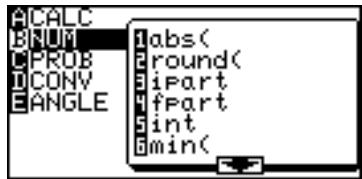
Another way of selecting the sub-menu item is to press (or ENTER) on the menu item B NUM. The cursor will be extended into the sub-menu on the right. Now, move the cursor on the sub-menu down to 2 round(), then press ENTER.

5.Type34 5670）,andpressENTER

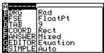
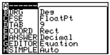
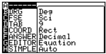
SETUP Menu

Use this menu to verify basic configurations, such as to define the calculator's editing preferences, and scientific and mathematical base units.

Checking the calculator's configuration

To check the current configuration of the calculator, press 2ndF, then SETUP.

By entering menu items (B DRG through H SIMPLE), various setups can be changed. To exit the SETUP menu, press CL.

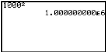
Example

Display the calculation result of "1000" in scientific notation.

1. Press 2ndF, then SETUP. Within the SETUP menu, press C, then 3 to select 3 Sci under the C FSE menu.

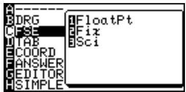
Tips: Using the arrow keys, move the cursor down to the C FSE position, press ENTER, and then move the cursor down to the 3 Sci position. Press ENTER to select the sub-menu item.

1. The display goes back to the SETUP menu's initial screen.
2. Press CL to exit the SETUP menu.

1. Press CL to clear the Calculation screen, type 1000 x^2 , then ENTER

SETUP Menu Items

DRG: For trigonometric calculations and coordinate conversions, various angle units can be selected:

Deg Angle values to be set in degrees (default for Basic mode)

Rad Angle values to be set in radians (default for Advanced mode)

Grad Angle values to be set in gradients (for Advanced mode only)

FSE: Various decimal formats can be set:

FloatPt Answers are given in decimal form with a floating decimal point (default).

Fix Answers are given in decimal form. The decimal point can be set in the TAB menu.

Sci Answers are given in "scientific" notation. For example, "3500" is displayed as "3.500000000E3". The decimal point can be set in the TAB menu.

Eng Answers are given in "engineering" notation with exponents set to be multiples of 3. "100000" will be displayed as "100.0000000E3", and "1000000" will be shown as "1.000000000E6". The decimal point can be set in the TAB menu. (for Advanced mode only)

Note: If the value of the mantissa does not fit within the range ± 0.000000001 to ± 9999999999 , the display changes to scientific notation. The display mode can be changed according to the purpose of the calculation.

TAB: Sets the number of digits beyond the decimal point (0 through 9). The default is "9".

COORD: Sets the calculator to various graph coordinate systems.

Rect Rectangular coordinates (default)

Param Parametric equation coordinates (for Advanced mode only)

Polar Polar coordinates (for Advanced mode only)

Seq Sequential graph coordinates (for Advanced mode only)

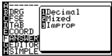
ANSWER: Sets the answer preference to various number formats.

Decimal (Real) Answers will be given in decimal form (default for Advanced mode)

Mixed (Real) Answers will be given in mixed fractions, whenever appropriate (default for Basic mode)

Improp (Real) Answers will be given in improper fractions, whenever appropriate

x ± yi (Complex) Answers will be given in complex rectangular form (for Advanced mode only)

r (Complex) Answers will be given in complex polar form (for Advanced mode only)

EDITOR: Sets the editing style to one of two available formats.

Equation

Formulas can be entered in a "type it as you see it approach" (default setting).

One line

Formulas will be displayed on one line.

Notes: Immediately after changing the EDITOR, the calculator will return to the calculation screen and the following data will be cleared.

• ENTRY memory
  Equations stored in the graph equation window ( = )
• Equations temporally stored in the SOLVER window (2ndF SOLVER)
• Resetting to the default settings (2ndF OPTION E 1) will also clear the above data.

Expression of up to 114 bytes can be entered in the Equation edit mode. If the expression exceeds the screen width, it is horizontally extended.

Expression of up to 160 bytes can be entered in One-line edit mode. if the expression exceeds the screen width, it goes to the next line.

SIMPLE: Sets the preference for handling reducible fractions.

Auto Fractions will automatically be reduced down (default)

Manual Fractions will not be reduced unless Simp is pressed

Note: All the procedures in this manual are explained using the default settings unless otherwise specified.

Precedence of Calculations

When solving a mathematical expression, this calculator internally looks for the following figures and methods (sorted in the order of evaluation):

1) Fractions (1/4, a/b, , etc.)
2) Complex angles ()
3) Single calculation functions where the numerical value occurs before the function (X^2, X^-1, 1, "^ , "^ , and ^ )
4) Exponential functions (a,b, a√, etc)
5) Multiplications between a value and a stored variable/constant, with “ × ” abbreviated (2π, 2A, etc.)
6) Single calculation functions where the numerical value occurs after the function (sin, cos, tan, sin ^-1 , cos ^-1 , tan ^-1 , log, 10x, In, ex, , abs, int, ipart, fpart, (-), not, neg, etc.)

7) Multiplications between a number and a function in #6 (3cos20, etc. "cos20" is evaluated first)
8) Permutations and combinations (nPr, nCr)
9) x, ÷
10) +, -
11) and
12) or, xor xnor
13) Equalities and nonequalities (<, , >, ≥, , , dms, etc.)

Example

The key operation and calculation precedence

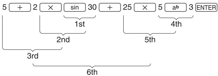
• If parentheses are used, parenthesized calculations have precedence over any other calculations.

Error Messages

The calculator will display an error message when a given command is handled incorrectly, or when instructions cannot be handled correctly such that the task cannot be processed further. Various types of error messages are given to inform users the types of situations to be remedied.

For example, performing the following key strokes:

will result in an error, and the error message will be displayed.

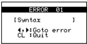
In such a situation, you can go back to the expression to correct its syntax by pressing < or , or you can erase the entire line to start over by pressing .

For a list of various error codes and messages, refer to the appendix.

Resetting the Calculator

Use the reset when a malfunction occurs, to delete all data, or to set all mode values to the default settings. The resetting can be done by either pressing the reset switch located in the battery compartment, or by selecting the reset in the OPTION menu.

Resetting the calculator's memory will erase all data stored by the user; proceed with caution.

1. Using the reset switch

1. Pull down the notch to open the battery cover located on the back of the calculator.
2. Place the battery cover back until the notch is snapped on.
3. Press ON.

The verification window will appear on the screen.

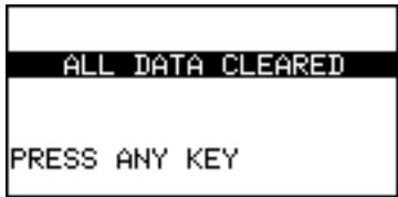
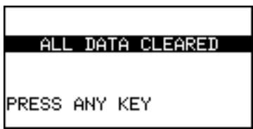
1. Press CL to clear all the stored data. Press ON to cancel resetting. After CL is pressed, the calculator's memory will be initialized. Press any key to display the calculation screen.

Note: If the above verification window does not appear, remove the battery cover and gently push the RESET switch with the tip of a ball-point pen or a similar object.

DO NOT use a tip of a pencil or mechanical pencil, a broken lead may cause a damage to the button mechanism.

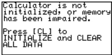
• The message on the right may occasionally appear. In this case, repeat the procedure from step 1 to prevent loss of data.

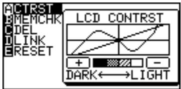
2. Selecting the RESET within the OPTION menu

1. Press 2ndF then The OPTION menu appears.

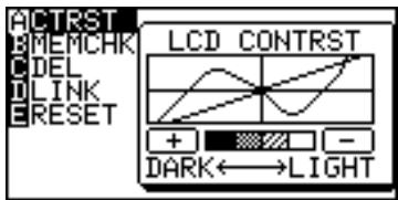
1. While in the OPTION menu, press E to select E RESET; the RESET submenu items should appear on the right side of the screen.

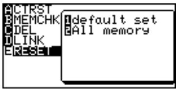
1. The first item 1 default set will initialize only the SETUP and FORMAT settings, while the second item 2 All memory will erase all memory contents and settings. To reset the memory, select 2 All memory by pressing 2. The verification window will appear.

2. Press the CL key to clear all data stored on the calculator. Press any key to continue.

Chapter 3

Basic Calculations — Basic Keyboard

In this chapter, we explore more features of this calculator using the Basic Keyboard. Features such as fraction to decimal conversion and the quotient-remainder key, as well as basic arithmetic calculations, will be covered in this chapter.

Note: To try the examples in the chapter, it is required that the Basic Keyboard is already set up by the user. To learn how to set up the Basic Keyboard, read "Changing the Keyboard" in Chapter 1.

1. Try it!

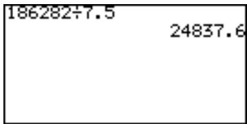
The speed of light is known to be 186,282 miles (approximately 300,000 kilometers) per second. That means light can go around the earth 7 and a half times within a second!

Suppose you are standing at the equator. While the earth rotates over the period of one day, you also rotate around the globe at a certain speed. Knowing the facts above, can you figure out how fast you are traveling, in miles per hour?

Since distance traveled = average speed × time taken, the following equation can be formed to find out the circumference of the earth (x miles):

$$ x \times 7. 5 = 1 8 6 2 8 2 $$

Then,

$$ x = 1 8 6 2 8 2 \div 7. 5 $$

Since you know the earth turns around once a day (which means, in 24 hours), divide the above "x" with 24 to get a value in miles per hour.

$$ 2 4 \times v = x $$

$$ v = \frac {x}{2 4} $$

CONCEPT

1. Enter a math expression, then perform the calculation.
2. Save a number into a variable, then recall the value later.

PROCEDURE

1. First, press 日 , then to clear any screen entries.

2. Type 186282 ÷ 7.5, then press ENTER. The circumference of the earth is thus obtained.

1. Store the answer in a variable. A variable is a symbol under which you can store a numerical value.

We will use variable A to store the circumference of the earth. Press STO to set the "store" mode. Press ALPHA A, then ENTER to

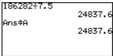
store the answer. To call up

the stored answer, press ALPHA A ENTER again.

Note: While checking the stored values, you may see "0"; this means that no value is stored in the variable.

1. Now, since the value you have stored under "A" is the distance you will be travelling in 24 hours, divide the number by 24. Press ALPHA

A 24, then ENTER.

So, you are travelling at 1034.9 miles/hour. That is fast!

2. Arithmetic Keys

Performing addition, subtraction, multiplication and division

There are various keys for arithmetic calculations. Use the + - X ÷ ,(-), and) keys to perform basic arithmetic calculations. Press ENTER to solve an equation.

ENTER executes an expression.

Example

Calculate 1 + 2

A Note about expressions

An expression is a mathematical statement that may use numbers and/or variables that represent numbers. This works just like a regular word sentence; one may ask "how are you?", and you may answer "okay." But what if an incomplete sentence is thrown, such as "how are"? You'll wonder, "how are... what?"; it just doesn't make sense. A math expression needs to be complete as well. 1 + 2 , 4x , 2 x + x form valid expressions, while "1 +" and "cos" do not. If an expression is not complete, the calculator will display an error message upon pressing the ENTER key.

• Enters a " ^+ " sign for addition.

Example

Calculate 12 + 34

• Enters a “-” sign for subtraction.

Example

• Subtract 21 from 43.

× Enters a " x " sign for multiplication.

Example

• Multiply 12 by 34.

12 X 34 ENTER

12×34	408
54÷32	1.6875

Enters a 12 sign for division.

Example

Divide 54 by 32.

54÷ 32ENTER

When to leave out the “×” sign

The multiplication sign can be left out when:

a. It is placed in front of an open parenthesis.
b. It is followed by a variable or a mathematical constant (, e, etc.) :
c. It is followed by a scientific function, such as sin, log, etc.:

2(3+4)	14
(X-3)(X+4)	-12

2A	49675.2
3π	9.424777961
2108 10	2

Entering a number with a negative value

(-) Sets a negative value.

Example

Calculate -12× 4

(-) 12 X 4 ENTER

-12×4

-48

Note: Do not use the - key to enter a negative value; use the (-) key instead.

Enters an open parenthesis. Use with “)” as a pair, or the calculation will result in an error.
) Enters a closing parenthesis; a parenthesis left open will result in an error.

Example

Calculate (4 + 6)÷ 5

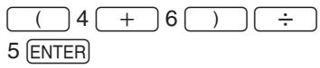
Note: Functions, such as "round( automatically include an open parentheses. Each of these functions needs to be closed with a closing parenthesis.

3. Calculations Using Various Function Keys

Use the calculator's function keys to simplify various calculation tasks. The calculator's Basic Keyboard is specially designed to help you learn/solve fraction calculations easier.

Simp

Simplifies a given fraction stored in the ANSWER memory.

(Set the SIMPLE mode to Manual in the SETUP menu to use this key.)

Specifying no common factor

Simplify the fraction using the lowest common factor other than 1.

Example

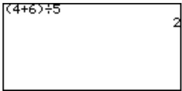
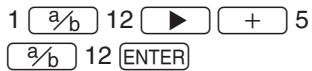
1 a b 12 +5

a b 12 ENTER

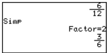
Simp ENTER (Simplified by 2, the lowest common factor of 12 and 6.)

Simp ENTER (Simplified by 3, the lowest common factor of 6 and 3.)

Specifying a common factor

Simplify the fraction using the specified common factor.

Example

Simp 6 ENTER (Manually specify 6, the Greatest Common Factor of 12 and 6, to simplify the fraction.)

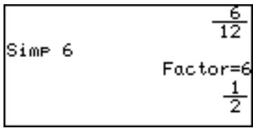
Note: If the wrong number is specified for a common factor, an error will occur.

Simp is effective in a fraction calculation mode only (when the ANSWER mode is set to Mixed or Improp in the SETUP menu).

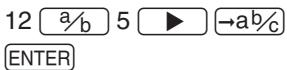
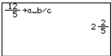
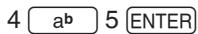
a% Converts an improper fraction to a mixed number.

Example

• Change 125 to a mixed number.

% Converts a mixed number to an improper fraction.

Example

• Change 225 to an improper fraction.

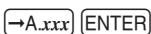
A.xxx Converts a fraction to a decimal number.

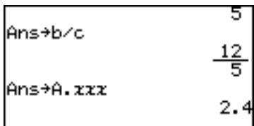
Example

• Change 125 to a decimal number.

Note: Above three conversions will not affect the ANSWER settings in the SET UP menu.

If a decimal number is not rational, fraction conversion will not function and display the answer in decimal format.

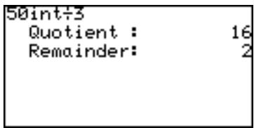
Performs an integer division, and returns a quotient and a remainder.

Example

• Get a quotient and a remainder of 50 ÷ 3 .

50 int ÷ 3 ENTER

• Quotient value is set to An
  memory and remainder is not
  stored.

Squares the preceding number.

Example

• Obtain the answer to 12^2 . (= 144)

12 ^2

Note: When no base number is entered, the base number area will be left blank and just the exponent appear.

CL x2 1 2 ENTER 

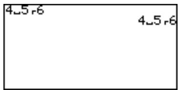
Enters a mixed number.

Example

Enter 4 5

4abc56ENTER 

Note: When no value is entered prior to this key, the number areas will be left blank.

• If the calculator is set to one-line mode, % enters “ ” (integer-fraction separator) only. Use % in combination with % as follows.

• Enter 456 in one-line mode

4ab 5 a6 ENTER 

• Integer part of the mixed number must be a natural number. A variable can not be

used. Equation or use of parenthesis, such as (1 + 2) 2- 3 or (5) 2- 3 , causes syntax error.

• When a numerator or a denominator is negative, the calculator will cause error.

a/b

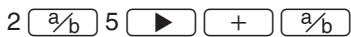
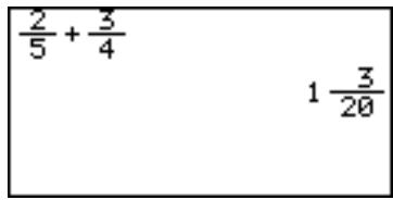
Enters a fraction, setting the preceding number as its numerator.

• If the calculator is set to one-line mode, then “ ” will be entered instead. For example, “ 2 5 ” indicates “ 25 .

Example

Calculate 25 +34

a

Enters an exponent, setting the preceding number as its base.

Example

• Raise 4 to the 5th power. (= 1024)

Note: When no base value is entered, “a” will be entered with both number areas left blank.

When calculating x to the power of m -th power of n , enter as follows;

Calculate 2^32 (= 512)

The above calculation is interpreted as 2^3^2 = 2^9 .

If you wish to calculate (2^3)^2 = 8^2 , press () 2 3 ) 2 .

，

Enters a comma “, ” at the cursor. A comma is required in some of the MATH functions. For more information, refer to the next section “Calculations Using MATH Menu Items” in this chapter.

STO

Stores a number in a variable.

Example

• Let A = 4 , and B = 6 .

Calculate A + B

Enters an "x", an unknown variable. Use this key when working with graph equations. Refer to Chapter 4 "Basic Graphing Features" to learn how to use this feature.

Second functions

To access the second function of a key (printed above the keys in yellow), press and release 2ndF , then press the key you want to use.

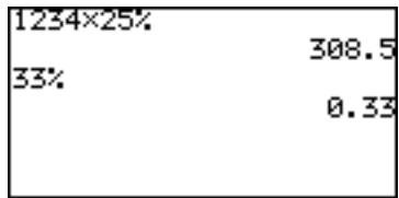
% Set the preceding value as a percentage.

Example

• Get 25% of 1234.

1234 X 25 [2ndF]

% ENTER

• Percentage must be a positive value equal to or less than 100.

x^-1 Enters "x", and returns an inverse by raising a value to the -1 power. The inverse of "5", for example, is 15 .

Example

• Raise 12 to the -1 power. (= 0.08333333)

12ndF x-1 ENTER

Note: When no base number is entered, “ x^-1 ” will be entered, with “ x ” left blank.

CL 2ndF x-1 1 2 ENTER

a√ Enters“a

Example

• Bring 4 to the 5^th root. (= 1.319507911)

5 2ndF a√ 4 ENTER

Note: When no depth of power is entered, “ [n]n ” is entered, with both number areas left blank.

CL 2ndF a√5 4 ENTER

Enters a square root symbol.

Example

• Obtain the square root of 64. (= 8)

2ndF 64 ENTER

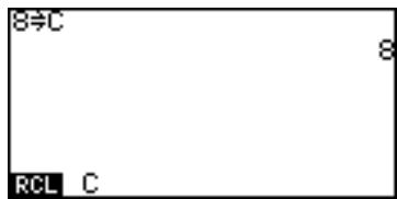
RCL Recalls a variable.

Example

• Set C = 8

8 STO ALPHA C ENTER

Recall the value of C.

2ndF RCL ALPHA C ENTER

VARS Accesses the VARS menu. Refer to chapters 4 and 6 to learn how to use each item in this menu.

Enter braces to group numbers as a list.

ANS Recalls the previous answer. Use this key to incorporate the answer to the previous calculation into an expression.

Example

• Perform 3 × 3 .

3 X 3 ENTER

Subtract the value of the previous answer from "10".

10 - 2ndF ANS ENTER

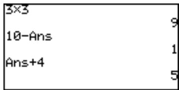
Note: ANS can be considered as a variable; its value is automatically set when ENTER is pressed. If ANS is not empty, then pressing +, -, ×, or ÷ will recall "Ans" and places it at the beginning of an expression. If "1" was the previous answer, then pressing + 4 ENTER will result in "5".

ENTRY

Recalls the previous entry. This is useful when you want to modify the previous entry, rather than reenter the whole expression over.

Example

Calculate 4× 6

4 X 6 ENTER

Next, calculate 4 × 8 .

2ndF ENTRY BS 8 ENTER

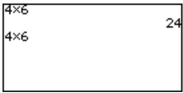
Note: Executed expressions are stored in a temporary memory in the executed order. If the temporary memory is full, the oldest data is automatically deleted. Be aware that may not function on these occasions.

A maximum of 160 bytes can be stored in the temporary memory. The capacity may vary when there are division codes between expressions.

When switching from equation edit mode to one-line edit mode in the SETUP menu, all the numerical and graph equations stored in the temporary memory are cleared and cannot be recalled.

π

Enters "pi". Pi is a mathematical constant, representing the ratio of the circumference of a circle to its diameter.

Example

• Enter "2π". (= 6.283185307)

2ndF ENTER

CATALOG

Calls up the CATALOG menu. From the CATALOG menu, you can directly access various functions in the menus.

• Functions are listed in alphabetic order.
• Move the cursor using the keys and press ENTER to access or enter the function.
• Press ALPHA and an appropriate alphabetic key (A to Z) to navigate the catalog.
• Press ALPHA + ▲ to scroll the catalog page by page and press 2ndF + ▲ to jump to the beginning or the end of the catalog.
  See page 246 for details.

4. Calculations Using MATH Menu Items

The MATH menu contains functions used for more elaborate math concepts, such as trigonometry, logarithms, probability, and math unit/format conversions. The MATH menu items may be incorporated into your expressions.

Note: The default angle measurement unit while using the calculator's Basic Keyboard is degrees. If you wish to work in radians, then the configuration must be changed in the SET UP menu. For more information, see page 25.

A Note about Degrees and Radians

The degree and radian systems are two of the basic methods of measuring angles. There are 360 degrees in a circle, and “2-pi” radians. 1 degree is equal to pi/180 radians. “Then, what’s this pi?”, you may ask. Pi, or to use its symbol “π”, is the ratio of the circumference of a circle to its diameter. The value of π is the same for any circle “3.14...”, and it is believed to have an infinite number of digits beyond the decimal point.

A CALC

The CALC sub-menu contains items to be used in calculations containing trigonometric and logarithmic functions.

Note: The following examples show keystrokes with keyboard shortcuts. It is also possible to select a sub-menu item using the cursor keys.

1 sin Enters a sine function to be used in a trigonometric calculation.

Example

Calculate sine 90^

MATH A 1 90 ENTER

2 cos Enters a cosine function to be used in a trigonometric calculation.

Example

Calculate cosine 60^

MATH A 2 60 ENTER

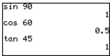
3 tan Enters a tangent function to be used in a trigonometric calculation.

Example

Calculate tangent 45^

MATH A 3 45 ENTER

4 log Enters a "log" function for a logarithmic calculation

Example

Calculate log 100.

MATH A 4 100

ENTER

5 10^× Enters a base of 10, setting the cursor at the exponent.

Example

Calculate 5 × 10^5 .

5 X MATH A 5 5 ENTER

B NUM

Use the NUM sub-menu items when converting between various number systems.

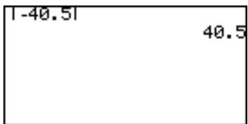
1 abs( abs(value)

Returns an absolute value.

• A real number, a list, matrix, variable, or equation can be used as values.

Example

Find an absolute value of "40.5".

MATH B 1 (-) 40

.5ENTER

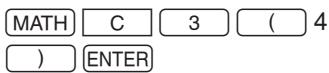
2 round( round(value [, digit number of decimals])

Returns the rounded value of the term in parentheses. A rounding point can be specified.

• A real number, a list, matrix, variable, or equation can be used as values.

Example

• Round off 1.2459 to the nearest hundredth. (= 1.25)

MATH B 2 1.2459 , 2 ENTER

3 ipart ipart value

Returns only the integer part of a decimal number.

• A real number, a list, matrix, variable, or equation can be used as values.

Example

• Discard the fraction part of 42.195. (= 42)

MATH B 3 42.195 ENTER

4 fpart fpart value

Returns only the fraction part of a decimal number.

• A real number, a list, matrix, variable, or equation can be used as values.

Example

• Discard the integer part of 32.01. (= 0.01)

MATH B 4 32.01 ENTER

5 int int value

Rounds down a decimal number to the closest integer.

Example

• Round down 34.56 to the nearest whole number. (= 34)

MATH B 5 34.56 ENTER

6 min( min(list)

Finds and returns the minimum value within a list of numbers. To define a list of more than two numbers, group the numbers with brackets (2ndF { and 2ndF}), with each element separated by a comma.

Example

Find the smallest value among 4, 5, and -9.

Finds and returns the maximum value within a list of numbers.

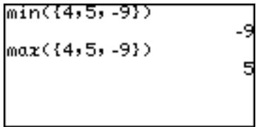
Example

Find the largest value among 4, 5, and -9.

MATH B 7 2ndF { 4 , 5 , -9

2ndF ENTER

8 Icm( Icm(natural number, natural number)

Returns the least common multiple of two integers.

Example

Find the least common multiple of 12 and 18.

Returns the greatest common divisor of two integers.

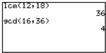
Example

Find the greatest common divisor of 16 and 36.

MATH B 9 16 , 36 ( ) ENTER

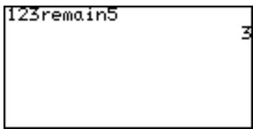
0 remain natural number remain natural number

Returns the remainder of a division.

Example

• Obtain the remainder when 123 is divided by 5.

123 MATH B 05

ENTER

C PROB

Use the PROB sub-menu items for probability calculations.

1 random random [(number of trial)]

Returns a random decimal number between 0 and 1.

Example

• Make a list with three random numbers.

Note: Set the "FSE" to "Fix" and "TAB" to "0".

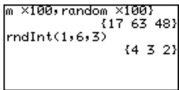
2ndF { MATH C

1 X 100 , MATH C 1 X 100

MATH C 1 X 100 2ndF} ENTER

Note: The random functions (random, rndInt(), rndCoin, and rndDice) will generate different numbers every time when the display is redrawn. Therefore, the table values of the random functions will be different every time. When in case of random-based graphing calculations, the tracing values and other parameters of the graph will not match the graph's visual representation.

2 rndInt( rndInt(minimum value, maximum value [, number of trial])

Returns a specified number of random integers, between a minimum and a maximum value.

Example

• Produce eight random integers, ranging between values of 1 and 6.

MATH C 2 1 , 6 , 3 ENTER

• Minimum value: 0 ≤ x_ ≤ 10^10

Maximum value: 0 ≤ x_ ≤ 10^10

Number of trial: 1≤ n≤ 999

3 rndCoin rndCoin [(number of trial)]

Returns a specified number of random integers to simulate a coin flip: 0 (head) or 1 (tail). The size of the list (i.e., how many times the virtual coin is thrown) can be specified. (The same as rndInt (0, 1, number of times))

Example

• Make the calculator flip a virtual coin 4 times.

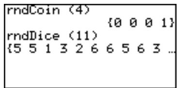
4 rndDice rndDice [(number of trial)]

Returns specified number of random integers (1 to 6) to simulate rolling dice. The size of the list (i.e., how many times the die is thrown) can be specified. (The same as rndInt (1, 6, number of times))

Example

• Make the calculator roll a virtual die 11 times.

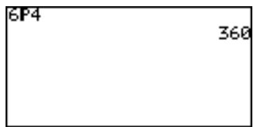
5 nPr Returns the total number of different arrangements (permutations) for selecting "r" items out of "n" items.

$$ { } _ { n } P _ { r } = \frac { n ! } { ( n - r ) ! } $$

Example

How many different ways can 4 people out of 6 be seated in a car with four seats?

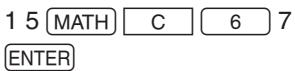
6 nCr Returns the total number of combinations for selecting "r" item out of "n" items.

$$ { } _ { n } C _ { r } = \frac { n ! } { r ! ( n - r ) ! } $$

Example

How many different groups of 7 students can be formed with 15 students?

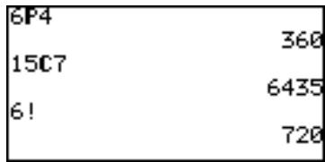
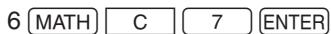
7! Returns a factorial.

Example

Calculate 6× 5× 4× 3× 2× 1

D CONV

CONV sub-menu items are to be used when converting a number in decimal form (degrees) to a number in sexagesimal form (degrees, minutes, seconds), or vice versa.

Sexagesimal and Degree System

The "base 60" sexagesimal system, as well as the minutes-second measurement system, was invented by the Sumerians, who lived in the Mesopotamia area around the fourth millennium B.C.(!) The notion of a 360 degrees system to measure angles was introduced to the world by Hipparchus (555-514 B.C.) and Ptolemy (2nd cent. A.D.), about 5000 years later. We still use these ancient systems today, and this calculator supports both formats.

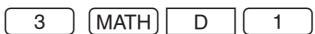
1 deg Takes a number in sexagesimal form, and converts it into a decimal number.

Example

• Convert 34^ 56' 78'' to degrees.

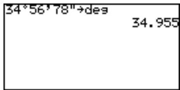
2 dms Takes a number in decimal form (in degrees), and converts it into a sexagesimal number. To enter a number in sexagesimal form, use items in the "ANGLE" sub-menu, described in the next subsection of this Chapter.

Example

• Show 40.0268 degrees in degrees, minutes, and seconds.

40 0268 MATH D

2 ENTER

E ANGLE

The Basic mode has two angle modes: Deg (degree) and Rad (radian). Use the E ANGLE menu to enter a degree value in Rad mode or a radian value in Deg mode. (The gradient mode is not included in the Basic mode. Refer to Chapter 5 for details.)

1. Inserts a degree, and sets the preceding value in degrees.
   2’ Inserts a minute, and sets the preceding value in minutes.
   3”Inserts a second, and sets the preceding value in seconds.

Example

• Enter 34^ 56^ 78^ .

34 MATH E 1
56 2 "E ANGLE" remains selected;
78 MATHE 3 type the number to enter the symbols.

ENTER

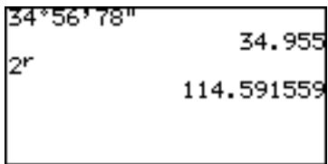
4 r Enters an "r", to enter a number in radians.

Example

• Type 2 radian.

2 MATH E 4 ENTER

Chapter 4 Basic Graphing Features - Basic Keyboard

This chapter takes the knowledge you have gained in Chapter 3 several steps further.

Note: To try the examples in this chapter, it is required that the Basic Keyboard is already set up by the user. To learn how to set up the Basic Keyboard, read "Changing the Keyboard" in Chapter 1.

1. Try it!

There are two taxi cab companies in your city, Tomato Cab and Orange Cab, with different fare systems. The Tomato Cab charges 2.00 upon entering the taxi cab, and1.80 for each mile the taxi travels. The Orange Cab, on the other hand, charges 3.50 plus1.20 per mile. This means that taking the Tomato

Cab will initially cost less than going with the Orange Cab, but will be more expensive as you travel longer distances.

Suppose you need to go to a place 3 miles away from where you are now. Which cab company should you take to save money?

Two math expressions can be derived from the above fare systems. If "y" represents the cost, while "x" represents the mileage, then:

y = 2 + 1.8x .Tomato Cab's fare system
y = 3.5 + 1.2x ......... Orange Cab's fare system

Use the calculator's graphing capabilities to figure out the approximate point where the Orange Cab gets ahead of the Tomato Cab, in terms of cost performance.

CONCEPT

1. By using two linear graphs, the approximate crossing point can be found.
2. The exact crossing point can be found with the TABLE function.

PROCEDURE

1. Press = to enter the Graph Equation window. Six equation entry areas appear, from "Y1=" to "Y6=". Since we need only two equations in this exercise, let's use "Y1=" and "Y2=".
2. By default, the cursor should be placed on the right side of the "Y1=" equation, next to the equal sign. If this is not so, use the cursor keys to bring the cursor to the "Y1=" line, then press the CL key to clear any entries. The cursor will automatically be placed to the right of the equal sign.
3. Enter the first equation, "2 + 1.8X", to represent the Tomato Cab's fare system.

$$ 2 \boxed {+} 1. 8 \boxed {x} $$

Use the key to enter the "x", representing the distance in miles.

1. When the equation line is complete, press ENTER. The first equation is now stored, and the cursor automatically jumps to the second line, where the second equation can be entered.

2. At the second line, press CL to clear any entries, then enter "3.5 + 1.2X" to represent the Orange Cab's fare system. When done entering the equation, press

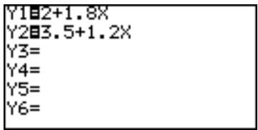
ENTER. The two equations are now ready to graph.

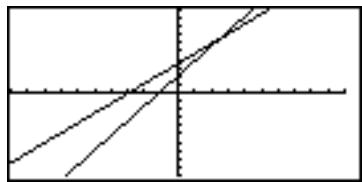
1. Press GRAPH to draw the graphs.

To draw a graph, “=” must be highlighted. If not, move the cursor to “=” of the targeted equation and press ENTER to draw a graph, and press ENTER again not to draw a graph.

Graph Basics

The graph examples in this exercise are called X-Y graphs. An X-Y graph is quite useful for clearly displaying the relationship between two variables.

1. Let's take a look at the graph. The vertical axis represents the Y value, while X is represented by the horizontal axis. It appears that the two diagonal lines

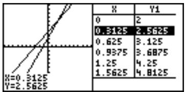
cross at the point where the X value is somewhere between 2 and 3, indicating that Orange Cab costs less than the other, after 3 miles of traveling.

1. Next, press TABLE to find the values per graph increment. When the traveling distance is 2 miles, the Tomato Cab charges 30 cents less overall than the Orange Cab, but it

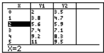
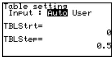
costs 30 cents more at 3 miles. To make the X increment smaller, press 2ndF TBLSET.

1. When the Table setting window appears, move the cursor down to "TBLStep", type · 5, and press ENTER. Now the Y values will be sampled at every 0.5 mile.

2. Press TABLE to show the table again. It indicates that when the X value is 2.5, both Y1 and Y2 values are 6.5. It is now clear that if you are traveling 2.5 miles or more, the Orange Cab costs less.

2. Explanations of Various Graphing Keys

Displays the Graph Equation window. Up to 10 different equations can be entered.

After the graph expression is entered, press ENTER to store the equation.

The expression can be represented as a graph.

= : The expression cannot be drawn as a graph.

• Move the cursor pointer to the “=” sign and press ENTER to change between to-draw and not-to-draw.

Note: To switch the window back to the calculation screen, simply press the key.

GRAPH: Draws a full-screen graph based on the equation(s) entered in the Graph Equation window. To cancel the graph drawing, press ON.

Note: If no equations are entered in the Graph equation window, only the vertical (Y) and horizontal (X) axis will be displayed upon pressing the GRAPH key.

TABLE: Displays the graph values in a table. The default sample increment value of the graph's X axis is "1".
ZOOM: Displays the ZOOM menu. Within the ZOOM menu, various preferences can be set for the graph appearance on zooming in/out.

The menu items with each function and the sub-menu items are described below:

A ZOOM

There are a myriad of tools under this menu item, by which the graph can be zoomed in/out in various styles. Press “A” within the ZOOM menu to select this menu item.

1 Auto According to the WINDOW setup, the graph will be zoomed in by adjusting the "Ymin" (the minimum Y value) and "Ymax" (the maximum Y value) according to the "Xmin" (the minimum X value) and "Xmax" (the maximum X value). When this item is selected, the graph will automatically be redrawn.

Note: The "Auto" sub-menu item is directly affected by how the WINDOW items are set up. Refer to the WINDOW key section in this chapter to learn how to set up the Xmin and Xmax items.

2 Box A box area can be specified with this sub-menu tool so that the area within the box will be displayed full screen.

To select a box area to zoom:

1. While the ZOOM menu item is selected within the ZOOM window, press 2 to select 2 Box.
2. The graph appears on the screen. Use the cursor keys to position the cursor at a corner of the required box area. Press ENTER to mark the point as an anchor.
3. Once the initial anchor is set, move the cursor to a diagonal corner to define the box area. When the required area is squared off, press ENTER. If a mistake is made, the anchor can be removed by pressing the CL key.
4. The graph will automatically be redrawn.

3 In A zoomed-in view of the graph will be displayed, sized according to the B FACTOR set up under the ZOOM menu. For example, if the vertical and horizontal zoom factors are set to “2”, then the graph will be magnified two times. Refer to the B FACTOR segment of this section for more information.
4 Out The graph image will be zoomed out according to the B FACTOR setup under the ZOOM menu.
5 Default The graph will be displayed with default graph setting (Xmin = -10, Xmax = 10, Xscl = 1, Ymin = -10, Ymax = 10, Yscl = 1)
6 Square Set the same scale for X and Y axes. The Y-axis scale is adjusted to the current X-axis scale. The graph will be redrawn automatically.
7 Dec Sets the screen dot as 0.1 for both axes. The graph will then be redrawn automatically.
8 Int Sets the screen dot as 1.0 for both axes. The graph will then be redrawn automatically.
9 Stat Displays all points of statistical data set.

B FACTOR

Use this menu to set the vertical and horizontal zooming factor. The factor set under this menu directly affects the zoom rate of the 3 In and 4 Out sub-menu tools under the ZOOM menu, as described above.

To set the zooming factor, do the following:

1. Within the

BFACTOR menu, press ENTER to activate the setup tool.

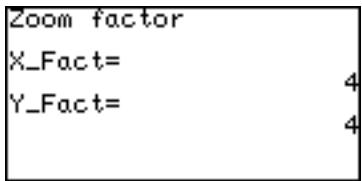
1. When the "Zoom factor" window appears, the cursor is automatically placed at "X_Fact=". The default zoom factor is 4; enter the required value here.

2. Pressing ENTER after entering a value will switch the cursor position to "Y_Fact=". Enter the required zooming factor, and press ENTER.

3. To go back to the ZOOM menu, press the ZOOM key.

C POWER

1 x^2 Use this zooming tool when the equation contains a form of "x ^ 2 "

2 x^-1 Use this zooming tool when the equation contains a form of "x^-1"

3 Use this tool to zoom correctly when the equation contains a form of "

EXP

1 10^x Use this tool when the equation contains a form of "10".

2 log X Use this tool when the equation contains a form of "log x "

ETRIG

1 sin X Use this when the equation contains a sine function.
2 cos X Use this when the equation contains a cosine function.
3 tan X Use this when the equation contains a tangent function.

F STO

Under this menu item there is one tool that enables the storing of graph window settings.

1 StoWin By selecting this sub-menu item, the current graph window setup will be stored.

Note: The actual graph image will not be stored with this tool.

G RCL

Under this menu item there are two tools that enable the recalling of the previous graph window setup:

1 RclWin On selecting this sub-menu item, the previously stored window setup will be recalled, and the graph will be redrawn accordingly. If no window setup has been stored previously, the default graph window setup will be used.
2 PreWin On selecting this sub-menu item, the window setup prior to the current zoom setup will be recalled, and the graph will be redrawn accordingly.

TRACE:

Press this button to trace the graph drawn on the screen, to obtain the X-Y coordinates:

1. While the graph is displayed, press the key. The cursor appears, flashing on the graph line, with the present X-Y coordinates.

1. Trace the graph using the or keys. The key decreases the value of x , while the key increases it.
2. Pressing the key again will redraw the graph, with the cursor at the center of the screen. If the cursor is moved beyond the range of the screen, pressing the key will redraw the screen centered around the cursor.
3. When done, press the CL key to escape the tracing function.

If more than one graph is displayed on the screen, use the or keys to switch the cursor from one graph to the other.

Note: If the key is not activated, the cursor will not be bound to the graph. Pressing the , , , or keys will position the free-moving flashing cursor on the graph display.

WINDOW:

Displays the graph window setup. The setup values — the minimum/maximum X/Y values, and X/Y-axis scale — can be changed manually:

1. While the graph is displayed on the screen, press the WINDOW key. The following window appears, with the cursor set at "Xmin=".

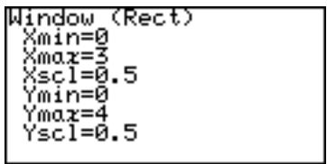
1. The required X-minimum value can be entered here. This limits the left boundary of the graph window. For example, if "Xmin=" is set to "0", then the portion of the graph's Y-axis to the left will not be displayed.

2. Once the "Xmin=" value is entered ("0", for example), press ENTER. The left limit of the graph is now set, and the cursor moves to "Xmax=".

3. Now the right boundary of the graph can be set. Enter the required value here ("3", for example), and press ENTER.

Note: The "Xmax=" value cannot be set equal to or smaller than the value of "Xmin". If so done, the calculator will display an error message upon attempting to redraw the graph, and the graph will not be displayed.

1. The next item "Xscl=" sets the frequency of the X-axis indices. The default value is "1". If, for example, the value is set to "0.5", then indices will be displayed on the X-axis at increments of 0.5. Enter the required "Xscl=" value ("0.5", for example), and press ENTER.
2. The "Ymin=", "Ymax=", and "Yscl" can be set, as was described for "Xmin=", "Xmax=", and "Xscl" above.
3. When done, press the GRAPH key to draw the graph with the newly configured window setup.

3. Other Useful Graphing Features

SPLIT: Splits the display vertically, to show the graph on the left side of the screen while showing the X-Y values in a table on the right. The cursor is positioned on the table, and can be scrolled up/ down using the or keys.

Graph and table

Graph and equation

• When 2ndF SPLIT are pressed on the graph screen, the graph and table are displayed on the same screen.
• When 2ndF SPLIT are pressed on the equation input screen, the graph and equation are displayed on the same screen.

The following illustration shows these relationships.

• The split screen is always in the trace mode. Therefore, the cursor pointer appears on the graph. Accordingly, the coordinate values are displayed reverse in the table and in the equation at which the cursor pointer is located is also displayed reversely.
• Using or , move the cursor along the graph. (Values displayed reverse in the table are also changed accordingly.)
• When two or more graphs are displayed on the screen, the desired graph is selected using or . (The table or equation on the right of the screen is also changed accordingly.)
• The table on the split screen does not relate to the table settings on the full-screen table.
• The table on the split screen is displayed in units of trace movement amount based on the cursor pointer position on the graph screen. When the full-screen table is displayed by pressing TABLE, a different table may appear on the screen.
• When the EXPRES or Y' is set to ON on the FORMAT menu, the equation or coordinates are displayed on the graph screen.
• Only equations to be graphed are displayed on the split screen.
• Press or on the split screen to display the full-screen of the graph or table. To exit the split screen, press any of other function keys.

CALC:

Calculations can be performed on the entered graph equation(s). Press 2ndF CALC to access. The following 6 sub-menu tools are available:

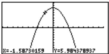
1 Value With this sub-menu tool, the Y value can be obtained by entering an X value. The flashing graph cursor will then be placed in that position on the graph. If more than one graph equation is set, use the or keys to switch to the equation you wish to work with.

Note: If the entered X value is incalculable, an error message will be displayed. Also, if the Y value exceeds the calculation range, the

2 Intact With this tool, the intersection(s) of two or more graphs can be found, where the flashing cursor will be placed. When the intersection is found, then the X-Y coordinates of the intersection will be displayed at the bottom of the screen. If there is more than one intersection, the next intersection(s) can be found by selecting the tool again.

Note: If there is only one graph equation entered there will be no other graph(s) to form an intersection, so selecting this tool will result in an error.

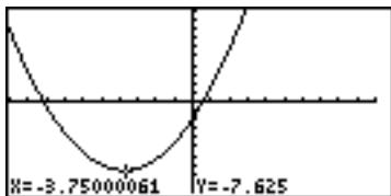
3 Minimum Finds the minimum of the given graph, and places the flashing cursor at that position.

Note: If the given graph has no minimum value, an error message will be displayed.

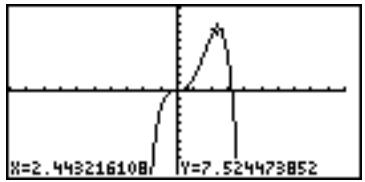
4 Maximum Finds the maximum of the given graph, and places the flashing cursor at that position.

Note: If the given graph has no maximum value, an error message will be displayed.

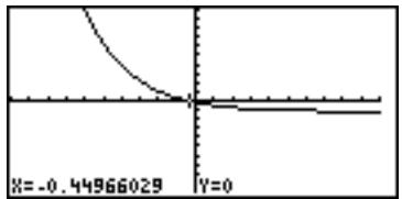
5 X_Incpt Finds an X-intercept (a crossing point of the graph on the X-axis) of the given graph, and places the flashing cursor at that position. If there is more than one X-intercept, the next X-intercept can be found by selecting the tool again.

Note: If the graph has no X-intercept, an error message will be displayed.

6 Y_Incpt Finds an Y-intercept of the given graph, and places the flashing cursor at that position.

Note: If the graph has no Y-intercept, an error message will be displayed.

Note: The result may be different when the ZOOM function is used.

DRAW: There is an extensive set of features under this menu item that enhance the graphing capabilities of the calculator. Only the shading function will be covered here; refer to Chapter 6 "Advanced Graphing Features — Advanced Keyboard" in this manual for more information.

To access the DRAW menu, press 2ndF DRAW.

An inequation can be expressed with the calculator's graphing capability. Here's how:

1. Set up a simple graph within the Graph Equation window. Enter "X²" for Y1, for example.

2. Press 2ndF, and DRAW to enter the DRAW menu, then press G to select G SHADE. The SHADE sub-menu appears.

3. Press 1 to select 1 SET. The "Set shade" window appears.
4. Using the cursor keys, move the cursor pointer to the appropriate position.
5. Press 2ndF VARS A
6. Press 1 to select Y1.
7. When the value is set, press the GRAPH key. The graph will be redrawn.
8. Let's add another inequation, so that the area where the

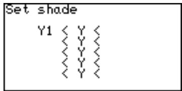
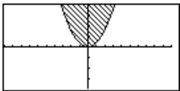
two inequality overlap can be shaded. Press the = key, and enter another simple graph equation such as "X + 4" for "Y2".

1. Now, return to the SHADE menu by pressing 2ndF DRAW, and G. Press 1 to select "1 SET".
2. Within the "Set shade" window, add the second equation at the right of the topmost inequation. Use the or key to position the underscore cursor, then select "Y2" using the VARS menu.
3. Press the GRAP to redraw the graph with the new shading appearance.

FORMAT: The graph appearance can be set and verified under this menu. Press 2ndF FORMAT to access.

A ---- Displays the current FORMAT settings. The default setting is:

OFF (for the graph equation to be displayed on the graph)

OFF (for displaying numeric derivatives on the graph)

ON (for displaying the X/Y axis on the graph)

OFF (for displaying a grid on the graph)

B EXPRES This sets whether or not graph equations are displayed on the graph screen (in the trace mode, etc.). To display the equations on the graph, select 1 ON by pressing 1 at this menu item.

C Y' The numeric derivative (dx/dy) can be displayed on the graph screen (in the trace mode, etc.). To activate this function, select 1 ON by pressing 1 at this menu item.

D AXIS The graph axis can be set invisible with this menu item. To hide the X/Y axis of the graph, select 2 OFF by pressing 2 at this menu item.

E GRID The graph display can be backed with an X-Y grid. To show the grid on the graph, select 1 ON by pressing 1 at this menu item.

Substitution feature

• The substitution feature allows you to input an equation using characters and variables, and then substitute numeric values for the characters to draw the graph.
• The substitution feature is valid only in the rectangular coordinate system. Using this feature, any number of numeric value sets can be substituted while referring to the graph drawing screen. This clearly shows the changes in the graph depending on numeric values.

For example, the graph for “ Y1 = AX^3 + BX^2 + CX^2 - D ” is drawn by substituting numeric values for variables A, B, C, and D of the equation.

• 22 kinds of variables (characters), A to Z except for R, T, X, and Y can be used for the substitution feature.
• Up to seven variables (characters) can be used for one equation. (If the equation contains more than seven variables (characters), up to seven characters from the top of the equation are determined as variables and subsequent characters are ignored.)
• If you attempt to execute an equation containing no variables, the substitution feature becomes invalid and the error message, "NO VARIABLE", appears on the screen.
• To input the equation, there are the following two methods after = has been pressed. After the equation has been input, the same operations apply to subsequent steps.

Example

Substitute numeric values under the conditions that “Y1 = AX² + BX + C” and “Y2 = AX” have been input.

Equation Entry screen

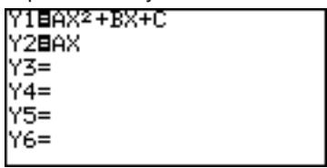
The cursor pointer is located at Y1. Drawing of both graphs Y1 and Y2 is valid.

1. Press 2ndF SUB

The substitution feature screen will appear. The equation on which the cursor pointer is located and its variables are displayed on the right of the screen.

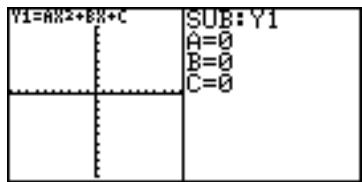
If variables (characters) contain no values, the graph is not drawn.

If independent memories A to C contain any numeric values, the graph is drawn based on these values.

• If the equation (in this example, Y1) on which the cursor is located contains no variables, the substitution feature screen will not appear.

2. Press 2 ENTER

(2 is input to A.)

The graph for “ Y1 = 2X^2 ” is drawn. (Since B and C have no values, they are ignored.)

At this time, the graph for Y2

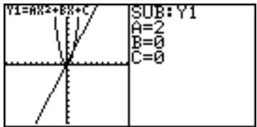
is also drawn. Y2 also uses variable A which is used in Y1.

Therefore, the drawing of the graph for Y2 is also valid.

• If you need to draw only the graph for Y2, it is necessary to change variables (characters) or make the graph drawing for Y1 invalid.

3. Press 1 ENTER

(1 is input to B.)

The graph is changed from

$$ " Y 1 = 2 X ^ {2}" t o " Y 1 = 2 X ^ {2} + $$

$$ 1 X ^ {\prime \prime}. $$

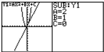
4. Press (-) 3 ENTER.

(-3 is input to C.)

Now, the graph for "Y1 = 2X^2

+1X-3" is drawn on the

screen.

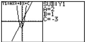
Next, change variable A from 2 to 5 and see how the graph changes.

1. Press 5 ENTER

(The cursor is moved from C to A and 5 is input.)

The slope of the graph becomes sharp.

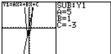
• Move the cursor accordingly and substitute other numeric values for variables to view how the graph changes.

• The trace function cannot be used in the substitution feature. (When is pressed, the full-screen graph will appear.)

Chapter 5 Advanced Calculations - Advanced Keyboard

Note: To try the examples in the chapter, it is required that the Advanced Keyboard is already set up by the user. To learn how to set up the Advanced Keyboard, read "Changing the Keyboard" in Chapter 1.

1. Try it!

The Mendocino Tree, a coast redwood growing in Montgomery Woods State Reserve in California, is known to be the tallest living tree in the world. You are to find out how tall the tree is by using the following factors:

• The distance from you to the bottom of the tree is exactly 505.8 feet, and the tree stands vertically.
• The angle of elevation between the top and the bottom of the tree is 36 degrees

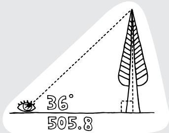
If the base length of the right triangle is 505.8 feet, and the angle of elevation is 36 degrees, then the following expression can be derived:

the height of the Mendocino tree (ft.) = 505.8 ft. × tan(36°)

CONCEPT

1. Verify/change the calculator's angle unit.
2. Use the calculator's trigonometric function key on the Advanced keyboard to enter/perform the calculation.

PROCEDURE

1. Since the angle of elevation is measured in degrees, the calculator's angle setting will

need to be matched with that. Press 2ndF SETUP to bring up the SETUP menu.

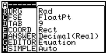
1. On the right side of the SETUP menu, the current setup will be displayed. Make sure that the top line is indicated as Deg (i.e., degrees). If not, then the angle system will need to be changed. Press B to select B DRG, then press 1 to select 1 Deg.

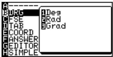
1. Now, let's work on the actual calculation part. Press the key to enter the Calculation screen, and press CL to clear any screen entries.

2. Press 505.8 X tan 36. Press ENTER to execute the calculation.

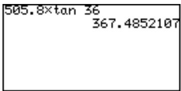
2. Various Calculation Keys

The calculator's Advanced Keyboard is designed so that various advanced-level expressions can be written quickly with few strokes of the keys.

Note: The default angle unit for the Advanced mode is radians. The examples hereafter will therefore feature the radian angle system, unless otherwise specified.

The keys with each associated math function are described below. Refer to the usage diagram in the Appendix for the parameters for each sub-menu item.

Enters a sine function to be used in a trigonometric expression.
cos Enters a cosine function to be used in a trigonometric expression.
tan Enters a tangent function to be used in a trigonometric expression.
log Enters a common logarithm function.
In Enters a natural logarithm function.

Example

Calculate In e^4

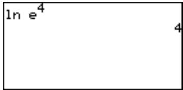
x^2 Raises the preceding value to the 2nd power.
If no preceding value exists, then the base value will be left blank.
% Enters a mixed number, with all elements left blank. If a preceding number exists, then the number is assumed as the integer part of the mixed number. (See page 37.)
a b Enters a fraction. Sets the preceding value as its numerator while the denominator left blank. (See page 38.)

If no preceding value exists, then both the numerator and the denominator will be left blank.

^b Raises the preceding value to a power. The exponent value can subsequently be entered.

If no preceding value exists, then both the base and the exponent area will be left blank. (See page 38.)

The following math functions can be accessed with the use of 2ndF key. To learn the basic steps of how to access the second function of each key, refer to the section "Second Function Key" of Chapter 2.

sin-1

Enters an arcsine function to be used in a trigonometric expression.

Example

Calculate arcsine 1.

2ndF sin-1 1 ENTER

sin-1 1	1.570796327
cos-1 0.5	1.047197551
tan-1 1	0.785398163

COS-1

Enters an arccosine function to be used in a trigonometric expression.

Example

Calculate arccosine 0.5.

2ndF cos-0.5 ENTER

tan-1

Enters an arctangent function to be used in a trigonometric expression.

Example

Calculate arctangent 1.

2ndF tan-1 1 ENTER.

Note: Expressions with inverse trigonometric functions evaluate in the following ranges.

$$ \theta = \sin^ {- 1} x, \theta = \tan^ {- 1} x \quad \theta = \cos^ {- 1} x $$

Deg: 0≤ | |≤ 90 Deg: 0≤ | |≤ 180

Rad: 0≤ | |≤ 2 Rad: 0≤ | |≤

Grad: 0≤ | |≤ 100 Grad: 0≤ | |≤ 200

10x

Raises 10 to the power of x .

ex

Enters the Euler Number e (2.71...) to a power. The cursor will then be placed at the exponent.

Example

• Obtain a value of e^3 .

2ndF ^x 3ENTER

e3	20.08553692

^-1 Raises a preceding value to the power of -1. If no value is preceded, then the cursor will be placed at the base.
a√ Enters an ath root of a base. When a value precedes, then the value will be incorporated as the index number. Otherwise, both entry areas will be left blank.
Enters a square root; sets the cursor at the base entry area.
Enters (3.14...).
Sets the following value as , assuming the preceding value is the radius of the polar coordinates.
Enters i (representing -1 ), to make imaginary or combination numbers.

3. Calculations Using MATH Menu

The Advanced keyboard has considerably more MATH menu items to choose from than that of the Basic keyboard:

A CALC

Contains sub-menu tools for advanced calculations. To access each sub-menu item, make sure that this A CALC menu item is selected. Pressing the cursor key will extend the cursor to the sub-menu items. Items can then be highlighted by scrolling with , , or , and selected by pressing ENTER, or simply use the short cut key stroke (i.e., select 01 by pressing 0 and 1).

A sub-menu item with open parenthesis will need to be completed by the closing parenthesis; failure to do so will result in an error.

01 _2 _2 value

Enters a base-2 logarithm (_2)

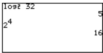
02 2^X 2value

Raises 2 to a power. Sets the cursor to exponent.

03 fmin( fmin(equation, lower limit of x , upper limit of x )

Returns the value of variable x when the equation Y has the minimum value within the specified range of x .

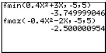
04 fmax( fmax(equation, lower limit of x , upper limit of x )

Return the value of variable x when the equation Y has the maximum value within the specified range of x .

05 d/dx( d/dx(equation, value of x [tolerance])

Returns derivative of equation Y at the specified X value using the tolerance (if not specified, default value is 1E-5).

06J equation,lower limit,upper limit [,tolerance]dx

Calculates an integral value of equation Y from the lower limit to the upper limit using the specified tolerance (if not specified,

default value is 1E-5). Use in conjunction with the 07 dx sub-menu item.

• Press the keys as follows in the Equation edit mode.

07 dx Enters a differential "dx" in an integration expression.

08 (expression, initial value, end value [, increment])

Returns the cumulative sum of a given expression from an initial value to an end value in the specified increment value (if not specified, default

09 sec sec value

Enters a secant function to be used in a trigonometric expression.

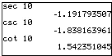
10csc cscvalue

Enters a cosecant (cosec) function to be used in a trigonometric expression.

11 cot cot value

Enters a cotangent (cotan) function to be used in a trigonometric expression.

12 sec-1 sec-1 value

Enters an inverse secant.

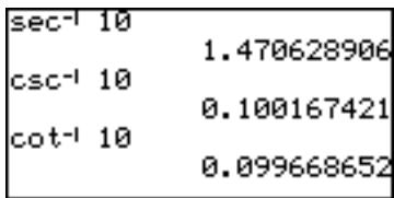
13csc-1 csc-1value

Enters an inverse cosecant.

14 cot-1 cotvalue

Enters an inverse cotangent.

15 sinh sinh value

Enters a hyperbolic sine.

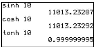
16 cosh cosh value

Enters a hyperbolic cosine.

17 tanh tanh value

Enters a hyperbolic tangent.

18 sinh-1 sinh-1 value

Enters an inverse hyperbolic sine.

sinh⁻¹(1)	0.881373587
cosh⁻¹(2)	1.316957897
tanh⁻¹(.05)	0.050041729

19 cosh ^-1 cosh ^-1 value

Enters an inverse hyperbolic cosine.

20 tanh ^-1 tanh ^-1 value

Enters an inverse hyperbolic tangent.

B NUM Use the sub-menu items below to convert a value. Refer to "Chapter 3: Basic Calculation — Basic Keyboard" to learn how these tools can be used.

1 abs( Returns the absolute value of a given number.
2 round( Returns a rounded value of a given term in parentheses. A rounding point can be specified.
3 ipart Returns only the integer part of a decimal number.
4 fpart Returns only the fraction part of a decimal number.
5 int Rounds a decimal number to the closest integer.
6 min( Finds and returns the minimum value within a list of numbers.
7 max( Finds and returns the maximum value within a list of numbers.
8 Icm( Returns the least common multiple of two integers.
9 gcd( Returns the greatest common divisor of two integers.

C PROB These sub-menu items are useful for probability calculations. Refer to "Chapter 3: Basic Calculations — Basic Keyboard" for details. A comprehensive list of menu items can be found in the Appendix.

1 random Returns a random number form between 0 and 1.
2 rdInt( Returns a list of random integers, between a minimum and a maximum value.
3 nPr Returns the total number of permutations for selecting "r" items out of "n" items.
4 nCr Returns the total number of combinations for selecting "r" items out of "n" items.

5! Returns a factorial.

D CONV These tools deal with conversions between different angle units and between rectangular and polar coordinates.

1 deg value (sexagesimal number) deg Takes a number in sexagesimal form, and converts it into a decimal number.
2 dms value (degrees) dms Takes a number in decimal form (in degrees), and converts it into a sexagesimal number. To enter a number in sexagesimal form, use items in the ANGLE sub-menu, described in Chapter 3.

Rectangular/polar coordinate conversion

This calculator is equipped with rectangular coordinates and polar coordinates conversion capabilities.

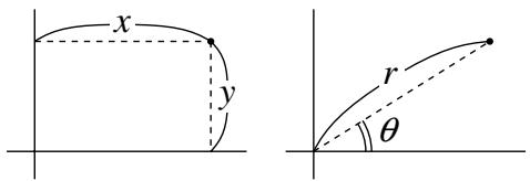
Rectangular to polar coordinate conversion functions

Conversion formulas: r = (x^2 + y^2)^1 / 2 = ^-1(y / x)

3xy→r(xy→r(x coordinate,y coordinate)

Returns polar coordinate radius value from X-Y rectangular coordinates.

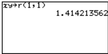
4xy→θ( xy→0(x coordinate, y coordinate)

Returns polar coordinate value from X-Y rectangular coordinates. The following ranges are used to find .

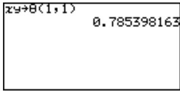
Degree mode: 0 ≤ || ≤ 180

Radian mode: 0 ≤ || ≤

Gradient mode: 0 ≤ || ≤ 200

Polar to rectangular coordinate conversion functions

Conversion formulas: x = r , y = r

5 r x(r x(r coordinate, coordinate)

Returns rectangular coordinate X value from r-θ polar coordinates.

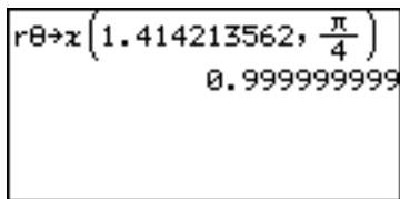
6 r y(r coordinate, coordinate)

Returns rectangular coordinate Y value from r-θ polar coordinates.

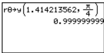
E ANGLE Use these tools to enter the symbols to specify angle units.

1° Inserts a symbol for "degrees".
2’ Inserts a symbol for "minutes".
3” Inserts a symbol for "seconds".
4 r Enters an "r" symbol, to enter a number in radians.
5 g Enters an "g" symbol, to enter a number in gradients.

F INEQ Use the equality/inequality figures to compare two values. These sub-item tools return 1 (true) or 0 (false).

1 = Tests whether a preceding value and a following value are equal.

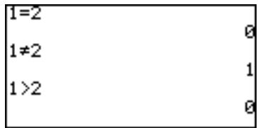
2 Tests whether a preceding value and a following value are not equal.

3> Tests whether a preceding value is larger than a following value.

4 ≥ Tests whether a preceding value is larger than OR equal to a following value.

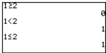
5 < Tests whether a preceding value is smaller than a following value.
6 ≤ Tests whether a preceding value is smaller than OR equal to a following value.

G LOGIC Use the LOGIC sub-menu items to perform boolean operations.

In the N-base calculation mode (binary, octal, decimal and hexadecimal), A LOGIC will directly appear when is pressed.

The following is the truth table of the combination of input A and B:

A	B	A and B	A or B	A xor B	A xnor B	A	notA
1	1	1	1	0	1	1	0
1	0	0	1	1	0	0	1
0	1	0	1	1	0
0	0	0	0	0	1

The following examples show the answer screen when executing a boolean operation for AND, OR, XOR, XNOR between "1100" and "1010" in binary mode. Compare the results (binary) to the above table.

1. Press 2ndF TOOL A ENTER to enter the binary, octal, and hexadecimal calculation mode.
2. Press to select the binary mode.

1 and value A and value B

Enters an "AND" logic figure.

1100 MATH 1

1010 ENTER

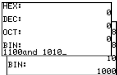
2 or value A or value B

Enters an "OR" logic figure.

1100 MATH 2

1010 ENTER

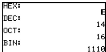
3 not not value

Enters a "NOT" logic figure.

MATH 3 10

ENTER

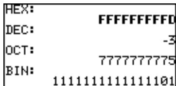
4 neg neg value

Enters a "neg" logic figure.

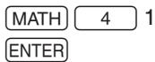
Note: "4 neg" menu

appears only in the N-base calculation (binary, octal, decimal and hexadecimal) mode.

5 xor value A xor value B

Enters an Exclusive-OR (xor) logic figure.

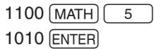
6xnor valueAxnorvalueB

Enters an Exclusive-NOR (xnor) logic figure.

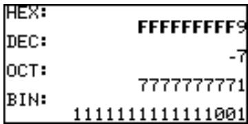
H COMPLX

In order to use the sub-menu items within the COMPLX menu, the calculator must be set up to handle complex numbers. Otherwise the result will be a data type error.

Refer to the section "6. SETUP Menu" in this chapter for changing/verifying the calculator's setup to enable complex number answers, in either rectangular or polar coordinates.

1 conj( conj(complex number)

Returns the complex conjugate of the specified complex number (or list of complex numbers).

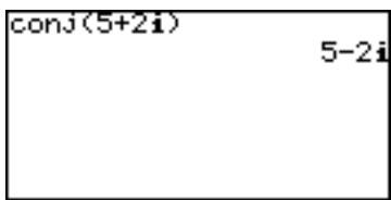
2 real( real(complex number)

Returns the real part of a complex number (or list of complex numbers).

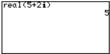
3 image( image(complex number)

Returns the imaginary part of a complex number (or list of complex numbers).

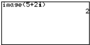
4 abs( abs(complex number)

Returns the absolute value of a complex number (or list of complex numbers).

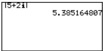
5 arg( arg(complex number)

Takes the coordinates (x + yi) , and returns the .

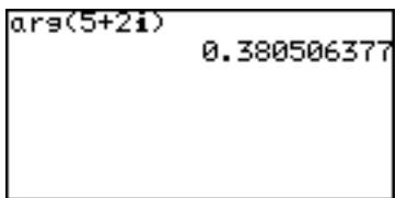
Calculations using complex numbers

To calculate using complex numbers, select the sub-menu item 4 x ± yi or 5r in the F ANSWER of the SETUP menu items.

The initial screen for the complex number calculation mode is the same as for the real number mode.

Complex numbers can be noted using either 4x ± yi (rectangular coordinates) or 5r (polar coordinates).

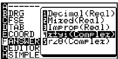
Example

Calculate (3 + 4i)× (4 - 6i)

Note: It is possible to input complex numbers (i) in the real number mode, however an error message will return.

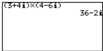
Functions available for complex number calculations

The following function keys are available for complex number calculations without the limits existing in the real number calculations.

The following MATH menu functions are also available for complex number calculations.

abs(), round(), ipart, fpart, int

4. More Variables: Single Value Variables and LIST Variables

Additional single value variables (from A to Z, and ) may be accessed. In addition, six LIST variables (from L1 to L6) are readily accessible through the second function of the Advanced Keyboard.

To save a list of numbers, follow the procedure below:

1. On the Calculation screen (2), create a list of numbers ("1, 2, 3", in this example). Separate numbers with a comma (1), and group the numbers with braces (2) and (3).
2. Press STO, then select one of the six LIST variables. To store the list in "L1", press 2ndF L1 to call up the LIST variable.
3. Pressing ENTER will store the list in the LIST variable. Note that this procedure will overwrite the list previously stored in the LIST variable.

Refer to Chapter 9 "LIST Features" to learn more about how LIST variables can be utilized.

5.TOOL Menu

The TOOL menu contains items to help calculating in different number systems, as well as to help solve both linear and polynomial equation. Press 2ndF TOOL to access the TOOL menu. Press the key (or 2ndF QUIT) to escape from the menu.

A NBASE Calculations can be performed in different number base systems, while simultaneously converting the calculation result into hexadecimal, decimal, octal, and binary systems.

1. While this menu item A NBASE is selected, press the ENTER key. The NBASE tool opens, with the cursor set at HEX: (hexadecimal).

1. Type 1B × 9, for example. When entering the hexadecimal B, simply press the B key; using the ALPHA key will call up the variable B instead.

2. When done entering the hexadecimal expression, press ENTER. The calculation result will be displayed in three other number base systems, as well as in hexadecimal format.

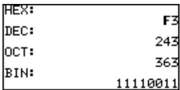
Note: Numerical values in binary, octal, and hexadecimal modes can be expressed in the following number of digits:

Binary: 16 digits

Octal: 10 digits

Hexadecimal: 10 digits

If you enter a number exceeding the range specified above for calculations or conversions, the calculator will return an error. If the answer exceeds the above range, the calculator will also return an error.

Decimals can be used for DEC mode only ( cannot be used in the other modes). If you convert decimal values to binary, octal, or hexadecimal number, the decimal part is discarded and only the integer part is converted.

When numerical values of binary, octal, and hexadecimal modes are negative, the display is switched to complements of 2.

B SYSTEM With this tool, linear equations containing up to 6 unknown values (i.e., ax + by + cz + du + ev + fw = g ) can be solved.

1. Press B to select B SYSTEM, and select the number of unknown values. For example, press 2 if values x and y are unknown.

2. In the next screen, an equation ax + by = c is displayed, with an entry table for the known values — a, b , and c .

3. Enter 2 sets of the known values, as shown in the figure. Pressing ENTER at each entry will store the value, and sets the cursor at the next entry area.

4. When done entering the known values, press 2ndF EXE. The calculation result will be displayed on the next screen.

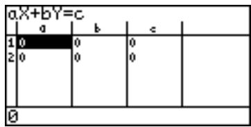
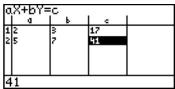
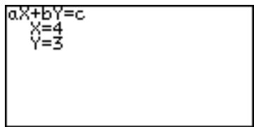
Pressing CL will bring back the previous entry screen.

1. To go back to the TOOL menu to perform another calculation, press 2ndF TOOL.

C POLY This tool is designed so that quadratic (ax^2 + bx + c = 0) or cubic (ax^3 + bx^2 + cx + d = 0) equation may be solved.

1. Press C to select C POLY, and select the degree. For example, press 2 if a quadratic equation is desired.

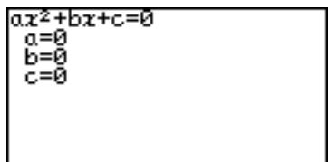
1. In the next screen, an equation ax^2 + bx + c = 0 is displayed, with an entry area for the known values — a , b , and c .

2. Enter the values, as shown in the screen to the right. Pressing ENTER at each entry will store the value, and sets the cursor at the next entry area.

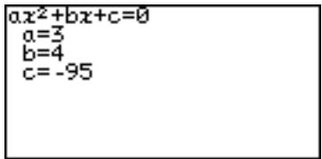
1. When done, press 2ndF EXE to execute the calculation. The results (i.e. the x -intersects) will be displayed.

2. To enter a different set of numbers for a, b, and c, press CL to go back to the previous screen. To select a different degree of polynomial, press 2ndF

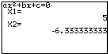
TOOL to go back to the TOOL menu.

• If the solution cannot be displayed on the screen, a symbol will appear at the bottom left corner of the screen. Press to scroll the screen.

6. SETUP Menu

Use the SETUP menu to verify the calculator's current setup for mathematical and scientific base units and the global editing style, as well as to change each configuration.

It is very important that each item within this menu is properly set up, or calculation results may not turn out as expected. For example, entering 1 × 90 in the Calculation screen will result as either "1" (when set to degree mode), or "0.893996663" (when set to radian mode), or "0.98768834" (when set to gradient mode). Refer to the "SETUP Menu" in Chapter 2 to learn about each setup configuration.

Chapter 6 Advanced Graphing Features

In this chapter, some real-life situations are featured. You are encouraged to modify the examples to make your own graph schemes.

Note: To try the examples in this chapter, it is required that the Advanced Keyboard is already set up by the user. To learn how to set up the Advanced Keyboard, read "Changing the Keyboard" in Chapter 1.

It should be noted that the following examples assume that the angle mode is set to Rad (radian), the default angle unit for the Advanced Keyboard. If set to degree or gradient, some unexpected results will be obtained.

1. Try it!

You have just opened your own bank account, with an initial deposit amount of 2,000. Suppose your monthly income is3,000, and you will spend 60 percent of what you have in the account every month, how much will your balance be after one year? How much will you have in the account, 6 months from now?

The example can be expressed as a sequential equation, as follows:

$$ u _ {n} = u _ {n - 1} \times (1 - 0. 6) + 3 0 0 0 $$

where ±bun is the balance of the current month and ±bun-1 is the balance of the previous month, and n is the month.

CONCEPT

1. Grasp the idea of sequential equations.
2. Use the graph tracing function to obtain approximate values.

PROCEDURE

1. First, let us set the calculator to the appropriate graphing coordinate mode. Press 2ndF SETUP to enter the SETUP menu, press E to select E COORD, then press 4 to select 4 Seq,

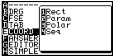
1. We will use the "Time" sequential graph type within the FORMAT menu. Press 2ndF FORMAT, press G to select G TYPE, and 2 to select 2 TIME.

1. Then press = . The Graph Equation Entry window will open.
2. Enter a new equation set u(n - 1) × (1 - 0.6) + 3000 for u(n) = . Press 2ndF (7) to enter u and press / / T / n for n . Press ENTER when done entering.

Note: Press CL to clear the previous entry.

Using a capitalized "U" or "N" here will result in an error upon pressing the GRAPH key.

1. On the second entry row (u(nMin) =) , enter 2000, then press ENTER. The figure is automatically enclosed by braces.

1. The and the entry sets will not be necessary in this case, so press CL to clear, then press ENTER to move one row down. Repeat until the four unnecessary entry rows are cleared.

2. Press GRAPH to draw the graph.

3. If the line is outside of the graph's range, press ZOOM then 1 to select automatic zoom. This will only display a small portion of the graph, so the graph's range will need to be

1. Press Window. Find nMax= and change the value to 15 (default: 10). Next, find Xmax= and change the value to 15 too (default: 10).

1. Press the GRAPH key again.

2. Use the graph trace function by pressing . As is pressed several times, the n value (=X value, since the graph is set to "Time" format) increases, and the Y value (the balance of your account) will change. Find the Y value when the n value is 6 (after 6 months) as well as the value when n = 12 (after 12

You can obtain the value directly from the CALC menu.

1. Press 2ndF CALC and select 1 VALUE. n = will appear on the bottom line of the screen.

1. Enter the n value of 6, and press ENTER.

2. Follow the procedure 1 to 2 to obtain the Y value for 12.

2. Graphing Parametric Equations

A two-dimensional parametric equation assumes that both X and Y are represented by functions in a third variable T . When set in parametric graphing mode, the calculator automatically sets up the Graph Equation Entry screen to take one set of X and Y per each graph, with the equation's right side variable to be set as "T".

Example

• Draw a graph: x(t) = 16(t), y(t) = 9(t) .

• Press 2ndF SETUP to enter the SETUP menu.

• Press E to select E COORD, then 2 to select 2 Param.

Be sure that the other settings are as shown on the right.

To exit the SETUP menu, press CL.

1. Press = to go to the Graph Equation Entry window.
2. Enter 16(t) for X1T = Press ENTER when done entering.
3. Enter 9(t) for Y1T=. Press ENTER when done entering.

Note: The right side variable is automatically set to "T". When the / / T / n key is pressed within the Graph Equation Entry window, it will enter the variable "T".

1. Press to draw the graph.
2. If the graph line extends beyond the screen, press ZOOM and select A ZOOM then 1 AUTO.

Use 3 IN or 4 OUT of the A

ZOOM to adjust the drawing size.

You can also set the drawing size in the WINDOW menu by determining the maximum and minimum values of T, X and Y.

3. Polar Graphing

Polar coordinates are a different method of specifying a point in two dimensions; the location of the point is described by the distance from the X-Y intersect "r", and its elevation angle "θ".

Example

Draw a graph: r = 16 () ()

1. Press 2ndF SETUP. The SETUP menu appears.

2. Press E to select E COORD, then press 3 to select 3 Polar. Be sure that the other settings are as shown on the right. To exit the SETUP menu, press CL.

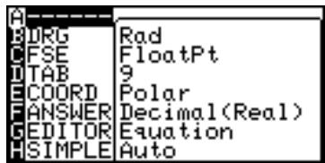
1. Press = The Graph Equation Entry window will appear.

2. At the first entry row R1 = enter 16 ()× () Press ENTER

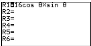
1. Press GRAPH to draw the graph. Press ZOOM, then press 6 to select 6 Square.

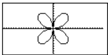
4. Graphing Sequences

The sequence graph mode can store and simultaneously draw three graph equations u(n), v(n) , and w(n) .

Variables u, v, and w are entered as 2ndF u (or , w).

Use / / T / n to enter the natural number n

A sequence is an ordered set of numbers with a defined relationship. The recursive sequential formulas can be described as

$$ u _ {n} = u _ {n - 1} + d \quad \text {a n d / o r} $$

$$ \boldsymbol {u} _ {n} = \boldsymbol {u} _ {n - I} \times \boldsymbol {r} $$

where ±bun is the n -th term, d is the common difference, and r is the ratio. In many occasions however, the term before un-1 (i.e., one term before u_n ) is not known. In such cases, the explicit formulas must then be derived as:

$$ u _ {n} = u _ {I} + d \times (n - 1) \quad \text {a n d / o r} $$

$$ \boldsymbol {u} _ {n} = \boldsymbol {u} _ {I} \times \boldsymbol {r} ^ {n - I} $$

where ±bu_n is the n -th term, ±bu_l is the first term of the sequence, ±bd is the common difference, and r is the ratio.

A sequence 2, 4, 8, 16, 32, may suggest the following recursive sequence expression:

$$ u _ {n} = 2 \times 2 ^ {n - 1} $$

or it may also suggest the following non-recursive expression:

$$ u _ {n} = 2 ^ {n} $$

The calculator can plot sequential graphs in three different schemes, as follows:

n -based (Time)

The ±bu_n values will be plotted against the ±bn value.

u(n)=

u(nMin)=

v(n)=

v(nMin)=

w(n)=

w(nMin)=

phase-based (uv, uw, or vw)

The u_n values will be plotted against the v_n values (uv).

(n - 1) -based (Web)

The ±bun values will be plotted against the ±bun - 1 value.

Note:

• When u_n-2 is incorporated in the equation, the u(nMin) requires two values: the minimum, and the second smallest. For example, you will need 0, 1 in the u(nMin) entry row if u(n-1) + u(n-2) is entered as the equation.
• When Web is selected, n - 2 cannot be referred to. n also cannot be directly referred to; entering u(n - 1) + n will result in an error.

Before entering graphing sequences, the calculator's graphing coordinates will need to be set up:

1. Press 2ndF SETUP. The SETUP menu appears.
2. Press E to select E COORD, then press 4 to select 4 Seq.
3. Press CL to exit the SETUP menu.

Example 1: n -based Graphing (Time)

• Draw a sequential graph of u_n = 2 × 2^n - 1 .

First, make sure that the graph coordinate mode is set to sequential (see above.)

1. Press 2ndF FORTMAT to open the FORMAT menu. The FORMAT menu allows user to change the graph configurations.

2. When the menu appears, select the item G TYPE.

3. Press 2 to select 2 Time.

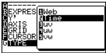
1. Now, go to the Graph Equation Entry window by pressing Y =

The cursor is set at the first line u(n) ; pressing CL will clear any previous entry, as well as to put the cursor at the right side of the equation.

1. Enter 2 × 2^n-1 . Use the / / T / n key to enter n . When done, press . The cursor moves down to the second row.

1. In the entry area u(nMin) = enter the minimum value of the n 1, then press ENTER

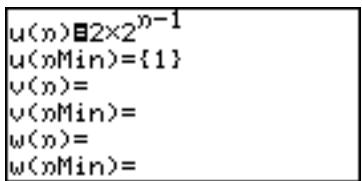
1. Press the GRAPH key.

2. Press ZOOM, then press 1 to select 1 Auto (automatic zoom).

3. Press the key, then use the key to trace the graph.

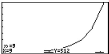
Example 2: Phase-based Graphing (uv)

• Compare 2 × 0.9^n - 1 with the previously entered sequence.

Phase-based graphing requires a set of two sequential equations. Since we already have one entered as above, we will create another one here, but first the sequential graph format will need to be set to uv.

1. Press 2ndF FORMAT to enter the FORMAT menu, then press

G to select G TYPE.

1. Select uv by pressing 3

2. Press = to go to the Graph Equation Entry window.

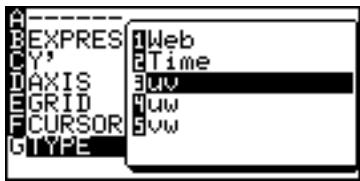
The calculator can accept up to three sequential equation entries. We will use the set, since the u set already has an entry. Move the cursor down to the v(n) entry area, and press CL.

1. Enter 2 × 0.9^n-1 , then press ENTER.

The cursor will be set to the fourth entry row v(nMin=).

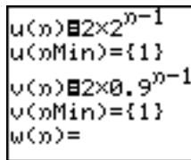
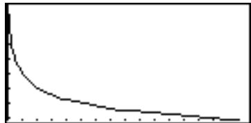
1. Press CL, then enter 1.
2. Press the GRAPH key to draw the graph, then zoom the graph so that it be comes visible (ZOOM, 1 Auto).
3. Use the function to

trace the graph. Press the key to trace the plotted graph values.

When w , the third sequential equation set is entered, it can also be compared with the two other equations; simply set the TYPE under the FORMAT menu to either 4 uw to compare the first set with the third, or 5 vw to compare the second and the third.

Note: Comparing a sequence with an empty set will result in an error. If the set is to be used, then the equation entry rows will need to have appropriate entries.

Example 3: n-1 -based Graphing (Web)

• Compare the u(n - 1) value against the u(n) value of u(n - 1) + 100 .

This particular graph equation requires an index to the previous

term (±bu_n - 1)

1. Press 2ndF FORMAT to enter the FORMAT menu, then press G to select G TYPE.

2. Select 1 Web by pressing 1.

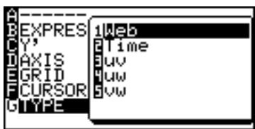
1. Press the = key to go to the Graph Equation Entry window.

2. At the first equation entry row, enter u(n - 1) + 100 . When done entering, press ENTER.

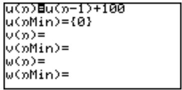
1. At the next entry row, make sure that it has the starting value “0”.
2. Bring the cursor down, and clear the rest of the four rows.
3. Press GRAPH, then press ZOOM, 1 Auto to view the graph. Two diagonal parallel lines should appear; the top line repre

sents the n value, while the n - 1 value is represented by the line below.

1. Press to trace the graph. As is pressed, you will see the traced points

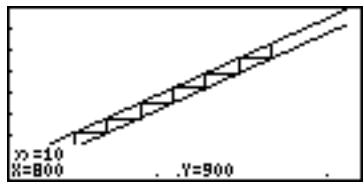
connected with lines, indicating the comparison between the n and n - 1 values.

5. The CALC Function

The Calc function utilizes the entered graph equation to calculate values. In conjunction with the 4 graph coordinates, it can be called up anywhere. Note however that the Calc function will not do anything if no graph equation has been entered or specified.

The following is an example that uses the previously entered polar graph equations above.

1. First, verify the graph coordinate mode by pressing 2ndF SETUP; check to see if ECOORD is set to Polar. If not, this will need to be changed accordingly. Also,

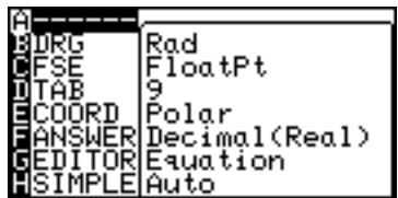
make sure the angle unit B DRG is set to Rad. Otherwise the graph will not be drawn correctly.

1. Press = to verify the previously entered polar graph equation, then press GRAPhto draw the graph. Adjust the view by using ZOOM menu items.

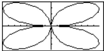
1. Press 2ndF CALC

2. Press 1 to select 1 Value. The graph is drawn back on the screen again, with the = prompt visible at the bottom left side of the screen.

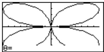
1. Enter the value at the prompt. Enter , for example. Be aware that cannot be more than 2 (2 radians = 360 degrees).

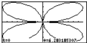
1. Upon pressing ENTER, the radian r coordinate will be calculated.

Note: When coordinate system is Polar, Param or Seq, only 1 Value is selectable in the CALC menu.

Advanced keyboard specific sub-menus

See Chapter 4 "Basic Graphing Features — Basic Keyboard" on pages 60 to 61 for details of the other sub-menu tools available.

7 Inflec Calculates the inflection point of the given graph and moves the cursor to that point.

Example

1. Enter the graph equation Y1 = x^3 - 3x^2 + 2

2. Press 2ndF CALC 7

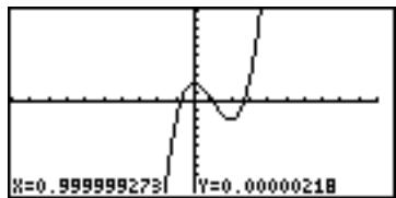
6. Format Setting

You can set up the Graph screen format from the FORMAT menu.

Press 2ndF FORMAT to display the Graph format menu.

Advanced keyboard specific sub-menus

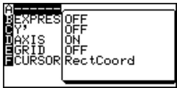
Note: G TYPE appears only when the sequence coordinate graph mode is selected.

A - - - - - Displays the current FORMAT settings. The default setting is:

OFF (for the graph equation to be displayed on the graph)

OFF (for displaying numeric derivatives on the graph)

ON (for displaying the X/Y axis on the graph)

OFF (for displaying a grid on the graph)

RectCoord (for displaying the cursor location)

B EXPRES This sets whether or not graph equations are displayed on the graph screen (in the trace mode, etc.). To display the equations on the graph, select 1 ON by pressing 1 at this menu item.

C Y' The numeric derivative (dx/dy) can be displayed on the graph screen (in the trace mode, etc.). To activate this function, select 1 ON by pressing 1 at this menu item.

D AXIS The graph axis can be set invisible with this menu item. To hide the X/Y axis of the graph, select 2 OFF by pressing 2 at this menu item.

E GRID The graph display can be backed with an X-Y grid. To show the grid on the graph, select 1 ON by pressing 1 at this menu item.

F CURSOR The coordinate system that indicates the location selected by the trace or other function can be selected from 1 RectCoord (Rectangular coordinates) or 2 PolarCoord (Polar coordinates) (In the parametric system, the T indication is added.)

G TYPE This menu is only active when the sequence coordinate graph mode is selected in the SETUP menu. The G TYPE menu will not appear in the other modes.

1 Web A web graph plot mode where x = u(n - 1) and y = u(n)
2 Time Time graph plot mode where x = n and y = u(n) , v(n) , w(n) . (default)
3 uv A uv mode where x = u(n) and y = v(n) .
4 uw A uw mode where x = u(n) and y = w(n) .
5 vw A vw mode where x = v(n) and y = w(n)

Note: u(n), v(n) and w(n) indicate the n-th term of the sequences.

7. Zoom Functions

Displays the ZOOM menu. Within the ZOOM menu, various preferences can be set for the graph appearance on zooming in and out.

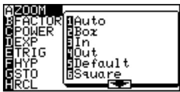
Advanced keyboard specific sub-menus

See Chapter 4 "Basic Graphing Features — Basic Keyboard" on pages 53 to 56 for details of the other menu items and their submenu items.

D EXP

2e^x Use this tool when the equation contains a form of e^x .

4 In X Use this tool when the equation contains a form of "In x ".

ETRIG

4 sin-1 X Use this when the equation contains an arc sine function.

5 cos-1 X Use this when the equation contains an arc cosine function.

6 tan ^-1 X Use this when the equation contains an arc tangent function.

F HYP

1 sinh X Use this when the equation contains a hyperbolic sine function.

2 cosh X Use this when the equation contains a hyperbolic cosine function.

3 tanh X Use this when the equation contains a hyperbolic tangent function.

4 ^-1 X Use this when the equation contains an inverse hyperbolic sine function.

5 ^-1 X Use this when the equation contains an inverse hyperbolic cosine function.

6 ^-1 X Use this when the equation contains an inverse hyperbolic tangent function.

8. Setting a Window

The Window key displays the graph window setup. The display will differ according to the selected coordinate system. See also Chapter 4 "Basic Graphing Features — Basic Keyboard" on pages 57 to 58 for details of rectangular coordinate system settings.

Rectangular coordinate system

Xmin/Xmax Minimum and maximum values of x-axis, respectively

Xscale Scale of x-axis

Ymin/Ymax Minimum and maximum values of y-axis, respectively

Yscale Scale of y-axis

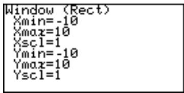
Parametric coordinate system

Tmin/Tmax Minimum and maximum values for T, respectively

Tstep Cursor pointer step value for tracing

Others Same as rectangular coordinate system

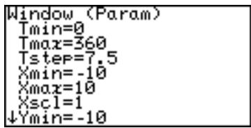
Polar coordinate system

0min/0max Minimum and maximum angle for , respectively

Step Cursor pointer step value for tracing

Others Same as rectangular coordinate system

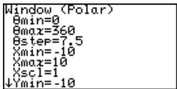
Sequential coordinate system

nMin/nMax Minimum and maximum value for n , respectively

PlotStart Starting value of sequential variable n

PlotStep Increments of sequential variable n

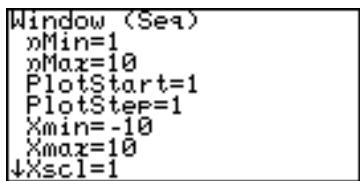
Others Same as rectangular coordinate system

9.Tables

The calculator enables you to illustrate the changes using the equation and graph you have input. It also has tables for showing a list of X and Y values. Each column item can display up to 7 digits, including a sign and/or a decimal point.

There are four kinds of tables available corresponding to the coordinate system.

Rectangular coordinate system

• The variable X is displayed in the left end column.
• The columns Y1 to Y3 are displayed on the first screen.
  Press to

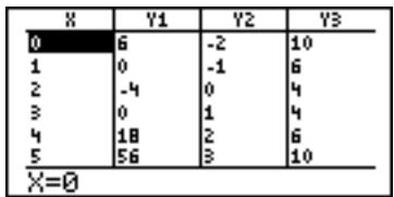
horizontally scroll the table. (The variable X is always displayed in the left end column.)

• The 10-digit value in the column where the cursor is currently located is displayed on the bottom line of the screen.
• Move the cursor using .
• Non-input equation numbers and equations invalid for graphing will not be displayed in the above table.

Parametric coordinate system

• The variable T is displayed in the left end column.
• The columns X1T, Y1T, and X2T are displayed on the first screen.

• Press to horizontally scroll the table.
• The 10-digit value in the column where the cursor is currently located is displayed on the bottom line of the screen.
• Move the cursor using
• Non-input equation numbers and equations invalid for graphing will not be displayed in the above table.

Polar coordinate system

• The variable is displayed in the left end column.
• The columns , R1 to R3 are displayed on the first screen.
• Press 4 to horizontally scroll the table.
• The 10-digit value in the column where the cursor is currently located is displayed on the bottom line of the screen.
• The cursor can be moved using
• Non-input equation numbers and equations invalid for graphing will not be displayed in the above table.

Sequential coordinate system

• The variable n is displayed in the left end column.
• Tables values u( n) ,v( n) ,and w (n) are simultaneously displayed.
• The 10-digit value in the column where the cursor is currently located is displayed on the bottom line of the screen.
• The cursor can be moved using .
• Non-input equation numbers and equations invalid for graphing will not be displayed in the above table.

Setting a table

To display the table, press TABLE.
- Table setting allows you set how to input data for a table.
- Press 2ndF TBLSET to enter the table setting screen.
- The cursor is initially located at Auto, showing the variable input method.

Auto: Automatically creates a table based on the graph equations and given TableStart and TableStep values.

User: Displays a blank table. As you input values for variable columns, table values are automatically calculated by the equation. Thus, although TableStart and TableStep inputs can be made when selecting User, set values will be ignored.

• Press < or to switch between Auto and User.
• TableStart is a start value of the variable in the table, and TableStep is a step value of the variable. Both are numeric values.

Example

Automatically create a table starting from -5 with a step of 1 in the X-Y coordinate after equations, based on "Y1 = X", "Y2 = X²", and

$$ " Y 3 = - X ^ {2} + 3". $$

1. Press 2ndF TBLSET and (-)5 ENTER 1 ENTER.

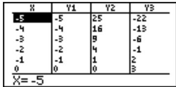
1. Press TABLE

2. If the cursor is on the top or bottom line of the table, ▲ or ▼ can still be used. The table contents will move to become visible in the display area.

Example

Create a table in the User mode under the above conditions.

1. Press 2ndF TBLSET and ENTER 0 ENTER 1 ENTER

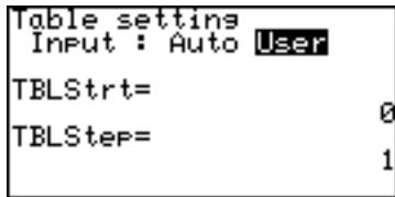
1. Press TABLE. Blank table will appear.

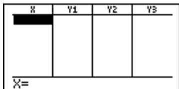
1. Press 2 ENTER (-) 3 ENTER to enter X values.

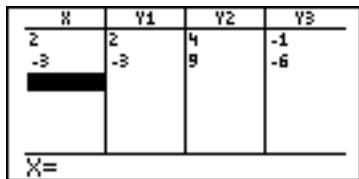
• An automatically created table in the User mode cannot be scrolled vertically.

Note: While the table is in the User mode, a selected row can be deleted by pressing DEL.

10. The DRAW Function

With the DRAW function, lines, circles, graphs, and pixel points can be added to the graph window. The DRAW menu also contains configuration tools for the ordinary graphs entered in the Graph Equation Entry window: line types, shading, and visibility status of each graph.

Press 2ndF DRAW to enter the DRAW menu.

Note: When entering coordinates, the DRAW function assumes that rectangular coordinates will be entered. The exception to this is for PxION(), PxIOFF(), PxICHG(), and PxITST(), all within the B POINT menu item.

A DRAW The tools in this menu add lines, circles, additional graphs and text on the graph screen.

The tools below can be accessed from the GRAPH window, or any other windows such as the Graph Equation Entry window and Calculation screen. Most of these tools, such as Line(), can be entered directly onto a graph from the cursor point.

1 ClrDraw Clears all items on the graph window EXCEPT for the graphs entered via the Graph Equation Entry window.

1. From the GRAPH window, press 2ndF DRAW to enter the DRAW menu.

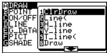
1. Press A to select A DRAW, then press 1 to select 1 CirDraw.

or

1. From the Calculation screen, press 2ndF DRAW A 1

"ClrDraw" will appear.

1. Press ENTER

All the items on the graph will be deleted and the message "Done" will appear.

2 Line( Draws a line according to the given X-Y coordinates of a start/end point.

Note: This tool can be used with any type of graph.

From the Calculation screen

Line(x-coordinate of start point, y-coordinate of start point, x-coordinate of end point, y-coordinate of end point [,0])

Example

1. Select the DRAW menu. Select A DRAW in the menu, then select 2 Line().

"Line" will appear.

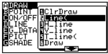
Suppose you wish to draw a line, starting from an X-Y coordinate (1,2) to end at (8,8).

1. Enter "1,2,8,8" right after the "Line(" object, then close the expression with .

1. Press ENTER.

The GRAPH window will appear with the specified line drawn on the graph.

Note: If you enter 0 for the 5th element of Line( function, (e.g. Line(1,2,8,8,0)) and press ENTER, you can clear the specified line.

From the GRAPH Line(

window

1. Press 2ndF
   DRAW to enter the DRAW menu.

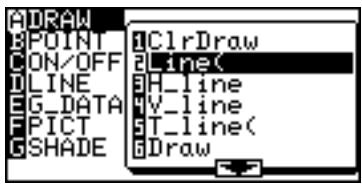
1. Press A to select A DRAW, then press 2 to select 2 Line().

The GRAPH window reappears, with the coordinate of the cursor showing at the bottom of the screen.

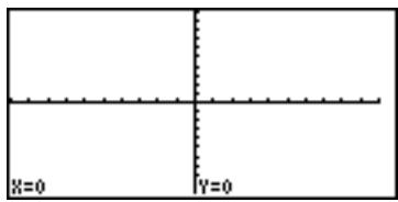
Note: To change the cursor coordinate system, use the FORMAT menu. Select F CURSOR, then select the required coordinate system for the cursor.

1. Move the flashing cursor on the screen to set the starting point of the line.

Note: The pixel increment can be set within the ZOOM menu. While A ZOOM is selected, choose 7 Dec to set each pixel size to “0.1 × 0.1”, or 8 Int to set to “1 × 1”.

1. When the starting point is set, press ENTER to anchor the location.

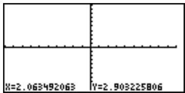
1. Move the cursor to indicate the end point of the line. When set, press ENTER to finalize the line drawing.

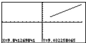
1. You may draw as many lines as you wish, by repeating the procedure from 4 to 5. When done drawing, press CL to exit the entry mode.

3 H_line Draws a horizontal line on the graph window.

From the Calculation screen

H_Line y-value

Draws a horizontal line ( y = value) on the graph window.

Example

• Draw a horizontal line of y = 5 .

• Press 2ndF
  DRAW A
  3 and enter the value 5.

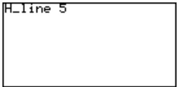
From the GRAPH window

H_Line

Example

• Draw a horizontal line manually.

• Press 2ndF
  DRAW A
  3.

• Use the cursor navigation keys

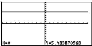
(▲ ▼ ▲ ▶) to move the flashing cursor to the appropriate position.

1. Press ENTER to draw the line.

4 V_line Draws a vertical line on the graph window.

From the Calculation screen

V_Line x -value

Draws a vertical line (x = value) on the graph window.

Example

• Draw a horizontal line of x = 3 .

• Press 2ndF DRAW A 4 and enter the value 3.

From the GRAPH V_Line

window Example

• Draw a vertical line manually.

• Press 2ndF DRAW A 4

• Use the cursor navigation keys (▲▼

) to move the flashing cursor to the appropriate position.

1. Press ENTER to draw the line.

5 T_line( Draws a tangential line at the specified point of a graph curve.

From the Calculation T_line(equation, x -value)

screen Example

• Draw the tangential line of y = x^2 at x = 1 .

• Select T_Line().

• Enter "x², 1)" on the line.

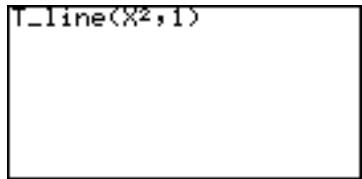
Note: It is also possible to specify a function equation from Y0 to Y9 if stored. (T_line(Y1, 1))

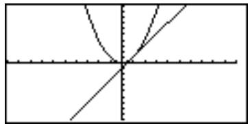
From the GRAPH T_line(

window Example

• Draw a tangential line by manually specifying the point.

• Select T_Line().

• Use 4 to move the flashing cursor on the targeted graph line.

Use ▲ to select a graph to draw the tangential line.

1. When the point is set at the tangent point, press ENTER.

6 Draw Draw equation

Draws an additional graph based on a given expression.

Example

• Draw the graph of y = 3x^2 - 4x + 2 .

• Select Draw.

• Enter "3x²-4x+2" on the line.
• Press ENTER

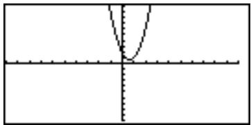
Note: This tool can be used with rectangular coordinate graphs only.

7 Shade( Shade(equation1, equation2 [, lower value, upper value])

Draws two graphs, and shades the area between the two. If the x range is specified, it shades the area within the specified range.

Example

• Shade the area enclosed by y = 14 x^2 - 8 and y = x .

• Select Shade().

• Enter 14 x^2 - 8 , x on the line.
• Press ENTER.

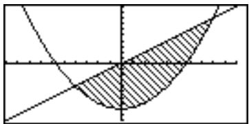
Example

• Shade the area enclosed by y = 14 x^2 - 8 and y = x within the range of -2 ≤ x ≤ 3 .

Before starting operation, Select ClrDraw to clear the graphs previously drawn.

1. Select Shade().
2. Enter 14 x^2 - 8 , x , -2, 3) on the line.
3. Press ENTER

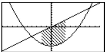
Note: It is also possible to specify a function equation from Y0 to Y9 if stored.

8 DrawInv DrawInv equation

Draws an inverse of a given graph expression.

Example

Draw the inverse graph of y = 14 x^2 - 8 .

1. Select DrawInv.
2. Enter 14 x^2 - 8 on the line.
3. Press ENTER

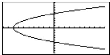
Note: It is also possible to

specify a function equation from Y0 to Y9 if stored.

9 Circle( Draw a circle on the graph screen.

From the Calculation screen

Circle(x-coordinate of center, y-coordinate of center, radius)

Example

• Draw a circle with center at (2,3) and of radius 7.

• Select Circle().

• Enter "2,3,7" on the line.
• Press ENTER.

Note: Before drawing a

circle, press ZOOM A 6 to set the X-Y coordinates to square.

From the GRAPH Circle

window Example

• Draw a circle manually.

• Select Circle().

• Move the cursor to set the center point of the circle. Press ENTER to set the anchor.
• Move the cursor to determine the radius length of

the circle.

1. When done, press ENTER.

The circle is drawn at the location.

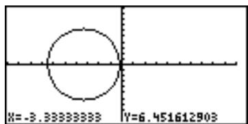
0 Text( Text(column, row, "strings")

Enters a text string at a given coordinate.

Example

• Draw "HELLO" on the graph at column 2, row 1.

Text(2,1,"HELLO")

Note:

3 to enter " " (double quotes).

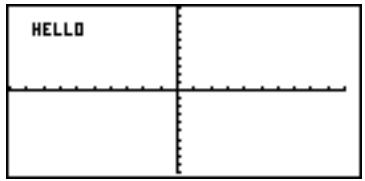
Column and row definitions for text input

• Refer to the following diagram to specify the coordinates where you wish to start writing the text.

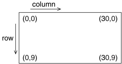
Note: Lines, points, and curves drawn by the Draw menu are handled as pictures. Therefore, they cannot be traced.

Graphs drawn by the Draw menu are automatically cleared if any screen settings are changed. To save the graph, use the StoPict menu.

B POINT Utilize these tools to manage point drawing and deletion on the graph.

There are two operation methods. One is to directly move the cursor pointer to the location on the graph screen where you wish to insert the point. The other is to call a relevant command on the Calculation screen and to directly input the coordinates to draw or delete the point. (X and Y coordinates should be separated by a comma.)

1 PntON( PntON(x-coordinate, y-coordinate)

Draws a point at a given coordinate. It takes the X-Y coordinate as an argument.

This tool can either be accessed from the GRAPH window or other windows. Entering from the GRAPH window enables a graphic entry, while entering from other windows enables text-based entry.

2 PntOFF( PntOFF(x-coordinate, y-coordinate)

Erases a pixel point. It takes the X-Y coordinate as an argument.

3 PntCHG(PntCHG(x-coordinate, y-coordinate)

Changes the status (i.e., visible/invisible) of a pixel at a given coordinate. Deletes the point when it is displayed and draws the point when it is not displayed.

4 PxION( PxION(column, row)

Draws a pixel point at a given screen location indicated by column and row.

The column and row definitions are as follows:

Column: 0 to 132,

Row: 0 to 64.

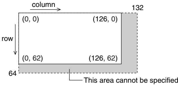
5 PxIOFF( PxIOFF(column, row)

Erases a pixel point at a given screen location indicated by column and row.

6 PxICHG( PxICHG(column, row)

Changes the status (i.e., visible/invisible) of a pixel at a given screen location indicated by column and row.

7 PxITST( PxITST(column, row)

Returns "1" if a pixel point is present at a given screen location indicated by column and row. Returns "0" if no pixel point exists.

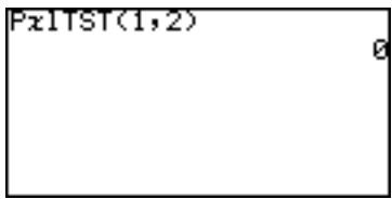
C ON/OFF Sets the visibility status of a given graph number (0-9).

1 DrawON DrawON [equation number 1,...] or DrawON

Sets the specified graphs visible. If no argument is given, then all graphs will be set visible.

2 DrawOFF DrawOFF [equation number 1, ...,] or DrawOFF

Sets the specified graphs invisible. If no argument is given, then all graphs will be set invisible.

Example

• Set Y1 and Y2 to visible and Y3 to invisible.

• Press 2ndF DRAW C 1

• Enter "1, 2" for equation numbers.
• Press ENTER
• Press 2ndF DRAW C 2
• Enter 3 for equation number.
• Press ENTER

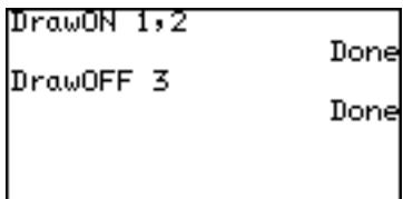
D LINE Sets the line appearance of each graph. Each graph coordinate mode (i.e., rectangular, polar, etc.) can retain a set of line appearance preferences. Solid line, dotted line, bold line, locus and dots can be selected.

1. Press 2ndF DRAW D to select D LINE, then press ENTER.

2. The next window enables you to select the line types of each graph in the set coordinate mode. (The rectangular coordinate mode is selected in this example.) Use the cursor keys to select the required line type, and press ENTER.

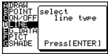
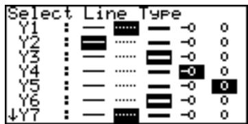
E G_DATA All graph data, including the graph equations and window settings, can be stored in 10 graph storage areas (1-9, and 0), which can be called up later.

1 StoGD StoGD number (0-9)

Saves the graph data.

Example

• Store the current graph data in location #1.

Note: The lines, graphs and pixels drawn with the A DRAW tools will not be saved here; use StoPict under F PICT instead.

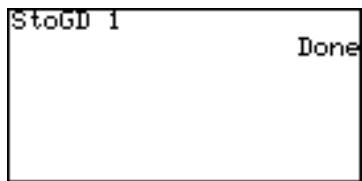
2 RclGD RclGD number (0-9)

Recalls the saved graph data.

Example

• Call back the previously stored graph data from location #1.

Note: Attempting to call back graph data from an empty location will result in an error.

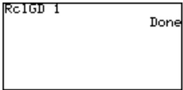
F PICT Stores and recalls the displayed pixel data for the graph window. The graph equations will not be saved or recalled with these tools.

1 StoPict StoPict number (0-9)

Saves the pixel data.

Example

• Store the current graph, including the drawings, in location #1.

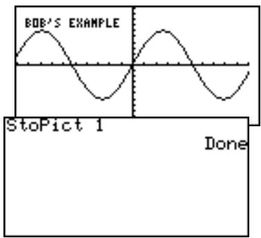
2 RclPict RclPict number (0-9)

Recalls the saved pixel data.

Example

• Call back the previously stored graph data from

location #1.

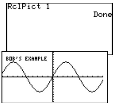
G SHADE With these sub-menu tools, inequalities, intersections and compliments of multiple graphs can be visualized.

1 SET Sets up the shading area for each graph. Refer to "3. Other Useful Graphing Features" in Chapter 4 of this manual to learn how to utilize this tool.

2 INITIAL Initialized the shading setup, and brings up the shading setup window.

11. Substitution Feature

Refer to the page 63 for details.

As for the Advanced keyboard, you can rewrite the equation based on the numeric values input on the substitution feature screen.

Example

Follow the step 1 on page 65:

1. Press 2ndF EXE to return to the equation display screen. The equation is written based on the last numeric values input on the substitution feature screen.

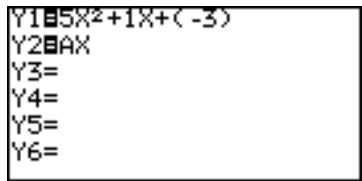
• Once 2ndF EXE have been pressed, the screen cannot be returned to the previous substitution feature screen.

Chapter 7

SLIDE SHOW Feature

The SLIDE SHOW feature is especially incorporated to help students understand math concepts utilizing the calculator's graphing capabilities. With this feature, the calculator's screen images can be captured, organized, and stored.

The SLIDE SHOW feature is designed to be used with SHARP's optional overhead projection system, which offers a hassle-free math presentation environment for the entire class.

The SLIDE SHOW can be used in both Basic and Advanced mode.

To enter the SLIDE SHOW, press SlIDE. To exit the SLIDE SHOW feature, press 100

1. Try it!

Make a SLIDE SHOW named "CUBIC" to explain how to draw the graph of a factorbase cubic function and explain how to solve cubic equations using factors. Use the following cubic function as a sample.

$$ y = (x - 3) (x - I) (x + 2) $$

Create a new SLIDE SHOW

1. Set up a SLIDE SHOW file.

Press SLIDE to enter the SLIDE SHOW menu.

1. Press C ENTER to select C NEW.
2. Name your project (type "CUBIC," for example), and press

ENTER.

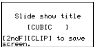
Capture images

1. Press = to enter the graph equation mode.
2. Enter (x - 3)(x - 1)(x + 2) at the first equation.

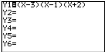
1. Press 2ndF CLIP.

The message "STORE SCREEN: 01" will appear. The image will be stored on page 1 of the SLIDE SHOW "CUBIC," and the screen will automatically return to the previous screen.

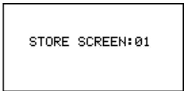
Each time you press 2ndF CLIP, the screen image will be captured and stored in the SLIDE SHOW.

Note:

1. Press GRAPH.

2. You cannot capture an image while drawing.

3. If the cursor flashes at the upper right corner of the

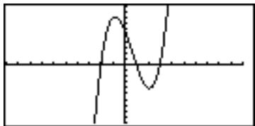
screen, the calculator is busy processing tasks. The SLIDE SHOW feature cannot capture images during this period.

• A captured image cannot be recaptured.
• After the graph is drawn, press 2ndF CLIP.

The image will be stored on page 2 of the SLIDE SHOW "CUBIC".

1. Press 2ndF SPLIT to split the screen between the graph and the table.
2. After drawing is done, press 2ndF CLIP

The screen image is stored on page 3.

1. Press once, and press 2ndF CLIP. Continue this operation.

Playing back the newly created SLIDE SHOW

1. Press SLIDE SHOW to go to the SLIDE SHOW menu.

A list of saved SLIDE SHOW projects will be shown.

1. Select the one you want to play back, either by using the shortcut key strokes, or by moving the cursor. (Select the item and press ENTER.)

The first page of the SLIDE SHOW will appear.

The number appearing at the upper right of the screen is the slide number.

1. Use the key or ENTER to display the next image; press the key to show the previous image.

Rearranging the captured images

Let's change the last image of the SLIDE SHOW feature to before the third.

1. Press SLIDE to bring up the SLIDE SHOW menu.

Select a file

1. Press D to select D SELECT.
2. Choose the project you want to edit from the sub-menu list.
3. Press ENTER to select. The target SLIDE SHOW will be selected.

Select an image

1. Press SLIDE E to select EEDIT, then press 1 to select 1 MOVE.

The first image of the selected SLIDE SHOW file appears.

1. Go down to the last captured image using the key.
2. Press ENTER to mark the image.

Specify the insertion point

1. Go up to the page 3 using the key.
2. Press ENTER. The marked image will be inserted at page 3.

2. The SLIDE SHOW menu

A CURR

This section of the chapter summarizes each item in the SLIDE SHOW feature menu.

Displays the name of the currently selected or working

SLIDE SHOW. Press 2ndF CLIP to capture an image.

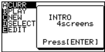
B PLAY

Enables you to select a SLIDE SHOW file for playback.

C NEW

Creates a new SLIDE SHOW file to store screen images.

D SELECT

Enables you to select a SLIDE SHOW file to be edited and display its name in the A CURR window.

EEDIT

Enables you to move/delete captured images, or change the file name of the current SLIDE SHOW.

Note:

If no SLIDE SHOW file is stored, selecting any of the following sub-menu items will result in an error.

1 MOVE

With this sub-menu tool, a selected screen image can be moved, so that the playback order will change. To escape from this mode and go back to the SLIDE SHOW menu, press the SLIDE SHOW key.

1. While in the SLIDE SHOW menu, press E to select E EDIT, then press 1 to select the 1 MOVE sub-menu item.
2. With the and cursor keys, select the captured image you wish to move, then press ENTER.
3. Select the position to which you wish to move the previously selected image using the and cursor keys.
4. Pressing ENTER will place the selected image at the new location. The selected image will be placed immediately before the current screen.

2 DEL

This sub-menu tool deletes the selected image captured in the SLIDE SHOW.

1. While in the SLIDE SHOW menu, press E to select EEDIT, then press 2 to select the 2 DEL sub-menu item.

1. With the and cursor keys, select the image you wish to delete.
2. Press ENTER to remove the selected image from the SLIDE SHOW file.

3 RENAME

Use this sub-menu tool to rename the SLIDE SHOW.

1. In the SLIDE SHOW menu, press E to select E EDIT, then press 3 to select the 3 RENAME sub-menu item.
2. The following screen enables you to change the SLIDE SHOW name.

3. Type the new name. The default input mode is A-LOCK. If you wish to incorporate numbers, press the ALPHA key to enter numbers. To switch back into the ALPHA mode, press ALPHA again.

4. Pressing ENTER will store the new SLIDE SHOW name.

Chapter 8 Matrix Features

Within the Matrix features, up to ten different matrices can be entered.

To get to the Matrix features, press 2ndF MATRIX. Define and edit the matrices within this mode too.

1. Try it!

Three sheaves of the first class crop, two of the second, and one of the third are sold for 39 dollars. Two of the first, three of the second and, one of the third for 34 dollars. And one of the first, two of the second and three of the third for 26 dollars. How much did you receive from each sheaf of the first, second and third class crops?

(Chapter VIII of Chiu Chang Suan Shu - Nine Chapters of Arithmetic Arts, 200 B.C., China)

Three equations can be derived as follows, containing three unknown quantities:

$$ 3 x + 2 y + z = 3 9 $$

$$ 2 x + 3 y + z = 3 4 $$

$$ x + 2 y + 3 z = 2 6 $$

x, y and z represent the price for each sheaf of the first, second and third class crops, respectively.

You can solve the above system of linear equations by using a matrix.

CONCEPT

1. Enter the coefficients as elements in a matrix.
2. Use the rrowEF function to obtain the reduced row echelon form.

PROCEDURE

Select a matrix to edit

1. Press 2ndF MATRIX to enter the MATRIX menu.

2. Press B to select EDIT and then 1 to select 1 mat A.

3. Press 3 ENTER 4 ENTER to define the dimensions of the matrix (3 rows × 4 columns).

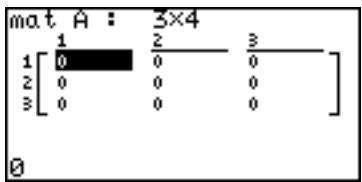
Define dimensions

Enter the values

1. Press 3 ENTER 2 ENTER 1 ENTER 3 9 ENTER to enter the first row of 3x + 2y + z = 39 The cursor will automatically position itself at the beginning of the second row.

2. Press 2 ENTER 3 ENTER 1 ENTER 3 4 ENTER to enter the second row of 2x + 3y + z = 34

3. Press 1 ENTER 2 ENTER 3 ENTER 2 6 ENTER to enter the third row of x + 2y + 3z = 26

4. Press to return to the calculation screen. Matrix A is now set.

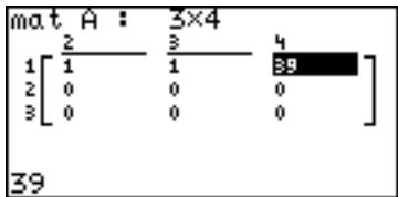
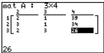
Solve the problem

1. Press 2ndF MATRIX to display the MATRIX MENU, and press D to select D MATH and then press 4 to select 4

rrowEF. The reduced row echelon form is now set, as shown:

1. Press 2ndF MATRIX, then press A to select NAME and press 1 to select 1

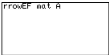
mat A. The Matrix A is now set and ready to be calculated.

1. Press ENTER.

The reduced row echelon form of the matrix is displayed.

Display

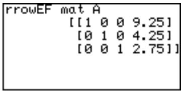
Solution

$$ I x + \theta y + \theta z = x = 9. 2 5 $$

$$ 0 x + I y + 0 z = y = 4. 2 5 $$

$$ 0 x + 0 y + 1 z = z = 2. 7 5 $$

2. Entering and Viewing a Matrix

Select a matrix

1. Press 2ndF MATRIX, then press B (select EDIT) and select the matrix you want to define.

Note: Up to 10 matrices from 1 matA to 0 matJ can be defined.

Define dimensions

1. Enter the row dimension number and press ENTER Cursor moves to the column dimension.

2. Enter the column dimension number and press ENTER. The matrix will be displayed with null values. (See below.)

3. It is not required to press ENTER when the dimension number is 2 digits.

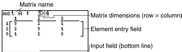
Up to 5 rows by 3 columns of elements can be displayed on the screen.

Press to scroll the matrix. Use row and column numbers on the left and upper side of the matrix to check the display location.

• If the dimensions of the matrix have previously been defined, the values will be displayed. You can retain or alter the dimensions accordingly.

Enter elements in the matrix

1. Press appropriate number keys to enter numbers at the 1st row and 1st column.

The number is displayed at the bottom of the screen.

1. Press ENTER

The cursor moves to the 1st row, 2nd column.

1. Sequentially input the element data.
2. Press [ ] after completion of data input.

Editing keys and functions

Move the cursor within the current row or scroll horizontally.

Move the cursor within the current column or scroll vertically. On the top row, moves the cursor to the dimensions field.

ENTER the number in the cursor position and move the cursor to the next position.

Clear the value of bottom line (input field).

Store all the elements of the matrix and returns to the calculation screen.

3. Normal Matrix Operations

Many calculations can be made between a matrix and a real number or between matrices.

Examples of each calculation are as follows:

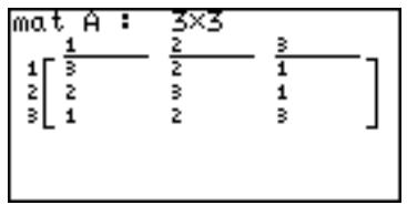
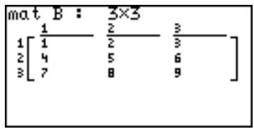
Matrix + Matrix Matrix - Matrix

To add or subtract matrices, the dimensions must be the same.

Example

1. Press [CL].
2. Press 2ndF MATRIX A

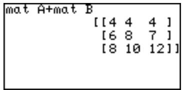
1. Press ENTER

Matrix × Matrix

To multiply two matrices, the column dimension of the first matrix must match the row dimension of the second matrix.

Example

1. Press CL
2. Press 2ndF MATRIX A

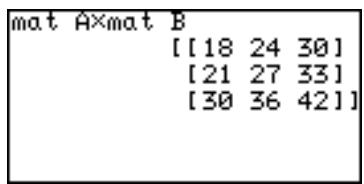
1. Press ENTER

Square of Matrix

To obtain the square of a matrix:

Example

1. Press [CL].
2. Press 2ndF MATRIX A

1. Press ENTER

4. Special Matrix Operations

This calculator has three Matrix calculation menus: OPE, MATH and [ ].

Examples of each calculation are as follows:

Calculations using OPE menus

01 dim( dimmatrixname)

Returns the dimensions of the specified matrix.

Example

• Check the dimensions of mat A.
• Newly define or change the dimensions to 2 × 3 for Mat C.

02 fill( fill(value, matrix name)

Fills each element with a specified value.

Example

• Enter the value 5 into all the empty elements of matrix C.

03 cumul cumul matrix name

Returns the cumulative matrix.

Example

• Obtain the cumulative sum of mat A.

cumulative sum of a_ij = a_il + a_i2 + +a_ij

cumul mat A [[54] [99] ausment(matA,matB) [[5431] [4526]] 

04 augment( augment matrix name, matrix name)

Appendeds the second matrix to

the first matrix as new columns. The first and second matrices must have the same number of rows.

Example

• Create a new matrix with matrix A augmented by matrix B.

05 identity identity dimension value

Returns the identity matrix with specified value of rows and columns.

Example

• Create the identity matrix of 3 rows × 3 columns.

identity3 [100] [010] [001]] 

06 rnd_mat( rnd_mat(number of row, number of column)

Returns a random matrix with specified values of rows and columns.

Example

• Create a matrix of 2 rows × 3 columns with generated random values.

(when TAB = 2 and FSE = "FIX" at SETUP menu)

rnd_mat(2,3)  
[[0.66 0.63 0.49]  
[0.36 0.33 0.56]] 

07 row_swap( row_swap matrix name, row number, row number)

Returns the matrix with specified rows swapped.

Example

• Swap the 2nd and 3rd rows in the matrix E .

$$ e _ {2 j} = e _ {3 j}, e _ {3 j} = e _ {2 j} $$

[4 9 2]

[1 5 6]]

row_swap(mat E,2,3)

[[5 2 3]]

[1 5 6]]

[4 9 2]]

08 row_plus( row_plusmatrix name, row number, row number)

Adds the first specified row data to the second specified row data.

Example

• Add the 2nd row data to the first row of matrix E.

$$ e _ {1 j} = e _ {1 j} + e _ {2 j} $$

row_plus(mat E,2,1)

[[9 11 5]]

[[4 9 2]]

[[1 5 6]]

09 row_mult( row_mult(multiplied number, matrix name, row number)

Returns the scalar multiplication of elements in a specified row.

Example

• 3 × each element of 1st row of mat E

$$ e _ {l j} = 3 \times e _ {l j} $$

rowMULT(3,mat E,1)

[[15 6 9]]

[[4 9 2]]

[[1 5 6]]

10 row_m.p.( row_m.p.(multiplied number, matrix name, row number, row number)

Returns the scalar multiplication of elements in a specified row and adds result to elements in another specified row.

Example

• 2 × each element of 3rd row and add the result to each element of the 1st row.

$$ e _ {l j} = e _ {l j} + 2 \times e _ {2 j} $$

row_m.P. (2, mat E, 3, 1)

[7 12 15]

[4 9 2 ]

[1 5 6 ]]

11 mat→list( Creates lists with elements from each column in the matrix. If dimensions of columns is greater than the number of lists specified, extra columns are ignored. Also, if it is less than the number of lists specified, extra lists are ignored.

mat list matrix name, list name 1, ..., list name n)

Example

• Make List 1 and List 2 by using the 1st and 2nd columns of matrix E, respectively.

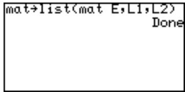
mat list matrix name, column number, list name)

Example

• Make List 3 by using the 3rd column of matrix E.

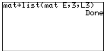
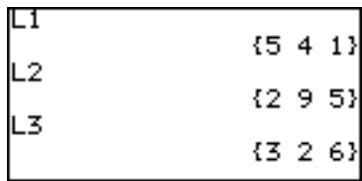
12 list mat( list mat(list 1, ..., list n, matrix name)

Creates a matrix using specified lists. This function is the same as list mat( in the List OPE menu.

Note: The list items must be prepared prior to executing this function.

Example

• Create columns of matrix D by using list items in L1 and L2.

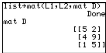
Calculations using MATH menus

1 det det matrix name

Returns the determinant of a square matrix.

The determinant can only be applied to a matrix which has the same row and column dimensions.

Example

• Give the determinant of matrix A.

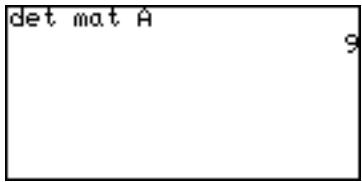
2 trans trans matrix name

Returns the matrix with the columns transposed to rows and the rows transposed to columns.

Example

• Transpose rows and columns of matrix B.

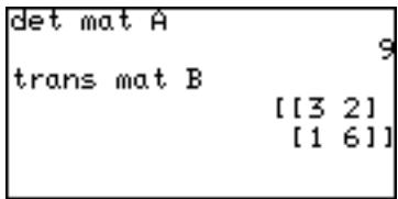
3 rowEF rowEF matrix name

Returns the row Echelon Form of the specified matrix. The number of columns must be greater than or equal to the number of rows.

Example

• Give the row-echelon form of matrix B.

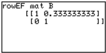
4 rrowEF rrowEF matrix name

Returns the reduced row Echelon Form of the specified matrix. The number of columns must be greater than or equal to the number of rows.

Example

• Give the reduced row-echelon form of matrix B.

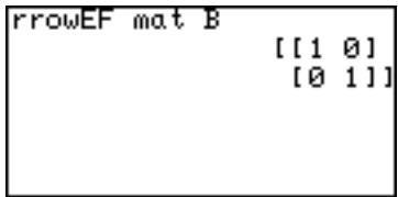
Use of [ ] menus

Using [ ] menus, you can manually enter a matrix on the calculation screen.

1. Press 2ndF MATRIX E 1 ([]) at the beginning of the matrix.
2. Press 2ndF MATRIX 1 ([]) to indicate the beginning of the first row.

Once you enter the manual matrix entry mode, you can directly enter "or" by selecting 1 or 2.

1. Enter a number or expression for each element. Separate each element with commas.

2. Press 2ndF MATRIX 2 () to indicate the end of the first row.

1. Repeat above steps 2 to 4 to enter all the rows.
2. Press 2ndF MATRIX 2 () to indicate the end of the matrix.
3. Press ENTER

The matrix will be displayed.

Using a Matrix in an expression

To use a matrix in an expression, you can do any of the followings:

• Select a matrix from the MATRIX NAME menu.
• Enter the matrix directly using the [ ] function menus.

Chapter 9 List Features

List features can be used in both Advanced and Basic mode. In this chapter, all the procedures are based on the Advanced mode. In the Basic mode, press 2ndF LIST and select A NAME to access L1 to L6.

1. Try it!

By analyzing years of data, we found that it takes the driver of a car approximately 0.75 seconds to react to a situation before actually applying the brakes. Once the brake pedal is depressed, it takes additional time for the car to come to a complete stop. Here is the equation used to compute total stopping distance on dry, level concrete:

The reaction time distance (in feet) = 1.1 times the speed (in miles per hour);

The braking distance = 0.06 times the speed squared;

$$ y = (1. 1 \times v) + (0. 0 6 \times v ^ {2}), $$

where y represents the total stopping distance (in feet), and v represents the speed (miles/ hour)

Calculate the total stopping distances at the speeds of 30, 40, 50, 60, 70, 80 miles per hour.

CONCEPT

1. You can calculate all answers individually, but if you use list, you can obtain the results with one calculation.

PROCEDURE

Enter each speed value in the list

1. Press CL to enter the calculation screen.
2. Press 2ndF { 30
   , 40 , 50
   60 , 70 , 80
   2ndF }

The calculator displays the set of data.

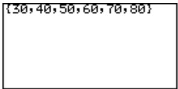
Store the list in L1

1. Press STO 2ndF L1
2. Press ENTER to store the list in L1.

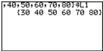
Enter the equation using L1

1. Press 1.1 X 2ndF L1 + 0.06 X 2ndF L1 x²
2. Press ENTER.
3. List {87, 140, 205, 282, 371, 472} will appear. So the solutions are:

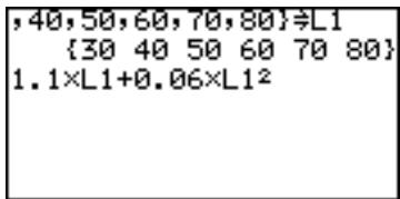
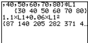
Car speed	Stopping distance
30 miles/hour	87 feet
40 miles/hour	140 feet
50 miles/hour	205 feet
60 miles/hour	282 feet
70 miles/hour	371 feet
80 miles/hour	472 feet

Note: You can also perform the above calculation using the direct list input method (using braces).

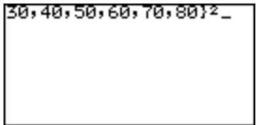
1.1 × {30, 40, 50, 60, 70, 80} + 0.06 × {30, 40, 50, 60, 70, 80} ^2 and press ENTER.

• In the Basic mode, you can access L1 to L6 from A NAME and “{}” (braces) from E {} in the LIST menu.

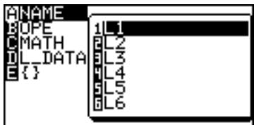
2. Creating a list

A list is a series of values enclosed by braces, and is treated as a single value in calculations or an equations.

The calculator has 6 storage areas for lists from L1 to L6.

You can edit or access lists by pressing 2ndF L1 to L6 (numeric keys from 1 to 6).

Using 2ndF LIST (L_DATA) menus, you can store up to 10 sets (L_DATA 0 to L_DATA 9) of lists (L1 to L6) in a memory and recall any of the stored sets as required.

Store a series of data 1, 3, 2, and 9 in the list L1, and 5, 4, 6, 3 in L2

1. Press CL to enter the calculation screen.
2. Press 2ndF { 1 , 3 , 2 , 9 2ndF }
3. Press STO 2ndF L1
4. Press ENTER to store the list in L1.
5. Press 2ndF { 5 ,
   4 , 6 , 3 2ndF
   } STO 2ndF L2
   ENTER for L2.

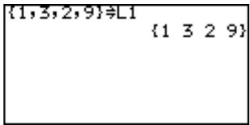
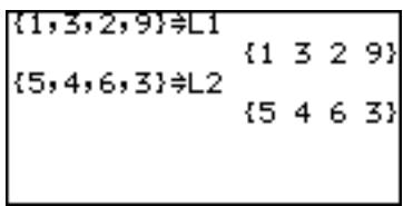
Tips: To view a specific list, press

2ndF L1 to L6, then ENTER at the calculation screen.

3. Normal List Operations

• Lists can contain real and complex numbers.
• Lists can be used as values (or variables) in calculations or equations.
• Calculations between lists are also possible. (Both lists must contain the same number of elements.)
• The following examples use the L1 and L2 values stored in the previous section.

Calculate 10 × L1 and store the results in L3

1. Press 10 X 2ndF L1 STO 2ndF L3 ENTER.

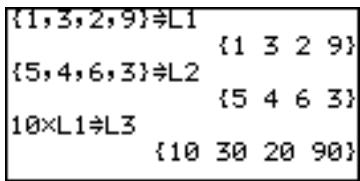
Calculate the sine of L3

1. Press sin 2ndF L3 ENTER. ..” shows that results extend beyond the display to the right. Use to scroll left or right, respectively.

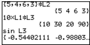
Calculate L1 + L2

1. Press 2ndF L1 + 2ndF L2 ENTER

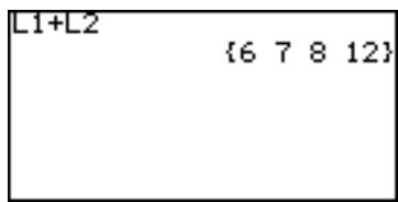
Change the 3rd element of L1 to -3

1. Press (-) 3 STO 2ndF L1 ( 3 ALPHA : 2ndF L1 ENTER).

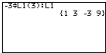
Append the new value 7 to L1 as the 5th element

1. Press 7 STO 2ndF L1 (5 ALPHA : 2ndF L1 ENTER.

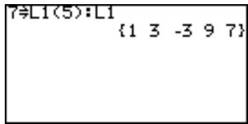
Note: Separated by a colon (:), two or more commands can be entered in one line.

Calculate the root of L2

1. Press 2ndF 2ndF L2 ENTER

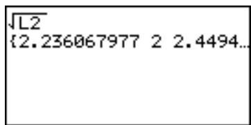
4. Special List Operations

This calculator has three list calculation menus: OPE, MATH and L_DATA.

• In the Basic mode, L1 to L6 (list names) can be accessed from the LIST menu.

Calculations using the OPE menu functions

1 sortA( sortA(list name)

Sorts lists in ascending order.

Example

• Store list 2, 7, 4 in L1, and sort L1 in ascending order.

{2,7,4}÷L1	{2 7 4}
sortA(L1)	Done
L1	{2 4 7}

2 sortD( sortD(list name)

Sorts lists in descending order.

Example

• Sort the above list L1 in descending order.

L1	{2 4 7}
sortD(L1)	Done
L1	{7 4 2}

Note: sortA(list name 1, subordinate list name 1,...)

If two or more lists are entered separated by commas, a sort is performed on the first list as a key, and the following lists are sorted in the order corresponding to the elements in first list (key list).

Example

• Store lists 2, 7, 4 and -3, -4, -1 in L1 and L2 respectively, and sort L1 and L2 in ascending order using list L1 as a key list.

Returns the number of items (dimension) in the list.

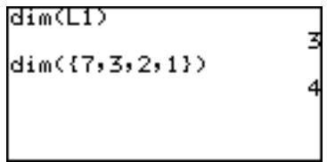
Example

• Display the dimension of list L1.

natural number dim(list name)

Set the number of items (dimension) of specified list to the specified number.

Example

• Set the dimension of list L6 to 4.

All the elements are initially 0. This operation overwrites the existing list dimensions.

The existing values within the new dimensions remain as they are.

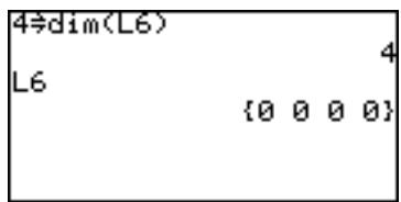
4 fill( fill(value, list)

Enter the specified value for all the items in the specified list.

• The dimension of the list must be set beforehand.

Example

• Set the dimension of list L6 to 4 and substitute 5 for all the items of list L6.

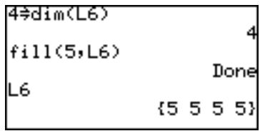
5 seq( seq(equation, start value, end value[, increments]) target list name

Makes a list using the specified equation, range (start value and end value) and increments.

Example

• Fill the list using the equation y = x^2 - 8 ,where x increases from -4 to 4 by increments of 2 .

• If increment is omitted, the default value 1 is used.

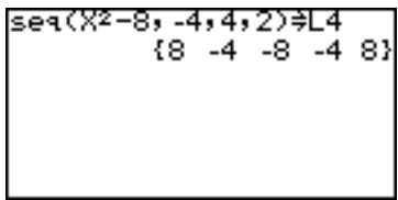
6 cumul cumul list

Sequentially cumulates each item in the list (for Advanced mode only).

l_i = l_1 + l_2 + + l_i , where l_i is the i-th item of the list.

Example

• Set the list L1 to {4, 2, 7}, and obtain the cumulated list L1.
• Cumulate the above result.

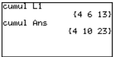
7 df_list df_list list

Returns a new list using the difference between adjacent items in the list.

l_i = l_i + J - l_i , where l_i is the i-th item of the list.

Example

• Set the list L1 to {4, 2, 7}, and calculate the difference between adjacent items.

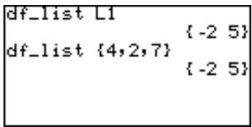
8 augment( augment(list 1, list 2)

Returns a list appending the specified lists.

Example

• Obtain the list appending L1 ({4, 2, 7}) and L2 ({-1, -3, -4}).

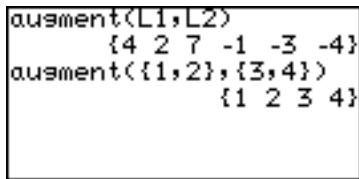
9 list mat( list mat(list 1, ..., list n, matrix name)

Makes a matrix using the specified list as column data, stored under the specified matrix name (for Advanced mode only).

Example

• Make a matrix mat A using list L1 as the first column and list L2 as the second column.

• The dimensions of the two lists must be the same.

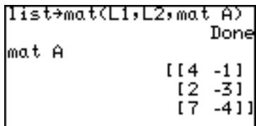
• Complex numbers cannot be used with this function.
• This function is the same as list→mat of the OPE menu in the MATRIX function.

0 mat→list( mat→listmatrixname, list name 1,..., list name n) mat→listmatrixname, column number, list name)

Makes lists from the matrix (for Advanced mode only).

This function is the same as "mat→list" of the OPE menu in the MATRIX function. See page 128 for details.

Calculations using MATH Menus

During the following explanations, the values of lists, L1 and L2 will be assumed to be:

$$ \begin{array}{l} \mathsf {L} 1 = {2, 8, - 4 } \ \mathsf {L} 2 = {- 3, - 4, - 1 } \ \end{array} $$

1 min( min(list)

Returns the minimum value in the list.

Example

Calculate the minimum value of the list L1.

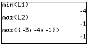
2 max( max(list)

Returns the maximum value in the list.

Example

Calculate the maximum value of the specified list L2.

Note: min(list 1, list 2)

max(list1, list2)

If two lists are specified in parenthesis separated by a comma, then a list consisting of minimum (or maximum) values is returned.

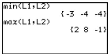
3 mean( mean(list[, frequency list])

Returns the mean value of items in the specified list.

Example

Calculate the mean value of list L1.

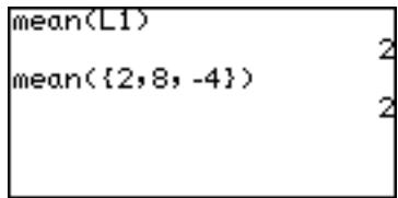
4 median( median(list [, frequency list])

Returns the median value of items in the specified list.

Example

Calculate the median value of the list L2.

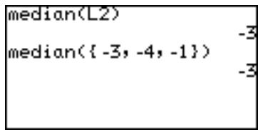
5 sum( sum(list [, start number, end number])

Returns the sum of items in the specified list.

Example

• Calculated the sum of the list items of L1.
• You can specify the range of items in the list to sum.

sum(L1,1,2) means sum

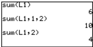
the 1st to 2nd items of the list L1.

sum(L1, 2) means sum all items from the second to the last of the list L1.

6 prod( prod(list [, start number, end number])

Returns the multiplication of items in the specified list (for Advanced mode only).

Example

Calculate the multiplication of items in the list L1.
* You can specify the range of items in the list to multiply. prod(L1, 1, 2) means

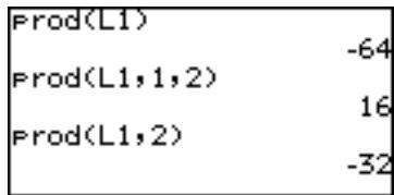
multiply the 1st to 2nd items of the list L1.

prod(L1,2) means multiplication of all items from the second to the last of the list L1.

7 stdDv( stdDv(list[, frequency list])

Returns the standard deviation of the specified list items.

Example

• Calculate the standard deviation using the list items of list L2.

stdBv(L2)

1.527525232

stdBv({-3,-4,-1})

1.527525232

8 varian(varian(list[, frequency list])

Returns the variance of the specified list items.

Example

Calculate the variance using the list items of list L2.

varian(L2)	2.333333333
varian([-3,-4,-1])	2.333333333

Standard deviation and variance

Standard deviation: s =

$$ \text {V a r i a n c e} = \sqrt {\frac {\sum_ {k = 1} ^ {n} \left(l _ {k} - m\right) ^ {2}}{n - 1}} $$

where n = number of list items

l_k = list item value

m = mean value of the list

5. Drawing multiple graphs using the list function

Using list items as coordinates, you can simultaneously draw multiple graphs.

1. Press = .
2. Enter the equation;

$$ \Upsilon 1 = {3, - 2 } x ^ {2} + {5, 3 } x + {2, 4 } $$

1. Press GRAPH.

Two graphs are drawn as shown on the right.

In this case, the first one represents the equation y =

3x^2 + 5x + 2 and the second y = -2x^2 + 3x + 4 .

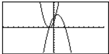
You can also use L1 to L6 to enter the equation;

1. Set the lists L1 to L3 as follows;

3, -2 L1
5,3 L2
2,4 L3 , and then

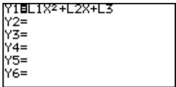
1. Enter the equation as follows.

$$ Y 1 = L 1 x ^ {2} + L 2 x + L 3 $$

6. Using L_DATA functions

The calculator can store up to 10 list groups in memory (L_DATA 0 to L_DATA 9). You may store or recall any one of these list groups. Each list group can contain up to 6 lists.

1 StoLD StoLD natural number (0-9)

Stores the current group of lists (L1 to L6) in L_DATA 0 to 9.

Example

1. Press 2ndF LIST and select C 1
2. Enter the preferred number from 0 to 9 and press ENTER.

"Done" will appear and the current lists will be stored in L_DATA#.

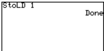
2 RcILD RcILD natural number (0-9)

Recall the stored group of lists for use.

Any current list data (not stored in L_DATA) is overwritten.

Example

1. Press 2ndF LIST and select C 2

2. Enter the number to recall and press ENTER.

"Done" will appear and the

current lists will be overwritten by the recalled list group.

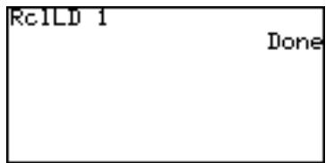
7. Using List Table to Enter or Edit Lists

You can use List Table in the STAT menu to easily access the contents of the lists.

Though the STAT menu was originally designed for Statistics function calculations, the List Table is very useful for entering or editing list items.

How to enter the list

1. Press STAT A ENTER

The list table will appear.

The first column indicates the order number of each list, and the 2nd column

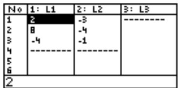
corresponds to the list L1, the 3rd to the L2, and so on.

1. Move the cursor to the target cell and enter the appropriate value.

The value will appear on the bottom line.

1. Press ENTER

The value will enter the cell and the cursor move down to the next cell.

• “------” indicates the end of the list. When you enter the value, “------” goes down to the next cell.

How to edit the list

1. Press STAT and select A EDIT, then press ENTER.
2. Use the cursor keys to move the cursor to the target cell.
3. Enter the new value and press ENTER.

The new value will be stored in the target cell.

• The display on the bottom line relates to the cell where the cursor pointer is located.

Though any number can be entered in a cell, the bottom line of the screen can display up to a maximum of 10 digits excluding exponents, and the cell can display up to a maximum of 8 digits including exponents.

Chapter 10 Statistics & Regression Calculations

Note: The explanation of this chapter is based on the Advanced Keyboard.

The following statistical and regression features are available:

• Statistical calculations such as means and standard deviations
• Graphing statistical data
• Plotting regression curves
  Statistical tests
  Estimation
• Obtaining coefficients from regressions
  Distribution functions

1. Try it!

The following table shows the access counts (per hour) of a certain web site from Sunday midnight to Monday midnight.

Hours	01	02	03	04	05	06	07	08	09	10	11	12	13	14	15	16	17	18	19	20	21	22	23	24
Sunday	98	72	55	3	6	24	15	30	59	72	55	43	21	10	150	151	135	108	204	253	232	251	75	30
Monday	32	8	12	2	4	19	32	72	95	91	123	201	184	108	95	72	45	38	75	111	153	90	84	35

Let's input these data into the calculator (List function) and plot a histogram.

Opening the list 1. Press STAT.
table to enter The Stat menu will appear.
data

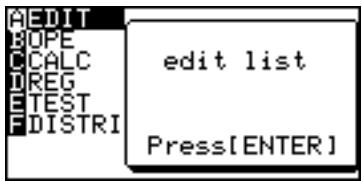
1. Select A EDIT and press ENTER. The List table will appear. Initially, all elements are blank and the cursor pointer is located at L1-1 (top left).

Entering hours (index value)

1. Input 1 for hour.
2. 1 will be displayed at the bottom line of the display.
3. Press ENTER to input the index value.
4. Continue the procedure to input 2 to 24.

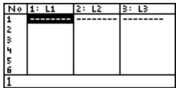
Entering the data for Sunday

1. Press to move the cursor to the top line of L2.
2. Input 98 for hour 01. 98 will be displayed at the bottom line of the display.
3. Press ENTER to input the data. 98 will appear in position L2-1 and the cursor will move to the second row.
4. Input 72 for hour 02 and press ENTER. Continue the procedure to the end of the data.

Entering the data for Monday

1. Press l to move the cursor to the top line of L3.
2. Input 32 for hour 01 and press ENTER
3. Continue the procedure to the end of the data.

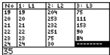
If you enter the wrong data

1. Press , or to move the cursor pointer to the target cell.
2. Input the correct number and press ENTER

Graphing the statistical data (Histogram)

Now we can plot the data to make histograms, broken line graphs and other statistical graphs.

1. Press STAT PLOT.
2. Select A PLOT1 and press ENTER). The following screen will appear.

Setting the graph drawing "on"

1. The first line shows if the graph drawing is on or off. Initially, the graph drawing is off. With the cursor pointer at the "on" position, press ENTER to set the graph drawing on.

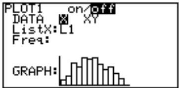
Selecting whether 1-variable plotting or 2-variable plotting

1. Press to move the cursor to the next line (DATA).
2. Select X for 1-variable plotting and press ENTER.

Select the list number used for graphing

Determining ListX and Freq Frequency relates to the number of times access occurred (L2) at the ListX stage. You can refer that the Access of ListX (L1) hour occurred Freq (L2) number of times.

1. Press to move the cursor to the next line (ListX).
2. The default list name for ListX is L1. If another list name is set, press 2ndF L1 to enter L1.
3. L1 is set to be used for x-axis items.

Setting the frequency

1. Press to move the cursor to the next line (Freq).
2. Press 2ndF L2 to enter L2.

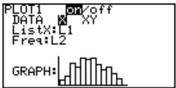
Selecting the graph

1. Press to move the cursor to the next line (GRAPH).
2. The graph format defaults to histogram, so if that is what is required, this does not need to be changed.

Making a graph

1. Press ZOOM, and then select A ZOOM.
2. Press l to move the cursor right and then press several times.

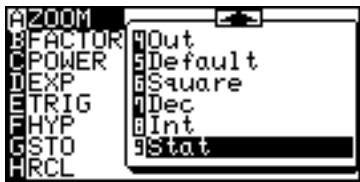
9 Stat will appear.

1. Select 9 Stat and press ENTER

You can directly press 9 at step 13 to select 9 Stat.

The histogram will appear on the display.

When you draw the graph using the automatic statistics zoom function (9 Stat), the division number is automatically set to - X_scl (default value: 10). If you wish to show the graph hour by hour, change the value in the WINDOW menu.

Set the WINDOW settings

1. Press WINDOW

Window (Rect) setting menu will appear.

1. Enter the values as shown in the diagram to the right.

Ymax is determined by the maximum access number (253 at 20:00 on Sunday).

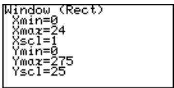
1. Press GRAPH

You can compare up to 3 statistical data by setting PLOT2/PLOT3 to on.

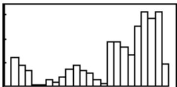
Compare the access rates on Sunday and Monday

Set the statistical plotting of PLOT1 (Sunday data) to a broken line

1. Press STAT PLOT A ENTER and move the cursor to GRAPH.
2. Press STAT PLOT again.
3. Press B and 1 (broken line with circle dots).
4. Press GRAPht. The histogram is now changed to a broken line graph.
5. Press 2ndF QUIT to clear the screen.
6. Press STAT PLOT and select B PLOT2.
7. Set as follows. PLOT: on, DATA: X, ListX: L1, and Freq: L3.

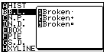
1. Move the cursor to GRAPH and press STAT PLOT

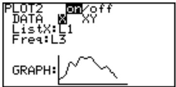
1. Press B 2 (broken line with cross points).

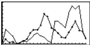
1. Press GRAPH. Now you can compare the difference in web site access counts between Sunday and Monday. Press 2ndF QUIT.

2. Statistics Features

1. STAT menus

Press the STAT key to access the statistical calculation menus. The menus are as follows:

A EDIT Provides the entry or edit mode and displays a list table.

B OPE Calculation menu for operations such as ascending or descending sort.

C CALC Obtains statistical values.

D REG Calculates regression curves.

E TEST Statistical hypothesis tests

F DISTRIBUTION menu items

Data Entry

Use a list table to enter the statistical data (press STAT to access). Up to 999 elements can be used for each list, though the amount of data able to be entered will vary according to the memory usage.

Calculating statistic values (CALC menu)

Use the CALC menu under the STAT menu to obtain statistic values.

Press STAT C to access the CALC menu.

2. Statistical evaluations available under the C CALC menu

1_Stats 1-variable (x) statistical a calculations

Mean of sample (x)

sx Standard deviation of sample (x)

$$ \mathsf {S X} = \sqrt {\frac {\Sigma \mathsf {x} ^ {2} - \mathsf {n} \overline {{\mathsf {x}}} ^ {2}}{\mathsf {n} - 1}} $$

x Population standard deviation of sample (x)

$$ \sigma X = \sqrt {\frac {\Sigma x ^ {2} - n \bar {x} ^ {2}}{n}} $$

x Sum of sample (x)

x^2 Sum of squares of sample (x)

n Sample number

xmin Smallest value of sample (x)

Q1 First quartile of sample (x)

Med Median of sample (x)

Q3 Third quartile of sample (x)

xmax Largest value of sample (x)

2_Stats 2-variable (x, y) statistical calculations

The following values are added to the 1-variable statistic calculations

Mean of sample (y)

sy Standard deviation of sample (y)

Population standard deviation of sample (y)

Σy Sum of sample (y)

y^2 Sum of squares of sample (y)

Σxy Sum of product of sample (x, y)

ymin Smallest value of sample (y)

ymax Largest value of sample (y)

The web site access counts example on page 145 will be used again to demonstrate the calculation of statistical values.

Hours	01	02	03	04	05	06	07	08	09	10	11	12	13	14	15	16	17	18	19	20	21	22	23	24
Sunday	98	72	55	3	6	24	15	30	59	72	55	43	21	10	150	151	135	108	204	253	232	251	75	30
Monday	32	8	12	2	4	19	32	72	95	91	123	201	184	108	95	72	45	38	75	111	153	90	84	35

• If you did not previously enter the above values in the list table, press STAT and select A EDIT to display the list entry mode and enter the values.

Calculating one-variable statistics using web site access counts for Sunday (L2) and Monday (L3).

Statistical calculations using the Sunday data (L2)

1. Press CL and STAT to display the statistics menu.
2. Press C and then 1. 1_Stats will be displayed on the top line of the screen followed by the cursor.
3. Press 2ndF L2 to enter L2 and press ENTER. All the statistical values will be displayed on the screen.

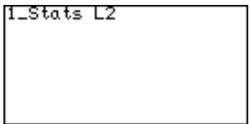
1_Stats = 89.66666667 sx = 79.35646965 x = 77.68562 x = 2152 x^2 = 337804

1. Press or to scroll the screen.

Statistical calculations using the Monday data (L3)

1. Press STAT to display the statistics menu.
2. Press C and then 1. 1_Stats will be displayed on the bottom line of the screen followed by the cursor.
3. Press 2ndF L3 to enter L3 and press ENTER.

1 Stats = 74.20833333 sx = 54.94105867 x = 53.78427525 x = 1781 x^2 = 201591

Calculating the previous two-variable statistical values can be performed in a single operation. Use a “, ” (comma) to separate the two variables.

1. Press CL and STAT to display the statistics menu.

2. Press C and then 2

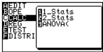
2_Stats will be displayed on the top line of the screen followed by the cursor.

1. Press 2ndF L2 , 2ndF L3 to enter L2 and L3, and press ENTER.

All the statistical values will be displayed on the screen.

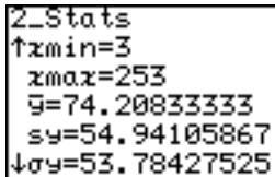
1. Press or to scroll the screen.

ANOVA( The ANOVA( feature performs an analysis of variance to compare up to six population means.

1. Press CL and STAT to display the statistics menu.

2. Press C and then 3 ANOVA will display on the top line of the screen.

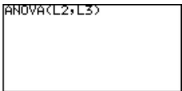
1. Press ENTER. The answer will appear on the screen.

Each character represents the following variables.

F The F statistic for the analysis

p The p value for the analysis

df Degrees of freedom

SS Sum of squares

MS Mean Square

sxp Pooled standard deviation

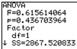
3. Graphing the statistical data

Press STAT PLOT to access the statistical graphing mode.

The calculator can plot statistical data on up to 3 types of graph (PLOT1 to PLOT3) to check the state of distribution.

The graph types can be selected from histogram, broken line plot, normal probability plot, normal distribution plot, box plot, modified box plot, pie chart, scatter diagram and XY line. Broken line plot, normal probability plot, modified box plot, scatter diagram and XY line can use 3 different types of points — circle, cross, and square.

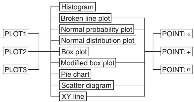
Statistical graph types overview (chart)

1. Graph Types

Histogram (HIST)

A bar graph of sample (x)
The width of the bars is set by the Xscl*.
The Y-axis shows the frequency.

• The Xscl can be changed to between 1 and 64. Use the Window Setting Menu to change the Xscl. (See page 57.)

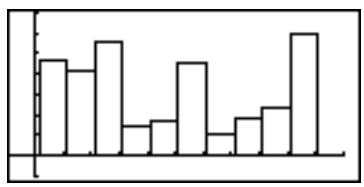
Broken line plot (B.L.)

A broken line graph for the frequency distribution of sample (x) Three types of points can be selected from circle, cross and square. The broken line is displayed by connecting the upper left points of the bars of the histogram, as the upper left point of each bar

represents each class value in the histogram.

The calculator can draw both a histogram and a broken line plot at the same time.

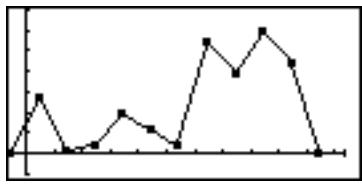
Normal probability plot (N.P.)

Plots the variance of the standardized normal distribution with the statistical data (x) on the X axis or Y axis. If the points plot almost linearly, it indicates that the data is of normal distribution.

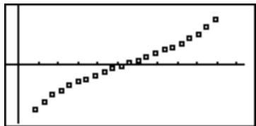
The distance between the dots is set by the Xscl.

• The Xscl can be changed between 1 and 64. Use the Window Setting Menu to change the figure. (See page 57)
• You cannot set the frequency in the Normal probability plot. The statistical data must be created using only one list without splitting into the data and frequency.

Normal distribution plot (N.D.)

A normal distribution curve of sample(x)

The x-axis is in the range of Xmin to Xmax.

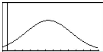
Box plot (Box)

A box plot graph of sample (x)

A. The minimum value (xmin) of the sample (x)
B. The first quartile (Q1)
C. Median (Med) of the sample (x)
D. The third quartile (Q3)
E. The maximum value (xmax) of the sample (x)

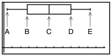
Modified box plot (MBox)

A modified box plot graph of sample (x)

A. The minimum value (xmin) of the sample (x)
B. The tip of extension which is defined by (Q3 - Q1) × 1.5
C. The first quartile (Q1)
D. Median (Med) of the sample (x)
E. The third quartile (Q3)
F. The tip of extension which is defined by (Q3 - Q1)× 1.5
G. The maximum value (xmax) of the sample (x)

• Statistical data on the outside of the extension are indicated by points, selectable from circle, cross, or square.

• The length of the extension from the box is determined by Q1 and Q3.

Pie chart (PIE)

Pie graph of sample (x)

Maximum number of division is 8.
- Calculation range: 0 ≤ x < 10^100
- Data can be displayed in two modes:

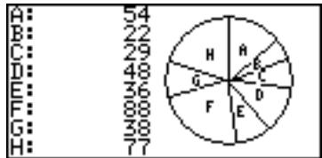
• Value display: 8 digits
  Percentage display: Fixed decimal (2 digits decimal)

• Pie graphs are drawn in the same order as on the specifying list.

• Pie graphs cannot be displayed simultaneously with other graphs and X/Y axis, though lines or dots can be drawn. The coordinates of the free-moving cursor depend on the Window settings.
• The values are stored in variables A to H.
• As all the displayed values are rounded down in the percentage display mode, the total percentage may not be 100.

Scatter diagram (S.D.)

A two-dimensional plot graph using two samples (x,y) Two sets of statistical data are required for the scatter diagram.

• Three types of points are selectable from circle, cross and square.
• Two statistical data lists can be set to either x- or y-axis according to your requirements.

XY Line (XYLINE)

• Displays a graph that connects each point of the scatter diagram.
  Each point is connected in the sequence (rows) of the statistical data.

2. Specifying statistical graph and graph functions

• Up to three graphs can be plotted per sample data.

Specifying type of statistics graphing

1. Press STAT PLOT.
2. Select from A PLOT1, B PLOT2 or C PLOT3 and press ENTER to set the statistical graphing specifications.

Press 2ndF QUIT before step #3.

• You may just press A to C to select.
• You can overlap 3 plotting graphs (from PLOT1 to PLOT3) on a single screen. Choose on or off at the top line to determine whether each graph is displayed or not.

Limit settings (x value)

1. Press STAT D (D Limit) to specify the graphing range. The D Limit menu is used to set the upper and lower limit lines of sample (x) of the statistical graph.

Displaying the upper and lower limit lines

1. Press 1 (1 SET).
2. Enter the appropriate value for Lower limit and press ENTER.
3. Enter the appropriate value for Upper limit and press ENTER.

Displaying the mean value line of sample (x)

1. Press STAT D (D Limit) and press 2 (2 LimON) ENTER to display a line that indicates the mean value of sample (x), as well as the upper and lower limit lines.

2. Press STAT PLOT D 3 (3 LimOFF) and ENTER not to display the lines.

3. Upper and lower limit values are displayed using short broken lines.

4. The default value of the upper/ lower limit is 1 .

5. The mean value line is indicated by a long broken line.

3. Statistical plotting on/off function

• You can set the statistical plotting of PLOT 1 to 3 at once.

• Press STAT PLOT.

• Press E

• • To set the all plotting ON: Press 1 (1 PlotON).
  To set the all plotting OFF: Press 2 (2 PlotOFF).

• You can control the plotting of PLOT1 to PLOT3 separately by pressing 1 3 after PlotON (or PlotOFF).

• Press ENTER to set.

4. Trace function of statistical graphs

• The trace feature is available in statistical graphing and can be used to trace the curves of graphs with the cursor.

Tracing the graph

1. Press .
2. Use 4 or 7 to move the cursor pointer to trace the graph curve.

Histogram

How tracing is done

• After pressing , the cursor pointer will appear on the top left corner of the first bar.

• If you press or , the cursor pointer sequentially jumps between top left corners of the bars.
• X and Y values are displayed at the bottom line of the screen.
• Use or to change between graphs to trace.

Box plots and modified box plots

After pressing , the cursor pointer will appear on the Med value of sample (x).
If you press or the cursor pointer sequentially jumps among specific values, s
- The value of cursor pointer position is displayed at the bottom line of the screen.

Pie chart

• If you press or , the cursor pointer sequentially trace the chart. The cursor is displayed at the outside the graph, and the selected chart is highlighted.

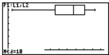
4. Data list operations

Descending sort, ascending sort, changing the list order and deleting the lists can be done in the Operation menu.

Press STAT B OPE to access the data list operations.

1 sortA( sortA(list)

Sorts the list in ascending order.

This function is the same as the sortA( menu item in List functions.

See page 135 for details.

2 sortD( sortD(list)

Sorts the list in descending order.

This function is the same as the sortD( menu item in List functions.

See page 135 for details.

3 SetList SetList list name 1 [, list name 2 ...]

Changes the list order as specified.

Example

To change the order of lists in order of L2, L3, L1.

Press ENTER to execute.

Each list must be separated by a " , " (comma).

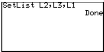
• If only a single list name is specified, the specified list moves to the left end of the table.
• After changing the list order, execute SetList with no argument. The list names are redefined according to the changing order.

4 ClrList ClrList list name 1 [, list name 2 ...]

Deletes all the data from the specified list(s).

Example

To delete the data of L1 and L2.

Press ENTER to execute.

Each list must be separated by a “,” (comma).

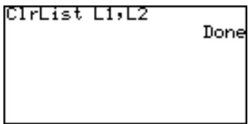
5. Regression Calculations

Accessing the regression menu

1. Press STAT D REG. The Regression menu is displayed.

01 Med_Med Med_Med(list name for x ,list name for [frequency list] [equation name to store]) Finds the regression line using the median-median method. (linear regression) Formula: y = ax + b Parameters:a,b

02 Rg_ax+b Rg_ax+b (list name for x, list name for y [, frequency list] [equation name to store]) Finds the regression line. (linear regression) Formula: y = ax + b Parameters: a, b, r, r^2

03 Rg_a+bx Rg_a+bx (list name for x, list name for y [, frequency list] [equation name to store]) Finds the regression line. (linear regression) Formula: y = a + bx Parameters: a, b, r, r^2

04 Rg_x2 Rg_x^2 (list name for x, list name for y [, frequency list] [, equation name to store]) Finds the regression line using the second degree polynomial. (quadratic regression) Formula: y = ax^2 + bx + c Parameters: a, b, c, ^2

05 Rg_x3 Rg_x3(list name for x, list name for y [, frequency list] [, equation name to store]) Finds the regression line using the third degree polynomial. (cubic regression) Formula: y = ax^3 +bx^2 +cx + d Parameters: a, b, c, d, R^2

06 Rg_x4 Rg_x4 (list name for x, list name for y [, frequency list] [, equation name to store])

Finds the regression curve using the fourth degree polynomial. (quartic regression)

Formula: y = ax^4 + bx^3 + cx^2 + dx + e

Parameters: a, b, c, d, e, R²

07 Rg_In Rg_In (list name for x, list name for y [, frequency list] [, equation name to store])

Finds the regression curve using the natural logarithm. (natural logarithm regression)

Formula: y = a + b x

Parameters: a, b, r, r^2

08 Rg_log Rg_log(list name for x, list name for y [, frequency list] [, equation name to store])

Finds the regression curve using the common logarithm. (common logarithm regression)

Formula: y = a + b x

Parameters: a, b, r, r^2

09 Rg_ab ^x Rg_ab ^x (list name for x , list name for y , frequency list) [equation name to store])

Finds the regression curve using the exponential function. (exponential regression)

Formula: y = ab^x

Parameters: a, b, r, r^2

10 Rg_aebx Rg_aebx(list name for x, list name for y [, frequency list] [equation name to store])

Finds the regression curve using the Euler exponential function. (Euler exponential regression)

Formula: y = ae^

Parameters: a, b, r, r^2

11 Rg_x-1 Rg_x-1(list name for x, list name for y [, frequency list] [equation name to store])

Finds the regression curve using the reciprocal function. (reciprocal regression)

Formula: y = a + bx^-1

Parameters: a, b, r, r^2

12 Rg_axb Rg_axb(list name for x, list name for y [, frequency list] [, equation name to store])

Finds the regression curve using the power function. (power regression)

Formula: y = ax^b

Parameters: a, b, r, r^2

13 Rg_logistic Rg_logistic (list name for x , list name for y , [frequency list] [, equation name to store])

Finds the regression curve using the logistic function. (logistic regression)

Formula: y = c ÷ (1 + ae^-bx)

Parameters: a, b, c

14 Rg_sin Rg_sin ([iterations, list name for x, list name for y [, frequency list], [period], [equation name to store])

Finds the regression curve using the sine function.

The calculator will fit a sine curve for unequal and equal spacing.

Formula: y = a (bx + c) + d

Parameters: a, b, c, d

Note: The default iterations value is 3. The user may specify the value up to 25. To raise the accuracy, set the iterations value to 25 and enter 2 / b to the period, where b = result obtained from the calculation beforehand.

15 x' value or list x'

Finds the estimated value of x for a given value of y by applying the function determined by the regression.

Example

When the following is entered as statistical data:

x	10	20	30	40	50
y	20	40	60	80	100

Find estimated value of x given y = 140 .

1. Enter the above data into L1 (x) and L2 (y) and execute Rg_ax+b (L1, L2).

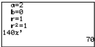
1. Press 140 STAT D 1 5 ENTER.

16 y' value or list y'

Find the estimated value of y for a given value of x by applying the function determined by the regression formula.

Example

Using above data, find the estimated value for y given x = 80 , 100.

• 15 x' and 16 y' will be valid

after executing a regression calculation excluding 2nd, 3rd, 4th, degree polynomial, logistic, and sine regressions.

Using the regression functions

The following table shows the relationship between the time and temperature of water, when heating a beaker filled with water.

Time (min)	2	3	4	5	6	7	8	9	10	10.5	11	11.5	12	12.5
Temperature (°C)	38.4	46.4	54.4	62.5	69.6	76.1	82.4	88.6	93.4	94.9	96.5	98.2	99.1	100

Enter a data in a list table

1. Press STAT A ENTER
2. Enter the time into list 1 (L1).
3. Enter the temperature into list 2 (L2).

Plotting the data

1. Press STAT PLOT A ENTER
2. Press ENTER to turn on the plotting.
3. Press and to select XY of DATA menu and press ENTER.

Freq will change to ListY and set L2 to ListY.

Selecting the graph type

1. Press to move the cursor to GRAPH.
2. Press STAT G and 2 (2 Scattr+) to set the graph type to scatter and point type to ^+
3. Press ZOOM A 9 Stat) to plot the scatter diagram for this data.
4. Selecting A 9 in the ZOOM mode allows for quick graphing in an optimum range since window setting values of the graph plotting screen are automatically set using the list data.

Drawing a regression curve using quadratic regression

1. Press CL STAT D 0 4 (04 Rg_x2).
2. Press ( 2ndF L1 , 2ndF L2 , 2ndF VARS A ENTER A 1

If you enter Y1 as the last variable, the obtained formula will automatically be set to the formula Y1.

1. Press ENTER
   The regression formula and parameters will be displayed on the screen.
2. Press GRAPH
   The calculator will draw the scatter diagram using the determined parameter values.
3. If there is a large difference between the regression curve and plotted dots, change the regression curve and repeat the above procedures.

About the residual list

• There are residuals between regression curves and actual values.
• The residual list stores these residuals automatically.
• The resid list can be found in B REGEQN of the STAT VARS menu (2ndF VARS H ENTER B 0).
• Use the following key operation to recall the residual list from the calculation screen.

CL 2ndF VARS H ENTER B 0

• Press ENTER to display the residual list on-screen.
• To show the residual list in the form of a graph, first store as a list, then follow the graphing operation.
• resid cannot be graphed when specified independently.

6. Statistical Hypothesis Testing

• The calculator performs hypothesis tests on statistical data.

Start a statistical test

The statistics test menu will appear.

1. There are 17 options in the statistics test menu. Press

to navigate between pages, and press or to scroll the window.

1. Press the appropriate number to access a specific test.

The statistics test window will appear.

1. Input appropriate information in the test window.

2. There are two types of input, from a statistics data list or inputting numerical values.

3. Some tests may not allow for inputting from the statistics data lists.

4. 16 InputList and 17 InputStats specify the above input methods.

16 InputList: Sets the input mode to the statistic data list method

17 InputStats: Sets the input mode to the value input mode For example, press STAT E 1 6 ENTER to set to the list input mode.

1. Press 2ndF EXE to execute the hypothesis test.

Note:

• Either list input or parameter input may be used for tests other than 01 ^2 test, 05 TtestLinreg, 10 Ztest1prop, 11Ztest2prop, 14 Zint1prop and 15 Zint2prop.
• To clear the contents entered in Freq, move the cursor to the list name then press DEL ENTER.

01 ^2 test Uses the sample data from a two-dimensional table represented by a matrix.

Example

If mat A = 3254

6138

2351

execute the ^2 test and store the obtaining results in mat B.

1. Press STAT E 0 1.
2. Enter mat A as the Observed Matrix, and mat B as the Expected Matrix.

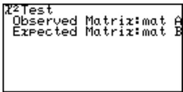
1. Press 2ndF EXE to execute the ^2 test. The result is entered in mat B.

^2 : -squared statistic for the test

p: p value for the test

df: degrees of freedom

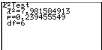
02 Ftest2samp Two samples data are tested for equality of standard deviation _1 and _2 .

Example

Test when population standard deviation _1 < _2

$$ n _ {1} = 2 0, $$

standard deviation sx_1 = 5.6

$$ n _ {2} = 5 0, a n d $$

standard deviation Sx_2 = 6.2

Set the input method to value input mode

1. Press [日] STAT E 1 7 ENTER).
2. Press STAT E 0 2

The parameter input screen will appear.

1. Press ENTER to select _1 < _2
2. Enter the values into the parameter fields.

5.6 ENTER 20 ENTER 6.2 ENTER 50 ENTER

1. Press 2ndF EXE to execute the test.

F: Statistics

p: Probability

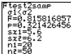
03 Ttest1samp Tests the hypothesis of population mean

Example

Test the population mean _0 = 65 with the sample data of {65.6, 62.8, 66.0, 64.5, 65.1, 65.3, 63.8, 64.2, 63.5, 64.4},

from a given population

(alternate hypothesis of < _0

1. Enter the above statistical data into L1.

Press STAT E 1 6 ENTER to set the list input mode.

1. Press STAT E 0 3

The parameter input screen will appear.

1. Press ENTER to select < _0 and press ENTER.
2. Move the cursor pointer to _0 and input 65 and press ENTER.
3. Set the List to L1 and press ENTER
4. Press 2ndF EXE. Answers are displayed on the screen, where t is the t statistic for the test, p is the p value for the test and sx indicates sample standard deviation.

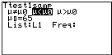
• If there is no weight list, the Freq field can remain empty.

04 Ttest2samp Tests two sample means, _1 and _2 .

Example

Test the following two samples;

List 1 {2.37, 2.51, 2.43, 2.28, 2.46, 2.55, 2.49}

List 2 {2.63, 2.71, 2.56, 2.61, 2.55, 2.68, 2.42, 2.48, 2.51, 2.65}

1. Enter the above data into lists L1 and L2, respectively.

2. Press STAT E 0 4

The parameter input screen will appear.

1. Enter the appropriate value into each field. If no Freq specification data is input, an initial Freq value of 1 is used.

2. Pooled is prediction for unknown 1, 2 .

Select "No" if _1,_2 are subjectively unequal.

Select "Yes" if _1, _2 , are equal.

Calculation is executed using this prediction as the basis.

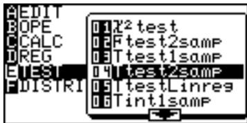
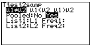
1. Press 2ndF EXE.

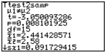
05 TtestLinreg Tests the significance of the slope for the linear regression and its correlation coefficient .

Example

The test is for the slope , and correlation coefficient obtained from statistical data X {65, 56, 78, 86, 92, 71, 68} and Y {95, 59, 88, 78, 75, 68, 80} are not equal to zero ( \& 0 .)

1. Input the above lists X and Y into lists L1 and L2, respectively.

2. Press STAT E 0 5

The parameter input screen will appear.

1. Enter the appropriate value into each field.

2. Equation items may not be required.

3. If a linear regression calculation has been

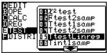
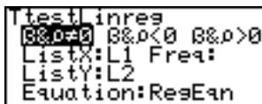
executed using the data, and the function equation has been stored in Y0 to Y9, input that equation number for the equation items.

1. Press 2ndF EXE.

Answers are displayed on the screen, where a, b indicate regression coefficients, s indicates standard deviation, r indicates the

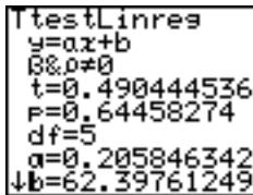
correlation coefficient, and r^2 indicates the coefficient of determination.

06 Tint1samp Finds the confidence interval for the population mean

Example

Find the confidence interval for the statistical data of {65.6, 62.8, 66.0, 64.5, 65.1, 65.3, 63.8, 64.2, 63.5, 64.4}, from a given population and the level of confidence is 0.99.

1. Enter the above statistical data into list L1.
2. Press STAT E 0 6 The parameter input screen will appear.
3. Enter the C-level value of 0.99.
4. Set the List to L1 and press ENTER
5. Press 2ndF EXE. Answers are displayed on the screen, where sx indicates the sample standard deviation.

If you enter a value from 1

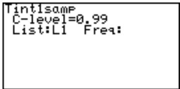
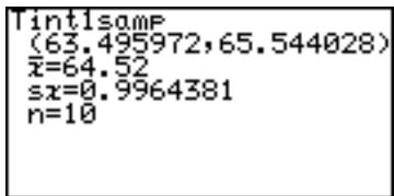
to 100 for the C-level, it will be changed to the % input mode.
- In the numerical value input mode, n is a positive integer.

07 Tint2samp Finds the confidence interval for the difference of two sample means, _1 and _2 .

Example

Use the following two sample data (used for example 04);

List 1 {2.37, 2.51, 2.43, 2.28, 2.46, 2.55, 2.49}

List 2 {2.63, 2.71, 2.56, 2.61, 2.55, 2.68, 2.42, 2.48, 2.51, 2.65},

with the level of confidence of 0.99.

1. Enter the above data in to lists L1 and L2.
2. Press STAT E 0 7

The parameter input screen will appear.

1. Enter the appropriate value in each field.

1. Press 2ndF EXE. Answers are displayed on the screen, where the numerical value within () indicates the confidence interval for the differences between _1 and _2 when the level of confidence is 99% . In the numerical value input mode, "n", "n" are positive i

08 Ztest1samp Tests the hypothesis of population mean

Example

The average weight of a newly developed product is known to be 53.4g and standard deviation () is 4.5. Judge the validity when the average weight of 20 units is 52.4g(x)

Set the input method to value input mode

1. Press [DAT] STAT E 1 7 ENTER.
2. Press STAT E 0 8

The parameter input screen will appear.

1. Set the alternate hypothesis to _0 , < _0 and > _0 (two-tail test, one-tail test settings). In this case, choose _0 (two-tail test).

• _0 indicates the hypothesis mean, indicates the population standard deviation, x indicates the sample mean and n indicates the sample size. (" n " is a positive integer.)

• Enter the appropriate value in each field.

• Press 2ndF EXE. Answers will be displayed on the screen, where z indicates the test statistic and p indicates the p value of the test.

09 Ztest2samp Tests the equality of two sample means, _1 and _2 .

Example

Test _1 > _2 where 1 = 77.3 , 1 = 3.4 , n_1 = 30 , and 2 = 75.2 , 2 = 2.8 , n_2 = 20 .

Set the input method to value input mode

1. Press STAT E 7 ENTER
2. Press STAT E 0 9

The parameter input screen will appear.

1. Enter the appropriate value into each field.

1. Press 2ndF EXE. Answers will be displayed on the screen.

10 Ztest1prop Tests the success probability P_0 of a population.

Example

A coin was tossed 100 times and landed head side up 42 times. Normally, the probability of head facing up is 0.5. Test to see if the coin is fair.

1. Press STAT E 1 0

The parameter input screen will appear.

• prop is the hypothesis probability. The test will be conducted using hypothesis prop P_0 .

• x is the number of successes observed and n is the number of trials (where n is a positive integer.)

• Enter the appropriate value into each field.

1. Press 2ndF EXE. : Success probability obtained from the sample data.

11 Ztest2prop executes a comparative test for two success probabilities, (P_1, P_2)

Example

Test the equality of P_1 and P_2 given the sample data n_1 = 50 , x_1 = 16 and n_2 = 20 , x_2 = 5 , where the hypothesis is P_1 < P_2 .

1. Press STAT E 1 1

The parameter input screen will appear.

1. Enter the appropriate value into each field.

1. Press 2ndF EXE

Answers will be displayed on the screen, where indicates the calculated success rate of the data combined

with sample data 1 and 2,

and _1 and _2 show the success rates of sample data 1 and 2, respectively. n_1 and n_2 are positive integers.

12 Zint1samp Finds the confidence interval of a population mean,

Example

The average weight of a newly developed product is known to be 52.4 g and standard deviation (σ) is 4.5. Given the average weight of 20 units is 53.4 g (x), find the confidence interval of the data where the level of confidence (C-level) is 0.95.

Set the input method to value input mode

1. Press STAT E 7 ENTER
2. Press STAT E 1 2

The parameter input screen will appear.

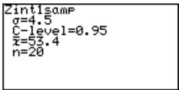
1. Enter the appropriate value into each field.
2. Press 2ndF EXE

Answers will be displayed on the screen, where the numerical value within () indicates the confidence interval with the level of

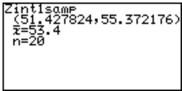
confidence at 0.95, that is, the confidence interval of this sample data with the confidence level of 95% is between 51.427... and 55.372....

C-level indicates the level of confidence and n is a positive integer.

13 Zint2samp Finds the confidence bound of two sample means _1 and _2 .

Example

Find the confidence interval of _1 and _2 of sample data with the confidence level of 0.9, where _1 = 77.3 , _1 = 3.4 , n_1 = 30 and _2 = 75.2 , _2 = 2.8 , n_2 = 20 ( _1 and _2 indicate sample means of two data.)

Set the input method to value input mode

1. Press STAT E 7 ENTER
2. Press STAT E 1 3

Parameter input screen will appear.

1. Enter the appropriate value into each field.

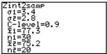
1. Press 2ndF EXE. Answers will be displayed on the screen, where the numeric value within () indicates the confidence

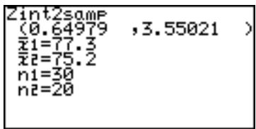
interval of _1 and _2 at a confidence level of 90% .

* n_1 and n_2 are positive integers.

14 Zint1prop Finds the confidence interval of the success probability of a population from the success probability obtained from sample data collected from a population.

Example

A coin was tossed 100 times and landed head side up 42 times. Normally, the probability of head facing up is 0.5. Find the confidence interval of the success probability at a confidence level of 0.95.

1. Press STAT E 1 4

The parameter input screen will appear.

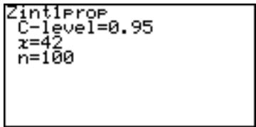
1. Enter the appropriate value into each field.
2. Press 2ndF EXE
   Answers will be displayed on the screen, where the numerical value within () indicates the confidence

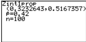
interval of the success probability at a confidence level of 95% .

• n is a positive integer.

15 Zint2prop

Finds the confidence interval of the difference (P_1 - P_2) of the success probability obtained from the two sets of sample data collected from two different populations.

Example

Find the confidence interval of the success probability (P_1, P_2) at a confidence level of 0.9 for the two sets of sample data n_1 = 50 , x_1 = 16 and n_2 = 20 , x_2 = 5 .

1. Press STAT E 1 5

The parameter input screen will appear.

1. Enter the appropriate value into each field.

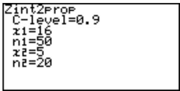
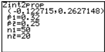
1. Press 2ndF EXE
2. Answers will be displayed on the screen, where the numerical value within () indicates the confidence

interval of the success probability P_1 - P_2 at a confidence level of 90%.

^* n_1 and n_2 are positive integers.

7. Distribution functions

The calculator has distribution features to find statistical calculations.

To enter the distribution menu,

1. Press STAT F (F DISTRI).

The distribution menu will appear.

1. There are 15 options in the distribution menu. Press

to navigate between pages, and press ▲ or

to scroll the window.

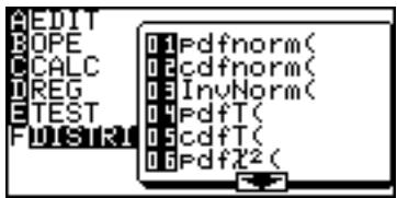
1. Press ENTER to select the function.
2. Input the specified values.
3. Press ENTER to solve.

01 pdfnorm( pdfnorm(value [, mean, standard deviation])

Finds the probability density of the specified value x for the normal distribution N(, _2) . A list cannot be used.

• When mean () and standard deviation () are omitted, = 0 and = 1 are applied.

Example

Find the nominal distribution probability density for x = 65 when the normal distribution of the test score averages is 60 with a standard deviation of 6.

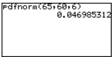
02 cdfnorm( cdfnorm(lower limit, upper limit [, mean, standard deviation])

Calculates the normal distribution probability of a specified range x for the normal distribution N( ,^2) . A list cannot be used.

• When mean (μ) and standard deviation (σ) are omitted, μ = 0 and σ = 1 are applied.

Example

Calculate the probability of range x = 54 to 66 in the above sample.

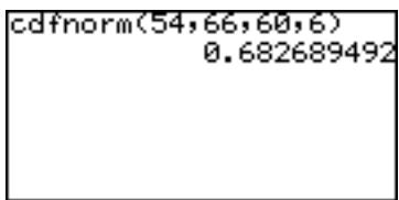
03 InvNorm( InvNorm(probability [, mean, standard deviation])

Finds the value of x of a given normal distribution probability. A list cannot be used.

• When mean () and standard deviation () are omitted, = 0 and = 1 are applied.

Example

Find the value of x for the probability of 0.8 in the above sample.

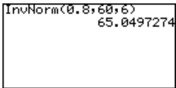
04 pdfT( pdfT(value, degree of freedom)

Finds the probability density of a specified value x for the T distribution with n degrees of freedom. A list cannot be used.

Limitations:

Degree of freedom ≤ 140

• Degrees of freedom is a positive real number.
  If decimal values are used for the degrees of freedom, the calculator uses the closest integer of the given degree of freedom.
• An error may occur when an extremely large number is entered for degree of freedom.

Example

Find the probability density of the T distribution with 9 degrees of freedom when x = 2.5 .

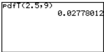
05cdfT( cdfT(lower limit, upper limit, degree of freedom)

Finds the T distribution probability within the specified range of x for the T distribution with n degrees of freedom. A list cannot be used.

Limitations:

Degree of freedom ≤ 670

• Degrees of freedom is a positive real number.

Example

Find the probability of range X = 0.5 to 3.2 for T distribution with 9 degrees of freedom.

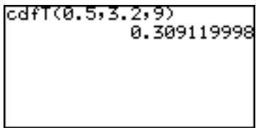
06 pdfx2( pdfx2(value, degree of freedom)

Finds the probability density of a specified value x for the ^2 distribution with n degrees of freedom. A list cannot be used.

Limitations:

Degree of freedom ≤ 141

• Degree of freedom is a positive real number.

Example

Find the probability density of ^2 distribution with 15 degrees of freedom when x = 6.5 .

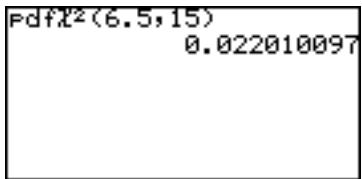
07 cdf ^2 (cdf ^2 (lower limit, upper limit, degree of freedom)

Finds the ^2 distribution probability of a specified range of x for the ^2 distribution with n degrees of freedom. A list cannot be used.

• Degree of freedom is a positive real number.

Example

Find the probability of range x = 3 to 15 for the ^2 distribution with 10 degrees of freedom.

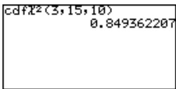
08 pdfF( pdfF(value, degree of freedom of numerator, degree of freedom of denominator)

Finds the probability density of a specified value x for the F distribution that possesses two independent degrees of freedom, m and n. A list cannot be used.

Limitations: Degree of freedom ≤ 70

• Degree of freedom is a positive real number.
• An error may occur when an extremely large number is entered for degrees of freedom.

Example

Find the probability density for the F distribution generated with degrees of freedom 15 and 10 when x = 3 .

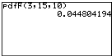
09 cdfF( cdfF(lower limit, upper limit, degree of freedom of numerator, degree of freedom of denominator)

Finds the F distribution probability of a specified range x for the F distribution with two independent degrees of freedom, m and n. A list cannot be used.

Limitations:

Degree of freedom ≤ 670

• Degree of freedom is a positive real number.
• An error may occur when an extremely large number is entered for degree of freedom.

Example

Find the probability of the range x = 0 to 2.5 for the F distribution generated with degrees of freedom 15 and 10.

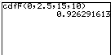
10 pdfbin( pdfbin(trial number, success probability [, success number]))

Finds the probability density of a specified value x for the binomial distribution. A list cannot be used except for success numbers.

When the success number is not specified, the calculation is executed by entering values from 0 to the trial number and displays the list.

Limitations:

Success probability is 0 ≤ p ≤ 1 .

Example

Find the probability density for 15 trials with x = 7 , for the binomial distribution with success probability of 30% .

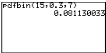
11 cdfbin( cdfbin(trial number, success probability [, success number])

Finds the probability of a specified range x for the binomial distribution. A list cannot be used except for success numbers.

When the success number is not specified, the calculation is executed by entering values from 0 to the trial number and displays the list.

Example

Find the probability of range up to x = 7 for the F distribution generated with degrees of freedom 15 and 10.

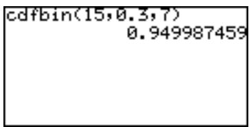
12 pdfpoi( pdfpoi(mean, value)

Finds the probability density of a specified value x for a Poisson distribution of mean .

Limitations: Mean of Poisson distribution ≤ 230

Example

Find the probability density of x = 4 , for the mean of a Poisson distribution of 3.6.

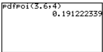
13 cdfpoi( cdfpoi(mean, value)

Finds the probability of a specified range x for a Poisson distribution of mean mu.

Example

Find the probability within the range up to x = 4 .

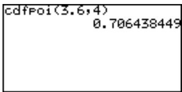
14 pdfgeo( pdfgeo(success probability, value)

Finds the probability density of a specified value x for the geometric distribution.

Limitations:

Success probability is 0 ≤ p ≤ 1 .

Example

Find the probability density of a geometric distribution of success at the 26th time with success probability of 5.6% .

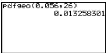
15 cdfgeo( cdfgeo(success probability, value)

Finds the probability of a specified range of x for the geometric distribution.

Limitations:

Success probability is 0 ≤ p ≤ 1

Example

Find the probability for the range up to x = 26 with success probability of 5.6% .

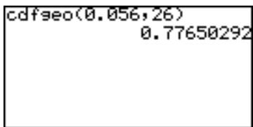
Chapter 11

Financial Features

The financial calculation features include capabilities for compound interest calculations.

Press 2ndF FINANCE.

The financial menu screen will appear.

• Specifies the TVM-SOLVER mode.
• Selects a financial calculation function
• Specifies payment due (to pay at the beginning or end of period)
• Determines individual settings (in TVM-SOLVER mode)

1. Try it! 1

You plan to purchase a house for a price of 300,000. The down payment is100,000. Calculate the monthly payments for a 30-year loan at an annual interest rate of 5% for the remaining $200,000.

Draw a cash flow diagram on paper

1. Draw the following cash flow diagram to simplify the problem.

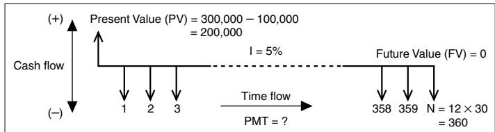
• A horizontal line indicates a time flow (left to right) divided into even sections — months in this case. Each section indicates a compound period and the total number of sections indicates the total number of periods for payment.

Vertical arrows along the horizontal line indicate the cash flow. An UP arrow indicates inflow (+) and a DOWN arrow indicates outflow (-) .
- The calculator considers the cash inflow for each period is constant. (Even payment.)

1. Determine the time each payment is due.

For deposits and loan payments, the time each payment is due (paid at the beginning or the end of the period) makes for a different cash flow diagram.

Payment due at the end of the period

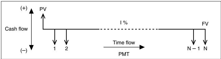
Payment due at the beginning of the period

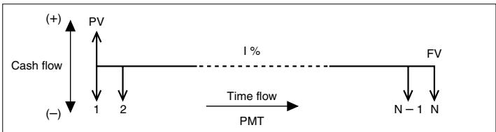
In this case payment is due at the end of the period.

1. Determine the inflow and outflow and place the present value ((\mathrm{PV} = \)200,000)) on the diagram.

We can consider the present value (PV) as a loan and thus inflow (revenue) from the customer's point of view. So, place the PV at the top left end of the diagram. We also can consider the principal interest total (Future value) as outflow (payment). Draw a vertical line with a DOWN arrow on the top of the diagram.

1. Complete the diagram with interest (1%), number of payment periods (N), future value (FV), and other required numbers.

Starting the calculation

Setting the payment due time

1. Press 2ndF FINANCE
2. Press C (C PERIOD).
3. Press 1 (1 PmtEnd) and press ENTER. Payment due time is now set to the end of the period.

Enter the value using the SOLVER function

1. Press 2ndF FINANCE
2. Press A ENTER
3. The following TVM-SOLVER screen will appear. The payment due time is set to the end of the period.

The payment due time is set to the end of period.

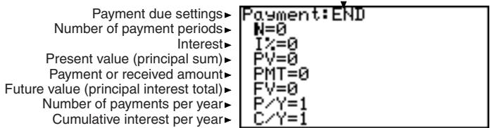
1. Input 360 for N (number of payment periods) and press ENTER. The cursor moves to "I%.
2. Input 5 for 1% (annual interest) and press ENTER.
3. Input 200000 for PV (present value) and press ENTER.
4. Press ENTER.

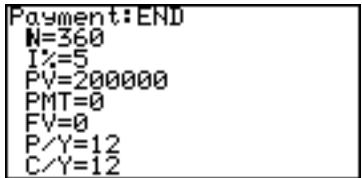
Since the payment amount is to be calculated from the other values, no value must be entered for PMT (payment or received amount).

1. Press ENTER again. Since FV (future value) is "0" at the end, no value must be entered for FV.

2. Press 12 for P/Y (number of payments per year) and press ENTER.

3. Press ENTER

Usually C/Y (cumulative interest per year) is the same value as P/Y. If not, enter the value instead.

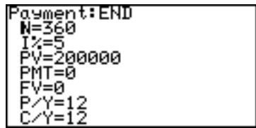
1. Press 3 times to move the cursor to PMT (payment amount).
2. Press 2ndF EXE.

The result will appear as follows.

1. Payment amount per month PMT = -1073.643246 (Negative value indicates payment.)

The numerical value input format and display format in

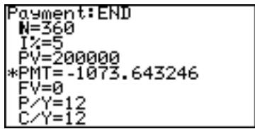
the FINANCE mode comply to that of SETUP.

The above answer is given when the FSE setting in SET UP menu is set to FloatPT. If you wish to display 2 digit decimal point format, set TAB to 2 and FSE to FIX.

Answer: You have to pay (1,073.64 per month for 30 years.

Simple interest and compound interest

There are two ways to calculate interest: simple and compound. In the FINANCE mode, the calculator can execute compound interest calculations.

Example of depositing (10,000 in a bank for 3 years at an annual interest rate of (3 \%)

Period	Simple interest	Compound interest
First year	Receive 10,000 × 0.03 =300	Receive 10,000 × 0.03 =300
Second year	Receive 300 (constantly)	Receive10,300 × 0.03 = 309
Third year	Receive300 (constantly)	Receive 10,609 × 0.03 =318.27

With compound interest, the amount in the bank is increased by receiving interest on the interest gained during each calculated period.

Try it! 2

If the monthly payments in the first example is limit to a fixed $800, how much must be the present value (PV) and the required amount of down payment.

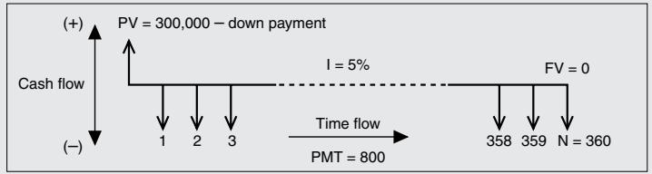
Set the TAB and FSE (2 and FIX respectively)

1. Press 2ndF SETUP C 2 D 2

TAB is set to 2 and FSE is set to FIX.

1. Press CL 2ndF FINANCE

A and ENTER.

The previous TVM-SOLVER screen will appear with the cursor flashing on N.

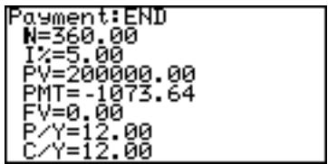
1. PV will change to 149025.29

2. Press three times to move the cursor to PMT.

3. Press (-) 800 and ENTER. Be sure to enter the minus sign to indicate payment.
4. Move the cursor to PV.

5. Press 2ndF EXE

6. This indicates that the total amount over 30 years will be 149,025.29 if the maximum monthly payment is limited to 800.

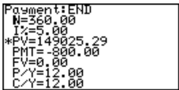
• So, the required amount of down payment is 300,000 -149,025.29 = $150,974.71.

Using the TVM-SOLVER screen, you can obtain various results by inputting the known variables and then moving the cursor to the unknown variable and pressing 2ndF EXE. The value where the cursor pointer is placed will be calculated from the known variables.

Example

Compare the principal interest total when accumulating an interest of 2.18% monthly on \ 100$ for 5 years with payment due at the beginning of the period and at the end of the period.

1. Payment due at the beginning of the period

2. Press 2ndF FINANCE C 2 and press ENTER

3. Press 2ndF FINANCE A ENTER

Payment due is now set to the beginning of the period.

1. Enter the values.
2. Move the cursor to FV and press 2ndF EXE

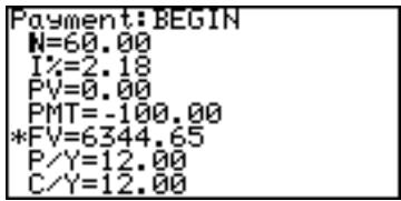
1. Payment due at the end of the period.

2. Press 2ndF FINANCE C 1 and press ENTER

3. Press 2ndF FINANCE A ENTER

Payment due is now set to the beginning of the period.

1. Enter the values.
2. Move the cursor to FV and press 2ndF EXE

2. CALC functions

Press 2ndF FINANCE B to access the CALC functions.

The Calc functions 01 to 05 calculate any of the following variables from the other variables. (The same calculations are possible as the SOLVER functions.)

N: Number of payment periods

1%: Interest

PV: Present value (principal sum)

PMT: Payment or received amount

FV: Future value (principal interest total)

P/Y: Number of payments per year

C/Y: Cumulative interest per year

• The contents calculated on the calculation screen do not affect the variable values in the TVM-SOLVER.

01 slv_pmt solv_pmt [(N, I%, PV, FV, P/Y, C/Y)]

Calculates monthly payment (PMT)

02 slv_I% slv_I% [(N, PV, PMT, FV, P/Y, C/Y)]

Calculates annual interest

03 slv_PV slv_PV[(N, I%, PMT, FV, P/Y, C/Y)]

Calculates present value (PV)

04 slv_N slv_N [(I%, PV, PMT, FV, P/Y, C/Y)]

Calculates the number of payment periods (N)

05 slv_FV slv_FV [(N, I%, PV, PMT, P/Y, C/Y)]

Calculates future value (FV)

06 Npv ( Npv (Interest rate, initial investment, list of following collected investment [, frequency list])

Calculates the net present value and evaluates the validity of the investment. You can enter unequal cash flows in the list of following collected investment.

Example

The initial investment is $25,000 planning to achieve the profits each year as shown on the right, Evaluate whether annual revenue of 18% is achieved.

• You can execute the calculation by using a list or a frequency list calculation.

The result indicates that annual revenue of 18% cannot be secured.

07 Irr ( Irr (initial investment, list of following collected investment [, frequency list] [, assumed revenue rate])

Calculates the investment revenue rate where the net present value is 0.

Example

If the investment for the sales plan in the previous example is (28,000, how much is the investment revenue rate?

12.42 is obtained as the

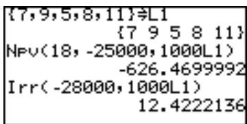
answer, thus, the investment revenue rate for the above condition is 12.42% .

• In the previous example, revenues following the investment value (input using minus sign) were assumed to be positive. However, when the assumed revenue is set to minus (in other words, more than two inverse symbols), the assumed revenue rate must be entered at the end. Otherwise an error may occur.

The following CALC functions, 08 Bal, 09 Prn and 10 Int require the values of 1% , PV and PMT variables. Enter the values beforehand in the TVM-SOLVER function.

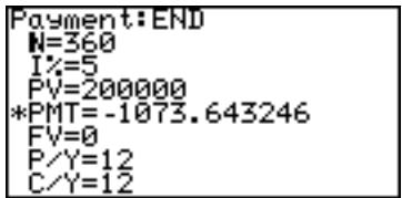
Example using the 08 and 10 calculations

You plan to purchase a house for the price of 300,000. The down payment is 100,000. Calculate the monthly payments for a 30-year loan at an annual interest rate of 5% for the remaining $200,000.

08 Bal ( Bal (number of payments [, decimal place to round])

Calculates loan balance.

Calculate the loan balance after 15 years (180 months).

09 Prn ( Prn (initial number of payments, end number of payments [, decimal place to round]).

Calculates the principal amount of the total payments.

Compare the principal amount of the total payments after 5 (1 to 60 months) and 10 years (61 to 120 months).

10 ΣInt ( ΣInt (Initial number of payments, end number of payments [, decimal place to round])

Calculates the sum of the interest on the payments.

Compare the sum of the interest on the payment sum after 5 years and 10 years.

Conversion functions

11 Apr ( Apr (effective interest rate, number of settlements)

Converts effective interest rate to nominal interest rate

Example

If the effective interest rate is 12.55% , how much is the nominal interest rate for the quarterly compound interest? If the monthly compound interest rate is 10.5% , how much is the nominal interest rate?

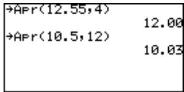
12 Eff ( Eff (nominal interest rate, number of settlements)

Converts nominal interest rate to effective interest rate

Example

If the annual (nominal) interest rate is 8% , how much is the effective interest rate for monthly compound interest? How much is it over half a year?

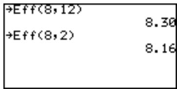
13 days (days (start month.day year, end month.day year) days (day month.year, day month.year)

Calculates the number of days between dates entered (within the range of 1950 to 2049)

Year, month, and day must be entered in 2-digit form. For example, enter 02 for 2002. Calculate the number of days from September 1, 1997 to December 31, 2004.

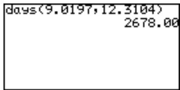
3. VARS Menu

The VARS menu consists of a list of the variables used for the TVM-SOLVER functions.

• The VARS menu can be used to enter values in the sub-menu within the Finance menu.

• Press 2ndF FINANCE D

• The VARS sub-menu will appear.
• Select the appropriate variable to use.

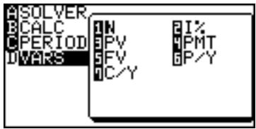
The variables in the VARS sub-menu are the same as those of the TVM-SOLVER feature.

How to recall the content of N

How to recall the content of 1 %

How to recall the content of PV

How to reenter the value

1. Press 2ndF FINANCE D 1 ENTER
2. Press 2ndF FINANCE D 2 ENTER

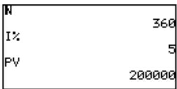
1. Press 2ndF FINANCE D 3 ENTER
   Each variable of the TVM-SOLVER can be recalled and then reentered.

Reenter 400 for N instead of 360

1. Press 400 STO
2. Press 2ndF FINANCE D 1 ENTER

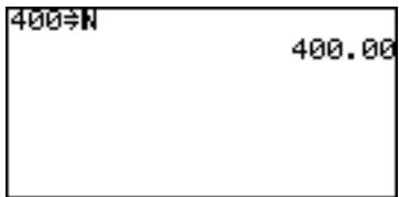
Chapter 12

The SOLVER Feature

The SOLVER feature is one of the calculator's most powerful and distinctive features, and helps you solve math problems with various analysis methods.

Using this feature, problems from linear equations to complex formulas can be solved with ease.

To access the SOLVER feature, press 2ndF SOLVER; to exit, press

Note: The SOLVER feature is not available in the Basic mode.

• The SOLVER feature shares variables with other calculator features. These variables can be called up or defined within the SOLVER feature OR any other features. For example, solving/ defining a value of “A” within the SOLVER feature will also change the global value of “A”.

1. Three Analysis Methods: Equation, Newton, and Graphic

To switch your preferred analysis style:

1. Go into the SOLVER menu by pressing 2ndF SOLVER WITHIN the SOLVER window. The SOLVER menu appears with four menu items.

2. While A METHOD item is selected on the left, select your preferred method by pressing 1, 2, or 3.

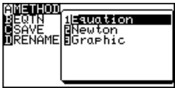
Equation method

The Equation method is useful when there is only one unknown variable. For example, if you know the values of B and C for an expression “ A + B = C ”, use the Equation method.

Example

Determine the value of "C" in "A = 2B² + 4C", when A = 4, and B = 5.

1. Enter SOLVER by pressing 2ndF SOLVER. The word SOLVER will flash on the screen, indicating that you are now in the SOLVER feature mode.

2. Enter the equation "A = 2B² + 4C". Press ALPHA A ALPHA = 2 ALPHA B x² + 4 ALPHA C.

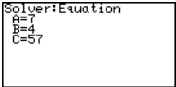
1. Press ENTER

The screen above right appears, indicating that there are 3 variables to be assigned.

Note: If values were assigned to those variables prior to this operation, then the previously set values will be shown here. For example,

C = 57 may show up in this

window; this simply indicates the value of "C" was previously set to "57".

1. Enter "4" for variable "A", and "5" for variable "B". Press 4 ENTER 5 ENTER.

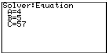
1. When the two known values have been specified, make sure that the cursor is at the value yet to be determined (in this case, the value of "C").

2. Press 2ndF EXE to execute the SOLVER. The value of "C" will be obtained.

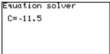
• After the solution has been found, press CL to return

to the variable input screen. You may change the numeric values for the variables and select another unknown variable to solve.

• To edit the equation, press CL on the variable input screen. The equation input screen allows you to correct or edit the previously input equation.

Newton's method

Newton's method is a technique of finding approximate solutions to a math problem via calculus, when conventional algebraic techniques just cannot work. If the Equation method fails, the calculator will automatically switch to Newton's method.

Example

Solve "X^2 + 4X - 2 = 0" .

1. Enter SOLVER by pressing 2ndF SOLVER. If you have items left on the screen, clear the entries by pressing the CL key several times.

2. Enter "X² + 4X - 2". When the expression is entered as a non-equation format, then "=0" is automatically assumed at the end. When done, press ENTER.

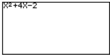
1. The next screen indicates the variable "X" and its previously set value. This value will be assumed as the starting point of the calculation segments, and the

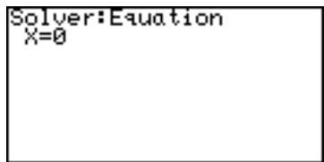
Newton SOLVER will find the closest approximation to the starting point. Enter "0", and press ENTER.

1. Now, press 2ndF EXE to execute the SOLVER. Since this cannot be solved using the Equation method, the calculator automatically switches analysis to Newton's method.

Change method to NEWTON

1. The next window confirms the starting point of the analysis (set to "X = 0" from step #3), and the size of each step (default is set to "0.001"). Press 2ndF EXE

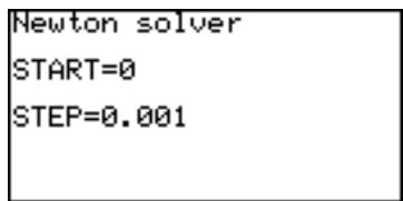
1. The following window shows the approximate value of X (0.449489742), the right side value of the equation (assumed as "0", at step #2), the left side value (which the

Newton solver X=0.449489742 

RIGHT=0  
LEFT =8.33E-11  
L-R =8.33E-11 

entered expression results to this value when the value X is entered), and the difference between the left and the right side.

1. Since the L-R difference above indicates a margin of error, try entering smaller steps. Press CL to go back to step #3. Enter the value of X, then press 2ndF

Newton solver START=0 

STEP=0.00001 

EXE to execute the SOLVER again. When the next window appears, try entering smaller step value ("0.00001", for example).

1. Press ENTER to register the step value change, then 2ndF EXE . Although the value of X appears to be unchanged, the margin of error will have become small

Newton solver X=0.449489742 

RIGHT=0  
LEFT =0  
L-R =0 

enough ("0", in this example), to be as close to zero as possible.

Note: As you may well know, there may be more than one solution to the equation. To obtain the value of the other solutions, set the starting point of Newton's method lower ("-10", for example) or execute the SOLVER again with the current solution as a starting point.

Graphic method

The Graphic method is another way of approximating solutions, using graphical representations. This method is particularly useful when finding more than one solution on a graph axis.

Example

Obtain values for Y = X^3 - 3X^2 + 1 , when Y = 0 .

1. Press 2ndF SOLVER to enter SOLVER. Clear screen entries by pressing CL several times.

2. Enter Y = X^3 - 3X^2 + 1 into the initial window, and press ENTER.

3. In the next window, set the Y value as "0", and press ENTER. The right side value of the equation is now set.

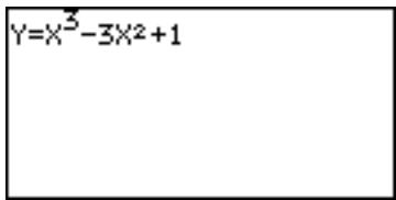
Note: Unlike in the Newton's method, the X value will not be assumed as the starting point for the Graphic method.

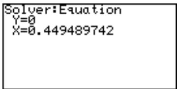
4.Before proceeding further, Solver:Graphic
you will need to set the Y=0 X=0.449489742 SOLVER to the Graphic method.Press 2ndF SOLVER to call up the SOLVER menu,and press A (for "AMETHOD"),then 3 (for "3 Graphic").The Graphic method is now set.
5. Press 2ndF EXE to proceed.
6. Next in the following window, specify the range of analysis that will incorporate all possible solution. In this example, we will set the beginning point at “-1”, and

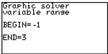
the end point at "3". Press ENTER at each variable entry.

Note: The analysis will be limited to the range specified; a solution outside of the analysis range will not be detected. If no crossing point is found in the range, then a message “No solution found” will show at the bottom of the screen.

1. Pressing 2ndF EXE at this point will engage the analysis, as well as the graphical representation of the equation. Note that while the cursor flashes at the upper right corners of the screen, the calculator is busy processing tasks.
2. When the processing is complete, you will get the first value of X (the smallest), with a flashing star on the graph at the crossing point.

To obtain the next X value, press 2ndF CALC.

Note: To enlarge a part of graph after the solution has been found, you may use the ZOOM Box

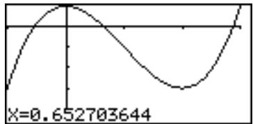
function. Press ZOOM and use the cursor for defining the box area.

2. Saving/Renaming Equations for Later Use

The expressions you have entered in the SOLVER can be named and stored:

1. Go to the SOLVER menu by pressing 2ndF SOLVER.
2. Press C to select the C SAVE menu, and press ENTER
3. When the next screen appears, ALPHA LOCK mode is automatically set and the cursor is changed to "H", indicating that alphabet characters can be entered.

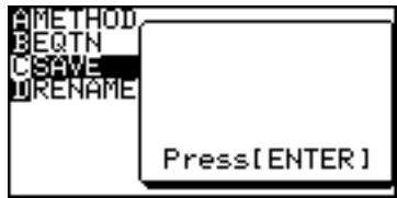
Equation title [POLYNOM]

To enter numbers, press ALPHA).

The equation name should consist of 8 characters/numbers or less.

1. When done, press ENTER. The screen goes back to the SOLVER function screen.

Saved SOLVER expressions can also be renamed:

1. Go to the SOLVER menu, and press D to select the D RENAME sub-menu.

2. A list of saved equation names appears in the submenu. Select the equation name you wish to change. For example, press 0 1 to select the first item of the list.

1. When renaming is complete, press ENTER to save the change. The screen goes back to the SOLVER function screen.

3. Recalling a Previously Saved Equation

To recall a stored SOLVER equation:

1. Go to the SOLVER menu, and press B to select the B EQTN sub-menu.
2. A list of saved equation names appears in the sub-

menu. Select the equation you wish to call back.

1. Press ENTER. The stored equation is called back.

Note: Any changes unsaved prior to recalling will be lost. Also be aware that any changes to the recalled equation will not be retained unless saved manually.

Chapter 13

Programming Features

The calculator has programming features that enable automatic processing of a series of calculations any number of times.

• The Programming features are only supported by the Advanced mode. In the Basic mode, only the execution of programs is available.

Almost all the calculation and graphing language can be used in programs as well as the usual control flow statements such as If, For, While and Goto (with Label).

Please note that complex numbers cannot be used in programming.

1. Try it!

Display a message "HELLO WORLD" on the display.

Creating a new program

1. Press PRGM.

The program menu screen will appear.

A EXECutes the selected program

BEDIT Opens a stored program file.

C NEW Creates a new program file

• In the Basic mode, only the A EXEC menu item will appear.

• Press C ENTER

A new program window will open.

1. Input the program name (HELLO) on the top line of the screen.

Up to 8 characters can be used for the title.

1. Press ENTER

2. The cursor will move to the program input field just under the title.

Starting programming

1. Press PRGM. The program menu will open. The commands and other statements are preinstalled in the calculator.

Do not directly type in commands using the Alphabetical mode, select each command from the program menu.

Note: Press 2ndF CATALOG, and you can access all the available commands at once.

Entering a command

1. Select A 1
2. Press PRGM.
3. Select A 2

The characters following a double quotation mark can

be manipulated as text. No double quotation mark is required to close the text.

Entering the alphabetical input lock mode

1. Press 2ndF A-LOCK to enter the alphabetic lock mode.
2. Type HELLO WORLD. Up to 160 alphanumeric characters can be input per

line. (Strings of up to 158 characters maximum can be entered per line excluding commands, because each command is regarded as a single character.

When a line exceeds the width of the screen, the display will shift to the left.

Store the program line by line

1. Press ENTER

The cursor will move to the next line and the data input will be stored.

Store the program line by line by pressing ENTER, or .

1. Press 2ndF QUIT to exit the program edit screen.

Execute the program

1. Press PRGM A

A list of stored programs will appear.

1. Press 0 1 to execute the program 01 "HELLO".

2. Programming Hints

Editing the program

Press PRGM B and then the appropriate numbers to open the stored program.

Adding commands, strings or command lines to the program

Press 2ndF INS to enter the insert type mode.

Press ENTER to go to the next line. Be sure to press 2ndF INS again to turn off the insert type mode and return to type over mode.

Press ENTER twice to insert a blank line.

Entering alphabetical characters (upccase only)

Press ALPHA to enter characters. Press 2ndF A-LOCK to use a ALPHA-LOCK mode to input a series of alphabetical characters.

Inputting commands

In general, only a single command can be input per line.

Storing a program line by line	After pressing ENTER, ▼ or ▲, the line will be stored in memory. Otherwise, it is not stored. Be sure to store the all lines by pressing ENTER (▲ or ▼) before quitting editing (pressing 2ndF QUIT).
Blank line	Blank lines are ignored during execution. You can include blank lines to gain better readability.
Deleting a line	Move the cursor to the line you wish to delete and press CL.
Deleting command or strings	Move the cursor to on or after the letter you wish to delete and press DEL or BS, respectively.
Deleting an entire program	Press 2ndF OPTION and use C DEL. (See Chapter 14 OPTION Menu, page 224).
Copying a line to another location	Press PRGM H in the program edit mode. (See page 216 for details)
Changing the program name	Press ▲ to move the cursor to the program name field. Enter the new name and press ENTER or ▼.
Re-executing the program	Press ENTER again after execution of the program completes.
Break the execution process	Press ON or 2ndF QUIT to break the execution process.

3. Variables

• Single letters (uppercase letter from A to Z and ) can be used as variables.
• Defined once in one program, a variable is set as a global variable across all other stored programs unless redefined.

Hence results calculated in one program can be used by another.

• Only value (numbers) can be set as variables.
• Strings cannot be set as variables.

Setting a variable

Use STO to input a specific value or the value of formula into the variable. Do not use = (comparison operands) to set the values into variable.

5 X The variable X is set to the value 5.

MX + B Y The variable Y is set to the value of formula MX + B

4. Operands

• Almost all the calculation operands can be used in a program.
• Input an operand directly from the keys (+, -, ×, ÷, , , and others) or using MATH, STAT, LIST, MATRIX and other menus.

Comparison operands

• The calculator has 6 comparison operands.
• Press MATH F and select an appropriate comparison operand.

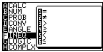
= Equal Not equal

Greater than ≥ Greater than or equal
<Less than ≤ Less than or equal

5. Programming commands

• Print, Input, Wait, Rem, End and other commands can be used in a program.
  Screen settings, data input/output, graph settings and others can be controlled from a program.
• Press PRGM in the program edit mode to input the command.

A PRGM menu PRGM A

1 Print Print variable

Print "character strings ["]

Displays the value of the variable on the screen.

The display format may vary according to the SET UP menu settings.

Character strings displayed by the print command will break at the edge of the screen.

2 “command “strings

Characters enclosed by double-quote marks are considered to be strings.

The closing double-quote can be omitted when it would appear at the end of a line.

3 Input Input["prompt strings"], variable

Enables the user to input a value (list, etc.) for the specified variable during execution. A message "variable = ?" or "prompt strings?" will appear on the screen while the calculator waits for data input.

Prompt strings include alphabetical words, numbers, and other character strings that can be entered by keys and menus.

4 Wait Wait [natural number (1 to 255)]

Interrupts execution for the (natural number) of seconds. If no value is specified, interruption continues until any key is pressed.

• A symbol will flash at the

upper right corner of the screen during the wait.

• This command can be used for displaying intermediate results or other information.

5 Rem Rem comments

Comments start with Rem and extend to the end of the line.

These lines are ignored at execution.

Comments should be entered as notes for future reference, though it should be noted that they do occupy some memory space.

6 End End

Indicates the end of a program.

End is not necessary at the last line of the program.

7 Key Key variable

If a numeric key or one of the cursor keys is pressed, the variable is set to the corresponding numeric value as specified in the following table.

Keys and Corresponding Numbers

keys	Numbers	keys	Numbers	keys	Numbers
0	0	5	5	▶	10
1	1	6	6	〈	11
2	2	7	7	▲	12
3	3	8	8	▼	13
4	4	9	9

B BRNCH menu PRGM B

See 6. Flow control tools on page 214.

C SCRN menu PRGM C

C SCRN menu commands are used to display or clear the screen.

1 ClrT ClrT

Cleared the program text screen without affecting the plotted graph.

2 ClrG ClrG

Cleared the graph screen without affecting the specified graph.

After the graph screen is cleared, the specified graph statement is drawn.

3 DispT DispT

Displays the program text screen.

4 DispG DispG

Displays the graph screen.

D I/O menu PRGM D

This menu is used to send or receive data from externally connected devices.

1 Get Get variable

Receives data from externally connected devices.

2 Send Send variable

Sends data to externally connected devices.

E SETUP menu PRGM E

SETUP menu commands are used to set the various settings used in graphing and calculations.

01 Rect Rect

Sets the graph coordinates as X and Y coordinates.

02Param Param

Sets the graph coordinates as parametric coordinates.

03 Polar Polar

Sets the graph coordinates as polar coordinates.

04 Web Web

Sets the graph coordinates as axes in sequence graphs.

u(n - 1) is set to the X axis and u(n) is set to the Y axis.

05 Time Time

Sets the graph coordinates as axes in sequence graphs.

n is set to the X axis and u(n), v(n) and w(n) is set to the Y axis.

06 uv uv

Sets the graph coordinates as the axes of sequence graphs.

u(n) is set to the X axis and v(n) is set to the Y axis.

07 uw uw

Sets the graph coordinates as the axes of sequence graphs.

u(n) is set to the X axis and w(n) is set to the Y axis.

08 vw vw

Sets the graph coordinates as the axes of sequence graphs.

v(n) is set to the X axis and w(n) is set to the Y axis.

09 Deg Deg

10 Rad Rad

11 Grad Grad

Sets the angle mode to degree, radian and gradient, respectively.

12 FloatPt FloatPt

13 Fix Fix

14 Sci Sci

15 Eng Eng

16 Tab Tab integer (0 to 9)

Sets the number display mode to floating point, fixed decimal, scientific and engineering, respectively.

17 Decimal Decimal

18 Mixed Mixed

19 Improp Improp

20 x±yi x±yi

21r∠θ r∠θ

Sets the answering mode to the one specified.

F FORMAT menu PRGM F

F FORMAT menu commands are used to set the graph format.

01 RectCursor RectCursor

Sets the graph coordinate display format to X - Y axes.

02 PolarCursor PolarCursor

Sets the graph coordinates display format to polar coordinates.

03 ExprON ExprON

Sets the graph equation to be displayed on the graph screen.

04 ExprOFF ExprOFF

Sets the graph equation to not be displayed on the graph screen.

05Y'ON Y'ON

Sets the derived function (Y^) to be displayed on the graph screen.

06Y'OFF Y'OFF

Sets the derived function (Y^) to not be displayed on the graph screen.

07 AxisON AxisON

Sets the specified axis to be displayed on the graph screen.

08 AxisOFF AxisOFF

Sets the specified axis to not be displayed on the graph screen.

09 GridON GridON

Sets the grid lines to be displayed on the graph screen.

10GridOFF GridOFF

Sets the grid lines to not be displayed on the graph screen.

11 Connect Connect

Draws a graph with connected lines.

12 Dot Dot

Draws a graph with dots.

13 Sequen Sequen

Draws the graphs in sequential order.

14 Simul Simul

Draws the graphs simultaneously.

G S_PLOT menu PRGM G

S_PLOT menu commands are used for statistics plotting.

1 Plt 1( Sets the statistical graph settings for plot 1.
2 Plt 2( Sets the statistical graph settings for plot 2.
3 Plt 3( Sets the statistical graph settings for plot 3.

The above menu commands have the same usage as the following:

Plt1.graph type, X list name [, Y list name, frequency list])
* Press [STAT PLOT] to specify a graph type.

4 PlotON PlotON [number]

Sets drawing of the specified statistical graph to on.

If no number is specified, this command turns on all of the statistical graphs.

5 PlotOFF PlotOFF [number]

Sets drawing of the specified statistical graph to off.

If no number is specified, this command turns off all of the statistical graphs.

6 LimON LimON

This commands turns on the limit lines for upper, lower, and mean values.

7 LimOFF LimOFF

This commands turns off the limit lines for upper, lower, and mean values.

6. Flow control tools

The calculator has the common flow control tools such as Goto - Label loop structures, and If-, For- and While-statement clauses for enhancing a program's efficiency. It also has the capability for subroutines.

It is recommended to use If, For or While statements rather than Goto-Label loop structures.

To access the flow control tools, use the PRGM B BRNCH menu.

01 Label Label label name

Specifies a branch destination for Goto or Gosub.

The same Label name cannot be used in two places within the same program.

Up to 10 characters can be used for a Label name.

Up to 50 Labels can be used in a single program.

02 Goto Goto label name

To shift the program execution to a label.

03 If If conditional statements Goto label name

or

If conditional statements

Then

commands or multiple statements *

Else

commands or multiple statements]

Endlf

• Multiple statements mean a group of statement lines separated by colons(:) that are evaluated as a single line.

Within a second structure it is possible to use the following menu items.

04 Then

05 Else

06 Endlf

• Use a comparison operand in a condition statement.
• Up to 115 If clauses can be nested, though if combined with other types of loops, the maximum nested loop number may vary due to the memory capacity.

07 For For variable, initial value, end value [, increment]

08 Next commands or multiple statements Next

• The increment value can be omitted. The default value is 1.
• For and Next statements must be placed at the beginning of the line.
• If the comparisons variable > end value (positive) or variable < end value (negative) are satisfied, the program will end the loop and go to the line indicated by the Next command.
• Up to 5 For loops can be nested, though if combined with other types of loops, the maximum nested loop number may vary due to the memory capacity.
• It is highly recommended that Label and Goto statements are not used in For loop structures.

09 While While conditional statements

10 WEnd commands or multiple statements WEnd

• While and WEnd statements must be placed at the beginning of the line.
• Multiple While loops can be nested to within the memory capacity.
• Conditional statements are evaluated before entering the While clause.
• It is highly recommended that Label and Goto statements are not used in While loop structures.
• Up to 8 while loops can be nested, though if combined with other types of loops, the maximum nested loop number may vary due to the memory capacity.

Note: Else clause cannot be omitted when the matching If clause is contained in a For or a While loop.

11 Gosub Gosub label name
12 Return

End

[Rem start of the subroutine (label name)]

Label label name

Statements

Return

Subroutine structures can be used for programming.

• The Gosub label name must be the same as the Label starting the subroutine.
• A Return statement is necessary at the end of the subroutine.

When the Return statement is executed, the calculator executes the next line after the Gosub statement.

• Up to 10 subroutines can be nested.

7. Other menus convenient for programming

H COPY menu PRGM H

You can copy and paste line by line using the COPY menu commands.

1. Move the cursor to the line that you wish to copy.
2. Press PRGM H
3. Select 1 StoLine and press ENTER

The selected line will be stored in the memory.

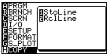
1. Move the cursor to the line where you wish to paste the stored line.

2. Press PRGM H, select 2 RclLine and press ENTER. The stored line will be inserted at the targeted position.

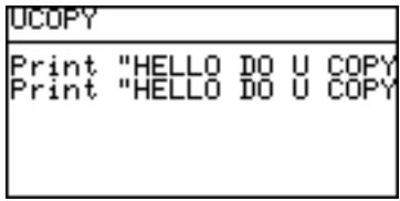
• Please note that only a single line can be stored in the memory.

VARS menu

• Functions that control the graph screen can be selected from the VARS menu.
• Press 2ndF VARS to display the VARS menu (shown to the right).

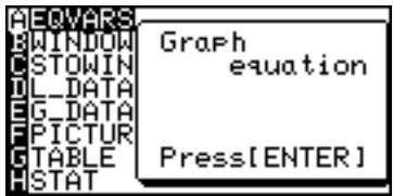
• There are differences in functions between the Advanced mode and the Basic mode. The following menus and their descriptions are based on the Advanced mode.

A EQVARS Specifies the graph equation (Y1 to Y9, and Y0, X1T·Y1T to X6T·Y6T, R1 to R6).

B WINDOW Specifies the functions that set the graph display screen size (Xmin, Ymax, Tstep, etc.).

C STOWIN Specifies the stored zoom (window) setting value (Zm_Xmin, Zm_Ymax, etc.).

D L_DATA Specifies list data (L_Data1 to L_Data9, and L_Data0).

E G_DATA Specifies the graph data (G_Data1 to G_Data9, and G_Data0).

F PICTUR Specifies picture data (Pict1 to Pict9, and Pict0).

G TABLE Specifies table setting values (Table Start, Table Step, Table List).

H STAT Specifies statistics, functions ( , x , ...), regression expressions, points and statistical verification functions.

• The commands and functions in the VARS menu can be displayed on the screen. Current setting data can also be reset.
• The results of arithmetic functions can also be displayed.
• The ZOOM command is selected directly from the ZOOM menu. Names of some ZOOM commands change when inserted into programs. These are [A ZOOM], [C POWER], [D EXP], [E TRIG], and [F HYP] of the ZOOM menu.

"Zm_ " is automatically added to each of these functions when inserted into programs.

Example

Zm_Auto, Zm_x², Zm_sin, etc.

• Always enter the argument for functions requiring an argument at the end of the command, such as the CALC function (2ndF). An error will be returned for commands not accompanied by an argument.

Example

Value 5

Example

Set Xmin = -3, Tmax = 10, Xscl = 1, Ymin = -5, Ymax = 5, Yscl = 1 in the WINDOW screen.

Use STO to input the settings.

Expression	Operational sequence
-3 ⇒ Xmin	(-) 3 STO 2ndF VARS B ENTER A 1 ENTER
10 ⇒ Xmax	10 STO 2ndF VARS ENTER 2 ENTER
1 ⇒ Xscl	1 STO 2ndF VARS ENTER 3 ENTER
-5 ⇒ Ymin	(-) 5 STO 2ndF VARS ENTER 4 ENTER
5 ⇒ Ymax	5 STO 2ndF VARS ENTER 5 ENTER
1 ⇒ Yscl	1 STO 2ndF VARS ENTER 6 ENTER

• Operation to input a function equation (for example, x^2 + 2 ) to the graphic equation "Y1" is also made using STO in the same manner as described above.

$$ \begin{array}{c c c c c c c c} \text {" X ^ {2} + 2 "} \Rightarrow \mathrm {Y} 1: & \boxed {\text {P R G M}} & \boxed {\text {A}} & \boxed {2} & \boxed {x / \theta / T / n} & \boxed {x ^ {2}} & \boxed {+} & 2 \boxed {\text {P R G M}} \ \hline \text {A} & \boxed {2} & \boxed {\text {S T O}} & \boxed {2 \text {n d F}} & \boxed {\text {V A R S}} & \boxed {\text {A}} & \boxed {\text {E N T E R}} & \boxed {\text {A}} & \boxed {1} \end{array} $$

Note: Function equations cannot be assigned in the graphic equations, such as Y1, if the EDITOR mode under SET UP is set to Equation. Switch the EDITOR to One line mode prior to assigning such graphic equations.

Example

The following data are included in list L1.

L1: 165, 182.5, 173.8, 166.5, 185.3

A one-variable calculation was executed based on this data.

After returning to the calculation screen, average values can be viewed by using the following procedure.

• Press 2ndF VARS H ENTER A 0 2 to display "x" on the screen.
• Press ENTER to obtain the average value of X as

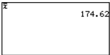
determined in the previous calculation.

• In this way, the contents of an immediately preceding statistical calculation can be stored as statistical values.
• These contents remain valid until the next statistical calculation is executed, even if the power is turned off.
• The same is true even for regression calculations and verification calculations.

8. Debugging

After programming, it is required to debug the program.

1. Press PRGM A and select the program to debug.

If any bugs are present, error messages will appear.

The following example indicates that the same label name has been used two or more times.

1. Press 4 or 7 to display the line where the error exists and correct the mistake.

When an infinite loop occurs

Execution can be interrupted by pressing ON.

Use this command if the program enters an infinite loop. Press < or to display the program source with the cursor on the line where interrupted.

• Refer to Appendix "Error Codes and Error Messages" on page 235.
• It is highly recommended that goto-Label statements are not used in If, While and For loop structures.
• Multiple statements cannot be used in a command line such as Else, EndIf, Next, While and WEnd. It is recommended not to use multiple statements.

9. Sample programs

MATFILL

• Fill the matrix M × N with random numbers from 0 to 9.

Ask and set the dimension of mat A

Input "ROW:", M

Input "COLUMN: ", N

M,N (matA)

Generate integer from 0 to 9 using int and random function and set it to each element

1 1

While 1≤ M

1

While J ≤ N

int (random x10) mat A(I, J)

$$ J + 1 \Rightarrow J $$

WEnd

$$ \mid + 1 \Rightarrow \mid $$

WEnd

Print mat A for confirmation

Print mat A

Wait

End

HIST

$$ 1 0 \Rightarrow \dim (L 1) $$

Gosub INSCORE

Gosub AVGSCORE

Plt1(Hist, L1)

Zm_Stat

Wait

End

Sequentially input the data in list L1.

Label INSCORE

$$ 1 \Rightarrow 1 $$

Input "ENTER SCORE", A

$$ \mathrm {A} \Rightarrow \mathrm {L} 1 (1) $$

$$ 2 \Rightarrow 1 $$

For I, 2, 10

Input "ENTER NEXT", A

$$ A \Rightarrow L 1 (I) $$

Next

Return

Calculate the median of List L1.

Label AVGSCORE

Print "AVERAGE IS

Median(L1) M

Print M

Wait 3

Return

Chapter 14 OPTION Menu

The calculator is equipped with OPTION menu for adjusting the display contrast, checking memory usage, deleting stored data, transferring data, and resetting the calculator's memory.

Accessing the OPTION Menu

Press 2ndF OPTION.

The OPTION Menu will appear.

A: Adjusts the display contrast

B: Checks the memory usage

C: deletes files

D: Link command to use with another calculator or PC.

E: Resets the calculator

1. Adjusting the screen contrast

1. Press 2ndF OPTION.

The screen contrast setting window will appear.

1. Press + to darken or - to lighten the screen.

2. Checking the memory usage

The memory usage window enables you to check how much memory you have used. If the memory is nearly full, delete files or reset the calculator to operate safely.

1. Press 2ndF OPTION.
2. Press B

The memory check window will appear. The remaining number of bytes of user

memory will be shown on the display.

The user memory is used to store data for graph equations, graph screens, matrices, lists and so on.

1. If you want check the details, press ENTER.

The detailed memory usage window will appear.

The total remaining memory will appear on the bottom line of the screen.

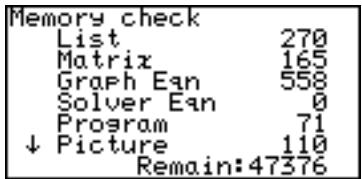
1. Press to scroll the window.

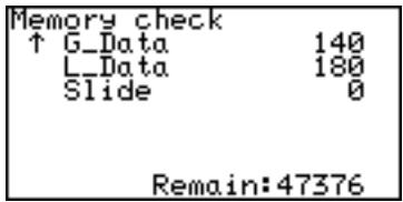
List: The amount of memory (bytes) used by lists

Matrix: The amount of memory (bytes) used by matrices

Graph Eqn: The amount of memory (bytes) used by graph equations

Solver Eqn: The amount of memory (bytes) used by solver equations

Program: The amount of memory (bytes) used by program files

Picture: The amount of memory (bytes) used by graph pictures

G_Data: The amount of memory (bytes) used by stored graph data

L_Data: The amount of memory (bytes) used by stored list data

Slide: The amount of memory (bytes) used by slide shows the user has created

3. Deleting files

Press 2ndF OPTION C to enter the delete menu.

The sub-menu items are the same as those of the Memory Check menu (List, Matrix, Graph Eqn, Solver Eqn, Program, Picture, G_Data, L_Data and Slide).

Deletions can be executed entry by entry.

To delete the matrix mat C

1. Press 2ndF OPTION C 2

The matrix deletion window will appear with the cursor pointer at the top (mat A).

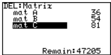
1. Move the cursor pointer to mat C using / .
2. Press ENTER. mat C will disappear and the mat C line will become empty.

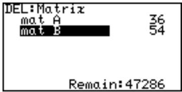
• Press 2ndF QUIT to cancel the delete option.
• Above procedures and displays are only an example. Displayed items may vary according to data input and use.
• Press 2ndF OPTION C 0 to delete the memories previously entered.

4. Linking to another EL-9900 or PC

Using the optional CE-451L or CE-LK2, the EL-9900 can be linked to another EL-9900 or PC, respectively.

To transfer data, press 2ndF OPTION D to open the Link option window. Press 1 to send data and press 2 to receive data.

Transmission between EL9900's

1. Connect the calculators securely using the optional CE-451L communication cable.

Make sure the commu-nication cable is firmly inserted into the ports of both calculators.
* Use the CE-451L only for linking two EL-9900's. The EL-9900 can only be linked to another EL-9900.

1. Press 2ndF OPTION D on both calculators.
2. Press 2 on the receiving machine. The receive mode screen will appear on the display.
3. Press 1 on the sending machine.
4. The send menu will appear on the display. Specify the data to send from the following categories.

A SELECT Displays the menu window to send the data specified as follows:

01 ALL Displays a list of all the stored files category by category.

02 List Displays a list of all the stored list files.

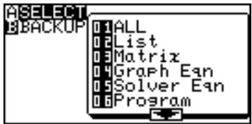
03 Matrix Displays a list of all the stored matrix files.

04 Graph Eqn Displays a list of all the stored graph equations.

05 Solver Eqn Displays a list of all the stored solver equations.

06 Program Displays a list of all the stored program files.

07 G_Data Displays a list of all the stored graph data files.

08 L_Data Displays a list of all the stored list data files.

09 Picture Displays a list of all the stored picture files.

10 Slide Displays a list of all the user-made slide show data.

11 A - Z, Displays a list of variables A to Z and .

B BACKUP Send all the data stored in the calculator memory.

1. Select the item to send using / and pressing ENTER. A " ^ 喜 will be placed by the selected item.
2. Press 2ndF ENTER to send.
3. Transmission begins and a busy message will appear on the displays of the both calculators.

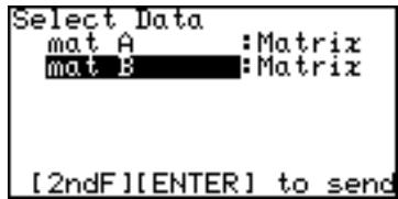
• An data in the same memory locations in the receiver will be automatically overwritten.
• Up to 10 files can be selected to send at once.

Example

If you wish to send the list L1, matrices mat A and mat B and graph equation Y2 to the other calculator.

1. Prepare the receiving calculator by pressing 2ndF OPTION D 2
2. Press 2ndF OPTION D 1 on the sending calculator

The send menu will appear.

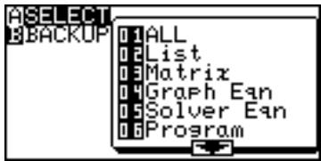
1. Press 0 1

A list of all the data stored will be displayed and the cursor positioned on the top line.

• You can also select 02 List for "L1", 03 Matrix for "mat A" and "mat B", and 04 Graph Eqn for "Y2", for example, and send the data category by category.

• Move the cursor to L1 and press ENTER.

A " ^ 丰 mark will flash to the left of "L1", indicating that the item has been selected to be sent.

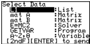
Press ENTER again to deselect.

1. Select the other files you wish to send in the same manner.
2. Press 2ndF ENTER to start transmission.

Transmission between the EL-9900 and PC

• The optional kit CE-LK2 (cable and Windows software) is required for calculator to data communication with PC.
  Refer to the CE-LK2 operation manual for details.
• During communications between calculator and PC, no operation of the calculator is required. Just connect the cable and press the power on key, and the entire operation can be controlled from the PC.

5. Reset function

If a problem occurs after replacing batteries, or the calculator does not function correctly, use the RESET option.

1. Press 2ndF OPTION E
2. Press 1 to return the calculator's SETUP and FORMAT settings to the default value, or 2 to delete all the stored data.

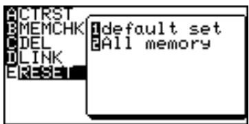
See "Resetting the Calculator" on page 29 for details.

Appendix

1. Replacing Batteries

The calculator uses two different kinds of batteries: manganese (AAA) for unit operation, and lithium (CR2032) for memory backup.

Compatible battery types

Type (use)	Model	Quantity
Manganese battery (for unit operation)	AAA	4
Lithium battery (for memory backup)	CR2032	1

• To prevent loss of stored data, DO NOT remove both the unit operation and memory backup batteries at the same time.

Precautions for handling batteries

• Fluid from a leaking battery accidentally entering an eye could result in serious injury. Should this occur, wash with clean water and immediately consult a doctor.
• Should fluid from a leaking battery come into contact with your skin or clothes, immediately wash with clean water.
• If the product is not to be used for some time, to avoid damage to the unit from leaking batteries, remove them and store in a safe place.
• Do not leave exhausted batteries inside the product.
• Do not fit partially used batteries, and be sure not to mix different batteries types.
• Keep batteries out of the reach of children.
• Do not allow batteries to become completely exhausted; doing so may cause the batteries to leak, and may damage the calculator's hardware.
• Do not throw batteries into a fire or water, as this may cause them to explode.

Procedures for replacing unit operation batteries

When battery power becomes low, a message will show indicating that a new set of batteries are needed.

1. Turn off the calculator's power (2ndF OFF).
2. Turn over the calculator.

Locate the battery compartment cover, and open the cover as illustrated.

1. Replace all four AAA batteries as illustrated.

2. Replace the battery compartment cover.

3. Press ON

The following message will appear.

If the message does not appear, repeat the procedures from step 2.

The OPERATING batteries are depleted Read OPERATION MANUAL for detail.

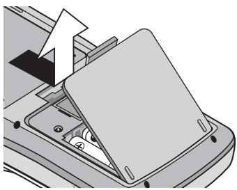
PRESS [CL] KEY TO
CLEAR ALL DATA
PRESS [ON] KEY TO
CANCEL

1. Press ON

Do not press CL. This will clear all the data.

Replacing the memory backup battery

Once every 5 years, the lithium battery will need to be replaced. The lithium battery is used to maintain the memory of the calculator.

Note: Do not remove the lithium battery while the unit operation batteries are removed; otherwise all the calculator's stored memory will be lost.

1. Perform procedures 1 and 2, as shown above. Do not remove the unit operation batteries.
2. Remove the screw and the lithium battery cover, as shown.

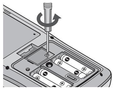
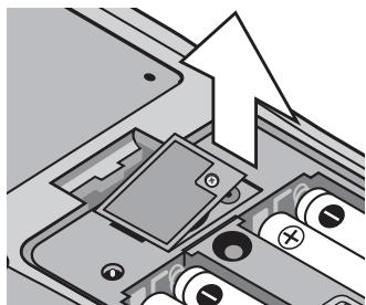
1. Use a pen to lift the lithium battery out of the battery compartment.
2. Insert the new battery with the PLUS (+) side facing up.
3. Replace the lithium battery cover and fasten the screw.

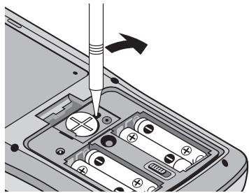
1. Replace the battery compartment cover and press ON. The following message will appear.
2. Press ON.

Do not press CL. This will clear all the data.

PRESS [CL] KEY TO CLEAR ALL DATA

PRESS [ON] KEY TO CANCEL

2. Troubleshooting Guide

Refer to the list of possible symptoms, and solutions may be found here.

The calculator's power won't turn on!

• The operation batteries may not be installed, may be exhausted, or may be inserted incorrectly. Check the operation batteries in the battery compartment.
• Place the battery cover securely or the calculator will not turn on.

The saved calculator configurations are not retained!

• Both the lithium battery and the operation batteries may need to be replaced.

The power seems to be on, but the characters and numbers cannot be seen clearly on the display!

• The screen contrast may need to be adjusted.

Press 2ndF OPTION, then press A to enter A CTRST; the screen contrast can be adjusted by using the + or the - key.

The calculator won't take the minus (-) sign; calculation results in a syntax error!

• To set a negative value, use the (-) key instead of the - key.

The calculation results are very different from what is usually expected!

• The angle unit and other configurations may be incorrectly set. Check the configuration under the 2ndF SETUP.

The graph cannot be seen!

• Check the zoom configuration. Try selecting the automatic zoom tool, by pressing , then A 1.
• The graph line may be set differently; check the line configuration under 2ndF DRAW menu.
• The calculator may not be set to display graphs. Check the “=” sign in Y = screen.

The screen images cannot be stored (SLIDE SHOW)

• The available memory may be too small to store the screen image. Select "B MEMCHK" under 2ndF OPTION menu. Select and delete unnecessary items under "C DEL".

There appears to be no functions available for integral/differential calculations!

• Make sure that the Advanced mode is selected. The integral/differential calculation tools can be found in the MATH menu.
• Access CATALOG menu by pressing 2ndF CATALOG.

The calculator is not responding; the software appears to have crashed!

• Press ON. If this does not work, then press 2ndF, then ON to tell the running application to quit.

If everything fails, then the calculator's memory may need to be reset. Resetting the calculator's memory will clear all the stored information, such as programs, lists, and variables.

To reset the unit's memory, open and close the battery compartment cover, and press ON to open the verification window. To prevent data loss, try ON first. If it does not work, repeat the reset operation and press CL when prompted.

3. Specifications

Model EL-9900

Product name Graphing Calculator

Display 132 x 64 dot matrix liquid crystal display Number of digits: mantissa 10 digits, exponents 2 digits (standard screen); 7 digit display (including negatives, decimals) for table screen, split screen, etc. Mantissa of 10 digits in the complex number mode Display method: Numerical value, calculation equation input (direct algebraic logic input / one-line input method), fraction, and complex number display method specification.

Reversible keyboard Basic and Advanced

Note: Advanced mode specific functions are: financial function, statistical test function and distribution function, solver function, matrix function, and tools function, etc.

Calculation method D.A.L. (Direct Algebraic Logic)

Calculation features Manual calculation (arithmetic, parentheses calculation, memory calculation, function calculation, integral calculation, coordinate conversion), binary/octal/decimal/hexadecimal calculation, Boolean operation, matrix calculation, complex number calculation, complex function calculation, statistic calculation, regression calculation, statistic authorization calculation, financial calculation, etc.

Input method Manual key entry

Graphic features Rectangular/polar/parametric/sequence coordinate graph Graph range specification, graph window mode automatic specification, graph plotting, trace, calculation function, zoom, picture input, paint, graph database register split-screen, etc.

Statistic features 1-/2-variable statistical data input/calculus, register, edit and frequency input, regression calculation function, and estimated statistic/authorization function, etc.

Solver features Equation solver: numerical syntax analysis, Newton's method, graph analysis, and solver equation register.

Appendix

List features	Direct data entry/edit to list, calculation function for various lists, and list/matrix conversion.
Substitution features	Graph drawing, numerical input from split-screen
Slide Show features	Screen image capture, play function
	The maximum number of pages to be captured: Approx. 250 pages (pages equivalent to the Y = X² graph screen)
Program features	Condition statement command, subroutine, graph, various function commands
Option menu	Screen contrast adjustment, memory usage check, data delete, data link (between EL-9900 and PC or another EL-9900)
Memory size	64 KB (user area: approx. 47.4 KB)
Power supply	Operation: 6 V DC:: AAA manganese battery (R03) × 4 Memory backup: 3 V DC:: Lithium battery (CR2032) × 1
Automatic power-off	Approx. 10 minutes
Operating temperature range	0 °C to 40 °C (32 °F to 104 °F)
Power consumption	0.23 W
Battery life	Operation battery set: approx. 150 hours (with 5 minutes of continual use and 55 minutes in the display state for every hour at a temperature of approx. 20 °C/68 °F) Memory backup: approx. 5 years (at a temperature of approx. 20 °C/68 °F, and when the operation batteries are replaced frequently)
Note:	The life span may differ according to battery brand, type, usage, and ambient temperature.
External dimensions	86 mm (W) × 183 mm (D) × 23 mm (H) 3-3/8" (W) × 7-7/32" (D) × 29/32" (H)
Weight	240 g (0.53 lb) (with batteries, without the hard cover)
Accessories	4 AAA manganese batteries (included), 1 lithium battery (installed), operation manual

4. Error Codes and Error Messages

Error Code	Error Message	Description
01	Syntax	Syntax error found in equation/program
02	Calculate	Calculation-related error found (division by 0, calculation beyond range, etc.)
03	Nesting	Cannot nest more than 14 numerical values, or 32 functions during execution.
04	Invalid	Matrix definition error or entering an invalid value.
05	Dimension	Matrix dimension, or STAT list dimension, inconsistent.
07	Invalid DIM	Size of list/matrix exceeds calculation range.
08	Argument	Inconsistency found in argument of the structured function.
09	Data Type	Invalid data type used in calculation.
10	No Sign Change	Financial calculation error found.
11	No define	Undefined list/matrix used in calculation.
12	Domain	Argument definition outside of domain.
13	Increment	Increment error found.
16	Irr Calc	More than two inflection points for Irr calculation.
17	Stat Med	Med-Med law (statistic) error found.
20	No Argument	Argument missing.
21	Not pair ∩ dx	∫ and dx are not used in a pair.
22	Not pair []	Brackets are not used in a pair.
23	Not pair()	Parentheses are not used in a pair.
24	Not pair {}	Braces are not used in a pair.
25	Line over	Line is over the capacity.
26	Not delete	Unable to delete a selected item.
27	Buffer over	Input/equation exceeds buffer capability.
30	Editor type	Invalid editor type found.*
31	Continue =	“=” exists in equation that has been recalled (RCL).
32	No data	Data does not exist.
33	Graph Type	Graph type setting incorrect.
34	Too many var.	Too many variables assigned in the SOLVER.
35	No variable	No variable specified in the SOLVER.
36	No solution	No solution found.
37	No title	No title entered.
38	Too many obj	More than 30 objects selected.
40	Lbl duplicate	Labels with identical name found in program.
41	Lbl undefined	Goto/Gosub encountered with no defined label.
42	Lbl over	More than 50 labels found in program.
43	Gosub stack	Nesting of more than 10 subroutines found.
44	Line too long	Line contains more than 160 characters.
45	Can't return	Return used without jumping from subroutine.
46	Storage full	Cannot create more than 99 files.
47	Coord type	Invalid coordinate system for command.
48	Without For	For is missing corresponding to the Next command.
49	Without WEnd	WEnd is missing corresponding to the While command.
50	Without While	While is missing corresponding to the WEnd command.
51	Without Then	Then is missing corresponding to the If command.
52	Without EndIf	EndIf is missing corresponding to the If command.
53	Without If	If is missing corresponding to the EndIf command.
70	I/O device	Communication error found among devices.
71	Wrong Mode	Wrong communication mode set.
90	Memory over	Memory is full; cannot store data as requested.
99	System error	System error found; user memory space is insecure.
	Low battery	Operation interrupted due to low battery power.
	BREAK!!	Operation break specified.

• The following operations may cause Editor type error. Correct the Editor type to continue.

• Recall the SOLVER equations (EQTN) or Graph data (G_DATA) stored in a different EDITOR mode than currently in use.

• Receive the Graph equation (Y1 and others) entered in a different EDITOR mode than currently in use.

5. Error Conditions Relating to Specific Tasks

1. Financial

• Define constants "r" and "s" as used in the equation below.

$$ r = \left(\frac {I (\%)}{100} \div C / Y + 1\right) ^ {\frac {C / Y}{P / Y}} - 1, \left{ \begin{array}{l} S = 1 (P m t _ {-} B e g i n) \ S = 0 (P m t _ {-} E n d) \end{array} \right} $$

1.1% calculation

① If PMT = 0

$$ r = \left(- \frac {P V}{F V}\right) ^ {- \frac {1}{n}} - 1 $$

② If PMT 0

$$ f (r) = P V + (1 + r \times s) \times P M T \times \frac {1 - (1 + r) ^ {- n}}{r} + F V (1 + r) ^ {- n}: (r \neq 0) $$

$$ f (r) = P V + P M T \times n + F V: (r = 0) $$

calculate the following for r solved in 1 and 2

$$ I (\%) = 100 \times C / Y \times ((r + 1)^{\frac{P / Y}{C / Y}} - 1) $$

2. PV calculation

① If r 0,r > - 1

$$ P V = - (1 + r \times s) \times \frac {1 - (1 + r) ^ {- n}}{r} \times P M T - F V \times (1 + r) ^ {- n} $$

② If r = 0

$$ P V = - n \times P M T - F V $$

③ If r≤ -1

Error

3. FV calculation

① If r 0,r > - 1

$$ F V = - \frac {P V + (1 + r \times s) \times \frac {1 - (1 + r) ^ {n}}{r} \times P M T}{(1 + r) ^ {n}} $$

② If r = 0

$$ F V = - n \times P M T - P V $$

③ If r≤ -1

Error

4. PMT calculation

① If r 0,r > - 1

$$ P M T = - \frac {P V + F V \times (1 + r) ^ {- n}}{(1 + r \times s) \times \frac {1 - (1 + r) ^ {- n}}{r}} $$

② If r = 0

$$ P M T = - \frac {P V + F V}{n} $$

③ If r≤ -1

Error

5. N calculation

① If r 0,r > - 1

$$ N = - \frac {\log \left{\frac {P V + \frac {1}{r} \times (1 + r \times s) \times P M T}{\frac {1}{r} \times (1 + r \times s) \times P M T - F V} \right}}{\log (1 + r)} $$

② If r = 0

$$ N = - \frac {F V + P V}{P M T} $$

③ If r≤ -1

Error

2. Error conditions during financial calculations

-1
- N = 0 in PMT calculations
- 1% = 0 and PMT = 0, or 1% 0 and FV = (1/r) (1 + r × s) × PMT, in N calculations.

$$ s = 1 (P m t _ {-} B e g i n) $$

$$ s = 0 (P m t _ E n d) $$

In 1% calculations

If PMT > 0:

Pmt_End mode: PV≥0 and FV+PMT≥0

PV < 0 and FV + PMT < 0

Pmt_Begin mode: PV + PMT ≥ 0 and FV ≥ 0

PV + PMT < 0 and FV < 0

If PMT < 0

Pmt_End mode: PV > 0 and FV + PMT > 0

PV ≤ 0 and FV + PMT ≤ 0

Pmt_Begin mode: PV + PMT > 0 and FV > 0

PV + PMT ≤ 0 and FV ≤ 0

• FV, N × PMT, PV ≥ 0 or FV, N × PMT, PV ≤ 0
• Irr calculation: all cash flows have the same sign.

3. Distribution function

① pdfnorm(

$$ f (x) = \frac {1}{\sqrt {2 \pi} \sigma} \exp \left(- \frac {(x - \mu) ^ {2}}{2 \sigma^ {2}}\right) $$

Calculation result Xreg μ: Mean σ: Standard deviation

② pdfT(

$$ f (x) = \frac {\Gamma (\frac {d f + 1}{2})}{\Gamma (\frac {d f}{2})} \frac {\left(1 + \frac {x ^ {2}}{d f}\right) ^ {- \frac {d f + 1}{2}}}{\sqrt {\pi d f}} $$

However: (s) = _0^ x^s-1 e^-x dx

Calculation result Xreg

③ pdfx²(

$$ f \left(\chi^ {2}, d f\right) = \frac {1}{2 \Gamma \left(\frac {d f}{2}\right)} \left(\frac {\chi^ {2}}{2}\right) ^ {\frac {d f}{2} - 1} e ^ {\left(- \frac {\chi^ {2}}{2}\right)} $$

However: (s) = _0^ x^s-1 e^x dx

df: Degree of freedom

④ pdfF(

$$ f (x) = \frac {\Gamma (\frac {m + n}{2})}{\Gamma (\frac {m}{2}) \Gamma (\frac {n}{2})} \left(\frac {m}{n}\right) ^ {\frac {m}{2}} x ^ {\frac {m}{2} - 1} \left(1 + \frac {m x}{n}\right) ^ {- \frac {m + n}{2}} $$

However: (s) = _0^ x^s-1 e^x dx

m: Degree of freedom of numerator

n: Degree of freedom of denominator

⑤ pdfbin(

$$ P (x = 0) = (1 - p) ^ {n} $$

$$ P (x = c + 1) = \frac {(n - c) p}{(c + 1) (1 - p)} P (x = c) $$

$$ (c = 0, 1, \dots , n - 1) $$

n: Trial number (integers greater than 0)

p: Success probability (0≤ p≤ 1)

c: Success number

⑥ pdfpoi

$$ f (x) = \frac {e ^ {- \mu} \mu^ {x}}{x !} $$

$$ (x = 0, 1, 2, \ldots) $$

⑦ pdfgeo(

$$ f (x) = p (1 - p) ^ {x - 1} $$

x: First successful trial number

6. Calculation Range

1. Arithmetic calculation

The results for dividend, multiplicand and operand are:

$$ - 1 \times 1 0 ^ {1 0 0} < x \leq - 1 \times 1 0 ^ {- 9 9}, 1 \times 1 0 ^ {- 9 9} < x \leq 1 \times 1 0 ^ {1 0 0} \text {o r} x = 0 $$

(valid within the range of display capability)

Note: Calculation results and input values less than 1 × 10^-99 are considered equal to 0.

2. Function calculation

Calculation accuracy

In principle, calculation errors are ± 1 of the last digit. (In case of exponential display, the calculation errors are ± 1 of the last digit of the mantissa display.) However, a calculation error increases in continuous calculations due to accumulation of each calculation error. (This is the same for a^b , [3]b , n! , e^x , ln , etc. where continuous calculations are performed internally.)

Additionally, a calculation error will accumulate and become larger in the vicinity of inflection points and singular points of functions. (for example, calculating X or X at X = 0 )

Function	Calculation range	Notes
sin x	DEG : |x| < 1 × 1010
	RAD : |x| < π/180 × 1010
cos x	GRAD : |x| < 10/9 × 1010
tan x	However, the following are excluded for tan x
	DEG : |x| = 90 (2n - 1)	“n” is an integer
	RAD : |x| = π/2 (2n - 1)
	GRAD : |x| = 100 (2n - 1)
sin-1x	-1 ≤ x ≤ 1
cos-1x
tan-1x	|x| < 1 × 10100
sinh x	-230.2585093 ≤ x ≤ 230.2585092
cosh x
tanh x
sinh-1x	|x| < 1 × 1050
cosh-1x	1 ≤ x ≤ 1 × 1050
tanh-1x	|x| < 1
In x log x	1 × 10-99 ≤ x < 1 × 10100	ln x = logₑ x
ex	-1 × 10100 < x ≤ 230.2585092	e÷2.71828...
10x	-1 × 10100 < x < 100
x-1	|x| < 1 × 10100	x ≠ 0
x²	|x| < 1 × 1050
√x	0 ≤ x < 1 × 10100
n!	-0.5 ≤ n ≤ 69.5	n is an integer or integer + 0.5
ab(Λ)	When a > 0: -1 × 10100 < b log a < 100 When a = 0: 0 < b < 1 × 10100 When a < 0: b is an integer, or 1/b is an odd number (b ≠ 0) However, -1 × 10100 < b log |a| < 100	ab = 10b-log a
a√b	When b > 0: -1 × 10100 < 1/a log b < 100, a ≠ 0 When b = 0: 0 < a < 1 × 10100 When b < 0: a is an odd number, or 1/a is an integer (a ≠ 0) However, -1 × 10100 < 1/a log |b| < 100	a√b = 101a log b
nPnCr	0 ≤ r ≤ n ≤ 69	n and r are positive integers
dec bin oct hex	Decimal: |x| ≤ 9999999999 Binary: 1000000000000000 ≤ x ≤ 1111111111111111111111111111111111111111111111111111111111111111111111111111111111111111111111111111	x is an integer
	Octal: 4000000000 ≤ x ≤ 7777777777777777777777777777777777777777777777777777777777777777777777777777777777777777777777777777
	Hexadecimal: FDABF41C01 ≤ x ≤ FFFFFFFFFF 0 ≤ x ≤ 2540BE3FF
→dms	|x|<1×10100
→deg
xy→r	|x|<1×10100, |y|<1×10100	r = √x2+y2
xy→θ	√x2+y2<1×10100	θ = tan-1 y/x
	|y/x|<1×10100
rθ→x	|r|<1×10100	x = r cosθ
rθ→y		y = r sinθ
		The range of θ is the same as x of sin x and cos x
not	Binary: 1000000000000000≤x	Other Boolean operations are the same as not and neg
	≤1111111111111111
	0≤x≤011111111111111
	Octal: 4000000000≤x≤7777777777
	0≤x≤3777777777
	Hexadecimal: FDABF41C01≤x≤FFFFFF
	0≤x≤2540BE3FE
neg	Binary: 1000000000000001≤x
	≤1111111111111111
	0≤x≤011111111111111
	Octal: 4000000001≤x≤7777777777
	0≤x≤3777777777
	Hexadecimal: FDABF41C01≤x≤FFFFFF
	0≤x≤2540BE3FF
Statistic calculations	|x|<1×1050
	|y|<1×1050
	|Σx|<1×10100
	Σx2<1×10100
	|Σy|<1×10100
	Σy2<1×10100
	|Σxy|<1×10100
	|n|<1×10100
x̄	n ≠ 0	Same for y, sy and cy
sx	n > 1 |Σx| < 1 × 1050 0 ≤ Σx2/n < 1 × 10100
σx	n > 0 |Σx| < 1 × 1050 0 ≤ Σx2/n < 1 × 10100
r	n > 0 |Σx| < 1 × 1050 |Σy| < 1 × 1050 0 < (Σx2/n - (Σx)2)/n (Σy2/n) < 1 × 10100 |Σxy - ΣxΣy/n| < 1 × 10100 |Σxy - ΣxΣy/n/n|/√(Σx2/n - (Σx)2/n) (Σy2/n) | < 1 × 10100
b	n > 0 |Σx| < 1 × 1050 |(Σx) (Σy)| < 1 × 10100 0 < |Σx2/n| < 1 × 10100 |Σxy - ΣxΣy/n| < 1 × 10100 |Σxy - ΣxΣy/n/n|/ (Σx2/n - (Σx)2/n) | < 1 × 10100	Regression calculations excluding 2nd, 3rd, and 4th degree polynomials.
a	|b̄x| < 1 × 10100 |y - b̄x| < 1 × 10100	Same as above. Same as b for other.
y'	|bx| < 1 × 10100 |a + bx| < 1 × 10100
x'	|y - a| < 1 × 10100 |y - a/b| < 1 × 10100
int÷	0 ≤ x < 1010
remain	0 ≤ x < 1010
%	|x| < 10100
→ a b/c	|x| < 1010	A number with 10 or less decimal places, or the 1010-th or above decimal places are 0.
→ b/c
List	Error is returned when the number of elements exceeds 1000.	This is the same when the result of a list function specifies 1000 or more elements.
Matrix	Error is returned when specifying columns or rows that exceed 100.

3. Complex number calculation

In a complex number calculation, a calculation error may occur and increase due to inner continuous calculations.

Function	Calculation range	Notes
1/x+yi	|x|<1050|y|<1050	x+yi≠0
(x+yi)2	|x|<1050|y|<1050|xy|<5×1099
ln (x+yi)	|x|<1050
log (x+yi)	|y|<1050
√x+yi	|y/x|<10100
e(x+yi)	|x|<230|y|<230
10(x+yi)	|x|<100|y|<100
(x+yi)(a+bi)	|x|<1050|y|<1050|a|<10100|b|<10100

7. CATALOG Feature

Press 2ndF CATALOG to display the CATALOG menu.

You can directly access various features and commands from the CATALOG menu.

CATALOG menu lists are different between the Basic mode and the Advanced mode.

For example, in Program edit mode of the Advanced mode, you can access the program commands from the CATALOG menu.

Please note that you can enter the eular number e only from the CATALOG menu.

The Basic mode features and commands accessible only from the CATALOG menu are:

and, ANOVA( ^-1 , cosh, ^-1 , cot, ^-1 , csc, ^-1 , cumul, d/dx(, dx, e, e^x ), fmax(, fmin(, Inflec, In, log2, not, or, prod(, Rg_a+bx, Rg_ae^{bx}, Rg_ax^b, Rg_ln, Rg_log, Rg_logistic, Rg_sin, Rg_x^3, Rg_x^4, sec, ^-1 , sinh, sinh^{-1}, tan^{-1}, tanh, tanh^{-1}, xnor, xor, [, ], :, =, ≠, >, ≥, <, ≤, 2x, (,) .

The Advanced mode features and commands accessible only from the CATALOG menu are:

→a⊥b/c, →A.xxxx, →b/c, e, int÷, remain, rndCoin, rndDice, Simp, %.

The CATALOG commands and the equivalent keys:

CATAROG command	Equivalent key
-	a/b
^	ab
2	x2
-1	x-1
⇒	STO
C	MATH C nCr
P	MATH C nPr
\	ab%

8. List of Menu/Sub-menu Items

CATALOG function lets you access almost all the functions and commands.

Square brackets indicate that the value or variable is optional.

1. MATH menus

Functions Commands	Syntax	Keystrokes		Page
		Advanced mode	Basic mode
MATH CALC
\( \log_2 \)	\( \log_2 \) value	A01		70
\( 2^X \)	\( 2^value \)	A02		71
fmin(	fmin(equation, lower limit of x, upper limit of x)	A03		71
fmax(	fmax(equation, lower limit of x, upper limit of x)	A04		71
d/dx(	d/dx(equation, value of x [, tolerance])	A05		71
∫	∫ equation, lower limit, upper limit [, tolerance] dx	A06		71
dx	∫ equation, lower limit, upper limit [, tolerance] dx	A07		71
Σ(	Σ (expression, initial value, end value [, increment])	A08		72
sec	sec value	A09		72
csc	csc value	A10		72
cot	cot value	A11		72
\( sec^{-1} \)	\( sec^{-1} \) value	A12		72
\( csc^{-1} \)	\( csc^{-1} \) value	A13		72
\( cot^{-1} \)	\( cot^{-1} \) value	A14		72
sinh	sinh value	A15		72
cosh	cosh value	A16		72
tanh	tanh value	A17		72
\( \sinh^{-1} \)	\( \sinh^{-1} \) value	A18		73
\( \cosh^{-1} \)	\( \cosh^{-1} \) value	A19		73
\( \tanh^{-1} \)	\( \tanh^{-1} \) value	A20		73
sin	sin value		A1	42
cos	cos value		A2	42
tan	tan value		A3	43
log	log value		A4	43
\( 10^X \)	\( 10^value \)		A5	43
MATH NUM
abs(	abs(value)	B 1	B 1	73/43
round(	round(value [, digit number of decimals])	B 2	B 2	73/44
ipart	ipart value	B 3	B 3	73/44
fpart	fpart value	B 4	B 4	73/44
int	int value	B 5	B 5	73/44
min(	min(value A, value B) or min(list)	B 6	B 6	73/45
max(	max(value A, value B) or max(list)	B 7	B 7	73/45
lcm(	lcm(natural number, natural number)	B 8	B 8	73/45
gcd(	gcd(natural number, natural number)	B 9	B 9	73/45
remain	natural number remain natural number		B 0	46
MATH PROB
random	random [(number of trial)]	C 1	C 1	74/46
rndInt(	rndInt(minimum value, maximum value [, number of trial])	C 2	C 2	74/46
rndCoin	rndCoin [(number of trial)]		C 3	47
rndDice	rndDice [(number of trial)]		C 4	47
nPr	value A nPr value B	C 3	C 5	74/47
nCr	value A nCr value B	C 4	C 6	74/48
!	value!	C 5	C 7	74/48
MATH CONV
→deg	value →deg	D 1	D 1	74/48
→dms	value →dms	D 2	D 2	74/49
xy→r(	xy→r(x-coordinate, y-coordinate)	D 3		75
xy→θ(	xy→θ(x-coordinate, y-coordinate)	D 4		75
rθ→x(	rθ→x(r-coordinate, θ-coordinate)	D 5		75
rθ→y(	rθ→y(r-coordinate, θ-coordinate)	D 6		75
MATH ANGLE
°	value °[value', value"]	E 1	E 1	76/49
'	value °value', [value"]	E 2	E 2	76/49
"	value °value', value"Print "character strings"["]	E 3	E 3	76/49
r	value r	E 4	E 4	76/49
g	value g	E 5		76
MATH INEQ
=	value A = value B	F 1		76
≠	value A ≠ value B	F 2		76
>	value A > value B	F 3		76
≥	value A ≥ value B	F 4		76
<	value A < value B	F 5		76
≤	value A ≤ value B	F 6		76
MATH LOGIC
and	value A and value B	G 1		77
or	value A or value B	G 2		77
not	not value	G 3		77
xor	value A xor value B	G 4		78
xnor	value A xnor value B	G 5		78
MATH COMPLEX
conj(	conj(complex number)	H 1		78
real(	real(complex number)	H 2		79
image(	image(complex number)	H 3		79
abs(	abs(complex number)	H 4		79
arg(	arg(complex number)	H 5		79
MATH (in the N-base calculation mode) LOGIC
and	value A and value B	A 1		77
or	value A or value B	A 2		77
not	not value	A 3		77
neg	neg value	A 4		78
xor	value A xor value B	A 5		78
xnor	value A xnor value B	A 6		78

2. LIST menus

Functions Commands	Syntax	Keystrokes		Page
		Advanced mode	Basic mode
2ndF LIST OPE/NAME
L1	No arguments		A 1	132
L2	No arguments		A 2	132
L3	No arguments		A 3	132
L4	No arguments		A 4	132
L5	No arguments		A 5	132
L6	No arguments		A 6	132
sortA(	sortA(list name [, subordinate list name1, ..., subordinate list name n])	A 1	B 1	135
sortD(	sortD(list name [, subordinate list name1, ..., subordinate list name n])	A 2	B 2	135
dim(	dim(list)	A 3	B 3	136
fill(	fill(value, list)	A 4	B 4	136
seq(	seq(equation, start value, end value [, increment])	A 5	B 5	137
cumul	cumul list	A 6		137
df_list	df_list list	A 7	B 6	137
augment(	augment(list 1, list 2)	A 8	B 7	138
list→mat(	list→mat(list 1, ..., list n, matrix name)	A 9		138
mat→list(	mat→list(matname, list name1, ..., list name n) mat→list(matname, column number, list name)	A 0		138
2ndF LIST MATH
min(	min(value A, value B) or min(list)	B 1	C 1	139
max(	max(value A, value B) or max(list)	B 2	C 2	139
mean(	mean(list [, frequency list])	B 3	C 3	139
median(	median(list [, frequency list])	B 4	C 4	140
sum(	sum(list [, start number, end number])	B 5	C 5	140
prod(	prod(list [, start number, end number])	B 6		140
stdDv(	stdDv(list [, frequency list])	B 7	C 6	141
varian(	varian(list [, frequency list])	B 8	C 7	141
2ndF LIST L_DATA
StoLD	StoLD natural number	C 1	D 1	142
RclLD	RclLD natural number	C 2	D 2	143

• "list" in the above table means a list or a list name.

Functions Commands	Syntax	Keystrokes		Page
		Advanced mode	Basic mode
2ndF LIST {}
{	No arguments		E 1	132
}	No arguments		E 2	132

3. STAT menus

Functions Commands	Syntax	Keystrokes		Page
		Advanced mode	Basic mode
STAT EDIT/OPE
EDIT	No arguments	A ENTER	A ENTER	149
sortA(	sortA(list [, subordinate list 1, ..., subordinate list n])	B 1	B 1	159
sortD(	sortD(list [, subordinate list 1, ..., subordinate list n])	B 2	B 2	159
SetList	SetList [list name 1, list name 2, list name 3, ...]	B 3	B 3	159
CrlList	CrlList list name1 [, list name 2, ...]	B 4	B 4	159
STAT CALC
1_Stats	1_Stats [x list name [, frequency list]]	C 1	C 1	150
2_Stats	2_Stats [x list name, y list name [, frequency list]]	C 2	C 2	150
ANOVA(	ANOVA(list name 1, list name 2 [, ...])	C 3		152
STAT REG
Med_Med	Med_Med (list name for x, list name for y [, frequency list ], equation name to store])	D 0 1	D 1	160
Rg_ax+b	Rg_ax+b (list name for x, list name for y [, frequency list ], equation name to store])	D 0 2	D 2	160
Rg_a+bx	Rg_a+bx (list name for x, list name for y [, frequency list ], equation name to store])	D 0 3		160
Rg_x2	Rg_x2 (list name for x, list name for y [, frequency list ], equation name to store])	D 0 4	D 3	160
Rg_x3	Rg_x3 (list name for x, list name for y [, frequency list ], equation name to store])	D 0 5		160
Rg_x4	Rg_x4 (list name for x, list name for y [, frequency list ], equation name to store])	D 0 6		161
Rg_ln	Rg_ln (list name for x, list name for y [, frequency list ], equation name to store])	D 0 7		161
Rg_log	Rg_log (list name for x, list name for y [, frequency list ], equation name to store])	D 0 8		161

• "list" in the above table means a list or a list name.

Functions Commands	Syntax	Keystrokes			Page
		Advanced mode		Basic mode
Rg_abx	Rg_abx(list name for x, list name for y [, frequency list ], equation name to store])	D	0	9	D 4
Rg_aebx	Rg_aebx(list name for x, list name for y [, frequency list ], equation name to store])	D	1	0		161
Rg_x-1	Rg_x-1(list name for x, list name for y [, frequency list ], equation name to store])	D	1	1	D 5	162
Rg_axb	Rg_axb(list name for x, list name for y [, frequency list ], equation name to store])	D	1	2		162
Rg_logistic	Rg_logistic(list name for x, list name for y [, frequency list ], equation name to store])	D	1	3		162
Rg_sin	Rg_sin([iterations,], list name for x, list name for y [, frequency list ], period], equation name to store])	D	1	4		162
x'	value or list x'	D	1	5	D 6	163
y'	value or list y'	D	1	6	D 7	163
STAT TEST
x2 test	No arguments	E	0	1		166
Ftest2samp	No arguments	E	0	2		167
Ttest1samp	No arguments	E	0	3		167
Ttest2samp	No arguments	E	0	4		168
TtestLinreg	No arguments	E	0	5		169
Tint1samp	No arguments	E	0	6		170
Tint2samp	No arguments	E	0	7		170
Ztest1samp	No arguments	E	0	8		171
Ztest2samp	No arguments	E	0	9		172
Ztest1prop	No arguments	E	1	0		173
Ztest2prop	No arguments	E	1	1		173
Zint1samp	No arguments	E	1	2		174
Zint2samp	No arguments	E	1	3		175
Zint1prop	No arguments	E	1	4		175
Zint2prop	No arguments	E	1	5		176
InputList	No arguments	E	1	6		166
InputStats	No arguments	E	1	7		166
STAT DISTRIBUTION
pdfnorm(	pdfnorm(value [., mean, standard deviation])	F	0	1		177

Functions Commands	Syntax	Keystrokes		Page
		Advanced mode	Basic mode
cdfnorm(	cdfnorm(lower limit, upper limit [, mean, standard deviation])	F 0 2		177
InvNorm(	InvNorm(probability [, mean, standard deviation])	F 0 3		178
pdfT(	pdfT(value, degree of freedom)	F 0 4		178
cdfT(	cdfT(lower limit, upper limit, degree of freedom)	F 0 5		179
pdfx2(	pdfx2(value, degree of freedom)	F 0 6		179
cdfx2(	cdfx2(lower limit, upper limit, degree of freedom)	F 0 7		179
pdfF(	pdfF(value, degree of freedom of numerator, degree of freedom of denominator)	F 0 8		180
cdfF(	cdfF(lower limit, upper limit, degree of freedom of numerator, degree of freedom of denominator)	F 0 9		180
pdfbin(	pdfbin(number of trial, success probability [, success numbers])	F 1 0		181
cdfbin(	cdfbin(number of trial, success probability [, success numbers])	F 1 1		181
pdfpoi(	pdfpoi(mean, value)	F 1 2		181
cdfpoi(	cdfpoi(mean, value)	F 1 3		182
pdfgeo(	pdfgeo(success probability, value)	F 1 4		182
cdfgeo(	cdfgeo(success probability, value)	F 1 5		182

4. STAT PLOT menus

Functions Commands	Syntax	Keystrokes		Page
		Advanced mode	Basic mode
STAT PLOT PLOT1/PLOT2/PLOT3/LIMIT/ON/OFF
PLOT1	No arguments	A ENTER	A ENTER	157
PLOT2	No arguments	B ENTER	B ENTER	157
PLOT3	No arguments	C ENTER	C ENTER	157
SET	No arguments	D 1	D 1	157
LimON	No arguments	D 2	D 2	157
LimOFF	No arguments	D 3	D 3	157
PlotON	PlotON [number]	E 1	E 1	158
PlotOFF	PlotOFF [number]	E 2	E 2	158
STAT PLOT (in STAT PLOT mode) HIST/B.L./N.P./N.D./BOX/PIE/S.D./XYLINE
Hist	No arguments	A 1	A 1	153
Broken •	No arguments	B 1	B 1	154
Broken +	No arguments	B 2	B 2	154
Broken□	No arguments	B 3	B 3	154
Norm •_X	No arguments	C 1	C 1	154
Norm+_X	No arguments	C 2	C 2	154
Norm□_X	No arguments	C 3	C 3	154
Norm •_Y	No arguments	C 4	C 4	154
Norm+_Y	No arguments	C 5	C 5	154
Norm□_Y	No arguments	C 6	C 6	154
NormDis	No arguments	D 1	D 1	154
Box	No arguments	E 1	E 1	155
MBox •	No arguments	E 2	E 2	155
MBox+	No arguments	E 3	E 3	155
MBox□	No arguments	E 4	E 4	155
Pie	No arguments	F 1	F 1	156
Pie%	No arguments	F 2	F 2	156
Scattr •	No arguments	G 1	G 1	156
Scattr+	No arguments	G 2	G 2	156
Scattr□	No arguments	G 3	G 3	156
xyLine •	No arguments	H 1	H 1	156
xyLine+	No arguments	H 2	H 2	156
xyLine□	No arguments	H 3	H 3	156

5. DRAW menus

Functions Commands	Syntax	Keystrokes		Page
		Advanced mode	Basic mode
2ndF DRAW DRAW
CrlDraw	No arguments	A 1	A 1	102
Line(	Line(x-coordinate of start point, y-coordinate of start point, x-coordinate of end point, y-coordinate of end point [,0])	A 2	A 2	103
H_line	H_line y-value	A 3	A 3	105
V_line	V_line x-value	A 4	A 4	105
T_line(	T_line(equation, x-value)	A 5	A 5	106
Draw	Draw equation	A 6	A 6	107
Shade(	Shade(equation 1, equation 2 [, begin, end])	A 7	A 7	107
DrawInv	DrawInv equation	A 8	A 8	108
Circle(	Circle(x-coordinate of center, y-coordinate of cen-ter, radius)	A 9	A 9	108
Text(	Text(column, row, "character strings")	A 0	A 0	109
2ndF DRAW POINT
PntON(	PntON(x-coordinate, y-coordinate)	B 1	B 1	110
PntOFF(	PntOFF(x-coordinate, y-coordinate)	B 2	B 2	110
PntCHG(	PntCHG(x-coordinate, y-coordinate)	B 3	B 3	110
PxION(	PxION(column, row)	B 4	B 4	110
PxIOFF(	PxIOFF(column, row)	B 5	B 5	110
PxICHG(	PxICHG(column, row)	B 6	B 6	110
PxITST(	PxITST(column, row)	B 7	B 7	111
2ndF DRAW ON/OFF/LINE/G_DATA/PICT/SHADE
DrawON	DrawON [equation number 1, equation number 2,...]	C 1	C 1	111
DrawOFF	DrawOFF [equation number 1, equation number 2,...]	C 2	C 2	111
LINE	No arguments	D ENTER	D ENTER	112
StoGD	StoGD number	E 1	E 1	112
RcIGD	RcIGD number	E 2	E 2	112
StoPict	StoPict number	F 1	F 1	113
RcPict	RcPict number	F 2	F 2	113
SET	No arguments	G 1	G 1	114
INITIAL	No arguments	G 2	G 2	114

6. ZOOM menus

Functions Commands	Syntax	Keystrokes		Page
		Advanced mode	Basic mode
ZOOM ZOOM
Auto Zm_Auto	No arguments	A 1	A 1	53
Box Zm_Box	No arguments	A 2	A 2	54
In Zm_In	No arguments	A 3	A 3	54
Out Zm_Out	No arguments	A 4	A 4	54
Default Zm 默认	No arguments	A 5	A 5	54
Square Zm_Square	No arguments	A 6	A 6	54
Dec Zm_Dec	No arguments	A 7	A 7	54
Int Zm_Int	No arguments	A 8	A 8	54
Stat Zm_Stat	No arguments	A 9	A 9	54
(ZOOM) FACTOR/POWER
FACTOR	No arguments	B ENTER	B ENTER	55
x2_Zm_x2	No arguments	C 1	C 1	55
x-1_Zm_x-1	No arguments	C 2	C 2	55
√x_Zm_√	No arguments	C 3	C 3	55
(ZOOM) EXP
10^x Zm_10^x	No arguments	D 1	D 1	55
ex_Zm_ex	No arguments	D 2		97
log x Zm_log	No arguments	D 3	D 2	55
ln x Zm_ln	No arguments	D 4		97
(ZOOM) TRIG
sin x Zm_sin	No arguments	E 1	E 1	56
cos x Zm_cos	No arguments	E 2	E 2	56
tan x Zm_tan	No arguments	E 3	E 3	56
\( \sin^{-1}x \)Zm_sin-1	No arguments	E 4		97
\( \cos^{-1}x \)Zm_cos-1	No arguments	E 5		97
\( tan^{-1}x \)Zm_tan-1	No arguments	E 6		97
(ZOOM) HYP/STO/RCL
\( \sinh x \)Zm_sinh	No arguments	F 1		97
\( \cosh x \)Zm_cosh	No arguments	F 2		97
\( \tanh x \)Zm_tanh	No arguments	F 3		97
\( \sinh^{-1}x \)Zm_sinh-1	No arguments	F 4		97
\( \cosh^{-1}x \)Zm_cosh-1	No arguments	F 5		97
\( \tanh^{-1}x \)Zm_tanh-1	No arguments	F 6		97
StoWin	No arguments	G 1	F 1	56
RclWin	No arguments	H 1	G 1	56
PreWin	No arguments	H 2	G 2	56

7.CALC menus

Functions Commands	Syntax	Keystrokes		Page
		Advanced mode	Basic mode
2ndF CalcCALC
Value	Value x	A 1	A 1	60
Intsct	No arguments	A 2	A 2	60
Minimum	No arguments	A 3	A 3	60
Maximum	No arguments	A 4	A 4	61
X_Incpt	No arguments	A 5	A 5	61
Y_Incpt	No arguments	A 6	A 6	61
Inflec	No arguments	A 7		94

1. SLIDE SHOW menus

Functions Commands	Syntax	Keystrokes		Page
		Advanced mode	Basic mode
SLIDE SHOW	CURR/PLAY/NEW/SELECT/EDIT
CURR	No arguments	A ENTER	A ENTER	118
PLAY	No arguments	B	B	118
NEW	No arguments	C ENTER	C ENTER	118
SELECT	No arguments	D	D	118
MOVE	No arguments	E 1	E 1	118
DEL	No arguments	E 2	E 2	119
RENAME	No arguments	E 3	E 3	119

1. PRGM menus

Functions Commands	Syntax	Keystrokes		Page
		Advanced mode	Basic mode
PRGM
EXEC	No arguments	A	A	202
EDIT	No arguments	B		202
NEW	No arguments	C ENTER		202
PRGM (in the Pragramming mode) PRGM
Print	Print variable Print "character strings ["	A 1		207
"	"characters ["	A 2		207
Input	Input ["prompt strings", ] variable	A 3		207
Wait	Wait [natural number]	A 4		208
Rem	Rem comments	A 5		208
End	No arguments	A 6		208
Key	Key variable	A 7		208
PRGM (in the Pragramming mode) BRNCH
Label	Label label name	B 0 1		214
Goto	Goto label name	B 0 2		214
If	If conditional statements Then commands [Else commands] EndIf	B 0 3		214
Then		B 0 4		214
Else		B 0 5		214
EndIf		B 0 6		214
For	For variable, start value, end value [, increment] commands	B 0 7		215
Next	Next	B 0 8		215
While	While conditional statements commands	B 0 9		215
WEnd	WEnd	B 1 0		215
Gosub	Gosub label name	B 1 1		216
Return	No arguments	B 1 2		216
PRGM(in the Prgramming mode) SCRN
CrlT	No arguments	C 1		209
CrlG	No arguments	C 2		209
DispT	No arguments	C 3		209
DispG	No arguments	C 4		209
PRGM(in the Prgramming mode) I/O
Get	Get variable	D 1		209
Send	Send variable	D 2		209
PRGM(in the Prgramming mode) SETUP
Rect	No arguments	E 0 1		210
Param	No arguments	E 0 2		210
Polar	No arguments	E 0 3		210
Web	No arguments	E 0 4		210
Time	No arguments	E 0 5		210
uv	No arguments	E 0 6		210
uw	No arguments	E 0 7		210
vw	No arguments	E 0 8		210
Deg	No arguments	E 0 9		210
Rad	No arguments	E 1 0		210
Grad	No arguments	E 1 1		210
FloatPt	No arguments	E 1 2		211
Fix	No arguments	E 1 3		211
Sci	No arguments	E 1 4		211
Eng	No arguments	E 1 5		211
Tab	Tab integer	E 1 6		211
Decimal	No arguments	E 1 7		211
Mixed	No arguments	E 1 8		211
Improp	No arguments	E 1 9		211
x ± yi	No arguments	E 2 0		211
r ∠ θ	No arguments	E 2 1		211
PRGM (in the Pragramming mode) FORMAT
RectCursor	No arguments	F 0 1		211
PolarCursor	No arguments	F 0 2		211
ExprON	No arguments	F 0 3		211
ExprOFF	No arguments	F 0 4		211
Y'ON	No arguments	F 0 5		211
Y'OFF	No arguments	F 0 6		211
AxisON	No arguments	F 0 7		212
AxisOFF	No arguments	F 0 8		212
GridON	No arguments	F 0 9		212
GridOFF	No arguments	F 1 0		212
Connect	No arguments	F 1 1		212
Dot	No arguments	F 1 2		212
Sequen	No arguments	F 1 3		212
Simul	No arguments	F 1 4		212
PRGM (in the Pragramming mode) S_PLOT
Plt1(	Plt1.graph type, X list name [, Y list name, frequency list])	G 1		213
Plt2(	Plt2.graph type, X list name [, Y list name, frequency list])	G 2		213
Plt3(	Plt3.graph type, X list name [, Y list name, frequency list])	G 3		213
PlotON	PlotON [number]	G 4		213
PlotOFF	PlotOFF [number]	G 5		213
LimON	No arguments	G 6		213
LimOFF	No arguments	G 7		213
(PRGM) (in the Prgramming mode) COPY
StoLine	No arguments	H 1		216
RclLine	No arguments	H 2		217

10. MATRIX menus

Functions Commands	Syntax	Keystrokes		Page
		Advanced mode	Basic mode
2ndF MATRIX NAME
mat A	No arguments	A 1		130
mat B	No arguments	A 2		130
mat C	No arguments	A 3		130
mat D	No arguments	A 4		130
mat E	No arguments	A 5		130
mat F	No arguments	A 6		130
mat G	No arguments	A 7		130
mat H	No arguments	A 8		130
mat I	No arguments	A 9		130
mat J	No arguments	A 0		130
2ndF MATRIX EDIT
mat A	No arguments	B 1		122
mat B	No arguments	B 2		122
mat C	No arguments	B 3		122
mat D	No arguments	B 4		122
mat E	No arguments	B 5		122
mat F	No arguments	B 6		122
mat G	No arguments	B 7		122
mat H	No arguments	B 8		122
mat I	No arguments	B 9		122
mat J	No arguments	B 0		122
2ndF MATRIX OPE
dim(	dim matrix name)	C 0 1		125
fill(	fill(value, matrix name)	C 0 2		125
cumul	cumul matrix name	C 0 3		126
augment(	augmentmatrixnameA, matrixnameB)	C04		126
identity	identity dimension value	C05		126
rnd_mat(	rnd_mat(number of row, number of column)	C06		126
row_swap(	row_swapmatrixname, row number, row number)	C07		127
row_plus(	row_plusmatrixname, row number, row number)	C08		127
row或多(	row_multy(multiple multiplied number, matrix name, row number)	C09		127
row_m.p.(	row_m.p.(multiplied number, matrix name, row number, row number)	C10		127
mat→list(	mat→listmatrixname, list name 1, ..., list name n)	C11		128
	mat→listmatrixname, column number, list name)
list→mat(	list→mat(list 1, ..., list n, matrix name)	C12		128
2ndF MATRIX MATH/[ ]
det	det matrix name	D1		129
trans	trans matrix name	D2		129
rowEF	rowEF matrix name	D3		129
rrowEF	rrowEF matrix name	D4		129
[	No arguments	E1		130
]	No arguments	E2		130

11. FINANCE menus

Functions Commands	Syntax	Keystrokes		Page
		Advanced mode	Basic mode
2ndF FINANCE SOLVER/CALC
SOLVER	(TVM SOLVER screen appears)	A ENTER		185
slv_pmt	slv_pmt [(N, I%, PV, FV, P/Y, C/Y)]	B 0 1		189
slv_l%	slv_l% [(N, PV, PMT, FV, P/Y, C/Y)]	B 0 2		189
slvPV	slvPV [(N, I%, PMT, FV, P/Y, C/Y)]	B 0 3		189
slv_N	slv_N [(I%, PV, PMT, FV, P/Y, C/Y)]	B 0 4		189
slv_FV	slv_FV [(N, I%, PV, PMT, P/Y, C/Y)]	B 0 5		189
Npv(	Npv(interest rate, initial investment, list of following collected investment [, frequency list])	B 0 6		190
Irr(	Irr(initial investment, list of following collected investment [ , frequency list] [, assumed revenue rate])	B 0 7		190
Bal(	Bal(number of payments [ , decimal place to round])	B 0 8		191
ΣPrn(	ΣPrn(initial number of payments, end number of payments [ , decimal place to round])	B 0 9		191
ΣInt(	ΣInt(initial number of payments, end number of payments [ , decimal place to round])	B 1 0		191
→Apr(	→Apr(effective interest rate, number of settlements)	B 1 1		192
→Eff(	→Eff(nominal interest rate, number of settlements)	B 1 2		192
days(	days(start month. day year, end month. day year) days(day month. year, day month. year)	B 1 3		192
2ndF FINANCE PERIOD
PmtEnd	No arguments	C 1		188
PmtBegin	No arguments	C 2		188
2ndF FINANCE VARS
N	No arguments	D 1		193
I%	No arguments	D 2		193
PV	No arguments	D 3		193
PMT	No arguments	D 4		193
FV	No arguments	D 5		193
P/Y	No arguments	D 6		193
C/Y	No arguments	D 7		193

12.TOOL menus

Functions Commands	Syntax	Keystrokes		Page
		Advanced mode	Basic mode
2ndF TOOL N BASE/System/POLY
NBASE	No arguments	A ENTER		81
2	No arguments	B 2		82
3	No arguments	B 3		82
4	No arguments	B 4		82
5	No arguments	B 5		82
6	No arguments	B 6		82
2	No arguments	C 2		82
3	No arguments	C 3		82

13. SOLVER menus

Functions Commands	Syntax	Keystrokes		Page
		Advanced mode	Basic mode
2ndF SOLVER (in the Solver mode) METHOD/EQTN/SAVE/RENAME
Equation	No arguments	A 1		194
Newton	No arguments	A 2		196
Graphic	No arguments	A 3		198
EQTN	No arguments	B		201
SAVE	No arguments	C ENTER		200
RENAME	No arguments	D		200

INDEX

: (colon) 134, 214
(n-1)-based (Web), sequence 90
"，PRGM 207
1_Stats, CALC 150
2nd Function key 18
2ndF key 5,8,18
2^× ,CALC 71
2_Stats, CALC 150
10^× 43
^2 test, TEST 166
Int(,CALC 191
Prn ,CALC 191
Apr(CALC 192
Eff, CALC 192

A

A-LOCK key 5
abs( 43

abs, COMPLX 79
abs(), NUM 73
Absolute value 43
absolute value, COMPLX 79

Advanced keyboard 66

Advanced Mode. iii, 7, 9
ALPHA key 5,8,19
and, LOGIC 77
ANGLE 49

ANGLE, MATH 76

ANOVA(CALC 152
ANS key 40

ANSWER 26
Answer mode, changing the 12

Arc cosine 69
Arc sine 69
Arc tangent 69
arg, COMPLX 79

augment,OPE 126,138
Auto, SIMPLE 27

Auto, TABLE 100
Auto, ZOOM 53

AXIS, FORMAT 63, 95
AxisOFF, FORMAT 212
AxisON, FORMAT 212

B

Bal, CALC. 191
Basic keyboard 31, 50
Basic Mode . 7,9

Battery, inserting 2
Battery, replacing the 228
Binary, NBASE 81
Blank line, programming 205
Box plot, Graph type 155
Box, ZOOM 54
Braces 40
BRNCH menu, Programming 209, 214
Broken line plot, Graph type 154
BS key 6

C

CALC 42,60,70
CALC function 93
CALC functions, financial 189
CALC key 5
CALC menu, STAT 150
CALC, MATH 70
Calculation screen, entering the 11

CATALOG 41
cdfbin(DISTRl 181
cdfF(DISTRl 180
cdfgeo(DISTRl 182
cdfnorm(DISTRl 177
cdfpoi(DISTRl 182
cdfT(DISTRl 179
cdfx2(DISTRl 179
Circle, DRAW 108
CL key 6
CLIP key 6
CirDraw, DRAW 102
ClrG,SCRN 209
CrlList, OPE 159
CirT,SCRN 209
Combination 48
Comma 38
Command, programming 207
Common math function keys 21
Comparison operand, program 206
Complex conjugate, COMPLX 78

Complex number 78
Complex number, available keys 80
Complex number, calculation 79
COMPLX, MATH 78

compound interest 186
Cumulative sum, CALC 72
conj, COMPLX 78
Connect, FORMAT 212

CONV 48

CONV, MATH 74

Conversion 48

Conversion keys, fraction and decimal 36

Conversion, coordinates 74

COORD 26

COPY menu, programming 216

cos 42

cos-1X,TRIG 97

cosecant, CALC 72

cosh X, HYP 97

cosh, CALC 72

^-1X , HYP 97

^-1 ,CALC 73

cosine 68

^1 72

cotangent, CALC 72

csc^-1 72

cumul, OPE 126, 137

cumulative matrix 126

CURR,SLIDESHOW 118

Cursor 15, 16

Cursor appearance 16

Cursor key 6

Cursor navigation 17

CURSOR, FORMAT 96

D

d / dx(, CALC 71

Data list operation, statistics 159

days(CALC 192

Debugging, program 219

Dec, ZOOM 54

Decimal (Real) 26

Decimal 49, 74

Decimal, NBASE 81

Decimal, SETUP 211

Default, ZOOM 54

Deg 25

Deg,SETUP 210

Degree 49, 74

Degree, angle 49

DEL key 6

DEL,SLIDESHOW 119

Delete files 224

det,MATH 129

df_list,OPE 137

Differential, CALC 71

dim,OPE 125,136

DispG, SCRN 209

Display contrast, adjusting 3

Display screen 5

Display, clear the 11

DispT,SCRN 209

DISTRIMenu,STAT 177

Distribution functions, statistics 177

Dot, FORMAT 212

DRAW 61

DRAW function 102

DRAWkey 5

Draw, DRAW 107

DrawInv, DRAW 108

DrawOFF,ON/OFF 111

DrawON, ON/OFF 111

DRG 25

Derivative, CALC 71

E

EDIT,SLIDESHOW 118

Editing mode 17

EDITOR 26

Else, BRNCH 214

End, PRGM 208

Endlf, BRNCH 214

Eng 25

Eng,SETUP 211

ENTERkey 6,33

ENTRY key 41

Equality 76

Equation 26

Equation method, SOLVER 194

Equation mode 17

Equation, recalling a 201

Equation, renaming a 200

Equation, saving a 200

EQVARS,VARS 217

Error codes 235

Error messages 28

Euler number 246

e^x 69

e^x ,EXP 97

EXP,ZOOM 55,97

Exponent 38

EXPRES, FORMAT 63, 95

ExprOFF, FORMAT 211

ExprON, FORMAT 211

F

FACTOR, ZOOM 55

Factorial 48

Factorial, PROB 74

fill,OPE 125,136

FINANCE key 7

Financial features 183

Fix 25

Fix,SETUP 211

FloatPt 25

FloatPT,SETUP 211

Flow control, programming 214

Flow diagram, financial 183

fmax(CALC 71

fmin(CALC 71

For, BRNCH 215

FORMAT 63

FORMAT key 5

FORMAT menu, programming 211

Format setting 95

fpart 44

Fraction calculation keys 7,20,35

Fraction, entering 11

Frequency, setting the 147

FSE 25

Ftest2samp,TEST 167

G

gcd( 45

gcd(, NUM 73

Get, I/O 209

Gosub, BRNCH 216

Goto, BRNCH 214

Grad 25

Grad,SETUP 210

GRAPHkey 5,53

Graph Equation window 51

Graph type, statistics 153

Graphic method, SOLVER 198

Graphic parametric equation 87

Graphing sequences 89

Greater than 76

Greatest common divisor 45

GRID, FORMAT 63, 95

GridOFF, FORMAT 212

GridON, FORMAT 212

G_DATA, DRAW 112

G_DATA, VARS 217

H

Hard cover, using the 3

Hexadecimal,NBASE 81

Histogram, Graph type 153

HYP, ZOOM 97

Hyperbolic cosine, CALC 72

Hyperbolic sine, CALC 72

Hyperbolic tangent, CALC 72

H_line, DRAW 105

1

I/O menu, programming 209

identity,OPE 126

If, BRNCH 214

image(,COMPLX 79

Imaginary part, COMPLX 79

imaginary number 70

Improp,SETUP 211

Improp (Real) 26

In, ZOOM 54

INEQ, MATH 76

Inequality 76

Infinite loop, programming 220

Inflec, CALC 94

INITIAL, SHADE 114

Input method 16

Input, PRGM 207

INS key 6

Insert mode 17

int 44

Int, NUM 73

Int, ZOOM 54

Integer 44

Integer division keys 7,37

Integer division 20,37

Integral, CALC 71

Intsect, CALC 60

Inverse cotangent, CALC 72

Inverse cosecant, CALC 72

Inverse hyperbolic cosine, CALC 73

Inverse hyperbolic sine, CALC 73

Inverse hyperbolic tangent, CALC 73

Inverse secant, CALC 72

InvNorm(DISTRl 178

ipart 44

ipart, NUM 73

Irr.,CALC 190

K

Key, PRGM 208

Keyboard, changing the 9

L

Label, BRNCH 214

lcm( 45

lcm(), NUM 73

Least common multiple 45

Less than 76

LimOFF, S_PLOT 213

LimON, S_PLOT 213

Line(, DRAW 103

LINE, DRAW 112

Linking to another EL-9900 or PC 224

LIST key 6

List features. 131

List variable 80

list matrix(OPE 128,138

List, creating a 133

List, drawing multiple graphs 141

List, normal operations 133

List, special operations 135

List, Table 143

In 68

In X, EXP 97

log 43,68

log, CALC 70

Logarithm keys 7,68

LOGIC, MATH 77

L_DATA function, List 142

L_DATA, VARS 217

M

Manual, SIMPLE 27

MATH menu 42

MATH menu key 7,23

MATH menu, List 139

MATH menu, Matrix 129

Math calculation 15

MATRIXkey 7

Matrix 120

matrix→list(OPE 128,138

Matrix, define dimensions 122

Matrix, editing keys and functions 123

Matrix, entering a 122

Matrix, entering manually 130

Matrix, normal calculations 124

Matrix, using in an expression 130

Matrix, viewing a 122

max( 45

max(MATH 139

max(), NUM 73

Maximum value 45

Maximum, CALC 61

mean, MATH 139

median(MATH 140

Med_Med, REG 160

Memory usage, checking the 222

min( 45

min,MATH 139

min, NUM 73

Minimum value 45

Minimum, CALC 60

Minute, angle 49

Mixed (Real) 26

Mixed number, entering the 36

Mixed,SETUP 211

Modified box type, Graph type 155

N

n-based (Time), sequence 90

NBASE, TOOL 81

nCr 48

inCr,PROB 74

neg, LOGIC 78

Negative value 34

Negative value, entering the 14

NEW,SLIDE SHOW 118

Newton's method, SOLVER 196

Next, BRNCH 215

Normal distribution plot, Graph type 154

Normal probability plot, Graph type 154

not,LOGIC 77

nPr 47

nPr,PROB 74

Npv(CALC 190

NUM 43

NUM, MATH 73

Numbers, entering 14

0

Octal,NBASE 81

OFF, turn 3

ON/OFF, DRAW 111

One-line mode 17, 26

OPE menu, List 135
OPE menu, Matrix 125
OPE menu, STAT 159

Operand, programming 206
OPTION key 6
OPTION Menu 222

or,LOGIC 77
Out, ZOOM 54

P

Param 26

Param,SETUP 210

Parametric coordinate system, TABLE 99
Parametric coordinate system, WINDOW 98

Parentheses 15, 35

Payment due at the beginning of the period 188
Payment due at the end of the period 184
pdfbin(DISTRl 181
pdfF(DISTRl 180
pdfgeo(DISTRl 182
pdfnorm(DISTRl 177
pdfpoi(DISTRl 181
pdfT(DISTRl 178
pdfx2(DISTRl 179
Permutation 47

phase-based (uv, uw, vw), sequence 91
PICT, DRAW 113
PICTUR,VARS 217
41,70
Pie chart, Graph type 156
PLAY,SLIDESHOW 118
PlotOFF, S_PLOT 213
PlotON,S_PLOT 213
Plotting on/off, statistical graph 157
Plt1,S_PLOT 213
Plt2(S_PLOT 213
Plt3,S_PLOT 213
PntCHG(，POINT 110
PntOFF(，POINT 110
PntON(，POINT 110
POINT, DRAW 109
Polar 26

Polar coordinate system, TABLE 100
Polar coordinate system, WINDOW 98
Polar coordinate, CURSOR 96
Polar coordinates 74
Polar graphing 88
Polar, SETUP 210

PolarCursor, FORMAT 211
POLY, TOOL 82
Power 69
Power ON/OFF key 5
POWER,ZOOM 55
Precedence of calculation 27
PreWin, ZOOM 56
PRGM menu key 7,23

PRGM menu, programming 207

Print, PRGM 207
PROB 46

PROB, MATH 74
Probability 46
prod, MATH 140
Program, blank line 205

Program, changing a name 205
Program, copying 205
Program, creating a 202
Program, debugging 219
Program, deleting a line 205
Program, entering a command 203
Program, entering an alphabet 203
Program, executing the 204
Program, operand 206
Program, storing a 205
Program, variable 206
Programming command 207
Programming features 202
Programming hints 204
Programming, infinite loop 220

PxICHG(，POINT 110
PxIOFF, POINT 110
PxION(，POINT 110
PxITST, POINT 111

Q

QUIT key 6

R

r∠θ (Complex) 26

Recalling a equation 201

Rect 26

Rect,SETUP 210

Rectangular coordinate system, TABLE 99

Rectangular coordinate system, WINDOW 98

Rectangular coordinate, CURSOR 96

Rectangular coordinates 74

RectCursor, FORMAT 211

REG menu, STAT 160

Regression 145

Regression calculation 160

Regression function, using the 163

Rem, PRGM 208

remain 46

Remainder 46

Remainder, division 37

Renaming a equation 200

Reset function, OPTION 227

Reset switch 6, 29

RESET,OPTION menu 30

Resetting the calculator 29

Residual list 165

Return, BRNCH 216

Reversible Keyboard .

Rg_a+bx, REG 160

Rg_abx, REG 161

Rg_aebx, REG 161

Rg_ax+b, REG 160

Rg_axb, REG 162

Rg_In, REG 161

Rg_log, REG 161

Rg_logistic, REG 162

Rg_sin, REG 162

SOLVER, equation method 194

SOLVER function, Financial 185

SOLVER, graphic method 198

SOLVER, Newton's method 196

SOLVER key 7

sortA(OPE 135,159

sortD(OPE 135,159

Specifications 233

SPLIT 58

SPLITkey. 5

Square 37

Square, ZOOM 54

Standard deviation 141

STAT menu 149

STAT menu key 7,23

STAT PLOT key 6

STAT,VARS 217

Stat, ZOOM 54

Statistical graph functions 157

Statistical graph, plotting on/off 157

Statistical graph, specifying 157

Statistical graph, trancing the 158

Statistical hypothesis testing 165

Statistics 145

Statistics, graphing 153

Statistics, opening the list table 145

Statistics, plotting 147

Statistics features 149

stdDv(,MATH 141

STO key 38

STO,ZOOM 56

StoGD, G_DATA 112

StoLD, L_DATA 142

StoPict, PICT 113

STOWIN,VARS 217

SUBkey 5,63

Substitution 63

Substitution feature (Advanced) 114

sum(，MATH 140

SYSTEM, TOOL 82

S_PLOT menu, programming 213

T

TAB 26

Tab, SETUP 211

TABLEkey 5,53

TABLE, VARS 217

Table, editing the list 144

Table, entering the list 143

Table, List 143

Table, setting a 100

Tables 99

tan 43

tan-1X,TRIG 97

tangent 68

tanh X, HYP 97

tanh, CALC 72

tanhX,HYP 97

tanh1, CALC 73

TBLSETkey 5

TEST menu, STAT 165

Text, DRAW 109

Then, BRNCH 214

Time,SETUP 210

Time, TYPE 96

Tint1samp,TEST 170

Tint2samp,TEST 170

TOOLkey 7

TOOL menu 81

TRACE 57

TRACE key 5

Trace function, statistical graph 158

trans,MATH 129

TRIG,ZOOM 56,97

Trigonometric keys 7, 20, 21, 68, 69

Trouble shooting 231

Ttest1samp,TEST 167

Ttest2samp,TEST 168

Variable, programming 206

Variable,store 38

varian, MATH 141

Variance 141

VARskey 7,40

VARS menu, financial 193

VARS menu, programming 217

vw, SETUP 210

vw, TYPE 96

V_line, DRAW 105

W

Wait, PRGM 208

Web,SETUP 210

Web, TYPE 96

WEnd, BRNCH 215

While, BRNCH 215

WINDOW 57

WINDOWkey 5

WINDOW, setting the 148

WINDOW,VARS 217

Window, setting a 98

X

XY Line, Graph type 156

X_Incpt, CALC 61

x± y_i (Complex) 26

X±yi,SETUP 211

Y

Y', FORMAT 63, 95

y', REG 163

Y'OFF, FORMAT 211

Y'ON, FORMAT 211

Y=key 5

Y_Incpt, CALC 61

Z

Zint1prop,TEST 175

Zint1samp,TEST 174

Zint2prop,TEST 176

Zint2samp,TEST 175

ZOOM 53

ZOOM key 5

Zoom Functions 96

Ztest1prop,TEST 173

Ztest1samp,TEST 171

Ztest2prop,TEST 173

Ztest2samp,TEST 172

Authorized representative responsible for the European Union Community Market

SHARP ELECTRONICS (Europe) GmbH

This Class B digital apparatus complies with Canadian ICES-003.

For Australia / New Zealand only: For warranty information please see www,+sharp.net.au

For USA only:

This product contains a CR Coin Lithium Battery which contains Perchlorate Material - special handling may apply, California residents,

See www.dtsc.ca.gov/hazardouswaste/perchlorate/

SHARP CORPORATION