
50G - Calculator HP - Free user manual and instructions
Find the device manual for free 50G HP in PDF.
User questions about 50G HP
0 question about this device. Answer the ones you know or ask your own.
Ask a new question about this device
Download the instructions for your Calculator in PDF format for free! Find your manual 50G - HP and take your electronic device back in hand. On this page are published all the documents necessary for the use of your device. 50G by HP.
USER MANUAL 50G HP
THIS MANUAL AND ANY EXAMPLES CONTAINED HEREIN ARE PROVIDED "AS IS" AND ARE SUBJECT TO CHANGE WITHOUT NOTICE. HEWLETT-PACKARD COMPANY MAKES NO WARRANTY OF ANY KIND WITH REGARD TO THIS MANUAL, INCLUDING, BUT NOT LIMITED TO, THE IMPLIED WARRANTIES OF MERCHANTABILITY, NON-INFRINGEMENT AND FITNESS FOR A PARTICULAR PURPOSE.
HEWLETT-PACKARD CO. SHALL NOT BE LIABLE FOR ANY ERRORS OR FOR INCIDENTAL OR CONSEQUENTIAL DAMAGES IN CONNECTION WITH THE FURNISHING, PERFORMANCE, OR USE OF THIS MANUAL OR THE EXAMPLES CONTAINED HEREIN.
© Copyright 2003, 2006 Hewlett-Packard Development Company, L.P.
Reproduction, adaptation, or translation of this manual is prohibited without prior written permission of Hewlett-Packard Company, except as allowed under the copyright laws.
Hewlett-Packard Company
4995 Murphy Canyon Rd,
Suite 301
San Diego, CA 92123
Printing History
Edition 1
April 2006
Preface
You have in your hands a compact symbolic and numerical computer that will facilitate calculation and mathematical analysis of problems in a variety of disciplines, from elementary mathematics to advanced engineering and science subjects.
This manual contains examples that illustrate the use of the basic calculator functions and operations. The chapters in this user's manual are organized by subject in order of difficulty: from the setting of calculator modes, to real and complex number calculations, operations with lists, vectors, and matrices, graphics, calculus applications, vector analysis, differential equations, probability and statistics.
For symbolic operations the calculator includes a powerful Computer Algebraic System (CAS), which lets you select different modes of operation, e.g., complex numbers vs. real numbers, or exact (symbolic) vs. approximate (numerical) mode. The display can be adjusted to provide textbook-type expressions, which can be useful when working with matrices, vectors, fractions, summations, derivatives, and integrals. The high-speed graphics of the calculator are very convenient for producing complex figures in very little time.
Thanks to the infrared port, the USB port, and the RS232 port and cable provided with your calculator, you can connect your calculator with other calculators or computers. This allows for fast and efficient exchange of programs and data with other calculators and computers.
We hope your calculator will become a faithful companion for your school and professional applications.
Chapter 1 - Getting started
Basic Operations, 1-1
Batteries, 1-1
Turning the calculator on and off, 1-2
Adjusting the display contrast, 1-2
Contents of the calculator's display, 1-3
Menus, 1-3
The TOOL menu, 1-3
Setting time and date, 1-4
Introducing the calculator's keyboard, 1-4
Selecting calculator modes, 1-6
Operating Mode, 1-7
Number Format and decimal dot or comma, 1-10
Standard format, 1-10
Fixed format with decimals, 1-10
Scientific format, 1-11
Engineering format, 1-12
Decimal comma vs. decimal point, 1-13
Angle Measure, 1-14
Coordinate System, 1-14
Selecting CAS settings, 1-15
Explanation of CAS settings, 1-16
Selecting Display modes, 1-17
Selecting the display font, 1-18
Selecting properties of the line editor, 1-18
Selecting properties of the Stack, 1-19
Selecting properties of the equation writer (EQW), 1-20
References, 1-20
Chapter 2 - Introducing the calculator
Calculator objects, 2-1
Editing expressions in the stack, 2-1
Creating arithmetic expressions, 2-1
Creating algebraic expressions, 2-4
Using the Equation Writer (EQW) to create expressions, 2-5
Creating arithmetic expressions, 2-5
Creating algebraic expressions, 2-7
Organizing data in the calculator, 2-8
The HOME directory, 2-8
Subdirectories, 2-9
Variables, 2-9
Typing variable names, 2-9
Creating variables, 2-10
Algebraic mode, 2-10
RPN mode, 2-11
Checking variables contents, 2-13
Algebraic mode, 2-13
RPN mode, 2-13
Using the right-shift key followed by soft menu key labels, 2-13
Listing the contents of all variables in the screen, 2-14
Deleting variables, 2-14
Using function PURGE in the stack in Algebraic mode, 2-14
Using function PURGE in the stack in RPN mode, 2-15
UNDO and CMD functions, 2-16
CHOOSE boxes vs. Soft MENU, 2-16
References, 2-18
Chapter 3 - Calculations with real numbers
Examples of real number calculations, 3-1
Using powers of 10 in entering data, 3-3
Real number functions in the MTH menu, 3-5
Using calculator menus, 3-5
Hyperbolic functions and their inverses, 3-5
Operations with units, 3-7
The UNITS menu, 3-7
Available units, 3-9
Attaching units to numbers, 3-9
Unit prefixes, 3-10
Operations with units, 3-11
Unit conversions, 3-12
Physical constants in the calculator, 3-13
Defining and using functions, 3-15
Reference, 3-16
Chapter 4 - Calculations with complex numbers
Definitions, 4-1
Setting the calculator to COMPLEX mode, 4-1
Entering complex numbers, 4-2
Polar representation of a complex number, 4-3
Simple operations with complex numbers, 4-4
The CMPLX menus, 4-4
CMPLX menu through the MTH menu, 4-4
CMPLX menu in keyboard, 4-6
Functions applied to complex numbers, 4-6
Function DROITE: equation of a straight line, 4-7
Reference, 4-7
Chapter 5 - Algebraic and arithmetic operations
Entering algebraic objects, 5-1
Simple operations with algebraic objects, 5-2
Functions in the ALG menu, 5-3
Operations with transcendental functions, 5-5
Expansion and factoring using log-exp functions, 5-5
Expansion and factoring using trigonometric functions, 5-6
Functions in the ARITHMETIC menu, 5-7
Polynomials, 5-8
The HORNER function, 5-8
The variable VX, 5-8
The PCOEF function, 5-8
The PROOT function, 5-9
The QUOT and REMAINDER functions, 5-9
The PEVAL function, 5-9
Fractions, 5-9
The SIMP2 function, 5-10
The PROPFRAC function, 5-10
The PARTFRAC function, 5-10
The FCOEF function, 5-10
The FROOTS function, 5-11
Step-by-step operations with polynomials and fractions, 5-11
Reference, 5-12
Chapter 6 - Solution to equations
Symbolic solution of algebraic equations, 6-1
Function ISOL, 6-1
Function SOLVE, 6-2
Function SOLVEVX, 6-4
Function ZEROS, 6-4
Numerical solver menu, 6-5
Polynomial Equations, 6-6
Finding the solutions to a polynomial equation, 6-6
Generating polynomial coefficients given the polynomial's roots, 6-7
Generating an algebraic expression for the polynomial, 6-8
Financial calculations, 6-8
Solving equations with one unknown through NUM.SLV, 6-9
Function STEQ, 6-9
Solution to simultaneous equations with MSLV, 6-10
Reference, 6-11
Chapter 7 - Operations with lists
Creating and storing lists, 7-1
Operations with lists of numbers, 7-1
Changing sign, 7-1
Addition, subtraction, multiplication, division, 7-2
Functions applied to lists, 7-4
Lists of complex numbers, 7-4
Lists of algebraic objects, 7-5
The MTH/LIST menu, 7-5
The SEQ function, 7-7
The MAP function, 7-7
Reference, 7-7
Chapter 8 - Vectors
Entering vectors, 8-1
Typing vectors in the stack, 8-1
Storing vectors into variables in the stack, 8-2
Using the Matrix Writer (MTRW) to enter vectors, 8-3
Simple operations with vectors, 8-5
Changing sign, 8-5
Addition, subtraction, 8-5
Multiplication by a scalar, and division by a scalar, 8-6
Absolute value function, 8-6
The MTH/VECTOR menu, 8-6
Magnitude, 8-7
Dot product, 8-7
Cross product, 8-7
Reference, 8-8
Chapter 9 - Matrices and linear algebra
Entering matrices in the stack, 9-1
Using the Matrix Writer, 9-1
Typing in the matrix directly into the stack, 9-2
Operations with matrices, 9-3
Addition and subtraction, 9-4
Multiplication, 9-4
Multiplication by a scalar, 9-4
Matrix-vector multiplication, 9-5
Matrix multiplication, 9-5
Term-by-term multiplication, 9-6
Raising a matrix to a real power, 9-6
The identity matrix, 9-7
The inverse matrix, 9-7
Characterizing a matrix (The matrix NORM menu), 9-8
Function DET, 9-8
Function TRACE, 9-8
Solution of linear systems, 9-9
Using the numerical solver for linear systems, 9-9
Solution with the inverse matrix, 9-11
Solution by "division" of matrices, 9-11
References, 9-12
Chapter 10 - Graphics
Graphs options in the calculator, 10-1
Plotting an expression of the form y = f(x) , 10-2
Generating a table of values for a function, 10-4
Fast 3D plots, 10-5
Reference, 10-7
Chapter 11 - Calculus Applications
The CALC (Calculus) menu, 11-1
Limits and derivatives, 11-1
Function lim, 11-1
Functions DERIV and DERVX, 11-3
Anti-derivatives and integrals, 11-3
Functions INT, INTVX, RISCH, SIGMA and SIGMAVX, 11-3
Definite integrals, 11-4
Infinite series, 11-5
Functions TAYLR, TAYLRO, and SERIES, 11-5
Reference, 11-6
Chapter 12 - Multi-variate Calculus Applications
Partial derivatives, 12-1
Multiple integrals, 12-2
Reference, 12-2
Chapter 13 - Vector Analysis Applications
The del operator, 13-1
Gradient, 13-1
Divergence, 13-2
Curl, 13-2
Reference, 13-2
Chapter 14 - Differential Equations
The CALC/DIFF menu, 14-1
Solution to linear and non-linear equations, 14-1
Function LDEC, 14-1
Function DESOLVE, 14-3
The variable ODETYPE, 14-3
Laplace Transforms, 14-4
Laplace transform and inverses in the calculator, 14-4
Fourier series, 14-5
Function FOURIER, 14-5
Fourier series for a quadratic function, 14-6
Reference, 14-7
Chapter 15 - Probability Distributions
The MTH/PROBABILITY.. sub-menu - part 1, 15-1
Factorials, combinations, and permutations, 15-1
Random numbers, 15-2
The MTH/PROB menu - part 2, 15-3
The Normal distribution, 15-3
The Student-t distribution, 15-3
The Chi-square distribution, 15-4
The F distribution, 15-4
Reference, 15-4
Chapter 16 - Statistical Applications
Entering data, 16-1
Calculating single-variable statistics, 16-2
Sample vs. population, 16-2
Obtaining frequency distributions, 16-3
Fitting data to a function y = f(x) , 16-5
Obtaining additional summary statistics, 16-6
Confidence intervals, 16-7
Hypothesis testing, 16-9
Reference, 16-11
Chapter 17 - Numbers in Different Bases
The BASE menu, 17-1
Writing non-decimal numbers, 17-2
Reference, 17-2
Chapter 18 - Using SD cards
Inserting and removing an SD card, 18-1
Formatting an SD card, 18-1
Accessing objects on an SD card, 18-2
Storing objects on the SD card, 18-2
Recalling an object from the SD card, 18-3
Purging an object from the SD card, 18-3
Purging all objects on the SD card (by reformatting), 18-4
Specifying a directory on an SD card, 18-4
Chapter 19 - Equation Library
Reference, 19-4
Limited Warranty, W-1
Service, W-3
Regulatory information, W-5
Disposal of Waste Equipment by Users in Private Household in the European Union, W-7
Chapter 1 Getting started
This chapter provides basic information about the operation of your calculator. It is designed to familiarize you with the basic operations and settings before you perform a calculation.
Basic Operations
Batteries
The calculator uses 4 AAA (LR03) batteries as main power and a CR2032 lithium battery for memory backup.
Before using the calculator, please install the batteries according to the following procedure.
To install the main batteries
a. Make sure the calculator is OFF. Slide up the battery compartment cover as illustrated.

natural_image
Line drawing of a hand holding a device with an upward arrow, no text or symbols presentb. Insert 4 new AAA (LRO3) batteries into the main compartment. Make sure each battery is inserted in the indicated direction.
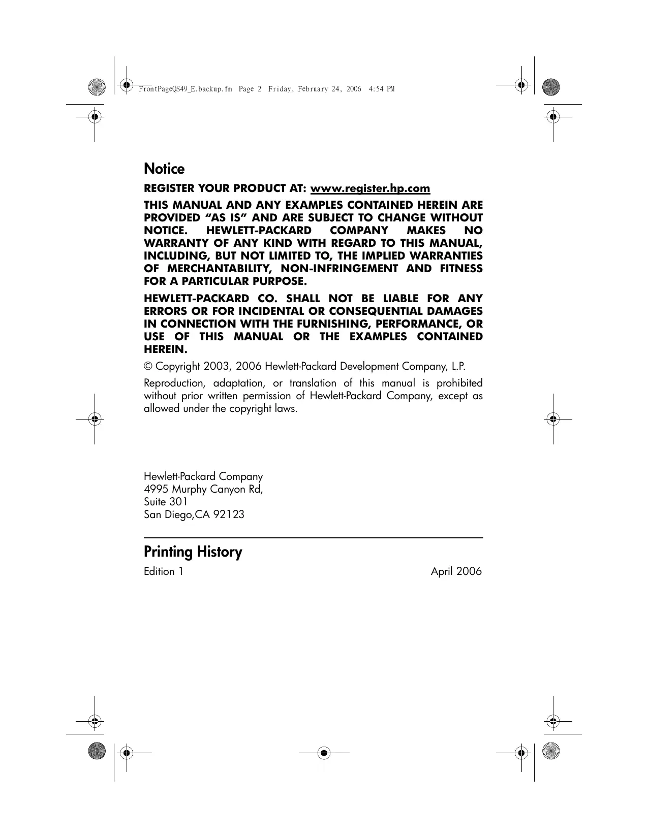
To install the backup battery
a. Make sure the calculator is OFF. Press down the holder. Push the plate to the shown direction and lift it.
text_image
Plate Holderb. Insert a new CR2032 lithium battery. Make sure its positive (+) side is facing up.
c. Replace the plate and push it to the original place.
After installing the batteries, press ON to turn the power on.
Warning: When the low battery icon is displayed, you need to replace the batteries as soon as possible. However, avoid removing the backup battery and main batteries at the same time to avoid data lost.
Turning the calculator on and off
The ON key is located at the lower left corner of the keyboard. Press it once to turn your calculator on. To turn the calculator off, press the right-shift key (first key in the second row from the bottom of the keyboard), followed by the ON key. Notice that the ON key has a OFF label printed in the upper right corner as a reminder of the OFF command.
Adjusting the display contrast
You can adjust the display contrast by holding the ON key while pressing the + or - keys.
The ON (hold) + key combination produces a darker display
The ON (hold) — key combination produces a lighter display
Contents of the calculator's display
Turn your calculator on once more. At the top of the display you will have two lines of information that describe the settings of the calculator. The first line shows the characters:
$$ \text { RAD XYZ HEX R = 'X' } $$
For details on the meaning of these symbols see Chapter 2 in the calculator's user's guide.
The second line shows the characters
$$ \left{ \begin{array}{l} \text {HOME} \end{array} \right. $$
indicating that the HOME directory is the current file directory in the calculator's memory.
At the bottom of the display you will find a number of labels, namely,
$$ \boxed {1 0 0} \boxed {9 4 7 3} \boxed {8 4 7 3} \boxed {6 2 0 1} \boxed {5 1 3 7} \boxed {4 8 7 3} $$
associated with the six soft menu keys, F1 through F6:
$$ \boxed {F 1} \boxed {F 2} \boxed {F 3} \boxed {F 4} \boxed {F 5} \boxed {F 6} $$
The six labels displayed in the lower part of the screen will change depending on which menu is displayed. But F_1 will always be associated with the first displayed label, F_2 with the second displayed label, and so on.
Menus
The six labels associated with the keys F1 through F6 form part of a menu of functions. Since the calculator has only six soft menu keys, it only display 6 labels at any point in time. However, a menu can have more than six entries. Each group of 6 entries is called a Menu page. To move to the next menu page (if available), press the NXT (NeXT menu) key. This key is the third key from the left in the third row of keys in the keyboard.
The TOOL menu
The soft menu keys for the default menu, known as the TOOL menu, are associated with operations related to manipulation of variables (see section on variables in this Chapter):
3011
FI
EDIT the contents of a variable (see Chapter 2 in this guide and Chapter 2 and Appendix L in the user's guide for more information on editing)
四:3.1
F2
VIEW the contents of a variable
ReCall the contents of a variable
F4 STOre the contents of a variable
FURGE F5 PURGE a variable
F6 CLEAR the display or stack
These six functions form the first page of the TOOL menu. This menu has actually eight entries arranged in two pages. The second page is available by pressing the NXT (NeXT menu) key. This key is the third key from the left in the third row of keys in the keyboard.
In this case, only the first two soft menu keys have commands associated with them. These commands are:
CASCMD: CAS CoMmanD, used to launch a command from the CAS (Computer Algebraic System) by selecting from a list
F2 HELP facility describing the commands available in the calculator
Pressing the NXT key will show the original TOOL menu. Another way to recover the TOOL menu is to press the TOOL key (third key from the left in the second row of keys from the top of the keyboard).
Setting time and date
See Chapter 1 in the calculator's user's guide to learn how to set time and date.
Introducing the calculator's keyboard
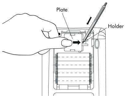
The figure on the next page shows a diagram of the calculator's keyboard with the numbering of its rows and columns. Each key has three, four, or five functions. The main key function corresponds to the most prominent label in the key. Also, the left-shift key, key (8,1), the right-shift key, key (9,1), and the ALPHA key, key (7,1), can be combined with some of the other keys to activate the alternative functions shown in the keyboard.
text_image
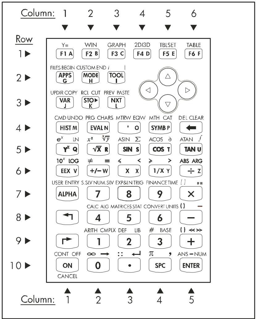
Column: 1 2 3 4 5 6 ▼ ▼ ▼ ▼ ▼ ▼ ▼ Row Y= WIN GRAPH 2D/3D TBLSET TABLE F1 A F2 B F3 C F4 D F5 E F6 F FILES BEGIN CUSTOM END i APPS MODE TOOL G H I UPDIR COPY RCL CUT PREV PASTE VAR STO NXT J K L CMD UNDO PRG CHARS MTRW EQW MTH CAT DEL CLEAR HIST M EVALN ' O SYMB P ← e^x LN x^2 √y ASIN Σ ACOS δ ATAN f Y^x Q √X R SIN S COS T TAN U 10^x LOG ≠ = < < > ABS ARG EEX V +/- W X X 1/X Y ÷ Z USER ENTRY S.SIV NUM.SIV EXP&IN TRIG FINANCETIME [ ] "" ALPHA 7 8 9 × CALC ALG MATRICES STAT CONVERT UNITS ( ) - ← 4 5 6 - ARITH CMPIX DEF LIB # BASE { } << >> → 1 2 3 + CONT OFF ∞ → :: ← π , ANS-NUM ON 0 • SPC ENTER CANCEL Column: 1 2 3 4 5For example, the SYMB key, key(4,4), has the following six functions associated with it:
SYMB
←
→
ALPHA
ALPHA
Main function, to activate the SYMBOLic menu
Left-shift function, to activate the MTH (Math) menu
Right-shift function, to activate the CATalog function
ALPHA function, to enter the upper-case letter P
ALPHA-Left-Shift function, to enter the lower-case letter p
Of the six functions associated with a key only the first four are shown in the keyboard itself. The figure in next page shows these four labels for the SYMB key. Notice that the color and the position of the labels in the key, namely, SYMB, MTH, CAT and P, indicate which is the main function (SYMB), and which of the other three functions is associated with the left-shift (MTH), right-shift (CAT), and ALPHA (P) keys.
text_image
MTH SYMB CAT PFor detailed information on the calculator keyboard operation refer to Appendix B in the calculator's user's guide.
Selecting calculator modes
This section assumes that you are now at least partially familiar with the use of choose and dialog boxes (if you are not, please refer to appendix A in the user's guide).
Press the MODE button (second key from the left on the second row of keys from the top) to show the following CALCULATOR MODES input form:

text_image
CALCULATOR MODES Operating Mode...Algebraic Number Format....Std _FM, Angle Measure.....Radians Coord System.....Rectangular ✓Beep _Key Click ✓Last Stack Choose calculator operating mode FLAGSCHOOS CAS DISP CANCEL OKPress the soft menu key to return to normal display. Examples of selecting different calculator modes are shown next.
Operating Mode
The calculator offers two operating modes: the Algebraic mode, and the Reverse Polish Notation (RPN) mode. The default mode is the Algebraic mode (as indicated in the figure above), however, users of earlier HP calculators may be more familiar with the RPN mode.
To select an operating mode, first open the CALCULATOR MODES input form by pressing the MODE button. The Operating Mode field will be highlighted. Select the Algebraic or RPN operating mode by either using the +/- key (second from left in the fifth row from the keyboard bottom), or pressing the F100E soft menu key. If using the latter approach, use up and down arrow keys, ▲ ▼ , to select the mode, and press the 4K soft menu key to complete the operation.
To illustrate the difference between these two operating modes we will calculate the following expression in both modes:
$$ \sqrt {\frac {3 . 0 \cdot \left(5 . 0 - \frac {1}{3 . 0 \cdot 3 . 0}\right)}{2 3 . 0 ^ {3}} + e ^ {2 . 5}} $$
To enter this expression in the calculator we will first use the equation writer, EQW. Please identify the following keys in the keyboard, besides the numeric keypad keys:

text_image
Diagram showing various mathematical and logical symbols with arrows and operators, including left, forward, SPC, and EQW.The equation writer is a display mode in which you can build mathematical expressions using explicit mathematical notation including fractions, derivatives, integrals, roots, etc. To use the equation writer for writing the expression shown above, use the following keystrokes:
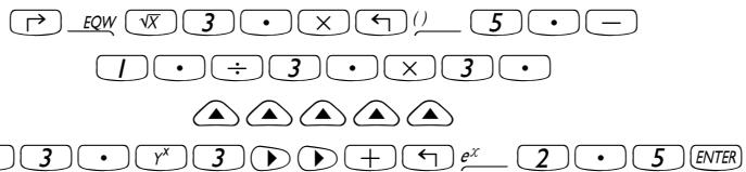
text_image
→ EQW √X 3 • × ← () 5 • — 1 • ÷ 3 • × 3 • ▲ ▲ ▲ ▲ ▲ 3 • γ^x 3 ▶ ▶ + ← e^x 2 • 5 ENTERAfter pressing ENTER the calculator displays the expression:
$$ \sqrt {(3 . * (5 . - 1 / (3 . * 3 .)) / 2 3 . ^ {\wedge} 3 + \text { EXP } (2 . 5))} $$
Pressing ENTER again will provide the following value (accept Approx mode on, if asked, by pressing OK):
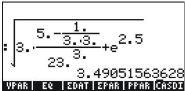
text_image
3.5 - 1/3.3.3.3.3.3.3.3.3.3.3.3.3.3.3.3.3.3.3.3.3.3.3.3.3.3.3.3.3.3.3.3.3.3.3.3.3.3.3.3.3.3.3.3.3.3.3.3.3.3.3 VPAR EQ EQAT EPAR PPAR CASDIYou could also type the expression directly into the display without using the equation writer, as follows:
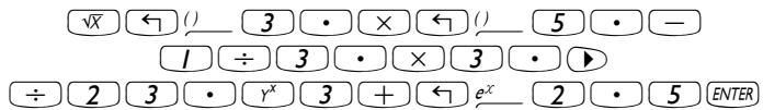
text_image
√X ← () 3 • × ← () 5 • — 1 ÷ 3 • × 3 • ▶ ÷ 2 3 • γ^x 3 + ← e^x 2 • 5 ENTERto obtain the same result.
Change the operating mode to RPN by first pressing the MODE button. Select the RPN operating mode by either using the +/- key, or pressing the 4000 soft menu key. Press the 401 soft menu key to complete the operation. The display, for the RPN mode looks as follows:

text_image
1: 2: 3: 1: EDIT VIEW RCL STOP PURGE CLEARNotice that the display shows several levels of output labeled, from bottom to top, as 1, 2, 3, etc. This is referred to as the stack of the calculator. The different levels are referred to as the stack levels, i.e., stack level 1, stack level 2, etc.
What RPN means is that, instead of writing an operation such as 3 + 2 by pressing
$$ 3 + 2 \text { ENTER } $$
we write the operands first, in the proper order, and then the operator, i.e.,
$$ \boxed {3} \boxed {\text { ENTER }} \boxed {2} \boxed {+} $$
As you enter the operands, they occupy different stack levels. Entering 3 ENTER puts the number 3 in stack level 1. Next, entering 2 pushes the 3 upwards to occupy stack level 2. Finally, by pressing +, we are telling the calculator to apply the operator, +, to the objects occupying levels 1 and 2. The result, 5, is then placed in level 1.
Let's try some other simple operations before trying the more complicated expression used earlier for the algebraic operating mode:
123/32
1 2 3 ENTER 3 2 ÷
4^2
4 ENTER 2 ^x
^3(27)
2 7 √x 3 → √y
Note the position of the y and x in the last two operations. The base in the exponential operation is y (stack level 2) while the exponent is x (stack level 1) before the key ^x is pressed. Similarly, in the cubic root operation, y (stack level 2) is the quantity under the root sign, and x (stack level 1) is the root.
Try the following exercise involving 3 factors: (5 + 3) × 2
5 ENTER 3 +
Calculates (5 +3) first.
2 x
Completes the calculation.
Let's try now the expression proposed earlier:
$$ \sqrt {\frac {3 \cdot \left(5 - \frac {1}{3 \cdot 3}\right)}{2 3 ^ {3}} + e ^ {2 . 5}} $$
3 ENTER Enter 3 in level 1
5 ENTER Enter 5 in level 1, 3 moves to level 2
3 ENTER Enter 3 in level 1, 5 moves to level 2, 3 to level 3
3 × Place 3 and multiply, 9 appears in level 1
1/(3×3), last value in lev. 1; 5 in level 2; 3 in level 3
5 - 1/(3×3), occupies level 1 now; 3 in level 2
3 × (5 - 1/(3×3)), occupies level 1 now.
2 3 ENTER Enter 23 in level 1, 14.66666 moves to level 2.
3 r^x Enter 3, calculate 23^3 into level 1. 14.666 in lev. 2.
(3 × (5-1/(3 × 3)))/23^3 into level 1
2 · 5 Enter 2.5 level 1
e^x e^2.5 , goes into level 1, level 2 shows previous value.
$$ (3 \times (5 - 1 / (3 \times 3))) / 2 3 ^ {3} + e ^ {2. 5} = 1 2. 1 8 3 6 9, \text { into lev. } 1. $$
$$ \sqrt {X} \quad \sqrt {\left((3 \times (5 - 1 / (3 \times 3))) / 2 3 ^ {3} + e ^ {2 . 5}\right)} = 3. 4 9 0 5 1 5 6, \text { into } 1. $$
To select between the ALG vs. RPN operating mode, you can also set/clear system flag 95 through the following keystroke sequence:
$$ \boxed {\text { MODE }} \quad \boxed {\text { 1 2 3 4 5 }} \quad \boxed {9} \quad \boxed {\downarrow} \quad \boxed {\downarrow} \quad \boxed {\downarrow} \quad \boxed {\downarrow} \quad \boxed {\text { Z A B I B }} \quad \boxed {\text { ENTER }} $$
Number Format and decimal dot or comma
Changing the number format allows you to customize the way real numbers are displayed by the calculator. You will find this feature extremely useful in operations with powers of tens or to limit the number of decimals in a result.
To select a number format, first open the CALCULATOR MODES input form by pressing the MODE button. Then, use the down arrow key, ▼, to select the option Number format. The default value is Std, or Standard format. In the standard format, the calculator will show floating-point numbers with no set decimal placement and with the maximum precision allowed by the calculator (12 significant digits)."To learn more about reals, see Chapter 2 in this guide. To illustrate this and other number formats try the following exercises:
Standard format
This mode is the most used mode as it shows numbers in the most familiar notation. Press the ☐ soft menu key, with the Number format set to Std, to return to the calculator display. Enter the number 123.4567890123456 (with 16 significant figures). Press the ENTER key. The number is rounded to the maximum 12 significant figures, and is displayed as follows:
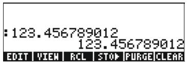
text_image
:123.456789012 123.456789012 EDIT VIEW RCL STOP PURGE CLEARFixed format with decimals
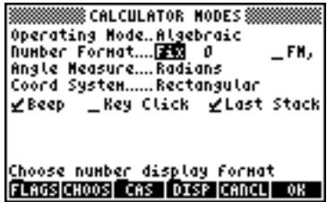
Press the MODE button. Next, use the down arrow key, ▼, to select the option Number format. Press the 📄️ soft menu key, and select the option Fixed with the arrow down key ▼.
text_image
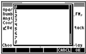
CALCULATOR MODES Operating Mode...Algebraic Number Format.....FM 0 _FM, Angle Measure....Radians Coord System.....Rectangular Beep _Key Click Last Stack Choose number display format FLAGS CHOOS CAS DISP CANCEL OKPress the right arrow key, ▶, to highlight the zero in front of the option Fix. Press the 📄️ soft menu key and, using the up and down arrow keys, ▲▼, select, say, 3 decimals.
text_image
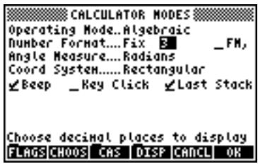
Oper Numb Angl Coor Be Choo 0 1 2 3 4 5 6 7 8 FM, tack lay CANCEL ORPress the ☐ soft menu key to complete the selection:
text_image
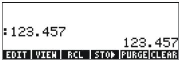
CALCULATOR MODES Operating Mode...Algebraic Number Format....Fix 3_ _FM, Angle Measure....Radians Coord System.....Rectangular ✓Beep _Key Click ✓Last Stack Choose decimal places to display FLAGS CHOOS CAS DISP CANCEL OKPress the ☐ soft menu key return to the calculator display. The number now is shown as:
text_image
:123.457 EDIT VIEW RCL STOP PURGE CLEAR 123.457Notice how the number is rounded, not truncated. Thus, the number 123.4567890123456, for this setting, is displayed as 123.457, and not as 123.456 because the digit after 6 is > 5.
Scientific format
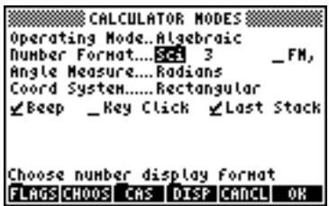
To set this format, start by pressing the MODE button. Next, use the down arrow key, ▼, to select the option Number format. Press the CHECK soft menu key, and select the option Scientific with the arrow down key ▼.
Keep the number 3 in front of the Sci. (This number can be changed in the same fashion that we changed the Fixed number of decimals in the example above).
text_image
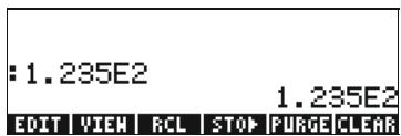
CALCULATOR MODES Operating Mode...Algebraic Number Format.....SCI 3 _FM, Angle Measure...Radians Coord System.....Rectangular ✓Beep _Key Click ✓Last Stack Choose number display format FLAGS CHOOS CAS DISP CANCEL OKPress the 03 soft menu key return to the calculator display. The number now is shown as:
text_image
:1.235E2 EDIT VIEW RCL STOP PURGE CLEAR 1.235E2This result, 1.23E2, is the calculator's version of powers-of-ten notation, i.e., 1.235 × 10^2 . In this, so-called, scientific notation, the number 3 in front of the Sci number format (shown earlier) represents the number of significant figures after the decimal point. Scientific notation always includes one integer figure as shown above. For this case, therefore, the number of significant figures is four.
Engineering format
The engineering format is very similar to the scientific format, except that the powers of ten are multiples of three. To set this format, start by pressing the MODE button. Next, use the down arrow key, ▼, to select the option Number format. Press the MODE soft menu key, and select the option Engineering with the arrow down key ▼. Keep the number 3 in front of the Eng. (This number can be changed in the same fashion that we changed the Fixed number of decimals in an earlier example).

text_image
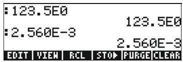
CALCULATOR MODES Operating Mode...Algebraic Number Format....Eng 3 Angle Measure....Radians Coord System.....Rectangular ✓ Beep _Key Click ✓ Last Stack Choose decimal places to display FLAGS CHOOS CAS DISP CANCEL OKPress the ☐ soft menu key return to the calculator display. The number now is shown as:

text_image
:123.5E0 EDIT VIEW RCL STOP PURGE CLEAR 123.5E0Because this number has three figures in the integer part, it is shown with four significative figures and a zero power of ten, while using the Engineering format. For example, the number 0.00256, will be shown as:
text_image
:123.5E0 :2.560E-3 EDIT VIEW RCL STOP PURGE CLEAR 123.5E0 2.560E-3Decimal comma vs. decimal point
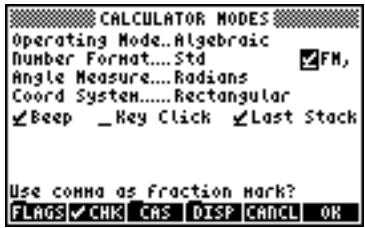
Decimal points in floating-point numbers can be replaced by commas, if the user is more familiar with such notation. To replace decimal points for commas, change the FM option in the CALCULATOR MODES input form to commas, as follows (Notice that we have changed the Number Format to Std):
Press the MODE button. Next, use the down arrow key, ▼, once, and the right arrow key, ▶, highlighting the option _FM,. To select commas, press the 2003 soft menu key. The input form will look as follows:
text_image
CALCULATOR MODES Operating Mode...Algebraic Number Format....Std Angle Measure....Radians Coord System.....Rectangular Beep _Key Click Last Stack Use comma as Fraction Mark? FLAGS CHK CAS DISP CANCEL OKPress the 0: soft menu key return to the calculator display. The number 123.4567890123456, entered earlier, now is shown as:
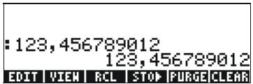
text_image
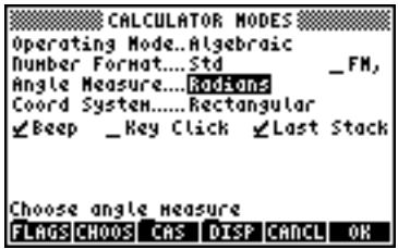
:123,456789012 123,456789012 EDIT VIEW RCL STOP PURGE CLEARAngle Measure
Trigonometric functions, for example, require arguments representing plane angles. The calculator provides three different Angle Measure modes for working with angles, namely:
- Degrees: There are 360 degrees (360°) in a complete circumference.
- Radians: There are 2 radians (2^) in a complete circumference.
- Grades: There are 400 grades (400 ^9 ) in a complete circumference.
The angle measure affects the trig functions like SIN, COS, TAN and associated functions.
To change the angle measure mode, use the following procedure:
- Press the MODE button. Next, use the down arrow key, ▼, twice. Select the Angle Measure mode by either using the +/- key (second from left in the fifth row from the keyboard bottom), or pressing the MODE soft menu key. If using the latter approach, use up and down arrow keys, ▲ ▼, to select the preferred mode, and press the Radians mode key to complete the operation. For example, in the following screen, the Radians mode is selected:
text_image
CALCULATOR MODES Operating Mode...Algebraic Number Format....Std __FM, Angle Measure.....Radians Coord System.....Rectangular ✓Beep __Key Click ✓Last Stack Choose angle measure FLAGSCHOOS CAS DISP CANCEL OKCoordinate System
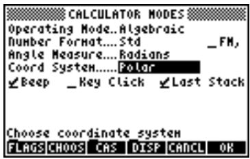
The coordinate system selection affects the way vectors and complex numbers are displayed and entered. To learn more about complex numbers and vectors, see Chapters 4 and 8, respectively, in this guide. There are three coordinate systems available in the calculator: Rectangular (RECT), Cylindrical (CYLIN), and Spherical (SPHERE). To change coordinate system:
- Press the MODE button. Next, use the down arrow key, ▼, three times. Select the Coord System mode by either using the +/- key (second from left in the fifth row from the keyboard bottom), or pressing the ◎◆◆◆ soft menu key. If using the latter approach, use up and down arrow keys, ▲▼, to select the preferred mode, and press the ◎◆◆◆
soft menu key to complete the operation. For example, in the following screen, the Polar coordinate mode is selected:
text_image
CALCULATOR MODES Operating Mode...Algebraic Number Format....Std Angle Measure....Radians Coord System.....Polar Beep _Key Click Last Stack Choose coordinate system FLAGS CHOOS CAS DISP CANCEL OKSelecting CAS settings
CAS stands for Computer Algebraic System. This is the mathematical core of the calculator where the symbolic mathematical operations and functions are programmed. The CAS offers a number of settings can be adjusted according to the type of operation of interest. To see the optional CAS settings use the following:
- Press the MODE button to activate the CALCULATOR MODES input form.
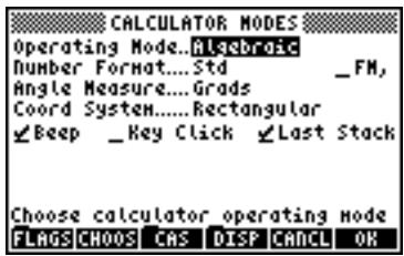
text_image
CALCULATOR MODES Operating Mode...Algebraic Number Format....Std _FM, Angle Measure.....Grads Coord System.....Rectangular ✓Beep _Key Click ✓Last Stack Choose calculator operating mode FLAGS CHOOS CAS DISP CANCEL OK- To change CAS settings press the ☐ soft menu key. The default values of the CAS setting are shown below:
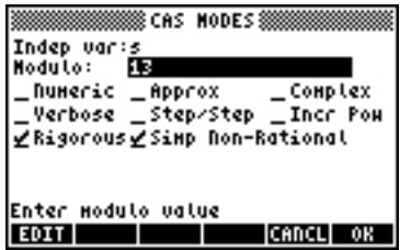
text_image
CAS MODES Indep var:s Modulo: 13 _Numeric _Approx _Complex _Verbose _Step/Step _Incr Pow ✓Rigorous✓Simp Non-Rational Enter modulo value EDIT CANCEL OK- To navigate through the many options in the CAS MODES input form, use the arrow keys: ◀ ▶ ▼ ▲.
- To select or deselect any of the settings shown above, select the underline before the option of interest, and toggle the 📄️ soft menu key until the right setting is achieved. When an option is selected, a check mark will be shown in the underline (e.g., the Rigorous and Simp
Non-Rational options above). Unselected options will show no check mark in the underline preceding the option of interest (e.g., the _Numeric, _Approx, _Complex, _Verbose, _Step/Step, _Incr Pow options above).
- After having selected and unselected all the options that you want in the CAS MODES input form, press the ☐ soft menu key. This will take you back to the CALCULATOR MODES input form. To return to normal calculator display at this point, press the ☐ soft menu key once more.
Explanation of CAS settings
- Indep var: The independent variable for CAS applications. Typically, VX = 'X'.
- Modulo: For operations in modular arithmetic this variable holds the modulus or modulo of the arithmetic ring (see Chapter 5 in the calculator's user's guide).
- Numeric: If set, the calculator produces a numeric, or floating-point result, in calculations. Note that constants will always be evaluated numerically.
- Approx: If set, Approximate mode uses numerical results in calculations. If unchecked, the CAS is in Exact mode, which produces symbolic results in algebraic calculations.
- Complex: If set, complex number operations are active. If unchecked the CAS is in Real mode, i.e., real number calculations are the default. See Chapter 4 for operations with complex numbers.
- Verbose: If set, provides detailed information in certain CAS operations.
- Step/Step: If set, provides step-by-step results for certain CAS operations. Useful to see intermediate steps in summations, derivatives, integrals, polynomial operations (e.g., synthetic division), and matrix operations.
- Incr Pow: Increasing Power, means that, if set, polynomial terms are shown in increasing order of the powers of the independent variable.
- Rigorous: If set, calculator does not simplify the absolute value function |X| to X .
- Simp Non-Rational: If set, the calculator will try to simplify non-rational expressions as much as possible.
Selecting Display modes
The calculator display can be customized to your preference by selecting different display modes. To see the optional display settings use the following:
- First, press the MODE button to activate the CALCULATOR MODES input form. Within the CALCULATOR MODES input form, press the soft menu key to display the DISPLAY MODES input form.

text_image
DISPLAY MODES Font: Ft8_0: SYSTEM 8 Edit: Shall _Full Page _Indent Stack:_Small Textbook EEM: Shall _Small Stack Disp Header:2 _Clock _Analog Edit using shall font? EDIT ✓CHK CANCEL OK- To navigate through the many options in the DISPLAY MODES input form, use the arrow keys: ◀▶▼▲.
- To select or deselect any of the settings shown above, that require a check mark, select the underline before the option of interest, and toggle the 2003 soft menu key until the right setting is achieved. When an option is selected, a check mark will be shown in the underline (e.g., the Textbook option in the Stack: line above).
Unselected options will show no check mark in the underline preceding the option of interest (e.g., the _Small, _Full page, and _Indent options in the Edit: line above).
- To select the Font for the display, highlight the field in front of the Font: option in the DISPLAY MODES input form, and use the CHODS soft menu.
- After having selected and unselected all the options that you want in the DISPLAY MODES input form, press the ☐ soft menu key. This will take you back to the CALCULATOR MODES input form. To return to normal calculator display at this point, press the ☐ soft menu key once more.
Selecting the display font
First, press the MODE button to activate the CALCULATOR MODES input form. Within the CALCULATOR MODES input form, press the 000 soft menu key to display the DISPLAY MODES input form. The Font: field is highlighted, and the option Ft8_0: system 8 is selected. This is the default value of the display font. Pressing the 000 soft menu key will provide a list of available system fonts, as shown below:
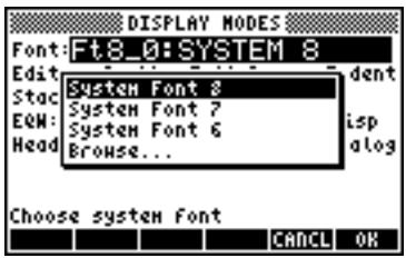
text_image
DISPLAY MODES Font: Ft8_0:SYSTEM 8 Edit Stac EOM: Head System Font 8 System Font 7 System Font 6 Browse... Choose system font CANCEL OKThe options available are three standard System Fonts (sizes 8, 7, and 6) and a Browse.. option. The latter will let you browse the calculator memory for additional fonts that you may have created or downloaded into the calculator.
Practice changing the display fonts to sizes 7 and 6. Press the OK soft menu key to effect the selection. When done with a font selection, press the ☐ soft menu key to go back to the CALCULATOR MODES input form. To return to normal calculator display at this point, press the ☐ soft menu key once more and see how the stack display change to accommodate the different font.
Selecting properties of the line editor
First, press the MODE button to activate the CALCULATOR MODES input form. Within the CALCULATOR MODES input form, press the 100mm soft menu key to display the DISPLAY MODES input form. Press the down arrow key, ▼, once, to get to the Edit line. This line shows three properties that can be modified. When these properties are selected (checked) the following effects are activated:
_Small Changes font size to small
_Full page Allows to place the cursor after the end of the line
_Indent Auto indent cursor when entering a carriage return
Instructions on the use of the line editor are presented in Chapter 2 in the user's guide.
Selecting properties of the Stack
First, press the MODE button to activate the CALCULATOR MODES input form. Within the CALCULATOR MODES input form, press the soft menu key (F4) to display the DISPLAY MODES input form. Press the down arrow key, ▼, twice, to get to the Stack line. This line shows two properties that can be modified. When these properties are selected (checked) the following effects are activated:
_Small
Changes font size to small. This maximizes the amount of information displayed on the screen. Note, this selection overrides the font selection for the stack display.
_Textbook
Displays mathematical expressions in graphical mathematical notation
To illustrate these settings, either in algebraic or RPN mode, use the equation writer to type the following definite integral:
→ EQW → ∫ 0 ▶ ← ∞ ▶ ← e^x +/- X ▶ (X ENTER)
In Algebraic mode, the following screen shows the result of these keystrokes with neither _Small nor _Textbook are selected:
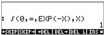
text_image
: J(0,∞,EXP(-X),X) +SKIP|SKIP+ +DEL | DEL+ DEL L INS = 1With the _Small option selected only, the display looks as shown below:
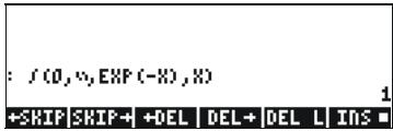
text_image
: f(0, %, EXP(-X), X) +SKIP | SKIP + | +DEL | DEL + | DEL | INS = 1With the _Textbook option selected (default value), regardless of whether the _Small option is selected or not, the display shows the following result:
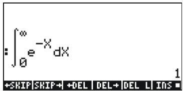
text_image
∫∞e−Xdx +SKIP|SHIP+ +DEL | DEL+ |DEL L INS • 1Selecting properties of the equation writer (EQW)
First, press the MODE button to activate the CALCULATOR MODES input form. Within the CALCULATOR MODES input form, press the 1000 soft menu key to display the DISPLAY MODES input form. Press the down arrow key, ▼, three times, to get to the EQW (Equation Writer) line. This line shows two properties that can be modified. When these properties are selected (checked) the following effects are activated:
_Small Changes font size to small while using the equation editor
_Small Stack Disp Shows small font in the stack after using the equation editor
Detailed instructions on the use of the equation editor (EQW) are presented elsewhere in this manual.
For the example of the integral _0^ e^-XdX , presented above, selecting the _Small Stack Disp in the EQW line of the DISPLAY MODES input form produces the following display:

text_image
: ∫₀^∞ e⁻⁸ dX +SKIP | SHIP + | DEL | DEL + | DEL L | INS = 1References
Additional references on the subjects covered in this Chapter can be found in Chapter 1 and Appendix C of the calculator's user's guide.
Chapter 2
Introducing the calculator
In this chapter we present a number of basic operations of the calculator including the use of the Equation Writer and the manipulation of data objects in the calculator. Study the examples in this chapter to get a good grasp of the capabilities of the calculator for future applications.
Calculator objects
Some of the most commonly used objects are: reals (real numbers, written with a decimal point, e.g., -0.0023, 3.56), integers (integer numbers, written without a decimal point, e.g., 1232, -123212123), complex numbers (written as an ordered pair, e.g., (3,-2)), lists, etc. Calculator objects are described in Chapters 2 and 24 in the calculator's user guide.
Editing expressions in the stack
In this section we present examples of expression editing directly into the calculator display or stack.
Creating arithmetic expressions
For this example, we select the Algebraic operating mode and select a Fix format with 3 decimals for the display. We are going to enter the arithmetic expression:
$$ 5. 0 \cdot \frac {1 . 0 + \frac {1 . 0}{7 . 5}}{\sqrt {3 . 0} - 2 . 0 ^ {3}} $$
To enter this expression use the following keystrokes:
5 • × ← () 1 • + 1 ÷ 7 • 5 ▶ ÷
←() √X 3 • - 2 • γx 3
The resulting expression is: 5^*(1+1/7.5)/(3-2^3) .
Press ENTER to get the expression in the display as follows:
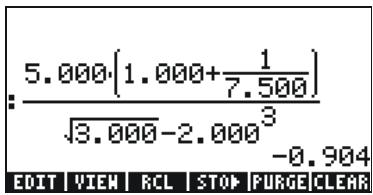
text_image
5.000·(1.000+1/7.500) √3.000-2.000³ -0.904 EDIT VIEW RCL STOP PURGE CLEARNotice that, if your CAS is set to EXACT (see Appendix C in user's guide) and you enter your expression using integer numbers for integer values, the result is a symbolic quantity, e.g.,

text_image
5 × ← () 1 + 1 ÷ 7 • 5 ▶ ÷
Before producing a result, you will be asked to change to Approximate mode. Accept the change to get the following result (shown in Fix decimal mode with three decimal places – see Chapter 1):
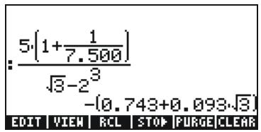
text_image
: 5·(1+1/7.500)/√3-2^3 -(0.743+0.093√3) EDIT VIEW RCL STOP PURGE CLEARIn this case, when the expression is entered directly into the stack, as soon as you press ENTER, the calculator will attempt to calculate a value for the expression. If the expression is preceded by a tickmark, however, the calculator will reproduce the expression as entered. For example:

text_image
1 5 × ← () 1 + 1 ÷ 7 • 5 ▶ ÷
The result will be shown as follows:

text_image
: \frac{(7.5)}{\sqrt{3}-2^3} \quad \frac{5\cdot\left(1+\frac{1}{7.5}\right)}{\sqrt{3}-2^3} EDIT VIEW RCL STOP PURGE CLEARTo evaluate the expression we can use the EVAL function, as follows:

If the CAS is set to Exact, you will be asked to approve changing the CAS setting to Approx. Once this is done, you will get the same result as before.
An alternative way to evaluate the expression entered earlier between quotes is by using the option NUM.
We will now enter the expression used above when the calculator is set to the RPN operating mode. We also set the CAS to Exact, the display to Textbook, and the number format to Standard. The keystrokes to enter the expression between quotes are the same used earlier, i.e.,

text_image
1 5 × ← () 1 + 1 ÷ 7 • 5 ▶ ÷
Resulting in the output
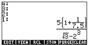
text_image
4: 3: 2: 1: 5·(1+1/7.5)/√3-2³ EDIT VIEW RCL STOP PURGE CLEARPress ENTER once more to keep two copies of the expression available in the stack for evaluation. We first evaluate the expression by pressing:

This expression is semi-symbolic in the sense that there are floating-point components to the result, as well as a 3 . Next, we switch stack locations [using ▶] and evaluate using function NUM, i.e., ▶→→→NUM.
This latter result is purely numerical, so that the two results in the stack, although representing the same expression, seem different. To verify that they are not, we subtract the two values and evaluate this difference using function EVAL: - EVAL. The result is zero (0.).
For additional information on editing arithmetic expressions in the display or stack, see Chapter 2 in the calculator's user's guide.
Creating algebraic expressions
Algebraic expressions include not only numbers, but also variable names. As an example, we will enter the following algebraic expression:
$$ \frac {2 L \sqrt {1 + \frac {x}{R}}}{R + y} + 2 \frac {L}{b} $$
We set the calculator operating mode to Algebraic, the CAS to Exact, and the display to Textbook. To enter this algebraic expression we use the following keystrokes:
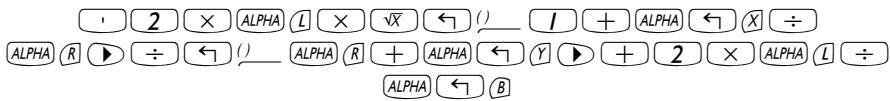
text_image
1 2 × ALPHA L × √X ← ( ) 1 + ALPHA ← X ÷ ALPHA R ▶ ÷ ← ( ) ALPHA R + ALPHA ← Y ▶ + 2 × ALPHA L ÷ ALPHA ← BPress ENTER to get the following result:
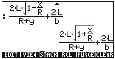
text_image
: \frac{2\cdot L \cdot \sqrt{1 + \frac{X}{R}}}{R + y} + \frac{2\cdot L}{b}\n\frac{2\cdot L \cdot \sqrt{1 + \frac{X}{R}}}{R + y} + \frac{2\cdot L}{b}\nEDIT VIEW STACK RCL PURGE CLEAREntering this expression when the calculator is set in the RPN mode is exactly the same as this Algebraic mode exercise.
For additional information on editing algebraic expressions in the calculator's display or stack see Chapter 2 in the calculator's user's guide.
Using the Equation Writer (EQW) to create expressions
The equation writer is an extremely powerful tool that not only let you enter or see an equation, but also allows you to modify and work/apply functions on all or part of the equation.
The Equation Writer is launched by pressing the keystroke combination _EQW (the third key in the fourth row from the top in the keyboard). The resulting screen is the following. Press NXT to see the second menu page:

text_image
EDIT CURS BIG EVAL FACTO SIMP
text_image
CHDS HELPThe six soft menu keys for the Equation Writer activate functions EDIT, CURS, BIG, EVAL, FACTOR, SIMPLIFY, CMDS, and HELP. Detailed information on these functions is provided in Chapter 3 of the calculator's user's guide.
Creating arithmetic expressions
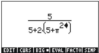
Entering arithmetic expressions in the Equation Writer is very similar to entering an arithmetic expression in the stack enclosed in quotes. The main difference is that in the Equation Writer the expressions produced are written in "textbook" style instead of a line-entry style. For example, try the following keystrokes in the Equation Writer screen: 5 ÷ 5 + 2
The result is the expression:
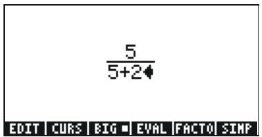
text_image
5 5+2♦ EDIT CURS BIG ■ EVAL FACTO SIMPThe cursor is shown as a left-facing key. The cursor indicates the current edition location. For example, for the cursor in the location indicated above, type now:

The edited expression looks as follows:
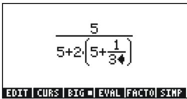
text_image
5 5+2·(5+1/3φ) EDIT CURS BIG ■ EVAL FACTO SIMPSuppose that you want to replace the quantity between parentheses in the denominator (i.e., 5+1/3 ) with (5+^2/2) . First, we use the delete key (☐) delete the current 1/3 expression, and then we replace that fraction with ^2/2 , as follows:

When hit this point the screen looks as follows:
text_image
5 5+2(5+π²♦) EDIT CURS BIG ■ EVAL FACTO SIMPIn order to insert the denominator 2 in the expression, we need to highlight the entire ^2 expression. We do this by pressing the right arrow key (▶) once. At that point, we enter the following keystrokes:

The expression now looks as follows:
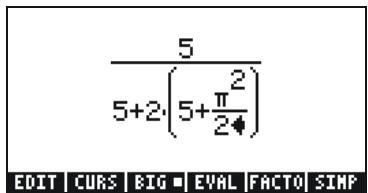
text_image
5 5+2·(5+π/2) EDIT | CURS | BIG ■ EVAL | FACTO | SIMPSuppose that now you want to add the fraction 1/3 to this entire expression, i.e., you want to enter the expression:
$$ \frac {5}{5 + 2 \cdot \left(5 + \frac {\pi^ {2}}{2}\right)} + \frac {1}{3} $$
First, we need to highlight the entire first term by using either the right arrow (▶) or the upper arrow (▲) keys, repeatedly, until the entire expression is highlighted, i.e., seven times, producing:
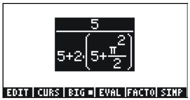
text_image
5 5+2·(5+π²/2) EDIT | CURS | BIG ■ EVAL | FACTO | SIMPNOTE: Alternatively, from the original position of the cursor (to the right of the 2 in the denominator of ^2 / 2 ), we can use the keystroke combination ▲, interpreted as ( ▲).
Once the expression is highlighted as shown above, type + I ÷ 3 to add the fraction 1/3. Resulting in:
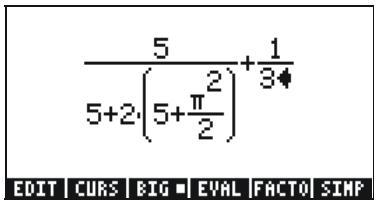
text_image
5/5+2·(5+π/2)²+1/3♦ EDIT CURS BIG EVAL FACTO SIMPCreating algebraic expressions
An algebraic expression is very similar to an arithmetic expression, except that English and Greek letters may be included. The process of creating an algebraic expression, therefore, follows the same idea as that of creating an arithmetic expression, except that use of the alphabetic keyboard is included.
To illustrate the use of the Equation Writer to enter an algebraic equation we will use the following example. Suppose that we want to enter the expression:
$$ \frac {2}{\sqrt {3}} \lambda + e ^ {- \mu} \cdot L N \left(\frac {x + 2 \mu \cdot \Delta y}{\theta^ {1 / 3}}\right) $$
Use the following keystrokes:

text_image
2 ÷ √X 3 ▶ ▶ × ALPHA → (N) + ← e^x +/− ALPHA → (M) ▶ ▶ × → _ LN ALPHA ← (X) + 2 × ALPHA → (M) × ALPHA → (C)This results in the output:
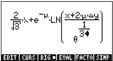
text_image
2/√3·λ+e^−μ·LN(x+2μ·Δy)/1/3φ θ EDIT CURS BIG EVAL FACTO SIMPIn this example we used several lower-case English letters, e.g., x (ALPHA ← X), several Greek letters, e.g., λ(ALPHA → N), and even a combination of Greek and English letters, namely, Δy (ALPHA → C ALPHA ← Y). Keep in mind that to enter a lower-case English letter, you need to use the combination: ALPHA ← followed by the letter you want to enter. Also, you can always copy special characters by using the CHARS menu (→ CHARS) if you don't want to memorize the keystroke combination that produces it. A listing of commonly used ALPHA → keystroke combinations is listed in Appendix D of the user's guide.
For additional information on editing, evaluating, factoring, and simplifying algebraic expressions see Chapter 2 of the calculator's user's guide.
Organizing data in the calculator
You can organize data in your calculator by storing variables in a directory tree. The basis of the calculator's directory tree is the HOME directory described next.
The HOME directory
To get to the HOME directory, press the UPDIR function ( UPDIR ) -- repeat as needed - until the {HOME} spec is shown in the second line of the display header. Alternatively, use (hold) UPDIR . For this example, the HOME directory contains nothing but the CASDIR. Pressing VAR will show the variables in the soft menu keys:

text_image
CASDISubdirectories
To store your data in a well organized directory tree you may want to create subdirectories under the HOME directory, and more subdirectories within subdirectories, in a hierarchy of directories similar to folders in modern computers. The subdirectories will be given names that may reflect the contents of each subdirectory, or any arbitrary name that you can think off. For details on manipulation of directories see Chapter 2 in the calculator's user's guide.
Variables
Variables are similar to files on a computer hard drive. One variable can store one object (numerical values, algebraic expressions, lists, vectors, matrices, programs, etc). Variables are referred to by their names, which can be any combination of alphabetic and numerical characters, starting with a letter (either English or Greek). Some non-alphabetic characters, such as the arrow ( ) can be used in a variable name, if combined with an alphabetical character. Thus, ' A' is a valid variable name, but ' ' is not. Valid examples of variable names are: 'A', 'B', 'a', 'b', ' ', ' ', 'A1', 'AB12', ' A12', 'Vel', 'Z0', 'z1', etc.
A variable can not have the same name as a function of the calculator. Some of the reserved calculator variable names are the following: ALRMDAT, CST, EQ, EXPR, IERR, IOPAR, MAXR, MINR, PICT, PPAR, PRTPAR, VPAR, ZPAR, der_, e, i, n1,n2, ..., s1, s2, ..., ΣDAT, ΣPAR, π, ∞.
Variables can be organized into sub-directories (see Chapter 2 in the calculator's user's guide).
Typing variable names
To name variables, you will have to type strings of letters at once, which may or may not be combined with numbers. To type strings of characters you can lock the alphabetic keyboard as follows:
ALPHA ALPHA locks the alphabetic keyboard in upper case. When locked in this fashion, pressing the before a letter key produces a lower case letter, while pressing the key before a letter key produces a special character. If the alphabetic keyboard is already locked in upper case, to lock it in lower case, type, ALPHA.
ALPHA ALPHA ← ALPHA locks the alphabetic keyboard in lower case. When locked in this fashion, pressing the ← before a letter key produces an upper case letter. To unlock lower case, press ← ALPHA.
To unlock the upper-case locked keyboard, press ALPHA.
Try the following exercises:
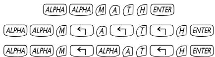
text_image
ALPHA ALPHA M A T H ENTER ALPHA ALPHA M ← A ← T ← H ENTER ALPHA ALPHA M ← ALPHA A T ← H ENTERThe calculator display will show the following (left-hand side is Algebraic mode, right-hand side is RPN mode):
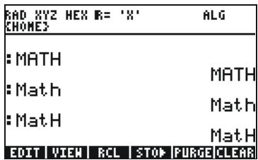
text_image
RAD XYZ HEX R= 'X' ALG CHONE3 :MATH :Math :MatH MATH Math MatH EDIT VIEW RCL STOP PURGE CLEAR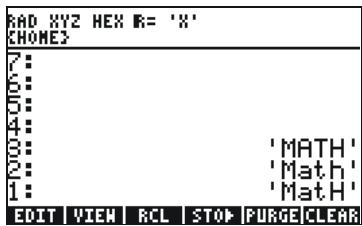
text_image
RAD XYZ HEX R= 'X' CHOME3 7: 6: 0: 4: 3: 2: 1: 'MATH' 'Math' 'Math' EDIT VIEW RCL STOP PURGE CLEARCreating variables
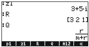
The simplest way to create a variable is by using the STO. The following examples are used to store the variables listed in the following table (Press VAR if needed to see variables menu):
| Name | Contents | Type |
| -0.25 | real | |
| A12 | 3 × 10^5 | real |
| Q | ‘r/(m+r)’ | algebraic |
| R | [3,2,1] | vector |
| z1 | 3+5i | complex |
| p1 | r' ^* r^2' | program |
Algebraic mode
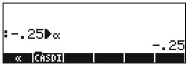
To store the value of -0.25 into variable : 0 · 2 5 +/- STOP ALPHA → A. AT this point, the screen will look as follows:

text_image
-0.25▶α CASDIPress ENTER to create the variable. The variable is now shown in the soft menu key labels when you press VAR :
text_image
:-.25▶α - .25 × CASDIThe following are the keystrokes for entering the remaining variables:
A12: 3 EEX 5 STO▶ ALPHA A 1 2 ENTER
Q: ALPHA ← R ÷ ← ()
ALPHA ← M + ALPHA ← R ► ► STO▶ ALPHA Q ENTER
R: ← [ ] 3 → , 2 → , 1 ▶ STO▶ ALPHA R ENTER
z1: 3 + 5 × ← i STOP ALPHA ← Z I ENTER (Accept change to Complex mode if asked).
p1: << >> ↗ → ALPHA ← R , ← π ×
ALPHA ← R γ ^x 2 ► ► STO► ALPHA ← P I ENTER .
The screen, at this point, will look as follows:
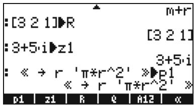
You will see six of the seven variables listed at the bottom of the screen: p1, z1, R, Q, A12, a.
RPN mode
(Use MODE +/- to change to RPN mode). Use the following keystrokes to store the value of -0.25 into variable α: · 2 5 +/- ENTER ALPHA → A ENTER. At this point, the screen will look as follows:
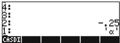
text_image
4: 3: 2: 1: CASDI -,25 αWith -0.25 on the level 2 of the stack and 'α' on the level 1 of the stack, you can use the STOP key to create the variable. The variable is now shown in the soft menu key labels when you press VAR :

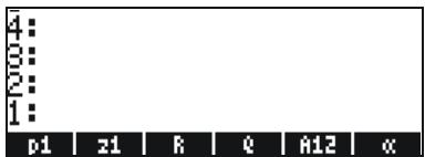
text_image
4: 1: 3: 2: 1: α CASDITo enter the value 3 × 10^5 into A12, we can use a shorter version of the procedure: 3 EEX 5 , ALPHA (A) 1 2 ENTER STO
Here is a way to enter the contents of Q:
Q: ALPHA ← R ÷ ← ()
ALPHA ← M + ALPHA ← R ► ► ↓ ALPHA Q ENTER STO
To enter the value of R, we can use an even shorter version of the procedure:
R: ←[] 3 SPC 2 SPC 1 ▶ ALPHA R STO
Notice that to separate the elements of a vector in RPN mode we can use the space key (SPC), rather than the comma (→—) used above in Algebraic mode.
z1: 1 3 + 5 × ← i ALPHA ← Z I STO
p1: , ×
ALPHA ← R Y ^x 2 ▶ ▶ ▶ ↓ ALPHA ← P I ▶ ENTER STO
The screen, at this point, will look as follows:
text_image
4: 13: 20: 1: p1 z1 R Q A12 cYou will see six of the seven variables listed at the bottom of the screen: p1, z1, R, Q, A12, .
Checking variables contents
The simplest way to check a variable content is by pressing the soft menu key label for the variable. For example, for the variables listed above, press the following keys to see the contents of the variables:
Algebraic mode
Type these keystrokes: VAR ENTER ENTER ENTER. At this point, the screen looks as follows:
In RPN mode, you only need to press the corresponding soft menu key label to get the contents of a numerical or algebraic variable. For the case under consideration, we can try peeking into the variables z1, R, Q, A12, , created above, as follows: VAR
At this point, the screen looks like this:
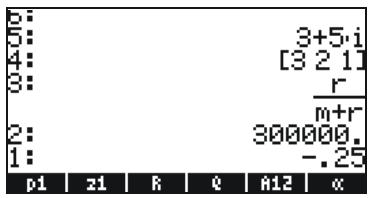
text_image
5: 5: 4: 3: 2: 1: p1 z1 R Q A12 C 3+5·i [3 2 1] r m+r 300000. -.25Using the right-shift key followed by soft menu key labels
In Algebraic mode, you can display the content of a variable by pressing VAR → and then the corresponding soft menu key. Try the following examples:

text_image
VAR → 91 → 44 → 32 → X → 9K-NOTE: In RPN mode, you don't need to press ↗ (just VAR and then the corresponding soft menu key.)
This produces the following screen (Algebraic mode in the left, RPN in the right)
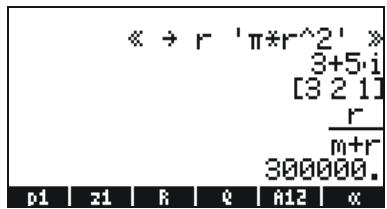
text_image
« → r 'π*r^2' » 3+5·i [3 2 1] r m+r 300000. p1 z1 R Q A12 α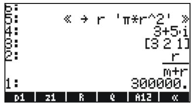
text_image
5: 6: « → r 'π*r^2' » 4: 3: [3 2 1] 2: r m+r 1: 300000. p1 z1 R Q A12Notice that this time the contents of program p1 are listed in the screen. To see the remaining variables in this directory, press NXT.
Listing the contents of all variables in the screen
Use the keystroke combination ↗▼ to list the contents of all variables in the screen. For example:

text_image
p1: « → r 'π*r^2.' z1: (3.,5.) R: [3.,2.,1.] Q: r/(m+r) A12: 300000. α: -.25 p1 z1 R Q A12 αPress ON to return to normal calculator display.
Deleting variables
The simplest way of deleting variables is by using function PURGE. This function can be accessed directly by using the TOOLS menu (TOOL), or by using the FILES menu ← FILES .
Using function PURGE in the stack in Algebraic mode
Our variable list contains variables p1, z1, Q, R, and . We will use command PURGE to delete variable p1. Press TOOL ☐ ☐ ☐ ☐ ☐ ☐ ☐ ☐ ☐ ☐ ☐ ☐ ☐ ☐ ☐ ☐ ☐ ☐ ☐ ☐ ☐ ☐ ☐ ☐ ☐ ☐ ☐ ☐ ☐ ☐ ☐ ☐ ☐ ☐ ☐ ☐ ☐ ☐ ☐ ☐ ☐ ☐ ☐ ☐ ☐ ☐ ☐ ☐ ☐ ☐ ☑ ☐ ☐ ☐ ☐ ☐ ☐ ☐ ☐ ☐ ☐ ☐ ☐ ☐ ☐ ☐ ☐ ☐ ☐ ☐ ☐ ☐ ☐ ☐ ☐ ☐ ☐ ☐ ☐ ☐ ☐ ☐ ☐ ☐ ☐ ☐ ☐ ☐ ☐ ☐ ☐ ☐ ☐ ☐ ☐ ☐
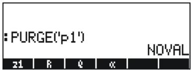
text_image
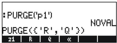
: PURGE('p1') NOVAL z1 R Q CYou can use the PURGE command to erase more than one variable by placing their names in a list in the argument of PURGE. For example, if now we wanted to purge variables R and Q, simultaneously, we can try the following exercise. Press :

text_image
TOOL ← { } VAR → , VARAt this point, the screen will show the following command ready to be executed:
text_image
:PURGE('p1') PURGE(('R', 'Q')) NOVAL z1 R Q <To finish deleting the variables, press ENTER. The screen will now show the remaining variables:

text_image
:PURGE('p1') :PURGE(('R' 'Q')) NOVAL NOVAL z1 xUsing function PURGE in the stack in RPN mode
Assuming that our variable list contains the variables p1, z1, Q, R, and . We will use command PURGE to delete variable p1. Press ☐ ENTER TOOL ☐ ☐ ☐ ☐ ☐ ☐ ☐ ☐ ☐ ☐ ☐ ☐ ☐ ☐ ☐ ☐ ☐ ☐ ☐ ☐ ☐ ☐ ☐ ☐ ☐ ☐ ☐ ☐ ☐ ☐ ☐ ☐ ☐ ☐ ☐ ☐ ☐ ☐ ☐ ☐ ☐ ☐ ☐ ☐ ☐ ☐ ☐ ☐ ☐ ☐ ☑ ☐ ☐ ☐ ☐ ☐ ☐ ☐ ☐ ☐ ☐ ☐ ☐ ☐ ☐ ☐ ☐ ☐ ☐ ☐ ☐ ☐ ☐ ☐ ☐ ☐ ☐ ☐ ☐ ☐ ☐ ☐ ☐ ☐ ☐ ☐ ☐ ☐ ☐ ☐ ☐ ☐ ☐ ☐ ☐

text_image
4: 3: 2: 1: EDIT VIEW STACK RCL PURGE CLEARTo delete two variables simultaneously, say variables R and Q, first create a list (in RPN mode, the elements of the list need not be separated by commas as in Algebraic mode):

Then, press TOOL FURFE use to purge the variables.
Additional information on variable manipulation is available in Chapter 2 of the calculator's user's guide.
UNDO and CMD functions
Functions UNDO and CMD are useful for recovering recent commands, or to revert an operation if a mistake was made. These functions are associated with the HIST key: UNDO results from the keystroke sequence UNDO, while CMD results from the keystroke sequence CMD.
CHOOSE boxes vs. Soft MENU
In some of the exercises presented in this chapter we have seen menu lists of commands displayed in the screen. These menu lists are referred to as CHOOSE boxes. Herein we indicate the way to change from CHOOSE boxes to Soft MENUs, and vice versa, through an exercise.
Although not applied to a specific example, the present exercise shows the two options for menus in the calculator (CHOOSE boxes and soft MENUs). In this exercise, we use the ORDER command to reorder variables in a directory. The steps are shown for Algebraic mode.

Show PROG menu list and select MEMORY

text_image
RAD CHON PROG MENU 1.STACK.. 2.MEMORY.. 3.BRANCH.. 4.TEST.. 5.TYPE.. 6.LIST.. 7.GROE.. 8.PICT.. CANCEL OK
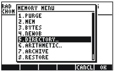
Show the MEMORY menu list and select DIRECTORY
text_image
RAD CHON MEMORY MENU 1.PURGE 2.MEM 3.BYTES 4.NEWOB 5. DIRECTORY.. 6.ARITHMETIC.. 7.ARCHIVE 8.RESTORE
Show the DIRECTORY menu list and select ORDER

text_image
RAD CHOM DIRECTORY MENU 3.STO 4.PATH 5.CRDIR 6.PGDIR 7.VARS 8.TVARS 9.ORDER 10.MEMORY.. CANCEL OK00:30
activate the ORDER command
There is an alternative way to access these menus as soft MENU keys, by setting system flag 117. (For information on Flags see Chapters 2 and 24 in the calculator's user's guide). To set this flag try the following:
MODE
The screen shows flag 117 not set (CHOOSE boxes), as shown here:
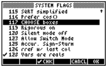
text_image
SYSTEM FLAGS 115 SORT simplified 116 Prefer cos() 117 CHOOSE boxes 119 Rigorous on 120 Silent mode off 123 Allow Switch Mode 125 Accur. Sign-Sturm 126 rref w/ last col ✓ 128 Vars are reals ✓ CHK Cancel OKPress the 📄️ soft menu key to set flag 117 to soft MENU. The screen will reflect that change:
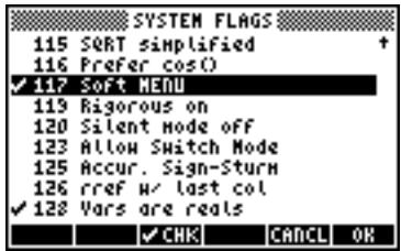
text_image
SYSTEM FLAGS 115 SORT simplified 116 Prefer cos() ✓ 117 SORT MENU 119 Rigorous on 120 Silent mode off 123 Allow Switch Mode 125 Accur. Sign-Sturm 126 rref w/ last col ✓ 128 Vars are reals ✓ CHK Cancel OKPress ☐ twice to return to normal calculator display.
Now, we'll try to find the ORDER command using similar keystrokes to those used above, i.e., we start with PRG. Notice that instead of a menu list, we get soft menu labels with the different options in the PROG menu, i.e.,

text_image
STACK MEN BRCH TEST TYPE LISTPress F2 to select the MEMORY soft menu (☐13:☐). The display now shows:

text_image
PURGE MEN BYTES NEOE DIR ARITHPress F5 to select the DIRECTORY soft menu (OK)

text_image
PURGE | RCL | STO | PATH | CRDIR | PGDIRThe ORDER command is not shown in this screen. To find it we use the NXT key to find it:

text_image
VARS TVARS ORDER MEMTo activate the ORDER command we press the F3 (ORDER) soft menu key.
NOTE: most of the examples in this user manual assume that the current setting of flag 117 is its default setting (that is, not set). If you have set the flag but want to strictly follow the examples in this manual, you should clear the flag before continuing.
References
For additional information on entering and manipulating expressions in the display or in the Equation Writer see Chapter 2 of the calculator's user's guide. For CAS (Computer Algebraic System) settings, see Appendix C in the calculator's user's guide. For information on Flags see, Chapter 24 in the calculator's user's guide.
Chapter 3
Calculations with real numbers
This chapter demonstrates the use of the calculator for operations and functions related to real numbers. The user should be acquainted with the keyboard to identify certain functions available in the keyboard (e.g., SIN, COS, TAN, etc.). Also, it is assumed that the reader knows how to change the calculator's operating system (Chapter 1), use menus and choose boxes (Chapter 1), and operate with variables (Chapter 2).
Examples of real number calculations
To perform real number calculations it is preferred to have the CAS set to Real (as opposed to Complex) mode. Exact mode is the default mode for most operations. Therefore, you may want to start your calculations in this mode.
Some operations with real numbers are illustrated next:
- Use the +/- key for changing sign of a number. For example, in ALG mode, +/- 2 • 5 ENTER. In RPN mode, e.g., 2 • 5 +/- .
- Use the 1/x key to calculate the inverse of a number. For example, in ALG mode, 1/x 2 ENTER. In RPN mode use 4 1/x .
- For addition, subtraction, multiplication, division, use the proper operation key, namely, + - × ÷. Examples in ALG mode:
Examples in RPN mode:
Alternatively, in RPN mode, you can separate the operands with a space (SPC) before pressing the operator key. Examples:
3 · 7 SPC 5 · 2 +

text_image
6 • 3 SPC 8 • 5 — 4 • 2 SPC 2 • 5 × 2 • 3 SPC 4 • 5 ÷- Parentheses ( ) can be used to group operations, as well as to enclose arguments of functions.
In ALG mode:

text_image
← () 5 + 3 • 2 ▶ ÷ ← () 7 - 2 • 2 ENTERIn RPN mode, you do not need the parenthesis, calculation is done directly on the stack:

text_image
5 ENTER 3 • 2 + 7 ENTER 2 • 2 - ÷In RPN mode, typing the expression between single quotes will allow you to enter the expression like in algebraic mode:

text_image
Diagram showing a sequence of labeled boxes with arrows and symbols, possibly representing a logic or state transition diagram.For both, ALG and RPN modes, using the Equation Writer:

text_image
→ EQW 5 + 3 · 2 ▶ ÷ 7 - 2 · 2The expression can be evaluated within the Equation writer, by using

- The absolute value function, ABS, is available through ABS. Example in ALG mode:

Example in RPN mode:

- The square function, SQ, is available through ^2 . Example in ALG mode:

Example in RPN mode:

The square root function, , is available through the R key. When calculating in the stack in ALG mode, enter the function before the argument, e.g.,

In RPN mode, enter the number first, then the function, e.g.,

- The power function, ^ , is available through the ^x key. When calculating in the stack in ALG mode, enter the base (y) followed by the ^x key, and then the exponent (x), e.g.,
In RPN mode, enter the number first, then the function, e.g.,
- The root function, XROOT(y,x), is available through the keystroke combination y . When calculating in the stack in ALG mode, enter the function XROOT followed by the arguments (y,x), separated by commas, e.g.,
→ √y 3 → , 2 7 ENTER
In RPN mode, enter the argument y, first, then, x, and finally the function call, e.g.,
2 7 ENTER 3 → √y
- Logarithms of base 10 are calculated by the keystroke combination LOG (function LOG) while its inverse function (ALOG, or antilogarithm) is calculated by using 10^x . In ALG mode, the function is entered before the argument:

text_image
→ LOG 2 • 4 5 ENTER ← 10^x +/- 2 • 3 ENTERIn RPN mode, the argument is entered before the function

text_image
2 • 4 5 → LOG 2 • 3 +/- ← 10^xUsing powers of 10 in entering data
Powers of ten, i.e., numbers of the form -4.5 × 10^-2 , etc., are entered by using the EEX key. For example, in ALG mode:
+/- 4 • 5 EEX +/- 2 ENTER
Or, in RPN mode:
4 • 5 +/- EEX 2 +/- ENTER
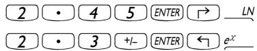
- Natural logarithms are calculated by using LN (function LN) while the exponential function (EXP) is calculated by using e^x . In ALG mode, the function is entered before the argument:

text_image
→ LN 2 • 4 5 ENTER ← e^x +/- 2 • 3 ENTERIn RPN mode, the argument is entered before the function
text_image
2 • 4 5 ENTER → LN 2 • 3 +/- ENTER ← e^x- Three trigonometric functions are readily available in the keyboard: sine ( ), cosine ( ), and tangent ( ). Arguments of these functions are angles in either degrees, radians, grades. The following examples use angles in degrees (DEG):
In ALG mode:
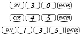
text_image
SIN 3 0 ENTER COS 4 5 ENTER TAN 1 3 5 ENTERIn RPN mode:
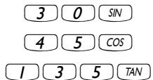
text_image
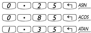
3 0 SIN 4 5 COS 1 3 5 TAN- The inverse trigonometric functions available in the keyboard are the arcsine ( ), arccosine ( ), and arctangent ( ). The answer from these functions will be given in the selected angular measure (DEG, RAD, GRD). Some examples are shown next: In ALG mode:

text_image
ASIN 0 • 2 5 ENTER ACOS 0 • 8 5 ENTER ATAN 1 • 3 5 ENTERIn RPN mode:
text_image
0 • 2 5 ← ASIN 0 • 8 5 ← ACOS 1 • 3 5 ← ATANAll the functions described above, namely, ABS, SQ, √, ^, XROOT, LOG, ALOG, LN, EXP, SIN, COS, TAN, ASIN, ACOS, ATAN, can be combined with the fundamental operations (+ - × ÷) to form more complex expressions. The Equation Writer, whose operations is described in Chapter 2, is ideal for building such expressions, regardless of the calculator operation mode.
Real number functions in the MTH menu
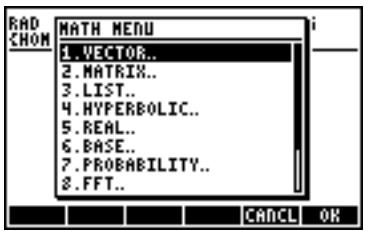
The MTH ( MTH) menu include a number of mathematical functions mostly applicable to real numbers. With the default setting of CHOOSE boxes for system flag 117 (see Chapter 2), the MTH menu shows the following functions:
text_image
RAD CHOM MATH MENU 1.VECTION.. 2.MATRIX.. 3.LIST.. 4.HYPERBOLIC.. 5.REAL.. 6.BASE.. 7.PROBABILITY.. 8.FFT.. CANCEL OK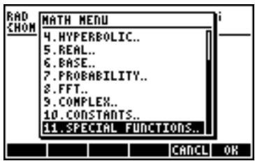
text_image
RAD CHOM MATH MENU 4.HYPERBOLIC.. 5.REAL.. 6.BASE.. 7.PROBABILITY.. 8.FFT.. 9.COMPLEX.. 10.CONSTANTS.. 11.SPECIAL FUNCTIONS.. CANCEL OKThe functions are grouped by th type of argument (1. vectors, 2. matrices, 3. lists, 7. probability, 9. complex) or by the type of function (4. hyperbolic, 5. real, 6. base, 8. fft). It also contains an entry for the mathematical constants available in the calculator, entry 10.
In general, be aware of the number and order of the arguments required for each function, and keep in mind that, in ALG mode you should select first the function and then enter the argument, while in RPN mode, you should enter the argument in the stack first, and then select the function.
Using calculator menus
- We will describe in detail the use of the 4. HYPERBOLIC.. menu in this section with the intention of describing the general operation of calculator menus. Pay close attention to the process for selecting different options.
- To quickly select one of the numbered options in a menu list (or CHOOSE box), simply press the number for the option in the keyboard. For example, to select option 4. HYPERBOLIC.. in the MTH menu, simply press 4.
Hyperbolic functions and their inverses
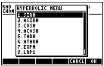
Selecting Option 4. HYPERBOLIC.., in the MTH menu, and pressing 📄, produces the hyperbolic function menu:
text_image
RAD CHOM HYPERBOLIC MENU 1.SINH 2.ASINH 3.COSH 4.ACOSH 5.TANH 6.ATANH 7.EXPM 8.LNP1 CANCEL OK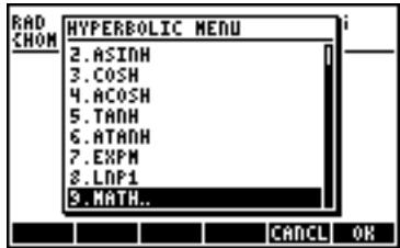
text_image
RAD CHOM HYPERBOLIC MENU 2.ASINH 3.COSH 4.ACOSH 5.TANH 6.ATANH 7.EXPM 8.LNP1 9.MATH.. CANCEL OKFor example, in ALG mode, the keystroke sequence to calculate, say, (2.5) , is the following:
← MTH 4 5 2 • 5 ENTER
In the RPN mode, the keystrokes to perform this calculation are the following:
2 • 5 ENTER ← MTH 4 5
The operations shown above assume that you are using the default setting for system flag 117 (CHOOSE boxes). If you have changed the setting of this flag (see Chapter 2) to SOFT menu, the MTH menu will show as follows (left-hand side in ALG mode, right – hand side in RPN mode):

text_image
VECTR MATRIX LIST HYP REAL BASE
text_image
4: 3: 2: 1: VECTR MATRIX LIST HYP REAL BASEPressing NXT shows the remaining options:

text_image
PROB FFT CHPLX CONST SPECI
text_image
4: 3: 2: 1: PROB FFT CMPLX CONST SPECIThus, to select, for example, the hyperbolic functions menu, with this menu format press 📄, to produce:

text_image
SINH ASINH COSH ACOSH TANH ATANH
text_image
4: 3: 2: 1: SINH ASINH COSH ACOSH TANH ATANHFinally, in order to select, for example, the hyperbolic tangent (tanh) function, simply press 📄.
NOTE: To see additional options in these soft menus, press the NXT key or the ← PREV keystroke sequence.
For example, to calculate (2.5) , in the ALG mode, when using SOFT menus over CHOOSE boxes, follow this procedure:
← MTH 2 · 5 ENTER
In RPN mode, the same value is calculated using:
2 • 5 ENTER ← MTH
As an exercise of applications of hyperbolic functions, verify the following values:
$$ \mathrm{SINH} (2. 5) = 6. 0 5 0 2 0.. $$
$$ \mathrm{ASINH} (2. 0) = 1. 4 4 3 6 \dots $$
$$ \mathrm{COSH} (2. 5) = 6. 1 3 2 2 8.. $$
$$ \mathrm{ACOSH(2.0)} = 1. 3 1 6 9 \dots $$
$$ \mathrm{TANH} (2. 5) = 0. 9 8 6 6 1.. $$
$$ \mathrm{ATANH} (0. 2) = 0. 2 0 2 7 \dots $$
$$ \text { EXPM } (2. 0) = 6. 3 8 9 0 5 \dots $$
$$ \mathrm{LNP1(1.0)} = 0. 6 9 3 1 4 \dots $$
Operations with units
Numbers in the calculator can have units associated with them. Thus, it is possible to calculate results involving a consistent system of units and produce a result with the appropriate combination of units.
The UNITS menu
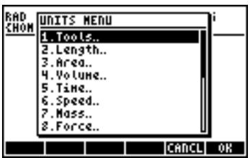
The units menu is launched by the keystroke combination (associated with the 6 key). With system flag 117 set to CHOOSE boxes, the result is the following menu:
text_image
RAD CHOM UNITS MENU 1. Tools.. 2. Length.. 3. Area.. 4. Volume.. 5. Time.. 6. Speed.. 7. Mass.. 8. Force.. CANCEL OK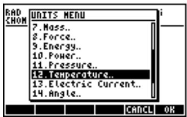
text_image
RAD CHOM UNITS MENU 7.Mass.. 8.Force.. 9.Energy.. 10.Power.. 11.Pressure.. 12.Temperature.. 13.Electric Current.. 14.Angle.. CANCEL OK
text_image
RAD CHOM UNITS MENU 10.Power.. 11.Pressure.. 12.Temperature.. 13.Electric Current.. 14.Angle.. 15.Light.. 16.Radiation.. 17.Viscosity.. CANCEL OKOption 1. Tools.. contains functions used to operate on units (discussed later). Options 2. Length.. through 17. Viscosity.. contain menus with a number of units for each of the quantities described. For example, selecting option 8. Force.. shows the following units menu:

text_image
RAD CHOM FORCE MENU 1.d 2.dyn 3.gf 4.kip 5.lbf 6.pdl 7.Units.. CANCEL OK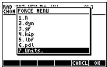
text_image
RAD CHOM FORCE MENU 1.n 2.dyn 3.gf 4.kip 5.lbf 6.pdl 7.Units.. CANCEL OKThe user will recognize most of these units (some, e.g., dyne, are not used very often nowadays) from his or her physics classes: N = newtons, dyn = dynes, gf = grams – force (to distinguish from gram-mass, or plainly gram, a unit of mass), kip = kilo-poundal (1000 pounds), lbf = pound-force (to distinguish from pound-mass), pdl = poundal.
To attach a unit object to a number, the number must be followed by an underscore. Thus, a force of 5 N will be entered as 5_N.
For extensive operations with units SOFT menus provide a more convenient way of attaching units. Change system flag 117 to SOFT menus (see Chapter 2), and use the keystroke combination ↗ UNITS to get the following menus. Press NXT to move to the next menu page.

text_image
4: 3: 2: 1: TOOLS LENG AREA VOL TIME SPEED
text_image
4: 3: 2: 1: MASS FORCE ENRG POWR PRESS TEMP
text_image
4: 3: 2: 1: ELEC ANGL LIGHT RAD VISCPressing on the appropriate soft menu key will open the sub-menu of units for that particular selection. For example, for the 📄sub-menu, the following units are available:

text_image
4: 10: 20: 1: H/s CH/s Ft/s kph Hph knot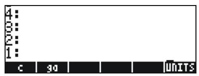
text_image
4: 3: 2: 1: c go UNITSPressing the soft menu key 📄 will take you back to the UNITS menu.
Recall that you can always list the full menu labels in the screen by using ⏻, e.g., for the ⏻ set of units the following labels will be listed:

text_image
J erg Kcal cal Btu ft*1bf J | erg | Kcal | cal | Btu | Ft*1b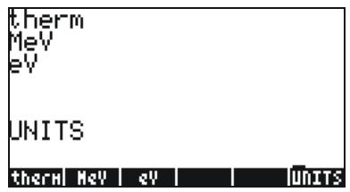
text_image
therm MeV eV UNITS therm MeV eV UnitsNOTE: Use the NXT key or the ← PREV keystroke sequence to navigate through the menus.
Available units
For a complete list of available units see Chapter 3 in the calculator's user's guide.
Attaching units to numbers
To attach a unit object to a number, the number must be followed by an underscore (→—-, key(8,5)). Thus, a force of 5 N will be entered as 5_N.
Here is the sequence of steps to enter this number in ALG mode, system flag 117 set to CHOOSE boxes:
5 → - → UNITS 8 ENTER
NOTE: If you forget the underscore, the result is the expression 5*N, where N here represents a possible variable name and not Newtons.
To enter this same quantity, with the calculator in RPN mode, use the following keystrokes:
Notice that the underscore is entered automatically when the RPN mode is active.
The keystroke sequences to enter units when the SOFT menu option is selected, in both ALG and RPN modes, are illustrated next. For example, in ALG mode, to enter the quantity 5_N use:
5 → - → UNITS NXT ENTER
The same quantity, entered in RPN mode uses the following keystrokes:
5 → UNITS NXT
NOTE: You can enter a quantity with units by typing the underline and units with the ALPHA keyboard, e.g., 5 → - ALPHA N will produce the entry: 5...N
Unit prefixes
You can enter prefixes for units according to the following table of prefixes from the SI system. The prefix abbreviation is shown first, followed by its name, and by the exponent x in the factor 10^x corresponding to each prefix:
| Prefix | Name | x | Prefix | Name | x |
| Y | yotta | +24 | d | deci | -1 |
| Z | zetta | +21 | c | centi | -2 |
| E | exa | +18 | m | milli | -3 |
| P | peta | +15 | micro | -6 | |
| T | tera | +12 | n | nano | -9 |
| G | giga | +9 | p | pico | -12 |
| M | mega | +6 | f | femto | -15 |
| k,K | kilo | +3 | a | atto | -18 |
| h,H | hecto | +2 | z | zepto | -21 |
| D(*) | deka | +1 | y | yocto | -24 |
(*) In the SI system, this prefix is da rather than D. Use D for deka in the calculator, however.
To enter these prefixes, simply type the prefix using the ALPHA keyboard. For example, to enter 123 pm (picometer), use:

Using UBASE (type the name) to convert to the default unit (1 m) results in:

text_image
: 123-1_pm : UBASE(ANS(1)) .000000000123_m CONVEUBASE UVAL UFACT UNIT UNITSOperations with units
Here are some calculation examples using the ALG operating mode. Be warned that, when multiplying or dividing quantities with units, you must enclosed each quantity with its units between parentheses. Thus, to enter, for example, the product 12.5m × 5.2 yd, type it to read (12.5_m)*(5.2_yd) ENTER :

text_image
:12.5_m·5.2_yd 65_(m·yd) CONVEUBASE UVAL UFACT+UNITUNITSwhich shows as 65_(m·yd). To convert to units of the SI system, use function UBASE (find it using the command catalog, _CAT):
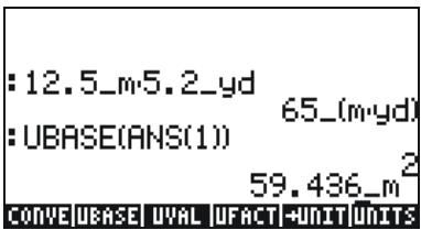
text_image
:12.5_m5.2_yd :UBASE(ANS(1)) 65_(m-yd) 59.436_m^2 CONVE|UBASE|UVAL |UFACT|UNIT|UNITSNOTE: Recall that the ANS(1) variable is available through the keystroke combination ANS (associated with the ENTER key).
To calculate a division, say, 3250 mi / 50 h, enter it as
(3250_mi)/(50_h) ENTER
which transformed to SI units, with function UBASE, produces:
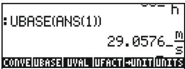
text_image
:UBASE(ANS(1)) 29.0576_m/s CONVEUBASE UVAL UFACT+UNITUNITSAddition and subtraction can be performed, in ALG mode, without using parentheses, e.g., 5 m + 3200 mm, can be entered simply as
$$ 5 _ m + 3 2 0 0 _ m m \text { ENTER }. $$
More complicated expression require the use of parentheses, e.g.,
$$ (1 2 _ m m) ^ {*} (1 _ c m ^ {\wedge} 2) / (2 _ s) \text { ENTER }: $$
Stack calculations in the RPN mode do not require you to enclose the different terms in parentheses, e.g.,

text_image
12 ENTER 1.5 ENTER × 3250 ENTER 50 ENTER ÷These operations produce the following output:

text_image
3: 2: 1: 18_(m·yd) 65_mi h z1 R MANS CASDIUnit conversions
The UNITS menu contains a TOOLS sub-menu, which provides the following functions:
CONVERT(x,y) convert unit object x to units of object y
UBASE(x) convert unit object x to SI units
UVAL(x) extract the value from unit object x
UFACT(x,y) factors a unit y from unit object x
→UNIT(x,y) combines value of x with units of y
Examples of function CONVERT are shown below. Examples of the other UNIT/TOOLS functions are available in Chapter 3 of the calculator's user's guide.
For example, to convert 33 watts to btu's use either of the following entries:
$$ \begin{array}{l} \text {CONVERT(33_W,1_hp)} \boxed {\text {ENTER}} \ \text {CONVERT(33_W,11_hp)} \boxed {\text {ENTER}} \end{array} $$
Physical constants in the calculator
The calculator's physical constants are contained in a constants library activated with the command CONLIB. To launch this command you could simply type it in the stack: ALPHA ALPHA C O N L I B ENTER, or, you can select the command CONLIB from the command catalog, as follows: First, launch the catalog by using: → CAT ALPHA C. Next, use the up and down arrow keys ▲ ▼ to select CONLIB. Finally, press ENTER. Press ENTER, if needed. Use the up and down arrow keys (▲ ▼) to navigate through the list of constants in your calculator.
The soft menu keys corresponding to this CONSTANTS LIBRARY screen include the following functions:
SI when selected, constants values are shown in SI units (*)
ENGL when selected, constants values are shown in English units (*)
UNIT when selected, constants are shown with units attached (*)
VALUE when selected, constants are shown without units
→STK copies value (with or without units) to the stack
QUIT exit constants library
(*) Activated only if the VALUE option is selected.
This is the way the top of the CONSTANTS LIBRARY screen looks when the option VALUE is selected (units in the SI system):

text_image
CONSTANTS LIBRARY NA: 6.0221367E23_1/gm k: 1.380658E-23_J/K Vm: 22.4141_1/gmol R: 8.31451_J/(gmol*K) StdT: 273.15_K StdP: 101.325_kPa σ: 5.67051E-8_W/(m^2... c: 299792458._m/s SI ▪ ENGL UNIT ▪ VALU ▪ STR QUITTo see the values of the constants in the English (or Imperial) system, press the ☐☐☐☐ option:
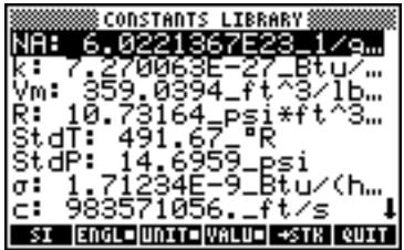
text_image
CONSTANTS LIBRARY NA: 6.0221367E23_1/q... k: 7.270063E-27_Btu/... Vm: 359.0394_ft^3/1b... R: 10.73164_Psi*ft^3... StdT: 491.67 °R StdP: 14.6959_Psi σ: 1.71234E-9_Btu/(h... c: 983571056._ft/s SI ENGL UNIT VALU STK QUITIf we de-select the UNITS option (press 📄) only the values are shown (English units selected in this case):

text_image
CONSTANTS LIBRARY NA: 6.0221367E23 k: 7.270063E-27 Vm: 359.0394 R: 10.73164 StdT: 491.67 StdP: 14.6959 σ: 1.71234E-9 c: 983571056. SI ENGL UNITS VALU →STR QUITTo copy the value of Vm to the stack, select the variable name, and press 📄, then, press 📄. For the calculator set to the ALG, the screen will look like this:
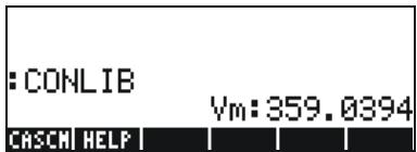
text_image
:CONLIB Vm:359.0394 CASCM HELPThe display shows what is called a tagged value, Vm:359.0394. In here, Vm, is the tag of this result. Any arithmetic operation with this number will ignore the tag. Try, for example:

which produces:

text_image
:CONLIB Vm:359.0394 :LN(2·ANS(1)) 6.57657931233 CASCH HELPThe same operation in RPN mode will require the following keystrokes (after the value of Vm was extracted from the constants library):

Defining and using functions
Users can define their own functions by using the DEFINE command available thought the keystroke sequence DEF (associated with the 2 key). The function must be entered in the following format:
Function_name(arguments) = expression_containing_arguments
For example, we could define a simple function
$$ H (x) = \ln (x + 1) + \exp (- x) $$
Suppose that you have a need to evaluate this function for a number of discrete values and, therefore, you want to be able to press a single button and get the result you want without having to type the expression in the right-hand side for each separate value. In the following example, we assume you have set your calculator to ALG mode. Enter the following sequence of keystrokes:

text_image
← DEF ↑ ALPHA H ← () ALPHA ← X ▶ → =
text_image
→ LN ALPHA ← X + / ▶ + ← e^x ALPHA ← X ENTERThe screen will look like this:
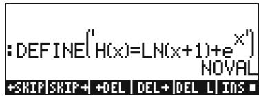
text_image
:DEFINE('H(x)=LN(x+1)+e^x') NOVAL +SKIP|SHIP+|DEL|DEL+|DEL L INSPress the VAR key, and you will notice that there is a new variable in your soft menu key (☐). To see the contents of this variable press → ☐. The screen will show now:
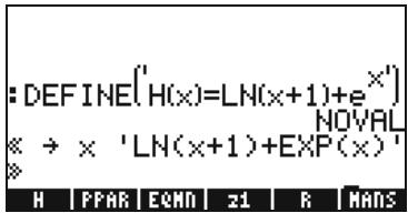
text_image
:DEFINE('H(x)=LN(x+1)+e^x') NOVAL ⇒ × 'LN(x+1)+EXP(x)' H | PPAR | EQMN | z1 | R | MANSThus, the variable H contains a program defined by:
$$ < < \rightarrow x ^ {\prime} L N (x + 1) + E X P (x) ^ {\prime} > > $$
This is a simple program in the default programming language of the calculator. This programming language is called UserRPL (See Chapters 20 and 21 in the calculator's user's guide). The program shown above is
relatively simple and consists of two parts, contained between the program containers
- Input: → x → x
- Process: 'LN(x+1) + EXP(x)'
This is to be interpreted as saying: enter a value that is temporarily assigned to the name x (referred to as a local variable), evaluate the expression between quotes that contain that local variable, and show the evaluated expression.
To activate the function in ALG mode, type the name of the function followed by the argument between parentheses, e.g., 2 ENTER. Some examples are shown below:
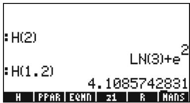
text_image
:H(2) :H(1.2) LN(3)+e^2 4.1085742831 H PPAR EQMN z1 R MANS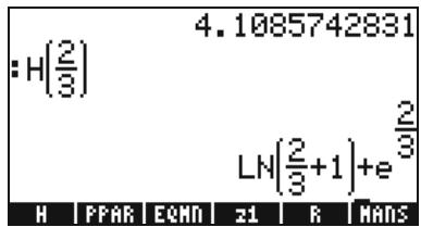
text_image
:H(2/3) 4.1085742831 LN(2/3+1)+e^(2/3) H PPAR EQMD z1 R MADSIn the RPN mode, to activate the function enter the argument first, then press the soft menu key corresponding to the variable name ☐. For example, you could try: 2 ☐. The other examples shown above can be entered by using: 1 • 2 ☐, 2 ENTER 3 ÷ ☐.
Reference
Additional information on operations with real numbers with the calculator is contained in Chapter 3 of the user's guide.
Chapter 4 Calculations with complex numbers
This chapter shows examples of calculations and application of functions to complex numbers.
Definitions
A complex number z is a number z = x + iy , where x and y are real numbers, and i is the imaginary unit defined by i^2 = -1 . The complex number x + iy has a real part, x = Re(z) , and an imaginary part, y = Im(z) . The complex number z = zx + iy is often used to represent a point P(x,y) in the x-y plane, with the x-axis referred to as the real axis, and the y-axis referred to as the imaginary axis.
A complex number in the form x + iy is said to be in a rectangular representation. An alternative representation is the ordered pair z = (x, y) . A complex number can also be represented in polar coordinates (polar representation) as z = r e^i = r · + i r · , where r = |z| = ^2 + y^2 is the magnitude of the complex number z , and = Arg(z) = (y / x) is the argument of the complex number z .
The relationship between the Cartesian and polar representation of complex numbers is given by the Euler formula: ei^i = + i . The complex conjugate of a complex number ( z = x + iy = re^i ) is = x - iy = re^-i . The complex conjugate of i can be thought of as the reflection of z about the real (x) axis. Similarly, the negative of z, -z = -x - iy = -re^{i\theta}, can be thought of as the reflection of z about the origin.
Setting the calculator to COMPLEX mode
To work with complex numbers select the CAS complex mode:

The COMPLEX mode will be selected if the CAS MODES screen shows the option _Complex checked, i.e.,

text_image
CAS MODES Indep var: X Modulo: 13 _Numeric _Approx ▼Complex ✓Verbose _Step/Step _Incr Pow ✓Rigorous ▼Simp Non-Rational Allow complex numbers? EDIT ✓CHK Cancel OKPress ☐, twice, to return to the stack.
Entering complex numbers
Complex numbers in the calculator can be entered in either of the two Cartesian representations, namely, x+iy , or (x,y) . The results in the calculator will be shown in the ordered-pair format, i.e., (x,y) . For example, with the calculator in ALG mode, the complex number (3.5,-1.2) , is entered as:
← () 3 • 5 → +/- 1 • 2 ENTER
A complex number can also be entered in the form x+iy . For example, in ALG mode, 3.5-1.2i is entered as (accept mode changes):
3 • 5 - 1 • 2 × ← i ENTER
NOTE: to enter the unit imaginary number alone type i , the I key.
In RPN mode, these numbers could be entered using the following keystrokes:
← () 3 • 5 → , 1 • 2 +/- ENTER
(Notice that the change-sign keystroke is entered after the number 1.2 has been entered, in the opposite order as the ALG mode exercise).
Polar representation of a complex number
The polar representation of the complex number 3.5-1.2i, entered above, is obtained by changing the coordinate system to cylindrical or polar (using function CYLIN). You can find this function in the catalog ( CAT). You can also change the coordinate to polar using MODE. Changing to polar coordinate with standard notation and the angular measure in radians, produces the result in RPN mode:
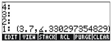
text_image
4: 3: 2: 1: (3.7,∠.330297354829) EDIT VIEW STACK RCL PURGE CLEARThe result shown above represents a magnitude, 3.7, and an angle 0.33029.... The angle symbol ( ) is shown in front of the angle measure.
Return to Cartesian or rectangular coordinates by using function RECT (available in the catalog, ). A complex number in polar representation is written as z = r · e^i . You can enter this complex number into the calculator by using an ordered pair of the form (r, ) . The angle symbol () can be entered as 6 . For example, the complex number z = 5.2e^1.5i , can be entered as follows (the figures show the RPN stack, before and after entering the number):
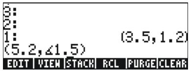
text_image
3: 2: 1: (3.5,1.2) (5.2,∠1.5) EDIT VIEW STACK RCL PURGE CLEAR
text_image
4: 3: 2: (3.5,1.2) 1: (.367833448672,5.18) EDIT VIEW STACK RCL PURGE CLEARBecause the coordinate system is set to rectangular (or Cartesian), the calculator automatically converts the number entered to Cartesian coordinates, i.e., x = r , y = r , resulting, for this case, in (0.3678..., 5.18...).
On the other hand, if the coordinate system is set to cylindrical coordinates (use CYLIN), entering a complex number (x,y) , where x and y are real numbers, will produce a polar representation. For example, in cylindrical coordinates, enter the number (3.,2.) . The figure below shows the RPN stack, before and after entering this number:

text_image
3: 2: 1: (3.,2.♦ EDIT VIEW RCL STOP PURGE CLEAR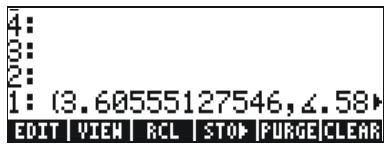
text_image
4: 1: (3.60555127546,∠.58) EDIT VIEW RCL STOP PURGE CLEARSimple operations with complex numbers
Complex numbers can be combined using the four fundamental operations ( +-×÷ ). The results follow the rules of algebra with the caveat that i2=-1. Operations with complex numbers are similar to those with real numbers. For example, with the calculator in ALG mode and the CAS set to Complex, try the following operations:
$$ (3 + 5 \mathrm{i}) + (6 - 3 \mathrm{i}) = (9, 2); $$
$$ (5 - 2 \mathrm{i}) - (3 + 4 \mathrm{i}) = (2, - 6) $$
$$ (3 - \mathrm{i}) \cdot (2 - 4 \mathrm{i}) = (2, - 1 4); $$
$$ (5 - 2 \mathrm{i}) / (3 + 4 \mathrm{i}) = (0. 2 8, - 1. 0 4) $$
$$ 1 / (3 + 4 \mathrm{i}) = (0. 1 2, - 0. 1 6); $$
$$ - (5 - 3 \mathrm{i}) = - 5 + 3 \mathrm{i} $$
The CMPLX menus
There are two CMPLX (CoMPLeX numbers) menus available in the calculator. One is available through the MTH menu (introduced in Chapter 3) and one directly into the keyboard (→ CMPLX). The two CMPLX menus are presented next.
CMPLX menu through the MTH menu
Assuming that system flag 117 is set to CHOOSE boxes (see Chapter 2), the CMPLX sub-menu within the MTH menu is accessed by using: MTH 9. The functions available are the following:
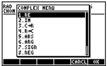
text_image
RAD CHOM COMPLEX MENU 1.3 2.IN 3.C+R 4.R+C 5.ABS 6.ARG 7.SIGN 8.NEG CANCEL OK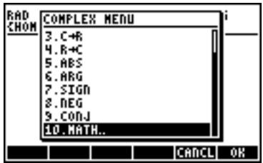
text_image
RAD CHOM COMPLEX MENU 3.C+C 4.R+C 5.ABS 6.ARG 7.SIGN 8.NEG 9.CONJ 10.MATH.. CANCEL OKThe first menu (options 1 through 6) shows the following functions:
Examples of applications of these functions are shown next in RECT
RE(z) Real part of a complex number
IM(z) Imaginary part of a complex number
C R(z) Separates a complex number into its real and imaginary parts
R C(x, y) Forms the complex number (x, y) out of real numbers x and y
ABS(z) Calculates the magnitude of a complex number.
ARG(z) Calculates the argument of a complex number.
SIGN(z) Calculates a complex number of unit magnitude as z/|z|.
NEG(z) Changes the sign of z
CONJ(z) Produces the complex conjugate of z
coordinates. Recall that, for ALG mode, the function must precede the argument, while in RPN mode, you enter the argument first, and then select the function. Also, recall that you can get these functions as soft menu labels by changing the setting of system flag 117 (See Chapter 2).

text_image
:RE(3.-2..i) :IM(3.-2..i) :C→R(3.+5..i) 3. -2. (3. 5.) RE | IM | C+R | R+C | ABS | ARG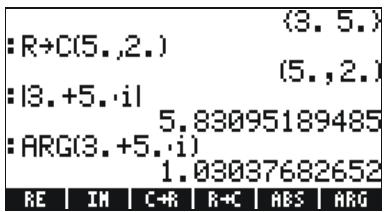
text_image
:R→C(5.,2.) (3, 5.) :|3.+5.·i| (5.,2.) :ARG(3.+5.·i) 5.83095189485 1.03037682652 RE | IN | C+R | R+C | ABS | ARG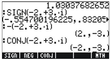
text_image
1.03037682652 :SIGN(-2.+3..i) (-.554700196225,.83205) :-(-2.+3..i) (2.,-3.) :CONJ(-2.+3..i) (-2.,-3.) SIGN NEG CONJ MTHCMPLX menu in keyboard
A second CMPLX menu is accessible by using the right-shift option associated with the 1 key, i.e., CMPLX. With system flag 117 set to CHOOSE boxes, the keyboard CMPLX menu shows up as the following screens:
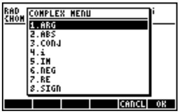
text_image
RAD CHOM COMPLEX MENU 1.ARG 2.ABS 3.CONJ 4.i 5.IM 6.REG 7.RE 8.SIGN CANCEL OK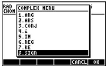
text_image
RAD CHOM COMPLEX MENU 1.ARG 2.ABS 3.CONJ 4.i 5.IM 6.NEG 7.RE 8.SIGN CANCEL OKThe resulting menu include some of the functions already introduced in the previous section, namely, ARG, ABS, CONJ, IM, NEG, RE, and SIGN. It also includes function i which serves the same purpose as the keystroke combination i .
Functions applied to complex numbers
Many of the keyboard-based functions and MTH menu functions defined in Chapter 3 for real numbers (e.g., SQ, LN, e^x , etc.), can be applied to complex numbers. The result is another complex number, as illustrated in the following examples.

text_image
:SQ(3.+4.i) (-7.,24.) :√3.+4.i (2.,1.) :ALOG(2.-i) (-66.820151019,-74.398) CASDI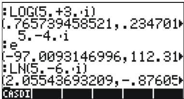
text_image
:LOG(5.+3.·i) (.765739458521,.234701) 5.-4.·i :e (-97.0093146996,112.31) :LN(5,-6.·i) (2.05543693209,-.87605) CASDI
text_image
:SIN(4,-3,·i) (-7.61923172032,6.5481) :COS(-5,+7,·i) (155.536808519,-525.79) :TAN(8,+3,·i) (-1.43408158162E-3,1.0) CASDI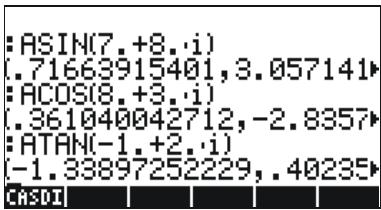
text_image
:ASIN(7.+8.·i) (.71663915401,3.057141) :ACOS(8.+3.·i) (.361040042712,-2.8357) :ATAN(-1.+2.·i) -1.33897252229,.40235 CASDI
text_image
:SINH(4.-6..i) (26.2029676178,7.63034) :COSH(1.-i) (.833730025131,-.98889) :TANH(-1.+i) (-1.08392332734,.27175) SINH ASINH COSH ACOSH TANH ATANH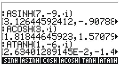
text_image
:ASINH(7,-9,i) (3.12644592412,-.90788) :ACOSH(3,i) (1.81844645923,1.57079) :ATANH(1,-6,i) (2.63401289145E-2,-1.4) SINH |ASINH COSH |ACOSH TANH |ATANHNOTE: When using trigonometric functions and their inverses with complex numbers the arguments are no longer angles. Therefore, the angular measure selected for the calculator has no bearing in the calculation of these functions with complex arguments.
Function DROITE: equation of a straight line
Function DROITE takes as argument two complex numbers, say, x_1 + iy_1 and x_2 + iy_2 , and returns the equation of the straight line, say, y = a + bx , that contains the points (x_1, y_1) and (x_2, y_2) . For example, the line between points A(5, -3) and B(6, 2) can be found as follows (example in Algebraic mode):
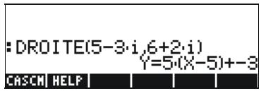
text_image
:DROITE(5-3·i,6+2·i) Y=5·(X-5)+-3 CASCN HELPFunction DROITE is found in the command catalog ( CAT). If the calculator is in APPROX mode, the result will be Y = 5.*(X-5.)-3.
Reference
Additional information on complex number operations is presented in Chapter 4 of the calculator's user's guide.
Chapter 5
Algebraic and arithmetic operations
An algebraic object, or simply, algebraic, is any number, variable name or algebraic expression that can be operated upon, manipulated, and combined according to the rules of algebra. Examples of algebraic objects are the following:
• A number: 12.3, 15.2_m, 'π', 'e', 'i'
- A variable name: 'a', 'ux', 'width', etc.
- An expression: 'p*D^2/4', 'f*(L/D)*(V^2/(2*g))',
• An equation: 'p*V = n*R*T', 'Q=(Cu/n)*A(y)*R(y)^(2/3)*√So'
Entering algebraic objects
Algebraic objects can be created by typing the object between single quotes directly into stack level 1 or by using the equation writer (EQW). For example, to enter the algebraic object 'π*D^2/4' directly into stack level 1 use:
$$ \boxed {1} \boxed {\leftarrow} \pi \quad \times \boxed {A L P H A} \boxed {D} \boxed {Y ^ {X}} \boxed {2} \boxed {\div} \boxed {4} \boxed {E N T E R} $$
An algebraic object can also be built in the Equation Writer and then sent to the stack, or operated upon in the Equation Writer itself. The operation of the Equation Writer was described in Chapter 2. As an exercise, build the following algebraic object in the Equation Writer:

text_image
f·(L/D)·v²/2·g EDIT CURS BIG EVAL FACTO SIMPAfter building the object, press ENTER to show it in the stack (ALG and RPN modes shown below):
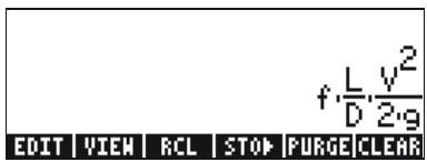
text_image
f·L·v²/D·2·g EDIT VIEW RCL STOP PURGE CLEAR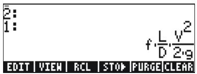
text_image
2: 1: f·L·y²/D·2·g EDIT VIEW RCL STOP PURGE CLEARSimple operations with algebraic objects
Algebraic objects can be added, subtracted, multiplied, divided (except by zero), raised to a power, used as arguments for a variety of standard functions (exponential, logarithmic, trigonometry, hyperbolic, etc.), as you would any real or complex number. To demonstrate basic operations with algebraic objects, let's create a couple of objects, say 'π*R^2' and 'g*t^2/4', and store them in variables A1 and A2 (See Chapter 2 to learn how to create variables and store values in them). Here are the keystrokes for storing variables A1 in ALG mode:

text_image
1 ← π × ALPHA R γ^x 2 ▶ STO▶ ALPHA A I ENTERresulting in:

text_image
: π·R²▶A1 π·R² EDIT VIEW RCL STOP PURGE CLEARThe keystrokes corresponding to RPN mode are:

text_image
← π ALPHA R ENTER 2 γ^x × ALPHA A I STO▶After storing the variable A2 and pressing the key, the screen will show the variables as follows:

text_image
' 2' : 9t/4 ▶A2 π·R 9t/4 A2 A1 CASDIIn ALG mode, the following keystrokes will show a number of operations with the algebraics contained in variables ☐ and ☑ (press VAR to recover variable menu):


text_image
:A1+A2 4·R²·π+t²·g 4 A2 | A1 | CASDI
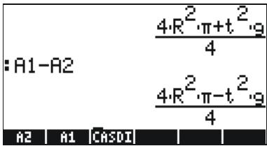
text_image
:A1-A2 4·R²·π+t²·g 4 4·R²·π-t²·g 4 A2 | A1 | CASDI | | |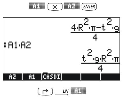
text_image
:A1:A2 4·R²·π-t²·g 4 t²·g·R²·π 4 A2 | A1 | CA3DI LN
text_image
: A1 A2 4 4·R²·π t²·9 A2 A1 CASDI ← e^x 注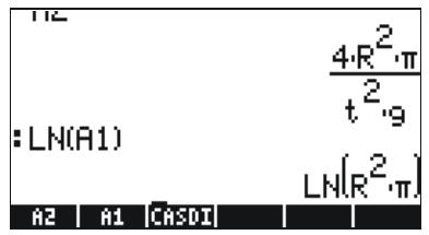
text_image
: LN(A1) A2 A1 CASDI 4·R²·π t²·g LN(R²·π)
text_image
: e^A2 LN(R²·π) t^2·g / 4 e^A2 A1 CASDIThe same results are obtained in RPN mode if using the following keystrokes:

text_image
Diagram showing four grid-based icons with symbols and labels, including plus, cross, and LN labels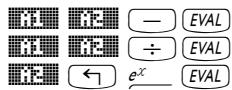
text_image
Diagram showing pixelated and simplified symbols with labels like 'EVAL' and mathematical notationFunctions in the ALG menu
The ALG (Algebraic) menu is available by using the keystroke sequence ALG (associated with the 4 key). With system flag 117 set to CHOOSE boxes, the ALG menu shows the following functions:
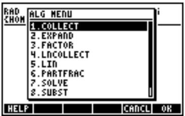
text_image
RAD CHOM ALG MENU 1.COLLECT 2.EXPAND 3.FACTOR 4.LNCOLLECT 5.LIN 6.PARTFRAC 7.SOLVE 8.SUBST HELP CANCEL OK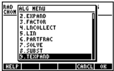
text_image
RAD CHOM ALG MENU 2. EXPAND 3. FACTOR 4. LNCOLLECT 5. LIN 6. PARTFRAC 7. SOLVE 8. SUBST 9. EXPAND HELP CANCEL OKRather than listing the description of each function in this manual, the user is invited to look up the description using the calculator's help facility: TOOL NXT ENTER. To locate a particular function, type the first letter of the function. For example, for function COLLECT, we type ALPHA C, then use the up and down arrow keys, ▲▼, to locate COLLECT within the help window.
To complete the operation press ☐. Here is the help screen for function COLLECT:
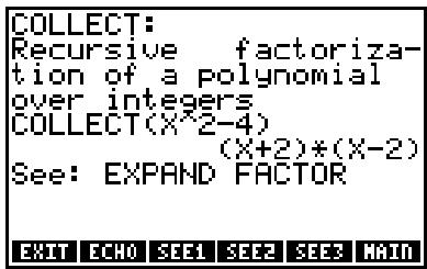
text_image
COLLECT: Recursive factoriza- tion of a polynomial over integers COLLECT(X^2-4) (X+2)*(X-2) See: EXPAND FACTOR EXIT ECHO SEE1 SEE2 SEE3 MAINWe notice that, at the bottom of the screen, the line See: EXPAND FACTOR suggests links to other help facility entries, the functions EXPAND and FACTOR. To move directly to those entries, press the soft menu key 📄 for EXPAND, and 📄 for FACTOR. Pressing 📄, for example, shows the following information for EXPAND, while 📄 shows information for FACTOR:

text_image
EXPAND: Expands and simplifies an algebraic expr. EXPAND((X+2)*(X-2)) X^2-4 See: COLLECT SIMPLIFY EXIT ECHO SEE1 SEE2 SEE3 MAIN
text_image
FACTOR: Factorizes an integer or a polynomial FACTOR(X^2-2) (X+√2)(X-√2) See: EXPAND COLLECT EXIT ECHO SEE1 SEE2 SEE3 MAINCopy the examples provided onto your stack by pressing 📄. For example, for the EXPAND entry shown above, press the 📄 soft menu key to get the following example copied to the stack (press ENTER to execute the command):
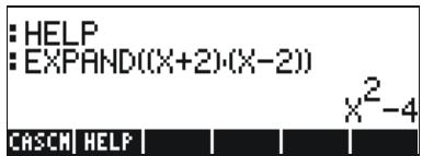
text_image
: HELP : EXPAND((X+2)-(X-2)) CASCH | HELP | | | | | | X²-4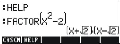
text_image
: HELP : FACTOR(x²-2) (x+√2)·(x-√2) CASCH HELPThus, we leave for the user to explore the applications of the functions in the ALG menu. This is a list of the commands:

text_image
RAD CHOM ALG MENU 1.COLLECT 2.EXPAND 3.FACTOR 4.LNCOLLECT 5.LIN 6.PARTFRAC 7.SOLVE 8.SUBST HELP CANCEL OK
text_image
RAD CHOM ALG MENU 2. EXPAND 3. FACTOR 4. LNCOLLECT 5. LIN 6. PARTFRAC 7. SOLVE 8. SUBST 9. EXPAND HELP CANCEL OKFor example, for function SUBST, we find the following CAS help facility entry:
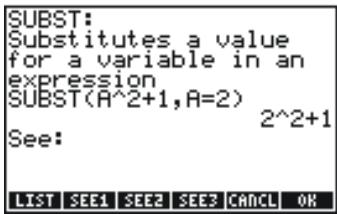
text_image
SUBST: Substitutes a value for a variable in an expression SUBST(A^2+1, A=2) 2^2+1 See: LIST SEE1 SEE2 SEE3 CANDL OKNOTE: Recall that, to use these, or any other functions in the RPN mode, you must enter the argument first, and then the function. For example, the example for TEXPAND, in RPN mode will be set up as:

At this point, select function TEXPAND from menu ALG (or directly from the catalog CAT), to complete the operation.
Operations with transcendental functions
The calculator offers a number of functions that can be used to replace expressions containing logarithmic and exponential functions ( EXP&LN ), as well as trigonometric functions ( TRIG ).
Expansion and factoring using log-exp functions
The ← EXP&LN produces the following menu:
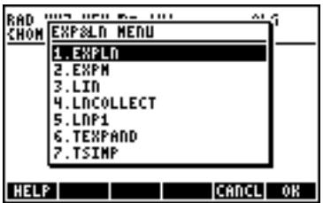
text_image
RAD CHOM EXP&LN MENU 1. EXPLN 2. EXPM 3. LIN 4. LOCOLLECT 5. LNP1 6. EXPAND 7. TSIMP HELP CANCEL OK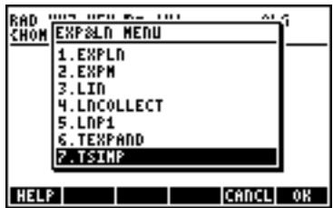
text_image
RAD CHOM EXP&LN MENU 1.EXPLN 2.EXPM 3.LIN 4.LDCOLLECT 5.LNP1 6.TEXPAND 7.TSIMP HELP CANCEL OKInformation and examples on these commands are available in the help facility of the calculator. For example, the description of EXPLN is shown in the left-hand side, and the example from the help facility is shown to the right:
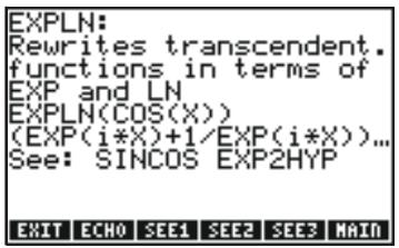
text_image
EXPLN: Rewrites transcendent. functions in terms of EXP and LN EXPLN(COS(X)) (EXP(i*X)+1/EXP(i*X))... See: SINCOS EXP2HYP EXIT ECHO SEE1 SEE2 SEE3 MAIN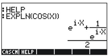
text_image
: HELP : EXPLN(COS(X)) e^i·X + 1/(e^i·X) 2 CASCHE HELPExpansion and factoring using trigonometric functions
The TRIG menu, triggered by using TRIG, shows the following functions:
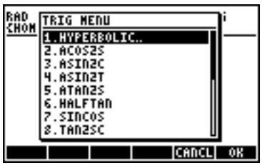
text_image
RAD CHOM TRIG MENU 1. HYPERBOLIC... 2. ACOS2S 3. ASIN2C 4. ASIN2T 5. ATAN2S 6. HALFTAN 7. SINCO5 8. TAN2SC CANCEL OK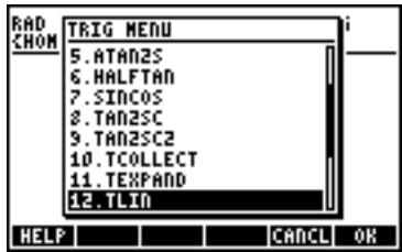
text_image
RAD CHOM TRIG MENU 5.ATAN2S 6.HALFTAN 7.SINCOS 8.TAN2SC 9.TAN2SC2 10.TCOLLECT 11.TEXPAND 12.TLIN HELP CANCEL OK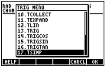
text_image
RAD CHOM TRIG MENU 10.TCOLLECT 11.TEXPAND 12.TLIN 13.TRIG 14.TRIGCOS 15.TRIGSIN 16.TRIGTAN 17.TSIMP HELP CANCEL OKThese functions allow to simplify expressions by replacing some category of trigonometric functions for another one. For example, the function ACOS2S allows to replace the function arccosine (acos(x)) with its expression in terms of arcsine (asin(x)).
Description of these commands and examples of their applications are available in the calculator's help facility (TOOL NXT). The user is invited to explore this facility to find information on the commands in the TRIG menu.
Functions in the ARITHMETIC menu
The ARITHMETIC menu is triggered through the keystroke combination ARITH (associated with the / key). With system flag 117 set to CHOOSE boxes, ARITH shows the following menu:

text_image
RAD CHOM ARITH MENU 1. INTEGER.. 2. POLYNOMIAL.. 3. MODULE.. 4. PERMUTATION.. 5. DIVIS.. 6. FACTORS.. 7. LGCD 8. PROPFAC CANCEL OK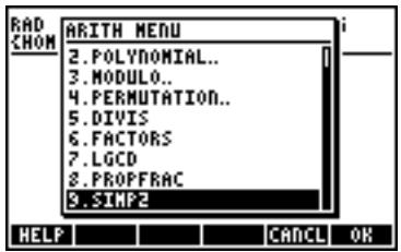
text_image
RAD CHOM ARITH MENU 2.POLYNOMIAL.. 3.MODULO.. 4.PERMUTATION.. 5.DIVIS 6.FACTORS 7.LGCD 8.PROPPFRAC 9.SIMP2 HELP CANCEL OKOut of this menu list, options 5 through 9 (DIVIS, FACTORS, LGCD, PROPFRAC, SIMP2) correspond to common functions that apply to integer numbers or to polynomials. The remaining options (1. INTEGER, 2. POLYNOMIAL, 3. MODULO, and 4. PERMUTATION) are actually sub-menus of functions that apply to specific mathematical objects. When system flag 117 is set to SOFT menus, the ARITHMETIC menu (← ARITH ) produces:

text_image
INTEG POLY MODUL PERM DIVIS FACTO
text_image
LGCD |PROPF |SIMP2Following, we present the help facility entries for functions FACTORS and SIMP2 in the ARITHMETIC menu(TOOL NXT):
FACTORS:

text_image
FACTORS: Returns irreducible factors of an integer or a polynomial FACTORS(X^2-1) { X+1 1. X-1 1. } See: FACTOR EXIT ECHO SEE1 SEE2 SEE3 MAINSIMP2:
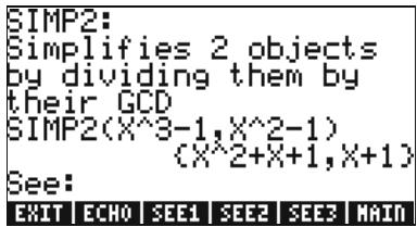
text_image
SIMP2: Simplifies 2 objects by dividing them by their GCD SIMP2(X^3-1,X^2-1) (X^2+X+1,X+1) See: EXIT ECHO SEE1 SEE2 SEE3 MAINThe functions associated with the ARITHMETIC submenus: INTEGER, POLYNOMIAL, MODULO, and PERMUTATION, are presented in detail in Chapter 5 in the calculator's user's guide. The following sections show some applications to polynomials and fractions.
Polynomials
Polynomials are algebraic expressions consisting of one or more terms containing decreasing powers of a given variable. For example, 'X^3+2*X^2-3*X+2' is a third-order polynomial in X, while 'SIN(X)^2-2' is a second-order polynomial in SIN(X). Functions COLLECT and EXPAND, shown earlier, can be used on polynomials. Other applications of polynomial functions are presented next:
The HORNER function
The function HORNER ( , POLYNOMIAL, HORNER) produces the Horner division, or synthetic division, of a polynomial P(X) by the factor (X-a), i.e., HORNER(P(X),a) = {Q(X), a, P(a)}, where P(X) = Q(X)(X-a)+P(a). For example,
$$ \text { HORNER } (^ {\prime} X ^ {3} + 2 * X ^ {2} - 3 * X + 1 ^ {\prime}, 2) = {X ^ {2} + 4 * X + 5 \quad 2 \quad 1 1 } $$
i.e., X^3+2X^2-3X+1=(X^2+4X+5)(X-2)+11 . Also,
$$ \text { HORNER } (^ {\prime} X ^ {\wedge} 6 - 1 ^ {\prime}, - 5) = $$
$$ {X ^ {\wedge} 5 - 5 * X ^ {\wedge} 4 + 2 5 * X ^ {\wedge} 3 - 1 2 5 * X ^ {\wedge} 2 + 6 2 5 * X - 3 1 2 5 \quad - 5 \quad 1 5 6 2 4 } $$
i.e., X^6 - 1 = (X^5 - 5 * X^4 + 25X^3 - 125X^2 + 625X - 3125)(X + 5) + 15624 .
The variable VX
Most polynomial examples above were written using variable X. This is because a variable called VX exists in the calculator's {HOME CASDIR} directory that takes, by default, the value of 'X'. This is the name of the preferred independent variable for algebraic and calculus applications. Avoid using the variable VX in your programs or equations, so as to not get it confused with the CAS' VX. For additional information on the CAS variable see Appendix C in the calculator's user's guide.
The PCOEF function
Given an array containing the roots of a polynomial, the function PCOEF generates an array containing the coefficients of the corresponding polynomial. The coefficients correspond to decreasing order of the independent variable. For example:
$$ \operatorname{PCOEF} ([ - 2, - 1, 0, 1, 1, 2 ]) = [ 1. - 1. - 5. 5. 4. - 4. 0. ], $$
which represents the polynomial X^6-X^5-5X^4+5X^3+4X^2-4X .
The PROOT function
Given an array containing the coefficients of a polynomial, in decreasing order, the function PROOT provides the roots of the polynomial. Example, from X^2+5X+6=0 , PROOT([1,-5,6])=[2.3] .
The QUOT and REMAINDER functions
The functions QUOT and REMAINDER provide, respectively, the quotient Q(X) and the remainder R(X) , resulting from dividing two polynomials, P_1(X) and P_2(X) . In other words, they provide the values of Q(X) and R(X) from P_1(X)/P_2(X) = Q(X) + R(X)/P_2(X) . For example,
$$ \text { QUOT } (^ {\prime} X ^ {\wedge} 3 - 2 * X + 2 ^ {\prime}, ^ {\prime} X - 1 ^ {\prime}) = ^ {\prime} X ^ {\wedge} 2 + X - 1 ^ {\prime} $$
$$ \text { REMAINDER } (^ {\prime} X ^ {\wedge} 3 - 2 ^ {*} X + 2 ^ {\prime}, ^ {\prime} X - 1 ^ {\prime}) = 1. $$
Thus, we can write: (X^3-2X+2)/(X-1)=X^2+X-1+1/(X-1) .
NOTE: you could get the latter result by using PARTFRAC:
$$ \text { PARTFRAC } (^ {\prime} (X ^ {\wedge} 3 - 2 * X + 2) / (X - 1) ^ {\prime}) = ^ {\prime} X ^ {\wedge} 2 + X - 1 + 1 / (X - 1) ^ {\prime}. $$
The PEVAL function
The function PEVAL (Polynomial EVALuation) can be used to evaluate a polynomial
$$ p (x) = a _ {n} \cdot x ^ {n} + a _ {n - 1} \cdot x ^ {n - 1} + \dots + a _ {2} \cdot x ^ {2} + a _ {1} \cdot x + a _ {0}, $$
given an array of coefficients [a_n, a_n-1, , a_2, a_1, a_0] and a value of x_0 . The result is the evaluation p(x_0) . Function PEVAL is not available in the ARITHMETIC menu, instead use the CALC/DERIV&INTEG Menu. Example: PEVAL([1,5,6,1],5) = 281.
Additional applications of polynomial functions are presented in Chapter 5 in the calculator's user's guide.
Fractions
Fractions can be expanded and factored by using functions EXPAND and FACTOR, from the ALG menu (→ ALG). For example:
$$ \text { EXPAND } (^ {\prime} (1 + X) ^ {\wedge} 3 / ((X - 1) ^ {*} (X + 3)) ^ {\prime}) = ^ {\prime} (X ^ {\wedge} 3 + 3 * X ^ {\wedge} 2 + 3 * X + 1) / (X ^ {\wedge} 2 + 2 * X - 3) ^ {\prime} $$
$$ \text { EXPAND } (^ {\prime} (X ^ {\wedge} 2) ^ {} (X + Y) / (2 ^ {} X - X ^ {\wedge} 2) ^ {\wedge} 2) ^ {\prime}) = ^ {\prime} (X + Y) / (X ^ {\wedge} 2 - 4 ^ {*} X + 4) ^ {\prime} $$
$$ \text { FACTOR } (^ {\prime} (3 * X ^ {\wedge} 3 - 2 * X ^ {\wedge} 2) / (X ^ {\wedge} 2 - 5 * X + 6) ^ {\prime}) = ^ {\prime} X ^ {\wedge} 2 * (3 * X - 2) / ((X - 2) * (X - 3)) ^ {\prime} $$
$$ \text { FACTOR } (^ {\prime} (X ^ {\wedge} 3 - 9 * X) / (X ^ {\wedge} 2 - 5 * X + 6) ^ {\prime}) = ^ {\prime} X ^ {*} (X + 3) / (X - 2) ^ {\prime} $$
The SIMP2 function
Function SIMP2, in the ARITHMETIC menu, takes as arguments two numbers or polynomials, representing the numerator and denominator of a rational fraction, and returns the simplified numerator and denominator. For example:
$$ \text { SIMP2 } (^ {\prime} X ^ {\wedge} 3 - 1 ^ {\prime}, ^ {\prime} X ^ {\wedge} 2 - 4 ^ {*} X + 3 ^ {\prime}) = {^ {\prime} X ^ {\wedge} 2 + X + 1 ^ {\prime}, ^ {\prime} X - 3 ^ {\prime} } $$
The PROPFRAC function
The function PROPFRAC converts a rational fraction into a “proper” fraction, i.e., an integer part added to a fractional part, if such decomposition is possible. For example:
$$ \text { PROPFRAC } \left(^ {\prime} 5 / 4 ^ {\prime}\right) = ^ {\prime} 1 + 1 / 4 ^ {\prime} $$
$$ \text { PROPFRAC } (^ {\prime} (x ^ {2} + 1) / x ^ {2}) = ^ {\prime} 1 + 1 / x ^ {2} $$
The PARTFRAC function
The function PARTFRAC decomposes a rational fraction into the partial fractions that produce the original fraction. For example:
$$ \text { PARTFRAC } (^ {\prime} (2 * X ^ {6} - 1 4 * X ^ {5} + 2 9 * X ^ {4} - 3 7 * X ^ {3} + 4 1 * X ^ {2} - 1 6 * X + 5) / (X ^ {5} - $$
$$ 7 ^ {} X ^ {\wedge} 4 + 1 1 ^ {} X ^ {\wedge} 3 - 7 ^ {} X ^ {\wedge} 2 + 1 0 ^ {} X) ^ {\prime}) = $$
$$ ^ {\prime} 2 ^ {*} X + (1 / 2 / (X - 2) + 5 / (X - 5) + 1 / 2 / X + X / (X ^ {2} + 1)) ^ {\prime} $$
The FCOEF function
The function FCOEF, available through the ARITHMETIC/POLYNOMIAL menu, is used to obtain a rational fraction, given the roots and poles of the fraction.
NOTE: If a rational fraction is given as F(X) = N(X)/D(X) , the roots of the fraction result from solving the equation N(X) = 0 , while the poles result from solving the equation D(X) = 0 .
The input for the function is a vector listing the roots followed by their multiplicity (i.e., how many times a given root is repeated), and the poles followed by their multiplicity represented as a negative number. For example, if we want to create a fraction having roots 2 with multiplicity 1, 0 with multiplicity 3, and -5 with multiplicity 2, and poles 1 with multiplicity 2 and -3 with multiplicity 5, use:
$$ \begin{array}{l} \operatorname{FCOEF} ([ 2, 1, 0, 3, - 5, 2, 1, - 2, - 3, - 5 ]) = ^ {\prime} (X - 5) ^ {\wedge} 2 ^ {} X ^ {\wedge} 3 ^ {} (X - 2) / (X + 3) ^ {\wedge} 5 ^ {} (X - 1) ^ {\wedge} 2 ^ {\prime} \ ^ {\prime} (X ^ {\wedge} 6 + 8 * X ^ {\wedge} 5 + 5 * X ^ {\wedge} 4 - 5 0 * X ^ {\wedge} 3) / (X ^ {\wedge} 7 + 1 3 * X ^ {\wedge} 6 + 6 1 * X ^ {\wedge} 5 + 1 0 5 * X ^ {\wedge} 4 - \ 4 5 ^ {} X ^ {\wedge} 3 - 2 9 7 ^ {} X 6 2 - 8 1 ^ {} X + 2 4 3) ^ {\prime} \ \end{array} $$
If you press EVAL ← ANS ENTER (or, simply EVAL, in RPN mode) you will get:
The FROOTS function
The function FROOTS, in the ARITHMETIC/POLYNOMIAL menu, obtains the roots and poles of a fraction. As an example, applying function FROOTS to the result produced above, will result in: [1 -2. -3 -5. 0 3. 2 1. -5 2.]. The result shows poles followed by their multiplicity as a negative number, and roots followed by their multiplicity as a positive number. In this case, the poles are (1, -3) with multiplicities (2,5) respectively, and the roots are (0, 2, -5) with multiplicities (3, 1, 2), respectively.
Another example is: FROOTS((X^2-5*X+6)/(X^5-X^2)) = [0 - 2. 1 - 1. 3 1. 2 1.], i.e., poles = 0 (2), 1(1), and roots = 3(1), 2(1). If you have had Complex mode selected, then the results would be:
$$ [ 0 - 2. 1 - 1. - ((1 + \mathrm{i} ^ {} \sqrt {3}) / 2) - 1. - ((1 - \mathrm{i} ^ {} \sqrt {3}) / 2) - 1. 3 1. 2 1. ]. $$
Step-by-step operations with polynomials and fractions
By setting the CAS modes to Step/step the calculator will show simplifications of fractions or operations with polynomials in a step-by-step fashion. This is very useful to see the steps of a synthetic division. The example of dividing
$$ \frac {X ^ {3} - 5 X ^ {2} + 3 X - 2}{X - 2} $$
is shown in detail in Appendix C of the calculator's user's guide. The following example shows a lengthier synthetic division (DIV2 is available in the ARITH/POLYNOMIAL menu):
$$ \frac {X ^ {9} - 1}{X ^ {2} - 1} $$
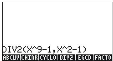
text_image
DIV2(X^9-1, X^2-1) RECUV CHINA CYCLO DIV2 EGCD FACTO
text_image
Division A=BQ+R A: (1,0,0,0,0,0,0,0,0,0, B: (1,0,-1) Q: (1) R: (0,1,0,0,0,0,0,0,-1) Press a key to go on ABCUY CHINA CYCLO DIV2 EGCD FACTO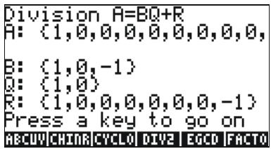
text_image
Division A=BQ+R A: (1,0,0,0,0,0,0,0,0,0, B: (1,0,-1) Q: (1,0) R: (1,0,0,0,0,0,-1) Press a key to go on ABCUY CHINR CYCLO DIV2 EGCD FACTO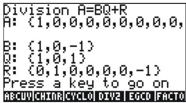
text_image
Division A=BQ+R A: (1,0,0,0,0,0,0,0,0,0, B: (1,0,-1) Q: (1,0,1) R: (0,1,0,0,0,0,-1) Press a key to go on ABCUY CHINR CYCLO DIV2 EGCD FACTO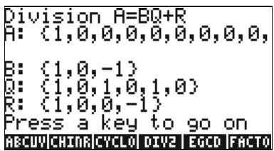
text_image
Division A=BQ+R A: (1,0,0,0,0,0,0,0,0,0, B: (1,0,-1) Q: (1,0,1,0,1,0) R: (1,0,0,-1) Press a key to go on ABCUV CHINR CYCLO DIV2 EGCD FACTO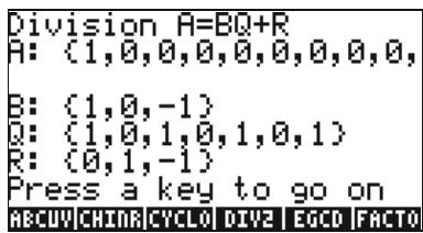
text_image
Division A=BQ+R A: (1,0,0,0,0,0,0,0,0,0, B: (1,0,-1) Q: (1,0,1,0,1,0,1) R: (0,1,-1) Press a key to go on ABCUV CHINR CYCLO DIV2 EGCD FACTO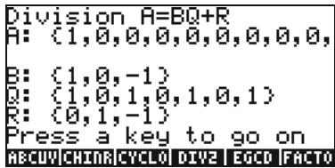
text_image
Division A=BQ+R A: (1,0,0,0,0,0,0,0,0, B: (1,0,-1) D: (1,0,1,0,1,0,1) R: (0,1,-1) Press a key to go on ABCUV CHINRC CYCLO DIV2 EGCD FACTO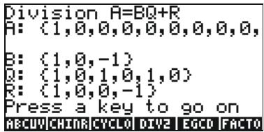
text_image
Division A=BQ+R A: {1,0,0,0,0,0,0,0,0,0, B: {1,0,-1} D: {1,0,1,0,1,0} R: {1,0,0,-1} Press a key to go on ABCUV CHINRC CYCLO DIV2 EGCD FACTO
text_image
Division A=BQ+R A: (1,0,0,0,0,0,0,0,0,0, B: (1,0,-1) Q: (1,0,1,0,1,0,1,0) R: (1,-1) Press a key to go on ABCUV|CHINR|CYCLO |DIV2 |EGCD |FACTO
text_image
:DIV2(X^9-1,X^2-1) {Q:(X^7+X^5+X^3+X) R:(X-1)} ABCUY |CHINR |CYCLO |DIV2 |EGCD |FACTOReference
Additional information, definitions, and examples of algebraic and arithmetic operations are presented in Chapter 5 of the calculator's user's guide.
Chapter 6 Solution to equations
Associated with the 7 key there are two menus of equation-solving functions, the Symbolic SOLVer ( S.SLV ), and the NUMerical SOLVer ( NUM.SLV ). Following, we present some of the functions contained in these menus.
Symbolic solution of algebraic equations
Here we describe some of the functions from the Symbolic Solver menu. Activate the menu by using the keystroke combination \$SLV. With system flag 117 set to CHOOSE boxes, the following menu lists will be available:

text_image
RAD CHOM S.SLY MENU 1. DESOLVE 2.ISOL 3.LDEC 4.LINSOLVE 5.SOLVEVX 6.SOLVE 7.ZEROS HELP CANCEL OK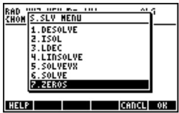
text_image
RAD CHOM S.SLY MENU 1.DESOLVE 2.ISOL 3.LDEC 4.LINSOLVE 5.SOLVEVX 6.SOLVE 7.ZEROS HELP CANCEL OKFunctions ISOL and SOLVE can be used to solve for any unknown in a polynomial equation. Function SOLVEVX solves a polynomial equation where the unknown is the default CAS variable VX (typically set to 'X'). Finally, function ZEROS provides the zeros, or roots, of a polynomial.
Function ISOL
Function ISOL(Equation, variable) will produce the solution(s) to Equation by isolating variable. For example, with the calculator set to ALG mode, to solve for t in the equation at^3-bt = 0 we can use the following:
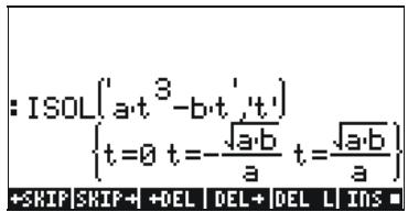
text_image
:ISOL('a·t^3-b·t', 't') {t=0 t=-√a·b/a t=√a·b/a} +SHIF|SHIP+ +DEL | DEL+ |DEL L | INS ■Using the RPN mode, the solution is accomplished by entering the equation in the stack, followed by the variable, before entering function ISOL. Right before the execution of ISOL, the RPN stack should look as in
the figure to the left. After applying ISOL, the result is shown in the figure to the right:
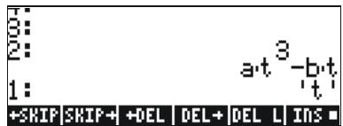
text_image
3: 2: 1: +SKIP | SKIP+ | +DEL | DEL+ | DEL | L | INS =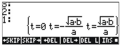
text_image
s: 2: 1: {t=0 t=-√a·b/a t=√a·b/a} +SKIP | SKIP+ | +DEL | DEL+ | DEL | INS ■The first argument in ISOL can be an expression, as shown above, or an equation. For example, in ALG mode, try:
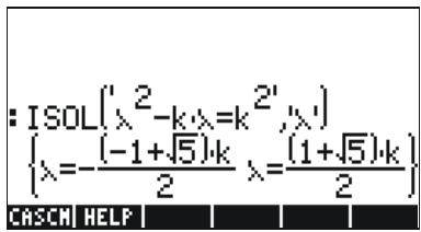
text_image
: ISOL('2-k·λ=k 2', 'λ') {λ=-(-1+√5)·k/2 λ=(1+√5)·k/2} CASCCH HELPNOTE: To type the equal sign (=) in an equation, use = (associated with the +/- key).
The same problem can be solved in RPN mode as illustrated below (figures show the RPN stack before and after the application of function ISOL):
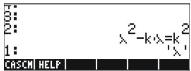
text_image
3: 2: 1: CASCH HELP λ² -k λ=k 2 λ'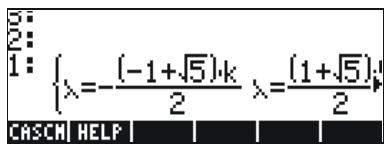
text_image
5: 2: 1: {λ=-(-1+√5)·k λ=(1+√5)· CASCH HELPFunction SOLVE
Function SOLVE has the same syntax as function ISOL, except that SOLVE can also be used to solve a set of polynomial equations. The help-facility entry for function SOLVE, with the solution to equation X^4 - 1 = 3 , is shown next:
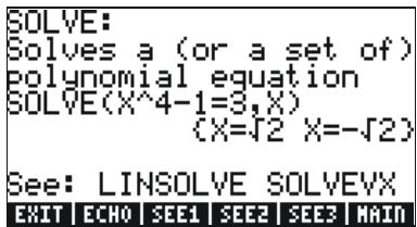
text_image
SOLVE: Solves a (or a set of) polynomial equation SOLVE(X^4-1=3,X) (X=√2 X=-√2) See: LINSOLVE SOLVEVX EXIT ECHO SEE1 SEE2 SEE3 MAINThe following examples show the use of function SOLVE in ALG and RPN modes (Use Complex mode in the CAS):

text_image
:SOLVE('β^4-5,β=125',β') ( ) :SOLVE('β^4-5,β=6',β') {β=-1 β=2 β=-\frac{1+i\sqrt{11}}{2} β=-} +SKIP|SKIP+ +DEL |DEL+ DEL L INS ■The screen shot shown above displays two solutions. In the first one, ^4-5=125 , SOLVE produces no solutions { }. In the second one, ^4-5=6 , SOLVE produces four solutions, shown in the last output line. The very last solution is not visible because the result occupies more characters than the width of the calculator's screen. However, you can still see all the solutions by using the down arrow key (▼), which triggers the line editor (this operation can be used to access any output line that is wider than the calculator's screen):
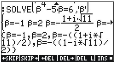
text_image
: SOLVE[β^4 - 5·β = 6, 'β'] {β=-1 β=2 β=-\frac{1+i\sqrt{11}}{2} β=-+ (β=-1, β=2, β=-(1+i*√11)/2), β=-(1-i*√11)/2)} +SKIP|SKIP+|+DEL |DEL+|DEL L|INS-The corresponding RPN screens for these two examples, before and after the application of function SOLVE, are shown next:

text_image
3: 2: 1: +SKIP | SKIP + | +DEL | DEL + | DEL | L | INS ■ β⁴ -5·β = 1.25 β'
text_image
4: 3: 2: 1: +SKIP | SKIP+ | +DEL | DEL+ | DEL | INS *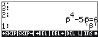
text_image
3: 2: 1: +SKIP | SKIP-+ | +DEL | DEL-+ | DEL | L | INS -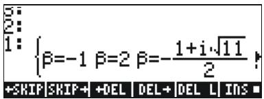
text_image
3: 2: 1: {β=-1 β=2 β=-\frac{1+i\sqrt{11}}{2} + +SKIP |SKIP+ |DEL |DEL+ |DEL L |INS =Function SOLVEVX
The function SOLVEVX solves an equation for the default CAS variable contained in the reserved variable name VX. By default, this variable is set to 'X'. Examples, using the ALG mode with VX = 'X', are shown below:
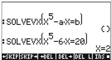
text_image
: SOLVEVX(x^5 - a*x = b) : :SOLVEVX(x^5 - 6*x = 20) X=2 +SKIP | SKIP + | +DEL | DEL + | DEL L | INS ■In the first case SOLVEVX could not find a solution. In the second case, SOLVEVX found a single solution, X = 2.
The following screens show the RPN stack for solving the two examples shown above (before and after application of SOLVEVX):
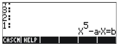
text_image
3: 2: 1: X^5 - a X = b CASCH HELP
text_image
4: 10: 1: ( ) CASCH HELP
text_image
1: 2: 3: 1: CASCHE HELP X^5 -6×=20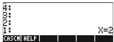
text_image
4: 3: 2: 1: CASCM HELP X=2Function ZEROS
The function ZEROS finds the solutions of a polynomial equation, without showing their multiplicity. The function requires having as input the expression for the equation and the name of the variable to solve for. Examples in ALG mode are shown next:

text_image
:ZEROS[k^5-k^2,k] {0 1 -\frac{1+i\cdot\sqrt{3}}{2} -\frac{1-i\cdot\sqrt{3}}{2}} +SKIP |SKIP+ |+DEL |DEL+ |DEL L INS ■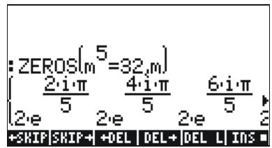
text_image
: ZEROS[m^5=32,m] { 2·i·π / 5 4·i·π / 5 6·i·π / 5 } 2·e 2·e 2·e +SHIP | SHIP + | DEL | DEL + | DEL L | INS ■To use function ZEROS in RPN mode, enter first the polynomial expression, then the variable to solve for, and then function ZEROS. The following
screen shots show the RPN stack before and after the application of ZEROS to the two examples above (Use Complex mode in the CAS):

text_image
3: 2: 1: +SKIP | SKIP + | DEL | DEL + | DEL | INS ■ k 5 - k 2 ' k'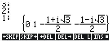
text_image
5: 2: 1: {0 1 -1+i√3/2 -1-i√3/2} +SKIP | SKIP+ | +DEL | DEL+ | DEL L | INS =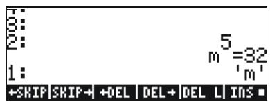
text_image
1: 2: 1: +SKIP SKIP+ +DEL DEL+ DEL L INS = 32 m' m'
text_image
2: 1: { 2·i·π / 5 4·i·π / 5 6·i 2·e 2·e 2·e +SKIP |SKIP+ +DEL |DEL+ |DEL L INS =The Symbolic Solver functions presented above produce solutions to rational equations (mainly, polynomial equations). If the equation to be solved for has all numerical coefficients, a numerical solution is possible through the use of the Numerical Solver features of the calculator.
Numerical solver menu
The calculator provides a very powerful environment for the solution of single algebraic or transcendental equations. To access this environment we start the numerical solver (NUM.SLV) by using NUM.SLV. This produces a drop-down menu that includes the following options:
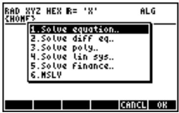
text_image
RAD XYZ HEX R= 'X' CHOMP3 1.Solve equation.. 2.Solve diff eq.. 3.Solve poly.. 4.Solve lin sys.. 5.Solve Finance.. 6.MSLV CANCEL OKFollowing, we present applications of items 3. Solve poly., 5. Solve finance, and 1. Solve equation., in that order. Appendix 1-A, in the calculator's user's guide, contains instructions on how to use input forms
with examples for the numerical solver applications. Item 6. MSLV (Multiple equation SolVer) will be presented later in page 6-10.
Notes:
- Whenever you solve for a value in the NUM.SLV applications, the value solved for will be placed in the stack. This is useful if you need to keep that value available for other operations.
- There will be one or more variables created whenever you activate some of the applications in the NUM.SLV menu.
Polynomial Equations
Using the Solve poly...option in the calculator's SOLVE environment you can:
(1) find the solutions to a polynomial equation;
(2) obtain the coefficients of the polynomial having a number of given roots; and,
(3) obtain an algebraic expression for the polynomial as a function of X.
Finding the solutions to a polynomial equation
A polynomial equation is an equation of the form: an_xn + a_n-1x_n-1 + + a_1x + a_0 = 0 . For example, solve the equation: 3s^4 + 2s^3 - s + 1 = 0 .
We want to place the coefficients of the equation in a vector:
[3,2,0,-1,1]. To solve for this polynomial equation using the calculator, try the following:

Select Solve poly...

Enter vector of coefficients

Solve equation
The screen will show the solution as follows:
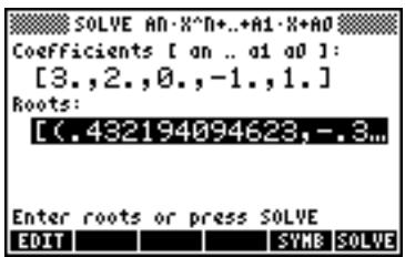
text_image
SOLVE AO·X^O+..+AI·X+AO Coefficients [ an .. ai ao ]: [3.,2.,0.,-1.,1.] Roots: [(.432194094623,-.3... Enter roots or press SOLVE EDIT SYMB SOLVEPress ENTER to return to stack. The stack will show the following results in ALG mode (the same result would be shown in RPN mode):

text_image
Roots: [C. 432194094623,] +SKIP | SKIP+ | +DEL | DEL+ | DEL L | INS -All the solutions are complex numbers: (0.432, -0.389), (0.432, 0.389), (-0.766, 0.632), (-0.766, -0.632).
Generating polynomial coefficients given the polynomial's roots
Suppose you want to generate the polynomial whose roots are the numbers [1, 5, -2, 4] . To use the calculator for this purpose, follow these steps:

Select Solve poly...

Enter vector of roots

text_image
→ , 2 +/- → , 4 Solve for coefficientsPress ENTER to return to stack, the coefficients will be shown in the stack.
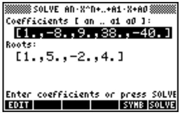
text_image
SOLVE AO·X^N+..+A1·X+AO Coefficients [ an .. a1 a0 ]: [1.,-8.,9.,38.,-40.] Roots: [1.,5.,-2.,4.] Enter coefficients or press SOLVE EDIT SYMB SOLVEPress ▼ to trigger the line editor to see all the coefficients.
Generating an algebraic expression for the polynomial
You can use the calculator to generate an algebraic expression for a polynomial given the coefficients or the roots of the polynomial. The resulting expression will be given in terms of the default CAS variable X.
To generate the algebraic expression using the coefficients, try the following example. Assume that the polynomial coefficients are [1,5,-2,4] . Use the following keystrokes:

Select Solve poly...

Enter vector of coefficients

text_image
→ , 2 +/- 4 ▲Generate symbolic expression

Return to stack.
The expression thus generated is shown in the stack as: 'X^3+5*X^2+-2*X+4'
To generate the algebraic expression using the roots, try the following example. Assume that the polynomial roots are [1, 3, -2, 1] . Use the following keystrokes:

Select Solve poly...

Enter vector of roots

text_image
→ , 2 +/- → , 1 ▼▼ ▼Generate symbolic expression

Return to stack.
The expression thus generated is shown in the stack as:
$$ ^ {\prime} (X - 1) ^ {} (X - 3) ^ {} (X + 2) ^ {*} (X - 1) ^ {\prime}. $$
To expand the products, you can use the EXPAND command.
The resulting expression is: 'X^4+-3*X^3+ -3*X^2+11*X-6'.
Financial calculations
The calculations in item 5. Solve finance.. in the Numerical Solver (NUM.SLV) are used for calculations of time value of money of interest in the discipline of engineering economics and other financial applications. This application can also be started by using the keystroke combination FINANCE (associated with the 9 key). Detailed explanations of these types of calculations are presented in Chapter 6 of the calculator's user's guide.
Solving equations with one unknown through NUM.SLV
The calculator's NUM.SLV menu provides item 1. Solve equation.. solve different types of equations in a single variable, including non-linear algebraic and transcendental equations. For example, let's solve the equation: ex-sin( x/3) = 0 .
Simply enter the expression as an algebraic object and store it into variable EQ. The required keystrokes in ALG mode are the following:
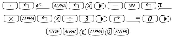
text_image
1 ← e^x ALPHA ← X ▶ — SIN ← π × ALPHA ← X ÷ 3 ▶ → = 0 ▶ STO ▶ ALPHA E ALPHA Q ENTERFunction STEQ
Function STEQ will store its argument into variable EQ, e.g., in ALG mode:

text_image
: STEQ\left(e^X - SIN\left(\frac{\pi \cdot X}{3}\right) = 0\right) NOVAL EC |LSTS |CHANL |POLRA |MESS |MSLVSIn RPN mode, enter the equation between apostrophes and activate command STEQ. Thus, function STEQ can be used as a shortcut to store an expression into variable EQ.
Press VAR to see the newly created EQ variable:
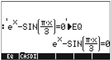
text_image
: e^x - SIN(π·x)/3 = 0 ▶ EQ e^x - SIN(π·x)/3 = 0 EQ CASDIThen, enter the SOLVE environment and select Solve equation..., by using:
→ NUM.SLV ☐. The corresponding screen will be shown as:
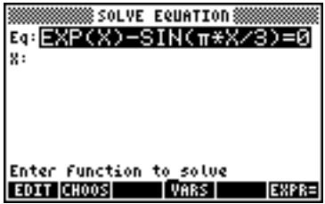
text_image
SOLVE EQUATION Eq: EXP(X) - SIN(π*X/3) = 0 X: Enter Function to solve EDIT CHOOS YARS EXP=The equation we stored in variable EQ is already loaded in the Eq field in the SOLVE EQUATION input form. Also, a field labeled x is provided. To solve the equation all you need to do is highlight the field in front of X: by using ▼, and press 📄. The solution shown is X: 4.5006E-2:

text_image
SOLVE EQUATION Eq: EXP(X) - SIN(π*X/3) = 0 X: 4.50061385902E-2 Enter value or press SOLVE EDIT VARS INFO SOLVEThis, however, is not the only possible solution for this equation. To obtain a negative solution, for example, enter a negative number in the X: field before solving the equation. Try 3 +/- OK ▼ SOLICE. The solution is now X: -3.045.
Solution to simultaneous equations with MSLV
Function MSLV is available in the NUM.SLV menu. The help-facility entry for function MSLV is shown next:
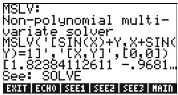
text_image
MSLV: Non-polynomial multi- variate solver MSLV('[SIN(X)+Y,X+SIN( (Y)=1]', '[X,Y]',[0,0]) [1.82384112611 -.9681... See: SOLVE EXIT ECHO SEE1 SEE2 SEE3 MAIDNotice that function MSLV requires three arguments:
- A vector containing the equations, i.e., ‘[SIN(X)+Y,X+SIN(Y)=1]’
- A vector containing the variables to solve for, i.e., '[X,Y]'
- A vector containing initial values for the solution, i.e., the initial values of both X and Y are zero for this example.
In ALG mode, press 📄 to copy the example to the stack, press ENTER to run the example. To see all the elements in the solution you need to activate the line editor by pressing the down arrow key (▼):

text_image
: HELP :MSLV([SIN(X)+Y X+SIN(Y):> [SIN(X)+Y X+SIN(Y)=1.] [>> [SIN(X)+Y, X+SIN(Y)=1... [X,Y], [1.82384112611,-.9681... +SKIP | SKIP + | DEL | DEL + | DEL | INS ■In RPN mode, the solution for this example is produced by using:

text_image
4: 3: [SIN(X)+Y X+SIN(Y)=1.] 2: [X Y] 1: [0. 0.] CASCH HELPActivating function MSLV results in the following screen.

text_image
4: 3: [SIN(X)+Y X+SIN(Y)=1.] 2: [X Y] 1: [1.82384112611 -.96&# CASCH HELPYou may have noticed that, while producing the solution, the screen shows intermediate information on the upper left corner. Since the solution provided by MSLV is numerical, the information in the upper left corner shows the results of the iterative process used to obtain a solution. The final solution is X = 1.8238, Y = -0.9681.
Reference
Additional information on solving single and multiple equations is provided in Chapters 6 and 7 of the calculator's user's guide.
Chapter 7
Operations with lists
Lists are a type of calculator's object that can be useful for data processing. This chapter presents examples of operations with lists. To get started with the examples in this Chapter, we use the Approximate mode (See Chapter 1).
Creating and storing lists
To create a list in ALG mode, first enter the braces key , then type or enter the elements of the list, separating them with commas ( __, ). The following keystrokes will enter the list {1.,2.,3.,4.} and store it into variable L1.

text_image
← {} 1 → , 2 → , 3 → , 4 ▶ STO▶ ALPHA L I ENTEREntering the same list in RPN mode requires the following keystrokes:
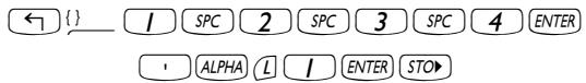
text_image
← {} 1 SPC 2 SPC 3 SPC 4 ENTER ' ALPHA L 1 ENTER STO▶Operations with lists of numbers
To demonstrate operations with lists of numbers enter and store the following lists in the corresponding variables.
The sign-change key ( +/- ), when applied to a list of numbers, will change the sign of all elements in the list. For example:
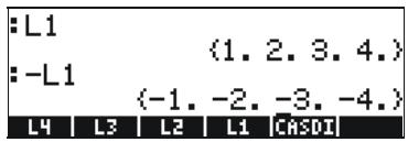
text_image
:L1 : -L1 (1. 2. 3. 4.) (-1. -2. -3. -4.) L4 | L3 | L2 | L1 | CASDIAddition, subtraction, multiplication, division
Multiplication and division of a list by a single number is distributed across the list, for example:
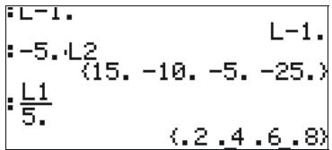
text_image
L-1. -5.L2 (15. -10. -5. -25.) L1/5. (.2 .4 .6 .8)Subtraction of a single number from a list will subtract the same number from each element in the list, for example:
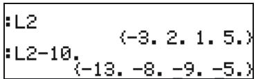
text_image
:L2 (-3. 2. 1. 5.) :L2-10. (-13. -8. -9. -5.)Addition of a single number to a list produces a list augmented by the number, and not an addition of the single number to each element in the list. For example:

text_image
:L1 :L1+6. (1. 2. 3. 4.) (1. 2. 3. 4. 6.)Subtraction, multiplication, and division of lists of numbers of the same length produce a list of the same length with term-by-term operations. Examples:
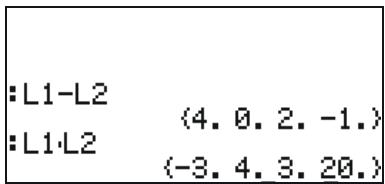
text_image
:L1-L2 :(4. 0. 2. -1.) :L1·L2 (-3. 4. 3. 20.)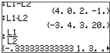
text_image
L1-L2 (4.0.2.-1.) L1-L2 (-3.4.3.20.) L1/L2 (-.3333333333333 1.3..)The division L4/L3 will produce an infinity entry because one of the elements in L3 is zero, and an error message is returned.
NOTE: If we had entered the elements in lists L4 and L3 as integers, the infinite symbol would be shown whenever a division by zero occurs. To produce the following result you need to re-enter the lists as integer (remove decimal points) using Exact mode:
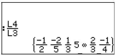
text_image
:L4 L3 { -1/2 -2/5 1/3 5 ∘ 2/3 -1/4}If the lists involved in the operation have different lengths, an error message (Invalid Dimensions) is produced. Try, for example, L1-L4.
The plus sign (+), when applied to lists, acts a concatenation operator, putting together the two lists, rather than adding them term-by-term. For example:
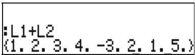
text_image
:L1+L2 (1. 2. 3. 4. -3. 2. 1. 5.)In order to produce term-by-term addition of two lists of the same length, we need to use operator ADD. This operator can be loaded by using the function catalog ( CAT). The screen below shows an application of ADD to add lists L1 and L2, term-by-term:
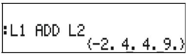
text_image
:L1 ADD L2 (-2. 4. 4. 9.)Functions applied to lists
Real number functions from the keyboard (ABS, e^x , LN, 10^x , LOG, SIN, x^2 , , COS, TAN, ASIN, ACOS, ATAN, y^x ) as well as those from the MTH/HYPERBOLIC menu (SINH, COSH, TANH, ASINH, ACOSH, ATANH), and MTH/REAL menu (%, etc.), can be applied to lists, e.g.,
ABS

text_image
·L2 :IL21 (-3. 2. 1. 5.) (3. 2. 1. 5.)INVERSE (1/x)
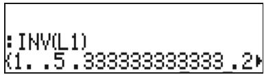
text_image
: INV(L1) (1..5.333333333333.2)Lists of complex numbers
You can create a complex number list, say L1 ADD i*L2. In RPN mode, you could enter this as L1 i L2 ADD *. The result is:
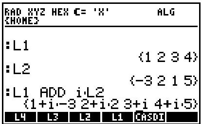
text_image
RAD XYZ HEX C= 'X' (HOME) :L1 :(1 2 3 4) :L2 (-3 2 1 5) :L1 ADD i·L2 (1+i-3 2+i·2 3+i 4+i·5) L4 L3 L2 L1 CASDIFunctions such as LN, EXP, SQ, etc., can also be applied to a list of complex numbers, e.g.,
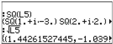
text_image
:SQ(L5) (SQ(1.+i-3.) SQ(2.+i2).) :√L5 {(1.44261527445,-1.039)
text_image
: e^L5 (e 1.+i-3. e^2.+i^2. e^3.+; :e^LN(L5) (LN(1.+i-3.) LN(2.+i^2.) )Lists of algebraic objects
The following are examples of lists of algebraic objects with the function SIN applied to them (select Exact mode for these examples -- See Chapter 1):
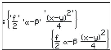
text_image
: \(\left\{\frac{f}{2},\alpha-\beta,\frac{(x-y)^{2}}{4}\right\}\) \(\left\{\frac{f}{2}\alpha-\beta\frac{(x-y)^{2}}{4}\right\}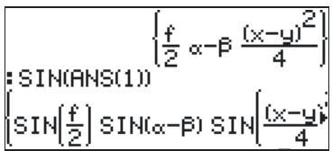
text_image
\2-(x-y)^24\ :SIN(ANS(1)) (2)SIN(-)SIN((x-y)4).The MTH/LIST menu
The MTH menu provides a number of functions that exclusively to lists. With system flag 117 set to CHOOSE boxes, the MTH/LIST menu offers the following functions:
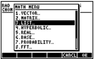
text_image
RAD CHOM MATH MENU 1. VECTOR.. 2. MATRIX.. 3. LIST.. 4. HYPERBOLIC.. 5. REAL.. 6. BASE.. 7. PROBABILITY.. 8. FFT.. CANCEL OK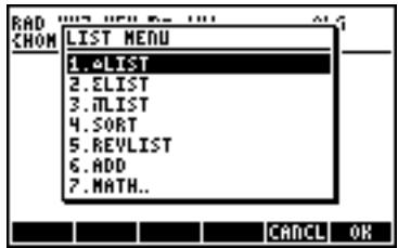
text_image
RAD CHOM LIST MENU 1.ELIST 2.ELIST 3.MLIST 4.SORT 5.REVLIST 6.ADD 7.MATH.. CANCEL OKWith system flag 117 set to SOFT menus, the MTH/LIST menu shows the following functions:

text_image
LIST|ELIST|LIST |SORT |REYLI | ADDThe operation of the MTH/LIST menu is as follows:
ΔLIST: Calculate increment among consecutive elements in list
ΣLIST: Calculate summation of elements in the list
ΠLIST: Calculate product of elements in the list
SORT: Sorts elements in increasing order
REVLIST: Reverses order of list
ADD: Operator for term-by-term addition of two lists of the same length (examples of this operator were shown above)
Examples of application of these functions in ALG mode are shown next:
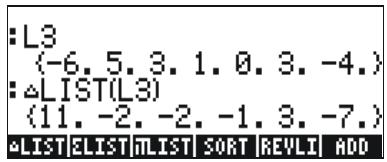
text_image
:L3 (-6.5.3.1.0.3.-4.) :△LIST(L3) (11.-2.-2.-1.3.-7.) △LIST |ELIST |MLIST |SORT |REVLI |ADD
text_image
:L3 (-6.5.3.1.0.3.-4.) :ELIST(L3) 2. *LIST ELIST MLIST SORT REVLI ADD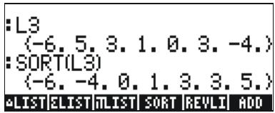
text_image
:L3 (-6.5.3.1.0.3.-4.) :SORT(L3) (-6.-4.0.1.3.3.5.) ●LIST|ELIST|MLIST SORT |REVLI |ADD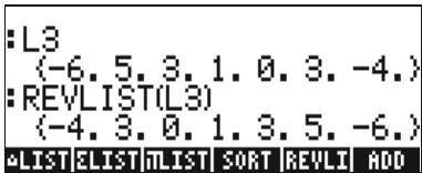
text_image
:L3 (-6. 5. 3. 1. 0. 3. -4.) :REVLIST(L3) (-4. 3. 0. 1. 3. 5. -6.) ●LIST | ELIST | MLIST | SORT | REVLI | ADDSORT and REVLIST can be combined to sort a list in decreasing order:
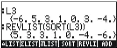
text_image
:L3 (-6. 5. 3. 1. 0. 3. -4.) :REVLIST(SORT(L3)) (5. 3. 3. 1. 0. -4. -6.) *LIST*ELIST*MLIST SORT REVLI ADDIf you are working in RPN mode, enter the list onto the stack and then select the operation you want. For example, to calculate the increment between consecutive elements in list L3, press:

This places L3 onto the stack and then selects the LIST operation from the MTH menu.
The SEQ function
The SEQ function, available through the command catalog ( CAT), takes as arguments an expression in terms of an index, the name of the index, and starting, ending, and increment values for the index, and returns a list consisting of the evaluation of the expression for all possible values of the index. The general form of the function is
SEQ(expression, index, start, end, increment)
For example:
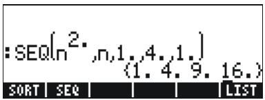
text_image
:SEQ(n^2..n,1..4..1.) (1. 4. 9. 16.) SORT | SEQ | LISTThe list produced corresponds to the values 1^2, 2^2, 3^2, 4^2 .
The MAP function
The MAP function, available through the command catalog ( CAT), takes as arguments a list of numbers and a function f(X), and produces a list consisting of the application of that function to the list of numbers. For example, the following call to function MAP applies the function SIN(X) to the list {1,2,3}:

text_image
: MAP((1 2 3),SIN(X)) (SIN(1) SIN(2) SIN(3))In ALG mode, the syntax is:

text_image
ALPHA ALPHA M A P ALPHA ← ( ) ← { } 1 → , 2 → , 3 ▶ → , SIN ALPHA X ENTERIn RPN mode, the syntax is:

text_image
← {} 1 → , 2 → , 3 ENTER | SIN ALPHA X ENTER ALPHA ALPHA M A P ENTERIn both cases, you can either type out the MAP command (as in the examples above) or select the command from the CAT menu.
Reference
For additional references, examples, and applications of lists see Chapter 8 in the calculator's user's guide.
Chapter 8
Vectors
This Chapter provides examples of entering and operating with vectors, both mathematical vectors of many elements, as well as physical vectors of 2 and 3 components.
Entering vectors
In the calculator, vectors are represented by a sequence of numbers enclosed between brackets, and typically entered as row vectors. The brackets are generated in the calculator by the keystroke combination [] , associated with the × key. The following are examples of vectors in the calculator:
$$ [ 3. 5, 2. 2, - 1. 3, 5. 6, 2. 3 ] $$
$$ [ 1, 5, - 2, 2 ] $$
$$ [ 3, - 1, 2 ] $$
$$ [ ^ {\prime} t ^ {\prime}, ^ {\prime} t ^ {2 ^ {\prime}}, ^ {\prime} S I N (t) ^ {\prime} ] $$
A general row vector
A 2-D vector
A 3-D vector
A vector of algebraics
Typing vectors in the stack
With the calculator in ALG mode, a vector is typed into the stack by opening a set of brackets ( l ) and typing the components or elements of the vector separated by commas ( ), The screen shots below show the entering of a numerical vector followed by an algebraic vector. The figure to the left shows the algebraic vector before pressing ENTER. The figure to the right shows the calculator's screen after entering the algebraic vector:
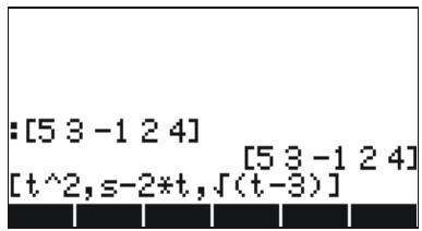
text_image
:[5 3 -1 2 4] [t^2, s-2*t, √(t-3)] [5 3 -1 2 4]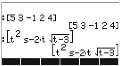
text_image
: [5 3 -1 2 4] [5 3 -1 2 4] : [t² s-2·t √t-3] [t² s-2·t √t-3]In RPN mode, you can enter a vector in the stack by opening a set of brackets and typing the vector components or elements separated by either commas (→) or spaces (SPC). Notice that after pressing ENTER, in either mode, the calculator shows the vector elements separated by spaces.
Storing vectors into variables in the stack
Vectors can be stored into variables. The screen shots below show the vectors
$$ \mathbf {u} _ {2} = \left[ \begin{array}{c c} 1, & 2 \end{array} \right], \mathbf {u} _ {3} = \left[ \begin{array}{c c c} - 3, & 2, & - 2 \end{array} \right], \mathbf {v} _ {2} = \left[ \begin{array}{c c} 3, & - 1 \end{array} \right], \mathbf {v} _ {3} = \left[ \begin{array}{c c c} 1, & - 5, & 2 \end{array} \right] $$
Stored into variables ☐E, ☐E, ☐E, and ☐E, respectively. First, in ALG mode:
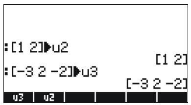
text_image
: [1 2]▶u2 : [-3 2 -2]▶u3 [1 2] [-3 2 -2]
text_image
:[-3 2 -2]▶u3 : [3 -1]▶v2 : [1 -5 2]▶v3 [1 2] [-3 2 -2] [3 -1] [1 -5 2]Then, in RPN mode (before pressing , repeatedly):
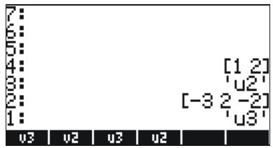
text_image
7: 6: 5: 4: 3: 2: 1: [1 2] 'u2' [-3 2 -2] 'u3'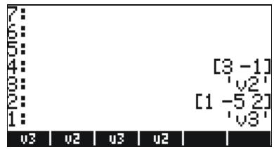
text_image
7: 6: 5: 4: 3: 2: 1: [3 -1] 'v2' [1 -5 2] 'v3'NOTE: The apostrophes (') are not needed ordinarily in entering the names u2, v2, etc. in RPN mode. In this case, they are used to overwrite the existing variables created earlier in ALG mode. Thus, the apostrophes must be used if the existing variables are not purged previously.
Using the Matrix Writer (MTRW) to enter vectors
Vectors can also be entered by using the Matrix Writer MTRW (third key in the fourth row of keys from the top of the keyboard). This command generates a species of spreadsheet corresponding to rows and columns of a matrix (Details on using the Matrix Writer to enter matrices will be presented in Chapter 9). For a vector we are interested in filling only elements in the top row. By default, the cell in the top row and first column is selected. At the bottom of the spreadsheet you will find the following soft menu keys:
1000 1000 1000 1000 1000
The 300 key is used to edit the contents of a selected cell in the Matrix Writer.
The 1330 key, when selected, will produce a vector, as opposed to a matrix of one row and many columns.
The 2010 key is used to decrease the width of the columns in the spreadsheet. Press this key a couple of times to see the column width decrease in your Matrix Writer.
The H103 key is used to increase the width of the columns in the spreadsheet. Press this key a couple of times to see the column width increase in your Matrix Writer.
The ☐ key, when selected, automatically selects the next cell to the right of the current cell when you press ENTER. This option is selected by default. This option, if desired, needs to be selected before entering elements.
The ☐ key, when selected, automatically selects the next cell below the current cell when you press ENTER. This option, if desired, needs to be selected before entering elements.
Moving to the right vs. moving down in the Matrix Writer
Activate the Matrix Writer and enter 3 ENTER 5 ENTER 2 ENTER ENTER with the ☐☐☐☐ key selected (default). Next, enter the same sequence of numbers with the ☐☐☐☐ key selected to see the difference. In the first case you entered a vector of three elements. In the second case you entered a matrix of three rows and one column.
Activate the Matrix Writer again by using MTRW , and press NXT to check out the second soft key menu at the bottom of the display. It will show the keys:
580 580 540 540 510 700
The ☐ key will add a row full of zeros at the location of the selected cell of the spreadsheet.
The ☐ key will delete the row corresponding to the selected cell of the spreadsheet.
The ☐☐☐ key will add a column full of zeros at the location of the selected cell of the spreadsheet.
The ☐key will delete the column corresponding to the selected cell of the spreadsheet.
The 3318 key will place the contents of the selected cell on the stack.
The ☐ key, when pressed, will request that the user indicate the number of the row and column where he or she wants to position the cursor.
Pressing NXT once more produces the last menu, which contains only one function (delete).
The function ☐ will delete the contents of the selected cell and replace it with a zero.
To see these keys in action try the following exercise:
(1) Activate the Matrix Writer by using MTRW. Make sure the and keys are selected.
(2) Enter the following:

text_image
1 ENTER 2 ENTER 3 ENTER NXT COTO 2 OK 1 OK OK 4 ENTER 5 ENTER 6 ENTER 7 ENTER 8 ENTER 9 ENTER(3) Move the cursor up two positions by using ▲ ▲. Then press 📄. The second row will disappear.
(4) Press ☐. A row of three zeroes appears in the second row.
(5) Press ☐. The first column will disappear.
(6) Press ☐. A column of two zeroes appears in the first column.
(7) Press 3 to move to position (3,3).
(8) Press ☐310. This will place the contents of cell (3,3) on the stack, although you will not be able to see it yet. Press ENTER to return to normal display. The number 9, element (3,3), and the full matrix entered will be available in the stack.
Simple operations with vectors
To illustrate operations with vectors we will use the vectors u2, u3, v2, and v3, stored in an earlier exercise. Also, store vector A=[-1,-2,-3,-4,-5] to be used in the following exercises.
Changing sign
To change the sign of a vector use the key +/- , e.g.,
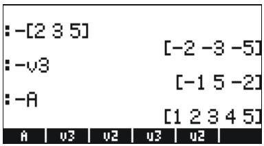
text_image
: -[2 3 5] : -v3 : -A [-2 -3 -5] [-1 5 -2] [1 2 3 4 5]Addition, subtraction
Addition and subtraction of vectors require that the two vector operands have the same length:
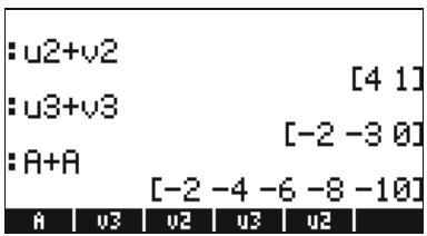
text_image
:u2+v2 [u3+v3] :A+A [4 1] [-2 -3 0] [-2 -4 -6 -8 -10] A u3 u2 u3 u2Attempting to add or subtract vectors of different length produces an error message:
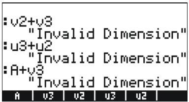
text_image
:v2+v3 "Invalid Dimension" :u3+u2 "Invalid Dimension" :A+v3 "Invalid Dimension"Multiplication by a scalar, and division by a scalar
Multiplication by a scalar or division by a scalar is straightforward:
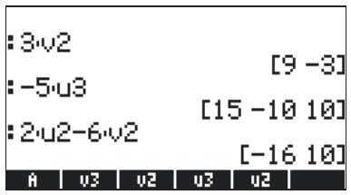
text_image
:3-v2 :-5-v3 :2-v2-6-v2 A v3 v2 u3 u2 [9 -3] [15 -10 10] [-16 10]
text_image
: u3/2 [−3/2 1 −1] A | v3 | v2 | u3 | u2 |Absolute value function
The absolute value function (ABS), when applied to a vector, produces the magnitude of the vector. For example: ABS([1,-2,6]), ABS(A), ABS(U3), will show in the screen as follows:
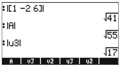
text_image
: [1 -2 6]l : |AI : |u3l A v3 v2 u3 u2 √41 √55 √17The MTH/VECTOR menu
The MTH menu ( MTH ) contains a menu of functions that specifically to vector objects:

text_image
RAD CHOM MATH MENU 1. VECTOR.. 2. MATRIX.. 3. LIST.. 4. HYPERBOLIC.. 5. REAL.. 6. BASE.. 7. PROBABILITY.. 8. FFT.. CANCEL OKThe VECTOR menu contains the following functions (system flag 117 set to CHOOSE boxes):
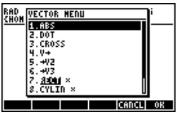
text_image
RAD CHOM VECTOR MENU 1.MES 2.DOT 3.CROSS 4.V+ 5.→V2 6.→V3 7.BCM1 × 8.CYLIN × CANCEL OK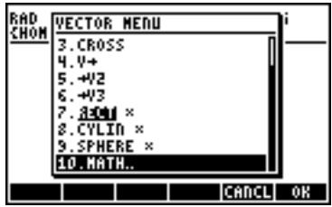
text_image
RAD CHOM VECTOR MENU 3.CROSS 4.Y+ 5.+V2 6.+V3 7.A301 × 8.CYLIN × 9.SPHERE × 10.MATH.. CANCEL OKMagnitude
The magnitude of a vector, as discussed earlier, can be found with function ABS. This function is also available from the keyboard ( ABS). Examples of application of function ABS were shown above.
Dot product
Function DOT (option 2 in CHOOSE box above) is used to calculate the dot product of two vectors of the same length. Some examples of application of function DOT, using the vectors A, u2, u3, v2, and v3, stored earlier, are shown next in ALG mode. Attempts to calculate the dot product of two vectors of different length produce an error message:

text_image
:DOT(A,A) :DOT(u2,v2) 55 :DOT(v3,u3) 1 -17 A v3 v2 u3 u2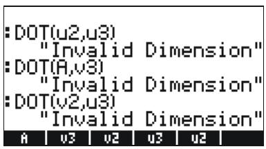
text_image
:DOT(u2,u3) "Invalid Dimension" :DOT(A,v3) "Invalid Dimension" :DOT(v2,u3) "Invalid Dimension" A | U3 | U2 | U3 | U2Cross product
Function CROSS (option 3 in the MTH/VECTOR menu) is used to calculate the cross product of two 2-D vectors, of two 3-D vectors, or of one 2-D and one 3-D vector. For the purpose of calculating a cross product, a 2-D vector of the form [A_x, A_y] , is treated as the 3-D vector [A_x, A_y, 0] . Examples in ALG mode are shown next for two 2-D and two 3-D vectors. Notice that the cross product of two 2-D vectors will produce a vector in the z-direction only, i.e., a vector of the form [0, 0, C_z] :
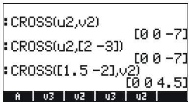
text_image
: CROSS(u2,v2) [0 0 -7] : CROSS(u2,[2 -3]) [0 0 -7] : CROSS([1.5 -2],v2) [0 0 4.5] A v3 v2 v3 v2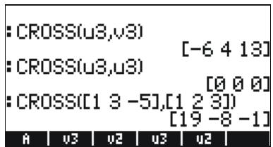
text_image
: CROSS(u3,v3) [-6 4 13] : CROSS(u3,u3) [0 0 0] : CROSS([1 3 -5],[1 2 3]) [19 -8 -1]Examples of cross products of one 3-D vector with one 2-D vector, or vice versa, are presented next:

text_image
: CROSS(u3,v2) [-2 -6 -3] : CROSS(v2,v3) [-2 -6 -14] : CROSS([1 2 3],[5 -6]) [18 15 -16]Attempts to calculate a cross product of vectors of length other than 2 or 3, produce an error message:
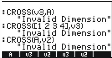
text_image
:CROSS(v3,A) "Invalid Dimension" :CROSS([1 2 3 4],v3) "Invalid Dimension" :CROSS(A,v2) "Invalid Dimension" A u3 u2 u3 u2Reference
Additional information on operations with vectors, including applications in the physical sciences, is presented in Chapter 9 of the calculator's user's guide.
Chapter 9
Matrices and linear algebra
This chapter shows examples of creating matrices and operations with matrices, including linear algebra applications.
Entering matrices in the stack
In this section we present two different methods to enter matrices in the calculator stack: (1) using the Matrix Writer, and (2) typing the matrix directly into the stack.
Using the Matrix Writer
As with the case of vectors, discussed in Chapter 8, matrices can be entered into the stack by using the Matrix Writer. For example, to enter the matrix:
$$ \left[ \begin{array}{c c c} - 2. 5 & 4. 2 & 2. 0 \ 0. 3 & 1. 9 & 2. 8 \ 2 & - 0. 1 & 0. 5 \end{array} \right], $$
first, start the Matrix Writer by using MTRW . Make sure that the option is selected. Then use the following keystrokes:
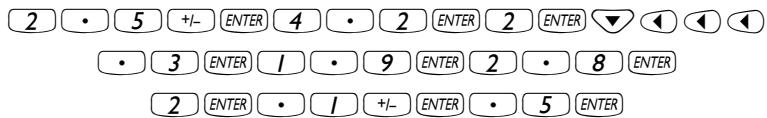
text_image
2 • 5 +/- ENTER 4 • 2 ENTER 2 ENTER ▼ ◀ ◀ ◀ • 3 ENTER 1 • 9 ENTER 2 • 8 ENTER 2 ENTER • 1 +/- ENTER • 5 ENTERAt this point, the Matrix Writer screen looks like this:
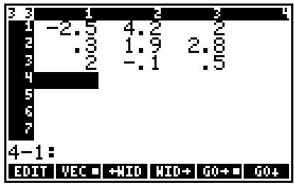
bar
| Category | Value | |---|---| | 1 | -2.5 | | 2 | .3 | | 3 | .2 | | 4 | | | 5 | | | 6 | | | 7 | | 4-1: EDIT VEC +MID MID+ GO+ GO+Press ENTER once more to place the matrix on the stack. The ALG mode stack is shown next, before and after pressing ENTER, once more:
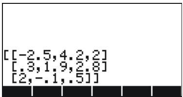
text_image
[[-2,5,4,2,2] [.3,1,9,2,8] [2,-.1,.5]]
text_image
: \begin{bmatrix}-2.5 4.2 2\\ .3 1.9 2.8\\ 2 -.1 .5\end{bmatrix}\n\begin{bmatrix}-2.5 4.2 2\\ .3 1.9 2.8\\ 2 -.1 .5\end{bmatrix}If you have selected the textbook display option (using MODE and checking off √Textbook), the matrix will look like the one shown above. Otherwise, the display will show:
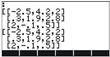
text_image
[[-2,5,4,2,2] [.,3,1,9,2,8] [2,-.1,.5]] [[-2,5,4,2,2] [.,3,1,9,2,8] [2,-.1,.5]]The display in RPN mode will look very similar to these.
Typing in the matrix directly into the stack
The same result as above can be achieved by entering the following directly into the stack:
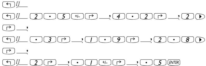
text_image
← [J] ← [J] 2 · 5 +/− → __, 4 · 2 → __, 2 ► → __, ← [J] · 3 → __, 1 · 9 → __, 2 · 8 ► → __, ← [J] 2 → __, · 1 +/- → __, · 5 ENTERThus, to enter a matrix directly into the stack open a set of brackets ( ) and enclose each row of the matrix with an additional set of brackets ( ). Commas ( · , · ) should separate the elements of each row, as well as the brackets between rows.
For future exercises, let's save this matrix under the name A. In ALG mode use . In RPN mode, use -1 .
Operations with matrices
Matrices, like other mathematical objects, can be added and subtracted. They can be multiplied by a scalar, or among themselves, and raised to a real power. An important operation for linear algebra applications is the inverse of a matrix. Details of these operations are presented next.
To illustrate the operations we will create a number of matrices that we will store in the following variables. Here are the matrices A22, B22, A23, B23, A33 and B33 (The random matrices in your calculator may be different):
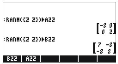
text_image
:RANM(<2 2>)B22 [ -8 0 ] [0 2] :RANM(<2 2>)B22 [7 -8] [-8 8] B22 A22
text_image
:RANM(2 33)→A23 :RANM(2 33)→B23 B23 A23 B22 A22 [7 -8] -8 2 [8 6 5] -2 4 5 [0 4 -4] 6 -6 -8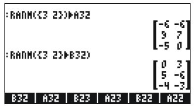
text_image
:RANM(C3 23)▶A32 [−6 -6] [9 7] −5 0] :RANM(C3 23)▶B32) [0 3] [5 -6] −4 -3] B32 | A32 | B23 | A23 | B22 | A22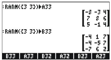
text_image
:RANM(C3 32)→A33 [ -8 -3 4 ] [7 8 6 ] [5 -1 4 ] :RANM(C3 32)→B33 [ -4 1 7 ] [ -4 -5 7 ] [ -7 6 2 ] B33 A33 B32 A32 B23 A23In RPN mode, the steps to follow are:
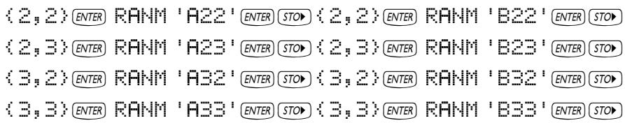
text_image
(2,2) ENTER RANM 'A22' ENTER STO▶ (2,2) ENTER RANM 'B22' ENTER STO▶ (2,3) ENTER RANM 'A23' ENTER STO▶ (2,3) ENTER RANM 'B23' ENTER STO▶ (3,2) ENTER RANM 'A32' ENTER STO▶ (3,2) ENTER RANM 'B32' ENTER STO▶ (3,3) ENTER RANM 'A33' ENTER STO▶ (3,3) ENTER RANM 'B33' ENTER STO▶Addition and subtraction
Four examples are shown below using the matrices stored above (ALG mode).
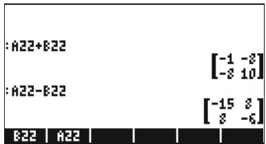
text_image
:A22+B22 [-1 -8] [-2 10] :A22-B22 [-15 8] [2 -6] B22 A22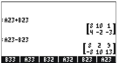
text_image
:A23+B23 [8 10 1] [4 -2 -3] :A23-B23 [8 2 9] [-2 10 13] B33 A33 B32 A32 B23 A23In RPN mode, try the following eight examples:
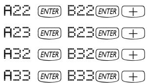
text_image
A22 ENTER B22 ENTER + A23 ENTER B23 ENTER + A32 ENTER B32 ENTER + A33 ENTER B33 ENTER +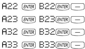
text_image
A22 ENTER B22 ENTER — A23 ENTER B23 ENTER — A32 ENTER B32 ENTER — A33 ENTER B33 ENTER —Multiplication
There are a number of multiplication operations that involve matrices. These are described next. The examples are shown in algebraic mode.
Multiplication by a scalar
Some examples of multiplication of a matrix by a scalar are shown below.
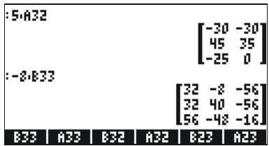
text_image
:5:A32 [ -30 -30 ] 45 35 -25 0 ] :-8:B33 [32 -8 -56] 32 40 -56 56 -48 -16] B33 A33 B32 A32 B23 A23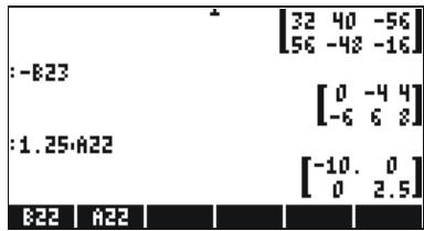
text_image
32 40 -56 56 -42 -16 :-B23 [0 -4 4] -6 6 2 :1.25·A22 [-10. 0] 0 2.5 B22 A22Matrix-vector multiplication
Matrix-vector multiplication is possible only if the number of columns of the matrix is equal to the length of the vector. A couple of examples of matrix-vector multiplication follow:
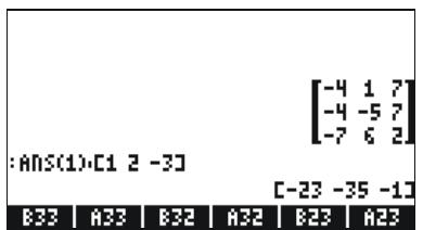
text_image
:ANS(1)·C1 2 -33 B33 A33 B32 A32 B23 A23 [-4 1 7] [-4 -5 7] -7 6 2] [-23 -35 -1]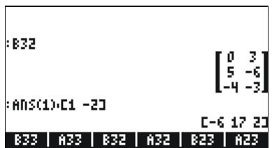
text_image
:B32 [0 3] 5 -6 -4 -3] :ANS(1)·C1 -23 C-6 17 23 B33 A33 B32 A32 B23 A23Vector-matrix multiplication, on the other hand, is not defined. This multiplication can be performed, however, as a special case of matrix multiplication as defined next.
Matrix multiplication
Matrix multiplication is defined by C_m ×_n = A_m × p · B_p × n . Notice that matrix multiplication is only possible if the number of columns in the first operand is equal to the number of rows of the second operand. The general term in the product, c_ij , is defined as
$$ c _ {i j} = \sum_ {k = 1} ^ {p} a _ {i k} \cdot b _ {k j}, f o r i = 1, 2, \dots , m; j = 1, 2, \dots , n. $$
Matrix multiplication is not commutative, i.e., in general, A · B B · A . Furthermore, one of the multiplications may not even exist. The following screen shots show the results of multiplications of the matrices that we stored earlier:
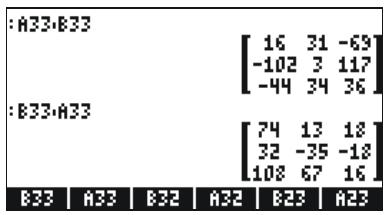
text_image
:A33:B33 [16 31 -69] [-102 3 117] [-44 34 36] :B33:A33 [74 13 18] [32 -35 -18] [108 67 16] B33 | A33 | B32 | A32 | B23 | A23
text_image
:A22:B22 [-56 64] [-16 16] :B22:A22 [-56 -16] [64 16] B22 A22Term-by-term multiplication
Term-by-term multiplication of two matrices of the same dimensions is possible through the use of function HADAMARD. The result is, of course, another matrix of the same dimensions. This function is available through Function catalog ( CAT), or through the MATRICES/OPERATIONS submenu ( MATRICES). Applications of function HADAMARD are presented next:
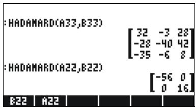
text_image
:HADAMARD(A33,B33) [32 -3 28] -28 -40 42] -35 -6 2] :HADAMARD(A22,B22) [-56 0] [0 16] B22 A22
text_image
:HADAMARD(B32,A32) [0 -18] [45 -42] [20 0] :HADAMARD(B23,A23) [0 24 -20] [-12 -24 -40] B33 | A33 | B32 | A32 | B23 | A23Raising a matrix to a real power
You can raise a matrix to any power as long as the power is either an integer or a real number with no fractional part. The following example shows the result of raising matrix B22, created earlier, to the power of 5:
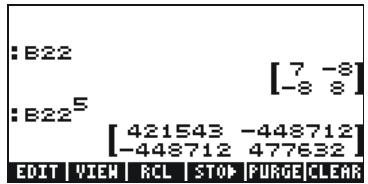
text_image
:B22 [7 -8] [-8 8] :B22^5 [421543 -448712] [-443712 477632] EDIT VIEW RCL STOP PURGE CLEARYou can also raise a matrix to a power without first storing it as a variable:
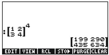
text_image
[: [1 2]⁴ [3 4] EDIT VIEW RCL STOP PURGE CLEAR [199 290] [435 634]In algebraic mode, the keystrokes are: [enter or select the matrix] ^x [enter the power] .
In RPN mode, the keystrokes are: [enter or select the matrix] SPC [enter the power] ^X ENTER.
The identity matrix
The identity matrix has the property that A · I = I · A = A . To verify this property we present the following examples using the matrices stored earlier on. Use function IDN (find it in the MTH/MATRIX/MAKE menu) to generate the identity matrix as shown here:
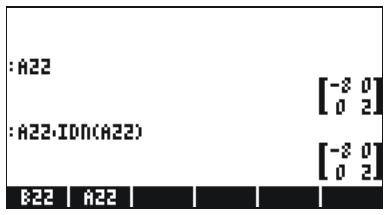
text_image
:A22 [ -8 0 ] [ 0 2 ] :A22·IDN(A22) [ -8 0 ] [ 0 2 ] B22 A22
text_image
:A22·IDN(A22) :IDN(A22)·A22 B22 | A22 [-8 0] [0 2] [-8 0] [0 2] [-8 0] [0 2]The inverse matrix
The inverse of a square matrix A is the matrix A^-1 such that A · A^-1 = A^-1 · A = I , where I is the identity matrix of the same dimensions as A. The inverse of a matrix is obtained in the calculator by using the inverse function, INV (i.e., the 1x key). Examples of the inverse of some of the matrices stored earlier are presented next:

text_image
:INV(A22) [ -1/2 0 0 1/2 ] B22 A22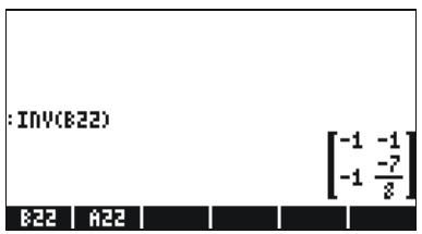
text_image
:INV(B22) [ -1 -1 -1 -7/2 ]To verify the properties of the inverse matrix, we present the following multiplications:

text_image
:A33·INV(A33) [1 0 0] 0 1 0] 0 0 1] :INV(B33)·B33 [1 0 0] 0 1 0] 0 0 1] B33 | A33 | B32 | A32 | B23 | A23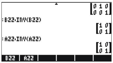
text_image
:B22·INV(B22) :A22·INV(A22)Characterizing a matrix (The matrix NORM menu)
The matrix NORM (NORMALIZE) menu is accessed through the keystroke sequence MTH . This menu is described in detail in Chapter 10 of the calculator's user's guide. Some of these functions are described next.
Function DET
Function DET calculates the determinant of a square matrix. For example,
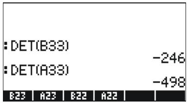
text_image
: DET(B33) -246 : DET(A33) -498 B23 A23 B22 A22
text_image
: DET(B22) : DET(A22) B23 A23 B22 A22 -8 -16Function TRACE
Function TRACE calculates the trace of square matrix, defined as the sum of the elements in its main diagonal, or
$$ t r (\mathbf {A}) = \sum_ {i = 1} ^ {n} a _ {i i} $$
Examples:
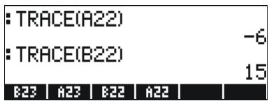
text_image
:TRACE(A22) :TRACE(B22) B23 | A23 | B22 | A22 -6 15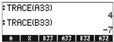
text_image
:TRACE(A33) :TRACE(B33) A X B33 A33 B32 A32 4 -7Solution of linear systems
A system of n linear equations in m variables can be written as
$$ \begin{array}{l} a _ {1 1} \cdot x _ {1} + a _ {1 2} \cdot x _ {2} + a _ {1 3} \cdot x _ {3} + \dots + a _ {1, m - 1} \cdot x _ {m - 1} + a _ {1, m} \cdot x _ {m} = b _ {1}, \ a _ {2 1} \cdot x _ {1} + a _ {2 2} \cdot x _ {2} + a _ {2 3} \cdot x _ {3} + \dots + a _ {2, m - 1} \cdot x _ {m - 1} + a _ {2, m} \cdot x _ {m} = b _ {2}, \ a _ {3 1} \cdot x _ {1} + a _ {3 2} \cdot x _ {2} + a _ {3 3} \cdot x _ {3} + \dots + a _ {3, m - 1} \cdot x _ {m - 1} + a _ {3, m} \cdot x _ {m} = b _ {3}, \ a _ {n - 1, 1} \cdot x _ {1} + a _ {n - 1, 2} \cdot x _ {2} + a _ {n - 1, 3} \cdot x _ {3} + \dots + a _ {n - 1, m - 1} \cdot x _ {m - 1} + a _ {n - 1, m} \cdot x _ {m} = b _ {n - 1}, \ a _ {n 1} \cdot x _ {1} + a _ {n 2} \cdot x _ {2} + a _ {n 3} \cdot x _ {3} + \dots + a _ {n, m - 1} \cdot x _ {m - 1} + a _ {n, m} \cdot x _ {m} = b _ {n}. \ \end{array} $$
This system of linear equations can be written as a matrix equation, A_n× m· x_m×1 = b_n×1 , if we define the following matrix and vectors:
$$ A = \left[ \begin{array}{c c c c} a _ {1 1} & a _ {1 2} & \dots & a _ {1 m} \ a _ {2 1} & a _ {2 2} & \dots & a _ {2 m} \ \vdots & \vdots & \ddots & \vdots \ a _ {n 1} & a _ {n 2} & \dots & a _ {n m} \end{array} \right] _ {n \times m}, x = \left[ \begin{array}{c} x _ {1} \ x _ {2} \ \vdots \ x _ {m} \end{array} \right] _ {m \times 1}, b = \left[ \begin{array}{c} b _ {1} \ b _ {2} \ \vdots \ b _ {n} \end{array} \right] _ {n \times 1} $$
Using the numerical solver for linear systems
There are many ways to solve a system of linear equations with the calculator. One possibility is through the numerical solver NUM.SLV. From the numerical solver screen, shown below (left), select the option 4. Solve lin sys., and press 08 . The following input form will be provide (right):
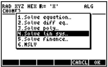
text_image
RAD XYZ HEX R= 'X' CHOMF3 1.Solve equation.. 2.Solve diff eq.. 3.Solve poly.. 4.Solve lin sys.. 5.Solve Finance.. 6.MSLV CANCEL OK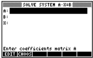
text_image
SOLVE SYSTEM A·X=B A: B: X: Enter coefficients matrix A EDIT CHOOSTo solve the linear system A · x = b , enter the matrix A , in the format [a_11, a_12, ], []] in the A: field. Also, enter the vector b in the B: field. When the X: field is highlighted, press SOLIC. If a solution is available, the solution vector x will be shown in the X: field. The solution is also copied to stack level 1. Some examples follow.
The system of linear equations
$$ 2 x _ {1} + 3 x _ {2} - 5 x _ {3} = 1 3, $$
$$ x _ {1} - 3 x _ {2} + 8 x _ {3} = - 1 3, $$
$$ 2 x _ {1} - 2 x _ {2} + 4 x _ {3} = - 6, $$
can be written as the matrix equation A · x = b , if
$$ \mathbf {A} = \left[ \begin{array}{c c c} 2 & 3 & - 5 \ 1 & - 3 & 8 \ 2 & - 2 & 4 \end{array} \right], \quad \mathbf {x} = \left[ \begin{array}{c} x _ {1} \ x _ {2} \ x _ {3} \end{array} \right], \quad a n d \quad \mathbf {b} = \left[ \begin{array}{c} 1 3 \ - 1 3 \ - 6 \end{array} \right]. $$
This system has the same number of equations as of unknowns, and will be referred to as a square system. In general, there should be a unique solution to the system. The solution will be the point of intersection of the three planes in the coordinate system (x_1, x_2, x_3) represented by the three equations.
To enter matrix A you can activate the Matrix Writer while the A: field is selected. The following screen shows the Matrix Writer used for entering matrix A, as well as the input form for the numerical solver after entering matrix A (press ENTER in the Matrix Writer):
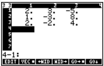
text_image
3 3 1 2 3 1 2. 3. -5. 2 1. -3. 8. 3 2. -2. 4. 4 5 6 7 4-1: EDIT VEC +MID MID+ GO+ G0+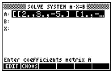
text_image
SOLVE SYSTEM A·X=B A: [[2.,3.,-5.] [1.,-... B: X: Enter coefficients matrix A EDIT CHOOSPress ▼ to select the B: field. The vector b can be entered as a row vector with a single set of brackets, i.e., [13,-13,-6]
After entering matrix A and vector b, and with the X: field highlighted, we can press ☐ to attempt a solution to this system of equations:
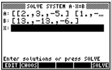
text_image
SOLVE SYSTEM A-X=B A: [[2.,3.,-5.] [1.,-... B: [13.,-13.,-6.] X: Enter solutions or press SOLVE EDIT CHOOS SOLVEA solution was found as shown next.
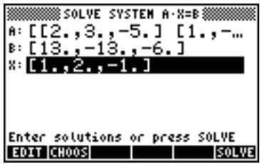
text_image
SOLVE SYSTEM A: X=B A: [[2.,3.,-5.] [1.,-... B: [13.,-13.,-6.] X: [1.,2.,-1.] Enter solutions or press SOLVE EDIT CHOOS SOLVESolution with the inverse matrix
The solution to the system A · x = b , where A is a square matrix is
x = A^-1 · b . For the example used earlier, we can find the solution in the calculator as follows (First enter matrix A and vector b once more):
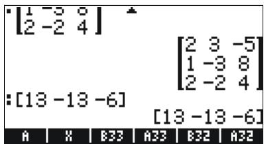
text_image
•[1 -3 0] [2 -2 4] [2 3 -5] [1 -3 8] [2 -2 4] :[13 -13 -6] [13 -13 -6] A X B33 A33 B32 A32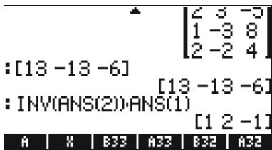
text_image
2 3 -5 1 -3 8 2 -2 4 : [13 -13 -6] [13 -13 -6] : INV(ANS(2))·ANS(1) [1 2 -1] A X B33 A33 B32 A32Solution by "division" of matrices
While the operation of division is not defined for matrices, we can use the calculator's ÷ key to "divide" vector b by matrix A to solve for x in the matrix equation A · x = b . The procedure for the case of "dividing" b by A is illustrated below for the example above.
The procedure is shown in the following screen shots (type in matrices A and vector b once more):
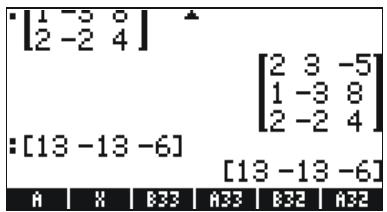
text_image
•[1 -3 0] [2 -2 4] [2 3 -5] [1 -3 8] [2 -2 4] : [13 -13 -6] [13 -13 -6] A X B33 A33 B32 A32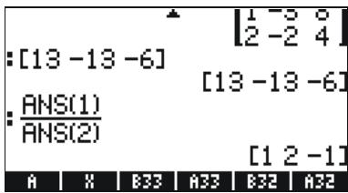
text_image
1 - 3 0 2 - 2 4 : [13 - 13 - 6] [13 - 13 - 6] ANS(1) ANS(2) [1 2 - 1] A X B33 A33 B32 A32References
Additional information on creating matrices, matrix operations, and matrix applications in linear algebra is presented in Chapters 10 and 11 of the calculator's user's guide.
Chapter 10 Graphics
In this chapter we introduce some of the graphics capabilities of the calculator. We will present graphics of functions in Cartesian coordinates and polar coordinates, parametric plots, graphics of conics, bar plots, scatterplots, and fast 3D plots.
Graphs options in the calculator
To access the list of graphic formats available in the calculator, use the keystroke sequence 2D/3D (F4) Please notice that if you are using the RPN mode these two keys must be pressed simultaneously to activate any of the graph functions. After activating the 2D/3D function, the calculator will produce the PLOT SETUP window, which includes the TYPE field as illustrated below.
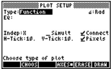
text_image
PLOT SETUP Type:Function EQ: Indep:X H-Tick:10. _Simult V-Tick:10. ✓Connect ✓Pixels Choose type of plot CHOOS AXES■ERASE DRAWRight in front of the TYPE field you will, most likely, see the option Function highlighted. This is the default type of graph for the calculator. To see the list of available graph types, press the soft menu key labeled 📄. This will produce a drop down menu with the following options (use the up- and down-arrow keys to see all the options):

text_image
Type EQ: Inde H-Ti Choo Function Polar Parametric Diff Eq Conic Truth Histogram Bar Scatter Rad nects OK Cancel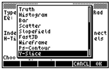
text_image
Type EQ: Inde H-Ti Choo Truth Histogram Bar Scatter SlopeField Fast3D Wireframe Ps-Contour Y-Slice Rad nects OK CANCEL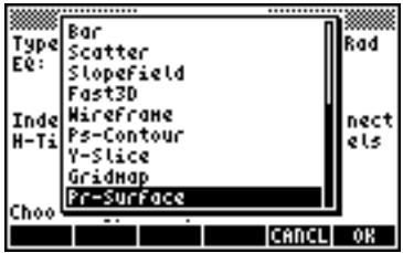
text_image
Type EQ: Bar Scatter SlopeField Fast3D Inde H-Ti Wireframe Ps-Contour Y-Slice Gridmap Pr-Surface Choo Rad nects CANCEL OKPlotting an expression of the form y = f(x)
As an example, let's plot the function,
$$ f (x) = \frac {1}{\sqrt {2 \pi}} \exp (- \frac {x ^ {2}}{2}) $$
- First, enter the PLOT SETUP environment by pressing, 2D/3D. Make sure that the option Function is selected as the TYPE, and that 'X' is selected as the independent variable (INDEP). Press NXT to return to normal calculator display. The PLOT SET UP window should look similar to this:
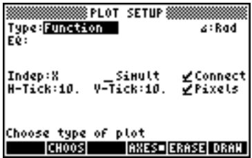
text_image
PLOT SETUP Type:Function EQ: Indep:X H-Tick:10. Simult Y-Tick:10. Connect Pixels Choose type of plot CHOOS AXES ERASE DRAW- Enter the PLOT environment by pressing Y= (press them simultaneously if in RPN mode). Press [10] to get you into the equation writer. You will be prompted to fill the right-hand side of an equation Y1(x) = ■. Type the function to be plotted so that the Equation Writer shows the following:

text_image
Y1(X)=e^(-x^2)/\sqrt{2·π} EDIT CURS BIG EVAL FACTO SIMP- Press ENTER to return to the PLOT - FUNCTION window. The expression 'Y1(X) = EXP(-X^2/2)/√(2*π)' will be highlighted. Press NXT to return to normal calculator display.
- Enter the PLOT WINDOW environment by entering WIN (press them simultaneously if in RPN mode). Use a range of -4 to 4 for H-VIEW, then press 100 to generate the V-VIEW automatically. The PLOT WINDOW screen looks as follows:
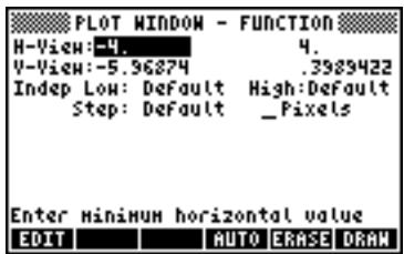
text_image
PLOT WINDOW - FUNCTION H-View:-4. 4. V-View:-5.96874 .3989422 Indep Low: Default High:Default Step: Default _Pixels Enter MINIMUM horizontal value EDIT AUTO ERASE DRAW- Plot the graph: [REDA] [REDA] (wait till the calculator finishes the graphs)
• To see labels: 📄300 📝NXT 📋1834 📋1300
• To recover the first graphics menu: NXT NXT - To trace the curve: 📄️. Then use the right- and left-arrow keys (◀▶) to move about the curve. The coordinates of the points you trace will be shown at the bottom of the screen. Check that for x = 1.05, y = 0.0231. Also, check that for x = -1.48, y = 0.134. Here is picture of the graph in tracing mode:
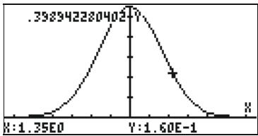
line
| X Value | Y Value | | ----------- | --------- | | 1.35E0 | 0 | | 1.60E-1 | 0.398942280402 | | | 0 |- To recover the menu, and return to the PLOT WINDOW environment, press NXT 📄️. Press NXT 📄️ to return to normal display.
Generating a table of values for a function
The combinations TBLSET (F5) and TABLE (F6), pressed simultaneously if in RPN mode, let's the user produce a table of values of functions. For example, we will produce a table of the function Y(X) = X / (X + 10) , in the range -5 < X < 5 following these instructions:
- We will generate values of the function f(x) , defined above, for values of x from -5 to 5, in increments of 0.5. First, we need to ensure that the graph type is set to FUNCTION in the PLOT SETUP screen (←2D/3D, press them simultaneously, if in RPN mode). The field in front of the Type option will be highlighted. If this field is not already set to FUNCTION, press the soft key CHECK and select the FUNCTION option, then press OK.
- Next, press ▼ to highlight the field in front of the option EQ, and type the function expression: 'X/(X+10)'. Press ENTER.
- To accept the changes made to the PLOT SETUP screen press NXT OK. You will be returned to normal calculator display.
- The next step is to access the Table Set-up screen by using the keystroke combination TBLSET (i.e., soft key F5) – simultaneously if in RPN mode. This will produce a screen where you can select the starting value (Start) and the increment (Step). Enter the following: 5 +/- 0 · 5 0 · 5 (i.e., Zoom factor = 0.5).
Toggle the 📄️ soft menu key until a check mark appears in front of the option Small Font if you so desire. Then press 📄️. This will return you to normal calculator display.
- To see the table, press TABLE (i.e., soft menu key F6 ) - simultaneously if in RPN mode. This will produce a table of values of x = -5, -4.5, , and the corresponding values of f(x) , listed as Y1 by default. You can use the up and down arrow keys to move about in the table. You will notice that we did not have to indicate an ending value for the independent variable x . Thus, the table continues beyond the maximum value for x suggested early, namely x = 5 .
Some options available while the table is visible are ☐001, ☐34, and ☐030:
- The [REED], when selected, shows the definition of the independent variable.
- The ☐key simply changes the font in the table from small to big, and vice versa. Try it.
-
The ☐ key, when pressed, produces a menu with the options: In, Out, Decimal, Integer, and Trig. Try the following exercises:
-
With the option In highlighted, press 0.8. The table is expanded so that the x-increment is now 0.25 rather than 0.5. Simply, what the calculator does is to multiply the original increment, 0.5, by the zoom factor, 0.5, to produce the new increment of 0.25. Thus, the zoom in option is useful when you want more resolution for the values of x in your table.
- To increase the resolution by an additional factor of 0.5 press [1001], select In once more, and press [0]. The x-increment is now 0.0125.
- To recover the previous x-increment, press 📄0001 ▲ 0.8 to select the option Un-zoom. The x-increment is increased to 0.25.
- To recover the original x-increment of 0.5 you can do an un-zoom again, or use the option zoom out by pressing 📄.
- The option Decimal in 📄 produces x-increments of 0.10.
- The option Integer in 📄 produces x-increments of 1.
- The option Trig in produces increments related to fractions of , thus being useful when producing tables of trigonometric functions.
• To return to normal calculator display press ENTER.
Fast 3D plots
Fast 3D plots are used to visualize three-dimensional surfaces represented by equations of the form z = f(x, y) . For example, if you want to visualize z = f(x, y) = x^2 + y^2 , we can use the following:
- Press 2D/3D , simultaneously if in RPN mode, to access to the PLOT SETUP window.
- Change TYPE to Fast3D. ( [100E, find Fast3D, 08]).
- Press ▼ and type 'X^2+Y^2'
- Make sure that 'X' is selected as the Indep: and 'Y' as the Depnd: variables.
- Press NXT to return to normal calculator display.
- Press WIN, simultaneously if in RPN mode, to access the PLOT WINDOW screen.
- Keep the default plot window ranges to read:
X-Left:-1 X-Right:1
Y-Near:-1 Y-Far: 1
Z-Low: -1 Z-High: 1
Step Indep: 10 Depnd: 8
NOTE: The Step Indep: and Depnd: values represent the number of gridlines to be used in the plot. The larger these number, the slower it is to produce the graph, although, the times utilized for graphic generation are relatively fast. For the time being we'll keep the default values of 10 and 8 for the Step data.
- Press FREE TO draw the three-dimensional surface. The result is a wireframe picture of the surface with the reference coordinate system shown at the lower left corner of the screen. By using the arrow keys (◀▶▲▼) you can change the orientation of the surface. The orientation of the reference coordinate system will change accordingly. Try changing the surface orientation on your own. The following figures show a couple of views of the graph:

natural_image
3D wireframe surface plot with coordinate axes labeled TRACE and EXIT (no text or symbols on the surface itself)
natural_image
Pure 3D wireframe diagram of a curved surface with coordinate axes labeled TRACE and EXIT (no text or symbols beyond labels)- When done, press 📄.
- Press PRICE to return to the PLOT WINDOW environment.
- Change the Step data to read: Step Indep: 20 Depnd: 16
- Press ☐ to see the surface plot. Sample views:

natural_image
3D wireframe surface plot with coordinate axes labeled TRACE and EXIT (no text or symbols on the surface itself)
natural_image
3D wireframe grid model of a curved surface, labeled with 'TRACE' and 'EXIT' at bottom (no other text or symbols)- When done, press 📄.
- Press 📄 to return to PLOT WINDOW.
- Press ON, or NXT, to return to normal calculator display.
Try also a Fast 3D plot for the surface z = f(x, y) = (x^2 + y^2)
- Press 2D/3D , simultaneously if in RPN mode, to access the PLOT SETUP window.
- Press ▼ and type 'SIN(X^2+Y^2)'
- Press 📄️ 📄️ 📄️ 📄️ to draw the slope field plot. Press 📄️ 📄️ 📄️ 📄️ 📄️ 📄️ 📄️ 📄️ 📄️ 📄️ 📄️ 📄️ 📄️ 📄️ 📄️ 📄️ 📄️ 📄️ 📄️ 📄️ 📄️ 📄️ 📄️ 📄️ 📄️ 📄> to see the plot unencumbered by the menu and with identifying labels.
- Press NXT NXT to leave the EDIT environment.
- Press 📄 to return to the PLOT WINDOW environment. Then, press ON, or NXT OK, to return to normal calculator display.
Reference
Additional information on graphics is available in Chapters 12 and 22 in the calculator's user's guide.
Chapter 11 Calculus Applications
In this Chapter we discuss applications of the calculator's functions to operations related to Calculus, e.g., limits, derivatives, integrals, power series, etc.
The CALC (Calculus) menu
Many of the functions presented in this Chapter are contained in the calculator's CALC menu, available through the keystroke sequence ← CALC (associated with the 4 key):

text_image
RAD XYZ HEX R- 'X' ALG CHOM CALC MENU 1. DERIV. & INTEG.. 2. LIMITS & SERIES.. 3. DIFFERENTIAL EENS.. 4. GRAPH.. 5. DERVX 6. INTVX CANCEL OKThe first four options in this menu are actually sub-menus that apply to (1) derivatives and integrals, (2) limits and power series, (3) differential equations, and (4) graphics. The functions in entries (1) and (2) will be presented in this Chapter. Functions DERVX and INTVX are discussed in page 11-3, respectively.
Limits and derivatives
Differential calculus deals with derivatives, or rates of change, of functions and their applications in mathematical analysis. The derivative of a function is defined as a limit of the difference of a function as the increment in the independent variable tends to zero. Limits are used also to check the continuity of functions.
Function lim
The calculator provides function lim to calculate limits of functions. This function uses as input an expression representing a function and the value where the limit is to be calculated. Function lim is available through the command catalog (CAT ALPHA) or through option 2. LIMITS & SERIES... of the CALC menu (see above).
Function lim is entered in ALG mode as _x af(x) , x=a) to calculate the limit _x af(x) . In RPN mode, enter the function first, then the expression 'x=a', and finally function lim. Examples in ALG mode are shown next, including some limits to infinity, and one-sided limits. The infinity symbol is associated with the 0 key, i.e., .

text_image
: lim(X+1) X→1 2 : lim(X²-2) X→1 -1 CASCM HELP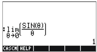
text_image
: lim_{θ→0} \left( \frac{SIN(θ)}{θ} \right) \quad 1 CASCM | HELP | | | | | | |
text_image
RAD XYZ HEX R= 'X' ALG CHOME3 : lim(x→ω(1/x²)) CASCH HELPTo calculate one-sided limits, add +0 or -0 to the value to the variable. A “+0” means limit from the right, while a “-0” means limit from the left. For example, the limit of -1 as x approaches 1 from the left can be determined with the following keystrokes (ALG mode):

text_image
CAT ALPHA ← L √X ∽ ( ) X —
The result is as follows:
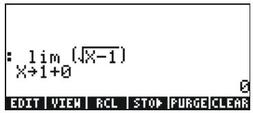
text_image
: lim (√x-1) X→1+0 EDIT VIEW RCL STOP PURGE CLEARFunctions DERIV and DERVX
The function DERIV is used to take derivatives in terms of any independent variable, while the function DERVX takes derivatives with respect to the CAS default variable VX (typically 'X'). While function DERVX is available directly in the CALC menu, both functions are available in the DERIV.&INTEG sub-menu within the CALCL menu ( CALC ).
Function DERIV requires a function, say f(t) , and an independent variable, say, t, while function DERVX requires only a function of VX. Examples are shown next in ALG mode. Recall that in RPN mode the arguments must be entered before the function is applied.
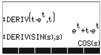
text_image
:DERIV(t·e^t, t) :DERIV(SIN(s), s) e^t + t·e^t COS(s)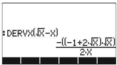
text_image
:DERVX(√x-x) -((-1+2√x)-√x)/2*xAnti-derivatives and integrals
An anti-derivative of a function f(x) is a function F(x) such that f(x) = dF/dx . One way to represent an anti-derivative is as a indefinite integral, i.e.,
$$ \int f (x) d x = F (x) + C $$
if and only if, f(x) = dF/dx , and C = constant.
Functions INT, INTVX, RISCH, SIGMA and SIGMAVX
The calculator provides functions INT, INTVX, RISCH, SIGMA and SIGMAVX to calculate anti-derivatives of functions. Functions INT, RISCH, and SIGMA work with functions of any variable, while functions INTVX, and SIGMAVX utilize functions of the CAS variable VX (typically, 'x'). Functions INT and RISCH require, therefore, not only the expression for the function being integrated, but also the independent variable name. Function INT, requires also a value of x where the anti-derivative will be evaluated. Functions INTVX and SIGMAVX require only the expression of the function to integrate in terms of VX. Functions INTVX, RISCH, SIGMA and SIGMAVX are available in the CALC/DERIV&INTEG menu, while INT is available in the command catalog. Some examples are shown next in ALG mode (type the function names to activate them):
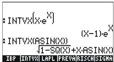
text_image
: INTVX(x·e^X) (X-1)e^X : INTVX(ASIN(X)) √(1-SQ(X)+X·ASIN(X)) IBP INTVX LAPL PREVA RISCH SIGMA
text_image
:INT(s²-s,s,z) 2/3 :RISCH(s²-s,s) 1/3·s²-1/2·s² IBP |INTVX| LAPL |PREVA|RISCH|SIGMA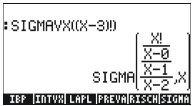
text_image
:SIGMAVX((X-3)!) SIGMA(!X-0\\-1X-2,X) IBP |INTVX| LAPL |PREVA|RISCH|SIGMA
text_image
:SIGMA(s·s!,s) IBP |INTVX| LAFL |PREVA|RISCH|SIGMAPlease notice that functions SIGMAVX and SIGMA are designed for integrands that involve some sort of integer function like the factorial (!) function shown above. Their result is the so-called discrete derivative, i.e., one defined for integer numbers only.
Definite integrals
In a definite integral of a function, the resulting anti-derivative is evaluated at the upper and lower limit of an interval (a,b) and the evaluated values subtracted. Symbolically, _a^bf(x)dx = F(b) - F(a) , where f(x) = dF/dx .
The PREVAL(f(x),a,b) function of the CAS can simplify such calculation by returning f(b)-f(a) with x being the CAS variable VX.
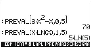
text_image
:PREVAL(3·x²-x,0,5) 70 :PREVAL(X·LN(X),1,5) 5·LN(5) IBP |INTYX| LAPL |PREVA|RISCH|SIGMAInfinite series
A function f(x) can be expanded into an infinite series around a point x=x_0 by using a Taylor's series, namely,
$$ f (x) = \sum_ {n = 0} ^ {\infty} \frac {f ^ {(n)} (x _ {o})}{n !} \cdot (x - x _ {o}) ^ {n}, $$
where f^(n)(x) represents the n-th derivative of f(x) with respect to x, f^(0)(x) = f(x) .
If the value x_0=0 , the series is referred to as a Maclaurin's series.
Functions TAYLR, TAYLRO, and SERIES
Functions TAYLR, TAYLRO, and SERIES are used to generate Taylor polynomials, as well as Taylor series with residuals. These functions are available in the CALC/LIMITS&SERIES menu described earlier in this Chapter.
Function TAYLOR0 performs a Maclaurin series expansion, i.e., about X = 0, of an expression in the default independent variable, VX (typically 'X'). The expansion uses a 4-th order relative power, i.e., the difference between the highest and lowest power in the expansion is 4. For example,
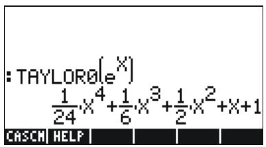
text_image
: TAYLOR0(e^X) 1/24 x^4 + 1/6 x^3 + 1/2 x^2 + x + 1 CASCH HELP
text_image
:TAYLOR0(SIN(X)) 1/120·x^5 + -1/6·x^3 + x DIVPC Lin SERIE TAYLO TAYLR CALCFunction TAYLR produces a Taylor series expansion of a function of any variable x about a point x = a for the order k specified by the user. Thus, the function has the format TAYLR(f(x-a),x,k). For example,
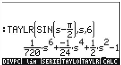
text_image
:TAYLR[SIN[s-π/2],s,6] 1/720·s^6+ -1/24·s^4+ 1/2·s^2-1 DIVPC LIN SERIE TAYLO TAYLR CALC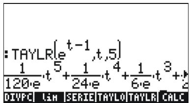
text_image
:TAYLR(e^t-1,t,5)\n\frac{1}{120\cdot e}\cdot t^5+\frac{1}{24\cdot e}\cdot t^4+\frac{1}{6\cdot e}\cdot t^3+\frac{1}{2}\nDIVPC LIN SERIE TAYLO TAYLR CALCFunction SERIES produces a Taylor polynomial using as arguments the function f(x) to be expanded, a variable name alone (for Maclaurin's
series) or an expression of the form 'variable = value' indicating the point of expansion of a Taylor series, and the order of the series to be produced. Function SERIES returns two output items: a list with four items, and an expression for h = x - a, if the second argument in the function call is 'x=a', i.e., an expression for the increment h. The list returned as the first output object includes the following items:
- Bi-directional limit of the function at point of expansion, i.e., _x af(x)
- An equivalent value of the function near x = a
- Expression for the Taylor polynomial
- Order of the residual or remainder
Because of the relatively large amount of output, this function is easier to handle in RPN mode. For example, the following screen shots show the RPN stack before and after using the TAYLR function, as illustrated above:

text_image
8 5 4 3 2 1: 'S' EDIT VIEW RCL STOP PURGE CLEAR
text_image
4: 3: 2: 1: ' s' π 2 EDIT VIEW RCL STOP PURGE CLEAR
text_image
4: 03: 2: 1: EDIT VIEW RCL STOP PURGE CLEAR S-π/2
text_image
4: 3: 2: 1: SIN[s-π/2] EDIT VIEW RCL STOP PURGE CLEAR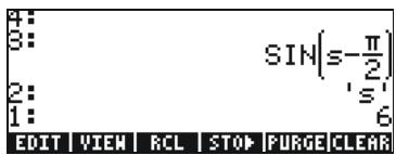
text_image
4: 3: 2: 1: SIN(s-π/2) 's' 6 EDIT VIEW RCL STOP PURGE CLEAR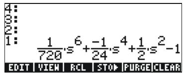
text_image
4: 3: 2: 1: 1/720·s^6 + -1/24·s^4 + 1/2·s^2 -1 EDIT VIEW RCL STOP PURGE CLEARThe keystrokes that generate this particular example are:

text_image
ALPHA ← S ENTER ← π 2 ÷ — SIN ALPHA ← S ENTER 6 ← CALC ▼ ▼ ▼ ▼ ▼Reference
Additional definitions and applications of calculus operations are presented in Chapter 13 in the calculator's user's guide.
Chapter 12 Multi-variate Calculus Applications
Multi-variate calculus refers to functions of two or more variables. In this Chapter we discuss basic concepts of multi-variate calculus: partial derivatives and multiple integrals.
Partial derivatives
To quickly calculate partial derivatives of multi-variate functions, use the rules of ordinary derivatives with respect to the variable of interest, while considering all other variables as constant. For example,
$$ \frac {\partial}{\partial x} (x \cos (y)) = \cos (y), \frac {\partial}{\partial y} (x \cos (y)) = - x \sin (y) $$
You can use the derivative functions in the calculator: DERVX, DERIV, , described in detail in Chapter 11 of this manual, to calculate partial derivatives (DERVX uses the CAS default variable VX, typically, 'X'). Some examples of first-order partial derivatives are shown next. The functions used in the first two examples are f(x,y) = x (y) , and g(x,y,z) = (x^2 + y^2)^1/2 (z) .

text_image
: ∂(f(x,y)) ∂x COS(y) : ∂(f(x,y)) ∂y x1-SIN(y) g | f | HNS | PPAR | GRPHS | HPFIT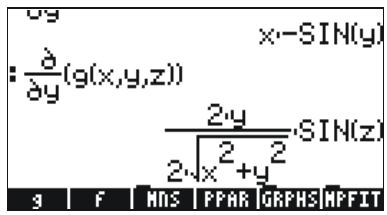
text_image
y x-SIN(y) : ∂(g(x,y,z)) 2·y SIN(z) 2√x²+y² g | F | MDS | PPAR | GRAPHS | HPFIT
text_image
:DERVX(x·Y²-Y²) :DERVX(X·SIN(Y+X)) COS(X+Y)·X+SIN(X+Y) CURL DERIVDERVX DIV FOURI HESS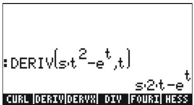
text_image
:DERIV(s·t^2-e^t,t) s·2·t-e^t CURL DERIV DERIV DIV FOURI HESSTo define the functions f(x,y) and g(x,y,z) , in ALG mode, use:
$$ \operatorname{DEF} (f (x, y) = x ^ {} \cos (y)) \boxed {\text { ENTER }} \quad \operatorname{DEF} (g (x, y, z) = \sqrt {(x ^ {\wedge} 2 + y ^ {\wedge} 2) ^ {} \sin (z)} \boxed {\text { ENTER }} $$
To type the derivative symbol use ____. The derivative x(f(x,y)) , for example, will be entered as x(f(x,y)) ENTER in ALG mode in the screen.
Multiple integrals
A physical interpretation of the double integral of a function f(x,y) over a region R on the x-y plane is the volume of the solid body contained under the surface f(x,y) above the region R. The region R can be described as R = a < x < b, f(x) < y < g(x) or as R = c < y < d, r(y) < x < s(y) . Thus, the double integral can be written as
$$ \iint_ {R} \phi (x, y) d A = \int_ {a} ^ {b} \int_ {f (x)} ^ {g (x)} \phi (x, y) d y d x = \int_ {c} ^ {d} \int_ {r (y)} ^ {s (y)} \phi (x, y) d y d x $$
Calculating a double integral in the calculator is straightforward. A double integral can be built in the Equation Writer (see example in Chapter 2 in the user's guide), as shown below. This double integral is calculated directly in the Equation Writer by selecting the entire expression and using function [RELL]. The result is 3/2.

text_image
∫²/1∫x x+dy dx♦ EDIT | CURS | BIG ■ | EVAL | FACTO | SIMP
text_image
3 2 EDIT CURS BIG ■ EVAL FACTO SIMPReference
For additional details of multi-variate calculus operations and their applications see Chapter 14 in the calculator's user's guide.
Chapter 13 Vector Analysis Applications
This chapter describes the use of functions HESS, DIV, and CURL, for calculating operations of vector analysis.
The del operator
The following operator, referred to as the 'del' or 'nabla' operator, is a vector-based operator that can be applied to a scalar or vector function:
$$ \nabla [ \mathbf {\Phi} ] = i \cdot \frac {\partial}{\partial x} [ \mathbf {\Phi} ] + j \cdot \frac {\partial}{\partial y} [ \mathbf {\Phi} ] + k \cdot \frac {\partial}{\partial z} [ \mathbf {\Phi} ] $$
When applied to a scalar function we can obtain the gradient of the function, and when applied to a vector function we can obtain the divergence and the curl of that function. A combination of gradient and divergence produces the Laplacian of a scalar function.
Gradient
The gradient of a scalar function (x,y,z) is a vector function defined by grad = . Function HESS can be used to obtain the gradient of a function.. The function takes as input a function of n independent variables (x_1, x_2, ..., x_n) , and a vector of the functions ['x₁', 'x₂', ...'xₙ']. The function returns the Hessian matrix of the function, H = [h_ij] = [/ x_i x_j] , the gradient of the function with respect to the n-variables, grad f = [ / x_1 / x_2 ... / x_n ], and the list of variables ['x₁', 'x₂', ..., 'xₙ']. This function is easier to visualize in the RPN mode. Consider as an example the function (X,Y,Z) = X^2 + XY + XZ , we'll apply function HESS to this scalar field in the following example:
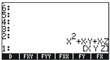
text_image
5 6 5 4 3 2 1: D | FXY | FYY | FXX | FY | FX X²+XY+XZ [X Y Z]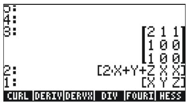
text_image
3: 4: 3: 2: 1: [2 1 1] [1 0 0] [1 0 0] [2-X+Y+Z X X] [CX Y Z] CURL DERIV DERIVX DIY FOURI HESSThus, the gradient is [2X+Y+Z, X, X] .
Alternatively, use function DERIV as follows:

text_image
:DERIV(X²+XY+XZ,[XYZ]) [2X+Y+ZXX] EDIT VIEW RCL STOP PURGE CLEARDivergence
The divergence of a vector function, F(x,y,z) = f(x,y,z)i + g(x,y,z)j + h(x,y,z)k , is defined by taking a "dot-product" of the del operator with the function, i.e., divF = F . Function DIV can be used to calculate the divergence of a vector field. For example, for F(X,Y,Z) = [XY,X^2 + Y^2 + Z^2, YZ] , the divergence is calculated, in ALG mode, as follows: DIV([X^Y,X^2 + Y^2 + Z^2, Y^Z],[X,Y,Z])
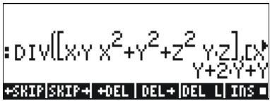
text_image
:DIV{[X·Y X²+Y²+z² Y·Z], [X·Y+2·Y+Y] +SKIP|SKIP+ | +DEL | DEL+ | DEL | L | INS =Curl
The curl of a vector field F(x,y,z)=f(x,y,z)i+g(x,y,z)j+h(x,y,z)k , is defined by a “cross-product” of the del operator with the vector field, i.e., curlF=×F . The curl of vector field can be calculated with function CURL. For example, for the function F(X,Y,Z)=[XY,X^2+Y^2+Z^2,YZ] , the curl is calculated as follows: CURL([X^Y,X^2+Y^2+Z^2,Y^Z],[X,Y,Z])

text_image
: CURL([x·y x²+y²+z² y·z], [z-2·z 0 2x-x]) CURL |DERIV|DERVX| DIV |FOURI| HESSReference
For additional information on vector analysis applications see Chapter 15 in the calculator's user's guide.
Chapter 14 Differential Equations
In this Chapter we present examples of solving ordinary differential equations (ODE) using calculator functions. A differential equation is an equation involving derivatives of the independent variable. In most cases, we seek the dependent function that satisfies the differential equation.
The CALC/DIFF menu
The DIFFERENTIAL EQNS.. sub-menu within the CALC ( CALC ) menu provides functions for the solution of differential equations. The menu is listed below with system flag 117 set to CHOOSE boxes:
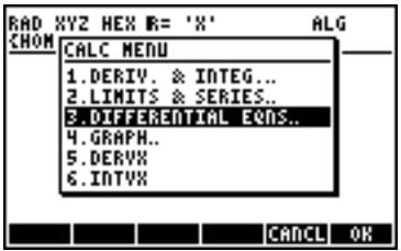
text_image
RAD XYZ HEX R= 'X' ALG CHOM CALC MENU 1.DERIV. & INTEG.. 2.LIMITS & SERIES.. 3.DIFFERENTIAL EQNS.. 4.GRAPH.. 5.DERVX.. 6.INTVX.. CANCEL OK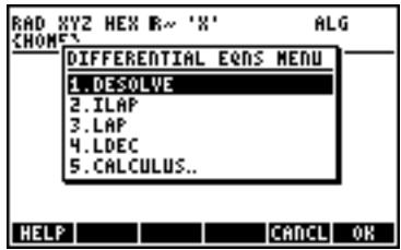
text_image
RAD XYZ HEX R- 'X' ALG CHOME DIFFERENTIAL EQNS MENU 1. DESOLVE 2. ILAP 3. LAP 4. LDEC 5. CALCULUS.. HELP CANCEL OKThese functions are briefly described next. They will be described in more detail in later parts of this Chapter.
DESOLVE: Differential Equation SOLVER, solves differential equations, when possible
ILAP: Inverse LAPlace transform, L^-1[F(s)] = f(t)
LAP: LAPlace transform, L[f(t)]=F(s)
LDEC: Linear Differential Equation Command
Solution to linear and non-linear equations
An equation in which the dependent variable and all its pertinent derivatives are of the first degree is referred to as a linear differential equation. Otherwise, the equation is said to be non-linear.
Function LDEC
The calculator provides function LDEC (Linear Differential Equation Command) to find the general solution to a linear ODE of any order with constant coefficients, whether it is homogeneous or not. This function requires you to provide two pieces of input:
• the right-hand side of the ODE
• the characteristic equation of the ODE
Both of these inputs must be given in terms of the default independent variable for the calculator's CAS (typically X). The output from the function is the general solution of the ODE. The examples below are shown in the RPN mode:
Example 1 – To solve the homogeneous ODE
$$ \mathrm{d} ^ {3} \mathrm{y} / \mathrm{dx} ^ {3} - 4 \cdot (\mathrm{d} ^ {2} \mathrm{y} / \mathrm{dx} ^ {2}) - 1 1 \cdot (\mathrm{dy} / \mathrm{dx}) + 3 0 \cdot \mathrm{y} = 0. $$
Enter:
$$ 0 \text { ENTER } ^ {\prime} X ^ {\wedge} 3 - 4 * X ^ {\wedge} 2 - 1 1 * X + 3 0 ^ {\prime} \text { ENTER LDEC EVAL } $$
The solution is (figure put together from EQW screenshots):
$$ \frac {(1 2 0 \cdot c C 0 + 1 6 \cdot c C 1 - 8 \cdot c C 2) \cdot e ^ {3 \cdot X} \cdot e ^ {2 \cdot X} - \left((3 0 \cdot c C 0 - (5 \cdot c C 1 + 5 \cdot c C 2)) \cdot e ^ {5 \cdot X} \cdot e ^ {3 \cdot X} - (3 0 \cdot c C 0 - (2 1 \cdot c C 1 - 3 \cdot c C 2))\right)}{1 2 0 \cdot e ^ {3 \cdot X}} $$
where cC0, cC1, and cC2 are constants of integration. This result is equivalent to
$$ y = K _ {1} \cdot e ^ {- 3 x} + K _ {2} \cdot e ^ {5 x} + K _ {3} \cdot e ^ {2 x}. $$
Example 2 - Using the function LDEC, solve the non-homogeneous ODE:
$$ d ^ {3} y / d x ^ {3} - 4 \cdot (d ^ {2} y / d x ^ {2}) - 1 1 \cdot (d y / d x) + 3 0 \cdot y = x ^ {2}. $$
Enter:
$$ ^ {\prime} X ^ {\wedge} 2 ^ {\prime} \boxed {E N T E R} ^ {\prime} X ^ {\wedge} 3 - 4 * X ^ {\wedge} 2 - 1 1 * X + 3 0 ^ {\prime} \boxed {E N T E R} L D E C \boxed {E V A L} $$
The solution is:
$$ \frac {(2 7 0 0 0 \mathrm{cC} 0 + 3 6 0 0 \mathrm{cC} 1 - (1 8 0 0 \mathrm{cC} 2 + 4 5 0)) \mathrm{e} ^ {3 \mathrm{X}} \mathrm{e} ^ {2 \mathrm{X}} - \left[ \left((6 7 5 0 \mathrm{cC} 0 - (1 1 2 5 \mathrm{cC} 1 + 1 1 2 5 \mathrm{cC} 2 + 1 8)) \mathrm{e} ^ {5 \mathrm{X}} - (9 8 0 \mathrm{X} ^ {2} + 6 6 0 \mathrm{X} + 4 8 2)\right) \mathrm{e} ^ {3 \mathrm{X}} - (6 7 5 0 \mathrm{cC} 0 - (4 7 2 5 \mathrm{cC} 1 - (6 7 5 \mathrm{cC} 2 - 5 0)) \right])}{2 7 0 0 0 \mathrm{e} ^ {3 \mathrm{X}}} $$
which is equivalent to
$$ y = K _ {1} \cdot e ^ {- 3 x} + K _ {2} \cdot e ^ {5 x} + K _ {3} \cdot e ^ {2 x} + (4 5 0 \cdot x ^ {2} + 3 3 0 \cdot x + 2 4 1) / 1 3 5 0 0. $$
Function DESOLVE
The calculator provides function DESOLVE (Differential Equation SOLVER) to solve certain types of differential equations. The function requires as input the differential equation and the unknown function, and returns the solution to the equation if available. You can also provide a vector containing the differential equation and the initial conditions, instead of only a differential equation, as input to DESOLVE. The function DESOLVE is available in the CALC/DIFF menu. Examples of DESOLVE applications are shown below using RPN mode.
Example 1 – Solve the first-order ODE:
$$ \mathrm{dy} / \mathrm{dx} + x ^ {2} \cdot y (x) = 5. $$
In the calculator use:
$$ ^ {\prime} d 1 y (x) + x ^ {2} * y (x) = 5 ^ {\prime} \boxed {E N T E R} ^ {\prime} y (x) ^ {\prime} \boxed {E N T E R} D E S O L V E $$
The solution provided is
$$ \left. \left{^ {\prime} y (x) = \left(5 ^ {} \text {INT} (\text {EXP} (x t ^ {\wedge} 3 / 3), x t, x) + c C O\right) ^ {} 1 / \text {EXP} (x ^ {\wedge} 3 / 3) \right} ^ {\prime} \right} $$
, which simplifies to
$$ y (x) = 5 \cdot \exp (- x ^ {3} / 3) \cdot \left(\int \exp (x ^ {3} / 3) \cdot d x + C _ {0}\right). $$
The variable ODETYPE
You will notice in the soft-menu key labels a new variable called ODE (ODETYPE). This variable is produced with the call to the DESOL function and holds a string showing the type of ODE used as input for DESOLVE. Press ODE to obtain the string "1st order linear".
Example 2 - Solving an equation with initial conditions. Solve
$$ \mathrm{d} ^ {2} \mathrm{y} / \mathrm{dt} ^ {2} + 5 \mathrm{y} = 2 \cos (\mathrm{t} / 2), $$
with initial conditions
$$ \mathsf {y} (0) = 1. 2, \mathsf {y} ^ {\prime} (0) = - 0. 5. $$
In the calculator, use:
$$ [ ^ {\prime} d 1 d 1 y (t) + 5 ^ {} y (t) = 2 ^ {} \text {COS} (t / 2) ^ {\prime} ^ {\prime} y (0) = 6 / 5 ^ {\prime} ^ {\prime} d 1 y (0) = - 1 / 2 ^ {\prime} ] \boxed {E N T E R} $$
$$ ^ {\prime} \mathrm{y} (\dagger) ^ {\prime} \boxed {E N T E R} $$
DESOLVE
Notice that the initial conditions were changed to their Exact expressions, 'y(0) = 6/5', rather than 'y(0)=1.2', and 'd1y(0) = -1/2', rather than,
'd1y(0) = -0.5'. Changing to these Exact expressions facilitates the solution.
NOTE: To obtain fractional expressions for decimal values use function Q (See Chapter 5).
Press EVAL EVAL to simplify the result. Use ▼ to see this result:

text_image
◆y(t)=-((19*√5*SIN(√5 *t)-(148*COS(√5*t)+80 *COS(t/2)))/190)' +SKIP |SKIP+ +DEL DEL+ DEL L INS =i.e.,
$$ ^ {\prime} \mathrm{y} (\mathrm{t}) = - ((1 9 * \sqrt {5} * \mathrm{SIN} (\sqrt {5} * \mathrm{t}) - (1 4 8 * \mathrm{COS} (\sqrt {5} * \mathrm{t}) + 8 0 * \mathrm{COS} (\mathrm{t} / 2))) / 1 9 0) ^ {\prime}. $$
Press ENTER ENTER VAR 0000 to get the string "Linear w/ cst coeff" for the ODE type in this case.
Laplace Transforms
The Laplace transform of a function f(t) produces a function F(s) in the image domain that can be utilized to find the solution of a linear differential equation involving f(t) through algebraic methods. The steps involved in this application are three:
- Use of the Laplace transform converts the linear ODE involving f(t) into an algebraic equation.
- The unknown F(s) is solved for in the image domain through algebraic manipulation.
- An inverse Laplace transform is used to convert the image function found in step 2 into the solution to the differential equation f(t) .
Laplace transform and inverses in the calculator
The calculator provides the functions LAP and ILAP to calculate the Laplace transform and the inverse Laplace transform, respectively, of a function f(VX) , where VX is the CAS default independent variable (typically X). The calculator returns the transform or inverse transform as a function of X. The functions LAP and ILAP are available under the CALC/DIFF menu. The examples are worked out in the RPN mode, but translating them to ALG mode is straightforward.
Example 1 – You can get the definition of the Laplace transform use the following: 'f'(X)' ENTER LAP in RPN mode, or LAP(F(X)) in ALG mode. The calculator returns the result (RPN, left; ALG, right):
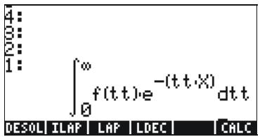
text_image
4: 0: 2: 1: ∫∞ f(tt)·e^-(tt·X) dt t 0 DESOL ILAP LAP LDEC CALC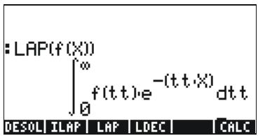
text_image
: LAP(f(X)) ∫∞ f(tt)·e^-(tt·X) dt.t DESOL ILAP LAP LDEC CALCCompare these expressions with the one given earlier in the definition of the Laplace transform, i.e.,
$$ L {f (t) } = F (s) = \int_ {0} ^ {\infty} f (t) \cdot e ^ {- s t} d t, $$
and you will notice that the CAS default variable X in the equation writer screen replaces the variable s in this definition. Therefore, when using the function LAP you get back a function of X, which is the Laplace transform of f(X).
Example 2 - Determine the inverse Laplace transform of F(s) = (s) . Use:
$$ ^ {\prime} 1 / (X + 1) ^ {\wedge} 2 ^ {\prime} \text { ENTER } I L A P $$
The calculator returns the result: 'X·e ^-X ', meaning that L ^-1 {1/(s+1) ^2 } = x·e ^-x .
Fourier series
A complex Fourier series is defined by the following expression
$$ f (t) = \sum_ {n = - \infty} ^ {+ \infty} c _ {n} \cdot \exp (\frac {2 i n \pi t}{T}), $$
where
$$ c _ {n} = \frac {1}{T} \int_ {0} ^ {T} f (t) \cdot \exp (\frac {2 \cdot i \cdot n \cdot \pi}{T} \cdot t) \cdot d t, \quad n = - \infty , \dots , - 2, - 1, 0, 1, 2, \dots \infty . $$
Function FOURIER
Function FOURIER provides the coefficient c_n of the complex-form of the Fourier series given the function f(t) and the value of n. The function FOURIER requires you to store the value of the period (T) of a T-periodic function into the CAS variable PERIOD before calling the function. The function FOURIER is available in the DERIV sub-menu within the CALC menu ( CALC).
Fourier series for a quadratic function
Determine the coefficients c_0 , c_1 , and c_2 for the function g(t) = (t-1)^2 + (t-1) , with period T = 2.
Using the calculator in ALG mode, first we define functions f(t) and g(t) :
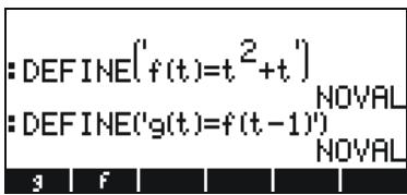
text_image
:DEFINE('f(t)=t^2+t') NOVAL :DEFINE('g(t)=f(t-1)') NOVAL g fNext, we move to the CASDIR sub-directory under HOME to change the value of variable PERIOD, e.g.,
← (hold) UPDIR ENTER VAR ENTER 2 STO▶ ENTER

text_image
: HOME : CASDIR : 2▶PERIOD PRIME CASID MODUL REALA PERIO VS NOVAL NOVAL NOVAL 2Return to the sub-directory where you defined functions f and g, and calculate the coefficients. Set CAS to Complex mode (see chapter 2) before trying the exercises. Function COLLECT is available in the ALG menu ( ).
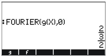
text_image
:FOURIER(g(X),0) g F 2/3 2/3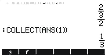
text_image
: COLLECT(ANS(1)) 23 23 13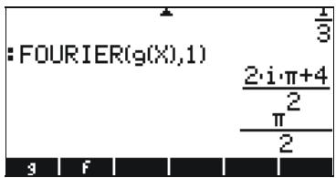
text_image
:FOURIER(g(X),1) 2·i·π+4 π/2 3 f 1/3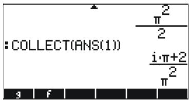
text_image
:COLLECT(ANS(1)) ^22 ·+2^2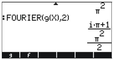
text_image
:FOURIER(g(X),2) π² i·π+1 2 π² 2 3 f
text_image
:COLLECT(ANS(1)) ^22 ·+12·^2Thus, c_0 = 1 / 3 , c_1 = ( · i + 2) / ^2 , c_2 = ( · i + 1) / (2^2) .
The Fourier series with three elements will be written as
$$ \mathsf {g} (t) \approx \operatorname{Re} [ (1 / 3) + (\pi \cdot i + 2) / \pi^ {2} \cdot \exp (i \cdot \pi \cdot t) + (\pi \cdot i + 1) / (2 \pi^ {2}) \cdot \exp (2 \cdot i \cdot \pi \cdot t) ]. $$
Reference
For additional definitions, applications, and exercises on solving differential equations, using Laplace transform, and Fourier series and transforms, as well as numerical and graphical methods, see Chapter 16 in the calculator's user's guide.
Chapter 15 Probability Distributions
In this Chapter we provide examples of applications of the pre-defined probability distributions in the calculator.
The MTH/PROBABILITY.. sub-menu - part 1
The MTH/PROBABILITY.. sub-menu is accessible through the keystroke sequence MTH . With system flag 117 set to CHOOSE boxes, the following functions are available in the PROBABILITY.. menu:

text_image
RAD CHOM MATH MENU 4.HYPERBOLIC.. 5.REAL.. 6.BASE.. 7.PROBABILITY.. 2.FFT.. 3.COMPLEX.. 10.CONSTANTS.. 11.SPECIAL FUNCTIONS.. CANCEL OR
text_image
RAD CHOM PROBABILITY MENU 1.COMB 2.PERM 3.! 4.RAND 5.RDZ 6.UTFC 7.UTFF 8.UTFN CANCEL OKIn this section we discuss functions COMB, PERM, ! (factorial), and RAND.
Factorials, combinations, and permutations
The factorial of an integer n is defined as: n! = n · (n-1) · (n-2) 3 · 2 · 1 . By definition, 0! = 1 .
Factorials are used in the calculation of the number of permutations and combinations of objects. For example, the number of permutations of r objects from a set of n distinct objects is
$$ _ n P _ {r} = n (n - 1) (n - 1)... (n - r + 1) = n! / (n - r)! $$
Also, the number of combinations of n objects taken r at a time is
$$ \binom {n} {r} = \frac {n (n - 1) (n - 2) \dots (n - r + 1)}{r !} = \frac {n !}{r ! (n - r) !} $$
We can calculate combinations, permutations, and factorials with functions COMB, PERM, and ! from the MTH/PROBABILITY.. sub-menu. The operation of those functions is described next:
- COMB(n,r): Calculates the number of combinations of n items taken r at a time
- PERM(n,r): Calculates the number of permutations of n items taken r at a time
- n!: Factorial of a positive integer. For a non-integer, x! returns (x+1) , where (x) is the Gamma function (see Chapter 3). The factorial symbol (!) can be entered also as the keystroke combination
ALPHA → 2.
Example of applications of these functions are shown next:
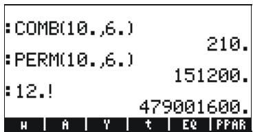
text_image
:COMB(10.,6.) :PERM(10.,6.) :12.! 210. 151200. 479001600.Random numbers
The calculator provides a random number generator that returns a uniformly distributed random real number between 0 and 1. To generate a random number, use function RAND from the MTH/PROBABILITY submenu. The following screen shows a number of random numbers produced using RAND. (Note: The random numbers in your calculator will differ from these).
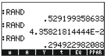
text_image
:RAND .529199358633 :RAND 4.35821814444E-2 :RAND .294922982088 H A Y t EQ PPARAdditional details on random numbers in the calculator are provided in Chapter 17 of the user's guide. Specifically, the use of function RDZ, to restart lists of random numbers is presented in detail in Chapter 17 of the user's guide.
The MTH/PROB menu - part 2
In this section we discuss four continuous probability distributions that are commonly used for problems related to statistical inference: the normal distribution, the Student's t distribution, the Chi-square (^2) distribution, and the F-distribution. The functions provided by the calculator to evaluate probabilities for these distributions are NDIST, UTPN, UTPT, UTPC, and UTPF. These functions are contained in the MTH/PROBABILITY menu introduced earlier in this chapter. To see these functions activate the MTH menu: MTH and select the PROBABILITY option:

text_image
RAD CHOM MATH MENU 4.HYPERBOLIC.. 5.REAL.. 6.BASE.. 7.PROBABILITY.. 8.FFT.. 9.COMPLEX.. 10.CONSTANTS.. 11.SPECIAL FUNCTIONS.. CANCEL OR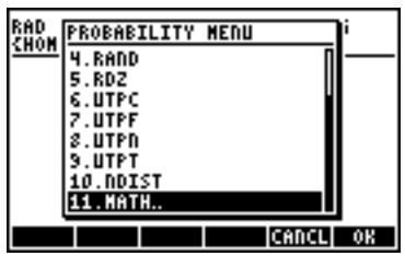
text_image
RAD CHOM PROBABILITY MENU 4.RAND 5.RDZ 6.UTPC 7.UTPF 8.UTPN 9.UTPT 10.NDIST 11.MATH.. CANCEL ORThe Normal distribution
Functions NDIST and UTPN relate to the Normal distribution with mean , and variance ^2 .
To calculate the value of probability density function, or pdf, of the f(x) for the normal distribution, use function NDIST(, ^2, x) . For example, check that for a normal distribution, NDIST(1.0, 0.5, 2.0) = 0.20755374 . This function is useful to plot the Normal distribution pdf.
The calculator also provides function UTPN that calculates the upper-tail normal distribution, i.e., UTPN(, 2, x) = P(X > x) = 1 - P(X < x) , where P() represents a probability. For example, check that for a normal distribution, with = 1.0 , ^2 = 0.5 , UTPN(1.0, 0.5, 0.75) = 0.638163 .
The Student-t distribution
The Student-t, or simply, the t-, distribution has one parameter v, known as the degrees of freedom of the distribution. The calculator provides for values of the upper-tail (cumulative) distribution function for the t-distribution, function UTPT, given the parameter v and the value of t, i.e., UTPT(v,t) = P(T>t) = 1-P(T<t) . For example, UTPT(5,2.5) = 2.7245...E-2 .
The Chi-square distribution
The Chi-square (^2) distribution has one parameter v, known as the degrees of freedom. The calculator provides for values of the upper-tail (cumulative) distribution function for the ^2 -distribution using UTPC given the value of x and the parameter v. The definition of this function is, therefore, UTPC(v,x)=P(X>x)=1-P(X<x) . For example, UTPC(5,2.5)=0.776495
The F distribution
The F distribution has two parameters vN = numerator degrees of freedom, and vD = denominator degrees of freedom. The calculator provides for values of the upper-tail (cumulative) distribution function for the F distribution, function UTPF, given the parameters vN and vD, and the value of F. The definition of this function is, therefore, UTPF(vN,vD,F) = P(ℐ>F) = 1 - P(ℐ<F). For example, to calculate UTPF(10,5, 2.5) = 0.1618347...
Reference
For additional probability distributions and probability applications, refer to Chapter 17 in the calculator's user's guide.
Chapter 16 Statistical Applications
The calculator provides the following pre-programmed statistical features accessible through the keystroke combination STAT (the 5 key):
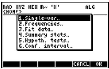
text_image
RAD XYZ HEX R- 'X' CHOM? 1.Single-var.. 2.Frequencies.. 3.Fit data.. 4.Summary stats.. 5.Hypoth. tests.. 6.Conf. interval.. CANCEL OREntering data
Applications numbered 1, 2, and 4 in the list above require that the data be available as columns of the matrix DAT. One way this can be accomplished is by entering the data in columns using the Matrix Writer, MTRW, and then using function STO to store the matrix into DAT.
For example, enter the following data using the Matrix Writer (see Chapters 8 or 9 in this guide), and store the data into DAT:
2.1 1.2 3.1 4.5 2.3 1.1 2.3 1.5 1.6 2.2 1.2 2.5.
The screen may look like this:
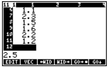
text_image
11 1 1 2 3 6 1.1 7 2.3 8 1.5 9 1.6 10 2.2 11 1.2 12 2.5 EDIT VEC +MID MID+ GO+= GO+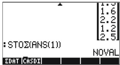
text_image
:STOZ(ANS(1)) EDAT CASDI [1.3] [1.6] [2.2] [1.2] [2.5] NOVALNotice the variable 📄 ranked in the soft menu keys.
A simpler way to enter statistical data is to launch a statistics application (such as Single-var, Frequencies or Summary stats, see first screenshot above) and press 📄. This launches the Matrix Writer. Enter the data as before. In this case, when you exit the Matrix Writer, the data you have entered is automatically saved in ΣDAT.
Calculating single-variable statistics
After entering the column vector into DAT, press STAT to select 1. Single-var.. The following input form will be provided:
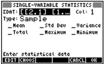
text_image
SINGLE-VARIABLE STATISTICS EDAT: [[2.1] [1... Col: 1 Type: Sample _Mean _Std Dev _Variance _Total _Maximum _Minimum Enter statistical data EDIT CHOOS | CANCEL OKThe form lists the data in DAT, shows that column 1 is selected (there is only one column in the current DAT). Move about the form with the arrow keys, and press the DAT soft menu key to select those measures (Mean, Standard Deviation, Variance, Total number of data points, Maximum and Minimum values) that you want as output of this program. When ready, press DAT. The selected values will be listed, appropriately labeled, in the screen of your calculator. For example:
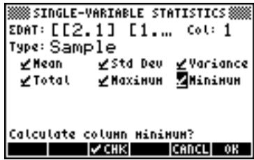
text_image
SINGLE-VARIABLE STATISTICS EDAT: [[2.1] [1... Col: 1] Type: Sample ✓ Mean ✓ Std Dev ✓ Variance ✓ Total ✓ Maximum ✓ Minimum Calculate column Minimum?
text_image
NOVAL Mean:2.13333333333 Std Dev:.964207949406 Variance:.929696969697 Total:25.6 Maximum:4.5 Minimum:1.1 EDAT |EPAR |CASDISample vs. population
The pre-programmed functions for single-variable statistics used above can be applied to a finite population by selecting the Type: Population in the SINGLE-VARIABLE STATISTICS screen. The main difference is in the values of the variance and standard deviation which are calculated using n in the denominator of the variance, rather than (n-1). For the example above, use now the 📄️ soft menu key to select population as Type: and re-calculate measures:

text_image
SINGLE-VARIABLE STATISTICS EDAT: [[2.1] [1.... Col: 1] Type: Sample ✓ Sample ✓ Population ance HUM Choose statistics type CANCEL OK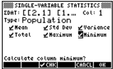
text_image
SINGLE-VARIABLE STATISTICS EDAT: [[2.1] [1... Col: 1 Type: Population ✓ Mean ✓ Std Dev ✓ Variance ✓ Total ✓ Maximum ✓ Minimum Calculate column Minimum?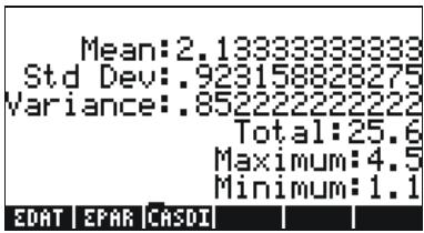
text_image
Mean:2.1333333333 Std Dev:.923158828275 Variance:.852222222222 Total:25.6 Maximum:4.5 Minimum:1.1 EDAT | EPAR | CASDIObtaining frequency distributions
The application 2. Frequencies.. in the STAT menu can be used to obtain frequency distributions for a set of data. The data must be present in the form of a column vector stored in variable ΣDAT. To get started, press → STAT ▼. The resulting input form contains the following fields:
ΣDAT: the matrix containing the data of interest.
Col: the column of DAT that is under scrutiny.
X-Min: the minimum class boundary to be used in the frequency distribution (default = -6.5).
Bin Count: the number of classes used in the frequency distribution (default = 13).
Bin Width: the uniform width of each class in the frequency distribution (default = 1).
Given a set of n data values: x_1, x_2, ..., x_n listed in no particular order, one can group the data into a number of classes, or bins by counting the frequency or number of values corresponding to each class. The application 2. Frequencies.. in the STAT menu will perform this frequency count, and will keep track of those values that may be below the minimum and above the maximum class boundaries (i.e., the outliers).
As an example, generate a relatively large data set, say 200 points, by using the command RANM({200,1}), and storing the result into variable
ΣDAT, by using function STOΣ (see example above). Next, obtain single-variable information using: → STAT. The results are:
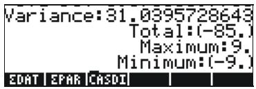
text_image
Variance:31.0395728643 Total:(-85.) Maximum:9. Minimum:(-9.) EDAT EPAR CASDIThis information indicates that our data ranges from -9 to 9. To produce a frequency distribution we will use the interval (-8, 8) dividing it into 8 bins of width 2 each.
- Select the program 2. Frequencies.. by using STAT ▼. The data is already loaded in ΣDAT, and the option Col should hold the value 1 since we have only one column in ΣDAT.
- Change X-Min to -8, Bin Count to 8, and Bin Width to 2, then press OK.
Using the RPN mode, the results are shown in the stack as a column vector in stack level 2, and a row vector of two components in stack level 1. The vector in stack level 1 is the number of outliers outside of the interval where the frequency count was performed. For this case, I get the values [14. 8.] indicating that there are, in the DAT vector, 14 values smaller than -8 and 8 larger than 8.
- Press ◆ to drop the vector of outliers from the stack. The remaining result is the frequency count of data.
The bins for this frequency distribution will be: -8 to -6, -6 to -4, ..., 4 to 6, and 6 to 8, i.e., 8 of them, with the frequencies in the column vector in the stack, namely (for this case):
$$ \begin{array}{l} 2 3, 2 2, 2 2, 1 7, 2 6, 1 5, 2 0, 3 3. \end{array} $$
This means that there are 23 values in the bin [-8,-6], 22 in [-6,-4], 22 in [-4,-2], 17 in [-2,0], 26 in [0,2], 15 in [2,4], 20 in [4,6], and 33 in [6,8]. You can also check that adding all these values plus the outliers, 14 and 8, show above, you will get the total number of elements in the sample, namely, 200.
Fitting data to a function y = f(x)
The program 3. Fit data..., available as option number 3 in the STAT menu, can be used to fit linear, logarithmic, exponential, and power functions to data sets (x, y), stored in columns of the ΣDAT matrix. For this application, you need to have at least two columns in your ΣDAT variable.
For example, to fit a linear relationship to the data shown in the table below:
| x | y |
| 0 | 0.5 |
| 1 | 2.3 |
| 2 | 3.6 |
| 3 | 6.7 |
| 4 | 7.2 |
| 5 | 11 |
- First, enter the two columns of data into variable DAT by using the Matrix Writer, and function STO .
- To access the program 3. Fit data.., use the following keystrokes: → STAT ▼ ▼ □. The input form will show the current ΣDAT, already loaded. If needed, change your set up screen to the following parameters for a linear fitting:
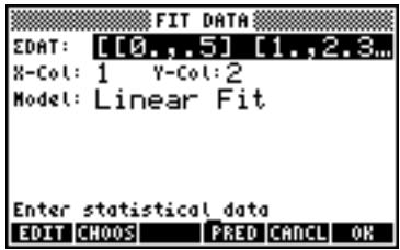
text_image
FIT DATA EDAT: [[0.,.5] [1.,2.3... X-Col: 1 Y-Col: 2 Model: Linear Fit Enter statistical data EDIT CHOOS PRED CANCEL OK- To obtain the data fitting press 📄. The output from this program, shown below for our particular data set, consists of the following three lines in RPN mode:
3: '0.195238095238 + 2.00857242857*X'
2: Correlation: 0.983781424465
1: Covariance: 7.03
Level 3 shows the form of the equation. Level 2 shows the sample correlation coefficient, and level 1 shows the covariance of x-y. For definitions of these parameters see Chapter 18 in the user's guide.
For additional information on the data-fit feature of the calculator see Chapter 18 in the user's guide.
Obtaining additional summary statistics
The application 4. Summary stats.. in the STAT menu can be useful in some calculations for sample statistics. To get started, press → STAT once more, move to the fourth option using the down-arrow key ▼, and press 📄. The resulting input form contains the following fields:
ΣDAT: the matrix containing the data of interest.
X-Col, Y-Col: these options apply only when you have more than two columns in the matrix DAT. By default, the x column is column 1, and the y column is column 2. If you have only one column, then the only setting that makes sense is to have X-Col: 1.
_ΣX _ ΣY...: summary statistics that you can choose as results of this program by checking the appropriate field using ☐ when that field is selected.
Many of these summary statistics are used to calculate statistics of two variables (x, y) that may be related by a function y = f(x) . Therefore, this program can be thought off as a companion to program 3. Fit data..
As an example, for the x-y data currently in DAT, obtain all the summary statistics.
• To access the summary stats... option, use:

- Select the column numbers corresponding to the x- and y-data, i.e., X-Col: 1, and Y-Col: 2.
- Using the ☐☐☐ key select all the options for outputs, i.e., _ΣX, _ΣY, etc.
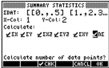
text_image
SUMMARY STATISTICS EDAT: [[0.,.5] [1.,2.3... X-Col: 1 Y-Col:2 Calculate: ✓EX ✓EY ✓EX2 ✓EY2 ✓EXY ✓NE Calculate number of data points? ✓CHK CANCEL OK- Press 📄 to obtain the following results:
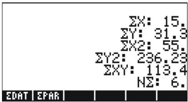
text_image
ΣX: 15. ΣY: 31.3 ΣX2: 55. ΣY2: 236.23 ΣXY: 113.4 NZ: 6. EDAT EPARConfidence intervals
The application 6. Conf Interval can be accessed by using STAT ▲. The application offers the following options:
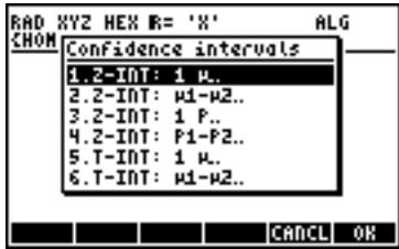
text_image
RAD XYZ HEX R= 'X' CHOM Confidence intervals 1.2-INT: 1 μ. 2.2-INT: μ1-μ2.. 3.2-INT: 1 P.. 4.2-INT: P1-P2.. 5. T-INT: 1 μ.. 6. T-INT: μ1-μ2.. CANCEL OKThese options are to be interpreted as follows:
- Z-INT: 1 μ.: Single sample confidence interval for the population mean, μ, with known population variance, or for large samples with unknown population variance.
- Z-INT: _1-_2 : Confidence interval for the difference of the population means, _1-_2 , with either known population variances, or for large samples with unknown population variances.
-
Z-INT: 1 p.: Single sample confidence interval for the proportion, p, for large samples with unknown population variance.
-
Z-INT: p1–p2.: Confidence interval for the difference of two proportions, p_1-p_2 , for large samples with unknown population variances.
- T-INT: 1 .: Single sample confidence interval for the population mean, , for small samples with unknown population variance.
- T-INT: 1-2 : Confidence interval for the difference of the population means, _1-_2 , for small samples with unknown population variances.
Example 1 - Determine the centered confidence interval for the mean of a population if a sample of 60 elements indicate that the mean value of the sample is = 23.3 , and its standard deviation is s = 5.2 . Use = 0.05 . The confidence level is C = 1 - = 0.95 .
Select case 1 from the menu shown above by pressing 📄. Enter the values required in the input form as shown:
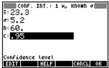
text_image
CONF. INT.: 1 μ, KNOWN σ x:23.3 σ:5.2 n:60. C:.95 Confidence level EDIT HELP CANCEL OKPress 📄 to obtain a screen explaining the meaning of the confidence interval in terms of random numbers generated by a calculator. To scroll down the resulting screen use the down-arrow key ▼. Press 📄 when done with the help screen. This will return you to the screen shown above.
To calculate the confidence interval, press 31. The result shown in the calculator is:

text_image
95.2 Confidence interval Critical Z=±1.959964 μ Min =21.98424 μ Max =24.61576 HELP GRAPH CANCEL OKPress 📄 to see a graphical display of the confidence interval information:
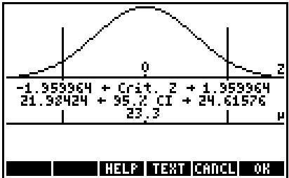
line
| Parameter | Value | | :--- | :--- | | -1.953964 + Crit. Z + 1.953964 | 21.98424 + 95.7 CI + 24.61576 | | μ | 23.3 | | HELF | | | TEXT | | | CANCEL | | | OK | |The graph shows the standard normal distribution pdf (probability density function), the location of the critical points ± z_ /2 , the mean value (23.3) and the corresponding interval limits (21.98424 and 24.61576). Press [13-14] to return to the previous results screen, and/or press [0.8] to exit the confidence interval environment. The results will be listed in the calculator's display.
Additional examples of confidence interval calculations are presented in Chapter 18 in the calculator's user's guide.
Hypothesis testing
A hypothesis is a declaration made about a population (for instance, with respect to its mean). Acceptance of the hypothesis is based on a statistical test on a sample taken from the population. The consequent action and decision-making are called hypothesis testing.
The calculator provides hypothesis testing procedures under application 5. Hypoth. tests.. can be accessed by using STAT
As with the calculation of confidence intervals, discussed earlier, this program offers the following 6 options:
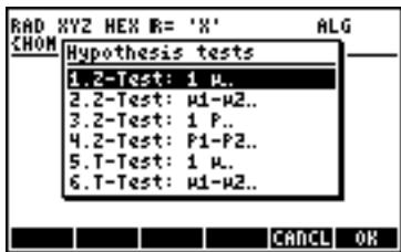
text_image
RAD XYZ HEX R= 'X' ALG CHOM Hypothesis tests 1.2-Test: 1 μ.. 2.2-Test: μ1-μ2.. 3.2-Test: 1 P.. 4.2-Test: P1-P2.. 5. T-Test: 1 μ.. 6. T-Test: μ1-μ2.. CANCEL OKThese options are interpreted as in the confidence interval applications:
-
Z-Test: 1 .: Single sample hypothesis testing for the population mean, , with known population variance, or for large samples with unknown population variance.
-
Z-Test: _1-_2 : Hypothesis testing for the difference of the population means, _1-_2 , with either known population variances, or for large samples with unknown population variances.
- Z-Test: 1 p.: Single sample hypothesis testing for the proportion, p, for large samples with unknown population variance.
- Z-Test: p1–p2.: Hypothesis testing for the difference of two proportions, p_1-p_2 , for large samples with unknown population variances.
- T-Test: 1 .: Single sample hypothesis testing for the population mean, , for small samples with unknown population variance.
- T-Test: 1-2 : Hypothesis testing for the difference of the population means, _1-_2 , for small samples with unknown population variances.
Example 1 - For _0 = 150 , = 10 , = 158 , n = 50 , for = 0.05 , test the hypothesis H_0: = _0 , against the alternative hypothesis, H_1: _0 .
Press → STAT ▲ ▲ to access the confidence interval feature in the calculator. Press ⚫ to select option 1. Z-Test: 1 μ.
Enter the following data and press 📄:
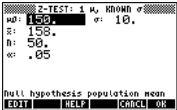
text_image
2-TEST: 1 μ, KNOWN σ μ0: 150. σ: 10. x̄: 158. n: 50. κ̄: .05 Null hypothesis population mean EDIT HELP CANCEL OKYou are then asked to select the alternative hypothesis:

text_image
2-TEST: 1 μ, KNOWN σ μ0: 150. σ: 10. : Alternative Hypothesis n: μ<150. κ: μ>150. μ≠150. Null hypothesis population mean CANCEL OKSelect 150 . Then, press ☐. The result is:

text_image
Reject μ=150. at 5.2 LVL Test Z=5.656854 Prob=1.541726E-8 Critical Z=±1.959964 Critical R=(147.2,152.8)Then, we reject H_0 : = 150 , against H_1 : 150 . The test z value is z_0 = 5.656854 . The P-value is 1.54 × 10^-8 . The critical values of ± z_/2 = ± 1.959964 , corresponding to critical range of 147.2 152.8 .
This information can be observed graphically by pressing the soft-menu key [GRAPH]:

line
| Test | Value | | :--- | :--- | | -1.959964 | +Crit. 2+ 1.959964 | | 147.2282 | +Crit. 5+ 152.7718 | | 150. | | HELP TEXT CANCEL OKReference
Additional materials on statistical analysis, including definitions of concepts, and advanced statistical applications, are available in Chapter 18 in the user's guide.
Chapter 17
Numbers in Different Bases
Besides our decimal (base 10, digits = 0-9) number system, you can work with a binary system (base 2, digits = 0,1), an octal system (base 8, digits = 0-7), or a hexadecimal system (base 16, digits=0-9,A-F), among others. The same way that the decimal integer 321 means 3 × 10^2 + 2 × 10^1 + 1 × 10^0 , the number 100110, in binary notation, means
$$ 1 \times 2 ^ {5} + 0 \times 2 ^ {4} + 0 \times 2 ^ {3} + 1 \times 2 ^ {2} + 1 \times 2 ^ {1} + 0 \times 2 ^ {0} = 3 2 + 0 + 0 + 4 + 2 + 0 = 3 8. $$
The BASE menu
The BASE menu is accessible through BASE (the 3 key). With system flag 117 set to CHOOSE boxes (see Chapter 1 in this guide), the following entries are available:
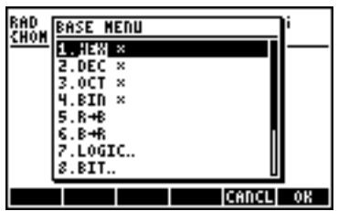
text_image
RAD CHOM BASE MENU 1. HEX * 2. DEC * 3. OCT * 4. BIN * 5. R+8 6. B+8 7. LOGIC.. 8. BIT.. CANCEL OR
text_image
RAD CHOM BASE MENU 5.R+B 6.B+B 7.LOGIC.. 8.BIT.. 9.BYTE.. 10.STWS 11.RCWS 12.MATH.. CANCEL OKWith system flag 117 set to SOFT menus, the BASE menu shows the following:

text_image
HEX ■ DEC OCT BIN R+B B+R
text_image
LOGIC BIT BYTE STMS RCMSThis figure shows that the LOGIC, BIT, and BYTE entries within the BASE menu are themselves sub-menus. These menus are discussed in detail in Chapter 19 of the calculator's user's guide.
Writing non-decimal numbers
Numbers in non-decimal systems, referred to as binary integers, are written preceded by the # symbol ( # ) in the calculator. To select the current base to be used for binary integers, choose either HEX (adecimal), DEC (imal), OCT (al), or BIN (ary) in the BASE menu. For example, if ☐ is selected, binary integers will be a hexadecimal numbers, e.g., #53, #A5B, etc. As different systems are selected, the numbers will be automatically converted to the new current base.
To write a number in a particular system, start the number with # and end with either h (hexadecimal), d (decimal), o (octal), or b (binary), examples:
HEX

text_image
: # A2F0h : # 2BC10h : # 125hA2F0h
2BC10h
125h
HEX ■ DEC | OCT | BIN | R+B | B+RDEC
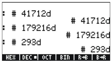
text_image
: # 41712d : # 179216d : # 293d41712d
179216d
293d
HEX DEC OCT BIN R+B B+ROCT
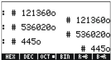
text_image
: # 121360o : # 536020o : # 445o121360o
536020o
445o
HEX | DEC | OCT ■ | BIN | R+R | B+RBIN
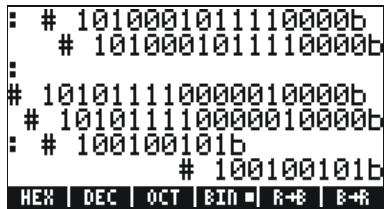
text_image
: # 1010001011110000b1010001011110000b
:101011110000010000b
101011110000010000b
: # 100100101b100100101b
HEX | DEC | OCT | BIN | R+R | B+RReference
For additional details on numbers from different bases see Chapter 19 in the calculator's user's guide.
Chapter 18 Using SD cards
The calculator has a memory card slot into which you can insert an SD flash card for backing up calculator objects, or for downloading objects from other sources. The SD card in the calculator will appear as port number 3.
Inserting and removing an SD card
The SD slot is located on the bottom edge of the calculator, just below the number keys. SD cards must be inserted facing down. Most cards have a label on what would usually be considered the top of the card. If you are holding the HP 50g with the keyboard facing up, then this side of the SD card should face down or away from you when being inserted into the HP 50g. The card will go into the slot without resistance for most of its length and then it will require slightly more force to fully insert it. A fully inserted card is almost flush with the case, leaving only the top edge of the card visible.
To remove an SD card, turn off the HP 50g, press gently on the exposed edge of the card and push in. The card should spring out of the slot a small distance, allowing it now to be easily removed from the calculator.
Formatting an SD card
Most SD cards will already be formatted, but they may be formatted with a file system that is incompatible with the HP 50g. The HP 50g will only work with cards in the FAT16 or FAT32 format.
You can format an SD card from a PC, or from the calculator. If you do it from the calculator (using the method described below), make sure that your calculator has fresh or fairly new batteries.
NOTE: formatting an SD card deletes all the data that is currently on it.
- Insert the SD card into the card slot (as explained in the previous section).
- Hold down the ON key and then press the F4 key. Release the F4 key and then release the ON key. The system menu is displayed with several choices.
-
Press 0 for FORMAT. The formatting process begins.
-
When the formatting is finished, the HP 50g displays the message "FORMAT FINISHED. PRESS ANY KEY TO EXIT". To exit the system menu, hold down the ON key, press and release the B key and then release the ON key.
The SD card is now ready for use. It will have been formatted in FAT32 format.
Accessing objects on an SD card
Accessing an object on the SD card is similar to when an object is located in ports 0, 1, or 2. However, port 3 will not appear in the menu when you are using the LIB function (→ LIB). The SD files can only be managed using the Filer, or File Manager (← FILES). When starting the Filer, the Tree view will show:
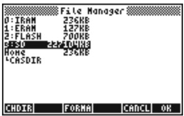
text_image
File Manager 0:IRAM 236KB 1:ERAM 127KB 2:FLASH 700KB P:50 227404KB Home 236KB *CASDIR CHDIR FORMA CANCEL OKLong names of files on an SD card are supported, but are displayed in 8.3 format in the Filer (that is, their names are truncated to 8 characters and a three character extension is added as a suffix). The type of each object will be displayed, unless it is a PC object or an object of unknown type. (In these cases, its type is listed as String.)
In addition to using File Manager operations, you can use STO and RCL to store objects on, and recall objects from, the SD card.
Storing objects on the SD card
To store an object, use function STO as follows:
- In algebraic mode:
Enter object, press STO▶, type the name of the stored object using port 3 (e.g., :3:VAR1), press ENTER.
- In RPN mode:
Enter object, type the name of the stored object using port 3 (e.g., :3:VAR1), press STO.
Note that if the name of the object you intend to store on an SD card is longer than eight characters, it will appear in 8.3 DOS format in port 3 in the Filer once it is stored on the card.
Recalling an object from the SD card
To recall an object from the SD card onto the screen, use function RCL, as follows:
• In algebraic mode:
Press RCL, type the name of the stored object using port 3 (e.g., 3:VAR1 ), press ENTER.
- In RPN mode:
Type the name of the stored object using port 3 (e.g., ⓢ:VAR1), press ← RCL .
With the RCL command, it is possible to recall variables by specifying a path in the command, e.g., in RPN mode: 3: {path} ENTER RCL. The path, like in a DOS drive, is a series of directory names that together specify the position of the variable within a directory tree. However, some variables stored within a backup object cannot be recalled by specifying a path. In this case, the full backup object (e.g., a directory) will have to be recalled, and the individual variables then accessed on the screen.
Note that in the case of objects with long files names, you can specify the full name of the object, or its truncated 8.3 name, when issuing an RCL command.
Purging an object from the SD card
To purge an object from the SD card onto the screen, use function PURGE, as follows:
- In algebraic mode:
Press TOOL 📄, type the name of the stored object using port 3 (e.g., ⌘:VAR1), press ENTER.
- In RPN mode:
Type the name of the stored object using port 3 (e.g., *3:VAR1), press TOOL FLUID.
Note that in the case of objects with long files names, you can specify the full name of the object, or its truncated 8.3 name, when issuing a PURGE command.
Purging all objects on the SD card (by reformatting)
You can purge all objects from the SD card by reformatting it. When an SD card is inserted, F03:10 appears an additional menu item in File Manager. Selecting this option reformats the entire card, a process which also deletes every object on the card.
Specifying a directory on an SD card
You can store, recall, evaluate and purge objects that are in directories on an SD card. Note that to work with an object at the root level of an SD card, the ☐ key is used. But when working with an object in a subdirectory, the name containing the directory path must be enclosed using the ☐ keys.
For example, suppose you want to store an object called PROG1 into a directory called PROGS on an SD card. With this object still on the first level of the stack, press:
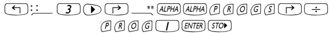
text_image
← :: 3 ▶ → "" ALPHA ALPHA P R O G S → ÷ P R O G I ENTER STO▶This will store the object previously on the stack onto the SD card into the directory named PROGS into an object named PROG1.
NOTE: If PROGS does not exist, the directory will be automatically created.
You can specify any number of nested subdirectories. For example, to refer to an object in a third-level subdirectory, your syntax would be:
:3:"DIR1/DIR2/DIR3/NAME"
Note that pressing ALPHA → ÷ produces the forward slash character.
Chapter 19 Equation Library
The Equation Library is a collection of equations and commands that enable you to solve simple science and engineering problems. The library consists of more than 300 equations grouped into 15 technical subjects containing more than 100 problem titles. Each problem title contains one or more equations that help you solve that type of problem.
NOTE: the examples in this chapter assume that the operating mode is RPN and that flag -117 is set. (Flag -117 should be set whenever you use the numeric solver to solve equations in the equations library.)
Example: Examine the equation set for Projectile Motion.
Step 1: Fix the display to 2 decimal places and then open the Equation Library application. (If 📄 and 📄 aren't flagged with small squares, press each of the corresponding menu keys once.)

text_image
MODE ALPHA F 2 ENTER APPS ENTER
text_image
EQUATION LIBRARY Columns and Beams Electricity Fluids Forces and Energy Gases Heat Transfer Magnetism Motion SI ▪ ENGL UNIT ▪ QUITStep 2: Select the Motion subject area and open its catalog.

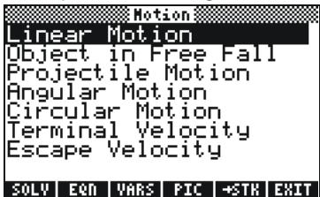
text_image
Motion Linear Motion Object in Free Fall Projectile Motion Angular Motion Circular Motion Terminal Velocity Escape Velocity SOLY | EQN | VARS | PIC | *STR | EXITStep 3: Select Projectile Motion and look at the diagram that describes the problem.

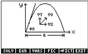
text_image
SOLV EQN VARS PIC →PICT EXIT Y VY V0 VX 80 K R M XStep 4: View the five equations in the Projectile Motion set. All five are used interchangeably in order to solve for missing variables (see the next example).
301 1839 1839 1839 1839

text_image
5. OF 5. x R=√θ²/9·SIN(2·θ0) SOLY | NEXQ | VARS | PIC |→STK |EXITStep 5: Examine the variables used by the equation set.
2012
and ▲ as ▼ needed
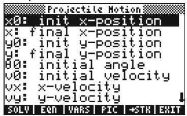
text_image
Projectile Motion x0: init x-position x: final x-position y0: init y-position y: final y-position 80: initial angle v0: initial velocity vx: x-velocity vy: y-velocity SOLY EQV VARS PIC +STR EXITNow use this equation set to answer the questions in the following example.
Example: You estimate that on average professional goalkeepers can punt a soccer ball a distance (R) of 65 meters downfield at an elevation angle ( 0 ) of 50 degrees. At what velocity ( v0 ) do they kick it? How high is the ball halfway through its flight? How far could they drop kick the ball if they used the same kicking velocity, but changed the elevation angle to 30 degrees? (Ignore the effects of drag on the ball.)
Step 1: Start solving the problem.
2014
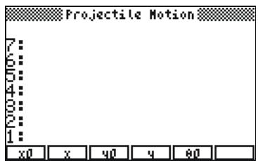
text_image
Projectile Motion 7: 00-4000 1: x0 x 40 4 80Step 2: Enter the known values and press the soft menu key corresponding to the variable. (You can assume that x_0 and y_0 are zero.) Notice that the menu labels turn black as you store values. (You will need to press NXT to see the variables that are initially shown.)


text_image
R: 65_m 7: 00: 04: 09: 1: w0 uv uv t R ALLStep 3: Solve for the velocity, v_0 . (You solve for a variable by pressing and then the variable's menu key.)

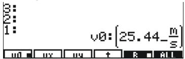
text_image
3: 2: 1: v0: [25.44 - m/s]Step 4: Recall the range, R, divide by 2 to get the halfway distance, and enter that as the x-coordinate. Notice that pressing the right-shifted version of a variable's menu key causes the calculator to recall its value to the stack. (The small square next to the R on the menu label indicates that it was used in the previous calculation.)
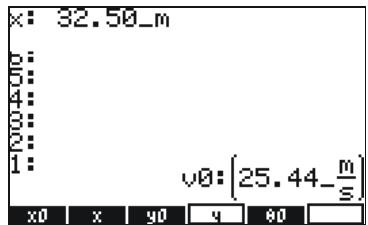
text_image
x: 32.50_m v0: v0: [25.44_m/s] x0 x y0 y 60Step 5: Solve for the height, y. Notice that the calculator finds values for other variables as needed (shown by the small squares) in order to solve for the specified variable.


text_image
1: y:(19.37_m) x0 x y0 y 80Step 6: Enter the new value for the elevation angle (30 degrees), store the previously computed initial velocity ( v_0 ) and then solve for R.


text_image
|1: R:(57.16_m) v0 □ vx v4 t R □ ALL
Reference
For additional details on the Equation Library, see Chapter 27 in the calculator's user's guide.
Limited Warranty
HP 50g graphing calculator; Warranty period: 12 months
- HP warrants to you, the end-user customer, that HP hardware, accessories and supplies will be free from defects in materials and workmanship after the date of purchase, for the period specified above. If HP receives notice of such defects during the warranty period, HP will, at its option, either repair or replace products which prove to be defective. Replacement products may be either new or like-new.
- HP warrants to you that HP software will not fail to execute its programming instructions after the date of purchase, for the period specified above, due to defects in material and workmanship when properly installed and used. If HP receives notice of such defects during the warranty period, HP will replace software media which does not execute its programming instructions due to such defects.
- HP does not warrant that the operation of HP products will be uninterrupted or error free. If HP is unable, within a reasonable time, to repair or replace any product to a condition as warranted, you will be entitled to a refund of the purchase price upon prompt return of the product with proof of purchase.
- HP products may contain remanufactured parts equivalent to new in performance or may have been subject to incidental use.
- Warranty does not apply to defects resulting from (a) improper or inadequate maintenance or calibration, (b) software, interfacing, parts or supplies not supplied by HP, (c) unauthorized modification or misuse, (d) operation outside of the published environmental specifications for the product, or (e) improper site preparation or maintenance.
- HP MAKES NO OTHER EXPRESS WARRANTY OR CONDITION WHETHER WRITTEN OR ORAL. TO THE EXTENT ALLOWED BY LOCAL LAW, ANY IMPLIED WARRANTY OR CONDITION OF MERCHANTABILITY, SATISFACTORY QUALITY, OR FITNESS FOR A PARTICULAR PURPOSE IS LIMITED TO THE DURATION OF THE EXPRESS WARRANTY SET FORTH ABOVE. Some countries, states or provinces do not allow limitations on the duration of an implied warranty, so the above limitation or exclusion might not apply to you. This warranty gives you specific legal rights and you might also have other rights that vary from country to country, state to state, or province to province.
- TO THE EXTENT ALLOWED BY LOCAL LAW, THE REMEDIES IN THIS WARRANTY STATEMENT ARE YOUR SOLE AND EXCLUSIVE
REMEDIES. EXCEPT AS INDICATED ABOVE, IN NO EVENT WILL HP OR ITS SUPPLIERS BE LIABLE FOR LOSS OF DATA OR FOR DIRECT, SPECIAL, INCIDENTAL, CONSEQUENTIAL (INCLUDING LOST PROFIT OR DATA), OR OTHER DAMAGE, WHETHER BASED IN CONTRACT, TORT, OR OTHERWISE. Some countries, States or provinces do not allow the exclusion or limitation of incidental or consequential damages, so the above limitation or exclusion may not apply to you.
- The only warranties for HP products and services are set forth in the express warranty statements accompanying such products and services. HP shall not be liable for technical or editorial errors or omissions contained herein.
FOR CONSUMER TRANSACTIONS IN AUSTRALIA AND NEW ZEALAND: THE WARRANTY TERMS CONTAINED IN THIS STATEMENT, EXCEPT TO THE EXTENT LAWFULLY PERMITTED, DO NOT EXCLUDE, RESTRICT OR MODIFY AND ARE IN ADDITION TO THE MANDATORY STATUTORY RIGHTS APPLICABLE TO THE SALE OF THIS PRODUCT TO YOU.
Service Europe
| Country : | Telephone numbers |
| Austria | +43-1-3602771203 |
| Belgium | +32-2-7126219 |
| Denmark | +45-8-2332844 |
| Eastern Europe countries | +420-5-41422523 |
| Finland | +358-9-640009 |
| France | +33-1-49939006 |
| Germany | +49-69-95307103 |
| Greece | +420-5-41422523 |
| Holland | +31-2-06545301 |
| Italy | +39-02-75419782 |
| Norway | +47-63849309 |
| Portugal | +351-229570200 |
| Spain | +34-915-642095 |
| Sweden | +46-851992065 |
| +41-1-4395358 (German) | |
| Switzerland | +41-22-8278780 (French) |
| +39-02-75419782 (Italian) | |
| Turkey | +420-5-41422523 |
| UK | +44-207-4580161 |
| Czech Republic | +420-5-41422523 |
| South Africa | +27-11-2376200 |
| Luxembourg | +32-2-7126219 |
| Other European countries | +420-5-41422523 |
| Country : | Telephone numbers |
| Australia | +61-3-9841-5211 |
| Singapore | +61-3-9841-5211 |
Asia Pacific
L.America
| Country : | Telephone numbers |
| Argentina | 0-810-555-5520 |
| Brazil | Sao Paulo 3747-7799; ROTC 0-800-157751 |
| Mexico | Mx City 5258-9922; ROTC 01-800-472-6684 |
| Venezuela | 0800-4746-8368 |
| Chile | 800-360999 |
| Columbia | 9-800-114726 |
| Peru | 0-800-10111 |
| Central America & Caribbean | 1-800-711-2884 |
| Guatemala | 1-800-999-5105 |
| Puerto Rico | 1-877-232-0589 |
| Costa Rica | 0-800-011-0524 |
N.America
| Country : | Telephone numbers |
| U.S. | 1800-HP INVENT |
| Canada | (905) 206-4663 or 800- HP INVENT |
ROTC = Rest of the country
Please logon to http://www.hp.com for the latest service and support information.
Regulatory information
Federal Communications Commission Notice
This equipment has been tested and found to comply with the limits
for a Class B digital device, pursuant to Part 15 of the FCC Rules. These limits are designed to provide reasonable protection against harmful interference in a residential installation. This equipment generates, uses, and can radiate radio frequency energy and, if not installed and used in accordance with the instructions, may cause harmful interference to radio communications. However, there is no guarantee that interference will not occur in a particular installation. If this equipment does cause harmful interference to radio or television reception, which can be determined by turning the equipment off and on, the user is encouraged to try to correct the interference by one or more of the following measures:
• Reorient or relocate the receiving antenna.
- Increase the separation between the equipment and the receiver.
- Connect the equipment into an outlet on a circuit different from that to which the receiver is connected.
- Consult the dealer or an experienced radio or television technician for help.
Modifications
The FCC requires the user to be notified that any changes or modifications made to this device that are not expressly approved by Hewlett-Packard Company may void the user's authority to operate the equipment.
Cables
Connections to this device must be made with shielded cables with metallic RFI/EMI connector hoods to maintain compliance with FCC rules and regulations.
Declaration of Conformity for Products Marked with FCC Logo, United States Only
This device complies with Part 15 of the FCC Rules. Operation is subject to the following two conditions: (1) this device may not cause harmful interference, and (2) this device must accept any interference received, including interference that may cause undesired operation.
For questions regarding your product, contact:
Hewlett-Packard Company
P. O. Box 692000, Mail Stop 530113
Houston, Texas 77269-2000
Or, call
1-800-474-6836
For questions regarding this FCC declaration, contact:
Hewlett-Packard Company
P. O. Box 692000, Mail Stop 510101
Houston, Texas 77269-2000
Or, call
1-281-514-3333
To identify this product, refer to the part, series, or model number found on the product.
Canadian Notice
This Class B digital apparatus meets all requirements of the
Canadian Interference-Causing Equipment Regulations.
Avis Canadien
European Union Regulatory Notice
This product complies with the following EU Directives:
• Low Voltage Directive 73/23/EEC
• EMC Directive 89/336/EEC
Compliance with these directives implies conformity to applicable harmonized European standards (European Norms) which are listed on the EU Declaration of Conformity issued by Hewlett-Packard for this product or product family.
This compliance is indicated by the following conformity marking placed on the product:
This compliance is indicated by the following conformity marking placed on the product:

This marking is valid for non-Telecom products and EU harmonized Telecom products (e.g. Bluetooth).

text_image
CE xxxx* !This marking is valid for EU non-harmonized Telecom products. *Notified body number (used only if applicable - refer to the product label)
Japanese Notice
Disposal of Waste Equipment by Users in Private Household in the European Union

This symbol on the product or on its packaging indicates that this product must not be disposed of with your other household waste. Instead, it is your responsibility to dispose of your waste equipment by handing it over to a designated collection point for the recycling of waste electrical and
electronic equipment. The separate collection and recycling of your waste equipment at the time of disposal will help to conserve natural resources and ensure that it is recycled in a manner that protects human health and the environment. For more information about where you can drop off your waste equipment for recycling, please contact your local city office, your household waste disposal service or the shop where you purchased the product.