
GRAPH90+E PYTHON - Graphing calculator CASIO - Free user manual and instructions
Find the device manual for free GRAPH90+E PYTHON CASIO in PDF.

| Product Type | Programmable Graphing Calculator |
| Brand | Casio |
| Model | GRAPH90+E PYTHON |
| Dimensions (Thickness × Width × Length) | 18.6 mm × 89 mm × 188.5 mm |
| Weight (with batteries) | 230 g |
| Power Source | 4 AAA alkaline batteries LR03 (AM4) or 4 rechargeable NiMH batteries |
| Battery Life (alkaline, standard conditions) | 170 hours (typical use) |
| Display | Monochrome LCD, 384 × 216 pixels, backlit |
| Main Functions | Mathematical calculations, function graphing, Python programming, spreadsheet, eActivity, geometry, statistics, financial calculations, probabilities, 3D graphs, exam mode |
| Storage Memory | 16 MB (max.) |
| Programming Capacity | 61,000 bytes (max.) |
| Connectivity | USB 2.0, 3-pin serial port, calculator-to-calculator communication |
| Auto Power Off | Configurable: approximately 10 minutes or 60 minutes |
| Operating Temperature Range | 0 °C to 40 °C |
| Care and Cleaning | Wipe with a soft, dry cloth; do not use volatile solvents |
| Safety | Keep batteries out of reach of children; do not incinerate; use only recommended batteries; avoid shocks and moisture |
| Spare Parts and Repairability | Not specified by the manufacturer; contact Casio after-sales service |
| General Information | Software version 3.60; manual available in multiple languages at edu.casio.com; built-in exam mode with flashing LED |
Frequently Asked Questions - GRAPH90+E PYTHON CASIO
User questions about GRAPH90+E PYTHON CASIO
0 question about this device. Answer the ones you know or ask your own.
Ask a new question about this device
Download the instructions for your Graphing calculator in PDF format for free! Find your manual GRAPH90+E PYTHON - CASIO and take your electronic device back in hand. On this page are published all the documents necessary for the use of your device. GRAPH90+E PYTHON by CASIO.
USER MANUAL GRAPH90+E PYTHON CASIO
Méthode : Start-stop (asynchrone), semi-duplex
115200 bits/seconde (normal)
38400 bits/seconde (Commande Send38k/Receive38k)
<115200 bits/seconde>
Parité : EVEN
Rechargeables Duracell
Rechargeables Energizer
Panasonic eneloop (SANYO eneloop)
This Class B digital apparatus complies with Canadian ICES-003.
https://world.casio.com/manual/calc/
E-CON4 Application (English)
- E-CON4 Mode Overview 2
- Sampling Screen 3
- Auto Sensor Detection (CLAB Only) 2
- Selecting a Sensor 10
- Configuring the Sampling Setup 2
- Performing Auto Sensor Calibration and Zero Adjustment 20
- Using a Custom Probe 23
- Using Setup Memory 25
- Starting a Sampling Operation 28
- Using Sample Data Memory 33
- Using the Graph Analysis Tools to Graph Data 35
- Graph Analysis Tool Graph Screen Operations 39
- Calling E-CON4 Functions from an eActivity 8-51
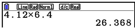
$$ 4, 1 2 \times 6, 4 = 2 6, 3 6 8 $$
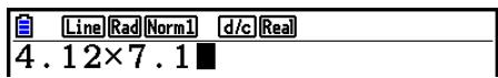
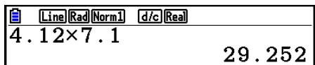
$$ 4, 1 2 \times 7, 1 = 2 9, 2 5 2 $$


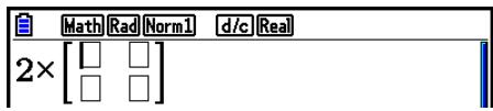
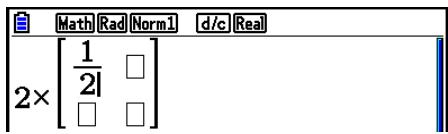
AC 2 X F4 (MATH) F1 (MAT/VCT) F1 (2×2)


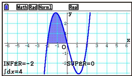
MENUGrapheOPTN F2(CALC)F3(jdx)
14X.67x²-12
X,0T 1 0 X,0T EXE
F6 (DRAW)
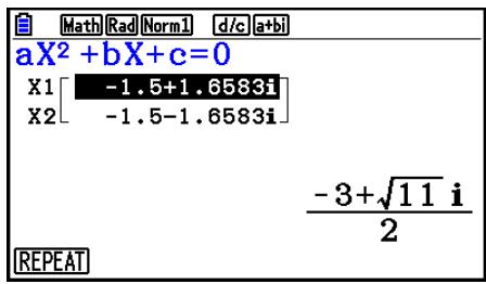
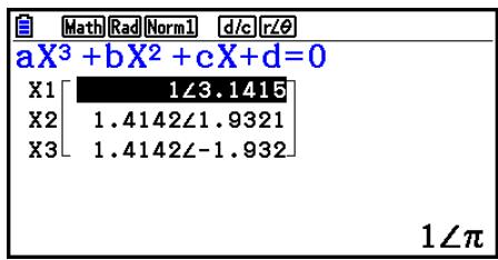
MENUEEquationSHIFT (SET UP)
(Complex Mode)
F2(a+bi)EXT
F2(POLY) F1(2) 1 EXE 3 EXE 5 EXE
[SET UP]- [Display]- [Fix]/[Sci]/[Norm]
| "ABC"→Str 1 Str 1 ABC | d/c | Real |
| Done |
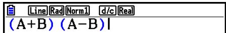
| Line | Rad | Norm1 | d/c | Real |
| (A+B) | (A-B) | | |
OPTN F6(>)F6(>)F3(FUNCMEM)
F1(STORE) 1 EXE
ACOPTN F6(>)F6(>)F3 (FUNCMEM)
F2(RECALL)1 EXE
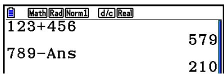
Example 123 + 456 = 579
$$ 7 8 9 - 5 7 9 = 2 1 0 $$


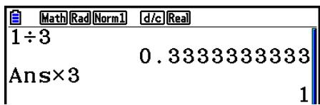
$$ 1 \div 3 \times 3 = $$

(En continuant) 3 EXE
Ran# [a] 1≤ a≤ 9
RanList# (n[,a]) 1≤ n≤ 999
RanSamp# (List X, n [,m])
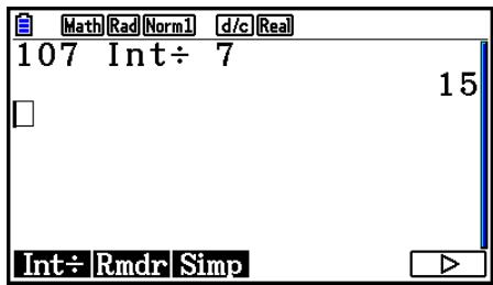
[OPTN]-[CALC]-[Int÷]
AC 1 0 7 OPTN F4 (CALC) F6 (>)
F6(▷) F1 (Int÷) 7
EXE
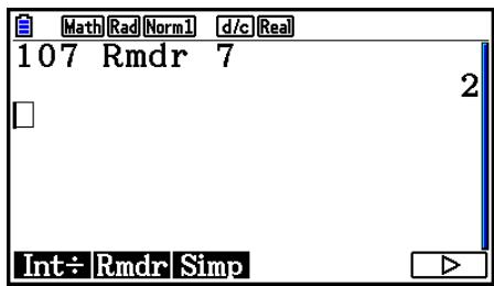
AC 1 0 7 OPTN F4 (CALC) F6 (>)
F6(>)F2(Rmdr)7
EXE
[OPTN]-[CALC]-[d/dx]
ACOPTN F4(CALC)F6(>)F1(FMin)X,0,Tx²-4X,0,T+9
AC OPTN F3 (COMPLEX) F2 (Abs)
3+4F1(i)EXE
Hexadécimale:0,1,2,3,4,5,6,7,8,9,A,B,C,D,E,F
Négative: -2147483648 ≤ x ≤ -1
[SET UP]-[Mode]-[Dec]/[Hex]/[Bin]/[Oct]
ALPHA X,0,T (A) SHIFT + ([ ] 1 9 2
SHIFT [] EXE
| Math|Rad|Norm1 | d/c|Real |
| 10→Mat A[1,2] | |
| 10 | |
OPTN F2 (MAT/VCT) F5 (Augment)
F1 (Mat) ALPHA X,θ,T (A)
F1 (Mat) ALPHA log (B) EXE
| Math | Rad | Norml | d/c | Real |
| Augment (Mat A, Mat B) | ||||
| 1 | 3 | |||
| 2 | 4 | |||
→OPTN F1(List)F1(List)1 EXE
F1(List) 1 EXE
Mat→List(Mat A,2)→Li{2,4,6}
Calculus matriciels
[OPTN]-[MAT/VCT]
[OPTN]-[MAT/VCT]-[Trn]
[OPTN]-[MAT/VCT]-[Ref]
Incorrect: {34, 53, 78}
OPTN F1(List) F1(List) 1 +
OPTN F1(List) F1(List) 2 EXE
SHIFT 1(List) n SHIFT +([0 SHIFT -]) [EXE
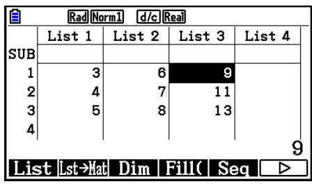
OPTN F1(List) F2(List Mat) F1(List)
OPTN F1(List) F3(Dim) F1(List)
OPTN F1(List) F4 (Fill()
OPTN F1(List) F5 (Seq)
F6(>)F6(>)F1(List) 1 EXE
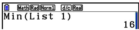
OPTN F1(List) F6(▷) F2(Max) F6(▷) F6(▷) F1(List)
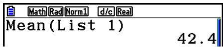
[OPTN]-[LIST]-[Mean]
OPTN F1(List) F6(D) F3(Mean) F6(D) F6(D) F1(List)
AC OPTN F1(List)F6(>)F3(Mean)
F6(>)F6(>)F1(List) 1 EXE
OPTN F1(List) F6(>) F4(Med) F6(>) F6(>) F1(List)
F1(List)
Math [Rad] Norm1 d/c| Real Median(List 1, List 246
- Pour combiner des listedes
[OPTN]-[LIST]-[Augment]
OPTN F1(List) F6(>) F5(Augment) F6(>) F6(>) F1(List)
AC OPTN F1(List) F6(▷) F5(Augment)
F6( )F6( )F1(List)1
F1(List) 2 EXE
Math [Rad] Norm1 d/c Real] Augment(List 1, List {-3,-2,1,9,10}
OPTN F1(List) F6(>) F6(>) F1(Sum) F6(>) F1(List)
OPTN F1(List) F6(>) F6(>) F3(Cuml) F6(>) F1(List)
OPTN F1(List) F6 (D) F6 (D) F4 (%) F6 (D) F1(List)
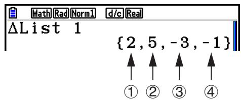
AC OPTN F1(List) F6(>) F6(>) F5(ΔList)
1 EXE
① 3 - 1 =
② 8 - 3 =
③ 5 - 8 =
④ 4-5=
AC OPTN F1(List)F1(List)
AC OPTN F1(List)F1(List)
OPTN F1(List) F1(List) 3 → F1(List) 1 EXE
sin OPTN F1(List) F1(List) 2 SHIFT + ([ ) 3 SHIFT - ([ ]) EXE
2 5 → OPTN F1(List) F1(List) 3 SHIFT + ([ ) 2 SHIFT - ([ ]) EXE
OPTN F1(List) F1(List) 1 EXE
OPTN F1(List) F1(List) SHIFT (-)(Ans) 3 6 EXE
sin OPTN F1(List) F1(List) 3 EXE
Complex Mode: r
- Grid: On (Axes: On, Label: Off)
- Label: On (Axes: On, Grid: Off)
④ F3(TYPE)F1(Y=)ALPHA X,θ,T(A)X,θ,T x² - 3
SHIFT + ( [ ) ALPHA X,θ,T (A) SHIFT = ( = ) 3 9 1 9 (-) 1
SHIFT []EXE
(5) F6 (DRAW)
(5) F3(TYPE)F1(Y=)SHIFT 1(List) 1 X,0,T x² - 3 EXE
(6) F6 (DRAW)
Type 1 (Y= expression)
$$ \begin{array}{l} \text {X m a x} = 6, \end{array} $$
$$ X s c a l e = 1 $$
$$ \mathbf {Y} \min = - 2, $$
$$ \mathbf {Y} \max = 1 0, $$
$$ \mathbf {Y s c a l e} = 2 $$
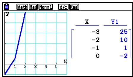
① MENU Table
② SHIFT F3 (V-WIN) 0 EXE 6 EXE 1 EXE

(3) F3(TYPE) F1(Y=) 3 X,θ,T x² - 2 EXE

④ F5 (SET) (-3 EXE 3 EXE 1 EXE EXIT
(5) F6(TABLE)
(6) F5(GPH-CON)
$$ \begin{array}{l} \text {X m a x} = 6, \end{array} $$
$$ X s c a l e = 1 $$
$$ \mathbf {Y} \min = - 2, $$
$$ \mathbf {Y} \max = 1 0, $$
$$ \mathbf {Y s c a l e} = 2 $$
① MENU Table
② SHIFT F3 (V-WIN) 0 EXE 6 EXE 1 EXE
$$ \begin{array}{c c c c c c c} \text {(-)} & 2 & \text {E X E} & 1 & 0 & \text {E X E} & 2 & \text {E X E} & \text {E X I T} \end{array} $$
③ SHIFT MENU (SET UP) F1 (T+G) EXIT
④ F3(TYPE)F1(Y=)3X,0,Tx²-2EXE
(5) F5 (SET)
(→) 3 EXE 3 EXE 1 EXE EXIT
(6) F6(Table)
⑦ F5(GPH-CON)
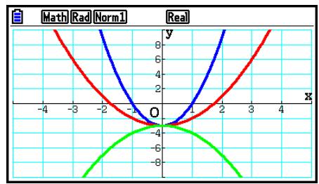
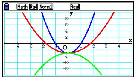
① MENU Graphe
② SHIFT F3 (V-WIN) F1 (INITIAL) EXIT
③ SHIFT (SET UP) (▼) (▼) (▼) (▼) (▼) (F1(COLOR) 1 (Black)
F1(一) EXIT
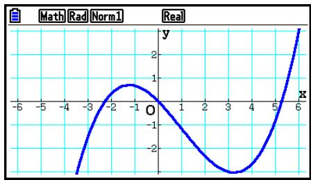
④ F3(TYPE)F1(Y=)X,0T C X,0T + 2 )C X,0T
2 EXE
(5) F6 (DRAW)
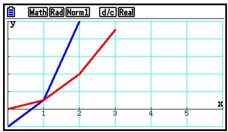
(6) SHIFT F4 (SKETCH) F2 (Tangent)
⑦ SHIFT 5 (FORMAT) 1 (Styl ligne) 5 (Thin)
(Couligne) (Red)
8 \~EXE*1
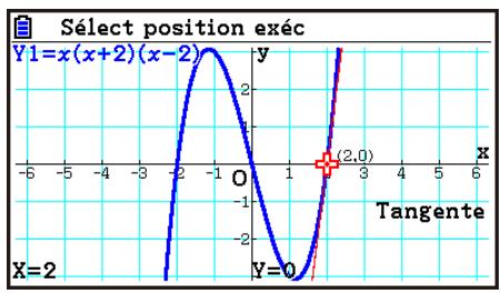
$$ \Upsilon 1 = x (x + 2) (x - 2) $$
- Mark Type (Type de point)
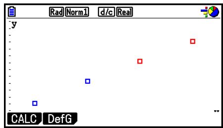
Color Link: OnlyX (diagramme de dispersion)
$$ \frac {② + ③}{2} = Q 1 $$
$$ \frac {(6) + (7)}{2} = Q 3 $$
F1(GRAPH) F6 (SET) F1 (Scatter) EMT F1 (GRAPH1)
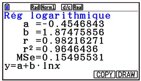
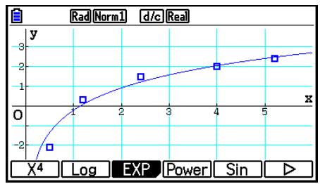
(3) F1(CALC)F6(>)F2(Log)
(4) F6 (DRAW)
F1(CALC) F3(Med)
F6 (DRAW)
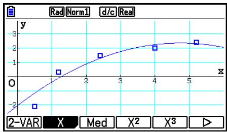
F1(CALC) F4(X2)
F6 (DRAW)
F1 (CALC) F6 (▷) F4 (Power)
F6 (DRAW)
$$ (\dot {=} 0, 4 9 6) $$
F1(P() 0 4 9 6) -
F1(P)(-)1634EXE
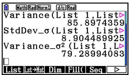
F1(List) F1(List) 1 F1(List) 2 EEX
EXIT F5 (STAT) F5 (Var) F1 (S²) EXIT
F1(List) F1(List) 1 F1(List) 2 EEX
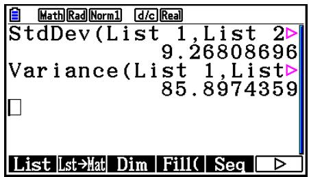
OPTN F5 (STAT) F4 (StdDev) F2 (σ) EXIT EXIT
F1(List) F1(List) 1 F1(List) 2 EEX
OPTN F5 (STAT) F5 (Var) F2 (^2) EXIT EXIT
F1(List) F1(List) 1 F1(List) 2 EEX
F1(List) F1(List) SHIFT (-)(Ans) EXE
List3={113,116,139,132,133,131,126,122}
F3 (CHI) ... distribution ^2 (page 6-55)
F4(F) ... distribution F (page 6-57)
F5 (BINOMIAL) ... Distribution binomial (page 6-58)
F6(>)F1(POISSON) ... Distribution de Poisson (page 6-60)
F6(>)F2(GEO) ... Distribution géométrie (page 6-62)
F6(>)F3(HYPRGEO) ... Distribution hypergéométrie (page 6-64)
$$ P V = - (P M T \times n + F V) $$
$$ F V = - (P M T \times n + P V) $$
$$ P M T = - \frac {P V + \beta \times F V}{\alpha} $$
$$ n = \frac {\log \left{\frac {(1 + i S) \times P M T - F V \times i}{(1 + i S) \times P M T + P V \times i} \right}}{\log (1 + i)} $$
$$ P M T = - \frac {P V + F V}{n} $$
$$ n = - \frac {P V + F V}{P M T} $$
$$ \alpha = (1 + i \times S) \times \frac {1 - \beta}{i}, \beta = (1 + i) ^ {- n} $$
$$ S = \left{ \begin{array}{l} 0 \text {......} \text {P a y m e n t : E n d} \ \text {(E c r a n d e c o n f i g u r a t i o n)} \ 1 \text {......} \text {P a y m e n t : B e g i n} \ \text {(E c r a n d e c o n f i g u r a t i o n)} \end{array} \right. $$
$$ i = \left{ \begin{array}{l} \frac {I \%}{100} \ (1 + \frac {I \%}{100 \times [C / Y]})^{\frac {C / Y}{P / Y}} - 1 \dots \dots \dots \dots \dots \dots \dots \dots \dots \dots \dots \dots \dots \dots \dots \dots \dots \dots \dots \dots \dots \dots \dots \dots \dots \dots \dots \dots \dots \dots \dots \dots \dots \dots \dots \dots \dots \dots \dots \dots \dots \dots \dots \dots \dots \dots \dots \dots \dots \dots \tag{P/Y=C/Y=1} \ (\text{Autres que ci-dessus}) \end{array} \right. $$
- I%
$$ P V + \alpha \times P M T + \beta \times F V = 0 $$
$$ N F V = N P V \times (1 + i) ^ {n} $$
- IRR
$$ 0 = C F _ {0} + \frac {C F _ {1}}{(1 + i)} + \frac {C F _ {2}}{(1 + i) ^ {2}} + \frac {C F _ {3}}{(1 + i) ^ {3}} + \dots + \frac {C F _ {n}}{(1 + i) ^ {n}} $$
$$ I N T = - \frac {A}{D} \times \frac {C P N}{M} \quad C S T = P R C + I N T $$
- Rendement annuel (YLD)
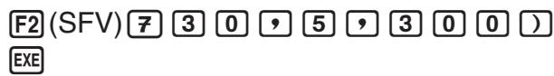
OPTN F6 (D) F6 (D) F2 (FINANCE)*
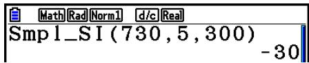
F1(SIMPLE)F1(SI)7305
3 0 0 EXE
'Program Mode: RUN (programme mode RUN - execution)
'Program Mode: BASE (programme mode BASE)
DrawFTG-Con, DrawFTG-Plt
Aucun paramètre
Blue Locate 7, 1, "CASIO FX"
Receive38k / Send38k
Mode RUN : Black, Blue, Red, Magenta, Green, Cyan, Yellow, ColorAuto, ColorCir Mode BASE : Black, Blue, Red, Magenta, Green, Cyan, Yellow
Mode BASE: SHIFT 5 (FORMAT) 2 (Blue)
Example: Red Graph Y = X^2 - 1
- Commandes Sketch
S-Gph1 DrawOn, NPPlot, List 1, Square, ColorLinkOff, Blue
S-Gph1 DrawOn, N-Dist, List 1, List 2, Blue
S-Gph1 DrawOn, Linear, List 1, List 2, List 3, Blue
S-Gph1 DrawOn, Logistic, List 1, List 2, Blue
S-Gph1 DrawOn, Bar, List 1, None, None, StickLength, ColorLinkOff, Blue ColorLighter, Black, Red ColorLighter, Black, Green ColorLighter, Black
2-Variable List 1, List 2, List 3
LinearReg(ax+b) List 1, List 2, List 3
Type de calcul*
LogisticReg List 1, List 2
= 1 = 0 tail =L (Left)
Syntaxe : TwoPropZTest "p1 condition", x_1,n_1,x_2,n_2
Syntax: Cash_NPV(1%, Csh)
| Touche (SHIFT) (SET UP) | |||
| Niveau 1 | Niveau 2 | Niveau 3 | Commande |
| Dec | Dec | ||
| Hex | Hex | ||
| Bin | Bin | ||
| Oct | Oct | ||
| Touche SHIFT 5 (FORMAT) | |||
| Niveau 1 | Niveau 2 | Niveau 3 | Commande |
| 1:Black | Black_ | ||
| 2:Blue | Blue_ | ||
| 3:Red | Red_ | ||
| 4:Magenta | Magenta_ | ||
| 5:Green | Green_ | ||
| 6:Cyan | Cyan_ | ||
| 7:Yellow | Yellow_ | ||
| Niveau 3 | Niveau 4 | Commande | |
| *1 | Exp | aebx | Exp(ae^bx) |
| abx | Exp(ab^x) | ||
| *2 | MARK | □ | Square |
| XXX | Cross | ||
| ■ | Dot | ||
| STICK | Length | StickLength | |
| Horz | StickHoriz | ||
| %DATA | % | % | |
| Data | Data | ||
| None | None | ||
| COLOR LINK | BothXY | ColorLinkX&Y | |
| X&Freq | ColorLinkX&Freq | ||
| OnlyX | ColorLinkOnlyX | ||
| OnlyY | ColorLinkOnlyY | ||
| On | ColorLinkOn | ||
| Off | ColorLinkOff | ||
| *3 | X | ax+b | LinearReg(ax+b) |
| a+bx | LinearReg(a+bx) | ||
| *4 | EXP | aebx | Exp(a•e^bx) |
| abx | Exp(a•b^x) | ||
| *5 | NORM | Npd | NormPD() |
| Ncd | NormCD() | ||
| InvN | InvNormCD() | ||
| t | tpd | tpD() | |
| tcd | tCD() | ||
| Invt | InvTCD() | ||
| CHI | Cpd | ChiPD() | |
| Ccd | ChiCD() | ||
| InvC | InvChiCD() | ||
| F | Fpd | FPD() | |
| Fcd | FCD() | ||
| InvF | InvFCD() | ||
| BINOMIAL | Bpd | BinomialPD() | |
| Bcd | BinomialCD() | ||
| InvB | InvBinomialCD() | ||
| POISSON | Ppd | PoissonPD() | |
| Pcd | PoissonCD() | ||
| InvP | InvPoissonCD() | ||
| GEO | Gpd | GeoPD() | |
| Gcd | GeoCD() | ||
| InvG | InvGeoCD() | ||
| HYPRGEO | Hpd | HypergeoPD() | |
| Hcd | HypergeoCD() | ||
| InvH | InvHyperGeoCD() | ||
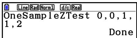
| *6 | Z | 1-Sample | OneSampleZTest_ |
| 2-Sample | TwoSampleZTest_ | ||
| 1-Prop | OnePropZTest_ | ||
| 2-Prop | TwoPropZTest_ | ||
| t | 1-Sample | OneSampleTTest_ | |
| 2-Sample | TwoSampleTTest_ | ||
| REG | LinRegTTest_ | ||
| CHI | GOF | ChiGOFTest_ | |
| 2WAY | ChiTest_ | ||
| F | TwoSampleFTest_ | ||
| ANOVA | 1WAYANO | OneWayANOVA_ | |
| 2WAYANO | TwoWayANOVA_ |
-
Appuyez sur [EXIT] pour quitter l'écran des paramètres généraux de graphe.
-
Appuyez sur F1(GRAPH1).
-
Le grapheREENuoulaueaoueauauauauauauauauauauauauauauauauauauauauauauauauauauauauauauauauauauauauauauauauauauauauauauauauauauauauuuuuuuuuuuuuuuuuuuuuuuuuuuuuuuuuuuuuuuuuuuuuuuuuuuuuuuuuuuuuuuuuuuuuuuuuuuuuuuuuuuuuuuuuuuuuuuuuuuuuuuuuuuuuuuuuuuuuuuuuuuuuuuuuuuuuuuuuuuuuuuuuuuuuuuuuuuuuuuuuuuuuuuuuuuuuuuuuuuuuuuuuuuUU
Mémoire de stockage*1
Windows 8.1 (32 bits, 64 bits)
Windows 10 (32 bits, 64 bits)
macOS 10.13, macOS 10.14, macOS 10.15, macOS 11.X
Longueur : mm, cm, m, km, inch, feet, yard, mile
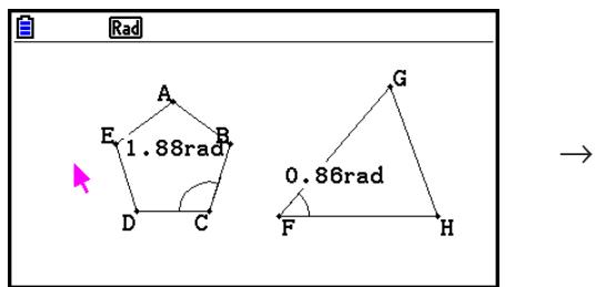
Angle:Rad, AngleUnit:On
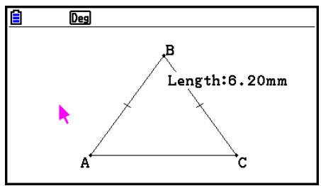
Length Unit : On (mm)
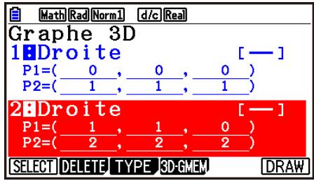
Droite 2:P1 = 1,1,0
P2=2,2,2
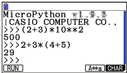
$$ (2 + 3) \times 1 0 ^ {2} = 5 0 0 $$
$$ \boxed { \begin{array}{c c c c c c c} \square & \square + & 3 \ \hline \end{array} } \times \boxed { \begin{array}{c c c c c c c} \times & 1 & 0 \ \hline \end{array} } \boxed { \begin{array}{c c c c c c c} \text {E X E} \ \hline \end{array} } $$
$$ 2 + 3 \times (4 + 5) = 2 9 $$
$$ \boxed {2} + \boxed {3} \times \boxed {(4} + \boxed {5)} \boxed {\mathrm {E X E}} $$
$$ \left| \begin{array}{l} \ggg a = \text {i n p u t (}" 1 2 3 ? ") \ 1 2 3? | \end{array} \right. $$
clear.Screen() show screenings
draw_string(0,0,"abc", (0,0,0), "large")
show screenings()
Remarque :
Distributions continues : Normale, Student, ^2 , Fisher
Distribution Student
df: Degres de liberté (df > 0)
Distribution ^2
Distribution Student
| Type | { } (≤X≤) |
| Inf | 0 |
| Sup | 1 |
| df | 1 |
Type: ≤ X≤
Type: X≥
The MIT License (MIT)
Copyright (c) 2013-2017 Damien P. George, and others
Permission is hereby granted, free of charge, to any person obtaining a copy of this software and associated documentation files (the "Software"), to deal in the Software without restriction, including without limitation the rights to use, copy, modify, merge, publish, distribute, sublicense, and/or sell copies of the Software, and to permit persons to whom the Software is furnished to do so, subject to the following conditions:
The above copyright notice and this permission notice shall be included in all copies or substantial portions of the Software.
THE SOFTWARE IS PROVIDED "AS IS", WITHOUT WARRANTY OF ANY KIND, EXPRESS OR IMPLIED, INCLUDING BUT NOT LIMITED TO THE WARRANTYES OF MERCHANTABILITY, FITNESS FOR A PARTICULAR PURPOSE AND NONINFRINGEMENT. IN NO EVENT SHALL THE AUTHORS OR COPYRIGHT HOLDERS BE LIABLE FOR ANY CLAIM, DAMAGES OR OTHER LIABILITY, WHETHER IN AN ACTION OF CONTRACT, TORT OR OTHERWISE, ARISING FROM, OUT OF OR IN CONNECTION WITH THE SOFTWARE OR THE USE OR OTHER DEALINGS IN THE SOFTWARE.
E-CON4 Application (English)
Important!
- All explanations in this section assume that you are fully familiar with all calculator and Data Logger (CMA CLAB* or CASIO EA-200) precautions, terminology, and operational procedures.
CLAB firmware must be version 2.10 or higher. Be sure to check the firmware version of your CLAB before using it.
- For information about CMA and the CLAB Data Logger, visit http://cma-science.nl/.
1. E-CON4 Mode Overview
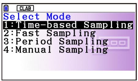
The first time you enter the E-CON4 mode, a screen will appear for selecting a Data Logger.

Data Logger Selection Screen
Press F1(CLAB) or F2(EA-200) to select the Data Logger you want to use.
Selecting a Data Logger will cause the sampling screen (Time-based Sampling screen) to appear.
Use the sampling screen to start sampling with the Data Logger and to view a graph of samples.
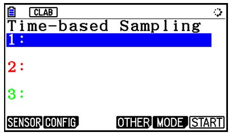
CLAB
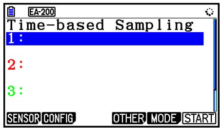
EA-200
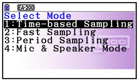
There are four sampling modes (sampling screens), described below.
- Time-based Sampling ... Draws a graph simultaneously as sampling is performed. Note, however, that the graph is drawn after sampling is finished when CH1, 2, or 3, SONIC, or [START] key is specified as the trigger source, or when the sampling interval is less than 0.2 seconds.
- Fast Sampling ... Select to sample high-speed phenomena (sound, etc.)
- Period Sampling ... Select to perform periodic sampling starting from a start trigger event and ending with an end trigger event.
- Manual Sampling ... Sampling is performed when the [EXE] key is pressed. Up to 100 samples can be taken by manual operation. Sampled data is stored in the Statistics mode list. (CLAB only)
-
Mic & Speaker Mode ... Select to sample sound using the built-in microphone. You can also output a waveform using the built-in speaker. (EA-200 only)
-
The Data Logger selection screen will not appear from the next time you enter the E-CON4 mode. Instead, the Time-based Sampling screen for the selected a Data Logger will appear first.
- To change the Data Logger, change the setting on the E-CON4 setup screen.
- Connecting a Data Logger that is different from the one specified for the calculator will cause an error message to appear. If this happens, use the setup screen to change the "Data Logger" setting.
E-CON4 Specific Setup Items
The items described below are E-CON4 setup items that displayed only when the
SHIFT MENU (SET UP) operation is performed in the E-CON4 mode.
Indicates the initial default setting of each item.
Data Logger
-
{CLAB}/{EA-200} ... {CLAB Data Logger}/{EA-200 Data Logger}
-
Graph Func
-
On /Off ... {show graph source data name}/{hide graph source data name}
-
Coord
-
On / Off ... {show coordinate values}/{hide coordinate values} during trace operations
-
E-CON Axes
-
/Off ... {show axes}/hide axes}
Real Scroll
- {On}/{Off} ... {enable real-time scrolling}/{disable real-time scrolling}
CMA Temp BT01
- C / F ... CMA Temperature BT01 measurement unit C / F
CMA Temp 0511
- C / F ... CMA Temperature 0511 measurement unit C / F
CASIO Temp
- C / F ... CASIO Temperature measurement unit C / F
Vrnr Baro
- atm /inHg /mbar /mmHg ... Vernier Barometer measurement unit atm /inHg / mbar /mmHg
Vrnr Gas Prs
- atm /inHg /kPa /mbar /mmHg /psi ... Vernier Gas Pressure measurement unit atm /inHg /kPa /mbar /mmHg /psi
Vrnr Mag F L
- mT / gauss ... Vernier Magnetic Field Low-amp measurement unit mT / gauss
Vrnr Mag F H
- mT /gauss ... Vernier Magnetic Field High-amp measurement unit mT /gauss
2. Sampling Screen
Changing the Sampling Screen
On any sampling screen, press F5 (MODE) to display the sampling mode selection screen.
CLAB
EA-200
Use keys 1 through 4 to select the sampling mode that matches the type of sampling you want to perform.
Time-based Sampling Screen
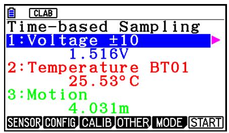
CLAB
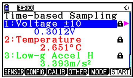
EA-200
- CLAB has three channels named CH1, CH2, and CH3.
- EA-200 has four channels named CH1, CH2, CH3, and SONIC. Note, however, that up to only three channels can be used for sampling at any one time. If you try to start sampling with four channels at the same time, a “Too Many Channels” error will appear.
Fast Sampling Screen
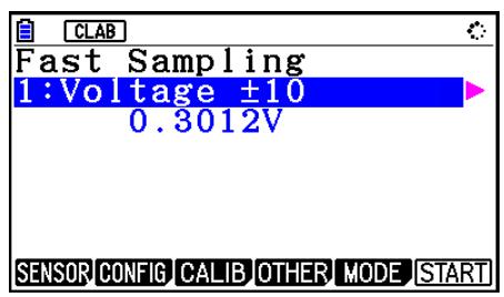
CLAB
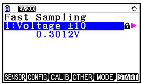
EA-200
- Both CLAB and EA-200 can use CH1 only.
Period Sampling Screen
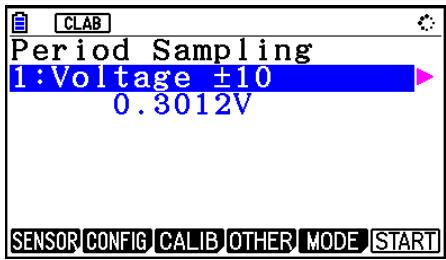
CLAB
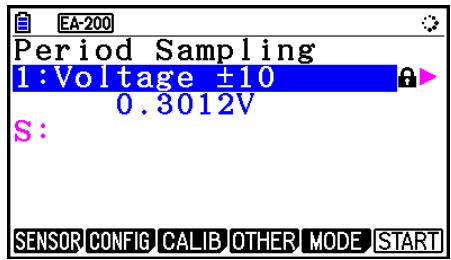
EA-200
- With CLAB, only CH1 can be used.
- EA-200 has two channels (CH1 and SONIC). However, only one of these can be used.
Manual Sampling Screen (CLAB Only)
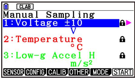
CLAB
- There are three channels named CH1, CH2, and CH3.
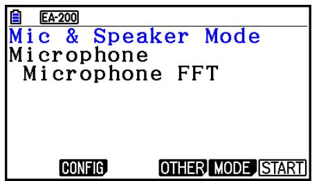
■ Mic & Speaker Mode Screen (EA-200 Only)
On the sampling mode selection screen, pressing 4 (Mic & Speaker Mode) displays the dialog box shown below.
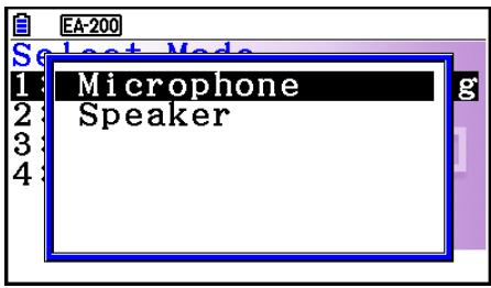
Select Microphone or Speaker.
- Selecting Microphone
This displays the dialog box shown below.
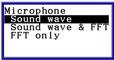
"Sound wave" records the following two dimensions for the sampled sound data: elapsed time (horizontal axis) and volume (vertical axis).
"FFT" records the following two dimensions: frequency (horizontal axis) and volume (vertical axis).
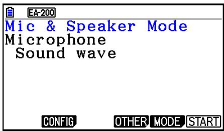
- Selecting "Sound wave" here will display the Mic & Speaker Mode screen.

- Selecting "Sound wave & FFT" or "FFT only" will display the dialog box shown below.
| Select FFT Range | |
| 2 - 1000Hz: [F1] | |
| 4 - 2000Hz: [F2] | |
| 6 - 3000Hz: [F3] | |
| 8 - 4000Hz: [F4] |
Selecting an option automatically configures parameters with the fixed values shown in the table below.
| Option Parameter | 2 - 1000Hz: F1 | 4 - 2000 Hz: F2 | 6 - 3000 Hz: F3 | 8 - 4000 Hz: F4 |
| Frequency Pitch | 2 Hz | 4 Hz | 6 Hz | 8 Hz |
| Frequency Upper Limit | 1000 Hz | 2000 Hz | 3000 Hz | 4000 Hz |
| Sampling Period | 61 μsec | 31 μsec | 20 μsec | 31 μsec |
| Number of Samples | 8192 | 8192 | 8192 | 4096 |
Using a function key (F1 through F4) to select an FFT range, will cause a Mic & Speaker Mode screen to appear.
Selecting "Sound wave & FFT"
Selecting "FFT only"
- Selecting Speaker
This displays the dialog box shown below.
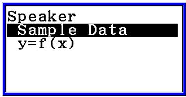
- Selecting "Sample Data" here will display the Mic & Speaker Mode screen.
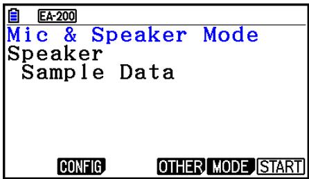
After selecting "y=f(x)", perform the steps below.
From the EA-200, output the sound of the waveform indicated by the function input on the calculator, and draw a graph of the function on the calculator unit screen.
-
Use the data communication cable (SB-62) to connect the communication port of the calculator with the MASTER port of the EA-200.
-
On the above dialog box, select "y=f(x)".
-
This displays a dialog box like the one shown below.
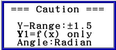
-
Press EXE to display the View Window screen.
-
The following settings will be configured automatically Ymin = -1.5 , Ymax = 1.5 . Do not change these settings.
-
Press EXE or EXIT to display the function registration screen.
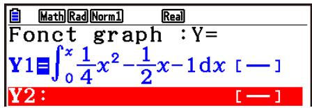
- In the "Y1=" line, register the function of the waveform of the sound you want to output.
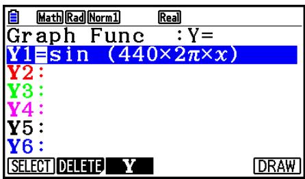
- For the angle unit, specify radians.
-
Register a function with an Y-value within the range of ± 1.5 .
-
Press F6 (DRAW) to draw the graph.
-
Drawing the graph causes a vertical cursor to appear on the display, as shown on the screenshot below. Use this graph to specify the range of the sound output from the speaker.
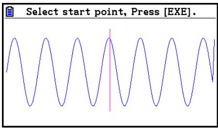
- Use the and keys to move the vertical cursor of the output range start point and then press to register the start point.
-
Use the and keys to move the vertical cursor of the output range end point and then press to register the end point.
-
Setting both the start point and end point will cause the Output Frequency dialog box shown below to appear.
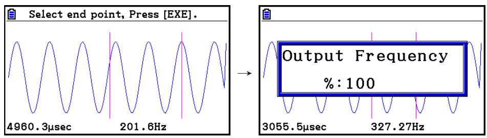
-
Specify the output frequency percent (%) value.
-
To output the original sound unchanged, specify 100 (%). To output a sound one octave higher than the original sound, input 200 (%). To output a sound one octave lower than the original sound, input 50 (%).
-
Input a percent (%) value and then press
-
This outputs the sound of the waveform within the selected range.
-
If the specified result cannot be output as a sound, the message “Range Error” will appear. If this happens, press to display the screen shown below and change the settings.
-
To stop sound output on the EA-200, press the [START/STOP] key.
-
Press .
-
This displays a screen like the one shown below.
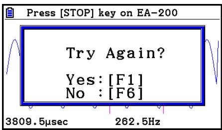
- Depending on what you want to do, perform one of the operations below.
To change the output frequency and try again:
Press F1 (Yes) to return to the Output Frequency dialog box. Next, perform the operation starting from step 9, above.
To change the output range of the waveform graph and try again:
Press F6 (No) to return to the graph screen in step 6, above. Next, perform the operation starting from step 7, above.
To change the function:
Press F6 (No) EXIT to return to the function registration screen in step 5, above. Next, perform the operation starting from step 5, above.
To exit the procedure and return to the sampling mode selection screen:
Press F6 (No). Next, press EXIT twice.
Sampling Screen Function Menu
- F1(SENSOR) ....... Selects the sensor assigned to a channel.
- F2 (CONFIG) .... Select to configure settings that control sampling (sampling period, number of samples, warm-up time, etc.)
- F3(CALIB) ....... Performs auto sensor calibration.
-
F4(OTHER) ....... Displays the submenu below.
-
F1(GRAPH) .... Graphs the samples measured by the Data Logger. You can use various graph analysis tools. (Cannot be used on the Period Sampling screen.)
- F2(MEMORY) ....... Saves Data Logger setup data.
- F5 (INITIAL) ....... initializes setting parameters.
-
F6 (ABOUT) .... Shows version information about the Data Logger currently connected to calculator.
-
F5 (MODE) ....... Selects a sampling mode.
- F6(START) ....... Starts sampling with the Data Logger.
3. Auto Sensor Detection (CLAB Only)
When using a CLAB Data Logger, sensors connected to each channel are detected automatically. This means that you can connect a sensor and immediately start sampling.
- On the setup screen, select "CLAB" for the "Data Logger" setting.
- Connect the CLAB Data Logger to the calculator.
-
Connect a sensor to each of the CLAB channels you want to use.
-
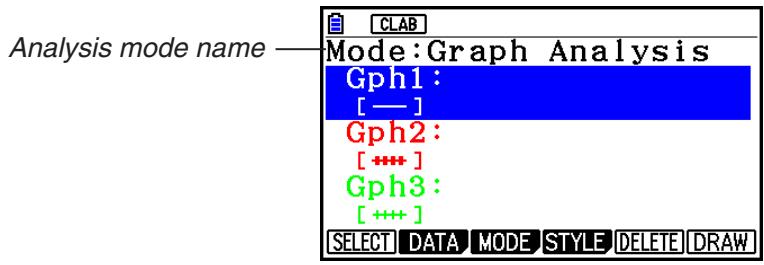
Detection of a sensor will cause a screen like the one below to appear.
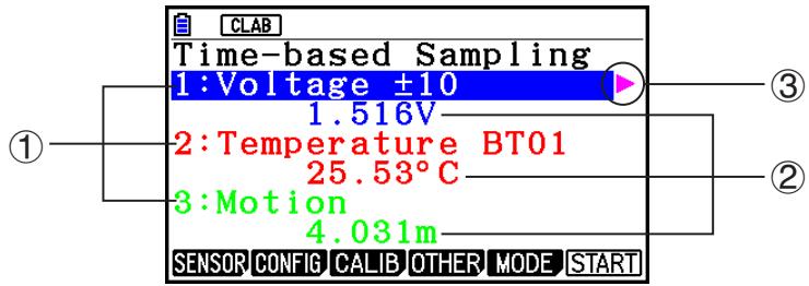
① Show the names of the sensor connected to each channel.
② Show the current sample values of each channel.
(3) Selecting (highlighting) a channel causes to appear next to it. Pressing displays sensor details as shown below for the currently selected sensor.
= SENSOR PROPERTIES = Voltage ±10 UNIT : V RANGE: -10 - 10
-
Press F6 (START) to start sampling.
-
Some sensors do not support auto detection. If this happens, press F1(SENSOR) and then select the applicable sensor.
Note
- If a sensor that supports auto detection is not detected automatically, restart CLAB.
4. Selecting a Sensor
On the sampling screen, press F1 (SENSOR) to display the sensor selection screen.
■Assigning a Sensor to a Channel
- On the sampling screen, use and to select the channel to which you want to assign the sensor.
-
Press F1(SENSOR).
-
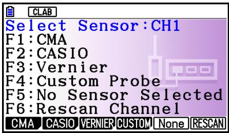
This displays the sensor selection screen like the one shown below. The appearance of the sensor selection screen depends on the Data Logger type and the selected channel.
-
Press one of the function keys below.
-
CH1, CH2, CH3
F1 (CMA) ... Displays a list of CMA sensors.
F2 (CASIO) ... Displays a list of CASIO sensors.
F3 (VERNIER) ... Displays a list of Vernier sensors.
(F4)(CUSTOM) ... Displays a list of custom sensors. See “7. Using a Custom Probe” (page 8-23).
(F5)(None) ... Even if a sensor is connected, it is disabled.
F6 (RESCAN) ... deletes the sensor currently assigned to a channel (CLAB only).
- SONIC (EA-200 only)
F2(CASIO) ... Displays a list of CASIO sensors. Only "Motion" can be selected.
F3 (VERNIER) ... Displays a list of Vernier sensors. You can select either "Motion" or "Photogate".
(F5) None) ... SONIC channel not used.
Note
- After selecting "Motion" on either the CASIO or the Vernier sensor list, pressing OPTN will toggle smoothing (sampling error correction) between on and off. "-Smooth" will be shown on the display while smoothing is on. Nothing is displayed when off.
- Selecting "Photogate" on the Vernier sensor list will display a menu that you can use to select [Gate] or [Pulley].
[Gate] ... Photogate sensor used alone.
[Pulley] ... Photogate sensor used in combination with smart pulley.
- Pressing a function key displays a dialog box like the one shown below. This shows the sensors that can be assigned to the selected channel.
| CMA Sensors |
| Voltage |
| Temperature |
| Motion |
| CLAB Accel X |
| CLAB Accel Y |
4.Use l and to select the sensor you want to assign and then press EXE.
- This returns to the screen in step 1 of this procedure with the name of the sensor you assigned displayed. At this time there will be a lock (A) icon to the right of the sensor name. This icon indicates the sensor you assigned with the operation above.
Note
- You can also assign a custom probe to a channel. To do so, press F4 (CUSTOM) to display the custom probe list. Use this list to select a custom probe and then press EXE.
Disabling a Sensor
Perform the steps below when you do not want to perform sampling with a sensor that is connected to the Data Logger.
- On the sampling screen, use and to select the sensor you want to disable.
-
Press F1(SENSOR).
-
This displays the sensor selection screen.
-
Press F5 (NONE).
-
This returns to the screen in step 1 of this procedure with no sensor assigned to the channel. There will be a lock ( ) icon indicated for the channel in this case.
- The above operation also disables sensor auto detection.
■ Removing the Sensor Assigned to a Channel (CLAB Only)
- On the sampling screen, use and to select the sensor you want to remove.
-
Press F1 (SENSOR).
-
This displays the sensor selection screen.
-
Press F6(RESCAN).
-
This returns to the screen in step 1 of this procedure with no sensor assigned to the channel. There will be no lock (B) icon indicated for the channel in this case.
- The above operation also enables sensor auto detection.
5. Configuring the Sampling Setup
You can configure detailed settings to control individual sampling parameters and to configure the Data Logger for a specific application. Use the Sampling Config screen to configure settings.
There are two configuration methods, described below.
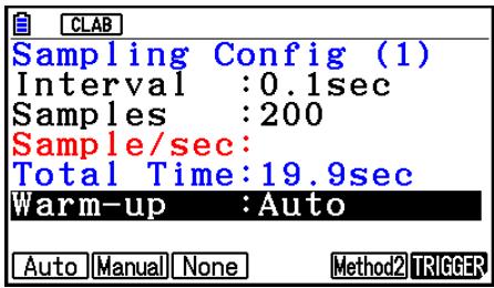
Method 1 ... With this method, you configure settings for the sampling interval (Interval) and number of samples (Samples).
Method 2 ... With this method, you configure settings for the number of samples per second (Sample/sec) and the total sampling time (Total Time).
You can also use the Sampling Config screen to configure trigger settings. See "Trigger Setup" (page 15).
Initial default settings are shown below.
- Setting Method: Method 1
- Interval: 0.2 sec
Samples: 101 - Sample/sec: 5 (This setting is not displayed in the case of Method 1.)
Total Time: 20 sec - Warm-up: Auto
In the case of "Manual Sampling", a special Manual Sampling Config screen will appear. For more information, refer to "Configuring Manual Sampling Settings" (page -19).
Using Method 1 to Configure Settings
-
On the sampling screen, press F2 (CONFIG).
-
This displays the Sampling Config screen with "Interval" highlighted.
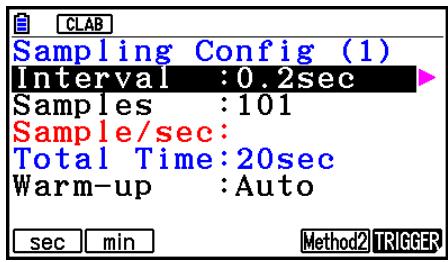
- Press F1(sec) or F2(min) to specify the sampling interval unit.
-
Press
-
This displays a dialog box for configuring the sampling interval setting.
-
Input the sampling interval and then press .
-
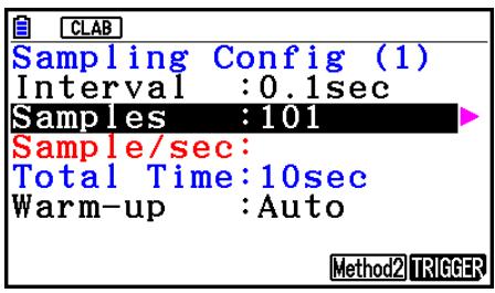
Press to move the highlighting to "Samples".
-
When the sampling mode is "Periodic Sampling" and a CMA or Vernier Photogate Pulley is assigned to the channel, "Distance" will be displayed in place of "Samples". For information about "Distance", see "To configure the Distance setting" below.
-
Press
- This displays a dialog box for specifying the number of samples.
- Input the number of samples and then press .
- Press to move the highlighting to "Warm-up".
- Press one of the functions keys below.
F1(Auto) ... Automatically configures warm-up time settings for each sensor.
F2 (Manual) ... Select for manual input of the warm-up time in seconds units.
(F3(None) ... Disables warm-up time.
- Pressing F2 (Manual) displays a dialog box for specifying the warm-up time. Input the warm-up time and then press EXE.
-
When the sampling mode is "Fast Sampling", "FFT Graph" will be displayed in place of "Warm-up". For information about "FFT Graph", see "To configure the FFT Graph setting" below.
-
After all of settings are the way you want, press EXIT
-
This returns to the sampling screen.
- To configure the Distance setting
Move the highlighting to "Distance" and then press F1 (NUMBER). This displays a dialog box for specifying the drop distance for the smart pulley weight.
Input a value from 0.1 to 4.0 to specify the distance in meters.
- To configure FFT Graph setting
In place of step 9 of the procedure under "Using Method 1 to Configure Settings", specify whether or not you want to draw a frequency characteristics graph (FFT Graph).
F1(On) ... Draws an FFT graph after sampling is finished. Use the dialog box that appears to select a frequency.
F2 (Off) ... FFT Graph no drawn after sampling is finished.
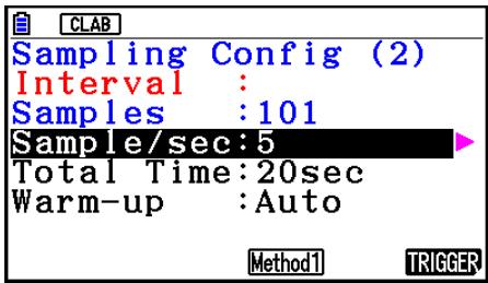
Using Method 2 to Configure Settings
-
On the sampling screen, press F2 (CONFIG).
-
This displays the Sampling Config screen.
-
Press F5 (Method2).
- This will cause the highlighting to move to "Sample/sec".
-
Press
-
This displays a dialog box for specifying the number of samples per second.
-
Input the number of samples and then press .
- Press to move the highlighting to "Total Time".
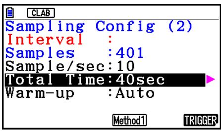
- Press
- This displays a dialog box for specifying the sampling time.
- Input the sampling time and then press .
- Press to move the highlighting to "Warm-up".
- Use the same procedure as that for Method 1 to configure the "Warm-up" setting.
- After all of settings are the way you want, press EXIT
- This returns to the sampling screen.
- To switch between Method 1 and Method 2
If the current method is Method 1, press F5 (Method2) to switch to Method 2. This will cause the highlighting to move to "Sample/sec".
If the current method is Method 2, press F4 (Method1) to switch to Method 1. This will cause the highlighting to move to "Interval".
If the highlighting is located at "Warm-up", it will not move when you switch from Method 1 to Method 2.
Switching from Method 1 to Method 2 will cause Method 2 values to be automatically calculated and configured in accordance with the values you input with Method 1. Values are also automatically calculated when you switch from Method 2 to Method 1.
- Input Ranges
Method 1
Interval (sec): 0.0005 to 299 sec
(0.02 to 299 sec for the Motion sensor. 0.0025 to 299 sec for the CLAB
built-in 3-axis accelerometer.)
Interval (min): 5 to 240 min
(With some sensors, a setting of five minutes or greater is not supported.)
Samples: 10 to 10001
Method 2
Sample/sec: 1 to 2000
(1 to 50 sec for the CMA Motion sensor. 1 to 400 for the CLAB built-in 3-axis accelerometer.)
- An error message will be displayed if you input a value for a setting that causes the automatically calculated number of samples (Samples) setting to become a value that is outside the allowable input range.
- Only Method 1 settings are supported when the Interval setting is 5min or greater.
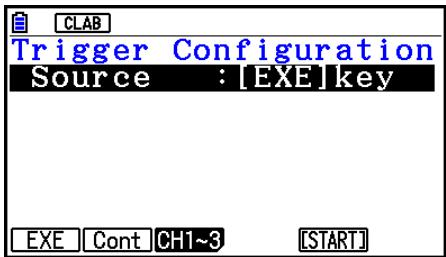
■ Trigger Setup
You can use the Trigger Setup screen to specify the event that causes sampling to start (key operation, etc.). The event that causes sampling to start is called the "trigger source", which is indicated as "Source" on the Trigger Setup screen.
The following table describes each of the eight available trigger sources.
| To start sampling when this happens: | Select this trigger source: |
| When the EXE key is pressed | [EXE] key |
| After the specified number of seconds are counted down | Count Down |
| When input at CH1 reaches a specified value | CH1 |
| When input at CH2 reaches a specified value | CH2 |
| When input at CH3 reaches a specified value | CH3 |
| When input at the SONIC channel reaches a specified value (EA-200 only) | SONIC |
| When the built-in microphone detects sound (EA-200 only) | Mic |
| When the [START/STOP] key is pressed (EA-200 only) | [START] key |
| When [Button] is pressed (CLAB only) | [START] key |
- To configure Trigger Setup settings
-
While the Sampling Config screen is on the display, press F6(Trigger).
-
This displays the Trigger Setup screen with the "Source" line highlighted.
- The function menu items that appears in the menu bar depend on the sampling mode. The nearby screen shows the function menu when "Time-based Sampling" is selected as the sample sampling mode.
-
Use the function keys to select the trigger source you want.
-
The following shows the trigger sources that can be selected for each sampling mode.
| Sampling Mode | Trigger Source |
| Time-based Sampling | F1(EXE) : [EXE] key, F2(Cont) : Count Down, F3(CH1~3), F4(Sonic), F5(START) : [START] key |
| Fast Sampling | F1(EXE) : [EXE] key, F2(Cont) : Count Down, F3(CH1) |
| Mic & Speaker Mode | F1(EXE) : [EXE] key, F2(Cont) : Count Down, F5(Mic) |
- When the sampling mode is "Time-based Sampling" and the "Interval" setting is five minutes or greater, the trigger source is always the [EXE] key.
-
When the sampling mode is "Period Sampling", the trigger source is always CH1. However, when the SONIC channel is being used on the EA-200, the trigger source is always SONIC.
-
Perform one of the following operations, in accordance with the trigger source that was selected in step 2.
| If this is the trigger source: | Do this next: |
| [EXE] key | Press ☑ to finalize Trigger Setup and return to the Sampling Config screen. |
| Count Down | Specify the countdown start time. See “To specify the countdown start time” below. |
| CH1 | Specify the trigger threshold value and trigger edge direction. See “To specify the trigger threshold value and trigger edge type” on page £-17, “To configure trigger threshold, trigger start edge, and trigger end edge settings” or “To configure Photogate trigger start and end settings” on page £-18. |
| CH2 | |
| CH3 | |
| SONIC | Specify the trigger threshold value and motion sensor level. See “To specify the trigger threshold value and motion sensor level” on page £-19. |
| Mic | Specify microphone sensitivity. See “To specify microphone sensitivity” on page £-17. |
| [START] key | Press ☑ to finalize Trigger Setup and return to the Sampling Config screen. |
- To specify the countdown start time
- Move the highlighting to "Timer".
- Press F1(Time) to display a dialog box for specifying the countdown start time.
- Input a value in seconds from 1 to 10.
- Press EXE to finalize Trigger Setup and return to the Sampling Config screen.
- To specify microphone sensitivity
- Move the highlighting to "Sense" and then press one of the function keys described below.
| To select this level of microphone sensitivity: | Press this key: |
| Low | F1 (Low) |
| Medium | F2 (Middle) |
| High | F3 (High) |
- Press ExE to finalize Trigger Setup and return to the Sampling Config screen.
- To specify the trigger threshold value and trigger edge type
Perform the following steps when "Time-based Sampling" or "Fast Sampling" is specified as the sampling mode.
- Move the highlighting to "Threshold".
- Press F1(EDIT) to display a dialog box for specifying the trigger threshold value, which is value that data needs to attain before sampling starts.
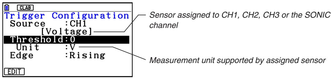
- Input the value you want, and then press .
- Move the highlighting to "Edge".
- Press one of the function keys described below.
| To select this type of edge: | Press this key: |
| Falling | F1 (Fall) |
| Rising | F2 (Rise) |
- Press ExE to finalize Trigger Setup and return to the Sampling Config screen.
- To configure trigger threshold, trigger start edge, and trigger end edge settings
Perform the following steps when "Period Sampling" is specified as the sampling mode.
- Move the highlighting to "Threshold".
- Press F1 (EDIT) to display a dialog box for specifying the trigger threshold value, which is value that data needs to attain before sampling starts.
- Input the value you want.
- Move the highlighting to "Start to".
- Press one of the function keys described below.
| To select this type of edge: | Press this key: |
| Falling | F1 (Fall) |
| Rising | F2 (Rise) |
- Move the highlighting to "End Edge".
- Press one of the function keys described below.
| To select this type of edge: | Press this key: |
| Falling | F1 (Fall) |
| Rising | F2 (Rise) |
- Press to finalize Trigger Setup and return to the Sampling Config screen.
- To configure Photogate trigger start and end settings
Perform the following steps when CH1 is selected as a Photogate trigger source.
Perform the operation below even while Vernier Photogate is assigned to the SONIC channel when performing Period Sampling with the EA-200.
- Move the highlighting to "Start to".
- Press one of the function keys described below.
| To specify this Photogate status: | Press this key: |
| Photogate closed | F1 (Close) |
| Photogate open | F2 (Open) |
- Move the highlighting to "End Gate".
- Press one of the function keys described below.
| To specify this Photogate status: | Press this key: |
| Photogate closed | F1 (Close) |
| Photogate open | F2 (Open) |
- Press to finalize Trigger Setup and return to the Sampling Config screen.
- To specify the trigger threshold value and motion sensor level
- Move the highlighting to "Threshold".
- Press F1(EDIT) to display a dialog box for specifying the trigger threshold value, which is value that data needs to attain before sampling starts.
- Input the value you want, and then press .
- Move the highlighting to "Level".
- Press one of the function keys described below.
| To select this type of level: | Press this key: |
| Below | F1 (Below) |
| Above | F2 (Above) |
- Press to finalize Trigger Setup and return to the Sampling Config screen.
■ Configuring Manual Sampling Settings
-
On the Manual Sampling screen, press F2 (CONFIG).
-
The Sampling Config screen is shown below.
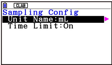
- Press
- Input up to 8 characters for the unit name and then press
- Press to move the highlighting to "Time Limit".
- Press one of the function keys below.
F1 (On) ... Auto sampling stop enabled.
F2(Off) ... Auto sampling stop disabled.
-
After all of settings are the way you want, press EXIT
-
This returns to the Manual Sampling screen.
6. Performing Auto Sensor Calibration and Zero Adjustment
You can use the procedures in this section to perform auto sensor calibration and sensor zero adjustment.
With auto calibration, you can configure applicable interpolation formula slope (Slope) and y -intercept (Intercept) values for a sensor based on two measured values.
With zero adjustment, you can configure a custom probe y -intercept based on measured values.
A sensor calibrated with auto calibration or zero adjustment is registered as a custom probe.
■ Sensor Calibration Screen
- On the sampling screen, use and to move the highlighting to the sensor you want to auto calibrate or zero adjust.
-
Press F3(CALIB).
-
This displays a sensor calibration screen like the one shown below.
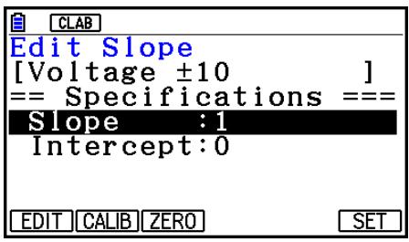
F1(EDIT) ... Select to manually modify the highlighted item.
(F2) (CALIB) ... Performs auto sensor calibration.
F3 (ZERO) ... Performs sensor zero adjustment.
F6 (SET) ... Select to assign the calibrated sensor to a channel. This registers the sensor as a custom probe.
- Press EXIT to return to the sampling screen.
Performing Auto Sensor Calibration
Important!
- Before performing the operation below, you will need to have two known measured values on hand.
-
When inputting reference values in step 3 of the procedure below, input values that were measured accurately under conditions used for the sampling operations in step 2 of the procedure. When inputting reference values in step 5 of the procedure below, input values that were measured accurately under conditions used for the sampling operations in step 4 of the procedure.
-
On the sensor calibration screen, press F2(CALIB).
-
A screen like the one shown below will appear after the first sampling operation starts.
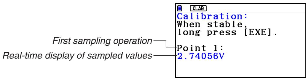
-
After the sampled value stabilizes, hold down for a few seconds.
-
This registers the first sampled valued and displays it on the screen. At this time, the cursor will appear at the bottom of the display, indicating that a reference value can be input.
-
Input a reference value for the first sample value and then press [EXE].
-
A screen like the one shown below will appear after the second sampling operation starts automatically.
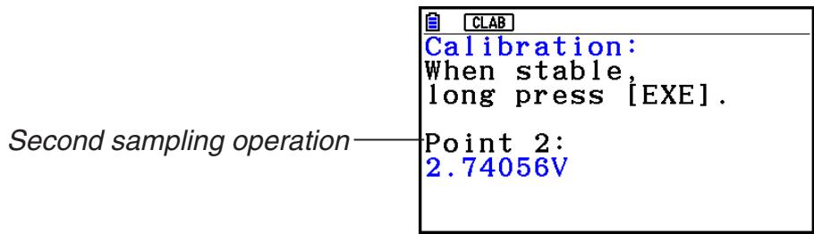
-
After the sampled value stabilizes, hold down for a few seconds.
-
This registers second sampled valued and displays it on the screen. At this time, the cursor will appear at the bottom of the display, indicating that a reference value can be input.
-
Input a reference value for the second sample value and then press .
-
This returns to the sensor calibration screen.
- E-CON4 calculates slope and y -intercept values based on the two input reference values and automatically configures settings. Automatically calculated values are displayed on the sensor calibration screen.
Performing Sensor Zero Adjustment
-
On the sensor calibration screen, press F3 (ZERO).
-
A screen like the one shown below will appear after sampling starts.
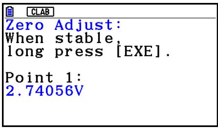
-
When the sampled value that you want to zero adjust is displayed, press
-
This returns to the sensor calibration screen.
- E-CON4 automatically sets a y -intercept value based on the measured value.
Automatically calculated values are displayed on the sensor calibration screen.
■ Configuring Settings Manually
- On the sensor calibration screen, use and to move the highlighting to the item whose setting you want to change.
- Press F1(EDIT).
- Input the information below for each of the items.
Probe Name ... Sensor name up to 18 characters long. (17 characters long when the sensor name includes “±”).
Slope ... Interpolation formula slope (value that specifies constant a of ax + b )
Intercept ... Interpolation formula y -intercept (value that specifies constant b of ax + b )
- After you finish inputting, press .
■Assigning a Calibrated Sensor to a Channel
- Perform auto sensor calibration and sensor zero adjustment. (Or configure settings manually.)
-
On the sensor calibration screen, press F6 (SET).
-
This displays a dialog box like the one shown below.
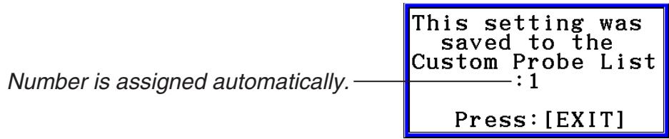
-
Press EXIT
-
This assigns the calibrated sensor to the channel and returns to the sampling screen.
- The calibrated sensor is stored under the custom probe number shown on the dialog box above.
7. Using a Custom Probe
The sensors shown in the CASIO, Vernier, and CMA sensor lists under "4. Selecting a Sensor" are E-CON4 mode standard sensors. If you want to sample with a sensor not included in a list, you must configure it as a custom probe.
■ Registering a Custom Probe
-
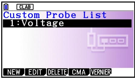
On the sensor selection screen, press F4(CUSTOM).
-
This displays the custom probe list screen.
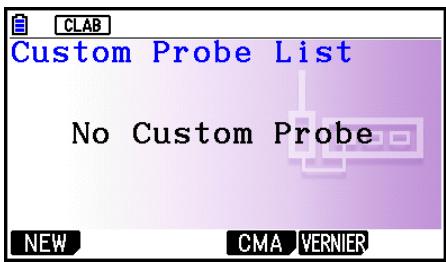
-
If there is no registered custom probe, the message "No Custom Probe" appears on the display.
-
Press F1 (NEW).
-
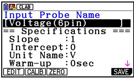
This displays a custom probe setup screen like the one shown below.
-
Press F1(EDIT).
-
Input up to 18 characters for the custom probe name and then press [EXE].
-
This will cause the highlighting to move to "Slope".
-
Move the highlighting to the setting you want to configure and then press F1(EDIT).
-
Setting items are described below.
Slope ... Input the interpolation formula slope (value that specifies constant a of ax + b )
Intercept ... Input the interpolation formula y -intercept (value that specifies constant b of ax + b )
Unit Name ... Input up to eight characters for the unit name.
Warm-up ... Specify the warm-up time.
Type ... Select the sensor type ("0-5V" or "±10V"). Press F4(0-5V) or F5(±10V).
-
Perform auto calibration and zero adjustment of the custom probe as required.
-
Press F2 (CALIB) to perform auto calibration of the custom probe. See "Performing Auto Sensor Calibration" (page 8-20).
-
Press F3 (ZERO) to perform zero adjustment of the custom probe. See "Performing Sensor Zero Adjustment" (page 21).
-
After configuring the required settings, press F6 (SAVE) or EXE.
-
This displays the dialog box shown below.
Memory Number
-
Input the custom probe registration number (1 to 99) and then press .
-
This registers the custom probe and returns to the custom probe list screen.
Assigning a Custom Probe to a Channel
- On the sampling screen, use and to select the channel to which you want to assign the custom probe.
- Press F1 (SENSOR) to display the sensor selection screen.
-
Press F4(CUSTOM).
-
This displays the custom probe list screen.
-
Use and to select the custom probe you want to assign and then press [EXE].
Changing the Settings of a Custom Probe
- On the custom probe list screen, use and to select the custom probe whose settings you want to change.
-
Press F2 (EDIT).
-
This displays a custom probe setup screen.
-
Perform steps 3 through 6 under "Registering a Custom Probe".
-
After configuring the required settings, press F6(SAVE) or EXE.
-
This returns to the custom probe list screen.
■ Recalling CMA or Vernier Sensor Settings to Register a Custom Probe
- On the custom probe list screen, press F4 (CMA) or F5 (VERNIER).
This displays a sensor list.
- Use the and cursor keys to move the highlighting to the sensor whose settings you want to use as the basis of the custom probe and then press .
- The name of the selected sensor and its setting information are shown on the custom probe setup screen.
- Perform steps 3 through 8 under "Registering a Custom Probe". However, you will not be able to change the sensor type.
8. Using Setup Memory
Data logger setup data (Data Logger settings, sampling mode, assigned sensor, sampling setup) is stored at the time it is created in a memory area called the "current setup memory area". The current contents of the current setup memory area are overwritten whenever you create other setup data.
You can use setup memory to save the current setup memory area contents to calculator memory to keep it from being overwritten, if you want.
Saving a Setup
- Display the sampling screen you want to save.
-
Press F4 (OTHER) F2 (MEMORY).
-
This displays the setup memory list.
-
The message "No Setup-MEM" will appear if there is no setup data stored in memory.
-
Press F2(SAVE).
- This displays a setup name input screen.
- Input up to 18 characters for the setup name and then press
- This displays a memory number input dialog box.
- Input a memory number (1 to 99) and then press .
- This returns to the setup memory list.
- Press EXIT
- This returns to the sampling screen.
Important!
- Since you assign both a setup name and a file number to each setup, you can assign the same name to multiple setups, if you want.
Using and Managing Setups in Setup Memory
All of the setups you save are shown in the setup memory list. After selecting a setup in the list, you can use it to sample data or you can edit it.
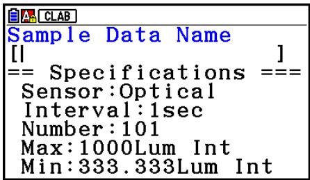
- To preview saved setup data
You can use the following procedure to check the contents of a setup before you use it for sampling.
- On the sampling screen, press F4 (OTHER) F2 (MEMORY) to display the setup memory list.
-
Use the and cursor keys to highlight the name of the setup you want.
-
Press OPTN (Setup Preview) (or ).
-
This displays the preview dialog box.
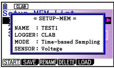
- To close the preview dialog box, press EXIT
- To recall a setup and use it for sampling
Be sure to perform the following steps before starting sampling with a Data Logger.
- Connect the calculator to a Data Logger.
- Turn on Data Logger power.
- In accordance with the setup you plan to use, connect the proper sensor to the appropriate Data Logger channel.
- Prepare the item whose data is to be sampled.
- On the sampling screen, press F4 (OTHER) F2 (MEMORY) to display the setup memory list.
- Use the and cursor keys to highlight the name of the setup you want.
- Press F1 (START).
-
In response to the confirmation message that appears, press F1.
-
Pressing sets up the Data Logger and then starts sampling.
To clear the confirmation message without sampling, press F6.
Note
- See "Operations during a sampling operation" on page 29 for information about operations you can perform while a sampling operation is in progress.
- To change the name of setup data
- On the sampling screen, press F4 (OTHER) F2 (MEMORY) to display the setup memory list.
- Use the and cursor keys to highlight the name of the setup you want.
-
Press F3 (RENAME).
-
This displays the screen for inputting the setup name.
-
Input up to 18 characters for the setup name, and then press .
- This changes the setup name and returns to the setup memory list.
- To delete setup data
- On the sampling screen, press F4 (OTHER) F2 (MEMORY) to display the setup memory list.
- Use the and cursor keys to highlight the name of the setup you want.
-
Press F4 (DELETE).
-
In response to the confirmation message that appears, press F1 (Yes) to delete the setup.
-
To clear the confirmation message without deleting anything, press F6 (No).
- To recall setup data
Recalling setup data stores it in the current setup memory area. After recalling setup data, you can edit it as required. This capability comes in handy when you need to perform a setup that is slightly different from one you have stored in memory.
- On the sampling screen, press F4 (OTHER) F2 (MEMORY) to display the setup memory list.
- Use the and cursor keys to highlight the name of the setup you want.
- Press F5 (LOAD).
-
In response to the confirmation message that appears, press F1 (Yes) to recall the setup.
-
To clear the confirmation message without recalling the setup, press F6 (No).
Note
- Recalling setup data replaces any other data currently in the current setup memory area. However, if there is setup data for a sampling mode that is different from the current mode, that data will not be overwritten.
9. Starting a Sampling Operation
This section describes how to use a setup configured using the E-CON4 mode to start a Data Logger sampling operation.
Before getting started...
Be sure to perform the following steps before starting sampling with a Data Logger.
- Connect the calculator to a Data Logger.
- Turn on Data Logger power.
- In accordance with the setup you plan to use, connect the proper sensor to the appropriate Data Logger channel.
- Prepare the item whose data is to be sampled.
Starting a Sampling Operation
A sampling operation can be started from the sampling screen or the setup memory list.
Here we will show the operation that starts from the sampling screen. See “To recall a setup and use it for sampling” on page 26 for information about starting sampling from the setup memory list.
You need to perform a special operation in the case of Manual Sampling. For more information, refer to "Manual Sampling" (page 31).
- To start sampling
-
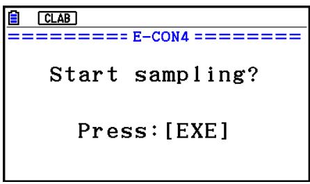
Enter the sampling mode you want to use and then press F6(START).
-
This displays a sampling start confirmation screen like the one shown below.
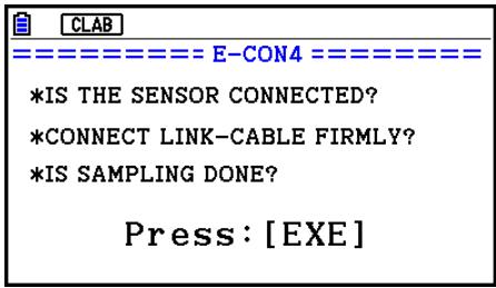
2. Press EXE.
- This sets up the Data Logger using the setup data in the current setup memory area.
- The message "Setting Data Logger..." remains on the display while Data Logger setup is in progress. You can cancel the setup operation any time this message is displayed by pressing AC.
- The screen shown nearby appears after Data Logger setup is complete.
-
Press EXE to start sampling.
-
The screens that appear while sampling is in progress and after sampling is complete depend on setup details (sampling mode, trigger setup, etc.). For details, see "Operations during a sampling operation" below.
- Operations during a sampling operation
Sending a sample start command from the calculator to a Data Logger causes the following sequence to be performed.
Setup Data Transfer Sampling Start Sampling End
Transfer of Sample Data from the Data Logger to the Calculator
The table on the next page shows how the trigger conditions and sensor type specified in the setup data affects the above sequence.
Starts Sampling
| Mode | 1. Data Logger Setup | 2. Start Standby | 3. Sampling | 4. Graphing |
| Time-based Sampling | Setting Data Logger...Cancel: [AC] | Start sampling?Press: [EXE] | → | Sampled values are saved as Current Sample Data. |
| Fast Sampling | Sampling...Cancel: [AC]The screen shown below appears when CH1~3, SONIC, or Mic is used as the trigger. | ·Mic & Speaker Mode: Speaker - Sample DataGraph screen does not show all sampled values, but only a partial preview. | ||
| Mic & Speaker Mode | When sampling is done, press [EXE] key. | ·MIC/Microphone(Sound)Output Frequency%:Time(sec)·Press [STOP] key on EA-200Try Again?Yes: [F1]No: [F6]·Time(sec)·Input values.·EXE·Press [STOP] key on EA-200 | ||
| Period Sampling | When sampling is done, press [EXE] key. | ·When Number of Samples = 1The following three graph types can be produced when Photogate -Pulley is being used.1. Time and distance graph2. Time and velocity graph3. Time and acceleration graphSample values are stored as List data only. |
Manual Sampling
- On the Manual Sampling screen, press F6(START).
- This displays a sampling start confirmation screen.
- Press EXE.
This displays the screen shown below.
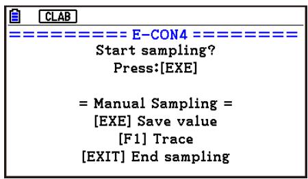
-
Press to start sampling.
-
This will display a screen like the one shown below.
-
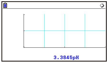
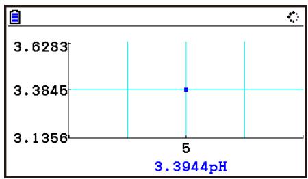
When you want to acquire data, press EXE.
-
This displays a dialog box for inputting the horizontal axis for the sample values.
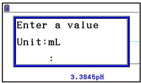
-
Input a horizontal axis value and then press .
-
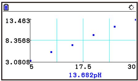
This displays a graph of the sample data. Input values will be displayed on the horizontal axis.
-
Repeat steps 4 and 5 as many times as necessary to sample all of the data you want.
-
You can sample data up to 100 times.
-
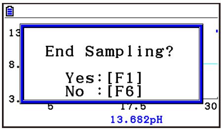
To exit the sampling operation, press EXIT
-
This displays an exit confirmation dialog box.
-
Press F1 (Yes).
-
This displays a screen like the one shown below.
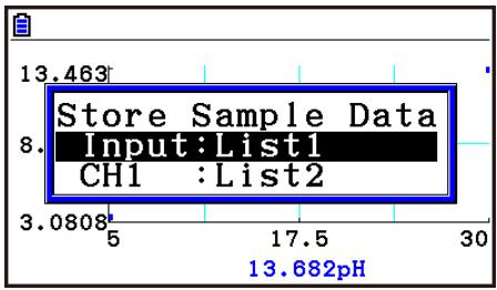
- Specify the list where you want to store the data.
Input ... Specify the list where you want to store the horizontal axis data.
CH1, CH2, CH3 ... Specify lists where you want to store the sample data of each channel.
-
After specifying the lists, press .
-
This will cause the message "Complete!" to appear. To return to the Manual Sampling screen, press .
- In the Statistics mode, sample data will be displayed as shown below.
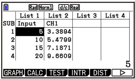
Note
- You can use trace while sampled data is shown on the graph. For details, see "Using Trace" (page 14).
- If "On" is selected for the sampling "Time Limit" setting, sampling will stop automatically if you do not perform any operation for 90 minutes. In this case, the sample data is not stored in a list.
10. Using Sample Data Memory
Performing a Data Logger sampling operation from the E-CON4 mode causes sampled results to be stored in the "current data area" of E-CON4 memory. Separate data is saved for each channel, and the data for a particular channel in the current data area is called that channel's "current data".
Any time you perform a sampling operation, the current data of the channel(s) you use is replaced by the newly sampled data. If you want to save a set of current data and keep it from being replaced by a new sampling operation, save the data in sample data memory under a different file name.
Managing Sample Data Files
- To save current sample data to a file
-
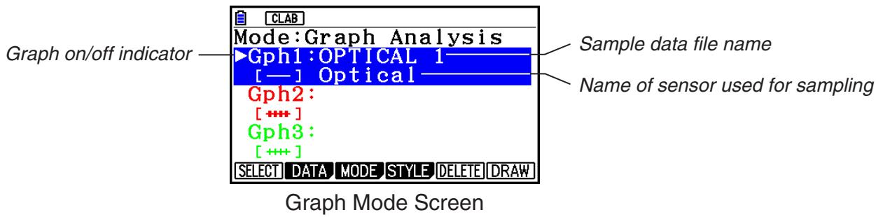
On the sampling screen, press F4(OTHER)F1(GRAPH).
-
This displays the Graph Mode screen.
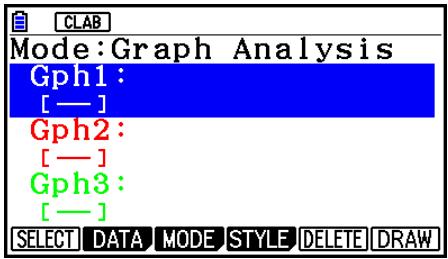
Graph Mode Screen
-
For details about the Graph Mode screen, see "Using the Graph Analysis Tools to Graph Data" (page 15).
-
Press F2 (DATA).
-
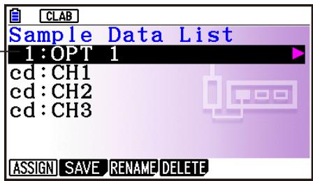
This displays the Sampling Data List screen.
List of current data files "cd" stands for "current data". The text on the right side of the colon indicates the channel name.
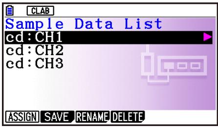
Sampling Data List Screen
-
Use the and cursor keys to move the highlighting to the current data file you want to save, and then press F2 (SAVE).
-
This displays the screen for inputting a data name.
- Enter up to 18 characters for the data file name, and then press .
- This displays a dialog box for inputting a memory number.
- Enter a memory number in the range of 1 to 99, and then press .
- This saves the sample data at the location specified by the memory number you input.
The sample data file you save is indicated on the display using the format:
-
If you specify a memory number that is already being used to store a data file, a confirmation message appears asking if you want to replace the existing file with the new data file. Press F1 to replace the existing data file, or F6 to return to the memory number input dialog box in step 4.
-
To return to the sampling screen, press EXIT twice.
Note
- You could select another data file besides a current data file in step 3 of the above procedure and save it under a different memory number. You do not need to change the file's name as long as you use a different file number.
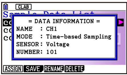
- Pressing while the Sampling Data List screen is shown will display information (sampling mode, sensor, number of samples) about the currently highlighted data. To exit the screen, press EXIT.
11. Using the Graph Analysis Tools to Graph Data
Graph Analysis tools make it possible to analyze graphs drawn from sampled data.
Note
- Sampled data cannot be graphed in the cases described below.
- Attempting to graph manually sampled data and data sampled using a different sampling mode simultaneously
- Manually sampled data whose horizontal axis values (number of samples) do not match
■ Accessing Graph Analysis Tools
You can access Graph Analysis tools using either of the two methods described below.
- Accessing Graph Analysis tools from the Graph Mode screen, which is displayed by pressing F4(OTHER)F1(GRAPH) on the sampling screen
Graph Mode Screen
- The sampling screen appears after you perform a sampling operation. Press F4 (OTHER) F1 (GRAPH) at that time.
- When you access Graph Analysis tools using this method, you can select from among a variety of other Analysis modes. See "Selecting an Analysis Mode and Drawing a Graph" (page £-36) for more information about the other Analysis modes.
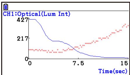
- Accessing Graph Analysis tools from the screen of a graph drawn after a sampling operation is executed from the sampling screen (Time-based Sampling, Fast Sampling, Mic & Speaker Mode - Microphone)
Graph Screen
- In this case, data is graphed after the sampling operation is complete, and the calculator accesses Graph Analysis tools automatically. See “Graph Screen Key Operations” on page 8-39.
■ Selecting an Analysis Mode and Drawing a Graph
This section contains a detailed procedure that covers all steps from selecting an analysis mode to drawing a graph.
Note
-
Step 4 through step 7 are not essential and may be skipped, if you want. Skipping any step automatically applies the initial default values for its settings.
-
If you skip step 2, the default analysis mode is the one whose name is displayed in the top line of the Graph Mode screen.
- To select an analysis mode and draw a graph
-
On the sampling screen, press F4(OTHER)F1(GRAPH).
-
This displays the Graph Mode screen.
-
Press F3 (MODE), and then select the analysis mode you want from the menu that appears.
| To do this: | Perform this menu operation: | To select this mode: |
| Graph three sets of sampled data simultaneously | [Norm] | Graph Analysis |
| Graph sampled data along with its first and second derivative graph | [diff] | d/dt & d²/dt² |
| Display the graphs of different sampled data in upper and lower windows for comparison | [COMPARE] → [GRAPH] | Compare Graph |
| Output sampled data from the speaker, displaying graph of the raw data in the upper window and the output waveform in the lower window (EA-200 only) | [COMPARE] → [Sound] | Compare Sound |
| Display the graph of sampled data in the upper window and its first derivative graph in the lower window | [COMPARE] → [d/dt] | Compare d/dt |
| Display the graph of sampled data in the upper window and its second derivative graph in the lower window | [COMPARE] → [d²/dt²] | Compare d²/dt² |
- The name of the currently selected mode appears in the top line of the Graph Mode screen.
-
Press F2 (DATA).
-
This displays the Sampling Data List screen.
-
Specify the sampled data for graphing.
a. Use the and cursor keys to move the highlighting to the name of the sampled data file you want to select, and then press F1 (ASSIGN) or EXE.
- This returns to the Graph Mode screen, which shows the name of the sample data file you selected.
b. Repeat step a above to specify sample data files for other graphs, if there are any.
- If you select "Graph Analysis" as the analysis mode in step 2, you must specify sample data files for three graphs. If you select "Compare Graph" as the analysis mode in step 2, you must specify sample data files for two graphs. With other modes, you need to specify only one sample data file.
-
For details about Sampling Data List screen operations, see "Using Sample Data Memory" (page 33).
-
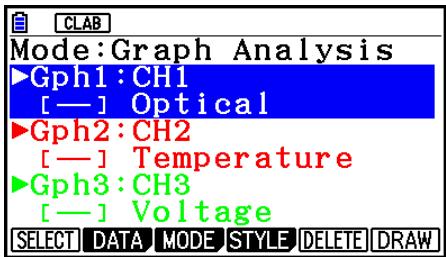
Turn on graphing for each of the graphs listed on the Graph Mode screen.
a. On the Graph Mode screen, use the and cursor keys to select a graph, and then press F1 (SELECT) to toggle graphing on or off.
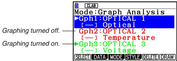
b. Repeat step a to turn each of the graphs listed on the Graph Mode screen on or off.
- Select the graph style you want to use.
a. On the Graph Mode screen, use the and cursor keys to move the highlighting to the graph (Gph1, Gph2, etc.) whose style you want to specify, and then press F4(STYLE). This will cause the function menu to change as shown below.
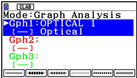
b. Use the function keys to specify the graph style you want.
| To specify this graph style: | Press this key: |
| Line graph with dot ( • ) data markers | F1( ——) |
| Line graph with square ( ■ ) data markers | F2( ++++) |
| Line graph with X (×) data markers | F3( ++++) |
| Scatter graph with 3×3-dot data markers | F4( …… ) |
| Scatter graph with 5×5-dot data markers | F5( …… ) |
| Scatter graph with X (×) data markers | F6( ++++) |
c. Repeat a and b to specify the style for each of the graphs on the Graph Mode screen.
-
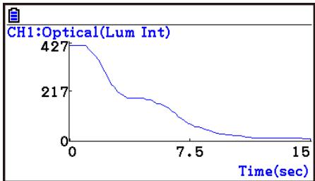
On the Graph Mode screen, press F6 (DRAW) or EXE.
-
This draws the graph(s) in accordance with the settings you configured in step 2 through step 6.
Graph Screen
- When a Graph screen is on the display, the function keys provide you with zooming and other capabilities to aid in graph analysis.
For details about Graph screen function key operations, see the following section.
- To deselect sampled data assigned for graphing on the Graph Mode screen
-
On the Graph Mode screen, use the and cursor keys to move the highlighting to the graph (Gph1, Gph2, etc.) whose sampled data you want to deselect.
-
Press F5 (DELETE).
-
This will deselect sample data assigned to the highlighted graph.
12. Graph Analysis Tool Graph Screen Operations
This section explains the various operations you can perform on the graph screen after drawing a graph.
You can perform these operations on a graph screen produced by a sampling operation, or by the operation described under "Selecting an Analysis Mode and Drawing a Graph" on page 36.
Graph Screen Key Operations
On the graph screen, you can use the keys described in the table below to analyze (CALC) graphs by reading data points along the graph (Trace) and enlarging specific parts of the graph (Zoom).
| Key Operation | Description |
| SHIFT F1 (TRACE) | Displays a trace pointer on the graph along with the coordinates of the current cursor location. Trace can also be used to obtain the periodic frequency of a specific range on the graph and assign it to a variable. See “Using Trace” on page £-40. |
| SHIFT F2 (ZOOM) | Starts a zoom operation, which you can use to enlarge or reduce the size of the graph along the x-axis or the y-axis. See “Using Zoom” on page £-41. |
| SHIFT F3 (V-WIN) | Displays a function menu of special View Window commands for the E-CON4 mode graph screen. For details about each command, see “Configuring View Window Parameters” on page £-49. |
| SHIFT F4 (SKETCH) | Displays a menu that contains the following commands: CIs, Plot, F-Line, Text, PEN, Vertical, and Horizontal. For details about each command, see “Drawing Dots, Lines, and Text on the Graph Screen (Sketch)” on page 5-52. |
| OPTN F1 (PICTURE) | Saves the currently displayed graph as a graphic image. You can recall a saved graph image and overlay it on another graph to compare them. For details about these procedures, see “Saving and Recalling Graph Screen Contents” on page 5-20. |
| OPTN F2 (MEMORY) F1 (LISTMEM) | Displays a menu of functions for saving the sample values in a specific range of a graph to a list. See “Transforming Sampled Data to List Data” on page £-42. |
| OPTN F2 (MEMORY) F2 (CSV) | Saves the sample data in the specific range of a graph to a CSV file. For details, see “Saving Sample Data to a CSV File” (page £-43). |
| OPTN F3 (EDIT) | Displays a menu of functions for zooming and editing a particular graph when the graph screen contains multiple graphs. See “Working with Multiple Graphs” on page £-46. |
| OPTN F4 (CALC) | Displays a menu that lets you transform a sample result graph to a function using Fourier series expansion, and to perform regression to determine the tendency of a graph. See “Using Fourier Series Expansion to Transform a Waveform to a Function” on page £-44, and “Performing Regression” on page £-45. |
| OPTN F5 (Y=fx) | Displays the graph relation list, which lets you select a Y=f(x) graph to overlay on the sampled result graph. See “Overlaying a Y=f(x) Graph on a Sampled Result Graph” on page £-46. |
| OPTN F6 (SPEAKER) | Starts an operation for outputting a specific range of a sound data waveform graph from the speaker (EA-200 only). See “Outputting a Specific Range of a Graph from the Speaker” on page £-48. |
■ Scrolling the Graph Screen
Press the cursor keys while the graph screen is on the display scrolls the graph left, right, up, or down.
Note
- The cursor keys perform different operations besides scrolling while a trace or graph operation is in progress. To perform a graph screen scroll operation in this case, press EXIT to cancel the trace or graph operation, and then press the cursor keys.
Using Trace
Trace displays a crosshair pointer on the displayed graph along with the coordinates of the current cursor position. You can use the cursor keys to move the pointer along the graph. You can also use trace to obtain the periodic frequency value for a particular range, and assign the range (time) and periodic frequency values in separate Alpha memory variables.
To use trace
-
On the graph screen, press SHIFT F1 (TRACE).
-
This causes a trace pointer to appear on the graph. The coordinates of the current trace pointer location are also shown on the display.

-
Use the and cursor keys to move the trace pointer along the graph to the location you want.
-
The coordinate values change in accordance with the trace pointer movement.
- You can exit the trace pointer at any time by pressing EXIT.
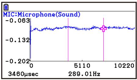
To obtain the periodic frequency value
- Use the procedure under "To use trace" above to start a trace operation.
-
Move the trace pointer to the start point of the range whose periodic frequency you want to obtain, and then press .
-
Move the trace pointer to the end point of the range whose periodic frequency you want to obtain.
-
This causes the period and periodic frequency value at the start point you selected in step 2 to appear along the bottom of the screen.
-
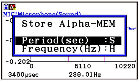
Press to assign the period and periodic frequency values to Alpha memory variables.
-
This displays a dialog box for specifying variable names for [Period] and [Frequency] values.
- The initial default variable name settings are "S" for the period and "H" for the periodic frequency. To change to another variable name, use the up and down cursor keys to move the highlighting to the item you want to change, and then press the applicable letter key.
-
After everything is the way you want, press [EXE].
-
This stores the values and exits the trace operation.
- For details about using Alpha memory, see Chapter 2 of this manual.
Using Zoom
Zoom lets you enlarge or reduce the size of the graph along the x -axis or the y -axis.
Note
- When there are multiple graphs on the screen, the procedure below zooms all of them. For information about zooming a particular graph when there are multiple graphs on the screen, see "Working with Multiple Graphs" on page £-46.
- To zoom the graph screen
-
On the graph screen, press SHIFT F2 (ZOOM).
-
This causes a magnifying glass cursor (⊕) to appear in the center of the screen.
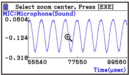
- Use the cursor keys to move the magnifying glass cursor to the location on the screen that you want at the center of the enlarged or reduced screen.
3. Press EXE.
- This causes the magnifying glass to disappear and enters the zoom mode.
- The cursor keys perform the following operations in the zoom mode.
| To do this: | Press this cursor key: |
| Enlarge the graph image horizontally | ◎ |
| Reduce the size of the graph image horizontally | ◎ |
| Enlarge the graph image vertically | ▲ |
| Reduce the size of the graph image vertically | ◎ |
4. To exit the zoom mode, press EXIT
Transforming Sampled Data to List Data
Use the following procedure to transform the sampled data in a specific range of a graph into list data.
To transform sampled data to list data
-
On the graph screen, press OPTN F2 (MEMORY), and then F1 (LISTMEM).
-
This displays the LISTMEM menu.
-
Press F2 (SELECT).
-
This displays the trace pointer for selecting the range on the graph.
-
Move the trace pointer to the start point of the range you want to convert to list data, and then press .
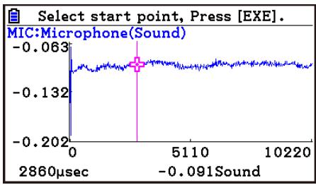
-
Move the trace pointer to the end point of the range you want to convert to list data, and then press .
-
This displays a dialog box for specifying the lists where you want to store the time data and the sampled data.

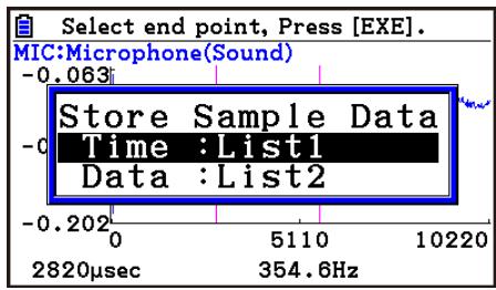
-
The initial default lists are List 1 for the time and List 2 for sample data. To change to another list (List 1 to List 26), use the up and down cursor keys to move the highlighting to the list you want to change, and then input the applicable list number.
-
After everything is the way you want, press .
-
This saves the lists and the message "Complete!" appears. Press to return to the graph screen.
- For details about using list data, see Chapter 3 of this manual.
Note
- Pressing F1(All) in place of F2(SELECT) in step 2 converts the entire graph to list data. In this case, the "Store Sample Data" dialog box appears as soon as you press F1(All).
- In the case of Manual Sampling, the dialog box in step 4 of the procedure will appear as shown below.
Store Sample Data
Input:List1
Data :List2
Saving Sample Data to a CSV File
Use the procedure below to save the sample data in the specific range of a graph to a CSV file.
- To save sample data to a CSV file
- On the graph screen, press OPTN F2 (MEMORY) F2 (CSV).
- This displays the CSV menu at the bottom of the display.
- Press F1 (SAVE·AS) F2 (SELECT).
- This will display a trace point for specifying a range on the graph.
- Move the trace point to the start point of the range you want to save to a CSV file, and then press .
- Move the trace point to the end point of the range you want to save to a CSV file, and then press .
- This displays the folder selection screen.
- Select the folder where you want to save the CSV file.
- Press F1(SAVE·AS).
- Input up to 8 characters for the file name and then press [EXE].
Note
- To select all of the graph data and save it as CSV data, press F1 (All) in place of F2 (SELECT) in step 2 above. The folder selection screen will appear as soon as you press F1 (All).
- If there are multiple graphs on the graph screen, use and to select the graph you want and then press . (Not included on the Manual Sampling)
- To specify the CSV file delimiter symbol and decimal point
Press OPTN F2 (MEMORY) F2 (CSV) F2 (SET) to display the CSV format setting screen. Next, perform the procedure from step 3 under "Specifying the CSV File Delimiter Symbol and Decimal Point" (page 3-20).
Using Fourier Series Expansion to Transform a Waveform to a Function
Fourier series expansion is effective for studying sounds by expressing them as functions. The procedure below assumes that there is a graph of sampled sound data already on the graph screen.
To perform Fourier series expansion
-
On the graph screen, press OPTN, and then F4(CALC).
-
The CALC menu appears at the bottom of the display.
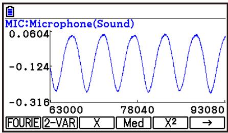
-
Press F1(FOURIE).
-
This displays the trace pointer for selecting the graph range.
-
Move the trace pointer to the start point of the range for which you want to perform Fourier series expansion, and then press .
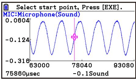
-
Move the trace pointer to the end point of the range for which you want to perform Fourier series expansion, and then press .
-
This displays a dialog box for specifying the start degree of the Fourier series.
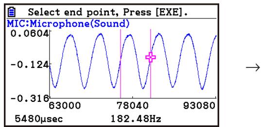
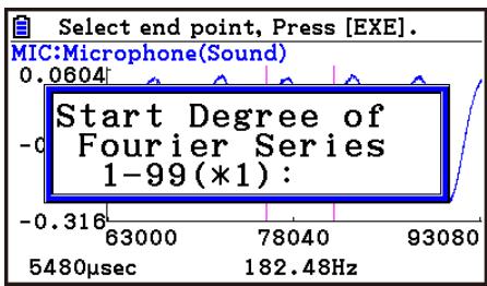
-
Input a value in the range of 1 to 99, and then press .
-
This displays a dialog box for inputting the degree of the Fourier series.
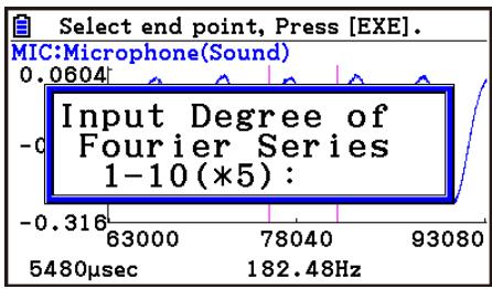
-
Input a value in the range of 1 to 10, and then press .
-
The graph relation list appears with the calculation result.
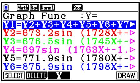
-
Pressing F6(DRAW) here graphs the function.
-
This lets you compare the expanded function graph and the original graph to see if they are the same.
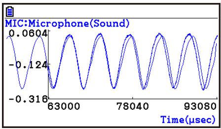
Note
- When you press F6 (DRAW) in step 7, the graph of the result of the Fourier series expansion may not align correctly with the original graph on which it is overlaid. If this happens, shift the position the original graph to align it with the overlaid graph.
For information about how to move the original graph, see "To move a particular graph on a multi-graph display" (page 1-48).
Performing Regression
You can use the procedure below to perform regression for a range specified using the trace pointer. All of the following regression types are supported: Linear, Med-Med, Quadratic, Cubic, Quartic, Logarithmic, Exponential, Power, Sine, and Logistic.
For details about these regression types, see Chapter 6 of this manual.
The following procedure shows how to perform quadratic regression. The same general steps can also be used to perform the other types of regression.
To perform quadratic regression
-
On the graph screen, press OPTN, and then F4(CALC).
-
The CALC menu appears at the bottom of the display.
-
Press F5(X2).
-
This displays the trace pointer for selecting the range on the graph.
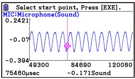
-
Move the trace pointer to the start point of the range for which you want to perform quadratic regression, and then press .
-
Move the trace pointer to the end point of the range for which you want to perform quadratic regression, and then press .
-
This displays the quadratic regression calculation result screen.
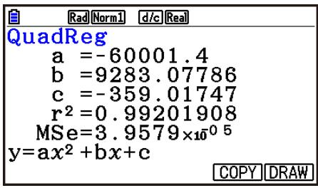
-
Press F6 (DRAW).
-
This draws a quadratic regression graph and overlays it over the original graph.
- To delete the overlaid quadratic regression graph, press SHIFT F4 (SKETCH) and then F1 (Cls).
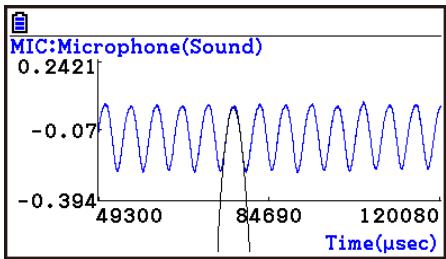
■ Overlaying a Y=f(x) Graph on a Sampled Result Graph
You can use the E-CON4 mode to graph equations based on the form Y = f(x) . From the graph screen, press OPTN F5 (Y=fx) to display the graph relation list screen. From there, operations are identical to those in the Graph mode.
Note
- The data on the graph relation list screen is shared with the Graph mode. Note, however, that only Y = type graphs can be used in the E-CON4 mode. Because of this, calling up the graph relation list screen from the E-CON4 mode will display a "Y" (Y= type) item for function menu key F3. Also, F5 (MODIFY) is not displayed, because it is not used in the E-CON4 mode.
■ Working with Multiple Graphs (Not included on the Manual Sampling)
The procedures in this section explain how you can zoom or move a particular graph when there are multiple graphs on the display.
- To zoom a particular graph on a multi-graph display
-
When the graph screen contains multiple graphs, press OPTN, and then F3 (EDIT).
-
The EDIT menu appears at the bottom of the display.
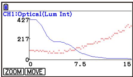
2. Press F1(ZOOM).
- This displays only one of the graphs that were originally on the graph screen.
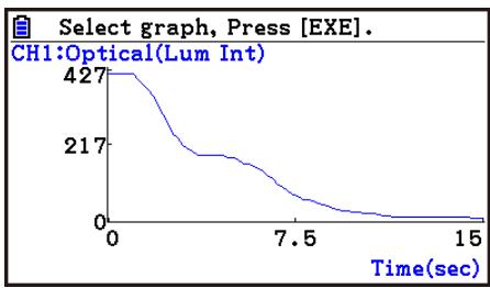
-
Use the and cursor keys to cycle through the graphs until the one you want is displayed, and then press .
-
This enters the zoom mode and causes all of the graphs to reappear, along with a magnifying glass cursor () in the center of the screen.
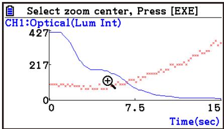
- Use the cursor keys to move the magnifying glass cursor to the location on the screen that you want at the center of the enlarged or reduced screen.
5. Press EXE.
- This causes the magnifying glass to disappear and enters the zoom mode.
- The cursor keys perform the following operations in the zoom mode.
| To do this: | Press this cursor key: |
| Enlarge the graph image horizontally | ◎ |
| Reduce the size of the graph image horizontally | ◎ |
| Enlarge the graph image vertically | ▲ |
| Reduce the size of the graph image vertically | ◎ |

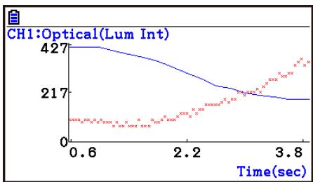
- To exit the zoom mode, press EXIT
- To move a particular graph on a multi-graph display
-
When the graph screen contains multiple graphs, press OPTN, and then F3 (EDIT).
-
This displays the EDIT menu.
-
Press F2 (MOVE).
-
This displays only one of the graphs that were originally on the graph screen.
-
Use the and cursor keys to cycle through the graphs until the one you want is displayed, and then press .
- This enters the move mode and causes all of the graphs to reappear.
- Use the and cursor keys to move the graph left and right, or the and cursor keys to move the graph up and down.
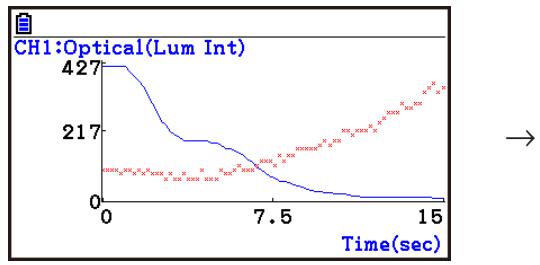
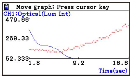
- To exit the move mode, press EXIT
■ Outputting a Specific Range of a Graph from the Speaker (EA-200 only)
Use the following procedure to output a specific range of a sound data waveform graph from the speaker.
- To output a graph from the speaker
-
On the graph screen, press OPTN, and then F6(SPEAKER).
-
This displays the trace pointer for selecting the range on the graph.
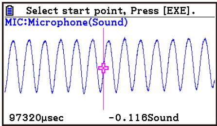
-
Move the trace pointer to the start point of the range you want to output from the speaker, and then press .
-
Move the trace pointer to the end point of the range you want to output from the speaker, and then press .
-
After you specify the start point and end point, an output frequency dialog box shown below appears on the display.
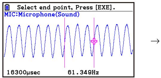
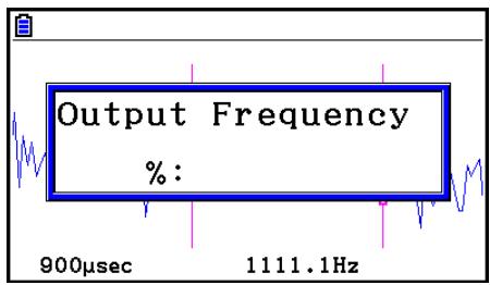
-
Input a percent value for the output frequency value you want.
-
The output frequency specification is a percent value. To output the original sound as-is, specify 100% . To raise the original sound by one octave, input a value of 200% . To lower the original sound by one octave, input a value of 50% .
-
After inputting an output frequency value, press .
-
This outputs the waveform between the start point and end point from the EA-200 speaker.
-
If the sound you configured cannot be output for some reason, the message “Range Error” will appear. If this happens, press EXIT to scroll back through the previous setting screens and change the setup as required.
-
To terminate sound output, press the EA-200 [START/STOP] key.
-
Press [EXE].
-
This displays a screen like the one shown nearby.
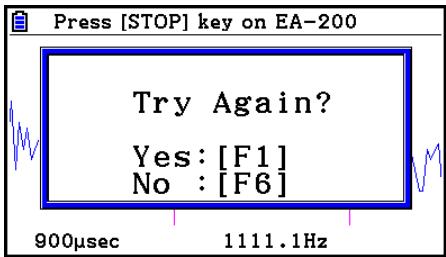
-
If you want to retry output from the speaker, press F1 (Yes). To exit the procedure and return to the graph screen, press F6 (No).
-
Pressing F1 (Yes) returns to the "Output Frequency" dialog box. From there, repeat the above steps from step 4.
■ Configuring View Window Parameters
- Pressing SHIFT F3 (V-Window) while the graph screen is on the display displays a View Window function key menu along the bottom of the display.
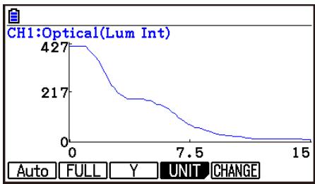
Press the function key that corresponds to the View Window parameter you want to configure.
| Function Key | Description |
| F1(Auto)* | Automatically applies the following View Window parameters. Y-axis Elements: In accordance with screen size X-axis Elements: In accordance with screen size when 1 data item equals 1 dot; 1 data equals 1 dot in other cases |
| F2(FULL) | Resizes the graph so all of it fits in the screen. |
| F3(Y) | Resizes the graph so all of it fits in the screen along the Y-axis, without changing the X-axis dimensions. |
| F4(UNIT)* | Specifies the unit of the numeric axis grid displayed by the E-CON Axes setting of the Setup Screen. F1(μsec): microseconds F2(msec): milliseconds F3(Sec): seconds F4(DHMS): days, hours, minutes, seconds (1 day, 2 hours, 30 minutes, 5 seconds = 1d2h30m5s) F5(Auto): Auto selection |
| F5(CHANGE) | Toggles display of the source data on the graph screen on and off. |
- Not included on the Manual Sampling
To exit the View Window function key menu and return to the standard function key menu, press EXIT.
13. Calling E-CON4 Functions from an eActivity
You can call E-CON4 functions from an eActivity by including an "E-CON strip" in the eActivity file. The following describes each of the two available E-CON strips.
- E-CON Top strip
This strip calls the Time-based Sampling screen. This strip provides access to almost all executable functions, including detailed Data Logger setup and sampling execution; graphing and Graph Analysis Tools, etc.
Note
- Using an E-CON Top strip to configure a setup causes the setup information to be registered in the applicable strip. This means that the next time you open the strip, sampling can be performed in accordance with the previously configured setup information.
E-CON Result strip
This strip graphs sampled data that is recorded in the strip. The sampled data is recorded to the strip the first time the strip is executed.
E-CON Strip Memory Capacity Precautions
- The memory capacity of each E-CON strip is 22.5 KB. An error will occur if you perform an operation that causes this capacity to be exceeded. Particular care is required when handling a large number of samples, which can cause memory capacity to be exceeded.
- Always make sure that FFT Graph is turned off whenever performing sampling with the microphone. Leaving FFT Graph turned on cause memory capacity to be exceeded.
- If an error occurs, press SHIFT (□) to return to the eActivity workspace screen and perform the procedure again.
- For information about checking the memory usage of each strip, see "To display the strip memory usage screen" on page 10-21.
For details about eActivity operations, see Chapter 10 of this manual.
EAC
CE
Manufacturer:
CASIO COMPUTER CO., LTD.
6-2, Hon-machi 1-chome
Shibuya-ku, Tokyo 151-8543, Japan
Responsible within the European Union:
Casio Europe GmbH
Casio-Platz 1
22848 Norderstedt, Germany
www.casio-europe.com
CASIO®
CASIO COMPUTER CO., LTD.
6-2, Hon-machi 1-chome Shibuya-ku, Tokyo 151-8543, Japan
- <115200 bits/seconde>
- E-CON4 Application (English)
- Calculus matriciels
- - Pour combiner des listedes
- Type 1 (Y= expression)
- - Mark Type (Type de point)
- - Rendement annuel (YLD)
- DrawFTG-Con, DrawFTG-Plt
- Aucun paramètre
- Receive38k / Send38k
- Remarque :
- Distribution Student
- Distribution 2
- Important!
- E-CON4 Mode Overview
- E-CON4 Specific Setup Items
- Sampling Screen
- Changing the Sampling Screen
- Time-based Sampling Screen
- Fast Sampling Screen
- Period Sampling Screen
- Manual Sampling Screen (CLAB Only)
- ■ Mic & Speaker Mode Screen (EA-200 Only)
- - Selecting Microphone
- - Selecting Speaker
- To change the output frequency and try again:
- To change the output range of the waveform graph and try again:
- To change the function:
- To exit the procedure and return to the sampling mode selection screen:
- Sampling Screen Function Menu
- Auto Sensor Detection (CLAB Only)
- Note
- Selecting a Sensor
- ■Assigning a Sensor to a Channel
- Disabling a Sensor
- ■ Removing the Sensor Assigned to a Channel (CLAB Only)
- Configuring the Sampling Setup
- Using Method 1 to Configure Settings
- - To configure the Distance setting
- - To configure FFT Graph setting
- Using Method 2 to Configure Settings
- - To switch between Method 1 and Method 2
- - Input Ranges
- Method 1
- Method 2
- ■ Trigger Setup
- - To configure Trigger Setup settings
- - To specify the countdown start time
- - To specify microphone sensitivity
- - To specify the trigger threshold value and trigger edge type
- - To configure trigger threshold, trigger start edge, and trigger end edge settings
- - To configure Photogate trigger start and end settings
- - To specify the trigger threshold value and motion sensor level
- ■ Configuring Manual Sampling Settings
- Performing Auto Sensor Calibration and Zero Adjustment
- ■ Sensor Calibration Screen
- Performing Auto Sensor Calibration
- Performing Sensor Zero Adjustment
- ■ Configuring Settings Manually
- ■Assigning a Calibrated Sensor to a Channel
- Using a Custom Probe
- ■ Registering a Custom Probe
- Assigning a Custom Probe to a Channel
- Changing the Settings of a Custom Probe
- ■ Recalling CMA or Vernier Sensor Settings to Register a Custom Probe
- Using Setup Memory
- Saving a Setup
- Using and Managing Setups in Setup Memory
- - To preview saved setup data
- - To recall a setup and use it for sampling
- - To change the name of setup data
- - To delete setup data
- - To recall setup data
- Starting a Sampling Operation
- Before getting started...
- Starting a Sampling Operation
- - To start sampling
- Press EXE.
- - Operations during a sampling operation
- Manual Sampling
- Using Sample Data Memory
- Managing Sample Data Files
- - To save current sample data to a file
- Using the Graph Analysis Tools to Graph Data
- ■ Accessing Graph Analysis Tools
- ■ Selecting an Analysis Mode and Drawing a Graph
- - To select an analysis mode and draw a graph
- - To deselect sampled data assigned for graphing on the Graph Mode screen
- Graph Analysis Tool Graph Screen Operations
- Graph Screen Key Operations
- ■ Scrolling the Graph Screen
- Using Trace
- To use trace
- To obtain the periodic frequency value
- Using Zoom
- - To zoom the graph screen
- Press EXE.
- To exit the zoom mode, press EXIT
- Transforming Sampled Data to List Data
- To transform sampled data to list data
- Saving Sample Data to a CSV File
- - To save sample data to a CSV file
- - To specify the CSV file delimiter symbol and decimal point
- Using Fourier Series Expansion to Transform a Waveform to a Function
- To perform Fourier series expansion
- Performing Regression
- To perform quadratic regression
- ■ Overlaying a Y=f(x) Graph on a Sampled Result Graph
- ■ Working with Multiple Graphs (Not included on the Manual Sampling)
- - To zoom a particular graph on a multi-graph display
- Press F1(ZOOM).
- Press EXE.
- - To move a particular graph on a multi-graph display
- ■ Outputting a Specific Range of a Graph from the Speaker (EA-200 only)
- - To output a graph from the speaker
- ■ Configuring View Window Parameters
- Calling E-CON4 Functions from an eActivity
- - E-CON Top strip
- E-CON Result strip
- E-CON Strip Memory Capacity Precautions
- CASIO®
- CASIO COMPUTER CO., LTD.
Brand : CASIO
Model : GRAPH90+E PYTHON
Category : Graphing calculator