ADDAC508 - Synthesizer ADDAC System - Free user manual and instructions
Find the device manual for free ADDAC508 ADDAC System in PDF.

User questions about ADDAC508 ADDAC System
0 question about this device. Answer the ones you know or ask your own.
Ask a new question about this device
Download the instructions for your Synthesizer in PDF format for free! Find your manual ADDAC508 - ADDAC System and take your electronic device back in hand. On this page are published all the documents necessary for the use of your device. ADDAC508 by ADDAC System.
USER MANUAL ADDAC508 ADDAC System
Instruments for Sonic Expression
Est.2009

text_image
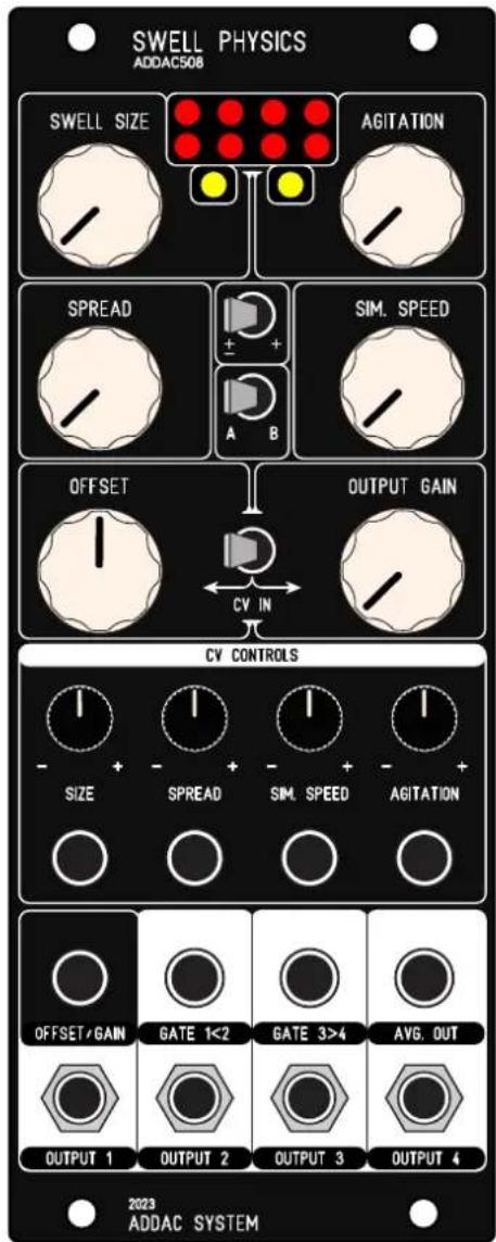
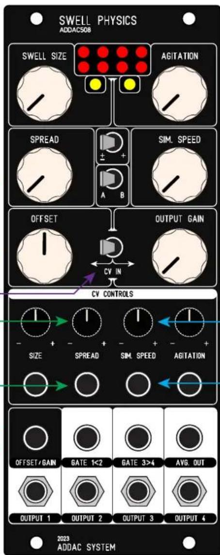
SWELL PHYSICS ADDAC508 SWELL SIZE AGITATION SPREAD ± + SIM. SPEED A B OFFSET OUTPUT GAIN CV IN CV CONTROLS SIZE SPREAD SIM. SPEED AGITATION OFFSET/GAIN GATE 1<2 GATE 3>4 AVG. OUT OUTPUT 1 OUTPUT 2 OUTPUT 3 OUTPUT 4 2023 ADDAC SYSTEMINTRODUCING
ADDAC508
SWELL
PHYSICS
USER'S GUIDE . REVO1
January.2024
ADDAC
System
From Portugal with Love!
WELCOME
Following our ADDC503 Marble Physics here is a new simulation of a physical system. This time imagine a small area in the middle of the ocean, in this area we place 4 equally spaced buoys anchored to the bottom in such a system that we can control the spacing between the buoys. Imagine we can control the elements and agitate the waters at will which in turn will make the buoys move up and down as the water surface moves.
Finally imagine the buoys would wirelessly transmit their absolute height directly to your module outputs where they would be mapped to a voltage signal.

flowchart
graph TD
    A["Red Node 1"] --> B["Green Node 2"]
    B --> C["Blue Node 3"]
    C --> D["Orange Node 4"]
    E["Red Node 1"] --> F["Green Node 2"]
    F --> G["Blue Node 3"]
    G --> H["Orange Node 4"]
We use a Gerstner Wave as the motor behind the 2d wave generation. In fluid dynamics a Gerstner Wave is described as "a progressive wave of permanent form on the surface of an incompressible fluid of infinite depth". Gerstner waves are often used in computer graphics to simulate any type of water surface, if you've seen any animation film or computer game with water surfaces in it most probably it features a Gerstner wave generating it.
text_image
SWELL PHYSICS ADDAC508 SWELL SIZE AGITATION SPREAD + + SIM. SPEED A B OFFSET OUTPUT GAIN CV IN CV CONTROLS SIZE + - SPREAD + - SIM. SPEED + - AGITATION OFFSET/GAIN GATE 1<2 GATE 3>4 AVG. OUT OUTPUT 1 OUTPUT 2 OUTPUT 3 OUTPUT 4 2023 ADDAC SYSTEMTech Specs:
10HP
4.5cm deep
70mA +12V
40mA -12V
MODULE DESCRIPTION
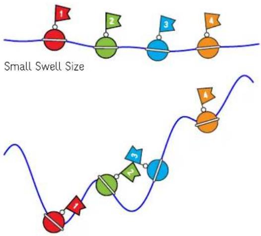
Starting from the top [SWELL Size] controls the virtual height of the ocean swell, or more precisely the maximum amplitude between the highest crest and the lowest trough.
text_image
Small Swell SizeBig Swell Size
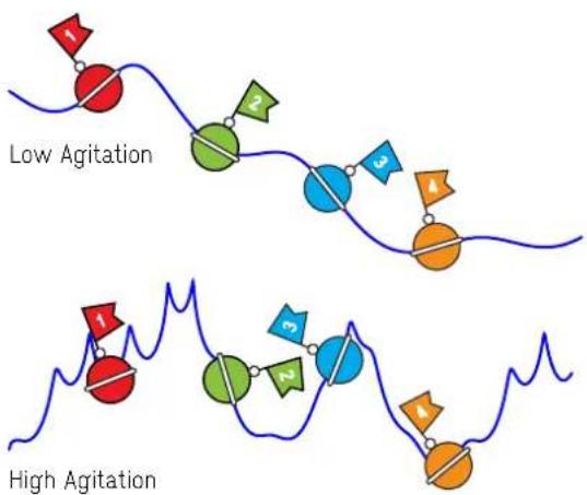
[AGITATION] is a peculiar macro that controls wind and secondary swells that create more complex interference waves.
text_image
Low Agitation High Agitation
text_image
SWELL PHYSICS ADDAC508 SWELL SIZE AGITATION SPREAD ± + SIM. SPEED A B OFFSET OUTPUT GAIN CV IN CV CONTROLS SIZE + - + - + SPREAD SIM. SPEED AGITATION OFFSET/GAIN GATE 1<2 GATE 3>4 AVG. OUT OUTPUT 1 OUTPUT 2 OUTPUT 3 OUTPUT 4 2023 ADDAC SYSTEMMODULE DESCRIPTION
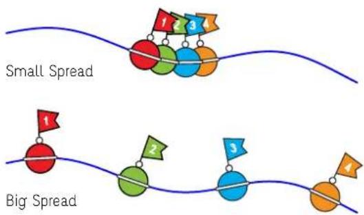
[SPREAD] sets the distance between buoys, smaller spreads make the outputs more related or closer to each other while bigger spreads will make the outputs more unrelated.
text_image
Small Spread Big Spread[SIMULATION SPEED] controls how fast the simulation is calculated just like a frequency control on an LFO.
[OFFSET] and [OUTPUT GAIN] allow to set all 4 CV outputs to any voltage range between ±5V or 0 to +10V. There's only one CV input for these 2 functions the [CV IN] — switch allows to route the input to a preferred one.
text_image
SWELL PHYSICS ADDAC508 SWELL SIZE AGITATION SPREAD ± + SIM. SPEED A B OFFSET OUTPUT GAIN CV IN CV CONTROLS SIZE + - + - + - + - + - + - OUTSET / GAIN GATE 1<2 GATE 3>4 AVG. OUT OUTPUT 1 OUTPUT 2 OUTPUT 3 OUTPUT 4 2023 ADDAC SYSTEMMODULE DESCRIPTION
[BIPOLAR / POSITIVE] switch sets all outputs voltage range to either ±5V or 0 to +10V
[A / B MODE] Sets the operation mode:
A - Scrolling Mode
B - Evolving Mode
Also used to set Clipping Mode (Page 8)
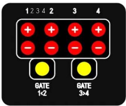
[GATE 1<2] Outputs a +5V Gate On while output 1 is smaller than output 2
[GATE 3>4] Outputs a +5V Gate On while output 3 is bigger than output 4
[OUTPUTS 1 to 4] 16 bit CV outputs
[AVERAGE OUTPUT] Average of all 4 CV Outputs
[TOP LEDS] Red LEDs show the bipolar state of all outputs. Yellow LEDs show the 2 gates state.
text_image
1 2 3 4 2 3 4 + + + + - - - - GATE 1×2 GATE 3×4
text_image
SWELL PHYSICS ADDAC508 SWELL SIZE AGITATION SPREAD ± + SIM. SPEED A B OFFSET OUTPUT GAIN CV IN CV CONTROLS SIZE + - + - + SPREAD SIM. SPEED AGITATION OFFSET/GAIN GATE 1<2 GATE 3>4 AVG, OUT OUTPUT 1 OUTPUT 2 OUTPUT 3 OUTPUT 4 2023 ADDAC SYSTEMA B MODES
MODE A - SCROLLING
Scrolling is a particular way to compute a Gerstner wave. At every step we calculate a single wave position at the left most point and push all previously generated points forward.
This makes all buoys follow the same exact path, in this mode [SPREAD] works as a delay
Here's a Mode A plot of all buoys over time

Here's the same plot with channels offsetted for better readability
flowchart
graph LR
    A["1"] --> B["2"]
    B --> C["3"]
    C --> D["4"]
MODE B - EVOLVING
Evolving is the normal computation for a Gerstner wave, at all steps all points in the wave are calculated according to the settings and the points close by which also affect each other in a symbiotic relationship resulting in different paths for all buoys which are more or less related according to the settings.
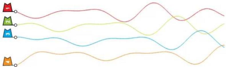
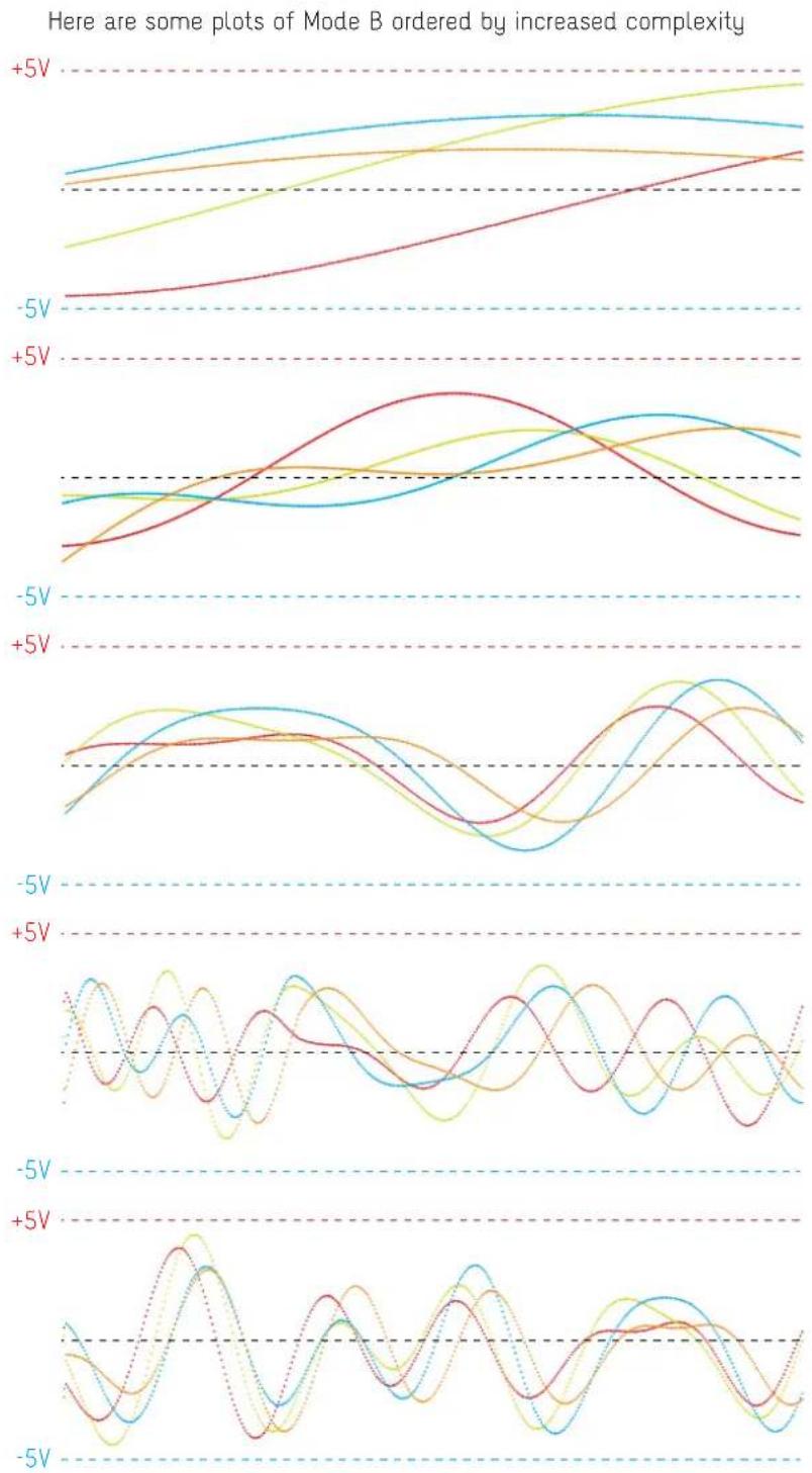
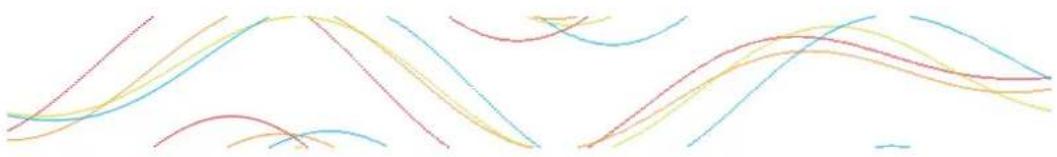
Here's a Mode B plot of all buoys over time

line
| Time | Voltage (V) | |------|-------------| | 0 | +5 | | 1 | -5 | | 2 | +5 | | 3 | -5 | | 4 | +5 | | 5 | -5 | | 6 | +5 | | 7 | -5 | | 8 | +5 | | 9 | -5 | | 10 | +5 | | 11 | -5 | | 12 | +5 | | 13 | -5 | | 14 | +5 | | 15 | -5 | | 16 | +5 | | 17 | -5 | | 18 | +5 | | 19 | -5 | | 20 | +5 | | 21 | -5 | | 22 | +5 | | 23 | -5 | | 24 | +5 | | 25 | -5 | | 26 | +5 | | 27 | -5 | | 28 | +5 | | 29 | -5 | | 30 | +5 | | 31 | -5 | | 32 | +5 | | 33 | -5 | | 34 | +5 | | 35 | -5 | | 36 | +5 | | 37 | -5 | | 38 | +5 | | 39 | -5 | | 40 | +5 | | 41 | -5 | | 42 | +5 | | 43 | -5 | | 44 | +5 | | 45 | -5 | | 46 | +5 | | 47 | -5 | | 48 | +5 | | 49 | -5 | | 50 | +5 | | 51 | -5 | | 52 | +5 | | 53 | -5 | | 54 | +5 | | 55 | -5 | | 56 | +5 | | 57 | -5 | | 58 | +5 | | 59 | -5 | | 60 | +5 | | 61 | -5 | | 62 | +5 | | 63 | -5 | | 64 | +5 | | 65 | -5 | | 66 | +5 | | 67 | -5 | | 68 | +5 | | 69 | -5 | | 70 | +5 | | 71 | -5 | | 72 | +5 | | 73 | -5 | | 74 | +5 | | 75 | -5 | | 76 | +5 | | 77 | -5 | | 78 | +5 | | 79 | -5 | | 80 | +5 | | 81 | -5 | | 82 | +5 | | 83 | -5 | | 84 | +5 | | 85 | -5 | | 86 | +5 | | 87 | -5 | | 88 | +5 | | 89 | -5 | | 90 | +5 | | 91 | -5 | | 92 | +5 | | 93 | -5 | | 94 | +5 | | 95 | -5 | | 96 | +5 | | 97 | -5 | | 98 | +5 | | 99 | -5 | | 100 | +5 |Here's the same plot with channels offsetted for better readability
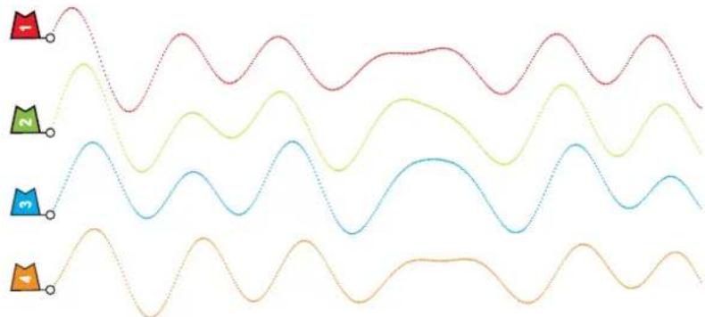
natural_image
Four wavy lines with dotted patterns, each marked with a unique icon (red, green, blue, orange), no text or symbols present.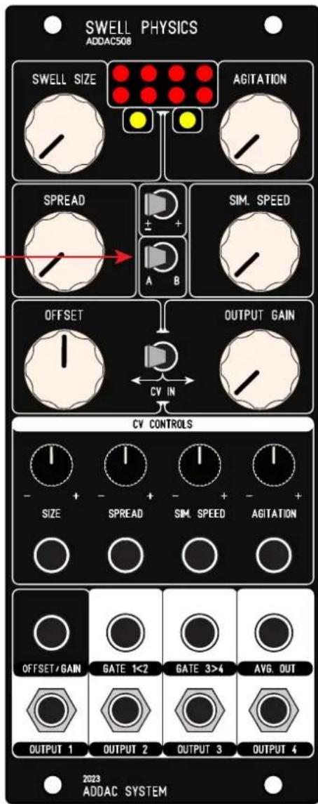
text_image
SWELL PHYSICS ADDAC508 SWELL SIZE AGITATION SPREAD ± + SIM. SPEED A B OFFSET OUTPUT GAIN CV IN CV CONTROLS SIZE + - + - + SPREAD SIM. SPEED AGITATION OFFSET/GAIN GATE 1<2 GATE 3>4 AVG, OUT OUTPUT 1 OUTPUT 2 OUTPUT 3 OUTPUT 4 2023 ADDAC SYSTEMOUTPUTS - WATER SURFACE
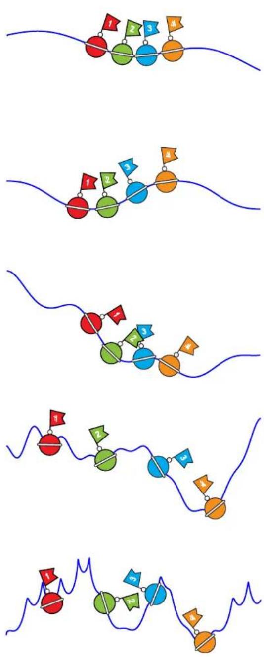
The outputs will always reflect the state of the water surface, the controls available allow to set this surface from the stillness of a pond to the complexity of a high sea storm.
If completely still, using [SWELL SIZE] fully ccw, the outputs will all be either zero or +5v depending if in Bipolar or Positive mode. As the user increases the [SWELL SIZE] and [AGITATION] controls the surface becomes more complex.
Here are some still of the water surface ordered by increased complexity
flowchart
graph TD
    A["Stage 1: Red Circle"] --> B["Stage 2: Green Circle"]
    B --> C["Stage 3: Blue Circle"]
    C --> D["Stage 4: Orange Circle"]
    D --> E["Stage 5: Blue Circle"]
    E --> F["Stage 6: Green Circle"]
    F --> G["Stage 7: Blue Circle"]
    G --> H["Stage 8: Orange Circle"]
    style A fill:#f9f,stroke:#333
    style B fill:#f9f,stroke:#333
    style C fill:#f9f,stroke:#333
    style D fill:#f9f,stroke:#333
    style E fill:#f9f,stroke:#333
    style F fill:#f9f,stroke:#333
    style G fill:#f9f,stroke:#333
    style H fill:#f9f,stroke:#333
CLIPPING MODES
It is possible to clip the waveform by setting the swell size higher than 12 o'clock.
To change the clipping mode flick the MODE A/B switch back and fourth faster than 1/2 a second.
The current mode is not visible but will be reflected on the outputs.
There are 3 clipping modes available:
- Fold (default)
Like any wavefolder it folds the wave by inverting the direction when above/below the maximum/minimum range.

line
| Time Point | Series 1 | Series 2 | Series 3 | Series 4 | Series 5 | | ---------- | -------- | -------- | -------- | -------- | -------- | | 1 | 0.8 | 0.6 | 0.7 | 0.9 | 0.5 | | 2 | 0.9 | 0.7 | 0.8 | 1.0 | 0.6 | | 3 | 0.7 | 0.8 | 0.9 | 0.8 | 0.7 | | 4 | 0.6 | 0.9 | 0.7 | 0.6 | 0.8 | | 5 | 0.5 | 0.8 | 0.6 | 0.5 | 0.9 | | 6 | 0.4 | 0.7 | 0.5 | 0.4 | 0.8 | | 7 | 0.3 | 0.6 | 0.4 | 0.3 | 0.7 | | 8 | 0.2 | 0.5 | 0.3 | 0.2 | 0.6 | | 9 | 0.1 | 0.4 | 0.2 | 0.1 | 0.5 | | 10 | 0.2 | 0.3 | 0.1 | 0.2 | 0.4 | | 11 | 0.3 | 0.2 | 0.2 | 0.3 | 0.3 | | 12 | 0.4 | 0.1 | 0.3 | 0.4 | 0.2 | | 13 | 0.5 | 0.2 | 0.4 | 0.5 | 0.1 | | 14 | 0.6 | 0.3 | 0.5 | 0.6 | 0.2 | | 15 | 0.7 | 0.4 | 0.6 | 0.7 | 0.3 | | 16 | 0.8 | 0.5 | 0.7 | 0.8 | 0.4 | | 17 | 0.9 | 0.6 | 0.8 | 0.9 | 0.5 | | 18 | 1.0 | 0.7 | 0.9 | 1.0 | 0.6 | | 19 | 1.1 | 0.8 | 1.0 | 1.1 | 0.7 | | 20 | 1.2 | 0.9 | 1.1 | 1.2 | 0.8 | | 21 | 1.3 | 1.0 | 1.2 | 1.3 | 0.9 | | 22 | 1.4 | 1.1 | 1.3 | 1.4 | 1.0 | | 23 | 1.5 | 1.2 | 1.4 | 1.5 | 1.1 | | 24 | 1.6 | 1.3 | 1.5 | 1.6 | 1.2 | | 25 | 1.7 | 1.4 | 1.6 | 1.7 | 1.3 | | 26 | 1.8 | 1.5 | 1.7 | 1.8 | 1.4 | | 27 | 1.9 | 1.6 | 1.8 | 1.9 | 1.5 | | 28 | 2.0 | 1.7 | 1.9 | 2.0 | 1.6 | | 29 | 2.1 | 1.8 | 2.0 | 2.1 | 1.7 | | 30 | 2.2 | 1.9 | 2.1 | 2.2 | 1.8 | | ... | ... | ... | ... | ... | ... | | Final | ... | ... | ... | ... | ... |- Thru
Thru forces the wave to go thru it's minimum/maximum range into the opposite end.
natural_image
Abstract wavy line patterns in various colors and hues, no text or symbols present- Limit
Simply limits the wave to the minimum/maximum range

natural_image
Abstract wavy line patterns in multiple colors and shapes, no text or symbols presentSIGNAL FLOW DIAGRAM
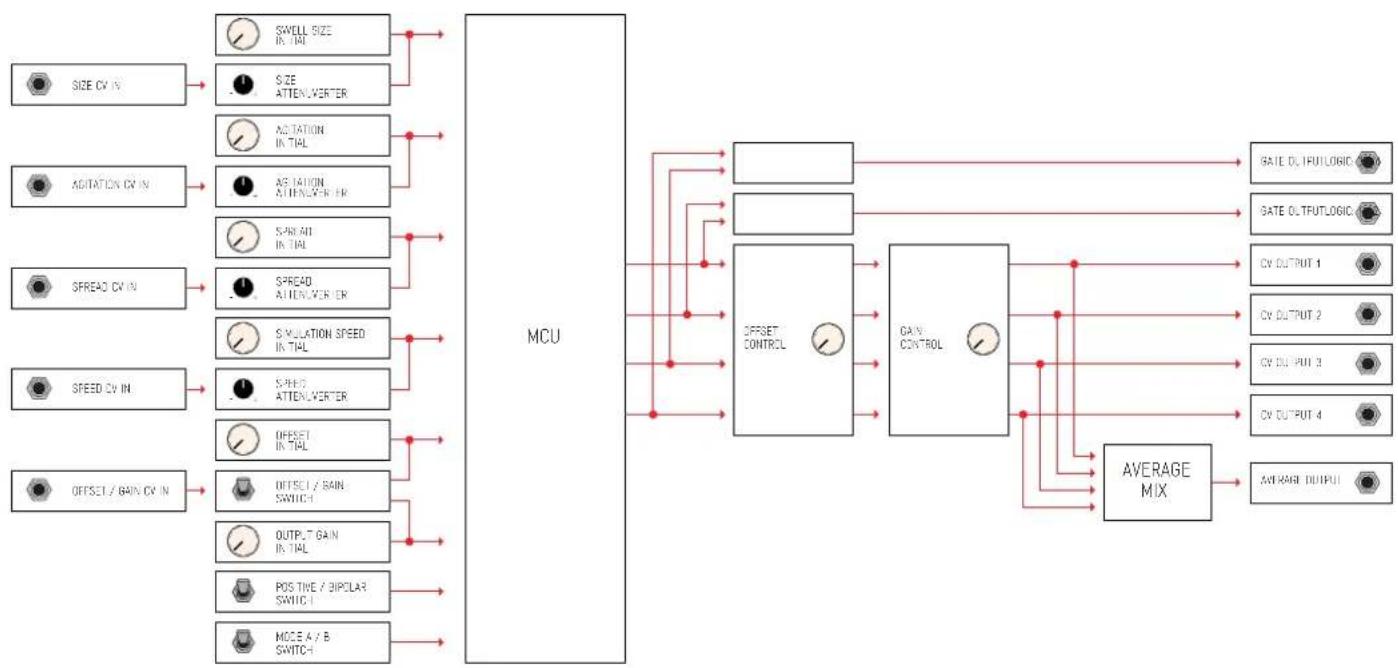
flowchart
graph LR
    A["SIZE CV IN"] --> B["SWELL SIZE IN TAL"]
    A --> C["SIZE ATTENUVERTER"]
    D["ADITATION CV IN"] --> E["ADITATION IN TIAL"]
    D --> F["ADITATION ATTENUVERTER"]
    G["SPREAD CV IN"] --> H["SPREAD IN TIAL"]
    G --> I["SPREAD ATTENUVERTER"]
    J["SIMULATION SPEED IN TIAL"] --> K["SIMULATION SPEED IN TIAL"]
    L["SPREAD ATTENUVERTER"] --> M["SPEED ATTENUVERTER"]
    N["OFFSET IN TIAL"] --> O["OFFSET IN TIAL"]
    P["OFFSET / GAIN CV IN"] --> Q["OFFSET / GAIN SWITCH"]
    R["OUTPUT / GAIN IN TIAL"] --> S["OUTPUT / GAIN SWITCH"]
    T["POS TINE / BIPOLAR SWITCH"] --> U["POS TINE / BIPOLAR SWITCH"]
    V["MODE A / B SWITCH"] --> W["MODE A / B SWITCH"]
    X["MCU"] --> Y["OFFSET CONTROL"]
    X --> Z["GAIN CONTROL"]
    X --> AA["AVERAGE MIX"]
    Y --> AB["BAE OUTPUT 1"]
    Y --> AC["BAE OUTPUT 2"]
    Y --> AD["BAE OUTPUT 3"]
    Y --> AE["BAE OUTPUT 4"]
    Y --> AF["AVERAGE OUTPUT"]
For feedback, comments or problems please contact us at: addac@addacsystem.com