
cnWave 60 - Electronic lock Cambium Networks - Free user manual and instructions
Find the device manual for free cnWave 60 Cambium Networks in PDF.


| Product Type | Electronic Lock |
| Brand | Cambium Networks |
| Model | cnWave 60 |
| Dimensions (L x W x H) | 120 x 60 x 30 mm |
| Weight | 0.8 kg |
| Power Supply | 4 x AA batteries (DC 6V) |
| Battery Life | Up to 12 months under normal use |
| Locking Mechanism | Motorized deadbolt |
| Keyless Entry | Yes – keypad, RFID, Bluetooth |
| Wireless Connectivity | Bluetooth 5.0, Wi-Fi (optional) |
| Mobile App Compatibility | iOS and Android |
| Remote Access | Via app with Wi-Fi hub |
| User Capacity | Up to 50 unique user codes |
| Activity Log | Yes – stores last 100 events |
| Weather Resistance | IP54 – dust and splash resistant |
| Operating Temperature | -20°C to 55°C |
| Security Rating | ANSI/BHMA Grade 2 |
| Low Battery Warning | Visual and audible alerts |
| Installation | DIY – fits standard door prep (2 1/8" bore) |
| Maintenance | Clean with dry cloth; lubricate mechanism annually |
| Replaceable Parts | Batteries, faceplate, latch |
| Included Accessories | Mounting screws, strike plate, user manual |
| Warranty | 2 years limited |
Frequently Asked Questions - cnWave 60 Cambium Networks
User questions about cnWave 60 Cambium Networks
0 question about this device. Answer the ones you know or ask your own.
Ask a new question about this device
Download the instructions for your Electronic lock in PDF format for free! Find your manual cnWave 60 - Cambium Networks and take your electronic device back in hand. On this page are published all the documents necessary for the use of your device. cnWave 60 by Cambium Networks.
USER MANUAL cnWave 60 Cambium Networks
natural_image
Street scene with surveillance cameras on elevated highways, no visible text or symbols
Cambium Networks™

natural_image
Aerial night view of a town nestled in a valley with hills and a river in the distance (no visible text or symbols)
natural_image
Young girl in blue shirt reading a tablet at a desk, with blurred background of other students (no visible text or symbols)
natural_image
Overhead view of people sitting at a table with laptops and coffee cups (no visible text or symbols)
natural_image
Desert landscape with a tall oil rig and surrounding hills under a dramatic cloudy sky (no text or symbols visible)USER GUIDE
60 GHz cnWave™
Release 1.4

natural_image
Aerial view of a coastal industrial area with ships, storage tanks, and green fields under a partly cloudy sky (no visible text or symbols)
natural_image
Man in blue shirt working at a wooden table with a laptop, surrounded by workbenches and tools (no visible text or symbols)Reservation of Rights
Cambium reserves the right to make changes to any products described herein to improve reliability, function, or design, and reserves the right to revise this document and to make changes from time to time in content hereof with no obligation to notify any person of revisions or changes. Cambium recommends reviewing the Cambium Networks website for the latest changes and updates to products. Cambium does not assume any liability arising out of the application or use of any product, software, or circuit described herein; neither does it convey license under its patent rights or the rights of others. It is possible that this publication may contain references to, or information about Cambium products (machines and programs), programming, or services that are not announced in your country. Such references or information must not be construed to mean that Cambium intends to announce such Cambium products, programming, or services in your country.
Copyrights
This document, Cambium products, and Party software products described in this document may include or describe copyrighted Cambium and other Party supplied computer programs stored in semiconductor memories or other media. Laws in the United States and other countries preserve for Cambium, its licensors, and other 3 supplied software certain exclusive rights for copyrighted material, including the exclusive right to copy, reproduce in any form, distribute and make derivative works of the copyrighted material. Accordingly, any copyrighted material of Cambium, its licensors, or the Party software supplied material contained in the Cambium products described in this document may not be copied, reproduced, reverse engineered, distributed, merged or modified in any manner without the express written permission of Cambium. Furthermore, the purchase of Cambium products shall not be deemed to grant either directly or by implication, estoppel, or otherwise, any license under the copyrights, patents or patent applications of Cambium or other 3rd Party supplied software, except for the normal non-exclusive, royalty free license to use that arises by operation of law in the sale of a product.
Restrictions
Software and documentation are copyrighted materials. Making unauthorized copies is prohibited by law. No part of the software or documentation may be reproduced, transmitted, transcribed, stored in a retrieval system, or translated into any language or computer language, in any form or by any means, without prior written permission of Cambium.
License Agreements
The software described in this document is the property of Cambium and its licensors. It is furnished by express license agreement only and may be used only in accordance with the terms of such an agreement.
High Risk Materials
Cambium and its supplier(s) specifically disclaim any express or implied warranty of fitness for any high-risk activities or uses of its products including, but not limited to, the operation of nuclear facilities, aircraft navigation or aircraft communication systems, air traffic control, life support, or weapons systems ("High Risk Use").
This product is not restricted in the EU. Any High Risk is unauthorized, is made at your own risk and you shall be responsible for any and all losses, damage or claims arising out of any High-Risk Use.
Contents
Contents 3
About This User Guide..10
Purpose 10
Cross-references 10
Feedback 10
Important regulatory information.10
Complying with rules for the country of operation 10.
Application firmware 12
Ethernet networking skills 12
Lightning protection..12
Specific expertise and training for professional installers. 13
Legal and Open-Source Software statements 13
Problems and warranty 13
Reporting problems.13
Repair and service 13
Hardware warranty 13
Security advice 14
Warnings, cautions, and notes 14
Caring for the environment 14
In the UK and EU countries 14
In non-EU countries 15
Product Description 16
Introduction 16
Frequency bands 16
Characteristics 17
802.11ay Standards and advantages 18
Terragraph 20
Theory of operation 21
Overview of cnWave family 22
Features 23
Wireless operation 24
Wireless topology .25
Modulation 27
Synchronization 28
Time-division duplexing access mechanism. 29
Wireless encryption.29
Designing wireless networks 30
TDD synchronization 30
System management 30
Management agent 30
Network management 30
IPv6 30
System logging 31
Software upgrade .31
System Hardware 32
Wireless nodes 32
V1000 Client Node (CN) 32
V2000 Client Node (CN) 33
V3000 Client Node (CN) 34
V5000 Distribution Node (DN) 35
Radio mounting brackets 36
Radio accessories 41
Radio external interfaces 44
Radio specifications 47
Power supply units (PSU) 48
PSU Options 48
V1000 - Power over Ethernet (PoE) 49
V2000 - PoE 50
V3000/V5000 - PoE 52
Ethernet and DC cables 57
Maximum cable lengths 57
Outdoor copper CAT6A Ethernet cable 59
Cable accessories 59
SFP Module kits 60
Optical cable and connectors 61
System Planning 63
Site planning 63
Grounding and lightning protection 63
Lightning protection zones 63
Site grounding system 64
ODU location 64
Drop cable grounding points 64
ODU wind loading 65
PSU DC power supply 66
PSU AC power supply 66
PSU location 66
Outdoor AC/DC PSU 66
Lightning Surge Protection Units (LPU) 66
Drop cable grounding points 66
Lightning Surge Protection Units location 67
Deployment Considerations 67
Key deployment guidelines 68
Sector and alignment 68
Minimum CN spacing 70
Near-far radio 71
Early weak interference 72
Avoiding the tight angle deployment 72
Avoiding the straight line interference 73
When two V5000 devices are co-located at a site 74
Polarity 74
Link Adaptation and Transmit Power Control (LATPC) 75
Radio spectrum planning 76
General wireless specifications 76
Regulatory limits 76
Link planning 77
LINKPlanner 77
Range and obstacles 77
Path loss 77
Planning for data networks 78
Point to Point-based single link Ethernet bridge 78
IPv4/L2 based PMP and mesh network planning 79
Support for dual networking (IPv4 and IPv6) 80
IPv6 Mode network planning 80
IPv6 Network design consideration 81
Reserved IPv6 address space 82
E2E and cnMaestro deployment consideration 82
Ethernet bridging 82
Layer 2 control protocols 84
IP Interface 84
Daisy-chaining 60 GHz links 84
Installation 85
Safety 85
Power lines 85
Working at heights 85
PSU 85
Grounding and protective earth 85.
AC Supply 85
Powering down before servicing 85
Primary disconnect device 85
External cables 86
Drop cable tester 86
RF Exposure near the antenna 86
Minimum separation distances 86
Grounding and lightning protection requirements 86
Grounding cable installation methods 86
Siting radios 86
60 GHz cnWave radios and mounting bracket options 86
Installing the cnWave radio nodes 87
ODU Interface with LPU on the pole 92.
Attach ground cables to the radio 96
Mounting the ODU 96
Connect to the PSU port of the radio 118.
Using Power over Ethernet (PoE) 118
Using AC/DC PSU 121
Install the PSU 124
Installing the 60W DC power injector 125
Installing the AC/DC PSU 126
Installing 15W or 30W power injector 128
Connecting to the SFP+ optical module or SFP+ to the copper module to ODU 129
Removing the cable and SFP module 135
Configuring 60 GHz cnWave™ 137
Nodes deployment 137
Connecting to the unit 137
Configuring the management PC 137
Connecting to the PC and powering up 139
Using the web interface 139
Logging into the web interface 139
Enabling internal E2E Controller 145
Topology 147
Configuration 152
Operation 197
Software upgrade 197
Diagnostics 198
Statistics 200
Links 200
Ethernet 204
GPS 205
Radio 206
Performance 207
Prefix zone Statistics 212
Border Gateway Protocol (BGP) 212
Maps 213
Tools 214
Factory reset 214
Field diags 214
Antenna alignment 215
Remote Command 222
Ping 226
Quick PTP setup 227
iPerf 228
cnMaestro support for Onboard Controller 230
Backup CN link 233
Auto Manage IPv6 Routes (External E2E Controller) 235
Unconnected PoPs 238
High Availability (HA) support for Onboard E2E Controller 239
Regulatory Information 243
Compliance with safety standards 243
Electrical safety compliance 243
Human exposure to radio frequency energy 244
Compliance with radio regulations 246
Type approvals 247
Federal Communications Commission (FCC) compliance 247
Innovation, Science and Economic Development Canada (ISEDC) compliance 247
60 GHz cnWave example product labels 248
Troubleshooting 251
Field diagnostics logs 251
Setup issues in IPv4 tunneling 253
Link is not established.255
PoP not online from E2E or cnMaestro. UI 258
Link is not coming up.258
Link does not come up after some configuration change. 259
Link is not having expected throughput performance 259
Factory reset 259
Cambium Networks 261
About This User Guide
This document provides detailed information about the 60 GHz cnWave™ products, hardware, and supported features. The guide also explains how to deploy the product along with important safety measures. It is intended for system designers, system installers, and system administrators.
Purpose
The 60 GHz cnWave product documents are intended to instruct and assist personnel in operation, installation, and maintenance of the equipment and ancillary devices. It is recommended that all personnel engaged in such activities must be properly trained.
Cambium Networks disclaims all liability whatsoever, implied or express, for any risk of damage, loss or reduction in system performance arising directly or indirectly out of the failure of the customer, or anyone acting on the customer's behalf, to abide by the instructions, system parameters, or recommendations made in this document.
Cross-references
References to external publications are shown in italics. Other cross-references, emphasized in blue text in electronic versions, are active links to the references.
This document is divided into numbered chapters that are divided into sections. Sections are not numbered but are individually named at the top of each page and are listed in the table of contents.
Feedback
We appreciate feedback from the users of our documents. This includes feedback on the structure, content, accuracy, or completeness of our documents. To provide feedback, visit our support website: https://support.cambiumnetworks.com.
Important regulatory information
Complying with rules for the country of operation
USA specific information

Caution
This device complies with Part 15 of the Federal Communications Commission (FCC) Rules. Operation is subject to the following two conditions:
• This device may not cause harmful interference, and
- This device must accept any interference received, including interference that may cause undesired operation.

Note
This equipment has been tested and found to comply with the limits for a Class B digital device, pursuant to part 15 of the FCC Rules. These limits are designed to provide reasonable protection against harmful interference in a residential installation. This equipment generates, uses and can radiate radio frequency energy and, if not installed and used in accordance with the instructions, may cause harmful interference to radio communications. However, there is no guarantee that interference will not occur in a particular installation. If this equipment does cause harmful interference to radio or television reception, which can be determined by turning the equipment off and on, the user is encouraged to try to correct the interference by one or more of the following measures:
- Reorient or relocate the receiving antenna.
- Increase the separation between the equipment and receiver.
- Connect the equipment into an outlet on a circuit different from that to which the receiver is connected.
- Consult the dealer or an experienced radio/TV technician for help.
Canada specific information

Caution
This device complies with Innovation, Science and Economic Development Canada (ISEDC) license-exempt RSSs. Operation is subject to the following two conditions:
• This device may not cause interference; and
- This device must accept any interference, including interference that may cause undesired operation of the device.
European specific information
Cambium Networks 60 GHz cnWave products are compliant with applicable European Directives required for CE marking:
- 2014/53/EU of the European Parliament and of the Council of 16 April 2014 on the harmonisation of the laws of the Member States relating to the making available on the market of radio equipment and repealing Directive 1999/5/EC; Radio Equipment Directive (RED).
- 2011/65/EU of the European Parliament and of the Council of 8 June 2011 on the restriction of the use of certain hazardous substances in electrical and electronic equipment (RoHS Directive).
EU Declaration of conformity
Hereby, Cambium Networks declares that the Cambium Networks 60 GHz cnWave Series of Wireless Ethernet Bridge complies with the essential requirements and other relevant provisions of Directive 2014/53/EU. The declaration of conformity may be consulted at https://www.cambiumnetworks.com/eu_dofc.
United Kingdom (UK) specific information
Cambium Networks 60 GHz cnWave products are compliant with applicable United Kingdom (UK) Regulations required for UKCA marking:
• Radio Equipment Regulations 2017 (SI 2017 No. 1206, as amended)
- Restriction of the Use of Certain Hazardous Substances in Electrical and Electronic Equipment Regulations 2012 (SI 2012 No. 3032, as amended) (RoHS)
The 59-63.9 GHz frequency band is subject to specific exclusion zones. For more information, see the 59 - 63.9 GHz transmission exclusion zones table.
UK Unmetered Supplies Operational Charge Codes:
• V1000: 8820008004100
• V2000: 8820011004100
• V3000: 8820022000100
• V5000: 8820029000100
For more details, check https://www.elexon.co.uk/operations-settlement/unmetered-supplies/charge-codes-and-switch-regimes/.
UK Declaration of conformity
Hereby, Cambium Networks declares that the Cambium Networks 60 GHz cnWave Series of Wireless
Ethernet Bridge complies with the essential requirements and other relevant provisions of Radio Equipment Regulations 2017 (SI 2017 No. 1206, as amended) The declaration of conformity may be consulted at https://www.cambiumnetworks.com/ukca_dofc.
Application firmware
Download the latest 60 GHz products family software and install it in the Outdoor Units (ODUs) before deploying the equipment. Instructions for installing software are provided in this guide.
Ethernet networking skills
The installer must have the ability to configure IP addressing on a PC and to set up and control products using a web browser user interface (UI).
Lightning protection
To protect outdoor radio installations from the impact of lightning strikes, the installer must be familiar with the normal procedures for site selection, bonding and grounding. Installation guidelines for the 60 GHz platform of products are available in System Hardware and System Planning sections.
Specific expertise and training for professional installers
To ensure that the 60 GHz cnWave Series is installed and configured in compliance with the requirements of the EU, ISEDC and the FCC, installers must have the radio engineering skills and training described in this section.
The Cambium Networks technical training program details can be accessed from the following link: https://learning.cambiumnetworks.com/
Legal and Open-Source Software statements
Refer to the 60 GHz cnWave™ Legal and Open-Source Guide
• Cambium Networks end user license agreement
- Open-Source Software Notices.
Problems and warranty
Reporting problems
If any problems are encountered when installing or operating this equipment, follow this procedure to investigate and report:
- Search this document and the software release notes of supported releases.
- Visit the support website (http://www.cambiumnetworks.com/support).
- Ask for assistance from the Cambium Networks product supplier.
- Gather information from affected units, such as any available diagnostic downloads.
- Escalate the problem by emailing or telephoning support.
Repair and service
If unit failure is suspected, obtain details of the Return Material Authorization (RMA) process from the support website (http://www.cambiumnetworks.com/support).
Hardware warranty
Cambium's standard hardware warranty is for one (1) year from the date of shipment from Cambium Networks or a Cambium distributor. Cambium Networks warrants that hardware will conform to the relevant published specifications and will be free from material defects in material and workmanship under normal use and service. Cambium shall within this time, at its own option, either repair or replace the defective product within thirty (30) days of receipt of the defective product. Repaired or replaced products will be subject to the original warranty period but not less than thirty (30) days.
To register positioner products or activate warranties, visit the support website. For warranty assistance, contact the reseller or distributor. The removal of the tamper-evident seal will void the warranty.

Caution
Using non-Cambium parts for repair could damage the equipment or void warranty. Contact Cambium for service and repair instructions.
Portions of Cambium equipment may be damaged from exposure to electrostatic discharge. Use precautions to prevent damage.
Security advice
Cambium Networks systems and equipment provide security parameters that can be configured by the operator based on their particular operating environment. Cambium recommends setting and using these parameters following industry-recognized security practices. Security aspects to be considered are protecting the confidentiality, integrity, and availability of information and assets. Assets include the ability to communicate, information about the nature of the communications, and information about the parties involved.
In certain instances, Cambium makes specific recommendations regarding security practices, however the implementation of these recommendations and final responsibility for the security of the system lies with the operator of the system.
Warnings, cautions, and notes
The following describes how warnings and cautions are used in this document and all Cambium Networks document sets:
Warnings
Warnings precede instructions that contain potentially hazardous situations. Warnings are used to alert the reader to possible hazards that could cause loss of life or physical injury. A warning has the following format:

Warning
Warning text and consequence for not following the instructions in the warning.
Cautions
Cautions precede instructions and are used when there is a possibility of damage to systems, software, or individual items of equipment within a system. However, this damage presents no danger to personnel. A caution has the following format:

Caution
Caution text and consequence for not following the instructions in the caution.
Notes
A note means that there is a possibility of an undesirable situation or provides additional information to help the reader understand a topic or concept. A note has the following format:

Note
Note text.
Caring for the environment
The following information describes national or regional requirements for the disposal of Cambium Networks supplied equipment and for the approved disposal of surplus packaging.
In the UK and EU countries
The following information is provided to enable regulatory compliance with the European Union (EU) directives and UK regulations identified and any amendments made to these directives and regulations when using Cambium equipment in the UK or EU countries:
Disposal of Cambium equipment
European Union (EU) Directive 2012/19/EU Waste Electrical and Electronic Equipment (WEEE) and UK Statutory Instrument The Waste Electrical and Electronic Equipment Regulations 2013 No. 3113.
Do not dispose of Cambium equipment in landfill sites. For disposal instructions, refer to http://www.cambiumnetworks.com/support/weee-compliance
Disposal of surplus packaging
Do not dispose of surplus packaging in landfill sites. In the EU and UK, it is the individual recipient's responsibility to ensure that packaging materials are collected and recycled according to the requirements of EU and UK environmental law.
In non-EU countries
In non-EU countries, dispose of Cambium equipment and all surplus packaging in accordance with national and regional regulations.
Product Description
This section provides information about the 60 GHz cnWave product from Cambium Networks. It also describes its features, characteristics, and other related concepts.
Introduction
The 60 GHz cnWave products support a wide spectrum of up to 9 GHz (57-66 GHz) that is typically divided into channels of 2 GHz each. The 60 GHz band is largely uncongested when compared to 2.5 GHz and 5 GHz public bands, which are currently used for Wi-Fi. The 60 GHz band is an unlicensed millimeter-wave band that can provide massive speeds and throughput with Line of Sight (LoS) applications.
The 60 GHz band is located in the millimeter-wave (30 GHz to 300 GHz) portion of the electromagnetic spectrum.
The millimeter-wave portion of the RF spectrum has been largely unexploited for commercial wireless applications. 60 GHz wireless products enable two-way wireless communications at data rates that was previously achieved using fiber optic cables.
In addition to the high-data rates (accomplished in this spectrum), energy propagation in the 60 GHz band has benefits such as excellent immunity to interference, high security, and frequency reuse.
Frequency bands
The 60 GHz band is divided into 11 channels, each with a bandwidth of 2.16 GHz starting from 57.24 to 70.2 GHz. Channels 1 to 6 support 2.16 GHz bandwidth and are defined in 802.11ad. Channels 9 to 13 support 4.32 GHz bandwidth and are added to 802.11ay.
Figure 1: Frequency bands

Table 1 lists the channels and the corresponding bandwidths supported by 60 GHz cnWave products:
Table 1: Channels and corresponding bandwidths
| Channel Bandwidth (GHz) Center (GHz) | Minimum (GHz) Maximum (GHz) | |||||
| CH1 | 2.16 | 58.32 | 57.24 | 59.40 | ||
| CH2 | 2.16 | 60.43 | 59.40 | 61.56 | ||
| CH3 | 2.16 | 62.64 | 61.56 | 63.72 | ||
| CH4 | 2.16 | 64.80 | 63.72 | 65.88 | ||
| CH9 | 4.32 | 59.40 | 57.24 | 61.56 | ||
| CH10 | 4.32 | 61.56 | 59.40 | 63.72 | ||
| CH11 | 4.32 | 63.72 | 61.56 | 65.88 | ||
Characteristics
Following are the important characteristics of 60 GHz cnWave products:
• High throughput capability
CnWave products support 802.11ad Modulation and Coding Schemes (MCS) in a single channel (CB1) as well as 802.11ay Enhanced Directional Multi-Gigabit (EDMG) modes in dual Channel Bonding (CB2). This enables you to achieve Multi-Gigabit wireless rates. Refer to Table 3 and Table 4 for the supported CB1 and CB2 modes along with the expected throughput values.
• Unlicensed and interference free
Typically, the V band is either an unlicensed or lightly licensed band, which is relatively a new band. This band has limited interference when compared to 2.4 and 5 GHz bands.
• Line of Sight (LoS)
60 GHz is affected by oxygen absorption, it varies throughout the band. The absorption gets reduced if the frequency gets increased. For example, the absorption is 15 dB/km in 60 GHz frequency, 5 dB/km in 64 GHz, and 0.5 dB/km in 68 GHz. If the total channel is divided into 6 channels, then the mid-channel that is channels 2 and 3 has more absorption loss. From channel 4, the absorption level starts to drop. So only Line of Sight links are available and Near LoS or non LoS links do not work with 60 GHz.
Figure 2: Line of Sight

line
| Frequency (GHz) | Low Latitude | Mid Latitude | High Latitude | | --------------- | ------------ | ------------ | ------------- | | 55 | 4.0 | 4.0 | 4.0 | | 56 | 7.0 | 8.0 | 9.0 | | 57 | 10.0 | 11.0 | 12.0 | | 58 | 12.0 | 13.0 | 14.0 | | 59 | 13.0 | 14.0 | 15.0 | | 60 | 14.0 | 15.0 | 16.0 | | 61 | 13.5 | 15.5 | 17.0 | | 62 | 13.0 | 15.0 | 16.5 | | 63 | 12.0 | 14.0 | 15.5 | | 64 | 10.0 | 12.0 | 13.0 | | 65 | 8.0 | 10.0 | 11.0 | | 66 | 6.0 | 8.0 | 9.0 | | 67 | 4.0 | 6.0 | 7.0 | | 68 | 2.0 | 4.0 | 5.0 | | 69 | 1.0 | 2.0 | 3.0 | | 70 | 0.5 | 1.0 | 2.0 |- Rain fade
You can view significant rain fade for 60 GHz links, particularly those pushing the longer distances. Attenuation depends on the rain rate which must be factored in while planning the network. Rain attenuation depends on the level of the rain. The following table describes the rain level and absorption loss.
Table 2: Rain and attenuation
| Rain Attenuation | |
| Drizzle (0.25 mm/hr) 0.2 dB/km | |
| Light Rain (2.5 mm/hr) 1.8 dB/km | |
| Medium Rain (12.5 mm/hr) 5.6 dB/km | |
| Heavy Rain (25 mm/hr) 9.5 dB/km | |
| Downpour (50 mm/hr) 17 dB/km | |
| Tropical (100 mm/hr) 28 dB/km | |
| Monsoon (200 mm/hr) 38 dB/km |
The following figure shows the absorption loss due to the rain level (seasons):
Figure 3: Variation in Loss/km with frequency and rain rate
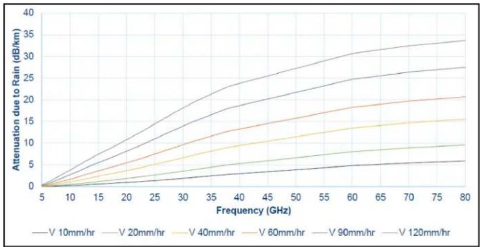
line
| Frequency (GHz) | V 10mm/hr | V 20mm/hr | V 40mm/hr | V 60mm/hr | V 90mm/hr | V 120mm/hr | | --------------- | --------- | --------- | --------- | --------- | --------- | ---------- | | 5 | 0 | 0 | 0 | 0 | 0 | 0 | | 10 | ~2 | ~1.5 | ~1 | ~0.5 | ~0.2 | ~0.1 | | 15 | ~4 | ~3 | ~2 | ~1.5 | ~1 | ~0.5 | | 20 | ~6 | ~4.5 | ~3.5 | ~2.5 | ~1.5 | ~1 | | 25 | ~8 | ~6 | ~5 | ~3.5 | ~2 | ~1.5 | | 30 | ~10 | ~7.5 | ~6.5 | ~4.5 | ~2.5 | ~2 | | 35 | ~12 | ~9 | ~8 | ~5.5 | ~3 | ~2.5 | | 40 | ~14 | ~10.5 | ~9.5 | ~6.5 | ~3.5 | ~3 | | 45 | ~16 | ~12 | ~11 | ~7.5 | ~4 | ~3.5 | | 50 | ~18 | ~13.5 | ~12.5 | ~8.5 | ~4.5 | ~4 | | 55 | ~20 | ~15 | ~14 | ~9.5 | ~5 | ~4.5 | | 60 | ~22 | ~16.5 | ~15.5 | ~10.5 | ~5.5 | ~5 | | 65 | ~24 | ~18 | ~17 | ~11.5 | ~6 | ~5.5 | | 70 | ~26 | ~19.5 | ~18.5 | ~12.5 | ~6.5 | ~6 | | 75 | ~28 | ~21 | ~20 | ~13.5 | ~7 | ~6.5 | | 80 | ~30 | ~22.5 | ~21.5 | ~14.5 | ~7.5 | ~7 |Drizzle - 0.25 mm/hr; Light rain - 2.5 mm/hr; Medium rain - 12.5 mm/hr; Heavy rain - 25 mm/hr.
- Short range
The range of a 60 GHz cnWave link can be limited due to oxygen absorption and rain fade which needs to be factored in for link planning. One advantage of a shorter range is the frequent reusability and security (as the signal does not travel long distances).
802.11ay Standards and advantages
IEEE 802.11ay is an IEEE standard that covers 60 GHz cnWave, this standard is an amendment of the IEEE 802.11ad standard. There are IEEE 802.11ay is designed with a higher throughput capacity of over 10 Gbps data rate over distances of 200 to 500 meters. 802.11ay includes features such as Channel Bonding and Synchronization. 802.11ay based 60 GHz solution transforms fixed wireless access from a broadband option of last resort into a competitive alternative to fiber and cable-based solution.
This standard is designed with a throughput capacity of over 10 Gbps data rate over distances of 200 to 500 meters. 802.11ay includes features such as Channel Bonding and Synchronization. 802.11ay is WLAN type in the IEEE 802.11. It has a frequency of 60 GHz. It has also been noted that it is likely to have mechanisms for channel bonding and MU-MIMO technologies. 802.11ad uses a maximum of 2.16 GHz bandwidth, whereas 802.11ay bonds four of those channels together for a maximum bandwidth of 8.64 GHz.
802.11ay standard has the following advantages with the Terragraph solution:
- Channel Bonding
802.11ay standard has channel bonding capability to combine adjacent channels to form wider channels, in this case, wider channels combine to form 4.32 GHz, there are additional wider channels created which provide double capacity throughput compared to the 802.11ad standard.
• Network Synchronization
Synchronization is used to control the transmit and receive signals to prevent self-interference. Radios assigned with the same polarity will be transmitting and receiving at the same time.
There are four types of polarity:
- Odd Polarity
- Even Polarity
- Hybrid odd Polarity
- Hybrid Even Polarity
- Mesh Routing
Mesh is an interconnection of devices that can have multiple paths between any two nodes, some advantages of using mesh are better connectivity, capacity sharing, load balancing, and re-routing in case of link failure.
- Increased capacity
802.11ay supports Channel Bonding which allows two immediate channels to be merged into a single wide-band channel, thereby doubling the channel bandwidth to 4.32 GHz.
• Supports a greater number of client nodes
802.11ay supports 15 client nodes per sector.
Advantages
• 802.11ay product, Terragraph certified
The 60 GHz cnWave is an 802.11ay product and Terragraph certified.
- Highest capacity
It has highest the capacity in the industry, up to 5.4 Gbps per sector.
- Low total cost ownership
- cnWave V5000 is 280-degree coverage with dual-sector. Installation is simple, uses beam forming for installation. No need for a site router.
-
cnWave V1000, V2000, and V3000 meet various range challenges.
• Using beam forming, the V3000 has a super long range. -
cnMaestro panel is used for device management.
- cnHeat and LINKPlanner help for easy planning.
• Unlicensed and interference-free
This spectrum spans 57 - 66 GHz and is widely available, especially when compared to the 2.4 and 5 GHz bands. This 9 GHz of the spectrum can be divided up into channels ranging between 1 and 2 GHz wide.
• Massive throughput
This band can allow over 10 Gbps of throughput from some products on the market today.
Terragraph
Terragraph is a connectivity solution from Facebook. The mission of Terragraph is to bring more people online to a faster internet. It is freely licensed technology that is designed to deliver cost-effective and reliable fiber like connectivity over a wireless mesh network (as shown in Figure 4).
Figure 4: Terra graph

flowchart
graph TD
    A["Controller"] --> B["Terragraph Distribution Nodes"]
    B --> C["Client Node"]
    C --> D["Cloud"]
    D --> E["Component 1"]
    D --> F["Component 2"]
    D --> G["Component 3"]
    D --> H["Component 4"]
    style A fill:#f9f,stroke:#333
    style B fill:#ccf,stroke:#333
    style C fill:#cfc,stroke:#333
    style D fill:#fcc,stroke:#333
    style E fill:#ffc,stroke:#333
    style F fill:#cfc,stroke:#333
    style G fill:#fcc,stroke:#333
    style H fill:#ffc,stroke:#333
1- Controller
2- PoP (Fiber, RF)
3- Distribution Node
4- Client Node
Key components
Terragraph contains the following key components:
- Distribution Node (DN) - DN connects with other DN to form a mesh in a distribution network.
- Client Node (CN) - CN is a customer premise radio that connects with a DN node to provide high-speed connectivity.
- E2E Controller - The E2E Controller allows for configuration, control, and monitoring of the nodes and network. Cambium Networks supports two methods to utilize the E2E Controller:
- On-Premises installed as a VM and can be used for small or large deployment (limited to 500 nodes).
- Onboard the PoP, for PTP, PMP, and small mesh networks the PoP can be configured to host the controller (limited to 31 nodes).
Features
The following are the features of Terragraph:
• 802.11ay - Delivers multi-gigabit speeds over wide frequency bands.
- Mesh - Efficiently distributes capacity and improves availability, using Open/R.
• Efficient MAC and PHY - Scheduled MAC (TDD / TDMA) for scalability and dense deployments.
- Cloud management - Used for configuration, management, visualization, alarms, and monitoring.
- Network planning - Automated design and optimization using imagery, population, and optionally other data sources.
Responsibilities
The Terragraph software initializes and configures radios (DN and CN). It tracks and optimizes meshed routing paths. It also monitors and maintains Syslog, alarms, and Firmware upgrades.
Theory of operation
The 60 GHz cnWave devices support Facebook connectivity technology called Terragraph. cnWave devices implement IEEE 802.11ay WLAN standard and use 60GHz frequency band for wider spectrum and higher capacity. cnWave devices can provide multi-gigabit throughput from 100 M to 1.5 KM.
Deployment of the devices uses Open/R based layer3/IPv6 mesh for efficient distribution of traffic between the nodes and higher availability of the traffic. This also overcomes non-line of sight issues.
Devices use TDMA/TDD technology to achieve density deployment efficiency. Network and the nodes are configured, controlled, and monitored by a cloud-based E2E Controller.
Following terminologies are used for the network deployment:
- Distribution Node (DN) - DN connects with other DN for mesh network
- Client Node (CN) - CN connects to DN to provide high-speed connectivity
- PoP - DN connected to the back-haul
• CPE - Customer premises equipment devices like Wi-Fi router
Figure 5: Deployment scenario

flowchart
graph TD
    CPE --> DN1["DN"]
    DN1 --> DN2["DN"]
    DN2 --> DN3["DN"]
    DN3 --> DN4["DN"]
    DN4 --> DN5["DN"]
    DN5 --> CN1["CPE"]
    DN5 --> CN2["CPE"]
    DN1 -.->|Backhaul| E2E["E2E"]
    E2E --> NOC["NOC"]
    NOC --> NMS["NMS"]
    PoP_DN["PoP DN"] --> DN1
    PoP_DN --> DN2
    PoP_DN --> DN3
    PoP_DN --> DN4
    PoP_DN --> CN1
    PoP_DN --> CN2
    PoP_DN --> CN3
    PoP_DN --> CPE["CPE"]
    PoP_DN --> CPE["CPE"]
    style E2E fill:#90EE90,stroke:#333
    style NMS fill:#90EE90,stroke:#333
    style CPE fill:#66CCFF,stroke:#333
    style CPE fill:#66CCFF,stroke:#333
    style CPE fill:#66CCFF,stroke:#333
    style CPE fill:#66CCFF,stroke:#333
    style CPE fill:#66CCFF,stroke:#333
    style CPE fill:#66CCFF,stroke:#333
    style CPE fill:#68CCFF,stroke:#333
    style CPE fill:#66CCFF,stroke:#333
    style CPE fill:#66CCFF,stroke:#333
    style CPE fill:#66CCFF,stroke:#333
    style CPE fill:#66CCFF,stroke:#333
    style CPE fill:#66CCFF,stroke:#333
    style CPE fill:green
    style CPE fill:green
    style CPE fill:green
    style CPE fill:green
    style CPE fill:green
    style CPE fill:green
    style CPE fill:green
    style CPE fill:green
    style CPE fill:green
    style CPE fill:green
    style CPE fill:green
    style CPE fill:green
    style CPE fill:green
    style D2E fill:#90EE90,stroke:#333
    style E2E fill:#90EE90,stroke:#333
Overview of cnWave family
The 60 GHz cnWave solution (from Cambium Networks) provides easy, fast, and cost-effective wireless Gigabit connectivity for edge access and/or high-capacity backhaul for edge access solutions at a significantly lower cost than fiber infrastructure. Service providers and enterprises now have access to Gigabit for business and residential connectivity, backhaul for Wi-Fi access. Certified for Facebook Terragraph, 60 GHz cnWave Mesh solutions are highly efficient at handling high-density deployments in cities and suburban areas.
The 60 GHz solution consists of a Distribution Node (DN), which acts as an Access Point (AP), and a Client Node (CN) that acts as a cnWave client.
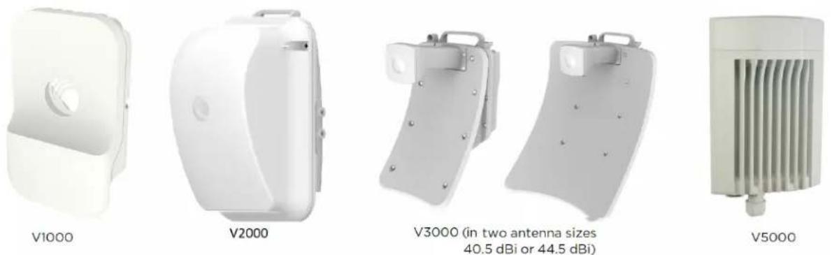
60 GHz cnWave consists of the following four variants (as shown in Figure 6):
- V1000 : A Client Node (CN) that contains a wide-range, 80 degrees beamforming for easy installation. This CN is powered by 802.3af PoE and supports up to 2 Gbps for PTP and PMP configurations.
- V2000: A CN that contains a 34.5 dBi antenna with beamforming. This client node can support up to 3.6 Gbps for PTP and PMP configurations.
- V3000: A Client Node (CN) is available in two sizes - 44.5 dBi high-gain antenna and 40.5 dBi lower gain antenna, both with beamforming. These client nodes can support up to 5.4 Gbps, with channel bonding for PTP configurations.
- V5000: A dual-sector Distribution Node (DN) that contains two sectors covering up to 280 degrees with beamforming. A single V5000 can connect up to four other distribution nodes or up to 30 client nodes. V5000 can be used for PTP, PMP, and Mesh configurations.
Figure 6:60 GHz cnWave products
Features
This section lists the features of each product of 60 GHz cnWave.
V1000 CN
• Supports modulations BPSK to 16 QAM (MCS1 to MCS12)
• Integrated antenna with beam forming
• 38 dBm EIRP
- Gigabit Ethernet
• 1 Gbps UL/1 Gbps DL throughput
- Powered by passive PoE or 802.3af/at PoE
IP66/67
V2000 CN
• Supports modulations BPSK to 16 QAM (MCS1 to MCS12)
• 34.5 dBi ultra-high gain antenna with beam forming, peak 49 dBm EIRP
• 2.5 Gigabit Ethernet Main interface
• 2.5 Gigabit Ethernet Auxiliary (Aux) interface
• 1.8 Gbps UL or 1.8 Gbps DL throughput
• 802.3at POE (2-pair or 4-pair for higher wattage) or a Passive PoE
• Supports Aux PoE out (802.3af/at PoE)
IP66/67
V3000 CN
• Supports modulations BPSK to 16 QAM (MCS1 to MCS12)
• 44.5 dBi ultra-high gain antenna with beam forming 60.5 dBm EIRP
• 40.5 dBi ultra-high gain antenna with beam forming 54.5 dBm EIRP
• 10 Gigabit Ethernet
• Supports 10G SFP+ or 1G SFP
• 1.8 Gbps UL/1.8 Gbps DL throughput
• CB2 2.7 Gbps UL / 2.7 Gbps DL
• Gigabit Ethernet Auxiliary Interface
• 802.3at POE (2-pair or 4-pair for higher wattage) or a Passive POE
• Supports Aux PoE out (802.3af/at PoE)
IP66/67
V5000 DN
• Supports modulations BPSK to 16QAM (MCS1 to MCS12)
- Dual sector - 280-degree antenna with beamforming
• 38 dBm EIRP
• 10 Gigabit Ethernet
• Supports 10G SFP or 1G SFP
• 1.8 Gbps UL/1.8 Gbps DL throughput per sector
• Gigabit Ethernet Auxiliary Interface
• 802.3at POE (2-pair or 4-pair for higher wattage) or a Passive POE
• Supports Aux PoE out (802.3af/at PoE)
IP 66/67
Wireless operation
This section describes how the 60 GHz cnWave is operated, including topology, modulation modes, power control, and security.
Wireless topology
60 GHz cnWave supports operation in three topologies:
- Point to point (PTP)
- Point to Multipoint (PMP)
- Mesh
PTP
The PTP topology provides a point-to-point link using V1000, V2000, and V3000.
Figure 7:PTP Topology

PMP
The PMP topology provides a point to multi-point where a V5000 acts as a PoP DN and V5000, V3000, V2000, V1000 act as Clients.
Figure 8:PMP Topology

Mesh
Mesh efficiently distributes capacity and improves availability, using Open/R based layer 3 IPv6 meshing. It allows for route diversity which provides high network availability and supports up to 15 hops away from a PoP node. Network bandwidth is reduced at each hop, and the total bandwidth available in the network is limited to a PoP node's network reappearance. Mesh is a distributed network application platform that determines appropriate routes between the mesh nodes.
Figure 9:Mesh topology

natural_image
Isometric architectural rendering of a city layout with buildings, roads, and green spaces (no text or symbols)Modulation
Following tables list modulation supported during L2 and L3 throughput:
Table 3: Modulation and coding rate for CB1
| MCS Modulation | Coding Rate L2 Throughput (Mb/s) | DMG-CB1 (2.16 GHz Channel) |
| 2 n/2 BPSK 1/2 572 | ||
| 3 n/2 BPSK 5/8 800 | ||
| 4 n/2 BPSK 3/4 914 | ||
| 6 n/2 QPSK 1/2 1256 | ||
| 7 n/2 QPSK 5/8 1600 | ||
| 8 n/2 QPSK 3/4 1828 | ||
| 9 n/2 QPSK 13/16 1942 | ||
| 10 n/2 16QAM 1/2 2400 | ||
| 11 n/2 16QAM 5/8 3200 | ||
| 12 n/2 16QAM 3/4 3656 |
Table 4: Modulation and coding rate for CB2
| MCS Modulation | Coding Rate L2 Throughput (Mb/s) | EDMG-CB2 (4.32 GHz Channel) | |
| 2 n/2 BPSK 1/2 | 1244 | ||
| 3 n/2 BPSK 5/8 | 1524 | ||
| 4 n/2 BPSK 3/4 | 1750 | ||
| 5 n/2 BPSK 13/16 | 1792 | ||
| 7 n/2 QPSK 1/2 | 2280 | ||
| 8 n/2 QPSK 5/8 | 2740 | ||
| 9 n/2 QPSK 3/4 | 3480 | ||
| 10 n/2 QPSK 13/1 | 63800 | ||
| 11 n/2 QPSK 7/8 | 4260 | ||
| 12 n/2 16QAM 1/2 | 5000 | ||
| 13 n/2 16QAM 5/8 | 5420 | ||
Link adaptation
Link adaptation is performed independently for each link for data traffic, and it is closed-loop based. Adjusting the Tx modulation and coding scheme from MCS2 to MCS12 selected for transmission. It is adjusted based on the following:
- Packet Error Ratio (PER),
• SNR,
- local measurements of successful and unsuccessful frame transmissions (for example, count of frames Acknowledged (ACKed) or Not ACKed).
Figure 10:Adjusting links

line
| Level | Value | |---|---| | MCS-2 | MCS-2 | | MCS-12 | MCS-12 | | MCS-9 idle | MCS-9 | | MCS-11 | MCS-11 | | MCS-9 idle | MCS-9 | | MCS-7 idle | MCS-7 | | idle | idle |Start from MCS2, adjust based on signal quality, when the session is idle, fall back to MCS-9 or any highest MCS achieved below MCS-9.
Synchronization
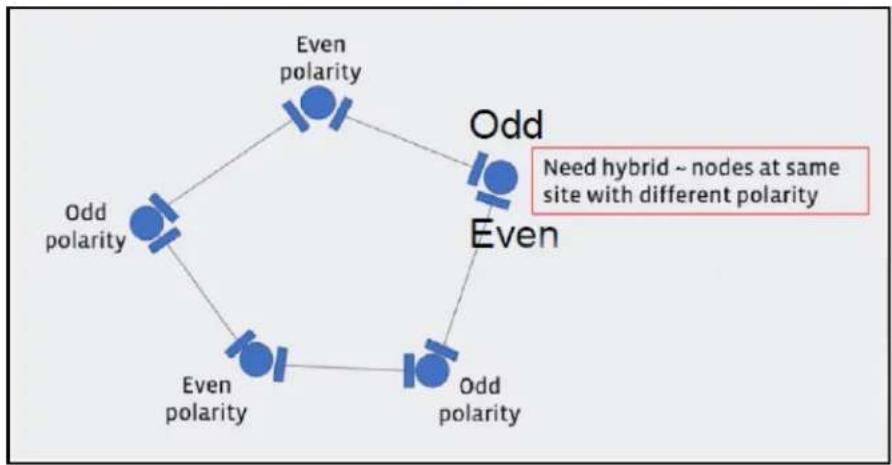
Synchronization is used to control the transmit and receive signals to prevent self-interference. Radios assigned with the same polarity will be transmitting and receiving at the same time. There are two types of polarities:
- Odd (if Odd nodes are Tx)
• Even (if Even nodes are Rx)
Figure 11:Odd and even polarities

flowchart
graph TD
    A["Odd"] --> B["Even"]
    B --> C["Odd"]
    C --> D["Even"]
    D --> E["Odd"]
    E --> F["Even"]
    F --> G["Odd"]
    G --> H["Even"]
    H --> I["Odd"]
    I --> J["Even"]
    J --> K["Odd"]
    K --> L["Even"]
    L --> M["Odd"]
    M --> N["Even"]
    N --> O["Odd"]
    O --> P["Even"]
    P --> Q["Odd"]
    Q --> R["Even"]
    R --> S["Odd"]
    S --> T["Even"]
    T --> U["Odd"]
    U --> V["Even"]
    V --> W["Odd"]
    W --> X["Even"]
    X --> Y["Odd"]
    Y --> Z["Even"]
    Z --> AA["Odd"]
    AA --> AB["Even"]
    AB --> AC["Odd"]
    AC --> AD["Even"]
    AD --> AE["Odd"]
    AE --> AF["Even"]
    AF --> AG["Odd"]
    AG --> AH["Even"]
    AH --> AI["Odd"]
    AI --> AJ["Even"]
    AJ --> AK["Odd"]
    AK --> AL["Even"]
    AL --> AM["Odd"]
    AM --> AN["Even"]
    AN --> AO["Odd"]
    AO --> AP["Even"]
    AP --> AQ["Odd"]
    AQ --> AR["Even"]
    AR --> AS["Odd"]
    AS --> AT["Even"]
    AT --> AU["Odd"]
    AU --> AV["Even"]
    AV --> AW["Odd"]
    AW --> AX["Even"]
    AX --> AY["Odd"]
    AY --> AZ["Even"]
    AZ --> BA["Odd"]
    BA --> BB["Even"]
    BB --> BC["Odd"]
    BC --> BD["Even"]
    BD --> BE["Odd"]
    BE --> BF["Even"]
    BF --> BG["Odd"]
    BG --> BH["Even"]
    BH --> BI["Odd"]
    BI --> BJ["Even"]
    BJ --> BK["Odd"]
    BK --> BL["Even"]
    BL --> BM["Odd"]
    BM --> BN["Even"]
    BN --> BO["Odd"]
    BO --> BP["Even"]
    BP --> BQ["Odd"]
    BQ --> BR["Even"]
    BR --> BS["Odd"]
    BS --> BT["Even"]
    BT --> BU["Odd"]
    BU --> BV["Even"]
    BV --> BW["Odd"]
    BW --> BX["Even"]
    BX --> BY["Odd"]
    BY --> BZ["Even"]
The MAC synchronizes its timers to an external, accurate time source, such as GPS or IEEE 1588. A timing pulse that resets the Timing Synchronization Function (TSF) on the DN is repeated once every second. This timing pulse occurs exactly at the turn of each second.
Figure 12:The MAC synchronization
flowchart
graph TD
    A["Odd"] --> B["Even"]
    B --> C["Odd polarity"]
    C --> D["Even polarity"]
    D --> E["Odd polarity"]
    E --> F["Odd polarity"]
    F --> G["Odd polarity"]
    G --> H["Odd polarity"]
    H --> I["Odd polarity"]
    I --> J["Odd polarity"]
    J --> K["Odd polarity"]
    K --> L["Odd polarity"]
    L --> M["Odd polarity"]
    M --> N["Odd polarity"]
    N --> O["Odd polarity"]
    O --> P["Odd polarity"]
    P --> Q["Odd polarity"]
    Q --> R["Odd polarity"]
    R --> S["Odd polarity"]
    S --> T["Odd polarity"]
    T --> U["Odd polarity"]
    U --> V["Odd polarity"]
    V --> W["Odd polarity"]
    W --> X["Odd polarity"]
    X --> Y["Odd polarity"]
    Y --> Z["Odd polarity"]
    Z --> AA["Odd polarity"]
    AA --> AB["Odd polarity"]
    AB --> AC["Odd polarity"]
    AC --> AD["Odd polarity"]
    AD --> AE["Odd polarity"]
    AE --> AF["Odd polarity"]
    AF --> AG["Odd polarity"]
    AG --> AH["Odd polarity"]
    AH --> AI["Odd polarity"]
    AI --> AJ["Odd polarity"]
    AJ --> AK["Odd polarity"]
    AK --> AL["Odd polarity"]
Time-division duplexing access mechanism
60 GHz cnWave uses a Time Division Duplex (TDD) channel access mechanism. All cnWave nodes are time-synchronized and this is achieved through internal GPS, IEEE 1588(roadmap), or Cambium Sync (roadmap), and each sector of a node is assigned specific times during which it can transmit or receive. A timing pulse that resets the Timing Synchronization Function (TSF) on the DN is repeated once every second (1PPS). This timing pulse occurs exactly at the turn of each second and Sub-Frames begins every 200 microseconds.
General operation of MAC layer
MAC is highly modified from that in IEEE 802.11-2016. Use TDD MAC by substituting TDD access for all other access. 60 GHz cnWave supports a fixed 50-50 up/down ratio.
60 GHz cnWave uses only the following frames:
- Data
• QoS-Null (frame does not carry any data) - Management Action (for example, beam-forming, and others.)
- Block ACK (used for sending an ACK to multiple nodes/packets at once)
- ACK
Frame types
Below are the types of frames in 60 GHz cnWave:
- Management frames - A node sends all management frames using the DMG control mode PHY, MCS 0.
- Control frames - A node sends the ACK frame using the DMG control mode PHY, MCS 0. A node sends the Block ACK frame using the DMG single carrier PHY, MCS 1.
- Data frames - A node sends data frames using MCS 2 through MCS 12 of the DMG single carrier PHY, as determined by the link adaptation algorithm.
Wireless encryption
60 GHz cnWave supports an optional encryption, for data transmitted over the wireless link, using the following options:
- Disabled wireless encryption (which is disabled).
- Pre-Shared Key (PSK) is set, where a pre-configured secret at both ends is configured. The derivation of shared secret is based on WPA2.
- With a configured Radius server IP, cnWave nodes do EAP-TLS using X.509 certificates.
Designing wireless networks
For designing wireless networks, refer to LINKPlanner.
TDD synchronization
V2000, V3000, and V5000 have built-in GPS receivers. The E2E Controller manages the TDD synchronization.
System management
This section introduces the 60 GHz cnWave management system, including the web interface, installation, configuration, alerts, and upgrades.
Management agent
The 60 GHz cnWave equipment is managed through an embedded management agent. Management workstations, network management systems, or PCs can be connected to this agent using a choice of in-band or out-of-band network management modes.
The management agent includes an IPv4/IPv6 interface at the management agent. The IP interface operates in the following modes:
- IPv4 only
- IPv6 only
- Dual IPv4/IPv6
Network management
cnMaestro is a Cambium Network Management System (NMS). This is a single plane to manage the complete Cambium product portfolio. It uses secure WebSocket for management traffic to manage all Cambium products on the same system. Configurations can be pushed from the cnMaestro through the E2E Controller to the end devices.
cnMaestro NMS is used to:
- Manage cnWave network including E2E, CN, and DN.
• Show the connection topologies. - Collect KPIs/statistics, alarms, logs (via the E2E device agent).
• Perform software upgrade.
IPv6
IPv6 address is 128 bits (16 Bytes) address. The subnet ID in IPv4 is called a prefix in IPv6. In IPv6, Neighbor Discovery Protocol (NDP) is used with ICMPv6 to resolve the MAC address. IPv6 does not have broadcast but only has multicast.
60 GHz cnWave products get assigned with a unique IP in mesh, either from Controller (CPA) or PoP (DPA), known as loopback address (Io). In Layer 3 mode, nodes can also send Router Advertisement(RA) for all its downstream devices to acquire an IPv6 address. Prefix for RA can either be configured or device from Io.
System logging
For information on logging into the system using user interface (UI), refer to Logging into the web interface.
Software upgrade
Refer to Software upgrade for more information.
This topic provides information about the hardware of 60 GHz cnWave.
Wireless nodes
The 60 GHz cnWave solution includes three types of wireless nodes:
• V1000 Client Node
• V2000 Client Node
• V3000 (44.5 dBi and 40.5 dBi) Client Node
• V5000 Distribution Node
V1000 Client Node (CN)
V1000 is an outdoor CN that can be connected to a distribution node wirelessly. V1000 supports a Gigabit Ethernet interface and is powered by 802.3af/at PoE compliant power supply or a passive PoE.
Figure 13:V1000 CN's front and rear views

natural_image
White plastic electronic device with a rectangular body and a small protruding port, shown against a black background (no text or symbols visible)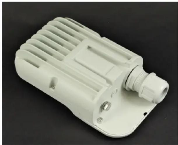
natural_image
White plastic industrial component with ribbed structure and threaded port (no text or symbols visible)V1000 CN - Part numbers
Order the V1000 CN from Cambium Networks (as listed in Table 5). Each V1000 CN is supplied with a mounting bracket for wall mount or pole mount, and an indoor power supply.
Table 5: V1000 CN part numbers
| Product description Part number | |
| 60GHz cnWave V1000 Client Node with US cord C600500C001B | |
| 60GHz cnWave V1000 Client Node with EU cord C600500C003B | |
| 60GHz cnWave V1000 Client Node with UK Cord C600500C004B | |
| 60GHz cnWave V1000 Client Node with ANZ Cord C600500C008B | |
| 60GHz cnWave V1000 Client Node with Brazil Cord C600500C009B | |
| 60GHz cnWave V1000 Client Node with Argentina Cord C600500C010B | |
| 60GHz cnWave V1000 Client Node with China Cord C600500C011B | |
| 60GHz cnWave V1000 Client Node with South Africa Cord C600500C012B | |
| 60GHz cnWave V1000 Client Node with India Cord C600500C013B | |
| 60GHz cnWave V1000 Client Node with no Cord C600500C014B | |
| 60GHz cnWave V1000 Client Node with Israel cord - for Israel Only C600500C016B | |
| 60GHz cnWave V1000 Client Node with no Cord and no Power supply C600500C017B |
V2000 Client Node (CN)
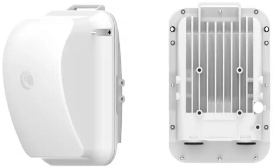
V2000 is an outdoor CN that can be connected to a DN. This CN can also act as a DN for PTP deployments. It supports a 2.5 Gigabit Ethernet Main interface and 2.5 Gigabit Ethernet Auxiliary (Aux) interface. The V2000 CN can support a single wireless link and therefore, it can be used as a CN in all topologies or POP in a PTP topology.
A V2000 CN can be powered using 30W passive POE or using 802.3at compliant POE switch. For more information about the supported power supply and cable lengths, refer to the Power supply units (PSU) section. A V2000 CN can also power 802.3af/at compliant auxiliary device through the Aux Ethernet interface. For more information about Aux PoE interface, refer to the Aux PoE - Powering options section.
Figure 14:V2000 CN's front and rear views
natural_image
Two views of a white electronic device casing, one showing internal structure and the other showing internal components (no text or symbols visible)V2000 CN - Part numbers
Order the V2000 CN from Cambium Networks (as listed in Table 6). A V2000 CN radio is supplied without a mounting bracket and with or without power supply.
Table 6: V2000 CN part numbers
| Product description Part number | |
| 60GHz cnWave V2000 Client Node 30W with Israel Cord C600500C026B | |
| 60GHz cnWave V2000 Client Node 30W with South Africa Cord C600500C027B | |
| 60GHz cnWave V2000 Client Node 30W with India Cord C600500C028B | |
| 60GHz cnWave V2000 Client Node 30W with no Cord C600500C029B | |
| 60GHz cnWave V2000 Client Node no power supply, no power cord C600500C030B | |
| 60GHz cnWave V2000 Client Node 30W with US cord C600500C020B | |
| 60GHz cnWave V2000 Client Node 30W with EU cord C600500C031B | |
| 60GHz cnWave V2000 Client Node 30W with UK Cord C600500C032B | |
| 60GHz cnWave V2000 Client Node 30W with ANZ Cord C600500C033B | |
| 60GHz cnWave V2000 Client Node 30W with Brazil Cord C600500C034B | |
| 60GHz cnWave V2000 Client Node 30W with Argentina Cord C600500C035B |
V3000 Client Node (CN)
V3000 is an outdoor CN that can be connected (wireless) to a DN or another V3000 DN. V3000 supports a 10 Gigabit Ethernet interface, a 10G SFP+ interface port, and a Gigabit Ethernet Aux interface.
V3000 can be powered using 60W passive POE or using an AC/DC PSU through a mini adapter (for more information, refer to the power supply and cable lengths supported in the Power supply units section). V3000 DN can also power 802.3af/at compliant auxiliary device through the Gigabit Aux interface.
For more information about Aux PoE interface, refer to the Aux PoE - Powering options section.
Figure 15: V3000 Client Node without antenna assembly and with 44.5 dBi and 40.5 dBi antenna assemblies

natural_image
White plastic mechanical component with a handle and mounting base (no visible text or symbols)
natural_image
White plastic clipboard with a clip and screw holes, no visible text or symbols
natural_image
Exterior view of a gray mechanical device with mounting holes and a handle (no text or symbols visible)V3000 Part numbers
Order the V3000 CN from Cambium Networks (V3000 CN part numbers). The V3000 CN radio is supplied without an antenna assembly, bracket, or power supply. Refer to the Precision brackets section for details of suitable brackets.
Table 7: V3000 CN part numbers
| Cambium description Cambium part number | |
| 60 GHz cnWave V3000 CN radio only C600500C024B | |
| 60 GHz cnWave V3000 CN antenna assembly, 44.5 dBi C600500D001B | |
| 60 GHz cnWave V3000 CN antenna assembly, 40.5 dBi, 4 Pack C600500D002B | |
| 60 GHz cnWave V3000 CN antenna assembly, 44.5 dBi, 4 Pack C600500D003B | |
| 60 GHz cnWave V3000 CN Radio only - Israel Only C600500C025B |
V5000 Distribution Node (DN)
V5000 is an outdoor DN that can be connected to multiple V1000 or V3000 CNs wirelessly. V5000 supports a 10 Gigabit Ethernet interface, a 10G SFP+ interface port, and a Gigabit Ethernet Aux interface.
V5000 can be powered using 60W passive POE or using an AC/DC PSU through mini an adapter (for more information, refer to the power supply and cable lengths supported in the Power supply units section). V5000 DN can also power 802.3af/at compliant auxiliary device through the Gigabit Aux interface.
For more information about Aux PoE interface, refer to the Aux PoE - Powering options section.
Figure 16:V5000 Distribution Node front and rear views

natural_image
White industrial heat exchanger component with cooling fins and connectors (no text or symbols visible)
natural_image
White plastic heat exchanger housing with ribbed internal structure and mounting holes (no text or symbols visible)V5000 Part numbers
Order the V5000 Distribution Node (DN) from Cambium Networks (as shown in below table). The V5000 DN is supplied without a mounting bracket or power supply.
Table 8: V5000 DN part numbers
| Cambium description Cambium part number | |
| 60GHz cnWave V5000 Distribution Node C600500A004B | |
| 60GHz cnWave V5000 Distribution Node - Israel Only C600500A005B |
Radio mounting brackets
V1000 Wall and pole mount
The V1000 CN is supplied with a mounting plate and a band clamp. The mounting plate can be used for mounting the V1000 on a wall, or it can be used with the supplied band clamp to mount the V1000 on a pole with a diameter in the range of 25 mm to 70 mm (1 inch to 2.75 inches). Note that the larger diameters can be accommodated with the customer supplied clamps.
Figure 17: V1000 mounting plate and band clamp

natural_image
Two white plastic mechanical components: a bracket with mounting holes and a coiled hose with a metal clip, against a black background (no text or symbols visible)V1000 Adjustable pole mount (N000900L022A)
The adjustable pole mount is used to provide elevation adjustment when a V1000 CN is mounted on a pole. The adjustable pole mount works with poles with diameters in the range of 25 mm to 70 mm (1 inch to 2.75 inches).

Note
The adjustable pole mount does not come with a clamp. You can use the one that is supplied with the V1000 box. Larger diameter poles can be accommodated with the customer supplied clamps.
Figure 18: V1000 adjustable pole mount

natural_image
Three views of a white plastic mechanical assembly: front, side, and side (no text or symbols visible)V2000 Adjustable pole mount
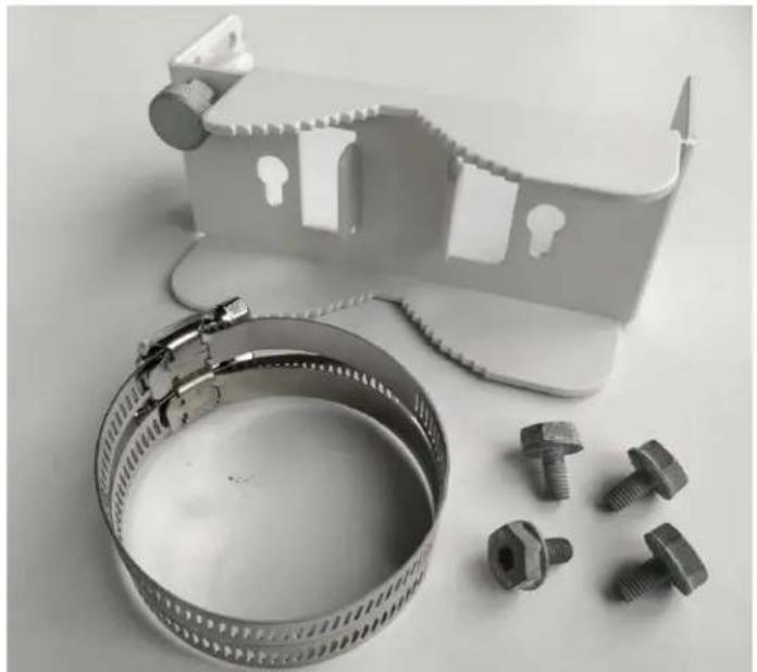
The V2000 CN is supplied with adjustable pole mounting accessories such as mounting plate, a hose clamp, and four screws (as shown in Figure 19). These mounting accessories can be used to mount the V2000 CN on a vertical pole.
Figure 19:V2000 and pole mounting accessories
natural_image
Black-and-white photo of a mechanical clamp assembly with bolts and a plastic housing (no text or symbols visible)
natural_image
White plastic medical device with a small attached device labeled 'EFT20' (no visible text or symbols on the device itself)The adjustable pole mount bracket (as shown in Figure 20) is used to mount the V2000 CN on a vertical pole with a diameter in the range of 25mm to 70mm (1 inch to 2.75 inches). The bracket provides a fine adjustment of up to +/-20irc in elevation for accurate alignment of V2000.
Figure 20:V2000 Adjustable pole mount

natural_image
Two white industrial sensors mounted on vertical metal posts, showing mounting brackets and wiring (no text or symbols visible)V3000 Precision bracket (C000000L125A)
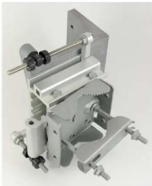
The precision bracket (as shown in Figure 21) is used to mount the V3000 CN on a vertical pole with a diameter in the range of 25 mm to 70 mm (1 inch to 2.75 inches). It accepts band clamps for larger diameter poles.
The precision bracket provides fine adjustment of up to 18irc in azimuth and +/-30irc in elevation for accurate alignment of the V3000.
Figure 21: Precision bracket
natural_image
Mechanical clamp assembly with metallic frame and multiple levers (no visible text or symbols)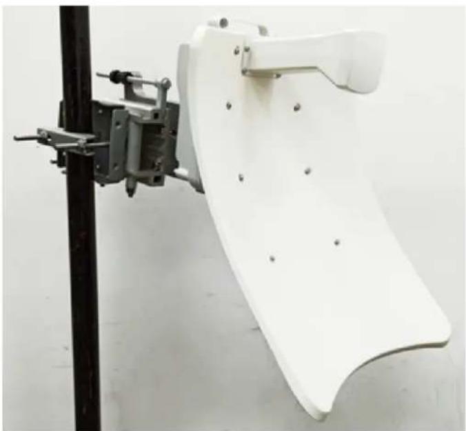
natural_image
White ergonomic chair with black frame and metal clamping bracket, mounted on a pole (no text or symbols visible)Figure 22: Precision bracket components

natural_image
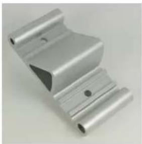
3D rendering of a gray metal enclosure with mounting holes and internal compartments (no text or symbols)Bracket body
natural_image
Metallic mechanical component with ribbed structure and mounting holes (no text or symbols visible)Azimuth arm

natural_image
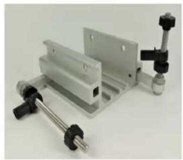
Assorted metal bolts and hex nuts on a plain background (no text or symbols visible)Long (120 mm) M8 screws and flange nuts
natural_image
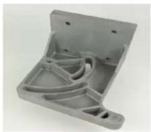
Mechanical assembly with metallic frame and clamping tool (no visible text or symbols)Bracket base

natural_image
Assorted metal bolts and washers on a plain surface (no text or symbols visible)40 mm M8 screws, plain washers, and Nyloc nuts
natural_image
Metallic plastic housing component with internal channels and mounting holes (no text or symbols visible)V3000 mount
natural_image
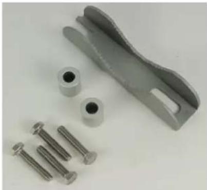
Close-up of metallic mechanical components including a clip, cylindrical parts, and screws (no text or symbols visible)28 mm M6 screws, M8 spacers, and pole mount clamp
V3000 Tilt bracket (N000045L002A)
The tilt bracket (as shown in Figure 23) is used to provide elevation adjustment when a V3000 CN or V5000 DN is mounted on a pole. The tilt bracket works with poles with diameters in the range of 25 mm to 70 mm (1 inch to 2.75 inches).
The tilt bracket assembly may be used with third-party band clamps to mount the ODU on a larger pole (the diameter range depends on the clamps used).
Figure 23:Tilt bracket assembly

natural_image
Three-panel image showing metal automotive components: a bracket, plastic housing with bolts, and a mechanical clamp assembly (no text or symbols visible)V5000 Pole mount (C000000L137A)
The pole mount (as shown in Figure 24) is used to mount a V5000 DN on a vertical pole with a diameter in the range of 25 mm to 70 mm (1 inch to 2.75 inches. It provides coarse azimuth (but not elevation) adjustment. Band clamps can be used for V5000 pole mount to accommodate the larger diameter poles.
Figure 24:Pole mount

natural_image
Three-panel image showing metal hardware components: a bracket with screws, a close-up of a vertical lock, and a multi-plate assembly (no visible text or symbols)V5000 Wall mount (C000000L136A)
The wall mount (Wall mount figure below) is used to mount a V5000 DN on a vertical wall. It does not provide azimuth or elevation adjustment. The wall mount requires additional fixing hardware suitable for the type of wall.
Figure 25: Wall mount

natural_image
Metal bracket housing with multiple screws and a separate metal plate, accompanied by small bolts (no text or symbols visible)
natural_image
Close-up of a white mechanical hinge or latch component with metallic contacts and mounting holes (no visible text or symbols)Bracket part numbers
Order mounting brackets by using the Cambium part numbers listed in below table.
Table 9: Radio mounting bracket part numbers
| Bracket Radio nodes Cambium Part Number | ||
| Adjustable pole mount V1000 N000900L022A | ||
| Tilt bracket assembly V3000 N000045L002A | ||
| Wall mount bracket V5000 C000000L136A | ||
| Pole mount bracket V5000 C000000L137A | ||
| Precision bracket V3000 C000000L125A |
Radio accessories
Telescope mounting kit for precision brackets
The Precision bracket and an alignment telescope provide the most accurate option for aligning the radio during installation. The telescope is temporarily mounted on the bracket using the telescope mounting kit for precision brackets.
The telescope mounting kit consists of a mounting plate, a knurled screw, and two rubber O-rings.
Order the telescope mounting kit from Cambium Networks.
Figure 26: Telescope mounting kit
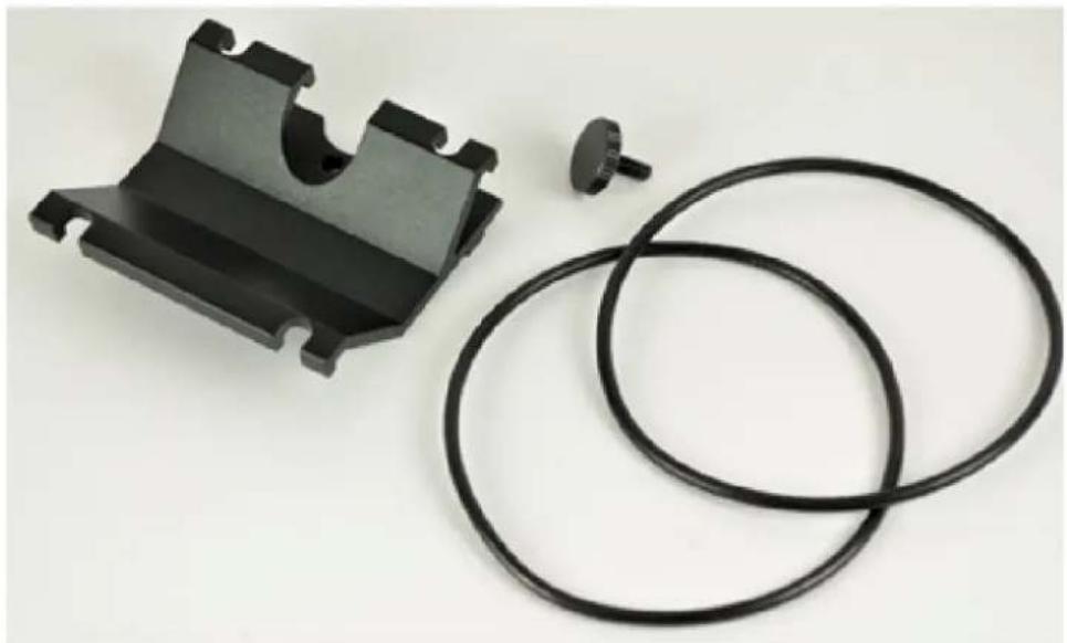
natural_image
Black plastic mechanical component with two coiled black rings, no text or symbols visibleOrder a suitable telescope from a specialist supplier specifying the following details:
Right angle, erecting, 9x50 mm alignment scope with 5° field of view
Figure 27: Typical alignment telescope

natural_image
Close-up of a black mechanical component with cylindrical shaft and protruding port (no visible text or symbols)Alignment Tube
The Alignment tube (as shown in Figure 28) is designed to be used with V3000 when setting up a Point-to-Point link. It is Ideal for aligning a Point-to-Point link that spans up to 600 m.
Figure 28: Alignment Tube

natural_image
Close-up of a metallic dental or prosthetic tool with a conical tip and flared shaft (no visible text or symbols)For longer links up to 3 km, Cambium Networks suggests using the telescopic mounting kit (C000000L139) and a finder scope.

Note
For details on how to fit the Alignment tube for V3000, refer to Fixing the alignment tube.
Radio accessory part numbers
Order radio accessories using the Cambium Part Number in the Radio accessory part numbers table below.
Table 10: Radio accessory part numbers
| Accessory Radio nodes Cambium Part Number | ||
| Telescope mounting kit V3000 C000000L139A | ||
| Alignment Tube V3000 C000000L190A | ||
| Radome for 44.5 dBi antenna V3000 C600500D004A |

Note
For more information on the radome for a V3000 44.5 dBi antenna, refer to the 60 GHz cnWave Quick Start Guide.
Radio external interfaces
V1000 CN
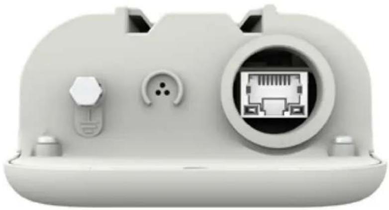
Figure 29: External interfaces for V1000 CN
natural_image
3D rendered image of a gray device casing with internal components and a central connector (no text or symbols visible)Table 11: External interfaces V1000 CN
| Port name Connector Interface Description | |||
| PSU RJ45 PoE | input Standard 802.3af/at PoE | ||
| 100/1000 BASE-T Ethernet Data and management | |||
V2000 CN
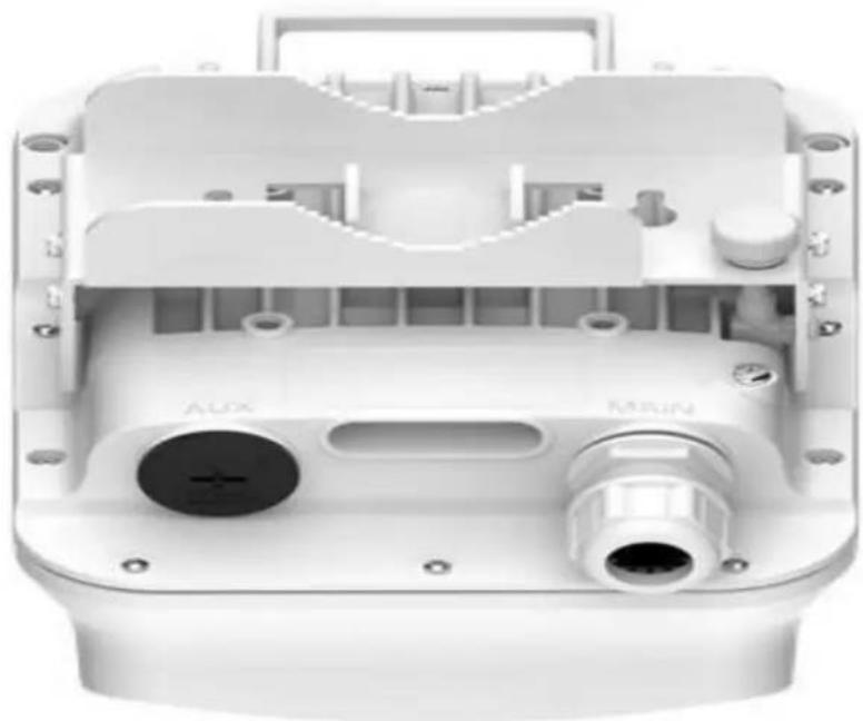
Figure 30: External interfaces for V2000 CN
natural_image
Cross-sectional view of a white industrial device casing with labeled ports (no readable text or symbols)Table 12: External interfaces - V2000 CN
| Port name | Connector Interface Description | |
| PSU RJ45 POE Input | Passive PoE or 802.3at (two pairs or four pairs for higher wattage) | |
| 100m/1000m/2.5G BASE-T Ethernet | Data and management | |
| AUX RJ45 POE Output | IEEE 802.3af/at compliant, higher wattage supported (For more information, refer to theAux PoE - Powering optionssection.) | |
| 100m/1000m/2.5G BASE-T Ethernet | Data and management | |
V3000 CN
Figure 31: External interfaces for V3000 CN

Table 13: External interfaces V3000 CN
| Port name | Connector Interface Description | ||
| SFP+ S | FP 10G BASE | -SR/10G BASE-LR/1GBase-SX using optional SFP+/SFP optical or copper moduleSFP-1G-SX / SFP-1G-LX using optional SFP optical or copper module | Data and management |
| PSU RJ | 45 PoE input | Passive PoE or 802.3at (two pairs or four pairs for higher wattage) | |
| 100m/1000m/2.5G BASE-T/5GBASE-T/ 10G BASE-T Ethernet | Data and management | ||
| Port name | Connector Interface Description | |
| AUX RJ45 PoE output | IEEE 802.3af/at compliant, higher | wattage supportedfor specific cases (For more information, refer toAux PoE - Powering optionssection.) |
| 100/1000 BASE-T Ethernet Data | and management |
V5000 DN
Figure 32: External interfaces for V5000 DN

Table 14: External interfaces V5000 DN
| Port name | Connector Interface Description | |
| SFP+ SFP 10G BASE | -SR/10G BASE-LR/1GBase-SX using optional SFP+/SFP optical or copper moduleSFP-1G-SX / SFP-1G-LX using optional SFP optical or copper module | Data and management |
| PSU RJ45 PoE input | Passive PoE or 802.3at (two pairs or four pairs for higher wattage) | |
| 100m/1000m/2.5G BASE-T/5GBASE-T/ 10G BASE-T Ethernet | Data and management | |
| AUX RJ45 PoE output | IEEE 802.3af/at compliant, higher wattage supported for specific cases (For more information, refer to Aux PoE - Powering options section.) | |
| 100/1000 BASE-T Ethernet Data and management | ||
Radio specifications
The 60 GHz cnWave Radios conform to the specifications listed in Radio node specifications.
Table 15: Radio node specifications
| Category Specification | ||
| Dimensions V1000 Client | nt Node 169 mm × 100 mm × 54 | mm (6.6 in × 3.9 in × 2.1 in) |
| V2000 Client Node 250 mm × 16 | mm × 220 mm (9.8 in × 6.5 in × 8.6 in) | |
| V3000 Client Node (44.5 dBi)V3000 Client Node (40.5 dBi) | 421 mm × 347 mm × 349 mm (16.5 in × 13.6 in × 13.7 in)343 mm × 198 mm × 251 mm (13.5 in × 7.7 in) | |
| V5000 Distribution Node 280 mm | × 186 mm × 103 mm (11.0 in × 7.3 in × 4.0 in) | |
| Weight V1000 Client N | Node 0.46 kg (1.01 lbs) | |
| V2000 Client Node 1.9 kg (4.18 lbs) | ||
| V3000 Client Node (44.5 dBi) 4.17 | kg (9.1 lbs) including big antenna dish6.12 kg (13.4 lbs) = radio with dish + precision bracket | |
| V3000 Client Node (40.5 dBi) 3.2 | kg (7.05 lbs) including small antenna dish5.15 kg (11.3 lbs) = radio with dish + precision bracket | |
| V5000 Distribution Node 3.12 kg | (6.8 lbs) including antenna dish3.76 kg (8.2 lbs) = radio with dish + universal pole bracket | |
| Temperature -40°C (-40°F) to +60°C (140°F) | ||
| Wind survival 200 kph | (124 mph) maximum | |
| Humidity 100% condensing | ||
| Liquid and particle ingress | IP66, IP67 | |
| Power consumption | V1000 Client Node 10 W | |
| V2000 Client Node 20 W without | PoE and up to 60 W with PoE Out enabled | |
| V3000 Client Node 30 W, up to | 60 W with PoE Out enabled | |
| V5000 Distribution Node 35 W, up | to 65 W with PoE Out enabled | |
| Power input interface V | V1000 Client Node IEEE 802.3af | |
| V2000 Client Node Passive PoE or 802.3at (two pairs or four pairs for higher wattage) | ||
| V3000 Client Node Passive PoE or 802.3at (two pairs or four pairs for higher wattage) | ||
| V5000 Distribution Node Passive PoE or 802.3at (two pairs or four pairs for higher wattage) | ||
| Power output interface | V2000 Client Node IEEE 802.3af/at, 30 W maximum | |
| V3000 Client Node IEEE802.3af/at, 25 W maximum | ||
| V5000 Distribution Node IEEE 802.3af/at, 25 W maximum | ||
Power supply units (PSU)
PSU Options
Order PSUs from Cambium Networks. The power supply component and the part numbers are described in the following table.
Table 16: Power supply component part numbers
| Product description Radio node Cambium part | number | |
| Outdoor AC/DC PSU, 100W, 54V DC V3000 and V5000 N000000L179B | ||
| Waterproof PSU Cable Joiner 14-16 AWG | V3000 and V5000 N000000L180A | |
| DC to RJ45 Plug Power Adaptor | V3000 and V5000 C000000L184A | |
| Cable Gland, Long, M25, Qty 5 | V3000 and V5000 C000000L124A | |
| PoE, 60W, 56V, 5GbE DC Injector, Indoor, Energy Level 6 Supply | V2000, V3000N000000L142Aand V5000 | |
| PoE, 60W, 56V, 10GbE DC Injector, Indoor, Energy Level 6 Supply | V2000, V3000N000000L141Aand V5000 | |
| PoE, 30W, 56V, 5GbE DC Injector, Indoor, Energy Level 6 Supply | V1000 and V2000 N000000L034B | |
| PoE Gigabit DC Injector, 15W Output at 56V, Energy Level 6, 0C to 50C | V1000 | N000900L017AN000900L017B(main PoE) |
| AC power Injector 56V, 60W | V3000 and V5000 N000065L001C | |
| CABLE, UL POWER SUPPLY CORD SET, 720mm, AUS/NZ | V1000, V2000N000900L011AV3000, andV5000 | |
| CABLE, UL POWER SUPPLY CORD SET, INDIA | V1000, V2000N000900L012AV3000, andV5000 | |
| CABLE, UL POWER SUPPLY CORD SET, ARGENTINA V1000, V2000, V3000, and V5000 | N000900L013A | |
| CABLE, UL POWER SUPPLY CORD SET, CHINA V1000, V2000, V3000, and V5000 | N000900L015A | |
| CABLE, UL POWER SUPPLY CORD SET, 720mm, US V1000, V2000, V3000, and V5000 | N000900L031A | |
| CABLE, UL POWER SUPPLY CORD SET, 720mm, EU V1000, V2000, V3000, and V5000 | N000900L032A | |
| CABLE, UL POWER SUPPLY CORD SET, 720mm, UK V1000, V2000, V3000, and V5000 | N000900L033A | |
| CABLE, UL POWER SUPPLY CORD SET, 720mm, Brazil V1000, V2000, V3000, and V5000 | N000900L034A | |
| CABLE, UL POWER SUPPLY CORD SET, 720mm, Israel V1000, V2000, V3000, and V5000 | N000900L037A | |
Refer to Maximum cable lengths for details of the maximum cable lengths and the maximum PoE output power for different powering options.
V1000 - Power over Ethernet (PoE)
The V1000 CN is always powered using Power over Ethernet (PoE) at a nominal 56V, as shown in the PoE power supply to V1000 figure using the Gigabit power injector supplied with the radio, or using an IEEE 802.3af PoE output from an Ethernet switch.
Figure 33: PoE power supply to V1000

natural_image
Three black electronic devices with network ports and connectors, shown from different angles (no visible text or symbols on the devices themselves)Table 17: PoE, 15W 56V, 1 Gigabit DC injector
| Category Specification | |
| Dimensions 118 mm (4.64 in) x 43 mm (1.69 in) x 32.4 mm (1.27 in) | |
| Weight 0.18 Kg (0.39 lbs) | |
| Temperature 0°C (32°F) to | +50°C (140°F) |
| Humidity 10% to 95 % non-condensing | |
| AC Input 90-264V AC, 47-63 Hz | |
| DC Output Voltage 56V | |
| DC Output current 0.25A | |
| Efficiency Better than 84% | at full load |
| Over Current Protection Hiccup mode, recovers automatically after the fault condition is removed | |
| Hold up time At least 10 milliseconds | |
| RJ45 POE Port 7,8 ---- DC V-5,6 ---- DC V+ | |

Note
The Gigabit power injector is supplied with the cnWave V1000 CN. Order part N000900L017B to obtain spares.

Warning
Always use an appropriately rated and approved AC supply cord-set in accordance with the regulations of the country of use.
V2000 - PoE
The V2000 CN is always powered using POE at a nominal 56V using 5GbE POE Injector, which is optional (Cambium part number: N000000L034B), or using an IEEE 802.3at POE output from an Ethernet Switch.
Figure 34: PoE power supply to V2000
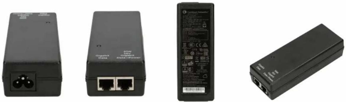
Figure 35: Power supply to V1000 or V2000

flowchart
graph TD
    A["cnWave V1000/V2000"] --> B["LPU at the top of the pole"]
    A --> C["LPU at the base of the pole"]
    B --> D["LPD-CDU Power Cable < 600 mm (24 inches)"]
    C --> E["Power Cable"]
    D --> F["POE Power Injector"]
    E --> G["PoE + Data"]
    F --> H["LAN Cable"]
    G --> I["LPU-PSU Power Cable"]
Table 18: PoE, 30W 56V, 5GbE DC injector (N000000L034B)
| Category Specification | |
| Dimensions 140 mm (5.5 in) x 53 mm (2.08 in) x 35 mm (1.37 in) | |
| Weight 0.24 Kg (0.5 lbs) | |
| Temperature 0°C (32°F) to | +50°C (140°F) |
| Humidity 10% to 95 % non-condensing | |
| AC Input 90-264 V AC, 47-63 Hz | |
| DC Output voltage 56V | |
| DC Output current 0.54 A | |
| Efficiency Better than 88% | at full load |
| Over Current Protection Hiccup mode, recovers automatically after the fault condition is removed | |
| Hold up time At least 10 milliseconds | |
| RJ45 POE Port 1,2,7,8 ---- DC V-3,4,5,6 ---- DC V+ | |
V3000/V5000 - PoE
The V3000 CN and V5000 DN can be powered using DC power at a nominal 54V, using 14 AWG or 16 AWG cable, as shown in the DC power supply to V3000 or V5000 figure.
Figure 36: PoE power supply to V3000 or V5000
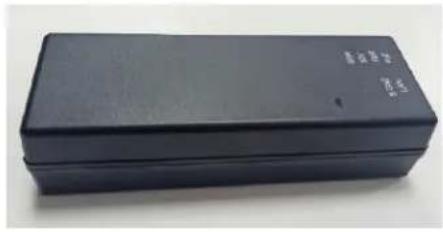
natural_image
Black rectangular electronic device with printed labels (no visible text or symbols on body)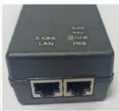

natural_image
Black rectangular electronic device with three-pin socket (no visible text or symbols)Figure 37:10 GbE PoE (C000000L141A)


Table 19: PoE, 60W, 56V, 10 GbE DC injector (C000000L141A)
| Category Specification | |
| Dimensions 140 mm (5.5 in) x 53 mm (2.08 in) x 35 mm (1.37 in) | |
| Weight 0.24 Kg (0.5 lbs) | |
| Temperature 0°C (32°F) to | +50°C (140°F) |
| Humidity 10% to 95 % non-condensing | |
| AC Input 90-264 V AC, 47-63 Hz | |
| DC Output voltage 56V | |
| DC Output current 1.07 A | |
| Efficiency Better than 88% | at full load |
| Over Current Protection Hiccup mode, recovers automatically after the fault condition is removed | |
| Hold up time At least 10 milliseconds | |
| RJ45 POE Port 1,2,7,8 ---- DC V-3,4,5,6 ---- DC V+ | |
V3000/V5000 - Outdoor AC/DC power supply unit
Figure 38: DC power supply to V3000 or V5000
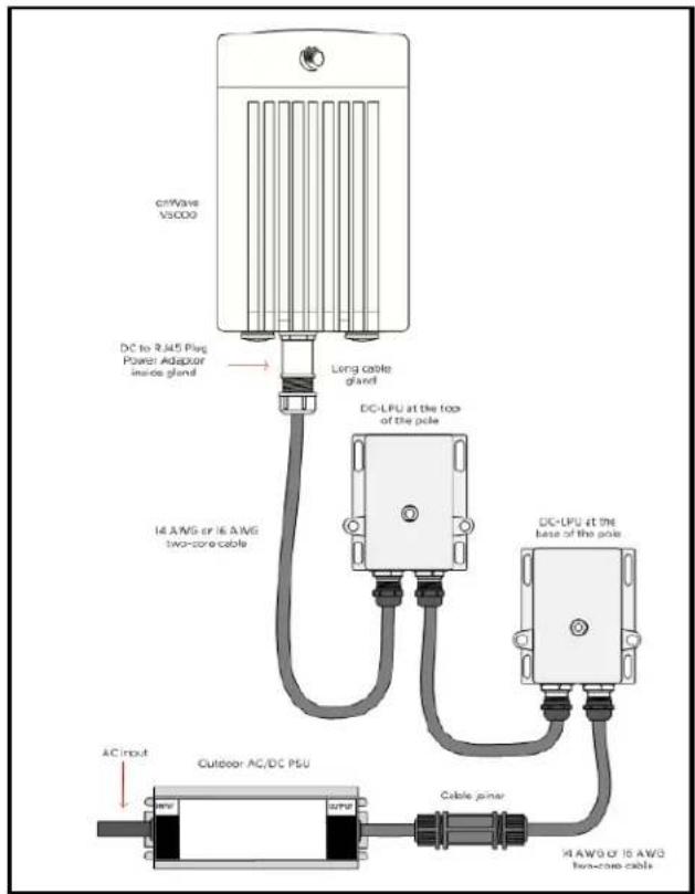
The outdoor PSU can be installed indoors, in an outdoor cabinet, or inside street furniture.
Figure 39: Outdoor AC/DC PSU, 100 W, 54V DC (N000000L179B)
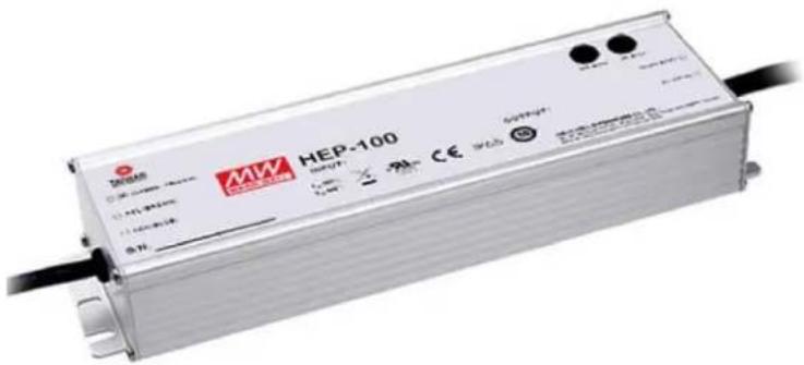
Table 20: Outdoor AC/DC PSU, 54V DC
| Category PSU Specification | ||
| Part number and dimensions | N000000L179B (100W) 220 mm (8.7 in) x 68 mm (2.7 in) x 39 mm (1.5 in) | |
| Power 100W | ||
| Temperature -40°C (-40°F) to +60°C (140°F) | ||
| Humidity 20 to 95 % non-condensing | ||
| Waterproofing IP65/IP67 | ||
| AC Input 90-305 V AC, 47-53 Hz | ||
| DC Output Voltage 54V | ||
| DC Output current 60W | 1.15 A | |
| 100W | 1.77 A | |
| Efficiency | Better than 90% at full load | |
| Over Current Protection | Hiccup mode, recovers automatically after the fault condition is removed | |
| Hold up time | At least 16 milliseconds | |
| Power factor | Better than 0.95 | |
Figure 40:Cable joiner
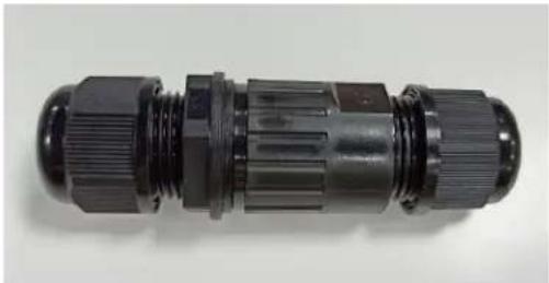
natural_image
Close-up of a black plastic electrical connector with threaded ends and mounting flanges (no visible text or symbols)Figure 41:DC to RJ45 plug power adapter

natural_image
Two black connectors with blue terminal blocks and green circuit board, shown from different angles (no text or symbols visible)Cable joiners and DC to RJ45 cable adapters are used to connect to outdoor AC/DC PSU. Refer to Maximum cable lengths for details of the maximum cable lengths and the maximum PoE output power for different powering options.

Note
If you are using the mini RJ45 power adapter, you must use the cable gland (C000000L123A) to ensure that the cable is protected. This cable gland comes in the radio box. For more details about the cable gland, refer to Table 28.
If the cable is <= 6 mm, you must use the gland (C000000L176A).
Aux PoE - Powering options
V2000, V3000, and V5000 devices support 802.3at compliant Aux POE output, using which these devices can power each other. This section lists and describes the supported cable lengths and maximum power available on the Aux port of these devices.
Table 21 provides details of the power consumption of the devices without Aux PoE enabled.
Table 21: Power consumption without Aux PoE enabled
| ODU In typical cases In | maximum (worst) case | |
| V2000 20W 22W | ||
| V3000 24W 27W | ||
| V5000 28W 32W |
The Aux PoE output power depends on:
• Voltage of the PoE injector used to power on the main ODU and
• Cable length from the PoE injector to the main ODU.
Table 22 lists the different PoE injector voltages used and the Aux power output available for the various ODUs.
Table 22: Aux power output for the different ODUs
| ODU ODU PoE | voltage Minimum Aux power available ODU PoE Voltage Maximum | Aux power available | ||
| V2000 48 30W | 56 36W | |||
| V3000 48 25W | 56 30W | |||
| V5000 48 25W | 56 30W | |||
Table 23 provides information of cable lengths of main PSU and Aux PoE for powering each ODU with other devices.
Table 23: Details of cable lengths of main PSU and Aux PoE - powering
| ODU Aux Device | Main PSU cable length (Max) | Aux PoE cable length (Max) | Feasible (Yes/No) | |
| Using V2000 and powering V2000/V3000/V5000: | ||||
| V2000 V2000 0m to 100m | 0m to 100m | Yes | ||
| V3000 0m to 100m | 0m to 100m | Yes | ||
| V5000 0m to 100m | 0m to 100m | Yes | ||
| Using V3000 and powering V2000/V3000/V5000: | ||||
| V3000 V2000 100m | 100m | Yes | ||
| V3000 100m | 100m | Yes | ||
| V5000 100m | 100m | Yes only | when 56V PoE is used | |
| Using V5000 and powering V2000/V3000/V5000: | ||||
| V5000 V2000 100m | 100m | Yes | ||
| V3000 100m | 100m | Yes | ||
| V5000 100m | 100m | Yes only | ||
Table 24 lists the possible and feasible combinations of devices (V1000, V2000, V3000, V5000) and power injectors.
Table 24: Possible combinations of devices, voltage, and PoE injector
| ODU/Aux device | V1000 | V2000 | V3000 | V5000 |
| 56V, 60W PoE: | ||||
| V1000 | Not applicable | Not applicable | Not applicable | Not applicable |
| V2000 | Yes | Yes | Yes Yes | |
| ODU/Aux device V1000 V | 2000 V3000 V5000 | |||
| V3000 Yes Yes Yes Yes | ||||
| V5000 Yes Yes Yes Yes | ||||
| 48V, 60W PoE: | ||||
| V1000 Not applicable Not | applicable Not applicable Not | applicable | ||
| V2000 Yes Yes Yes Yes | ||||
| V3000 Yes Yes Yes No | ||||
| V5000 Yes Yes Yes No | ||||

Note
Consider the following key points:
- It is recommended using 56V PoE Injector to achieve the described powering options. Powering options vary depending on the PoE Injector's voltage rating.
- For V3000 and V5000, the main PoE cable can be CAT6/6A and Aux PoE cable can be CAT5/5e for powering V3000, V5000, or V2000.
- For V2000, the main PoE cable can be CAT5e and Aux PoE cable can be CAT5e for powering V2000, V3000, or V5000.
Ethernet and DC cables
Maximum cable lengths
Ethernet
For all cnWave radios, the maximum cable length for data transmission over copper Ethernet (100BASE-TX, 1000BASE-T, 2.5GBASE-T, 5GBASE-T, 10GBASE-T) is 100 m (328 ft) from the radio to the connected equipment.
Cambium Networks recommends using outdoor braided CAT6A cable for V2000, V3000, and V5000, and outdoor braided CAT5e cable for V1000.
For installations where the auxiliary device is powered using ODU Aux POE port, refer to the Maximum cable lengths supported table.
The maximum cable length for fiber Ethernet (10GBASE-SR, 10GBASE-LR) connections depends on the fiber used. Refer to the SFP module kits section for details of the Ethernet standards supported and maximum permitted cable lengths.
Power over Ethernet (PoE)
The maximum length for supplying power from a 60 W DC injector over a CAT6A Ethernet cable is shown in the Maximum cable length for Power over Ethernet table. A 60W DC injector is used to power the V2000, V3000, or V5000.
The maximum length for supplying power from a 30 W DC injector over a CAT6A Ethernet cable is shown in the Maximum cable length for Power over Ethernet table. A 30W DC injector is used to power on V2000.
Table 25: Maximum cable length for PoE supported
| Radio PoE enabled | Maximum cable length | |
| V2000 - 390m | ||
| 25W 100m | ||
| V3000 - 390m | ||
| 25W 72m | ||
| V5000 - 330m | ||
| 25W 0m to 5m |
The available output power for the auxiliary PoE in V2000, V3000, and V5000 is reduced at longer cable lengths as shown in Table 26.
Table 26: Maximum PoE output power
| Radio Cable length | Maximum Aux PoE output | |
| V2000 0m to 20m | 36W | |
| 20m to 70m 30W | ||
| 70m to 100m 30W | ||
| V3000 0m to 20m | 25W | |
| 25m | 24.6W | |
| 100m | 23.6W | |
| V5000 | 0m to 5m | 25W |
| 10m | 23.1 W | |
| 20m | 22.6W | |
| 30m | 22.1W | |
| 40m | 21.6W | |
| 60m | 20.6W | |
| 80m | 19.6W | |
| 100m | 18.6W |

Note
The maximum PoE output power is based on the IEEE 802.3af/at compliant PoE requirements. The power ratings are different for 56V PoE. For more details on the Aux PoE - powering options, refer to the Aux PoE - Powering options section.
Using AC/DC PSU with a DC power feed
The maximum length for supplying power over a CAT6A Ethernet cable is shown in the Maximum cable length for DC power table.
Table 27: Maximum cable length for DC power
| Radio PSU PoE en | abled Maximum | cable length 14 AWG Maximum cable length 16 AWG | |
| V3000 60W - 780m | 490m | ||
| 25W 140m 90m | |||
| 100W - 780m 490m | |||
| 25W 390m 250m | |||
| V5000 60W - 660m | 410m | ||
| 25W Not supported | |||
| 100W - 660m 410m | |||
| 25W 360m 220m | |||
Outdoor copper CAT6A Ethernet cable
Select an outdoor-rated CAT6A cable, ready with RJ45 connectors in one of the following lengths:
- 25m
- 50m
• 100m

Note
Cambium Networks offers the following cable bundles as accessories:
- 305m (N000082L172B - which can be used to make 25m, 50m, 100m, or any other length cables depending on the requirement at the time of installation)
• 100m (N000000L155A)
Alternatively, terminate bulk CAT6A cable with RJ45 connectors at a length to suit each installation.

Attention
Always use CAT6A or better cable that has an overall copper braid shield, is outdoor rated with a UV-resistant sheath.
Table 28: Ethernet cable part numbers
| Cambium description Cambium part number | |
| CAT6A outdoor cable, 305m | N000082L172B |
| RJ45 connector for CAT6A cable | N000082L174B |
| CAT6A outdoor cable, 100m | N000000L155A |
| CAT5E Outdoor Cable, 100m drum | N000082L016A |
Cable accessories
This section provides information about the required cable accessories.
Figure 42: Standard cable gland

natural_image
Close-up of a white plastic connector with threaded shaft and flange (no visible text or symbols)
natural_image
White plastic connector component with hexagonal end caps (no text or symbols visible)Figure 43: Long cable gland (C000000L124A)

natural_image
White plastic pipe fitting with flanged ends and a central threaded port (no text or symbols visible)Cable accessories available from Cambium Networks are listed in the Cable accessory part numbers table below.
Table 29: Cable accessory part numbers
| Cambium description Cambium part number | |
| Cable gland for 6-9mm cable, M25, Qty 10 C000000L123A | |
| Cable gland Long, M25, Qty 5 C000000L124A | |
| Grounding cable, 0.6m with M6 ring to M6 ring C000000L138A | |
| Standard cable gland for 4-6mm cable, M25, Qty 10 C000000L176A | |
| DC to RJ45 plug power adapter C000000L184A | |
| Grounding cable, 1m with M6 ring to M6 ring N000082L116A |

Note
One cable gland for 6-9mm cable size is included with each cnWave radio. Order additional cable glands as spares, where smaller cable size is to be used, or where the V3000 or V5000 Aux port is to be used.
SFP Module kits
SFP Module kits allow the connection of a V3000 CN or V5000 DN radio to a network over a 10 Gigabit optical Ethernet interface in one of the following full-duplex modes:
- 10GBASE-SR
- 10GBASE-LR
Order SFP+ module kits from Cambium Networks (SFP module part numbers).
The SFP+ module must be used with the long cable gland.
Table 30: SFP module part numbers
| Cambium description Cambium part number | |
| 10G SFP+ MMF SR Transceiver, 850nm. -40C to 85C SFP-10G-SR | |
| 10G SFP+ SMF LR Transceiver, 1310nm. -40C to 85C SFP-10G-LR | |
| 1G SFP MMF SX Transceiver, 850nm. -40C to 85C SFP-1G-SX | |
| 1G SFP SMF LX Transceiver, 1310nm. -40C to 85C SFP-1G-LX | |
| 10G SFP+ BaseT (RJ45), -40C to 85C SFP-10G-Cu-EXT | |
| 1000Base-T (RJ45) SFP Transceiver. -40C to 85C SFP-1G-Copper |
Optical cable and connectors
Order an optical cable with LC connectors from a specialist fabricator, quoting the specification shown in the Optical optic cable and connector specification. It must be the correct length to connect the ODU to the other device. LC connectors should be supplied with dust caps to prevent dust build-up.
Figure 44: Optical optic cable and connector specification
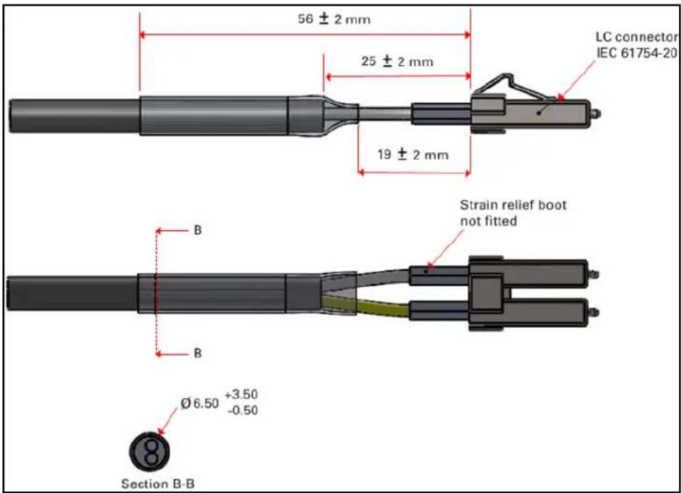
Table 31: Optical cable part numbers
| Cambium description Cambium part number | |
| Optical CABLE,MM, 1m N000082L215A | |
| Optical CABLE,MM, 2.2m N000082L191A | |
| Optical CABLE,MM, 10m | N000082L192A |
| Optical CABLE,MM, 20m N000082L193A | |
| Optical CABLE,MM, 30m N000082L194A | |
| Optical CABLE,MM, 50m N000082L195A | |
| Optical CABLE,MM, 80m N000082L196A | |
| Optical CABLE,MM, 100m N000082L197A | |
| Optical CABLE,MM, 150m N000082L198A | |
| Optical CABLE,MM, 200m N000082L199A | |
| Optical CABLE,MM, 300m N000082L200A | |
| Optical CABLE,SM, 2.2m N000082L186A | |
| Optical CABLE,SM, 10m N000082L187A | |
| Optical CABLE,SM, 20m N000082L188A | |
| Optical CABLE,SM, 30m N000082L139A | |
| Optical CABLE,SM, 50m N000082L140A | |
| Optical CABLE,SM, 80m N000082L141A | |
| Optical CABLE,SM, 100m N000082L142A | |
| Optical CABLE,SM, 150m N000082L143A | |
| Optical CABLE,SM, 200m N000082L189A | |
| Optical CABLE,SM, 300m N000082L190A |
System Planning
Site planning
This section describes factors to be considered when planning the proposed link end sites, including grounding, lightning protection, and equipment location for Outdoor Units (ODUs) and power supply units (PSU).
Grounding and lightning protection

Warning
Electro-magnetic discharge (lightning) damage is not covered under warranty. The recommendations in this guide, when followed correctly, give the user the best protection from the harmful effects of EMD. However, 100% protection is neither implied nor possible.
Structures, equipment, and people must be protected against power surges (typically caused by lightning) by conducting the surge current to the ground via a separate preferential solid path. The actual degree of protection required depends on local conditions and applicable local regulations. To adequately protect a 60 GHz cnWave installation, both ground bonding and transient voltage surge suppression are required.
Full details of lightning protection methods and requirements can be found in the International Standards IEC 61024-1 and IEC 61312-1, the U.S. National Electric Code ANSI/NFPA No. 70-1984, or section 54 of the Canadian Electric Code.

Note
International and national standards take precedence over the requirements in this guide.
Lightning protection zones
Use the rolling sphere method (Rolling sphere method to determine the lightning protection zones) to determine where it is safe to mount equipment. An imaginary sphere, typically 50 meters in radius, is rolled over the structure. Where the sphere rests against the ground and a strike termination device (such as a finial or ground bar), all the space under the sphere is in the zone of protection (Zone B). Similarly, where the sphere rests on two finials, the space under the sphere is in the zone of protection.
Figure 45: Rolling sphere method to determine the lightning protection zones

Site grounding system
Ensure that the site has a correctly installed grounding system on a common ground ring with access points for grounding ODU.
If the outdoor equipment is to be installed on the roof of a high building, refer to the Installation section.
Ensure that the system meets the following additional requirements:
- A grounding conductor is installed around the roof perimeter to form the main roof perimeter lightning protection ring.
- Air terminals are installed along the length of the main roof perimeter lightning protection ring, typically every 6.1 m (20 ft).
- The main roof perimeter lightning protection ring contains at least two down conductors connected to the grounding electrode system. The down conductors should be physically separated from one another, as far as practical.
ODU location
Find a location for the ODU (and external antenna for connectorized units) that meets the following requirements:
• The equipment is high enough to achieve the best radio path.
• People can be kept a safe distance away from the equipment when it is radiating.
- The equipment is lower than the top of the supporting structure (tower, mast, or building) or its lightning air terminal.
- If the ODU is connectorized, select a mounting position that gives it maximum protection from the elements, but still allows easy access for connecting and weather proofing the cables. To minimize cable losses, select a position where the antenna cable lengths can be minimized. If diverse or two external antennas are being deployed, it is not necessary to mount the ODU at the mid-point of the antennas.
Drop cable grounding points
To estimate how many grounding kits are required for each drop cable, refer to site installation and use the following criteria:
- The drop cable shield must be grounded near the ODU at the first point of contact between the drop cable and the mast installation, tower or building.
• The drop cable shield must be grounded at the building entry point.
For mast or tower installations installation, use the following additional criteria:
- The drop cable shield must be grounded at the bottom of the tower, near the vertical to the horizontal transition point. This ground cable must be bonded to the tower or tower ground bus bar (TGB) if installed.
- If the tower is greater than 61 m (200 ft) in height, the drop cable shield must be grounded at the tower midpoint, and at additional points as necessary to reduce the distance between ground cables to 61 m (200 ft) or less.
- In high lightning-prone geographical areas, the drop cable shield must be grounded at a spacing between 15 to 22 m (50 to 75 ft). This is especially important for towers taller than 45 m (150 ft).
For roof installations, use the following additional criteria:
- The drop cable shield must be bonded to the building grounding system at its top entry point (usually on the roof).
- The drop cable shield must be bonded to the building grounding system at the entry point to the equipment room.
ODU wind loading
Ensure that the ODU and the structure on which it is mounted are capable of withstanding the prevalent wind speeds at a proposed site. Wind speed statistics should be available from national meteorological offices.
The ODU and its mounting bracket are capable of withstanding wind speeds of up to 325 kph (200 mph).
Wind blowing on the ODU subjects the mounting structure to significant lateral force. The magnitude of the force depends on both wind strength and the surface area of the ODU. Wind loading is estimated using the following formulae:
• Force (in newtons) = 0.5 × β × A / × d C
- “ρ” is the density of air (1.225 kg/m
- "V" is the wind speed in meters per second
- "A" is the projected surface area of the ODU in square meters
- “ Cd ” is the drag coefficient = 1.385.
The drag co-efficient has been measured when the cover plate or antenna is perpendicular to the air flow.
Applying these formulae to the cnWave ODU at different wind speeds, the resulting wind loadings are shown in the following ODU wind loading (newtons) table:
Table 32: ODU wind loading (newtons)
| Type of ODU | Max surface area (square meters) Wind | speed (km/h Newtons) | |||||
| 200* 225 | 250 | 275 | 300 | 325 | |||
| V1000 0.017544 | 44 56 69 83 99 116 | ||||||
| V2000 0.0368 | 61 78 96 | 116 | 138 | 162 | |||
| v3000** | 0.1764 | 462 | 583 | 719 | 871 | 1036 | 1216 |
| V5000 | 0.052597188 | 118 | 148 | 185 | 224 | 266 | 312 |
Equivalent results in US customary units are shown in following ODU wind loading (pounds force) table:
Table 33: ODU wind loading (pounds-force)
| Type of ODU | Max surface area (square meters) | Wind speed (km/h lbf) | |||||
| 200* | 225 | 250 | 275 | 300 | 325 | ||
| V1000 | 0.017544 | 10 | 13 | 16 | 19 | 23 | 26 |
| V2000 | 0.0368 | 14 | 18 | 22 | 26 | 31 | 36 |
| v3000** | 0.1764 | 104 | 131 | 162 | 196 | 233 | 273 |
| V5000 | 0.052597188 | 27 | 33 | 42 | 50 | 60 | 70 |
* 200 km/h is from measured data and used to calculate the remaining figures.
** Worst case setup with the product in -30° tilt position.
PSU DC power supply
Use Cambium Networks recommended DC PSU for wireless nodes and ensure the power cords and cables are appropriately rated and in accordance with the regulations of the country of use.
PSU AC power supply
Use Cambium recommended AC power supply for wireless nodes and ensure the power cords and cables are appropriately rated and in accordance with the regulations of the country of use.
PSU location
Find a location for the PSU that meets the following requirements:
DC PoE power injector
- DC power injector can be mounted on a flat surface.
- PSU is installed in a dry location where no condensation, flooding or rising damp is possible.
- The PSU is located in an environment where it is not likely to exceed its operational temperature rating, allowing for natural convection cooling and placed not close to any fire source.
- PSU can be connected to the ODU drop cable and network terminating equipment.
- PSU can be connected to a compatible power supply.
Outdoor AC/DC PSU
Find a location for the PSU that meets the following requirements:
- The PSU is installed in a dry location where no flooding or rising damp is possible.
- The PSU is located in an environment where it is not likely to exceed its operational temperature rating, allowing for natural convection cooling and placed not close to any fire source.
- The PSU is not stacked and placed adjacent to the heat-generating equipment.
- The PSU shall be connected to protective earth.
- The PSU shall be connected to ODU drop cable using cable joiner and appropriately rated cables should be used.
Lightning Surge Protection Units (LPU)
All drop cables connected to the ODU (for example, PSU and AUX drop cables) require their own Lighting Protection Unit (LPU) or Gigabit Surge Suppressor installed close to the ODU and close to the enclosure/building entry point. The copper SFP drop cable also requires surge protection. Optical cables do not require lightning surge protection or ground cables. Guidance on the positioning of required lighting surge protection is given in the Lightning Surge Protection Units Location.
Drop cable grounding points
To estimate how many grounding kits are required for each drop cable, use the following criteria:
- The drop cable shield must be grounded near the ODU at the first point of contact between the drop cable and the mast, tower or building.
- The drop cable shield must be grounded at the building entry point.
For mast or tower installations, use the following additional criteria:
- The drop cable shield must be grounded at the bottom of the tower, near the vertical to the horizontal transition point. This ground cable must be bonded to the tower or TGB, if installed.
- If the tower is greater than 61 m (200 ft) in height, the drop cable shield must be grounded at the tower midpoint, and at additional points as necessary to reduce the distance between ground cables to 61 m (200 ft) or less.
- In high lightning-prone geographical areas, the drop cable shield must be grounded at the spacing between 15 to 22 m (50 to 75 ft). This is especially important on towers taller than 45 m (150 ft).
For roof installations, use the following additional criteria:
- The drop cable shield must be bonded to the building grounding system at its top entry point (usually on the roof).
- The drop cable shield must be bonded to the building grounding system at the entry point to the equipment room.
Lightning Surge Protection Units location
Lightning Surge Protection Units or Gigabit Surge Suppressors must be installed at two points on drop cables:
- There is room to mount the LPU, either on the ODU mounting bracket or on the mounting pole below the ODU.
- The drop cable length between the ODU and top LPU must not exceed 600 mm.
- There is access to a metal grounding point to allow the ODU and top LPU to be bonded in the following ways: top LPU to ODU; ODU to a grounding system.
Find a location for the bottom LPU that meets the following requirements:
- The bottom LPU can be connected to the drop cable from the ODU.
- The bottom LPU is within 600 mm (24 in) of the point at which the drop cable enters the building, enclosure or equipment room within a larger building.
- The bottom LPU can be bonded to the grounding system.
Deployment Considerations
This section provides brief information specific to the deployment of 60 GHz cnWave series of products. This section covers the following topics:
• Key deployment guidelines
• Sector and alignment
• Minimum CN spacing
- Near-far radio
• Early weak interference
- Avoiding the tight angle deployment
- Avoiding the straight line interference
- When two V5000 devices are co-located at a site
- Polarity
• Link Adaptation and Transmit Power Control (LATPC)
Key deployment guidelines
Following are some of the key guidelines that you must consider for the deployment of 60 GHz cnWave series of products:
- Mounting accuracy: Cambium Networks has different Stock Keeping Units (SKU) models. These three SKUs have different requirements in terms of alignment coverage, as shown in Table 34.
Table 34: Details of alignment coverage - 60 GHz cnWave products
| 60 GHz cnWave product version Azimuth (in degrees) Elevation (in degrees) | ||
| V5000 +/-70 per sector +/-20 | ||
| V3000 +/-2 +/-1 | ||
| V2000 +/-10 +/-4.5 | ||
| V1000 +/-40 +/-20 | ||
- Minimum deployment distance: A typical minimum deployment distance is based on the maximum receive signal strength of -40 dBm, as listed:
• 25 meters for V1000 and V5000
• 150 meters for V3000
• 60 meters for V2000
- In deployments where the range is less than 25 meters (for V1000 and V5000), 150 meters (for V3000), or 60 meters (for V2000) a short range or long range specific check box is provided in the user interface (UI) to allow this.
- Deployment frequency range: 60 GHz cnWave products support the use of CH1 to CH4 (channels). Deployment in these channels depends on the allowed channels in that region. Each channel is 2.16 GHz wide, and the raster frequencies supported are - 58.32 GHz, 60.48 GHz, 62.64 GHz, and 64.8 GHz.
Sector and alignment
Each sector is an independent radio or a baseband unit. Each sector has 2 RF tiles connected to provide extended azimuth scan range, as shown in Figure 46.
Figure 46:The sector diagram


Maximize the pole or box height during the deployment. This action minimizes the ground bounce and avoids channel fluctuations, especially for links with long distances. The suggested height is >5m.
You must consider the orientation of a DN node in P2MP. For example, orient the V5000 to the boresight of the RF tile to the longest link (where possible). The optimal beam angle to achieve the maximum antenna gain is at boresight of the active tile face (as shown in Figure 47 using the Red dotted line).
Figure 47:Optimal beam angle

Consider the following deployment specific points:
- Avoid sticking any metallic labels on the radome.
• The 60 GHz cnWave antenna tiles are located on the four marked faces. - The GPS antenna is located at the middle of the top face of the radome that is pointed to the sky.
Minimum CN spacing
Consider the following key points for the minimum CN spacing at a sector intersection:
- Up to 15 CNs can be installed in a single sector. Time Division Multiple Access scheme (TDMA) dynamically schedules the time slots for each wireless link on an access point, such that they do not interfere with one another.
- When CNs are installed in multiple sectors, more than one CN can be talking at a given time as the sectors have independent schedulers.
If both CNs installed in different sectors are located within the highlighted 20 degree range, then configure the two sectors to be on different channels to avoid interference.
Figure 48 shows the minimum CN spacing at a sector intersection.
Figure 48: Minimum CN spacing

Near-far radio
Near-far ratio for links from different sectors on the same pole is based on the following factors:
- Scenario:
• One wireless link on DN sector 1 at long range, link 2
• One wireless link on DN sector 2 at short range, link 1
- Narrow angular separation between link1 and link2 (less than 20 degrees)
- Configured for the same channel
- Problem:
- The TG system utilizes the active Transmit Power control.
- The transmit power for link 1 is automatically set to a low level.
- The transmit power for link 2 is automatically set to a high level.
- Due to narrow angular separation, the sidelobe of link 2 is interfered with link 1. As a result, the Signal-to-Noise Ratio (SNR) of link1 could degrade and this might cause the transmit power of link 1 to be boosted to a much higher level. This problem ends up in a cycle resulting in both links eventually transmitting at full power by causing network interference.
- Solution:
- Perform traffic test on one link at a time and then simultaneously.
- If the simultaneous traffic results show degradation along with transmit power that is railed high to maximum, consider the following tasks:
- Setting the two sectors on different channels or
- Capping the maximum power of the short range link.
Figure 49 illustrates the problem and the solution for near-far radio.
Figure 49: Near-far radio - Problem and solution

Early weak interference
Early weak interference occurs when the receiver correlates to a preamble from an unwanted node, with the same Golay code (as desired). If the receiver starts decoding the preamble from the wrong node, it may be too late to recover the preamble from the correct node for that cycle.
Terragraph has four Golay codes to mitigate this interference. Users can select the Golay codes 1,2,3 .

Note
Golay 0 is used for another purpose. Therefore, avoid selecting the Golay 0 (The use of Golay 0 has been deprecated in System Release 1.2).
Consider the following points specific to the Golay codes in 802.11ad/ay:
- The 802.11ad/ay frame consists of PHY preamble, which consists of short training frame (STF) and Channel Estimation Symbol (CES).
- The STF and CES are made up of complimentary Golay codes. Due to the repetition of the Golay codes, the signal can be correlated with even low SNRs.
• This PHY preamble is used for frequency synchronization, timing synchronization, and channel estimation.
Avoiding the tight angle deployment
Avoid tight P2MP angles in the deployment for the following reasons:
- In Figure 50 (shown as an example), a downlink data transmission from the DN1 to CN1 can interfere with the uplink data reception at CN2 to DN2. This interference can be both down to the main lobe in very tight angles or sidelobes with up to 20 degrees delta between two CNs.
- The level of interference depends on the link distances between DN1->CN1 versus DN->DN2 versus CN2->DN2.
• In most cases, the main interference is due to the early weak interference. - To mitigate this early-weak interference, different Golay code assignment could be used. This issue only relates to the two links transmitting at the same time in the same physical direction.
Figure 50: Tight angle deployment

flowchart
graph LR
    A["Sector 1"] -->|10 deg| B["GN1-Odd"]
    B --> C["Sector 2"]
    C -->|10 deg| D["GN2-Even"]
    D -->|10 deg| E["GN2-Odd"]
    E --> F["CN1-Even"]
    F --> G["GN1 to CN1 DL Data"]
    G --> H["Golay - 1"]
    H --> I["GN2 to DN2 UL Data"]
    I --> J["Golay - 2"]
    J --> K["GN2-Odd"]
    K --> L["GN1-Odd"]
    L --> M["GN2-Odd"]
Avoiding the straight line interference
It is recommended to avoid the straight line interference. When the desired link and interference link angles are the same, there is no assistance from the beamforming interference suppression.
Figure 51: Representation of straight line interference

flowchart
graph TD
    A["Polarity Odd"] --> B["Sector 2"]
    A --> C["Sector 1"]
    D["Polarity Even"] --> E["Sector 2"]
    D --> F["Sector 1"]
    G["Polarity Odd"] --> H["Sector 2"]
    G --> I["Sector 1"]
    J["Polarity Even"] --> K["Sector 2"]
    J --> L["Sector 1"]
    M["Polarity Odd"] --> N["Sector 2"]
    M --> O["Sector 1"]
    P["Polarity Even"] --> Q["Sector 2"]
    P --> R["Sector 1"]
    S["Polarity Odd"] --> T["Sector 2"]
    S --> U["Sector 1"]
    V["Polarity Even"] --> W["Sector 2"]
    V --> X["Sector 1"]
    Y["Polarity Odd"] --> Z["Sector 2"]
    Y --> AA["Sector 1"]
    AB["Polarity Even"] --> AC["Sector 2"]
    AB --> AD["Sector 1"]
    AE["Polarity Odd"] --> AF["Sector 2"]
    AE --> AG["Sector 1"]
    AH["Polarity Even"] --> AI["Sector 2"]
It is recommended to assign appropriate Golay codes to mitigate early-weak interference. In Figure 52, the red and orange arrows show the possible weak interference. The code assignment must be in the form of 2-2-1-1 or 1-1-2-2 but not in the 1-2-1-2 form.
Figure 52: Assigning Golay codes
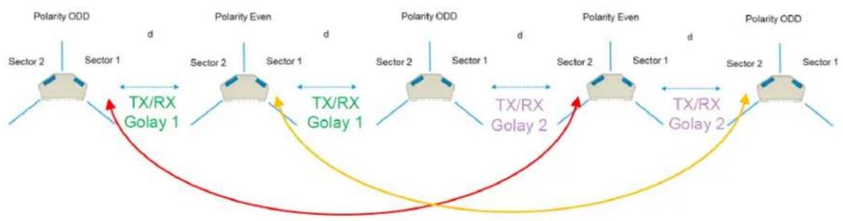
flowchart
graph LR
    A["Polarity ODD"] --> B["Sector 2"]
    B --> C["TX/RX Golay 1"]
    C --> D["Sector 1"]
    D --> E["TX/RX Golay 1"]
    E --> F["Polarity Even"]
    F --> G["Sector 2"]
    G --> H["TX/RX Golay 2"]
    H --> I["Sector 1"]
    I --> J["TX/RX Golay 2"]
    J --> K["Polarity ODD"]
    K --> L["Sector 2"]
    L --> M["TX/RX Golay 2"]
    M --> N["Sector 1"]
    N --> O["TX/RX Golay 2"]
    O --> P["Polarity ODD"]
When two V5000 devices are co-located at a site
When two V5000 devices are co-located at the same site, it is recommended that one must use different channels on the two V5000 devices to start with.
Evaluate the issues specific to near-far radio and Tight Angle deployment. Then, you have to configure two different channels for the two sectors or consider option 2, as shown in Figure 53.
Figure 53: When two V5000 devices are co-located at the same site

Where local regulations allow the usage of four channels, it is advisable to choose CHA and CHB such that there are two channels apart. Example: Consider that CHA = 1 or 2 CHB = 3 or 4. The reason is that it may be easier to upgrade to Channel bonding (CB2) in the future and still experience the channel isolation.

Note
It is important to use the same polarity at the same site. For more details about the polarity, refer to the Polarity section.
Polarity
60 GHz CnWave uses TDD, which is synchronized across the network. As one sector is in the transmit phase, the neighbor sector is in the receive phase. The transmit and receive phases of the sectors are determined by the EVEN or ODD polarity.
All sectors with a common polarity in a network could be transmitting or receiving at the same time.
Hybrid polarity is when a node uses an EVEN polarity on one sector and an ODD on another sector. Although hybrid polarity is possible through configuration, you must avoid this unless the installer is sure that the two links on the sectors are orthogonal. Figure 54 shows an example of the hybrid polarity.
Figure 54: Hybrid polarity
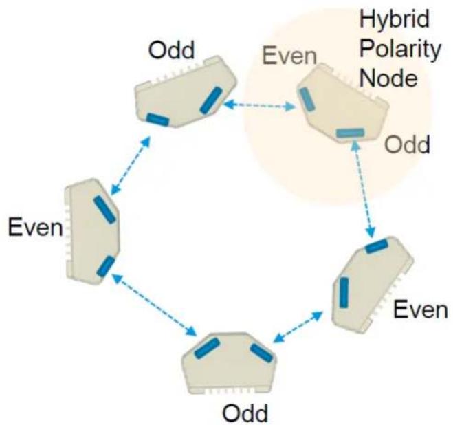
flowchart
graph TD
    A["Odd"] --> B["Even"]
    B --> C["Odd"]
    C --> D["Even"]
    D --> E["Odd"]
    E --> F["Even"]
    F --> G["Odd"]
    G --> H["Even"]
    H --> I["Odd"]
    I --> J["Even"]
    J --> K["Odd"]
    K --> L["Even"]
    L --> M["Odd"]
    M --> N["Even"]
    N --> O["Odd"]
    O --> P["Even"]
    P --> Q["Odd"]
    Q --> R["Even"]
    R --> S["Odd"]
    S --> T["Even"]
    T --> U["Odd"]
    U --> V["Even"]
    V --> W["Odd"]
    W --> X["Even"]
    X --> Y["Odd"]
    Y --> Z["Even"]
    Z --> A
    style A fill:#f9f,stroke:#333
    style B fill:#f9f,stroke:#333
    style C fill:#f9f,stroke:#333
    style D fill:#f9f,stroke:#333
    style E fill:#f9f,stroke:#333
    style F fill:#f9f,stroke:#333
    style G fill:#f9f,stroke:#333
    style H fill:#f9f,stroke:#333
    style I fill:#f9f,stroke:#333
    style J fill:#f9f,stroke:#333
    style K fill:#f9f,stroke:#333
    style L fill:#f9f,stroke:#333
    style M fill:#f9f,stroke:#333
    style N fill:#f9f,stroke:#333
    style O fill:#f9f,stroke:#333
    style P fill:#f9f,stroke:#333
    style Q fill:#f9f,stroke:#333
    style R fill:#f9f,stroke:#333
    style S fill:#f9f,stroke:#333
    style T fill:#f9f,stroke:#333
    style U fill:#f9f,stroke:#333
    style V fill:#f9f,stroke:#333
    style W fill:#f9f,stroke:#333
Link Adaptation and Transmit Power Control (LATPC)
The modulation and code scheme (MCS) rate and transmit power are both adaptive values. These values are set at the transmitter, independently, for every link and for both directions. The adaptive MCS selection procedure is referred to as link adaptation (LA) and the transmit power procedure as transmit power control (TPC).
Following are the two versions of this adaptation, data traffic, and standby:
- When there is data traffic, adaptation is driven by block error rate (BLER) reported every SF (1.6ms). A lower BLER causes the algorithm to adapt the transmit power or MCS.
- When there is no data traffic, the algorithm is driven by the short training frame (STF) SNR as reported by each management packet. The SNR is compared to an MCS table. If the SNR is greater or lesser than table value, the transmit power or the MCS rate is adapted accordingly.
There is a maximum TX power per MCS mode (which is defined in the configuration section).
During the adaptation process, the transmit power is either increased or decreased first to:
- increase the power till the maximum per MCS power is reached or
- reduce the power if there is enough headroom.
If the maximum power for the MCS mode has been reached, the MCS mode is reduced.
Radio spectrum planning
General wireless specifications
The following 60 GHz cnWave wireless specifications (all variants) table lists the wireless specifications that apply to all 60 GHz cnWave frequency bands:
Table 35: 60 GHz cnWave wireless specifications (all variants)
| Item Specification | |
| Channel selection | Open/R protocol or manual selection |
| Manual power control | Supports ATPC automatic transmit power control and maximum EIRP can be set lower the default power limit. |
| Integrated antenna type | V1000 - 22.5 dBi gainV2000 - 34.5 dBi gainV3000 - 44.5 dBi gain and 40.5 dBi gainV5000 -22.5 dBi gain |
| Duplex schemes Symmetric 50:50 fixed and asymmetric fixed | |
| Range 100 m to 2 KMs, depends on the following factors:Frequency selectedRain conditionAvailabilityEIRP limitation | |
| Over-the-air encryption | AES 128-bit |
| Weather sensitivity | Highly sensitive due to rain range conditions. For more information in range, refer Rain and attenuation table. |
Regulatory limits
Many countries impose EIRP limits (allowed EIRP) on products operating in the bands used by the 60 GHz cnWave. These are commonly identified by limitations on conducted transmit power or by antenna gain. For example:
Table 36: ERC recommendation (70-03)
| Frequency Band | Power / Magnetic Field | |
| c2 57 | - 71 GHz | 40 dBm E.I.R.P., 23 dBm/MHz E.I.R.P. density and maximum transmit power of 27 dBm antenna port/ports. |
| c3 57-71 GHz | 55 dBm E.I.R.P., 38 dBm/MHz E.I.R.P. density and transmit antenna gain ≥ 30 dBi. | |
CFR47 Part 15.255(c)(ii):
For fixed point-to-point transmitters located outdoors, the average power of any emission shall not exceed 82 dBm and shall be reduced by 2 dB for every dB that the antenna gain is less than 51 dBi. The peak power of any emission shall not exceed 85 dBm, and shall be reduced by 2 dB for every dB that the antenna gain is less than 51 dBi.
Link planning
This section describes factors that must be considered when planning links, such as range, obstacles path loss, and throughput. It is highly recommended to use Cambium LINKPlanner software when planning the links.
LINKPlanner
The Cambium LINKPlanner software and user guide may be downloaded from the support website (see https://support.cambiumnetworks.com/files/linkplanner/).
LINKPlanner imports path profiles and predicts data rates and reliability over the path. It allows the system designer to try different antenna heights and RF power settings. It outputs an installation report that defines the parameters to be used for configuration, alignment, and operation. Use the installation report to compare predicted and actual link performance.
Exclusion zones for the 59 - 63.9 GHz band
In the three geographical areas outlined in 59 - 63.9 GHz Transmission Exclusion Zones (UK IR 2078 Section 4 and IR 2030 IR2030/7/4 (2018/316/UK)), no transmissions are permitted.
Table 37: 59 - 63.9 GHz transmission exclusion zones
| Site Name | Site Location Radius of exclusion | zone from the center of site location |
| Site 1 07° | 23' 36.6" W, 57° 21' 3.6" N 6 Km | |
| Site 2 04° | 58' 21" W, 51° 37' 16.8" N 6 Km | |
| Site 3 00° | 36' 22.8" W, 52° 38' 1.8" N 6 Km |
Range and obstacles
Calculate the range of the link and identify any obstacles that may affect radio performance.
Perform a survey to identify all the obstructions (such as trees or buildings) in the path and to assess the risk of interference. This information is necessary to achieve an accurate link feasibility assessment. The 60 GHz cnWave radios are designed to operate in Line-of-Sight (LoS) environments.
The 60 GHz cnWave radios operate at ranges from 15 m (49 ft) to 2000 m (1.2 miles). The operation of the system depends on the frequency channel chosen.
Path loss
Path loss is the amount of attenuation the radio signal undergoes between the two ends of the link. The path loss is the sum of the attenuation of the path if there were no obstacles in the way (Free Space Path Loss), the attenuation caused by obstacles (Excess Path Loss) and a margin to allow for possible fading of the radio signal (Fade Margin). The following calculation needs to be performed to judge whether a particular link can be installed:
L _ free _ space + L _ excess + L _ fade + L _ seasonal lt; L _ capability
Table 38: Input details for the link calculation
| Where: Is: | |
| Lfreespace | Free Space Path Loss (dB) |
| Lexcess | Excess Path Loss (dB) |
| Lfade | Fade Margin Required (dB) |
| Lseasonal | Seasonal Fading (dB) |
| Lcapability | Equipment Capability (dB) |
At 60 GHz cnWave, the oxygen absorption is a key component of the free space path loss and varies substantially depending on the frequency channel selected. Use LINKPlanner to calculate the oxygen absorption component for the required path and frequency channel.
Planning for data networks
This section describes factors to be considered when planning 60 GHz cnWave data networks.
60 GHz cnWave network can be deployed as point-to-point backhaul-bridge, Point-to-Multipoint coverage network and mesh network that provide network rebound.
By default, cnWave radios operate in IPv6 layer 3 network mode, requiring IPv6-based routing gears. The network can be designed to operate in pure IPv4 network mode, transporting layer 2 traffic (VLAN tagged and untagged) with GRE tunnels built-in by the system.
There is no fundamental difference between configurations of PTP vs. PMP vs. Mesh because the underlying routing mechanism of the cnWave network is always IPv6-based OpenR routing.
In a PTP network, you have one PoP DN and a CN to form a link. In a PMP network, you have one PoP DN and multiple CNs (up to 30 CNs if V5000 is used) to form a PMP cluster. You can have multiple PMP clusters to form a coverage area network.
You can have one PoP node with multiple DNs or CNs. If DNs are connected, the user gets a mesh network. User can them have multiple PoPs and DNs and if the link with each other and form a complex mesh network.
Point to Point-based single link Ethernet bridge
A Point to Point cnWave link can be configured to work as an Ethernet bridge. The operator needs to configure one end as PoP DN, and the other end as CN.
Enable Layer 2 Bridge. While the radios still run on IPv6, the Layer 2 Bridge configuration allows user Layer 2 data (VLAN tagged and untagged) to be transmitted transparently through the link.
IPv6 address of the PoP and CN can be automatically generated and they do not need to be routable through the external network as long as the E2E is collocated with the PoP DN or within the same VLAN of the PoP DN. The operator can assign IPv4 addresses to the radios for management purposes.
Figure 55: Point to Point cnWave link

flowchart
graph LR
    A["CPE"] --> B["CN"]
    B --> C["RF Link"]
    C -.-> D["POP DN"]
    D --> E["Pop interface"]
    D --> F["Backhaul"]
IPv4/L2 based PMP and mesh network planning
You can build a complete IPv4-based network without the need for any IPv6 routers. The following figure shows the network:
Figure 56:Example of IPv4-based network

flowchart
graph TD
    A["IPv6 OpenR Mesh network"] -->|IPv4| B["CN"]
    A -->|IPv4| C["CPE"]
    A -->|IPv4| D["DN"]
    A -->|IPv4| E["CN"]
    A -->|IPv4| F["CPE"]
    A -->|IPv4| G["DN"]
    A -->|IPv4| H["CN"]
    A -->|IPv4| I["CPE"]
    A -->|IPv4| J["DN"]
    A -->|IPv4| K["CN"]
    A -->|IPv4| L["CPE"]
    A -->|IPv4| M["DN"]
    A --> N["SNP"]
    A --> O["SNP"]
    A --> P["SNP"]
    A --> Q["SNP"]
    A --> R["SNP"]
    A --> S["SNP"]
    A --> T["SNP"]
    A --> U["SNP"]
    A --> V["SNP"]
    A --> W["SNP"]
    A --> X["SNP"]
    A --> Y["SNP"]
    A --> Z["SNP"]
    A --> AA["SNP"]
    A --> AB["SNP"]
    A --> AC["SNP"]
    A --> AD["SNP"]
    A --> AE["SNP"]
    A --> AF["SNP"]
    A --> AG["SNP"]
    A --> AH["SNP"]
    A --> AI["SNP"]
    A --> AJ["SNP"]
    A --> AK["SNP"]
    A --> AL["SNP"]
    A --> AM["SNP"]
    A --> AN["SNP"]
    A --> AO["SNP"]
    A --> AP["SNP"]
    A --> AQ["SNP"]
    A --> AR["SNP"]
    A --> AS["SNP"]
    A --> AT["SNP"]
    A --> AU["SNP"]
    A --> AV["SNP"]
    A --> AW["SNP"]
    A --> AX["SNP"]
    A --> AY["SNP"]
    A --> AZ["SNP"]
    A --> BA["SNP"]
    A --> BB["SNP"]
    A --> BC["SNP"]
    A --> BD["SNP"]
    A --> BE["SNP"]
    A --> BF["SNP"]
    A --> BG["SNP"]
    A --> BH["SNP"]
    A --> BI["SNP"]
    A --> BJ["SNP"]
    A --> BK["SNP"]
    A --> BL["SNP"]
    A --> BM["SNP"]
    A --> BN["SNP"]
    A --> BO["SNP"]
    A --> BP["SNP"]
    A --> BQ["SNP"]
    A --> BR["SNP"]
    A --> BS["SNP"]
    A --> BT["SNP"]
    A --> BU["SNP"]
    A --> BV["SNP"]
    A --> BW["SNP"]
    A --> BX["SNP"]
    A --> BY["SNP"]
    A --> BZ["SNP"]
    A --> CA["SNP"]
    A --> CB["SNP"]
    A --> CC["SNP"]
    A --> CD["SNP"]
    A --> CE["SNP"]
    A --> CF["SNP"]
    A --> CG["SNP"]
    A --> CH["SNP"]
    A --> CI["SNP"]
    A --> CJ["SNP"]
    A --> CK["SNP"]
    A --> CL["SNP"]
    A --> CM["SNP"]
    A --> CN["SNP"]
    A --> CO["SNP"]
    A --> CP["SNP"]
    A --> CQ["SNP"]
    A --> CR["SNP"]
    A --> CS["SNP"]
    A --> CT["SNP"]
    A --> CU["SNP"]
    A --> CV["SNP"]
    A --> CW["SNP"]
    A --> CX["SNP"]
    A --> CY["SNP"]
    A --> CZ["SNP"]
    A --> DA["SNP"]
    A --> DB["SNP"]
    A --> DC["SNP"]
    A --> DV["SNP"]
    A --> DW["SNP"]
    A --> DX["SNP"]
    A --> DXB["SNP"]
    A --> DXC["CPE"]
    A --> DXD["CPE"]
    A --> DXE["CPE"]
    A --> DXF["CPE"]
    A --> DXG["CPE"]
    A --> DXH["CPE"]
    A --> DXI["CPE"]
    A --> DXJ["CPE"]
    A --> DXK["CPE"]
    A --> DXL["CPE"]
    A --> DXM["CPE"]
    A --> DXN["CPE"]
    A --> DXO["CPE"]
    A --> DXN["CPE"]
60 GHz cnWave IPv6 IP address is generated automatically by the system.
- Single PoP, E2E resides in the PoP DN
When configuring the PoP E2E, the operator can configure the IPv6 address to be generated automatically.
- Multiple PoPs, E2E controls all the PoPs
cnMaestro generates the IPv6 configuration for all the PoPs. The user can download the config file from cnMaestro. This config file contains all the PoPs IPv6 configuration. The IPv6 configuration is associated with the MAC address of each PoP DN. When loading the config file to the PoP DN during initial configuration, the PoP DN chooses the IPv6 address by matching its MAC address, so there is no IPv6 address conflict.
The PoP DNs automatically use the E2E controller as the default gateway of IPv6 traffic. Since IPv6 traffic is used only for management purposes, there may be no concern about overloading the E2E. (IPv6 payload traffic should be disabled in the radio configuration).
The E2E chooses any one of the active PoP DN as the IPv6 default gateway. If the E2E detects that the default gateway PoP DN is down, it selects another PoP DN as a default gateway.
Control traffic from E2E to all cnWave radios will be sent to the default gateway PoP, which relies on OpenR to route through correlated POP to the target radio.
Select the Relay Port Interface for the PoP DN's Ethernet interface for inter-PoPs OpenR routing to work.

Note
IPv6 routers in the network are not required. Ensure that the PoP DNs and the E2E be in the same VLAN.
Configure the IPv4 address of the radios manually. The CPE IPv4 address can be manually configured or use a DHCP server sitting in the core network. Depending on the complexity of the network, IPv4 based router may be required to route the IPv4 traffic from the CPEs.
Support for dual networking (IPv4 and IPv6)
The operator can design the network so that both IPv4 and IPv6 user data are supported. In this case, an IPv6 router is required at the core network. Ensure that if Layer 2 Bridge is enabled, by default all the user traffic including IPv6 is encapsulated in the GRE tunnel. The IPv6 user traffic is passed through the cnWave network in the GRE tunnel so that it does not be routed by the cnWave radios, but rather by an external IPv6 router.
Figure 57:Example of an IPv4 and IPv6 supported network

flowchart
Network architecture diagram showing IPv6 OpenR mesh network connecting to core network via POP and CN protocols, with L2 and backhaul interfaces.The operator can choose certain of the radio Ethernet port to be SLAAC based port or (CPE interface), user traffic from this port is only IPv6 based and does not be encapsulated into the GRE Layer 2 bridge when transmitted over the wireless network. Although this reduces overhead, it is not recommended since this adds complexity to the network design (the operator may need to add a BGP router to the network).
IPv6 Mode network planning
If the operator chooses to have the network completely run on IPv6 mode, then GRE Layer 2 Bridge is not required and a BGP router is usually required to route traffic between the wireless network and the external network.
Figure 58:Example of IPv6 mode network

flowchart
graph TD
    A["IPv6 OpenR Mesh network"] -->|IPv6| B["CN"]
    A -->|IPv6| C["CPE"]
    A -->|DN| D["DN"]
    A -->|DN| E["CN"]
    A -->|DN| F["CPE"]
    A -->|DN| G["CN"]
    A -->|DN| H["CPE"]
    A -->|DN| I["CN"]
    A -->|DN| J["CPE"]
    A --> K["POP DN"]
    K --> L["Backhaul Network"]
    K --> M["IPv6"]
    K --> N["IPv6"]
    K --> O["IPv6"]
    K --> P["POP DN"]
    P --> Q["IPV6"]
    P --> R["IPv6"]
    P --> S["POP DN"]
    S --> T["IPV6"]
    S --> U["Backhaul Network"]
    U --> V["IPV6"]
    U --> W["IPv6"]
    U --> X["POP DN"]
    X --> Y["IPV6"]
    X --> Z["Backhaul Network"]
    Z --> AA["IPV6"]
    Z --> AB["IPv6"]
    Z --> AC["POP DN"]
    AC --> AD["IPV6"]
    AC --> AE["Backhaul Network"]
    AE --> AF["IPV6"]
    AE --> AG["IPv6"]
    AE --> AH["POP DN"]
    AH --> AI["IPV6"]
    AH --> AJ["Backhaul Network"]
    AJ --> AK["IPV6"]
    AJ --> AL["IPv6"]
    AJ --> AM["POP DN"]
    AM --> AN["IPV6"]
    AM --> AO["Backhaul Network"]
    AO --> AP["IPV6"]
    AO --> AQ["IPv6"]
    AO --> AR["POP DN"]
    AR --> AS["IPV6"]
    AR --> AT["Backhaul Network"]
    AT --> AU["IPV6"]
    AT --> AV["IPv6"]
    AT --> AW["POP DN"]
    AW --> AX["IPV6"]
    AW --> AY["Backhaul Network"]
    AX --> AZ["IPV6"]
    AX --> BA["IPv6"]
    AX --> BB["CPE"]
    AX --> BC["CPE"]
    AX --> BD["CPE"]
    AX --> BE["CPE"]
    AX --> BF["CPE"]
    AX --> BG["CPE"]
    AX --> BH["CPE"]
    AX --> BI["CPE"]
    AX --> BJ["CPE"]
    AX --> BK["CPE"]
    AX --> BL["CPE"]
    AX --> BM["CPE"]
    AX --> BN["CPE"]
    AX --> BO["CPE"]
    AX --> BP["CPE"]
    AX --> BQ["CPE"]
    AX --> BR["CPE"]
    AX --> BS["CPE"]
    AX --> BT["CPE"]
    AX --> BU["CPE"]
    AX --> BV["CPE"]
    AX --> BW["CPE"]
    AX --> BX["CPE"]
    AX --> BY["CPE"]
    AX --> BZ["CPE"]
    AX --> CA["CPE"]
    AX --> CB["CPE"]
    AX --> CC["CPE"]
    AX --> CD["CPE"]
    AX --> DE["CPE"]
    AX --> FD["CPE"]
    AX --> DG["CPE"]
    AX --> DH["CPE"]
    AX --> DI["CPE"]
    AX --> DJ["CPE"]
    AX --> DK["CPE"]
IPv6 Network design consideration
There are two sets of networks when designing the IPv6 network. one set is for the OpenR subnets (e.g. prefix of 56 bits and partition into multiple 64 bits subnet).
Each PoP node, besides being part of the OpenR mesh network, has a subnet assigned to it and has an IPv6 address assigned to it as PoP interface IPv6 address.
If you let the system automatically generate an IP address configuration, the IP address is always in the format of FD00:xxxxxxxx, which is a standard routable private IPv6 address.
Figure 59:Example of an IPv6 network design

flowchart
graph LR
    A["OpenR IPv6 Subnets"] --> B["DN"]
    A --> C["POP interface Backhaul IPv6 Network"]
    D["DN"] --> E["Pop DN"]
    F["DN"] --> G["Pop DN"]
Reserved IPv6 address space
If the operator let the system automatically generate the IPv6 addresses for the network, the following private IPv6 address spaces are reserved:
- FD00:CEED::0/32 for seed prefix of the mesh network
- FD00:BA5E::0/32 for all the PoP nodes and the E2E Controller
E2E and cnMaestro deployment consideration
While the E2E and cnMaestro are two separate entities, they can be hosted on separate computers or the same computer. While the E2E communicates with the cnMaestro using IPv4, the E2E communicates with the cnWave radios using IPv6.
Ethernet bridging
Layer 2 (L2) bridging
L2 Bridge employs Ethernet over GRE (EoGRE) to carry the customer traffic across the Terragraph network. When L2 Bridge is enabled, all CNs and DNs automatically create an EoGRE tunnel with their PoP node and the PoP node creates a tunnel back to each of those CNs/DNs. The tunnel is capable of carrying both IPv4 and IPv6 customer traffic between CN and PoP. The IPv6 over the tunnel can be optionally disabled from the UI.
An ingress Ethernet frame from a customer's network must not exceed 1942 bytes. On top of this, the device (CN, DN, or PoP) adds 58 bytes of tunnel headers. Hence, the maximum size of an encapsulated Ethernet frame is 2000 bytes.
If the device nodes are configured to insert VLANs (native Q or native QinQ), additional room must be left free for that in the ingress Ethernet frame.
Broadcast/Multicast control
The downstream broadcast can be controlled by explicitly disabling it from the UI. Disabling IPv6 over the tunnel also reduces the downstream multicast traffic.
Limitations
- In bridge mode, the V5000 PoP node can forward 1.8 Gbps of TCP traffic and 2.0 Gbps of UDP traffic in the down-link direction.
Layer 2 Bridge support in multi-PoP deployments
This feature applies to Layer 2 bridging and Deterministic Prefix Allocation (DPA) are configured to be used in the network.
In the Terragraph network, CNs and DNs are allocated prefixes from a seed prefix. There are various ways for allocating prefixes. In DPA, the controller assigns prefix zones to PoPs based on the network topology to allow PoP nodes to take advantage of summarizing the route and helps in load balancing ingress traffic.
CNs and DNs get prefixes from the respective PoP zone which is allocated by the controller. CNs and DNs see multiple PoP nodes in the mesh, they select PoP to form GRE tunnel, by matching their Io IPv6 address with PoPs Io IPv6 address. The longest prefix match is selected as the best PoP for L2 GRE Tunnel establishment. The multi-PoP setup gives the advantage that user data traffic can take alternate routes if the best route is unavailable for some reason. Open/R makes this selection to route the traffic. If PoP is unavailable, CNs and DNs switch to the next best PoP. They however keep track of their primary PoP availability and switch to it once it becomes online.
External Layer 2 Concentrator support
The external device can be used as an L2 GRE Concentrator. Concentrator could be a Linux server or any router or switch supporting IPv6 L2 GRE tunnels. Example: Juniper MX 100.
Select the Static tunnel concentrator option and provide an IPv6 address to configure the external concentrator IPv6 address.
Figure 60: Layer 2 Tunnel Concentrator

Multi-PoP deployments
You must take care of the following aspects in the multi-PoP deployments:
- Layer 2 domain
- Open/R on the PoP interface port
• MTU of upstream switch ports - Prefix allocation
Layer 2 domain
All cnWave PoP nodes must be connected to the same Layer 2 broadcast domain. PoP nodes learn about other PoP nodes using IPv6 multicast packets, which do not cross broadcast domain.
This allows cnWave PoP nodes to forward traffic to other cnWave PoP nodes via a wired connection when the routing path of the other PoP node is closer to the traffic's destination. This concept is called Tromboning, as the traffic enters one PoP node and then leaves to another PoP node.
Open/R on the PoP interface port
PoP interface port must be configured to run the Open/R protocol. To enable this option, select Multi-PoP/ Relay port Interface.
Figure 61:Multi-PoP/Relay Port Interface

MTU of upstream switch ports
PoP ports use a 2000 MTU size. So, all the switch ports must be at least 2000 MTU size. Even if the user traffic is limited to 1500 sized packets, switch ports should allow the higher MTU size. The following packets exchanged between the PoPs that can be of higher size:
- Open/R packets,
• L2GRE packets (in Layer 2 mode), and - Software download packets.
Prefix allocation
It is recommended to select the Deterministic Prefix Allocation option for multi-PoP deployments.
Figure 62: The prefix allocation options

Prefix Allocation
○ Centralized

Deterministic
Layer 2 control protocols
60 GHz cnWave identifies layer 2 control protocols (L2CPs) from the Ethernet destination address or Ethertype of bridged frames.
IP Interface
Select the IP version for the IP interface of the ODU management agent. 60 GHz cnWave can operate in IPv4 mode (via L2 tunneling), IPv6 mode. Choose one IPv4 address and/or one IPv6 address for the IP interface of the ODU management agent. The IP address or addresses must be unique and valid for the connected network segment and VLAN.
Find out the correct subnet mask (IPv4) or prefix length (IPv6) and gateway IP address for this network segment and VLAN.
Ensure that the design of the data network permits bidirectional routing of IP datagrams between network management systems and the ODUs. For example, ensure that the gateway IP address identifies a router or another gateway that provides access to the rest of the data network.
Daisy-chaining 60 GHz links
When connecting two or more 60 GHz cnWave links together in a network (daisy-chaining), do not install direct copper CAT5e connections between the PSUs. Each PSU must be connected to the network terminating equipment using the LAN port. To daisy-chain 60 GHz cnWave links, install each ODU-to-ODU links using one of the following solutions:
- A copper CAT5e connection between the Aux ports of two ODUs.
- A copper CAT5e connection between the Aux port of one ODU and the SFP port of the next ODU (using a copper SFP module).
• Optical connections between the ODUs (SFP ports) using optical SFP modules at each ODU.

Note
Wherever CAT5e is applicable, you can use CAT5e or better category cables. Similarly, you can use CAT6 or better category cables wherever CAT6 is applicable.
Installation
Safety

Warning
To prevent loss of life or physical injury, observe the following safety guidelines. In no event shall Cambium Networks be liable for any injury or damage caused during the installation of the Cambium 60 GHz cnWave radio nodes. Ensure that only qualified personnel install 60 GHz cnWave radios.

Attention
Exercise extreme care when working near power lines.
Working at heights
Exercise extreme care when working at heights.
PSU
Always use one of the approved power supply options. Failure to use the Cambium supplied PSUs can result in equipment damage and will invalidate the safety certification and may cause a safety hazard.
Grounding and protective earth
The cnWave radios must be properly grounded to protect against lightning. It is the user's responsibility to install the equipment in accordance with national regulations. In the USA follow the requirements of the National Electrical Code NFPA 70-2005 and 780-2004 Installation of Lightning Protection System in Canada, follow Section 54 of the Canadian Electrical Code These codes describe correct installation procedures for grounding the outdoor unit, mast, lead-in wire, and discharge unit, size of grounding conductors, and connection requirements for grounding electrodes. Other regulations may apply in different countries and therefore it is recommended that installation of the outdoor unit be contracted to a professional installer.
AC Supply
Always use an appropriately rated and approved AC supply cord-set in accordance with the regulations of the country of use.
Powering down before servicing
Before servicing 60 GHz cnWave equipment, always switch off the power supply and unplug it from the PSU.
Do not disconnect the RJ45 drop cable connectors from the radio while the PSU is connected to the power supply. Always remove the AC or DC input power from the PSU.
Primary disconnect device
The primary disconnect device is the main power supply.
External cables
Safety may be compromised if outdoor rated cables are not used for connections that are exposed to the outdoor environment.
Drop cable tester
The PSU output voltage may be hazardous in some conditions such as wet weather. Do not connect a drop cable tester to the PSU, either directly or via LPUs.
RF Exposure near the antenna
Strong Radio Frequency (RF) fields are present close to the antenna when the transmitter is ON. Always turn off the power to the radio before undertaking maintenance activities in front of the antenna.
Minimum separation distances
Ensure that personnel is not exposed to unsafe levels of RF energy. The units start to radiate RF energy as soon as they are powered up. Never work in front of the antenna when the radio is powered. Install the radios to provide and maintain the minimum separation distances from all persons. For minimum separation distances, see Calculated distances and power compliance margins.
Grounding and lightning protection requirements
Ensure that the installation meets the requirements defined in the Installation section.
Grounding cable installation methods
To provide effective protection against lightning-induced surges, observe these requirements:
- Grounding conductor runs are as short, straight and smooth as possible, with bends and curves kept to a minimum.
- Grounding cables must not be installed with drip loops.
- All bends must have a minimum radius of 200 mm (8 in) and a minimum angle of 90°. A diagonal run is preferable to a bend, even though it does not follow the contour or run parallel to the supporting structure.
- All bends, curves and connections must be routed towards the grounding electrode system, ground rod/ground bar.
- Grounding conductors must be securely fastened.
- Braided grounding conductors must not be used.
- Approved bonding techniques must be used for the connection of dissimilar metals.
Siting radios
Radios are not designed to survive direct lightning strikes. For this reason, they must be installed in Zone B as defined in Lightning protection zones. Mounting in Zone A may put equipment, structures, and life at risk.
60 GHz cnWave radios and mounting bracket options
The 60 GHz cnWave series supports eight mounting bracket options. Select the optimum mounting bracket arrangement based on the ODU type and the choice of wall or pole mounting. The wall mount plate for V1000 and V5000 are included with the ODU. Order the remaining brackets separately.
Table 39: ODU mounting bracket part numbers
| Bracket Pole diameter ODU | variants | Bracket part number | |
| V1000 pole mount 25 mm to 70 mm (1 inch to 2.75 inches) | V1000 Included with V1000 | ||
| V1000 wall mount Wall mount | V1000 Included with V1000 | ||
| V1000 adjustable pole mount 25 mm to 70 mm (1 inch to 2.75 inches) | V1000 N000900L022A | ||
| V2000 Adjustable pole mount 25 mm to 70 mm (1 inch to 2.75 inches) | V2000 Included with V2000 | ||
| V3000 precision bracket 25 mm to 70 mm (1 inch to 2.75 inches) | V3000 C000000L125A | ||
| V3000 tilt bracket assembly 25 mm to 70 mm (1 inch to 2.75 inches) | V3000, V5000 | N000045L002A | |
| V3000 tilt bracket assembly with band clamps | The diameter range depends on the clamps used. | V3000, V5000 | N000045L002A + third-party band clamps |
| V5000 pole mount 25 mm to 70 mm (1 inch to 2.75 inches) | V5000 C000000L137A | ||
| V5000 wall mount Wall mount | V5000 C000000L136A | ||
Installing the cnWave radio nodes
To install the radio, use the following procedure and guidelines:
- Typical installation
- ODU interface with LPU on the pole
- SFP and Aux Ethernet interfaces
- Attach ground cables to the radio
- Mounting the ODU
Typical installation
V1000
Consider the following key points when installing V1000:
- Use the recommended grounding and surge suppressor connections.
- Use the recommended cables for interfacing ODU (refer to the supported power supply and cable length details in the Power supply units (PSU) section).
- Always install the ODU 0.5 meters below the tip of the pole.
Figure 63 shows a typical installation of V1000 CN on a mast and powered through PoE power injector.
Figure 63: Typical installation - V1000 CN

V2000
Consider the following key points when installing V2000:
- Use the recommended grounding and LPU connections.
- Use the recommended cables for interfacing ODU (refer to the supported power supply and cable length details in the Power supply units (PSU) section).
- Always install the ODU 0.5 meters below the tip of the pole.
Figure 64 shows a typical installation of V2000 CN on a mast and powered through outdoor AC/DC PSU.
Figure 64: Typical installation - V2000 CN
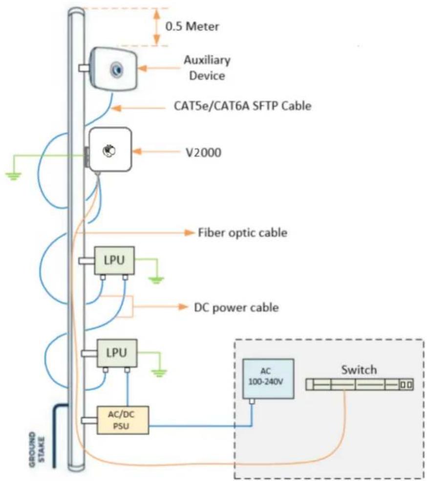
flowchart
graph TD
    A["Ground Stake"] --> B["AC/DC PSU"]
    B --> C["LPU"]
    C --> D["DC power cable"]
    D --> E["Fiber optic cable"]
    E --> F["V2000"]
    F --> G["CAT5e/CAT6A SFTP Cable"]
    G --> H["Auxiliary Device"]
    H --> I["0.5 Meter"]
    I --> J["Switch"]
Consider the following key points when installing V3000:
- Use the recommended grounding and LPU connections.
- Use the recommended cables for interfacing ODU (refer to the supported power supply and cable length details in the Power supply units (PSU) section).
- Always install the ODU 0.5 meters below the tip of the pole.
Figure 65 shows a typical installation of V3000 CN on a mast and powered through outdoor AC/DC PSU.
Figure 65: Typical installation - V3000 CN
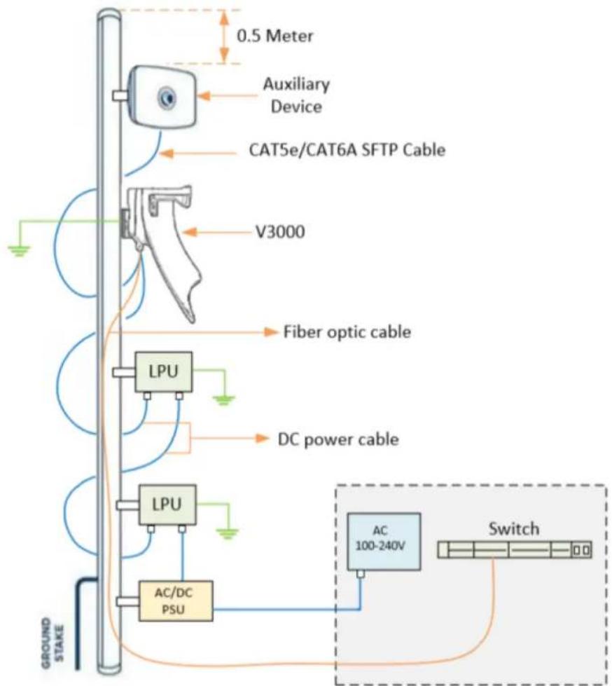
flowchart
graph TD
    A["Ground Stake"] --> B["AC/DC PSU"]
    B --> C["LPU"]
    C --> D["DC power cable"]
    D --> E["Fiber optic cable"]
    E --> F["V3000"]
    F --> G["CAT5e/CAT6A SFTP Cable"]
    G --> H["Auxiliary Device"]
    H --> I["0.5 Meter"]
    I --> J["Switch"]
    style A fill:#f9f,stroke:#333
    style J fill:#bbf,stroke:#333
Consider the following key points when installing V5000:
- Use the recommended grounding and LPU connections.
- Use the recommended cables for interfacing ODU (refer to the supported power supply and cable length details in the Power supply units (PSU) section).
- Always install the ODU 0.5 meters below the tip of the pole.
Figure 66 shows a typical installation of cnWave DN on a mast and powered through outdoor AC/DC PSU.
Figure 66: Typical installation - V5000 DN
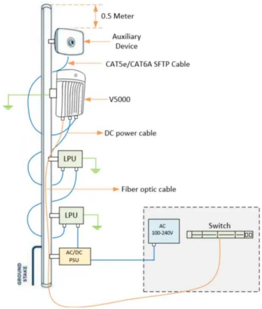
flowchart
graph TD
    A["Ground Stake"] --> B["AC/DC PSU"]
    B --> C["LPU"]
    C --> D["LC"]
    D --> E["V5000"]
    E --> F["DC power cable"]
    F --> G["Switch"]
    H["Auxiliary Device"] --> I["0.5 Meter"]
    J["Fiber optic cable"] --> K["LC"]
    L["AC 100-240V"] --> M["Switch"]
    style A fill:#f9f,stroke:#333
    style B fill:#ccf,stroke:#333
    style C fill:#cfc,stroke:#333
    style D fill:#fcc,stroke:#333
    style E fill:#ffc,stroke:#333
    style F fill:#fcc,stroke:#333
    style G fill:#cff,stroke:#333
    style H fill:#ffc,stroke:#333
    style I fill:#cfc,stroke:#333
    style J fill:#fcc,stroke:#333
    style K fill:#ffc,stroke:#333
    style L fill:#cfc,stroke:#333
    style M fill:#fcc,stroke:#333
ODU Interface with LPU on the pole
V1000:
You can install the V1000 CN on a pole. During the installation, use the 56V Gigabit Surge Suppressor for lightning protection. Ensure that the cable glands and grounding connections are made, as shown in Figure 67.
Figure 67: Installing the V1000 CN on a pole

V2000:
During the installation of V2000 CN on a pole, use the 56V Gigabit surge suppressor for lightning protection. Ensure that the cable glands and grounding connections are made, as shown in Figure 68.
Figure 68: Installing the V2000 CN on a pole
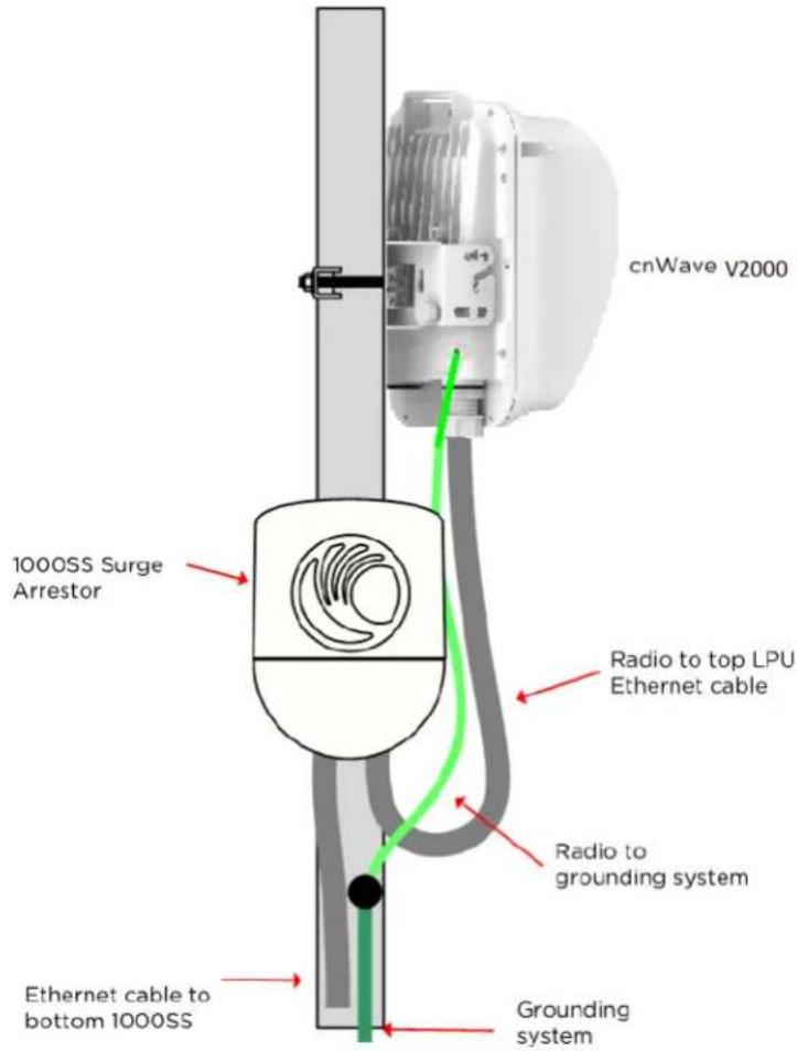
V3000:
You can install the V3000 CN on a pole using a precision bracket. During the installation, Use a recommended LPU for surge protection. Ensure glands and grounding connections are made, as shown in Figure 69.
Figure 69: Installing the V3000 CN on a pole
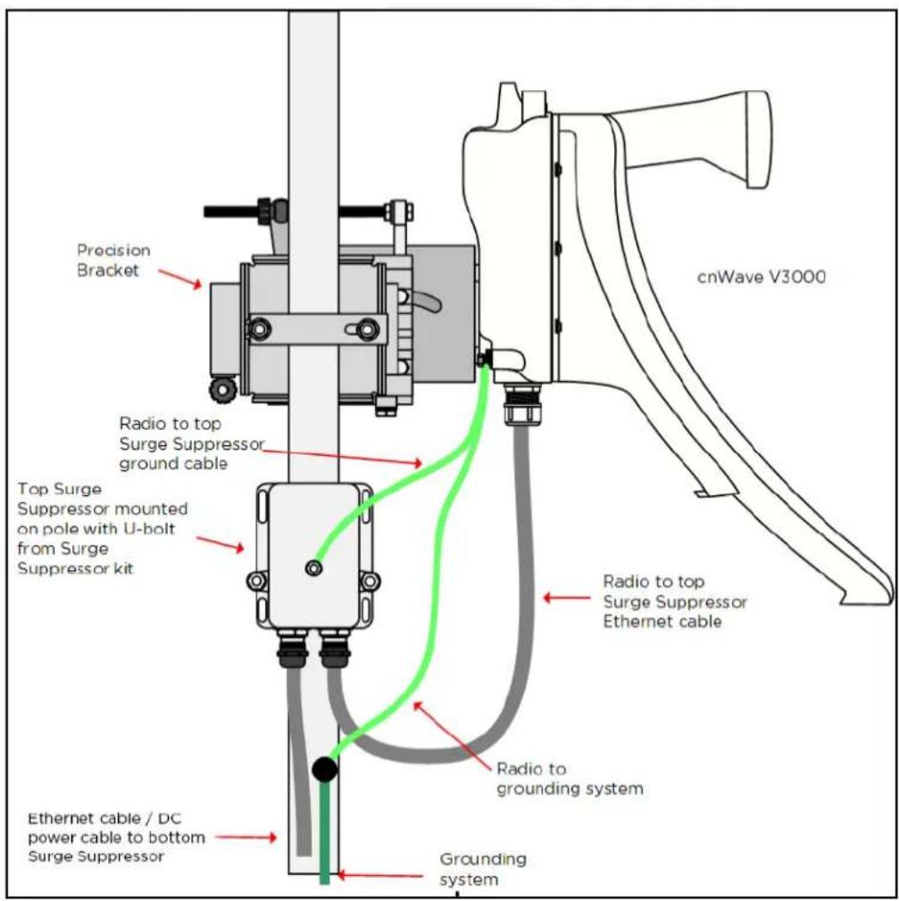
V5000:
You can install the V5000 DN on a pole using a tilt bracket. Use the recommended LPU for surge protection. Ensure glands and grounding connections are made, as shown in Figure 70.
Figure 70: Installing the V5000 DN on a pole
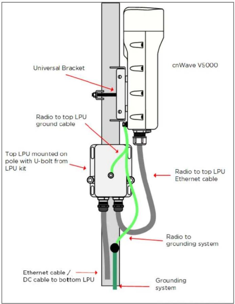
Attach ground cables to the radio
- Fasten the ground cable to the radio grounding point using the M6 lug.
Figure 71: Radio grounding point

- Tighten the ODU grounding bolt to a torque of 5 Nm (3.9 lb-ft).
Mounting the ODU
Select the most appropriate bracket mounting arrangement from the options listed in the Mounting bracket options. Refer to individual procedures below for each of the options:
• V1000 Pole mount
• V1000 Wall mount
• V1000 Adjustable pole mount
• V2000 Adjustable pole mount
• V3000 Precision bracket
• V3000 Tilt bracket assembly
• V3000 Tilt bracket assembly with band clamps
• V5000 Pole mount bracket
• V5000 Wall mount bracket
V1000 Pole mount
The V1000 CN can be installed to a pole using the supplied mounting plate and jubilee clip. Follow the below instructions to mount V1000 to the pole:
- Insert the hose clamps through the mounting plate and clamp to the pole by applying 3.0 Nm torque.
Figure 72: Inserting the hose clamps

natural_image
Two white plastic mechanical components with mounting holes and a coiled cable, shown against black background (no text or symbols)- Insert the radio into the mounting plate on the pole.
Figure 73: Inserting the radio

natural_image
Two white plastic electrical connectors mounted on black vertical posts, one with a cable and the other a rectangular component (no text or symbols visible)V1000 Wall mount
Follow the below instructions to mount V1000 on the wall:
- Fix the mounting plate (supplied with the V1000 ODU) securely to a vertical wall, using suitable fixings.

Note
Fixing hardware is not supplied with the V1000.
- Slide the V1000 ODU onto the mounting plate from above, ensuring that the spring clip in the mounting plate clicks into place on the radio.
Figure 74: Fixing the mounting plate and the spring clip

natural_image
Two views of a white plastic electrical connector with mounting holes and terminal blocks (no text or symbols visible)V1000 Adjustable pole mount
Follow the below instructions to mount V1000 to the adjustable pole:
- Insert the hose clamps through the adjustable pole mount bracket and clamp to the pole by applying 3.0 Nm torque.
Figure 75: Fixing hose clamps through adjustable pole mount bracket
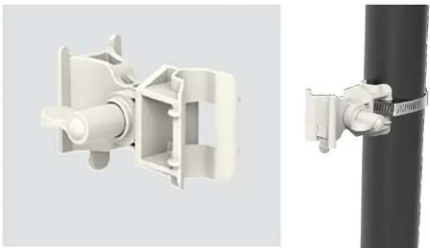
natural_image
Two technical diagrams showing a white plastic mechanical component and a black cylindrical pipe with a coiled cable (no text or symbols present)- Insert the radio into the adjustable pole mount bracket on the pole.
Figure 76: Fixing the radio on the pole

natural_image
Two mechanical clamping mechanisms mounted on vertical rods, showing different assembly configurations (no text or symbols visible)The adjustment can be made up to maximum +/- 30 degrees and each serration movement is 5 degrees.
V1000 Alignment
The V1000 CN requires minimal effort to align as the internal antenna can beam steer +/- 40 degrees in azimuth and +/- 20 degrees in elevation from boresight. If the unit is installed with the remote node visible within this range, no further adjustment is required.
V2000 Adjustable pole mount
You can install the V2000 CN on a pole using a jubilee clip (hose clamps). Perform the following steps to mount the V2000 CN on a pole:
- Insert the two hose clamps through the adjustable mounting bracket and clamp it to the pole by applying 5.0 Nm torque, as shown in Figure 77.
Figure 77: Fixing V2000 to a pole

natural_image
Two white industrial sensors mounted on vertical metal posts, showing front and side views (no text or symbols visible)- Align the device by viewing through the eye piece and the notch on radome, as shown in Figure 78.
Figure 78: Aligning the V2000 device
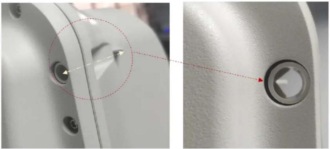
natural_image
Close-up of a mechanical component with a highlighted circular feature and a separate view showing a hexagonal bolt (no text or symbols)- Use the bracket knob (as shown in Figure 80) to rotate fine adjustable bracket until the alignment is complete in the elevation plane.
The adjustable bracket supports fine adjustment of up to +/-20° in elevation for an accurate alignment.
Figure 79: Aligning V2000

natural_image
Close-up of a medical or laboratory device with a transparent dome and vertical rod, no visible text or symbolsFigure 80: Using the adjustable bracket knob for alignment

natural_image
Mechanical assembly diagram showing a motor housing with a close-up view of its internal components (no text or symbols visible)V2000 Antenna alignment
The V2000 CN requires minimal effort to align as the internal antenna can beam steer +/-10 degrees in azimuth and +/-4.5 degrees in elevation from boresight. If the unit is installed with the remote node visible within this range, no further adjustment is required.
V3000 Precision bracket
The precision bracket is used to mount the cnWave V3000 CN on a vertical pole, providing fine adjustment up to 18° in azimuth and +/-30° in elevation for accurate alignment of the V3000. The precision bracket is compatible with pole diameters in the range of 25 mm to 70 mm (1 inch to 2.75 inches). Note that the Jubilee clamp allows for larger diameter poles and the range depends on the clamps used.
These instructions illustrate the procedure for assembling and using the precision bracket. The mounting of the optional alignment telescope also explained.
Figure 81:V3000 Precision bracket
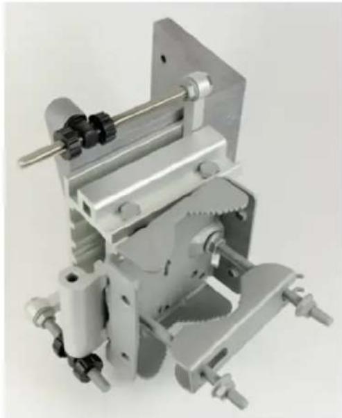
natural_image
Mechanical clamp assembly with metallic components and metal brackets (no visible text or symbols)- Insert two of the long (120 mm) screws through the azimuth arm and the bracket body. The screws are located in the slots in the azimuth arm.
Figure 82: Two screws in the slots of the azimuth arm
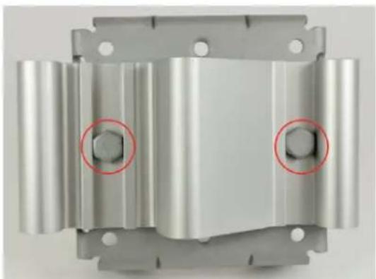
natural_image
Metal mechanical component with two red-circled holes, no visible text or symbols- Fit two flanged M8 nuts to the long screws on the back of the bracket. Tighten using a 13 mm spanner.
Figure 83: Two MB nuts on the back of bracket
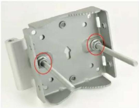
natural_image
Metal mechanical component with two red-circled holes, no visible text or symbols- Insert the three medium-length (40 mm) M8 screws through the bracket base and the V3000 mount. The screws are located in the slots in the bracket base.
Figure 84:MB Screws in the slots in the bracket base

natural_image
Close-up of a mechanical clamp or fixture with three red-circled features, no visible text or symbols.You must ensure that the pivot pin in the elevation adjuster is located in the circular hole in the V3000 mount.
Figure 85: The pivot pin in the circular hole of mount

natural_image
Close-up of a mechanical assembly with a red-circled component, no visible text or symbols- Fit plain washers and M8 Nyloc nuts to the screws on the back of the bracket base. Tighten using a 13 mm spanner.
Figure 86: Plain washers and M8 Nyloc nuts on the back of the bracket

natural_image
Mechanical component with three red-circled features, no visible text or symbols- Insert the two remaining long (120 mm) M8 screws through the bracket body and the azimuth arm. The screws must be located in the slots in the bracket body.
Figure 87:MB Screws located in the slots in the bracket body

natural_image
Mechanical assembly with metallic components and two red-circled features (no visible text or symbols)You must ensure that the pivot pin in the azimuth adjuster is located in the circular hole in the bracket body.
Figure 88: The pivot pin in the circular hole of bracket body
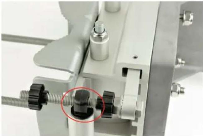
natural_image
Close-up of a mechanical clamp or clamping device with black bolts and metal components, no visible text or symbols- Fit three sets of spacers, plain washers and M8 Nyloc nuts to the screws on the underside of the bracket base. Tighten using a 13 mm spanner.
Figure 89: Fixing pacers, plain washers and M8 Nyloc nuts
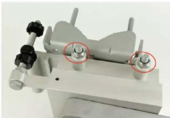
natural_image
Close-up of a mechanical clamp or fixture with two metallic bolts and a central housing (no visible text or symbols)- Attach the V3000 mount to the radio using the four short M6 bolts. Tighten the four bolts to a torque setting of 5.0 Nm (3.7 lb-ft) using a 13 mm spanner or socket.
Figure 90: Attaching the V3000 mount

natural_image
Close-up of a mechanical component with four screws and wiring, no visible text or symbols- Attach the precision bracket to the pole using the clamp and the remaining flanged nuts. Adjust azimuth approximately and tighten the nuts to 10 Nm (7.4 lbft) using a 13 mm spanner.
Figure 91: Attaching the precision bracket

natural_image
Close-up of a mechanical assembly with two red-circled bolts inserted, no visible text or symbols- Lock the antenna alignment by tightening the five Nyloc nuts (see step 5 and step 8) to 10 Nm (7.4 lb-ft) using a 13 mm spanner or socket.
Figure 92:Locking the antenna alignment
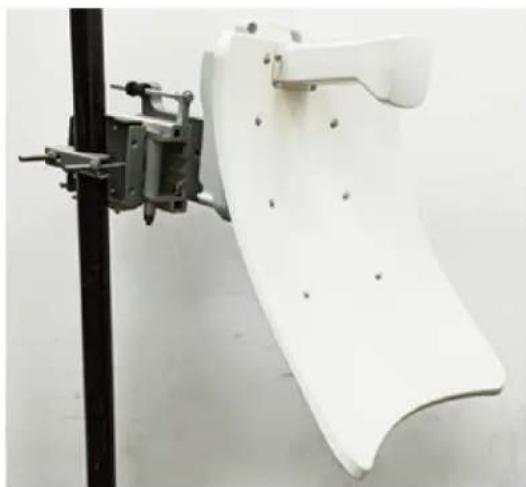
natural_image
White plastic electronic device mounted on a black vertical pole, no visible text or symbols
Note
Visit the Cambium Learning website to learn more about the precision bracket assembly.
Precision bracket alignment
- Ensure that the three Nyloc screws for securing the bracket in elevation are loose and the fine elevation adjuster is holding the weight of the unit.
Figure 93: Three Nyloc screws on the unit
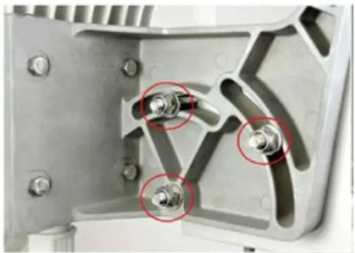
natural_image
Close-up of a mechanical component with three red-circled features, no visible text or symbols- Ensure the two Nyloc screws securing the bracket in the azimuth are loose.
Figure 94: Two Nyloc screws in the azimuth
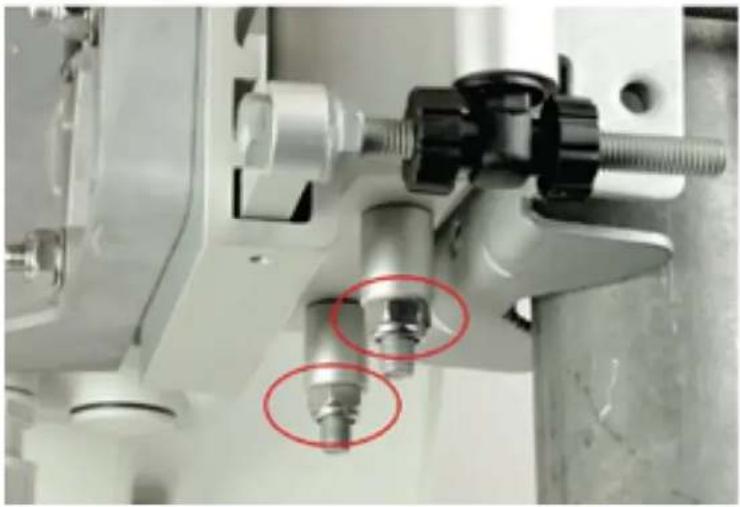
natural_image
Close-up of a mechanical assembly with two red-circled features, no visible text or symbols- Before starting the mechanical alignment, move the fine elevation adjuster 2/3 of the way across the screw until the unit is sitting at approximately 0 degrees in elevation.
Figure 95: Moving the elevation adjuster
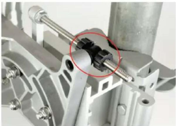
natural_image
Close-up of a mechanical assembly with a red-circled component, showing internal components and mounting holes (no text or symbols visible)- Move the fine azimuth adjuster to approximately the center of the available range and lock it in position.
Figure 96: Moving the azimuth adjuster

natural_image
Close-up of a mechanical assembly with threaded components and a red-circled detail (no visible text or symbols)-
Loosen the clamp which attaches the bracket to the pole until there is enough freedom to rotate the unit in azimuth.
-
From behind the unit, using the sight to aim towards the remote node, rotate the unit until it is approximately aligned in azimuth. Tighten the clamp.
-
While looking for the far node through the site, rotate the fine elevation adjuster until the alignment is complete in the elevation plane. One turn of the adjustment wheel is equivalent to approximately one degree of elevation. Lock the fine elevation adjuster screws in place.
Figure 97: Locking the fine elevation adjuster
natural_image
White plastic chair with ribbed side panels, set against a blue sky and green field (no text or symbols visible)You can use the alignment tube for adjustment, as described in Fixing the alignment tube.
-
While looking for the far node through the site, rotate the fine azimuth adjuster until the alignment is complete in the azimuth plane. One turn of the adjustment wheel is equivalent to approximately one degree of azimuth. Lock the fine azimuth adjuster screws in place.
-
Make any remaining adjustments to the elevation and azimuth as required. Once complete, tighten the three Nyloc screws in place to fix the elevation alignment and do the same for the two Nyloc screws for azimuth alignment to 10 Nm (7.4 lbft) using a 13 mm spanner or socket.
Precision bracket alignment - optional telescope
-
Attach the telescope mount to the V3000 radio using the knurled screw.
-
Attach the telescope by looping the two elastic O-rings over the ears of the mount, ensuring that the telescope is located securely in the mount.
Figure 98: Attaching the telescope

natural_image
Three-panel image showing a microscope setup with labeled parts (1a, 1b, 2), no visible text or symbols beyond labels.-
If a telescope with a smaller body is used, shorten the O-rings by twisting
-
Following the previously described precision bracket alignment method, align the radio starting with the site, and fine-tune using the scope for increased accuracy.
Fixing the alignment tube for V3000
Perform the following steps to fix the alignment tube for V3000:
- Slide the alignment tube through the alignment slot, as shown in Figure 99.
Figure 99: Sliding the alignment tube
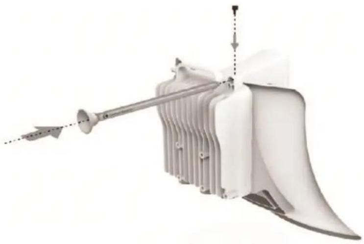
natural_image
3D rendering of a mechanical component with directional arrows indicating motion or force (no text or symbols)- Tighten the screw to fix the alignment tube in place, as shown in Figure 100. The tube fits into the circular area.
Figure 100: Fixing the alignment tube
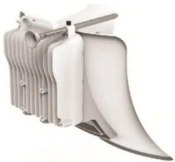
natural_image
3D rendering of a white mechanical component with ribbed and curved surfaces (no text or symbols visible)- Align the device by viewing through the eyepiece, as shown in Figure 101.
Figure 101: Aligning the device

natural_image
Close-up of a metallic megaphone with a star-shaped knob, mounted on a stand (no text or symbols visible)V3000 Tilt bracket assembly
- Fix the mounting plate of the tilt bracket to the back of the radio using four of the short bolts, ensuring that the arrow in the plate points towards the top of the radio. Tighten the four bolts to a torque setting of 5.0 Nm (3.7 lb-ft) using a 13 mm spanner or socket.
Figure 102: Fixing the mounting plate of the tilt bracket

natural_image
Close-up of a metallic industrial heat exchanger housing with four red-circled mounting holes (no text or symbols visible)- Fit the two long bolts through the bracket body so that the bolt heads engage in the slots as shown. Fit two of the short bolts into the side of the bracket body but do not tighten.
Figure 103: Fixing two long and short bolts

natural_image
Close-up of a mechanical component with two circular red circles highlighting features, no visible text or symbols.- Thread two of the nuts to the long bolts and tighten against the bracket body using a 13 mm spanner. Fit the bracket strap and thread the remaining nuts onto the long bolts.
Figure 104: Fixing the bracket strap

natural_image
3D model of a metal bracket with three red-circled fasteners inserted (no text or symbols visible)- Fix the assembled bracket body to the pole, adjust the azimuth angle, and tighten the nuts to a torque setting of 10.0 Nm (7.4 lb-ft) using a 13 mm spanner, ensuring that the arrow in the body is pointing upwards.
Figure 105: Fixing the assembled bracket body

natural_image
Close-up of a metal bracket with two red-circled fasteners securing a bolt (no text or symbols visible)- Fit the mounting plate to the bracket body by positioning the open-ended slots over the short bolts. Insert the remaining short bolts through the longer curved slots into the threaded holes in the bracket body. Adjust the elevation angle and tighten the bolts to a torque setting of 5.0 Nm (3.7 lb-ft) using a 13 mm spanner or socket.
Figure 106: Fixing the mounting plate and adjusting the elevation

natural_image
Close-up of mechanical components with red circles highlighting features, no visible text or symbolsV3000 Tilt bracket assembly with band clamps
Follow the below instructions to assemble the tilt bracket with band clamps:
- Follow step 1 of the V3000 tilt bracket assembly procedure.
- Feed the band clamps through the slots in the bracket body. Secure the bracket body to the pole using band clamps (not supplied by Cambium), ensuring that the arrow in the body is pointing upwards. Adjust the azimuth angle and tighten the band clamps to a torque setting of 6.0 Nm (4.5 lb-ft).
- Fix the mounting plate to the bracket body with four of the short bolts, using a 13 mm spanner or socket. Adjust the elevation angle and tighten the bolts to a torque setting of 5.0 Nm (3.7 lb-ft).
Figure 107: Fixing the mounting plate of bracket body and adjusting the elevation angle

natural_image
Close-up of mechanical components with red-circled annotations, no visible text or symbolsV5000 Pole mount bracket
- Pass the long screws through the bracket body. The screws are located in the recess in the bracket.
- Fit two flanged nuts to the long screws on the back of the bracket. Tighten using a 13 mm spanner.
- Fix the bracket to the back of the radio using the four short M6 bolts, ensuring that the arrow in the plate points towards the top of the radio. Tighten the four bolts to a torque setting of 5.0 Nm (3.7 lb-ft) using a 13 mm spanner or socket.
- Attach the pole-mount bracket to the pole using the clamp and the remaining flanged nuts. Adjust azimuth and tighten the nuts to 10 Nm (7.4 lbft) using a 13 mm spanner.
Figure 108: Fixing the V5000 pole mount bracket

V5000 Alignment
The V5000 distribution node has two sectors, situated side by side, each covering a 140-degree range in azimuth, giving a combined coverage of 280 degrees. In elevation, the antenna can beam steer in a +/- 20-degree range. The boundary between where Sector 1 ends and Sector 2 begins is the centerline/boresight from the unit.
Figure 109:V5000 alignment - Top view
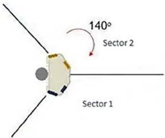
V5000 Wall mount bracket
- Install the mounting plate of the wall mount bracket securely on a vertical wall, using suitable fixing hardware.

Note
Fixing hardware is not supplied with the wall mount bracket.
- Fix the bracket body to the back of the radio using the four short M6 bolts, ensure that the arrow in the plate points towards the top of the radio. Tighten the four bolts to a torque setting of 5.0 Nm (3.7 lb-ft) using a 13 mm spanner or socket.
- Insert the four short M8 bolts into the sides of the bracket body.
- Fit the bracket body to the mounting plate by positioning the short bolts into the open-ended slots. Tighten the bolts to a torque setting of 5.0 Nm (3.7 lb-ft) using a 13 mm spanner or socket.
Figure 110: Fixing the V5000 wall mount bracket

natural_image
Three-panel image showing a white plastic electrical enclosure with red circular annotations highlighting bolt holes, alongside its close-up view of the internal structure (no text or symbols present)Connect to the PSU port of the radio Using Power over Ethernet (PoE)
- Disassemble the gland and thread each part onto the cable (the rubber bung is split). Assemble the spring clip and the rubber bung.
Figure 111: Assembling the spring clip and the rubber bung
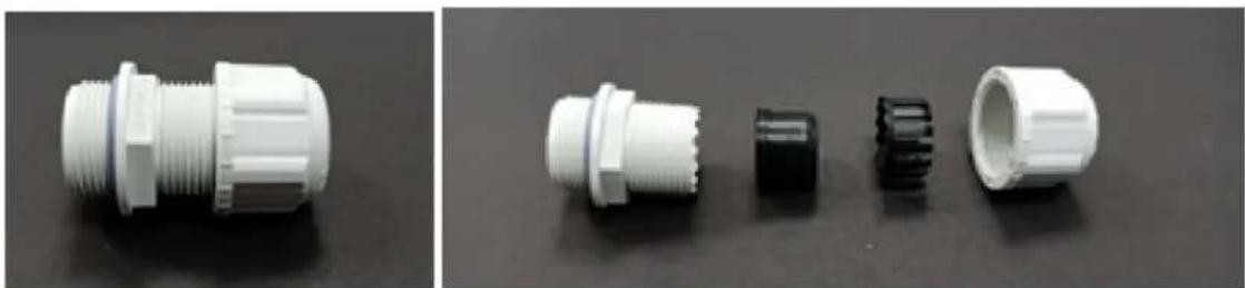
natural_image
Two views of a white plastic connector with threaded and segmented parts, shown from different angles (no text or symbols visible)- Fit the parts into the body and lightly screw on the gland nut (do not tighten it).
Figure 112: Fixing the gland nut
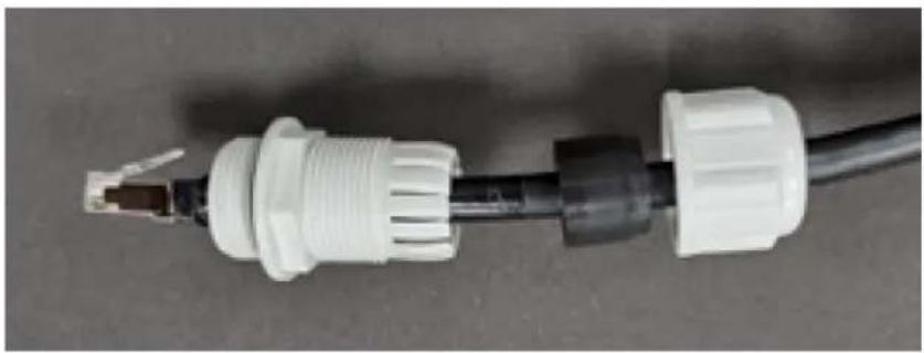
natural_image
Close-up of a white plastic electrical plug with a black connector and metal connector (no text or symbols visible)- Connect the RJ45 plug into the main PSU port of the ODU (which can be either V1000, V2000, V3000, or V5000).
Figure 113: Connecting the RJ45 plug
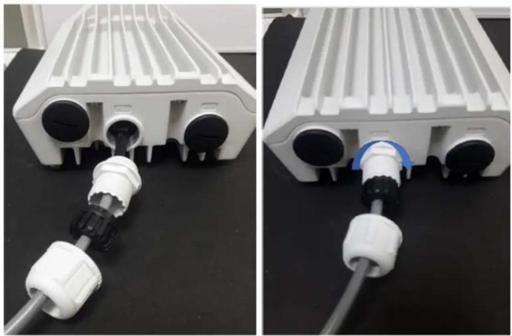
natural_image
Two views of a white industrial device with black connectors, showing internal wiring and mounting points (no text or symbols visible)- Rotate the gland clockwise to tightly fit the gland on the PSU port.

Warning
Ensure that the cable clamp is not attached/ tightened at this stage, this may cause damage to the RJ45 or PCB.
Figure 114: Rotating the gland
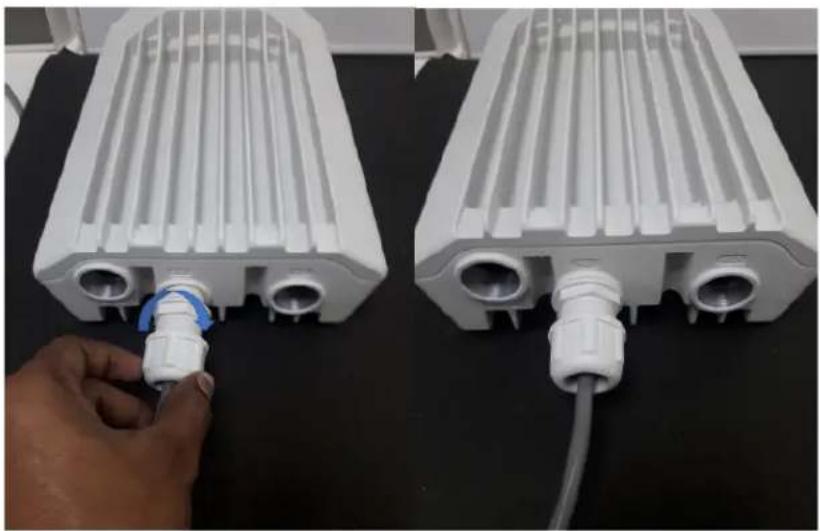
natural_image
Close-up of a white heat exchanger component being inserted into a blue plastic outlet, with a hand adjusting the port (no text or symbols visible)- Tighten the gland (cap or nut), this must be done last. Otherwise, it may damage the RJ45 or PCB.
Disconnecting drop cable from the radio
- Loosen and remove the cable clamp by rotating anti-clockwise from the PSU port.
Figure 115:Removing the cable clamp

natural_image
Hand inserting a white plastic plug into a white cylindrical component, no text or symbols visible
Warning
Loosen the cable clamp completely and then unscrew the gland. Not releasing the cable may cause damage to the RJ45 socket and/or PCB.
- Remove the gland.
Figure 116:Removing the gland

natural_image
Close-up of a white plastic electrical connector with black connectors and a coiled cable (no text or symbols visible)
natural_image
Close-up of a hand inserting a plug into a white industrial device component (no visible text or symbols)-
Press tab on RJ45 plug to remove the cable from PSU port.
-
Remove the latch of the RJ45 plug to remove the cable from the PSU port.
Figure 117:Removing the latch of the RJ45 plug

natural_image
Hand inserting a white plastic plug into a white rack-mounted device (no text or symbols visible)Using AC/DC PSU
Cable joiner
A cable joiner is used to connect the wires. Insert the wires into the cable joiner by loosening the screws on the joiner.
Figure 118:Cable joining parts

natural_image
Set of seven black plastic connectors with threaded heads, shown from different angles (no text or symbols visible)Figure 119 is an example of connecting wires using the cable joining parts.
Figure 119: Connecting wires

natural_image
Exploded view of a black plastic electrical connector with multiple ports and connectors (no text or symbols visible)
natural_image
Close-up of a black plastic electrical connector with a metal screw being inserted (no text or symbols visible)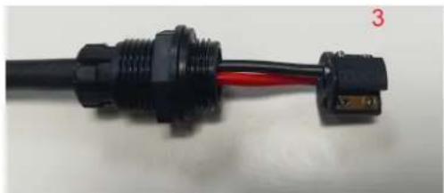
natural_image
Close-up of a black electrical connector with red insulation, attached to a terminal block (no text or symbols visible)
natural_image
Close-up of two black plastic electrical connectors with red and blue wires, no visible text or symbols
natural_image
Close-up of a black plastic electrical connector with red pin, attached to a curved cable (no text or symbols visible)Figure 120:Mini adapter connections

Fitting the long cable gland
Figure 121:The long cable gland

natural_image
Close-up of a white plastic electrical plug with black connectors and red wires, placed on a green surface (no text or symbols visible)Connecting the mini adapter to ODU
- Plug the input side of the AC/DC PSU to the AC power line and tighten the gland. Tighten the cable clamp cap.
Figure 122: Connecting the input side of AC/DC PSU

natural_image
White industrial ventilation unit mounted on a green surface, connected to a black connector (no visible text or symbols)- Connect output side of DC PSU to ODU through cable joiner and DC mini adapter.
Figure 123: Connecting the output side of AC/DC PSU

natural_image
White industrial fan with cooling fins connected to a black electrical component (no visible text or symbols)Install the PSU
Install one of the following types of PSU:
• Installing the 60W DC power injector
• Installing the AC/DC PSU
• Installing 15W or 30W power injector
Table 40: Details of PoE injector to be used for cnWave 60 GHz products
| Product Without AUX POE Enabled With AUx | POE enabled |
| V1000 15W Not | applicable |
| V2000 30W 60W | |
| V3000 60W 60W | |
| V5000 60W 100W |

Warning
Always use an appropriately rated and approved AC supply cord-set in accordance with the regulations of the country of use.

Attention
As the 60W DC power injector and V1000 power injector are not waterproof, locate it away from sources of moisture, either in the equipment building or in a ventilated moisture-proof enclosure. Do not locate the PSU in a position where it may exceed its temperature rating.

Attention
Do not plug any device other than a 60 GHz cnWave ODU into the ODU port of the PSU. Other devices may be damaged due to the non-standard techniques employed to inject DC power into the Ethernet connection between the PSU and the ODU.
Do not plug any device other than a Cambium 60 GHz cnWave PSU into the PSU port of the ODU. Plugging any other device into the PSU port of the ODU may damage the ODU and device.
Installing the 60W DC power injector
- Connect the input side of the DC power injector to the AC power line.
Figure 124:60W DC power injector and powering diagram


flowchart
graph TD
    A["56V,10G PoE"] --> B["Monitor"]
    B --> C["V3000/V5000"]
    C --> D["SFP+ 10G"]
    C --> E["Aux POE Out (1G)"]
- Connect 10 Gbe LAN port of the power injector to network equipment.
- Connect 60 W 56V 10 GbE PoE port of the power injector to ODU drop cable (ODU can be either V3000 or V5000).

Note
For V2000, use the 60 W device, especially when POE Out is required, and the 5 GbE PoE (000000L142A).
Figure 125: Connecting the power injector to ODU drop cable

natural_image
Close-up of a white LED flash unit connected to a black cable, no visible text or symbolsInstalling the AC/DC PSU
- Connect the input side of the AC/DC PSU to the AC power line.
- Connect output side of DC PSU to ODU through cable joiner and DC mini adapter. Refer to the Cable joiner section for connecting, installing cable joiner and mini adapter.
Figure 126:AC/DC PSU (N000000L179B)

Figure 127: Cable joiner

natural_image
Close-up of a black plastic electrical connector with multiple connectors (no visible text or symbols)Figure 128:DC to RJ45 plug, mini adapter

natural_image
Close-up of a black USB connector with blue and green connectors (no text or symbols visible)Figure 129:AC/DC powering diagram
Figure 130:AC/DC PSU

flowchart
graph TD
    A["Switch"] --> B["DC PSU"]
    B --> C["SFP/SFP+ 10G"]
    C --> D["V5000/V3000"]
    D --> E["Aux POE Out (1G)"]
    F["Ground"] --> B

natural_image
White portable heater with cooling fins connected to a black electrical terminal block (no visible text or symbols)For detailed assembly of cable joiner and mini adapter to ODU PSU port, refer to the Cable joiner section.

Note
Both short and long glands can be used to connect to outdoor PSU.
Installing 15W or 30W power injector
- Connect the 56V Gigabit Data and power port to ODU (which can be either V1000 or V2000)
Figure 131:V1000 Power injector

Figure 132:V2000 Power injector
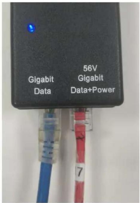

Note
30 W (N000000L034B) supports up to 5 GbE.
Figure 133: V1000 or V2000 Powering diagram

flowchart
graph TD
    A["Monitor"] -->|a| B["5GbE PoE (V1000)/5GbE PoE (V2000)"]
    B -->|b| C["Charging Station"]
    C -->|c| D["Power Line"]
    D -->|d| E["V1000/V2000"]
Figure 134: Connecting the V1000 Power injector Figure 135: Connecting the V2000 power injector
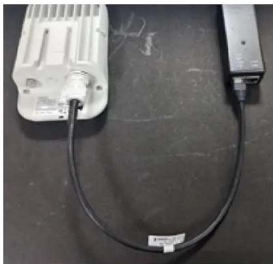
natural_image
Close-up of a white electrical component with a black cable attached, placed on a dark surface (no visible text or symbols)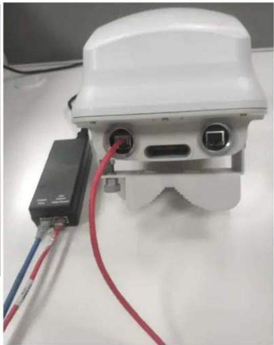
natural_image
White electronic device with attached black and red cables, placed on a white surface (no visible text or symbols)- Connect the Gigabit data port to the network equipment.
Connecting to the SFP+ optical module or SFP+ to the copper module to ODU
When ODU is powered through AC/DC PSU, an optical or copper Cat6A Ethernet interface can be connected to the SFP port of the ODU for the data interface.
Adapt the installation procedures in this section as appropriate for SFP interfaces, noting the following differences from a PSU interface.
Fitting the long cable gland
Optical SFP interface: Disassemble the long cable gland and thread its components over the LC connector at the ODU end as shown below.
Copper CAT6A SFP interface: Disassemble the cable gland and thread its components over the RJ45 connector at the ODU end.
- Disassemble the long cable gland used for the optical SFP interface.
Figure 136: Disassembling the long cable gland - optical SFP interface

natural_image
Two white plastic connectors with threaded ends and a separate black plastic component, shown against a dark background (no text or symbols visible)You must also disassemble the long cable gland used for the copper SFP interface.
Figure 137: Disassembling the long cable gland - copper SFP interface

natural_image
Four types of plastic connectors shown from different angles, including a white plastic fitting and black plastic components (no text or symbols visible)- Thread each part onto the cable (the rubber bung is split).
Figure 138: Threading the part onto the cable

natural_image
Close-up of a white plastic electrical plug with a black plastic housing and a yellow connector, showing internal wiring (no text or symbols visible)- Fit the parts into the body and lightly screw on the gland nut (do not tighten it).
Figure 139: Fixing parts to the gland
Optical

natural_image
Close-up of a white plastic electrical connector with threaded leads and terminal connectors (no visible text or symbols)Copper

natural_image
Close-up of a white plastic electrical connector with black and white plastic caps, no visible text or symbolsInserting the SFP module
To insert the SFP module into the ODU, follow the below steps:
- Remove the blanking plug from the SFP port of the ODU.
Figure 140:Removing the blanking plug from the SFP port
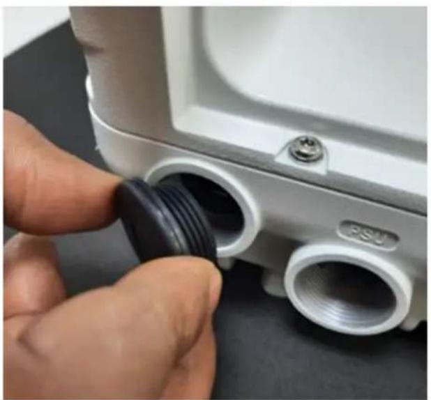
natural_image
Close-up of a hand inserting a black plastic plug into a white cylindrical device with labeled ports (no text or symbols visible)Optical SFP+ module
Copper SFP module


- Insert the SFP module into the SFP receptacle with the label on the bottom.
Figure 141: Inserting the SFP module
Optical
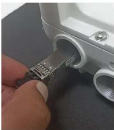
natural_image
Close-up of a hand inserting a small electronic component into a device housing (no visible text or symbols)Copper

natural_image
Close-up of a hand inserting a metallic USB into a mechanical component (no visible text or symbols)- Push the module home until it clicks into place.
Figure 142:Pushing the module home
Optical
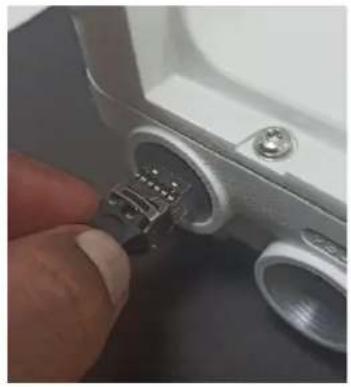
natural_image
Close-up of a hand inserting a small metallic connector into a mechanical housing (no text or symbols visible)Copper

natural_image
Close-up of a hand inserting a small electronic component into a device housing (no visible text or symbols)- Rotate the latch to the locked position.
Figure 143: Rotating the latch
Optical

natural_image
Close-up of a camera lens component with metallic exposure (no visible text or symbols)Copper

natural_image
Close-up of a finger inserting a USB into a small electronic device (no visible text or symbols)Connecting the cable

Attention
The Fiber optic cable assembly is very delicate. To avoid damage, handle it with extreme care. Ensure that the fiber optic cable does not twist during assembly, especially when fitting and tightening the weatherproofing gland. Do not insert the power over Ethernet drop cable from the PSU into the copper SFP module, as this will damage the module.
- Remove the LC connector dust caps from the ODU end (optical cable only).
Figure 144:Removing the LC connector dust caps
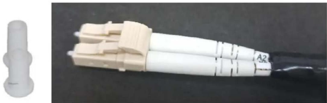
natural_image
Close-up of a white medical or laboratory device with attached connectors, next to a small white plastic component (no visible text or symbols)- Plug the connector into the SFP module, ensuring that it snaps home.
Figure 145: Plugging the connector into the SFP module
Optical

natural_image
Close-up of a hand inserting a plug into a device socket (no visible text or symbols)Copper

natural_image
Close-up of a hand inserting a small electronic component into a mechanical housing (no visible text or symbols)Fitting the gland
- Fit the gland body to the SFP port and tighten it to a torque of 5.5 Nm (4.3 lb-ft).
Figure 146: Fitting the land body
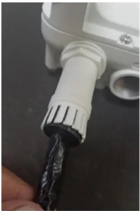
natural_image
Close-up of a hand holding a black plastic plug inserted into a white plastic connector (no text or symbols visible)- Fit the gland nut and tighten until the rubber seal closes on the cable. Do not over-tighten the gland nut, as there is a risk of damage to its internal components.
Figure 147: Fitting the gland nut

natural_image
Close-up of a hand inserting a white plastic plug into a black cable, with a yellow curved arrow indicating rotation (no text or symbols visible)- Fit the gland nut to the rubber seal on the gland body and tighten it to a torque of 5.5 Nm (4.3 lb-ft).
Figure 148: Fitting the gland nut to the rubber seal

natural_image
Close-up of a hand inserting a black cable into a white plastic plug (no text or symbols visible)Removing the cable and SFP module
Do not attempt to remove the module without disconnecting the cable, otherwise, the locking mechanism in the ODU will be damaged.
- Remove the cable connector by pressing its release tab before pulling it out.
Figure 149:Removing the cable connector
Optical
natural_image
Close-up of a car's electrical plug inserted into a terminal block (no visible text or symbols)Copper
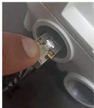
natural_image
Close-up of a finger inserting a small electronic component into a socket (no visible text or symbols)- Pull the bale clasp (latch) to the unlocked position. Extract the module by using a screwdriver.
Figure 150: Pulling the bale clasp (latch)
Optical
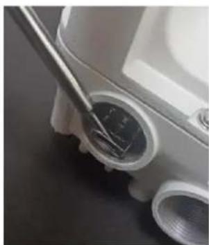
natural_image
Close-up of a mechanical component with a metal tool inserted, showing internal components (no visible text or symbols)Copper

natural_image
Close-up of a mechanical component with a metallic tool inserted, showing internal wiring and a small copper-colored connector (no text or symbols visible)This topic explains how to configure the 60 GHz cnWave products.
Nodes deployment
The configuration of cnWave nodes is handled automatically by the E2E service. However, the first PoP node must be configured manually since connectivity to the E2E controller has not yet been established. After establishing communication with the E2E controller, the nodes report a hash of their local configuration file, and the controller automatically pushes configuration changes to the nodes upon seeing any mismatches. The centralized configuration management architecture is implemented in which the E2E controller serves as the single point for configurations in the network.
Figure 151: Nodes deployment

flowchart
graph TD
    A["PoP DN"] -->|1 connects| B["E2E"]
    B -->|2 Push Config| A
    C["DN2"] -->|2 Association Request| D["PoP DN1"]
    D -->|3 connects| C
    D -->|1 pairing| E["E2E"]
    E -->|Provision: MAC of DN2| F["Provision: MAC of CN1"]
    F -->|Create link: 1. MAC of DN1 Radio, 2. MAC of DN2 Radio| E
    G["CN1"] -->|2 Association Request| H["DN2"]
    H -->|3 connects| G
    H -->|1 pairing| I["POP DN1"]
    I -->|4 Push Config| G
    J["E2E"] -->|Push Config| A
    K["Polarity and Tx/Rx Golay index are sent over association request."] --> L["E2E URL and means to talk to E2E"]
    M["PoPDN MAC"] --> N["E2E"]
Connecting to the unit
This section describes how to connect the unit to a management PC and power it up.
Configuring the management PC
Use this procedure to configure the local management PC to communicate with the 60 GHz cnWave devices. Procedure:
- Select Properties for the Ethernet port. In Windows 7 this is found in Control Panel > Network and Internet > Network Connections > Local Area Connection.
- Select Internet Protocol Version 4 (TCP/IPv4).
Figure 152:The Ethernet Properties dialog box
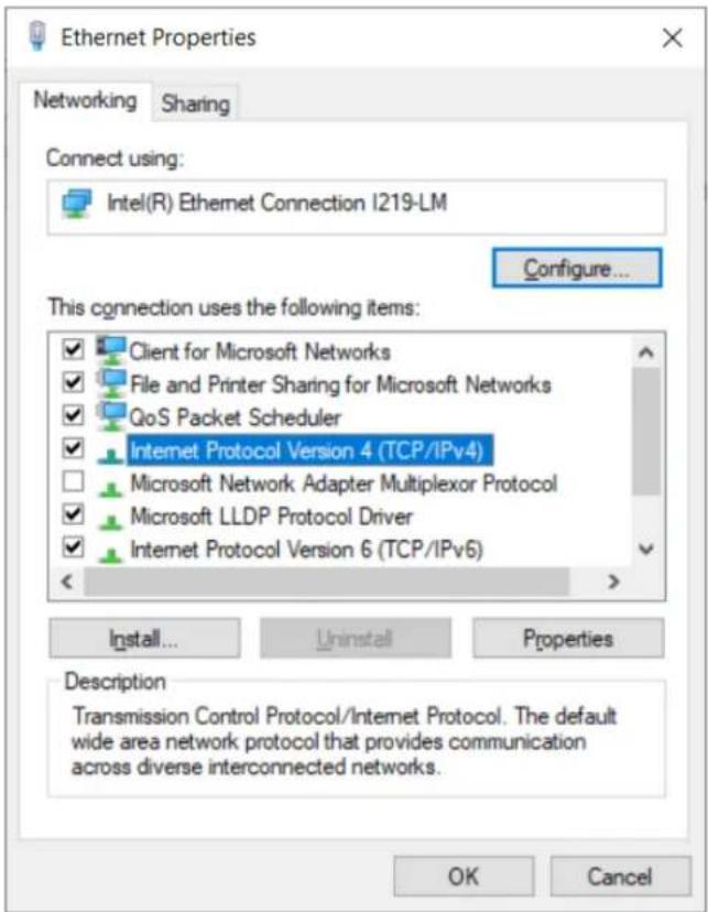
- Click Properties.
- Enter an IP address that is valid for the 169.254.X.X/16 network, avoiding 169.254.1.1 (for example: 169.254.1.3).
Figure 153: The Internet Protocol Version 4 (TCP/IPv4) dialog box

- Enter a subnet mask of 255.255.0.0. Leave the default gateway blank.
Connecting to the PC and powering up
Use this procedure to connect a management PC and power up the 60 GHz cnWave devices.
Procedure:
- Check that the ODU is connected to the power supply (AC/DC according to the configuration).
- Connect the PC Ethernet port to the LAN port of the PSU or AUX port (according to device configuration).
- Open a web browser and type: 169.254.1.1.
- When prompted, enter admin/admin to login to the GUI and complete the configuration.
Using the web interface
This section describes how to log into the 60 GHz cnWave web interface and use its menus.
Logging into the web interface
Use this procedure to log into the web interface as a system administrator.
Procedure:
- Start the web browser from the management PC.
- Type the IP address of the unit into the address bar. The factory default IP address is 169.254.1.1 and press Enter.
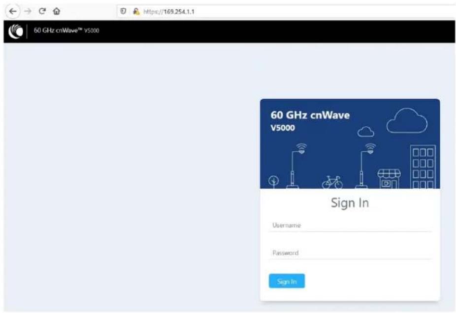
- Type the username and password as admin and admin. Click Sign In.

The Dashboard page appears.
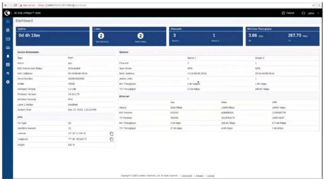
Users can select the refresh time interval. Click admin at the top-right and select the Refresh Interval from the drop-down.
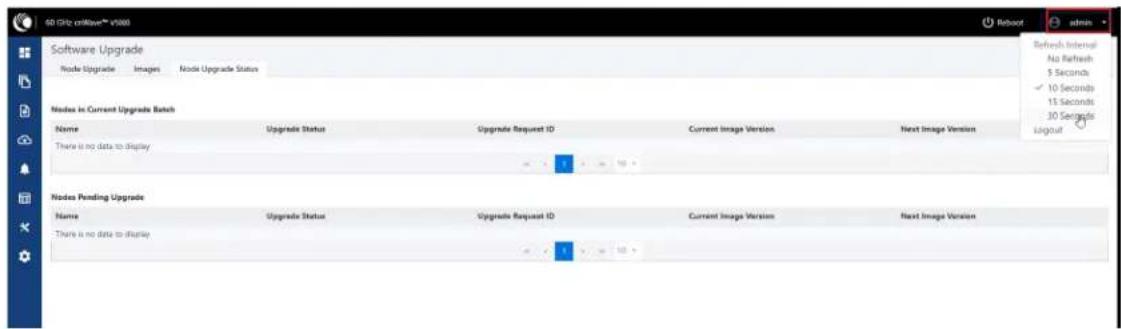
The Dashboard contains the following options at the top:
- Uptime
- Links
- Channels
- Wireless Throughput
Uptime
Displays the total running time of the device.
Links
Displays the total number of active links which are connected to the 60 GHz cnWave™ device.
Channels
Displays the total number of channels (Sector 1, Sector 2, etc.,) which are connected to the 60 GHz cnWave™ device.
Wireless Throughput
Displays the transmitting and receiving throughput values.
Dashboard elements
The Dashboard page consist of the following elements:
• Device Information
• GPS
- Sectors
- Ethernet
Figure 154: Dashboard - Device Information
| Device Information | |
| Type | DN |
| Name | - |
| E2E Connection Status | Not Onboarded |
| MAC Address | 00:04:56:88:31:21 |
| Serial Number | V5WH004ZNX7V |
| Model | V5000 |
| Software Version | 1.0-dev12 |
| Firmware Version | 10.11.0.70 |
| Wireless Security | None |
| Layer 2 Bridge | Disabled |
| System Time | Nov 5, 2020, 12:12:57 PM |
Table 41: Elements in the Device Information section
| Element Description | |
| Type Displays type of the device. The device types are:DNPoP DNCN | |
| Name Displays name of the device. | |
| E2E Connection Status Displays the connection status of the E2E controller. | |
| MAC address Displays the MAC address of the 60 GHz cnWave device. | |
| Serial Number Displays the serial number of the 60 GHz cnWave device | |
| Model Displays the model of the 60 GHz cnWave device. The models are: | |
| V1000V2000V3000V5000 | |
| Software version Displays the software version used in 60 GHz cnWave device. | |
| Firmware version Displays the Firmware version used in 60 GHz cnWave device. | |
| Wireless security Displays the security type. The types are:DisabledPSK802.1X | |
| Layer 2 Bridge Displays bridge status. | |
| System Time Displays current time. | |
GPS
The GPS section displays the positioning information of the site.
Figure 155: Dashboard - GPS
| GPS | |
| Fix Type | 3D |
| Satellites tracked | 15 |
| Latitude | 12° 56' 2.163" N |
| Longitude | 77° 41' 39.912" E |
| Height | 927 m |
Table 42: Elements in the GPS section
| Element Description | |
| Fix Type Fix Type | |
| Satellites tracked Number of registered | satellites |
| Latitude Displays latitude of the site | |
| Longitude Displays longitude of the site | |
| Height Displays height of the device |
Sectors
The Sectors section displays the number of nodes added to the device and its information.
Figure 156: Dashboard - Sectors
| Sectors | ||
| Sector 1 | Sector 2 | |
| Channel | 3 | 4 |
| Sync Mode | RF | RF |
| MAC Address | 12:04:56:88:31:21 | 22:04:56:88:31:21 |
| Active Links | 0 | 0 |
| RX Throughput | 0 kbps | 0 kbps |
| TX Throughput | 0 kbps | 0 kbps |
Table 43: Elements in the Sectors section
| Element Description | |
| Channel Displays the channel information used by the sector | |
| Sync mode Displays the sync mode of the sectors | |
| MAC address Displays the MAC address of the sectors | |
| Active links Displays the number of active links in connected sectors | |
| RX Throughput Displays RX Throughput of the individual sectors | |
| TX Throughput Displays TX Throughput of the individual sectors | |
Ethernet
The Ethernet section displays the information about Aux, Main, and SFP ports.
Figure 157: Dashboard - Ethernet
| Ethernet | |||
| Aux | Main | SFP | |
| Status | 1000 Mbps | 10000 Mbps | 10000 Mbps |
| RX Packets | 637166 | 445648283 | 1250718835 |
| TX Packets | 777923 | 3983518625 | 109768893 |
| RX Throughput | 14.46 kbps | 348.40 Mbps | 974.40 Mbps |
| TX Throughput | 28.78 kbps | 4.84 Gbps | 3.65 Mbps |
Table 44: Elements in the Ethernet section
| Element Description | |
| Status Displays the speed of | Ethernet ports |
| RX Packets Number of packets received | |
| TX Packets Number of packets transmitted | |
| RX Throughput Displays the | RX Throughput of the Ethernet |
| TX Throughput Displays the | TX Throughput of the Ethernet |
Enabling internal E2E Controller
E2E Controller handles important management functions such as link bring-up, software upgrades and configuration management.

Note
The internal E2E controller is not required if you want to run the E2E controller On-Premise platform. For details, refer to the 0 GHz E2E Controller User Guide
Currently, the internal E2E controller is restricted to 31 nodes.
To enable E2E Controller to configure and establish the connection, perform the following steps:
- Click the E2E Controller option on the left pane of the Dashboard.

- Click Enable E2E.
The Enable Onboard E2E dialog box appears.

- Enter the required details and click Enable.
- After enabling E2E Controller, the dashboard displays the links which are connected to the device.
Figure 158: Dashboard

Right-click on the site pin to see additional information about the site, as shown below:

Topology
After enabling the E2E Controller, add Sites, Nodes and Links to establish the connection.
To add sites, nodes and links, perform the following steps:
- In the main dashboard page, click Topology on the left navigation pane.
The Topology page appears. By default, the Sites tab is selected, as shown below:
Figure 159:The Sites page
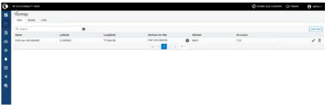
- To add a DN site, click Add New.
The Add Site dialog box appears, as shown below:
Figure 160:The Add Site dialog box

- Enter the Name, Latitude, Longitude, Altitude, Accuracy information, and click Save.
The new DN site information gets added to the topology, as shown below:
Figure 161: The updated Sites page with new site details
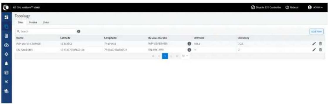
- To add a DN node, click on the Nodes tab in the Topology page.
The Nodes page appears, as shown below:
Figure 162:The Nodes page

- Click Add New and provide values in the Add Node dialog box, as shown below:
Figure 163:The Add Node dialog box

- Click Save.
The DN node gets added to the topology.
- To add a link, click on the Links tab in the Topology page.
The Links page appears.
- Click Add New and provide values in the Add Link dialog box, as shown below:
Figure 164:The Add Link dialog box

9. Click Save.
The new link gets added to the topology, as shown below:
Figure 165: The updated Links page with the new link details

Support for renaming nodes
A node can be renamed in the topology. To rename the node, perform the following steps:
- From the dashboard page, navigate to Topology > Nodes.
- Select the required node and click in the corresponding row. Then, select Edit Node.
The Edit Node dialog box appears with information for the selected node. - Rename the node, as shown below:
Figure 166:The Edit Node dialog box
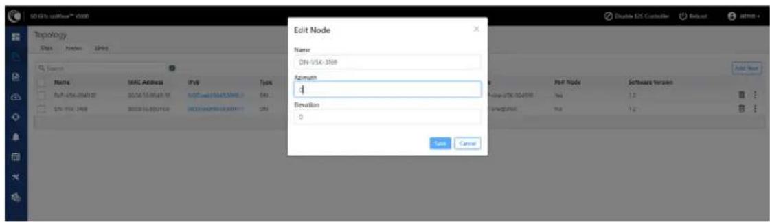
- Click Save.
Configuration
The configuration page contains the following two configuration options:
• Network configuration
- Node configuration
Network configuration
Network configuration is used to configure the network. Users can modify the network settings. It has Basic, Management, Security and Advanced options for the configuration. Settings under Network apply to all the nodes in the network. Some apply to the E2E Controller. Enter the required information and click Submit to configure the network.
Figure 167:The Network page with multiple tabs

The Network page contains the following tabs:
- Basic
- Management
Radio
• Security - Advanced
Basic
By default, cnWave is an IPv6-only network. By selecting this checkbox, Layer 2 network bridging is enabled (via automatically created tunnels) across all nodes connected to a PoP. This facilitates the bridging of IPv4 traffic across the wireless networks.
Figure 168: The Layer 2 Bridge section in the Basic page
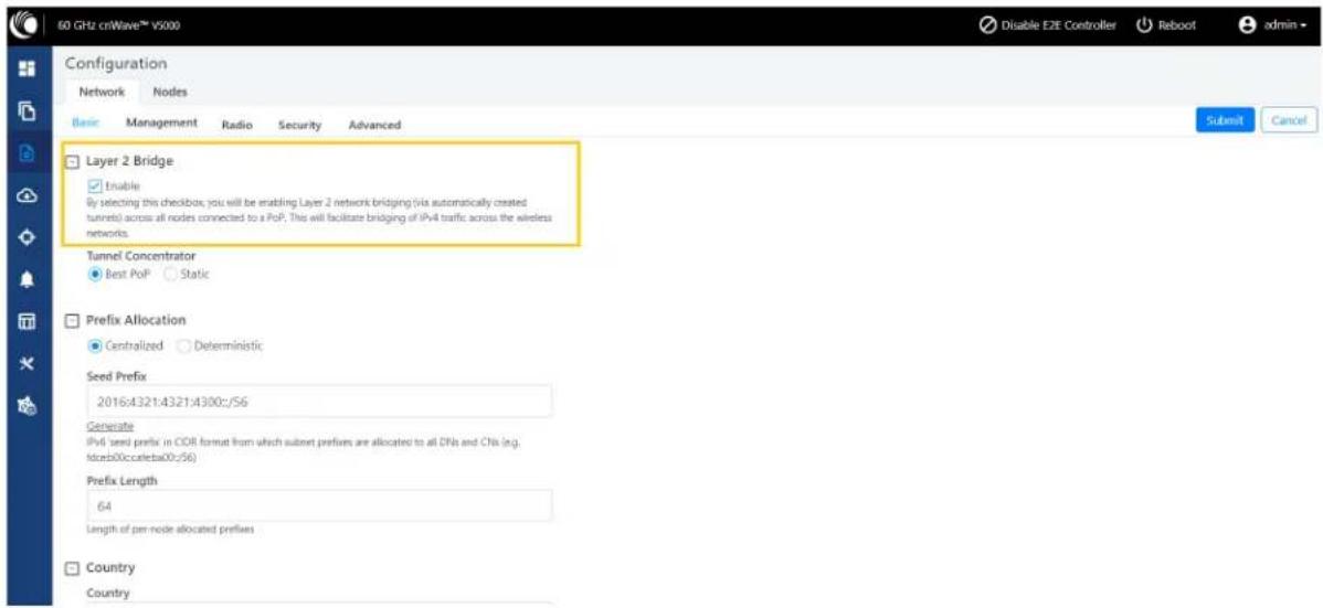
The Tunnel Concentrator does encapsulation and de-encapsulation of GRE packets. If Best PoP is selected, then the node selects the best PoP as a Concentrator. If Static is selected, then the user can configure the external Concentrator that can be Linux machine/router/PoP.
To configure the parameters on the Basic page, perform the following steps:
- Click Generate under Prefix Allocation to generate a unique local seed prefix automatically.
cnWave networks are given an IPv6 seed prefix (e.g. face:b00c:cafe:ba00::/56) from which subnet prefixes are allocated to all DNs and CNs. There are two methods for allocating node prefixes with Open/R.

Note
PoP interface IPv6 address and seed prefix should not be in the same /64 prefix range to avoid the address conflict.
- Centralized (default) - Centralized prefix allocation is handled by the E2E controller. The controller performs all prefix allocations, which prevents collisions and enables more sophisticated allocation algorithms. This is recommended for single PoP networks
- Deterministic - Deterministic prefix allocation is also handled by the E2E controller. The controller assigns prefixes to nodes based on the network topology to allow PoP nodes to take advantage of route summarization and help load balance ingress traffic. This is recommended for multi-PoP networks.
Figure 169:The Prefix Allocation section

- Seed Prefix
The prefix of the entire cnWave network is given in CIDR notation.
- Select Prefix Length, Country, Channels, DNS Servers, and Time zone from the drop-down list.
Prefix Length
Specifies the bit-length of prefixes allocated to each node.
Country
Country for regulatory settings like the EIRP limit, allowed channels, and other elements.
Channels
Indicates the channel number required for forming a link through an onboard E2E Controller or an external E2E Controller (if deployed).
By default, Channel 2 is supported. This parameter also supports a comma-separated list of channel numbers (for example: 2,3, 4,5), which you can give to a controller for auto configuration. Manual settings (which are made using the Node > Radio page) do not depend on this channel setting. This channel setting is useful, especially for PTP and small meshes that use a single channel for the entire network. In such a case, set the required channel number in this field and do not override the value that you set on the Node > Radio page. Modifying this Channels parameter is sufficient for the channel change.
DNS Servers
DNS server list is used for :
• Resolution of NTP Server host name (can be IPv4 when Layer 2 bridge is enabled)
• Given to IPv6 CPE as part of router advertisement
Time Zone
Time zone for all the nodes. System time in the dashboard, time field in the Events section, Log files use this timezone.
NTP Servers
This is NTP Server FQDN or IP Address. All nodes use this NTP Server to set the time. Node time is important when 802.1X radius authentication is used as it requires certificate validation. The time is reflected in the dashboard, time field in the Events section, and Log files.
CPE Prefix Zoning
You can configure the Summarized CPE Prefix parameter using the Basic page.
The Summarized CPE Prefix feature restricts a PoP to advertise the IPv6 CPE prefixes of its zone alone, thereby allowing an upstream BGP router to select an optimal PoP for downstream traffic. Figure 170 is an example of multi-PoP Layer 3 IPv6 topology, which is used to explain the feature in detail.
Figure 170:Multi-PoP Layer 3 IPv6 topology

flowchart
graph TD
    A["Internet"] --> B["IPv6 BGP Router"]
    B --> C["POP1"]
    B --> D["POP2"]
    B --> E["POP3"]
    B --> F["DN1"]
    B --> G["DN2"]
    B --> H["DN3"]
    B --> I["CN11"]
    B --> J["CN12"]
    B --> K["CPE"]
    B --> L["CPE"]
    M["E2E Controller"] --> B
    N["Zone 1"] --> O["POP1"]
    N --> P["POP2"]
    N --> Q["POP3"]
    N --> R["DN1"]
    N --> S["DN2"]
    N --> T["DN3"]
    N --> U["CN11"]
    N --> V["CN12"]
    N --> W["CPE"]
    N --> X["CPE"]
    Y["Zone 3"] --> Z["POP1"]
    Y --> AA["POP2"]
    Y --> AB["POP3"]
    Y --> AC["DN1"]
    Y --> AD["DN2"]
    Y --> AE["DN3"]
    Y --> AF["CN11"]
    Y --> AG["CN12"]
    Y --> AH["CPE"]
    Y --> AI["CPE"]
    style A fill:#f9f,stroke:#333
    style M fill:#ccf,stroke:#333
    style N fill:#cfc,stroke:#333
In Figure 170 (which is an example), consider the following points:
- Seed Prefix is 2001::/56.
• Deterministic Prefix Allocation (DPA) is enabled and has three zones. - An operator wants CPE Address to be in different ranges than Seed Prefix. Therefore, the user traffic can be distinguished from the traffic generated by the cnWave nodes.
- Customized CPE prefix is used with the range 3001:0:0:00XY::/64, where X contains values from 1 to 3.
- IPv6 addresses of CPEs that fall in the range of 3001:0:0:00XY::/64 prefix.
Prior to the introduction of this feature, all PoP BGP Peers advertised all the customized prefixes.
In this example (as shown in Figure 170), PoP1 BGP advertises 3001:0:0:11::/64, 3001:0:0:20::/64, and 3001:0:0:32::/64 prefixes. Similarly, PoP2 and PoP3 advertise all the three prefixes. The upstream BGP router is not able to route the packets to the best PoP. With this feature, PoP advertises the prefix of its zone alone. In the example:
• PoP1 BGP is advertising 3001:0:0:11::/64.
• PoP2 BGP is advertising 3001:0:0:20::/64.
- PoP3 is advertising 3001:0:0:32::/64.
A summarized prefix (shorter prefix) comprising of all the customized prefixes must be configured. When a PoP is down, traffic flows through another PoP. In this example, the summarized prefix is 3001::/58 (six bits from 11 to 30). The same concept is applicable when the DHCPv6 relay is used. In that scenario, CPEs obtain IPv6 address or delegated prefix directly from the DHCPv6 server.
Configuring Summarized CPE Prefix
To configure the Summarized CPE Prefix feature, perform the following steps:
- Navigate to Network > Basic from the home page.
The Basic page appears. The Summarized CPE Prefix text box is available in the CPE Prefix Zoning section, as shown in Figure 171.
Figure 171: The Summarized CPE Prefix text box

- Type an appropriate value in the Summarized CPE Prefix text box.

Note
Using a customized CPE prefix and not configuring the summarized CPE prefix can result in routing loops.
Management
On the Configuration > Network page, click Management and select SNMP, SNMPv2 Settings, SNMPv3 Settings, GUI Username and password.
Figure 172:The Management page

- Enable SNMP - Statistics can be read from the nodes using SNMP. This setting enables SNMP.
- System Contact - Sets the contact name as the System.sysContact.0 MIB-II variable.
- System Location - Sets the location name as the System.sysLocation.0 MIB-II variable.
- SNMPv2c Settings:
• SNMP Community string - Supports read-only access to all OIDs.
- IPV4 Source address - Specified, SNMP queries are allowed from the hosts belonging to this IPv4 address subnet.
- IPV6 Source Address - Specified, SNMP queries are allowed from the hosts belonging to this IPv6 address prefix.
- SNMPv3c Settings:
- SNMPv3 User - Name of the SNMPv3c user responsible for managing the system and networks.
• Security Level - Following security levels are supported for the network communication:
- None - Implies that there is communication without authentication and privacy.
- Authentication Only - Implies that there is communication with authentication only (without privacy).
- Authentication & Privacy - Implies that there is communication with authentication and privacy.
- Authentication Type - Type of protocol used for the security of network communication. Example: MD5 and Secure Hash Algorithm) (SHA) are used for authentication.
- Authentication Key - A password for the authentication user.
- For UI Users:
- Admin User Password - A password that you can set for GUI management.
- Installer User Password - A password that you can set for the required installers.
- Monitor User Password - A read-only password that you set for the monitoring purposes.
Radio
The Radio page allows you to perform the following configurations:
• Wireless Scan scheduling for beam adjustment
• CN Channel scanning options
- Fast Acquisition
- Asymmetric TDD
Wireless Scan scheduling for beam adjustment
The Scheduled Beam Adjustment parameter, when enabled, allows you to make small adjustments to the selected fixed beam for optimal RF alignment in azimuth and elevation. You can select this schedule option using the Scan Schedule Type parameter (Day/Time or Interval schedule type).
To configure the Scheduled Beam Adjustment parameter, navigate to the Wireless Scans section on the Configuration > Network > Radio page (as shown in Figure 173).
A normal scan without the Scheduled Beam Adjustment setting does the following operations:
- Beam selection occurs only on wireless link acquisition.
- Disassociating and re-associating the link or otherwise causing the link to drop and re-acquire is needed to perform a new beam selection.
- Any degradation in the wireless conditions does not trigger a new beam selection unless the link drops and reacquires.
The advantages of the Scheduled Beam Adjustment scan are:
- If the link is to acquire during heavy rain, then the optimal beam at that time may be suboptimal when the weather changes.
- If snow accumulation is present on the unit during acquisition, the optimally selected beam may be different when the snow has melted.
- Network-wide ignition in a dense deployment can cause interference when multiple nodes are acquiring. This interference can cause sub-optimal beam selection.
- Any physical change to alignment that is not severe enough to cause a link drop and subsequent beam scan can be corrected for.
The cost of Scheduled Beam Adjustment is:
• This feature causes a 50% throughput reduction for about 20 minutes, depending on the size of the network
- Simple deployments (especially PTP links) without significant external factors such as snow may not benefit from regular beam adjustment.
To configure the wireless scan scheduling options using the device UI, perform the following steps:
- From the home page of the device UI, navigate to Configuration > Network > Radio.
The Radio page appears with the Wireless Scans section, as shown in Figure 173.
Figure 173:The Wireless Scans section

Table 45 lists the parameters in the Wireless Scans section of the Radio page.
Table 45: Parameters in the Wireless Scans section
| Parameter Description | |
| Scheduled Beam Adjustment Allows you to enable or disable the scheduled beam adjustment feature.This parameter, when enabled, allows you to make small adjust to the selected fixed beam for optimal RF alignment in azimuth elevation. You can select this schedule option using the Scan Schedule Type parameter. | |
| Scan Schedule Type Allows you to select the scan scheduling option for beam adjustment.This parameter supports the following scan scheduling options:Day/Time: This schedule option allows you to select any day (or all days) of the week and time of the day.When you select the Day/Time option, following parameters are applicable:Schedule Day(s): Select the check boxes to choose the day(s).Schedule Time: Use the icon to set the time of the day.Apart from the interval scans, you are allowed to select any day (or all days) of the week and time of the day. This setting enables you to schedule the scan during maintenance activities.Interval: This scan schedule option allows you to set an interval (in seconds) for wireless scans. The default value is 3600 seconds. | |
- Set the parameters based on your requirements, as shown in Figure 173.
- Click Submit to save the changes.
CN Channel scanning options
When a CN loses its wireless connection, it initially scans the previously configured channel. This process speeds up the link acquisition in cases where the corresponding DN has not changed its channel. However, if the DN has switched channels, the CN scans all available channels, after a timeout period, to re-establish the connection.

Note
The advantages of CN channel rescan are:
- Moving the connected DN to a different channel is automatically detected by the CN when the configured timeout period expires.
- There is more flexibility in the topology as CNs can easily be reassigned to a different DN on a different channel without CN specific channel overrides.
The main reason to disable the CN channel rescan is to have the fastest possible network recovery following an event (for example, a software upgrade or network wide power cut). In networks, which have been fully deployed and where the configuration is not being changed, there may not be a requirement for channel rescan.
Using the device UI or the cnMaestro UI, you can configure the CN channel scanning options. These configurable options enhance the adaptability and responsiveness of your cnWave network, allowing it to better accommodate varying network conditions and configurations.
Using the device UI, perform the following steps:
- From the home page of the device UI, navigate to Configuration > Network > Radio.
The Radio page appears with the CN Channel Re-scan section, as shown in Figure 174.
Figure 174: The CN Channel Re-scan section - Device UI
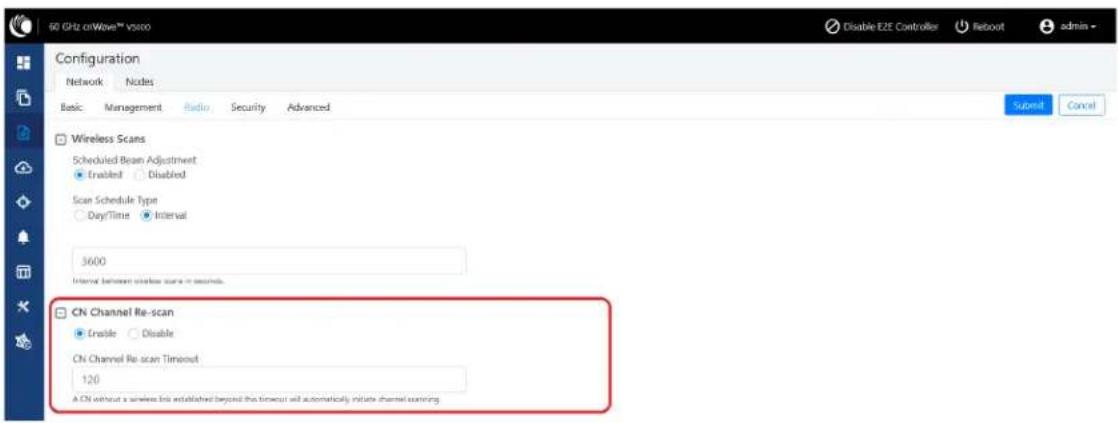
Table 46 lists the parameters in the CN Channel Re-scan section.
Table 46: CN Channel Re-scan specific parameters
| Parameter Description | |
| Enable By default, the Enable option | is selected (enabled), as shown inFigure 174. This option allows you to disable the full channel rescan feature.When this option is selected, the CN scans only the configured channel while attempting to re-establish a lost connection. This option can be beneficial in stable environments where DNs are unlikely to switch channels frequently, thereby accelerating the reconnection process. |
| CN Channel Re-scan Timeout When | the rescan feature (Enable CN Channel Re-scan) is not disabled, you can set a custom timeout value (in seconds) for the CN before it initiates a full channel scan. This capability allows you to adjust the balance between quicker reconnection times (by scanning the configured channel) and broader network coverage (by scanning all channels after the timeout).By default, the value of this timeout option is set to 120 seconds. This option allows the value ranging from 120 to 3600 seconds |
- Set the CN channel re-scan functionality using Enable or Disable check boxes, as described in Table 46.
By default, this parameter is enabled.
-
Set the required value (in seconds) in the CN Channel Re-Scan Timeout text box.
-
Click Submit to save the changes.
Fast Acquisition
During normal link acquisition, both ends of the wireless link scan multiple fixed beams to digitally steer the radio signal in the optimal direction and form a link. Aside from the Scheduled Beam Adjustment feature, the link then remains on
these chosen beams and continues to point in this direction until the link is dropped and re-acquired, triggering a new beam scan.
Assuming both units stay in the same location, orientation, and the wireless conditions do not change, the same beams should be selected (in theory) every time the link is established. By saving this beam on the first successful link acquisition, the link up time can be greatly reduced by only scanning that single beam, instead of all available beams.
Reliable operation of Fast Acquisition requires a given responding node to know from precisely which direction to listen for an ignition attempt. A responding DN sector can potentially be ignited, from either of two igniting DNs, in different directions. Therefore, Fast Acquisition does not occur when a DN is igniting another DN and a full beam scan triggers instead.
A full beam scan, across all available fixed beams, at both ends of the link, and on all four supported channels, takes between 2 and 9 seconds to complete. A successful acquisition on a single beam on a single channel completes within 160ms approximately. A successful acquisition has the following advantages:
- Reducing the link acquisition time will reduce the overall time taken for full network recovery, following outages caused by software upgrade, configuration changes, and power cuts.
- During the beam scan, the maximum throughput capability of the scanning DN sector is halved. By reducing this time, the impact on other links sharing the same sector on the igniting DN is reduced.
- The interference profile across the network is vastly reduced, as the link is brought up only on the single optimal beam as opposed to transmitting on all available beams across the full scan range.
This section covers the following details of the feature:
• Operation modes
- Use cases
- Setting the Fast Acquisition mode
Operation modes:
The Fast Acquisition feature supports the following three operational modes:
- Disable (default mode)
- Compatibility Mode
- Static Mode
For detailed information about each mode, refer to Table 47.
Use cases:
Consider the following use cases before configuring the Fast Acquisition feature:
- What to do if a link is establishing with poor signal and requires a beam change?
- It is difficult to detect this scenario. Check the Beam Angle statistics for the link. This scenario may occur when the unit is moved, an obstruction has moved into or away from the radio path, or interference has been introduced or removed from the receiver.
- To trigger a network wide rescan of all beams, reconfigure the Fast Acquisition setting to Disabled and back to Compatibility or Static after all wireless links have re-established.
- To trigger a full beam scan on the next association for a single link, navigate to the Topology > Links UI page and select the link. Then, click Clear Fast Acquisition Beams and re-associate the link.
- What to do if a link is failing to establish with either of the Fast Acquisition modes enabled?
- All units delete their fast acquisition beams if they are offline for more than 50 minutes as part of the PoP reachability reboot.
- In compatibility mode, there should be no additional risk of failing link acquisition when compared to Disabled mode. Therefore, the cause is unlikely to be related to this feature.
- In static mode, if the saved acquisition beam is no longer valid, wireless link up may take a long time to succeed. This is the main disadvantage of this mode. Therefore, this mode must be enabled only for networks that are stable with all units fixed in location and without ongoing topology changes. If the fast acquisition beam is invalid for any reason, then use the Clear Fast Acquisition Beams control (available on the Topology > Links UI page) to trigger a full beam scan on the next association.
• What interactions should be considered when using Fast Acquisition?
- DN channel rescan is not supported with the Fast Acquisition feature. Therefore, do not configure the DN channel rescan parameter.
- When switching the role of a DN to CN, CN to DN, or relocating an existing node to another part of the network, the best practice is to factory default the node before the change. This action can be taken centrally from cnMaestro.
- Backup CN links must not be used in combination with this feature.
- Nodes straight from the factory, running pre-1.3.1 software, are not able to respond to a fast acquisition association. Therefore, when using the Static mode, there is a delay in achieving a successful linkup. The solution to this is to use either Disabled or Compatibility mode or upgrade the node software to the latest before introducing into the network.

Note
cnMaestro 4.1.0 and later versions support the UI controls for configuring the Fast Acquisition feature.
The Enable post acquisition beam refinement feature is related to the Fast Acquisition feature. This feature (also previously known as Auto PBF) is present and enabled (by default) from Release 1.0.
The Enable post acquisition beam refinement UI control allows you to disable, if required. This feature fine tunes the beam selection, immediately, after a successful link acquisition for optimal performance. This can increase the link budget by up to 2dB. This feature is available on the Configuration > Radio page of the device UI and the cnMaestro UI. The following minor drawbacks of this feature might lead you to disable it (using the UI):
- The beam refinement scan lasts for 1.5 seconds. During this period, the transmitting DN sector operates at half capacity. You may not notice this behaviour.
- The beam refinement can cause interference during the scan to nearby links. The solution is to implement a channel plan (which takes this into account) but the option is there to disable.
Setting the Fast Acquisition mode
You can set the Fast Acquisition mode using either the device UI or cnMaestro UI.

Note
cnMaestro 4.1.0 and later versions support the UI controls for configuring the Fast Acquisition feature.
Device UI:
Using the device UI, perform the following steps:
- From the home page of the device UI, navigate to Configuration > Network > Radio.
The Radio page appears.
- Go to the Fast Acquisition section on the Radio page.
By default, the Fast Acquisition feature is disabled as shown in Figure 175.
Figure 175: Fast Acquisition settings- Device UI

Table 47 describes the operation modes supported by the Fast Acquisition feature.
Table 47: Operational modes
| Mode Description | |
| Disable (default mode) In this mode, | a traditional full beam scan is performed on every link up attempt.The only difference between the current and previous software is that this mode now saves the selected beam on the successful link acquisition for later use when Fast Acquisition is enabled. |
| Compatibility Mode On every link up | attempt, this mode checks to see if there is a saved beam available for the intended link and ignites on that single beam (if available). If this Fast Acquisition attempt fails, the association attempt immediately runs the full beam scan.This mode supports CNs configured for CN channel rescan because the full beam scan runs on all four channels.Note: The compatibility mode is recommended for most deployments as it offers the fast single beam acquisition where available and successful, whilst still offering the standard mode of acquisition for fallback. |
| Static Mode In this mode, the initiator | checks to see if there is a saved beam available for the intended link and ignites on that single beam (if available). If this ignition fails, the association also fails.The static mode does not support the configuration of CN channel rescan. This gives the highest chance of success to fast acquisition without performing a full beam scan.In static mode, the fallback mechanism occasionally performs a full beam scan to prevent stranded nodes that cannot respond on the fast acquisition beam. However, this case occurs infrequently, due to which there is some delay before the successful link acquisition. |
-
Select the required operation mode.
-
Click Submit to apply the changes.
cnMaestro UI:
Using the Monitor and Manage > Networks > Configuration > Radio page of cnMaestro UI, you can select the required operation mode of the Fast Acquisition feature.

Note
cnMaestro 4.1.0 and later versions support the UI controls for configuring the Fast Acquisition feature.
Figure 176 displays the Fast Acquisition section located on the Radio page of cnMaestro UI.
Figure 176: Fast Acquisition settings - cnMaestro UI

For detailed information about each mode, refer to Table 47.
Asymmetric TDD
The asymmetric TDD feature allows you to configure an asymmetric duty cycle instead of the default 50% downlink/50% uplink. The supported duty cycle ratios, denoted by downlink/uplink timeslot allocation, are:
75/25
70/30
60/40
• 50/50 (default ratio value)
40/60
• 30/70
Single wireless hop limitations (Standalone PTP and PMP only):
The meshing technology is designed around a 50/50 duty cycle to allow efficient synchronised communication in multi-hop networks. Using asymmetrical duty cycles across a multiple wireless hop network can be counterproductive and therefore, you must avoid this configuration.
Duty cycle ratio selection:
- For downlink biased traffic, for example - Internet video streaming, choose a high downlink ratio such as 75/25.
- For uplink biased traffic, for example - video camera backhaul, sensor backhaul, or data backup, choose a high uplink ratio such as 30/70.
Configuring the asymmetric TDD split ratio
You can configure an asymmetric TDD ratio using either the device UI or cnMaestro UI.
Device UI:
Using the device UI, perform the following steps:
- Log in to the device UI and navigate to Configuration > Network > Radio.
The Radio page appears.
- Go to the Asymmetric TDD section on the Radio page, as shown in Figure 177.
Figure 177: The Asymmetric TDD section - Device UI

- From the Duty Cycle drop-down list, select the required duty cycle ratio.
By default, the 50% Downlink / 50% Uplink ratio is selected.
When you modify the value of the Duty Cycle parameter, the Confirm message box prompts you to confirm the modification. You must click Continue to save the changes.
- Click Submit to apply the changes.
cnMaestro UI:
Using the cnMaestro UI, perform the following steps:
-
Log in to the cnMaestro UI and select the Monitor and Manage icon on the left navigation pane. The Dashboard page appears.
-
Select a network name under the Networks group and navigate to the Configuration > Radio page.
The Radio page appears, as shown in Figure 178.
Figure 178: Asymmetric TDD - cnMaestro UI

- In the Asymmetric TDD section, select the required TDD ratio from the Duty Cycle drop-down list.
By default, 50% Downlink / 50% Uplink is selected. When you modify the value of the Duty Cycle parameter, the Confirm message box prompts you to confirm the modification. You must click Continue to save the changes.
- Click Save to apply the changes.
Security
The Security page allows you to set the following configurations:
- Wireless security
• Security banner
Wireless security
On the Configuration > Network > Security page, the Wireless Security section contains the following options:
- Disabled - There is no wireless security.
- PSK - WPA2 pre-shared key can be configured. A default key is used if this configuration is not present. AES-128 encryption is used for data encryption.
- 802.1X - Nodes are authenticated using Radius server and EAP-TLS. Encryption is based on the negotiated scheme in EAP TLS. When 802.1X is selected, the following parameters are applicable:
• RADIUS Server IP - IPv4/IPv6 address of the Radius authentication server.
- RADIUS Server port - Port number of the Radius authentication server.
• RADIUS server shared secret - The shared secret of a Radius server.
Figure 179: The Wireless Security section
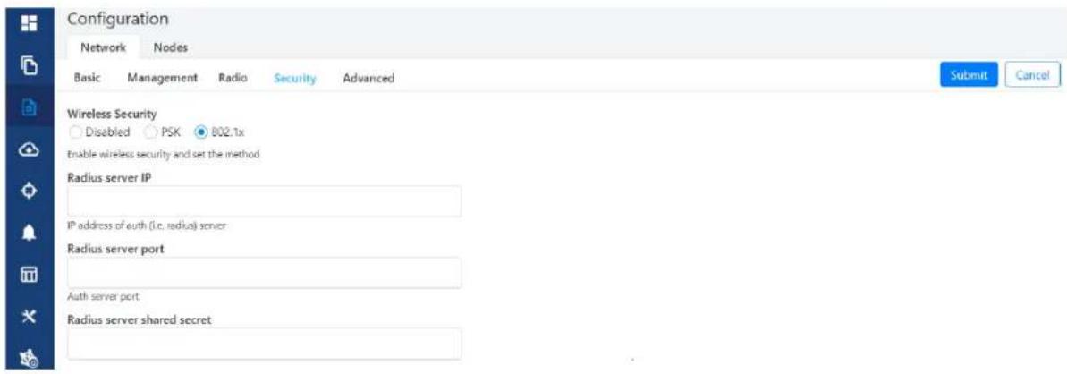
Security banner
You can enable or disable a security banner using the Configuration > Network > Security page.
When you enable a security banner, the login page of a device UI displays the security notice. You can view and accept (optional based on the configuration) the terms and conditions of a company before logging into the device UI.
For 60 GHz cnWave devices, the configuration of a security banner involves the following process:
- Enable or disable the security banner option using the Configuration > Network > Security page of the device UI (as shown in Figure 180).
Figure 180: Configuring the security banner

-
If the Enable Security Banner during Login parameter is enabled, provide the security text for intended users in the Security Banner Notice text box. This text box supports up to 1000 characters.
-
Determine whether the users must accept the security banner before logging into the device UI using the Accept security banner before login parameter.
- Click Submit to save the changes.
When you enable and configure the security banner settings (as shown in Figure 180), the login page of a device UI displays the security banner as shown in Figure 181. The users must accept the security notice and then log into the device UI, as shown in Figure 181.
Figure 181:Example of a Security Banner on the login page

If you have disabled the Accept security banner before login option for users, then the users are not forced to accept the security notice before logging in to the device UI.
Advanced
The Advanced page settings are for advanced users only. This page displays the merged configuration of all layers for a particular node.

Caution
The users are not recommended to modify or change settings on the Advanced page.
Figure 182:The Advanced page

The Network > Advanced page supports the configuration of the following features:
• DN Channel rescan
• Gratuitous ARP support
DN Channel Rescan
The DN Rescan feature optimizes the deployment and management of temporary network structures in settings such as concerts, recreational vehicle (RV) parks, and others. The feature also enables a seamless reconnection of DNs that have moved within new network environments.
How this feature works?
The DN Rescan feature comes into action when a DN loses a DN-DN link, consequently leading to a Point of Presence (PoP) being unreachable.
In a normal operation, the DN remains on the same channel and does not perform a rescan. This is due to the lost link that might be in the downstream direction where rescan does not apply or the affected sector might be serving other active links. However, the DN Rescan feature changes this behaviour under specific circumstances.
How to configure the feature?
To enable the DN Rescan feature, configure the envParams.CAMBIUM_ENABLE_DN_CHANNEL_RESCAN parameter using the Configuration > Advanced page of the device UI. By default, the value of this parameter is false (disabled). To enable the DN Rescan feature, set the value of this parameter to true.
If you set the value of this parameter to true and the DN is unable to detect a PoP for a certain duration (which is configurable using the envParams.CAMBIUM_DN_CHANNEL_RESCAN_TIMEOUT parameter), the DN resets the channel, Golay, and polarity on all its sectors by proceeding to scan all channels. This scan process facilitates the DN to form new links with an upstream PoP or DN without any manual intervention, achieving a true zero-touch experience.

Note
To set the timeout duration (in minutes) for different environments, configure the envParams.CAMBIUM_DN_CHANNEL_RESCAN_TIMEOUT parameter using the Configuration > Advanced page of the device UI. The default value of this parameter is 20 minutes, and the minimum allowed value is 10 minutes.
Use cases
The DN Rescan feature supports the movement of DNs in temporary deployments with zero touch (main use case). In addition, the feature supports the modification of the channel on the near end DN first.
The correct method is to change the far end DN channel first and then the near end. However, this feature can serve as a fail-safe in case if the near end DN channel is modified first. Note that both the ends must match, otherwise the controller does not ignite the link.
Frequently asked questions (FAQs)
The following table lists the FAQs specific to the DN Rescan feature.
| FAQ Answer | |
| How the feature detects the DN-DN link loss? | The DN Rescan feature does not detect the link loss, directly. It monitoring the visibility of the POP, periodically. |
| What happens if the DN fails to detect PoP even after the channel, golay, and polarity reset and rescan process? | aThe DN continues to scan until it reaches the timeout period (configured using the CAMBIUM_POP_UNREACHABLE_REBOOT_TIMEOUT_INTERVAL parameter), after which it reboots.Note: The CAMBIUM_POP_UNREACHABLE_REBOOT_TIMEOUT_INTERVAL parameter is available on the Configuration > Advanced page of the device UI. |
| Are there any impacts or disruptions to other active links in the same sector when the feature initiates a rescan process? | Yes. All the active links within the same sector goes down. |
| What are the prerequisites or requirement for the feature to work properly? | The DN Rescan feature does not require any specific prerequisites. |
| Can this feature be enabled or disabled each DN or is it a global setting? | The DN Rescan feature can be enabled either at the node level or the network level. There are no restrictions. |
| Are there any caveats (cautions) when using the feature? | Yes. You must consider the following:1. The DN will lose all its links and recovery will be slower, necessitating careful usage of this feature.2. If the channel is modified via the local GUI (for instance, to run Antenna Alignment), it is recommended to disable the feature first. Otherwise, the timeout might kick in and erase the set channel.3. Scanning of CB1 and CB2 channels at a time is not supported. |
Gratuitous ARP support
You must enable the Gratuitous Address Resolution Protocol (ARP) support for the 60 GHz cnWave products.
Disabling the downstream broadcast at the Point of Presence (PoP) in L2 mode results in upstream nodes losing access to cnWave nodes through their IPv4 addresses. This is due to the deletion of ARP entries in the upstream routers or devices beyond the POP on their expiration.
To maintain connectivity, the support initiates Gratuitous ARP updates for the configured IPv4 management IP.
To enable (activate) the Gratuitous ARP support for DN/CN, you can set the following parameters using the Configuration > Network > Advanced page of the device UI or cnMaestro UI:
- envParams.CAMBIUM GRATUITOUS ARP ENABLE: This parameter supports the following Boolean values:
- false: To disable the Gratuitous ARP support. By default, the value of this parameter is false.
- true: To enable (activate) the Gratuitous ARP support.
- envParams.CAMBIUM_GRATUITOUS_ARP_TIME: Specifies the time interval (in seconds) between the two Gratuitous ARP packets that are sent by the node to the upstream network. The default value of this parameter is 150 seconds.
The integer value of this parameter ranges between 20 and 6000 seconds. This parameter is applicable only when the envParams.CAMBIUM_GRATUITOUS_ARP_ENABLE parameter is set to true (enabled).

Note
The Gratuitous ARP support is not applicable when DN/CN is configured with the default IPv4 address (169.254.1.1).
Node configuration
Node configuration is used to configure the nodes via E2E Controller. E2E Controller can modify the node settings. Select the node(Radio) on the left pane to modify the settings.
The Node configuration contains the following tabs:
- Radio
- Networking
• VLAN
• Security - Advanced
Radio
To configure the Radio page, navigate to Nodes > Radio page from the Configuration page. The Radio page settings apply to individual nodes selected in the left side panel. Select the required options for Transmit Power, Adaptive Modulation, Sector 1, Sector 2 from the drop-down. Enable Force GPS Disable to establish the link between indoor nodes.
Figure 183:The Radio page
![Configuration Network Nodes Search PoP-V5K-884938 DN-V5K-3f69 Radio Networking VLAN Security Advanced Submit Cancel EIRP Maximum EIRP 38 Allowed range is 13 dblm to 30 dblm IBF Transmit Power Short range (<25m) optimized Long range optimized Initial Beam Forming transmit power setting Adaptive Modulation Minimum MCS 2 Range - [2, 12] Maximum MCS 12 Range - [2, 12] Sector 1 Channel/Polarity change should originate from the leaf nodes. Please make sure to change on the CNs first and then higher up on DNs. Override Name Auto Config Node Config ✓ Channel 1 1 ☐ Polarity Even Sector 1 Link (s) Golay Override Name Auto Config (Rx/Tx) Node Golay Rx Node Golay Tx link DN-V5K-3f69-PoP- 2/2 Override All Sector 2 Channel/Polarity change should originate from the leaf nodes. Please make sure to change on the CNs first and then higher up on DNs. Override Name Auto Config Node Config ☐ Channel ☐ Polarity Sector 2 Link (s) Golay Override Name Auto Config (Rx/Tx) Node Golay Rx Node Golay Tx. No Data GPS Force GPS Disable When checked, the radio will use internal sync rather than GPS sync](/content/2026/05/1088487/images/801b3fff11426894dfa67c83151d7e9841cb75c160fd6c434b72fe90dec3ae2a.jpg)
The Radio page contains the following elements:
Table 48: Elements in the Radio page
| Elements Description | |
| EIRP Transmit | power of the radioMaximum EIRP - The maximum EIRP transmitted by the radio. Range differs based on the platform and country selected (in the Network page).IBF Transmit power - Transmit power using during initial beam forming. When all the links are in short-range, high transmit power can cause interference. Selecting short-range optimized will prevent this. Post beam forming, automatic power control will make sure the radio transmits at optimal power. |
| Adaptive Select | minimum and maximum coding scheme ranging from 2 to 12. |
| Elements Description | |
| Modulation | |
| Sector 1 | Select the frequency channel and polarity.Channel and Polarity - When a link is created in topology, the controller automatically sets the sector's channel and polarity. To manually override, click the check box and select the channel in the node configuration. Note that changing channel/polarity breaks the link. It is important to change for leaf nodes first and then higher up on DNs. |
| Sector 1 Link(s)Golay | Golay codes help in avoiding inter-sector interference. In rare scenarios, individual links might require separate Golay codes. In most scenarios, all the links belonging to a sector are configured same Golay code. The controller automatically sets the Golay code. To manually override, select the check box and set the Golay from the drop-down. The Override All button helps in setting the same Golay code for all the links. NoteGolay codes and frequency on both ends of the link should match. NoteGolay codes and frequency on both ends of the link should match. |
| Sector 2 Select | the frequency channel and polarity. |
| Sector 2 Link(s)Golay | Golay code. |
| GPS If enabled | the radio uses internal sync rather than GPS sync. In some scenarios like lab setups, it may be necessary to disable GPS. |

Caution
60 GHz cnWave V1000 and V3000 devices has only Sector 1.
V3000 Small dish support
The software allows the selection of smaller 40.5 dBi antenna dish. To select V3000 small dish, navigate to Configuration > Nodes > Radio. The Antenna section is available in the Radio page.
Figure 184:The Antenna section
![Configuration Network Nodes Search V3K-416b-Pop V3K-DN-S419 V3K-CN@7049 V3K-DN2-6497 Radio Networking VLAN Security Advanced EIRP Maximum EIRP 51 Allowed range is 35 dBm to 55 dBm IBF Transmit Power Short range (<25m) optimized Long range optimized Initial Beam Forming transmit power setting Antenna Antenna Dish Gain 44.5 dBi PTP Deployment Range PTP Deployment Range Upto 1.5 km Deployment range applicable in Point to Point deployment. Please change for the far end node first. Adaptive Modulation Minimum MCS 2 Range - [2, 12]](/content/2026/05/1088487/images/f4205a8cd856f8f53a484cd0e697fe936154f1693bfecc7e304be0d32ecb82ec.jpg)

Caution
Small dish is supported only for 60 GHz cnWave V3000.
Networking
Using the Nodes > Networking page, you can set the following configurations:
- Configuring static IPv4 management and other network settings
- Configuring DHCPv4 client on PoP nodes
• Enabling the DHCP Option 82 feature - Configuring Monitor IPV4 Gateway
- Setting the Out of Band (OOB) interface
- Configuring PTP External failover
Configuring static IPv4 management and other network settings
To configure static IPv4 management, PoP interface, and other network settings, perform the following steps:
-
From the home page of device UI, navigate to Nodes > Networking.
The Networking page appears. -
In the IPv4 Management section, enter the local IPv4 address.
Figure 185: The IPv4 Management section in the Networking page

Table 49: Elements in the IPv4 Management section
| Elements Description | |
| IPv4 Address | Static IPv4 address of the individual node. Node's GUI /CLI can be opened using this address when directly connected over Ethernet. For Over the air access, L2 Bridge sh enabled. Its predominantly used on PoP nodes with the onboard controller. |
| Subnet Mask | Subnet mask for the IPv4 address. |
| Gateway IP Address | IPv4 Gateway address. |
- In the PoP Configuration section, select the options for PoP Routing, PoP Interface, and click Generate to generate PoP Interface IP Address.
Figure 186: The PoP Configuration section in the Networking page
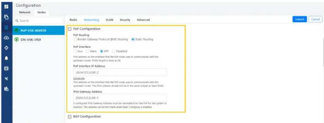
Table 50: Elements in the PoP Configuration section
| Elements Description |
| PoP PoP nodes connect to the upstream IPv6 router in one of two ways: |
| Elements Description | |
| Routing | Border Gateway Protocol (BGP) Routing - PoP acts as a BGP peerStatic routing - IP gateway address should be specified on the PoP and static route should be added on the upstream router.When the system is targeted for L2 traffic (Layer 2 bridge enabled) and an onboard controller is used, this configuration is of not much significance, recommended to set to static routing. |
| PoP Interface | The wired interface on which PoP communicates to an upstream router or switch when the L2 bridge is enabled. |
| PoP Interface IP Address | IPv6 address on the interface that the PoP node uses to communicate with the upstream router. |
| IPv6 Gateway Address | Gateway address. Can be left empty when the L2 bridge is enabled and no IPv6 services like NTP /Radius are used. |
- Under E2E Controller Configuration, enter E2E IPv6 Address (Address of E2E Controller). When using the onboard controller on the same node, can be left empty and GUI automatically fills the POP IPv6 address.

Note
If PoP DN is V5000/V3000 then, IPv6 both address is same.
Table 51: Elements in the E2E Controller Configuration section
| Elements Description | |
| E2E IPv6 Address Address | of E2E Controller. When using the onboard controller on the same node, can be left empty and GUI automatically fills the POP IPv6 add |
| E2E Network Prefix Seed P | prefix in the CIDR format followed by a comma and the prefix length.Should be specified when BGP is used. Otherwise, optional. |
| IPv6 CPE Interface IPv6 SL | AAC provides IP prefix to downstream CPE devices. Keep it disabled when L2 Bridge is active. |
- Select the required BGP configuration.
Figure 187: The BGP Configuration section

Table 52: Elements in the BGP Configuration section
| Elements Description | |
| Local ASN Local ASN | |
| KeepAlive The BGP keepalive period in seconds. | |
| Neighbour ASN Upstream router's ASN | |
| Neighbour IPv6 Upstream router's IPv6 address | |
| Specific Network prefixes Specifically allocated network prefixes to be advertised via BGP | |
- Enable the required Ethernet ports. Individual Ethernet ports can be turned off with this configuration.
Figure 188:The Ethernet Ports section
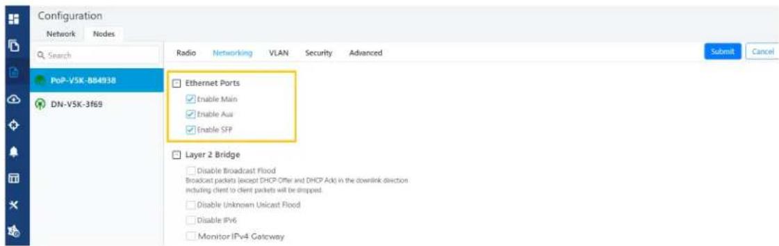
- Select the required options for Layer 2 Bridge, IPv6 Layer 3 CPE, Aux PoE (enable to power on Aux port), and Multi-PoP / Relay Port. By default, this option is disabled and PoP floods any unknown unicast ingress packets on all the L2 GRE tunnels. When the option is enabled, PoP drops such packets.
Figure 189: The Layer 2 Bridge section in the Networking page

Table 53: Elements in the Layer 2 Bridge section
| Elements Description | |
| Layer 2 Bridge | It has three options:Disable Broadcast FloodDisable Unknown Unicast FloodDisable IPv6Monitor IPv4 GatewayFor information on Monitor IPv4 Gateway, refer toConfiguring Monitor IPv4 Gateway. |
| Aux PoE Enable PoE out (25 W) on V5000/V3000 aux port. 802.3af and 802.3at compliant devices could be powered up, passive PoE devices cannot be powered up. Note that the aux port cannot power another V5000/V3000. | |
| Multi-PoP / Relay Port | Indicates the wired interfaces (or Ethernet) on which OpenR is running. This element must be used:When DNs are connected back-to-back.When multiple PoPs are in the network. This allows PoP nodes to forward traffic to other PoP nodes via a wired connection when the routing path of the other PoP node is closer to the traffic destinationFollowing options are supported:AuxMainSFPDisabled |
Configuring DHCPv4 client on PoP nodes
When you configure DHCPv4 on the PoP nodes, the DHCP client simplifies and automates the process of network configuration for devices. A manual configuration of the network settings is not required. The DHCP client automates the process by interacting with DHCP servers on the network. The DHCP client uses the information received from the DHCP server to configure its network interface, including obtaining an IP address, subnet mask, default gateway, DNS server addresses, and other relevant settings.
To set the DHCP configuration, perform the following steps:
- From the home page of device UI, navigate to Nodes > Networking.
The Networking page appears.
- In the IPv4 Management section, select DHCP from the IP Assignment parameter options, as shown in Figure 190.
Figure 190:DHCPv4 Configuration - device UI

- Click Submit to apply the changes.
When you set the DHCP configuration, the IPv4 address, Subnet mask, and Gateway IP address are automatically obtained from the DHCP server.
The dashboard page of both the device UI (running Onboard Controller) and cnMaestro display the IPv4 address. Figure 191 shows the dashboard page of a device UI.
Figure 191: The dashboard page displaying the IPv4 address

Enabling the DHCP Option 82 feature
When the DHCP Option 82 feature is enabled, 60 GHz cnWave intercepts DHCPv4 REQUEST and DISCOVER packets and inserts option 82 fields.

Note
This feature is supported in the L2 bridge mode.
In addition, you can also configure Circuit ID and Remote ID fields. Use the following wildcards to configure Circuit ID and Remote ID fields:
- \nodeMac\ - MAC address of the node in ASCII format without colons. This is a default option.
- \nodeName\ - Topology name of the node.
• \siteName\ - Name of the site. - \networkName\ - Network name as shown in cnMaestro.
Multiple wildcards can be combined with a : delimiter. The total length of the option (after replacing wildcards with corresponding values) is truncated to 120 characters. You can also configure a custom string, which must not start with a \$ character. For example, a customer's phone number.

Note
You cannot use the customized string and predefined wildcards together as a single sub option (Circuit ID / Remote ID).
To enable the DHCP Option 82 feature, perform the following steps:
- Navigate to Nodes > Networking from the home page.
The Networking page appears. The DHCP Option 82 feature is available in the Layer 2 Bridge section, as shown in Figure 192.
Figure 192:The DHCP Option 82 feature
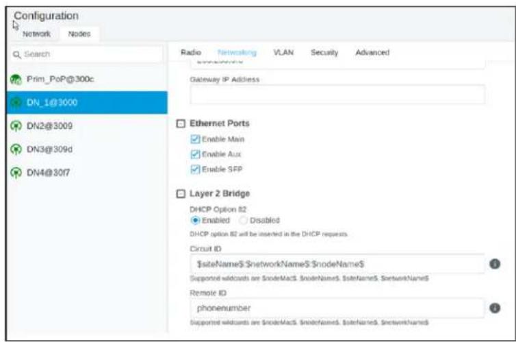
The enabled status of DHCP Option 82 implies that the feature is activated.
-
Type appropriate values in Circuit ID and Remote ID text boxes.
-
To save the configuration, click Submit.
Configuring Monitor IPV4 Gateway
The Monitor IPV4 Gateway parameter is applicable when static routing and Layer 2 bridge are enabled in the device UI.
When you enable this parameter using the device UI, the IPv4 gateway is monitored. In Layer 2 bridging with multiple PoP nodes, this parameter (when enabled) configures the PoP to periodically ARP ping the configured IPv4 gateway. If the ARP ping fails for consecutive 12 seconds, all the other nodes (within the mesh network) choose one of the other available PoP nodes to route.
The Monitor IPV4 Gateway configuration results in failover of Layer 2 tunnels to next best PoP when the PoP cannot reach the IPv4 gateway. This configuration is applicable when static routing is used and IPv4 gateway is configured.
Before configuring the Monitor IPv4 Gateway parameter, perform the following configurations using the device UI:
- Enable the Layer 2 Bridge parameter using the Configuration > Network > Basic page. This action enables Layer 2 network bridging (through automatically created tunnels) across all nodes connected to a PoP. This action also facilitates the bridging of IPv4 traffic across the wireless networks.
- Set the value of PoP Configuration parameter to Static Routing for the required PoP using the Configuration > Nodes > Networking page. This action results in failover of Layer 2 tunnels to next best PoP when the PoP cannot reach the IPv4 gateway. This configuration is applicable when static routing is used and IPv4 gateway is configured.
To enable and configure the Monitor IPV4 Gateway parameter, perform the following steps:
- From the home page, navigate to Configuration > Nodes > Networking.
The Networking page appears. The Monitor IPV4 Gateway check box is available in the Layer 2 Bridge section, as shown in Figure 193.
Figure 193:The Monitor IPV4 Gateway parameter

-
Select the Monitor IPV4 Gateway check box to enable the parameter.
-
Click Submit to save the changes.
Setting the Out of Band (OOB) interface
Out of band (OOB) management interface to access the device. Management VLAN is bypassed, and data traffic will not be routed or bridged on this interface. The OOB management interface is supported at PoP. A separate IPv4 address should be configured by bypassing the Management VLAN. Navigate to Configuration > Nodes > Networking > OOB and select the required option. Enter the IPv4 address and Subnet Mask to access the device.
Figure 194: The OCB section in the Networking page

Configuring PTP External failover
The PTP External Failover feature supports the failover of a 60 GHz cnWave RF link using external devices such as PTP450 and ePMP.
System Release 1.2.2 and later subsequent release versions support the external failover link feature for Point-to-Point (PTP) links. The external failover interface must not be same as PoP, Relay, or Out of Band (OOB) interface.
This feature does not support V1000 (which contains only one port).
Figure 195 shows how a 60 GHz cnWave PTP link is backed up with a PTP450 link. You can consider the 60 GHz link (as shown in Figure 195) as the primary link and 5 GHz link as the secondary link.
Figure 195: Backing up the 60 GHz cnWave PTP link
Scenario 1:

flowchart
graph TD
    A["Backhaul"] -->|Data| B["POE 56V"]
    B --> C["Data + PWR"]
    C --> D["V3000"]
    D --> E["AUX"]
    E --> F["PMP450i/MicroPo P conn/MicroPoP Omni-sector"]
    F --> G["60 GHz"]
    G --> H["V3000"]
    H --> I["AUX"]
    I --> J["PMP450i/MicroPo P conn/MicroPoP Omni-sector"]
    J --> K["5 GHz"]
    K --> L["POE 56V"]
    H --> M["SFP"]
    H --> N["PU"]
    H --> O["CPE"]
    style A fill:#cce5ff,stroke:#333
    style H fill:#cce5ff,stroke:#333
Note: Enable AUX PoE Power on V3000.
Scenario 2:
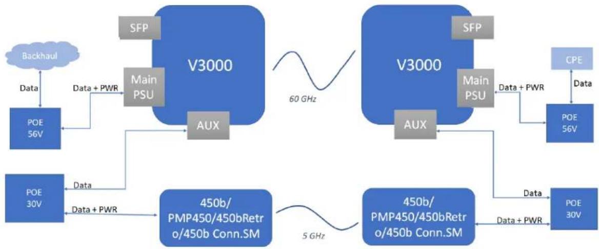
flowchart
graph TD
    A["POE 56V"] -->|Data + PWR| B["Main PSU"]
    C["POE 30V"] -->|Data + PWR| D["450b/PMP450/450bRetro/450b Conn.SM"]
    B --> E["AUX"]
    D --> E
    E --> F["V3000"]
    F --> G["60 GHz"]
    G --> H["V3000"]
    H --> I["Main PSU"]
    I --> J["Data + PWR"]
    J --> K["POE 56V"]
    K --> L["CPE"]
    L --> M["Data"]
    M --> N["POE 30V"]
    N --> O["450b/PMP450/450bRetro/450b Conn.SM"]
    O --> P["Data + PWR"]
    P --> Q["POE 30V"]
    Q --> R["450b/PMP450/450bRetro/450b Conn.SM"]
    R --> S["Data + PWR"]
    S --> T["POE 30V"]
    T --> U["450b/PMP450/450bRetro/450b Conn.SM"]
    U --> V["Data + PWR"]
    V --> W["POE 30V"]
    W --> X["450b/PMP450/450bRetro/450b Conn.SM"]
    X --> Y["Data + PWR"]
    Y --> Z["POE 30V"]
    Z --> AA["450b/PMP450/450bRetro/450b Conn.SM"]
    AA --> AB["Data + PWR"]
    AB --> AC["POE 30V"]
    AC --> AD["450b/PMP450/450bRetro/450b Conn.SM"]
    AD --> AE["Data + PWR"]
    AE --> AF["POE 30V"]
    AF --> AG["450b/PMP450/450bRetro/450b Conn.SM"]
    AG --> AH["Data + PWR"]
    AH --> AI["POE 30V"]
    AI --> AJ["450b/PMP450/450bRetro/450b Conn.SM"]
    AJ --> AK["Data + PWR"]
    AK --> AL["POE 30V"]
    AL --> AM["450b/PMP450/450bRetro/450b Conn.SM"]
    AM --> AN["Data + PWR"]
    AN --> AO["POE 30V"]
    AO --> AP["450b/PMP450/450bRetro/450b Conn.SM"]
    AP --> AQ["Data + PWR"]
    AQ --> AR["POE 30V"]
    AR --> AS["450b/PMP450/450bRetro/450b Conn.SM"]
    AS --> AT["Data + PWR"]
    AT --> AU["POE 30V"]
    AU --> AV["450b/PMP450/450bRetro/450b Conn.SM"]
    AV --> AW["Data + PWR"]
    AW --> AX["POE 30V"]
    AX --> AY["450b/PMP450/450bRetro/450b Conn.SM"]
    AY --> AZ["Data + PWR"]
    AZ --> BA["POE 30V"]
    BA --> BB["450b/PMP450/450bRetro/450b Conn.SM"]
    BB --> BC["Data + PWR"]
    BC --> BD["POE 30V"]
    BD --> BE["450b/PMP450/450bRetro/450b Conn.SM"]
    BE --> BF["Data + PWR"]
    BF --> BG["POE 30V"]
    BG --> BH["450b/PMP450/450bRetro/450b Conn.SM"]
    BH --> BI["Data + PWR"]
    BI --> BJ["POE 30V"]
    BJ --> BK["450b/PMP450/450bRetro/450b Conn.SM"]
    BK --> BL["Data + PWR"]
    BL --> BM["POE 30V"]
    BM --> BN["450b/PMP450/450bRetro/450b Conn.SM"]
    AF --> BO["SFP"]
    BO --> BP["Backhaul"]
Note: Disable AUX PoE Power on V3000.
Whenever a 60 GHz link is up or active, traffic flows through the 60 GHz cnWave link. When the 60 GHz link is down, traffic fails over (shifts) to the 5 GHz link (PTP450). When the 60 GHz link is back (up), the traffic shifts instantly over to the 60 GHz cnWave link.
You can configure the external failover link feature using the device UI or the cnMaestro UI.
Using the device UI:
To enable and configure the external failover link feature using the device UI, perform the following steps:
-
From the home page of the device UI, navigate to the Configuration > Nodes > Networking page.
The Networking page appears. -
In the PTP External Failover section (as shown in Figure 196), set the following configurations:
a. To set the Ethernet interface for a node connected to external failover link, select either Aux or Main (Ethernet ports) from the External Failover Link parameter.
By default, the Disabled option is selected.
Figure 196:The PTP External Failover section in the device UI
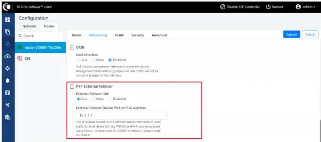
b. Enter either IPv4 or IPv6 address of the external failover device In the External Failover Device IPv4 or IPv6 Address text box.

Note Ensure that IPv6 is enabled in the external failover device.
- Click Submit to save the changes.
Using the cnMaestro UI
To configure the external failover link feature, add and manage the following configurations in the Advanced page of cnMaestro UI:
- Ethernet interface for each node: Configure the Ethernet interface in PoP and CN, which are connected to the failover link. You must select the Ethernet port to which the external device is connected. Open/R protocol runs on this interface.
- External failover interface address (IP address): An optional configuration that is required only if you want to access the AP or SM UI from upstream. You must configure the IP address of external devices (for example, PTP450 or ePMP). This IP address must be in a different subnet other than node IP address or seed prefix. The IP address can be either IPv4 or IPv6. However, ensure that external failover devices have IPv6 enabled.
- Remote external failover node address: Configure the remote external failover node address. You can access the external failover device UI using http://
To configure the external failover link feature using the cnMaestro UI, perform the following steps:
- From the dashboard page of the cnMaestro UI, navigate to the Monitor and Manage > Networks > Configuration > Node > Advanced page.
The Advanced page appears.
- To add and manage the Ethernet interface for each node (PoP and CN), Click Add New located at the right side of the page.
The Add new field page appears.
- In the Field Name text box, provide envParams.CAMBIUM_EXTERNAL_FAILOVER_IFACE (in String format) for each node, as shown in Figure 197.
Figure 197:The Add new field page in the cnMaestro UI

-
In the Value field, enter an appropriate value.
-
Click Save.
The Advanced page is updated the new entry that you added.
- Click Submit located at the right side of the Advanced page.
Similarly, you must add and manage the following configurations, separately, using the Add New button on the Advanced page:
- For external failover interface address (IP address), provide envParams.CAMBIUM_EXTERNAL_FAILOVER_IFACE_ADDR (in String format) in the Field Name text box, as shown in Figure 198.
Figure 198: Configuring the external failover interface address

- For remote external failover node address, provide envParams.CAMBIUM_EXTERNAL_FAILOVER_NODE_ADDR (in String format) in the Field Name text box, as shown in Figure 199.
Figure 199: Configuring the remote external failover node address

Then, you must ensure to provide an appropriate value in the Value text box for each configuration. Finally, you must save and submit each configuration.

Note
Following limitations are observed in this release specific to the external failover feature:
- There is no representation of an external failover link on the Map page.
• There are no statistics available on the external failover link.
- No other UI or cnMaestro used for configuring the external failover interface and address. This feature can be configured only through the Configuration > Nodes > Advanced page.
VLAN
Data VLAN
The following 802.1Q features are supported per port:
- Adding single VLAN tag to untagged packets
- Adding QinQ/double-tag to untagged packets
- Adding QinQ outer tag to single tagged packets
- Transparently bridge single/double-tagged packets (default behavior)
- Remarking VLAN ID
• Remarking 802.1p priority - Option to allow only the selected range of VLAN IDs
- Option to drop untagged packets
- Option to drop single tagged packets
- Option to select the ethertype of the outer tag
These options are per Ethernet port.

Note
VLAN configuration is applicable only when Layer 2 bridge is enabled.
Port Type
Figure 200:The port types
Type


Transparent
Transparent
By default, the Ethernet port is in transparent mode. Packets will be transparently bridged without any 802.1Q processing.
Q
Q mode allows adding a single C-VLAN tag to untagged packets.
Figure 201: Native VLAN ID and priority
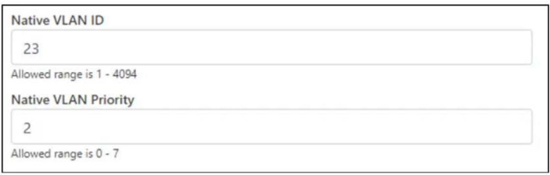
Native VLAN ID and priority fields define the C-VLAN tag properties.
Figure 202 Allowed VLANs

Allow only the listed range of VLAN IDs.
Figure 203: Untagged types
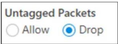
This option allows dropping untagged packets. Native VLAN properties are not necessary to fill when untagged packets are dropped.
QinQ
QinQ mode allows adding a double tag to untagged packets and outer S-VLAN to single-tagged packets.
Figure 204: Native C-VLAN ID and priority

These are the C-VLAN tag properties of added tag.
Figure 205: Native S-VLAN ID and priority
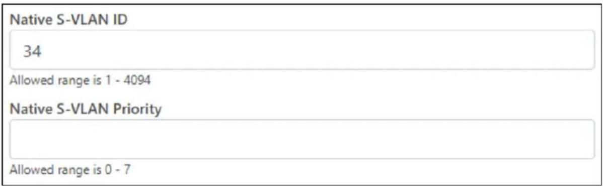
These are the S-VLAN tag properties of the added outer tag.
Figure 206: Untagged and Single tagged packets

In QinQ mode, the above options allow dropping untagged/single-tagged ingress packets. Native C-VLAN fields are not necessary only when dropping single-tagged packets. Native S-VLAN fields are not necessary when dropping untagged and single tagged packets.
Figure 207 Allowed VLANs

Allow only the listed range of VLAN IDs. VLAN ID of the outer tag is used for this check.
Figure 208: QinQ EtherType

QinQ EtherType is used while adding an outer tag. There are no other checks for EtherType.
Figure 209: VLAN ID Remarking
| VLAN Remarking | ||
| Ingress VLAN | Remark VLAN | |
| 10 | 100 |  |
| Add New | ||
VLAN ID of the ingress packet is remarked. In the above example, if a packet with VLAN ID 10 enters an Ethernet port, it is remarked to 100. In the egress path, the reverse remarking occurs. VLAN ID 100 is remarked to 10 and egresses the ethernet port.
The VLAN ID of the outer tag is used for remaking. For a double-tagged packet, S-VLAN ID gets remarked and for a single-tagged packet, C-VLAN 1D.
802.1p overriding
The Priority field in the (outer) VLAN tag of ingress packet can be overwritten using this option.
Figure 210: VLAN Priority Override
| VLAN Priority Override | ||
| Ingress VLAN | Override Priority | |
| 20 | 7 |  |
| Add New | ||
Management VLAN
A Single tag or double tag can be added to Management traffic.
Figure 211:The Management section

Security
In the Security tab, enter Private key password and Radius user password.
- Private key password
- Radius user password
Figure 212:The Security page

Configuring 60 GHz cnWave™ 193
Controller UI configuration
This Controller GUI configuration to be made on each DN.
Figure 213: Elements specific to Controller configuration
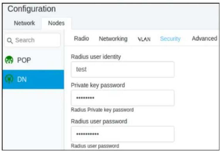
Node UI configuration
You can configure the Security page for a single node. The Security page is available on the single node UI.
Figure 214:Elements specific to node configuration


Note
Both the configurations are important for a successful authentication.
RADIUS Server configuration
Any RADIUS server can be used for authentication. Perform the following steps to configure the RADIUS Server:
-
Ensure that RADIUS packets from IPv6 subnet (IP subnet) is accepted in RADIUS configuration.
-
Configure EAP-TLS for RADIUS Server and setup server certificate, key.
Configuring 60 GHz cnWave™ 194
- Set the CA certificate which signed the client certificate installed on each node.
Advanced
These settings are for advanced users only.

Caution
Users are not recommended to do these settings.
Figure 215:The Advanced page - Node configuration

Configuration options under Network > Advanced and Node > Advanced are for advanced users who understand the cnWave configuration model well. It is not recommended to use these options. Shows the merged configuration from the Base layer to the Network override layer.
cnWave is based on Facebook's Terragraph architecture. It follows a layered configuration model, with a node's "full" configuration computed as the union of all layers in the following order:
- Base configuration - The default configuration, which is tied to a specific software version and is included as part of the image. The controller finds the closest match for a node's software version string and falls back to the latest if no match was found.
- Firmware-specific base configuration - The default configuration is tied to a specific firmware version, which is also included as part of the image. Values are applied on top of the initial base configuration layer.
- Hardware-specific base configuration - The default configuration is tied to a specific hardware type, which is also included as part of the image. Each hardware type supplies configuration that changes with software versions. Values are applied on top of the firmware-based configuration layer.
-
Automated node overrides - Contains any configuration parameters for specific nodes that were automatically set by the E2E controller.
-
Network overrides - Contains any configuration parameters that should be uniformly overridden across the entire network. This takes precedence over the base configuration and automatic overrides.
- Node overrides - Contains any configuration parameters that should be overridden only on specific nodes (e.g. PoP nodes). This takes precedence over the network overrides.
The E2E controller manages and stores the separate configuration layers. The cnWave nodes have no knowledge of these layers, except the base configuration on the image. The nodes copy the latest base version (via natural sort order) if the configuration file on disk is missing or corrupt.
Click Submit to apply the changes.
Software upgrade
The Software Upgrade page is used to upgrade the installed software. This page contains the following three tabs:
- Node Upgrade - to upgrade the node
• Images - to upgrade the software images - Node Upgrade Status - displays the upgrade status
To upgrade a node, perform the following steps:
- From the main dashboard page, click Software upgrade on the left navigation pane.
The Software Upgrade page appears, as shown below:
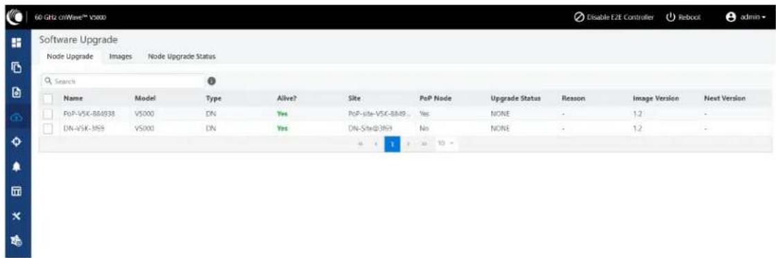
By default, the Node Upgrade tab is selected.
- In the Node Upgrade page, select the required device for which you want to upgrade the node and click Prepare (as shown below).

The Prepare Nodes dialog box appears.
- In the Prepare Nodes dialog box, select the required image file for the node and click Save.
You can also set additional options, if required, such as Upgrade Timeout, Download options, and Download Timeout.
-
Click Commit to upgrade the node.
-
To upgrade the software image, click on the Images tab in the Software Upgrade page.
The Images page appears, as shown below:
Figure 216:The Images page

- In the Images page, click Upload Image.
You must browse and select the required image file from your machine. Example: Software image or package (cnWave60-
You can also delete an existing image file in the Images page.
- To view the node upgrade status, click on the Node Upgrade Status tab in the Software Upgrade page.
The Node Upgrade Status page appears, as shown below:
Figure 217:The Node Upgrade Status page

You can view the upgrade status for the required device nodes.
Diagnostics
The Diagnostics page contains the following tabs:
- Events
• DA Logs
• Engineering logs
Events
The Events page displays the running and completed task list. These events can be exported. To export the event list, click Export.
Statistics
The Statistics menu contains the following options:
- Links
- Ethernet
• GPS - Radio
- Performance
- Prefix Zone Statistics
• Border Gateway Protocol (BGP)
Links
The Links page contains Uplink and Downlink statistical data. It displays TX and RX data of the reporting nodes from A to Z and Z to A. The page also displays statistics (for example, Rx/Tx Throughput and Rx/Tx Airtime %) that provide the necessary insights to manage and optimize cnWave networks effectively.
Based on the filters that you select using the iii icon (as shown in Figure 218), the Links page displays the relevant elements and statistics.
Figure 218:The Links page
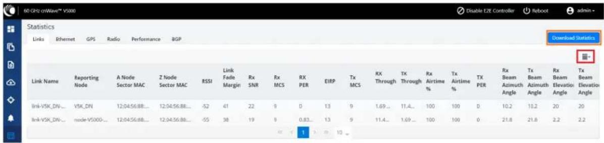
The Links page displays the following elements:
Table 54: Elements in the Links page
| Element Description | |
| Link Name Link name | |
| Reporting Node | Name of the reporting node for which the statistics are available. |
| A Node Sector MAC | MAC address of the initiator node. |
| Z Node Sector MAC | MAC address of the responder node. |
| RSSI The Receiver Signal Strength Indicator (RSSI) value | |
| Link Fade Margin | The statistic value (in dB) available for each RF linkThe Link Fade Margin statistic values help operators to quickly assess any additional system gain or low marginal RF links (if any), which must be addressed.The Link Fade Margin statistic value calculation is based on:Checking the RSSI received from a remote transmitter,Assessing the availability of TX power (from the remote transmitter), andConsidering the RSSI value that is calculated based on how far away it is from an receiver sensitively floor of -72 dBm. |
| Rx SNR Signal to Noise Ratio | |
| Rx MCS Modulation Code Scheme of Receiver | |
| RX PER Receiver packer error rate | |
| TX Power Index | Transmitter power index |
| EIRP The Effective Isotropic Radiated Power (EIRP) value. | |
| TX MCS Modulation Code Scheme of Transmitter | |
| TX PER Transmitter packer error rate | |
| RX Errors Receiver errors | |
| RX Frames Receiver frames | |
| TX Errors Transmitter errors | |
| TX Frames Transmitter frames | |
| Rx Throughput | The receive throughput as received by the reporting node. |
| Tx Throughput | The throughput transmitted by the reporting node. Monitoring of this metric can clarify the data transmission rate, providing a clearer view of the network's outbound data performance. |
| Rx Airtime % | The percentage of airtime allocated by the scheduler to each link in the Rx direction from the perspective of reporting node. This metric is relevant for a DN as it indicates how airtime is shared across multiple links. |
| Tx Airtime % | The percentage of airtime allocated by the scheduler to each link in the Tx direction from the perspective of reporting node. Similar to Rx Airtime %, this metric provides insights into how airtime is distributed among links when transmitting data. This metric is only relevant for a DN. |
| Following replace Rx Scan Beams and Tx Scan Beam elements: | |
| Rx Beam Azimuth Angle | The angle of the selected fixed beam (in degrees) in the azimuth direction for each link.The selected beam is independent of transmit and receive directions. For more information on Tx/Rx azimuth beam angle statistics, refer tothe Link diagnostics - Beam angle statistics section. |
| Tx Beam Azimuth Angle | |
| Tx Beam Elevation Angle | The angle of the selected fixed beam (in degrees) in the elevation direction for each link.The selected beam is independent of transmit and receive directions. For more information on Tx/Rx azimuth beam angle statistics, refer tothe Link diagnostics - Beam angle statistics section. |
| Rx Beam Elevation Angle | |
To download the statistics in .xls format, click Download Statistics.
Link diagnostics - Beam angle statistics
To understand about Tx/Rx azimuth and elevation beam angle statistics, let's consider the following examples:
- In Figure 219, the reported beam angle is relative to the reporting nodes boresight and not a bearing from North. Therefore, an elevation angle of +5 degrees is from the unit's perspective, choosing a fixed beam pointing of 5 degrees above the horizontal axis (towards the sky). An azimuth angle of +5 degrees is from the centre line or boresight of the unit with 5 degrees counting clockwise. An azimuth angle of -5 degrees is from the centre line or boresight of the unit with 5 degrees counting anti-clockwise.
Figure 219: An example of V5000 azimuth angles relative to boresight
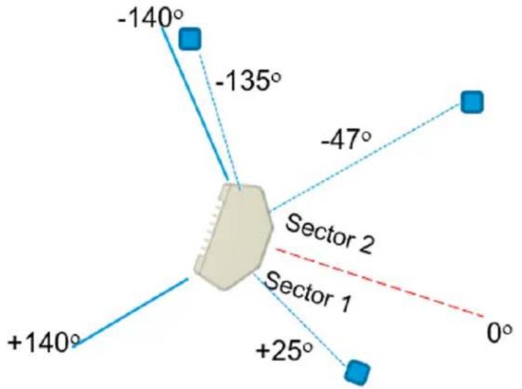
- In Figure 220, a V1000 has been pole mounted with 0 degrees elevation tilt and is pointing approximately 20-30 degrees to the left of the target node (which is located on the tower, as shown in Figure 220). The location of the remote node is at the top of the cell tower so therefore has a higher elevation.
Figure 220: An example of V1000 installation

From V1000 CN's perspective, the reported beam angles are as follows:
• Tx Beam Azimuth Angle: +25.2 degrees
• Rx Beam Azimuth Angle: +25.2 degrees
• Tx Beam Elevation Angle: +14.3 degrees
• Rx Beam Elevation Angle: +14.3 degrees
Table 55 lists the fixed beam scan ranges for 60 GHz cnWave products.
Table 55: Fixed beam scan ranges
| Product Azimuth scan | range Elevation scan range | |
| V1000 -45 degrees to | +45 degrees - 20 degrees to +20 degrees | |
| V2000 -12 degrees to | +12 degrees -6 degrees to +4 degrees | |
| V3000 -2.3 degrees to | +2.3 degrees -2 degrees to +1 degrees | |
| V5000 (both sectors combined) | -140 degrees to +140 degrees - 20 degrees to +20 degrees |
The Tx/Rx x/Rx beam azimuth and elevation angle statistic help in:
-
identifying links, which are operating near the boundary of the scan range, for example, within 5 degrees of +/-140 degrees on a V5000. This implies that the link can be aligned off the edge of the sector and possibly requires the realignment.
• analysing whether interference affects the beam selection - -
when the physical node alignment matches LINKPlanner but the beam angles are significantly out from what is predicted, and/or
- when there is considerable variability in the beam angles used from linkup to linkup.
- determining whether signal obstruction, signal multipath, or interference causes an issue when there is a significant difference between the Tx and Rx beam angle for the same link at the same node.
- On a CN with only one wireless link to align, aiming at an azimuth beam angle close to 0 degrees is optimal.
Ethernet
The Ethernet page displays Transmitting and receiving data of the nodes.
Figure 221:The Ethernet page

The following elements are displayed in the Ethernet page:
Table 56: Elements in the Ethernet page
| Elements Description | |
| Device Name Name of the device | |
| Status Ethernet link status | |
| RX Packets Receiver packets | |
| TX Packets Transmitter packets | |
| RX Bytes Receiver bytes | |
| TX Bytes Transmitter bytes | |
| RX Errors Receiver errors | |
| TX Errors Transmitter errors | |
| RX Dropped Receiver dropped | |
| TX Dropped Transmitter dropped | |
| RX PPS | Receiver Packets Per Second |
| TX PPS | Transmitter Packets Per Second |
| RX Throughput | Receiver throughput |
| TX Throughput | Transmitter throughput |
GPS
The GPS page displays geographical data of the nodes.
Figure 222:The GPS page
The following elements are displayed in the GPS page:
Table 57: Elements in the GPS page
Elements Description
| Device Name | Name of the device |
| MAC Address | MAC address of the device |
Fix Type GPS fix type. The fix status indicates the type of signal or technique being used by the GPS receiver to determine its location. The fix status is important for the GPS consumer, as it indicates the quality of the signal, or the accuracy and reliability of the location being reported.
Satellites The number of satellites tracked tracked
Latitude Latitude of the device
Longitude Longitude of the device
Height Height of the device
Radio
The Radio page displays the radio data of the nodes.
Figure 223:The Radio page

The Radio page has the following elements:
Table 58: Elements in the Radio page
| Elements Description | |
| Device Name Name of the device | |
| MAC Address MAC address of the device | |
| Sync Mode | GPS sync:Entry condition Valid samples from GPS have been received for a few consecutive seconds (typically 2 seconds).Exit condition Valid samples from GPS have not been received for a few consecutive seconds (typically 10 seconds).RF sync: Not in “GPS sync”, but is reachable to a DN with “GPS sync” over wireless links (1-2 hops away).Entry condition Conditions for “GPS sync” have not been met, but a link exists to at least one other DN from which to derive timing.Exit condition Conditions for “GPS sync” have not been met and no links to other DNs exist from which to derive timing.No sync: Neither in GPS sync nor RF sync. This is the default state.Entry condition Conditions for “GPS sync” or “RF sync” are not met.Exit condition Condition for “GPS sync” or “RF sync” are met. |
| Channel Operating channel | |
| Security Security type | |
| Error Association Error Association | |
| Channel Last State Channel Last State | |
| RX Throughput Receiver throughput | |
| TX Throughput Transmitter throughput | |
Performance
The Performance page displays the performance graph.
Figure 224:The Performance page

line
| Metric | Value | | ---------------- | ----- | | RSSI | -30 | | Transmit Power | 60 | | SNR | 40 | | MCS Index | 13 |The Performance page contains the following graphs:
Table 59: Elements in the Performance page
| Elements Description | |
| RSSI Receiver | Signal Strength Indicator. It is a measurement of the power present in a received radio signal |
| Transmit Power | Transmitting power |
| SNR Signal to Noise Ratio | |
| MCS Index Modulation and Coding Scheme (MCS) Index Values can be used to determine the likely data your wireless connection. The MCS value essentially summarizes the number of spatial stream modulation type and the coding rate that is possible when connecting your wireless access | |
| Packet Error Ratio | Packet error ratio. It is the ratio, in percent, of the number of Test Packets not successfully by the node to the number of Test Packets sent to the node by the test set. |
| Received Frames | The number of frames received at the node. |
| Transferred Frames | The number of frames transferred from the node. |
rate of ms, the point. received
RSSI graph
Figure 225:RSSI graph

line
| Date | Max | Min | Avg | | ---------- | ---- | ---- | ---- | | 21:41:55 | -41 | -42 | -40.7| | | -40 | -42 | -40.7|Transmit Power graph
Figure 226: Transmit Power graph
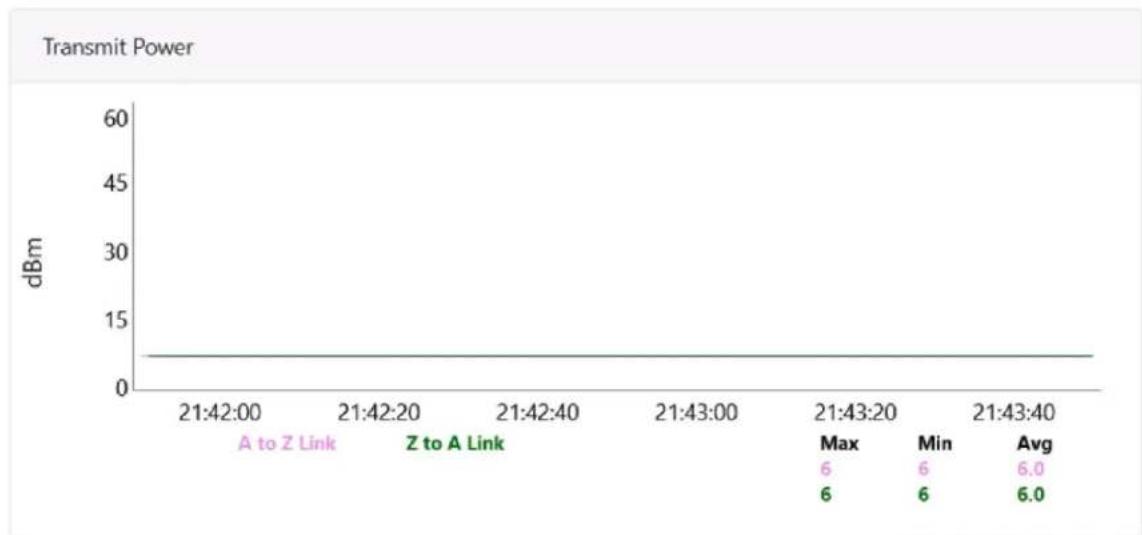
line
| Time | Max | Min | Avg | | ---------- | --- | --- | --- | | 21:42:00 | 6 | 6 | 6.0 | | 21:42:20 | 6 | 6 | 6.0 | | 21:42:40 | 6 | 6 | 6.0 | | 21:43:00 | 6 | 6 | 6.0 | | 21:43:20 | 6 | 6 | 6.0 | | 21:43:40 | 6 | 6 | 6.0 |SNR graph
Figure 227:SNR graph

line
| Date | Max | Min | Avg | | ---------- | --- | --- | --- | | 5-11-2020 21:42:42 | 32 | 31 | 31.1 | | Z to A Link | 30 | 31 | 31.1 |MCS Index graph
Figure 228:MCS Index graph

line
| | Max | Min | Avg | | ------ | --- | --- | --- | | A to Z Link | 9 | 9 | 9.3 | | Z to A Link | 9 | 9 | 9.2 |Packet Error Ratio graph
Figure 229: Packet Error Ratio graph

line
| Date | Max | Min | Avg | | ---------- | ------- | ------- | ------- | | 21:42:00 | 0.00000 | 0.00000 | 0.00000 | | 21:42:23 | 0.00000 | 0.00000 | 0.00000 | | 21:42:40 | 0.00000 | 0.00000 | 0.00000 | | 21:43:00 | 0.00000 | 0.00000 | 0.00000 | | 21:43:20 | 0.00000 | 0.00000 | 0.00000 | | 21:43:40 | 0.00000 | 0.00000 | 0.00000 | | 21:44:00 | 0.00000 | 0.00000 | 0.00000 |Received Frames graph
Figure 230:Received Frames graph

line
| Time | Max | Min | Avg | | ---------- | ----- | ----- | ----- | | 21:42:00 | 2986 | 2332 | 2612.2| | 21:42:20 | 2986 | 2332 | 2612.2| | 21:42:40 | 2986 | 2332 | 2612.2| | 21:43:00 | 2986 | 2332 | 2612.2| | 21:43:20 | 2986 | 2332 | 2612.2| | 21:43:40 | 2986 | 2332 | 2612.2| | 21:44:00 | 2986 | 2332 | 2612.2|Transferred Frames graph
Figure 231: Transferred Frames graph

line
| Date | Max | Min | Avg | | ---------- | ----- | ----- | ----- | | 21:42:51 | 2776 | 2121 | 2399.7 | | | 2776 | 2121 | 2399.7 |Prefix zone Statistics
In the multi-PoP deployments, the mesh is divided into prefix zones. Prefix zone statistics are available on the Statistics > Prefix Zone page.

Note
You can view the prefix zone statistics only when Deterministic prefix (DPA) is enabled. With CPA enabled, the Prefix Zone tab is not visible on the Statistics page.
Figure 232:The Prefix Zones page
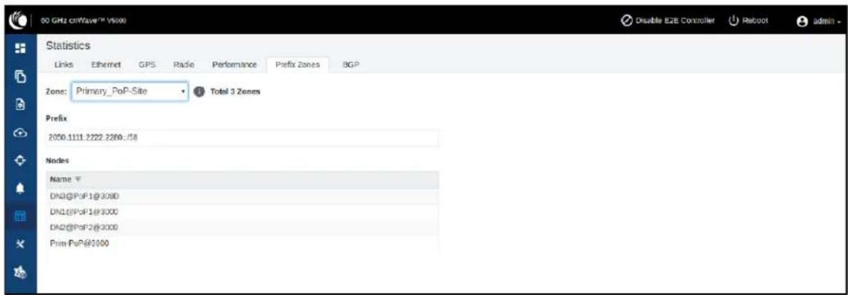
Border Gateway Protocol (BGP)
The BGP is the protocol used throughout the Internet to exchange routing information between networks. It is the language spoken by routers on the Internet to determine how packets can be sent from one router to another to reach their final destination. BGP has worked extremely well and continues to be protocol that makes the Internet work.
The BGP page displays the routing information. This page also contains the details of routes advertised by PoPs to their peers and the routes received by the peers.
Figure 233:The BGP page
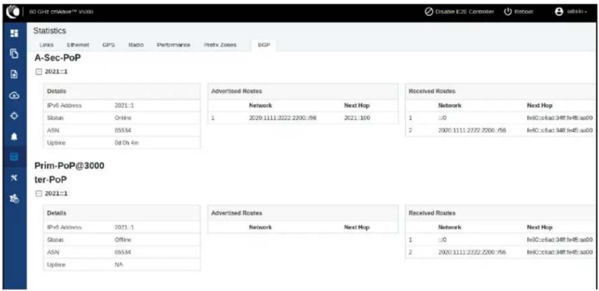
Maps
The Maps page displays the topology and location/sites of the deployed nodes in the cnWave network. Click the Maps icon on the left panel to display the nodes.
Figure 234:The Map page

flowchart
graph TD
    A["DN121P-0009"] --> B["DN341P-2000"]
    B --> C["PN1-Po-Fo-0301"]
    B --> D["DN27-0.3801"]
    B --> E["DN46-3007"]
Tools
The Tools page contains the following tabs:
- Factory Reset
- Field Diags
- Antenna Alignment
- Remote Command
• Ping - Quick PTP Setup
• iPerf
Factory reset
The Factory Reset page is used to set the default settings.
Figure 235:The Factory Reset page


Warning
Factory reset is followed immediately by a system reboot. You must carefully configure the factory reset settings as the device comes up with the default settings. All the existing configurations are lost when the system comes up.
Field diags
The Field Diags tab is used to view and download the error logs. To download the DN logs, select the DN node from the Select Node drop-down and click Download Logs (as shown in Figure 236).
Figure 236:The Field Diags page
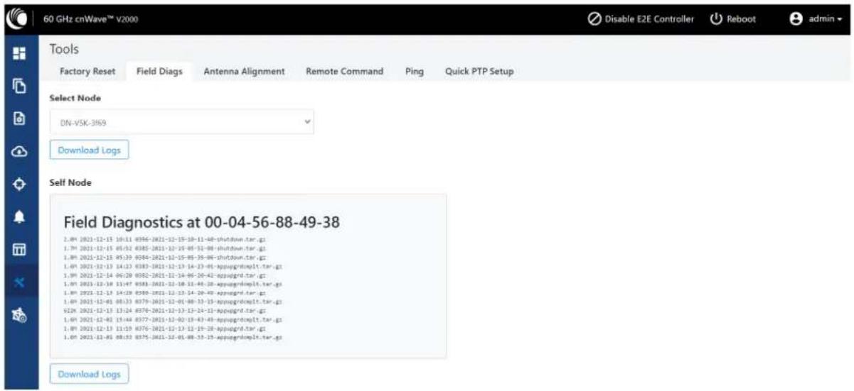
To download the logs for a self-node, click Download Logs at the bottom of the page. Save the log file.
Figure 237: Saving log files

Antenna alignment
The Antenna Alignment tool assists in optimizing the alignment of V3000 to V3000, V5000, V2000, or V1000. This feature helps you to install and align the devices to achieve optimal performance.

Warning
The antenna alignment tool is not a substitute for optical alignment. The optical alignment is the key for getting the signal within the +/-2 degree azimuth and +/-1 degree Elevation window. At this window level, the tool can be used to get away from the edge, corner or spurious beams to ensure optimal alignment.
Prerequisite tasks:
- Complete a Link Plan with Link Planner from Cambium Networks. This prerequisite task provides the information on the RSSI expected for the PTP link. This must be used as a target while using the antenna alignment feature.
-
Enter the PTP topology in cnMaestro or the UI of a device (with the Onboard Controller on it). Then, perform the following steps:
-
Create two Sites and nodes.
- Set up the wireless link between the two nodes.
- Ensure that the nodes are already mounted at the sites.
- An installer must have access to the UI of the device.

Note When the antenna alignment test is executed between the following devices, ensure that GPS is disabled at the CN side:
• V3000 PoP and V1000 CN
• V3000 PoP and V2000 CN
• V3000 PoP and V3000 CN
Using the Antenna Alignment tool
To use the Antenna Alignment tool, perform the following steps:
- From the home page of the device UI, navigate to Tools > Antenna Alignment.
The Antenna Alignment page appears, as shown in Figure 238.
Figure 238: The Antenna Alignment page


Note
If the alignment is initiated from a CN, ensure that the operating channel is set on the radio (before alignment). If the channel is not set, you must set the required channel in the Configuration page of the V3000 single node UI.
- Click the Start Alignment button located at the top left side of the Antenna Alignment page.
The Confirm message box appears (as shown in Figure 239), indicating that the link will be disrupted. For running the antenna alignment tool, the auto ignition needs to be disabled. If a link has been established already, it is disassociated at this level.
Figure 239: The Confirm message box in the Antenna Alignment page
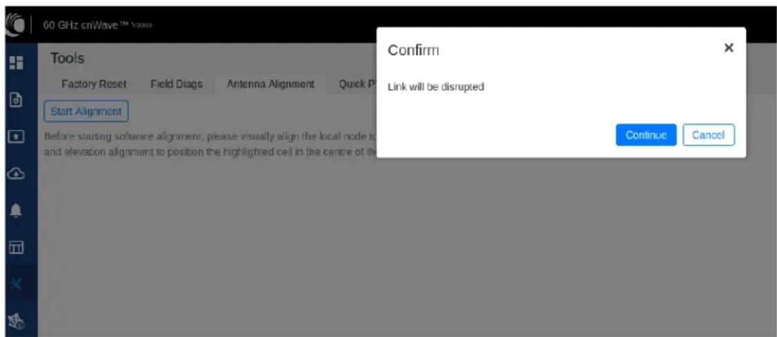
- In the Confirm message box, click Continue to start the antenna alignment process.
The antenna alignment process begins.

Note
If the alignment is initiated from a device (which is not running with Onboard Controller), perform the following actions:
a. Disable the ignition of the link at the Controller.
b. Send Dis-assoc for the link from the Controller.
c. When the alignment starts, select the required node from the Remote Node Model drop-down list.
The Time Frame section populates the RSSI time series as shown in Figure 240.
Figure 240:The RSSI time series
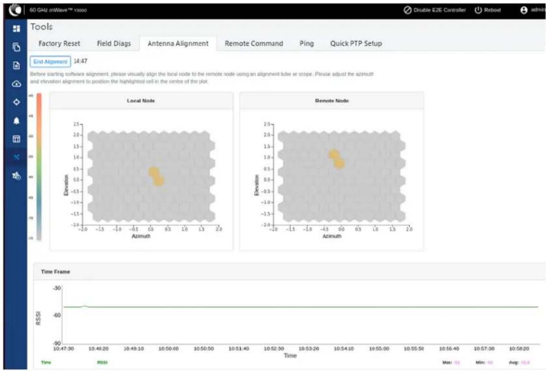
Following details explain about the RSSI time series that populates in the Antenna Alignment page:
- The Local Node section (located at the left side of the Antenna Alignment page) displays the direction of arrival angle with respect to the local (PoP) device.
- The Remote Node section (located at the right side of the Antenna Alignment page) displays the direction of arrival angle with respect to the remote device.
- In Local Node and Remote Node sections, a cell marks the direction of arrival. The color of the cell represents the RSSI based on the heatmap scale given on the left side.
- The Time Frame section (located at the bottom of the Antenna Alignment page) displays the RSSI time series, along with the peak RSSI time and the latest data point (on the right end of the plot).
The RSSI time series and the heatmap plots get updated every six seconds. This is due to the processing time taken for a complete sweep of all the combinations of beams and channels.
During the alignment phase, the transmit power used is the maximum configured power and the transmit power control is disabled.

Note
If the installer has enabled the short-range installation in the radio configuration, the transmit power control is set to the minimum configured power.
- Adjust the optimal RSSI that must be reached when the beams are close to the central region, as shown in Figure 241.
Figure 241:The optional RSSI alignment
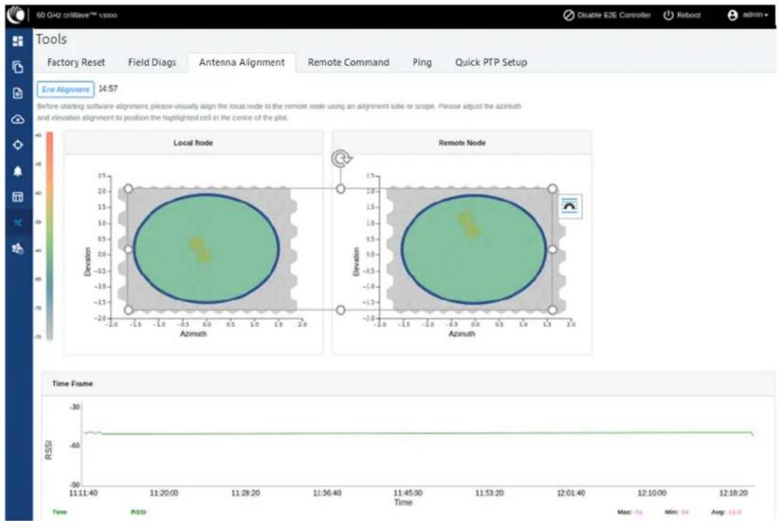
The RSSI time series must be close to the Link planner's predicted RSSI (the receive level when aligning, as shown in Figure 242), with an error of +/-5dB. Consider the following points when adjusting the optional RSSI:
- If the time series reporting RSSI is more than 10dB from that of the Link Planner's expected RSSI, then the device has been aligned incorrectly and is being picked up by the sidelobes or spurious beams.
- If a cell is highlighted and the time series reporting RSSI is more than 10dB off the expected RSSI, then it is necessary to sweep beyond the current position of both azimuth and elevation, in turn to ride past the sidelobes.
Figure 242: An example of the receive level when aligning - Link planner
| Radio Commissioning Notes for CN | |
| Model | V3000 |
| Maximum EIRP | 60 dBm |
| Minimum MCS | MCS 2 |
| Maximum MCS | MCS12 (16QAM 0.75 Sngl) |
| Channel | 64.80 GHz (Channel 4) |
| Polarity | Auto |
| Predicted Receive Power | -46 dBm ± 5 dB while aligning |
| Operational EIRP | 46 dBm |
| Operational Receive Power | -60 dBm ± 5 dB |
| Predicted Link Loss | 116.25 dB ± 5.00 dB |
- Make use of the direction of arrival information (if there is any elevation or azimuth mismatch) to physically align the radio antennas.
- When there is an elevation mismatch (as shown in Figure 243):
Figure 243:Example of the elevation mismatch
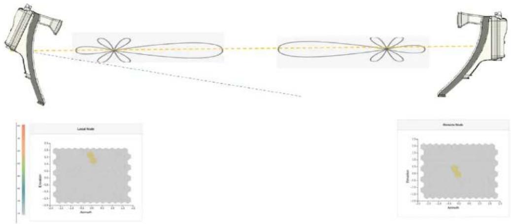
In Figure 243, the angles are exaggerated to show the point. In this example, consider that the radio has been misaligned by a down-tilt of 2 degrees behind the unit (from an installer's view side). This means that the angle of the beam selected might be in the +2 degrees direction in the elevation due to beamforming. The aim is to get the optimal boresight beam. Therefore, the radio must be up tilted in the elevation direction by 2 degrees. The selected beam is now closer to the boresight beam, as shown in Figure 244.
Figure 244: On correcting the elevation mismatch
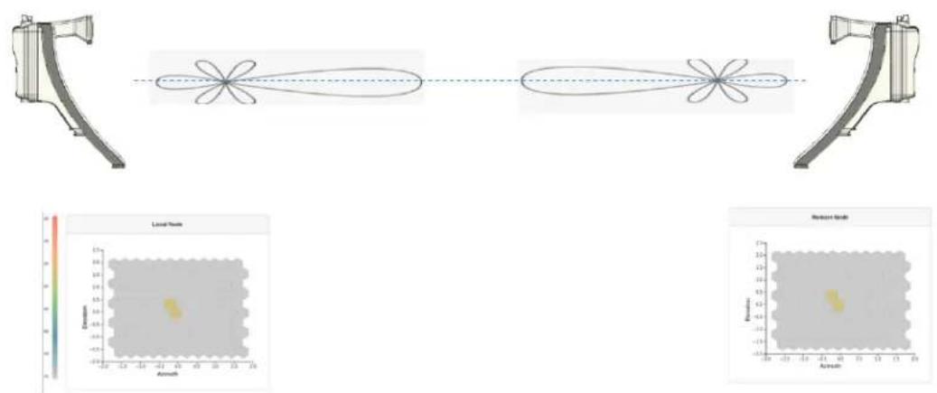
- When there is an azimuth mismatch (as shown in Figure 245):
Figure 245:Example of the azimuth mismatch

In Figure 245, the angles are exaggerated to show the point. In this example, consider that the radio has been misaligned in azimuth by 2 degrees to the right behind the unit (from an installer's view side). This means that the angle of the beam selected might be in the -2 degrees direction due to beamforming. The aim is to get the optimal boresight beam. Therefore, the radio must be tilted in the azimuthal direction to the left by 2 degrees. The selected beam is now closer to the boresight beam, as shown in Figure 246.
Figure 246: On correcting the azimuth mismatch
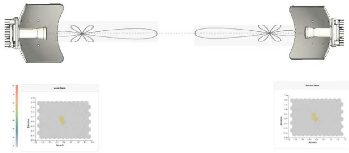
- When you achieve the desired alignment and RSSI, click the End Alignment button located at the top left side of the Antenna Alignment page.
If you do not click the End Alignment button, the alignment cycle ends automatically after 15 minutes. When the alignment cycle ends, the ignition state (disabled earlier) is enabled to auto ignition and the link is established. Figure 247 shows how the Antenna Alignment dashboard page looks on completing the antenna alignment task.
Figure 247: The updated Antenna Alignment dashboard page
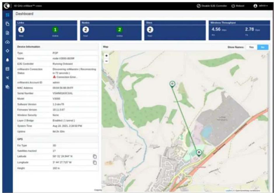
Remote Command
The Remote Command tool page supports the following commands:
• Show SFP power details
• Show ipv4 neighbors
• Show ipv6 neighbors
• Show Wired Interface State Changes
Show SFP power details
The Show SFP Power Details command is available on the Tools page. When you execute this remote command from the Onboard Controller UI or the node CLI, the command provides the SFP power details (as an output) for the required SFP ports and interfaces.

Note
Currently, the Show SFP Power Details remote command is not available in cnMaestro.
To execute the Show SFP Power Details remote command, perform the following steps:
- From the home page of the device UI, navigate to Tools > Remote Command.
The Remote Command page appears. - Select the required node from the Select Node drop-down list.
- Select Show SFP Power Details from the Select Command drop-down list.
4. Click Execute.
The Output section displays the SFP power details for the selected node, as shown in Figure 248.
Figure 248: The UI supported output - SFP Power details

Table 60 lists and describes each parameter in the output.
Table 60: Output details
| Output Parameter Description | |
| Status Determines whether | the output is valid.If the Status field contains OK, it implies that the rest of the output isIf the Status field does not contain OK, it implies that only the Status field is valid. In such cases, the Status field provides the reason for not being read the laser powers. |
| CalibrationType Indicates the | measurement type that is calibrated over the criteria, such as the following (for example):Specified transceiver temperature,Transceiver supply voltage,TX output power, andRX received optical power.The value of this parameter is Internal. |
| Units Indicates the unit of | measurement.The value of this parameter is micro-watts (mW). |
| txPwr Indicates the TX output power in mW. | |
| rxPwr Indicates the RX received optical power in mW. |
valid.
able to
| Output Parameter Description | |
| rxPwrMeasType Indicates wh | whether the received power measurement represents an average input optical power.The value of this parameter is Average. |
| txPwr_dBm Indicates the TX | output power in dBm. |
| rxPwr_dBm Indicates the RX | received optical power in dBm. |
- To download the output, click the download icon located at the top left side of the Remote Command page.
You can also execute the Show SFP Power Details command by using the device CLI. Log on to the device and open the CLI. At the command prompt, provide the Show SFP value and hit Enter on your keyboard. The command displays the output, as shown in Figure 249.
Figure 249: The CLI supported output - SFP Power details
CLISH>show sfp
{
    "status": "OK",
    "calibrationType": "Internal",
    "units": "micro-watts",
    "txPwr": 564.3,
    "rxPwr": 557.1,
    "rxPwrMeasType": "Average",
    "txPwr_dBm": -2.485,
    "rxPwr_dBm": -2.541
}
CLISH>
Show ipv4 neighbors
The Show ipv4 neighbors remote command reveals the Address Resolution Protocol (ARP) table for IPv4 addresses in the network. The ARP table, also known as the neighbour table for IPv4, links IP addresses to MAC addresses for devices within the same local network.
When you execute the Show ipv4 neighbors command using the Tools > Remote Command page, you can view information of the active IPv4 neighbours in the output. In addition, the output information can also aid in identifying potential network anomalies or connectivity issues.
To execute the Show ipv4 neighbors command, perform the following steps:
- On the Tools > Remote Command Page, select the required node from the Select Node drop-down list.
- Select Show ipv4 neighbors from the Select Command drop-down list.
- Click Execute.
The Output section displays the IPv4 neighbor details for the selected PoP or CN, as shown in Figure 250.
Figure 250: The Show ipv4 neighbors command output

You can use the icon to download the output (in .txt format).
Show ipv6 neighbors
The Show ipv6 neighbors remote command displays the neighbour table for IPv6 addresses, analogous to the IPv4 ARP table but for IPv6 addresses. As the adoption of IPv6 continues to rise, the visibility into these connections becomes more critical.
When you run the Show ipv6 neighbors command from the Tools > Remote Command page, the command unveils the relationship between IPv6 addresses and MAC addresses within a local network. In addition, the command enables effective monitoring and troubleshooting of IPv6 network issues.
On selecting the required node from the Select Node drop-down list and Show ipv6 neighbors from the Select Command drop-down list, click Execute. The Output section displays the IPv6 neighbor details for the selected node, as shown in Figure 251.
Figure 251: The Show ipv6 neighbors command output

To download the output (in .txt format), use the icon.
Show Wired Interface State Changes
The Show Wired Interface State Changes remote command displays up or down events on wired interfaces. This command is useful for debugging and troubleshooting network events.
This remote command enables network administrators to identify and analyze Ethernet port state changes, and provides insights into network events such as connection issues or device status changes.
To execute the Show Wired Interface State Changes command, perform the following steps:
- On the Tools > Remote Command Page, select the required node from the Select Node drop-down list.
-
Select Show Wired Interface State Changes from the Select Command drop-down list.
-
Click Execute.
The Output section displays the up or down events for the selected criteria, as shown in Figure 252.
Figure 252: The Show Wired Interface State Changes output

To download the output, use the icon.
Ping
The Ping tool provides information that is used to identify the reachability between the required node and another nodes or destination (for IPv4 and IPv6). The ping tool is useful in troubleshooting radio links.
To use the ping tool, perform the following steps:
- From the home page of the device UI, navigate to Tools > Ping.
The Ping page appears.
- Set the parameters with the required values, as described in Table 61.
Table 61: List of parameters in the Ping page
| Parameter Description | |
| Source Node | The source node for which you want to find the reachability with another node or destination.Select the required source node from the drop-down list. |
| Destination Type | The required node or destination address (IPv4 or IPv6) that for which the reachability has to be identified.Following options are supported:NodeIPv4• IPv6Select the required option (mandatory). |
| Number of Packets (-c) | Number of times that a packet is transmitted to find the reachability.Default value: 3This parameter supports values between 1 (minimum) and 10 (maximum).Type an appropriate value in the text box. |
| Buffer Size (-s) | Size (in bytes) of the packet.Default value: 56This parameter supports values between 1 (minimum) and 65507 (maximum).Type an appropriate value in the text box. |
3. Click Start Ping.
The Ping Result section displays the information for the selected criteria, as shown in Figure 253.
Figure 253:The Ping page

You can use the icon to download the ping result.
Quick PTP setup
Quick PTP Setup is a simple user-friendly tool used for quickly creating a PTP link between the PoP and the CN. This option eliminates the long process of creating a PTP link with Onboard Controller in the Topology UI page.
With the Quick PTP Setup option, you can skip the long process of creating a PTP link that involves the following actions:
- Enabling Onboard Controller on the required node that can also act as a PoP node.
- Adding a site for the CN node.
- Adding a node for the CN node.
- Creating a link between the PoP and the CN nodes.
The Quick PTP Setup option enables you to create the PTP link using the simple process on the Tools page of the device UI.
To create the PTP link quickly for the required nodes, perform the following steps:
- Navigate to Tools > Quick PTP Setup from the home page of device UI.
The Quick PTP Setup page appears, as shown in Figure 254.
Figure 254:The Quick PTP Setup tab on the Tools page

- In the CN MAC Address text box, enter the MAC address of the required CN node (which is connected).

Note
You can also access the MAC address of the connected CN in the Device Information section of the main Dashboard page (of the device UI).
- Click Start PTP Setup.
This action creates the PTP link between the PoP and the CN nodes, quickly.
When you configure Quick PTP Setup, the unit turns to a DN running E2E Controller with Layer 2, and default IPv4 address of 169.256.1.1. When the client onboards, E2E Controller pushes the configuration to a CN with the IPv4 address of 169.254.1.2.
You can view the connected PoP and CN details on the Topology page of the device UI.
iPerf
The iPerf tool is a user-friendly tool for conducting network performance tests using the device UI. The tool makes network performance testing more accessible and manageable. It helps you with tools required for effective measuring
and understanding the network's performance.
The iPerf tool is built around the widely recognized iPerf testing tool (open-source) and provides a graphical UI for conducting the network performance tests with ease.
Following are the features of the iPerf tool:
- Server Node and Client Node selection: The iPerf tool allows you to easily select the server and client nodes for your network performance tests. The node selection sets up the endpoints required for the test. In addition, the test traffic is unidirectional, flowing from the client to the server.
- Time and Parallel Streams selection: You can specify the time in seconds to customize the duration of the tests. You can also select the number of parallel streams to run during the test, providing more granular control over the testing parameters.
- TCP, IPv6 Layer 3 Traffic Profile: Network performance tests are conducted using a TCP, IPv6 Layer 3 traffic profile. The iPerf tool internally handles the selection and implementation of the traffic profile, and simplifies the test process.
- Network performance profiling: The iPerf tool allows you to profile the performance of your network on a link-by-link basis. This tool is instrumental in identifying performance blockers and optimizing network performance.
- Coexisting with customer data: The iPerf tool tests traffic that competes with customer data, rather than blocks or stops. There is no prioritization given to either data, ensuring that the test results reflect real-world network conditions.
- Complete iPerf output display: On conducting the network performance test, you can view the entire iPerf output in a dedicated panel on the Tools > iPerf page. This tool offers an easy and a convenient way to interpret the results (within the interface).

Note
The throughput, measured by the iPerf tool, must only be used as a guideline. Using traffic testing software onboard the radio carries additional processing overheads, which are not present in the normal operation.
To use the iPerf tool, perform the following steps:
- From the homepage of the device UI, navigate to Tools > iPerf.
The iPerf page appears.
- Set the values for the parameters, as described in Table 62.
Table 62: Parameters required for running the iPerf tool
| Parameter Description | |
| Server Node | The server node for which you want to conduct the network performance test.Select the required server node from the drop-down list.Note: You can use the icon to reverse the server and client node names. |
| Client Node | The client node for which you want to conduct the network performance test.Select the required client node from the drop-down list.Note: You can use the icon to reverse the server and client node names. |
| Duration (Seconds) | Period (in seconds) that you want to set for the test.Type an appropriate value (in seconds) in the text box.Default value: 10 secondsNote: This parameter supports values from 1 to 300 (in seconds). |
| Parallel Streams | Number of parallel streams that you want to run during the test.Default value: 4Type the required value in the text box.Note: This parameter supports values from 1 to 4. |
3. Click Start iPerf.
The Server Node Results section and the Client Node Results section display the results for the selected criteria, as shown in Figure 255.
Figure 255:The iPerf tool page
![60 MHz drive** 9500 Tools Factory Name Final Drugs Benuee Command Reg Perf Server Note node V5000-88833d Ovation (Seconds) 10 Min = 1, Max = 300 Parallel Streams 8 Min = 1, Max = 4 Best Perf Server NodeResult "node-V5000-88833d" [ ] 7.88-8.88 sec 55.4 Mytes 602 MHz/sec [12] 7.88-8.88 sec 55.5 Mytes 602 MHz/sec [14] 7.88-8.88 sec 55.6 Mytes 602 MHz/sec [16] 7.88-8.88 sec 55.7 Mytes 602 MHz/sec [18] 7.88-8.88 sec 55.8 Mytes 602 MHz/sec [ ] 7.88-8.88 sec 55.9 Mytes 602 MHz/sec [12] 7.88-8.88 sec 55.9 Mytes 602 MHz/sec [14] 7.88-8.88 sec 55.9 Mytes 602 MHz/sec [16] 7.88-8.88 sec 55.9 Mytes 602 MHz/sec [18] 7.88-8.88 sec 55.9 Mytes 602 MHz/sec [ ] 7.88-8.88 sec 55.9 Mytes 602 MHz/sec [12] 7.88-8.88 sec 55.9 Mytes 602 MHz/sec [14] 7.88-8.88 sec 55.9 Mytes 602 MHz/sec [16] 6.40-9.40 sec 55.4 Mytes 604 MHz/sec [12] 6.40-9.40 sec 55.4 Mytes 604 MHz/sec [14] 6.40-9.40 sec 55.4 Mytes 604 MHz/sec [16] 6.40-9.40 sec 55.4 Mytes 604 MHz/sec [18] 6.40-9.40 sec 55.4 Mytes 604 MHz/sec [ ] 6.40-9.40 sec 55.4 Mytes 604 MHz/sec [12] 6.40-9.40 sec 55.4 Mytes 604 MHz/sec [14] 6.40-9.40 sec 55.4 Mytes 604 MHz/sec [16] 6.40-9.40 sec 602 MHz/sec [18] 6.40-9.40 sec 602 MHz/sec [ ] 6.40-9.40 sec 602 MHz/sec [12] 6.40-9.40 sec 602 MHz/sec [14] 6.40-9.40 sec 602 MHz/sec [16] 6.40-9.40 sec 602 MHz/sec [18] 6.40-9.40 sec 602 MHz/sec [ ] Interval Transfer Rate Next [ ] Interval Transfer Rate Next [ ] Interval Transfer Rate Next [ ] Interval Transfer Rate Next [ ] Interval Transfer Rate Next [ ] Interval Transfer Rate Next [ ] Interval Transfer Rate Next [ ] Interval Transfer Rate Next [ ] Interval Transfer Rate Next [ ] Interval Transfer Rate Next [ ] Interval Transfer Rate Next [ ] Interval Transfer Rate Next [ ] Interval Transfer Rate Next [ ] Interval Transfer Rate Next [ ] Interval Transfer Rate Next [] perf name](/content/2026/05/1088487/images/48eca385bb1a93a4e1ca774e50dec6d0bcc287eebb4f87d401a12fd68c662aa8.jpg)
To download the server and client node results (in .txt format), use the ↓ icon on the iPerf page.
cnMaestro support for Onboard Controller
The Onboard E2E controller can be managed by cnMaestro 2.5.0 (On-Premises) for network management.
-
After the Onboard E2E controller is enabled from UI, enter the cnMaestro URL. If Cambium ID based authentication option is enabled in cnMaestro, then enter the Cambium ID and onboarding key.
-
Click Enable E2E on Onboard E2E Controller in UI.
Figure 256:The Onboard E2E Controller page

-
Enter the cnMaestro management configuration information.
-
Remote Management - Select the required remote management option
- cnMaestro URL - cnMaestro address
• Cambium ID - Cambium ID of the device - Onboarding key - Password to onboard the device
Figure 257:The cnMaestro section
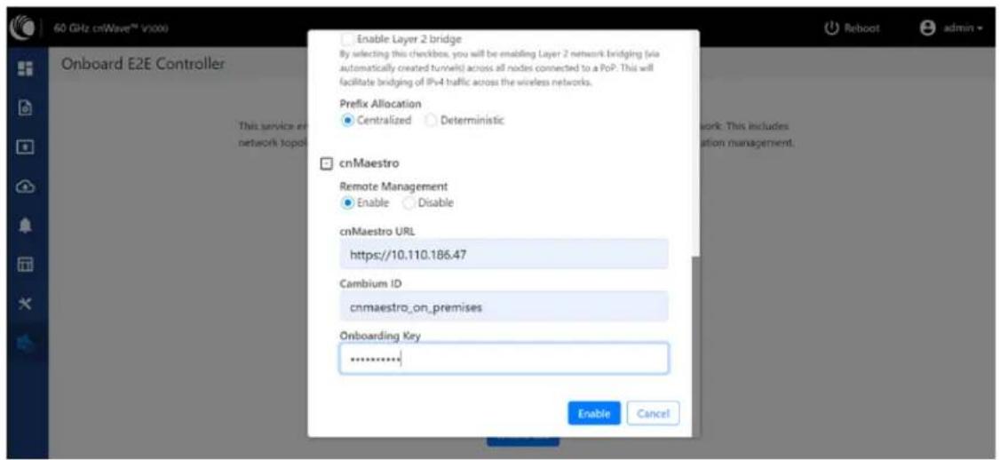
- Click Enable.
- A new E2E Network appears in cnMaestro. Click Approve to manage it.
Figure 258: Information on the new E2E network
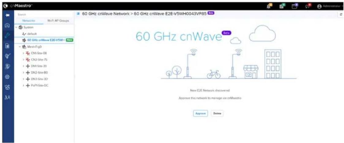
-
The Network Onboard window appears and provides an option to edit the network name.
-
Click Save.
Figure 259:The 60 GHZ cnWave - Network Onboard

After the successful onboarding of the E2E Network, it can be managed through cnMaestro.
Figure 260: The Onboard 60 GHZ cnWave E2E dashboard page

Backup CN link
If a link between Pop or DN and CN gets disconnected, then a backup CN link (if enabled using the cnMaestro UI) provides connectivity from PoP or DN to a particular CN. CNs can form only one link but additional backup links can be provided for use when the primary link is unavailable (for at least 300 seconds).
To add and enable the backup CN link, perform the following actions:
- From the landing page of the device UI, navigate to Networks > required link name and select the icon. A drop-down list appears with multiple options, as shown in Figure 261.
Figure 261: The drop-down list with the Add Link option

- From the drop-down list, select Add Link as shown in Figure 261.
The Add Link page appears with the Backup CN Link checkbox, as shown in Figure 262.
Figure 262:The Backup CN Link checkbox
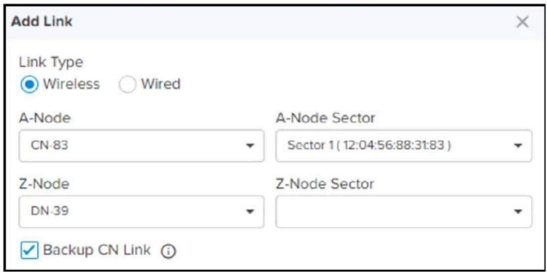
You must configure the required node-specific parameters, such as A-Node, A-Node Sector, and Z-Node, before enabling the backup CN link.
- Select the Backup CN Link checkbox.
On the Maps page, backup CN links are shown in a dash line format (as shown in Figure 263).
Figure 263: Representation of the backup CN links on the Maps page
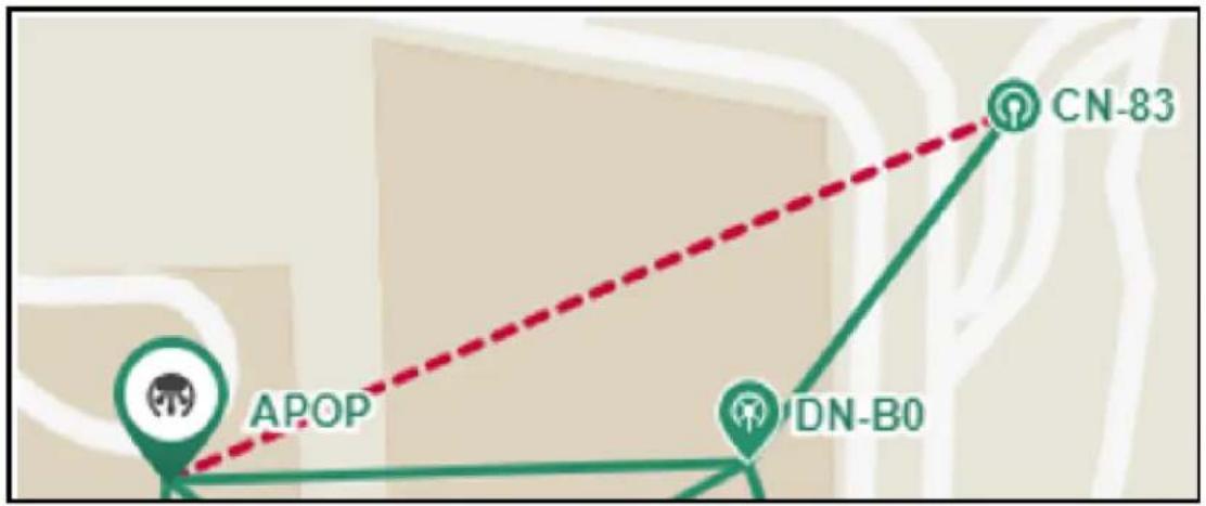
flowchart
graph TD
    A["APPOP"] --> B["DN-B0"]
    B --> C["CN-83"]
    style A fill:#99ccff,stroke:#333
    style B fill:#99ccff,stroke:#333
    style C fill:#99ccff,stroke:#333
Auto Manage IPv6 Routes (External E2E Controller)
E2E Controller communicates with all nodes over IPv6. PoP nodes use IPv6 address of the statically configured interface to communicate with E2E Controller. CNs and DNs use the IPv6 address derived from Seed Prefix.

Note
The Auto Manage Routes feature requires cnMaestro 3.0.4.
The Auto Manage Routes feature adds and manages the IPv6 routes at E2E Controller. These IPv6 routes are required for routing the IPv6 packets to CNs and DNs.
The feature is applicable only when PoP and E2E Controller are in the same subnet.
Single PoP network
When the feature is disabled, you must add the IPv6 route by performing the following steps:
- From the landing page of the device UI, navigate to Tools > Settings > IPv6 Routes > Add new. The Add Route page appears, as shown in the Figure 264.
Figure 264:The Add Route page in the cnMaestro UI

- Type the seed prefix value in the Destination text box.
- Type the required PoP's interface IP address in the Gateway text box.
- Click Add.
The IPv6 route is added.
When the feature is enabled, all the above steps (described from step 1 to step 5 in this section) are not required and IPV6 routes are added automatically.
- Select the Auto Manage Routes check box in the IPv6 Routes page.
Figure 265 shows the location of the Auto Manage Routes check box in the IPv6 Routes page.
Figure 265: The Auto Manage Routes check box

Multi-PoP network
In a multi-PoP network, the Auto Manage Routes feature allows to avoid a BGP v6 router under the following conditions:
- When the Layer 2 bridge is enabled (which implies that the BGP v6 router is not required for managing data traffic).
- When PoPs and E2E Controller are in the same subnet or L2 broadcast domain.
In a multi-PoP network, Deterministic Prefix Allocation (DPA) is used. The mesh gets divided into zones. Each PoP is the best gateway to reach nodes in its zone. When a PoP is down, a different alive PoP must be used as a gateway to reach zones. When the Auto Manage Routes feature is enabled, it performs the following functions in a multi-PoP network:
• Understands the network topology of 60 GHz cnWave,
- Keeps a track of aliveness of PoPs, and
• Dynamically builds and manages the routing table.
Figure 266 is an example of an IPv6 route table that is built automatically by the feature for a four PoP network.
Figure 266:Example of IPv6 route entries in the IPv6 Routes page
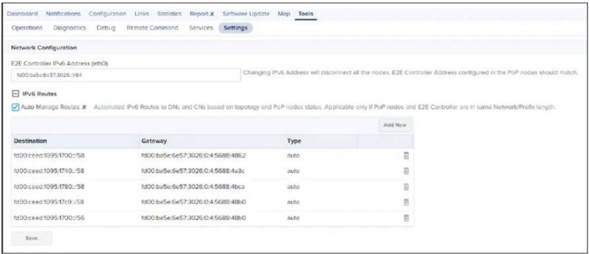
Figure 267 shows how the cnMaestro dashboard diagrammatically displays the routes taken by E2E Controller and the traffic controlled by cnWave nodes.
Figure 267: Diagrammatic representation of IPv6 routes and traffic control

flowchart
graph TD
    A["E2E Controller\nSeed Prefix Range\nfd00:ceed:1095:1700::/56"] --> B["POP1"]
    A --> C["POP2"]
    A --> D["POP3"]
    A --> E["POP4"]
    B --> F["FAT1-RT-N1"]
    C --> G["FAT1-RT-N2"]
    D --> H["FAT1-RT-S1"]
    E --> I["FAT1-RT-S2"]
    F --> J["DN Count: 4\nCN Count: 0"]
    G --> K["DN Count: 4\nCN Count: 0"]
    H --> L["DN Count: 2\nCN Count: 0"]
    I --> M["DN Count: 4\nCN Count: 0"]
Unconnected PoPs
In a multi-PoP network, PoPs must be able to exchange openR packets either on wired or wireless path. Otherwise, DNs might not receive the IPv6 address allocation and might not onboard to E2E Controller. This is observed when Controller sends the Prefix Allocation message to one of the PoPs and expects the message to reach other PoPs through openR.
In some cases, PoPs might be isolated temporarily, especially while building the network. Figure 268 is an example that shows two unconnected zones.
Figure 268: Unconnected zones due to isolated PoPs
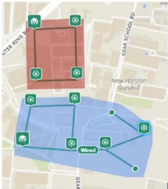
To facilitate such a scenario, a new configuration parameter flags.enable_pop_prefix_broadcast has been introduced in this release. This parameter supports the following Boolean values:
- true - When the value of this parameter is set to true, E2E Controller sends the prefix allocation message to all PoPs individually.
- false -When the value of this parameter is set to false, E2E Controller sends the prefix allocation message to one of the PoPs.
The default value of this parameter is false (default setting).

Note
You must set this parameter's flag to false when there is a wired or wireless path between PoPs.
You can modify the flags.enable_pop_prefix_broadcast parameter in the UI of 60 GHz cnWave.
To configure the parameter, perform the following steps:
- From the landing page of the device UI, navigate to Configuration > E2E Controller.
The E2E Controller page appears. The flags.enable_pop_prefix_broadcast parameter is available in the E2E Controller page, as shown in Figure 269.
Figure 269:The flags.enable_pop_prefix_broadcast parameter
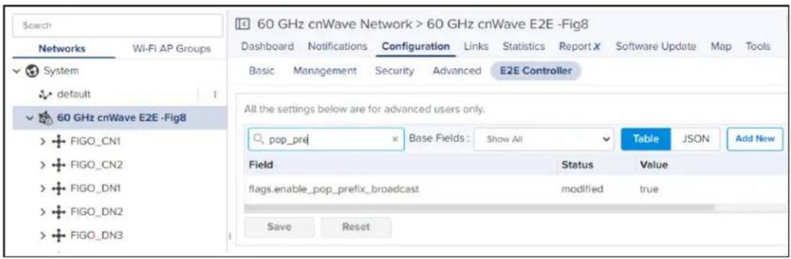
- Modify the value of the parameter.
- Click Save to save the configuration changes.
High Availability (HA) support for Onboard E2E Controller
In this release, the high availability (HA) support for Onboard E2E Controller has been added.
Using cnMaestro, you can enable and configure HA support in a Multi-PoP Onboard E2E Controller that is running 60 GHz cnWave devices in a mesh network. This HA support configuration allows you to configure a primary (active mode) and a backup or secondary (passive mode) E2E Controller from cnMaestro.
If the active primary E2E Controller, with HA enabled and functioning, goes down, then the backup E2E Controller is active and manages the 60 GHz cnWave devices. All the devices report to the backup E2E Controller until the primary E2E Controller comes back.
This topic covers the following sections:
• Theory of operation
- Configuring HA support using cnMaestro
• Caveats of HA configuration
Theory of operation
E2E Controllers use the high-availability protocol (primary-backup) and support the HA configuration. In such a primary-backup setup, two controllers (peers) run on separate PoP nodes and are designated primarily backup. If the primary controller catastrophically fails (for example, power outage, network failure, hardware failure), the backup controller assumes control of the cnWave 60 GHz network.
The HA configuration supports the following operational mechanisms for Onboard E2E Controller:
- Role designation: At setup, one controller is statically designated as primary, and the other as backup. This designation determines their initial operational roles during network management.
- Initial state: The primary controller starts in an active state, overseeing network configuration and collecting network statistics. The backup controller remains in a passive state, prepared to assume control if needed.
-
Health monitoring: Both primary and backup controllers monitor each other's status through regular heartbeat messages, sent every five seconds. These messages are crucial for detecting any disruptions or failures in the primary (active) controller.
-
Data synchronization: Both primary and backup controllers periodically synchronize topology and configuration data. This synchronization is key to enabling a fast and seamless transition from passive to active state, ensuring the backup controller can immediately manage the network with up-to-date settings and configurations.
-
Failover process: If the primary (active) controller fails, detected by a loss of heartbeat messages for 20 seconds, the backup controller automatically transitions from passive to active. This change ensures continuous network management without manual intervention.
-
Recovery and Reversion: After the failed primary controller is repaired and comes back online, it starts in a passive state. It remains in this passive state until it has successfully exchanged heartbeat messages for 150 seconds, ensuring stability. Following this period, a role reversal occurs where the primary controller transitions back to active and the backup controller reverts to passive.
Configuring HA support using cnMaestro

Note
The HA support is applicable only to cnMaestro X accounts. Consider the following key points:
- The Onboard E2E Controller must be managed using cnMaestro.
- The Onboard network must have at least two PoP nodes to enable HA.
- The two PoP nodes are selected to host Primary. The backup controllers should be able to communicate over wire/ethernet.
- For HA, all the DN/CN nodes in network are expected to have a route to report to both the HA peers.
- The HA feature is supported in a network when devices are running 1.4 or above software version.
To enable the HA support for E2E Controller, complete the following steps:
- From the Home page of cnMaestro, navigate to Monitor and Manage > E2E Network > Configuration > High Availability X.
The Enable High Availability checkbox appears.
Figure 270: The Enable High Availability check box - cnMaestro UI

- To enable the HA support for E2E Controller, select the Enable High Availability check box.
The High Availability X page displays options to configure the backup Controller.
Figure 271: The HA support configuration options
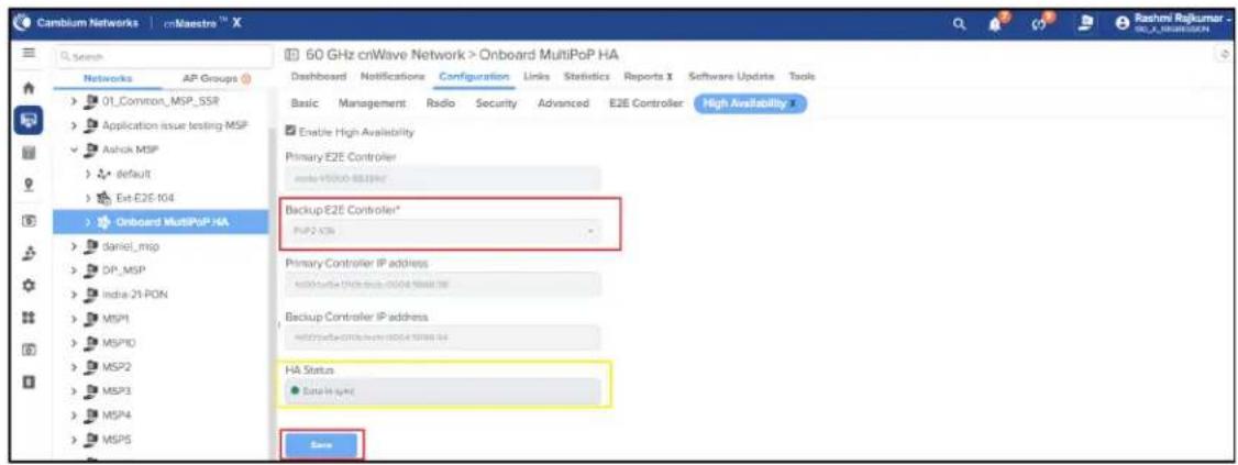
By default, the current Onboard Controller is selected as the primary controller.
- From the Backup E2E Controller drop-down list, select the required node that is connected to the complete network.
You can check the IP addresses (read only) of primary and backup controllers.
- Click Save to apply the changes.
- When you configure the HA support, ensure to check the HA Status parameter.
The HA Status parameter must display the green button, indicating that the HA support is functioning and data is in sync. If HA Status displays the red button, then it indicates that the HA support is not functioning.
You can also view the HA status in the High Availability X section on the Dashboard page.
Figure 272: Viewing the HA status on the Dashboard page - cnMaestro UI

The Primary field displays the primary node name. The Backup field displays the backup node name. Green bullets in Primary and Backup fields show the online or offline status of nodes. The keyword Active toggles between Primary and Backup fields, indicating that the respective node is currently functioning as the active controller, managing the network, and is connected to cnMaestro.
Caveats of HA configuration
Consider the following caveats of the HA configuration for 60 GHz cnWave devices:
| Configuration Caveats | |
| Configuration backup and restoration | The configuration backups are supported when the HA is enabled.The backup collected from a non-HA network can only be restored in a non-HA network.The backup collected from a HA enabled network is restored only in a HA enabled network.When HA is enabled, the restoration is allowed only when the primary node is active, managing the network and connected to cnMaestro. |
| Software update flow | When HA is enabled, it is recommended to update the nodes when primary is functioning as the active controller.It is recommended to run the HA pairs on the same version to avoid HA functionality issues.Avoid downgrading the device version to less than 1.4 when HA is enabled in the network.Avoid updating the device software from a device UI when HA is enabled. You must update the software from cnMaestro. |
| Device UI | It is recommended to make changes to the network only from cnMaestro.Making changes through device UIs may have issues in HA functionality. |
| cnMaestro X to Essentials downgrade | The HA functionality will be disabled leaving the current active controller that is connected to cnMaestro as the only controller in the network.The HA functionality can be enabled back when the subscription is enabled. |
| Connecting a HA enabled E2E Controller network to an Essential cnMaestro account | The HA functionality will be disabled leaving the current active controller (which is connected to cnMaestro) as the only controller in the network.The HA functionality can be enabled back when the network is connected to cnMaestro X account. |
For more information on configuring the HA support using cnMaestro, refer to the cnMaestro 5.1.0 User Guide.
Regulatory Information
This chapter provides regulatory notifications.

Caution
Intentional or unintentional changes or modifications to the equipment must not be made unless under the express consent of the party responsible for compliance. Any such modifications could void the user's authority to operate the equipment and will void the manufacturer's warranty.

Attention
The following topics are described in this chapter:
- Compliance with safety standards lists the safety specifications against which the 60 GHz cnWave family of ODUs has been tested and certified. It also describes how to keep RF exposure within safe limits.
- Compliance with radio regulations describes how the 60 GHz cnWave family of ODUs complies with the radio regulations that are in force in various countries.
Compliance with safety standards
This section lists the safety specifications against which the 60 GHz cnWave™ platform family is tested and certified. It also describes how to keep RF exposure within safe limits.
Electrical safety compliance
The 60 GHz cnWave platform family hardware is tested for compliance to the electrical safety specifications listed in following Safety compliance specifications table.
Table 63: Safety compliance specifications
| Region Specification | |
| USA UL 62368-1, UL 60950-22 | |
| Canada CSA C22.2 No.62368-1, CSA C22.2 No. 60950-22 | |
| Europe EN 62368-1, EN60950-22 | |
| International CB certifiedIEC 62368-1 Edition 2 IEC 60950 -22 | |
Electromagnetic Compatibility (EMC) compliance
The EMC specification type approvals that are granted for 60 GHz cnWave platform family are listed in following table.
Table 64: EMC compliance
| Region Specification | |
| USA FCC Part 15 Class B | |
| Canada RSS Gen | |
| Europe/International EN 301 489-1 V | 2.2.3, EN 301 489-17 V3.2.4 |
Human exposure to radio frequency energy
Relevant standards (USA and EC) applicable when working with RF equipment are:
- ANSI IEEE C95.1-2005, IEEE Standard for Safety Levels with Respect to Human Exposure to Radio Frequency Electromagnetic Fields, 3 kHz to 300 GHz
- Council recommendation of 12 July 1999 on the limitation of exposure of the general public to electromagnetic fields (0 Hz to 300 GHz) (1999/519/EC) and respective national regulations
- Directive 2013/35/EU - electromagnetic fields 26 June 2013 on the minimum health and safety requirements regarding the exposure of workers to the risks arising from physical agents (electromagnetic fields) (20th individual Directive within the meaning of Article 16(1) of Directive 89/391/EEC) and repealing Directive 2004/40/EC.
- US FCC limits for the general population. See the FCC web site at http://www.fcc.gov, and the policies, guidelines, and requirements in Part 1 of Title 47 of the Code of Federal Regulations, as well as the guidelines and suggestions for evaluating compliance in FCC OET Bulletin 65
- Health Canada limits for the general population. See the Health Canada web site at https://www.canada.ca/en.html.
- EN 62232: 2017 Determination of RF field strength, power density and SAR in the vicinity of radiocommunication base stations for the purpose of evaluating human exposure (IEC 62232:2017)
- EN 50385:2017 Product standard to demonstrate the compliance of base station equipment with radiofrequency electromagnetic field exposure limits (110 MHz - 100 GHz), when placed on the market
- ICNIRP (International Commission on Non-Ionizing Radiation Protection) guidelines for the general public. See the ICNIRP web site at https://www.icnirp.org/cms/upload/publications/ICNIRPemfgdl.pdf and Guidelines for Limiting Exposure to Time-Varying Electric, Magnetic, and Electromagnetic Fields.
Power density exposure limit
Install the radios for the 60 GHz cnWave platform family of wireless solutions to provide and maintain the minimum separation distances from all persons.
The applicable FCC power density exposure limit for RF energy in the 57 - 66 GHz frequency bandsFor 10 W/m more information, see Human exposure to radio frequency energy.
Calculation of power density
The following calculation is based on the ANSI IEEE C95.1-1991 method, as that provides a worst-case analysis.
Peak power density in the far field of a radio frequency point source is calculated as follows:
S = P.G4 πd 2
Where:
S: power density in W/m
p: maximum average transmit power capability of the radio, in W
G: total Tx gain as a factor, converted from dB
d: distance from point source, in m
Rearranging terms to solve for distance yields:
d = [] P . G / 4 πS
Calculated distances and power compliance margins
The following table displays recommended calculated separation distances, for the 60 GHz cnWave ™ for Europe the USA and Canada. These are conservative distances that include compliance margins.

Note
At these and greater separation distances, the power density from the RF field is below generally accepted limits for the general population.

Note
60 GHz cnWave™ Platform Family ODU adheres to all applicable EIRP limits for transmit power when operating in MIMO mode. Separation distances and compliance margins include compensation for the antenna configuration of each product.

Note
Table 65: Calculated distances and power compliance margins
| Product Countries EIRP | (dBm) | EIRP (W) | Maximum power density (W/m2) | Compliance distance (m) | |
| V1000 USA | Canada, EU | 38 6.3 10 | 0.22 | ||
| V2000 USA | Canada, EU | 49 79.4 10 | 0.9 | ||
| V3000 USA | Canada 60.5 | 122 10 3.0 | |||
| V3000 EU | 55 316.2 10 1.6 | ||||
| V5000 USA | Canada, EU | 38 6.3 10 | 0.22 | ||

Note
The regulations require that the power used for the calculations is the maximum power in the transmit burst subject to allowance for source-based time-averaging.
The calculations above are based upon platform maximum EIRP and worst case 100% duty cycle.

Remarque
Compliance with radio regulations
This section describes how the 60 GHz cnWave platform family complies with the radio regulations that are in force in various countries.

Caution
Where necessary, the end user is responsible for obtaining any national licenses required to operate this product and these must be obtained before using the product in any particular country. Contact the appropriate national administrations for details of the conditions of use for the bands in question and any exceptions that might apply.

Attention
Changes or modifications not expressly approved by Cambium Networks could void the user's authority to operate the system.

Attention
The system is tested against various local technical regulations and found to comply. The Radio specifications section lists the radio specification type approvals that is granted for the 60GHz cnWave products.
Some of the frequency bands in which the system operates are “license exempt” and the system is allowed to be used provided it does not cause interference. In these bands, the licensing authority does not guarantee protection against interference from other products and installations.
| Region Regulatory approvals FCC ID IC ID | ||
| USA Part 15C QWP-60V1000 | QWP-60V2000QWP-60V3000QWP-60V5000 | - |
| Canada ISED RSS-210 - 109AO-60V1000 | 109AO-60V2000109AO-60V3000109AO-60V5000 |
Federal Communications Commission (FCC) compliance
The 60 GHz cnWave V1000, V2000, V3000 and V5000 comply with the regulations that are in force in the USA.

Caution
If this equipment does cause interference to radio or television reception.
FCC Notification
This device complies with part 15C of the US FCC Rules. Operation is subject to the following two conditions: (1) This device may not cause harmful interference, and (2) This device must accept any interference received, including interference that may cause undesired operation.
Innovation, Science and Economic Development Canada (ISEDC) compliance
The 60 GHz cnWave V1000, V2000, V3000 and V5000 comply with the regulations that are in force in Canada.

Caution
If this equipment does cause interference to radio or television reception.
60 GHz cnWave example product labels
Figure 273:60 GHz cnWave™ V5000 Distribution Node
Model No/HVIN:V5000

Part No:C600500A004A

SERIAL NO (MSN):###

MAC (ESN):###

This device complies with part 15 of the FCC Rules. Operation is subject to the following two conditions: (1) This device may not cause harmful interference, and (2) this device must accept any interference received, including interference that may cause undesired operation
IMPORTANT:
See the System User Guide before connecting to
AC Power. The Guide is available online at
www.cambiumnetworks.com/guides
MADE IN CHINA
X-SZHO-H

Cambium Networks™
Ashburton, TQ13 7UP, UK
60GHz cnWave V5000 Distribution Node
VIN: 42.5-57V IMAX: 1.41A

E112443 COMPLIES WITH
UL62368-1 / CSA C22.2 No. 62368-1-14
UL60950-22 / CSA C22.2 No. 60950-22-17
FCC ID: QWP-60V5000
IC: 109AO-60V5000





Figure 274:60 GHz cnWave™ V3000 Client Node Radio only
Model No/HVIN:V3000

Part No:C600500C024A

SERIAL NO (MSN):###

MAC (ESN):###

This device complies with part 15 of the FCC Rules. Operation is subject to the following two conditions: (1) This device may not cause harmful interference, and (2) this device must accept any interference received, including interference that may cause undesired operation
IMPORTANT
See the System User Guide before connecting to
AC Power. The Guide is available online at
www.camblumnetworks.com/guides
MADE IN CHINA
X-SZHO-H

Cambium Networks™
Ashburton, TQ13 7UP, UK
60GHz cnWave V3000 Client Node Radio Only
VIN: 42.5-57V IMAX:1.29A

E112443 COMPLIES WITH
UL62368-1 / CSA C22.2 No. 62368-1-14
UL60950-22 / CSA C22.2 No. 60950-22-17
FCC ID: QWP-60V3000
IC: 109AO-60V3000


IP66/67


Figure 275:60 GHz cnWave™ V2000 Client Node with no power cord

Figure 276:60 GHz cnWave™ V1000 Client Node with no cord

Figure 277:60 GHz cnWave™ V1000 with US cord
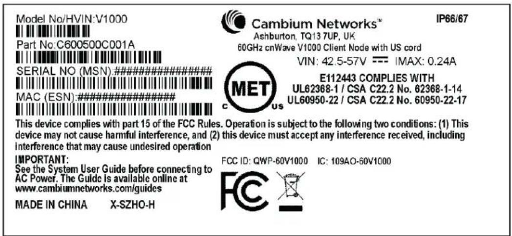
Table 66: Details of accessories, radio nodes, and part numbers
| Accessories Radio nodes Cambium Part Number | ||
| 60 GHz cnWaveTM V5000 Distribution Node V5000 C600500A004B | ||
| 60 GHz cnWaveTM V3000 Client Node radio only V3000 C600500C024B | ||
| 60GHz cnWave V2000 Client Node no power supply, no power cord V2000 C600500C030B | ||
| 60 GHz cnWaveTM V1000 Client Node with no cord V1000 C600500C014B | ||
| 60 GHz cnWaveTM V1000 with US cord V1000 C600500C001B |
Troubleshooting
This section describes the troubleshooting steps and addresses frequently asked questions related to 60 GHz cnWave product deployment.
• Field diagnostics logs
• Setup issues in IPv4 tunneling
- Link is not established
- PoP not online
- Link is not coming up
- Link is not having expected throughput performance
- Factory reset
Field diagnostics logs
Download the logs to view more information about the error. To download the error logs select the node from the dropdown and click Download Logs.
Figure 278:The Logs tab in the Tools page

On clicking Download Logs, the status for download is displayed.
Figure 279: Downloading the logs

To download the logs for a self node, click Download Logs at the bottom and save the log file.
Setup issues in IPv4 tunneling
In IPv4 tunneling, if setup issues occur then perform the below steps:
- Click Configuration on the left pane, navigate to Network > Basic > Layer 2 Bridge and verify Enable Layer 2 bridge is selected.

- On the same page under Configuration Management, verify E2E Managed Config is selected.

- Click Configuration > Nodes > PoP DN > Networking > Layer 2 Bridge and verify Disable Broadcast Flood and Disable IPv6 are disabled.
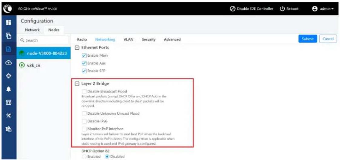
- Ensure that PoP DN and DNs are in the same subnet and verify gateway is correct.
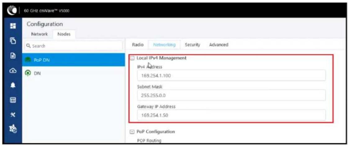
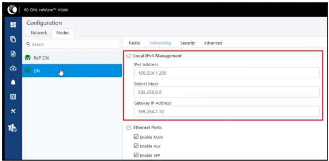
Link is not established
If link is not established between the nodes, then verify the below options:
- Click Configuration on the left navigation pane of the home UI page.
- Navigate to Nodes > Radio. Verify Sector 2 PoP DN and DN's polarities, frequency, and Golay codes.
Figure 280: The Sector 2 section in the Radio page
![90 GHz onWare™ v3400 Configuration Network Nodes Search PoP DN DNS Radio Networking Security Advanced Minimum MCS 2 Range - [0, 12] Maximum MCS 12 Range - [0, 12] Sector 1 Override Name Auto Config Node Config Channel Polarity Sector 1 Link (a) Golay Override Name Auto Config (Rx/Tx) Node Golay Rx Node Golay Tx No Data Sector 2 Override Name Auto Config Node Config Channel 2 Polarity Odd Sector 2 Link (b) Golay Override Name Auto Config (Rx/Tx) Node Golay Rx Node Golay Tx Win: DIN-PoP DN 2/2 Outside All](/content/2026/05/1088487/images/274e87269ea7345133b5302ca1266dd267ec4de5d6f449cba4489995db8b8202.jpg)
- Select DN > Networking > Ethernet Ports and ensure that specific Ethernet ports are enabled.
Figure 281: The Ethernet Ports section in the Networking page

- From the left navigation pane, navigate to Topology > Nodes and verify the Status is Online Initiator.
Figure 282: Status of nodes in the Topology page

- From the left navigation pane, go to Statistics > Links and verify RSSI, MCS, and TX Power Index.
Figure 283: Link details in the Statistics page
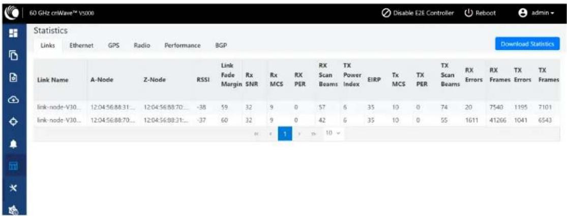
- Go to Performance and verify the graphs.
Figure 284: Graphs in the Performance page
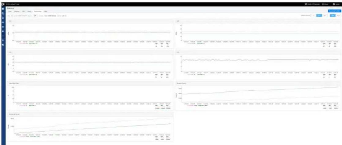
line
| Metric | Value | |--------|-------| | Top Left | 80 | | Top Right | 90 | | Bottom Left | 70 | | Bottom Right | 85 | | Bottom Right | 95 |- Go to Radio and monitor the throughput capacity.
Figure 285: Monitoring the throughput in the Radio page
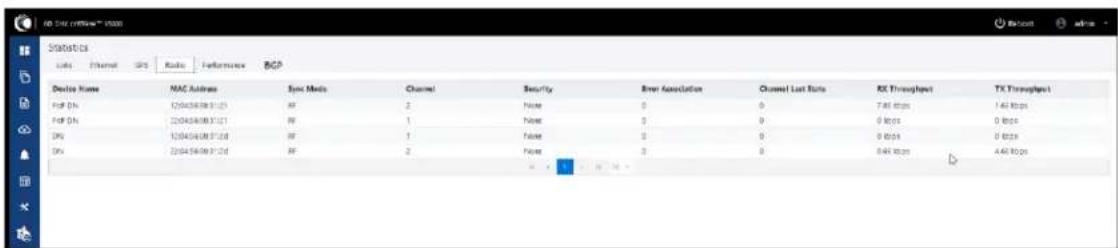
- If internal GPS is used, then verify Configuration > Nodes > Radio > GPS > Force GPS Disable is enabled.
Figure 286: Verifying the Force GPS Disable check box

PoP not online from E2E or cnMaestro UI
This usually means that the PoP node is not able to talk to the E2E controller. Ensure that the PoP node has the E2E IPv6 configured properly. Also ensure that there is a route between the E2E controller and the PoP node, if they are not in the same VLAN. Try to ping the E2E from the PoP node (by logging in to SSH).
Link is not coming up
- Ensure that the two ends of the radios can see each other (clear line of sight in between). If the link is using V3000, ensure that they are properly aligned.
- Ensure that the MAC address of the radios is configured correctly in the E2E Controller.
- Ensure that GPS sync is not enabled if indoor and ensure that GPS sync is enabled if outdoor.
-
Ensure that both ends of the link have the same software version.
-
Ensure to configure country code on the E2E GUI.
- Ensure that the two ends of the link use opposite polarity and Golay codes that match each other.
- Ensure that the remote ends can reach the E2E Controller - IPv6 configuration (if beamforming is successful but the remote end cannot reach back to the E2E Controller, the E2E Controller/cnMaestro GUI displays link status as up, but the remote radio is offline).
- If you already have experience in setting up a link and you are trying to set up a daisy chain, ensure that there is no any interference caused by the existing link. Example: Make sure that the two neighboring links use different Golay code.
Link does not come up after some configuration change
There is a possibility that the remote unit could be in a state that it uses different channel/Golay code/polarity from the near-end unit. Try to factory default the remote radio if possible.
On the E2E Controller/cnMaestro, it shows that the link is up, but the remote radio is NOT online - This means that link is established but the remote end radio cannot reply to the E2E Controller. Check the E2E configuration to make sure that the IPv6 default gateway is configured correctly to allow a route between the E2E controller and the remote radio.
Link is not having expected throughput performance
- Check the radio GUI to ensure that the link is running as the expected MCS mode when user data is passing through.
- Check to ensure that the Ethernet ports of the radios and the testing devices are negotiated to expected data rate (10Gbps).
- Ensure that your testing devices are capable of handling the throughput - run data throughput test by bypassing the radio link.
- Do not use radio internal iperf tool to test throughput.
Factory reset
Recovery mode is used to reset the configuration to the factory settings. To reset the configuration, perform the following steps:
- From the main home page, navigate to Tools > Factory Reset.
The Factory Reset page appears, as shown in the following figure:


Warning
Factory reset is followed immediately by a system reboot. You must carefully configure the factory reset settings as the device comes up with the default settings. All the existing configurations are lost when the system comes up.
2. Click Factory Reset and Reboot.
The Confirm message box appears, as shown in the following figure:

- Click Yes to confirm on the factory reset of the system.
The system reboots immediately following the factory reset.
- When the reboot is complete, access the device using 169.254.1.1 (IP address).

Note
After factory reset, all configurations are set to default mode.
Cambium Networks
Cambium Networks delivers wireless communications that work for businesses, communities, and cities worldwide. Millions of our radios are deployed to connect people, places and things with a unified wireless fabric that spans multiple standards and frequencies of fixed wireless and Wi-Fi, all managed centrally via the cloud. Our multi-gigabit wireless fabric offers a compelling value proposition over traditional fiber and alternative wireless solutions. We work with our Cambium certified ConnectedPartners to deliver purpose built networks for service provider, enterprise, industrial, and government connectivity solutions in urban, suburban, and rural environments, with wireless that just works.
| Installation and User Guides http://www.cambiumnetworks.com/guides | |
| Technical training https://learning.cambiumnetworks.com/learn | |
| Support website (enquiries) https://support.cambiumnetworks.com | |
| Main website http://www.cambiumnetworks.com | |
| Sales enquiries solutions@cambiumnetworks.com | |
| Warranty https://www.cambiumnetworks.com/support/standard-warranty/ | |
| Telephone number list to contact http://www.cambiumnetworks.com/contact-us/ | |
| Address Cambium Networks Limited,Unit B2, Linhay Business Park,Eastern Road,Ashburton,Devon, TQ13 7UPUnited Kingdom |

Cambium Networks™ www.cambiumnetworks.com
Cambium Networks and the stylized circular logo are trademarks of Cambium Networks, Ltd. All other trademarks are the property of their respective owners.
© Copyright 2024 Cambium Networks, Ltd. All rights reserved.
- Reservation of Rights
- Copyrights
- Restrictions
- License Agreements
- High Risk Materials
- Contents
- Contents 3
- About This User Guide..10
- Product Description 16
- System Hardware 32
- System Planning 63
- Configuring 60 GHz cnWave™ 137
- Operation 197
- Troubleshooting 251
- Cambium Networks 261
- About This User Guide
- Purpose
- Cross-references
- Feedback
- Important regulatory information
- Complying with rules for the country of operation
- Caution
- Note
- Canada specific information
- European specific information
- EU Declaration of conformity
- United Kingdom (UK) specific information
- UK Declaration of conformity
- Application firmware
- Ethernet networking skills
- Lightning protection
- Specific expertise and training for professional installers
- Legal and Open-Source Software statements
- Problems and warranty
- Reporting problems
- Repair and service
- Hardware warranty
- Security advice
- Warnings, cautions, and notes
- Warnings
- Cautions
- Notes
- Caring for the environment
- In the UK and EU countries
- Disposal of Cambium equipment
- Disposal of surplus packaging
- In non-EU countries
- Product Description
- Introduction
- Frequency bands
- Characteristics
- - Short range
- 802.11ay Standards and advantages
- Advantages
- Terragraph
- Key components
- Features
- Responsibilities
- Theory of operation
- Overview of cnWave family
- V1000 CN
- V2000 CN
- V3000 CN
- V5000 DN
- Wireless operation
- Wireless topology
- PTP
- PMP
- Mesh
- Modulation
- Link adaptation
- Synchronization
- Time-division duplexing access mechanism
- General operation of MAC layer
- Frame types
- Wireless encryption
- Designing wireless networks
- TDD synchronization
- System management
- Management agent
- Network management
- IPv6
- System logging
- Software upgrade
- Wireless nodes
- V1000 Client Node (CN)
- V1000 CN - Part numbers
- V2000 Client Node (CN)
- V2000 CN - Part numbers
- V3000 Client Node (CN)
- V3000 Part numbers
- V5000 Distribution Node (DN)
- V5000 Part numbers
- Radio mounting brackets
- V1000 Wall and pole mount
- V1000 Adjustable pole mount (N000900L022A)
- V2000 Adjustable pole mount
- V3000 Precision bracket (C000000L125A)
- V3000 Tilt bracket (N000045L002A)
- V5000 Pole mount (C000000L137A)
- V5000 Wall mount (C000000L136A)
- Bracket part numbers
- Radio accessories
- Telescope mounting kit for precision brackets
- Alignment Tube
- Radio accessory part numbers
- Radio external interfaces
- Radio specifications
- Power supply units (PSU)
- PSU Options
- V1000 - Power over Ethernet (PoE)
- V2000 - PoE
- V3000/V5000 - PoE
- V3000/V5000 - Outdoor AC/DC power supply unit
- Aux PoE - Powering options
- Ethernet and DC cables
- Maximum cable lengths
- Ethernet
- Power over Ethernet (PoE)
- Using AC/DC PSU with a DC power feed
- Outdoor copper CAT6A Ethernet cable
- Attention
- Cable accessories
- SFP Module kits
- Optical cable and connectors
- System Planning
- Site planning
- Grounding and lightning protection
- Warning
- Lightning protection zones
- Site grounding system
- ODU location
- Drop cable grounding points
- ODU wind loading
- PSU DC power supply
- PSU AC power supply
- PSU location
- Outdoor AC/DC PSU
- Lightning Surge Protection Units (LPU)
- Lightning Surge Protection Units location
- Deployment Considerations
- Key deployment guidelines
- Sector and alignment
- Minimum CN spacing
- Near-far radio
- Early weak interference
- Avoiding the tight angle deployment
- Avoiding the straight line interference
- When two V5000 devices are co-located at a site
- Polarity
- Link Adaptation and Transmit Power Control (LATPC)
- Radio spectrum planning
- General wireless specifications
- Regulatory limits
- Link planning
- LINKPlanner
- Range and obstacles
- Path loss
- Planning for data networks
- Point to Point-based single link Ethernet bridge
- IPv4/L2 based PMP and mesh network planning
- Support for dual networking (IPv4 and IPv6)
- IPv6 Mode network planning
- IPv6 Network design consideration
- Reserved IPv6 address space
- E2E and cnMaestro deployment consideration
- Ethernet bridging
- Layer 2 (L2) bridging
- Broadcast/Multicast control
- Limitations
- Layer 2 Bridge support in multi-PoP deployments
- External Layer 2 Concentrator support
- Multi-PoP deployments
- Layer 2 domain
- Open/R on the PoP interface port
- MTU of upstream switch ports
- Prefix allocation
- Layer 2 control protocols
- IP Interface
- Daisy-chaining 60 GHz links
- Installation
- Safety
- Working at heights
- PSU
- Grounding and protective earth
- AC Supply
- Powering down before servicing
- Primary disconnect device
- External cables
- Drop cable tester
- RF Exposure near the antenna
- Minimum separation distances
- Grounding and lightning protection requirements
- Grounding cable installation methods
- Siting radios
- GHz cnWave radios and mounting bracket options
- Installing the cnWave radio nodes
- Typical installation
- V2000
- ODU Interface with LPU on the pole
- Attach ground cables to the radio
- Mounting the ODU
- V1000 Pole mount
- V1000 Wall mount
- V1000 Adjustable pole mount
- V1000 Alignment
- V2000 Antenna alignment
- V3000 Precision bracket
- Precision bracket alignment
- Precision bracket alignment - optional telescope
- V3000 Tilt bracket assembly
- V3000 Tilt bracket assembly with band clamps
- V5000 Pole mount bracket
- V5000 Alignment
- V5000 Wall mount bracket
- Connect to the PSU port of the radio Using Power over Ethernet (PoE)
- Disconnecting drop cable from the radio
- Using AC/DC PSU
- Install the PSU
- Installing the 60W DC power injector
- Installing the AC/DC PSU
- Installing 15W or 30W power injector
- Connecting to the SFP+ optical module or SFP+ to the copper module to ODU
- Inserting the SFP module
- Connecting the cable
- Fitting the gland
- Removing the cable and SFP module
- Nodes deployment
- Connecting to the unit
- Configuring the management PC
- Connecting to the PC and powering up
- Procedure:
- Using the web interface
- Logging into the web interface
- Dashboard elements
- GPS
- Sectors
- Enabling internal E2E Controller
- Topology
- Click Save.
- Support for renaming nodes
- Configuration
- Network configuration
- Basic
- CPE Prefix Zoning
- Configuring Summarized CPE Prefix
- Management
- Radio
- CN Channel scanning options
- Fast Acquisition
- Asymmetric TDD
- Configuring the asymmetric TDD split ratio
- cnMaestro UI:
- Security
- Wireless security
- Advanced
- Gratuitous ARP support
- Node configuration
- Networking
- Using the cnMaestro UI
- VLAN
- Transparent
- Q
- QinQ
- Diagnostics
- Events
- Statistics
- Links
- Performance
- RSSI graph
- Transmit Power graph
- SNR graph
- MCS Index graph
- Packet Error Ratio graph
- Received Frames graph
- Transferred Frames graph
- Prefix zone Statistics
- Border Gateway Protocol (BGP)
- Maps
- Tools
- Factory reset
- Field diags
- Antenna alignment
- Prerequisite tasks:
- Using the Antenna Alignment tool
- Remote Command
- Show SFP power details
- Click Execute.
- Show ipv4 neighbors
- Show ipv6 neighbors
- Show Wired Interface State Changes
- Ping
- Click Start Ping.
- Quick PTP setup
- iPerf
- Click Start iPerf.
- cnMaestro support for Onboard Controller
- Backup CN link
- Auto Manage IPv6 Routes (External E2E Controller)
- Single PoP network
- Multi-PoP network
- Unconnected PoPs
- High Availability (HA) support for Onboard E2E Controller
- Configuring HA support using cnMaestro
- Caveats of HA configuration
- Regulatory Information
- Compliance with safety standards
- Electrical safety compliance
- Electromagnetic Compatibility (EMC) compliance
- Human exposure to radio frequency energy
- Power density exposure limit
- Calculation of power density
- Calculated distances and power compliance margins
- Remarque
- Compliance with radio regulations
- Federal Communications Commission (FCC) compliance
- FCC Notification
- Innovation, Science and Economic Development Canada (ISEDC) compliance
- GHz cnWave example product labels
- Cambium Networks™
- Troubleshooting
- Field diagnostics logs
- Setup issues in IPv4 tunneling
- Link is not established
- PoP not online from E2E or cnMaestro UI
- Link is not coming up
- Link does not come up after some configuration change
- Link is not having expected throughput performance
- Click Factory Reset and Reboot.
- Cambium Networks
Brand : Cambium Networks
Model : cnWave 60
Category : Electronic lock