
32sll - Calculator HP - Free user manual and instructions
Find the device manual for free 32sll HP in PDF.


| Product Type | Scientific Calculator |
| Display | 2-line LCD, 12-digit |
| Dimensions | 5.7 x 3.2 x 0.5 inches (145 x 81 x 13 mm) |
| Weight | 4 ounces (113 grams) with batteries |
| Power Source | 2 x CR2032 lithium coin cells |
| Battery Life | Approximately 1 year with normal use |
| Logic System | RPN (Reverse Polish Notation) |
| Built-in Functions | Over 125 including trigonometric, logarithmic, statistical, and programming functions |
| Memory | 32 KB RAM for user programs and storage |
| Programming Capability | Yes, key-programmable with up to 400 program steps |
| Input/Output | None |
| Case Material | Plastic with rubberized finish |
| Operating Temperature | 32°F to 104°F (0°C to 40°C) |
| Maintenance | Clean with a soft, dry cloth; do not use liquids or solvents |
| Safety Precautions | Keep away from moisture, heat, and strong magnetic fields; do not disassemble |
| Spare Parts Available | Replacement batteries and protective case |
| Repairability | Not user-serviceable; contact HP support for repairs |
| Manufacturer | HP (Hewlett-Packard) |
| Model Number | 32sll |
Frequently Asked Questions - 32sll HP
User questions about 32sll HP
0 question about this device. Answer the ones you know or ask your own.
Ask a new question about this device
Download the instructions for your Calculator in PDF format for free! Find your manual 32sll - HP and take your electronic device back in hand. On this page are published all the documents necessary for the use of your device. 32sll by HP.
USER MANUAL 32sll HP
HP 32SII RPN Scientific Calculator Owner's Manual

HEWLETT
PACKARD
HP Part No. 00032-90068
Printed in Singapore
Edition 5
Notice
This manual and any examples contained herein are provided "as is" and are subject to change without notice. Hewlett-Packard Company makes no warranty of any kind with regard to this manual, including, but not limited to, the implied warranties of merchantability and fitness for a particular purpose.
Hewlett-Packard Co. shall not be liable for any errors or for incidental or consequential damages in connection with the furnishing, performance, or use of this manual or the examples contained herein.
© Hewlett-Packard Co. 1990, 1991, 1992, 1993. All rights reserved. Reproduction, adaptation, or translation of this manual is prohibited without prior written permission of Hewlett-Packard Company, except as allowed under the copyright laws.
The programs that control your calculator are copyrighted and all rights are reserved. Reproduction, adaptation, or translation of those programs without prior written permission of Hewlett–Packard Co. is also prohibited.
Hewlett-Packard Company
Corvallis Division
1000 N.E. Circle Blvd.
Corvallis, OR 97330, U.S.A.
Printing History
Edition 1 November 1990
Edition 2 March 1991
Edition 3 June 1992
Edition 4
Edition 5
April 1993
November 1994
Contents
Part 1. Basic Operation
1. Getting Started
Important Preliminaries 1–1
Turning the Calculator On and Off.... 1-1
Adjusting Display Contrast 1–1
Highlights of the Keyboard an Display 1-1
Shifted Keys.... 1-1
Alpha Keys 1–2
Backspacing and Clearing.... 1–2
Using Menus 1-4
Exiting Menus 1–7
Annunciator.... 1–7
Keying in Numbers 1–9
Making Numbers Negative.... 1–10
Exponent of Ten.... 1–10
Understanding Digit Entry 1–11
Range Number and OVERFLOW 1-12
Doing Arithmetic.... 1–12
One-Number Functions.... 1-12
Two-Number Functions.... 1–13
Controlling the Display Format.... 1–14
Periods and Commas in Numbers 1–14
Contents
Number of Decimal Places.... 1–15
SHOWing Full 12-Digit Precision 1-16
Fractions.... 1–17
Entering Fractions 1–17
Displaying Fractions.... 1–19
Messages 1-19
Calculator Memory 1-20
Checking Available Memory.... 1-20
Clearing All of Memory.... 1–20
2. The Automatic Memory Stack
What the Stack Is 2-1
The X-Register Is in the Display.... 2-2
Clearing the X-Register 2-2
Reviewing the stack.... 2-3
Exchanging the X- and Y-Registers in the Stack...... 2-4
Arithmetic-How the Stack Does It 2-4
How ENTER Works.... 2-5
How CLEAR x Works.... 2–7
The LAST X Register 2-8
Correcting Mistakes with LAST X 2–9
Reusing Numbers with LAST X 2–10
Chain Calculations.... 2–12
Work from the Parentheses Out.... 2–12
Exercises 2–14
Order of Calculation 2-15
More Exercises.... 2–16
2 Contents
3. Storing Data into Variables
Storing and Recalling Numbers.... 3–1
Viewing a Variable without Recalling It 3-2
Reviewing Variables in the VAR Catalog.... 3-3
Clearing Variables 3-3
Arithmetic with Stored Variables 3-4
Storage Arithmetic 3-4
Recall Arithmetic.... 3–5
Exchanging x with Any Variable 3-6
The Variable "i" 3-7
4. Real-Number Functions
Exponential and Logarithmic Functions.... 4-1
Power Functions 4-2
Trigonometry 4-3
Entering π 4-3
Setting the Angular Mode.... 4-3
Trigonometric Functions.... 4-4
Hyperbolic Functions 4–5
Percentage Functions 4–5
Conversion Functions.... 4–7
Coordinate Conversions 4–7
Time Conversions.... 4–9
Angle Conversions.... 4–10
Unit conversions 4-11
Probability Functions 4–11
Contents
Factorial.... 4–11
Gamma 4-11
Probability Menu.... 4–12
Parts of Numbers 4–14
Names of Function.... 4-14
5. Fractions
Entering Fractions.... 5–1
Fractions in the Display.... 5-2
Display Rules 5-2
Accuracy Indicators 5-3
Longer Fractions 5–4
Changing the Fraction Display.... 5-5
Setting the Maximum Denominator.... 5-5
Choosing Fraction Format 5-6
Examples of Fraction Displays.... 5-7
Rounding Fractions.... 5–8
Fractions in Equations 5–9
Fractions in Programs 5–10
6. Entering and Evaluating Equations
How You Can Use Equations 6-1
Summary of Equation Operations....6-3
Entering Equations into the Equation List 6-4
Variables in Equations....6-5
Number in Equations 6–5
Functions in Equations 6–6
4 Contents
Parentheses in Equations....6-7
Displaying and Selecting Equations 6–7
Editing and Clearing Equations.... 6–9
Types of Equations 6-10
Evaluating Equations 6–11
Using ENTER for Evaluation 6-12
Using XEQ for Evaluation....6–14
Responding to Equation Prompts 6–14
The Syntax of Equations 6–15
Operator Precedence 6–15
Equation Function 6-17
Syntax Errors....6-20
Verifying Equations 6-20
7. Solving Equations
Solving an Equation 7-1
Understanding and Controlling SOLVE 7-5
Verifying the Result....7-6
Interrupting a SOLVE Calculation 7-7
Choosing Initial Guesses for SOLVE....7-7
For More Information....7–11
8. Integrating Equations
Integrating Equations (∫FN).... 8-2
Accuracy of Integration....8-6
Specifying Accuracy 8-6
Interpreting Accuracy 8–7
Contents
For More Information....8-9
9. Operations with Comb Numbers
The Complex Stack 9-1
Complex Operations 9-3
Using Complex Number in Polar Notation.... 9–6
10. Base Conversions and Arithmetic
Arithmetic in Bases 2, 8, and 16.... 10-2
The Representation of Numbers.... 10–4
Negative Numbers 10-4
Range of Numbers 10–5
Windows for Long Binary Numbers.... 10–6
SHOWing Partially Hidden Numbers 10–6
11. Statistical Operations
Entering Statistical Data 11-1
Entering One-Variable Data 11-2
Entering Two-Variable Data 11-2
Correcting Errors in Data Entry 11-3
Statistical Calculations ...... 11–4
Mean 11-4
Sample Standard Deviation.... 11-6
Population Standard Deviation.... 11–7
Linear regression 11–7
Limitations on Precision of Data.... 11–10
Summation Values and the Statistics Registers .... 11–11
6 Contents
Summation Statistics.... 11–11
The Statistics Registers in Calculator Memory ...... 11–12
Access to the Statistics Registers.... 11–13
Part 2. Programming
12. Simple Programming
Designing a Program 12-2
Program Boundaries (LBL and RTN) 12-3
Using RPN and Equations in Programs.... 12-4
Data Input and Output 12-4
Entering a Program 12-5
Keys That Clear 12-6
Function Names in Programs.... 12–7
Running a Program 12-8
Executing a Program (XEQ)....12-9
Testing a Program.... 12–9
Entering and Displaying Data 12–11
Using INPUT for Entering Data 12-11
Using VIEW for Displaying Data.... 12–14
Using Equations to Display Messages.... 12–14
Displaying Information without Stopping 12–17
Stopping or Interrupting a Program.... 12–18
Programming a Stop or Pause (STOP, PSE).... 12–18
Interrupting a Running Program 12–18
Error Stops.... 12–18
Editing Program.... 12–19
Contents
Program Memory.... 12-20
Viewing Program Memory 12-20
Memory Usage 12-20
The Catalog of Programs (MEM).... 12-21
Clearing One or More Programs 12-22
The Checksum.... 12-22
Nonprogrammable Functions.... 12–23
Programming with BASE 12-23
Selecting a Base Mode in a Program 12-24
Numbers Entered in Program Lines 12–24
Polynomial Expressions and Horner's Method 12–25
13. Programming Techniques
Routines in Programs 13–1
Calling Subroutines (XEQ, RTN).... 13-2
Nested Subroutines.... 13-3
Branching (GTO).... 13-5
A Programmed GTO Instruction.... 13-5
Using GTO from the Keyboard.... 13-6
Conditional Instructions.... 13-7
Tests of Comparison (x?y, x?0).... 13–8
Flags 13–9
Loops 13–16
Conditional Loops (GTO) 13–16
Loops With Counters (DSE, ISG).... 13-17
Indirectly Addressing Variables and Labels 13–20
The Variable "i" 13-20
8 Contents
The Indirect Address, (i) 13-21
Program Control with (i).... 13–22
Equations with (i).... 13–24
14. Solving and Integrating Programs
Solving a Program 14-1
Using SOLVE in Program.... 14-5
Integrating a Program.... 14–7
Using Integration in a Program 14–9
Restrictions o Solving and Integrating.... 14–10
15. Mathematics Programs
Vector Operations.... 15-1
Solutions of Simultaneous Equations.... 15–12
Polynomial Root Finder.... 15–20
Coordinate Transformations.... 15–31
16. Statistics Programs
Curve Fitting 16-1
Normal and Inverse–Normal Distributions.... 16–11
Grouped Standard Deviation.... 16–18
17. Miscellaneous Programs and Equations
Time Value of Money.... 17-1
Prime Number Generator.... 17-6
Contents
Part 3. Appendixes and Regence
A. Support, Batteries, and Service
Calculator Support.... A-1
Answers to Common Questions ...... A–1
Environmental Limits ...... A–2
Changing the Batteries ......A-3
Testing Calculator Operation....A-4
The Self-Test ...... A-5
Limited One-Year Warranty ......A-6
What Is Covered....A-6
What Is Not Covered....A-6
Consumer Transaction in the United Kingdom ...... A–7
If the Calculator Requires Service ......A-7
Service Charge ......A-8
Shipping Instructions ...... A-8
Warranty on Service.... A-8
Service Agreements....A-9
Regulatory Information...... A-9
B. User Memory and the Stack
Managing Calculator Memory...... B-1
Resetting the Calculator ...... B-3
Clearing Memory ...... B-3
The Status of Stack Lift ...... B-4
Disabling Operations....B-5
10 Contents
Neutral Operations...... B-5
The Status of the LAST X Register....B-6
C. More about Solving
How SOLVE Finds a Root ....C-1
Interpreting Results ...... C-3
When SOLVE Cannot Find Root ....C-8
Round-Off Error ......C-14
Underflow....C-15
D. More about Integration
How the Integral Is Evaluated .... D-1
Conditions That Could Cause Incorrect Results...... D-2
Conditions That Prolong Calculation Time...... D-8
E. Messages
F. Operation Index
Index
Contents
Part 1
Basic Operation
1
Getting Started
Important Preliminaries
Turning the Calculator On and Off
To turn the calculator on, press ☐. ON is printed below the key.
To turn the calculator off, press ☑ OFF. That is, press and release the ☑ shift key, then press C (which has OFF printed in blue above it). Since the calculator has Continuous Memory, turning it off does not affect any information you've stored, (You can also press ☑ OFF to turn the calculator off.)
To conserve energy, the calculator turns itself off after 10 minutes of no use. If you see the low-power indicator (☐) in the display, replace the batteries as soon as possible. See appendix A for instructions.
Adjusting Display Contrast
Display contrast depends on lighting, viewing angle, and the contrast setting. To increase or decrease the contrast, hold down the Ⓔ key and press + or -.
Highlights of the Keyboard an Display
Shifted Keys
Each key has three functions: one printed on its face, a left-shifted function (orange), and a right-shifted function (blue). The shifted function
Getting
names are printed in orange and blue above each key. Press the appropriate shift key (◀ or ▶) before pressing the key for the desired function. For example, to turn the calculator off, press and release the ▶ shift key, then press ▶.
Pressing 📄 or 📋 turns on the corresponding ⇔ or ➡ annunciator symbol at the top of the display. The annunciator remains on until you press the next key. To cancel a shift key (and turn off its annunciator), press the same shift key again.
Alpha Keys
![graph TD A["Shifted function"] --> B["x²"] B --> C["PART"] C --> D["Menu name"] E["√x"] --> F["Letter for alphabetic key"]](/content/2026/05/973866/images/f22453af549be24272c2f506a17b1bf67c6b84a2af312aa29431c5e374e4051d.jpg)
Most keys have a letter written next to them, as shown above. Whenever you need to type a letter (for example, a variable or a program label), the A.Z annunciator appears in the display, indicating that the alpha keys are "active".
Variables are covered in chapter 3; labels are covered in chapter 6.
Backspacing and Clearing
One of the first things you need to know is how to clear; how to correct numbers, clear the display, or start over.
1-2 Getting Started
Keys for Clearing
| Key Description | |
| Backspace. | Keyboard-entry mode: Erases the character immediately to the left of "_" (the digit-entry cursor) or backs out of the current menu. (Menus are described in "Using Menus" on page 1-4.) If the number is completed (no cursor), clears the entire number. |
| Equation-entry mode: Erases the character immediately to the left of "■" (the equation-entry cursor). If a number entry in your equation is complete, erases the entire number. If the number is not complete, erases the character immediately to the left of "_" (the number-entry cursor. "_" changes back to "■" when number entry is complete. | |
| also clears error messages, and deletes the current program line during program entry. | |
| C | Clear or Cancel. Clears the displayed number to zero or cancels the current situation (such as a menu, a message, a prompt, a catalog, or Equation-entry or Program-entry mode). |
Getting
Keys for Clearing (continued)
| Key Description | |
| The CLEAR menu ( \ \ \ \Σ\ Contains options for clearing x (the number in the X-register), all Data, all variables, all of memory, or all statistical data.If you select \ , a new menu (CLR ALL? \ \ ) is displayed so you can verify your decision before erasing everything in memory.During program entry, \ is replaced by \ . If you select \ , a new menu (CL PGMS? \ \ ) is displayed, so you can verify your decision before erasing all your programs.During equation entry (either keyboard equations or equations in program lines), the CLR EQN? \ \ menu is displayed, so you can verify your decision before erasing the equation.If you are viewing a completed equation, the equation is deleted with no verification. | |
Using Menus
There is a lot more power to the HP 32SII than what you see on the keyboard. This is because 12 of the keys (with a shifted function name printed on a dark-colored background above them) are menu keys. There are 14 menus in all, which provide many more functions, or more options for more functions. Pressing a menu key (shifted) produces a menu in the display-a series of choices.
1-5 PICTURE
1-4 Getting Started
- Menu choices.
- Keys matched to menu choices.
- Menu keys.
HP 32II Menus
| Menu Name | Menu Description | Chapter |
| Numeric Functions | ||
| PARTS | IP FP ABSNumber-altering functions: integer part, fractional part, and absolute value. | 4 |
| PROB | Cn,r Pn,r SD RProbability functions: combinations, permutations, seed, and random number. | 4 |
| L.R. | xyrmb Linear regression: curve fitting and linear estimation. | 11 |
| , | w Arithmetic mean of statistical x- and y-values; weighted mean of statistical x-values. | 11 |
| s, σ | x y σx σy Sample standard deviation, population standard deviation. | 11 |
| SUMS | n × y ×2 y2 xy Statistical data summations. | 11 |
| BASE | DEC HX OC BNBase conversions (decimal, hexadecimal, octal, and binary). | 11 |
| Programming Instructions | ||
| FLAGS | SF CF FS?Functions to set, clear, and test flags. | 13 |
| x?y | ≠ ≤ > < ≥ = Comparison tests of the X-and Y-registers. | 13 |
| x?0 | ≠ ≤ > < ≥ = Comparison tests of the X-register and zero. | 13 |
Getting
HP 32II Menus (continued)
| Menu Name | Menu Description | Chapter |
| Other functions | ||
| MEM | nnn.n VAR PGMMemory status (bytes of memory available); catalog of variables; catalog of programs (program labels). | 1, 3, 12 |
| MODES | DG RD GR . ,Angular modes and " . ' or " , " radix (decimal point) convention. | 4, 1 |
| DISP | FX SC EN ALLFix, scientific, engineering, and ALL display formats. | 1 |
| CLEAR Functions to clear different portions of memory—refer to [IMAGE] CLEAR in the table on page 1–4. | 1, 3, 6, 12 | |
The following example shows you how to use a menu function:
Example:
How many permutations (n different arrangements) are possible from 28 items taken four (r) at a time?
Keys:
Display:
Description:
28 ENTER 4
4

Cn,r Pn,r SDR
Displays r.
Displays the probability menu.
Repeat the example for 28 items taken 2 at a time. (Result=756.)
Menus help you execute dozens of functions by guiding you to them with menu choices. You don't have to remember the names of
1-6 Getting Started
the functions built into the calculator nor search through the names printed on its keyboard.
Exiting Menus
Whenever you execute a menu function, the menu automatically disappears, as in the above example. If you want to leave a menu without executing a function, you have three options:
- Pressing ← backs out of the 2-level CLEAR or MEM menu, one level at a time. Refer to ← CLEAR in the table on page 1–4.
- Pressing ← or C cancels any other menu.
Keys:
| 123 | 123_ |
| [PROB] | Cn,r Pn,r SD R |
| or C | 123.0000 |
Display:
- Pressing another menu key replaces the old menu with the new one.
Keys:
| 123 | 123_ |
| [PROB] | Cn,r Pn,r SD R |
| CLEAR | X VARS ALL Σ |
| C | 123.0000 |
Display:
Annunciator
The symbols along the top and bottom of the display, shown in the following figure, are called annunciators. Each one has a special significance when it appears in the display.
picture 1–8
Getting
HP 32SII Annunciator
| Annunciator Meaning Chapter | ||
| ▼▲ | Upper Row:The ↓ and ↑ keys are active for stepping through a list.When in Fraction-display mode (press ← FDISP), only one of the "▲" or "▼" halves of the "▼▲"annunciator will be turned on to indicate whether the displayed numerator is slightly less than or slightly greater than its true value. If neither part of "▲▼" is on, the exact value of the fraction is being displayed. | 1, 65 |
| ← | Left shift is active. 1 | |
| → | Right shift is active. 1 | |
| PRGM Program-entry is active. Blinks while program is running. | 12 | |
| EQN | Equation-entry mode is active, or the calculator is evaluating an expression or executing an equation. | 6 |
| 0 1 2 3 | Indicates which flags are set (flags 4 through 11 have no annunciator. | 13 |
| RAD or GRAD | Radians or Grad angular mode is set. DEC mode (default) has no annunciator. | 4 |
| HEX OCT BIN | Indicates the active number base. DEC (base 10, default) has no annunciator. | 10 |
1-8 Getting Started
HP 32SII Annunciator (continued)
| Annunciator Meaning Chapter | ||
| Lower Row: | ||
| ↓ | The top-row keys on the calculator are redefined according to the menu labels displayed above menu pointers. | 1 |
| ←,→ There are | more digits to the left or right.Use [IMAGE] [SHOW] to see the rest of a decimal number; use the left and right- scrolling keys ( , + ) to see the rest of an equation or binary number.Both these annunciators may appear simultaneously in the display, indicating that there are more characters to the left and to the right. Press either of the indicated menu keys ( or + ) to see the leading or trailing characters. | 1, 6 |
| A..Z | The alphabetic keys are active. | 3 |
| ⚠ | Attention! Indicates a special condition or an error. | 1 |
| ☐ | Battery power is low. | A |
Keying in Numbers
You can key in a number that has up to 12 digits plus a 3-digit exponent up to ±499. If you try to key in a number larger than this, digit entry halts and the ▲ annunciator briefly appears.
If you make a mistake while keying in a number, press → to backspace and delete the last digit, or press to clear the whole number.
Getting
Making Numbers Negative
The +/- key changes the sign of a number.
■ To key in a negative number, type the number, then press +/-
To change the sign of a number that was entered previously, just press +/- . (If the number has an exponent, +/- affects only the mantissa — the non-exponent part of the number.)
Exponent of Ten
Exponents in the Display
Numbers with exponents of ten (such as 4.2 × 10⁻⁵ are displayed with an E preceding the exponent (such as 4·2000E-5).
A number whose magnitude is too large or too small for the display format will automatically be displayed in exponential form.
For example, in FIX 4 format for four decimal places, observe the effect of the following keystrokes:
| Keys: | Display: | Description: |
| .000062 | .000062_ | Shows number being entered. |
| ENTER | 0.0001 | Rounds number to fit the display format. |
| .000042 | 4.2000E-5 | Automatically uses scientific notation because otherwise no significant digits would appear. |
| ENTER |
Keying in Exponents of Ten
Use E (exponent) to key in numbers multiplied by powers of ten. For example, take Planck's constant, 6.6262 × 10⁻³⁴ :
- Key in the mantissa (the non-exponent part) of the number. If the mantissa is negative, press +/- after keying in its digits.
1–10 Getting Started
Keys:
Display:
6.6262
6.6262
- Press E. Notice that the cursor moves behind the E:

6.6262E_
- Key in the exponent. (The largest possible exponent is ±499.) If the exponent is negative, press +/− after you key in the E or after you key in the value of the exponent:
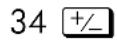
6.6262E-34
For a power of ten without a multiplier, such as 1034 , just press E 34. The calculator displays 1E34.
Other Exponent Functions
To calculate an exponent of ten (the base 10 antilogarithm), use 10x . To calculate the result of any number raised to a power (exponentiation), use yx (see chapter 4).
Understanding Digit Entry
As you key in a number, the cursor (_) appears in the display. The cursor shows you where the next digit will go; it therefore indicates that the number is not complete.
Keys:
Display:
Description:
123
123_
Digit entry not terminated: the number is not complete.
If you execute a function to calculate a result, the cursor disappears because the number is complete — digit entry has been terminated.
Getting

11.0905
Digit entry is terminated.
Pressing ENTER terminates digit entry. To separate two numbers, key in the first number, press ENTER to terminate digit, entry, and then key in the second number
123 ENTER
123.0000
A completed number.
4 +
127.0000
Another completed number.
If digit entry is not terminated (if the cursor is present), ← backspaces to erase the last digit. If digit entry is terminated (no cursor), ← acts like C and clears the entire number. Try it!
Range Number and OVERFLOW
The smallest number available on the calculator is 1 × 10-499 . The largest number is 9.99999999999 × 10499 (displayed as 1.0000E500 because of rounding).
If a calculation produces a result that exceeds the largest possible number, 9.99999999999 × 10499 is returned, and the warning message OVERFLOW appears.
If a calculation produces a result smaller than the smallest possible number, zero is returned. No warning message appears.
Doing Arithmetic
All operands (numbers) must be present before you press a function key. (When you press a function key, the calculator immediately executes the function shown on that key.)
All calculations can be simplified into one-number functions and/or two-number functions.
One-Number Functions
To use a one-number function (such as 1/x , . ← 2 , or +/- )
1-12 Getting Started
- Key in the number. (You don't need to press ENTER.)
- Press the function key. (For a shifted function, press the appropriate 📄 or 📇 shift key first.)
For example, calculate 1/32 and √148.84 Then square the last result and change its sign.
Keys:
Display:
| 32 | 32_ | Operand. |
| 1/x | 0.0313 | Reciprocal of 32. |
| 148.84 | 12.2000 | Square root of 148.84. |
| ← 2 | 148.8400 | Square of 12.2. |
| +/ _ - | -148.8400 | Negation of 148.8400. |
Description:
The one-number functions also include trigonometric, logarithmic, hyperbolic, and parts-of-numbers functions, all of which are discussed in chapter 4.
Two-Number Functions
To use a two-number function (such as +, -, ×. ÷, y x or %CHG).
- Key in the first number.
- Press ENTER to separate the first number from the second.
- Key in the second number. (Do not press ENTER.)
- Press the function key. (For a shifted function, press the appropriate shift key first.)
Note

Type in both cumbers (separate them by pressing ENTER) by before pressing a function key.
Getting
For example:
To calculate: Press: Display:
| 123 + 3 12 | ENTER 3 + | 15.0000 |
| 12 - 3 12 | ENTER 3 - | 9.0000 |
| 12 × 3 12 | ENTER 3 × | 36.00 |
| 123 | 12 ENTER 3 yx | 1,728.0000 |
Percent change from 88 ENTER 5 %CHG -37.5000
to 5
The order of entry is important only for non-commutative functions such as - , ÷ , yx or > \%CHG. If you type numbers in the wrong order, you can still get the correct answer (without re-typing them) by pressing x↔ y to swap the order of the numbers on the stack. Then press the intended function key. (This is explained in detail in chapter 2 under "Exchanging the X- and Y-Registers in the Stack.")
Controlling the Display Format
Periods and Commas in Numbers
To exchange the periods and commas used for the decimal point (radix mark) and digit separators in a number:
- Press ← MODES to display the MODES menu.
- Specify the decimal point (radix mark) by pressing {} or { } .
For example, the number one million looks like:
■ 1,000,000,0000 if you press {·} or
■ 1.000,000,0000 if you press {,}.
1-14 Getting Started
Number of Decimal Places
All numbers are stored with 12-digit precision, but you can select the number of decimal places to be displayed by pressing DISP (the display menu). During some complicated internal calculations, the calculator uses 15-digit precision for intermediate results. The displayed number is rounded according to the display format. The DISP menu gives you four options;
FX SC EN ALL
Fixed-Decimal Format ( \ )
FIX format displays a number with up to 11 decimal places (11 digits to the right of the " , " or " , " radix mark) if they fit. After the prompt FIX_type in the number of decimal places to be displayed. For 10 or 11 places, press □ 0 or □ 1.
For example, in the number 123,456,7089, the "7", "0", "8", and "9" are the decimal digits you see when the calculator is set to FIX 4 display mode.
Any number teat is too large or too small to display in the current decimal-place setting will automatically be displayed in scientific format.
Scientific Format ( \ )
SCI format displays a number in scientific notation (one digit before the "·" or "·" radix mark) with up to 11 decimal places (if they fit) and up to three digits in the exponent. After the prompt, SCI_, type in the number of decimal places to be displayed. For 10 or 11 places, press ☐ 0 or ☐ 1. (The integer part of the number will always be less than 10.)
For example, in the number 1·2346E5, the "2", "3", "4", and "6" are the decimal digits you see when the calculator is set to SCI 4 display mode The "5" following the "E" is the exponent of 10: 1.2346 × 10⁵ .
Getting
Engineering Format ( \ )
ENG format displays a number in a manner similar to scientific notation, except that the exponent is a multiple of three (there can be up to three digits before the "·" or "·" radix mark). This format is most useful for scientific and engineering calculations that use units specified in multiples of 103 (such as micro-, milli-, and kilo-units.)
After the prompt, ENG_, type in the number of digits you want after the first significant digit. For 10 or 11 places, press ☐ 0 or ☐ 1.
For example, in the number 123.46E3, the "2", "3", "4", and "6" are the significant digits after the first significant digit you see when the calculator is set to ENG 4 display mode. The "3" following the "E" is the (multiple of 3) exponent of 10: 123.46x 10 3 .
ALL Format ( { RLL })
ALL format displays a number as precisely as possible (12 digits maximum). If all the digits don't fit in the display, the number is automatically displayed in scientific format: 123,456.
SHOWing Full 12-Digit Precision
Changing the number of displayed decimal places affects what you see, but it does not affect the internal representation of numbers. Any number stored internally always has 12 digits.
For example, in the number 14.8745632019, you see only "14.8746" when the display mode is set to FIX 4, but the last six digits ("632019") are present internally in the calculator.
To temporarily display a number in full precision, press 📄 SHOW. This shows you the mantissa (but no exponent) of the number for as long as you hold down SHOW.
1-16 Getting Started
| Keys: | Display: | Description: |
| Displays four decimal places. | ||
| 45 ENTER 1.3 ✗ | 58.5000 | Four decimal places displayed. |
| Scientific format: two decimal places and an exponent. | ||
| Engineering format. | ||
| All significant digits; trailing zeros dropped. | ||
| Four decimal places, no exponent. | ||
| Reciprocal of 58.5. | ||
| Shows full precision until you release SHOW |
Fractions
The HP 32SII allows you to type in and display fractions, and to perform math operations on them. Fractions are real numbers of the form
ab / c
where a, b, and c are integers; 0 ≤ b ≤ c ; and the denominator (c) must be in the range 2 through 4095.
Entering Fractions
Fractions can be entered onto the stack at any time:
- Key in the integer part of the number and press ☐. (The first ☐ separates the integer part of the number from its fractional part.)
- Key in the fraction numerator and press ☐ again. The second ☐ separates the numerator from the denominator.
- Key in the denominator, then press ENTER or a function key to
Getting
terminate digit entry. The number or result is formatted according to the current display format.
The a b/c symbol under the ☐ key is a reminder that the ☐ key is used twice for fraction entry.
For example, to enter the fractional number 123/8 , press these keys:
| Keys: | Display: | Description: |
| 12 | 12_ | Enters the integer part of the number. |
| 12._ | The ☐ key is interpreted in the normal manner. | |
| 3 | 12.3_ | Enters the numerator of the fraction (the number is still displayed in decimal form). |
| 12.3/_ | The calculator interprets the second ☐ as a fraction and separates the numerator from denominator. | |
| 8 | 12.3/8_ | Appends the denominator of the fraction. |
| ENTER | 12.3750 | Terminates digit entry; displays the number in the current display format. |
If the number you enter has no integer part (for example, 3/8 ), just start the number without an integer.
| Keys: | Display: | Description: |
| 3 8 | 0 3/8 | Enters no integer part. (3 8 also works.) |
| ENTER | 0.3750 | Terminates digit entry; displays the number in the current display format (FIX 4). |
1–18 Getting Started
Displaying Fractions
Press 📄 FDISP to switch between Fraction–display mode and the current decimal display mode.
| Keys: | Display: | Description: |
| 12 3 8 | 12 3/8 | Displays characters as you key them in. |
| ENTER | 12.3750 | Terminates digit entry; displays the number in the current display format. |
| FDISP | 12 3/8 | Displays the number as a fraction. |
Now add 3/4 to the number in the X-register (12 3 /8):
| Keys: | Display: | Description: |
| 3 4 | 0 3/4 | Displays characters as, you key them in. |
| 13 1/8 | Adds the numbers in the X- and Y-registers; displays the result as a fraction. | |
| FDISP | 13.1250 | Switches to current decimal display format. |
Refer to chapter 5, "Fractions," for more information about using fractions.
Messages
The calculator responds to certain conditions or keystrokes by displaying a message. The ⚠ symbol comes on to call your attention to the message.
■ To clear a message, press C or ←.
■ To clear a message and perform another function, press any other key.
If no message appears but ▲ does, you have pressed an inactive key (a key that has no meaning in the current situation, such as 3 in Binary mode).
All displayed messages are explained in appendix E, "Messages."
Getting
Calculator Memory
The HP 32SII has 384 bytes of memory in which you can store any combination of data (variables, equations, or program lines). The memory requirements of specific activities are given under "Managing Calculator Memory" in appendix B.
Checking Available Memory
Pressing ← MEM displays the following menu:
216.0 VAR PGM
Where
216.0 is the number of bytes of memory available.
Pressing the {VAR} menu key displays the catalog of variables (see "Reviewing Variables in the VAR Catalog" in chapter 3). Pressing the PGM} menu key displays the catalog of programs.
- To enter the catalog of variables, press {VAR} to enter the catalog of programs, press {PGM}.
- To review the catalogs, press ← ↓ or ← ↑.
- To delete a variable or a program, press ⬤1 CLEAR while viewing it in its catalog.
- To exit the catalog, press C.
Clearing All of Memory
Clearing all of memory erases all numbers, equations, and programs you've stored. It does not affect mode and format settings. (To clear settings as well as data, see "Clearing Memory" in appendix B.)
To clear all of memory:
- Press ← CLEAR {ALL}. You will then see the confirmation prompt CLR
1-20 Getting Started
ALL? {Y} {N}, which safeguards against the unintentional clearing of memory.
- Press {'} (yes).
Getting
2
The Automatic Memory Stack
This chapter explains how calculations take place in the automatic memory stack. You do not need to read and understand this material to use the calculator, but understanding the material will greatly enhance your use of the calculator, especially when programming.
In part 2, "Programming", you will learn how the stack can help you to manipulate and organize data for programs.
What the Stack Is
Automatic storage of intermediate results is the reason that the HP 32SII easily processes complex calculations, and does so without parentheses. The key to automatic storage is the automatic, RPN memory stack.
HP's operating logic is based on an unambiguous, parentheses-free mathematical logic known as "Polish Notation," developed by the Polish logician Jan Łukasiewicz (1878–1956).
While conventional algebraic notation places the operators between the relevant numbers or variables, Łhukasiewicz's notation places them before the numbers or variables. For optimal efficiency of the stack, we have modified that notation to specify the operators after the numbers. Hence the term Reverse Polish Notation, or RPN.
The stack consists of four storage locations, called registers, which are "stacked" on top of each other. These registers—labeled X, Y, Z, and T—store and manipulate four current numbers. The "oldest" number is stored in the T—(top) register. The stack is the work area for calculations.
The Automatic Memory Stack 2-1

The most "recent" number is in the X-register: this is the number you see in the display.
In programming, the slack is used to perform calculations, to temporarily store intermediate results, to pass stored data (variables) among programs and subroutines, to accept input, and to deliver output.
The X-Register Is in the Display
The X-register is what you see except when a menu, a message, or a program line is being displayed. You might have noticed that several function names include an x or y.
This is no coincidence: these letters refer to the X- and Y-registers. For example, 10x raises ten to the power of the number in the X-register (the displayed number).
Clearing the X-Register
Pressing ⬆ CLEAR {×} always clears the X-register to zero; it is also used to program this instruction. The Ⓐ key, in contrast, is context-sensitive. It either clears or cancels the current display, depending on the situation: it acts like ⬆ CLEAR {×} only when the X-register is displayed. ⬇ also acts like ⬆ CLEAR {×} when the X-register is displayed and digit entry is terminated (no cursor present). It cancels other displays: menus, labeled numbers, messages, equation entry, and program entry.
2-2 The Automatic Memory Stack
Reviewing the stack
R↓ (Roll Down)
The R↓ (roll down) key lets you review the entire contents of the stack by "rolling" the contents downward, one register at a time. You can see each number when it enters the X-register.
Suppose the stack is filled with 1, 2, 3, 4 (press 1 ENTER 2 ENTER 3 ENTER 4. Pressing R↓ four times rolls the numbers all the way around and back to where they started:
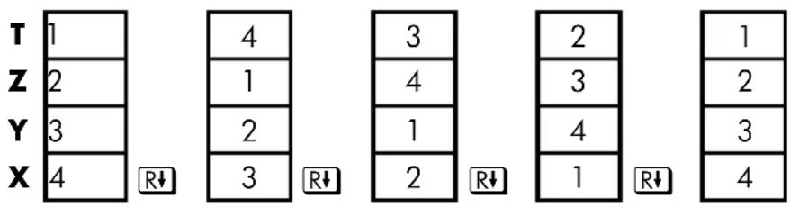
What was in the X-register rotates into the T-register, the contents of the T-register rotate into the Z-register, etc. Notice that only the contents of the registers are rolled — the registers themselves maintain their positions, and only the X-register's contents are displayed.
R↑ (Roll Up)
The 📄 R↑ (roll up) key has a similar function to ⌘ except that it "rolls" the stack contents upward, one register at a time.
The contents of the X-register rotate into the Y-register; what was in the T-register rotates into the X-register, and so on.

The Automatic Memory Stack 2-3
Exchanging the X- and Y-Registers in the Stack
Another key that manipulates the stack contents is ↔ y (x exchange y). This key swaps the contents of the X- and Y-registers without affecting the rest of the stack. Pressing ↔ y twice restores the original order of the X- and Y-register contents.
The x ↔ y function is used primarily for two purposes:
To view the contents of the Y-register and then return them to y (press x ↔ y twice).
Some functions yield two results: one in the X-register and one in the Y-register. For example, ⇔ → 0, r converts rectangular coordinates in the X- and Y-registers into polar coordinates in the X- and Y-registers.
■ To swap the order of numbers in a calculation.
For example, one way to calculate 9 ÷ (13 × 8) :
Press 13 ENTER 8 × 9 x←y ÷
The keystrokes to calculate this expression from left-to-right are:
9 ENTER 13 ENTER 8 ✗ ÷

Always make sure that there are no more than four numbers in the stack at any given time – the contents of the T-register (the top register) will be lost whenever a fifth number is entered.
Arithmetic-How the Stack Does It
The contents of the stack move up and down automatically as new numbers enter the X-register (lifting the stack) and as operators combine two numbers in the X- and Y-registers to produce one new number in the X-register (dropping the stack).
Suppose the stack is filled with the numbers 1, 2, 3, and 4. See how the stack drops and lifts its contents while calculating
2-4 The Automatic Memory Stack
3 + 4 - 9
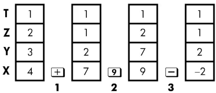
- The stack "drops" its contents. The T- (top) register replicates its contents.
- The stack "lifts" its contents. The T-register's contents are lost.
-
The stack drops.
-
Notice that when the stack lifts, it replaces the contents of the T– (top) register with the contents of the Z–register, and that the former contents of the T–register are lost. You can see, therefore, that the stack's memory is limited to four numbers.
Because of the automatic movements of the stack, you do not need to clear the X-register before doing a new calculation.
■ Most functions prepare the stack to lift its contents when the next number enters the X-register. See appendix B for lists of functions that disable stack lift.
How ENTER Works
You know that ENTER separates two numbers keyed in one after the other. In terms of the stack, how does it do this? Suppose the stack is again filled with 1, 2, 3, and 4. Now enter and add two new numbers:
The Automatic Memory Stack 2-5
5 + 6

- Lifts the stack.
- Lifts the stack and replicates the X-register.
- Does not lift the stack.
- Drops the stack n replicate the T-register.
ENTER replicates the contents of the X-register into the Y-register. The next number you key in (or recall) writes over the copy of the first number left in the X-register. The effect is simply to separate two sequentially entered numbers.
You can use the replicating effect of ENTER clear the stack quickly: press 0 ENTER ENTER ENTER. All stack registers now contain zero. Note, however, that you don't need to clear the tech before doing calculations.
Using a Number Twice in a Row
You can use the replicating feature of ENTER to other advantages. To add a number to itself, press ENTER +
Filling the to with a Constant
The replicating effect of ENTER together with the replicating effect of stack drop (from T into Z) allows you t fill the stack with a numeric constant for calculations.
2-6 The Automatic Memory Stack
Example:
Given bacterial culture with a constant growth rate of 50%, how large would population of 100 be at the end 3 days?
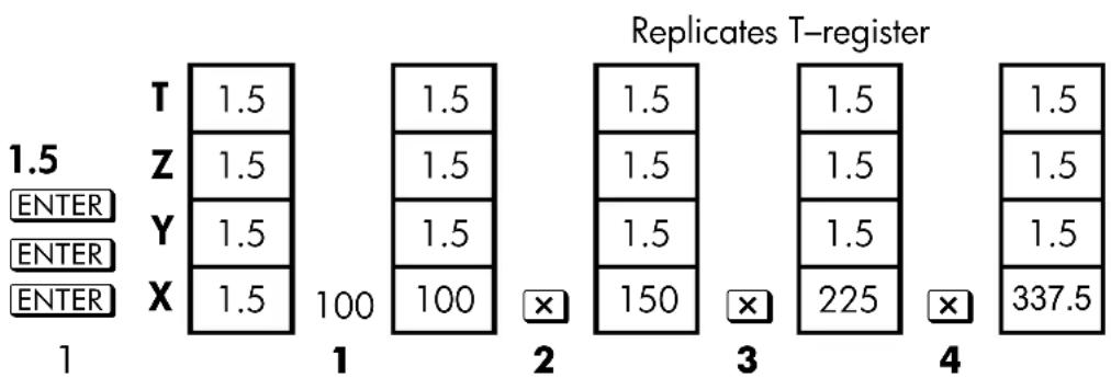
- Fills the stack with the growth rate.
- Keys in the initial population.
- Calculates the population after 1 day.
- Calculates the population after 2 days.
- Calculates the population after 3 days.
How CLEAR x Works
Clearing the display (X-register) put zero in the X-register. The next number you key in (or recall writes over this zero.
There are three ways to clear the contents of the X-register, that is, to clear x:
- Press C
- Press
- Press ← CLEAR {x} (Mainly used during program entry.)
Note these exceptions:
During program entry, ← deletes the currently–displayed program line and C cancels program entry.
■ During digit entry, ← backspaces over the displayed number.
■ If the display shows a labeled number (such as A=2.0000), pressing
The Automatic Memory Stack 2-7
C or ← cancel that display and shows the X-register.
■ When viewing an equation, ← displays the cursor at the end the equation to allow for editing.
During equation entry, ← backspaces over the displayed equation, one function at a time.
For example, if you intended to enter 1 and 3 but mistakenly entered 1 and 2, this what you should do to correct your error:
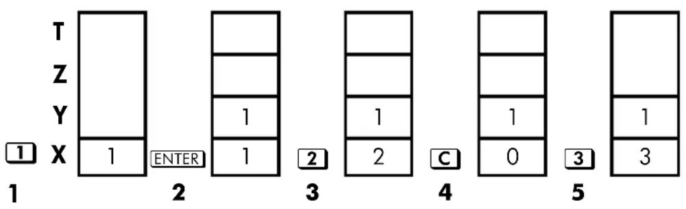
- Lifts the stack
- Lift the stack and replicates the X-register.
- Overwrites the X-register.
- Clears x by overwriting it with zero.
- Overwrites x (replaces the zero.)
The LAST X Register
The LAST X register is a companion to the stack: it holds the number that was in the X-register before the last numeric function was executed. (A numeric function is an operation that produces a result from another number or numbers, such as .) Pressing ← LAST x returns this value into the X-register.
This ability to retrieve the "last x" has two main uses:
- Correcting errors.
- Reusing a number in a calculation.
2-8 The Automatic Memory Stack
See appendix B for a comprehensive list of the functions that save x in the LAST X register.
Correcting Mistakes with LAST X
Wrong One-Number Function
If you execute the wrong one-number function, use 📄 LASTx to retrieve the number so you can execute the correct function. (Press 📄 first if you want to clear the incorrect result, from the stack.)
Since 📄 % and 📄 %CHG don't cause the stack to drop, you can recover from these functions in the same manner as from one-number functions.
Example:
Suppose that you had just computed In 4.7839 × (3.879 × 105) and wanted to find its square root, but pressed ex by mistake. You don't have to start over! To find the correct result, press .
Mistakes with a Two-number operation
If you make a mistake with a two-number operation, ( +, -, ×, ÷, y x or x y ), you can correct it by using ← LAST x and inverse of the two-number function ( - or +, ÷ or ×, x y or y x ).
- Press 1 to recover the second number (x just before the operation).
- Execute the inverse operation. This returns the number that was originally first. The second number is still in the LAST X register. Then:
If you had used the wrong function, press 5 again to restore the original stack contents. Now execute the correct function.
If you had used the wrong second number, key in the correct one and execute the function.
If you had used the wrong first number, key in the correct first number, press to recover the second number, and execute the function again.
(Press C first if you want to clear the incorrect result from the stack.)
Example:
The Automatic Memory Stack 2-9
Suppose you made a mistake while calculating
1 6 × 1 9 = 3 0 4.
There are three kinds of mistakes you could have made:
Wring Calculation:
16 ENTER 19 — Wrong function


15 ENTER 19 ✗ Wrong first number

16 ENTER 18 ✗ Wrong second number

Reusing Numbers with LAST X
You can use 📄 LASTx to reuse a number (such as a constant) in a calculation. Remember to enter the constant second, just before executing the arithmetic operation, so that the constant is the last number in the X-register, and therefore can be saved and retrieved with 📄 LASTx
Example:
Calculates + 3 9 4 7 . 5 2 7 0 4 . 9 6/3 9 4 7 . 5 2
2–10 The Automatic Memory Stack
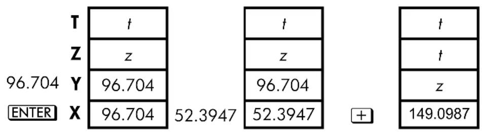

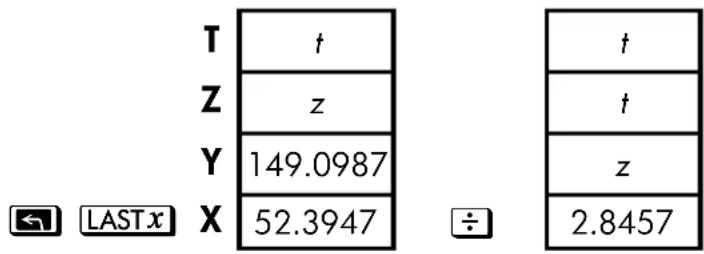

| Keys: | Display: | Description: |
| 96.704 ENTER | 96.704 | Enters first number. |
| 52.3947 + | 149.0987 | Intermediate result. |
| ← LAST.x | 52.3947 | Brings back display from before +. |
| ÷ | 2.8457 | Final result. |
Example:
Two close stellar neighbors of Earth are Rigel Centaurus (4.3 light-years away) and Sirius (8.7 light-years away). Use c, the speed of light (9.5 × 10¹⁵ meters per year) to convert the distances from the Earth to these stars into meters:
The Automatic Memory Stack 2-11
To Rigel Centaurus: 4.3 yr × (9.5 × 10 15 m/yr).
To Sirius: 8.7 yr × (9.5 × 10 15 m/yr).
Keys:
| 4.3 ENTER | 4.3000 | Light-years to Rigel Centaurus. |
| 9.5 E 15 | 9.5E15 | Speed of light, c. |
| × | 4.0850E16 | Meters to R. Centaurus. |
| 8.7 ← LASTx | 9.5000E15 | Retrieves c. |
| × | 8.2650E16 | Meters to Sirius. |
Chain Calculations
The automatic lifting and dropping of the stack's contents let you retain intermediate results without storing or reentering them, and without using parentheses.
Work from the Parentheses Out
For example, solve (12 + 3) × 7 .
If you were working out this problem on paper, you would first calculate the intermediate result of (12 + 3) ...
(1 2 + 3) = 1 5
... then you would multiply the intermediate result by 7:
(1 5) × 7 = 1 0 5
Solve the problem in the same way on the HP 32SII, starting inside the parentheses:
Keys:
| 12 | ENTER | 3 | + | 15.0000 | Calculates the intermediate result first. |
Display:
2-12 The Automatic Memory Stack
You don't need to press ENTER to save this intermediate result before proceeding; since it is a calculated result, it is saved automatically.
Keys:
Display:
Description:
7 ×
105,0000
Pressing the function key produces the answer. This result can be used in further calculations.
Now study the following examples. Remember that you need to press ENTER only to separate, sequentially-entered numbers, such as at the beginning of a problem The operations themselves ( +, -, etc.) separate subsequent numbers and save intermediate results. The last result saved is the first one retrieved as needed to carry out the calculation.
Calculate 2 ÷ (3 + 10) :
Keys:
Display:
Description:
3 ENTER 10 +
13.0000
Calculates (3 + 10) first.
2 ↔ y÷
0.1538
Puts 2 before 13 so the division is correct: 2 ÷ 13 .
Calculate 4 ÷ [(14 + (7 × 3) - 2] :
Keys:
Display:
Description:
7 ENTER 3 ✗
21.0000
Calculates (7 × 3) .
14 + 2 -
33,0000
Calculates denominator.
4 x ↔ y
33.0000
Puts 4 before 33 in preparation for division.
÷
0.1212
Calculates 4 ÷ 33 , the answer.
Problems that have multiple parentheses can be solved in the same manner using the automatic storage of intermediate results. For example, to solve (3 + 4) × (5 + 6) on paper, you would first calculate the quantity (3 + 4) . Then you would calculate (5 + 6) . Finally, you would multiply the two intermediate results to get the answer.
The Automatic Memory Stack 2-13
Work through the problem the same way with the HP 32SII, except that you don't have to write down intermediate answers—the calculator remembers them for you.
| Keys: | Display: | Description: |
| 3 ENTER 4 + | 7.0000 | First adds (3+4) |
| 5 ENTER 6 + | 11.0000 | Then adds (5+6) |
| × | 77.0000 | Then multiplies the intermediate answers together for the final answer. |
Exercises
Calculate:
√ (1 6 . 3 8 0 5 × 5)0 5 . 0 = 0 0 0 0. 1 8 1
Solution:
16.3805 ENTER 5 × √x .05 ÷
Calculate:
√ [(2 + 3) × (4 + 5)] + √ [(6 + 7) × (8 + 9) = 2 1. 5 7 4 3
Solution:
2 ENTER 3 + 4 ENTER 5 + × √x 6 ENTER 7 + 8 ENTER 9 + × √x +
Calculate:
(1 0 - 5) ÷ [(1 7 - 1 2) × 4] = 0. 2 5 0 0
Solution:
17 ENTER 12 - 4 × 10 ENTER 5 - x←y ÷ or 10 ENTER 5 - 17 ENTER 12 - 4 × ÷
2–14 The Automatic Memory Stack
Order of Calculation
We recommend solving chain calculations by working from the innermost parentheses outward. However, you can also choose to work problems in a left-to-right order.
For example, you have already calculated:
4 ÷ [1 4 + (7 × 3) - 2]
by starting with the innermost parentheses (7 × 3) and working outward, just as you would with pencil and paper. The keystrokes were 7 ENTER 3 ✗ 14 + 2 - 4 x→y ÷
If you work the problem from left-to-right, press
4 ENTER 14 ENTER 7 ENTER 3 ✗ + 2 - ÷.
This method takes one additional keystroke. Notice that the first intermediate result is still the innermost parentheses (7 × 3). The advantage to working a problem left-to-right is that you don't have to use x→y to reposition operands for nomcommutative functions (— and ÷).
However, the first method (starting with the innermost parentheses) is often preferred because:
■ It takes fewer keystrokes.
■ It requires fewer registers in the stack.
Note

When using the left-to-right method, be sure that no more than four intermediate numbers (or results) will be needed at one time (the stack can hold no more than four numbers).
The above example, when solved left-to-right, needed all registers in the stack at one point:
Keys:
4 ENTER 14
ENTER
Display:
14.0000
Description:
Saves 4 and 14 as intermediate numbers in the stack.
The Automatic Memory Stack 2–15
| 7 ENTER 3 | 3_ | At this point the stack is full with numbers for this calculation. |
| × | 21.0000 | Intermediate result. |
| + | 35.0000 | Intermediate result. |
| 2 - | 33.0000 | Intermediate result. |
| ÷ | 0.1212 | Final result. |
More Exercises
Practice using RPN by working through the following problems:
Calculate:
(1 4 + 1 2) × (1 8 - 1 2) ÷ (9 - 7) = 7 8. 0 0 0 0
A Solution:
14 ENTER 12 + 18 ENTER 12 - × 9 ENTER 7 - ÷
Calculate:
2 3 ^ 2 - (1 3 × 9) + 1 / 7 = 4 1 2. 1 4 2 9
A Solution:
23 ← x² 13 ENTER 9 × - 7 1/x +
Calculate:
√ (5 . 4 × 0 . 8) ÷ (1 2 . 5 - 0 . 7 ^ 3) = 0. 5 9 6 1
Solution:
5.4 ENTER .8 × .7 ENTER 3 y x 12.5 x←y - ÷ √x
or
5.4 ENTER .8 × 12.5 ENTER .7 ENTER 3 y x — ÷ √x
Calculate:
√ 8 . 3 3 × (4 - 5 . 2) ÷ [(8 . 3 3 - 7 . 4 6) × 0 . 3 2]/4 . 3 × (3 . 1 5 - 2 . 7 5) - (1 . 7 1 × 2 . 0 1) = 5 7 2 8. 4
A Solution:
2-16 The Automatic Memory Stack
4 ENTER 5.2 - 8.33 ✗ LASTx 7.46 - 0.32 ✗ ÷ 3.15
ENTER 2.75 - 4.3 × 1.71 ENTER 2.01 × - ÷ √x
3
Storing Data into Variables
The HP 32II has 384 bytes of user memory: memory that you can use to store numbers, equations, and program lines. Numbers are stored in locations called variables, each named with a letter from A through Z. (You can choose the letter to remind you of what is stored there, such as B for bank balance and C for the speed of light.)
3-1 Picture
- Cursor prompts for variable.
- Indicates letter keys are active.
- Letter keys.
Each white letter is associated with a key and a unique variable. The letter keys are automatically active when needed. (The A..Z annunciator in the display confirms this.)
Note that the variables, X, Y, Z and T are different storage locations from the X-register, Y-register, Z-register, and T-register in the stack.
Storing and Recalling Numbers
Numbers are stored into and recalled from lettered variables with the STO (store) and RCL (recl) functions.
To store a copy of a displayed number (X-register) to a variable:
Press STO letter-key.
To recall a copy of a number from a variable to the display:
Press RCL letter-key.
Storing
Data
Example: Storing Numbers.
Store Avogadro's number (approximately 6.0225 × 10²³ ) in A.
| Keys: | Display: | Description: |
| 6.0225 E 23 | 6.0225E23_ | Avogadro's numbers. |
| STO | STO_ | Prompts for variable. |
| A (HOLD key) | STO A | Displays function as long as key is held down. |
| (release) | 6.0225E23 | Stores a copy of Avogadro's numbers in A. This also terminates digit entry (no cursor present) |
| C | 0.0000 | Clears the number in the display. |
| RCL | RCL_ | Prompts for variable. |
| A | 6.0225E23 | Copies Avogadro's numbers from A the display. |
Viewing a Variable without Recalling It
The VIEW function shows you the contents of a variable without putting that number in the X-register. The display is labeled for the variable, such as:
A = 1 2 3 4. 5 6 7 8
If the number is too large to fit completely in the display with its label, it is rounded and the rightmost digits are dropped. (An exponent is displayed in full.) To see the full mantissa, press 📄 SHOW.
In Fraction-display mode (☐ FDISP), part of the integer may be dropped. This will be indicated by "..." at the left end of the integer.
To see the full mantissa, press 📄 SHOW. The integer part is the portion to the left of the radix ( · or · ).
VIEW is most often used in programming, but it is useful anytime you want to view a variable's value without affecting the contents of the stack.
3-2 Storing Data into Variables
To cancel the VIEW display, press ← or C once.
Reviewing Variables in the VAR Catalog
The ← MEM (memory) function provides information about memory:
nnn.n VAR PGM
where nnn.n is the number of bytes of available memory.
Pressing the {VAR} menu key displays the catalog of variables.
Pressing the {PGM} menu key displays the catalog of programs.
To review the values at any or all non-zero variables:
-
Press MEM {VAR}.
-
Press ← ↓ or ← ↑ to move the list and display the desired variable. (Note the ▼▲ annunciator, indicating that the left-shifted ↓ and ↑ keys are active, If Fraction-display mode is active, ▼▲ does not indicate accuracy.) To see all the significant digits of a number displayed in the {VAR} catalog, press → SHOW. (If it is a binary number with more than 12 digits, use the √x and Σ+ keys to see the rest.)
-
To copy a displayed variable from the catalog to the X-register, press ENTER.
-
To clear a variable to zero, press ☑ CLEAR while it is displayed in the catalog.
-
Press C to cancel the catalog.
Clearing Variables
Variables' values are retained by Continuous Memory until you replace there or clear them. Clearing a variable stores a zero there; a value of zero takes no memory.
To clear a single variable:
Storing
Data
Store zero in it: Press 0 STO variable.
To clear selected variables:
- Press ← MEM {VAR} and use ← ↓ or ← ↑ to display the variable.
- Press ← CLEAR .
- Press C to cancel the catalog.
To clear all variables at once:
Press ← CLEAR {VARS}.
Arithmetic with Stored Variables
Storage arithmetic and recall arithmetic allow you to do calculations with a number stored in a variable without recalling the variable into the stack. A calculation uses one number from the X-register and one number from the specified variable.
Storage Arithmetic
Storage arithmetic uses STO +, STO -, STO ×, or STO ÷ to do arithmetic in the variable itself and to store the result there. It uses the value in the X-register and does riot affect the stack.
New value of variable = Previous value of variable +, -, ×, ÷ x.
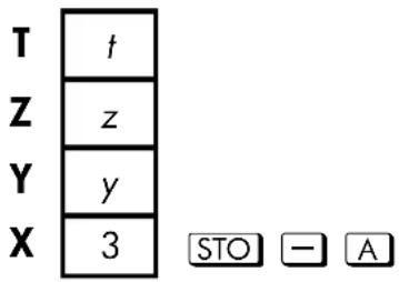
For example, suppose you want to reduce the value in A(15) by the number in the X-register (3, displayed). Press STO — A. Now A = 12, while 3 is still in the display.
3-4 Storing Data into Variables


Results: 15–3 thatis, A−x

Recall Arithmetic
Recall arithmetic uses a RCL +, RCL ×, or RCL ÷ to do arithmetic in the X-register using a recalled number and to leave the result in the display. Only the X-register is affected.
New x = Previous x {+, -, ×, ÷} Variable
For example, suppose you want to divide the number in the X-register (3, displayed) by the value in A(12). Press RCL ÷ A. Now x = 0.25, while 12 is still in A. Recall arithmetic saves memory in programs: using RCL + A (one instruction) uses half as much memory as RCL A, + (two instructions).


Results: 3 ÷ 12 , thatis, x ÷ A
Storing
Data
Example:
Suppose the variables D, E, and F contain the values 1, 2, and 3. Use storage arithmetic to add 1 to each of those variables.
| Keys: | Display: | Description: |
| 1 STO D | 1.0000 | Stores the assumed values into the variable. |
| 2 STO E | 2.0000 | |
| 3 STO F | 3.0000 | |
| 1 STO + D | Add 1 to D, E, And F. | |
| STO + E STO | ||
| + F | 1.0000 | |
| VIEW D | D=2.0000 | Displays the current value of D. |
| VIEW E | E=3.0000 | |
| VIEW F | F=4.0000 | |
| ← | 1.0000 | Clears the VIEW display; displays X-register again. |
Suppose the variables D, E, and F contain the values 2, 3, and 4 from the last example. Divide 3 by D, multiply it by E, and add F to the result.
| Keys: | Display: | Description: |
| 3 RCL ÷ D | 1.5000 | Calculates 3 ÷ D. |
| RCL × E | 4.5000 | 3 ÷ D × E. |
| RCL + F | 8.5000 | 3 ÷ D × E + F |
Exchanging x with Any Variable
The 2 key allows yon to exchange the contents of (the Displayed X-register with 1 contents of any variable. Executing this function does not effect the Y-, Z-, or T-registers
3-6 Storing Data into Variables
Example:
| Keys: | Display: | Description: |
| 12 STO A | 12.0000 | Stores 12 in variable A. |
| 3 | 3_ | Display x. |
| x> A | 12.0000 | Exchange contents of the X-register and variable A. |
| x> A | 3.0000 | Exchange contents of the X-register and variable A. |


The Variable "i"
There is a 27th variables that you can access directly—the variable i. The key is labeled "i", and it means i whenever the A..Z annunciator is on. Although it stores numbers as other variables do, i is special in that it can be used to refer to other variables, including the statistics registers, using the (i) function. This is a programming technique called indirect addressing that is covered under "Indirectly Addressing variables and labels" in chapter 13.
Storing
Data
4
Real-Number Functions
This chapter covers most of the calculator's functions that perform computations on real numbers, including some numeric functions used in programs (such as ABS, the absolute-value function):
■ Exponential and logarithmic functions.
■ Power functions. ( yx and x )
■ Trigonometric functions.
■ Hyperbolic functions.
■ Percentage functions.
■ Conversion functions for coordinates, angles, and units.
■ Probability functions.
■ Parts of numbers (number-altering functions).
Arithmetic functions and calculations were covered in chapters 1 and 2. Advanced numeric operations (root-finding, integrating, complex numbers, base conversions, and statistics) are described in later chapters.
All the numeric functions are on keys except for the probability and parts-of-numbers functions.
The probability functions (Cn,r, Pn,r, SD, and R) are in the PROB menu (press [PROB]).
The-parts-of numbers functions(IP, FP, and, ABS) are in PARTS menu (press [PARS]).
Exponential and Logarithmic Functions
Put the number in the display, then execute the function — there is no need to press ENTER.
Real-Number
Func
| To Calculate: Press: | |
| Natural logarithm (base e) | LN |
| Common logarithm (base 10) | ← LOG |
| Natural exponential | ex |
| Common exponential (antilogarithm) | ← 10x |
Power Functions
To calculate the square of a number x, key in x and press ← 2 .
To calculate a power x of 10, key in x and press 10x .
'To calculate a number y raised to a power x, key in y ENTER x, then press yx .(For y > 0, x can be any rational number; for y < 0, x must be are integer; for y = 0, x must be positive.)
| To Calculate: Press: Result: | ||
| 152 | 15 ← x2 | 225.0000 |
| 106 | 6 5 10x | 1,000,000,0000 |
| 54 | 5 ENTER 4 yx | 635.0000 |
| 2-1.4 | 2 ENTER 1.4 +/- yx | 0.3789 |
| (-1.4)3 | 1.4 +/- ENTER 3 yx | -2.7440 |
To calculate a root x of a number y (the xth root of y), key in y ENTER x, then press 51 ,y . For y<0, x must be an integer.
To Calculate:
√[3]-125
3/125
Press:
125


Result:
-5.0000
125



5.0000
4-2 Real-Number Functions
Trigonometry
Entering π
Press → π to place the first 12 digits of π into the X-register.
(The number displayed depends on the display format.) Because π is a function, it doesn't need to be separated from another number by ENTER.
Note that calculator cannot exactly represent π , since π is an irrational number.
Setting the Angular Mode
The angular rode specifies which unit of measure do assume for angles used in trigonometric functions. The mode does not convert numbers already present (see "Conversion Functions" later in this chapter)
360 degrees = 2π radians = 400 grads
To set, an angular mode, press Ⓜ MODES . A menu will be displayed from which you can select an option.
| Option | Description | Annunciator |
| {DG} | Sets Degrees mode (DEG). Uses decimal degrees, not degrees, minutes, and seconds. | none |
| {RD} | Sets Radians mode (RAD). | RAD |
| {GR} | Sets Grads mode (GRAD). | GRAD |
Real-Number
Func
Trigonometric Functions
With x in the display:
| To Calculate: Press: | |
| Sine of x. | SIN |
| Cosine of x. | COS |
| Tangent of x. | TAN |
| Arc sine of x. | ASIN |
| Arc cosine of x. | ACOS |
| Arc tangent of x. | ATAN |

Calculations with the irrational number π cannot be expressed exactly by the 12-digit internal precision of the calculator. This is particularly noticeable in trigonometry. For example, the calculated π (radians) is not zero but -2.0676 × 10⁻¹³ , a very small number close to zero.
Example:
Show that cosine (5 ÷ 7) π radians and cosine 128.57° are equal (to four significant digits).
| Keys: | Display: | Description: |
| Sets Radians mode; RAD annunciator on. | ||
| 5 7 ENTER | 0.7143 | 5 ÷ 7 in decimal format. |
| π × COS | -0.6235 | Cos (5/7)π. |
| MODES {DG} | -0.6235 | Switches to Degrees mode (no annunciator). |
| 128.57 COS | -0.6235 | Calculates cos 128.57°, which is the same as cos (5/7)π. |
4-4 Real-Number Functions
Programming Note:
Equations using inverse trigonometric functions to determine an angle θ , often look something like this:
θ = (y / x).
If x = 0, then y/x is undefined, resulting in the error: DIVIDE BY 0. For a program, then, it would be more reliable to determine θ by a rectangular-to polar conversion, which converts (x, y) to (r, θ). See "Coordinate Conversions" later in this chapter.
Hyperbolic Functions
With x in the display:
| To Calculate Press: | |
| Hyperbolic sine of x (SINH). | HYP SIN |
| Hyperbolic cosine of x (COSH). | HYP COS |
| Hyperbolic tangent of x (TANH). | HYP TAN |
| Hyperbolic arc sine of x (ASINH). | HYP ASIN |
| Hyperbolic arc cosine of x (ACOSH). | HYP ACOS |
| Hyperbolic arc tangent of x (ATANH). | HYP ATAN |
Percentage Functions
The percentage functions are special (compared with × and ÷) because they preserve the value of the base number (in the Y-register) when they return the result of the percentage calculation (in the X-register). You can then carry out subsequent calculations using both the base number and the result without reentering the base number.
Real-Number
Func
| To Calculate Press: | |
| x% of y yPercentage change from y to x. (y≠ 0) | ENTER x % ENTER x %CHG |
Example:
Find the sales tax at 6% and the total cost of a \$15.76 item.
Use FIX 2 display format so the costs are rounded appropriately.
| Keys: | Display: | Description: |
| Rounds display to two decimal places. | ||
| 15.76 ENTER | 15.76 | |
| 6 % | 0.95 | Calculates 6% tax. |
| + | 16.71 | Total cost (base price + 6% tax). |
Suppose that the \15.76 item cost \16.12 last year. What is the percentage change from last year's price to this year's?
| Keys: | Display: | Description: |
| 16.12 ENTER | 16.12 | |
| 15.76 P %CHG | -2.23 | This year's price dropped about 2.2% from last year's price. |
| DISP {FX} 4 | -2.2333 | Restores FIX 4 format. |

The order of the two numbers is important for the \%CHG function. The order affects whether the percentage change is considered positive or negative.
4-6 Real-Number Functions
Conversion Functions
There are four types of conversions: coordinate (polar/rectangular), angular (degrees/radians), time (decimal/minutes–seconds), and unit (cm/in, °C/°F, l/gal, Kg/lb).
Coordinate Conversions
The function names for these conversions are y, x → θ, r and θ, r → y, x .
Polar coordinates (r,θ) and rectangular coordinates (x,y) are measured as shown in the illustration. The angle θ uses units set by the current angular mode. A calculated result for θ will be between -180° and 180° , between -π and π radians, or between -200 and 200 grads.
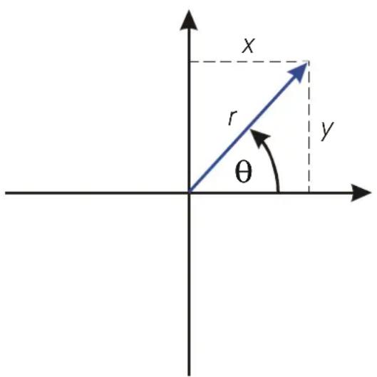
To convert between rectangular and polar coordinates:
- Enter the coordinates (in rectangular or polar form) that you want to convert. The order is y ENTER x or θ ENTER r.
- Execute the conversion you want: press →θ,r (rectangular-to-polar) or → y,x (polar-to-rectangular). The converted coordinates occupy the X- and Y-registers.
- The resulting display (the X-register) shows either r (polar result) or x (rectangular result). Press ↔ y to see θ or y.
Real-Number
Func
![graph TD X["X"] --> Y["Y"] Y --> R["r"] R --> Y Y -->|θ, r→y| R R -->|θ, x→θ| Y Y -->|x, y| Y](/content/2026/05/973866/images/afe9c542a23f1b227b10633b7bd256d087996b65de7fd25970dac77660af106b.jpg)
Example: Polar to Rectangular Conversion.
In the following right triangles, find sides x and y in the triangle on the left, and hypotenuse r and angle θ in the triangle on the right.

Keys:


Display:
Sets Degrees mode.
Calculates x .
Displays y.
Calculates hypotenuse (r).
Displays θ .
Description:
4-8 Real-Number Functions
Example: Conversion with Vectors.
Engineer P.C. Bard has determined that in the RC circuit shown, the total impedance is 77.8 ohms and voltage lags current by 36.5°. What a .re the values of resistance R and capacitive reactance XC in the circuit?
Use a vector diagram as shown, with impedance equal to the polar magnitude, r, and voltage lag equal to the angle, θ , in degrees. When the values are converted to rectangular coordinates, the x-value yields R, in ohms; the y-value yields XC , in ohms.

Keys:
| MODES | {DG} | |
| 36.5 | +/- | ENTER |
| 77.8 | ||
| →y.x | ||
| x↔y |
Display:
| Sets Degrees mode. |
| Enters θ , degrees of voltage lag. |
| Enters r , ohms of total impedance. |
| Calculates x , ohms resistance, R . |
| Displays y , ohms reactance, XC . |
Description:
For more sophisticated operations with vectors (addition, subtraction, cross product, and dot product), refer to the "Vector Operations" program in chapter 15, "Mathematics Programs"
Time Conversions
Values for time (in hours, H) or angles (in degrees, D) can be converted between a decimal-fraction form (H.h or D.d) and a minutes-seconds form (H.MMSSss or D.MMSSss) using the → HR or → HMS keys.
Real-Number
Func
To convert between decimal fractions and minutes-seconds:
- Key in the time or angle (in decimal form or minutes–seconds form) that you want to convert.
- Press → HMS or → HR. The result is displayed.
Example: Converting Time Formats.
How many minutes and seconds are there in 1 ÷ 7 of an hour? Use FIX 6 display format.
| Keys: | Display: | Description: |
| Sets FIX 6 display format. | ||
| 0 1/7 | 1 ÷ 7 as a decimal fraction. | |
| 0.083429 | Equals 8 minutes and 34.29 seconds. | |
| 0.0834 | Restores FIX 4 display format. |
Angle Conversions
When converting to radians, the number in the x-register is assumed to be degrees; when converting to degrees, the number in the x-register is assumed to be radians.
To convert an angle between degrees and radians:
- Key in the angle (in decimal degrees or radians) that you want to convert.
- Press →RAD or ←→DEG. The result is displayed.
4-10 Real-Number Functions
Unit conversions
The HP 32SII has eight unit-conversion functions on the keyboard: → kg, → lb, →° C, →° F, → cm, → in, → l, → gal.
| To Convert: | To: Press: Displayed Results: | ||
| 1 lb | kg | 1 kg kg | 0.4536 (kilograms) |
| 1 kg lb | 1 | →lb | 2.2046 (pounds) |
| 32 °F | °C | 32 °C | 0.0000 (°C) |
| 100 °C | °F | 100 °F | 212.0000 (°F) |
| 1 in | cm | 1 cm | 2.5400 (centimeters) |
| 100 cm | in | 100 in | 39.3701 (inches) |
| 1 gal | l | 1 l | 3.7854 (liters) |
| 1 l | gal | 1 gal | 0.2642 (gallons) |
Probability Functions
Factorial
To calculate the factorial of a displayed positive integer x ( o ≤ x ≤ 253 ), press ! (the left-shifted 1/x key).
Gamma
To calculate the gamma function of a noninteger x, (x) , key in (x - 1) and press → ! . The x! function calculates (x + 1) . The value for x cannot be a negative integer.
Real-Number
Func
Probability Menu
Press [PROB] to see the PROB (probability) menu shown, in the following table. It has functions to calculate combinations and permutations, to generate seeds for random numbers, and to obtain random numbers from those seeds.
PROB Menu
| Menu Label | Description |
| {Cn, r} | Combinations. Enter n first, then r (nonnegative integers only). Calculates the number of possible sets of n items taken r at a time. No item occurs more than once in a set, and different orders of the same r items are not counted separately. |
| {Pn, r} | Permutations. Enter n first, then r (nonnegative integers only). Calculates the number of possible arrangements of n items taken r at a time. No item occurs more than once in an arrangement, and different orders of the same r items are counted separately. |
| {SD} | Seed. Stores the number in x as a new seed for the random number generator. |
| {R} Random number generator. Generates a random number in the range 0 ≤ x < 1 (The number is part of a uniformly-distributed pseudo-random number sequence. It passes the spectral test of D. Knuth, Seminumerical Algotithims, vol. 2, London: Addison Wesley, 1981.) | |
The RANDOM function (executed by pressing R ) uses a seed to generate a random number. Each random number generated becomes the seed for the next random number. Therefore, a sequence of random numbers can be repeated by starting with the same seed. You can store a new seed with the SEED function (executed by pressing SD ). If memory is cleared, the seed is reset to zero.
4-12 Real-Number Functions
Example: Combinations of People.
A company employing 14 women and 10 men is forming a six-person safety committee. How many different combinations of people are possible?
| Keys: | Display: | Description: |
| 24 ENTER 6 | 6_ | Twenty-four people grouped six at a time. |
| [PROB] | Cn,r Pn,r SDR | Probability menu. |
| {Cn,r} | 134,596,0000 | Total number of combinations possible. |
If employees are chosen at random, what is the probability that the committee will contain six women? To find the probability of an event, divide the number of combinations for that event by the total number of combinations.
| Keys: | Display: | Description: |
| 14 ENTER 6 | 6_ | Fourteen worriers grouped six at a time. |
| [PROB] {Cn,r} | 3,003,0000 | Number of combinations of six women on the committee. |
| x↔y | 134,596,0000 | Brings total number of combinations back into the X-register. |
| ÷ | 0.0223 | Divides combinations of |
Real-Number
Func
Parts of Numbers
The functions in the PARTS menu (PARTS) shown in the following table and the RND function alter the number in the X-register in simple ways. These functions are primarily used in programming.
PARTS Menu
| Menu Label | Description |
| {IP} | Integer part. Removes the fractional part of x and replaces it with zeros. (For example, the integer part of 14.2300 is 14.000.) |
| {FP} | Fractional part. Removes the integer part of x and replaces it with zeros. (For example, the fractional part of 14.2300 is 0.2300) |
| {ABS} | Absolute value. Replaces x with its absolute value. |
The RND function ( ← RND ) rounds x internally to the number of digits specified by the display format. (The internal number is represented by 12 digits.) Refer to chapter 5 for the behavior of RND in Fraction–display mode.
Names of Function
You might have noticed that the name of a function appears in the display when you press and hold the key to execute it. (The name remains displayed for as long as you hold the key down.) For instance, while pressing , the display shows SQRT. "SQRT" is the name of the function as it will appear in program lines (and usually in equations also).
4–14 Real-Number Functions
5
Fractions
"Fractions" in chapter 1 introduces the basics about entering, displaying, and calculating with fractions:
■ To enter a fraction, press twice—after the integer part, and between the numerator and denominator. To enter 23/8 , press 2 3 8. To enter 5/8 , press 5 8 or 5 8.
To turn Fraction-display mode on and off, press [6] [FDISP]. When you turn off Fraction-display mode, the display goes back to the previous display format. (FIX, SCI, ENG, and ALL also turn off Fraction-display mode.)
■ Functions work the same with fractions as with decimal numbers—except for RND, which is discussed later in this chapter.
This chapter gives more information about using and displaying fractions.
Entering Fractions
You can type almost any number as a fraction on the keyboard — including an improper fraction (where the numerator is larger than the denominator). However, the calculator displays ⚠ if you disregard these two restrictions.
■ The integer and numerator must not contain more than 12 digits total.
■ The denominator must not contain more than 4 digits.
Fractions
Example:
| Keys: | Display: | Description: |
| Turns on Fraction-display mode. | ||
| 1.5 ENTER | 1 1/2 | Enters 1.5; shown as a fraction. |
| 1 3 4 ENTER | 1 3/4 | Enters 1 3/4. |
| 1.7500 | Displays x as a decimal number. | |
| 1 3/4 | Displays x as a fraction. |
If you didn't get the same results as the example, you may have accidentally changed how fractions are displayed. (See "Changing the Fraction Display" later in this chapter.)
The next topic includes more examples of valid and invalid input fractions.
You can type fractions only if the number base is 10 — the normal number base. See chapter 10 for information about changing the number base.
Fractions in the Display
In Fraction–display mode, numbers are evaluated internally as decimal numbers, then they're displayed using the most precise fractions allowed. In addition, accuracy annunciators show the direction of any inaccuracy of the fraction compared to its 12-digit decimal value. (Most statistics registers are exceptions — they're always shown as decimal numbers.)
Display Rules
The fraction you see may differ from the one you enter. In its default condition, the calculator displays a fractional number according to the following rules. (To change the rules, see "Changing the Fraction Display" later in this chapter.)
The number has an integer part and, if necessary, a proper fraction (the numerator is less than the denominator).
5-2 Fractions
■ The denominator is no greater than 4095.
■ The fraction is reduced as far as possible.
Examples:
These are examples of entered values and the resulting displays. For comparison, the internal 12-digit values are also shown. The ▲ and ▼ annunciators in the last column are explained below.
| Entered Value | Internal Value | Displayed Fraction |
| 23/8 | 2.37500000000 | 2 3/8 |
| 1415/32 | 14.4687500000 | 14 15/32 |
| 54/12 | 4.50000000000 | 4 1/2 |
| 618/5 | 9.60000000000 | 9 3/5 |
| 34/12 | 2.83333333333 | ▼2 5/6 |
| 15/8192 | .183105468750 | ▲0 7/3823 |
| 1234567812345/3 | (Illegal entry) | |
| 163/16384 | (Illegal entry) |
Accuracy Indicators
The accuracy of a displayed fraction is indicated by the ▲ and ▼ annunciators at the top of the display. The calculator compares the value of the fractional part of the internal 12-digit number with the value of the displayed fraction:
If no indicator is lit, the fractional part of the internal 12-digit value exactly matches the value of the displayed fraction.
If is fit, the fractional part of the internal 12-digit value is slightly less than the displayed fraction — the exact numerator is no more than 0.5 below the displayed numerator.
Fractions
This diagram shows how the displayed fraction relates to nearby values — ▲ means the exact numerator is "a little above" the displayed numerator, and ▼ means the exact numerator is "a little below".

This is especially important if you change the rules about how fractions are displayed. (See "Changing the Fraction Display" later.) For example, if you force all fractions to have 5 as the denominator, then 2/3 is displayed as 3/5 because the exact fraction is approximately 3.3333/5 , "a little above" 3/5 . Similarly, -2/3 is displayed as - 3/5 because the true numerator is "a little above" 3.
If you press ⬇ MEM {VAR} to view the VAR catalog, the ▲▼ annunciator doesn't indicate accuracy — it means you can use ↑ and ↓ to move through the list of variables. The accuracy isn't shown.
Sometimes an annunciator is lit when you wouldn't expect it to be. For example, if you enter 22/3 , you see 22/3 , even though that's the exact number you entered. The calculator always compares the fractional part of the internal value and the 12-digit value of just the fraction. If the internal value has an integer part, its fractional part contains less than 12 digits—and it can't exactly match a fraction that uses all 12 digits.
Longer Fractions
If the displayed fraction is too long to fit in the display, it's shown with ... at the beginning. The fraction part always fits — the ... means the integer part isn't shown completely. To see the integer part (and the decimal fraction), proms and hold 📄 SHOW (You can't scroll a fraction in the display.)
5-4 Fractions
Example:
| Keys: | Display: | Description: |
| 14 ex | ...04 888/3125 | Calculates e14 . |
| SHOW | 1202604.28416 | Shows all decimal digits. |
| STO A | ...04 888/3125 | Stores value in A. |
| VIEW A | A=... 888/3125 | Views A. |
| C C | 0 | Clears x. |
Changing the Fraction Display
In its default condition, the calculator displays a fractional number according to certain rules. (See "Display Rules" earlier in this chapter.) However, you can change the rules according to how you want fractions displayed:
■ You can set the maximum denominator that's used.
■ You can select one of three fraction formats.
The next few topics show how to change the fraction display.
Setting the Maximum Denominator
For any fraction, the denominator is selected based on a value stored in the calculator. If you think of fractions as a b/c, then /c corresponds to the value that controls the denominator.
The /c value defines only the maximum denominator used in Fraction–display mode — the specific denominator that's used is determined by the fraction format (discussed in the next topic).
To set the /c value, press n 📄 /c, where n is the maximum denominator you want. n can't exceed 4095. This also turns on Fraction-display mode.
■ To recall the /c value to the X-register, press 1 ↗ ↗ ↗.
■ To restore the default value or 4095, press 0 ↗ /c. (You also restore
Fractions
the default if you use 4095 or greater.) This also turns on Fraction-display mode.
The /c function uses the absolute value of the integer part of the number in the X-register. It doesn't change the value in the LAST X register.
Choosing Fraction Format
The calculator has three fraction formats. Regardless of the format, the displayed fractions are always the closest fractions within the rules for that format.
■ Most precise fractions. Fractions have any denominator up to the /c value, and they're reduced as much as possible. For example, if you're studying math concepts with fractions, you might want any denominator to be possible (/c value is 4095). This is the default fraction format.
Factors of denominator. Fractions have only denominators that are factors of the /c value, and they're reduced as much as possible. For example, if you're calculating stock prices, you might want to see 53 1/14 and 37 7/8 (/c value is 8). Or if the /c value is 12, possible denominators are 2, 3, 4, 6, and 12.
■ Fixed denominator. Fractions always use the /c value as the denominator—they're not reduced. For example, if you're working with time measurements, you might want to see 1 25/60 (/c value is 60).
To select a fraction format, you must change the states of two flags. Each flag can be "set" or "clear," and in one case the state of flag 9 doesn't matter.
| Change These Flags: To Get This Fraction For | ||
| 8 | 9 | |
| Most precise | Clear | — |
| Factors of denominator | Set | Clear |
| Fixed denominator | Set | Set |
5-6 Fractions
You can change flags 8 and 9 to set the fraction format using the steps listed here. (Because flags are especially useful in program, their use us covered in detail in chapter 13.)
- Press → FLAGS to get the flag menu.
- To set a flag, press {SF} and type the flag number, such as 8.
To clear a flag, press and type the flag number.
To see if a flag is set, press {FS?} and type the flag number. Press C or
to clear the YES or NO response.
Examples of Fraction Displays
The following table shows how the number 2.77 is displayed in the three fraction formats for two /c values.
| Format | How 2.77 Is Displayed Fraction /c= 4095 /c= 16 | |
| Most precise Factors of denominator | 2 77/100 (2.7700) | ▲2 10/13 (2.7692) |
| ▲2 1051/1365 (2.7699) | ▲2 3/4 (2.7500) | |
| Fixed denominator | ▲2 3153/4095 (2.7699) | ▲2 12/16 (2.7500) |
Fractions
The following table shows how different numbers are displayed in the three fraction formats for a /c value of 16.
| Format * | Number Entered and Fraction Displayed Fra | ||||
| 2 | 2.5 | 22/3 | 2.9999 | 16/25 | |
| Most precise | 2 | 2 | 1/2 2/3 | ▼3 | ▲2 7/11 |
| Factors of denominator | 2 | 2 | 7/2 11/16 | ▼3 | ▲2 5/8 |
| Fixed denominator | 2 0/16 2 8/16 | ▼2 11/16 | ▼2 16/16 | ▲2 10/16 | |
| * For a /c value of 16. | |||||
Example:
Suppose a stock has a current value of 481/4 . If it goes down 25/8 , what would be its value? What would then be 85 percent of that value?
| Keys: | Display: | Description: |
| Sets flag 8, clears flag 9 for"factors of denominator" format. | ||
| 8 /c | Sets up fraction format for 1/8 increments. | |
| 48 · 1 · 4 ENTER 48 1/4 | Enters the starting value. | |
| 2 · 5 · 8 · — 45 5/8 | Subtracts the change. | |
| 85 % ▲38 3/4 | Finds the 85-percent value to thenearest 1/8 . | |
Rounding Fractions
If Fraction-display mode is active, the RND function converts the number in the X-register to the closest decimal representation of the fraction. The rounding is done according to the current /c value and the states of flags 8
5-8 Fractions
and 9. The accuracy indicator turns off if the fraction matches the decimal representation exactly. Otherwise, the accuracy indicator stays on, (See "Accuracy Indicators" earlier in this chapter.)
In an equation or program, the RND function does fractional rounding if Fraction-display mode is active.
Example:
Suppose you have a 56 3/4 -inch space that you want to divide into six equal sections. How wide is each section, assuming you can conveniently measure 1/16 -inch increments? What's the cumulative roundoff error?
| Keys: | Display: | Description: |
| 16 [IMAGE] /c | Sets up fraction format for 1/16 -inch increments. (Flags 8 and 9 should be the same as for the previous example.) | |
| 56 [IMAGE] 3 [IMAGE] 4 STO D | Stores the distance in D. | |
| 56 3/4 | ||
| 6 ÷ | ▲9 7/16 | The sections are a bit wider than 9\ 7/16 inches. |
| [IMAGE] RND | 9 7/16 | Rounds the width to this value. |
| 6 × | 56 5/8 | Width of six sections. |
| RCL D — | -0 1/8 | The cumulative round off error. |
| [IMAGE] FLAGS {CF} 8 | -0 1/8 | Clears flag 8. |
| [IMAGE] FDISP | -0.1250 | Turns off Fraction-display mode. |
Fractions in Equations
When you're typing an equation, you can't type a number as a fraction. When an equation is displayed, all numeric values are shown as decimal values—Fraction — display mode is ignored.
Fractions
When you're evaluating an equation and you're prompted for variable values, you may enter fractions — values are displayed using the current display format.
See chapter 6 for information about working with equations.
Fractions in Programs
When you're typing a program, you can type a number as a fraction — but it's converted to its decimal value. All numeric values in a program are shown as decimal values — Fraction-display mode is ignored.
When you're running a program, displayed values are shown using Fraction-display mode if it's active. If you're prompted for Values by INPUT instructions, you may enter fractions, regardless of the display mode.
A program can control the fraction display using the /c function and by setting and clearing flags 7, 8, and 9. Setting flag 7 turns on Fraction-display mode — ← FDISP isn't programmable. See "Flags" in chapter 13.
See chapters 12 and 13 for information about working with programs.
5–10 Fractions
Entering and Evaluating Equations
How You Can Use Equations
You can use equations on the HP 32SII in several ways:
■ For specifying an equation to evaluate (this chapter).
■ For specifying an equation to solve for unknown values (chapter 7).
■ For specifying a function to integrate (chapter 8).
Example: Calculating with an Equation.
Suppose you frequently need to determine the volume of a straight section of pipe. The equation is
V = . 2 5 πd ^ 2 I
There d is the inside diameter of the pipe, and l is its length.
You could key in the calculation over and over, for example, .25 ENTER π × 2.5 x² × 16 × calculates the volume of 16 inches of 2 1/2 -inch diameter pipe (78.5398 cubic inches). However, by storing the equation, you get the HP 32SII to "remember" the relationship between diameter, length, and volume—so you can use it many times.
Put the calculator in Equation mode and type in the equation using the following keystrokes:
Keys:

Display:
EQN LIST TOP
or the current equation
Description:
Selects Equation mode, or the current shown by the EQN annunciator.
Entering and Evaluating Equations 6–1
| RCL | ■ | Begins a new equation, turning on the "■" equation-entry cursor. | |
| RCL turns on the A..Z annunciator so you can enter a variable name. | |||
| V | = | V=■ | RCL V types V and moves the cursor to the right. |
| .25 | V=0.25_ | Digit entry uses the "_" digit-entry cursor. | |
| × | π | V=0.25×π×■ | × ends the number and restores the "■" cursor. |
| RCL D | yx 2 | =0.25×π×D^2_ | yx types ^. |
| × | RCL L | 0.25×π×D^2×L■ | V=scrolls of the left side of the display. |
| ENTER | V=0.25×π×D^2× | Terminates and displays the equation. → shows that part of the equation doesn't fit in the display, and ↓ above + means you can press + to see characters in that direction. | |
| SHOW | CK=5836 0.26.0 | Shows the checksum and length for the equation, so you can check your keystrokes. |
By comparing the checksum and length of your equation with those in the example, you can verify that you've entered the equation properly. (See "Verifying Equations" at the end of this chapter for more information.)
Evaluate the equation (to calculate V):
Keys:
Display:
Description:
ENTER
D?value
Prompts for variables on the right-hand side of the equation.
6-2 Entering and Evaluating Equations
Keys:
Display:
Description:
2 □ 1 □ 2 0? 2 1/2
R/S L?value
16 R/S V=78.5398
Prompts for D first; value is the current value of D.
Enters 21/2 inches as a fraction.
Stores D, prompts for L; value is current value of L.
Stores L; calculates V in cubic inches and stores the result in V.
Summary of Equation Operations
All equations you create are saved in the equation list. This list is visible whenever you activate Equation mode.
You use certain keys to perform operations involving equations. They're described in more detail later.
| Key Operation | |
| Enters and leaves Equation mode. | |
| ENTER Evaluates the displayed equation. If the equation is an assignment, evaluates the right-hand side and stores the result in the variable on the left-hand side. If the equation is an equality or expression, calculates its value like XEQ. (See "Types of Equations" later in this chapter.) | |
| XEQ Evaluates the displayed equation. Calculates its value, replacing "=" with "-" if an "=" is present. | |
| Solves the displayed equation for the unknown variable you specify. (See chapter 7.) | |
| Integrates the displayed equation with respect, to the variable you specify. (See chapter 8.) | |
| Begins editing the displayed equation; subsequent presses delete the rightmost function or variable. | |
| Deletes the displayed equation from the equation list. | |
| Steps up or down through the equation list. | |
| Shows the displayed equation's checksum (verification value) and length (bytes of memory). | |
| Leaves Equation mode. | |
You can also use equations in programs—this is discussed in chapter 12.
Entering Equations into the Equation List
The equation list is a collection of equations you enter. The list is saved in the calculator's memory. Each equation you enter is automatically saved in the equation list.
6-4 Entering and Evaluating Equations
To enter an equation:
- Make sure the calculator is in its normal operating mode, usually with a number in the display. For example, you can't be viewing the catalog of variables or programs.
- Press ☐ EQN. The EQN annunciator shows that Equation mode is active, and an entry from the equation list is displayed.
- Start typing the equation. The previous display is replaced by the equation you're entering — the previous equation isn't affected. If you make a mistake, press ← as required.
- Press ENTER to terminate the equation and see it in the display. The equation is automatically saved in the equation list—right after the entry that was displayed when you started typing. (If you press C instead, the equation is saved, but Equation mode is turned off.)
You can make an equation as long as you want—you're limited only by the amount of memory available.
Equations can contain variables, numbers, functions, and parentheses — they're described in the following topics. The example that follows illustrates these elements.
Variables in Equations
You can use any of the calculator's 28 variables in an equation: A through Z, i, and (i). You can use each variable as many times as you want. (For information about (i), see "Indirectly Addressing Variables and Labels" in chapter 13.)
To enter a variable in an equation, press RCL variable (or STO variable). When you press RCL, the A..Z annunciator shows that you can press a variable key to enter its name in the equation.
Number in Equations
You can enter any valid number in an equation except fractions and numbers that aren't base 10 numbers. Numbers are always shown using ALL display format, which displays up to 12 characters.
Entering and Evaluating Equations 6–5
To enter a number in an equation, you can use the standard number-entry keys, including , + , and . Press + only after you type one or more digits. Don't use + for subtraction.
When you start entering the number, the cursor changes from "■" to "_" to show numeric entry. The cursor changes back when you press a nonnumeric key.
Functions in Equations
You can enter many HP 32SII functions in an equation. A complete list is given tinder "Equation Functions" later in this chapter. Appendix F, "Operation Index," also gives this information.
When you enter an equation, you enter functions in about the same way you put them in ordinary algebraic equations:
In an equation, certain functions are normally shown between its arguments, such as "+" and "÷". For such infix operators, enter them in an equation in the same order.
■ Other functions normally have one or more arguments after the function name, such as "COS" and "LN". For such prefix functions, enter them in an equation where the function occurs—the key you press puts a left parenthesis after the function name so you can enter its arguments.
If the function has two or more arguments, press SPACE (on the R/S key) to separate them.
If the function is followed by other operations, press → 1 to complete the function arguments — otherwise, you don't have to add the trailing """.
If the first key in an equation is a function from the top row of keys on the calculator, and if the displayed equation has the ↓ annunciator turned on, you have to press [SCRL] first to turn off the annunciator. (See "Displaying and Selecting Equations" later in this chapter for more information.)
6–6 Entering and Evaluating Equations
Parentheses in Equations
You can include parentheses in equations to control the order in which operations are performed. Press ☐ and ☐ to insert parentheses. (For more information, see "Operator Precedence" later in this chapter.)
Example: Entering an Equation.
Enter the equation r = 2 × c × (t - a) .
| Keys: | Display: | Description: |
| V=0.25×π × D2 × | Shows the last equation used in the equation list. | |
| Starts a new equation with variable R. | ||
| 2 | R=2_ | Enters a number, changing the cursor to " _.". |
| R=2 × C × | Enters infix operators. | |
| R=2 × C × COS( | Enters a prefix function with a left parenthesis. | |
| × C × COS(T-A) | Enters the argument and right parenthesis. This final parenthesis is optional. | |
| R=2 × C × COS(T- | Terminates the equation and displays it. | |
| CK=56C1 018.0 | Shows its checksum and length. | |
| Leaves Equation mode. |
Displaying and Selecting Equations
The equation list contains the equations you've entered. You can display the equations and select one to work with.
Entering and Evaluating Equations 6–7
To display equations:
- Press ☐ EQN. This activates Equation mode and turns on the EQN annunciator. The display shows an entry from the equation list:
■ EQN LIST TOP if there are no equations in the equation list or if the equation pointer is at the top of the list.
■ The current equation (the last equation you viewed).
- Press 1 or 1 to step through the equation list and view each equation. The list "wraps around" at the top and bottom. EQN LIST TOP marks the "top" of the list.
To view a long equation:
- Display the equation in the equation list, as described above. If it's more than 12 characters long, only 12 characters are shown. The → annunciator indicates more characters to the right. The↓ annunciator over Σ+ means scrolling is turned on.
- Press + to scroll the equation one character at a time, showing characters to the right. Press to show characters to the left. ← and → turn off if there are no more characters to the left or right.
Press [SCRL] to turn scrolling off and on. When scrolling is turned off, the left end of the equation is displayed, the ↓ annunciators are off, and the unshifted top-row keys perform their labeled functions. You must turn off scrolling if you want to enter a new equation that starts with a top-row function, such as LN.
To select an equation:
Display the equation in the equation list, as described above. The displayed equation is the one that's used for all equation operations.
Example: Viewing an Equation.
View the last equation you entered.
Keys:

Display:
R = 2 × C × COS (T -
2 × C × COS (T - A)
Description:
Displays the current equation in the equation list.
Shows two more characters to the
6–8 Entering and Evaluating Equations
right.

= 2 × C × COS (T - A
Shows one character to the left.

Leaves Equation mode.
Editing and Clearing Equations
You can edit or clear an equation that you're typing. You can also edit or clear equations saved in the equation list.
To edit an equation you're typing:
- Press ← repeatedly until you delete the unwanted number or function.
If you're typing a decimal number and the "_" digit-entry cursor is on, ← deletes only the rightmost character. If you delete all characters in the number, the calculator switches back to the ■" equation-entry cursor.
If the "■" equation-entry cursor is on, pressing ← deletes the entire rightmost number or function.
-
Retype the rest of the equation.
-
Press ENTER (or C) to save the equation in the equation list.
To edit a saved equation:
- Display the desired equation. (See "Displaying and Selecting Equations" above.)
- Press ← (once only) to start editing the equation. The "■" equation-entry cursor appears at the end of the equation. Nothing is deleted from the equation.
- Use ← to edit the equation as described above.
- Press ENTER (or C) to save the edited equation in the equation list, replacing the previous version.
To clear an equation you're typing:
Press CLEAR then press {Y}. The display goes back to the previous entry in the equation list.
Entering and Evaluating Equations 6–9
To clear a saved equation:
- Display the desired equation. (See "Displaying and Selecting Equations" above.)
- Press ⬇ CLEAR. The display shows the previous entry in the equation list.
To clear all equations, clear them one at a time: scroll through the equation list until you come to EQN LIST TOP, press ← ↑, then press ← CLEAR repeatedly as each equation is displayed until you see EQN LIST TOP.
Example: Editing an Equation.
Remove the optional right parenthesis in the equation from the previous example.
| Keys: | Display: | Description: |
| R=2xCxCOS(T- | Shows the current equation in the equation list. | |
| xCxCOS(T-A)■ | Turns on Equation-entry mode and shows the "■" cursor at the end of the equation. | |
| 2xCxCOS(T-A)■ | Deletes the right parenthesis. | |
| ENTER Σ+ | =2xCxCOS(T-A | Shows the end of edited equation in the equation list. |
| Σ+ | ||
| C | Leaves Equation mode. |
Types of Equations
The HP 32SII works with three types of equations:
■ Equalities. The equation contains an "=" and the left side contains more than just a single variable. For example, x + y2 = r2 is an equality.
■ Assignments. The equation contains an "=" and the left side contains just a single variable. For example, A = 0.5 × b × h is an assignment.
6–10 Entering and Evaluating Equations
■ Expressions. The equation does not contain an "=". For example, x3 + 1 is an expression.
When you're calculating with an equation, you might use any type of equation—although the type can affect how it's evaluated. When you're solving a problem for an unknown variable, you'll probably use an equality or assignment. When you're integrating a Function, you'll probably use an expression.
Evaluating Equations
One of the most useful characteristics of equations is their ability to be evaluated — to generate numeric values. This is what enables you to calculate result from an equation. (It also enables you to solve and integrate equations, as described in chapters 7 and 8).
Because many equations have two sides separated by "=", the basic value of an equation is the difference between the values of the two sides. For this calculation, "=" in an equation essentially treated as " _".
The value is a measure of lour well the equation balances.
The HP 32SII has two keys for evaluating equations: ENTER and XEQ. Their actions differ only in how they evaluate assignment equations:
■ XEQ returns the value of the equation, regardless of the type: equation.
ENTER returns the value of the equation—unless it's an assignment-type equation. For an assignment equation, ENTER returns the value f the right side only, and also "enters" that value into the variable on the left side — it stores the value in the variable.
Entering and Evaluating Equations 6–11
The following table shoves the two ways to evaluate equations.
| Type of Equation Result for ENTER | Result for EQ |
| Equality: g(x) = f(x) Example: x2 + y2 = r2 | g(x) - f(x) x2 + y2 - r2 |
| Assignment: y = f(x) Example: A = 0.5 × b × h | f(x)* 0.5 × b × h* |
| Expression: f(x) Example: x3 + 1 | f(x) x3 + 1 |
| * Also stores the result in the left-hand variable, A for example. | |
To evaluate an equation:
- Display the desired equation. (See "Displaying and Selecting Equations" above.)
- Press ENTER or XEQ. The equation prompts for a value for each variable needed. (If you've changed the number base, it's automatically changed back to base 10.)
- For each prompt, enter the desired value:
■ If the displayed value is good, press R/S.
If you want, a different value, type the value and press R/S. (Also see "Responding to Equation Prompts" later in this chapter.)
The evaluation of an equation takes no values from the stack — it uses only numbers in the equation and variable values. The value of the equation is returned to the X-register. The LAST X register isn't affected.
Using ENTER for Evaluation
If an equation is displayed in the equation list, you can press ENTER to evaluate the equation. (If you're in the process of typing the equation, pressing ENTER only ends the equation—it doesn't evaluate it.)
6–12 Entering and Evaluating Equations
If the equation is an assignment, only the right-hand side is evaluated. The result is returned to the X-register and stored in the left-hand variable, then the variable is VIEWed in the display. Essentially ENTER finds the value of the left-hand variable.
If the equation is an equality or expression, the entire equation is evaluated — just as it is for XEQ. The result is returned to the X-register.
Example: Evaluating an Equation with ENTER.
Use the equation from the beginning of this chapter to find the volume of a 35-mm diameter pipe that's 20 meters long.
| Keys: | Display: | Description: |
| EQN (as required) | V=0.25×π× D2 × | Displays the desired equation. |
| ENTER | D?2.5000 | Starts evaluating the assignment equation so the value will be stored in V. Prompts for variables on the right-hand side of the equation. Tile current value for D is 2.5000. |
| 35 R/S | L?16.0000 | Stores D, prompts for L, whose current value, 16.0000. |
| 20 ENTER 1000 | Stores L in millimeters; calculates V in cubic: millimeters, stores the result in V, and displays V. | |
| × R/S | V=19,242,255.00 | |
| E 6 ÷ | 19.2423 | Changes cubic millimeters to liters (but doesn't change V). |
Entering and Evaluating Equations 6–13
Using XEQ for Evaluation
If an equation is displayed in the equation list, you can press XEQ to evaluate the equation. The entire equation is evaluated, regardless of the type of equation. The result is returned to the X-register.
Example: Evaluating an Equation with XEQ.
Use the results from the previous example to find out how much the volume of the pipe changes if the diameter is changes to 35.5 millimeters.
| Keys: | Display: | Description: |
| EQN | V=0.25×π× D2 × | Displays the desired equation. |
| XEQ | v?19,242,255.00 | Starts evaluating the equation to find its value. Prompts for all variables. |
| R/S | D?35.0000 | Keeps the same V, prompts for D. |
| 35.5 R/S | L?20,000,0000 | store new D, Prompts for L. |
| R/S | -553,705,7051 | Keeps the same L; calculates the value of the equation—the imbalance between the left and right sides. |
| E 6 ÷ | -0.5537 | Changes cubic millimeters to liters. |
The value of the equation is the old volume (from V) minus the new volume (calculated using the new D value) — so the old volume is smaller by the amount shown.
Responding to Equation Prompts
When you evaluate an equation, you're prompted for a value for each variable that's needed. The prompt gives the variable name and its current value, such as X?2.5000.
6–14 Entering and Evaluating Equations
■ To leave the number unchanged, just press R/S.
■ To change the number, type the new number and press R/S. This new number writes over the old value in the X-register. You can enter a number as a fraction if you want. If you need to calculate a number, use normal keyboard calculations, then press R/S. For example, you can press 2 ENTER 5 yx R/S.
■ To calculate with the displayed number, pressENTER before typing another number.
■ To cancel the prompt, press C. The current value for the variable remains in the X-register. If you press C during digit entry, it clears the number to zero. Press C again to cancel the prompt.
■ To display digits hidden by the prompt, press 📄 SHOW .
Each prompt puts the variable value in the X-register and disables stack lift. If you type a number at the prompt, it replaces the value in the X-register. When you press R/S, stack lift is enabled, so the value is retained on the stack.
The Syntax of Equations
Equations follow certain conventions that determine how they're evaluated:
■ How operators interact.
■ What functions are valid in equations.
■ How equations are checked for syntax errors.
Operator Precedence
Operators in an equation are processed in a certain order that makes the evaluation logical and predictable:
Entering and Evaluating Equations 6–15
| Order Operation Example | ||
| 1 | Functions and Parentheses | SIN(X+1), (X+1) |
| 2 | Unary Minus ( +/- ) | -A |
| 3 | Power ( x ) | X3 |
| 4 | Multiply and Divide | X × Y, A ÷ B |
| 5 | Add and Subtract | P+Q, A-B |
| 6 | Equality | B=C |
So, for example, all operations inside parentheses are performed before operations outside the parentheses.
Examples:
| Equations Meaning | |
| A × B3 = C | a × (b3) = c |
| (A × B)3 = C | (a × b)3 = c |
| A + B ÷ C = 12 | a + (b ÷ c) = 12 |
| (A + B) ÷ C = 12 | (a + b) ÷ c = 12 |
| %CHG(T + 12 A - 6)2 | [%CHG(t + 12), (a - 6)]2 |
You can't use parentheses for implied multiplication. For example, the expression p(1 - f) must be entered as P × (1 - F) , with the " x " operator inserted between P and the left parenthesis.
6–16 Entering and Evaluating Equations
Equation Function
The following table lists the functions that are valid in equations. Appendix F, "Operation Index," also gives this information.
| LN | LOG | EXP | ALOG | SQ | SQRT | |
| INV | IP | FP | RND | ABS | x! | |
| SIN | COS | TAN | ASIN | ACOS | ATAN | |
| SINH | COSH | TANH | ASINH | ACOSH | ATANH | |
| →DEG | →RAD | →HR | →HMS | %CHG | XROOT | |
| Cn,r | Pn,r | →KG | →LB | →°C | →°F | |
| →CM | →IN | →L | →GAL | RANDOM | π | |
| + | - | × | ÷ | ^ | ||
| sx | sy | σx | σy | |||
| x | y | r | m | b | ||
| n | Σx | Σy | Σx2 | Σx2y2 | Σxy |
For convenience, prefix-type functions, which require one or two arguments, display a left parenthesis when you enter them.
The prefix functions that require two arguments are %CHG, XROOT, Cn,r and Pn,r. Separate the two arguments with a space.
In an equation, the XROOT function takes its arguments in the opposite order from RPN usage. For example, -8 ENTER 3 xy to is equivalent to XROOT(3-8).
All other two-argument functions take their arguments in the Y, X order used for RPN. For example, 28 ENTER 4 {Cn,r} is equivalent to Cn,r(28 4).
For two-argument functions, be careful if the second argument is negative. The second argument must not start with "subtraction" (☐). For a number, use +/-. For a variable, use parentheses and ☐. These are valid equations:
Entering and Evaluating Equations 6–17
% CHG (- X - 2) % CHG (X (- Y))
Six of the equation functions have names that differ from their equivalent RPN operations:
RPN Operation Equation function
| x2 SQ | |
| ex EXP | |
| 10x ALOG | |
| 1/x INV | |
| √[x]y X ROOT | |
| yx | ^ |
Example: Perimeter of a Trapezoid.
The following equation calculates the perimeter of a trapezoid. This is how the equation might appear in a book:
Perimeter = a + b + h (1/ θ + 1/ φ)
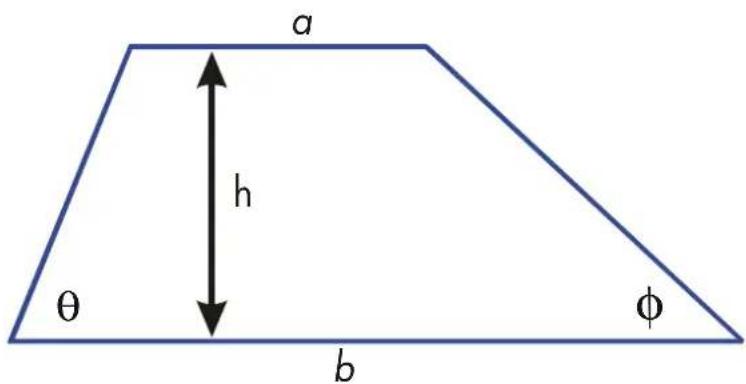
The following equation obeys the syntax rules for HP 32SII equations:
6–18 Entering and Evaluating Equations
![graph TD A["Parent heses used to group items"] --> B["P=A+B+Hx(1÷SIN(T)+1÷SIN(F))"] B --> C["Single letter name"] B --> D["No implied multiplication"] B --> E["Division is done before addition"]](/content/2026/05/973866/images/0d902c98cee2a8f1390fa20067b7ea13479690f20e6135b742039881ddb00937.jpg)
The next equation also obeys the syntax rules. This equation uses the inverse function, INV(SIN(T)), instead of the fractional form, 1÷SIN(T). Notice that the SIN function is "nested" inside the INV function. (INV is typed by 1/x .)
P = A + B + H × ( INV ( SIN (T)) + ( INV ( SIN (F)))
Example: Area of a Polygon.
The equation for area of a regular polygon with n sides of length d is:
Area = 1/4 nd ^ 2 (π / n)/ (π / n)
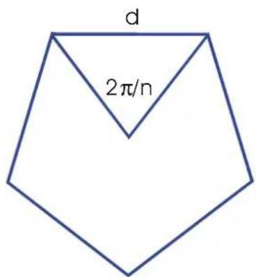
You can specify this equation as
Entering and Evaluating Equations 6–19
A = 0. 2 5 × N × D ^ 2 × COS (π ÷ N) ÷ SIN (π ÷ N)
Notice how the operators and functions combine to give the desired equation.
You can enter the equation into the equation list using the following keystrokes:

Syntax Errors
The calculator doesn't check the syntax of an equation until you evaluate the equation and respond to all the prompts-only when a value is actually being calculated. If an error is detected, INVALID EQN is displayed. You have to edit the equation to correct the error. (See "Editing and Clearing Equations" earlier in this chapter.)
By not checking equation syntax until evaluation, the HP 32SII lets you create "equations" that might actually be messages. This is especially useful in programs, as described in chapter 12.
Verifying Equations
When you're viewing an equation — not while you're typing an equation — you can press 📄 SHOW to show you two things about the equation: the equation's checksum and its length. Hold the SHOW key to keep the values in the display.
The checksum is a four-digit hexadecimal value that uniquely identifies this equation. No other equation will have this value. If you enter the equation incorrectly, it will not have this checksum. The length is the number of bytes of calculator memory used by the equation.
6–20 Entering and Evaluating Equations
The checksum and length allow you to verify that equations you type are correct. The checksum and length of the equation you type in an example should match the values shown in this manual.
Example: Checksum and Length of an Equation.
Find the checksum and length for the pipe-volume equation at the beginning of this chapter.
Keys:
Display:
Description:


V = 0. 2 5 × π × D ^ 2 x
Displays the desired equation.

as required)


(hold) CK = 5 8 3 6 0 2 6. 0
Display equation's checksum and length.
(release)
V = 0. 2 5 × π × D ^ 2 x
Redisplays the equation.

Leaves Equation mode.
7
Solving Equations
In chapter 6 you saw how you can use ENTER to find the value of the left-hand variable in an assignment-type equation. Well, you can use SOLVE to find the value of any variable in any type of equation.
For example, consider the equation
x ^ 2 - 3 y = 1 0
If you know the value of y in this equation, then SOLVE can solve for the unknown x. If you know the value of x, then SOLVE can solve for the unknown y. This works for "word problems" just as well:
Markup × Cost = Price
If you know any two of these variables, then SOLVE can calculate the value of the third.
When the equation has only one variable, or when known values are supplied for all variables except one, then to solve for x is to find a root of the equation. A root of an equation occurs where an equality or assignment equation balances exactly, or where an expression equation equals zero. (This is equivalent to the value of the equation being zero.)
Solving an Equation
To solve an equation for an unknown variable:
- Press EQN and display the desired equation. If necessary, type the equation as explained in chapter under "Entering Equations into the Equation List."
- Press ☐ SOLVE then press the key for the unknown variable. For example, press ☐ SOLVE X to solve for x. The equation then prompts
Solving
for a value for every other variable in the equation.
- For each prompt, enter the desired value;
■ If the displayed clue is the one you want, press R/S.
If you want a different clue, type or calculate the value and press[R/S]. (For details, see "Responding to Equation Prompts" in chapter 6.)
You can half a running calculation b pressing C or R/S.
When the root is found, it's stored in the unknown variable, and the variable value is VIEWed in the display. In addition, the X-register contains the root, the Y-register contains the previous estimate, and the Z-register contains the value of the equation at the root (which should be zero).
For some complicated mathematical conditions, a definitive solution cannot be found—and the calculator displays NO ROOT FOUND. See "Verifying the Result" later in this chapter, and "Interpreting results" and "When SOLVE Cannot Find Root" in appendix C.
For certain equations it helps t provide one or two initial guesses for the unknown variable before solving the equation. This can speed up the calculation, direct the answer toward realistic solution, and find more than one solution, if appropriate. See "Choosing Initial Guesses" later in this chapter.
Example: Solving the Equation of Linear Motion.
The equation of motion for a free-falling object is:
d = v _ 0 t + 1 / 2 gt ^ 2
where d is the distance, v0 is the initial velocity, t is the time, and g is the acceleration due to gravity.
Type in the equation:
Keys:
Display:
Description:

Clears memory.
{ALL} {Y}

EQN LIST TOP
Selects Equation mode.
7-2 Solving Equations
or current equation

Starts the equation.



Terminates the equation and displays the left end.

Checksum end length.
g (acceleration due to gravity) is included as a variable so you can change it for different units (98 m/s 2 or 32.2 ft/s 2 ).
Calculate hove ran meters an object falls in 5 seconds, starting from rest. Since Equation mode is turned on and the desired equation is turn on and the desired is already in the display, you can start solving for D:
Keys:
Display:
Description:
| SOLVE_ | Prompts for unknown known variable. | |
| D | V?value | Selects D; prompts for V. |
| 0 R/S | T?value | Stores 0 in V; prompts for T. |
| 5 R/S | G?value | Stores 5 in T; prompts for G. |
| 9.8 R/S | SOLVING | Stores 9.8 in G; prompts for D. |
| D=122.5000 |
Try another calculation using the same equation: how long does it take are object to fall 500 meters from rest?
Keys:
Display:
Description:

Displays the equation.

Solves for T; prompts for D.

Stores 500 in D; prompts for V.

Retains 0 in V; prompts for G.
Solving
R/S
SOLVING
Retains 9.8 in G; prompts for T.
T=10.1015
Example: Solving the Ideal Gas Law Equation.
The Ideal Gas Law describes the relationship between pressure, volume, temperature, and the amount (moles) of an ideal gas:
P × V = N × R × T
where P is pressure (in atmospheres or N/m2 ), V is volume (in liters), N is the number of moles of gas, R is the universal gas constant (0.0821 liter–atm mole–K or 8.314 J/mole–K), and T is temperature (Kelvins: K=°C + 273.1 ).
Enter the equation:
Keys:
Display:
Description:


Selects Equation mode and starts the equation.



Terminates and displays the equation.



Checksum and length.
A 2-liter bottle contains 0.005 moles of carbon dioxide gas at 24° C. Assuming that the gas behaves as an ideal gas, calculate its pressure. Since Equation mode is turned on and the desired equation is already in the display, you can start solving for P:
Keys:
Display:
Description:


U?value
Solves for P; prompts for V.
2 R/S
N?value
Stores 2 in V; prompts for N.
.005 R/S
R?value
Stores .005 in N; prompts for R.
.0821 R/S
T?value
Stores .0821 in R; prompts for T.
7-4 Solving Equations
24 ENTER
T?297.1000
Calculates T (Kelvins).
273.1
R/S
SOLVING
Stores 297.1 in T; solves for P in
P=0.0610
atmospheres.
A 5-liter flask contains nitrogen gas. The pressure is 0.05 atmospheres when the temperature is 18°C. Calculate the density of the gas ( N × 28/V , where 28 is the molecular weight of nitrogen).
Keys:
| EQN | P×V=N×R×T | Displays the equation. |
| SOLVE N | P?0.0610 | Solves for N; prompts for P. |
| .05 R/S | V?2.0000 | Stores .05 in P; prompts for V. |
| 5 R/S | R?0.0821 | Stores 5 in V; prompts for H. |
| R/S | T?297.1000 | Retains previous R; prompts for T. |
| 18 ENTER | Calculates T (Kelvins). | |
| 273.1 + | T?291.1000 | |
| R/S | SOLVING | Stores 291.1 in T; solves for N. |
| N=0.0105 | ||
| 28 × | 0.2929 | Calculates mass in grams, N × 28 . |
| RCL V ÷ | 0.0586 | Calculates density in grams per |
Understanding and Controlling SOLVE
SOLVE uses an iterative (repetitive) procedure to solve for the unknown variable. The procedure starts by evaluating the equation using two initial guesses for the unknown variable. Based on the results with those two guesses, SOLVE generates another, better guess. Through successive iterations, SOLVE finds a value for the unknown that makes the value of the equation equal to zero.
Solving
When SOLVE evaluates an equation, it does it the same way does — any "=" in the equation is treated as a " - " For example, the Ideal Gas Law equation is evaluated as P × V - (N × R × T) . This ensures that an equality or assignment equation balances at the root, and that an expression equation equals zero at the root.
Some equations are more difficult to solve than others. In some cases, you need to enter initial guesses in order to find a solution. (See "Choosing Initial Guesses for SOLVE," below.) If SOLVE is unable to find a solution, the calculator displays NO ROOT FIND.
See appendix C for more information about how SOLVE works.
Verifying the Result
After the SOLVE calculation ends, you can verify that the result is indeed a solution of the equation by reviewing the values left in the stack:
The X-register (press C to clear the VIEWed variable) contains the solution (root) for the unknown; that is, the value that makes the evaluation of the equation equal to zero,
The Y-register (press R↓) contains the previous estimate for the root. This number should be the same as the value in the X-register. If it is not, then the root returned was only an approximation, and the values in the X- and Y-registers bracket the root. These bracketing numbers should be close together.
The Z- register (press again) contains this value of the equation at the root. For an exact root, this should be zero. If it is not zero, the root given was only an approximation; this number should be close to zero.
If a calculation ends with the NO ROOT FIND, the calculator could not converge on a root. (You can see the value in the X-register — the final estimate of the root — by pressing C or ← to clear the message.) The values in the X- and Y-registers bracket the interval that was last searched to find the root. The Z-register contains the value of the equation at the final estimate of the root.
If the X- and Y-register values aren't close together, or the Z-register value isn't close to zero, the estimate from the X-register probably isn't a
7-6 Solving Equations
root.
If the X- and Y-register values are close together, and the Z-register value is close to zero, the estimate from the X-register may be an approximation to a root.
Interrupting a SOLVE Calculation
To halt a calculation, press C or R/S. The current best estimate of the root is in the unknown variable; use F2 VIEW to view it without disturbing the stack.
Choosing Initial Guesses for SOLVE
The two initial guesses come from:
■ The number currently stored in the unknown variable.
■ The number in the X-register (the display).
These sources are used for guesses whether you enter guesses or not. If you enter only one guess and store it in the variable, the second guess will be the same value since the display also holds the number you just stored in the variable. (If such is the case, the calculator changes one guess slightly so that it has two different guesses.)
Entering your own guesses has the following advantages:
■ By narrowing the range of search, guesses can reduce the time to find a solution.
If there is more than one mathematical solution, guesses can direct tote SOLVE procedure to the desired answer or range of answers. For example, the equation of linear motion
d = v _ 0 t + 1 / 2 gt ^ 2
can have two solutions for t. You can direct the answer to the only meaningful one (t > 0) by entering appropriate guesses.
The example using this equation earlier in this chapter didn't require you
Solving
to enter guesses before solving for T because in the first part of that example you stored a value for T and solved for D. The value that was left in T was a good (realistic) one, so it was used as a guess when solving for T.
If an equation does not allow certain values for the unknown, guesses can prevent these values from occurring. For example,
y = t + x
results in an error if x ≤ 0 (messages LOG(0) or LOG(NEG)).
In the following example, the equation has more than one root, but guesses help find the desired root.
Example. Using Guesses to Find a Root.
Using a rectangular piece of sheet metal 40 cm by 80 cm, form an open-top box having a volume of 7500 cm 3 . You need to find the height of the box (that is, the amount to be folded up along each of the four sides) that gives the specified volume. A taller box is preferred to a shorter one.
7-8 Solving Equations
If H is the height, then the length of the box is (80 - 2H) and the width is (40 - 2H) . The volume V is:
V = (8 0 - 2 H) × (4 0 - 2 H) × H
which you can simplify and enter as
V = (4 0 - H) × (2 0 - H) × 4 × H
Type in the equation:
| Keys: | Display: | Description: |
| Selects Equation mode and starts the equation. | ||
| RCL V = V=■ | ||
| RCL H ) V=(40-H)■ | ||
| × (20 -0-H)×(20-H)■ | ||
| RCL H ) | ||
| × 4 × RCL H ×(20-H)×4×H■ | ||
| ENTER V=(40-H)×(20 | Terminates and displays the equation. | |
| SHOW CK=02AC 027.0 | Checksum and length. | |
It seems reasonable that either a tall, narrow box or a short, flat box could be formed having the desired volume. Because the taller box is preferred, larger initial estimates of the height are reasonable. However, heights greater than 20 cm are not physically possible because the metal sheet is only 40 cm wide. Initial estimates of 10 and 20 cm are therefore appropriate.
| Keys: | Display: | Description: |
| C | Leaves Equation mode. | |
| 10 STO H 20 | 20_ | Stores lower and upper limit guesses. |
Solving


V = (40 - H)× 20
Displays current equation.


v?value
Solves for H; prompts for V.
7500

H=15.0000
Stores 7500 in V; solves for H.
Now check the quality of this solution — that is, whether it returned an exact root — by looking at the value of the previous estimate of the root (in the Y-register) and the value of the equation at the root (in the Z-register).
Keys:
Display:
Description:

15.0000
This value from the Y-register is the estimate made just prior to the final result. Since it is the same as the solution, the solution is an exact root.

0.0000
This value from the Z-register shows the equation equals zero at the root.
The dimensions of the desired box are 50 × 10 × 15 cm. If you ignored the upper limit on the height (20 cm) and used initial estimates of 30 and 40 cm, you would obtain a height of 42.0256 cm — a root that is physically meaningless. If you used small initial estimates such as 0 and 10 cm, you would obtain a height of 2.9774 cm — producing an undesirably short, flat box.
If you don't know what guesses to use, you can use a graph to help the behavior of the equation. Evaluate your equation for several values of the unknown. For each point on the graph, display the equation and press — at the prompt for x enter the x -coordinate, and then obtain the corresponding value of the equation, the y -coordinate. For the problem above, you would always set V = 7500 and vary the value of H to produce different values for the equation. Remember that the value for this equation is the difference between the left and right sides of the equation. The plot of the value of this equation looks like this.
7–10 Solving Equations

For More Information
This chapter gives you instructions for solving for unknowns or roots over a wide range of applications. Appendix C contains more detailed information about how the algorithm for SOLVE works, how to interpret results, what happens when no solution is found, and conditions that can cause incorrect results.
Solving
8
Integrating Equations
Many problems in mathematics, science, and engineering require calculating the definite integral of a function—If the function is denoted by f(x) and the interval of integration is a to b, then the integral can be expressed mathematically as
= _ a ^ b dxx (I)

The quantity I can be interpreted geometrically as the area of a region bounded by the graph of the function f(x) , the x -axis, and the limits x = a and x = b (provided that f(x) is nonnegative throughout the interval of integration).
The operation operation (∫ FN) integrates the current equation with respect to a specified variable (∫ FN d_). The function may have more than one variable.
Integrating
Integrating Equations ( ∫ FN)
To Integrating Equations:
To integrate an equation:
- If the equation that defines the integrand's function isn't stored in the equation list, key it in (see "Entering Equations Into the Equation List" in chapter 6) and leave Equation mode. The equation usually contains just an expression.
- Enter the limits of integration: key in the lower limit and press ENTER, then key in the upper limit.
- Display the equation: Press EQN and, if necessary, scroll through the equation list (press ← or ← ) to display the desired equation.
- Select the variable of integration: Press ☐ f variable. This starts the calculation.
f uses far more memory than any other operation in the calculator. If executing f causes a MEMORY FULL message, refer to appendix B.
You can halt a running integration calculation by pressing C or R/S. However, no information about the integration is available until the calculation finishes normally
The display format setting affects the level of accuracy assumed for your function and used for the result. The integration is more precise but takes much longer in the {ALL} and higher {FX}, {SC}, and {EN} settings. The uncertainty of the result ends up in the Y-register, pushing the limits of integration up into the T- and Z-registers. For more information, see "Accuracy of Integration" later in this chapter.
8-2 Integrating Equations
To integrate the same equation with different information:
If you use the same limits of integration, press R↓ R↓ move them into the X- and Y-registers. Then start at step 3 in the above list. If you want to use different limits, begin at step 2.
To work another problem using a different equation, start over from step 1 with an equation that defines the integrated.
Example: Bessel Function.
The Bessel function of the first kind of order 0 can be expressed as
_ 0 = 1/π _ 0 ^ πJ ) x (
Find the Bessel function for x-values of 2 and 3.
Enter the expression that defines the integrand's function:
cos (x sin t)
| Keys: | Display: | Description: |
| CLEAR{ALL} | Clears memory. | |
| EQN | Current equation or EQN LIST TOP | Selects Equation mode. |
| COS RCL X | COS(X■ | Types the equation. |
| SIN | COS(X×SIN(■ | |
| RCL T | COS(X×SIN(T■ | |
| ) ) ) | S(X×SIN(T))■ | Right closing parentheses are optional. |
| ENTER | COS(X×SIN(T) | Terminates the expression and displays its left end. |
| SHOW | CK=F93B 012.0 | Checksum and length. |
Integrating

Leaves Equation mode.
Now integrate this function with respect to t from zero to π ; x = 2.
Keys:
Display:
Description:
| MODES{RD} | Selects Radians mode. | ||
| 0 ENTER π 3.1416 | Enters the limits of integration(lower limit first). | ||
| EQN | COS(X×SIN(T)) | Displays the function. | |
| f | ∫FN d_ | Prompts for the variable of integration. | |
| T | X?value | Prompts for value of X. | |
| 2 R/S | INTEGRATING | x = 2. Starts integrating;calculates result for 0π (tf | |
| ∫=0.7034 | |||
| π ÷ | 0.2239 | The final result forJ0(2). | |
Now calculate J0(3) with the same limits of integration. You must respecify the limits of integration (0, π) since they were pushed off the stack by the subsequent division by π .
Keys:
Display:
Description:
| 0 ENTER π 3.1416 | Enters the limits of integration(lower limit first). | ||
| EQN | COS(X×SIN(T) | Displays the current equation. | |
| ∫FN d_ | Prompts for the variable ofintegration. | ||
| T | X?2.0000 | Prompts for value of X. | |
| 3 R/S | INTEGRATING∫=-0.870 | x = 3. Starts integrating andcalculates the result for 0π ) (tf | |
| π ÷ | -0.260 | The final result forJ o(3). | |
8-4 Integrating Equations
Example: Sine Integral.
Certain problems in communications theory (for example, pulse transmission through idealized networks) require calculating an integral (sometimes called the sine integral) of the form
S _ i (t) = _ 0 ^ t ( x/x) dx
Find Si (2).
Enter the expression that defines the integrand's function:
x x
If the calculator attempted to evaluate this function at x = 0, the lower limit of integration, an error (DIVIDE BY 0) would result. However, the integration algorithm normally does not evaluate functions at either limit of integration, unless the endpoints of the interval of integration are extremely close together or the number of sample points is extremely large.
| Keys: | Display: | Description: |
| The current equationor EQN LIST TOP | Selects Equation mode. | |
| SIN RCL X | Starts the equation. | |
| SIN(X)■ | The closing right parenthesis isrequired in this case. | |
| SIN(X)÷X■ | ||
| ENTER | SIN(X)÷X | Terminates the equation. |
| CK=4919 009.0 | Checksum and length. | |
| Leaves Equation mode. |
Now integrate this function with respect to x (that is, X) from zero to 2 (t = 2).
Keys:
MODES {RD}
Display:
Description:
Selects Radians mode.
Integrating
0 ENTER 2 2_
Enters limits of integration (lower first).
EQN SIN(X)÷X
Displays the current equation.
INTEGRATING
Calculates the result for Si(2) .
= 1. 6 0 5 4
Accuracy of Integration
Since the calculator cannot compute the value of an integral exactly, it approximates it. The accuracy of this approximation depends on the accuracy of the integrand's function itself, as calculated by your equation. This is affected by round-off error in the calculator and the accuracy of the empirical constants.
Integrals of functions with certain characteristics such as spikes or very rapid oscillations might be calculated inaccurately, but the likelihood is very small. The general characteristics of functions that can cause problems, as well as techniques for dealing with them, are discussed in appendix D.
Specifying Accuracy
The display format's setting (FIX, SCI, ENG, or ALL) determines the precision of the integration calculation, the greater the number of digits displayed, the greater the precision of the calculated integral (and the greater the time required to calculate it.). The fewer the number of digits displayed, the faster the calculation, but the calculator will presume that the function is accurate to only the number of digits specified in the display format.
To specify the accuracy of the integration, set the display format so that the display shows no more than the number of digits that you consider accurate in the integrand's values. This same level of accuracy and precision will be reflected in the result of integration.
If Fraction-display mode is on (flag 7 set), the accuracy is specified by the previous display format.
8-6 Integrating Equations
Interpreting Accuracy
After calculating the integral, the calculator places the estimated uncertainty of that integral's result in the Y-register. Press ↔ y to view the value of the uncertainty.
For example, if the integral Si(2) is 1.6054 ± 0.0001 , then 0.0001 is its uncertainty.
Example: Specifying Accuracy.
With the display format set to SCI 2, calculate the integral in the expression for Si(2) (from the previous example).
| Keys: | Display: | Description: |
| 1.61E0 | Sets scientific notation with two decimal places, specifying that the function is accurate to two decimal places. | |
| 2.00E0 | Rolls down the limits of integration frown the Z-and T-registers into the X-and Y-registers. | |
| SIN(X)÷X | Displays the current Equation. | |
| INTEGRATING | The integral approximated to two decimal places. | |
| 1.00E-3 | The uncertainty of the approximation of the integral. |
The integral is 1.61 ± 0.00100 . Since the uncertainty would not affect the approximation until its third decimal place, you can consider all the displayed digits in this approximation to be accurate.
If the uncertainty of an approximation is larger than what you choose to tolerate, you can increase the number of digits in the display format and repeat the integration (provided that f(x) is still calculated accurately to the number of digits shown in the display), In general, the uncertainty of an
Integrating
integration calculation decreases by a factor of ten for each additional digit, specified in the display format.
Example: Changing the Accuracy.
For the integral of Si(2) just calculated, specify that the result be accurate to four decimal places instead of only two.
| Keys: | Display: | Description: |
| 1.0000E-3 | Specifies accuracy to four decimal places. The uncertainty from the last example is still in the display. | |
| 2.0000E0 | Rolls down the limits of integration from the Z- and T-registers into the X- and Y-registers. | |
| SIN(X)÷X | Displays the current equation. | |
| INTEGRATING∫=1.6054E0 | Calculates the result. | |
| 1.0000E-5 | Note that the uncertainty is about 1/100 as large as the uncertainty of the SCI 2 result calculated previously. | |
| 1.0000E-5 | Restores FIX 4 format. | |
| 1.0000E-5 | Restores Degrees mode. |
This uncertainty indicates that the result might be correct to only four decimal places. In reality, this result is accurate to seven decimal places when compared with the actual value of this integral. Since the uncertainty of a result is calculated conservatively, the calculator's approximation in most cases is more accurate than its uncertainty indicates.
8–8 Integrating Equations
For More Information
This chapter gives you instructions for using integration in the HP 32SII over a wide range of applications. Appendix D contains more detailed information about how the algorithm for integration works, conditions that could cause incorrect results, conditions that prolong calculation time, and obtaining the current approximation to an integral.
Integrating
9
Operations with Comb Numbers
The HP 32SII can use complex numbers in the form
x + iy.
It has operations for complex arithmetic (+, -, ×, ÷) , complex trigonometry (sin, cos, tan), and the mathematics functions -z, 1/z, z1z2 , ln z, and ez . (where z1 and z2 are complex numbers).
To enter a complex number:
- Type the imaginary part.
- Press ENTER.
- Type the real part.
Complex numbers in the HP 32SII are handled by entering each part (imaginary and real) of a complex number as a separate entry. To enter two complex numbers, you enter four separate numbers. To do a complex operation, press CMPLX before the operator. For example, to do
(2 + i 4) + (3 + i 5),
press 4 ENTER 2 ENTER 5 ENTER 3 CMPLX +.
The result is 5 + i 9. (Press ↔ y to see the imaginary part.)
The Complex Stack
The complex stack is really the regular memory stack split into two double registers for holding two complex numbers, z1Xi + izZ1y and z2Xi + izZ2y :
Operations with Comb Numbers 9–1

Real Stack Complex Stack
Since the imaginary and real parts of a complex number are entered and stored separately, you can easily work with or alter either part by itself.
![graph LR Z1["Z₁"] --> y1["y₁"] Z1 --> x1["x₁"] Z2["Z₂"] --> y2["y₂"] Z2 --> x2["x₂"] y1 --> ComplexFunction["Complex function"] x1 --> ComplexFunction y2 --> ComplexFunction x2 --> ComplexFunction ComplexFunction --> y["Complex part: y imaginary part"] ComplexFunction --> x["Complex part: x real par…](/content/2026/05/973866/images/da46c09bf193fec2290a1a1c4249a09e1c50ea421a0a8a21a707537ebca6042f.jpg)
Always enter the imaginary part (the y-part) of a number first. The real portion of the result (zx) is displayed; press ↔ y to view the imaginary portion (zy) . (For two-number operations, the first complex number, z1, is replicated in the stack's Z and T registers.)
9-2 Operations with Comb Numbers
Complex Operations
Use the complex operations as you do real operations, but precede the operator with CMPLX.
To do an operation with one complex number:
- Enter the complex number z, composed of x + i y , by keying in y ENTER x.
- Select the complex function.
Functions for One Complex Number, z
| To Calculate: | Press: |
| Change sign,-z | CMPLX +/- |
| Inverse, 1/z | CMPLX 1/x |
| Natural log, ln z | CMPLX LN |
| Natural antilog, ez | CMPLX ex |
| Sin z | CMPLX SIN |
| Cos z | CMPLX COS |
| Tan z | CMPLX TAN |
Operations with Comb Numbers 9–3
To do an arithmetic operation with two complex numbers:
- Enter the first complex number, z1 (composed of x1 + iy1 ), by keying in y ENTER x1 ENTER. (For Z1z2 , key in the base part, z1 , first.)
- Enter the second complex number, z2 , by keying in y2 ENTER x2 . (For z1z2 , key in the exponent, z2 , second.)
- Select the arithmetic operation:
Arithmetic With Two Complex Numbers, z1 and z2
| To Calculate: Press: | |
| Addition, z1 + z2 |  |
| Subtraction, z1 - z2 |  |
| Multiplication, z1 × z2 |  |
| Division, z1 ÷ z2 |  |
| Power function, Z1z2 |  |
Examples:
Here are some examples of trigonometry and arithmetic with complex numbers:
Evaluate sin (2 + i 3)
| Keys: | Display: | Description: |
| 3 ENTER 2 | Real part of result. | |
| 9.1545 | ||
| x←y | -4.1689 | Result is 9.1545 - i 4.1689. |
Evaluate the expression
Since the stack can retain only two complex numbers at a time, perform the calculation as
9-4 Operations with Comb Numbers
z _ 1 × [1 ÷ (z _ 2 + z _ 3)]
Keys:
| 1 | ENTER | 2 | +/_ | ENTER |
| 3 | +/- | ENTER | 4 |
| CMPLX | + | 2.0000 |
| CMPLX | 1/x |
| 13 | ENTER | 23 |
| CMPLX | × | 2.5000 |
| x↔y | 9.0000 |
Display:
Description:
Result is 2.5 + i 9.
Evaluate (4 - i\ 2/5) (3 - i\ 2/3) . Do not use complex operations when calculating just one part of a complex number.
Keys:
| 2 | 5 | +/− | ENTER | -0.4000 |
| 4 | ENTER | 4.0000 |
| 2 | 3 | +/— | ENTER | -0.6667 |
| 3 | ← | CMPLX | × | 11.7333 |
| x↔y | -3.8667 |
Evaluate ez-2 , where z = (1 + i) . Use 1 x to evaluate z-2 ; enter -2 as -2 + i0 .
Keys:
Display:
Description:
| Enters imaginary part of first complex number as a fraction. |
Enters real part of first complex number.
Enters imaginary part of second complex number as a fraction.
Completes entry of second number and then multiplies the two complex numbers.
Result is 11.7333 - i 3.8667.
Description:
Operations with Comb Numbers 9–5
1 ENTER 1 ENTER
0 ENTER 2 +/-
CMPLX yx 0.0000
CMPLX ex 0.8776
x↔y -0.4794
Intermediate result of
(1 + i) ^ - 2
Real part of final results.
Final result is
0.8776 - i 0.4794.
Using Complex Number in Polar Notation
Many applications use real numbers in polar form or polar notation. These forms use pairs of numbers, as do complex numbers, so you can do arithmetic with these numbers by using the complex operations. Since the HP 32SII's complex operations work on numbers in rectangular form, convert polar form to rectangular form (using → y.x before executing the complex operation, then convert the result back to polar form.
a + ib = r ( θ + i θ) = re ^ i θ
= r θ ( Polar or phasor form )
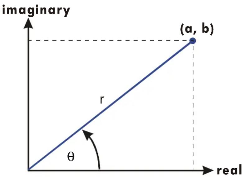
Example: Vector Addition.
9–6 Operations with Comb Numbers
Add the following three loads. You will first need to convert the polar coordinates to rectangular coordinates.

| Keys: | Display: | Description: |
| Sets Degrees mode. | ||
| 62 ENTER 185 | Enters L1 and converts it to rectangular form. | |
| 86.8522 | ||
| 143 ENTER 170 | -135.7680 | Eaters and converts L2. |
| -48.9158 | Adds vectors. | |
| 261 ENTER 100 | -15.6434 | Enters and converts L3. |
| -64.5592 | Adds L1 + L2 + L3. | |
| 178.9372 | Converts vector hack to polar form; displays r. | |
| 111.1489 | Displays θ. |
Operations with Comb Numbers 9–7
10
Base Conversions and Arithmetic
The BASE menu (←BASE) lets you change the number base used for entering numbers and other operations (including programming). Changing bases also converts the displayed number to the new base.
BASE Menu
| Menu label | Description |
| {DEC} | decimal mode. No annunciator. Converts numbers to base 10. Numbers have integer and fractional parts. |
| {HX} | Hexadecimal mode. HEX annunciator on. Converts numbers to base 16; uses integers only. The top-row keys become digits A through F. |
| {OC} | Octal mode. OCT annunciator on. Converts numbers to base 8; uses integers only. The 8, 9, and unshifted top-row keys are inactive. |
| {BN} | Binary mode. BIN annunciator on. Converts numbers to base 2; uses integers only. Digit keys other than 0 and 1, and the unshifted top-row functions are inactive. If a number is longer than 12 digits, then the outer top-row keys ( and + are active for viewing windows. (See "Windows for Long Binary Numbers" later in this chapter.) |
Examples: Converting the Base of a Number.
The following keystrokes do various base conversions.
Convert 125.99 10 to hexadecimal, octal, and binary numbers.
Keys:
125.99

Display:
7D
Description:
Converts just the integer part (125)
Base Conversions and Arithmetic 10–1
BASE {HX} of the decimal number to base 16
and displays this value.


175
Base 8.


1111101
Base 2.


125.9900
Restores base 10; the original decimal value has been preserved, including its fractional part.
Convert 24FF 16 to binary base. The binary number will be more than 12 digits (the maximum display) long.
| Keys: | Display: | Description: |
| BASE {HX}24FF | 24FF_ | Use the Σ+ key to type "F". |
| BASE {BN} | 010011111111 | The entire binary number does riot fit. The ← annunciator indicates that the number continues to the left; the ↓ annunciator Points to . |
| 10 | Displays the rest of the number.The full number is 100100111111112. | |
| Σ+ | 010011111111 | Displays the first 12 digits again. |
| BASE {DEC} | 9,471,00 | Restores base 10. |
Arithmetic in Bases 2, 8, and 16
You can perform arithmetic operations using (+, -, ×, and ÷) in any base. The only function keys that are actually deactivated outside of Decimal mode are , ex, LN, yx, 1/x and + . However, you should realize that most operations other than arithmetic will not produce meaningful results since the fractional parts of numbers are truncated.
10-2 Base Conversions and Arithmetic
Arithmetic in bases 2, 8, and 16 is in 2's complement form and uses integers only:
If a number has a fractional part, only the integer part is used for an arithmetic calculation.
■ The result of an operation is always an integer (any fractional portion is truncated).
Whereas conversions change only the displayed number and not the number in the X-register, arithmetic does alter the number in the X-register.
If the result of an operation cannot be represented in 36 bits, the display shows OVERFLOW and then shows the largest positive or negative number possible.
Example:
Here are some examples of arithmetic in Hexadecimal, Octal, and Binary modes:
1 2 F _ 1 6 + E 9 A _ 1 6 = ?
Keys:
| BASE {HX} | Sets base 16;HEX annunciator on. | ||
| 12F ENTER E9A + | FC9 | Result. | |
| 77608-43268=? | |||
| BASE {OC} | 7711 | Sets base 8: OCT annunciator on. Converts displayed number to octal. | |
| 7760 ENTER 4326 - | 3432 | Result. | |
| 1008-58=? | |||
| 100 ENTER 5 ÷ | 14 | Integer part of result. | |
| 5A016+10011002=? | |||
| BASE {HX} 5A0 | 5A0_ | Set base 16;HEX | |
Base Conversions and Arithmetic 10–3
| annunciator on. | ||
| BASE {BN} 1001100 | 1001100_ | Changes to base 2; BIN annunciator on. This terminates digit entry, so no ENTER is needed between the numbers. |
| + | 10111101100 | Result in binary base. |
| BASE {HX} | 5EC | Result in hexadecimal base. |
| BASE {DEC} | 1,516,0000 | Restores decimal base. |
The Representation of Numbers
Although the display of a number is converted when the base is changed, its stored form is not modified, so decimal numbers are not truncated — until they are used in arithmetic calculations.
When a number appears in hexadecimal, octal, or binary base, it is shown as a right-justified integer with up to 36 bits (12 octal digits or 9 hexadecimal digits). Leading zeros are riot displayed, but they are important because they indicate a positive number. For example, the binary representation of 12510 is displayed as:
11111101
which is the same as these 36 digits:
00000000000000000000000000001111101
Negative Numbers
The leftmost (most significant or "highest") bit of a number's binary representation is the sign bit; it is set (1) for negative numbers. If there are (undisplayed) leading zeros, then the sign bit is 0 (positive). A negative number is the 2's complement of its positive binary number.
Keys:
Display:
Description:
10-4 Base Conversions and Arithmetic
| 546 BASE {HX} | 222 | Enters a positive, decimal number; then converts it to hexadecimal. |
| FFFFFFDDE | 2's complement (sign changed). | |
| BASE {BN} | 110111011110 | Binary version; ← indicates more digits. |
| 111111111111 | Displays the leftmost window; the number is negative since the highest bit is 1. | |
| BASE {DEC} | -546.0000 | Negative decimal number. |
Range of Numbers
The 36-bit word size determines the range of numbers that can be represented in hexadecimal (9 digits), octal (12 digits), and binary bases (36 digits), and the range of decimal numbers (11 digits) that can be converted to these other bases.
Range of Numbers for Base Conversions
| Base Positive Integer of Largest Magnitude | Negative Integer of Largest Magnitude | |
| Hexadecimal | 7FFFFFFF 800000000 | |
| Octal | 377777777777 | 400000000000 |
| Binary | 01111111111111111111111111111111111111111111111111111111111111111111111111111111111111111111111111111 | 10000000000000000000000000000000000000000000000000000000000000000000000000000000000000000000000000000 |
| Decimal | 34,359,738,367 | -34,359,738;368 |
When you key in numbers, the calculator will not accept more than the maximum number of digits for each base. For example, if you attempt to key in a 10-digit hexadecimal number, digit entry halts and the ▲ annunciator appears.
Base Conversions and Arithmetic 10–5
If a number entered in decimal base is outside the range given above, then it produces the message TOO BIG in the other base modes. Any operation using TOO BIG causes an overflow condition, which substitutes the largest positive or negative number possible for the too-big number.
Windows for Long Binary Numbers
The longest binary number can have 36 digits—three times as many digits as fit in the display. Each 12-digit display of a long number is called a window.
36 - bit number
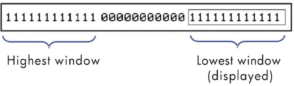
When a binary number is larger than the 12 digits, the ← or → annunciator (or both) appears, indicating in which direction the additional digits lie. Press the indicated key ( or + ) to view the obscured window.
10-7B Picture
SHOWing Partially Hidden Numbers
The VIEW and INPUT functions work with non-decimal numbers as they do with decimal numbers. However, if the Bali octal or binary number does not fit in the display, the leftmost digits are replaced with an ellipsis
10–6 Base Conversions and Arithmetic
( . . . ). Press Ⓞ SHOW to view the digits obscured by the A=... or A?...label.
Keys:
| BASE {OC} | 23456712345_ | Enters a large octal number. |
| 123456712345 | ||
| STO A | 123456712345 | |
| VIEW A | A=...456712345 | Drops leftmost three digit's. |
| SHOW (hold) | 123456712345 | Shows all digits. |
| BASE {DEC} | 11,219,473,637.0 | Restores Decimal mode. |
11
Statistical Operations
The statistics menus in the HP 32SII provide functions to statistically analyze a set of one- or two-variable data:
■ Mean, sample and population standard deviations.
■ Linear regression and linear estimation ( x and y ).
■ Weighted mean (x weighted by y).
A Summation statistics: n , x , y , x2 , y2 , and xy .
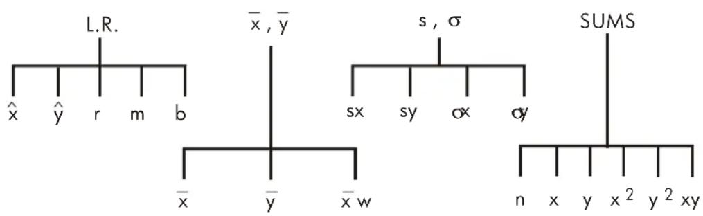
Entering Statistical Data
One- and two-variable statistical data are entered (or deleted) in similar fashion using the + (or - ) key. Data values are accumulated as summation statistics in six statistic's registers (28 through 33), whose names are displayed in the SUMS menu. (Press and see nxyx2y2xy .
Note

Always clear the statistics registers before entering a new set of statistical data (press ☑ CLEAR {Σ}).
Statistical
Entering One-Variable Data
- Press ← CLEAR to clear existing statistical data.
- Key in each x-value and press + .
- The display shows n, the number of statistical data values now accumulated.
Pressing + actually enters two variables into the statistics registers because the value already in the Y-register is accumulated as the y-value. For this reason, the calculator will perform linear regression and show you values based on y even when you have entered only x-data — or even if you have entered an unequal number of x-and y-values. No error occurs, but the results are obviously not meaningful.
To recall a value to the display immediately after it has been entered, press ← LASTx.
Entering Two-Variable Data
When your data consist of two variables, x is the independent variable and y is the dependent variable. Remember to enter an (x, y) pair in reverse order (y ENTER x) so that y ends up in the Y-register and X in the X-register.
- Press ← CLEAR to clear existing statistical data.
- Key in the y-value first and press ENTER.
- Key in the corresponding x-value and press + .
- The display shows n, the number of statistical data pairs you have accumulated.
- Continue entering x, y-pairs. n is updated with each entry.
To recall an x-value to the display immediately after it has been entered, press Ⓜ LASTx.
11-2 Statistical Operations
Correcting Errors in Data Entry
If you make a mistake when entering statistical data, delete the incorrect data and add the correct data. Even if only one value of an x, y-pair is incorrect, you must delete and reenter both values.
To correct statistical data:
- Reenter the incorrect data, but instead of pressing + , press ←- . This deletes the value(s) and decrements n.
- Enter the correct value(s) using + .
If the incorrect values were the ones just entered, press x to retrieve them, then press Σ- to delete them. (The incorrect y-value was still in the Y-register, and its T-value was saved in the LAST X register.)
Example:
Key in the x, y-values on the left, these make the corrections shown on the right:
| Initial x, y | Corrected x, y |
| 20,4 | 20,5 |
| 400,6 | 40,6 |
Keys:

4 ENTER 20 Σ+ 1.0000
6 ENTER 400 Σ+ 2.0000


6 ENTER 40 +
Display:
Clears existing statistical data.
Enters the first new data pair.
Display shows n, the number of data pairs yon entered.
Brings back last x-value. Last y is still in Y-register. (Press
x↔y twice to check y.)
Deletes the last data pair.
Reenters the last data pair.
Statistical
Ope
4 ENTER 20 ← Σ- 1.0000
5 ENTER 20 Σ+ 2.0000
Deletes the first data pair.
Reenters the first data pair. There is still a. total of two data pairs in the statistics registers.
Statistical Calculations
Once you have entered your data, you can use the functions in the statistics menus.
Statistics Menus
| Menu Key Description | ||
| L.R. | L.R. The linear-regression menu: linear estimation {x} {y} and curve-fitting {r} {m} {b}. See "Linear Regression" later in this chapter. | |
| , | , The mean menu: { } {y} {xw}. See "Mean" below. | |
| s,σ | S,σ The standard-deviation menu: { s× } {s·y } {σ× } {σ·y}. See "Sample Standard Deviation" and "Population Standard Deviation" later in this chapter. | |
| SUMS | SUMS The summation menu: {n} {x} {y} {x2} {y2} {x·y}. See "Summation Statistics" later in this chapter. | |
Mean
Mean is the arithmetic average of a group of numbers.
■ Press → , for the mean of the x-values.
■ Press → , { } for the mean of the y-values.
■ Press 2 , for the weighted mean of the x-values using the
11-4 Statistical Operations
y-values as weights or frequencies. The weights can be integers or non-integers.
Example: Mean (One Variable).
Production supervisor May Kitt wants to determine the average time that a certain process takes. She randomly picks six people, observes each one as he or she carries out the process, and records the time required (in minutes):
15.5 9.25 10.0
12.5 12.0 8.5
Calculate the mean of the times. (Treat all data as x-values.)
| Keys: | Display: | Description: |
| CLEAR {Σ} | Clears the statistics registers. | |
| 15.5 Σ+ | 1.0000 | Enters the first time. |
| 9.25 Σ+ 10 Σ+ 12.5 | Enters the remaining data; | |
| Σ+ 12 Σ+ 8.5 Σ+ | 6.0000 | six data points accumulated. |
| x,y {×} | 11.2917 | Calculates the mean time tocomplete the process. |
Example: Weighted Mean (Two Variables).
A manufacturing company purchases a certain part four times a year. Last year's purchases were:
Price per Part (x) \4.25 \4.60 \4.70 \4.10
Number of Parts (y) 250 800 900 1000
Find the average: price (weighted for the purchase quantity) for this part. Remember to enter y, the weight (frequency), before x, the price.
| Keys: | Display: | Description: | |
| CLEAR {Σ} | Clears the statistics registers. | ||
| 250 | ENTER 4.25 Σ+ | 1.0000 | Enters data; displays n. |
| 800 | ENTER 4.6 Σ+ | 2.0000 | |
| 900 | ENTER 4.7 Σ+ | 3.0000 | |
Statistical
Ope
1000 ENTER 4.1 Σ+ 4.0000
, { }
Four data pairs accumulated.
Calculates the mean price weighted for the quantity purchased.
Sample Standard Deviation
Sample standard deviation is a measure of how dispersed the data values are about the mean. standard deviation assumes the data is a sampling of a larger, complete set of data, and is calculated using n - 1 as a divisor.
■ Press → ,σ ≤ x for the standard deviation of x-values.
■ Press 2 Siσ y for the standard deviation of y-values.
The σ× and σν keys in this menu are described in the next section, "Population Standard Deviation."
Example: Sample Standard Deviation.
Using the same process-times as in the above "mean" example, May Kitt now wants to determine the standard deviation time (sx) of the process:
15.5 9.25 10.0
12.5 12.0 8.5
Calculate the standard deviation of the times. (Treat all the data as x-values.)
| Keys: | Display: | Description: |
| CLEAR {Σ} | Clears the statistics registers. | |
| 15.5 Σ+ | 1.0000 | Enters the first time. |
| 9.25 Σ+ 10 Σ+ 12.5 | Enters the remaining data; six data points entered. | |
| Σ+ 12 Σ+ 8.5 Σ+ | 6.0000 | |
| S,σ {SX} | 2.5808 | Calculates the standard deviation time. |
11-6 Statistical Operations
Population Standard Deviation
Population standard deviation is a measure of how dispersed the data values are about the mean. Population standard deviation assumes the data constitutes the complete set of data, and is calculated using n as a divisor.
■ Press ,σ σx for the population standard deviation of the x-values.
■ Press 2 .σ σν for the population standard deviation of the y-values.
Example: Population Standard Deviation.
Grandma Tinkle has four grown sons with heights of 170, 173, 174, and 180 cm. Find the population standard deviation of their heights.
| Keys: | Display: | Description: |
| CLEAR {Σ} | Clears the statistics registers. | |
| 170 Σ+ 173 Σ+ 174 | Enters data. | |
| Σ+ 180 Σ+ | 2.0000 | |
| S,σ {σ×} | 4.0000 | Four data points accumulated. |
| 3.6315 | Calculates the population standard deviation. |
Linear regression
Linear regression, L.R. (also called linear estimation) is a statistical method for finding a straight line that best fits a set of x,y-data.
Note

To avoid a STAT ERROR message, enter your data before executing any of the functions in the L.R. menu.
Statistical
Ope
L.R. (Linear Regression) Menu
| Menu Label | Description |
| \ | Estimates (predicts) x for a given hypothetical value of y, based on the line calculated to fit the data. |
| \ | Estimates (predicts) y for a given hypothetical value of x, based on the line calculated to fit the data. |
| \ | Correlation coefficient for the (x, y) data. The correlation coefficient is a. number in the range -1 through +1 that measures how closely the calculated line fits the data. |
| \ Slope of the calculated line. \ y-intercept of the calculated line. | |
To find an estimated value for x (or y), key in a given hypothetical value for y (or x), then press L.R. {x} (or L.R. {y}).
To find the values that define the line that best fits your data, press L.R. followed by r , m , or b .
Example: Curve Fitting.
The yield of a new variety of rice depends on its rate of fertilization with nitrogen. For the following data, determine the linear relationship: the correlation coefficient, the slope, and the y-intercept.
X, Nitrogen Applied 0.00 20.00 40.00 60.00 80.00
(kg per hectare)
Y, Grain Yield
(metric tons per hectare)
Keys:

CLEAR
{Σ}
Display:
Description:
Clears all, previous statistical
11–8 Statistical Operations
| data. | ||
| 4.63 ENTER 0 Σ+ | 1.0000 | Enters data; displays n. |
| 5.78 ENTER 20 Σ+ | 2.0000 | |
| 6.61 ENTER 40 Σ+ | 3.0000 | |
| 7.21 ENTER 60 Σ+ | 4.0000 | |
| 7.78 ENTER 80 Σ+ | 5.0000 | Five data pairs entered. |
| L.R. | x y rmb | Displays linear-regression menu. |
| {r} | 0.9880 | Correction coefficient; data closely approximate a straight line. |
| L.R. {m} | 0.0387 | Slope of the line. |
| L.R. {b} | 4.8560 | y-intercept. |
Statistical
Ope

What if 70 kg of nitrogen fertilizer were applied to the rice field? Predict the grain yield based on the above statistics.
| Keys: | Display: | Description: |
| 70 | 70_ | Enters hypothetical x-value. |
| L.R. {ŷ} | 7.5615 | The predicted yield in tons per hectare. |
Limitations on Precision of Data
Since the calculator uses finite precision (12 to 15 digits), it follows that there are limitations to calculations due to rounding. Here are two examples:
11–10 Statistical Operations
Normalizing Close, Large Numbers
The calculator might be unable to correctly calculate the standard deviation and linear regression for a variable whose data values differ by a relatively small amount. To avoid this, normalize the data by entering each value as the difference from one central value (such as the mean). For normalized x-values, this difference must then be added back to the calculation of and x , and y and b roust also be adjusted. For example, if your x-values were 7776999, 7777000, and 7777001, you should enter the data as -1, 0, and 1; then add 7777000 back to and x . For b, add back 7777000 × m . To calculate y , be sure to supply an x-value that is less 7777000.
Similar inaccuracies can result if your x and y values have greatly different magnitudes. Again, scaling the data can avoid this problem.
Effect of Deleted Data
Executing ☐ ☐ ☐ does not delete any rounding errors that might have been generated in the statistics registers by the original data values. This difference is not serious unless the incorrect data have a magnitude that is enormous compared with the correct data; in such a case, it would be wise to clear and reenter all the data.
Summation Values and the Statistics Registers
The statistics registers are six unique locations in memory that store the accumulation of the six summation values.
Summation Statistics
Pressing 📄 SUMS gives you access to the contents of the statistics registers:
■ Press {n} to recall the number of accumulated data sets.
■ Press x to recall the sum of the x-values.
■ Press y to recall the sum of the y-values.
Statistical
Ope
■ Press x2 , y2 , and x y to recall the sums of the squares and the sum of the products of the x and y — values that are of interest when performing other statistical calculations in addition to those provided by the calculator.
If you've entered statistical data, you can see the contents of the statistics registers. Press ⬇ MEM {VAR}, then use ⬇ ↑ and ⬇ ↓ to view the statistics registers.
Example: Viewing the Statistics Registers.
Use + to store data pairs (1,2) and (3,4) in the statistics registers. Then view the stored statistical values.
| Keys: | Display: | Description: |
| Clears the statistics registers. | ||
| 2 ENTER 1 Σ+ | 1.0000 | Stores the first data pair (1,2). |
| 4 ENTER 3 Σ+ | 2.0000 | Stores the second data pair (3,4). |
| Σxy=14.0000 | Displays VAR catalog and views Σxy register. | |
| Σy2=20.0000 | Views Σy2register. | |
| Σx2=10.0000 | Views Σx2register. | |
| Σy=6.0000 | Views Σy register. | |
| Σx=4.0000 | Views Σx register. | |
| n=2.0000 | Views n register. | |
| 2.0000 | Leaves VAR, catalog. |
The Statistics Registers in Calculator Memory
The memory space (48 bytes) for the statistics registers is automatically allocated (if it doesn't already exist) when you press + or - . The registers are deleted and the memory deallocated when you execute CLEAR .
11–12 Statistical Operations
If not enough calculator memory is available to hold the statistics registers when you first press + (or - ), the calculator displays MEMORY FULL. You will rived to clear variables, equations, or programs (or a combination) to make room for the statistics registers before you can enter statistical data. Refer to "Managing Calculator Memory" in appendix B.
Access to the Statistics Registers
The statistics register assignments in the HP 32SII are shown in the following table.
Statistics Registers
| Register | Number | Description |
| n | 28 | Number of accumulated data pairs. |
| Σx | 29 | Sum of accumulated x-values. |
| Σy | 30 | Sum of accumulated y-values. |
| Σx 2 | 31 | Sum of squares of accumulated x-values. |
| Σy 2 | 32 | Sum of squares of accumulated y-values. |
| Σxy | 33 | Sum of products of accumulated x-and y-values. |
You can load a statistics register with a summation by storing the numb r (28 through 33) of the register you want in i (number STO i and then storing the summation (value STO (i)). Similarly, you can press VIEW (j) to view a register value—the display is labeled with the register name. The SUMS menu contains functions for recalling the register values. See "Indirectly Addressing Variables and Labels" in chapter 13 for more information.
Statistical
Ope
Part 2
Programming
Statistics
Programs
12
Simple Programming
Part 1 of this manual introduced you to functions and operations that you can use manually, that is, by pressing a key for each individual operation. And you saw how you can use equations to repeat calculations without doing all of the keystrokes each time.
In part 2, you'll learn how you can use programs for repetitive calculations — calculations that may involve more input or output control or more intricate logic. A program lets you repeat operations and calculations in the precise manner you want.
In this chapter you will learn how to program a series of operations. In the next chapter, "Programming Techniques," you will learn about subroutines and conditional instructions.
Example: A Simple Program.
To find the area of a circle with a radius of 5, you would use the
formula A = πr2 and press
5 ← x2 → π ×
to get the result for this circle, 78.5398.
But what if you wanted to find the area of many different circles?
Rather than repeat the given keystrokes each time (varying only the "5" for the different radii), you can put the repeatable keystrokes into a program:
001 ײ
002π
003 ×
Simple
Progrc
This very simple program assumes that the value for the radius is in the X-register (the display) when the program starts to run. It computes the area and leaves it in the X-register.
To enter this program into program memory, do the following:
| Keys: | Display: | Description: | |
| CLEAR {ALL} {Y} | Clears memory. | ||
| PRGM | Activates Program-entry mode (PRGM annunciator on). | ||
| GTO · · | PRGM TOP | Resets program pointer to PRGM TOP. | |
| x2 | 001 × 2 | (Radius) 2 | |
| π | 002 π | ||
| × | 003 × | Area = πx2 | |
| PRGM | Exits Program-entry mode. | ||
Try running this program to find the area of a circle with a radius of 5:
| Keys: | Display: | Description: |
| This sets the program to its beginning. | ||
| 5 R/S | 78.5398 | The answer! |
We will continue using the above program for the area of a circle to illustrate programming concepts and methods.
Designing a Program
The following topics show what instructions you can put in a program. What you put in a program affects how it appears when you view it and how it works when you run it.
12-2 Simple Programming
Program Boundaries (LBL and RTN)
If you want more than one program stored in program memory, then a program needs a label to mark its beginning (such as A01 LBL A) and a return to mark its end (such as A05 RTN).
Notice—that the line numbers acquire an A to match their label.
Program Labels
Programs and segments of programs (called routines) should start with a label. To record a label, press:
LBL letter-key
The label is a single letter from A through Z. The letter keys are used as they are for variables (as discussed in chapter 3). You cannot assign the same label more than once (this causes the message DUPLICAT·LEL), but a label can use the same letter that a variable uses.
It is possible to have one program (the top one) in memory without any label. However, adjacent programs need a label between them to keep them distinct.
Program Line Numbers
Line numbers are preceded by the letter for the label, such as A01.
If one label's routine has more than 99 lines, then the line number appears with a decimal point instead of the leftmost number, such as A·01 for line 101 in label A. For more than 199 lines, the line number uses a comma, such as A·01 for line 201.
Program Returns
Programs and subroutines should end with a return instruction. The keystrokes are:
RTN
When a program finishes running, the last RTN instruction returns the program pointer to PRGM TOP, the top of program memory.
Simple
Progrc
Using RPN and Equations in Programs
You can calculate in programs the same ways you calculate on the keyboard:
■ Using RPN operations (which work with the stack, as explained in chapter 2).
■ Using equations (as explained in chapter 6).
The previous example used a series of RPN operations to calculate the area of the circle. Instead, you could have used an equation in the program. (An example follows later in this chapter.) Many programs are a combination of RPN and equations, using the strengths of both.
Strengths of RPN Operations Strengths of Equations
Use less memory. Easier to write and read.
Execute a bit faster. Can automatically prompt.
When a program executes a line containing an equation, the equation is evaluated in the same way that XEQ evaluates an equation in the equation list. For program evaluation, "=" in an equation is essentially treated as "-" (There's no programmable equivalent to ENTER for an assignment equation—other than writing the equation as an expression, then using STO to store the value in a variable.)
For both types of calculations, you can include RPN instructions to control input, output, and program flow.
Data Input and Output
For programs that need more than one input or return more than one output, you can decide how you want the program to enter and return information.
For input, you can prompt for a variable with the INPUT instruction, you can get an equation to prompt for its variables, or you can take values entered in advance onto the stack.
12-4 Simple Programming
For output, you can display a variable with the VIEW instruction, you can display a message derived from an equation, or you can leave unmarked values on the stack.
These are covered later in this chapter tinder "Entering and Displaying Data."
Entering a Program
Pressing ☑ PRGM toggles the calculator into and out of Program-entry mode — turns the PRGM annunciator on and off. Keystrokes in Program-entry mode are stored as program lines in memory. Each instruction or number occupies one program line, and there is no limit (other than available memory) on the number of lines in a program.
To enter a program into memory:
- Press PRGM to activate Program-entry mode.
- Press GTO to display PRGM TOP. This sets the program pointer to a known spot, before any other programs. As you enter program lines, they are inserted before all other program lines.
If you don't need any other programs that might be in memory, clear program memory by pressing ← CLEAR {PGM}. To confirm that you want all programs deleted, press {Y} after the message CL PGM? Y N.
- Give the program a label—a single letter, A through Z. Press LBL letter. Choose a letter that will remind you of the program, such as "A" for "area."
If the message DUPLICAT·LBL is displayed, use a different letter. You can clear the existing program instead—press MEM {PGM}, use ↑ or ↓ to find the label, and press CLEAR and C.
- To record calculator operations as program instructions, press the same keys you would to do an operation manually. Remember that many functions don't appear on the keyboard but must be accessed using menus. To enter an equation in a program line, see the instructions below.
Simple
Progrc
- End the program with a return instruction, which sets the program pointer back to PRGM TOP after the program runs. Press 📄 RTN.
- Press C (or PRGM) to cancel program entry.
Numbers in program lines are stored as precisely as you entered them, and they're displayed using ALL or SCI format. (If a long number is shortened in the display, press → SHOW to view all digits.)
To enter an equation in a program line:
- Press 📄 EQN to activate Equation-entry mode, The EQN annunciator turns on.
- Enter the equation as you would in the equation list. See chapter 6 for details. Use ← to correct errors as you type.
- Press ENTER to terminate the equation and display its left end. (The equation does not become part of the equation list.)
After you've entered an equation, you can press 📄 SHOW to see its checksum and length. Hold the SHOW key to keep the values in the display.
For a long equation, the → and annunciators show that scrolling is active for this program line. You can use + and to scroll the display. Press [SCRL] to turn off and to use the top-row keys to enter program instructions
Keys That Clear
Note these special conditions during program entry:
■ C always cancels program entry. It never clears a number to zero.
If the program line doesn't contain an equation, ← deletes the current program line. It backspaces if a digit is being entered ("_" cursor present).
If the program line contains an equation, → begins editing the equation. It deletes the rightmost function or variable if an equation is being entered ("■" cursor present).
- CLEAR {EQN} deletes a program lime if it contains an equation.
■ To program a function to clear the K-register, use ← CLEAR {x}.
12–6 Simple Programming
Function Names in Programs
Then name of function that is used in a program line is not necessarily the same as the function's name on its key, in its menu, or in an equation. The name that is used in a program is usually a fuller abbreviation than that which can fit on a key or in a menu. This fuller name appears briefly in the display whenever you execute a function — as long as you hold down the key, the name is displayed.
Example: Entering a Labeled Program.
The following keystrokes delete the previous program for the area of a circle and enter a new one that includes a label and a return instruction. If you make a mistake during entry, press ← to delete the current program line, then reenter the line correctly.
| Keys: | Display: | Description: | ||
| PRGM | Activates Program-entry mode (PRGM on). | |||
| PRGM {PGM} {Y} | PRGM TOP | Clears all of program memory. | ||
| LBL A | A01 LBL A | Labels this program routine A (for "area"). | ||
| x2 | A02 x2 | Enters the three program lines. | ||
| π | A03 π | |||
| A04 x | ||||
| RTN | A05 RTN | Ends the program. | ||
| MEM {PGM} | LBL A | 007.5 | Displays label A and the length of the program in bytes. | |
| SHOW | CK=E02C | 007.5 | Checksum and length of program. | |
| Cancels program entry (PRGM annunciator off). | ||||
Simple
Progrc
A different checksum means the program was not entered exactly as given here.
Example: Entering a Program with an Equation.
The following program calculates the area of a circle using an equation, rather than using RPN operation like the previous program.
| Keys: | Display: | Description: |
| PRGM TOP | Activates Program-entry mode;sets pointer to top of memory. | |
| E01 LBL E | Labels this program routine E (for "equation"). | |
| E02 STO R | Stores radius in variable R. | |
| Selects Equation-entry mode;enters the equation; returns to | ||
| E03 π × R2 | Program-entry mode. | |
| CK=E3FD | Checksum and length ofequation. | |
| E04 RTN | Ends the program. | |
| LBL E | Displays label E and the length ofthe program in bytes. | |
| CK=1352 | Cancels program entry. |
Running a Program
To run or execute a program, program entry cannot be active (no program-line numbers displayed; PRGM off). Pressing C will cancel Program-entry mode.
12–8 Simple Programming
Executing a Program (XEQ)
Press XEQ label to execute the program labeled with that letter. If there is only one program in memory, you can also execute it by pressing GTO R/S (run/stop). The PRGM annunciator blinks on and off while the program is running.
If necessary, enter the data before executing the program.
Example:
Run the programs labeled A and E to find the areas of three different circles with radii of 5, 2.5, and 2π . Remember to enter the radius before executing .A or E.
| Keys: | Display: | Description: |
| 5 XEQ A | RUNNING | Enters the radius, then starts program A. The resulting area is displayed. |
| 78.5398 | ||
| 2.5 XEQ E | 19.6350 | Calculates area of the second circle using program E. |
| 2 π X EQ A | 124.0251 | Calculates area of the third circle. |
Testing a Program
If you know there is an error in a program, but are not sure where the error is, then a good way to test the program is by stepwise execution. It is also a good idea to test a long or complicated program before relying on it. By stepping through its execution, one line at a time, you can see the result after each program line is executed, so you can verify the progress of known data whose correct results are also known.
- As for regular execution, make sure program entry is not active (PRGM annunciator off).
- Press GTO label to set the program pointer to the start of the program (that is, at its LBL instruction). The GTO instruction moves the program pointer without starting execution. (If the program is the first or
Simple
Progrc
only program, you can press 📄 GTO · to move to its beginning.)
- Press and hold 51 ↓ . This displays the current program line. When you release ↓ , the line is executed. The result of that execution is then displayed (it is in the X-register).
To move to the preceding line, you can press 📄 ↑. No execution occurs.
- The program pointer moves to the next line. Repeat step 3 until you find an error (an incorrect result occurs) or reach the end of the program.
If Program-entry mode is active, then ↓ or ↑ simply changes the programs pointer, without executing lines. Holding down an arrow key during program entry makes the lines roll by automatically.
Example: Testing a Program.
Step through the execution of the program labeled A. Use a radius of 5 for the test data. Check that Program-entry mode is not active before you start:
| Keys: | Display: | Description: |
| 5 GTO A | 5.0000 | Moves program counter to label A. |
| (hold) (release) | A01 LBL A5.0000 | |
| (hold) (release) | A02 x225.0000 | Squares input. |
| (hold) (release) | A03 π3.1416 | Value of π. |
| (hold) (release) | A04 x78.5398 | 25π. |
| (hold) (release) | A05 RTN78.5398 | End of program. Result is correct. |
12–10 Simple Programming
Entering and Displaying Data
The calculator's variables are used to store data input, intermediate results, and final results. (Variables, as explained in chapter 3, are identified by a letter from A through Z or i, but the variable names have nothing to do with program labels.)
In a program, you can get data in these ways:
■ From an INPUT instruction, which prompts for the value of a variable. (This is the most handy technique.)
■ From the stack. (You can use STO to store the value in a variable for later use.)
■ From variables that already have values stored.
■ From automatic equation prompting (if enabled by flag 11 set). (This is also handy if you're using equations.)
In a program, you can display information in these ways:
■ With a VIEW instruction, which shows the name and value of a variable. (This is the most handy technique.)
On the stack—only the value in the X-register is visible. (You can use PSE for a 1-second look at the X-register.)
In a displayed equation (if enabled by flag 10 set). (The "equation" is usually a message, not a true equation.)
■ Some of these input and output techniques are described in the following topics.
Using INPUT for Entering Data
The INPUT instruction (← INPUT Variable) stops a running program and displays a prompt for the given variable. This display includes the existing value for the variable, such as
R?0.0000
where
Simple
Progrc
"R" is the variable's name,
"?" is the prompt for information, and
0.0000 is the current value stored in the variable.
Press R/S (run/stop) to resume the program. The value you keyed in then writes over the contents of the X-register and is stored in the given variable. If you have not changed the displayed value, then that value is retained in the X-register.
The area-of-a-circle program with an INPUT instruction looks like this:
A01 LBL A
A02 INPUT R
A03 x²
A04π
A05 ×
A06 RTN
To use the INPUT function in a program:
- Decide which data values you will need, and assign them names.
(In the area-of-a-circle example, the only input needed is the radius, which we can assign to R.)
- In the beginning of the program, insert an INPUT instruction for each variable whose value you will need. Later in the program, when you write the part of the calculation that needs a given value, insert a RCL variable instruction to bring that value back into the stack.
Since the INPUT instruction also leaves the value you just entered in the X-register, you don't have to recall the variable at a later time — you could INPUT it and use it when you need it. You might be able to save some memory space this way. However, in a long program it is simpler to just input all your data up front, and then recall individual variables as you need them.
Remember also that the user of the program can do calculations while the program is stopped, waiting for input. This can alter the contents of the stack, which might affect the next calculation to be done by the program.
12–12 Simple Programming
Thus the program should not assume that the X-, Y-, and Z-registers' contents will be the same before and after the INPUT instruction. If you collect, all the data in the beginning and then recall then when needed for calculation, then this prevents the stack's contents from being altered just, before a calculation.
For example, see the "Coordinate Transformations" program in chapter 15. Routine D collects all the necessary input for the variables M, N, and T (lines D02 through D04) that define the x and y coordinates and angle θ of a new system.
To respond to a prompt:
Mien you run the program, it will stop at each INPUT and prompt you for that variable, such as R?0.0000. The value displayed (and the contents of the X-register) will be the current contents of R.
■ To leave the number unchanged, just press R/S.
To change the number, type the new number and press R/S, This new number writes over the old value in the X-register. You can enter a number as a fraction if you want. If you need to calculate a number, use normal keyboard calculations, then press R/S. For example, you can press 2 ENTER 5 yx R/S.
■ To calculate with the displayed number, press ENTER before typing another number.
■ To cancel the INPUT prompt, press C. The current value for the variable remains in the X-register. If you press R/S to resume the program, the canceled INPUT prompt is repeated. If you press C during digit entry, it clears the number to zero. Press C again to cancel the INPUT prompt.
■ To display digits hidden by the prompt, press 📄 SHOW. (If it is a binary number with more than 12 digits, use the and √x and Σ+ keys to see the rest.)
Simple
Progrc
Using VIEW for Displaying Data
The programmed VIEW instruction 📄 VIEW variable stops a running program and displays and identifies the contents of the given variable, such as
A = 7 8, 5 3 9 8
This is a display only, and does not copy the number to the X-register. If Fraction-display mode is active, the value is displayed as a fraction.
- Pressing ENTER copies this number to the X-register.
If the number is wider than 10 characters, pressing SHOW displays the entire number. (If it is a binary number with more than 12 digits, use the and + keys to see the rest.) - Pressing C (or ←) erases the VIEW display and shows the X-register.
- Pressing ← CLEAR clears the contents of the displayed variable.
Press R/S to continue the program,
If you don't want the program to stop, see "Displaying Information without Stopping" below.
For example, see the program for "Normal and Inverse-Normal Distributions" in chapter 16. Lines T15 and T16 at, the end of the T routine display the result for X. Note also that this VIEW instruction in this program is preceded by a RCL instruction. The RCL instruction is not necessary, but it is convenient because it brings the VIEWed variable to the X-register, making it available for manual calculations. (Pressing ENTER while viewing a VIEW display would have the same effect.) The other application programs in chapters 15 through 17 also ensure that the VIEWed variable is in the X-register as well — except for the "Polynomial Root Finder" program.
Using Equations to Display Messages
Equations aren't checked for valid syntax until they're evaluated. This means you can enter almost any sequence of characters into a program as an equation — you enter it just as you enter any equation. On any program line,
12–14 Simple Programming
press 📄 EQN to start the equation. Press number and math keys to get numbers and symbols. Press RCL before each letter. Press ENTER to end the equation.
If flag 10 is set, equations are displayed instead of being evaluated. This means you can display any message you enter as are equation. (Flags are discussed in detail in chapter 13.)
When the message is displayed, the program stops—.—press R/S to resume execution. If the displayed message is longer than 12 characters, the → and ↓ annunciators turn on when the message is displayed. You can then use + and to scroll the display. You can press → [SCRL] to turn off ↓ and make the top-row keys perform their normal functions.
If you don't want the program to stop, see "Displaying Information without Stopping" below.
Example: INPUT, VIEW, and Messages in a Program.
Write an equation to find the surface area and volume of a cylinder given its radius and height. Label the program C (for cylinder), and use the variables S (surface area), V (volume), R (radius), and H (height). Use these formulas:
V = πR ^ 2 H
S = 2 πR ^ 2 + 2 πRH = 2 πR (R + H)
Keys:





Display:
PRGM TOP
C01 LBL C
C02 INPUT R
CO3 INPUT H
Description:
Program, entry; sets pointer to top of memory.
Labels program.
Labels program.
Instructions to prompt for radius and height.
Calculates the volume.



Simple
Progrc
| Keys: | Display: | Description: |
| ENTER | C04 π×R^2×H | |
| SHOW | CK=9194 012.0 | Checksum and length of equation. |
| STO V | C05 STO V | Store the volume in V. |
| EQN 2 | Calculates the surface area. | |
| × | π | |
| × RCL R × | ||
| ( RCL R | ||
| + RCL H | ||
| ) ENTER | C06 2×π×R×R( | |
| SHOW | CK=A911 018.0 | Checksum and length of equation. |
| STO S | C07 STO S | Stores the surface area in S. |
| FLAGS {SF} | Sets flag 10 to display equations. | |
| 0 | C08 SF 10 | |
| EQN RCL | Displays message in equations. | |
| V RCL O RCL L | ||
| SPACE + | ||
| SPACE RCL A | ||
| RCL R RCL E | ||
| RCL A ENTER | C09 VOL + AR | |
| FLAGS {CF} | Clears flag 10. | |
| 0 | C10 CF 10 | |
| VIEW V | C11 VIEW V | Displays volume. |
| VIEW S | C12 VIEW S | Displays surface area. |
| RTN | C13 RTN | Ends program. |
| MEM {PGM} | LBL C 061.5 | Displays label C and the length of the program in bytes. |
| SHOW | CK=6047 061.5 | Checksum and length of program. |
| C C | Cancels program entry. |
12–16 Simple Programming
Now find the volume and surface area-of a cylinder with a radius of 2 1/2 cm and a height of 8 cm.
| Keys: | Display: | Description: |
| XEQ C | R?value | Starts executing C; prompts for R. (It displays whatever value happens to be in R.) |
| 2 1 2 | H?value | Enters 21/2 as a fraction. Prompts for H. |
| R/S | ||
| 8 R/S | VOL + AREA | Message displayed. |
| R/S | V=157.0796 | Volume in cm3. |
| R/S | S=164.9336 | Surface area in cm2. |
Displaying Information without Stopping
Normally, a program stops when it displays a variable with VIEW or displays an equation message. You normally have to press R/S to resume execution.
If you want, you can make the program continue while the information is displayed. If the next program line — after a VIEW instruction or a viewed equation — contains a PSE (pause) instruction, the information is displayed and execution continues after a 1-second pause. In this case, no scrolling or keyboard input is allowed.
The display is cleared by other display operations, and by the RND operation if flag 7 is set (rounding to a fraction).
Press PSE to enter PSE in a program.
The VIEW and PSE lines—or the equation and PSE lines — are treated as one operation when you execute a program one line at a time.
Simple
Progrc
Stopping or Interrupting a Program
Programming a Stop or Pause (STOP, PSE)
- Pressing R/S (run/stop) during program entry inserts a STOP instruction. This will halt a running program until you resume it by pressing R/S from the keyboard. You can use STOP rather than RTN in order to end a program without returning the program pointer to the top of memory.
- Pressing PSE during program entry inserts a PSE (pause) instruction. This will suspend a running program and display the contents of the X-register for about 1 second — with the following exception. If PSE immediately follows a VIEW instruction or an equation that's displayed (flag 10 set), the variable or equation is displayed instead — and the display remains after the 1-second pause.
Interrupting a Running Program
You can interrupt a running program at any time by pressing C or R/S. The program completes its current instruction before stopping. Press R/S (run/stop) to resume the program.
If you interrupt a program and then press XEQ, GTO, or RTN, you cannot resume the program with R/S. Reexecute the program instead (XEQ label).
Error Stops
If an error occurs in the course of a running program, program execution halts and an error message appears in the display. (There is a list of messages and conditions in appendix E.)
To see the line in the program containing the error-causing instruction, Press PRGM. The program will have stopped at that point, (For instance, it might be a÷ instruction, which caused an illegal division by zero.)
12–18 Simple Programming
Editing Program
You can modify a program in program memory by inserting, deleting, and editing program lines. If a program line contains an equation, you can edit the equation—if any other program line requires even a minor change, you must delete the old line and insert a new one.
To delete a program line:
- Select the relevant program or routine ( GTO label), activate program entry ( PRGM ), and press ↓ or ↑ ) to locate the program line that must be changed. Hold the arrow key down to continue scrolling. (If you know the line number you want, pressing GTO □ label nn moves the program pointer there.)
- Delete the line you want to change—if it contains an equation, press CLEAR {EQN}; otherwise, press ←. The pointer then moves to the preceding line. (If you are deleting more than one consecutive program line, start with the last line in the group.)
- Key in the new instruction, if any. This replaces the one you deleted.
- Exit program entry C or PRGM).
To insert a program line:
- Locate and display the program line that is before the spot where you would like to insert a line.
- Key in the new instruction; it is inserted after the currently displayed line.
For example, if you wanted to insert a new line between lines A04 and A05 of a program, you would first display line A04, then key in the instruction or instructions. Subsequent program lines, starting with the original line A05, are moved down and renumbered accordingly.
To edit an equation in a program line:
- Locate and display the program line containing the equation.
- Press ←. This turns on the "■" editing cursor, but does riot delete anything in the equation.
- Press ← as required to delete the function or number you want to change,
Simple
Progrc
then enter the desired corrections.
- Press ENTER to end the equation.
Program Memory
Viewing Program Memory
Pressing ☑ PRGM toggles the calculator into and out of program entry (PRGM annunciator on, program lines displayed). When Program-entry mode is active, the contents of program memory are displayed.
Program memory starts at PRGM TOP. The list of program lines is circular, so you can wrap the program pointer froze the bottom to the top and reverse. While program entry is active, there are three ways to change the program pointer (the displayed line):
■ Use the arrow keys, ↓ and ↑. Pressing ↓ at the last line wraps the pointer around toPRGM TOP, while pressing ↑ at PRGM TOP wraps the pointer around to the last program line.
To move more than one line at a time ("scrolling"), continue to hold the ↓ or ↑ key.
■ Press GTO to move the program pointer to PRGM TOP.
■ Press GTO □ label nn to move to a labeled line number less than 100.
If Program-entry mode is riot active (if no program lines are displayed), you can also move the program pointer by pressing GTO label.
Canceling Program-entry mode does not change the position of the program pointer.
Memory Usage
Each program line uses a certain amount of memory:
■ Numbers use 9.5 bytes, except for integer numbers from 0 through 254,
12–20 Simple Programming
which use only 1.5 bytes.
■ All other instructions use 1.5 bytes.
■ Equations use 1.5 bytes, plus 1.5 bytes for each function, plus 9.5 or 1.5 bytes for each number. Each "(" and each ")" uses 1.5 bytes except "(" for prefix functions.
If during program entry you encounter the message MEMORY FULL, then there is not enough room in program memory for the line you just tried to enter. You can make more room available by clearing programs or other data. See "Clearing One or More Programs" below, or "Managing calculator Memory" in appendix B.
The Catalog of Programs (MEM)
The catalog of programs is a list of all program labels with the number of bytes of memory used by each label and the lines associated with it. Press
MEM {PGM} to display the catalog, and press ↓ or ↑
to move within the list. You can use this catalog to:
■ Review the labels in program memory and the memory cost of each labeled program or routine.
■ Execute a labeled program. (Press XEQ or R/S while the label is displayed.)
■ Display a labeled program. (Press ☑ PRGM while the label is displayed.)
■ Delete specific programs. (Press ← CLEAR while the label is displayed.)
■ See the checksum associated with a given program segment. (Press SHOW.)
The catalog shows you how many bytes of memory each labeled program segment uses. The programs are identified by program label:
LBL C 061.5
where 61.5 is the number of bytes used by the program.
Simple
Progrc
Clearing One or More Programs
To clear a specific program from memory
- Press ← MEM {PGM} and display (using ← ↓ and ← ↑) the label of the program.
- Press ◀ CLEAR.
- Press C to cancel the catalog or ← to back out.
To clear all programs from memory:
- Press PRGM to display program lines (PRGM annunciator on).
- Press ☑ CLEAR {PGM} to clear program memory.
- The messageCL PGMS? Y N prompts you for confirmation. Press {'}
- Press PRGM to cancel program entry.
Clearing all of memory ( [←] CLEAR {ALL}) also clears all programs.
The Checksum
The checksum is a unique hexadecimal value given to each program label and its associated lines (until the next label). This number is useful for comparison with a known checksum for an existing program that you have keyed into program memory. If the known checksum and the one shown by your calculator are the same, then you have correctly entered all the lines of the program, To see your checksum:
- Press MEM {PGM} for the catalog of program labels.
- Display the appropriate label by using the arrow keys, if necessary.
- Press and hold 📄 SHOW to display CK=value length.
For example, to see the checksum for the current program (the "cylinder" program):
Keys:
Display:
Description:


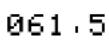
Displays label C, which takes 61.5 bytes.


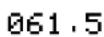
Checksum and length.
12–22 Simple Programming
(hold)
If your checksum does not match this number, then you have not entered this program correctly.
You will see that all of the application programs provided in chapters 15 through 17 include checksum values with each labeled routine so that you can verify the accuracy of your program entry.
In addition, each equation in a program has a checksum. See "To enter an equation in a program line" earlier in this chapter.
Nonprogrammable Functions
The following functions of the HP 32 II are not programmable:
CLEAR {PGM}
CLEAR {ALL}

← ↓ , ← ↑
PRGM
GTO
GTO label nn
MEM
SHOW
EQN
FDISP
Programming with BASE
You can program instructions to change the base mode using ⏻ BASE. These settings work in programs just as they do as functions executed from the keyboard. This allows you to write programs that accept numbers in any of the four bases, do arithmetic in any base, and display results in any base.
When writing programs that use numbers in a base other than 10, set the base mode both as the current setting for the calculator and in the program (as an instruction).
Simple
Progrc
Selecting a Base Mode in a Program
Insert a BIN, OCT, or HEX instruction into the beginning of the program. You should usually include a DEC instruction at the end of the program so that the calculator's setting will revert, to Decimal mode when the program is done.
An instruction in a program to change the base mode will determine bow input is interpreted and how output looks during and after program execution, but it does not affect the program lines as you enter them.
Equation evaluation, SOLVE, and FN automatically set Decimal mode.
Numbers Entered in Program Lines
Before starting program entry, set the base mode. The current setting for the base mode determines the base of the numbers that are entered into program lines. The display of these numbers changes when you change the base mode.
Program line numbers always appear in base 10.
An annunciator tells you which base is the current setting. Compare the program lines below in the left and right columns. All non-decimal numbers are right justified in the calculator's display. Notice how the number 13 appears as "D" in Hexadecimal mode.
Decimal mode set: Hexadecimal mode set:
Polynomial Expressions and Horner's Method
Some expressions, such as polynomials, use the same variable several times for their solution. For example, the expression
Ax ^ 4 + Bx ^ 3 + Cx ^ 2 + Dx + E
uses the variable x four different times. A program to calculate such an expression using RPN operations could repeatedly recall a stored copy of x from a variable. A shorter RPN programming method, however, would be to use a stack which has been filled with the constant (see "Filling the Stack with a Constant" in chapter 2).
Rorer's Method is a useful means of rearranging polynomial expressions to cut calculation steps and calculation time. It is especially expedient with SOLVE and FN , two relatively complex operations that use subroutines.
This method involves rewriting a polynomial expression in a nested fashion to eliminate exponents greater than 1:
Ax ^ 4 + 1 3 x ^ 3 + Cx ^ 2 + Dx + E
(Ax ^ 3 + Bx ^ 2 + Cx + D) x + E
((Ax ^ 2 + Bx + C) x + D) x + E
(((Ax + B) x + C) x + D) x + E
Example:
Write a program using RPN operations for 5x4 + 2x3 as (((5x + 2)x)x)x , then evaluate it for x = 7.
Keys:
Display:
Description:




Simple
Progrc
ENTER P04 ENTER
ENTER P05 ENTER
5 P06 5
P07 x 5x.
2 P08 2
+ P09 + 5x + 2.
× P10 × (5x + 2)x.
☒ P11 × (5x + 2)x2 .
☒ P12 x (5x + 2)x3 .
RTN P13 RTN
MEM {PGM}LBL P 019.5
Displays label P, which takes 19.5 bytes.
SHOW CK=7FB4 019.5
Checksum and length.
C C
Cancels program entry.
Now evaluate this polynomial x = 7.
Keys:
Display:
Description:
XEQ P X? value
Prompts for x.
7 R/S 12,691.0000
Result.
A more general form of this program for any equation
((Ax + B) × + C) × + D) × + E would be:
P01 LBL P
P02 INPUT A
P03 INPUT B
P04 INPUT C
P05 INPUT D
P06 INPUT E
P07 INPUT X
P08 ENTER
P09 ENTER
12–26 Simple Programming
P10 ENTER
P11 RCL×A
P12 RCL+B
P13 ×
P14 RCL+C
P15 ×
P16 RCL+D
P17 ×
P18 RCL+E
P19 RTN
Checksum and length: E93F 028.5
Simple
Progrc
13
Programming Techniques
Chapter 12 covered the basics of programming. This chapter explores more sophisticated but useful techniques:
■ Using subroutines to simplify programs by separating and labeling portions of the program that are dedicated to particular tasks. The use of subroutines also shortens a program that must perform a series of steps more than once.
■ Using conditional instructions (comparisons and flags) to determine which instructions or subroutines should be used,
■ Using loops with counters to execute a set of instructions a certain number of times.
■ Using indirect addressing to access different variables using the same program instruction.
Routines in Programs
A program is composed of one or more routines. A routine is a functional unit that accomplishes something specific, Complicated programs need routines to group and separate tasks. This makes a program easier to write, read, understand, and alter.
For example, look at the program for "Normal and Inverse-Normal Distributions" in chapter 16. Routine S "initializes" the program by collecting the input for the mean and standard deviation. Routine D sets a limit of integration, executes routine Q, and displays the result, Routine Q integrates the function defined in routine F and finishes the probability calculation of Q(x) .
Programming
Techniq
A routine typically starts with a label (LBL) and ends with an instruction that alters or stops program execution, such as RTN, GTO, or STOP, or perhaps another label.
Calling Subroutines (XEQ, RTN)
A subroutine is a routine that is called from (executed by) another routine and returns to that same routine when the subroutine is finished. The subroutine must start with a LBL and end with a RTN. A subroutine is itself a routine, and it can call other subroutines.
■ XEQ must branch to a label (LBL) for the subroutine. (It cannot branch to a line number.)
At the very next RTN encountered, program execution returns to the line after the originating XBQ.
For example, routine Q in the "Normal and Inverse-Normal Distributions" program in chapter 16 is a subroutine (to calculate Q(x) ) that is called from routine D by line D03 XEQ Q. Routine Q ends with a RTN instruction that sends program execution back to routine D (to store and display the result) at line D04. See the flow diagrams below.
The flow diagrams in this chapter use this notation:
A05 GTO B → ① Program execution branches from this line to the line marked ← ① ("from 1").
B01 LBL B ←① Program execution branches from a line marked → ① ("to 1") to this line.
13-2 Programming Techniques
| D01 LBL D | Starts here. | |
| D02 INPUT X | ||
| D03 XEQ Q | →① | Calls subroutine Q. |
| D04 STO Q | ←② | Return here. |
| D05 VIEW Q | ||
| D06 GTO D | Starts D again. | |
| Q01 LBL Q | ←① | Starts subroutine. |
| : | ||
| : | ||
| Q16 RTN | →② | Returns to routines D. |
Nested Subroutines
A subroutine can call another subroutine, and that subroutine can call yet another subroutine. This "nesting" of subroutines—the calling of a subroutine within another subroutine—is limited to a stack of subroutines seven levels deep (not counting the topmost program level). The operation of nested subroutines is as shown below:
MAIN program (top level)
![graph TD A["LBL A<br>•<br>•<br>•<br>XEQ B<br>SIN<br>•<br>•<br>•<br>RTN"] --> B["↓"] B --> C["LBL B<br>•<br>•<br>•<br>XEQ C<br>3.1416<br>•<br>•<br>•<br>RTN"] C --> D["↓"] D --> E["LBL C<br>•<br>•<br>•<br>XEQ D<br>SQRT<br>•<br>•<br>•<br>RTN"] E --> F["↓"] F --> G["LBL D<br>•<br>•<br>•<br>XEQ E<br>RCL…](/content/2026/05/973866/images/1015126bbece470344dab048389bd87bc61e9f88efe744ad3a38e146f0354d0c.jpg)
End of program
Attempting to execute a subroutine nested more than seven levels deep causes an XEQ OVERFLOW error.
Programming
Techniq
Example: A Nested Subroutine.
The following subroutine, labeled S, calculates the value of the expression
√ a ^ 2 + b ^ 2 + c ^ 2 + d ^ 2
as part of a larger calculation in a larger program. The subroutine calls upon another subroutine (a nested subroutine), labeled Q, to do the repetitive squaring and addition. This saves memory by keeping the program shorter than it would be without the subroutine.
| S01 LBL S | Starts subroutine here. |
| S02 INPUT A | Enters A. |
| S03 INPUT B | Enters B. |
| S04 INPUT C | Enters C. |
| S05 INPUT D | Enters D. |
| S06 RCL D | Recalls the data. |
| S07 RCL C | |
| S08 RCL B | |
| S09 RCL A | |
| S10 x2 | |
| S11 XEQ Q → 1 | A2 . |
| 2 → S12 XEQ Q → 3 | A2 + B2 . |
| 4 → S13 XEQ Q → 5 | A2 + B2 + C2 |
| 6 → S14 SQRT | B +C22D22 |
| S15 RTN | Returns to main routine. |
| Q01 LBL Q ← 135 | Nested subroutine |
| Q02 x<>y | |
| Q03 x2 | |
| Q04 + | Adds x2 . |
| 246 ← Q05 RTN | Returns to subroutine S. |
13-4 Programming Techniques
Branching (GTO)
As we have seen with subroutines, it is often desirable to transfer execution to a part of the program other than the next line. This is called branching.
Unconditional branching uses the GTO (go to) instruction to branch to a program label. It is not possible to branch to a specific line number during a program.
A Programmed GTO Instruction
The GTO label instruction (press 📄 GTO label) transfers the execution of a running program to the program line containing that label, wherever it may be. The program continues running from the new location, and never automatically returns to its point of origination, so GTO is not used for subroutines.
For example, consider the "Curve Fitting" program in chapter 16, TheGTO Z instruction branches execution from any one of three independent initializing routines to LBL Z, the routine that is the common entry point into the heart of the program:
Programming
Techniq

Using GTO from the Keyboard
You can use 📄 GTO to move the program pointer to a specified label or line number without starting program execution.
■ To PRGM TOP: GTO
To a line number: GTO □ label nn (nn < 100). For example, GTO □ A05.
■ To a label: 📄 GTO label —but only if program entry is not active (no program lines displayed; PRGM off). For example, 📄 GTO A.
13–6 Programming Techniques
Conditional Instructions
Another way to alter the sequence of program execution is by a conditional test, a true/false test that compares two numbers and skips the next program instruction if the proposition is false.
For instance, if a conditional instruction on line A05 is x=0? (that is, is x equal to zero?), then the program compares the contents of the X-register with zero. If the X-register does contain zero, then the program goes on to the next line. If the X-register does not contain zero, then the program skips the next line, thereby branching to line A07. This rule is commonly known as "Do if true."
| A01 LBL A | |||
| Do next if true. | A05 x=0? | → ② | Skip next if false. |
| ① ← A06 GTO B | |||
| A07 LN | ← ② | ||
| A08 STO A | |||
| ① → B01 LBL B | |||
The above example points out a common technique used with conditional tests: the line immediately after the test (which is only executed in the "true" case) is a branch to another label. So the net effect of the test is to branch to a different routine under certain circumstances.
There are three categories of conditional instructions:
■ Comparison tests. These compare the X- and Y-registers, or the X-register and zero.
■ Flag tests. These check the status of flags, which can be either set or clear.
■ Loop counters. These are usually used to loop a specified number of times.
Programming
Techniq
Tests of Comparison (x?y, x?0)
There are 12 comparisons available for programming. Pressing → x?y or → x?0 displays a. menu for one of the two categories of tests:
■ x?y for tests comparing x and y.
■ x?0 for tests comparing x and 0.
Remember that x refers to the number in the X-register, and y refers to the number in the Y-register. These do not compare the variables X and Y.
Select the category of comparison, then press the menu key for the conditional instruction you want.
The Test Menus
| x?y | x?0 |
| {≠} for x ≠ y? | {≠} for x≠0? |
| {≤} for x≤y? | {≤} for x≤0? |
| {<} for x<=} for x<0? | =} for x<0? |
| {>} for x>y? | >} for x>0? |
| {≥} for x ≥y? | ≥} for x≥0? |
| {=} for x=y? | =} for x=0? |
If you execute a conditional test from the keyboard, the calculator will display YES or NO.
Example:
The "Normal and Inverse–Normal Distributions" program in chapter 16 uses the x<y? conditional in routine T:
Program Lines:
Description
T09 ÷
Calculates the correction for Xguess .
T10 STO+ X
Adds the correction to yield a new Xguess .
T11 ABS
T120.00001
13–8 Programming Techniques
T13 x<y? Tests to see if the correction is significant.
T14 GT0 T Goes back to start of loop if correction is significant. Continues if correction is not significant.
T15 RCL X
T16 VIEW X Displays the calculated value of X.
Line T09 calculates the correction for Xguess . Line T13 compares the absolute value of the calculated correction with 0.0001. If the value is less than 0.0001 ("Do If True"), the program executes line T14; if the value is equal to or greater than 0.0001, the program skips to line T15.
Flags
A flag is an indicator of status. It is either set (true) or clear (false). Testing a flag is another conditional test that follows the "Do if true" rule: program execution proceeds directly if the tested flag is set, and skips one line if the flag is clear.
Meanings of Flags
The HP 32SII has 12 flags, numbered 0 through 11. All flags can be set., cleared, and tested from the keyboard or by a program instruction. The default state of all 12 flags is clear. The three-key memory clearing operation described in appendix B clears all flags. Flags are not affected by CLEAR {ALL} {Y}.
- Flags 0, 1, 2, 3, and 4 have no preassigned meanings. That is, their states will mean whatever you define it to mean in a given program. (See the example below.)
■ Flag 5, when set, will interrupt a program when an overflow occurs within the program, displaying OVERFLOW and ▲. An overflow occurs when a result exceeds the largest number that the calculator can handle. The largest possible number is substituted for the overflow result. If flag 5 is clear, a program with an overflow is not interrupted, though OVERFLOW is displayed briefly when the program eventually stops.
■ Flag 6 is automatically set by the calculator any time an overflow occurs (although you can also set flag 6 yourself). It has no effect, but can be
Programming
Techniq
tested.
Flags 5 and 6 allow you to control overflow conditions that occur during a program. Setting flag 5 stops a program at the line just after the line that caused the overflow. By testing flag 6 in a program, you can alter the program's flow or change a result anytime an overflow occurs.
- Flags 7, 8, and 9 control the display of fractions. Flag 7 can also be controlled from the keyboard, When Fraction-display mode is toggled on or off by pressing ← FDISP, flag 7 is set or cleared as well.
| Flag Status | Fraction-Control Flags | ||
| 7 8 9 | |||
| Clear (Default) | Fraction display off; display real numbers in the current display format. | Fraction denominators not greater than the /c value. | Reduce fractions to smallest form. |
| Set Fraction display on; display real numbers as fractions. | Fraction denominators are factors of the /c Value. | No reduction of fractions. (Used only if flag 8 is set.) | |
■ Flag 10 controls program execution of equations:
When flag 10 is clear (the default state), equations in running programs are evaluated and the result put on the stack.
When flag 10 is set, equations in running programs are displayed as messages, causing them to behave like a VIEW statement:
- Program execution halts.
- The program pointer moves to the next program line.
- The equation is displayed without affecting the stack. You can clear the display by pressing ← or . Pressing any other key executes that key's function.
13–10 Programming Techniques
- If the next program line is a PSE instruction, execution continues after a 1-second pause.
The status of flag 10 is controlled only by execution of the SF and CF operations from the keyboard, or by SF and CF, statements in programs.
■ Flag 11 controls prompting when executing equations in a program — it doesn't affect automatic prompting during keyboard execution:
When flag 11 is clear (the default state), evaluation, SOLVE, and FN of equations in programs proceed without interruption. The current value of each variable in the equation is automatically recalled each time the variable is encountered. INPUT prompting is not affected.
When flag 11 is set, each variable is prompted for wheat it is first encountered in the equation. A prompt for a variable occurs only once, regardless of the number of times the variable appears in the equation. When solving, no prompt occurs for the unknown; when integrating, no prompt occurs for the variable of integration. Prompts halt execution. Pressing R/S resumes the calculation using the value for the variable you keyed in, or the displayed (current) value of the variable if R/S is your sole response to the prompt.
Flag 11 is automatically cleared after evaluation, SOLVE, or ∫ FN of an equation in a program. The status of flag 11 is also controlled by execution of the SF and CF operations from the keyboard, or by SF and CF statements in programs.
Annunciators for Set Flags
Flags 0, 1, 2, and 3 have annunciators in the display that turn on when the corresponding flag is set. The presence or absence of 0, 1, 2, or 3 lets you know at any time whether any of these four flags is set or not. However, there is no such indication for the status of flags 4 through 11. These status of these flags can be determined by executing the FS? Instruction from the keyboard. (See "Using Flags" below.)
Programming
Techniq
Using Flags
Pressing 📄 FLAGS displays the FLAGS menu: {SF} {CF} {FS?}
After selecting the function you want, you will be prompted for the flag number (0–11). For example, press 📄 FLAGS {SF} 0 to set flag 0; press 📄 FLAGS {SF} ▪ to set flag 10; press 📄 FLAGS {SF} ▪ 1 to set flag 11.
FLAGS Menu
| Menu Key | Description |
| {SF} n | Set flag. Set flag n. |
| {CF} n | Clear flag. Clears flag n. |
| {FS?} n Is | flag set ? Tests the status of flag n. |
A flag test is a conditional test that affects program execution just as the comparison tests do. The FS? n instruction tests whether the given flag is set. If it is, then the next line in the program is executed. If it is not, then the next line is skipped. This is the "Do if True" rule, illustrated under "Conditional Instructions" earlier in this chapter.
If you test a flag from the keyboard, the calculator will display "YES" or "NO".
It is good practice in a program to make sure that any conditions you will be testing start out in a known state. Current flag settings depend on how they have been left by earlier programs that have been run. You should not assume that any given flag is clear, for instance, and that it will be set only if something in the program sets it. You should make sure of this by clearing the flag before the condition arises that might set it. See the example below.
Example: Using Flags.
The "Curve Fitting" program in chapter 16 uses flags 0 and 1 to determine whether to take the natural logarithm of the X- and Y-inputs:
■ Lines S03 and S04 clear both of these flags so that lines W07 and W11 (in the input loop routine) do not take the natural logarithms of the X- and Y-inputs for a Straight-line model curve.
13–12 Programming Techniques
Line L03 sets flag 0 so that line W07 takes the natural log of the X-input for a Logarithmic-model curve.
Line E04 sets flag 1 so that line W11 takes the natural log of the Y-input for an Exponential-model curve.
■ Lines P03 and P04 set both flags so that lines W07 and W11 take the natural logarithms of both the X- and Y-inputs for a Power-model curve.
Note that lines S03, S04, L04, and E03 clear flags 0 and 1 to ensure that they will be set only as required for the four curve models.
Program Lines: Description:
. . .
S03 CF 0 Clears flag 0, the indicator for In X.
S04 CF 1 Clears flag 1, the indicator for In Y.
•
L03 SF 0 Sets flag 0, the indicator for In X.
L04 CF 1 Clears flag 1, the indicator for In Y.
: :
E03 CF 0 Clears flag 0, the indicator for In X.
E04 SF 1 Sets flag 1, the indicator for In Y.
. . . .
P03 SF 0 Sets flag 0, the indicator for In X.
P04 SF 1 Sets flag 1, the indicator for In Y.
· · · · · ·
W06 FS? 0 If flag 0 is set ...
W07 LN ... takes the natural log of the X-input.
W10 FS? 1 If flag 1 is set ...
W11 LN ... takes the natural log of the Y-input.
Programming
Techniq
Example: Controlling the Fraction Display.
The following program lets you exercise the calculator's fraction-display capability. The program prompts for and uses your inputs for a fractional number and a denominator (the /c value). The program also contains examples of how the three fraction-display flags (7, 8, and 9) and the "message-display" flag (10) are used.
Messages in this program are listed a MESSAGE and are entered as equations:
- Set Equation-entry mode by pressing 📄 EQN (the EQN annunciator turns on).
- Press RCL letter for each alpha character in the message; press SPACE (the R/S key) for each space character.
- Press ENTER to insert the message in the current program line and end Equation-entry mode.
Program Lines: Description:
| F01 | LBLBegins the fraction program. | |
| F02 | ∅FClears three fraction flags. | |
| F03 | ∅F | |
| F04 | ∅F | |
| F05 | $∅ Displays messages. | |
| F06 | DEC | Selects decimal base. |
| F07 | INPUT | Prompts for a number. |
| F08 | INPD | Prompts for denominator (2 - 4095). |
| F09 | RQLDisplays message, then shows the decimal number. | |
| F10 | DECIMAL | |
| F11 | PSE | |
| F12 | STOP | |
| F13 | ROL | |
| F14 | /°C | Sets /c value and sets flag 7. |
| F15 | MOBRECISE | Displays message, then shows the fraction. |
13–14 Programming Techniques
Program Lines: Description:
| F16 | PSE | |
| F17 | STOP | |
| F18 | 8F | Sets flag 8. |
| F19 | FACTDENOM | Displays message, then shows the fraction. |
| F20 | PSE | |
| F21 | STOP | |
| F22 | 9F | Sets flag 9. |
| F23 | FIXBENOM | Displays message, then shows the fraction. |
| F24 | PSE | |
| F25 | STOP | |
| F26 | GFO | Goes to beginning of program. |
Checksum and length: 10C3 102.0
Use the above program to see the different forms of fraction display:
| Keys: | Display: | Description: |
| XEQ F | V?value | Executes label F; prompts for a fractional number (V). |
| 2.53 R/S | D?value | Stores 2.53 in V; prompts for denominator (D). |
| 16 R/S | DECIMAL2.5300 | Stores 16 as the /c value. Displays message, then the decimal number. |
| R/S | MOST PRECISE▼28/15 | Message indicates the fraction format (denominator is no greater than 16), then shows the fraction.▼ indicates that the numerator is "a little below" 8.. |
| R/S | FACTOR DENOM | Message indicates the fraction |
Programming
Techniq
| Keys: | Display: | Description: |
| 2\ 1/2 | format (denominator is factor of 16), then shows the fraction. | |
| R/S | FIXED DENOM | Message indicates the fraction |
| 2\ 8/16 | format (denominator is 16), then shows the fraction. | |
| R/S C | 2.5300 | Stops the program and clears flag |
| FLAGS {CF} | 0 | 10 |
Loops
Branching backwards — that is, to a label in a previous line — makes it possible to execute part of a program more than once. This is called looping.
D01 LBL D
D02 INPUT M
D03 INPUT N
D04 INPUT T
D05 GTO D
This routine (taken from the "Coordinate Transformations" program on page 15–31 in chapter 15) is an example of an infinite loop. It is used to collect the initial data prior to the coordinate transformation. After entering the three values, it is up to the user to manually interrupt this loop by selecting the transformation to be performed (pressing XEQ N for the old-to-new system or XEQ O for the new-to-old system).
Conditional Loops (GTO)
When you want to perform an operation until a certain condition is met, but you don't know how many times the loop needs to repeat itself, you can create a loop with a conditional test and a GTO instruction.
For example, the following routine uses a loop to diminish a value A by a constant amount B until the resulting A is less than or equal to B.
13–16 Programming Techniques
Program lines: Description:
A01 LBL A
A02 INPUT A
A03 INPUT B
Checksum and length: 6157 004.5
S01 LBL S
S02 RCL A It is easier to recall A than to remember where it is in the stack.
S03 RCL-B Calculates A-B.
S04 STO A Replaces old A with new result.
S05 RCL B Recalls constant for comparison.
S06 x<y? Is <neBw A?
S07 GTO S Yes: loops to repeat subtraction.
S08 VIEW A No: displays new A.
S09 RTN
Checksum and length: 5FE1 013.5
Loops With Counters (DSE, ISG)
When you want to execute a loop a specific number of times, use the ISG (increment; skip if greater than). or DSE (decrement; skip if less than or equal to) conditional function keys. Each time a loop function is executed in a program, it automatically decrements or increments a counter value stored in a variable. It compares the current counter value to a final counter value, then continues or exits the loop depending on the result.
For a count-down loop, use DSE variable
For a count-up loop, use ⏻ ISG variable
These functions accomplish the same thing as a FOR-NEXT loop in BASIC:
FOR variable = initial-value TO final-value STEP increment
Programming
Techniq
• • •
NEXT variable
A DSE instruction is like a FOR-NEXT loop with a negative increment.
After pressing a shifted key for ISG or DSE (☐ ISG or ☐ DSE), you will be prompted for a variable that will contain the loop-control number (described below).
The Loop-Control Number
The specified variable should contain a loop-control number ±ccccccc.ffii, where:
±ccccccc is the current counter value (1 to 12 digits). This value changes with loop execution.
■ fff is the final counter value (must be three digits). This value does not change as the loop runs.
ii is the interval for incrementing and decrementing (must be two digits or unspecified). This value does not change. An unspecified value for ii is assumed to be 01 (increment/decrement by 1).
Given the loop-control number cccccccc.fffii, DSE decrements cccccccc to cccccccc — ii, compares the new cccccccc with fff, and makes program execution skip the next program line if this cccccccc ≤ fff.
Given the loop-control number cccccccc.ffii, ISG increments cccccccc to cccccccc + ii, compares the new cccccccc with fff, and makes program execution skip the next program line if this cccccccc >fff.
13–18 Programming Techniques
| 1→ | W01 LBL W | |||
| . | ||||
| . | ||||
| W09 DSE A | →2 | |||
| 1← | W10 GTOW | |||
| If current value > final value, continue loop. | W11 XEQ X | ←2 | If current value ≤ final value, exit loop. | |
| . | ||||
| . | ||||
| 1→ | W01 LBL W | |||
| . | ||||
| . | ||||
| W09 ISGA | →2 | |||
| 1← | W10 GTOW | |||
| If current value ≤ final value, continue loop. | W11 XEQ X | ←2 | If current value > final value, exit loop. | |
| . | ||||
| . |
For example, the loop-control number 0.050 for ISG means: start counting at zero, count up to 50, and increase the number by 1 each loop.
The following program uses ISG to loop 10 times. The loop counter (0000001.01000) is stored in the variable Z. Leading and trailing zeros can be left off.
L01 LBL
L021.01
L03 ST0 Z
M01 LBL M
M02 ISG Z
M03 GTO
M04 RTN
Press 📄 VIEW Z to see that the loop-control number is now 11.0100.
Programming
Techniq
Indirectly Addressing Variables and Labels
Indirect addressing is a technique used in advanced programming to specify a variable or label without specifying beforehand exactly which one. This is determined when the program runs, so it depends on the intermediate results (or input) of the program.
Indirect addressing uses two different keys: i (with ) and (i) (with R/S).
The variable I has nothing to do with (i) or the variable i. These keys are active for many functions that take A through Z as variables or labels.
■ i is a variable whose contents can refer to another variable or label. It holds a number just like any other variable (A through Z).
(i) is a programming function that directs, "Use the number in i to determine which variable or label to address."
This is an indirect address. (A through Z are direct addresses.)
Both and (i) are used together to create an indirect address. (See the examples below.)
By itself, i is just another variable.
By itself, (i) is either undefined (no number in i) or uncontrolled (using whatever number happens to be left over in i).
The Variable "i"
Your can store, recall, and manipulate the contents of i just as you car, the contents of other variables. You can even solve for i and integrate using i. The functions listed below can use variable "i".
STO i INPUT i DSE i
RCL i VIEW i ISG i
STO +,-, ×,÷ i ∫ FN d i x <> i
RCL +,-, ×,÷ i SOLVE i
13–20 Programming Techniques
The Indirect Address, (i)
Many functions that use A through Z (as variables or labels) can use (i) to refer to A through Z (variables or labels) or statistics registers indirectly. The function (i) uses the value in variable i to determine which variable, label, or register to address. The following table shows how.
| If i contains: | Then (i) will address: |
| ±1 variable A or label A | |
| ±26 | variable Z |
| ±27 | variable |
| ±28 n register | |
| ±29 | Σx register |
| ±30 | Σy register |
| ±31 | Σx 2 register |
| ±32 | Σy 2 register |
| ±33 | Σxy register |
| ≥34 or ≤-34 or 0 | error: INVALID < i > |
or label Z
Only the absolute value of the integer portion of the number in i is used for addressing.
The INPUT(i) and VIEW(i) operations label the display with the name of the indirectly-addressed variable or register.
The SUMS menu enables you to recall values from the statistics registers. However, you must use indirect addressing to do other operations, such as STO, VIEW, and INPUT.
The functions listed below can use (i) as an address. For GTO, XEQ, and FN=, (i) refers to a label; for all other functions (i) refers to a variable or register.
Programming
Techniq
| STO(i) | INPUT(i) |
| RCL(i) | VIEW(i) |
| STO +, -, × , ÷, (i) | DSE(i) |
| RCL +, -, × , ÷, (i) | ISG (i) |
| XEQ(i) | SOLVE(i) |
| GTO(i) | ∫ FN d(i) |
| X<> (i) | FN=(i) |
Program Control with (i)
Since the contents of i can change each time a program runs—or even in different parts of the same program — a program instruction such as GTO can branch to a different label at different times. This maintains flexibility by leaving open (until the program runs) exactly which variable or program label will be needed. (See the first example below.)
Indirect addressing is very useful for counting and controlling loops. The variable i serves as an index, holding the address of the variable that contains the loop-control number for the functions DSE and ISG. (See the second example below.)
Example: Choosing Subroutines With (i).
The "Curve Fitting" program in chapter 16 uses indirect addressing to determine which model to use to compute estimated values for x and y. (Different subroutines compute x and y for the different models.) Notice that i is stored and then indirectly addressed in widely separated parts of the program.
The first four routines (S, L, E, P) of the program specify the curve-fitting model that will be used and assign a number (1, 2, 3, 4) to each of these models. This number is then stored during routine Z, the common entry point for all models:
203 STO i
Routine Y uses i to call the appropriate subroutine (by model) to calculate the x- and y-estimates. Line Y03 calls the subroutine to compute y:
Y03 XEQ(i)
13–22 Programming Techniques
and line Y08 calls a different subroutine to compute x after i has been increased by 6:
Y06 6
Y07 STO+ i
Y08 XEQ(i)
| If i hold: Then XEQ(i) calls: To: | ||
| 1 LBL A | Compute | y for straight-line model. |
| 2 | LBL B | Compute y for logarithmic model. |
| 3 LBL C | Compute | y for exponential model. |
| 4 LBL D | Compute | y for power model. |
| 7 | LBL G | Compute x for straight-line model. |
| 8 LBL H | Compute | x for logarithmic model. |
| 9 | LBL I | Compute x for exponential model. |
| 10 | LBL J | Compute x for power model. |
Example: Loop Control With (i).
An index value in i is used by the program "Solutions of Simultaneous Equations—Matrix Inversion Method" in chapter 15. This program uses the looping instructions ISG i and DSE i in conjunction with the
indirect instructions RCL(i) and STO(i) to fill and manipulate a matrix.
The first part of this program is routine A, which stores the initial loop-control number in i.
Program lines:
A01 LBL A
A021.012
Description:
The starting point for data input.
Loop-control number: loop from 1 to 12 in intervals of 1.
Programming
Techniq
A03 STO i Stores loop-control number in i.
The next routine is L, a loop to collect all 12 known values for a 3x3 coefficient matrix (variables A - l) and the three constants (J - L) for the equations.
Program Lines: Description:
L01 LBL L This routine collects all known values in three equations.
L02 INPUT(i) Prompts for and stores a number into the variable addressed by i.
L03 ISG i Adds 1 to i and repeats the loop until i re 13.012.
L04 GTO L
L05 GTO A When i exceeds the final counter value, execution branches back to A.
Label J is a loop that completes the inversion of the 3 × 3 matrix.
Program Lines: Description:
J01 LBL J This routine completes inverse by dividing by determinant.
J02 STO÷(i) Divides element.
J03 DSE i Decrements index value so it points closer to A
J04 GTO J Loops for next value.
J05 RTN Returns to the calling program or to PRGM TOP.
Equations with (i)
You can use (i) in an equation to specify a variable indirectly. Notice that (i) means the variable specified by the number in variable i (an indirect reference), but that i or (i) means variable i.
The following program uses an equation to find the sum of the squares of variables A through Z.
Program Lines: Description:
E01 LBL E Begins the program.
E02 CF 10 Sets equations for execution.
13–24 Programming Techniques
E03 CF 11 Disables equation prompting.
E04 1.026 Sets counter for 1 to 26.
E05 STO i Stores counter.
Checksum and length: EA5F 017.0
Program Lines: Description:
F01 LBL F Starts summation loop.
F02(i)^2 Equation to evaluate the ith square. (Press ☐EQN to start the equation.)
Ckecksum and length of equation: 48AD 006.0
F04 ISG i Tests for end of loop.
F05 GTO F Branches for next variable.
F06 RTN Ends program.
Checksum and length of program: 19A8 013.5
Programming
Techniq
14
Solving and Integrating Programs
Solving a Program
In chapter 7 you saw how you can enter an equation — it's added to the equation list — and then solve it for any variable. You can also, enter a program that calculates a function, and then solve it for any variable. This is especially useful if the equation you're solving changes for certain conditions or if it requires repeated calculations.
To solve a programmed function:
- Enter a program that defines the function. (See "To write a program for SOLVE" below.)
- Select the program to solve: press ☐ FN= label. (You can skip this step if you're re-solving the same program.)
- Solve for the unknown variable: press → SOLVE variable.
Notice that FN= is required if you're solving a programmed function, but not if you're solving an equation from the equation list.
To halt a calculation, press C or R/S. The current best estimate of the root is in the unknown variable; use VIEW to view it without disturbing the stack. To resume the calculation, press R/S.
To write a program for SOLVE:
The program can use equations and RPN operations — in whatever combination is most convenient.
- Begin the program with a label. This label identifies the function that you want SOLVE to evaluate (FN=label).
Solving and Integrating Programs 14–1
- Include an INPUT instruction for each variable, including the unknown. INPUT instructions enable you to solve for any variable in a multi-variable function. INPUT for the unknown is ignored by the calculator, so you need to write only one program that contains a separate INPUT instruction for every variable (including the unknown).
If you include no INPUT instructions, the program uses the values stored in the variables or entered at equation prompts.
- Enter the instructions to evaluate the function.
A function programmed as a multi-line RPN sequence must be in the form of an expression that goes to zero at the solution. If your equation is f(x) = g(x) , your program should calculate f(x) - g(x) . "=0" is implied.
A function programmed as an equation can be any type of equation—equality, assignment, or expression. The equation is evaluated by the program, and its value goes to zero at the solution. If you want the equation to prompt for variable values instead of including INPUT instructions, make sure flag 11 is set.
- End the program with a RTN. Program execution should end with the value of the function in the X-register.
SOLVE works only with real numbers. However, if you have a complex-valued function that can be written to isolate its real and imaginary parts, SOLVE can solve for the parts separately.
Example: Program Using RPN.
Write a program using RPN operations that solves for any unknown in the equation for the "Ideal Gas Law." The equation is:
P × V = N × R × T
where
P = Pressure (atmospheres or N / m ^ 2).
V = Volume (liters) .
N = Number of moles of gas.
14–2 Solving and Integrating Programs
R = The universal gas constant
(0.0821 liter-atm/mole-K or 8.314 J/mole-K).
T = Temperature (kelvins; K = °C + 273.1).
To begin, put the calculator in Program mode; if necessary, position the program pointer to the top of program memory.
Keys:
Display:
Description:


PRGM TOP
Sets Program mode.
Type in the program:
Program Lines: Description:
G01 LBL G Identifies the programmed function.
G02 INPUT P Stores P.
G03 INPUT V Stores V.
G04 INPUT N Stores N.
G05 INPUT R Stores R.
G06 INPUT T Stores T.
G07 RCL P Pressure.
G08 RCL× V Pressure × volume.
G09 RCL N Number of moles of gas.
G10 RCL×R Moles × gas constant.
G11 RCL×T Moles × gas constant × temp.
G12 _ (P × V) - (N × R × T) .
G13 RTN Ends the program.
Checksum and length: 053B 019.5
Press C to cancel Program-entry mode.
Use program "G" to solve for the pressure of 0.005 moles of carbon dioxide in a 2-liter bottle at 24 °C.
Keys:
Display:
Description:


Selects "G"—the program. SOLVE evaluates to find the value of the
Solving and Integrating Programs 14–3
| unknown variable. | ||
| SOLVE P | V?value | Selects P; prompts for V. |
| 2 R/S | N?value | Stores 2 in V; prompts for N. |
| .005 R/S | R?value | Stores .005 in N; prompts for R. |
| .0821 R/S | T?value | Stores .0821 in R; prompts for T. |
| 24 ENTER 273.1 | Calculates T. | |
| + | T?297.1000 | |
| R/S | SOLVING | Stores 297.1 in T; solves for P. |
| P=0.0610 | Pressure is 0.0610 atm. |
Example: Program Using Equation.
Write a program that uses an equation to solve the "Ideal Gas Law."
| Keys: | Display: | Description: |
| Selects Program-entry mode. | ||
| GTO | PRGM TOP | Moves program pointer to top of the list of programs. |
| H01 LBL H | Labels the program. | |
| H02 SF 11 | Enables equation prompting. | |
| Evaluates the equation, clearing flag 11. (Checksum and length: 13E3 015.0). | ||
| H03 P×V=N×Rx | ||
| H04 RTN | Ends the program. | |
| 0.0610 | Cancels Program-entry mode. |
Checksum and length of program: 8AD6 19.5
14–4 Solving and Integrating Programs
Now calculate the change in pressure of the carbon dioxide if its temperature drops by 10\ °C from the previous example.
| Keys: | Display: | Description: |
| STO L | 0.0610 | Stores previous pressure. |
| FN= H | 0.0610 | Enters the limits of integration(lower limit first). |
| SOLVE P | V?2.0000 | Selects variable P; prompts for V. |
| R/S | N?0.0050 | Retains 2 in V; prompts for N. |
| R/S | R?0.0821 | Retains .005 in N; prompts for R. |
| R/S | T?297.1000 | Retains .0821 in R; prompts for T. |
| ENTER 10 — | T?287.1000 | Calculates new T. |
| R/S | SOLVINGP=0.0589 | Stores 287.1 in T; solves for new P. |
| RCL L — | -0.0021 | Calculates pressure change of the gas when temperature drops from 297.1 K to 287.1 K (negative result indicates drop in pressure). |
Using SOLVE in Program
You can use the SOLVE operation as part of a program.
If appropriate, include or prompt for initial guesses (into the unknown variable and into the X-register) before executing the SOLVE variable instruction. The two instructions for solving an equation for an unknown variable appear in programs as:
FH = label
SOLVE variable
The programmed SOLVE instruction does not produce a labeled display (variable = value) since this might not be the significant output for your program (that is, you might want to do further calculations with this number
Solving and Integrating Programs 14–5
before displaying it). If you do want this result displayed, add a VIEW variable instruction after the SOLVE instruction.
If no solution is found for the unknown variable, then the next program line is skipped (in accordance with the "Do if True" rule, explained in chapter 13). The program should then handle the case of not finding a root, such as by choosing new initial estimates or changing an input value.
Example: SOLVE in a Program.
The following excerpt is from a program that allows you to solve for x or y by pressing XEQ X or Y.
Program Lines: Description:
| X01 LBL X | Setup | for | X. | |
| X02 24 | Index | for | X. | |
| X03 GTO L Branches to main routine. Checksum and length: CCEC 004.5 | ||||
| Y01 LBL Y | Setup | for | Y. | |
| Y02 25 | Index | for | Y. | |
| Y03 GTO L Branches to main routine. Checksum and length. 2E48 004.5 | ||||
| L01 LBL L | Main routine. |
| L02 STO i | Stores index in i. |
| L03 FN= F | Defines program to solve. |
| L04 SOLVE(i) | Solves for appropriate variable. |
| L05 VIEW(i) | Displays solution. |
| L06 RTN | Ends program. Checksum and length: E159 009.0 |
| F01 LBL F | Calculates f(x,y). Include INPUT or equation prompting as required. |
| F10 RTN |
14–6 Solving and Integrating Programs
Integrating a Program
In chapter 8 you saw how you can enter an equation (or expression) — it's added to the list of equations — and then integrate it with respect to any variable. You can also enter a program that calculates a function, and then integrate it with respect to any variable. This is especially useful if the function you're integrating changes for certain conditions or if it requires repeated calculations.
To integrate a programmed function:
- Enter a program that defines the integrand's function. (See "To write a program for FN below.)
- Select the program that defines the function to integrate: press ▶ FN=label. (You can skip this step if you're reintegrating the same program.)
- Enter the limits of integration: key in the lower limit and press ENTER then key in the upper limit.
- Select the variable of integration and start the calculation: press ☐ SOLVE variable.
Notice that FN= is required if you're integrating a programmed function, but riot if you're integrating an equation from the equation list.
You can halt a running integration calculation by pressing C or R/S.
However, no information about the integration is available until the calculation finishes normally. To resume the calculation, press R/S again. Pressing XEQ while an integration calculation is running cancels the FN operation. In this case, you should start FN again from the beginning.
To write a program for ∫ FN;
The program can use equations and RPN operations — in whatever combination is most convenient.
- Begin the program with a label. This label identifies the function that you want to integrate (FN=label).
- Include an INPUT instruction for each variable, including the variable of integration. INPUT instructions enable you to integrate with respect to any variable in a multi-variable function. INPUT for the variable of integration
Solving and Integrating Programs 14–7
is ignored by the calculator, so you need to write only one program that contains a separate INPUT instruction for every variable (including the variable of integration).
If you include no INPUT instructions, the program uses the values stored in the variables or entered at equation prompts.
- Enter the instructions to evaluate the function.
A function programmed as a multi-line RPN sequence must calculate the function values you want to integrate.
■ A function programmed as an equation is usually included as an expression specifying the integrand — though it can be any type of equation. If you want the equation to prompt for variable values instead of including INPUT instructions, make sure flag 11 is set.
- End the program with a RTN. Program execution should end with the value of the function in the X-register.
Example: Program Using Equation.
The sine integral function in the example in chapter 8 is
S _ i (t) = _ 0 ^ t ( x/x) dx
This function can be evaluated by integrating a program that defines the integrand:
S01 LBL S Defines the function.
S02 SIN(X)÷X The function as an expression. (Checksum and length: 4914 009.0).
S03 RTN Ends the subroutine
Checksum and length of program: C62A 012.0
Enter this program and integrate the sine integral function with respect to x from 0 to 2 (t = 2).
Keys:
Display:
Description:
14–8 Solving and Integrating Programs
MODES {RD}
FN=S
0 ENTER 2 2_
f X INTEGRATING
1.6054
MODES {DG} 1.6054
Selects Radians mode.
Selects label S as the integrand.
Enters lower and upper limits of integration.
Integrates function from 0 to 2;
displays result.
Restores Degrees mode.
Using Integration in a Program
Integration can be executed from a program. Remember to include or prompt for the limits of integration before executing the integration, and remember that accuracy and execution time are controlled by the display format at the time the program runs. The two integration instructions appear in the program as:
FN = label
∫ FN d variable
The programmed ∫ FN instruction does not produce a labeled display (∫ = value) since this might riot be the significant output for your program (that is, you might want to do further calculations with this number before displaying it). If you do want this result displayed, add a PSE (PSE) or STOP (R/S) instruction to display the result in the X-register after the ∫ FN instruction.
Example: ∫ FN in a Program.
The "Normal and Inverse–Normal Distributions" program in chapter 16 includes an integration of the equation of the normal density function
1S √ 2 π _ M ^ D e ^ - (D - M/S) ^ 2 / 2 dD.
Solving and Integrating Programs 14–9
The eD - M ÷ S2 ÷ 2) function is calculated by the routine labeled F. Other routines prompt for the known values and do the other calculations to find Q(D) , the upper-tail area of a normal curve. The integration itself is set up and executed from routine Q:
| Q01 LBL Q | |
| Q02 RCL M | Recalls lower limit of integration. |
| Q03 RCL X | Recalls upper limit of integration. (X = D.) |
| Q04 FN= F | Specifies the function. |
| Q05 ∫FN a D | Integrates the normal function using the dummy variable D. |
Restrictions o Solving and Integrating
The SOLVE variable and ∫FN d variable instructions cannot call a routine that contains another SOLVE or ∫FN instruction. That is, neither of these instructions can be used recursively. For example, attempting to calculate a multiple integral will result in an ∫(∑FN) error. Also, SOLVE and ∫FN cannot call a routine that contains an FN=label instruction; if attempted, a SOLVE ACTIVE or ∫FN ACTIVE error will be returned. SOLVE cannot call a routine that contains an ∫FN instruction (produces a SOLVE(∑FN) error), just as ∫FN cannot call a routine that contains a SOLVE instruction (produces an ∫(SOLVE) error).
The SOLVE variable and jFN d variable instructions in a program use one of the seven pending subroutine returns in the calculator. (Refer to "Nested Subroutines" in chapter 13.)
The SOLVE and JFN operations automatically set Decimal display format.
14–10 Solving and Integrating Programs
15
Mathematics Programs
Vector Operations
This program performs the basic vector operations of addition, subtraction, cross product, and dot (or scalar) product. The program uses three-dimensional vectors and provides input and output in rectangular or polar form. Angles between vectors can also be found.

Mathematics
Prog
This program uses the following equations. Coordinate conversion:
X = R (P) (T) R = √ X ^ 2 + Y ^ 2 + Z ^ 2
Y = R (P) (T) T = (Y / X)
Z = R (P) P = Z√ X ^ 2 + Y ^ 2
Vector addition and subtraction:
v _ 1 + v _ 2 = (X + U) i + (Y + V) j + (Z + W) k
v _ 2 - v _ 1 = (U - X) i + (V - Y) j + (W - Z) k
Cross product:
v _ 1 × v _ 2 = (YW - ZV) i + (ZU - XW) j + (XV - YU) k
Dot Product:
D = XU + YV + ZW
Angle between vectors (γ):
G = DR _ 1 × R _ 2
where
v _ 1 = Xi + Yj + Zk
and
v _ 2 = Ui + Vj + Wk
The vector displayed by the input routines (LBL P and LBL R) is V1 .
Program Listing:
15-2 Mathematics Programs
Program Lines: Description
R01 LBL R Defines the beginning of the rectangular input/display routine.
R02 INPUT X Displays or accepts input of X.
R03 INPUT Y Displays or accepts input of Y.
R04 INPUT Z Displays or accepts input of Z.
Checksum and length: F8AB 006.0
Q01 LBL Q Defines beginning of rectangular-to-polar conversion process.
Q02 RCL Y
Q03 RCL X
004 y, x→θ, r Calculates √2 + 2 Y φXd arctan(Y/X).
Q05 x<>y
Q06 STO T Saves T = (Y/X) .
Q07 R↓ Gets √2X(Y2) back.
Q08 RCL Z
Q09 y,x→θ,r Calculates √2X(Y2 + Z2) and P .
Q10 STO R Saves R.
Q11 x<>y
Q12 STO P Saves P
Checksum and length: 3D28 018.0
P01 LBL P Defines the beginning of the polar input/display routine.
P02 INPUT R Displays or accepts input of R.
P03 INPUT T Displays or accepts input of T.
P04 INPUT P Displays or accepts input of P.
P05 RCL T
P06 RCL P
P07 RCL R
P08 θ, r→y, x Calculates R cos(P) and R sin(P).
P09 STO Z Stores Z = R (P) .
P10 R↓
P11 θ, r → y, x Calculates R (P) (T) and R (P) (T) .
P12 STO Z Saves X = R (P) (T) .
Mathematics
Prog
Program Listing:
Program Lines: Description
P13 x<>y
P14 STO Y Saves Y = R (P) (T) .
P15 GTO P Loops back for another display of polar form.
Checksum and length: D518 022.5
E01 LBL E Defines the beginning of the vector-enter routine.
E02 RCL X Copies values in X, Y and Z to U, V and W respectively.
E01 STO U
E04 RCL Y
E05 STO V
E06 RCL Z
E07 STO W
E08 GTO Q Loops back for polar conversion and display/input.
Checksum and length: 1032 012.0
X01 LBL X Defines beginning of vector-exchange routine.
X02 RCL X Exchanges X, Y and Z with U, V and W respectively.
X03 X<> U
X04 STO X
X05 RCL Y
X06 X<> V
X07 STO Y
X08 RCL Z
X09 X<> W
X10 STO Z
X11 GTO Q Loops back for polar conversion and display/input.
Checksum and length: DACE 016.5
A01 LBL A Defines beginning of vector-addition routine.
A02 RCL X
A03 RCL+U
15-4 Mathematics Programs
Program Listing:
Program Lines: Description
| A04 STO X | Saves X + U in X . |
| A05 RCL V | |
| A06 RCL+ Y | |
| A07 STO Y | Saves V + Y in Y . |
| A08 RCL Z | |
| A09 RCL+ W | |
| A10 STO Z | Saves Z + W in Z . |
| A11 GTO Q | Loops back for polar conversion and display/input. |
Checksum and length: 641B 016.5
| S01 LBL S | Defines the beginning of the vector–subtraction routine. |
| S02 -1 | Multiplies X, Y and Z by (-1) to change the sign. |
| S03 STOx X | |
| S04 STOx Y | |
| S05 STOx Z | |
| S06 GTO A | Goes to the vector–addition routine. |
Checksum and length: D051 017.0
| C01 LBL C | Defines the beginning of the cross-product routine. |
| C02 RCL Y | |
| C03 RCL× W | |
| C04 RCL Z | |
| C05 RCL× V | |
| C06 - | Calculates (YW-ZV), which is the X component. |
| C07 RCL Z | |
| C08 RCL× V | |
| C09 RCL X | |
| C10 RCL× W | |
| C11 - | Calculates (ZU-WX), which is the Y component. |
| C12 RCL X | |
| C13 RCL× U | |
| C14 RCL Y |
Mathematics
Proc
Program Listing:
Program Lines: Description
| C15 RCL× V | |
| C16 - | |
| C17 STO Z | Stores (XV - YU), which is the Z component. |
| C18 R↓ | |
| C19 STO Y | Stores Y component. |
| C20 R↓ | |
| C21 STO X | Stores X component. |
| C22 GTO Q | Loops back for polar conversion and display/input. |
| Checksum and length: FEB2 033.0 | |
| D01 LBL D | Defines beginning of dot-product and vector-angle routine. |
| D02 RCL X | |
| D03 RCL× U | |
| D04 RCL Y | |
| D05 RCL× V | |
| D06 + | |
| D07 RCL Z | |
| D08 RCL× W | |
| D09 + | |
| D10 STO D | Stores the dot product of XU + YV + ZW . |
| D11 VIEW D | Displays the dot product. |
| D12 RCL D | |
| D13 RCL÷ R | Divides the dot product by the magnitude of the X- , Y- , Z -vector. |
| D14 RCL W | |
| D15 RCL V | |
| D16 RCL U | |
| D17 y, x→θ, r | |
| D18 x<>y | |
| D19 R↓ | |
| D20 y, x→θ, r | Calculates the magnitude of the U , V , W vector. |
| D21 x<>y |
15–6 Mathematics Programs
Program Listing:
Program Lines: Description
D22 R↓
023 ÷ Divides previous result by the magnitude.
D24 ACOS Calculates angle.
D25 ST0 G
D26 VIEW G Displays angle.
D27 GTO P Loops back for polar display/input.
Checksum and length: 1DFC 040.5
Flags Used:
None.
Memory Required:
270 bytes: 182 for program, 88 for variables.
Remarks:
The length of routine S can be shortened by 6.5 bytes. The value -1 as shown uses 9.5 bytes. If it appears as 1 followed by +/-, it will require only 3 bytes. To do this, you can press 1 SHOW +/-
The terms "polar" and "rectangular," which refer to two-dimensional systems, are used instead of the proper three-dimensional terms of "spherical" and "Cartesian." This stretch of terminology allows the labels to be associated with their function without confusing conflicts. For instance, if LBL C had been associated with Cartesian coordinate input, it would not have been available for cross product.
Program Instructions:
- Key in the program routines; press C when done.
- If your vector is in rectangular form, press XEQ R and go to step 4. If your vector is in polar form, press XEQ P and continue with step 3.
Mathematics
Proc
- Key in R and press / , key in T and press / , then key in P and press / . Continue at step 5.
- Key in X and press R/S, key in Y and press R/S, and key in Z and press R/S.
- To key in a second vector, press XEQ E (for enter), then go to step 2.
- Perform desired vector operation:
a. Add vectors by pressing XEQ A;
b. Subtract vector one from vector two by pressing XEQ S;
c. Compute the cross product by pressing XEQ C;
d. Compute the dot product by pressing XEQ D and the angle between vectors by pressing R/S.
- Optional: to review v1 in polar form, press XEQ P, then press R/S repeatedly to see the individual elements.
- Optional: to review v1 in rectangular form, press XEQ R, then press R/S repeatedly to see the individual elements.
- If you added, subtracted, or computed the cross product, v1 has been replaced by the result, v2 is not altered. To continue calculations based on the result, remember to press XEQ E before keying in a new vector.
- Go to step 2 to continue vector calculations.
Variables Used:
X, Y, Z The rectangular components of v1.
U, V, W The rectangular components of v2 .
R, T, P The radius, the angle in the x-y plane ( θ ), and the angle from the Z axis of v1 (U).
D The dot product
G The angle between vector ( γ )
Example 1
A microwave antenna is to be pointed at a transmitter which is 15.7 kilometers North, 7.3 kilometers East and 0.76 kilometers below. Use the
15–8 Mathematics Programs
rectangular to polar conversion capability to find the total distance and the direction to the transmitter.

Keys:
Display:
Description:


X?value

Y?value
Z?value

R?17.3308

T?65.0631

P?92.5134
Sets Degrees mode.
Starts rectangular input/display routine.
Sets X equal to 7.3. Sets Y equal to 15.7.
Sets Z equal to -0.76 and calculates R, the radius.
Calculates T, the angle in the x/y plane.
Calculates P , the angle from the z-axis.
Mathematics
Prog
Example 2:
What is the moment at the origin of the lever shown below? What is the component of force along the lever? What is the angle between the resultant of the force vectors and the lever?
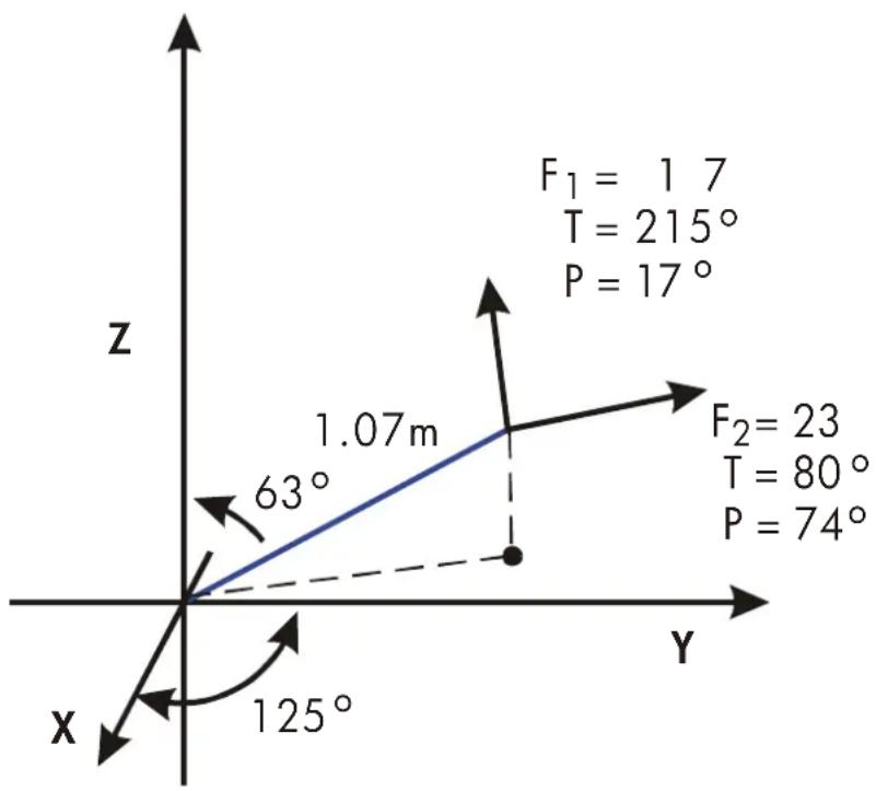
First, add the force vectors.
| Keys: | Display: | Description: |
| P | R?value | Starts polar input routine. |
| 17 /S | T?value | Sets radius equal to 17. |
| 215 /S | P?value | Sets T equal to 215. |
| 17 /S | R?17.000 | Sets P equal to 17. |
| E | R?17.000 | Enters vector by copying it into v2. |
| 23 /S | T?-145.0000 | Sets radius of v1, equal to 23. |
| 80 /S | P?17.0000 | Sets T equal to 80. |
15–10 Mathematics Programs
| 74 R/S | R?23.0000 | Sets P equal to 74. |
| XEQ A | R?29.4741 | Adds the vectors and displays the resultant R. |
| R/S | T?90.7032 | Displays T of resultant vector. |
| R/S | P?39.9445 | Displays P of resultant vector. |
| XEQ E | R?29.4741 | Enters resultant vector. |
Since the moment equals the cross product of the radius vector and the force vector (r × F) , key in the vector representing the lever and take the cross product.
| Keys: | Display: | Description: |
| 1.07 R/S | T?90.7032 | Sets R equal to 1.07. |
| 125 R/S | P?39.9445 | Sets T equal to 125. |
| 63 R/S | R?1.0700 | Sets P equal to 63. |
| XEQ C | R?18.0209 | Calculates cross product and displays R of result. |
| R/S | T?55.3719 | Displays T of cross product. |
| R/S | P?124.3412 | Displays P of cross product. |
| XEQ R | X?8.4554 | Displays rectangular form of cross product. |
| R/S | Y?12.2439 | |
| R/S | Z?-10.1660 |
The dot product can be used to resolve the force (still in v 2) along the axis of the lever.
| Keys: | Display: | Description: |
| XEQ P | R?18.0209 | Starts polar input routine. |
| 1 R/S | T?55.3719 | Defines the radius as one unit vector. |
| 125 R/S | P?124.3412 | Sets T equal to 125. |
| 63 R/S | R?1.0000 | Sets P equal to 63. |
Mathematics
Prog
XEQ D
D=24.1882
Calculates dot product.
R/S
G=34.8490
Calculates angle between resultant force vector and lever.
R/S
R?1.0000
Gets back to input routine.
Solutions of Simultaneous Equations
This program solves simultaneous linear equations in two or three unknowns. It does this through matrix inversion and matrix multiplication.
A system of three linear equations
AX + DY + GZ = J
BX + EY + HZ = K
CX + FY + IZ = L
can be represented by the matrix equation below.
[A amp; D amp; G B amp; E amp; H C amp; F amp; I ] [X Y Z ] = [J K L ]
The matrix equation may be solved for X, Y, and Z by multiplying the result matrix by the inverse of the coefficient matrix.
[^ amp; D ^ A amp; G ^ B ^ amp; E ^ amp; H ^ ^ amp; C amp; IF ] [J K L ] = [X Y Z ]
Specifics regarding the inversion process are given in the comments for the inversion routine, l.
15–12 Mathematics Programs
Program Listing:
Program Lines: Description
| A01 LBL A | Starting point for input of coefficients. |
| A02 1.012 | Loop-control value: loops from I to 12, one at a time. |
| A03 STO i | Stores control value in index variable. |
Checksum and length: 9F76 012.5
| L01 LBL L | Starts the input loop. |
| L02 INPUT(i) | Prompts for and stores the variable addressed by i. |
| L03 ISG i | Adds one to i. |
| L04 GTO L | If i is less than 13, goes back to LBL L and gets the next value. |
| L05 GTO A | Returns to LBL A to review values. |
Checksum and length: 8356 007.5
| I01 LBL I | This routine inverts a 3 × 3 matrix. |
| I02 XEQ D | Calculates determinant and saves value for the division loop, J. |
| I03 STO W | |
| I04 RCL A | |
| I05 RCL× I | |
| I06 RCL C | |
| I07 RCL× G | |
| I08 - | |
| I09 STO X | Calculates E' × determinant = AI - CG. |
| I10 RCL C | |
| I11 RCL× D | |
| I12 RCL A | |
| I13 RCL× F | |
| I14 - | |
| I15 STO Y | Calculates F' × determinant = CD - AF. |
| I16 RCL B | |
| I17 RCL× G |
Mathematics
Proc
Program Lines: Description
| I18 RCL A | |
| I19 RCL× H | |
| I20 - | |
| I21 STO Z | Calculates H' × determinant = BG - AH. |
| I22 RCL A | |
| I23 RCL× E | |
| I24 RCL B | |
| I25 RCL× D | |
| I26 - | |
| I27 STO i | Calculates I' × determinant = AE - BD. |
| I28 RCL E | |
| I29 RCL× I | |
| I30 RCL F | |
| I31 RCL× H | |
| I32 - | |
| I33 STO A | Calculates A' × determinant = EI - FH, |
| I34 RCL C | |
| I35 RCL× H | |
| I36 RCL B | |
| I37 RCL× I | |
| I38 - | Calculates B' × determinant = CH - BI. |
| I39 RCL B | |
| I40 RCL× F | |
| I41 RCL C | |
| I42 RCL× E | |
| I43 - | |
| I44 STO C | Calculates C' × determinant = BF - CE. |
| I45 R↓ | |
| I46 STO B | Stores B' . |
| I47 RCL F | |
| I48 RCL× G | |
| I49 RCL D | |
| I50 RCL× I | |
| I51 - | Calculates D' × determinant = FG - DI. |
15–14 Mathematics Programs
Program Lines: Description
| I52 RCL D | |
| I53 RCL× H | |
| I54 RCL E | |
| I55 RCL× G | |
| I56 - | |
| I57 STO G | Calculates G' , × determinant = DH - EG. |
| I58 R↓ | |
| I59 STO D | Stores D' . |
| I60 RCL i | |
| I61 STO I | Stores I' . |
| I62 RCL X | |
| I63 STO E | Stores E' . |
| I64 RCL X | |
| I65 STO F | Stores F' . |
| I66 RCL Z | |
| I67 STO H | Stores H' |
| I68 9 | |
| I69 STO i | Sets index |
| I70 RCL W | Recalls vc |
Checksum and length: 4C14 105.0
| J01 LBL J | This routine completes inverse by dividing by determinant. |
| J02 STO÷(i) | Divides element. |
| J03 DSE i | Decrements index value so it points closer to A. |
| J04 GTO J | Loops for next value. |
| J05 RTN | Returns to the calling program or to PRGM TOP. |
| Checksum and length: 9737 007.5 | |
| M01 LBL M | This routine multiplies a column matrix and a 3×3 matrix. |
| M02 7 | Sets index value to point, to last clement in first row. |
Mathematics
Proc
Program Lines: Description
| M03 XEQ N | |
| M04 8 | Sets index value to point to last element in second row. |
| M05 XEQ N | |
| M06 9 | Sets index value to point to last element in third row. |
Checksum and length: C1D3 009.0
| N01 LBL N | This routine calculates product of column vector and row pointed to by index value. |
| N02 STO i | Saves index value in i. |
| N03 RCL J | Recalls J from column vector. |
| N04 RCL K | Recalls K from column vector. |
| N05 RCL L | Recalls L from column vector. |
| N06 RCLx(i) | Multiplies by last element in row. |
| N07 XEQ P | Multiplies by second element in row and adds. |
| N08 XEQ P | Multiplies by first element in row and adds. |
| N09 23 | Sets index value to display X, Y, or Z based on input row. |
N10 STO i
N11 R↓ Gets result back.
N12 STO(i) Stores result.
N13 VIEW(i) Displays result.
N14 RTN Returns to the calling program or to PRGM TOP.
Checksum and length: 4E9D 021.0
| P01 LBL P | This routine multiples and adds values within a row. |
| P02 x<>y | Gets next column value. |
| P03 DSE i | Sets index value to point to next row value. |
| P04 DSE i | |
| P05 DSE i | |
| P06 RCLx(i) | Multiples column value by row value. |
| P07 + | Adds product to previous sum. |
| P08 RTN | Returns to the calling program. |
15–16 Mathematics Programs
Program Lines: Description
Checksum and length: 4E79 012.0
D01 LBL D This routine calculates the determinant.
D02 RCL A
D03 RCL×E
D04 RCL× I Calculates A × E × I.
D05 RCL D
D06 RCL×H
D07 RCL×C
D08 + Calculates (A × E × I) + (D × H × C) .
D09 RCL G
D10 RCL×F
D11 RCL×B
D12 + Calculates (A × E × I) + (D × H × C) + (G × F × B) .
D13 RCL G
D14 RCL×E
D15 RCL×C
D16 - (A × E × I) + (D × H × C) + (G × F × B) - (G × E × C).
D17 RCL A
D18 RCL×F
D19 RCL×H
D20 - (A× E× I) + (D× H× C) + (G× F× B) - (G× E× C) - (A× F× H).
D21 RCL D
D22 RCL×B
D23 RCL× I
D24 - (A× E× I) + (D× H× C) + (G× F× B) - (G× E× B) - (A× F× H) - (D× B× I).
D25 RTN Returns to the calling program or to PRGM TOP.
Checksum and length: 44B2 037.5
Mathematics
Proc
Flags Used:
None.
Memory Required:
348 bytes: 212 for program, 136 for variables.
Program Instructions:
- Key in the program routines; press C when done.
- Press XEQ A to input coefficients of matrix and column vector.
- Key in coefficient or vector value (A through L) at each prompt and press R/S.
- Optional: press XEQ D to compute determinant of 3 × 3 system.
- Press XEQ I to compute inverse of 3 × 3 matrix.
- Optional: press XEQ A and repeatedly press R/S to review the values of the inverted matrix.
- Press XEQ M to multiply the inverted matrix by the column vector and to see the value of X. Press R/S to see the value of Y, then press R/S again to see the value of Z.
- For a new case, go back to step 2.
Variables Used:
| A through I | Coefficients of matrix. |
| J through L | Column vector values. |
| W | Scratch variable used to store the determinant. |
| X through Z | Output vector values; also used for scratch. |
| i | Loop–control value (index variable); also used for scratch. |
Remarks:
For 2 × 2 solutions use zero for coefficients C, F, H, G and for L. Use 1 for coefficient I.
Not all systems of equations have solutions.
15–18 Mathematics Programs
Example:
For the system below, compute the inverse and the system solution. Review the inverted matrix. Invert the matrix again and review the result to make sure that the original matrix is returned.
2 3 X + 1 5 Y + 1 7 Z = 3 1
8 X + 1 1 Y - 6 Z = 1 7
4 X + 1 5 Y + 1 2 Z = 1 4
Keys:
| XEQ A | A?value | Starts input routine. |
| 23 R/S | B?value | Sets first coefficient, A, equal to 23. |
| 8 R/S | C?value | Sets B equal to 8. |
| 4 R/S | D?value | Sets C equal to 4. |
| 15 R/S | E?value | Sets D equal to 15. |
| : | : | Continues entry for E through L. |
| : | : | |
| 14 R/S | A?23.0000 | Returns to first coefficient entered. |
| XEQ I | 4.598.0000 | Calculates the inverse and displays the determinant. |
| XEQ M | X=0.9306 | Multiplies by column vector to compute X. |
| R/S | y=0.7943 | Calculates and displays Y. |
| R/S | Z=-0.1364 | Calculates and displays Z. |
| XEQ A | A?0.0483 | Begins review of the inverted matrix. |
| R/S | B?-0.0261 | Displays next value. |
| R/S | C?0.0165 | Displays next value. |
| R/S | D?0.0163 | Displays next value. |
| R/S | E?0.0452 | Displays next value. |
| R/S | F?-0.0620 | Displays next value. |
Display:
Description:
Mathematics
Proc
| R/S | G?-0.0602 | Displays next value. |
| R/S | H?0.0596 | Displays next value. |
| R/S | I?0.0289 | Displays next value. |
| XEQ I | 0.0002 | Inverts inverse to produce original matrix. |
| XEQ A | A?23.0000 | Begins review of inverted matrix. |
| R/S | B?8.0000 | Displays next value, ...... and so on. |
| : | : | |
| : | : |
Polynomial Root Finder
This program finds the roots of a polynomial of order 2 through 5 with real coefficients. It calculates both real and complex roots.
For this program, a general polynomial has the form
x ^ n + a _ n - 1 x ^ n - 1 + ... + a _ 1 x + a _ 0 = 0
where n = 2, 3, 4, or 5. The coefficient of the highest-order term ( an ) is assumed to be 1. If the leading coefficient is not 1, you should make it I by dividing all the coefficients in the equation by the leading coefficient. (See example 2.)
The routines for third- and fifth-order polynomials use SOLVE to find one real root of the equation, since every odd-order polynomial must have at least one real root. After one root is found, synthetic division is performed to reduce the original polynomial to a second- or fourth-order polynomial.
To solve a fourth-order polynomial, it is first necessary to solve the resolvant cubic polynomial:
y ^ 3 + b _ 2 y ^ 2 + b _ 1 y + b _ 0 = 0
where b2 = -a2
b _ 1 = a 3 a _ 1 - 4 a _ 0
15–20 Mathematics Programs
b _ 0 = a _ 0 (4 a _ 2 - a _ 3 ^ 2) - a _ 1 ^ 2.
Let y0 be the largest real root of the above cubic. Then the fourth-order polynomial is reduced to two quadratic polynomials:
x ^ 2 + (J + L) × + (K + M) = 0
x ^ 2 + (J - L) x + (K - M) = 0
where J = a3/2
K = y _ 0 / 2
L = √ J ^ 2 - a _ 2 + y _ 0 × ( the sign of JK - a _ 1 / 2)
M = √ K ^ 2 - a _ 2
Roots of the fourth degree polynomial are found by solving these two quadratic polynomials.
A quadratic equation x2 + a1x + a0 = 0 is solved by the formula
x _ 1, 2 = - α_ 12 ± √ ( α_ 12) ^ 2 - α_ 0
If the discriminant d = (a1 / 2)2 - a0 ≥ 0 , the roots are real; if d < 0 , the roots are complex, being ± = -(1/2) ± i ν d .
Program Listing:
Program Lines:
Description
P01 LBL P Defines the beginning of the polynomial root finder routine.
P02 INPUT F Prompts for and stores the order of the polynomial.
P03 STO i Uses order as loop counter.
Checksum and length: 699F 004.5
I01 LBL I Starts prompting routine.
I02 INPUT(i) Prompts for a coefficient.
I03 DSE i Counts down the input loop.
I04 GTO I Repeats until done.
I05 RCL F
I06 STO i Uses order to select root finding routine.
Mathematics
Proc
Program Lines: Description
I07 GTO(i) Starts root finding routine.
Checksum and length: CE86 010.5
H01 LBL H Evaluates polynomials using Horner's method, and synthetically reduces the order of the polynomial using the root.
H02 RCL H
H03 STO i Uses pointer to polynomial as index.
H04 1 Starting value for Horner's method.
Checksum and length: B85F 006.0
J01 LBL J Starts the Horner's method loop.
J02 ENTER Saves synthetic division coefficient.
J03 RCL× X Multiplies current sum by next power of x.
J04 RCL+(i) Adds new coefficient.
J05 DSE i Counts down the loop.
J06 GTO J Repeats until done.
J07RTN
Checksum and length: 139C 010.5
S01 LBL S Starts solver setup routine.
S02 STO H Stores location of coefficients to use.
S03 250
S04 STO X First initial guess.
S05 +/− Second initial guess.
S06 FN= H Specifies routine to solve.
S07 SOLVE X Solves for a real root.
S08 GTO H Gets synthetic division coefficients for next lower order polynomial.
S09 0
S10 ÷ Generates DIVIDE BY 0 error if no real root found.
Checksum and length: 27C3 015.0
Q01 LBL Q Starts quadratic solution routine.
Q02 x<>v Exchanges a0 and a1.
15–22 Mathematics Programs
Program Lines: Description
| Q03 2 | |
| Q04 ÷ | a1/2. |
| Q05 +/− | -a1/2. |
| Q06 ENTER | |
| Q07 ENTER | Saves -a1/2. |
| Q08 STO F | Stores real part if complex root. |
| Q09 x2 | (a1/2)2. |
| Q10 R↑ | a0. |
| Q11 - | (a1/2)2 - a0. |
| Q12 CF 0 | Initializes flag 0. |
| Q13 ×<0? | Discriminant ( d ) < 0 |
| Q14 SF 0 | Sets flag 0 if d < 0 (complex roots). |
| Q15 ABS | |d| |
| Q16 SQRT | √|d| |
| Q17 STO G | Stores imaginary part if complex root. |
| Q18 FS? | Complex roots? |
| Q19 RTN | Returns if complex roots. |
| Q20 STO- F | Calculates -a1/2 - √|d| |
| Q21 R↓ | |
| Q22 STO+ G | Calculates -a1/2 + √|d| |
| Q23 RTN | |
Checksum and length= E454 034.5
B01 LBL B Starts second-order solution routine.
B02 RCL B Gets L.
B03 RCL A Gets M.
B04 GTO T Calculates and displays two roots.
Checksum and length: 52B9 006.0
C01 LBL C Starts third-order solution routine.
C02 3 Indicates cubic polynomial to be solved.
C03 XEQ S Solves for one real root and puts a0 and a1 for second-order polynomial on stack.
C04 R↓ Discards polynomial function value.
Mathematics
Proc
Program Lines: Description
C05 XEQ Q Solves remaining second-order polynomial and stores roots.
C06 VIEW X Displays real root of cubic.
C07 GTO N Displays remaining roots.
Checksum and length: CCF5 010.5
E01 LBL E Starts fifth-order solution routine.
E02 5 Indicates fifth-order polynomial to be solved.
E03 XEQ S Solves for one real root and puts three synthetic division coefficients for fourth-order polynomial on stack.
E04 R↓ Discards polynomial function value.
E05 STO A Stores coefficient.
E06 R↓
E07 STO B Stores coefficient.
E08 R↓
E09 STO C Stores coefficient.
E10 RCL E
E11 RCL+ X Calculates α3 .
E12 ST0 D Stores α3 .
E13 VIEW X Displays real root of fifth-order polynomial.
Checksum and length: 0FE9 019.5
D01 LBL D Starts fourth-order solution routine.
D024
D03 RCL×C 4a2
D04 RCL D a3.
D05 ×2 a32 .
D06 - 4a2-a32
D07 RCL× A ao(4a2-a32) .
D08 RCL B a1.
D09 ×2 a12 .
D10 - b0 = a0(4a0 - a32) - a12 .
D11 STO E Stores b0 .
D12 RCL C a2.
15–24 Mathematics Programs
Program Lines: Description
| D13 +/- | b2 = -a2. |
| D14 STO G | Stores b2. |
| D15 RCL D | a3. |
| D16 RCL× B | a3 a1. |
| D17 4 | |
| D18 RCL× A | 4a0. |
| D19 - | b1 = a3 a1 - 4a0. |
| D20 STO F | Stores b1. |
| D21 4 | To enter lines D21 and D22 |
| D22 3 | Press 4 [IMAGE] SHOW 3. |
| D23 10× | |
| D24 ÷ | |
| D25 7 | |
| D26 + | Creates 7.004 as a pointer to the cubic coefficients. |
| D27 XEQ S | Solves for real root and puts a0 and a1 forsecond-order polynomial on stack. |
| D28 R↓ | Discards polynomial function value. |
| D29 XEQ Q | Solves for remaining roots of cubic and stores roots. |
| D30 RCL X | Gets real root of cubic. |
| D31 STO E | Stores real root. |
| D32 FS? 0 | Complex roots? |
| D33 GTO F | Calculate four roots of remaining fourth-orderpolynomial. |
| D34 RCL F | If not complex roots, determine largest real root ( y0 ) |
| D35 x | |
| D36 x | |
| D37 RCL G | |
| D38 x | |
| D39 x | |
| D40 STO E | Stores largest real root of cubic. |
| Checksum and length: C333 060.0 | |
F01 LBL F Starts fourth-order solution routine.
F022
F03 STO÷D J=a3/2
Mathematics
Proc
Program Lines: Description
| F04 STO÷ E | K = y0/2 |
| F05 9 | |
| F06 10x | |
| F07 1/x | Creates 10-9 as a lower bound for M2 |
| F08 RCL E | K |
| F09 x2 | K2 . |
| F10 RCL-A | M2 = K2 - a0 . |
| F11 x(y? | |
| F12 CLx | If M2 < 10-9 , use 0 for M2 . |
| F13 SQRT | M = 2 - a0 |
| F14 STO A | Stores M. |
| F15 RCL D | J. |
| F16 RCL× E | JK. |
| F17 RCL B | a1 . |
| F18 2 | |
| F19 ÷ | a1/2 |
| F20 - | JK - a1/2 . |
| F21 x=0? | |
| F22 1 | Use 1 if JK - a1/2 = 0 |
| F23 STO B | Stores 1 or JK - a1/2 . |
| F24 ABS | |
| F25 STO÷ B | Calculates sign of C. |
| F26 RCL D | J. |
| F27 x2 | J2 |
| F28 RCL-C | J2 - a2 . |
| F29 RCL+E | |
| F30 RCL+E | J2 - a2 + y0 . |
| F31 SQRT | C = 2 - a2 + y0 . |
| F32 STO× B | Stores C with proper sign. |
| F33 RCL D | J. |
| F34 RCL+B | J + L . |
| F35 RCL E | K. |
| F36 RCL+A | K + M . |
| F37 XEQ T | Calculate and display two roots of the fourth-order |
15–26 Mathematics Programs
Program Lines: Description
polynomial.
F38 RCL D J.
F39 RCL-B J-L.
F40 RCL E K.
F41 RCL-A K-M.
Checksum and length: 9133 061.5
T01 LBL T Starts routine to calculate and display two roots.
T02 XEQ Q Uses quadratic routine to calculate two roots.
Checksum and length: 0019 003.0
N01 LBL N Starts routine to display two real roots or two roots.
N02 RCL F Gets the first real root.
N03 STO X Stores the first real root.
N04 VIEW X Displays real root or real part of complex root.
N05 RCL G Gets the second real root or imaginary part of complex root.
N06 FS? 0 Were there any complex roots?
N07 GTO U Displays complex roots if any.
N08 STO X Stores second real root.
N09 VIEW X Displays second real root.
N10 RTN Returns to calling routine.
Checksum and length: BE87 015.0
U01 LBL U Starts routine to display complex roots.
U02 STO i Stores the imaginary part of the first complex root.
U03 VIEW i Displays the imaginary part of the first complex root.
U04 VIEW X Displays the real part of the second complex root.
U05 RCL i Gets the imaginary part of the complex roots.
U06 +/− Generates the imaginary part of the second complex root.
U07 STO i Stores the imaginary part of the second complex root.
U08 VIEW i Displays the imaginary part of the second complex root.
Checksum and length: OEE4 012.0
Mathematics
Proc
Flags Used:
Flag 0 is used to remember if the root is real or complex (that is, to remember the sign of d). If d is negative, then flag 0 is set. Flag 0 is tested later in the program to assure that both the real and imaginary parts are displayed if necessary.
Memory Required:
382.0 bytes: 268.5 for programs, 33.5 for SOLVE, 80 for variables.
Remarks:
The program accommodates polynomials of order 2, 3, 4, and 5. It does not check if the order you enter is valid.
The program requires that the constant term a0 is nonzero for these polynomials. (If a0 is 0, then 0 is a real root. Reduce the polynomial by one order by factoring out x .)
The order and the coefficients are not preserved by the program.
Because of round-off error in numerical computations, the program may produce values that are not true roots of the polynomial. The only way to confirm the roots is to evaluate the polynomial manually to see if it is zero at the roots.
For a third- or higher-order polynomial, if SOLVE cannot find a real root, the error DIVIDE BY 0 is displayed.
You can save time and memory by omitting routines you don't need. If you're not solving fifth-order polynomials, you can omit routine E. If you're not solving fourth- or fifth-order polynomials, yoga can omit routines D, E, and F. If you're not solving third-, fourth-, or fifth-order polynomials, you can omit routines C, D, E, and F.
Program Instructions:
- Press CLEAR {ALL} to clear all programs and variables. This program requires all but 2 bytes of memory while running.
15–28 Mathematics Programs
- Key in the program routines; press C when done.
- Press XEQ P to start the polynomial root finder.
- Key in F, the order of the polynomial, and press R/S
- At each prompt, key in the coefficient and press R/S. You're not prompted for the highest-order coefficient — it's assumed to be 1. You must enter 0 for coefficients that are 0. Coefficient A must not be 0.
| Order | Terms mid Coefficients | ||||||
| x | 5 | x4 | x3 | x2 | x | Constant | |
| 5 | 1 | E | D | C | B | A | |
| 4 | 1 | D | C | B | A | ||
| 3 | 1 | C | B | A | |||
| 2 | 1 | B | A | ||||
- After you enter the coefficients, the first root is calculated. A real root is displayed as = real value. A complex root is displayed as = real part, (Complex roots always occur in pairs of the for u± i v , and are labeled in the output as = real part and i = imaginary part, which you'll see in the next step.)
- Press R/S repeatedly to see the other roots, or to see i = imaginary part, the imaginary part of a complex root. The order of the polynomial is same as the number of roots you get.
- For a new polynomial, go to step 3.
A through E Coefficients of tints of polynomial; scratch.
F Order of polynomial; scratch.
G Scratch.
H Pointer to polynomial coefficients.
X The value f a real root, or the real part of complex root
i The imaginary part of a complex root; also used as are index variable.
Mathematics
Prog
Example 1:
Find the roots of x5-x4-101x3+101x2+100x-100=0 .
| Keys: | Display: | Description: |
| XEQ P | F?value | Starts the polynomial root finder; prompts for order. |
| 5 R/S | E?value | Stores 5 its F; prompts for E. |
| 1 +/- R/S | D?value | Stores -1 in E; prompts for D. |
| 101 R/S | C?value | Store -101 in D. prompts for C. |
| 101 R/S | B?value | Stores 101 in C; prompts for B. |
| 100 R/S | A?value | Stores 100 in B; prompts for A. |
| 100 +/- R/S | X=1.0000 | Stores -100 in A; calculates the first root. |
| R/S | X=1.0000 | Calculates the second root. |
| R/S | X=10.0000 | Displays the third root. |
| R/S | X=-10.0000 | Displays the fourth root. |
| R/S | i=-1.0000 | Displays the fifth root. |
Example 2:
Find the roots of 4x4-8x3-13x2-10x+22=0 . Because the coefficient of the highest-order term must be 1, divide that coefficient into each of the other coefficients.
| Keys: | Display: | Description: |
| XEQ P | F?value | Starts the polynomial root finder; prompts for order. |
| 4 R/S | D?value | Stores 4 its F; prompts for D. |
| 8 +/- ENTER 4 | Stores -8/4 in D; prompts for C. | |
| ÷ R/S | C?value | |
| 13 +/- ENTER | Store -13/4 in C. prompts for B. | |
| 4 ÷ R/S | B?value |
15–30 Mathematics Programs
| 22 ENTER | A?value | Stores -10/4 in B; prompts for A. |
| 4 ÷ R/S | X=0.8820 | Stores 22/4 in A; calculates the first root. |
| R/S | X=3.1180 | Calculates the second root. |
| R/S | X=-1.0000 | Displays the real part of the third root. |
| R/S | X=1.0000 | Displays the imaginary part of the third root. |
| R/S | X=-1.0000 | Displays the real part of the fourth root. |
| R/S | i=-1.0000 | Displays the imaginary part of the fourth root. |
The third and fourth roots are -1.00 ± 1.00 i.
Example 3:
Find the roots of the following quadratic polynomial:
x ^ 2 + x - 6 = 0
| Keys: | Display: | Description: |
| XEQ P | F?value | Starts the polynomial root finder; prompts for order. |
| 2 R/S | F?value | Stores 2 its F; prompts for B. |
| 1 R/S | F?value | Stores 4 its B; prompts for A. |
| 6 +/- R/S | X=-3.0000 | Stores -6 its A; calculates the first root. |
| R/S | X=2.0000 | Calculates the second root. |
Coordinate Transformations
This program provides two-dimensional coordinate translation and rotation.
Mathematics
Proc
The following formulas are used to convert a point P from the Cartesian coordinate pair (x, y) in the old system to the pair (u, v) in the new, translated, rotated system.
u = (x - m) θ + (y - n) θ
v = (y - n) θ - (y - n) θ
The inverse transformation is accomplished with the formulas below.
x = u θ - v θ + m
y = u θ + v θ + n
The HP 32SII complex and polar-to-rectangular functions make these computations straightforward.
15–32 Mathematics Programs
![Old coordinate system [0, 0] P x u y v x' θ [m, n] New coordinate system](/content/2026/05/973866/images/39356047b66e7d920002c42bd48df9f0a6b7cd02564abeb65d43479122f7b026.jpg)
Program Listing:
Program Lines: Description
D01 LBL D This routine defines the new coordinate system.
D02 INPUT M Prompts for and stores M, the new origin's x-coordinate.
D03 INPUT N Prompts for and stores N, the new origin's y-coordinate.
D04 INPUT T Prompts for and stores T, the angle θ .
D05 GTO D Loops for review of inputs.
Checksum and length: 2ED3 007.5
N01 LBL N This routine converts from the old system to the new system.
Mathematics
Prog
Program Lines: Description
| N02 INPUT X | Prompts for and stores X, the old x-coordinate. |
| N03 INPUT Y | Prompts for and stores Y, the old y-coordinate. |
| N04 RCL X | Pushes Y up and recalls X to the X-register. |
| N05 RCL N | Pushes X and Y up and recalls N to the X-register. |
| N06 RCL M | Pushes N, X, and Y up and recalls M. |
| N07 CMPLX- | Calculates (X-M) and (Y-N). |
| N08 RCL T | Pushes (X-M) and (Y-N) up and recalls T. |
| N09 +/- | Charges the sign of T because sin(-T) equals -sin(T). |
| N10 1 | Sets radius to 1 for computation of cos(T) and -sin(T). |
| N11 θ,r→y,x | Calculates cost (T) and -sin(T) in X- and Y-registers. |
| N12 CMPLXX | Calculates (X-M) cos (T) + (Y-N) sin (T) and (Y-N) cos (T) - (X-M) sin(T). |
| N13 STO U | Stores x-coordinate in variable U. |
| N14 x<>y | Swaps positions of the coordinates. |
| N15 STO U | Stores y-coordinate in variable V. |
| N16 x<>y | Swaps positions of coordinates back. |
| N17 VIEW U | Halts program to display U. |
| N18 VIEW V | Halts program to display V. |
| N19 GTO N | Goes back for another calculation. |
Checksum and length: 3A46 028.5
| 001 LBL 0 | This routine converts from the new system to the old system. |
| 002 INPUT U | Prompts for and stores U. |
| 003 INPUT V | Prompts for and stores V. |
| 004 RCL U | Pushes V up and recalls U. |
| 005 RCL T | Pushes U and V up and recalls T. |
| 006 1 | Sets radius to 1 for the computation of sin(T) and cos(T). |
| 007 θ,r→v,x | Calculates cos(T) and sin(T). |
| 008 CMPLXx | Calculates U cos(T) V sin(T) and U sin(T) + V cos(T). |
| 009 RCL N | Pushes up previous results and recalls N. |
| 010 RCL M | Pushes up results and recalls M. |
| 011 CMPLX+ | Completes calculation by adding M and N to previous results. |
15–34 Mathematics Programs
Program Lines: Description
012 STO X Stores the x-coordinate in variable X.
013 x<>v Swaps the positions of the coordinates.
014 STO Y Stores the y-coordinate in variable Y.
015 x<>y Swaps the positions of the coordinates back.
016 VIEW X Halts the program to display X.
017 VIEW Y Halts the program to display Y.
018 GTO 0 Goes back for another calculation.
Checksum and length: 7C14 027.0
Flags Used:
None.
Memory Required:
119 bytes: 63 for program, 56 for variables.
Program Instructions:
- Key in the program routines; press C when done.
- Press XEQ D to start the prompt sequence which defines the coordinate transformation.
- Key in the x-coordinate of the origin of the new system M and press R/S.
- Key in the y-coordinate of the origin of the new system N and press R/S
- Key in the rotation angle T and press R/S.
- To translate from the old system to the new system, continue with step 7. To translate from the new system to the old system, skip to step 12.
- Press XEQ N to start the old-to-new transformation routine.
- Key in X and press R/S.
- Key in Y, press R/S, and see the x-coordinate, U, in the new system.
- Press R/S and see the y-coordinate, V, in the new system.
- For another old-to-new transformation, press R/S and go to step 8. For a new-to-old transformation, continue with step 12.
- Press XEQ O to start the new-to-old transformation routine.
Mathematics
Proc
- Key in U (the x-coordinate in the new system) and press R/S.
- Key in V (the y-coordinate in the new system) and press R/S to see X.
- Press R/S to see Y.
- For another new-to-old transformation, press R/S and go to step 13. For an old-to-new transformation, go to step 7.
Variables Used:
M The x-coordinate of the origin of the new system.
N The y-coordinate of the origin of the new system.
T The rotation angle, θ , between the old and new systems.
X The x-coordinate f a point in the old system.
Y The y-coordinate of a point in the old system.
U The x-coordinate of a point in the new system.
V The y-coordinate of a point in the new system.
Remark:
For translation only, key in zero for T. For rotation only, key in zero for M and N.
Example:
For the coordinate stems shorn below, convert points P1 , P2 and P3 , which are currently in the (X, Y) system, to points in the (X', Y') system. Convert point P'4 , which is lid the (X', Y') system, to the (X, Y) system.
15–36 Mathematics Programs

Keys:
| MODES | {DG} |
| XEQ | D |
| 7 | R/S |
| 4 | +/– | R/S |
| 27 | R/S |
| XEQ | N |
Display:
| M?value |
| N?value |
| T?value |
| M??,0000 |
| X?value |
Description:
Sets Degrees mode since T is given in degrees.
Starts the routine that defines the transformation.
Store 7 in M.
Store -4 in N.
Stores 27 in T.
Starts the old-to-new routine.
Mathematics
Prog
| 9 +/- R/S | Y?value | Stores -9 in X. |
| 7 R/S | U=-9.2622 | Stores 7 in Y and calculates U. |
| R/S | V=17.0649 | Calculates V. |
| R/S | X?-9.0000 | Resumes the old-to-new routine for next problem. |
| 5 +/- R/S | Y?7.0000 | Stores -5 in X. |
| 4 +/- R/S | U=-10.6921 | Stores -4 in Y. |
| R/S | V=5.4479 | Calculates V. |
| R/S | X?-5.000 | Resumes the old-to-new routine for next problem. |
| 6 R/S | Y?-4.000 | Stores 6 in X. |
| 8 R/S | U=4.5569 | Stores 8 in Y and calculates U. |
| R/S | V=11.1461 | Calculates V. |
| XEQ O | U?4.5569 | Starts the new-to-old routine. |
| 2.7 R/S | V?11.1461 | Stores 2.7 in U. |
| 3.6 +/- R/S | X=11.0401 | Stores -3.6 in V and calculates X. |
| R/S | Y=-5.9818 | Calculates Y. |
15–38 Mathematics Programs
16
Statistics Programs
Curve Fitting
This program can be used to fit one of four models of equations to your data. These models are the straight line, the logarithmic curve, the exponential curve and the power curve. The program accepts two or more (x, y) data pairs and then calculates the correlation coefficient, r, and the two regression coefficients, m and b. The program includes a routine to calculate the estimates x and y . (For definitions of these values, see "Linear Regression" in chapter 11.)
Samples of the curves and the relevant equations are shown below. The internal regression functions of the HP 32SII are used to compute the regression coefficients.
Statistics

To fit logarithmic curves, values of x must be positive. To fit exponential curves, values of y must be positive. To fit power curves, both x and y must be positive. A LOG(NEG) error will occur if a negative number is entered for these cases.
Data values of large magnitude but relatively small differences can incur problems of precision, as can data values of greatly different magnitudes. Refer to "Limitations in Precision of Data" in chapter 11.
16-2 Statistics Programs
Program Listing:
Program Lines: Description
| S01 LBL S | This routine set, the status for the straight-line model. |
| S02 1 | Enters index value for later storage in i (for indirectaddressing). |
| S03 CF 0 | Clears flag 0, the indicator for In X. |
| S04 CF 1 | Clears flag 1, the indicator for In Y. |
| S05 GTO Z | Branches to common entry point Z. |
Checksum and length: EBD2 007.5
| L01 LBL L | This routine sets the status fog the logarithmic model. |
| L02 2 | Enters index value for later storage in i (for indirectaddressing). |
| L03 SF 0 | Sets flag 0, the indicator for In X. |
| L04 CF 1 | Clears flag 1, the indicator In Y |
| L05 GTO Z | Branches to common entry point Z. |
| Checksum and length: 7462 007.5 | |
| E01 LBL E | This routine sets the status for the exponential model. |
| E02 3 | Enters index value for later storage in i (for indirectaddressing). |
| E03 CF 0 | Clears flag 0, the indicator for In X. |
| E04 SF 1 | Sets flag 1, the indicator for In Y |
| E05 GTO Z | Branches to common entry point Z. |
| Checksum and length: DCEA 007.5 | |
| P01 LBL P | This routine sets the status for the power model. |
| P02 4 | Enters index value for later storage in i (for indirect addressing.) |
| P03 SF 0 | Sets flag 0, the indicator for In X. |
| P04 SF 1 | Sets flag 1 the indicator for In Y. |
| Checksum and length: F399 006.0 | |
| Z01 LBL Z | Defines common entry point for all models. |
| Z02 CLΣ | Clears the statistics registers. |
Statistics
Program Lines: Description
Z03 STO i Stores the index value in i for indirect addressing.
Z04 0 Sets the loop counter to zero for the first input.
Checksum and length: 8C2F 006.0
W01 LBL W Defines the beginning of the input loop.
W02 1 Adjusts the loop counter by one to prompt for input.
W03 +
W04 STO X Stores loop counter in X so that it will appear with the prompt for X.
W05 INPUT X Displays counter with prompt and stores X input.
W06 FS? 0 If flag 0 is set ...
W07 LN ... takes the natural log of the X-input.
W08 STO B Stores that value for the correction routine.
W09 INPUT Prompts for and stores Y.
W10 FS? 1 If flag 1 is set ...
W11 LN ... takes the natural log of the Y-input.
W12 STO R
W13 RCL B
W14 + Accumulates B and R as x,y -data pair in statistics registers.
W15 GTO W Loops for another X, Y pair.
Checksum and length: AAD5 022.5
U01 LBL U Defines the beginning of the "undo" routine.
U02 RCL R Recalls the most recent data pair.
U03 RCL B
U04 Σ- Deletes this pair from the statistical accumulation.
U05 GTO W Loops for another X, Y pair.
Checksum and length: AFAA 007.5
R01 LBL R Defines the start f the output routine
R02 r Calculates the correlation coefficient.
R03 STO R Stores it in R.
R04 VIEW R Displays the correlation coefficient.
R05 b Calculates the coefficient b.
16–4 Statistics Programs
Program Lines: Description
R06 FS? 1 If flag 1 is seta takes the natural antilog of b.
R07 e x
R08 STO B Stores b in B.
R09 VIEW B Displays value,
R10 m Calculates coefficient m.
R11 STO M Stores m in M.
R12 VIEW M Displays value.
Checksum aril length: EBF3 018.0
Y01 LBL Y Defines the beginning of the estimation (projection) loop.
Y02 INPUT X Displays, prompts for, and, if changed, stores x-value in X.
Y03 XEQ(i) Calls subroutine to compute y .
Y04 STO Y Stores y -value in Y.
Y05 INPUT Y Displays, prompts for, and, if changed, stores y-value in Y.
Y06 6
Y07 ST0+ i Adjusts index value to address the appropriate subroutine.
Y08 XEQ(i) Calls subroutine to compute X .
Y09 STO X Stores X in X for next loop.
Y10 GTO Y Loops for another estimate.
Checksum and length: BA07 015.
A01 LBL A This subroutine calculates y for the straight-line model.
A02 RCL M
A03 RCL×X
A04 RCL + B Calculates y = MX + B .
A05 RTN Returns to the calling routine.
Checksum and length: 2FDA 007.5
G01 LBL G This subroutine calculates x for the straight-line model.
Statistics
Program Lines: Description
G02 STO- i Restores index value to its original value.
G03 RCL Y
G04 RCL-B
G05 RCL÷M Calculates X=(Y-B)÷ M.
G06 RTN Returns to the calling routine.
Checksum and length: 0D3F 009.0
B01 LBL B This subroutine calculates y for the logarithmic model.
B02 RCL X
B03 LN
B04 RCL×M
B05 RCL + B Calculates y = M X + B .
B06 RCL Returns to the calling routine.
Checksum and length: 7AB7 009.0
H01 LBL H This subroutine calculates for the logarithmic model.
H02 STO- i Restores index value to its original value.
H03 RCL Y
H04 RCL-B
H05 RCL÷M
H06 e X Calculates X = e(Y - B) ÷ M
H07 RTN Returns to the calling routine.
Checksum and length: B00D 010.5
C01 LBL C This subroutine calculates y for the exponential model.
C02 RCL M
C03 RCL×X
C04 e x
C05 RCL×B Calculates y=BeMX
C06 RTN Returns to the calling routine.
Checksum and length: AA19 009.0
16–6 Statistics Programs
Program Lines: Description
I01 LBL I This subroutine calculates X for the exponential model.
I02 STO- i Restores index value to its original value.
I03 RCL Y
I04 RCL÷ B
I05 LN
I06 RCL÷ M Calculates X = ( (Y ÷ B)) ÷ M.
I07 RTN Returns to the calling routine.
Checksum and length: 7D3B 010.5
D01 LBL D This subroutine calculates y for the power model.
D02 RCL X
D03 RCL M
D04 yx
D05 RCL× B Calculates Y = B(XM) .
D06 RTN Returns to the calling routine.
Checksum and length: 30CD 009.0
J01 LBL J This subroutine calculates X for the power model.
J02 STO- i Restores index value to its original value.
J03 RCL Y
J04 RCL÷B
J05 RCL M
J06 1/x
J07 y^X Calculates X = (Y / B)1 / M
J08 RTN Returns to the calling routine.
Checksums and length: 7139 012.0
Flags Used:
Flag 0 is set if a natural log is required of the X input. Flag 1 is set if a natural log is required of the Y input.
Statistics
Memory Required:
270 bytes: 174 for program, 96 for data (statistic. registers 48).
Program instructions:
- Key in the program routines; press C when done.
- Press XEQ and select the type of curve you wish to fit by pressing:
■ S for a straight line;
■ L for a logarithmic curvy.;
■ E for an exponential curve; or
■ P for a power curve.
- Key in x-value and press R/S.
- Key in y-value and press R/S.
- Repeat steps 3 and 4 for each data pair. If you discover that you have made an error after you have pressed R/S in step 3 (with the Y?value prompt still visible), press R/S again (displaying the X?value prompt) and press XEQ U to undo (remove) the last data pair. If you discover that you made an error after step 4, press XEQ U. In either case continue at step 3.
- After all data are keyed in, press XEQ R to see the correlation coefficient, R.
- Press R/S to see the regression coefficient B.
- Press R/S to see the regression coefficient M.
- Press R/S to see the X?value prompt for the x , y -estimation routine.
- If you wish to estimate y based on x, key in x at the X? value prompt, then press R/S to see y (Y?).
- If you wish to estimate x based on y , press / until you see the ?value prompt, key in y , then press / to see x ( ?).
- For more estimations, go to step 10 or 11.
- For a new case, go to step 2.
Variables Used:
B
Regression coefficient (y-intercept of a straight line);
16–8 Statistics Programs
also used for scratch.
M Regression coefficient (slope of a straight line).
R Correlation coefficient; also used for scratch.
X The x-value of a data pair when entering data; the hypothetical x when projecting y ; or x (x-estimate) when given a hypothetical y.
Y The y-value of a data pair when entering data; the hypothetical y when projecting x ; or y (y-estimate) when given a hypothetical x.
i Index variable used to indirectly address the correct - , -projection equation.
Statistics registers Statistical accumulation and computation.
Example 1:
Fit a straight line to the data below. Make an intentional error when keying in the third data pair and correct it with the undo routine. Also, estimate y for an x value of 37. Estimate x for a y value of 101.
| X | 40.5 | 38.6 | 37.9 | 36.2 | 35.1 | 34.6 |
| Y | 104.5 | 102 | 1.00 | 97.5 | 95.5 | 94 |
Keys:
XEQ S X?1.0000
40.5 R/S Y?value
104.5 R/S X?2.000
38.6 R/S Y?104.5000
102 R/S X?3.000
Description:
Starts straight-line routine.
Enters x-value of data pair.
Enters y-value of data pair.
Enters x-value of data pair.
Enters y-value of data pair.
Now intentionally enter 379 instead of 37.9 so that you can see how to correct incorrect entries.
Keys:
379 R/S Y?102.0000
Display:
Description:
Enters wrong x-value of data pair.
Statistics
| R/S | X?4.0000 | Retrieves X? prompt. |
| XEQ U | X?3.0000 | Deletes the last pair. Now proceed with the correct data entry. |
| 37.9 R/S | Y?102.0000 | Enters correct x-value of data pair. |
| 100 R/S | X?4.0000 | Enters y-value of data pair. |
| 36.2 R/S | Y?100.0000 | Enters x-value of data pair. |
| 97.5 R/S | X?5.0000 | Enters y-value of data pair. |
| 35.1 R/S | Y?97.5000 | Enters x-value of data pair. |
| 95.5 R/S | X?6.0000 | Enters y-value of data pair. |
| 34.6 R/S | Y?95.5000 | Enters x-valise of data pair. |
| 94 R/S | X?7.0000 | Enters y-value of data pair. |
| XEQ R | R=0.9955 | Calculates the correlation coefficient. |
| R/S | B=33.5271 | Calculates regression coefficient B. |
| R/S | M=1.7601 | Calculates regression coefficient M. |
| R/S | X?7.0000 | Prompts for hypothetical x-value. |
| 37 R/S | Y?98.6526 | Stores 37 in X and calculates y . |
| 101 R/S | X?38.3336 | Stores 101 in Y and calculates x . |
Example 2:
Repeat example 1 (using the same data) for logarithmic, exponential, and power curve fits. The table below gives you the starting execution label and the results (the correlation and regression coefficients and the x- and y-estimates) for each type of curve. You will need to reenter the data values each time you run the program for a different curve fit.
16–10 Statistics Programs
| Logarithmic | Exponential | ||
| To start: | XEQ L | XEQ E | XEQ P |
| R 0.9965 | 0.9945 | 0.9959 | |
| M -139.0088 | 51.1312 | 8.9730 | |
| B | 65.8446 | 0.0177 | 0.6640 |
| Y ( y when X=37) | 98.7508 | 98.5870 | 98.6845 |
| X ( x when Y=101) | 38.2857 | 38.3628 | 38.3151 |
Power
Normal and Inverse–Normal Distributions
Normal distribution is frequently used to model the behavior of random variation about a mean. This model assumes that the sample distribution is symmetric about the mean, M, with a standard deviation, S, and approximates the shape of the bell-shaped curve shown below. Given a value x, this program calculates the probability that a random selection from the sample data will have a higher value. This is known as the upper tail area, Q(x) . This program also provides the inverse: given a value Q(x) , the program calculates the corresponding value x.
!["Upper tail" area Q [x]](/content/2026/05/973866/images/4e2ced5e9342f4741f178eb26204df643ba216b31d1d7e633d164fe481fc7141.jpg)
Statistics
() = 0. 5 - 1σ √ 2 π _ x ^ x - ((x - x) + σ) ^ 2 + 2 dxexQ
This program uses the built-in integration feature of the HP 32SII to integrate the equation of the normal frequency curve. The inverse is obtained using Newton's method to iteratively search for a value of x which yields the given probability Q(x) .
Program Lines:
Description
S01 LBL S This routine initializes the standard-deviation program.
S02 0 Stores default value for mean.
S03 STO M
S04 INPUT M Prompts for and stores mean, M.
S05 1 Stores default value for standard deviation.
S06 STO S
S07 INPUT S Prompts for and stores standard deviation, S.
S08 RTN Stops displaying value of standard deviation.
Checksum and length: E5FA 012.0
D01 LBL D This routine calculates Q(X) given X.
D02 INPUT X Prompts for and stores X.
D03 XEQ Q Calculates upper tail area.
D04 STO Q Stores value in Q so VIEW function can display it.
D05 VIEW Q Displays Q(X).
D06 GTO D Loops to calculate another Q(X).
Checksum and length: 2D6A 009.0
I01 LBL I This routine calculates X given Q(X).
I02 INPUT Q Prompts for and stores Q(X) .
I03 RCL M Recalls the mean.
I04 STO X Stores the mean as the guess for X, called Xguess .
Checksum and length: 35BF 006.0
T01 LBT T This label defines the start of the iterative loop.
T02 XEQ Q Calculates (Q(Xguess - Q(X)).
16–12 Statistics Programs
Program Lines: Description
| T03 RCL- Q | |
| T04 RCL X | |
| T05 STO D | |
| T06 R↓ | |
| T07 XEQ F | Calculates the derivative at Xguess . |
| T08 RCL÷ T | |
| T09 ÷ | Calculates the correction for Xguess |
| T10 STO+ X | Adds the correction to yield a new Xguess . |
| T11 ABS | |
| T12 0.0001 | |
| T13 x | |
| T14 GTO T | Tests to see if the correction is significant.Goes back to start of loop if correction is significant.Continues if correction is not significant. |
| T15 RCL X | |
| T16 VIEW X | Displays the calculated value of X. |
| T17 GTO I | Loops to calculate another X. |
| Checksum and length: C2AD 033.5 | |
| Q01 LBL Q | This subroutine calculates the upper-tail area Q(x) . |
| Q02 RCL M | Recalls the lower limit of integration. |
| Q03 RCL X | Recalls the upper limit of integration. |
| Q04 FN= F | Selects the function defined by LBL F for integration. |
| Q05 ∫ FN ∂ D | Integrates the normal function using the dummy variable D. |
Q06 2
Q07π
Q08 x
Q09 SQRT
Q10 RCL×S Calculates S × √2π .
Q11 STO T Stores result temporarily for inverse routine.
Q12 ÷
Q13 +/−
Q14 0.5
Q15 + Adds half the area under the curve since we integrated using the mean as the lower limit.
Statistics
Program Lines: Description
Q16 RTN Returns to the calling routine.
Checksum and length: F79E 032.0
F01 LBL F This subroutine calculates the integrand for the normal function e-X-M÷ S2÷2) ((
F02 RCL D
F03 RCL-M
F04 RCL÷S
F05 x²
F06 2
F07 ÷
F08 +/−
F09 e x
F10 RTN Returns to the calling routine.
Checksum and length: 3DC2 015.0
Flags Used:
None.
Memory Required:
155.5 bytes: 107.5 for program, 48 for variables.
Remarks:
The accuracy of this program is dependent on the display setting. For inputs in the rare between ±3 standard deviations a display of four or more significant figures is adequate for most application.
At full precision, the input limit becomes ±5 standard deviations. Computation time is significantly less with a lower number of displayed digits.
In routine N, the constant 0.5 may be replaced by 2 and 1/x . This will save 6.5 byte at the expense of clarity.
16–14 Statistics Programs
Yom do riot need to key in the inverse routine (in routines I and T) if you are not interested in the inverse capability.
Program Instructions:
- Key in the program routines; press C when done.
- Press XEQ S.
- After the prompt for M, key in the population mean and press R/S. (If the mean is zero, just press R/S.)
- After the prompt for S, key in the population standard deviation and press R/S. (If the standard deviation is 1, just press R/S)
- To calculate X given Q(X), skip to step 9 of these instructions.
- To calculate Q(X) given X, XEQ D.
- After the prompt, key in the value of X and press R/S. The result, Q(X), is displayed.
- To calculate Q(X) for a new X with the same mean and standard deviation, press R/S and go to step 7.
- To calculate X given Q(X), press XEQ I.
- After the prompt, key in the value of Q(X) and press / . The result, X , is displayed.
- To calculate X for a new Q(X) with the same mean and standard deviation, press R/S and go to step 10.
Variables Used:
D Dummy variable of integration.
M Population mean, default value zero.
Q Probability corresponding to the upper-tail area.
S Population standard deviation, default value of 1.
T Variable used temporarily to pass the value S × √2π to the inverse program.
X Input value that defines the left side of the upper-tail area.
Statistics
Example 1:
Your good friend informs you that your blind date has "3σ" intelligence. You interpret this to mean that this person is more intelligent than the local population except for people more than three standard deviations above the mean.
Suppose that you intuit that the local population contains 10,000 possible blind dates. How many people fall into the "3σ" band? Since this problem is stated in terms of standard deviations, use the default value of zero for M and 1 for S.
| Keys: | Display: | Description: |
| XEQ S | M?0.0000 | Starts the initialization routine. |
| R/S | S?1.0000 | Accepts the default value of zero for M. |
| R/S | 1.0000 | Accepts the default value of 1 for S. |
| XEQ D | X?value | Starts the distribution program and prompts for X. |
| 3 R/S | Q=0.0014 | Enters 3 for X and starts computation of Q(X). Displays the ratio of the population smarter than everyone within three standard deviations of the mean. |
| 10000 × | 13.5049 | Multiplies by the population.Displays the approximate number of blind dates in the local population that meet the criteria. |
Since your friend has been known to exaggerate from time to tame, you decide to see how rare a "2σ" date might be. Note that the program may be rerun simply by pressing R/S.
Keys:
Display:
Description:
16–16 Statistics Programs
| R/S | X?3.0000 | Resumes program. |
| 2 R/S | Q=0.0227 | Enters X-value of 2 and calculates Q(X). |
| 10000 × | 227.4937 | Multiplies by the population for the revised estimate. |
Example 2:
The mean of a set of test scores is 55. The standard deviation is 15.3. Assuming that the standard normal curve adequately models the distribution, what is the probability that a randomly selected student scored 90? What is the score that only 10 percent of the students would be expected to have surpassed? What would he the score that only 20 percent of the students would have failed to achieve?
| Keys: | Display: | Description: |
| XEQ S | M?0.0000 | Starts the initialization routine. |
| 55 R/S | S?1.0000 | Stores 55 for the mean. |
| 15.3 R/S | 15.3000 | Stores 15.3 for the standard deviation. |
| XEQ D | X?value | Starts the distribution program and prompts for X. |
| 90 R/S | Q=0.0111 | Enters 90 for X and calculates Q(X). |
Thus, we would expect that only about 1 percent of the students would do better than score 90.
| Keys: | Display: | Description: |
| XEQ I | Q?0.0111 | Starts the inverse routine. |
| 0.01 R/S | X=74.6078 | Stores 0.1 (10 percent) in Q(X) and calculates X. |
| R/S | Q?0.1000 | Resumes the inverse routine. |
Statistics
Grouped Standard Deviation
The standard deviation of grouped data, Sxy , is the standard deviation of data points x1, x2, ..., xn , occurring at positive integer frequencies f1, f2, ..., fn .
S _ xg = √ x _ i ^ 2 - ( x _ i f _ i) ^ 2 f _ i( f _ i) - 1
This program allows you to input data, correct entries, and calculate the standard deviation and weighted mean of the grouped data.
Program Lines: Description
S01 LBL S Start grouped standard deviation program.
S02 CLZ Clears statistics registers (28 through 33).
S03 0
S04 STO N Clears the count N.
Checksum and length: 104F 006.0
I01 LBL I Input statistical data points.
102 INPUT X Stores data point in X.
I03 INPUT F Stores data-point frequency in F.
I04 1 Enters increment for N.
I05 RCL F Recalls data-point frequency fi .
Checksum and length: 4060 007.5
F01 LBL F Accumulate summations.
F02 28
F03 STO i Stores index for register 28.
F04 R↓
16–18 Statistics Programs
Program Lines: Description
F05 STO+(i) Updates fi in register 28.
F06 RCL×X xifi
F07 29
F08 STO i Stores index for register 29.
F09 R↓
F10 STO+(i) Updates xifi in register 29.
F11 RCL×X xi2f
F12 31
F13 STO i Stores index for register 31.
F14 R↓
F15 STO+(i) Updates xi2fi in register 31.
F16 x<>y Gets 1 (or -1).
F17 STO+N Increments (or decrements) N.
F18 RCL N
F19 VIEW N Displays current number of data pairs.
F20 GTO I Goes to label / for next data input.
Checksum and length: 214E 030.0
G01 LBL G Calculates statistics for grouped data.
G02 sx Grouped standard deviation.
G03 STO S
G04 VIEW S Display grouped standard deviation.
G05 x Weighted mean.
G06 STO M
G07 VIEW M Displays weighted mean.
G08 GTO I Goes back for more points
Checksum and length: 4A4A 012.0
U01 LBL U Undo data-entry error.
U02 -1 Enters decrement for N.
U03 RCL F Recalls last data frequency input.
U04 +/- Changes sign of fi .
U05 GTO F Adjusts court and summations.
Checksum and length: 615A 015.5
Statistics
Flags Used:
None.
Memory Required:
143 bytes: 71 for programs, 72 for data.
Program Instructions:
- Key in the program routines; press C when done.
- Press XEQ S to start entering new data.
- Key in x-value (data point) and press R/S.
- Key in f-value (frequency) and press R/S.
- Press R/S after VIEWing the number of points entered.
- Repeat steps 3 through 5 for each data point.
If you discover that you have made a data-entry error (x or fi ) after you have pressed R/S in step 4, press XEQ U and then press R/S again. Then go back to step 3 to enter the correct data.
-
When the last data pair has been input, press XEQ G to calculate and display the grouped standard deviation.
-
Press R/S to display the weighted mean of the grouped data.
-
To add additional data points, press R/S and continue at step 3. To start a new problem, start at step 2.
Variables Used:
| X | Data point. |
| F | Data-point frequency. |
| N | Data-pair counter. |
| S | Grouped standard deviation. |
| M | Weighted mean. |
16–20 Statistics Programs
i Index variable used to indirectly address the correct statistics register.
| Register 28 | Summation | fi. |
| Register 29 | Summation | xifi. |
| Register 31 | Summation | xi2fi. |
Example:
Enter the following data and calculate the grouped standard deviation.
| Group | 1 | 2 | 3 | 4 | 5 | 6 |
| xi | 5 | 8 | 13 | 15 | 22 | 37 |
| fi | 17 | 26 | 37 | 43 | 73 | 115 |
Keys:
| XEQ S | X?value | Prompts for the first xi . |
| 5 R/S | F?value | Stores 5 in X; prompts for first fi . |
| 17 R/S | N=1.0000 | Stores 17 in F; displays the counter. |
| R/S | X?5.0000 | Prompts for the second xi . |
| 8 R/S | F?17.0000 | Prompts for second fi . |
| 26 R/S | N=2.0000 | Displays the counter. |
| R/S | X?8.0000 | Prompts for the third xi . |
| 14 R/S | F?26.0000 | Prompts for the third fi . |
| 37 R/S | N=3.0000 | Displays the counter. |
You erred by entering 14 instead of 13 for x3. Undo your error by executing routine U:
| XEQ U | N=2.0000 | Removes the erroneous data; displays the revised counter. |
| R/S | X?14.0000 | Prompts for new third xi . |
| 13 R/S | F?37.0000 | Prompts for the new third fi . |
Statistics
| Keys: | Display: | Description: |
| R/S | N=3.0000 | Displays the counter. |
| R/S | X?13.0000 | Prompts for the fourth xi . |
| 15 R/S | F?37.0000 | Prompts for the fourth fi . |
| 43 R/S | N=4.0000 | Displays the counter. |
| R/S | X?15.0000 | Prompts for the fifth xI . |
| 22 R/S | F?43.0000 | Prompts for the fifth fi . |
| 73 R/S | N=5.0000 | Displays the counter. |
| R/S | X?22.0000 | Prompts for the sixth xi . |
| 37 R/S | F?73.0000 | Prompts for the sixth fi . |
| 115 R/S | N=6.0000 | Displays the counter. |
| XEQ G | S=11.4118 | Calculates and displays the grouped standard deviation (sx) of the six data points. |
| R/S | M=23.4084 | Calculates and displays weighted mean ( ). |
| C | 23.4084 | Clears VIEW. |
16–22 Statistics Programs
17
Miscellaneous Programs and Equations
Time Value of Money
Given any four of the five values in the "Time-Value-of-Money equation" (TVM), you can solve for the fifth value. This equation is useful in a wide variety of financial applications such as consumer and home loans and savings accounts.
The TVM equation is:
P [ - ( 1 + I / 1 0 0 ^ - NI / 1 0 0 ] + F + I / ^ - N + B = 0)) 1 0 0 (1
![graph LR A["Balance, B"] --> B["Payments, P"] B --> C["1"] B --> D["2"] B --> E["3"] C --> F["N-1"] D --> F E --> F F --> G["N"] H["Future Value, F"] --> I["N"]](/content/2026/05/973866/images/8ac065857b481a7a7cc0c404d19d96136e2bb12344106502c0523b55b58345c5.jpg)
The signs of the cash values (balance, B; payment, P; and future balance, F) correspond to the direction of the cash flow. Money that you receive has a positive sign while money that you pay has a negative sign. Note that any
Miscellaneous Programs and Equations 17–1
problem can he viewed from two perspectives. The lender and the borrower view the same problem with reversed signs.
Equation Entry:
Key in this equation:
P × 100 × (1 - (1 + I ÷ 100)-N) ÷ I + F × (1 + I ÷ 100)-N + B
| Keys: | Display: | Description: |
| EQN LIST TOPor current equation | Selects Equation mode. | |
| RCL P × 100 | Px 100_ | Starts entering equation. |
| Px100×(1-■ | ||
| x100×(1-(1+■ | ||
| RCL I ÷ 100 | 1-(1+I÷100_ | |
| -(1+I÷100)^■ | ||
| +I÷100)^-N)■ | ||
| 0)^-N)÷I+Fx■ | ||
| N)÷I+Fx(1+I■ | ||
| Fx(1+I÷100)■ | ||
| 1+I÷100)^-N■ | ||
| I÷100)^-N+B■ | ||
| ENTER | Px100×(1-(1+ | Terminates the equation. |
| CK=45C4 054.0 | Checksum and length. |
Memory Required:
94 bytes: 54 bytes for the equation, 40 bytes for variables.
17-2 Miscellaneous Programs and Equations
Remarks:
The TVM equation requires that I must be non-zero to avoid a DIVIDE BY 0 error. If you're solving for I and aren't sure of its current value, press 1 STO I before you begin the SOLVE calculation ( → SOLVE 1 ).
The order in which you're prompted for values depends upon the variable you're solving for.
SOLVE instructions:
- If your first TVM calculation is to solve for interest rate, I, press 1 STO I.
- Press EQN. If necessary, press ↑ or ↓ to scroll through the equation list until you come to the TVM equation.
- Do one of the following five operations:
a. Press 📄 SOLVE N to calculate the number of compounding periods.
b. Press → SOLVE I to calculate periodic interest.
For monthly payments, the result returned for I is the monthly interest rate, i ; press 12 ✗ to see the annual interest rate.
c. Press 📋 SOLVE B to calculate initial balance of a loan or savings account.
d. Press → SOLVE P to calculate periodic payment.
e. Press 📄 SOLVE F to calculate future value or balance of a loan.
- Key in the values of the four known variables as they are prompted for; press R/S after each value.
- When you press the last R/S, the value of the unknown variable is calculated and displayed.
- To calculate a new variable, or recalculate the carne variable using different data, go back to step 2.
SOLVE works effectively in this application without initial guesses.
Miscellaneous Programs and Equations 17–3
Variables Used:
N The number of compounding periods.
The periodic interest rate as a percentage. (For example, if the annual interest rate is 15% and there are 12 payments per year, the periodic interest rate, i, is 15 ÷ 12 = 1.25% .)
B The initial balance of loan or savings account.
P The periodic payment.
F The future value of a savings account or balance of a loan.
Example:
Part 1. You are financing the purchase of a car with a 3-year (36-month) loan at 10.5% annual interest compounded monthly. The purchase price of the car is \7,250. Your down payment is \1,500.
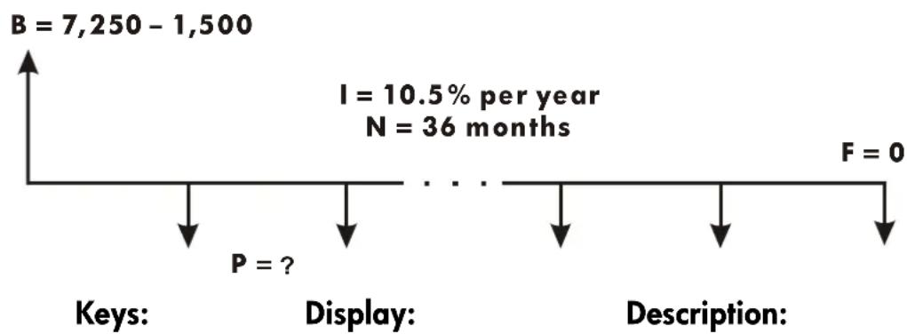
DISP {FX}
2
EQN (Px100×(1-(1+
↓ as needed)
SOLVE P I?value
10.5 ENTER 12 I?0.88
÷
R/S N?value
Selects FIX 2 display format.
Displays the leftmost part of the TVM equation.
Selects P; prompts for I.
Converts your annual interest rate input to the equivalent monthly rate.
Stores 0.88 in I; prompts for N.
17-4 Miscellaneous Programs and Equations
| 36 R/S | F?value | Stores 36 in N; prompts for F. |
| 0 R/S | B?value | Stores 0 in F; prompts for D. |
| 7250 ENTER | B?5,750.00 | Calculates B, the beginning loan balance. |
| 1500 — | ||
| R/S | SOLVING | Stores 5750 in B; calculates monthly payment, P. |
| P=-186.89 |
The answer is negative since the loan has been viewed from the borrower's perspective. Money received by the borrower (the beginning balance) is positive, while money paid out is negative.
Part 2. What interest rate would reduce the monthly payment by \$10?
| Keys: | Display: | Description: |
| EQN | P×100×(1-(1+ | Displays the leftmost hart of the TVM equation. |
| SOLVE I | P?-186.89 | Selects I; prompts for P. |
| RND | P?-186.89 | Rounds the payment to two decimal places. |
| 10 + | P?-176.89 | Calculates new payment. |
| R/S | N?36.00 | Stores -176,89 in P; prompts for N. |
| R/S | F?0.00 | Retains 36 in N; prompts for F. |
| R/S | B?5,750.00 | Retains 0 in F; prompts for B. |
| R/S | SOLVING | Retains 5750 in B; calculates monthly interest rate. |
| I=0.56 | ||
| 12 × | 6.75 | Calculates annual interest, rate. |
Part 3. Using the calculated interest rate (6.75%), assume that you sell the car after 2 years. What balance will you still owe? In other words, what is the future balance in 2 years?
Miscellaneous Programs and Equations 17–5
Note that the interest rate, I , from part 2 is not zero, so you won't get a DIVIDE BY 0 error when you calculate the new I .
| Keys: | Display: | Description: |
| EQN | Px100×(1-(1+ | Displays leftmost part of the TVM equation. |
| SOLVE F | P?-176.89 | Selects F; prompts for P. |
| R/S | I?0.56 | Retains P; prompts for I. |
| R/S | N?36.00 | Retains 0.56 in I; prompts for N. |
| 24 R/S | B?5,750.00 | Stores 24 in N; prompts for B. |
| R/S | SOLVING | Retains 5750 in B; calculates F, the future balance. Again, the sign is negative, indicating that you must, pay out this money. |
| F=-2,047.05 | ||
| DISP {FX} 4 | Sets FIX 4 display format. |
Prime Number Generator
This program accepts any positive integer greater than 3. If the number is a prime number (not evenly divisible by integers other than itself and 1), then the program returns the input value. If the input is not a prime number, then the program returns the first prime number larger than the input.
The program identifies non-prime numbers by exhaustively trying all possible factors. If a number is riot prime, the program adds 2 (assuring that the value is still odd) and tests to see if it, has found a prime. This process continues until a prime number is found.
17–6 Miscellaneous Programs and Equations
![graph TD A["LBL Y"] --> B["VIEW Prime"] B --> C["LBL Z"] C --> D["P + 2 → x"] D --> E["LBL P"] E --> F["x → P\n3 →D"] F --> G["LBL X"] G --> H["FP [P/∅ ×"] H --> I{x = 0?} I -->|yes| J["D >√P ?"] I -->|no| K["D + 2 → D"] J --> L["Start"] K --> L L --> E style A fill:#fff,stroke:#000 style B fill:#ff…](/content/2026/05/973866/images/2fe831b54e1887fe255bf9658e7a1177ecaef25fe151592f368a776e7770bc32.jpg)
Miscellaneous Programs and Equations 17–7
Program Listing:
Program Lines: Description
Y01 LBL Y This routine displays prime number P.
Y02 VIEW P
Checksum and length: 5D0B 003.0
Z01 LBL Z This routine adds 2 to P.
2022
Z03 RCL+P
Checksum and length: 0C68 004.5
P01 LBL P This routine stores the input value for P.
P02 STO P
P03 2
P04 ÷
P05 FP
P06 0
P07 x=y? Tests for even input.
P08 1
P09 STO+ P
P10 3 Increments P if input an even number.
P11 STO D Stores 3 in test divisor, D.
Checksum and length: 40BA 016.5
X01 LBL X This routine tests P to see if it is prime.
X02 RCL P
X03 RCL÷D
X04 FP Finds the fractional part of P ÷ D .
X05 x=0? Tests for a remainder of zero (not prime).
X06 GTO Z If the number is not prime, tries next possibility.
X07 RCL P
X08 SQRT
X09 RCL D
X10 x>y? Tests to see whether all possible factors have been tried.
17–8 Miscellaneous Programs and Equations
Program Lines: Description
X11 GTO Y If all factors have been tried, branches to the display routine.
X12 2 Calculates the next possible factor, D + 2.
X13 STO+ D
X14 GTO X Branches to test potential prime with new factor.
Checksum and length: 061F 021.0
Flags Used:
None.
Memory Required:
61 bytes: 45 for program, 16 for variables.
Program Instructions:
- Key in the program routines; press C when done.
- Key in a positive integer greater than 3.
- Press XEQ P to run program. Prime number, P will be displayed.
- To see the next prime number, press R/S.
Variables Used:
P Prime value and potential prime values.
D Divisor used to test the current value of P.
Remarks:
No test is made to ensure that the input is greater than 3.
Example.
What is the first prime number after 789? What is the next prime number?
Keys:
Display:
Description:
Miscellaneous Programs and Equations 17–9
789 XEQ P
P=797.0000
Calculates next prime number after 789.
R/S
P=809.0000
Calculates next prime number after 797.
Part 3
Appendixes and Reference
A
Support, Batteries, and Service
Calculator Support
You can obtain answers to questions about using your calculator from our Calculator Support Department. Our experience shows that many customers have similar questions about our products, so we have provided the following section, "Answers to Common Questions." If you don't find an answer to your question, contact us at the address or phone number listed on the inside back cover.
Answers to Common Questions
Q: How can I determine if the calculator is operating properly?
A: Refer to page A–5, which describes the diagnostic self-test.
Q. My numbers contain commas instead of periods as decimal points. How do I restore the periods?
A: Use the ⬇ MODES { } function (page 1–14).
Q: How do I change the number of decimal places in the display?
A: Use the ◀ DISP menu (page 1–15).
Q; How do 1 clear all or portions of memory?
A: CLEAR displays the CLEAR menu, which allows you to clear all variables, all programs (in program entry only), the statistics registers, or all of user memory (not during program entry).
Q: What does an "E" in a number (for example, 2.51E-13) mean?
Support, Batteries, and Service A-1
A: Exponent of ten; that is, 2.51 × 10⁻¹³ .
Q: The calculator has displayed the message MEMORY FULL. What should I do?
A: You must clear a portion of memory before proceeding. (See appendix B.)
Q: Why does calculating the sine (or tangent) of π radians display a very small number instead of 0?
A: π cannot be represented exactly with the 12-digit precision of the calculator.
Q: Why do I get incorrect answers when I use the trigonometric functions?
A: You must make sure the calculator is using the correct angular mode ( MODES {DG}, {RD}, or {GR}).
Q. What does the symbol in the display mean?
A: This is an annuncidor, and it indicates something about the status of the calculator. See "Annunciators" in chapter 1.
Q: Numbers show up as fractions. How do I get decimal numbers?
A: Press ← FDISP.
Environmental Limits
To maintain product reliability, observe the following temperature and humidity limits:
■ Operating temperature: 0 to 45 °C (32 to 113 °F).
■ Storage temperature: -20 to 65°C (-4 to 149°F).
■ Operating and storage humidity: 90% relative humidity at 40° C (104 °F) maximum.
A-2 Support, Batteries, and Service
Changing the Batteries
Replace the batteries as soon as possible when the low battery annunciator (☐) appears. If the battery annunciator is on, and the display dims, you may lose data. If data is lost, the MEMORY CLEAR message is displayed.
Once you've removed the batteries, replace them within 2 minutes to avoid losing stored information. (Have the new batteries readily at hand before you open the battery compartment.) Use any brand of fresh I.E.C LR44 (or manufacturer's equivalent) button-cell batteries.
Equivalent 1.5-volt, button-cell batteries you might find from various manufacturers are LR44, A76, V13GA, KA76, 357, SP357, V357, and SR44W.
- Have three fresh button-cell batteries at hand. Avoid touching the battery terminals — handle batteries only by their edges.
- Make sure the calculator is OFF. Do not press ON (C) again until the entire battery-changing procedure is completed. If the calculator is ON when the batteries are removed, the contents of Continuous Memory will be erased.
- Remove the battery-compartment door by pressing down and outward on it until the door slides off (left illustration).
A-3 picture
- Turn the calculator over and shake the batteries out.
Warning

Do not mutilate, puncture, or dispose of batteries in fire. The batteries can burst or explode, releasing hazardous chemicals.
- Insert the new batteries (right illustration). Stack them according to the diagram inside the battery compartment.
- Replace the battery-compartment door (slide the tab on the door back into the slot in the calculator case).
Support, Batteries, and Service A-3
Testing Calculator Operation
Use the following guidelines to determine if the calculator is working properly. Test the calculator after every step to see if its operation has been restored. If your calculator requires service, refer to page A–7.
■ The calculator won't turn on (steps 1–4) or doesn't respond when you press the keys (steps 1–3):
- Reset the calculator. Hold down the C key and press LN. It may be necessary to repeat these reset keystrokes several times.
- Erase memory. Press and hold down C, then press and hold down both and + , Memory is cleared and the MEMORY CLEAR message is displayed when you release all three keys.
- Remove the batteries (see "Changing the Batteries") and lightly press a coin against both battery contacts in the calculator. Replace the batteries and turn on the calculator. It should display MEMORY CLEAR.
- Install new batteries (see "Changing the Batteries").
If these steps fail to restore calculator operation, it requires service.
■ If the calculator responds to keystrokes but you suspect that it is malfunctioning:
- Do the self-test described in the next section. If the calculator fails the self test, it requires service.
- If the calculator passes the self-test, you may have made a mistake operating the calculator. Reread portions of the manual and check "Answers to Common Questions" (page A-1).
- Contact the Calculator Support Department. The address and phone number are listed on the inside back cover.
A-4 Support, Batteries, and Service
The Self-Test
If the display can be turned on, but the calculator does not seem to be operating properly, do the following diagnostic self-test.
- Hold down the C key, then press yx , at the same time.
- Press any key eight times and watch the various patterns displayed. After you've pressed the key eight times, the calculator displays the copyright message COPR, HP87, 90 and then the message KBD 01.
- Starting at the upper left corner ( ) and moving from left to right, press each key in the top row. Then, moving left to right, press each key in the second row, the third row, and so on, until you've pressed every key.
If you press the keys in the proper order and they are functioning properly, the calculator displays KB0 followed by two-digit numbers. (The calculator is counting the keys using hexadecimal base.)
If you press a key out of order, or if a key isn't functioning properly, the next keystroke displays a fail message (see step 4).
- The self-test produces one of these two results:
■ The calculator displays 3211-0K if it passed the self-test. Go to step 5.
The calculator displays 32SII-FAIL followed by a one-digit number, if it failed the self-test. If you received the message because you pressed a key out of order, reset the calculator (hold down C, press LN) and do the self test again. If you pressed the keys in order, but got this message, repeat the self-test to verify the results. If the calculator fails again, it requires service (see page A-7). Include a copy of the fail message with the calculator when you ship it for service.
- To exit the self-test, reset the calculator (hold down C and press LN).
Pressing C and 1/x starts a continuous self-test that is used at the factory. You can halt this factory test by pressing any key.
Support, Batteries, and Service A-5
Limited One-Year Warranty
What Is Covered
The calculator (except for the batteries, or damage caused by the batteries) is warranted by Hewlett-Packard against defects in materials and workmanship for one year from the date of original purchase. If you sell your unit or give it as a gift, the warranty is automatically transferred to the new owner and remains in effect for the original one-year period. During the warranty period, we will repair or, at our option, replace at no charge a product that proves to be defective, provided you return the product, shipping prepaid, to a Hewlett-Packard service center. (Replacement may be with a newer model of equivalent or better functionality.
This warranty gives you specific legal rights, and you may also have other rights that vary from state to state, province to province, or country to country.
What Is Not Covered
Batteries, and damage caused by the batteries, are not covered by the Hewlett-Packard warranty. Check with the battery manufacturer about battery and battery leakage warranties.
This warranty does not apply if the product has been damaged by accident or misuse or as the result of service or modification by other than an authorized Hewlett-Packard service center.
No other express warranty is given. The repair or replacement of a product is your exclusive remedy. ANY OTHER IMPLIED WARRANTY OF MERCHANTABILITY OR FITNESS IS LIMITED TO THE ONE-YEAR DURATION OF THIS WRITTEN WARRANTY. Some states, provinces, or countries do not allow limitations on how long an implied warranty lasts, so the above limitation may not apply to you. IN NO EVENT SHALL HEWLETT-PACKARD COMPANY BE LIABLE FOR CONSEQUENTIAL DAMAGES. Some states, provinces, or countries do not allow the exclusion or limitation of incidental or consequential damages, so the above limitation or exclusion may not apply to you.
A-6 Support, Batteries, and Service
Products are sold on the basis of specifications applicable at the time of manufacture. Hewlett–Packard shall have no obligation to modify or update products once sold.
Consumer Transaction in the United Kingdom
This warranty shall not apply to consumer transactions and shall not affect the statutory rights of a consumer. In relation to such transactions, the rights and obligations of Seller and Buyer shall be determined by statute.
If the Calculator Requires Service
Hewlett-Packard maintains service centers in many countries. These centers will repair a calculator or replace it (with an equivalent or newer model), whether it is under warranty or not. There is a charge for service after the warranty period. Calculators normally are serviced and reshipped within 5 working days.
In the United States: Send the calculator to the Calculator Service Center listed on the inside of the back cover.
In Europe: Contact your HP sales office or dealer, or HP's European headquarters for the location of the nearest service center. Do not ship the calculator for service without first contacting a Hewlett-Packard office.
Hewlett-Packard S.A.
In other countries: Contact your HP sales office or dealer or write to the U.S. Calculator Service Center (listed on the inside of the back cover) for the location of other service centers. If local service is unavailable, you can ship the calculator to the U.S. Calculator Service Center for repair.
Support, Batteries, and Service A-7
All shipping, reimportation arrangements, and customs costs are your responsibility.
Service Charge
There is a standard repair charge for out-of-warranty service. The Calculator Service Center (listed on the inside of the back cover) can tell you how much this charge is. The full charge is subject to the customer's local sales or value-added tax wherever applicable.
Calculator products damaged by accident or misuse are not covered by the fixed service charges. In these cases, charges are individually determined based on time and material.
Shipping Instructions
If your calculator requires service, ship it to the nearest authorized service center or collection point. Be sure to:
■ Include your return address and description of the problem.
■ Include proof of purchase date if the warranty has not expired.
■ Include a purchase order, check, or credit card number plus expiration date (Visa or MasterCard) to cover the standard repair charge. In the United States and some other countries, the serviced calculator can be returned C.O.D. if you do not pay in advance.
- Ship the calculator in adequate protective packaging to prevent damage. Such damage is not covered by the warranty, so we recommend that you insure the shipment.
Pay the shipping charges for delivery to the Hewlett-Packard service center, whether or not the calculator is under warranty.
Warranty on Service
Service is warranted against defects in materials and workmanship for 90 days from the date of service.
A-8 Support, Batteries, and Service
Service Agreements
In the U.S., a support agreement is available for repair and service. Refer to the form that was packaged with the manual. For additional information, contact the Calculator Service Center (see the inside of the back cover).
Regulatory Information
U.S.A. The HP 32SII generates and uses radio frequency energy and may interfere with radio and television reception. The calculator complies with the limits for a Class B computing device as specified in Subpart J of Part 15 of FCC Rules, which provide reasonable protection against such interference in a residential installation. In the unlikely event that there is interference to radio or television reception (which can be determined by turning the calculator off and on or by removing the batteries), try:
■ Reorienting the receiving antenna.
■ Relocating the calculator with respect to the receiver.
For more information, consult your dealer, an experienced radio or television technician, or the following booklet, prepared by the Federal Communications Commission: How to Identify and Resolve Radio-TV Interference Problems. This booklet is available from the U.S. Government Printing Office, Washington, D.C.20402, Stock Number 004=000-00345-4. At the first printing of this manual, the telephone number was (202) 783-3238.
West Germany. The HP 32SII complies with VFG 1046/84, VDE 0871B, and similar non-interference standards. If you use equipment that is not authorized by Hewlett-Packard, that system configuration has to comply with the requirements of Paragraph 2 of the German Federal Gazette, Order (VFG) 1046/84, dated December 14, 1984.
Noise Declaration. In the operator position under normal operation (per ISO 7779): LpA<70dB.
Support, Batteries, and Service A-9
B
User Memory and the Stack
This appendix covers
■ The allocation and requirements of user memory,
■ How to reset the calculator without affecting memory,
■ How to clear (purge) all of user memory and reset the system defaults, and
■ Which operations affect stack lift.
Managing Calculator Memory
The HP 32SII has 384 bytes of user memory available to you for any combination of stored data (variables, equations, or program lines). SOLVE, ∫ FN, and statistical calculations also require user memory. (The ∫ FN operation is particularly "expensive" to run.)
All of your stored data is preserved until you explicitly clear it. The message MEMORY FULL means that there is currently not enough memory available for the operation you just attempted. You need to clear some (or all) of user memory. For instance, you can:
- Clear the contents of any or all variables (see "Clearing Variables" its chapter 3).
■ Clear any or all equations (see "Editing and Clearing Equations" in chapter 6).
■ Clear any or all programs (see "Clearing One or More Programs" in chapter 12).
Clear the statistics registers (press ← CLEAR {Σ}).
Clear all of user memory (press← CLEAR {ALL}).
User Memory and the Stack B-1
Memory Requirements
| Data or Operation Amount of Memory Used | |
| Variables 8 bytes per non-zero | value. (No bytes for zero values.) |
| Instructions in program lines 1.5 | bytes. |
| Numbers in program lines Integers 0 through 254: 1.5 bytes. All other numbers: 9.5 bytes. | |
| Operations in equations 1.5 bytes. | |
| Numbers in equations | Integers 0 through 254: 1.5 bytes. All other numbers: 9.5 bytes. |
| Statistics data | 48 bytes maximum (8 bytes for each non-zero summation register). |
| SOLVE calculations | 33.5 bytes. |
| ∫ FN (integration) calculations | 140 bytes. |
To see how much memory is available, press ⬆ MEM. The display shows the number of bytes available.
To see the memory requirements of specific equations in the equation list:
- Press ☐ EQN to activate Equation mode. (EQN LIST TOP or the left end of the current equation will be displayed.)
- If necessary, scroll through the equation list (press □ ↑ or □ ↓ ) until you see the desired equation.
- Press SHOW to see the checksum (hexadecimal) and length (in bytes) of the equation. For example, CK=7F49 009.0.
To see the total memory requirements of specific programs:
- Press ← MEM {PGM} to display the first label in the program list.
- Scroll through the program list (press ← ↑ or ← ↓ until you see the desired program label and size). For example, LBL F 012.0.
- Optional: Press 📄 SHOW to see the checksum (hexadecimal) and length (in bytes) of the program\$. For example, CK=5DER 012.0 for program F.
To see the memory requirements of an equation in a program:
B-2 User Memory and the Stack
- Display the program line containing the equation.
- Press SHOW to see the checksum and length. For example, CK=7F49 009.0.
To manually deallocate the memory allocated for a SOLVE or FN calculation that has been interrupted, press RTN. This deallocation is done automatically whenever you execute a program or another SOLVE or FN calculation.
Resetting the Calculator
If the calculator doesn't respond to keystrokes or if it is otherwise behaving unusually, attempt to reset it. Resetting the calculator halts the current calculation and cancels program entry, digit entry, a running program, a SOLVE calculation, an FN calculation, a VIEW display, or an INPUT display. Stored data usually remain intact.
To reset the calculator, hold down the C key and press LN. If you are unable to reset the calculator, try installing fresh batteries. If the calculator cannot be reset, or if it still fails to operate properly, you should attempt to clear memory using the special procedure described in the next section.
The calculator can reset itself if it is dropped or if power is interrupted.
Clearing Memory
The usual way to clear user memory is to press ← CLEAR {RLL}. However, there is 1 so more powerful clearing procedure that resets additional information and is useful if e keyboard is not functioning properly.
If the calculator fails to respond to keystrokes, and you are unable to restore operation by resetting it or changing the batteries, try the following MEMORY CLEAR procedure. These keystrokes clear all of memory, reset the calculator, and restore all format and modes to their original, default settings (shown below):
User Memory and the Stack B-3
- Press and hold down the C key.
- Press and hold down .
- Press + . (You will be pressing three keys simultaneously). When you release all three keys, the display shows MEMORY CLEAR if the operation is successful.
| Category | CLEAR | ALL MEMORY(Default) |
| Angular mode | Unchanged | Degrees |
| Base mode | Unchanged | Decimal |
| Contrast setting | Unchanged | Medium |
| Decimal point | Unchanged | ". " |
| Denominator (/c value) | Unchanged | 4095 |
| Display format | Unchanged | FIX 4 |
| Flags | Unchanged | Cleared |
| Fraction-display mode | Unchanged | Off |
| Random-number seed | Unchanged | Zero |
| Equation pointer | EQN LIST TOP | EQN LIST TOP |
| Equation list | Cleared | Cleared |
| FN = label | Null | Null |
| Program pointer | PRGM TOP | PRGM TOP |
| Program memory | Cleared | Cleared |
| Stack lift | Enabled | Enabled |
| Stack registers | Cleared to zero | Cleared to zero |
| Variables | Cleared to zero | Cleared to zero |
CLEA
Memory may inadvertently be cleared if the calculator is dropped or if power is interrupted.
The Status of Stack Lift
The four stack registers are always present, and the stack always has a stack-lift status. That is to say, the stack lift is always enabled or disabled regarding its behavior when the next number is placed in the X-register. (Refer to chapter 2, "The Automatic Memory Stack.")
B-4 User Memory and the Stack
All functions except those in the following two lists will enable stack lift.
Disabling Operations
The four operations ENTER, + , - , and CLx disable stack lift. A number keyed in after one of these disabling operations writes over the number currently in the X-register. The Y-, Z- and T-registers remain unchanged.
In addition, when C and ← act like CLx, they also disable stack lift.
The INPUT function disables stack lift as it halts a program for prompting (so any number you then enter writes over the X-register), but it enables stack lift when the program resumes.
Neutral Operations
The following operations do not affect the status of stack lift:
| DEG, RAD, GRADPSE SHOW | FIX, SCI, ENG, ALLRADIX . | DEC, HEX, OCT, BINRADIX , | CLVARSCLΣ | |
| OFF | R/S and STOP | ↑ and↓ | C * and ← * | |
| MEM {VAR}**EQN | MEM {PGM}**FDISP | GTO · Errors | GTO □ label nnPRGM andprogram entry | |
| Switching binary windows | Digit entry | |||
| * Except when used like CLx.** Including all operations performed while the catalog is displayed except {VAR} ENTER and {PGM} XEQ, which enable stack lift. | ||||
User Memory and the Stack B-5
The Status of the LAST X Register
The following operations save x in the LAST X register:
+, -, × , ÷ SQRT , ^ 2 x e ^ x, 1 0 x
LN, LOG y x, √ [x]y 1 / x
x, y SIN,COS,TAN
SINH, COSH, TANH amp; ASINH, ACOSH, amp; IP, FP, RND, ABS amp; ATANH
%, % CHG +, - RCL+, -, × , ÷
y, x → θ , r → HR, → HMS → DEG, → RAD
θ , r → y, x
Cn, r x! CMPLX + / -
Pn, r
CMPLX + . - , x , ÷ amp; CMPLX ex, LN, yx, amp; CMPLX SIN, COS, amp; 1 / x amp; TAN
→ kg, → lb, → ^ ° C, → ^ ° F → cm, → in
→ , → gal
Notice that /c does riot affect the LAST X register,
The recall–arithmetic sequence x RCL + variable stores a different value in the LAST X register than the sequence x RCL variable + does. The former stores x in LAST X; the latter stores the recalled number in LAST X.
B-6 User Memory and the Stack
C
More about Solving
This appendix provides information about the SOLVE operation beyond that given in chapter 7.
How SOLVE Finds a Root
SOLVE is an iterative operation; that is, it repetitively executes the specified equation. The value returned by the equation is a function f(x) of the unknown variable x. ( f(x) is mathematical shorthand for a function defined in terms of the unknown variable x.) SOLVE starts with an estimate for the unknown variable, x, and refines that estimate with each successive execution of the function, f(x) .
If any two successive estimates of the function f(x) have opposite signs, then SOLVE presumes that the function f(x) crosses the x-axis in at least one place between the two estimates. This interval is systematically narrowed until a root is found.
For SOLVE to find a root, the root has to exist within the range of numbers of the calculator, and the function must be mathematically defined where the iterative search occurs. SOLVE always finds a root, provided one exists (within the overflow bounds), if one or more of these conditions are met:
■ Two estimates yield f(x) values with opposite signs, and the function's graph crosses the x-axis in at least one place between those estimates (figure a, below).
■ f(x) always increases or always decreases as x increases (figure b, below).
The graph of f(x) is either concave everywhere or convex everywhere (figure c, below).
More
abou
If f(x) has one or more local minima or minima, each occurs singly between adjacent roots off f(x) (figure d, below).
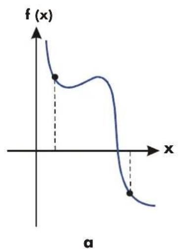
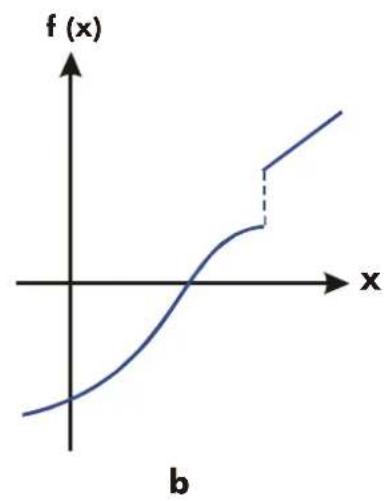

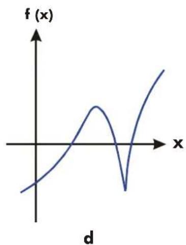
Function Whose Roots Can Be Found
In most situations, the calculated root is an accurate estimate of the theoretical, infinitely precise root of the equation. An "ideal" solution is one for which f(x) = 0 . However, a very small non-zero value for f(x) is often acceptable because it might result from approximating numbers with limited (12-digit) precision.
C-2 More about Solving
Interpreting Results
The SOLVE operation will produce a solution under either of the following conditions:
If it finds an estimate for which f(x) equals zero. (See figure a, below.)
If it finds an estimate where f(x) is not equal to zero, but the calculated root is a 12-digit number adjacent to the place where the function's graph crosses the x -axis (see figure b, below). This occurs when the two final estimates are neighbors (that is, they differ by 1 in the 12th digit), and the function's value is positive for one estimate and negative for the other. Or they are (0, 10-499) or (0, -10-499) . In most cases, f(x) will be relatively close to zero.
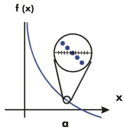

Cases Where a Root Is Found
To obtain additional information about the result, press see the previous estimate of the root (x), which was left in the Y-register. Press again to see the value of f(x) , which was left in the Z-register. If f(x) equals zero or is relatively small, it is very likely that a solution has been found. However, if f(x) is relatively large, you must use caution in interpreting the results.
Example: An Equation With One Root.
Find the root of the equation:
- 2 x ^ 3 + 4 x ^ 2 - 6 x + 8 = 0
Enter the equation as an expression:
More
abou
| Keys: | Display: | Description: |
| Select Equation mode. | ||
| 2 +/- × | Enters the equation. | |
| RCL X yx 3 | ||
| + 4 × | ||
| RCL X yx 2 | ||
| - 6 × RCL X | ||
| + 8 ENTER | -2×X^3+4X^2- | |
| CK=0C6A 035.0 | Clecksum and length. | |
| Cancels Equation mode. |
Now, salve the equation to find the root:
| Keys: | Display: | Description: |
| 0 STO X 10 | 10_ | Initial guesses for the root. |
| EQN | -2xX^3+4xX^2- | Selects Equation mode; displays the left end of the equation. |
| SOLVE X | SOLVING | Solves for X; displays the result. |
| X=1.6506 | ||
| R↓ | 1.6506 | Final two estimates are the same to four decimal places. |
| R↓ | -4.0000E-11 | f(x) is very small, so the approximation is a good root. |
Example: An Equation with Two Roots.
Find the two roots of the parabolic equation:
x ^ 2 + x - 6 = 0.
Enter the equation as an expression:
C-4 More about Solving
Keys:



Display:
Selects Equation mode.
Enters the equation.
Checksum and length.
Cancels Equation mode.
Now, solve the equation to find its positive and negative roots:
| Keys: | Display: | Description: |
| 0 STO X 10 | 10_ | Your initial guesses for the positive root. |
| EQN | X2 + X - 6 | Selects Equation mode; displays the equation. |
| SOLVE X | SOLVING | Calculates the positive root using guesses 0 an 10. |
| X = 2.0000 | ||
| R↓ | 2.000 | Final two estimates are they same. |
| R↓ SHOW | 0.000000000000 | f( x) = 0 . |
| 0 STO X 10 +/- | -10_ | Your initial guesses for the negative root. |
| EQN | X2 + X - 6 | Redisplays the equation. |
| SOLVE X | SOLVING | Calculates negative root using guesses 0 and -10. |
| X = -3.0000 | ||
| R↓ R↓ SHOW | 0.000000000000 | f( x) = 0 . |
Certain cases require special consideration:
If the function's graph has a discontinuity that crosses the x-axis, then the SOLVE operation returns a value adjacent to the discontinuity (see figure a, below). In this case, f(x) may be: relatively large.
■ Values of f(x) may be approaching infinity at the location where the graph changes sign (see figure b, below). This situation is called a pole. Since the SOLVE operation determines that there is a sign change
More
abou
between two neighboring values of x, it returns the possible root. However, the value for f(x) will be relatively large. If the pole occurs at a value of x that is exactly represented with 12 digits, then that value would cause the calculation to halt with an error message.

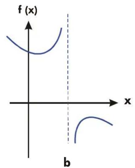
Special Case: A Discontinuity and a Pole
Example: Discontinuous Function.
Find the root of the equation:
IP (x) = 1. 5
Enter the equation:
Keys:
Display:
Description:

Selects Equation mode. Enter the equation.



CK = 8 A 5 5 0 1 7. 0
Checksum and length.
C-6 More about Solving

Cancels Equation mode.
Now, solve to find the root:
| Keys: | Display: | Description: |
| 0 STO X 5 | 5_ | Your initial guesses for the root. |
| EQN | IP(X)=1.5 | Selects Equation mode; displays the equation. |
| SOLVE X | SOLVING | Finds a root with guesses 0 and 5. |
| X=2.0000 | ||
| SHOW | 1.99999999999 | Shows root, to 11 decimal places. |
| SHOW | 2.00000000000 | The previous estimate is slightly bigger. |
| R | -5.000 | f(x) is relatively large. |
Note the difference between the last two estimates, as well as the relatively large value for f(x) . The problem is that there is no value of x for which f(x) equals zero. However, at x = 1.99999999999, there is a neighboring value of x that yields ant opposite sign for f(x) .
Example: A Pole.
Find the root of the equation
xx ^ 2 - 6 - 1 = 0
As x approaches √6 , f(x) becomes a very large positive or negative number.
Enter the equation as an expression.
Keys:
Display:
Description:

Selects Equation mode.
More
abou
RCL X ÷
Enters the equation.
( RCL X
yx 2 - 6
→ ) - 1
ENTER X÷(X^2-6))-1
SHOW CK=CF7C 018.0
Cancels Equation mode.
Now, solve to find the root.
Keys:
Display:
Description:
2.3 STO X 2.7 2.7
EQN
X ÷ (X2-6) - 1
Your initial guesses for the root.
Selects Equation mode; displays the equation.
SOLVE X SOLVING
X=2.4495
Calculates the root using guesses that bracket √6 .
81,649,658,092,0f(x) is relatively large.
There is a pole between the final estimates. The initial guesses yielded opposite signs for f(x) , and the interval between successive estimates was narrowed until two neighbors were found. Unfortunately, these neighbors made f(x) approach a pole instead of the x-axis. The function does have roots at -2 and 3, which can be found by entering better guesses.
When SOLVE Cannot Find Root
Sometimes SOLVE fails to find a root. The following conditions cause the message NO ROOT FIND:
The search terminates near a local minimum or maximum (see figure a, below). If the ending value of f(x) (stored in the Z-register) is relatively close to zero, it is possible that a root has been found; the number stored in the unknown variable might be a 12-digit number very close to a theoretical root.
C-8 More about Solving
■ The search halts because SOLVE is working on a horizontal asymptote—an area where f(x) is essentially constant for a wide range of x (see figure b, below). The ending value of f(x) is the value of the potential asymptote.
The search is concentrated in a local "flat" region of the function (see figure c, below). The ending value of f(x) is the value of the function in this region.
f(x)

a
f (x)

b
f(x)

C
Case Where No Root Is Found
The SOLVE operation returns a math error if an estimate produces an operation that is not allowed — for example, division by zero, a square root of a negative number, or a logarithm of zero. Keep in mind that SOLVE can generate estimates over a wide range. You can sometimes avoid math errors by using good guesses. If a math error occurs, press RCL unknown variable (or VIEW variable) to see the value that produced the error.
More
abou
Example: A Relative Minimum.
Calculate the root of this parabolic equation:
x ^ 2 - 6 x + 1 3 = 0.
It has a minimum at x = 3.
Enter the equation as an expression:
Keys:
Display:
Description:

Selects Equation mode.

Enters the equation.

13 ENTER X^2-6xX+13

Checksum and length.
C CK=5FCC 015.0 Cancels Equation mode.
Now, solve to find the root:
Keys:
Display:
Description:
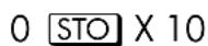
10
Your initial guesses for the root.

X^2-6×X+13
Selects Equation mode; displays the equation.

NO ROOT FND
Search fails with guesses 0 and 10

3.000000100001
Displays the final estimate of x.

3.00000468443
Previous estimate was not the same.

Final value for f(x) is relatively large.
Example: An Asymptote.
Find the root of the equation
C-10 More about Solving
1 0 - 1/X = 0
Enter the equation as an expression.
| Keys: | Display: | Description: |
| Selects Equation mode. | ||
| 10 — 1/x RCL X | Enters the equation. | |
| 10-INV(X) | ||
| CK=6C6D 09.0 | Checksum and length. | |
| .005 STO X 5 | 5_ | Cancels Equation mode. |
| 10-INV(X) | Your positive guesses for the root. | |
| X=0.1000 | Selects Equation mode; displays the equation. | |
| 0.1000 | Solves for x using guesses 0.005 and 5. | |
| 0.00000000000 | Previous estimate is the same. |
Watch what happens when you use negative values for guesses:
| Keys: | Display: | Description: |
| 1 +/- STO X | -1.0000 | Your negative guesses for the root. |
| 2 +/- EQN | 10-INV(X) | Selects Equation mode; displays the equation. |
| SOLVE X | NO ROOT FND | No root found for f(x). |
| ← | -46.666,666,692.1 | Displays last estimate of x. |
| R↓ | -5.7750E15 | Previous estimate was much larger. |
| R↓ | 10.0000 | f(x) for last estimate is rather large. |
More
abou
It's apparent from inspecting the equation that if x is a negative number, the smallest that f(x) can be is 10. f(x) approaches 10 as x becomes a negative number of large magnitude.
Example: A Math Error.
Find the root of the equation:
√ [x ÷ (x + 0 . 3)] - 0. 5 = 0
Enter the equation as an expression:
Keys:







Description:
Selects Equation mode.
Enters the equation.
First attempt to find a positive root:
Keys:


Display:
10_
SQRT(X÷(X+0.3
X=0.1000
Description:
Your positive guesses for the root.
Selects Equation mode; displays the left end of the equation.
Calculates the root using guesses 0 and 10.
Now attempt to find a negative root by entering guesses 0 and -10. Notice that the function is undefined for values of x between 0 and -0.3 since those values produce a positive denominator but a negative numerator, causing a negative square root.
C-12 More about Solving
Keys:
Display:
Description:
0 STO X 10 +/- -10_

SQRT(X÷(X+0.3
Selects Equation mode; displays the left end of the equation.
SOLVE X SQRT(NEG)
Math error.

Clears error message; cancels Equation mode.
VIEW X = -0.1988
Displays the final estimate of x.
Example : A Local "Flat" Region.
Find the root of the function
f (x) = x + 2 if x lt; - 1,
f (x) = 1 for - 1 ≤ x ≤ 1 ( a local flat region ),
f (x) = - x + 2 if x gt; 1.
Enter the function as the program:
J01 LBL J
J02 -
J03 ENTER
J04 2
J05 RCL+ X
J06 x<y
J07 RTN
J08 4
J09 -
J10+/-
J11 x>y?
J 12 R↓
J13 RTN
Checksum and length: 23C2 019.5
You can subsequently delete line J03 to save memory.
More
abou
Solve for X using initial guesses of 10-8 and -10-8 .
| Keys: | Display: | Description: |
| E 8 +/- STO X | -1E-8_ | Enters guesses. |
| 1 +/- E 8 +/- | ||
| FN= J | -1.0000E-8 | Selects program "J" as the function. |
| SOLVE X | NO ROOT FND | No root found using very small guesses near zero (thereby restricting the search to the flat region of the function). |
| 1.0000E-8 | The last two estimates are far apart, and the final value of f(x) is large. | |
| R↓ | 0.0025 | |
| R↓ | 1.0000 |
If you use larger guesses, then SOLVE can find the roots, which are outside the flat region (at x = 2 and x = -2).
Round-Off Error
The limited (12-digit) precision of the calculator can cause errors due to rounding off, which adversely affect the iterative solutions of SOLVE and integration. For example,
[(| x | + 1) + 1 0 ^ 1 5] ^ 2 - 1 0 ^ 3 0 = 0
has no roots because f(x) is always greater than zero. However, given initial guesses of 1 and 2, SOLVE returns the answer 1.0000 due to round-off error.
Round-off error can also cause SOLVE to fail to find a root. The equation
| 2 amp; | = √ 7
has a root at √7 . However, no 12-digit number exactly equals √7 , so the calculator can never make the function equal to zero. Furthermore, the
C-14 More about Solving
function never changes sign SOLVE returns the message NO ROOT FIND. However, the final estimate of x (press ← to see it) is the best possible 12-digit approximation of the root when the routine quits.
Underflow
Underflow occurs when the magnitude of a number is smaller than the calculator can represent, so it substitutes zero. This can affect SOLVE results. For example, consider the equation
1x ^ 2
whose root is infinite in value. Because of underflow, SOLVE returns a very large value as a root. (The calculator cannot represent infinity, anyway.)
More
abou
D
More about Integration
This appendix provides information about integration beyond that given in chapter 8.
How the Integral Is Evaluated
The algorithm used by the integration operation, FN dx , calculates the integral of a function f(x) by computing a weighted average of the function's values at many values of x (known as sample points) within the interval of integration. The accuracy of the result of any such sampling process depends on the number of sample points considered: generally, the more sample points, the greater the accuracy, if f(x) could be evaluated at an infinite number of sample points, the algorithm could — neglecting the limitation imposed by the inaccuracy in the calculated function f(x) — always provide an exact answer.
Evaluating the function at an infinite number of sample points would take forever. However, this is not necessary since the maximum accuracy of the calculated integral is limited by the accuracy of the calculated function values. Using only a finite number of sample points, the algorithm can calculate an integral that is as accurate as is justified considering the inherent uncertainty in f(x) .
The integration algorithm at first considers only a few sample points, yielding relatively inaccurate approximations. If these approximations are not yet as accurate as the accuracy of f(x) would permit, the algorithm is iterated (repeated) with a larger number of sample points. These iterations continue, using about twice as many sample points each time, until the resulting approximation is as accurate as is justified considering the inherent uncertainty in f(x) .
More
about
As explained in chapter 8, the uncertainty of the final approximation is a number derived from the display format, which specifies the uncertainty for the function. At the end of each iteration, the algorithm compares the approximation calculated during that iteration with the approximations calculated during two previous iterations. If the difference between any of these three approximations and the other two is less than the uncertainty tolerable in the final approximation, the calculations ends, leaving the current approximation in the X-register and its uncertainty in the Y-register.
It is extremely unlikely that the errors in each of three successive approximations — that is, the differences between the actual integral and the approximations — would all be larger than the disparity among the approximations themselves. Consequently, the error in the final approximation will be less than its uncertainty (provided that f(x) does not vary rapidly). Although we can't know the error in the final approximation, the error is extremely unlikely to exceed the displayed uncertainty of the approximation. In other words, the uncertainty estimate in the Y-register is an almost certain "upper bound" on the difference between the approximation and the actual integral.
Conditions That Could Cause Incorrect Results
Although the integration algorithm in the HP 32SII is one of the best available, in certain situations it — like all other algorithms for numerical integration—might give you an incorrect answer. The possibility of this occurring is extremely remote. The algorithm has been designed to give accurate results with almost any smooth function. Only for functions that exhibit extremely erratic behavior is there any substantial risk of obtaining an inaccurate answer. Such functions rarely occur in problems related to actual physical situations; when they do, they usually can be recognized and dealt with ire a straightforward manner.
Unfortunately, since all that the algorithm knows about f(x) are its values at the sample points, it cannot distinguish between f(x) and any other function that agrees with f(x) at all the sample points. This situation is depicted below,
D-2 More about Integration
showing (over a portion of the interval of integration) three functions whose graphs include the many sample points in common.

With this number of sample pints, the algorithm will calculate the same approximation for the integral of any of the functions shown. The actual integrals of the functions shown with solid blue and black lines are about the same, so the approximation will be fairly accurate if f(x) is one of these functions. However, the actual integral of the function shown with a dashed line is quite different from those of the others, so the current approximation will be rather inaccurate if f(x) is this function.
The algorithm cores to know the general behavior of the function by sampling the function at more and more points. If a fluctuation of the function in one region is not unlike the behavior over the rest of the interval of integration, at some iteration the algorithm will likely detect the fluctuation. When this happens, the number of sample points is increased until successive iterations yield approximations that take into account the presence of the most rapid, but characteristic, fluctuations.
For example, consider the approximation of
More
about
_ 0 ^ ∞ xe ^ - x dx
Since you're evaluating this integral numerically, you might think that you should represent the upper limit of integration as 10499 , which is virtually the largest cumber you ears key into the calculator.
Try it and what happens. Enter the function f(x) = x e-x .
Keys:
Display:
Description:

Select equation mode.

XxEXP(■
Enter the equation.

XxEXP(-X)
End of the equation.


CK=297F 010.5 Checksum and length.

Cancels Equation mode.
Set the display format to SCI 3, specify the lower and upper limits of integration as zero and 100499 , than start the integration.
Keys:
Display:
Description:

Specifies accuracy level and limits of integration.

1E499_

X×E×P(-X)
Selects Equation mode; displays the equation.

INTEGRATING
Approximation of the integral.
= 0,000E0
The answer returned by the calculator is clearly incorrect, since the actual integral of f(x) = xe-x from zero to ∞ is exactly 1. But the problem is not that ∞ was represented by 10499 , since the actual integral of this function from zero to 10499 is very close to 1. The reasons or the incorrect answer becomes apparent from the graph of f(x) over the interval of integration.
D-4 More about Integration

The graph is a spike very close to the origin. Because no sample point happened to discover the spike, the algorithm assumed that f(x) was identically equal to zero throughout the interval of integration. Even if you increased the number of sample points by calculating the integral in SCI 11 or ALL format, none of the additional sample points would discover the spike when this particular function is integrated over this particular interval. (For better approaches to problems such as this, see the next topic, "Conditions That Prolong Calculation Time.")
Fortunately, functions exhibiting such aberrations (a fluctuation that is uncharacteristic of the behavior of the function elsewhere) are unusual enough that you are unlikely to have to integrate one unknowingly. A function that could lead to incorrect results can be identified in simple terms by how rapidly it and its low-order derivatives vary across the interval of integration. Basically, the more rapid the variation in the function or its derivatives, and the lower the order of such rapidly varying derivatives, the less quickly will the calculation finish, and the less reliable will be the resulting approximation.
Note that the rapidity of variation in the function (or its low-order derivatives) must be determined with respect to the width of the interval of integration. With a given number of sample points, a function f(x) that has three
More
about
fluctuations can be better characterized by its samples when these variations are spread out over most of the interval of integration than if they are confined to only a small fraction of the interval. (These two situations are shown in the following two illustrations.) Considering the variations or fluctuation as a type of oscillation in the function, the criterion of interest is the ratio of the period of the oscillations to the width of the interval of integration: the larger this ratio, the more quickly the calculation will finish, and the more reliable will be, the resulting approximation.
D-6 More about Integration


In many cases you will be familiar enough with the function you want to integrate that you will know whether the function has any quick wiggles relative to the interval of integration. If you're not familiar with the function,
More
about
and you suspect that it may cause problems, you can quickly plot a few points by evaluating the function using the equation or program you wrote for that purpose.
If, for any reason, after obtaining an approximation to an integral, you suspect its validity, there's a simple procedure to verify it: subdivide the interval of integration into two or more adjacent subintervals, integrate the function over each subinterval, then add the resulting approximations. This causes the function to be sampled at a brand new set of sample points, thereby more likely revealing any previously hidden spikes. If the initial approximation was valid, it will equal the sum of the approximations over the subintervals.
Conditions That Prolong Calculation Time
In the preceding example, the algorithm gave an incorrect answer because it never detected the spike in the function. This happened because the variation in the function was too quick relative to the width of the interval of integration. If the width of the interval were smaller, you would get the correct answer; but it would take a very long time if the interval were still too wide.
Consider an integral where the interval of integration is wide enough to require excessive calculation time, but not so wide that it would be calculated incorrectly. Note that because f(x) = xe-x approaches zero very quickly as x approaches ∞ , the contribution to the integral of the function at large values of x is negligible. Therefore, you can evaluate the integral by replacing ∞ , the upper limit of integration, by a number not so large as 10499 - say 103 .
Rerun the previous integration problem with this new limit of integration:
Keys:
Display:
Description:
0 ENTER
E 3
1E3
New upper limit.
EQN
XxEXP(-X)
Selects Equation mode; displays the equation.
→ f X
INTEGRATING
Integral. (The calculation takes a
= 1,000E0
minute or two.)
D-8 More about Integration

1.824E-4
Uncertainty of approximation.
This is the correct answer, but it took a very long time. To understand why, compare the graph of the function between x = 0 and x = 103 , which looks about the same as that shown in the previous example, with the graph of the function between x = 0 and x = 10:
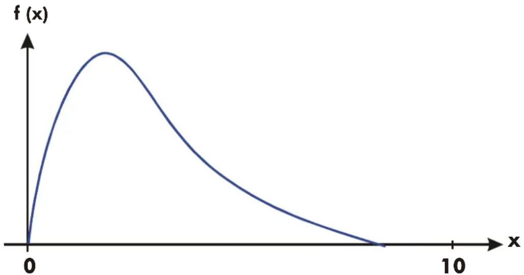
You can see that this function is "interesting" only at small values of x. At greater values of x, the function is not interesting, since it decreases smoothly and gradually in a predictable manner.
The algorithm samples the function with higher densities of sample points until the disparity between successive approximations becomes sufficiently small. For a narrow interval in an area where the function is interesting, it takes less time to reach this critical density.
To achieve the same density of sample points, the total number of sample points required over the larger interval is much greater than the number required over the smaller interval. Consequently, several more iterations are required over the larger interval to achieve an approximation with the same accuracy, and therefore calculating the integral requires considerably more time.
Because the calculation time depends on how soon a certain density of sample points is achieved in the region where the function is interesting, the
More
about
calculation of the integral of any function will be prolonged if the interval of integration includes mostly regions where the function is not interesting. Fortunately, if you must calculate such an integral, you can modify the problem so that the calculation time is considerably reduced. Two such techniques are subdividing the interval of integration and transformation of variables. These methods enable you to change the function or the limits of integration so that the integrand is better behaved over the intervals) of integration.
D-10 More about Integration
E
Messages
The calculator responds to certain conditions or keystrokes by displaying a message. The ⚠ symbol comes on to call your attention to the message. For significant conditions, the message remains until you clear it. Pressing ⓒ or ← clears the message; pressing am other key clears the message and executes that key's function.
∫ FN ACTIVE A running program attempted t select a program label (FN=label) while an integration calculation was running.
∫ (∫FN) A running program attempted to integrate a program (∫FN ∩ variable) while another integration calculation was running.
∫ (SOLVE) A running program attempted to solve a program while an integration calculation was running.
ALL VARS=0 The catalog of variables ( ← MEM {VAR}) indicates no values stored.
CALCULATING The calculator is executing a function that might take a while.
CLR EQN? Y N Allows you to verily clearing the equation you are editing. (Occurs only in Equation-entry mode.)
CLR PGMS? Y N Allows you to verify clearing all program in memory. (Occurs only in Program-entry mode.)
DIVIDE BY 0 Attempted to divide by zero. (Includes %CHG if Y-register contains zero.)
DUPLICAT.LBL Attempted to enter a program label that already exists for another program routine.
EQN LIST TOP Indicates the "top" of equation memory. The memory scheme is circular, so EQN LIST TOP is also the "equation" after the last equation in equation memory.
Messages
INTEGRATING
The calculator is calculating the integral of an equation or program. This might take a while.
INTERRUPTED
A running SOLVE or FN operation was interrupted by pressing C or R/S.
INVALID DATA
Data error:
■ Attempted to calculate combinations or permutations with r>n, with non-integer r or n, or with n ≥ 1012 .
■ Attempted to use a trigonometric or hyperbolic function with an illegal argument:
■ TAN with x an odd multiple of 90° .
■ ACOS or ASIN with x<-1 or x>1.
■ HYP ATAN with x ≤ -1 ; or x ≥ 1 .
■ HYP ACOS with x < 1.
INVALID EQN
A syntax error in the equation was detected during equation evaluation, SOLVE, or FN.
INVALID ×!
Attempted a factorial or gamma operation with x as a negative integer.
INVALID y x
Exponentiation error:
■ Attempted to raise 0 to the 0th power or to a negative power.
- Attempted to raise a negative number to a non-integer power.
■ Attempted to raise complex number (0 + i\ 0) to a number with a negative real part.
INVALID (i)
Attempted an operation with an indirect address, but the number in the index register is invalid ( |i| ≥ 34or |i| < 1 ).
LOG(0)
Attempted to take a logarithm of zero or (0 + i0) .
LOG(NEG)
Attempted to take a logarithm of a negative number.
MEMORY CLEAR
All of user memory has been erased (see page B-3).
MEMORY FULL
The calculator has insufficient memory available to do the operation (See appendix B).
NO
The condition checked by a test instruction is not true. (Occurs only when executed from the keyboard.)
E-2 Messages
| NONEXISTENT | Attempted to refer to a nonexistent program label (or line number) with GTO, GTO, XEQ, or {FN}. Note that the error NONEXISTENT can mean■ you explicitly (from the keyboard) called a program label that does not exist; or■ the program that you called referred to another label, which does not exist. |
| NO LABELS | The catalog of programs (MEM {PGM}) indicates no program labels stored. |
| NO ROOT FND | SOLVE cannot find the root of the equation using the current initial guesses (see page C-8). A SOLVE operation executed in a program does not produce this error; the same condition causes it instead to skip the next program line (the line following the instruction SOLVE variable). |
| OVERFLOW | Warning (displayed momentarily); the magnitude of a result is too large for the calculator to handle. The calculator returns ±9.99999999999E499 in the current display format. (See "Range of Numbers and Overflow" on page 1-12.) This condition sets flag 6. If flag 5 is set, overflow has the added effect of halting a running program and leaving the message in the display until you press a key. |
| PRGM TOP | Indicates the "top" of program memory. The memory scheme is circular, so PRGM TOP is also the "line" after the last line in program memory. |
| RUNNING | The calculator is running a program (other than a SOLVE or ∫FN routine). |
| SELECT FN | Attempted to execute SOLVE variable or ∫FN d variable without a selected program label. This can happen only the first time that you use SOLVE or ∫FN after the message MEMORY CLEAR, or it can happen if the current label no longer exists. |
| SOLVE ACTIVE | A running program attempted to select a program label (FN=label) while a SOLVE operation was running. |
| SOLVE(SOLVE) | A running program attempted to solve a program while a SOLVE operation was running. |
| SOLVE(∫FN) | A running program attempted to integrate a programwhile a SOLVE operation was running. |
| SOLVING | The calculator is solving an equation or program for its root. This might take a while. |
| SQRT (NEG) | Attempted to calculate the square root of a negative number. |
| STAT ERROR | Statistics error:■ Attempted to do a statistics calculation with n = 0.■ Attempted to calculate sx sy , x , y , m, r, or b with n = 1.■ Attempted to calculate r, x or with x-data only (all y-values equal to zero).■ Attempted to calculate x , y , r, m, or b with all x-values equal. |
| TOO BIG | The magnitude of the number is too large to be converted to HEX, OCT, or BIN base; the number must be in the range -34,359,738,368 ≤ n ≤ 34,359,738,367 . |
| XEQ OVERFLOW | A running program attempted an eighth nested XEQ label. (Up to seven subroutines can be nested.) Since SOLVE and FN each uses a level, they can also generate this error. |
| YES | The condition checked by a test instruction is true.(Occurs only when executed frown the keyboard. |
Messages
Self-Test Messages:
| 32SII-OK | The self-test and the keyboard test passed. |
| 32SII-FAIL n | The self test or the keyboard test failed, and the calculator requires service. |
| COPR, HP 87,90 | Copyright message displayed after successfully completing the self test. |
E-4 Messages
F
Operation Index
This section is a quick reference for all functions and operations and their formulas, where appropriate. The listing is in alphabetical order by the function's name. This name is the one used in program lines. For example, the function named FIX n is executed as ☑ DISP {FX} n.
Nonprogrammable functions have their names in key boxes. For example,
Non-letter and Greek characters are alphabetized before all the letters; function names preceded by arrows (for example, → DEG) are alphabetized as if the arrow were not there.
The last column, marked *, refers to notes at the end of the table.
| Name | Keys and | Description |
| +/- | + Changes the sign of a number. | 1-10 1 |
| + | + Addition. Returns y + x. | 1-13 1 |
| - | - Subtraction. Returns y - x. | 1-13 1 |
| × | × Multiplication. Returns y × x. | 1-13 1 |
| ÷ | ÷ Division. Returns y ÷ x. | 1-13 1 |
| ^ | yx Power. Indicates an exponent. | 6-17 2 |
| Deletes the last digit keyed in; clears x; clears a menu; erases last function keyed in an equation; starts equation editing; deletes a program step. | 1-2 1-7 6-3 12-6 | |
| Displays previous entry in catalog; moves to previous equation in equation list; moves program pointer to previous step. | 1-20 6-3 12-19 | |
| Displays next entry in catalog; moves | 1-20 |
Operation
| Name | Keys and | Desc | |
| to next equation in equation list;moves program pointer to next line(during program entry); executes the current program line (not during program entry). | 6-312-912-19 | ||
| 1/x | 1/x Reciprocal. | 1-12 | |
| 10x | 10x Common exponential.Returns 10 raised to the x power. | 4-2 | 1 |
| % | 2 % Percent.Returns (y × x) ÷ 100 . | 4-5 | 1 |
| %CHG | 2 %CHG Percent change.Returns (x - y)(100 ÷ y) . | 4-5 | 1 |
| π | 2 π Returns the approximation3.14159265359 (12 digits). | 4-3 | 1 |
| Σ+ | Σ+ Accumulates (y, x) into statistics registers. | 11-2 | |
| Σ- | 2 Σ- Removes (y, z) fromstatistics registers. | 11-2 | |
| Σx | 2 SUMS {x}Returns the sum of x-values. | 11-11 | 1 |
| Σx2 | 2 SUMS {x2}Returns the sum of squares of x-values. | 11-11 | 1 |
| Σxy | 2 SUMS {xy}Returns the sum of products of x-and y-values. | 11-11 | 1 |
| Σy | 2 SUMS {y}Returns the sum of y-values. | 11-11 | 1 |
| Σy2 | 2 SUMS {y2}Returns the sum of squares of y-values. | 11-11 | 1 |
| σx | 2 S,σ {σx}Returns population standard deviation of x-values: √ (xi - )2 ÷ n | 11-7 | 1 |
F-2 Operation Index
| Name | Keys and | Desc |
| σy | ,σ \σy\ Returns population standard deviation of y -values: √ (yi - )2 ÷ n | 11-7 |
| θ, r → y,x | →y,x Polar to rectangular coordinates. Converts (r, θ) to (x, y) . | 4-7 |
| FN \ d \ variable | ∫ \ FN \ d \ _\ variable Integrates the displayed equation or the program selected by FN=, using lower limit of the variable of integration in the Y-register and upper limit of the variable if integration in the X-register. | 8-214-7 |
| ( | () Open parenthesis. Starts a quantity associated with a function in an equation. | 6-7 |
| ) | () Close parenthesis. Ends a quantity associated with a function in an equation. | 6-7 |
| A through Z | variable or variable Value of named variable. | 6-5 |
| ABS | {ABS} Absolute value. Returns |X| . | 4-14 |
| ACOS | Arc cosine. Returns cos -1x . | 4-4 |
| ACOSH | Hyperbolic arc cosine. Returns cosh-1 x . | 4-5 |
| ALOG | 10x Common exponential. Returns 10 raised to the specified power (antilogarithm). | 6-17 |
| ALL | {ALL} Selects display of all significant digits. | 1-16 |
| ASIN | Arc sine | 4-4 |
| Returns -1 x. | ||
| ASINH | HYP ASINHyperbolic arc sine.Returns -1 x. | 4-5 |
| ATAN | ATAN Arc tangent.Returns -1 x. | 4-4 |
| ATANH | HYP ATANHyperbolic arc tangent.Returns -1 x. | 4-5 |
| b | L.R.{b}Returns the y-intercept of theregression line: - m . | 11-11 |
| BASE Displays | the base-conversion menu. 10-1 | |
| BIN | BASE {BN}Selects Binary (base 2) mode. | 10-1 |
| C | Turns on calculator; clears x; clearsmessages and prompts; cancelsmenus; cancels catalogs; cancelsequation entry; cancels programentry; halts execution of an equation;halts a running program. | 1-11-31-71-206-312-612-18 |
| /c | Denominator.Sets denominator limit for displayedfractions to x. If x = 1, displayscurrent /c value. | 5-5 |
| →°C | Converts ° F to ° C. | 4-11 |
| CF n | FLAGS {CF} nClears flag n (n = 0 through 11). | 13-12 |
| CLEAR | Displays menu to clear numbers orparts of memory; clears indicatedvariable or program from a MEMcatalog; clears displayed equation. | 1-41-20 |
| CLEAR {ALL} | Clears all stored data, equations,and programs. | 1-20 |
| CLEAR {PGM} | Clears all programs (calculator inProgram mode). | 12-22 |
Operation
F-4 Operation Index
| Name | Keys and | Description |
| CLEAR {EQN} | Clears the displayed equation (calculator in Program mode). | 12-6 |
| CLΣ | CLEAR {Σ} | 11-12 |
| Clears statistics registers. | ||
| CLVARS | CLEAR {VARS} | 3-3 |
| Clears all variables to zero. | ||
| CLx | CLEAR {x} | 2-2 |
| Clears x (the X-register) to zero. | 2-7 | |
| 12-6 | ||
| →CM | →cm Converts inches to centimeters. | 4-11 |
| CMPLX Displays the CMPLX prefix for complex functions. | 9-3 | |
| CMPLX +/- | CMPLX +Complex change sign. | 9-3 |
| Returns -(zx+izy). | ||
| CMPLX + | CMPLX -Complex addition. | 9-3 |
| Returns (z1x+izy) + (z2x+iz2y). | ||
| CMPLX - | CMPLX -Complex subtraction. | 9-3 |
| Returns (z1x+izy) - (z2x+iz2y). | ||
| CMPLX × | CMPLX Complex multiplication. | 9-3 |
| Returns (z1x+izy) × (z2x+iz2y). | ||
| CMPLX ÷ | CMPLX Complex division. | 9-3 |
| Returns (z1x+izy) ÷ (z2x+iz2y). | ||
| CMPLX1/x | CMPLX Complex reciprocal. Returns 1/(zx+izy). | 9-3 |
| CMPLXCOS | CMPLX COS Complex cosine. | 9-3 |
| Returns cos (zx+izy). | ||
| CMPLXex | CMPLX eComplex natural exponential. | 9-3 |
| Returns e(zx+izy). | ||
| CMPLXLN | CMPLX LNComplex natural log. | 9-3 |
| Returns log, (zx+izy). | ||
| Name | Keys and | Desc |
| CMPLXSIN | [IMAGE] CMPLX SIN Complex sine.Returns sin ( zy + i zy ). | 9-3 |
| CMPLXTAN | [IMAGE] CMPLX TAN Complex tangent.Returns tan ( zx + i zy ). | 9-3 |
| CMPLXyx | [IMAGE] CMPLX yx Complex power.Returns ( z1x + i z1y ) 2x+2y(z/2)z . | 9-3 |
| Cn,r | [IMAGE] [PROB] {Cn,r}Combinations of n items taken r at a time.Returns n! ÷ (r! (n - r)!). | 4-11 |
| COS | [IMAGE] COSine.Returns cos x. | 4-4 |
| COSH | [IMAGE] HYP COS Hyperbolic cosine.Returns cosh x. | 4-5 |
| DEC | [IMAGE] BASE {DEC}Selects Decimal mode. | 10-1 |
| DEG | [IMAGE] MODES {DG}Selects Degrees angular mode. | 4-3 |
| →DEG | [IMAGE] →DEG Radians to degrees.Returns (360/2π) x. | 4-10 |
| [IMAGE] DISP | Displays menu to set the display format. | 1-15 |
| DSE variable | [IMAGE] DSE variableDecrement, Skip if Equal or less. For control number ccccccc.ffii stored in a variable, subtracts ii (increment value) from ccccccc (counter value) and, if the result ≤fff (final value), skips the next program line. | 13-17 |
| E | Be gins entry of exponents and adds "E" to the number being entered.Indicates that a power of 10 follows. | 1-10 |
| ENG n | [IMAGE] DISP {EN} nSelects Engineering display with n | 1-16 |
Operation
F-6 Operation Index
| Name | Keys and | Desc |
| digits following the first digit (n = 0 through 11). | ||
| ENTER Separates two numbers keyed in sequentially; completes equation entry; evaluates the displayed equation (and stores result if appropriate). | 1-116-46-12 | |
| ENTER | ENTERCopies x into the Y-register, lifts y into the Z-register, lifts z into the T-register, and loses t. | 2-5 |
| EQN Activates or cancels (toggles) | 6-3 | |
| Equation-entry mode. | 12-6 | |
| ex | exNatural exponential.Returns e raised to the x power. | 4-1 |
| EXP | exNatural exponential.Returns e raised to the specified power. | 6-17 |
| →°F | →°FConverts °C to °F. 4-11 | 1 |
| FDISP | Turn on and off Fraction-display mode. | 5-1 |
| FIX n | DISP{FX} nSelects Fixed display with n decimal places: 0 ≤ n ≤ 11. | 1-15 |
| FLAGS | Displays the menu to set, clear, and test flags. | 13-12 |
| FN = label | FN=labelSelects labeled program as the current function (used by SOLVE and ∫ FN). | 14-114-7 |
| FP | PARTS{FP} Fractional part of x. | 4-14 |
| FS? n | FLAGS{FS?} nIf flag n (n = 1 through 11) is set, executes the next program line; if flag n is clear, skips the next program line. | 13-12 |
| →GAL | →galConverts liters to gallons. | 4-11 |
Operation
| Name | Keys and | Description | |
| GRAD | MODES {GR}Sets Grads angular mode. | 4-3 | |
| GTO label | GTO labelSets the program pointer to the beginning of program label in program memory. | 13-513-16 | |
| GTOlabel nn | Sets program pointer to line nn of program label. | 12-20 | |
| GTO GTO | Sets program pointer to PRGM TOP. | 12-20 | |
| HEX | BASE {HX}Selects Hexadecimal (base :16) mode. | 10-1 | |
| HYP | Displays the HYP prefix for hyperbolic functions. | 4-5 | |
| →HMS | →HMSHours to hours, minutes, seconds. Converts x from a decimal fraction to hours-minutes-seconds format. | 4-9 | 1 |
| →HR | →HRHours, minutes, seconds to hours. Converts x from hours-minutes-seconds format to a decimal fraction. | 4-9 | 1 |
| i | RCL i or STO iValue of variable i. | 6-5 | 2 |
| (i) | RCL (i) STO (i)Indirect. Value of variable whose letter corresponds to the numeric value stored in variable i. | 6-513-21 | 2 |
| →IN | →in Converts centimeters to inches. | 4-11 | 1 |
| INPUT variable | INPUT variableRecalls the variable to the X-register, displays the variable's name and value, and halts program execution. Pressing R/S (to resume program execution) or ↓ (to execute the current program line) stores your | 12-11 |
F-8 Operation Index
| Name | Keys and | Desc |
| input in the variable. (Used only in programs.) | ||
| INV | 1/x Reciprocal of argument. 6-17 2 | |
| IP | [PARTS] {IP}Integer part of x. | 4-14 1 |
| ISG variable | ↔ ISG variableIncrement, Skip if Greater.For control number ccccccc.fffii stored in variable, adds ii (increment value) to ccccccc (counter value) and, if the result > fff (final value), skips the next program line. | 13-17 |
| →KG | ↔ →kg Converts pounds to kilograms. | 4-11 1 |
| →L | ↔ →l Converts gallons to liters. 4-11 1 | |
| LASTx | ↔ LAST.xReturns number stored in the LAST X register. | 2-8 |
| →LB | [↔] →lbConverts kilograms to pounds. | 4-11 1 |
| LBL label | ↔ LBL labelLabels a program with a single letter for reference by the XEQ, GTO, or FN= operations. (Used only in programs.) | 12-3 |
| LN | Natural logarithm.Returns log e x. | 4-1 1 |
| LOG | ↔ LOG Common logarithm.Returns log 10 x. | 4-1 1 |
| [↔] L.R. | Displays menu for linear regression. | 11-4 |
| m | ↔ L.R. {m}Returns the slope of the regression line: [(xi-)(yi-)]÷(xi-)2 | 11-7 1 |
| ↔ MEM | Displays the amount of available memory and the catalog menu. | 1-20 |
| ↔ MEM {PGM} | Begins catalog of programs. 12-21 | |
| ↔ MEM {VAR} | Begins catalog of variables. | 3-3 |
| Name | Keys and | Description |
| MODES | Displays menu to set and the radix (• or , ). | Angular modes4-3 |
| n | SUMS {n}Returns the number of sets of data points. | 11-11 1 |
| OCT | BASE {OC}Selects Octal (base 8) mode. | 10-1 |
| OFF or OFF | Turns the calculator off. | 1-1 |
| [PARTS] | Displays the menu for selecting parts of numbers. | 4-14 |
| Pn,r | [PROB] {Pn,r}Permutations of n items taken r at a time. Returns n!÷(n-r)! | 4-11 1 |
| PRGM | Activates or cancels (toggles)Program-entry mode. | 12-5 |
| [PROB] | Displays the menu for probability functions. | 4-11 |
| PSE | PSE Pause.Halts program execution briefly to display x, variable, or equation, then resumes. (Used only in programs.) | 12-1712-18 |
| r | L.R. {r} Returns the correlation coefficient between the x- and y-values: (xi - )(yi - )(xi - )2 × (yi - )2 | 11-7 1 |
| RAD | MODES {RD}Selects Radians angular mode. | 4-3 |
| →RAD | →RAD Degrees to radians.Returns (2π/360) x. | 4-10 1 |
| RADIX, | MODES { }Selects the comma as the radix mark (decimal point). | 1-14 |
| RADIX. | MODES { } | 1-14 |
Operation
F-10 Operation Index
| Name | Keys and | Description | |
| Selects the period as the radix mark (decimal point). | |||
| RANDOM | PROB {R}Executes the RANDOM function.Returns a random number in the range 0 through 1. | 4-11 | 1 |
| RCL variable | RCL variableRecall.Copies variable into the X-register. | 3-1 | |
| RCL+ variable | RCL + variableReturns x + variable. | 3-5 | |
| RCL- variable | RCL - variable.Returns x - variable. | 3-5 | |
| RCLx variable | RCL × variable.Returns x × variable. | 3-5 | |
| RCL÷ variable | RCL ÷ Round.Returns x ÷ variable. | 3-5 | |
| RND | RND Round.Rounds x to n decimal places in FIX n display mode; to n + 1 significant digits in SCI n or ENG n display mode; or to decimal number closest to displayed fraction in Fraction-display mode. | 4-145-8 | 1 |
| RTN | RTN Return.Marks the end of a program; the program pointer returns to the top or to the calling routine. | 12-313-2 | |
| R↓ | Roll down.Moves t to the Z-register, z to the Y-register, y to the X-register, and x to the T-register. | 2-3 | |
| R↑ | Roll up.Moves t to the X-register, z to the T-register, y to the T-register, and x to the Y-register. | 2-3 | |
| S,σ | Displays the standard-deviationMenu. | ||
| Name | Keys and | Description | |
| SCI n | DISP {SC} nSelects Scientific display with n decimal places. (n = 0 through 11.) | 1-15 | |
| [SCRL] | Scroll. Enables and disables scrolling of equations in Equation and Program modes. | 6-712-6 | |
| SEED | [PROB] {SD}Restarts the random-number sequence with the seed |x|. | 4-11 | |
| SF n | FLAGS {SF} nSets flag n (n - 0 through 11). | 13-12 | |
| SHOW Shows | the full mantissa (all 12 digits)of x (or the number in the current program line); displays hex checksum and decimal byte length for equations and programs. | 6-2012-22 | |
| SIN | SIN Sine.Returns sin x. | 4-4 | 1 |
| SINH | HYP SIN Hyperbolic sine.Returns sinh x. | 4-5 | 1 |
| SOLVE variable | SOLVE variableSolves the displayed equation or the program selected by FN=, using initial estimates in variable and x. | 7-114-1 | |
| SPACE | R/S Inserts a blank space character during equation entry. | 6-6 | 2 |
| SQ | 2 Square of argument. 6-17 | 2 | |
| SQRT | Square root of x. | 1-12 | 1 |
| STO variable | STO variableStore. Copies x into variable. | 3-1 | |
| STO + variable | STO + variableStores variable + x into variable. | 3-4 | |
| STO - variable | STO - variableStores variable - x into variable. | 3-4 | |
| STO × variable | STO × variableStores variable × x into variable. | 3-4 | |
| STO ÷ variable | STO ÷ variable | 3-4 | |
Operation
F-12 Operation Index
| Name | Keys and | Desc | |
| STOP | Stores variable ÷ x into variable.R/S Run/stop.Begins program execution at the current program line; stops a running program and displays the X-register. | 12-18 | |
| sX | the summation menu. 11-4S.O {≡x}Returns sample standard deviation of x-values: | 11-6 | |
| sy | √ (xi - )2 ÷ (n-1) S.O {≡y}Returns sample standard deviation of y-values: | 11-6 | |
| TANTANH | √ (yi - )2 ÷ (n-1) TAN Tangent. Returns tan x.HYP TAN Hyperbolic tangent. | 4-4 | |
| VIEW variable | Returns tanh x.VIEW variableDisplays the labeled contents of variable without recalling the value to the stack. | 4-5 | |
| XEQ | Evaluates the displayed equation. | 3-2 | |
| XEQ label | XEQ labelExecutes the program identified by label. | 12-14 | |
| x2 | of x. xth root of y. | 6-14 | |
| √[x]y | 13-2 | ||
| xth root of y. \ \ Returns the mean of x values: xi ÷ n. | 4-2 | ||
| x | Given a y-value in the X-register, | 11-4 | |
| Name | Keys and | Description | |
| returns the x-estimate based on the regression line: X = (y - b) ÷ m. | |||
| x! | Factorial (or gamma).Returns (x)(x - 1) ... (2)(1), or Γ (x + 1). | 4-11 | 1 |
| X ROOT | The argument1 root of argument2. | 6-17 | 2 |
| w Returns weighted mean of x values: ( yi xi) ÷ yi . | 11-4 | 1 | |
| Displays the mean (arithmetic average) menu. | 11-4 | ||
| x<> variable | x exchange. Exchanges x with a variable. | 3-6 | |
| x<>y | x exchange y.Moves x to the Y-register and y to the X-register. | 2-4 | |
| Displays ?y" comparison tests"x menu. | 13-8 | ||
| x≠y | If x≠y, executes next program line; if x=y, skips the next program line. | 13-8 | |
| x≤y? | If x≤y, executes next program line; if x>y, skips next program line, | 13-8 | |
| x1 x?y {<}If x13-8 | If x13-8 | 13-8 | |
| x>y? | If x>y, executes next program line; if x≤y, skips next program line. | 13-8 | |
| x≥y? | If x≥y, executes next program line; if x13-8 | 13-8 | |
| x=y? | If x=y, executes next program line; if x≤y, skips the next program line. | 13-8 | |
| x?0 | Displays ?0" comparison tests | 13-8 | |
Operation
F-14 Operation Index
| Name | Keys and | Description |
| menu. | ||
| x≠0? | ?0\≠\ If x≠0, executes next program line;if x=0, skips the next program line. | 13-8 |
| x≤0? | ?0\≤\ If x≤0, executes next program line;if x>0, skips next program line. | 13-8 |
| x<0? | ?0\\ If x<0, executes next program line;if x≥0, skips the next program line. | 13-8 |
| x>0? | ?0\\ If x>0, executes next program line;if x≤0, skips the next program line. | 13-8 |
| x≥0? | ?0\≥\ If x≥0, executes next program line;if x<0, skips the next program line. | 13-8 |
| x=0? | ?0\\ If x=0, executes next program line;if x≠0, skips next program lire: | 13-8 |
| ,\\ Returns the mean of y values. yi ÷ n. | 11-4 1 | |
| y | .R.\\ Given an x-value in the X-register, returns the y-estimate based on the regression line: y = m x + b. | 11-11 1 |
| y,x→θ,r | ,θ,r Rectangular to polar coordinates. Converts (x, y) to (r, θ). | 4-7 |
| yx | x Power.Returns y raised to the xth power. | 4-2 1 |
Notes:
- Function can be used in equations.
- Function appears only in equations.
Operation
Index
Special characters
A, 1-21
←. See backspace key
□ annunciator, 1-1, A-2
← → annunciators
binary numbers, 10-7
equations, 6-8, 12-7, 12-16
_. See equation-entry cursor
■. See digit-entry cursor
annunciators, 1-2
↓ annunciator
menus, 1-5
scrolling, 6-8, 12-7, 12-16
▲▼ annunciator
in catalogs, 3-4, 5-4
in fractions, 3-4, 5-2, 5-3
(in fractions), 1-19, 5-1
f. See integration
+/−, 1-11
% functions, 4-6
∫ FN. See integration
π, 4-3, A-2
A
absolute value (real number), 4-15
addressing
indirect, 13-19, 13-20,.13-21
ALL format. See display format
in equations, 6-6
in programs, 12-6
Setting, 1-17
alpha characters, 1-2
angles
between vectors, 15-1
converting format, 4-11
converting units, 4-11
implied units, 4-3, A-2
angular mode, 4-3, A-2, B-5
annunciators
alpha, 1-2
battery, 1-1, A-2
descriptions, 1-8
flags, 13-11
list of, 1-9
low-power, 1-1, A-2
shift keys, 1-2
answers to questions, A-1
arithmetic
binary, 10-3
complex-number, 9-4
general procedure, 1-14
hexadecimal, 10-3
intermediate results, 2-13
long calculations, 2-13
octal, 10-3
order of calculation, 2-16
stack operation, 2-5, 9-2
assignment equations, 6-11, 6-12,
6-13, 7-1
asymptotes of functions, C-9
Index-1
A..Z annunciator, 1-2, 3-2, 6-5
B
backspace key
canceling VIEW, 3-4
clearing messages, 1-3, E-1
clearing X-register, 2-2, 2-8
deleting program lines, 12-20
equation entry, 1-3, 6-9
leaving menus, 1-3, 1-8
operation, 1-3
program entry, 12-7
starts editing, 6-10, 12-7, 12-20
balance (finance), 17-1
base
affects display, 10-5
arithmetic, 10-3
converting, 10-1
default, B-5
programs, 12-25
setting, 10-1, 14-10
BASE menu, 10-1
base mode
default, B-5
equations, 6-6, 6-13, 12-25
fractions, 5-2
programming, 12-25
setting, 12-25, 14-10
batteries, 1-1, A-2
Bessel function, 8-3
best-fit regression, 11-8, 16-1
BIN annunciator, 10-1
binary numbers. See numbers
arithmetic, 10-3
converting to, 10-1
range of, 10-6
scrolling, 10-7
typing, 10-1
viewing all digits, 3-4, 10-7
borrower (finance), 17-1
branching, 13-2, 13-15, 14-6
C
C
adjusting contrast, 1-1
canceling prompts, 1-3, 6-16, 12-14
canceling VIEW, 3-4
clearing messages, .1-3, .E-1
clearing X-register, 2-2, 2-8
interrupting programs, 12-19
leaving catalogs, 1-3, 3-4
leaving Equation mode, 6-4, 6-5
leaving menus, 1-3, 1-8
leaving Program mode, 12-6, 12-7
on and off, 1-1
operation, 1-3
stopping integration, 8-2, 14-7
stopping SOLVE, 7-7, 14-1
calculator
adjusting contrast, 1-11
default settings, B-5
environmental limits, A-2
questions about, A-1
repair service, A-7
resetting, A-4, B-3
self-test, A-5
shorting contacts, A-4
testing operation, A-4, A-5
turning on and off, 1-1
warranty, A-6
Index-2
cash flows, 17-1
catalogs
leaving, 1-3
program, 1-21, 12-22
using, 1-21
variable, 1-21, 3-4
chain calculations, 2-13
change-percentage function, 4-6
changing sign of numbers, 1-11, 1-14, 9-3
checksums
equations, 6-21, 12-7, 12-24
programs, 12-22, 12-23
%CHG arguments, 4-7
clearing
equations, 6-10
general information, 1-3
memory, 1-22, A-1
messages, 1-21
numbers, 1-11, 1-13
programs, 1-22, 12-23
statistics registers, 11-2, 11-13
variables, 1-22, 3-4, 3-5
X-register, 2-2, 2-7
clearing memory, A-4, B-4
CLEAR menu, 1-4
CMPLX, 9-1, 9-3
combinations, 4-13
commas (in numbers), 1-16, A-1
comparison tests, 13-7 complex numbers
coordinate systems, 9-6
entering, 9-1
on stack, 9-2
operations, 9-1, 9-3
polynomial roots, 15-22
viewing, 9-2
conditional tests, 13-6, 13-7, 13-8, 13-11, 13-16, 14-6
constant (filling stack), 2-7
Continuous Memory, 1-1
contrast adjustment, 1-1
conversion functions, 4-8
conversions
angle format, 4-11
angle units, 4-11
coordinates, 4-8, 9-6, 15-1
length units, 4-12
mass units, 4-12
number bases, 10-1
temperature units, 4-12
time format, 4-11
volume units, 4-12
coordinates
converting, 4-5, 4-8, 15-1
transforming, 15-34
correlation coefficient, 11-8, 16-1
cosine (trig), 4-4, 9-3
cross product, 15-1
cubic equations, 15-22
curve fitting, 11-8, 16-1
/c value, 5-6, B-5, B-8
D
Decimal mode. See base mode
decimal point,, 1-16, A-1
degrees
angle units, 4-3, A-2
converting to radians, 4-11
Index-3
denominators
controlling, 5-6, 13-9, 13-13
range of, 1-19, 5-1, 5-3
setting maxim urn, 5-5
digit-entry cursor
backspacing, 1-3, 6-9, 12-7
in equations, 6-6
in programs, 12-7
meaning, 1-12
discontinuities of functions, C-6
display
adjusting contrast, 1-1
annunciators, 1-8
function names in, 4-15
X-register shown, 2-2
display format
affects integration, 8-2, 8-6, 8-8
affects numbers, 1-16
affects rounding, 4-15
default, B-5
periods and commas in, 1-16, A-1
setting, 1-16, A-1
DISP menu, 1-16
"do if true", 13-6, 14-6
dot product, 15-1
DSE, 13-16
E
E (exponent), 1-12
E in numbers, 1-11, 1-17, A-1
ENG format, 1-17. See also display format
ENTER
clearing stack, 2-6
copying viewed variable, 12-15
duplicating numbers, 2-6
ending equations, 6-5, 6-9, 6-10, 12-6
evaluating equations, 6-12, 6-13
separating numbers, 1-13, 1-15, 2-6
stack operation, 2-6
EQN annunciator
in equation list, 6-5, 6-8
in Program mode, 12-6
EQN LIST TOP, 6-8, E-2
equality equations, 6-11, 6-12, 7-1
equation-entry cursor
backspacing, 1-3, 6-9, 12-21
operation, 6-6
equation list
adding to, 6-5
displaying, 6-8
editing, 6-10
EQN annunciator, 6-5
in Equation mode, 6-4
operation summary, 6-4
Equation mode
backspacing, 1-3, 6-9
during program entry, 12-6
leaving, 1-3, 6-4
shows equation list, 6-4
starting, 6-4, 6-8
equations
and fractions, 5-10
as applications, 17-1
base mode, 6-6, 6-13, 12-25
checksums, 6-21, 12-7, 12-24, B-2
compared to RPN, 6-18, 12-4
controlling evaluation, 13-10
deleting, 1-4, 6-10
Index-4
deleting in programs, 12-7, 12-20
displaying, 6-8
displaying in programs, 12-15, 12-18, 13-10
editing, 1-3, 6-9, 6-10
editing the programs, 12-7, 12-20
entering, 6-5, 6-9
entering in programs, 12-6
evaluating, 6-12, 6-13, 6-14, 7-6, 12-4, 13-10
functions, 6-6, 6-17, F-1
in programs, 12-4, 12-6, 12-7, 12-24, 13-10
integrating, 8-2
lengths, 6-21, 12-7, H-2
list of. See equation list
long, 6-8
memory usage, 12-22, B-2
messages in, 12-15
multiple roots, 7-8
no root, 7-7
no size, limit, 6,5
numbers in, 6-6
numeric value of, 6-12, 6-13, 6-14, 7-1, 7-6, 12-4
operation summary, 6-4
parentheses, 6-6, 6-7, 6-16
polynomial, 15-22
precedence of operators, 6-16
prompt for values, 6-13, 6-15
prompting in programs, 13-10, 14-2, 14-8
roots, 7-1
scrolling, 6-8, 12-7, 12-16
simultaneous, 15-13
solving, 7-2, C-1
stack usage, 6-13
storing variable value, 6-13
syntax, 6-16, 6-20, 12-15
TVM equation, 17-1
types of, 6-11
uses, 6-1
variables in, 6-5, 7-1
with (i), 13-24
error messages, E-1
errors
clearing, 1-3
correcting, 2-9, E-1
estimation (statistical), 11-8, 16-1
executing programs, 12-10
exponential curve fitting, 16-1
exponential functions, 1-12, 4-2, 9-3
exponents of ten, 1-11, 1-12
expression equations, 6-11, 6-12, 7-1
F
factorial function, 4-12
FDISP
not programmable, 5-10, 13-9, 13-13
toggles display mode, 1-20, 5-1, A-2
toggles flag, 13-9
financial calculations, 17-1
FIX format, 1-16. See also display format
flags
annunciators, 13-11
clearing, 13-11
default states, 13-8, B-5
equation evaluation, 13-10
Index-5
equation prompting, 13-10
fraction display, 5-6, 13-9
meanings, 13-8
operations, 13-11
overflow, 13-9
setting, 13-11
testing, 13-8, 13-11
unassigned, 13-9
FLAGS menu, 13-11
flow diagrams, 13-2
∫ FN. See integration
FN=
in programs, 14-5, 14-9
integrating programs, 14-7
solving programs, 14-1
fractional-part function, 4-15
Fraction-display mode
affects rounding, 5-9
affects VIEW, 12-15
setting, 1-20, 5-1., A-2
showing hidden digits, 3-3
fractions
accuracy indicator, 5-2, 5-3
and equations, 5-10
and programs, 5-10, 12-15
base 10 only, 5-2
calculating with, 5-1
denominators, 1-19, 5-5, 5-6, 13-9, 13-3
displaying, 1-20, 5-1, 5-2, 5-5, A-2
flags, 5-6, 13-9 formats, 5-6
not statistics registers, 5-2
reducing, 5-3, 5-6
rounding, 5-9
round-off, 5-4, 5-9
setting format, 5-6, 13-9, 13-13
showing integer digits, 3-3, 5-5
typing, 1-19, 5-1
functions
complex-number, 9-3
in equations, 6-6, 6-17, F-1
in programs, 12-7 list of, F-1
memory usage, 12-22, B-2
names in display, 4-15, 12-7
nonprogrammable, 12-24
one-number, 1-14, 2-9, 9-3
real-number, 4-1
two-number, 1-15, 2-10, 9-3
future balance (finance), 17-1
G
gamma function, 4-12
go to. See GTO
grads (angle units), 4-3, A-2
Grandma Hinkle, 11-7
grouped standard deviation, 16-19
GTO
finds PRGM TOP, 12-6, 12-21, 13-5
finds program labels, 12-10, 12-21, 13-5
finds program lines, 12-20, 12-21, 13-5
GTO, 13-4, 13-16
guesses (for SOLVE), 7-2, 7-6, 7-7, 7-10, 145
H
help about calculator, A-1
hexadecimal numbers. See hex
Index-6
numbers
HEX annunciator, 10-1
hex numbers. See numbers arithmetic, 10-3
converting to, 10-1
range of, 10-6
typing, 10-1
Horner's method, 12-26
humidity limits for calculator, A-2
hyperbolic functions, 4-6
|
i, 3-8, 13-19
(i), 3-8, 13-19, 13-20, 13-24
imaginary part (complex numbers), 9-1, 9-2
indirect addressing, 13-19, 13-20, 13-21
INPUT
always prompts, 13-10
entering program data, 12-12
in integration programs, 14-8
in SOLVE programs, 14-2
responding to, 12-14
showing hidden digits, 12-14
integer-part function, 4-15
integration
accuracy, 8-2, 8-6, 8-7, D-2
base mode, .12-25, 14-10
difficult functions, D-2, D-7
display format, 8-2, 8-6, 8-8
evaluating programs, 14-7
how it works, D-1
in programs, 14-9
interrupting, B-3
limits of, 8-2, 14-7, D-7
memory usage, 8-2, 12-22, B-2, B-3
purpose, 8-1
restrictions, 14-10
results on stack, 8-2, 8-7
resuming, 14-7
stopping, 8-2, 14-7
subintervals, D-7, D-9
time required, 8-6, D-7
transforming variables, D-9
uncertainty of result, 8-2, 8-6, 8-7, D-2
using, 8-2
variable of, 8-2
intercept (curve-fit), 11-8, 16-1
interest (finance), 17-3
intermediate results, 2-13
inverse function, 1-14, 9-3
inverse hyperbolic functions, 4-6.
inverse-normal distribution, 16-12
inverse trigonometric functions, 4-4
ISG, 13-16
K
keys
alpha, 1-2
letters, 1-2
shifted, 1-2
top-row actions, 6-8, 12-7
L
LASTx function, 2-9
LAST X register, 2-9, B-8
Index-7
lender (finance), 17-1
length conversions, 4-12
letter keys, 1-2
limits of integration, 8-2, 14-7
linear regression (estimation), 11-8, 16-1
linear-regression menu, 11-8
logarithmic curve fitting, 16-1
logarithmic functions, 4-2, 9-3
loop counter, 13-16, 13-17, 13-21
looping, 13-15, 13-16
Łukasiewicz, 2-1
M
mantissa, 1-12, 1-18
mass conversions, 4-12
math
complex-number, 9-1, 9-4
general procedure, 1-14
intermediate results, 2-13
long calculations, 2-13
order of calculation, 2-16
real-number, 4-1
stack operation, 2-5, 9-2
matrix inversion, 15-13
maximum of function, C-9
mean menu, 11-4
means (statistics)
calculating, 11-4
normal distribution, 16-12
MEM
program catalog, 1-21, 12-22
reviews memory, 1-21
variable catalog, 1-21, 3-4
memory
amount available, 1-21, B-2
clearing, 1-4, 1-22, A-1, A-4, B-1, 11-4
clearing equations, 6-10
clearing programs, 1-22, 12-6, 12-23
clearing statistics registers, 11-2, 11-13
clearing variables, 1-22, 3-5
contents, 1-21
deallocating, B-3
equations, B-2
full, A-1
integration usage, 8-2
maintained while off, 1-1
programs, 12-21, 12-22, B-3
size, 1-21, B-1
stack, 2-1
statistics registers, 11-13
usage, 12-22, B-1, B-2
variables, 3-5
MEMORY CLEAR, A-4, B-4, E-3
MEMORY FULL, B-1, E-3
menu keys, 1-5
menus
example of using, 1-7
general operation, 1-5
leaving, 1-3, 1-8
list of, 1-6
messages
clearing, 1-3, 1-21
displaying, 12-15, 12-18
in equations, 12-15
responding to, 1-21, E-1
summary of, E-1
Index-8
minimum of function, C-9
modes. See angular mode, base mode, Equation mode, Fraction-display mode, Program-entry mode
MODES menu
angular mode, 4-4
setting radix, 1-1.6
money (finance), 17-1
N
negative numbers, 1-11, 9-3, 10-5
nested routines, 13-3, 14-10
normal distribution, 16-12
numbers. See binary numbers, hex numbers, octal numbers, variables
bases, 10-1, 12-25
changing sign of, 1-11, 1-14, 9-3
clearing, 1-3, 1-4, 1-11, 1-13
complex, 9-1
decimal places, 1-16
display format, 1-16, 10-5
doing arithmetic, 1-14
editing, 1-3, 1-11, 1-13
E in, 1-11, 1-12, A-1
exchanging, 2-4
finding parts of, 4-15
fractions in, 1-19, 5-1
in equations, 6-0i
in programs, 12-6
internal representation, 1-16, 10-5
large and small, 1-11, 1-13
limitations, 1-11
mantissa, 1-12
memory usage, 12-22, B-2
negative, 1-11, 9-3, 10-5
order in calculations, 1-15
periods and commas in, 1-16, A-1
precision, 1-16, C-16
prime, 17-7
range of, 1-13, 10-6
real, 4-1, 8-1
recalling, 3-2
reusing, 2-6, 2-11
rounding, 4-15
showing all digits, 1-18, 10-8
storing, 3-2
truncating, 10-5
typing, 1-11, 1-12, 10-1
O
octal numbers. See numbers
arithmetic, 10-3
converting to, 10-1
range of, 10-6
typing, 10-1
OCT annunciator, 10-1
OFF, 1-1
one-variable statistics, 11-2
overflow
flags, 13-9, E-4
result of calculation, 1-13, 10-3, 10-6
setting response, 13-9, E-4
testing occurrence, 13-9
P
π ,4 - 3,A - 2
parentheses
in arithmetic, 2-13
Index-9
in equations, 6-6, 6-7, 6-16
memory usage, 12-22
PARTS menu, 4-15
pause. See PSE
payment (finance), 17-1
percentage functions, 4-6
periods (in numbers), 1-16, A-1
permutations, 4-13
polar-to-rectangular coordinate conversion, 4-8, 9-6, 15-1
poles of functions, C-6
polynomials, 12-26, 15-22
population standard deviations, 11-7
power annunciator, 1-1, A-2
power curve fitting, 16-1
power functions, 1-12, 4-2, 9-4
precedence (equation operators), 6-16
precision (numbers), 1-16, 1-18, C-16
present value, See financial calculations
PRGM TOP, 12-4, 12-6, 12-21, E-4
prime number generator, 17-7
probability
functions, 4-12
normal distribution, 16-12
PROB menu, 4-13
program catalog, 1-21, 12-22
Program-entry mode, 1-3, 12-6
program labels
branching to, 13-2, 13-4, 13-15
checksums, 12-23
clearing, 12-6
duplicate, 12-6
entering, 12-3, 12-6
executing, 12-10
indirect addressing, 13-19, 13-20, 13-21
moving to, 12-10, 12-21
purpose, 12-3
typing name, 1-2
viewing, 12-22
program lines. See programs
program names. See program labels
program pointer, 12-6, 12-10, 12-11, 12-19, 12-21, B-5
programs. See program labels
base mode, 12-25
branching, 13-2, 13-4, 13-6, 13-15
calculations in, 12-13
calling routines, 13-2, 13-3
catalog of, 1-21, 12-22
checksums, 12-22, 12-23, B-3
clearing, 12-6, 12-22, 12-23
clearing all, 12-6, 12-23
comparison test, 13-7
conditional tests, 13-6, 13-7, 13-8, 13-11, 13-16, 14-6
data input, 12-5, 12-12
data output, 12-5, 12-12, 12-14, 12-18
deleting, 1-22
deleting all, 1-4
deleting equations, 12-7, 12-20
deleting lines, 12-20
designing, 12-3, 13-1
editing, 1-3, 12-7, 12-20
editing equations, 12-7, 12-20
Index-10
entering, 12-5
equation evaluation, 13-10
equation prompting, 13-10
equations in, 12-4, 12-6
errors in, 12-19
executing, 12-10
flags, 13-8, 13-11
for integration, 14-7
for SOLVE, 14-1, C-1
fractions with, 5-10, 12-15, 13-9
functions not allowed, 12-24
indirect addressing, 13-19, 13-20, 13-21
inserting lines, 12-6, 12-20
interrupting, 12-19
lengths, 12-22, 12-23, B-3
line numbers, 12-3, 12-20, 12-21
loop counter, 13-16, 13-17
looping, 13-15, 13-16
memory usage, 12-22, B-2
messages in, 12-15, 1.2-18
moving through, 12-11
not stopping, 12-18
numbers in, 12-6
pausing, 12-19
prompting for data, 12-12
purpose, 12-1
resuming, 1.2-15
return at end, 12-4
routines, 13-1
RPN operations, 12-4
running, 12-10, 12-22
showing long number, 12-6
stepping through, 12-10
stopping, 12-14, 12-16, 12-19
techniques, 13-1
testing, 12-10
using integration, 14-9
using SOLVE, .14-5
variables in, 12-12, 1.4-1, 14-7
prompts
affect stack, 6-16, 12-13
clearing, 1-3, 6-16, 12-14
equations, 6-15
INPUT, 12-12, 12-14, 14-2, 14-8
programmed equations, 13-10, 14-2, 14-8
responding to, 6-15, 12-14
showing hidden digits, 6-16, 12-14
PSE
pausing programs, 12-12, 12-19, 14-9
preventing program stops, 12-18, 13-10
Q
quadratic equations, 15-22
questions, A-1
R
R↓ and R↑, 2-3
radians
angle units, 4-3, A-2
converting to degrees, 4-11
radix mark, 1-16, A-1
random numbers, 4-13, B-5
RCL, 3-2, 12-13
RCL arithmetic, 3-6, B-8
real numbers
integration with, 8-1
operations, 4-1
SOLVE with, 14-2
Index-11
real part (complex numbers), 9-1, 9-2
recall arithmetic, 3-6, B-8
rectangular-to-polar coordinate conversion, 4-8, 9-6, 15-1
regression (linear), 11-8, 16-1
repair service, A-7
resetting the calculator, A-4, B-3
return (program). See programs
Reverse Polish Notation. See RPN
rolling the stack, 2-3
root functions, 4-2
roots. See SOLVE
checking, 7-6, C-3
in programs, 14-5
multiple, 7-8
none found, 7-7, C-9
of equations, 7-1
of programs, 14-1
polynomial, 15-22
quadratic, 15-22
rounding
fractions, 5-9, 12-18
numbers, 4-15
round-off
fractions, 5-4, 5-9
integration, 8-6
SOLVE, C-16
statistics, 11-11
trig functions, 4-4
routines
calling, 13-2
nesting, 13-3, 14-10
parts of programs, 13-1
RPN
compared to equations, 6-18,
12-4
in programs, 12-4 origins, 2-1
R/S
ending prompts, 6-13, 6-15, 7-2, 12-14
interrupting programs, 12-19
resuming programs, 12-15, 12-16, 12-19
running programs, 12-22 stopping integration, 8-2, 14-7
stopping SOLVE, 7-7, 14-1
running programs, 12-10, 12-22
S
sample standard deviations, 11-6
SCI format. See display format
in programs, 12-6
setting, 1-17
[SCRL], 6-8, 12-7
scrolling
binary numbers, 1.0-7
equations, 6-8, 12-7, 12-16
seed (random number), 4-13
self-test (calculator), A-5
service, A-7
shift keys, 1-2
SHOW
equation checksums, 6-21, R-2
equation lengths, 6-21, B-2
fraction digits, 3-3, 5-5
number digits, 1-18, 12-6
program checksums, 12-22, 12-23, B-3
program lengths, 12-23, B-3
prompt digits, 6-16, 10-8, 12-14
Index-12
variable digits, 3-3, 3-4, 10-8, 12-15
sign conventions (finance), 17-1
sign (of numbers), 1-11, 1-14, 9-3, 10-5
simultaneous equations, 15-13
sine (trig), 4-4, 9-3, A-2
single-step execution, 12-10
slope (curve-fit), 11-8, 16-1
SOLVE
asymptotes, C-9
base mode, 12-25, 14-10
checking results, 7-6, C-3
discontinuity, C-6
evaluating equations, 7-1, 7-6
evaluating programs, 14-1
flat regions, C-9
how it works, 7-6, C-1
initial guesses, 7-2, 7-6, 7-7, 7-10, 14-5
in programs, 14-5
interrupting, 8-3
memory usage, 12-22, B-2, B-3
minimum or maximum, C-9
multiple roots, 7-8
no restrictions, 14-10
no root found, 7-7, 14-6, C-9
pole, C-6
purpose, 7-1
real numbers, 14-2
results on stack, 7-2, 7-6, C-3
resuming, 14-1
round-off, C-16
stopping, 7-2, 7-7
underflow, C-16
using, 7-2
SPACE, 6-6, 6-18
square function, 1-14, 4-2
square-root function, 1-14 stack. See stack lift
affected by prompts, 6-16, 12-13
complex numbers, 9-2
effect of ENTER, 2-6
equation usage, 6-13
exchanging with variables, 3-8
exchanging X and Y, 2-4
filling with constant, 2-7
long calculations, 2-13
operation, 2-1, 2-5, 9-2
program calculations, 12-13
program input, 12-12
program output, 12-12
purpose, 2-1, 2-2
registers, 2-1
reviewing, 2-3
rolling, 2-3
separate from variables, 3-2
size limit, 2-4, 9-2
unaffected by VIEW, 12-15
stack lift. See stack
default state, B-5
disabling, B-6
enabling, B-6
not affecting, B-7
operation, 2-5
standard-deviation menu, 11-6, 11-7
standard deviations
calculating, 11-6, 11-7
grouped data, 16-19
normal distribution, 1.6-12
statistical data. See statistics registers
clearing, 1-4, 11-2
correcting, 11-2
Index-13
entering, 11-1
initializing, 11-2
memory usage, 12-22, B-2
one-variable, 11-2
precision, 11-11
sums of variables, 11-12
two-variable, 11-2
statistics
calculating, 11-4
curve fitting, 11-8, 16-1
distributions, 16-12
grouped data, 16-19
one-variable data, 11-2
operations, 11-1
two-variable data, 11-2
statistics menus, 11-1, 1.1-4
statistics registers- See statistical data
accessing, 11-14
clearing, 1-4, 11-2, 11-13
contain summations, 11-1, 11-12, 11-14
correcting data, 11-2
initializing, 11-2
memory, 11-13
memory usage, 12-22, B-2
no fractions, 5-2
viewing, 11-12
STO, 3-2, 12-12
STO arithmetic, 3-5
STOP, 12-19
storage arithmetic, 3-5
subroutines. See routines sums of statistical variables, 11-12
syntax (equations), 6-16, 6-20, 12-15
T
tangent (trig), 4-4, 9-3, A-2
temperatures
converting units, 4-12
limits for calculator, A-2
testing the calculator, .A-4, A-5
test menus, 13-7
time formats, 4-11
time value of money, 17-1
transforming coordinates, 15-34
T-register, 2-5, 2-7
trigonometric functions, 4-4, 9-3
troubleshooting, A-4, A-5
turning on and off, 1-1
TVM, 17-1
twos complement, 10-3, 10-5
two-variable statistics, 11-2
U
uncertainty (integration), 8-2, 8-6, 8-7
underflow, C-16
units conversions, 4-12
V
variable catalog, 1-21, 3-4
variables
arithmetic inside, 3-5
clearing while viewing, 12-15
default, B-5
exchanging with X, 3-8
indirect addressing, 13-19, 13-20
in equations, 6-5, 7-1
in programs, 12-12, 14-1, 14-7
memory usage:, 12-22, B-2
names, 3-1
number storage, 3-1
of integration, 8-2, 14-7
polynomials, 12-26
program input, 12-13
program output, 12-14, 12-18
recalling, 3-2, 3-4
separate from stack, 3-2
showing all digits, 3-3, 3-4, 10-8, 12-15
solving for, 7-2, 14-1, 14-5, C-1
storing, 3-2
storing from equation, 6-13
typing name, 1-2
viewing, 3-3, 12-14, 12-18
vectors
application program, 15-1
coordinate conversions, 4-10, 9-7, 15-1
operations, 15-1
VIEW
displaying program data, 12-14, 12-18, 14-5
displaying variables, 3-3, 10-8
no stack effect, 12-15
stopping programs, 12-14
volume conversions, 4-12
W
warranty, A-6
weight conversions, 4-12
weighted means, 11-4 windows
(binary numbers), 10-7
X
XEQ
evaluating equations, 6-12, 6-14
running programs 12-10, 12-22
X-register
affected by prompts, 6-16
arithmetic with variables, 3-5
clearing, 1-4, 2-2, 2-7
clearing in programs, 12-7
displayed, 2-2
during programs pause, 12-19
exchanging with variables, 3-8
exchanging with Y, 2-4
not clearing, 2-5 part of stack, 2-1
testing, 13-7
unaffected by VIEW, 12-15
X ROOT arguments, 6-18
Index-15

Batteries are delivered with this product, when empty do not throw them away but correct as small chemical waste.


- HP 32SII RPN SCIENTIFIC CALCULATOR OWNER'S MANUAL
- NOTICE
- PRINTING HISTORY
- CONTENTS
- PART 1. BASIC OPERATION
- GETTING STARTED
- THE AUTOMATIC MEMORY STACK
- 2 CONTENTS
- STORING DATA INTO VARIABLES
- REAL-NUMBER FUNCTIONS
- FRACTIONS
- ENTERING AND EVALUATING EQUATIONS
- 4 CONTENTS
- SOLVING EQUATIONS
- INTEGRATING EQUATIONS
- OPERATIONS WITH COMB NUMBERS
- BASE CONVERSIONS AND ARITHMETIC
- STATISTICAL OPERATIONS
- 6 CONTENTS
- PART 2. PROGRAMMING
- SIMPLE PROGRAMMING
- PROGRAMMING TECHNIQUES
- 8 CONTENTS
- SOLVING AND INTEGRATING PROGRAMS
- MATHEMATICS PROGRAMS
- STATISTICS PROGRAMS
- MISCELLANEOUS PROGRAMS AND EQUATIONS
- PART 3. APPENDIXES AND REGENCE
- SUPPORT, BATTERIES, AND SERVICE
- USER MEMORY AND THE STACK
- 10 CONTENTS
- MORE ABOUT SOLVING
- MORE ABOUT INTEGRATION
- MESSAGES
- OPERATION INDEX
- PART 1
- BASIC OPERATION
- 1
- IMPORTANT PRELIMINARIES
- TURNING THE CALCULATOR ON AND OFF
- ADJUSTING DISPLAY CONTRAST
- HIGHLIGHTS OF THE KEYBOARD AN DISPLAY
- SHIFTED KEYS
- GETTING
- ALPHA KEYS
- BACKSPACING AND CLEARING
- USING MENUS
- PICTURE
- EXAMPLE
- KEYS
- DISPLAY
- DESCRIPTION
- EXITING MENUS
- ANNUNCIATOR
- KEYING IN NUMBERS
- MAKING NUMBERS NEGATIVE
- EXPONENT OF TEN
- EXPONENTS IN THE DISPLAY
- KEYING IN EXPONENTS OF TEN
- OTHER EXPONENT FUNCTIONS
- UNDERSTANDING DIGIT ENTRY
- RANGE NUMBER AND OVERFLOW
- DOING ARITHMETIC
- ONE-NUMBER FUNCTIONS
- TWO-NUMBER FUNCTIONS
- NOTE
- FOR EXAMPLE
- CONTROLLING THE DISPLAY FORMAT
- PERIODS AND COMMAS IN NUMBERS
- NUMBER OF DECIMAL PLACES
- FIXED-DECIMAL FORMAT ( \ )
- SCIENTIFIC FORMAT ( \ )
- ENGINEERING FORMAT ( \ )
- ALL FORMAT ( { RLL })
- SHOWING FULL 12-DIGIT PRECISION
- ENTERING FRACTIONS
- DISPLAYING FRACTIONS
- CALCULATOR MEMORY
- CHECKING AVAILABLE MEMORY
- CLEARING ALL OF MEMORY
- TO CLEAR ALL OF MEMORY
- 2
- WHAT THE STACK IS
- THE AUTOMATIC MEMORY STACK 2-1
- THE X-REGISTER IS IN THE DISPLAY
- CLEARING THE X-REGISTER
- REVIEWING THE STACK
- R↓ (ROLL DOWN)
- R↑ (ROLL UP)
- THE AUTOMATIC MEMORY STACK 2-3
- EXCHANGING THE X- AND Y-REGISTERS IN THE STACK
- ARITHMETIC-HOW THE STACK DOES IT
- HOW ENTER WORKS
- THE AUTOMATIC MEMORY STACK 2-5
- USING A NUMBER TWICE IN A ROW
- FILLING THE TO WITH A CONSTANT
- HOW CLEAR X WORKS
- THE AUTOMATIC MEMORY STACK 2-7
- THE LAST X REGISTER
- CORRECTING MISTAKES WITH LAST X
- WRONG ONE-NUMBER FUNCTION
- MISTAKES WITH A TWO-NUMBER OPERATION
- THE AUTOMATIC MEMORY STACK 2-9
- WRING CALCULATION
- REUSING NUMBERS WITH LAST X
- THE AUTOMATIC MEMORY STACK 2-11
- CHAIN CALCULATIONS
- WORK FROM THE PARENTHESES OUT
- 7 ×
- THE AUTOMATIC MEMORY STACK 2-13
- EXERCISES
- CALCULATE
- SOLUTION
- ORDER OF CALCULATION
- THE AUTOMATIC MEMORY STACK 2–15
- MORE EXERCISES
- A SOLUTION
- 3
- STORING AND RECALLING NUMBERS
- STORING
- DATA
- EXAMPLE: STORING NUMBERS
- VIEWING A VARIABLE WITHOUT RECALLING IT
- REVIEWING VARIABLES IN THE VAR CATALOG
- TO REVIEW THE VALUES AT ANY OR ALL NON-ZERO VARIABLES
- CLEARING VARIABLES
- TO CLEAR A SINGLE VARIABLE
- TO CLEAR SELECTED VARIABLES
- ARITHMETIC WITH STORED VARIABLES
- STORAGE ARITHMETIC
- RECALL ARITHMETIC
- EXCHANGING X WITH ANY VARIABLE
- THE VARIABLE "I
- 4
- EXPONENTIAL AND LOGARITHMIC FUNCTIONS
- REAL-NUMBER
- POWER FUNCTIONS
- TRIGONOMETRY
- ENTERING Π
- SETTING THE ANGULAR MODE
- TRIGONOMETRIC FUNCTIONS
- PROGRAMMING NOTE
- HYPERBOLIC FUNCTIONS
- PERCENTAGE FUNCTIONS
- CONVERSION FUNCTIONS
- COORDINATE CONVERSIONS
- TO CONVERT BETWEEN RECTANGULAR AND POLAR COORDINATES
- EXAMPLE: POLAR TO RECTANGULAR CONVERSION
- EXAMPLE: CONVERSION WITH VECTORS
- TIME CONVERSIONS
- TO CONVERT BETWEEN DECIMAL FRACTIONS AND MINUTES-SECONDS
- EXAMPLE: CONVERTING TIME FORMATS
- ANGLE CONVERSIONS
- TO CONVERT AN ANGLE BETWEEN DEGREES AND RADIANS
- UNIT CONVERSIONS
- PROBABILITY FUNCTIONS
- FACTORIAL
- GAMMA
- PROBABILITY MENU
- EXAMPLE: COMBINATIONS OF PEOPLE
- PARTS OF NUMBERS
- NAMES OF FUNCTION
- 5
- FRACTIONS IN THE DISPLAY
- DISPLAY RULES
- EXAMPLES
- ACCURACY INDICATORS
- LONGER FRACTIONS
- CHANGING THE FRACTION DISPLAY
- SETTING THE MAXIMUM DENOMINATOR
- CHOOSING FRACTION FORMAT
- EXAMPLES OF FRACTION DISPLAYS
- ROUNDING FRACTIONS
- FRACTIONS IN EQUATIONS
- FRACTIONS IN PROGRAMS
- HOW YOU CAN USE EQUATIONS
- EXAMPLE: CALCULATING WITH AN EQUATION
- ENTERING AND EVALUATING EQUATIONS 6–1
- SUMMARY OF EQUATION OPERATIONS
- ENTERING EQUATIONS INTO THE EQUATION LIST
- TO ENTER AN EQUATION
- VARIABLES IN EQUATIONS
- NUMBER IN EQUATIONS
- ENTERING AND EVALUATING EQUATIONS 6–5
- FUNCTIONS IN EQUATIONS
- PARENTHESES IN EQUATIONS
- EXAMPLE: ENTERING AN EQUATION
- DISPLAYING AND SELECTING EQUATIONS
- ENTERING AND EVALUATING EQUATIONS 6–7
- TO DISPLAY EQUATIONS
- TO VIEW A LONG EQUATION
- TO SELECT AN EQUATION
- EXAMPLE: VIEWING AN EQUATION
- EDITING AND CLEARING EQUATIONS
- TO EDIT AN EQUATION YOU'RE TYPING
- TO EDIT A SAVED EQUATION
- TO CLEAR AN EQUATION YOU'RE TYPING
- ENTERING AND EVALUATING EQUATIONS 6–9
- TO CLEAR A SAVED EQUATION
- EXAMPLE: EDITING AN EQUATION
- TYPES OF EQUATIONS
- EVALUATING EQUATIONS
- ENTERING AND EVALUATING EQUATIONS 6–11
- TO EVALUATE AN EQUATION
- USING ENTER FOR EVALUATION
- EXAMPLE: EVALUATING AN EQUATION WITH ENTER
- ENTERING AND EVALUATING EQUATIONS 6–13
- USING XEQ FOR EVALUATION
- EXAMPLE: EVALUATING AN EQUATION WITH XEQ
- RESPONDING TO EQUATION PROMPTS
- THE SYNTAX OF EQUATIONS
- OPERATOR PRECEDENCE
- ENTERING AND EVALUATING EQUATIONS 6–15
- EQUATION FUNCTION
- ENTERING AND EVALUATING EQUATIONS 6–17
- EXAMPLE: PERIMETER OF A TRAPEZOID
- EXAMPLE: AREA OF A POLYGON
- ENTERING AND EVALUATING EQUATIONS 6–19
- SYNTAX ERRORS
- VERIFYING EQUATIONS
- EXAMPLE: CHECKSUM AND LENGTH OF AN EQUATION
- 7
- SOLVING AN EQUATION
- TO SOLVE AN EQUATION FOR AN UNKNOWN VARIABLE
- SOLVING
- EXAMPLE: SOLVING THE EQUATION OF LINEAR MOTION
- EXAMPLE: SOLVING THE IDEAL GAS LAW EQUATION
- UNDERSTANDING AND CONTROLLING SOLVE
- VERIFYING THE RESULT
- INTERRUPTING A SOLVE CALCULATION
- CHOOSING INITIAL GUESSES FOR SOLVE
- EXAMPLE. USING GUESSES TO FIND A ROOT
- FOR MORE INFORMATION
- 8
- INTEGRATING
- INTEGRATING EQUATIONS ( ∫ FN)
- TO INTEGRATING EQUATIONS
- TO INTEGRATE THE SAME EQUATION WITH DIFFERENT INFORMATION
- EXAMPLE: BESSEL FUNCTION
- EXAMPLE: SINE INTEGRAL
- ACCURACY OF INTEGRATION
- SPECIFYING ACCURACY
- INTERPRETING ACCURACY
- EXAMPLE: SPECIFYING ACCURACY
- EXAMPLE: CHANGING THE ACCURACY
- 9
- TO ENTER A COMPLEX NUMBER
- THE COMPLEX STACK
- OPERATIONS WITH COMB NUMBERS 9–1
- COMPLEX OPERATIONS
- TO DO AN OPERATION WITH ONE COMPLEX NUMBER
- OPERATIONS WITH COMB NUMBERS 9–3
- TO DO AN ARITHMETIC OPERATION WITH TWO COMPLEX NUMBERS
- OPERATIONS WITH COMB NUMBERS 9–5
- USING COMPLEX NUMBER IN POLAR NOTATION
- OPERATIONS WITH COMB NUMBERS 9–7
- 10
- EXAMPLES: CONVERTING THE BASE OF A NUMBER
- BASE CONVERSIONS AND ARITHMETIC 10–1
- ARITHMETIC IN BASES 2, 8, AND 16
- BASE CONVERSIONS AND ARITHMETIC 10–3
- THE REPRESENTATION OF NUMBERS
- NEGATIVE NUMBERS
- RANGE OF NUMBERS
- BASE CONVERSIONS AND ARITHMETIC 10–5
- WINDOWS FOR LONG BINARY NUMBERS
- 10-7B PICTURE
- SHOWING PARTIALLY HIDDEN NUMBERS
- 11
- ENTERING STATISTICAL DATA
- STATISTICAL
- ENTERING ONE-VARIABLE DATA
- ENTERING TWO-VARIABLE DATA
- CORRECTING ERRORS IN DATA ENTRY
- STATISTICAL CALCULATIONS
- MEAN
- EXAMPLE: MEAN (ONE VARIABLE)
- EXAMPLE: WEIGHTED MEAN (TWO VARIABLES)
- SAMPLE STANDARD DEVIATION
- EXAMPLE: SAMPLE STANDARD DEVIATION
- POPULATION STANDARD DEVIATION
- EXAMPLE: POPULATION STANDARD DEVIATION
- LINEAR REGRESSION
- EXAMPLE: CURVE FITTING
- LIMITATIONS ON PRECISION OF DATA
- NORMALIZING CLOSE, LARGE NUMBERS
- EFFECT OF DELETED DATA
- SUMMATION VALUES AND THE STATISTICS REGISTERS
- SUMMATION STATISTICS
- EXAMPLE: VIEWING THE STATISTICS REGISTERS
- THE STATISTICS REGISTERS IN CALCULATOR MEMORY
- ACCESS TO THE STATISTICS REGISTERS
- PART 2
- PROGRAMMING
- 12
- EXAMPLE: A SIMPLE PROGRAM
- SIMPLE
- PROGRC
- DESIGNING A PROGRAM
- PROGRAM BOUNDARIES (LBL AND RTN)
- PROGRAM LABELS
- PROGRAM LINE NUMBERS
- PROGRAM RETURNS
- USING RPN AND EQUATIONS IN PROGRAMS
- STRENGTHS OF RPN OPERATIONS STRENGTHS OF EQUATIONS
- DATA INPUT AND OUTPUT
- ENTERING A PROGRAM
- TO ENTER AN EQUATION IN A PROGRAM LINE
- KEYS THAT CLEAR
- FUNCTION NAMES IN PROGRAMS
- EXAMPLE: ENTERING A LABELED PROGRAM
- EXAMPLE: ENTERING A PROGRAM WITH AN EQUATION
- RUNNING A PROGRAM
- EXECUTING A PROGRAM (XEQ)
- TESTING A PROGRAM
- EXAMPLE: TESTING A PROGRAM
- ENTERING AND DISPLAYING DATA
- USING INPUT FOR ENTERING DATA
- TO USE THE INPUT FUNCTION IN A PROGRAM
- TO RESPOND TO A PROMPT
- USING VIEW FOR DISPLAYING DATA
- USING EQUATIONS TO DISPLAY MESSAGES
- EXAMPLE: INPUT, VIEW, AND MESSAGES IN A PROGRAM
- DISPLAYING INFORMATION WITHOUT STOPPING
- STOPPING OR INTERRUPTING A PROGRAM
- PROGRAMMING A STOP OR PAUSE (STOP, PSE)
- INTERRUPTING A RUNNING PROGRAM
- ERROR STOPS
- EDITING PROGRAM
- TO DELETE A PROGRAM LINE
- TO INSERT A PROGRAM LINE
- TO EDIT AN EQUATION IN A PROGRAM LINE
- PROGRAM MEMORY
- VIEWING PROGRAM MEMORY
- MEMORY USAGE
- THE CATALOG OF PROGRAMS (MEM)
- CLEARING ONE OR MORE PROGRAMS
- TO CLEAR A SPECIFIC PROGRAM FROM MEMORY
- TO CLEAR ALL PROGRAMS FROM MEMORY
- THE CHECKSUM
- NONPROGRAMMABLE FUNCTIONS
- PROGRAMMING WITH BASE
- SELECTING A BASE MODE IN A PROGRAM
- NUMBERS ENTERED IN PROGRAM LINES
- POLYNOMIAL EXPRESSIONS AND HORNER'S METHOD
- 13
- ROUTINES IN PROGRAMS
- TECHNIQ
- CALLING SUBROUTINES (XEQ, RTN)
- NESTED SUBROUTINES
- EXAMPLE: A NESTED SUBROUTINE
- BRANCHING (GTO)
- A PROGRAMMED GTO INSTRUCTION
- USING GTO FROM THE KEYBOARD
- CONDITIONAL INSTRUCTIONS
- TESTS OF COMPARISON (X?Y, X?0)
- PROGRAM LINES
- FLAGS
- MEANINGS OF FLAGS
- ANNUNCIATORS FOR SET FLAGS
- USING FLAGS
- EXAMPLE: USING FLAGS
- PROGRAM LINES: DESCRIPTION
- EXAMPLE: CONTROLLING THE FRACTION DISPLAY
- LOOPS
- CONDITIONAL LOOPS (GTO)
- LOOPS WITH COUNTERS (DSE, ISG)
- THE LOOP-CONTROL NUMBER
- INDIRECTLY ADDRESSING VARIABLES AND LABELS
- THE INDIRECT ADDRESS, (I)
- PROGRAM CONTROL WITH (I)
- EXAMPLE: CHOOSING SUBROUTINES WITH (I)
- EXAMPLE: LOOP CONTROL WITH (I)
- EQUATIONS WITH (I)
- 14
- SOLVING A PROGRAM
- TO SOLVE A PROGRAMMED FUNCTION
- TO WRITE A PROGRAM FOR SOLVE
- SOLVING AND INTEGRATING PROGRAMS 14–1
- EXAMPLE: PROGRAM USING RPN
- SOLVING AND INTEGRATING PROGRAMS 14–3
- EXAMPLE: PROGRAM USING EQUATION
- USING SOLVE IN PROGRAM
- SOLVING AND INTEGRATING PROGRAMS 14–5
- EXAMPLE: SOLVE IN A PROGRAM
- INTEGRATING A PROGRAM
- TO INTEGRATE A PROGRAMMED FUNCTION
- TO WRITE A PROGRAM FOR ∫ FN
- SOLVING AND INTEGRATING PROGRAMS 14–7
- USING INTEGRATION IN A PROGRAM
- EXAMPLE: ∫ FN IN A PROGRAM
- SOLVING AND INTEGRATING PROGRAMS 14–9
- RESTRICTIONS O SOLVING AND INTEGRATING
- 15
- VECTOR OPERATIONS
- PROGRAM LISTING
- MATHEMATICS
- FLAGS USED
- MEMORY REQUIRED
- REMARKS
- PROGRAM INSTRUCTIONS
- VARIABLES USED
- EXAMPLE 1
- EXAMPLE 2
- SOLUTIONS OF SIMULTANEOUS EQUATIONS
- POLYNOMIAL ROOT FINDER
- EXAMPLE 3
- COORDINATE TRANSFORMATIONS
- REMARK
- 16
- CURVE FITTING
- STATISTICS
- NORMAL AND INVERSE–NORMAL DISTRIBUTIONS
- GROUPED STANDARD DEVIATION
- 17
- TIME VALUE OF MONEY
- MISCELLANEOUS PROGRAMS AND EQUATIONS 17–1
- EQUATION ENTRY
- SOLVE INSTRUCTIONS
- MISCELLANEOUS PROGRAMS AND EQUATIONS 17–3
- MISCELLANEOUS PROGRAMS AND EQUATIONS 17–5
- PRIME NUMBER GENERATOR
- MISCELLANEOUS PROGRAMS AND EQUATIONS 17–9
- PART 3
- APPENDIXES AND REFERENCE
- A
- CALCULATOR SUPPORT
- ANSWERS TO COMMON QUESTIONS
- SUPPORT, BATTERIES, AND SERVICE A-1
- ENVIRONMENTAL LIMITS
- A-2 SUPPORT, BATTERIES, AND SERVICE
- CHANGING THE BATTERIES
- A-3 PICTURE
- WARNING
- SUPPORT, BATTERIES, AND SERVICE A-3
- TESTING CALCULATOR OPERATION
- A-4 SUPPORT, BATTERIES, AND SERVICE
- THE SELF-TEST
- SUPPORT, BATTERIES, AND SERVICE A-5
- LIMITED ONE-YEAR WARRANTY
- WHAT IS COVERED
- WHAT IS NOT COVERED
- A-6 SUPPORT, BATTERIES, AND SERVICE
- CONSUMER TRANSACTION IN THE UNITED KINGDOM
- IF THE CALCULATOR REQUIRES SERVICE
- SUPPORT, BATTERIES, AND SERVICE A-7
- SERVICE CHARGE
- SHIPPING INSTRUCTIONS
- WARRANTY ON SERVICE
- A-8 SUPPORT, BATTERIES, AND SERVICE
- SERVICE AGREEMENTS
- REGULATORY INFORMATION
- SUPPORT, BATTERIES, AND SERVICE A-9
- B
- THIS APPENDIX COVERS
- MANAGING CALCULATOR MEMORY
- USER MEMORY AND THE STACK B-1
- B-2 USER MEMORY AND THE STACK
- RESETTING THE CALCULATOR
- CLEARING MEMORY
- USER MEMORY AND THE STACK B-3
- THE STATUS OF STACK LIFT
- B-4 USER MEMORY AND THE STACK
- DISABLING OPERATIONS
- NEUTRAL OPERATIONS
- USER MEMORY AND THE STACK B-5
- THE STATUS OF THE LAST X REGISTER
- B-6 USER MEMORY AND THE STACK
- C
- HOW SOLVE FINDS A ROOT
- MORE
- FUNCTION WHOSE ROOTS CAN BE FOUND
- C-2 MORE ABOUT SOLVING
- INTERPRETING RESULTS
- CASES WHERE A ROOT IS FOUND
- EXAMPLE: AN EQUATION WITH ONE ROOT
- EXAMPLE: AN EQUATION WITH TWO ROOTS
- C-4 MORE ABOUT SOLVING
- EXAMPLE: DISCONTINUOUS FUNCTION
- C-6 MORE ABOUT SOLVING
- EXAMPLE: A POLE
- WHEN SOLVE CANNOT FIND ROOT
- C-8 MORE ABOUT SOLVING
- CASE WHERE NO ROOT IS FOUND
- EXAMPLE: A RELATIVE MINIMUM
- EXAMPLE: AN ASYMPTOTE
- C-10 MORE ABOUT SOLVING
- EXAMPLE: A MATH ERROR
- C-12 MORE ABOUT SOLVING
- EXAMPLE : A LOCAL "FLAT" REGION
- ABOU
- ROUND-OFF ERROR
- C-14 MORE ABOUT SOLVING
- UNDERFLOW
- D
- HOW THE INTEGRAL IS EVALUATED
- ABOUT
- CONDITIONS THAT COULD CAUSE INCORRECT RESULTS
- D-2 MORE ABOUT INTEGRATION
- D-4 MORE ABOUT INTEGRATION
- D-6 MORE ABOUT INTEGRATION
- CONDITIONS THAT PROLONG CALCULATION TIME
- D-8 MORE ABOUT INTEGRATION
- D-10 MORE ABOUT INTEGRATION
- E
- INTERRUPTED
- INVALID DATA
- INVALID EQN
- INVALID ×
- INVALID Y X
- INVALID (I)
- LOG(0)
- LOG(NEG)
- MEMORY CLEAR
- MEMORY FULL
- NO
- E-2 MESSAGES
- E-4 MESSAGES
- F
- OPERATION
- F-2 OPERATION INDEX
- F-4 OPERATION INDEX
- F-6 OPERATION INDEX
- F-8 OPERATION INDEX
- F-10 OPERATION INDEX
- F-12 OPERATION INDEX
- F-14 OPERATION INDEX
- NOTES
- INDEX
- SPECIAL CHARACTERS
- INDEX-2
- INDEX-4
- FDISP
- G
- GTO
- H
- INDEX-6
- K
- L
- M
- MEM
- INDEX-8
- N
- O
- P
- INDEX-10
- Q
- R
- R/S
- S
- SHOW
- INDEX-12
- T
- U
- V
- W
- X
- XEQ
Brand : HP
Model : 32sll
Category : Calculator