
FX-7400GII - Graphing calculator CASIO - Free user manual and instructions
Find the device manual for free FX-7400GII CASIO in PDF.

| Product type | Graphing calculator |
| Brand | Casio |
| Model | FX-7400GII |
| Dimensions (L x W x H) | approx. 188 x 83 x 17 mm |
| Weight | approx. 210 g (with batteries) |
| Power supply | 1 AAA battery (LR03) + lithium backup battery CR2032 |
| Screen type | 128 x 64 dot matrix LCD |
| Memory | Approx. 1.5 MB user flash memory |
| Main functions | Scientific calculations, function graphs, statistics, matrices, equations, programming |
| Graphs | Function plotting, parametric, polar, sequence, scatter plots |
| Statistics | Single-variable, two-variable statistics, regressions (linear, logarithmic, exponential, power, sinusoidal) |
| Programming | Proprietary language (Casio Basic) with control instructions |
| Financial calculations | Compound interest, cash flow, amortization, bonds |
| Connectivity | Serial port (SB-62) for connection to a computer or another calculator |
| Maintenance and cleaning | Wipe with a soft, dry cloth. Do not use solvents. |
| Safety | Do not expose to moisture, shocks, extreme temperatures. Remove batteries if not used for extended periods. |
| Spare parts and repairability | Replacement batteries available. For any other repairs, contact an authorized service center. |
| General information | Calculator approved for exams (exam mode available). Complete manual downloadable. |
Frequently Asked Questions - FX-7400GII CASIO
User questions about FX-7400GII CASIO
0 question about this device. Answer the ones you know or ask your own.
Ask a new question about this device
Download the instructions for your Graphing calculator in PDF format for free! Find your manual FX-7400GII - CASIO and take your electronic device back in hand. On this page are published all the documents necessary for the use of your device. FX-7400GII by CASIO.
USER MANUAL FX-7400GII CASIO
fx-9860G Slim (Updated to OS 2.00)
fx-9860G SD (Updated to OS 2.00)
fx-9860G (Updated to OS 2.00)
fx-9860G AU (Updated to OS 2.00)
fx-9750GII
fx-7400GII
Software Version 2.00
User's Guide
CASIO Worldwide Education Website
http://edu.casio.com
CASIO EDUCATIONAL FORUM
http://edu.casio.com/forum/
- The contents of this user's guide are subject to change without notice.
- No part of this user's guide may be reproduced in any form without the express written consent of the manufacturer.
- The options described in Chapter 13 of this user's guide may not be available in certain geographic areas. For full details on availability in your area, contact your nearest CASIO dealer or distributor.
- Be sure to keep all user documentation handy for future reference.
Getting Acquainted — Read This First!
Chapter 1 Basic Operation
- Keys 1-1
- Display 1-2
- Inputting and Editing Calculations.... 1-5
- Using the Math Input/Output Mode 1-10
- Option (OPTN) Menu 1-22
- Variable Data (VARS) Menu 1-23
- Program (PRGM) Menu 1-25
- Using the Setup Screen 1-26
- Using Screen Capture....1-29
- When you keep having problems... 1-30
Chapter 2 Manual Calculations
- Basic Calculations....2-1
- Special Functions....2-6
- Specifying the Angle Unit and Display Format....2-10
- Function Calculations....2-11
- Numerical Calculations ...... 2-21
- Complex Number Calculations....2-30
- Binary, Octal, Decimal, and Hexadecimal Calculations with Integers......2-33
- Matrix Calculations....2-36
- Mertic Conversion Calculations.... 2-48
Chapter 3 List Function
- Inputting and Editing a List....3-1
- Manipulating List Data....3-5
- Arithmetic Calculations Using Lists 3-10
- Switching Between List Files....3-13
Chapter 4 Equation Calculations
- Simultaneous Linear Equations 4-1
- High-order Equations from 2nd to 6th Degree 4-2
- Solve Calculations......4-4
Chapter 5 Graphing
- Sample Graphs 5-1
- Controlling What Appears on a Graph Screen....5-2
- Drawing a Graph 5-6
- Storing a Graph in Picture Memory....5-10
- Drawing Two Graphs on the Same Screen....5-11
- Manual Graphing....5-12
- Using Tables 5-15
- Dynamic Graphing 5-20
- Graphing a Recursion Formula....5-22
- Graphing a Conic Section 5-27
- Changing the Appearance of a Graph 5-27
- Function Analysis 5-29
Chapter 6 Statistical Graphs and Calculations
- Before Performing Statistical Calculations....6-1
- Calculating and Graphing Single-Variable Statistical Data 6-4
- Calculating and Graphing Paired-Variable Statistical Data....6-9
- Performing Statistical Calculations....6-15
- Tests 6-22
- Confidence Interval 6-35
- Distribution 6-38
- Input and Output Terms of Tests, Confidence Interval, and Distribution 6-50
- Statistic Formula 6-53
Chapter 7 Financial Calculation (TVM)
- Before Performing Financial Calculations....7-1
- Simple Interest 7-2
- Compound Interest....7-3
- Cash Flow (Investment Appraisal) 7-5
- Amortization 7-7
- Interest Rate Conversion 7-9
- Cost, Selling Price, Margin 7-10
- Day/Date Calculations....7-11
- Depreciation 7-12
- Bond Calculations 7-14
- Financial Calculations Using Functions 7-16
Chapter 8 Programming
- Basic Programming Steps......8-1
- PRGM Mode Function Keys....8-2
- Editing Program Contents 8-3
- File Management 8-5
- Command Reference 8-7
- Using Calculator Functions in Programs....8-21
- PRGM Mode Command List 8-37
- Program Library 8-42
Chapter 9 Spreadsheet
- Spreadsheet Basics and the Function Menu 9-1
- Basic Spreadsheet Operations 9-2
- Using Special S•SHT Mode Commands 9-14
- Drawing Statistical Graphs, and Performing Statistical and Regression Calculations....9-15
- S•SHT Mode Memory 9-20
Chapter 10 eActivity
- eActivity Overview 10-1
- eActivity Function Menus 10-2
- eActivity File Operations 10-3
- Inputting and Editing Data....10-4
- eActivity Guide 10-13
Chapter 11 Memory Manager
- Using the Memory Manager.... 11-1
Chapter 12 System Manager
- Using the System Manager.... 12-1
- System Settings 12-1
Chapter 13 Data Communications
- Connecting Two Units.... 13-1
- Connecting the Calculator to a Personal Computer.... 13-1
- Performing a Data Communication Operation 13-2
- Data Communications Precautions.... 13-5
- Screen Image Send 13-11
Chapter 14 Using SD Cards (fx-9860GII SD only)
- Using an SD Card 14-1
- Formatting an SD Card 14-3
- SD Card Precautions during Use 14-3
Appendix
- Error Message Table ....α-1
- Input Ranges ....α-5
E-CON2 Application
1 E-CON2 Overview
2 Using the Setup Wizard
3 Using Advanced Setup
4 Using a Custom Probe
5 Using the MULTIMETER Mode
6 Using Setup Memory
7 Using Program Converter
8 Starting a Sampling Operation
9 Using Sample Data Memory
10 Using the Graph Analysis Tools to Graph Data
11 Graph Analysis Tool Graph Screen Operations
12 Calling E-CON2 Functions from an eActivity
■ About this User's Guide
- Model-specific Function and Screen Differences
This User's Guide covers multiple different calculator models. Note that some of the functions described here may not be available on all of the models covered by this User's Guide. All of the screen shots in this User's Guide show the fx-9860GII SD screen, and the appearance of the screens of other models may be slightly different.
• Math natural input and display
Under its initial default settings, the fx-9860GII SD, fx-9860GII, or fx-9860G AU PLUS is set up to use the “Math input/output mode”, which enables natural input and display of math expressions. This means you can input fractions, square roots, differentials, and other expressions just as they are written. In the “Math input/output mode”, most calculation results also are displayed using natural display.
You also can select a “Linear input/output mode” if you like, for input and display of calculation expressions in a single line. The initial default setting of the fx-9860GII SD, fx-9860GII, and fx-9860G AU PLUS input/output mode is the Math input/output mode.
The examples shown in this User's Guide are mainly presented using the Linear input/output mode. Note the following points if you are using an fx-9860GII SD, fx-9860GII, or fx-9860GAU PLUS.
- For information about switching between the Math input/output mode and Linear input/output mode, see the explanation of the “Input/Output” mode setting under “Using the Setup Screen” (page 1-26).
- For information about input and display using the Math input/output mode, see “Using the Math Input/Output Mode” (page 1-10).
- For owners of models not equipped with a Math input/output mode (fx-7400GII, fx-9750GII)...
The fx-7400GII and fx-9750GII do not include a Math input/output mode. When performing the calculations in this manual on these models, use the linear input mode.
fx-7400GII and fx-9750GII owners should ignore all explanations in this manual concerned with the Math input/output mode.
- SHIFT ^2 ( )
The above indicates you should press SHIFT and then x^2 , which will input a symbol. All multiple-key input operations are indicated like this. Key cap markings are shown, followed by the input character or command in parentheses.
- MENU EQUA
This indicates you should first press MENU, use the cursor keys (▲, ▼, ◀, ▶) to select the EQUA mode, and then press EXE. Operations you need to perform to enter a mode from the Main Menu are indicated like this.
• Function Keys and Menus
- Many of the operations performed by this calculator can be executed by pressing function keys F1 through F6. The operation assigned to each function key changes according to
the mode the calculator is in, and current operation assignments are indicated by function menus that appear at the bottom of the display.
- This User's Guide shows the current operation assigned to a function key in parentheses following the key cap for that key. F1 (Comp), for example, indicates that pressing F1 selects {Comp}, which is also indicated in the function menu.
- When (▷) is indicated in the function menu for key F6, it means that pressing F6 displays the next page or previous page of menu options.
- Menu Titles
- Menu titles in this User's Guide include the key operation required to display the menu being explained. The key operation for a menu that is displayed by pressing and then LIST would be shown as: [OPTN]-[LIST].
- F6 (▷) key operations to change to another menu page are not shown in menu title key operations.
- Command List
The PRGM Mode Command List (page 8-37) provides a graphic flowchart of the various function key menus and shows how to maneuver to the menu of commands you need.
Example: The following operation displays Xfct: [VARS]-[FACT]-[Xfct]
• E-CON2
This manual does not cover the E-CON2 mode. For more information about the E-CON2 mode, download the E-CON2 manual (English version only) from: http://edu.casio.com.
■ Contrast Adjustment
Adjust the contrast whenever objects on the display appear dim or difficult to see.
- Use the cursor keys (▲, ▼, ◀, ▶) to select the SYSTEM icon and press EXE, then press F1( ◇ ) to display the contrast adjustment screen.
![Contrast [◀]Key [▶]Key Light Dark INIT](/content/2025/01/86832/images/19222553d91774efce06c1e488de0c3641fdf08c410e682d693ae64c45943393.jpg)
-
Adjust the contrast.
-
The ▶ cursor key makes display contrast darker.
- The ◀ cursor key makes display contrast lighter.
-
F1(INIT) returns display contrast to its initial default.
-
To exit display contrast adjustment, press MENU.
Chapter 1 Basic Operation
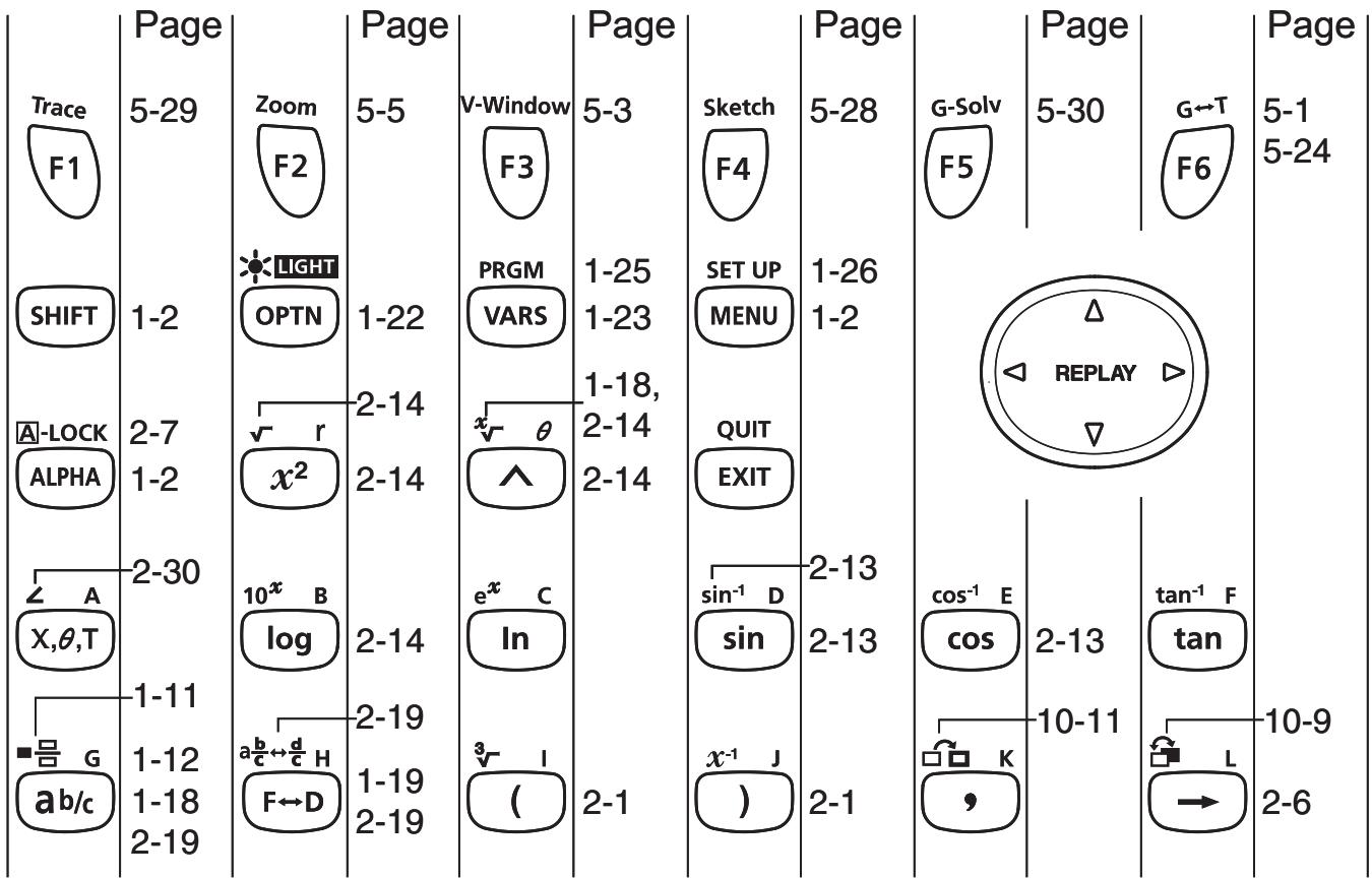
1. Keys
1
Key Table
other
| Category | Value | |---|---| | Trace F1 | 5-29 | | SHIFT | 1-2 | | AL-LOCK ALPHA | 2-7 | | X, θ, T | 1-11 | | G ab/c | 1-12 | | Zoom F2 | 5-5 | | LIGHT OPTN | 1-22 | | r x² | 2-14 | | 10^x B log | 2-14 | | 1-11 | 2-19 | | a b c d H F D | 1-19 | | 2-19 | 2-19 | | V-Window F3 | 5-5 | | PRGM VARS | 1-22 | | x y θ | 2-14 | | ^ | 2-14 | | e^x C In | 2-14 | | 3 y I | 2-14 | | 5-3 | 5-3 | | Sketch F4 | 5-3 | | SET UP MENU | 1-23 | | QUIT EXIT | 2-14 | | sin^-1 D | 2-13 | | sin | 2-13 | | x^-1 J | 2-1 | | 5-28 | 5-28 | | G-Solv F5 | 5-28 | | cos^-1 E | 2-13 | | K K | 2-1 | | Cos | 2-13 | | □ □ K | 10-11 | | □ □ K | 10-11 | | □ □ K | 10-9 | | □ □ K | 2-6 | | G←T F6 | 5-30 | | G←T F6 | 5-30 | | Page Page Page Page Page Page Page Page Page Page Page Page Page Page Page Page Page Page Page Page Page Page Page Page Page Page Page Page Page Page Page Page Page Page Page Page Page Page Page Page Page Page Page Page Page Page Page Page Page Page Page Page Page Page Page Page Page Page Page Page Page Page Page Page Page Page Page Page Page Page Page Page Page Page Page Page Page Page Page Page Page Page Page Page Page Page Page Page Page Page Page Page Page Page Page Page Page Page Page Page Frame Trace F1 SHIFT AL-LOCK ALPHA X, θ, T G ab/c Zoom F2 LIGHT OPTN 2-7 2-30 10^x B log a b c d H F D 2-14 2-19 1-19 2-19 2-14 2-14 2-14 2-14 2-14 2-14 2-14 2-14 2-14 2-14 2-14 2-14 2-14 2-14 2-14 2-14 2-14 2-14 2-14 2-14 2-19 2-19 2-19 2-19 2-19 2-19 2-19 2-19 2-19 2-19 2-19 2-19 2-19 2-19 2-19 2-19 2-19 2-19 2-19 2-19 2-16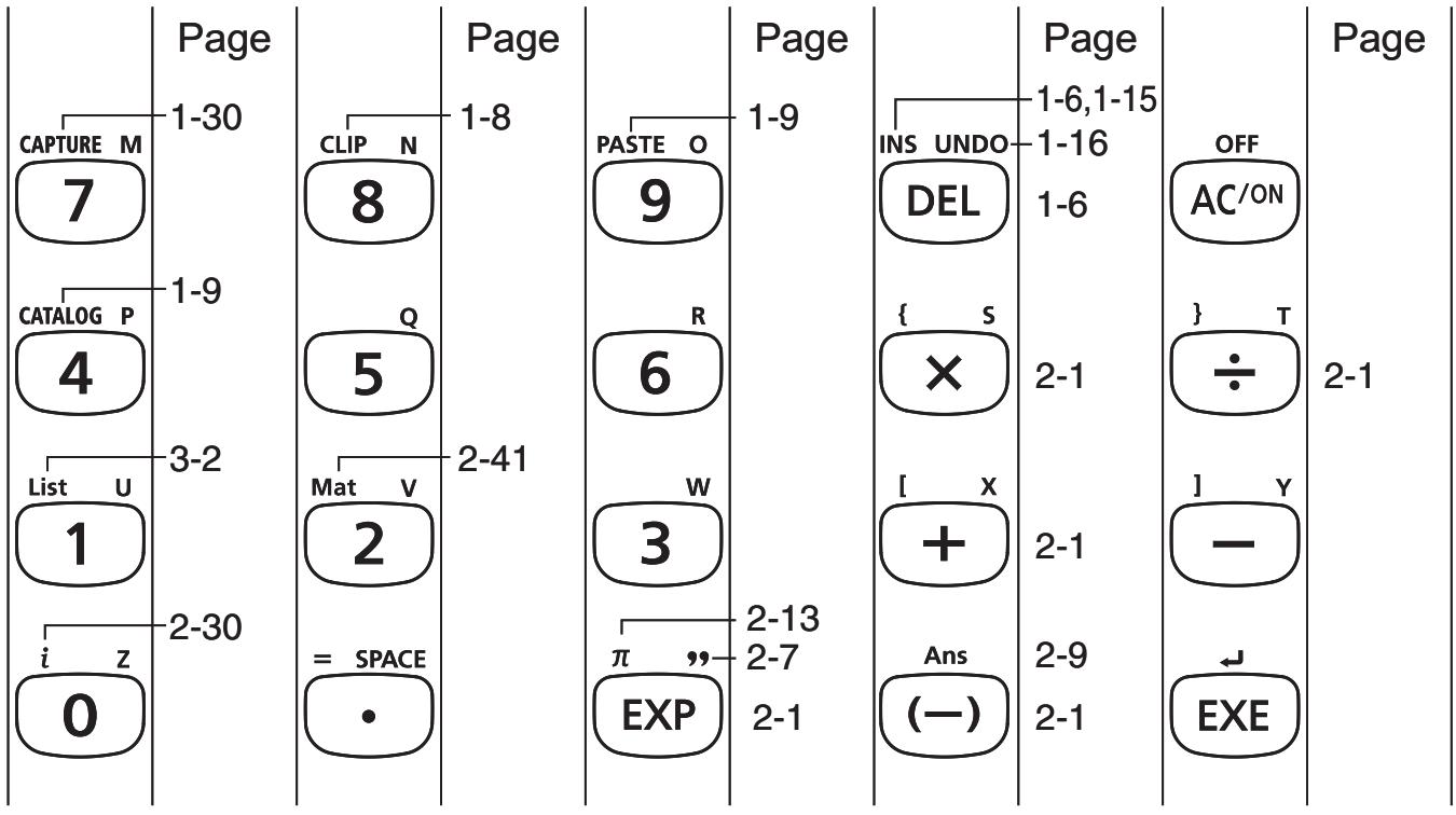
other
| Function | Value | | -------- | ----- | | CAPTURE M | 1-30 | | CLIP N | 1-8 | | PASTE O | 1-9 | | INS UNDO | 1-6,1-15 | | DEL | 1-16 | | OFF | 1-6 | | AC/ON | 1-6 | | CATALOG P | 1-9 | | Q | 5 | | R | 6 | | { S } 2-1 | { T } 2-1 | | × | 2-1 | | ÷ | 2-1 | | List U | 3-2 | | Mat V | 2-41 | | W | 3 | | [ X ] 2-1 | 2-1 | | Y | 2-1 | | i z | 2-30 | | = SPACE | 2-7 | | EXP | 2-1 | | Ans (-) | 2-9 | | EXE | 2-1 |Not all of the functions described above are available on all models covered by this manual. Depending on calculator model, some of the above keys may not be included on your calculator.
■ Key Markings
Many of the calculator's keys are used to perform more than one function. The functions marked on the keyboard are color coded to help you find the one you need quickly and easily.
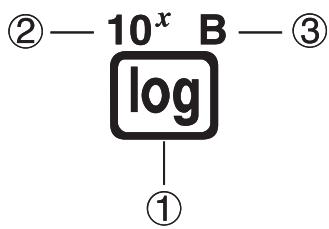
| Function | Key Operation | |
| 1 | log | log |
| 2 | 10^x | SHIFT log |
| 3 | B | ALPHA log |
The following describes the color coding used for key markings.
| Color | Key Operation |
| Yellow | Press SHIFT and then the key to perform the marked function. |
| Red | Press ALPHA and then the key to perform the marked function. |
A-LOCK
• ALPHA Alpha Lock
Normally, once you press ALPHA and then a key to input an alphabetic character, the keyboard reverts to its primary functions immediately.
If you press SHIFT and then ALPHA, the keyboard locks in alpha input until you press ALPHA again.
2. Display
■ Selecting Icons
This section describes how to select an icon in the Main Menu to enter the mode you want.
- To select an icon
- Press MENU to display the Main Menu.
- Use the cursor keys (◀, ▶, ▲, ▼) to move the highlighting to the icon you want.
Currently selected icon
![MAIN MENU RUN-MAT STAT e-ACT S-SHT X=[0,B] +C 2 B GRAPH DYMA TABLE RECUR CONICS EQUA FRGM TVM 3x+ 0 ¥$FF E==0](/content/2025/01/86832/images/4f3a2c35d443738e29ed763c1f188f7fa50b5d3d484e3196b572f945874ba8c9.jpg)
- Press EXE to display the initial screen of the mode whose icon you selected. Here we will enter the STAT mode.
- You can also enter a mode without highlighting an icon in the Main Menu by inputting the number or letter marked in the lower right corner of the icon.
- Use only the procedures described above to enter a mode. If you use any other procedure, you may end up in a mode that is different than the one you thought you selected.
The following explains the meaning of each icon.
| Icon | Mode Name | Description |
 | RUN (fx-7400GII only) | Use this mode for arithmetic calculations and function calculations, and for calculations involving binary, octal, decimal, and hexadecimal values. |
 | RUN • MAT*1 (Run • Matrix) | Use this mode for arithmetic calculations and function calculations, and for calculations involving binary, octal, decimal, and hexadecimal values and matrices. |
 | STAT (Statistics) | Use this mode to perform single-variable (standard deviation) and paired-variable (regression) statistical calculations, to perform tests, to analyze data and to draw statistical graphs. |
 | e • ACT*2 (eActivity) | eActivity lets you input text, math expressions, and other data in a notebook-like interface. Use this mode when you want to store text or formulas, or built-in application data in a file. |
 | S • SHT*2 (Spreadsheet) | Use this mode to perform spreadsheet calculations. Each file contains a 26-column × 999-line spreadsheet. In addition to the calculator's built-in commands and S • SHT mode commands, you can also perform statistical calculations and graph statistical data using the same procedures that you use in the STAT mode. |
 | GRAPH | Use this mode to store graph functions and to draw graphs using the functions. |
 | DYNA*1 (Dynamic Graph) | Use this mode to store graph functions and to draw multiple versions of a graph by changing the values assigned to the variables in a function. |
 | TABLE | Use this mode to store functions, to generate a numeric table of different solutions as the values assigned to variables in a function change, and to draw graphs. |
 | RECUR*1 (Recursion) | Use this mode to store recursion formulas, to generate a numeric table of different solutions as the values assigned to variables in a function change, and to draw graphs. |
 | CONICS*1 | Use this mode to draw graphs of conic sections. |
 | EQUA (Equation) | Use this mode to solve linear equations with two through six unknowns, and high-order equations from 2nd to 6th degree. |
 | PRGM (Program) | Use this mode to store programs in the program area and to run programs. |
 | TVM*1(Financial) | Use this mode to perform financial calculations and to draw cash flow and other types of graphs. |
 | E-CON2*1 | Use this mode to control the optionally available EA-200 Data Analyzer.For more information about the E-CON2 mode, download the E-CON2 manual (English version only) from: http://edu.casio.com. |
 | LINK | Use this mode to transfer memory contents or back-up data to another unit or PC. |
 | MEMORY | Use this mode to manage data stored in memory. |
 | SYSTEM | Use this mode to initialize memory, adjust contrast, and to make other system settings. |
*1 Not included on the fx-7400GII.
*2 Not included on the fx-7400GII/fx-9750GII.
■ About the Function Menu
Use the function keys (F1 to F6) to access the menus and commands in the menu bar along the bottom of the display screen. You can tell whether a menu bar item is a menu or a command by its appearance.
■ About Display Screens
This calculator uses two types of display screens: a text screen and a graph screen. The text screen can show 21 columns and 8 lines of characters, with the bottom line used for the function key menu. The graph screen uses an area that measures 127 (W) × 63 (H) dots.
Text Screen
![Graph Func :Y= Y1sin X [—] Y2: [—] Y3: [—] Y4: [—] Y5: [—] Y6: [—] SEL DEL TYPE STYL AMEM DRAW](/content/2025/01/86832/images/a01bc5d893ef9a8d54e8cfd6a0c7db6395473b9afcfbf739f79a416899023a9a.jpg)
Graph Screen
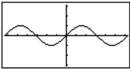
natural_image
Pure waveforms plotted on a Cartesian coordinate system with no text or symbolsNormal Display
The calculator normally displays values up to 10 digits long. Values that exceed this limit are automatically converted to and displayed in exponential format.
- How to interpret exponential format
1.2E12
1.2E+12
1.2_E + 12 indicates that the result is equivalent to 1.2 × 10^12 . This means that you should move the decimal point in 1.2 twelve places to the right, because the exponent is positive. This results in the value 1,200,000,000,000.
$$ \boxed { \begin{array}{c c} 1. 2 \mathrm{E} - 3 & \ & 1. 2 \mathrm{E} - 0 3 \end{array} } $$
1.2_E - 03 indicates that the result is equivalent to 1.2 × 10^-3 . This means that you should move the decimal point in 1.2 three places to the left, because the exponent is negative. This results in the value 0.0012.
You can specify one of two different ranges for automatic changeover to normal display.
Norm 1 ...... 10^-2(0.01) > |x|, |x| ≥ 10^10
Norm 2 ...... 10^-9 (0.000000001) > |x|, |x| ≥ 10^10
All of the examples in this manual show calculation results using Norm 1.
See page 2-11 for details on switching between Norm 1 and Norm 2.
■ Special Display Formats
This calculator uses special display formats to indicate fractions, hexadecimal values, and degrees/minutes/seconds values.
- Fractions
$$ \boxed { \begin{array}{c c} 4 5 6, 1 2, 2 3 & \ & 4 5 6, 1 2, 2 3 \end{array} } \dots\dotsIndicates: 4 5 6 \frac {1 2}{2 3} $$
- Hexadecimal Values
$$ \boxed { \begin{array}{c c} \text {ABCDEF1} & \ & 0 \text {ABCDEF1} \end{array} } \dots\dots\text {Indicates: 0ABCDEF1_{(16)}, which equals} \ & 1 8 0 1 5 0 0 0 1 _ {(1 0)} $$
• Degrees/Minutes/Seconds
$$ \boxed {1 2. 5 8 2 4 4 \quad 1 2 ^ {\circ} 3 4 ^ {\prime} 5 6. 7 8 ^ {\prime \prime}} \dots\dotsIndicates: 1 2 ^ {\circ} 3 4 ^ {\prime} 5 6. 7 8 ^ {\prime \prime} $$
- In addition to the above, this calculator also uses other indicators or symbols, which are described in each applicable section of this manual as they come up.
3. Inputting and Editing Calculations
■ Inputting Calculations
When you are ready to input a calculation, first press AC to clear the display. Next, input your calculation formulas exactly as they are written, from left to right, and press EXE to obtain the result.
Example 2 + 3 - 4 + 10 =
$$ \boxed {A C} \boxed {2} + \boxed {3} - \boxed {4} + \boxed {1} \boxed {0} \boxed {E X E} $$
$$ \boxed { \begin{array}{c c} 2 + 3 - 4 + 1 0 & \ & 1 1 \end{array} } $$
■ Editing Calculations
Use the ◀ and ▶ keys to move the cursor to the position you want to change, and then perform one of the operations described below. After you edit the calculation, you can execute it by pressing EXE. Or you can use ▶ to move to the end of the calculation and input more.
- You can select either insert or overwrite for input ^*1 . With overwrite, text you input replaces the text at the current cursor location. You can toggle between insert and overwrite by performing the operation: SHIFT DEL (INS). The cursor appears as “■” for insert and as “—” for overwrite.
*1 With all models except the fx-7400GII/fx-9750GII, insert and overwrite switzng is possible only when the Linear input/output mode (page 1-29) is selected.
- To change a step
Example To change cos60 to sin60

cos 60

cos 60

60

sin 160
- To delete a step
Example To change 369 × × 2 to 369 × 2

369xx2

369×2
In the insert mode, the DEL key operates as a backspace key.
- To insert a step
Example To change 2.36^2 to 2.36^2
2.36리

2.36 ^2

sin D.36 ^2
■ Using Replay Memory
The last calculation performed is always stored into replay memory. You can recall the contents of the replay memory by pressing ◀ or ▶.
If you press ▶, the calculation appears with the cursor at the beginning. Pressing ◀ causes the calculation to appear with the cursor at the end. You can make changes in the calculation as you wish and then execute it again.
- Replay memory is enabled in the Linear input/output mode only. In the Math input/output mode, the history function is used in place of replay memory. For details, see “History Function” (page 1-17).
Example 1 To perform the following two calculations
| 4.12 × 6.4 = 26.368 | |
| 4.12 × 7.1 = 29.252 | |
| AC 4 · 1 2 ✗ 6 · 4 EXE | 4.12×6.4 26.368 |
| 4.12×6.4 | |
| SHIFT DEL (INS) | 4.12×6.4 |
| 7 · 1 | 4.12×7.1_ |
| EXE | 4.12×7.1 29.252 |
After you press AC, you can press ▲ or ▼ to recall previous calculations, in sequence from the newest to the oldest (Multi-Replay Function). Once you recall a calculation, you can use ▶ and ◀ to move the cursor around the calculation and make changes in it to create a new calculation.
Example 2
| AC 1 2 3 + 4 5 6 EXE | 123+456 | 579 |
| 2 3 4 - 5 6 7 EXE | 234-567 | -333 |
| AC | ||
| ▲ (One calculation back) | 234-567 | |
| ▲ (Two calculations back) | 123+456 |
- A calculation remains stored in replay memory until you perform another calculation.
- The contents of replay memory are not cleared when you press the AC key, so you can recall a calculation and execute it even after pressing the AC key.
■ Making Corrections in the Original Calculation
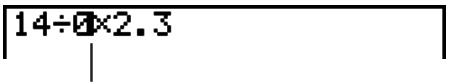
Example 14 ÷ 0 × 2.3 entered by mistake for 14 ÷ 10 × 2.3
AC 1 4 ÷ 0 ✗ 2 · 3
14÷0×2.3
EXE
![14:0v0.7 Ma ERROR Press: [EXIT]](/content/2025/01/86832/images/9651b711e34486ffa471099795ae2c4bd794745d244a285910a8bcf102638544.jpg)
Press EXIT.
Cursor is positioned automatically at the location of the cause of the error.
Make necessary changes.
◀ 1
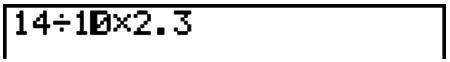
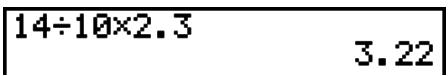
Execute again.
EXE
■ Using the Clipboard for Copy and Paste
You can copy (or cut) a function, command, or other input to the clipboard, and then paste the clipboard contents at another location.
- The procedures described here all use the Linear input/output mode. For details about the copy and paste operation while the Math input/output mode is selected, see “Using the Clipboard for Copy and Paste in the Math Input/Output Mode” (page 1-18).
- To specify the copy range
- Move the cursor (Ⅱ) to the beginning or end of the range of text you want to copy and then press SHIFT 8 (CLIP). This changes the cursor to “☐”.
14÷10×2.30
- Use the cursor keys to move the cursor and highlight the range of text you want to copy.
14÷15×2.8
- Press F1(COPY) to copy the highlighted text to the clipboard, and exit the copy range specification mode.
14÷10×2.3
The selected characters are not changed when you copy them.
To cancel text highlighting without performing a copy operation, press EXIT.
- To cut the text
- Move the cursor (Ⅰ) to the beginning or end of the range of text you want to cut and then press SHIFT 8 (CLIP). This changes the cursor to “☐”.
14÷00×2.3
- Use the cursor keys to move the cursor and highlight the range of text you want to cut.
14÷152.3
- Press F2 (CUT) to cut the highlighted text to the clipboard.
14÷2.3
Cutting causes the original characters to be deleted.
- Pasting Text
Move the cursor to the location where you want to paste the text, and then press SHIFT 9 (PASTE). The contents of the clipboard are pasted at the cursor position.
AC
SHIFT 9 (PASTE)

10×|
■ Catalog Function
The Catalog is an alphabetic list of all the commands available on this calculator. You can input a command by calling up the Catalog and then selecting the command you want.
- To use the Catalog to input a command
-
Press SHIFT 4 (CATALOG) to display an alphabetic Catalog of commands.
-
The screen that appears first is the last one you used for command input.
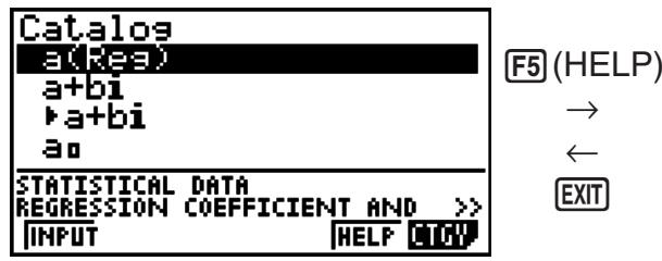
- With the fx-9860G Slim, the first two lines of explanation text for the currently selected command will appear at the bottom of the screen. Pressing F5 (HELP) will display a full-screen view of the text for reading. If the text does not fit within a single screen, you can use ▲ and ▼ to scroll it.
![a STATISTICAL DATA REGRESSION COEFFICIENT AND POLYNOMIAL COEFFICIENTS [VARS]-[STAT]-[GRAPH]](/content/2025/01/86832/images/26df3466f7249534d65dcc11bdafd37a61ac0e0fd2db8c200eb733f1cfb012cf.jpg)
To close the help text screen, press EXIT.
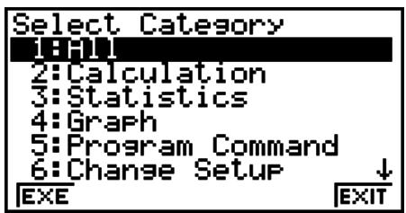
- Press F6(CTGY) to display the category list.
- You can skip this step and go straight to step 5, if you want.
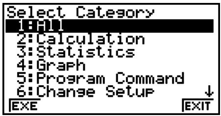
- Use the cursor keys (▲, ▼) to highlight the command category you want, and then press F1(EXE) or EXE.
- This displays a list of commands in the category you selected.
- Input the first letter of the command you want to input. This will display the first command that starts with that letter.
- Use the cursor keys (▲, ▼) to highlight the command you want to input, and then press F1(INPUT) or EXE.
Example To use the Catalog to input the ClrGraph command


Pressing EXIT or SHIFT EXIT (QUIT) closes the Catalog.
- To input a command with Ⓗ (fx-9860G Slim only)
1. Press Ⓗ HELP.
- This will display the category selection screen.
- F1(EXE)... {displays a list of commands in the currently selected category}
-
F6(EXIT)... {exits the category selection screen}
-
Continue from step 3 of the procedure under "To use the Catalog to input a command".
4. Using the Math Input/Output Mode
Important!
- The fx-7400GII and fx-9750GII are not equipped with a Math input/output mode.
Selecting “Math” for the “Input/Output” mode setting on the Setup screen (page 1-29) turns on the Math input/output mode, which allows natural input and display of certain functions, just as they appear in your textbook.
- The operations in this section all are performed in the Math input/output mode.
- The initial default setting for the fx-9860GII SD/fx-9860GII/fx-9860G AU PLUS is the Math input/output mode. If you have changed to the Linear input/output mode, switch back to the Math input/output mode before performing the operations in this section. See “Using the Setup Screen” (page 1-26) for information about how to switch modes.
- The initial default setting for the fx-9860G Slim/fx-9860G SD/fx-9860G/fx-9860G AU is the Linear input/output mode. Switch to the Math input/output mode before performing the operations in this section. See “Using the Setup Screen” (page 1-26) for information about how to switch modes.
- In the Math input/output mode, all input is insert mode (not overwrite mode) input. Note that the SHIFT DEL (INS) operation (page 1-6) you use in the Linear input/output mode to switch to insert mode input performs a completely different function in the Math input/output mode. For more information, see “Using Values and Expressions as Arguments” (page 1-14).
- Unless specifically stated otherwise, all operations in this section are performed in the RUN•MAT mode.
■ Input Operations in the Math Input/Output Mode
- Math Input/Output Mode Functions and Symbols
The functions and symbols listed below can be used for natural input in the Math input/output mode. The “Bytes” column shows the number of bytes of memory that are used up by input in the Math input/output mode.
| Function/Symbol | Key Operation | Bytes |
| Fraction (Improper) | ab% | 9 |
| Mixed Fraction^*1 | SHIFT ab% (■□) | 14 |
| Power | 4 | |
| Square | x^2 | 4 |
| Negative Power (Reciprocal) | SHIFT ( x^-1 ) | 5 |
| SHIFT x^2 ( ) | 6 | |
| Cube Root | SHIFT ( ^3 ) | 9 |
| Power Root | SHIFT ( x ) | 9 |
| e^x | SHIFT ( e^x ) | 6 |
| 10^x | SHIFT ( 10^x ) | 6 |
| log(a,b) | (Input from MATH menu*2) | 7 |
| Abs (Absolute Value) | (Input from MATH menu*2) | 6 |
| Linear Differential*3 | (Input from MATH menu*2) | 7 |
| Quadratic Differential*3 | (Input from MATH menu*2) | 7 |
| Integral*3 | (Input from MATH menu*2) | 8 |
| Σ Calculation*4 | (Input from MATH menu*2) | 11 |
| Matrix | (Input from MATH menu*2) | 14^*5 |
| Parentheses | and | 1 |
| Braces (Used during list input.) | SHIFT × ( { ) and SHIFT ÷ ( { ) | 1 |
| Brackets (Used during matrix input.) | SHIFT ( [ ) and SHIFT ( ] ) | 1 |
*1 Mixed fraction is supported in the Math input/output mode only.
*2 For information about function input from the MATH function menu, see “Using the MATH Menu” described below.
*3 Tolerance cannot be specified in the Math input/output mode. If you want to specify tolerance, use the Linear input/output mode.
*4 For calculation in the Math input/output mode, the pitch is always 1. If you want to specify a different pitch, use the Linear input/output mode.
*5 This is the number of bytes for a 2 × 2 matrix.
• Using the MATH Menu
In the RUN•MAT mode, pressing F4 (MATH) displays the MATH menu. You can use this menu for natural input of matrices, differentials, integrals, etc.
- {MAT} ... {displays the MAT submenu, for natural input of matrices}
- 2 × 2 ... {inputs a 2 × 2 matrix}
- 3 × 3 ... {inputs a 3 × 3 matrix}
- m × n ... {inputs a matrix with m lines and n columns (up to 6 × 6 )}
- _ab ... {starts natural input of logarithm _ab
- {Abs} ... {starts natural input of absolute value |X|}
- d / dx {starts natural input of linear differential f(x)_x = a }
- d^2 / dx^2 ... {starts natural input of quadratic differential ^2dx^2 f(x)_x = a }
- dx {starts natural input of integral _a^b f(x) dx
- (·) starts natural input of calculation _x=^ f(x)
- Math Input/Output Mode Input Examples
This section provides a number of different examples showing how the MATH function menu and other keys can be used during Math input/output mode natural input. Be sure to pay attention to the input cursor position as you input values and data.
Example 1 To input 2^3 + 1
| AC 2 ∧ | 2^0 |
| 3 | 2^3 |
| 2^3 | |
| + 1 | 2^3 + 1 |
| EXE | 2^3 + 1 9 |
Example 2 To input (1 + 25)^2
| AC (1 + | (1+ |
| a% | ( 1+20 . |
| 2 ▼ | ( 1+20 . |
5
$$ \left[ 1 + \frac {2}{5} \right] $$
▶
$$ \left(1 + \frac {2}{5} \right\rvert $$
) x^2
$$ \left(1 + \frac {2}{5}\right) ^ {2} \Bigg | $$
EXE
$$ \boxed {\left(1 + \frac {2}{5}\right) ^ {2}} $$
10
49/25
Example 3 To input 1 + _0^1 x + 1dx
AC 1 + F4 (MATH) F6 (▷) F1 (∫dx)
$$ \boxed {1 + \int_ {\square} ^ {\square} \square d x} $$
X,θ,T + 1
$$ \boxed {1 + \int_ {0} ^ {\square} x + 1 \mathrm{d} x} $$
0
$$ \boxed {1 + \int_ {\mathbb {Q}} ^ {\square} X + 1 d x} $$
▲1
$$ \boxed {1 + \int_ {0} ^ {1 1} X + 1 d x} $$
▶
$$ 1 + \int_ {0} ^ {1} X + 1 d x $$
EXE
$$ 1 + \int_ {0} ^ {1} x + 1 d x $$
10
5/2
Example 4 To input 2 × 12 & 2 2 & 12
AC 2 ✗ F4 (MATH) F1 (MAT) F1 (2×2)
$$ \boxed {2 \times [ \begin{array}{c c} \square & \square \ \square & \square \end{array} ]} $$
ab/c 1 ▼ 2
$$ \boxed {2 \times \left[ \begin{array}{c c} \frac {1}{2} & 0 \ 0 & 0 \end{array} \right]} $$
▶▶
$$ \boxed {2 \times \left[ \begin{array}{c c} \frac {1}{2} & \square \ \square & \square \end{array} \right]} $$
SHIFT x^2() 2 ▶
$$ \boxed {2 \times \left[ \begin{array}{c c} \frac {1}{2} & \sqrt {2} \ 0 & 0 \end{array} \right]} $$

$$ \boxed {2 \times \left[ \begin{array}{l l} \frac {1}{2} & \sqrt {2} \ \sqrt {2} & \frac {1}{2 1} \end{array} \right]} $$

$$ \left[ \begin{array}{l l} 2 \times \left[ \begin{array}{c c} 2 & 1 \ \sqrt {2} & \frac {1}{2} \end{array} \right] & \ & \left[ \begin{array}{c c} 1 & 2 \sqrt {2} \ 2 \sqrt {2} & 1 \end{array} \right] \ \square & \end{array} \right] $$
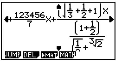
- When the calculation does not fit within the display window
Arrows appear at the left, right, top, or bottom edge of the display to let you know when there is more of the calculation off the screen in the corresponding direction. When you see an arrow, you can use the cursor keys to scroll the screen contents and view the part you want.
- Math Input/Output Mode Input Restrictions
Certain types of expressions can cause the vertical width of a calculation formula to be greater than one display line. The maximum allowable vertical width of a calculation formula is about two display screens (120 dots). You cannot input any expression that exceeds this limitation.
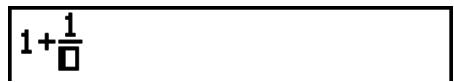
- Using Values and Expressions as Arguments
A value or an expression that you have already input can be used as the argument of a function. After you have input “(2+3)”, for example, you can make it the argument of , resulting in (2+3) .
Example
- Move the cursor so it is located directly to the left of the part of the expression that you want to become the argument of the function you will insert.
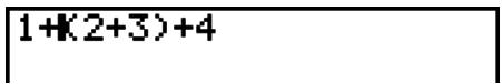
- Press SHIFT DEL (INS).
- This changes the cursor to an insert cursor (▶).
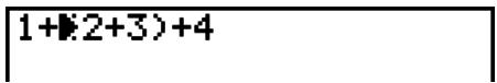
- Press SHIFT ^2() to insert the function.
- This inserts the function and makes the parenthetical expression its argument.
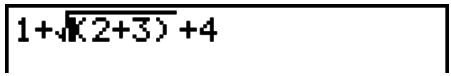
As shown above, the value or expression to the right of the cursor after SHIFT DEL (INS) are pressed becomes the argument of the function that is specified next. The range encompassed as the argument is everything up to the first open parenthesis to the right, if there is one, or everything up to the first function to the right (sin(30), log2(4), etc.).
This capability can be used with the following functions.
| Function | Key Operation | Original Expression | Expression After Insertion |
| Improper Fraction | % | 1+(2+3)+4 | 1+ (2+3) +4 |
| Power | 1+2(2+3)+4 | 1+2 (2+3) +4 | |
| ^2 ( ) | 1+(2+3)+4 | 1+ (2+3) +4 | |
| Cube Root | ([3]) | 1+ [3](2+3) +4 | |
| Power Root | ( [x]) | 1+ (2+3) +4 | |
| e^x | (e^x) | 1+e (2+3) +4 | |
| 10^x | (10^x) | 1+ (2+3) +4 | |
| log(a,b) | 4 (MATH) 2 (loga,b) | 1+lo=□((2+3))+4 | |
| Absolute Value | 4 (MATH) 3 (Abs) | 1+|K2+3|+4 | |
| Linear Differential | 4 (MATH) 4 (d/dx) | 1+(X+3)+4 | 1+ (KX+3))|x=□+4 |
| Quadratic Differential | 4 (MATH) 5 ( d^2/dx^2 ) | 1+ ^2dx^2 (KX+3))|x=□+4 | |
| Integral | 4 (MATH) 6 (▷)F1(∫dx) | 1+ _^ (KX+3)dx+4 | |
| Σ Calculation | 4 (MATH) 6 (▷)F2(Σ() | 1+ _=0^ (KX+3))+4 |
- In the Linear input/output mode, pressing SHIFT DEL (INS) will change to the insert mode. See page 1-6 for more information.
- Editing Calculations in the Math Input/Output Mode
The procedures for editing calculations in the Math input/output mode are basically the same as those for the Linear input/output mode. For more information, see “Editing Calculations” (page 1-6).
Note however, that the following points are different between the Math input/output mode and the Linear input/output mode.
- Overwrite mode input that is available in the Linear input/output mode is not supported by the Math input/output mode. In the Math input/output mode, input is always inserted at the current cursor location.
- In the Math input/output mode, pressing the DEL key always performs a backspace operation.
- Note the following cursor operations you can use while inputting a calculation with Math input/output mode.
| To do this: | Press this key: |
| Move the cursor from the end of the calculation to the beginning | |
| Move the cursor from the beginning of the calculation to the end |
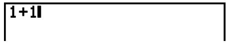
■ Using Undoing and Redoing Operations
You can use the following procedures during calculation expression input in the Math input/output mode (up until you press the EXE key) to undo the last key operation and to redo the key operation you have just undone.
- To undo the last key operation, press: ALPHA DEL (UNDO).
- To redo a key operation you have just undone, press: ALPHA DEL (UNDO) again.
- You also can use UNDO to cancel an AC key operation. After pressing AC to clear an expression you have input, pressing ALPHA DEL (UNDO) will restore what was on the display before you pressed AC.
- You also can use UNDO to cancel a cursor key operation. If you press ▶ during input and then press ALPHA DEL (UNDO), the cursor will return to where it was before you pressed ▶.
- The UNDO operation is disabled while the keyboard is alpha-locked. Pressing ALPHA DEL (UNDO) while the keyboard is alpha-locked will perform the same delete operation as the DEL key alone.
Example


■ Math Input/Output Mode Calculation Result Display
Fractions, matrices, and lists produced by Math input/output mode calculations are displayed in natural format, just as they appear in your textbook.
![[1 2]×2 [2 4] [6 8] 0 DEL:L DEL:A](/content/2025/01/86832/images/b03345f2de5ebe18d7327167277520d3f43487ea307328c920f7af9ea7e454f1.jpg)
Sample Calculation Result Displays
- Fractions are displayed either as improper fractions or mixed fractions, depending on the “Frac Result” setting on the Setup screen. For details, see “Using the Setup Screen” (page 1-26).
- Matrices are displayed in natural format, up to 6 × 6 . A matrix that has more than six rows or columns will be displayed on a MatAns screen, which is the same screen used in the Linear input/output mode.
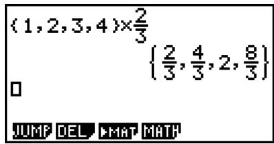
- Lists are displayed in natural format for up to 20 elements. A list that has more than 20 elements will be displayed on a ListAns screen, which is the same screen used in the Linear input/output mode.
- Arrows appear at the left, right, top, or bottom edge of the display to let you know when there is more data off the screen in the corresponding direction.
![(√2,√3) [414216562, 1.782058] JUMP DEL MAT MATH](/content/2025/01/86832/images/de99d0e73eedd061134495e31d52a101045716ca237f4676394af0a4573e569e.jpg)
You can use the cursor keys to scroll the screen and view the data you want.
- Pressing F2 (DEL) F1 (DEL·L) while a calculation result is selected will delete both the result and the calculation that produced it.
- The multiplication sign cannot be omitted immediately before an improper fraction or mixed fraction. Be sure to always input a multiplication sign in this case.
Example: 2 × 25
2 × 2 a^b 5
- A , ^2 , or (x^-1) key operation cannot be followed immediately by another , ^2 , or (x^-1) key operation. In this case, use parentheses to keep the key operations separate.
Example: (3^2)^-1
(3) x^2 (SHIFT) (x^-1)
■ History Function
The history function maintains a history of calculation expressions and results in the Math input/output mode. Up to 30 sets of calculation expressions and results are maintained.
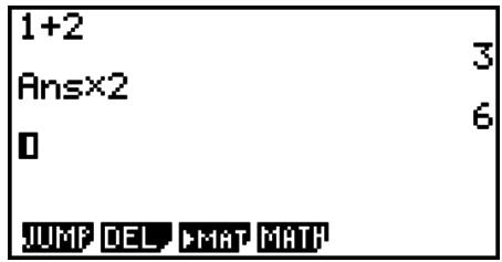
You can also edit the calculation expressions that are maintained by the history function and recalculate. This will recalculate all of the expressions starting from the edited expression.
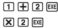
Example To change “1+2” to “1+3” and recalculate
Perform the following operation following the sample shown above.

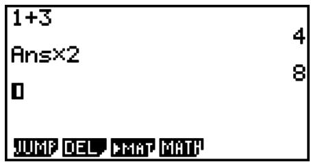
- The value stored in the answer memory is always dependent on the result produced by the last calculation performed. If history contents include operations that use the answer memory, editing a calculation may affect the answer memory value used in subsequent calculations.
- If you have a series of calculations that use the answer memory to include the result of the previous calculation in the next calculation, editing a calculation will affect the results of all the other calculations that come after it.
- When the first calculation of the history includes the answer memory contents, the answer memory value is “0” because there is no calculation before the first one in history.
■ Using the Clipboard for Copy and Paste in the Math Input/Output Mode
You can copy a function, command, or other input to the clipboard, and then paste the clipboard contents at another location.
- In the Math input/output mode, you can specify only one line as the copy range.
- The CUT operation is supported for the Linear input/output mode only. It is not supported for the Math input/output mode.
- To copy text
- Use the cursor keys to move the cursor to the line you want to copy.
- Press SHIFT 8 (CLIP). The cursor will change to “☐”.
- Press F1(CPY·L) to copy the highlighted text to the clipboard.
- To paste text
Move the cursor to the location where you want to paste the text, and then press SHIFT 9 (PASTE). The contents of the clipboard are pasted at the cursor position.
■ Calculation Operations in the Math Input/Output Mode
This section introduces Math input/output mode calculation examples.
- For details about calculation operations, see “Chapter 2 Manual Calculations”.
- Performing Function Calculations Using Math Input/Output Mode
| Example | Operation |
| 64 × 5 = 310 | AC 6 ab% 4 ✗ 5 EXE |
| (3) = 12 (Angle: Rad) | AC cos (SHIFT EXP ( ) ab% 3 ▶ ) EXE |
| _28 = 3 | AC F4 (MATH) F2 ( _a b ) 2 ▶ 8 EXE |
| [7]123 = 1.988647795 | AC SHIFT ∧ ( ^x ) 7 ▶ 123 EXE |
| 2 + 3 × [3]64 - 4 = 10 | AC 2 + 3 ✗ SHIFT ∧ ( ^x ) 3 ▶ 64 ▶ — 4 EXE |
| | 34 | = 0.1249387366 | AC F4 (MATH) F3 (Abs) log 3 ab% 4 EXE |
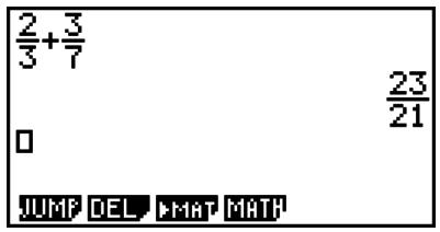
$$ \frac {2}{5} + 3 \frac {1}{4} = \frac {7 3}{2 0} $$
$$ 1. 5 + 2. 3 i = \frac {3}{2} + \frac {2 3}{1 0} i $$
$$ \frac {d}{d x} \left(x ^ {3} + 4 x ^ {2} + x - 6\right) _ {x = 3} = 5 2 $$
$$ \int_ {1} ^ {5} 2 x ^ {2} + 3 x + 4 d x = \frac {4 0 4}{3} $$
$$ \sum_ {k = 2} ^ {6} \left(k ^ {2} - 3 k + 5\right) = 5 5 $$
AC 2 ab% 5 ▶ + 3 SHIFT ab% (■음)1 ▶ 4 EXE
AC 1.5 + 2.3 SHIFT 0 (i) EXE F→D
AC F4 (MATH) F4 (d/dx) X,θ,T ∧ 3 ▶ + 4
X,θ,T x² + X,θ,T - 6 ▶ 3 EXE
AC F4 (MATH) F6 (▷) F1 (∫dx) 2 X,θ,T x² +3 X,θ,T +4 ▶ 1
5 EXE
AC F4 (MATH) F6 (▷) F2 (Σ) ALPHA, (K) x^2 — 3 ALPHA, (K)
- To input cell values
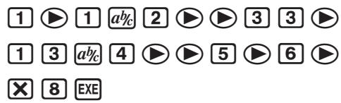
Example To perform the calculation shown below
$$ \left[ \begin{array}{c c c} 1 & \frac {1}{2} & 3 3 \ \frac {1 3}{4} & 5 & 6 \end{array} \right] \times 8 $$
The following operation is a continuation of the example calculation on the previous page.
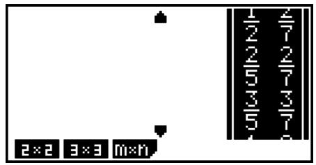
- To assign a matrix created using Math input/output mode to a MAT mode matrix
Example To assign the calculation result to Mat J
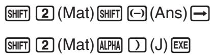
![L 4 J [8 4 264] 26 40 48] Mat Ans→Mat J [8 4 264] 26 40 48] □ 2×2 3×3 m×n](/content/2025/01/86832/images/ca99426ce60a0fee929b82b5ac3b264a3373944e15916ea12ccec1237db4eeb5.jpg)
- Pressing the DEL key while the cursor is located at the top (upper left) of the matrix will delete the entire matrix.
![2×[112 0 0] [34 0 0] DEL ⇒ 2×1 2×2 3×3 m×n 2×2 3×3 m×n](/content/2025/01/86832/images/f6b745daf20c9709544d6a232f57425430987aeae194e794d36d1ff3aae862fa.jpg)
■ Using Graph Modes and the EQUA Mode in the Math Input/Output Mode
Using the Math input/output mode with any of the modes below lets you input numeric expressions just as they are written in your text book and view calculation results in natural display format.
Modes that support input of expressions as they are written in textbooks:
RUN•MAT, e•ACT, GRAPH, DYNA, TABLE, RECUR, EQUA (SOLV)
Modes that support natural display format:
The following explanations show Math input/output mode operations in the GRAPH, DYNA, TABLE, RECUR and EQUA modes, and natural calculation result display in the EQUA mode.
• See the sections that cover each calculation for details about its operation.
- See “Input Operations in the Math Input/Output Mode” (page 1-11) and “Calculation Operations in the Math Input/Output Mode” (page 1-18) for details about Math input/output mode input operations and calculation result displays in the RUN•MAT mode.
- e•ACT mode input operations and result displays are the same as those in the RUN•MAT mode. For information about e•ACT mode operations, see “Chapter 10 eActivity”.
Important!
- On a model whose operating system has been updated to OS 2.00 from an older OS version, Math input/output mode input and result display are not supported in any mode except the RUN•MAT mode and e•ACT mode.
- Math Input/Output Mode Input in the GRAPH Mode
You can use the Math input/output mode for graph expression input in the GRAPH, DYNA, TABLE, and RECUR modes.
Example 1 In the GRAPH mode, input the function y=^22-2-1 and then graph it. Make sure that initial default settings are configured on the View Window.
![MENU GRAPH [X,θ,T] x² ab% SHIFT x² (√) 2 ▶ ▶ — [X,θ,T] ab% SHIFT x² (√) 2 ▶ ▶ — 1 EXE](/content/2025/01/86832/images/47a8d510649599cc1a305e529e1090bdf316f4d7175c768ea9e3e8e771b1556d.jpg)
![Graph Func :Y= Y1E x²/√2 - x/√2 - 1 [—] Y2: [—]](/content/2025/01/86832/images/d599cb2ab0f5dd9398362244ef3467578d70adf9fd5efb9d7d134f0890c4b756.jpg)
F6 (DRAW)
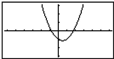
Example 2 In the GRAPH mode, input the function y=_0^x14x^2-12x-1dx and then graph it. Make sure that initial default settings are configured on the View Window.
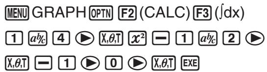
![Graph Func :Y= Y1E∫₀ˣ₁/4ˣ²-½ˣ-1dx[—] Y2: [—]](/content/2025/01/86832/images/291b5ad48a4df94c8eb50f6ccc5f6ddcb31c1a6c6946b8932e25971c4c8a5f0a.jpg)
F6 (DRAW)
line
| x | y | | ---- | ----- | | 0 | 0 | | 100 | 1 | | 200 | 0 | | 300 | -1 | | 400 | -2 | | 500 | -3 | | 600 | -4 | | 700 | -5 | | 800 | -6 | | 900 | -7 | | 1000 | -8 | | 1100 | -9 | | 1200 | -10 | | 1300 | -11 | | 1400 | -12 | | 1500 | -13 | | 1600 | -14 | | 1700 | -15 | | 1800 | -16 | | 1900 | -17 | | 2000 | -18 | | 2100 | -19 | | 2200 | -20 | | 2300 | -21 | | 2400 | -22 | | 2500 | -23 | | 2600 | -24 | | 2700 | -25 | | 2800 | -26 | | 2900 | -27 | | 3000 | -28 | | 3100 | -29 | | 3200 | -30 | | 3300 | -31 | | 3400 | -32 | | 3500 | -33 | | 3600 | -34 | | 3700 | -35 | | 3800 | -36 | | 3900 | -37 | | 4000 | -38 | | 4100 | -39 | | 4200 | -40 | | 4300 | -41 | | 4400 | -42 | | 4500 | -43 | | 4600 | -44 | | 4700 | -45 | | 4800 | -46 | | 4900 | -47 | | 5000 | -48 | | 5100 | -49 | | 5200 | -50 | | 5300 | -51 | | 5400 | -52 | | 5500 | -53 | | 5600 | -54 | | 5700 | -55 | | 5800 | -56 | | 5900 | -57 | | 6000 | -58 | | 6100 | -59 | | 6200 | -60 | | 6300 | -61 | | 6400 | -62 | | 6500 | -63 | | 6600 | -64 | | 6700 | -65 | | 6800 | -66 | | 6900 | -67 | | 7000 | -68 | | 7100 | -69 | | 7200 | -70 | | 7300 | -71 | | 7400 | -72 | | 7500 | -73 | | 7600 | -74 | | 7700 | -75 | | 7800 | -76 | | 7900 | -77 | | 8000 | -78 | | 8100 | -79 | | 8200 | -80 | | 8300 | -81 | | 8400 | -82 | | 8500 | -83 | | 8600 | -84 | | 8700 | -85 | | 8800 | -86 | | 8900 | -87 | | 9000 | -88 | | 9100 | -89 | | 9200 | -90 | | 9300 | -91 | | 9400 | -92 | | 9500 | -93 | | 9600 | -94 | | 9700 | -95 | | 9800 | -96 | | 9900 | -97 | | 10000| -98 |- Math Input/Output Mode Input and Result Display in the EQUA Mode
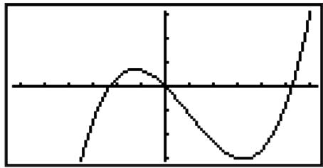
You can use the Math input/output mode in the EQUA mode for input and display as shown below.
- In the case of simultaneous equations (F1(SIML)) and high-order equations (F2(POLY)), solutions are output in natural display format (fractions, , are displayed in natural format) whenever possible.
- In the case of Solver (F3(SOLV)), you can use Math input/output mode natural input.
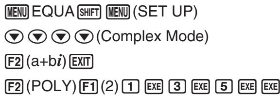
![aX²+bX+c=0 x1[-1.5+1.6583i] x2[-1.5-1.6583i] -3+√11 i 2 REPT](/content/2025/01/86832/images/4227825bc613e7bd84c5da93bf7758597bab8df87c27a3f413e2ed0889d1ac17.jpg)
5. Option (OPTN) Menu
The option menu gives you access to scientific functions and features that are not marked on the calculator's keyboard. The contents of the option menu differ according to the mode you are in when you press the OPTN key.
- The option menu does not appear if you press OPTN while binary, octal, decimal, or hexadecimal is set as the default number system.
- For details about the commands included on the option (OPTN) menu, see the “OPTN key” item in the “PRGM Mode Command List” (page 8-37).
- The meanings of the option menu items are described in the sections that cover each mode.
The following list shows the option menu that is displayed when the RUN•MAT (or RUN) or PRGM mode is selected.
Item names below that are marked with an asterisk (*) are not included on the fx-7400GII.
- {LIST} ... {list function menu}
- MAT^* ... {matrix operation menu}
- {CPLX} ... {complex number calculation menu}
- {CALC} ... {functional analysis menu}
- {STAT} ... {paired-variable statistical estimated value menu} (fx-7400GII) {menu for paired-variable statistical estimated value, distribution, standard deviation, variance, and test functions} (all models except fx-7400GII)
- {CONV} ... {metric conversion menu}
- {HYP} ... {hyperbolic calculation menu}
- {PROB} ... {probability/distribution calculation menu}
- {NUM} ... {numeric calculation menu}
- {ANGL} ... {menu for angle/coordinate conversion, sexagesimal input/conversion}
- {ESYM} ... {engineering symbol menu}
- {PICT} ... {graph save/recall menu}
- {FMEM} ... {function memory menu}
- {LOGIC} ... {logic operator menu}
- {CAPT} ... {screen capture menu}
- TVM^* ... {financial calculation menu}
- The PICT, FMEM and CAPT items are not displayed when “Math” is selected for the “Input/Output” mode setting on the Setup screen.
6. Variable Data (VARS) Menu
To recall variable data, press VARS to display the variable data menu.
{V-WIN}/{FACT}/{STAT}/{GRPH}/{DYNA}/{TABL}/{RECR}/{EQUA}/{TVM}/{Str}
- Note that the EQUA and TVM items appear for function keys (F3 and F4) only when you access the variable data menu from the RUN•MAT (or RUN) or PRGM mode.
- The variable data menu does not appear if you press VARS while binary, octal, decimal, or hexadecimal is set as the default number system.
- Depending on the calculator model, some menu items may not be included.
- For details about the commands included on the variable data (VARS) menu, see the “VARS key” item in the “PRGM Mode Command List” (page 8-37).
- Item names below that are marked with an asterisk (*) are not included on the fx-7400GII.
• V-WIN — Recalling V-Window values
- X /Y /T, ... x -axis menu/ y -axis menu/ T, menu}
- R - X /R - Y /R - T, x-axis menu /y-axis menu /T, menu for right side of Dual Graph
- {min}/{max}/{scal}/{dot}/{ptch} ... {minimum value}/{maximum value}/{scale}/{dot value*1}/{pitch}
*1 The dot value indicates the display range (Xmax value – Xmin value) divided by the screen dot pitch (126). The dot value is normally calculated automatically from the minimum and maximum values. Changing the dot value causes the maximum to be calculated automatically.
• FACT — Recalling zoom factors
- {Xfct}/{Yfct} ... {x-axis factor}/{y-axis factor}
• STAT — Recalling statistical data
- X ... {single-variable, paired-variable x -data}
- n / / x / x^2 / _x / s_x / X / X ... {number of data}/{mean}/{sum}/{sum of squares}/{population standard deviation}/{sample standard deviation}/{minimum value}/{maximum value}
- {Y} ... {paired-variable y-data}
- / y / y^2 / xy / _x / s_y / Y / Y ... {mean}/{sum}/{sum of squares}/{sum of products of x -data and y -data}/{population standard deviation}/{sample standard deviation}/{minimum value}/{maximum value}
- {GRPH} ... {graph data menu}
- a / b / c / d / e ... {regression coefficient and polynomial coefficients}
- r/r^2 ... {correlation coefficient}/{coefficient of determination}
- {MSe} ... {mean square error}
- Q_1 / Q_3 ... {first quartile}/{third quartile}
- {Med}/{Mod} ... {median}/{mode} of input data
- {Strt}/{Pitch} ... histogram {start division}/{pitch}
- {PTS} ... {summary point data menu}
- x_1 / y_1 / x_2 / y_2 / x_3 / y_3 ... {coordinates of summary points}
- {INPT}* ... {statistical calculation input values}
- n / / sx / n_1 / n_2 / _1 / _2 / sx_1 / s_x_2 / s_p ... {size of sample}/{mean of sample}/{sample standard deviation}/{size of sample 1}/{size of sample 2}/{mean of sample 1}/{mean of sample 2}/{standard deviation of sample 1}/{standard deviation of sample 2}/{standard deviation of sample p}
- RESLT^* ... {statistical calculation output values}
- {TEST} ... {test calculation results}
• p/z/t/Chi/F//1/2/df/se/r/r^2/pa/Fa/Adf/SSa/MSa/pb/Fb/Bdf/SSb/MSb/pab/Fab/ABdf/SSab/MSab/Edf/SSe/MSe ... p-value/z score/t score/^2 value/F value/estimated sample proportion/ estimated proportion of sample 1/estimated proportion of sample 2/degrees of freedom/standard error/correlation coefficient/coefficient of determination/ factor A p-value/factor A F value/factor A degrees of freedom/factor A sum of squares/factor A mean squares/factor B p-value/factor B F value/factor B degrees of freedom/factor B sum of squares/ factor B mean squares/factor AB p-value/factor AB F value/factor AB degrees of freedom/factor AB sum of squares/factor AB mean squares/error degrees of freedom/error sum of squares/error mean squares
- {INTR} ... {confidence interval calculation results}
- {Left}/{Right}/{\hat{p}}/{\hat{p} _1}/{\hat{p} _2}/{df} ... {confidence interval lower limit (left edge)}/ {confidence interval upper limit (right edge)}/{estimated sample proportion}/ {estimated proportion of sample 1}/{estimated proportion of sample 2}/{degrees of freedom}
- {DIST} ... {distribution calculation results}
- p / xInv / x1Inv / x2Inv / zLow / zUp / tLow / tUp ... {probability distribution or cumulative distribution calculation result ( p -value)}/{inverse Student- t , ^2 , F , binomial, Poisson, geometric or hypergeometric cumulative distribution calculation result}/{inverse normal cumulative distribution upper limit (right edge) or lower limit (left edge)}/{inverse normal cumulative distribution upper limit (right edge)}/{normal cumulative distribution lower limit (left edge)}/{normal cumulative distribution upper limit (right edge)}/{Student- t cumulative distribution lower limit (left edge)}/{Student- t cumulative distribution upper limit (right edge)}
• GRPH — Recalling graph functions
- Y / ... {rectangular coordinate or inequality function}/ polar coordinate function
- {Xt}/{Yt} ... parametric graph function {Xt}/{Yt}
- {X} ... {X=constant graph function}
- Press these keys before inputting a value to specify a memory area.
- DYNA\* — Recalling dynamic graph setup data
- {Strt}/{End}/{Pitch} ... {coefficient range start value}/{coefficient range end value}/{coefficient value increment}
- TABL — Recalling table setup and content data
- {Strt}/{End}/{Pitch} ... {table range start value}/{table range end value}/{table value increment}
- ResIt^*1 ... {matrix of table contents}
*1 The Reslt item appears only when the TABL menu is displayed in the RUN•MAT (or RUN) and PRGM modes.
- RECR* — Recalling recursion formula ^*1 , table range, and table content data
- {FORM} ... {recursion formula data menu}
- a_n / a_n+1 / a_n+2 / b_n / b_n+1 / b_n+2 / c_n / c_n+1 / c_n+2 a_n / a_n+1 / a_n+2 / b_n / b_n+1 / b_n+2 / c_n / c_n+1 / c_n+2 expressions
- {RANG} ... {table range data menu}
- {Strt}/{End} ... table range {start value}/{end value}
- a_0 / a_1 / a_2 / b_0 / b_1 / b_2 / c_0 / c_1 / c_2 ... a_0 / a_1 / a_2 / b_0 / b_1 / b_2 / c_0 / c_1 / c_2 value
- a_nSt / b_nSt / c_nSt ... origin of a_n / b_n / c_n recursion formula convergence/divergence graph (WEB graph)
- ResIt^2^ ... matrix of table contents^*3
*1 An error occurs when there is no function or recursion formula numeric table in memory.
*2 "Reslt" is available only in the RUN•MAT and PRGM modes.
*3 Table contents are stored automatically in Matrix Answer Memory (MatAns).
- EQUA* — Recalling equation coefficients and solutions ^*1 *2
- S-RIt / S-Cof ... matrix of solutions / coefficients for linear equations with two through six unknowns ^*3
- {P-RIt}/{P-Cof} ... matrix of {solution}/{coefficients} for a quadratic or cubic equation
*1 Coefficients and solutions are stored automatically in Matrix Answer Memory (MatAns).
*2 The following conditions cause an error.
- When there are no coefficients input for the equation
- When there are no solutions obtained for the equation
*3 Coefficient and solution memory data for a linear equation cannot be recalled at the same time.
- TVM* — Recalling financial calculation data
- n/I%/PV/PMT/FV ... {payment periods (installments)}/{annual interest rate}/{present value}/{payment}/{future value}
- P / Y /C / Y ... {installment periods per year}/{compounding periods per year}
- Str — Str command
- {Str} ... {string memory}
7. Program (PRGM) Menu
To display the program (PRGM) menu, first enter the RUN•MAT (or RUN) or PRGM mode from the Main Menu and then press SHIFT VARS (PRGM). The following are the selections available in the program (PRGM) menu.
- {COM} ..... {program command menu}
- {CTL} ...... {program control command menu}
- {JUMP}.....{jump command menu}
- {?} ...... {input command}
- {▲} ...... {output command}
-
{CLR} ...... {clear command menu}
-
{DISP} ...... {display command menu}
- {REL} ...... {conditional jump relational operator menu}
- {I/O} ...... {I/O control/transfer command menu}
- {:} ....{multi-statement command}
- {STR} ...... {string command}
The following function key menu appears if you press SHIFT VARS (PRGM) in the RUN•MAT (or RUN) mode or the PRGM mode while binary, octal, decimal, or hexadecimal is set as the default number system.
- {Prog}...... {program recall}
- {JUMP}/{?}/{▲}/{REL}/{:}
The functions assigned to the function keys are the same as those in the Comp mode.
For details on the commands that are available in the various menus you can access from the program menu, see “Chapter 8 Programming”.
8. Using the Setup Screen
The mode's Setup screen shows the current status of mode settings and lets you make any changes you want. The following procedure shows how to change a setup.
- To change a mode setup
-
Select the icon you want and press EXE to enter a mode and display its initial screen. Here we will enter the RUN•MAT (or RUN) mode.
-
Press SHIFT MENU (SET UP) to display the mode's Setup screen.
- This Setup screen is just one possible example. Actual Setup screen contents will differ according to the mode you are in and that mode's current settings.
- Use the ▲ and ▼ cursor keys to move the highlighting to the item whose setting you want to change.
- Press the function key (F1 to F6) that is marked with the setting you want to make.
- After you are finished making any changes you want, press EXIT to exit the Setup screen.
■ Setup Screen Function Key Menus
This section details the settings you can make using the function keys in the Setup screen.
\~\~\~\~ indicates default setting.
Item names below that are marked with an asterisk (*) are not included on the fx-7400GII.
- Mode (calculation/binary, octal, decimal, hexadecimal mode)
- {Comp} ... {arithmetic calculation mode}
- {Dec}/{Hex}/{Bin}/{Oct} ... {decimal}/{hexadecimal}/{binary}/{octal}
- Frac Result (fraction result display format)
- {d/c}/{ab/c} ... {improper}/{mixed} fraction
- Func Type (graph function type)
Pressing one of the following function keys also switches the function of the ,,T key.
- {Y=}/{r=}/{Parm}/{X=} ... {rectangular coordinate (Y=f(x) type)}/{polar coordinate}/{parametric}/{rectangular coordinate (X=f(y) type)} graph
- Y > / Y < / Y ≥ / Y ≤ y > f(x) / y < f(x) / y ≥ f(x) / y ≤ f(x) inequality graph
- X > / X < / X ≥ / X ≤ x > f(y) / x < f(y) / x ≥ f(y) / x ≤ f(y) inequality graph
- Draw Type (graph drawing method)
- {Con}/{Plot} ... {connected points}/{unconnected points}
• Derivative (derivative value display)
- {On}/{Off} ... {display on}/{display off} while Graph-to-Table, Table & Graph, and Trace are being used
- Angle (default angle unit)
- {Deg}/{Rad}/{Gra} ... {degrees}/{radians}/{grads}
- Complex Mode
• {Real} ... {calculation in real number range only}
- a + bi / r ... {rectangular format}/{polar format} display of a complex calculation
- Coord (graph pointer coordinate display)
- {On}/{Off} ... {display on}/{display off}
- Grid (graph gridline display)
- {On}/{Off} ... {display on}/{display off}
- Axes (graph axis display)
- {On}/{Off} ... {display on}/{display off}
- Label (graph axis label display)
- {On}/{Off} ... {display on}/{display off}
- Display (display format)
- {Fix}/{Sci}/{Norm}/{Eng} ... {fixed number of decimal places specification}/{number of significant digits specification}/{normal display setting}/{engineering mode}
- Stat Wind (statistical graph V-Window setting method)
• {Auto}/{Man} ... {automatic}/{manual}
- Resid List (residual calculation)
- {None}/{LIST} ... {no calculation}/{list specification for the calculated residual data}
- List File (list file display settings)
- {FILE} ... {settings of list file on the display}
- Sub Name (list naming)
- {On}/{Off} ... {display on}/{display off}
- Graph Func (function display during graph drawing and trace)
- {On}/{Off} ... {display on}/{display off}
- Dual Screen (dual screen mode status)
- {G+G}/{GtoT}/{Off} ... {graphing on both sides of dual screen}/{graph on one side and numeric table on the other side of dual screen}/{dual screen off}
- Simul Graph (simultaneous graphing mode)
- {On}/{Off} ... {simultaneous graphing on (all graphs drawn simultaneously)}/{simultaneous graphing off (graphs drawn in area numeric sequence)}
- Background (graph display background)
- {None}/{PICT} ... {no background}/{graph background picture specification}
- Sketch Line (overlaid line type)
• {—}/{—}/{……}/{……} ... {normal}/{thick}/{broken}/{dotted}
• Dynamic Type* (dynamic graph type)
- {Cnt}/{Stop} ... {non-stop (continuous)}/{automatic stop after 10 draws}
- Locus* (dynamic graph locus mode)
- {On}/{Off} ... {locus drawn}/{locus not drawn}
- Y=Draw Speed* (dynamic graph draw speed)
- {Norm}/{High} ... {normal}/{high-speed}
- Variable (table generation and graph draw settings)
- {RANG}/{LIST} ... {use table range}/{use list data}
- Display* ( value display in recursion table)
- {On}/{Off} ... {display on}/{display off}
- Slope* (display of derivative at current pointer location in conic section graph)
- {On}/{Off} ... {display on}/{display off}
- Payment* (payment period setting)
- {BGN}/{END} ... {beginning}/{end} setting of payment period
- Date Mode* (number of days per year setting)
- 365 / 360 ... interest calculations using 365^*1 / 360 days per year
*1 The 365-day year must be used for date calculations in the TVM mode. Otherwise, an error occurs.
- Periods/YR. * (payment interval specification)
- {Annu}/{Semi} ... {annual}/{semiannual}
- Ineq Type (inequality fill specification)
- {AND}/{OR} ... When graphing multiple inequalities, {fill areas where all inequality conditions are satisfied}/{fill areas where each inequality condition is satisfied}
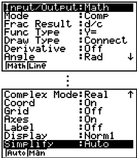
- Simplify (calculation result auto/manual reduction specification)
- {Auto}/{Man} ... {auto reduce and display}/{display without reduction}
• Q1Q3 Type ( Q_1/Q_3 calculation formulas)
- {Std}/{OnData} ... {Divide total population on its center point between upper and lower groups, with the median of the lower group Q1 and the median of the upper group Q3}/{Make the value of element whose cumulative frequency ratio is greater than 1/4 and nearest to 1/4 Q1 and the value of element whose cumulative frequency ratio is greater than 3/4 and nearest to 3/4 Q3}
The following items are not included on the fx-7400GII/fx-9750GII.
- Input/Output (input/output mode)
- Math / Line^*1 ... Math / Linear input/output mode
• Auto Calc (spreadsheet auto calc)
- {On}/{Off} ... {execute}/{not execute} the formulas automatically
• Show Cell (spreadsheet cell display mode)
- {Form}/{Val} ... {formula}*2/{value}
- Move (spreadsheet cell cursor direction) ^*3
- {Low}/{Right} ... {move down}/{move right}
*1 The initial default setting of the fx-9860G Slim (OS 2.00)/fx-9860G SD (OS 2.00)/fx-9860G (OS 2.00)/fx-9860G AU (OS 2.00) is the "Line" input/output mode.
*2 Selecting “Form” (formula) causes a formula in the cell to be displayed as a formula. The “Form” does not affect any non-formula data in the cell.
*3 Specifies the direction the cell cursor moves when you press the EXE key to register cell input, when the Sequence command generates a number table, and when you recall data from List memory.
9. Using Screen Capture
Any time while operating the calculator, you can capture an image of the current screen and save it in capture memory.
• To capture a screen image
-
Operate the calculator and display the screen you want to capture.
-
Press SHIFT 7 (CAPTURE).
- This displays a memory area selection dialog box.
![su Store In Capture Memory Capture[1~20]:I GRAPH CALC TEST UNTR DIST](/content/2025/01/86832/images/9ab6f8e79bb76b9f21566f5d337a43d326fb85f2bbd671596e29cedde35b4f03.jpg)
- Input a value from 1 to 20 and then press EXE.
- This will capture the screen image and save it in capture memory area named “Capt n” (n = the value you input).
- You cannot capture the screen image of a message indicating that an operation or data communication is in progress.
- A memory error will occur if there is not enough room in main memory to store the screen capture.
- To recall a screen image from capture memory
This operation is possible only while the Linear input/output mode is selected.
- In the RUN•MAT (or RUN) mode, press OPTN F6 (▷) F6 (▷) F5 (CAPT) (F4 (CAPT) on the fx-7400GII) F1 (RCL).

- Enter a capture memory number in the range of 1 to 20, and then press EXE.
- This displays the image stored in the capture memory you specified.
- To exit the image display and return to the screen you started from in step 1, press EXIT.
- You can also use the RclCapt command in a program to recall a screen image from capture memory.
10. When you keep having problems...
If you keep having problems when you are trying to perform operations, try the following before assuming that there is something wrong with the calculator.
■ Getting the Calculator Back to its Original Mode Settings
- From the Main Menu, enter the SYSTEM mode.
- Press F5 (RSET).
- Press F1(STUP), and then press F1(Yes).
- Press EXIT MENU to return to the Main Menu.
Now enter the correct mode and perform your calculation again, monitoring the results on the display.
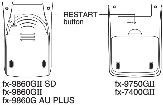
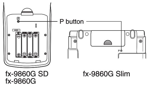
- Restart
Should the calculator start to act abnormally, you can restart it by pressing the RESTART button (P button). Note, however, that you should only use the RESTART button only as a last resort. Normally, pressing the RESTART button reboots the calculator's operating system, so programs, graph functions and other data in calculator memory is retained.
Important!
The calculator backs up user data (main memory) when you turn power off and loads the backed up data when you turn power back on.
When you press the RESTART button, the calculator restarts and loads backed up data. This means that if you press the RESTART button after you edit a program, graph function, or other data, any data that has not been backed up will be lost.
- Reset
Use reset when you want to delete all data currently in calculator memory and return all mode settings to their initial defaults.
Before performing the reset operation, first make a written copy of all important data. For details, see "Reset" (page 12-3).
■ Low Battery Message
If the following message appears on the display, immediately turn off the calculator and replace batteries as instructed.

If you continue using the calculator without replacing batteries, power will automatically turn off to protect memory contents. Once this happens, you will not be able to turn power back on, and there is the danger that memory contents will be corrupted or lost entirely.
- You will not be able to perform data communications operations after the low battery message appears.
Chapter 2 Manual Calculations
1. Basic Calculations
Arithmetic Calculations
- Enter arithmetic calculations as they are written, from left to right.
- Use the (-) key to input the minus sign before a negative value.
- Calculations are performed internally with a 15-digit mantissa. The result is rounded to a 10-digit mantissa before it is displayed.
- For mixed arithmetic calculations, multiplication and division are given priority over addition and subtraction.
| Example | Operation |
| 56 × (-12) ÷ (-2.5) = 268.8 (2 + 3) × 10^2 = 500 2 + 3 × (4 + 5) = 29 64 × 5 = 0.3 | 56 × (-) 12 ÷ (-) 2.5 EXE (2 + 3) × 1 EXP 2 EXE 2 + 3 × (4 + 5)^*1 6 ÷ (4 × 5) EXE |
*1 Final closed parentheses (immediately before operation of the EXE key) may be omitted, no matter how many are required.
■ Number of Decimal Places, Number of Significant Digits, Normal
Display Range
[SET UP]- [Display] - [Fix] / [Sci] / [Norm]
- Even after you specify the number of decimal places or the number of significant digits, internal calculations are still performed using a 15-digit mantissa, and displayed values are stored with a 10-digit mantissa. Use Rnd of the Numeric Calculation Menu (NUM) (page 2-12) to round the displayed value off to the number of decimal place and significant digit settings.
- Number of decimal place (Fix) and significant digit (Sci) settings normally remain in effect until you change them or until you change the normal display range (Norm) setting.
*1 Displayed values are rounded off to the place you specify.
Example 2 200 ÷ 7 × 14 = 400
| Condition | Operation | Display |
| 200÷7×14EXE | 400 | |
| 3 decimal places | SHIFT MENU (SET UP)▲▲F1 (Fix) 3 EXE EXIT EXE | 400.000 |
| Calculation continues using display capacity of 10 digits | 200÷7EXE | 28.571 |
| ×14EXE | Ans ×I400.000 |
- If the same calculation is performed using the specified number of digits:
| 200÷7EXE | 28.571 | |
| The value stored internally is rounded off to the number of decimal places specified on the Setup screen. | OPTN F6 (▷) F4 (NUM)* F4 (Rnd) EXE | 28.571 |
| 14 EXE | 399.994 | |
| 200÷7EXE | 28.571 | |
| You can also specify the number of decimal places for rounding of internal values for a specific calculation.(Example: To specify rounding to two decimal places) | F6 (▷) F1 (RndFi) SHIFT (-) (Ans) 2 EXE | RndFix(Ans,2)28.570 |
| 14 EXE | 399.980 |
* fx-7400GII: F3 (NUM)
■ Calculation Priority Sequence
This calculator employs true algebraic logic to calculate the parts of a formula in the following order:
① Type A functions
• Coordinate transformation Pol (x, y) , Rec (r, )
- Functions that include parentheses (such as derivatives, integrations, , etc.) d/dx , d^2/dx^2 , dx , , Solve, FMin, FMax, List→Mat, Fill, Seq, SortA, SortD, Min, Max, Median, Mean, Augment, Mat→List, P(, Q(, R(, t(, RndFix, log_a b
- Composite functions ^*1 , List, Mat, fn, Yn, rn, Xtn, Ytn, Xn
② Type B functions
With these functions, the value is entered and then the function key is pressed. x^2, x^-1, x!, ^ , ENG symbols, angle unit ^ , ^r , ^g
③ Power/root ^(x^y) , ^x
④ Fractions a^b/_c
⑤ Abbreviated multiplication format in front of , memory name, or variable name. 2 , 5A, Xmin, F Start, etc.
⑥ Type C functions
With these functions, the function key is pressed and then the value is entered. , ^3 , , , e^x , 10^x , , , , ^-1 , ^-1 , ^-1 , , , , ^-1 , ^-1 ,
^-1 , (-) , d, h, b, o, Neg, Not, Det, Trn, Dim, Identity, Ref, Rref, Sum, Prod, Cuml, Percent, List, Abs, Int, Frac, Intg, Arg, Conjg, ReP, ImP
⑦ Abbreviated multiplication format in front of Type A functions, Type C functions, and parenthesis.
23 , A log2, etc.
⑧ Permutation, combination nPr, nCr
⑨ Metric conversion commands
⑩ ×, ÷, Int÷, Rnd
⑪ +, -
⑫ Relational operators =, ≠, >, <, ≥, ≤
⑬ And (logical operator), and (bitwise operator)
⑭ Or, Xor (logical operator), or, xor, xnor (bitwise operator)
*1 You can combine the contents of multiple function memory (fn) locations or graph memory (Yn, rn, Xtn, Ytn, Xn) locations into composite functions. Specifying fn1(fn2), for example, results in the composite function fn1°fn2 (see page 5-7). A composite function can consist of up to five functions.
Example 2 + 3 × ( 2^2 + 6.8) = 22.07101691 (angle unit = Rad)
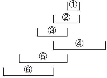
flowchart
graph TD
    A["①"] --> B["②"]
    B --> C["③"]
    C --> D["④"]
    D --> E["⑤"]
    E --> F["⑥"]
- You cannot use a differential, quadratic differential, integration, , maximum/minimum value, Solve, RndFix or _a b calculation expression inside of a RndFix calculation term.
- When functions with the same priority are used in series, execution is performed from right to left.
$$ e ^ {x} \ln \sqrt {1 2 0} \rightarrow e ^ {x} {\ln (\sqrt {1 2 0}) } $$
Otherwise, execution is from left to right.
- Compound functions are executed from right to left.
- Anything contained within parentheses receives highest priority.
■ Calculation Result Irrational Number Display
(fx-9860GII SD/fx-9860GII/fx-9860G AU PLUS only)
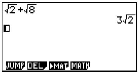
You can configure the calculator to display calculation results in irrational number format (including or ) by selecting “Math” for the “Input/Output” mode setting on the Setup screen.
Example 2 + 8 = 32 (Input/Output: Math)

- Calculation Result Display Range with
Display of a calculation result in format is supported for result with in up to two terms. Calculation results in format take one of the following forms.
$$ \pm a \sqrt {b}, \pm d \pm a \sqrt {b}, \pm \frac {a \sqrt {b}}{c} \pm \frac {d \sqrt {e}}{f} $$
- The following are the ranges for each of the coefficients (a, b, c, d, e, f) can be displayed in the calculation result format.
$$ 1 \leq a < 1 0 0, 1 < b < 1 0 0 0, 1 \leq c < 1 0 0 $$
$$ 0 \leq d < 1 0 0, 0 \leq e < 1 0 0 0, 1 \leq f < 1 0 0 $$
- In the cases shown below, a calculation result may be able to be displayed in format even if their coefficients (a, c, d) are outside the above ranges.
A format calculation result uses a common denominator.
$$ \frac {a \sqrt {b}}{c} + \frac {d \sqrt {e}}{f} \rightarrow \frac {a ^ {\prime} \sqrt {b} + d ^ {\prime} \sqrt {e}}{c ^ {\prime}} \quad * c ^ {\prime} \text { is the least common multiple of } c \text { and } f. $$
Since the calculation result uses a common denominator, calculation result still may be displayed using the format even when coefficients (a', c', d') are outside the corresponding range of coefficients (a, c, d) .
Example: 311+210=103+112110
Calculation Examples
| This calculation: | Produces this type of display: |
| 2 × (3 - 25) = 6 - 45 | format |
| 352 × 3 = 148.492424 (= 1052)^*1 | Decimal format |
| 150225 = 8.485281374^*1 | |
| 23 × (5 - 23) = 35.32566285 (= 115 - 463)^*1 | Decimal format |
| 2 + 3 + 8 = 3 + 32 | format |
| 2 + 3 + 6 = 5.595754113^*2 | Decimal format |
*1 Decimal format because values are outside of range.
*2 Decimal format because calculation result has three terms.
- The calculation result is displayed using decimal format even if an intermediate result goes greater than two terms.
Example: (1 + 2 + 3)(1 - 2 - 3) (= -4 - 26)
$$ = - 8. 8 9 8 9 7 9 4 8 6 $$
- If the calculation formula has a term and a term that cannot be displayed as a fraction, the calculation result will be displayed in decimal format.
Example: 3 + 2 = 1.891334817
- Calculation Result Display Range with
A calculation results is displayed using format in the following cases.
- When the calculation result can be displayed in the form n n is an integer up to |10^6| .
- When the calculation result can be displayed in the form a or . However, number of a digits + number of b digits + number of c digits must be 9 or less when the above a or is reduced. ^12 Also, the maximum number of allowable c digits is three. ^*2
*1 When c < b , the number of a, b , and c digits are counted when the fraction is converted from an improper fraction () to a mixed fraction (a) .
*2 When “Manual” is specified for the Setup screen “Simplify” setting, the calculation result may be displayed in decimal format, even if these conditions are met.
Calculation Examples
| This calculation: | Produces this type of display: |
| 78 × 2 = 156 | format |
| 123456 × 9 = 3490636.164 (= 11111104_~~~~~~ )^*3 | Decimal format |
| 105568824 = 10571103 | format |
| 22583238 = 6.533503684_~~~~~~ (21291619 )^*4 | Decimal format |
*3 Decimal format because calculation result integer part is |10^6| or greater.
*4 Decimal format because number of denominator digits is four or greater for the a form.
■ Multiplication Operations without a Multiplication Sign
You can omit the multiplication sign (×) in any of the following operations.
- Before Type A functions (① on page 2-2) and Type C functions (⑥ on page 2-2), except for negative signs
Example 1 2sin30, 10log1.2, 23 , 2Pol(5, 12), etc.
- Before constants, variable names, memory names
Example 2 2, 2AB, 3Ans, 3Y_1, etc.
• Before an open parenthesis
Example 3 3(5 + 6) , (A + 1)(B - 1) , etc.
■ Overflow and Errors
Exceeding a specified input or calculation range, or attempting an illegal input causes an error message to appear on the display. Further operation of the calculator is impossible while an error message is displayed. For details, see the “Error Message Table” on page -1.
- Most of the calculator's keys are inoperative while an error message is displayed. Press EXIT to clear the error and return to normal operation.
■ Memory Capacity
Each time you press a key, either one byte or two bytes is used. Some of the functions that require one byte are: 1, 2, 3, sin, cos, tan, log, ln, √, and π.
Some of the functions that take up two bytes are d/dx (, Mat, Xmin, If, For, Return, DrawGraph, SortA(, PxIOn, Sum, and a_n+1 ).
- The required number of bytes to input functions and commands is different in the Linear input/output mode and the Math input/output mode. For details about the number of bytes required for each function in the Math input/output mode, see page 1-11.
2. Special Functions
■ Calculations Using Variables
| Example | Operation | Display |
| 193.2 → ALPHA X,θ,T (A) EXE | 193.2 | |
| 193.2 ÷ 23 = 8.4 | ALPHA X,θ,T (A) ÷ 23 EXE | 8.4 |
| 193.2 ÷ 28 = 6.9 | ALPHA X,θ,T (A) ÷ 28 EXE | 6.9 |
■ Memory
• Variables (Alpha Memory)
This calculator comes with 28 variables as standard. You can use variables to store values you want to use inside of calculations. Variables are identified by single-letter names, which are made up of the 26 letters of the alphabet, plus r and . The maximum size of values that you can assign to variables is 15 digits for the mantissa and 2 digits for the exponent.
- Variable contents are retained even when you turn power off.
- To assign a value to a variable
[value] → [variable name] EXE
Example 1 To assign 123 to variable A
AC 1 2 3 → ALPHA X,θ,T (A) EXE
123→A
123
Example 2 To add 456 to variable A and store the result in variable B
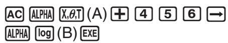
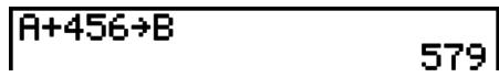
- To assign the same value to more than one variable
[value]→ [first variable name]ALPHA F3 (\~) [last variable name]EXE
- You cannot use “r” or “ ” as a variable name.
Example To assign a value of 10 to variables A through F
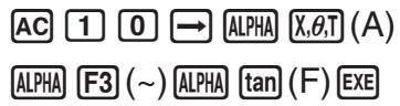
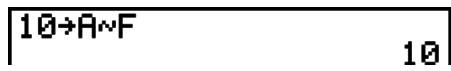
- String Memory
You can store up to 20 strings (named Str 1 to Str 20) in string memory. Stored strings can be output to the display or used inside functions and commands that support the use of strings as arguments.
For details about string operations, see "Strings" (page 8-18).
Example To assign string “ABC” to Str 1 and then output Str 1 to the display
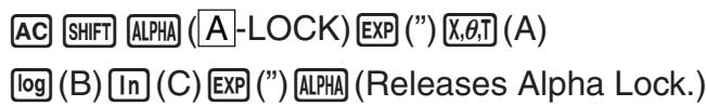


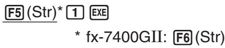
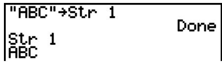
String is displayed justified left.
- Perform the above operation in the Linear input/output mode. It cannot be performed in the Math input/output mode.
- Function Memory
[OPTN]-[FMEM]
Function memory is convenient for temporary storage of often-used expressions. For longer term storage, we recommend that you use the GRAPH mode for expressions and the PRGM mode for programs.
- {STO}/{RCL}/{fn}/{SEE} ... {function store}/{function recall}/{function area specification as a variable name inside an expression}/{function list}
- To store a function
Example To store the function (A+B) (A-B) as function memory number 1
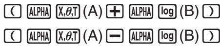


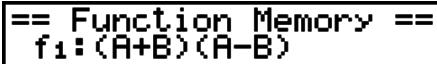

* fx-7400GII: F2 (FMEM)

- If the function memory number to which you store a function already contains a function, the previous function is replaced with the new one.
- You can also use to store a function in function memory in a program. In this case, you must enclose the function inside of double quotation marks.

- To recall a function
Example To recall the contents of function memory number 1


* fx-7400GII: F2 (FMEM)
- The recalled function appears at the current location of the cursor on the display.
- To recall a function as a variable
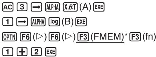
| 3→A | 3 |
| 1→B | 1 |
| fn1+2 | 10 |
* fx-7400GII: F2 (FMEM)
- To display a list of available functions
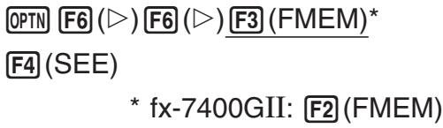
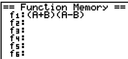
- To delete a function
Example To delete the contents of function memory number 1

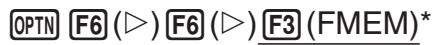
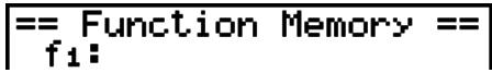

* fx-7400GII: F2 (FMEM)
- Executing the store operation while the display is blank deletes the function in the function memory you specify.
Answer Function
The Answer Function automatically stores the last result you calculated by pressing EXE (unless the EXE key operation results in an error). The result is stored in the answer memory.
- The largest value that the answer memory can hold is 15 digits for the mantissa and 2 digits for the exponent.
- Answer memory contents are not cleared when you press the AC key or when you switch power off.
- To use the contents of the answer memory in a calculation
Example 123 + 456 = 579
789 - 579 = 210

| 123+456 | 579 |
| 789-Ans | 210 |

fx-7400GII, fx-9750GII users...
- The answer memory contents are not changed by an operation that assigns values to Alpha memory (such as: 5 → ALPHA log(B) EXE).
fx-9860GII SD, fx-9860GII, fx-9860G AU PLUS, fx-9860G Slim users...
- In the Math input/output mode, the operation to recall answer memory contents is different from the operation in the Linear input/output mode. For details, see “History Function” (page 1-17).
- Performing an operation that assigns a value to an Alpha memory (such as 5 → ALPHA log(B) EXE), answer memory contents are updated in the Math input/output mode but not in the Linear input/output mode.
■ Performing Continuous Calculations
Answer memory also lets you use the result of one calculation as one of the arguments in the next calculation.
Example 1 ÷ 3 = 1 ÷ 3 × 3 =
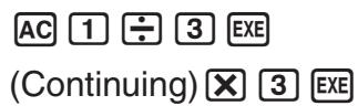
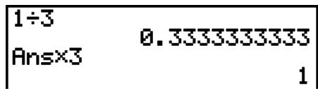
Continuous calculations can also be used with Type B functions (x^2, x^-1, x! , on page 2-2), +, -, (x^y), x,^, , etc.
3. Specifying the Angle Unit and Display Format
Before performing a calculation for the first time, you should use the Setup screen to specify the angle unit and display format.
■ Setting the Angle Unit
[SET UP]- [Angle]
- On the Setup screen, highlight "Angle".
-
Press the function key for the angle unit you want to specify, then press EXIT.
-
{Deg}/{Rad}/{Gra} ... {degrees}/{radians}/{grads}
- The relationship between degrees, grads, and radians is shown below.
$$ 3 6 0 ^ {\circ} = 2 \pi \text { radians } = 4 0 0 \text { grads } $$
$$ 9 0 ^ {\circ} = \pi / 2 \text { r a d i a n s } = 1 0 0 \text { g r a d s } $$
■ Setting the Display Format
[SET UP]- [Display]
- On the Setup screen, highlight "Display".
- Press the function key for the item you want to set, then press EXIT.
- {Fix}/{Sci}/{Norm}/{Eng} ... {fixed number of decimal places specification}/{number of significant digits specification}/{normal display}/{Engineering mode}
- To specify the number of decimal places (Fix)
Example To specify two decimal places
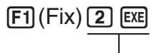

Press the number key that corresponds to the number of decimal places you want to specify (n = 0 to 9) .
- Displayed values are rounded off to the number of decimal places you specify.
- To specify the number of significant digits (Sci)
Example To specify three significant digits
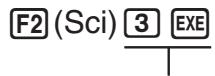

Press the number key that corresponds to the number of significant digits you want to specify n = 0 to 9 . Specifying 0 makes the number of significant digits 10.
- Displayed values are rounded off to the number of significant digits you specify.
- To specify the normal display (Norm 1/Norm 2)
Press F3 (Norm) to switch between Norm 1 and Norm 2.
Norm 1: 10^-2(0.01) > |x|, |x| ≥ 10^10
Norm 2: 10^-9 (0.000000001) > |x|, |x| ≥ 10^10
- To specify the engineering notation display (Eng mode)
Press F4 (Eng) to switch between engineering notation and standard notation. The indicator "/E" is on the display while engineering notation is in effect.
You can use the following symbols to convert values to engineering notation, such as 2,000 ( = 2 × 10^3 ) → 2k.
| E (Exa) | × 10^18 | m (milli) | × 10^-3 | |
| P (Peta) | × 10^15 | (micro) | × 10^-6 | |
| T (Tera) | × 10^12 | n (nano) | × 10^-9 | |
| G (Giga) | × 10^9 | p (pico) | × 10^-12 | |
| M (Mega) | × 10^6 | f (femto) | × 10^-15 | |
| k (kilo) | × 10^3 |
- The engineering symbol that makes the mantissa a value from 1 to 1000 is automatically selected by the calculator when engineering notation is in effect.
4. Function Calculations
■ Function Menus
This calculator includes five function menus that give you access to scientific functions not printed on the key panel.
- The contents of the function menu differ according to the mode you entered from the Main Menu before you pressed the OPTN key. The following examples show function menus that appear in the RUN • MAT (or RUN) or PRGM mode.
• Hyperbolic Calculations (HYP)
[OPTN]-[HYP]
- {sinh}/{cosh}/{tanh} ... hyperbolic {sine}/{cosine}/{tangent}
- ^-1 / ^-1 / ^-1 ... inverse hyperbolic sine / cosine / tangent
- Probability/Distribution Calculations (PROB)
[OPTN]-[PROB]
- x! ... {press after inputting a value to obtain the factorial of the value}
- nPr / nCr permutation / combination
- {RAND} ... {random number generation}
- {Ran#}/{Int}/{Norm}/{Bin}/{List} ... {random number generation (0 to 1)}/{random integer generation}/{random number generation in accordance with normal distribution based on mean (\mu) and standard deviation (\sigma}}/{random number generation in accordance with binomial distribution based on number of trials (n) and probability (p}}/{random number generation (0 to 1)) and storage of result in ListAns}
- P(·) / Q(·) / R(·) normal probability P(t) /Q(t) /R(t)
- t(·) value of normalized variate t(x)
- Numeric Calculations (NUM)
[OPTN]-[NUM]
- {Abs} ... {select this item and input a value to obtain the absolute value of the value}
- {Int}/{Frac} ... select the item and input a value to extract the {integer}/{fraction} part.
- {Rnd} ... {rounds off the value used for internal calculations to 10 significant digits (to match the value in the answer memory), or to the number of decimal places (Fix) and number of significant digits (Sci) specified by you}
- {Intg} ... {select this item and input a value to obtain the largest integer that is not greater than the value}
- {RndFi} ... {rounds off the value used for internal calculations to specified digits (0 to 9) (see page 2-2).}
- {GCD} ... {greatest common divisor for two values}
- {LCM} ... {least common multiple for two values}
- {MOD} ... {remainder of division (remainder output when n is divided by m )}
- {MOD·E} ... {remainder when division is performed on a power value (remainder output when n is raised to p power and then divided by m )}
- Angle Units, Coordinate Conversion, Sexagesimal Operations (ANGL)
[OPTN]-[ANGL]
- { ^° }/{ r }/{ g } ... {degrees}/{{radians}}/{{grads}} for a specific input value
- {° ' "} ... {specifies degrees (hours), minutes, seconds when inputting a degrees/minutes/seconds value}
- ,, ... {converts decimal value to degrees/minutes/seconds value}
- The , menu operation is available only when there is a calculation result on the display.
- {Pol()/{Rec()} ... {rectangular-to-polar}/{polar-to-rectangular} coordinate conversion
- DMS} ... {converts decimal value to sexagesimal value}
• Engineering Symbol (ESYM)
[OPTN]-[ESYM]
- m / / n / p / f ... milli (10^-3) / micro (10^-6) / nano (10^-9) / pico (10^-12) / femto (10^-15)
- k / M / G / T / P / E ... kilo (10^3) / mega (10^6) / giga (10^9) / tera (10^12) / peta (10^15) / exa (10^18)
- {ENG}/{ENG} ... shifts the decimal place of the displayed value three digits to the {left}/{right} and {decreases}/{increases} the exponent by three.
When you are using engineering notation, the engineering symbol is also changed accordingly.
- The {ENG} and {ENG} menu operations are available only when there is a calculation result on the display.
Angle Units
- Be sure to specify Comp for Mode in the Setup screen.
| Example | Operation |
| To convert 4.25 rad to degrees:243.5070629 | SHIFT MENU (SET UP) ▼ ▼ ▼ ▼ ▼ ▼ * F1 (Deg) EXIT4.25 OPTN F6 (▷) F5 (ANGL)** F2 (r) EXE |
| 47.3° + 82.5rad = 4774.20181° | 47.3 ⊕ 82.5 OPTN F6 (▷) F5 (ANGL)** F2 (r) EXE |
| 2°20′30′′ + 39′30′′ = 3°00′00′′ | 2 OPTN F6 (▷) F5 (ANGL)** F4 (° ′′) 20 F4 (° ′′) 30F4 (° ′′) ⊕ 0 F4 (° ′′)39 F4 (° ′′) 30 F4 (° ′′) EXE F5 (° ′′) |
| 2.255° = 2°15′18′′ | 2.255 OPTN F6 (▷) F5 (ANGL)** F6 (▷) F3 (►DMS) EXE |
* fx-7400GII, fx-9750GII: ▼ ▼ ▼ ▼ ** fx-7400GII: F4 (ANGL)
■ Trigonometric and Inverse Trigonometric Functions
- Be sure to set the angle unit before performing trigonometric function and inverse trigonometric function calculations.
$$ (9 0 ^ {\circ} = \frac {\pi}{2} \text { r a d i a n s } = 1 0 0 \text { g r a d s }) $$
- Be sure to specify Comp for Mode in the Setup screen.
| Example | Operation |
| ( 3 rad ) = 0.5 | SHIFT MENU (SET UP) ▼ ▼ ▼ ▼ ▼ ▼ * F2 (Rad) EXIT cos ( SHIFT EXP (π) ⊕ 3 ) EXE |
| 2 · 45^ × 65^ = 0.5976724775 | SHIFT MENU (SET UP) ▼ ▼ ▼ ▼ ▼ ▼ * F1 (Deg) EXIT 2 × sin 45 × cos 65 EXE *1 |
| ^-10.5 = 30^ (x when x = 0.5 ) | SHIFT sin ( ^-1 ) 0.5*2 EXE |
*1 ☒ can be omitted.
* fx-7400GII, fx-9750GII: ▼ ▼ ▼ ▼ ▼
*2 Input of leading zero is not necessary.
■ Logarithmic and Exponential Functions
- Be sure to specify Comp for Mode in the Setup screen.
| Example | Operation |
| 1.23 (_101.23) = 0.08990511144 _28 = 3 (-3)^4 = (-3) × (-3) × (-3) × (-3) = 81 ^7123(= 123^17) = 1.988647795 | 1.23 4 (CALC)^* 6 (▷) 4 (log_ab 2,8) ((-)3) 4 7 (x)123 |
* fx-7400GII: F3 (CALC)
- The Linear input/output mode and Math input/output mode produce different results when two or more powers are input in series, like: 2 △ 3 △ 2.
Linear input/output mode: 2^3^2 = 64 Math input/output mode: 2^3^2 = 512
This is because the Math input/output mode internally treats the above input as: 2^(3^(2)) .
■ Hyperbolic and Inverse Hyperbolic Functions
- Be sure to specify Comp for Mode in the Setup screen.
| Example | Operation |
| 3.6 = 18.28545536 | 6 () 2 (HYP)^* 1 () 3.6 |
| ^-1(2015) = 0.7953654612 | 6 () 2 (HYP)^* 5 (^-1) (20 ÷ 15) |
* fx-7400GII: F1 (HYP)
■ Other Functions
- Be sure to specify Comp for Mode in the Setup screen.
| Example | Operation |
| 2 + 5 = 3.65028154 (-3)^2 = (-3) × (-3) = 9 8! (= 1 × 2 × 3 × .... × 8 ) = 40320What is the integer part of -3.5?-3 | SHIFT ^2( )2 + ^2( )5 ( (-)3 ) ^2 8OPTN F6 (▷)F3 (PROB)*1F1 (x!) EXEOPTN F6 (▷)F4 (NUM)*2F2 (Int) (-)3.5 EXE |
*1 fx-7400GII: F2 (PROB) *2 fx-7400GII: F3 (NUM)
- Random Number Generation (0 to 1) (Ran#, RanList#)
Ran# and RanList# generate 10 digit random numbers randomly or sequentially from 0 to 1. Ran# returns a single random number, while RanList# returns multiple random numbers in list form. The following shows the syntaxes of Ran# and RanList#.
| Ran# [a] | 1 ≤ a ≤ 9 |
| RanList# (n [,a]) | 1 ≤ n ≤ 999 |
- n is the number of trials. RanList# generates the number of random numbers that corresponds to n and displays them on the ListAns screen. A value must be input for n .
- “a” is the randomization sequence. Random numbers are returned if nothing is input for “a”. Entering an integer of 1 through 9 for a will return the corresponding sequential random number.
- Executing the function Ran# 0 initializes the sequences of both Ran# and RanList#. The sequence also is initialized when a sequential random number is generated with a different sequence of the previous execution using Ran# or RanList#, or when generating a random number.
Ran# Examples
| Example | Operation |
| Ran#(Generates a random number.) | OPTN F6 (▷) F3 (PROB)* F4 (RAND)F1 (Ran#) EXE |
| (Each press of EXE generates a new random number.) | EXEEXE |
| Ran# 1(Generates the first random number in sequence 1.) | OPTN F6 (▷) F3 (PROB)* F4 (RAND)F1 (Ran#)1 EXE |
| (Generates the second random number in sequence 1.) | EXE |
| Ran# 0(Initializes the sequence.) | F1 (Ran#)0 EXE |
| Ran# 1(Generates the first random number in sequence 1.) | F1 (Ran#)1 EXE |
* fx-7400GII: F2 (PROB)
| Example | Operation |
| RanList# (4)(Generates four random numbers and displays the result on the ListAns screen.) | 6 ( ) 3 (PROB)* 4 (RAND) 5 (List)4 ) EXE |
| RanList# (3, 1)(Generates from the first to the third random numbers of sequence 1 and displays the result on the ListAns screen.) | 6 ( ) 3 (PROB)* 4 (RAND) 5 (List) 3 ) 1 ) EXE |
| (Next, generates from the fourth to the sixth random number of sequence 1 and displays the result on the ListAns screen.) | EXE |
| Ran# 0(Initializes the sequence.) | 1 (Ran#) 0 EXE |
| RanList# (3, 1)(Re-generates from the first to the third random numbers of sequence 1 and displays the result on the ListAns screen.) | 5 (List) 3 ) 1 ) EXE |
* fx-7400GII: F2 (PROB)
- Random Integer Generation (RanInt#)
RanInt# generates random integers that fall between two specified integers.
RanInt# (A, B [,n])
A < B
|A|,|B|<1_E10
B - A < 1E10
1 ≤ n ≤ 999
- A is the start value and B is the end value. Omitting a value for n returns a generated random number as-is. Specifying a value for n returns the specified number of random values in list form.
| Example | Operation |
| RanInt# (1, 5)(Generates one random integer from 1 and 5.) | 6 (▷) 3 (PROB)* 4 (RAND) 2 (Int)1 □ 5 □ EXE |
| RanInt# (1, 10, 5)(Generates five random integers from 1 to 10 and displays the result on the ListAns screen.) | 6 (▷) 3 (PROB)* 4 (RAND) 2 (Int)1 □ 10 □ 5 □ EXE |
* fx-7400GII: F2 (PROB)
- Random Number Generation in Accordance with Normal Distribution (RanNorm#)
This function generates a 10-digit random number in accordance with normal distribution based on a specified mean and standard deviation values.
RanNorm# (σ, μ [,n])
> 0
1 ≤ n ≤ 999
- Omitting a value for n returns a generated random number as-is. Specifying a value for n returns the specified number of random values in list form.
| Example | Operation |
| RanNorm# (8, 68)(Randomly produces a body length value obtained in accordance with the normal distribution of a group of infants less than one year old with a mean body length of 68cm and standard deviation of 8.) | OPTN F6 (▷) F3 (PROB)* F4 (RAND) F3 (Norm)8 68 EXE |
| RanNorm# (8, 68, 5)(Randomly produces the body lengths of five infants in the above example, and displays them in a list.) | OPTN F6 (▷) F3 (PROB)* F4 (RAND) F3 (Norm)8 68 5 EXE |
* fx-7400GII: F2 (PROB)
- Random Number Generation in Accordance with Binomial Distribution (RanBin#)
This function generates random integers in accordance with binomial distribution based on values specified for the number of trials n and probability p.
RanBin# (n, p [,m]) 1 ≤ n ≤ 100000 1 ≤ m ≤ 999 0 ≤ p ≤ 1
- Omitting a value for m returns a generated random number as-is. Specifying a value for m returns the specified number of random values in list form.
| Example | Operation |
| RanBin# (5, 0.5)(Randomly produces the number of headsthat can be expected in accordance withbinomial distribution for five coin tosseswhere the probability of heads is 0.5.) | 6 ( ) 3 (PROB)* 4 (RAND) 4 (Bin)5 , 0.5 ) EXE |
| RanBin# (5, 0.5, 3)(Performs the same coin toss sequencedescribed above three times and displaysthe results in a list.) | 6 ( ) 3 (PROB)* 4 (RAND) 4 (Bin)5 , 0.5 , 3 ) EXE |
* fx-7400GII: F2 (PROB)
■ Coordinate Conversion
- Rectangular Coordinates
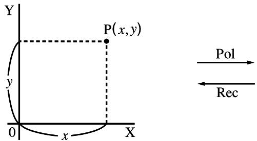
- Polar Coordinates
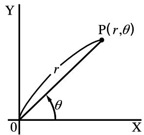
- With polar coordinates, can be calculated and displayed within a range of -180^ < ≤ 180^ (radians and grads have same range).
- Be sure to specify Comp for Mode in the Setup screen.
| Example | Operation |
| Calculate r and ^ when x = 14 and y = 20.7 1 [ 24.989 \ 55.928 ] 24.98979792 (r) 2 55.928 55.92839019 () | SHIFT MENU (SET UP) [▼ ▼ ▼ ▼ ▼ ▼ *F1 (Deg) EXITOPTN F6 (▷) F5 (ANGL)** F6 (▷) F1 (Pol()14 , 20.7 ) EXE EXIT |
| Calculate x and y when r = 25 and = 56^ 1 [ 13.979 \ 20.725 ] 13.97982259 (x) 2 20.725 20.72593931 (y) | F2 (Rec() 25 , 56 ) EXE |
* fx-7400GII, fx-9750GII: ▼ ▼ ▼ ▼ ** fx-7400GII: F4 (ANGL)
■ Permutation and Combination
- Permutation
$$ n \mathsf {P r} = \frac {n !}{(n - r) !} $$
- Combination
$$ n \mathsf {C} r = \frac {n !}{r ! (n - r) !} $$
- Be sure to specify Comp for Mode in the Setup screen.
Example 1 To calculate the possible number of different arrangements using 4 items selected from among 10 items
| Formula | Operation |
| _10P_4 = 5040 | 10 6 () 3 (PROB)^* 2 (nP_r) 4 |
* fx-7400GII: F2 (PROB)
Example 2 To calculate the possible number of different combinations of 4 items that can be selected from among 10 items
| Formula | Operation |
| _10C_4 = 210 | 10 6 () 3 (PROB)^* 3 (nC_r) 4 |
* fx-7400GII: F2 (PROB)
■ Greatest Common Divisor (GCD), Least Common Multiple (LCM)
| Example | Operation |
| To determine the greatest common divisor of 28 and 35(GCD (28, 35) = 7) | OPTN F6 (▷) F4 (NUM)* F6 (▷) F2 (GCD) 28 , 35 ) EXE |
| To determine the least common multiple of 9 and 15(LCM (9, 15) = 45) | OPTN F6 (▷) F4 (NUM)* F6 (▷) F3 (LCM) 9 , 15 ) EXE |
* fx-7400GII: F3 (NUM)
■ Division Remainder (MOD), Remainder of Exponential Division (MOD Exp)
| Example | Operation |
| To determine the remainder when 137 is divided by 7(MOD (137, 7) = 4) | OPTN F6 (▷) F4 (NUM)* F6 (▷) F4 (MOD) 137 , 7 ) EXE |
| To determine the remainder when 5^3 is divided by 3(MOD • E (5, 3, 3) = 2) | OPTN F6 (▷) F4 (NUM)* F6 (▷) F5 (MOD • E) 5 , 3 , 3 ) EXE |
* fx-7400GII: F3 (NUM)
Fractions
- In the Math input/output mode, the fraction input method is different from that described below. For fraction input operations in the Math input/output mode, see page 1-11.
- Be sure to specify Comp for Mode in the Setup screen.
| Example | Operation |
| 25 + 314 = 7320 = 3.65 (Conversion to decimal)* ^1 12578 + 14572 = 6.066202547 × 10^-4 * ^2 | 2 _c^b 5 + 3 _c^b 1 _c^b 4 -D 1 _c^b 2578 + 1 _c^b 4572 1 _c^b 2 ×.5 |
| 12 × 0.5 = 0.25^*3 |
*1 Fractions can be converted to decimal values and vice versa.
*2 When the total number of characters, including integer, numerator, denominator and delimiter marks exceeds 10, the fraction is automatically displayed in decimal format.
*3 Calculations containing both fractions and decimals are calculated in decimal format.
- Pressing the SHIFT F→D (a b/c ⇔ d/c) key toggles the display fraction between mixed fraction and improper fraction format.
■ Engineering Notation Calculations
Input engineering symbols using the engineering notation menu.
- Be sure to specify Comp for Mode in the Setup screen.
| Example | Operation |
| 999k (kilo) + 25k (kilo)= 1.024M (mega) | SHIFT MENU (SET UP)▲ ▲ F4 (Eng) EXIT 999 OPTN F6 (▷) F6 (▷)F1 (ESYM)* F6 (▷) F1 (k) + 25 F1 (k) EXE |
| 9 ÷ 10 = 0.9 = 900m (milli)= 0.9 | 9 ÷ 10 EXEOPTN F6 (▷) F6 (▷) F1 (ESYM)* F6 (▷) F6 (▷) F3 (ENG)*1 |
$$ = 0. 0 0 0 9 \mathrm{k} (\text { k i l o }) $$
$$ = 0. 9 $$
$$ = 9 0 0 \mathrm{m} $$
$$ \boxed {F 3} (\overleftarrow {E N G}) ^ {* 1} $$
$$ \boxed {F 2} (E N G) ^ {* 2} $$
$$ \boxed {F 2} (E N G) ^ {* 2} $$
* fx-7400GII: F5 (ESYM)
*1 Converts the displayed value to the next higher engineering unit, by shifting the decimal point three places to the right.
*2 Converts the displayed value to the next lower engineering unit, by shifting the decimal point three places to the left.
■ Logical Operators (AND, OR, NOT, XOR)
[OPTN]-[LOGIC]
The logical operator menu provides a selection of logical operators.
- {And}/{Or}/{Not}/{Xor} ... {logical AND}/{logical OR}/{logical NOT}/{logical XOR}
- Be sure to specify Comp for Mode in the Setup screen.
Example What is the logical AND of A and B when A = 3 and B = 2? A AND B = 1
| Operation | Display |
| 3 → ALPHA X,θ,T (A) EXE2 → ALPHA log (B) EXEALPHA X,θ,T (A) OPTN F6 (▷) F6 (▷)F4 (LOGIC)* F1 (And) ALPHA log (B) EXE | 1 |
* fx-7400GII: F3 (LOGIC)
- About Logical Operations
- A logical operation always produces either 0 or 1 as its result.
- The following table shows all of possible results that can be produced by AND, OR and XOR operations.
| Value or Expression A | Value or Expression B | A AND B | A OR B | A XOR B | |
| A ≠ 0 | B ≠ 0 | 1 | 1 | 0 | |
| A ≠ 0 | B = 0 | 0 | 1 | 1 | |
| A = 0 | B ≠ 0 | 0 | 1 | 1 | |
| A = 0 | B = 0 | 0 | 0 | 0 |
- The following table shows the results produced by the NOT operation.
| Value or Expression A | NOT A | |
| A ≠ 0 | 0 | |
| A = 0 | 1 |
5. Numerical Calculations
The following explains the numerical calculation operations included in the function menu displayed when 4 (CALC) ( 3 (CALC) on the fx-7400GII) is pressed. The following calculations can be performed.
- {Int÷}/{Rmdr}/{Simp} ... {quotient}/{remainder}/{simplification}
- {Solve}/{d/dx}/{d²/dx²}/{∫dx}/{SolvN} ... {equality solution}/{differential}/{quadratic differential}/{integration}/{f(x) function solution}
- {FMin}/{FMax}/{Σ}/{log_a b} ... {minimum value}/{maximum value}/{summation}/{logarithm log_a b}
■ Quotient of Integer ÷ Integer
[OPTN]-[CALC]-[Int÷]
The “Int÷” function can be used to determine the quotient when one integer is divided by another integer.
Example To calculate the quotient of 107 ÷ 7
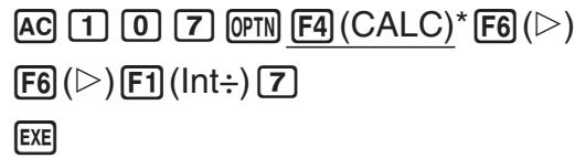
* fx-7400GII: F3 (CALC)
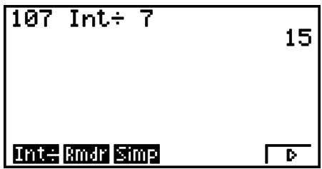
■ Remainder of Integer ÷ Integer
[OPTN]-[CALC]-[Rmdr]
The “Rmdr” function can be used to determine the remainder when one integer is divided by another integer.
Example To calculate the remainder of 107 ÷ 7
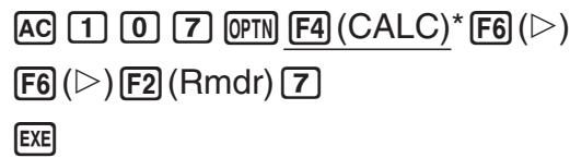
* fx-7400GII: F3 (CALC)
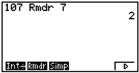
■ Simplification
[OPTN]-[CALC]-[Simp]
The “▶Simp” function can be used to simplify fractions manually. The following operations can be used to perform simplification when an unsimplified calculation result is on the display.
- {Simp} EXE ... This function automatically simplifies the displayed calculation result using the smallest prime number available. The prime number used and the simplified result are shown on the display.
- {Simp} n EXE ... This function performs simplification according to the specified divisor n.
Under initial default settings, this calculator automatically simplifies fraction calculation results before displaying them. Before performing the following examples, use the Setup screen to change the “Simplify” setting from “Auto” to “Manual” (page 1-29).
- When “a+bi” or “r∠θ” is specified for the Setup screen “Complex Mode” setting, fraction calculation results always are simplified before being displayed, even if the “Simplify” setting is “Manual”.
- If you want to simplify fractions manually (Simplify: Manual), make sure that the “Real” is selected for the “Complex Mode” setting.
Example 1 To simplify 1560 (1560 = 520 = 14)
AC 1 5 a_c^b 6 0 EXE
OPTN F4 (CALC)* F6 (▷) F6 (▷) F3 (Simp) EXE
* fx-7400GII: F3 (CALC)
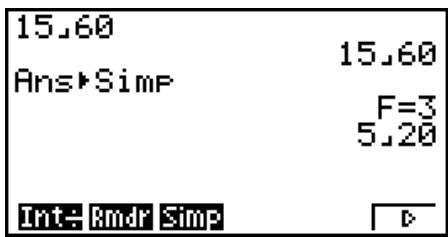
F3 (Simp) EXE
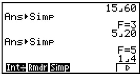
The “F=” value is the divisor.
Example 2 To simplify 2763 specifying a divisor of 9 (2763=37)
AC 2 7 a_c^b 6 3 EXE OPTN F4 (CALC)*
F6 (▷) F6 (▷) F3 (Simp) 9 EXE
* fx-7400GII: F3 (CALC)
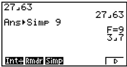
- An error occurs if simplification cannot be performed using the specified divisor.
- Executing ▶Simp while a value that cannot be simplified is displayed will return the original value, without displaying “F=”.
■ Solve Calculations
[OPTN]-[CALC]-[Solve]
The following is the syntax for using the Solve function in a program.
Solve( f(x) , n, a, b) (a: lower limit, b: upper limit, n: initial estimated value)
There are two different input methods that can be used for Solve calculations: direct assignment and variable table input.
With the direct assignment method (the one described here), you assign values directly to variables. This type of input is identical to that used with the Solve command used in the PRGM mode.
Variable table input is used with the Solve function in the EQUA mode. This input method is recommended for most normal Solve function input.
An error (Time Out) occurs when there is no convergence of the solution.
For information about Solve calculations, see page 4-4.
- You cannot use a quadratic differential, , maximum/minimum value or Solve calculation expression inside of any of the above functions.
- Pressing AC during calculation of Solve (while the cursor is not shown on the display) interrupts the calculation.
■ Solving an f(x) Function
[OPTN]-[CALC]-[SolvN]
You can use SolvN to solve an f(x) function using numerical analysis. The following is the input syntax.
SolveN (left side [=right side] [,variable] [, lower limit, upper limit])
- The right side, variable, lower limit and upper limit all can be omitted.
- “left side[=right side]” is the expression to be solved. Supported variables are A through Z, r, and θ. When the right side is omitted, solution is perform using right side = 0.
- The variable specifies the variable within the expression to be solved for (A through Z , r , ). Omitting a variable specification cause X to be used as the variable.
- The lower limit and upper limit specify the range of the solution. You can input a value or an expression as the range.
- The following functions cannot be used within any of the arguments. Solve (d^2 / dx^2, FMin(), FMax(),
Up to 10 calculation results can be displayed simultaneously in ListAns format.
- The message “No Solution” is displayed if no solution exists.
- The message “More solutions may exist.” is displayed when there may be solutions other than those displayed by SolvN.
Example To solve x^2-5x-6=0
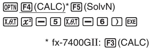
EXIT
![WARNING! More solutions may exist. Press: [EXIT]](/content/2025/01/86832/images/1d2fcc8048a739403be7d29acecc4faf5b8445f35b7499c19a0e5dba1355a5b9.jpg)
![Ans 1[ ] -1 2[ ] 6 -1](/content/2025/01/86832/images/0154fbbfe9eee92525ec3c7c372e552451602cbe2d8331cd1c4e3275a262685a.jpg)
To perform differential calculations, first display the function analysis menu, and then input the values using the syntax below.
$$ \boxed {\text {OPTN}} \boxed {\mathsf {F 4}} (\text {CALC}) ^ {*} \boxed {\mathsf {F 2}} (d / d x) f (x) \boxed {\bullet} a \boxed {\bullet} t o l \boxed {\bullet} $$
$$ ^ {*} \mathrm{fx-7400GII:} \boxed {\mathrm{F3}} (\text {CALC}) $$
(a: point for which you want to determine the derivative, tol: tolerance)
$$ d / d x (f (x), a) \Rightarrow \frac {d}{d x} f (a) $$
The differentiation for this type of calculation is defined as:
$$ f ^ {\prime} (a) = \lim _ {\varDelta x \to 0} \frac {f (a + \varDelta x) - f (a)}{\varDelta x} $$
In this definition, infinitesimal is replaced by a sufficiently small x , with the value in the neighborhood of f'(a) calculated as:
$$ f ^ {\prime} (a) \doteq \frac {f (a + \Delta x) - f (a)}{\Delta x} $$
In order to provide the best precision possible, this unit employs central difference to perform differential calculations.
Example To determine the derivative at point x = 3 for the function
$$ y = x ^ {3} + 4 x ^ {2} + x - 6, \text { with a tolerance of ``tol'' } = 1 _ {\mathrm{E}} - 5 $$
Input the function f(x) .
$$ \boxed {A C} \boxed {O P T N} \boxed {F 4} (C A L C) ^ {*} \boxed {F 2} (d / d x) \boxed {X, \theta , T} \boxed {\wedge} \boxed {3} + \boxed {4} \boxed {X, \theta , T} \boxed {x ^ {2}} + \boxed {X, \theta , T} - \boxed {6}, $$
$$ ^ {*} \mathrm{fx-7400GII:} \boxed {\mathrm{F3}} (\text {CALC}) $$
Input point x = a for which you want to determine the derivative.
$$ ③ , $$
Input the tolerance value.
$$ ⓛ \boxed {\mathrm{EXP}} (-) 5 () \boxed {\mathrm{EXE}} $$
$$ \left[ \begin{array}{c c} \mathrm{d} / \mathrm{d} x (X ^ {\wedge} 3 + 4 X ^ {2} + X - 6, 3, 1 \varepsilon \ - 5) & 5 2 \end{array} \right] $$
Using Differential Calculation in a Graph Function
- Omitting the tolerance (tol) value when using the differential command inside of a graph function simplifies the calculation for drawing the graph. In such a case, precision is sacrificed for the sake of faster drawing. The tolerance value is specified, the graph is drawn with the same precision obtained when you normally perform a differential calculation.
- You can also omit input of the derivative point by using the following format for the differential graph: Y2 = d / dx(Y1) . In this case, the value of the X variable is used as the derivative point.
Differential Calculation Precautions
- In the function f(x) , only X can be used as a variable in expressions. Other variables (A through Z excluding X , r , ) are treated as constants, and the value currently assigned to that variable is applied during the calculation.
- Input of the tolerance (tol) value and the closing parenthesis can be omitted. If you omit tolerance (tol) value, the calculator automatically uses a value for tol as 1_E - 10 .
- Specify a tolerance (tol) value of 1_E - 14 or greater. An error (Time Out) occurs whenever no solution that satisfies the tolerance value can be obtained.
- Pressing AC during calculation of a differential (while the cursor is not shown on the display) interrupts the calculation.
- Inaccurate results and errors can be caused by the following:
- discontinuous points in x values
- extreme changes in x values
- inclusion of the local maximum point and local minimum point in x values
- inclusion of the inflection point in x values
- inclusion of undifferentiable points in x values
-
differential calculation results approaching zero
-
Always use radians (Rad mode) as the angle unit when performing trigonometric differentials.
- You cannot use a differential, quadratic differential, integration, , maximum/minimum value, Solve, RndFix or _a b calculation expression inside a differential calculation term.
- In the Math input/output mode, the tolerance value is fixed at 1_E - 10 and cannot be changed.
■ Quadratic Differential Calculations
[OPTN]-[CALC]- [d^2 /dx^2]
After displaying the function analysis menu, you can input quadratic differentials using the following syntax.
OPTN F4 (CALC)* F3 (d^2 /dx^2)f(x) a tol
* fx-7400GII: F3 (CALC)
(a: differential coefficient point, tol: tolerance)
$$ \frac {d ^ {2}}{d x ^ {2}} (f (x), a) \Rightarrow \frac {d ^ {2}}{d x ^ {2}} f (a) $$
Quadratic differential calculations produce an approximate differential value using the following second order differential formula, which is based on Newton's polynomial interpretation.
$$ f ^ {\prime \prime} (a) = \frac {2 f (a + 3 h) - 2 7 f (a + 2 h) + 2 7 0 f (a + h) - 4 9 0 f (a) + 2 7 0 f (a - h) - 2 7 f (a - 2 h) + 2 f (a - 3 h)}{1 8 0 h ^ {2}} $$
In this expression, values for “sufficiently small increments of h” are used to obtain a value that approximates f''(a) .
Example To determine the quadratic differential coefficient at the point where
x = 3 for the function y = x^3 + 4x^2 + x - 6
Here we will use a tolerance tol = 1_E - 5
Input the function f(x) .
AC OPTN F4 (CALC)* F3 (d^2 /dx^2) X,θ,T ∧ 3 + 4 X,θ,T x² + X,θ,T - 6 ,
* fx-7400GII: F3 (CALC)
Input 3 as point a, which is the differential coefficient point.
3,
Input the tolerance value.
1 EXP (-) 5 )
EXE
^2 /dx^2 (X^3 +4X^2 +X - 6,3, 1 -5) 26
Quadratic Differential Calculation Precautions
- In the function f(x) , only X can be used as a variable in expressions. Other variables (A through Z excluding X , r , ) are treated as constants, and the value currently assigned to that variable is applied during the calculation.
- Input of the tolerance (tol) value and the closing parenthesis can be omitted.
- Specify a tolerance (tol) value of 1_E - 14 or greater. An error (Time Out) occurs whenever no solution that satisfies the tolerance value can be obtained.
- The rules that apply for linear differential also apply when using a quadratic differential calculation for the graph formula (see page 2-24).
-
Inaccurate results and errors can be caused by the following:
-
discontinuous points in x values
- extreme changes in x values
- inclusion of the local maximum point and local minimum point in x values
- inclusion of the inflection point in x values
- inclusion of undifferentiable points in x values
- differential calculation results approaching zero
- You can interrupt an ongoing quadratic differential calculation by pressing the AC key.
- Always use radians (Rad mode) as the angle unit when performing trigonometric quadratic differentials.
- You cannot use a differential, quadratic differential, integration, , maximum/minimum value, Solve, RndFix or _a b calculation expression inside of a quadratic differential calculation term.
- With quadratic differential calculation, calculation precision is up to five digits for the mantissa.
- In the Math input/output mode, the tolerance value is fixed at 1_E - 10 and cannot be changed.
■ Integration Calculations
[OPTN]-[CALC]-[∫dx]
To perform integration calculations, first display the function analysis menu and then input the values using the syntax below.
OPTN F4 (CALC)* F4 (∫dx) f(x) a b tol )
* fx-7400GII: F3 (CALC)
(a: start point, b: end point, tol: tolerance)
$$ \int (f (x), a, b, t o l) \Rightarrow \int_ {a} ^ {b} f (x) d x $$
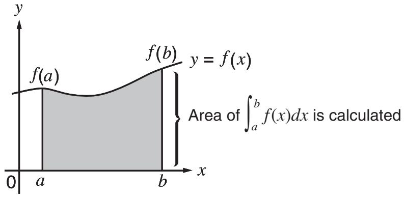
As shown in the illustration above, integration calculations are performed by calculating integral values from a through b for the function y = f(x) where a ≤ x ≤ b , and f(x) ≥ 0 . This in effect calculates the surface area of the shaded area in the illustration.
Example To perform the integration calculation for the function shown below, with a tolerance of “tol” = 1_E - 4
$$ \int_ {1} ^ {5} (2 x ^ {2} + 3 x + 4) d x $$
Input the function f(x) .
AC OPTN F4 (CALC)* F4 (∫dx) 2 X,θ,T x² + 3 X,θ,T + 4 ,
* fx-7400GII: F3 (CALC)
Input the start point and end point.
1,5,
Input the tolerance value.
1 EXP (-) 4 ) EXE
J(2X^2+3X+4,1,5,1E-4) 404.3
Note the following points to ensure correct integration values.
(1) When cyclical functions for integration values become positive or negative for different divisions, perform the calculation for single cycles, or divide between negative and positive, and then add the results together.
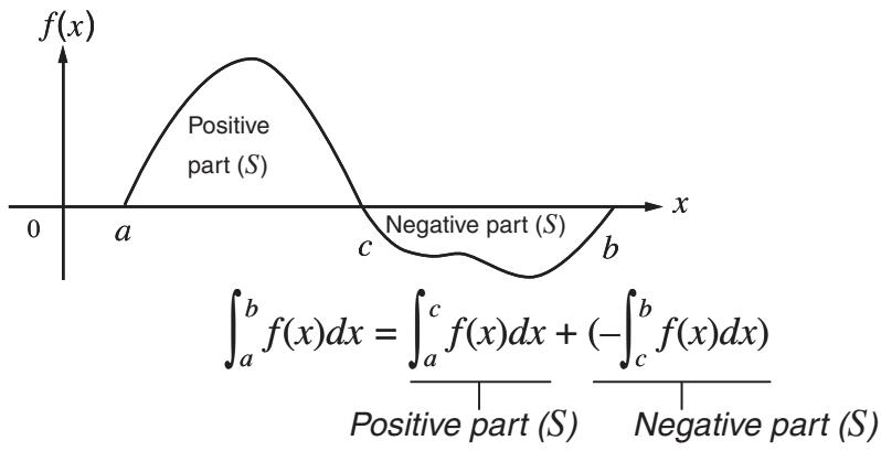
line
| x | f(x) | |-------|------| | a | 0 | | c | Peak | | b | 0 |(2) When minute fluctuations in integration divisions produce large fluctuations in integration values, calculate the integration divisions separately (divide the large fluctuation areas into smaller divisions), and then add the results together.
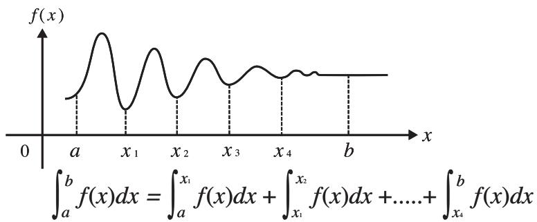
line
| x | f(x) | | ---- | -------- | | a | ~0.5 | | x₁ | ~1.0 | | x₂ | ~0.5 | | x₃ | ~0.8 | | x₄ | ~0.6 | | b | ~0.5 |- Pressing AC during calculation of an integral (while the cursor is not shown on the display) interrupts the calculation.
- Always use radians (Rad mode) as the angle unit when performing trigonometric integrations.
- An error (Time Out) occurs whenever no solution that satisfies the tolerance value can be obtained.
Integration Calculation Precautions
- In the function f(x) , only X can be used as a variable in expressions. Other variables (A through Z excluding X , r , ) are treated as constants, and the value currently assigned to that variable is applied during the calculation.
- Input of “tol” and closing parenthesis can be omitted. If you omit “tol,” the calculator automatically uses a default value of 1_E-5 .
- Integration calculations can take a long time to complete.
- You cannot use a differential, quadratic differential, integration, , maximum/minimum value, Solve, RndFix or _ab calculation expression inside of an integration calculation term.
- In the Math input/output mode, the tolerance value is fixed at 1_E - 5 and cannot be changed.
■ Σ Calculations
[OPTN]-[CALC]-[Σ()]
To perform calculations, first display the function analysis menu, and then input the values using the syntax below.
OPTN F4 (CALC)* F6 (▷) F3 (Σ( ) a_k k α β n *) fx-7400GII: F3 (CALC)
$$ \sum (a _ {k}, k, \alpha , \beta , n) = \sum_ {k = \alpha} ^ {\beta} a _ {k} = a _ {\alpha} + a _ {\alpha + 1} + \dots \dots + a _ {\beta} $$
(n: distance between partitions)
Example To calculate the following:
$$ \sum_ {k = 2} ^ {6} (k ^ {2} - 3 k + 5) $$
Use n = 1 as the distance between partitions.
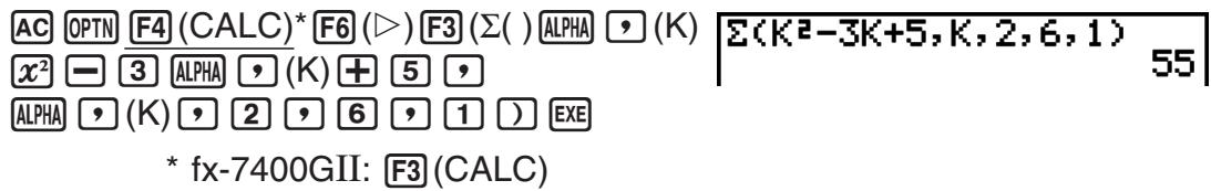
Σ Calculation Precautions
- The value of the specified variable changes during a calculation. Be sure to keep separate written records of the specified variable values you might need later before you perform the calculation.
- You can use only one variable in the function for input sequence a_k .
- Input integers only for the initial term () of sequence a_k and last term () of sequence a_k .
- Input of n and the closing parentheses can be omitted. If you omit n , the calculator automatically uses n = 1 .
- Make sure that the value used as the final term is greater than the value used as the initial term . Otherwise, an error will occur.
- To interrupt an ongoing calculation (indicated when the cursor is not on the display), press the AC key.
- You cannot use a differential, quadratic differential, integration, , maximum/minimum value, Solve, RndFix or _a b calculation expression inside of a calculation term.
- In the Math input/output mode, the distance between partitions (n) is fixed at 1 and cannot be changed.
After displaying the function analysis menu, you can input maximum/minimum calculations using the formats below, and solve for the maximum and minimum of a function within interval a ≤ x ≤ b .
- Minimum Value
OPTN F4 (CALC)* F6 (▷) F1 (FMin) f(x) a b n * fx-7400GII: F3 (CALC)
(a: start point of interval, b: end point of interval, n: precision (n = 1 to 9))
• Maximum Value
OPTN F4 (CALC)* F6 (▷) F2 (FMax) f(x) a b n * fx-7400GII: F3 (CALC)
(a: start point of interval, b: end point of interval, n: precision (n = 1 to 9))
Example To determine the minimum value for the interval defined by start point a = 0 and end point b = 3, with a precision of n = 6 for the function y = x^2 - 4x + 9
Input f(x) .
AC OPTN F4 (CALC)* F6 (▷) F1 (FMin) X,θ,T x² - 4 X,θ,T + 9 ,
* fx-7400GII: F3 (CALC)
Input the interval a = 0, b = 3.
0,3,
Input the precision n = 6.
6 ) EXE
![AnS 1 [3] 2 [5]](/content/2025/01/86832/images/05f922649833a8f7719aa0c290e56f93545780ccb670e035bec53e8e3ab82ec6.jpg)
- In the function f(x) , only X can be used as a variable in expressions. Other variables (A through Z excluding X , r , ) are treated as constants, and the value currently assigned to that variable is applied during the calculation.
- Input of n and the closing parenthesis can be omitted.
- Discontinuous points or sections with drastic fluctuation can adversely affect precision or even cause an error.
- Inputting a larger value for n increases the precision of the calculation, but it also increases the amount of time required to perform the calculation.
- The value you input for the end point of the interval (b) must be greater than the value you input for the start point (a). Otherwise an error occurs.
- You can interrupt an ongoing maximum/minimum calculation by pressing the AC key.
- You can input an integer in the range of 1 to 9 for the value of n. Using any value outside this range causes an error.
- You cannot use a differential, quadratic differential, integration, , maximum/minimum value, Solve, RndFix or _a b calculation expression inside of a maximum/minimum calculation term.
6. Complex Number Calculations
You can perform addition, subtraction, multiplication, division, parentheses calculations, function calculations, and memory calculations with complex numbers just as you do with the manual calculations described on pages 2-1 to 2-14.
You can select the complex number calculation mode by changing the Complex Mode item on the Setup screen to one of the following settings.
- {Real} ... Calculation in the real number range only ^*1
- a+bi ... Performs complex number calculation and displays results in rectangular form
- r ... Performs complex number calculation and displays results in polar form*2
*1 When there is an imaginary number in the argument, however, complex number calculation is performed and the result is displayed using rectangular form.
Examples:
$$ \ln 2 i = 0. 6 9 3 1 4 7 1 8 0 6 + 1. 5 7 0 7 9 6 3 2 7 i $$
$$ \ln 2 i + \ln (- 2) = (\text { Non - Real ERROR }) $$
*2 The display range of depends on the angle unit set for the Angle item on the Setup screen.
- Deg ... -180 < ≤ 180
- Rad ... - < ≤
- Gra ... -200 < ≤ 200
Press OPTN F3 (CPLX) (OPTN F2 (CPLX) on the fx-7400GII) to display the complex calculation number menu, which contains the following items.
- i ... {imaginary unit i input}
- {Abs}/{Arg} ... obtains {absolute value}/{argument}
- {Conj} ... {obtains conjugate}
- {ReP}/{ImP} ... {real}/{imaginary} part extraction
- r/ a+bi ... converts the result to polar/rectangular form
- You can also use SHIFT 0 (i) in place of OPTN F3 (CPLX) (OPTN F2 (CPLX) on the fx-7400GII) F1 (i).
- Solutions obtained by the Real, a + bi and r modes are different for power root ( x^y ) calculations when x < 0 and y = m/n when n is an odd number.
$$ \begin{array}{l} \text { Example: } 3 ^ {x} \sqrt {- (- 8)} = - 2 (\text { Real }) \ = 1 + 1. 7 3 2 0 5 0 8 0 8 \mathbf {i} (a + b \mathbf {i}) \ = 2 \angle 6 0 (r \angle \theta) \ \end{array} $$
- To input the “ ” operator into the polar coordinate expression ( r ), press ,,T ( ).
■ Arithmetic Operations
[OPTN]-[CPLX]-[i]
Arithmetic operations are the same as those you use for manual calculations. You can even use parentheses and memory.
Example (1 + 2i) + (2 + 3i)
AC OPTN F3 (CPLX)*
(1+2F1(i))
+ (2 + 3 F1(i) ) EXE
* fx-7400GII: F2 (CPLX)
(1+2i)+(2+3i) 3+5i
■ Reciprocals, Square Roots, and Squares
Example (3 + i)
AC OPTN F3 (CPLX)*
SHIFT ^2() (3 + F1(i) ) EXE
* fx-7400GII: F2 (CPLX)
(3+i) 1.755317302 +0.2848487846i
■ Complex Number Format Using Polar Form
Example 230 × 345 = 675
SHIFT MENU (SET UP) ▼ ▼ ▼ ▼ ▼ ▼ *
F1 (Deg) ▼ F3 (r∠θ) EXIT
AC 2 SHIFT X,θ,T (∠) 3 0 × 3
SHIFT X,θ,T (∠) 4 5 EXE
* fx-7400GII, fx-9750GII: ▼ ▼ ▼ ▼ ▼
2∠30×3∠45 6∠75
■ Absolute Value and Argument
[OPTN]-[CPLX]-[Abs]/[Arg]
The unit regards a complex number in the form a + bi as a coordinate on a Gaussian plane, and calculates absolute value |Z| and argument (arg).
Example To calculate absolute value (r) and argument () for the complex number 3 + 4i , with the angle unit set for degrees
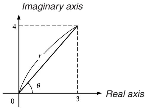
AC OPTN F3 (CPLX)* F2 (Abs)
Abs (3+4i) 5
( 3 + 4 F1(i) ) EXE
(Calculation of absolute value)
* fx-7400GII: F2 (CPLX)
AC OPTN F3 (CPLX)* F3 (Arg)
Arg (3+4i) 53.13010235
( 3 + 4 F1(i) ) EXE
(Calculation of argument)
* fx-7400GII: F2 (CPLX)
- The result of the argument calculation differs in accordance with the current angle unit setting (degrees, radians, grads).
■ Conjugate Complex Numbers
[OPTN]-[CPLX]-[Conj]
A complex number of the form a + bi becomes a conjugate complex number of the form a - bi .
Example To calculate the conjugate complex number for the complex number 2 + 4i
AC OPTN F3 (CPLX)* F4 (Conj)
Conjs (2+4i) 2-4i
( 2 + 4 F1(i) ) EXE
* fx-7400GII: F2 (CPLX)
■ Extraction of Real and Imaginary Parts
[OPTN]-[CPLX]-[ReP]/[ImP]
Use the following procedure to extract the real part a and the imaginary part b from a complex number of the form a + bi .
Example To extract the real and imaginary parts of the complex number 2 + 5i
AC OPTN F3 (CPLX)* F6 (▷) F1 (ReP)
ReP (2+5i) 2
(2 + 5 F6 (▷) F1 (i) ) EXE
(Real part extraction)
* fx-7400GII: F2 (CPLX)
AC OPTN F3 (CPLX)* F6 (▷) F2 (ImP)
ImP (2+5i) 5
(2 + 5 F6 (▷) F1 (i) ) EXE
(Imaginary part extraction)
* fx-7400GII: F2 (CPLX)
■ Polar and Rectangular Form Transformation
[OPTN]-[CPLX]-[▶r∠θ]/[▶a+bi]
Use the following procedure to transform a complex number displayed in rectangular form to polar form, and vice versa.
Example
To transform the rectangular form of complex number 1 + 3 i to its polar form
SHIFT MENU (SET UP) ▼ ▼ ▼ ▼ ▼ ▼ *
F1 (Deg) ▼ F2 (a+bi) EXIT
AC 1 + (SHIFT x^2() 3)
OPTN F3 (CPLX)** F1 (i) F6 (▷) F3 (▶r∠θ) EXE
* fx-7400GII, fx-9750GII: ▼ ▼ ▼ ▼ ▼
** fx-7400GII: F2 (CPLX)
1+(√3)i-r∠8 2∠60
AC 2 SHIFT X,θ,T (∠) 6 0
OPTN F3 (CPLX)* F6 (▷) F4 (▶a+bi) EXE
* fx-7400GII: F2 (CPLX)
2∠60▶a+bi 1+1.732050808i
- The input/output range of complex numbers is normally 10 digits for the mantissa and two digits for the exponent.
- When a complex number has more than 21 digits, the real part and imaginary part are displayed on separate lines.
- The following functions can be used with complex numbers.
, x^2 , x^-1 , (x^y) , ^3 , x , In, , _ab , 10^x , e^x , Int, Frac, Rnd, Intg, RndFix(, Fix, Sci, ENG, ENG, ^ , ^ , ^ , ^ , ^ , a^b/_c , d/c
7. Binary, Octal, Decimal, and Hexadecimal Calculations with Integers
You can use the RUN • MAT (or RUN) mode and binary, octal, decimal, and hexadecimal settings to perform calculations that involve binary, octal, decimal and hexadecimal values. You can also convert between number systems and perform bitwise operations.
- You cannot use scientific functions in binary, octal, decimal, and hexadecimal calculations.
- You can use only integers in binary, octal, decimal, and hexadecimal calculations, which means that fractional values are not allowed. If you input a value that includes a decimal part, the calculator automatically cuts off the decimal part.
- If you attempt to enter a value that is invalid for the number system (binary, octal, decimal, hexadecimal) you are using, the calculator displays an error message. The following shows the numerals that can be used in each number system.
Binary: 0, 1
Octal: 0, 1, 2, 3, 4, 5, 6, 7
Decimal: 0, 1, 2, 3, 4, 5, 6, 7, 8, 9
Hexadecimal: 0, 1, 2, 3, 4, 5, 6, 7, 8, 9, A, B, C, D, E, F
- Negative binary, octal, and hexadecimal values are produced using the two's complement of the original value.
- The following are the display capacities for each of the number systems.
| Number System | Binary | Octal | Decimal | Hexadecimal |
| Display Capacity | 16 digits | 11 digits | 10 digits | 8 digits |
- The alphabetic characters used in the hexadecimal number appear differently on the display to distinguish them from text characters.
| Normal Text | A | B | C | D | E | F |
| Hexadecimal Values | IB | |||||
| Keys | ,,T |
- The following are the calculation ranges for each of the number systems.
Binary Values
Positive: 0 ≤ x ≤ 1111111111111111
Negative: 1000000000000000 ≤ x ≤ 1111111111111111
Octal Values
Positive: 0 ≤ x ≤ 17777777777
Negative: 20000000000 ≤ x ≤ 3777777777
Decimal Values
Positive: 0 ≤ x ≤ 2147483647
Negative: -2147483648 ≤ x ≤ -1
Hexadecimal Values
Positive: 0 ≤ x ≤ 7FFFFFFF
Negative: 80000000 ≤ x ≤ FFFFFFFF
- To perform a binary, octal, decimal, or hexadecimal calculation
[SET UP]-[Mode]-[Dec]/[Hex]/[Bin]/[Oct]
-
In the Main Menu, select RUN • MAT (or RUN).
-
Press SHIFT MENU (SET UP). Move the highlighting to "Mode", and then specify the default number system by pressing F2 (Dec), F3 (Hex), F4 (Bin), or F5 (Oct) for the Mode setting.
-
Press EXIT to change to the screen for calculation input. This causes a function menu with the following items to appear.
- {d\~o}/{LOG}/{DISP} ... {number system specification}/{bitwise operation}/{decimal/hexadecimal/binary/octal conversion} menu
■ Selecting a Number System
You can specify decimal, hexadecimal, binary, or octal as the default number system using the Setup screen.
- To specify a number system for an input value
You can specify a number system for each individual value you input. Press F1(d\~o) to display a menu of number system symbols. Press the function key that corresponds to the symbol you want to select and then input the value.
- {d}/{h}/{b}/{o} ... {decimal}/{hexadecimal}/{binary}/{octal}
- To input values of mixed number systems
Example To input 123_10 , when the default number system is hexadecimal
SHIFT MENU (SET UP)
Move the highlighting to "Mode", and then press F3 (Hex) EXIT.
■ Negative Values and Bitwise Operations
Press F2(LOG) to display a menu of negation and bitwise operators.
- {Neg} ... {negation}*1
- {Not}/{and}/{or}/{xor}/{xnor} ... {NOT}*2/{AND}/{OR}/{XOR}/{XNOR}*3
*1 two's complement
*2 one's complement (bitwise complement)
*3 bitwise AND, bitwise OR, bitwise XOR, bitwise XNOR
- Negative Values
Example To determine the negative of 110010_2
SHIFT MENU (SET UP)
Move the highlighting to "Mode", and then press F4 (Bin) EXIT.
Neg 110010
1111111111001110
- Negative binary, octal, and hexadecimal values are produced by taking the binary two's complement and then returning the result to the original number base. With the decimal number base, negative values are displayed with a minus sign.
- Bitwise Operations
Example To input and execute “ 120_16 and AD_16 ”
SHIFT MENU (SET UP)
Move the highlighting to "Mode", and then press F3 (Hex) EXIT.
120andAD
00000020
AC 1 2 0 F2(LOG)
F3 (and) A D EXE
■ Number System Transformation
Press F3 (DISP) to display a menu of number system transformation functions.
- {▶Dec}/{▶Hex}/{▶Bin}/{▶Oct} ... transformation of displayed value to its {decimal}/{hexadecimal}/{binary}/{octal} equivalent
- To convert a displayed value from one number system to another
Example To convert 22_10 (default number system) to its binary or octal value
AC SHIFT MENU (SET UP)
Move the highlighting to "Mode", and then press F2 (Dec) EXIT.
- Matrix calculations cannot be performed on the fx-7400GII.
From the Main Menu, enter the RUN•MAT mode, and press F1(▶MAT) to perform Matrix calculations.
26 matrix memories (Mat A through Mat Z) plus a Matrix Answer Memory (MatAns), make it possible to perform the following matrix operations.
- Addition, subtraction, multiplication, division
- Scalar multiplication calculations
• Determinant calculations - Matrix transposition
- Matrix inversion
- Matrix squaring
- Raising a matrix to a specific power
- Absolute value, integer part extraction, fractional part extraction, maximum integer calculations
- Inputting complex numbers in matrix elements and using complex number related functions
- Matrix modification using matrix commands
The maximum number of rows that can be specified for a matrix is 999, and the maximum number of columns is 999.
About Matrix Answer Memory (MatAns)
- The calculator automatically stores matrix calculation results in Matrix Answer Memory. Note the following points about Matrix Answer Memory.
- Whenever you perform a matrix calculation, the current Matrix Answer Memory contents are replaced by the new result. The previous contents are deleted and cannot be recovered.
- Inputting values into a matrix does not affect Matrix Answer Memory contents.
■ Inputting and Editing Matrices
Pressing F1(▶MAT) displays the Matrix Editor screen. Use the Matrix Editor to input and edit matrices.
m × n m (row) × n (column) matrix None... no matrix preset
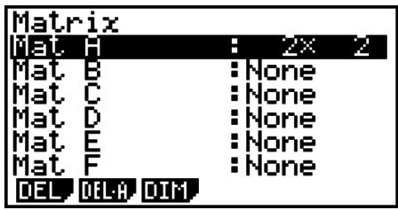
- {DEL}/{DEL·A} ... deletes {a specific matrix}/{all matrices}
- {DIM} ... {specifies the matrix dimensions (number of cells)}
- Creating a Matrix
To create a matrix, you must first define its dimensions (size) in the Matrix Editor. Then you can input values into the matrix.
- To specify the dimensions (size) of a matrix
Example To create a 2-row × 3-column matrix in the area named Mat B
Highlight Mat B.

F3 (DIM) (This step can be omitted.)
Specify the number of rows.

Specify the number of columns.


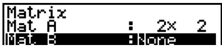

![B 1 2 3 1 [0 0 0] 2 [0 0 0]](/content/2025/01/86832/images/ce2a75f2fd66ecae8e1579c4b45bcd91a05a749f6c43bb9e6c3e05f99aba5571.jpg)
- All of the cells of a new matrix contain the value 0.
- Changing the dimensions of a matrix deletes its current contents.
- If “Memory ERROR” remains next to the matrix area name after you input the dimensions, it means there is not enough free memory to create the matrix you want.
- To input cell values
Example To input the following data into Matrix B:
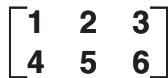
The following operation is a continuation of the example calculation on the previous page.
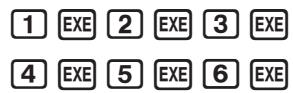
(Data is input into the highlighted cell. Each time you press EXE, the highlighting moves to the next cell to the right.)
![B 1 2 3 1 [ 1 2 3] 2 [ 4 5 6] 6](/content/2025/01/86832/images/81b1356270537458b850475a4c55ddfdfef1bef542618525e11cb8992282bfa1.jpg)
- Displayed cell values show positive integers up to six digits, and negative integers up to five digits (one digit used for the negative sign). Exponential values are shown with up to two digits for the exponent. Fractional values are not displayed.
- Deleting Matrices
You can delete either a specific matrix or all matrices in memory.
- To delete a specific matrix
- While the Matrix Editor is on the display, use ⚙️ and ⼕ to highlight the matrix you want to delete.
- Press F1 (DEL).
- Press F1 (Yes) to delete the matrix or F6 (No) to abort the operation without deleting anything.
- To delete all matrices
- While the Matrix Editor is on the display, press F2 (DEL • A).
- Press F1 (Yes) to delete all matrices in memory or F6 (No) to abort the operation without deleting anything.
■ Matrix Cell Operations
Use the following procedure to prepare a matrix for cell operations.
-
While the Matrix Editor is on the display, use ▲ and ▼ to highlight the name of the matrix you want to use. You can jump to a specific matrix by inputting the letter that corresponds to the matrix name. Inputting ALPHA 8 (N), for example, jumps to Mat N. Pressing SHIFT (-) (Ans) jumps to the matrix current memory.
-
Press EXE and the function menu with the following items appears.
-
{R-OP} ... {row operation menu}
• {ROW} - {DEL}/{INS}/{ADD} ... row {delete}/{insert}/{add}
• {COL} - {DEL}/{INS}/{ADD} ... column {delete}/{insert}/{add}
• {EDIT} ... {cell editing screen}
All of the following examples use Matrix A.
- Row Calculations
The following menu appears whenever you press F1(R-OP) while a recalled matrix is on the display.
- {Swap} ... {row swap}
- × Rw product of specified row and scalar
- × Rw + ... {addition of one row and the product of a specified row with a scalar}
- Rw + ... {addition of specified row to another row}
- To swap two rows
Example To swap rows two and three of the following matrix:
All of the operation examples are performed using the following matrix.
$$ \text { Matrix } \mathbf {A} = \left[ \begin{array}{c c} 1 & 2 \ 3 & 4 \ 5 & 6 \end{array} \right] $$
F1(R-OP) F1(Swap)
Input the number of the rows you want to swap.
2 EXE 3 EXE EXE
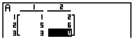
- To calculate the scalar multiplication of a row
Example To calculate the product of row 2 and the scalar 4
F1 (R-OP) F2 (×Rw)
Input multiplier value.*
4 EXE
Specify row number.
2 EXE EXE
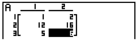
* A complex number also can be input as multiplier value (k).
- To calculate the scalar multiplication of a row and add the result to another row
Example To calculate the product of row 2 and the scalar 4, then add the result to row 3
F1 (R-OP) F3 (×Rw+)
Input multiplier value.*
4 EXE
Specify number of row whose product should be calculated.
2 EXE
Specify number of row where result should be added.
3 EXE EXE
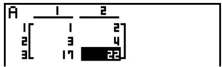
* A complex number also can be input as multiplier value (k).
• To add two rows together
Example To add row 2 to row 3
F1 (R-OP) F4 (Rw+)
Specify number of row to be added.
2 EXE
Specify number of row to be added to.
3 EXE EXE
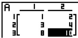
- Row Operations
- {DEL} ... {delete row}
- {INS} ... {insert row}
- {ADD} ... {add row}
- To delete a row
Example To delete row 2
F2 (ROW)
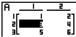
F1 (DEL)
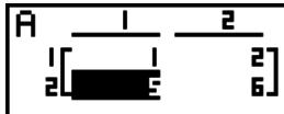
- To insert a row
Example To insert a new row between rows one and two
F2 (ROW)
![A 1 2 1 [1 2] 2 [0 0] 3 [3 4] 4 [5 6]](/content/2025/01/86832/images/e379a05093c63c4e6a3f54427fa3b2993126a33210ad03f0bca0178959684e5c.jpg)
F2 (INS)
- To add a row
Example To add a new row below row 3
F2 (ROW) ▼ ▼
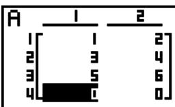
F3 (ADD)
- Column Operations
- {DEL} ... {delete column}
- {INS} ... {insert column}
- {ADD} ... {add column}
- To delete a column
Example
To delete column 2


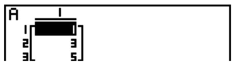
■ Modifying Matrices Using Matrix Commands
[OPTN]-[MAT]
- To display the matrix commands
- From the Main Menu, enter the RUN • MAT mode.
- Press ☐OPTN to display the option menu.
- Press F2 (MAT) to display the matrix command menu.
The following describes only the matrix command menu items that are used for creating matrices and inputting matrix data.
- {Mat} ... {Mat command (matrix specification)}
- M L ... Mat List command (assign contents of selected column to list file)
- {Aug} ... {Augment command (link two matrices)}
- {Iden} ... {Identity command (identity matrix input)}
- {Dim} ... {Dim command (dimension check)}
- {Fill} ... {Fill command (identical cell values)}
- You can also use SHIFT 2 (Mat) in place of OPTN F2 (MAT) F1 (Mat).
- Matrix Data Input Format
[OPTN]-[MAT]-[Mat]
The following shows the format you should use when inputting data to create a matrix using the Mat command.
$$ \left[ \begin{array}{c c c c} \mathsf {a} _ {1 1} & \mathsf {a} _ {1 2} & \ldots & \mathsf {a} _ {1 n} \ \mathsf {a} _ {2 1} & \mathsf {a} _ {2 2} & \ldots & \mathsf {a} _ {2 n} \ \vdots & \vdots & & \vdots \ \mathsf {a} _ {m 1} & \mathsf {a} _ {m 2} & \ldots & \mathsf {a} _ {m n} \end{array} \right] = [ [ \mathsf {a} _ {1 1}, \mathsf {a} _ {1 2}, \ldots , \mathsf {a} _ {1 n} ] [ \mathsf {a} _ {2 1}, \mathsf {a} _ {2 2}, \ldots , \mathsf {a} _ {2 n} ] \ldots .. [ \mathsf {a} _ {m 1}, \mathsf {a} _ {m 2}, \ldots , \mathsf {a} _ {m n} ] ] $$
→ Mat [letter A through Z]
![Example To input the following data as Matrix A: [ 1 3 5 ] [ 2 4 6 ] SHIFT + ( ) SHIFT + ( ) 1 , 3 , 5 SHIFT - ( ) SHIFT + ( ) 2 , 4 , 6 SHIFT - ( ) SHIFT - ( ) → OPTN F2 (MAT) F1 (Mat) ALPHA X,θ,T (A) EXE Matrix name — A 1 2 3 [ ] [ ] [ ] 2 [ ] 2 [ ] 4 [ ] 6 [ ]](/content/2025/01/86832/images/34456dd0c0906aa876c2b69ccb25f07ea5b88d1d59367960821ac28ab3c9fa06.jpg)
- The maximum value of both m and n is 999.
- An error occurs if memory becomes full as you are inputting data.
- You can also use the above format inside a program that inputs matrix data.
- To input an identity matrix
[OPTN]-[MAT]-[Iden]
Use the Identity command to create an identity matrix.
Example To create a 3 × 3 identity matrix as Matrix A
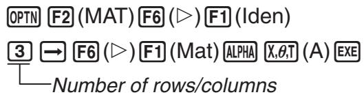
![A 1 2 3 1 [ ] 0 0 2 [ ] 0 1 0 3 [ ] 0 0 1](/content/2025/01/86832/images/0e69b2b5c494e481de379b95ef21275324571298ce9a19bc4525ebd1ea3ee031.jpg)
• To check the dimensions of a matrix
[OPTN]-[MAT]-[Dim]
Use the Dim command to check the dimensions of an existing matrix.
Example 1 To check the dimensions of Matrix A
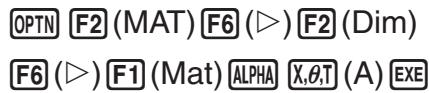
![AnS 1 [ ] E 2 [ ] 3 ]](/content/2025/01/86832/images/a65b0723e6d02e849abcb48d29800c25aef1764ef22d70673c014598cdc1a7bb.jpg)
The display shows that Matrix A consists of two rows and three columns. Since the result of the Dim command is list type data, it is stored in ListAns Memory.
You can also use {Dim} to specify the dimensions of the matrix.
Example 2 To specify dimensions of 2 rows and 3 columns for Matrix B
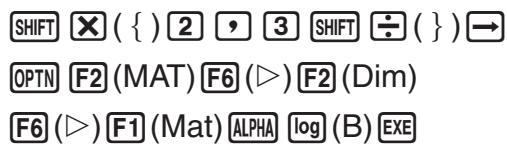
![B 1 2 3 1 [0 0 0] 2 [0 0 0]](/content/2025/01/86832/images/e70703ec4d6aa4af941f31b8c6fab344563bfd6d867a0ef333fe5ae33d872d92.jpg)
- Modifying Matrices Using Matrix Commands
You can also use matrix commands to assign values to and recall values from an existing matrix, to fill in all cells of an existing matrix with the same value, to combine two matrices into a single matrix, and to assign the contents of a matrix column to a list file.
- To assign values to and recall values from an existing matrix
[OPTN]-[MAT]-[Mat]
Use the following format with the Mat command to specify a cell for value assignment and recall.
Mat X [m, n]
X = matrix name (A through Z, or Ans)
m = row number
n = column number
Example 1 To assign 10 to the cell at row 1, column 2 of the following matrix:
$$ \text { Matrix } \mathbf {A} = \left[ \begin{array}{c c} 1 & 2 \ 3 & 4 \ 5 & 6 \end{array} \right] $$
1 0 → OPTN F2 (MAT) F1 (Mat)
10→Mat A[1,2] 10
ALPHA X,θ,T (A) SHIFT + ( [ ) 1 , 2
SHIFT - ( ) EXE
Example 2 Multiply the value in the cell at row 2, column 2 of the above matrix by 5
OPTN F2 (MAT) F1 (Mat)
Mat A[2,2]×5 20
ALPHA X,θ,T (A) SHIFT + ( [ ) 2 , 2
SHIFT - ( ) ✗ 5 EXE
- To fill a matrix with identical values and to combine two matrices into a single matrix [OPTN]-[MAT]-[Fill]
[OPTN]-[MAT]-[Fill]/[Aug]
Use the Fill command to fill all the cells of an existing matrix with an identical value and the Augment command to combine two existing matrices into a single matrix.
Example 1 To fill all of the cells of Matrix A with the value 3
OPTN F2 (MAT) F6 (▷) F3 (Fill)
![AnS 1 2 1 [ ] 3 3 2 [ ] 3 3 3 [ ] 3 3](/content/2025/01/86832/images/ae1396a7067e028e49cc8f76934c0d572d42f10102167f4f15efe43960c5761e.jpg)
3 F6 (▷) F1 (Mat) ALPHA X,θ,T (A) EXE
F1 (Mat) ALPHA X,θ,T (A) EXE
Example 2 To combine the following two matrices:
$$ \mathbf {A} = \left[ \begin{array}{c} 1 \ 2 \end{array} \right] \qquad \mathbf {B} = \left[ \begin{array}{c} 3 \ 4 \end{array} \right] $$
OPTN F2 (MAT) F5 (Aug)
F1 (Mat) ALPHA X,θ,T (A),
F1 (Mat) ALPHA log (B) EXE
![AnS 1 2 1 [ ] 3 2 [ ] 2 4](/content/2025/01/86832/images/32ff12f1f93fd0662f581550f239a3461c634a8c1b4ea965171c9add8f13cd58.jpg)
- The two matrices you combine must have the same number of rows. An error occurs if you try to combine two matrices that have different number of rows.
- You can use Matrix Answer Memory to assign the results of the above matrix input and edit operations to a matrix variable. To do so, use the following syntax.
Fill (n, Mat α)
Augment (Mat α, Mat β) → Mat γ
In the above, , , and are any variable names A through Z, and n is any value.
The above does not affect the contents of Matrix Answer Memory.
- To assign the contents of a matrix column to a list
[OPTN]-[MAT]-[M→L]
Use the following format with the Mat→List command to specify a column and a list.
Mat → List (Mat X, m) → List n
X = matrix name (A through Z)
m = column number
n = list number
Example To assign the contents of column 2 of the following matrix to list 1:
$$ \text { Matrix } \mathbf {A} = \left[ \begin{array}{c c} 1 & 2 \ 3 & 4 \ 5 & 6 \end{array} \right] $$
OPTN F2 (MAT) F2 (M→L)
F1 (Mat) ALPHA X,θ,T (A) 2 )
→ OPTN F1 (LIST) F1 (List) 1 EXE
F1 (List) 1 EXE
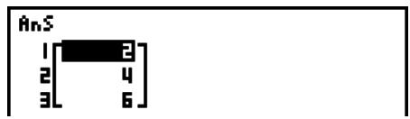
■ Matrix Calculations
[OPTN]-[MAT]
Use the matrix command menu to perform matrix calculation operations.
- To display the matrix commands
- From the Main Menu, enter the RUN • MAT mode.
- Press ☐OPTN to display the option menu.
- Press F2 (MAT) to display the matrix command menu.
The following describes only the matrix commands that are used for matrix arithmetic operations.
- {Mat} ... {Mat command (matrix specification)}
- {Det} ... {Det command (determinant command)}
- {Trn} ... {Trn command (transpose matrix command)}
- {lden} ... {Identity command (identity matrix input)}
- {Ref} ... {Ref command (row echelon form command)}
- {Rref} ... {Rref command (reduced row echelon form command)}
All of the following examples assume that matrix data is already stored in memory.
- Matrix Arithmetic Operations
[OPTN]-[MAT]-[Mat]/[Iden]
Example 1 To add the following two matrices (Matrix A + Matrix B):
$$ \mathbf {A} = \left[ \begin{array}{c c} 1 & 1 \ 2 & 1 \end{array} \right] \quad \mathbf {B} = \left[ \begin{array}{c c} 2 & 3 \ 2 & 1 \end{array} \right] $$
$$ \boxed {A C} \boxed {O P T N} \boxed {F 2} (M A T) \boxed {F 1} (M a t) \boxed {A L P H A} \boxed {X, \theta , T} (A) \boxed {+} $$
$$ \boxed {\mathrm{F1}} (\text {Mat}) \boxed {\mathrm{ALPHA}} \boxed {\log} (\mathrm{B}) \boxed {\mathrm{EXE}} $$
![AnS 1 2 1 [ ] 4 2 [ ] 4 2](/content/2025/01/86832/images/ae4ae91d80e3b9beb7f12cf706e01bb31173866fb571dd4ecf8de93b01394aac.jpg)
Example 2 To multiply the two matrices in Example 1 (Matrix A × Matrix B)
$$ \boxed {A C} \boxed {O P T N} \boxed {F 2} (M A T) \boxed {F 1} (M a t) \boxed {A L P H A} \boxed {X, \theta , T} (A) \boxed {\times} $$
$$ \boxed {\mathrm{F1}} (\text {Mat}) \boxed {\mathrm{ALPHA}} \boxed {\log} (\mathrm{B}) \boxed {\mathrm{EXE}} $$
![AnS 1 2 1 [ ] 4 2 [ ] 6 7](/content/2025/01/86832/images/293a6c6375efe62e120acee9c65a52446d7220f1835d35afdbf5798af9de3ed0.jpg)
- The two matrices must have the same dimensions in order to be added or subtracted. An error occurs if you try to add or subtract matrices of different dimensions.
- For multiplication (Matrix 1 × Matrix 2), the number of columns in Matrix 1 must match the number of rows in Matrix 2. Otherwise, an error occurs.
- Determinant
[OPTN]-[MAT]-[Det]
Example Obtain the determinant for the following matrix:
$$ \text {Matrix} \mathbf {A} = \left[ \begin{array}{r r r} 1 & 2 & 3 \ 4 & 5 & 6 \ - 1 & - 2 & 0 \end{array} \right] $$
$$ \boxed {\text {OPTN}} \boxed {\text {F2}} (\text {MAT}) \boxed {\text {F3}} (\text {Det}) \boxed {\text {F1}} (\text {Mat}) $$
$$ \boxed {\text { ALPHA }} \boxed {X, \theta , T} (A) \boxed {\text { EXE }} $$
Det Mat A -9
- Determinants can be obtained only for square matrices (same number of rows and columns). Trying to obtain a determinant for a matrix that is not square produces an error.
- The determinant of a 2 × 2 matrix is calculated as shown below.
$$ | A | = \left[ \begin{array}{l l} a _ {1 1} & a _ {1 2} \ a _ {2 1} & a _ {2 2} \end{array} \right] = a _ {1 1} a _ {2 2} - a _ {1 2} a _ {2 1} $$
- The determinant of a 3 × 3 matrix is calculated as shown below.
$$ | \mathsf {A} | = \left[ \begin{array}{l l l} a _ {1 1} & a _ {1 2} & a _ {1 3} \ a _ {2 1} & a _ {2 2} & a _ {2 3} \ a _ {3 1} & a _ {3 2} & a _ {3 3} \end{array} \right] = a _ {1 1} a _ {2 2} a _ {3 3} + a _ {1 2} a _ {2 3} a _ {3 1} + a _ {1 3} a _ {2 1} a _ {3 2} - a _ {1 1} a _ {2 3} a _ {3 2} - a _ {1 2} a _ {2 1} a _ {3 3} - a _ {1 3} a _ {2 2} a _ {3 1} $$
- Matrix Transposition
[OPTN]-[MAT]-[Trn]
A matrix is transposed when its rows become columns and its columns become rows.
Example To transpose the following matrix:
$$ \text { Matrix } A = \left[ \begin{array}{c c} 1 & 2 \ 3 & 4 \ 5 & 6 \end{array} \right] $$
- Row Echelon Form
[OPTN]-[MAT]-[Ref]
This command uses the Gaussian elimination algorithm to find the row echelon form of a matrix.
Example To find the row echelon form of the following matrix:
$$ \text { Matrix } \mathbf {A} = \left[ \begin{array}{c c c} 1 & 2 & 3 \ 4 & 5 & 6 \end{array} \right] $$
$$ \boxed {\text {OPTN}} \boxed {\text {F2}} (\text {MAT}) \boxed {\text {F6}} (\triangleright) \boxed {\text {F4}} (\text {Ref}) $$
$$ \boxed {F 6} (\triangleright) \boxed {F 1} (\text { Mat }) \boxed {\text { ALPHA }} \boxed {X, \theta , T} (A) \boxed {\text { EXE }} $$
![AmS 1 2 3 1[1 1.25 1.5] 2[0 1 2] 1](/content/2025/01/86832/images/5e2cf619872c2d63581440643b1be48a1b89340c30f1367e838a25b44191ed4b.jpg)
- Reduced Row Echelon Form
[OPTN]-[MAT]-[Rref]
This command finds the reduced row echelon form of a matrix.
Example To find the reduced row echelon form of the following matrix:
$$ \text {Matrix} \mathbf {A} = \left[ \begin{array}{c c c c} 2 & - 1 & 3 & 1 9 \ 1 & 1 & - 5 & - 2 1 \ 0 & 4 & 3 & 0 \end{array} \right] $$
$$ \boxed {\text {OPTN}} \boxed {\text {F2}} (\text {MAT}) \boxed {\text {F6}} (\triangleright) \boxed {\text {F5}} (\text {Rref}) $$
$$ \boxed {F 6} (\triangleright) \boxed {F 1} (\text { Mat }) \boxed {\text { ALPHA }} \boxed {X, \theta , T} (A) \boxed {\text { EXE }} $$
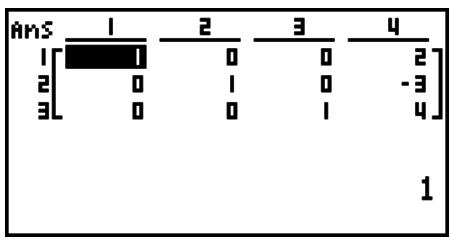
other
| AmS | 1 | 2 | 3 | 4 | |---|---|---|---|---| | 1 | 1 | 0 | 0 | 2 | | 2 | 0 | 1 | 0 | -3 | | 3 | 0 | 0 | 1 | 4 | 1- The row echelon form and reduced row echelon form operation may not produce accurate results due to dropped digits.
- Matrix Inversion
[x^-1]
Example To invert the following matrix:
$$ \text { Matrix } \mathbf {A} = \left[ \begin{array}{c c} 1 & 2 \ 3 & 4 \end{array} \right] $$
$$ \boxed {\text {OPTN}} \boxed {\text {F2}} (\text {MAT}) \boxed {\text {F1}} (\text {Mat}) $$
$$ \boxed {\mathrm{ALPHA}} \boxed {X, \theta , T} (A) \boxed {\text {SHIFT}} \boxed {)} (x ^ {- 1}) \boxed {\mathrm{EXE}} $$
![AnS 1 2 1[-2] 1 2[1.5 -0.5]](/content/2025/01/86832/images/c196c605b999a4a5c52ad26ff5d03c80ba5ad0938f53ebfbffa0335287fc6dad.jpg)
- Only square matrices (same number of rows and columns) can be inverted. Trying to invert a matrix that is not square produces an error.
- A matrix with a determinant of zero cannot be inverted. Trying to invert a matrix with determinant of zero produces an error.
- Calculation precision is affected for matrices whose determinant is near zero.
- A matrix being inverted must satisfy the conditions shown below.
$$ \mathbf {A} \mathbf {A} ^ {- 1} = \mathbf {A} ^ {- 1} \mathbf {A} = \mathbf {E} = \left[ \begin{array}{c c c} & 1 & 0 \ & 0 & 1 \end{array} \right] $$
The following shows the formula used to invert Matrix A into inverse matrix A^-1 .
$$ \mathbf {A} = \left[ \begin{array}{c c c} \mathbf {a} & \mathbf {b} \ \mathbf {c} & \mathbf {d} \end{array} \right] $$
$$ \mathbf {A} ^ {- 1} = \frac {1}{a d - b c} \left[ \begin{array}{c c} d & - b \ - c & a \end{array} \right] $$
Note that ad - bc ≠ 0.
- Squaring a Matrix
[x^2]
Example To square the following matrix:
$$ \text { Matrix } \mathbf {A} = \left[ \begin{array}{c c} 1 & 2 \ 3 & 4 \end{array} \right] $$
OPTN F2 (MAT) F1 (Mat) ALPHA X,θ,T (A) x^2 EXE
![AnS 1 2 1 [ ] 4 10 2 [ ] 15 22](/content/2025/01/86832/images/6b8c0ab42feff068a4ea4fffa739463c1a57b59426b439b36617db2903a11c49.jpg)
• Raising a Matrix to a Power
[^]
Example To raise the following matrix to the third power:
$$ \text { Matrix } \mathbf {A} = \left[ \begin{array}{c c} 1 & 2 \ 3 & 4 \end{array} \right] $$
OPTN F2 (MAT) F1 (Mat) ALPHA X,θ,T (A)
3 EXE
![AnS 1 2 1 [34 54] 2 [81 118]](/content/2025/01/86832/images/e8b4dc48aa20ab977664c48b52ad2c8d689a126c7dfb7e90a2a0ce8b9c9a59c8.jpg)
- For matrix power calculations, calculation is possible up to a power of 32766.
- Determining the Absolute Value, Integer Part, Fraction Part, and Maximum Integer of a Matrix [OPTN]-[NUM]-[Abs]/[Frac]/[Int]/[Intg]
Example To determine the absolute value of the following matrix:
$$ \text { Matrix } \mathbf {A} = \left[ \begin{array}{c c} 1 & - 2 \ - 3 & 4 \end{array} \right] $$
OPTN F6 (▷) F4 (NUM) F1 (Abs)
OPTN F2 (MAT) F1 (Mat) ALPHA X,θ,T (A) EXE
![CASIO FX-7400GII - - Determining the Absolute Value, Integer Part, Fraction Part, and Maximum Integer of a Matrix [OPTN]-[NUM]-[Abs]/[Frac]/[Int]/[Intg] - 1](/content/2025/01/86832/images/841ecd521cd916fa9172d270344e2512428ef2d312dea59755b35e19ef7caddb.jpg)
- Complex Number Calculations with a Matrix
Example
To determine the absolute value of a matrix with the following complex number elements:
$$ \text {Matrix} \mathsf {D} = \left[ \begin{array}{c c} - 1 + i & 1 + i \ 1 + i & - 2 + 2 i \end{array} \right] $$
$$ \begin{array}{l} \boxed {\mathrm{AC}} \boxed {\mathrm{OPTN}} \boxed {\mathrm{F6}} (\triangleright) \boxed {\mathrm{F4}} (\mathrm{NUM}) \boxed {\mathrm{F1}} (\mathrm{Abs}) \ \boxed {\mathrm{OPTN}} \boxed {\mathrm{F2}} (\mathrm{MAT}) \boxed {\mathrm{F1}} (\mathrm{Mat}) \boxed {\mathrm{ALPHA}} \boxed {\sin} (\mathrm{D}) \boxed {\mathrm{EXE}} \end{array} $$
![AmS 1 2 1[1.4142 1.4142] 2[1.4142 2.8284] 1.414213562](/content/2025/01/86832/images/cd2a8de3165e988a7f441ef89552dda4611649db288ba962b0c828440df0c8e0.jpg)
- The following complex number functions are supported in matrices.
i, Abs, Arg, Conjg, ReP, ImP, ▶a+b i, ▶r∠θ
Note, however, that “▶a+bi” and “▶r∠θ” cannot be used in the Linear input/output mode.
Matrix Calculation Precautions
- Determinants and inverse matrices are subject to error due to dropped digits.
- Matrix operations are performed individually on each cell, so calculations may require considerable time to complete.
- The calculation precision of displayed results for matrix calculations is ± 1 at the least significant digit.
- If a matrix calculation result is too large to fit into Matrix Answer Memory, an error occurs.
- You can use the following operation to transfer Matrix Answer Memory contents to another matrix (or when Matrix Answer Memory contains a determinant to a variable).
MatAns → Mat α
In the above, is any variable name A through Z. The above does not affect the contents of Matrix Answer Memory.
9. Metric Conversion Calculations
You can convert values from one unit of measurement to another. Measurement units are classified according to the following 11 categories. The indicators in the “Display Name” column show the text that appears in the calculator’s function menu.
| Display Name | Category | Display Name | Category | Display Name | Category |
| LENG | Length | TMPR | Temperature | PRES | Pressure |
| AREA | Area | VELO | Velocity | ENGY | Energy/Work |
| VLUM | Volume | MASS | Mass | PWR | Power |
| TIME | Time | FORC | Force/Weight | ||
You can convert from any unit in a category to any other unit in the same category.
- Attempting to convert from a unit in one category (such as “AREA”) to a unit in another category (such as “TIME”) results in a Conversion ERROR.
- See the “Unit Conversion Command List” (page 2-50) for information about the units included in each category.
■ Performing a Unit Conversion Calculation
[OPTN]-[CONV]
Input the value you are converting from and the conversion commands using the syntax shown below to perform a unit conversion calculation.
{value converting from}{conversion command 1} ▶ {conversion command 2}
- Use {conversion command 1} to specify the unit being converted from and {conversion command 2} to specify the unit being converted to.
- ▶ is a command that links the two conversion commands. This command is always available at F1(▶) of the Conversion menu.
- Real numbers or a list that contains real number elements only can be used as the value being converted from. When values being converted from are input into a list (or when list memory is specified), conversion calculation is performed for each element in the list and calculation results are returned in list format (ListAns screen).
- A complex number cannot be used as a value to be converted from. An error occurs if even a single element of a list being used as the value being converted from contains a complex number.
Example 1 To convert 50cm to inches
AC 5 0 OPTN F6 (▷) F1(CONV)* F2(LENG)
5 (cm) F1 (▶) F2 (LENG) ▶ 2 (in) EXE
* fx-7400GII: F5 (CONV)
50[cm]▶[in] 19.68503937
Example 2 To convert \175, 162, 180\ centimeters to feet
AC SHIFT ✗ ( { } 1 7 5 , 1 6 2 ,
1 8 0 SHIFT ÷ ( }
OPTN F6 (▷) F1 (CONV)* F3 (AREA) 2 (m²)
F1 (▶) F3 (AREA) 3 (ha) EXE
* fx-7400GII: F5 (CONV)
![Ans 1[0.0145] 2[0.0162] 3[0.018] 0.0175](/content/2025/01/86832/images/c81e07156744116a5c14a605c72e71e58777314adcc15057fba2c73ed2bbfbac.jpg)
■ Unit Conversion Command List
| Cat. | Display Name | Unit | Cat. | Display Name | Unit |
| Length | fm | fermi | Volume | cm^3 | cubic centimeter |
| Å | angstrom | mL | milliliter | ||
| μm | micrometer | L | liter | ||
| mm | millimeter | m^3 | cubic meter | ||
| cm | centimeter | in^3 | cubic inch | ||
| m | meter | ft^3 | cubic foot | ||
| km | kilometer | fl_oz(UK) | ounce | ||
| AU | astronomical unit | fl_oz(US) | fluid ounce (U.S.) | ||
| l.y. | light year | gal(US) | gallon | ||
| pc | parsec | gal(UK) | UK gallon | ||
| Mil | 1/1000 inch | pt | pint | ||
| in | inch | qt | quart | ||
| ft | foot | tsp | teaspoon | ||
| yd | yard | tbsp | tablespoon | ||
| fath | fathom | cup | cup | ||
| rd | rod | Time | ns | nanosecond | |
| mile | mile | μs | microsecond | ||
| n mile | nautical mile | ms | millisecond | ||
| Area | cm^2 | square centimeter | s | second | |
| m^2 | square meter | min | minute | ||
| ha | hectare | h | hour | ||
| km^2 | square kilometer | day | day | ||
| in^2 | square inch | week | week | ||
| ft^2 | square foot | yr | year | ||
| yd^2 | square yard | s-yr | sidereal year | ||
| acre | acre | t-yr | tropical year | ||
| mile^2 | square mile | ||||
| Temperature | °C | degrees Celsius | Pressure | Pa | Pascal |
| K | Kelvin | kPa | Kilo Pascal | ||
| °F | degrees Fahrenheit | mmH2O | millimeter of water | ||
| °R | degrees Rankine | mmHg | millimeter of Mercury | ||
| Velocity | m/s | meter per second | atm | atmosphere | |
| km/h | kilometer per hour | inH2O | inch of water | ||
| knot | knot | inHg | inch of Mercury | ||
| ft/s | foot per second | lbf/in2 | pound per square inch | ||
| mile/h | mile per hour | bar | bar | ||
| Mass | u | atomic mass unit | kgf/cm2 | kilogram force per square centimeter | |
| mg | milligram | Energy/Work | eV | electron Volt | |
| g | gram | J | Joule | ||
| kg | kilogram | calth | calorieth | ||
| mton | metric ton | cal15 | calorie (15°C) | ||
| oz | avoirdupois ounce | calIT | calorieIT | ||
| lb | pound mass | kcalth | kilocalorieth | ||
| slug | slug | kcal15 | kilocalorie (15°C) | ||
| ton(short) | ton, short (2000lbm) | kcalIT | kilocalorieIT | ||
| ton(long) | ton, long (2240lbm) | I-atm | liter atmosphere | ||
| Force/Weight | N | newton | kW·h | kilowatt hour | |
| lbf | pound of force | ft·lbf | foot-pound | ||
| tonf | ton of force | Btu | British thermal unit | ||
| dyne | dyne | erg | erg | ||
| kgf | kilogram of force | kgf·m | kilogram force meter | ||
| Power | W | watt | |||
| calth/s | calorie per second | ||||
| hp | horsepower | ||||
| ft·lbf/s | foot-pound per second | ||||
| Btu/min | British thermal unit per minute | ||||
Source: NIST Special Publication 811 (1995)
Chapter 3 List Function
A list is a storage place for multiple data items.
This calculator lets you store up to 26 lists in a single file, and you can store up to six files in memory. Stored lists can be used in arithmetic and statistical calculations, and for graphing.
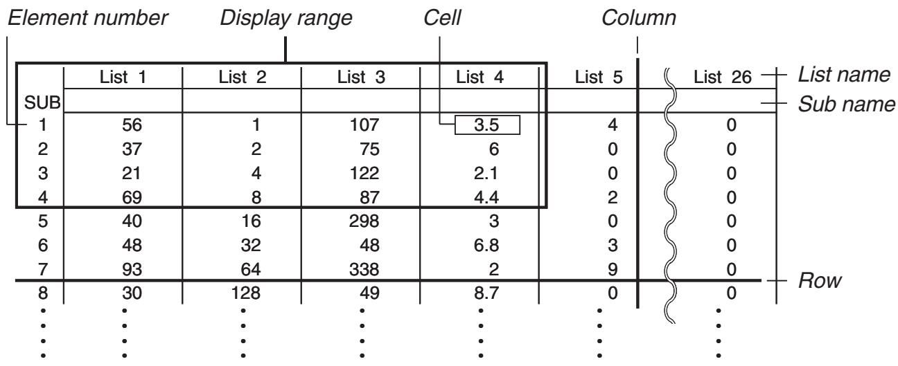
other
| Element number | Sub | Row | | :--- | :--- | :--- | | 1 | 56 | 0 | | 2 | 37 | 0 | | 3 | 21 | 0 | | 4 | 69 | 0 | | 5 | 40 | 0 | | 6 | 48 | 0 | | 7 | 93 | 0 | | 8 | 30 | 0 | Display range: List 1, List 2, List 3, List 4; Column: List 5, List 26; Sub name: List name, Sub name; Row: All elements shown; Column: All elements shown.1. Inputting and Editing a List
When you enter the STAT mode, the “List Editor” will appear first. You can use the List Editor to input data into a list and to perform a variety of other list data operations.
- To input values one-by-one
Use the cursor keys to move the highlighting to the list name, sub name or cell you want to select. Note that ▼ does not move the highlighting to a cell that does not contain a value.
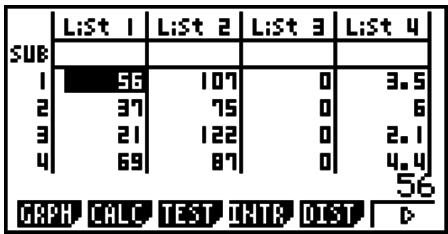
The screen automatically scrolls when the highlighting is located at either edge of the screen.
The following example is performed starting with the highlighting located at Cell 1 of List 1.
- Input a value and press EXE to store it in the list.
3 EXE
- The highlighting automatically moves down to the next cell for input.
- Input the value 4 in the second cell, and then input the result of 2 + 3 in the next cell.
4 EXE 2 + 3 EXE
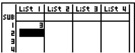
| SUB | Li:St 1 | Li:St 2 | Li:St 3 | Li:St 4 |
| 1 | 3 | |||
| 2 | 4 | |||
| 3 | 5 | |||
| 4 |
- You can also input the result of an expression or a complex number into a cell.
- You can input values up to 999 cells in a single list.
- To batch input a series of values
- Use the cursor keys to move the highlighting to another list.
- Press SHIFT ✗ ( { ), and then input the values you want, pressing ▼ between each one. Press SHIFT ⊙ ( { ) after inputting the final value.

- Press EXE to store all of the values in your list.


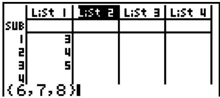
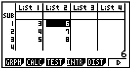
- Remember that a comma separates values, so you should not input a comma after the final value of the set you are inputting.
Right: {34, 53, 78}
Wrong: {34, 53, 78,}
You can also use list names inside of a mathematical expression to input values into another cell. The following example shows how to add the values in each row in List 1 and List 2, and input the result into List 3.
- Use the cursor keys to move the highlighting to the name of the list where you want the calculation results to be input.
- Press OPTN and input the expression.


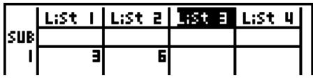
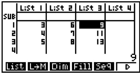
- You can also use SHIFT 1 (List) in place of OPTN F1 (LIST) F1 (List).
■ Editing List Values
• To change a cell value
Use the cursor keys to move the highlighting to the cell whose value you want to change. Input the new value and press EXE to replace the old data with the new one.
• To edit the contents of a cell
- Use the cursor keys to move the highlighting to the cell whose contents you want to edit.
- Press F6 (▷) F2 (EDIT).
- Make any changes in the data you want.
- To delete a cell
- Use the cursor keys to move the highlighting to the cell you want to delete.
- Press F6 (▷) F3 (DEL) to delete the selected cell and cause everything below it to be shifted up.
- The cell delete operation does not affect cells in other lists. If the data in the list whose cell you delete is somehow related to the data in neighboring lists, deleting a cell can cause related values to become misaligned.
- To delete all cells in a list
Use the following procedure to delete all the data in a list.
- Use the cursor key to move the highlighting to any cell of the list whose data you want to delete.
- Pressing F6(▷)F4(DEL·A) causes a confirmation message to appear.
- Press F1 (Yes) to delete all the cells in the selected list or F6 (No) to abort the delete operation without deleting anything.
- To insert a new cell
- Use the cursor keys to move the highlighting to the location where you want to insert the new cell.
- Press 6 (▷) 5 (INS) to insert a new cell, which contains a value of 0, causing everything below it to be shifted down.
- The cell insert operation does not affect cells in other lists. If the data in the list where you insert a cell is somehow related to the data in neighboring lists, inserting a cell can cause related values to become misaligned.
■ Naming a List
You can assign List 1 through List 26 "sub names" of up to eight bytes each.
- To name a list
- On the Setup screen, highlight "Sub Name" and then press F1(On)EXIT.
- Use the cursor keys to move the highlighting to the SUB cell of the list you want to name.
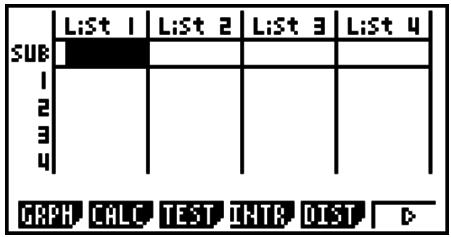
- Type in the name and then press EXE.
- To type in a name using alpha characters, press SHIFT ALPHA to enter the ALPHA-LOCK mode.
Example: YEAR

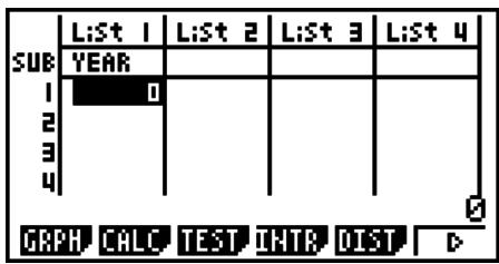
- The following operation displays a sub name in the RUN • MAT (or RUN) mode.

(n = list number from 1 to 26)
![List 1[0] YEAR ▶MAT](/content/2025/01/86832/images/4a2b5c22052a37e057c82e6a914e842ccc89ef30777b1e62c615bf410426b60a.jpg)
- Though you can input up to 8 bytes for the sub name, only the characters that can fit within the List Editor cell will be displayed.
- The List Editor SUB cell is not displayed when “Off” is selected for “Sub Name” on the Setup screen.
■ Sorting List Values
You can sort lists into either ascending or descending order. The highlighting can be located in any cell of the list.
- To sort a single list
Ascending order
- While the lists are on the screen, press F6(▷)F1(TOOL)F1(SRT·A).
- The prompt "How Many Lists?:" appears to ask how many lists you want to sort. Here we will input 1 to indicate we want to sort only one list.

- In response to the "Select List List No:" prompt, input the number of the list you want to sort.

Descending order
Use the same procedure as that for the ascending order sort. The only difference is that you should press F2(SRT·D) in place of F1(SRT·A).
- To sort multiple lists
You can link multiple lists together for a sort so that all of their cells are rearranged in accordance with the sorting of a base list. The base list is sorted into either ascending order or descending order, while the cells of the linked lists are arranged so that the relative relationship of all the rows is maintained.
Ascending order
- While the lists are on the screen, press F6 (▷) F1 (TOOL) F1 (SRT • A).
- The prompt "How Many Lists?:" appears to ask how many lists you want to sort. Here we will sort one base list linked to one other list, so we should input 2.
2 EXE
- In response to the "Select Base List List No:" prompt, input the number of the list you want to sort into ascending order. Here we will specify List 1.
1 EXE
- In response to the "Select Second List List No:" prompt, input the number of the list you want to link to the base list. Here we will specify List 2.
2 EXE
Descending order
Use the same procedure as that for the ascending order sort. The only difference is that you should press F2(SRT·D) in place of F1(SRT·A).
- You can specify a value from 1 to 6 as the number of lists for sorting.
- If you specify a list more than once for a single sort operation, an error occurs.
An error also occurs if lists specified for sorting do not have the same number of values (rows).
2. Manipulating List Data
List data can be used in arithmetic and function calculations. In addition, various list data manipulation functions make manipulation of list data quick and easy.
You can use list data manipulation functions in the RUN • MAT (or RUN), STAT, TABLE, EQUA and PRGM modes.
■ Accessing the List Data Manipulation Function Menu
All of the following examples are performed after entering the RUN • MAT (or RUN) mode.
Press OPTN and then F1(LIST) to display the list data manipulation menu, which contains the following items.
- {List}/{L→M}/{Dim}/{Fill}/{Seq}/{Min}/{Max}/{Mean}/{Med}/{Aug}/{Sum}/{Prod}/{Cuml}/{%}/{∆}
Note that all closing parentheses at the end of the following operations can be omitted.
- To transfer list contents to Matrix Answer Memory
[OPTN]-[LIST]-[L→M]
(Not included on the fx-7400GII)
OPTN F1 (LIST) F2 (L→M) F1 (List) F1 (List)
...
F1 (List) ) EXE
- You can skip input F1 (List) in the part of the above operation.
- All the lists must contain the same number of data items. If they don't, an error occurs.
Example: List → Mat (1, 2) EXE
Example
To transfer the contents of List 1 (2, 3, 6, 5, 4) to column 1, and the contents of List 2 (11, 12, 13, 14, 15) to column 2 of Matrix Answer Memory
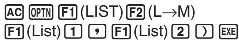
![AnS 1 2 1 [ ] 2 11 2 [ ] 3 12 3 [ ] 6 13 4 [ ] 5 14 5 [ ] 4 15](/content/2025/01/86832/images/9077ee1c16c3c5150f9cb8e765994aa4651772e7a9567d6871108464fda94e7b.jpg)
- To count the number of data items in a list
[OPTN]-[LIST]-[Dim]
OPTN F1 (LIST) F3 (Dim) F1 (List) EXE
- The number of cells a list contains is its “dimension.”
Example To count the number of values in List 1 (36, 16, 58, 46, 56)
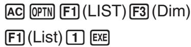
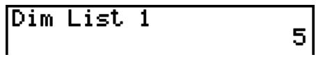
- To create a list by specifying the number of data items
[OPTN]-[LIST]-[Dim]
Use the following procedure to specify the number of data in the assignment statement and create a list.
EXE (n = 1 - 999)
Example To create five data items (each of which contains 0) in List 1
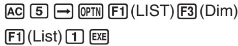
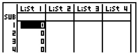
You can view the newly created list by entering the STAT mode.
- To replace all data items with the same value
[OPTN]-[LIST]-[Fill]
OPTN F1 (LIST) F4 (Fill) EXE
Example To replace all data items in List 1 with the number 3
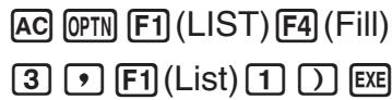

The following shows the new contents of List 1.
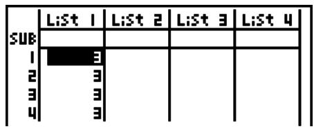
- To generate a sequence of numbers
[OPTN]-[LIST]-[Seq]
OPTN F1 (LIST) F5 (Seq)
- The result of this operation is stored in ListAns Memory.
Example
To input the number sequence 1^2 , 6^2 , 11^2 , into a list, using the function f(x) = X^2 . Use a starting value of 1, an ending value of 11, and an increment of 5.
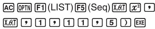
![AnS 1 [ ] 1 2 [ ] 36 3 [ ] 121](/content/2025/01/86832/images/aab1cb9d63f6faadbdc54f0f9d399890c8537cdb850b2a0187b35de9060dfdbb.jpg)
Specifying an ending value of 12, 13, 14, or 15 produces the same result as shown above since they are less than the value produced by the next increment (16).
- To find the minimum value in a list
[OPTN]-[LIST]-[Min]
OPTN F1 (LIST) F6 (▷) F1 (Min) F6 (▷) F6 (▷) F1 (List) ☐ EXE
Example To find the minimum value in List 1 (36, 16, 58, 46, 56)
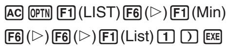
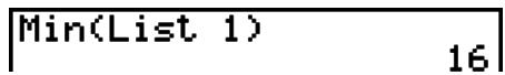
- To find which of two lists contains the greatest value
[OPTN]-[LIST]-[Max]
OPTN F1 (LIST) F6 (▷) F2 (Max) F6 (▷) F6 (▷) F1 (List) F1 (List)
EXE
- The two lists must contain the same number of data items. If they don't, an error occurs.
- The result of this operation is stored in ListAns Memory.
Example To find whether List 1 (75, 16, 98, 46, 56) or List 2 (35, 59, 58, 72, 67) contains the greatest value
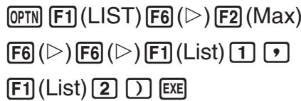
![Ans 1[75] 2 59 3 98 4 72 5L 67](/content/2025/01/86832/images/810ccd69a6b5c8220ec75e813b47991f7d1935e8a136bb948db5d4f312ee12e4.jpg)
- To calculate the mean of data items
[OPTN]-[LIST]-[Mean]
OPTN F1 (LIST) F6 (▷) F3 (Mean) F6 (▷) F6 (▷) F1 (List) ☐ EXE
Example To calculate the mean of data items in List 1 (36, 16, 58, 46, 56)
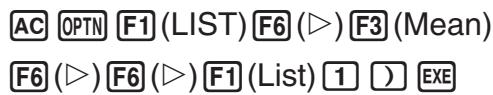
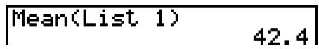
- To calculate the median of data items of specified frequency
[OPTN]-[LIST]-[Med]
This procedure uses two lists: one that contains values and one that indicates the frequency (number of occurrences) of each value. The frequency of the data in Cell 1 of the first list is indicated by the value in Cell 1 of the second list, etc.
- The two lists must contain the same number of data items. If they don't, an error occurs.
OPTN F1 (LIST) F6 (▷) F4 (Med) F6 (▷) F6 (▷) F1 (List) F1 (List)
EXE
Example To calculate the median of values in List 1 (36, 16, 58, 46, 56), whose frequency is indicated by List 2 (75, 89, 98, 72, 67)
AC OPTN F1 (LIST) F6 (▷) F4 (Med)
Median(List 1, List 2) 46
F6 (▷) F6 (▷) F1 (List) 1
F1 (List) 2 ) EXE
- To combine lists
[OPTN]-[LIST]-[Aug]
- You can combine two different lists into a single list. The result of a list combination operation is stored in ListAns memory.
OPTN F1 (LIST) F6 (▷) F5 (Aug) F6 (▷) F6 (▷) F1 (List) , F1 (List)
) EXE
Example To combine the List 1 (-3, -2) and List 2 (1, 9, 10)
AC OPTN F1 (LIST) F6 (▷) F5 (Aug)
F6 (▷) F6 (▷) F1 (List) 1 ,
F1 (List) 2 ) EXE
![AnS 1[-3] 2[-2] 3 1 4 9 5 10](/content/2025/01/86832/images/f531185d791a81ad8895ff116e50099ba85c843c0113ad872bae973fd2a83591.jpg)
- To calculate the sum of data items in a list
[OPTN]-[LIST]-[Sum]
OPTN F1 (LIST) F6 (▷) F6 (▷) F1 (Sum) F6 (▷) F1 (List) EXE
Example To calculate the sum of data items in List 1 (36, 16, 58, 46, 56)
AC OPTN F1 (LIST) F6 (▷) F6 (▷) F1 (Sum)
Sum List 1 212
F6 (▷) F1 (List) 1 EXE
- To calculate the product of values in a list
[OPTN]-[LIST]-[Prod]
OPTN F1 (LIST) F6 (▷) F6 (▷) F2 (Prod) F6 (▷) F1 (List) EXE
Example To calculate the product of values in List 1 (2, 3, 6, 5, 4)
AC OPTN F1 (LIST) F6 (▷) F6 (▷) F2 (Prod)
Prod List 1 720
F6 (▷) F1 (List) 1 EXE
- To calculate the cumulative frequency of each data item [OPTN]-[LIST]-[CumI]
OPTN F1 (LIST) F6 (▷) F6 (▷) F3 (Cuml) F6 (▷) F1 (List) EXE
- The result of this operation is stored in ListAns Memory.
Example To calculate the cumulative frequency of each data item in List 1 (2, 3, 6, 5, 4)
AC OPTN F1 (LIST) F6 (▷) F6 (▷) F3 (Cuml)
F6 (▷) F1 (List) 1 EXE
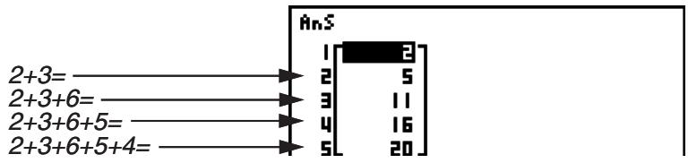
flowchart
graph LR
    A["2+3="] --> B["1"]
    C["2+3+6="] --> D["2"]
    E["2+3+6+5="] --> F["3"]
    G["2+3+6+5+4="] --> H["4"]
    I["AnS"] --> J["1 3 5"]
    I --> K["1 1 16 20"]
- To calculate the percentage represented by each data item [OPTN]-[LIST]-[%]
OPTN F1 (LIST) F6 (▷) F6 (▷) F4 (%) F6 (▷) F1 (List) EXE
- The above operation calculates what percentage of the list total is represented by each data item.
- The result of this operation is stored in ListAns Memory.
Example To calculate the percentage represented by each data item in List 1 (2, 3, 6, 5, 4)
AC OPTN F1 (LIST) F6 (▷) F6 (▷) F4 (%)
F6 (▷) F1 (List) 1 EXE
![2/(2+3+6+5+4) × 100 = ————→ 3/(2+3+6+5+4) × 100 = ————→ 6/(2+3+6+5+4) × 100 = ————→ 5/(2+3+6+5+4) × 100 = ————→ 4/(2+3+6+5+4) × 100 = ————→ AnS 1 [ ] 10 2 15 3 30 4 25 5 20](/content/2025/01/86832/images/9cbc9ee421ed2ae28cde655fb17d09f47c26e6733562c39a76eb0430558eb8ef.jpg)
- To calculate the differences between neighboring data inside a list
[OPTN]-[LIST]-[Δ]
OPTN F1 (LIST) F6 (▷) F6 (▷) F5 (△) EXE
- The result of this operation is stored in ListAns Memory.
Example To calculate the difference between the data items in List 1 (1, 3, 8, 5, 4)
AC OPTN F1 (LIST) F6 (▷) F6 (▷) F5 (△)
1 EXE
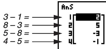
- You can specify the storage location in list memory for a calculation result produced by a list calculation whose result is stored in ListAns memory. For example, specifying “ List 1 List 2” will store the result of List 1 in List 2.
- The number of cells in the new List is one less than the number of cells in the original list.
- An error occurs if you execute List for a list that has no data or only one data item.
3. Arithmetic Calculations Using Lists
You can perform arithmetic calculations using two lists or one list and a numeric value.
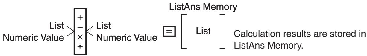
flowchart
graph TD
    A["List Numeric Value"] --> B["+ - × ÷"]
    B --> C["List Numeric Value"]
    C --> D["= List Ans Memory"]
    D --> E["Calculation results are stored in ListAns Memory."]
■ Error Messages
- A calculation involving two lists performs the operation between corresponding cells. Because of this, an error occurs if the two lists do not have the same number of values (which means they have different “dimensions”).
- An error occurs whenever an operation involving any two cells generates a mathematical error.
■ Inputting a List into a Calculation
There are three methods you can use to input a list into a calculation.
- Specification of the list number of a list created with List Editor.
- Specification of the sub name of a list created with List Editor.
- Direct input of a list of values.
- To specify the list number of a list created with List Editor
- In the RUN • MAT (or RUN) mode, perform the following key operation.
AC OPTN F1 (LIST) F1 (List)
- Enter the "List" command.
- Enter the list number (integer from 1 to 26) you want to specify.
List 11
- To specify the sub name of a list created with List Editor
- In the RUN • MAT (or RUN) mode, perform the following key operation.
AC OPTN F1 (LIST) F1 (List)
- Enter the "List" command.
- Enter the sub name of the list you want to specify, enclosed in double quotes (" " ).
Example: "QTY"
List "QTY"
- To directly input a list of values
You can also directly input a list of values using {, }, and ☐.
Example To input the list: 56, 82, 64
SHIFT ✗ ( { ) 5 6 , 8 2 ,
6 4 SHIFT ÷ ( } )
(56,82,64)
- To assign the contents of one list to another list
Use to assign the contents of one list to another list.
Example To assign the contents of List 3 (41, 65, 22) to List 1
OPTN F1 (LIST) F1 (List) 3 → F1 (List) 1 EXE
In place of F1(LIST)F1(List) 3 operation in the above procedure, you could input SHIFT ✗( { ) 4 1 , 6 5 , 2 2 SHIFT ÷( } ).
- To recall the value in a specific list cell
You can recall the value in a specific list cell and use it in a calculation. Specify the cell number by enclosing it inside square brackets.
Example To calculate the sine of the value stored in Cell 3 of List 2
sin OPTN F1 (LIST) F1 (List) 2 SHIFT + ( [ ) 3 SHIFT - ( ] ) EXE
- To input a value into a specific list cell
You can input a value into a specific list cell inside a list. When you do, the value that was previously stored in the cell is replaced with the new value you input.
Example To input the value 25 into Cell 2 of List 3
2 5 → OPTN F1 (LIST) F1 (List) 3 SHIFT + ( [ ) 2 SHIFT - ( ] ) EXE
■ Recalling List Contents
Example To recall the contents of List 1
OPTN F1 (LIST) F1 (List) 1 EXE
- The above operation displays the contents of the list you specify and also stores them in ListAns Memory. You can then use the ListAns Memory contents in a calculation.
- To use list contents in ListAns Memory in a calculation
Example To multiply the list contents in ListAns Memory by 36
OPTN F1 (LIST) F1 (List) SHIFT (-) (Ans) ✗ 3 6 EXE
- The operation OPTN F1 (LIST) F1 (List) SHIFT (-) (Ans) recalls ListAns Memory contents.
- This operation replaces current ListAns Memory contents with the result of the above calculation.
■ Graphing a Function Using a List
When using the graphing functions of this calculator, you can input a function such as Y1 = List 1X. If List 1 contains the values 1, 2, 3, this function will produce three graphs: Y = X, Y = 2X, Y = 3X.
There are certain limitations on using lists with graphing functions.
■ Inputting Scientific Calculations into a List
You can use the numeric table generation functions in the TABLE mode to input values that result from certain scientific function calculations into a list. To do this, first generate a table and then use the list copy function to copy the values from the table to the list.
Example To use the TABLE mode to create a number table for the formula (Y1 = x^2 - 1) , and then copy the table to List 1 in the STAT mode
- In the TABLE mode, input the formula Y_1 = x^2 - 1 .
- Create the number table.
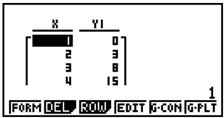
-
Use ▶ to move the highlighting to the Y1 column.
-
Press OPTN F1 (LMEM).
![Store In List Memory List[1~26]: 1 0 LH0 | 533 | ENG | ENG](/content/2025/01/86832/images/0e252d670f68dc8f47634ff5e3e8c61679a34cd6e970db0da72d60a72b80108e.jpg)
- Press 1 EXE.
- Enter the STAT mode to confirm that TABLE mode column Y1 has been copied to List 1.
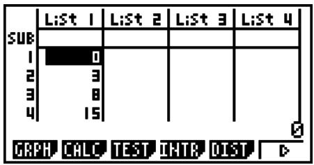
■ Performing Scientific Function Calculations Using a List
Lists can be used just as numeric values are in scientific function calculations. When the calculation produces a list as a result, the list is stored in ListAns Memory.
Example To use List 3 41 65 22 to perform sin (List 3)
Use radians as the angle unit.
sin OPTN F1 (LIST) F1 (List) 3 EXE
4. Switching Between List Files
You can store up to 26 lists (List 1 to List 26) in each file (File 1 to File 6). A simple operation lets you switch between list files.
- To switch between list files
- From the Main Menu, enter the STAT mode.
Press SHIFT MENU (SET UP) to display the STAT mode Setup screen.
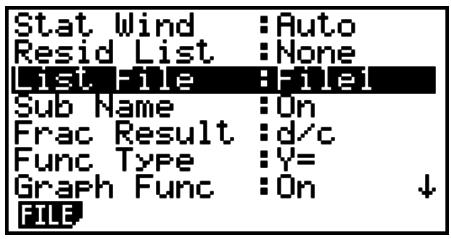
- Use ▼ to highlight "List File".
- Press F1(FILE) and then input the number of the list file you want to use.
Example To select File 3
F1 (FILE) 3
![Select File No. File[1~6]: 3 List File : Files](/content/2025/01/86832/images/93aad67b7a5598b6463e18e6e4745667b169bfcface94c23477113cfba2c476f.jpg)
EXE
All subsequent list operations are applied to the lists contained in the file you select (List File 3 in the above example).
Chapter 4 Equation Calculations
From the Main Menu, enter the EQUA mode.
- {SIML} ... {linear equation with 2 to 6 unknowns}
• {POLY} ... {degree 2 to 6 equation} - {SOLV} ... {solve calculation}
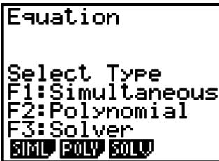
1. Simultaneous Linear Equations
You can solve simultaneous linear equations with two to six unknowns.
- Simultaneous Linear Equation with Two Unknowns:
$$ a _ {1} x + b _ {1} y = c _ {1} $$
$$ a _ {2} x + b _ {2} y = c _ {2} $$
- Simultaneous Linear Equation with Three Unknowns:
$$ a _ {1} x + b _ {1} y + c _ {1} z = d _ {1} $$
$$ a _ {2} x + b _ {2} y + c _ {2} z = d _ {2} $$
$$ a _ {3} x + b _ {3} y + c _ {3} z = d _ {3} $$
■ ■ ■
- From the Main Menu, enter the EQUA mode.
- Select the SIML (Simultaneous) mode, and specify the number of unknowns (variables). You can specify from 2 to 6 unknowns.
- Sequentially input the coefficients.
- The cell that is currently selected for input is highlighted. Each time you input a coefficient, the highlighting shifts in the sequence:
$$ a _ {1} \rightarrow b _ {1} \rightarrow c _ {1} \rightarrow \dots a _ {n} \rightarrow b _ {n} \rightarrow c _ {n} \rightarrow (n = 2 \text { to } 6) $$
- You can also input fractions and values assigned to variables as coefficients.
- You can cancel the value you are inputting for the current coefficient by pressing EXIT at any time before you press EXE to store the coefficient value. This returns to the coefficient to what it was before you input anything. You can then input another value if you want.
- To change the value of a coefficient that you already stored by pressing EXE, move the cursor to the coefficient you want to edit. Next, input the value you want to change to.
-
Pressing F3 (CLR) clears all coefficients to zero.
-
Solve the equations.
Example To solve the following simultaneous linear equations for x, y, and z
$$ 4 x + y - 2 z = - 1 $$
$$ x + 6 y + 3 z = 1 $$
$$ - 5 x + 4 y + z = - 7 $$
① MENU EQUA
② F1(SIML)
F2 (3)
③ 4 EXE 1 EXE (−) 2 EXE (−) 1 EXE
1 EXE 6 EXE 3 EXE 1 EXE
- Internal calculations are performed using a 15-digit mantissa, but results are displayed using a 10-digit mantissa and a 2-digit exponent.
- Simultaneous linear equations are solved by inverting the matrix containing the coefficients of the equations. For example, the following shows the solution (x, y, z) of a simultaneous linear equation with three unknowns.
$$ \left[ \begin{array}{c} x \ y \ z \end{array} \right] = \left[ \begin{array}{c c c} a _ {1} & b _ {1} & c _ {1} \ a _ {2} & b _ {2} & c _ {2} \ a _ {3} & b _ {3} & c _ {3} \end{array} \right] ^ {- 1} \left[ \begin{array}{c} d _ {1} \ d _ {2} \ d _ {3} \end{array} \right] $$
Because of this, precision is reduced as the value of the determinant approaches zero. Also, simultaneous equations with three or more unknowns may take a very long time to solve.
- An error occurs if the calculator is unable to find a solution.
- After calculation is complete, you can press F1(REPT), change coefficient values, and then re-calculate.
2. High-order Equations from 2nd to 6th Degree
Your calculator can be used to solve high-order equations from 2nd to 6th degree.
• Quadratic Equation: ax^2 + bx + c = 0 (a 0)
- Cubic Equation: ax^3 + bx^2 + cx + d = 0 (a 0)
- Quartic Equation: ax^4 + bx^3 + cx^2 + dx + e = 0 (a 0)
-
From the Main Menu, enter the EQUA mode.
-
Select the POLY (Polynomial) mode, and specify the degree of the equation.
You can specify a degree 2 to 6.
- Sequentially input the coefficients.
- The cell that is currently selected for input is highlighted. Each time you input a coefficient, the highlighting shifts in the sequence:
$$ a \rightarrow b \rightarrow c \rightarrow \dots $$
- You can also input fractions and values assigned to variables as coefficients.
-
You can cancel the value you are inputting for the current coefficient by pressing EXIT at any time before you press EXE to store the coefficient value. This returns to the coefficient to what it was before you input anything. You can then input another value if you want.
-
To change the value of a coefficient that you already stored by pressing EXE, move the cursor to the coefficient you want to edit. Next, input the value you want to change to.
- Pressing F3 (CLR) clears all coefficients to zero.
4. Solve the equations.
Example To solve the cubic equation (Angle unit = Rad)
$$ x ^ {3} - 2 x ^ {2} - x + 2 = 0 $$
① MENU EQUA
② F2 (POLY)
F2 (3)
Complex Mode: Real (page 1-27)
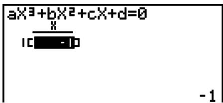
Complex Mode: a + bi
![aX³ + bX² + cX + d = 0 x1[ ] -1 x2[ -0.5 + 1.3228i x3[ -0.5 - 1.3228i] -1](/content/2025/01/86832/images/5b597c96c57b1d45f15a4034c9989c8b02357acdd58294166e24c6c6cc1158cf.jpg)
Complex Mode: r
![aX³+bX²+cX+d=0 x1[1.3.1415] x2[1.4142-1.9321] x3[1.4142-1.932] 1∠3.141592654](/content/2025/01/86832/images/05011e2effb47cb3a053616cc967e3108c0c2e934531d2981ea0db72503a77d5.jpg)
- Internal calculations are performed using a 15-digit mantissa, but results are displayed using a 10-digit mantissa and a 2-digit exponent.
- It may take considerable time for the calculation result of a high-order equation of 3rd degree or higher to appear on the display.
- An error occurs if the calculator is unable to find a solution.
- High-order equation calculations may not produce accurate results when the equation has multiple solutions.
- After calculation is complete, you can press F1(REPT), change coefficient values, and then re-calculate.
3. Solve Calculations
The Solve Calculation mode lets you determine the value of any variable in a formula without having to solve the equation.
- From the Main Menu, enter the EQUA mode.
-
Select the SOLV (Solver) mode, and input the equation as it is written.
-
If you do not input an equals sign, the calculator assumes that the expression is to the left of the equals sign, and there is a zero to the right.
-
An error occurs if you input more than one equals sign.
-
In the table of variables that appears on the display, input values for each variable.
-
You can also specify values for Upper and Lower to define the upper and lower limits of the range of solutions.
-
An error occurs if the solution falls outside the range you specify.
-
Select the variable for which you want to solve to obtain the solution.
“Lft” and “Rgt” indicate the left and right sides that are calculated using the solution. ^*1
*1 Solutions are approximated using Newton's method. Lft and Rgt values are displayed for confirmation, because Newton's method may produce results that are the real solution. The closer the difference between the Lft and Rgt values is to zero, the lower degree of error in the result.
Example
An object thrown into the air at initial velocity V takes time T to reach height H. Use the following formula to solve for initial velocity V when H = 14 (meters), T = 2 (seconds) and gravitational acceleration is G = 9.8 (m/s ^2 ).
$$ \mathsf {H} = \mathsf {V T} - 1 / 2 \mathsf {G T} ^ {2} $$
① MENU EQUA
② F3(SOLV)
ALPHA F→D (H) SHIFT (=) ALPHA 2 (V) ALPHA ÷ (T)
(1) ÷ 2) ALPHA a_c^b (G) ALPHA ÷ (T) ^2 EXE
③ 1 4 EXE (H = 14)
0 EXE (V = 0)
2 EXE (T = 2)
9 • 8 EXE (G = 9.8)
④ Press ▲ ▲ ▲ to highlight V = 0, and then press F6 (SOLV).
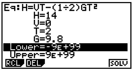
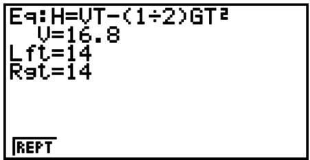
- The message “Retry” appears on the display when the calculator judges that convergence is not sufficient for the displayed results.
- A Solve operation will produce a single solution. Use POLY when you want to obtain multiple solutions for a high-order equation (such as ax^2 + bx + c = 0 ).
Chapter 5 Graphing
Select the icon in the Main Menu that suits the type of graph you want to draw or the type of table you want to generate.
• GRAPH ... General function graphing
- RUN•MAT (or RUN) ... Manual graphing (pages 5-12 to 5-15)
- TABLE ... Number table generation (pages 5-15 to 5-19)
- DYNA* ... Dynamic graphing (pages 5-20 to 5-22)
- RECUR* ... Recursion graphing or number table generation (pages 5-22 to 5-26)
- CONICS* ... Conic section graphing (page 5-27)
* Not included on the fx-7400GII.
1. Sample Graphs
■ How to draw a simple graph (1)
To draw a graph, simply input the applicable function.
- From the Main Menu, enter the GRAPH mode.
- Input the function you want to graph.
Here you would use the V-Window to specify the range and other parameters of the graph. See page 5-2. - Draw the graph.
Example To graph y = 3x^2
① MENU GRAPH
② 3 X,θ,T x^2 EXE
③ F6 (DRAW) (or EXE)
- Press AC to return to the screen in step 2 (Graph relation list). After drawing a graph, you can toggle between the Graph relation list and graph screen by pressing SHIFT F6 (G↔T).
■ How to draw a simple graph (2)
You can store up to 20 functions in memory and then select the one you want for graphing.
- From the Main Menu, enter the GRAPH mode.
- Specify the function type and input the function whose graph you want to draw. You can use the GRAPH mode to draw a graph for the following types of expressions: rectangular coordinate expression (Y=f(x)), polar coordinate expression, parametric function, rectangular coordinate expression (X=f(y)), inequality.
F3(TYPE) F1(Y=)... rectangular coordinates (Y=f(x) type)
F2 (r=) ... polar coordinates
F3(Parm) ... parametric function
F4 (X=) ... rectangular coordinates (X=f(y) type)
F5 (CONV) F1 (▶Y=) to F5 (▶Y≤) F6 (▷) F1 (▶X=) to F5 (▶X≤) ... changes the function type F6 (▷) F1 (Y>) to F4 (Y≤) .... Y inequality on left side F6 (▷) F6 (▷) F1 (X>) to F4 (X≤) .... X inequality on left side
Repeat this step as many times as required to input all of the functions you want.
Next you should specify which of the functions among those that are stored in memory you want to graph (see page 5-6). If you do not select specific functions here, the graph operation will draw graphs of all the functions currently stored in memory.
3. Draw the graph.
- You can use the function menu that appears when you press F4(STYL) in step 2 of the above procedure to select one of the following line styles for each graph.
F1(—) ... Normal (initial default)
F2(一) ... Thick (twice the thickness of Normal)
F3 (……) ... Broken (thick broken)
F4 (……) ... Dot (dotted)
- When simultaneously graphing multiple inequalities, you can use the “Ineq Type” setting on the Setup screen (SHIFT MENU (SETUP)) to specify either of two fill ranges.
F1(AND) ... Fills areas only where the conditions of all of the graphed inequalities are satisfied. This is the initial default.
F2 (OR) ..... Fills all areas where the conditions of the graphed inequalities are satisfied.
natural_image
Pure geometric diagram with intersecting lines and shaded region, no text or symbols presentExample Input the functions shown below and draw their graphs.
$$ \mathbf {Y} 1 = 2 x ^ {2} - 3, r 2 = 3 \sin 2 \theta $$
① MENU GRAPH
② F3 (TYPE) F1 (Y=) 2 X,θ,T x² - 3 EXE
F3 (TYPE) F2 (r=) 3 sin 2 X,θ,T EXE
③ F6 (DRAW)
natural_image
Symmetrical abstract line drawing with four petal-like loops on a Cartesian coordinate system (no text or symbols)2. Controlling What Appears on a Graph Screen
■ V-Window (View Window) Settings
Use the View Window to specify the range of the x- and y-axes, and to set the spacing between the increments on each axis. You should always set the V-Window parameters you want to use before graphing.
- To make V-Window settings
- From the Main Menu, enter the GRAPH mode.
- Press SHIFT F3 (V-WIN) to display the V-Window setting screen.
Rectangular coordinate parameter
Xmin/Xmax ... Minimum/maximum x-axis value
Xscale ... Spacing of x-axis increments
Xdot ... Value that corresponds to one x-axis dot
Ymin/Ymax ... Minimum/maximum y-axis value
Yscale ... Spacing of y-axis increments
Polar coordinate parameter
Tθ min/Tθ max ... Minimum/maximum T, θ values
Tθ ptch ... T, θ pitch
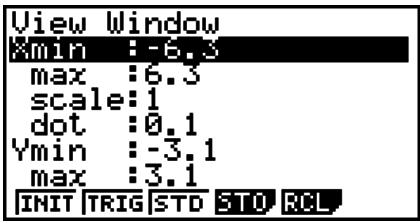
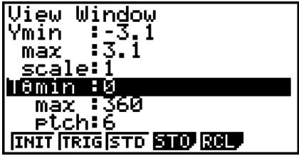
-
Press ▼ to move the highlighting and input an appropriate value for each parameter, pressing EXE after each.
-
{INIT}/{TRIG}/{STD} ... V-Window {initial settings}/{initial settings using specified angle unit}/{standardized settings}
- {STO}/{RCL} ... V-Window setting {store}/{recall}
After settings are the way you want them, press EXIT or SHIFT EXIT (QUIT) to exit the V-Window setting screen.
- Pressing EXE without inputting anything while ■ (busy indicator) is displayed exits the V-Window setting screen.
• V-Window Setting Precautions
- Inputting zero for Tθ ptch causes an error.
- Any illegal input (out of range value, negative sign without a value, etc.) causes an error.
- When T max is less than T min, T ptch becomes negative.
- You can input expressions (such as 2 ) as V-Window parameters.
- When the V-Window setting produces an axis that does not fit on the display, the scale of the axis is indicated on the edge of the display closest to the origin.
- Changing the V-Window settings clears the graph currently on the display and replaces it with the new axes only.
- Changing the Xmin or Xmax value causes the Xdot value to be adjusted automatically. Changing the Xdot value causes the Xmax value to be adjusted automatically.
- A polar coordinate ( r = ) or parametric graph will appear coarse if the settings you make in the V-Window cause the Tθ ptch value to be too large, relative to the differential between the Tθ min and Tθ max settings. If the settings you make cause the Tθ ptch value to be too small relative to the differential between the Tθ min and Tθ max settings, on the other hand, the graph will take a very long time to draw.
- The following is the input range for V-Window parameters.
-9.9999999999E 97 to 9.9999999999E 97
■ V-Window Memory
You can store up to six sets of V-Window settings in V-Window memory for recall when you need them.
- To store V-Window settings
- From the Main Menu, enter the GRAPH mode.
- Press SHIFT F3 (V-WIN) to display the V-Window setting screen, and input the values you want.
- Press F4(STO) to display the pop-up window.
- Press a number key to specify the V-Window memory where you want to save the settings, and then press EXE. Pressing 1 EXE stores the settings in V-Window Memory 1 (V-Win1).
- To recall V-Window memory settings
- From the Main Menu, enter the GRAPH mode.
- Press SHIFT F3 (V-WIN) to display the V-Window setting screen.
- Press F5 (RCL) to display the pop-up window.
- Press a number key to specify the V-Window memory number for the settings you want to recall, and then press EXE. Pressing 1 EXE recalls the settings in V-Window Memory 1 (V-Win1).
■ Specifying the Graph Range
You can define a range (start point, end point) for a function before graphing it.
- From the Main Menu, enter the GRAPH mode.
- Make V-Window settings.
- Specify the function type and input the function. The following is the syntax for function input.
Function ⚙ SHIFT ➕ ( [ ) Start Point ⚙ End Point SHIFT ➕ ( ])
- Draw the graph.
Example Graph y = x^2 + 3x - 2 within the range -2 ≤ x ≤ 4 .
Use the following V-Window settings.
$$ \mathrm{Xmin} = - 3, \quad \mathrm{Xmax} = 5, \quad \mathrm{Xscale} = 1 $$
$$ \mathrm{Ymin} = - 1 0, \quad \mathrm{Ymax} = 3 0, \quad \text { Yscale } = 5 $$
① MENU GRAPH
② SHIFT F3 (V-WIN) (-) 3 EXE 5 EXE 1 EXE ▼
$$ ① (-) 1 0 E X E 3 0 E X E 5 E X E E X I T $$
③ F3 (TYPE) F1 (Y=) X,θ,T x² + 3 X,θ,T - 2 ,
$$ \boxed {\text {SHIFT}} \boxed {+} ([) (-) \boxed {2}, \boxed {4} \boxed {\text {SHIFT}} \boxed {-} (]) \boxed {\text {EXE}} $$
④ F6 (DRAW)
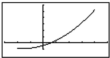
line
| x | y | | ---- | ---- | | 0 | 0 | | 1 | 0.5 | | 2 | 1 | | 3 | 1.5 | | 4 | 2 | | 5 | 2.5 | | 6 | 3 | | 7 | 3.5 | | 8 | 4 | | 9 | 4.5 | | 10 | 5 |- You can specify a range when graphing rectangular expressions, polar expressions, parametric functions, and inequalities.
Zoom
This function lets you enlarge and reduce the graph on the screen.
- Draw the graph.
- Specify the zoom type.
SHIFT F2 (ZOOM) F1 (BOX) ... Box zoom
Draw a box around a display area, and that area is enlarged to fill the entire screen.
F2 (FACT)
Specifies the x-axis and y-axis zoom factors for factor zoom.
F3 (IN)/F4 (OUT) ... Factor zoom
The graph is enlarged or reduced in accordance with the factor you specify, centered on the current pointer location.
F5 (AUTO) ... Auto zoom
V-Window y-axis settings are automatically adjusted so the graph fills the screen along the y-axis.
F6 (▷) F1 (ORIG) ... Original size
Returns the graph to its original size following a zoom operation.
F6 (▷) F2 (SQR) ... Graph correction
V-Window x-axis values are corrected so they are identical to the y-axis values.
F6 (▷) F3 (RND) ... Coordinate rounding
Rounds the coordinate values at the current pointer location.
F6 (▷) F4 (INTG) ... Integer
Each dot is given a width of 1, which makes coordinate values integers.
F6 (▷) F5 (PRE) ... Previous
V-Window parameters are returned to what they were prior to the last zoom operation.
Box zoom range specification
- Use the cursor keys to move the pointer (✝) in the center of the screen to the location where you want one corner of the box to be, and then press EXE.
- Use the cursor keys to move the pointer. This causes a box to appear on the screen. Move the cursor until the area you want to enlarge is enclosed in the box, and then press EXE to enlarge it.
Example Graph y = (x + 5)(x + 4)(x + 3) , and then perform a box zoom.
Use the following V-Window settings.
Xmin = -8, Xmax = 8, Xscale = 2
Ymin = -4, Ymax = 2, Yscale = 1
① MENU GRAPH
SHIFT F3 (V-WIN) (-) 8 EXE 8 EXE 2 EXE ▼
(一) 4 EXE 2 EXE 1 EXE EXIT
F3 (TYPE) F1 (Y=) (X,θ,T) + 5 ) (X,θ,T) + 4 )
( X,θ,T + 3 ) EXE
F6 (DRAW)
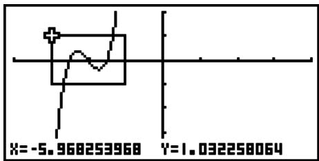
line
| X Value | Y Value | | ------- | ------- | | -5.968253968 | 1.032258064 |② SHIFT F2 (ZOOM) F1 (BOX)
③ ◀️ \~ ◀️ EXE
④ ◀️ \~ ◀️, ▲️ \~ ▲️ EXE
natural_image
Simple line drawing of a wave with a horizontal axis and a vertical boundary (no text or symbols)- You must specify two different points for box zoom, and the two points cannot be on a straight line vertically or horizontally from each other.
3. Drawing a Graph
You can store up to 20 functions in memory. Functions in memory can be edited, recalled, and graphed.
■ Specifying the Graph Type
Before you can store a graph function in memory, you must first specify its graph type.
-
While the Graph relation list is on the display, press F3(TYPE) to display the graph type menu, which contains the following items.
-
{Y=}/{r=}/{Parm}/{X=} ... {rectangular coordinate (Y=f(x) type)}/{polar coordinate}/{parametric}/{rectangular coordinate (X=f(y) type)} graph
- Y > / Y < / Y ≥ / Y ≤ Y > f(x) / Y < f(x) / Y ≥ f(x) / Y ≤ f(x) inequality graph
- X > / X < / X ≥ / X ≤ X > f(y) / X < f(y) / X ≥ f(y) / X ≤ f(y) inequality graph
• {CONV}
- Y = / Y > / Y < / Y ≥ / Y ≤ / X = / X > / X < / X ≥ / X ≤ ... {changes the function type of the selected expression}
- Press the function key that corresponds to the graph type you want to specify.
■ Storing Graph Functions
- To store a rectangular coordinate function (Y=)
Example To store the following expression in memory area Y1: y = 2x^2 - 5
F3(TYPE) F1(Y=)(Specifies rectangular coordinate expression.)
2 X,θ,T x^2 — 5 (Inputs expression.)
EXE (Stores expression.)
Graph Func :Y= Y102X²-5 [—]
- A function cannot be stored into a memory area that already contains a function of a different type from the one you are trying to store. Select a memory area that contains a function that is the same type as the one you are storing, or delete the function in the memory area to which you are trying to store.
- To store a parametric function
Example To store the following expressions in memory areas Xt3 and Yt3:
$$ x = 3 \sin T $$
$$ y = 3 \cos T $$
F3(TYPE) F3(Parm) (Specifies parametric expression.)
3 sin X,θ,T EXE (Inputs and stores x expression.)
3 cos X,θ,T EXE (Inputs and stores y expression.)
- To create a composite function
Example To use relations in Y1 and Y2 to create composite functions for Y3 and Y4
$$ \mathrm{Y} 1 = \sqrt {(\mathrm{X} + 1)}, \mathrm{Y} 2 = \mathrm{X} ^ {2} + 3 $$
Assign Y1°Y2 to Y3, and Y2°Y1 to Y4.
$$ (Y 1 \circ Y 2 = \sqrt {\left(\left(x ^ {2} + 3\right) + 1\right)} = \sqrt {\left(x ^ {2} + 4\right)} \quad Y 2 \circ Y 1 = (\sqrt {(X + 1)}) ^ {2} + 3 = X + 4 (X \geq - 1)) $$
Input relations into Y3 and Y4.
F3 (TYPE) F1 (Y=) VARS F4 (GRPH)
F1(Y) 1 ( F1(Y) 2 ) EXE
VARS F4 (GRPH) F1 (Y) 2
( F1(Y) 1 ) EXE
![Graph Func :Y= Y1B(Y+1) [—] Y2B(X²+3) [—] Y3B(Y1)(Y2) [—] Y4B(Y2)(Y1) [—] Y5: [—] Y6: [—] SEL DEL TYPE STYL JMEM DRAW](/content/2025/01/86832/images/a751dd0d6a154c0e9aa1348527d81be8a30ae37950cace9454888af1c722535a.jpg)
- A composite function can consist of up to five functions.
- To assign values to the coefficients and variables of a graph function
Example To assign the values -1, 0, and 1 to variable A in Y = AX ^2 –1, and draw a graph for each value
F3(TYPE) F1(Y=)
ALPHA X,θ,T (A) X,θ,T x^2 — 1 EXE
VARS F4 (GRPH) F1 (Y) 1 ( ALPHA X,θ,T (A)
SHIFT • (=) (-) 1 ) EXE
VARS F4 (GRPH) F1 (Y) 1 ( ALPHA X,θ,T (A)
SHIFT (=) 0 ) EXE
VARS F4 (GRPH) F1 (Y) 1 ( ALPHA X,θ,T (A)
SHIFT • (=) 1 ) EXE
▲ ▲ ▲ ▲ F1 (SEL)
F6 (DRAW)
![Graph Func :Y= Y1BAX²-1 [—] Y2BY1(A=-1) [—] Y3BY1(A=0) [—] Y4BY1(A=1) [—] Y5: Y6: [—] SEL DEL TYPE STYLE JMEM DRAW](/content/2025/01/86832/images/27aa6b5a30ce7a49b83dfb2651865fd3c93a1b1a3178460fe68b0a228a830b00.jpg)
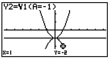
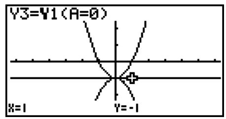
The above three screens are produced using the Trace function.
See “Function Analysis” (page 5-29) for more information.
■ Editing and Deleting Functions
• To edit a function in memory
Example To change the expression in memory area Y1 from y = 2x^2 - 5 to
$$ y = 2 x ^ {2} - 3 $$
(Displays cursor.)
▶▶▶▶▶DEL 3 (Changes contents.)
EXE (Stores new graph function.)
- To change the line style of a graph function
- On the Graph relation list screen, use ▲ and ▼ to highlight the relation whose line style you want to change.
- Press F4(STYL).
- Select the line style.
Example To change the line style of y = 2x^2 - 3 , which is stored in area Y1, to “Broken”
F4(STYL) F3(……) (Selects "Broken".)
- To change the type of a function \*1
- While the Graph relation list is on the display, press ▲ or ▼ to move the highlighting to the area that contains the function whose type you want to change.
- Press F3(TYPE)F5(CONV).
- Select the function type you want to change to.
Example To change the function in memory area Y1 from y = 2x^2 - 3 to
$$ y < 2 x ^ {2} - 3 $$
F3(TYPE) F5(CONV) F3(▶Y<) (Changes the function type to "Y<".)
*1 The function type can be changed for rectangular coordinate functions and inequalities only.
- To delete a function
- While the Graph relation list is on the display, press ▲ or ▼ to move the highlighting to the area that contains the function you want to delete.
-
Press F2 (DEL) or DEL.
-
Press F1 (Yes) to delete the function or F6 (No) to abort the procedure without deleting anything.
- Using the above procedure to delete one line of a parametric function (such as Xt2) also will delete the applicable paired line (Yt2, in the case of Xt2).
■ Selecting Functions for Graphing
- To specify the draw/non-draw status of a graph
-
On the Graph relation list, use ▲ and ▼ to highlight the relation you do not want to graph.
-
Press F1 (SEL).
• Each press of F1(SEL) toggles graphing on and off.
- Press F6 (DRAW).
Example To select the following functions for drawing:
$$ \mathbf {Y 1} = 2 x ^ {2} - 5, r 2 = 5 \sin 3 \theta $$
Use the following V-Window settings.
$$ \mathrm{Xmin} = - 5, \quad \mathrm{Xmax} = 5, \quad \mathrm{Xscale} = 1 $$
$$ \mathrm{Ymin} = - 5, \quad \mathrm{Ymax} = 5, \quad \mathrm{Yscale} = 1 $$
$$ \mathbf {T} \theta \min = 0, \quad \mathbf {T} \theta \max = \pi , \quad \mathbf {T} \theta \operatorname{ptch} = 2 \pi / 6 0 $$
☑ (Select a memory area that contains a function for which you want to specify non-draw.)
F1 (SEL) (Specifies non-draw.)
F6 (DRAW) or EXE (Draws the graphs.)
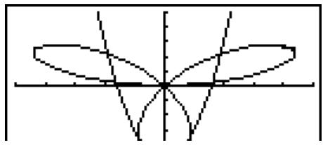
natural_image
Symmetrical geometric line drawing with intersecting curves and a central axis (no text or symbols)- You can use the Setup screen settings to alter the appearance of the graph screen as shown below.
- Grid: On (Axes: On Label: Off)
This setting causes dots to appear at the grid intersects on the display.
natural_image
Symmetrical geometric line drawing with intersecting curves and a central axis (no text or symbols)- Axes: Off (Label: Off Grid: Off)
This setting clears the axis lines from the display.
natural_image
Abstract geometric line drawing with intersecting curves and ovals (no text or symbols)- Label: On (Axes: On Grid: Off)
This setting displays labels for the x- and y-axes.
■ Graph Memory
Graph memory lets you store up to 20 sets of graph function data and recall it later when you need it.
A single save operation saves the following data in graph memory.
- All graph functions in the currently displayed Graph relation list (up to 20)
- Graph types
• Function graph line information - Draw/non-draw status
• V-Window settings (1 set)
- To store graph functions in graph memory
- Press F5 (GMEM) F1 (STO) to display the pop-up window.
- Press a number key to specify the Graph memory where you want to save the graph function, and then press EXE. Pressing 1 EXE stores the graph function to Graph Memory 1 (G-Mem1).
- There are 20 graph memories numbered G-Mem1 to G-Mem20.
- Storing a function in a memory area that already contains a function replaces the existing function with the new one.
- If the data exceeds the calculator's remaining memory capacity, an error occurs.
• To recall a graph function
- Press F5 (GMEM) F2 (RCL) to display the pop-up window.
- Press a number key to specify the Graph memory for the function you want to recall, and then press EXE. Pressing 1 EXE recalls the graph function in Graph Memory 1 (G-Mem1).
- Recalling data from graph memory causes any data currently on the Graph relation list to be deleted.
4. Storing a Graph in Picture Memory
You can save up to 20 graphic images in picture memory for later recall. You can overdraw the graph on the screen with another graph stored in picture memory.
- To store a graph in picture memory
- After graphing in GRAPH mode, press OPTN F1 (PICT) F1 (STO) to display the pop-up window.
- Press a number key to specify the Picture memory where you want to save the picture, and then press EXE. Pressing 1 EXE stores the picture function to Picture Memory 1 (Pict 1).
- There are 20 picture memories numbered Pict 1 to Pict 20.
- Storing a graphic image in a memory area that already contains a graphic image replaces the existing graphic image with the new one.
- A dual graph screen or any other type of graph that uses a split screen cannot be saved in picture memory.
- To recall a stored graph
- After graphing in GRAPH mode, press OPTN F1 (PICT) F2 (RCL) to display the pop-up window.
- Press a number key to specify the Picture memory for the picture you want to recall, and then press EXE. Pressing 1 EXE recalls the picture function in Picture Memory 1 (Pict 1).
- Recalling picture memory contents causes the currently displayed graph to be overwritten.
- Use the sketch CIs function (page 5-28) to clear a graph that was recalled from picture memory.
5. Drawing Two Graphs on the Same Screen
■ Copying the Graph to the Sub-screen
Dual Graph lets you split the screen into two parts. Then you can graph two different functions in each for comparison, or draw a normal size graph on one side and its enlarged version on the other side. This makes Dual Graph a powerful graph analysis tool.
With Dual Graph, the left side of the screen is called the “main screen”, while the right side is called the “sub-screen”.
- Main Screen
The graph in the main screen is actually drawn from a function.
- Sub-screen
The graph on the sub-screen is produced by copying or zooming the main screen graph. You can even make different V-Window settings for the sub-screen and main screen.
- To copy the graph to the sub-screen
- From the Main Menu, enter the GRAPH mode.
- On the Setup screen, select "G+G" for Dual Screen.
- Make V-Window settings for the main screen.
Press F6 (RIGHT) to display the sub-graph settings screen. Pressing F6 (LEFT) returns to the main screen setting screen.
- Store the function, and draw the graph in the main screen.
- Perform the Dual Graph operation you want.
OPTN F1 (COPY) ... Duplicates the main screen graph in the sub-screen
OPTN F2 (SWAP) ... Swaps the main screen contents and sub-screen contents
- Indicators appear to the right of the formulas in the Graph relation list to tell where graphs are drawn with Dual Graph.
![Graph+Graph : Y= Y1X0X+2(X-2) ——R Y2B2X²-3 [—]B](/content/2025/01/86832/images/c4c8e6cc4bb15fdbbe64157e2c64d237bc838058fcef9314fb10a1f1c5d188ce.jpg)
Indicates sub-screen graph (on right side of display) Indicates graph drawn on both sides of display
Performing a draw operation with the function marked “R” in the above example screen causes the graph to be drawn on the right side on the display. The function marked “B” is drawn on both sides of the graph.
Pressing F1 (SEL) while one of the function's is highlighted would causes its “R” or “B” indicator to be cleared. A function without an indicator is drawn as the main screen graph (on the left side of the display).
Example Graph y = x(x + 1)(x - 1) in the main screen and sub-screen.
Use the following V-Window settings.
(Main Screen) Xmin = -2, Xmax = 2, Xscale = 0.5
Ymin = -2, Ymax = 2, Yscale = 1
(Sub-screen) Xmin = -4, Xmax = 4, Xscale = 1
Ymin = -3, Ymax = 3, Yscale = 1
① MENU GRAPH
② SHIFT MENU (SET UP) ▼ ▼ ▼ ▼ * F1 (G + G) EXIT
*fx-7400GII, fx-9750GII: ▼ ▼ ▼
③ SHIFT F3 (V-WIN) (-) 2 EXE 2 EXE 0 • 5 EXE ▼
natural_image
Pure waveform diagram with no text, numbers, or symbols- Pressing AC while a graph is on the display will return to the screen in step 4.
6. Manual Graphing
■ Rectangular Coordinate Graph
Inputting the Graph command in the RUN•MAT (or RUN) mode enables drawing of rectangular coordinate graphs.
- From the Main Menu, enter the RUN•MAT (or RUN) mode.
- Make V-Window settings.
- Input the commands for drawing the rectangular coordinate graph.
- Input the function.
Example Graph y = 2x^2 + 3x - 4 .
Use the following V-Window settings.
- Certain functions can be graphed easily using built-in function graphs.
- You can draw graphs of the following built-in scientific functions.
Rectangular Coordinate Graph
| · x | · x | · x | · ^-1 x |
| · ^-1 x | · ^-1 x | · x | · x |
| · x | · ^-1 x | · ^-1 x | · ^-1 x |
| · | x^2 | x | x |
| 10^x | e^x | x^-1 | ^3 |
| (x) | ^2dx^2(x) | (x)dx |
Polar Coordinate Graph
| · | · | · | · ^-1 |
| · ^-1 | · ^-1 | · | · |
| · | · ^-1 | · ^-1 | · ^-1 |
| · | · ^2 | · | · |
| · 10^ | · e^ | · ^-1 | · ^3 |
- Input for x and variables is not required for a built-in function.
- When inputting a built-in function, other operators or values cannot be input.
■ Drawing Multiple Graphs on the Same Screen
Use the following procedure to assign various values to a variable contained in an expression and overwrite the resulting graphs on the screen.
- From the Main Menu, enter the GRAPH mode.
- On the Setup screen, change the "Dual Screen" setting to "Off".
- Make V-Window settings.
- Specify the function type and input the function. The following is the syntax for function input.
Expression containing one variable ⚙ SHIFT + ( [ ) variable SHIFT ⊙ (=)
value □ value □ ... □ value SHIFT — ( ] )
- Draw the graph.
Example To graph y = Ax^2 - 3 as the value of A changes in the sequence 3, 1, -1 Use the following V-Window settings.
natural_image
Pure mathematical line diagram showing intersecting curves and a horizontal axis (no text or symbols)- The value of only one of the variables in the expression can change.
- Any of the following cannot be used for the variable name: X, Y, r, θ, T.
- You cannot assign a variable to the variable inside the function.
- When Simul Graph is turned on, all of the graphs for the specified variable values are drawn simultaneously.
• Overwrite can be used when graphing rectangular expressions, polar expressions, parametric functions, and inequalities.
■ Using Copy and Paste to Graph a Function
You can graph a function by copying it to the clipboard, and then pasting it into the graph screen.
There are two types of functions you can paste into the graph screen.
Type 1 (Y= expression)
A function with the Y variable to the left of the equal sign is graphed as Y= expression.
Example: To paste Y=X and graph it
- Any spaces to the left of Y are ignored.
Type 2 (expression)
Pasting this type of expression graphs Y= expression.
Example: To paste X and graph Y=X
- Any spaces to the left of the expression are ignored.
- To graph a function using copy and paste
- Copy the function you want to graph to the clipboard.
- From the Main Menu, enter the GRAPH mode.
- On the Setup screen, change the "Dual Screen" setting to "Off".
- Make V-Window settings.
- Draw the graph.
- Paste the expression.
Example While the graph of y = 2x^2 + 3x - 4 is currently displayed, to paste the previously copied function Y=X from the clipboard
Use the following V-Window settings.
- Paste is supported only when “Off” is selected for the “Dual Screen” setting on the Setup screen.
- Though there is no limit on the number of graphs you can draw by pasting a function, the total number of graphs supported by trace and other functions is 30 (number of graphs drawn using expression number 1 to 20, plus graphs drawn using pasted functions).
- For the graph of a pasted function, the graph expression that appears when using trace or other functions is displayed in the format: Y= expression.
- Re-executing a draw without clearing graph screen memory will redraw all the graphs, including those produced by pasting functions.
7. Using Tables
To enter the TABLE mode, select the TABLE icon on the Main Menu.
■ Storing a Function and Generating a Number Table
- To store a function
Example To store the function y = 3x^2 - 2 in memory area Y1
Use ▲ and ▼ to move the highlighting in the Table relation list to the memory area where you want to store the function. Next, input the function and press EXE to store it.
- Variable Specifications
There are two methods you can use to specify value for the variable x when generating a numeric table.
- Table range method
With this method, you specify the conditions for the change in value of the variable.
- List
With this method, the data in the list you specify is substituted for the x-variable to generate a number table.
- To generate a table using a table range
Example
To generate a table as the value of variable x changes from -3 to 3, in increments of 1
MENU TABLE
F5 (SET)
The numeric table range defines the conditions under which the value of variable x changes during function calculation.
Start ...... Variable x start value
End ...... Variable x end value
Step ...... Variable x value change (interval)
After specifying the table range, press EXIT to return to the Table relation list.
- To generate a table using a list
- While the Table relation list is on the screen, display the Setup screen.
- Highlight Variable and then press F2 (LIST) to display the pop-up window.
- Select the list whose values you want to assign for the x-variable.
- To select List 6, for example, press ☑ EXE. This causes the setting of the Variable item of the Setup screen to change to List 6.
- After specifying the list you want to use, press EXIT to return to the previous screen.
- Generating a Table
Example
To generate a table of values for the functions stored in memory areas Y1 and Y3 of the Table relation list
Use ▲ and ▼ to move the highlighting to the function you want to select for table generation and press F1(SEL) to select it.
The “=” sign of selected functions is highlighted on the screen. To deselect a function, move the cursor to it and press F1(SEL) again.
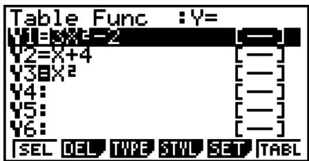
Press F6 (TABL) to generate a number table using the functions you selected. The value of variable x changes according to the range or the contents of the list you specified.
The example screen shown here shows the results based on the contents of List 6 (-3, -2, -1, 0, 1, 2, 3).
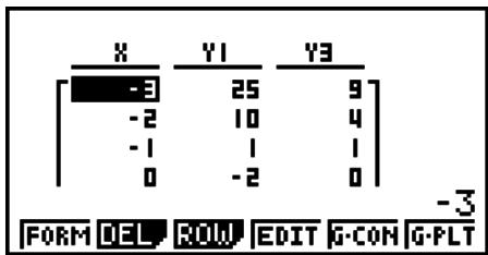
Each cell can contain up to six digits, including negative sign.
- To generate a differential number table
Changing the setting of Setup screen's Derivative item to On causes a number table that includes the derivative to be displayed whenever you generate a number table.
Locating the cursor at a differential coefficient displays “dy/dx” in the top line, which indicates differential.
- An error occurs if a graph for which a range is specified or an overwrite graph is included among the graph expressions.
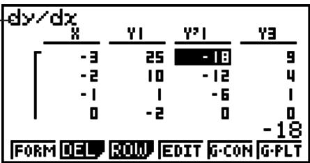
- Specifying the Function Type
You can specify a function as being one of three types.
- Rectangular coordinate (Y=)
- Polar coordinate (r=)
-
Parametric (Parm)
-
Press F3(TYPE) while the relation list is on the screen.
- Press the number key that corresponds to the function type you want to specify.
- The number table is generated only for the function type specified on the relation list (Table Func). You cannot generate a number table for a mixture of different function types.
■ Editing Tables
You can use the table menu to perform any of the following operations once you generate a table.
- Change the values of variable x
- Edit (delete, insert, and append) rows
- Delete a table
- Draw a connect type graph
- Draw a plot type graph
- {FORM} ... {return to Table relation list}
- {DEL} ... {delete table}
• {ROW}
- {DEL}/{INS}/{ADD} ... {delete}/{insert}/{add} row
- {G·CON}/{G·PLT} ... {connected type}/{draw plot type} graph draw
- If you try to replace a value with an illegal operation (such as division by zero), an error occurs and the original value remains unchanged.
- You cannot directly change any values in the other (non- x ) columns of the table.
■ Copying a Table Column to a List
A simple operation lets you copy the contents of a numeric table column into a list.
Use ◀ and ▶ to move the cursor to the column you want to copy. The cursor can be in any row.
- To copy a table to a list
Example To copy the contents of Column x into List 1
OPTN F1 (LMEM)
Input the number of the list you want to copy and then press EXE.
1 EXE
![Store In List Memory List[1~26]: I 3](/content/2025/01/86832/images/cb6daa2aed8437cad8c8533394a4aaefa6a16d31c7ca97260ba3b07b9bfb29ca.jpg)
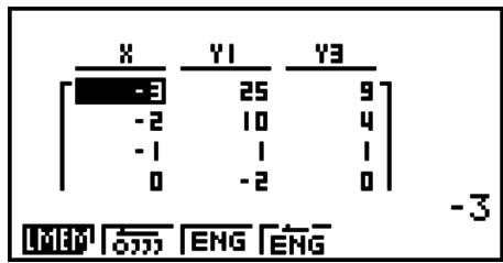
■ Drawing a Graph from a Number Table
Use the following procedure to generate a number table and then draw a graph based on the values in the table.
- From the Main Menu, enter the TABLE mode.
- Make V-Window settings.
- Store the functions.
- Specify the table range.
- Generate the table.
- Select the graph type and draw it.
F5 (G·CON) ... line graph
F6 (G • PLT) ... plot type graph
- After drawing the graph, pressing SHIFT F6 (G ↔ T) or AC returns to the number table screen.
Example Store the two functions below, generate a number table, and then draw a line graph. Specify a range of -3 to 3, and an increment of 1.
$$ \mathsf {Y 1} = 3 x ^ {2} - 2, \mathsf {Y 2} = x ^ {2} $$
Use the following V-Window settings.
$$ \mathrm{Xmin} = 0, \quad \mathrm{Xmax} = 6, \quad \mathrm{Xscale} = 1 $$
$$ \mathrm{Ymin} = - 2, \quad \mathrm{Ymax} = 1 0, \quad \text { Yscale } = 2 $$
① MENU TABLE
② SHIFT F3 (V-WIN) 0 EXE 6 EXE 1 EXE ▼
$$ ① \boxed {2} \boxed {\mathrm{EXE}} \boxed {1} \boxed {0} \boxed {\mathrm{EXE}} \boxed {2} \boxed {\mathrm{EXE}} \boxed {\mathrm{EXIT}} $$
③ F3 (TYPE) F1 (Y=) 3 X,θ,T x² - 2 EXE
X,θ,T x^2 EXE
④ F5 (SET) (-) 3 EXE 3 EXE 1 EXE EXIT
⑤ F6 (TABL)
⑥ F5 (G·CON)
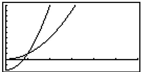
line
| X | Y1 | Y2 | Y3 | |---|----|----|----| | 0 | 0 | 0 | 0 | | 1 | 0.5 | 0.3| 0.6| | 2 | 1.0 | 0.7| 1.2| | 3 | 1.5 | 1.2| 1.8| | 4 | 2.0 | 1.7| 2.4| | 5 | 2.5 | 2.2| 3.0| | 6 | 3.0 | 2.7| 3.6|- You can use Trace, Zoom, or Sketch after drawing a graph.
■ Simultaneously Displaying a Number Table and Graph
Specifying T+G for Dual Screen on the Setup screen makes it possible to display a number table and graph at the same time.
- From the Main Menu, enter the TABLE mode.
- Make V-Window settings.
- On the Setup screen, select T+G for Dual Screen.
- Input the function.
- Specify the table range.
- The number table is displayed in the sub-screen on the right.
- Specify the graph type and draw the graph.
F5(G·CON) ... line graph
F6 (G • PLT) ... plot type graph
Example Store the function Y_1 = 3x^2 - 2 and simultaneously display its number table and line graph. Use a table range of -3 to 3 with an increment of 1.
Use the following V-Window settings.
Xmin = 0, Xmax = 6, Xscale = 1
Ymin = -2, Ymax = 10, Yscale = 2
① MENU TABLE
② SHIFT F3 (V-WIN) 0 EXE 6 EXE 1 EXE ▼
(一) 2 EXE 1 0 EXE 2 EXE EXIT
③ SHIFT MENU (SET UP) ▼ ▼ ▼ * F1 (T+G) EXIT
*fx-7400GII, fx-9750GII: ▼ ▼
④ F3 (TYPE) F1 (Y=) 3 X,θ,T x² - 2 EXE
⑤ F5 (SET)
- The Setup screen's “Dual Screen” setting is applied in the TABLE mode and the RECUR mode.
- You can make the number table active by pressing OPTN F1 (CHNG) or AC.
8. Dynamic Graphing
Important!
- The fx-7400GII is not equipped with the DYNA mode.
■ Using Dynamic Graph
Dynamic Graph lets you define a range of values for the coefficients in a function, and then observe how a graph is affected by changes in the value of a coefficient. It helps to see how the coefficients and terms that make up a function influence the shape and position of a graph.
- From the Main Menu, enter the DYNA mode.
- Make V-Window settings.
- On the Setup screen, specify the Dynamic Type.
F1(Cnt) ... Continuous
F2 (Stop) ... Automatic stop after 10 draws
- Use the cursor keys to select the function type on the built-in function type list.*1
- Input values for coefficients, and specify which coefficient will be the dynamic variable.*2
- Specify the start value, end value, and increment.
- Specify the drawing speed.
F3 (SPEED) F1 (IID).... Pause after each draw (Stop&Go)
F2(>) ..... Half normal speed (Slow)
F3 (▶) ..... Normal speed (Normal)
F4(※)..... Twice normal speed (Fast)
- Draw the Dynamic Graph.
*1 The following are the seven built-in function types.
- Y = A X + B
- Y = A(X + B)^2 + C
- Y = AX^2 + BX + C
- Y = AX^3 + BX^2 + CX + D
- Y = A (B X + C)
- Y = A (BX + C)
- Y = Atan( BX + C)
After you press F3(TYPE) and select the function type you want, you can then input the actual function.
*2 You could also press EXE here and display the parameter setting menu.
- The message “Too Many Functions” appears when more than one function is selected for Dynamic Graphing.
Example
Use Dynamic Graph to graph y = A(x - 1)^2 - 1 , in which the value of coefficient A changes from 2 through 5 in increments of 1. The graph is drawn 10 times.
① MENU DYNA
② SHIFT F3 (V-WIN) F1 (INIT) EXIT
③ SHIFT MENU (SET UP) ▼* F2 (Stop) EXIT
*fx-9750GII: SHIFT MENU (SET UP)
④ F5 (B-IN) ▼ F1 (SEL)
⑤ F4 (VAR) 2 EXE (-) 1 EXE (-) 1 EXE
⑥ F2 (SET) 2 EXE 5 EXE 1 EXE EXIT
⑦ F3 (SPEED) F3 (▶) EXIT
⑧ F6 (DYNA)
Repeats from ① through ④.
①
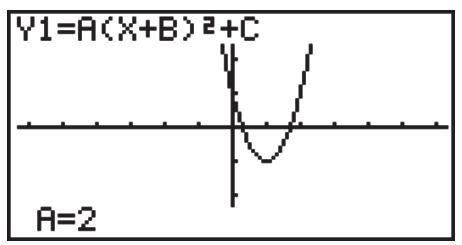
②
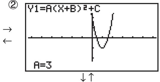
line
| x | y | | ---- | ------ | | 0 | 0 | | 1 | 0.5 | | 2 | 0.8 | | 3 | 0.6 | | 4 | 0.7 | | 5 | 0.9 | | 6 | 1.0 | | 7 | 0.8 | | 8 | 0.6 | | 9 | 0.4 | | 10 | 0.2 | | 11 | 0.1 | | 12 | 0.05 | | 13 | 0.02 | | 14 | 0.01 | | 15 | 0.005 | | 16 | 0.002 | | 17 | 0.001 | | 18 | 0.0005 | | 19 | 0.0002 | | 20 | 0.0001 | | 21 | 0.00005| | 22 | 0.00002| | 23 | 0.00001| | 24 | 0.000005| | 25 | 0.000002| | 26 | 0.000001| | 27 | 0.0000005| | 28 | 0.0000002| | 29 | 0.0000001| | 30 | 0.00000005| | 31 | 0.00000002| | 32 | 0.00000001| | 33 | 0.000000005| | 34 | 0.000000002| | 35 | 0.000000001| | 36 | 0.0000000005| | 37 | 0.0000000002| | 38 | 0.0000000001| | 39 | 0.00000000005| | 40 | 0.0 | | 41 | 1 | | 42 | 1 | | 43 | 1 | | 44 | 1 | | 45 | 1 | | 46 | 1 | | 47 | 1 | | 48 | 1 | | 49 | 1 | | 50 | 1 | | 51 | 1 | | 52 | 1 | | 53 | 1 | | 54 | 1 | | 55 | 1 | | 56 | 1 | | 57 | 1 | | 58 | 1 | | 59 | 1 | | 60 | 1 | | 61 | 1 | | 62 | 1 | | 63 | 1 | | 64 | 1 | | 65 | 1 | | 66 | 1 | | 67 | 1 | | 68 | 1 | | 69 | 1 | | 70 | 1 | | 71 | 1 | | 72 | 1 | | 73 | 1 | | 74 | 1 | | 75 | 1 | | 76 | 1 | | 77 | 1 | | 78 | 1 | | 79 | 1 | | 80 | 1 | | 81 | 1 | | 82 | 1 | | 83 | 1 | | 84 | 1 | | 85 | 1 | | 86 | 1 | | 87 | 1 | | 88 | 1 | | 89 | 1 | | 90 | 1 | | 91 | 1 | | 92 | 1 | | 93 | 1 | | 94 | 1 | | 95 | 1 | | 96 | 1 | | 97 | 1 | | 98 | 1 | | 99 | 1 | | | |④
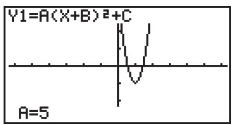
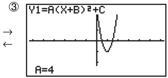
line
| x | y | | ---- | ------ | | 0 | 0 | | 1 | 0.5 | | 2 | 1.0 | | 3 | 0.8 | | 4 | 0.6 | | 5 | 0.7 | | 6 | 0.9 | | 7 | 1.2 | | 8 | 1.5 | | 9 | 1.8 | | 10 | 2.0 | | 11 | 2.2 | | 12 | 2.4 | | 13 | 2.6 | | 14 | 2.8 | | 15 | 3.0 | | 16 | 3.2 | | 17 | 3.4 | | 18 | 3.6 | | 19 | 3.8 | | 20 | 4.0 | | 21 | 4.2 | | 22 | 4.4 | | 23 | 4.6 | | 24 | 4.8 | | 25 | 5.0 | | 26 | 5.2 | | 27 | 5.4 | | 28 | 5.6 | | 29 | 5.8 | | 30 | 6.0 | | 31 | 6.2 | | 32 | 6.4 | | 33 | 6.6 | | 34 | 6.8 | | 35 | 7.0 | | 36 | 7.2 | | 37 | 7.4 | | 38 | 7.6 | | 39 | 7.8 | | 40 | 8.0 | | 41 | 8.2 | | 42 | 8.4 | | 43 | 8.6 | | 44 | 8.8 | | 45 | 9.0 | | 46 | 9.2 | | 47 | 9.4 | | 48 | 9.6 | | 49 | 9.8 | | 50 | 10.0 | | 51 | 10.2 | | 52 | 10.4 | | 53 | 10.6 | | 54 | 10.8 | | 55 | 11.0 | | 56 | 11.2 | | 57 | 11.4 | | 58 | 11.6 | | 59 | 11.8 | | 60 | 12.0 | | 61 | 12.2 | | 62 | 12.4 | | 63 | 12.6 | | 64 | 12.8 | | 65 | 13.0 | | 66 | 13.2 | | 67 | 13.4 | | 68 | 13.6 | | 69 | 13.8 | | 70 | 14.0 | | 71 | 14.2 | | 72 | 14.4 | | 73 | 14.6 | | 74 | 14.8 | | 75 | 15.0 | | 76 | 15.2 | | 77 | 15.4 | | 78 | 15.6 | | 79 | 15.8 | | 80 | 16.0 | | 81 | 16.2 | | 82 | 16.4 | | 83 | 16.6 | | 84 | 16.8 | | 85 | 17.0 | | 86 | 17.2 | | 87 | 17.4 | | 88 | 17.6 | | 89 | 17.8 | | 90 | 18.0 | | 91 | 18.2 | | 92 | 18.4 | | 93 | 18.6 | | 94 | 18.8 | | 95 | 19.0 | | 96 | 19.2 | | 97 | 19.4 | | 98 | 19.6 | | 99 | 19.8 | | A=40 |■ Drawing a Dynamic Graph Locus
Turning on the Dynamic Graph locus setting on the Setup screen lets you overlay a graph drawn by changing the coefficient values.
- From the Main Menu, enter the DYNA mode.
- Make V-Window settings.
- On the Setup screen, select "On" for "Locus".
- Use the cursor keys to select the function type on the built-in function type list.
- Input values for coefficients, and specify which coefficient will be the dynamic variable.
- Specify the start value, end value, and increment.
- Specify Normal for the draw speed.
- Draw the Dynamic Graph.
Example
Use Dynamic Graph to graph y = Ax , in which the value of coefficient A changes from 1 through 4 in increments of 1. The Graph is drawn 10 times.
① MENU DYNA
② SHIFT F3 (V-WIN) F1 (INIT) EXIT
③ SHIFT MENU (SET UP) ▼ ▼ * F1 (On) EXIT
*fx-9750GII: ▼
④ F5 (B-IN) F1 (SEL)
⑤ F4 (VAR) 1 EXE 0 EXE
⑥ F2 (SET) 1 EXE 4 EXE 1 EXE EXIT
⑦ F3 (SPEED) F3 (F) EXIT
⑧ F6 (DYNA)
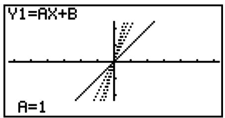

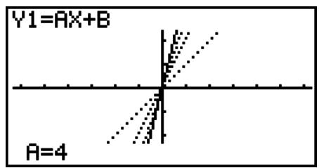
■ Graph Calculation DOT Switching Function
Use this function to specify drawing of all the dots on the Dynamic Graph X-axis, or every other dot. This setting is value for Dynamic Func Y= graphic only.
- Press SHIFT MENU (SET UP) to display the Setup screen.
- Press ▼▼▼* to select Y=Draw Speed.
*fx-9750GII: ▼ ▼
- Select the graphing method.
F1 (Norm) ... Draws all X-axis dots. (initial default)
F2 (High) ... Draws every other X-axis dot. (faster drawing than Normal)
- Press EXIT.
■ Using Dynamic Graph Memory
You can store Dynamic Graph conditions and screen data in Dynamic Graph memory for later recall when you need it. This lets you save time, because you can recall the data and immediately begin a Dynamic Graph draw operation. Note that you can store one set of data in memory at any one time.
- To save data in Dynamic Graph memory
- While a Dynamic Graph draw operation is being performed, press AC to change to the speed adjustment menu.
- Press F5(STO). In response to the confirmation dialog that appears, press F1(Yes) to save the data.
- To recall data from Dynamic Graph memory
- Display the Dynamic Graph relation list.
- Pressing F6(RCL) recalls Dynamic Graph memory contents and draws the graph.
9. Graphing a Recursion Formula
Important!
- The fx-7400GII is not equipped with the RECUR mode.
■ Generating a Number Table from a Recursion Formula
You can input up to three of the following types of recursion formulas and generate a number table.
- General term of sequence a_n , composed of a_n, n
- Linear two-term recursion composed of a_n+1, a_n, n
-
Linear three-term recursion composed of a_n+2 , a_n+1 , a_n , n
-
From the Main Menu, enter the RECUR mode.
-
Specify the recursion type.
F3(TYPE) F1( a_n ) ... {general term of sequence a_n }
F2 (a_n + 1) ... {linear two-term recursion}
F3 (a_n + 2) ... {linear three-term recursion}
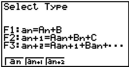
- Input the recursion formula.
- Specify the table range. Specify a start point and end point for n. If necessary, specify a value for the initial term, and a pointer start point value if you plan to graph the formula.
- Display the recursion formula number table.
Example
Generate a number table from recursion between three terms as expressed by a_n+2 = a_n+1 + a_n , with initial terms of a_1 = 1 , a_2 = 1 (Fibonacci sequence), as n changes in value from 1 to 6.
① MENU RECUR
② F3(TYPE)F3( a_n+2 )
③ F4 ( n.a_n ·) F3 ( a_n+1 ) + F2 ( a_n ) EXE
④ F5 (SET) F2 ( a_1 ) 1 EXE 6 EXE 1 EXE 1 EXE EXIT
⑤ F6 (TABL)
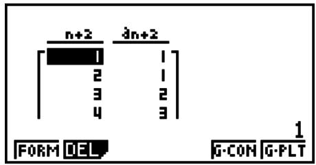
* The first two values correspond to a_1=1 and a_2=1 .
- Pressing F1(FORM) will return to the screen for storing recursion formulas.
- Specifying “On” for the “ΣDisplay” of the Setup screen causes the sum of each term to be included in the table.
■ Graphing a Recursion Formula
After generating a number table from a recursion formula, you can graph the values on a line graph or plot type graph.
- From the Main Menu, enter the RECUR mode.
- Make V-Window settings.
- Specify the recursion formula type and input the formula.
- Select the line style for the graph.
- Display the recursion formula number table.
-
Specify the graph type and draw the graph.
-
Specify the table range, and start and ending values for n. If necessary, specify the initial term value and pointer start point.
F5(G·CON) ... line graph
F6 (G • PLT) ... plot type graph
Example
Generate a number table from recursion between two terms as expressed by a_n+1 = 2a_n + 1 , with an initial term of a_1 = 1 , as n changes in value from 1 to 6. Use the table values to draw a line graph.
Use the following V-Window settings.
Xmin = 0, Xmax = 6, Xscale = 1
Ymin = -15, Ymax = 65, Yscale = 5
① MENU RECUR
② SHIFT F3 (V-WIN) 0 EXE 6 EXE 1 EXE ▼
(一) 1 5 EXE 6 5 EXE 5 EXE EXIT
③ F3 (TYPE) F2 ( a_n+1 ) 2 F2 ( a_n ) + 1 EXE
④ F5 (SET) F2 ( a_1 ) 1 EXE 6 EXE 1 EXE EXIT
⑤ F1 (SEL+S) ▲ F2 (—) EXIT
⑥ F6 (TABL)
⑦ F5(G·CON)
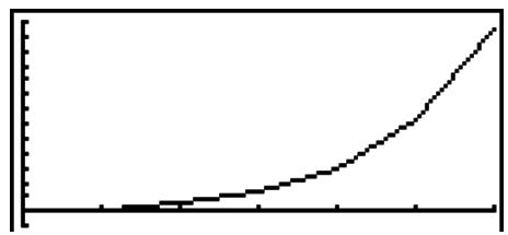
line
| x | y | |---|---| | 0 | 0 | | 1 | 0.1 | | 2 | 0.3 | | 3 | 0.6 | | 4 | 1.0 | | 5 | 1.8 | | 6 | 3.0 | | 7 | 5.0 | | 8 | 7.5 | | 9 | 10.0 | | 10 | 13.0 | | 11 | 16.0 | | 12 | 20.0 | | 13 | 25.0 | | 14 | 32.0 | | 15 | 40.0 | | 16 | 50.0 | | 17 | 62.0 | | 18 | 78.0 | | 19 | 98.0 | | 20 | 128.0 | | 21 | 168.0 | | 22 | 218.0 | | 23 | 288.0 | | 24 | 378.0 | | 25 | 488.0 | | 26 | 618.0 | | 27 | 778.0 | | 28 | 978.0 | | 29 | 1218.0 | | 30 | 1588.0 | | 31 | 1998.0 | | 32 | 2568.0 | | 33 | 3348.0 | | 34 | 4328.0 | | 35 | 5568.0 | | 36 | 7188.0 | | 37 | 9328.0 | | 38 | 12688.0 | | 39 | 17448.0 | | 40 | 23568.0 | | 41 | 31928.0 | | 42 | 42648.0 | | 43 | 56488.0 | | 44 | 74888.0 | | 45 | 107568.0 | | 46 | 155688.0 | | 47 | 225488.0 | | 48 | 323768.0 | | 49 | 456888.0 | | 50 | 625688.0 | | 51 | 932888.0 | | 52 | 1397688.0 | | 53 | 1998888.0 | | 54 | 2756888.0 | | 55 | 3784888.0 | | 56 | 5192888.0 | | 57 | 7143288.0 | | 58 | 10456488.0 | | 59 | 14976888.0 | | 60 | 21928888.0 | | 61 | 31432888.0 | | 62 | 44768888.0 | | 63 | 63743288.0 | | 64 | 97356488.0 | | 65 | 146777778.0 | | 66 | 219288888.0 | | 67 | 314328888.0 | | 68 | 447688888.0 | | 69 | 637432888.0 | | 70 | 973564888.0 | | 71 | 1467777788.0 | | 72 | 2192888888.0 | | 73 | 3143288888.0 | | 74 | 4476888888.0 | | 75 | 6374328888.0 | | 76 | 9735648888.0 | | 77 | 14677777888.0 | | 78 | 21928888888.0 | | 79 | 31432888888.0 | | 80 | 44768888888.0 | | 81 | 63743288888.0 | | 82 | 97356488888.0 | | 83 | 14677777888.0 | | 84 | 21928888888.0 | | 85 | 31432888888.0 | | 86 | 44768888888.0 | | 87 | 63743288888.0 | | 88 | 9735648888• After drawing a graph, you can use Trace, Zoom, and Sketch.
- Press AC to return to the number table screen. After drawing a graph, you can toggle between the number table screen and graph screen by pressing SHIFT F6 (G↔T).
■ Graphing a Phase Plot from Two Numeric Sequences
You can draw the phase plot for numeric sequences generated by two expressions input in the RECUR mode with one value on the horizontal axis and the other value on the vertical axis.
For a_n(a_n+1,a_n+2) , b_n(b_n+1,b_n+2) , c_n(c_n+1,c_n+2) , the numeric sequence of the alphabetically first expression is on the horizontal axis while the following numeric sequence is on the vertical axis.
-
From the Main Menu, enter the RECUR mode.
-
Configure V-Window settings.
-
Enter two recursion formulas and select both of them for table generation.
-
Configure table generation settings.
Specify the start and end values for variable n and the initial term for each recursion formula.
-
Display the recursion formula number table.
-
Draw the phase plot.
Example
To input the two sequence formulas for regression between two terms a_n+1 = 0.9a_n and b_n+1 = b_n + 0.1_n - 0.2 , and specify initial terms a_1 = 1 and b_1 = 1 for each. Generate a number table as the value of the n variable goes from 1 to 10 and use it to draw a phase plot.
Use the following V-Window settings.
Xmin = 0, Xmax = 2, Xscale = 1
Ymin = 0, Ymax = 4, Yscale = 1
① MENU RECUR
② SHIFT F3 (V-WIN) 0 EXE 2 EXE 1 EXE ▼
0 EXE 4 EXE 1 EXE EXIT
③ F3(TYPE)F2( a_n+1 )0·9F2( a_n )EXE
F4 (n.a n ·) F3 (b n ) + 0 · 1 F1 (n) - 0 · 2 EXE
④ F5 (SET) F2 ( a_1 ) 1 EXE 1 0 EXE 1 EXE 1 EXE EXIT
⑤ F6 (TABL)
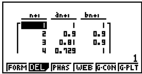
other
| Category | Value | |---|---| | n+1 | 1 | | a(n+1) | 0.9 | | b(n+1) | 0.81 | | | 0.729 | | | 1 | FORM DEL PHAS WEB G-CON G-PLT⑥ F3 (PHAS)
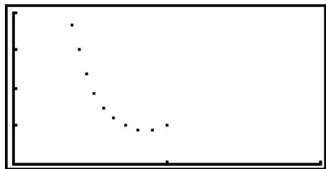
scatter
| x | y | |---|---| | 0.0 | 1 | | 0.2 | 0.8 | | 0.4 | 0.6 | | 0.6 | 0.4 | | 0.8 | 0.2 | | 1.0 | 0.1 |- If you enter three expressions on the RECUR mode screen and select all of them for table creation, you will need to specify which two of the three expressions you want to use to draw the phase plot. To do so, use the function menu that appears when you press F3 (PHAS) on the table screen.
F1(a•b)...... Graph using a_n ( a_n+1 , a_n+2 ) and b_n ( b_n+1 , b_n+2 ).
F2(b·c)......Graph using b_n ( b_n+1 , b_n+2 ) and c_n ( c_n+1 , c_n+2 ).
F3 (a· c) ...... Graph using a_n(a_n+1,a_n+2) and c_n(c_n+1,c_n+2) .
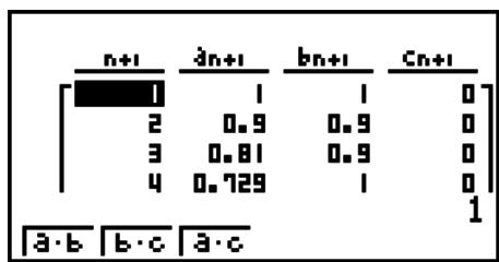
- Specifying “On” for the “ΣDisplay” of the Setup screen causes the sum of each term to be included in the table. At this time you can select use of the two numeric sequences as-is to draw the plot graph, or use of the sums of each of the two numeric sequences. To do so, use the function menu that appears when you press F3(PHAS) on the table screen.
F1 (a_n) ..... Use numeric sequence for graphing.
F6(Σan).....Use numeric sequence sums for graphing.
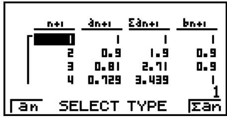
bar
| Category | n+1 | an+1 | Σan+1 | bn+1 | |---|---|---|---|---| | Select | 1 | 0.9 | 1.9 | 0.9 | | Type | 2 | 0.81 | 2.71 | 0.9 | | | 3 | 0.729 | 3.439 | 1 | | | 4 | | | 1 | | Select | an | SELECT | TYPE | Σan | The chart displays a single bar for 'an' at the bottom of the bar chart. The other three bars (an, Σan) are not explicitly labeled but are visually present in the legend.- When “On” is selected “ΣDisplay” on the Setup screen and all three of the expressions you input in the RECUR mode are selected for table creation, use the function menu that appears when you press F3(PHAS) on the table screen to specify which two of the expressions you want to use, and to specify whether you want to use numeric sequence data or numeric sequence sum data.
F1(a · b) ...... Graph using number sequences a_n ( a_n+1 , a_n+2 ) and b_n ( b_n+1 , b_n+2 )
F2(b · c) ...... Graph using number sequences b_n ( b_n+1 , b_n+2 ) and c_n ( c_n+1 , c_n+2 )
F3 (a· c) ...... Graph using number sequences a_n (a_n + 1, a_n + 2) and c_n (c_n + 1, c_n + 2)
F4 ( a · b) ...... Graph using the sums of number sequences a_n ( a_n+1 , a_n+2 ) and b_n ( b_n+1 , b_n+2 )
F5 ( b · c) ...... Graph using the sums of number sequences b_n ( b_n+1 , b_n+2 ) and c_n ( c_n+1 , c_n+2 )
F6 ( a · c ) ..... Graph using the sums of number sequences a_n ( a_n+1 , a_n+2 ) and c_n ( c_n+1 , c_n+2 )
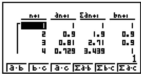
other
| Category | n+1 | a.n+1 | Σa.n+1 | bn+1 | |---|---|---|---|---| | n+1 | 1 | 1 | 1 | 1 | | a.n+1 | 2 | 0.9 | 1.9 | 0.9 | | Σa.n+1 | 3 | 0.81 | 2.71 | 0.9 | | bn+1 | 4 | 0.729 | 3.439 | 1 | | a·b | | | | | | b·c | | | | | | a·c | | | | | | Σa·b | | | | | | Σb·c | | | | | | Σa·c | | | | |■ WEB Graph (Convergence, Divergence)
y = f(x) is graphed by presuming a_n+1 = y , a_n = x for linear two-term regression a_n+1 = f(a_n) composed of a_n+1 , a_n . Next, it can be determined whether the function is convergent or divergent.
- From the Main Menu, enter the RECUR mode.
- Make V-Window settings.
- Select 2-term recursion as the recursion formula type, and input the formula.
- Specify the table range, n start and end points, initial term value, and pointer start point.
- Display the recursion formula number table.
- Draw the graph.
- Press EXE, and the pointer appears at the start point you specified.
Press EXE several times.
If convergence exists, lines that resemble a spider web are drawn on the display. Failure of the web lines to appear indicates either divergence or that the graph is outside the boundaries of the display screen. When this happens, change to larger V-Window values and try again.
You can use ▲▼ to select the graph.
Example To draw the WEB graph for the recursion formula a_n+1 = -3(a_n)^2 + 3a_n , b_n+1 = 3b_n + 0.2 , and check for divergence or convergence. Use the following table range: Start = 0, End = 6, a_0 = 0.01 , a_nStr = 0.01 , b_0 = 0.11 , b_nStr = 0.11
① MENU RECUR
② SHIFT F3 (V-WIN) 0 EXE 1 EXE 1 EXE ▼
$$ ⓠ \quad \boxed {E X E} \quad 1 \quad \boxed {E X E} \quad 1 \quad \boxed {E X E} \quad \boxed {E X I T} $$
③ F3 (TYPE) F2 ( a_n+1 ) (-) 3 F2 ( a_n ) x^2 + 3 F2 ( a_n ) EXE
- To change the graph line style, press F1(SEL+S) after step 4.
- With WEB Graph, you can specify the line type for a y = f(x) graph. The line type setting is valid only when "Connect" is selected for "Draw Type" on the Setup screen.
10. Graphing a Conic Section
Important!
- The fx-7400GII is not equipped with the CONICS mode.
■ Graphing a Conic Section
You can use the CONICS mode to graph parabolas, circles, ellipses, and hyperbolas. You can input a rectangular coordinate function, polar coordinate function, or parametric function for graphing.
- From the Main Menu, enter the CONICS mode.
- Select the function type.
F1 (RECT).... {rectangular coordinate}
F2 (POL).... {polar coordinate}
F3 (PARM).... {parametric}
- Select the pattern of the function in accordance with the type of graph you want to draw.
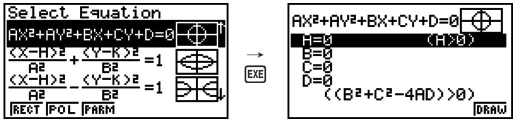
- Enter the coefficients of the function and draw the graph.
Example
To input the rectangular coordinate function x = 2y^2 + y - 1 and graph a parabola open on the right, and then input the polar coordinate function r = 4 and draw a circle graph.
① MENU CONICS
② F1 (RECT) ▼ (X=AY²+BY+C) EXE
③ 2 EXE 1 EXE (−) 1 EXE F6 (DRAW)
④ EXIT EXIT
⑤ F2 (POL) ▼ ▼ ▼ ▼ (R=2Acosθ) EXE
⑥ 2 EXE F6 (DRAW)
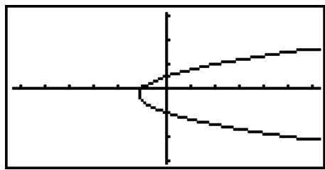
natural_image
Pure mathematical curve diagram with no text, numbers, or symbols
natural_image
Simple geometric diagram with a circle and perpendicular lines (no text or symbols)11. Changing the Appearance of a Graph
■ Drawing a Line
The sketch function lets you draw points and lines inside of graphs.
You can select one of four different line styles for drawing with the sketch function.
-
From the Main Menu, enter the GRAPH mode.
-
Make V-Window settings.
-
On the Setup screen, use the "Sketch Line" setting to specify the line style you want.
F1(—) ... Normal (initial default)
F2(一) ... Thick (twice the thickness of Normal)
F3 (……) ... Broken (thick broken)
F4 (……) ... Dot (dotted)
-
Input the function of the graph.
-
Draw the graph.
-
Select the sketch function you want to use.*1
SHIFT F4 (SKTCH) F1 (Cls) ... Screen clear
F2 (Tang) ... Tangent line
F3 (Norm) ... Line normal to a curve
F4 (Inv) ... Inverse function*2
F6 (▷) F1 (PLOT)
{Plot}/{PI·On}/{PI·Off}/{PI·Chg} ... Point {Plot}/{On}/{Off}/{Change}
F6 (▷) F2 (LINE)
{Line}/{F·Line} ... {connects 2 points plotted by F6 (▷) F1 (PLOT) with a line}/{for drawing a line between any 2 points}
F6 (▷) F3 (Crcl) ... Circle
F6 (▷) F4 (Vert) ... Vertical line
F6 (▷) F5 (Hztl) ... Horizontal line
F6 (▷) F6 (▷) F1 (PEN) ... Freehand
F6 (▷) F6 (▷) F2 (Text) ... Text input
- Use the cursor keys to move the pointer ( ) to the location where you want to draw, and press EXE.*3
*1 The above shows the function menu that appears in the GRAPH mode. Menu items may differ somewhat in other modes.
*2 In the case of an inverse function graph, drawing starts immediately after you select this option.
*3 Some sketch functions require specification of two points. After you press EXE to specify the first point, use the cursor keys to move the pointer to the location of the second point and press EXE.
- You can specify line type for the following sketch functions: Tangent, Normal, Inverse, Line, F•Line, Circle, Vertical, Horizontal, Pen
Example Draw a line that is tangent to point (2, 0) on the graph for y = x(x + 2)(x - 2) .
① MENU GRAPH
② SHIFT F3 (V-WIN) F1 (INIT) EXIT
③ SHIFT MENU (SET UP) ▼ ▼ ▼ ▼ ▼ ▼ ▼ ▼ ▼ * F1 (—) EXIT
*fx-7400GII, fx-9750GII: ▼▼▼▼▼▼▼▼
④ F3 (TYPE) F1 (Y=) X,θ,T (X,θ,T + 2 ) (X,θ,T
- 2 ) EXE
⑤ F6 (DRAW)
⑥ SHIFT F4 (SKTCH) F2 (Tang)
⑦ ▶ \~ ▶ EXE *1
*1 You can draw a tangent line in succession by moving the “+” pointer and pressing EXE.
12. Function Analysis
■ Reading Coordinates on a Graph Line
Trace lets you move a pointer along a graph and read out coordinates on the display.
- From the Main Menu, enter the GRAPH mode.
- Draw the graph.
- Press SHIFT F1 (TRCE), and a pointer appears in the center of the graph.*1
- Use ◀ and ▶ to move the pointer along the graph to the point at which you want to display the derivative.
When there are multiple graphs on the display, press ▲ and ▼ to move between them along the x-axis of the current pointer location.
line
| X | Y | |---|---| | 2 | -2 | | 3 | -1 | | 4 | 0 | | 5 | 1 |- You can also move the pointer by pressing ,,T to display the pop-up window, and then inputting coordinates.
The pop-up window appears even when you input coordinates directly.
To exit a trace operation, press SHIFT F1(TRCE).
*1 The pointer is not visible on the graph when it is located at a point outside the graph display area or when an error of no value occurs.
- You can turn off display of the coordinates at the pointer location by specifying "Off" for the "Coord" item on the Setup screen.
- The following shows how coordinates are displayed for each function type.
Polar Coordinate Graph
| r=1.732050808 | θ=0.3490658504 |
Parametric Graph
| T=0.7853981634 | |
| X=6.797506533 | Y=5.651313924 |
Inequality Graph
| x=1 | y<-7 |
■ Displaying the Derivative
In addition to using Trace to display coordinates, you can also display the derivative at the current pointer location.
- From the Main Menu, enter the GRAPH mode.
- On the Setup screen, specify On for Derivative.
- Draw the graph.
- Press SHIFT F1 (TRCE), and the pointer appears at the center of the graph. The current coordinates and the derivative also appear on the display at this time.
line
| X | Y | |---|---| | -2.77777778 | 4.716049383 | | -2.77777778 | -5.555 |■ Graph to Table
You can use trace to read the coordinates of a graph and store them in a number table. You can also use Dual Graph to simultaneously store the graph and number table, making this an important graph analysis tool.
- From the Main Menu, enter the GRAPH mode.
- On the Setup screen, specify GtoT for Dual Screen.
- Make V-Window settings.
- Save the function and draw the graph on the main (left) screen.
- Activate Trace. When there are multiple graphs on the display, press ▲ and ▼ to select the graph you want.
- Use ◀ and ▶ to move the pointer and press EXE to store coordinates into the number table. Repeat this step to store as many values as you want.
- Press OPTN F1(CHNG) to make the number table active.
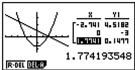
line
| X | Y | |---|---| | -2.741 | 4.5182 | | 0 | -3 | | 1.7741 | 0.1477 | | 1.774193548 | 1.774193548 |■ Coordinate Rounding
This function rounds off coordinate values displayed by Trace.
- From the Main Menu, enter the GRAPH mode.
- Draw the graph.
- Press SHIFT F2 (ZOOM) F6 (▷) F3 (RND). This causes the V-Window settings to be changed automatically in accordance with the Rnd value.
- Press SHIFT F1 (TRCE), and then use the cursor keys to move the pointer along the graph. The coordinates that now appear are rounded.
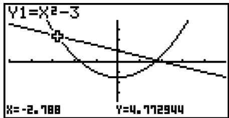
line
| x | y1=X²-3 | | ------- | ------- | | -2.788 | | | 4.712944| |■ Calculating the Root
This feature provides a number of different methods for analyzing graphs.
- From the Main Menu, enter the GRAPH mode.
- Draw the graphs.
- Select the analysis function.
SHIFT F5 (G-SLV) F1 (ROOT) ... Calculation of root
F2(MAX) ... Local maximum value
F3 (MIN) ... Local minimum value
F4 (Y-ICPT) ... y-intercept
F5(ISCT) ... Intersection of two graphs
F6 (▷) F1 (Y-CAL) ... y-coordinate for given x-coordinate
F6 (▷) F2 (X-CAL) ... x-coordinate for given y-coordinate
F6 (▷) F3 (∫dx) ... Integral value for a given range
-
When there are multiple graphs on the screen, the selection cursor (■) is located at the lowest numbered graph. Press ⬆ and ▼ to move the cursor to the graph you want to select.
-
Press EXE to select the graph where the cursor is located and display the value produced by the analysis.
When an analysis produces multiple values, press ▶ to calculate the next value. Pressing ◀ returns to the previous value.
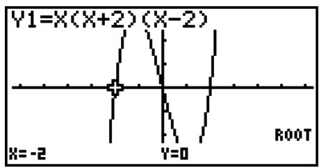
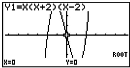
line
| X | Y | |---|---| | 0 | 0 | | 1 | 1 | | 2 | 2 | | 3 | 3 | | 4 | 4 | | 5 | 5 | | 6 | 6 | | 7 | 7 | | 8 | 8 | | 9 | 9 | | 10 | 10 | | 11 | 11 | | 12 | 12 | | 13 | 13 | | 14 | 14 | | 15 | 15 | | 16 | 16 | | 17 | 17 | | 18 | 18 | | 19 | 19 | | 20 | 20 | | 21 | 21 | | 22 | 22 | | 23 | 23 | | 24 | 24 | | 25 | 25 | | 26 | 26 | | 27 | 27 | | 28 | 28 | | 29 | 29 | | 30 | 30 | | 31 | 31 | | 32 | 32 | | 33 | 33 | | 34 | 34 | | 35 | 35 | | 36 | 36 | | 37 | 37 | | 38 | 38 | | 39 | 39 | | 40 | 40 | | 41 | 41 | | 42 | 42 | | 43 | 43 | | 44 | 44 | | 45 | 45 | | 46 | 46 | | 47 | 47 | | 48 | 48 | | 49 | 49 | | 50 | 50 | | 51 | 51 | | 52 | 52 | | 53 | 53 | | 54 | 54 | | 55 | 55 | | 56 | 56 | | 57 | 57 | | 58 | 58 | | 59 | 59 | | 60 | 60 | | 61 | 61 | | 62 | 62 | | 63 | 63 | | 64 | 64 | | 65 | 65 | | 66 | 66 | | 67 | 67 | | 68 | 68 | | 69 | 69 | | 70 | 70 | | 71 | 71 | | 72 | 72 | | 73 | 73 | | 74 | 74 | | 75 | 75 | | 76 | 76 | | 77 | 77 | | 78 | 78 | | 79 | 79 | | 80 | 80 | | 81 | 81 | | 82 | 82 | | 83 | 83 | | 84 | 84 | | 85 | 85 | | 86 | 86 | | 87 | 87 | | 88 | 88 | | 89 | 89 | | 90 | 90 | | 91 | 91 | | 92 | 92 | | 93 | 93 | | 94 | 94 | | 95 | 95 | | 96 | 96 | | 97 | 97 | | 98 | 98 | | 99 | 99 | | R00T- Either of the following can cause poor accuracy or even make it impossible to obtain solutions.
- When the graph of the solution obtained is a point of tangency with the x-axis
- When a solution is an inflection point
■ Calculating the Point of Intersection of Two Graphs
Use the following procedure to calculate the point of intersection of two graphs.
- Draw the graphs.
- Press SHIFT F5 (G-SLV) F5 (ISCT). When there are three or more graphs, the selection cursor (■) appears at the lowest numbered graph.
- Press ▲ and ▼ to move the cursor to the graph you want to select.
- Press EXE to select the first graph, which changes the shape of the cursor from ■ to ◆.
- Press ▲ and ▼ to move the cursor to the second graph.
- Press EXE to calculate the point of intersection for the two graphs.
When an analysis produces multiple values, press ▶ to calculate the next value.
Pressing ◀ returns to the previous value.
Example Graph the two functions shown below, and determine the point of intersection between Y1 and Y2.
$$ \mathbf {Y 1} = x + 1, \mathbf {Y 2} = x ^ {2} $$
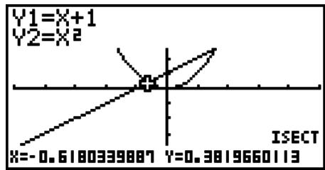
scatter
| X | Y | | ------- | ------ | | -0.6 | 0.6 | | 0.6 | 1.0 |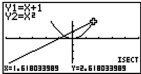
line
| x | y1=X+1 | y2=X² | | ------- | ------ | ----- | | 1.618033989 | 1.618033989 | 2.618033989 |- You can calculate the point of intersection for rectangular coordinate graphs (Y=f(x) type) and inequality graphs (Y>f(x), Y<f(x), Y≥f(x) or Y≤f(x)) only.
- Either of the following can cause poor accuracy or even make it impossible to obtain solutions.
- When a solution is a point of tangency between two graphs
- When a solution is an inflection point
■ Determining the Coordinates for Given Points
The following procedure describes how to determine the y-coordinate for a given x, and the x-coordinate for a given y.
- Draw the graph.
- Select the function you want to perform. When there are multiple graphs, the selection cursor (■) appears at the lowest numbered graph.
SHIFT F5 (G-SLV) F6 (▷) F1 (Y-CAL) ... y-coordinate for given x
F6 (▷) F2 (X-CAL) ... x-coordinate for given y
-
Use ▲▼ to move the cursor (■) to the graph you want, and then press EXE to select it.
-
Input the given x-coordinate value or y-coordinate value.
Press EXE to calculate the corresponding y-coordinate value or x-coordinate value.
Example
Graph the two functions shown below and then determine the y-coordinate for x = 0.5 and the x-coordinate for y = 2.2 on graph Y2.
$$ \mathsf {Y 1} = x + 1, \mathsf {Y 2} = x (x + 2) (x - 2) $$
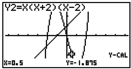
line
| X | Y (Y-CAL) | |---|---| | 0.5 | -1.875 |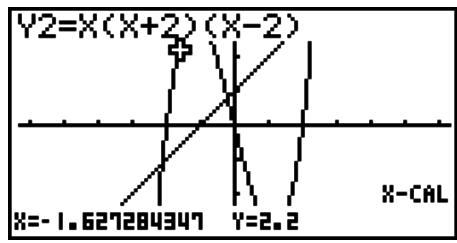
line
| X | Y | |---|---| | -1.627 | 627284347 | | 2.2 | 2.2 | Y2=X(X+2)(X-2) (X-CAL)- When there are multiple results for the above procedure, press ▶ to calculate the next value. Pressing ◀ returns to the previous value.
- The X-CAL value cannot be obtained for a parametric function graph.
■ Calculating the Integral Value for a Given Range
Use the following procedure to obtain integration values for a given range.
- Draw the graph.
- Press SHIFT F5 (G-SLV) F6 (▷) F3 (∫dx). When there are multiple graphs, this causes the selection cursor (■) to appear at the lowest numbered graph.
- Use ▲▼ to move the cursor (■) to the graph you want, and then press EXE to select it.
- Use ◀▶ to move the lower limit pointer to the location you want, and then press EXE.
- Use ▶ to move the upper limit pointer to the location you want.
- Press EXE to calculate the integral value.
Example Graph the function shown below, and then determine the integral value at (-2, 0) .
$$ \mathbf {Y 1} = x (x + 2) (x - 2) $$
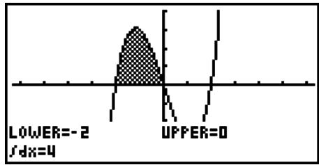
area
| x-axis label | Area (approximate) | | :--- | :--- | | LOWER=-2 / dx=4 | Peak value | | UPPER=0 | 0 |- You can also specify the lower limit and upper limit by inputting them on the 10-key pad.
- When setting the range, make sure that the lower limit is less than the upper limit.
- Integral values can be calculated for rectangular coordinate graphs only.
■ Conic Section Graph Analysis
Important!
- The fx-7400GII is not equipped with the CONICS mode.
You can determine approximations of the following analytical results using conic section graphs.
- From the Main Menu, enter the CONICS mode.
- Select the function type.
F1(RECT).... {rectangular coordinate}
F2 (POL).... {polar coordinate}
F3 (PARM).... {parametric}
-
Use ▲ and ▼ to select the conic section you want to analyze.
-
Input the conic section constants.
-
Draw the Graph.
After graphing a conic section, press SHIFT F5 (G-SLV) to display the following graph analysis menus.
• Parabolic Graph Analysis
- {FOCS}/{VTX}/{LEN}/{e} ... {focus}/{vertex}/{length of latus rectum}/{eccentricity}
- {DIR}/{SYM} ... {directrix}/{axis of symmetry}
- {X-IN}/{Y-IN} ... {x-intercept}/{y-intercept}
• Circular Graph Analysis
- {CNTR}/{RADS} ... {center}/{radius}
- {X-IN}/{Y-IN} ... {x-intercept}/{y-intercept}
- Elliptical Graph Analysis
- {FOCS}/{VTX}/{CNTR}/{e} ... {focus}/{vertex}/{center}/{eccentricity}
- {X-IN}/{Y-IN} ... {x-intercept}/{y-intercept}
• Hyperbolic Graph Analysis
- {FOCS}/{VTX}/{CNTR}/{e} ... {focus}/{vertex}/{center}/{eccentricity}
- {ASYM} ... {asymptote}
- {X-IN}/{Y-IN} ... {x-intercept}/{y-intercept}
- To calculate the focus and length of latus rectum
[G-SLV]-[FOCS]/[LEN]
Example To determine the focus and length of latus rectum for the parabola X = (Y - 2)^2 + 3
Use the following V-Window settings.
Xmin = -1, Xmax = 10, Xscale = 1
Ymin = -5, Ymax = 5, Yscale = 1
MENU CONICS
EXE
1 EXE 2 EXE 3 EXE F6 (DRAW)
SHIFT F5 (G-SLV)
F1(FOCS)
(Calculates the focus.)
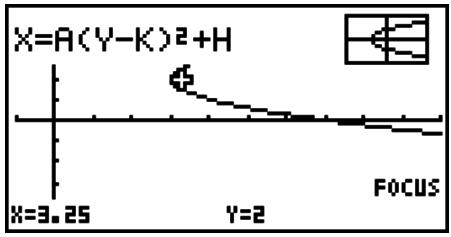
line
| X | Y | |---|---| | 3.25 | 2 | | 2 | 1 |SHIFT F5 (G-SLV)
F5 (LEN)
(Calculates the length of latus rectum.)
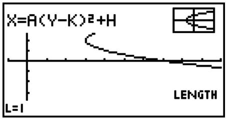
- When calculating two foci for an ellipse or hyperbolic graph, press ▶ to calculate the second focus. Pressing ◀ returns to the first focus.
- When calculating two vertexes for a hyperbolic graph, press ▶ to calculate the second vertex. Pressing ◀ returns to the first vertex.
- Pressing ▶ when calculating the vertices of an ellipse will calculate the next value. Pressing ◀ will scroll back through previous values. An ellipse has four vertices.
• To calculate the center
[G-SLV]-[CNTR]
Example To determine the center for the circle
$$ (X + 2) ^ {2} + (Y + 1) ^ {2} = 2 ^ {2} $$
MENU CONICS
EXE
(-) 2 EXE (-) 1 EXE 2 EXE F6 (DRAW)
SHIFT F5 (G-SLV)
F1 (CNTR)
(Calculates the center.)
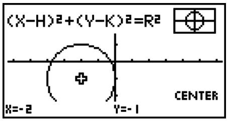
Chapter 6 Statistical Graphs and Calculations
Important!
This chapter contains a number of graph screen shots. In each case, new data values were input in order to highlight the particular characteristics of the graph being drawn. Note that when you try to draw a similar graph, the unit uses data values that you have input using the List function. Because of this, the graphs that appear on the screen when you perform a graphing operation will probably differ somewhat from those shown in this manual.
1. Before Performing Statistical Calculations
Entering the STAT mode from the Main Menu displays the List Editor screen.
You can use the List Editor screen to input statistical data and perform statistical calculations.
Use ▲, ▼, ◀ and ▶ to move the highlighting around the lists.
Once you input data, you can use it to produce a graph and check for tendencies. You can also use a variety of different regression calculations to analyze the data.
- For information about using the statistical data lists, see "Chapter 3 List Function".
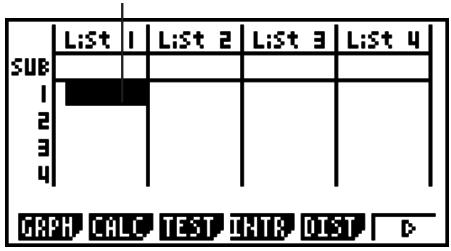
■ Changing Graph Parameters
Use the following procedures to specify the graph draw/non-draw status, the graph type, and other general settings for each of the graphs in the graph menu (GPH1, GPH2, GPH3).
While the statistical data list is on the display, press F1(GRPH) to display the graph menu, which contains the following items.
- {GPH1}/{GPH2}/{GPH3} ... graph {1}/{2}/{3} drawing*1
- {SEL} ... {simultaneous graph (GPH1, GPH2, GPH3) selection} You can specify the multiple graphs.
- {SET} ... {graph settings (graph type, list assignments)}
*1 The initial default graph type setting for all the graphs (Graph 1 through Graph 3) is scatter diagram, but you can change to one of a number of other graph types.
1. General graph settings
[GRPH]-[SET]
This section describes how to use the general graph settings screen to make the following settings for each graph (GPH1, GPH2, GPH3).
- Graph Type
The initial default graph type setting for all the graphs is scatter graph. You can select one of a variety of other statistical graph types for each graph.
- List
The initial default statistical data is List 1 for single-variable data, and List 1 and List 2 for paired-variable data. You can specify which statistical data list you want to use for x-data and y-data.
- Frequency
Normally, each data item or data pair in the statistical data list is represented on a graph as a point. When you are working with a large number of data items however, this can cause problems because of the number of plot points on the graph. When this happens, you can specify a frequency list that contains values indicating the number of instances (the frequency) of the data items in the corresponding cells of the lists you are using for x-data and y-data. Once you do this, only one point is plotted for the multiple data items, which makes the graph easier to read.
- Mark Type
This setting lets you specify the shape of the plot points on the graph.
- To display the general graph settings screen
Pressing F1 (GRPH) F6 (SET) displays the general graph settings screen.
• StatGraph (statistical graph specification)
• {GPH1}/{GPH2}/{GPH3} ... graph {1}/{2}/{3}
• Graph Type (graph type specification)
- {Scat}/{xy}/{NPP}/{Pie} ... {scatter diagram}/{xy line graph}/{normal probability plot}/{pie graph}
- {Hist}/{Box}/{Bar}/{N·Dis}/{Brkn} ... {histogram}/{med-box graph}/{bar graph}/{normal distribution curve}/{broken line graph}
- {X}/{Med}/{X^2}/{X^3}/{X^4} ... {linear regression graph}/{Med-Med graph}/{quadratic regression graph}/{cubic regression graph}/{quartic regression graph}
- {Log}/{Exp}/{Pwr}/{Sin}/{Lgst} ... {logarithmic regression graph}/{exponential regression graph}/{power regression graph}/{sinusoidal regression graph}/{logistic regression graph}
- XList (x-axis data list)/YList (y-axis data list)
- {List} ... {List 1 to 26}
• Frequency (number of times a value occurs)
• {1} ... {1-to-1 plot}
- {List} ... {List 1 to 26}
• Mark Type (plot mark type)
- /×/ ... scatter diagram plot points
When “Pie” (pie graph) is selected as the Graph Type:
- Data (Specifies the list to be used as graph data.)
- {LIST} ... {List 1 to List 26}
[GRPH]-[SET]
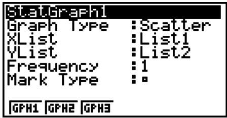
- Display (pie graph value display setting)
- {\%}/{Data} ... For each data element {display as percentage}/{display as value}
• % Sto Mem (Specifies storage of percentage values to a list.) - {None}/{List} ... For percentage values: {Do not store to list}/{Specify List 1 to 26 and store}
When “Box” (med-box graph) is selected as the Graph Type:
- Outliers (outliers specification)
- {On}/{Off} ... {display}/{do not display} Med-Box outliers
When “Bar” (bar graph) is selected as the Graph Type:
• Data1 (first stick data list)
- {LIST} ... {List 1 to 26}
- Data2 (second stick data list)/Data3 (third stick data list)
- {None}/{LIST} ... {none}/{List 1 to 26}
- Stick Style (stick style specification)
- {Leng}/{HZtl} ... {length}/{horizontal}
2. Graph draw/non-draw status
[GRPH]-[SEL]
The following procedure can be used to specify the draw (On)/non-draw (Off) status of each of the graphs in the graph menu.
- To specify the draw/non-draw status of a graph
- Pressing F1 (GRPH) F4 (SEL) displays the graph On/Off screen.
| StatGraph1 | DrawUn |
| StatGraph2 | DrawOff |
| StatGraph3 | DrawOff |
- Note that the StatGraph1 setting is for Graph 1 (GPH1 of the graph menu), StatGraph2 is for Graph 2, and StatGraph3 is for Graph 3.
-
Use the cursor keys to move the highlighting to the graph whose status you want to change, and press the applicable function key to change the status.
-
{On}/{Off} ... {On (draw)}/{Off (non-draw)}
-
{DRAW} ... {draws all On graphs}
-
To return to the graph menu, press EXIT.
- V-Window parameters are normally set automatically for statistical graphing. If you want to set V-Window parameters manually, you must change the Stat Wind item to “Manual”.
While the statistical data list is on the display, perform the following procedure.
SHIFT MENU (SET UP) F2 (Man)
EXIT (Returns to previous menu.)
Note that V-Window parameters are set automatically for the following types of graphs regardless of whether or not the Stat Wind item is set to “Manual”.
Pie, 1-Sample Z Test, 2-Sample Z Test, 1-Prop Z Test, 2-Prop Z Test, 1-Sample t Test, 2-Sample t Test, ^2 GOF Test, ^2 2-way Test, 2-Sample F Test (x-axis only disregarded).
- The default setting automatically uses List 1 data as x -axis (horizontal) values and List 2 data as y -axis (vertical) values. Each set of x / y data is a point on the scatter diagram.
2. Calculating and Graphing Single-Variable Statistical Data
Single-variable data is data with only a single variable. If you are calculating the average height of the members of a class for example, there is only one variable (height).
Single-variable statistics include distribution and sum. The following types of graphs are available for single-variable statistics.
You can also use the procedures under “Changing Graph Parameters” on page 6-1 to make the settings you want before drawing each graph.
■ Normal Probability Plot
This plot compares the data accumulated ratio with a normal distribution accumulated ratio. XList specifies the list where data is input, and Mark Type is used to select from among the marks /×/ you want to plot.
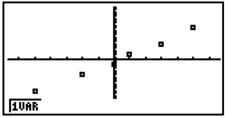
scatter
| x | y | |---|---| | 0.5 | 0.2 | | 0.7 | 0.4 | | 0.9 | 0.6 | | 1.1 | 0.8 | | 1.3 | 1.0 | | 1.5 | 1.2 | | 1.7 | 1.4 | | 1.9 | 1.6 | | 2.1 | 1.8 | | 2.3 | 2.0 | | 2.5 | 2.2 | | 2.7 | 2.4 | | 2.9 | 2.6 | | 3.1 | 2.8 | | 3.3 | 3.0 | | 3.5 | 3.2 | | 3.7 | 3.4 | | 3.9 | 3.6 | | 4.1 | 3.8 | | 4.3 | 4.0 | | 4.5 | 4.2 | | 4.7 | 4.4 | | 4.9 | 4.6 | | 5.1 | 4.8 | | 5.3 | 5.0 | | 5.5 | 5.2 | | 5.7 | 5.4 | | 5.9 | 5.6 | | 6.1 | 5.8 | | 6.3 | 6.0 | | 6.5 | 6.2 | | 6.7 | 6.4 | | 6.9 | 6.6 | | 7.1 | 6.8 | | 7.3 | 7.0 | | 7.5 | 7.2 | | 7.7 | 7.4 | | 7.9 | 7.6 | | 8.1 | 7.8 | | 8.3 | 8.0 | | 8.5 | 8.2 | | 8.7 | 8.4 | | 8.9 | 8.6 | | 9.1 | 8.8 | | 9.3 | 9.0 | | 9.5 | 9.2 | | 9.7 | 9.4 | | 9.9 | 9.6 | | 10.1 | 9.8 | | 10.3 | 10.0 | | 10.5 | 10.2 | | 10.7 | 10.4 | | 10.9 | 10.6 | | 11.1 | 10.8 | | 11.3 | 11.0 | | 11.5 | 11.2 | | 11.7 | 11.4 | | 11.9 | 11.6 | | 12.1 | 11.8 | | 12.3 | 12.0 | | 12.5 | 12.2 | | 12.7 | 12.4 | | 12.9 | 12.6 | | 13.1 | 12.8 | | 13.3 | 13.0 | | 13.5 | 13.2 | | 13.7 | 13.4 | | 13.9 | 13.6 | | 14.1 | 13.8 | | 14.3 | 14.0 | | 14.5 | 14.2 | | 14.7 | 14.4 | | 14.9 | 14.6 | | 15.1 | 14.8 | | 15.3 | 15.0 | | 15.5 | 15.2 | | 15.7 | 15.4 | | 15.9 | 15.6 | | 16.1 | 15.8 | | 16.3 | 16.0 | | 16.5 | 16.2 | | 16.7 | 16.4 | | 16.9 | 16.6 | | 17.1 | 16.8 | | 17.3 | 17.0 | | 17.5 | 17.2 | | 17.7 | 17.4 | | 17.9 | 17.6 | | 18.1 | 17.8 | | 18.3 | 18.0 | | 18.5 | 18.2 | | 18.7 | 18.4 | | 18.9 | 18.6 | | 19.1 | 18.8 | | 19.3 | 19.0 | | 19.5 | 19.2 | | 19.7 | 19.4 | | 19.9 | 19.6 | | - | - |Press AC, EXIT or SHIFT EXIT (QUIT) to return to the statistical data list.
Pie Graph
You can draw a pie graph based on the data in a specific list. The maximum number of graph data items (list lines) is 20. The graph is labeled A, B, C, and so on, corresponding to lines 1, 2, 3, and so on of the list used for the graph data.
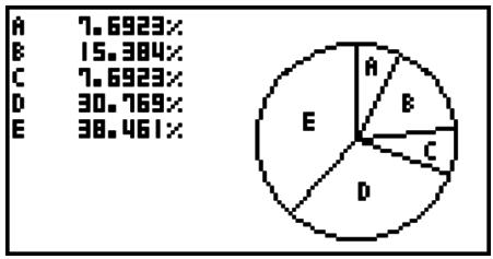
pie
| Category | Value (%) | |---|---| | A | 7.6923 | | B | 15.384 | | C | 7.6923 | | D | 30.769 | | E | 38.461 |When “%” is selected for the “Display” setting on the general graph settings screen (page 6-3), a value showing the percentage is displayed for each of the alphabetic label letters.
Histogram
XList specifies the list where the data is input, while Freq specifies the list where the data frequency is input. 1 is specified for Freq when frequency is not specified.
![Histogram Settings Start:1 Width:0.889 Draw:[EXE] GPH1 GPH2 GPH3 SEL SET EXE (DRAW)](/content/2025/01/86832/images/99e4e46acd86dbb6ce9cd4c03c814de7788f4d28a531087b3d057c896d54c299.jpg)
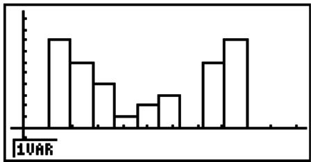
bar
| Category | Value | |---|---| | 1个周期 | 100 | | 2个周期 | 80 | | 3个周期 | 60 | | 4个周期 | 20 | | 5个周期 | 30 | | 6个周期 | 70 | | 7个周期 | 90 |The display screen appears as shown above before the graph is drawn. At this point, you can change the Start and Width values.
■ Med-box Graph
This type of graph lets you see how a large number of data items are grouped within specific ranges. A box encloses all the data in an area from the first quartile (Q1) to the third quartile (Q3), with a line drawn at the median (Med). Lines (called whiskers) extend from either end of the box up to the minimum (minX) and maximum (maxX) of the data.
From the statistical data list, press F1 (GRPH) to display the graph menu, press F6 (SET), and then change the graph type of the graph you want to use (GPH1, GPH2, GPH3) to med-box graph.
To plot the data that falls outside the box, first specify "MedBox" as the Graph Type. Then, on the same screen you use to specify the graph type, turn the Outliers item "On", and draw the graph.
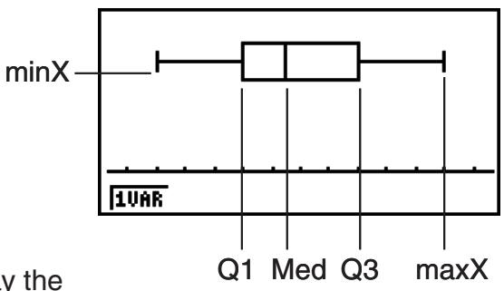
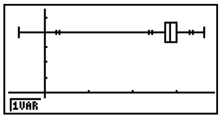
- Changing the “Q1Q3 Type” setting on the Setup screen can cause the Q1 and Q3 positions to change, even when a Med-box graph is drawn based on a single list.
Bar Graph
You can specify up to three lists for drawing a bar graph. The graph is labeled [1] , [2] , [3] , and so on, corresponding to lines 1, 2, 3, and so on of the list used for the graph data.
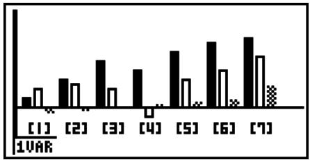
bar
| Category | Value | |---|---| | [1] | 0.5 | | [2] | 0.8 | | [3] | 1.2 | | [4] | 0.6 | | [5] | 1.5 | | [6] | 1.8 | | [7] | 2.0 |- Any of the following causes an error and cancels bar graph drawing.
- A Condition ERROR occurs when drawing of multiple graphs is specified using the graph On/Off screen (page 6-3), and bar graph is specified for one of the graphs and a different graph type is specified for another graph.
- A Dimension ERROR occurs when you draw a graph with two or three lists specified and the specified lists have a different number of list elements.
- A Condition ERROR occurs when lists are assigned for Data1 and Data3, while “None” is specified for Data2.
■ Normal Distribution Curve
The normal distribution curve is graphed using the normal distribution function.
XList specifies the list where the data is input, while Freq specifies the list where the data frequency is input. 1 is specified for Freq when frequency is not specified.
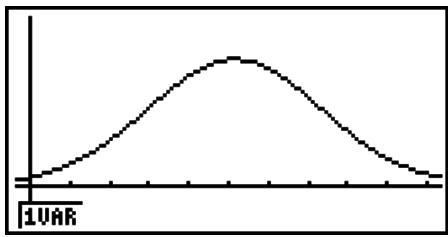
line
| Time (10AR) | Value | |-------------|-------| | 0 | 0 | | 1 | 1 | | 2 | 3 | | 3 | 5 | | 4 | 7 | | 5 | 8 | | 6 | 7 | | 7 | 5 | | 8 | 3 | | 9 | 1 | | 10 | 0 |■ Broken Line Graph
Lines connect center points of a histogram bar.
XList specifies the list where the data is input, while Freq specifies the list where the data frequency is input. 1 is specified for Freq when frequency is not specified.
![Histogram Setting Start:1 Width:0.889 Draw:[EXE] GPH1 GPH2 GPH3 SEL SET EXE (DRAW)](/content/2025/01/86832/images/e468e0b0dd92e2172a7e3dd5588ddeaf690275d9012e6555a2ca3f8f09ac941c.jpg)
line
| X-Axis Label | Y-Axis Value | | :--- | :--- | | 1 | 100 | | 2 | 80 | | 3 | 60 | | 4 | 40 | | 5 | 20 | | 6 | 30 | | 7 | 50 | | 8 | 70 | | 9 | 90 | | 10 | 100 | | 11 | 80 | | 12 | 60 | | 13 | 40 | | 14 | 20 | | 15 | 0 | | 16 | -20 | | 17 | -40 | | 18 | -60 | | 19 | -80 | | 20 | -100 | | 21 | -80 | | 22 | -60 | | 23 | -40 | | 24 | -20 | | 25 | 0 | | 26 | 20 | | 27 | 40 | | 28 | 60 | | 29 | 80 | | 30 | 100 | | 31 | 80 | | 32 | 60 | | 33 | 40 | | 34 | 20 | | 35 | 0 | | 36 | -20 | | 37 | -40 | | 38 | -60 | | 39 | -80 | | 40 | -100 | | 41 | -80 | | 42 | -60 | | 43 | -40 | | 44 | -20 | | 45 | 0 | | 46 | 20 | | 47 | 40 | | 48 | 60 | | 49 | 80 | | 50 | 100 | | 51 | 80 | | 52 | 60 | | 53 | 40 | | 54 | 20 | | 55 | 0 | | 56 | -20 | | 57 | -40 | | 58 | -60 | | 59 | -80 | | 60 | -100 | | 61 | -80 | | 62 | -60 | | 63 | -40 | | 64 | -20 | | 65 | 0 | | 66 | 20 | | 67 | 40 | | 68 | 60 | | 69 | 80 | | 70 | 100 | | 71 | 80 | | 72 | 60 | | 73 | 40 | | 74 | 20 | | 75 | 0 | | 76 | -20 | | 77 | -40 | | 78 | -60 | | 79 | -80 | | 80 | -100 | | 81 | -80 | | 82 | -60 | | 83 | -40 | | 84 | -20 | | 85 | 0 | | 86 | 20 | | 87 | 40 | | 88 | 60 | | 89 | 80 | | 90 | 100 | | 91 | -80 | | 92 | -60 | | 93 | -40 | | 94 | -20 | | 95 | 0 | | 96 | 20 | | 97 | 40 | | 98 | 60 | | 99 | -80 | | 100 (Last) | -100 |The display screen appears as shown above before the graph is drawn. At this point, you can change the Start and Width values.
■ Displaying the Calculation Results of a Drawn Single-Variable Graph
Single-variable statistics can be expressed as both graphs and parameter values. When these graphs are displayed, the single-variable calculation results appear as shown to the right when you press F1(1VAR).
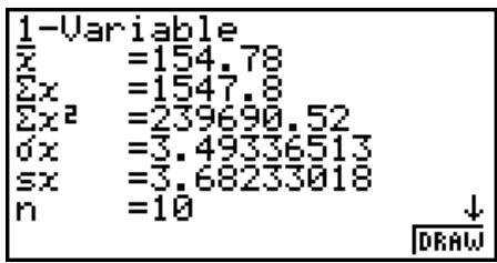
- Use ▼ to scroll the list so you can view the items that run off the bottom of the screen.
The following describes the meaning of each of the parameters.
......mean
Σx ......sum
x^2 ......sum of squares
_x ...... population standard deviation
S_x .....sample standard deviation
n ......number of data items minX......minimum
Q1 ......first quartile
Med......median
Q3 ......third quartile
maxX......maximum
Mod.....mode
Mod:n ......number of data mode items
Mod:F ......data mode frequency
- Press F6 (DRAW) to return to the original single-variable statistical graph.
- When Mod has multiple solutions, they are all displayed.
- You can use the Setup screen's “Q1Q3 Type” setting to select either “Std” (standard calculation) or “OnData” (French calculation) for the Q1 and Q3 calculation mode.
For details about calculation methods while “Std” or “OnData” is selected, see “Calculation Methods for the Std and OnData Settings” below.
■ Calculation Methods for the Std and OnData Settings
Q1 and Q3 can be calculated in accordance with the Setup screen's "Q1Q3 Type" setting as described below.
- Std
With this calculation method, processing depends on whether the number of elements n in the population is an even number or odd number.
When the number of elements n is an even number:
Using the center point of the total population as the reference, the population elements are divided into two groups: a lower half group and an upper half group. Q1 and Q3 then become the values described below.
Q1 = {median of the group of 2 items from the bottom of the population}
Q3 = {median of the group of 2 items from the top of the population}

flowchart
graph TD
    A["1"] --> B["2"]
    B --> C["3"]
    C --> D["4"]
    D --> E["5"]
    E --> F["6"]
    F --> G["7"]
    G --> H["8"]
    style A fill:#fff,stroke:#000
    style B fill:#fff,stroke:#000
    style C fill:#fff,stroke:#000
    style D fill:#fff,stroke:#000
    style E fill:#fff,stroke:#000
    style F fill:#fff,stroke:#000
    style G fill:#fff,stroke:#000
    style H fill:#fff,stroke:#000
    note right of D: (4 + 5) = Median
    note right of F: (6 + 7) = Q3
When the number of elements n is an odd number:
Using the median of the total population as the reference, the population elements are divided into two groups: a lower half group (values less than the median) and an upper half group (values greater than the median). The median value is excluded. Q1 and Q3 then become the values described below.
Q1 = {median of the group of -12 items from the bottom of the population}
Q3 = {median of the group of -12 items from the top of the population}
- When n = 1 , Q1 = Q3 = population center point.
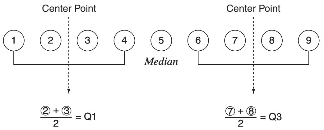
$$ \frac {② + ③}{2} = Q 1 $$
$$ \frac {⑦ + ⑧}{2} = \mathrm{Q3} $$
- OnData
The Q1 and Q3 values for this calculation method are described below.
Q1 = {value of element whose cumulative frequency ratio is greater than 1/4 and nearest to 1/4}
Q3 = {value of element whose cumulative frequency ratio is greater than 3/4 and nearest to 3/4}
The following shows an actual example of the above.
(Number of Elements: 10)
| Data Value | Frequency | Cumulative Frequency | Cumulative Frequency Ratio |
| 1 | 1 | 1 | 1/10 = 0.1 |
| 2 | 1 | 2 | 2/10 = 0.2 |
| 3 | 2 | 4 | 4/10 = 0.4 |
| 4 | 3 | 7 | 7/10 = 0.7 |
| 5 | 1 | 8 | 8/10 = 0.8 |
| 6 | 1 | 9 | 9/10 = 0.9 |
| 7 | 1 | 10 | 10/10 = 1.0 |
- 3 is the value of whose cumulative frequency ratio is greater than 1/4 and nearest to 1/4 , so Q1 = 3 .
- 5 is the value of whose cumulative frequency ratio is greater than 3/4 and nearest to 3/4 , so Q3 = 5 .
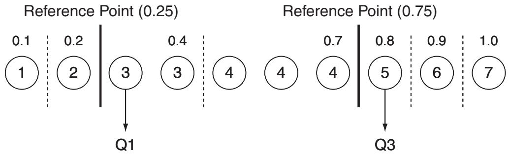
other
| Reference Point | Value | | --------------- | ----- | | 0.25 | 0.1 | | 0.25 | 0.2 | | 0.25 | 0.4 | | 0.25 | 0.4 | | 0.75 | 0.7 | | 0.75 | 0.8 | | 0.75 | 0.9 | | 0.75 | 1.0 |3. Calculating and Graphing Paired-Variable Statistical Data
■ Drawing a Scatter Diagram and xy Line Graph
The following procedure plots a scatter diagram and connects the dots to produce an xy line graph.
- From the Main Menu, enter the STAT mode.
- Input the data into a list.
- Specify Scat (scatter diagram) or xy (xy line graph) as the graph type, and then execute the graph operation.
Press AC, EXIT or SHIFT EXIT (QUIT) to return to the statistical data list.
Example Input the two sets of data shown below. Next, plot the data on a scatter diagram and connect the dots to produce an xy line graph.
0.5, 1.2, 2.4, 4.0, 5.2 (xList)
-2.1, 0.3, 1.5, 2.0, 2.4 (yList)
① MENU STAT
② 0 · 5 EXE 1 · 2 EXE 2 · 4 EXE 4 EXE 5 · 2 EXE ▶
(一) 2 · 1 EXE 0 · 3 EXE 1 · 5 EXE 2 EXE 2 · 4 EXE
③ (Scatter diagram) F1 (GRPH) F6 (SET) ▼ F1 (Scat) EXIT F1 (GPH1)
③ (xy line graph) F1 (GRPH) F6 (SET) ▼ F2 (xy) EXIT F1 (GPH1)
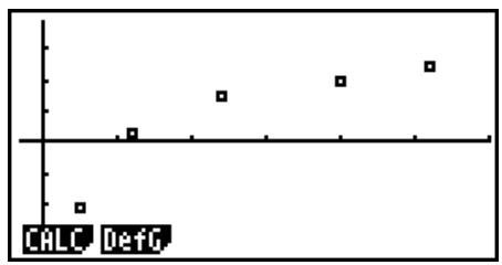
scatter
| Category | Value | | -------- | ----- | | CHLC | 1 | | Def0 | 2 | | | 3 | | | 4 | | | 5 | | | 6 | | | 7 | | | 8 |(Scatter diagram)
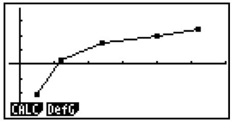
line
| Point | Value | |---|---| | CHLC | 0.1 | | DefG | 0.3 | | | 0.5 | | | 0.6 | | | 0.7 | | | 0.8 | | | 0.9 | | | 1.0 |(xy line graph)
■ Drawing a Regression Graph
Use the following procedure to input paired-variable statistical data, perform a regression calculation using the data, and then graph the results.
- From the Main Menu, enter the STAT mode.
- Input the data into a list, and plot the scatter diagram.
- Select the regression type, execute the calculation, and display the regression parameters.
- Draw the regression graph.
Example
Input the two sets of data shown below and plot the data on a scatter diagram. Next, perform logarithmic regression on the data to display the regression parameters, and then draw the corresponding regression graph.
0.5, 1.2, 2.4, 4.0, 5.2 (xList)
-2.1, 0.3, 1.5, 2.0, 2.4 (yList)
- You can perform trace on a regression graph. You cannot perform trace scroll.
- Input a positive integer for frequency data. Other types of values (decimals, etc.) cause an error.
■ Selecting the Regression Type
After you graph paired-variable statistical data, you can use the function menu at the bottom of the display to select from a variety of different types of regression.
- ax + b /a + bx /Med /X^2 /X^3 /X^4 /Log /ae^bx /ab^x /Pwr /Sin /Lgst ... {linear regression ( ax + b form)}/{linear regression ( a + bx form)}/{Med-Med}/{quadratic regression}/{cubic regression}/{quartic regression}/{logarithmic regression}/{exponential regression ( ae^bx form)}/{exponential regression ( ab^x form)}/{power regression}/{sinusoidal regression}/{logistic regression} calculation and graphing
- {2VAR}... {paired-variable statistical results}
■ Displaying Regression Calculation Results
Whenever you perform a regression calculation, the regression formula parameter (such as a and b in the linear regression y = ax + b ) calculation results appear on the display. You can use these to obtain statistical calculation results.
Regression parameters are calculated as soon as you press a function key to select a regression type, while a graph is on the display.
The following parameters are used by linear regression, logarithmic regression, exponential regression, and power regression.
r ...... correlation coefficient
r^2 ...... coefficient of determination
MSe......mean square error
■ Graphing Statistical Calculation Results
While the parameter calculation result is on the display, you can graph the displayed regression formula by pressing F6(DRAW).
■ Linear Regression Graph
Linear regression uses the method of least squares to plot a straight line that passes close to as many data points as possible, and returns values for the slope and y-intercept (y-coordinate when x = 0) of the line.
The graphic representation of this relationship is a linear regression graph.
F1(CALC) F2(X)
F1 (ax + b) or F2 (a + bx)
F6 (DRAW)
The following is the linear regression model formula.
$$ y = a x + b $$
a ...... regression coefficient (slope)
b ...... regression constant term (y-intercept)
$$ y = a + b x $$
a ...... regression constant term (y-intercept)
b ...... regression coefficient (slope)
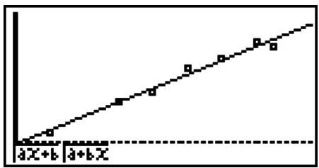
■ Med-Med Graph
When it is suspected that there are a number of extreme values, a Med-Med graph can be used in place of the least squares method. This is similar to linear regression, but it minimizes the effects of extreme values.
F1 (CALC) F3 (Med)
F6 (DRAW)
The following is the Med-Med graph model formula.
$$ y = a x + b $$
a......Med-Med graph slope
b......Med-Med graph y-intercept
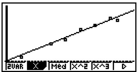
line
| X-Axis Label | Y-Axis Value | | :--- | :--- | | 2VAR | 0 | | Med | 1 | | X^2 | 2 | | X^3 | 3 | D | 4 |■ Quadratic/Cubic/Quartic Regression Graph
A quadratic/cubic/quartic regression graph represents connection of the data points of a scatter diagram. It uses the method of least squares to draw a curve that passes close to as many data points as possible. The formula that represents this is quadratic/cubic/quartic regression.
Ex. Quadratic regression
F1 (CALC) F4 (X^2)
F6 (DRAW)
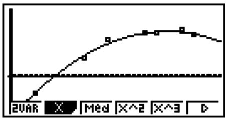
line
| X-Axis Label | Value | | :--- | :--- | | 2Var | 0 | | Med | Med | | X^2 | X^2 | | X^3 | X^3 | | D | D |Quadratic regression
Model formula...... y = ax^2 + bx + c
a...... regression second coefficient
b...... regression first coefficient
c ...... regression constant term (y-intercept)
Cubic regression
Model formula..... y = ax^3 + bx^2 + cx + d
a...... regression third coefficient
b...... regression second coefficient
c...... regression first coefficient
d...... regression constant term (y-intercept)
Quartic regression
Model formula..... y = ax^4 + bx^3 + cx^2 + dx + e
a...... regression fourth coefficient
b...... regression third coefficient
c...... regression second coefficient
d...... regression first coefficient
e...... regression constant term (y-intercept)
■ Logarithmic Regression Graph
Logarithmic regression expresses y as a logarithmic function of x. The standard logarithmic regression formula is y = a + b × x , so if we say that X = x , the formula corresponds to linear regression formula y = a + bX .
F1 (CALC) F6 (▷) F2 (Log)
F6 (DRAW)
The following is the logarithmic regression model formula.
$$ y = a + b \cdot \ln x $$
a......regression constant term
b......regression coefficient
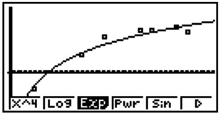
line
| X | Log9 Exp | |---|---| | 1 | 0.5 | | 2 | 1.0 | | 3 | 1.5 | | 4 | 2.0 | | 5 | 2.5 | | 6 | 3.0 | | 7 | 3.5 | | 8 | 4.0 | | 9 | 4.5 | | 10 | 5.0 | | 11 | 5.5 | | 12 | 6.0 | | 13 | 6.5 | | 14 | 7.0 | | 15 | 7.5 | | 16 | 8.0 | | 17 | 8.5 | | 18 | 9.0 | | 19 | 9.5 | | 20 | 10.0 | | 21 | 10.5 | | 22 | 11.0 | | 23 | 11.5 | | 24 | 12.0 | | 25 | 12.5 | | 26 | 13.0 | | 27 | 13.5 | | 28 | 14.0 | | 29 | 14.5 | | 30 | 15.0 | | 31 | 15.5 | | 32 | 16.0 | | 33 | 16.5 | | 34 | 17.0 | | 35 | 17.5 | | 36 | 18.0 | | 37 | 18.5 | | 38 | 19.0 | | 39 | 19.5 | | 40 | 20.0 | | 41 | 20.5 | | 42 | 21.0 | | 43 | 21.5 | | 44 | 22.0 | | 45 | 22.5 | | 46 | 23.0 | | 47 | 23.5 | | 48 | 24.0 | | 49 | 24.5 | | 50 | 25.0 | | 51 | 25.5 | | 52 | 26.0 | | 53 | 26.5 | | 54 | 27.0 | | 55 | 27.5 | | 56 | 28.0 | | 57 | 28.5 | | 58 | 29.0 | | 59 | 29.5 | | 60 | 30.0 | | 61 | 30.5 | | 62 | 31.0 | | 63 | 31.5 | | 64 | 32.0 | | 65 | 32.5 | | 66 | 33.0 | | 67 | 33.5 | | 68 | 34.0 | | 69 | 34.5 | | 70 | 35.0 | | 71 | 35.5 | | 72 | 36.0 | | 73 | 36.5 | | 74 | 37.0 | | 75 | 37.5 | | 76 | 38.0 | | 77 | 38.5 | | 78 | 39.0 | | 79 | 39.5 | | 80 | 40.0 | | Note: The values in the 'Log9 Exp' column are estimated based on the 'Log9 Exp' label, so they are not explicitly provided in the code snippet.■ Exponential Regression Graph
Exponential regression expresses y as a proportion of the exponential function of x. The standard exponential regression formula is y = a × e^bx , so if we take the logarithms of both sides we get y = a + bx . Next, if we say Y = y , and A = a , the formula corresponds to linear regression formula Y = A + bx .
F1 (CALC) F6 (▷) F3 (Exp)
F1(ae^bx) or F2(ab^x)
F6 (DRAW)
The following is the exponential regression model formula.
$$ y = a \cdot e ^ {b x} $$
a......regression coefficient
b......regression constant term
$$ y = a \cdot b ^ {x} $$
a......regression constant term
b......regression coefficient
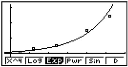
line
| X | Y | |---|---| | 1 | 0.5 | | 2 | 0.6 | | 3 | 0.7 | | 4 | 0.8 | | 5 | 0.9 | | 6 | 1.0 | | 7 | 1.2 | | 8 | 1.4 | | 9 | 1.6 | | 10 | 1.8 | | 11 | 2.0 | | 12 | 2.2 | | 13 | 2.4 | | 14 | 2.6 | | 15 | 2.8 | | 16 | 3.0 | | 17 | 3.2 | | 18 | 3.4 | | 19 | 3.6 | | 20 | 3.8 | | 21 | 4.0 | | 22 | 4.2 | | 23 | 4.4 | | 24 | 4.6 | | 25 | 4.8 | | 26 | 5.0 | | 27 | 5.2 | | 28 | 5.4 | | 29 | 5.6 | | 30 | 5.8 | | 31 | 6.0 | | 32 | 6.2 | | 33 | 6.4 | | 34 | 6.6 | | 35 | 6.8 | | 36 | 7.0 | | 37 | 7.2 | | 38 | 7.4 | | 39 | 7.6 | | 40 | 7.8 | | 41 | 8.0 | | 42 | 8.2 | | 43 | 8.4 | | 44 | 8.6 | | 45 | 8.8 | | 46 | 9.0 | | 47 | 9.2 | | 48 | 9.4 | | 49 | 9.6 | | 50 | 9.8 | | 51 | 10.0 | | 52 | 10.2 | | 53 | 10.4 | | 54 | 10.6 | | 55 | 10.8 | | 56 | 11.0 | | 57 | 11.2 | | 58 | 11.4 | | 59 | 11.6 | | 60 | 11.8 | | 61 | 12.0 | | 62 | 12.2 | | 63 | 12.4 | | 64 | 12.6 | | 65 | 12.8 | | 66 | 13.0 | | 67 | 13.2 | | 68 | 13.4 | | 69 | 13.6 | | 70 | 13.8 | | 71 | 14.0 | | 72 | 14.2 | | 73 | 14.4 | | 74 | 14.6 | | 75 | 14.8 | | 76 | 15.0 | | 77 | 15.2 | | 78 | 15.4 | | 79 | 15.6 | | 80 | 15.8 | | 81 | 16.0 | | 82 | 16.2 | | 83 | 16.4 | | 84 | 16.6 | | 85 | 16.8 | | 86 | 17.0 | | 87 | 17.2 | | 88 | 17.4 | | 89 | 17.6 | | 90 | 17.8 | | 91 | 18.0 | | 92 | 18.2 | | 93 | 18.4 | | 94 | 18.6 | | 95 | 18.8 | | 96 | 19.0 | | 97 | 19.2 | | 98 | 19.4 | | 99 | 19.6 | | Note: The actual values for the series 'Exp' are not provided in the code, so they are calculated based on the formula 'x'. The values for 'Log9' and 'Exp' are estimated based on the formula 'Pwr'. The values for 'Exp' are estimated based on the formula 'Sin'. The values for 'Exp' are estimated based on the formula 'D'.■ Power Regression Graph
Power regression expresses y as a proportion of the power of x. The standard power regression formula is y = a × x^b , so if we take the logarithm of both sides we get y = a + b × x . Next, if we say X = x , Y = y , and A = a , the formula corresponds to linear regression formula Y = A + bX .
F1 (CALC) F6 (▷) F4 (Pwr)
F6 (DRAW)
The following is the power regression model formula.
$$ y = a \cdot x ^ {b} $$
a......regression coefficient
b......regression power
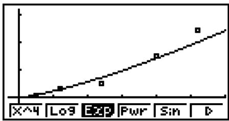
■ Sinusoidal Regression Graph
Sinusoidal regression is best applied for cyclical data.
The following is the sinusoidal regression model formula.
$$ y = a \cdot \sin (b x + c) + d $$
F1 (CALC) F6 (▷) F5 (Sin)
F6 (DRAW)
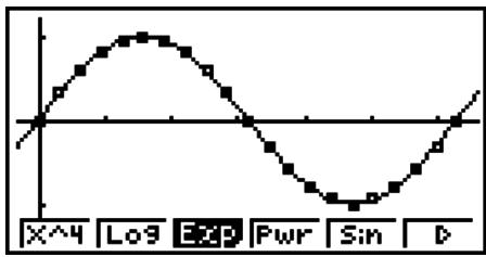
line
| X | Y | |-------|-------| | 0 | 0 | | 1 | 0.5 | | 2 | 1.0 | | 3 | 1.5 | | 4 | 2.0 | | 5 | 1.5 | | 6 | 1.0 | | 7 | 0.5 | | 8 | 0 | | 9 | -0.5 | | 10 | -1.0 | | 11 | -1.5 | | 12 | -2.0 | | 13 | -1.5 | | 14 | -1.0 | | 15 | -0.5 | | 16 | 0 | | 17 | 0.5 | | 18 | 1.0 | | 19 | 1.5 | | 20 | 2.0 | | 21 | 1.5 | | 22 | 1.0 | | 23 | 0.5 | | 24 | 0 | | 25 | -0.5 | | 26 | -1.0 | | 27 | -1.5 | | 28 | -2.0 | | 29 | -1.5 | | 30 | -1.0 | | 31 | -0.5 | | 32 | 0 | | 33 | 0.5 | | 34 | 1.0 | | 35 | 1.5 | | 36 | 2.0 | | 37 | 1.5 | | 38 | 1.0 | | 39 | 0.5 | | 40 | 0 | | 41 | -0.5 | | 42 | -1.0 | | 43 | -1.5 | | 44 | -2.0 | | 45 | -1.5 | | 46 | -1.0 | | 47 | -0.5 | | 48 | 0 | | 49 | 0.5 | | 50 | 1.0 | | 51 | 1.5 | | 52 | 2.0 | | 53 | 1.5 | | 54 | 1.0 | | 55 | 0.5 | | 56 | 0 | | 57 | -0.5 | | 58 | -1.0 | | 59 | -1.5 | | 60 | -2.0 | | 61 | -1.5 | | 62 | -1.0 | | 63 | -0.5 | | 64 | 0 | | 65 | 0.5 | | 66 | 1.0 | | 67 | 1.5 | | 68 | 2.0 | | 69 | 1.5 | | 70 | 1.0 | | 71 | 0.5 | | 72 | 0 | | 73 | -0.5 | | 74 | -1.0 | | 75 | -1.5 | | 76 | -2.0 | | 77 | -1.5 | | 78 | -1.0 | | 79 | -0.5 | | 80 | 0 | | 81 | 0.5 | | 82 | 1.0 | | 83 | 1.5 | | 84 | 2.0 | | 85 | 1.5 | | 86 | 1.0 | | 87 | 0.5 | | 88 | 0 | | 89 | -0.5 | | 90 | -1.0 | | 91 | -1.5 | | 92 | -2.0 | | 93 | -1.5 | | 94 | -1.0 | | 95 | -0.5 | | 96 | 0 | | 97 | 0.5 | | 98 | 1.0 | | 99 | 1.5 | | D | D |Drawing a sine regression graph causes the angle unit setting of the calculator to automatically change to Rad (radians). The angle unit does not change when you perform a sine regression calculation without drawing a graph.
- Certain types of data may take a long time to calculate. This does not indicate malfunction.
■ Logistic Regression Graph
Logistic regression is best applied for time-based phenomena in which there is a continual increase until a saturation point is reached.
The following is the logistic regression model formula.
$$ y = \frac {c}{1 + a e ^ {- b x}} $$
F1 (CALC) F6 (▷) F6 (▷) F1 (Lgst)
F6 (DRAW)
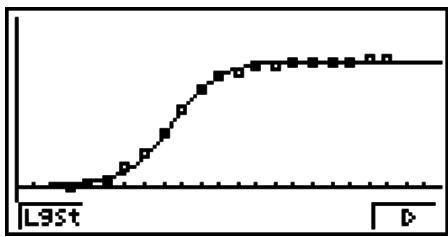
line
| L9St | Value | | ---- | ----- | | 0 | 0 | | 1 | 0.5 | | 2 | 1.0 | | 3 | 1.5 | | 4 | 2.0 | | 5 | 2.5 | | 6 | 3.0 | | 7 | 3.5 | | 8 | 4.0 | | 9 | 4.5 | | 10 | 5.0 | | 11 | 5.5 | | 12 | 6.0 | | 13 | 6.5 | | 14 | 7.0 | | 15 | 7.5 | | 16 | 8.0 | | 17 | 8.5 | | 18 | 9.0 | | 19 | 9.5 | | 20 | 10.0 |- Certain types of data may take a long time to calculate. This does not indicate malfunction.
■ Residual Calculation
Actual plot points (y-coordinates) and regression model distance can be calculated during regression calculations.
While the statistical data list is on the display, recall the Setup screen to specify a LIST ("List 1" through "List 26") for "Resid List". Calculated residual data is stored in the specified list.
The vertical distance from the plots to the regression model will be stored in the list.
Plots that are higher than the regression model are positive, while those that are lower are negative.
Residual calculation can be performed and saved for all regression models.
Any data already existing in the selected list is cleared. The residual of each plot is stored in the same precedence as the data used as the model.
■ Displaying the Calculation Results of a Drawn Paired-Variable Graph
Paired-variable statistics can be expressed as both graphs and parameter values. When these graphs are displayed, the paired-variable calculation results appear as shown below when you press F1(CALC)F1(2VAR).
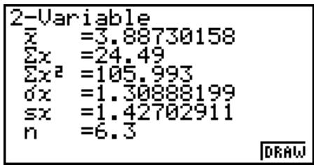
- Use ▼ to scroll the list so you can view the items that run off the bottom of the screen.
...... mean of data stored in xList
Σx ...... sum of data stored in xList
x^2 ......sum of squares of data stored in xList
_x ..... population standard deviation of data stored in xList
S_x ..... sample standard deviation of data stored in xList
n ...... number of data
...... mean of data stored in yList
Σy ......sum of data stored in yList
y^2 ...... sum of squares of data stored in yList
_y ...... population standard deviation of data stored in yList
Sy ...... sample standard deviation of data stored in yList
Σxy ...... sum of the product of data stored in xList and yList
minX...... minimum of data stored in xList
maxX..... maximum of data stored in xList
minY...... minimum of data stored in yList
maxY..... maximum of data stored in yList
■ Copying a Regression Graph Formula to the GRAPH Mode
You can copy regression formula calculation results to the GRAPH mode Graph relation list, and store and compare.
- While a regression calculation result is on the display (see “Displaying Regression Calculation Results” on page 6-10), press F5 (COPY).
- This will display the GRAPH mode Graph relation list.*1
-
Use ▲ and ▼ to highlight the area to which you want to copy the regression formula of the displayed result.
-
Press EXE to save the copied graph formula and return to the previous regression calculation result display.
*1 You cannot edit regression formulas for graph formulas in the GRAPH mode.
4. Performing Statistical Calculations
All of the statistical calculations up to this point were performed after displaying a graph. The following procedures can be used to perform statistical calculations alone.
- To specify statistical calculation data lists
You have to input the statistical data for the calculation you want to perform and specify where it is located before you start a calculation. Display the statistical data and then press F2(CALC)F6(SET).
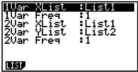
The following is the meaning for each item.
1Var XList......location of single-variable statistic x values (XList)
1Var Freq......location of single-variable frequency values (Frequency)
2Var XList......location of paired-variable statistic x values (XList)
2Var YList ...... location of paired-variable statistic y values (YList)
2Var Freq......location of paired-variable frequency values (Frequency)
- Calculations in this section are performed based on the above specifications.
■ Single-Variable Statistical Calculations
In the previous example under “Displaying the Calculation Results of a Drawn Single-Variable Graph”, statistical calculation results were displayed after the graph was drawn. These were numeric expressions of the characteristics of variables used in the graphic display.
These values can also be directly obtained by displaying the statistical data list and pressing F2 (CALC) F1 (1VAR).
| 1-Variable | |
| x̄ | =154.8 |
| Σx | =1548 |
| Σxa² | =239722 |
| dx | =3.02654919 |
| sx | =3.19026296 |
| n | =10 |
After this, pressing ▲ or ▼ scrolls the statistical calculation result display so you can view variable characteristics.
For details on the meanings of these statistical values, see “Displaying the Calculation Results of a Drawn Single-Variable Graph” (page 6-6).
■ Paired-Variable Statistical Calculations
In the previous example under “Displaying the Calculation Results of a Drawn Paired-Variable Graph”, statistical calculation results were displayed after the graph was drawn. These were numeric expressions of the characteristics of variables used in the graphic display.
These values can also be directly obtained by displaying the statistical data list and pressing F2 (CALC) F2 (2VAR).
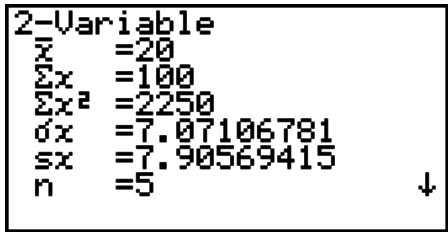
After this, pressing ▲ or ▼ scrolls the statistical calculation result display so you can view variable characteristics.
For details on the meanings of these statistical values, see “Displaying the Calculation Results of a Drawn Paired-Variable Graph” (page 6-14).
■ Regression Calculation
In the explanations from “Linear Regression Graph” to “Logistic Regression Graph”, regression calculation results were displayed after the graph was drawn. Here, each coefficient value of the regression line or regression curve is expressed as a number.
You can directly determine the same expression from the data input screen.
Pressing F2(CALC)F3(REG) displays a function menu, which contains the following items.
- ax + b / a + bx / Med / X^2 / X^3 / X^4 / Log / ae^bx / ab^x / Pwr / Sin / Lgst ... {linear regression ( ax + b form)}/{linear regression ( a + bx form)}/{Med-Med}/{quadratic regression}/{cubic regression}/{quartic regression}/{logarithmic regression}/{exponential regression ( ae^bx form)}/{exponential regression ( ab^x form)}/{power regression}/{sinusoidal regression}/{logistic regression} parameters
Example To display single-variable regression parameters
F2 (CALC) F3 (REG) F1 (X) F1 (ax+b)
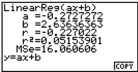
The meanings of the parameters that appear on this screen are the same as those for “Linear Regression Graph” to “Logistic Regression Graph”.
- Calculation of the Coefficient of Determination (r^2) and MSe
You can use the STAT mode to calculate the coefficient of determination ( r^2 ) for quadratic regression, cubic regression, and quartic regression. The following types of MSe calculations are also available for each type of regression.
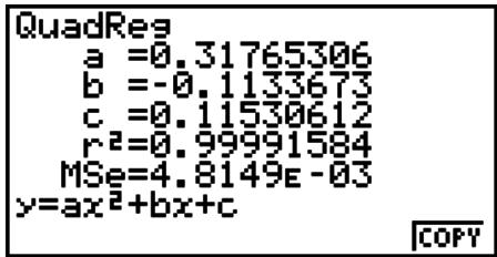
- Linear Regression (ax + b) ...... MSe = 1n - 2 _i=1^n (y_i - (ax_i + b))^2
$$ (a + b x) \dots\dotsMSe = \frac {1}{n - 2} \sum_ {i = 1} ^ {n} \left(y _ {i} - (a + b x _ {i})\right) ^ {2} $$
- Quadratic Regression....MSe = 1n - 3_i=1^n(y_i - (ax_i^2 + bx_i + c))^2
- Cubic Regression.... MSe = 1n - 4 _i=1^n (y_i - (ax_i^3 + bx_i^2 + cx_i + d))^2
- Quartic Regression ....MSe = 1n - 5_i=1^n(y_i - (ax_i^4 + bx_i^3 + cx_i^2 + dx_i + e))^2
- Logarithmic Regression......MSe = 1n - 2_i=1^n(y_i - (a + b x_i))^2
- Exponential Repression (a · e^bx) ...... MSe = 1n - 2 _i=1^n ( y_i - ( a + bx_i))^2
$$ (a \cdot b ^ {x}) \dots \dots M S e = \frac {1}{n - 2} \sum_ {i = 1} ^ {n} \left(\ln y _ {i} - \left(\ln a + (\ln b) \cdot x _ {i}\right)\right) ^ {2} $$
- Power Regression ....MSe = 1n - 2 _i=1^n ( y_i - ( a + b x_i))^2
- Sin Regression.... MSe = 1n - 2 _i=1^n (y_i - (a (bx_i + c) + d))^2
- Logistic Regression....MSe = 1n - 2_i=1^n(y_i - 1 + ae^-bx_i)^2
• Estimated Value Calculation for Regression Graphs
The STAT mode also includes a Y-CAL function that uses regression to calculate the estimated y-value for a particular x-value after graphing a paired-variable statistical regression.
The following is the general procedure for using the Y-CAL function.
- After drawing a regression graph, press SHIFT F5 (G-SLV) F1 (Y-CAL) to enter the graph selection mode, and then press EXE.
If there are multiple graphs on the display, use ▲ and ▼ to select the graph you want, and then press EXE.
- This causes an x -value input dialog box to appear.
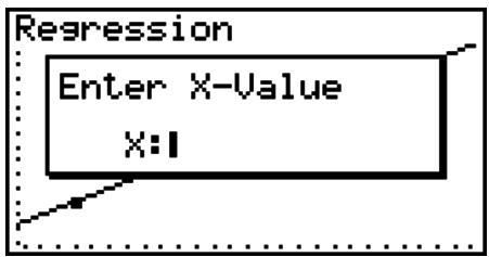
- Input the value you want for x and then press EXE.
- This causes the coordinates for x and y to appear at the bottom of the display, and moves the pointer to the corresponding point on the graph.
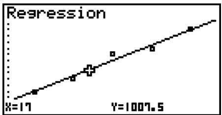
line
| x | y | | ---- | ----- | | 17 | 1007.5 |-
Pressing ,,T or a number key at this time causes the x-value input dialog box to reappear so you can perform another estimated value calculation if you want.
-
The pointer does not appear if the calculated coordinates are not within the display range.
- The coordinates do not appear if “Off” is specified for the “Coord” item of the Setup screen.
- The Y-CAL function can also be used with a graph drawn by using DefG feature.
- Regression Formula Copy Function from a Regression Calculation Result Screen
In addition to the normal regression formula copy function that lets you copy the regression calculation result screen after drawing a statistical graph (such as Scatter Plot), the STAT mode also has a function that lets you copy the regression formula obtained as the result of a regression calculation. To copy a resulting regression formula, press F6(COPY).
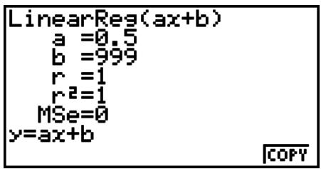
■ Estimated Value Calculation ( , )
After drawing a regression graph with the STAT mode, you can use the RUN • MAT (or RUN) mode to calculate estimated values for the regression graph's x and y parameters.
Example
To perform a linear regression using the nearby data and estimate the values of and when xi = 20 and yi = 1000
| xi | 10 | 15 | 20 | 25 | 30 |
| yi | 1003 | 1005 | 1010 | 1011 | 1014 |
- From the Main Menu, enter the STAT mode.
- Input data into the list and draw the linear regression graph.
- From the Main Menu, enter the RUN • MAT (or RUN) mode.
- Press the keys as follows.
2 0 (value of xi)
OPTN F5 (STAT)* F2 (ŷ) EXE
* fx-7400GII: F4 (STAT)
The estimated value is displayed for xi = 20.
1 0 0 0 (value of yi)
F1 ( ) EXE
| 209 | 1008.6 |
| 1000x | 4.642857143 |
The estimated value is displayed for yi = 1000.
- You cannot obtain estimated values for a Med-Med, quadratic regression, cubic regression, quartic regression, sinusoidal regression, or logistic regression graph.
■ Normal Probability Distribution Calculation
You can calculate normal probability distributions for single-variable statistics with the RUN • MAT (or RUN) mode.
Press OPTN F6 (▷) F3 (PROB) (F2 (PROB) on the fx-7400GII) F6 (▷) to display a function menu, which contains the following items.
- P( / Q( / R( ... obtains normal probability P(t) /Q(t) /R(t) value
- t(·) obtains normalized variate t(x) value
- Normal probability P(t) , Q(t) , and R(t) , and normalized variate t(x) are calculated using the following formulas.
Standard Normal Distribution
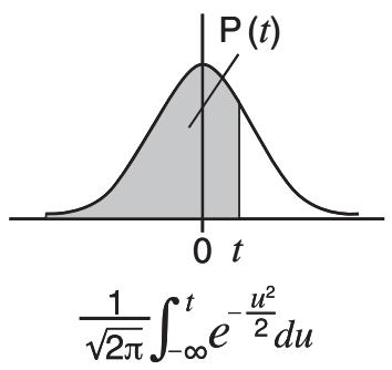
line
| t | P(t) | |-------|----------| | 0 | Peak | | t | 0 |
line
| t | Q(t) | |-------|------| | 0 | Peak | | t | 0 |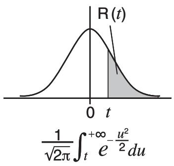
line
| t | R(t) | |-------|------| | 0 | Peak | | ∞ | 0 |$$ t (x) = \frac {x - \bar {x}}{\mathbf {\sigma} _ {x}} $$
Example
The following table shows the results of measurements of the height of 20 college students. Determine what percentage of the students fall in the range 160.5 cm to 175.5 cm. Also, in what percentile does the 175.5 cm tall student fall?
| Class no. | Height (cm) | Frequency |
| 1 | 158.5 | 1 |
| 2 | 160.5 | 1 |
| 3 | 163.3 | 2 |
| 4 | 167.5 | 2 |
| 5 | 170.2 | 3 |
| Class no. | Height (cm) | Frequency |
| 6 | 173.3 | 4 |
| 7 | 175.5 | 2 |
| 8 | 178.6 | 2 |
| 9 | 180.4 | 2 |
| 10 | 186.7 | 1 |
- From the Main Menu, enter the STAT mode.
- Input the height data into List 1 and the frequency data into List 2.
- Perform the single-variable statistical calculations.
You can obtain the normalized variate immediately after performing single-variable statistical calculations only.
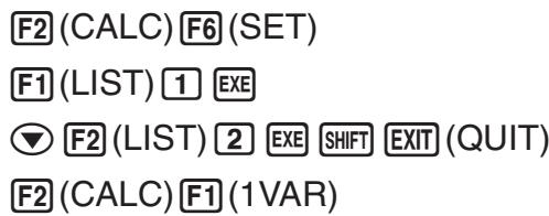
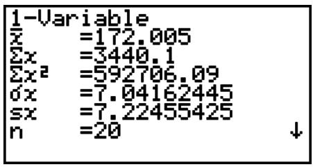
- Press MENU, select the RUN • MAT (or RUN) mode, press OPTN F6 (▷) F3 (PROB) (F2 (PROB) on the fx-7400GII) to recall the probability calculation (PROB) menu.
3 (PROB)^*F6 (▷)F4 (t() 1 6 0 • 5 ) EXE * fx-7400GII: F2 (PROB)
(Normalized variate t for 160.5 cm)
Result: -1.633855948
(≡-1.634)
F4(t() 1 7 5 • 5 ) EXE
(Normalized variate t for 175.5 cm)
Result: 0.4963343361
(≡ 0.496)
F1(P()0·496)—
F1(P() (-) 1 • 6 3 4 ) EXE
(Percentage of total)
Result: 0.638921
(63.9% of total)
F3 (R() 0 • 4 9 6 ) EXE
(Percentile)
Result: 0.30995
(31.0 percentile)
■ Drawing a Normal Probability Distribution Graph
You can draw a normal probability distribution graph using manual graphing with the RUN • MAT (or RUN) mode.
- From the Main Menu, enter the RUN • MAT (or RUN) mode.
- Input the commands to draw a rectangular coordinate graph.
- Input the probability value.
Example To draw a normal probability P (0.5) graph.
① MENU RUN • MAT (or RUN)
② SHIFT F4 (SKTCH) F1 (Cls) EXE
F5 (GRPH) F1 (Y=)
③ OPTN F6 (▷) F3 (PROB)* F6 (▷) F1 (P() 0 • 5 ) EXE
* fx-7400GII: F2 (PROB)
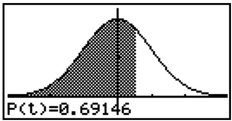
histogram
| Statistic | Value | | --------- | --------- | | P(t) | 0.69146 |■ Calculations Using the Distribution Function
Important!
- The following operations cannot be performed on the fx-7400GII.
You can use special functions in the RUN • MAT mode or PRGM mode to perform calculations that are the same as the STAT mode distribution function calculation (page 6-38).
Example To calculate normal probability distribution in the RUN • MAT mode for the data 1, 2, 3 , when the population standard deviation is = 1.5 and the population mean is = 2 .
- From the Main Menu, enter the RUN • MAT mode.
- Press the keys as follows.
OPTN F5 (STAT) F3 (DIST) F1 (NORM)
F1 (NPd) SHIFT ✗ ( { ) 1 , 2 , 3
SHIFT ÷ ( ) , 1 · 5 , 2 ) EXE
![AmS 1[0.2129] 2[0.2659] 3[0.2129] 0.212965337](/content/2025/01/86832/images/402ba1465c9e4287f67c086a03c17bfb065efa13806a46e3a66739e763ee2e4e.jpg)
- For details about what you can do with the distribution function and its syntax, see “Performing Distribution Calculations in a Program” (page 8-29).
■ Determining Standard Deviation and Variance from List Data
You can use functions to determine standard deviation and variance for specified list data. This calculation is performed in the RUN • MAT (or RUN) mode. You can perform calculations using data you saved to a list (List 1 to List 26) with the STAT mode List Editor or list data you input directly on the RUN • MAT (or RUN) mode screen.
Syntax StdDev(List n [,List m])
Variance(List n [,List m])
Example To store the x-data below in List 1, the frequency values in List 2, and determine the standard deviation and variance
| x | 60 | 70 | 80 | 90 |
| Frequency | 3 | 5 | 4 | 1 |
- From the Main Menu, enter the STAT mode.
- Use the List Editor to store the above data.
- From the Main Menu, enter the RUN • MAT (or RUN) mode.
- Press the keys as follows.
OPTN F5 (STAT) F4 (S • Dev)* EXIT
F1 (LIST) F1 (List) 1 , F1 (List) 2 ) EXE
* fx-7400GII: F4 (STAT) F3 (S • Dev)
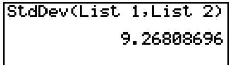
EXIT F5 (STAT) F5 (Var)* EXIT
F1 (LIST) F1 (List) 1 , F1 (List) 2 ) EXE
* fx-7400GII: F4 (STAT) F4 (Var)
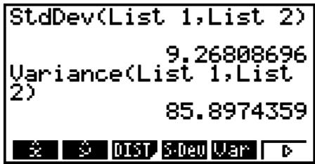
■ Calculations Using the TEST Command
Important!
- The following operations cannot be performed on the fx-7400GII.
You can use special functions in the RUN • MAT mode or PRGM mode to perform calculations that are the same as the STAT mode Z Test, t Test, and other test calculations (page 6-22).
Example
To determine the z score and p-value when a one-sample Z test is performed under the conditions below: test condition ( condition) _0^* , assumed population mean _0 = 0 , population standard deviation = 1 , sample mean = 1 , number of samples n = 2
* “μ condition ≠ μ₀” can be specified by entering 0 as the initial argument of the one-sample Z test command “OneSampleZTest”.
- From the Main Menu, enter the RUN • MAT mode.
- Perform the following key operation.
OPTN F5 (STAT) F6 (▷) F1 (TEST) F1 (Z)
F1(1-S)0,0,1,1,2
EXE
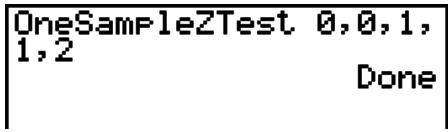
EXIT EXIT EXIT
F1 (LIST) F1 (List) SHIFT (-) (Ans) EXE
![Ans 1[1,4,4,2] 2[0,15,72] 3[1 4[2] 1.414213562](/content/2025/01/86832/images/99a9eee211862ec89ff289d1783ffeb5bdc44d2cc8b28803ec9a9f244bff07d8.jpg)
The following calculation results are displayed as ListAns elements 1 through 4.
1: z score
2: p-value
3:
4:n
- For details about the function of the supported TEST command and their syntax, see “Using the TEST Command to Execute a Command in a Program” (page 8-32).
5. Tests
Important!
- Test calculations cannot be performed on the fx-7400GII.
The Z Test provides a variety of different standardization-based tests. They make it possible to test whether or not a sample accurately represents the population when the standard deviation of a population (such as the entire population of a country) is known from previous tests. Z testing is used for market research and public opinion research, that need to be performed repeatedly.
1-Sample Z Test tests for the unknown population mean when the population standard deviation is known.
2-Sample Z Test tests the equality of the means of two populations based on independent samples when both population standard deviations are known.
1-Prop Z Test tests for an unknown proportion of successes.
2-Prop Z Test tests to compare the proportion of successes from two populations.
The t Test tests the hypothesis when the population standard deviation is unknown. The hypothesis that is the opposite of the hypothesis being proven is called the null hypothesis, while the hypothesis being proved is called the alternative hypothesis. The t Test is normally applied to test the null hypothesis. Then a determination is made whether the null hypothesis or alternative hypothesis will be adopted.
1-Sample t Test tests the hypothesis for a single unknown population mean when the population standard deviation is unknown.
2-Sample t Test compares the population means when the population standard deviations are unknown.
LinearReg t Test calculates the strength of the linear association of paired data.
With the ^2 test, a number of independent groups are provided and a hypothesis is tested relative to the probability of samples being included in each group.
The ^2 GOF test ( ^2 one-way Test) tests whether the observed count of sample data fits a certain distribution. For example, it can be used to determine conformance with normal distribution or binomial distribution.
The ^2 two-way test creates a cross-tabulation table that structures mainly two qualitative variables (such as “Yes” and “No”), and evaluates the independence of the variables.
2-Sample F Test tests the hypothesis for the ratio of sample variances. It could be used, for example, to test the carcinogenic effects of multiple suspected factors such as tobacco use, alcohol, vitamin deficiency, high coffee intake, inactivity, poor living habits, etc.
ANOVA tests the hypothesis that the population means of the samples are equal when there are multiple samples. It could be used, for example, to test whether or not different combinations of materials have an effect on the quality and life of a final product.
One-Way ANOVA is used when there is one independent variable and one dependent variable.
Two-Way ANOVA is used when there are two independent variables and one dependent variable.
The following pages explain various statistical calculation methods based on the principles described above. Details concerning statistical principles and terminology can be found in any standard statistics textbook.
On the initial STAT mode screen, press F3(TEST) to display the test menu, which contains the following items.
- F3 (TEST) F1 (Z) ... Z Tests (page 6-24)
F2(t) ... t Tests (page 6-26)
F3 (CHI) ... ^2 Test (page 6-29)
F4 (F) ... 2-Sample F Test (page 6-30)
F5 (ANOV) ... ANOVA (page 6-31)
After setting all the parameters, use ▼ to move the highlighting to “Execute” and then press one of the function keys shown below to perform the calculation or draw the graph.
• F1(CALC) ... Performs the calculation.
• F6(DRAW) ... Draws the graph.
- V-Window settings are automatically optimized for drawing the graph.
Z Tests
• Z Test Common Functions
You can use the following graph analysis functions after drawing a Z Test result output graph.
• F1(Z) ... Displays z score.
Pressing F1(Z) displays the z score at the bottom of the display, and displays the pointer at the corresponding location in the graph (unless the location is off the graph screen).
Two points are displayed in the case of a two-tail test. Use ◀ and ▶ to move the pointer.
• F2(P) ... Displays p-value.
Pressing F2(P) displays the p-value at the bottom of the display without displaying the pointer.
- Executing an analysis function automatically stores the z and p values in alpha variables Z and P , respectively.
• 1-Sample Z Test
This test is used when the population standard deviation is known to test the hypothesis. The 1-Sample Z Test is applied to the normal distribution.
Perform the following key operations from the statistical data list.
F3 (TEST)
F1(Z)
F1(1-S)
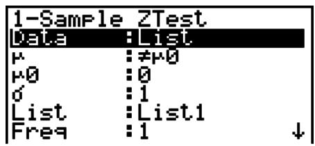
| Save Res: None | Execute
The following shows the parameter data specification items that are different from list data specification.
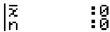
Calculation Result Output Example
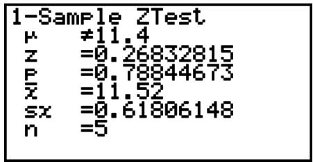
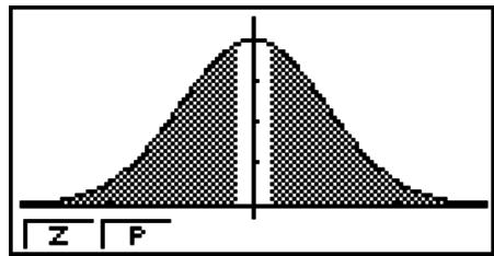
histogram
| Category | Value | | -------- | ----- | | Z | Low | | P | High |11.4 ..... direction of test
s_x ...... Displayed only for Data: List setting.
- [Save Res] does not save the condition in line 2.
• 2-Sample Z Test
This test is used when the standard deviations for two populations are known to test the hypothesis. The 2-Sample Z Test is applied to the normal distribution.
Perform the following key operations from the statistical data list.
F3 (TEST)
F1(Z)
F2 (2-S)
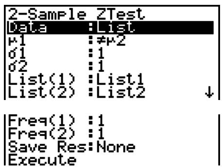
The following shows the parameter data specification items that are different from list data specification.
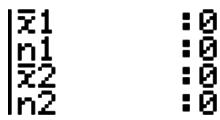
Calculation Result Output Example
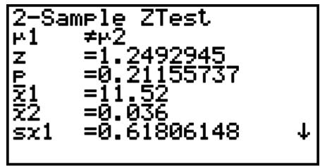
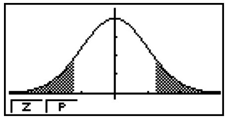
histogram
| Category | Value | | -------- | ----- | | Z | 0 | | P | 0 |_1_2 ..... direction of test
s_x1 ...... Displayed only for Data: List setting.
s_x2 ...... Displayed only for Data: List setting.
- [Save Res] does not save the _1 condition in line 2.
• 1-Prop Z Test
This test is used to test for an unknown proportion of successes. The 1-Prop Z Test is applied to the normal distribution.
Perform the following key operations from the statistical data list.
F3 (TEST)
F1(Z)
F3 (1-P)
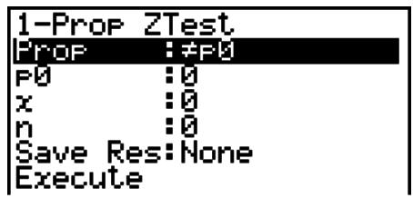
Calculation Result Output Example
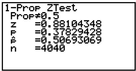
Prop≠0.5 ..... direction of test
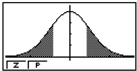
histogram
| Category | Value | | -------- | ----- | | Top Left | Z | | Top Right| P |- [Save Res] does not save the Prop condition in line 2.
- 2-Prop Z Test
This test is used to compare the proportion of successes. The 2-Prop Z Test is applied to the normal distribution.
Perform the following key operation from the statistical data list.
F3 (TEST)
F1(Z)
F4 (2-P)
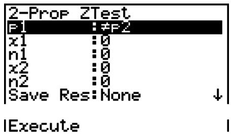
Calculation Result Output Example

p_1>p_2 ..... direction of test
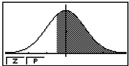
area
| Category | Value | | -------- | ----- | | Z | Low | | P | High |- [Save Res] does not save the p_1 condition in line 2.
■ t Tests
- t Test Common Functions
You can use the following graph analysis functions after drawing a t Test result output graph.
• F1(T) ... Displays t score.
Pressing F1(T) displays the t score at the bottom of the display, and displays the pointer at the corresponding location in the graph (unless the location is off the graph screen).
Two points are displayed in the case of a two-tail test. Use ◀ and ▶ to move the pointer.
- F2(P) ... Displays p-value.
Pressing F2(P) displays the p-value at the bottom of the display without displaying the pointer.
- Executing an analysis function automatically stores the t and p values in alpha variables T and P, respectively.
• 1-Sample t Test
This test uses the hypothesis test for a single unknown population mean when the population standard deviation is unknown. The 1-Sample t Test is applied to t distribution.
Perform the following key operations from the statistical data list.
F3 (TEST)
F2(t)
F1(1-S)
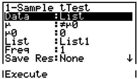
The following shows the parameter data specification items that are different from list data specification.
$$ \left| \begin{array}{l l} \overline {{x}} & : 0 \ s x & : 0 \ n & : 0 \end{array} \right. $$
Calculation Result Output Example
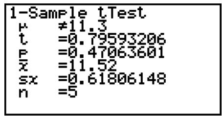
11.3 ..... direction of test
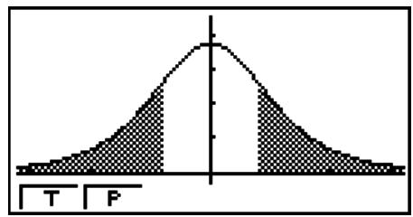
histogram
| Category | Value | | -------- | ----- | | T | 0 | | P | 0 |- [Save Res] does not save the condition in line 2.
- 2-Sample t Test
2-Sample t Test compares the population means when the population standard deviations are unknown. The 2-Sample t Test is applied to t distribution.
Perform the following key operations from the statistical data list.
F3 (TEST)
F2 (t)
F2 (2-S)
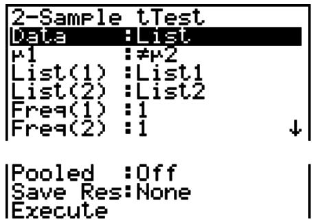
The following shows the parameter data specification items that are different from list data specification.
$$ \begin{array}{rl} & \left| \begin{array}{ll} \overline{x} 1 & :0 \ s x 1 & :0 \ n 1 & :0 \ \overline{x} 2 & :0 \end{array} \right. \ & \left| \begin{array}{ll} s x 2 & :0 \ n 2 & :0 \end{array} \right. \end{array} $$
Calculation Result Output Example
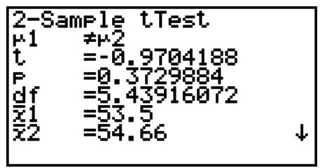
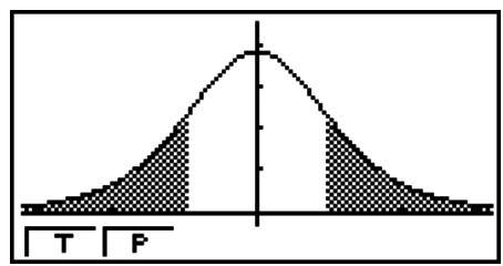
histogram
| Category | Value | | -------- | ----- | | T | 0 | | P | 0 |_1_2 ..... direction of test
s_p ...... Displayed only when Pooled: On setting.
- [Save Res] does not save the _1 condition in line 2.
- LinearReg t Test
LinearReg t Test treats paired-variable data sets as (x, y) pairs, and uses the method of least squares to determine the most appropriate a, b coefficients of the data for the regression formula y = a + bx . It also determines the correlation coefficient and t score, and calculates the extent of the relationship between x and y.
Perform the following key operations from the statistical data list.
F3 (TEST)
F2 (t)
F3 (REG)
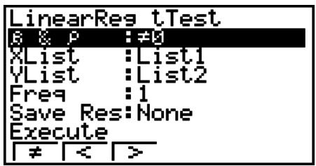
Calculation Result Output Example
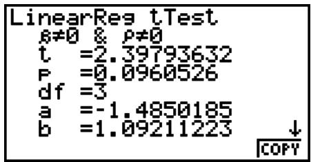
0 & 0 ..... direction of test
Pressing F6(COPY) while a calculation result is on the display copies the regression formula to the Graph relation list.
![Graph Func Y1: Y2: [—] Y3: [—] Y4: [—] Y5: [—] Y6: [—]](/content/2025/01/86832/images/be0a82a4f3ea0e1a83f86460ddbc8dcc07ab071d2470e0ec4596124468412f37.jpg)
When there is a list specified for the [Resid List] item on the Setup screen, regression formula residual data is automatically saved to the specified list after the calculation is finished.
- You cannot draw a graph for LinearReg t Test.
- [Save Res] does not save the & conditions in line 2.
- When the list specified by [Save Res] is the same list specified by the [Resid List] item on the Setup screen, only [Resid List] data is saved in the list.
■ ^2 Test
- ^2 Test Common Functions
You can use the following graph analysis functions after drawing a graph.
- F1(CHI) ... Displays ^2 value.
Pressing F1(CHI) displays the ^2 value at the bottom of the display, and displays the pointer at the corresponding location in the graph (unless the location is off the graph screen).
• F2(P) ... Displays p-value.
Pressing F2(P) displays the p-value at the bottom of the display without displaying the pointer.
- Executing an analysis function automatically stores the ^2 and p values in alpha variables C and P, respectively.
- ^2 GOF Test ( ^2 one-way Test)
The ^2 GOF Test ( ^2 one-way test) tests whether the frequency of sample data fits a certain distribution. For example, it can be used to determine conformance with normal distribution or binomial distribution.
Perform the following key operations from the statistical data list.
F3 (TEST)
F3 (CHI)
F1 (GOF)
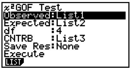
Next, specify the lists that contain the data. The following shows the meaning of the above items.
Observed ..... name of List (1 to 26) that contains observed counts (all cells positive integers)
Expected..... name of List (1 to 26) that is for saving expected frequency
CNTRB ...... Specifies a list (List 1 to List 26) as the storage location of the contribution of each observed count obtained as calculation results.
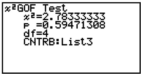
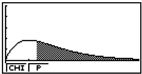
area
| Category | Value | | -------- | ----- | | CHI | Low | | P | High |CNTRB ...... list for output of contribution values
- ^2 two-way Test
^2 two-way Test sets up a number of independent groups and tests hypothesis related to the proportion of the sample included in each group. The ^2 Test is applied to dichotomous variables (variable with two possible values, such as yes/no).
Perform the following key operations from the statistical data list.
F3 (TEST)
F3 (CHI)
F2 (2WAY)
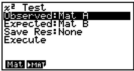
Next, specify the matrix that contains the data. The following shows the meaning of the above items.
Observed ..... name of matrix (A to Z) that contains observed counts (all cells positive integers)
Expected..... name of matrix (A to Z) that is for saving expected frequency
Calculation Result Output Example
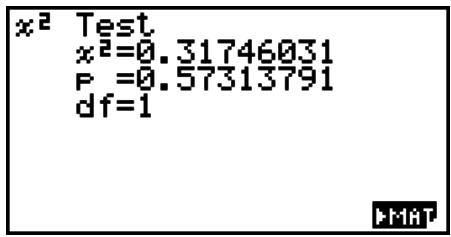
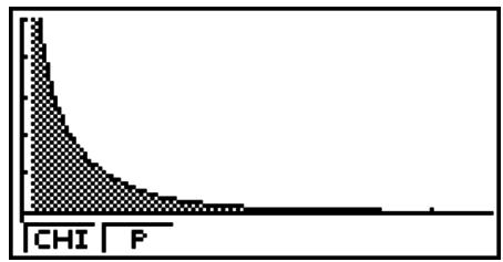
- The matrix must be at least two lines by two columns. An error occurs if the matrix has only one line or one column.
- Pressing F1(Mat) while the “Observed” and “Expected” parameter settings are highlighted will display the Matrix (A to Z) setting screen.
- Pressing F2 (▶MAT) while setting parameters enters the Matrix Editor, which you can use to edit and view the contents of matrices.
- Pressing F6 (▶MAT) while a calculation result is displayed enters the Matrix Editor, which you can use to edit and view the contents of matrices.
■ 2-Sample F Test
2-Sample F Test tests the hypothesis for the ratio of sample variances. The F Test is applied to the F distribution.
Perform the following key operations from the statistical data list.
F3 (TEST)
F4(F)
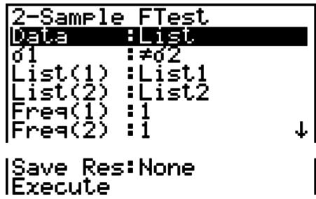
The following shows the parameter data specification items that are different from list data specification.
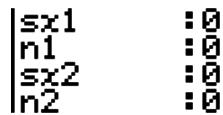
Calculation Result Output Example
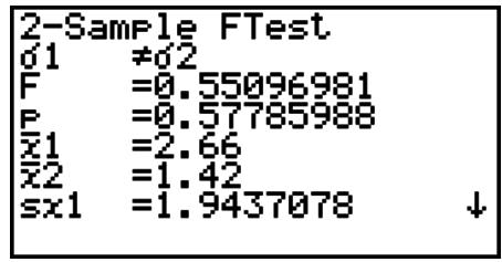
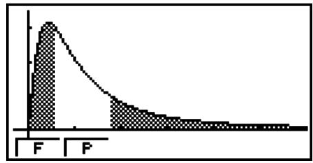
histogram
| Category | Value | | -------- | ----- | | F | 100 | | P | 50 |^1^2 ..... direction of test
_1 ...... Displayed only for Data: List setting.
_2 ..... Displayed only for Data: List setting.
You can use the following graph analysis functions after drawing a graph.
- F1(F) ... Displays F value.
Pressing F1(F) displays the F value at the bottom of the display, and displays the pointer at the corresponding location in the graph (unless the location is off the graph screen).
Two points are displayed in the case of a two-tail test. Use ◀ and ▶ to move the pointer.
- F2(P) ... Displays p-value.
Pressing F2(P) displays the p-value at the bottom of the display without displaying the pointer.
- Executing an analysis function automatically stores the F and p values in alpha variables F and P , respectively.
- [Save Res] does not save the _1 condition in line 2.
ANOVA
ANOVA tests the hypothesis that the population means of the samples are equal when there are multiple samples.
One-Way ANOVA is used when there is one independent variable and one dependent variable.
Two-Way ANOVA is used when there are two independent variables and one dependent variable.
Perform the following key operations from the statistical data list.
F3 (TEST)
F5 (ANOV)
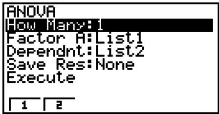
The following is the meaning of each item in the case of list data specification.
How Many..... selects One-Way ANOVA or Two-Way ANOVA (number of levels)
Factor A ...... category list (List 1 to 26)
Dependnt ..... list to be used for sample data (List 1 to 26)
Save Res ..... first list for storage of calculation results (None or List 1 to 22) ^*1
Execute...... executes a calculation or draws a graph (Two-Way ANOVA only)
*1 [Save Res] saves each vertical column of the table into its own list. The leftmost column is saved in the specified list, and each subsequent column to the right is saved in the next sequentially numbered list. Up to five lists can be used for storing columns. You can specify an first list number in the range of 1 to 22.
The following item appears in the case of Two-Way ANOVA only.
Factor B ...... category list (List 1 to 26)
After setting all the parameters, use ▼ to move the highlighting to “Execute” and then press one of the function keys shown below to perform the calculation or draw the graph.
• F1(CALC) ... Performs the calculation.
- F6 (DRAW) ... Draws the graph (Two-Way ANOVA only).
Calculation results are displayed in table form, just as they appear in science books.
Calculation Result Output Example
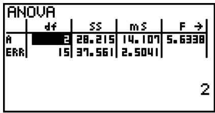
other
ANOVA | | df | SS | mS | F → | |---|---|---|---|---| | A | 2 | 28.215 | 14.107 | 5.6338 | | ERR | 15 | 37.561 | 2.5041 | | 2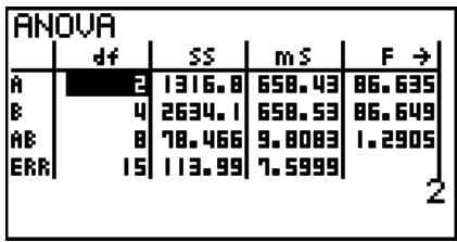
One-Way ANOVA
Line 1 (A) ...... Factor A df value, SS value, MS value, F value, p-value
Line 2 (ERR) ..... Error df value, SS value, MS value
Two-Way ANOVA
Line 1 (A) ...... Factor A df value, SS value, MS value, F value, p-value
Line 2 (B) ...... Factor B df value, SS value, MS value, F value, p-value
Line 3 (AB)...... Factor A × Factor B df value, SS value, MS value, F value, p-value
* Line 3 does not appear when there is only one observation in each cell.
Line 4 (ERR)..... Error df value, SS value, MS value
F ...... F value
p ...... p-value
df ...... degrees of freedom
SS ...... sum of squares
MS ...... mean squares
With Two-Way ANOVA, you can draw Interaction Plot graphs. The number of graphs depends on Factor B, while the number of X-axis data depends on the Factor A. The Y-axis is the average value of each category.
You can use the following graph analysis function after drawing a graph.
- F1 (Trace) or SHIFT F1 (TRCE) ... Trace function
Pressing ◀ or ▶ moves the pointer on the graph in the corresponding direction. When there are multiple graphs, you can move between graphs by pressing ▲ and ▼.
- Graphing is available with Two-Way ANOVA only. V-Window settings are performed automatically, regardless of Setup screen settings.
- Using the Trace function automatically stores the number of conditions to alpha variable A and the mean value to variable M, respectively.
■ ANOVA (Two-Way)
- Description
The nearby table shows measurement results for a metal product produced by a heat treatment process based on two treatment levels: time (A) and temperature (B). The experiments were repeated twice each under identical conditions.
| B (Heat Treatment Temperature)A (Time) | B1 | B2 |
| A1 | 113, 116 | 139, 132 |
| A2 | 133, 131 | 126, 122 |
Perform analysis of variance on the following null hypothesis, using a significance level of 5%.
H_0 : No change in strength due to time
H_0 : No change in strength due to heat treatment temperature
H_0 : No change in strength due to interaction of time and heat treatment temperature
- Solution
Use Two-Way ANOVA to test the above hypothesis.
Input the above data as shown below.
List1={1,1,1,1,2,2,2,2}
List2={1,1,2,2,1,1,2,2}
List3={113,116,139,132,133,131,126,122}
Define List 3 (the data for each group) as Dependent. Define List 1 and List 2 (the factor numbers for each data item in List 3) as Factor A and Factor B respectively. Executing the test produces the following results.
• Time differential (A) level of significance P = 0.2458019517
The level of significance p = 0.2458019517 is greater than the significance level (0.05), so the hypothesis is not rejected.
• Temperature differential (B) level of significance P = 0.04222398836
The level of significance p = 0.04222398836 is less than the significance level (0.05), so the hypothesis is rejected.
- Interaction (A × B) level of significance P = 2.78169946e-3
The level of significance p = 2.78169946e-3 is less than the significance level (0.05), so the hypothesis is rejected.
The above test indicates that the time differential is not significant, the temperature differential is significant, and interaction is highly significant.
- Input Example
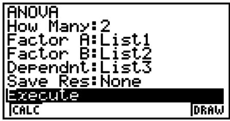
- Results
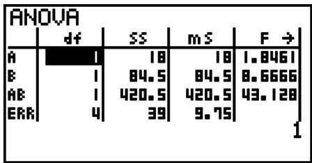
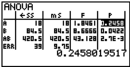
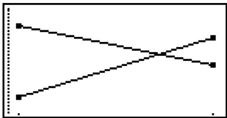
flowchart
graph TD
    A[" "] --> B[" "]
    C[" "] --> D[" "]
    E[" "] --> F[" "]
6. Confidence Interval
Important!
- Confidence interval calculations cannot be performed on the fx-7400GII.
A confidence interval is a range (interval) that includes a statistical value, usually the population mean.
A confidence interval that is too broad makes it difficult to get an idea of where the population value (true value) is located. A narrow confidence interval, on the other hand, limits the population value and makes it difficult to obtain reliable results. The most commonly used confidence levels are 95% and 99%. Raising the confidence level broadens the confidence interval, while lowering the confidence level narrows the confidence level, but it also increases the chance of accidentally overlooking the population value. With a 95% confidence interval, for example, the population value is not included within the resulting intervals 5% of the time.
When you plan to conduct a survey and then t test and Z test the data, you must also consider the sample size, confidence interval width, and confidence level. The confidence level changes in accordance with the application.
1-Sample Z Interval calculates the confidence interval for an unknown population mean when the population standard deviation is known.
2-Sample Z Interval calculates the confidence interval for the difference between two population means when the population standard deviations of two samples are known.
1-Prop Z Interval calculates the confidence interval for an unknown proportion of successes.
2-Prop Z Interval calculates the confidence interval for the difference between the proportion of successes in two populations.
1-Sample t Interval calculates the confidence interval for an unknown population mean when the population standard deviation is unknown.
2-Sample t Interval calculates the confidence interval for the difference between two population means when both population standard deviations are unknown.
On the initial STAT mode screen, press F4(INTR) to display the confidence interval menu, which contains the following items.
• F4 (INTR) F1 (Z) ... Z intervals (page 6-36)
F2(t) ... t intervals (page 6-37)
After setting all the parameters, use ▼ to move the highlighting to “Execute” and then press the function key shown below to perform the calculation.
• F1(CALC) ... Performs the calculation.
- There is no graphing for confidence interval functions.
- General Confidence Interval Precaution
Inputting a value in the range of 0 ≤ C -Level < 1 for the C-Level setting sets a value you input. Inputting a value in the range of 1 ≤ C -Level < 100 sets a value equivalent to your input divided by 100.
• 1-Sample Z Interval
1-Sample Z Interval calculates the confidence interval for an unknown population mean when the population standard deviation is known.
Perform the following key operations from the statistical data list.
F4 (INTR)
F1(Z)
F1(1-S)
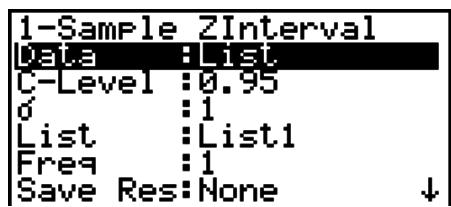
|Execute |
The following shows the parameter data specification items that are different from list data specification.

Calculation Result Output Example
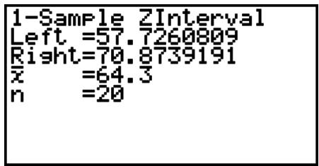
• 2-Sample Z Interval
2-Sample Z Interval calculates the confidence interval for the difference between two population means when the population standard deviations of two samples are known.
Perform the following key operations from the statistical data list.
F4 (INTR)
F1(Z)
F2 (2-S)
• 1-Prop Z Interval
1-Prop Z Interval uses the number of data to calculate the confidence interval for an unknown proportion of successes.
Perform the following key operations from the statistical data list.
F4 (INTR)
F1(Z)
F3 (1-P)
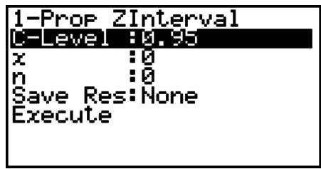
Data is specified using parameter specification.
Calculation Result Output Example
1-Prop ZInterval Left =0.71056582 Right=0.78943417 =0.75 n =800
- 2-Prop Z Interval
2-Prop Z Interval uses the number of data items to calculate the confidence interval for the difference between the proportion of successes in two populations.
Perform the following key operations from the statistical data list.
F4 (INTR)
F1(Z)
F4 (2-P)
■ t Interval
• 1-Sample t Interval
1-Sample t Interval calculates the confidence interval for an unknown population mean when the population standard deviation is unknown.
Perform the following key operations from the statistical data list.
F4 (INTR)
F2 (t)
F1(1-S)
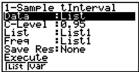
The following shows the parameter data specification items that are different from list data specification.
& :0 s x & :0 n & :0
Calculation Result Output Example
1-Sample tInterval
Left =60.9628946
Right=71.6371054
x =66.3
sx =8.4
n =12
• 2-Sample t Interval
2-Sample t Interval calculates the confidence interval for the difference between two population means when both population standard deviations are unknown. The t interval is applied to t distribution.
Perform the following key operations from the statistical data list.
F4 (INTR)
F2(t)
F2 (2-S)
7. Distribution
Important!
- Distribution calculations cannot be performed on the fx-7400GII.
There is a variety of different types of distribution, but the most well-known is “normal distribution”, which is essential for performing statistical calculations. Normal distribution is a symmetrical distribution centered on the greatest occurrences of mean data (highest frequency), with the frequency decreasing as you move away from the center. Poisson distribution, geometric distribution, and various other distribution shapes are also used, depending on the data type.
Certain trends can be determined once the distribution shape is determined. You can calculate the probability of data taken from a distribution being less than a specific value.
For example, distribution can be used to calculate the yield rate when manufacturing some product. Once a value is established as the criteria, you can calculate normal probability when estimating what percent of the products meet the criteria. Conversely, a success rate target (80% for example) is set up as the hypothesis, and normal distribution is used to estimate the proportion of the products will reach this value.
Normal probability density calculates the probability density of normal distribution from a specified x value.
Normal cumulative distribution calculates the probability of normal distribution data falling between two specific values.
Inverse normal cumulative distribution calculates a value that represents the location within a normal distribution for a specific cumulative probability.
Student-t probability density calculates t probability density from a specified x value.
Student-t cumulative distribution calculates the probability of t distribution data falling between two specific values.
Inverse Student-t cumulative distribution calculates the lower bound value of a Student-t cumulative probability density for a specified percentage.
Like t distribution, probability density (or probability), cumulative distribution and inverse cumulative distribution can also be calculated for ^2 , F, Binomial, Poisson, Geometric and Hypergeometric distributions.
On the initial STAT mode screen, press F5(DIST) to display the distribution menu, which contains the following items.
- F5 (DIST) F1 (NORM) ... Normal distribution (page 6-39)
F2 (t) ... Student-t distribution (page 6-41)
F3 (CHI) ... ^2 distribution (page 6-42)
F4(F) ... F distribution (page 6-43)
F5 (BINM) ... Binomial distribution (page 6-44)
F6 (▷) F1 (POISN) ... Poisson distribution (page 6-46)
F6 (▷) F2 (GEO) ... Geometric distribution (page 6-47)
F6 (▷) F3 (H.GEO) ... Hypergeometric distribution (page 6-49)
After setting all the parameters, use ▼ to move the highlighting to “Execute” and then press one of the function keys shown below to perform the calculation or draw the graph.
• F1(CALC) ... Performs the calculation.
- F6 (DRAW) ... Draws the graph.
■ Common Distribution Functions
- V-Window settings for graph drawing are set automatically when the Setup screen's “Stat Wind” setting is “Auto”. Current V-Window settings are used for graph drawing when the “Stat Wind” setting is “Manual”.
- After drawing a graph, you can use the P-CAL function to calculate an estimated p -value for a particular x value. The P-CAL function can be used only after a Normal Probability Density, Student- t Probability Density, ^2 Probability Density, or F Probability Density graph is drawn.
The following is the general procedure for using the P-CAL function.
- After drawing a distribution graph, press SHIFT F5 (G-SLV) F1 (P-CAL) to display the x value input dialog box.
- Input the value you want for x and then press EXE.
- This causes the x and p values to appear at the bottom of the display, and moves the pointer to the corresponding point on the graph.
- Pressing ,,T or a number key at this time causes the x value input dialog box to reappear so you can perform another estimated value calculation if you want.
- After you are finished, press EXIT to clear the coordinate values and the pointer from the display.
- Executing an analysis function automatically stores the x and p values in alpha variables X and P, respectively.
■ Normal Distribution
• Normal Probability Density
Normal Probability Density calculates the probability density (p) for a specified single x-value or a list. When a list is specified, calculation results for each list element are displayed in list form.
F5 (DIST) F1 (NORM) F1 (NPd)
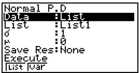
- Normal probability density is applied to standard normal distribution.
- Specifying = 1 and = 0 specifies standard normal distribution.
Calculation Result Output Examples
![Normal P.D 1[0.2419] 2[0.1497] 3[0.0539] 4[0.7E-4] 5[1.4E-6] 0.2419707245](/content/2025/01/86832/images/3aeb8e70380c26e4e0c327ee920d10f0b949e72712e2ebe2b152275cf182428b.jpg)
When a list is specified
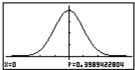
histogram
| Statistic | Value | | ------------- | --------- | | X | 0 | | P | 3989422804 |Graph when an x-value is specified
- Graphing is supported only when a variable is specified and a single x -value is entered as data.
• Normal Cumulative Distribution
Normal Cumulative Distribution calculates the normal cumulative probability of a normal distribution between a lower bound and an upper bound.
F5 (DIST) F1 (NORM) F2 (NCd)
![Normal C.D Data : List L.List : List1 U.List : List2 d : 1 k : 0 Save Res: None ↓ [List |var]](/content/2025/01/86832/images/c32b740d108e55b0da9a4d36e406532573abcd12ec6e471972d86db1368bab63.jpg)
Calculation Result Output Examples
![Normal C.D F z:Low z:UP 1 [1.1578] 1 3 2 0.0807 1.4 4 3 0.0227 2 4 4 2.3E-4 3.5 5 0.1573053559](/content/2025/01/86832/images/da7c0c447ddcb1694ca05e64bdba7a3cc5bf688da1e329835a86188efe0f8c82.jpg)
When a list is specified
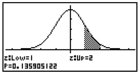
histogram
| Category | Value | | -------- | --------- | | z≤Low=1 | Low | | z≥Up=2 | High |Graph when an x-value is specified
- Graphing is supported only when a variable is specified and a single x -value is entered as data.
- Inverse Normal Cumulative Distribution
Inverse Normal Cumulative Distribution calculates the boundary value(s) of a normal cumulative distribution probability for specified values.
F5 (DIST) F1 (NORM) F3 (InvN)
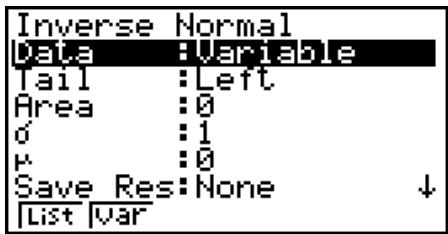
Area: probability value
$$ (0 \leq \text { Area } \leq 1) $$
Inverse cumulative normal distribution calculates a value that represents the location within a normal distribution for a specific cumulative probability.
$$ \int_ {- \infty} ^ {U p p e r} f (x) d x = p $$
Tail: Left
upper boundary
of integration
interval
$$ \int_ {L o w e r} ^ {+ \infty} f (x) d x = p $$
Tail: Right
lower boundary
of integration
interval
$$ \int_ {L o w e r} ^ {U p p e r} f (x) d x = p $$
Tail: Central
upper and lower
boundaries of
integration interval
Specify the probability and use this formula to obtain the integration interval.
- This calculator performs the above calculation using the following: = 1E99, - = -1E99
- There is no graphing for Inverse Normal Cumulative Distribution.
■ Student-t Distribution
- Student- t Probability Density
Student-t Probability Density calculates the probability density (p) for a specified single x-value or a list. When a list is specified, calculation results for each list element are displayed in list form.
F5 (DIST) F2 (t) F1 (tPd)
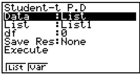
Calculation Result Output Examples
![Student-t P.D 1[3.1E-3] 2[1.2E-3] 3[8.7E-4] 4[7.2E-4] 2.195240594E-03](/content/2025/01/86832/images/4ba11be25e0293f884d1746b5e08c22907061afb2f03441d54d84185d90a79ef.jpg)
When a list is specified
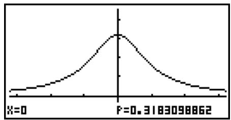
line
| x | y | | ------- | ----- | | 0 | 0 | | P=0.3183098862 | 0 |Graph when variable (x) is specified
- Graphing is supported only when a variable is specified and a single x -value is entered as data.
- Student- t Cumulative Distribution
Student-t Cumulative Distribution calculates the Student-t cumulative probability of a Student-t distribution between a lower bound and an upper bound.
F5 (DIST) F2 (t) F2 (tCd)
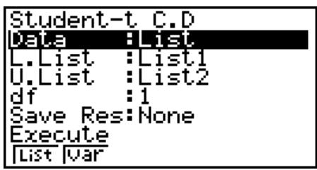
Calculation Result Output Examples
![Student-t C.D P tLow tUP 1[1.2335 1 12] 2 0.1277 2 16 3 0.0856 3 19 4 0.0628 4 21] 0.2235353239](/content/2025/01/86832/images/b6896364c480343124855767266adf53208948cf93db2bc93d1d23ec4cce92e3.jpg)
When a list is specified
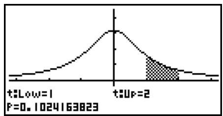
histogram
| Range | Count | | ----------- | ----- | | t≤Low=1 | 0 | | t≤Up=2 | 1024163823 |Graph when variable (x) is specified
- Graphing is supported only when a variable is specified and a single x -value is entered as data.
- Inverse Student- t Cumulative Distribution
Inverse Student-t Cumulative Distribution calculates the lower bound value of a Student-t cumulative distribution for a specified df (degrees of freedom) value.
F5 (DIST) F2 (t) F3 (InvN)
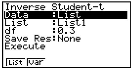
Calculation Result Output Examples
![Inverse Student-t 1[34.186] 2 6.4145 3 1.6126 4 0.5023] 64.78654564](/content/2025/01/86832/images/69154bf08f7f7b6e1cfc553ea2802b4211019412e43eda24bf2b76c0104de37c.jpg)
When a list is specified
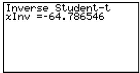
When variable (x) is specified
- There is no graphing for Inverse Student- t Cumulative Distribution.
■ ^2 Distribution
- ^2 Probability Density
^2 Probability Density calculates the ^2 probability density (p) for a specified single x-value or a list. When a list is specified, calculation results for each list element are displayed in list form.
F5 (DIST) F3 (CHI) F1 (CPd)
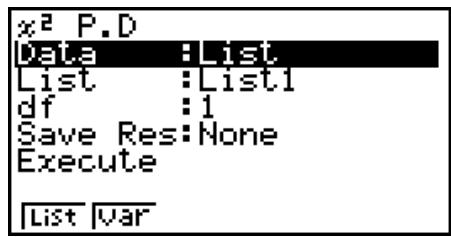
Calculation Result Output Examples
![x² P.D 1[0.2419] 2 0.1037 3 0.0513 4 0.0269] 0.2419707245](/content/2025/01/86832/images/8155f27ee9b0deca28c39e987f9561ca80d32396131c3664a6a6ee518e69bcc2.jpg)
When a list is specified
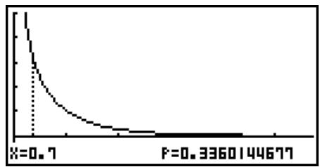
line
| x | y | |-------|--------| | 0.7 | 1.0 | | 0.3360144677 | 0.1 |Graph when variable (x) is specified
- Graphing is supported only when a variable is specified and a single x -value is entered as data.
- ^2 Cumulative Distribution
^2 Cumulative Distribution calculates the cumulative probability of a ^2 distribution between a lower bound and an upper bound.
F5 (DIST) F3 (CHI) F2 (CCd)
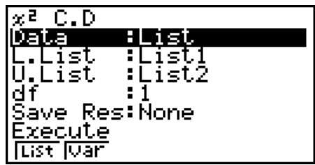
Calculation Result Output Examples
![x² C.D 1 [1.0187] 2 0.1572 3 0.0832 4 0.0454] 0.3167785024](/content/2025/01/86832/images/333d2d2f56fdde2bf81e14b94a8259ea281b4efdca269f8fe248a0234e227cec.jpg)
When a list is specified
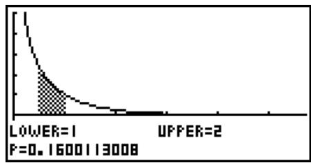
line
| Category | Value | | -------- | ----- | | LOWER=1 | 1 | | UPPER=2 | 2 |Graph when variable (x) is specified
- Graphing is supported only when a variable is specified and a single x -value is entered as data.
- Inverse ^2 Cumulative Distribution
Inverse ^2 Cumulative Distribution calculates the lower bound value of a ^2 cumulative distribution probability for a specified df (degrees of freedom) value.
F5 (DIST) F3 (CHI) F3 (InvC)
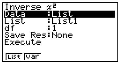
Calculation Result Output Examples
![Inverse x² 1[3.1055] 2 1.6423 3 1.0741 4 0.7083] 2.705543454](/content/2025/01/86832/images/dbf8bffebf5b20893683e2ce0d5ff7022a1a806346dffd4333533593f210532e.jpg)
When a list is specified
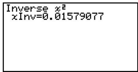
When variable (x) is specified
- There is no graphing for Inverse ^2 Cumulative Distribution.
■ F Distribution
- F Probability Density
F Probability Density calculates the F probability density (p) for a specified single x-value or a list. When a list is specified, calculation results for each list element are displayed in list form.
F5 (DIST) F4 (F) F1 (FPd)
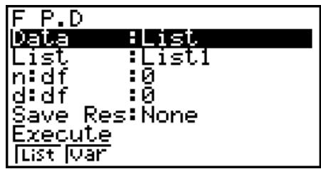
Calculation Result Output Examples
![F P.D 1[0.1924] 2[0.0883] 3[0.0516] 4[0.034] 0.1924500897](/content/2025/01/86832/images/dc6b4e3f0c262071d1c9f67033de79c4be4caac729ff8f7d809d6291bf05c43a.jpg)
When a list is specified
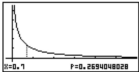
line
| x | y | | ------- | ----- | | 0.7 | 1.0 | | 1.0 | 0.5 | | 2.0 | 0.2 | | 3.0 | 0.1 | | 4.0 | 0.05 | | 5.0 | 0.02 | | 6.0 | 0.01 | | 7.0 | 0.005 | | 8.0 | 0.002 | | 9.0 | 0.001 | | 10.0 | 0.0005| | 11.0 | 0.0002| | 12.0 | 0.0001| | 13.0 | 0.00005| | 14.0 | 0.00002| | 15.0 | 0.00001| | 16.0 | 0.000005| | 17.0 | 0.000002| | 18.0 | 0.000001| | 19.0 | 0.0000005| | 20.0 | 0.0000002| | 21.0 | 0.0000001| | 22.0 | 0.00000005| | 23.0 | 0.00000002| | 24.0 | 0.00000001| | 25.0 | 0.000000005| | 26.0 | 0.000000002| | 27.0 | 0.000000001| | 28.0 | 0.0000000005| | 29.0 | 0.0000000002| | 30.0 | 0.0000000001| | 31.0 | 0.00000000005| | 32.0 | 0.00000000002| | 33.0 | 0.00000000001| | 34.0 | 0.00000000001| | 35.0 | 0.00000000001| | 36.0 | 0.0 | | 37.5 | - | | 38.5 | - | | 39.5 | - | | 4 | - | | 41 | - | | 42 | - | | 43 | - | | 44 | - | | 45 | - | | 46 | - | | 47 | - | | 48 | - | | 49 | - | | 5 | - | | 51 | - | | 52 | - | | 53 | - | | 54 | - | | 55 | - | | 56 | - | | 57 | - | | 58 | - | | 59 | - | | 6 | - | | 61 | - | | 62 | - | | 63 | - | | 64 | - | | 65 | - | | 66 | - | | 67 | - | | 68 | - | | 69 | - | | 7 | - | | 71 | - | | 72 | - | | 73 | - | | 74 | - | | 75 | - | | 76 | - | | 77 | - | | 78 | - | | 79 | - | | 8 | - | | 81 | - | | 82 | - | | 83 | - | | 84 | - | | 85 | - | | 86 | - | | 87 | - | | 88 | - | | 89 | - | | 9 | - | | 91 | - | | 92 | - | | 93 | - | | 94 | - | | 95 | - | | 96 | - | | 97 | - | | 98 | - | | 99 | - | | | +1 |Graph when variable (x) is specified
- Graphing is supported only when a variable is specified and a single x -value is entered as data. 6-43
• F Cumulative Distribution
F Cumulative Distribution calculates the cumulative probability of an F distribution between a lower bound and an upper bound.
F5 (DIST) F4 (F) F2 (FCd)
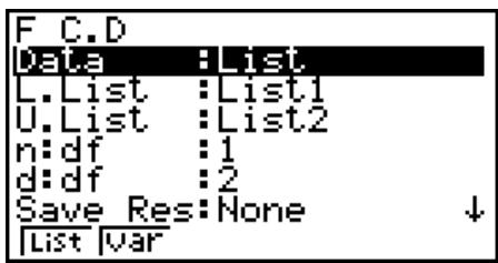
Calculation Result Output Examples
![F C.D 1 [0.2618] 2 0.1748 3 0.1299 4 0.1033 0.2678039855](/content/2025/01/86832/images/4de749c8c32f8ef7d876ace1072f2e62a46acd777604556eb5cd42298183fca3.jpg)
When a list is specified
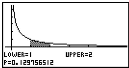
line
| Category | Value | | -------- | --------- | | LOWER | 1 | | UPPER | 2 | | P value | 0.129756512 |Graph when variable (x) is specified
- Graphing is supported only when a variable is specified and a single x -value is entered as data.
- Inverse F Cumulative Distribution
Inverse F Cumulative Distribution calculates the lower bound value of an F cumulative distribution probability for specified n:df and d:df (degrees of freedom of numerator and denominator) values.
F5 (DIST) F4 (F) F3 (InvF)
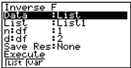
Calculation Result Output Examples
![Inverse F 1[3.5268] 2 3.5555 3 1.9215 4 1.125] 8.526315789](/content/2025/01/86832/images/138ec20705147c1e87cafedbbdd25788a6067ed4cfc70bafff2fc70bc4137568.jpg)
When a list is specified
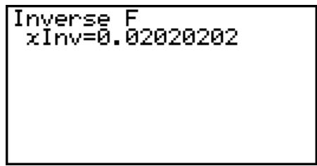
When variable (x) is specified
- There is no graphing for Inverse F Cumulative Distribution.
Binomial Distribution
- Binomial Probability
Binomial Probability calculates a probability at a specific single x-value or each list element for the discrete binomial distribution with the specified number of trials and probability of success on each trial. When a list is specified, calculation results for each list element are displayed in list form.
F5 (DIST) F5 (BINM) F1 (BPd)
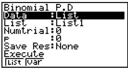
Calculation Result Output Examples
![Binomial P.D 1[0.1562] 2[0.3125] 3[0.1562] 4[0.3125] 0.15625](/content/2025/01/86832/images/510d503b8dca2d2ea73473773aca4447d24599bd0176694e7f15857033639690.jpg)
When a list is specified
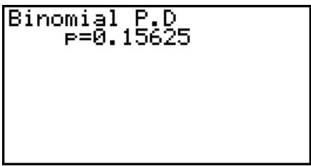
When variable (x) is specified
- There is no graphing for Binomial Probability.
• Binomial Cumulative Distribution
Binomial Cumulative Distribution calculates the cumulative probability in a binomial distribution that the success will occur on or before a specified trial.
F5 (DIST) F5 (BINM) F2 (BCd)
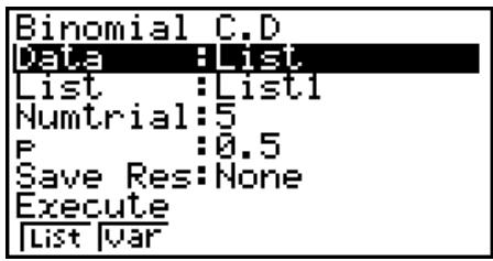
Calculation Result Output Examples
![Binomial C.D 1[0.1875] 2 0.5 3[0.1875] 4[ 0.5] 0.1875](/content/2025/01/86832/images/656f6e5dfaa2e56b19d8efae0752d7bce57a1530b4e8b0060ade68a8c8ab96dd.jpg)
When a list is specified
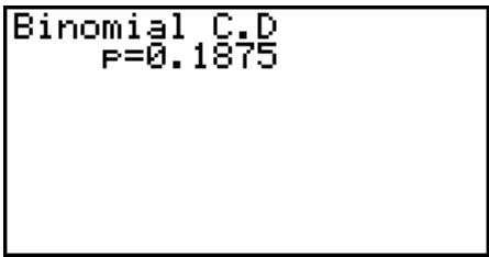
When variable (x) is specified
- There is no graphing for Binomial Cumulative Distribution.
• Inverse Binomial Cumulative Distribution
Inverse Binomial Cumulative Distribution calculates the minimum number of trials of a binomial cumulative distribution for specified values.
F5 (DIST) F5 (BINM) F3 (InvB)
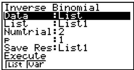
Calculation Result Output Examples
![Inverse Binomial 1 [ ] 1 2 | 3 | 4 [ ] 0 1](/content/2025/01/86832/images/8a79812f6b63db24e1ea4ab636fd14b347c3892b4e8ff2e82eed2549cd157d1d.jpg)
When a list is specified
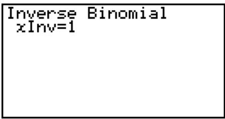
When variable (x) is specified
- There is no graphing for Inverse Binomial Cumulative Distribution.
Important!
When executing the Inverse Binomial Cumulative Distribution calculation, the calculator uses the specified Area value and the value that is one less than the Area value minimum number of significant digits (*Area value) to calculate minimum number of trials values.
The results are assigned to system variables xInv (calculation result using Area) and xInv (calculation result using Area ). The calculator always displays the xInv value only. However, when the xInv and *xInv values are different, the message shown below will appear with both values.
![WARNING! Area:0.2 xInv:3 Area-0.1 *xInv:2 Press:[EXIT]](/content/2025/01/86832/images/03c7eb91d15db1a26aa76e570a432dcccfb775e46d5c06eb604f86248c486aca.jpg)
The calculation results of Inverse Binomial Cumulative Distribution are integers. Accuracy may be reduced when the first argument has 10 or more digits. Note that even a slight difference in calculation accuracy affects calculation results. If a warning message appears, check the displayed values.
■ Poisson Distribution
- Poisson Probability
Poisson Probability calculates a probability at a specific single x-value or each list element for the discrete Poisson distribution with the specified mean.
F5 (DIST) F6 (▷) F1 (POISN) F1 (PPd)

Calculation Result Output Examples
![Poisson P.D 1 [0.3032] 2 [0.0758] 3 [0.3032] 4 [0.0758] 0.3032653299](/content/2025/01/86832/images/623c7aabc7bbbe08063b4525c99acda75cc8e378de8d6c61dc6e68a805407ae7.jpg)
When a list is specified
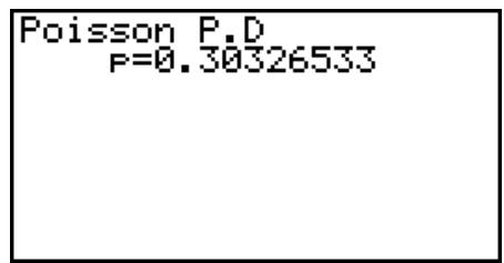
When variable (x) is specified
- There is no graphing for Poisson Probability.
- Poisson Cumulative Distribution
Poisson Cumulative Distribution calculates the cumulative probability in a Poisson distribution that the success will occur on or before a specified trial.
F5 (DIST) F6 (▷) F1 (POISN) F2 (PCd)
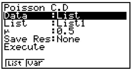
Calculation Result Output Examples
![Poisson C.D 1[0.9097] 2 0.9856 3 0.9097 4 0.9856] 0.9097959896](/content/2025/01/86832/images/2de43916d38e745dad3588f6db77f1fd27ceb43eaa0f5b07e66b77e5a966964a.jpg)
When a list is specified
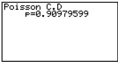
When variable (x) is specified
- There is no graphing for Poisson Cumulative Distribution.
- Inverse Poisson Cumulative Distribution
Inverse Poisson Cumulative Distribution calculates the minimum number of trials of a Poisson cumulative probability distribution for specified values.
F5 (DIST) F6 (▷) F1 (POISN) F3 (InvP)
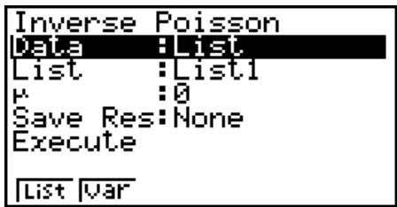
Calculation Result Output Examples
![Inverse Poisson 1 [ ] 4 2 [9.9E99] 3 [ ] 2 4 [ ] 3 4](/content/2025/01/86832/images/0b145b935341093115418a98f86294da2e69fe2cb42d56d5ea92b29b227eb7a4.jpg)
When a list is specified
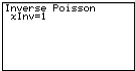
When variable (x) is specified
- There is no graphing for Inverse Poisson Cumulative Distribution.
Important!
When executing the Inverse Poisson Cumulative Distribution calculation, the calculator uses the specified Area value and the value that is one less than the Area value minimum number of significant digits (*Area value) to calculate minimum number of trials values.
The results are assigned to system variables xInv (calculation result using Area) and *xInv (calculation result using *Area). The calculator always displays the xInv value only. However, when the xInv and *xInv values are different, the message will appear with both values.
The calculation results of Inverse Poisson Cumulative Distribution are integers. Accuracy may be reduced when the first argument has 10 or more digits. Note that even a slight difference in calculation accuracy affects calculation results. If a warning message appears, check the displayed values.
■ Geometric Distribution
- Geometric Probability
Geometric Probability calculates the probability at a specific single x-value or each list element, and the number of the trial on which the first success occurs, for the geometric distribution with a specified probability of success.
F5 (DIST) F6 (▷) F2 (GEO) F1 (GPd)
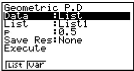
Calculation Result Output Examples
![Geometric P.D 1[0.5] 2[0.25] 3[0.125] 4[0.0625] 0.5](/content/2025/01/86832/images/276c25b8f1cdb49ddd222afc7420a2c44d618df34a1846a49f448e77a054eb14.jpg)
When a list is specified
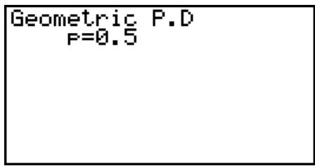
When variable (x) is specified
- There is no graphing for Geometric Probability.
- Geometric Cumulative Distribution
Geometric Cumulative Distribution calculates the cumulative probability in a geometric distribution that the success will occur on or before a specified trial.
F5 (DIST) F6 (▷) F2 (GEO) F2 (GCd)
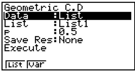
Calculation Result Output Examples
![Geometric C.D 1 [0.5] 2 [0.75] 3 [0.875] 4 [0.9375] 0.5](/content/2025/01/86832/images/a62ce664aca11c79882f7c8ed60d30a38e0578242288904f0c53eb5c6896423c.jpg)
When a list is specified
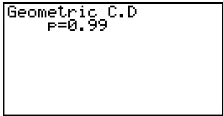
When variable (x) is specified
- There is no graphing for Geometric Cumulative Distribution.
- Inverse Geometric Cumulative Distribution
Inverse Geometric Cumulative Distribution calculates the minimum number of trials of a geometric cumulative probability distribution for specified values.
F5 (DIST) F6 (▷) F2 (GEO) F3 (InvG)
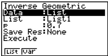
Calculation Result Output Examples
![Inverse Geometric 1 [3] 2 [3] 3 [5] 4 [1]](/content/2025/01/86832/images/8e9739b60ce079a8394ad9fe79dcf6e922baee065e62c0fc5f44216da5a5c475.jpg)
When a list is specified
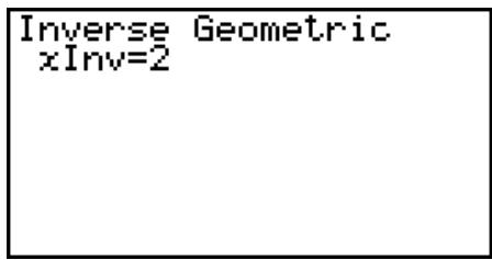
When variable (x) is specified
- There is no graphing for Inverse Geometric Cumulative Distribution.
Important!
When executing the Inverse Geometric Cumulative Distribution calculation, the calculator uses the specified Area value and the value that is one less than the Area value minimum number of significant digits (*Area value) to calculate minimum number of trials values.
The results are assigned to system variables xInv (calculation result using Area) and xInv (calculation result using Area ). The calculator always displays the xInv value only. However, when the xInv and *xInv values are different, the message will appear with both values.
The calculation results of Inverse Geometric Cumulative Distribution are integers. Accuracy may be reduced when the first argument has 10 or more digits. Note that even a slight difference in calculation accuracy affects calculation results. If a warning message appears, check the displayed values.
■ Hypergeometric Distribution
• Hypergeometric Probability
Hypergeometric Probability calculates the probability at a specific single x-value or each list element, and the number of the trial on which the first success occurs, for the hypergeometric distribution with a specified probability of success.
F5 (DIST) F6 (▷) F3 (H.GEO) F1 (HPd)
![Hypergeometric P.D Data : List List : List1 n : 5 M : 10 N : 20 Save Res: None ↓ [List |var]](/content/2025/01/86832/images/0d914f36258a07a48b3cc60a7bcc7920001f8c0f01e34780efbec8f05cc4ea5d.jpg)
Calculation Result Output Examples
![Hypergeometric P.D [0.1354] 2 0.3482 3 0.3482 4 0.0162] 0.1354489164](/content/2025/01/86832/images/f0636f9abf84a71d751fbd3c40ba8fa6f652a4fa628c62d10ad1035bc0fcf823.jpg)
When a list is specified
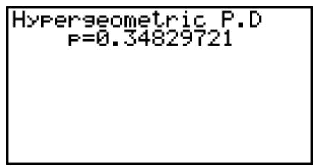
When variable (x) is specified
- There is no graphing for Hypergeometric Probability.
• Hypergeometric Cumulative Distribution
Hypergeometric Cumulative Distribution calculates the cumulative probability in a hypergeometric distribution that the success will occur on or before a specified trial.
F5 (DIST) F6 (▷) F3 (H.GEO) F2 (HCd)
![Hypergeometric C.D Data : List List : List1 n : 5 M : 10 N : 20 Save Res: None ↓ [List |var]](/content/2025/01/86832/images/f3f61f449479515233b5bf7906d1d6ba6f2ef2f6ce3ce0acb1f0cf6d35ac21e7.jpg)
Calculation Result Output Examples
![Hypergeometric C.D 1[0.1514] 2[0.5] 3[0.8482] 4[1] 0.1517027864](/content/2025/01/86832/images/c62dc2ef9aa56e6ee90a854b2706be813a87ffb86e5f42476707f7488d779fe0.jpg)
When a list is specified
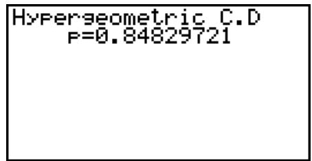
When variable (x) is specified
- There is no graphing for Hypergeometric Cumulative Distribution.
- Inverse Hypergeometric Cumulative Distribution
F5 (DIST) F6 (▷) F3 (H.GEO) F3 (InvH)
Inverse Hypergeometric Cumulative Distribution calculates the minimum number of trials of a hypergeometric cumulative probability distribution for specified values.
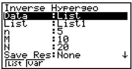
Calculation Result Output Examples
![Inverse Hypergeometri 1 [3] 2 [2] 3 [3] 4 [2] 2](/content/2025/01/86832/images/c6cb1bd30f3e77606bf656a131478c784478dbf608cbbb020d7bf27360866fec.jpg)
When a list is specified
When variable (x) is specified
- There is no graphing for Inverse Hypergeometric Cumulative Distribution.
Important!
When executing the Inverse Hypergeometric Cumulative Distribution calculation, the calculator uses the specified Area value and the value that is one less than the Area value minimum number of significant digits (*Area value) to calculate minimum number of trials values.
The results are assigned to system variables xInv (calculation result using Area) and *xInv (calculation result using *Area). The calculator always displays the xInv value only. However, when the xInv and *xInv values are different, the message will appear with both values.
The calculation results of Inverse Hypergeometric Cumulative Distribution are integers. Accuracy may be reduced when the first argument has 10 or more digits. Note that even a slight difference in calculation accuracy affects calculation results. If a warning message appears, check the displayed values.
8. Input and Output Terms of Tests, Confidence Interval, and Distribution (All models except fx-74000)
(All models except fx-7400GII)
The following explains the input and output terms that are used by tests, confidence interval, and distribution.
■ Input Terms
Data ......data type
(1-Sample Z Test) ......population mean value test conditions (“≠ _0 ” specifies two-tail test, “< _0 ” specifies lower one-tail test, “> _0 ” specifies upper one-tail test.)
_1 (2-Sample Z Test)......population mean value test conditions (“ _2 ” specifies two-tail test, “< _2 ” specifies one-tail test where sample 1 is smaller than sample 2, “> _2 ” specifies one-tail test where sample 1 is greater than sample 2.)
Prop (1-Prop Z Test) ......sample proportion test conditions (“≠ p_0 ” specifies two-tail test, “< p_0 ” specifies lower one-tail test, “> p_0 ” specifies upper one-tail test.)
p_1 (2-Prop Z Test).....sample proportion test conditions (“ p_2 ” specifies two-tail test, “< p_2 ” specifies one-tail test where sample 1 is smaller than sample 2, “> p_2 ” specifies one-tail test where sample 1 is greater than sample 2.)
(1-Sample t Test) ......population mean value test conditions (“≠ _0 ” specifies two-tail test, “< _0 ” specifies lower one-tail test, “> _0 ” specifies upper one-tail test.)
_1 (2-Sample t Test) ......sample mean value test conditions (“ _2 ” specifies two-tail test, “< _2 ” specifies one-tail test where sample 1 is smaller than sample 2, “> _2 ” specifies one-tail test where sample 1 is greater than sample 2.)
& (LinearReg t Test) ..... -value test conditions (“≠ 0” specifies two-tail test, “< 0” specifies lower one-tail test, “> 0” specifies upper one-tail test.)
_1 (2-Sample F Test)......population standard deviation test conditions (“ _2 ” specifies two-tail test, “ <_2 ” specifies one-tail test where sample 1 is smaller than sample 2, “ >_2 ” specifies one-tail test where sample 1 is greater than sample 2.)
_0 ......assumed population mean
......population standard deviation ( >0)
_1 ......population standard deviation of sample 1 ( _1 > 0 )
_2 ......population standard deviation of sample 2 ( _2 > 0 )
List ......list whose contents you want to use as data (List 1 to 26)
List1 ....list whose contents you want to use as sample 1 data (List 1 to 26)
List2......list whose contents you want to use as sample 2 data (List 1 to 26)
Freq......frequency (1 or List 1 to 26)
Freq1.....frequency of sample 1 (1 or List 1 to 26)
Freq2.....frequency of sample 2 (1 or List 1 to 26)
Execute....executes a calculation or draws a graph
......mean of sample
_1 ......mean of sample 1
_2 ......mean of sample 2
n......size of sample (positive integer)
n_1 ......size of sample 1 (positive integer)
n_2 ......size of sample 2 (positive integer)
p_0 ......expected sample proportion (0 < p_0 < 1)
p_1 ......sample proportion test conditions
x (1-Prop Z Test) ......sample value (x ≧ 0 integer)
x (1-Prop Z Interval)......data (0 or positive integer)
x_1 ......data value of sample 1 ( x_1 ≥ 0 integer)
x_2 ......data value of sample 2 ( x_2 ≥ 0 integer)
s_x ......sample standard deviation ( s_x > 0 )
s_x1 ......standard deviation of sample 1 ( s_x1 > 0 )
s_x2 ......standard deviation of sample 2 ( s_x2 > 0 )
XList......list for x-axis data (List 1 to 6)
YList......list for y-axis data (List 1 to 6)
C-Level.....confidence level (0 ≧ C-Level < 1)
Pooled....pooling On (in effect) or Off (not in effect)
x (Distribution)......data
(Distribution) ......standard deviation ( > 0 )
μ (Distribution) ......mean
Lower (Distribution)......lower boundary
Upper (Distribution)......upper boundary
df (Distribution) .....degrees of freedom (df > 0)
n:df (Distribution) ......numerator degrees of freedom (positive integer)
d:df (Distribution) ......denominator degrees of freedom (positive integer)
Numtrial (Distribution) ......number of trials
p (Distribution)......success probability (0 ≤ p ≤ 1)
Output Terms
z ......z score
p....p-value
t......t score
^2 …… ^2 value
F ......F value
......estimated sample proportion
_1 ......estimated proportion of sample 1
_2 ......estimated proportion of sample 2
......mean of sample
_1 ......mean of sample 1
_2 mean of sample 2
S_x ......sample standard deviation
S_x1 standard deviation of sample 1
S_x2 ......standard deviation of sample 2
s_p ......pooled sample standard deviation
n ......size of sample
n_1 ......size of sample 1
n_2 ......size of sample 2
df.....degrees of freedom
a......constant term
b....coefficient
S_e ...... standard error
r ....correlation coefficient
r^2 ...... coefficient of determination
Left.....confidence interval lower limit (left edge)
Right.....confidence interval upper limit (right edge)
9. Statistic Formula
Test
| Test | |
| 1-Sample Z Test | z = ( - _0)/( /) |
| 2-Sample Z Test | z = (_1 - _2)/(_1^2/n_1) + (_2^2/n_2) |
| 1-Prop Z Test | z = (x/n - p_0)/_0(1 - p_0)/n |
| 2-Prop Z Test | z = (x_1/n_1 - x_2/n_2)/(1 - )(1/n_1 + 1/n_2) |
| 1-Sample t Test | t = ( - _0)/(s_x/) |
| 2-Sample t Test (pooled) | t = (_1 - _2)/_p^2(1/n_1 + 1/n_2) s_p = ((n_1 - 1)s_x1^2 + (n_2 - 1)s_x2^2)/(n_1 + n_2 - 2) df = n_1 + n_2 - 2 |
| 2-Sample t Test (not pooled) | t = (_1 - _2)/_x1^2/n_1 + s_x2^2/n_2 df = 1/(C^2/(n_1 - 1) + (1 - C)^2/(n_2 - 1)) C = (s_x1^2/n_1)/(s_x1^2/n_1 + s_x2^2/n_2) |
| LinearReg t Test | b = _i=1^n(x_i - )(y_i - )/_i=1^n(x_i - )^2 a = - b t = r(n - 2)/(1 - r^2) |
| ^2 GOF Test | ^2 = _i^k(O_i - E_i)^2/E_i O_i: The i-th element of the observed list E_i: The i-th element of the expected list |
| ^2 two-way Test | ^2 = _i^k_j^l(O_ij - E_ij)^2/E_ij O_ij: The element at row i, column j of the observed matrix E_ij = _i=1^kx_ij · _j=1^lx_ij/ n E_ij: The element at row i, column j of the expected matrix |
| 2-Sample F Test | F = s_x1^2/s_x2^2 |
| ANOVA Test | F = MS/MSe MS = SS/Fdf MSe = SSe/Edf SS = _i=1^kn_i(_i - )^2 SSe = _i=1^k(n_i - 1)s_xi^2 Fdf = k - 1 Edf = _i=1^k(n_i - 1) |
■ Confidence Interval
| Confidence Interval | Left: confidence interval lower limit (left edge)Right: confidence interval upper limit (right edge) |
| 1-Sample Z Interval | Left, Right = Z(/2) · / |
| 2-Sample Z Interval | Left, Right = (_1 - _2) Z(/2)_1^2/n_1 + _2^2/n_2 |
| 1-Prop Z Interval | Left, Right = x/n Z(/2)1/n · (x/n · (1 - x/n)) |
| 2-Prop Z Interval | Left, Right = (x_1/n_1 - x_2/n_2) Z(/2)(x_1/n_1 · (1 - x_1/n_1))/n_1 + (x_2/n_2 · (1 - x_2/n_2))/n_2 |
| 1-Sample t Interval | Left, Right = t_n-1(/2) · s_x/ |
| 2-Sample t Interval(pooled) | Left, Right = (_1 - _2) t_n_1+n_2-2(/2)_p^2(1/n_1 + 1/n_2) s_p = ((n_1 - 1)s_x_1^2 + (n_2 - 1)s_x_2^2)/(n_1 + n_2 - 2) |
| 2-Sample t Interval(not pooled) | Left, Right = (_1 - _2) t_df(/2)_x_1^2/n_1 + s_x_2^2/n_2 df = 1/(C^2/(n_1 - 1) + (1 - C)^2/(n_2 - 1)) C = (s_x_1^2/n_1)/(s_x_1^2/n_1 + s_x_2^2/n_2) |
: level of significance = 1 - [C - Level] C-Level: confidence level (0≤ C - Level < 1)
Z( /2) : upper /2 point of standard normal distribution
t_df ( /2 ): upper /2 point of t distribution with df degrees of freedom
■ Distribution (Continuous)
| Distribution | Probability Density | Cumulative Distribution |
| Normal Distribution | p(x) = 12 e^-(x-)^22^2 ( > 0) |  |
| Student-t Distribution | p(x) = (+12)(2) × (1+^2df)^-+12 × df | |
| ^2 Distribution | p(x) = 1(2) × (12)^2 × x^(2-1) × e^-2 (x ≥ 0) | |
| F Distribution | p(x) = (+ddf2)(2) × (2) ()^2 x^2-1 (1 + × xddf)^-+ddf2 (x ≥ 0) |
| Distribution | Inverse Cumulative Distribution | ||
| Normal Distribution | p = _-^Upper p(x)dx tail = Left | p = _Lower^ p(x)dx tail = Right | p = _Lower^Upper p(x)dx tail = Central |
| Student-t Distribution | p = _Lower^ p(x)dx | ||
| ^2 Distribution | |||
| F Distribution | |||
■ Distribution (Discrete)
| Distribution | Probability | |
| Binomial Distribution | p(x) = _nC_xp^x(1-p)^n-x (x = 0, 1, ·s, n) n : number of trials | |
| Poisson Distribution | p(x) = ^- × ^xx! (x = 0, 1, 2, ·s) : mean ( > 0 ) | |
| Geometric Distribution | p(x) = p(1-p)^x-1 (x = 1, 2, 3, ·s) | |
| Hypergeometric Distribution | p(x) = _x × N - MC_n-xNC_n n : Number of elements extracted from population ( 0 ≤ x integer) M : Number of elements contained in attribute A ( 0 ≤ M integer) N : Number of population elements ( n ≤ N, M ≤ N integer) | |
| Distribution | Cumulative Distribution | Inverse Cumulative Distribution |
| Binomial Distribution | p = _x=0^X p(x) | p ≤ _x=0^X p(x) |
| Poisson Distribution | ||
| Geometric Distribution | p = _x=1^X p(x) | p ≤ _x=1^X p(x) |
| Hypergeometric Distribution | p = _x=0^X p(x) | p ≤ _x=0^X p(x) |
Chapter 7 Financial Calculation (TVM)
Important!
- The fx-7400GII is not equipped with the TVM mode.
1. Before Performing Financial Calculations
From the Main Menu, enter the TVM mode and display the Financial screen like the one shown below.
Financial 1 screen
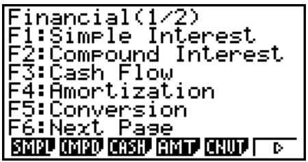
Financial 2 screen
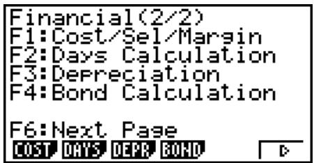
- {SMPL} ... {simple interest}
- {CMPD} ... {compound interest}
- {CASH} ... {cash flow (investment appraisal)}
- {AMT} ... {amortization}
- {CNVT} ... {interest rate conversion}
- {COST} ... {cost, selling price, margin}
- {DAYS} ... {day/date calculations}
- {DEPR} ... {depreciation calculations}
• {BOND} ... {bond calculations}
Setup Items
- Payment
- {BGN}/{END} ... Specifies {beginning of the period}/{end of the period} payment
- Date Mode
- {365}/{360} ... Specifies calculation according to a {365-day}/{360-day} year
- Periods/YR. (payment interval specification)
- {Annu}/{Semi} ... {annual}/{semiannual}
Note the following points regarding Setup screen settings whenever using the TVM mode.
- The following graph Setup screen settings are all turned off for graphing in the TVM mode: Axes, Grid, Dual Screen.
- Drawing a financial graph while the Label item is turned on, displays the label CASH for the vertical axis (deposits, withdrawals), and TIME for the horizontal axis (frequency).
■ Graphing in the TVM Mode
After performing a financial calculation, you can use F6 (GRPH) to graph the results as shown below.
natural_image
Simple geometric shape with two adjacent rectangles (no text or symbols)- Pressing SHIFT F1 (TRCE) while a graph is on the display activates Trace, which can be used to look up other financial values. In the case of simple interest, for example, pressing ▶ displays PV, SI, and SFV. Pressing ◀ displays the same values in reverse sequence.
- Zoom, Scroll, and Sketch cannot be used in the TVM mode.
- Whether you should use a positive or a negative value for the present value (PV) or the purchase price (PRC) depends on the type of calculation you are trying to perform.
- Note that graphs should be used only for reference purposes when viewing TVM mode calculation results.
- Note that calculation results produced in this mode should be regarded as reference values only.
- Whenever performing an actual financial transaction, be sure to check any calculation results obtained using this calculator with against the figures calculated by your financial institution.
2. Simple Interest
This calculator uses the following formulas to calculate simple interest.
- Formula
$$ \begin{array}{l l l l} 3 6 5 \text {-day Mode} & S I ^ {\prime} = \frac {n}{3 6 5} \times P V \times i \quad \left(i = \frac {I \%}{1 0 0}\right) & S I: \text {interest} \ 3 6 0 \text {-day Mode} & S I ^ {\prime} = \frac {n}{3 6 0} \times P V \times i \quad \left(i = \frac {I \%}{1 0 0}\right) & P V: \text {principal} \ & & I \%: \text {annual interest} \ & S I = - S I ^ {\prime} & S F V: \text {principal plus interest} \ & S F V = - (P V + S I ^ {\prime}) \end{array} $$
Press F1(SMPL) from the Financial 1 screen to display the following input screen for simple interest.
F1(SMPL)
n ...... number of interest periods (days)
I% ...... annual interest rate
PV ...... principal
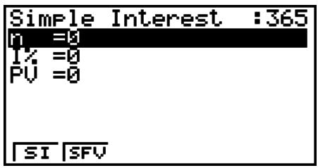
After configuring the parameters, use one of the function menus noted below to perform the corresponding calculation.
- {SI} ... {simple interest}
- {SFV} ... {simple future value}
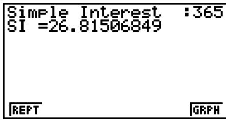
- An error (Ma ERROR) occurs if parameters are not configured correctly.
Use the following function menus to maneuver between calculation result screens.
- {REPT} ... {parameter input screen}
- {GRPH} ... {draws graph}

natural_image
Simple geometric shape with two adjacent rectangles, no text or symbols presentAfter drawing a graph, you can press SHIFT F1 (TRCE) to turn on trace and read calculation results along the graph.
Each press of ▶ while trace is turned on cycles the displayed value in the sequence: present value (PV) simple interest (SI) simple future value (SFV) . Pressing ◀ cycles in the reverse direction.
Press EXIT to return to the parameter input screen.
3. Compound Interest
This calculator uses the following standard formulas to calculate compound interest.
- PV, PMT, FV, n
$$ \underline {{I \% \neq 0}} $$
$$ P V = - (\alpha \times P M T + \beta \times F V) $$
$$ P M T = - \frac {P V + \beta \times F V}{\alpha} $$
$$ F V = - \frac {P V + \alpha \times P M T}{\beta} $$
$$ n = \frac {\log \left{\frac {(1 + i S) \times P M T - F V \times i}{(1 + i S) \times P M T + P V \times i} \right}}{\log (1 + i)} $$
$$ \underline{I \%} = 0 $$
$$ P V = - (P M T \times n + F V) $$
$$ P M T = - \frac {P V + F V}{n} $$
$$ F V = - (P M T \times n + P V) $$
$$ n = - \frac {P V + F V}{P M T} $$
$$ \alpha = (1 + i \times S) \times \frac {1 - \beta}{i}, \beta = (1 + i) ^ {- n} $$
$$ S = \left{ \begin{array}{l} 0 \dots\dots \ (S e t u p S c r e e n) \ 1 \dots\dots \ (S e t u p S c r e e n) \end{array} \right. $$
$$ i = \left{ \begin{array}{l} \frac {I \%}{1 0 0} \dots \dots (P / Y = C / Y = 1) \ \left(1 + \frac {I \%}{1 0 0 \times [ C / Y ]}\right) ^ {\frac {C / Y}{P / Y}} - 1 \dots .. (\text { Other than } \ \text { those above }) \end{array} \right. $$
• I %
i (effective interest rate)
i (effective interest rate) is calculated using Newton's Method.
$$ P V + \alpha \times P M T + \beta \times F V = 0 $$
To I % from i (effective interest rate)
$$ I \% = \left{ \begin{array}{l} i \times 100 \dots\dots (P / Y = C / Y = 1) \ \left{(1 + i)^{\frac{P / Y}{C / Y}} - 1\right} \times C / Y \times 100... (\text{Other than those above}) \end{array} \right. $$
n...... number of compound periods
FV...... future value
I% ...... annual interest rate
P/Y ...... installment periods per year
PV...... present value
C/Y ...... compounding periods per year
PMT..... payment
- A deposit is indicated by a plus sign (+), while a withdrawal is indicated by a minus sign (−).
Press F2(CMPD) from the Financial 1 screen to display the following input screen for compound interest.
F2 (CMPD)
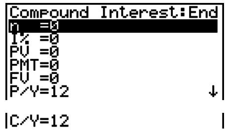
n ...... number of compound periods
I% ...... annual interest rate
PV ...... present value (loan amount in case of loan; principal in case of savings)
PMT ..... payment for each installment (payment in case of loan; deposit in case of savings)
FV ...... future value (unpaid balance in case of loan; principal plus interest in case of savings)
P/Y ...... installment periods per year
C/Y ..... compounding periods per year
Important!
Inputting Values
A period (n) is expressed as a positive value. Either the present value (PV) or future value (FV) is positive, while the other (PV or FV) is negative.
Precision
This calculator performs interest calculations using Newton's Method, which produces approximate values whose precision can be affected by various calculation conditions. Because of this, interest calculation results produced by this calculator should be used keeping the above limitation in mind or the results should be verified.
After configuring the parameters, use one of the function menus noted below to perform the corresponding calculation.
- n ... {number of compound periods}
- 1% ... {annual interest rate}
- {PV} ... {present value} (Loan: loan amount; Savings: balance)
- {PMT} ... {payment} (Loan: installment; Savings: deposit)
- {FV} ... {future value} (Loan: unpaid balance; Savings: principal plus interest)
- {AMT} ... {amortization screen}
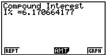
- An error (Ma ERROR) occurs if parameters are not configured correctly.
Use the following function menus to maneuver between calculation result screens.
- {REPT} ... {parameter input screen}
- {AMT} ... {amortization screen}
- {GRPH} ... {draws graph}

natural_image
Simple geometric shape with a horizontal line and right-angle corner, no text or symbols present.After drawing a graph, you can press SHIFT F1 (TRCE) to turn on trace and read calculation results along the graph.
Press EXIT to return to the parameter input screen.
4. Cash Flow (Investment Appraisal)
This calculator uses the discounted cash flow (DCF) method to perform investment appraisal by totalling cash flow for a fixed period. This calculator can perform the following four types of investment appraisal.
- Net present value (NPV)
- Net future value (NFV)
- Internal rate of return (IRR)
- Payback period (PBP)
A cash flow diagram like the one shown below helps to visualize the movement of funds.
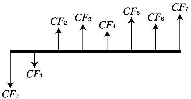
With this graph, the initial investment amount is represented by CF_0 . The cash flow one year later is shown by CF_1 , two years later by CF_2 , and so on.
Investment appraisal can be used to clearly determine whether an investment is realizing profits that were originally targeted.
• NPV
$$ N P V = C F _ {0} + \frac {C F _ {1}}{(1 + i)} + \frac {C F _ {2}}{(1 + i) ^ {2}} + \frac {C F _ {3}}{(1 + i) ^ {3}} + \dots + \frac {C F _ {n}}{(1 + i) ^ {n}} \quad \left(i = \frac {I \%}{1 0 0}\right) $$
n: natural number up to 254
• NFV
$$ N F V = N P V \times (1 + i) ^ {n} $$
- IRR
$$ 0 = C F _ {0} + \frac {C F _ {1}}{(1 + i)} + \frac {C F _ {2}}{(1 + i) ^ {2}} + \frac {C F _ {3}}{(1 + i) ^ {3}} + \dots + \frac {C F _ {n}}{(1 + i) ^ {n}} $$
In this formula, NPV = 0, and the value of IRR is equivalent to i × 100 . It should be noted, however, that minute fractional values tend to accumulate during the subsequent calculations performed automatically by the calculator, so NPV never actually reaches exactly zero. IRR becomes more accurate the closer than NPV approaches to zero.
• PBP
$$ P B P = \left{ \begin{array}{l} 0 \dots \dots (C F _ {0} \geq 0) \ n - \frac {N P V _ {n}}{N P V _ {n + 1} - N P V _ {n}} \dots (\text {Other than those above}) \end{array} \right. \quad N P V _ {n} = \sum_ {k = 0} ^ {n} \frac {C F _ {k}}{(1 + i) ^ {k}} $$
n: smallest positive integer that satisfies the conditions NPV_n ≤ 0 , NPV_n+1 ≥ 0 , or 0
Press F3 (CASH) from the Financial 1 screen to display the following input screen for Cash Flow.
F3 (CASH)
I% ...... interest rate
Csh ..... list for cash flow
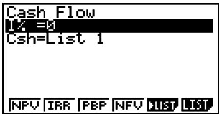
If you have not yet input data into a list, press F5(▶LIST) and input data into a list.
After configuring the parameters, use one of the function menus noted below to perform the corresponding calculation.
- {NPV} ... {net present value}
- {IRR} ... {internal rate of return}
- {PBP} ... {payback period}
- {NFV} ... {net future value}
- {▶LIST} ... {inputs data into a list}
- {LIST} ... {specifies a list for data input}
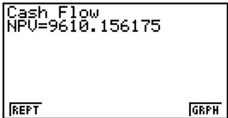
- An error (Ma ERROR) occurs if parameters are not configured correctly.
Use the following function menus to maneuver between calculation result screens.
- {REPT} ... {parameter input screen}
- {GRPH} ... {draws graph}
natural_image
Pure horizontal line with vertical tick marks, no text or symbols presentAfter drawing a graph, you can press SHIFT F1 (TRCE) to turn on trace and read calculation results along the graph.
Press EXIT to return to the parameter input screen.
5. Amortization
This calculator can be used to calculate the principal and interest portion of a monthly installment, the remaining principal, and amount of principal and interest repaid up to any point.
- Formula
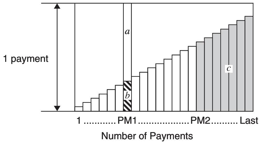
bar
| Number of Payments | Payment Amount | | ------------------ | -------------- | | 1 | 0 | | PM1 | 1 | | PM2 | 2 | | Last | 3 |a: interest portion of installment PM1 (INT)
b: principal portion of installment PM1 (PRN)
c: balance of principal after installment PM2 (BAL)
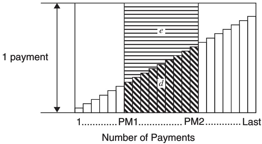
bar
| Number of Payments | Value | |---|---| | 1 payment | 1 | | PM1 | e | | PM2 | d | | Last | |d: total principal from installment PM1 to payment of installment PM2 ( PRN )
e: total interest from installment PM1 to payment of installment PM2 (ΣINT)
$$ ^ {*} a + b = \text { one repayment } (P M T) $$
$$ a: I N T _ {\mathrm{PM} 1} = \left| B A L _ {\mathrm{PM} 1 - 1} \times i \right| \times (P M T \text { sign }) $$
$$ b: P R N _ {\mathrm{PM} 1} = P M T + B A L _ {\mathrm{PM} 1 - 1} \times i $$
$$ c: B A L _ {\mathrm{PM} 2} = B A L _ {\mathrm{PM} 2 - 1} + P R N _ {\mathrm{PM} 2} $$
$$ d: \sum_ {\mathrm{PM} 1} ^ {\mathrm{PM} 2} P R N = P R N _ {\mathrm{PM} 1} + P R N _ {\mathrm{PM} 1 + 1} + \dots + P R N _ {\mathrm{PM} 2} $$
$$ e: \sum_ {\mathrm{PM} 1} ^ {\mathrm{PM} 2} I N T = I N T _ {\mathrm{PM} 1} + I N T _ {\mathrm{PM} 1 + 1} + \dots + I N T _ {\mathrm{PM} 2} $$
BAL_0=PV(INT_1=0 and PRN_1=PMT at beginning of installment term)
- Converting between the nominal interest rate and effective interest rate
The nominal interest rate (I% value input by user) is converted to an effective interest rate (I%') for installment loans where the number of installments per year is different from the number of compound interest calculation periods.
$$ I \% ^ {\prime} = \left{\left(1 + \frac {I \%}{100 \times [ C / Y ]}\right) ^ {\frac {[ C / Y ]}{[ P / Y ]}} - 1 \right} \times 100 $$
The following calculation is performed after conversion from the nominal interest rate to the effective interest rate, and the result is used for all subsequent calculations.
$$ i = I\%^{\prime}\div 100 $$
Press F4(AMT) from the Financial 1 screen to display the following input screen for amortization.
F4 (AMT)
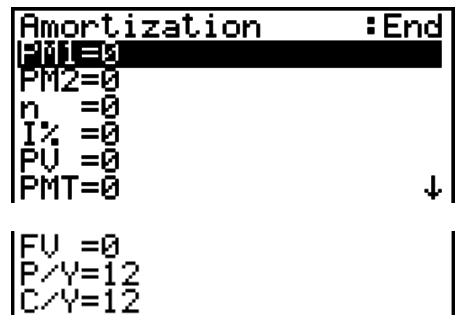
PM1...... first installment of installments 1 through n
PM2...... second installment of installments 1 through n
n ...... installments
I% ...... interest rate
PV ...... principal
PMT ..... payment for each installment
FV ...... balance following final installment
P/Y ...... installments per year
C/Y ..... compoundings per year
After configuring the parameters, use one of the function menus noted below to perform the corresponding calculation.
- {BAL} ... {balance of principal after installment PM2}
- {INT} ... {interest portion of installment PM1}
- {PRN} ... {principal portion of installment PM1}
- ... {total interest paid from installment PM1 to installment PM2}
- PRN ... {total principal paid from installment PM1 to installment PM2}
- {CMPD} ... {compound interest screen}
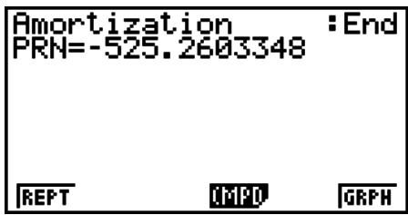
-
An error (Ma ERROR) occurs if parameters are not configured correctly.
Use the following function menus to maneuver between calculation result screens. -
{REPT} ... {parameter input screen}
- {CMPD} ... {compound interest screen}
- {GRPH} ... {draws graph}
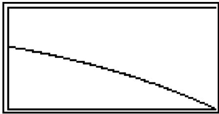
natural_image
Simple black dashed diagonal line on white background, no text or symbols presentAfter drawing a graph, you can press SHIFT F1 (TRCE) to turn on trace and read calculation results along the graph.
The first press of SHIFT F1 (TRCE) displays INT and PRN when n = 1. Each press of ▶ shows INT and PRN when n = 2, n = 3, and so on.
Press EXIT to return to the parameter input screen.
6. Interest Rate Conversion
The procedures in this section describe how to convert between the annual percentage rate and effective interest rate.
- Formula
$$ E F F = \left[ \left(1 + \frac {A P R / 1 0 0}{n}\right) ^ {n} - 1 \right] \times 1 0 0 $$
APR : annual percentage rate (%)
EFF: effective interest rate (%)
$$ A P R = \left[ \left(1 + \frac {E F F}{1 0 0}\right) ^ {\frac {1}{n}} - 1 \right] \times n \times 1 0 0 $$
n : number of compoundings
Press F5(CNVT) from the Financial 1 screen to display the following input screen for interest rate conversion.
F5 (CNVT)
n .... number of compoundings I% .... interest rate
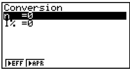
After configuring the parameters, use one of the function menus noted below to perform the corresponding calculation.
- EFF} ... {converts annual percentage rate to effective interest rate}
- ... {converts effective interest rate to annual percent rate}
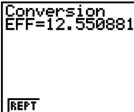
- An error (Ma ERROR) occurs if parameters are not configured correctly.
Use the following function menu to maneuver between calculation result screens. - {REPT} ... {parameter input screen}
7. Cost, Selling Price, Margin
Cost, selling price, or margin can be calculated by inputting the other two values.
- Formula
$$ C S T = S E L \left(1 - \frac {M R G}{1 0 0}\right) $$
CST : cost
$$ S E L = \frac {C S T}{1 - \frac {M R G}{1 0 0}} $$
SEL : selling price
$$ M R G (\%) = \left(1 - \frac {C S T}{S E L}\right) \times 100 $$
MRG : margin
Press F1(COST) from the Financial 2 screen to display the following input screen.
F6 (▷) F1 (COST)
Cst...... cost
Sel...... selling price
Mrg...... margin
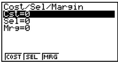
After configuring the parameters, use one of the function menus noted below to perform the corresponding calculation.
- {COST} ... {cost}
- {SEL} ... {selling price}
- {MRG} ... {margin}
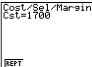
- An error (Ma ERROR) occurs if parameters are not configured correctly.
Use the following function menu to maneuver between calculation result screens.
- {REPT} ... {parameter input screen}
8. Day/Date Calculations
You can calculate the number of days between two dates, or you can determine what date comes a specific number of days before or after another date.
Press F2(DAYS) from the Financial 2 screen to display the following input screen for day/date calculation.
F6 (▷) F2 (DAYS)
d1 ..... date 1
d2...... date 2
D ...... number of days
To input a date, first highlight d1 or d2. Pressing a number key to input the month causes an input screen like the one shown below to appear on the display.
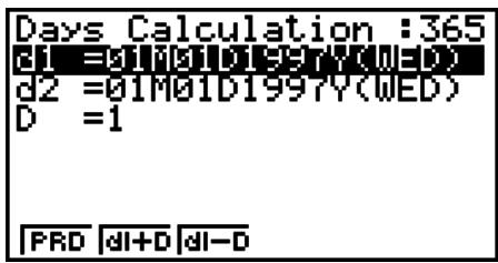
![Input a Date ...Month M[1~12]: 8 PRD dI+D dI-D](/content/2025/01/86832/images/acccb2ce2fb0d73b1c8d139c6ebea825c21573b57420040d3bdec9564f2cea63.jpg)
Input the month, day, and year, pressing EXE after each.
After configuring the parameters, use one of the function menus noted below to perform the corresponding calculation.
- {PRD} ... {number of days from d1 to d2 (d2 - d1)}
- d1 + D d1 plus a number of days (d1 + D)
- {d1-D} ... {d1 minus a number of days (d1 - D)}
- An error (Ma ERROR) occurs if parameters are not configured correctly.
Use the following function menu to maneuver between calculation result screens.
- {REPT} ... {parameter input screen}
- The Setup screen can be used to specify either a 365-day or 360-day year for financial calculations. Day/date calculations are also performed in accordance with the current setting for number of days in the year, but the following calculations cannot be performed when the 360-day year is set. Attempting to do so causes an error.
(Date) + (Number of Days)
(Date) – (Number of Days)
- The allowable calculation range is January 1, 1901 to December 31, 2099.
• 360-day Date Mode Calculations
The following describes how calculations are processed when 360 is specified for the Date Mode item in the Setup screen.
- If d1 is day 31 of a month, d1 is treated as day 30 of that month is used.
- If d2 is day 31 of a month, d2 is treated as day 1 of the following month, unless d1 is day 30.
9. Depreciation
Depreciation lets you calculate the amount that a business expense can be offset by income (depreciated) over a given year.
- This calculator supports the following four types of depreciation calculations.
straight-line (SL), fixed-percentage (FP), sum-of-the-years'-digits (SYD), or declining-balance (DB). - Any one of the above methods can be used to calculate depreciation for a specified period.
A table and graph of the depreciated amount and undepreciated amount in year j.
- Straight-Line Method (SL)
$$ S L _ {1} = \frac {(P V - F V)}{n} \cdot \frac {{Y - 1 }}{1 2} $$
$$ S L _ {j} = \frac {(P V - F V)}{n} $$
$$ S L _ {n + 1} = \frac {(P V - F V)}{n} \cdot \frac {1 2 - {Y - 1 }}{1 2} $$
$$ ({Y - 1 } \neq 1 2) $$
SL_j : depreciation charge for the jth year n : useful life
PV : original cost (basis)
FV : residual book value
j : year for calculation of depreciation cost
Y-1 : number of months in the first year of depreciation
• Fixed-Percentage Method (FP)
$$ F P _ {1} = P V \times \frac {I \%}{1 0 0} \times \frac {{Y - 1 }}{1 2} $$
$$ F P _ {j} = \left(R D V _ {j - 1} + F V\right) \times \frac {I \%}{1 0 0} $$
$$ F P _ {n + 1} = R D V _ {n} \quad ({Y - 1 } \neq 1 2) $$
$$ R D V _ {1} = P V - F V - F P _ {1} $$
$$ R D V _ {j} = R D V _ {j - 1} - F P _ {j} $$
$$ R D V _ {n + 1} = 0 \quad ({Y - 1 } \neq 1 2) $$
FP_j : depreciation charge for the jth year RDV_j : remaining depreciable value at the end of jth year
I% : depreciation ratio
- Sum-of-the-Years’-Digits Method (SYD)
$$ Z = \frac {n (n + 1)}{2} \quad n ^ {\prime} = n - \frac {{Y - 1 }}{1 2} $$
$$ Z ^ {\prime} = \frac {(n ^ {\prime} \text {integer part} + 1) (n ^ {\prime} \text {integer part} + 2 ^ {*} n ^ {\prime} \text {fraction part})}{2} $$
$$ S Y D _ {1} = \frac {n}{Z} \times \frac {{Y - 1 }}{1 2} (P V - F V) $$
$$ S Y D _ {j} = \left(\frac {n ^ {\prime} - j + 2}{Z ^ {\prime}}\right) \left(P V - F V - S Y D _ {1}\right) \quad (j \neq 1) $$
$$ S Y D _ {n + 1} = \left(\frac {n ^ {\prime} - (n + 1) + 2}{Z ^ {\prime}}\right) \left(P V - F V - S Y D _ {1}\right) \times \frac {1 2 - {Y - 1 }}{1 2} \quad ({Y - 1 } \neq 1 2) $$
$$ R D V _ {1} = P V - F V - S Y D _ {1} $$
$$ R D V _ {j} = R D V _ {j - 1} - S Y D _ {j} $$
SYD_j : depreciation charge for the jth year
RDV_j : remaining depreciable value at the end of jth year
- Declining-Balance Method (DB)
$$ D B _ {1} = P V \times \frac {I \%}{1 0 0 n} \times \frac {Y - 1}{1 2} $$
$$ R D V _ {1} = P V - F V - D B _ {1} $$
$$ D B _ {j} = \left(R D V _ {j - 1} + F V\right) \times \frac {I \%}{1 0 0 n} $$
$$ R D V _ {j} = R D V _ {j - 1} - D B _ {j} $$
$$ D B _ {n + 1} = R D V _ {n} \quad ({Y - 1 } \neq 1 2) $$
$$ R D V _ {n + 1} = 0 \quad ({Y - 1 } \neq 1 2) $$
DB_j : depreciation charge for the jth year
RDV_j : remaining depreciable value at the end of jth year
I% : depreciation factor
Press F3 (DEPR) from the Financial 2 screen to display the following input screen for depreciation calculation.
F6 (▷) F3 (DEPR)
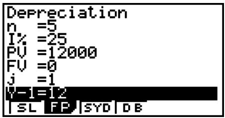
n...... useful life
I% ...... depreciation ratio in the case of the fixed percent (FP) method, depreciation factor in the case of the declining balance (DB) method
PV...... original cost (basis)
FV...... residual book value
j...... year for calculation of depreciation cost
Y-1...... number of months in the first year of depreciation
After configuring the parameters, use one of the function menus noted below to perform the corresponding calculation.
- {SL} ... {Calculate depreciation for year j using the straight-line method}
- {FP} ... {FP} ....{Calculate depreciation for year j using the fixed-percentage method} {I%} ....{Calculate depreciation ratio}
- {SYD} ... {Calculate depreciation for year j using the sum-of-the-years'-digits method}
- {DB} ... {Calculate depreciation for year j calculated using the declining-balance method}
Calculation Result Output Examples

{SYD}
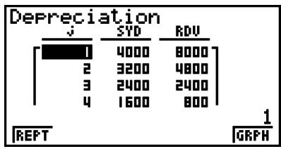
bar
Depreciation | j | SYD | RDU | |---|---|---| | 1 | 4000 | 8000 | | 2 | 3200 | 4800 | | 3 | 2400 | 2400 | | 4 | 1600 | 800 | REPT 1 GRAPH{SYD} - {TABL}
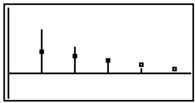
bar
| Category | Value | |---|---| | 1 | 0.8 | | 2 | 0.6 | | 3 | 0.4 | | 4 | 0.2 | | 5 | 0.1 |{SYD} - {GRPH}
An error (Ma ERROR) occurs if parameters are not configured correctly.
Use the following function menu to maneuver between calculation result screens.
- {REPT} ... {parameter input screen}
- {TABL} ... {displays table}
- {GRPH} ... {draws graph}
10. Bond Calculations
Bond calculation lets you calculate the purchase price or the annual yield of a bond. Before starting bond calculations, use the Setup screen to configure “Date Mode” and “Periods/YR.” settings (page 7-1).
- Formula
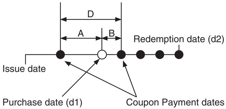
flowchart
graph TD
    A["Issue date"] --> B["Purchase date (d1)"]
    B --> C["Coupon Payment dates"]
    C --> D["Redemption date (d2)"]
    style A fill:#000,stroke:#fff,color:#fff
    style B fill:#000,stroke:#fff,color:#fff
    style C fill:#000,stroke:#fff,color:#fff
    style D fill:#000,stroke:#fff,color:#fff
PRC : price per \$100 of face value
CPN : annual coupon rate (%)
YLD : yield to maturity (%)
A : accrued days
M : number of coupon payments per year (1=annual, 2=semi annual)
N : number of coupon payments between settlement date and maturity date
RDB : redemption price or call price per \$100 of face value
D : number of days in coupon period where settlement occurs
B : number of days from settlement date until next coupon payment date = D - A
INT : accrued interest
CST : price including interest
• Price per \$100 of face value (PRC)
- For one or fewer coupon period to redemption
$$ P R C = - \frac {R D V + \frac {C P N}{M}}{1 + \left(\frac {B}{D} \times \frac {Y L D / 1 0 0}{M}\right)} + \left(\frac {A}{D} \times \frac {C P N}{M}\right) $$
- For more than one coupon period to redemption
$$ P R C = - \frac {R D V}{\left(1 + \frac {Y L D / 1 0 0}{M}\right) ^ {(N - 1 + B / D)}} - \sum_ {k = 1} ^ {N} \frac {\frac {C P N}{M}}{\left(1 + \frac {Y L D / 1 0 0}{M}\right) ^ {(k - 1 + B / D)}} + \frac {A}{D} \times \frac {C P N}{M} $$
$$ I N T = - \frac {A}{D} \times \frac {C P N}{M} \quad C S T = P R C + I N T $$
• Annual Yield (YLD)
YLD is calculated using Newton's Method.
Press F4 (BOND) from the Financial 2 screen to display the following input screen for Bond calculation.
F6 (▷) F4 (BOND)
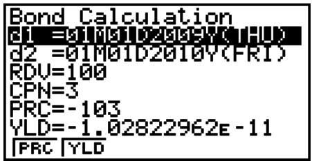
d1 ...... purchase date (month, date, year)
d2...... redemption date (month, date, year)
RDV..... redemption price per \$100 of face value
CPN..... coupon rate
PRC ..... price per \$100 of face value
YLD ..... annual yield
After configuring the parameters, use one of the function menus noted below to perform the corresponding calculation.
- {PRC} ... {Calculate the bond's price (PRC), accrued interest (INT), and cost of bond (CST)}
- {YLD} ... {Calculate the yield to maturity}
Calculation Result Output Examples
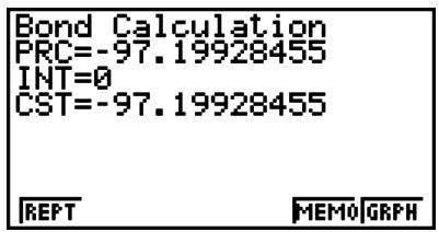
{PRC}
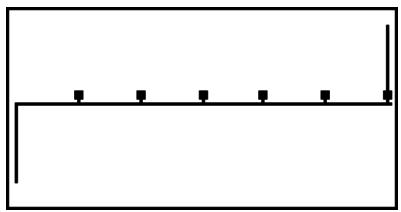
natural_image
Pure electrical circuit lines without any symbols{PRC} - {GRPH}
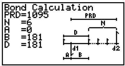
{PRC} - {MEMO}
An error (Ma ERROR) occurs if parameters are not configured correctly.
Use the following function menu to maneuver between calculation result screens.
- {REPT} ... {parameter input screen}
- {GRPH} ... {draws graph}
- {MEMO} ... {displays numbers of days used in calculations}
MEMO Screen
- The following describes the meaning of the MEMO screen display items.
N...... number of coupon payments between settlement date and maturity date
A...... accrued days
B...... number of days from settlement date until next coupon payment date (D-A)
D ...... number of days in coupon period where settlement occurs
- Each press of EXE while the MEMO screen is displayed cycles the Coupon Payment Day (CPD) display sequentially from the redemption year up to the purchase year. This is true only when the “Date Mode” setting on the “Setup” screen is “365”.
Bond Calculation CPD=01M01D2012Y(SUN)
11. Financial Calculations Using Functions
Important!
- The following operations cannot be performed on the fx-7400GII.
You can use special functions in the RUN•MAT mode or PRGM mode to perform calculations that are the same as the TVM mode financial calculations.
Example To calculate the total interest and principal paid for a 2-year (730-day) \$300 loan at a simple annual interest rate of 5%. Use a Date Mode setting of 365.
- From the Main Menu, enter the RUN•MAT mode.
- Press the keys as follows.
OPTN F6 (▷) F6 (▷) F6 (▷) F1 (TVM)
F1 (SMPL) F1 (SI) 7 3 0 , 5 ,
3 0 0 ) EXE
SmP1_SI(730,5,300) -30
F2 (SFV) 7 3 0 , 5 , 3 0 0 ) EXE
SmP1_SI(730,5,300) -30 SmP1_SFV(730,5,300) -330
SI SFV
- Use the TVM mode Setup screen (SHIFT MENU (SET UP)) to change the Date Mode setting. You also can use special commands (DateMode365, DateMode360) in the PRGM mode to change the setting.
- For details about what you can do with the financial calculation functions and their syntax, see “Performing Financial Calculations in a Program” (page 8-35).
Chapter 8 Programming
1. Basic Programming Steps
Commands and calculations are executed sequentially, just like manual calculation multi-statements.
- From the Main Menu, enter the PRGM mode. When you do, a program list appears on the display.
Selected program area — (use ▲ and ▼ to move)
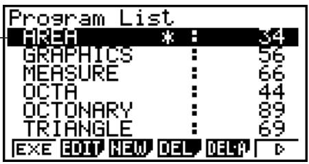
Files are listed in the alphabetic sequence of their names.
- Register a file name.
- Input the program.
-
Run the program.
-
The values to the right of the program list indicate the number of bytes used by each program.
- A file name can be up to eight characters long.
- The following are the characters you can use in a file name: A through Z, r, θ, spaces, [, ], {, }, ' ,", \~, 0 through 9, ., +, -, ×, ÷
- Registering a file name uses 32 bytes of memory.
Example
To calculate the surface area (cm ^2 ) and volume (cm ^3 ) of three regular octahedrons when the length of one side is 7, 10, and 15 cm, respectively
Store the calculation formula under the file name OCTA.
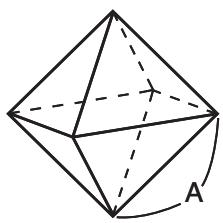
natural_image
Geometric diagram of a polyhedron with labeled point A and dashed internal lines (no text or symbols beyond label)The following are the formulas used for calculating surface area S and volume V of a regular octahedron for which the length of one side A is known.
$$ \mathsf {S} = 2 \sqrt {3} \mathsf {A} ^ {2}, \quad \mathsf {V} = \frac {\sqrt {2}}{3} \mathsf {A} ^ {3} $$
① MENU PRGM
② F3 (NEW) 9 (O) In (C) ÷ (T) X,θ,T (A) EXE
③ SHIFT VARS (PRGM) F4 (?) → ALPHA X,θ,T (A) F6 (▷) F5 (:)
2 ✗ SHIFT x^2() 3 ✗ ALPHA X,θ,T (A) x^2 F6 (▷) F6 (▷) F5 (▲)
SHIFT x^2() 2 ÷ 3 ✗ ALPHA X,θ,T (A) ∧ 3
EXIT EXIT
④ F1(EXE) or EXE
7 EXE (Value of A)
EXE
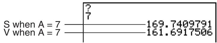
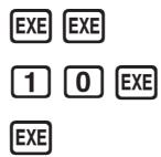
| ? i0 | ||
| S when A = 10 | 346.4101615 | |
| V when A = 10 | 471.4045208 |
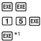
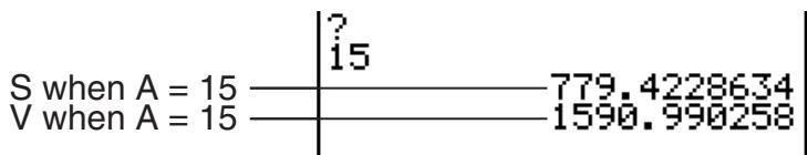
*1 Pressing EXE while the program's final result is on the display exits the program.
- You can also run a program while in the RUN•MAT (or RUN) mode by inputting: Prog "
" EXE. - Pressing EXE while the final result of a program executed using this method is on the display re-executes the program.
- An error occurs if the program specified by Prog "
" cannot be found.
2. PRGM Mode Function Keys
- {NEW} ... {new program}
- When you are registering a file name
- {RUN}/{BASE} ... {general calculation}/{number base} program input
- {π0} ... {password registration}
- {SYBL} ... {symbol menu}
- When you are inputting a program — F1(RUN) ... default
- {TOP}/{BTM} ... {top}/{bottom} of program
- {SRC} ... {search}
- {MENU} ... {mode menu}
- {STAT}/{MAT}*/{LIST}/{GRPH}/{DYNA}*/{TABL}/{RECR}* ... {statistic}/{matrix}/{list}/{graph}/{Dynamic Graph}/{Table}/{recursion} menu
- A a ... {toggles between upper-case and lower-case input}
- {CHAR} ... {displays a screen for selecting various mathematical symbols, special symbols, and accented characters}
* Not included on the fx-7400GII
- Pressing SHIFT VARS (PRGM) displays the following program (PRGM) menu.
- {COM} ... {program command menu}
- {CTL} ... {program control command menu}
- {JUMP} ... {jump command menu}
- {?}/{▲} ... {input}/{output} command
- {CLR}/{DISP} ... {clear}/{display} command menu
-
{REL} ... {conditional jump relational operator menu}
-
{I/O} ... {I/O control/transfer command menu}
- {:} ... {multi-statement command}
- {STR} ... {string command}
See “Command Reference” on page 8-7 for full details on each of these commands.
- Pressing SHIFT MENU (SET UP) displays the mode command menu shown below.
• {ANGL}/{COOR}/{GRID}/{AXES}/{LABL}/{DISP}/{S/L}/{DRAW}/{DERV}/{BACK}/{FUNC}/{SIML}/{S-WIN}/{LIST}/{LOCS}*/{T-VAR}/{ΣDSP}*/{RESID}/{CPLX}/{FRAC}/{Y·SPD}*/{DATE}*/{PMT}*/{PRD}*/{INEQ}/{SIMP}/{Q1Q3} * Not included on the fx-7400GII
See “Setup Screen Function Key Menus” on page 1-26 for details about each of these commands.
- When you are inputting a program — F2 (BASE) ^*1
- {TOP}/{BTM}/{SRC}
• {MENU} - {d\~o} ... {decimal}/{hexadecimal}/{binary}/{octal} value input
- {LOG} ... {bitwise operator}
- {DISP} ... conversion of displayed value to {decimal}/{hexadecimal}/{binary}/{octal}
• {A↔a}/{SYBL}
- Pressing SHIFT VARS (PRGM) displays the following PRGM (PROGRAM) menu.
- {Prog} ... {program recall}
- {JUMP}/{?}/{▲}
- {REL} ... {conditional jump relational operator menu}
- {:} ... {multi-statement command}
- Pressing SHIFT MENU (SET UP) displays the mode command menu shown below.
- {Dec}/{Hex}/{Bin}/{Oct}
*1 Programs input after pressing F2(BASE) are indicated by B to the right of the file name.
- {EXE}/{EDIT} ... program {execute}/{edit}
- {NEW} ... {new program}
- {DEL}/{DEL·A} ... {specific program}/{all program} delete
- {SRC}/{REN} ... file name {search}/{change}
3. Editing Program Contents
■ Debugging a Program
A problem in a program that keeps the program from running correctly is called a “bug”, and the process of eliminating such problems is called “debugging”. Either of the following symptoms indicates that your program contains bugs that require debugging.
- Error messages appearing when the program is run
• Results that are not within your expectations
- To eliminate bugs that cause error messages
An error message, like the one shown to the right, appears whenever something illegal occurs during program execution.
Ma ERROR
Press: [EXIT]
When such a message appears, press EXIT to display the place in the program where the error was caused. The cursor will be flashing at the location of the problem. Check the “Error Message Table” (page -1) for steps you should take to correct the situation.
- Note that pressing EXIT does not display the location of the error if the program is password protected.
- To eliminate bugs that cause bad results
If your program produces results that are not what you normally expect, check the contents of the program and make necessary changes.
F1(TOP)... Moves the cursor to the top of the program
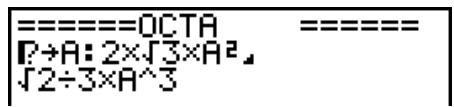
F2 (BTM)... Moves the cursor to the bottom of the program
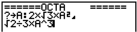
■ Searching for Data Inside a Program
Example To search for the letter “A” inside the program named OCTA
- Recall the program.
- Press F3(SRC) and input the data you want to find.
F3 (SRC)
ALPHA X,θ,T (A)
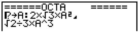

- Press EXE to begin the search. The contents of the program appear on the screen with the cursor located at the first instance of the data you specified.*1
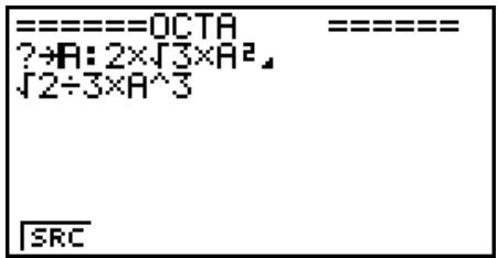
- Each press of EXE or F1(SRC) causes the cursor to jump to the next instance of the data you specified.*2
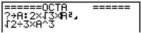
*1 The message “Not Found” appears when the search data you specify cannot be found in the program.
*2 If there are no more instances of the data you specified, the search operation ends.
- You cannot specify the newline symbol (←) or display command (▲) for the search data.
- Once the contents of the program are on the screen, you can use the cursor keys to move the cursor to another location before searching for the next instance of the data. Only the part of the program starting from the current cursor location is searched when you press EXE.
- Once the search finds an instance of your data, inputting characters or moving the cursor causes the search operation to be cancelled.
- If you make a mistake while inputting characters to search for, press AC to clear your input and re-input from the beginning.
4. File Management
■ Searching for a File
- To find a file using initial character search
Example To use initial character search to recall the program named OCTA
- While the program list is on the display, press F6(▷)F1(SRC) and input the initial characters of the file you want to find.
F6 (▷) F1 (SRC)
9 (O) In (C) ÷ (T)

- Press EXE to search.
- The name that starts with the characters you input highlights.
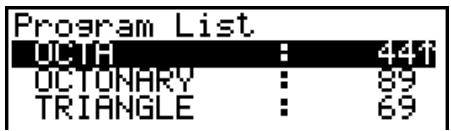
- If there is no program whose file name starts with the characters you input, the message "Not Found" appears on the display. If this happens, press EXIT to clear the error message.
■ Editing a File Name
- While the program list is on the display, use ▲ and ▼ to move the highlighting to the file whose name you want to edit and then press F6 (▷) F2 (REN).
- Make any changes you want.
- Press EXE to register the new name and return to the program list.
The program list is resorted according to the changes you made in the file name.
- If the modifications you make result in a file name that is identical to the name of a program already stored in memory, the message “Already Exists” appears. When this happens, you can perform either of the following two operations to correct the situation.
- Press EXIT to clear the error and return to the file name editing screen.
- Press AC to clear the input file name and input a new one.
■ Deleting a Program
- To delete a specific program
- While the program list is on the display, use ⚠️ and ⼋ to move the highlighting to the name of the program you want to delete.
- Press F4 (DEL).
- Press F1(YES) to delete the selected program or F6(NO) to abort the operation without deleting anything.
- To delete all programs
- While the program list is on the display, press F5 (DEL·A).
- Press F1(YES) to delete all the programs in the list or F6(NO) to abort the operation without deleting anything.
- You also can delete all programs by entering the MEMORY mode from the Main Menu. See “Chapter 11 Memory Manager” for details.
■ Registering a password
When inputting a program, you can protect it with a password that limits access to the program contents to those who know the password.
- You do not need to input the password to run a program.
-
The password input procedure is identical to that used for file name input.
-
While the program list is on the display, press F3 (NEW) and input the file name of the new program file.
- Press F5(π0) and then input the password.
- Press EXE to register the file name and password. Now you can input the contents of the program file.
- After inputting the program, press SHIFT EXIT (QUIT) to exit the program file and return to the program list. Files that are password protected are indicated by an asterisk to the right of the file name.

■ Recalling a Password Protected Program
- In the program list, use ▲ and ▼ to move the highlighting to the name of the program you want to recall.
- Press F2 (EDIT).
- Input the password and press EXE to recall the program.
- Inputting the wrong password when recalling a password protected program causes the message “Mismatch” to appear.
Command Index
Break......8-10
CloseComport38k....8-17
ClrGraph 8-14
ClrList 8-14
ClrMat 8-14
ClrText 8-14
DispF-Tbl, DispR-Tbl 8-14
Do\~LpWhile 8-10
DrawDyna 8-14
DrawFTG-Con, DrawFTG-Plt 8-15
DrawGraph 8-15
DrawR-Con, DrawR-Plt 8-15
DrawRΣ-Con, DrawRΣ-Plt 8-15
DrawStat 8-15
DrawWeb 8-15
Dsz 8-12
Exp(....8-19
Exp▶Str( 8-19
For\~To\~(Step\~)Next 8-9
Getkey 8-16
Goto\~Lbl 8-12
If\~Then\~(Else\~)IfEnd 8-9
lsz 8-12
Locate 8-17
Menu 8-13
OpenComport38k 8-17
Prog 8-11
PlotPhase....8-16
RclCapt 8-21
Receive(....8-17
Receive38k 8-18
Return 8-11
Send( 8-17
Send38k....8-18
Stop 8-11
StrCmp(....8-19
StrInv(....8-19
StrJoin(....8-19
StrLeft(....8-19
StrLen(....8-19
StrLwr(....8-19
StrMid( 8-20
StrRight(....8-20
StrRotate(....8-20
StrShift(....8-20
StrSrc(....8-20
StrUpr( 8-20
While\~WhileEnd 8-10
? (Input Command)......8-8
▲ (Output Command) 8-8
: (Multi-statement Command)......8-8
← (Carriage Return) 8-8
' (Comment Text Delimiter) 8-8
(Jump Code) 8-13
= , , > , < ,≥ ,≤ (Relational Operators) ..8 - 18
+....8-20
The following are conventions that are used in this section when describing the various commands.
Boldface Text ...... Actual commands and other items that always must be input are shown in boldface.
{Curly Brackets}...... Curly brackets are used to enclose a number of items, one of which must be selected when using a command. Do not input the curly brackets when inputting a command.
[Square Brackets] ...... Square brackets are used to enclose items that are optional. Do not input the square brackets when inputting a command.
Numeric Expressions... Numeric expressions (such as 10, 10 + 20, A) indicate constants, calculations, numeric constants, etc.
Alpha Characters ...... Alpha characters indicate literal strings (such as AB).
■ Basic Operation Commands
? (Input Command)
Function: Prompts for input of values for assignment to variables during program execution.
Syntax: ? →
Example: ? → A
Description:
- This command momentarily interrupts program execution and prompts for input of a value or expression for assignment to a variable. If you do not specify a prompt, execution of this command causes “?” to appear indicating the calculator is standing by for input. If a prompt is specified, “
?” appears to prompt input. Up to 255 bytes of text can be used for a prompt. - Input in response to the input command must be a value or an expression, and the expression cannot be a multi-statement.
- You can specify a list name, matrix name, string name, function memory (fn), graph (Yn), etc. as a variable name.
▲ (Output Command)
Function: Displays an intermediate result during program execution.
Description:
- This command momentarily interrupts program execution and displays alpha character text or the result of the calculation immediately before the command.
- The output command should be used at locations where you would normally press the EXE key during a manual calculation.
: (Multi-statement Command)
Function: Connects two statements for sequential execution without stopping.
Description:
- Unlike the output command (▲), statements connected with the multi-statement command are executed non-stop.
- The multi-statement command can be used to link two calculation expressions or two commands.
- You can also use a carriage return indicated by in place of the multi-statement command.
← (Carriage Return)
Function: Connects two statements for sequential execution without stopping.
Description:
- Operation of the carriage return is identical to that of the multi-statement command.
- You can create a blank line in a program by inputting a carriage return only. Using a carriage return in place of the multi-statement command makes the displayed program easier to read.
' (Comment Text Delimiter)
Function: Indicates comment text inserted inside a program.
Description: Anything following the apostrophe is treated as non-executable comment text.
■ Program Commands (COM)
If\~Then\~(Else\~)IfEnd
Function: The Then-statement is executed only when the If-condition is true (non-zero). The Else-statement is executed when the If-condition is false (0). The IfEnd-statement is always executed following either the Then-statement or Else-statement.
Syntax:
![If \\\\\\ Then [\\\\\\ [\\\\\ ] \\\\\\ (Else [\\\\\ ]\\\\\\) IfEnd](/content/2025/01/86832/images/7f160fe0c1d9416dd36393a06f481855084db1f409400002d0435c4c01a3c1f1.jpg)
Parameters: condition, numeric expression
Description:
(1) If \~ Then \~ IfEnd
- When the condition is true, execution proceeds with the Then-statement and then continues with the statement following IfEnd.
- When the condition is false, execution jumps to the statement following IfEnd.
(2) If \~ Then \~ Else \~ IfEnd
- When the condition is true, execution proceeds with the Then-statement and then jumps to the statement following IfEnd.
- When the condition is false, execution jumps to the Else-statement and then continues with the statement following IfEnd.
For\~To\~(Step\~)Next
Function: This command repeats everything between the For-statement and the Next-statement. The starting value is assigned to the control variable with the first execution, and the value of the control variable is changed according to the step value with each execution. Execution continues until the value of the control variable exceeds the ending value.
Syntax: For
$$ \left(\text{Step} < \text{step value} >\right)\left{ \begin{array}{c}\leftarrow \ :\end{array} \right} \text{Next} $$
Parameters:
• control variable name: A to Z
- starting value: value or expression that produces a value (i.e. x , A, etc.)
• ending value: value or expression that produces a value (i.e. sin x, A, etc.)
- step value: numeric value (default: 1)
Description:
- The default step value is 1.
- Making the starting value less than the ending value and specifying a positive step value causes the control variable to be incremented with each execution. Making the starting value greater than the ending value and specifying a negative step value causes the control variable to be decremented with each execution.
Do\~LpWhile
Function: This command repeats specific commands as long as its condition is true (non-zero).
Syntax:
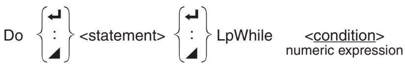
Parameters: expression
Description:
- This command repeats the commands contained in the loop as long as its condition is true (non-zero). When the condition becomes false (0), execution proceeds from the statement following the LpWhile-statement.
- Since the condition comes after the LpWhile-statement, the condition is tested (checked) after all of the commands inside the loop are executed.
While\~WhileEnd
Function: This command repeats specific commands as long as its condition is true (non-zero).
Syntax:

Parameters: expression
Description:
- This command repeats the commands contained in the loop as long as its condition is true (non-zero). When the condition becomes false (0), execution proceeds from the statement following the WhileEnd-statement.
- Since the condition comes after the While-statement, the condition is tested (checked) before the commands inside the loop are executed.
■ Program Control Commands (CTL)
Break
Function: This command breaks execution of a loop and continues from the next command following the loop.
Syntax: Break
Description:
- This command breaks execution of a loop and continues from the next command following the loop.
- This command can be used to break execution of a For-statement, Do-statement, and While-statement.
Prog
Function: This command specifies execution of another program as a subroutine. In the RUN•MAT (or RUN) mode, this command executes a new program.
Syntax: Prog "file name"
Example: Prog "ABC"
Description:
- Even when this command is located inside of a loop, its execution immediately breaks the loop and launches the subroutine.
- This command can be used as many times as necessary inside of a main routine to call up independent subroutines to perform specific tasks.
- A subroutine can be used in multiple locations in the same main routine, or it can be called up by any number of main routines.
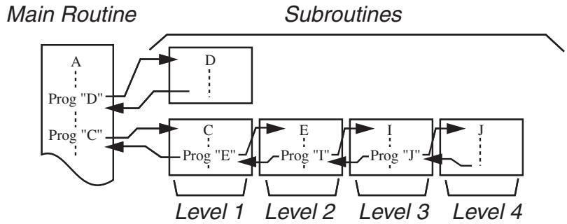
flowchart
graph TD
    A["Main Routine"] --> B["Subroutines"]
    B --> C1["Level 1"]
    B --> C2["Level 2"]
    B --> C3["Level 3"]
    B --> C4["Level 4"]
    A --> D["Prog "D""]
    A --> E["Prog "C""]
    D --> F["D"]
    E --> G["C"]
    F --> H["E"]
    G --> I["I"]
    H --> J["J"]
    I --> K["End"]
    J --> L["End"]
- Calling up a subroutine causes it to be executed from the beginning. After execution of the subroutine is complete, execution returns to the main routine, continuing from the statement following the Prog command.
- A Goto\~Lbl command inside of a subroutine is valid inside of that subroutine only. It cannot be used to jump to a label outside of the subroutine.
- If a subroutine with the file name specified by the Prog command does not exist, an error occurs.
- In the RUN•MAT (or RUN) mode, inputting the Prog command and pressing EXE launches the program specified by the command.
Return
Function: This command returns from a subroutine.
Syntax: Return
Description: Execution of the Return command inside a main routine causes execution of the program to stop. Execution of the Return command within a subroutine terminates the subroutine and returns to the program from which the subroutine was jumped to.
Stop
Function: This command terminates execution of a program.
Syntax: Stop
Description:
- This command terminates program execution.
- Execution of this command inside of a loop terminates program execution without an error being generated.
■ Jump Commands (JUMP)
Dsz
Function: This command is a count jump that decrements the value of a control variable by 1, and then jumps if the current value of the variable is zero.
Syntax:
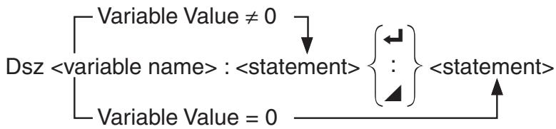
flowchart
graph TD
    A["Variable Value ≠ 0"] --> B["Dsz <variable name>: <statement>"]
    C["Variable Value = 0"] --> B
    B --> D{←}
    B --> E{:}
    B --> F["<statement>"]
    D --> G["<statement>"]
    E --> G
    F --> G
Parameters: variable name: A to Z, r, θ
[Example] Dsz B : Decrements the value assigned to variable B by 1.
Description: This command decrements the value of a control variable by 1, and then tests (checks) it. If the current value is non-zero, execution continues with the next statement. If the current value is zero, execution jumps to the statement following the multi-statement command (:), display command (▲), or carriage return (←).
Goto\~Lbl
Function: This command performs an unconditional jump to a specified location.
Syntax: Goto
Parameters: label name: value (0 to 9), variable (A to Z, r, θ)
Description:
- This command consists of two parts: Goto n (where n is a parameter as described above) and Lbl n (where n is the parameter referenced by Goto n). This command causes program execution to jump to the Lbl-statement whose n parameter matches that specified by the Goto-statement.
- This command can be used to loop back to the beginning of a program or to jump to any location within the program.
- This command can be used in combination with conditional jumps and count jumps.
- If there is no Lbl-statement whose value matches that specified by the Goto-statement, an error occurs.
lsz
Function: This command is a count jump that increments the value of a control variable by 1, and then jumps if the current value of the variable is zero.
Syntax:
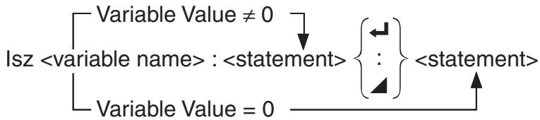
flowchart
graph TD
    A["Isz <variable name> : <statement>"] --> B{<statement>}
    C["Variable Value ≠ 0"] --> A
    D["Variable Value = 0"] --> C
Parameters: variable name: A to Z, r, θ
[Example] Isz A : Increments the value assigned to variable A by 1.
Description: This command increments the value of a control variable by 1, and then tests (checks) it. If the current value is non-zero, execution continues with the next statement. If the current value is zero, execution jumps to the statement following the multi-statement command (:), display command (▲), or carriage return (◀).
$$ \Rightarrow (\text { Jump Code }) $$
Function: This code is used to set up conditions for a conditional jump. The jump is executed whenever the conditions are false.
Syntax:
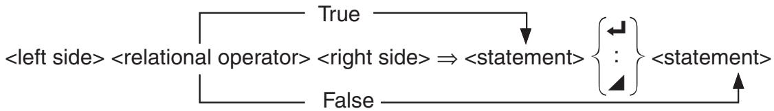
flowchart
graph TD
    A["<left side>"] --> B["<relational operator>"]
    B --> C["<right side>"]
    C --> D["<statement>"]
    D --> E{<statement>}
    F["True"] --> C
    G["False"] --> D
    H["<left side>"] --> I["<relational operator>"]
    I --> J["<right side>"]
    J --> K["<statement>"]
    K --> L["<statement>"]
Parameters:
- left side/right side: variable (A to Z, r, θ), numeric constant, variable expression (such as: A × 2)
- relational operator: =, , >, <, ≥, ≤ (page 8-18)
Description:
- The conditional jump compares the contents of two variables or the results of two expressions, and a decision is made whether or not to execute the jump based on the results of the comparison.
- If the comparison returns a true result, execution continues with the statement following the command. If the comparison returns a false result, execution jumps to the statements following the multi-statement command (:), display command (▲), or carriage return (←).
Menu
Function: Creates a branching menu in a program.
Syntax: Menu "
Parameters: value (0 to 9), variable (A to Z, r, θ)
Description:
- Each "
" , part is a branch set, and the entire branch set must be included. - From two to nine branching sets can be included. An error occurs when there is only one or more than nine branching sets.
- Selecting a branch on the menu while the program is running jumps to the same type of label (Lbl n) as the one used in combination with the Goto command. Specifying “"OK", 3" for the "\"
", " part specifies a jump to Lbl 3.
Example: Lbl 2
Menu "IS IT DONE?", "OK", 1, "EXIT", 2
Lbl 1
"IT'S DONE!"
■ Clear Commands (CLR)
ClrGraph
Function: This command clears the graph screen.
Syntax: ClrGraph
Description: This command clears the graph screen during program execution.
ClrList
Function: This command deletes list data.
Syntax: ClrList
ClrList
Parameters: list name: 1 to 26, Ans
Description: This command deletes the data in the list specified by "list name". All list data is deleted if nothing is specified for "list name".
ClrMat
(Not included on the fx-7400GII)
Function: This command deletes matrix data.
Syntax: ClrMat
Parameters: matrix name: A to Z, Ans
Description: This command deletes the data in the matrix specified by “matrix name”. All matrix data is deleted if nothing is specified for “matrix name”.
ClrText
Function: This command clears the text screen.
Syntax: ClrText
Description: This command clears text from the screen during program execution.
■ Display Commands (DISP)
DispF-Tbl, DispR-Tbl*
* (Not included on the fx-7400GII) No parameters
Function: These commands display numeric tables.
Description:
- These commands generate numeric tables during program execution in accordance with conditions defined within the program.
- DispF-Tbl generates a function table, while DispR-Tbl generates a recursion table.
DrawDyna
(Not included on the fx-7400GII) No parameters
Function: This command executes a Dynamic Graph draw operation.
Description: This command draws a Dynamic Graph during program execution in accordance with the drawing conditions defined within the program.
Function: This command uses values in a generated table to graph a function.
Description:
- This command draws a function graph in accordance with conditions defined within the program.
- DrawFTG-Con produces a connect type graph, while DrawFTG-Plt produces a plot type graph.
DrawGraph
No parameters
Function: This command draws a graph.
Description: This command draws a graph in accordance with the drawing conditions defined within the program.
DrawR-Con, DrawR-Plt
(Not included on the fx-7400GII)
No parameters
Function: These commands graph recursion expressions, with a_n(b_n or c_n) as the vertical axis and n as the horizontal axis.
Description:
- These commands graph recursion expressions in accordance with conditions defined within the program, with a_n ( b_n or c_n ) as the vertical axis and n as the horizontal axis.
- DrawR-Con produces a connect type graph, while DrawR-Plt produces a plot type graph.
DrawRΣ-Con, DrawRΣ-Plt
(Not included on the fx-7400GII)
No parameters
Function: These commands graph recursion expressions, with a_n ( b_n or c_n ) as the vertical axis and n as the horizontal axis.
Description:
- These commands graph recursion expressions in accordance with conditions defined within the program, with a_n ( b_n or c_n ) as the vertical axis and n as the horizontal axis.
- DrawRΣ-Con produces a connect type graph, while DrawRΣ-Plt produces a plot type graph.
DrawStat
Function: This draws a statistical graph.
Syntax: See “Using Statistical Calculations and Graphs in a Program” on page 8-25.
Description: This command draws a statistical graph in accordance with conditions defined within the program.
DrawWeb
(Not included on the fx-7400GII)
Function: This command graphs convergence/divergence of a recursion expression (WEB graph).
Syntax: DrawWeb
Example: DrawWeb a_n+1 ( b_n+1 or c_n+1 ), 5
Description:
- This command graphs convergence/divergence of a recursion expression (WEB graph).
- Omitting the number of lines specification automatically specifies the default value 30.
Function: Graphs a phase plot based on numeric sequences that correspond to the x-axis and y-axis.
Syntax: PlotPhase
Description:
- Only the following commands can be input for each argument to specify the recursion table. a_n, b_n, c_n, a_n+1, b_n+1, c_n+1, a_n+2, b_n+2, c_n+2, a_n, b_n, c_n, a_n+1, b_n+1, c_n+1, a_n+2, b_n+2, c_n+2
- A memory ERROR occurs if you specify a numeric sequence name that does not have values stored in the recursion table.
Example: PlotPhase b_n+1 , a_n+1
Graphs a phase plot using b_n+1 for the x-axis and a_n+1 for the y-axis.
■ Input/Output Commands (I/O)
Getkey
Function: This command returns the code that corresponds to the last key pressed.
Syntax: Getkey
Description:
- This command returns the code that corresponds to the last key pressed.
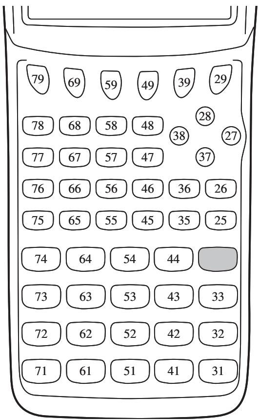
- A value of zero is returned if no key was pressed previous to executing this command.
- This command can be used inside of a loop.
Locate
Function: This command displays alpha-numeric characters at a specific location on the text screen.
Syntax: Locate
Locate
Locate
[Example] Locate 1, 1, "AB"
Parameters:
• line number: number from 1 to 7
• column number: number from 1 to 21
• value and numeric expression
- string: character string
Description:
- This command displays values (including variable contents) or text at a specific location on the text screen. If there is a calculation input, that calculation result is displayed.
- The line is designated by a value from 1 to 7, while the column is designated by a value from 1 to 21.
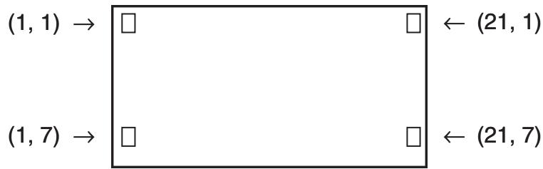
flowchart
graph TD
    A["(1, 1) →"] --> B[" "]
    B --> C[" "]
    C --> D["(21, 1)"]
    E["(1, 7) →"] --> F[" "]
    F --> G[" "]
    G --> H["(21, 7)"]
Example: Cls
Locate 7, 1, "CASIO FX"
This program displays the text “CASIO FX” in the center of the screen.
- In some cases, the CIrText command should be executed before running the above program.
Receive( / Send(
Function: This command receives data from and sends data to a connected device.
Syntax: Receive() / Send()
Description:
- This command receives data from and sends data to a connected device.
- The following types of data can be received (sent) by this command.
- Individual values assigned to variables
- Matrix data (all values - individual values cannot be specified)
- List data (all values - individual values cannot be specified)
OpenComport38k / CloseComport38k
Function: Opens and closes the 3-pin COM port (serial).
Description: See the Receive38k/Send38k command below.
Receive38k / Send38k
Function: Executes data send and receive at a data rate of 38 kbps.
Syntax: Send38k
Receive38k
Description:
- The OpenComport38k command must be executed before this command is executed.
- The CloseComport38k command must be executed after this command is executed.
- If this command is executed when the communication cable is not connected, program execution will continue without generating an error.
■ Conditional Jump Relational Operators (REL)
$$ = , \neq , >, < , \geq , \leq $$
Function: These relational operators are used in combination with the conditional jump command.
Syntax:
Parameters:
- left side/right side: variable (A to Z, r, θ), numeric constant, variable expression (such as: A × 2)
- relational operator: =, , >, <, ≥, ≤
■ Strings
A string is a series of characters enclosed in double quotes. In a program, strings are used to specify display text. A string made up of numbers (like "123") or an expression (like "x-1") cannot be processed as a calculation.
To display a string at a specific location on the screen, use the Locate command (page 8-17).
- To include double quotes (") or a backslash () in a string, put a backslash () in front of the double quotes (") or backslash ().
Example 1: To include Japan: "Tokyo" in a string "Japan:"Tokyo"
Example 2: To include main\abc in a string "main"
You can input a backslash from the menu that appears when you press F6 (CHAR) F2 (SYBL) in the PRGM mode, or from the String category of the catalog that appears when you press SHIFT 4 (CATALOG).
- You can assign strings to string memory (Str 1 through Str 20). For details about strings, see "String Memory" (page 2-7).
- You can use the “+” command (page 8-20) to connect strings inside of an argument.
- A function or command within a string function (Exp(, StrCmp(, etc.) is treated as a single character. For example, the “sin” function is treated as a single character.
Exp(
Function: Converts a string to an expression, and executes the expression.
Syntax: Exp("
Exp▶Str(
Function: Converts a graph expression to a string and assigns it to the specified variable.
Syntax: Exp▶Str(
Description: A graph expression (Y_n, r, X_t, Y_t, X) , recursion formula (a_n, a_n+1, a_n+2, b_n, b_n+1, b_n+2, c_n, c_n+1, c_n+2) , or function memory (f_n) can be used as the first argument (
StrCmp(
Function: Compares "
Syntax: StrCmp("
Description: Compares two strings and returns one of the following values.
Returns 0 when "
Returns 1 when "
Returns -1 when "
StrInv(
Function: Inverts the sequence of a string.
Syntax: StrInv("
StrJoin(
Function: Joins "
Syntax: StrJoin("
Note: The same result also can be achieved using the “+” command (page 8-20).
StrLeft(
Function: Copies a string up to the nth character from the left.
Syntax: StrLeft("
StrLen(
Function: Returns the length of a string (the number of its characters).
Syntax: StrLen("
StrLwr(
Function: Converts all the characters of a string to lower case.
Syntax: StrLwr("
StrMid(
Function: Extracts from the n-th to the m-th character of a string.
Syntax: StrMid("
Description: Omitting “m” will extract from the n-th character to the end of the string.
StrRight(
Function: Copies a string up to the nth character from the right.
Syntax: StrRight("
StrRotate(
Function: Rotates the left side part and right side part of a string at the nth character.
Syntax: StrRotate("
Description: Rotation is to the left when “n” is positive, and to the right when “n” is negative.
Omitting “n” uses a default value of +1.
Example: StrRotate("abcde", 2) ...... Returns the string "cdeab".
StrShift(
Function: Shifts a string left or right n characters.
Syntax: StrShift("
Description: Shift is to the left when “n” is positive, and to the right when “n” is negative.
Omitting “n” uses a default value of +1.
Example: StrShift("abcde", 2) ...... Returns the string "cde".
StrSrc(
Function: Searches "
Syntax: StrSrc("
Description: Omitting the start point causes the search to start from the beginning of "
StrUpr(
Function: Converts all the characters of a string to upper case.
Syntax: StrUpr("
+
Function: Joins "
Syntax: "
Example: "abc"+"de"→Str 1...... Assigns "abcde" to Str 1.
Other
RclCapt
Function: Displayed the contents specified by the capture memory number.
Syntax: RclCapt
(capture memory number: 1 to 20)
6. Using Calculator Functions in Programs
■ Text Display
You can include text in a program by simply enclosing it between double quotation marks. Such text appears on the display during program execution, which means you can add labels to input prompts and results.
| Program | Display |
| "CASIO" | CASIO |
| ? → X | ? |
| "X = " ? → X | X = ? |
- If the text is followed by a calculation formula, be sure to insert a display command (▲) between the text and calculation.
- Inputting more than 21 characters causes the text to move down to the next line. The screen scrolls automatically if the text exceeds 21 characters.
- You can specify up to 255 bytes of text for a comment.
■ Using Matrix Row Operations in a Program
(Not available on the fx-7400GII)
These commands let you manipulate the rows of a matrix in a program.
- For this program, enter the RUN•MAT mode and then use the Matrix Editor to input the matrix, and then enter the PRGM mode to input the program.
- To swap the contents of two rows (Swap)
Example 1 To swap the values of Row 2 and Row 3 in the following matrix:
$$ \text { Matrix } \mathbf {A} = \left[ \begin{array}{c c} 1 & 2 \ 3 & 4 \ 5 & 6 \end{array} \right] $$
The following is the syntax to use for this program.
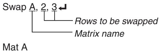
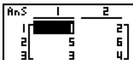
- To calculate a scalar multiplication (\* Row)
Example 2 To calculate the product of Row 2 of the matrix in Example 1 and the scalar 4
The following is the syntax to use for this program.
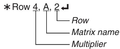
flowchart
graph TD
    A["*Row 4, A, 2"] --> B["Row"]
    A --> C["Matrix name"]
    A --> D["Multiplier"]
Mat A
- To calculate a scalar multiplication and add the results to another row (\*Row+)
Example 3 To calculate the product of Row 2 of the matrix in Example 1 and the scalar 4, then add the result to row 3
The following is the syntax to use for this program.
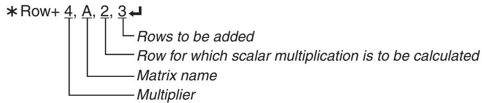
flowchart
graph TD
    A["*Row+ 4, A, 2, 3"] --> B["Rows to be added"]
    B --> C["Row for which scalar multiplication is to be calculated"]
    C --> D["Matrix name"]
    D --> E["Multiplier"]
Mat A
- To add two rows (Row+)
Example 4 To add Row 2 to Row 3 of the matrix in Example 1
The following is the syntax to use for this program.
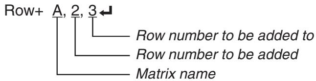
Mat A
■ Using Graph Functions in a Program
You can incorporate graph functions into a program to draw complex graphs and to overlay graphs on top of each other. The following shows various types of syntax you need to use when programming with graph functions.
- V-Window View Window -5, 5, 1, -5, 5, 1
- Graph function input Y = Type ← .......Specifies graph type.
$$ " X ^ {2} - 3" \rightarrow Y 1 ^ {* 1} \leftarrow $$
- Graph draw operation DrawGraph
*1 Input this Y1 with VARS F4 (GRPH) F1 (Y) 1 (displayed as Y1). A Syntax ERROR will occur if you input "Y" with the calculator keys.
- Syntax of other graphing functions
• V-Window View Window <Xmin>, <Xmax>, <Xscale>, <Ymin>, <Ymax>, <Yscale>, <Tθ min>, <Tθ max>, <Tθ pitch>
StoV-Win <area of V-Win>...... area: 1 to 6
RclV-Win <area of V-Win>...... area: 1 to 6
• Zoom Factor <X factor>, <Y factor>
ZoomAuto...... Non-parameter
• Pict StoPict <area of picture>...... area: 1 to 6
numeric expression
RclPict <area of picture>...... area: 1 to 6
numeric expression
• Sketch PlotOn <X-coordinate>, <Y-coordinate>
PlotOff <X-coordinate>, <Y-coordinate>
PlotChg <X-coordinate>, <Y-coordinate>
PxlOn <line number>, <column number>
PxlOff <line number>, <column number>
PxlChg <line number>, <column number>
PxlTest <line number>, <column number>
Text <line number>, <column number>, "<text>"
Text <line number>, <column number>, <expression>
SketchThick <Sketch or Graph statement>
SketchBroken <Sketch or Graph statement>
SketchDot <Sketch or Graph statement>
SketchNormal <Sketch or Graph statement>
Tangent <function>, <X-coordinate>
Normal <function>, <X-coordinate>
Inverse <function>
Line
F-Line <X-coordinate 1>, <Y-coordinate 1>, <X-coordinate 2>, <Y-coordinate 2>
Circle <center point X-coordinate>, <center point Y-coordinate>, <radius R value>
Vertical <X-coordinate>
Horizontal <Y-coordinate>
■ Using Dynamic Graph Functions in a Program
Using Dynamic Graph functions in a program makes it possible to perform repeated Dynamic Graph operations. The following shows how to specify the Dynamic Graph range inside a program.
• Dynamic Graph range
1 → D Start
5 → D End ←
1 → D pitch ←
■ Using Table & Graph Functions in a Program
Table & Graph functions in a program can generate numeric tables and perform graphing operations. The following shows various types of syntax you need to use when programming with Table & Graph functions.
- Table range setting
1 → F Start
5 → F End ←
1 → F pitch ←
- Numeric table generation
DispF-Tbl
- Graph draw operation
Connect type: DrawFTG-Con
Plot type: DrawFTG-Plt
■ Using Recursion Table & Graph Functions in a Program
Incorporating Recursion Table & Graph functions in a program lets you generate numeric tables and perform graphing operations. The following shows various types of syntax you need to use when programming with Recursion Table & Graph functions.
- Recursion formula input
a_n+1 Type ← .... Specifies recursion type.
$$ " 3 a _ {n} + 2" \rightarrow a _ {n + 1} \leftarrow $$
$$ " 4 b _ {n} + 6" \rightarrow b _ {n + 1} \leftarrow $$
- Table range setting
1 → R Start
5 → R End ←
1 a_0
2 b_0
1 a_n Start
3 b_n Start
- Numeric table generation
DispR-Tbl
- Graph draw operation
Connect type: DrawR-Con←, DrawRΣ-Con←
Plot type: DrawR-Plt←, DrawRΣ-Plt←
• Statistical convergence/divergence graph (WEB graph)
DrawWeb a_n+1 , 10
■ Using List Sort Functions in a Program
These functions let you sort data in lists into ascending or descending order.
- Ascending order
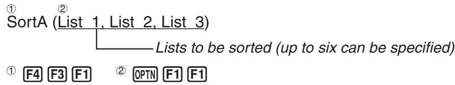
- Descending order
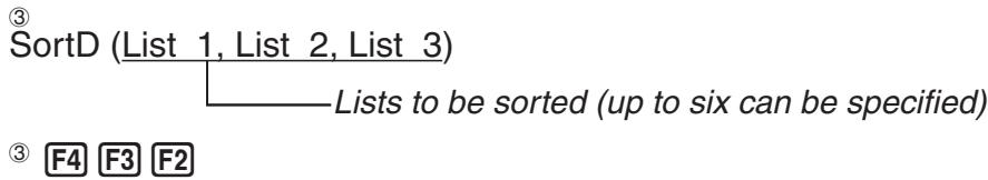
■ Using Statistical Calculations and Graphs in a Program
Including statistical calculations and graphing operations in a program lets you calculate and graph statistical data.
- To set conditions and draw a statistical graph
Following a StatGraph command ("S-Gph1", "S-Gph2", or "S-Gph3"), you must specify the following graph conditions:
- Graph draw/non-draw status (DrawOn/DrawOff)
- Graph Type
- x -axis data location (list name)
- y-axis data location (list name)
• Frequency data location (list name) - Mark Type
- Pie graph display setting (% or Data)
- Pie graph percentage data storage list specification (None or list name)
- First bar graph data (list name)
• Second and third bar graph data (list name) - Bar graph orientation (Length or Horizontal)
The graph conditions that are required depends on the graph type. See “Changing Graph Parameters” (page 6-1).
-
The following is a typical graph condition specification for a scatter diagram or xy Line graph.
S-Gph1 DrawOn, Scatter, List 1, List 2, 1, Square
In the case of an xy line graph, replace "Scatter" in the above specification with "xyLine". -
The following is a typical graph condition specification for a normal probability plot.
S-Gph1 DrawOn, NPPlot, List 1, Square
- The following is a typical graph condition specification for a single-variable graph.
S-Gph1 DrawOn, Hist, List 1, List 2
The same format can be used for the following types of graphs, by simply replacing “Hist” in the above specification with the applicable graph type.
Histogram ...... Hist Normal Distribution ...... N-Dist
Median Box ...... MedBox*1 Broken Line ...... Broken
*1 Outliers:On
S-Gph1 DrawOn, MedBox, List 1, 1, 1 S-Gph1 DrawOn, MedBox, List 1, 1, 0
- The following is a typical graph condition specification for a regression graph.
S-Gph1 DrawOn, Linear, List 1, List 2, List 3
The same format can be used for the following types of graphs, by simply replacing “Linear” in the above specification with the applicable graph type.
Linear Regression ...... Linear Logarithmic Regression ...... Log
Med-Med...... Med-Med Exponential Regression ...... ExpReg(a·e^bx)
Quadratic Regression .... Quad ExpReg(a·b^x)
Cubic Regression .... Cubic Power Regression .... Power
Quartic Regression ..... Quart
- The following is a typical graph condition specification for a sinusoidal regression graph.
S-Gph1 DrawOn, Sinusoidal, List 1, List 2
- The following is a typical graph condition specification for a logistic regression graph.
S-Gph1 DrawOn, Logistic, List 1, List 2
- The following is a typical graph condition specification for a pie graph.
S-Gph1 DrawOn, Pie, List 1, %, None
- The following is a typical graph condition specification for a bar graph.
S-Gph1 DrawOn, Bar, List 1, None, None, StickLength
- To draw a statistical graph, insert the “DrawStat” command following the graph condition specification line.
ClrGraph
S-Wind Auto
{1, 2, 3} → List 1
{1, 2, 3} → List 2
S-Gph1 DrawOn, Scatter, List 1, List 2, 1, Square
DrawStat
■ Using Distribution Graphs in a Program
(Not available on the fx-7400GII)
Special commands are used to draw distribution graphs in a program.
- To draw a normal cumulative distribution graph
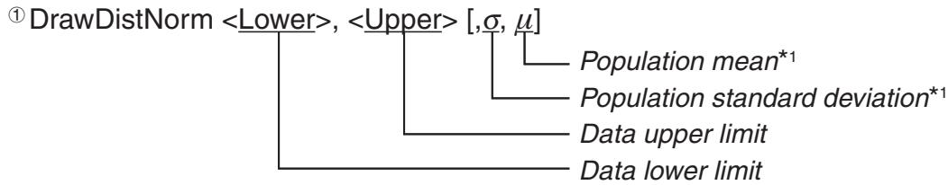
flowchart
graph TD
    A["① DrawDistNorm <Lower>, <Upper> [,σ, μ"]] --> B["Population mean*1"]
    A --> C["Population standard deviation*1"]
    A --> D["Data upper limit"]
    A --> E["Data lower limit"]
① F4 F1 F5 F1
*1 This can be omitted. Omitting these items performs the calculation using = 1 and = 0 .
$$ p = \frac {1}{\sqrt {2 \pi} \sigma} \int_ {\text {Lower}} ^ {\text {Upper}} e ^ {- \frac {(x - \mu) ^ {2}}{2 \sigma^ {2}}} d x \quad Z L o w = \frac {\text {Lower} - \mu}{\sigma} \quad Z U p = \frac {\text {Upper} - \mu}{\sigma} $$
- Executing DrawDistNorm performs the above calculation in accordance with the specified conditions and draws the graph. At this time the ZLow ≤ x ≤ ZUp region on the graph is filled in.
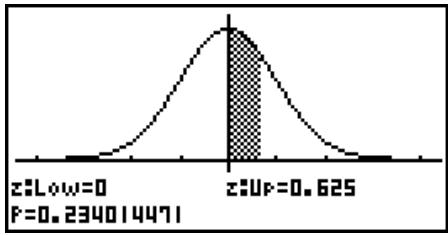
histogram
| Statistic | Value | | --------- | --------- | | z≤Low | 0 | | z≤High | 0.625 | | P=0.234014471 | 0.234014471 |- At the same time, the p , ZLow, and ZUp calculation result values are assigned respectively to variables p , ZLow, and ZUp, and p is assigned to Ans.
- To draw a Student- t cumulative distribution graph

flowchart
graph TD
    A["DrawDistT <Lower>, <Upper>, <df>"] --> B["Degree of freedom"]
    A --> C["Data upper limit"]
    A --> D["Data lower limit"]
① F4 F1 F5 F2
$$ p = \int_ {L o w e r} ^ {U p p e r} \frac {\Gamma \left(\frac {d f + 1}{2}\right)}{\Gamma \left(\frac {d f}{2}\right)} \times \frac {\left(1 + \frac {x ^ {2}}{d f}\right) ^ {- \frac {d f + 1}{2}}}{\sqrt {\pi \times d f}} d x \quad t L o w = L o w e r \quad t U p = U p p e r $$
- Executing DrawDistT performs the above calculation in accordance with the specified conditions and draws the graph. At this time the Lower ≤ x ≤ Upper region on the graph is filled in.
- At the same time, the p calculation result value and the Lower and Upper input values are assigned respectively to variables p , tLow, and tUp, and p is assigned to Ans.
• To draw a ^2 cumulative distribution graph
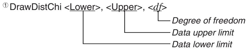
flowchart
graph TD
    A["DrawDistChi <Lower>, <Upper>, <df>"] --> B["Degree of freedom"]
    A --> C["Data upper limit"]
    A --> D["Data lower limit"]
① F4 F1 F5 F3
$$ p = \int_ {L o w e r} ^ {U p p e r} \frac {1}{\Gamma \left(\frac {d f}{2}\right)} \times \left(\frac {1}{2}\right) ^ {\frac {d f}{2}} \times x ^ {\left(\frac {d f}{2} - 1\right)} \times e ^ {- \frac {x}{2}} d x $$
- Executing DrawDistChi performs the above calculation in accordance with the specified conditions and draws the graph. At this time the Lower ≤ x ≤ Upper region on the graph is filled in.
- At the same time, calculation result p is assigned to variables p and Ans.
- To draw an F cumulative distribution graph
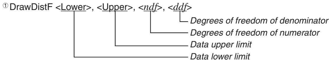
flowchart
graph TD
    A["DrawDistF <Lower>, <Upper>, <ndf>, <ddf>"] --> B["Degrees of freedom of denominator"]
    A --> C["Degrees of freedom of numerator"]
    A --> D["Data upper limit"]
    A --> E["Data lower limit"]
① F4 F1 F5 F4
$$ p = \int_ {L o w e r} ^ {U p p e r} \frac {\Gamma \left(\frac {n d f + d d f}{2}\right)}{\Gamma \left(\frac {n d f}{2}\right) \times \Gamma \left(\frac {d d f}{2}\right)} \times \left(\frac {n d f}{d d f}\right) ^ {\frac {n d f}{2}} \times x ^ {\left(\frac {n d f}{2} - 1\right)} \times \left(1 + \frac {n d f \times x}{d d f}\right) ^ {- \frac {n d f + d d f}{2}} d x $$
- Executing DrawDistF performs the above calculation in accordance with the specified conditions and draws the graph. At this time the Lower ≤ x ≤ Upper region on the graph is filled in.
- At the same time, calculation result p is assigned to variables p and Ans.
■ Performing Statistical Calculations in a Program
- Single-variable statistical calculation
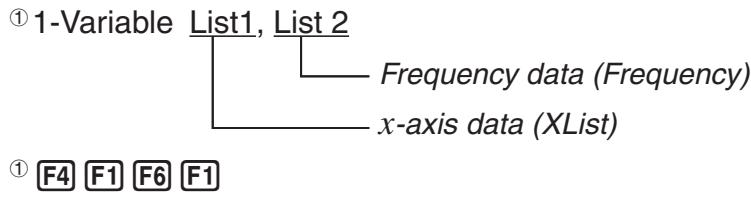
flowchart
graph TD
    A["① 1-Variable List1, List 2"] --> B["Frequency data (Frequency)"]
    A --> C["x-axis data (XList)"]
    D["① F4 F1 F6 F1"]
- Paired-variable statistical calculation
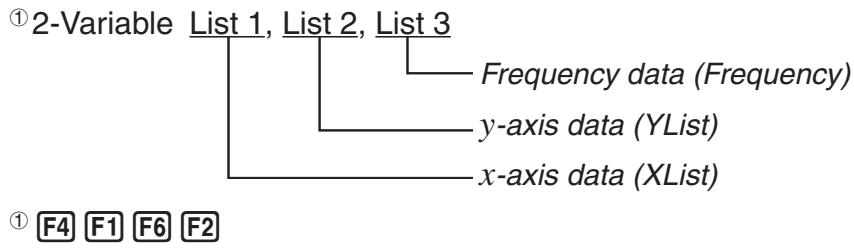
flowchart
graph TD
    A["① 2-Variable"] --> B["List 1, List 2, List 3"]
    B --> C["Frequency data (Frequency)"]
    B --> D["y-axis data (YList)"]
    B --> E["x-axis data (XList)"]
    F["① F4"] --> G["F1"]
    F --> H["F6"]
    F --> I["F2"]
- Regression statistical calculation
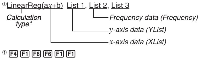
flowchart
graph TD
    A["Calculation type*"] --> B["LinearReg(ax+b)"]
    B --> C["List 1, List 2, List 3"]
    C --> D["Frequency data (Frequency)"]
    C --> E["y-axis data (YList)"]
    C --> F["x-axis data (XList)"]
    G["① F4 F1 F6 F6 F1 F1"] --> H["End"]
* Any one of the following can be specified as the calculation type.
LinearReg(ax+b).....linear regression (ax+b type) LinearReg(a+bx).....linear regression (a+bx type) Med-MedLine .....Med-Med calculation QuadReg .....quadratic regression CubicReg.....cubic regression QuartReg.....quartic regression LogReg .....logarithmic regression ExpReg(a·e^bx).....exponential regression (a·e^bx type) ExpReg(a·b^x).....exponential regression (a·b^x type) PowerReg .....power regression
flowchart
graph TD
    A["• Sinusoidal regression statistical calculation"] --> B["SinReg List 1, List 2"]
    B --> C["y-axis data (YList)"]
    B --> D["x-axis data (XList)"]
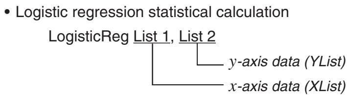
flowchart
graph TD
    A["Logistic regression statistical calculation"] --> B["LogisticReg List 1, List 2"]
    B --> C["y-axis data (YList)"]
    B --> D["x-axis data (XList)"]
■ Performing Distribution Calculations in a Program
(Not available on the fx-7400GII)
- The following values are substituted whenever any of the values enclosed in brackets ([]) are omitted.
$$ \sigma = 1, \mu = 0, \text { tail } = L (\text { Left }) $$
- For the calculation formula of each probability density function, see “Statistic Formula” (page 6-53).
- Normal Distribution
NormPD(: Returns the normal probability density (p value) for the specified data.
Syntax: NormPD(x[, σ, μ)]
- A single value or a list can be specified for x . Calculation result p is assigned to variables p and Ans (ListAns when x is a list).
NormCD(: Returns the normal cumulative distribution (p value) for the specified data.
Syntax: NormCD(Lower, Upper[, σ, μ])
- Single values or lists can be specified for Lower and Upper. Calculation results p , ZLow, and ZUp are assigned respectively to variables p , ZLow, and ZUp. Calculation result p also is assigned to Ans (ListAns when Lower and Upper are lists).
InvNormCD(: Returns the inverse normal cumulative distribution (lower and/or upper value(s)) for the specified p value.
Syntax: InvNormCD(["L(or -1) or R(or 1) or C(or 0)", ]p[,σ, μ]) tail (Left, Right, Central)
- A single value or a list can be specified for p . Calculation results are output in accordance with the tail setting as described below.
$$ \text { tail } = \text { Left } $$
The Upper value is assigned to variables x1InvN and Ans (ListAns when p is a list).
$$ \text { tail } = \text { Right } $$
The Lower value is assigned to variables x1InvN and Ans (ListAns when p is a list).
$$ \text { tail } = \text { Central } $$
The Lower and Upper values are assigned respectively to variables x1InvN and x2InvN. Lower only is assigned to Ans (ListAns when p is a list).
- Student- t Distribution
tPD(: Returns the Student-t probability density (p value) for the specified data.
Syntax: tPD(x, df [])
- A single value or a list can be specified for x . Calculation result p is assigned to variables p and Ans (ListAns when x is a list).
tCD(): Returns the Student-t cumulative distribution (p value) for the specified data.
Syntax: tCD(Lower, Upper, df [])
- Single values or lists can be specified for Lower and Upper. Calculation results p , tLow, and tUp are assigned respectively to variables p , tLow, and tUp. Calculation result p also is assigned to Ans (ListAns when Lower and Upper are lists).
InvTCD(: Returns the inverse Student-t cumulative distribution (Lower value) for the specified p value.
Syntax: InvTCD(p,df[])
- A single value or a list can be specified for p . The Lower value is assigned to the xInv and Ans variables (ListAns when p is a list).
- ^2 Distribution
ChiPD(: Returns the ^2 probability density (p value) for the specified data.
Syntax: ChiPD(x,df[])
- A single value or a list can be specified for x . Calculation result p is assigned to variables p and Ans (ListAns when x is a list).
ChiCD(): Returns the ^2 cumulative distribution (p value) for the specified data.
Syntax: ChiCD(Lower, Upper, df [])
- Single values or lists can be specified for Lower and Upper. Calculation result p is assigned to variables p and Ans (ListAns when Lower and Upper are lists).
InvChiCD(: Returns the inverse ^2 cumulative distribution (Lower value) for the specified p value.
Syntax: InvChiCD(p,df[])
- A single value or a list can be specified for p . The Lower value is assigned to the xInv and Ans variables (ListAns when p is a list).
- F Distribution
FPD(): Returns the F probability density (p value) for the specified data.
Syntax: FPD(x,ndf,ddf[])
- A single value or a list can be specified for x . Calculation result p is assigned to variables p and Ans (ListAns when x is a list).
FCD(:Returns the F cumulative distribution (p value) for the specified data.
Syntax: FCD(Lower, Upper, ndf, ddf [])
- Single values or lists can be specified for Lower and Upper. Calculation result p is assigned to variables p and Ans (ListAns when Lower and Upper are lists).
InvFCD(): Returns the inverse F cumulative distribution (Lower value) for the specified data.
Syntax: InvFCD(p, ndf, ddf [])
- A single value or a list can be specified for p . The Lower value is assigned to the xInv and Ans variables (ListAns when p is a list).
- Binomial Distribution
BinomialPD(): Returns the binomial probability (p value) for the specified data.
Syntax: BinomialPD([x,]n,P[])
- A single value or a list can be specified for x . Calculation result p is assigned to variables p and Ans (ListAns when x is a list).
BinomialCD(: Returns the binomial cumulative distribution (p value) for the specified data.
Syntax: BinomialCD([X,]n,P[])
- A single value or a list can be specified for each X. Calculation result p is assigned to variables p and Ans (ListAns when X is omitted or is a list).
InvBinomialCD(: Returns the inverse binomial cumulative distribution for the specified data.
Syntax: InvBinomialCD(p,n,P[])
- A single value or a list can be specified for p . The calculation result X value is assigned to the xInv and Ans variables (ListAns when p is a list).
- Poisson Distribution
PoissonPD(: Returns the Poisson probability (p value) for the specified data.
Syntax: PoissonPD(x, μ[])
- A single value or a list can be specified for x . Calculation result p is assigned to variables p and Ans (ListAns when x is a list).
PoissonCD(: Returns the Poisson cumulative distribution (p value) for the specified data.
Syntax: PoissonCD(X,μ[])
- A single value or a list can be specified for each X. Calculation result p is assigned to variables p and Ans (ListAns when X is a list).
InvPoissonCD(): Returns the inverse Poisson cumulative distribution for the specified data.
Syntax: InvPoissonCD(p,μ[])
- A single value or a list can be specified for p . The calculation result X value is assigned to the xInv and Ans variables (ListAns when p is a list).
- Geometric Distribution
GeoPD(: Returns the geometric probability (p value) for the specified data.
Syntax: GeoPD(x, P[])
- A single value or a list can be specified for x . Calculation result p is assigned to variables p and Ans (ListAns when x is a list).
GeoCD(: Returns the geometric cumulative distribution (p value) for the specified data.
Syntax: GeoCD(X,P[])
- A single value or a list can be specified for each X. Calculation result p is assigned to variables p and Ans (ListAns when X is a list).
InvGeoCD(: Returns the inverse geometric cumulative distribution for the specified data.
Syntax: InvGeoCD(p,P[])
- A single value or a list can be specified for p . The calculation result X value is assigned to the xInv and Ans variables (ListAns when p is a list).
• Hypergeometric Distribution
HypergeoPD(: Returns the hypergeometric probability (p value) for the specified data.
Syntax: HypergeoPD(x, n, M, N[])
- A single value or a list can be specified for x . Calculation result p is assigned to variables p and Ans (ListAns when x is a list).
HypergeoCD(: Returns the hypergeometric cumulative distribution (p value) for the specified data.
Syntax: HypergeoCD(X, n, M, N[])
- A single value or a list can be specified for each X. Calculation result p is assigned to variables p and Ans (ListAns when X is a list).
InvHypergeoCD(: Returns the inverse hypergeometric cumulative distribution for the specified data.
Syntax: InvHypergeoCD(p, n, M, N[])
- A single value or a list can be specified for p . The calculation result X value is assigned to the x Inv and Ans variables (ListAns when p is a list).
■ Using the TEST Command to Execute a Command in a Program
(Not available on the fx-7400GII)
- The following are the specifications ranges for the “ condition” argument of the command.
“<” or -1 when < _0
“≠” or 0 when μ ≠ μ₀
“>” or 1 when >_0
The above also apply for the “ condition” and “ \& condition” specification methods.
- For explanations of arguments that are not covered in detail here, see “Tests” (page 6-22) and “Input and Output Terms of Tests, Confidence Interval, and Distribution” (page 6-50).
- For the calculation formula of each command, see “Statistic Formula” (page 6-53).
• Z Test
OneSampleZTest: Executes 1-sample Z-test calculation.
Syntax: OneSampleZTest " condition", _0 , , , n
Output Values: Z, p, , n are assigned respectively to variables z, p, , n and to ListAns elements 1 through 4.
| Syntax: | OneSampleZTest "μ condition", μ0, σ, List[, Freq] |
| Output Values: | Z, p, x̄, sx, n are assigned respectively to variables z, p, x̄, sx, n and to ListAns elements 1 through 5. |
| TwoSampleZTest: | Executes 2-sample Z-test calculation. |
| Syntax: | TwoSampleZTest "μ1 condition", σ1, σ2, x̄1, n1, x̄2, n2 |
| Output Values: | Z, p, x̄1, x̄2, n1, n2 are assigned respectively to variables z, p, x̄1, x̄2, n1, n2 and to ListAns elements 1 through 6. |
| Syntax: | TwoSampleZTest "μ1 condition", σ1, σ2, List1, List2[, Freq1 [, Freq2]] |
| Output Values: | Z, p, x̄1, x̄2, sx1, sx2, n1, n2 are assigned respectively to variables z, p, x̄1, x̄2, sx1, sx2, n1, n2 and to ListAns elements 1 through 8. |
| OnePropZTest: | Executes 1-proportion Z-test calculation. |
| Syntax: | OnePropZTest "p condition", p0, x, n |
| Output Values: | Z, p, p̂, n are assigned respectively to variables z, p, p̂, n and to ListAns elements 1 through 4. |
| TwoPropZTest: | Executes 2-proportion Z-test calculation. |
| Syntax: | TwoPropZTest "p1 condition", x1, n1, x2, n2 |
| Output Values: | Z, p, p̂1, p̂2, p̂, n1, n2 are assigned respectively to variables z, p, p̂1, p̂2, p̂, n1, n2 and to ListAns elements 1 through 7. |
- t Test
| OneSampleTTest: | Executes 1-sample t-test calculation. |
| Syntax: | OneSampleTTest "μ condition", μ0, x̄, sx, nOneSampleTTest "μ condition", μ0, List[, Freq] |
| Output Values: | t, p, x̄, sx, n are assigned respectively to the variables with the same names and to ListAns elements 1 through 5. |
| TwoSampleTTest: | Executes 2-sample t-test calculation. |
| Syntax : | TwoSampleTTest "μ1 condition", x̄1, sx1, n1, x̄2, sx2, n2[, Pooled condition]TwoSampleTTest "μ1 condition", List1, List2, [, Freq1[, Freq2[, Pooled condition ]] |
| Output Values: | When Pooled condition = 0, t, p, df, x̄1 x̄2, sx1, sx2, n1, n2 are assigned respectively to the variables with the same names and to ListAns elements 1 through 9.When Pooled condition = 1, t, p, df, x̄1, x̄2, sx1, sx2, sp, n1, n2 are assigned respectively to the variables with the same names and to ListAns elements 1 through 10. |
| Note: | Specify 0 when you want to turn off the Pooled condition and 1 when you want to turn it on. Omitting the input is treated as Pooled condition off. |
| LinRegTTest: | Executes linear regression t-test calculation. |
| Syntax: | LinRegTTest "β&ρ condition", XList, YList[, Freq] |
| Output Values: | t, p, df, a, b, s, r, r2 are assigned respectively to the variables with the same names and to ListAns elements 1 through 8. |
- ^2 Test
ChiGOFTest: Executes a chi-square goodness of fit test.
Syntax: ChiGOFTest List 1, List 2, df, List 3 (List 1 is the Observed list, List 2 is the Expected list, and List 3 is the CNTRB list.)
Output Values: ^2, p, df are assigned respectively to the variables with the same names and to ListAns elements 1 through 3. The CNTRB list is stored in List 3.
ChiTest: Executes a chi-square test.
Syntax: ChiTest MatA, MatB (MatA is the Observed matrix and MatB is the Expected matrix.)
Output Values: ^2 , p, df are assigned respectively to the variables with the same names and to ListAns elements 1 through 3. The Expected matrix is assigned to MatB.
- F Test
TwoSampleFTest: Executes 2-sample F-test calculation.
Syntax: TwoSampleFTest " _1 condition", s_x1 , n_1 , s_x2 , n_2
Output Values: F, p, Sx_1, Sx_2, n_1, n_2 are assigned respectively to the variables with the same names and to ListAns elements 1 through 6.
Syntax: TwoSampleFTest " _1 condition", List1, List2, [, Freq1 [, Freq2]]
Output Values: F, p, 1, 2, s_x1, s_x2, n_1, n_2 are assigned respectively to the variables with the same names and to ListAns elements 1 through 8.
• ANOVA
OneWayANOVA: Executes one-factor ANOVA analysis of variance.
Syntax: OneWayANOVA List1, List2 (List1 is Factor list (A) and List2 is the Dependent list.)
Output Values: Adf, Ass, Ams, AF, Ap, ERRdf, ERRss, ERRms are assigned respectively to variables Adf, SSa, MSa, Fa, pa, Edf, SSe, MSe.
Also, output values are assigned to MatAns as shown below.
$$ \text {MatAns} = \left[ \begin{array}{c c c c c} A d f & A s s & A m s & A F & A p \ E R R d f & E R R s s & E R R m s & 0 & 0 \end{array} \right] $$
TwoWayANOVA: Executes two-factor ANOVA analysis of variance.
Syntax: TwoWayANOVA List1, List2, List3 (List1 is Factor list (A), List2 is Factor list (B), and List3 is the Dependent list.)
Output Values: Adf, Ass, Ams, AF, Ap, Bdf, Bss, Bms, BF, Bp, ABdf, ABss, ABms, ABF, ABp, ERRdf, ERRss, ERRms are assigned respectively to variables Adf, SSa, MSa, Fa, pa, Bdf, SSb, MSb, Fb, pb, ABdf, SSab, MSab, Fab, pab, Edf, SSe, MSe.
Also, output values are assigned to MatAns as shown below.
$$ \text { MatAns } = \left[ \begin{array}{c c c c c} A d f & A s s & A m s & A F & A p \ B d f & B s s & B m s & B F & B p \ A B d f & A B s s & A B m s & A B F & A B p \ E R R d f & E R R s s & E R R m s & 0 & 0 \end{array} \right] $$
■ Performing Financial Calculations in a Program
(Not available on the fx-7400GII)
- Setup Commands
- Date Mode Setting for Financial Calculations
DateMode365...... 365 days
DateMode360...... 360 days - Payment Period Setting
PmtBgn...... Start of period
PmtEnd...... End of period
• Bond Calculation Payment Periods
PeriodsAnnual ..... Annual
PeriodsSemi ...... Semiannual
• Financial Calculation Commands
For the meaning of each argument, see “Chapter 7 Financial Calculation (TVM)”.
- Simple Interest
Smpl_SI: Returns the interest based on simple interest calculation.
Syntax: Smpl_SI(n, I%, PV)
Smpl_SFV: Returns the total of principal and interest based on simple interest calculation.
Syntax: Smpl_SFV(n, I%, PV)
- Compound Interest
Note:
- P/Y and C/Y can be omitted for all compound interest calculations. When they are omitted, calculations are performed using P/Y=12 and C/Y=12.
- If you perform a calculation that uses a compound interest function (Cmpd_n(, Cmpd_1%(), Cmpd_PV(, Cmpd_PMT(, Cmpd_FV(), the argument(s) you input and the calculation results will be saved to the applicable variables (n, I%, PV, etc.). If you perform a calculation that uses any other type of financial calculation function, the argument and calculation results are not assigned to variables.
Cmpd_n: Returns the number of compound periods.
Syntax: Cmpd_n(I%, PV, PMT, FV, P/Y, C/Y)
Cmpd_I%: Returns the annual interest.
Syntax: Cmpd_I%(n, PV, PMT, FV, P/Y, C/Y)
Cmpd_PV: Returns the present value (loan amount for installment payments, principal for savings).
Syntax: Cmpd_PV(n, I%, PMT, FV, P/Y, C/Y)
Cmpd_PMT: Returns equal input/output values (payment amounts for installment payments, deposit amounts for savings) for a fixed period.
Syntax: Cmpd_PMT(n, I%, PV, FV, P/Y, C/Y)
Cmpd_FV: Returns the final input/output amount or total principal and interest.
Syntax: Cmpd_FV(n, I%, PV, PMT, P/Y, C/Y)
• Cash Flow (Investment Appraisal)
Cash_NPV: Returns the net present value.
Syntax: Cash_NPV(I%, Csh)
Cash_IRR: Returns the internal rate of return.
Syntax: Cash_IRR(Csh)
Cash_PBP: Returns the payback period.
Syntax: Cash_PBP(I%, Csh)
Cash_NFV: Returns the net future value.
Syntax: Cash_NFV(I%, Csh)
- Amortization
Amt_BAL: Returns the remaining principal balance following payment PM2.
Syntax: Amt_BAL(PM1, PM2, I%, PV, PMT, P/Y, C/Y)
Amt_INT: Returns the interest paid for payment PM1.
Syntax: Amt_INT(PM1, PM2, I%, PV, PMT, P/Y, C/Y)
Amt_PRN: Returns the principal and interest paid for payment PM1.
Syntax: Amt_PRN(PM1, PM2, I%, PV, PMT, P/Y, C/Y)
Amt_ΣINT: Returns the total principal and interest paid from payment PM1 to PM2.
Syntax: Amt_ΣINT(PM1, PM2, I%, PV, PMT, P/Y, C/Y)
Amt_ΣPRN: Returns the total principal paid from payment PM1 to PM2.
Syntax: Amt_ΣPRN(PM1, PM2, I%, PV, PMT, P/Y, C/Y)
- Interest Rate Conversion
Cnvt_EFF: Returns the interest rate converted from the nominal interest rate to the effective interest rate.
Syntax: Cnvt_EFF(n, I%)
Cnvt_APR: Returns the interest rate converted from the effective interest rate to the nominal interest rate.
Syntax: Cnvt_APR(n, I%)
- Cost, Selling Price, Margin Calculations
Cost: Returns the cost based on a specified selling price and margin.
Syntax: Cost(Sell, Margin)
Sell: Returns the selling price based on a specified cost and margin.
Syntax: Sell(Cost, Margin)
Margin: Returns the margin based on a specified cost and selling price.
Syntax: Margin(Cost, Sell)
• Day/Date Calculations
Days_Prd: Returns the number of days from a specified d1 to specified d2.
Bond_PRC: Returns in list form bond prices based on specified conditions.
Bond_YLD: Returns the yield based on specified conditions.
7. PRGM Mode Command List
Not all of the commands listed below are available on all models covered by this manual.
RUN Program
| F4 (MENU) key | |||
| Level 1 | Level 2 | Level 3 | Command |
| STAT | DRAW | On | DrawOn |
| Off | DrawOff | ||
| GRPH | GPH1 | S-Gph1_ | |
| GPH2 | S-Gph2_ | ||
| GPH3 | S-Gph3_ | ||
| Scat | Scatter | ||
| xy | xyLine | ||
| Hist | Hist | ||
| Box | MedBox | ||
| Bar | Bar | ||
| N-Dis | N-Dist | ||
| Brkn | Broken | ||
| X | Linear | ||
| Med | Med-Med | ||
| X^2 | Quad | ||
| X^3 | Cubic | ||
| X^4 | Quart | ||
| Log | Log | ||
| *1 | |||
| Pwr | Power | ||
| Sin | Sinusoidal | ||
| NPP | NPPlot | ||
| Lgst | Logistic | ||
| Pie | Pie | ||
| List | List_ | ||
| TYPE | *2 | ||
| DIST | DrwN | DrawDistNorm_ | |
| Drwt | DrawDistT_ | ||
| DrwC | DrawDistChi_ | ||
| DrwF | DrawDistF_ | ||
| CALC | 1VAR | 1-Variable_ | |
| 2VAR | 2-Variable_ | ||
| *3 | |||
| Med | Med-MedLine_ | ||
| X^2 | QuadReg_ | ||
| X^3 | CubicReg_ | ||
| X^4 | QuartReg_ | ||
| Log | LogReg_ | ||
| *4 | |||
| Pwr | PowerReg_ | ||
| Sin | SinReg_ | ||
| Lgst | LogisticReg_ | ||
| MAT | Swap | Swap_ | |
| ×Rw | *Row_ | ||
| ×Rw+ | *Row+_ | ||
| Rw+ | Row+_ | ||
| LIST | Srt-A | SortA( | |
| Srt-D | SortD( | ||
| GRPH | SEL | On | G_SelOn_ |
| Off | G_SelOff_ | ||
| TYPE | Y= | Y=Type | |
| r= | r=Type | ||
| Parm | ParamType | ||
| X= | X=Type | ||
| Y> | Y>Type | ||
| Y< | Y | ||
| Y≥ | Y≥Type | ||
| Y≤ | Y≤Type | ||
| X> | X>Type | ||
| X< | X | ||
| X≥ | X≥Type | ||
| X≤ | X≤Type | ||
| STYL | — | NormalG_ | |
| — | ThickG_ | ||
| ...... | BrokenThickG_ | ||
| ...... | DotG_ | ||
| GMEM | Sto | StoGMEM_ | |
| Rcl | RclGMEM_ | ||
| DYNA | On | D_SelOn_ | |
| Off | D_SelOff_ | ||
| Var | D_Var_ | ||
| TYPE | Y= | Y=Type | |
| r= | r=Type | ||
| Parm | ParamType | ||
| TABL | On | T_SelOn_ | |
| Off | T_SelOff_ | ||
| TYPE | Y= | Y=Type | |
| r= | r=Type | ||
| Parm | ParamType | ||
| STYL | — | NormalG_ | |
| — | ThickG_ | ||
| ...... | BrokenThickG_ | ||
| ...... | DotG_ | ||
| RECR | SEL+S | On | R_SelOn_ |
| Off | R_SelOff_ | ||
| — | NormalG_ | ||
| — | ThickG_ | ||
| ...... | BrokenThickG_ | ||
| ...... | DotG_ | ||
| TYPE | an | anType | |
| an+1 | an+1Type | ||
| an+2 | an+2Type | ||
| n.an" | n | n | |
| an | an | ||
| an+1 | an+1 | ||
| an+2 | an+2 | ||
| bn | bn | ||
| bn+1 | bn+1 | ||
| bn+2 | bn+2 | ||
| cn | cn | ||
| cn+1 | cn+1 | ||
| cn+2 | cn+2 | ||
| Σan | Σan | ||
| Σan+1 | Σan+1 | ||
| Σan+2 | Σan+2 | ||
| Σbn | Σbn | ||
| Σbn+1 | Σbn+1 | ||
| Σbn+2 | Σbn+2 | ||
| Σcn | Σcn | ||
| Σcn+1 | Σcn+1 | ||
| Σcn+2 | Σcn+2 | ||
| RANG | a0 | Sel_a0 | |
| a1 | Sel_a1 |
| OPTN key | |||
| Level 1 | Level 2 | Level 3 | Command |
| LIST | List | List_ | |
| L→M | List→Mat( | ||
| Dim | Dim_ | ||
| Fill | Fill( | ||
| Seq | Seq( | ||
| Min | Min( | ||
| Max | Max( | ||
| Mean | Mean( | ||
| Med | Median( | ||
| Aug | Augment( | ||
| Sum | Sum_ | ||
| Prod | Prod_ | ||
| Cuml | Cuml_ | ||
| % | Percent_ | ||
| List_ | |||
| MAT | Mat | Mat_ | |
| M→L | Mat→List( | ||
| Det | Det_ | ||
| Trn | Trn_ | ||
| Aug | Augment( | ||
| Iden | Identity_ | ||
| Dim | Dim_ | ||
| Fill | Fill( | ||
| Ref | Ref_ | ||
| Rref | Rref_ | ||
| CPLX | i | i | |
| Abs | Abs_ | ||
| Arg | Arg_ | ||
| Conj | Conjg_ | ||
| ReP | ReP_ | ||
| ImP | ImP_ | ||
| r | r | ||
| a+bi | a+bi | ||
| CALC | Solve | Solve( | |
| d/dx | d/dx( | ||
| d^2/dx^2 | d^2/dx^2 ( | ||
| dx | ( | ||
| SolveN | SolveN( | ||
| FMin | FMin( | ||
| FMax | FMax( | ||
| ( | ( | ||
| _ab | _ab ( | ||
| Int÷ | Int÷ | ||
| Rmdr | Rmdr | ||
| Simp | Simp | ||
| STAT | |||
| DIST | *5 | ||
| S·Dev | StdDev( | ||
| Var | Variance( | ||
| TEST | *6 | ||
| CONV | |||
| LENG | fm | [fm] | |
| [] | |||
| μm | [μm] | |
| mm | [mm] | |
| cm | [cm] | |
| m | [m] | |
| km | [km] | |
| AU | [AU] | |
| l.y. | [l.y.] | |
| pc | [pc] | |
| Mil | [Mil] | |
| in | [in] | |
| ft | [ft] | |
| yd | [yd] | |
| fath | [fath] | |
| rd | [rd] | |
| mile | [mile] | |
| n mile | [n mile] | |
| AREA | cm^2 | [cm^2] |
| m^2 | [m^2] | |
| ha | [ha] | |
| km^2 | [km^2] | |
| in^2 | [in^2] | |
| ft^2 | [ft^2] | |
| yd^2 | [yd^2] | |
| acre | [acre] | |
| mile^2 | [mile^2] | |
| VLUM | cm^3 | [cm^3] |
| mL | [mL] | |
| L | [L] | |
| m^3 | [m^3] | |
| in^3 | [in^3] | |
| ft^3 | [ft^3] | |
| fl_oz(UK) | [fl_oz(UK)] | |
| fl_oz(US) | [fl_oz(US)] | |
| gal(US) | [gal(US)] | |
| gal(UK) | [gal(UK)] | |
| pt | [pt] | |
| qt | [qt] | |
| tsp | [tsp] | |
| tbsp | [tbsp] | |
| cup | [cup] | |
| TIME | ns | [ns] |
| μs | [μs] | |
| ms | [ms] | |
| s | [s] | |
| min | [min] | |
| h | [h] | |
| day | [day] | |
| week | [week] | |
| yr | [yr] | |
| s-yr | [s-yr] | |
| t-yr | [t-yr] | |
| TMPR | °C | [°C] |
| K | [K] | |
| °F | [°F] | |
| °R | [°R] | |
| VELO | m/s | [m/s] |
| km/h | [km/h] | |
| knot | [knot] | |
| ft/s | [ft/s] | |
| mile/h | [mile/h] | |
| MASS | u | [u] |
| mg | [mg] | ||
| g | [g] | ||
| kg | [kg] | ||
| mton | [mton] | ||
| oz | [oz] | ||
| lb | [lb] | ||
| slug | [slug] | ||
| ton(short) | [ton(short)] | ||
| ton(long) | [ton(long)] | ||
| RORC | N | [N] | |
| lbf | [lbf] | ||
| tonf | [tonf] | ||
| dyne | [dyne] | ||
| kgf | [kgf] | ||
| PRES | Pa | [Pa] | |
| kPa | [kPa] | ||
| mmH2O | [mmH2O] | ||
| mmHg | [mmHg] | ||
| atm | [atm] | ||
| inH2O | [inH2O] | ||
| inHg | [inHg] | ||
| lbf/in2 | [lbf/in2] | ||
| bar | [bar] | ||
| kgf/cm2 | [kgf/cm2] | ||
| ENGY | eV | [eV] | |
| J | [J] | ||
| calth | [calth] | ||
| cal15 | [cal15] | ||
| calIT | [calIT] | ||
| kcalth | [kcalth] | ||
| kcal15 | [kcal15] | ||
| kcalIT | [kcalIT] | ||
| I-atm | [I-atm] | ||
| kW·h | [kW·h] | ||
| ft·lbf | [ft·lbf] | ||
| Btu | [Btu] | ||
| erg | [erg] | ||
| kgf·m | [kgf·m] | ||
| PWR | W | [W] | |
| calth/s | [calth/s] | ||
| hp | [hp] | ||
| ft·lbf/s | [ft·lbf/s] | ||
| Btu/min | [Btu/min] | ||
| HYP | sinh | sinh_ | |
| cosh | cosh_ | ||
| tanh | tanh_ | ||
| sinh-1 | sinh-1_ | ||
| cosh-1 | cosh-1_ | ||
| tanh-1 | tanh-1_ | ||
| PROB | X! | ! | |
| nPr | P | ||
| nCr | C | ||
| RAND | Ran# | Ran#_ | |
| Int | RanInt#( | ||
| Norm | RanNorm#( | ||
| Bin | RanBin#( | ||
| List | RanList#( | ||
| P( | P( | ||
| Q( | Q( | ||
| R( | R( | ||
| t(Abs | t(Abs_ | ||
| NUM | |||
| Int | Int_ | ||
| Frac | Frac_ | ||
| Rnd | Rnd | ||
| Intg | Intg_ | ||
| RndFi | RndFix( | ||
| GCD | GCD( | ||
| LCM | LCM( | ||
| MOD | MOD( | ||
| MOD•E | MOD_Exp( | ||
| ANGL | ° | ° | |
| r | r | ||
| g | g | ||
| °, " | ■ | ||
| Pol( | Pol( | ||
| Rec( | Rec( | ||
| ►DMS | ►DMS | ||
| ESYM | m | m | |
| μ | μ | ||
| n | n | ||
| p | p | ||
| f | f | ||
| k | k | ||
| M | M | ||
| G | G | ||
| T | T | ||
| P | P | ||
| E | E | ||
| PICT | Sto | StoPict_ | |
| Rcl | RclPict_ | ||
| FMEM | fn | fn | |
| LOGIC | And | _And_ | |
| Or | _Or_ | ||
| Not | Not_ | ||
| Xor | Xor_ | ||
| CAPT | Rcl | RclCapt_ | |
| TVM | SMPL | SI | Smpl_SI( |
| SFV | Smpl_SFV( | ||
| CMPD | n | Cmpd_n( | |
| I% | Cmpd_I%( | ||
| PV | Cmpd_PV( | ||
| PMT | Cmpd_PMT( | ||
| FV | Cmpd_FV( | ||
| CASH | NPV | Cash_NPV( | |
| IRR | Cash_IRR( | ||
| PBP | Cash_PBP( | ||
| NFV | Cash_NFV( | ||
| AMT | BAL | Amt_BAL( | |
| INT | Amt_INT( | ||
| PRN | Amt_PRN( | ||
| ΣINT | Amt_ΣINT( | ||
| ΣPRN | Amt_ΣPRN( | ||
| CNVT | EFF | Cnvt_EFF( | |
| APR | Cnvt_APR( | ||
| COST | Cost | Cost( | |
| Sell | Sell( | ||
| Mrg | Margin( | ||
| DAYS | PRD | Days_Prd( | |
| BOND | PRC | Bond_PRC( | |
| YLD | Bond_YLD( |
| VARS key | |||
| Level 1 | Level 2 | Level 3 | Command |
| V-WIN | X | min | Xmin |
| max | Xmax | ||
| scal | Xscl | ||
| dot | Xdot | ||
| Y | min | Ymin | |
| max | Ymax | ||
| scal | Yscl | ||
| T,θ | min | Tθmin | |
| max | Tθmax | ||
| ptch | Tθptch | ||
| R-X | min | RightXmin | |
| max | RightXmax | ||
| scal | RightXscl | ||
| dot | RightXdot | ||
| R-Y | min | RightYmin | |
| max | RightYmax | ||
| scal | RightYscl | ||
| R-T, θ | min | RightTθmin | |
| max | RightTθmax | ||
| ptch | RightTθptch | ||
| FACT | Xfct | Xfct | |
| Yfct | Yfct | ||
| STAT | X | n | n |
| Σx | Σx | ||
| Σx^2 | Σx^2 | ||
| σx | σx | ||
| sx | sx | ||
| minX | minX | ||
| maxX | maxX | ||
| Y | |||
| Σy | Σy | ||
| Σy^2 | Σy^2 | ||
| Σxy | Σxy | ||
| σy | σy | ||
| sy | sy | ||
| minY | minY | ||
| maxY | maxY | ||
| GRPH | a | a | |
| b | b | ||
| c | c | ||
| d | d | ||
| e | e | ||
| r | r | ||
| r^2 | r^2 | ||
| MSe | MSe | ||
| Q1 | Q1 | ||
| Med | Med | ||
| Q3 | Q3 | ||
| Mod | Mod | ||
| Strt | H_Start | ||
| Pitch | H_pitch | ||
| PTS | x1 | x1 | |
| y1 | y1 | ||
| x2 | x2 | ||
| y2 | y2 | ||
| x3 | x3 | ||
| y3 | y3 | ||
| INPT | n | n | |
| Sx | Sx | ||
| n1 | n1 | ||
| n2 | n2 | ||
| _1 | _1 | ||
| _2 | _2 | ||
| Sx1 | Sx1 | ||
| Sx2 | Sx2 | ||
| Sp | Sp | ||
| RESLT | *7 | ||
| GRPH | Y | Y | |
| r | r | ||
| Xt | Xt | ||
| Yt | Yt | ||
| X | X | ||
| DYNA | Strt | D_Start | |
| End | D_End | ||
| Pitch | D_pitch | ||
| TABL | Strt | F_Start | |
| End | F_End | ||
| Pitch | F_pitch | ||
| Reslt | F_Result | ||
| RECR | FORM | an | an |
| an+1 | an+1 | ||
| an+2 | an+2 | ||
| bn | bn | ||
| bn+1 | bn+1 | ||
| bn+2 | bn+2 | ||
| Cn | Cn | ||
| Cn+1 | Cn+1 | ||
| Cn+2 | Cn+2 | ||
| RANG | Strt | R_Start | |
| End | R_End | ||
| a0 | a0 | ||
| a1 | a1 | ||
| a2 | a2 | ||
| b0 | b0 | ||
| b1 | b1 | ||
| b2 | b2 | ||
| c0 | c0 | ||
| c1 | c1 | ||
| c2 | c2 | ||
| anSt | anStart | ||
| bnSt | bnStart | ||
| cnSt | cnStart | ||
| Reslt | R_Result | ||
| EQUA | S-RIt | Sim_Result | |
| S-Cof | Sim_Coef | ||
| P-RIt | Ply_Result | ||
| P-Cof | Ply_Coef | ||
| TVM | n | n | |
| I% | I% | ||
| PV | PV | ||
| PMT | PMT | ||
| FV | FV | ||
| P/Y | P/Y | ||
| C/Y | C/Y | ||
| Str | Str_ | ||
| SHIFT VARS (PRGM) key | |||
| Level 1 | Level 2 | Level 3 | Command |
| COM | If | If_ | |
| Then | Then_ | ||
| Else | Else_ | ||
| I-End | IfEnd | ||
| For | For_ | ||
| To | _To_ | ||
| Step | _Step_ | ||
| Next | Next | ||
| While | While_ | ||
| WEnd | WhileEnd | ||
| Do | Do | ||
| Lp-W | LpWhile_ | ||
| CTL | Prog | Prog_ | |
| Rtrn | Return | ||
| Brk | Break | ||
| Stop | Stop | ||
| JUMP | Lbl | Lbl_ | |
| Goto | Goto_ | ||
| ⇒ | ⇒ | ||
| Isz | Isz_ | ||
| Dsz | Dsz_ | ||
| Menu | Menu_ | ||
| ? | ? | ||
| ▲ | ▲ | ||
| CLR | Text | ClrText | |
| Grph | ClrGraph | ||
| List | ClrList_ | ||
| Mat | ClrMat_ | ||
| DISP | Stat | DrawStat | |
| Grph | DrawGraph | ||
| Dyna | DrawDyna | ||
| F-Tbl | Tabl | DispF-Tbl | |
| G-Con | DrawFTG-Con | ||
| G-Plt | DrawFTG-Plt | ||
| R-Tbl | Tabl | DispR-Tbl | |
| Phase | PlotPhase | ||
| Web | DrawWeb_ | ||
| an-Cn | DrawR-Con | ||
| Σa-Cn | DrawR Σ-Con | ||
| an-Pl | DrawR-Plt | ||
| Σa-Pl | DrawR Σ-Plt | ||
| REL | = | = | |
| ≠ | ≠ | ||
| > | > | ||
| < | < | ||
| ≥ | ≥ | ||
| ≤ | ≤ | ||
| I/O | Lcte | Locate_ | |
| Gtky | Getkey | ||
| Send | Send( | ||
| Recv | Receive( | ||
| S38k | Send38k_ | ||
| R38k | Receive38k_ | ||
| Open | OpenComport38k | ||
| Close | CloseComport38k | ||
| : | : | ||
| STR | Join | StrJoin( | |
| Len | StrLen( | ||
| Cmp | StrCmp( | ||
| Src | StrSrc( | ||
| Left | StrLeft( | ||
| Right | StrRight( | ||
| Mid | StrMid( | ||
| E▶S | Exp▶Str( | ||
| Exp | Exp( | ||
| Upr | StrUpr( | ||
| Lwr | StrLwr( | ||
| Inv | StrInv( | ||
| Shift | StrShift( | ||
| Rot | StrRotate( |
| SHIFT MENU (SET UP) key | |||
| Level 1 | Level 2 | Level 3 | Command |
| ANGL | Deg | Deg | |
| Rad | Rad | ||
| Gra | Gra | ||
| COOR | On | CoordOn | |
| Off | CoordOff | ||
| GRID | On | GridOn | |
| Off | GridOff | ||
| AXES | On | AxesOn | |
| Off | AxesOff | ||
| LABL | On | LabelOn | |
| Off | LabelOff | ||
| DISP | Fix | Fix_ | |
| Sci | Sci_ | ||
| Norm | Norm_ | ||
| Eng | On | EngOn | |
| Off | EngOff | ||
| Eng | Eng | ||
| S/L | — | S-L-Normal | |
| — | S-L-Thick | ||
| ...... | S-L-Broken | ||
| ...... | S-L-Dot | ||
| DRAW | Con | G-Connect | |
| Plot | G-Plot | ||
| DERV | On | DerivOn | |
| Off | DerivOff | ||
| BACK | None | BG-None | |
| Pict | BG-Pict_ | ||
| FUNC | On | FuncOn | |
| Off | FuncOff | ||
| SIML | On | SimulOn | |
| Off | SimulOff | ||
| S-WIN | Auto | S-WindAuto | |
| Man | S-WindMan | ||
| LIST | File | File_ | |
| LOCS | On | LocusOn | |
| Off | LocusOff | ||
| T-VAR | Rang | VarRange | |
| List | VarList_ | ||
| ΣDSP | On | ΣdispOn | |
| Off | ΣdispOff | ||
| RESID | None | Resid-None | |
| List | Resid-List_ | ||
| CPLX | Real | Real | |
| a+bi | a+bi | ||
| r∠θ | r∠θ | ||
| FRAC | d/c | d/c | |
| ab/c | ab/c | ||
| Y·SPD | Norm | Y=DrawSpeedNorm | |
| High | Y=DrawSpeedHigh | ||
| DATE | 365 | DateMode365 | |
| 360 | DateMode360 | ||
| PMT | Bgn | PmtBgn | |
| End | PmtEnd | ||
| PRD | Annu | PeriodsAnnual | |
| Semi | PeriodsSemi | ||
| INEQ | And | IneqTypeAnd | |
| Or | IneqTypeOr | ||
| SIMP | Auto | SimplifyAuto | |
| Man | SimplifyMan | ||
| Q1Q3 | Std | Q1Q3TypeStd | |
| OnD | Q1Q3TypeOnData |
| SHIFT key | |||
| Level 1 | Level 2 | Level 3 | Command |
| ZOOM | Fact | Factor_ | |
| Auto | ZoomAuto | ||
| V-WIN | V-Win | ViewWindow_ | |
| Sto | StoV-Win_ | ||
| Rcl | RcIV-Win_ | ||
| SKTCH | Cls | Cls | |
| Tang | Tangent_ | ||
| Norm | Normal_ | ||
| Inv | Inverse_ | ||
| GRPH | Y= | Graph_Y= | |
| r= | Graph_r= | ||
| Parm | Graph(X,Y)=( | ||
| X=c | Graph_X= | ||
| G-/dx | Graph_/ | ||
| Y> | Graph_Y> | ||
| Y< | Graph_Y< | ||
| Y≥ | Graph_Y≥ | ||
| Y≤ | Graph_Y≤ | ||
| X> | Graph_X> | ||
| X< | Graph_X< | ||
| X≥ | Graph_X≥ | ||
| X≤ | Graph_X≤ | ||
| PLOT | Plot | Plot_ | |
| PI-On | PlotOn_ | ||
| PI-Off | PlotOff_ | ||
| PI-Chg | PlotChg_ | ||
| LINE | Line | Line | |
| F-Line | F-Line_ | ||
| Crl | Circle_ | ||
| Vert | Vertical_ | ||
| Hztl | Horizontal_ | ||
| Text | Text_ | ||
| PIXL | On | PxION_ | |
| Off | PxIOff_ | ||
| Chg | PxIChg_ | ||
| Test | PxlTest( | ||
| STYL | — | SketchNormal_ | |
| — | SketchThick_ | ||
| ...... | SketchBroken_ | ||
| ...... | SketchDot_ | ||
BASE Program
| F4 (MENU) key | |||
| Level 1 | Level 2 | Level 3 | Command |
| d~o | d | d | |
| h | h | ||
| b | b | ||
| o | o | ||
| LOG | Neg | Neg_ | |
| Not | Not_ | ||
| and | and | ||
| or | or | ||
| xor | xor | ||
| xnor | xnor | ||
| DISP | ►Dec | ►Dec | |
| ►Hex | ►Hex | ||
| ►Bin | ►Bin | ||
| ►Oct | ►Oct | ||
| SHIFT VARS (PRGM) key | |||
| Level 1 | Level 2 | Level 3 | Command |
| Prog | Prog_ | ||
| JUMP | Lbl | Lbl_ | |
| Goto | Goto_ | ||
| Isz | Isz_ | ||
| Dsz | Dsz_ | ||
| Menu | Menu_ | ||
| ? | ? | ||
| ▲ | ▲ | ||
| REL | = | = | |
| ≠ | ≠ | ||
| > | > | ||
| < | < | ||
| ≥ | ≥ | ||
| ≤ | ≤ | ||
| : | : | ||
| SHIFT MENU (SET UP) key | |||
| Level 1 | Level 2 | Level 3 | Command |
| Dec | Dec | ||
| Hex | Hex | ||
| Bin | Bin | ||
| Oct | Oct | ||
| Level 3 | Level 4 | Command | |
| *1 | Exp | ae^bx | Exp(ae^bx) |
| ab^x | Exp(ab^x) | ||
| *2 | MARK | ■ | Square |
| × | Cross | ||
| ■ | Dot | ||
| STICK | Leng | StickLength | |
| Hztl | StickHoriz | ||
| %DATA | % | % | |
| Data | Data | ||
| None | None | ||
| *3 | X | ax+b | LinearReg(ax+b) |
| a+bx | LinearReg(a+bx) | ||
| *4 | EXP | ae^bx | ExpReg(a•e^bx) |
| ab^x | ExpReg(a•b^x) | ||
| *5 | NORM | NPd | NormPD( |
| NCd | NormCD( | ||
| InvN | InvNormCD( | ||
| t | TPd | tPD( | |
| TCd | tCD( | ||
| Invt | InvTCD( | ||
| CHI | CPd | ChiPD( | |
| CCd | ChiCD( | ||
| InvC | InvChiCD( | ||
| F | FPd | FPD( | |
| FCd | FCD( | ||
| InvF | InvFCD( | ||
| BINM | BPd | BinomialPD( | |
| BCd | BinomialCD( | ||
| InvB | InvBinomialCD( | ||
| POISN | PPd | PoissonPD( | |
| PCd | PoissonCD( | ||
| InvP | InvPoissonCD( | ||
| GEO | GPd | GeoPD( | |
| GCd | GeoCD( | ||
| InvG | InvGeoCD( | ||
| H•GEO | HPd | HypergeoPD( | |
| HCd | HypergeoCD( | ||
| InvH | InvHyperGeoCD( | ||
| *6 | Z | 1-S | OneSampleZTest_ |
| 2-S | TwoSampleZTest_ | ||
| 1-P | OnePropZTest_ | ||
| 2-P | TwoPropZTest_ | ||
| t | 1-S | OneSampleTTest_ | |
| 2-S | TwoSampleTTest_ | ||
| REG | LinRegTTest_ | ||
| Chi | GOF | ChiGOFTest_ | |
| 2-WAY | ChiTest_ | ||
| F | TwoSampleFTest_ | ||
| ANOV | 1-W | OneWayANOVA_ | |
| 2-W | TwoWayANOVA_ |
| *7 | TEST | p | p |
| z | z | ||
| t | t | ||
| Chi | ^2 | ||
| F | F | ||
| _1 | _1 | ||
| _2 | _2 | ||
| df | df | ||
| Se | Se | ||
| r | r | ||
| r^2 | r^2 | ||
| pa | pa | ||
| Fa | Fa | ||
| Adf | Adf | ||
| SSa | SSa | ||
| MSa | MSa | ||
| pb | pb | ||
| Fb | Fb | ||
| Bdf | Bdf | ||
| SSb | SSb | ||
| MSb | MSb | ||
| pab | pab | ||
| Fab | Fab | ||
| ABdf | ABdf | ||
| SSab | SSab | ||
| MSab | MSab | ||
| Edf | Edf | ||
| SSe | SSe | ||
| MSe | MSe | ||
| INTR | Left | Left | |
| Right | Right | ||
| _1 | _1 | ||
| _2 | _2 | ||
| df | df | ||
| DIST | p | p | |
| xInv | xInv | ||
| x1Inv | x1Inv | ||
| x2Inv | x2Inv | ||
| zLow | zLow | ||
| zUp | zUp | ||
| tLow | tLow | ||
| tUp | tUp |
8. Program Library
- Be sure to check how many bytes of unused memory are remaining before attempting to perform any programming.
Program Name
Prime Factorization
Description
This program continually divides a natural number by factors until all its prime factors are produced.
Purpose
This program accepts input of natural number A, and divides it by B (2, 3, 5, 7....) to find the prime factors of A.
- If a division operation does not produce a remainder, the result of the operation is assigned to A.
- The above procedure is repeated until B > A .
Example 462 = 2 × 3 × 7 × 11
ClrText←
"INPUT NUMBER"?→A←
2→B←
Do←
While Frac (A÷B)=0←
B←
A÷B→A←
WhileEnd←
If B=2←
Then 3→B←
Else B+2→B←
IfEnd←
LpWhile B≤A←
"END"
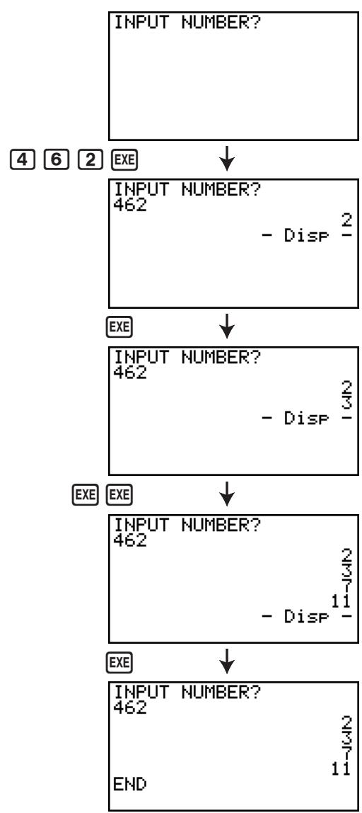
flowchart
graph TD
    A["INPUT NUMBER?"] --> B["4 6 2 EXE"]
    B --> C["INPUT NUMBER? 462 - Disp 2 /"]
    C --> D["EXE"]
    D --> E["INPUT NUMBER? 462 - Disp 3 /"]
    E --> F["EXE EXE"]
    F --> G["INPUT NUMBER? 462 - Disp 11 /"]
    G --> H["EXE"]
    H --> I["INPUT NUMBER? 462 - END 3/7"]
Description
This program displays a number table of the following values based on input of the foci of an ellipse, the sum of the distance between the loci and foci, and the pitch (step size) of X.
Y1: Coordinate values of upper half of ellipse
Y2: Coordinate values of lower half of ellipse
Y3: Distances between right focus and loci
Y4: Distances between left focus and loci
Y5: Sum of Y3 and Y4
Next, the program plots the foci and values in Y1 and Y2.
Purpose
This program shows that the sums of the distances between the loci and two foci of an ellipse are equal.
AxesOff
Do
ClrText
"FOCUS (C,0),(-C,0)"
"C="?→C
"SUM DISTANCE"?→D
LpWhile 2Abs C≥D Or D≤0
D÷2→A
√(A²-C²)→B
Y=Type
"B√(1-X²÷A²)"→Y1
"-Y1"→Y2
"√((X-C)²+Y1²)"→Y3
"√((X+C)²+Y1²)"→Y4
"Y3+Y4"→Y5
For 1→E To 20
If E≤5
Then T SelOn E
Else T SelOff E
IfEnd
Next
-Int A→F Start
Int A→F End
"F pitch"?→F pitch
DispF-Tbl
ClrGraph
1.2A→Xmax
-1.2A→Xmin
1.2B→Ymax
-1.2B→Ymin
T SelOff 3
T SelOff 4
T SelOff 5
DispF-Tbl
DrawFTG-Plt
PlotOn C,0
PlotOn -C,0
"END"
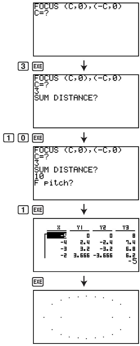
flowchart
graph TD
    A["FOCUS (C,0), (-C,0) C=?"] --> B["FOCUS (C,0), (-C,0) C=? SUM DISTANCE?"]
    B --> C["FOCUS (C,0), (-C,0) C=? SUM DISTANCE? 10 F Pitch?"]
    C --> D["X Y1 Y2 Y3 -5 0 0 8 -4 2.4 -2.4 7.4 -3 3.2 -3.2 6.8 -2 3.666 -3.666 6.2 -5"]
    D --> E["EXE"]
Chapter 9 Spreadsheet
The Spreadsheet application provides you with powerful, take-along-anywhere spreadsheet capabilities.
All of the operations in this section are performed in the S·SHT mode.
Important!
- The fx-7400GII and fx-9750GII are not equipped with the S·SHT mode.
1. Spreadsheet Basics and the Function Menu
Selecting S·SHT on the Main Menu will display a spreadsheet screen. Entering the S·SHT mode automatically creates a new spreadsheet file named "SHEET".
The spreadsheet screen shows a number of cells (squares) and the data contained in each cell.
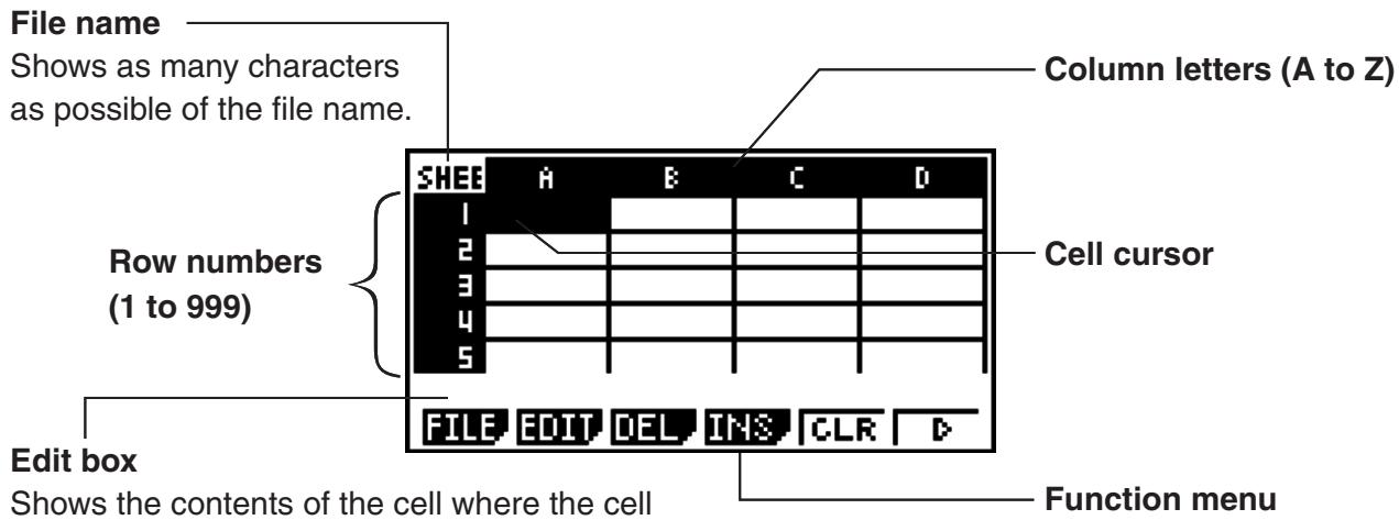
Edit box
Shows the contents of the cell where the cell cursor is currently located. When multiple cells are selected, the edit box indicates the selected cell range.
You can enter the following types of data into a cell.
Constants A constant is something whose value is fixed as soon as you finalize its input. A constant can be either a numeric value, or a calculation formula (such as 7+3 , 30 , A1×2 , etc.) that does not have an equal sign (=) in front of it.
Text A character string that starts with a quote mark (") is treated as text.
Formula A formula that starts out with an equal sign (=), such as =A1×2, is executed as it is written.
Note that complex numbers are not supported in the S·SHT mode.
■ Spreadsheet Screen Function Menu
- {FILE} ... Displays the following FILE submenu.
- {NEW}/{OPEN}/{SV·AS}/{RECAL}
- {EDIT} ... Displays the following EDIT submenu.
• {CUT}/{PASTE}/{COPY}/{CELL}/{JUMP}/{SEQ}/{FILL}/{SRT·A}/{SRT·D}
- PASTE is displayed only immediately after CUT or COPY is executed.
- {DEL} ... Displays the following DEL (delete) submenu.
- {ROW}/{COL}/{ALL}
- {INS} ... Displays the following INS (insert) submenu.
- {ROW}/{COL}
- {CLR} ... Clears the content from a selected range of cells.
- {GRPH} ... Displays the following GRPH menu. (Same as in the STAT mode.)
• {GPH1}/{GPH2}/{GPH3}/{SEL}/{SET} - {CALC} ... Displays the following CALC (statistical calculation) menu. (Same as in the STAT mode.)
• {1VAR}/{2VAR}/{REG}/{SET} - {STO} ... Displays the following STO (store) submenu.
- {VAR}/{LIST}/{FILE}/{MAT}
- {RCL} ... Displays the following RCL (recall) submenu.
- {LIST}/{FILE}/{MAT}
• Data Entry Function Menu - {GRAB} ... Enters the GRAB mode for entering a cell reference name.
- {\... Inputs the cell absolute reference command (\).
- {:} ... Inputs the cell range specification command (:).
- {If} ... Inputs the CellIf( command.
- {CEL} ... Displays a submenu for inputting the following commands.
- CellMin(, CellMax(, CellMean(, CellMedian, CellSum, CellProd(
- {REL} ... Displays a submenu for inputting the following relational operators.
=, , >, <, ≥, ≤
2. Basic Spreadsheet Operations
This section explains spreadsheet file operations, how to move the cursor and select one or more cells, and how to enter and edit data.
■ Spreadsheet File Operations
- To create a new file
-
Press F1 (FILE) F1 (NEW).
-
On the dialog box that appears, enter up to eight characters for the file name, and then press EXE.
- This will create a new file and display a blank spreadsheet.
- A new file will not be created it there is already a file with the same file name you enter in step 2. Instead, the existing file will be opened.
- To open a file
- Press F1 (FILE) F2 (OPEN).
- On the file list that appears, use ▲ and ▼ to select the file you want and then press EXE.
- Auto Save
In the S·SHT mode, Auto Save saves the currently open file automatically whenever you edit it. This means you do not need to perform any manual save operation.
- To save a file under a new name
- Press F1 (FILE) F3 (SV·AS).
- On the dialog box that appears, enter up to eight characters for the new file name, and then press EXE.
- If a file already exists with the same file name you enter in step 2, a message will appear asking if you want to replace the existing file with the new one. Press F1 (Yes) to replace the existing file, or F6 (No) to cancel the save operation and return to the file name input dialog box in step 2.
- To delete a file
- Press F1 (FILE) F2 (OPEN).
- On the file list that appears, use ▲ and ▼ to select the file you want to delete and then press F1(DEL).
- This causes a confirmation message to appear. Press F1 (Yes) to delete the file, or F6 (No) to cancel without deleting anything.
- To return to the spreadsheet from the file list, press EXIT.
- Deleting the currently open file will automatically create a new file named "SHEET" and display its spreadsheet.
■ Recalculating All of the Formulas in the Currently Open Spreadsheet
The S·SHT mode has an Auto Calc features that automatically recalculates all of the formulas in a spreadsheet whenever you open it or perform any editing operation. Auto Calc is enabled under initial factory default settings. You also can execute a recalculation manually, if you want.
- Auto Calc
Auto Calc is an S·SHT mode Setup item (page 1-29).
When Auto Calc is enabled (On), all of the formulas in a spreadsheet are recalculated when the spreadsheet is opened or when any editing operation is performed. It should be noted, however, that recalculation can slow down the overall processing speed. When Auto Calc is disabled (Off), you need to execute recalculation manually as required.
- To execute spreadsheet re-calculation manually
Press F1(FILE)F4(RECAL). This recalculates all of the formulas in the currently open file and displays the applicable results.
■ Using the Cell Cursor
The cell cursor shows the cell that is selected on a spreadsheet. The highlighted cell is the one that is currently selected by the cell cursor.
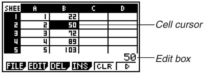
When a single cell is selected by the cell cursor, the contents of that cell are displayed in the edit box. The cell contents can be edited in the edit box.
When a multiple cells are selected by the cell cursor, the selection range is displayed in the edit box. In this case, you can copy, delete, or perform other cell operations on the entire range of selected cells.
- To select cells
| To select this: | Do this: |
| A single cell | Use the cursor keys to move the cell cursor to the cell you want, or use the JUMP comment to jump directly to the cell. |
| A range of cells | See “To select a range of cells” (page 9-5). |
An entire row of cells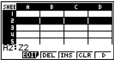 | Move the cell cursor to column A of the row whose cells you want to select and then press ◀. Pressing ◀ while the cell cursor is located at cell A2, for example, will select the entire second row (from A2 to Z2). This will cause A2:Z2 (which indicates the selected range) to appear in the edit box. |
An entire column of cells.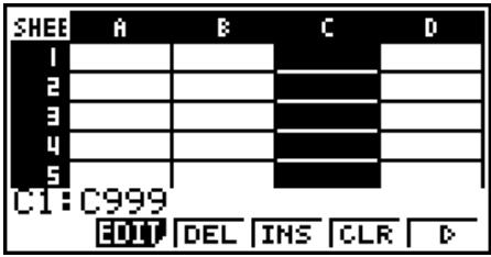 | Move the cell cursor to row 1 of the column whose cells you want to select and then press ▲. Pressing ▲ while the cell cursor is located at cell C1, for example, will select the entire column C (from C1 to C999). This will cause C1:C999 (which indicates the selected range) to appear in the edit box. |
All of the cells in the spreadsheet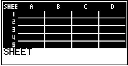 | Press ◀ while the entire column A is selected or press ▲ while the entire row 1 is selected. This will select all of the cells in the spreadsheet and display the spreadsheet file name in the edit box. |
- Using the JUMP Command to Move the Cell Cursor
| To move the cell cursor to here: | Do this: |
| A particular cell | 1. Press F2 (EDIT) F4 (JUMP) F1 (GO).2. On the dialog box that appears, enter the name of the cell (A1 to Z999) to which you want to jump.3. Press EXE. |
| Line 1 of the current column | Press F2 (EDIT) F4 (JUMP) F2 (TOP↑). |
| Column A of the current row | Press F2 (EDIT) F4 (JUMP) F3 (TOP←). |
| Last line of the current column | Press F2 (EDIT) F4 (JUMP) F4 (BOT↓). |
| Column Z of the current row | Press F2 (EDIT) F4 (JUMP) F5 (BOT→). |
• To select a range of cells
- Move the cell cursor to the start point of the range of cells you want to select.
- You could select and entire row or column of cells as the start point, if you want. For details about selecting cells, see “To select cells” on page 9-4.
- Press SHIFT 8 (CLIP).
- This will change the cell cursor to a thick-line boundary instead of the normal highlighting.
- Use the cursor keys to move the cell cursor to the end point of the range of cells you want to select.
- The edit box will show the range of the selected cells.
- To cancel cell selection, press EXIT. If you do, the cell cursor will be located at the end point of the range you selected.
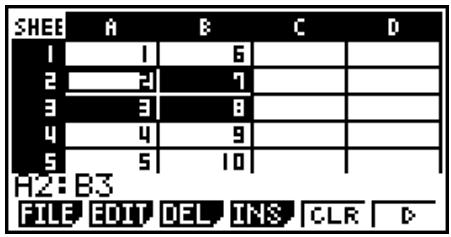
■ Data (Constants, Text, Formula) Input Basics
First let's have a look at a few basic procedures that apply regardless of the type of data you are inputting.
- To overwrite data currently in a cell with new data
- Move the cell cursor to the cell where you want to input data.
- If the cell you select already contains data, the following step will overwrite the existing data with new input.
- Use the calculator's keys to input data.
- As you perform key operations to input values or text (such as 1, ALPHA log(B), etc.), the applicable figures will appear aligned left inside the edit box.
- To cancel an input operation part way through at any point before advancing to step 3 below, press EXIT. This will return the cell contents to what they were in step 1 of this procedure.
- To finalize and apply your input, press EXE.
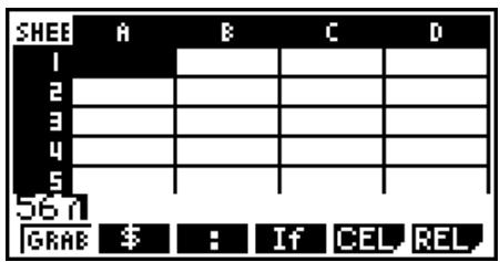
- To edit cell data
- Move the cell cursor to the cell whose contents you want to edit.
- Press F2 (EDIT) F3 (CELL).
- Cell contents in the edit box will change from align left to align right. A text cursor will appear in the edit box so you can edit its contents.
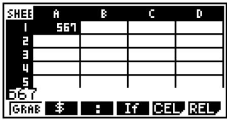
- Use ▶ and ◀ to move the cursor around the contents of the cell, and edit them as required.
- To cancel an edit operation part way through at any point before advancing to step 4 below, press EXIT. This will return the cell contents to what they were in step 1 of this procedure.
- To finalize and apply your edits, press EXE.
- To move the cell cursor while inputting data into a cell
Under factory default settings, pressing EXE while inputting data into a cell will cause the cell cursor to move to the next line. You can specify movement to the next column instead using the "Move" setting as described on page 1-29.
■ Inputting a Constant (Value, Calculation Result, Number Sequence) into a Cell
A constant is something whose value is fixed as soon as you finalize its input. A constant can be either a numeric value, or a calculation formula (such as 7+3 , 30 , A1×2 , etc.) that does not have an equal sign (=) in front of it. Inputting 3 0 , for example will cause the value 0.5 (the calculation result) to appear in the cell (when Deg is selected as the Angle unit).
- To input a number sequence automatically based on a function expression
- Move the cell cursor to the cell where you want number sequence input to start.
- Under initial default settings, automatic input of the number sequence will proceed downwards from the start cell. You can specify a different direction using the “Move” setting as described on page 1-29.
- Press F2 (EDIT) F5 (SEQ) to display the Sequence screen, and then specify the function expression and values required to generate the required number sequence.
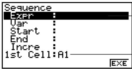
You can input data for the item that is highlighted on the screen.
Reference name of the cell selected in step 1
| Item | Description |
| Expr | Input the function expression f(x) for generating the number sequence.Example: ALPHA + (X) x^2 + 1 EXE (X^2 + 1) |
| Var | Input the variable name used in the function expression input for Expr.Example: ALPHA + (X) EXE (X) |
| Start | Input the starting value ( X_1 ) of the value to be substituted for the variable specified by Var.Example: 2 EXE |
| End | Input the ending value ( X_n ) of the value to be substituted for the variable specified by Var.Example: 1 0 EXE |
| Incre | Input the increment value ( m ) for successive value of X_1 , as in: ( X_2 = X_1 + m ), ( X_3 = X_2 + m ), and so on. The number sequence is generated in the range of X_1 + (n - 1) m ≤ X_n .Example: 2 EXE |
| 1st Cell | Input the reference name (A1, B2, etc.) of the cell where you want the first value of the number sequence to be input. Specify a cell here only if the starting cell is different from the one you specified in step 1 of this procedure.Example: ALPHA log (B) 1 EXE (B1) |
- Each time you press EXE after inputting data for a setting item, the highlighting will move to the next setting item. You also can use ▲ and ▼ to move the highlighting upwards and downwards as required.
-
Performing the next step will input the number string automatically starting from the specified cell. If any cell that is within the range of cells where the number sequence values will be input already contains data, the existing data will be replaced with the number sequence values.
-
After inputting data for all the setting items, press F6(EXE) or the EXE key to start number sequence generation and input.
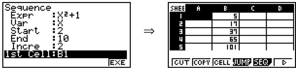
■ Inputting Text into a Cell
To input text, make sure the first thing you input into the cell is ALPHA EXP ("). The quote mark (") tells the calculator that what follows is text, and should be displayed as-is without calculation. The quote mark (") is not displayed as part of the text.
■ Inputting a Formula into a Cell
For the sake of example, let's try making a table that contains data based on the formula <PRICE>×<QUANTITY>=<TOTAL> . To do this, we would put <PRICE> values in column A, <QUANTITY> values in column B, and calculation formulas (like = A1 × B1, = A2 × B2, and so on) in column C. If the Auto Calc feature is enabled (On), the values in column C would be recalculated and updated any time we change the values in column A or B.
In this example, note that we must start out the data in column C with the equal sign (=) in order to indicate it is a formula. In addition to values, arithmetic operators, and cell reference names, a formula also can contain built-in function commands (page 2-11) and special S·SHT mode commands (page 9-14).
- Formula Input Example
| A | B | C | |
| 1 | PRICE | QUANTITY | TOTAL |
| 2 | 35 | 15 | 525 |
| 3 | 52 | 15 | 780 |
| 4 | 78 | 20 | 1560 |
Procedure
- Input the text for line 1, and the applicable values in cells A2 through B4.
- Move the cursor to cell C2, and input the formula for A2 × B2.
SHIFT □ (=) ALPHA X,θ,T (A) 2 ✗ ALPHA log (B) 2 EXE
- Copy the formula in cell C2 and copy it into cells C3 and C4. Move the cell cursor to cell C2 and then perform the following operation.
F2 (EDIT) F2 (COPY) ▼ F1 (PASTE) ▼ F1 (PASTE) EXIT
- For details about the copy and paste operations, see “Copying and Pasting Cell Contents” (page 9-10).
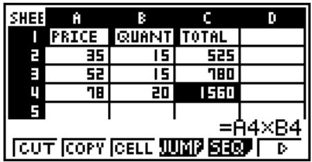
■ Inputting a Cell Reference Name
Each cell on a spreadsheet has what is called a “reference name”, which is derived by combining its column name (A through Z) with its row name (1 through 999). A cell reference name can be used inside of a formula, which makes the value of the called cell part of the formula. See “Inputting a Formula into a Cell” above for more information. There are two methods you can use to input a cell reference name: direct input of the name and input using the GRAB command. The following illustrates how you would use each of these methods to input =A1+5 into cell B1.
- To input a cell reference name using direct input
Move the cell cursor to cell B1 and then perform the following operation.
SHIFT • (=) ALPHA X,θ,T (A) 1 + 5 EXE
- To input a cell reference name using the GRAB command
Move the cell cursor to cell B1 and then perform the following operation.
SHIFT ☐ (=) F1 (GRAB) ◀ F1 (SET) + 5 EXE
- Commands F2(GO) through F6(BOT→) on the submenu that appears when you press F1(GRAB) are identical to commands F1(GO) through F5(BOT→) of the JUMP command submenu. See “Using the JUMP Command to Move the Cell Cursor” on page 9-5 about these commands.
■ Relative and Absolute Cell Reference Names
There are two types of cell reference names: relative and absolute. Normally, cell reference names are treated as being relative.
Relative Cell Reference Names
In the formula =A1+5, the cell reference name A1 indicates a relative cell reference. It is “relative” because copying the formula and pasting in a different cell will cause the cell reference name to change in accordance with the location of cell where it is pasted. If the formula =A1+5 is originally located in cell B1, for example, copying at pasting in cell C3 will result in =B3+5 in cell C3. Moving from column A to column B (one column) causes A to change to B, while moving from row 1 to row 3 changes (two rows) changes the 1 to 3.
Important!: If the result of a copy and paste operation causes a relative cell reference name to change to something that is outside the range of the spreadsheet cells, the applicable column letter and/or row number will be replaced by a question mark (?), and “ERROR” will be displayed as the cell’s data.
Absolute Reference Names
If you want the row or the column, or both the row and the column parts of a cell reference name to remain the same to matter where you paste them, you need to create an absolute cell reference name. You do this by affixing a dollar sign (\) in front of the part of the cell reference name you want to remain unchanged. You have three options when using the dollar sign (\) to create an absolute cell reference name: absolute column with relative row ( A1 ), relative column with absolute row (A 1 ), and absolute row and column ( A 1).
- To input the absolute cell reference name symbol (\$)
When inputting a cell reference into a spreadsheet cell, press F2 (\$).
For example, the following key operation inputs the absolute cell reference name = \B\1
SHIFT • (=) F2 () ALPHA log (B) F2 () 1
■ Copying and Pasting Cell Contents
You can copy the contents of one or more cells and paste them into another location. Once you perform the copy operation, you can copy the contents to multiple locations, if you want.
- To copy and paste spreadsheet data
- Select the cell(s) you want to copy.
- See “To select cells” (page 9-4) for more information.
2 Press F2(EDIT)F2(COPY).
- This will go into paste standby for the selected data, indicated by the F1 menu item changing to (PASTE).
-
You can exit the paste standby at any time before you perform step 4 below by pressing EXIT.
-
Use the cursor keys to move the cell cursor to location where you want to paste the data.
-
If you selected a range of cells in step 1, the cell you select with the cell cursor will be the upper left cell of the paste range.
-
If the location you select is within the range that you copied, performing step below will cause the exiting data to be overwritten with the pasted data.
-
Press F1 (PASTE).
• This will paste the copied data.
- To paste the same data in other locations, repeat steps 3 and 4.
- After you are finish pasting the data, press EXIT to exit paste standby.
■ Cutting and Pasting Cell Contents
You can use cut and paste to move the contents of one or more cells to another location. Cell contents (regardless of whether it includes relative or absolute cell name references) generally are unchanged by a cut and paste operation.
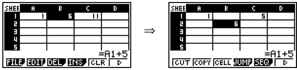
Cutting the formula =A1+5 in cell B1 and pasting it into cell B2. The A1 reference name is unchanged.
When you are cut and paste a range cells, reference names that affect relationships within the range are changed accordingly when the range is pasted in order to maintain the correct relationship, regardless of whether they are relative or absolute reference names.
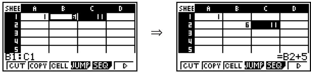
- To cut and paste spreadsheet data
- Select the cell(s) you want to cut.
- See “To select cells” (page 9-4) for more information.
2 Press F2(EDIT)F1(CUT).
- This will go into paste standby for the selected data, indicated by the F1 menu item changing to (PASTE).
-
You can exit the paste standby at any time before you perform step 4 below by pressing EXIT.
-
Use the cursor keys to move the cell cursor to location where you want to paste the data.
-
If you selected a range of cells in step 1, the cell you select with the cell cursor will be the upper left cell of the paste range.
-
If the location you select is within the range that you cut, performing step below will cause the exiting data to be overwritten with the pasted data.
-
Press F1 (PASTE).
-
This will paste the data from the cell(s) you selected in step 1 and paste it into the location you selected in step 3.
- Regardless of whether Auto Calc is enabled or disabled (page 9-3), pasting cut data will cause all of the formulas in the spreadsheet to be recalculated.
■ Inputting the Same Formula into a Range of Cells
Use the Fill command when you want to input the same formula into a specified range of cells. The rules governing relative and absolute cell name references are the same as those for copy and paste.
When you need to input the same formula into cells B1, B2, and B3, for example, the Fill command lets you do so by inputting the formula once, into cell B1. Note the following about how the Fill command handles cell name references in this case.
| When cell B1 contains this: | The Fill command will do this: | |
| =A1×2 | 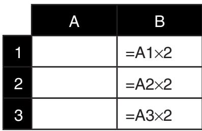 | * Note that in actual practice cells B1, B2, and B3 will show the calculation results, not the formulas as shown here. |
| =A2×2 | 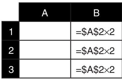 | |
- To input the same formula into a range of cells
- Select the range of cells into which you want to input the same formula.
- In this example we will assume the B1:B3 is selected. See “To select a range of cells” (page 9-5).
2 Press F2(EDIT)F6(▷)F1(FILL).
- On the Fill screen that appears, enter the formula you want to input.
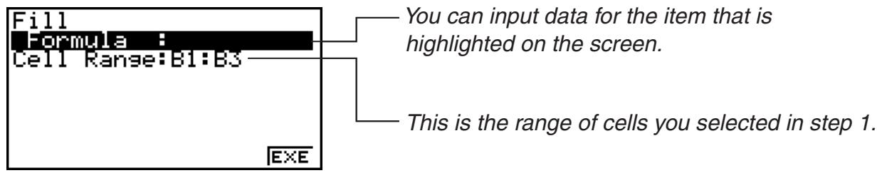
- In the “Formula” line, input = A1×2 (SHIFT ⊙ (=) ALPHA X,θ,T (A) 1 ✗ 2 EXE). Pressing EXE will cause the cell cursor to move to the “Cell Range” line.
-
If any cell within the cell range already contains data, performing the next step will cause the existing data to be overwritten with the new fill data (formula).
-
Press F6(EXE) or the EXE key.
- This will input the formula into the range of cells you specified.
■ Sorting Constant Data
Note that only constant data can be sorted. You can select multiple columns within a single line or multiple lines within a single column for sorting.
- To sort constant data
-
Select a range of column cells in a single row or a range of row cells in a single column.
-
See “To select a range of cells” (page 9-5).
-
A Syntax ERROR message will appear if any of the cells in the range you select contain data other than constant data.
-
Depending on the type of sort you want to perform, perform either one of the following operations.
To sort ascending: F2 (EDIT) F6 (▷) F2 (SRT·A)
To sort descending: F2 (EDIT) F6 (▷) F3 (SRT·D)
■ Deleting and Inserting Cells
- To delete an entire line or column of cells
Select the row(s) or column(s) you want to delete and then press F3 (DEL). This will delete the selected row(s) or column(s) immediately, without displaying a confirmation message.
You also can perform the following steps to delete a row or column.
-
Select one or more cells inside the row(s) or column(s) you want to delete.
-
If you want to delete lines 2 through 4, for example, you could select A2:B4, C2:C4, or any other range of cells that includes the lines to be deleted.
-
If you want to delete columns A and B, for example, you could select A1:B1, A2:B4, etc.
-
Press F3 (DEL).
- This enters delete standby. If you decide you want to cancel the delete operation at this time, press EXIT.
- To delete the entire line(s) that include the cells you selected in step 1, press F1(ROW). To delete the entire column, press F2(COL).
- To delete the contents of all the cells in a spreadsheet
-
Press F3 (DEL) F3 (ALL).
-
In response to the confirmation message that appears, press F1 (Yes) to delete the data or F6 (No) to cancel without deleting anything.
- To insert a row or column of blank cells
- Perform one of the following operations to specify the location of the insert and the number of rows or columns to be inserted.
- To insert rows
Starting with the row immediately below of the row where you want the insert to be performed, select the same number of rows that you want to insert.
Example: To insert three rows above row 2, you could select A2:A4, B2:C4, etc.
- To insert columns
Starting with the column immediately to the right of the column where you want the insert to be performed, select the same number of columns that you want to insert.
Example: To insert three columns to the left of column B, you could select B2:D4, B10:D20, etc.
- Press F4 (INS).
- This will enter insert standby. If you decide you want to cancel the insert operation at this time, press EXIT.
- Press F1(ROW) to insert the applicable number of rows or F2(COL) to insert columns.
- A Range ERROR occurs if an insert operation causes existing cells that contain data to move outside the range of A1:Z999.
• To clear the contents of specific cells
Select the cell or range of cells you want to clear and then press F5 (CLR).
3. Using Special S·SHT Mode Commands
The S·SHT mode has a number of special commands like CellSum(), which returns the sum of a range of cells, and CellIf(), which specifies branching conditions. These special commands can be used inside of formulas.
■ Special S·SHT Mode Command List
“Input Key Operation” operations can be performed during cell input only.
You can omit anything enclosed in brackets ([]) in the Syntax of each command.
| Command | Description |
| CellIf(Branch Condition) | Returns Expression 1 when the equality or inequality provided as the branch condition is true, and Expression 2 when it is false.Input Key Operation: F4 (If)Syntax: CellIf(equality, expression 1, expression 2[]) or CellIf(inequality, expression 1, expression 2[])Example: =CellIf(A1>B1, A1, B1)Returns the value of A1 when {Cell A1 value} > {Cell B1 value}. Otherwise, returns the value of B1. |
| CellMin(Cell Minimum Value) | Returns the minimum value in a specified range of cells.Input Key Operation: F5 (CEL) F1 (Min)Syntax: CellMin(start cell:end cell[])Example: =CellMin(A3:C5)Returns the minimum value of the data in cell range A3:C5. |
| CellMax(Cell Maximum Value) | Returns the maximum value in a specified range of cells.Input Key Operation: F5 (CEL) F2 (Max)Syntax: CellMax(start cell:end cell[])Example: =CellMax(A3:C5)Returns the maximum value of the data in cell range A3:C5. |
| CellMean(Mean of Cells) | Returns the mean value in a specified range of cells.Input Key Operation: F5 (CEL) F3 (Mean)Syntax: CellMean(start cell:end cell[])Example: =CellMean(A3:C5)Returns the mean value of the data in cell range A3:C5. |
| CellMedian(Median of Cells) | Returns the median value in a specified range of cells.Input Key Operation: F5 (CEL) F4 (Med)Syntax: CellMedian(start cell:end cell[])Example: =CellMedian(A3:C5)Returns the median value of the data in cell range A3:C5. |
| CellSum(Sum of Cells) | Returns the sum of the data in a specified range of cells.Input Key Operation: F5 (CEL) F5 (Sum)Syntax: CellSum(start cell:end cell[])Example: =Cellsum(A3:C5)Returns the sum of the data in cell range A3:C5. |
| CellProd(Product of Cells) | Returns the product of the data in a specified range of cells.Input Key Operation: F5 (CEL) F6 (Prod)Syntax: CellProd(start cell:end cell[])Example: =CellProd(B3:B5)Returns the product of the data in cell range B3:B5. |
■ S·SHT Mode Command Example
This example inputs the special S·SHT mode formula CellSum( into cell C1 in order to calculate the sum of all the data in cell range A1:B5. It is assumed that there is already data in the cell range A1:B5.
- Move the cell cursor to cell C1 and then perform the following operation.
SHIFT ☐ (=) F5 (CEL) F5 (Sum)
EXIT ALPHA X,θ,T (A) 1 F3 (:) ALPHA log (b) 5 )
- You can perform the following operation, which uses the GRAB function (page 9-9) and CLIP function (page 9-5) in place of the underlined part in the above operation.
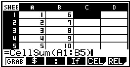
EXIT F1 (GRAB) F4 (TOP←)
(Enters the GRAB mode and moves the cursor to A1.)
SHIFT 8 (CLIP) ▶ ▼ ▼ ▼ ▼
(Specifies the selection range for the CLIP function.)
EXE )
- Press EXE to finalize input of the formula.
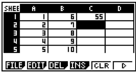
4. Drawing Statistical Graphs, and Performing Statistical and Regression Calculations
When you want to check the correlation between two sets of data (such as temperature and the price of some product), trends become easier to spot if you draw a graph that uses one set of data as the x-axis and the other set of data as the y-axis.
With the spreadsheet you can input the values for each set of data and draw a scatter plot or other types of graphs. Performing regression calculations on the data will produce a regression formula and correlation coefficient, and you can overlay a regression graph over the scatter plot.
S·SHT mode graphing, statistical calculations, and regression calculations use the same functions as the STAT mode. The following shows an operation example that is unique to the S·SHT mode.
■ Example of Statistical Graph Operations (GRPH Menu)
Input the following data and draw a statistical graph (scatter plot in this example).
0.5, 1.2, 2.4, 4.0, 5.2 (x-axis data)
-2.1, 0.3, 1.5, 2.0, 2.4 (y-axis data)
- To input data and draw a statistical graph (scatter plot)
- Input the statistical calculation data into the spreadsheet.
- Here we will input the x -axis data into column A, and the y -axis data into column B.
- Select the range of cells you want to graph (A1:B5).
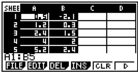
-
Press F6(▷)F1(GRPH) to display the GRPH menu, and then press F1(GRPH1).
-
This will produce a scatter plot of the data in the range of cells you selected in step 2 of this procedure.
- The graph shown here is what is produced under initial default S·SHT mode settings. You can change the configuration of graph settings on the screen that appears when you press F6 (SET) on the GRPH menu. For details see “General Graph Settings Screen Operations” below.
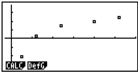
scatter
| x | y | |---|---| | 1 | 0.5 | | 2 | 0.8 | | 3 | 1.2 | | 4 | 1.5 | | 5 | 1.8 |■ General Graph Settings Screen Operations
You can use the general graph setting screen to specify the range of data to be used for graphing, and to select the type of graph to be drawn.
- To configure statistical graph settings
- Input the statistical calculation data into the spreadsheet and then select the range of cells you want to graph.
- Actually, the above step is not necessary at this point. You also could configure settings first before inputting data and selecting the range of cells to be graphed.
- Press F6 (▷) F1 (GRPH) F6 (SET).
- This will display the general graph settings screen (StatGraph1 in this example).
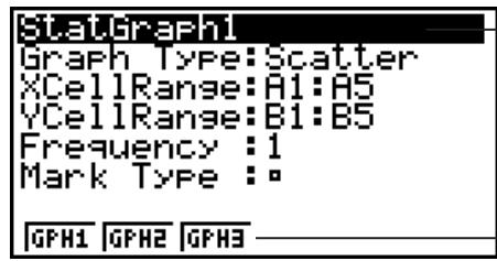
You can configure the setting for the item that is highlighted on the screen.
A function menu will appear when certain setting items are selected.
- The number of columns you select in step 1 will determine what information is input automatically on the general graph settings screen.
| If you select this number of columns: | This information will be input automatically: |
| 1 | XCellRange |
| 2 | XCellRange, YCellRange |
| 3 | XCellRange, YCellRange, Frequency |
- The following describes each of the setting items for this screen.
| Item | Description |
| StatGraph1 | Select the name of the setup you want. You can have up to three different setups registered, named StatGraph 1, 2, or 3. |
| Graph Type | Select the graph type. The initial default setting is Scat (scatter plot). |
| XCellRange | Specifies the cell range assigned to the graph x-axis (XCellRange). Only XCellRange is displayed for some Graph Types. |
| YCellRange | Specifies the cell range assigned to the graph y-axis (YCellRange). The YCellRange is not displayed for some Graph Types. |
| Frequency | Specifies the range cells that contain values indicating the frequency of each graph data item. Select F1(1) if you do not want to use frequency values. |
| Mark Type | Specify the type of mark (□, ×, or •) to use as the mark on the scatter plot. |
-
Use ▲ and ▼ to move the highlighting to the setting item you want to change. On the function menu that appears, select the setting you want.
-
For details about the StatGraph1, Graph Type, and Mark Type settings, see “To display the general graph settings screen” (page 6-2).
-
If you want to change the XCellRange, YCellRange, or Frequency setting, move the highlighting to the item you want to change and then input the cell range directly, or select F1(CELL) (F2(CELL) for Frequency) and then edit the currently input range. When inputting a cell range manually, use F1(:) to enter a colon (:) between two cells that define the range.
-
After configuring the required settings, press EXIT or EXE.
■ Example of Statistical Calculation Operation (CALC Menu)
This example uses the data from the “Drawing a Scatter Diagram and xy Line Graph” (page 6-9) to perform paired-variable statistical calculations.
$$ \begin{array}{l} \begin{array}{l l l l l} 0. 5, & 1. 2, & 2. 4, & 4. 0, & 5. 2 \end{array} (x - d a t a) \ - 2. 1, \quad 0. 3, \quad 1. 5, \quad 2. 0, \quad 2. 4 \quad (y - d a t a) \ \end{array} $$
- To perform paired-variable statistical calculations and regression calculations
-
Input the above x-data into cells A1:A5 of the spreadsheet and the y-data into cells B2:B5, and then select the range of the cells where you input the data (A1: B5).
-
Press F6 (▷) F2 (CALC) to display the CALC menu, and then press F2 (2VAR).
-
This will display a screen of paired variable calculation results based on the data you selected in step 1. Use ▶ and ◀ to scroll the result screen. To close the screen, press EXIT.
-
For information about the meaning of each of the values on the result screen, see “Displaying the Calculation Results of a Drawn Paired-Variable Graph” on page 6-14.
-
To return to the spreadsheet screen, press EXIT.
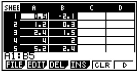
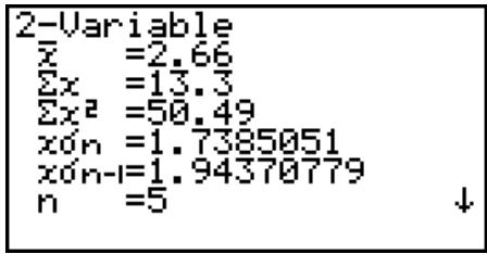
■ Using the Statistical Calculation Data Range Specification Screen
You can use a special setting screen to specify the range of data to be used for statistical calculation.
- To specify the data range for statistical calculation
- Input the statistical calculation data into the spreadsheet and then select its range of cells.
- Press F6 (▷) F2 (CALC) F6 (SET).
- This will display a setting screen like the one shown to the right.
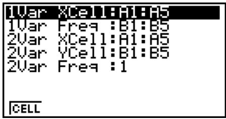
- The number of columns you select in step 1 will determine what information is input automatically on the statistical calculation data range specification screen.
| If you select this number of columns: | This information will be input automatically: |
| 1 | 1Var XCell and 2Var XCell |
| 2 | 1Var Freq and 2Var YCell |
| 3 | 2Var Freq |
- The following describes each of the setting items for this screen.
| Item | Description |
| 1Var XCell1Var Freq | The cell range data specified here is used for variable x and Frequency values when performing single-variable statistical calculations. |
| 2Var XCell2Var YCell2Var Freq | The cell range data specified here is used for variable x, variable y, and Frequency values when performing paired-variable statistical calculations. |
-
If you want to change the cell range, use ⚙️ and ⼑ to move the highlighting to the item you want to change and the input the new cell range.
-
To input the colon (:), press F1(:).
-
To edit the currently input cell range, press F1 (CELL) (in the case of 1Var XCell, 2Var XCell, and 2Var YCell) or F2 (CELL) (in the case of 1Var Freq and 2Var Freq).
-
After configuring the required settings, press EXIT or EXE.
■ STAT Mode and S·SHT Mode Function Menu Correspondence Table
In both the STAT mode and the S·SHT mode, statistical graph functions are on the GRPH function menu and statistical/regression calculation functions are on the CALC function menu. The structures of these menus and their submenus are the same in the STAT mode and the S·SHT mode. For details about each menu item, refer to the pages referenced in the table below.
| For information about this menu item: | Refer to: |
| {GRPH} - {GPH1} | “Changing Graph Parameters” (page 6-1) |
| {GRPH} - {GPH2} | |
| {GRPH} - {GPH3} | |
| {GRPH} - {SEL} | “Graph draw/non-draw status” (page 6-3) |
| {GRPH} - {SET} | “Changing Graph Parameters” (page 6-1)“General graph settings”(page 6-1)“To display the general graph settings screen”(page 6-2)“General Graph Settings Screen Operations” (page 9-16) |
| {CALC} - {1VAR} | “Single-Variable Statistical Calculations” (page 6-15) |
| {CALC} - {2VAR} | “Paired-Variable Statistical Calculations” (page 6-15) |
| {CALC} - {REG} | “Regression Calculation” (page 6-16) |
| {CALC} - {SET} | “Using the Statistical Calculation Data Range Specification Screen” (page 9-18) |
5. S • SHT Mode Memory
You can use the calculator's different types of memory (variables, list memory, file memory, matrix memory) to store data, and recall data from a memory into the spreadsheet.
■ Saving Spreadsheet Data to a Memory
The following table shows an overview of the store operations for each type of memory. For details about each operation, see the example operations following the table.
| Memory Type | Store Operation |
| Variables(A ~ Z, r, θ) | You can assign the content of a single cell to a variable.While a single cell is selected, press F6 (▷) F3 (STO) F1 (VAR), and then specify the variable name on the screen that appears. |
| List Memory(List 1 ~ List 26) | You can store data in a range of cells in a single row or a single column in list memory.While a range of cells in a single row or single column is selected, press F6 (▷) F3 (STO) F2 (LIST), and then specify the list number on the screen that appears. |
| File Memory(File 1 to File 6) | You can store data in a range of cells that spans a multiple rows and columns in file memory. While a range of cells is selected, press F6 (▷) F3 (STO) F3 (FILE), and then specify the file number on the screen that appears.The first column of the selected range is stored in the specified file as List 1, the second column is saved as List 2, and so on. |
| Matrix Memory(Mat A ~ Mat Z) | You can store data in a range of cells that spans a multiple rows and columns in matrix memory. While a range of cells is selected, press F6 (▷) F3 (STO) F4 (MAT), and then specify the matrix name on the screen that appears.The first column of the selected range is stored in the specified matrix as List 1, the second column is saved as List 2, and so on. |
Important!
The following describes what happens if you try to store data in memory when a cell does not contain any data, when a cell contains text, or when ERROR is displayed for a cell.
- If you are assigning data to a variable, an error occurs.
- If you are storing data in list memory, file memory, or matrix memory, 0 is written into the applicable cell(s).
• Example: To store column data in list memory
- In a single column, select the range of cells you want to store in list memory.
- For example, you could select A1:A10.
- Press F6 (▷) F3 (STO) F2 (LIST).
- This will display a screen like the one shown to the right. The “Cell Range” setting will show the range of cells you selected in step 1.
![Store In List Memory Cell Range: Hi Hi I0 List[1~26]:1](/content/2025/01/86832/images/f3967b2d7ce0a7f1ec20b078da195122d4999dc531e8c9924e147ff1f7885e8c.jpg)
-
Press ▼ to move the highlighting to "List[1-26]".
-
Input the List number (1 to 26) of the list memory where you want to store the data and then press EXE.
- Performing the next step will overwrite any data currently stored under the list memory number you specified here with the data in the range of cells specified by "CellRange".
- Press F6 (EXE) or the EXE key to store the data.
■ Recalling Data from Memory to a Spreadsheet
The following table shows an overview of the recall operations for each type of memory. For details about each operation, see the example operations following the table.
| Memory Type | Recall Operation |
| List Memory(List 1 ~ List 26) | You can recall data from a specified list memory to a range of cells in a single row or a single column. While the first cell of the range in a single row or single column is selected, press F6(▷)F4(RCL)F1(LIST), and then specify the list number on the screen that appears.Whether the data is recalled in a column direction or row direction depends on the Setup screen's “Move” setting (page 1-29). |
| File Memory(File 1 ~ File 6) | You can recall data from a specified file memory to the spreadsheet. Select the cell you want to be the upper left corner of the recalled data and then press F6(▷)F4(RCL)F2(FILE). Next, specify the file memory number on the screen that appears. |
| Matrix Memory(Mat A ~ Mat Z) | You can recall data from a specified matrix memory to the spreadsheet. Select the cell you want to be the upper left corner of the recalled data and then press F6(▷)F4(RCL)F3(MAT). Next, specify the matrix name on the screen that appears. |
- Example: To recall data from a matrix memory to a spreadsheet
- On the spreadsheet, select the upper left cell of the range where you want the recalled data to be input.
- Press F6 (▷) F4 (RCL) F3 (MAT).
- This will display a screen like the one shown to the right. The “1st Cell” setting will show the name of the cell you selected in step 1.

- Input the name (A to Z) of the matrix memory whose data you want to recall and then press EXE.
- Press F6(EXE) or EXE to recall the data.
Important!
When recalling list memory, file memory, or matrix memory data, an error will occur if the recalled data runs outside the allowable range of the spreadsheet (A1:Z999).
Chapter 10 eActivity
You can use the eActivity mode to input data into an eActivity file. You can input text and numeric expressions, and also paste data (like graphs, tables, etc.) from the calculator's built-in applications as "strips".
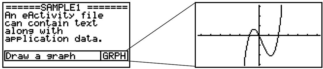
eActivity files can be used by a teacher, for example, to create math problems or exercises that provide hints to solutions, for distribution to students. Students can use eActivity files to keep classroom notes, memos of problems and their solutions, etc.
Important!
- The fx-7400GII and fx-9750GII are not equipped with the e•ACT mode.
1. eActivity Overview
The first thing that appears when you select the e•ACT mode on the Main Menu is the file menu.
![eAct List [ ] No Files NEW SD](/content/2025/01/86832/images/9c4587a3e761ebd62b72322771b976186b540e453d0e11fdd8e19d4b992892f7.jpg)
No e·ACT mode files in memory
![eAct List [ ] [FOLDER1] [FOLDER2] CONICS.g2e : 740 GEO.g2e : 260 GRAPH.g2e : 600 INTEG.g2e : 640↓ OPEN NEW DEL SRC S.D](/content/2025/01/86832/images/297e68dd58e63fd946390527154114139f8b71ad909880c52740ee44170161ba.jpg)
At least one e·ACT mode file in
Opening a file in the eActivity mode will display a workspace screen that you can use for inputting and editing text, calculation expressions, and other data.
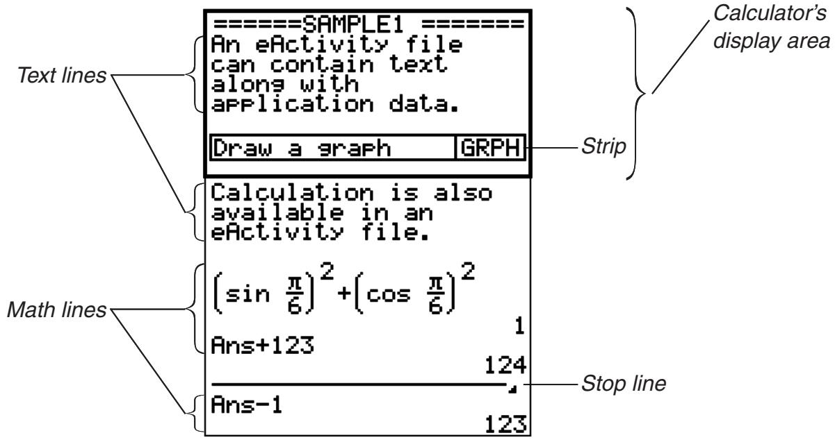
The following explains the type of data you can input and edit in an eActivity file.
Text line......A text line can be used to input characters, numbers, and expressions as text.
Calculation line.....Use the calculation line to enter an executable calculation formula. The result will appear in the following line. Calculations are performed the same way as they are performed in the RUN·MAT mode, while natural input is enabled.
Stop line......A stop line can be used to stop calculation at a particular point.
Strip ......A strip can be used to embed data into an eActivity from the Graph, Conics Graph, Spreadsheet, or other built-in applications.
2. eActivity Function Menus
■ File List Function Menu
- {OPEN} ... Opens an eActivity file or folder.
- {NEW} ... Creates a new eActivity file.
- {DEL} ... Deletes an eActivity file.
- {SRC} ... Searches for an eActivity file.
- {SD}/{SMEM} ... Toggles the files displayed in the file menu between calculator main memory files and SD card memory files (models that support SD cards only). This menu item shows {SD} while the file menu is showing main memory files and {SMEM} while the file menu is showing SD card files.
- Only the F2 (NEW) function key is are displayed when there are no eActivity files in memory.
- At least 128 kbytes of memory area is required when the e·ACT mode is used for the first time. A Memory Full error will appear if there is not enough memory available.
■ Workspace Screen Function Menu
Part of the content of the workspace function menu depends on the line (or strip) that is currently selected.
- Workspace Screen Common Menu Items
-
{FILE} ... Displays the following file operation submenu.
-
{SAVE} ... Saves the file currently being edited.
- {SV·AS} ... Saves the file currently being edited under another name.
- {OPT} ... See “Optimizing the Storage Memory or SD Card Memory” on page 11-11.
-
{CAPA} ... Displays a screen showing the data size of the file being edited and how much memory capacity remains.
-
{STRP} ... Inserts a strip.
- {JUMP} ... Displays the following submenu to control cursor movement.
- {TOP}/{BTM}/{PgUp}/{PgDn} ... See page 10-4.
- {DEL-L} ... Deletes the line that is currently selected or where the cursor is located.
- {INS} ... Displays the following insert submenu, for inserting a new line above the line that is currently selected or where the cursor is located.
- {TEXT} ... Inserts a text line.
- {CALC} ... Inserts a calculation line.
-
{STOP} ... Inserts a calculation stop line.
-
{▶MAT} ... Displays the Matrix Editor (page 10-7).
- {▶LIST} ... Displays the List Editor (page 10-7).
- Menu when a Text Line is Selected
- {TEXT} ... Changes the current line from a text line to a calculation line.
- {CHAR} ... Displays a menu for inputting math symbols, special symbols, and characters of various languages.
- A a ... Toggles between uppercase and lowercase input while alpha character input is enabled (by pressing the ALPHA key).
- {MATH} ... Displays the MATH menu (page 1-12).
- Menu when a Calculation Line or Stop Line is Selected
- {CALC} ... Changes the current line from a calculation line to a text line.
- {MATH} ... Same as {MATH} under "Menu when a Text Line is Selected".
- Menu when a Strip is Selected
- {FILE} ... Displays the following file operation submenu.
- {SAVE}/{SV·AS}/{OPT}/{CAPA} ... Same as the {FILE} submenus under “Workspace Screen Common Menu Items”.
- {SIZE} ... Displays the size of the strip at the current cursor position.
- {CHAR} ... Same as {CHAR} under "Menu when a Text Line is Selected".
- A a ... Same as A a under "Menu when a Text Line is Selected".
3. eActivity File Operations
This section explains the different file operations you can perform from the eActivity file menu screen. All of the operations in this section can be performed while the file menu is displayed. This section does not cover folder operations. For details about folders, see “Chapter 11 Memory Manager”.
- To create a new file
- While the file menu is displayed, press F2 (NEW).
- This will display a file name input screen.

- Input up to 8 characters for the file name and then press EXE.
- This displays a blank workspace screen.
- The following are the characters allowed in a file name.
A to Z, {, }, ', \~, 0 to 9
- To open a file
Use ▲ and ▼ to highlight the file you want to open, and then press F1 (OPEN) or EXE *.
* If an error occurs, delete capture memory and clipboard data, or transfer the data to your computer.
- To delete a file
- Use ▲ and ▼ to highlight the file you want to delete, and then press F3 (DEL).
- This will display a “Delete eActivity?” confirmation message.
- Press F1 (Yes) to delete the file or F6 (No) to cancel without deleting anything.
- To search for a file
- While the file menu is displayed, press F4(SRC).
- This will display a file search screen.
- Enter part or the entire name of the file you want to find.
- File name characters are searched from left to right. Entering “IT” will count names like ITXX, ITABC, IT123 as hits, but not names like XXIT or ABITC.
- Press EXE.
- If a name matches the text you input in step 2, it will be selected on the file menu.
![eAct List [ ] INTEG.92e : 640ft SAMPLE1.92e : 284 OPEN HEW DEL SRC S.D](/content/2025/01/86832/images/1258bb927204b82f3f8b3e7284f30d32bdb48ca860bd1a5c851c1aa9556fcb0e.jpg)
- The message “Not Found” will appear if a match cannot be found. Press the EXIT key to close the message dialog box.
4. Inputting and Editing Data
All of the operations in this section are performed on the eActivity workspace screen. Use the procedures under “eActivity File Operations” (page 10-3) to create a new file or to open an existing file.
■ Cursor Movement and Scroll Operations
| When you want to do this: | Use this key operation: |
| Move the cursor forward and back | ▲ or ▼ |
| Scroll one screen forward | SHIFT ▲ orF6 (▷) F1 (JUMP) F3 (PgUp) |
| Scroll one screen back | SHIFT ▼ orF6 (▷) F1 (JUMP) F4 (PgDn) |
| Move the cursor to the beginning of the workspace screen | F6 (▷) F1 (JUMP) F1 (TOP) |
| Move the cursor to the end of the workspace screen | F6 (▷) F1 (JUMP) F2 (BTM) |
■ Inputting into a Text Line
Use a text line to input alphanumeric characters, expressions, etc.
- Inputting characters and expressions as text
1. Move the cursor to a text line.
- While the cursor is in a text line, “TEXT” will be displayed for the F3 function menu item. This indicates that text input is enabled.
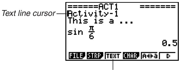
F3 key menu becomes "TEXT".
- “CALC” will be displayed for the F3 function menu item if the cursor is located in a calculation line. Pressing F3 (CALC) will change the calculation line to a text line.
- If the cursor is located in a strip, use ▲ and ▼ to move to the cursor to a text line.
- On the function menu, selecting {INS} and then {TEXT} will insert a new text line above the line where the cursor is currently located.
2. Input the text or expression you want into the text strip.
- See “Text Line Input and Editing Operations” described below.
• Text Line Input and Editing Operations
- You can input up to 255 bytes of text into a single text line. Text in the text line wraps automatically to fit inside the display area (Word Wrap Function). Note, however, that numeric expressions and commands do not wrap.*1 Scroll arrows (◀▶) will appear on the left and right sides of the calculation line to let you know some of the calculation does not fit within the calculation line display area. In this case, you can use the left and right cursor keys to scroll the calculation.
- The F5(A↔a) function key toggles between upper-case and lower-case input. This function is available only while alpha text input is enabled. See page 2-7 for details. The text line cursor is ☐ while upper-case input is selected, and ☑ during lower-case input.
- Press EXE to input a carriage return into text. No symbol will be displayed for a carriage return.
- If the text is wrapped into multiple lines, pressing the AC key will delete the line where the cursor is currently located only. The part of the text that is wrapped to other lines will not be deleted.
- Always use natural input (page 1-10) to input an expression into a text line.
*1 Also, any word that includes the symbol “ ’ ”, “ { ” or “ I□ ”, which are input using the menu that appears when you press F4 (CHAR), does not wrap.
■ Inputting into a Calculation Line
Inputting a calculation expression into an eActivity calculation line and pressing EXE will display the calculation result in the following line. Such a calculation line can be used in the same way as the RUN·MAT mode (page 1-3). A calculation line and its result make up one set.
- Note that the word wrap function does not apply in the case of math lines. Scroll arrows (◀▶) will appear on the left and right sides of the calculation line to let you know some of the calculation does not fit within the calculation line display area. In this case, you can use the left and right cursor keys to scroll the calculation.
- To input a calculation formula into an eActivity
- Move the cursor to a calculation line.
- While the cursor is in a calculation line, “CALC” will be displayed for the F3 function menu item. This indicates that calculation expression input is enabled.
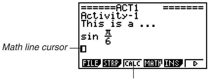
This will cause the F3 key menu to change to "CALC".
- “TEXT” will be displayed for the F3 function menu item if the cursor is located in a text line. Pressing F3 (CALC) will change the calculation line to a text line.
- If the cursor is located in a strip, use ▲ and ▼ to move to the cursor to a calculation line.
-
On the function menu, selecting {INS} and then {CALC} will insert a new calculation line above the line where the cursor is currently located.
-
Input a calculation expression (Example: sin _c^b SHIFT EXP(π) ▼ 6).
- Calculation line input and editing operations are the same as those in the natural input RUN·MAT mode.
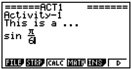
- To obtain the result of the calculation, press EXE.
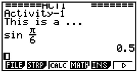
- Matrix Calculations Using the Matrix Editor
Selecting {▶MAT} on the function menu displays the Matrix Editor.
Matrix Editor operations and matrix calculations in the eActivity mode are the fundamentally identical to those in the RUN·MAT mode. For details about the Matrix Editor and matrix calculation operations, see “Matrix Calculations” (page 2-36). Note, however, that eActivity mode Matrix Editor operations and matrix calculations differ from those in the RUN·MAT mode as described below.
- eActivity mode matrix variable values are saved separately for each file. Matrix variable values will be different from those produced when called from a non-eActivity mode.
- List Calculations Using the List Editor
Selecting {▶LIST} on the function menu displays the List Editor.
List Editor operations in the eActivity mode are identical to those in the STAT mode (“Inputting and Editing a List”, page 3-1). This processing and calculations are fundamentally the identical to those in the RUN·MAT mode (“Manipulating List Data” on page 3-5, “Arithmetic Calculations Using Lists” on page 3-10). Note, however, that eActivity mode List Editor operations and list calculations differ from those in other modes as described below.
- The eActivity mode List Editor function menu provides only screen two of the STAT mode List Editor function menu.
- To return to the workspace screen from the List Editor in the eActivity mode, press EXIT.
- In the eActivity mode, values for list variables are saved separately for each file. List variable values will be different from those produced when called from a non-eActivity mode.
■ Inserting a Calculation Stop Line
Pressing EXE after you edit a calculation line on a workspace screen that contains multiple calculation lines will cause all of the calculations following the edited line to be re-calculated. Re-calculation can take quite a bit of time if there are a large number of calculation lines or if some of the calculations are complex. Inserting a calculation stop line will stop the re-calculation process at the point where the line is located.
- To insert a stop line
On the function menu, select {INS} and then {STOP} to insert a stop line above the currently selected line or strip.
■ Using Strips
Strips are tools that let you embed built-in application data into an eActivity file. Only one built-in application screen can be associated with each strip, and the strip can store the data (graphs, etc.) produced by the screen.
The table below shows the built-in application screens that can be inserted into strips. The "Strip Name" column shows the names included on the dialog box that appears when you press F2 (STRP).
Strip Data Type Table
| Data Type | Strip Name |
| RUN·MAT mode calculation data (When the RUN·MAT mode is called from an eActivity, it starts up in the natural input mode.) | Run (Math) |
| GRAPH mode graph screen data | Graph |
| GRAPH mode graph relation list screen data | Graph Editor |
| TABLE mode table relation list screen data | Table Editor |
| CONICS mode graph screen data | Conics Graph |
| CONICS mode function list screen data | Conics Editor |
| STAT mode statistical graph screen data | Stat Graph |
| STAT mode List Editor data | List Editor |
| EQUA mode calculation solution screen data | Solver |
| RECUR mode recursion type selection screen | Recur Editor |
| Notes screen data (Notes is a special eActivity application. See “Notes Strips” on page 10-10 for more information.) | Notes |
| RUN·MAT mode Matrix Editor data | Matrix Editor |
| EQUA mode simultaneous equation solution screen data | Simul Equation |
| EQUA mode high-order equation solution screen data | Poly Equation |
| DYNA mode graph screen data | Dynamic Graph |
| TVM mode calculation solution screen data | Financial |
| S·SHT mode spreadsheet screen data | SpreadSheet |
| E-CON2 mode setup wizard data | Econ SetupWizard |
| E-CON2 mode advanced setup data | Econ AdvancSetup |
| E-CON2 mode advanced setup data(Executing this strip starts sampling immediately based on the setup information that is recorded to the strip the first time the strip is executed.) | Econ Sampling |
| E-CON2 mode advanced setup data(Executing this strip graphs sampled data that is recorded to the strip the first time the strip is executed.) | Econ Graph |
- To insert a strip
- Move the cursor to the location where you want to insert the strip.
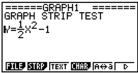
2. Press F2 (STRP).
- This will display a dialog box with a list if insertable strips. For information about the display names and data types that appear on this dialog box, see the “Strip Data Type Table” (page 10-8).
- Use ▼ and ▲ to select the strip that corresponds to the type of data you want to insert.
- In this example we will select “Graph” (GRAPH mode graph screen data).
- Press EXE.
- This will insert the type of strip you selected (Graph strip in this example) one line above the line where you located the cursor in step 1 of this procedure.
- Input up to 16 characters for the strip title, and then press EXE.
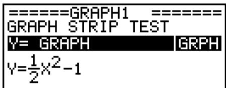
- Press ☒ again to start creating strip data.
- This will start up the built in application for the selected strip type (GRAPH mode in this example), and display the graph screen. At this point, a blank graph screen appears because there is no data yet.
natural_image
Simple Cartesian coordinate system with x and y axes (no labels or data points)-
Press EXIT to display the graph function list screen.
-
Enter the function you want to graph.
(Example: Y = 12 X^2 - 1 )
![Graph Func :Y= Y10 1/2X²-1 [—] Y24: Y3: [—] Y4: [—] Y5: [—] SEL DEL TYPE STYL CMEM DRAW](/content/2025/01/86832/images/d53fa84d06ea7abf4773ef8120abea98495246bbbc0d0f36c66c9edd1678882f.jpg)
- Press F6 (DRAW).
- This will graph the function you entered.
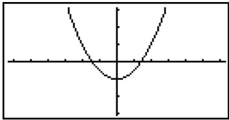
natural_image
Simple parabolic curve drawn on a Cartesian coordinate system (no labels or text)-
To return to the eActivity workspace screen, press SHIFT → (☐).
-
The data that is graphed in step 8 will be saved in the Graph strip.
-
The saved graph data is linked to this Graph strip only. It is independent of data for modes that are entered from the Main Menu.
-
Pressing EXE here again will display the graph screen, and draw the graph based on the data saved by the strip.
- Notes Strips
“Notes” is a special eActivity text editor that comes in handy when you want to write long text explanations on the workspace screen. You can call up the Notes screen from a Notes strip on the workspace screen. Input and editing operations on the Notes screen are identical to those you use for an eActivity text line.
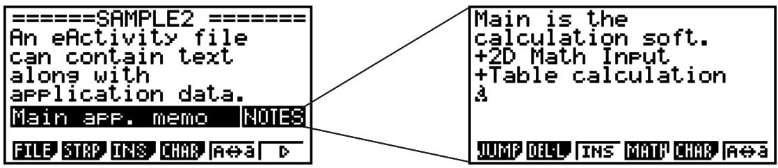
The following describes the Notes screen function menu items.
- {JUMP}... Displays a JUMP menu that you can use to jump to the top (F1(TOP)) of the data, the bottom (F2(BTM)) of the data, the previous page (F3(PgUp)), or the next page (F4(PgDn)).
- {DEL-L} ... Deletes the line that is currently selected or where the cursor is located.
- {INS} ... Inserts one new line above the line where the cursor is currently located.
- {MATH} ... Displays the MATH menu (page 1-12).
- {CHAR} ... Displays a menu for inputting math symbols, special symbols, and characters of various languages.
- A a ... Toggles between uppercase and lowercase input while alpha character input is enabled (by pressing the ALPHA key).
• To change the title of a strip
- Use ▼ and ▲ to select the strip whose title you want to change.
- Input up to 16 characters for the strip title, and then press EXE.
- The remainder of the existing title will disappear as soon as you input the first character. Input the new title in its entirety. If you want to partially edit the existing title, press 🔑 or ➤ first to move the cursor.
- Pressing EXIT instead of EXE will exit trip title editing without changing anything.
- To call an application from a strip
Use ▼ and ▲ to select the strip whose application you want to call and then press EXE.
- This will display the application screen that corresponds to the selected strip. If the strip already contains data, the application is called using the data that was last saved.
- If you select a Conics Graph strip and press EXE without inputting any graph data, the Conics Editor screen appears in place of the Conics Graph screen.
- To toggle between the eActivity workspace screen and an application screen called from a strip
Press SHIFT → ( ).
Each press of SHIFT → (☐) toggles between the eActivity workspace screen and the application screen called from the strip.
- To switch from an application screen called up from a strip to another application screen
Press SHIFT (☐). On the dialog box that appears, use ▼ and ▲ to select the name of an application and then press EXE.
- To display the strip memory usage screen
-
Use ▼ and ▲ to select the strip whose memory usage screen you want to view.
-
Press F1(FILE)F5(SIZE).
- This will display the memory usage screen of the currently selected strip.
![Strip Data Size 376 Bytes Press: [EXIT]](/content/2025/01/86832/images/7c2b1fd5ad19248b6bda0c43f11c3ac169830712ce8632521d4e08ead1f547d7.jpg)
- To exit the memory usage screen, press EXIT.
- To delete a line or strip
- Move the cursor to the line or strip you want to delete.
- If you move the cursor to a calculation line, note that both the calculation and the result will be deleted.
- Press F6 (▷) F2 (DEL-L).
- This causes a confirmation message to appear.
- Press F1 (Yes) to delete, or F6 (No) to cancel without deleting anything.
Saving a File
Use the procedures in this section to save a file after inputting or editing it on the workspace screen.
An eActivity file for OS Version 2.00 or later may have a file name extension of "g2e".
Performing either of the following operations on a calculator model covered by this manual (with OS Version 2.00 or later operating system) to save an eActivity file always will cause the extension “g2e” to be appended to the file name.
- Saving a newly created file
- Saving an existing file using the "save as" operation (F1(FILE) F2(SV-AS))
If you save an eActivity file using a calculator model covered by this manual to save a file with a file name extension "g1e" (a file transferred from an older version calculator), the file name extension will be determined according to the following rules.
- The “g2e” extension is used for an eActivity file that includes data for new features (except for math functions and commands) added by OS Version 2.00 or later.
Here, the expression “data for new features added by OS Version 2.00 or later” means, for example, calculation result data displayed in or format.
- The “g1e” extension is used for eActivity files other than those described above.
- To replace the existing file with the new version
Press F1(FILE)F1(SAVE) to save the currently open file.
- To save a file under a new name
- On the eActivity workspace screen, press F1 (FILE) F2 (SV-AS).
- This will display a file name input screen.
- Input up to 8 characters for the file name and then press EXE.
- If a file already exists with the same file name you enter in step 2, a message will appear asking if you want to replace the existing file with the new one. Press F1 (Yes) to replace the existing file, or F6 (No) to cancel the save operation and return to the file name input dialog box in step 2.
Important!
- An eActivity file with the “g2e” file name extension cannot be opened on a calculator running an operating system older than OS Version 2.00.
- Opening an eActivity file with the “g1e” filename extension, inputting functions added with OS Version 2.00 or later, and then saving the file may cause the new save to retain the “g1e” file name extension. Though you will be able to open such a file on a calculator running an operating system older than OS Version 2.00 (since it has the “g1e” file name extension), you will not be able to use the math functions and commands added since OS Version 2.00.
■ Displaying the eActivity Memory Usage Screen
The maximum size of an eActivity file is approximately 30,000 bytes.* You can use the eActivity file memory usage screen to check how much memory capacity remains for the file you are currently working on.
* Actual maximum file size depends on capture memory and clipboard memory usage, and may be less than 30,000 bytes.
- To display the eActivity memory usage screen
On the workspace screen, press F1(FILE)F4(CAPA).
![Total Data Size 1760 Bytes Free Bytes 28624 Bytes Press: [EXIT] File usage Remaining file memory capacity](/content/2025/01/86832/images/38ac7671cf6431e480af307b0629264d3cb559e62a5a7fc9ce6d73a07701a383.jpg)
To exit the memory usage screen, press EXIT.
- To return to the file list from the workspace screen
Press EXIT.
If a confirmation message appears asking if you want to save the current file appears, perform one of the operations described below.
| To do this: | Press this key: |
| Overwrite the existing eActivity file with the edited version and return to the file list | F1 (Yes) |
| Return to the file list without saving the file you are currently editing | F6 (No) |
| Return to the eActivity workspace screen | AC |
5. eActivity Guide (fx-9860G Slim only)
eActivity Guide is a function that helps you navigate through scientific function calculation operations.
You can perform calculator operations simply by following the instructions that appear on the display.
- Using eActivity Guide to prepare lessons makes it possible for students to become familiar with calculator operations without using the user's guide.
• Students can learn operations in the classroom are their own pace.
Creating a Guide
Key operations are recorded in each eActivity strip. You can also add comments about key operations.
Since a guide records only key operations that are contained within a strip, operations performed after exiting the strip (to go to another strip, to go to another file) cannot be recorded.
Running a Guide
Running a guide that you created will sequentially display key operations and comments. The student can become familiar with calculator operations simply by performing input as instructed.
Three Types of Operation Patterns
eActivity Guide has three operation pattern types as described below. A guide can be created by combining these three patterns.
- 1-key Operation: A comment is attached to each key operation.
- n-key Operation: One comment is attached to a key operation sequence.
- AUTO Operation: A key operation sequence is performed automatically, with one comment attached to the auto operation.
(Examples: Graph and box zoom; specification of an integration graph range)
■ Creating a Guide
- To enter the guide creation mode
- On the eActivity workspace screen, select a strip and then press F6(▷) to display page two of the function menu.
- In this example we will select a Graph Editor strip.
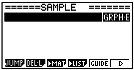
2. Press F5 (GUIDE).
- This will enter the guide creation mode and display the operation pattern selection screen.
- {nKEYS} ... {creates an n-key operation}
- {1-KEY} ... {creates a 1-key operation}
- {AUTO} ... {creates an AUTO operation}
- {END} ... {exits the guide creation mode}
- {PLAY} ... {plays back recorded key operations}
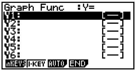
You should also select this option when you want to select a recorded key operation and edit it. PLAY does not appear if there are no key operations recorded.
- If you press F5 (GUIDE) while a strip you selected already contains data, a confirmation will appear asking whether you want to delete the existing operation data.
![Delete data in this strip? Yes: [F1] No : [F6]](/content/2025/01/86832/images/b65fb738546185384fe54864d4cdf350c7399bd8d69cc3d414e07459aa2387de.jpg)
F1 (Yes) ... Deletes the strip's existing operation data and starts guide creation from an empty strip.
F6 (No) ... Cancels guide creation and returns to the eActivity workspace screen.
- To create an n-key operation
- On the operation pattern selection screen, press F1(nKEYS).
- This will display the dialog box shown below.
![To end recordings, Press [AC]. OK : [F1] Key Position : [▲]/[▼] OK Key indicator](/content/2025/01/86832/images/76f0596d112a66349810566a59ea1b98c7e0697b77745a5c73558e6cd0e65945.jpg)
• F1(OK) ... Starts key input recording.
- ▲ ... Displays the key indicator in the upper right corner.
- ▼ ... Displays the key indicator in the lower right corner.
-
Press F1(OK).
-
Input the key operation sequence.
- In this example, we will input a graphing key sequence.

(Inputs the graph function.)
Indicates that recording is in progress.
![Graph Func :Y= Y1B-X²+1 [—] Y2B [—] Y3: [—] Y4: [—] Y5: [—] Y6: [—] SEL DEL TYPE STYL AMEM DRAW](/content/2025/01/86832/images/076860da7443381013dfae5951532e14d2ccc78ef83ef5f3d35a164207112840.jpg)
F6 (DRAW)
(Draws the graph.)
SHIFT F5 (G-SLV) F6 (▷) F3 (∫dx)
(Selects the integration command.)
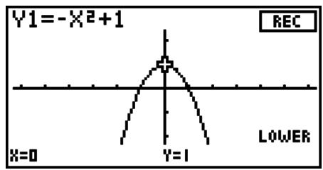
line
| X | Y | | ---- | ----- | | 0 | 0 | | 1 | -X² + 1 |- After input is complete, press AC.
- This will display a comment box.
- Input any comment text you want about the key operation sequence.
- You can input up to two lines in the comment box.
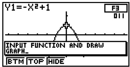
- After inputting comment text, press EXE to register the n-key operation input.
- This will return to the operation pattern selection screen. You can now edit the guide by pressing F5(PLAY) and selecting the key operation you want to change.
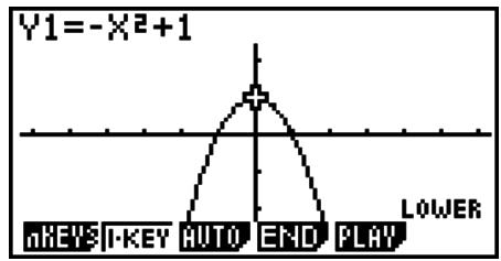
See “Editing a Guide” (page 10-18) for details about editing guides.
• To create a 1-key operation
The following operation assumes that you are continuing from the procedure under “To create an n-key operation” (page 10-14).
- On the operation pattern selection screen, press F2 (1-KEY).
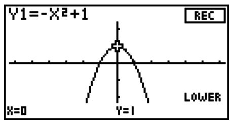
line
| x | y | | ---- | ----- | | 0 | 0 | | 1 | 1 |-
Press a key.
-
Here we will press EXE.
- This will display a comment box.
EXE (Executes the integration command.)
- Input any comment text you want about the key operation sequence.
- After inputting comment text, press EXE to register the 1-key operation input.
- This will return to the operation pattern selection screen. You can now edit the guide by pressing F5(PLAY) and selecting the key operation you want to change.
See “Editing a Guide” (page 10-18) for details about editing guides.
• To create an AUTO operation
The following operation assumes that you are continuing from the procedure under “To create a 1-key operation” (page 10-15).
- On the operation pattern selection screen, press F3 (AUTO).
- This will display the dialog box shown to the right.
![To end recordings, Press [AC]. OK : [F1] Key Position : [▲]/[▼] OK](/content/2025/01/86832/images/9d7b51179fcf2ba21b598ada5c8b740e61a7abc815d3bd4f18c9e0d68d7feab3.jpg)
- Press F1(OK).
![To Key Recording Play Speed? Slow : [F1] Medium : [F2] Fast : [F3] Ultra-fast: [F4]](/content/2025/01/86832/images/f7d4015f4b5a1dda28a7440599ae3eaef96969221304b6659b91f9ed5e182532.jpg)
- F1 ... Executing the guide performs auto key input at low speed. Use this option for operations that the teacher explains while they are being performed, and for trace operations performed G-Solve analysis.
- F2 ... Executing the guide performs auto key input at medium speed. Use this option for simple value input, expression input, and function menu operations.
- F3 ... Executing the guide performs auto key input at high speed. Use this option for tracing or box zooming a graph.
-
F4 ... Executing the guide performs auto key input at ultra-high speed. Use this option when creating list or matrix data. This speed is too fast for the eye to follow.
-
Press F1, F2, F3, or F4.
- Input the key operation sequence.
• Here we will input the following key sequence.
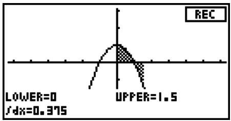
line
| Parameter | Value | | --------- | ----- | | LOWER | 0 | | dx | 0.375 | | UPPER | 1.5 |- After input is complete, press AC.
- This will display a comment box.
-
Input any comment text you want about the key operation sequence.
-
After inputting comment text, press EXE to register the AUTO operation input.
- This will return to the operation pattern selection screen. You can now edit the guide by pressing F5 (PLAY) and selecting the key operation you want to change.
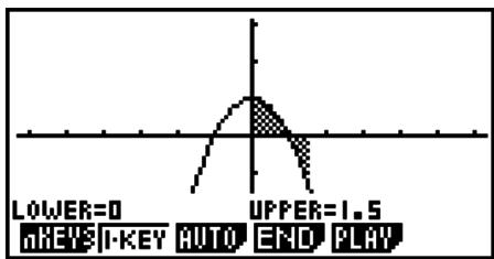
- ⒽELP key and ⚙️ key operations are not recorded. The ⒽELP and ⚙️ keys are disabled while creating a guide. (Models with ⒽELP and ⚙️ keys only.)
- Up to 999 key operations can be recorded per strip.
- To change the position of the comment box
While inputting comment text, you can use the function keys to change the display position of the comment box. This capability comes in handy when an important part of the screen becomes blocked by the comment box.
- {BTM} ... {displays the comment box at the bottom of the screen}
- {TOP} ... {displays the comment box at the top of the screen}
- {HIDE} ... {hides the comment box}
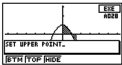
F1 (BTM)
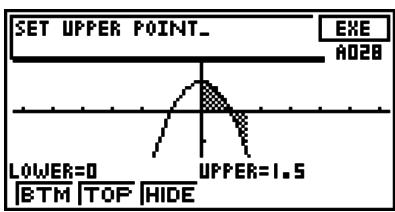
F2 (TOP)
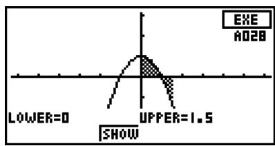
line
| Parameter | Value | | --------- | ----- | | LOWER=0 | 0 | | UPPER=1.5 | 1.5 |F3 (HIDE)
- To exit the guide creation mode
- While creating a guide, press F4 (END).
- This will display the dialog box shown to the right.
![Exit strip when guide finishes? Yes:[F1] No :[F6]](/content/2025/01/86832/images/24f8ef41493e3b801d2391495bc82817d5390cfde7188da48c2850f653fec8eb.jpg)
- F1 (Yes) ... Turns on the exit strip setting. When using the guide as a demo, the strip is exited and the eActivity workspace screen returns to the display after the guide is complete.
-
F6 (No) ... Turns off the exit strip setting. The strip is not exited when the guide is complete. Select this option when you want students to continue operation using the strip after the guide is complete.
-
Press F1 (Yes) or F6 (No).
- Exits the guide creation operation and returns to the eActivity workspace screen.
- An ongoing guide creation operation can be cancelled by pressing SHIFT → (☐). The exit strip dialog box will not appear when a guide creation operation is cancelled.
- Guide creation also canceled if the MENU key is pressed to change to another mode while a guide creation operation is in progress. The exit strip dialog box will not appear in this case, either.
- The amount of memory used by strips is calculated when you press F1 (Yes) or F6 (No). See “To display the strip memory usage screen” (page 10-11) for more information.
- You cannot exit a guide creation operation while the application list (page 10-9) is on the display. Select an application on the application list or close the application list, and then exit guide creation.
■ Editing a Guide
There are two methods that can be used to edit a guide.
- Editing of the guide you are currently creating
- Editing of the guide of an existing strip from the eActivity workspace screen
■ Editing the Guide You Are Creating
- To display the key editing screen
In this example, we show how to display the ① key editing screen of a graph function (Y1 = -X ^2 + 1) that is input at the end of the operation under “To create an n-key operation” (page 10-14).
- On the operation pattern selection screen, press F5 (PLAY).
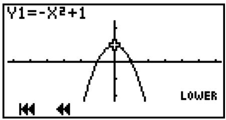
- { } ... {jumps to the first key}
• { ◀ } ... {jumps back n keys}
Pressing this key will display a dialog box for input of a value to specify how many keys to jump.
- { ▶ } ... {starts auto play from the current position}
A dialog box appears which can be used to specify the playback speed. To stop auto play, press AC.
- {▶} ... {jumps forward n keys}
Pressing this key will display a dialog box for input of a value to specify how many keys to jump.
- {▶▶} ... {jumps to the last key and displays the guide creation screen}
- Press F2(◀).
- This will display the dialog box shown to the right.
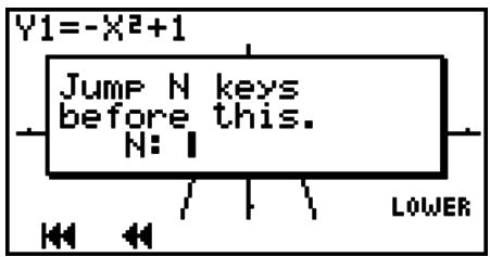
- Input a value to specify the number of keys you want to jump and then press EXE.
- Here we want to jump to the ① key, so we will input ⑦ EXE.
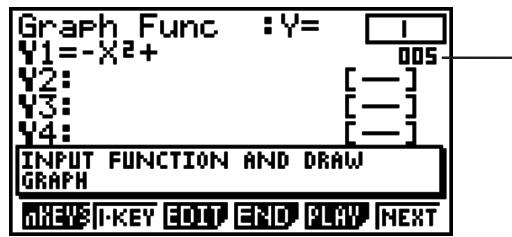
This number indicates the number of the current key operation from the beginning of the function. In the case of an AUTO operation, the letter “A” is appended to the beginning of this number (A005).
- {nKEYS} ... {inserts an n-key operation at the display position}
- {1-KEY} ... {inserts a 1-key operation at the display position}
- {EDIT} ... {starts editing of the key at the current position}
- {END} ... {exits the editing operation}
- {PLAY} ... {displays a dialog box for selecting the key to be edited}
- {NEXT} ... {displays the next key}
- Use ▲ and ▼ to change the key indicator display position.
▲ ... Displays the key indicator in the upper right corner.
▼ ... Displays the key indicator in the lower right corner.
-
Press F3 (EDIT).
-
This will display the 1 key editing screen.
- {INS} ... {inserts one key before the current key}
- {OVW} ... {overwrites the current key}
• {NOTE} ... {edits the current comment} - {AUTO} ... {inserts an AUTO operation after the current key} See “To create an AUTO operation” (page 10-16).
- {DEL} ... {deletes the current key}
- {DEL • A} ... {deletes everything from the current key to the end}
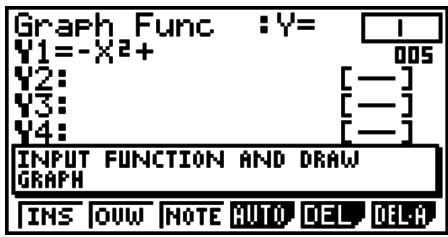
■ Editing Example
In this example, we show how to edit the graph function (Y1 = -X^2 + 1) that is input at the end of the operation under “To create an n-key operation” (page 10-14).
- To change -X^2 + 1 to -2X^2 + 1 (by inserting a ② key before the X, , T key)
- This will display the ,,T key editing screen.
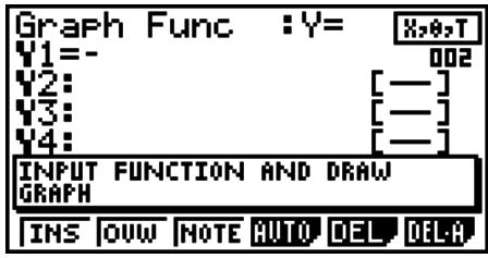
- Press F1(INS).
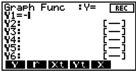
- Press 2.
- This inputs a 2 key before the ,,T key and displays the guide creation screen from the ,,T key.
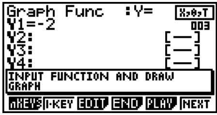
- To change -2X^2 + 1 to -2X^2 + 2 (by overwriting the ① key with the ② key)
- This will display the ① key editing screen.
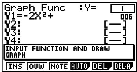
- Press F2 (OVW).
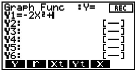
- Press 2.
- This will overwrite the ① key with the ② key and display the guide creation screen from the next key (EXE key).
![Graph Func :Y= Y1=-2X²+2 Y2: Y3: Y4: INPUT FUNCTION AND DRAW GRAPH EXE 007 [—] [—] [—] NEW I-KEY EDIT END PLAY NEXT](/content/2025/01/86832/images/bb8bbb9b5666445776af8fa783374d23f7c1476c31017d0d2c59c9d450395eec.jpg)
- To edit an n-key operation comment
- This will display the Ⓗ key editing screen.
![Graph Func : Y= ( ) Y1 001 Y2: [—] Y3: [—] Y4: [—] INPUT FUNCTION AND DRAW GRAPH INS OUV NOTE AUTO DEL DELA](/content/2025/01/86832/images/9626bf75b0bc957bde1dcf413209a648e6c8c1bfcadc4d8182b4f5ff76bbdde7.jpg)
- Press F3 (NOTE).
![Graph Func :Y= ( ) Y1 001 Y2: [—] Y3: [—] [—] INPUT FUNCTION AND DRAW GRAPH BTM TOP HIDE](/content/2025/01/86832/images/0fae2763452ddd52e88f4941a92a08a34ac042905f83fe912ed4cec3a1103e18.jpg)
- Edit the comment and then press EXE.
- This will display the guide creation screen from the Ⓑ key.
![Graph Func :Y= ( ) Y1: 001 Y2: [—] Y3: [—] Y4: [—] HOW TO USE INTEGRAL COMMAND IN GRAPH NEW | KEY EDIT END PLAY NEXT](/content/2025/01/86832/images/b583f73f13fd0d4af0b0a0329cea135425910b907dbc233ade96f9d6a56568dc.jpg)
- To change -2X^2 + 2 to 2X^2 + 2 (by deleting the (-) key)
- This will display the Ⓗ key editing screen.
![Graph Func :Y= ( ) Y1 001 Y2: [—] Y3: [—] Y4: [—] HOW TO USE INTEGRAL COMMAND IN GRAPH INS OUV NOTE AUTO DEL DELA](/content/2025/01/86832/images/d04ef44435cfb151498d89c7cb629933a620db8a940b771ef3b232518ab5838c.jpg)
- Press F5 (DEL).
![Delete this key? Yes: [F1] No : [F6]](/content/2025/01/86832/images/3232ab193931c86e4079e4c57c85061985a10a14fb9028decc2ae5bdd24a07d4.jpg)
- Press F1 (Yes).
- This will delete the (-) key and display the guide creation screen from the next key ( 2 key).
![Graph Func :Y= ¥8 ¥2: ¥3: ¥4: 001 [—] [—] [—] HOW TO USE INTEGRAL COMMAND IN GRAPH NEW$I-KEY EDIT END PLAY NEXT](/content/2025/01/86832/images/613de16914e799f223f3110eb94cd02ab0bcb8b85b4846734c84d74583aa0278.jpg)
- To exit a editing operation
-
Press F4(END).
-
Press F1 (Yes) or F6 (No).
- Exits the editing operation and returns to the eActivity workspace screen.
- To edit the guide of an existing strip from the eActivity workspace screen
- On the eActivity workspace screen, select a strip that already has a guide and then press F6(▷) to display page two of the function menu.

2. Press F5 (GUIDE).
- This will display the first key editing screen.
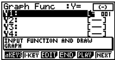
- Operations from this points are identical to those under “Creating a Guide” (page 10-13) and “Editing the Guide You Are Creating” (page 10-18).
- Running a Guide
This example shows how to run the guide created under “Creating a Guide” (page 10-13).
- On the eActivity workspace screen, select the Graph strip and then press EXE.
- This will display the screen shown to the right.
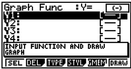
- Press the key indicated by the key indicator that appears in the upper or lower right corner of the screen.
- This will cause the next key to be pressed to appear in the upper or lower right corner.
![Graph Func :Y= Y1=-I Y2: [—] Y3: [—] Y4: [—] INPUT FUNCTION AND DRAW GRAPH Y F Xt Yt X](/content/2025/01/86832/images/0432292a4dd81ea6739a5f2269e10c85d264e966c286cbc8011e08b782e0f6b2.jpg)
- Perform the key operation in accordance with the keys that appear on the screen.
- Exit Strip ON: EXE will appear in the upper or lower right corner when the guide is complete.
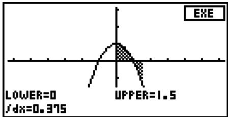
line
| Parameter | Value | | --------- | ----- | | LOWER | 0 | | dfx | 0.375 | | UPPER | 1.5 |- Exit Strip OFF: The strip will be freely usable when the guide is complete. Note, however, that this operation does not save the strip.
- If exit strip is turned on, press EXE.
- This will display the dialog box shown to the right.
![End of guide Exit strip? Yes: [F1] No : [F6]](/content/2025/01/86832/images/e8ba82b319518efb9b298299ecee71b69ba914f42a014cf57389f751b593f340.jpg)
- F1(Yes) ... Exits the strip and returns to the eActivity workspace screen.
- F6 (No) ... Returns to the screen in step 3.
- Pressing a key that is different from the one displayed in the upper or lower right corner of the screen will display the dialog box shown below. The guide operation cannot proceed if you do not follow its instructions.
![Press the key on the right of the display. OK : [EXIT] End : [SHIFT][→]](/content/2025/01/86832/images/e103f676e735b6cc7db7daa4a899763ce56bf97fc6d3a976a975b6fffa465e95.jpg)
EXIT or AC ......Returns to the previous screen.
SHIFT → (☐).... Exits the strip and displays the eActivity workspace screen.
- Pressing AC during auto key input of an AUTO operation will stop key input and display the normal script screen. Guide playback cannot be restarted from the place where playback is stopped.
■ eActivity Guide Editing Techniques
• To edit a guide from the end
On the editing screen, press F5(PLAY) F5(▶).
- To insert SETUP or V-Window setting changes into a key operation sequence
On the editing screen, display the location where you want to insert the setting change operation, insert an n-key operation, and then input the change operation.
- To allow students to continue with their own operation after executing a problem guide
Input an n-key operation with the example, and specify "No" for the exit strip option at the end of the guide creation operation.
- To create a guide that starts with list data input
Use an AUTO operation for the list data input operation when creating a guide that starts with list data input. Select “Ultra-fast” for the play speed of the data input. This will cause the data to be input at very high speed when the guide is executed.
Chapter 11 Memory Manager
fx-7400GII/fx-9750GII
These models support the following data operations: data display, search, and delete.
Important!
fx-7400GII/fx-9750GII calculators are not equipped with storage memory or an SD card slot. Because of this, the storage memory and SD card memory operations described below are not supported.
fx-9860GII/fx-9860GII SD/fx-9860G AU PLUS/fx-9860G Slim
These models are equipped with both a main memory and a storage memory, so the following data operations are supported: data display, search, and delete, as well as data copy between memories.
The main memory is a work area where you can input data, perform calculations, and run programs. Data in the main memory is relatively safe, but it can be deleted by batteries going dead or when you perform a full reset.
The storage memory uses “flash memory,” so data is safe even when power is interrupted.
Normally, you should use the storage memory for data you need to store securely for long periods, loading data into the main memory only when you need it.
- Use of SD card memory (when an SD card is loaded in the SD card slot) also is supported by the fx-9860GII SD.
1. Using the Memory Manager
From the Main Menu, select the MEMORY icon to enter the MEMORY mode.
- On the fx-7400GII/fx-9750GII, the main memory information screen shown to the right will appear. For information about using this screen, see “Memory Information Screen” (page 11-2).
- On other models, the screen shown to the right appears.
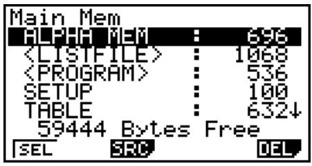
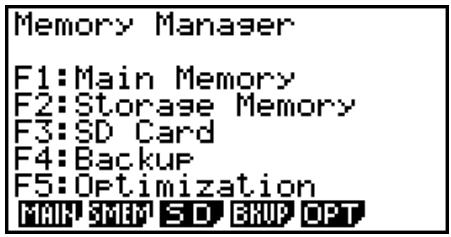
- {MAIN} ... {displays main memory information}
- {SMEM} ... {displays storage memory information}
- {SD} ... {displays SD card memory information} (fx-9860GII SD only)
- {BKUP} ... {main memory backup}
- {OPT} ... {storage memory, SD card optimization}
■ Memory Information Screen
The memory information screen shows information about one memory at a time: the calculator's main memory or storage memory, or the SD card memory.
- Since an fx-7400GII or fx-9750GII calculator has only main memory, main memory contents only appear on the main memory information screen.
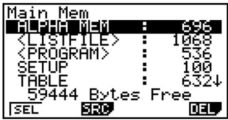
- With other model calculators, perform one of the following MEMORY mode menu operations to display the memory information screen you want.
| When this memory information screen is displayed: | Press this key: |
| Main memory | F1 (MAIN)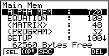 |
| Storage memory | F2 (SMEM)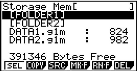 |
| SD card memory (fx-9860GII SD only) | F3 (SD)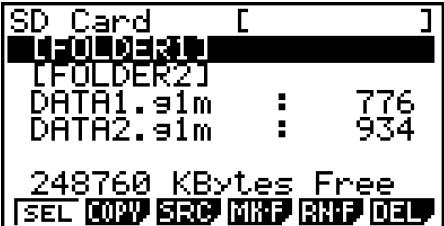 |
- Use the cursor ▲ and ▼ keys to move the highlighting and check the number of bytes used by each type of data.
- Line 7 shows how many bytes of memory are currently unused in the currently selected memory (main, storage, or SD card).
- The first time you store data to the storage memory, the calculator will reserve a management memory area automatically, which will reduce the “Free” value by 65536 bytes.
- On the main memory screen, < > indicates a data group. On the storage memory and SD card screens, [ ] indicates folders.
Moving the highlighting to a data group or folder and pressing EXE will display the data group or folder contents. Pressing EXIT will return to the previous screen.
When the contents of a storage memory or SD card folder are displayed, the first line of the screen shows the name of the folder.
The following data can be checked.
Main Memory
| Data Name | Contents |
| ALPHA MEM | Alpha letter variables |
| Capture memory group | |
| CAPT n (n = 1 to 20) | Capture memory |
| CONICS*1 | Conics setting data |
| DYNA MEM*1 | Dynamic Graph memory |
| EQUATION | Equation data |
| FINANCIAL*1 | Financial data |
| Function memory group | |
| F-MEM n (n = 1 to 20) | Function memory |
| Graph memory group | |
| G-MEM n (n = 1 to 20) | Graph memory |
| List file group | |
| LIST n (n = 1 to 26, and Ans) | List memory contents |
| LIST FILE n (n = 1 to 6) | List file |
| Matrix group | |
| MAT n (n = A to Z, and Ans)*1 | Matrix |
| Picture memory group | |
| PICT n (n = 1 to 20) | Picture memory |
| Program group | |
| Each program name | Programs |
| RECURSION*1 | Recursion data |
| SETUP | Setup data |
| STAT | Stat result data |
| String memory group | |
| STR n (n = 1 to 20) | String memory |
| SYSTEM | OS and data shared by applications (clipboard, replay, history, etc.) |
| Spreadsheet group | |
| Each spreadsheet name*2 | Spreadsheet data |
| Each add-in application name*2 | Application-specific data |
| TABLE | Table data |
| V-Window memory group | |
| V-WIN n (n = 1 to 6) | V-Window memory |
| Y=DATA | Graph expression |
Storage Memory, SD Card ^*1
| Data Name | Contents |
| *.g1m or .g2m file names | Data items listed in the Main Memory table that has been copied to storage memory or an SD card.The names of these files have the extension “.g1m” or “.g2m”. |
| eActivity data names | eActivity data stored in storage memory or on an SD card. |
| Add-in software names (Applications, languages, menus) | Add-in applications, add-in languages, and add-in menus stored in storage memory or on an SD card. |
| Folder names | Enclosed in square brackets ([ ]). |
| Unknown | Area that is unusable due to writing error, etc. |
*1 "No Data" is displayed when there is no data in storage memory or on the SD card. The message "No Card" indicates there is no SD card loaded in the calculator.
■ Creating a Folder in Storage Memory or on an SD Card
- To create a new folder
-
While storage memory or SD card memory data is on the display, press F4(MK·F) to display the folder name input screen.
-
Input up to eight characters for the name you want to give to the folder.
![Folder Name [A ]](/content/2025/01/86832/images/85c7fcbfadfde15169f3965dbc00805f5259e9a979dfdca8680e36e927a29e6a.jpg)
- Only the following characters are supported: A through Z, {, }, ', \~, 0 through 9 Inputting any invalid character will cause an “Invalid Name” error.
- An “Invalid Name” also occurs if the name you input is already being used by an existing file.
-
To cancel folder creation, press EXIT.
-
Press EXE to create the folder and return to the storage memory or SD card memory information screen.
![Storage Mem[ ] UFOLDER1 393184 Bytes Free SEL COPY SRC MRF RNF DEL](/content/2025/01/86832/images/053841d0d5fcda5472065ff77be5771f0b999537a9ba8fe0d8beffd2226eb7a8.jpg)
- To rename a folder
- On the storage memory or SD card memory information screen, select the folder you want to rename.
-
Press F5 (RN·F) to display the rename folder screen.
-
Input up to eight characters for the name you want to give to the folder.
![Rename [&OLDER1]](/content/2025/01/86832/images/d7ae1a4daae2a929e09878c3682d9b8c00a768fdb1ab6c4790b999ca76ca2b1e.jpg)
- Only the following characters are supported: A through Z, {, }, ', \~, 0 through 9 Inputting any invalid character will cause an “Invalid Name” error.
- An “Invalid Name” also occurs if the name you input is already being used by an existing file.
-
To cancel folder creation, press EXIT.
-
Press EXE to rename the folder and return to the storage memory or SD card memory information screen.
![Storage Mem[ ] LIVDATA] 393184 Bytes Free SEL COPY SRC MKF RNF DEL](/content/2025/01/86832/images/86652ab62dbcfeaceae73e6304b5885a980c281852a74ac351d42614c080b9eb.jpg)
■ Selecting Data
- Press F1 (SEL) to select the currently highlighted item, which is indicated by the black selection pointer (▶) appearing next to it. Pressing F1 (SEL) again will deselect the item, causing the selection pointer to disappear.
- You can select multiple files, if you want.
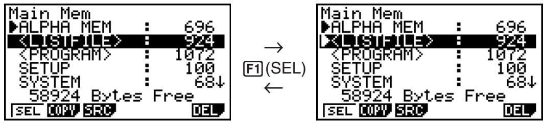
- Selecting a group or folder also selects everything inside of it. Deselecting a group or folder deselects all of its contents.
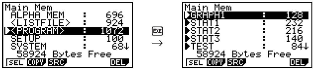
- If you select one or more individual items inside of a data group or folder, the black selection pointer (▶) appears next to each item, while a white selection pointer (▷) appears next to the group or folder name.
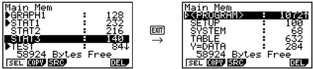
- Returning to the MEMORY mode initial screen deselects all currently selected items.
■ Copying Data
Important!
- Data copy is not supported on an fx-7400GII or fx-9750GII calculator.
- To copy from main memory to storage memory
Note
- The following procedure saves the selected data into a single file. You assign a name to the file, which is stored in storage memory.
-
On the main memory data information screen, select the data you want to copy.
-
Press F2(COPY).
- This displays the storage memory/SD card selection screen (fx-9860GII SD only).*1
![Copy to Storage Mem: [1] SD Card : [2] 62544 Bytes Free SEL COPY SEC DEL](/content/2025/01/86832/images/5bf52989c1fc54b254dfa6fa680cf3554205b998610f05a4cc38114a0ba8c46f.jpg)
- Press 1 to select storage memory (fx-9860GII SD only).*2
- This displays the folder selection screen.
- Select the folder to which you want to copy the data.
- This displays the file name input screen.

- Input the file name you want to give to the file.
- To cancel the copy operation, press EXIT.
- Press EXE.
• This copies the data.
- The message "Complete!" appears when the copy operation is complete. Pressing EXIT will return to the MEMORY mode initial screen.
*1 Copying data from the storage memory or an SD card causes one of the screens shown below to appear (fx-9860GII SD only).
![ST Copy to Main Mem : [1] SD Card : [2] 257420 Bytes Free SEL COPY SEC MRF RNF DEL](/content/2025/01/86832/images/c884ddeb476f76aa47dbd122f77e0e6ae9e3adc8514283a5e408ac6e281e5617.jpg)
![Copy to Main Mem :[1] Storage Mem:[2] 248736 KBytes Free SEL COPY SEC MRF RNF DEL](/content/2025/01/86832/images/10aaea5f87f720d5155462b1a051a964f7b27f669562e3008939cc4395911507.jpg)
Pressing ① selects main memory and copies the data, without displaying the folder selection screen.
The file name input screen does not appear when you copy data from storage memory or/and SD card to main memory.
*2 To copy to the SD card, press ②. The “No Card” error message will appear if there is no SD card loaded in the calculator.
■ Error Checks During Data Copy
The following error checks are performed while a data copy operation is being executed.
Low battery check
The calculator performs low battery check before starting the data copy operation. If the battery is at Level 1, a low battery error occurs and the copy operation is not performed.
Available memory check
The calculator checks to see if there is enough free memory available to store the copied data.
A “Memory Full” error occurs if there is not enough memory available.
A “Too Many Data” error occurs when the number of data items is too great.
A “Fragmentation ERROR” occurs when there is enough free memory available, but a garbage collection operation is required.
If a “Fragmentation ERROR” occurs, perform the optimization procedure (page 11-11).
Overwrite check
The calculator checks to see if there is any existing data at the copy destination with the same name as the data being copied.
An overwrite confirmation message appears if there is data with the same name.
![[D [DATA1.91m ] Already Exists Overwrite OK? Yes:[F1] No :[F6]](/content/2025/01/86832/images/70cd9cc5f84173b839f95eb63f38a28c73533c9fa9b5ed29b40220eb96267133.jpg)
- F1 (Yes) ... overwrites the existing data with the new data
- F6 (No) ... advances to the next data item without copying the data with the same name
- Pressing AC will cancel the copy operation and return to the MEMORY mode initial screen.
Overwrite check is performed for the following types of data only. All other types of data are copied, without checking for data files with the same name.
- Programs
- Matrices
- List files
- Graph memories
• Dynamic Graph memories - Spreadsheet data
Overwrite check is performed for data of the same type only. If different types of data have the same name, the copy operation is performed without regard to the data with the same name.
Overwrite check applies only to the destination of the copy operation.
Type mismatch error check
eActivity data, add-in applications, add-in languages, add-in menus, and backup data cannot be copied to main memory. Attempting to do so will cause a type mismatch error.
- To delete a main memory file
- Display the main memory information screen.
- See “Memory Information Screen” on page 11-2.
-
Select the file(s) you want to delete. You can select multiple files, if you want.
-
Press F6 (DEL).
- Press F1 (Yes) to delete the file.
- Press F6(No) to cancel the delete operation.
![Delete All The Selected Data? Yes:[F1] No:[F6]](/content/2025/01/86832/images/91455f7faf24878d10f22bd5a3c63864ed34263bb53947f90ab8335945429e15.jpg)
- To delete a storage memory file
- Display the storage memory information screen.
- See “Memory Information Screen” on page 11-2.
-
Select the file(s) you want to delete. You can select multiple files, if you want.
-
Press F6 (DEL).
- Press F1 (Yes) to delete the file.
- Press F6(No) to cancel the delete operation.
- To delete SD card files (fx-9860GII SD only)
- Display the SD card memory information screen.
- See “Memory Information Screen” on page 11-2.
-
Select the file(s) you want to delete. You can select multiple files, if you want.
-
Press F6 (DEL).
- Press F1 (Yes) to delete the file.
- Press F6(No) to cancel the delete operation.
■ Searching for a File
- To search for a file in the main memory
Example To search for all files in the main memory whose names begin with the letter “R”
- Display the main memory information screen.
- See “Memory Information Screen” on page 11-2.
- Press F3 (SRC).
- Input the letter "R" for the keyword.
Search [R&]
- The first file name that begins with the letter "R" appears highlighted on display.
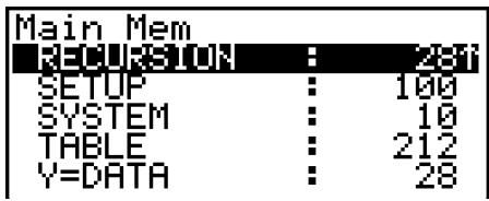
- You can input up to eight characters for the keyword.
- To search for a file in the storage memory
Example To search for all files in the storage memory whose names begin with the letter “S”
- Display the storage memory information screen.
- See “Memory Information Screen” on page 11-2.
- Press F3(SRC).
- Input the letter "S" for the keyword.
- The first file name that begins with the letter "S" appears highlighted on display.
![Storage Mem[ ] SHADE.s1m : 4200T TRIG.s1m : 348 VENN.s1m : 236](/content/2025/01/86832/images/b898055c105603c7fb43f9d40e9d019ee2382adc4245c6116ab216690ed274a1.jpg)
- To search for a file in the SD card (fx-9860GII SD only)
Example To search for all files in the SD card whose names begin with the letter "R"
- Display the SD card memory information screen.
- See “Memory Information Screen” on page 11-2.
- Press F3 (SRC).
- Input the letter "R" for the keyword.
- The first file name that begins with the letter "R" appears highlighted on display.
![SD Card [ ] REF.s1m : 3727 SHADE.s1m : 336 TRIG.s1m : 284](/content/2025/01/86832/images/67e49df215a484ccdaa47eb1b5b272cc2b56b2e4cfa4b67befb9e43e08042143.jpg)
- The message “Not Found” appears if there are no file names that match your keyword.
■ Backing Up Main Memory Data
Important!
- Data back-up is not supported on an fx-7400GII or fx-9750GII calculator.
- To back up main memory data
- On the initial MEMORY mode screen press F4 (BKUP).
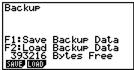
- Press F1(SAVE).
This displays the save location selection screen (fx-9860GII SD only).
- 1 ... storage memory
-
2 ... SD card
-
Press ① or ② (fx-9860GII SD only).
This displays a folder selection screen.
![Back Save to Storage Mem: [1] SD Card : [2] 393216 Bytes Free SAVE LOAD](/content/2025/01/86832/images/78ac945e75e41f8696eb64274ebf0f32cf9e658dacaf21aa699c1cdd816fb0fb.jpg)
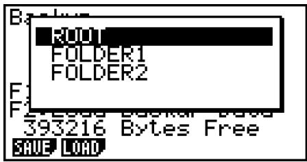
- Use ▲ and ▼ to select the folder where you want to save the data.
- Press EXE to start the backup.
- Backup data is saved in a file named BACKUP.g2m.
The message “Complete!” appears when the backup operation is finished.
Press EXIT to return to the screen displayed in step 1.
The following message appears if there is already backup data in the storage memory.
![[BACKUP.g2m ] Already Exists Overwrite OK? Yes:[F1] No :[F6]](/content/2025/01/86832/images/cefca2bdc3d12ca64aee04566b2196becebefa7715e22a98fa824185a4c96305.jpg)
Press F1(Yes) to back up the data, or F6(No) to cancel the backup operation.
A “Memory Full” occurs when there is not enough space available in the storage memory to complete the backup operation.
- To restore backup data to the main memory
- On the initial MEMORY mode screen press F4 (BKUP).
- On the screen that appears, you can confirm whether or not there is backup data in the storage memory.
- Press F2 (LOAD).
This displays the restore source data selection screen (fx-9860GII SD only).
- 1 ... Restore from storage memory
-
② ... Restore from SD card
-
Press ① or ② (fx-9860GII SD only).
This displays the folder selection screen.
![Load from Storage Mem: [1] SD Card : [2] 393216 Bytes Free SAVE LOAD](/content/2025/01/86832/images/f14574d10325d73edd69d90165e1b4981c5fff9e53bf35f07c353b6e3aee37f7.jpg)
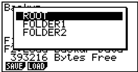
-
Use ▲ and ▼ to select a folder.
-
Press EXE.*1
- A message appears to confirm whether or not you really want to restore the backed up data.
*1 The message “No Data” will appear if there is no backup data stored in memory. Pressing EXIT will return the screen in step 1.
![Overwrite OK? Yes: [F1] No: [F6] 391688 Bytes Free SAVE LOAD](/content/2025/01/86832/images/2cbee93e0a092f5ea23b40e834e8249bfcdb13b019f582a4b0730aee66b8b628.jpg)
Press F1(Yes) to restore the data and delete any data currently in the area.
Press F6 (No) to cancel the data backup operation.
The message “Complete!” appears when the restore operation is finished.
Press EXIT to return to the screen displayed in step 1.
■ Optimizing the Storage Memory or SD Card Memory
Storage memory or SD card memory can become fragmented after many store and load operations. Fragmentation can cause blocks of memory to become unavailable for data storage. Because of this, you should periodically perform the storage memory or SD card optimization procedure, which rearranges the data in the storage memory or SD card and makes memory usage more economical.
- To optimize the storage memory
- On the initial MEMORY mode screen press F5(OPT) to optimize the storage memory.
-
Select the memory you want to optimize (fx-9860GII SD only).
-
1 ... storage memory
-
2 ... SD card
-
Press ① or ② to start optimization.
![Optimize Storage Mem: [1] SD Card : [2] F5:Optimization MAIN S/MEM S/D BKUP OPT](/content/2025/01/86832/images/763879b85c4ccccab464702ad26c32465225b0a9e5b15aa2830e9e6c93a25b15.jpg)

The message “Complete!” appears when the optimize operation is complete.
Press EXIT to return to the initial MEMORY mode screen.
- In some cases, the amount of free memory capacity may be unchanged when you check it after performing the optimization procedure. This does not indicate any problem with the calculator.
Chapter 12 System Manager
Use the System Manager to view system information and make system settings.
1. Using the System Manager
From the Main Menu, enter the SYSTEM mode and display the following menu items.
• F1 (◀) ... {display contrast adjustment}
- F2 (+ -) ... {Auto Power Off time setting}
- F3 (LANG) ... {system language}
- F4 (VER) ... {version}
- F5(RSET) ... {system reset operations}
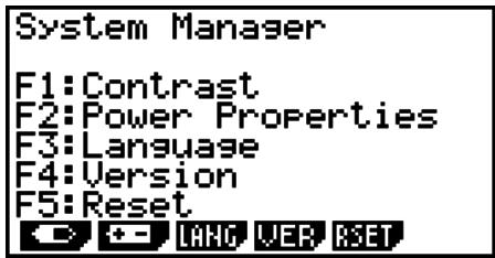
2. System Settings
■ Contrast Adjustment
While the initial SYSTEM mode screen is displayed, press F1(◀) to display the Contrast Adjustment screen.
- The ▶ cursor key makes display contrast darker.
- The ◀ cursor key makes display contrast lighter.
- F1(INIT) returns display contrast to its initial default.
Press EXIT or SHIFT EXIT (QUIT) to return to the initial SYSTEM mode screen.
You can adjust contrast while any screen is on the display by pressing SHIFT and then ▶ or ◀. To exit contrast adjustment, press SHIFT again.
■ Power Properties Settings
- To specify the Auto Power Off trigger time
While the initial SYSTEM mode screen is displayed, press F2(+) to display the Power Properties setting screen.
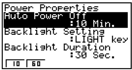
Models equipped with a backlight
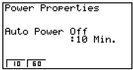
Models not equipped with a backlight
- F1(10) ... {10 minutes} (initial default setting)
• F2 (60) ... {60 minutes}
Press EXIT or SHIFT EXIT (QUIT) to return to the initial SYSTEM mode screen.
- To specify the backlight key (for models equipped with a backlight only)
-
While the initial SYSTEM mode screen is displayed, press F2(+) to display the Power Properties setting screen.
-
Use ▲ and ▼ to select "Backlight Setting".
-
F1 (LIGHT) ... {Backlight on/off: SHIFT OPTN (LIGHT)}
• F2 (ANY) ... {Backlight on: Any key} -
Press EXIT or SHIFT EXIT (QUIT) to return to the initial SYSTEM mode screen.
- To specify the backlight duration (for models equipped with a backlight only)
-
On the initial SYSTEM mode screen, press F2 (+ -) to display the Power Properties setting screen.
-
Use ▲ and ▼ to select "Backlight Duration".
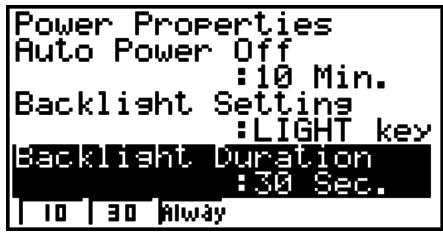
- F1(10) ... {turns off the backlight 10 seconds after the last key operation is performed}
- F2(30) ... {turns off the backlight 30 seconds after the last key operation is performed} (initial default setting)
-
F3 (Always) ... {leaves the backlight turned on until the backlight key is pressed or until the calculator is turned off}
-
Press EXIT or SHIFT EXIT (QUIT) to return to the initial SYSTEM mode screen.
■ System Language Setting
Use LANG to specify the display language for built-in applications.
- To select the message language
- From the initial SYSTEM mode screen, press F3 (LANG) to display the Message Language selection screen.
- Use the ▲ and ▼ cursor keys to select the language you want, and then press F1(SEL).
- The pop up window appears using the language you selected. Check the contents and then press EXIT.
- Press EXIT or SHIFT EXIT (QUIT) to return to the initial SYSTEM mode screen.
- To select the Menu Language (fx-9860GII SD/fx-9860GII/fx-9860G AU PLUS)
- From the initial SYSTEM mode screen, press F3 (LANG) to display the Message Language selection screen.
- Press F6 (MENU).
- Use the ▲ and ▼ cursor keys to select the language you want, and then press F1(SEL).
- The pop up window appears using the language you selected. Check the contents and then press EXIT. 12-2
- Press F6(MSG) to return to the Message Language selection screen.
- Press EXIT or SHIFT EXIT (QUIT) to return to the initial SYSTEM mode screen.
Version List
Use VER (version) to display the operating system version. You can also register the user name you want.
- To display version information
- On the initial SYSTEM mode screen, press F4 (VER) to display the Version list.
- Use ▲ and ▼ to scroll the screen. The contents of the list are shown below.
- Items marked with an asterisk (*) are displayed for all models. Other items are displayed on models that support the applicable functions.
- Operating system version*
- Add-in application names and versions (only installed add-ins are displayed)
- Message languages and versions*
- Menu languages and versions
-
User name*
-
Press EXIT or SHIFT EXIT (QUIT) to return to the initial SYSTEM mode screen.
- The operating system version that actually appears depends on the calculator model.
- To register a user name
- While the Version list is displayed, press F1(NAME) to display the user name input screen.
- Input up to eight characters for the user name you want.
- After inputting the name, press EXE to register it, and return to the Version list.
- If you want to cancel user name input and return to the Version list without registering a name, press EXIT.
![User Name [& ]](/content/2025/01/86832/images/7d921d58c8f1ab8f1ad94a9dcd233819bd49692758cf0a2367fab84a6fdc4d7a.jpg)
Reset
- While the initial SYSTEM mode screen is displayed, press F5(RSET) to display the Reset Screen 1.
Important!
Items that appear on the Reset Screen(s) depend on the calculator mode.
- F1(STUP) ... {setup initialization}
• F2 (MAIN) ... {main memory data clear} - F3 (ADD) ... {add-in application clear}*
- F4 (SMEM) ... {storage memory data clear}*
- F5(A&S) ... {add-in application and storage memory data clear}*
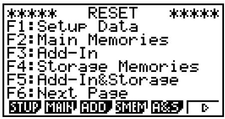
Pressing F6(▷) on the above screen displays the Reset Screen 2 shown below.
- F1(M&S) ... {main memory data and storage memory data clear}*
- F2 (ALL) ... {all memory clear}*
- F3 (SD) ... {SD card format} (fx-9860GII SD only)
* Not included on the fx-7400GII/fx-9750GII.
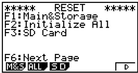
The following table shows the functions of the function keys. You can use the function keys to delete the specific data you want.
Function Key Functions
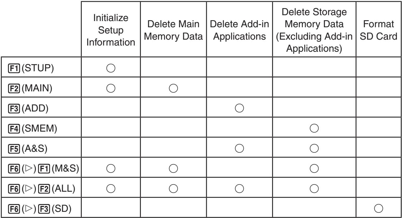 |
- Press the function key that corresponds to the reset operation you want to perform.
- In response to the confirmation message that appears, press F1 (Yes) to perform the reset operation you specified, or F6 (No) to cancel.
- A message appears to let you know when the reset operation is complete.
![Reset OK? Main Memories Yes: [F1] No : [F6]](/content/2025/01/86832/images/762d0b58c48b82a8efe461c62a9b22d61793cf1de5eb5c3695138e94ba0c87ed.jpg)
Screen produced when
F2 (MAIN) is pressed in step 2.
![Reset! Main Memories Press: [EXIT]](/content/2025/01/86832/images/b99c4366af9a822ff9f32bde6fd6fdf15c5bc3f09fe5378dcd393ffb2a6fcf4a.jpg)
Screen produced when
F2 (MAIN) is pressed in step 2.
Chapter 13 Data Communications
This chapter tells you everything you need to know to transfer programs between two CASIO Power Graphic calculators connected using the cable that is equipped as a standard accessory.
1. Connecting Two Units
The following procedure describes how to connect two units with the connecting cable that comes equipped as a standard accessory.
- To connect two units
- Check to make sure that the power of both units is off.
- Connect the two units using the cable.
- Step 3 is not required on the fx-7400GII.
- Perform the following steps on both units to specify 3PIN as the cable type.
(1) From the Main Menu, enter the LINK mode.
(2) Press F4 (CABL). This displays the cable type selection screen.
(3) Press F2 (3PIN).
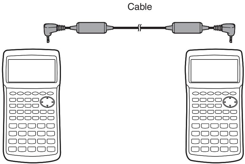
- Models that are supported for this configuration are shown below.
fx-9860GII SD, fx-9860GII, fx-9860G AU PLUS, fx-9750GII, fx-7400GII, fx-9860G Slim (OS 2.00/1.11), fx-9860G SD (OS 2.00/1.05), fx-9860G (OS 2.00/1.05), fx-9860G AU (OS 2.00/1.05), fx-7400G series, CFX-9850G series
2. Connecting the Calculator to a Personal Computer
You can transfer data between the calculator and a computer by using the Program-Link Software (FA-124) and a special cable ^*1 to establish a connection between them.
For details about establishing a connection and data transfer procedures, see the FA-124 User's Guide.
*1 With the fx-9860GII SD, fx-9860GII, fx-9860G AU PLUS, and fx-9860G Slim (OS 2.00), use the Program-Link Software and USB cable that comes with the calculator. For the fx-9750GII and fx-7400GII, you will need to purchase the separately available FA-124.
3. Performing a Data Communication Operation
From the Main Menu, enter the LINK mode. The following data communication main menu appears on the display.
- {TRAN} ... {displays the data send screen}
- {RECV} ... {displays the data receive screen}
- {CABL} ... {displays the cable type selection screen} (not included on the fx-7400GII)
- {WAKE} ... {displays the wakeup setting screen}
- {CAPT} ... {displays the screen image send setting screen}

Communication parameters are fixed at the following settings.
- 3-pin serial port
- Speed (BPS): 9600 bps max. (Connected with CFX-9850G series or fx-7400G series calculator)
115200 bps max. (Connected with another fx-9860GII SD, fx-9860GII, fx-9860G AU PLUS, fx-9750GII, fx-7400GII, fx-9860G Slim (OS 2.00/1.11), fx-9860G SD (OS 2.00/1.05), fx-9860G (OS 2.00/1.05) or fx-9860G AU (OS 2.00/1.05) calculator)
- Parity (PARITY): NONE
- USB port*
- Communication speed is in accordance with USB standards.
* The fx-7400GII is not equipped with a USB port.
■ Select Connection Mode Screen (All models except fx-7400GII)
Connecting the USB cable to the calculator will cause the dialog box shown nearby to appear. You can use this dialog box to select the USB cable Connection Mode (screen image send mode).
![Communication Select Ca Connection Mode Wa DataTrans: [F1] Ca ScreenCapt: [F2] Projector: [F3] ScreenRecv: [F4]](/content/2025/01/86832/images/abe891ff9efad734f4a98634595fae30530dd37f38b315a0dc8e8e88a1ffd84e.jpg)
- F1(DataTrans) ... {mode selection for data transfer with PC}
- F2 (ScreenCapt) ... {mode selection for sending calculator screen captures to PC using FA-124 Screen Capture function}
- F3 (Projector) ... {mode selection for calculator screen output to a CASIO OHP unit or CASIO projector}
- F4 (ScreenRecv) ... {mode selection for sending calculator screen images to PC using fx-9860G Manager PLUS Screen Receiver function}
To transfer data between a PC and calculator memory, press F1.
Use keys F2 through F4 to select the appropriate mode for sending the calculator screen image to an external device. For details about calculator operations when keys F2 through F4 are pressed, see “Screen Image Send” (page 13-11).
■ Performing a Data Transfer Operation
Connect the two units and then perform the following procedures.
Receiving unit
To set up the calculator to receive data, press F2(RECV) while the data communication main menu is displayed.
Receiving...
AC : Cancel
The calculator enters a data receive standby mode and waits for data to arrive. Actual data receive starts as soon as data is sent from the sending unit.
Sending unit
To set up the calculator to send data, press F1 (TRAN) while the data communication main menu is displayed.
This displays a screen for specifying the data selection method.
- {SEL} ... {selects new data}
- {CRNT} ... {automatically selects previously selected data*1}
Select Trans Type
F1:Select
F2: Current
SEL CRHT
*1 The previously selected data memory is cleared whenever you change to another mode.
- To send selected data items (Example: To send user data)
Press F1(SEL) or F2(CRNT) to display a data item selection screen.
- {SEL} ... {selects data item where cursor is located}
- {ALL} ... {selects all data}
- {TRAN} ... {sends selected data items}
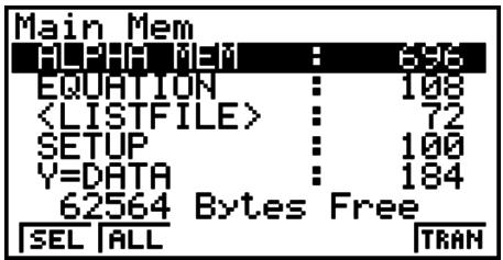
Use the ⬆ and ⬇ cursor keys to move the cursor to the data item you want to select and press F1(SEL) to select it. Currently selected data items are marked with “▶”. Pressing F6(TRAN) sends all the selected data items.
- To deselect a data item, move the cursor to it and press F1(SEL) again.
Only items that contain data appear on the data item selection screen. If there are too many data items to fit on a single screen, the list scrolls when you move the cursor to the bottom line of the items on the screen.
- To execute a send operation
After selecting the data items to send, press F6 (TRAN). A message appears to confirm that you want to execute the send operation.
- F1 (Yes) ... sends data
• F6 (No) ... returns to data selection screen
Press F1(Yes) to send the data.
![Transmit OK? Yes: [F1] No : [F6]](/content/2025/01/86832/images/059b9ac07a25fa9037e985e74aeb0a433fe1a709ef90480fe968af20cceb881c.jpg)
Transmitting... AC : Cancel
- You can interrupt a data operation at any time by pressing AC.
The following shows what the displays of the sending and receiving units look like after the data communication operation is complete.
![Sending Unit Transmitting A0 Complete! Press: [EXIT]](/content/2025/01/86832/images/01ea68116b1c35ede778e6dfbf40e653cf2e1d6db3ac0fc675c2e79eb242ed89.jpg)
![Receiving Unit Receiving A0 Complete! Press: [EXIT]](/content/2025/01/86832/images/2ca04852b30f985ebb684fae360a68f39e757459c233c1fa077242076f97c832.jpg)
Press EXIT to return to the data communication main menu.
- Configuring the Receiver’s Wakeup Feature
When Wakeup is turned on the receiver, the receiver turns on automatically when data transfer starts.
fx-7400GII
- The receiver enters the receive mode automatically after it wakes up.
All models except fx-7400GII
- When communicating between two calculators (3PIN selected as the cable type), the receiver enters the receive mode automatically after it wakes up.
-
When communication is with a computer (USB selected as the cable type), connecting the USB cable to a computer and then to the calculator (while the calculator is turned off) will cause the calculator to turn on and the “Select Connection Mode” dialog box to appear.
-
On the receiver's data communication main menu, press F5 (WAKE).
This displays the Wakeup setting screen.
- {On} ... {turns Wakeup on}
-
{Off} ... {turns Wakeup off}
-
Press F1(On).
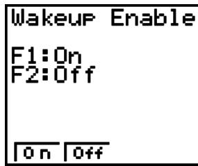
This turns on Wakeup and returns of the data communication main menu.
- Turn off the receiver.
- Connect the receiver to the sender.
- Starting a send operation on the sender causes the receiver to turn on automatically and performs the data transfer operation.
4. Data Communications Precautions
The following are the types of data items that can be sent.
- Data names marked with an asterisk (*) in the table are not included on the fx-7400GII.
| Data Item | Contents | Overwrite Check*1 |
| ALPHA MEM | Alpha memory contents | No |
| Capture memory group | ||
| CAPT n | Capture memory (1 to 20) data | No |
| CONICS* | Conics setting data | No |
| DYNA MEM* | Dynamic Graph functions | Yes |
| EQUATION | Equation calculation coefficient values | No |
| E-CON2* | E-CON2 setup memory contents | No |
| FINANCIAL* | Financial data | No |
| Function memory group | ||
| F-MEM n | Function memory (1 to 20) contents | No |
| Graph memory group | ||
| G-MEM n | Graph memory (1 to 20) contents | Yes |
| List file group | ||
| LIST n | List memory (1 to 26, and Ans) contents | Yes |
| LIST FILE n | List file memory (1 to 6) contents | Yes |
| Matrix group | ||
| MAT n* | Matrix memory (A to Z, and Ans) contents | Yes |
| Picture memory group | ||
| PICT n | Picture (graph) memory (1 to 20) data | No |
| Program group | ||
| Program names | Program contents (All programs are listed.) | Yes |
| RECURSION* | Recursion data | No |
| SETUP | Setup data | No |
| STAT | Stat result data | No |
| String memory group | ||
| STR n | String memory (1 to 20) data | No |
| SYSTEM | OS and data shared by applications (clipboard, replay, history, etc.) | No |
| Spreadsheet group | ||
| Spreadsheet data names | Spreadsheet data(All spreadsheet data are listed.) | Yes |
| TABLE | Table data | No |
| V-Window memory group | ||
| V-WIN n | V-Window memory (1 to 6) contents | No |
| Y=DATA | Graph expressions, graph draw/non-draw status, V-Window contents, zoom factors | No |
*1 No overwrite check: If the receiving unit already contains the same type of data, the existing data is overwritten with the new data.
With overwrite check: If the receiving unit already contains the same type of data, a message appears to ask if the existing data should be overwritten with the new data.
Data item name
![[MAT A ] Already Exists Overwrite OK? F1 :Yes F6 :No AC :Cancel YES NO](/content/2025/01/86832/images/a115c56f44602581ce988997fd1fa32e90643cc03ead67084a5aa398da3645d2.jpg)
- F1(YES) ... {replaces the receiving unit's existing data with the new data}
- F6(NO) ... {skips to next data item}
Note the following precautions whenever you perform data communications.
- An error occurs whenever you try to send data to a receiving unit that is not yet standing by to receive data. When this happens, press EXIT to clear the error and try again, after setting up the receiving unit to receive data.
- An error occurs whenever the receiving unit does not receive any data approximately six minutes after it is set up to receive data. When this happens, press EXIT to clear the error.
- An error occurs during data communications if the cable becomes disconnected, if the parameters of the two units do not match, or if any other communications problem occurs. When this happens, press EXIT to clear the error, then correct the problem before trying data communications again. If data communications are interrupted by the EXIT key operation or an error, any data successfully received up to the interruption will be in the memory of the receiving unit.
- An error occurs if the receiving unit memory becomes full during data communications. When this happens, press EXIT to clear the error and delete unneeded data from the receiving unit to make room for the new data, and then try again.
■ Exchanging Data with another Model Calculator
In this section, the term “OS 2.00 calculators” refers to the following models.
- fx-9860GII SD, fx-9860GII, fx-9860G AU PLUS, fx-9750GII, fx-7400GII
- fx-9860G Slim, fx-9860G SD, fx-9860G and fx-9860G AU whose operating systems have been updated to Version 2.00
An OS 2.00 calculator supports data exchange with the following calculator models.
OS 2.00 calculators, fx-9860G series, fx-7400G series, CFX-9850G series
When you perform a data exchange operation with the above calculator models, the OS 2.00 calculator will decide whether or not specific data can be sent or received, and convert data as required. The following describes the basic operations that are performed when exchanging data between an OS 2.00 calculator and another model calculator.
- Sending data from the OS 2.00 calculator to another calculator model
Data that is supported by the OS 2.00 calculator but is not supported by the receiving model either is not sent or is converted to a format supported by the receiving model before it is sent. - Sending data from another calculator model to an OS 2.00 calculator
Basically, data sent from another calculator model is received as it is. However, when there is a difference between an OS 2.00 calculator function and the function of the sending model, the OS 2.00 calculator will convert the data as required.
The following provides details about data compatibility between an OS 2.00 calculator and other calculator models.
- Transferring Data between the fx-9860GII SD, fx-9860GII, fx-9860G AU PLUS, fx-9750GII, fx-9860G Slim (OS 2.00), fx-9860G SD (OS 2.00), fx-9860G (OS 2.00), fx-9860G AU (OS 2.00) and fx-7400GII
Sender: fx-7400GII
Receiver: fx-9860GII SD, fx-9860GII, fx-9860G AU PLUS, fx-9860G Slim (OS 2.00), fx-9860G SD (OS 2.00), fx-9860G (OS 2.00), fx-9860G AU (OS 2.00)
All data transferred.
Sender: fx-9860GII SD, fx-9860GII, fx-9860G AU PLUS, fx-9860G Slim (OS 2.00), fx-9860G SD (OS 2.00), fx-9860G (OS 2.00), fx-9860G AU (OS 2.00)
Receiver: fx-7400GII
- The following data is not sent from the fx-9860GII SD, fx-9860GII, fx-9860G AU PLUS, fx-9860G Slim (OS 2.00), fx-9860G SD (OS 2.00), fx-9860G (OS 2.00), fx-9860G AU (OS 2.00) or is disregarded when received by the fx-7400GII.
- CONICS mode data
- DYNA mode data
- E-CON2 mode data
- Matrix data
- RECUR mode data
- TVM mode data
- STAT mode function and variable data for which there is no corresponding function for variable on the fx-7400GII (Example: ^2 GOF Test calculation result data, etc.)
- Clipboard and history data (Including the "SYSTEM" data item.)
- e • ACT mode data*1
- S • SHT mode data*1
*1 Can be transferred from an fx-9860GII SD, fx-9860GII, fx-9860G AU PLUS, fx-9860G Slim (OS 2.00), fx-9860G SD (OS 2.00), fx-9860G (OS 2.00) or fx-9860G AU (OS 2.00) calculator.
- Program data is transferred as-is.
However, any command in a transferred program that is not supported by the fx-7400GII will be replaced by the at sign (@). Running such a program on the fx-7400GII will cause an error.
- Sending Data from an OS 2.00 Calculator to any Older Model Calculator
The following are general rules that apply when transferring data from an OS 2.00 calculator to an fx-9860G series or CFX-9850G series calculator.
- The following data is not transferred.
- String memory data
- TVM mode bond calculation and depreciation calculation data
- STAT mode function and variable data for which there is no corresponding function for variable on the receiving calculator model (Example: ^2 GOF Test calculation result data, etc.)
- The following data is converted by the OS 2.00 calculator to a format that is supported by the receiving calculator model before it is sent.
- GRAPH mode, DYNA mode Graph Type setting data
When transferring to an fx-9860G series or CFX-9850G series calculator, X=, X>, X<, X≥, and X≤ type expressions are converted to an X=c type expression - Graph line type setting data
When sending to a CFX-9850G series calculator, line settings are converted as follows before being sent: Normal: Blue; Thick: Orange; Broken, Dotted: Green. - STAT mode Graph1, Graph2, and Graph3 setting data
When sending to an fx-9860G series calculator, pie and bar type graphs are converted to ScatterPlot before being sent. Other settings are not sent.
- Program data is transferred as-is.
However, any command in a transferred program that is not supported by the other model calculator will be replaced by the at sign (@). Running such a program on the other model calculator will cause an error.
- Refer to the following if an error message appears on the OS 2.00 calculator when you are sending data to another calculator model.
Invalid Data Size
- Matrix data exceeds 256 rows or 256 columns ^*1
- List data exceeds 256 lines
- Table data exceeds 256 rows
- Recursion table data exceeds 256 lines ^13
- EQUA mode input data includes 4 to 6-degree equation
Complex Number in data
- Matrix data includes an element containing a complex number ^*1
- List data includes an element containing a complex number
- EQUA mode simultaneous equation input data has a complex number coefficient
- EQUA mode simultaneous equation calculation result includes a complex number solution
- List data with a number greater than List 6
- Picture data with a number greater than Pict 6 ^*2
- Function memory data with a number greater than F-Mem 6*2
- Graph memory data with a number greater than G-Mem 6 ^*2
Invalid Data Number
*1 Can be transferred from an OS 2.00 calculator except the fx-7400GII.
*2 Can be transferred to an fx-9750G series or CFX-9850G series calculator only.
*3 Can be transferred to an fx-9860G series calculator only.
- Sending Data from an OS 2.00 Calculator to a CFX-9850G Series Calculator
Sender: OS 2.00 calculator
Receiver: CFX-9850G series
The following data is not sent from an OS 2.00 calculator or is disregarded when received by the CFX-9850G series calculator.
- Capture memory data
- Clipboard, replay, and history data (Including the “SYSTEM” data item.)
- CONICS mode data ^*1
• E-CON2 mode data*1 - RECUR mode C_n ( C_n+1 , C_n+2 ) expressions ^*1
- RECUR mode table data ^*1
- Setup data
- STAT mode data
- TABLE mode table data
- TVM mode data*1
• V-Window x-dot data - Calculation results of simultaneous equations and high-order equations
*1 Can be transferred from an OS 2.00 calculator except the fx-7400GII.
- Sending Data from an OS 2.00 Calculator to an fx-7400G Series Calculator
Sender: OS 2.00 calculator
Receiver: fx-7400G series
The following data is not sent from the OS 2.00 calculator or is disregarded when received by the fx-7400G series calculator
- Any alpha memory variable (A to Z, r, θ) with a complex number assigned
- Answer Memory
- Capture memory data
- Clipboard, replay, and history data (Including the “SYSTEM” data item.)
- CONICS mode data ^*1
- DYNA mode data ^*1
- E-CON2 mode data ^*1
- EQUA mode data
- Function memory data
- Graph memory data
- Matrix data ^*1
• Picture memory data
- RECUR mode data ^*1
- Setup data
- STAT mode data
- TABLE mode table data
- TVM mode data ^*1
• V-Window Memory with number V-Win 2 or greater
• V-Window x-dot data
- Graph expressions excluding Y = f(x) type expression, Y inequalities and parametric expressions
*1 Can be transferred from an OS 2.00 calculator except the fx-7400GII.
- Sending Data from the OS 2.00 Calculator (except the fx-9750GII/fx-7400GII) to an fx-7400GII, fx-9860G Series, CFX-9850G Series or fx-7400G Series Calculator
Sender: fx-9860GII SD, fx-9860GII, fx-9860G AU PLUS
Receiver: fx-9750GII, fx-7400GII, fx-9860G series, CFX-9850G series, fx-7400G series
- When the following data includes a square root ( ) or pi ( ) expression, it is sent as a decimal value.
- Alpha memory data (A to Z, r, θ)
- Ans memory data ^*1
- Coefficients and calculation results of EQUA mode simultaneous linear equations and high-order equations ^*1
- History data (Including the "SYSTEM" data item.)*1
- List data
-
Matrix data*1
-
The following numeric expressions input in the Math input/output mode are converted to Linear input/output mode before being sent.
- Graph expressions registered in the DYNA mode and RECUR mode*1
- Solve expressions registered in the EQUA mode
- Graph expressions registered in the GRAPH mode and TABLE mode *1
*1 Not receivable by an fx-7400G series calculator.
- Sending Data from an fx-9860G Series Calculator to an OS 2.00 Calculator
Sender: fx-9860G series
Receiver: OS 2.00 calculator
- X=c type expressions are converted to X= type expressions.
- Sending Data from a CFX-9850G Series Calculator to an OS 2.00 Calculator
Sender: CFX-9850G series
Receiver: OS 2.00 calculator
- X=c type expressions are converted to X= type expressions.
- V-Window Xmin and Xmax values are sent as-is. Since, the Xdot value does not exist on the CFX-9850G series calculators, the OS 2.00 calculator calculates it automatically from the Xmin and Xmax values they send.
- Performing the data transfer operation changes the graph memory and dynamic graph memory setup values to their initial defaults.
- When graph expression data is received from a CFX-9850 series calculator, line settings are converted as follows: Blue: Normal; Orange: Thick; Green: Dotted.
5. Screen Image Send
Pressing F6 (CAPT) while the data communication main menu is displayed will cause the "Capture Set Mode" screen to appear. You can use this screen to select the screen image send mode.
Capture Set Mode
F1:Memory
F2:ScreenCapture
F3:Projector
F4: ScreenReceiver
Mem Capt Proj Recu
- F1(Mem) ... {mode selection for data transfer with PC (screen image send turned off)}
- F2 (Capt) ... {mode selection for sending calculator screen captures to PC using FA-124 Screen Capture function (manual screen image send turned on)}
-
F3 (Proj)* ... {mode selection for calculator screen output to a CASIO OHP unit or CASIO projector (auto screen image send turned on)}
-
F4(Recv)* ... {mode selection for sending calculator screen images to PC using fx-9860G Manager PLUS Screen Receiver function (auto screen image send turned on)}
* Not included on the fx-7400GII.
■ Select Connection Mode Screen (All models except fx-7400GII)
You also can perform the same mode selection operations as the Capture Set Mode screen on the “Select Connection Mode” dialog box that appears when you connect the USB cable to the calculator.
![Communication Select Connection Mode DataTrans: [F1] ScreenCapt: [F2] Projector: [F3] ScreenRecv: [F4]](/content/2025/01/86832/images/eda066df823ba80e5c3f3ab9ce2c6e89f8d35b6cf2eb2c179e4009603f268470.jpg)
The options on the Select Connection Mode screen correspond to the options on the Capture Set Mode screen as follows: 1 (DataTrans) = 1 (Mem), 2 (ScreenCapt) = 2 (Capt), 3 (Projector) = 3 (Proj), 4 (ScreenRecv) = 4 (Recv).
- The following types of screen images cannot be transferred to another calculator or computer using auto screen image send.
- The screen displayed during data transfer
- The screen displayed during a calculation
- The screen displayed after reset is performed
- The low battery screen
■ Transferring Screen Images to a Computer
Use the following procedure to transfer calculator screen images to a computer. Perform this procedure using FA-124 software running on the computer.
- Use the USB cable to connect the calculator to the computer.
On the fx-7400GII
- On the calculator, press F6 (CAPT) F2 (Capt).
On other models
- On the calculator, press F2 (ScreenCapt) in response to the "Select Connection Mode" dialog box that appears when connecting the USB cable to the calculator.
- On the calculator, display the screen you want to transfer.
- Use FA-124 to perform the transfer operation.
- On the calculator, press SHIFT 7 (CAPTURE).
- The screen data is sent to the computer.
■ Auto Screen Image Send to an OHP Unit (Not available on the fx-7400GII)
The following procedure sends the screen of this calculator to an OHP unit at fixed intervals.
- Use the USB cable to connect the calculator to the OHP unit.
- Connecting the USB cable to the calculator will cause the “Select Connection Mode” dialog box to appear.
- Press F3 (Projector).
- Display the image you want to send.
- The displayed image is sent automatically to the OHP unit.
- To continue with auto screen image send, return to step 3.
- To stop auto screen image send, press F6(CAPT)F1(Mem) on the data communication main menu.
See the User's Guide that comes with the OHP unit for information about connecting the OHP unit and how to use the calculator while the OHP unit is attached.
■ Auto Screen Image Send to a Computer Using the fx-9860G Manager PLUS (Not available on the fx-7400GII)
Use the following procedure to transfer calculator screen images to a computer. Perform this procedure using fx-9860G Manager PLUS software running on the computer.
- After starting up Screen Receiver on the fx-9860G Manager PLUS software, use the USB cable to connect the calculator to your computer.
- Connecting the USB cable to the calculator will cause the “Select Connection Mode” dialog box to appear.
- Press F4 (ScreenRecv).
- On the calculator, display the screen you want to transfer.
- The displayed image is sent automatically to the computer.
- To continue with auto screen image send, return to step 3.
- To stop auto screen image send, press F6(CAPT)F1(Mem) on the data communication main menu.
■ Connecting to a Projector (Not available on the fx-7400GII)
You can connect the calculator to a CASIO projector and project calculator screen contents onto a screen.
- Connectable Projectors (As of January 2009)
XJ-S35, XJ-S36, XJ-S46, XJ-S37, XJ-S47, XJ-S57, XJ-SC215
- You can also connect the calculator to a YP-100 Multifunctional Presentation Kit and project from the projectors other than the model shown above.
- To project calculator screen contents from a projector
- Use the USB cable that comes with the calculator to connect to the projector (or YP-100 unit).
- Connecting the USB cable to the calculator will cause the “Select Connection Mode” dialog box to appear.
- Press F3 (Projector).
- Precautions when Connecting
- An hourglass figure may remain projected on the screen after you connect the calculator to a projector (or YP-100). If this happens, performing some operation on the calculator will restore normal display.
- If the calculator stops operating normally, disconnect the USB cable and then reconnect it. If this does not correct the problem, disconnect the USB cable, turn the projector (or YP-100) off and then back on, and then reconnect the USB cable.
Chapter 14 Using SD Cards (fx-9860GII SD only)
You can use SD cards to store calculator data. You can copy main memory and storage memory data to and from an SD card.

Important!
- Always use an SD memory card. Operation is not guaranteed when another type of memory card is used.
- Be sure to read the user documentation that comes with an SD card before using it.
- Certain types of SD cards can slow down processing speeds.
- Certain types of SD cards and operating conditions can shorten battery life.
- SD cards have a write protect switch, which protects against accidental erasure of data. Note, however, that you need to remove write protection before you can copy data to or delete data from, or format a disk that is write-protected.
- Static electric charge, electric noise, and other phenomena can delete or corrupt card data unexpectedly. Because of this you should always backup valuable data to other media (CD-R, CD-RW, MO disk, hard disk, etc.)
- SD Logo is a trademark.
1. Using an SD Card
Important!
- Always turn off the calculator before inserting or removing an SD card.
- Note that a card needs to be oriented correctly (proper side must be facing upwards, the proper end must be inserted) when inserting it into the calculator. Trying to force card into the slot while it is oriented incorrectly can damage the card and slot.
- Removing the Dummy Card
- Your calculator is shipped from the factory with a dummy card inserted in the SD card slot. Before using an SD card, first use the procedure under “To remove the SD card” on page 14-2 to remove the dummy card.
- To insert an SD card
- Orient the SD card so its back is facing upwards (in the same direction as the calculator keyboard).
- Carefully insert the SD card into the calculator's SD card slot.
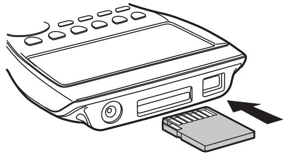
natural_image
Line drawing of a remote control device with a USB flash drive (no text or symbols)
Front

Back
Important!
- Never insert anything other than SD cards into the SD card slot. Doing so can damage the calculator.
- Should water or any foreign matter ever get into the SD card slot, immediately turn off the calculator, remove its batteries, and contact your original retailer or nearest CASIO authorized service center.
- To remove the SD card
- Press in on the SD card and then release it.
- This will cause the card to pop part way out of the slot.
- Grasp the SD card with your fingers and pull it out of the slot.
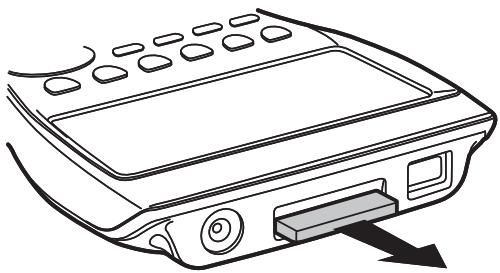
natural_image
Line drawing of a remote control device with a scroll wheel and drive button (no text or symbols)Important!
- Never remove the SD card while data is being transferred to it. Doing so not only stops the data you are transferring to the card from being saved, it can also corrupt SD card contents.
- Exerting undue force when removing an SD card can damage the card slot or the card.
2. Formatting an SD Card
- Use the procedure under “Reset” (page 12-3) to format an SD card.
3. SD Card Precautions during Use
- SD card problems can normally be corrected by reformatting the card. However, it is always a good idea to take along more than one SD card to avoid data storage problems.
- Card formatting (initialization) is recommended before using a new SD card for the first time.
- If an SD card has been formatted on a computer or other device, you can use it as-is without reformatting. A computer or other device also will be able to use an SD card that has been formatted with the calculator.
-
Never perform any of the following operations while the SD card is being accessed.
-
Removing the SD card
- Connecting or disconnecting a USB cable
- Turning off the calculator
-
When connected to a computer, exiting the FA-124 software or shutting down the computer
-
Note that an SD card needs to be oriented correctly (proper side must be facing upwards, the proper end must be inserted) when inserting it into the calculator. Trying to force an SD card into the slot when it is oriented incorrectly can damage the card and slot.
- Use of certain SD cards while calculator battery power is low can cause the display to go blank without displaying the low battery warning message. If this happens, replace the batteries.
■ Recommended SD Card Types
Toshiba
For detailed information (specifications, features, etc.) about the SD card, contact the SD card manufacturer.
Appendix
- Error Message Table
* fx-9860GII SD only
| Message | Meaning | Countermeasure |
| SyntaxERROR | ·Illegal syntax·Attempt to input an illegal command | ·PressEXITto display the error and make necessary corrections. |
| Ma ERROR | ·Calculation result exceeds the display range.·Calculation is outside the input range of a function.·Mathematical error (division by zero, etc.)·Sufficient precision could not be obtained for Σ calculation, differential calculation, etc.·Solution could not be obtained for equation calculation, etc. | ·Check input values and make corrections to ensure that values are within allowable limits. |
| Go ERROR | 1 No corresponding Lbl n for Goto n.2 No program stored in program area Prog "file name". | 1 Correctly input a Lbl n to correspond to the Goto n, or delete the Goto n if not required.2 Store a program in program area Prog "file name", or delete the Prog "file name" if not required. |
| NestingERROR | ·Nesting of subroutines by Prog "file name" exceeds 10 levels. | ·Ensure that Prog "file name" is not used to return from subroutines to main routine. If used, delete any unnecessary Prog "file name".·Trace the subroutine jump destinations and ensure that no jumps are made back to the original program area. Ensure that returns are made correctly. |
| Stack ERROR | ·Execution of calculations that exceed the capacity of the stack for numeric values or stack for commands. | ·Simplify the formulas to keep stacks within 10 levels for the numeric values and 26 levels for the commands.·Divide the formula into two or more parts. |
| MemoryERROR | ·Operation or memory storage operation exceeds remaining memory capacity. | ·Keep the number of memories you use within the currently specified number of memories.·Simplify the data you are trying to store to keep it within the available memory capacity.·Delete no longer needed data to make room for the new data. |
| Argument ERROR | Incorrect argument specification for a command that requires an argument. | Correct the argument. |
| Dimension ERROR | Illegal dimension used during matrix or list calculations. | Check the matrix or list dimension. |
| Range ERROR | 1 Input of an improper V-Window value.2 V-Window range settings exceeded when a graph is redrawn.3 Input of an improper value on the range screen and use of that value for execution.4 The spreadsheet cell range was exceeded by paste, recall, or other cell operation. | 1 Change the V-Window value so it is within range.2 Redraw using the proper settings.3 Input a proper range value.4 Repeat the procedure taking care that the cell range is not exceeded. |
| Condition ERROR | Execution of a calculation or function before all conditions required for execution are met. | Check the conditions and make any necessary corrections. |
| Non-Real ERROR | Calculation that produces a complex number when Real is specified for the Complex Mode setting on the Setup screen, even though the argument is a real number. | Change the Complex Mode setting to something other than Real. |
| Complex Number In List | List containing complex number used in a calculation or operation for which complex number data is invalid. | Change all data in the list to real numbers. |
| Complex Number in Matrix | Matrix containing complex number used in a calculation or operation for which complex number data is invalid. | Change all data in the matrix to real numbers. |
| Complex Number in Data | Data sent from a function of this calculator (matrix, etc.) includes complex number data, but the corresponding function of the receiving calculator does not support data that includes complex numbers.Example: Attempting to send a matrix containing a complex number in an element to CFX-9850G. | Send data that does not include complex numbers. |
| Can’t Simplify | Fraction simplification was attempted using the ▶Simp function (page 2-21), but simplification could not be performed using the specified divisor.Example: Specifying a divisor of 3 to simplify the fraction 4/8. | Specify a different divisor or execute ▶Simp without specifying any divisor. |
| Can't Solve! Adjust initial value or bounds. Then try again | A Solve calculation could not obtain a solution within the specified range. | Change the specified range.Correct the input expression. |
| No Variable | 1 No variable specified within a graph function being used for Dynamic Graph.2 No variable within a Solve equation. | 1 Specify a variable for the graph function.2 Input a Solve equation that includes a variable. |
| Conversion ERROR | Attempting to use the unit conversion command to convert between two units in different categories.Executing a conversion calculation using the same command twice in a conversion expression. | In a conversion expression, specify two different commands that are in the same category. |
| Com ERROR | Problem with cable connection or parameter setting during program data communications. | Check to make sure there is nothing wrong with the cable connection, and that parameters are configured correctly. |
| Transmit ERROR | Problem with cable connection or parameter setting during data communications. | Check to make sure there is nothing wrong with the cable connection, and that parameters are configured correctly. |
| Receive ERROR | Problem with cable connection or parameter setting during data communications. | Check to make sure there is nothing wrong with the cable connection, and that parameters are configured correctly. |
| Memory Full | Memory of receiving unit became full during program data communications. | Delete some data stored in the receiving unit and try again. |
| Invalid Data Size | Attempting to send data of a size that is not supported by the receiving device.Example: Attempting to send a matrix with more than 256 lines from the fx-9750GII to an older model. | Make sure the data being sent is of a size that is supported by the receiving device. |
| Invalid Data Number | Attempting to send data with a data number that is not supported by the receiving device.Example: Attempting to send List 7 from the fx-9750GII to an older model that supports only up to List 6. | Specify a data number supported by the receiving device when sending data. |
| Time Out | A Solve calculation or integration calculation was unable to satisfy convergence conditions. | If you are performing a Solve calculation, try changing to the initial default estimated value.If you are performing an integration calculation, try changing to a larger tol value. |
| Circular ERROR | There is a circular reference (such as “=A1” in cell A1) in the spreadsheet. | Change cell contents to remove the circular references. |
| Please Reconnect | The connection was dropped for some reason while updating the operating system. | Reconnect and try again. |
| Too Many Data | The number of data items is too large. | Delete unneeded data. |
| Fragmentation ERROR | Memory must be optimized before any more data can be stored. | Optimize memory. |
| Invalid Name | The file name you input includes invalid characters. | Use the correct characters to input a valid file name. |
| Invalid Type | An illegal data type is specified. | Specify valid data. |
| Storage Memory Full | The storage memory is full. | Delete unneeded data. |
| No Card* | There is no SD card loaded in the calculator. | Load an SD card. |
| SD Card Full* | The SD card is full. | Delete unneeded data. |
| Invalid file name or folder name.* | Data or folders that are supported by this calculator cannot be found on the SD card. | Replace the card with one that contains data/folders that are supported by this calculator. |
| Invalid Card* | A card that is not compatible with the calculator is loaded. | Replace the card with a compatible card. |
| Card is protected* | The SD card is write protected. | Remove write protection. |
| Data ERROR | A data error occurred. | Check to make sure you are writing correct type of data and try again. |
| Card ERROR* | An SD card error occurred. | Remove and correctly insert the SD card and try again. If this error occurs again, re-format the SD card. |
| Data is protected* | The Read Only attribute of the SD card loaded in the calculator has been turned on using a computer, etc. | Turn off the SD card's Read Only attribute. |
- Input Ranges
| Function | Input range for real number solutions | Internal digits | Precision | Notes |
| x x x | (DEG) |x| < 9 × (10^9)^ (RAD) |x| < 5 × 10^7 rad (GRA) |x| < 1 × 10^10grad | 15 digits | As a rule,precision is ±1 at the 10th digit.* | However, for x : |x| 90(2n+1) : DEG |x| /2(2n+1) : RAD |x| 100(2n+1) : GRA |
| ^-1x ^-1x ^-1x | |x| ≤ 1 | " | " | |
| |x| < 1 × 10^100 | ||||
| x x x | |x| ≤ 230.9516564 | " | " | |
| |x| < 1 × 10^100 | ||||
| ^-1x ^-1x ^-1x | |x| < 1 × 10^100 | " | " | |
| 1 ≤ x < 1 × 10^100 | ||||
| |x| < 1 | ||||
| x x | 1 × 10^-99 ≤ x < 1 × 10^100 | " | " | Complex numbers can be used as arguments. |
| 10^x e^x | -1 × 10^100 < x < 100 | " | " | Complex numbers can be used as arguments. |
| -1 × 10^100 < x ≤ 230.2585092 | ||||
| x^2 | 0 ≤ x < 1 × 10^100 | " | " | Complex numbers can be used as arguments. |
| |x| < 1 × 10^50 | ||||
| 1/x ^3 | |x| < 1 × 10^100, x 0 | " | " | Complex numbers can be used as arguments. |
| |x| < 1 × 10^100 | ||||
| x! | 0 ≤ x ≤ 69 ( x is an integer) | " | " | |
| nPr nCr | Result < 1 × 10^100 n, r (n and r are integers) 0 ≤ r ≤ n, n < 1 × 10^10 | " | " | |
| Pol (x, y) | ^2 + y^2 < 1 × 10^100 | " | " | |
| Rec (r, ) ○, ” | |r| < 1 × 10^100 (DEG) |θ| < 9 × (10^9)^ (RAD) |θ| < 5 × 10^7 rad (GRA) |θ| < 1 × 10^10grad |a|, b, c < 1 × 10^100 0 ≤q b, c | "15 digits | "As a rule,precision is ±1 at the 10th digit.* | However, for θ : |θ| 90(2n+1) : DEG |θ| /2(2n+1) : RAD |θ| 100(2n+1) : GRA |
| ←○, ” | |x| < 1 × 10^100 Sexagesimal display: |x| < 1 × 10^7 | |||
| ^(x^y) | x > 0: -1 × 10^100 < y x < 100 x = 0 : y > 0 x < 0 : y = n, 2n+1 ( m, n are integers)However; -1 × 10^100 < y |x| < 100 | " | " | Complex numbers can be used as arguments. |
| ^x | y > 0 : x 0 -1 × 10^100 < 1x y < 100 y = 0 : x > 0 y < 0 : x = 2n+1, 2n+1m ( m 0; m, n are integers)However; -1 × 10^100 < 1x |y| < 100 | " | " | Complex numbers can be used as arguments. |
| a^b/c | Total of integer, numerator and denominator must be within 10 digits (includes division marks). | " | " |
* For a single calculation, calculation error is ±1 at the 10th digit. (In the case of exponential display, calculation error is ±1 at the last significant digit.) Errors are cumulative in the case of consecutive calculations, which can also cause them to become large. (This is also true of internal consecutive calculations that are performed in the case of (x^y), x, x!, ^3, nPr, nCr, etc.)
In the vicinity of a function's singular point and point of inflection, errors are cumulative and may become large.
| Function | Input range |
| Binary, octal, decimal, hexadecimal calculation | Values fall within following ranges after conversion:DEC: -2147483648 ≤ x ≤ 2147483647BIN: 1000000000000000 ≤ x ≤ 1111111111111111 (negative)0 ≤ x ≤ 111111111111111 (0, positive)OCT: 20000000000 ≤ x ≤ 37777777777 (negative)0 ≤ x ≤ 17777777777 (0, positive)HEX: 80000000 ≤ x ≤ FFFFFFFF (negative)0 ≤ x ≤ 7FFFFFFF (0, positive) |

natural_image
Grid of black dots on white background, no text or symbols presentE-CON2 Application

natural_image
Grid of black dots on white background with no text or symbolsAll of the explanations provided here assume that you are already familiar with the operating precautions, terminology, and operational procedures of the calculator and the EA-200.
1 E-CON2 Overview
- From the Main Menu, select E-CON2 to enter the E-CON2 Mode.
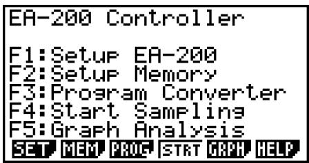
E-CON2 Main Menu
- The “E-CON2 Mode” provides the functions listed below for simple and more efficient data sampling using the CASIO EA-200.
- F1 (SET) ...... Displays a screen for setting up the EA-200.
- F2 (MEM) ...... Displays a screen for saving EA-200 setup data under a file name.
- F3 (PROG) ..... Performs program conversion.
- This function can be used to convert EA-200 setup data configured using E-CON2 to an EA-200 control program (or EA-100 control program) that can run on the fx-9860G SD/fx-9860G.
- It also can be used to convert data to a program that can be run on a CFX-9850 Series/fx-7400 Series calculator.
- F4 (STRT) ..... Starts data collection.
- F5 (GRPH) ..... Graphs data sampled by the EA-200, and provides tools for analyzing graphs. Graph Analysis tools include calculation of periodic frequency, various types of regression, Fourier series calculation, and more.
- F6 (HELP) ..... Displays E-CON2 help.
- Pressing the OPTN key (Setup Preview) or a cursor key while the E-CON2 main menu is on the screen displays a preview dialog box that shows the contents of the setup in the current setup memory area.
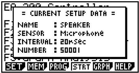
To close the preview dialog box, press EXIT.
Note
For details about setup data and the current setup memory area, see “6 Using Setup Memory” (page 6-1).
About online help
Pressing the F6(HELP) key displays online help about the E-CON2 Mode.
2 Using the Setup Wizard
This section explains how to use the Setup Wizard to configure the EA-200 setup quickly and easily simply by replying to questions as they appear. If you need more control over specific sampling parameters, you should consider using the Advanced Setup procedure on page 3-1.
■ Setup Wizard Parameters
Setup Wizard lets you make changes to the following three EA-200 basic sampling parameters using an interactive wizard format.
- Sensor (Select Sensor):
Specify a CASIO or VERNIER* sensor from a menu of choices.
*Vernier Software & Technology
• Total Sampling Time:
Specify a value within the range of 0.01 second to 30 days. - Sampling Time Unit (Select Unit):
Specify seconds (sec), minutes (min), hours (hour), or days (day) as the time unit of the value you input for the total sampling time (Total Sampling Time).
Note
For some sensors (EA-200 built-in microphone, Vernier PhotoGate, etc.), sampling parameters are different from those shown above. The differences between sampling parameters and setup procedures for each sensor are described in this section.
Setup Wizard Rules
Note the following rules whenever you use the Setup Wizard.
- The EA-200 sampling channel is CH1 or SONIC.
- The trigger for a Setup Wizard setup is always the EXE key.
- To configure an EA-200 setup using Setup Wizard
Before getting started...
- Before starting the procedure below, make sure you first decide if you want to start sampling immediately using the setup you configure with Setup Wizard, or if you want to store the setup for later sampling.
- See sections 6-1, 7-1, and 8-1 of this manual for information about procedures required to start sampling and to store a setup. We recommend that you read through the entire procedure first, referencing the other sections and pages as noted, before actually trying to perform it.
-
To terminate Setup Wizard part way through and cancel the setup, press SHIFT EXIT (QUIT).
-
Display the E-CON2 main menu (page 1-1).
-
Press F1 (SET) and then F1 (WIZ).
- This launches the Setup Wizard and displays the “Select Sensor” screen.
![Select Sensor CASIO :[F1] VERNIER:[F2]](/content/2025/01/86832/images/3ca1b78ce4e170cc1de799cfe17c5c70109e3d088c24a54840ad4ffb3d4c0475.jpg)
- Press F1 to specify a CASIO sensor or F2 to specify a Vernier sensor.
- Pressing either key will display the corresponding sensor list. The following shows the sensor list that appears when you press F1.
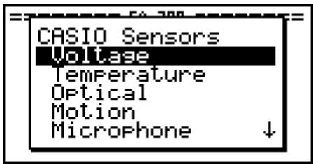
- Specify the sensor you want to use.
Use the ▲ and ▼ cursor keys to move the highlighting to the sensor you want to use, and then press EXE.
- If the sensor you specified has more than one option (more detailed specifications, such as sampling unit, mode, etc.), an option list will appear on the display at this time. If this happens, advance to step 5 (where you will see an example of the screen that appears when you select F1 - [Temperature] in step 4).
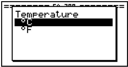
- If the “Input Total Sampling Interval” screen appears, skip to step 6.
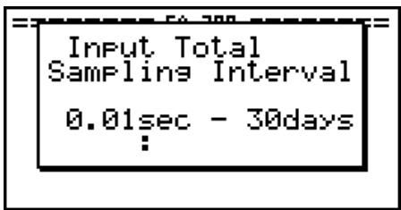
- Select the options for the sensor you specified in step 4.
Use the ▲ and ▼ cursor keys to move the highlighting to the option you want to select, and then press EXE.
- If the “Input Total Sampling Interval” screen appears, advance to step 6.
Important!
When special settings are required by the sensor and/or option you select, other screens other than the “Input Total Sampling Interval” screen will appear on the display. The following shows where you should go to find information about the operations you need to perform for each sensor/option selection.
| If you select this sensor/option: | Go here for more information: |
| [CASIO] - [Microphone] - [Sound wave & FFT] | “Using Setup Wizard to Configure Settings for FFT (Frequency Characteristics) Data Sampling” on page 2-5 |
| [CASIO] - [Microphone] - [FFT only] | |
| [VERNIER] - [Photogate] - [Gate] | “To configure a setup for PhotoGate alone” on page 2-6 |
| [VERNIER] - [Photogate] - [Pulley] | “To configure a setup for PhotoGate and Smart Pulley” on page 2-7 |
| [CASIO] - [Speaker] - [y=f(x)] | “Outputting the Waveform of a Function through the Speaker” on page 2-8 |
- Use the number input keys to input the total sampling time. Just input a value.
In step 8 of this procedure, you will be able to specify the unit (seconds, minutes, hours, days) of the value you input here.
Note
- With some sensors ([CASIO] - [Microphone] - [Sound wave], etc.) sampling time is limited to a few seconds. The unit for such a sensor is always seconds, and so the “Select Unit” screen does not appear.
-
If you specify a total sampling time value in the range of 10 seconds to 23 hours, 59 minutes, 59 seconds, real-time graphing will be performed during sampling. This is the same as selecting the Realtime Mode on the “Advanced Setup” screen.
-
After inputting total sampling time value you want, press EXE. This displays the "Select Unit" screen.
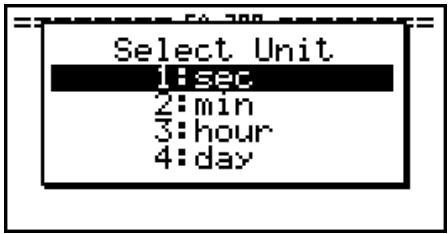
- Use number keys ① through ④ to specify the unit for the value you specified in step 6.
- This displays a confirmation screen like the one shown below.
![CH1:Voltage total:30sec OK :[F1] Cancel:[F6]](/content/2025/01/86832/images/31bd14d8b9bfe076c034ad0f43d43c872a69d361faaa8ede7f6bb2479edc0edc.jpg)
- If there is not problem with the contents of the confirmation screen, press F1.
If you need to change the setup, press F6 or EXIT. This will return to the screen in step 4 (for setting the total sampling interval), where you can change the setting.
- Pressing F1 will take you to the final Setup Wizard screen.
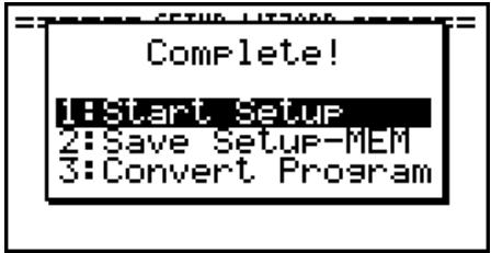
- Press number keys described below to specify what you want to do with the setup you have configured.
① (Start Setup) ...... Starts sampling using the setup (page 8-1)
② (Save Setup-MEM) ..... Saves the setup (page 6-1)
③ (Convert Program) ..... Converts the setup to a program (page 7-1)
■ Using Setup Wizard to Configure Settings for FFT (Frequency Characteristics) Data Sampling
When you perform sound sampling executed the EA-200's built-in microphone (by specifying [CASIO] - [Microphone] as the sensor), Setup Wizard will provide you with three options: [Sound wave], [Sound wave & FFT], and [FFT only]. "Sound wave" records the following two dimensions for the sampled sound data: elapsed time (horizontal axis) and volume (vertical axis). "FFT" records the following two dimensions: frequency (horizontal axis) and volume (vertical axis).
The following shows the settings for recording FFT data.
-
Perform the first two steps of the procedure under "To configure an EA-200 setup using Setup Wizard" on page 2-2.
-
On the “Select Sensor” screen, select [CASIO] - [Microphone] - [Sound wave & FFT] or [CASIO] - [Microphone] - [FFT only].
- This causes a “Select FFT Range” screen to appear.
![Select FFT Range 2 - 1000Hz: [F1] 4 - 2000Hz: [F2] 6 - 3000Hz: [F3] 8 - 4000Hz: [F4]](/content/2025/01/86832/images/02ec2f259c1d2f1382be75f93cb6267ffe0b631212c35a6ac8246d2832e43e6f.jpg)
- You can select one of four settings for FFT Range. The setting you select will automatically apply the applicable fixed parameters shown below.
| Setting Parameter | 2 - 1000 Hz: F1 | 4 - 2000 Hz: F2 | 6 - 3000 Hz: F3 | 8 - 4000 Hz: F4 |
| Frequency pitch | 2 Hz | 4 Hz | 6 Hz | 8 Hz |
| Frequency max | 1000 Hz | 2000 Hz | 3000 Hz | 4000 Hz |
| Sampling interval | 61 μsec | 31 μsec | 20 μsec | 31 μsec |
| Number of samples | 8192 | 8192 | 8192 | 4096 |
The following explains the meaning of each parameter.
Frequency pitch: Pitch in Hz at which sampling is performed
Frequency max: Upper limit of sampling frequency (lower limit is fixed at 0 Hz)
Sampling interval: Interval in seconds at which sampling is performed
Number of samples: Number of times sampling is performed
- Use function keys F1 through F4 to select an FFT Range setting.
- Selecting an FFT Range causes the final Setup Wizard screen to appear.
- Perform step 10 under "To configure an EA-200 setup using Setup Wizard" on page 2-2 to finalize the procedure.
■ Using Setup Wizard to Configure a PhotoGate Setup
Connection of a Vernier PhotoGate requires configuration of setup parameters that are slightly different from parameters for other types of sensors.
- To configure a setup for PhotoGate alone
-
Perform the first two steps of the procedure under "To configure an EA-200 setup using Setup Wizard" on page 2-2.
-
On the "Select Sensor" screen, select [VERNIER] - [Photogate] - [Gate].
- This displays a screen where you specify whether PhotoGate is connected to the CH1 or SONIC channel.
![Select Channel CH 1 :[F1] SONIC :[F2]](/content/2025/01/86832/images/1b47f24220ef295a3baf669a5ae887b6baa7a0f9faeb9fd056b99202a43a9d8c.jpg)
- Press F1 to specify CH1 or F2 to specify SONIC.
- This causes a “Gate Status” screen to appear.
![Gate Status Open -Open : [F1] Open -Close: [F2] Close-Open : [F3] Close-Close: [F4]](/content/2025/01/86832/images/82c9e4edc5c155c2ab2e038bfc2a91370b18a213a9a1b292c58f81bec7ca80fe.jpg)
- “Open” means the photo path is not blocked, while “Close” means the photo path is blocked.
- The gate status defines what PhotoGate status should cause timing to start, and what status should cause timing to stop.
Open-Open ..... Timing starts when the gate opens, and continues until it closes and then opens again.
Open-Close ..... Timing starts when the gate opens, and continues until it closes.
Close-Open ..... Timing starts when the gate closes, and continues until it opens.
Close-Close ..... Timing starts when the gate closes, and continues until it opens and then closes again.
- Use function keys F1 through F4 to select a Gate Status setting.
- Selecting a gate status causes a screen for specifying the number of samples to appear.
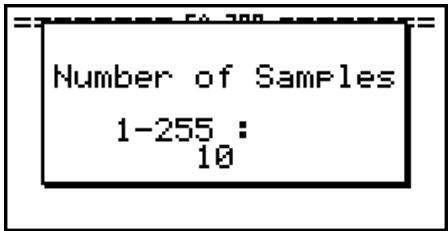
- Input an integer in the range of 1 to 255 to specify the number of samples.
- Perform step 10 under "To configure an EA-200 setup using Setup Wizard" on page 2-2 to finalize the procedure.
- To configure a setup for PhotoGate and Smart Pulley
- Perform the first two steps of the procedure under "To configure an EA-200 setup using Setup Wizard" on page 2-2.
- On the "Select Sensor" screen, select [VERNIER] - [Photogate] - [Pulley].
- This causes an “Input Distance(m)” screen to appear.
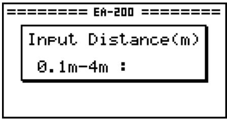
- The distance you specify here is the distance the weight travels after it is released.
-
Input a value in the range of 0.1 to 4 to specify the distance in meters.
-
Perform step 10 under "To configure an EA-200 setup using Setup Wizard" on page 2-2 to finalize the procedure.
■ Outputting the Waveform of a Function through the Speaker
Normally, the Setup Wizard helps you configure setups for sensors connected to the EA-200. If you select [CASIO] - [Speaker] - [y=f(x)] on the “Select Sensor” screen, however, it configures the EA-200 to output the sound that corresponds to a function that you input and graph on the calculator.
- To configure a setup for speaker output
- Connect the data communication cable (SB-62) to the communication port of the calculator and the MASTER port of the EA-200.
- Perform the first two steps of the procedure under "To configure an EA-200 setup using Setup Wizard" on page 2-2.
- On the "Select Sensor" screen, select [CASIO] - [Speaker] - [y=f(x)]. This displays a screen like the one shown below.
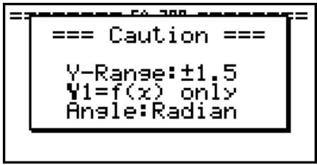
-
Press EXE to advance to the View Window setting screen.
-
The following settings are configured automatically: Ymin = -1.5 and Ymax = 1.5. Do not change these settings.
- Press EXE or EXIT to advance to the graph function list.
- In line "Y1", input the function of the waveform for the sound you want to input.
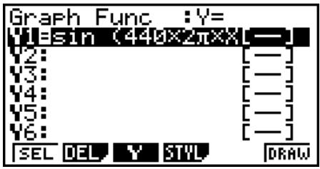
- Note that the angle unit is always radians.
-
Input a function where the value of “Y” is within the range of -1.5 to +1.5 .
-
Press F6 (DRAW) to graph the function.
- This graphs the function and displays a vertical cursor line as shown below. Use the graph to specify the range that you want to output to the speaker.
![SELECT START POINT, PRESS [EXE]](/content/2025/01/86832/images/c330687706691d68878b038903c89d79aad7797b0decb3bc4598aa54153f11a7.jpg)
-
Use the ◀ and ▶ cursor keys to move the cursor to the start point of the output, and then press EXE to register it.
-
Use the ◀ and ▶ cursor keys to move the cursor to the end point of the output, and then press EXE to register it.
- After you specify the start point and end point, an output frequency dialog box shown below appears on the display.
![SELECT END POINT, PRESS [EXE]. 2301.5rSec 434.48Hz Output Frequency %:100 2301.5rSec 434.48Hz](/content/2025/01/86832/images/53098823a23ab8b57951b3505b988aebf6d8da7989282c9093db26dc16b77fb5.jpg)
- Input a percent value for the output frequency value you want.
- To output the original sound as-is, specify 100%. To raise the original sound by one octave, input a value of 200%. To lower the original sound by one octave, input a value of 50%.
- After inputting an output frequency value, press EXE.
- This outputs the waveform between the start point and end point from the EA-200 speaker.
- If the sound you configured cannot be output for some reason, the message “Range Error” will appear. If this happens, press EXIT to scroll back through the previous setting screens and change the setup as required.
-
To terminate sound output, press the EA-200 [START/STOP] key.
-
Press EXE.
- This displays a screen like the one shown below.
![PRESS FSTOR1 KEY 04.56-200 Try Again? Yes: [F1] No : [F6] 2301.5kSec 434.48Hz](/content/2025/01/86832/images/34d03d1be738bf9f36640236553682c04350881ea269759b516185266a768170.jpg)
- Perform one of the following operations, depending on what you want to do.
To change the output frequency and try again:
Press F1(Yes) to return to the "Output Frequency" dialog box. Next, repeat the above steps from step 10.
To change the output range of the waveform graph and try again:
Press F6 (No) to return to the graph screen in step 7. Next, repeat the above steps from step 8.
To change the function:
Press F6 (No) and then EXIT to return to the graph function list in step 6. Next, repeat the above steps from step 6.
To exit the procedure and return to the E-CON2 main menu:
Press F6 (No) and then press EXIT twice.
3 Using Advanced Setup
Advanced Setup provides you with total control over a number of parameters that you can adjust to configure the EA-200 setup that suits your particular needs.
The procedures in this section provide the general steps you should perform when using Advanced Setup to configure an EA-200 setup, and to returns setup settings to their initial default values. You can find details about individual settings and the options that are available with each setting are provided by the explanations that start on page 3-3.
■ Advanced Setup Operations
- To configure an EA-200 setup using Advanced Setup
The following procedure describes the general steps for using Advanced Setup. Refer to the pages as noted for more information.
- Display the E-CON2 main menu (page 1-1).
- Press F1 (SET). This displays the "Setup EA-200" submenu.
- Press F2 (ADV). This displays the Advanced Setup menu.
![Advanced Setup for EXPERT [1]: Channel [2]: Sample [3]: Trigger [4]: Graph [5]: Custom Probe [6]: Initialize START MLTI MEM PROC GRAPH RET](/content/2025/01/86832/images/9e03d0f80e7b1598d192dbb0b09ba5ede124ecdeb49eb6ddf1ed6f34ce838af7.jpg)
Advanced Setup Menu
-
If you want to configure a custom probe at this point, press 5 (Custom Probe). Next, follow the steps under "To configure a custom probe setup" on page 4-1.
-
You can also configure a custom probe during the procedure under “To configure Channel Setup settings” on page 3-3.
-
Custom probe configurations you have stored in memory can be selected using Channel in step 5, below.
-
Use the Advanced Setup function keys described below to set other parameters.
-
① (Channel) .... Displays a screen that shows the sensors that are currently assigned to each channel (CH1, CH2, CH3, SONIC, Mic). You can also use this dialog to change sensor assignments. See “Channel Setup” on page 3-3 for more information.
-
② (Sample) ..... Displays a screen for selecting the sampling mode, and for specifying the sampling interval, the number of samples, and the warm-up mode. When “Fast” is selected for “Mode”, this dialog box also displays a setting for turning FFT (frequency characteristics) graphing on and off. See “Sample Setup” on page 3-5 for more information.
-
③ (Trigger) ..... Displays a screen for configuring sampling start (trigger) conditions. See “Trigger Setup” on page 3-8 for more information.
- 4 (Graph) ...... Displays a screen for configuring graph settings. See “Graph Setup” on page 3-13 for more information.
- You can return the settings on the above setup screens (1 through 4) using the procedure described under “To return setup parameters to their initial defaults”.
-
After you configure a setup, you can use the function key operations described below to start sampling or perform other operations.
-
F1 (STRT) ..... Starts sampling using the setup (page 8-1).
- F2 (MLTI) ...... Starts MULTIMETER Mode sampling using the setup (page 5-1).
- F3 (MEM) ...... Saves the setup (page 6-1).
- F4 (PROG) ..... Converts the setup to a program (page 7-1).
- F5 (GRPH) ..... Graphs data sampled by the EA-200, and provides tools for analyzing graphs (page 10-1).
- F6 (ABT) ...... Displays version information about the EA-200 unit that is currently connected to the calculator.
- To return setup parameters to their initial defaults
Perform the following procedure when you want to return the parameters of the setup in the current setup memory area to their initial defaults.
- While the Advanced Setup menu (page 3-1) is on the display, press 6 (Initialize).
![Initialize Current Setup? Yes: [F1] No : [F6]](/content/2025/01/86832/images/5b27ab6994303bdf1e1d68dd1b6c0de6b6181aa9b4b8cb5796d54a4169f707f0.jpg)
- In response to the confirmation message that appears, press F1(Yes) to initialize the setup.
- To clear the confirmation message without initializing the setup, press F6 (No).
Channel Setup
The Channel Setup screen shows the sensors that are currently assigned to each channel (CH1, CH2, CH3, SONIC, Mic).
- To configure Channel Setup settings
- While the Advanced Setup menu (page 3-1) is on the display, press ☐ (Channel).
- This displays the Channel Setup screen.
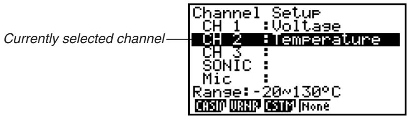
Channel Setup Screen
-
Use the ▲ and ▼ cursor keys to move the highlighting to the channel whose setting you want to change.
-
What you need to do next depends on the currently selected channel.
- CH1, CH2, or CH3
Press a function key to display a menu of sensors that can be assigned to the selected channel.
F1(CASIO) ..... Displays a menu of CASIO sensors.
F2 (VRNR) ...... Displays a menu of Vernier sensors.
F3 (CSTM) ...... Displays a menu of custom probes.
(F4) (None) ...... Press this key when you want leave the channel without any sensor assigned to it.
- SONIC Channel
Press a function key to display a menu of sensors that can be assigned to this channel.
F1(CASIO) ..... Displays a menu of CASIO sensors, but only “Motion” can be selected.
F2 (VRNR) ...... Displays a menu of Vernier sensors. You can select “Motion” or “Photogate”.
Note
- On the menu that appears after you select “Motion” from either the CASIO or Vernier sensor menu, select either “meters” or “feet” as the sampling unit.
- After selecting “Motion” from either the CASIO or Vernier sensor menu, you can press the OPTN key to toggle “smoothing (correction of measurement error)” on (“-Smooth” displayed) and off (“-Smooth” not displayed).
- From the menu that appears after you select “Photogate” as the sensor, select [Gate] or [Pulley].
[Gate]...... Select this option when using the PhotoGate sensor alone.
[Pulley] ...... Select this option when using the PhotoGate sensor along with a smart pulley.
F4 (None) ...... Select this option to disable the SONIC channel.
- Mic Channel
For this channel, the sensor is automatically set to Built-in (External) Microphone. However, you need to configure the settings described below.
F1 (Snd) ...... Select this option to record elapsed time and volume 2-dimensional sampled sound data (elapsed time on the horizontal axis, volume on the vertical axis).
F2 (FFT) ...... Select this option to record frequency and volume 2-dimensional sampled sound data (frequency on the horizontal axis, volume on the vertical axis).
F4 (None) ...... Select this option to disable the Mic channel.
-
Repeat steps 2 and 3 as many times as necessary to configure all the channels you want.
-
After all the settings are the way you want, press EXE.
- This returns to the Advanced Setup menu.
Note
- When you select a channel on the Channel Setup screen, the sampling range of the selected channel appears in the bottom line of the screen.
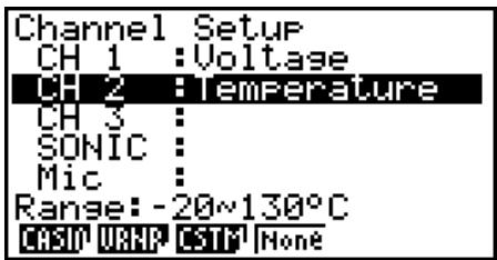
In the above example, the range of the temperature sensor assigned to CH2 appears on the display.
If the sampling range value is too long to fit on the display, only the part of the value that fits on the display will be shown.
- Whenever the current Sample Setup (page 3-5) and Trigger Setup (page 3-8) settings become incompatible due to a change in Channel Setup settings, these settings revert automatically to their initial defaults. Selecting the Mic channel with Channel Setup while the Sample Setup has “Extended” selected for the sampling mode, for example, will cause the sampling mode to change automatically to “Fast” (which is the initial default setting when the Mic channel is selected). For information about the channels that can be selected for each sampling mode, see “Sample Setup” (page 3-5).
Sample Setup
The Sample Setup screen lets you configure a number of settings that control sampling.
- To configure Sample Setup settings
- While the Advanced Setup menu (page 3-1) is on the display, press ☐ (Sample).
- This displays the Sample Setup screen, with the “Mode” line highlighted, which indicates that you can select the sampling mode.
![Sample Setup Mode :Real-time Interval :1sec Number :101 [0h01m40s] Warm-up :Auto R-T Fast Norm Extd HELP D](/content/2025/01/86832/images/d290cfcb43a3f3cc5d50beb76055460be2ac2d350a1b13d65b0befffe390ac08.jpg)
- Select the sampling mode that suits the type of sampling you want to perform.
| To do this: | Press this key: | To select this mode: |
| Graph data in real-time as it is sampled | F1(R-T) | Realtime |
| Perform sampling of high-speed phenomena (sound, etc.) | F2(Fast) | Fast |
| Perform sampling over a long time (weather, etc.)• The EA-200 enters a power off sleep state while standing by. | F4(Extd) | Extended |
| Sample sound using the EA-200's built-in microphone | F6(▷)F1(Snd) | Sound |
| Record the time of the occurrence of a particular trigger event as an absolute value starting from 0, which is the sampling start time | F6(▷)F2(Click) | Clock |
| Perform periodic sampling, from a start trigger event to an end trigger event | F6(▷)F3(Priod) | Period |
| Perform sampling other than that described above | F3(Norm) | Normal |
- Note that the mode you select also determines the channel(s) you can use.
| Sampling mode: | Selectable Channel(s) |
| Realtime, Extended, Normal | CH1, CH2, CH3, SONIC |
| Fast | CH1, Mic |
| Sound | Mic |
| Clock, Period | CH1 |
- To change the sampling interval setting, move the highlighting to "Interval". Next, press F1 to display a dialog box for specifying the sampling interval.
- The range of values you can select depends on the current sampling mode setting.
| If this sampling mode is selected: | This is the allowable setting range: |
| Realtime | 0.2 to 299 sec |
| Fast | 20 to 500 μsec |
| Extended | 5 to 240 min |
| Period | “=Trigger” only (no value input required) |
| Sound | 20 to 27 μsec |
| Clock | “=Trigger” only (no value input required) |
| Normal | 0.0005 to 299 sec |
-
To change the number of samples setting, move the highlighting to "Number". Next, press F1 to display a dialog box for specifying the number of samples.
-
You can specify a value in the range of 10 to 30,000.
- The total sampling time shown at the bottom of the dialog box is calculated by multiplying the “Sampling Interval” value you specified in step 3 by the number of samples you specify here.
Important!
- When all of the following conditions exist, a “Distance” setting appears in place of the “Number” setting. See “To configure the Distance setting” (page 3-7) for information about configuring the “Distance” setting.
- Channel Setup (page 3-3): F2 (VRNR) - [Photogate] - [Pulley]
-
Sampling Mode (page 3-5): Clock
-
To change the warm-up time setting, move the highlighting to "Warm-up". Next, perform one of the function key operations described below.
Note
- The “Warm-up” setting will not be displayed on the Sample Setup screen if “Fast”, “Sound” or “Extended” is currently selected as the sampling mode.
| To do this: | Press this key: |
| Have the warm-up time for each sensor set automatically | F1 (Auto) |
| Input a warm-up time, in seconds, manually | F2 (Man) |
| Disable the warm-up time | F3 (None) |
Important!
- When the following condition exists, an “FFT Graph” setting appears in place of the “Warm-up” setting. See “To configure the FFT Graph setting” (page 3-7) for information about configuring the “FFT Graph” setting.
- Sampling Mode (page 3-5): Fast
- After all the settings are the way you want, press EXE.
- This returns to the Advanced Setup menu.
Note
- Whenever the current Channel Setup (page 3-3) and Trigger Setup (page 3-8) settings become incompatible due to a change in Sample Setup settings, these settings revert automatically to their initial defaults. Selecting “Realtime” as the sampling mode with Sample Setup while the Mic channel is selected with Channel Setup and the Trigger Setup has “Mic” selected for “Source”, for example, will cancel the Channel Setup Mic channel selection and change the Trigger Setup “Source” setting to “[EXE] key”. For information about the channels that can be selected for each sampling mode, see step 2 of “To configure Sample Setup settings”. For information about the trigger sources that can be selected for each sampling mode, see “Trigger Setup” (page 3-8).
- To configure the Distance setting
In place of step 3 of the procedure under “To configure Sample Setup settings”, press F1 to display a dialog box for specifying the distance the weight travels in meters.
- Specify a value in the range of 0.1 to 4 meters.
- To configure the FFT Graph setting
In place of step 5 of the procedure under “To configure Sample Setup settings”, press F1 to display a dialog box for turning frequency characteristic graphing (FFT Graph) on and off.
| To do this: | Press this key: |
| Turn on graphing of frequency characteristics after sampling | F1 (On) |
| Turn off graphing of frequency characteristics after sampling | F2 (Off) |
■ Trigger Setup
You can use the Trigger Setup screen to specify the event that causes sampling to start (EXE key operation, etc.) The event that causes sampling to start is called the “trigger source”, which is indicated as “Source” on the Trigger Setup screen.
![Trigger Setup Source : [EXE]key EXE CNT CH1 Sonic [STR] HELP](/content/2025/01/86832/images/2245c21d260fff21d6927e8ad48b6b9b2ce8740307754cf1d15d5d0b4557b112.jpg)
![Trigger Setup Source :CountDown Timer :5sec EXE CNT CH1 [STR] HELP](/content/2025/01/86832/images/de1136ed7d308c04b23a8ede3780b85f12f58c4c8249cf99f26ebce60c033a51.jpg)
![Trigger Setup Source :CH1 [Optical] Threshold:549.5 Unit :Lum Int Edge :Rising EXE CNT CH1 [STR] HELP](/content/2025/01/86832/images/c4e92e6812675a064840e3aa2a8b1cf868341597ae9a5d6cf1538ec85b59f53d.jpg)
![Trigger Setup Source : [S1HRT]key EXE CNT CH1 [STR] HELP](/content/2025/01/86832/images/6eb3b8f87140fcd6b08565dbe54cdd9808a96e2d73aa94a9e5e3c7cc607ee6ff.jpg)
The following table describes each of the six available trigger sources.
| To start sampling when this happens: | Select this trigger source: |
| When the EXE key is pressed | [EXE] key |
| After the specified number of seconds are counted down | Count Down |
| When input at CH1 reaches a specified value | CH1 |
| When input at the SONIC channel reaches a specified value | SONIC |
| When the EA-200's built-in microphone detects sound | Mic |
| When the EA-200's [START/STOP] key is pressed | [START] key |
Note
The trigger sources you can select depends on the sampling mode selected with the Sample Setup (page 3-5).
| For this sampling mode: | The following trigger source(s) can be selected: |
| Realtime | [EXE] key, Count Down |
| Fast | [EXE] key, Count Down, CH1, Mic |
| Normal | [EXE] key, Count Down, CH1, SONIC, [START] key |
| Extended | [EXE] key |
| Sound | [EXE] key, Count Down, Mic |
| Clock | CH1 |
| Period | CH1 |
- To configure Trigger Setup settings
- While the Advanced Setup menu (page 3-1) is on the display, press ☐(Trigger).
- This displays the Trigger Setup screen with the “Source” line highlighted.
![Trigger Setup Source : [EXE]key EXE CNT CH1 Sonic [STR] HELP](/content/2025/01/86832/images/6c162d010b8889f29d4582388c650ab670ed317fdb0cf5620dfab9e161dd582f.jpg)
- The function menu items that appears in the menu bar depend on the sampling mode selected with Sample Setup (page 3-5). The above screen shows the function menu when “Normal” is selected as the sample sampling mode.
- Use the function keys to select the trigger source you want.
- The following shows the trigger sources that can be selected for each sampling mode.
| Sampling Mode | Trigger Source |
| Realtime | 1 (EXE) : [EXE] key, 2 (Cnt) : Count Down |
| Fast | 1 (EXE) : [EXE] key, 2 (Cnt) : Count Down, 3 (CH1), 5 (Mic) |
| Normal | 1 (EXE) : [EXE] key, 2 (Cnt) : Count Down, 3 (CH1), 4 (Sonic), 5 (STR) : [START] key |
| Sound | 1 (EXE) : [EXE] key, 2 (Cnt) : Count Down, 5 (Mic) |
- The trigger source is always “[EXE] key” when the sampling mode is “Extended”, and “CH1” when the sampling mode is “Clock” or “Period”.
- Perform one of the following operations, in accordance with the trigger source that was selected in step 2.
| If this is the trigger source: | Do this next: |
| [EXE] key | Press EXE to finalize Trigger Setup and return to the Advanced Setup menu. |
| Count Down | Specify the countdown start time. See “To specify the countdown start time” below. |
| CH1 | Specify the trigger threshold value and trigger edge direction. See “To specify the trigger threshold value and trigger edge type”, “To configure trigger threshold, trigger start edge, and trigger end edge settings” on page 3-11 or “To configure PhotoGate trigger start and end settings” on page 3-12. |
| SONIC | Specify the trigger threshold value and motion sensor level. See “To specify the trigger threshold value and motion sensor level” on page 3-12. |
| Mic | Specify microphone sensitivity. See “To specify microphone sensitivity” below. |
| [START] key | Press EXE to finalize Trigger Setup and return to the Advanced Setup menu. |
- To specify the countdown start time
- Move the highlighting to "Timer".
- Press F1(Time) to display a dialog box for specifying the countdown start time.
- Input a value in seconds from 1 to 10.
- Press EXE to finalize Trigger Setup and return to the Advanced Setup menu.
- To specify microphone sensitivity
- Move the highlighting to "Sense" and then press one of the function keys describe below.
| To select this level of microphone sensitivity: | Press this key: |
| Low | 1 (Low) |
| Medium | 2 (Mid) |
| High | 3 (High) |
- Press EXE to finalize Trigger Setup and return to the Advanced Setup menu (page 3-1).
- To specify the trigger threshold value and trigger edge type
Perform the following steps when “Fast”, “Normal”, or “Clock” is specified as the sampling mode (page 3-5).
- Move the highlighting to "Threshold".
- Press F1(EDIT) to display a dialog box for specifying the trigger threshold value, which is value that data needs to attain before sampling starts.
![Trigger Setup Source :CH1 [Voltage] Threshold:0 Unit :U Edge :Rising EDIT HELP](/content/2025/01/86832/images/0022f4a4afa6c26ef71f0191a795d31c7f9929affa1572588d0e8b26473df5eb.jpg)
Sensor assigned to CH1 or SONIC by Channel Setup (page 3-3)
Measurement unit supported by assigned sensor
- Input the value you want, and then press EXE.
- Move the highlighting to "Edge".
- Press one of the function keys described below.
| To select this type of edge: | Press this key: |
| Falling | 1 (Fall) |
| Rising | 2 (Rise) |
- Press EXE to finalize Trigger Setup and return to the Advanced Setup menu (page 3-1).
- To configure trigger threshold, trigger start edge, and trigger end edge settings
Perform the following steps when “Period” is specified as the sampling mode (page 3-5).
- Move the highlighting to "Threshold".
- Press F1(EDIT) to display a dialog box for specifying the trigger threshold value, which is value that data needs to attain before sampling starts.
- Input the value you want.
- Move the highlighting to "Start to".
- Press one of the function keys described below.
| To select this type of edge: | Press this key: |
| Falling | 1 (Fall) |
| Rising | 2 (Rise) |
- Move the highlighting to "End Edge".
- Press one of the function keys described below.
| To select this type of edge: | Press this key: |
| Falling | 1 (Fall) |
| Rising | 2 (Rise) |
- Press EXE to finalize Trigger Setup and return to the Advanced Setup menu (page 3-1).
- To configure PhotoGate trigger start and end settings
Perform the following steps when CH1 is selected as a Photogate trigger source.
- Move the highlighting to "Start to".
- Press one of the function keys described below.
| To specify this PhotoGate status: | Press this key: |
| PhotoGate closed | F1 (Close) |
| PhotoGate open | F2 (Open) |
- Move the highlighting to "End Gate".
- Press one of the function keys described below.
| To specify this PhotoGate status: | Press this key: |
| PhotoGate closed | F1 (Close) |
| PhotoGate open | F2 (Open) |
- Press EXE to finalize Trigger Setup and return to the Advanced Setup menu (page 3-1).
- To specify the trigger threshold value and motion sensor level
- Move the highlighting to "Threshold".
- Press F1(EDIT) to display a dialog box for specifying the trigger threshold value, which is value that data needs to attain before sampling starts.
- Input the value you want, and then press EXE.
- Move the highlighting to "Level".
- Press one of the function keys described below.
| To select this type of level: | Press this key: |
| Below | F1 (Blw) |
| Above | F2 (Abv) |
- Press EXE to finalize Trigger Setup and return to the Advanced Setup menu (page 3-1).
■ Graph Setup
Use the Graph Setup screen to configure settings for the graph produced after sampling is complete. You use the Sample Setup settings (page 3-5) to turn graphing on or off.
- To configure Graph Setup settings
- While the Advanced Setup menu (page 3-1) is on the display, press 4 (Graph).
- This displays the Graph Setup screen.
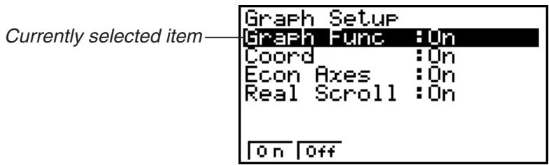
Graph Setup Screen
- To change the graph source data name display setting, use the ⚠️ and ⼀ cursor keys to move the highlighting to “Graph Func”. Next, press one of the function keys described below.
| To specify this graph source data name display setting: | Press this key: |
| Display source data name | F1 (On) |
| Hide source data name | F2 (Off) |
- When the graph data is stored in a sample data memory file, the file name appears as the source data name. When the graph data is stored in current data area, the channel name appears.
Note
- For details about sample data memory and current data area, see “9 Using Sample Data Memory”.
- To change the trace operation coordinate display setting, use the ▲ and ▼ cursor keys to move the highlighting to "Coord". Next, press one of the function keys described below.
| To specify this coordinate display setting for the trace operation: | Press this key: |
| Display trace coordinates | F1 (On) |
| Hide trace coordinates | F2 (Off) |
- To change the numeric axes display setting, use the ⬆ and ⬇ cursor keys to move the highlighting to “Econ Axes”. Next, press one of the function keys described below.
| To specify this axes display setting: | Press this key: |
| Display axes | F1 (On) |
| Hide axes | F2 (Off) |
- To change the real-time scroll setting, use the ⚠️ and ⼀ cursor keys to move the highlighting to “RealScroll”. Next, press one of the function keys described below.
| To specify this real-time scrolling setting: | Press this key: |
| Real-time scrolling on | F1 (On) |
| Real-time scrolling off | F2 (Off) |
- Press EXE to finalize Graph Setup and return to the Advanced Setup menu.
4 Using a Custom Probe
You can use the procedures in this section to configure a custom probe for use with the EA-200. The term “custom probe” means any sensor other than the CASIO or Vernier sensors specified as standard for the E-CON2 Mode.
■ Configuring a Custom Probe Setup
To configure a custom probe setup, you must input values for the constants of the fixed linear interpolation formula (ax + b) . The required constants are slope (a) and intercept (b). x in the above expression (ax + b) is the sampled voltage value (sampling range: 0 to 5 volts).
- To configure a custom probe setup
- From the E-CON2 main menu (page 1-1), press F1 (SET) and then 2 (ADV) to display the Advanced Setup menu.
- See “3 Using Advanced Setup” for more information.
- On the Advanced Setup menu (page 3-1), press 5 (Custom Probe) to display the Custom Probe List.
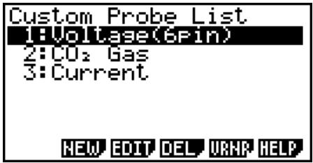
- The message “No Custom Probe” appears if the Custom Probe List is empty.
- Press F2 (NEW).
- This displays a custom probe setup screen like the one shown below.
![Input Probe Name [Vol Lase(6Pin)] == Specifications === Slope :1 Intercept:0 Unit Name:0 Warm-up :0sec EDIT CALIB ZERO HELP](/content/2025/01/86832/images/fbfdf252ca99933b0d8af5da1ef66bde256546729f9d65f7f8c6b47689053997.jpg)
- The initial default setting for the probe name is “Voltage(6pin)”. The first step for configuring custom probe settings is to change this name to another one. If you want to leave the default name the way it is, skip steps 4 and 5.
- Press F1 (EDIT).
- This enters the probe name editing mode.
- Input up to 18 characters for the custom probe name, and then press EXE.
- This will cause the highlighting to move to “Slope”.
- Use the function keys described below to configure the custom probe setup.
- To change the setting of an item, first use the ▲ and ▼ cursor keys to move the highlighting to the item. Next, use the function keys to select the setting you want.
(1) Slope
Press F1 (EDIT) to input the slope for the linear interpolation formula.
(2) Intercept
Press F1 (EDIT) to input the intercept for the linear interpolation formula.
(3) Unit Name
Press F1(EDIT) to input up to eight characters for the unit name.
(4) Warm-up
Press F1 (EDIT) to input the warm-up time.
- Press EXE and then input a memory number (1 to 99).
- This saves the custom probe setup and returns to the Custom Probe List, which should now contain the new custom probe setup you configured.
- To recall the specifications of a Vernier sensor and configure custom probe settings
-
Perform the first two steps of the procedure under "To configure a custom probe setup" on page 4-1.
-
Press F5 (VRNR).
• This displays a Vernier sensor list.
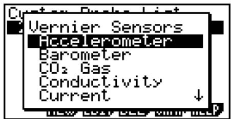
- Use the ▲ and ▼ keys to move the highlighting to the Vernier sensor whose setting you want to use as the basis of the custom probe settings, and then press EXE.
- The name and specifications of the Vernier sensor you select will appear on the custom probe setup screen.
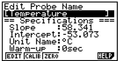
- To complete this procedure, perform steps 4 through 7 under “To configure a custom probe setup” (page 4-1).
■ Auto Calibrating a Custom Probe
Auto calibration automatically corrects the slope and intercept values of a custom probe setup based on two actual samples.
Important!
- Before performing the procedure below, you should prepare two conditions whose measurement values are known.
- When inputting reference value in step 5 of the procedure below, input the exact known measurement value of the condition you will sample in step 4. When inputting reference value in step 7 of the procedure below, input the exact known measurement value of the condition you will sample in step 6.
- To auto calibrate a custom probe
- Connect the calculator and EA-200, and connect the custom probe you want to auto calibrate to CH1 of the EA-200.
- What you should do first depends on whether you are configuring a new custom probe for calibration, or editing the configuration of an existing custom probe.
If you are configuring a new custom probe:
- Perform steps 1 through 6 of the procedure under “To configure a custom probe setup” on page 4-1.
- Auto calibrate will automatically set the slope and intercept, so you do not need to specify them in step 6 of the above procedure.
If you are editing the configuration of an existing custom probe:
- Perform steps 1 through 3 of the procedure under “To edit a custom probe setup” on page 4-6.
3. Press F2 (CALIB).
- This will start the first sampling operation with the sensor connected to EA-200's CH1, and then display a screen like the one shown below.
![Calibration: When stable, long press [EXE]. First sampling operation Point 1: 1.31021V Real-time display of sampled values](/content/2025/01/86832/images/fe572f063ac249166400bccb5a7b9fdd7d69f5dd6536251f0afe4fffd74ceae5.jpg)
- After the sampled value stabilizes, hold down EXE for a few seconds.
- This will register the first sampled value and display it on the screen. At this time the cursor will appear at the bottom of the display, ready for input of a reference value.
Calibration:
When stable,
long press [EXE].
Point 1:
1.31021V
Input Value(U)?
- Use the key pad to input the reference value for the first sampled value, and then press EXE.
- This cause sampling of the second value to be performed automatically, and display the same type of screen that appeared in step 3.
Second sampling operation
Calibration:
When stable,
long press [EXE].
Point 2: 4.38035U
- After the sampled value stabilizes, hold down EXE for a few seconds.
- This will register the second sampled value and display it on the screen. The cursor will appear at the bottom of the display, ready for input of a reference value.
Calibration:
When stable,
long press [EXE].
Point 2:
4.38035U
Input Value(U)?
-
Use the key pad to input the reference value for the second sampled value, and then press EXE.
-
This will return to the custom probe setup screen.
- The E-CON2 will calculate the slope and intercept value based on the two reference values that you input, and configure the settings automatically. The automatically configured values will appear on the custom probe setup screen, where you can view them.
![[CST ] = Specifications === Slope :0.998751 Intercept:1.4267E-03 Unit Name:U Warm-up :0sec EDIT CALIB ZERO HELP](/content/2025/01/86832/images/849000723b18d2b666b8d6fe6505ffe32631d595fb64bce3b7353ae7f040fe63.jpg)
- Press EXE, and then input a memory number from 1 to 99.
- This saves the custom probe setup and returns to the custom probe list.
■ Zero Adjusting a Custom Probe
This procedure zero adjusts a custom probe and sets its intercept value based on an actual sample using the applicable custom probe.
- To zero adjust a custom probe
- Connect the calculator and EA-200, and connect the custom probe you want to zero adjust to CH1 of the EA-200.
- What you should do first depends on whether you are configuring a new custom probe for zero adjusting, or editing the configuration of an existing custom probe.
If you are configuring a new custom probe:
- Perform steps 1 through 6 of the procedure under “To configure a custom probe setup” on page 4-1.
- Auto calibrate will automatically set the intercept, so you do not need to specify it in step 6 of the above procedure.
If you are editing the configuration of an existing custom probe:
- Perform steps 1 through 3 of the procedure under “To edit a custom probe setup” on page 4-6.
- Press F3 (ZERO).
- This will start the sampling operation with the sensor connected to EA-200's CH1, and then display a screen like the one shown below.
Zero Adjust: When stable, long press [EXE].
Point 1: 0.99682U
-
At the point your want to perform zero adjustment (the point that the displayed value is the appropriate zero adjust value), press EXE.
-
This will return to the custom probe setup screen.
- The E-CON2 will set the intercept value automatically based on the sampled value. The automatically configured value will appear on the custom probe setup screen, where you can view it.
![Input Slope [CDS ] == Specifications === Slope :0.996698 Intercept:-4.5660424 Unit Name:U Warm-up :0sec EDIT CALIB ZERO HELP](/content/2025/01/86832/images/68e40e4fff450249121df6e14123fc68533b1c02c6e5859d780dfbd3aa7e0fba.jpg)
- Press EXE, and then input a memory number from 1 to 99.
- This saves the custom probe setup and returns to the custom probe list.
■ Managing Custom Probe Setups
Use the procedures in this section to edit and delete existing custom probe setups.
- To edit a custom probe setup
- Display the Custom Probe List.
- Select the custom probe setup whose configuration you want to edit.
- Use the ▲ and ▼ cursor keys to highlight the name of the custom probe you want.
-
Press F3 (EDIT).
-
This displays the screen for configuring a custom probe setup.
- To edit the custom probe setup, perform the procedure starting from step 6 under “To configure a custom probe setup” on page 4-1.
- To delete a custom probe setup
- Display the Custom Probe List.
- Select the custom probe setup you want to delete.
- Use the ▲ and ▼ cursor keys to highlight the name of the custom probe setup you want.
-
Press F4 (DEL).
-
In response to the confirmation message that appears, press F1(Yes) to delete the custom probe setup.
- To clear the confirmation message without deleting anything, press F6 (No).
5 Using the MULTIMETER Mode
You can use the Channel Setup screen (page 3-3) to configure a channel so that EA-200 MULTIMETER Mode sampling is triggered by a calculator operation.
- To use the MULTIMETER Mode
- Connect the calculator and EA-200, and connect the sensors you want to the applicable EA-200 channels.
- From the Advanced Setup menu (page 3-1), use the Channel Setup screen (page 3-3) to configure sensor setups for each channel you will be using.
- After configuring the sensor setups, press EXE to return to the Advanced Setup menu (page 3-1), and then press F2 (MLTI).
- This starts sampling in the EA-200 MULTIMETER mode and displays a list of sample values for each channel.
![HA-200 CH 1 : 1.76V CH 2 : 25.8°C CH 3 : -50.4m/s² SONIC: 1.88meters STOP: [EXE] long press](/content/2025/01/86832/images/d0c23c27f59ecb12e1e879cbe2c9273c6342ab19f800f1d02d2c13251fcea2b7.jpg)
- Displayed sample data is refreshed at 0.5-second intervals.
- Do not connect sensors to any other channels except for those you specified in step 2.
-
Data sampled in the MULTIMETER mode is not saved in memory.
-
To end MULTIMETER mode sampling, press the EXE key.
6 Using Setup Memory
Creating EA-200 setup data using the Setup Wizard or Advanced Setup causes the data to be stored in the “current setup memory area”. The current contents of the current setup memory area are overwritten whenever you create other setup data.
You can use setup memory to save the current setup memory area contents to calculator memory to keep it from being overwritten, if you want.
■ Saving a Setup
A setup can be saved when any one of the following conditions exist.
- After configuring a new setup with Setup Wizard See step 8 under "To configure an EA-200 setup using Setup Wizard" on page 2-2.
- After configuring a new setup with Advanced Setup See step 6 under “To configure an EA-200 setup using Advanced Setup” on page 3-1 for more information.
- While the E-CON2 main menu (page 1-1) is on the display Performing the setup save operation while the E-CON2 main menu is on the display saves the contents of the current setup memory area (which were configured using Setup Wizard or Advanced Setup).
Details on saving a setup are listed below.
- To save a setup
- If the final Setup Wizard screen (page 2-4) is on the display, advance to step 2. If it isn't, start the save operation by performing one of the function key operations described below.
√ If the Advanced Setup menu (page 3-1) is on the display, press F3 (MEM).
√ If the E-CON2 main menu (page 1-1) is on the display, press F2(MEM).
- Performing any one of the above operations causes the setup memory list to appear.
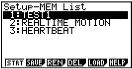
- The message “No Setup-MEM” appears if setup memory is empty.
- If you are starting from the final Setup Wizard screen, press ② (Save Setup-MEM). If you are starting from another screen, press F2 (SAVE).
- This displays the screen for inputting the setup name.
![Setup-MEM Name [ ]](/content/2025/01/86832/images/d1d21374153fa8e9e0324222c39d00a305468072a0ee95979e59cef887131032.jpg)
- Input up to 18 characters for the setup name.
-
Press EXE and then input a memory number (1 to 99).
-
If you start from the final Setup Wizard screen (page 2-4), this saves the setup and the message “Complete!” appears. Press EXE to return to the final Setup Wizard screen (page 2-4).
- If you start from the Advanced Setup menu (page 3-1) or the E-CON2 main menu (page 1-1), this saves the setup and returns to the setup memory list which includes the name you assigned it.
Important!
- Since you assign both a setup name and a file number to each setup, you can assign the same name to multiple setups, if you want.
■ Using and Managing Setups in Setup Memory
All of the setups you save are shown in the setup memory list. After selecting a setup in the list, you can use it to sample data or you can edit it.
- To preview saved setup data
You can use the following procedure to check the contents of a setup before you use it for sampling.
- On the E-CON2 main menu (page 1-1), press F2(MEM) to display the setup memory list.
- Use the ▲ and ▼ cursor keys to highlight the name of the setup you want.
- Press OPTN (Setup Preview).
- This displays the preview dialog box.
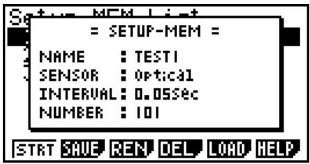
- To close the preview dialog box, press EXIT.
- To recall a setup and use it for sampling
Be sure to perform the following steps before starting sampling with the EA-200.
- Connect the calculator to the EA-200.
- Turn on EA-200 power.
-
In accordance with the setup you plan to use, connect the proper sensor to the appropriate EA-200 channel.
-
Prepare the item whose data is to be sampled.
-
On the E-CON2 main menu (page 1-1), press F2(MEM) to display the setup memory list.
-
Use the ▲ and ▼ cursor keys to highlight the name of the setup you want.
-
Press F1 (STRT).
-
In response to the confirmation message that appears, press F1.
-
Pressing EXE sets up the EA-200 and then starts sampling.
- To clear the confirmation message without sampling, press F6.
Note
- See “Operations during a sampling operation” on page 8-2 for information about operations you can perform while a sampling operation is in progress.
- To change the name of setup data
-
On the E-CON2 main menu (page 1-1), press F2(MEM) to display the setup memory list.
-
Use the ▲ and ▼ cursor keys to highlight the name of the setup you want.
-
Press F3 (REN).
- This displays the screen for inputting the setup name.
Setup-MEM Name [TEST1]
- Input up to 18 characters for the setup name, and then press EXE.
- This changes the setup name and returns to the setup memory list.
- To delete setup data
- On the E-CON2 main menu (page 1-1), press F2(MEM) to display the setup memory list.
- Use the ▲ and ▼ cursor keys to highlight the name of the setup you want.
- Press F4 (DEL).
- In response to the confirmation message that appears, press F1(Yes) to delete the setup.
- To clear the confirmation message without deleting anything, press F6 (No).
- To recall setup data
Recalling setup data stores it in the current setup memory area. You can then use Advanced Setup to edit the setup. This capability comes in handy when you need to perform a setup that is slightly different from one you have stored in memory.
- On the E-CON2 main menu (page 1-1), press F2(MEM) to display the setup memory list.
- Use the ▲ and ▼ cursor keys to highlight the name of the setup you want.
-
Press F5 (LOAD).
-
In response to the confirmation message that appears, press F1 (Yes) to recall the setup.
- To clear the confirmation message without recalling the setup, press F6 (No).
Note
- Recalling setup data replaces any other data currently in the current setup memory area.
7 Using Program Converter
Program Converter converts an EA-200 setup you configured using Setup Wizard or Advanced Setup to a program that can run on the calculator. You can also use Program Converter to convert a setup to a CFX-9850 Series/fx-7400 Series-compatible program.*1 *2
*1 See the documentation that came with your scientific calculator or EA-200 for information about how to use a converted program.
*2 See online help (PROGRAM CONVERTER HELP) for information about supported CFX-9850 Series and fx-7400 Series models.
■ Converting a Setup to a Program
A setup can be converted to a program when any one of the following conditions exists.
• After configuring a new setup with Setup Wizard
See step 8 under "To configure an EA-200 setup using Setup Wizard" on page 2-2.
• After configuring a new setup with Advanced Setup
See step 6 under “To configure an EA-200 setup using Advanced Setup” on page 3-1 for more information.
- While the E-CON2 main menu (page 1-1) is on the display
Performing the program converter operation while the E-CON2 main menu is on the display converts the contents of the current setup memory area (which were configured using Setup Wizard or Advanced Setup).
The program converter procedure is identical in all of the above cases.
- To convert a setup to a program
- Start the converter operation by performing one of the key operations described below.
√ If the final Setup Wizard screen (page 2-4) is on the display, press ☐3 (Convert Program).
√ If the Advanced Setup menu (page 3-1) is on the display, press F4 (PROG).
√ If the E-CON2 main menu (page 1-1) is on the display, press F3 (PROG).
- After you perform any one of the above operations, the program converter screen will appear on the display.
![Input Program Name [ ] F1:Calculator :9860 F2:Model Type :EA-200 F3:Calibration:None CALC TYPE CALB [→O SYMBOL HELP]](/content/2025/01/86832/images/8016b3d00305dfa9b5b74624317075aa8fc06dde91ed28a4c7c2cd27b1876538.jpg)
- Enter up to eight characters for the program name.
Note
Using the program converter initial default settings will create a program like the one below.
• Associated Scientific Calculator: fx-9860 Series
• Associated Data Analyzer: EA-200
- Calibration: None
- Password: None
If you want to use these settings the way they are without changing them, skip steps 3 through 7 and go directly to step 8. If you want to change any of the settings, perform the applicable operations in steps 3 through 7.
- Specify the scientific calculator model to be associated with the program. Perform one of the following key operations to associate the program with a scientific calculator.
| To associate the program with this calculator: | Perform this key operation: |
| fx-9860 Series | 1 (CALC) 1 (9860) |
| CFX-9850 Series | 1 (CALC) 2 (9850) |
| fx-7400 Series | 1 (CALC) 3 (7400) |
- The number part of the scientific calculator model number you specify will appear in line "F1:" of the program converter screen.
Note
For information about F1 (CALC) F4 ( 38K), see “Converting a CFX-9850 Series Program to a fx-9860 Series Compatible Program” (page 7-4).
- Specify the Data Analyzer model (EA-100 or EA-200) to be associated with the program. Perform one of the following key operations to associate the program with a Data Analyzer.
| To associate the program with this Data Analyzer: | Perform this key operation: |
| EA-200 | F2 (TYPE) F1 (200) |
| EA-100 | F2 (TYPE) F2 (100) |
- The number part of the Data Analyzer model number you specify will appear in line “F2:” of the program converter screen.
Important!
- Note that the capabilities of the EA-100 and EA-200 are different. Because of this, you should keep in mind that an EA-200 program converted to an EA-100 program and used to perform sampling with an EA-100 setup may not produce the desired results.
- If you plan to use a custom probe connected to CH1 of the Data Analyzer, specify whether calibration or zero adjust should be performed. Perform one of the following key operations to configure the desired setting.
| To perform this operation: | Perform this key operation: |
| Calibration of the CH1 custom probe | F3 (CALB) F1 (CALIB) |
| Zero adjust of the CH1 custom probe | F3 (CALB) F2 (ZERO) |
| No calibration | F3 (CALB) F3 (None) |
- The operation you specify will appear in line “F3:” of the program converter screen.
- To password protect the program, press F4(πO).
- This will cause the “Password?” prompt and password input field to appear under the program name input field.
![Input Program Name [NEWTON ] Password? [ ] F1:Calculator :9860 F2:Model Type :EA-100 F3:Zero Adjust:CH 1 CALC TYPE CALB |→O SYMBOL HELP](/content/2025/01/86832/images/f9ffa18a36a54dc5b07e32285d553bdbdb8e8437dd55a8b2c4e21c20aa9fcfad.jpg)
- Enter up to eight characters for the password.
- If you change your mind about assigning a password, press EXIT here. This will cause the password input field to disappear and cancel password input.
- After everything is the way you want, press EXE to convert the program in accordance with the setup.
- The message “Complete!” appears when conversion is complete. To clear the message and return to the screen that was on the display in step 1, press EXE or EXIT.
■ Converting a CFX-9850 Series Program to a fx-9860 Series Compatible Program
To use an EA-200 control program created on the CFX-9850 Series calculator (for use on the CFX-9850) on the E-CON2, you need to convert the program to an fx-9860 program. Conversion can be performed using the program converter.
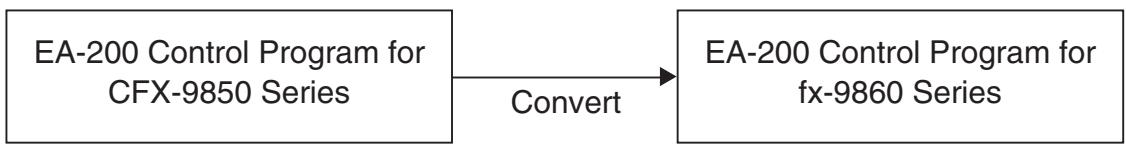
flowchart
graph LR
    A["EA-200 Control Program for CFX-9850 Series"] -->|Convert| B["EA-200 Control Program for fx-9860 Series"]
- To convert a program
- Transfer the EA-200 control program created for the CFX-9850 Series to the fx-9860 main memory.
- Use the cable that comes bundled with the fx-9860 to connect its 3-pin serial port to the 3-pin serial port of the CFX-9850. For details, see the chapter titled “Data Communications” in the manuals that come with each unit.
- Perform step 1 under "To convert a setup to a program" on page 7-1, which displays the program converter screen.
- Press F1 (CALC) and then press F4 ( 38K).
- This displays a list of programs currently in main memory.
- Use ▲ and ▼ to move the highlighting of the program you want to convert, and then press F1(EXE) or EXE.
- A program name input screen will appear after conversion is complete.
![Input Program Name [NEWTON] πO SVBL](/content/2025/01/86832/images/697c2f747314b7bbdf4f9c7587e3c4d9cb49bc0965f65a9103ccd36a48dee80b.jpg)
- Enter up to eight characters for the program name.
- If you want to password protect the program, perform steps 6 and 7 under “To convert a setup to a program” after inputting the program name.
- Press EXE to start conversion of the program.
- The message “Complete!” appears when conversion is complete. To clear the message, press EXE or EXIT.
8 Starting a Sampling Operation
The section describes how to use a setup configured using the E-CON2 Mode to start an EA-200 sampling operation.
■ Before getting started...
Be sure to perform the following steps before starting sampling with the EA-200.
- Connect the calculator to the EA-200.
- Turn on EA-200 power.
- In accordance with the setup you plan to use, connect the proper sensor to the appropriate EA-200 channel.
- Prepare the item whose data is to be sampled.
■ Starting a Sampling Operation
A sampling operation can be started when any one of the following conditions exist.
• After configuring a new setup with Setup Wizard
See step 8 under "To configure an EA-200 setup using Setup Wizard" on page 2-2.
• After configuring a new setup with Advanced Setup
See step 6 under “To configure an EA-200 setup using Advanced Setup” on page 3-1.
- While the E-CON2 main menu (page 1-1) is on the display
Starting a sampling operation while the E-CON2 main menu is on the display performs sampling using the contents of the current setup memory area (which were configured using Setup Wizard or Advanced Setup).
- While the setup memory list is on the display
You can select the setup you want on the setup memory list and then start sampling.
The following procedures explain the first three conditions described above. See “To recall a setup and use it for sampling” on page 6-3 for information about starting sampling from the setup memory list.
- To start sampling
- Start the sampling operation by performing one of the function key operations described below.
√ If the final Setup Wizard screen (page 2-4) is on the display, press ① (Start Setup).
√ If the Advanced Setup menu (page 3-1) is on the display, press F1(STRT).
√ If the E-CON2 main menu (page 1-1) is on the display, press F4(STRT).
- After you perform any one of the above operations, a sampling start confirmation screen like the one shown below will appear on the display.
![====== EA-200 ==== *IS THE SENSOR CONNECTED? *CONNECT LINK-CABLE FIRMLY? *IS SAMPLING DONE? Press: [EXE]](/content/2025/01/86832/images/d52b94de87cae4d1db23eae51bdfbff8e750ec3030ec3e07f9886f38b2f06c53.jpg)
-
Press EXE.
-
This sets up the EA-200 using the setup data in the current setup memory area.
- The message “Setting EA-200...” remains on the display while EA-200 setup is in progress. You can cancel the setup operation any time this message is displayed by pressing AC.
- The screen shown below appears after EA-200 setup is complete.
![================== EA-200 =================== Start sampling? Press: [EXE]](/content/2025/01/86832/images/77893e2dbc47e07c0acb96e49119c3eb18f930b8ba6cce0a3a4ba763b36dea97.jpg)
- Press EXE to start sampling.
- The screens that appear while sampling is in progress and after sampling is complete depend on setup details (sampling mode, trigger setup, etc.). For details, see “Operations during a sampling operation” below.
- Operations during a sampling operation
Sending a sample start command from the calculator to the EA-200 causes the following sequence to be performed.
Setup Data Transfer → Sampling Start → Sampling End →
Transfer of Sample Data from the EA-200 to the Calculator
The table on the next page shows how the trigger conditions and sensor type specified in the setup data affects the above sequence.
Starts Sampling
| Mode | 1. EA-200 Setup | 2. Start Standby | 3. Sampling | 4. Graphing |
| Real-time | 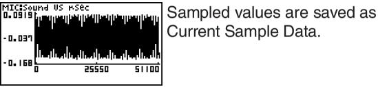 When Mode = SoundGraph screen does not show all sampled values,but only a partial preview. When Mode = SoundGraph screen does not show all sampled values,but only a partial preview. EXE EXE EXE EXE Input values. EXE EXE Input values. EXE EXE | |||
| Fast | = \\= \\= \\= \\= \\= \\= \\= \\= \\= \\= \\= \\= \\= \\= \\= \\= \\= \\= \\= \\= \ The screen shown below appears when CH1,SONIC, or Mic is used as the trigger. | |||
| Normal | ||||
| Sound | ||||
| Extended | = \\= \\= \\= \\= \\= \\= \\= \\= \\= \\= \\= \\= \\= \\= \\= \\= \\= Pressing F1 advances to"4. Graphing".Pressing EXE there returns to"3. Sampling". | |||
| Period | = \\= \\= \\= \\= \\= \\= \\= \\= \\= \\= \\= \\= \\= \\= \\= \\= \\=\ When sampling is done.Press [EXE] key. |  3. Time and acceleration graphZ2] 3. Time and acceleration graphZ2]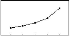 Sample values is stored as List data only. Sample values is stored as List data only. | ||
| Clock |
Graph screen does not show all sampled values, but only a partial preview.
9 Using Sample Data Memory
Performing an EA-200 sampling operation from the E-CON2 Mode causes sampled results to be stored in the “current data area” of E-CON2 memory. Separate data is saved for each channel, and the data for a particular channel in the current data area is called that channel’s “current data”.
Any time you perform a sampling operation, the current data of the channel(s) you use is replaced by the newly sampled data. If you want to save a set of current data and keep it from being replaced by a new sampling operation, save the data in sample data memory under a different file name.
■ Managing Sample Data Files
- To save current sample data to a file
- On the E-CON2 main menu (page 1-1), press F5(GRPH).
- This displays the Graph Mode screen.
![Mode:Graph Analysis GPh1: [---] GPh2: [---] GPh3: [---] SEL DATA MODE STYLE DEL DRAW](/content/2025/01/86832/images/22a9c8fe2c2e4c004498253981e3b1d5c0fce8dfaf51030ff9dfbae931cf9daa.jpg)
Graph Mode Screen
- For details about the Graph Mode screen, see “10 Using the Graph Analysis Tools to Graph Data”.
- Press F2 (DATA).
- This displays the Sampling Data List screen.
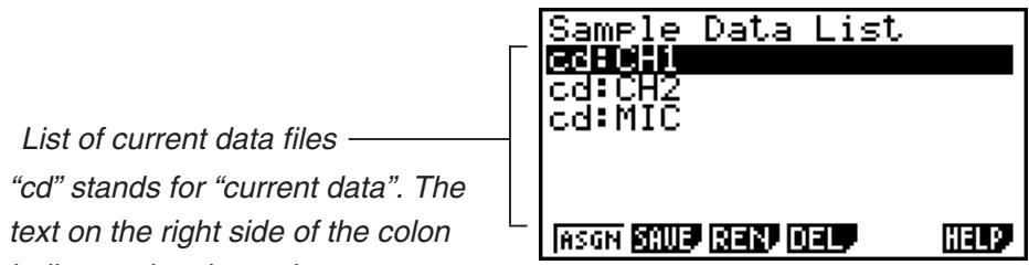
Sampling Data List Screen
- Use the ▲ and ▼ cursor keys to move the highlighting to the current data file you want to save, and then press F2(SAVE).
- This displays the screen for inputting a data name.
![Sample Data Name [ ] == Specifications === Sensor:Optical Interval:0.2sec Number:101 Max:317Lum Int Min:0.666667Lum Int](/content/2025/01/86832/images/a80ce3008790e32179e66eb202bd1233c6d356bb7facf9f7a716fd6d80a619dd.jpg)
- Enter up to 18 characters for the data file name, and then press EXE.
- This displays a dialog box for inputting a memory number.
- Enter a memory number in the range of 1 to 99, and then press EXE.
- This saves the sample data at the location specified by the memory number you input.
The sample data file you save is indicated on the display using the format:
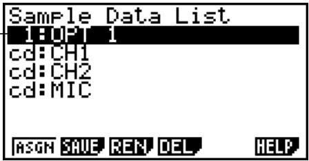
- If you specify a memory number that is already being used to store a data file, a confirmation message appears asking if you want to replace the existing file with the new data file. Press F1 to replace the existing data file, or F6 to return to the memory number input dialog box in Step 4.
- To return to the E-CON2 main menu (page 1-1), press EXIT twice.
Note
- You could select another data file besides a current data file in step 3 of the above procedure and save it under a different memory number. You do not need to change the file's name as long as you use a different file number.
- To rename an existing sample data file
Note
- You cannot use this procedure to rename a current data file name.
- On the E-CON2 main menu (page 1-1), press F5 (GRPH).
- This displays the Graph Mode screen.
- Press F2 (DATA).
- This displays the Sampling Data List screen.
- Use the ▲ and ▼ cursor keys to move the highlighting to the data file you want to rename, and then press F3 (REN).
- This displays the screen for inputting a file name.
- Enter up to 18 characters for the new data file name, and then tap EXE.
- This returns to the Sampling Data List screen.
- To return to the E-CON2 main menu (page 1-1), press EXIT twice.
- To delete a sample data file
- On the E-CON2 main menu (page 1-1), press F5(GRPH).
- This displays the Graph Mode screen.
- Press F2 (DATA).
- This displays the Sampling Data List screen.
-
Use the ▲ and ▼ cursor keys to move the highlighting to the data file you want to delete, and then press F4(DEL).
-
In response to the confirmation message that appears, press F1(Yes) to delete the data file.
- To clear the confirmation message without deleting the data file, press F6(No).
- This returns to the Sampling Data List screen.
- To return to the E-CON2 main menu (page 1-1), press EXIT twice.
10 Using the Graph Analysis Tools to Graph Data
Graph Analysis tools make it possible to analyze graphs drawn from sampled data.
■ Accessing Graph Analysis Tools
You can access Graph Analysis tools using either of the two methods described below.
- Accessing Graph Analysis tools from the Graph Mode screen, which is displayed by pressing F5 (GRPH) on the E-CON2 main menu (page 1-1)
![Mode:Graph Analysis ▶GPh1:CH1 [---]Optical ▶GPh2:MIC [---]Microphone ▶GPh3:FFT Spectrum [---]Microphone SEL DATA MODE STYLE DEL DRAW](/content/2025/01/86832/images/d8a586dcd0ebfc46c1e82c475cb1a95dc1b157948ba547f8aae3436c7ebfcd4f.jpg)
Graph Mode Screen
- The main menu appears after you perform a sampling operation. Press F5 (GRPH) at that time.
- When you access Graph Analysis tools using this method, you can select from among a variety of other Analysis modes. See “Selecting an Analysis Mode and Drawing a Graph” (page 10-2) for more information about the other Analysis modes.
- Accessing Graph Analysis tools from the screen of a graph drawn after a sampling operation is executed from the Setup Wizard or from Advanced Setup (Realtime Mode)
line
| Time (s) | Int US Sec | | -------- | ---------- | | 0 | 196.66 | | 2.5 | -5 | | 5 | 95.666 |Graph Screen
- In this case, data is graphed after the sampling operation is complete, and the calculator accesses Graph Analysis tools automatically. See “Graph Screen Key Operations” on page 11-1.
■ Selecting an Analysis Mode and Drawing a Graph
This section contains a detailed procedure that covers all steps from selecting an analysis mode to drawing a graph.
Note
- Step 4 through step 6 are not essential and may be skipped, if you want. Skipping any step automatically applies the initial default values for its settings.
- If you skip step 2, the default analysis mode is the one whose name is displayed in the top line of the Graph Mode screen.
- To select an analysis mode and draw a graph
- On the E-CON2 main menu (page 1-1), press F5(GRPH).
- This displays the Graph Mode screen.
- Press F3(MODE), and then select the analysis mode you want from the menu that appears.
| To do this: | Perform this menu operation: | To select this mode: |
| Graph three sets of sampled data simultaneously | [Norm] | Graph Analysis |
| Graph sampled data along with its first and second derivative graph | [diff] | d/dt \& d^2/dt^2 |
| Display the graphs of different sampled data in upper and lower windows for comparison | [CMPR] [GRPH] | Compare Graph |
| Output sampled data from the speaker, displaying graph of the raw data in the upper window and the output waveform in the lower window | [CMPR] [Snd] | Compare Sound |
| Display the graph of sampled data in the upper window and its first derivative graph in the lower window | [CMPR] [d/dt] | Compare d/dt |
| Display the graph of sampled data in the upper window and its second derivative graph in the lower window | [CMPR] [ d^2/dt^2 ] | Compare d^2/dt^2 |
- The name of the currently selected mode appears in the top line of the Graph Mode screen.
Analysis mode name
![Mode: Graph Analysis GPh1: [---] GPh2: [▪] GPh3: [▪] SEL DATA MODE STYLE DEL DRAW](/content/2025/01/86832/images/1e58c003bef61e1d9259fe28c1a17569086a38dddbae72acb5e763b67da80d3e.jpg)
- Press F2 (DATA).
- This displays the Sampling Data List screen.
- Specify the sampled data for graphing.
a. Use the ▲ and ▼ cursor keys to move the highlighting to the name of the sampled data file you want to select, and then press F1 (ASGN) or EXE.
- This returns to the Graph Mode screen, which shows the name of the sample data file you selected.
![Graph on/off indicator Mode: Graph Analysis GPh1:OPTICAL1 [---]Optical GPh2: [ * ] GPh3: [ * ] SEL DATA MODE STYL DEL DRAW Sample data file name Name of sensor used for sampling](/content/2025/01/86832/images/31904f74791092167151d9b0b267329b6d66a6efa653b955b47f99299ecd3b20.jpg)
Graph Mode Screen
b. Repeat step a above to specify sample data files for other graphs, if there are any.
- If you select “Graph Analysis” as the analysis mode in step 2, you must specify sample data files for three graphs. If you select “Compare Graph” as the analysis mode in step 2, you must specify sample data files for two graphs. With other modes, you need to specify only one sample data file.
-
For details about Sampling Data List screen operations, see “9 Using Sample Data Memory”.
-
Turn on graphing for each of the graphs listed on the Graph Mode screen.
a. On the Graph Mode screen, use the ▲ and ▼ cursor keys to select a graph, and then press F1(SEL) to toggle graphing on or off.
![Mode: Graph Analysis ▶GPh1:OPTICAL1 [---]Optical Graphing turned off. ▶GPh2:OPTICAL2 [ • ]Optical Graphing turned on. ▶GPh3:OPTICAL3 [ * ]Optical SEL DATA MOD STYLE DEL DRAW](/content/2025/01/86832/images/6a379a7ae3baaea1b021e7b838d34c0864dc0b4895527e3956fbca10bf7b11f3.jpg)
b. Repeat step a to turn each of the graphs listed on the Graph Mode screen on or off.
- Select the graph style you want to use.
a. On the Graph Mode screen, use the ⬆ and ⬇ cursor keys to move the highlighting to the graph (Gph1, Gph2, etc.) whose style you want to specify, and then press F4(STYL). This will cause the function menu to change as shown below.
![Mode:Graph Analysis GPh1:CH1 [---]Optical GPh2: [---] GPh3: [---]](/content/2025/01/86832/images/4eb9b391990e902770d8d5a4625e42924e1fb0b4caac4a2b2801c0e3af5013e9.jpg)
b. Use the function keys to specify the graph style you want.
| To specify this graph style: | Press this key: |
| Line graph with dot ( • ) data markers | F1( —— ) |
| Line graph with square ( □ ) data markers | F2( ****+) |
| Line graph with X (×) data markers | F3( ****+) |
| Scatter graph with dot ( • ) data markers | F4( ...... ) |
| Scatter graph with square ( □ ) data markers | F5( ***** ) |
| Scatter graph with X (×) data markers | F6( ×××× ) |
c. Repeat a and b to specify the style for each of the graphs on the Graph Mode screen.
- On the Graph Mode screen, press F6 (DRAW) or EXE.
- This draws the graph(s) in accordance with the settings you configured in step 2 through step 6.
line
| x | y | |-------|---------| | 0.02 | 233.33 | | 0.5 | 113.66 | | 0.98 | -5.666 |Graph Screen
- When a Graph screen is on the display, the function keys provide you with zooming and other capabilities to aid in graph analysis.
For details about Graph screen function key operations, see the following section.
- To deselect sampled data assigned for graphing on the Graph Mode screen
-
On the Graph Mode screen, use the ⬆ and ⬇ cursor keys to move the highlighting to the graph (Gph1, Gph2, etc.) whose sampled data you want to deselect.
-
Press F5 (DEL).
- This will deselect sample data assigned to the highlighted graph.
11 Graph Analysis Tool Graph Screen Operations
This section explains the various operations you can perform on the graph screen after drawing a graph.
You can perform these operations on a graph screen produced by a sampling operation, or by the operation described under “Selecting an Analysis Mode and Drawing a Graph” on page 10-2.
■ Graph Screen Key Operations
On the graph screen, you can use the keys described in the table below to analyze (CALC) graphs by reading data points along the graph (Trace) and enlarging specific parts of the graph (Zoom).
| Key Operation | Description |
| SHIFT F1 (TRCE) | Displays a trace pointer on the graph along with the coordinates of the current cursor location. Trace can also be used to obtain the periodic frequency of a specific range on the graph and assign it to a variable. See “Using Trace” on page 11-3. |
| SHIFT F2 (ZOOM) | Starts a zoom operation, which you can use to enlarge or reduce the size of the graph along the x-axis or the y-axis. See “Using Zoom” on page 11-4. |
| SHIFT F3 (V-WIN) | Displays a function menu of special View Window commands for the E-CON2 Mode graph screen.For details about each command, see “Configuring View Window Parameters” on page 11-14. |
| SHIFT F4 (SKTCH) | Displays a menu that contains the following commands: CIs, Plot, F-Line, Text, PEN, Vert, and Hztl. For details about each command, see “5-10 Changing the Appearance of a Graph” in the manual that comes with the fx-9860G SD/fx-9860G calculator. |
| OPTN F1 (PICT) | Saves the currently displayed graph as a graphic image. You can recall a saved graph image and overlay it on another graph to compare them. For details about these procedures, see “5-4 Storing a Graph in Picture Memory” in the manual that comes with the fx-9860G SD/fx-9860G calculator. |
| OPTN F2 (LMEM) | Displays a menu of functions for saving the sample values in a specific range of a graph to a list. See “Transforming Sampled Data to List Data” on page 11-5. |
| OPTN F3 (EDIT) | Displays a menu of functions for zooming and editing a particular graph when the graph screen contains multiple graphs. See “Working with Multiple Graphs” on page 11-10. |
| OPTN F4 (CALC) | Displays a menu that lets you transform a sample result graph to a function using Fourier series expansion, and to perform regression to determine the tendency of a graph. See “Using Fourier Series Expansion to Transform a Waveform to a Function” on page 11-6, and “Performing Regression” on page 11-8. |
| OPTN F5 (Y=fx) | Displays the graph function list, which lets you select a Y=f(x) graph to overlay on the sampled result graph. See “Overlaying a Y=f(x) Graph on a Sampled Result Graph” on page 11-9. |
| OPTN F6 (SPKR) | Starts an operation for outputting a specific range of a sound data waveform graph from the speaker. See “Outputting a Specific Range of a Graph from the Speaker” on page 11-12. |
■ Scrolling the Graph Screen
Press the cursor keys while the graph screen is on the display scrolls the graph left, right, up, or down.
Note
- The cursor keys perform different operations besides scrolling while a trace or graph operation is in progress. To perform a graph screen scroll operation in this case, press EXIT to cancel the trace or graph operation, and then press the cursor keys.
■ Using Trace
Trace displays a crosshair pointer on the displayed graph along with the coordinates of the current cursor position. You can use the cursor keys to move the pointer along the graph. You can also use trace to obtain the periodic frequency value for a particular range, and assign the range (time) and periodic frequency values in separate Alpha-Memory values.
- To use trace
- On the graph screen, press SHIFT F1 (TRCE).
- This causes a trace pointer to appear on the graph. The coordinates of the current trace pointer location are also shown on the display.
line
| Time (sec) | Int (Lum) | | ---------- | --------- | | 0 | 131.33 | | 5 | 64 | | 10 | -3.333 |-
Use the ◀ and ▶ cursor keys to move the trace pointer along the graph to the location you want.
-
The coordinate values change in accordance with the trace pointer movement.
- You can exit the trace pointer at any time by pressing EXIT.
- To obtain the periodic frequency value
- Use the procedure under "To use trace" above to start a trace operation.
- Move the trace pointer to the start point of the range whose periodic frequency you want to obtain, and then press EXE.
- Move the trace pointer to the end point of the range whose periodic frequency you want to obtain.
- This causes the period and periodic frequency value at the start point you selected in step 2 to appear along the bottom of the screen.
line
| Time (s) | Value | | -------- | --------- | | 16900 | -0.034 | | 19350 | 0.078 | | 21800 | -0.148 |- Press EXE to assign the period and periodic frequency values to Alpha-Memory variables.
- This displays a dialog box for specifying variable names for [Period] and [Frequency] values.
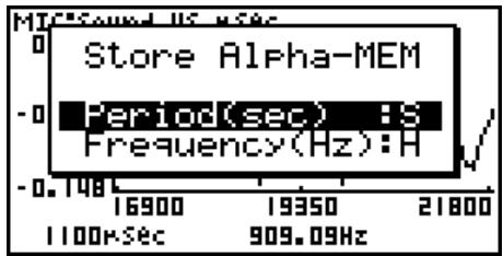
- The initial default variable name settings are “S” for the period and “H” for the periodic frequency. To change to another variable name, use the up and down cursor keys to move the highlighting to the item you want to change, and then press the applicable letter key.
-
After everything is the way you want, press EXE.
-
This stores the values and exits the trace operation.
- For details about using Alpha-Memory, see the manual that comes with the fx-9860G SD/fx-9860G calculator.
■ Using Zoom
Zoom lets you enlarge or reduce the size of the graph along the x-axis or the y-axis.
Note
- When there are multiple graphs on the screen, the procedure below zooms all of them. For information about zooming a particular graph when there are multiple graphs on the screen, see “Working with Multiple Graphs” on page 11-10.
- To zoom the graph screen
- On the graph screen, press SHIFT F2 (ZOOM).
- This causes a magnifying glass cursor ( _a ) to appear in the center of the screen.
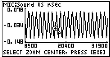
line
| Time | Value | | ------ | ------ | | 8900 | 0.078 | | 20400 | -0.034 | | 31900 | -0.148 |- Use the cursor keys to move the magnifying glass cursor to the location on the screen that you want at the center of the enlarged or reduced screen.
3. Press EXE.
- This causes the magnifying glass to disappear and enters the zoom mode.
- The cursor keys perform the following operations in the zoom mode.
| To do this: | Press this cursor key: |
| Enlarge the graph image horizontally | |
| Reduce the size of the graph image horizontally | |
| Enlarge the graph image vertically | |
| Reduce the size of the graph image vertically |
4. To exit the zoom mode, press EXIT.
■ Transforming Sampled Data to List Data
Use the following procedure to transform the sampled data in a specific range of a graph into list data.
- To transform sampled data to list data
- On the graph screen, press OPTN, and then F2 (LMEM).
- This displays the [LMEM] menu.
- Press F2 (SEL).
- This displays the trace pointer for selecting the range on the graph.
- Move the trace pointer to the start point of the range you want to convert to list data, and then press EXE.
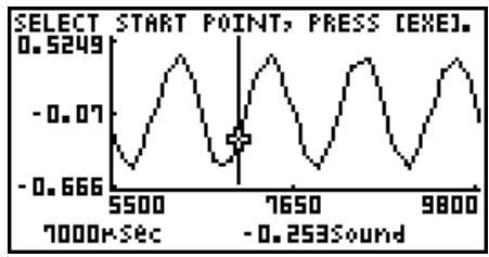
line
| Time (sec) | Value | | ---------- | ------- | | 5500 | -0.666 | | 7650 | 0.5249 | | 9800 | -0.253Sound |- Move the trace pointer to the end point of the range you want to convert to list data, and then press EXE.
- This displays a dialog box for specifying the lists where you want to store the time data and the sampled data.
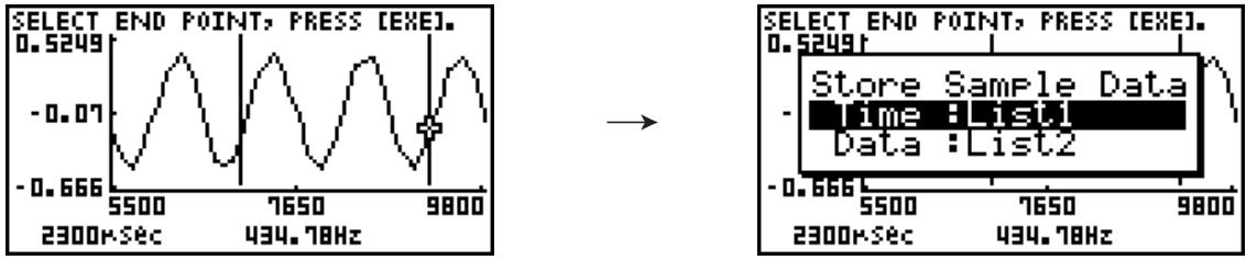
line
| Time (sec) | Value | | ---------- | ----- | | 2300 | -0.666 | | 434 | 0.5249 | | 9800 | -0.07 |- The initial default lists are List 1 for the time and List 2 for sample data. To change to another list (List 1 to List 26), use the up and down cursor keys to move the highlighting to the list you want to change, and then input the applicable list number.
-
After everything is the way you want, press EXE.
-
This saves the lists and the message "Complete!" appears. Press EXE to return to the graph screen.
- For details about using list data, see the manual that comes with the fx-9860G SD/fx-9860G calculator.
Note
- Pressing F1(All) in place of F2(SEL) in step 2 converts the entire graph to list data. In this case, the “Store Sample Data” dialog box appears as soon as you press F1(All).
■ Using Fourier Series Expansion to Transform a Waveform to a Function
Fourier series expansion is effective for studying sounds by expressing them as functions. The procedure below assumes that there is a graph of sampled sound data already on the graph screen.
- To perform Fourier series expansion
- On the graph screen, press OPTN, and then F4(CALC).
- The [CALC] menu appears at the bottom of the display.
line
| Time (s) | Value | | -------- | --------- | | 5500 | -0.666 | | 7650 | 0.5249 | | 9800 | -0.07 |- Press F1(Furie).
- This displays the trace pointer for selecting the graph range.
- Move the trace pointer to the start point of the range for which you want to perform Fourier series expansion, and then press EXE.
line
| Time (sec) | Value | | ---------- | ------- | | 5700 | -0.666 | | 5800 | 0.5249 | | 5900 | -0.07 | | 6000 | 0.5249 | | 6100 | -0.07 | | 6200 | 0.5249 | | 6300 | -0.07 | | 6400 | 0.5249 | | 6500 | -0.07 | | 6600 | 0.5249 | | 6700 | -0.07 | | 6800 | 0.5249 | | 6900 | -0.07 | | 7000 | 0.5249 | | 7100 | -0.07 | | 7200 | 0.5249 | | 7300 | -0.07 | | 7400 | 0.5249 | | 7500 | -0.07 | | 7600 | 0.5249 | | 7700 | -0.07 | | 7800 | 0.5249 | | 7900 | -0.07 | | 8000 | 0.5249 | | 8100 | -0.07 | | 8200 | 0.5249 | | 8300 | -0.07 | | 8400 | 0.5249 | | 8500 | -0.07 | | 8600 | 0.5249 | | 8700 | -0.07 | | 8800 | 0.5249 | | 8900 | -0.07 | | 9000 | 0.5249 | | 9100 | -0.07 | | 9200 | 0.5249 | | 9300 | -0.07 | | 9400 | 0.5249 | | 9500 | -0.07 | | 9600 | 0.5249 | | 9700 | -0.07 | | 9800 | 0.5249 | | 9900 | -0.07 | | 1000k | 0.5249 |- Move the trace pointer to the end point of the range for which you want to perform Fourier series expansion, and then press EXE.
- This displays a dialog box for specifying the start degree of the Fourier series.
line
| Time (sec) | Value | | ---------- | ------ | | 5500 | -0.666 | | 7650 | 0.5249 | | 9800 | 0.5249 |
![SELECT END POINT, PRESS [EXE]. 0.5249t Start Degree of Fourier Series 1-99(*1): -0.666 5500 7650 9800 3400Ksec 294.11Hz](/content/2025/01/86832/images/0e80c240230fd4b6dbba8cc3cc7a1e873d18efc932dc74fc551f2826ca472049.jpg)
- Input a value in the range of 1 to 99, and then press EXE.
- This displays a dialog box for inputting the degree of the Fourier series.
![SELECT END POINT, PRESS [EXE]. 0.5249T Input Degree of Fourier Series 1-10(*5): -0.666 5500 7650 9800 3400Ksec 294.11Hz](/content/2025/01/86832/images/c9e7c4f8ee7902bd73f98474f11ae1fde48477ce8ed02c036148d6e90ddda538.jpg)
- Input a value in the range of 1 to 10, and then press EXE.
- The graph function list appears with the calculation result.
![Graph Func :Y= Y1=Y2+Y3+Y4+Y5+Y- Y2=0.0006515sin [—] Y3=0.001315sin ( [—] Y4=0.4454sin (55[—] Y5=0.0006912sin [—] Y6=0.0006088sin [—] SEL DEL Y STYL DRAW](/content/2025/01/86832/images/074567d4fb854c3eb9ffacb8cd7e0636675ea13cc3297b71b855946fbbcecfbd.jpg)
- Pressing F6(DRAW) here graphs the function.
line
| X | Y | | ------ | ------- | | 5500 | 0.5249 | | 7650 | -0.666 | | 9800 | 0.5249 |- This lets you compare the expanded function graph and the original graph to see if they are the same.
Note
When you press F6 (DRAW) in step 7, the graph of the result of the Fourier series expansion may not align correctly with the original graph on which it is overlaid. If this happens, shift the position the original graph to align it with the overlaid graph.
For information about how to move the original graph, see “To move a particular graph on a multi-graph display” (page 11-12).
■ Performing Regression
You can use the procedure below to perform regression for a range specified using the trace pointer. All of the following regression types are supported: Linear, Med-Med, Quadratic, Cubic, Quartic, Logarithmic, Exponential, Power, Sine, and Logistic.
For details about these regression types, see page 6-3-5 through 6-3-10 of the manual that comes with the fx-9860G SD/fx-9860G calculator.
The following procedure shows how to perform quadratic regression. The same general steps can also be used to perform the other types of regression.
- To perform quadratic regression
- On the graph screen, press OPTN, and then F4(CALC).
- The [CALC] menu appears at the bottom of the display.
- Press F5(X^2).
- This displays the trace pointer for selecting the range on the graph.
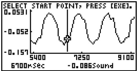
line
| Time (sec) | Value | | ---------- | --------- | | 5400 | -0.0531 | | 7250 | -0.157 | | 9100 | -0.086 |-
Move the trace pointer to the start point of the range for which you want to perform quadratic regression, and then press EXE.
-
Move the trace pointer to the end point of the range for which you want to perform quadratic regression, and then press EXE.
- This displays the quadratic regression calculation result screen.
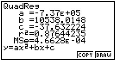
5. Press F6 (DRAW).
- This draws a quadratic regression graph and overlays it over the original graph.
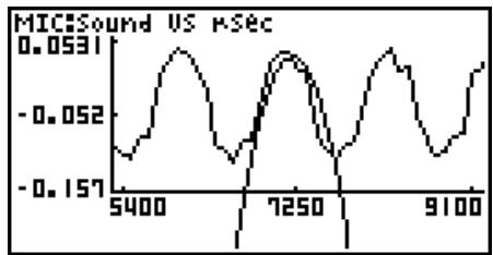
line
| Time (s) | Value | | -------- | --------- | | 5400 | -0.157 | | 7250 | 0.0531 | | 9100 | -0.157 |- To delete the overlaid quadratic regression graph, press SHIFT F4 (SKTCH) and then F1 (Cls).
■ Overlaying a Y=f(x) Graph on a Sampled Result Graph
Use the following procedure when you want to overlay a Y=f(x) graph on the sampled result graph.
- To overlay a Y=f(x) graph on an existing graph
- On the graph screen, press OPTN, and then F5 (Y=fx).
- This displays the graph function list. Any functions you have previously input on the graph function list appear at this time.
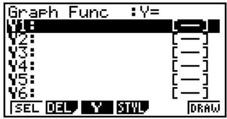
- Input the function you want to graph.
- To input a function, use the ▲ and ▼ cursor keys to move the highlighting to the line where you want to input it, and then use the calculator keys for input. Press EXE to store the function.
- On the graph function list, specify which functions you want to graph.
- Graphing is turned on for any function whose “=” symbol is highlighted. To toggle graphing of a function on or off, use the ▲ and ▼ cursor keys to move the highlighting to the function, and then press F1(SEL).
- After the graph function list settings are configured the way you want, press F6 (DRAW).
- This overlays graphs of all the functions for which graphing is turned on, over the graph that was originally on the graph screen.
scatter
| Time | MIC:Sound US Ksec | |-------|-------------------| | 9600 | -0.082 | | 12900 | -0.239 | | 16200 | 0.075 |Original Graph

line
| Time | Value | |-------|--------| | 9600 | 0.075 | | 12900 | -0.239 | | 16200 | 0.075 |Overlaid with Y=f(x) Graph
- To delete the overlaid graph, press SHIFT F4 (SKTCH) and then F1 (Cls).
Important!
- The screenshot shown in step 4 above is of a function that was calculated and stored by performing regression on a graph that was drawn using sampled data. Note that overlaying a Y = f(x) graph on a sampled data graph does not automatically draw a regression graph based on sampled data.
■ Working with Multiple Graphs
The procedures in this section explain how you can zoom or move a particular graph when there are multiple graphs on the display.
- To zoom a particular graph on a multi-graph display
- When the graph screen contains multiple graphs, press OPTN, and then F3 (EDIT).
- The [EDIT] menu appears at the bottom of the display.
line
| Time | Value | |-------|---------| | 62900 | 0.0399 | | 65650 | -0.034 | | 68400 | -0.108 |- Press F1 (ZOOM).
- This displays only one of the graphs that were originally on the graph screen.
line
| Time | Value | | ------ | --------- | | 62900 | -0.108 | | 65650 | 0.0399 | | 68400 | -0.108 |- Use the ▲ and ▼ cursor keys to cycle through the graphs until the one you want is displayed, and then press EXE.
- This enters the zoom mode and causes all of the graphs to reappear, along with a magnifying glass cursor ( _n ) in the center of the screen.
line
| Time | SND1Sound US Psec | | ------ | ----------------- | | 62900 | -0.173 | | 65650 | 0.152 | | 68400 | -0.01 |-
Use the cursor keys to move the magnifying glass cursor to the location on the screen that you want at the center of the enlarged or reduced screen.
-
Press EXE.
-
This causes the magnifying glass to disappear and enters the zoom mode.
- The cursor keys perform the following operations in the zoom mode.
| To do this: | Press this cursor key: |
| Enlarge the graph image horizontally | |
| Reduce the size of the graph image horizontally | |
| Enlarge the graph image vertically | |
| Reduce the size of the graph image vertically |
line
| Time | SND1:Sound US kSec | | ------ | ------------------ | | 62900 | 0.152 | | 65650 | -0.01 | | 68400 | -0.173 |
line
| Time | Value | | ------ | ------- | | 63700 | -0.137 | | 64500 | 0.0465 | | 65300 | -0.045 |- To exit the zoom mode, press EXIT.
- To move a particular graph on a multi-graph display
- When the graph screen contains multiple graphs, press OPTN, and then F3(EDIT).
- This displays the [EDIT] menu.
- Press F2 (MOVE).
- This displays only one of the graphs that were originally on the graph screen.
- Use the ▲ and ▼ cursor keys to cycle through the graphs until the one you want is displayed, and then press EXE.
- This enters the move mode and causes all of the graphs to reappear.
- Use the ◀ and ▶ cursor keys to move the graph left and right, or the ▲ and ▼ cursor keys to move the graph up and down.
line
| Time | Value | | ------ | ------- | | 63700 | -0.137 | | 64500 | 0.0465 | | 65300 | -0.137 |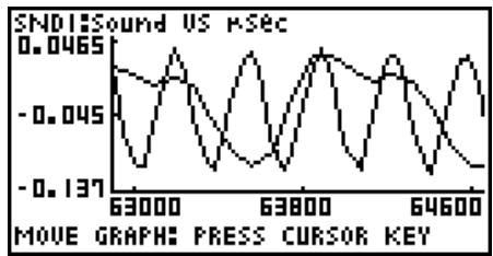
line
| Time | Value | | ------ | ------ | | 63000 | 0.0465 | | 63800 | -0.045 | | 64600 | -0.137 |- To exit the move mode, press EXIT.
■ Outputting a Specific Range of a Graph from the Speaker
Use the following procedure to output a specific range of a sound data waveform graph from the speaker.
- To output a graph from the speaker
- On the graph screen, press OPTN, and then F4 (SPKR).
- This displays the trace pointer for selecting the range on the graph.
![SELECT START POINT, PRESS [EXE]. 1701RSec -0.025Sound](/content/2025/01/86832/images/0ededca5d709996bb7033ad05aae21edd48debc977ab0a1b696636ddbcb22b97.jpg)
-
Move the trace pointer to the start point of the range you want to output from the speaker, and then press EXE.
-
Move the trace pointer to the end point of the range you want to output from the speaker, and then press EXE.
- After you specify the start point and end point, an output frequency dialog box shown below appears on the display.
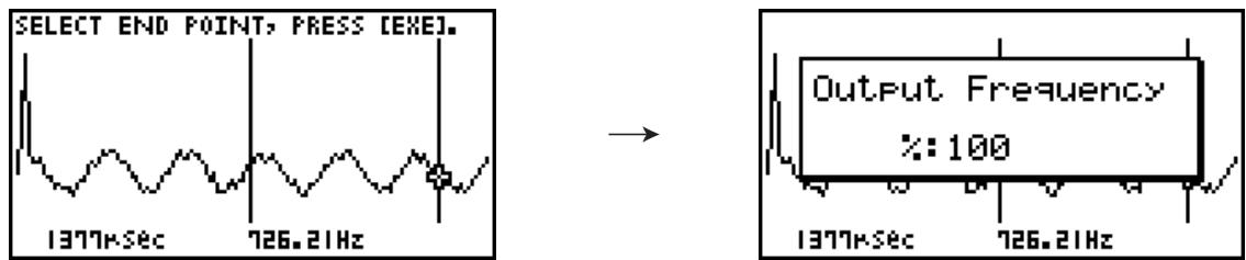
line
| Time (sec) | Value | | ---------- | ----- | | 1377 | 1377 | | 726 | 726 |- Input a percent value for the output frequency value you want.
- The output frequency specification is a percent value. To output the original sound as-is, specify 100%. To raise the original sound by one octave, input a value of 200%. To lower the original sound by one octave, input a value of 50%.
-
After inputting an output frequency value, press EXE.
-
This outputs the waveform between the start point and end point from the EA-200 speaker.
-
If the sound you configured cannot be output for some reason, the message “Range Error” will appear. If this happens, press EXIT to scroll back through the previous setting screens and change the setup as required.
-
To terminate sound output, press the EA-200 [START/STOP] key.
-
Press EXE.
- This displays a screen like the one shown below.
![Try Again? Yes: [F1] No : [F6]](/content/2025/01/86832/images/0058b83017041e8f4256cf7199a08c92240c625c372e590279b49dbd73dc274f.jpg)
- If you want to retry output from the speaker, press F1(Yes). To exit the procedure and return to the graph screen, press F6(No).
- Pressing F1 (Yes) returns to the "Output Frequency" dialog box. From there, repeat the above steps from step 4.
■ Configuring View Window Parameters
Pressing SHIFT F3 (V-Window) while the graph screen is on the display displays a View Window function key menu along the bottom of the display.
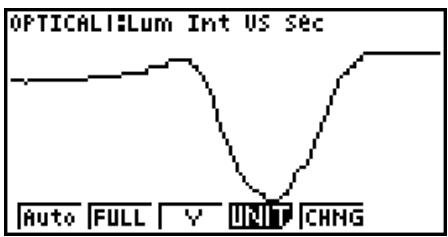
Press the function key that corresponds to the View Window parameter you want to configure.
| Function Key | Description |
| F1 (Auto) | Automatically applies the following View Window parameters.Y-axis Elements: In accordance with screen sizeX-axis Elements: In accordance with screen size when 1 data item equals 1 dot; 1 data equals 1 dot in other cases |
| F2 (FULL) | Resizes the graph so all of it fits in the screen. |
| F3 (Y) | Resizes the graph so all of it fits in the screen along the Y-axis, without changing the X-axis dimensions. |
| F4 (UNIT) | Specifies the unit of the numeric axis grid displayed by the Econ Axes setting of the graph setup screen (page 3-13).F1(μ sec): microsecondsF2(msec): millisecondsF3(sec): secondsF4(DHMS):days, hours, minutes, seconds (1 day, 2 hours, 30 minutes, 5 seconds = 1d2h30m5s)F5(Auto):Auto selection |
| F5 (CHNG) | Toggles display of the source data on the graph screen on and off. |
To exit the View Window function key menu and return to the standard function key menu, press EXIT.
12 Calling E-CON2 Functions from an eActivity
You can call E-CON2 functions from an eActivity by including an “Econ strip” in the eActivity file. The following describes each of the four available Econ strips.
- Econ SetupWizard strip
This strip calls the E-CON2 Setup Wizard. The Econ Setup Wizard strip makes it possible to perform the following series of operations from the eActivity: EA-200 setup using the Setup Wizard → Sampling → Graphing.
- Econ AdvancedSetup strip
This strip calls the E-CON2 Advanced Setup screen. The Advanced Setup provides access to almost all executable functions (except for the program converter), including detailed EA-200 setup and sampling execution; graphing and Graph Analysis Tools; simultaneous sampling with multiple sensors using the MULTIMETER Mode, etc.
- Econ Sampling strip
This strip records on set of EA-200 setup information configured using Advanced Setup, and performs sampling. Once setup information is recorded to this type of strip, sampling starts immediately based on the recorded setup information the next time the strip is executed.
- Econ Graph strip
This strip graphs sampled data that is recorded in the strip. The sampled data is recorded to the strip the first time the strip is executed.
This section explains how to insert each type of Econ strip into an eActivity file, and how to use inserted Econ strips. For details about eActivity operations, see “Chapter 10 eActivity” in the manual that comes with the fx-9860G SD or fx-9860G.
■ Inserting an Econ Strip into an eActivity File
The following procedure assumes that the eActivity file into which you want to insert the Econ strip is already open. For information about creating a new file and other basic eActivity operations, see “Basic eActivity File Operation” (page 10-1-5) in the manual that comes with the fx-9860G SD or fx-9860G.
- To insert an Econ Strip into an eActivity file
-
On the eActivity workspace screen, move the cursor the location where you want to insert the Econ strip.
-
Press F2 (STRP).
- This will display a dialog box with a list of insertable strips.
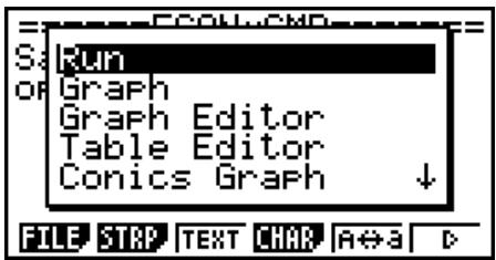
- Use ▲ and ▼ to move the highlighting to the type of Econ strip you want to insert.
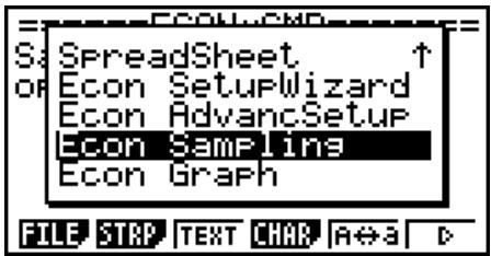
- See the beginning of this section (page 12-1) for details about each Econ strip type.
- Press EXE.
- The strip is inserted above the line or the strip where the cursor is currently located.
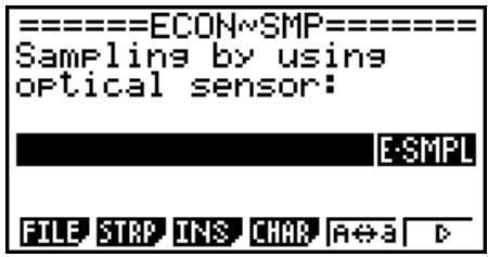
-
Enter up to 16 characters for the strip title.
-
Press EXE to assign the title to the strip.
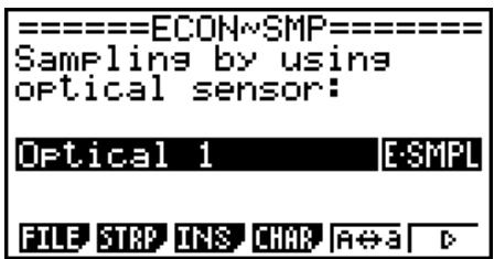
• This will highlight the strip.
- You can execute the strip here by pressing EXE. For details about operations that are required when you execute a strip, see “Calling an E-CON2 Function from an Econ Strip” below.
■ Calling an E-CON2 Function from an Econ Strip
This section explains operations for each type of Econ strip that can be inserted into an eActivity file. The following procedure assumes that the applicable Econ strip has already been inserted into an eActivity that is currently open.
- To access the Setup Wizard from an Econ SetupWizard strip
- On the eActivity workspace screen, use the ⬆ and ⬇ keys to move the highlighting to the Econ SetupWizard strip.
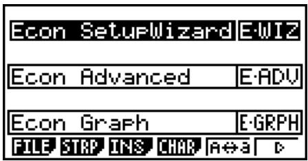
- Press EXE.
- This launches the Setup Wizard and displays the “Select Sensor” screen.
![Select Sensor CASIO :[F1] VERNIER:[F2]](/content/2025/01/86832/images/589ade70d5a49c5664b0fc77c7f4d93bf4463c90f1ad99ba44459a11d07e9cf7.jpg)
- Perform the procedure under "To configure an EA-200 setup using Setup Wizard" (page 2-2) from step 3 to set up the EA-200 and execute sampling.
Note
- In the case of the Econ SetupWizard strip, only the “1: Start Setup” is available on the “Complete!” dialog box. Other options are not available.

- To return to the eActivity workspace screen, press SHIFT → (→) EXIT.
- To access Advanced Setup from an Econ Advanced Setup strip
-
On the eActivity workspace screen, use the ⬆ and ⬇ keys to move the highlighting to the Econ Advanced Setup strip.
-
Press EXE.
- This displays the Advanced Setup screen.
![Advanced Setup for EXPERT [1]: Channel [2]: Sample [3]: Trigger [4]: Graph [5]: Custom Probe [6]: Initialize START MLTI MEM PROC GRAPH RET](/content/2025/01/86832/images/14375342b5a77d50e30d84b8a3b91cbe8b6f9eef553be0c9e01af24ce59434c2.jpg)
- From here, perform the procedure under “To configure an EA-200 setup using Advanced Setup” (page 3-1) from step 4.
- To return to the eActivity workspace screen after you finished the procedure or at any point during the procedure, press SHIFT → (☐).
Note
- Using an Econ Advanced Setup strip to configure a setup causes the setup information to be registered in the applicable strip. This means that the next time you open the strip, sampling can be performed in accordance with the previously configured setup information.
- To execute sampling from an Econ Sampling strip
- On the eActivity workspace screen, use the ⬆ and ⬇ keys to move the highlighting to the Econ Sampling strip.

- Press EXE.
- This displays a sampling start confirmation screen.
![====== EA-200 ==== *IS THE SENSOR CONNECTED? *CONNECT LINK-CABLE FIRMLY? *IS SAMPLING DONE? Press: [EXE]](/content/2025/01/86832/images/f33e3e4744923bd048986c0d3d03836d0645ac6c3d568fc96f3d8d87d8a50f43.jpg)
- If this is the first time you are using this Econ Sampling strip for sampling, continue on to step 3.
-
If this is an Econ Sampling strip that you have used for sampling in the paste and want to re-execute with the same setup, jump to step 8.
-
Press SHIFT 🔍 (☐) to display the application list.
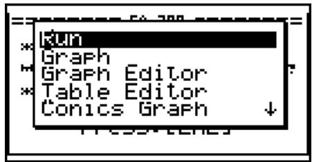
- Use the ▲ and ▼ cursor keys to move the highlighting to “Econ AdvancSetup”, and then press EXE.
- This displays the Advanced Setup screen.
-
Perform steps 4 and 5 under "To configure an EA-200 setup using Advanced Setup (page 3-1) to configure the setup for sampling.
-
Press SHIFT 🔍 (☐) to display the application list.
-
Use the ▲ and ▼ cursor keys to move the highlighting to “Econ Sampling”, and then press EXE.
- This will return to the sampling start confirmation screen in step 2 of this procedure.
8. Press EXE.
- This will set up the EA-200 in accordance with the setup data registered in the Econ Sampling strip. The message “Start sampling?” appears on the screen after EA-200 set up is complete.
9. Press EXE to start sampling.
- The screens that appear while sampling is in progress and after sampling is complete depend on setup details. For more information, see “Starting a Sampling Operation” (page 8-1). - After sampling is complete, the data will be graphed in accordance with the setup settings.
- To return to the eActivity workspace screen from the graph screen, press SHIFT → (💡).
- To graph sampled data from an Econ Graph strip
- On the eActivity workspace screen, use the ⬆ and ⬇ keys to move the highlighting to the Econ Graph strip.
2. Press EXE.
- If this Econ Graph strip already has sampled data registered to it because of a previous execution, a graph of the existing data will appear on the display. In this case, jump to step 5 of this procedure. - If this is the first time you are executing this Econ Graph strip, the Advanced Setup screen will appear on the display. If this happens, proceed with step 3 of this procedure.
- Perform steps 4 and 5 under "To configure an EA-200 setup using Advanced Setup (page 3-1) to configure the setup for sampling.
4. Press F1 (STRT).
- As instructed by the message that appears on the display, press the EXE key to perform sampling. - After sampling is complete, the data will be graphed in accordance with the setup settings.
- To return to the eActivity workspace screen from the graph screen, press SHIFT → (💡).
- Econ Strip Memory Capacity Precautions
- The memory capacity of each Econ strip is 25 KB. An error will occur if you perform an operation that causes this capacity to be exceeded. Particular care is required when handling a large number of samples, which can cause memory capacity to be exceeded.
- Always make sure that FFT Graph is turned off whenever performing sampling with the microphone. Leaving FFT Graph turned on cause memory capacity to be exceeded.
- If an error occurs, press SHIFT → (☐) to return to the eActivity workspace screen and perform the procedure again.
- For information about checking the memory usage of each strip, see “10-5 eActivity File Memory Usage Screen” in the manual that comes with the fx-9860G SD or fx-9860G.

Responsible within the European Union:
CASIO EUROPE GmbH
Casio-Platz 1
22848 Norderstedt, Germany

This mark applies in EU countries only.
CASIO®
CASIO COMPUTER CO., LTD.
6-2, Hon-machi 1-chome Shibuya-ku, Tokyo 151-8543, Japan
One or more of the following patents may be used in the product. U.S.Pats. 5,166,897 5,210,708 5,535,317 5,539,867
- Getting Acquainted — Read This First!
- Chapter 1 Basic Operation
- Chapter 2 Manual Calculations
- Chapter 3 List Function
- Chapter 4 Equation Calculations
- Chapter 5 Graphing
- Chapter 6 Statistical Graphs and Calculations
- Chapter 7 Financial Calculation (TVM)
- Chapter 8 Programming
- Chapter 9 Spreadsheet
- Chapter 10 eActivity
- Chapter 11 Memory Manager
- Chapter 12 System Manager
- Chapter 13 Data Communications
- Chapter 14 Using SD Cards (fx-9860GII SD only)
- Appendix
- E-CON2 Application
- ■ About this User's Guide
- - Model-specific Function and Screen Differences
- • Math natural input and display
- - For owners of models not equipped with a Math input/output mode (fx-7400GII, fx-9750GII)...
- - SHIFT x2 ( )
- - MENU EQUA
- • Function Keys and Menus
- - Menu Titles
- - Command List
- • E-CON2
- ■ Contrast Adjustment
- Keys
- ■ Key Markings
- Display
- ■ Selecting Icons
- - To select an icon
- ■ About the Function Menu
- ■ About Display Screens
- Normal Display
- - How to interpret exponential format
- ■ Special Display Formats
- Inputting and Editing Calculations
- ■ Inputting Calculations
- ■ Editing Calculations
- - To change a step
- - To delete a step
- - To insert a step
- ■ Using Replay Memory
- ■ Making Corrections in the Original Calculation
- ■ Using the Clipboard for Copy and Paste
- - To specify the copy range
- - To cut the text
- - Pasting Text
- ■ Catalog Function
- - To use the Catalog to input a command
- - To input a command with Ⓗ (fx-9860G Slim only)
- Press Ⓗ HELP.
- Using the Math Input/Output Mode
- Important!
- ■ Input Operations in the Math Input/Output Mode
- - Math Input/Output Mode Functions and Symbols
- • Using the MATH Menu
- - Math Input/Output Mode Input Examples
- - When the calculation does not fit within the display window
- - Math Input/Output Mode Input Restrictions
- - Using Values and Expressions as Arguments
- Example
- - Editing Calculations in the Math Input/Output Mode
- ■ Using Undoing and Redoing Operations
- ■ Math Input/Output Mode Calculation Result Display
- ■ History Function
- Example To change “1+2” to “1+3” and recalculate
- ■ Using the Clipboard for Copy and Paste in the Math Input/Output Mode
- - To copy text
- - To paste text
- ■ Calculation Operations in the Math Input/Output Mode
- - To input cell values
- Example To perform the calculation shown below
- ■ Using Graph Modes and the EQUA Mode in the Math Input/Output Mode
- - Math Input/Output Mode Input in the GRAPH Mode
- - Math Input/Output Mode Input and Result Display in the EQUA Mode
- Option (OPTN) Menu
- Variable Data (VARS) Menu
- • V-WIN — Recalling V-Window values
- • FACT — Recalling zoom factors
- • STAT — Recalling statistical data
- • GRPH — Recalling graph functions
- - DYNA\* — Recalling dynamic graph setup data
- - TABL — Recalling table setup and content data
- Program (PRGM) Menu
- Using the Setup Screen
- - To change a mode setup
- ■ Setup Screen Function Key Menus
- Using Screen Capture
- When you keep having problems...
- ■ Getting the Calculator Back to its Original Mode Settings
- - Restart
- - Reset
- ■ Low Battery Message
- Basic Calculations
- Arithmetic Calculations
- ■ Number of Decimal Places, Number of Significant Digits, Normal
- Display Range
- ■ Calculation Priority Sequence
- ■ Calculation Result Irrational Number Display
- - Calculation Result Display Range with
- Calculation Examples
- - Calculation Result Display Range with
- ■ Multiplication Operations without a Multiplication Sign
- ■ Overflow and Errors
- ■ Memory Capacity
- Special Functions
- ■ Memory
- • Variables (Alpha Memory)
- - To assign a value to a variable
- Example 2 To add 456 to variable A and store the result in variable B
- - To assign the same value to more than one variable
- Example To assign a value of 10 to variables A through F
- - String Memory
- Example To assign string “ABC” to Str 1 and then output Str 1 to the display
- - Function Memory
- - To store a function
- Example To store the function (A+B) (A-B) as function memory number 1
- - To recall a function
- Example To recall the contents of function memory number 1
- - To recall a function as a variable
- - To display a list of available functions
- - To delete a function
- Example To delete the contents of function memory number 1
- Answer Function
- - To use the contents of the answer memory in a calculation
- fx-7400GII, fx-9750GII users...
- fx-9860GII SD, fx-9860GII, fx-9860G AU PLUS, fx-9860G Slim users...
- ■ Performing Continuous Calculations
- Specifying the Angle Unit and Display Format
- ■ Setting the Angle Unit
- ■ Setting the Display Format
- - To specify the number of decimal places (Fix)
- Example To specify two decimal places
- - To specify the number of significant digits (Sci)
- Example To specify three significant digits
- - To specify the normal display (Norm 1/Norm 2)
- - To specify the engineering notation display (Eng mode)
- Function Calculations
- ■ Function Menus
- • Hyperbolic Calculations (HYP)
- - Probability/Distribution Calculations (PROB)
- - Numeric Calculations (NUM)
- - Angle Units, Coordinate Conversion, Sexagesimal Operations (ANGL)
- • Engineering Symbol (ESYM)
- Angle Units
- ■ Trigonometric and Inverse Trigonometric Functions
- ■ Logarithmic and Exponential Functions
- ■ Hyperbolic and Inverse Hyperbolic Functions
- ■ Other Functions
- - Random Number Generation (0 to 1) (Ran#, RanList#)
- - Random Integer Generation (RanInt#)
- - Random Number Generation in Accordance with Normal Distribution (RanNorm#)
- - Random Number Generation in Accordance with Binomial Distribution (RanBin#)
- ■ Coordinate Conversion
- ■ Permutation and Combination
- ■ Division Remainder (MOD), Remainder of Exponential Division (MOD Exp)
- Fractions
- ■ Engineering Notation Calculations
- ■ Logical Operators (AND, OR, NOT, XOR)
- - About Logical Operations
- Numerical Calculations
- ■ Quotient of Integer ÷ Integer
- ■ Remainder of Integer ÷ Integer
- ■ Simplification
- ■ Solve Calculations
- ■ Solving an f(x) Function
- Using Differential Calculation in a Graph Function
- Differential Calculation Precautions
- ■ Quadratic Differential Calculations
- Example To determine the quadratic differential coefficient at the point where
- Quadratic Differential Calculation Precautions
- ■ Integration Calculations
- Example To perform the integration calculation for the function shown below, with a tolerance of “tol” = 1_E - 4
- Integration Calculation Precautions
- ■ Σ Calculations
- Example To calculate the following:
- Σ Calculation Precautions
- - Minimum Value
- • Maximum Value
- Complex Number Calculations
- ■ Arithmetic Operations
- ■ Reciprocals, Square Roots, and Squares
- ■ Complex Number Format Using Polar Form
- ■ Absolute Value and Argument
- ■ Conjugate Complex Numbers
- ■ Extraction of Real and Imaginary Parts
- ■ Polar and Rectangular Form Transformation
- To transform the rectangular form of complex number 1 + 3 i to its polar form
- Binary, Octal, Decimal, and Hexadecimal Calculations with Integers
- ■ Selecting a Number System
- - To input values of mixed number systems
- ■ Negative Values and Bitwise Operations
- - Negative Values
- - Bitwise Operations
- ■ Number System Transformation
- - To convert a displayed value from one number system to another
- Example To convert 22_10 (default number system) to its binary or octal value
- About Matrix Answer Memory (MatAns)
- ■ Inputting and Editing Matrices
- - Creating a Matrix
- - To specify the dimensions (size) of a matrix
- - Deleting Matrices
- - To delete a specific matrix
- - To delete all matrices
- ■ Matrix Cell Operations
- - Row Calculations
- - To swap two rows
- - To calculate the scalar multiplication of a row
- - To calculate the scalar multiplication of a row and add the result to another row
- • To add two rows together
- Example To add row 2 to row 3
- - Row Operations
- - To delete a row
- Example To delete row 2
- - To insert a row
- Example To insert a new row between rows one and two
- - To add a row
- Example To add a new row below row 3
- - Column Operations
- - To delete a column
- ■ Modifying Matrices Using Matrix Commands
- - To display the matrix commands
- - Matrix Data Input Format
- - To input an identity matrix
- Example To create a 3 × 3 identity matrix as Matrix A
- • To check the dimensions of a matrix
- Example 1 To check the dimensions of Matrix A
- Example 2 To specify dimensions of 2 rows and 3 columns for Matrix B
- - Modifying Matrices Using Matrix Commands
- - To assign values to and recall values from an existing matrix
- Example 1 To assign 10 to the cell at row 1, column 2 of the following matrix:
- Example 2 Multiply the value in the cell at row 2, column 2 of the above matrix by 5
- - To fill a matrix with identical values and to combine two matrices into a single matrix [OPTN]-[MAT]-[Fill]
- Example 1 To fill all of the cells of Matrix A with the value 3
- Example 2 To combine the following two matrices:
- - To assign the contents of a matrix column to a list
- Example To assign the contents of column 2 of the following matrix to list 1:
- ■ Matrix Calculations
- - Matrix Arithmetic Operations
- - Determinant
- - Matrix Transposition
- - Row Echelon Form
- - Reduced Row Echelon Form
- - Matrix Inversion
- - Squaring a Matrix
- • Raising a Matrix to a Power
- - Determining the Absolute Value, Integer Part, Fraction Part, and Maximum Integer of a Matrix [OPTN]-[NUM]-[Abs]/[Frac]/[Int]/[Intg]
- - Complex Number Calculations with a Matrix
- Matrix Calculation Precautions
- Metric Conversion Calculations
- ■ Performing a Unit Conversion Calculation
- Example 1 To convert 50cm to inches
- Example 2 To convert \175, 162, 180\ centimeters to feet
- Inputting and Editing a List
- - To input values one-by-one
- - To batch input a series of values
- ■ Editing List Values
- • To change a cell value
- • To edit the contents of a cell
- - To delete a cell
- - To delete all cells in a list
- - To insert a new cell
- ■ Naming a List
- - To name a list
- ■ Sorting List Values
- - To sort a single list
- Ascending order
- Descending order
- - To sort multiple lists
- Manipulating List Data
- ■ Accessing the List Data Manipulation Function Menu
- - To count the number of data items in a list
- - To create a list by specifying the number of data items
- - To replace all data items with the same value
- - To generate a sequence of numbers
- - To find the minimum value in a list
- - To find which of two lists contains the greatest value
- - To calculate the mean of data items
- - To calculate the median of data items of specified frequency
- Example To calculate the median of values in List 1 (36, 16, 58, 46, 56), whose frequency is indicated by List 2 (75, 89, 98, 72, 67)
- - To combine lists
- Example To combine the List 1 (-3, -2) and List 2 (1, 9, 10)
- - To calculate the sum of data items in a list
- Example To calculate the sum of data items in List 1 (36, 16, 58, 46, 56)
- - To calculate the product of values in a list
- Example To calculate the product of values in List 1 (2, 3, 6, 5, 4)
- Arithmetic Calculations Using Lists
- ■ Error Messages
- ■ Inputting a List into a Calculation
- - To specify the list number of a list created with List Editor
- - To specify the sub name of a list created with List Editor
- - To directly input a list of values
- - To assign the contents of one list to another list
- - To recall the value in a specific list cell
- - To input a value into a specific list cell
- ■ Recalling List Contents
- ■ Graphing a Function Using a List
- ■ Inputting Scientific Calculations into a List
- ■ Performing Scientific Function Calculations Using a List
- Switching Between List Files
- - To switch between list files
- Simultaneous Linear Equations
- High-order Equations from 2nd to 6th Degree
- Solve the equations.
- Example To solve the cubic equation (Angle unit = Rad)
- Solve Calculations
- Sample Graphs
- ■ How to draw a simple graph (1)
- ■ How to draw a simple graph (2)
- Draw the graph.
- Controlling What Appears on a Graph Screen
- ■ V-Window (View Window) Settings
- - To make V-Window settings
- Rectangular coordinate parameter
- Polar coordinate parameter
- • V-Window Setting Precautions
- ■ V-Window Memory
- - To store V-Window settings
- - To recall V-Window memory settings
- ■ Specifying the Graph Range
- Zoom
- Drawing a Graph
- ■ Specifying the Graph Type
- ■ Storing Graph Functions
- - To store a parametric function
- - To create a composite function
- - To assign values to the coefficients and variables of a graph function
- ■ Editing and Deleting Functions
- • To edit a function in memory
- - To change the line style of a graph function
- - To change the type of a function \*1
- ■ Selecting Functions for Graphing
- - To specify the draw/non-draw status of a graph
- ■ Graph Memory
- - To store graph functions in graph memory
- • To recall a graph function
- Storing a Graph in Picture Memory
- - To store a graph in picture memory
- - To recall a stored graph
- Drawing Two Graphs on the Same Screen
- ■ Copying the Graph to the Sub-screen
- - Main Screen
- - Sub-screen
- - To copy the graph to the sub-screen
- Example Graph y = x(x + 1)(x - 1) in the main screen and sub-screen.
- Manual Graphing
- ■ Rectangular Coordinate Graph
- ■ Drawing Multiple Graphs on the Same Screen
- ■ Using Copy and Paste to Graph a Function
- Type 1 (Y= expression)
- Type 2 (expression)
- - To graph a function using copy and paste
- Using Tables
- ■ Storing a Function and Generating a Number Table
- - Variable Specifications
- - Table range method
- - List
- - To generate a table using a table range
- - To generate a table using a list
- - Generating a Table
- - To generate a differential number table
- - Specifying the Function Type
- ■ Editing Tables
- ■ Copying a Table Column to a List
- - To copy a table to a list
- ■ Drawing a Graph from a Number Table
- ■ Simultaneously Displaying a Number Table and Graph
- Example Store the function Y_1 = 3x2 - 2 and simultaneously display its number table and line graph. Use a table range of -3 to 3 with an increment of 1.
- Dynamic Graphing
- ■ Using Dynamic Graph
- ■ Drawing a Dynamic Graph Locus
- ■ Graph Calculation DOT Switching Function
- ■ Using Dynamic Graph Memory
- - To save data in Dynamic Graph memory
- - To recall data from Dynamic Graph memory
- Graphing a Recursion Formula
- ■ Generating a Number Table from a Recursion Formula
- ■ Graphing a Recursion Formula
- ■ Graphing a Phase Plot from Two Numeric Sequences
- ■ WEB Graph (Convergence, Divergence)
- Graphing a Conic Section
- ■ Graphing a Conic Section
- Changing the Appearance of a Graph
- ■ Drawing a Line
- Function Analysis
- ■ Reading Coordinates on a Graph Line
- ■ Displaying the Derivative
- ■ Graph to Table
- ■ Coordinate Rounding
- ■ Calculating the Root
- ■ Calculating the Point of Intersection of Two Graphs
- Example Graph the two functions shown below, and determine the point of intersection between Y1 and Y2.
- ■ Determining the Coordinates for Given Points
- ■ Calculating the Integral Value for a Given Range
- ■ Conic Section Graph Analysis
- • Parabolic Graph Analysis
- • Circular Graph Analysis
- - Elliptical Graph Analysis
- • Hyperbolic Graph Analysis
- - To calculate the focus and length of latus rectum
- • To calculate the center
- Before Performing Statistical Calculations
- ■ Changing Graph Parameters
- General graph settings
- - Graph Type
- - Frequency
- - Mark Type
- - To display the general graph settings screen
- • StatGraph (statistical graph specification)
- • Graph Type (graph type specification)
- - XList (x-axis data list)/YList (y-axis data list)
- • Frequency (number of times a value occurs)
- • Mark Type (plot mark type)
- When “Pie” (pie graph) is selected as the Graph Type:
- - Data (Specifies the list to be used as graph data.)
- Graph draw/non-draw status
- Calculating and Graphing Single-Variable Statistical Data
- ■ Normal Probability Plot
- Pie Graph
- Histogram
- ■ Med-box Graph
- Bar Graph
- ■ Normal Distribution Curve
- ■ Broken Line Graph
- ■ Displaying the Calculation Results of a Drawn Single-Variable Graph
- ■ Calculation Methods for the Std and OnData Settings
- - Std
- - OnData
- Calculating and Graphing Paired-Variable Statistical Data
- ■ Drawing a Scatter Diagram and xy Line Graph
- Example Input the two sets of data shown below. Next, plot the data on a scatter diagram and connect the dots to produce an xy line graph.
- ■ Drawing a Regression Graph
- ■ Selecting the Regression Type
- ■ Displaying Regression Calculation Results
- ■ Graphing Statistical Calculation Results
- ■ Linear Regression Graph
- ■ Med-Med Graph
- ■ Quadratic/Cubic/Quartic Regression Graph
- Quadratic regression
- Cubic regression
- Quartic regression
- ■ Logarithmic Regression Graph
- ■ Exponential Regression Graph
- ■ Power Regression Graph
- ■ Sinusoidal Regression Graph
- ■ Logistic Regression Graph
- ■ Residual Calculation
- ■ Displaying the Calculation Results of a Drawn Paired-Variable Graph
- ■ Copying a Regression Graph Formula to the GRAPH Mode
- Performing Statistical Calculations
- - To specify statistical calculation data lists
- ■ Single-Variable Statistical Calculations
- ■ Paired-Variable Statistical Calculations
- ■ Regression Calculation
- Example To display single-variable regression parameters
- - Calculation of the Coefficient of Determination (r2) and MSe
- • Estimated Value Calculation for Regression Graphs
- - Regression Formula Copy Function from a Regression Calculation Result Screen
- ■ Estimated Value Calculation ( x, y )
- ■ Normal Probability Distribution Calculation
- Standard Normal Distribution
- ■ Drawing a Normal Probability Distribution Graph
- ■ Calculations Using the Distribution Function
- ■ Determining Standard Deviation and Variance from List Data
- ■ Calculations Using the TEST Command
- Tests
- Z Tests
- • Z Test Common Functions
- • 1-Sample Z Test
- • 2-Sample Z Test
- • 1-Prop Z Test
- - 2-Prop Z Test
- ■ t Tests
- - t Test Common Functions
- • 1-Sample t Test
- - 2-Sample t Test
- - LinearReg t Test
- ■ 2 Test
- - 2 Test Common Functions
- - 2 GOF Test ( 2 one-way Test)
- - 2 two-way Test
- Calculation Result Output Example
- ■ 2-Sample F Test
- ANOVA
- ■ ANOVA (Two-Way)
- - Description
- - Solution
- - Input Example
- - Results
- Confidence Interval
- - General Confidence Interval Precaution
- • 1-Sample Z Interval
- • 2-Sample Z Interval
- • 1-Prop Z Interval
- - 2-Prop Z Interval
- ■ t Interval
- • 1-Sample t Interval
- • 2-Sample t Interval
- Distribution
- ■ Common Distribution Functions
- ■ Normal Distribution
- • Normal Probability Density
- • Normal Cumulative Distribution
- - Inverse Normal Cumulative Distribution
- ■ Student-t Distribution
- - Student- t Probability Density
- - Student- t Cumulative Distribution
- - Inverse Student- t Cumulative Distribution
- ■ 2 Distribution
- - 2 Probability Density
- - 2 Cumulative Distribution
- - Inverse 2 Cumulative Distribution
- ■ F Distribution
- - F Probability Density
- • F Cumulative Distribution
- - Inverse F Cumulative Distribution
- Binomial Distribution
- - Binomial Probability
- • Binomial Cumulative Distribution
- • Inverse Binomial Cumulative Distribution
- ■ Poisson Distribution
- - Poisson Probability
- - Poisson Cumulative Distribution
- - Inverse Poisson Cumulative Distribution
- ■ Geometric Distribution
- - Geometric Probability
- - Geometric Cumulative Distribution
- - Inverse Geometric Cumulative Distribution
- ■ Hypergeometric Distribution
- • Hypergeometric Probability
- • Hypergeometric Cumulative Distribution
- - Inverse Hypergeometric Cumulative Distribution
- Input and Output Terms of Tests, Confidence Interval, and Distribution (All models except fx-74000)
- ■ Input Terms
- Output Terms
- Statistic Formula
- ■ Distribution (Discrete)
- Before Performing Financial Calculations
- Setup Items
- ■ Graphing in the TVM Mode
- Simple Interest
- - Formula
- Compound Interest
- Inputting Values
- Precision
- Cash Flow (Investment Appraisal)
- Amortization
- - Converting between the nominal interest rate and effective interest rate
- Interest Rate Conversion
- Cost, Selling Price, Margin
- Day/Date Calculations
- • 360-day Date Mode Calculations
- Depreciation
- - Straight-Line Method (SL)
- • Fixed-Percentage Method (FP)
- - Sum-of-the-Years’-Digits Method (SYD)
- - Declining-Balance Method (DB)
- Calculation Result Output Examples
- Bond Calculations
- • Price per \$100 of face value (PRC)
- • Annual Yield (YLD)
- MEMO Screen
- Financial Calculations Using Functions
- Example To calculate the total interest and principal paid for a 2-year (730-day) \$300 loan at a simple annual interest rate of 5%. Use a Date Mode setting of 365.
- Basic Programming Steps
- PRGM Mode Function Keys
- - When you are registering a file name
- - When you are inputting a program — F1(RUN) ... default
- Editing Program Contents
- ■ Debugging a Program
- - To eliminate bugs that cause error messages
- - To eliminate bugs that cause bad results
- ■ Searching for Data Inside a Program
- Example To search for the letter “A” inside the program named OCTA
- File Management
- ■ Searching for a File
- - To find a file using initial character search
- Example To use initial character search to recall the program named OCTA
- ■ Editing a File Name
- ■ Deleting a Program
- - To delete a specific program
- - To delete all programs
- ■ Registering a password
- ■ Recalling a Password Protected Program
- Command Index
- ■ Basic Operation Commands
- ? (Input Command)
- Example: ? → A
- Description:
- ▲ (Output Command)
- : (Multi-statement Command)
- ← (Carriage Return)
- ' (Comment Text Delimiter)
- ■ Program Commands (COM)
- If\~Then\~(Else\~)IfEnd
- Syntax:
- For\~To\~(Step\~)Next
- Parameters:
- Do\~LpWhile
- Parameters: expression
- While\~WhileEnd
- ■ Program Control Commands (CTL)
- Break
- Syntax: Break
- Prog
- Return
- Stop
- ■ Jump Commands (JUMP)
- Dsz
- Goto\~Lbl
- lsz
- Menu
- ■ Clear Commands (CLR)
- ClrGraph
- ClrList
- ClrMat
- ClrText
- ■ Display Commands (DISP)
- DrawDyna
- DrawGraph
- No parameters
- DrawR-Con, DrawR-Plt
- (Not included on the fx-7400GII)
- DrawRΣ-Con, DrawRΣ-Plt
- DrawStat
- DrawWeb
- ■ Input/Output Commands (I/O)
- Getkey
- Locate
- Example: Cls
- Receive( / Send(
- OpenComport38k / CloseComport38k
- Receive38k / Send38k
- ■ Conditional Jump Relational Operators (REL)
- ■ Strings
- Exp(
- Exp▶Str(
- StrCmp(
- StrInv(
- StrJoin(
- StrLeft(
- StrLen(
- StrLwr(
- StrMid(
- StrRight(
- StrRotate(
- StrShift(
- StrSrc(
- StrUpr(
- Other
- RclCapt
- Using Calculator Functions in Programs
- ■ Text Display
- ■ Using Matrix Row Operations in a Program
- - To calculate a scalar multiplication (\* Row)
- Example 2 To calculate the product of Row 2 of the matrix in Example 1 and the scalar 4
- - To calculate a scalar multiplication and add the results to another row (\*Row+)
- Example 3 To calculate the product of Row 2 of the matrix in Example 1 and the scalar 4, then add the result to row 3
- - To add two rows (Row+)
- Example 4 To add Row 2 to Row 3 of the matrix in Example 1
- ■ Using Graph Functions in a Program
- - Syntax of other graphing functions
- ■ Using Dynamic Graph Functions in a Program
- ■ Using Table & Graph Functions in a Program
- ■ Using Recursion Table & Graph Functions in a Program
- ■ Using List Sort Functions in a Program
- ■ Using Statistical Calculations and Graphs in a Program
- - To set conditions and draw a statistical graph
- ■ Using Distribution Graphs in a Program
- - To draw a normal cumulative distribution graph
- - To draw a Student- t cumulative distribution graph
- • To draw a 2 cumulative distribution graph
- - To draw an F cumulative distribution graph
- ■ Performing Statistical Calculations in a Program
- ■ Performing Distribution Calculations in a Program
- - Normal Distribution
- - Student- t Distribution
- - 2 Distribution
- - F Distribution
- - Binomial Distribution
- - Poisson Distribution
- - Geometric Distribution
- Syntax: GeoCD(X,P[])
- • Hypergeometric Distribution
- ■ Using the TEST Command to Execute a Command in a Program
- • Z Test
- - 2 Test
- - F Test
- • ANOVA
- ■ Performing Financial Calculations in a Program
- - Setup Commands
- • Financial Calculation Commands
- - Simple Interest
- - Compound Interest
- Note:
- • Cash Flow (Investment Appraisal)
- - Amortization
- - Interest Rate Conversion
- - Cost, Selling Price, Margin Calculations
- PRGM Mode Command List
- Program Library
- Program Name
- Prime Factorization
- Description
- Purpose
- Spreadsheet Basics and the Function Menu
- Edit box
- ■ Spreadsheet Screen Function Menu
- Basic Spreadsheet Operations
- ■ Spreadsheet File Operations
- - To create a new file
- - To open a file
- - Auto Save
- - To save a file under a new name
- - To delete a file
- ■ Recalculating All of the Formulas in the Currently Open Spreadsheet
- - Auto Calc
- - To execute spreadsheet re-calculation manually
- ■ Using the Cell Cursor
- - Using the JUMP Command to Move the Cell Cursor
- • To select a range of cells
- ■ Data (Constants, Text, Formula) Input Basics
- - To overwrite data currently in a cell with new data
- - To edit cell data
- - To move the cell cursor while inputting data into a cell
- ■ Inputting a Constant (Value, Calculation Result, Number Sequence) into a Cell
- - To input a number sequence automatically based on a function expression
- ■ Inputting Text into a Cell
- ■ Inputting a Formula into a Cell
- - Formula Input Example
- Procedure
- ■ Inputting a Cell Reference Name
- - To input a cell reference name using direct input
- - To input a cell reference name using the GRAB command
- ■ Relative and Absolute Cell Reference Names
- Relative Cell Reference Names
- Absolute Reference Names
- - To input the absolute cell reference name symbol (\$)
- ■ Copying and Pasting Cell Contents
- - To copy and paste spreadsheet data
- ■ Cutting and Pasting Cell Contents
- - To cut and paste spreadsheet data
- ■ Inputting the Same Formula into a Range of Cells
- - To input the same formula into a range of cells
- ■ Sorting Constant Data
- - To sort constant data
- ■ Deleting and Inserting Cells
- - To delete an entire line or column of cells
- - To delete the contents of all the cells in a spreadsheet
- - To insert a row or column of blank cells
- • To clear the contents of specific cells
- Using Special S·SHT Mode Commands
- ■ Special S·SHT Mode Command List
- ■ S·SHT Mode Command Example
- Drawing Statistical Graphs, and Performing Statistical and Regression Calculations
- ■ Example of Statistical Graph Operations (GRPH Menu)
- - To input data and draw a statistical graph (scatter plot)
- ■ General Graph Settings Screen Operations
- - To configure statistical graph settings
- ■ Example of Statistical Calculation Operation (CALC Menu)
- - To perform paired-variable statistical calculations and regression calculations
- ■ Using the Statistical Calculation Data Range Specification Screen
- - To specify the data range for statistical calculation
- ■ STAT Mode and S·SHT Mode Function Menu Correspondence Table
- S • SHT Mode Memory
- ■ Saving Spreadsheet Data to a Memory
- • Example: To store column data in list memory
- ■ Recalling Data from Memory to a Spreadsheet
- - Example: To recall data from a matrix memory to a spreadsheet
- eActivity Overview
- eActivity Function Menus
- ■ File List Function Menu
- ■ Workspace Screen Function Menu
- eActivity File Operations
- - To search for a file
- Inputting and Editing Data
- ■ Cursor Movement and Scroll Operations
- ■ Inputting into a Text Line
- - Inputting characters and expressions as text
- Move the cursor to a text line.
- Input the text or expression you want into the text strip.
- • Text Line Input and Editing Operations
- ■ Inputting into a Calculation Line
- - To input a calculation formula into an eActivity
- - Matrix Calculations Using the Matrix Editor
- - List Calculations Using the List Editor
- ■ Inserting a Calculation Stop Line
- - To insert a stop line
- ■ Using Strips
- - To insert a strip
- Press F2 (STRP).
- - Notes Strips
- • To change the title of a strip
- - To call an application from a strip
- - To switch from an application screen called up from a strip to another application screen
- - To display the strip memory usage screen
- - To delete a line or strip
- Saving a File
- - To replace the existing file with the new version
- ■ Displaying the eActivity Memory Usage Screen
- - To display the eActivity memory usage screen
- - To return to the file list from the workspace screen
- eActivity Guide (fx-9860G Slim only)
- Creating a Guide
- Running a Guide
- Three Types of Operation Patterns
- ■ Creating a Guide
- - To enter the guide creation mode
- Press F5 (GUIDE).
- - To create an n-key operation
- • To create a 1-key operation
- • To create an AUTO operation
- - To change the position of the comment box
- - To exit the guide creation mode
- ■ Editing a Guide
- ■ Editing the Guide You Are Creating
- - To display the key editing screen
- ■ Editing Example
- GRPHE
- - Running a Guide
- ■ eActivity Guide Editing Techniques
- fx-9860GII/fx-9860GII SD/fx-9860G AU PLUS/fx-9860G Slim
- Using the Memory Manager
- ■ Memory Information Screen
- ■ Creating a Folder in Storage Memory or on an SD Card
- - To create a new folder
- - To rename a folder
- ■ Selecting Data
- ■ Copying Data
- - To copy from main memory to storage memory
- Note
- ■ Error Checks During Data Copy
- Low battery check
- Available memory check
- Overwrite check
- Type mismatch error check
- - To delete a main memory file
- - To delete a storage memory file
- - To delete SD card files (fx-9860GII SD only)
- - To search for a file in the main memory
- Example To search for all files in the main memory whose names begin with the letter “R”
- - To search for a file in the storage memory
- Example To search for all files in the storage memory whose names begin with the letter “S”
- - To search for a file in the SD card (fx-9860GII SD only)
- Example To search for all files in the SD card whose names begin with the letter "R"
- ■ Backing Up Main Memory Data
- - To back up main memory data
- - To restore backup data to the main memory
- ■ Optimizing the Storage Memory or SD Card Memory
- - To optimize the storage memory
- Using the System Manager
- System Settings
- ■ Power Properties Settings
- - To specify the Auto Power Off trigger time
- ■ System Language Setting
- Version List
- - To display version information
- - To register a user name
- Reset
- Connecting Two Units
- - To connect two units
- Connecting the Calculator to a Personal Computer
- Performing a Data Communication Operation
- ■ Select Connection Mode Screen (All models except fx-7400GII)
- ■ Performing a Data Transfer Operation
- Receiving unit
- Sending unit
- - To execute a send operation
- - Configuring the Receiver’s Wakeup Feature
- fx-7400GII
- All models except fx-7400GII
- Data Communications Precautions
- ■ Exchanging Data with another Model Calculator
- - Transferring Data between the fx-9860GII SD, fx-9860GII, fx-9860G AU PLUS, fx-9750GII, fx-9860G Slim (OS 2.00), fx-9860G SD (OS 2.00), fx-9860G (OS 2.00), fx-9860G AU (OS 2.00) and fx-7400GII
- - Sending Data from an OS 2.00 Calculator to any Older Model Calculator
- Invalid Data Size
- Complex Number in data
- Invalid Data Number
- - Sending Data from an OS 2.00 Calculator to a CFX-9850G Series Calculator
- - Sending Data from an OS 2.00 Calculator to an fx-7400G Series Calculator
- - Sending Data from an fx-9860G Series Calculator to an OS 2.00 Calculator
- - Sending Data from a CFX-9850G Series Calculator to an OS 2.00 Calculator
- Screen Image Send
- ■ Transferring Screen Images to a Computer
- On the fx-7400GII
- On other models
- ■ Auto Screen Image Send to an OHP Unit (Not available on the fx-7400GII)
- ■ Auto Screen Image Send to a Computer Using the fx-9860G Manager PLUS (Not available on the fx-7400GII)
- ■ Connecting to a Projector (Not available on the fx-7400GII)
- - Connectable Projectors (As of January 2009)
- - To project calculator screen contents from a projector
- - Precautions when Connecting
- Using an SD Card
- - Removing the Dummy Card
- - To insert an SD card
- - To remove the SD card
- Formatting an SD Card
- SD Card Precautions during Use
- ■ Recommended SD Card Types
- E-CON2 Overview
- About online help
- Using the Setup Wizard
- ■ Setup Wizard Parameters
- Setup Wizard Rules
- - To configure an EA-200 setup using Setup Wizard
- Before getting started...
- ■ Using Setup Wizard to Configure Settings for FFT (Frequency Characteristics) Data Sampling
- ■ Using Setup Wizard to Configure a PhotoGate Setup
- - To configure a setup for PhotoGate alone
- - To configure a setup for PhotoGate and Smart Pulley
- ■ Outputting the Waveform of a Function through the Speaker
- - To configure a setup for speaker output
- To change the output frequency and try again:
- To change the output range of the waveform graph and try again:
- To change the function:
- To exit the procedure and return to the E-CON2 main menu:
- Using Advanced Setup
- ■ Advanced Setup Operations
- - To configure an EA-200 setup using Advanced Setup
- - To return setup parameters to their initial defaults
- Channel Setup
- - To configure Channel Setup settings
- Sample Setup
- - To configure Sample Setup settings
- - To configure the Distance setting
- - To configure the FFT Graph setting
- ■ Trigger Setup
- - To configure Trigger Setup settings
- - To specify the countdown start time
- - To specify microphone sensitivity
- - To specify the trigger threshold value and trigger edge type
- - To configure trigger threshold, trigger start edge, and trigger end edge settings
- - To configure PhotoGate trigger start and end settings
- - To specify the trigger threshold value and motion sensor level
- ■ Graph Setup
- - To configure Graph Setup settings
- Using a Custom Probe
- ■ Configuring a Custom Probe Setup
- - To configure a custom probe setup
- ■ Auto Calibrating a Custom Probe
- - To auto calibrate a custom probe
- If you are configuring a new custom probe:
- If you are editing the configuration of an existing custom probe:
- Press F2 (CALIB).
- ■ Zero Adjusting a Custom Probe
- - To zero adjust a custom probe
- ■ Managing Custom Probe Setups
- - To edit a custom probe setup
- - To delete a custom probe setup
- Using the MULTIMETER Mode
- - To use the MULTIMETER Mode
- Using Setup Memory
- ■ Saving a Setup
- - To save a setup
- ■ Using and Managing Setups in Setup Memory
- - To preview saved setup data
- - To recall a setup and use it for sampling
- - To change the name of setup data
- - To delete setup data
- - To recall setup data
- Using Program Converter
- ■ Converting a Setup to a Program
- - To convert a setup to a program
- ■ Converting a CFX-9850 Series Program to a fx-9860 Series Compatible Program
- - To convert a program
- Starting a Sampling Operation
- ■ Before getting started...
- ■ Starting a Sampling Operation
- - To start sampling
- - Operations during a sampling operation
- Using Sample Data Memory
- ■ Managing Sample Data Files
- - To save current sample data to a file
- - To rename an existing sample data file
- - To delete a sample data file
- Using the Graph Analysis Tools to Graph Data
- ■ Accessing Graph Analysis Tools
- ■ Selecting an Analysis Mode and Drawing a Graph
- - To select an analysis mode and draw a graph
- Graph Analysis Tool Graph Screen Operations
- ■ Graph Screen Key Operations
- ■ Scrolling the Graph Screen
- ■ Using Trace
- - To use trace
- - To obtain the periodic frequency value
- ■ Using Zoom
- - To zoom the graph screen
- Press EXE.
- To exit the zoom mode, press EXIT.
- ■ Transforming Sampled Data to List Data
- - To transform sampled data to list data
- ■ Using Fourier Series Expansion to Transform a Waveform to a Function
- - To perform Fourier series expansion
- ■ Performing Regression
- - To perform quadratic regression
- Press F6 (DRAW).
- ■ Overlaying a Y=f(x) Graph on a Sampled Result Graph
- - To overlay a Y=f(x) graph on an existing graph
- ■ Working with Multiple Graphs
- - To zoom a particular graph on a multi-graph display
- - To move a particular graph on a multi-graph display
- ■ Outputting a Specific Range of a Graph from the Speaker
- - To output a graph from the speaker
- ■ Configuring View Window Parameters
- Calling E-CON2 Functions from an eActivity
- - Econ SetupWizard strip
- - Econ AdvancedSetup strip
- - Econ Sampling strip
- - Econ Graph strip
- ■ Inserting an Econ Strip into an eActivity File
- - To insert an Econ Strip into an eActivity file
- ■ Calling an E-CON2 Function from an Econ Strip
- - To access the Setup Wizard from an Econ SetupWizard strip
- - To access Advanced Setup from an Econ Advanced Setup strip
- - To execute sampling from an Econ Sampling strip
- Press EXE.
- Press EXE to start sampling.
- - To graph sampled data from an Econ Graph strip
- Press EXE.
- Press F1 (STRT).
- - Econ Strip Memory Capacity Precautions
- CASIO®
- CASIO COMPUTER CO., LTD.
Brand : CASIO
Model : FX-7400GII
Category : Graphing calculator