SR-282 - Calculator CITIZEN - Free user manual and instructions

Product Type	Scientific Calculator
Brand	Citizen
Model	SR-282
Display	12-digit LCD
Power Source	Solar cell with battery backup (LR54)
Dimensions (W x H x D)	Approx. 80 x 145 x 12 mm
Weight	Approx. 85 g
Functions	Basic arithmetic, square root, percentage, memory, trigonometric, logarithmic, exponential, statistical
Key Features	Dual power, auto power-off, plastic keys, slide-on hard case
Operating Temperature	0°C to 40°C
Maintenance	Clean with a dry, soft cloth. Do not use solvents.
Safety	Keep away from moisture and heat. Do not disassemble.
Spare Parts / Repairability	Not user-serviceable. Contact authorized service center.
General Information	Citizen SR-282 is a basic scientific calculator suitable for students and professionals.

Frequently Asked Questions - SR-282 CITIZEN

How do I turn off the calculator?

The calculator automatically turns off after a period of inactivity (auto power-off). To manually turn off, press the OFF key if available.

What type of battery does the SR-282 use?

The calculator uses a solar cell with a backup battery. The battery is typically a LR54 or equivalent.

How to reset the calculator?

Press the RESET button on the back using a pointed object, or remove and reinsert the backup battery.

How to perform square root calculation?

Enter the number and press the √ key. For example, to calculate √25, press 2 5 then √.

The display shows 'E' or 'Error'. What should I do?

An error occurs if an operation is invalid (e.g., division by zero). Press AC or C to clear the error and start a new calculation.

How to use memory functions?

Use M+ to add to memory, M- to subtract, MR to recall, and MC to clear memory.

Why does the display seem dim?

Ensure there is sufficient light for the solar cell. If indoors, try a brighter location. The backup battery should still provide power.

How to calculate percentage?

To find 20% of 150, enter 150 × 20 then press the % key. The result will be 30.

Can I use the SR-282 for trigonometry?

Yes, it has sin, cos, tan functions. Ensure the angle mode (DEG/RAD/GRAD) is set correctly.

How to clean the calculator?

Use a soft, dry cloth. Do not use any liquid or chemical cleaners. Keep the calculator away from direct sunlight and moisture.

USER MANUAL SR-282 CITIZEN

Battery replacement....2

Auto power-off function.... 2

Reset operation 2

Contrast adjustment.... 3

Display readout.... 3

Before Starting Calculation ....4

Using "MODE" keys.... 4

Using "2nd" Keys....4

Corrections 4

Undo function ....4

Replay function.... 5

Memory calculation.... 5

Order of operations....6

Accuracy and Capacity....7

Error conditions 9

Basic Calculations ...... 9

Arithmetic calculation.... 10

Parentheses calculations.... 10

Percentage calculation 11

Display notations 11

Scientific Functional Calculations.... 13

Logarithms and Antilogarithms 13

Fraction calculation ....13

Angle unit conversions ....14

Sexagesimal Decimal transformation....15

Trigonometric / Inverse-Tri. functions 15

Hyperbolic / Inverse-Hyp. functions....16

Coordinates transformation 16

Probability....17

Other functions ( 1/x, √ 3√, x√, x², x³, x⁴, INT, FRAC )...... 18

Unit Conversion 19

Physics constants.... 19

Base-n calculations.... 24

Bases conversions ....25

Block Function 25

Basic arithmetic operations for bases.... 27

Negative expressions 27

Logical operation 27

Statistical Calculations ...... 27

Entering data 28

Displaying results 28

Deleting data ....31

Editing data.... 32

FULL message.... 32

Complex Calculations....33

General Guide

Turning on or off

To turn the calculator on, press [ON/C]; To turn the calculator off, press [2nd] [OFF].

Battery replacement

SR-281 is powered by two alkaline batteries (GP76A or LR44).

SR-282 is powered two AA-size (UM-3) batteries. If the display becomes dim and difficult to read, the batteries should be replaced as soon as possible.

1) Slide the battery compartment cover in the direction indicated by the arrow and remove it.
2) Remove the old batteries and install new ones with polarity in correct directions, then replace the battery compartment cover and press [ON/C].

Auto power-off function

This calculator automatically turns it off when not operated for approximately 6\~9 minutes. It can be reactivated by pressing [ON/C] key and the display, memory, settings are retained.

Reset operation

If the calculator is on but you get unexpected results, press [MODE] [4] (RESET) in sequence. A message appears on the display to confirm whether you want to reset the calculator and clear memory contents.

RESET: N Y

Move the cursor to "Y" by [→], then press [ENTER] to clear all variables, pending operations, statistical data, answers, all previous entries, and memory; To cancel the reset operation without clearing the calculator, please choose "N".

If the calculator is lock and further key operations becomes impossible, please press [0] [CE] at the same time to release the condition. It will return all settings to default settings.

Contrast adjustment

Pressing the [-] or [+] following [MODE] key can make the contrast of the screen lighter or darker. Holding either key down will make the display become respectively lighter or darker.

Display readout

The display comprises two lines and indicators. The upper line is a dot display up to 128 characters. The lower line is capable of displaying a result of up to 12 digits, as well as 2-digits positive or negative exponent.

When formulas are input and executed the calculation by [ ENTER _x they are displayed on the upper line, and then results are shown on the lower line.

The following indicators appear on the display to indicate you the current status of the calculator.

Indicator	Meaning
M	Running memory
- Result is negative
E	Error
STO	Storing variable mode is active
RCL	Recalling variable mode is active
2nd 2nd set of function keys are active
HYP	Hyperbolic-trig function will be calculated
ENG	Engineering symbol notation
CPLX	Complex number mode is active
CONST	Display physics constants
DEGRAD	Angle mode : DEGrees, GRADs, or RADs
BIN	Binary base
OCT	Octal base
HEX	Hexadecimal base
( )	Open parentheses
TAB	Number of decimal places displayed is fixed
STAT	Statistics mode is active
REG	Regression mode is active
EDIT	Statistics data is being edited
CPK	CPK : Process capability
	CP : Precision capability
USL	Set upper specification limit
LSL	Setting lower specification limit
i	Imaginary part
	Allow to use undo function

Before Starting Calculation

Using "MODE" keys

Press [ MODE ] to display mode menus when specifying an operating mode ( " 1 MAIN ", " 2 STAT ", " 3 CPLX ", " 4 RESET " ) or the engineering symbol notation ( " 5 ENG " ).

1 MAIN : Use this mode for basic calculations, including scientific calculations and Base-n calculations.
2 STAT : Use this mode to perform single-variable and paired-variable statistical calculations and regression calculations.
3 CPLX : Use this mode to perform complex number calculation.
4 RESET : Use this mode to perform reset operation.
5 ENG : Use this mode to allow engineering calculations utilizing engineering symbol.

Give " 2 STAT " as an example :

Method 1: Press [MODE] and then scroll through the menus using [→] or [2nd][←] until "2 STAT" is underlined, then enter the desired mode by pressing [ENTER]

Method 2 : Press [MODE] and then key in directly the number of the mode, [2], to enter the desired mode immediately.

Using "2nd" Keys

When you press [2nd], the "2nd" indicator shown in the display is to tell you that you will be selecting the second function of the next key you press. If you press [2nd] by mistake, simply press [2nd] again to remove the "2nd" indicator.

Corrections

If you have made a mistake when entering a number (but you have not yet pressed an arithmetic operator key), just press [ CE ] to clear the last entry then input it again, or delete individual digits by the backspace key [ →], or clear all entry by [ ON/C ].

After making corrections, input of the formula is complete, the answer can be obtained by pressing [ENTV] You can also press [ON/C] to clear the immediate results completely (except clearing memory). If you press the wrong arithmetic operation key, just press the correct key to replace it.

Undo function

The unit offers an undo function which allows you to undo some of the errors you just have made.

When a character which is just deleted by [ → ], an entry which is just cleared [ CE ], or which is just cleared by [ ON/C ], the " indicator shown in the display is to tell you that you can press [ 2nd ] [ ↗] to cancel the operation.

Replay function

This function stores operations that just have been executed. After execution is completed, pressing [→] or [2nd] [↖] key will display the operation executed. Pressing [→] will display the operation from the beginning, with the cursor located under the first character. Pressing [2nd] [↖] will display the operation from the end, with the cursor located at the space following the last character. You can continue moving the cursor by [→] or [2nd] [↖] and editing values or commands for subsequent execution.

Memory calculation

Memory variable

The calculator has nine memory variables for repeated use -- A, B, C, D, E, F, M, X, Y. You can store a real number in any of the nine memory variables.

• [STO] + [A] \~ [F], [M], [X] \~ [Y] lets you store values to variables.
• [RCL] + [A] \~ [F], [M], [X] \~ [Y] recalls the value of the variable.
• [0] [STO] + [A] \~ [F], [M], [X] \~ [Y] clears the content to a specified memory variable.

(1) Put the value 30 into variable A

30 [STO] [A]

DEG30 → A30.

(2) Multiple 5 to variable A, then put the result into variable B

5 [x] [RCL] [A] [ENTER=	DEG5 * A = 150.
[STO] [B]	DEG150 → B 150.

(3) Clear the value of variable B

0 [STO] [B][RCL][B][ENTER=

DEG0 → B 0.DEGB = 0.

Running memory

You should keep the following rules in mind when using running memory.

• Press [M+] to add a result to running memory and the "M" indicator appears when a number is stored in the memory. Press [MR] to recall the content of running memory.
• Recalling from running memory by pressing [MR] key does not affect its contents.
• Running memory is not available when you are in statistics mode.
• The memory variable M and running memory utilize the same memory area.
• In order to replace the content of the memory with the displayed number, please press [X-M] key.
• To clear the content of running memory, you can press [0] [X-M], [CE] [X-M] or [0] [STO] [M] in sequence.

[(3×5)+(56÷7)+(74-8×7)]=41

0[X-M]	DEG0.
3[x]5[M+]56[÷]7[M+]74[-]8[x]7[M+]	DEG74-8*7M+18.
[MR]	DEGM41.
0[X-M]	DEG0.

(Note): Besides pressing [STO] or [X-M] key to store a value, you can also assign values to memory variable M by [M+]. However, when [STO][M] or [X-M] is used, previous memory contents stored in variable M are cleared and replaced it with the newly assigned value. When [M+] is used, values is added to present sum in memory.

Order of operations

Each calculation is performed in the following order of precedence:

1) Fractions
2) Expression inside parentheses.
3) Coordinates transformation (P R, R P)
4) Type A functions which are required entering values before pressing the function key, for example, x^2, 1/x , , x! , %, RND, ENG, o, , x' , y' ,

5) x^y ,

6) Type B functions which are required pressing the function key before entering, for example, sin, cos, tan, sin ^-1 , cos ^-1 , tan ^-1 , sinh, cosh, tanh, sinh ^-1 , cosh ^-1 , tanh ^-1 , log, ln, FRAC, INT, 3 , 10 ^x , e ^x , NOT, EXP, DATA in STAT mode.

7) + / -, NEG

8) nPr, nCr

9) x ÷,

10) +, -

11) AND, NAND --- only Base-n mode

12) OR, XOR, XNOR --- only Base-n mode

Accuracy and Capacity

Output digits : Up to 12 digits.

Calculating digits : Up to 14 digits

In general, every reasonable calculation is displayed up to 12 digits mantissa, or 12-digits mantissa plus 2-digits exponent up to 10^± 99 .

Numbers used as input must be within the range of the given function as follow :

Functions	Input range
sin xcos xtan x	Deg : | X| < 4.5 x 10^10 degRad : | X| < 2.5 x 10^8 π radGrad : | X| < 5 x 10^10 gradhowever, for tan xDeg : | X| ≠ 90 (2n+1)Rad : | X| ≠ 2 (2n+1)Grad : | X| ≠ 100 (2n+1), (n is an integer)
sin ^-1 x, cos ^-1 x x	| | ≤ 1
tan ^-1 x	| X| < 1 x 10^100
sinh x, cosh x	| X| ≤ 230.2585092
tanh x	|x|<1×10^100
sinh ^-1x	|x|<5×10^99
cosh ^-1x	1≤ x<5×10^99
tanh ^-1x	|x|<1
log x, ln x	1×10^-99≤ x<1×10^100
10^x	-1×10^100
e^x	-1×10^{100}
	0≤ x<1×10^100
x^2	|x|<1×10^50
x^3	|x|<2.15443469003×10^33
1/x	|x|<1×10^100,x0
[3]x	|x|<1×10^100
X!	0≤ x≤69,x is an integer.
R→P	^2+y^2<1×10^100
P→R	0≤ r<1×10^100 Deg: ||<4.5×10^10 degRad: ||<2.5×10^8 radGrad: ||<5×10^10 gradhowever, for tan xDeg: ||90(2n+1) Rad: ||2(2n+1) Grad: ||100(2n+1),(n is an integer)
→0:n	|D|,M,S<1×10^100,0≤ M,S
0:n→	|x|<1×10^100
x^y	x>0:-1×10^1000≤M,S x=0:y>0 x<0:y=n,1/(2n+1),n is an integer.but -1×10^1000≤M,S but -1×10^1000≤M,S but -1×10^1000≤M,S but -1×10^1000≤M,S but -1×10^1000≤M,S but -1×10^1000≤M,S but -1×10^100≤M,S but -1×10^100≤M,S but -1×10^100≤M,S but -1×10^100≤M,S but -1×10^100≤M,S but -1×10^100≤M,S but -1×12n+1,l/n,n is an integer.(n≠0)
[x]y	y>0:x0,-1×10^100<1x y<100 y=0:x>0 y<0:x=2n+1,l/n,n is an integer.(n≠0)but -1 x 10 ^100 < 1x |y| < 100
a ^b/c	Input: Total of integer, numerator and denominator must be within 12 digits (includes division marks)Result: Result displayed as fraction for integer when integer, numerator and denominator are less than 1 x 10 ^12
nPr, nCr	0 ≤ r ≤ n, n ≤ 10 ^100 , n,r are integers.
STAT	|x| < 1 x 10 ^50 , |y| < 1 x 10 ^50 σ x,σ y, , , a, b, r: n ≠ 0;Sx, Sy: n ≠ 0, 1; x _n = 50; y _n = 50;Number of repeats ≤ 255, n is an integer.
→DEC	-2147483648 ≤ X ≤ 2147483647
→BIN	0 ≤ X ≤ 0111111111111111111111111111(for zero or positive)10000000000000000000000000000000 ≤X ≤11111111111111111111111111111(for negative)
→OCT	0 ≤ X ≤ 177777777777 (for zero or positive)20000000000 ≤ X ≤ 377777777777(for negative)
→HEX	0 ≤ X ≤ 7FFFFFFF (for zero or positive)80000000 ≤ X ≤ FFFFFFFF (for negative)

Error conditions

Error message “E” will appear on the display and further calculation becomes impossible when any of the following condition occur.

1) You attempted to divide by 0
2) When allowable input range of function calculations exceeds the range specified
3) When result of function calculations exceeds the range specified
4) When the [ ( ] key is used more than 13 levels in a single expression
5) When USL LSL value

To release the above errors, please press [ON/C].

Basic Calculations

Use MAIN ([MODE] 1 (MAIN)) mode for basic calculations.

Arithmetic calculation

Arithmetic operations are performed by pressing the keys in the same sequence as in the expression.

7 + 5 × 4 = 27

7 [ + ] 5 [ x ] 4 [ ENTER=

DEG7 + 5 * 4 =27.

For negative values, press [+/-] after entering the value; You can enter a number in mantissa and exponent form by [EXP] key.

2.75 × 10^-5 = 0.0000275

2.75 [EXP] 5 [+/-] [ENTER=

DEG2.75 E-05=0.0000275

Results greater than 10^12 or less than 10^-11 are displayed in exponential form.

12369 x 7532 x 74103 = 6903680612720 = 6.90368061272 x 10 ^12

12369 [ x ] 7532 [ x ] 74103[ ENTER = ]

DEG1 2 3 6 9 * 7 5 3 2 * 7 _12 6.9 0 3 6 8 0 6 1 2 7 2

Parentheses calculations

Operations inside parentheses are always executed first. SR-281 / SR-282 can use up to 13 levels of consecutive parentheses in a single calculation.

Closed parentheses occurring immediately before operation of the [ ) ] key may be omitted, no matter how many are required.

2 × 7 + 6 × (5 + 4) = 122

2[()7[+]6[()5[+]4[ENTER=

DEG2*(7+6*(5+4=122.

(Note): A multiplication sign "x" occurring immediately before an open parenthesis can be omitted.

The correct result cannot be derived by entering [ ( ] 2 [ + ] 3 [ ) ] [ EXP ] 2. Be sure to enter [ x ] between the [ ) ] and [ EXP ] in the below example.

(2+3)×10^2=500

[ ( ] 2 [ + ] 3 [ ) ] [ x ] [ EXP ] 2[ ENTER ]

DEG( 2 + 3 ) * 1 E 0 2 =50 0 .

Percentage calculation

[2nd] [ % ] divides the number in the display by 100. You can use this key sequence to calculate percentages, add-ons, discounts, and percentage ratios.

120 × 30 % = 36

120 [x] 30 [2nd] [%][ENTER=

DEG1 20 * 30 % =36.

88 55% = 160

88 [÷] 55 [2nd ] [%] [ENTER=

DEG8 8 ÷ 5 5 % =160.

Display notations

The calculator has the following display notations for the display value.

Fixed-point / Floating Notations

To specify the number of decimal places, press [2nd] [TAB] and then a value indicating the number of places (0\~9). Values are displayed rounded off to the place specified. To return floating setting, press [2nd] [TAB] [•].

Scientific Notation

To change the display mode between floating and scientific notation, press [F E] .

Engineering Notation

Pressing [ENG] or [2nd] [←] will cause the exponent display for the number being displayed to change in multiples of 3.

6 7 = 0.85714285714...

6 [÷]7 [ENTER=	DEG6 7 =0.85714285714
[2nd][TAB]4	DEG TAB6 7 =0.8571
[2nd][TAB]2	DEG TAB67=0.86
[2nd][TAB][•]	DEG67=0.85714285714
[F↔E]	DEG67=8.57 142857143
[ENG]	DEG857.142857143-03
[2nd][←][2nd][ ]←	DEG0.0008571428503

Engineering Symbol Notation

Each time you specify the ENG mode, a displayed result is automatically shown with the corresponding engineering symbol.

$$ \mathrm{Y} ^ {\text { yotta }} = 1 0 ^ {2 4}, \quad \mathrm{Z} ^ {\text { zetta }} = 1 0 ^ {2 1}, \quad \mathrm{E} ^ {\text { exa }} = 1 0 ^ {1 8}, \quad \mathrm{P} ^ {\text { peta }} = 1 0 ^ {1 5}, \quad \mathrm{T} ^ {\text { tera }} = 1 0 ^ {1 2}, \quad \mathrm{G} ^ {\text { giga }} = 1 0 $$

$$ { } ^ { 9 } \text { m e g a } = 1 0 ^ { 6 } , \text { k i l o } = 1 0 ^ { 3 } , \text { m i l l i } = 1 0 ^ { - 3 } , \text { m i c r o } = 1 0 ^ { - 6 } , $$

$$ \mathrm{nano} = 1 0 ^ {- 9}, \quad \mathrm{pico} = 1 0 ^ {- 1 2}, \quad \mathrm{femto} = 1 0 ^ {- 1 5}, \quad \mathrm{atto} = 1 0 ^ {- 1 8}, $$

$$ \begin{array}{c} \text {zepto} \ z \end{array} = 1 0 ^ {- 2 1}, \begin{array}{c} \text {yocto} \ y \end{array} = 1 0 ^ {- 2 4} $$

Perform the following operation to specify engineering symbol notation.

[MODE] 5 (ENG)

To exit from this mode, press [MODE] 5 once again.

6 7 = 0.85714285714...

[MODE]5	ENG DEG0.
6[÷]7[ENTER=	ENG DEG67=m857.142857143
[ENG]	ENG DEGμ857142.857143
[2nd][←][2nd][ ][2nd][ ← ]	ENG DEGK0.00085714285

Scientific Functional Calculations

Use MAIN ([MODE] 1 (MAIN)) mode for scientific function calculations.

Logarithms and Antilogarithms

The calculator can calculate common and natural logarithms and anti-logarithms using [log], [ln], [2nd] [10^×] , and [2nd] [e^×] .

In 7 + log 100 = 3.94591014906

[In]7[+][log]100[ENTER=

DEGln7+log1003.94591014906

10^2+e^-5=100.006737947

[2nd][10 ^x ]2[+][2nd][e ^x ]5[+/−][ENTER]

DEG10 ^2 +e ^-5 =100.006737947

Fraction calculation

Fraction value display is as follow :

5 12 Display of 512 56 U 5 12 Display of 56 512

(Note): Values are automatically displayed in decimal format whenever the total number of digits of a fractional values (integer + numerator + denominator + separator marks) exceeds 12.

To enter a mixed number, enter the integer part, press [a b/c], enter the numerator, press [a b/c], and enter the denominator; To enter an improper fraction, enter the numerator, press [a b/c], and enter the denominator.

7 23 14 57 22 821

7 [a b/c] 2 [a b/c] 3 [+] 14 [a b/c]5 [a b/c] 7 [ENTER]

DEG7∪2∪3+14∪5∪722∪8∪21.

During a fraction calculation, if the figure is reducible, a figure is reduced to the lowest terms after pressing a function command key ([ + ], [ - ], [ x ] or [ ÷ ]) or the [ ENTER ] key. By pressing [ 2nd ]

[→d/e], the displayed value will be converted to the improper fraction and vice versa. To convert between a decimal and fractional result, press [a b/c].

424 = 412 4.5 92

4 [ab/c] 2 [ab/c] 4 [ENTER=	DEG4 2 4 =J4 1 2].
[ab/c]	DEG4 2 4 =J4
[2nd] [→d/e]	DEG4 2 4 =J9 2.
[2nd] [→d/e]	DEG4 2 4 =J4 1 2].

Calculations containing both fractions and decimals are calculated in decimal format.

845 + = 755.12

8 [ab/c] 4 [ab/c] 5 [+] 3.75[ENTER]

DEG8 ↓4 ↓5 + 3 . 7 5 =1 2.5 5

Angle unit conversions

The calculator enables you to convert an angle unit among degrees(DEG), radians(RAD), and grads(GRAD).

The relation among the three angle units is :

$$ 1 8 0 ^ {\circ} = \pi \text { rad } = 2 0 0 \text { grad } $$

1) To change the default setting to another setting, first press [2nd] [DRG] key repeatedly until the angle unit you want is indicated in the display.

2) After entering a value, press [2nd] [DRG→] repeatedly until the unit you want is displayed.

90 deg. = 1.57079632679 rad. = 100 grad.

[2nd][DRG]	DEG0.
90 [2nd] [DRG→]	RAD90°=1.57079632679
[2nd] [DRG→]	GRAD1.5707963267100.

Sexagesimal Decimal transformation

The calculator enables you to convert the sexagesimal figure (degree, minute and second) to decimal notation by pressing [◦”→] or convert the decimal notation to the sexagesimal notation by [2nd] [→◦”].

Sexagesimal figure value display is as follow :

125 □45 '30" 55

Represent 125 degrees (D), 45 minutes(M), 30.55 seconds(S)

(Note) : The total digits of D, M and S and separator marks must be within 12 digits, or the sexagesimal couldn't be shown completely.

12.755 = 12 □45'18"

12.755 [ 2nd ] [ ]→○,,

DEG1 2 ^ 4 5 ^I 1 8 ^II

2 □ 45' 10.5''= 2.75291666667

2[○,,→] 45 [○,,→] 10.5 [○,,→]	DEG
	2.7 5 2 9 1 6 6 6 6 6 7

Trigonometric / Inverse-Tri. functions

SR-281 / SR-282 provides standard trigonometric functions and inverse trigonometric functions - sin, cos, tan, sin ^-1 , cos ^-1 and tan ^-1 .

(Note): When using those keys, make sure the calculator is set for the angle unit you want.

sin 30 deg.= 0.5

[ sin ] 30 [ ENTER=

DEGs in 3 0 =0.5

3 cos ( 23 rad) = -1.5

3 [cos] [( ] 2 [x] [2nd] [π] [÷]3 [ENTER=]

RAD3 * cos (2*π3=-1 .5

3 sin ^-1 0.5 = 90 deg

3 [2nd] [sin-1] 0.5 [ENTER=

DEG3 * sin-10.5 =90.

Hyperbolic / Inverse-Hyp. functions

SR-281 / SR-282 uses [ 2nd ] [ HYP ] to calculate the hyperbolic functions and inverse-hyperbolic functions - sinh, cosh, tanh, ^-1 , ^-1 and ^-1 .

(Note): When using those keys, make sure the calculator is set for the angle unit you want.

▶ 1.5 + 2 = 4.35240961524

[2nd][HYP][cos]1.5[+]2[ENTER=]

DEGcosh 1.5+2=4.35240961524

^-17=2.64412076106

[2nd][HYP][2nd][ ^-1 ]7[ENTER]

DEGsinh 1^-1 7=2.64412076106

Coordinates transformation

Rectangular Coordinates Polar Coordinates

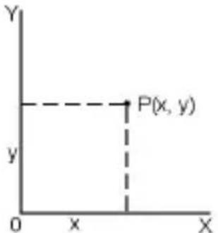
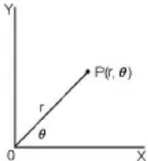
$$ x + y i = r (\cos \theta + i \sin \theta) $$

(Note): When using those key, make sure the calculator is set for the angle unit you want.

The calculator can perform the conversion between rectangular coordinates and polar coordinates by [2nd] [P→R] and [2nd] [R→P].

If x = 5, y = 30, what are r, 6? Ans : r = 30.4138126515, 80.537677792°

[2nd] [R-P] 5 [2 nd] [ , ] 30	DEG ( )R-P ( 5 ,30
[ ENTER=	DEGr30.4 1 3 8 1 2 6 5 1 5
[2nd] [x ↔y]	DEGθ8 0.5 3 7 6 7 7 7 9 2

If r = 25 , = 56^ what are x, y ? Ans : x = 13.9798225868, y = 20.7259393139

[2nd][PR]25[2nd][ ]56	DEG ( )PR(25,56
[ENTER=	DEGX13.9798225868
[2nd][x↔y]	DEGY20.7259393139

Probability

This calculator provides the following probability functions :

[nPr] Calculates the number of possible permutations of n item taken r at a time.

[nCr] Calculates the number of possible combinations of n items taken r at a time.

[X!] Calculates the factorial of a specified positive integer n, where n ≤ 69 .

[ RND ] Generates a random number between 0.000 and 0.999

7![(7-4)]!=840

7 [2nd] [nPr] 4 [ENTER=]

DEG7 P 4 =840.

7!4![(7-4)]!=35

7 [2nd] [nCr] 4 [ENTER=

DEG7 C 4 =35.

5! = 120

5 [2nd] [X!] [ENTER=

DEG5 !120.

Generates a random between 0.000 \~ 0.999

[2nd][RND]

DEGRnd0

.4 4

Other functions ( 1/x, √ 3, √, x², x³, x⁴, INT, FRAC )

The calculator also provides reciprocal ([ 2nd ] [ 1/x ]), square root ([ √ ]), cubic root ([ 2nd ] [ √³ ]), universal root ([ 2nd ] [ √x² ]), square ([ x² ]), cubic ([ 2nd ] [ x³ ]), and exponentiation ([ x^y ]) functions.

11.25=0.8

1.25 [2nd] [1/x][ENTER=

DEG1.25 ^-1 0

2^2+4+21+[3]125+5^3=139

2[x^2][+][][()]4[+]21[)] [+] [2nd][[3]]125[+]5[2nd] [x^3][ENTER=

DEG 2^2+(4+21)+ 139.

^5+625=16812

7[x^y]5[+]4[^-]625[ENTER]

DEG 7x^y5+4^x625= 16812.

INT Indicate the integer part of a given number

FRAC Indicate the fractional part of a given number

INT (10 ÷ 8) = INT (1.25) = 1

[2nd][INT] 10 [÷] 8 [ENTER=

DEGINT (10÷8=1.

FRAC (10 ÷ 8) = FRAC (1.25) = 0.25

[2nd][FRAC]10[÷]8[ENTER=

DEGFRAC(10÷8=0

Unit Conversion

The calculator has a built-in unit conversion feature that enables you to convert numbers among different units.

1. Enter the number you want to convert.

2. Press [CONV] to display the menu. There are 7 menus, covering distance, area, temperature, capacity, weight, energy, and pressure.

3. Use the [CONV] to scroll through the list of units until a appropriate units menu is shown, then [ENTER].

4. Pressing [→] or [2nd][←] can convert the number to another unit.

1 y d ^2 = 9 ft ^2 = 0.00000083612 km ^2

1 [CONV] [CONV] [→][ENTER]=	DEG ft^2 d^2 m^2 1
[2nd][↖]	DEG ft^2 d^2 m^2 9.
[→][→][→]	DEG km^2 c t a r e s 0.00000083612

Physics constants

You can use 136 physics constants in your calculations. With the following constants :

Data is referred to Peter J.Mohr and Barry N.Taylor, CODATA Recommended Values of the Fundamental Physical Constants:1998, Journal of Physical and Chemical Reference Data, Vol.28, No.6, 1999 and Reviews of Modern Physics, Vol.72, No.2, 2000.

No.	Quantity	Symbol	Value, Unit
1.	Speed of light in vacuum	c	299792458 m s ^-1
2.	Magnetic constant	_0	1.2566370614 x10 ^-6 N A ^-2
3.	Electric constant	_0	8.854187817 x 10 ^-12 F m ^-1
4.	Characteristic impedance of vacuum	Z_0	376.730313461
5.	Newtonian constant of gravitation	G	6.67310 × 10^-11 m^3 kg^1 s^2
6.	Planck constant	h	6.6260687652 × 10^-34 J s
7.	Planck constant over 2 pi		1.05457159682 × 10^-34 J s
8.	Avogadro constant	NA	6.0221419947 × 10^23 mol^-1
9.	Planck length	lp	1.616012 × 10^-35 m
10.	Planck time	tp	5.390640 × 10^-44 s
11.	Planck mass	mp	2.176716 × 10^-8 kg
12.	Atomic mass constant	mu	1.6605387313 × 10^-27 kg
13.	Atomic mass constant energy equivalent	m_^2	1.4924177812 × 10^-10 J
14.	Faraday constant IF 96485.341539 C mol ^-1
15.	Elementary charge	e 1.60217646263 x10 ^-19 C
16.	Electron volt-joule relationship	eV	1.60217646263 ^-19 J ×
17.	Elementary charge over h	e/h 2.41798949195 x10 ^14 AJ^-1
18.	Molar gas constant	R	8.31447215 J mol^-1 K^-1
19.	Boltzmann constant	k	1.380650324 × 10^-23 J K^-1
20.	Molar planck constant	NAh	3.99031268930 × 10^-10 Js mol^-1
21.	Sackur-Tetrode constant	SR	- 1.164867844
22.	Wien displacement law constant	b	2.897768651 × 10^-3 m K
23.	Lattice parameter of silicon	a	543.10208816 × 10^-12 m
24.	Stefan-Boltzmann constant	σ	5.67040040 × 10^-8 W m^-2 K^-4
25.	Standard acceleration of gravity	g	9.80665 m s^-2
26.	Atomic mass unit-kilogram relationship	μ	1.6605387313 × 10^-27 kg
27.	First radiation constant	c_1	3.7417710729 × 10^-16 W m^2
28.	First radiation constant for spectral radiance	c_1 L	1.19104272293 × 10^16 W m^2 sr^-1
29.	Second radiation constant	c_2	1.438775225 × 10^-2 m K
30.	Molar volume of ideal gas	Vm	22.41399639 × 10^-3 m^3 mol^-1
31.	Rydberg constant	R°	10973731.5685 m^-1
32.	Rydberg constant in Hz	R∞c	3.28984196037 × 10^15 Hz
33.	Rydberg constant in joules	R∞hc	2.1798719017 × 10^-18 J
34.	Hartree energy	Eh	4.3597438134 × 10^-18 J
35.	Quantum of circulation	h/me	7.27389503253 × 10^-4 m^2 s^-1
36.	Fine structure constant	α	7.29735253327 × 10^-3
37.	Loschmidt constant	o n	2.686777547 × 10^25 m^-3
38.	Bohr radius	θa	0.52917720832 × 10^-10 m
39.	Magnetic flux quantum	Φ0	2.06783363681 × 10^-15 Wb
40.	Conductance quantum	G	7.74809169628 × 10^-5 S
41.	Inverse of conductance quantum	G0−1	12906.4037865
42.	Josephson constant	KJ	483597.89819 × 10^9 Hz V^-1
43.	Von Klitzing constant	RK	25812.8075730 Ω
44.	Bohr magneton	μB	927.40089937 × 10^-26 J T^-1
45.	Bohr magneton in Hz/T	μB/h	13.9962462456 × 10^9 Hz T^-1
46.	Bohr magneton in K/T	μB/k	0.671713112 K T^-1
47.	Nuclear magneton	μN	5.0507831720 × 10^-27 J T^-1
48.	Nuclear magneton in MHz/T μ	N/h	7.6225939631 MHz T^-1
49.	Nuclear magneton in K/T	μN/k	3.658263864 × 10^-4 K T^-1
50.	Classical electron radius	re	2.81794028531 × 10^-15 m
51.	Electron mass	me	9.1093818872 × 10^-31 kg
52.	Electron mass energy equivalent	me ^2	8.1871041464 × 10^-14 J
53.	Electron–muon mass ratio m	e/mμ	4.8363321015 × 10^-3
54.	Electron–tau mass ratio	me/mτ	2.8755547 × 10^-4
55.	Electron–proton mass ratio	me/mp	5.44617023212 × 10^-4
56.	Electron–neutron mass ratio	me/mn	5.43867346212 × 10^-4
57.	Electron–deuteron mass ratio	me/md	2.72443711706 × 10^-4
58.	Electron charge to mass quotient	-e/me	-1.75882017471 × 10^11 Ckg^-1
59.	Compton wavelength	λc	2.42631021518 × 10^-12 m
60.	Compton wavelength over 2 pi	λc	386.159264228^-15 m × 10^-1
61.	Thomson cross section	σe	0.66524585415 × 10^-28 m^2
62.	Electron magnetic moment	μe	-928.47636237 × 10^-26 J T^-1
63.	Electron magnetic moment to Bohr magneton ratio	μe/μB	-1.00115965219
64.	Electron magnetic moment to nuclear magneton ratio	μe/μN	-1838.28196604
65.	Electron–muon magnetic moment ratio	μe/μμ	206.766972063
66.	Electron–proton magnetic moment ratio	μe/μp	-658.210687566
67.	Electron–neutron magnetic moment ratio	μe/μn	960.9205023
68.	Electron–deuteron magnetic moment ratio	μe/μd	-2143.92349823
69.	Electron to shielded helion magnetic moment ratio	μe/μ′h	864.05825510
70.	Electron magnetic moment anomaly	ae	1.15965218694 × 10^-3
71.	Electron g-factor	ge	-2.00231930437
72.	Electron gyromagnetic ratio γ	e	1.76085979471 × 10^11 s^-1 T^-1
73.	Muon mass	mμ	1.8835310916 x10-28kg
74.	Muon mass energy equivalent	mμc2	1.6928333214 x10-11J
75.	Muon-tau mass ratio	mμ/mτ	5.9457297 x10-2
76.	Muon-proton mass ratio	mμ/mp	0.11260951733
77.	Muon-neutron mass ratio	mμ/mn	0.11245450793
78.	Muon magnetic moment anomaly	a μ	1.1659160264 x10-3
79.	Muon g-factor	g μ	-2.00233183201
80.	Muon Compton wavelength	λc,μ	11.7344419735 x10-15m
81.	Muon Compton wavelength over 2 pi	λcμ 1.86759444455 x10-15m
82.	Muon magnetic moment	μ μ	-4.4904481322x10-26JT-1
83.	Muon magnetic moment to Bohr magneton ratio	μμ/μB	-4.8419708515 x10-3
84.	Muon magnetic moment to nuclear magneton ratio	μμ/μN	-8.8905977027
85.	Muon-proton magnetic moment ratio	μμ/μp	-3.1833453910
86.	Tau Compton wavelength	λcτ	0.6977011 x10-15m
87.	Tau Compton wavelength over 2 pi	λc,τ	0.11104218-15m
88.	Tau mass	mτ	3.1678852 x10-27kg
89.	Tau mass energy equivalent	mτc2	2.8471546 x10-10J
90.	Tau-proton mass ratio	mτ/mp	1.8939631
91.	Proton Compton wavelength	λc,p	1.32140984710 x10-15m
92.	Proton Compton wavelength over 2 pi	λc,p	0.21030890892 x10-15m
93.	Proton mass	mp	1.6726215813 x10-27kg
94.	Proton mass energy equivalent	mpc2	1.5032773112 x10-10J
95.	Proton-neutron mass ratio	mp/mn	0.99862347856
96.	Proton charge to mass quotient	e/mp	9.5788340838 x107C kg-1
97.	Proton magnetic moment	μ p	1.41060663358 x10-26JT-1
98.	Shielded proton magnetic moment	μ'p	1.41057039959 x10-26JT-1
99.	Proton magnetic moment to nuclear magneton ratio	μp/μN	2.79284733729
100.	Proton-neutron magnetic moment ratio	μp/μn	-1.4598980534
101.	Shielded proton magnetic moment to Bohr magneton ratio	μ'p/μB	1.52099313216 x10-3

x10

102.	Proton gyromagnetic ratio	_p	2.6752221211 x10 ^8 s ^-1 T ^-1
103.	Shielded proton gyromagnetic ratio	_p	2.6751534111 x10 ^8 s ^-1 T ^-1
104.	Proton magnetic shielding correction	_p	25.68715 x10 ^-6
105.	Proton g-factor	g p	5.58569467557
106.	Neutron Compton wavelength	λ_c,n	1.31959089810 x10 ^-15 m
107.	Neutron Compton wavelength over 2 pi	_c,n	0.21001941422 x10 ^-15 m
108.	Neutron mass	mn	1.6749271613 x10 ^-27 kg
109.	Neutron mass energy equivalent	mnc^2	1.5053494612 x10 ^-10 J
110.	Neutron magnetic moment	μn	-0.9662364023x10 ^-26 J T ^-1
111.	Neutron magnetic moment to Bohr magneton ratio	μn/μB	-1.0418756325 x10 ^-3
112.	Neutron g-factor	gn	-3.8260854590
113.	Neutron gyromagnetic ratio	γ_n	1.8324718844 x10 ^8 s ^-1 T ^-1
114.	Deuteron mass	md	3.3435830926 x10 ^-27 kg
115.	Deuteron mass energy equivalent	mdc^2	3.0050626224 x10 ^-10 J
116.	Deuteron molar mass M(d)	2.0135	5321271x10 ^-3 kg mol ^-1
117.	Deuteron-electron mass ratio	md/me	3670.48295508
118.	Deuteron-proton mass ratio	md/mp	1.99900750083
119.	Deuteron magnetic moment	μd	0.43307345718 x10 ^-26 J T ^-1
120.	Deuteron magnetic moment to Bohr magneton ratio	μd/μB	0.46697545565 x10 ^-3
121.	Deuteron magnetic moment to nuclear magneton ratio	μd/μN	0.85743822849
122.	Deuteron-proton magnetic moment ratio	μd/μp	0.30701220835
123.	Helion mass	mh	5.0064117439 x10 ^-27 kg
124.	Helion mass energy equivalent	mhc^2	4.4995384835 x10 ^-10 J
125.	Helion molar mass M(h)	3.014932	23470x10 ^-3 kg mol ^-1
126.	Helion-electron mass ratio	mh/me	5495.88523812
127.	Helion-proton mass ratio	mh/mp	2.99315265851
128.	Shielded helion magnetic moment	μh	-1.07455296745 x10 ^-26 J T ^-1
129.	Shielded helion magnetic moment to Bohr magneton ratio	^/ B	-1.15867147414 x10-3
130.	Shielded helion magnetic moment to nuclear magneton ratio	^/ N	-2.12749771825
131.	Shielded helion gyromagnetic ratio	h	2.03789476485 x108s-1T-1
132.	Alpha particle mass	m_	6.6446559852 x10-27kg
133.	Alpha particle mass energy equivalent	m_^2	5.9719189747 x10-10J
134.	Alpha particle molar mass	M_()	4.00150617471 x10-3kg mol^-1
135.	Alpha particle to electron mass ratio	m_/m_e	7294.29950816
136.	Alpha particle to proton mass ratio	m_/m_p	3.97259968461

To insert a constant at the cursor position :

1. Press [CONST] to display the physics constants menu.

2. Press [→] or [2nd][→] until the constant you want is underlined.

3. Press [ENTER].

You also can use the [CONST] key in combination with a number, 1 through 136, to recall a physical constants. For example, press 15 [CONST].

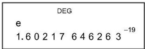
3 × N_A = 1.80664259841 × 10^24

3 [x] [CONST] [CONST] [→][→][ENTER=]	CONST DEGh NA l p tp236.0 2 2 1 4 1 9 9 4 7
	CONST DEG0 0 8 : m o l-1236.0 2 2 1 4 1 9 9 4 7
[ENTER] [ENTER=]	CONST DEG3 * NA =241.8 0 6 6 4 2 5 9 8 4 1

Base-n calculations

Use MAIN ([MODE] 1 (MAIN)) mode for Base-n calculations.

The unit enables you to calculate in number base other than decimal. The calculator can add, subtract, multiply, and divide binary, octal, and hexadecimal numbers.

The following shows the numerals that can be used in each number base.

Binary base (b): 0, 1

Octal base (o): 0, 1, 2, 3, 4, 5, 6, 7

Decimal base: 0, 1, 2, 3, 4, 5, 6, 7, 8, 9

Hexadecimal base (h): 0, 1, 2, 3, 4, 5, 6, 7, 8, 9, A, B, C, D, E, F

To distinguish the A, B, C, D, E and F used in the hexadecimal base from standard letters, they appear as shown in the below.

Key	Display (Upper)	Display (Lower)	Key	Display (Upper)	Display (Lower)
A	/A	R	D	I	Dd
B	IB	b E		E	E
C	IC	FC	I	F	F

Select the number base you want to use with [→BIN ], [→OCT ], [→DEC ], [→HEX ]. The " BIN ", " b ", " OCT ", " o ", " HEX ", " h " indicators show you which number base you are using. If none of the indictors appears in the display, you are in decimal base.

Bases conversions

37 (base 8) = 31 (base 10) = 1F (base 16)

[2nd][OCT]37	DEGOCT000000000037°
[2nd][DEC]	DEG31.
[2nd][HEX]	DEGHE X0000001Fh

Block Function

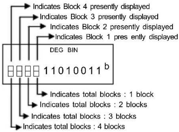
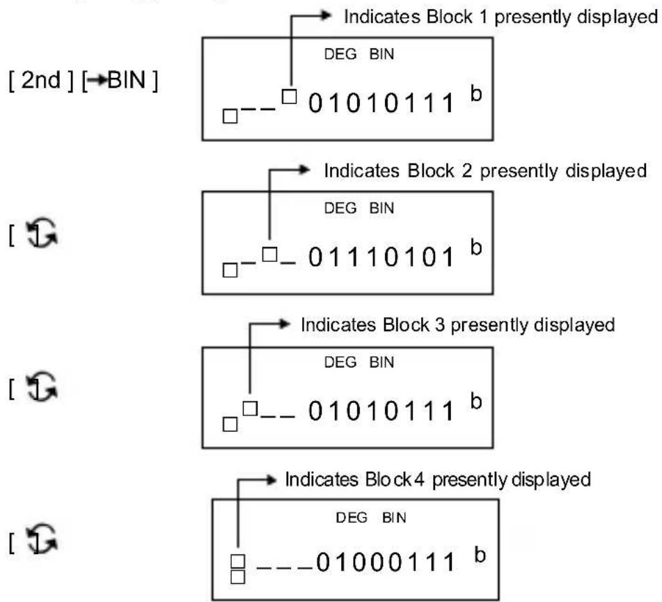
For a result in binary base, it will be displayed using block function. The maximum of 32 digits are displayed in 4 blocks of 8 digits.

graph TD
    A["DEG BIN"] --> B["11010011 b"]
    A --> C["Indicates Block 1 presently displayed"]
    A --> D["Indicates Block 2 presently displayed"]
    A --> E["Indicates Block 3 presently displayed"]
    A --> F["Indicates Block 4 presently displayed"]
    A --> G["Indicates Block 5 presently displayed"]
    A --> H["Indicates Block 6 presently displayed"]
    A --> I["Indicates Block 7 presently displayed"]
    A --> J["Indicates Block 8 presently displayed"]
    A --> K["Indicates Block 9 presently displayed"]
    A --> L["Indicates Block 10 presently displayed"]
    A --> M["Indicates Block 11 presently displayed"]
    A --> N["Indicates Block 12 presently displayed"]
    A --> O["Indicates Block 13 presently displayed"]
    A --> P["Indicates Block 14 presently displayed"]
    A --> Q["Indicates Block 15 presently displayed"]
    A --> R["Indicates Block 16 presently displayed"]
    A --> S["Indicates Block 17 presently displayed"]
    A --> T["Indicates Block 18 presently displayed"]
    A --> U["Indicates Block 19 presently displayed"]
    A --> V["Indicates Block 20 presently displayed"]
    A --> W["Indicates Block 21 presently displayed"]
    A --> X["Indicates Block 22 presently displayed"]
    A --> Y["Indicates Block 23 presently displayed"]
    A --> Z["Indicates Block 24 presently displayed"]
    A --> AA["Indicates Block 25 presently displayed"]
    A --> AB["Indicates Block 26 presently displayed"]
    A --> AC["Indicates Block 27 presently displayed"]
    A --> AD["Indicates Block 28 presently displayed"]
    A --> AE["Indicates Block 29 presently displayed"]
    A --> AF["Indicates Block 30 presently displayed"]
    A --> AG["Indicates Block 31 presently displayed"]
    A --> AH["Indicates Block 32 presently displayed"]
    A --> AI["Indicates Block 33 presently displayed"]
    A --> AJ["Indicates Block 34 presently displayed"]
    A --> AK["Indicates Block 35 presently displayed"]
    A --> AL["Indicates Block 36 presently displayed"]
    A --> AM["Indicates Block 37 presently displayed"]
    A --> AN["Indicates Block 38 presently displayed"]
    A --> AO["Indicates Block 39 presently displayed"]
    A --> AP["Indicates Block 40 presently displayed"]

The block function comprises upper and lower block indicators. The upper indicator means current block position, and the lower indicator means total blocks for a result.

In the binary base, the block 1 is displayed immediately after calculation. Other blocks (block 2 \~ block 4) are displayed by pressing [ ∽ ].

For example, input 47577557 _16

Press [2nd] [→HEX] 47577557

graph TD
    A["2nd"] --> B["DEG BIN"]
    B --> C["01010111 b"]
    C --> D["Indicates Block 1 presently displayed"]
    E["DEG BIN"] --> F["01110101 b"]
    F --> G["Indicates Block 2 presently displayed"]
    H["DEG BIN"] --> I["01010111 b"]
    I --> J["Indicates Block 3 presently displayed"]
    K["DEG BIN"] --> L["01000111 b"]
    L --> M["Indicates Block 4 presently displayed"]

$$ 4 7 5 7 7 5 5 7 _ {1 6} = \text { Block } 4 + \text { Block } 3 + \text { Block } 2 + \text { Block } 1 $$

$$ = 0 1 0 0 0 1 1 1 0 1 0 1 0 1 1 1 0 1 1 1 0 1 0 1 0 1 0 1 0 1 1 1 _ {2} $$

Basic arithmetic operations for bases

1IEIF 16 + 1234 10 ÷ 1001 2 = 1170 8

[2nd][HEX]1EF[+][2nd][→DEC]1234[÷][2nd][BIN]1001[ENTER][2nd][OCT]

DEGOCTh1IEIF+1234b1÷00000001170°

Negative expressions

In binary, octal, and hexadecimal bases, the calculator represents negative numbers using complement notation. The complement is the result of subtracting that number from 10000000000 in that number's base by pressing [NEG] key in non-decimal bases.

3/A_16=NEG IFIFIFIFIFIC6_16

[2nd][HEX]3A[NEG]

DEG HE XNEG h 3/A FFFFFFFC6h

Logical operation

Logical operations are performed through logical products (AND), negative logical (NAND), logical sums (OR), exclusive logical sums (XOR), negation (NOT), and negation of exclusive logical sums (XNOR).

1010_2 AND ( /A_16 OR 7_16) = 12_8

[2nd] [BIN] 1010 [AND] [( ] [2nd] [→HEX] A[OR] 7[)] [ENTER] [2nd] [→OCT]

DEG BINb 1010 AND ( h00000000012 °

Statistical Calculations

Use STAT ([MODE] 2 (STAT)) mode for statistical calculations.

The calculators can perform both single-variable statistical calculations and paired-variable in this mode.

Press [MODE] 2 (STAT) to enter STAT mode. There are six items in STAT mode, asking you to select one of them,

graph LR
    A["1-VAR"] --> B["DEG"]
    B --> C["LIN"]
    C --> D["LOG"]
    D --> E["STAT"]
    F["[→"]] --> G["[→"]]
    G --> H["[→"]]
    I["EXP"] --> J["DEG"]
    J --> K["PWR"]
    K --> L["D-CL"]
    M["STAT"] --> N["DEG"]
    N --> O["PWR"]
    O --> P["D-CL"]

Single-variable statistics

1-VAR Single-variable statistics

Paired-variable / Regression statistics

LIN Linear Regression y = a + b ×

LOG Logarithmic Regression y = a + b x

EXP Exponential Regression y = a • e

POW Power Regression y = a · x

D-CL Clear all statistical data

Entering data

Always make sure you clear statistical data by D–CL before performing statistical calculations.

(A) To input single-variable data using the following syntaxes :

# Individual data : [ DATA ] < x value >

# Multiple data of the same value :

[ DATA ] < x value > [ x ] < Number of repeats >

(B) To input paired-variable / regression data using the following syntaxes :

# Individual data-set : [ DATA ] < x value > [ , ] < y value >

# Multiple data of the same value :

[ DATA ] < x value > [ , ] < y value > [ x ] < Number of repeats >

(Note) : Even you exit STAT mode, all data are still retained unless you clear all data by selecting D-CL mode.

Displaying results

The values of the statistical variables depend on the data you input. You can recall them by the key operations shown in the below table.

Single-variable statistics calculations

Variables	Meaning
n ([ n ]) Number of the x values entered
([2nd]+[ ] ) Mean of the x values
Sx ([2nd]+[ ] )	Sample standard deviation of x values
σx ([2nd]+[ σx ] ) Population standard deviation of x values
Σx ([2nd]+[ Σx ] )	Sum of all x values
Σx^2 ([2nd]+[ Σx^2 ] )	Sum of all x^2 values
CP ([2nd]+[ CP ] )	Potential capability precision of the x values
CPK ([CPK])	Minimum (CPU, CPL) of the x values, where CPU is upper spec. limit of capabilityprecision and CPL is lower spec. limit of capability precisionCPK = Min (CPU, CPL) = CP (1 - Ca)

Paired-variable statistics / Regression calculations

Variables	Meaning
n ([n]) Number of x-y pairs entered
([2nd]+[ ]) ([2nd]+[ ])	Mean of the x values or y values
Sx ([2nd]+[ Sx ] Sy ([2nd]+[ Sy ])	Sample standard deviation of x values or y values
x ([2nd]+[ x ]) y ([2nd]+[ y ])	Population standard deviation of x values or y values
x ([2nd]+[ x ]) y ([2nd]+[ y ])	Sum of all x values or y values
x^2 ([2nd]+[ x^2 ]) y^2 ([2nd]+[ y^2 ])	Sum of all x^2 values or y^2 values
x y Sum of (x·y) for all x-y pairs
CP ([2nd]+[ CP ])	Potential capability precision of the x values
CPK ([ CPK ])	Minimum (CPU, CPL) of the x values, where CPU is upper spec. limit of capabilityprecision and CPL is lower spec. limit ofcapability precisionCPK = Min (CPU, CPL) = CP (1 - Ca)
a ([2nd]+[ a ])	Regression formula constant term a
b ([2nd]+[ b ])	Regression formula regression coefficient b
r ([2nd]+[ r ])	Correlation coefficient r
x'([x'])	Estimated value of x
y'([y'])	Estimated value of y

You also can add a new data anytime. The unit automatically recalculates statistics each time you press [ DATA ] and enter a new data value.

Enter data : USL = 95, LSL = 70, DATA 1 = 75, DATA 2 = 85, DATA 3 = 90, DATA 4 = 82, DATA 5 = 77, then find out n = 5, = 81.8, Sx = 6.05805249234, σx = 5.41848687366, CP = 0.76897236513, and CPK = 0.72590991268

[MODE]2	DEG1-VAR LIN LOG
[ENTDATA]75 [DATA]85[DATA]90 [DATA]82 [DATA]77	DEGDATA 577
[n]	DEGn5.
[2nd][ ]	DEGX81.8
[2nd][ Sx ]	DEGSX6.05805249234
[2nd][ x ]	DEG x 5.41848687366
[2nd][ CP ]95	DEGU SL=CP95 USL
[ENTER]	DEGL SL=CP70 LSL
[ENTER=	DEGCP0.76897236513
[CPK]	DEGU SL=CPK95 USL
[ENTER=	DEGL SL=CPK70 LSL
[ENTER=	DEGCPK0.72590991268

Find a, b and r for the following data using linear regression and estimate x = ? for y = 573 and y = ? for x = 19.

Data	item	15	17	21
FREQ.	451	475	525	678

28

[MODE]2[→	DEG STAT1-VAR LIN LOG
[ENTER][DATA]15[ , ]451 [DATA]17[ , ]475 [DATA]21[ , ]525 [DATA]28[ , ]678	DEG STAT DATA 4 = 28, REG 678
[2nd][a]	DEG STAT a REG 176.106329114
[2nd][b]	DEG STAT b REG 17.5873417722
[2nd][r]	DEG STAT r REG 0.98984516413
573[x']	DEG STAT x'573 REG 22.5670073413
19[y']	DEG STAT y'19 REG 510.265822785

Deleting data

The method to delete data depends on whether you have already stored the data by next pressing [DATA] key or not.

To delete data you just input but have not yet stored it by next pressing [DATA], simple press [CE].

To delete data that you have already stored by next pressing [DATA], (A) To delete single-variable data using the following syntaxes:

$$ # < x \text { value } > [ 2 n d ] [ D E L ] $$

$$ # < x \text { value } > [ x ] < \text { Number of repeats } > [ 2 \text { nd } ] [ \text { DEL } ] $$

(B) To delete paired-variable / regression data using the following syntaxes:

$$ # \text { Individual data - set }: < x \text { value } > [ \quad , ] < y \text { value } > [ 2 n d ] [ D E L ] $$

# Multiple data-set with the same value :

$$ \begin{array}{l} < x \text {value} > [ \quad ], < y \text {value} > [ x ] < \text {Number of repeats} > [ 2 n d ] \ [ D E L ] \end{array} $$

If you enter and delete a value that isn't included in the stored data by mistake, "dEL Error" appears, but the previous data are still retained.

Editing data

Press [2nd] [EDIT] to enter EDIT mode. The EDIT mode is convenient and friendly for you to view, correct, delete data.

(A) In 1–VAR mode, the method to view data depends on whether you want to view data item or not.

# Each time you press [ DATA ], first data item appears 1 second and then the corresponding value.

# Each time you press [ ENTER value appears directly on the display without data item.

(B) In REG mode, each time you press [ DATA ], data item and x value appear on the screen at the same time. You can press [ ’ ] to switch between x and y value.

If you want to correct data, find out and enter a new entry to replace it.

FULL message

A “FULL” is indicated when any of the following conditions occur and further data entry becomes impossible. Just pressing any key can clear the indicator. The previous data entries are still retained unless you exit STAT mode.

1) If the times of data entry by [DATA] is more than 50
2) The number of repeats is more than 255

3) n>12750 (n = 12750 appears when the times of data entry by [DATA] are up to 50 and the number of repeats for each value are all 255, i.e. 12750 = 50 × 255 )

Complex Calculations

Use CPLX ([MODE] 3 (CPLX)) mode for complex calculations.

Complex mode enables you to add, subtract, multiply, and divide complex numbers.

The results of a complex operation are displayed as follow :

Re Real value Im Imaginary value

ab Absolute value ar Argument value

(7 - 9 i) + (15 + 12 i) = 22 + 3 i, ab = 22.2036033112, ar = 7.76516601843

[MODE]3	CPLX DEG0.
7[-]9[i][+]15[+]12[i][ENTER=	CPLX DEGRe Im ab a r22.
[→]	CPLX DEGRe Im ab a r3.i
[→]	CPLX DEGRe Im ab a r22.2036033112
[→]	CPLX DEGRe Im ab a r7.76516601843