15C - Calculator HP - Free user manual and instructions

USER MANUAL 15C HP

Edition 2.4, Sep 2011

Legal Notice

This manual and any examples contained herein are provided "as is" and are subject to change without notice. Hewlett-Packard Company makes no warranty of any kind with regard to this manual, including, but not limited to, the implied warranties of merchantability non-infringement and fitness for a particular purpose. In this regard, HP shall not be liable for technical or editorial errors or omissions contained in the manual.

Hewlett-Packard Company shall not be liable for any errors or incidental or consequential damages in connection with the furnishing, performance, or use of this manual or the examples contained herein.

Copyright © 2011 Hewlett-Packard Development Company, LP.

Reproduction, adaptation, or translation of this manual is prohibited without prior written permission of Hewlett-Packard Company, except as allowed under the copyright laws.

Hewlett-Packard Company

Palo Alto, CA

94304

USA

Introduction

Congratulations! Whether you are new to HP calculators or an experienced user, you will find the HP-15C a powerful and valuable calculating tool. The HP-15C provides:

• 448 bytes of program memory (one or two bytes per instruction) and sophisticated programming capability, including conditional and unconditional branching, subroutines, flags, and editing.
• Four advanced mathematics capabilities: complex number calculations, matrix calculations, solving for roots, and numerical integration.
• Direct and indirect storage in up to 67 registers.

This handbook is written for you, regardless of your level of expertise. The beginning part covers all the basic functions of the HP-15C and how to use them. The second part covers programming and is broken down into three subsections – The Mechanics, Examples, and Further Information – in order to make it easy for users with varying backgrounds to find the information they need. The last part describes the four advanced mathematics capabilities.

Before starting these sections, you may want to gain some operating and programming experience on the HP-15C by working through the introductory material, The HP-15C: A Problem Solver, on page 12.

The various appendices describe additional details of calculator operation, as well as warranty and service information. The Function Summary and Index and the Programming Summary and Index at the back of this manual can be used for quick reference to each function key and as a handy page reference to more comprehensive information inside the manual.

Also available from Hewlett-Packard is the HP-15C Advanced Functions Handbook, which provides applications and technical descriptions for the root-solving, integration, complex number, and matrix functions.

Note: You certainly do not need to read every part of the manual before delving into the HP-15C Advanced Functions if you are already familiar with HP calculators. The use of and [f_y]x requires a knowledge of HP-15C programming.

Contents

The HP-15C: A Problem Solver 12

A Quick Look at ENTER 12

Manual Solutions 13

Programmed Solutions 14

Part I: HP-15C Fundamentals 17

Section 1: Getting Started 18

Power On and Off 18

Keyboard Operation 18

Primary and Alternate Functions 18

Prefix Keys 19

Changing Signs 19

Keying in Exponents 19

The "CLEAR" Keys 20

Display Clearing: and 21

Calculations 22

One-Number Functions 22

Two-Number Functions and ENTER 22

Section 2: Numeric Functions 24

Pi 24

Number Alteration Functions 24

One-Number Functions 25

General Functions 25

Trigonometric Operations 26

Time and Angle Conversions 26

Degrees/Radians Conversions 27

Logarithmic Functions 28

Hyperbolic Functions 28

Two-Number Functions 29

The Power Function 29

Percentages 29

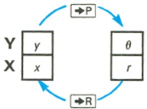
Polar and Rectangular Coordinate Conversions 30

Section 3: The Automatic Memory Stack, LAST X, and

Data Storage 32

The Automatic Memory Stack and Stack Manipulation 32
Stack Manipulation Functions 33
The LAST X Register and _x 35
36
Order of Entry and the ENTER Key 37
Nested Calculations 38
Arithmetic Calculations With Constants 39
Storage Register Operations 42
Storing and Recalling Numbers 42
Clearing Data Storage Registers 43
Storage and Recall Arithmetic 43
45
Problems 45

Section 4: Statistics Functions 47

Probability Calculations 47
Random Number Generator 48
Accumulating Statistics 49

Correcting Accumulated Statistics 52
Mean 53
Standard Deviation 53
Linear Regression 54
Linear Estimation and Correlation Coefficient 55
Other Applications 57

Section 5: The Display and Continuous Memory 58

Display Control 58

Fixed Decimal Display 58
Scientific Notation Display 59
Engineering Notation Display 59
Mantissa Display 60
Round-Off Error 60

Special Displays 60

Annunciators 60
Digit Separators 61
Error Display 61
Overflow and Underflow 61
Low-Power Indication 62

Continuous Memory 62

Status 62

Resetting Continuous Memory 63

Part II: HP-15C Programming 65

Section 6: Programming Basics 66

The Mechanics 66

Creating a Program 66

Loading a Program 66

Intermediate Program Stops 68

Running a Program 68

How to Enter Data 69

Program Memory 70

Further Information 74

Program Instructions 74

Instruction Coding 74

Memory Configuration 75

Program Boundaries 77

Unexpected Program Stops 78

Abbreviated Key Sequences 78

User Mode 79

Polynomial Expressions and Horner's Method 79

Nonprogrammable Functions 80

Problems 81

Section 7: Program Editing 82

The Mechanics 82

Moving to a Line in Program Memory 82

Deleting Program Lines 83

Inserting Program Lines 83

Examples 83

Further Information 85

Single-Step Operations 85

Line Position 86

Insertions and Deletions 87

Initializing Calculator Status 87

Problems 87

Section 8: Program Branching and Controls 90

The Mechanics 90

Branching 90

Conditional Tests 91

Flags 92

Examples 93

Example: Branching and Looping 93

Example: Flags 95

Further Information 97

GoTo 97

Looping 98

Conditional Branching 98

Flags 98

The System Flags: Flags 8 and 9 99

Section 9: Subroutines 101

The Mechanics 101

GoTo Subroutine and Return 101

Subroutine Limits 102

Examples 102

Further Information 105

The Subroutine Return 105

Nested Subroutines 105

Section 10: The Index Register and Loop Control 106

The I and (i) Keys 106

Direct Versus Indirect Data Storage With

The Index Register 106

Indirect Program Control With the Index Register 107

Program Loop Control 107

The Mechanics 107

Index Register Storage and Recall 107

Index Register Arithmetic 108

Exchanging the X-Register 108

Indirect Branching With I 108

Indirect Flag Control With I 109

Indirect Display Format Control With I 109

Loop Control with Counters: ISG and DSE 109

Examples 111

Examples:Register Operations 111

Example: Loop Control With DSE 112

Example: Display Format Control 114

Further Information 115

Index Register Contents 115

ISG and DSE 116

Indirect Display Control 116

Part III: HP-15C Advanced Functions 119

Section 11: Calculating With Complex Numbers 120

The Complex Stack and Complex Mode 120

Creating the Complex Stack 120

Deactivating Complex Mode 121

Complex Numbers and the Stack 121

Entering Complex Numbers 121

Stack Lift in Complex Mode 124

Manipulating the Real and Imaginary Stacks 124

Changing Signs 124

Clearing a Complex Number 125

Entering a Real Number 128

Entering a Pure Imaginary Number 129

Storing and Recalling Complex Numbers 130

Operations With Complex Numbers 130

One-Number Functions 131

Two-Number Functions 131

Stack Manipulation Functions 131

Conditional Tests 132

Complex Results from Real Numbers 133

Polar and Rectangular Coordinate Conversions 133

Problems 135

For Further Information 137

Section 12: Calculating With Matrices 138

Matrix Dimensions 140

Dimensioning a Matrix 141

Displaying Matrix Dimensions 142

Changing Matrix Dimensions 142

Storing and Recalling Matrix Elements 143

Storing and Recalling All Elements in Order 143

Checking and Changing Matrix Elements Individually 145

Storing a Number in All Elements of a Matrix 147

Matrix Operations 147

Matrix Descriptors 147

The Result Matrix 148

Copying a Matrix 149

One-Matrix Operations 149

Scalar Operations 151

Arithmetic Operations 153

Matrix Multiplication 154

Solving the Equation AX = B 156

Calculating the Residual 159

Using Matrices in LU Form 160

Calculations With Complex Matrices 160

Storing the Elements of a Complex Matrix 161

The Complex Transformations Between Z^p and Z 164

Inverting a Complex Matrix 165

Multiplying Complex Matrices 166

Solving the Complex Equation AX = B 168

Miscellaneous Operations Involving Matrices 173

Using a Matrix Element With Register Operations 173

Using Matrix Descriptors in the Index Register 173

Conditional Tests on Matrix Descriptors 174

Stack Operation for Matrix Calculations 174

Using Matrix Operations in a Program 176

Summary of Matrix Functions 177

For Further Information 179

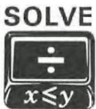
Section 13: Finding the Roots of an Equation 180

Using SOLVE 180

When No Root Is Found 186

Choosing Initial Estimates 188

Using SOLVE in a Program 192

Restriction on the Use of SOLVE 193

Memory Requirements 193

For Further Information 193

Section 14: Numerical Integration 194

Using _y^x 194

Accuracy of _y^x 200

Using _y^x in a Program 203

Memory Requirements 204

For Further Information 204

Appendix A: Error Conditions 205
Appendix B: Stack Lift and the LAST X Register 209

Digit Entry Termination 209
Stack Lift 209

Disabling Operations 210
Enabling Operations 210
Neutral Operations 211

LAST X Register 212

Appendix C: Memory Allocation 213
The Memory Space 213

213
Memory Status (MEM) 215

Memory Reallocation 215

The DIM (i) Function 215
Restrictions on Reallocation 216

Program Memory 217

Automatic Program Memory Reallocation 217
Two-Byte Program Instructions 218

Memory Requirements for the Advanced Functions 218

Appendix D: A Detailed Look at SOLVE 220

How Solve Works 220
Accuracy of the Root 222
Interpreting Results 226
Finding Several Roots 233
Limiting the Estimation Time 238

Counting Iterations 239

Specifying a Tolerance 239

For Advanced Information 239

Appendix E: A Detailed Look at _y^x 240

How f_y^x Works 240
Accuracy, Uncertainty, and Calculation Time 241
Uncertainty and the Display Format 245
Conditions That Could Cause Incorrect Results 249
Conditions That Prolong Calculation Time 254
Obtaining the Current Approximation to an Integral 257
For Advanced Information 258

Appendix F: Batteries 259

Low-Power Indication 259

Installing New Batteries 259

Verifying Proper Operation (Self-Tests) 261

Function Summary and Index 262

Complex Functions 262

Conversions 262

Digit Entry 262

Display Control 263

Hyperbolic Functions 263

Index Register Control 263

Logarithmic and Exponential Functions 263

Mathematics 264

Matrix Functions 264

NumberAlteration 265

Percentage 266

Prefix Keys 266

Probability 266

Stack Manipulation 266

Statistics 267

Storage 267

Trigonometry 268

Programming Summary and Index 269

Subject Index 271

The HP-15C: A Problem Solver

The HP-15C Advanced Programmable Scientific Calculator is a powerful problem solver, convenient to carry and easy to hold. Its continuous memory retains data and program instructions indefinitely until you choose to reset it. Though sophisticated, it requires no prior programming experience or knowledge of programming languages to use it.

The new HP-15C is a modern re-release of the original HP-15C introduced in 1982. While the battery life of the new version is now estimated to be 1 year for normal use, the calculator is now at least 150 times faster than the original. The low-power indicator gives you plenty of warning before the calculator stops functioning.

The HP-15C also conserves power by automatically shutting its display off if it is left inactive for a few minutes. But don't worry about losing data -- any information contained in the HP-15C is saved by Continuous Memory.

A Quick Look at ENTER

Your Hewlett-Packard calculator uses a unique operating logic, represented by the ENTER key, that differs from the logic in most other calculators. You will find that using ENTER makes nested and complicated calculations easier and faster to work out. Let's get acquainted with how this works.

For example, let's look at the arithmetic functions. First we have to get the numbers into the machine. Is your calculator on? If not, press ON. Is the display cleared? To display all zeros, you can press 9 CLx that is, press 9, then .* To perform arithmetic, key in the first number, press ENTER to separate the first number from the second, then key in the second number and press +, -, × or ÷. The result appears immediately after you press any numerical function key.

The display format used in this handbook is FIX 4 (the decimal point is "fixed" to show four decimal places) unless otherwise mentioned. If your calculator does not show four decimal places, you may want to press f FIX 4 to match the displays in the examples.

Manual Solutions

Run through the following two-number calculations. It is not necessary to clear the calculator between problems. If you enter a digit incorrectly, press to undo the mistake, then key in the correct number.

To Compute

$$ 9 - 6 = 3 $$

$$ 9 \times 6 = 5 4 $$

$$ 9 \div 6 = 1. 5 $$

$$ 9 ^ {6} = 5 3 1, 4 4 1 $$

Keystrokes

$$ 9 \boxed {E N T E R} 6 - $$

$$ 9 \boxed {E N T E R} 6 \boxed {\times} $$

$$ 9 \text {E N T E R} 6 \div $$

$$ 9 \text {E N T E R} 6 y ^ {x} $$

Display

$$ 3. 0 0 0 0 $$

$$ 5 4. 0 0 0 0 $$

$$ 1. 5 0 0 0 $$

$$ 5 3 1, 4 4 1. 0 0 0 0 $$

Notice that in the four examples:

• Both numbers are in the calculator before you press the function key.
• ENTER is used only to separate two numbers that are keyed in one after the other.
• Pressing a numeric function key, in this case - × ÷ or ^x , executes the function immediately and displays the result.

To see the close relationship between manual and programmed problem solving, let's first calculate the solution to a problem manually, that is, from the keyboard. Then we'll use a program to calculate the solution to the same problem with different data.

The time an object takes to fall to the ground (ignoring air friction) is given by the formula

$$ t = \sqrt {\frac {2 h}{g}} , $$

where t = time in seconds,

h = height in meters,

g = the acceleration due to gravity, 9.8m / s^2

Example: Compute the time taken by a stone falling from the top of the Eiffel Tower (300.51 meters high) to the earth.

Keystrokes

300.51 ENTER

2 X

9.8

√x

Display

300.5100

601.0200

61.3286

7.8313

Enter h

Calculates 2h

(2h) / g

Falling time, seconds.

Programmed Solutions

Suppose you wanted to calculate falling times from various heights. The easiest way is to write a program to cover all the constant parts of a calculation and provide for entry of variable data.

Writing the Program. The program is similar to the keystroke sequence you used above. A label is useful to define the beginning of a program, and a return is useful to mark the end of a program. Also, the program must accommodate the entry of new data.

Loading the Program. You can load a program for the above problem by pressing the following keys in sequence. (The display shows information which you can ignore for now, though it will be useful later.)

Keystrokes	Display
9 P/R	000-	Sets HP-15C to Program mode. (PRGM annunciator on.)
f CLEAR PRGM	000-	Clears program memory. (This step is optional here.)
f LBL A	001-42,21,11	Label "A" defines the beginning of the program.
2	002- 2
x	003- 20
9	004- 9
		The same keys you pressed to solve the problem manually.
•	005- 48
8	006- 8
÷	007- 10
√x	008- 11
9 RTN	009- 43 32	“Return” defines the end of the program.
9 P/R	7.8313	Switches to Run mode. (No PRGM annunciator.)

Running the Program. Enter the following information to run the program.

Keystrokes	Display
300.51	300.51	Height of the Eiffel Tower.
f A	7.8313	Falling time you calculated earlier.
1050 f A	14.6385	The time (seconds) for a stone to reach the ground after release from a blimp 1050 m high.

With this program loaded, you can quickly calculate the time of descent of an object from different heights. Simply key in the height and press f A. Find the time of descent for objects released from heights of 100m,2m,275m ,and 2,000m

The answers are: 4.5175 s; 0.6389 s; 7.4915 s; and 20.2031 s.

That program was relatively easy. You will see many more aspects and details of programming in part II. For now, turn the page to take an in-depth look at some of the calculator's important operating basics.

Part I

HP-15C

Fundamentals

Section 1

Getting Started

Power On and Off

The ON key turns the HP-15C on and off. To conserve power, the calculator automatically turns itself off after a few minutes of inactivity.

Keyboard Operation

Primary and Alternate Functions

Most keys on your HP-15C perform one primary and two alternate, shifted functions. The primary function of any key is indicated by the character(s) on the face of the key. The alternate functions are indicated by the gold characters printed above the key and the blue characters printed on the lower face of the key.

To select the primary function printed on the face of a key, press only that key. For example: ÷ .
To select the alternate function printed in gold or blue, press the like-colored prefix key (f or g) followed by the function key. For example: f SOLVE; g x ≤ y .

Throughout this handbook, we will observe certain conventions in referring to alternate functions. References to the function itself will appear as just the key name in a box, such as "the MEM function." References to the use of the key will include the prefix key, such as "press 9 MEM." References to the four gold functions printed under the bracket labeled "CLEAR" will be preceded by the word "CLEAR", such as "the CLEAR REG function," or "press f CLEAR PRGM."

Notice that when you press the f or g prefix key, an f or g annunciator appears and remains in the display until a function key is pressed to complete the sequence.

0.0000 f

Prefix Keys

A prefix key is any key which must precede another key to complete the key sequence for a function. Certain functions require two parts: a prefix key and a digit or other key. For your reference, the prefix keys are:

CF	ENG	FIX	GSB	fxy	MATRIX	SCI	STO
DIM	f	g	HYP	ISG	RCL	SF	TEST
DSE	F?	GTO	HYP-1	LBL	RESULT	SOLVE	x$

If you make a mistake while keying in a prefix for a function, press f CLEAR [PREFIX] to cancel the error. The CLEAR [PREFIX] key is also used to show the mantissa of a displayed number, so all 10 digits of the number in the display will appear for a moment after the [PREFIX] key is pressed.

Changing Signs

Pressing CHS (change sign) will change the sign (positive or negative) of any displayed number. To key in a negative number, press CHS after its digits have been keyed in.

Keying in Exponents

EEX (enter exponent) is used when keying in a number with an exponent. First key in the mantissa, then press EEX and key in the exponent.

For a negative exponent press CHS after keying in the exponent. For example, to key in Planck's constant (6.6262× 10^-34 Joule-seconds) and multiply it by 50:

Keystrokes	Display
6.6262	6.6262
EEX	6.6262	00	The 00 prompts you to key in the exponent.
3	6.6262	03	(6.6262×103).
4	6.6262	34	(6.6262×1034).
CHS	6.6262	-34	(6.6262×10-34).
ENTER	6.6262	-34	Enters number.
50 ×	3.3131	-32	Joule-seconds.

Note: Decimal digits from the mantissa that spill into the exponent field will disappear from the display when you press “, but will be retained internally.

To prevent a misleading display pattern, EEX will not operate with a number having more than seven digits to the left of the radix mark (decimal point), nor with a mantissa smaller than 0.000001. To key in such a number, use a form having a greater exponent value (whether positive or negative). For example, 123456789.8 × 10^23 can be keyed in as 1234567.898 × 10^25 ; 0.00000025 × 10^-15 can be keyed in as 2.5 × 10^-22 .

The "CLEAR" Keys

Clearing means to replace a number with zero. The clearing operations in the HP-15C are (the table is continued on the next page):

Clearing Sequence	Effect
g CLx ← In Run mode: In Program mode: f CLEAR Σ	Cleared display (X-register). Cleared last digit or entire display. Deletes current instruction. Cleared statistics storage registers, display, and the memory stack (described in section 3).
f CLEAR PRGM In Run mode: In Program mode: f CLEAR REG f CLEAR Prefix*	Repositions program memory to line 000. Deletes all program memory. Cleared all data storage registers. Clears any prefix from a partially entered key sequence.
* Also temporarily displays the mantissa.

Display Clearing: and

The HP-15C has two types of display clearing operations: (clear X ) and (back arrow).

In Run mode:

• clears the display to zero.
• deletes only the last digit in the display if digit entry has not been terminated by ENTER or most other functions. You can then key in a new digit or digits to replace the one(s) deleted. If digit entry has been terminated, then acts like CLx.

Keystrokes

12345

9

Display

12,345

1,234

12,349

111.1261

0.0000

Digit entry not terminated.

Clearly only the last digit.

Terminates digit entry.

Clears all digits to zero.

In Program mode:

• is programmable: it is stored as a programmed instruction, and will not delete the currently displayed instruction.
• is not programmable, so it can be used for program correction. Pressing will delete the entire instruction currently displayed.

Calculations

One-Number Functions

A one-number function performs an operation using only the number in the display. To use any one-number function, press the function key after the number has been placed in the display.

Keystrokes	Display
45	45
9 LOG	1.6532

Two-Number Functions and ENTER

A two-number function must have two numbers present in the calculator before executing the function. + , - , × and ÷ are examples of two-number functions.

Terminating Digit Entry. When keying in two numbers to perform an operation, the calculator needs a signal that digit entry is terminated for the first number. This is done by pressing ENTER to separate the two numbers. If, on the other hand, one of the numbers is already in the calculator as the result of a previous operation, you do not need to use the ENTER key. All functions except the digit entry keys themselves have the effect of terminating digit entry.

Notice that, regardless of the number, a decimal point always appears and a set number of decimal places are displayed when you terminate digit entry (as by pressing ENTER).

Chain Calculations. In the following calculations, notice that:

• The ENTER key is used only for separating the sequential entry of two numbers.
• The operator is keyed in only after both operands are in the calculator.
• The result of any operation may itself become an operand. Such intermediate results are stored and retrieved on a last-in, first-out basis. New digits keyed in following an operation are treated as a new number.

Example: Calculate (9 + 17 - 4) ÷ 4 .

Keystrokes	Display
9 ENTER	9.0000	Digit entry terminated.
17 +	26.0000	(9 + 17).
4 -	22.0000	(9 + 17 - 4).
4 ÷	5.5000	(9 + 17 - 4) ÷ 4.

Even more complicated problems are solved in the same manner-using automatic storage and retrieval of intermediate results. It is easiest to work from the inside of parentheses outwards, just as you would with calculations on paper.

Example: Calculate (6 + 7) × (9 - 3)

Keystrokes	Display
6 ENTER	6.0000	First solve for the intermediate result of (6 + 7).
7 +	13.0000
9 ENTER	9.0000	Then solve for the intermediate result of (9 - 3).
3 -	6.0000
×	78.0000	Then multiply the intermediate results together (13 and 6) for the final answer.

Try your hand at the following problems. Each time you press ENTER or a function key in a calculation, the preceding number is saved for the next operation.

$$ (1 6 \times 3 8) - (1 3 \times 1 1) = 4 6 5. 0 0 0 0 $$

$$ 4 \times (1 7 - 1 2) \div (1 0 - 5) = 4. 0 0 0 0 $$

$$ 2 3 ^ {2} - (1 3 \times 9) + 1 / 7 = 4 1 2. 1 4 2 9 $$

$$ \sqrt {[ (5 . 4 \times 0 . 8) \div (1 2 . 5 - 0 . 7 ^ {2}) ]} = 0. 5 9 9 8 $$

Section 2

Numeric Functions

This section discusses the numeric functions of the HP-15C (excluding statistics and advanced functions). The nonnumeric functions are discussed separately (digit entry in section 1, stack manipulation in section 3, and display control in section 5).

The numeric functions of the HP-15C are used in the same way whether executed from the keyboard or in a program. Some of the functions (such as ABS) are, in fact, primarily of interest for programming.

Remember that the numeric functions, like all functions except digit entry functions, automatically terminate digit entry. This means a numeric function does not need to be preceded or followed by ENTER.

Pi

Pressing 9 places the first 10 digits of into the calculator. does not need to be separated from other numbers by .

Number Alteration Functions

The number alteration functions act upon the number in the display (X-register).

Integer Portion. Pressing 9 INT replaces the number in the display with the nearest integer of lesser or equal magnitude.

Fractional Portion. Pressing f FRAC replaces the number in the display with its fractional part (that is, the difference between the number and its integer part).

Rounding. Pressing 9 RND rounds all 10 internally held digits of the mantissa of the displayed value to the number of digits specified by the current FIX, SCI, or ENG display format.

Absolute Value. Pressing 9 ABS yields the absolute value of the number in the display.

Keystrokes	Display
123.4567 ☨ INT	123.0000
9 LSTx CHS 9 INT	-123.0000	Reversing the sign does not alter digits.
9 LSTx f FRAC	-0.4567
1.23456789 CHS
9 RND	-1.2346
f CLEAR Prefix( release)	1234600000	Temporarily displays all digits in the mantissa.
9 ABS	1.2346

One-Number Functions

One-number math functions in the HP-15C operate only upon the number in the display (X-register).

General Functions

Reciprocal. Pressing [1]x calculates the reciprocal of the number in the display.

Factorial and Gamma. Pressing ! calculates the factorial of the displayed value, where x is an integer 0 ≤ x ≤ 69 .

You can also use ! to calculate the Gamma function, (x) , used in advanced mathematics and statistics. Pressing ! calculates (x + 1) , so you must subtract 1 from your initial operand to get (x) . For the Gamma function, x is not restricted to nonnegative integers.

Square Root. Pressing calculates the positive square root of the number in the display.

Squaring. Pressing 9 ^2 calculates the square of the number in the display.

Keystrokes	Display
25 1/x	0.0400
8 f x!	40,320.0000	Calculates 8! or Γ(9).
3.9 √x	1.9748
12.3 g x²	151.2900

Trigonometric Operations

Trigonometric Modes. The trigonometric functions operate in the trigonometric mode you select. Specifying a trigonometric mode does not convert any number already in the calculator to that mode; it merely tells the calculator what unit of measure (degrees, radians, or grads) to assign a number for a trigonometric function.

Pressing 9 DEG sets Degrees mode. No annunciator appears in the display. Degrees are in decimal, not minutes-seconds form.

Pressing 9 RAD sets Radians mode. The RAD annunciator appears in the display. In Complex mode, all functions (except P and R ) assume values are in radians, regardless of the trigonometric annunciator displayed.

Pressing GRD sets Grads mode. The GRAD annunciator appears in the display.

Continuous Memory will maintain the last trigonometric mode selected. At "power up" (initial condition or when Continuous Memory is reset), the calculator is in Degrees mode,

Trigonometric Functions. Given x in the display (X-register):

Pressing	Calculates
SIN	sine of x
9 SIN-1	arc sine of x
COS	cosine of x
9 COS-1	arc cosine of x
TAN	tangent of x
9 TAN-1	arc tangent of x

Before executing a trigonometric function, be sure that the calculator is set to the desired trigonometric mode (Degrees, Radians, or Grads).

Time and Angle Conversions

Numbers representing time (hours) or angles (degrees) can be converted by the HP-15C between a decimal-fraction and a minutes-seconds format:

Hours.Decimal Hours

(H.h)

Degrees.Decimal Hours

(D.d)

Hours.Minutes Seconds Decimal Seconds

(H.MMSSs)

Degrees.Minutes Seconds Decimal Seconds

(D.MMSSs)

Hours/Degrees-Minutes-Seconds Conversion. Pressing f H.MS converts the number in the display from a decimal hours/degrees format to an hours/degree-minutes-decimal seconds format.

For example, press f H.MS to convert

1.2345

hours

to

Press f Prefix to display the value to all possible decimal places:

1140420000

to the hundred-thousandth of a second.

Decimal Hours (or Degrees) Conversion. Pressing 9*H converts the number in the display from an hours/degrees-minutes-seconds-decimal seconds format to a decimal hours/degrees format.

Degrees/Radians Conversions

The DEG and RAD functions are used to convert angles to degrees or radians (D.d R.r). The degrees must be expressed as decimal numbers, and not in a minutes-seconds format.

Keystrokes

40.5

RAD

DEG

Display

0.7069

Radians.

40.5000

40.5 degrees (decimal fraction).

Logarithmic Functions

Natural Logarithm. Pressing 9 calculates the natural logarithm of the number in the display; that is, the logarithm to the base e .

Natural Antilogarithm. Pressing ^x calculates the natural antilogarithm of the number in the display; that is, raises e to the power of that number.

Common Logarithm. Pressing 9 LOG calculates the common logarithm of the number in the display; that is, the logarithm to the base 10.

Common Antilogarithm. Pressing 10^x calculates the common antilogarithm of the number in the display; that is, raises 10 to the power of that number.

Keystrokes

45 g LN

3.4012 ^x

12.4578

3.1354 10^x

Display

3.8067

30.0001

1.0954

1,365.8405

Natural log of 45.

Natural antilog of 3.4012.

Common log of 12.4578.

Common antilog of 3.1354.

Hyperbolic Functions

Given x in the display (X-register):

Pressing	Calculates
f HYP SIN	hyperbolic sine of x
g HYP SIN	inverse hyperbolic sine of x
f HYP COS	hyperbolic cosine of x
g HYP COS	inverse hyperbolic cosine of x
f HYP TAN	hyperbolic tangent of x
g HYP TAN	inverse hyperbolic tangent of x

Two-Number Functions

The HP-15C performs two-number math functions using two values entered sequentially into the display. If you are keying in both numbers, remember that they must be separated by or any other function - like 9 or 1/x - that terminates digit entry.

For a two-number function, the first value entered is considered the y -value because it is placed into the Y-register for memory storage. The second value entered is considered the x -value because it remains in the display, which is the X-register.

The arithmetic operators, + , - , × , and ÷ , are the four basic two-number functions. Others are given below.

The Power Function

Pressing ^x calculates the value of y raised to the x power. The base number, y , is keyed in before the exponent, x .

To Calculate	Keystrokes	Display
21.4	2 ENTER 1.4 yx	2.6390
2-1.4	2 ENTER 1.4 CHS yx	0.3789
(-2)3	2 CHS ENTER 3 yx	-8.0000
3√2 or 21/3	2 ENTER 3 1/x yx	1.2599

Percentages

The percentage functions, % and % , preserve the value of the original base number along with the result of the percentage calculation. As shown in the example below, this allows you to carry out subsequent calculations using the base number and the result without re-entering the base number.

Percent. The % function calculates the specified percentage of a base number.

For example, to find the sales tax at 3% and total cost of a $15.76 item:

Keystrokes

15.76 ENTER

3 g %

+

Display

15.7600

0.4728

16.2328

Enters the base number (the price).

Calculates 3% of $15.76 (the tax).

Total cost of item ( 15.76 + 0.47).

Percent Difference. The % function calculates the percent difference between two numbers. The result expresses the relative increase (a positive result) or decrease (a negative result) of the second number entered compared to the first number entered.

For example, suppose the 15.76 item only costs14.12 last year. What is the percent difference in last year's price relative to this year's?

Keystrokes

15.76 ENTER

14.12 9 △%

Display

15.7600

-10.4061

This year's price (our base number)

Last year's price was 10.41% less than this year's price.

Polar and Rectangular Coordinate Conversions

The and functions are provided in the HP-15C for conversions between polar coordinates and rectangular coordinates. The angle is assumed to be in the mode, whether degrees (in a decimal format, not a minutes-seconds format), radians, or grads. is measured as shown in the illustration at right.

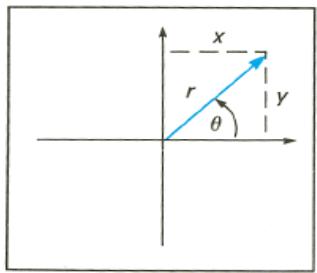
Polar Conversion. Pressing

g P

(polar) converts a set of rectangular coordinates (x, y) to polar coordinates (magnitude r , angle ). The y -value must be entered first, the x -value second. Upon executing 9 r will appear in the display. Press ( X exchange Y ) to bring out of the Y-register and into the display (X-register). will be returned as a value between -180^ and 180^ , between - and radians, or between -200 and 200 grads.

Rectangular Conversion. Pressing (rectangular) converts a set of polar coordinates (magnitude r angle ) into rectangular coordinates (x, y) . must be entered first then r . Upon executing , x will be displayed first; press ≤ y to display y .

Keystrokes

10

12

Display

5.0000

10

11.1803

26.5651

30.0000

12

10.3923

6.0000

Set to Degrees mode (no annunciator).

y -value.

x -value.

r

; rectangular coordinates converted to polar coordinates.

r

x -value.

y -value. Polar coordinates converted to rectangular coordinates.

Section 3

The Automatic Memory Stack, LAST X, and Data Storage

The Automatic Memory Stack and Stack Manipulation

HP operating logic is based on a mathematical logic known as "Polish Notation," developed by the noted Polish logician Jan Lukasiewicz (Wookashye'veech) (1878-1956). Conventional algebraic notation places the algebraic operators between the relevant numbers or variables when evaluating algebraic expressions. Lukasiewicz's notation specifies the operators before the variables. For optimal efficiency of calculator use, HP applied the convention of specifying (entering) the operators after specifying (entering) the variable(s). Hence the term "Reverse Polish Notation" (RPN).

The HP-15C uses RPN to solve complicated calculations in a straightforward manner, without parentheses or punctuation. It does so by automatically retaining and returning intermediate results. This system is implemented through the automatic memory stack and the ENTER key, minimizing total keystrokes.

The Automatic Memory Stack Registers

T	0.0000
Z	0.0000
Y	0.0000
X	0.0000

When the HP-15C is in Run mode (no PRGM annunciator displayed), the number that appears in the display is the number in the X-register.

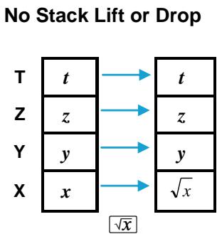
Any number that is keyed in or results from the execution of a numeric function is placed into the display (X-register). This action will cause numbers already in the stack to lift, remain in the same register, or drop, depending upon both the immediately preceding and the current operation. Numbers in the stack are stored on a last-in, first-out basis. The three stacks drawn below illustrate the three types of stack movement. Assume x , y , z , and t represent any numbers which may be in the stack.

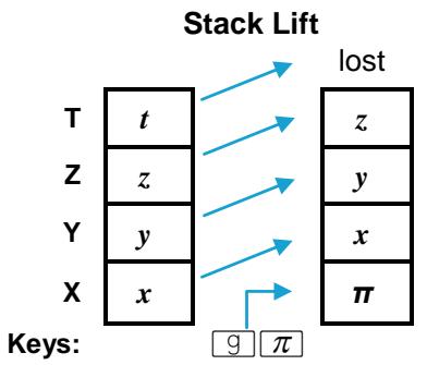
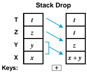
Notice the number in the T-register remains there when the stack drops, allowing this number to be used repetitively as an arithmetic constant.

Stack Manipulation Functions

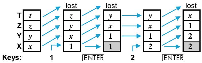
ENTER. Pressing ENTER separates two numbers keyed in one after the other. It does so by lifting the stack and copying the number in the display (X-register) into the Y-register. The next number entered then writes over the value in the X-register; there is no stack lift. The example below shows what happens as the stack is filled with the numbers 1, 2, 3, 4. (The

shading indicates that the contents of that register will be written over when the next number is keyed in or recalled.)

^ (roll down), ^ (roll up), and ≤ y ( X exchange Y ). ^ and ^ roll the contents of the stack registers up or down one register (one value moves between the X- and the T-register). No values are lost. ≤ y exchanges the numbers in the X- and Y-registers. If the stack were loaded with the sequence 1, 2, 3, 4, the following shifts would result from pressing ^ , ^ and ≤ y .

The LAST X Register and _x

The LAST X register, a separate memory register, preserves the value that was last in the display before execution of a numeric operation. Pressing 9 (LAST X ) places a copy of the contents of the LAST X register into the display (X-register). For example:

The _x feature saves you from having to re-enter numbers you want to use again (as shown under Arithmetic Calculations With Constants, page 39). It can also assist you in error recovery, such as executing the wrong function or keying in the wrong number.

For example, suppose you mistakenly entered the wrong divisor in a chain calculation:

Keystrokes

287 ENTER

12.9 +

9 [LSTx]

Display

287.0000

22.2481

12.9000

Oops! The wrong divisor.

Retrieves from LAST X the last entry to the X-register (the incorrect divisor) before + was executed.

Keystrokes

Display

287.0000

Reverses the function that produced the wrong answer.

13.9 +

20.6475

The correct answer.

Calculator Functions and the Stack

When you want to key in two numbers, one after the other, you press ENTER between entries of the numbers. However, when you want to key in a number immediately following any function (including manipulations like R), you do not need to use ENTER. Why? Executing most HP-15C functions has this additional effect:

• The automatic memory stack is lift-enabled that is, the stack will lift automatically when the next number is keyed or recalled into the display.
• Digit entry is terminated, so the next number starts a new entry.

There are four functions - , , ^+ , and ^- - that disable stack lift. They do not provide for the lifting of the stack when the next number is keyed in or recalled. Following the execution of one of these functions, a new number will simple write over the currently displayed number instead of causing the stack to lift. (Although the stack lifts when is pressed, it will not lift when the next number is keyed in or recalled. The operation of illustrated on page 34 shows how thus disables the stack.) In most cases, the above effects will come so naturally that you won't even think about them.

Order of Entry and the ENTER Key

An important aspect of two-number functions is the positioning of the numbers in the stack. To execute an arithmetic function, the numbers should be positioned in the stack in the same way that you would vertically position them on paper. For example:

98	98	98	98
-15	+15	x15	15

As you can see, the first (or top) number would be in the Y-register, while the second (or bottom) number would be in the X-register. When the mathematics operation is performed, the stack drops, leaving the result in the X-register. Here is how a subtraction operation is executed in the calculator:

The same number positioning would be used to add 15 to 98, multiply 98 by 15, or divide 98 by 15.

Nested Calculations

The automatic stack lift and stack drop make it possible to do nested calculations without using parentheses or storing intermediate results. A nested calculation is solved simply as a series of one- and two-number operations.

Almost every nested calculation you are likely to encounter can be done using just the four stack registers. It is usually wisest to begin the calculation at the innermost number or pair of parentheses and work outward (as you would for a manual calculation). Otherwise, you may need to place an intermediate result into a storage register. For example, consider the calculation of

$$ 3 \left[ 4 + 5 (6 + 7) \right]: $$

Keystrokes	Display
6 ENTER 7 +	13.0000	Intermediate result of (6 + 7).
5 ×	65.0000	Intermediate result of 5 (6 + 7).
4 +	69.0000	Intermediate result of [4 + 5 (6 + 7)].
3 ×	207.0000	Final result: 3 [4 + 5 (6 + 7)].

The following sequence illustrates the stack manipulation in this example. The stack automatically drops after each two-number calculation, and then lifts when a new number is keyed in. (For simplicity, throughout the rest of this handbook we will not show arrows between the stacks.)

Arithmetic Calculations With Constants

There are three ways (without using a storage register) to manipulate the memory stack to perform repeated calculations with a constant:

1. Use the LAST X register.
2. Load the stack with a constant and operate upon different numbers. (Clear the X-register every time you want to change the number operated upon)
3. Load the stack with a constant and operate upon an accumulating number. (Do not change the number in the X-register.)

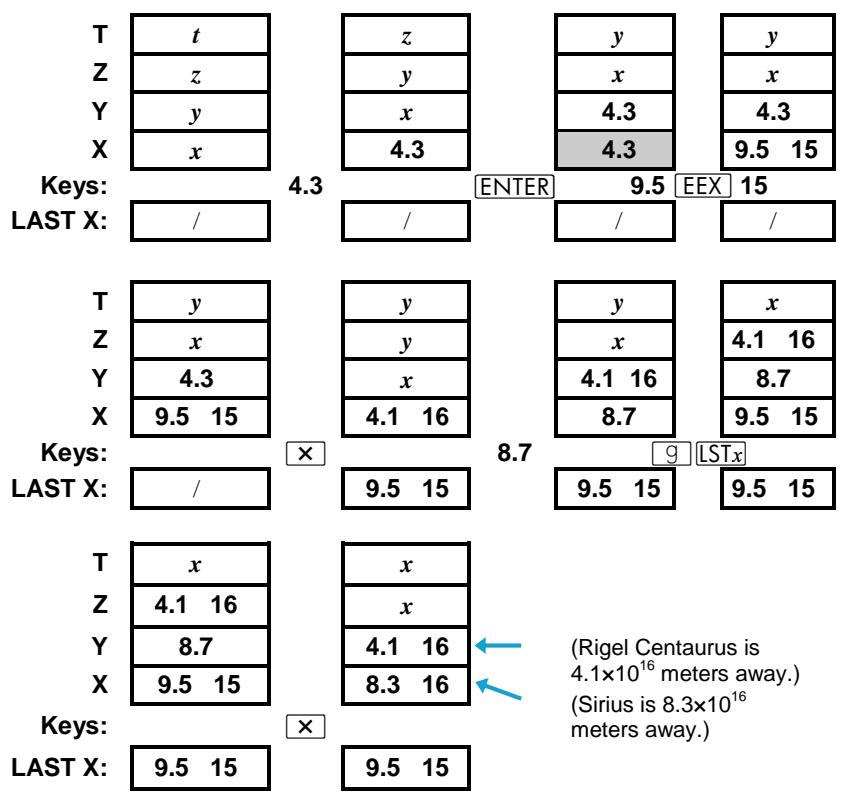
LAST X. Use your constant in the X-register (that is, enter it second) so that it always will be saved in the LAST X register. Pressing 9 will retrieve the constant and place it into the X-register (the display). This can be done repeatedly.

Example: Two close stellar neighbors of Earth are Rigel Centaurus (4.3 light-years away) and Sirius (8.7 light-years away). Use the speed of light, c ( 3.0 × 10^8 meters/second, or 9.5 × 10^15 meters/year), to figure the distances to these stars in meters. (The stack diagrams show only one decimal place.)

Loading the Stack with a Constant. Because the number in the T-register is replicated when the stack drops, this number can be used as a constant in arithmetic operations.

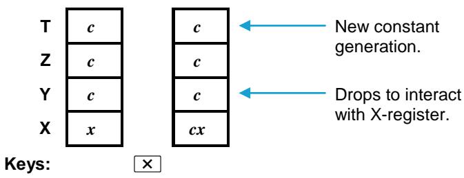
Fill the stack with a constant by keying it into the display and pressing ENTER three times. Key in your initial argument and perform the arithmetic operation. The stack will drop, a copy of the constant will "fall" into the Y-register, and a new copy of the constant will be generated in the T-register.

If the variables change (as in the preceding example), be sure and clear the display before entering the new variable. This disables the stack so that the arithmetic result will be written over and only the constant will occupy the rest of the stack.

If you do not have different arguments, that is, the operation will be performed upon a cumulative number, then do not clear the display—simply repeat the arithmetic operation.

Example: A bacteriologist tests a certain strain of microorganisms whose population typically increases by 15% each day (a growth factor of 1.15). If she starts with a sample culture of 1000, what will be the bacteria population at the end of each day for four consecutive days?

Keystrokes	Display
1.15	1.15	Growth factor.
ENTER ENTER	1.1500	Filling the stack.
ENTER
1000	1,000	Initial culture size.

Keystrokes Display

× 1,150.0000 Population at the end of day 1.

X 1,322.5000 Day 2.

X 1,520.8750 Day 3.

X 1,749.0063 Day 4.

Storage Register Operations

When numbers are stored or recalled, they are copied between the display (X-register) and the data storage registers. At "power-up" (initial turn-on or Continuous Memory reset) the HP-15C has 21 directly accessible storage registers: R0 through R9 , R0 through R9 , and the Index register (_1) (see the diagram of the registers on the inside back cover). Six registers, R_2 to R_7 , are also used for statistics calculations.

The number of available data storage registers can be increased or decreased. The DIM function, which is used to reallocate registers in calculator memory, is discussed in appendix C, Memory Allocation. The lowest-numbered registers are the last to be deallocated from data storage, therefore it is wisest to store data in the lowest-numbered registers available.

Storing and Recalling Numbers

STO (store). When followed by a storage register address (0 through 9 or .0 through .9*), this function copies a number from the display (X-register) into the specified data storage register. It will replace any existing contents of that register.
RCL (recall). Similarly, you can recall data from a particular register into the display by pressing RCL followed by the register address. This brings a copy of the desired data into the display; the contents of the storage register remain unaltered.
≤slant (X exchange). Followed by 0 through .9, this function exchanges the contents of the X-register and the addressed data storage register. This is useful to view storage registers without disturbing the stack.

The above are stack lift-enabling operations, so the number remaining in the X-register can be used for subsequent calculations. If you address a nonexistent register, the display will show Error 3.

Example: Springtime is coming and you want to keep track of 24 crocuses planted in your garden. Store the number of crocuses blooming the first day and add to this the number of new blooms the second day.

Keystrokes

3 STO 0

Display

3.0000

Stores the number of first-day blooms in R_0

Turn the calculator off. Next day, turn it back on again.

RCL0

3.0000

Recalls the number of crocuses that bloomed yesterday.

5 +

8.0000

Adds today's new blooms to get the total blooming crocuses.

Clearing Data Storage Registers

Pressing f CLEAR REG (clear registers) clears the contents of all data storage registers to zero. (It does not affect the stack or the LAST X register.) To clear a single data storage register, store zero in that register. Resetting Continuous Memory clears all registers and the stack.

Storage and Recall Arithmetic

Storage Arithmetic. Suppose you not only wanted to store a number, but perform arithmetic with it and store the result in the same register. You can do this directly - without using RCL - by using the following procedure.

1. Have your second operand (besides the one in storage) in the display (as the result of a calculation, a recall, or keying in).
2. Press STO
3. Press + , - , × , or ÷ .
4. Key in the register address (0 to 9, .0 to .9). (The Index register, discussed in section 10, can also be used.)

The number in the register is determined as follows:

For storage arithmetic,

$$ \begin{array}{c c} \text {n e w c o n t e n t s} & = \quad \text {o l d c o n t e n t s} \ \text {o f r e g i s t e r} & \end{array} \left{ \begin{array}{l} + \ - \ \times \ \div \end{array} \right} \text {n u m b e r i n} $$

R0

T Z Y X

R0

T Z Y X

Keys:

STO 0

Recall Arithmetic. Recall arithmetic allows you to perform arithmetic with the displayed value and a stored value without lifting the stack, that is, without losing any values from the Y-, Z, and T-registers. The keystroke sequence is the same as for storage arithmetic using RCL in place of STO.

For recall arithmetic,

$$ \text {n e w d i s p l a y} = \text {o l d d i s p l a y} \left{ \begin{array}{l} + \ - \ \times \ \div \end{array} \right} \text {c o n t e n t s o f} $$

R0

T
Z
Y
X

R0

T
Z
Y
X

Keys:

RCL 0

Example: Keep a running count of your newly blooming crocuses for two more days.

Keystrokes	Display
8 STO 0	8.0000	Places the total number of blooms as of day 2 in R0.
4 STO + 0	4.0000	Day 3: adds four new blooms to those already blooming.
3 STO + 0	3.0000	Day 4: adds three new blooms.
24 RCL - 0	9.0000	Subtracts total number of blooms summed in R0(15) from the total number of plants (24); 9 crocuses have not bloomed.
RCL 0	15.0000	(The number in R0 does not change.)

Overflow and Underflow

If an attempted storage or recall arithmetic operation would result in overflow in a data storage register, the value in the affected register will be replaced with ± 9.999999999 × 10^99 and the display will blink. To stop the blinking (clear the overflow condition), press or ON or 9 CF 9.

In case of underflow, the value in the register will be replaced with zero (no display blinking). Overflow and underflow are discussed further on page 61.

Problems

1. Calculate the value of x in the following equation.

$$ x = \sqrt {\frac {8 . 3 3 (4 - 5 . 2) \div [ (8 . 3 3 - 7 . 4 6) 0 . 3 2 ]}{4 . 3 (3 . 1 5 - 2 . 7 5) - (1 . 7 1) (2 . 0 1)}} $$

Answer: 4.5728.

A possible keystroke solution is:

4 ENTER 5.2 - 8.33 x g LSTx 7.46 - 0.32 x ÷ 3.15

ENTER 2.75 -4.3 X 1.71 ENTER 2.01 X - 2

1. Use arithmetic with constants to calculate the remaining balance of a 1000 loan after six payments of100 each and an interest rate of 1% (0.01) per payment period.

Procedure: Load the stack with (1 + i) , where i = interest rate, and key in the initial loan balance. Use the following formula to find the new balance after each payment.

New Balance = ( ( Old Balance) × ( 1 + i) ) - Payment

The first part of the key sequence would be:

1.01 ENTER ENTER ENTER 1000

For each payment, execute:

100

Balance after six payments: $446.32.

1. Store 100 in R_5 . Then:

2. Divide the contents of R_5 by 25.

3. Subtract 2 from the contents of _5
4. Multiply the contents of R_5 by 0.75.
5. Add 1.75 to the contents of R_5
6. Recall the contents of R_5 .

Answer: 3.2500.

Section 4

Statistics Functions

A word about the statistics functions: their use is based on an understanding of memory stack operation (Section 3). You will find that order of entry is important for most statistics calculations.

Probability Calculations

The input for permutation and combination calculations is restricted to nonnegative integers. Enter the y -value before the x -value. These functions, like the arithmetic operators, cause the stack to drop as the result is placed in the X-register.

Permutations. Pressing .x calculates the number of possible different arrangements of y different items taken in quantities of x items at a time. No item occurs more than once in an arrangement, and different orders of the same x items in an arrangement are counted separately. The formula is

$$ P _ {y, x} = \frac {y !}{(y - x) !} $$

Combinations. Pressing 9 ,x calculates the number of possible sets of y different items taken in quantities of x items at a time. No item occurs more than once in a set, and different orders of the same x items in a set are not counted separately. The formula is

$$ C _ {y, x} = \frac {y !}{x ! (y - x) !} $$

Examples: How many different arrangements are possible of five pictures which can be hung on the wall three at a time?

Keystrokes

5 ENTER 3

f Pxy

Display

3

60.0000

Five (y) pictures put up three (x) at a time.

Sixty different arrangement possible.

How many different four-card hands can be dealt from a deck of 52 cards?

Keystrokes

52 ENTER 4

Display

4

Fifty-two (y) cards dealt four (x) at a time.

g Cxy.x

270,725.0000

Number of different hands possible.

The maximum size of x or y is 9,999,999,999.

Random Number Generator

Pressing f RAN# (random number) will generate a random number (part of a uniformly distributed pseudo-random number sequence) in the range 0 ≤ r < 1 .

At initial power-up (including reset of Continuous Memory), the HP-15C random number generator will use zero as a "seed" to initiate a random number sequence. Any time you generate a random number, that number becomes the seed for the next random number. You can initiate a different random number sequence by storing a new seed for the random number generator. (Repetition of a random number seed will produce repetition of the random number sequence.)

STO f RAN# will store the X-register number (0≤ r < 1) as a new seed for the random number generator. (A value for r outside this range will be converted to fit within the range.)

RCL f RAN# will recall to the display the current random number seed.

Keystrokes

.5764

STO f

RAN#

f RAN#

f RAN#

Display

0.5764

0.5764

0.3422

0.2809

0.0000

Stores 0.5764 as random number seed.

(The keystroke may be omitted.)

Random number sequence initiated by the above seed.

Keystrokes

RCL f

RAN#

Display

0.2809

Recall last random number generated, which is the new seed. (The may be omitted.)

Accumulating Statistics

The HP-15C performs one- and two-variable statistical calculations. The data is first entered into the Y- and X-registers. Then the ^+ function automatically calculates and stores statistics of the data in storage registers R_2 through R_7 . These registers are therefore referred to as the statistics registers.

Before beginning to accumulate statistics for a new set of data, press f CLEAR to clear the statistics registers and stack. (If you have reallocated registers in memory and any of the statistics registers no longer exist, Error 3 will be displayed when you try to use CLEAR , + , or - Appendix C explains how to reallocate memory.)

In one-variable statistical calculations, enter each data point (x -value) by keying in x and then press ^+ .

In two-variable statistical calculations, enter each data pair (the x - and y -values) as follows:

1. Key y into the display first.
2. Press ENTER. The displayed y -value is copied into the Y-register.
3. Key x into the display.
4. Press + . The current number of accumulated data points, n , will be displayed. The x -value is saved in the LAST X register and y remains in the Y-register. + disable stack lift, so the stack will not lift when the next number is keyed in.

In some cases involving x or y data values that differ by a relatively small amount, the calculator cannot compute s , r , linear regression, or , and will display Error 2. This will not happen, however, if you normalize the data by keying in only the difference between each value and the mean or approximate mean of the values. This difference must be added back to the calculations of , , and the y -intercept (L.R.). For example, if your x -values were 665999, 666000, and 666001, you should enter the data as -1, 0, and 1; then add 666000 back to the relevant results.

The statistics of the data are compiled as follows:

Register	Contents
R2	n	Number of data points accumulated (n also appears in the X-register).
R3	Σx	Summation of x-values.
R4	Σx2	Summation of squares of x-values.
R5	Σy	Summation of y-values.
R6	Σy2	Summation of squares of y-values.
R7	Σxy	Summation of products of x- and y-values.

You can recall any of the accumulated statistics to the display (X-register) by pressing RCL and the number of the data storage register containing the desired statistic. If you press RCL + , y and x will be copied simultaneously from R_3 and R_5 respectively, into the X-register and the Y-register, respectively. (The sequence RCL + lifts the stack twice if stack lift is enabled, once if not, and then enables stack lift.)

Example: Agronomist Silas Farmer has developed a new variety of high-yield rice, and has measured the plant's yield as a function of fertilization. Use the ^+ function to accumulate the data below to find the values for x , x^2 , y , y^2 , and xy for nitrogen fertilizer application (x) versus grain yield (y) .

X	NITROGEN APPLIED (kg per hectare *), x	0.00	20.00	40.00	60.00	80.00
Y	GRAIN YIELD (metric tons per hectare), y	4.63	4.78	6.61	7.21	7.78
*A hectare equals 2.47 acres.

Keystrokes	Display
f CLEAR Σ	0.0000	C clears statistical storage registers (R2 through R7 and the stack).
f FIX 2	0.00	Limits display to two decimal places, like the data.
4.63 ENTER	4.63
0 Σ+	1.00	First data point.
4.78 ENTER	4.78
20 Σ+	2.00	Second data point.
6.61 ENTER	6.16
40 Σ+	3.00	Third data point.
7.21 ENTER	7.21
60 Σ+	4.00	Fourth data point.
7.78 ENTER	7.78
80 Σ+	5.00	Fifth data point.
RCL 3	200.00	Sum of x-values, Σx (kg of nitrogen).
RCL 4	12.000.00	Sum of squares of x-values, Σx2.
RCL 5	31.01	Sum of y-values, Σy (grain yield).
RCL 6	200.49	Sum of squares of y-values, Σy2.
RCL 7	1,415.00	Sum of products of x- and y-values, Σxy.

Correcting Accumulated Statistics

If you discover that you have entered data incorrectly, the accumulated statistics can be easily corrected. Even if only one value of an (x,y) data pair is incorrect, you must delete and re-enter both values.

1. Key the incorrect data pair into the Y- and X-register.
2. Press 9 - to delete the incorrect data.
3. Key in the correct values for x and y .
4. Press ^+

Alternatively, if the incorrect data point or pair is the most recent one entered and ^+ has been pressed, you can press 9 [LSTx] 9 [Σ-] to remove the incorrect data.

Example: After keying in the preceding data. Farmer realizes he misread a smeared figure in his lab book. The second y -value should have been 5.78 instead of 4.78. Correct the data input.

Keystrokes Display

4.78 4.78 ENTER

20 g - 4.00

5.78 5.78 ENTER

20 ^+ 5.00

Keys in the data pair we want to replace and deletes the accompanying statistics.

The n -value drops to four.

Keys in and accumulates the replacement data pair.

The n -value is back to five.

We will use these statistics in the rest of the examples in this section.

Mean

The function computes the arithmetic mean (average) of the x -and y -values using the formulas shown in appendix A and the statistics accumulated in the relevant registers. When you press 9 the contents of the stack lift (two registers if stack lift is enabled, one if not); the mean of x ( ) is copied into the X-register as the mean of y ( ) is copied simultaneously into the Y-register. Press ≤ y to view .

Example: From the corrected statistics data we have already entered and accumulated, calculate the average fertilizer application, . and average grain yield , for the entire range.

Keystrokes

Display

40.00 Average kg of nitrogen, , for all cases.

6.40 Average tons of rice, , for all cases.

Standard Deviation

Pressing 9 s computes the standard deviation of the accumulated statistics data. The formulas used to compute s_x , the standard deviation of the accumulated x -values, and s_y , the standard deviation of the accumulated y -values, are given in appendix A.

This function gives an estimate of the population standard deviation from the sample data, and is therefore termed the sample standard deviation.* When you press g s, the contents of the stack registers are lifted (twice if stack lift is enabled, once if not); s_x is placed into the X-register and s_y is placed into the Y-register. Press x\y to views_y$ .

Example: Calculate the standard deviation about the mean calculated above.

Keystrokes

Display

31.62

Standard deviation about the mean nitrogen application,

1.24

Standard deviation about the mean grain yield,

Linear Regression

Linear regression is a statistical method for finding a straight line that best fits a set of two or more data pairs, thus providing a relationship between two or more data pairs, thus providing a relationship between two variables. By the method of least squares, will calculate the slope, A , and y -intercept, B , of the linear equation:

$$ y = A x + B $$

1. Accumulate the statistics of your data using the ^+ key.
2. Press . The y -intercept, B , appears in the display (X-register). The slope, A , is copied simultaneously into the Y-register.
3. Press ≤ y to view A . (As is the case with the functions and , .R. causes the stack to lift two registers if it's enabled, one if not).

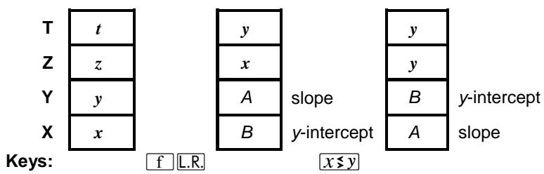
The slope and y-intercept of the least squares line of the accumulated data are calculated using the equations shown in appendix A.

Example: Find the y -intercept and slope of the linear approximation of the data and compare to the plotted data on the graph below.

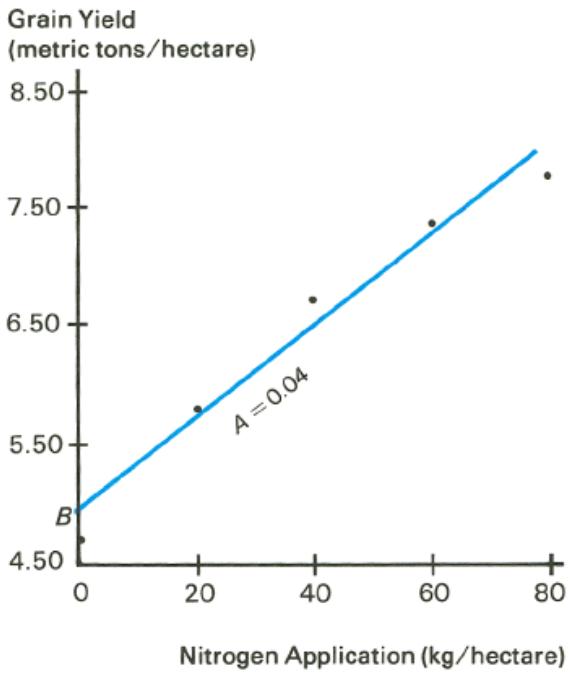
Keystrokes

f [L.R.]

x≤y

Display

4.86

0.04

y -intercept of the line.

Slope of the line.

Linear Estimation and Correlation Coefficient

When you press ,r the linear estimate, , is placed in the X-register and the correlation coefficient, r , is placed in the Y-register. To display r , press ≤ y .

Linear Estimation. With the statistics accumulated, an estimated value for y , denoted , can be calculated by keying in a proposed value for x and pressing f , r .

An Estimated value for x (denoted ) can be calculated as follows:

1. Press f L.R.
2. Key in the known y -value.
3. Press ≤ y- = ≤ y÷

Correlation Coefficient. Both linear regression and linear estimation presume that the relationship between the x and y data values can be approximated by a linear function. The correlation coefficient, r , is a determination of how closely your data fit a straight line. The range is -1 ≤ r ≤ 1 , with -1 representing a perfectly negative correlation and +1 representing a perfectly positive correlation.

Note that if you do not key in a value for x before executing ,r , the number previously in the X-register will be used (usually yielding a meaningless value for ).

Example: What if 70kg of nitrogen fertilizer were applied to the rice field? Predict the grain yield based on Farmer's accumulated statistics. Because the correlation coefficient is automatically included in the calculation, you can view how closely the data fit a straight line by pressing ≤ y after the y prediction appears in the display.

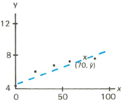
Keystrokes

Display

70 f ,r

7.56

Predicted grain yield in tons/hectare.

x≤y

0.99

The original data closely approximates a straight line.

Other Applications

Interpolation. Linear interpolation of tabular values, such as in thermodynamics and statistics tables, can be carried out very simply on the HP-15C by using the ,r function. This is because linear interpolation is linear estimation: two consecutive tabular values are assumed to form two points on a line, and the unknown intermediate value is assumed to fall on that same line.

Vector Arithmetic. The statistical accumulation functions can be used to perform vector addition and subtraction. Polar vector coordinates must be converted to rectangular coordinates upon entry ( , , r , ^+ ). The results are recalled from R_3 ( x ) and R_5 ( y ) (using ^+ ) and converted back to polar coordinates, if necessary. Remember that for polar coordinates the angle is between -180^ and 180^ (or - and radians, or -200 and 200 grads). To convert to a positive angle, add 360 (or 2 or 400) to the angle.

For the second vector entered, the final keystroke will be either ^+ or ^- , depending on whether the two vectors should be added or subtracted.

Section 5

The Display

and Continuous Memory

Display Control

The HP-15C has three display formats - FIX, SCI, and ENG - that use a given number (0 through 9) to specify display format. The illustration below shows how the number 123,456 would be displayed specified to four places in each possible mode.

Owing to Continuous Memory, any change you make in the display format will be preserved until Continuous Memory is reset.

The current display format takes effect when digit entry is terminated; until then, all digits you key in (up to 10) are displayed.

Fixed Decimal Display

FIX (fixed decimal) format displays a figure with the number of decimal places you specify (up to nine, depending on the size of the integer portion.) Exponents will be displayed if the number is too small or too large for the display. At "power-up," the HP-15C is in FIX 4 format. The key sequence is f FIX n.

Keystrokes

123.4567895
F FIX 4
F FIX 6

Display

123.4567895
123.4568
123.456790

Display is rounded to six decimal places. (Ten places are stored internally.)

f FIX 4

123.4568

Usual FIX 4 display.

Scientific Notation Display

SCI (scientific) format displays a number in scientific notation. The sequence f SC1 n specifies the number of decimal places to be shown. Up to six decimal places can be shown since the exponent display takes three spaces. The display will be rounded to the specified number of decimal places; however, if you specify more decimal places than the six places the display can hold (that is, SCI 7, 8, or 9), rounding will occur in the undisplayed seventh, eighth, or ninth decimal place.*

With the previous number still in the display:

Keystrokes

f SC1 6

f SCl 8

Display

1.234568

1.234567

02 Rounds to and shows six decimal places.

02 Rounds to eight decimal places, but displays only six.

Engineering Notation Display

ENG (engineering) format displays numbers in an engineering notation format in a manner similar to SCI, except:

• In engineering notation, the first significant digit is always present in the display. The number you key in after f ENG specifies the number of additional digits to which you want to round the display.
• Engineering notation shows all exponents in multiples of three.

Keystrokes

.012345

f ENG

1

f ENG 3

10 X

□F FIX 4

Display

0.012345

12.

-03

Rounds to the first digit after the leading digit.

12.35

-03

123.5

-03

Decimal shifts to maintain multiple of three in exponent.

0.1235

Usual FIX 4 format.

Mantissa Display

Regardless of the display format, the HP-15C always internally holds each number as a 10-digit mantissa and a two-digit exponent of 10. For example, is always represented internally as 3.141592654 × 10^00 , regardless of what is in the display.

When you want to view the full 10-digit mantissa of a number in the X-register, press f CLEAR [PREFIX]. To keep the mantissa in the display, hold the [PREFIX] key down.

Keystrokes

g

f CLEAR

PREFIX (hold)

Display

3.1416

3141592654

Round-Off Error

As mentioned earlier, the HP-15C holds every value to 10 digits internally. It also rounds the final result of every calculation to the 10th digit. Because the calculator can provide only a finite approximation for numbers such as or 2/3 (0.666...), a small error due to rounding can occur. This error can be increased in lengthy calculations, but usually is insignificant. To accurately assess this effect for a given calculation requires numerical analysis beyond our scope and space here! Refer to the HP-15C Advanced Functions Handbook for a more detailed discussion.

Special Displays

Annunciators

The HP-15C display contains eight annihilators that indicate the status of the calculator for various operations. The meaning and use of these annihilators is discussed on the following pages:

* Low-power indication, page 62.

USER User mode, pages 79 and 144.

f and g Prefixes for alternate functions, pages 18-19.

RAD and GRAD Trigonometric modes, page 26.

C Complex mode, page 121.

PRGM Program mode, page 66.

Digit Separators

The HP-15C is set at power-up so that it separates integral and fractional portions of a number with a period (a decimal point), and separates groups of three digits in the integer portion with a comma. You can reverse this setting to conform to the numerical convention used in many countries. To do so, turn off the calculator. Press and hold ON, press and hold , release ON, then release ( ON / ). (Repeating this sequence will set the calculator to the previous display convention.)

Keystrokes

12345.67

Display

12,345.67

12.345.6700

12,345.6700

Error Display

If you attempt an improper operation—such as division by zero—an error message (Error followed by a digit) will appear in the display. For a complete listing of error messages and their causes, refer to appendix A.

To clear the Error display and restore the calculator to its prior condition, press any key. You can then resume normal operation.

Overflow and Underflow

Overflow. When the result of a calculation in any register is a number with a magnitude greater than 9.999999999 × 10^99 , ± 9.999999999 × 10^99 is placed in the affected register and the overflow flag, flag 9, is set. * Flag 9 causes the display to blink. When overflow occurs in a running program, execution continues until completion of the program, and then the display blinks.

The blinking can be stopped and flag 9 cleared by pressing , ON or 9 CF 9.

Underflow. If the result of a calculation in any register is a number with a magnitude less than 1.000000000 × 10^-99 , that number will be replaced by zero. Underflow does not have any other effect.

Low-Power Indication

When a flashing asterisk, which indicates low battery power, appears in the lower left-hand side of the display, there is no reason to panic. You still have plenty of calculator time remaining: at least 10 minutes if you continuously run programs, and at least an hour if you do calculations manually. Refer to appendix F (page 259) for information on replacing the batteries.

0.0000

Continuous Memory

Status

The Continuous Memory feature of the HP-15C retains the following in the calculator, even when the display is turned off:

• All numeric data stored in the calculator.
• All programs stored in the calculator.
• Position of the calculator in program memory.
• Display mode and setting.
• Trigonometric mode (Degrees, Radians, or Grads).
• Any pending subroutine returns.
• Flag settings (except flag 9, which clears when the display is manually turned off).
• User mode setting.
  Complex mode setting.

When the HP-15C is turned on, it always "wakes up" in Run mode. If the calculator is turned off, Continuous Memory will be preserved for a short period while the batteries are removed. Data and programs are preserved longer than other aspects of calculator status. Refer to appendix F for instructions on changing batteries.

Resetting Continuous Memory

If at any time you want to reset (entirely clear) the HP-15C Continuous Memory:

1. Turn the calculator off.
2. Press and hold the ON key, then press and hold the -key.
3. Release the ON key, then the -key. (This convention is represented as ON / -.)

When Continuous Memory is reset, Pr Error (power error) will be displayed. Press any key to clear the display.

Note: Continuous Memory can inadvertently be interrupted and reset if the calculator is dropped or otherwise traumatized.

Part II

HP-15C

Programming

Section 6

Programming Basics

The next five sections are dedicated to explaining aspects of programming the HP-15C. Each of these programming sections will first discuss basic techniques (The Mechanics), then give examples for the implementation of these techniques (Examples), and lastly discuss finer points of operation in greater detail (Further Information). Read only as far as you need to support your use of the HP-15C.

The Mechanics

Creating a Program

Programming the HP-15C is an easy matter, based simply on recording the keystroke sequence used when calculating manually. (This is called "keystroke programming".) To create a program out of a series of calculation steps requires two extra manipulations: deciding where and how to enter your data; and loading and storing the program. In addition, programs can be instructed to make decisions and perform iterations through conditional and unconditional branching.

As we step through the fundamentals of programming, we'll rework the falling object program illustrated in the Problem Solver (page 14).

Loading a Program

Program Mode. Press 9 / R (program/run) to set the calculator to Program mode (PRGM annunciator on). Functions are stored and not executed when keys are pressed in Program mode.

Keystrokes

P/R

Display

000-

Switches to Program mode;

PRGM annunciator and line number (000) displayed.

Location in Program Memory. Program memory – and therefore the calculator's position in program memory – is demarcated by line numbers. Line 000 marks the beginning of program memory and cannot be used to store an instruction. The first line that contains an instruction is line 001. Program lines other than 000 do not exist until instructions are written for them.

You can start a program at any existent line (designated nnn), but it is simplest and safest to start an independent program (as opposed to a subroutine) at the beginning of program memory. As you write, any existing program lines will be preserved and "bumped" down in program memory.

Press GTO CHS 000 (in Program or Run mode) to move to line 000 without recording the GTO statement. In Run mode, f CLEAR PRGM will also reset the calculator to line 000- without clearing program memory.

Alternatively, you can clear program memory, which will erase all programs in memory and position you to line 000. To do so, press f CLEAR PRGM in Program mode.

Program Begin. A label instruction - fLBL followed by a letter (A through E) or number (0 through 9 or .0 through .9) - is used to define the beginning of a program or routine. The use of labels allows you to quickly select and run one particular program or routine out of several.

Keystrokes	Display
f CLEAR	000-	C clears program memory and sets to line 000 (start of program memory).
PRGM
f LBL A	001-42,21,11

Recording a Program. Any key pressed—operator or constant—will be recorded in memory as a programmed instruction.

Keystrokes	Display
2	002-	2
×	003-	20
9	004-	9
·	005-	48
8	006-	8
÷	007-	10
√x	008-	11

Program End. There are three possible endings for a program:

• [9] RTN (return) will end a program, return to line 000, and halt.
• R/S will stop a program without moving to line 000.
• The end of program memory contains an automatic RTN.

Keystrokes	Display
9 RTN	009-	43	32	Optional if this is the last program in memory.

Intermediate Program Stops

Use f PSE (pause) as a program instruction to momentarily stop a program and display an intermediate result. (Use more than one PSE for a longer pause.)

Use a / (run/stop) instruction to stop the program indefinitely. The program will remain positioned at that line. You can resume program execution (from that line) by pressing / during Run mode, that is, from the keyboard.

Running a Program

Run Mode. Switch back to Run mode when you are done programming:
9 P/R. Program execution must take place in Run mode.

Keystrokes Display

P/R

Run mode; no PRGM annunciator displayed. (The display will depend on any previous result.)

The position in program memory does not change when modes are switched. Should the calculator be shut off, it always "wakes up" in Run mode.

Executing a Program. In Run mode, press f letter label or GSB digit (or letter) label. This addresses a program and starts its execution. The display will flash running.

Keystrokes Display

300.51 300.51

f A 7.8313

Key a value for h into the X-register.

The result of executing program "A". (The number of seconds it takes an object dropped from 300.51 meters high to hit the ground.)

Restarting a Program. Press R/S to continue execution of a program that was stopped with a R/S instruction.

User Mode. User mode is an optional condition to save keystrokes when executing letter-named programs. Pressing f USER will interchange the f shifted and primary functions of the A through E keys. You can then execute a program using just one keystroke (skipping the f or GSB).

How to Enter Data

Every program must take into account how and when data will be supplied. This can be done in Run mode before running the program or during an interruption in the program.

1. Prior entry. If a variable value will be used in the first line of the program, enter it into the X-register before starting the program. If it will be used later, you can store it (with ) into a storage register, and recall it (with a programmed ) within the program.

This is the method used above, where h was placed in the X-register before running the program. No ENTER instruction is necessary because program execution (here: f A) both terminates digit entry and enables the stack lift. The above program then multiplied the contents of the X-register (h) by 2.

The presence of the stack even makes it possible to load more than one variable prior to running a program. Keeping in mind how the stack moves with subsequent calculations and how the stack can be manipulated (as with ≤ y ), it is possible to write a program to use variables which have been keyed into the X-, Y-, Z-, and T-registers.

1. Direct entry. Enter the data as needed as the program runs. Write a / S (run/stop) instruction into the program where needed so the program will stop execution. Enter your data, then press / S to restart the program.

Do not key variable data into the program itself. Any values that will vary should be entered anew with each program execution.

Program Memory

At power-up (Continuous Memory reset), the HP-15C offers 322 bytes of program memory and 21 storage registers. Most program steps (instructions) use one byte, but some use two. The distribution of memory capacity can be altered, as explained in appendix C. The maximum attainable program memory is 448 bytes (with the permanent storage registers— _1 , _0 , and _1 — remaining); maximum number of storage registers is 67 (with no program memory).

Example. Mother's Kitchen, a canning company, wants to package a ready-to-eat spaghetti mix containing three different cylindrical cans: one of spaghetti sauce, one of grated cheese, and one of meatballs. Mother's needs to calculate the base areas, total surface areas, and volumes of the three different cans. It would also like to know, per package, the total base area, surface area, and volume.

The program to calculate this information uses these formulas and data:

base area = r^2

volume = base area × height = r^2 h

surface area = 2 base areas + side area = 2 r^2 + 2 rh .

Radius, r	Height, h	Base Area	Volume	Surface Area
2.5cm	8.0 cm	?	?	?
4.0	10.5	?	?	?
4.5	4.0	?	?	?
TOTALS		?	?	?

Method:

1. Enter an r value into the calculator and save it for other calculations. Calculate the base area ( r^2) , store it for later use, and add the base area to a register which will hold the sum of all base areas.
2. Enter h and calculate the volume ( r^2 h) . Add it to a register to hold the sum of all volumes.
3. Recall r . Divide the volume by r and multiply by 2 to yield the side area. Recall the base area, multiply by 2, and add to the side area to yield the surface areas. Sum the surface areas in a register.

Do not enter the actual data while writing the program - just provide for their entry. These values will vary and so will be entered before and/or during each program run.

Key in the following program to solve the above problem. The display shows line numbers and keycodes (the row and column location of a key), which will be explained under Further Information.

Keystrokes

9 P/R

f CLEAR PRGM

Display

000-

000-

Sets calculator to Program mode (PRGM displayed).

Cleared program memory. Starts at line 000.

Keystrokes

f LBL A

STO 0

9 x²

9

X

STO 4

STO +1

R/S

X

f PSE

STO + 2

RCL0

2

X

RCL 4

2

X

Display

001-42,21,11

002- 44 0

003- 4311

004- 4326

005- 20

006- 44 4

007-44,40，1

008- 31

009- 20

010- 4231

011-44,40，2

012- 45 0

013- 10

014- 2

015- 20

016- 45 4

017- 2

018- 20

Assigns this program the label "A".

Stores the contents of X-register into R_0 . r must be in the X-register before running the program.

Squares the contents of the Xregister (which will be r ).

r^2 , the BASE AREA of a can.

Stores the BASE AREA in _4

Keeps a sum of all BASE AREAS in R_1

Stops to display BASE AREA and allow entry of the h value.

Multiplies h by the BASE AREA, giving VOLUME.

Pauses briefly to display VOLUME.

Keeps a sum of all can VOLUMES in R_2

Recalls r .

Divides VOLUME by r .

2 rh , the SIDE AREA of a can.

Recalls the BASE AREA of the can.

Multiplies base area by two (for top and bottom).

Keystrokes

Display

019- 40

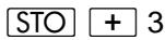
020-44,40，3

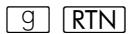
021- 4332

SIDE AREA + BASE AREA = SURFACE AREA.

Keeps a sum of all SURFACE AREAS in _3

Ends the program and returns program memory to line 000.

Now, let's run the program:

Keystrokes

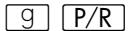
Display

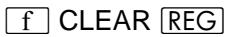
2.5

2.5

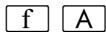
19.6350

(or: GSB A)

8

8

157.0796

4

164.9336

4

10.5

50.2655

10.5

4.5

527.7876

364.4247

4.5

63.6173

Sets calculator to Run mode. (PRGM cleared.)

Clears all storage registers. The display does not change.

Enter r of the first can.

Starts program A. BASE AREA of first can.

(running flashes during execution.)

Enter h of first can. Then restart program.

VOLUME of first can.

SURFACE AREA of first can.

Enter r of the second can.

BASE AREA of second can.

Enter h of second can.

VOLUME of second can.

SURFACE AREA of second can.

Enter r of the third can.

BASE AREA of third can.

Keystrokes	Display
4	4	Enter h of third can.
R/S	254.4690	VOLUME of third can.
	240.3318	SURFACE AREA of third can.
RCL 1	133.5177	Sum of BASE AREAS.
RCL 2	939.3362	Sum of VOLUMES.
RCL 3	769.6902	Sum of SURFACE AREAS.

The preceding program illustrates the basic techniques of programming. It also shows how data can be manipulated in Program and Run modes by entering, storing, and recalling data (input and output) using ENTER, STO, RCL, storage register arithmetic, and programmed stops.

Further Information

Program Instructions

Each digit, decimal point, and function key is considered an instruction and is stored in one line of program memory. An instruction may include prefixes (such as f, STO, GTO and LBL) and still occupy only one line. Most instructions require one byte of program memory; however, some require two. For a complete list of two-byte instructions, refer to Appendix C.

Instruction Coding

Each key on the HP-15C keyboard - except for the digit keys 0 through 9 - is identified in Program mode by a two-digit "keycode" that corresponds to the key's position on the keyboard.

Instruction

STO +1

Code

006-44,40，1

Sixth program line.

f DSE I

XXX-42, 5, 25

DSE is just "5".

The first digit of a keycode refers to the row (1 to 4 from top to bottom), and the second digit refers to the column (1, 2, 9, 0 from left to right). Exception: the keycode for a digit key is simply that digit.

Keycode 25: second row, fifth key.

Memory Configuration

Understanding memory configuration is not essential to your use of the HP-15C. It is essential, however, for obtaining maximum efficiency in memory and programming use. The more you program, the more useful this knowledge will be. Memory configuration and allocation is thoroughly explained in appendix C, Memory Allocation.

Should you ever get an Error 10, you have run up against limitations of the HP-15C memory. If you learn how to reallocate memory, you can greatly increase your ability to store information in the HP-15C.

The HP-15C memory consists of 67 registers ( R0 to R65 and the Index register) divided between data storage and programming/advanced function capability. The initial configuration is:

• 46 registers for both programming and the advanced functions (SOLVE, _y^x , the imaginary stack, and MATRIX functions). At seven bytes of memory per register, this is worth 322 program bytes if no memory is dedicated to advanced functions.
• 21 registers for data storage ( R0 to R_9 , R.0 to R_.9 , and the Index register).

Initial Memory Configuration

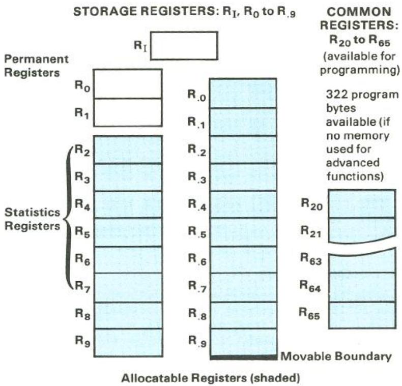
Memory is reallocated by telling the calculator which data storage register shall be the highest data register; all other registers are left for programming and advanced functions.

Keystrokes

60 f DIM (i)

Display

60.0000

R60 and below allocated to data storage; five (R61 to R_65) remain for programming.

Keystrokes

1 f DIM (i)

Display

1.0000

1 and _0 allocated for data storage; _2 to 65 available for programming and advanced functions.

19 f DIM (i)

19.0000

Original allocation: R19(R.9) and below for data storage; R20 to R65 for programming and advanced functions.

RCL DIM (i)

19.0000

Displays the current highest data register.

The DIM and MEM (memory status) functions are described in detail in appendix C.

Keep in mind that an error message will result (given the above memory configuration) if

1. You try to address a register higher than R19 ( R.9 ), which initially is the highest register allocated to data storage (Error 3).
2. You have 322 occupied program bytes and try to load more program lines (Error 4).
3. You try to run an advanced function with insufficient available memory (Error 10).

Program Boundaries

End. Not every program needs to end with a RTN or R/S instruction. If you are at the end of occupied program memory, there is an automatic RTN instruction, so you do not need to enter one. This can save you one line of memory. On the other hand, a program can "end" by simply transferring execution to another routine using GTO (section 7).

Labels. Labels in a program (or subroutine) are markers telling the calculator where to begin execution. Following an f label or GSB label instruction, the calculator will search downward in program memory for the

corresponding label. If need be, the search will wrap around at the end of program memory and continue at line 000. When it encounters an appropriate label, the search stops and execution begins.

If a label is encountered as part of a running program, it has no effect, that is, execution simply continues. Therefore, you can label a subordinate routine within a program (more on subroutines in section 9).

Since the calculator searches in only one direction from its present position, it is possible (though not advisable) to use duplicate program labels. Execution will begin at the first appropriately labeled line encountered.

If an f A entry starts the search for "A" here, it then proceeds downward through memory, wraps around to line 000, and stops at label "A". Execution then starts and continues (ignoring any other labels) until a halt instruction.

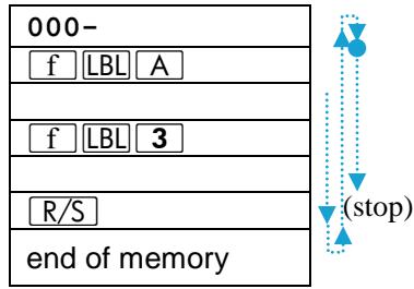
Unexpected Program Stops

Pressing Any Key. Pressing any key will halt program execution. It will not halt in the middle of an operation. This instruction will be completed before the program stops.

Error Stops. Program execution is immediately halted when the calculator attempts an improper operation that results in an Error display.

To see the line number and keycode of the error-causing instruction (the line at which the program stopped), press any one key to remove the Error message, then switch to Program mode.

If the display is flashing when a program stops, an overflow condition exists (page 61). Press ON, or CF 9 to stop the blinking.

Abbreviated Key Sequences

In certain cases, an prefix you might expect to include in a key sequence is not needed. The rule for using an abbreviated key sequence is: the prefix key is unnecessary after any other prefix key. (Page 19 contains a list of prefix keys.)

For example, f LBL f A becomes f LBL A, f DIM f (i) becomes f DIM (i), and STO f RAN# becomes STO RAN#. The removal of the f is not ambiguous because the f-shifted function is the only logical one in these cases. The keycodes for such instructions do not include the extraneous f even if you do key it in.

User Mode

User mode is a convenience to save keystrokes when addressing (calling up) programs for execution. Pressing f USER will exchange the primary functions and f -shifted functions of the A through E keys only. In User mode (USER annunciator displayed):

f shift

Primary

g shift

Press 9 USER again to deactivate User mode.

Polynomial Expressions and Horner's Method

Some expressions, such as polynomials, use the same variable several times for their solution. For example, the expression

$$ f (x) = A x ^ {4} + B x ^ {3} + C x ^ {2} + D x + E $$

uses the variable x four different times. A program to solve such an equation could repeatedly recall a stored copy of x from a storage register. A shorter programming method, however, would be to use a stack which has been filled with the constant (refer to Loading the Stack with a Constant, page 41).

Horner's Method is a useful means of rearranging polynomial expressions to cut calculation steps and calculation time. It is especially expedient in and _y^x , two rather long-running functions that use subroutines.

This method involves rewriting a polynomial expression in a nested fashion to eliminate exponents greater than 1:

$$ A x ^ {4} + B x ^ {3} + C x ^ {2} + D x + E $$

$$ \left(A x ^ {3} + B x ^ {2} + C x + D\right) x + E $$

$$ \left(\left(A x ^ {2} + B x + C\right) x + D\right) x + E $$

$$ \left(\left((A x + B) x + C\right) x + D\right) x + E $$

Example: Write a program for 5x^4 + 2x^3 as ((5x + 2)x)x , then evaluate for x = 7

Keystrokes	Display
9 P/R	000-		Assumes position in memory is line 000. If it is not, clear program memory.
f LBL B	001-42,21,12
5	002-	5
×	003-	20	5x.
2	004-	2
+	005-	40	5x+2.
×	006-	20	(5x+2)x.
×	007-	20	(5x+2)x2.
×	008-	20	(5x+2)x3.
9 RTN	009-	43 32
9 P/R			Returns to Run mode, Prior result remains in display.
7 ENTER ENTER	7.0000		Loads the stack (X-, Y-, Z-, and T-registers) with 7.
ENTER
f B	12,691.0000

Nonprogrammable Functions

When the calculator is in Program mode, almost every function on the keyboard can be recorded as an instruction in program memory. The following functions cannot be stored as instructions in program memory.

f	CLEAR	PREFIX
f	CLEAR	PRGM
f	(i)
f	USER

g BST		SST
g MEM		←
g P/R		ON/□·
GTO CHS nnn		ON/□-

Problems

1. The village of Sonance has installed a 12-o'clock whistle in the firehouse steeple. The sound level at the firehouse door, 3.2 meters from the whistle, is 138 decibels. Write a program to find the sound level at various distances from the whistle.

Use the equation L = L_0 - 20 (r / r_0) , where: L_0 is the known sound level (138 db) at a point near the source,

r_0 is the distance of that point from the source (3.2m) , L is the unknown sound level at a second point, and r is the distance of the second point from the source in meters.

What is the sound level at 3km from the source (r = 3km) ?

A possible keystroke sequence is:

9 P/R f LBL C 3.2 ÷ 9 LOG 20 x CHS 138 + 9 RTN 9 P/R taking 15 program lines and 15 bytes of memory. This problem can be solved in a more general way by removing the specific values 3.2 and 138 from the program, and instead recalling the L_0 and r_0 values from storage registers; or by removing 3.2 and 138 and loading L_0, r, and r_0 into the stack before execution: L_0 ENTER r ENTER r_0 .

Answer: for r = 3km L = 78.5606 db.)

1. A "typical large" tomato weighs about 200 grams, of which about 188g (94%) are water. A tomato grower is trying to produce tomatoes of lower percentage water. Write a program to calculate the percent change in water content of a given tomato compared to the typical tomato. Use a programmed stop to enter the water weight of the new tomato.

What is the percent change in water content for a 230g tomato of which 205g are water?

A possible keystroke sequence is:

f LBL D .94 ENTER R/S (enter water weight of new tomato)
ENTER R/S (enter total weight of new tomato) ÷ 9 % 9 RTN taking 11 program lines and 11 bytes of memory.

(Answer: for the 230g tomato above, the percent change in percent water weight is -5.1804% .)

Section 7

Program Editing

There are many reasons to modify a program after you've already stored it: you might want to add or delete an instruction (like STO, PSE, or R/S), or you might even find some errors! The HP-15C is equipped with several editing features to make this process as easy as possible.

The Mechanics

Making a program modification of any kind involves two steps: moving to the proper line (the location of the needed change) and making the deletion(s) and/or insertion(s).

Moving to a Line in Program Memory

The Go To (GTO) Instruction. The sequence GTO CHS nnn will move program memory to line number nnn, whether pressed in Run mode or Program mode (PRGM displayed). This is not a programmable sequence; it is for manually finding a specific position in program memory. The line number must be a three-digit number satisfying 000 ≤ nnn ≤ 448 .

The Single Step (SST) Instruction. To move only one line at a time forward through program memory, press SST (single step). This function is not programmable.

In Program mode: will move the memory position forward one line and display that instruction. The instruction is not executed. If you hold the key down, the calculator will continuously scroll through the lines in program memory.

In Run mode: will display the current program line while the key is held down. When the key is released, the current instruction is executed, the result displayed, and the calculator steps forward to the next program line to be executed.

The Back Step (BST) Instruction. To move one line backwards in program memory, press BST (back step) in Program or Run mode. This function is not programmable. BST will scroll (with the key held down) in Program mode. Program instructions are not executed.

Deleting Program Lines

Deletions of program instructions are made with (back arrow) in Program mode. Move to the line you want to delete, then press . Any remaining following lines will be renumbered to stay in sequence.

Pressing in Run mode does not affect program memory, but is used for display clearing. (Refer to page 21.)

Inserting Program Lines

Additions to a program are made by moving to the line preceding the point of insertion. Any instruction you key in will be added following the line currently in the display. To alter an instruction, first delete it, then add the new version.

Examples

Let's refer back to the can volume program on page 71 in section 6 and make a few changes in the instructions. (The can program as listed below is assumed to be in memory starting on line 001.)

Deletions: If we don't need the summed base area, volume, and surface area values, we can delete the storage register additions (lines 007, 011, and 020).

Changes: To eliminate the need to stop the program to enter the height value (h) , change the R/S instruction to a RCL 1 instruction (because of the above deletions, R_1 is no longer being used) and store h in R_1 before running the program. To clean things up, let's also alter STO 4 (line 006) to STO 2 and RCL 4 (old line 016) to RCL 2, since we are no longer using R_2 and R_3 .

The editing process is diagrammed on the next page.

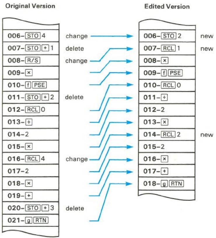
Let's start at the end of the program and work backwards. In this way, deletions will not change the line numbers of the preceding lines in the program.

Keystrokes

GTO CHS 020

(or use )

Display

000-

020-44,40，3

Program mode. (Assumes position is at line 000.)

Moves position to line 020

(instruction + 3.

Keystrokes	Display
←	019-	40	Line 020 deleted.
9 BST (hold)	016-	45	4	The next line to edit is line 016 (RCL 4).
←	015-	20	Line 016 deleted.
RCL 2	016-	45	2	Line 016 changed to RCL 2.
GTO CHS 011 (or hold BST)	011-44,40,	2	Moves to line 011 (STO + 2).
←	010-	42	31	Line 011 deleted.
9 BST (hold)	008-	31	Stop! (Single-stepping backwards to line 008: R/S.)
←	007-44,40,	1	R/S deleted.
RCL 1	008-	45	1	Line 008 changed to RCL 1.
9 BST	007-44,40,	1	Back-step to line 007.
←	006-	44	4	Line 007 (STO + 1) deleted.
←	005-	20	Line 006 (STO 4) deleted.
STO 2	006-	44	2	Changed to STO 2.

The replacement of a line proceeds like this:

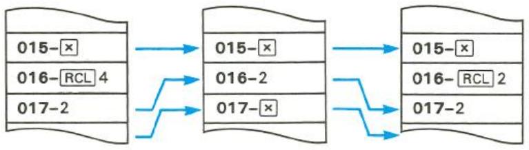
Further Information

Single-Step Operations

Single-Step Program Execution. If you want to check the contents of a program or the location of an instruction, you can single step through the program in Program mode. If, on the other hand, running the program produces an error, or you suspect that a portion of the program is faulty,

you can check the program by executing it stepwise. This is done by pressing in Run mode.

Keystrokes	Display
9 P/R			Run mode.
f CLEAR REG			Clear storage registers.
GTO A			Move to first line of program A.
8 STO 1	8.0000		Store a can height.
2.5	2.5		Enter a can radius.
SST (hold)	001-42,21,11		Keycode for line 001 (label).
(release)	2.5000		Result of executing line 001.
SST	002- 44 0		GTO 0.
	2.5000		Result.
SST	003- 43 11		9 x2.
	6.2500		Result.
SST	004- 43 26		9 π.
	3.1416		Result.
SST	005- 20		x
	19.6350		Result: the base area of the can.

Wrapping. SST will not move program position into "unoccupied" program territory. Instead, the calculator will "wrap around" to line 000. (In Run mode, SST will perform any instructions at the end of program memory, such as RTN, GTO or GSB.)

Line Position

Recall that the calculator's position in program memory does not change when it is shut off or Program/Run modes are changed. Upon returning to Program mode, the calculator line position will be where you left it. (If you executed a program ending with RTN, the position will be at line 000.) Therefore, if the calculator is left on and shuts itself off, you need only turn it on and switch to Program mode (the calculator always "wakes up" in Run mode) to be back where you were.

Insertions and Deletions

After an insertion, the display will show the instruction you just added. After a deletion, the display will show the line prior to the deleted (now nonexistent) one.

If all space available in memory is occupied, the calculator will not accept any program instruction insertions and Error 4 will be displayed.

Initializing Calculator Status

The contents of storage registers and the status of calculator settings will affect a program if the program uses those registers or depends on a certain status setting. If the current status is incorrect for the program being run, you will get incorrect results. Therefore, it is wise to clear registers and set relevant modes either just prior to running a program or within the program itself. A self-initializing program is more mistake-proof—but it also uses more program lines.

Calculator-initializing functions are: f CLEAR , f CLEAR PRGM, f CLEAR REG, 9 DEG, 9 RAD, 9 GRD, 9 SF, and 9 CF.

Problems

It is good programming technique to avoid using identical program labels. (This shouldn't be hard, since the HP-15C provides 25 different labels.) To ensure against duplication of labels, you can clear program memory first.

1. The following program is used by the manager of a savings and loan company to compute the future values of savings accounts according to the formula FV = PV(1 + i)^n , where FV is future value, PV is present value, i is the periodic interest rate, and n is the number of periods. Enter PV first (into the Y-register) and n second (into the X-register) before executing the program. Given is an annual interest rate of 7.5% (so i = 0.075 ).

Keystrokes	Display
f LBL • 1	001-42,21,.1
f FIX 2	002-42,7,2
1	003-	1
•	004-	48
0	005-	0
7	006-	7
5	007-	5
x$y	008-	34
y^x	009-	14
x	010-	20
g RTN	011-	43 32

Load the program and find the future value of 1,000 invested for 5 years; of 2,300 invested for 4 years. Remember to use GSB to run a program with a digit label. (Answers: 1,435.63;3,071.58.)

Alter the program to make the annual interest rate 8.0% .

Using the edited program, find the future value of 500 invested for 4 years; of 2,000 invested for 10 years. (Answers: 680.24;4,317.85.)

1. Create a program to calculate the length of a chord subtended by an angle (in degrees) on a circle of radius r , according to the equation

$$ \ell = 2 r \sin \frac {\theta}{2}. $$

Find when = 30^ and r = 25 .

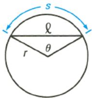
(Answer: 12.9410. A possible program is: f LBL A g DEG f FIX 4 2 x x y 2 ÷ SIN x RTN). (Assumes in Y-register and r in X-register when program is run.)

Make any necessary modifications in the program to also find and display s , the length of the circular arc cut by (in radians), according to the equation

$$ s = r \theta . $$

Complete the following table:

θ	r	l	s
45°	50	?	?
90°	100	?	?
270°	100	?	?

(Answers: 38.2683 and 39.2699; 141.4214 and 157.0796; 141.4214 and 471.2389.

A possible new sequence is:

fLBLA 9DEG fFIX4 STO02x x≤y STO1 2÷ SIN xf PSE fPSE RCL0 RCL1 f→RAD X RTN).

Section 8

Program Branching and Controls

Although the instructions in a program are normally executed sequentially, it is often desirable to transfer execution to a part of the program other than the next line. Branching in the HP-15C may be simple, or it may depend on a certain condition. By branching to a previous line, it is possible to execute part of a program more than once - a process called looping.

The Mechanics

Branching

The Go To (GTO) Instruction. Simple branching – that is, unconditional branching – is carried out with the instruction GTO label. In a running program, GTO will transfer execution to the next appropriately labeled program or routine (not to a line number).

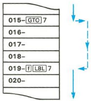
The calculator searches forward in memory, wrapping around through line 000 if necessary, and resumes execution at the first line containing the proper label.

Looping. If a GTO instruction specifies a label at a lower-numbered line (that is, a prior line), the series of instructions between the GTO and the label will be executed repeatedly – possibly indefinitely. The continuation

of this loop can be controlled by a conditional branch, an R/S instruction (written into the loop), or simply by pressing any key during execution (which stops the program).

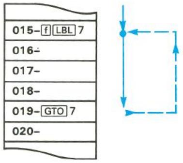
Conditional Tests

Another way to alter the sequence of program execution is by a conditional test, a true/false test which compares the number in the X-register either to zero or to the number in the Y-register. The HP-15C provides 12 different tests, two explicit on the keyboard and 10 others accessible using TEST n .

1. Direct: 9 ≤slant y and 9 = 0
2. Indirect: 9

Following a conditional test, program execution follows the "Do if True" Rule: it proceeds sequentially if the condition is true, and it skips one instruction if the condition is false. A [GTO] instruction is often placed right after a conditional test, making it a conditional branch; that is, the [GTO] branch is executed only if the test condition is met.

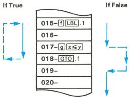
Program Execution After Test

Flags

Another conditional test for programming is a flag test. A flag is a status indicator that is either set (= true) or clear (= false). Again, execution follows the "Do if True" Rule: it proceeds sequentially if the flag is set, and skips one line if the flag is clear.

The HP-15C has eight user flags, numbered 0 to 7, and two system flags, numbered 8 (Complex mode) and 9 (overflow condition). The system flags are discussed later in this section. All flags can be set, cleared, and tested as follows:

• 9 n will set flag number n (0 to 9).
• 9 CF n will clear flag number n .
• 9 ? n will check if flag n is set.

A flag n that has been set remains set until it is cleared either by a CF n instruction or by clearing (resetting) Continuous Memory.

Examples

Example: Branching and Looping

A radiobiology lab wants to predict the diminishing radioactivity of a test amount of ^131I , a radioisotope. Write a program to figure the radioactivity at 3-day intervals until a given limit is reached. The formula for N_t , the amount of radioisotope remaining after t days, is

$$ N _ {t} = N _ {\mathrm {o}} \left(2 ^ {- t / k}\right), $$

where k = 8 days, the half-life of ^131I , and N_0 is the initial amount.

The following program uses a loop to calculate the number of millicuries (mci) of isotope theoretically remaining at 3-day intervals of decay. Included is a conditional test to check the result and end the program when radioactivity has fallen to a given value (a limit).

The program assumes t_1 – the first day of measurement – is stored in R_0 , N_0 – the initial amount of isotope – is stored in R_1 , and the limit value for radioactivity is stored in R_2 .

Keystrokes

P/R

f CLEAR PRGM

f LBL A

RCL0

f PSE

8

CHS

2

x≤y

y

Display

000-

000-

001-42,21,11

002- 45 0

003- 42 31

004- 8

005- 10

006- 16

007- 2

008- 34

009- 14

Program mode.

(Optional.)

Each loop returns to this line.

Recalls current t which changes with each loop.

Pauses to display t - k

-t / k

2^-t / k

Keystrokes	Display
RCL × 1	010-45,20, 1		Recall multiplication with the contents of R1 (N0), yielding Nt, the mci of 131 remaining after t days
f PSE	011- 42 31		Pauses to display Nt.
RCL 2	012- 45 2		Recalls limit value to X-register.
9 TEST 9	013-43,30, 9		x≥y? Tests whether limit value (in X) meets or exceeds Nt (in Y).
9 [RTN]	014- 43 32		If so, program ends.
3	015- 3		If not, program continues.
STO + 0	016-44,40, 0		Adds 3 days to t in R0.
GTO A	017- 22 11		Go to “A” and repeat execution to find a new Nt from a new t.

Notice that without lines 012 to 014, the loop would run indefinitely (until stopped from the keyboard).

Let's run the program, using t_1 = 2 days, N_0 = 100 mci, and a limit value of half of N_0 (50 mci).

Keystrokes

P/R

2 STO 0

100 STO 1

50 STO 2

f A

Display

2.0000

100.0000

50.0000

2.0000

84.0896

5.0000

64.8420

8.0000

50.0000

50.0000

Run mode (display will vary).

t_1

N_0

Limit value for N_t

t_1

N_1

t_2

N_2

t_3

N_3

N_t limit; program ends.

Example: Flags

Calculations on debts or investments can be calculated in two ways: for payments made in advance (at the beginning of a given period) and for payments made in arrears (at the end of a given period). If you write a program to calculate the value (or "present value") of a debt or investment with periodic interest and periodic payments, you can use a flag as a status indicator to tell the program whether to assume payments are made in advance or payments are made in arrears.

Suppose you are planning the payment of your child's future college tuition. You expect the cost to be about 3,000/year or about 250/month. If you wanted to withdraw the monthly payments from a bank account yielding 6% per year, compounded monthly (which equals 0.5% per month), how much must you deposit in the account at the start of the college years to fund monthly payments for the next 4 years?

The formula is

$$ V = P \left[ \frac {1 - (1 + i) ^ {- n}}{i} \right] (1 + i) $$

if payments are to be made each month in advance,

and the formula is

$$ V = P \left[ \frac {1 - (1 + i) ^ {- n}}{i} \right] $$

if payments are to be made each month in arrears.

V is the total value of the deposit you must make in the account;

P is the size of the periodic payment you will draw from the account;

i is the periodic interest rate (here: "periodic" means monthly, since interest is compounded monthly); and

n is the number of compounding periods (months).

The following program allows for either payment mode. It assumes that, before the program is run, P is in the Z-register, n is in the Y-register, and i is in the X-register.

Keystrokes

P/R

f LBL B

g CF0

GTO 1

f LBL E

g SF 0

f LBL 1

STO1

1

+

x<y

CHS

y

CHS

1

+

RCL 1

X

g F? 0

9 RTN

RCL 1

1

+

X

9 RTN

Display

000-

001-42,21,12

002-43，5，0

003- 221

004-42,21,15

005-43，4，0

006-42,21，1

007- 441

008- 1

009- 40

010- 34

011- 16

012- 14

013- 16

014- 1

015- 40

016-45,10，1

017- 20

018-43, 6, 0

019- 43 32

020- 45 1

021- 1

022- 40

023- 20

024- 4332

Program mode.

Start at "B" if payments to be made at the beginning.

Flag 0 clear (false); indicates advance payments.

Go to main routine.

Start at "E" if payments to be made at the end.

Flag 0 set (true); indicates payment in arrears.

Routine 1 (main routine).

Stores i (from X-register).

(1 + i)

Puts n in X ; (1 + i) in Y .

• n.

(1 + i)^-n

• (1 + i)^-n

1 - (1 + i)^-n

Recall division with R_1(i) to get [1 - (1 + i)^-n] / i

Multiplies quantity by P .

Flag 0 set?

End of calculation if flag 0 set (for payments in arrears).

Recalls i .

(1 + i)

Multiplies quantity by final term.

End of calculation if flag 0 clear.

Now run the program to find the total amount needed in an account from which you want to take (250/month for 48 months. Enter the periodic interest rate as a decimal fraction, that is, 0.005 per month. First find the sum needed if payments will be made at the beginning of the month (payments in advance), then calculate the sum needed if payments will be made at the end of the month (in arrears).

Keystrokes	Display
9 P/R		Set to Run mode.
250 ENTER	250.0000	Monthly payment.
48 ENTER	48.0000	Payment periods (4 years × 12 months).
.005	0.005	Monthly interest rate as a decimal fraction.
f B	10,698.3049	Deposit necessary for payments to be made in advance.
(Repeat stack entries.)
f E	10,645.0795	Deposit necessary for payment to be made in arrears. (The difference between this deposit and the tuition cost ($12,000) represents interest earned on the deposit!)

Further Information

Go to

In contrast to the nonprogrammable sequence GTO CHS nnn, the programmable sequence GTO label cannot be used to branch to a line number, but only to program label (a line containing f LBL label). Execution continues from the point of the new label, and does not return to the original routine unless given another GTO instruction.

GTO label can also be used in Run mode (that is, from the keyboard) to move to a labeled position in program memory. No execution occurs.

Looping

Looping is an application of branching which uses a [GTO] instruction to repeat a portion of the program. A loop can continue indefinitely, or may be conditional. A loop is frequently used to repeat a calculation with different variables. At the same time, a counter, which increments with each loop, may be included to keep track of loop iterations. This counter can then be checked with a conditional test to determine when to exit the loop. (This is shown in the example on page 112.)

Conditional Branching

There are two general applications for conditional branching. One is to control loops, as explained above. A conditional test can check for either a certain calculated value or a certain loop count.

The other major use is to test for options and pursue one. For example, if a salesperson made a variable commission depending on the amount of sale, you could write a program which takes the amount of sale, compares it to a test value, and then calculates a specific commission depending on whether the sale is less than or greater than the test value.

Tests. A conditional test takes what is in the X-register ("x") and compares it either to zero (such as = 0 ) or to "y", that is, what is in the Y-register (such as ≤ y ). For an x:y comparison, therefore, you must have the x- and y-values juxtaposed in the X- and Y-registers. This might require that you store a test value and then recall it (bringing it into the X-register). Or, the value might be in the stack and be moved, as necessary, using ≤ y , , or .

Tests With Complex Numbers and Matrix Descriptors. Four of the conditional tests also work with complex numbers and matrix descriptors:

= 0 , 0 (x 0) , 5 (x = y) , and 6 (x y) . Refer to sections 11 and 12 for more information.

Flags

As a conditional test can be used to pick an option by comparing two numbers in a program, a flag can be used to pick an option externally. Usually, a flag is set or cleared first thing in a program by choosing a different starting point (using different labels) depending on the condition or mode you want (refer to the example on page 95).

In this way, a program can accommodate two different modes of input, such as degrees and radians, and make the correct calculation for the mode chosen. You set a flag if a conversion needs to be made, for instance, and clear it if no conversion is needed.

Suppose you had an equation requiring temperature input in degrees Kelvin, although sometimes your data might be in degrees Celsius. You could use a program with a flag to allow either a Kelvin or Celsius input. In part, such a program might include:

f LBL C	Start program at “C” for degrees Celsius.
9 CF 7	Flag 7 cleared (=false).
GTO 1
f LBL D	Start program at “D” for degrees Kelvin.
9 SF 7	Flag 7 set (=true).
f LBL 1	(Assuming temperature in X-register.)
9 F? 7	Checks for flag 7 (checks for Celsius or Kelvin input).
GTO 2	If set (Kelvin input), goes to a later routine, skipping the next few instructions.
2	If cleared (Celsius input), adds 273 to the value in the X-register, since °K = °C + 273.
3
+
f LBL 2	Calculation continues for both modes.

The System Flags: Flags 8 and 9

Flag 8. Setting flag 8 will activate Complex mode (described in section 11), turning on the C annunciator. If another method is used to activate Complex mode, flag 8 will automatically be set. Complex mode is deactivated only by clearing flag 8; flag 8 is cleared in the same manner as the other flags.

Flag 9. An overflow condition (described on page 61) automatically sets flag 9. Flag 9 causes the display to blink or, if a program is running, waits until execution is complete and then starts blinking the display.

Flag 9 may be cleared in three ways:

• Press 9 CF 9 (the common procedure for clearing flags).
• Press . This will only clear flag 9 and stop the blinking—it will not clear the display.
• Turn the calculator off. (Flag 9 is not cleared if the calculator turns itself off.)

If you set flag 9 manually ( 9), it causes the display to blink irrespective of the overflow status of the calculator. As usual, a program will run to completion before the display starts blinking. Therefore, flag 9 can be used as a programming tool to provide a visual signal for a selected condition.

Section 9

Subroutines

When the same set of instructions needs to be used at more than one point in a program, memory space can be conserved by storing those instructions as a single subroutine.

The Mechanics

Go To Subroutine and Return

The GSB (go to subroutine) instruction is executed in the same way as the GTO branch, with one major difference: it establishes a pending return condition. GSB label, like GTO label, transfers program execution to the line with the corresponding label (A to E, 0 to 9 or .0 to .9). However, execution then continues until the first subsequent RTN instruction is encountered - at which point execution transfers back to the instruction immediately following the last GSB instruction, and continues on from there.

Subroutine Execution

Execution transfers to line 000 and halts.
Execution transfers back to original routine after GSB 1

Subroutine Limits

A subroutine can call up another subroutine, and that subroutine can call up yet another subroutine. This "subroutine nesting"—the execution of a subroutine within a subroutine—is limited to stack of subroutines seven levels deep (this does not count the main program level). The operation of nested subroutines is as shown below:

Main Program

Examples

Example: Write a program to calculate the slope of the secant line joining points (x_1,y_1) and (x_2,y_2) on the graph shown, where y = x^2 - x (given x in radians).

The secant slope is:

$$ \frac {y _ {2} - y _ {1}}{x _ {2} - x _ {1}}, \text {o r} \frac {\left(x _ {2} ^ {2} - \sin x _ {2}\right) - \left(x _ {1} ^ {2} - \sin x _ {1}\right)}{x _ {2} - x _ {1}} $$

The solution requires that the equation for y be evaluated twice—once for y_1 and once for y_2 , given the data input for x_1 and x_2 . Since the same calculation must be made for different values, it will save program space to call a subroutine to calculate y .

The following program assumes that x_1 has been entered into the Y-register and x_2 into the X-register.

MAIN PROGRAM

Calculate the slope for the following values of x_1 and x_2 : 0.52, 1.25; -1, 1; 0.81, 0.98. Remember to use GSB 9 (rather than f 9) when addressing a routine with a digit label.

Answers: 1.1507; -0.8415; 1.1652.

Example: Nesting. The following subroutine, labeled ".4", calculates the value of the expression ^2 + y^2 + z^2 + t^2 as part of a larger calculation in a larger program. The subroutine calls upon another subroutine (a nested subroutine), labeled ".5", to do the repetitive squaring.

The program is executed after placing the variables t , z , y , and x into the T-, Z-, Y-, and X-registers.

Start of main
subroutine. x^2 Calculates y^2 and x^2 + y^2 Calculates z^2 and ^2 + y^2 + z^2. Calculates t^2 and x^2 + y^2 + z^2 + t^2 ^2 + y^2 + z^2 + t^2 End of main subroutine;
returns to main program.

Start of nested subroutine.

Calculates a square and
adds it to current sum of squares.
End of nested sub-routine; returns
to main subroutine.

If you run the subroutine (with its nested subroutine) alone using x = 4.3 , y = 7.9 , z = 1.3 , and t = 8.0 , the answer you get upon pressing [GSB].4 is 12.1074.

Further Information

The Subroutine Return

The pending return condition means that the RTN instruction occurring subsequent to a GSB instruction causes a return to the line following the GSB rather than a return to line 000. This is what makes a subroutine useful and reusable in different parts of a program: it will always return execution to where it branched from, even as that point changes. The only difference between using a GSB branch and a GTO branch is the transfer of execution after a RTN.

Nested Subroutines

If you attempt to call a subroutine that is nested more than seven levels deep, the calculator will halt and display Error 5 when it encounters the [GSB] instruction at the eighth level.

Note that there is no limitation (other than memory size) on the number of nonnested subroutines or sets of nested subroutines that you may use.

Section 10

The Index Register and Loop Control

The Index register (R_J) is a powerful tool in advanced programming of the HP-15C. In addition to storage and recall of data the Index register can use an index number to:

• Count and control loops.
• Indirectly address storage registers, including those beyond R.9 (_19)
• Indirectly branch to program line numbers, as well as to labels.
• Indirectly control the display format.
• Indirectly control flag operations.

The I and (i) Keys

Direct Versus Indirect Data Storage With the Index Register

The Index register is a data storage register that can be used directly, with , or indirectly, with (i) . The difference is important to note:

I

The function uses the number itself in the Index register.

(i)

The (i) function uses the absolute value of the integer portion of the number in the Index register to address another data storage register. This is called indirect addressing.

Indirect Program Control With the Index Register

The key is used for all forms of indirect program control other than indirect register addressing. Hence, (not (i) ) is used for indirect program branching, indirect display format control, and indirect flag control.

Program Loop Control

Program loop counting and control can be carried out in the HP-15C by any storage register: R0 through R_9 , R,0 through R_,9 , or the Index register (I). Loop control can also be carried out indirectly with (i) .

The Mechanics

Both and (i) can be used in abbreviated key sequences, omitting the preceding prefix (as explained on page 78).

Index Register Storage and Recall

Direct. STO I and RCL I. Storage and recall between the Xregister and the Index register operate in the same manner as with other data storage registers (page 42).

Indirect. STO (or RCL) (i) stores into (or recalls from) the data storage register whose number is addressed by the integer portion of the value (0 to 65) in the Index register. See the table below and on the next page.

Indirect Addressing

If R1 contains:	(i) will address:	GTO I or GSB I will transfer to:*
± 0	R0	f LBL 0
:	:	:
9	R9	f LBL 9
10	R.0	" " .0
11	R.1	" " .1
:	:	:
19	R.9	f LBL .9
20	R20	" " A
*For R1≥0 only.

(Continued on next page.)

Indirect Addressing

If R1 contains:	(i) will address:	GTO I or GSB I will transfer to:*
21	R21	f LBL B
22	R22	" " C
23	R23	" " D
24	R24	" " E
:	:	—
65	R65	—
*For R1≥0 only.

Index Register Arithmetic

Direct. STO or RCL +,-,×,÷ . Storage or recall arithmetic operates with the Index register in the same manner as upon other data storage registers (page 43).

Indirect. STO or RCL +,-,×,÷ (i) carries out storage or recall arithmetic with the contents of the data storage register addressed by the integer portion of the number (0 to 65) in the Index register. See the above table.

Exchanging the X-Register

Direct. f I exchanges contents between the X-register and the Index register. (Works the same as n does with registers 0 through .9.)

Indirect. f (i) exchanges contents between the X-register and the data storage register addressed by the number (0 to 65) in the Index register. See the above table.

Indirect Branching With I

The key—but not the (i) key—can be used for indirect branching ( ) and subroutine calls ( ). (Only the integer portion of the number in R_I is used.) ( (i) is only used for indirect addressing of storage registers).

To Labels. If the _I value is positive, GTO I and GSB I will transfer execution to the label which corresponds to the number in the Index register (see the above table).

For instance, if the Index register contains 20.00500, then a GTO I instruction will transfer program execution to f LBL A. See the chart on page 107.

To Line numbers. If the RI value is negative, GTO I causes branching to that line number (using the absolute value of the integer portion of the value in RI ).

For instance, if R_I contains -20.00500 , then a GTO I instruction will transfer program execution to program line 020.

Indirect Flag Control With I

SF I, CF I, or F? I will set, clear, or test the flag (0 to 9) specified in R_1 (by the magnitude of the integer portion).

Indirect Display Format Control With I

f FIX I, f SCI I, and f ENG I will format the display in their customary manner (refer to pages 58-59), using the number in R_I (integer part only) for n , which must be from 0 to 9.

Loop Control With Counters: ISG and DSE

The ISG (increment and skip if greater than) and DSE (decrement and skip if less than or equal to) functions control loop execution by referencing and altering a loop control number in a given register. Program execution (skipping a line or not) then depends on that number.

The key sequence is {ISG, DSE} register number. This number is 0 to 9, .0 to .9, I or (i).

The Loop Control Number. The format of the loop control number is:

nnnnn.xxxxyy, where	±nnnnn	is the current counter value,
	xxx	is the test (goal) value, and
	yy	Is the increment of decrement value

For example, the number 0.05002 in a storage register represents:

ISG and DSE Operation. Each time a program encounters ISG or DSE it increments or decrements nnnnn (the integer portion of the loop control number), thereby keeping count of the loop iterations. It compares nnnnn to xxx, the prescribed test value, and exits the loop by skipping the next line if the loop counter (nnnnn) is either greater than (ISG) or less than or equal to (DSE) the test value (xxx). The amount that nnnnn is incremented or decremented is specified by yy.

With these functions (as opposed to the other conditional tests), the rule is "Skip if True".

For ISG: given nnnnn.xxxxyy, increment nnnnn to nnnnn + yy, compare it to xxx, and skip the next program line if the new value satisfies nnnnn > xxx. This allows you to exit a loop at this point when nnnnn becomes greater than xxx.

For DSE: given nnnnn.xxxyy, decrement nnnnn to nnnnn - yy, compare it to xxx, and skip the next program line if the new value satisfies nnnnn ≤ xxx. This allows you to exit a loop at this point when nnnnn becomes less than or equal to xxx.

For example, loop iterations will alter these control numbers as follows:

Iterations

Operation	0	1	2	3	4
ISG	0.00602	2.00602	4.00602	6.00602	8.00602 (skip next line)
DSE	6.00002	4.00002	2.00002	0.00002 (skip next line)

Examples

Examples: Register Operations

Storing and Recalling

Keystrokes

f CLEAR REG

12.3456

STO I

7√x

STO (1)

RCL I

Display

Clearly all storage registers.

12.3456

12.3456 Stores in _1

2.6458

2.6458 Storage in _· 2 by indirect addressing (R_I = 12.3456)

12.3456 Recalls contents of _1

Keystrokes

Display

RCL (i)

2.6458

Indirectly recalls contents of R_2

f x.2

2.6458

Check: same contents recalled by directly addressing R_2

Exchanging the X-Register

Keystrokes

Display

f xI

12.3456

Exchanges contents of R_I and Xregister.

RCL I

2.6458

Present contents of _I

f xS (i)

0.0000

Exchanges contents of R_2 (which is zero) with X.

RCL (1)

2.6458

f 2

2.6458

Check: directly address _2

Storage Register Arithmetic

Keystrokes

Display

10 STO + I

10.0000

Adds 10 to _I

RCL I

12.6458

New contents of R_I (= old + 10)

9 STO ÷

3.1416

Divides contents of R_2 by .

(i)

RCL (i)

0.8422

New contents of R_2

f .2

0.8422

Check: directly address R_2

Example: Loop Control with DSE

Remember the program in section 8 which used a loop to calculate radioactive decay? (Refer to page 93.) This program used a test condition ( x ≥ y ) to exit the loop when the calculated result passed the given limit (50). As we've seen in this section, there's another way to control loop execution: through a stored loop counter that is monitored by the ISG or DSE function.

Here is a revision of the original radioisotope decay program. This time, we will limit the program to three executions of the loop rather than setting a specific limit value. This example uses DSE with a loop control number in R_2 of

Make the following changes to the program (assuming it is in memory). A loop counter will be stored in R_2 and a line number in the Index register.

Keystrokes	Display
9 P/R	000-		Program mode.
GTO CHS 013	013-43,30,9		The second of the two loop test condition lines.
←←	011- 42 31		Delete lines 013 and 012.
f DSE 2	012-42,5,2		Add your loop counter function (counter stored in R2).
GTO I	013- 22 25		Go to given line number (015).

Now when the loop counter (stored in R_2 ) has reached zero, it will skip line 013 and go on to 014, the RTN instruction, thereby ending the program. If the loop counter has not yet decreased to zero, execution continues with line 013. This branches to line 015 and continues the program and the looping.

To run the program, put t_1 (day 1) in R_0 , N_0 (initial isotope batch) in R_1 the loop counter in R_2 , and the line number for branching in the Index register.

Keystrokes	Display
9 P/R		Run mode.
2 STO 0	2.00000	t1.
100 STO 1	100.0000	N0.
3.000001 STO 2	3.0000	Loop counter. (This instruction could also be programmed.)

Keystrokes

15 CHS STO

I f A

Display

-15.0000

2.0000

Branch line number.

Running program loop counter = 3

84.0896

5.0000

Loop counter = 2

64.8420

8.0000

Loop counter = 1

50.0000

50.0000

Loop counter = 0 ; program ends.

Example: Display Format Control

The following program pauses and displays an example of FIX display format for each possible decimal place. It utilizes a loop containing a DSE instruction to automatically change the number of decimal places.

Keystrokes

P/R

f CLEAR PRGM

f LBL B

9

nnnn = 9 . Therefore, xxx = 0 and by default yy = 1 (yy cannot be zero).

STO I

f LBL0

□F FIX I

RCL I

f PSE

f DSE I

GTO 0

9 TEST 1

GTO 0

9 RTN

Displays current value of mmmnn.

Value in R_I is decremented and tested. Skip a line if nnnnn ≤ test value.

Continue loop if nnnnn > test value (0).

Tests whether value in display is greater than 0, so loop will continue when nnnn has reached 0 but display still only shows 1.0.

To display fixed point notation for all possible decimal places on the HP-15C:

Keystrokes Display

P/R

f B

9.00000000
8.0000000
7.000000
6.000000
5.00000
4.0000
3.000
2.00
1.0
0. Display at f PSE instruction.
0. Display when program halts.

Further Information

Index Register Contents

Any value stored in the Index register can be referenced in three different ways:

• Using I like any other storage register. The value in R_I can be manipulated as it is: stored, recalled, exchanged, added to, etc.
• Using as a control number. The absolute value of the integer portion in R_I is a separate entity from the fractional portion. For indirect branching, flag control, and display format control with , only this portion is used. For loop control, the fractional portion is also used, but separately from the integer portion.
• Using (i) as a reference to the contents of another storage register. The (i) key uses the indirect addressing system shown in the tables on pages 107 and 108. (In turn, the contents of that second register may be used as a loop control number, in the fashion described above.)

ISG and DSE

For the purpose of loop control, the integer portion (the counter value) of the stored control number can be up to five digits long (nnnnn.xxxxy). The counter value (nnnnn) is zero if not specified otherwise.

xxx, in the decimal portion of the control number, must be specified as a three-digit number. (For example, "5" must be "005".) xxx is zero if not specified otherwise. Whenever ISG or DSE is encountered, nnnn is compared internally to xxx, which represents the end level for incrementing or decrementing.

yy must be specified as a two-digit number. yy cannot be zero, so if left (or specified) as 00, the value for yy defaults to 1. The value nnnnn is altered by the amount of yy each time the loop runs through ISG or DSE. Both yy and xxx are reference values, which do not change with loop execution.

Indirect Display Control

While you can use the Index register to format the display manually (that is, from the keyboard), this function is most commonly used in programming. This capability is especially valuable for the _y^x function, for which accuracy can be stipulated by specifying the number of digits to be displayed (as described in section 14).

There are, as usual, certain display limitations to keep in mind. Recall that any display format function merely alters the number of decimal places to which the display is rounded. In its memory, the calculator always retains a number in scientific notation as a 10-digit mantissa with a two-digit exponent.

The integer portion of the number in the Index register specifies the number of decimal places to which the display is rounded. A number less than zero defaults to zero (zero decimal places displayed in FIX format), while a number greater than 9 defaults to 9 (9 decimal places displayed in FIX).*

An exception is in the case of _y^x where the display format number in R_I may range from -6 to +9 . (This is discussed in appendix E on page 247.) A number less than zero will not affect the display format, but will affect accuracy with this function.

Part III

HP-15C

Advanced Functions

Section 11

Calculating With

Complex Numbers

The HP-15C enables you to calculate with complex numbers, that is, numbers of the form

$$ a + i b, $$

where a is the real part of the complex number,

b is the imaginary part of the complex number, and

$$ i = \sqrt {- 1}. $$

As you will see, the beauty of calculating with the HP-15C in Complex mode is that once the complex numbers are keyed in, most operations are executed in the same manner as with real numbers.

The Complex Stack and Complex Mode

Calculations with complex numbers are performed using a complex stack composed of two parallel four-register stacks (and two LAST X registers). One of these parallel stacks - referred to as the real stack - contains the real parts of complex numbers used in calculations. (This is the same stack used in ordinary calculations.) The other stack - referred to as the imaginary stack - contains the imaginary parts of complex numbers used in calculations.

Creating the Complex Stack

The imaginary stack is created (by converting five storage registers as described in appendix C) when you activate Complex mode; it does not exist when the calculator is not in Complex mode.

Complex mode is activated

1) automatically, when executing f I or f ReIm; or
2) by setting flag 8, the Complex mode flag (9 SF 8).

When the calculator is in Complex mode, the C annunciator in the display is lit. This tells you that flag 8 is set and the complex stack exists. In or out of Complex mode, the number appearing in the display is the number in the real X -register.

Note: In Complex mode (signified by the C annihilator), the HP-15C performs all trigonometric functions using radians. The trigonometric mode annihilator in the display (RAD, GRAD, or blank for Degrees) applies to two functions only: R and P (as explained later in this section).

Deactivating Complex Mode

Since Complex mode requires the allocation of five registers from memory, you will have more memory available for programming and other advanced functions if you deactivate Complex mode when you are working solely with real numbers.

To deactivate Complex mode, clear flag 8 (keystroke sequence: 9 CF 8). The C annunciator will disappear.

Complex mode is also deactivated when Continuous Memory is reset (as described on page 63). In any case, deactivating Complex mode dissolves the imaginary stack, and all imaginary numbers there are lost.

Complex Numbers and the Stack

Entering Complex Numbers

To enter a number with real and imaginary parts;

1. Key the real part of the number into the display.
2. Press ENTER
3. Key the imaginary part of the number into the display.
4. Press . (If not already in Complex mode, this creates the imaginary stack and displays the C annunciator.)

Example: Add 2 + 3i and 4 + 5i . (The operations are illustrated in the stack diagrams following the keystroke listing.)

Keystrokes f FIX 4		Display
2 ENTER		2.0000	Keys real part of first number into (real) Y-register.
3		3	Keys imaginary part of first number into (real) X-register.
f I		2.0000	Creates imaginary stack; moves the 3 into the imaginary X-register, and drops the 2 into the real X-register.
4 ENTER		4.0000	Keys real part of second number into (real) Y-register.
5		5	Keys imaginary part of second number into (real) X-register.
f I		4.0000	Copies 5 from real X-register into imaginary X-register, copies 4 from real Y-register into real X-register, and drops stack.
+ f (i) (hold) (release)		6.0000	Real part of sum.
		8.0000	Displays imaginary part of sum while the (i) key is held. (This also terminates digit entry.)

The operation of the real and imaginary stacks during this process is illustrated below. (Assume that the stack registers have been loaded already with the numbers shown as the result of previous calculations). Note that the imaginary stack, which is shown below at the right of the real stack, is not created until is pressed. (Recall also that the shading of the stack indicates that those contents will be written over when the next number is keyed in or recalled.)

The execution of causes the entire stack to drop, the T contents to duplicate, and the real X contents to move to the imaginary X-register.

When the second complex number is entered, the stacks operate as shown below. Note that lifts both stacks.

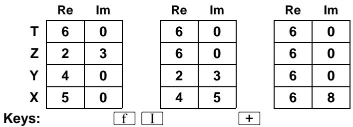
A second method of entering complex numbers is to enter the imaginary part first, then use ≤slant 1m and . This method is illustrated under Entering Complex Numbers With , page 127.

Stack Lift in Complex Mode

Stack lift operates on the imaginary stack as it does on the real stack (the real stack behaves identically in and out of Complex mode). The same functions that enable, disable, or are neutral to lifting of the real stack will enable, disable, or be neutral to lifting of the imaginary stack. (These processes are explained in detail in section 3 and appendix B.)

In addition, every nonneutral function, except and CLx causes the clearing of the imaginary X -register when the next number is entered. That is, these functions cause a zero to be placed in the imaginary X -register when the next number is keyed in or recalled. Refer to the stack diagrams above for illustrations. This feature allows you to execute calculator operations using the same key sequences you use outside of Complex mode.*

Manipulating the Real and Imaginary Stacks

1m (real exchange imaginary). Pressing 1m will exchange the contents of the real and imaginary X-registers, thereby converting the imaginary part of the number into the real part and vice-versa. The Y-, Z-, and T-registers are not affected. Press 1m twice restore a number to its original form.

≤ Im also activates Complex mode if it is not already activated.

Temporary Display of the Imaginary X-Register. Press (i) to momentarily display the imaginary part of the number in the X-register without actually switching the real and imaginary parts. Hold the key down to maintain the display.

Changing Signs

In Complex mode, the CHS function affects only the number in the real X-register - the imaginary X-register does not change. This enables you to change the sign of the real or imaginary part without affecting the other. To key in a negative real or imaginary part, change the sign of that part as you enter it.

If you want to find the additive inverse of a complex number already in the X -register, however, you cannot simply press as you would outside

of Complex mode. Instead, you can do either of the following:

• Multiply by -1.
• If you don't want to disturb the rest of the stack, press CHS f Re<Im CHS f Re<Im.

To find the negative of only one part of a complex number in the X-register:

• Press CHS to negate the real part only.
• Press f Re<Im CHS f Re<Im to negate the imaginary part only, forming the complex conjugate.

Clearing a Complex Number

Inevitably you will need to clear a complex number. You can clear only one part at a time, but you can then write over both parts (since and CLx disable the stack).

Clearing the Real X-Register. Pressing (or 9 CL_x ) with the calculator in Complex mode clears only the number in the real X-register; it does not clear the number in the imaginary X-register.

Example: Change 6 + 8i to 7 + 8i and subtract it from the previous entry. (Use or (i) to view the imaginary part in X.) Assume a, b, c and d represent parts of complex numbers.

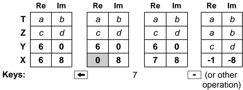
Since clearing disables the stack (as explained above), the next number you enter will replace the cleared value. If you want to replace the real part with zero, after clearing use [ENTER] or any other function to terminate digit entry (otherwise the next number you enter will write over the zero); the imaginary part will remain unchanged. You can then continue with any calculator function.

Clearing the Imaginary X-Register. To clear the number in the imaginary X-register, press f Re<lm, then press . Press f Re<lm again to return the zero, or any new number keyed in, to the imaginary X-register.

Example: Replace -1 -8i by -1 + 5i

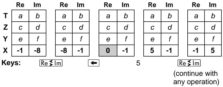
Clearing the Real and Imaginary X-Registers. If you want to clear or replace both the real and imaginary parts of the number in the X-register, simply press , which will disable the stack, and enter your new number. (Enter zeros if you want the X-register to contain zeros.) Alternatively, if the new number will be purely real (including 0 + 0i ), you can quickly clear or replace the old, complex number by pressing R followed by zero or the new, real number.

Example: Replace -1 + 5i with 4 + 7i .

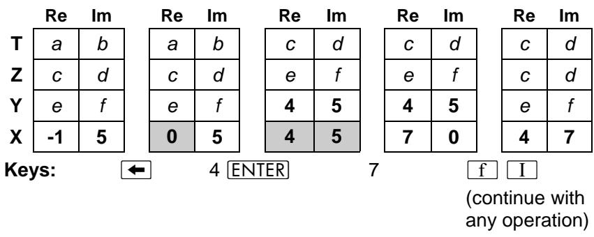
Entering Complex Numbers with . The clearing functions and can also be used with as an alternative method of entering (and clearing) complex numbers. Using this method, you can enter a complex number using only the X-register, without affecting the rest of the stack. (This is possible because and disable stack lift.) Executing will also create an imaginary stack if one is not already present.

Example: Enter 9 + 8i without moving the stack and then find its square.

Keystrokes (←)	Display (0.0000)	Prevents stack lift when the next digit (8) is keyed in. Omit this step if you'd rather save what's in X and lose what's in T.
8	8	Enter imaginary part first.
f Relm	7.0000	Displays real part; Complex mode activated.
←	0.0000	Disables stack. (Otherwise, it would lift following Relm.)
9	9	Enters real part (digit entry not terminated).
g x2	17.0000	Real part.
f (i) (hold) (release)	144.0000	Imaginary part.
	17.0000

You have already seen two ways of entering a complex number. There is a shorter way to enter a real number: simply key it (or recall it) into the display just as you would if the calculator were not in Complex mode. As you do so, a zero will be placed in the imaginary X-register (as long as the previous operation was not or , as explained on page 124).

The operation of the real and imaginary stacks during this process is illustrated below. (Assume the last key pressed was not or and the contents remain from the previous example.)

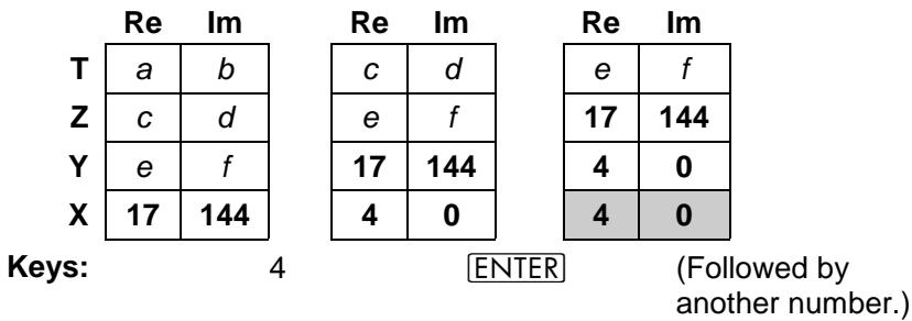
Entering a Pure Imaginary Number

There is a shortcut for entering a pure imaginary number into the X-register when you are already in Complex mode: key in the (imaginary) number and press f Re lm

Example: Enter 0 + 10i (assuming the last function executed was not or ).

Keystrokes

10

Display

10

Keys 10 into the displayed real X-register and zero into the imaginary X-register.

f ReIm

0.0000

Exchanges numbers in real and imaginary X-registers.

Display again shows that the number in the real Xregister is zero - as it should be for a pure imaginary number.

The operation of the real and imaginary stacks during this process is illustrated below. (Assume the stack registers contain the numbers resulting from the preceding examples.)

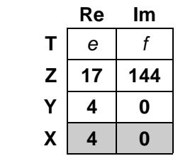
Keys: 10

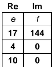
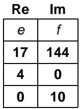
fRe<Im
(Continue with any operation.)

Note that pressing simply exchanges the numbers in the real and imaginary X -registers and not those in the remaining stack registers.

Storing and Recalling Complex Numbers

The STO and RCL functions act on the real X -register only; therefore, the imaginary part of a complex number must be stored or recalled separately. The keystrokes to do this can be entered as part of a program and executed automatically.*

To store a + ib from the complex X-register to R_1 and R_2 , you can use the sequence

$$ \boxed {S T O} 1 \quad f \quad R e > I m \quad S T O 2 $$

You can follow this by to return the stack to its original condition if desired. To recall a + ib from R_1 and R_2 you can use the sequence

$$ \begin{array}{c c c c} \hline \text {R C L} & 1 & \text {R C L} & 2 \ \hline \end{array} \quad \begin{array}{c c c c} \hline \text {f} & \text {I} \ \hline \end{array} $$

If you wish to avoid disturbing the rest of the stack, you can recall the number using the sequence

$$ \begin{array}{c c c c c} \hline \text {R C L} & 2 & f & \text {R e} \times \text {I m} & \leftarrow \ \hline \end{array} \quad \begin{array}{c c c c c} \hline \text {R C L} & 1 \end{array} $$

(In Program mode, use 9 instead of .)

Operations With Complex Numbers

Almost all functions performed on real numbers will yield the same answer whether executed in or out of Complex mode,† assuming the result is also real. In other words, Complex mode does not restrict your ability to calculate with real numbers.

Any functions not mentioned below or in the rest of this section (Calculating With Complex Numbers) ignore the imaginary stack.

One-Number Functions

The following functions operate on both the real and imaginary parts of the number in the X-register, and place the real and imaginary parts of the answer back into those registers.

$$ \sqrt {x} x ^ {2} \text {L N} \log 1 / x 1 0 ^ {x} e ^ {x} A B S \rightarrow P \rightarrow R $$

All trigonometric and hyperbolic functions and their inverses also belong to this group.*

The ABS function gives the magnitude of the number in the X-registers (the square root of the sum of the squares of the real and imaginary parts); the imaginary part of the magnitude is zero.

P converts to polar form and R converts to rectangular form, as described later in this section (page 133).

For the trigonometric functions, the calculator considers numbers in the real and imaginary X-registers to be expressed in radians—regardless of the current trigonometric mode. To calculate trigonometric functions for values given in degrees, use RAD to convert those values to radians before executing the trigonometric function.

Two-Number Functions

The following functions operate on both the real and imaginary parts of the numbers in the X- and Y-registers, and place the real and imaginary parts of the answer into the X-registers. Both stacks drop, just as the ordinary stack drops after a two-number function not in Complex mode.

$$ + \square - \times \div y ^ {x} $$

Stack Manipulation Functions

When the calculator is in Complex mode, the following functions simultaneously manipulate both the real and imaginary stacks in the same way as they manipulate the ordinary stack when the calculator is not in Complex mode. The 5y function. for instance, will exchange both the real and imaginary parts of the numbers in the X- and Y-registers.

$$ \begin{array}{c c c c} \hline x \leq y & R \downarrow & R \uparrow & E N T E R \ \hline \end{array} \text {E N T E R} \quad \mathrm {L S T} _ {x} $$

Conditional Tests

For programming, the four conditional tests below will work in the complex sense: = 0 and TEST 0 compare the complex number in the (real and imaginary) X-registers to 0 + 0i , while TEST 5 and TEST 6 compare the complex numbers in the (real and imaginary) X- and Y-registers. All other conditional tests besides those listed below ignore the imaginary stack.

$$ \boxed {x = 0} \quad \boxed {\text {T E S T}} 0 (x \neq 0) \quad \boxed {\text {T E S T}} 5 (x = y) \boxed {\text {T E S T}} 6 (x \neq y) $$

Example: Complex Arithmetic. The characteristic impedance of a ladder network is given by an equation of the form

$$ Z _ {0} = \sqrt {\frac {A}{B}} , $$

where A and B are complex numbers. Find Z_0 for the hypothetical values A = 1.2 + 4.7i and B = 2.7 + 3.2i .

Keystrokes

1.2 ENTER 4.7 f I

Display

1.2000

Enters A into real and imaginary X-registers.

2.7 ENTER 3.2 f I

2.7000

Enters B into real and imaginary X-registers, moving A into real and imaginary Y-registers.

1.0428

Calculates A / B

1.0491

Calculates Z_0 and displays real part.

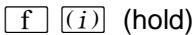
0.2406

Displays imaginary part of Z_0 while (i) is held down.

(release)

1.0491

Again displays real part of Z_0

Complex Results from Real Numbers

In the preceding examples, the entry of complex numbers had ensured the (automatic) activation of Complex mode. There will be times, however, when you will need Complex mode to perform certain operations on real numbers, such as -5 . (Without Complex mode, such as operation would result in an Error 0 – improper math function.) To activate Complex mode at any time and without disturbing the stack contents, set flag 8 before executing the function in question.*

Example: The arc sine (^-1) of 2.404 normally would result in an Error 0. Assuming 2.404 in the X-register, the complex value arc sin 2.404 can be calculated as follows:

Keystrokes	Display
g SF 8		Activates Complex Mode.
g SIN-1	1.5708	Real part of arc sin 2.404.
f (i) (hold)	-1.5239	Imaginary part of arc sin 2.404.
(release)	1.5708	Display shows real part again when (i) is released.

Polar and Rectangular Coordinate Conversions

In many applications, complex numbers are represented in polar form, sometimes using phasor notation. However, the HP-15C assumes that any complex numbers are in rectangular form. Therefore, any numbers in polar or phasor form must be converted to rectangular form before performing a function in Complex mode.

$$ a + i b = \left{ \begin{array}{l l} r (\cos \theta + i \sin \theta) = r e ^ {i \theta} & \text {(p o l a r)} \ r \angle \theta & \text {(p h a s o r)} \end{array} \right. $$

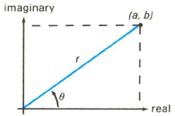
+R and +P can be used to interconvert the rectangular and polar forms of a complex number. They operate in Complex mode as follows:

converts the polar (or phasor) form of a complex number to its rectangular form by replacing the magnitude r in the real Xregister with a , and replacing the angle in the imaginary Xregister with b .

converts the rectangular coordinates of a complex number to the polar (or phasor) form by replacing the real part a in the real X-register with r , and replacing the imaginary part b in the imaginary X-register with .

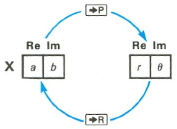
These are the only functions in Complex mode that are affected by the current trigonometric mode setting. That is, the angular units for must correspond to the trigonometric mode indicated by the annunciator (or absence thereof).

Example: Find the sum 2( 65^ + i 65^) + 3( 40^ + i 40^) and express the result in polar form, (In phasor form, evaluate 2 65^ + 3 40^ .)

Keystrokes	Display
9 DEG		Sets Degrees mode for any polar-rectangular conversions.
2 ENTER	2.0000
65 f I	2.0000	C annunciator displayed;Complex mode activated.
f *R	0.8452	Converts polar to rectangularform; real part (a) displayed.
3 ENTER	3.0000
40 f I	3.0000
f *R	2.2981	Converts polar to rectangularform; real part (a) displayed.
+	3.1434
g *P	4.8863	Converts rectangular to polarform; r displayed.
f (i) (hold)(release)	49.96124.8863	θ (in degrees).

Problems

By working through the following problems, you will see that calculating with complex numbers on the HP-15C is as easy as calculating with real numbers. In fact, once your numbers are entered, most mathematical operations will use exactly the same keystrokes. Try it and see!

1. Evaluate: 2i(-8 + 6i)^3(4 - 25i)(2 - 45i)

Keystrokes	Display
2 f Re$lm	0.0000	2i. Display shows real part.
8 CHS ENTER	-8.0000
6 f I	-8.0000	-8 + 6i.
3 yx	352.0000	(-8 + 6i)3.
×	-1.872.0000	2 i (-8 + 6i)3.
4 ENTER	4.0000
5 x̅	2.2361
2 CHS ×	-4.4721	-2√5.
f I	4.0000	4 - 2√5i.
÷	-295.4551	2i(-8 + 6i)3/4 - 2√5i.
2 ENTER 5 x̅	2.2361
4 CHS ×	-8.9443
f I	2.0000	2 - 4√5i.
÷	9.3982	Real part of result.
f (i)	-35.1344}	Answer: 9.3982 -35.1344i.
	9.3982

1. Write a program to evaluate the function = 2z + 15z + 3 for different values of z . ( represents a linear fractional transformation, a class of conformal mappings.) Evaluate for z = 1 + 2i .

(Answer: 0.3902 + 0.0122i . One possible keystroke sequence is: f LBL A ENTER ENTER 2 × 1 + x y 5 × 3 + ÷ R/S f Re Im RTN.)

1. Try your hand at a complex polynomial and rework the example on page 80. You can use the same program to evaluate P(z) = 5z^4 + 2z^3 , where z is some complex number.

Load the stack with z = 7 + 0i and see if you get the same answer as before. (Answer: 12,691.0000 + 0.0000i.)

Now run the program for z = 1 + i . (Answer -24.0000 + 4.0000i.)

For Further Information

The HP-15C Advanced Functions Handbook presents more detailed and technical aspects of using complex numbers in various functions with the HP-15C. Applications are included. The topics include:

Accuracy considerations.
- Principal branches of multi-valued functions.
- Complex contour integrals.
Complex potentials.
- Storing and recalling complex numbers using a matrix.
- Calculating the n th roots of a complex number.
- Solving an equation for its complex roots.
Using SOLVE and _y^x in Complex mode.

Section 12

Calculating With Matrices

The HP-15C enables you to perform matrix calculations, giving you the capability to handle advanced problems with ease. The calculator can work with up to five matrices, which are named A through E since they are accessed using the corresponding A through E keys. The HP-15C lets you specify the size of each matrix, store and recall the values of matrix elements, and perform matrix operations - for matrices with real or complex elements. (A summary of matrix functions is listed at the end of this section.)

A common application of matrix calculations is solving a system of linear equations. For example, consider the equations

$$ \begin{array}{l} 3. 8 x _ {1} + 7. 2 x _ {2} = 1 6. 5 \ 1. 3 x _ {1} - 0. 9 x _ {2} = - 2 2. 1 \ \end{array} $$

for which you must determine the values of x_1 and x_2 .

These equations can be expressed in matrix form as AX = B , where

$$ \mathbf {A} = \left[ \begin{array}{c c} 3. 8 & 7. 2 \ 1. 3 & - 0. 9 \end{array} \right], \quad \mathbf {X} = \left[ \begin{array}{c} x _ {1} \ x _ {2} \end{array} \right], \text {a n d} \quad \mathbf {B} = \left[ \begin{array}{c} 1 6. 5 \ - 2 2. 1 \end{array} \right]. $$

The following keystrokes show how easily you can solve this matrix problem using your HP-15C. (The matrix operations used in this example are explained in detail later in this section.)

First, dimension the two known matrices, A and B , and enter the values of their elements, from left to right along each row from the first row to the last. Also, designate matrix C as the matrix that you will use to store the result of your matrix calculation ( C = X ).

Keystrokes	Display
g CF 8			Deactivates Complex mode.
2 ENTER f DIM A	2.0000		Dimensions matrix A to be 2×2.
f MATRIX 1	2.0000		Prepares for automatic entry of matrix elements in User mode.
f USER	2.0000		(Turns on the USER annunciator.)
3.8 STO A	A 1,1		Denotes matrix A, row 1, column 1. (A display like this appears momentarily as you enter each element and remains as long as you hold the letter key.)
	3.8000		Stores a11.
7.2 STO A	7.2000		Stores a12.
1.3 STO A	1.3000		Stores a21.
.9 CHS STO A	-0.9000		Stores a22.
2 ENTER 1 f DIM B	1.0000		Dimensions matrix B to be 2×1.
16.5 STO B	16.5000		Stores b11.
22.1 CHS STO B	-22.1000		Stores b21.
f RESULT C	-22.1000		Designates matrix C for storing the result.

Using matrix notation, the solution of the matrix equation AX = B is

$$ \mathbf {X} = \mathbf {A} ^ {- 1} \mathbf {B} $$

where A^-1 is the inverse of matrix A . You can perform this operation by entering the "descriptors" for matrices B and A into the Y- and X-registers and then pressing . (A descriptor shows the name and dimensions of a matrix.) Note that if A and B were numbers, you could calculate the answer in a similar manner.

Keystrokes	Display
RCL MATRIX B	b 2	1	Enters descriptor for B, the 2×1 constant matrix.
RCL MATRIX A	A 2	2	Enters descriptor for A, the 2×2 coefficient matrix, into the X-register, moving the descriptor for B into the Y-register.
\(\boxed{\div}\)	running	Temporary display while A-1B is being calculated and stored in matrix C.
	C 2	1	Descriptor for the result matrix, C, a 2×1 matrix.

Now recall the elements of matrix C - the solution to the matrix equation. (Also remove the calculator from User mode and clear all matrices.)

Keystrokes	Display
RCL C	C	1,1
	-11.2887	Value of c11(x1).
RCL C	8.2496	Value of c21(x2).
f USER	8.2496	Deactivates User mode.
f MATRIX0	8.2496	Clears all matrices.

The solution to the system of equations is x_1 = -11.2887 and x_2 = 8.2496 .

Note: The description of matrix calculations in this section presumes that you are already familiar with matrix theory and matrix algebra.

Matrix Dimensions

Up to 64 matrix elements can be stored in memory. You can use all 64 elements in one matrix or distribute them among up to five matrices.

Matrix inversion, for example, can be performed on an 8 × 8 matrix with real elements (or on a 4 × 4 matrix with complex elements, as described later ^* ).

To conserve memory, all matrices are initially dimensioned as 0 × 0 . When a matrix is dimensioned or redimensioned, the proper number of registers is automatically allocated in memory. You may have to increase the number of registers allocated to matrix memory before dimensioning a matrix or before performing certain matrix operations. Appendix C describes how memory is organized, how to determine the number of registers currently available for storing matrix elements, and how to increase or decrease that number.

Dimensioning a Matrix

To dimension a matrix to have y rows and x columns, place those numbers in the Y- and X-registers, respectively, and then execute f DIM followed by the letter key specifying the matrix:

1. Key the number of rows (y) into the display, then press ENTER to lift it into the Y-register.
2. Key the number of columns (x) into the X-register.
3. Press f DIM followed by a letter key, A through E, that specifies the name of the matrix.

Y

number of rows

X

number of columns

Example: Dimension matrix A to be a 2× 3 matrix.

Keystrokes	Display
2 ENTER	2.0000	Keys number of rows into Y-register.
3	3	Keys number of columns into X-register.
f DIM A	3.0000	Dimensions matrix A to be 2×3.

Displaying Matrix Dimensions

There are two ways you can display the dimensions of a matrix:

• Press RCL MATRIX followed by the letter key specifying the matrix. The calculator displays the name of the matrix at the left, and the number of rows followed by the number of columns at the right.
• Press RCL DIM followed by the letter key specifying the matrix. The calculator places the number of rows in the Y-register and the number of columns in the X-register.

Keystrokes	Display
RCL MATRIX B	b	0	0 Matrix B has 0 rows and 0 columns, since it has not been dimensioned otherwise.
RCL DIM A	3.0000		Number of columns in A.
x$ y	2.0000		Number of rows in A.

Changing Matrix Dimensions

Values of matrix elements are stored in memory in order from left to right along each row, from the first row to the last. If you redimension a matrix to a smaller size, the required values are reassigned according to the new dimensions and the extra values are lost. For example, if the 2 × 3 matrix shown at the left below is redimensioned to 2 × 2 , then

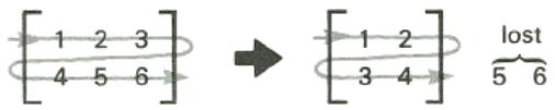
If you redimension a matrix to a larger size, elements with the value 0 are added at the end as required by the new dimensions. For example, if the same 2 × 3 matrix is re dimensioned, to 2 × 4 , then

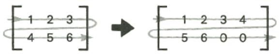
When you have finished calculating with matrices, you'll probably want to redimension all five matrices to 0 × 0 , so that the registers used for storing their elements will be available for program lines or for other advanced functions. You can redimension all five matrices to 0 × 0 at one time by pressing 0. (You can dimension a single matrix to 0 × 0 by pressing 0 {A} through E}.)

Storing and Recalling Matrix Elements

The HP-15C provides two ways of storing and recalling values of matrix elements. The first method allows you to progress through all of the elements in order. The second method allows you to access elements individually.

Storing and Recalling All Elements in Order

The HP-15C normally uses storage registers _0 and _1 to indicate the row and column numbers of a matrix element. If the calculator is in User mode, the row and column numbers are automatically incremented as you store or recall each matrix element, from left to right along each row from the first row to the last.

To set the row and column numbers in R_0 and R_1 to row 1, column 1, press f MATRiX 1.

To store or recall sequential elements of a matrix:

1. Be sure the matrix is properly dimensioned.
2. Press MATRIX1. This stores 1 in both storage registers R_0 and R_1 , so that elements will be accessed starting at row 1, column 1.
3. Activate User mode by pressing f USER. With the calculator in User mode, after each element is stored or recalled the row number in R_0 or the column number in R_1 is automatically incremented by 1, as shown in the example following.
4. If you are storing elements, key in the value of the element to be stored in row 1, column 1.
5. Press STO or RCL followed by the letter key specifying the matrix.
6. Repeat steps 4 and 5 for all elements of the matrix. The row and column numbers are incremented according to the dimensions of the matrix you specify.

While the letter key specifying the matrix is held down after or RCL is pressed, the calculator displays the name of the matrix followed by the row and column numbers of the element whose value is being stored or recalled. If the letter key is held down for longer than about 3 seconds, the calculator displays null, doesn't store or recall the element value, and doesn't increment the row and column numbers. (Also, the stack registers aren't changed.)

After the last element of the matrix has been accessed, the row and column numbers both return to 1.

Example: Store the values shown below in the elements of the matrix A dimensioned above. (Be sure matrix A is dimensioned to 2 × 3 .)

$$ \mathbf {A} = \left[ \begin{array}{l l l} a _ {1 1} & a _ {1 2} & a _ {1 3} \ a _ {2 1} & a _ {2 2} & a _ {2 3} \end{array} \right] = \left[ \begin{array}{l l l} 1 & 2 & 3 \ 4 & 5 & 6 \end{array} \right] $$

Keystrokes

f MATRlX 1

Display

Sets beginning row and column numbers in R_0 and R_1 to 1. (Display shows the previous result.)

f USER

1STO A A 1,1

Activates User mode.

2 STO A

Row 1, column 1 of A.

3 STO A 3.0000

(Displayed momentarily while A key held down.)

4.STO A 4.0000

Value of a_11

5 STO A 5.0000

Value of a_12

6 STO A 6.0000

Value of a_13

RCL A

1.0000

3.0000

4.0000

5.0000

6.0000

A 1,1

Value of a_21

Value of a_22

Value of a_23

Recalls element in row 1, column 1. (R_0 and _1 were reset in preceding step.)

1.0000

Value of a_11

RCL A

2.0000

Value of a_12

RCL A

3.0000

Value of a_13

RCL A

4.0000

Value of a_21

RCL A

5.0000

Value of a_22

RCL A

6.0000

Value of a_23

f USER

6.0000

Deactivates User mode.

Checking and Changing Matrix Elements Individually

The calculator provides two ways to check (recall) and change (store) the value of a particular matrix element. The first method uses storage registers R_0 and R_1 in the same way as described above - except that the row and column numbers aren't automatically changed when User mode is deactivated. The second method uses the stack to define the row and column numbers.

Using R_0 and R_1 . To access a particular matrix element, store its row number in R_0 and its column number in R_1 . These numbers won't change automatically (unless the calculator is in User mode).

• To recall the element value (after storing the row and column numbers), press RCL followed by the letter key specifying the matrix.
• To store a value in that element (after storing the row and column numbers), place the value in the X-register and press STO followed by the letter key specifying the matrix.

Example: Store the value 9 as the element in row 2, column 3 of matrix A from the previous example.

Keystrokes	Display
2 STO 0	2.0000	Stores row number in R0.
3 STO 1	3.0000	Stores column number in R1.
9	9	Keys the new element value into the X-register.
STO A	A 2,3	Row 2, column 3 of A.
	9.0000	Value of a23.

Using the Stack. You can use the stack registers to specify a particular matrix element. This eliminates the need to change the numbers in R_0 and R_1 .

• To recall an element value, enter the row number and column number into the stack (in that order). Then press RCL 9 followed by the letter key specifying the matrix. The element value is placed in the X-register. (The row and column numbers are lost from the stack.)
• To store an element value, first enter the value into the stack followed by the row number and column number. Then press STO g followed by the letter key specifying the matrix. (The row and column numbers are lost from the stack; the element value is returned to the X-register.)

Note that these are the only operations in which the blue 9 key precedes a gold letter key.

Example: Recall the element in row 2, column 1 of matrix A from the previous example. Use the stack registers.

Keystrokes

2 ENTER 1

Display

1

Enters row number into Yregister and column number into X-register.

RCL

g

A

4.0000

Value of a_21

Storing a Number in All Elements of a Matrix

To store a number in all elements of a matrix, simply key that number into the display, then press STO MATRIX followed by the letter key specifying the matrix.

Matrix Operations

In many ways, matrix operations are like numeric calculations. Numeric calculations require you to specify the numbers to be used; often you define a register for storing the result. Similarly, matrix calculations require you to specify one or two matrices that you want to use. A matrix descriptor is used to specify a particular matrix. For many calculations, you also must specify a matrix for storing the result. This is the result matrix.

Because matrix operations usually require many individual calculations, the calculator flashes the running display during most matrix operations.

Matrix Descriptors

Earlier in this section you saw that when you press RCL MATRIX followed by a letter key specifying a matrix, the name of the matrix appears at the left of the display and the number of rows followed by the number of columns appears at the right. The matrix name is called the descriptor of the matrix. Matrix descriptors can be moved among the stack and data storage registers just like a number - that is, using STO, RCL, ENTER, etc. Whenever a matrix descriptor is displayed in the X-register, the current dimensions of that matrix are shown with it.

You use matrix descriptors to indicate which matrices are used in each matrix operation. The matrix operations discussed in the rest of this section

operate on the matrices whose descriptors are placed in the X-register and (for some operations) the Y-register.

Two matrix operations - calculating a determinant and solving the matrix equation AX = B - involve calculating an LU decomposition (also known as an LU factorization) of the matrix specified in the X-register. A matrix that is an LU decomposition is signified by two dashes following the matrix name in the display of its descriptor. (Refer to page 160 for using a matrix in LU form.)

The Result Matrix

For many operations discussed in this section, you need to define the matrix in which the result of the operation should be stored. This matrix is called the result matrix.

Other matrix operations do not use or affect the result matrix. (This is noted in the descriptions of these operations.) Such an operation either replaces the original matrix with the result of the operation (if the result is a matrix, such as a transpose) or returns a number to the X-register (if the result is a number, such as a row norm).

Before you perform an operation that uses the result matrix, you must designate the result matrix. Do this by pressing f followed by the letter key specifying the matrix, (If the descriptor of the intended result matrix is already in the X-register, you can press STO instead.) The designated matrix remains the result matrix until another is designated. To display the descriptor of the result matrix, press RCL .

When you perform an operation that affects the result matrix, the matrix is automatically redimensioned to the proper size. If this redimensioning would require more additional elements than there are available in matrix memory (a maximum of 64 for all five matrices), then the operation can't be performed. This restriction can often be overcome by designating the result matrix to be one of the matrices being operated on. (However, there are certain operations for which the result matrix can not be the same one as either of the matrices being operated on – this is noted in the description of these operations.)

While the key used for any matrix operation that stores a result in the result matrix is held down, the descriptor of the result matrix is displayed. If the key is released within about 3 seconds, the operation is performed, and the descriptor of the result matrix is placed in the X-register. If the key is held down longer, the operation is not performed and the calculator displays null.

Copying a Matrix

To copy the elements of a matrix into the corresponding elements of another matrix, use the STO MATRIX sequence:

1. Press RCL MATRIX followed by the letter key specifying the matrix to be copied. This enters the descriptor of the matrix into the display.
2. Press STO MATRIX followed by the letter key specifying the matrix to be copied into.

If the matrix specified after RCL does not have the same dimensions as the matrix specified after STO, the second matrix is redimensioned to agree with the first. The matrix specified after STO need not already be dimensioned.

Example: Copy matrix A from the previous example into matrix B .

Keystrokes	Display
RCL MATRIX	A	2	3	Displays descriptor of matrix to be copied.
A
STO MATRIX	A	2	3	Redimensions matrix B and copies A into B.
B
RCL MATRIX	b	2	3	Displays descriptor of new matrix B.
B

One-Matrix Operations

The following table shows functions that operate on only the matrix specified in the X-register. Operations involving a single matrix plus a number in another stack register are described under Scalar Operations (page 151).

One-Matrix Operations: Sign Change, Inverse, Transpose, Norms, Determinant

Keystroke(s)	Result in X-register	Effect on Matrix Specified in X-register	Effect on Result Matrix
CHS	No change.	Changes sign of all elements.	None.‡
1/x(f 1/x in User Mode)	Descriptor of result matrix.	None.‡	Inverse of specified matrix.§
f MATRIX 4	Descriptor of transpose.	Replaced by transpose.	None.‡
f MATRIX 7	Row norm of specified matrix.*	None.	None.
f MATRIX 8	Frobenius or Euclidean norm of specified matrix.†	None.	None.
f MATRIX 9	Determinant of specified matrix.	None.‡	LU decomposition of specified matrix.§
* The row norm is the largest sum of the absolute values of the elements in each row of the specified matrix.† The Frobenius of Euclidean norm is the square root of the sum of the squares of all elements in the specified matrix.‡ Unless the result matrix is the same matrix specified in the X-register.§ If the specified matrix is a singular matrix (that is, one that doesn't have an inverse), then the HP-15C modifies the LU form by an amount that is usually small compared to round-off error. For 1/x, the calculated inverse is the inverse of a matrix close to the original, singular matrix. (Refer to the HP-15C Advanced Functions Handbook for further information.)

Example: Calculate the transpose of matrix B . Matrix B was set in preceding examples to

$$ \mathbf {B} = \left[ \begin{array}{c c c} 1 & 2 & 3 \ 4 & 5 & 9 \end{array} \right]. $$

Keystrokes	Display
RCL MATRIX B	b	2	3	Displays descriptor of 2×3 matrix B.
f MATRIX 4	b	3	2	Descriptor of 3×2 transpose.

Matrix B (which you can view using RCL B in User mode) is now

$$ \mathbf {B} = \left[ \begin{array}{c c} 1 & 4 \ 2 & 5 \ 3 & 9 \end{array} \right]. $$

Scalar Operations

Scalar operations perform arithmetic operations between a scalar (that is, a number) and each element of a matrix. The scalar and the descriptor of the matrix must be placed in the X- and Y-registers – in either order. (Note that the register position will affect the outcome of the - and ÷ functions.) The resulting values are stored in the corresponding elements of the result matrix.

The possible operations are shown in the following table.

Operation	Elements of Result Matrix*
	Matrix in Y-Register Scalar in X-Register	Scalar in Y-Register Matrix in X-Register
+	Adds scalar value to each matrix element.
×	Multiplies each matrix element by scalar value.
-	Subtracts scalar value from each matrix element.	Subtracts each matrix element from scalar value.
÷	Divides each matrix element by scalar value.	Calculates inverse of matrix and multiplies each element by scalar value.
* Result matrix may be the specified matrix.

Example: Calculate the matrix B = 2A . then subtract 1 from every element in B . From before, use

$$ \mathbf {A} = \left[ \begin{array}{c c c} 1 & 2 & 3 \ 4 & 5 & 9 \end{array} \right]. $$

Keystrokes

f RESULT B

Display

A 2 3

Designates matrix B as result matrix.

b 2 3

Displays descriptor of matrix A.

Redimensions matrix B to the same dimensions as A , multiplies the elements of A by 2, stores those values in the corresponding elements of B , and displays the descriptor of the result matrix.

Keystrokes

1

Display

b 2

3 Subtracts 1 from the elements of matrix B and stores those values in the same elements of B .

The result (which you can view using RCL B in User mode) is

$$ \mathbf {B} = \left[ \begin{array}{c c c} 1 & 3 & 5 \ 7 & 9 & 1 7 \end{array} \right]. $$

Arithmetic Operations

With matrix descriptors in both the X- and Y-registers, pressing + or - calculates the sum or difference of the matrices.

Pressing	Calculates*
+ -	Y + X Y - X
* Result is stored in result matrix. Result matrix may be X or Y

Example: Calculate C = B - A , where A and B are defined in the previous example.

$$ \mathbf {A} = \left[ \begin{array}{c c c} 1 & 2 & 3 \ 4 & 5 & 9 \end{array} \right] \text {a n d} \mathbf {B} = \left[ \begin{array}{c c c} 1 & 3 & 5 \ 7 & 9 & 1 7 \end{array} \right]. $$

Keystrokes

f RESULT C

RCL MATRIX B

RCL MATRIX A

Display

b 2

A 2

Designates C as result matrix.

3 Recalls descriptor of matrix B (This step can be skipped if descriptor is already in X-register.)
3 Recalls descriptor of matrix A into X-register, moving descriptor of matrix B to Y-register.

Keystrokes

Display

Calculates B - A and stores values in redimensioned result matrix C .

The result is C = 0 & 1 & 2 3 & 4 & 8

Matrix Multiplication

With matrix description in both the X- and Y-registers, you can calculate three different matrix products. The table below shows the results of the three functions for a matrix X specified in the X-register and a matrix Y specified in the Y-register. The matrix X^-1 is the inverse of X , and the matrix Y^T is the transpose of Y .

Pressing	Calculates*
×f MATRIX 5÷	YXYTXX-1Y
* Result is stored in result matrix. For ÷, the result matrix can be Y but not X. For the others, the result matrix must be other than X or Y.

Note: When you use the ÷ function to evaluate the expression A^-1B , you must enter the matrix descriptors in the order B , A rather than in the order that they appear in the expression.

The value stored in each element of the result matrix is determined according to the usual rules of matrix multiplication.

For 5, the matrix specified in the Y-register isn't changed by this operation, even though its transpose is used. The result is identical to that obtained using 4 (transpose) and × .

For ÷ , the matrix specified in the X-register is replaced by its LU decomposition. The ÷ function calculates X^-1Y using a more direct method than does 1 / x and , giving the result faster and with improved accuracy.

Example: Using matrices A and B from the previous example, calculate C = A^TB .

$$ \mathbf {A} = \left[ \begin{array}{c c c} 1 & 2 & 3 \ 4 & 5 & 9 \end{array} \right] \text {a n d} \mathbf {B} = \left[ \begin{array}{c c c} 1 & 3 & 5 \ 7 & 9 & 1 7 \end{array} \right] $$

Keystrokes

RCL MATRIX

A

RCL MATRIX

B

f RESULT

C

f MATRI5

Display

A 2 3

b 2 3

Recalls descriptor for matrix A.

Recalls descriptor for matrix B into X-register, moving matrix A descriptor into Y-register.

Designates matrix C as result matrix.

Calculates A^TB and stores result in matrix C , which is redimensioned to 3× 3 .

The result, matrix C, is

$$ \mathbf {C} = \left[ \begin{array}{l l l} 2 9 & 3 9 & 7 3 \ 3 7 & 5 1 & 9 5 \ 6 6 & 9 0 & 1 6 8 \end{array} \right]. $$

Solving the Equation AX = B

The ÷ function is useful for solving matrix equations of the form AX = B , where A is the coefficient matrix, B is the constant matrix, and X is the solution matrix. The descriptor of the constant matrix B should be entered in the Y-register and the descriptor of the coefficient matrix A should be entered in the X-register Pressing ÷ then calculates the solution X = A^-1B^* .

Y constant matrix
X coefficient matrix

Remember that the ÷ function replaces the coefficient matrix by its LU decomposition and that this matrix must not be specified as the result matrix. Furthermore, using ÷ rather than 1/x and × gives a solution faster and with improved accuracy.

At the beginning of this section, you found the solution for a system of linear equations in which the constant matrix and the solution matrix each had one column. The following example illustrates that you can use the HP-15C to find solutions for more than one set of constants—that is, for a constant matrix and solution matrix with more than one column.

Example: Looking at his receipts for his last three deliveries of cabbage and broccoli, Silas Farmer sees the following summary.

	Week
	1	2	3
Total Weight (kg)	274	233	331
Total Value	120.32	112.96	$151.36

Silas knows that he received 0.24 per kilogram for his cabbage and 0.86 per kilogram for his broccoli. Use matrix operations to determine the weights of cabbage and broccoli he delivered each week.

Solution: Each week's delivery represents two linear equations (one for weight and one for value) with two unknown variables (the weights of cabbage and broccoli). All three weeks can be handled simultaneously using the matrix equation

$$ \left[ \begin{array}{c c} 1 & 1 \ 0. 2 4 & 0. 8 6 \end{array} \right] \left[ \begin{array}{c c c} d _ {1 1} & d _ {1 2} & d _ {1 3} \ d _ {2 1} & d _ {2 2} & d _ {2 3} \end{array} \right] = \left[ \begin{array}{c c c} 2 7 4 & 2 3 3 & 3 3 1 \ 1 2 0. 3 2 & 1 1 2. 9 6 & 1 5 1. 3 6 \end{array} \right] $$

or

$$ \mathbf {A D} = \mathbf {B} $$

where the first row of matrix D is the weights of cabbage for the three weeks and the second row is the weights of broccoli.

Keystrokes

2

ENTER f DIM A

f MATRiX 1

fUSER

1 STO A

STO A

.24 STO A

.86 STO A

2 ENTER 3

f DIM B

Display

2.0000 Dimensions A as 2× 2 matrix.
2.0000 Sets row and column numbers in R0 and R_1 to 1.
2.0000 Activates User mode.
1.0000 Stores a11
1.0000 Stores a_12
0.2400 Stores a_21
0.8600 Stores a_22
3.0000 Dimensions B as 2× 3 matrix.

Keystrokes

274 STO B

233 STO B

331 STO B

120.32 STO B

112.96 STO B

151.36 STO B

f RESULT D

RCL MATRIX B

RCL MATRIX A

中

RCL D

RCL D

RCL D

RCL D

RCL D

RCL D

fUSER

Display

274.0000 Stores b_11

233.0000 Stores b_12

331.0000 Stores b_13

120.3200 Stores b_21

112.9600 Stores b_22

151.3600 Stores b_23

151.3600 Designates matrix D as result matrix.

2 3
2 2

Recalls descriptor of constant matrix.
Recalls descriptor of coefficient matrix A into X-register, moving descriptor of constant matrix B into Y-register.

2 3

186.0000
141.0000
215.0000
88.0000
92.0000
116.0000
116.0000

Calculates A^-1B and stores result in matrix D.

Recalls d_11 , the weight of cabbage for the first week.

Recalls d_12 the weight of cabbage for the second week.

Recalls d_13
Recalls d_21
Recalls d_22
Recalls d_23
Deactivates User mode.

Silas' deliveries were:

	Week
	1	2	3
Cabbage (kg)	186	141	215
Broccoli (kg)	88	92	116

Calculating the Residual

The HP-15C enables you to calculate the residual, that is, the matrix

$$ \text {R e s i d u a l} = \mathbf {R} - \mathbf {Y X} $$

where R is the result matrix and X and Y are the matrices specified in the X- and Y-registers.

This capability is useful, for example, in doing iterative refinement on the solution of a system of equations and for linear regression problems. For example, if C is a possible solution for AX = B , then B - AC indicates how well this solution satisfies the equation. (Refer to the HP-15C Advanced Functions Handbook for information about iterative refinement and linear regression.)

The residual function (MATRIX 6) uses the current contents of the result matrix and the matrices specified in the X- and Y-registers to calculate the residual defined above. The residual is stored in the result matrix, replacing the original result matrix. A matrix specified in the X- or Y-register can not be the result matrix.

Using 6 rather than and - gives a result with improved accuracy, particularly if the residual is small compared to the matrices being subtracted.

To calculate the residual:

1. Enter the descriptor of the Y matrix into the Y-register.
2. Enter the descriptor of the X matrix into the X-register.
3. Designate the R matrix as the result matrix.
4. Press 6. The residual replaces the original result matrix (R). The descriptor of the result matrix is placed in the Xregister.

Using Matrices in LU Form

As noted earlier, two matrix operations (calculating a determinant and solving the matrix equation (AX = B) create an LU decomposition of the matrix specified in the X-register. The descriptor of such a matrix has two dashes following the matrix name. A matrix in LU form has elements that differ from the elements of the original matrix.

However, the descriptor for a matrix in LU form can be used in place of the descriptor for the original matrix for operations involving the inverse of the matrix and for the determinant operation. That is, either the original matrix or its LU decomposition can be used for these operations:

1/x
for the matrix in the X-register
MATRIX 9

For these three functions, using the LU form of the matrix to be inverted gives a result that is identical to that using the original matrix.

As an example, if you solved the matrix equation AX = B , matrix A would be changed to its LU form. If you wanted to change the B matrix and solve the equation again, you could do so without changing the A matrix – the LU matrix will give the correct solution.

For all other matrix operations, a matrix that is an LU decomposition is not recognized as representing its original matrix. Instead, the elements of the LU matrix are used just as they appear in matrix memory and the result is not the result you would obtain using the original matrix.

Calculations With Complex Matrices

The HP-15C enables you to perform matrix multiplication and matrix inversion with complex matrices (that is, matrices whose elements are complex numbers) and to solve systems of complex equations (that is, equations whose coefficients and variables are complex).

However, the HP-15C stores and operates on only real matrices. The capability of doing calculations with complex matrices is completely independent of the capability of doing calculations with complex numbers described in the preceding section. You don't need to activate Complex mode for calculations with complex matrices.

Instead, calculations with complex matrices are performed by using real matrices derived from the original complex matrices – in a manner to be described below – and performing certain transformations in addition to the regular matrix operations. These transformations are performed by four calculator functions. This section will describe how to do these calculations. (There are more examples of calculations with complex matrices in the HP-15C Advanced Functions Handbook.)

Storing the Elements of a Complex Matrix

Consider an m × n complex matrix Z = X + iY , where X and Y are real m × n matrices. This matrix can be represented in the calculator as a 2m × n "partitioned" matrix:

$$ \mathbf {Z} ^ {P} = \left[ \begin{array}{l} \mathrm {X} \ \mathrm {Y} \end{array} \right] } \quad \text {R e a l P a r t} $$

The superscript P signifies that the complex matrix is represented by a partitioned matrix.

All of the elements of Z^P are real numbers - those in the upper half represent the elements of the real part (matrix X ), those in the lower half represent the elements of the imaginary part (matrix Y ). The elements of Z^P are stored in one of the five matrices ( A , for example) in the usual manner, as described earlier in this section.

For example, if Z = X + iY , where

$$ \mathbf {X} = \left[ \begin{array}{c c} x _ {1 1} & x _ {1 2} \ x _ {2 1} & x _ {2 2} \end{array} \right] \text {a n d} \quad \mathbf {Y} = \left[ \begin{array}{c c} y _ {1 1} & y _ {1 2} \ y _ {2 1} & y _ {2 2} \end{array} \right], $$

then Z can be represented in the calculator by

$$ \mathbf {A} = \mathbf {Z} ^ {P} = \left[ \begin{array}{c} \mathbf {X} \ \mathbf {Y} \end{array} \right] = \left[ \begin{array}{c c} x _ {1 1} & x _ {1 2} \ \frac {x _ {2 1}}{y _ {1 1}} & - \frac {x _ {2 2}}{y _ {1 2}} \ y _ {2 1} & y _ {2 2} \end{array} \right]. $$

Suppose you need to do a calculation with a complex matrix that is not written as the sum of a real matrix and an imaginary matrix - as was the matrix Z in the example above - but rather written with an entire complex number in each element, such as

$$ \mathbf {Z} = \left[ \begin{array}{c c} x _ {1 1} + i y _ {1 1} & x _ {1 2} + i y _ {1 2} \ x _ {2 1} + i y _ {2 1} & x _ {2 2} + i y _ {2 2} \end{array} \right]. $$

This matrix can be represented in the calculator by a real matrix that looks very similar – one that is derived simply by ignoring the i and the + sign. The 2 × 2 matrix Z shown above, for example, can be represented in the calculator in “complex” form by the 2 × 4 matrix.

$$ \mathbf {A} = \mathbf {Z} ^ {C} = \left[ \begin{array}{c c c c} x _ {1 1} & y _ {1 1} & x _ {1 2} & y _ {1 2} \ x _ {2 1} & y _ {2 1} & x _ {2 2} & y _ {2 2} \end{array} \right]. $$

The superscript C signifies that the complex matrix is represented in a "complex-like" form.

Although a complex matrix can be initially represented in the calculator by a matrix of the form shown for Z^C , the transformations used for multiplying and inverting a complex matrix presume that the matrix is represented by a matrix of the form shown for Z^P . The HP-15C provides two transformations that convert the representation of a complex matrix between Z^C and Z^P :

Pressing	Transforms	Into
f Py.x	Z^C	Z^P
g Cy.x	Z^P	Z^C

To do either of these transformations, recall the descriptor of Z^C or Z^P into the display, then press the keys shown above. The transformation is done to the specified matrix; the result matrix is not affected.

Example: Store the complex matrix

$$ \mathbf {Z} = \left[ \begin{array}{c c} 4 + 3 i & 7 - 2 i \ 1 + 5 i & 3 + 8 i \end{array} \right] $$

in the form Z^C , since it is written in a form that shows Z^C . Then transform Z^C into the form Z^P .

You can do this by storing the elements of Z^C in matrix A and then using the .x function, where

$$ \mathbf {A} = \mathbf {Z} ^ {c} = \left[ \begin{array}{c c c c} 4 & 3 & 7 & - 2 \ 1 & 5 & 3 & 8 \end{array} \right]. $$

Keystrokes

f MATRIX 0
2 ENTER 4
f DIM A
f MATRIX 1

Display

4.0000
4.0000

fUSER

4 STO A
3 STO A
7 STO A
2 CHS STO A

1 STO A
5 STO A
3 STO A
8 STO A

fUSER

RCL MATRIX A

f Pxy.x

4.0000

4.0000

3.0000

7.0000

-2.0000

1.0000
5.0000
3.0000
8.0000
80000

A 2 4

A 4 2

Clears all matrices.

Dimensions matrix A to be 2× 4

Sets beginning row and column numbers in R_0 and R_1 to 1.

Activates User mode.

Stores a_11

Stores a_12

Stores a_13

Stores a_14

Stores a_21

Stores a_22

Stores a_23

Stores a_24

Deactivates User mode.

Display descriptor of matrix A.

Transforms Z^C into Z^P and redimensions matrix A.

Matrix A now represents the complex matrix Z in Z^P form:

$$ \mathbf {A} = \mathbf {Z} ^ {\mathbf {P}} = \left[ \begin{array}{c c} 4 & 7 \ \frac {1}{3} & - \frac {3}{2} \ 5 & 8 \end{array} \right]. \quad \left{ \begin{array}{l} \text {R e a l P a r t} \ \text {I m a g i n a r y P a r t} \end{array} \right. $$

The Complex Transformations Between Z^P and

An additional transformation must be done when you want to calculate the product of two complex matrices, and still another when you want to calculate the inverse of a complex matrix. These transformations convert between the Z^P representation of an m × n complex matrix and a 2m × 2n partitioned matrix of the following form:

$$ \mathbf {Z} = \left[ \begin{array}{c c} \mathbf {X} & - \mathbf {Y} \ \mathbf {Y} & \mathbf {X} \end{array} \right]. $$

The matrix created by the MATRIX 2 transformation has twice as many elements as Z^P .

For example, the matrices below show how is related to Z^p .

$$ \mathbf {Z} ^ {P} = \left[ \begin{array}{c c} 1 & - 6 \ - 4 & 5 \end{array} \right] \leftrightarrow \widetilde {\mathbf {Z}} = \left[ \begin{array}{c c c c} 1 & - 6 & 4 & - 5 \ - 4 & 5 & - 1 & - 6 \end{array} \right] $$

The transformations that convert the representation of a complex matrix between Z^P and are shown in the following table.

Pressing	Transforms	Into
f MATRIX 2	ZP	Z
f MATRIX 3	Z	ZP

To do either of these transformations, recall the descriptor of Z^P or into the display, then press the keys shown above. The transformation is done to the specified matrix; the result matrix is not affected.

Inverting a Complex Matrix

You can calculate the inverse of a complex matrix by using the fact that ()^-1 = (^-1)

To calculate inverse, Z^-1 , of a complex matrix Z :

1. Store the elements of Z in memory, in the form either of Z^P or of Z^C
2. Recall the descriptor of the matrix representing Z into the display.
3. If the elements of Z were entered in the form Z^C , press .x to transform Z^C into Z^P
4. Press f MATRIX 2 to transform Z^P into .
5. Designate a matrix as the result matrix. It may be the same as the matrix in which is stored.
6. Press 1 / x . This calculates ()^-1 , which is equal to (^-1) . The values of these matrix elements are stored in the result matrix, and the descriptor of the result matrix is placed in the X-register.
7. Press MATRIX 3 to transform (^-1) into (Z^-1)^P
8. If you want the inverse in the form (Z^-1)^C , press [9] [Cy.x]

You can derive the complex elements of Z^-1 by recalling the elements of Z^P or Z^C and then combining them as described earlier.

Example: Calculate the inverse of the complex matrix Z from the previous example.

$$ \mathbf {A} = \mathbf {Z} ^ {\mathbf {P}} = \left[ \begin{array}{c c} 4 & 7 \ \hline 1 & 3 \ \hline 3 & - 2 \ 5 & 8 \end{array} \right]. $$

Keystrokes

RCL MATRIX A

f MATRiX 2

Display

A 4 2

A 4 4

Recalls descriptor of matrix A.

Transforms Z^P into and redimensions matrix A .

Keystrokes

f RESULT
B
1/x

f MATRIx 3

Display

A 4
b 4
b 4

4 Designates B as the result matrix.
4 Calculates ()^-1 = (^-1) and places the result in matrix B
2 Transforms (^-1) into (^-1)^P

The representation of Z^-1 in partitioned form is contained in matrix B .

$$ \mathbf {B} = \left[ \begin{array}{c c} - 0. 0 2 5 4 & 0. 2 4 2 0 \ - 0. 0 1 2 2 & - 0. 1 0 1 7 \ - 0. 2 8 2 9 & - 0. 0 0 2 2 \ 0. 1 6 9 1 & - 0. 1 3 1 5 \end{array} \right] \left{ \begin{array}{l l} \text {R e a l P a r t} \ \text {I m a g i n a r y P a r t} \end{array} \right. $$

Multiplying Complex Matrices

The product of two complex matrices can be calculated by using the fact that (YX)^P = ^P .

To calculate YX , where Y and X are complex matrices:

1. Store the elements of Y and X in memory, in the form either of Z^P or Z^C .
2. Recall the descriptor of the matrix representing Y into the display.
3. If the elements of Y were entered in the form of Y^C , press f Py.x to transform Y^C into Y^P .
4. Press MATRIX 2 to transform Y^P into .
5. Recall the descriptor of the matrix representing X into the display.
6. If the elements of X were entered in the form X^C , press .x to transform X^C into X^P .

7. Designate the result matrix; it must not be the same matrix as either of the other two.

8. Press to calculate ^P = (YX)^P . The values of these matrix elements are placed in the result matrix, and the descriptor of the result matrix is placed in the X-register.

9. If you want the product in the form (YX)^C , press 9 Cxy

Note that you don't transform X^P into .

You can derive the complex elements of the matrix product YX by recalling the elements of (XY)^P or (YX)^C and combining them according to the conventions described earlier.

Example: Calculate the product ZZ^-1 , where Z is the complex matrix given in the preceding example.

Since elements representing both matrices are already stored ( in A and (Z^-1)^P in B ), skip steps 1, 3, 4, and 6.

Keystrokes

RCL MATRIX A
RCL MATRIXB

Display

A 4
b 4

4 Displays descriptor of matrix A.
2 Displays descriptor of matrix B.

f RESULT C
X
fUSER
RCL C

b 4
C 4
C 4
c 1,1

2 Designates C as result matrix.
2 Calculates (Z^-1)^P = (ZZ^-1)^P
2 Activates User mode.

RCL C
RCL C
RCL C
RCL C
RCL C
RCL C
RCL C
f [USER]

1.0000
-2.8500 -10
-4.0000 -11

1.0000
1.0000 -11
3.8000 -10
1.0000 -11
-1.0500 -10
-1.0500 -10

Matrix C, row 1, column 1. (Displayed momentarily while last key held down.)
Value of c_11
Value of c_12
Value of c_21
Value of c_22
Value of c_31
Value of c_32
Value of c_41
Value of c_42
Deactivates User mode.

Writing down the elements of C

$$ \mathbf {C} = \left[ \begin{array}{c c} 1. 0 0 0 0 & - 2. 8 5 0 0 \times 1 0 ^ {- 1 0} \ - 4. 0 0 0 0 \times 1 0 ^ {- 1 1} & 1. 0 0 0 0 \ 1. 0 0 0 0 \times 1 0 ^ {- 1 1} & - 3. 8 0 0 0 \times 1 0 ^ {- 1 0} \ 1. 0 0 0 0 \times 1 0 ^ {- 1 1} & - 1. 0 5 0 0 \times 1 0 ^ {- 1 0} \end{array} \right] = \left(\mathbf {Z Z} ^ {- 1}\right) ^ {P}, $$

where the upper half of matrix C is the real part of ZZ^-1 and the lower half is the imaginary part. Therefore, by inspection of matrix C ,

$$ \begin{array}{l} \mathbf {Z Z} ^ {- 1} = \left[ \begin{array}{c c} 1. 0 0 0 0 & - 2. 8 5 0 0 \times 1 0 ^ {- 1 0} \ - 4. 0 0 0 0 \times 1 0 ^ {- 1 1} & 1. 0 0 0 0 \end{array} \right] \ + i \left[ \begin{array}{c c} 1. 0 0 0 0 \times 1 0 ^ {- 1 1} & 3. 8 0 0 0 \times 1 0 ^ {- 1 1} \ 1. 0 0 0 0 \times 1 0 ^ {- 1 1} & - 1. 0 5 0 0 \times 1 0 ^ {- 1 0} \end{array} \right] \ \end{array} $$

As expected,

$$ \mathbf {Z} \mathbf {Z} ^ {- 1} = \left[ \begin{array}{c c} 1 & 0 \ 0 & 1 \end{array} \right] + i \left[ \begin{array}{c c} 0 & 0 \ 0 & 0 \end{array} \right] $$

Solving the Complex Equation AX = B

You can solve the complex matrix equation AX = B by finding X = A^-1B . Do this by calculating X^P = ()^-1B^P .

To solve the equation AX = B , where A , X , and B are complex matrices:

1. Store the elements of A and B in memory, in the form either of Z^P or of Z^C .
2. Recall the descriptor of the matrix representing B into the display.

3. If the elements of B were entered in the form B^C , press .x to transform B^C into B^P .

4. Recall the descriptor of the matrix representing A into the display.

5. If the elements of A were entered in the form of A^C , press to transform A^C into A^P .

6. Press MATRIx 2 to transform A^P into .

7. Designate the result matrix; it must not be the same as the matrix representing A .

8. Press ÷ ; this calculates X^P . The values of these matrix elements are placed in the result matrix, and the descriptor of the result matrix is placed in the X-register.

9. If you want the solution in the form X^C , press [9] [Cy.x].

Note that you don't transform B^P into .

You can derive the complex elements of the solution X by recalling the elements of X^P or X^C and combining them according to the conventions described earlier.

Example: Engineering student A. C. Dimmer wants to analyze the electrical circuit shown below. The impedances of the components are indicated in complex form. Determine the complex representation of the currents I_1 and I_2 .

This system can be represented by the complex matrix equation

$$ \left[ \begin{array}{c c} 1 0 + 2 0 0 i & - 2 0 0 i \ - 2 0 0 i & (2 0 0 - 3 0) i \end{array} \right] \left[ \begin{array}{l} I _ {1} \ I _ {2} \end{array} \right] = \left[ \begin{array}{l} 5 \ 0 \end{array} \right] $$

or

$$ \mathbf {A X} = \mathbf {B}. $$

In partitioned form,

$$ \mathbf {A} = \left[ \begin{array}{c c} 1 0 & 0 \ 0 & 0 \ - - - - - - - - - - - - - - - - - - - - - - - - - - - - - - - - - - - - - - - - - - - - - - - - - - - - - - - - - - - - - - - - - - - - - - - - - - - - - - - - - - - + 0 \ 2 0 0 & - 2 0 0 \ - 2 0 0 & 1 7 0 \end{array} \right] \text {a n d} \mathbf {B} = \left[ \begin{array}{c} 5 \ 0 \ 0 \ 0 \ 0 \end{array} \right], $$

where the zero elements correspond to real and imaginary parts with zero value.

Keystrokes	Display
4 ENTER2 f DIM A	2.0000	Dimensions matrix A to be 4×2.
f MATRIX 1	2.0000	Set beginning row and column numbers in R0 and R1 to 1.
f USER	2.0000	Activates User mode.
10 STO A	10.0000	Stores a11.
0 STO A	0.0000	Stores a12.
STO A	0.0000	Stores a21.
STO A	0.0000	Stores a22.
200 STO A	200.0000	Stores a31.
CHS STO A	-200.0000	Stores a32.
STO A	-200.0000	Stores a41.
170 STO A	170.0000	Stores a42.
4 ENTER 1 f DIM B	1.0000	Dimensions matrix B to be 4×1.
0 STO MATRIX B	0.0000	Stores value 0 in all elements of B.
5 ENTER 1 ENTER	1.0000	Specifies value 5 for row 1, column 1.
STO g B	5.0000	Stores value 5 in b11.
RCL MATRIX B	b 4 1	Recalls descriptor for matrix B.
RCL MATRIX A	A 4 2	Places descriptor for matrix A into X-register, moving descriptor for matrix B into Y-register.

Keystrokes	Display
f MATRIX 2	A	4	4	Transforms A^P into \tilde{A} .
f RESULT C	A	4	4	Designates matrix C as result matrix. Calculates X^P and stores in C.
\div	C	4	1
9 Cy.x	C	2	2	Transforms X^P into X^C. Recalls c_{11}. Recalls c_{12}. Recalls c_{21}. Recalls c_{22}. Deactivates User mode. Redimensions all matrices to 0×0.
RCL C	0.0372
RCL C	0.1311
RCL C	0.0437
RCL C	0.1543
f USER	0.1543
f MATRIX 0	0.1543

The currents, represented by the complex matrix X , can be derived from C

$$ \mathbf {X} = \left[ \begin{array}{l} I _ {1} \ I _ {2} \end{array} \right] = \left[ \begin{array}{l} 0. 0 3 7 2 + 0. 1 3 1 \mathbf {f} \ 0. 0 4 3 7 + 0. 1 5 4 \mathbf {f} \end{array} \right] $$

Solving the matrix equation in the preceding example required 24 registers of matrix memory - 16 for the 4 × 4 matrix A (which was originally entered as a 4 × 2 matrix representing a 2 × 2 complex matrix), and four each for the matrices B and C (each representing a 2 × 1 complex matrix). (However, you would have used four fewer registers if the result matrix were matrix B .) Note that since X and B are not restricted to be vectors (that is, single-column matrices), X and B could have required more memory.

The HP-15C contains sufficient memory to solve, using the method described above, the complex matrix equation AX = B with X and B having up to six columns if A is 2× 2 , or up to two columns if A is 3× 3 . (The allowable number of columns doubles if the constant matrix B is used as the result matrix.) If X and B have more columns, or if A is 4× 4 , you can solve the equation using the alternate method below. This method differs from the preceding one in that it involves separate inversion and multiplication operations and fewer registers.

1. Store the elements of A in memory, in the form either of A^P or of A^C .
2. Recall the descriptor of the matrix representing A into the display.
3. If the elements of A were entered in the form A^C , press ,x to transform A^C into A^P .
4. Press 2 to transform A^P into .
5. Press STO RESULT to designate the matrix representing A as the result matrix.
6. Press 1 / x to calculate ()^-1 .
7. Redimension A to have half the number of rows as indicated in the display of its descriptor after the preceding step.
8. Store the elements of B in memory, in the form either of B^P or of B^C .
9. Recall the descriptor of the matrix representing A into the display.
10. Recall the descriptor of the matrix representing B into the display.
11. If the elements of B were entered in the form B^C , press ,x to transform B^C into B^P .
12. Press MATRIX 2 to transform B^P into
13. Designate the result matrix; it must not be the same matrix as either of the other two.
14. Press .
15. Press MATRIX 4 to transpose the result matrix.
16. Press f MATRIx 2.
17. Redimension the result matrix to have half the number of rows as indicated in the display of its descriptor after the preceding step.
18. Press RCL RESULT to recall the descriptor of the result matrix.
19. Press f MATRiX 4 to calculate X^P
20. If you want the solution in the form X^C , press 9,x

A problem using this procedure is given in the HP-15C Advanced Functions Handbook under Solving a Large System of Complex Equations.

Miscellaneous Operations Involving Matrices

Using a Matrix Element With Register Operations

If a letter key specifying a matrix is pressed after any of the following function keys, the operation is performed using the matrix element specified by the row and column numbers in R_0 and R_1 , just as though it were a data storage register.

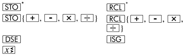
Using Matrix Descriptors in the Index Register

In certain applications, you may want to perform a programmed sequence of matrix operations using any of the matrices A through E . In this situation, the matrix operations can refer to whatever matrix descriptor is stored in the index register (_I) .

If the Index register contains a matrix descriptor:

• Pressing (i) after any of the functions listed above performs the operations using the element specified by R_0 and R_1 and the matrix specified in R_1 .

• Pressing (i) after STO 9 or RCL 9 performs the operation using the element specified by the row and column numbers in the Y- and X-registers and the matrix specified in R_I

• Pressing dimensions the matrix specified in R_1 according to the dimensions in the X- and Y-registers.

• Pressing RCL DIM I recalls to the X- and Y-registers the dimensions of the matrix specified in R_I .
• Pressing S B or T O has the same result as pressing S B or T O followed by the letter of the matrix specified in R_I . (This is not actually a matrix operation - only the letter in the matrix descriptor is used.)

Conditional Tests on Matrix Descriptors

Four conditional tests - = 0 , 0 (x 0) , 5 (x = y) , and 6 (x y) - can be performed with matrix descriptors in the X- and Y-registers, Conditional tests can be used to control program execution, as described in section 8.

If a matrix descriptor is in the X-register, the result of = 0 will be false and the result of TEST 0 will be true (regardless of the element values in the matrix.)

If matrix descriptors are in the X- and Y-registers when TEST 5 or TEST 6 conditional test is performed, x and y are equal if the same descriptor is in the X- and Y-registers, and not equal otherwise. The comparison is made between the descriptors themselves, not between the elements of the specified matrices.

Other conditional tests can't be used with matrix descriptors.

Stack Operation for Matrix Calculations

During matrix calculations, the contents of the stack registers shift much like they do during numeric calculations.

For some matrix calculations, the result is stored in the result matrix. The arguments - one or two descriptors or numbers in the X-register or the X- and Y-registers - are combined by the operation, and the descriptor of the result matrix is placed in the X-register. (The argument from the X-register is placed in the LAST X register.)

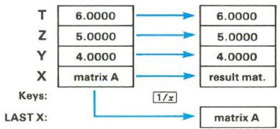
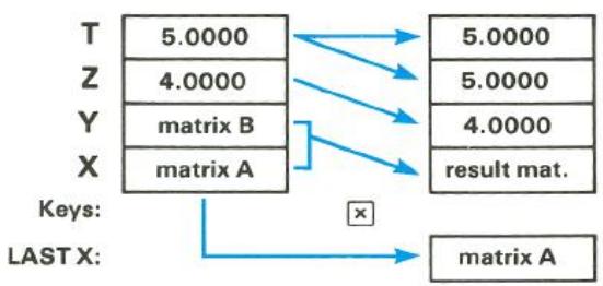
Several matrix functions operate on the matrix specified in the X-register only and store the result in the same matrix. For these operations the contents of the stack (including the LAST X register) are not moved – although the display changes to show the new dimensions if necessary.

For the MATRIX 7, MATRIX 8, and MATRIX 9 functions, the matrix descriptor specified in the X-register is placed in the LAST X register and the norm or (for MATRIX 9) the determinant is placed in the X-register. The Y-, Z-, and T-registers aren't changed.

When you recall descriptors or matrix elements into the X-register (with the stack enabled), other descriptors and numbers already in the stack move up in the stack - and the contents of the T-register are lost. (The LAST X register is not changed.) When you store descriptors or matrix elements, the stack (and the LAST X register) isn't changed.

In contrast to the operation described above, the STO g and RCL g functions do not affect the LAST X register and operate as shown on the next page.

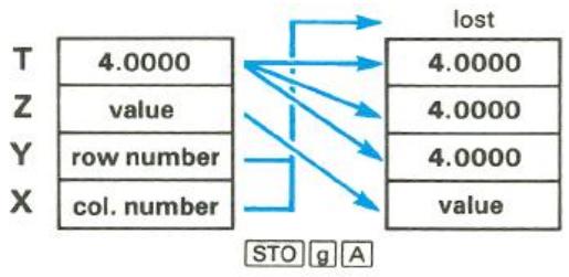
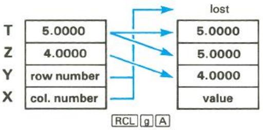
Using Matrix Operations in a Program

If the calculator is in User mode during program entry when you enter a STO or RCL{A through E, (i) } instruction to store or recall a matrix element, a u replaces the dash usually displayed after the line number. When this line is executed in a running program, it operates as though the calculator were in User mode. That is, the row and column numbers in R_0 and R_1 are automatically incremented according to the dimensions of the specified matrix. This allows you to access elements sequentially. (The USER annunciator has no effect during program execution.)

In addition, when the last element is accessed by the "User" or RCL instruction - when R_0 and R_1 are returned to 1 - program execution skips the next line. This is useful for programming a loop that stores or recalls each matrix element, then continues executing the program. For example, the following sequence squares all elements of matrix D:

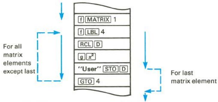
The MATRIX 7 (row norm) and MATRIX 8 (Frobenius norm) functions also operate as conditional branching instructions in a program. If the X-register contains a matrix descriptor, these functions calculate the norm in the usual manner, and program execution continues with the next program line. If the X-register contains a number, program execution skips the next line. In both cases, the original contents of the X-register are stored in the LAST X register. This is useful for testing whether a matrix descriptor is in the X-register during a program.

Summary of Matrix Functions

Keystroke(s)	Results
9 Cy, x	Transforms ZP into ZC.
CHS	Changes sign of all elements in matrix specified in X-register.
f DIM {A through E, I}	Dimensions specified matrix.
f MATRIX 0	Dimensions all matrices to 0×0.
f MATRIX 1	Sets row and column numbers in R0 and R1 to 1.
f MATRIX 2	Transform ZP into Z.
f MATRIX 3	Transform Z into ZP.
f MATRIX 4	Calculate transpose of matrix specified in X-register.
f MATRIX 5	Multiplies transpose of matrix specified in Y-register with matrix specified in X-register. Stores in

Keystroke(s)

Results

result matrix.

f MATRIX 6

Calculates residual in result matrix.

f MATRIx 7

Calculates row norm of matrix specified in Xregister.

f MATRIX 8

Calculates Frobenius or Euclidean norm of matrix specified in X-register.

f MATRIK 9

Calculates determinant of matrix specified in Xregister, Place LU in result matrix.

f Pxy.x

Transforms Z^C into Z^P .

RCL{A through E，（i）}

Recalls value from specified matrix, using row and column numbers in R_0 and R_1 .

RCL g{A through E, (i)}

Recalls value from specified matrix using row and column numbers in Y- and X-registers.

RCL DIM {A through E, (i)}

Recalls dimensions of specified matrix into X- and Y-registers.

RCL MATRIX {A through E}

Displays descriptor of specified matrix.

RCL RESULT

Displays descriptor of result matrix.

f RESULT{A through E}

Designates specified matrix as result matrix.

STO{A through E (i)}

Stores value from display into element of specified matrix, using row and column numbers in R_0 and R_1 .

STO 9{A through E (i)}

Stores value from Z-register into element of specified matrix, using row and column numbers in Y- and X-registers.

STOMATRIX {A through E}

If matrix descriptor is in display, copies all elements of that matrix into corresponding elements of specified matrix. If number is in display, stores that value in all elements of specified matrix.

Keystroke(s)

Results

STO RESULT

Designates matrix specified in X-register as result matrix.

f USER

Row and column numbers in R_0 and R_1 are automatically incremented each time or {A through E, (i)} is pressed.

1/x

Inverts matrix specified in X-register. Stores in result matrix. Use 1 / x if User mode is on.

+，-

If matrix descriptors specified in both X- and Y- registers, adds or subtracts corresponding elements of matrices specified. If matrix descriptor specified in only one of these registers, performs addition or subtraction with all elements in specified matrix and scalar in other register. Stores in result matrix.

X

If matrix descriptors specified in both X- and Y-registers, calculates product of specified matrices (as YX ). If matrix specified in only one of these registers, multiplies all elements in specified matrix by scalar in other register. Stores in result matrix.

中

If matrix descriptors specified in both X- and Y- registers, multiplies inverse of matrix specified in X- register with matrix specified in Y-register. If matrix specified in only Y-register, divides all elements of specified matrix by scalar in other register. If matrix specified in only X-register, multiplies each element of inverse of specified matrix by scalar in other register. Stores in result matrix.

For Further Information

The HP-15C Advanced Functions Handbook presents more detailed and technical aspects of the matrix functions in the HP-15C, including applications. The topics include: least-squares calculations, solving nonlinear equations, ill-conditioned and singular matrices, accuracy considerations, iterative refinement, and creating the identity matrix.

Section 13

Finding the Roots of an Equation

In many applications you need to solve equations of the form

$$ f (x) = 0. ^ {*} $$

This means finding the values of x that satisfy the equation. Each such value of x is called a root of the equation f(x) = 0 and a zero of the function f(x) . These roots (or zeros) that are real numbers are called real roots (or real zeros). For many problems the roots of an equation can be determined analytically through algebraic manipulation; in many other instances, this is not possible. Numerical techniques can be used to estimate the

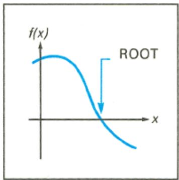
roots when analytical methods are not suitable. When you use the SOLVE key on your HP-15C, you utilize an advanced numerical technique that lets you effectively and conveniently find real roots for a wide range of equations. ^

Using SOLVE

In calculating roots, the SOLVE operation repeatedly calls up and executes a subroutine that you write for evaluating f(x) .

The basic rules for using SOLVE are:

1. In Program mode, key in a subroutine that evaluates the function f(x) that is to be equated to zero. This subroutine must begin with a label instruction (f Lbl label) and end up with a result for f(x) in the X-register.
   In Run mode:
2. Key two initial estimates of the desired root, separated by , into the X- and Y-registers. These estimates merely indicate to the calculator the approximate range of x in which it should initially seek a root of f(x) = 0 .
3. Press f SOLVE followed by the label of your subroutine. The calculator then searches for the desired zero of your function and displays the result. If the function that you are analyzing equals zero at more than one value of x , the routine will stop when it finds any one of those values. To find additional values, you can key in different initial estimates and use SOLVE again.

Immediately before addresses your subroutine it places a value of x in the X^- , Y^- , Z^- , and T-registers. This value is then used by your subroutine to calculate f(x) . Because the entire stack is filled with the x -value, this number is continually available to your subroutine. (The use of this technique is described on page 41).

Example: Use SOLVE to find the values of x for which

$$ f (x) = x ^ {2} - 3 x - 1 0 = 0. $$

Using Horner's method (refer to page 79), you can rewrite f(x) so that it is programmed more efficiently:

$$ f (x) = (x - 3) x - 1 0. $$

In Program mode, key in the following subroutine to evaluate f(x) .

Keystrokes

G P/R

f CLEAR PRGM

Display

000-

Program mode.

000-

Clear program memory.

Keystrokes

f LBL0

Display

001-42,21，0

Begin with LBL instruction.

Subroutine assumes stack loaded with x .

3 002- 3

003- 30

004- 20

1 005- 1

0 006- 0

007- 30

g RTN 008- 43 32

Calculate x - 3

Calculate (x - 3)x

Calculate (x - 3)x - 10

In Run mode, key two initial estimates into the X- and Y-registers. Try estimates of 0 and 10 to look for a positive root.

Keystrokes

g P/R

0 ENTER

10

Display*

0.0000

10

}

Run mode.

Initial estimates.

You can now find the desired root by pressing f SOLVE 0. When you do this, the calculator will not display the answer right away. The HP-15C uses an iterative algorithm to estimate the root. The algorithm analyzes your function by sampling it many times, perhaps a dozen times or more. It does this by repeatedly executing your subroutine. Finding a root will usually require about 2 to 10 seconds; but sometimes the process will require even more time.

Press f SOLVE 0 and sit back while your HP-15C exhibits one of its powerful capabilities. The display flashes running while SOLVE is operating.

Keystrokes

f SOLVE 0

Display

5.0000

The desired root.

After the routine finds and displays the root, you can ensure that the displayed number is indeed a root of f(x) = 0 by checking the stack. You have seen that the display (X-register) contains the desired root. The Y-register contains a previous estimate of the root, which should be very close to the displayed root. The Z-register contains the value of your function evaluated at the displayed root.

Keystrokes

R

Display

5.0000

A previous estimate of the root.

R

0.0000

Value of the function at the root showing that f(x) = 0 .

Quadratic equations, such as the one you are solving, can have two roots. If you specify two new initial estimates, you can check for a second root. Try estimates of 0 and -10 to look for a negative root.

Keystrokes

0 ENTER

10 [CHS]

SOLVE 0

R

R

Display

0.0000

-10

-2.0000

-2.0000

0.0000

Initial estimates.

The second root.

A previous estimate of the root.

Value of f(x) at second root.

You have now found the two roots of f(x) = 0 . Note that this quadratic equation could have been solved algebraically – and you would have obtained the same roots that you found using SOLVE.

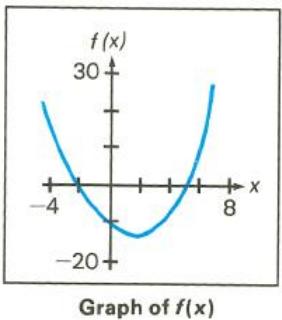
r

The convenience and power of the SOLVE key become more apparent when you solve an equation for a root that cannot be determined algebraically.

Example: Champion ridget hurler Chuck Fahr throws a ridget with an upward velocity of 50 meters/second. If the height of the ridget is expressed as

$$ h = 5 0 0 0 (1 - \mathrm {e} ^ {- t / 2 0}) - 2 0 0 t, $$

how long does it take for it to reach the ground again? In this equation, h is the height in meters and t is the time in seconds.

Solution: The desired solution is the positive value of t at which h = 0 .

Use the following subroutine to calculate the height.

Keystrokes	Display
g P/R	000-
f LBL A	001-42,21,11	Begin with label.
2	002- 2	Subroutine assumes t is loaded in X-and Y-registers.
0	003- 0
÷	004- 10

Keystrokes	Display
CHS	005-	16	-t/20.
ex	006-	12
CHS	007-	16	-e-t/20.
1	008-	1
+	009-	40	1-e-t/20.
5	010-	5
0	011-	0
0	012-	0
0	013-	0
×	014-	20	5000 (1-e-t/20).
x$y	015-	34	Brings another t-value into X-register.
2	016-	2
0	017-	0
0	018-	0
×	019-	20	200t.
-	020-	30	5000(1-e-t/20)-200t.
g RTN	021-	43 32

Switch to Run mode, key in two initial estimates of the time (for example, 5 and 6 seconds) and execute [SOLVE].

Keystrokes	Display
9 P/R		Run mode.
5 ENTER	5.0000	Initial estimates.
6	6
f SOLVE A	9.2843	The desired root.

Verify the root by reviewing the Y- and Z-registers.

Keystrokes	Display
R↓	9.2843	A previous estimate of the root.
R↓	0.0000	Value of the function at the root showing that h = 0.

Fahr's ridget falls to the ground 9.2843 seconds after he hurls it—a remarkable toss.

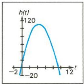
Graph of h versus t

When No Root Is Found

You have seen how the SOLVE key estimates and displays a root of an equation of the form f(x) = 0 . However, it is possible that an equation has no real roots (that is, there is no real value of x for which the equality is true). Of course, you would not expect the calculator to find a root in this case. Instead, it displays Error 8.

Example: Consider the equation

$$ \left| x \right| = - 1. $$

which has no solution since the absolute value function is never negative. Express this equation in the required form

$$ | x | + 1 = 0 $$

and attempt to use SOLVE to find a solution.

Graph of f(x) = |x| + 1
G

Keystrokes

P/R

f LBL 1

9 ABS

1

+

9 RTN

Display

000-

001-42,21，1

002- 4316

003- 1

004- 40

005- 4332

Program mode.

Because the absolute-value function is minimum near an argument of zero, specify the initial estimates in that region, for instance 1 and -1. Then attempt to find a root.

Keystrokes	Display
g P/R		Run mode.
1 ENTER	1.0000
1 CHS	-1	Initial estimates.
f SOLVE 1	Error 8	This display indicates that no root was found.
←	0.0000	Clear error display.

As you can see, the HP-15C stopped seeking a root of f(x) = 0 when it decided that none existed – at least not in the general range of x to which it was initially directed. The Error 8 display does not indicate that an "illegal" operation has been attempted; it merely states that no root was found where SOLVE presumed one might exist (based on your initial estimates).

If the HP-15C stops seeking a root and displays an error message, one of these three types of conditions has occurred:

• If repeated iterations all produce a constant nonzero value for the specified function, execution stops with the display Error 8.
  If numerous samples indicate that the magnitude of the function appears to have a nonzero minimum value in the area being searched, execution stops with the display Error 8.
• If an improper argument is used in a mathematical operation as part of your subroutine, execution stops with the display Error 0.

In the case of a constant function value, the routine can see no indication of a tendency for the value to move toward zero. This can occur for a function whose first 10 significant digits are constant (such as when its graph levels off at a nonzero horizontal asymptote) or for a function with a relatively broad, local "flat" region in comparison to the range of x -values being tried.

In the case where the function's magnitude reaches a nonzero minimum, the routine has logically pursued a sequence of samples for which the magnitude has been getting smaller. However, it has not found a value of x at which the function's graph touches or crosses the x -axis.

The final case points out a potential deficiency in the subroutine rather than a limitation of the root-finding routine. Improper operations may sometimes be avoided by specifying initial estimates that focus the search in a region where such an outcome will not occur. However, the SOLVE routine is very aggressive and may sample the function over a wide range. It is a good practice to have your subroutine test or adjust potentially improper arguments prior to performing an operation (for instance, use ABS prior to ). Rescaling variables to avoid large numbers can also be helpful.

The success of the SOLVE routine in locating a root depends primarily upon the nature of the function it is analyzing and the initial estimates at which it begins searching. The mere existence of a root does not ensure that the casual use of the SOLVE key will find it. If the function f(x) has a nonzero horizontal asymptote or a local minimum of its magnitude, the routine can be expected to find a root of f(x) = 0 only if the initial estimates do not concentrate the search in one of these unproductive regions—and, of course, if a root actually exists.

Choosing Initial Estimates

When you use SOLVE to find the root of an equation, the two initial estimates that you provide determine the values of the variable x at which the routine begins its search. In general, the likelihood that you will find the particular root you are seeking increases with the level of understanding that you have about the function you are analyzing. Realistic, intelligent estimates greatly facilitate the determination of a root.

The initial estimates that you use may be chosen in a number of ways:

If the variable x has a limited range in which it is conceptually meaningful as a solution, it is reasonable to choose initial estimates within this range. Frequently an equation that is applicable to a real problem has, in addition to the desired solution, other roots that are physically meaningless. These usually occur because the equation being analyzed is appropriate only between certain limits of the variable. You should recognize this restriction and interpret the results accordingly.

If you have some knowledge of the behavior of the function f(x) as it varies with different values of x , you are in a position to specify initial estimates in the general vicinity of a zero of the function. You can also avoid the more troublesome ranges of x such as those producing a relatively constant function value or a minimum of the function's magnitude.

Example: Using a rectangular piece of sheet metal 4 decimeters by 8 decimeters, an open-top box having a volume of 7.5 cubic decimeters is to be formed. How should the metal be folded? (A taller box is preferred to a shorter one.)

Solution: You need to find the height of the box (that is, the amount to be folded up along each of the four sides) that gives the specified volume. If x is the height (or amount folded up), the

length of the box is (8 - 2x) and the width is (4 - 2x) . The volume V is given by

$$ V = (8 - 2 x) (4 - 2 x) x. $$

By expanding the expression and then using Horner's method (page 79), this equation can be rewritten as

$$ V = 4 \left((x - 6) x + 8\right) x. $$

To get V = 7.5 , find the values of x for which

$$ f (x) = 4 \left((x - 6) x + 8\right) x - 7. 5 = 0. $$

The following subroutine calculates f(x) :

Keystrokes

g P/R

f LBL 3

6

Display
000-	Program mode.
001-42,21,3	Label.
002-6	Assumes stack loaded with x.

Keystrokes	Display
-	003-	30
×	004-	20	(x-6)x.
8	005-	8
+	005-	40
×	007-	20	((x-6)x+8)x.
4	008-	4
×	009-	20	4((x-6)x+8)x.
7	010-	7
·	011-	48
5	012-	5
-	013-	30
g RTN	014-	43 32

It seems reasonable that either a tall, narrow box or a short, flat box could be formed having the desired volume. Because the taller box is preferred, larger initial estimates of the height are reasonable. However, heights greater than 2 decimeters are not physically possible (because the metal is only 4 decimeters wide). Initial estimates of 1 and 2 decimeters are therefore appropriate.

Find the desired height:

Keystrokes	Display
g P/R		Run mode.
1 ENTER	1.0000	Initial estimates.
2	2
f SOLVE 3	1.5000	The desired height.
R↓	1.5000	Previous estimate.
R↓	0.0000	f(x) at root.

By making the height 1.5 decimeters, a 5.0 × 1.0 × 1.5 -decimeter box is specified.

If you ignore the upper limit on the height and use initial estimates of 3 and 4 decimeters (still less than the width), you will obtain a height of 4.2026 decimeters - a root that is physically meaningless. If you use small initial estimates such as 0 and 1 decimeter, you will obtain a height of 0.2974 decimeter - producing an undesirably short, flat box.

As an aid for examining the behavior of a function, you can easily evaluate the function at one or more values of x using your subroutine in program memory. To do this, fill the stack with x . Execute the subroutine to calculate the value of the function (press f letter label or GSB label.

The values you calculate can be plotted to give you a graph of the function. This procedure is particularly useful for a function whose behavior you do not know. A simple-looking function may have a graph with relatively extreme variations that you might not anticipate. A root that occurs near a localized variation may be hard to find unless you specify initial estimates that are close to the root.

If you have no informed or intuitive concept of the nature of the function or the location of the zero you are seeking, you can search for a solution using trial-and-error. The success of finding a solution depends partially upon the function itself. Trial-and-error is often – but not always – successful.

• If you specify two moderately large positive or negative estimates and the function's graph does not have a horizontal asymptote, the routine will seek a zero which might be the most positive or negative (unless the function oscillates many times, as the trigonometric functions do).

• If you have already found a zero of the function, you can check for another solution by specifying estimates that are relatively distant from any known zeros.

• Many functions exhibit special behavior when their arguments approach zero. You can check your function to determine values of x for which any argument within your function becomes zero, and then specify estimates at or near those values.

Although two different initial estimates are usually supplied when using SOLVE, you can also use SOLVE with the same estimate in both the X- and Y-registers. If the two estimates are identical, a second estimate is generated internally. If your single estimate is nonzero, the second estimate differs from your estimate by one count in the seventh significant digit. If your estimate is zero, 1 × 10^-7 is used as the second estimate. Then the root-finding procedure continues as it normally would with two estimates.

Using SOLVE in a Program

You can use the SOLVE operation as part of a program. Be sure that the program provides initial estimates in the X- and Y-registers just prior to the SOLVE operation. The SOLVE routine stops with a value of x in the X-register and the corresponding function value in the Z-register. If the x -value is a root, the program proceeds to the next line. If the x -value is not a root, the next line is skipped. (Refer also to Interpreting Results on page 226 for a further explanation of roots.) Essentially, the SOLVE instruction tests whether the x -value is a root and then proceeds according to the "Do if True" rule. The program can then handle the case of not finding a root, such as by choosing new initial estimates or changing a function parameter.

The use of as an instruction in a program utilizes one of the seven pending returns in the calculator. Since the subroutine called by utilizes another return, there can be only five other pending returns. Executed from the keyboard, on the other hand, itself does not utilize one of the pending returns, so that six pending returns are available for subroutines within the subroutine called by . Remember that if all seven pending returns have been utilized, a call to another subroutine will result in a display of Error 5. (Refer to page 105.)

Restriction on the Use of SOLVE

The one restriction regarding the use of is that cannot be used recursively. That is, you cannot use in a subroutine that is called during the execution of . If this situation occurs, execution stops and Error 7 is displayed. It is possible, however, to use with _y^xy thereby using the advanced capabilities of both of these keys.

Memory Requirements

SOLVE requires five registers to operate. (Appendix C explains how they are automatically allocated from memory.) If five unoccupied registers are not available, SOLVE will not run and Error 10 will be displayed.

A routine that combines and _y^xv requires 23 registers of space.

For Further Information

In appendix D, Advanced Use of , additional techniques and explanations for using are presented. These include:

• How SOLVE works.
  Accuracy of the root.
• Interpreting results.
• Finding several roots.
• Limiting estimation time.

Section 14

Numerical Integration

Many problems in mathematics, science, and engineering require calculating the definite integral of a function. If the function is denoted by f(x) and the interval of integration is a to b , the integral can be expressed mathematically as

$$ I = \int_ {a} ^ {b} f (x) d x. $$

The quantity I can be interpreted

geometrically as the area of a region bounded by the graph of f(x) , the x -axis, and the limits x = a and x = b .

When an integral is difficult or impossible to evaluate by analytical methods, it can be calculated using numerical techniques. Usually, this can be done only with a fairly complicated computer program. With your HP-15C, however, you can easily do numerical integration using the _y^x (integrate) key.

Using _y^x

The basic rules for using _y^x are:

1. In Program mode, key in a subroutine that evaluates the function f(x) that you want to integrate. This subroutine must begin with a label instruction (fLBL label) and end up with a value for f(x) in the X-register.

In Run mode:

1. Key the lower limit of integration (a) into the X-register, then press ENTER to lift it into the Y-register.
2. Key the upper limit of integration (b) in to the X-register.
3. Press followed by the label of your subroutine.

Example: Certain problems in physics and engineering require calculating Bessel functions. The Bessel function of the first kind of order 0 can be expressed as

$$ J _ {0} (x) = \frac {1}{\pi} \int_ {0} ^ {\pi} \cos (x \sin \theta) d \theta . $$

Find

$$ J _ {0} (1) = \frac {1}{\pi} \int_ {0} ^ {\pi} \cos (\sin \theta) d \theta . $$

In Program mode, key in the following subroutine to evaluate the function f() = ( ) .

Keystrokes

g P/R

f CLEAR PRGM

f LBL0

Display

000-

000-

001-42,21，0

Program mode.

Clear program memory.

Begin subroutine with a LBL instruction.

Subroutine assumes a value of is in X-register.

SIN

COS

RTN

002- 23

003- 24

004- 4332

Calculate

Calculate ( )

Now, in Run mode key the lower limit of integration into the Y-register and the upper limit into the X-register. For this particular problem, you also need to specify Radians mode for the trigonometric functions.

Keystrokes	Display
9 P/R		Run mode.
0 ENTER	0.0000	Key lower limit, 0, into Y-register.
9 π	3.1416	Key upper limit, π, into X-register.
9 RAD	3.1416	Specify Radians mode for trigonometric functions.

Now you are ready to press /y^x0 to calculate the integral. When you do so, you'll find that - just as with - the calculator will not display the result right away, as it does with other operations. The HP-15C calculates integrals using a sophisticated iterative algorithm. Briefly, this algorithm evaluates f(x) , the function to be integrated, at many values of x between the limits of integration. At each of these values, the calculator evaluates the function by executing the subroutine you write for that purpose. When the calculator must execute the subroutine many times - as it does when you press /y^x - you can't expect any answer right away. Most integrals will require on the order of 2 to 10 seconds; but some integrals will require even more. Later on we'll discuss how you can decrease the time somewhat; but for now press /_y^x0 and take a break (or read ahead) while the HP-15C takes care of the drudgery for you.

Keystrokes

2.4040
[ = \int_{0}^{\pi}\cos (\sin \theta)\mathrm{d}\theta . ]

Display

In general, don't forget to multiply the value of the integral by whatever constants, if any, are outside the integral. In this particular problem, we need to multiply the integral by 1 / to get J_0(1) :

Keystrokes

3.1416
0.7652
J_0 (1).

Display

Before calling the subroutine you provide to evaluate f(x) , the _y^x algorithm – just like the SOLVE algorithm – places the value of x in the X-, Y-, Z-, and T-registers. Because every stack register contains the x -value, your subroutine can calculate with this number without having to recall it from a storage register. The subroutines in the next two examples take advantage of this feature. (A polynomial evaluation technique that assumes the stack is filled with the value of x is discussed on page 79.)

Note: Since the calculator puts the value of x into all stack registers, any numbers previously there will be replaced by x . Therefore, if the stack contains intermediate results that you'll need after you calculate an integral, store those numbers in storage registers and recall them later.

Occasionally you may want to use the subroutine that you wrote for the _y^x operation to merely evaluate the function at some value of x . If you do so with a function that gets x from the stack more than once, be sure to fill the stack manually with the value of x , by pressing ENTER ENTER ENTER before you execute the subroutine.

Example: The Bessel function of the first kind of order 1 can be expressed as

$$ J _ {1} (x) = \frac {1}{\pi} \int_ {0} ^ {\pi} \cos (\theta - x \sin \theta) d \theta . $$

Find

$$ J _ {1} (I) = \frac {1}{\pi} \int_ {0} ^ {\pi} \cos (\theta - \sin \theta) d \theta . $$

Key in the following subroutine that evaluates the function f() = ( - ) .

Keystrokes

P/R

f LBL1

Display

000- Program mode.

001-42,21， 1 Begin subroutine with a label.

Keystrokes	Display
SIN	002-	23	Calculate sin θ.
-	003-	30	Since a value of θ will be placed into the Y-register by the fY algorithm before it executes this subroutine, the - operation at this point will calculate (θ - sin θ).
COS	004-	24	Calculate cos (θ - sin θ).
9 RTN	005-	43	32

In Run mode, key the limits of integration into the X- and Y-registers. Be sure that the trigonometric mode is set to Radians, then press /y^x 1 to calculate the integral. Finally, multiply the integral by 1 / to calculate J1 (1).

Keystrokes	Display
9 P/R0 ENTER	0.0000	Run mode.Key lower limit into Y-register.
9 π	3.1416	Key upper limit into X-register.
9 RAD	3.1416	(If not already in Radians mode.)
f f y x 1	1.3825	= ∫0πcos (θ - sin θ) dθ.
9 π ÷	0.4401	J1(1).

Example: Certain problems in communications theory (for example, pulse transmission through idealized networks) require calculating an integral (sometimes called the sine integral) of the form

$$ S i (t) = \int_ {0} ^ {t} \frac {\sin (x)}{x} d x. $$

Find Si(2)

Key in the following subroutine to evaluate the function f(x) = ( x) / x .

Keystrokes	Display
g P/R	000-		Program mode.
f LBL .2	001-42,21, .2		Begin subroutine with a LBL instruction.
SIN	002-	23	Calculate sin x.
x y	003-	34	Since a value of x will be placed in the Y-register by the f y' algorithm before it executes this subroutine, the x y operation at this point will return x to the X-register and move sin x to the Y-register.
÷	004-	10	Divide sin x by x.
g RTN	005-	43 32

Now key the limits of integration into the X- and Y-registers. In Radians mode, press _y^x .2 to calculate the integral.

Keystrokes	Display
9 P/R	0.4401	Run mode.
0 ENTER	0.0000	Key lower limit into Y-register.
2	2	Key upper limit, into X-register.
9 RAD	2.0000	(If not already in Radians mode.)
f f_y^x .2	1.6054	Si(2).

Accuracy of _y^x

The accuracy of the integral of any function depends on the accuracy of the function itself. Therefore, the accuracy of an integral calculated using _y^x is limited by the accuracy of the function calculated by your subroutine. To specify the accuracy of the function, set the display format so that the display shows no more than the number of digits that you consider accurate in the function's values. If you specify fewer digits, the calculator will compute the integral more quickly; but it will presume that the function is accurate to only the number of digits specified in the display format. We'll show you how you can determine the accuracy of the calculated integral after we say another word about the display format.

You'll recall that the HP-15C provides three types of display formatting: FIX, SCI, and ENG. Which display format should be used is largely a matter of convenience, since for many integrals you'll get about the same results using any of them (provided that the number of digits is specified correctly, considering the magnitude of the function). Because it's more convenient to use SCI display format when calculating most integrals, we'll use SCI when calculating integrals in subsequent examples.

Note: Remember that once you have set the display format, you can change the number of digits appearing in the display by storing a number in the Index register and then pressing f FIx I, f SCI I, or f ENG I, as described in section 10. This capability is especially useful when _y^xy is executed as part of a program.

Because the accuracy of any integral is limited by the accuracy of the function (as indicated in the display format), the calculator cannot compute the value of an integral exactly, but rather only approximates it. The HP-15C places the uncertainty* of an integral's approximation in the Y-register at the same time it places the approximation in the X-register. To determine the accuracy of an approximation, check its uncertainty by pressing ≤ y .

Example: With the display format set to 2, calculate the integral in the expression for J_1(I) (from the example on page 197).

Keystrokes	Display
0 ENTER	0.0000		Key lower limit into Y-register.
g π	3.1416		Key upper limit into X-register.
g RAD	3.1416		(If not already in Radians mode.)
f SCI 2	3.14	00	Set display format to SCI 2.
f f y 1	1.3	00	Integral approximated in SCI 2.
	8
x $ y	1.8	-	Uncertainty of SCI 2
	8	03	approximation.

The integral is 1.38 ± 0.00188 . Since the uncertainty would not affect the approximation until its third decimal place, you can consider all the displayed digits in this approximation to be accurate. In general, though, it is difficult to anticipate how many digits in an approximation will be unaffected by its uncertainty. This depends on the particular function being integrated, the limits of integration, and the display format.

If the uncertainty of an approximation is larger than what you choose to tolerate, you can decrease it by specifying a greater number of digits in the display format and repeating the approximation.

Whenever you want to repeat an approximation, you don't need to key the limits of integration back into the X- and Y-registers. After an integral is calculated, not only are the approximation and its uncertainty placed in the X- and Y-registers, but in addition the upper limit of integration is placed in the Z-register, and the lower limit is placed in the T-register. To return the limits to the X- and Y-registers for calculating an integral again, simply press R↓ R↓.

Example: For the integral in the expression for J_I(1) , you want an answer accurate to four decimal places instead of only two.

Keystrokes

f SCl 4

R R

f 1

x≤y

Display

1.8826

3.1416

1.3825

1.7091

-03 Set display format to 4.

00 Roll down stack until upper limit appears in X-register.

00 Integral approximated in [SCI]4.

-05 Uncertainty of 4 approximation.

The uncertainty indicates that this approximation is accurate to at least four decimal places. Note that the uncertainty of the 4 approximation is about one-hundredth as large as the uncertainty of the 2 approximation. In general, the uncertainty of any _y^xy approximation decreases by about a factor of 10 for each additional digit specified in the display format.

In the preceding example, the uncertainty indicated that the approximation might be correct to only four decimal places. If we temporarily display all 10 digits of the approximation, however, and compare it to the actual value of the integral (actually, an approximation known to be accurate to a sufficient number of decimal places), we find that the approximation is actually more accurate than its uncertainty indicates.

Keystrokes

x≤y

f CLEAR Prefix

Display

1.382

00

Return approximation to display.

5

1382459676

All 10 digits of approximation.

The value of this integral, correct to eight decimal places, is 1.38245969. The calculator's approximation is accurate to seven decimal places rather than only four. In fact, since the uncertainty of an approximation is calculated very conservatively, the calculator's approximation, in most cases will be more accurate than its uncertainty indicates. However, normally there is no way to determine just how accurate an approximation is.

For a more detailed look at the accuracy and uncertainty of _y^x approximations, refer to appendix E.

Using _y^x in a Program

_y^x can appear as an instruction in a program provided that the program is not called (as a subroutine) by _y^x itself. In other words, _y^x cannot be used recursively. Consequently, you cannot use _y^x to calculate multiple integrals; if you attempt to do so, the calculator will halt with Error 7 in the display. However, _y^x can appear as an instruction in a subroutine called by .

The use of _y^x as an instruction in a program utilizes one of the seven pending returns in the calculator. Since the subroutine called by _y^x utilizes another return, there can be only five other pending returns. Executed from the keyboard, on the other hand, _y^x itself does not utilize one of the pending returns, so that six pending returns are available for subroutines within the subroutine called by _y^x . Remember that if all seven pending returns have been utilized, a call to another subroutine will result in a display of Error 5. (Refer to page 105.)

Memory Requirements

_y^x requires 23 registers to operate. (Appendix C explains how they are automatically allocated from memory.) If 23 unoccupied registers are not available, _y^x will not run and Error 10 will be displayed.

A routine that combines [f_y^x] and also requires 23 registers of space.

For Further Information

This section has given you the information you need to use _y^x with confidence over a wide range of applications. In appendix E, more esoteric aspects of _y^x are discussed. These include:

• How _y^x works.
  Accuracy, uncertainty, and calculation time.
• Uncertainty and the display format.
• Conditions that could cause incorrect results.
• Conditions that prolong calculation time.
• Obtaining the current approximation to an integral.

Appendix A

Error Conditions

If you attempt a calculation containing an improper operation – say division by zero – the display will show Error and a number. To clear an error message, press any one key. This also restores the display prior to the Error display.

The HP-15C has the following error messages. (The description of Error 2 includes a list of statistical formulas used.)

Error 0: Improper Mathematics Operation

Illegal argument to math routine:

, where x = 0 .
^x , where:

out of Complex mode, y < 0 and x is noninteger;
out of Complex mode, y = 0 and x ≤ 0 ; or
- in Complex mode, y = 0 and Re(x) ≤ 0 .

, where, out of Complex mode, x < 0
[3]x , where x = 0
LOG, where:

out of Complex mode, x≤ 0 or
- in Complex mode, x = 0 .

LN, where:

out of Complex mode, x≤ 0 or
- in Complex mode, x = 0 .

^-1 , where, out of Complex mode, |x| > 1
, where, out of Complex mode, |x| > 1
STO , where x = 0
RCL , where the contents of the addressed register = 0
% , where the value in the Y-register is 0.
HYP-COS, where, out of Complex mode, x < 1
HYP TAN, where, out of Complex mode, |x| > 1
,x ,x , where:

• x or y is noninteger;
• x < 0 or y < 0 ;
• x > y
  x or y≥ 10^10

Error 1: Improper Matrix Operation

Applying an operation other than a matrix operation to a matrix, that is, attempting a nonmatrix operation while a matrix is in the relevant register (whether the X- or Y-register or a storage register).

Error 2: Improper Statistics Operation

n = 0
s n≤1
±by,r （20 n≤ 1
L.R. n≤ 1

Error 2 is also displayed if division by zero or the square root of a negative number would be required during computation with any of the following formulas:

$$ \bar {x} = \frac {\sum x}{n} \quad \bar {y} = \frac {\sum y}{n} $$

$$ s _ {x} = \sqrt {\frac {M}{n (n - 1)}} \quad s _ {y} = \sqrt {\frac {N}{n (n - 1)}} \quad r = \frac {P}{\sqrt {M \cdot N}} $$

$$ A = \frac {P}{M} \quad B = \frac {M \sum y - P \sum x}{n \cdot M} $$

$$ \hat {y} = \frac {M \sum y + P (n \cdot x - \sum x)}{n \cdot M} $$

where:

$$ M = n \Sigma x ^ {2} - (\Sigma x) ^ {2} $$

$$ N = n \Sigma \mathrm {y} ^ {2} - (\Sigma \mathrm {y}) ^ {2} $$

$$ P = n \Sigma x y - \Sigma x \Sigma y $$

(A and B are the values returned by the operation .R. , where y = Ax + B. )

Error 3: Improper Register Number or Matrix Element

Storage register named is nonexistent or matrix element indicated is nonexistent.

Error 4: Improper Line Number or Label Call

Line number called for is currently unoccupied or nonexistent (>448); or you have attempted to load a program line without available space; or the label called does not exist; or User mode is on and you did not press f before , e^x , 10^x , y^x or [1]x .

Error 5: Subroutine Level Too Deep

Subroutine nested more than seven deep.

Error 6: Improper Flag Number

Attempted a flag number >9

Error 7: Recursive SOLVE or ^xy

A subroutine which is called by also contains a instruction; a subroutine which is called by _y^x also contains an _y^x instruction.

Error 8: No Root

SOLVE unable to find a root using given estimates.

Error 9: Service

Self-test discovered circuitry problem, or wrong key pressed during key test.

Error 10: Insufficient Memory

There is not enough memory available to perform a given operation.

Error 11: Improper Matrix Argument

Inconsistent or improper matrix arguments for a given matrix operation:

• or -, where the dimensions are incompatible.

× , where:

the dimensions are incompatible; or
the result is one of the arguments.

1 / x , where the matrix is not square.

scalar/matrix , where the matrix is not square.

, where:

the matrix in the X-register is not square;
the dimensions are incompatible; or
- the result is the matrix in the X-register.

MATRIX 2, where the input is a scalar; or the number of rows is odd.
MATRIX 3, where the input is a scalar; or the number of columns is odd.
MATRIX 4, where the input is scalar.
MATRIX 5, where:

the input is a scalar;
- the dimensions are incompatible; or
- the result is one of the arguments.

MATRIX 6, where:

the input is scalar;
- the dimensions are incompatible (including the result); or
the result is one of the arguments.

MATRIX 9, where the matrix is not square.

RCL DIM I, where contents of _I are scalar.

DIM I, where contents of R_I are scalar.

STO RESULT, where the input is scalar.

. , where the number of columns is odd.

,x , where the number of rows is odd.

Pr Error (Power Error)

Continuous Memory interrupted and reset because of power failure.

Appendix B

Stack Lift and

the LAST X Register

The HP-15C calculator has been designed to operate in a natural manner. As you have seen working through this handbook, most calculations do not require you to think about the operation of the automatic memory stack.

There are occasions, however - especially as you delve into programming - when you need to know the effect of a particular operation upon the stack. The following explanation should help you.

Digit Entry Termination

Most operations on the calculator, whether executed as instructions in a program or pressed from the keyboard, terminate digit entry. This means that the calculator knows that any digits you key in after any of these operations are part of a new number.

The only operations that do not terminate digit entry are the digit entry keys themselves:

Stack Lift

There are three types of operations on the calculator based on how they affect stack lift. These are stack-disabling operations, stack-enabling operations, and neutral operations.

When the calculator is in Complex mode, each operation affects both the real and imaginary stacks. The stack lift effects are the same. In addition, the number keyed into the display (real X-register) after any operation except or is accompanied by the placement of a zero in the imaginary X-register.

Disabling Operations

Stack Lift. There are four stack-disabling operations on the calculator.* These operations disable the stack lift, so that a number keyed in after one of these disabling operations writes over the current number in the displayed X-register and the stack does not lift. These special disabling operations are:

$$ \begin{array}{c c c c} \text {E N T E R} & \text {C L x} & \sum + & \sum - \end{array} $$

Imaginary X-Register. A zero is placed in the imaginary X-register when the next number following , + , or - is keyed or recalled into the display (real X-register). However, the next number keyed in or recalled after or does not change the contents of the imaginary X-register.

Enabling Operations

Stack Lift. Most of the operations on the keyboard, including one-and two-number mathematical functions like ^2 and × , are stack-enabling operations. This means that a number keyed in after one of these operations will lift the stack (because the stack has been "enabled" to lift). Both the real and imaginary stacks are affected. (Recall that a shaded X-register means that its contents will be written over when the next number is keyed in or recalled.)

Imaginary X-Register. All enabling functions provide for a zero to be placed in the imaginary X-register when the next number is keyed or recalled into the display.

Neutral Operations

Stack Lift. Some operations, like , are neutral; that is, they do not alter the previous status of the stack lift. Thus, if you disable the stack lift by pressing , then press n and key in a new number, that number will write over the number in the X-register and the stack will not lift. Similarly, if you have previously enabled the stack lift by executing, say , then execute a instruction followed by a digit entry sequence, the stack will lift.

The following operations are neutral on the HP-15C:

Imaginary X-Register. The above operations are also neutral with respect to clearing the imaginary X-register.

LAST X Register

The following operations save x in the LAST X register:

Appendix C

Memory Allocation

The Memory Space

Storage registers, program lines, and advanced function execution * all draw on a common memory space in the HP-15C. The availability of memory for a specific purpose depends on the current allocation of memory, as well as on the total memory capacity of the calculator.

Registers

Memory space in the HP-15C is allocated on the basis of registers. This space is partitioned into two pools, which strictly define how a register may be used. There is always a combined total of 67 registers in these two pools.

• The data storage pool contains registers which may be used only for data storage. At power-up (Continuous Memory reset) this equals 21 registers. This pool contains at least three registers at all times: _1 , _0 , and _1 .
• The common pool contains uncommitted registers available for allocation to programming, matrices, the imaginary stack, and SOLVE and _y^x operation. At power-up there are 46 uncommitted registers in the common pool.

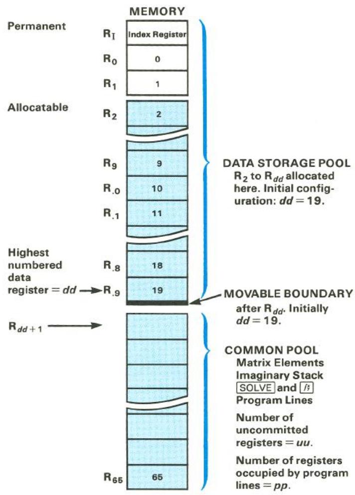
Total allocatable memory: 64 registers, numbered R2 through R65 . [(dd - 1) + uu + pp + (matrix~elements) + (imaginary~stack) + (SOLVE and _y^x)] = 64 . For memory allocation and indirect addressing, data registers R.0 through R.9 are referred to as R10 through R19 .

Memory Status (MEM)

To view the current memory configuration of the calculator, press 9 MEM (memory), holding MEM to retain the display. The display will be four numbers,

$$ d d \quad u u \quad p p - b $$

where:

dd = the number of the highest-numbered register in the data storage pool (making the total number of data registers dd + 2 because of R0 and I );

uu = the number of uncommitted registers in the common pool;

pp = the number of registers containing program instructions; and

b = the number of bytes left before uu is decremented (to supply seven more bytes of program memory) and pp is incremented.

The initial status of the HP-15C at power-up is:

19 46 0-0

The movable boundary between the data storage and common pools is always between Rdd and Rdd + 1 .

Memory Reallocation

There are 67 registers in memory, worth seven bytes each. Sixty-four of these registers (2 to 65 ) are interconvertible between the data storage and common pools.

The DIM (i) Function

If you should require more common space (as for programming) or more data storage space (but not both simultaneously!), you can make the necessary register reallocation using DIM (i) . The procedure is:

1. Place dd, the number of the highest data storage register you want allocated, into the display. 1 ≤ dd ≤ 65 . The number of registers in the uncommitted pool (and therefore potentially available for programming) will be (65 - dd) .
2. Press f DIM (i).

There are two ways to review your allocation:

• Press RCL DIM (i) to recall into the stack the number of the highest-allocated data storage register, dd. (Programmable.)
• Press 9 MEM (as explained above) to view a more complete memory status (dd uu pp-b).

Keystrokes

Display

(assuming a cleared program memory)*

1 f DIM (i)

1.0000

MEM (hold)

1 64 0-0

R1 _0 , and I

allocated for data storage. Sixty-four registers are uncommitted; none contain program instructions.

19 f DIM

19.0000

(i)

RCL DIM (i)

19.0000

R_19 (R.9) is the highest-numbered data storage register. Forty-six registers left in the common pool.

Restrictions on Reallocation

Continuous Memory will maintain the configuration you allocate until a new DIM (i) is executed or Continuous Memory is reset. If you try to allocate a number less than 1, dd = 1 . If you try to allocate a number greater than 65, Error 10 results.

When converting registers, note that:

• You can convert registers from the common pool only if they are uncommitted. If, for example, you try to convert registers which contain program instructions, you will get an Error 10 (insufficient memory).
• You can convert occupied registers from the data storage pool, causing a loss of stored data. An Error 3 results if you try to address a "lost" – that is, nonexistent – register. Therefore, it is good practice to store data in the lowest-numbered registers first, as these are the last to be converted.

Program Memory

As mentioned before, each register consists of seven bytes of memory. Program instructions use one or two bytes of memory. Most program lines use one byte; those using two bytes are listed on page 218.

The maximum programming capacity of the HP-15C is 448 program bytes (64 convertible registers at seven bytes per register). At power-up, memory can hold up to 322 program bytes (46 allocated registers at seven bytes per register).

Automatic Program Memory Reallocation

Within the common register pool, program memory will automatically expand as needed. One uncommitted register at a time, starting with the highest-numbered register available, will be allocated to seven bytes of program memory.

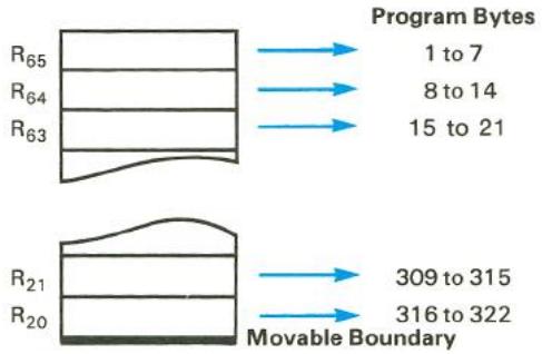
Conversion of Uncommitted Registers to Program Memory

Your very first program instruction will commit R65 (all seven bytes) from an uncommitted register to a program register. Your eighth program instruction commits R64 , and so on, until the boundary of the common pool is encountered. Registers from the data storage pool (at power-up, this is R_19 and below) are not available for program memory without reallocating registers using (i) .

Two-Byte Program Instructions

The following instructions are the only ones which require two bytes of calculator memory. (All others require only one byte.)

f LBL label
GTO label
9 CF (n or I)
(n or I)
G F? (n or I)
f FIX (n or I)
f SCl (n or I)
f ENG (n or I)

f SOLVE

f

f MATRIx{0 to 9}
f {2 to 9, .0 to .9}
f DSE {2 to 9, .0 to .9}
f ISG {2 to 9, .0 to .9}
STO +,-,,
RCL{+，-，X，÷}
STO MATRIX{A to E}
STO{A to E, (i) }in User
mode
RCL{A to E, (i) }in User
mode
STO g (i)
RCL g (i)

Memory Requirements for the Advanced Functions

The four advanced functions require temporary register space from the common register pool.

Function	Registers Needed
SOLVE /x y	5 23 if executed together
Complex Stack Matrices	5 1 per matrix element

For SOLVE and _y^x , allocation and deallocation of the required register space takes place automatically. * Memory is thereby allocated only for the duration of these operations.

Space for the imaginary stack is allocated whenever , , or 8 is pressed. The imaginary stack is deallocated when 8 is executed.

Space for matrix registers is not allocated until you dimension it (using DIM). Reallocation takes place when you redimension a matrix. MATRIX 0 dimensions all matrices to 0 × 0 .

Appendix D

A Detailed Look at SOLVE

Section 13, Finding the Roots of an Equation, includes the basic information needed for the effective use of the SOLVE algorithm. This appendix presents more advanced, supplemental considerations regarding SOLVE.

How SOLVE Works

You will be able to use SOLVE most effectively by having a basic understanding of how the algorithm works.

In the process of searching for a zero of the specified function, the algorithm uses the value of the function at two or three previous estimates to approximate the shape of the function's graph. The algorithm uses this shape to intelligently "predict" a new estimate where the graph might cross the x -axis. The function subroutine is then executed, computing the value of the

function at the new estimate. This procedure is performed repeatedly by the SOLVE algorithm.

If any two estimates yield function values with opposite signs, the algorithm presumes that the function's graph must cross the x -axis in at least one place in the interval between these estimates. The interval is systematically narrowed until a root of the equation is found.

A root is successfully found either if the computed function value is equal to zero or

if two estimates, differing by one unit in their last significant digit, give function values having opposite signs. In this case, execution stops and the estimate is displayed.

As discussed in section 13, page 186, the occurrence of other situations in the iteration process indicates the apparent absence of a function zero. The reason is that there is no way to logically predict a new estimate that is likely to have a function value closer to zero. In such cases, Error 8 is displayed.

You should note that the initial estimates you provide are used to begin the "prediction" process. By permitting more accurate predictions than might otherwise occur, properly chosen estimates greatly facilitate the determination of the root you seek.

The SOLVE algorithm will always find a root provided one exists (within the overflow bounds), if any one of four conditions are met:

• Any two estimates have function values with opposite signs.

• The function is monotonic, meaning that f(x) either always decreases or else always increases as x is increased.

• The function's graph is either convex everywhere or concave everywhere.

• The only local minima and maxima of the function's graph occur singly between adjacent zeros of the function.

In addition, it is assumed that the SOLVE algorithm will not be interrupted by an improper operation.

Accuracy of the Root

When you use the SOLVE key to find a root of an equation, the root is found accurately. The displayed root either gives a calculated function value (f(x)) exactly equal to zero or else is a 10-digit number virtually adjacent to the place where the function's graph crosses the x -axis. Any such root has an accuracy within two or three units in the 10th significant digit.

In most situations the calculated root is an accurate estimate of the theoretical (infinitely precise) root of the equation. However, certain conditions can cause the finite accuracy of the calculator to give a result that appears to be inconsistent with your theoretical expectation.

If a calculation has a result whose magnitude is smaller than 1.000000000 × 10^-99 , the result is set equal to zero. This effect is referred to as "underflow." If the subroutine that calculates your function encounters underflow for a range of x and if this affects the value of the function, then a root in this range may be expected to have some inaccuracy. For example, the equation

$$ x ^ {4} = 0 $$

has a root at x = 0 . Because of underflow, produces a root of 1.5060 -25 (for initial estimates of 1 and 2). As another example, consider the equation

$$ 1 / x ^ {2} = 0 $$

whose root is infinite in value. Because of underflow, gives a root of 3.1707 49 (for initial estimates of 10 and 20). In each of these examples, the algorithm has found a value of x for which the calculated function value equals zero. By understanding the effect of underflow, you can readily interpret results such as these.

The accuracy of a computed value sometimes can be adversely affected by "round-off" error, by which an infinitely precise number is rounded to 10 significant digits. If your subroutine requires extra precision to properly calculate the function for a range of x , the result obtained by SOLVE may be inaccurate. For example, the equation

$$ \mid x ^ {2} - 5 \mid = 0 $$

has a root at x = 5 . Because no 10-digit number exactly equals 5 , the result of using is Error 8 (for any initial estimates) because the function never equals zero nor changes sign. On the other hand, the equation

$$ [ (| x | + 1) + 1 0 ^ {1 5} ] ^ {2} = 1 0 ^ {3 0} $$

has no roots because the left side of the equation is always greater than the right side. However, because of round-off in the calculation of

$$ f (x) = \left[ \left(| x | + 1\right) + 1 0 ^ {1 5} \right] ^ {2} - 1 0 ^ {3 0}, $$

the root 1.0000 is found for initial estimates of 1 and 2. By recognizing situations in which round-off error may influence the operation of [SOLVE], you can evaluate the results accordingly and perhaps rewrite the function to reduce the effects of round-off.

In a variety of practical applications, the parameters in an equation – or perhaps the equation itself – are merely approximations. Physical parameters have an inherent accuracy (or inaccuracy). Mathematical representations of physical processes are only models of those processes, accurate only to the extent that the underlying assumptions are true. An awareness of these and other inaccuracies can be used to your advantage. By structuring your subroutine to return a function value of zero when the calculated value is negligible for practical purposes, you can usually save considerable time in finding a root with – particularly for cases that would normally take a long time.

Example: Ridget hurlers such as Chuck Fahr can throw a ridget to heights of 105 meters and more. In fact, Fahr's hurl usually reach a height of 107 meters. How long does it take for his remarkable toss, described on page 184 in section 13, to reach 107 meters?

Solution: The desired solution is the value of t at which h = 107 . Enter the subroutine from page 184 that calculates the height of the ridget. This subroutine can be used in a new function subroutine to calculate

$$ f (t) = h (t) - 1 0 7. $$

The following subroutine calculates f(t) :

Keystrokes	Display
g P/R	000-		Program mode.
f LBL B	001-42,21,12		Begin with new label.
GSB A	002-	32 11	Calculates h(t).
1	003-	1
0	004-	0
7	005-	7	Calculates h(t) - 107.
-	006-	30
g RTN	007-	43 32

In order to find the first time at which the height is 107 meters, use initial estimates of 0 and 1 second and execute SOLVE using B.

Keystrokes	Display
9 P/R		Run mode.
0 ENTER	0.0000	Initial estimates.
1	1
f SOLVE	4.1718	The desired root.
B
R↓	4.1718	A previous estimate of the root.
R↓	0.0000	Value of f(t) at root.

It takes 4.1718 seconds for the ridget to reach a height of exactly 107 meters. (It takes approximately two seconds to find this solution.)

However, suppose you assume that the function h(t) is accurate only to the nearest whole meter. You can now change your subroutine to give f(t) = 0 whenever the calculated magnitude of f(t) is less than 0.5 meter. Change your subroutine as follows:

Keystrokes	Display
9 P/R	000-		Program mode.
GTO CHS 006	006-	30	Line before RTN instruction.
9 ABS	007-	43 16	Magnitude of f(t).
•	008-	48	Accuracy
5	009-	5
9 TEST 7	010-43,30,7		Test for x > y and return zero if accuracy > magnitude (0.5 > |f(t)|).
9 CLx	011-	43 35
9 TEST 0	012-43,30,0		Test for x ≠ 0 and restore f(t) if value is nonzero.
9 LSTx	013-	43 36

Execute SOLVE again:

Keystrokes	Display
9 P/R		Run mode.
0 ENTER	0.0000
1	1	Initial estimates.
f ENTER B	4.0681	The desired root.
R↓	4.0681	A previous estimate of the root.
R↓	0.0000	Value of modified f(t) at root.

After 4.0681 seconds, the ridget is at a height of 107 ± 0.5 meters. This solution, although different from the previous answer, is correct considering the uncertainty of the height equation. (And this solution is found in just under half the time of the earlier solution.)

Interpreting Results

The numbers that places in the X-, Y-, and Z-registers help you evaluate the results of the search for a root of your equation. Even when no root is found, the results are still significant.

When SOLVE finds a root of the specified equation, the root and function values are placed in the X- and Z-registers. A function value of zero is the expected result. However, a nonzero function value is also acceptable because it indicates that the function's graph apparently crosses the x -axis within an infinitesimal distance from the calculated root. In most such cases, the function value will be relatively close to zero.

Special consideration is required for a different type of situation in which SOLVE finds a root with a nonzero function value. If your function's graph has a discontinuity that crosses the x -axis, SOLVE specifies as a root an x -value adjacent to the discontinuity. This is reasonable because a large change in the function value between two adjacent values of x might be the result of a very rapid, continuous transition. Because this cannot be resolved by the algorithm, the root is displayed for you to interpret.

A function may have a pole, where its magnitude approaches infinity. If the function value changes sign at a pole, the corresponding value of x looks like a possible root of your equation, just as it would for any other discontinuity crossing the x -axis. However, for such functions, the function value placed into the Z-register when that root is found will be relatively large. If the pole occurs at a value of x that is exactly represented with 10 digits, the

subroutine may try that value and halt prematurely with an error indication. In this case, the operation will not be completed. Of course, this may be avoided by the prudent use of a conditional statement in your subroutine.

Example: In her analysis of the stresses in a structural component, design consultant Lucy I. Beame has determined that the shear stress can be expressed as

$$ Q = \left{ \begin{array}{c l} 3 x ^ {3} - 4 5 x ^ {2} + 3 5 0 & \text {f o r} 0 < x < 1 0 \ 1 0 0 0 & \text {f o r} 1 0 \leq x < 1 4 \end{array} \right. $$

where Q is the shear stress in newtons per

square meter and x is the distance from one end in meters. Write a subroutine to compute the shear stress for any value of x . Use SOLVE to find the location of zero shear stress.

Solution: The equation for the shear stress for x between 0 and 10 is more efficiently programmed after rewriting it using Horner's method:

$$ Q = (3 x - 4 5) x ^ {2} + 3 5 0 \quad \text {f o r} 0 < x < 1 0. $$

Keystrokes	Display
g P/R	000-		Program mode.
f LBL 2	001-42,21,2
1	002-	1	Test for x range.
0	003-	0
g x≤y	004-	43 10
GTO 9	005-	22 9	Branch for x≥10.
g CLx	006-	43 35
3	007-	3
x	008-	20	3x.
4	009-	4
5	010-	5
-	011-	30	(3x-45).
x	012-	20
x	013-	20	(3x-45)x2.
3	014-	3
5	015-	5
0	016-	0
+	017-	40	(3x-45)x2+350.
g RTN	013-	43 32	End subroutine.
f LBL 9	019-42,21,9		Subroutine for x≥10.
EEX	020-	26
3	021-	3	10^3=1000.
g RTN	022-	43 32	End subroutine.

Execute SOLVE using initial estimates of 7 and 14 to start at the outer end of the beam and search for a point of zero shear stress.

Keystrokes

g P/R

7 ENTER

14

fSOLVE2

R↓ R

Display

7.0000

14

10.0000

1,000.0000

Run mode.

Initial estimates.

Possible root.

Stress not zero.

The large stress value at the root points out that the SOLVE routine has found a discontinuity. This is a place on the beam where the stress quickly changes from negative to positive. Start at the other end of the beam (estimates of 0 and 7) and use SOLVE again.

Keystrokes

0 ENTER

7

f SOLVE 2

R↓ R

Display

0.0000

7

3.1358

2.0000

-07

Initial estimates.

Possible root.

Negligible stress.

Beame's beam has zero shear stress at approximately 3.1358 meters and an abrupt change of stress at 10.0000 meters.

Graph of Q versus x .

When no root is found and Error 8 is displayed, you can press or any one key to clear the display and observe the estimate at which the function was closest to zero. By also reviewing the numbers in the Y- and Z-registers, you can often determine the nature of the function near the root estimate and use this information constructively.

If the algorithm terminates its search near a local minimum of the function's magnitude, clear the Error 8 display and observe the numbers in the X-, Y-, and Z-registers by rolling down the stack. If the value of the function saved in the Z-register is relatively close to zero, it is possible that a root of your equation has been found - the number returned in the X-register may be a 10-digit number very close to a theoretical root. You

can explore this potential minimum further by rolling the stack until the returned estimates are back in the X- and Y-registers and then executing SOLVE again using these numbers as initial estimates. If an actual minimum has been found, Error 8 will again be displayed and the number in the X-register will be approximately the same as before, but possibly closer to the actual location of the minimum.

Of course, you may deliberately use SOLVE to find the location of a local minimum of the function's magnitude. However, in this case you must be careful to confine the search in the region of the minimum. Remember, SOLVE tries hard to find a zero of the function.

If the algorithm stops searching and displays Error 8 because it is working on a horizontal asymptote (when the value of the function is essentially constant for a large range of x ), the estimates in X- and Y-registers usually are significantly different from each other. The number in the Z-register is the value of the potential asymptote. If you execute SOLVE again using as initial estimates the numbers that were returned in the X- and Y-registers, a

horizontal asymptote may again cause Error 8, but with numbers in the X- and Y-registers that will differ from the previous numbers. The value of the function in the Z-register would then be about the same as that obtained previously.

If Error 8 is displayed as a result of a search that is concentrated in a local "flat" region of the function, the estimates in the X- and Y-registers will be relatively close together or extremely small. Execute SOLVE again using for initial estimates the numbers from the X- and Y-registers (or perhaps two numbers somewhat further apart). If the magnitude of the function is neither a minimum nor constant, the algorithm will eventually expand its search and find a more significant result.

Example: Investigate the behavior of the function

$$ f (x) = 3 + e ^ {- | x | / 1 0} - 2 e ^ {x ^ {2} e ^ {- | x |}} $$

as evaluated in the following subroutine.

Keystrokes	Display
g P/R	000-		Program mode.
f LBL .0	001-42,21,.0
g ABS	002-	43 16
CHS	003-	16	e-|x|.
ex	004-	12
x y	005-	34	Bring x-value into X-register.
g x2	006-	43 11	x2e-|x|.
x	007-	20
ex	008-	12
2	009-	2
x	010-	20	-2ex2e-|x|.
CHS	011-	16
xy	012-	34	Bring x-value into X-register.
g ABS	013-	43 16
CHS	014-	16
1	015-	1
0	016-	0

Keystrokes	Display
÷	017-	10	-x/10.
e^x	018-	12
+	019-	40	e^-|x|/10 - 2e^x2e^-|x|.
3	020-	3
+	021-	40	3 + e^-|x|/10 - 2e^x2e^-|x|.
g RTN	022-	43 32

Use SOLVE with the following single initial estimates: 10, 1, and 10^-20 .

Keystrokes	Display
g P/R		Run mode.
10 ENTER	10.0000	Single estimate.
f SOLVE .0	Error 8
←	455.335	Best x-value.
R↓	48,026,721.85	Previous value.
R↓	1.0000	Function value.
g R↑ g R↑	455.4335	Restore the stack.
f SOLVE .0	Error 8
←	48,026,721.85	Another x-value
R↓ R↓	1.0000	Same function value (an asymptote).
1 ENTER	1.0000	Single estimate.
f SOLVE .0	Error 8
←	2.1213	Best x-value.
R↓	2.1471	Previous value.
R↓	0.3788	Function value.
g R↑ g R↑	2.1213	Restore the stack.
f SOLVE .0	Error 8
←	2.1213	Same x-value.
R↓ R↓	0.3788	Same function value (a minimum).
EEX | CHS 20	1.0000 -20	Single estimate.
ENTER

Keystrokes

f SOLVE.0

Display

Error 8

1.0000 -20

1.1250 -20

2.0000

1.0000 -20

Error 8

1.1250 -20

1.5626 -16

2.0000

Best x -value.

Previous value.

Function value.

Restore the stack.

Another x -value.

Previous value.

Same function value.

In each of the three cases, SOLVE initially searched for a root in a direction suggested by the graph around the initial estimate. Using 10 as the initial estimate, SOLVE found the horizontal asymptote (value of 1.0000). Using 1 as the initial estimate, a minimum of 0.3788 at x = 2.1213 was found. Using 10^-20 as the initial estimate, the function was essentially constant (at a value of 2.0000) for the small range of x that was sampled.

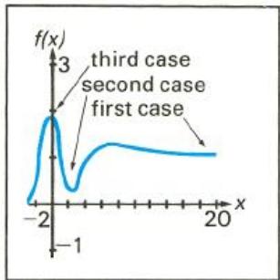
Finding Several Roots

Many equations that you encounter have more than one root. For this reason, you will find it helpful to understand some techniques for finding several roots of an equation.

The simplest method for finding several roots is to direct the root search in different ranges of x where roots may exist. Your initial estimates specify the range that is initially searched. This method was used for all examples in section 13. You can often find the roots of an equation in this manner.

Another method is known as deflation. Deflation is a method by which roots are "eliminated" from an equation. This involves modifying the equation so that the first roots found are no longer roots, but the rest of the roots remain roots.

If a function f(x) has a value of zero at x = a , then the new function f(x) / (x - a) will not approach zero in this region (if a is a simple root of f(x) = 0 ). You can use this information to eliminate a known root. Simply

add a few program lines at the end of your function subroutine. These lines should subtract the known root (to 10 significant digits) from the x -value and divide this difference into the function value. In many cases the root will be a simple one, and the new function will direct [SOLVE] away from the known root. On the other hand, the root may be a multiple root. A multiple root is one that appears to be present repeatedly, in the following sense: at such a root, not only does the graph of f(x) cross the x -axis, but its slope (and perhaps the next few higher-order derivatives) also equals zero. If the known root of your equation is a multiple root, the root is not eliminated by merely dividing by the factor described above. For example, the equation

$$ f (x) = x (x - a) ^ {3} = 0 $$

has a multiple root at x = a (with a multiplicity of 3). This root is not eliminated by dividing f(x) by (x - a) . But it can be eliminated by dividing by (x - a)^3 .

Example: Use deflation to help find the roots of

$$ 6 0 x ^ {4} - 9 4 4 x ^ {3} + 3 0 0 3 x ^ {2} + 6 1 7 1 x - 2 8 9 0 = 0. $$

Using Horner's method, this equation can be rewritten in the form

$$ \left(\left(6 0 x - 9 4 4\right) x + 3 0 0 3\right) x + 6 1 7 1) x - 2 8 9 0 = 0. $$

Program a subroutine that evaluates the polynomial.

Keystrokes	Display
9 P/R	000-	Program mode.
f CLEAR	000-
PRGM
f LBL2	001-42,21,2
6	002-	6
0	003-	0
×	004-	20
9	005-	9
4	006-	4
4	007-	4

Keystrokes

3

0

0

3

6

1

7

1

2

8

9

0

RTN

Display

008- 30

009- 20

010- 3

011- 0

012- 0

013- 3

014- 40

015- 20

016- 6

017- 1

018- 7

019- 1

020- 40

021- 20

022- 2

023- 8

024- 9

025- 0

026- 30

027- 4332

In Run mode, key in two large, negative initial estimates (such as -10 and -20) and use to find the most negative root.

Keystrokes

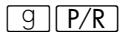
20 CHS

Display

-1.6667

-1.6667

4.0000 -06

Run mode.

Initial estimates.

First root.

Stores root for deflation.

Function value near zero.

Return to Program mode and add instructions to your subroutine to eliminate the root just found.

Keystrokes	Display
g P/R	000-		Program mode.
g BST g	026-	30	Line before RTN.
BST
x y	027-	34	Brings x into X-register.
RCL 0	028-	45 0	Divides by (x - a), where a is known root.
-	029-	30
÷	030-	10

Now use the same initial estimates to find the next root.

Keystrokes	Display
g P/R	4.0000 -06	Run mode.
10 CHS ENTER	-10.0000
20 CHS	-20	Same initial estimates.
f SOLVE 2	0.4000	Second root.
STO 1	0.4000	Stores root for deflation.
R↓ R↓	0.0000	Deflated function value.

Now modify your subroutine to eliminate the second root.

Keystrokes	Display
g P/R	000-			Program mode.
g BST g	030-		10	Line before RTN.
BST
x$ y	031-		34	Brings x into X-register.
RCL 1	032-	45	1
-	033-		30	Deflation for second root.
÷	034-		10

Again, use the same initial estimates to find the next root.

Keystrokes

P/R

10 [CHS] [ENTER]

20 CHS

f SOLVE 2

STO 2

R↓ R

Display

0.0000

-10.0000

-20

8.4999

8.4999

-1.0929 -07

Run mode.

Same initial estimates.

Third root.

Stores root for deflation.

Deflated function value near zero.

Now change your subroutine to eliminate the third root.

Keystrokes

g P/R

9 BST 9

BST

x≤y

RCL 2

中

Display

000-

034-

10

Program mode.

Line before RTN.

035-

036-

45 2

Brings x into X -register.

037-

038-

30

Deflation for third root.

Find the fourth root.

Keystrokes

G P/R

10 [CHS] [ENTER]

20 CHS

f SOLVE 2

STO 3

R↓ R↓

Display

-1.0929 -07

-10.0000

-20

8.5001

8.5001

-0.0009

Same initial estimates.

Fourth root.

Stores root for reference.

Deflated function value near zero.

Using the same initial estimates each time, you have found four roots for this equation involving a fourth-degree polynomial. However, the last two roots are quite close to each other and are actually one root (with a multiplicity of 2). That is why the root was not eliminated when you tried deflation once at this root. (Round-off error causes the original function to have small positive and negative values for values of x between 8.4999 and 8.5001; for x = 8.5 the function is exactly zero.)

Graph of f(x)

In general, you will not know in advance the multiplicity of the root you are trying to eliminate. If, after you have attempted to eliminate a root, finds that same root again, you can proceed in a number of ways:

• Use different initial estimates with the deflated function in an attempt to search for a different root.
• Use deflation again in an attempt to eliminate a multiple root. If you do not know the multiplicity of the root, you may need to repeat this a number of times.
• Examine the behavior of the deflated function at x -values near the known root. If the function's calculated values cross the x -axis smoothly, either another root or a greater multiplicity is indicated.
• Analyze the original function and its derivatives algebraically. It may be possible to determine its behavior for x -values near the known root. (A Taylor series representation, for example, may indicate the multiplicity of a root.)

Limiting the Estimation Time

Occasionally, you may desire to limit the time used by SOLVE to find a root. You can use two possible techniques to do this - counting iterations and specifying a tolerance.

Counting Iterations

While searching for a root, typically samples your function at least a dozen times. Occasionally, may need to sample it one hundred times or more. (However, will always stop by itself.) Because your function subroutine is executed once for each estimate that is tried, it can count and limit the number of iterations. An easy way to do this is with an instruction to accumulate the number of iterations in the Index register (or other storage register).

If you store an appropriate number in the register before using , your subroutine can interrupt the algorithm when the limit is exceeded.

Specifying a Tolerance

You can shorten the time required to find a root by specifying a tolerable inaccuracy for your function. Your subroutine should return a function value of zero if the calculated function value is less than the specified tolerance. This tolerance that you specify should correspond to a value that is negligible for practical purposes or should correspond to the accuracy of the computation. This technique eliminates the time required to define the estimate more accurately than is justify by the problem. The example on page 224 uses this method.)

For Advanced Information

In the HP-15C Advanced Functions Handbook, additional, advanced techniques and applications for using are presented. These topics include:

Using SOLVE with polynomials.
- Solving a system of equations.
- Finding local extremes of a function.
- Using SOLVE for financial problems.
- Using SOLVE in Complex mode.
- Solving an equation for its complex roots.

Appendix E

A Detailed Look at _y^x

Section 14, Numerical Integration, presented the basic information you need to use _y^x . This appendix discusses more intricate aspects of _y^x that are of interest if you use _y^x often.

How _y^x Works

The _y^x algorithm calculates the integral of a function f(x) by computing a weighted average of the function's values at many values of x (known as sample points) within the interval of integration. The accuracy of the result of any such sampling process depends on the number of sample points considered: generally, the more sample points, the greater the accuracy. If f(x) could be evaluated at an infinite number of sample points, the algorithm could - neglecting the limitation imposed by the inaccuracy in the calculated function f(x) - provide an exact answer.

Evaluating the function at an infinite number of sample points would take a very long time (namely, forever). However, this is not necessary, since the maximum accuracy of the calculated integral is limited by the accuracy of the calculated function values. Using only a finite number of sample points, the algorithm can calculate an integral that is as accurate as is justified considering the inherent uncertainty in f(x) .

The _y^x algorithm at first considers only a few sample points, yielding relatively inaccurate approximations. If these approximations are not yet as accurate as the accuracy of f(x) would permit, the algorithm is iterated (that is, repeated) with a larger number of sample points. These iterations continue, using about twice as many sample points each time, until the resulting approximation is as accurate as is justified considering the inherent uncertainty in f(x) .

The uncertainty of the final approximation is a number derived from the display format, which specifies the uncertainty for the function. At the end of each iteration, the algorithm compares the approximation calculated during that iteration with the approximations calculated during two previous iterations. If the difference between any of these three approximations and the other two is less than the uncertainty tolerable in the final approximation, the algorithm terminates, placing the current approximation in the X-register and its uncertainty in the Y-register.

It is extremely unlikely that the errors in each of three successive approximations – that is, the differences between the actual integral and the approximations – would all be larger than the disparity among the approximations themselves. Consequently, the error in the final approximation will be less than its uncertainty. ^ Although we can't know the error in the final approximation, the error is extremely unlikely to exceed the displayed uncertainty of the approximation. In other words, the uncertainty estimate in the Y-register is an almost certain “upper bound” on the difference between the approximation and the actual integral.

Accuracy, Uncertainty, and Calculation Time

The accuracy of an _y^x approximation does not always change when you increase by just one the number of digits specified in the display format, though the uncertainty will decrease. Similarly, the time required to calculate an integral sometimes changes when you change the display format, but sometimes does not.

Example: The Bessel function of the first kind, of order four, can be expressed as

$$ J _ {4} (x) = \frac {1}{\pi} \int_ {0} ^ {\pi} \cos (4 \theta - x \sin \theta) d \theta $$

Calculate the integral in the expression for J_4(1) ,

$$ \int_ {0} ^ {\pi} \cos (4 \theta - \sin \theta) d \theta $$

First, switch to Program mode and key in a subroutine that evaluates the function f() = (4 - ) .

Keystrokes	Display
g P/R	000-
f CLEAR PRGM	000-
f LBL 0	001-42,21,0
4	002-	4
×	003-	20
x$ y	004-	34
SIN	005-	23
-	006-	30
COS	007-	24
g RTN	008-	43 32

Now, switch to Run mode and key the limits of integration into the X- and Y-registers. Be sure the trigonometric mode is set to Radians, and set the display format to 2. Finally, press /y^x 0 to calculate the integral.

Keystrokes	Display		Run mode.
g P/R
0 ENTER	0.0000		Keys lower limit into Y-register.
g π	3.1416		Keys upper limit into X-register.
g RAD	3.1416		Sets the trigonometric mode to Radians.
f SCI 2	3.14	00	Sets display format to SCI 2.
f f y x 0	7.79	-03	Integral approximated in SCI 2.
x ≤ y	1.45	-03	Uncertainty of SCI 2 approximation.

The uncertainty indicates that the displayed digits of the approximation might not include any digits that could be considered accurate. Actually, this approximation is more accurate than its uncertainty indicates.

Keystrokes	Display
x$ y	7.79	-03	Return approximation to display.
f CLEAR Prefix	7785820888		All 10 digits of SCI approximation.
(hold)

The actual value of this integral, correct to five significant digits, is 7.7805 × 10^-3 . Therefore, the error in this approximation is about (7.7858 - 7.7805) × 10^-3 = 5.3 × 10^-6 . This error is considerably less than the uncertainty, 1.45 × 10^-3 . The uncertainty is only an upper bound on the error in the approximation; the actual error will generally be smaller.

Now calculate the integral in 3 and compare the accuracy of the resulting approximation to that of the 2 approximation.

Keystrokes	Display
f SCI 3	7.786	-03	Changes display format to SCI 3.
R↓ R↓	3.142	00	Rolls down stack until upper limit appears in X-register.
f f y 0	7.786	-03	Integral approximated in SCI 3
x y	1.448	-04	Uncertainty of SCI 3 approximation.
x y	7.786	-03	Returns approximation to display.
f CLEAR PRIX(hold)	7785820888		All 10 digits of SCI 3 approximation.

All 10 digits of the approximations in 2 and 3 are identical: the accuracy of the approximation in 3 is no better than the accuracy in 2 despite the fact that the uncertainty in 3 is less than the uncertainty in 2. Why is this? Remember that the accuracy of any approximation depends primarily on the number of sample points at which the function f(x) has been evaluated. The [f_y]x algorithm is iterated with increasing numbers of sample points until the disparity among three successive approximations is less than the uncertainty derived from the display format. After a particular iteration, the disparity among the approximations may already be so much less than the uncertainty that it would still be less if the uncertainty were decreased by a factor of 10. In such cases, if you decreased the uncertainty by specifying one more digit in the display format, the algorithm would not have to consider additional sample points, and the resulting approximation would be identical to the approximation calculated with the larger uncertainty.

If you calculated the two preceding approximations on your calculator, you may have noticed that it did not take any longer to calculate the integral in 3 than in 2. This is because the time to calculate the integral of a given function depends on the number of sample points at which the function must be evaluated to achieve an approximation of acceptable accuracy. For the 3 approximation, the algorithm did not have to consider more sample points than it did in 2, so it did not take any longer to calculate the integral.

Often, however, increasing the number of digits in the display format will require evaluating the function at additional sample points, so that calculating the integral will take more time. Now calculate the same integral in 4.

Keystrokes

f SCl 4

R↓ R↓

f 0

Display

7.7858

3.1416

7.7807

-03 SCl 4 display.

00 Rolls down stack until upper limit appears in X-register.

-03 Integral approximated in 4.

This approximation took about twice as long as the approximation in 3 or 2. In this case, the algorithm had to evaluate the function at about twice as many sample points as before in order to achieve an approximation of acceptable accuracy. Note, however, that you received a reward for your patience: the accuracy of this approximation is better, by almost two digits, than the accuracy of the approximation calculated using half the number of sample points.

The preceding examples show that repeating the approximation of an integral in a different display format sometimes will give you a more accurate answer, but sometimes it will not. Whether or not the accuracy is changed depends on the particular function, and generally can be determined only by trying it.

Furthermore, if you do get a more accurate answer, it will come at the cost of about double the calculation time. This unavoidable trade-off between accuracy and calculation time is important to keep in mind if you are considering decreasing the uncertainty in hopes of obtaining a more accurate answer.

The time required to calculate the integral of a given function depends not only on the number of digits specified in the display format, but also, to a certain extent on the limits of integration. When the calculation of an integral requires an excessive amount of time, the width of the interval of integration (that is, the difference of the limits) may be too large compared with certain features of the function being integrated. For most problems, however, you need not be concerned about the effects of the limits of integration on the calculation time. These conditions, as well as techniques for dealing with such situations, will be discussed later in this appendix.

Uncertainty and the Display Format

Because of round-off error, the subroutine you write for evaluating f(x) cannot calculate f(x) exactly, but rather calculates

$$ \hat {f} (x) = f (x) \pm \delta_ {1} (x), $$

where _1(x) is the uncertainty of f(x) caused by round-off error. If f(x) relates to a physical situation, then the function you would like to integrate is not f(x) but rather

$$ F (x) = f (x) \pm \delta_ {2} (x), $$

where _2(x) is the uncertainty associated with f(x) that is caused by the approximation to the actual physical situation.

Since f(x) = (x) ± _1(x) , the function you want to integrate is

$$ F (x) = \hat {f} (x) \pm \delta_ {1} (x) \pm \delta_ {2} (x) $$

or F(x) = (x)± (x),

where (x) is the net uncertainty associated with f(x) .

Therefore, the integral you want is

$$ \begin{array}{l} \int_ {a} ^ {b} F (x) d x = \int_ {a} ^ {b} [ \hat {f} (x) \pm \delta (x) ] d x \ = \int_ {a} ^ {b} \hat {f} (x) d x \pm \int_ {a} ^ {b} \delta (x) d x \ = I \pm \Delta \ \end{array} $$

where I is the approximation to _a^b F(x) dx and is the uncertainty associated with the approximation. The _y^x algorithm places the number I in the X-register and the number in the Y-register.

The uncertainty (x) of (x) , the function calculated by your subroutine, is determined as follows. Suppose you consider three significant digits of the function's values to be accurate, so you set the display format to [SCI] 2. The display would then show only the accurate digits in the mantissa of a function's values: for example, 1.23 -04.

Since the display format rounds the number in the X-register to the number displayed, this implies that the uncertainty in the function's values is ± 0.005 × 10^-4 = ± 0.5 × 10^-2 × 10^-4 = ± 0.5 × 10^-6 . Thus, setting the display

format to n or n , where n is an integer, implies that the uncertainty in the function's values is

$$ \begin{array}{l} \delta (x) = 0. 5 \times 1 0 ^ {- n} \times 1 0 ^ {m (x)} \ = 0. 5 \times 1 0 ^ {- n + m (x)} \ \end{array} $$

In this formula, n is the number of digits specified in the display format and m(x) is the exponent of the function's value at x that would appear if the value were displayed in [SCI] display format.

The uncertainty is proportional to the factor 10^m(x) , which represents the magnitude of the function's value at x . Therefore, [SCI] and [ENG] display formats imply an uncertainty in the function that is relative to the function's magnitude.

Similarly, if a function value is display in n , the rounding of the display implies that the uncertainty in the function's values is

$$ \delta (x) = 0. 5 \times 1 0 ^ {- n}. $$

Since this uncertainty is independent of the function's magnitude, display format implies an uncertainty that is absolute.

Each time the _y^x algorithm samples the function at a value of x , it also derives a sample of (x) , the uncertainty of the function's value at x . This is calculated using the number of digits n currently specified in the display format and (if the display format is set to or ) the magnitude m(x) of the function's value at x . The number , the uncertainty of the approximation to the desired integral, is the integral (x) :

$$ \begin{array}{l} \Delta = \int_ {a} ^ {b} \delta (x) d x \ = \int_ {a} ^ {b} [ 0. 5 \times 1 0 ^ {- n + m (x)} ] d x. \ \end{array} $$

This integral is calculated using the samples of (x) in roughly the same ways that the approximation to the integral of the function is calculated using the samples of (x) .

Because is proportional to the factor 10^-n , the uncertainty of an approximation changes by about a factor of 10 for each digit specified in the display format. This will generally not be exact in [SCI] or [ENG] display format, however, because changing the number of digits specified may require that the function be evaluated at different sample points, so that (x) 10^m(x) would have different values.

Note that when an integral is approximated in display format, m(x) = 0 and so the calculated uncertainty in the approximation turns out to be

$$ \Delta = 0. 5 \times 1 0 ^ {- n} (b - a). $$

Normally you do not have to determine precisely the uncertainty in the function. (To do so would frequently require a very complicated analysis.) Generally, it's more convenient to use [SCI] or [ENG] display format if the uncertainty in the function's values can be more easily estimated as a relative uncertainty. On the other hand, it's more convenient to use [FIX] display format if the uncertainty in the function's values can be more easily estimated as an absolute uncertainty. [FIX] display format may be inappropriate to use (leading to peculiar results) when you are integrating a function whose magnitude and uncertainty have extremely small values within the interval of integration. Likewise, [SCI] display format may be inappropriate to use (also leading to peculiar results) if the magnitude of the function becomes much smaller than its uncertainty. If the results of calculating an integral seem strange, It may be more appropriate to calculate the integral in the alternate display format.

Conditions That Could Cause Incorrect Results

Although the _y^x algorithm in the HP-15C is one of the best available, in certain situations it – like nearly all algorithms for numerical integration – might give you an incorrect answer. The possibility of this occurring is extremely remote. The _y^x algorithm has been designed to give accurate results with almost any smooth function. Only for functions that exhibit extremely erratic behavior is there any substantial risk of obtaining an inaccurate answer. Such functions rarely occur in problems related to actual physical situations; when they do, they usually can be recognized and dealt with in a straightforward manner.

As discussed on page 240, the _y^x algorithm samples the function f(x) at various values of x within the interval of integration. By calculating a weighted average of the function's values at the sample points, the algorithm approximates the integral of f(x) .

Unfortunately, since all that the algorithm knows about f(x) are its values at the sample points, it cannot distinguish between f(x) and any other function that agrees with f(x) at all the sample points. This situation is depicted in the illustration on the next page, which shows (over a portion of the interval of integration) three of the infinitely many functions whose graphs include the finitely many sample points.

With this number of sample points, the algorithm will calculate the same approximation for the integral of any of the functions shown. The actual integrals of the functions shown with solid lines are about the same, so the approximation will be fairly accurate if f(x) is one of these functions. However, the actual integral of the function shown with a dashed line is quite different from those of the others, so the current approximation will be rather inaccurate if f(x) is this function.

The _y^x algorithm comes to know the general behavior of the function by sampling the function at more and more points. If a fluctuation of the function in one region is not unlike the behavior over the rest of the interval of integration, at some iteration the algorithm will likely detect the fluctuation. When this happens, the number of sample points is increased until successive iterations yield approximations that take into account the presence of the most rapid, but characteristic, fluctuations.

For example, consider the approximation of

$$ \int_ {0} ^ {\infty} x e ^ {- x} d x. $$

Since you're evaluating this integral numerically, you might think (naively in this case, as you'll see) that you should represent the upper limit of integration by 10^99 – which is virtually the largest number you can key into the calculator. Try it and see what happens.

Key in a subroutine that evaluates the function f(x) = xe^-x

Keystrokes	Display			Program mode.
g P/R	000-
f LBL 1	001-42,21,1
CHS	002-	1	6
ex	003-		12
x	004-		20
g RTN	005-	43	32

Set the calculator to Run mode. Then set the display format to [SCI] 3 and key the limits of integration into the X- and Y-registers.

Keystrokes	Display		Run mode.
9 P/R			Sets display format to SCI 3.
f SCI 3
0 ENTER	0.000	00	Keys lower limit into Y-register.
EEX 99	1	99	Keys upper limit into X-register.
f /y x 1	0.000	00	Approximation of integral.

The answer returned by the calculator is clearly incorrect, since the actual integral of f(x) = xe^-x from 0 to is exactly 1. But the problem is not that you represented by 10^99 since the actual integral of this function from 0 to 10^99 is very close to 1. The reason you got an incorrect answer becomes apparent if you look at the graph of f(x) over the interval of integration:

The graph is a spike very close to the origin. (Actually, to illustrate f(x) the width of the spike has been considerably exaggerated. Shown in actual scale over the interval of integration, the spike would be indistinguishable from the vertical axis of the graph.) Because no sample point happened to discover the spike, the algorithm assumed that f(x) was identically equal to zero throughout the interval of integration. Even if you increased the number of sample points by calculating the integral in [SCI] 9, none of the additional sample points would discover the spike when this particular function is integrated over this particular interval. (Better approaches to problems such as this are mentioned at the end of the next topic, Conditions That Prolong Calculation Time.)

You've seen how the _y^x algorithm can give you an incorrect answer when f(x) has a fluctuation somewhere that is very uncharacteristic of the behavior of the function elsewhere. Fortunately, functions exhibiting such aberrations are unusual enough that you are unlikely to have to integrate one unknowingly.

Functions that could lead to incorrect results can be identified in simple terms by how rapidly it and its low-order derivatives vary across the interval of integration. Basically, the more rapid the variation in the function or its derivatives, and the lower the order of such rapidly varying derivatives, the less quickly will the _y^x algorithm terminate, and the less reliable will the resulting approximation be.

Note that the rapidity of variation in the function (or its low-order derivatives) must be determined with respect to the width of the interval of integration. With a given number of sample points, a function f(x) that has three fluctuations can be better characterized by its samples when these variations are spread out over most of the interval of integration than if they are confined to only a small fraction of the interval. (These two situations are shown in the next two illustrations.) Considering the variations or fluctuations as a type of oscillation in the function, the criterion of interest is the ratio of the period of the oscillations to the width of the interval of integration: the larger this ratio, the more quickly the algorithm will terminate, and the more reliable will be the resulting approximation.

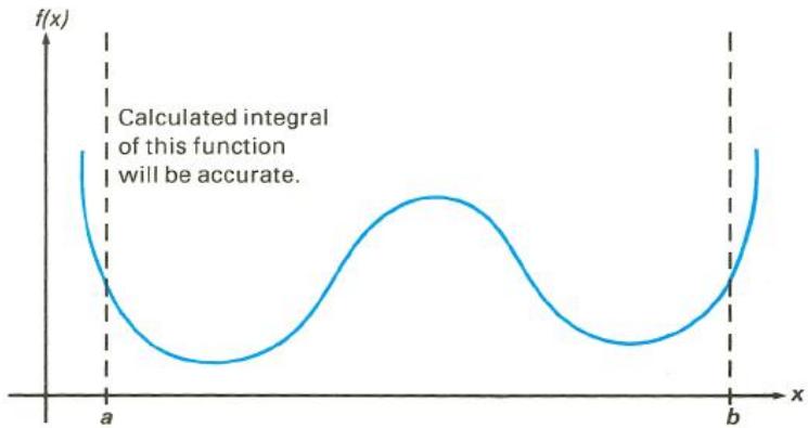
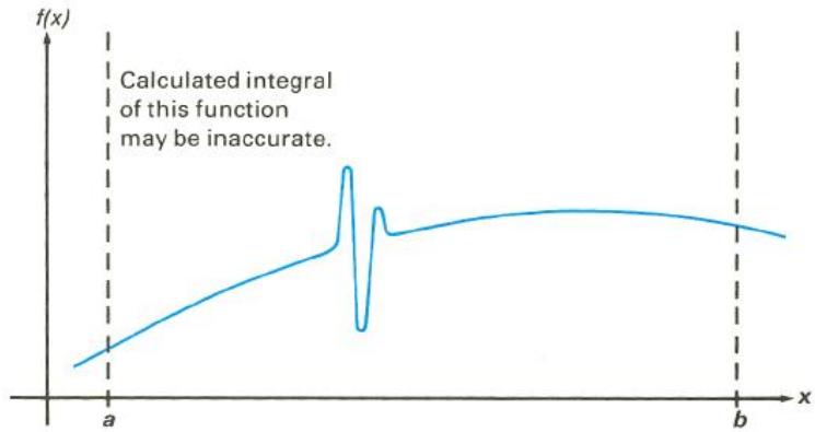
In many cases you will be familiar enough with the function you want to integrate that you'll know whether the function has any quick wiggles relative to the interval of integration. If you're not familiar with the function, and you have reason to suspect that it may cause problems, you can quickly plot a few points by evaluating the function using the subroutine you wrote for that purpose.

If for any reason, after obtaining an approximation to an integral, you have reason to suspect its validity, there's a very simple procedure you can use to verify it: subdivide the interval of integration into two or more adjacent subintervals, integrate the function over each subinterval, then add the resulting approximations. This causes the function to be sampled at a brand new set of sample points, thereby more likely revealing any previously hidden spikes. If the initial approximation was valid, it will equal the sum of the approximations over the subintervals.

Conditions That Prolong Calculation Time

In the preceding example (page 251), you saw that the algorithm gave an incorrect answer because it never detected the spike in the function. This happened because the variation in the function was too quick relative to the width of the interval of integration. If the width of the interval were smaller, you would get the correct answer; but it would take a very long time if the interval were still too wide.

For certain integrals such as the one in that example, calculating the integral may be unduly prolonged because the width of the interval of integration is too large relative to certain features of the functions being integrated. Consider an integral where the interval of integration is wide enough to require excessive calculation time but not so wide that it would be calculated incorrectly. Note that because f(x) = xe^-x approaches zero very quickly as x approaches , the contribution to the integral of the function at large values of x is negligible. Therefore, you can evaluate the integral by replacing , the upper limit of integration, by a number not so large as 10^99 , say 10^3 .

Keystrokes	Display
0 ENTER	0.000	00	Keys lower limit into Y-register.
EEX 3	1	03	Keys upper limit into X-register.
f /y x 1	1.000	00	Approximation to integral.
x $ y	1.824	-04	Uncertainty of approximation.

This is the correct answer, but it took almost 60 seconds. To understand why, compare the graph of the function over the interval of integration, which looks about identical to that shown on page 252, to the graph of the function between x = 0 and x = 10 .

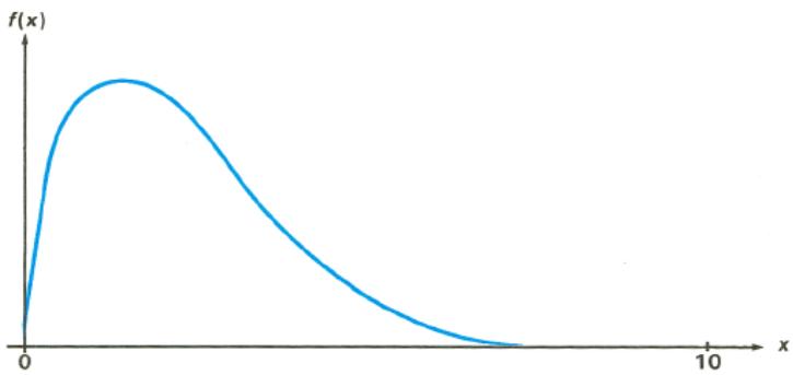
By comparing the two graphs, you can see that the function is "interesting" only at small values of x . At greater values of x , the function is "uninteresting," since it decreases smoothly and gradually in a very predictable manner.

As discussed earlier, the _y^x algorithm will sample the function with higher densities of sample points until the disparity between successive approximations becomes sufficiently small. In other words, the algorithm samples the function at increasing numbers of sample points until it has sufficient information about the function to provide an approximation that changes insignificantly when further samples are considered.

If the interval of integration were (0, 10) so that the algorithm needed to sample the function only at values where it was interesting but relatively smooth, the sample points after the first few iterations would contribute no new information about the behavior of the function. Therefore, only a few iterations would be necessary before the disparity between successive approximations became sufficiently small that the algorithm could terminate with an approximation of a given accuracy.

On the other hand, if the interval of integration were more like the one shown in the graph on page 252, most of the sample points would capture the function in the region where its slope is not varying much. The few sample points at small values of x would find that values of the function changed appreciably from one iteration to the next. Consequently the function would have to be evaluated at additional sample points before the disparity between successive approximations would become sufficiently small.

In order for the integral to be approximated with the same accuracy over the larger interval as over the smaller interval, the density of the sample points must be the same in the region where the function is interesting. To achieve the same density of sample points, the total number of sample points required over the larger interval is much greater than the number required over the smaller interval. Consequently, several more iterations are required over the larger interval to achieve an approximation with the same accuracy, and therefore calculating the integral requires considerably more time.

Because the calculation time depends on how soon a certain density of sample points is achieved in the region where the function is interesting, the calculation of the integral of any function will be prolonged if the interval of integration includes mostly regions where the function is not interesting. Fortunately, if you must calculate such an integral, you can modify the problem so that the calculation time is considerably reduced. Two such techniques are subdividing the interval of integration and transformation of variables. These methods enable you to change the function or the limits of integration so that the integrand is better behaved over the interval(s) of integration. (These techniques are described in the HP-15C Advanced Functions Handbook.)

Obtaining the Current Approximation to an Integral

When the calculation of an integral is requiring more time than you care to wait, you may want to stop and display the current approximation. You can obtain the current approximation, but not its uncertainty.

Pressing / while the HP-15C is calculating an integral halts the calculation, just as it halts the execution of a running program. When you do so, the calculator stops at the current program line in the subroutine you wrote for evaluating the function, and displays the result of executing the preceding program line. Note that after you halt the calculation, the current approximation to the integral is not the number in the X-register nor the number in any other stack register. Just as with any program, pressing / again starts the calculation from the program line at which it was stopped.

The _y^x algorithm updates the current approximation and stores it in the LAST X register after evaluating the function at each new sample point. To obtain the current approximation, therefore, simply halt the calculator, single-step if necessary through your function subroutine until the calculator has finished evaluating the function and updating the current approximation. Then recall the contents of the LAST X register, which are updated when the RTN instruction in the function subroutine is executed.

While the calculator is updating the current approximation, the display is blank and does not show running. (While the calculator is executing your function subroutine, running is displayed.) Therefore, you might avoid having to single-step through your subroutine by halting the calculator at a moment when the display is blank.

In summary, to obtain the current approximation to an integral, follow the steps below.

1. Press R/S to halt the calculator, preferably while the display is blank.

2. When the calculator halts, switch to Program mode to check the current program line.

3. If that line contains the subroutine label, return to Run mode and view the LAST X register (step 3).

4. If any other program line is displayed, return to Run mode and single-step (SST) through the program until you reach a RTN instruction (keycode 43 32) or line 000 (if there is no RTN). (Be sure to hold the SST key down long enough to view the program line numbers and keycodes.)

5. Press 9 to view the current approximation. If you want to continue calculating the final approximation, press + / S . This refills the stack with the current x -value and restarts the calculator.

For Advanced Information

The HP-15C Advanced Functions Handbook explores more esoteric aspects of _y^x and its applications. These topics include:

Accuracy of the function to be integrated.
Shortening calculation time.
Calculating difficult integrals.
Using _y^x in Complex mode.

Appendix F

Batteries

Batteries

The HP-15C is shipped with two 3 Volt CR2032 Lithium batteries. Battery life depends on how the calculator is used. If the calculator is being used to perform operations other than running programs, it uses much less power.

Low-Power Indication

A battery symbol () shown in the upper-left corner of the display when the calculator is on signifies that the available battery power is running low. When the battery symbol begins flashing, replace the battery as soon as possible to avoid losing data.

Use only a fresh battery. Do not use rechargeable batteries.

Warning

There is the danger of explosion if the battery is incorrectly replaced. Replace only with the same or equivalent type recommended by the manufacturer. Dispose of used batteries according to the manufacturer's instructions. Do not mutilate, puncture, or dispose of batteries in fire. The batteries can burst or explode, releasing hazardous chemicals. Replacement battery is a Lithium 3V Coin Type CR2032.

Installing New Batteries

To prevent memory loss, never remove two old batteries at the same time. Be sure to remove and replace the batteries one at a time.

To install new batteries, use the following procedure:

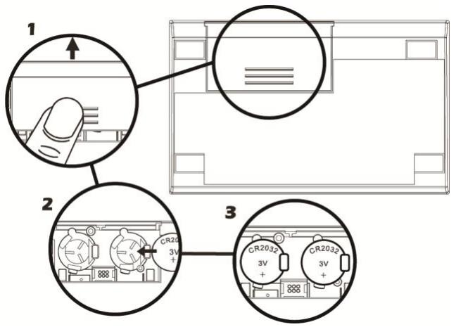
1. With the calculator turned off, slide the battery cover off.
2. Remove the old battery.
3. Insert a new CR2032 lithium battery, making sure that the positive sign (+) is facing outward.
4. Remove and insert the other battery as in steps 2 through 3. Make sure that the positive sign (+) on each battery is facing outward.
5. Replace the battery cover.

Note: Be careful not to press any keys while the battery is out of the calculator. If you do so, the contents of Continuous Memory may be lost and keyboard control may be lost (that is, the calculator may not respond to keystrokes).

1. Press ON to turn on the power. If for any reason Continuous Memory has been reset (that is, if its contents have been lost), the display will show Pr Error. Pressing any key will clear this message.

Verifying Proper Operation (Self-Tests)

If it appears that the calculator will not turn on or otherwise is not operating properly, use the following procedures to access the test system;

1) Turn the calculator off.
2) Press and HOLD the 9 and keys (keep both keys held down for the next step).
3) Press the ON key (while both g and ENTER keys are held down from Step 2 above).
4) Release the ON key.
5) Release the 9 and ENTER keys.

You will be presented with a main test screen that displays the following: 1.L 2.C 3.H

• Press 1 to perform the LCD test (all LCD segments will be turned on). Press any key to exit
• Press 2 to perform the checksum test and see the copyright messages. Press any key to go from one screen to the next until you return to the main test screen.
• Press 3 to perform the keyboard test. You then need to press EVERY key on the keyboard until all the keys have been pressed at least once (the screen will progressively turn off). You can press the keys in any order and any number of times. Once all the keys have been pressed and the screen is clear, press on any key to return to the test screen.

Press ON to exit the test system. This will also turn the calculator off.

If the calculator detects an error at any point, it will display an error message.

If you still experience difficulty, write or telephone Hewlett-Packard at an address or phone number listed on the web at: www.hp.com/support.

Function Summary and Index

ONTurns the calculator's display on and off (page 18).It is also used in resetting Continuous Memory page 63),changing the digit separator (page 61),and in various tests of the calculator's operation (pages 261).

Complex Functions

Real exchange imaginary. Activates Complex mode (establishing an imaginary stack) and exchanges the real and imaginary X-registers (page 124).

Used to enter complex numbers. Activates Complex mode (establishing an imaginary stack) (page 121). Also used with DIM to indirectly dimension matrices (page 174). (For Index register functions, refer to Index Register Control keys, page 263.) (i) Displays

the contents of the imaginary X-register while the key is held (page 124).

SF 8 Sets flag 8, which activates Complex mode (page 121).

CF 8 Clears flag 8, deactivating Complex mode (page 121).

Conversions

R Converts polar magnitude r and angle in X- and Y-registers respectively to rectangular x- and y-coordinates (page 31). For operation in Complex mode, refer to page 134.

Converts x, y rectangular coordinates placed in X- and Y- registers respectively to polar magnitude r and angle (page 30). For operation in Complex mode, refer to page 134.

H.MS Converts decimal hours (or degrees) to hours, minutes, seconds (or degrees, minutes, seconds) (page 27).

H Converts hours, minutes, seconds (or degrees, minutes, seconds) to decimal hours (or degrees) (page 27).

RAD Converts degrees to radians (page 27).

DEG Converts radians to degrees (page 27).

Digit Entry

ENTER Enters a copy of number in X-register (display) into Y-register; used to separate multiple number entries (pages 22, 37).

CHS Change sign of number or exponent of 10 in display (pages 19, 124).

EEX Enter exponent; next digits keyed in are exponents of 10 (page 19).

0 through 9 digit keys (page 22).

• Decimal point (page 22)

Display Control

Fix Selects fixed point display mode (page 58).

SCI Selects scientific notation display mode (page 59).

ENG Selects engineering notation display mode (page 59).

Mantissa. Pressing f CLEAR Prefix displays all 10 digits of the number in the Xregister as long as the Prefix key is held down (page 60). It also clears any partial key sequences (page 19).

Hyperbolic Functions

HYP SIN HYP COS HYP TAN Compute hyperbolic sine, hyperbolic cosine, or hyperbolic tangent, respectively (page 28).

HYP SIN, HYP COS, HYP TAN

Compute inverse hyperbolic sine, inverse hyperbolic cosine, or inverse hyperbolic tangent, respectively (page 28).

Index Register Control

I Index register (_I) Storage register for: indirect program execution - branching with GTO and GSB, looping with ISG and DSE - indirect flag control, and indirect display format control (page 107). Also used to enter complex numbers and activate Complex mode (page 121).

(i) Indirect operations. Used to address another storage register through _I for purposes of storage, recall, storage, arithmetic, and program loop control (page 107). Also used with DIM to allocate storage registers (page 215).

Logarithmic and Exponential Functions

LNComputes natural logarithm (page 28).

^x Natural antilogarithm. Raises e to power of number in display (X-register) (page 28).

LOGComputescommon logarithm(base 10)(page 28).

10 Common antilogarithm. Raises 10 to power of number in display (X-register) (page 28).

^x Raises number in Y-register to power of

number in display (Xregister) (enter y , then x ).Causes the stack to drop (page 29).

Mathematics

Arithmetic operators; cause the stack to drop (page 29).

Computing square root x (page 25).

^2 Computing the square of x (page 25).

! Calculates the factorial (n!) of x or Gamma function () of (1 + x) (page 25).

1 / x Computing reciprocal (page 25). (For matrix use, refer to Matrix Functions, page 264.)

Places value of in display (page 24).

SOLVE Solves for real root of a function f(x) , with the expression for f(x) defined by the user in a labeled subroutine (page 180).

_y^x Integrate.

Computes the definite integral of f(x) , with the expression f(x) defined by the user in a labeled subroutine (page 194).

Matrix Functions

DIM Dimensions a matrix of a given name {A to E, I} (page 141).

Designates the matrix into which the result of certain matrix operations is placed (page 148).

User mode. Row and column numbers in R_0 and _1 are automatically incremented each time STO or RCL {A to E, (i)} is pressed (page 144).

STO and RCL { A to E, (i) Stores or recalls matrix elements using the row and column numbers in _0 and _1 (pages 144, 146).

STO g and RCL g {A to E, (i)

} Stores or recalls matrix elements using the row and column numbers in the Y- and X-registers (page 146).

STO and RCL MATRiX { A to E} Stores or recalls matrices for the specified matrix (pages 142, 147).

STO and RCL RESULT Stores or recalls descriptor of the result matrix (page 148).

RCL DIM {A through E, I} Recalls the dimensions of the given matrix into the Y- (row) and X- (column) registers (page 142).

1 / x Inverts the matrix whose descriptor is displayed and places the result in the specified result matrix. The descriptor of the result matrix is then displayed (page 150).

• • X Adds, subtracts, or multiplies the corresponding elements of two

matrices or of one matrix and a scalar. Stores in result matrix (page 152-155).

For two matrices, multiplies inverse of matrix in X by matrix in Y. For only one matrix, if matrix in Y, divides all elements of matrix by scalar in X; if matrix in X, multiplies each element of inverse of matrix by the scalar in Y. Stores in result matrix (pages 152-155).

CHS changes sign of all elements in matrix specified in X-register (page 150).

MATRIX{0 through 9} Matrix operations.

MATRIX 0 Dimensions all matrices to 0× 0 (page 143).

MATRIX 1 Sets row and column numbers in R_0 and R_1 to 1 (page 143).

MATRIX 2 Complex transform: Z^P to (page 164).

MATRIX 3 inverse

complex transform. to Z^P (page164).

MATRIX 4 Transpose X to X^T (page 150).

MATRIX 5 Transpose multiply: Y and X to Y^TX (page 154).

MATRIX 6 Calculates residuals in result matrix (page 159).

MATRIX 7 Calculates row norm of matrix specified in X-register (page 150).

MATRIX 8 Calculates Frobenius norm of matrix specified in Xregister (page 150).

MATRIX 9 Calculates determinant of matrix specified in X-register (also does LU decomposition of the matrix) (page 150).

,x Transforms matrix stored in "partitioned form" (Z^P) to "complex form" (Z^C) (page 162).

,x Transforms matrix stored in "complex form" (Z^C) to

"partitioned form" (Z^P) (page 162).

= 0 TEST 0 TEST 5 TEST 6 Conditional tests for matrix descriptors in the X- or X- and Y-registers. = 0 and TEST 0 (x 0) test the quantity in the X-register for zero. Matrix descriptors are considered nonzero. TEST 5 (x = y) and TEST 6(x y) test if the descriptors in X and Y are the same. The result affects program execution: skip (one line) if false (page 174).

Number Alteration

ABS Yields absolute value of number in display (page 24).

FRAC Leaves only fractional portion of number in display (X-register) by truncating integer portion (page 24).

INT Leaves only integer portion of number in display (X-

register) by truncating fractional portion (page 24).

RND Rounds mantissa of entire (10-digit) number in X-register to match display format (page 24).

Percentage

% Percent. computes x % (value in display) of number in the Yregister (page 29). Unlike most two-number functions, % does not drop the stack.

% Percent difference.
Computes percent of
change between number
in Y-register and
number in display
(page 30).Does not
drop the stack.

Prefix Keys

f Pressed before a function key to select the gold function printed above that key (page 18).

9 Pressed before a function key to select

the blue function printed below that key (page 18).

For other prefix keys, refer to Display Control keys (page 263), Storage keys (page 267), and the Programming Summary and Index (page 269).

CLEAR [PREFIX]
Cancels any prefix keystrokes and partially entered instructions such as f [SCI] (page 19). Also displays the complete 10-digit mantissa of the number in the display (page 60).

Probability

Combination.
Computes the number
of possible sets of y different items taken x at a time, and causes the
stack to drop (page 47).
(For matrix use, refer to
Matrix Functions keys,
page 264.)

.x Permutation.
Computes the number
of possible different
arrangements of y

different items taken x at a time, and causes the stack to drop (page 47). (For matrix use, refer to Matrix Functions keys, page 264.)

Stack Manipulation

\& y Exchanges contents of X- and Ystack registers (page 34).

X-register exchange. Exchanges contents of X-register with those of any other named storage register. Used with I, (i), digit, or digit address (page 42).

Real exchange imaginary. Exchanges the contents of the real and imaginary X- registers and activates Complex mode (page 124).

Rolls down contents of stack (page 34).

Rolls up contents of stack (page 34).

Clears contents of display (X-register) to zero (page 21).
In Run mode: removes the last digit keyed in, or clears the display (if digit entry has been terminated) (page21).

Statistics

+ Accumulates numbers from X- and Y-registers into storage registers R_2 through R_7 (page 49).
- Removes numbers in X- and Y-registers from storage registers R_2 through R_7 for correcting + accumulations (page 52).
Computing mean of x - and y -values accumulated by + (page 53).
sComputes sample standard deviations of x - and y -values accumulated by ^+ (page 53).
, r Linear estimate

and correlation coefficient. Computing estimated value of y() for a given value of x by least squares method and places result in X-register. Computing the correlation coefficient, r , of the accumulated data and places result in Y-register (page 55).

L.R. Linear Regression. Computing the y -intercept and slope for the linear function best approximating the accumulated data. The value of the y -intercept is placed in the X-register; the value of the slope is placed in the Y-register (page 54).

RAN# Random number. Yields a pseudorandom number as generated from a seed stored using STO RAN# (page 48).

CLEAR Clears contents of the statistics registers (_2 to _7) (page 49).

Storage

STO Store. Stores a copy of a number into the storage register specified {0 to 9, .0 to .9, I, (i)} (page 42). Also used for storage register arithmetic: new register contents = old register contents { +, -, x, ÷} display (page 44).

RCL Recall. Recalls a copy of the number from the storage register specified {0 to 9, .0 to .9, I, (i)} (page 42). Also used for storage register arithmetic: new display = old display {+, - ×, ÷} register contents (page 44).

CLEAR REG Casks contents of all storage registers to zero (page 43).

_x Recalls into the display the number present before the previous operation (page 35).

Trigonometry

DEGSets decimal Degrees mode for trigonometric functions-indicated by absence of GRAD or RAD annunciator (page 26).Not operative for complex trigonometry.

RAD Sets Radians mode for trigonometric functions—indicated by RAD annunciator (page 26).

GRD Sets Grads mode for trigonometric functions—indicated by GRAD annunciator (page 26) Not operative for complex trigonometry.

SIN, COS, TAN Compute sine, cosine, or tangent, respectively, of number in display (X-register) (page 26).

^-1 , ^-1 , ^-1 Compute arc sine, arc cosine, or arc tangent, respectively, of number in display (X-register) (page 26).

Programming Summary and Index

P/R Program/Run mode. Sets the calculator to Program mode (PRGM annihilator on) or Run mode (PRGM annihilator cleared) (page 66).

MEM Displays current status of calculator memory (number of registers dedicated to data storage, the common pool, and program memory) (page 215).

MEM Displays current status of calculator memory (number of registers dedicated to data storage, the common pool, and program memory) (page 215).

Back arrow. In Program mode, deletes displayed instruction from program memory. All subsequent instructions are moved up (page 83).

LBL Label. Used with the label designations

below to denote the start of a program routine (page 67).

A B C D E 0
1 2 3 4 5 6 7 8 9 .0 .1 .2
.3 .4 .5 .6 .7 .8 .9 Label designations. When preceded by LBL, define the beginning of a program routine (page 67). Also used (without LBL) to initiate execution of a specific routine (page 69).

Activates and deactivates User mode, which exchanges the primary (white) and gold alternate functions ( through ) of the top left five functions (page 69). User mode also affects the matrix use of STO or RCL through , (i) User mode automatically increments _0 (row number) or _1 (column number) for storage or recall of matrix elements (page 144). GTO Go to. Used with

a label designator (listed above) or I to transfer the position of the calculator to the designated label. If it is a program instruction, program execution continues. If it is not a program instruction, only the position change occurs (page 90). If a negative number is stored in _I GTO I will effect a transfer to a line number (page 109).

GTO CHS nnn Go to line number. Positions calculator to the existing line number specified by nnn. Not programmable (page 82).

GSB Go to subroutine. Used with a label designator (listed above) or start the execution of a given, labeled routine. Can be used both in a program and from the keyboard (in Run mode). A RTN instruction transfers execution back to the first line

following the GSB (page 101).

BST Back step. Moves calculator back one or more lines in program memory. (Also scrolls in Program mode.) Displays line number and contents of previous program line (page 83).

SST Single step. In Program mode: moves calculator forward one or more lines in program memory. In Run mode: displays and executes the current program line, then steps to next line to be executed (page 82).

PSE Pause. Halts program execution for about 1 second to display contents of X-register, then resumes execution (page 68).

R/S Run/Stop.
Begins program
execution from current
line number in program
memory. Stops
execution if program is
running (page 68).

RTN Return. Causes

calculator to return to line 000 and halt execution (if running) (page 68). If in a subroutine, merely returns to line after GSB (page 101).

SF Set flag (= true) Sets designated flag (0 to 9). Flags 0 through 7 are user flags, flag 8 signifies Complex mode, and flag 9 signifies an overflow condition (page 92).

CF Clear flag (= false).Clearedesignatedflag(0to9) (page 92).

F? Is flag set? Tests for designated flag. If set, program execution continues; If cleared, program execution skips one line before continuing (page 92).

≤slant y = 0 {0 through 9} Conditional tests. Each test compares value in Xregister against 0 or value in Y-register as indicated. If true, calculator executes instruction in next line of program memory. If false, calculator skips

one line in program memory before resuming execution (page 91). = 0 and TEST 0,5,and 6 are also valid for complex numbers and matrix descriptors (pages 132. 174).

TEST 0x 0

TEST 1x > 0

TEST 2x < 0

TEST 3x≥ 0

TEST 4x≤ 0

TEST 5x = y

TEST 6x y

TEST 7x > y

TEST 8x < y

TEST 9x≥ y

DSE Decrement and skip if equal to or less than.Decrements counter value in given register as stipulated. Skips one program line if new counter value is equal to or less than specified test value (page 109).

ISG Increment and skip if greater than. Increments counter value in given register as stipulated. Skips one program line if new counter value is greater than specified test value (page 109).

Subject Index

Page numbers in bold type indicate primary references; page numbers in regular type indicate secondary references.

A

Abbreviated key sequences, 78

Absolute value (ABS), 24

Allocating memory, 42, 213-219

Altering program lines, 83

Annunciators,

complex, 121

list of, 60

PRGM, 32, 66

trigonometric, 26

Antilogarithms, common and natural, 28

Arithmetic operation, 29, 37

Asymptotes, horizontal, 230

Automatic incrementing of row and column numbers, 143

B

Back-stepping(BST),83

Bacterial population example, 41

Battery life, 259

Battery replacement, 260, 259-260

Bessel functions, 195, 197

Branching,

conditional, 91, 98, 177, 192

indirect, 108-109, 112-114, 115

simple, 90

C

annunciator, 99, 121

Can volume and area example, 70-74

Chain calculations, 22-23, 38

Changing signs, 19

in Complex mode, 124-125

in matrices, 177

[CHS], 19

Clearing

blinking in display, 100

complex numbers, 125-127

display, 21

memory, 63

operations, 20-21

overflow condition, 45, 61

prefix keys, 19

statistics registers, 49

Coefficient matrix, 156

Combinations function (.x) ,47

Common pool, 213

Complex arithmetic example, 132

Complex conjugate, forming, 125

Complex matrix,

inverting, 162, 164, 165

multiplying, 162, 164, 166

storing elements, 161

transforming, 162, 164

Complexmode,120-121

activating, 99, 120-121, 133

deactivating, 121

mathematics functions in, 131

stack lift in, 124

Complex numbers,

clearing, 125-127

converting polar and rectangular forms, 133-135

entering, 121, 127, 128-129

storing and recalling, 130

Conditionals, indirect, 109-111, 112, 116

Conditional tests, 91, 98, 192

in Complex mode, 132

with matrix descriptors, 174

Constant matrix, 156

Constants,

calculations with, 39-42

using in arithmetic calculations, 35, 39-42

Continuous Memory,

duration of, 62

resetting (clearing), 63

what it retains, 43, 48, 58, 61, 62

Conventions, handbook, 18

Conversions,

degrees and radians, 27

polar and rectangular coordinates, 30-31

time and angle, 26-27

Correcting accumulated statistics data, 52

Correlation coefficient, find the (,r) , 55-56

COS, COS, 26

Counters in program loops, 98, 112-114

Crocus example, 43

Cumulative calculations, 41

D

Data storage, 42

Data storage pool, 213-214

Debt payment example, 95

Decimal point, 22

Decimal point display, 61

Deflation, 233, 234, 237

DEG,26

Determinant, 150

Digit entry, 22

in Complex mode, 121, 125, 127, 128-129

termination, 22, 36, 209

Digit separator display, 61

DIM, 76-77, 215-217

Disabling stack lift, 36

Display (See also X-register),

blinking, 100

clearing, 21

error messages, 61

fullmantissa,60

in Complex mode, 121

Display format, 58-59, 61

effect on f 200, 241, 244, 245-249

Do if True rule, 92, 192

DSE 109-111, 112, 116

E

EEX,19

Electrical circuit example, 169-171

Enabling stack lift, 36

[ENG], 59

Engineering notation, 59

ENTER,12,33-34,36

effect on digit entry, 22, 29

effect on stack movement, 37, 41

Entering data for statistical analysis, 49

Error

conditions, 205-208

display, 61

stops, 78

Errors,

with _y^x , 203-204

withSOLVE,187,192,193

Euclidean norm (See Frobenius norm)

Exchanging the real and imaginary stacks, 124

Exponential function (See Power function)

Exponents, 19, 20

F

f,18

Factorial function (!) , 25

Falling stone example, 14

FIX,58

Fixed decimal notation, 58

Flag tests, 92, 98

Flag 8, 99

Flag 9, 100

Format, handbook, 2, 18

Fractional portion (FRAC), 24

Frobeniusnorm,150,177

Functions, nonprogrammable, 80

Functions, one-number, 22, 25

Functions, primary and alternate, 18

Functions, two-number, 22, 29

G

9,18

Gamma function (!) , 25

GRD,26

GSB,101

GTO,90,97,98

GTO CHS,82

H

Horner's Method, 79, 181 Hyperbolic

functions, 28

1

Imaginary stack,

clearing the, 124

creation of, 121-123, 133

display of, 124

stack lift of, 124

Index register

arithmetic, 108, 112

display format control, 109, 114, 115, 116

exchange with X-register, 108, 112

flag control, 109, 115

loop control, 107, 109-111

storage and recall, 107, 111, 115

Indirect addressing, 106-108, 115

Initialization, 87

Instructions, 74

Integer portion (INT), 24

Integrate function (_y^x) , 194-204

accuracy of, 200-203, 240, 241-245

algorithm for, 196, 240-241, 249-251, 255-256

display format with, 245-249

execution time for, 196, 200, 244, 245, 254-256

memoryusage,204

obtaining an approximation for, 257-258

problems with erratic functions, 249-254

programmed, 203-204

recursive use of, 203

subroutines for, 194-195

uncertainty in, 202-203, 240-244, 245-249
Interchanging functions (See User mode)
Interference, radio and television, 271
Intermediate results, 22, 38
Interpolation, using , r , 57
ISG, 109-111, 116
Iterations using ISG and DSE, 111

K

Keycodes, 74-75
Keying in chain calculations, 22
exponents, 19-20
one-number functions, 22
two-number functions, 22, 29

L

Labels, 67, 77, 90, 97
LAST X register, 35 in matrix functions, 174-176 operations saved by, 212 putting constants in, 39-40 to correct statistics data, 52
Linear equations, solving with matrices, 138, 156
Linear estimation (, r) , 55-56
Linear regression (.R.) , 54
Loading the stack with constants, 39, 41
Logarithmic functions, common and natural, 28
Loop control number, 109, 116
Looping, 90, 98
Low-power indication, 62, 259
LU decomposition, 148, 155, 156, 160
Łukasiewicz, Jan, 32

M

Mantissa, displaying full 10 digits, 60
Matrix complex, 160-163 copying, 149 descriptors, 139, 147, 160, in _I 173-174

dimensioning, 140, 142, 142, 174

dimensions, displaying, 142, 147

equation, complex, 168

memory, 140, 171

name (See Matrix descriptors)

partitioned, 161, 164

Matrix elements,

accessing individually, 145-147

displaying, 144

storing and recalling, 143-144, 147, 149, 176

Matrix functions,

using _1 173-174

using registers, 173

arithmetic, 153

conditional, 177

inverse, 150, 154

multiplication, 154

one-matrix, 149-151

programmed, 176-177

reciprocal, 150

residual, 159

rownorm,150,177

summary, 177-179

transpose, 150, 151, 154

Mean (X).53

MEM, 215

Memory

allocation, 76, 215-217

availability, 75-77, 213, 215

configuration, initial, 75-76

distribution, 75, 213-214

limitations, 75, 77, 217

requirements for advanced functions, 218-219

requirements for programming, 218

stack (See Stack)

status display, 215

registers in, 213-215

Metal box dimensions example, 189-191

Minima, finding with , 230

Modes, trigonometric, 26

Multiple roots, 234

N

Negative numbers, 19

in Complex mode, 124-125

Nested calculations, 38

Neutral operations, 211

Nonprogrammable functions, 80

Normalizing statistics data, 50

null display, 144, 149

Numerical integration, 194-204

O

ON,

and off, 18

to reset Continuous Memory, 63

to set decimal point display, 61

Overflow condition, 45, 61, 100

P

P/R,66,68

Pause(PSE), 68

Percent difference (%) ,29

Percentage functions, 29-30

Permutations function (_y.x) ,47

Phasor notation, 133

Pi, 24

Polar coordinates, 30, in Complex mode, 133-135

Power function (^x) , 29

Prefix keys, 19

PRGMannouncer,66,82

Program

control, indirect, 107, 109-111

data entry techniques, 69-70

end,68,77

entering, 66-68

labels,67,77

loading, 66

loop counters, 109, 112-114, 116

mode,66,68,86

position, changing, 82, 86

running, 68-69

starting, 69

stops, 68, 78

Program execution, 69

after [GSB], 101

after GTO, 97

afteroverflow,100

after test, 92

from or through labels, 78-79

Program lines (instructions), 67, 74

deleting, 83, 86

inserting,83,86

Program memory, 67, 70, 75, 217-219

automatic real location, 217-218

clearing, 67

moving in, 67

Quadratic equation, solving, 181

R_0 and R_1 , using to access matrix elements, 143, 146, 176

RAD,26

Radioisotope example, 93-94

Random number generator (RAN#), 48

Random number storage and recall, 48

Recall arithmetic, 44

Recalling accumulated statistics data, 50

Recalling numbers (RCL), 42, 44, with matrices, 144, 149, 176

Reciprocal ([1]x) , 25, with matrix, 150

Rectangular coordinates, 31, in Complex mode, 133-135

Registers, converting, 215-217

Reset Continuous Memory, 63

Residual, 159

Result matrix, 147, 148, 150, 152

Return (RTN), 68, 77

Returns, pending, 101, 105, 192, 204

Reverse Polish Notation, 32

ReIm 124, 127

Rice yield example, 50-56

Ridget hurling example, 184-186, 224-226

Roll down, 34

Roll up, 34

Roots, eliminating, 233, 234, 237

Roots,meaningless,188,191

Rounding (RND), 24

Rounding in the display, 59

Round-off errors, 52, 60, with SOLVE, 223, 237

Rownorm,150,177

Run/Stop (R/S), 68, 91

running display, 69, 147, 182

S

Scalar operations, 151-153

SCI,58

Scientific notation, 58

Scrolling, 82

Secant line calculation example, 102

Self-tests, 261

Service information, 267-270

Shear stress example, 227-228

SIN, SIn-26

Sine integral example, 198-199

Single-stepping (SST), 82, 85

Skip if True rule, 110

Slope, finding the, 54

SOLVE, 180-181

accuracy, 222-226, specifying, 238

algorithm, 182, 187-188, 220-222, 230-231

conditions necessary for, 221-222

constant function value with, 187, 189

execution time, 238

illegal math routine with, 187-188

initial estimates with, 181, 188-192, 221, 233, 237

memoryusage,193

nonzero minimum of function with, 187

programmed, 192

recursive use of, 193

restrictions on, 193

using as a conditional test, 192

using functions with discontinuities, 227

using functions with poles, 227

using functions with several roots, 233-238

with no root, 186-188, 192, 229

Square root () , 25

Squaring (^2) , 25

Stack

contents, with _v^x , 197, 202

drop, 33, 38

lift, 33, 36, 38, 44, 209-211

manipulation functions, 33-34, in Complex mode, 131

imaginary, 120-125

used to access matrix elements, 146-147

Stack-disabling operations, 210

Stack-enabling operations, 210-211

Stack movement, 32, 33-37

in matrix functions, 174-176

withSOLVE,181

Standard deviation (S), 53, sample vs. population, 53

Star example, 40

Statistics, accumulation of data (^+) , 49

Statistics, correction of accumulated data (^+) , 52

Statistics functions,

combinations, 47

correlation coefficient, 55

linear estimation, 55

linear regression, 54

mean, 53

permutations, 47

probability, 47

standard deviation, 53

Statistics registers, 49-50

Status indicators, 60

Storage and recall (STO, RCL), 42, 43, 44

complex numbers, 130

direct (with I), 106, 107

indirect, 106-107, 111

matrices, 144, 149, 176

matrix elements, 143-144, 147, 149

Storage arithmetic, 43

Storage registers, 42

allocation, 42, 215-217

arithmetic, 43

clearing, 43

statistics, 42, 49

Subroutine

levels, 102, 105

limits, 102, 105

nesting example, 103

returns, 101, 105

using with SOLVE, 180-181, 192

System flags, 92, 99

T

T-register, 32, 33

in matrix functions, 174-176

with _y^x , 202

TAN

TAN,26

TEST,91

Tracing, 82

Transpose, 150, 151, 154

Trigonometric modes in Complex mode, 121, 134

Trigonometric operations, 26

U

u display, 176

Uncommitted registers, 213, 215, 217

Underflow,

in any register, 61

storage register arithmetic, 45

withSOLVE,223

User flags, 92

User mode, 69, 79, with matrices, 143, 176

V

Vector arithmetic, using statistics functions, 57

W

Wrapping, 86, 90

X

X exchange (5) ,42

X exchange Y (xS y), 34

X-register, 32, 35, 37, 42, 60, 209-210

imaginary, 210, 211

in matrix functions, 141, 156, 175-176

with _y^x , 202

withSOLVE,181,183,102,226

Y

y -intercept, finding, 54

Y-register, 32, 37

in matrix functions, 141, 156, 175-176

with _y^x , 202

SOLVE, 181, 183, 192, 226

Z

Z-register, 32

in matrix functions, 174-176

with _y^x , 202

with SOLVE,181,183,192,226

Product Regulatory & Environment Information

Federal Communications Commission Notice

This equipment has been tested and found to comply with the limits for a Class B digital device, pursuant to Part 15 of the FCC Rules. These limits are designed to provide reasonable protection against harmful interference in a residential installation. This equipment generates, uses, and can radiate radio frequency energy and, if not installed and used in accordance with the instructions, may cause harmful interference to radio communications. However, there is no guarantee that interference will not occur in a particular installation. If this equipment does cause harmful interference to radio or television reception, which can be determined by turning the equipment off and on, the user is encouraged to try to correct the interference by one or more of the following measures:

• Reorient or relocate the receiving antenna.
• Increase the separation between the equipment and the receiver.
• Connect the equipment into an outlet on a circuit different from that to which the receiver is connected.
• Consult the dealer or an experienced radio or television technician for help.

Modifications

The FCC requires the user to be notified that any changes or modifications made to this device that are not expressly approved by Hewlett-Packard Company may void the user's authority to operate the equipment.

Declaration of Conformity for Products Marked with FCC Logo, United States Only

This device complies with Part 15 of the FCC Rules. Operation is subject to the following two conditions: (1) this device may not cause harmful interference, and (2) this device must accept any interference received, including interference that may cause undesired operation.

If you have questions about the product that are not related to this declaration, write to

Hewlett-Packard Company

P. O. Box 692000, Mail Stop 530113

Houston, TX 77269-2000

For questions regarding this FCC declaration, write to

Hewlett-Packard Company

P. O. Box 692000, Mail Stop 510101

Houston, TX 77269-2000

or call HP at 281-514-3333

To identify your product, refer to the part, series, or model number located on the product.

Canadian Notice

This Class B digital apparatus meets all requirements of the Canadian Interference-Causing Equipment Regulations.

Avis Canadien

European Union Regulatory Notice

Products bearing the CE marking comply with the following EU Directives:

• Low Voltage Directive 2006/95/EC
  EMC Directive 2004/108/EC
• Ecodesign Directive 2009/125/EC, where applicable

CE compliance of this product is valid if powered with the correct CE-marked AC adapter provided by HP.

Compliance with these directives implies conformity to applicable harmonized European standards (European Norms) that are listed in the EU Declaration of Conformity issued by HP for this product or product family and available (in English only) either within the product documentation or at the following web site: www.hp.eu/certificates (type the product number in the search field).

The compliance is indicated by one of the following conformity markings placed on the product:

CE	For non-telecommunications products and for EU harmonized telecommunications products, such as Bluetooth® within power class below 10mW.
CExxxx*	For EU non-harmonized telecommunications products (If applicable, a 4-digit notified body number is inserted between CE and!).

Please refer to the regulatory label provided on the product.

The point of contact for regulatory matters is:

Hewlett-Packard GmbH, Dept./MS: HQ-TRE, Herrenberger Strasse 140, 71034 Boeblingen, GERMANY.

Japanese Notice

Disposal of Waste Equipment by Users in Private Household in the European Union

This symbol on the product or on its packaging indicates that this product must not be disposed of with your other household waste. Instead, it is your responsibility to dispose of your waste equipment by handing it over to a designated collection point for the recycling of waste electrical and electronic equipment. The separate collection and recycling of your waste equipment at the time of disposal will help to conserve natural resources and ensure that it is recycled in a manner that protects human health and the environment. For more information about where you can drop off your waste equipment for recycling, please contact your local city office, your household waste disposal service or the shop where you purchased the product.

Chemical Substances

HP is committed to providing our customers with information about the chemical substances in our products as needed to comply with legal requirements such as REACH (Regulation EC No 1907/2006 of the European Parliament and the Council). A chemical information report for this product can be found at: www.hp.com/go/reach.

Perchlorate Material - special handling may apply

This calculator's Memory Backup battery may contain perchlorate and may require special handling when recycled or disposed in California.