
F2229AA 50g - Calculator HP - Free user manual and instructions
Find the device manual for free F2229AA 50g HP in PDF.


| Product Type | Graphing Calculator |
| Model | HP 50g (F2229AA) |
| Dimensions (W x D x H) | 185 x 87 x 26 mm (7.28 x 3.43 x 1.02 in) |
| Weight | 252 g (8.9 oz) including batteries |
| Power Supply | 4 AAA batteries (backup CR2032) |
| Display Type | Monochrome LCD, 131 x 64 pixels |
| Processor | ARM9-based at 75 MHz |
| Memory (Flash) | 2 MB |
| Memory (RAM) | 512 KB |
| Entry System | Algebraic and RPN (Reverse Polish Notation) |
| Built-in Functions | Algebra, calculus, matrices, statistics, unit conversion, equation solving |
| Programming Language | User RPL |
| Graphing Capabilities | Function, polar, parametric, 3D, differential equation plotting |
| Data Connectivity | USB 1.1, infrared, serial port |
| Included Accessories | USB cable, user manual, batteries |
| Languages Supported | English, French, German, Spanish, Italian, Portuguese, Dutch |
| Cleaning Instructions | Wipe with soft dry cloth; avoid solvents |
| Safety Features | Automatic power-off after 10 minutes of inactivity |
| Spare Parts Availability | Battery cover, keypad, screen protector (order from HP support) |
| Repairability | User-replaceable batteries; other repairs by authorized centers |
| Warranty | 1 year limited hardware warranty |
Frequently Asked Questions - F2229AA 50g HP
User questions about F2229AA 50g HP
0 question about this device. Answer the ones you know or ask your own.
Ask a new question about this device
Download the instructions for your Calculator in PDF format for free! Find your manual F2229AA 50g - HP and take your electronic device back in hand. On this page are published all the documents necessary for the use of your device. F2229AA 50g by HP.
USER MANUAL F2229AA 50g HP
THIS MANUAL AND ANY EXAMPLES CONTAINED HEREIN ARE PROVIDED "AS IS" AND ARE SUBJECT TO CHANGE WITHOUT NOTICE. HEWLETT-PACKARD COMPANY MAKES NO WARRANTY OF ANY KIND WITH REGARD TO THIS MANUAL, INCLUDING, BUT NOT LIMITED TO, THE IMPLIED WARRANTIES OF MERCHANTABILITY, NON-INFRINGEMENT AND FITNESS FOR A PARTICULAR PURPOSE.
HEWLETT-PACKARD CO. SHALL NOT BE LIABLE FOR ANY ERRORS OR FOR INCIDENTAL OR CONSEQUENTIAL DAMAGES IN CONNECTION WITH THE FURNISHING, PERFORMANCE, OR USE OF THIS MANUAL OR THE EXAMPLES CONTAINED HEREIN.
© 2003, 2006 Hewlett-Packard Development Company, L.P.
Reproduction, adaptation, or translation of this manual is prohibited without prior written permission of Hewlett-Packard Company, except as allowed under the copyright laws.
Hewlett-Packard Company
16399 West Bernardo Drive
MS 8-600
San Diego, CA 92127-1899
USA
Printing History
Edition 1 April 2006
Preface
You have in your hands a compact symbolic and numerical computer that will facilitate calculation and mathematical analysis of problems in a variety of disciplines, from elementary mathematics to advanced engineering and science subjects. Although referred to as a calculator, because of its compact format resembling typical hand-held calculating devices, the HP 50g should be thought of as a graphics/programmable hand-held computer.
The HP 50g can be operated in two different calculating modes, the Reverse Polish Notation (RPN) mode and the Algebraic (ALG) mode (see page 1-13 for additional details). The RPN mode was incorporated into calculators to make calculations more efficient. In this mode, the operands in an operation (e.g., '2' and '3' in the operation '2+3') are entered into the calculator screen, referred to as the stack, and then the operator (e.g., '+' in the operation '2+3') is entered to complete the operation. The ALG mode, on the other hand, mimics the way you type arithmetic expressions in paper. Thus, the operation '2+3', in ALG mode, will be entered in the calculator by pressing the keys '2', '+', and '3', in that order. To complete the operation we use the ENTER key. Examples of applications of the different functions and operations in this calculator are illustrated in this user's guide in both modes.
This guide contains examples that illustrate the use of the basic calculator functions and operations. The chapters are organized by subject in order of difficulty. Starting with the setting of calculator modes and display options, and continuing with real and complex number calculations, operations with lists, vectors, and matrices, detailed examples of graph applications, use of strings, basic programming, graphics programming, string manipulation, advanced calculus and multivariate calculus applications, advanced differential equations applications (including Laplace transform, and Fourier series and transforms), and probability and statistic applications.
For symbolic operations the calculator includes a powerful Computer Algebraic System (CAS) that lets you select different modes of operation, e.g., complex numbers vs. real numbers, or exact (symbolic) vs. approximate (numerical) mode. The display can be adjusted to provide textbook-type expressions, which can be useful when working with matrices, vectors, fractions, summations, derivatives, and integrals. The high-speed graphics of the calculator produce complex figures in very little time.
Thanks to the infrared port, the RS232 port, and the USB port and cable provided with your calculator, you can connect your calculator with other calculators or computers. This allows for fast and efficient exchange of programs and data with other calculators or computers. The calculator provides a flash memory card port to facilitate storage and exchange of data with other users.
The programming capabilities of the calculator allow you or other users to develop efficient applications for specific purposes. Whether it is advanced mathematical applications, specific problem solution, or data logging, the programming languages available in your calculator make it into a very versatile computing device.
We hope your calculator will become a faithful companion for your school and professional applications.
Table of contents
Chapter 1 - Getting started ,1-1
Basic Operations, 1-1
Batteries, 1-1
Turning the calculator on and off, 1-2
Adjusting the display contrast, 1-2
Contents of the calculator's display, 1-2
Menus, 1-3
SOFT menus vs. CHOOSE boxes, 1-4
Selecting SOFT menus or CHOOSE boxes, 1-5
The TOOL menu, 1-7
Setting time and date, 1-7
Introducing the calculator's keyboard, 1-11
Selecting calculator modes, 1-12
Operating Mode, 1-13
Number Format and decimal dot or comma ,1-17
Angle Measure, 1-23
Coordinate System, 1-24
Beep, Key Click, and Last Stack, 1-25
Selecting CAS settings, 1-26
Selecting Display modes, 1-27
Selecting the display font, 1-27
Selecting properties of the line editor, 1-28
Selecting properties of the Stack ,1-28
Selecting properties of the equation writer (EQW), 1-29
Selecting the size of the header, 1-30
Selecting the clock display, 1-30
Chapter 2 - Introducing the calculator ,2-1
Calculator objects ,2-1
Editing expressions on the screen, 2-3
Creating arithmetic expressions, 2-3
Editing arithmetic expressions, 2-6
Creating algebraic expressions, 2-7
Editing algebraic expressions, 2-8
Using the Equation Writer (EQW) to create expressions ,2-10
Creating arithmetic expressions, 2-11
Editing arithmetic expressions, 2-17
Creating algebraic expressions, 2-19
Editing algebraic expressions, 2-21
Creating and editing summations, derivatives, and integrals ,2-29
Organizing data in the calculator, 2-33
Functions for manipulation of variables, 2-34
The HOME directory, 2-35
The CASDIR sub-directory ,2-35
Typing directory and variable names ,2-37
Creating subdirectories, 2-39
Moving among subdirectories, 2-43
Deleting subdirectories, 2-43
Variables,2-47
Creating variables, 2-47
Checking variables contents, 2-52
Replacing the contents of variables, 2-55
Copying variables, 2-56
Reordering variables in a directory, 2-59
Moving variables using the FILES menu, 2-60
Deleting variables, 2-61
UNDO and CMD functions ,2-62
Flags,2-64
Example of flag setting: general solutions vs. principal value, 2-65
Other flags of interest, 2-66
CHOOSE boxes vs. Soft MENU, 2-67
Selected CHOOSE boxes, 2-69
Chapter 3 - Calculation with real numbers ,3-1
Checking calculators settings ,3-1
Checking calculator mode ,3-2
Real number calculations,3-2
Changing sign of a number, variable, or expression, 3-3
The inverse function ,3-3
Addition, subtraction, multiplication, division ,3-3
Using parentheses, 3-4
Absolute value function ,3-4
Squares and square roots ,3-5
Powers and roots ,3-5
Base-10 logarithms and powers of 10,3-5
Using powers of 10 in entering data ,3-6
Natural logarithms and exponential function ,3-6
Trigonometric functions ,3-6
Inverse trigonometric functions, 3-6
Differences between functions and operators ,3-7
Real number functions in the MTH menu ,3-7
Hyperbolic functions and their inverses ,3-9
Real number functions ,3-11
Special functions, 3-14
Calculator constants,3-16
Operations with units ,3-17
The UNITS menu ,3-17
Available units ,3-19
Converting to base units ,3-22
Attaching units to numbers ,3-23
Operations with units ,3-25
Units manipulation tools ,3-27
Physical constants in the calculator, 3-29
Special physical functions ,3-32
Function ZFACTOR, 3-32
Function FOλ ,3-33
Function SIDENS,3-33
Function TDELTA,3-33
Function TINC,3-34
Defining and using functions ,3-34
Functions defined by more than one expression, 3-36
The IFTE function, 3-36
Combined IFTE functions, 3-37
Chapter 4 - Calculations with complex numbers ,4-1
Definitions ,4-1
Setting the calculator to COMPLEX mode ,4-1
Entering complex numbers, 4-2
Polar representation of a complex number ,4-3
Simple operations with complex numbers ,4-4
Changing sign of a complex number ,4-5
Entering the unit imaginary number, 4-5
The CMPLX menus ,4-5
CMPLX menu through the MTH menu ,4-6
CMPLX menu in keyboard ,4-7
Functions applied to complex numbers ,4-8
Functions from the MTH menu, 4-9
Function DROITE: equation of a straight line ,4-9
Chapter 5 - Algebraic and arithmetic operations ,5-1
Entering algebraic objects ,5-1
Simple operations with algebraic objects ,5-1
Functions in the ALG menu ,5-3
COLLECT,5-4
EXPAND,5-4
FACTOR,5-5
LNCOLLECT,5-5
LIN ,5-5
PARTFRAC,5-5
SOLVE,5-5
SUBST,5-5
TEXPAND,5-5
Other forms of substitution in algebraic expressions ,5-6
Operations with transcendental functions ,5-7
Expansion and factoring using log-exp functions ,5-7
Expansion and factoring using trigonometric functions ,5-8
Functions in the ARITHMETIC menu ,5-9
DIVIS ,5-9
FACTORS,5-9
LGCD ,5-10
PROPFRAC,5-10
SIMP2,5-10
INTEGER menu ,5-10
POLYNOMIAL menu ,5-10
MODULO menu ,5-11
Applications of the ARITHMETIC menu ,5-12
Modular arithmetic ,5-12
Finite arithmetic rings in the calculator ,5-14
Polynomials ,5-17
Modular arithmetic with polynomials ,5-17
The CHINREM function ,5-17
The EGCD function ,5-18
The GCD function ,5-18
The HERMITE function ,5-18
The HORNER function ,5-19
The variable VX ,5-19
The LAGRANGE function ,5-19
The LCM function ,5-20
The LEGENDRE function ,5-20
The PCOEF function ,5-21
The PROOT function ,5-21
The PTAYL function, 5-21
The QUOT and REMAINDER functions ,5-21
The EPSX0 function and the CAS variable EPS ,5-22
The PEVAL function ,5-22
The TCHEBYCHEFF function ,5-22
Fractions ,5-23
The SIMP2 function, 5-23
The PROPFRAC function ,5-23
The PARTFRAC function ,5-23
The FCOEF function ,5-24
The FROOTS function ,5-24
Step-by-step operations with polynomials and fractions ,5-25
The CONVERT Menu and algebraic operations ,5-26
UNITS convert menu (Option 1),5-26
BASE convert menu (Option 2),5-27
TRIGONOMETRIC convert menu (Option 3),5-27
MATRICES convert menu (Option 5), 5-27
REWRITE convert menu (Option 4),5-27
Chapter 6 - Solution to single equations ,6-1
Symbolic solution of algebraic equations ,6-1
Function ISOL ,6-1
Function SOLVE,6-2
Function SOLVEVX,6-3
Function ZEROS,6-4
Numerical solver menu ,6-5
Polynomial Equations, 6-6
Financial calculations, 6-9
Solving equations with one unknown through NUM.SLV ,6-13
The SOLVE soft menu ,6-26
The ROOT sub-menu ,6-26
Function ROOT,6-26
Variable EQ,6-26
The SOLVR sub-menu ,6-26
The DIFFE sub-menu ,6-29
The POLY sub-menu ,6-29
The SYS sub-menu ,6-30
The TVM sub-menu ,6-30
Chapter 7 - Solving multiple equations ,7-1
Rational equation systems ,7-1
Example 1 – Projectile motion,7-1
Example 2 – Stresses in a thick wall cylinder, 7-2
Example 3 - System of polynomial equations, 7-4
Solution to simultaneous equations with MSLV,7-4
Example 1 - Example from the help facility, 7-5
Example 2 - Entrance from a lake into an open channel, 7-5
Using the Multiple Equation Solver (MES) ,7-9
Application 1 - Solution of triangles,7-9
Application 2 - Velocity and acceleration in polar coordinates ,7-17
Chapter 8 - Operations with lists ,8-1
Definitions,8-1
Creating and storing lists ,8-1
Composing and decomposing lists ,8-2
Operations with lists of numbers ,8-2
Changing sign ,8-3
Addition, subtraction, multiplication, division ,8-3
Real number functions from the keyboard ,8-4
Real number functions from the MTH menu, 8-5
Examples of functions that use two arguments, 8-6
Lists of complex numbers ,8-7
Lists of algebraic objects ,8-8
The MTH/LIST menu,8-8
Manipulating elements of a list ,8-10
List size ,8-10
Extracting and inserting elements in a list, 8-10
Element position in the list ,8-11
HEAD and TAIL functions ,8-11
The SEQ function ,8-11
The MAP function ,8-12
Defining functions that use lists ,8-13
Applications of lists, 8-15
Harmonic mean of a list, 8-15
Geometric mean of a list, 8-16
Weighted average, 8-17
Statistics of grouped data ,8-18
Chapter 9 - Vectors ,9-1
Definitions,9-1
Entering vectors,9-2
Typing vectors in the stack,9-2
Storing vectors into variables ,9-3
Using the Matrix Writer (MTRW) to enter vectors, 9-3
Building a vector with →ARRY,9-6
Identifying, extracting, and inserting vector elements, 9-7
Simple operations with vectors ,9-9
Changing sign ,9-9
Addition, subtraction ,9-9
Multiplication by a scalar, and division by a scalar ,9-9
Absolute value function ,9-10
The MTH/VECTOR menu ,9-10
Magnitude,9-10
Dot product ,9-11
Cross product,9-11
Decomposing a vector, 9-11
Building a two-dimensional vector, 9-12
Building a three-dimensional vector, 9-12
Changing coordinate system, 9-12
Application of vector operations,9-15
Resultant of forces, 9-15
Angle between vectors, 9-15
Moment of a force, 9-16
Equation of a plane in space, 9-17
Row vectors, column vectors, and lists ,9-18
Function OBJ→,9-19
Function →LIST,9-20
Function DROP,9-20
Transforming a row vector into a column vector, 9-20
Transforming a column vector into a row vector, 9-21
Transforming a list into a vector, 9-23
Transforming a vector (or matrix) into a list ,9-24
Chapter 10!- Creating and manipulating matrices ,10-1 Definitions ,10-1
Entering matrices in the stack, 10-2
Using the Matrix Writer, 10-2
Typing in the matrix directly into the stack ,10-3
Creating matrices with calculator functions, 10-3
Functions GET and PUT, 10-6
Functions GETI and PUTI, 10-6
Function SIZE, 10-7
Function TRN, 10-7
Function CON, 10-8
Function IDN, 10-9
Function RDM ,10-9
Function RANM, 10-11
Function SUB, 10-11
Function REPL, 10-12
Function →DIAG,10-12
Function DIAG→,10-13
Function VANDERMONDE, 10-13
Function HILBERT, 10-14
A program to build a matrix out of a number of lists, 10-14
Lists represent columns of the matrix, 10-15
Lists represent rows of the matrix, 10-17
Manipulating matrices by columns, 10-17
Function →COL, 10-18
Function COL→ ,10-19
Function COL+, 10-19
Function COL-, 10-20
Function CSWP, 10-20
Manipulating matrices by rows, 10-21
Function →ROW, 10-22
Function ROW→ ,10-23
Function ROW+, 10-23
Function ROW-, 10-24
Function RSWP, 10-24
Function RCI, 10-25
Function RCIJ, 10-25
Chapter 11 - Matrix Operations and Linear Algebra ,11-1 Operations with matrices ,11-1
Addition and subtraction, 11-2
Multiplication, 11-2
Characterizing a matrix (The matrix NORM menu), 11-7
Function ABS ,11-8
Function SNRM ,11-8
Functions RNRM and CNRM,11-9
Function SRAD ,11-10
Function COND,11-10
Function RANK,11-11
Function DET ,11-12
Function TRACE, 11-14
Function TRAN, 11-15
Additional matrix operations (The matrix OPER menu), 11-15
Function AXL, 11-16
Function AXM, 11-16
Function LCXM,11-16
Solution of linear systems, 11-17
Using the numerical solver for linear systems, 11-18
Least-square solution (function LSQ), 11-24
Solution with the inverse matrix, 11-27
Solution by "division" of matrices, 11-27
Solving multiple set of equations with the same coefficient matrix, 11-28
Gaussian and Gauss-Jordan elimination, 11-29
Step-by-step calculator procedure for solving linear systems, 11-38
Solution to linear systems using calculator functions, 11-41
Residual errors in linear system solutions (Function RSD), 11-44
Eigenvalues and eigenvectors, 11-45
Function PCAR, 11-45
Function EGVL,11-46
Function EGV,11-46
Function JORDAN, 11-47
Function MAD, 11-48
Matrix factorization, 11-49
Function LU, 11-50
Orthogonal matrices and singular value decomposition ,11-50
Function SVD,11-50
Function SVL, 11-51
Function SCHUR, 11-51
Function LQ ,11-51
Function QR,11-52
Matrix Quadratic Forms, 11-52
The QUADF menu, 11-52
Function AXQ ,11-53
Function QXA ,11-53
Function SYLVESTER, 11-54
Function GAUSS, 11-54
Linear Applications, 11-54
Function IMAGE, 11-55
Function ISOM, 11-55
Function KER, 11-56
Function MKISOM,11-56
Chapter 12 - Graphics ,12-1
Graphs options in the calculator, 12-1
Plotting an expression of the form y = f(x) , 12-2
Some useful PLOT operations for FUNCTION plots, 12-5
Saving a graph for future use, 12-7
Graphics of transcendental functions, 12-8
Graph of In(X), 12-8
Graph of the exponential function, 12-10
The PPAR variable, 12-11
Inverse functions and their graphs, 12-11
Summary of FUNCTION plot operation, 12-13
Plots of trigonometric and hyperbolic functions ,12-16
Generating a table of values for a function ,12-17
The TPAR variable ,12-17
Plots in polar coordinates, 12-18
Plotting conic curves, 12-20
Parametric plots, 12-22
Generating a table for parametric equations, 12-25
Plotting the solution to simple differential equations, 12-26
Truth plots, 12-28
Plotting histograms, bar plots, and scatter plots, 12-29
Bar plots, 12-29
Scatter plots, 12-31
Slope fields, 12-33
Fast 3D plots, 12-34
Wireframe plots, 12-36
Ps-Contour plots, 12-38
Y-Slice plots, 12-39
Gridmap plots, 12-40
Pr-Surface plots, 12-41
The VPAR variable, 12-42
Interactive drawing, 12-43
DOT+ and DOT-, 12-44
MARK,12-44
LINE,12-44
TLINE,12-45
BOX,12-45
CIRCL,12-45
LABEL,12-45
DEL,12-46
ERASE,12-46
MENU,12-46
SUB,12-46
REPL,12-46
PICT→,12-46
X,Y→,12-47
Zooming in and out in the graphics display, 12-47
ZFACT, ZIN, ZOUT, and ZLAST, 12-47
BOXZ,12-48
ZDFLT, ZAUTO, 12-48
HZIN, HZOUT, VZIN and VZOUT ,12-48
CNTR,12-48
ZDECI,12-48
ZINTG,12-48
ZSQR,12-49
ZTRIG,12-49
The SYMBOLIC menu and graphs, 12-49
The SYMB/GRAPH menu, 12-50
Function DRAW3DMATRIX,12-52
Chapter 13 - Calculus Applications ,13-1
The CALC (Calculus) menu, 13-1
Limits and derivatives, 13-1
Function lim, 13-2
Derivatives, 13-3
Functions DERIV and DERVX, 13-3
The DERIV&INTEG menu,13-4
Calculating derivatives with , 13-4
The chain rule, 13-6
Derivatives of equations , 13-7
Implicit derivatives, 13-7
Application of derivatives, 13-7
Analyzing graphics of functions, 13-8
Function DOMAIN, 13-9
Function TABVAL, 13-9
Function SIGNTAB,13-10
Function TABVAR,13-10
Using derivatives to calculate extreme points ,13-12
Higher order derivatives, 13-13
Anti-derivatives and integrals, 13-14
Functions INT, INTVX, RISCH, SIGMA and SIGMAVX, 13-14
Definite integrals, 13-15
Step-by-step evaluation of derivatives and integrals, 13-16
Integrating an equation ,13-17
Techniques of integration, 13-18
Substitution or change of variables, 13-18
Integration by parts and differentials, 13-19
Integration by partial fractions, 13-20
Improper integrals, 13-20
Integration with units, 13-21
Infinite series, 13-22
Taylor and Maclaurin's series, 13-23
Taylor polynomial and reminder, 13-23
Functions TAYLR, TAYLRO, and SERIES ,13-24
Chapter 14 - Multi-variate Calculus Applications, 14-1 Multi-variate functions, 14-1
Partial derivatives, 14-1
Higher-order derivatives, 14-3
The chain rule for partial derivatives, 14-4
Total differential of a function z = z(x, y) , 14-5
Determining extrema in functions of two variables, 14-5
Using function HESS to analyze extrema ,14-6
Multiple integrals, 14-8
Jacobian of coordinate transformation, 14-9
Double integral in polar coordinates, 14-9
Chapter 15 - Vector Analysis Applications, 15-1 Definitions, 15-1
Gradient and directional derivative, 15-1
A program to calculate the gradient, 15-2
Using function HESS to obtain the gradient, 15-2
Potential of a gradient, 15-3
Divergence,15-4
Laplacian, 15-4
Curl ,15-5
Irrotational fields and potential function, 15-5
Vector potential, 15-6
Chapter 16 - Differential Equations ,16-1
Basic operations with differential equations, 16-1
Entering differential equations, 16-1
Checking solutions in the calculator, 16-2
Slope field visualization of solutions, 16-3
The CALC/DIFF menu, 16-3
Solution to linear and non-linear equations, 16-4
Function LDEC, 16-4
Function DESOLVE, 16-7
The variable ODETYPE ,16-8
Laplace Transforms, 16-10
Definitions, 16-10
Laplace transform and inverses in the calculator ,16-11
Laplace transform theorems, 16-12
Dirac's delta function and Heaviside's step function, 16-15
Applications of Laplace transform in the solution of linear ODEs ,16-17
Fourier series, 16-26
Function FOURIER, 16-28
Fourier series for a quadratic function , 16-28
Fourier series for a triangular wave, 16-34
Fourier series for a square wave ,16-38
Fourier series applications in differential equations ,16-40
Fourier Transforms, 16-42
Definition of Fourier transforms, 16-45
Properties of the Fourier transform, 16-47
Fast Fourier Transform (FFT) ,16-47
Examples of FFT applications, 16-48
Solution to specific second-order differential equations, 16-51
The Cauchy or Euler equation ,16-51
Legendre's equation, 16-51
Bessel's equation, 16-52
Chebyshev or Tchebycheff polynomials ,16-55
Laguerre's equation, 16-56
Weber's equation and Hermite polynomials, 16-57
Numerical and graphical solutions to ODEs, 16-57
Numerical solution of first-order ODE, 16-57
Graphical solution of first-order ODE, 16-59
Numerical solution of second-order ODE, 16-61
Graphical solution for a second-order ODE, 16-63
Numerical solution for stiff first-order ODE, 16-65
Numerical solution to ODEs with the SOLVE/DIFF menu, 16-67
Function RKF,16-67
Function RRK, 16-68
Function RKFSTEP, 16-69
Function RRKSTEP, 16-70
Function RKFERR, 16-71
Function RSBERR, 16-71
Chapter 17 - Probability Applications ,17-1
The MTH/PROBABILITY.. sub-menu - part 1 ,17-1
Factorials, combinations, and permutations, 17-1
Random numbers, 17-2
Discrete probability distributions, 17-3
Binomial distribution, 17-4
Poisson distribution, 17-5
Continuous probability distributions, 17-6
The gamma distribution, 17-6
The exponential distribution, 17-6
The beta distribution, 17-7
The Weibull distribution, 17-7
Functions for continuous distributions, 17-7
Continuous distributions for statistical inference ,17-9
Normal distribution pdf, 17-9
Normal distribution cdf, 17-10
The Student-t distribution, 17-10
The Chi-square distribution ,17-11
The F distribution, 17-12
Inverse cumulative distribution functions, 17-13
Chapter 18 - Statistical Applications ,18-1
Pre-programmed statistical features ,18-1
Entering data, 18-1
Calculating single-variable statistics, 18-2
Obtaining frequency distributions, 18-5
Fitting data to a function y = f(x), 18-10
Obtaining additional summary statistics, 18-13
Calculation of percentiles, 18-14
The STAT soft menu, 18-15
The DATA sub-menu, 18-16
The ΣPAR sub-menu ,18-16
The 1VAR sub menu,18-17
The PLOT sub-menu ,18-17
The FIT sub-menu, 18-18
The SUMS sub-menu, 18-18
Example of STAT menu operations, 18-19
Confidence intervals, 18-22
Estimation of Confidence Intervals, 18-23
Definitions, 18-23
Confidence intervals for the population mean when the population variance is known, 18-24
Confidence intervals for the population mean when the population variance is unknown, 18-24
Confidence interval for a proportion, 18-25
Sampling distribution of differences and sums of statistics, 18-25
Confidence intervals for sums and differences of mean values ,18-26
Determining confidence intervals, 18-27
Confidence intervals for the variance, 18-33
Hypothesis testing, 18-35
Procedure for testing hypotheses, 18-35
Errors in hypothesis testing, 18-36
Inferences concerning one mean, 18-37
Inferences concerning two means, 18-39
Paired sample tests, 18-41
Inferences concerning one proportion, 18-41
Testing the difference between two proportions, 18-42
Hypothesis testing using pre-programmed features, 18-43
Inferences concerning one variance, 18-47
Inferences concerning two variances, 18-48
Additional notes on linear regression, 18-50
The method of least squares, 18-50
Additional equations for linear regression, 18-51
Prediction error, 18-52
Confidence intervals and hypothesis testing in linear regression, 18-52
Procedure for inference statistics for linear regression using the calculator, 18-54
Multiple linear fitting, 18-57
Polynomial fitting, 18-59
Selecting the best fitting, 18-62
Chapter 19 - Numbers in Different Bases ,19-1
Definitions,19-1
The BASE menu, 19-1
Functions HEX, DEC, OCT, and BIN, 19-2
Conversion between number systems, 19-3
Wordsize,19-4
Operations with binary integers, 19-4
The LOGIC menu, 19-5
The BIT menu, 19-6
The BYTE menu,19-7
Hexadecimal numbers for pixel references, 19-7
Chapter 20 - Customizing menus and keyboard ,20-1
Customizing menus, 20-1
The PRG/MODES/MENU menu,20-1
Menu numbers (RCLMENU and MENU functions) ,20-2
Custom menus (MENU and TMENU functions), 20-2
Menu specification and CST variable, 20-4
Customizing the keyboard, 20-5
The PRG/MODES/KEYS sub-menu, 20-5
Recall current user-defined key list, 20-6
Assign an object to a user-defined key, 20-6
Operating user-defined keys, 20-7
Un-assigning a user-defined key, 20-7
Assigning multiple user-defined keys, 20-7
Chapter 21 - Programming in User RPL language ,21-1
An example of programming ,21-1
Global and local variables and subprograms, 21-2
Global Variable Scope, 21-4
Local Variable Scope, 21-5
The PRG menu,21-5
Navigating through RPN sub-menus, 21-6
Functions listed by sub-menu, 21-7
Shortcuts in the PRG menu, 21-9
Keystroke sequence for commonly used commands, 21-10
Programs for generating lists of numbers, 21-13
Examples of sequential programming, 21-15
Programs generated by defining a function ,21-15
Programs that simulate a sequence of stack operations ,21-17
Interactive input in programs, 21-19
Prompt with an input string, 21-21
A function with an input string ,21-22
Input string for two or three input values, 21-24
Input through input forms ,21-27
Creating a choose box ,21-31
Identifying output in programs, 21-33
Tagging a numerical result, 21-33
Decomposing a tagged numerical result into a number and a tag, 21-33
"De-tagging" a tagged quantity, 21-33
Examples of tagged output, 21-34
Using a message box, 21-37
Relational and logical operators, 21-43
Relational operators, 21-43
Logical operators, 21-45
Program branching, 21-46
Branching with IF,21-47
The IF...THEN...END construct ,21-47
The CASE construct ,21-51
Program loops,21-53
The START construct, 21-53
The FOR construct,21-59
The DO construct, 21-61
The WHILE construct ,21-63
Errors and error trapping, 21-64
DOERR,21-64
ERRN,21-65
ERRM,21-65
ERRO,21-65
LASTARG,21-65
Sub-menu IFERR,21-65
User RPL programming in algebraic mode, 21-67
Chapter 22 - Programs for graphics manipulation ,22-1
The PLOT menu ,22-1
User-defined key for the PLOT menu, 22-1
Description of the PLOT menu, 22-2
Generating plots with programs, 22-14
Two-dimensional graphics, 22-14
Three-dimensional graphics, 22-15
The variable EQ,22-15
Examples of interactive plots using the PLOT menu, 22-15
Examples of program-generated plots, 22-17
Drawing commands for use in programming ,22-19
PICT,22-20
PDIM,22-20
LINE,22-20
TLINE,22-20
BOX,22-21
ARC,22-21
PIX?, PIXON, and PIXOFF, 22-21
PVIEW,22-22
PX→C,22-22
C→PX,22-22
Programming examples using drawing functions, 22-22
Pixel coordinates, 22-25
Animating graphics,22-26
Animating a collection of graphics, 22-27
More information on the ANIMATE function ,22-29
Graphic objects (GROBs), 22-29
The GROB menu,22-31
A program with plotting and drawing functions ,22-33
Modular programming, 22-35
Running the program, 22-36
A program to calculate principal stresses, 22-38
Ordering the variables in the sub-directory ,22-38
A second example of Mohr's circle calculations, 22-39
An input form for the Mohr's circle program, 22-40
Chapter 23 - Character strings ,23-1
String-related functions in the TYPE sub-menu ,23-1
String concatenation ,23-2
The CHARS menu,23-2
The characters list,23-3
Chapter 24 - Calculator objects and flags ,24-1
Description of calculator objects, 24-1
Function TYPE ,24-2
Function VTYPE,24-2
Calculator flags,24-3
System flags,24-3
Functions for setting and changing flags, 24-3
User flags, 24-4
Chapter 25 - Date and Time Functions ,25-1
The TIME menu ,25-1
Setting an alarm, 25-1
Browsing alarms, 25-2
Setting time and date ,25-2
TIME Tools,25-2
Calculations with dates ,25-3
Calculating with times ,25-4
Alarm functions,25-4
Chapter 26 - Managing memory ,26-1
Memory Structure,26-1
The HOME directory,26-2
Port memory,26-2
Checking objects in memory,26-3
Backup objects,26-4
Backing up objects in port memory,26-4
Backing up and restoring HOME,26-5
Storing, deleting, and restoring backup objects ,26-6
Using data in backup objects ,26-7
Using SD cards,26-7
Inserting and removing an SD card, 26-7
Formatting an SD card, 26-8
Accessing objects on an SD card ,26-9
Storing objects on an SD card, 26-9
Recalling an object from an SD card, 26-10
Evaluating an object on an SD card ,26-10
Purging an object from the SD card, 26-11
Purging all objects on the SD card (by reformatting), 26-11
Specifying a directory on an SD card, 26-11
Using libraries, 26-12
Installing and attaching a library, 26-12
Library numbers,26-13
Deleting a library, 26-13
Creating libraries, 26-13
Backup battery,26-13
Chapter 27 - The Equation Library ,27-1
Solving a Problem with the Equation Library, 27-1
Using the Solver, 27-2
Using the menu keys, 27-3
Browsing in the Equation Library, 27-4
Viewing equations, 27-4
Viewing variables and selecting units ,27-5
Viewing the picture,27-5
Using the Multiple-Equation Solver,27-6
Defining a set of equations, 27-8
Interpreting results from the Multiple-Equation Solver ,27-10
Checking solutions, 27-11
Appendices
Appendix A - Using input forms ,A-1
Appendix B - The calculator's keyboard ,B-1
Appendix C - CAS settings ,C-1
Appendix D - Additional character set ,D-1
Appendix E - The Selection Tree in the Equation Writer ,E-1
Appendix F - The Applications (APPS) menu ,F-1
Appendix G - Useful shortcuts ,G-1
Appendix H - The CAS help facility ,H-1
Appendix I - Command catalog list ,I-1
Appendix J - MATHS menu ,J-1
Appendix K - MAIN menu ,K-1
Appendix L - Line editor commands ,L-1
Appendix M - Table of Built-In Equations ,M-1
Appendix N - Index ,N-1
Limited Warranty ,LW-1
Service ,LW-2
Regulatory information ,LW-4
Disposal of Waste Equipment by Users in Private Household in the European
Union ,LW-6
Chapter 1 Getting started
This chapter provides basic information about the operation of your calculator. It is designed to familiarize you with the basic operations and settings before you perform a calculation.
Basic Operations
The following sections are designed to get you acquainted with the hardware of your calculator.
Batteries
The calculator uses 4 AAA (LR03) batteries as main power and a CR2032 lithium battery for memory backup.
Before using the calculator, please install the batteries according to the following procedure.
To install the main batteries
a. Make sure the calculator is OFF. Slide up the battery compartment cover as illustrated.

b. Insert 4 new AAA (LRO3) batteries into the main compartment. Make sure each battery is inserted in the indicated direction.
To install the backup battery
a. Make sure the calculator is OFF. Press down the holder. Push the plate to the shown direction and lift it.
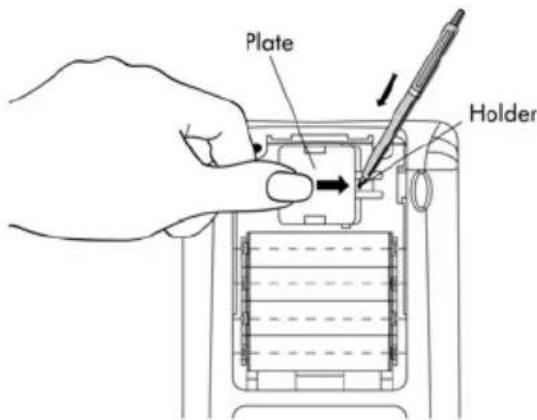
b. Insert a new CR2032 lithium battery. Make sure its positive (+) side is facing up.
c. Replace the plate and push it to the original place.
After installing the batteries, press [ON] to turn the power on.
Warning: When the low battery icon is displayed, you need to replace the batteries as soon as possible. However, avoid removing the backup battery and main batteries at the same time to avoid data lost.
Turning the calculator on and off
The ON key is located at the lower left corner of the keyboard. Press it once to turn your calculator on. To turn the calculator off, press the right-shift key (first key in the second row from the bottom of the keyboard), followed by the ON key. Notice that the ON key has a OFF label printed in the upper right corner as a reminder of the OFF command.
Adjusting the display contrast
You can adjust the display contrast by holding the ON key while pressing the + or - keys. The ON (hold) + key combination produces a darker display. The ON (hold) - key combination produces a lighter display
Contents of the calculator's display
Turn your calculator on once more. The display should look as indicated below.

At the top of the display you will have two lines of information that describe the settings of the calculator. The first line shows the characters:
RAD XYZ HEX R= 'X'
For details on the meaning of these symbols see Chapter 2.
The second line shows the characters: { HOME } indicating that the HOME directory is the current file directory in the calculator's memory. In Chapter 2 you will learn that you can save data in your calculator by storing them in files or variables. Variables can be organized into directories and sub-directories. Eventually, you may create a branching tree of file directories, similar to those in a computer hard drive. You can then navigate through the file directory tree to select any directory of interest. As you navigate through the file directory the second line of the display will change to reflect the proper file directory and sub-directory.
At the bottom of the display you will find a number of labels, namely,
[0] [1] [2] [3] [4] [5] [6] [7] [8] [9]
associated with the six soft menu keys, F1 through F6:
F1 F2 F3 F4 F5 F6
The six labels displayed in the lower part of the screen will change depending on which menu is displayed. But 1 will always be associated with the first displayed label, 2 with the second displayed label, and so on.
Menus
The six labels associated with the keys F1 through F6 form part of a menu of functions. Since the calculator has only six soft menu keys, it only display 6 labels at any point in time. However, a menu can have more than six entries.
Each group of 6 entries is called a Menu page. The current menu, known as the TOOL menu (see below), has eight entries arranged in two pages. The next page, containing the next two entries of the menu is available by pressing the NXT (NeXT menu) key. This key is the third key from the left in the third row of keys in the keyboard. Press NXT once more to return to the main TOOL menu, or press the TOOL key (third key in second row of keys from the top of the keyboard).
The TOOL menu is described in detain in the next section. At this point we will illustrate some properties of menus that you will find useful while using your calculator.
SOFT menus vs. CHOOSE boxes
Menus, or SOFT menus, associate labels in the lower part of the screen with the six soft menu keys (F1 through F6). By pressing the appropriate soft menu key, the function shown in the associated label gets activated. For example, with the TOOL menu active, pressing the CLEAR key (F6) activates function CLEAR, which erases (clears up) the contents of the screen. To see this function in action, type a number, say 1 2 3 ENTER, and then press the F6 key.
SOFT menus are typically used to select from among a number of related functions. However, SOFT menus are not the only way to access collections of related functions in the calculator. The alternative way will be referred to as CHOOSE boxes. To see an example of a choose box, activate the TOOL menu (press TOOL), and then press the keystroke combination → BASE (associated with the 3 key). This will provide the following CHOOSE box:

This CHOOSE box is labeled BASE MENU and provides a list of numbered functions, from 1. HEX x to 6. B→R. This display will constitute the first page of this CHOOSE box menu showing six menu functions. You can navigate through the menu by using the up and down arrow keys, ▲▼, located in the upper right side of the keyboard, right under the F5 and F6 soft menu keys. To activate any given function, first, highlight the function name by using the up and down arrow keys, ▲▼, or by pressing the number corresponding to the function in the CHOOSE box. After the function name is selected, press the soft menu key (F6). Thus, if you wanted to use function R→B (Real to Binary), you could press 6 F6.
If you want to move to the top of the current menu page in a CHOOSE box, use ← ▲. To move to the bottom of the current page, use ← ▼. To move to the top of the entire menu, use → ▲. To move to the bottom of the entire menu, use → ▼.
Selecting SOFT menus or CHOOSE boxes
You can select the format in which your menus will be displayed by changing a setting in the calculator system flags (A system flag is a calculator variable that controls a certain calculator operation or mode. For more information about flags, see Chapter 24). System flag 117 can be set to produce either SOFT menus or CHOOSE boxes. To access this flag use:

Your calculator will show the following screen, highlighting the line starting with the number 117:

By default, the line will look as shown above. The highlighted line (117 CHOOSE boxes) indicates that CHOOSE boxes are the current menu display setting. If you prefer to use SOFT menu keys, press the √☐ soft menu key (F3), followed by ☐ (F6). Press ☐ (F6) once more to return to normal calculator display.
If you now press → BASE, instead of the CHOOSE box that you saw earlier, the display will now show six soft menu labels as the first page of the STACK menu:

To navigate through the functions of this menu, press the NXT key to move to the next page, or ← PREV (associated with the NXT key) to move to the previous page. The following figures show the different pages of the BASE menu accessed by pressing the NXT key twice:


Pressing the NXT key once more will takes us back to the first menu page.
Note: With the SOFT menu setting for system flag 117, the keystroke combination (hold), will show a list of the functions in the current soft menu. For example, for the two first pages in the BASE menu, you will get:


To revert to the CHOOSE boxes setting, use:
MODE
Notes:
-
The TOOL menu, obtained by pressing TOOL, will always produce a SOFT menu.
-
Most of the examples in this User's Manual are shown using both SOFT menus and CHOOSE boxes. Programming applications (Chapters 21 and 22) use exclusively SOFT menus.
-
Additional information on SOFT menus vs. CHOOSE boxes is presented in Chapter 2 of this guide.
The TOOL menu
The soft menu keys for the menu currently displayed, known as the TOOL menu, are associated with operations related to manipulation of variables (see pages for more information on variables):
F1 EDIT the contents of a variable (see Chapter 2 and Appendix L for more information on editing)
F2 VIEW the contents of a variable
ReCall the contents of a variable
F4 STOre the contents of a variable
F5 PURGE a variable
F6 CLEAR the display or stack
The calculator has only six soft menu keys, and can only display 6 labels at any point in time. However, a menu can have more than six entries. Each group of 6 entries is called a Menu page. The TOOL menu has eight entries arranged in two pages. The next page, containing the next two entries of the menu are available by pressing the NXT (NeXT menu) key. This key is the third key from the left in the third row of keys in the keyboard.
In this case, only the first two soft menu keys have commands associated with them. These commands are:
F1 CASCMD: CAS CoMmanD, used to launch a command from the CAS by selecting from a list
HELP F2 HELP facility describing the commands available
Pressing the NXT key will show the original TOOL menu. Another way to recover the TOOL menu is to press the TOOL key (third key from the left in the second row of keys from the top of the keyboard).
Setting time and date
The calculator has an internal real time clock. This clock can be continuously displayed on the screen and be used for alarms as well as running scheduled tasks. This section will show not only how to set time and date, but also the basics of using CHOOSE boxes and entering data in a dialog box. Dialog boxes on your calculator are similar to a computer dialog box.
To set time and date we use the TIME choose box available as an alternative function for the 9 key. By combining the right-shift button, ↗, with the
9 key the TIME choose box is activated. This operation can also be represented as → TIME. The TIME choose box is shown in the figure below:
![RAD XYZ HEX R~ 'X' (HOME) 1.Browse alarms.. 2.Set alarm.. 3.Set time, date.. 4.Tools.. [CANCEL] OK](/content/2026/05/1018706/images/c44c02eced44497daff82860007bcb45c1fe559f48690462710b58b9c0278952.jpg)
As indicated above, the TIME menu provides four different options, numbered 1 through 4. Of interest to us as this point is option 3. Set time, date... Using the down arrow key, ▼, highlight this option and press the 📄 soft menu key. The following input form (see Appendix 1-A) for adjusting time and date is shown:

Setting the time of the day
Using the number keys, 1234567890, start by adjusting the hour of the day. Suppose that we change the hour to 11, by pressing 11 as the hour field in the SET TIME AND DATE input form is highlighted. This results in the number 11 being entered in the lower line of the input form:
![SET TIME AND DATE Time: 2:01:34 PM Date: 3/30/03 M/D/Y 11 [CANCEL] OK](/content/2026/05/1018706/images/4b05c5b7cc4a5cd4eb141fb7a4fb9b3c263b56d07c4444b3245c043e816e379c.jpg)
Press the soft menu key to effect the change. The value of 11 is now shown in the hour field, and the minute field is automatically highlighted:

Let's change the minute field to 25, by pressing: 2 5 . The seconds field is now highlighted. Suppose that you want to change the seconds field to 45, use: 4 5
The time format field is now highlighted. To change this field from its current setting you can either press the +/- key (the second key from the left in the fifth row of keys from the bottom of the keyboard), or press the 2 soft menu key ( F2 ).
- If using the +/- key, the setting in the time format field will change to either of the following options:
- AM: indicates that displayed time is AM time
o PM : indicates that displayed time is PM time
o 24-hr : indicates that that the time displayed uses a 24 hour format where 18:00, for example, represents 6pm
The last selected option will become the set option for the time format by using this procedure.
• If using the 📄️ soft menu key, the following options are available.

Use the up and down arrow keys, ▲ ▼, to select among these three options (AM, PM, 24-hour time). Press the soft menu key to make the selection.
Setting the date
After setting the time format option, the SET TIME AND DATE input form will look as follows:
![SET TIME AND DATE Time: 11:25:45 PM Date: 3/30/03 M/D/Y Choose AM, PM, or 24-hour time [CHOOS] | [CANCEL] OK](/content/2026/05/1018706/images/d96e6008e41363944809eedb1e723c5ae6648e05217a44158ade5e30f6b8b236.jpg)
To set the date, first set the date format. The default format is M/D/Y (month/day/year). To modify this format, press the down arrow key. This will highlight the date format as shown below:
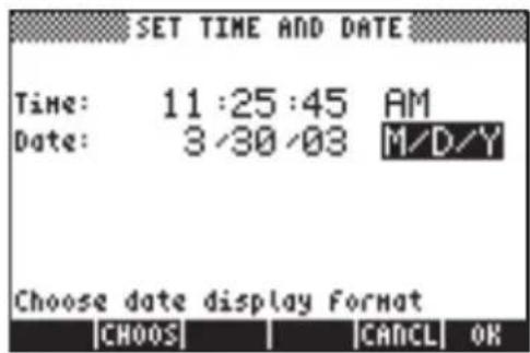
Use the ☐ soft menu key to see the options for the date format:

Highlight your choice by using the up and down arrow keys, ▲ ▼ , and press the soft menu key to make the selection.
Introducing the calculator's keyboard
The figure below shows a diagram of the calculator's keyboard with the numbering of its rows and columns.

The figure shows 10 rows of keys combined with 3, 5, or 6 columns. Row has 6 keys, rows 2 and 3 have 3 keys each, and rows 4 through 10 have 5 keys each. There are 4 arrow keys located on the right-hand side of the keyboard in the space occupied by rows 2 and 3.
Each key has three, four, or five functions. The main key function correspond to the most prominent label in the key. Also, the left-shift key, key (8,1), the right-
shift key, key (9,1), and the ALPHA key, key (7,1), can be combined with some of the other keys to activate the alternative functions shown in the keyboard. For example, the SYMB key, key(4,4), has the following six functions associated with it:
SYMB Main function, to activate the SYMBOLic menu
← MTH Left-shift function, to activate the MTH (Math) menu
CAT Right-shift function, to activate the CATalog function
ALPHA P ALPHA function, to enter the upper-case letter P
ALPHA ← P ALPHA-Left-Shift function, to enter the lower-case letter p
ALPHA → P ALPHA-Right-Shift function, to enter the symbol P
Of the six functions associated with the key only the first four are shown in the keyboard itself. This is the way that the key looks in the keyboard:
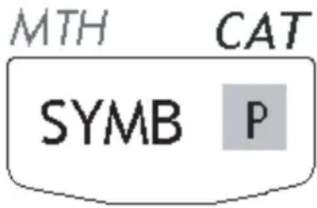
Notice that the color and the position of the labels in the key, namely, SYMB, MTH, CAT and P, indicate which is the main function (SYMB), and which of the other three functions is associated with the left-shift ← (MTH), right-shift → (CAT), and ALPHA (P) keys.
For detailed information on the calculator keyboard operation referee to Appendix B.
Selecting calculator modes
This section assumes that you are now at least partially familiar with the use of choose and dialog boxes (if you are not, please refer to Chapter 2).
Press the MODE button (second key from the left on the second row of keys from the top) to show the following CALCULATOR MODES input form:

Press the soft menu key to return to normal display. Examples of selecting different calculator modes are shown next.
Operating Mode
The calculator offers two operating modes: the Algebraic mode, and the Reverse Polish Notation (RPN) mode. The default mode is the Algebraic mode (as indicated in the figure above), however, users of earlier HP calculators may be more familiar with the RPN mode.
To select an operating mode, first open the CALCULATOR MODES input form by pressing the MODE button. The Operating Mode field will be highlighted. Select the Algebraic or RPN operating mode by either using the +/- key (second from left in the fifth row from the keyboard bottom), or pressing the soft menu key. If using the latter approach, use up and down arrow keys, ▲ ▼, to select the mode, and press the soft menu key to complete the operation.
To illustrate the difference between these two operating modes we will calculate the following expression in both modes:
√ 3 · (5 - 1/3 · 3)2 3 ^ 3 e ^ 2. 5
To enter this expression in the calculator we will first use the equation writer, → EQW. Please identify the following keys in the keyboard, besides the numeric keypad keys:

The equation writer is a display mode in which you can build mathematical expressions using explicit mathematical notation including fractions, derivatives, integrals, roots, etc. To use the equation writer for writing the expression shown above, use the following keystrokes:

After pressing ENTER the calculator displays the expression:
√ (3 * (5 - 1 / (3 * 3)) / 2 3 ^ 3 + EXP (2 . 5))
Pressing ENTER again will provide the following value. Accept Approx. mode on, if asked, by pressing 📄. [Note: The integer values used above, e.g., 3, 5, 1, represent exact values. The EXP(2.5), however, cannot be expressed as an exact value, therefore, a switch to Approx mode is required]:

You could also type the expression directly into the display without using the equation writer, as follows:

to obtain the same result.
Change the operating mode to RPN by first pressing the MODE button. Select the RPN operating mode by either using the +/- key, or pressing the 4000 soft menu key. Press the 4000 soft menu key to complete the operation. The display, for the RPN mode looks as follows:

Notice that the display shows several levels of output labeled, from bottom to top, as 1, 2, 3, etc. This is referred to as the stack of the calculator. The different levels are referred to as the stack levels, i.e., stack level 1, stack level 2, etc.
In RPN mode, instead of writing an operation such as 3 + 2 by pressing 3 + 2 ENTER, we write the operands first, in the proper order, and then the operator, i.e., 3 ENTER 2 +. As you enter the operands, they occupy different stack levels. Entering 3 ENTER puts the number 3 in stack level 1. Next, entering 2 pushes the 3 upwards to occupy stack level 2. Finally, by pressing +, we are telling the calculator to apply the operator, or program, + to the objects occupying levels 1 and 2. The result, 5, is then placed in level 1.
Let's try some other simple operations before trying the more complicated expression used earlier for the algebraic operating mode:
123/32
1 2 3 ENTER 3 2 ÷
42
4 ENTER 2 γx
3√[3]27
2 7 ENTER 3 → √y
Notice the position of the y and the x in the last two operations. The base in the exponential operation is y (stack level 2) while the exponent is x (stack level 1) before the key yx is pressed. Similarly, in the cubic root operation, y (stack level 2) is the quantity under the root sign, and x (stack level 1) is the root.
Try the following exercise involving 3 factors: (5 + 3) × 2
5 ENTER 3 + Calculates (5 + 3) first.
2 x Completes the calculation.
Let's try now the expression proposed earlier:
√ 3 · (5 - 1/3 · 3)2 3 ^ 3 e ^ 2. 5
3 · ENTER Enter 3 in level 1 ⑤ · ENTER Enter 5 in level 1, 3 moves to y 3 · ENTER Enter 3 in level 1,5 moves to level 2,3 to level 3 3 · × Place 3 and multiply, 9 appears in level 1 /x 1 / (3 × 3), last value in lev. 1; 5 in level 2; 3 in level 3 5 - 1 / (3 × 3), occupies level 1 now; 3 in level 2 × 3 × (5 - 1 / (3 × 3)), occupies level 1 now. 2 3 · ENTER Enter 23 in level 1, 14.66666 moves to level 2. 3 · r ^ x Enter 3, calculate 2 3 ^ 3 into level 1. 1 4. 6 6 6 in lev. 2. ÷ (3 × (5 - 1 / (3 × 3))) / 2 3 ^ 3 intolevel1 2 · 5 Enter 2. 5 level 1 ⓔ ^ x e ^ 2. 5, goes into level 1, level 2 shows previous value. + (3 × (5 - 1 / (3 × 3))) / 2 3 ^ 3 + e ^ 2. 5 = 1 2. 1 8 3 6 9, into lev. 1. √ X √ ((3 × (5 - 1 / (3 × 3))) / 2 3 ^ 3 + e ^ 2 . 5) = 3. 4 9 0 5 1 5 6, into 1.
Although RPN requires a little bit more thought than the algebraic (ALG) mode, there are multiple advantages in using RPN. For example, in RPN mode you can see the equation unfolding step by step. This is extremely useful to detect a possible input error. Also, as you become more efficient in this mode and learn more of the tricks, you will be able to calculate expression faster and will much less keystrokes. Consider, for example the calculation of (46 - 5)/(1 + 4 × 6 - 5) . In RPN mode you can write:
4 ENTER 6 × 5 - ENTER 1 + ÷
obviously, even In RPN mode, you can enter an expression in the same order as the algebraic mode by using the Equation writer. For example,
→ EQW √ X 3 × ← () 5 -
1 ÷ 3 · × 3 ·
÷ 2 3 y ^ x 3 + ← e ^ x 2 5 ENTER
The resulting expression is shown in stack level 1 as follows:

Notice how the expression is placed in stack level 1 after pressing ENTER. Pressing the EVAL key at this point will evaluate the numerical value of that expression Note: In RPN mode, pressing ENTER when there is no command line will execute the DUP function which copies the contents of stack level 1 of the stack onto level 2 (and pushes all the other stack levels one level up). This is extremely useful as showed in the previous example.
To select between the ALG vs. RPN operating mode, you can also set/clear system flag 95 through the following keystroke sequence:

Alternatively, you can use one of the following shortcuts:
• In ALG mode, CF(-95) selects RPN mode
- In RPN mode, 95 +/- ENTER SF selects ALG mode
For more information on calculator's system flags see Chapter 2.
Number Format and decimal dot or comma
Changing the number format allows you to customize the way real numbers are displayed by the calculator. You will find this feature extremely useful in operations with powers of tens or to limit the number of decimals in a result.
To select a number format, first open the CALCULATOR MODES input form by pressing the MODE button. Then, use the down arrow key, ▼, to select the option Number format. The default value is Std, or Standard format. In the standard format, the calculator will show floating-point numbers with the maximum precision allowed by the calculator (12 significant digits). To learn
more about reals, see Chapter 2. To illustrate this and other number formats try the following exercises:
- Standard format:
This mode is the most used mode as it shows numbers in the most familiar notation.
Press the 📄️ soft menu key, with the Number format set to Std, to return to the calculator display. Enter the number 123.4567890123456. Notice that this number has 16 significant figures. Press the ENTER key. The number is rounded to the maximum 12 significant figures, and is displayed as follows:
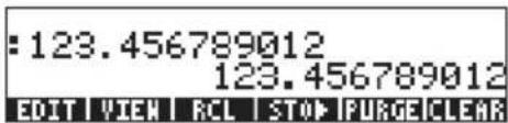
In the standard format of decimal display, integer numbers are shown with no decimal zeros whatsoever. Numbers with different decimal figures will be adjusted in the display so that only those decimal figures that are necessary will be shown. More examples of numbers in standard format are shown next:
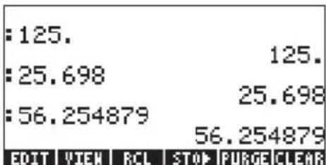
- Fixed format with no decimals: Press the MODE button. Next, use the down arrow key, ▼, to select the option Number format. Press the ◯ soft menu key, and select the option Fixed with the arrow down key ▼.

Notice that the Number Format mode is set to Fix followed by a zero (0). This number indicates the number of decimals to be shown after the decimal point in the calculator's display. Press the soft menu key to return to the calculator display. The number now is shown as:
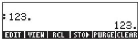
This setting will force all results to be rounded to the closest integer (0 digit displayed after the comma). However, the number is still stored by the calculator with its full 12 significant digit precision. As we change the number of decimals to be displayed, you will see the additional digits being shown again.
- Fixed format with decimals:
This mode is mainly used when working with limited precision. For example, if you are doing financial calculation, using a FIX 2 mode is convenient as it can easily represent monetary units to a 1/100 precision. Press the MODE button. Next, use the down arrow key, ▼, to select the option Number format. Press the ▼ soft menu key, and select the option Fixed with the arrow down key ▼.
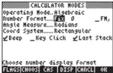
Press the right arrow key, ⬆, to highlight the zero in front of the option Fix. Press the □□□□□ soft menu key and, using the up and down arrow keys, ▲▼, select, say, 3 decimals.
![Oper Numb Angl Coor Be Choo 0 1 2 3 4 5 6 7 8 FM, tack lay [CANCEL] OK](/content/2026/05/1018706/images/5500a77cc254f30545a718cb0c716ccf213f737728c1c80d4e37748ae5ed4ce7.jpg)
Press the soft menu key to complete the selection:

Press the soft menu key return to the calculator display. The number now is shown as:

Notice how the number is rounded, not truncated. Thus, the number 123.4567890123456, for this setting, is displayed as 123.457, and not as 123.456 because the digit after 6 is > 5
- Scientific format
The scientific format is mainly used when solving problems in the physical sciences where numbers are usually represented as a number with limited precision multiplied by a power of ten.
To set this format, start by pressing the MODE button. Next, use the down arrow key, ▼, to select the option Number format. Press the EIDE soft menu key and select the option Scientific with the arrow down key ▼. Keep the number 3 in front of the Sci. (This number can be changed in the
same fashion that we changed the Fixed number of decimals in the example above).

Press the ☐ soft menu key return to the calculator display. The number now is shown as:

This result, 1.23E2, is the calculator's version of powers-of-ten notation, i.e., 1.235 × 10² . In this, so-called, scientific notation, the number 3 in front of the Sci number format (shown earlier) represents the number of significant figures after the decimal point. Scientific notation always includes one integer figure as shown above. For this case, therefore, the number of significant figures is four.
• Engineering format
The engineering format is very similar to the scientific format, except that the powers of ten are multiples of three.
To set this format, start by pressing the MODE button. Next, use the down arrow key, ▼, to select the option Number format. Press the 📄️ soft menu key and select the option Engineering with the arrow down key ▼. Keep the number 3 in front of the Eng. (This number can be changed in the same fashion that we changed the Fixed number of decimals in an earlier example).

Press the soft menu key return to the calculator display. The number now is shown as:

Because this number has three figures in the integer part, it is shown with four significative figures and a zero power of ten, while using the Engineering format. For example, the number 0.00256, will be shown as:
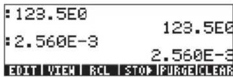
- Decimal comma vs. decimal point
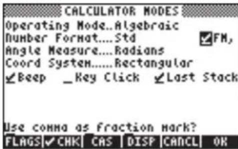
Decimal points in floating-point numbers can be replaced by commas, if the user is more familiar with such notation. To replace decimal points for commas, change the FM option in the CALCULATOR MODES input form to commas, as follows (Notice that we have changed the Number Format to Std):
- Press the MODE button. Next, use the down arrow key, ▼, once, and the right arrow key, ▶, highlighting the option _FM,. To select commas, press the √≡≡ soft menu key. The input form will look as follows:
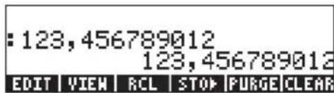
- Press the soft menu key return to the calculator display. The number 123.456789012, entered earlier, now is shown as:
Angle Measure
Trigonometric functions, for example, require arguments representing plane angles. The calculator provides three different Angle Measure modes for working with angles, namely:
- Degrees: There are 360 degrees (360°) in a complete circumference, or 90 degrees (90°) in a right angle. This representation is mainly used when doing basic geometry, mechanical or structural engineering, and surveying.
- Radians: There are 2 π radians ( 2 πr ) in a complete circumference, or π / 2 radians ( π / 2r ) in a right angle. This notation is mainly used when solving mathematics and physics problems. This is the default mode of the calculator.
- Grades: There are 400 grades (400 g) in a complete circumference, or 100 grades (100 g) in a right angle. This notation is similar to the degree mode, and was introduced in order to "simplify" the degree notation but is seldom used now.
The angle measure affects the trig functions like SIN, COS, TAN and associated functions.
To change the angle measure mode, use the following procedure:
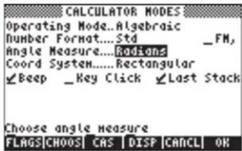
- Press the MODE button. Next, use the down arrow key, ▼, twice. Select the Angle Measure mode by either using the +/- key (second from left in the fifth row from the keyboard bottom), or pressing the soft menu
key. If using the latter approach, use up and down arrow keys, ▲ ▼, to select the preferred mode, and press the 🎯 soft menu key to complete the operation. For example, in the following screen, the Radians mode is selected:
Coordinate System
The coordinate system selection affects the way vectors and complex numbers are displayed and entered. To learn more about complex numbers and vectors, see Chapters 4 and 9, respectively.
Two- and three-dimensional vector components and complex numbers can be represented in any of 3 coordinate systems: The Cartesian (2 dimensional) or Rectangular (3 dimensional), Cylindrical (3 dimensional) or Polar (2 dimensional), and Spherical (only 3 dimensional). In a Cartesian or Rectangular coordinate system a point P will have three linear coordinates (x,y,z) measured from the origin along each of three mutually perpendicular axes (in 2 d mode, z is assumed to be 0). In a Cylindrical or Polar coordinate system the coordinates of a point are given by (rθ,z), where r is a radial distance measured from the origin on the xy plane, θ is the angle that the radial distance r forms with the positive x axis -- measured as positive in a counterclockwise direction -, and z is the same as the z coordinate in a Cartesian system (in 2 d mode, z is assumed to be 0). The Rectangular and Polar systems are related by the following quantities:
x = r · (θ) r = √ x ^ 2 + y ^ 2 y = r · (θ) θ = ^ - 1 (y/x) z = z
In a Spherical coordinate system the coordinates of a point are given by (ρ, θ, φ) where ρ is a radial distance measured from the origin of a Cartesian system, θ is an angle representing the angle formed by the projection of the linear distance ρ onto the xy axis (same as θ in Polar coordinates), and φ is the angle
from the positive z axis to the radial distance ρ . The Rectangular and Spherical coordinate systems are related by the following quantities:
ρ φx (θ) (ρ √ 2 ^ 2 + 2 x) = y = ρ · φ · (θ) in ( θ = ^ - 1 (y/x) z = ρ · φ) ( φ = ^ - 1 ( √ x ^ 2 + y ^ 2z)
To change the coordinate system in your calculator, follow these steps:
- Press the MODE button. Next, use the down arrow key, ▼, three times. Select the Angle Measure mode by either using the +/- key (second from left in the fifth row from the keyboard bottom), or pressing the EMODE soft menu key. If using the latter approach, use up and down arrow keys, ▲, to select the preferred mode, and press the □□□□ soft menu key to complete the operation. For example, in the following screen, the Polar coordinate mode is selected:

Beep, Key Click, and Last Stack
The last line of the CALCULATOR MODES input form include the options:
_Beep _Key Click _Last Stack
By choosing the check mark next to each of these options, the corresponding option is activated. These options are described next:
_Beep : When selected, , the calculator beeper is active. This operation mainly applies to error messages, but also some user functions like BEEP.
_Key Click : When selected, each keystroke produces a "click" sound.
_Last Stack: Keeps the contents of the last stack entry for use with the functions UNDO and ANS (see Chapter 2).
The _Beep option can be useful to advise the user about errors. You may want to deselect this option if using your calculator in a classroom or library.
The _Key Click option can be useful as an audible way to check that each keystroke was entered as intended.
The _Last Stack option is very useful to recover the last operation in case we need it for a new calculation.
To select, or deselect, any of these three options, first press the MODE button. Next,
- Use the down arrow key, ▼, four times to select the _Last Stack option. Use the √□□□□ soft menu key to change the selection.
- Press the left arrow key ⏻ to select the _Key Click option. Use the √Ⓧ soft menu key to change the selection.
- Press the left arrow key ⬆ to select the _Beep option. Use the √□□□ soft menu key to change the selection.
Press the ☐ soft menu key to complete the operation.
Selecting CAS settings
CAS stands for Computer Algebraic System. This is the mathematical core of the calculator where the symbolic mathematical operations and functions are programmed and performed. The CAS offers a number of settings can be adjusted according to the type of operation of interest. These are:
• The default independent variable
- Numeric vs. symbolic mode
- Approximate vs. Exact mode
- Verbose vs. Non-verbose mode
- Step-by-step mode for operations
- Increasing power format for polynomials
- Rigorous mode
- Simplification of non-rational expressions
Details on the selection of CAS settings are presented in Appendix C.
Selecting Display modes
The calculator display can be customized to your preference by selecting different display modes. To see the optional display settings use the following:
- First, press the MODE button to activate the CALCULATOR MODES input form. Within the CALCULATOR MODES input form, press the OES soft menu key to display the DISPLAY MODES input form.
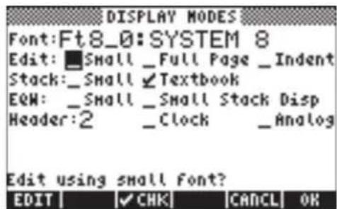
- To navigate through the many options in the DISPLAY MODES input form, use the arrow keys: ◀ ▶ ▼ ▲.
- To select or deselect any of the settings shown above, that require a check mark, select the underline before the option of interest, and toggle the ∥ ∥ ∥ ∥ ∥ ∥ ∥ ∥ ∥ ∥ ∥ ∥ ∥ ∥ ∥ ∥ ∥ ∥ ∥ ∥ ∥ ∥ ∥ ∥ ∥ ∥ ∥ ∥ ∥ ∥ ∥ ∥ ∥ ∥ ∥ ∥ ∥ ∥ ∥ ∥ ∥ ∥ ∥ ∥ ∥ ∥ ∥ ∥ ∥ ∥ ∣ ∣ ∣ ∣ ∣ ∣ ∣ ∣ ∣ ∣ ∣ ∣ ∣ ∣ ∣ ∣ ∣ ∣ ∣ ∣ ∣ ∣ ∣ ∣ ∣ ∣ ∣ ∣
• To select the Font for the display, highlight the field in front of the Font: option in the DISPLAY MODES input form, and use the soft menu key.
• After having selected and unselected all the options that you want in the DISPLAY MODES input form, press the soft menu key. This will take you back to the CALCULATOR MODES input form. To return to normal calculator display at this point, press the soft menu key once more.
Selecting the display font
Changing the font display allows you to have the calculator look and feel changed to your own liking. By using a 6-pixel font, for example, you can display up to 9 stack levels! Follow these instructions to select your display font: First, press the MODE button to activate the CALCULATOR MODES input form. Within the CALCULATOR MODES input form, press the soft menu key to display the DISPLAY MODES input form. The Font: field is highlighted, and the option Ft8_0:system 8 is selected. This is the default value of the display font.
Pressing the 📄️soft menu key will provide a list of available system fonts, as shown below:

The options available are three standard System Fonts (sizes 8, 7, and 6) and a Browse.. option. The latter will let you browse the calculator memory for additional fonts that you may have created (see Chapter 23) or downloaded into the calculator.
Practice changing the display fonts to sizes 7 and 6. Press the OK soft menu key to effect the selection. When done with a font selection, press the soft menu key to go back to the CALCULATOR MODES input form. To return to normal calculator display at this point, press the soft menu key once more and see how the stack display change to accommodate the different font.
Selecting properties of the line editor
First, press the MODE button to activate the CALCULATOR MODES input form. Within the CALCULATOR MODES input form, press the soft menu key to display the DISPLAY MODES input form. Press the down arrow key, ▼, once, to get to the Edit line. This line shows three properties that can be modified. When these properties are selected (checked) the following effects are activated:
_Small Changes font size to small
_Full page Allows to place the cursor after the end of the line
_Indent Auto intend cursor when entering a carriage return
Detailed instructions on the use of the line editor are presented in Chapter 2 in this guide.
Selecting properties of the Stack
First, press the MODE button to activate the CALCULATOR MODES input form. Within the CALCULATOR MODES input form, press the soft menu key to
display the DISPLAY MODES input form. Press the down arrow key, ▼, twice, to get to the Stack line. This line shows two properties that can be modified. When these properties are selected (checked) the following effects are activated:
_Small Changes font size to small. This maximized the amount of information displayed on the screen. Note, this selection overrides the font selection for the stack display.
_Textbook Display mathematical expressions in graphical mathematical notation
To illustrate these settings, either in algebraic or RPN mode, use the equation writer to type the following definite integral:

In Algebraic mode, the following screen shows the result of these keystrokes with neither _Small nor _Textbook are selected:

With the _Small option selected only, the display looks as shown below:

With the _Textbook option selected (default value), regardless of whether the _Small option is selected or not, the display shows the following result:

Selecting properties of the equation writer (EQW)
First, press the MODE button to activate the CALCULATOR MODES input form. Within the CALCULATOR MODES input form, press the soft menu key to display the DISPLAY MODES input form. Press the down arrow key, ▼, three
times, to get to the EQW (Equation Writer) line. This line shows two properties that can be modified. When these properties are selected (checked) the following effects are activated:
_Small Changes font size to small while using the equation editor
_Small Stack Disp Shows small font in the stack for textbook style display Detailed instructions on the use of the equation editor (EQW) are presented elsewhere in this manual.
For the example of the integral 0∞ preserved above, selecting the
_Small Stack Disp in the EQW line of the DISPLAY MODES input form produces the following display:

Selecting the size of the header
First, press the MODE button to activate the CALCULATOR MODES input form. Within the CALCULATOR MODES input form, press the soft menu key to display the DISPLAY MODES input form. Press the down arrow key, ▼, four times, to get to the Header line. The value 2 is assigned to the Header field by default. This means that the top part of the display will contain two lines, one showing the current settings of the calculator, and a second one showing the current sub directory within the calculator's memory (These lines were described earlier in the manual). The user can select to change this setting to 1 or 0 to reduce the number of header lines in the display.
Selecting the clock display
First, press the MODE button to activate the CALCULATOR MODES input form. Within the CALCULATOR MODES input form, press the soft menu key to display the DISPLAY MODES input form. Press the down arrow key, ▼, four times, to get to the Header line. The Header field will be highlighted. Use the
right arrow key (▶) to select the underline in front of the options _Clock or _Analog. Toggle the √□□□ soft menu key until the desired setting is achieved. If the _Clock option is selected, the time of the day and date will be shown in the upper right corner of the display. If the _Analog option is also selected, an analog clock, rather than a digital clock, will be shown in the upper right corner of the display. If the _Clock option is not selected, or the header is not present, or too small, the date and time of day will not be shown in the display.
Chapter 2 Introducing the calculator
In this chapter we present a number of basic operations of the calculator including the use of the Equation Writer and the manipulation of data objects in the calculator. Study the examples in this chapter to get a good grasp of the capabilities of the calculator for future applications.
Calculator objects
Any number, expression, character, variable, etc., that can be created and manipulated in the calculator is referred to as an object. Some of the most useful type of objects are listed below.
Real. These object represents a number, positive or negative, with 12 significant digits and an exponent ranging from -499 to +499. example of reals are: 1., -5., 56.41564 1.5E45, -555.74E-95
When entering a real number, you can use the EEX key to enter the exponent and the +/- key to change the sign of the exponent or mantissa.
Note that real must be entered with a decimal point, even if the number does not have a fractional part. Otherwise the number is taken as an integer number, which is a different calculator objects. Reals behave as you would expect a number to when used in a mathematical operation.
Integers. These objects represent integer numbers (numbers without fractional part) and do not have limits (except the memory of the calculator). Example of integers are: 1, 564654112, -413165467354646765465487. Note how these numbers do not have a decimal point.
Due to their storage format, integer numbers are always maintain full precision in their calculation. For example, an operation such as 30/14, with integer numbers, will return 15/7 and not 2.142.... To force a real (or floating-point) result, use function → NUM → → NUM .
Integers are used frequently in CAS-based functions as they are designed to keep full precision in their operation. If the approximate mode (APPROX) is selected in the CAS (see Appendix C), integers will be automatically converted to reals. If you are not planning to use
the CAS, it might be a good idea to switch directly into approximate mode. Refer to Appendix C for more details.
Mixing integers and reals together or mistaking an integer for a real is a common occurrence. The calculator will detect such mixing of objects and ask you if you want to switch to approximate mode.
Complex numbers, are an extension of real numbers that include the unit imaginary number, i2=-1 . A complex number, e.g., 3+2i , is written as (3, 2) in the calculator.
Complex numbers can be displayed in either Cartesian or polar mode depending on the setting selected. Note that complex numbers are always stored in Cartesian mode and that only the display is affected. This allows the calculator to keep as much precision as possible during calculations.
Most mathematics functions work on complex numbers. There is no need to use a special "complex +" function to add complex numbers, you can use the same + function that on reals or integers.
Vector and matrix operations utilize objects of type 3, real arrays, and, if needed, type 4, complex arrays. Objects type 2, strings, are simply lines of text (enclosed between quotes) produced with the alphanumeric keyboard.
A list is just a collection of objects enclosed between curly brackets and separated by spaces in RPN mode (the space key is labeled ), or by commas in algebraic mode. Lists, objects of type 5, can be very useful when processing collections of numbers. For example, the columns of a table can be entered as lists. If preferred, a table can be entered as a matrix or array.
Objects type 8 are programs in User RPL language. These are simply sets of instructions enclosed between the symbols << >>.
Associated with programs are objects types 6 and 7, Global and Local Names, respectively. These names, or variables, are used to store any type of objects. The concept of global or local names is related to the scope or reach of the variable in a given program.
An algebraic object, or simply, an algebraic (object of type 9), is a valid algebraic expression enclosed within quotation or tick marks.
Binary integers, objects of type 10, are used in some computer science applications.
Graphics objects, objects of type 11, store graphics produced by the calculator.
Tagged objects, objects of type 12, are used in the output of many programs to identify results. For example, in the tagged object: Mean: 23.2, the word Mean: is the tag used to identify the number 23.2 as the mean of a sample, for example.
Unit objects, objects of type 13, are numerical values with a physical unit attached to them.
Directories, objects of type 15, are memory locations used to organize your variables in a similar fashion as folders are used in a personal computer.
Libraries, objects of type 16, are programs residing in memory ports that are accessible within any directory (or sub-directory) in your calculator. They resemble built-in functions, objects of type 18, and built-in commands, objects of type 19, in the way they are used.
Editing expressions on the screen
In this section we present examples of expression editing directly into the calculator display (algebraic history or RPN stack).
Creating arithmetic expressions
For this example, we select the Algebraic operating mode and select a Fix format with 3 decimals for the display. We are going to enter the arithmetic expression:
5. 0 · 1 . 0 + 1 . 0/7 . 5√ - 0 . 3 2 0 . 3
To enter this expression use the following keystrokes:

The resulting expression is: 5.*(1.+1./7.5)/(√3.-2.^3).
Press ENTER to get the expression in the display as follows:

Notice that, if your CAS is set to EXACT (see Appendix C) and you enter your expression using integer numbers for integer values, the result is a symbolic quantity, e.g.,

Before producing a result, you will be asked to change to Approximate mode. Accept the change to get the following result (shown in Fix decimal mode with three decimal places – see Chapter 1):

In this case, when the expression is entered directly into the stack. As soon as you press ENTER, the calculator will attempt to calculate a value for the expression. If the expression is entered between quotes, however, the calculator will reproduce the expression as entered. In the following example, we enter the same expression as above, but using quotes. For this case we set the operating mode to Algebraic, the CAS mode to Exact (deselect _Approx), and the display setting to Textbook. The keystrokes to enter the expression are the following:

The result will be shown as follows:
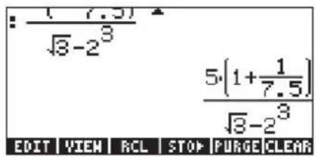
To evaluate the expression we can use the EVAL function, as follows:
EVAL ← ANS ENTER
As in the previous example, you will be asked to approve changing the CAS setting to Approx. Once this is done, you will get the same result as before.
An alternative way to evaluate the expression entered earlier between quotes is by using the option → → NUM. To recover the expression from the existing stack, use the following keystrokes: → NUM
We will now enter the expression used above when the calculator is set to the RPN operating mode. We also set the CAS to Exact and the display to Textbook. The keystrokes to enter the expression between quotes are the same used earlier, i.e.,

Resulting in the output
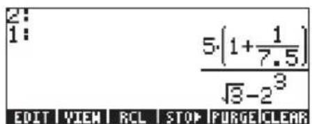
Press ENTER once more to keep two copies of the expression available in the stack for evaluation. We first evaluate the expression using the function EVAL, and next using the function → NUM.
Here are the steps explained in detail: First, evaluate the expression using function EVAL. The resulting expression is semi-symbolic in the sense that there are floating-point components to the result, as well as a√3. Next, we switch stack locations and evaluate using function →NUM:
Exchange stack levels 1 and 2 (the SWAP command)
Evaluate using function → NUM
This latter result is purely numerical, so that the two results in the stack, although representing the same expression, seem different. To verify that they are not, we subtract the two values and evaluate this difference using function EVAL:
- Subtract level 1 from level 2
EVAL Evaluate using function EVAL
The result is zero (0.).
Note: Avoid mixing integer and real data to avoid conflicts in the calculations. For many physical science and engineering applications, including numerical solution of equation, statistics applications, etc., the APPROX mode (see Appendix C) works better. For mathematical applications, e.g., calculus, vector analysis, algebra, etc., the EXACT mode is preferred. Become acquainted with operations in both modes and learn how to switch from one to the other for different types of operations (see Appendix C).
Editing arithmetic expressions
Suppose that we entered the following expression, between quotes, with the calculator in RPN mode and the CAS set to EXACT:
![1: 5·[1-1/1.75] √5-2³ EDIT VIEW RCL STOP PURGE CLEAR](/content/2026/05/1018706/images/e924dd45aa9590cfbc9180aea5a6d4f8a3b2429c964c894af1faf780fb32ef3c.jpg)
rather than the intended expression: 5. 1 + 1√3 - 23The incorrect expression
was entered by using:

To enter the line editor use ← ▼ . The display now looks as follows:

The editing cursor is shown as a blinking left arrow over the first character in the line to be edited. Since the editing in this case consists of removing some characters and replacing them with others, we will use the right and left arrow keys, ◀▶, to move the cursor to the appropriate place for editing, and the delete key, ◀, to eliminate characters.
The following keystrokes will complete the editing for this case:
- Press the right arrow key, ▶, until the cursor is immediately to the right of the decimal point in the term 1.75
- Press the delete key, ◀, twice to erase the characters 1.
- Press the right arrow key, ▶, once, to move the cursor to the right of the 7
- Type a decimal point with
- Press the right arrow key, ▶, until the cursor is immediately to the right of the √5
- Press the delete key, ▶, once to erase the Character 5
• Type a 3 with 3 - Press ENTER to return to the stack
The edited expression is now available in the stack.

Editing of a line of input when the calculator is in Algebraic operating mode is exactly the same as in the RPN mode. You can repeat this example in Algebraic mode to verify this assertion.
Creating algebraic expressions
Algebraic expressions include not only numbers, but also variable names. As an example, we will enter the following algebraic expression:
2 L √ 1 + x/RR + y + 2 L/b
We set the calculator operating mode to Algebraic, the CAS to Exact, and the display to Textbook. To enter this algebraic expression we use the following keystrokes:

Press ENTER to get the following result:

Entering this expression when the calculator is set in the RPN mode is exactly the same as this Algebraic mode exercise.
Editing algebraic expressions
Editing of an algebraic expression with the line editor is very similar to that of an arithmetic expression (see exercise above). Suppose that we want to modify the expression entered above to read
2 L √ 1 + x ^ 2RR + x + 2 √ L/b
To edit this algebraic expression using the line editor use ← . This activates the line editor, showing the expression to be edited as follows:

The editing cursor is shown as a blinking left arrow over the first character in the line to be edited. As in an earlier exercise on line editing, we will use the right and left arrow keys, ◀▶, to move the cursor to the appropriate place for editing, and the delete key, ◀◀, to eliminate characters.
The following keystrokes will complete the editing for this case:
- Press the right arrow key, ▶, until the cursor is to the right of the x
• Type x 2 to enter the power 2 for the x - Press the right arrow key, ▶, until the cursor is to the right of the y
- Press the delete key, ◀, once to erase the characters y.
• Type ALPHA ← X to enter an x - Press the right arrow key, ▶, 4 times to move the cursor to the right of the *
• Type √X to enter a square root symbol - Type ← to enter a set of parentheses (they come in pairs)
- Press the right arrow key, ▶, once, and the delete key, ◀, once, to delete the right parenthesis of the set inserted above
- Press the right arrow key, ▶, 4 times to move the cursor to the right of the b
- Type ← to enter a second set of parentheses
- Press the delete key, 🔔, once, to delete the left parenthesis of the set inserted above.
- Press ENTER to return to normal calculator display.
The result is shown next:
![: 2·L·√1+X/R + 2·L/b [(2·R+2·x)·√b·L·|R|+2·√R²+x²·] SQ(b·R)·(R+x) EDIT VIEW RCL STOP PURGE CLEAR](/content/2026/05/1018706/images/67975d9d40cc4dd13542275524d6c8c4d19766c3be7875c8bd2e11232d4c521d.jpg)
Notice that the expression has been expanded to include terms such as |R| , the absolute value, and SQ(b· R) , the square of b· R . To see if we can simplify this result, use FACTOR(ANS(1)) in ALG mode:
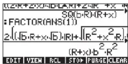
- Press ← ▼ to activate the line editor once more. The result is now:

- Pressing ENTER once more to return to normal display.
To see the entire expression in the screen, we can change the option _Small Stack Disp in the DISPLAY MODES input form (see Chapter 1). After effecting this change, the display will look as follows:
![h+3 [(2-R+2-x)-√b-L·|R|+2-√R²+x²-R·L·|b|]·|b| SQ(b-R)·(R+x) :FACTOR(ABS(1)) (2-√b·R+2-x-√b)-√L·|b|·R²+2-√R²+x²-R·L·| b²-R³+x·b²-R² EDIT VIEW RCL STOP PURGE CLEAR](/content/2026/05/1018706/images/18a2f36c372f3f62f4fec0c7ccd11fefee34a9a7d9a0f9ed7baaac12250c8dfa.jpg)
Note: To use Greek letters and other characters in algebraic expressions use the CHARS menu. This menu is activated by the keystroke combination ➔ CHARS . Details are presented in Appendix D.
Using the Equation Writer (EQW) to create expressions
The equation writer is an extremely powerful tool that not only let you enter or see an equation, but also allows you to modify and work/apply functions on all or part of the equation. The equation writer (EQW), therefore, allows you to perform complex mathematical operations, directly, or in a step-by-step mode, as you would do on paper when solving, for example, calculus problems.
The Equation Writer is launched by pressing the keystroke combination → EQW (the third key in the fourth row from the top in the keyboard). The resulting screen is the following:
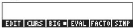
The six soft menu keys for the Equation Writer activate the following functions:
☐: lets the user edit an entry in the line editor (see examples above)
☐: highlights expression and adds a graphics cursor to it
☐: if selected (selection shown by the character in the label) the font used in the writer is the system font 8 (the largest font available)
☐: lets you evaluate, symbolically or numerically, an expression highlighted in the equation writer screen (similar to → EVAL)
☐: lets you factor an expression highlighted in the equation writer screen (if factoring is possible)
☐: lets you simplify an expression highlighted in the equation writer screen (as much as it can be simplified according to the algebraic rules of the CAS)
If you press the NXT key, two more soft menu options show up as shown below:

The six soft menu keys for the Equation Writer activate the following functions:
☐: allows access to the collection of CAS commands listed in alphabetical order. This is useful to insert CAS commands in an expression available in the Equation Writer.
: activates the calculator's CAS help facility to provide information and examples of CAS commands.
Some examples for the use of the Equation Writer are shown below.
Creating arithmetic expressions
Entering arithmetic expressions in the Equation Writer is very similar to entering an arithmetic expression in the stack enclosed in quotes. The main difference is that in the Equation Writer the expressions produced are written in "textbook" style instead of a line-entry style. Thus, when a division sign (i.e., ÷ ) is entered in the Equation Writer, a fraction is generated and the cursor placed in the numerator. To move to the denominator you must use the down arrow key. For example, try the following keystrokes in the Equation Writer screen:
5 ÷ 5 + 2
The result is the expression
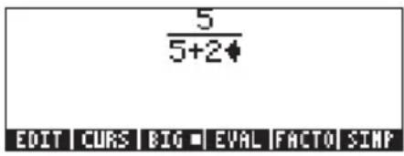
The cursor is shown as a left-facing key. The cursor indicates the current edition location. Typing a character, function name, or operation will enter the corresponding character or characters in the cursor location. For example, for the cursor in the location indicated above, type now:
× ← () 5 + 1 ÷ 3
The edited expression looks as follows:
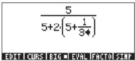
Suppose that you want to replace the quantity between parentheses in the denominator (i.e., 5+1/3) with (5+π2/2) . First, we use the delete key (◀) delete the current 1/3 expression, and then we replace that fraction with π2/2 , as follows: ◀ ◀ ◀ ← π γ^x 2
When we hit this point the screen looks as follows:
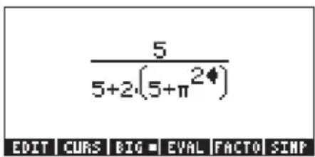
In order to insert the denominator 2 in the expression, we need to highlight the entire π2 expression. We do this by pressing the right arrow key (▶) once. At that point, we enter the following keystrokes: ÷ 2
The expression now looks as follows:
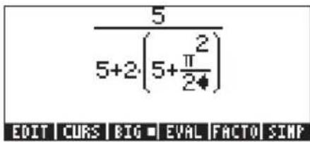
Suppose that now you want to add the fraction 1/3 to this entire expression, i.e., you want to enter the expression:
55 + 2 · (5 + π^ 22) + 1/3
First, we need to highlight the entire first term by using either the right arrow (▶) or the upper arrow (▲) keys, repeatedly, until the entire expression is highlighted, i.e., seven times, producing:

NOTE: Alternatively, from the original position of the cursor (to the right of the 2 in the denominator of π2/2 ), we can use the keystroke combination → ▲, interpreted as ( → ▲).
Once the expression is highlighted as shown above, type +1 ÷ 3 to add the fraction 1/3. Resulting in:

Showing the expression in smaller-size
To show the expression in a smaller-size font (which could be useful if the expression is long and convoluted), simply press the 📄️ soft menu key. For this case, the screen looks as follows:

To recover the larger-font display, press the ☐ soft menu key once more.
Evaluating the expression
To evaluate the expression (or parts of the expression) within the Equation Writer, highlight the part that you want to evaluate and press the 📄️ soft menu key.
For example, to evaluate the entire expression in this exercise, first, highlight the entire expression, by pressing ▶. Then, press the ▶ soft menu key. If your calculator is set to Exact CAS mode (i.e., the _Approx CAS mode is not checked), then you will get the following symbolic result:

If you want to recover the unevaluated expression at this time, use the function UNDO, i.e., → UNDO (the first key in the third row of keys from the top of the keyboard). The recovered expression is shown highlighted as before:
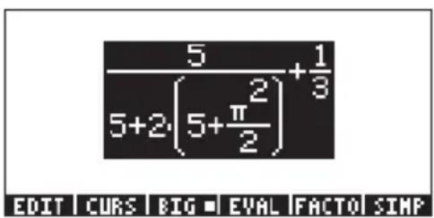
If you want a floating-point (numerical) evaluation, use the → NUM function (i.e., → → NUM). The result is as follows:

Use the function UNDO ( → UNDO) once more to recover the original expression:

Evaluating a sub-expression
Suppose that you want to evaluate only the expression in parentheses in the denominator of the first fraction in the expression above. You have to use the arrow keys to select that particular sub-expression. Here is a way to do it:
Highlights only the first fraction
Highlights the numerator of the first fraction
▶ Highlights denominator of the first fraction
Highlights first term in denominator of first fraction
▶ Highlights second term in denominator of first fraction
Highlights first factor in second term in denominator of first fraction
▶ Highlights expression in parentheses in denominator of first fraction
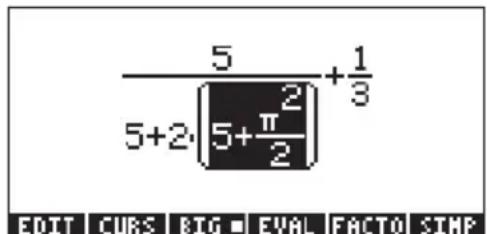
Since this is the sub-expression we want evaluated, we can now press the soft menu key, resulting in:

A symbolic evaluation once more. Suppose that, at this point, we want to evaluate the left-hand side fraction only. Press the upper arrow key (▲) three times to select that fraction, resulting in:
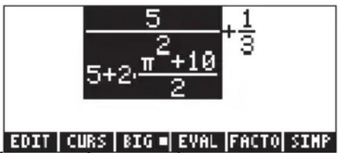
Then, press the ☐ soft menu key to obtain:

Let's try a numerical evaluation of this term at this point. Use → → NUM to obtain:

Let's highlight the fraction to the right, and obtain a numerical evaluation of that term too, and show the sum of these two decimal values in small-font format by using: ▶ → NUM F3 , we get:

To highlight and evaluate the expression in the Equation Writer we use: ▲ F4, resulting in:
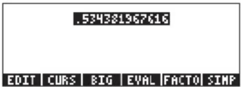
Editing arithmetic expressions
We will show some of the editing features in the Equation Writer as an exercise. We start by entering the following expression used in the previous exercises:

And will use the editing features of the Equation Editor to transform it into the following expression:
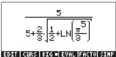
In the previous exercises we used the arrow keys to highlight sub-expressions for evaluation. In this case, we will use them to trigger a special editing cursor. After you have finished entering the original expression, the typing cursor (a left-pointing arrow) will be located to the right of the 3 in the denominator of the second fraction as shown here:

Press the down arrow key (▼) to trigger the clear editing cursor. The screen now looks like this:
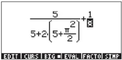
By using the left arrow key (◀) you can move the cursor in the general left direction, but stopping at each individual component of the expression. For example, suppose that we will first will transform the expression π2/2 into the expression LN(π5/3) . With the clear cursor active, as shown above, press the left-arrow key (◀) twice to highlight the 2 in the denominator of π2/2 . Next, press the delete key (◀) once to change the cursor into the insertion cursor. Press ◀ once more to delete the 2, and then □ to enter a 3. At this point, the screen looks as follows:

Next, press the down arrow key (▼) to trigger the clear editing cursor highlighting the 3 in the denominator of π2/3 . Press the left arrow key (◀) once to highlight the exponent 2 in the expression π2/3 . Next, press the delete key (◀) once to change the cursor into the insertion cursor. Press ◀ once more to delete the 2, and then 5 to enter a 5. Press the upper arrow key (▲) three times to highlight the expression π5/3 . Then, type → LN to apply the LN function to this expression. The screen now looks like this:
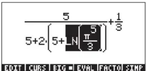
Next, we'll change the 5 within the parentheses to a 1/2 by using these keystrokes:
Next, we highlight the entire expression in parentheses an insert the square root symbol by using: ▲ ▲ ▲ ▲ √X
Next, we'll convert the 2 in front of the parentheses in the denominator into a
2/3 by using:

At this point the expression looks as follows:
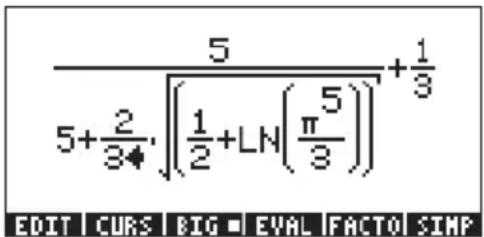
The final step is to remove the 1/3 in the right-hand side of the expression. This is accomplished by using: ▲ ▲ ▲ ▲ ▲ ▶ ◀ ◀ ◀ ◀ ◀
The final version will be:

In summary, to edit an expression in the Equation Writer you should use the arrow keys (◀ ▶ ▲ ▼) to highlight expression to which functions will be applied (e.g., the LN and square root cases in the expression above). Use the down arrow key (▼) in any location, repeatedly, to trigger the clear editing cursor. In this mode, use the left or right arrow keys (◀ ▶) to move from term to term in an expression. When you reach a point that you need to edit, use the delete key (◀) to trigger the insertion cursor and proceed with the edition of the expression.
Creating algebraic expressions
An algebraic expression is very similar to an arithmetic expression, except that English and Greek letters may be included. The process of creating an algebraic expression, therefore, follows the same idea as that of creating an arithmetic expression, except that use of the alphabetic keyboard is included.
To illustrate the use of the Equation Writer to enter an algebraic equation we will use the following example. Suppose that we want to enter the expression:
2√ 3 λ + ^ - µ · LNe ( x + 2 µ · Δyθ^ 1 / 3)
Use the following keystrokes:

This results in the output:
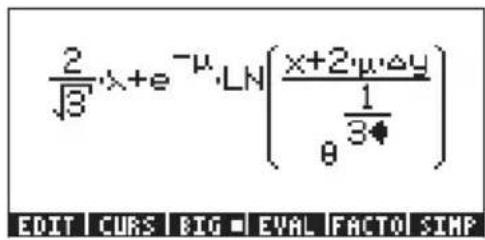
In this example we used several lower-case English letters, e.g., x (ALPHA ← X), several Greek letters, e.g., λ (ALPHA → N), and even a combination of Greek and English letters, namely, Δy (ALPHA → C ALPHA ← Y). Keep in mind that to enter a lower-case English letter, you need to use the combination: ALPHA ← followed by the letter you want to enter. Also, you can always copy special characters by using the CHARS menu (→ CHARS) if you don't want to memorize the keystroke combination that produces it. A listing of commonly used ALPHA → keystroke combinations was listed in an earlier section.
The expression tree
The expression tree is a diagram showing how the Equation Writer interprets an expression. See Appendix E for a detailed example.
The CURS function
The CURS function (☐) in the Equation Writer menu (the ☐ key) converts the display into a graphical display and produces a graphical cursor that can be controlled with the arrow keys (◀ ▶ ▲ ▼) for selecting sub-expressions. The sub-expression selected with ☐ will be shown framed in the graphics display. After selecting a sub-expression you can press ENTER to show the selected sub-expression highlighted in the Equation writer. The following figures show different sub-expressions selected with and the corresponding Equation Writer screen after pressing ENTER.
| ((y-3)x+5) ( x2+4 ) SIN(4x-2) | ((y-3)x+5) ( x2+4 ) SIN(4x-2) |
| ((y-3)x+5) ( x2+4 ) SIN(4x-2) | ((y-3)x+5) ( x2+4 ) SIN(4x-2) |
| ((y-3)x+5) ( x2+4 ) SIN(4x-2) | ((y-3)×+5) ( x2+4 ) SIN(4x-2) |
Editing algebraic expressions
The editing of algebraic equations follows the same rules as the editing of algebraic equations. Namely:
• Use the arrow keys (◀ ▶ ▲ ▼) to highlight expressions
- Use the down arrow key (▼), repeatedly, to trigger the clear editing cursor. In this mode, use the left or right arrow keys (◀▶) to move from term to term in an expression.
- At an editing point, use the delete key (◀) to trigger the insertion cursor and proceed with the edition of the expression.
To see the clear editing cursor in action, let's start with the algebraic expression that we entered in the exercise above:

Press the down arrow key, ⬇, at its current location to trigger the clear editing cursor. The 3 in the exponent of θ will be highlighted. Use the left arrow key, ⬆, to move from element to element in the expression. The order of selection of the clear editing cursor in this example is the following (press the left arrow key, ⬆, repeatedly):
- The 1 in the 1/3 exponent
2.θ
3. Δy
4. µ
5.2
6. x
7. µ in the exponential function
8. λ
9.3 in the √3 term
10. the 2 in the 2/√3 fraction
At any point we can change the clear editing cursor into the insertion cursor by pressing the delete key (◀). Let's use these two cursors (the clear editing cursor and the insertion cursor) to change the current expression into the following:
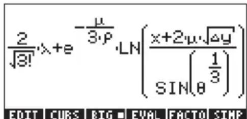
If you followed the exercise immediately above, you should have the clear editing cursor on the number 2 in the first factor in the expression. Follow these keystrokes to edit the expression:
▶ ALPHA → 2 Enters the factorial for the 3 in the square root (entering the factorial changes the cursor to the selection cursor)
▼ ▼ ▶ ▶ Selects the μ in the exponential function
÷ 3 × ALPHA → F Modifies exponential function argument
▶▶▶▶ Selects △y
√X Places a square root symbol on Δy
(this operation also changes the cursor to the selection cursor)
▼ ▼ ▶ ▲ ▲ SIN Select θ 1/3 and enter the SIN function
The resulting screen is the following:
![2/√3!λ+e^(-μ/3·ρ)·LN(x+2μ·√Δy)/[1/3]·SIN(θ) EDIT CURS BIG EVAL FACTO SIMP](/content/2026/05/1018706/images/b02ed4d62a53e1a8af972d153b0cbc7fbd12f4236ac67c3c8ad7c024be8d660e.jpg)
Evaluating a sub-expression
Since we already have the sub-expression S brighted , let's press the soft menu key to evaluate this sub-expression. The result is:
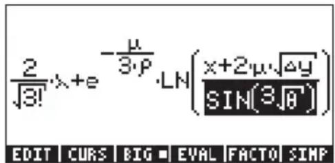
Some algebraic expressions cannot be simplified anymore. Try the following keystrokes: ▲ F4 . You will notice that nothing happens, other than the highlighting of the entire argument of the LN function. This is because this expression cannot be evaluated (or simplified) any more according to the CAS rules. Trying the keystrokes: ▲ F4 again does not produce any changes on the expression. Another sequence of ▲ F4 keystrokes, however, modifies the expression as follows:

One more application of the ▲ F4 keystrokes produces more changes:
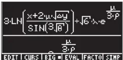
This expression does not fit in the Equation Writer screen. We can see the entire expression by using a smaller-size font. Press the ☐ soft menu key to get:

Even with the larger-size font, it is possible to navigate through the entire expression by using the clear editing cursor. Try the following keystroke sequence: F3 ▼ ▼ ▼ ▼ , to set the clear editing cursor atop the factor
3 in the first term of the numerator. Then, press the right arrow key, ▶, to navigate through the expression.
Simplifying an expression
Press the ☐ soft menu key to get the screen to look as in the previous figure (see above). Now, press the ☐ soft menu key, to see if it is possible to simplify this expression as it is shown in the Equation Writer. The result is the following screen:

This screen shows the argument of the SIN function, namely, √[3]θ transformed into eLN(θ)/This may not seem like a simplification, but it is in the sense that the cubic root function has been replaced by the inverse functions exp-LN.
Factoring an expression
In this exercise we will try factoring a polynomial expression. To continue the previous exercise, press the ENTER key. Then, launch the Equation Writer again by pressing the → EQW key. Type the equation:

resulting in
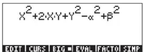
Let's select the first 3 terms in the expression and attempt a factoring of this sub-expression: ↗ ▲ ▼ ↗ ▶ ↗ ▶ . This produces:

Now, press the soft menu key, to get

Press ⬇ UNDO to recover the original expression. Next, enter the following keystrokes: ▼ ▼ ▼ ▶ ▶ ▶ ▶ ▶ ▶ ▶ ▶ ▶ ▶ ▶ ▶ ▶ ▶ to select the last two terms in the expression, i.e.,
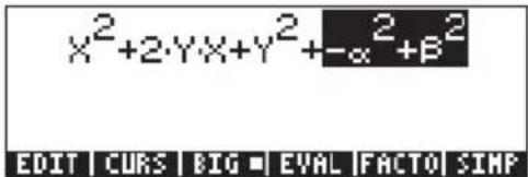
press the 📄️ soft menu key, to get

Press → UNDO to recover the original expression. Now, let's select the entire expression by pressing the upper arrow key (▲) once. And press the soft menu key, to get

Press → UNDO to recover the original expression.
Note: Pressing the 📄 or the 📄 soft menu keys, while the entire original expression is selected, produces the following simplification of the expression:
![X²+2·Y·X+Y²-[α²-β²] EDIT CURS BIG ■ EVAL FACTO SIMP](/content/2026/05/1018706/images/6490c0ef2f320dcee3d6bd4682d86cedea79a4abffff6cd5cdafb07753489589.jpg)
Using the CMDS menu key
With the original polynomial expression used in the previous exercise still selected, press the NXT key to show the ETT and ETT soft menu keys. These two commands belong to the second part of the soft menu available with the Equation Writer. Let's try this example as an application of the ETT soft menu key: Press the ETT soft menu key to get the list of CAS commands:

Next, select the command DERVX (the derivative with respect to the variable X, the current CAS independent variable) by using: ALPHA D ▼ ▼ ▼ .
Command DERVX will now be selected:
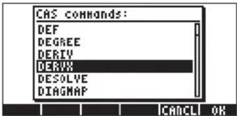
Press the soft menu key to get:
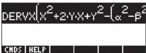
Next, press the NXT key to recover the original Equation Writer menu, and press the 3000 soft menu key to evaluate this derivative. The result is:

Using the HELP menu
Press the NXT key to show the ☐ and ☐ soft menu keys. Press the ☐ soft menu key to get the list of CAS commands. Then, press ALPHA ☐ ▼ ▼ to select the command DERVX. Press the ☐ soft menu key to get information on the command DERVX:

Detailed explanation on the use of the help facility for the CAS is presented in Chapter 1. To return to the Equation Writer, press the ☐ soft menu key. Press the ENTER key to exit the Equation Writer.
Using the editing functions BEGIN, END, COPY, CUT and PASTE
To facilitate editing, whether with the Equation Writer or on the stack, the calculator provides five editing functions, BEGIN, END, COPY, CUT and PASTE, activated by combining the right-shift key (→) with keys (2,1), (2,2), (3,1), (3,2), and (3,3), respectively. These keys are located in the leftmost part of rows 2 and 3. The action of these editing functions are as follows:
BEGIN: marks the beginning of a string of characters for editing
END: marks the ending of a string of characters for editing
COPY: copies the string of characters selected by BEGIN and END
CUT: cuts the string of characters selected by BEGIN and END
PASTE: pastes a string of characters, previously copied or cut, into the current cursor position
To see and example, lets start the Equation Writer and enter the following expression (used in an earlier exercise):

The original expression is the following:
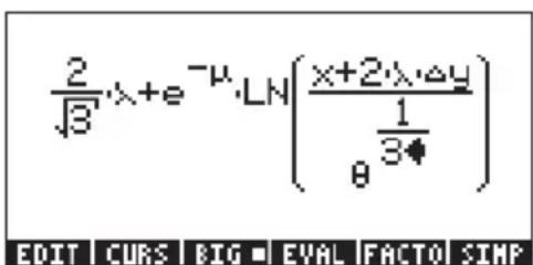
We want to remove the sub-expression x+2λ·Δy from the argument of the LN function, and move it to the right of the λ in the first term. Here is one possibility: ▼◀◀◀▲▲▲→_CUT◀◀▲X→_PASTE
The modified expression looks as follows:

Next, we'll copy the fraction 2 / √3 from the leftmost factor in the expression, and place it in the numerator of the argument for the LN function. Try the following keystrokes:

The resulting screen is as follows:

The functions BEGIN and END are not necessary when operating in the Equation Writer, since we can select strings of characters by using the arrow keys. Functions BEGIN and END are more useful when editing an expression with the line editor. For example, let's select the expression x + 2λ · Δy from this expression, but using the line editor within the Equation Writer, as follows:
The line editor screen will look like this (quotes shown only if calculator in RPN mode):
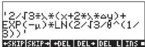
To select the sub-expression of interest, use:


The screen shows the required sub-expression highlighted:

We can now copy this expression and place it in the denominator of the LN argument, as follows: → COPY ▶ ▶ ... (27 times) ... ▶
◀◀ ... (9 times) ... ◀→ PASTE
The line editor now looks like this:

Pressing ENTER shows the expression in the Equation Writer (in small-font format, press the 300 soft menu key):

Press ENTER to exit the Equation Writer.
Creating and editing summations, derivatives, and integrals
Summations, derivatives, and integrals are commonly used for calculus, probability and statistics applications. In this section we show some examples of such operations created with the equation writer. Use ALG mode.
Summations
We will use the Equation Writer to enter the following summation:
_ k = 1 ^ ∞ 1k ^ 2
Press → EQW to activate the Equation Writer. Then press → to enter the summation sign. Notice that the sign, when entered into the Equation Writer screen, provides input locations for the index of the summation as well as for the quantity being summed. To fill these input locations, use the following keystrokes:
ALPHA ← K ▶ 1 ▶ ← ∞ ▶ 1 ÷ ALPHA ← K γ x 2
The resulting screen is:

To see the corresponding expression in the line editor, press ▶ and the ▶ soft menu key, to show:

This expression shows the general form of a summation typed directly in the stack or line editor:
(index = startingvalue, endingvalue, summation\ expression) Press ENTER to return to the Equation Writer. The resulting screen shows the value of the summation,

To recover the unevaluated summation use → UNDO. To evaluate the summation again, you can use the F4 soft menu key. This shows again that
_ = k ^ ∞ 1k ^ 2 = π^ 26.
You can use the Equation Writer to prove that
_ k = 1 ^ ∞ 1/k + ∞ =
This summation (representing an infinite series) is said to diverge. Double summations are also possible, for example:

Derivatives
We will use the Equation Writer to enter the following derivative:
d/dt (α · t ^ 2 + β · t + δ)
Press → EQW to activate the Equation Writer. Then press → ____ to enter the (partial) derivative sign. Notice that the sign, when entered into the Equation Writer screen, provides input locations for the expression being differentiated
and the variable of differentiation. To fill these input locations, use the following keystrokes:


The resulting screen is the following:
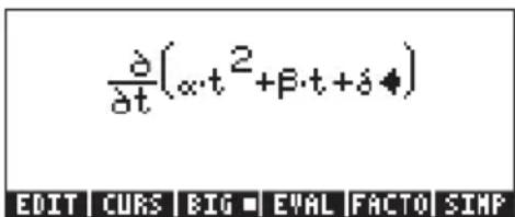
To see the corresponding expression in the line editor, press → ▲ and the FI soft menu key, to show:

This indicates that the general expression for a derivative in the line editor or in the stack is: variable(function of variables)
Press ENTER to return to the Equation Writer. The resulting screen is not the derivative we entered, however, but its symbolic value, namely,

To recover the derivative expression use → UNDO. To evaluate the derivative again, you can use the F4 soft menu key. This shows again that
d/dt (^ 2) 2 + βαδβ αt
Second order derivatives are possible, for example:
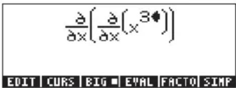
which evaluates to:

Note: The notation / x is proper of partial derivatives. The proper
notation for total derivatives (i.e., derivatives of one variable) is d/dx (the calculator, however, does not distinguish between partial and total derivatives
Definite integrals
We will use the Equation Writer to enter the following definite
integral: 0τ · )sin(dtPress → _EQW to activate the Equation Writer. Then press → _f to enter the integral sign. Notice that the sign, when entered into the Equation Writer screen, provides input locations for the limits of integration, the integrand, and the variable of integration. To fill these input locations, use the following keystrokes: 0 ▶ ALPHA → U ▶ ALPHA
T × SIN ALPHA ← T ▶ ALPHA ← T . The resulting screen is the following:

To see the corresponding expression in the line editor, press ▲ ▲ and the FI soft menu key, to show:

This indicates that the general expression for a derivative in the line editor or in the stack is: (lowerlimit, upperlimit, integrand, variableofintegration)
Press ENTER to return to the Equation Writer. The resulting screen is not the definite integral we entered, however, but its symbolic value, namely,
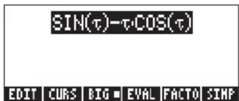
To recover the derivative expression use → UNDO. To evaluate the derivative again, you can use the F4 soft menu key. This shows again that
_ 0 ^ τt (t) dt (τ) τ · (τ)
Double integrals are also possible. For example,

which evaluates to 36. Partial evaluation is possible, for example:
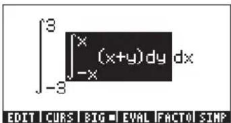
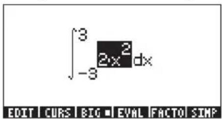
This integral evaluates to 36.
Organizing data in the calculator
You can organize data in your calculator by storing variables in a directory tree. To understand the calculator's memory, we first take a look at the file directory. Press the keystroke combination ← FILES (first key in second row of keys from the top of the keyboard) to get the calculator's File Manager screen:
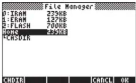
This screen gives a snapshot of the calculator's memory and of the directory tree. The screen shows that the calculator has three memory ports (or memory partitions), port 0:IRAM, port 1:ERAM, and port 2:FLASH. Memory ports are used to store third party application or libraries, as well as for backups. The size of the three different ports is also indicated. The fourth and subsequent lines in this screen show the calculator's directory tree. The top directory (currently highlighted) is the Home directory, and it has predefined into it a sub-directory called CASDIR. The File Manager screen has three functions associated with the soft-menu keys:
Change to selected directory
: Cancel action
Approve a selection
For example, to change directory to the CASDIR, press the down-arrow key, ▼, and press 🔊. This action closes the File Manager window and returns us to normal calculator display. You will notice that the second line from the top in the display now starts with the characters { HOME CASDIR } indicating that the current directory is CASDIR within the HOME directory.
Functions for manipulation of variables
This screen includes 20 commands associated with the soft menu keys that can be used to create, edit, and manipulate variables. The first six functions are the following:
To edit a highlighted variable
To copy a highlighted variable
To move a highlighted variable
To recall the contents of a highlighted variable
To evaluate a highlighted variable
To see the directory tree where the variable is contained
If you press the NXT key, the next set of functions is made available:
To purge, or delete, a variable
To rename a variable
To create a new variable
To order a set of variables in the directory
To send a variable to another calculator or computer
To receive a variable from another calculator or computer
If you press the NXT key, the third set of functions is made available:
To return to the stack temporarily
To see contents of a variable
To edit contents of a binary variable (similar to [10])
To show the directory containing the variable in the header
Provides a list of variable names and description
To sort variables according to a sorting criteria
If you press the NXT key, the last set of functions is made available:
RE10 To send variable with X-modem protocol
To change directory
To move between the different soft menu commands, you can use not only the NEXT key (NXT), but also the PREV key (←PREV).
The user is invited to try these functions on his or her own. Their applications are straightforward.
The HOME directory
The HOME directory, as pointed out earlier, is the base directory for memory operation for the calculator. To get to the HOME directory, you can press the UPDIR function (←UPDIR) -- repeat as needed -- until the {HOME} spec is shown in the second line of the display header. Alternatively, you can use (hold) UPDIR , press ENTER if in the algebraic mode. For this example, the HOME directory contains nothing but the CASDIR. Pressing VAR will show the variables in the soft menu keys:

Subdirectories
To store your data in a well organized directory tree you may want to create subdirectories under the HOME directory, and more subdirectories within subdirectories, in a hierarchy of directories similar to folders in modern computers. The subdirectories will be given names that may reflect the contents of each subdirectory, or any arbitrary name that you can think of.
The CASDIR sub-directory
The CASDIR sub-directory contains a number of variables needed by the proper operation of the CAS (Computer Algebraic System, see appendix C). To see the contents of the directory, we can use the keystroke combination:
← FILES which opens the File Manager once more:

This time the CASDIR is highlighted in the screen. To see the contents of the directory press the soft menu key or ENTER, to get the following screen:

The screen shows a table describing the variables contained in the CASDIR directory. These are variables pre-defined in the calculator memory that establish certain parameters for CAS operation (see appendix C). The table above contains 4 columns:
- The first column indicate the type of variable (e.g., 'EQ' means an equation-type variable, |R indicates a real-value variable, {} means a list, nam means 'a global name', and the symbol represents a graphic variable.
- The second column represents the name of the variables, i.e., PRIMIT, CASINFO, MODULO, REALASSUME, PERIOD, VX, and EPS.
- Column number 3 shows another specification for the variable type, e.g., ALG means an algebraic expression, GROB stands for graphics object, INTG means an integer numeric variable, LIST means a list of data, GNAME means a global name, and REAL means a real (or floating-point) numeric variable.
- The fourth and last column represents the size, in bytes, of the variable truncated, without decimals (i.e., nibbles). Thus, for example, variable PERIOD takes 12.5 bytes, while variable REALASSUME takes 27.5 bytes (1 byte = 8 bits, 1 bit is the smallest unit of memory in computers and calculators).
CASDIR Variables in the stack
Pressing the ON key closes the previous screen and returns us to normal calculator display. By default, we get back the TOOL menu:

We can see the variables contained in the current directory, CASDIR, by pressing the VAR key (first key in the second row from the top of the keyboard). This produces the following screen:

Pressing the NXT key shows one more variable stored in this directory:

- To see the contents of the variable EPS, for example, use → E. This shows the value of EPS to be .000000001
- To see the value of a numerical variable, we need to press only the soft menu key for the variable. For example, pressing 📄 followed by ENTER, shows the same value of the variable in the stack, if the calculator is set to Algebraic. If the calculator is set to RPN mode, you need only press the soft menu key for ENTER.
- To see the full name of a variable, press the tickmark key first, ☐, and then the soft menu key corresponding to the variable. For example, for the variable listed in the stack as PERIO, we use: ☐, which produces as output the string: 'PERIOD'. This procedure applies to both the Algebraic and RPN calculator operating modes.
Variables in CASDIR
The default variables contained in the CASDIR directory are the following:
PRIMIT Latest primitive (anti-derivative) calculated, not a default variable, but one created by a previous exercise
CASINFO a graph that provides CAS information
MODULO Modulo for modular arithmetic (default = 13)
REALASSUME List of variable names assumed as real values
PERIOD Period for trigonometric functions (default = 2 π)
VX Name of default independent variable (default = X)
EPS Value of small increment (epsilon), (default = 10 -10)
These variables are used for the operation of the CAS.
Typing directory and variable names
To name subdirectories, and sometimes, variables, you will have to type strings of letters at once, which may or may not be combined with numbers. Rather than pressing the ALPHA, ALPHA ←, or ALPHA → key combinations to type each letter, you can hold down the ALPHA key and enter the various letter. You can also
lock the alphabetic keyboard temporarily and enter a full name before unlocking it again. The following combinations of keystrokes will lock the alphabetic keyboard:
ALPHA ALPHA locks the alphabetic keyboard in upper case. When locked in this fashion, pressing the ← before a letter key produces a lower case letter, while pressing the → key before a letter key produces a special character. If the alphabetic keyboard is already locked in upper case, to lock it in lower case, type, ← ALPHA
ALPHA ALPHA ← ALPHA locks the alphabetic keyboard in lower case. When locked in this fashion, pressing the ← before a letter key produces an upper case letter. To unlock lower case, press ← ALPHA
To unlock the upper-case locked keyboard, press ALPHA
Let's try some exercises typing directory/variable names in the stack. Assuming that the calculator is in the Algebraic mode of operation (although the instructions work as well in RPN mode), try the following keystroke sequences. With these commands we will be typing the words 'MATH', 'Math', and 'MatH'

The calculator display will show the following (left-hand side is Algebraic mode, right-hand side is RPN mode):

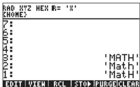
Note: if system flag 60 is set, you can lock the alphabetical keyboard by just pressing ALPHA. See Chapter 1 for more information on system flags.
Creating subdirectories
Subdirectories can be created by using the FILES environment or by using the command CRDIR. The two approaches for creating sub-directories are presented next.
Using the FILES menu
Regardless of the mode of operation of the calculator (Algebraic or RPN), we can create a directory tree, based on the HOME directory, by using the functions activated in the FILES menu. Press ← FILES to activate the FILES menu. If the HOME directory is not already highlighted in the screen, i.e.,
use the up and down arrow keys (▲ ▼) to highlight it. Then, press the soft menu key. The screen may look like this:

showing that only one object exists currently in the HOME directory, namely, the CASDIR sub-directory. Let's create another sub-directory called MANS (for MANualS) where we will store variables developed as exercises in this manual. To create this sub-directory first enter: NXT . This will produce the following input form:

The Object input field, the first input field in the form, is highlighted by default. This input field can hold the contents of a new variable that is being created. Since we have no contents for the new sub-directory at this point, we simply skip this input field by pressing the down-arrow key, ▼, once. The Name input field is now highlighted:

This is where we enter the name of the new sub-directory (or variable, as the case may be), as follows: ALPHA ALPHA M A N S ENTER
The cursor moves to the _Directory check field. Press the √2018 soft menu key to specify that you are creating a directory, and press 📄 to exit the input form. The variable listing for the HOME directory will be shown in the screen as follows:
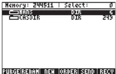
The screen indicates that there is a new directory (MANS) within the HOME directory.
Next, we will create a sub-directory named INTRO (for INTROduction), within MANS, to hold variables created as exercise in subsequent sections of this chapter. Press the ON key to return to normal calculator display (the TOOLS menu will be shown). Then, press VAR to show the HOME directory contents in the soft menu key labels. The display may look like this (if you have created other variables in the HOME directory they will show in the soft menu key labels too):

To move into the MANS directory, press the corresponding soft menu key (in this case), and ENTER if in algebraic mode. The directory tree will be shown in the second line of the display as (HOME MANS). However, there will be no labels associated with the soft menu keys, as shown below, because there are no variables defined within this directory.
Let's create the sub-directory INTRO by using:

Press the ON key, followed by the VAR key, to see the contents of the MANS directory as follows:

Press the 📄️ soft menu key to move into the INTRO sub-directory. This will show an empty sub-directory. Later on, we will do some exercises in creating variables.
Using the command CRDIR
The command CRDIR can be used to create directories. This command is available through the command catalog key (the → _CAT key, second key in fourth row of keys from the top of the keyboard), through the programming menus (the ← PRG key, same key as the → _CAT key), or by simply typing it.
• Through the catalog key
Press → CAT ALPHA C. Use the up and down arrow keys (▲▼) to locate the CRDIR command. Press the soft menu key to activate the command.
• Through the programming menus
Press PRG. This will produce the following pull-down menu for programming:
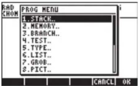
Use the down arrow key (▼) to select the option 2. MEMORY... , or just press 2. Then, press 📄. This will produce the following pull-down menu:
![RAD CHOM MEMORY MENU 1.PURGE 2.MEM 3.BYTES 4.NEWOB 5.DIRECTORY.. 6.ARITHMETIC.. 7.ARCHEIVE 8.RESTORE [CAND] OK](/content/2026/05/1018706/images/8119ba2bc0b43c8be3f1c41459440c085886f52cc82814209b812f57166a67e3.jpg)
Use the down arrow key (▼) to select the 5. DIRECTORY option, or just press 5. Then, press 📄. This will produce the following pull-down menu:
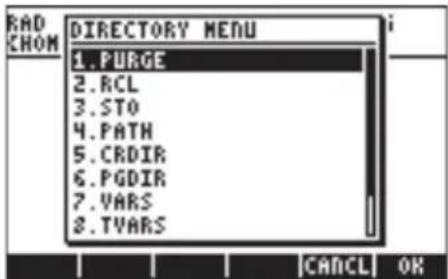
Use the down arrow key (▼) to select the 5. CRDIR option, and press
Command CRDIR in Algebraic mode
Once you have selected the CRDIR through one of the means shown above, the command will be available in your stack as follows:

At this point, you need to type a directory name, say chap1:
ALPHA ALPHA ← ALPHA C H A P I ALPHA ENTER
The name of the new directory will be shown in the soft menu keys, e.g.,

Command CRDIR in RPN mode
To use the CRDIR in RPN mode you need to have the name of the directory already available in the stack before accessing the command. For example:
ALPHA ALPHA ← ALPHA C H A P 2 ALPHA ENTER
Then access the CRDIR command by either of the means shown above, e.g., through the → CAT key:
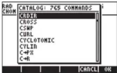
Press the soft menu key to activate the command, to create the sub-directory:

Moving among subdirectories
To move down the directory tree, you need to press the soft menu key corresponding to the sub-directory you want to move to. The list of variables in a sub-directory can be produced by pressing the VAR (VARiables) key. To move up in the directory tree, use the function UPDIR, i.e., enter ← UPDIR .
Alternatively, you can use the FILES menu, i.e., press ← FILES . Use the up and down arrow keys (▲▼) to select the sub-directory you want to move to, and then press the 🎨 (CHange DIRectory) or □ soft menu key. This will show the contents of the sub-directory you moved to in the soft menu key labels.
Deleting subdirectories
To delete a sub-directory, use one of the following procedures:
Using the FILES menu
Press the ← FILES key to trigger the FILES menu. Select the directory containing the sub-directory you want to delete, and press the ENTER if needed. This will close the FILES menu and display the contents of the directory you selected. In this case you will need to press ENTER. Press the soft menu key to list the contents of the directory in the screen. Select the sub-directory (or variable) that you want to delete. Press NXT ENTER. A screen similar to the following will be shown:

The 'S2' string in this form is the name of the sub-directory that is being deleted.
The soft menu keys provide the following options:
Proceed with deleting the sub-directory (or variable)
Proceed with deleting all sub-directories (or variables)
Do not delete sub-directory (or variable) from a list
Do not delete sub-directory (or variable)
After selecting one of these four commands, you will be returned to the screen listing the contents of the sub-directory. The command, however, will show an error message:

and you will have to press 📄, before returning to the variable listing.
Using the command PGDIR
The command PGDIR can be used to purge directories. Like the command CRDIR, the PGDIR command is available through the → _CAT or through the ← PRG key, or it can simply be typed in.
• Through the catalog key
Press CAT ALPHA ALPHA P G. This should highlight the PGDIR command. Press the soft menu key to activate the command.
• Through the programming menus
Press PRG. This will produce the following pull-down menu for programming:
![RAD CHOM PROG MENU 1.STACK.. 2.MEMORY.. 3.BRANCH.. 4.TEST.. 5.TYPE.. 6.LIST.. 7.GROB.. 8.PICT.. [CAND] OK](/content/2026/05/1018706/images/aa790e44fbcc753aa4f6d0916ef78a4ed7a6459cbf2f0f8e1d27b54e8414f5d2.jpg)
Use the down arrow key (▼) to select the option 2. MEMORY... Then, press 📄. This will produce the following pull-down menu:
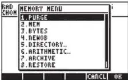
Use the down arrow key (▼) to select the 5. DIRECTORY option. Then, press 🔊. This will produce the following pull-down menu:

Use the down arrow key (▼) to select the 6. PGDIR option, and press 📄.
Command PGDIR in Algebraic mode
Once you have selected the PGDIR through one of the means shown above, the command will be available in your stack as follows:

At this point, you need to type the name of an existing directory, say S4 :
ALPHA S 4 ENTER
As a result, sub-directory is deleted:
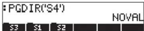
Instead of typing the name of the directory, you can simply press the corresponding soft menu key at the listing of the PGDIR() command, e.g.,
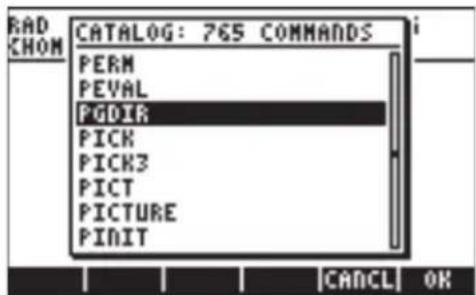
Press 📄, to get:
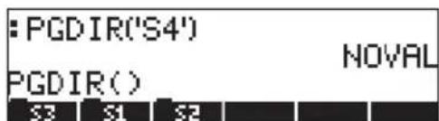
Then, press 📄 to enter 'S3' as the argument to PGDIR.

Press ENTER to delete the sub-directory:
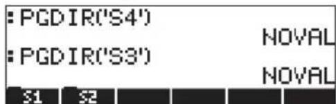
Command PGDIR in RPN mode
To use the PGDIR in RPN mode you need to have the name of the directory, between quotes, already available in the stack before accessing the command.
For example: 1 ALPHA S 2 ENTER
Then access the PGDIR command by either of the means shown above, e.g., through the → CAT key:

Press the soft menu key to activate the command and delete the sub-directory:

Using the PURGE command from the TOOL menu
The TOOL menu is available by pressing the TOOL key (Algebraic and RPN modes shown):

The PURGE command is available by pressing the ☐ soft menu key. In the following examples we want to delete sub-directory S1:
• Algebraic mode: Enter VAR ENTER
• RPN mode: Enter VAR , ENTER TOOL VAR
Variables
Variables are like files on a computer hard drive. One variable can store one object (numerical values, algebraic expressions, lists, vectors, matrices, programs, etc). Even sub-directories can be through of as variables (in fact, in the calculator, a subdirectory is also a type of calculator object).
Variables are referred to by their names, which can be any combination of alphabetic and numerical characters, starting with a letter (either English or Greek). Some non-alphabetic characters, such as the arrow ( → ) can be used in a variable name, if combined with an alphabetical character. Thus, → A' is a valid variable name, but →' is not. Valid examples of variable names are: 'A', 'B', 'a', 'b', 'α', 'β', 'A1', 'AB12', '→A12', 'Vel', 'Z0', 'z1', etc.
A variable can not have the same name than a function of the calculator. You can not have a SIN variable for example as there is a SIN command in the calculator. The reserved calculator variable names are the following: ALRMDAT, CST, EQ, EXPR, IERR, IOPAR, MAXR, MINR, PICT, PPAR, PRTPAR, VPAR, ZPAR, der_, e, i, n1,n2, ..., s1, s2, ...,ΣDAT, ΣPAR, π, ∞
Variables can be organized into sub-directories.
Creating variables
To create a variable, we can use the FILES menu, along the lines of the examples shown above for creating a sub-directory. For example, within the sub-directory (HOME MANS INTRO), created in an earlier example, we want to store the following variables with the values shown:
| Name Contents Type | ||
| A | 1 | 2 |
| α | -0.25 real | |
| A12 3 | × 105 | real |
| Q 'r/(m+r)' algebraic | ||
| R [3,2,1] | vector | |
| z1 | 3+5i | complex |
| p1 | << → r 'π*r^2' >> | program |
5
Using the FILES menu
We will use the FILES menu to enter the variable A. We assume that we are in the sub-directory (HOME MANS INTRO). To get to this sub-directory, use the following: ←FILES and select the INTRO sub-directory as shown in this screen:

Press 📄 to enter the directory. You will get a files listing with no entries (the INTRO sub-directory is empty at this point)

Press the NXT key to move to the next set of soft menu keys, and press the soft menu key. This will produce the NEW VARIABLE input form:
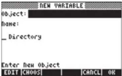
To enter variable A (see table above), we first enter its contents, namely, the number 12.5, and then its name, A, as follows: 1 2 · 5
ALPHA A. Resulting in the following screen:

Press 📄 once more to create the variable. The new variable is shown in the following variable listing:
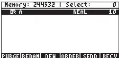
The listing indicates a real variable (IR), whose name is A, and that occupies 10.5 bytes of memory. To see the contents of the variable in this screen, press NXT
- Press the 📄️ soft menu key to see the contents in a graphical format.

- Press the soft menu key to see the contents in text format.
- Press 📄 to return to the variable list
- Press ON once more to return to normal display. Variable A should now be featured in the soft menu key labels:

Using the STO▶ command
A simpler way to create a variable is by using the STO command (i.e., the STO key). We provide examples in both the Algebraic and RPN modes, by creating the remaining of the variables suggested above, namely:
| Name Contents Type | ||
| α | -0.25 real | |
| A12 3 | × 105 | real |
| Q 'r/(m+r)' algebraic | ||
| R [3,2,1] vector | ||
| z1 3+5i complex | ||
| p1 << → r 'π*r^2' >> program | ||
- Algebraic mode
Use the following keystrokes to store the value of -0.25 into variableα: 0 · 2 5 +/- STO▶ ALPHA → A. AT this point, the screen will look as follows:

This expression means that the value -0.25 is being stored into α (the symbol ▶ suggests the operation). Press ENTER to create the variable. The variable is now shown in the soft menu key labels when you press VAR :

The following are the keystrokes required to enter the remaining variables:
A12: 3 EEX 5 STO▶ ALPHA A 1 2 ENTER
Q: ALPHA ← R ÷ ← ()
ALPHA ← M + ALPHA ← R ► ► STO▶ ALPHA Q ENTER
R: ← [1] 3 → , 2 → , 1 ▶ STO▶ ALPHA R ENTER
z1: 3 + 5 × ← i STO ALPHA ← Z I ENTER (if needed, accept change to Complex mode)
p1: → << → < - < π ×
ALPHA ← R γx 2 ▶ ▶ ▶ STO▶ ALPHA ← P I ENTER.
The screen, at this point, will look as follows:
![:[3 2 1]►R :3+5·i►z1 : « → r 'π*r^2' »►p1 « → r 'π*r^2' » m+r [3 2 1] 3+5·i p1 | z1 | R | Q | A12 |](/content/2026/05/1018706/images/018bfee72ae3aeac0292af5a41b208b718d8582531e2104a93024e6f6e5183fa.jpg)
You will see six of the seven variables listed at the bottom of the screen: p1, z1, R, Q, A12, α .
- RPN mode
Use the following keystrokes to store the value of -0.25 into variable: 2 5 +/- ENTER ALPHA → A ENTER. At this point, the screen will look as follows:
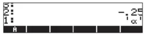
With -0.25 on the level 2 of the stack and 'α' on the level 1 of the stack, you can use the STOP key to create the variable. The variable is now shown in the soft menu key labels when you press VAR :

To enter the value 3 × 10⁵ into A12, we can use a shorter version of the procedure: 3 EEX 5 ALPHA 1 2 ENTER STO
Here is a way to enter the contents of Q:
Q: ALPHA ← R ÷ ← ()
ALPHA ← M + ALPHA ← R ▶ ▶ , ALPHA Q ENTER STO
To enter the value of R, we can use an even shorter version of the procedure:
R: ← [1] 3 SPC 2 SPC 1 ▶ ALPHA R STO
Notice that to separate the elements of a vector in RPN mode we can use the space key (SPC), rather than the comma (→—, ) used above in Algebraic mode.


You will see six of the seven variables listed at the bottom of the screen: p1, z1, R, Q, A12, α .
Checking variables contents
As an exercise on peeking into the contents of variables we will use the seven variables entered in the exercise above. We showed how to use the FILES menu to view the contents of a variable in an earlier exercise when we created the variable A. In this section we will show a simple way to look into the contents of a variable.
Pressing the soft menu key label for the variable
This procedure will show the contents of a variable as long as the variable contains a numerical value or an algebraic value, or an array. For example, for the variables listed above, press the following keys to see the contents of the variables:
Algebraic mode
Type these keystrokes: VAR ENTER ENTER . At this point, the screen looks as follows:
![z1 R Q 3+5·i [3 2 1] r m+r D1 Z1 R Q A12 α](/content/2026/05/1018706/images/6d7e162f80cdf42df0df63942e20e250cc282135896de84ddd0cafda9bd735cf.jpg)
Next, type these keystrokes: ENTER ENTER NXT ENTER. At this point, the screen looks as follows:

Pressing the soft menu key corresponding to p1 will provide an error message (try NXT ENTER):
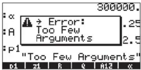
Note: By pressing ENTER we are trying to activate (run) the p1 program. However, this program expects a numerical input. Try the following exercise: ON ← () 5 ENTER . The result is:
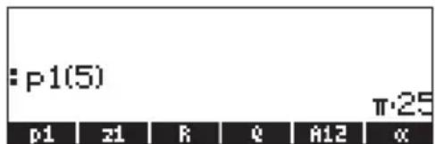
The program has the following structure: <<→ r 'π*r^2' >>
The « » symbols indicate a program in User RPL language. The characters→r indicate that an input, to be referred to as r, is to be provided to the program. The action from the program is to take that value of r and evaluate the algebraic 'π*r^2'. In the example shown above, r took the value of 5, and thus the value of πr² = π·25 is returned. This program, therefore, calculates the area of a circle given its radius r.
RPN mode
In RPN mode, you only need to press the corresponding soft menu key label to get the contents of a numerical or algebraic variable. For the case under consideration, we can try peeking into the variables z1, R, Q, A12, α, and A, created above, as follows: VAR
At this point, the screen looks like this:
![3: 5: 4: 3: 2: 1: 3+5·i [3 2 1] r m+r 300000. -.25 p1 z1 R Q A12 α](/content/2026/05/1018706/images/3262f9248291895202d5c5c7b4032c797c361c5839cead1097c51f37ea3efbd6.jpg)
To see the contents of A, use: NXT. To run program p1 with r = 5, use: NXT 5

Notice that to run the program in RPN mode, you only need to enter the input (5) and press the corresponding soft menu key. (In algebraic mode, you need to place parentheses to enter the argument).
Using the right-shift key → followed by soft menu key labels
In Algebraic mode, you can display the content of a variable by pressing VAR and then the corresponding soft menu key. Try the following examples:

Note: In RPN mode, you don't need to press ↗ (just VAR and then the corresponding soft menu key).
This produces the following screen (Algebraic mode in the left, RPN in the right)
![« → r 'π*r^2' » 3+5·i [3 2 1] r m+r 300000. p1 z1 R Q A12 «](/content/2026/05/1018706/images/ad00c2f60be9dfd5beea2e98b5a3dff10a19e8e3f2bb2735a8f4ea14ebe02700.jpg)
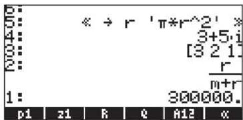
Notice that this time the contents of program p1 are listed in the screen. To see the remaining variables in this directory, press NXT :
Listing the contents of all variables in the screen
Use the keystroke combination → ▼ to list the contents of all variables in the screen. For example:
![p1: « → r 'π*r^2.' z1: (3.,5.) R: [3.,2.,1.] Q: r/(m+r) A12: 300000. x: -.25 p1 | z1 | R | Q | A12 | x](/content/2026/05/1018706/images/2295bb0d53548f491e409a32ce5edd38b0518cfc8061fdc3bca0a3689f50b78f.jpg)
Press ON to return to normal calculator display.
Replacing the contents of variables
Replacing the contents of a variable can be thought of as storing a different value in the same variable name. Thus, the examples for creating variables shown above can be used to illustrate the replacement of a variable's content.
Using the STO▶ command
Using as illustration the six variables, p1, z1, R, Q, A12, a, and A, created earlier, we will proceed to change the contents of variable A12 (currently a numerical variable) with the algebraic expression β/2' , using the STO▶ command. First, using the Algebraic operating mode:

Check the new contents of variable A12 by using ↗
Using the RPN operating mode:

or, in a simplified way,

Using the left-shift ← key followed by the variable's soft menu key (RPN)
This is a very simple way to change the contents of a variable, but it only works in the RPN mode. The procedure consists in typing the new contents of the variable and entering them into the stack, and then pressing the left-shift key
followed by the variable's soft menu key. For example, in RPN, if we want to change the contents of variable z1 to 'a+b·i', use:
1 ← + ← × ← i
This will place the algebraic expression 'a+bi' in level 1: in the stack. To enter this result into variable z1, use: VAR ←
To check the new contents of z1, use: →
An equivalent way to do this in Algebraic mode is the following:
ALPHA ← A + ALPHA ← B × ← i ENTER STO ENTER
To check the new contents of z1, use: →
Using the ANS(1) variable (Algebraic mode)
In Algebraic mode one can use the ANS(1) variable to replace the contents of a variable. For example, the procedure for changing the contents of z1 to 'a+bi' is the following: ← ANS STOP ENTER. To check the new contents of z1, use: →
Copying variables
The following exercises show different ways of copying variables from one sub-directory to another.
Using the FILES menu
To copy a variable from one directory to another you can use the FILES menu. For example, within the sub-directory {HOME MANS INTRO}, we have variables p1, z1, R, Q, A12, α , and A. Suppose that we want to copy variable A and place a copy in sub-directory {HOME MANS}. Also, we will copy variable R and place a copy in the HOME directory. Here is how to do it: Press ← FILES to produce the following list of variables:

Use the down-arrow key ▼ to select variable A (the last in the list), then press 📄. The calculator will respond with a screen labeled PICK DESTINATION:

Use the up arrow key ▲ to select the sub-directory MANS and press 📄. If you now press ← UPDIR, the screen will show the contents of sub-directory MANS (notice that variable A is shown in this list, as expected):

Press ON ENTER (Algebraic mode), or ON RPN mode) to return to the INTRO directory. Press ← FILES to produce the list of variables in {HOME MANS INTRO}. Use the down arrow key (▼) to select variable R, then press 📄. Use the up arrow key (▲) to select the HOME directory, and press 📄. If you now press ← UPDIR, twice, the screen will show the contents of the HOME directory, including a copy of variable R:

Using the history in Algebraic mode
Here is a way to use the history (stack) to copy a variable from one directory to another with the calculator set to the Algebraic mode. Suppose that we are within the sub-directory {HOME MANS INTRO}, and want to copy the contents of variable z1 to sub-directory {HOME MANS}. Use the following procedure: → ↗ STO→ ENTER This simply stores the contents of z1 into itself (no change effected on z1). Next, use ← UPDIR ENTER to move to the {HOME MANS} sub-directory. The calculator screen will look like this:

Next, use the delete key three times, to remove the last three lines in the display: ◀ ◀ ◀. At this point, the stack is ready to execute the command ANS(1)▶z1. Press ENTER to execute this command. Then, use → 📄, to verify the contents of the variable.
Using the stack in RPN mode
To demonstrate the use of the stack in RPN mode to copy a variable from one sub-directory to another, we assume you are within sub-directory {HOME MANS INTRO}, and that we will copy the contents of variable z1 into the HOME directory. Use the following procedure: → ENTER , ENTER This procedure lists the contents and the name of the variable in the stack. The calculator screen will look like this:

Now, use UPDIR UPDIR to move to the HOME directory, and press STOP to complete the operation. Use →, to verify the contents of the variable.
Copying two or more variables using the stack in Algebraic mode
The following is an exercise to demonstrate how to copy two or more variables using the stack when the calculator is in Algebraic mode. Suppose, once more, that we are within sub-directory {HOME MANS INTRO} and that we want to copy the variables R and Q into sub-directory {HOME MANS}. The keystrokes necessary to complete this operation are shown following:
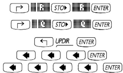
To verify the contents of the variables, use ↗ and ↗.
This procedure can be generalized to the copying of three or more variables.
Copying two or more variables using the stack in RPN mode
The following is an exercise to demonstrate how to copy two or more variables using the stack when the calculator is in RPN mode. We assume, again, that we are within sub-directory {HOME MANS INTRO} and that we want to copy the variables R and Q into sub-directory {HOME MANS}. The keystrokes necessary to complete this operation are shown following:

To verify the contents of the variables, use ↗ and ↗.
This procedure can be generalized to the copying of three or more variables.
Reordering variables in a directory
In this section we illustrate the use of the ORDER command to reorder the variables in a directory. We assume we start within the sub-directory {HOME MANS} containing the variables, A12, R, Q, z1, A, and the sub-directory INTRO, as shown below. (Copy A12 from INTRO into MANS).

Algebraic mode
In this case, we have the calculator set to Algebraic mode. Suppose that we want to change the order of the variables to INTRO, A, z1, Q, R, A12. Proceed as follows to activate the ORDER function:

Select MEMORY from the programming menu


The screen will show the following input line:

Next, we'll list the new order of the variables by using their names typed between quotes:

The screen now shows the new ordering of the variables:
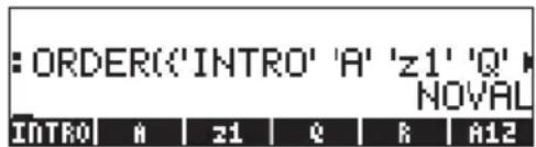
Moving variables using the FILES menu
To move a variable from one directory to another you can use the FILES menu. For example, within the sub-directory {HOME MANS INTRO}, we have variables p1, z1, R, Q, A12, α, and A. Suppose that we want to move variable A12 to sub-directory {HOME MANS}. Here is how to do it: Press ← FILES to show a variable list. Use the down-arrow key ▼ to select variable A12, then press 🎨. The calculator will respond with a PICK DESTINATION screen. Use the up arrow key ▲ to select the sub-directory MANS and press 🎨. The screen will now show the contents of sub-directory {HOME MANS INTRO}:  Notice that variable A12 is no longer there. If you now press UPDIR, the screen will show the contents of sub-directory MANS, including variable A12:  Note: You can use the stack to move a variable by combining copying with deleting a variable. Procedures for deleting variables are demonstrated in the next section.Deleting variables
Variables can be deleted using function PURGE. This function can be accessed directly by using the TOOLS menu (TOOL), or by using the FILES menu Using the FILES command
The FILES command can be used to purge one variable at a time. To delete a variable from a given directory you can use the FILES menu. For example, within the sub-directory {HOME MANS INTRO}, we have variables p1, z1, R, Q, α, and A left. Suppose that we delete variable A. Here is how to do it: Press ← FILES → to produce the variable list. Use the down-arrow key ▼ to select variable A (the last in the list), then press NXT → The screen will now show the contents of sub-directory INTRO without variable A. Using function PURGE in the stack in Algebraic mode
We start again at subdirectory {HOME MANS INTRO} containing now only variables p1, z1, Q, R, and α . We will use command PURGE to delete variable p1. Press TOOL VAR ENTER. The screen will now show variable p1 removed:  You can use the PURGE command to erase more than one variable by placing their names in a list in the argument of PURGE. For example, if now we wanted to purge variables R and Q, simultaneously, we can try the following exercise. Press : TOOL 📄 → { } VAR ▶ → , VAR At this point, the screen will show the following command ready to be executed:  To finish deleting the variables, press ENTER. The screen will now show the remaining variables: Using function PURGE in the stack in RPN mode
We start again at subdirectory {HOME MANS INTRO} containing variables p1, z1, Q, R, and α . We will use command PURGE to delete variable p1. Press ☐ ENTER TOOL ☐ ☐ ☐ The screen will now show variable p1 removed:  To delete two variables simultaneously, say variables R and Q, first create a list (in RPN mode, the elements of the list need not be separated by commas as in Algebraic mode): VAR ← {} , [ICON] ▶ , ENTER . Then, press TOOL USE to purge the variables.UNDO and CMD functions
Functions UNDO and CMD are useful for recovering recent commands, or to revert an operation if a mistake was made. These functions are associated with the HIST key: UNDO results from the keystroke sequence → UNDO, while CMD results from the keystroke sequence ← CMD. To illustrate the use of UNDO, try the following exercise in algebraic (ALG) mode: 5 × 4 ÷ 3 ENTER. The UNDO command (→ UNDO) will simply erase the result. The same exercise in RPN mode, will follow these keystrokes: 5 ENTER 4 ENTER × 3 ENTER ÷. Using → UNDO at this point will undo the most recent operation (20/3), leaving the original terms back in the stack:  To illustrate the use of CMD, let's enter the following entries in ALG mode. Press ENTER after each entry.  Next, use the CMD function ( ← CMD ) to show the four most recent commands entered by the user, i.e.,  You can use the up and down arrow keys (▲▼) to navigate through these commands and highlight any of them that you want to entry anew. Once you have selected the command to enter, press 📄. The CMD function operates in the same fashion when the calculator is in RPN mode, except that the list of commands only shows numbers or algebraics. It does not show functions entered. For example, try the following exercise in RPN mode: 5 ENTER 2 ENTER 3 ÷ × SIN 1 SIN 5 × 2 ENTER. Pressing ← CMD produces the following selection box:  As you can see, the numbers 3, 2, and 5, used in the first calculation above, are listed in the selection box, as well as the algebraic 'SIN(5x2)', but not the SIN function entered previous to the algebraic.Flags
A flag is a Boolean value, that can be set or cleared (true or false), that specifies a given setting of the calculator or an option in a program. Flags in the calculator are identified by numbers. There are 256 flags, numbered from -128 to 128. Positive flags are called user flags and are available for programming purposes by the user. Flags represented by negative numbers are called system flags and affect the way the calculator operates. To see the current system flag setting press the MODE button, and then the soft menu key (i.e., F1). You will get a screen labeled SYSTEM FLAGS listing flag numbers and the corresponding setting.  (Note: In this screen, as only system flags are present, only the absolute value of the flag number is displayed). A flag is said to be set if you see a check mark (√) in front of the flag number. Otherwise, the flag is not set or cleared. To change the status of a system flag press the √☐☐☐! soft menu key while the flag you want to change is highlighted, or use the +/- key. You can use the up and down arrow keys (▲ ▼) to move about the list of system flags. Although there are 128 system flags, not all of them are used, and some of them are used for internal system control. System flags that are not accessible to the user are not visible in this screen. A complete list of flags is presented in Chapter 24.Example of flag setting: general solutions vs. principal value
For example, the default value for system flag 01 is General solutions. What this means is that, if an equation has multiple solutions, all the solutions will be returned by the calculator, most likely in a list. By pressing the √∅∅∅ soft menu key you can change system flag 01 to Principal value. This setting will force the calculator to provide a single value known as the principal value of the solution. To see this at work, first set system flag 01 (i.e., select Principal Value). Press twice to return to normal calculator display. We will try solving a quadratic equation solution, say, f + 5t + 6 = 0 , with command QUAD.Algebraic mode
Use the following keystroke sequence: CAT ALPHA (use the up and down arrow keys, ▲▼, to select command QUAD), press 📄.  To enter the equation as the first argument of function QUAD, use the following keystrokes:  The result is:  Now, change the setting of flag 1 to General solutions: MODE FLADE √ ETR. And try the solution again: ▲ ▲ ENTER ENTER. The solution now includes two values: RPN mode
First set system flag 01 (i.e., Principal Value). Press ■ twice to return to normal calculator display. Then, type the quadratic equation as follows:  ENTER (keeping a second copy in the RPN stack)   Use the following keystroke sequence to enter the QUAD command: CAT ALPHA (use the up and down arrow keys, ▲▼, to select command QUAD), press 🎨. The screen shows the principal solution:  Now, change the setting of flag 01 to General solutions: MODE √ . And try the solution again: CAT ALPHA (use the up and down arrow keys, ▲▼, to select command QUAD), press 🎯. The screen now shows the two solutions: Other flags of interest
Bring up once more the current flag setting by pressing the MODE button, and then the soft menu key. Make sure to clear system flag 01, which was left set from the previous exercise. Use the up and down arrow keys (▲▼) to move about the system flag list. Some flags of interest and their preferred value for the purpose of the exercises that follow in this manual are: 02 Constant → symb: Constant values (e.g., π) are kept as symbols 03 Function → symb: Functions are not automatically evaluated, instead they are loaded as symbolic expressions. 27 'X+Y*i' → (X,Y): Complex numbers are represented as ordered pairs 60 [α][α] locks: The sequence ALPHA ALPHA locks the alphabetic keyboard Press ■ twice to return to normal calculator display.CHOOSE boxes vs. Soft MENU
In some of the exercises presented in this chapter we have seen menu lists of commands displayed in the screen. These menu lists are referred to as CHOOSE boxes. For example, to use the ORDER command to reorder variables in a directory, we use, in algebraic mode:  PRG  Show PROG menu list and select MEMORY      Show the MEMORY menu list and select DIRECTORY     Show the DIRECTORY menu list and select ORDER  ■ activate the ORDER command There is an alternative way to access these menus as soft MENU keys, by setting flag 117. To set this flag try the following:       The screen shows flag 117 not set (CHOOSE boxes), as shown here:  Press the √□□□ soft menu key to set flag 117 to soft MENU. The screen will reflect that change:  Press twice to return to normal calculator display. Now, we'll try to find the ORDER command using similar keystrokes to those used above, i.e., we start with PRG. Notice that instead of a menu list, we get soft menu labels with the different options in the PROG menu, i.e.,  Press F2 to select the MEMORY soft menu (☐3). The display now shows:  Press F5 to select the DIRECTORY soft menu (OK)  The ORDER command is not shown in this screen. To find it we use the NXT key to find it:  To activate the ORDER command we press the F3 (JPEG) soft menu key. Although not applied to a specific example, this exercise shows the two options for menus in the calculator (CHOOSE boxes and soft MENUs). Note: most of the examples in this user guide assume that the current setting of flag 117 is its default setting (that is, not set). If you have set the flag but want to strictly follow the examples in this guide, you should clear the flag before continuing.Selected CHOOSE boxes
Some menus will only produce CHOOSE boxes, e.g., \- The APPS (APPLICATIONS menu), activated with the APPS key, first key in the second row of keys from the top of the keyboard:  \- The CAT (CATalog menu), activated with the → _CAT key, second key in the fourth row of keys from the top of the keyboard:  • The HELP menu, activated with TOOL NXT  \- The CMDS (CoMmanDS) menu, activated within the Equation Writer, i.e., → EQW NXT Chapter 3
Calculation with real numbers
This chapter demonstrates the use of the calculator for operations and functions related to real numbers. Operations along these lines are useful for most common calculations in the physical sciences and engineering. The user should be acquainted with the keyboard to identify certain functions available in the keyboard (e.g., SIN, COS, TAN, etc.). Also, it is assumed that the reader knows how to adjust the calculator's operation, i.e., select operating mode (see Chapter 1), use menus and choose boxes (see Chapter 1), and operate with variables (see Chapter 2).Checking calculators settings
To check the current calculator and CAS settings you need to just look at the top line in the calculator display in normal operation. For example, you may see the following setting: RAD XYZ DEC R = 'X' This stands for RADians for angular measurements, XYZ for Rectangular (Cartesian) coordinates, DECimal number base, Real numbers preferred, = means "exact" results, and 'X' is the value of the default independent variable. Another possible listing of options could be DEG R∠Z HEX C \~ 't' This stands for DEGrees as angular measurements, R∠Z for Polar coordinates, HEXagesimal number base, Complex numbers allowed, \~ stands for "approximate" results, and 't' as the default independent variable. In general, this part of the display contains seven elements. Each element is identified next under numbers 1 through 7. The possible values for each element are shown between parentheses following the element description. The explanation of each of those values is also shown: 1. Angle measure specification (DEG, RAD, GRD) DEG: degrees, 360 degrees in a complete circle RAD: radians, 2π radians in a complete circle GRD: grades, 400 grades in a complete circle 2. Coordinate system specification (XYZ, R∠Z, R∠∠). The symbol ∠ stands for an angular coordinate. XYZ: Cartesian or rectangular (x,y,z) R∠Z: cylindrical Polar coordinates (r,θ,z) R∠∠: Spherical coordinates (ρ,θ,φ) 3. Number base specification (HEX, DEC, OCT, BIN) HEX: hexadecimal numbers (base 16) DEC: decimal numbers (base 10) OCT: octal numbers (base 8) BIN: binary numbers (base 2) 4. Real or complex mode specification (R, C) R: real numbers C: complex numbers 5. Exact or approximate mode specification (=, \~) = exact (symbolic) mode \~ approximate (numerical) mode 6. Default CAS independent variable (e.g., 'X', 't', etc.)Checking calculator mode
When in RPN mode the different levels of the stack are listed in the left-hand side of the screen. When the ALGEBRAIC mode is selected there are no numbered stack levels, and the word ALG is listed in the top line of the display towards the right-hand side. The difference between these operating modes was described in detail in Chapter 1.Real number calculations
To perform real number calculations it is preferred to have the CAS set to Real (as opposite to Complex) mode. In some cases, a complex result may show up, and a request to change the mode to Complex will be made by the calculator. Exact mode is the default mode for most operations. Therefore, you may want to start your calculations in this mode. Any change to Approx mode required to complete an operation will be requested by the calculator. There is no preferred selection for the angle measure or for the number base specification. Real number calculations will be demonstrated in both the Algebraic (ALG) and Reverse Polish Notation (RPN) modes.Changing sign of a number, variable, or expression
Use the +/- key. In ALG mode, you can press +/- before entering the number, e.g., +/- 2 • 5 ENTER. Result = -2.5. In RPN mode, you need to enter at least part of the number first, and then use the +/- key, e.g., 2 • 5 +/-. Result = -2.5. If you use the +/- function while there is no command line, the calculator will apply the NEG function (inverse of sign) to the object on the first level of the stack.The inverse function
Use the 1/x key. In ALG mode, press 1/x first, followed by a number or algebraic expression, e.g., 1/x 2. Result = 1/2 or 0.5. In RPN mode, enter the number first, then use the key, e.g., 4 ENTER 1/x . Result = 1/4 or 0.25.Addition, subtraction, multiplication, division
Use the proper operation key, namely, + - × ÷ . In ALG mode, press an operand, then an operator, then an operand, followed by an ENTER to obtain a result. Examples:  The first three operations above are shown in the following screen shot:  In RPN mode, enter the operands one after the other, separated by an ENTER, then press the operator key. Examples:  Alternatively, in RPN mode, you can separate the operands with a space (SPC) before pressing the operator key. Examples: Using parentheses
Parentheses can be used to group operations, as well as to enclose arguments of functions. The parentheses are available through the keystroke combination ← () . Parentheses are always entered in pairs. For example, to calculate (5 + 3.2) / (7 - 2.2) :In ALG mode:
 In RPN mode, you do not need the parenthesis, calculation is done directly on the stack:  In RPN mode, typing the expression between quotes will allow you to enter the expression like in algebraic mode:  For both, ALG and RPN modes, using the Equation Writer:  The expression can be evaluated within the Equation writer, by using: Absolute value function
The absolute value function, ABS, is available through the keystroke combination: ← ABS. When calculating in the stack in ALG mode, enter the function before the argument, e.g., ← ABS +/- 2 · 3 2 ENTER In RPN mode, enter the number first, then the function, e.g., Squares and square roots
The square function, SQ, is available through the keystroke combination: ← x2 . When calculating in the stack in ALG mode, enter the function before the argument, e.g., ← x2 +/- 2 · 3 ENTER In RPN mode, enter the number first, then the function, e.g., 2 · 3 +/- ← χ² The square root function, , is available through the R key. When calculating in the stack in ALG mode, enter the function before the argument, e.g., 1 2 3 · 4 ENTER In RPN mode, enter the number first, then the function, e.g., 1 2 3 · 4 √XPowers and roots
The power function, , is available through the γx key. When calculating in the stack in ALG mode, enter the base (y) followed by the γx key, and then the exponent (x), e.g., 5 · 2 γx 1 · 2 5 In RPN mode, enter the number first, then the function, e.g., 5 • 2 ENTER 1 • 2 5 ENTER γx The root function, XROOT(y,x), is available through the keystroke combination. When calculating in the stack in ALG mode, enter the function XROOT followed by the arguments (y,x), separated by commas, e.g., → √y 3 → , 2 7 ENTER In RPN mode, enter the argument y, first, then, x, and finally the function call, e.g., 2 7 ENTER 3 ENTER → √yBase-10 logarithms and powers of 10
Logarithms of base 10 are calculated by the keystroke combination → LOG (function LOG) while its inverse function (ALOG, or antilogarithm) is calculated by using ← 10x . In ALG mode, the function is entered before the argument: → LOG 2 · 4 5 ENTER ← 10 x +/- 2 • 3 ENTER In RPN mode, the argument is entered before the function 2 · 4 5 ENTER → LOG 2 • 3 +/- ENTER ← 10^xUsing powers of 10 in entering data
Powers of ten, i.e., numbers of the form -4.5'10-2 , etc., are entered by using the EEX key. For example, in ALG mode: + / - 4 · 5 EX + / - 2 ENTER Or, in RPN mode: 4 · 5 + / - EEX 2 + / - ENTERNatural logarithms and exponential function
Natural logarithms (i.e., logarithms of base e = 2.7182818282 ) are calculated by the keystroke combination → LN (function LN) while its inverse function, the exponential function (function EXP) is calculated by using ← ex . In ALG mode, the function is entered before the argument: → amp; LN amp;2 amp; amp;4 amp;5 amp; ENTER ; ← amp;e ^ x amp;+ / - amp;2 amp; amp;3 amp; ENTER In RPN mode, the argument is entered before the function 2 amp; amp;4 amp;5 amp; ENTER amp;→ LN ; 2 amp; amp;3 amp;+ / - amp; ENTER amp;← e ^ xTrigonometric functions
Three trigonometric functions are readily available in the keyboard: sine ( ), cosine ( ), and tangent ( ). The arguments of these functions are angles, therefore, they can be entered in any system of angular measure (degrees, radians, grades). For example, with the DEG option selected, we can calculate the following trigonometric functions: In ALG mode: SIN amp; 3 amp; 0 amp; ENTER \ COS amp; 4 amp; 5 amp; ENTER \ TAN amp; 1 amp; 3 amp; 5 amp; ENTER In RPN mode: 3 amp; 0 amp; ENTER amp; SIN \ 4 amp; 5 amp; ENTER amp; COS \ 1 amp; 3 amp; 5 amp; ENTER amp; TAN \Inverse trigonometric functions
The inverse trigonometric functions available in the keyboard are the arcsine (ASIN), arccosine (ACOS), and arctangent (ATAN), available through the keystroke combinations ← ASIN , ← ACOS , and ← ATAN , respectively. Since the inverse trigonometric functions represent angles, the answer from these functions will be given in the selected angular measure (DEG, RAD, GRD). Some examples are shown next: In ALG mode:  In RPN mode:  All the functions described above, namely, ABS, SQ, , ^ , XROOT, LOG, ALOG, LN, EXP, SIN, COS, TAN, ASIN, ACOS, ATAN, can be combined with the fundamental operations ( + - × ÷ ) to form more complex expressions. The Equation Writer, whose operations is described in Chapter 2, is ideal for building such expressions, regardless of the calculator operation mode.Differences between functions and operators
Functions like ABS, SQ, √, LOG, ALOG, LN, EXP, SIN, COS, TAN, ASIN, ACOS, ATAN require a single argument. Thus, their application is ALG mode is straightforward, e.g., ABS(x). Some functions like XROOT require two arguments, e.g., XROOT(x,y). This function has the equivalent keystroke sequence → √√y. Operators, on the other hand, are placed after a single argument or between two arguments. The factorial operator (!), for example, is placed after a number, e.g., 5 ALPHA → 2 ENTER. Since this operator requires a single argument it is referred to as a unary operator. Operators that require two arguments, such as + - × ÷ γ x , are binary operators, e.g., 3 × 5, or 4 γ x 2.Real number functions in the MTH menu
The MTH (MaTHematics) menu include a number of mathematical functions mostly applicable to real numbers. To access the MTH menu, use the keystroke combination MTH. With the default setting of CHOOSE boxes for system flag 117 (see Chapter 2), the MTH menu is shown as the following menu list:   As they are a great number of mathematic functions available in the calculator, the MTH menu is sorted by the type of object the functions apply on. For example, options 1. VECTOR., 2. MATRIX., and 3. LIST.. apply to those data types (i.e., vectors, matrices, and lists) and will be discussed in more detail in subsequent chapters. Options 4. HYPERBOLIC.. and 5. REAL.. apply to real numbers and will be discussed in detailed herein. Option 6. BASE.. is used for conversion of numbers in different bases, and is also to be discussed in a separate chapter. Option 7. PROBABILITY.. is used for probability applications and will be discussed in an upcoming chapter. Option 8. FFT.. (Fast Fourier Transform) is an application of signal processing and will be discussed in a different chapter. Option 9. COMPLEX.. contains functions appropriate for complex numbers, which will be discussed in the next chapter. Option 10. CONSTANTS provides access to the constants in the calculator. This option will be presented later in this section. Finally, option 11. SPECIAL FUNCTIONS.. includes functions of advanced mathematics that will be discussed in this section also. In general, to apply any of these functions you need to be aware of the number and order of the arguments required, and keep in mind that, in ALG mode you should select first the function and then enter the argument, while in RPN mode, you should enter the argument in the stack first, and then select the function.Using calculator menus:
1. Since the operation of MTH functions (and of many other calculator menus) is very similar, we will describe in detail the use of the 4. HYPERBOLIC.. menu in this section, with the intention of describing the general operation of calculator menus. Pay close attention to the process for selecting different options. 2. To quickly select one of the numbered options in a menu list (or CHOOSE box), simply press the number for the option in the keyboard. For example, to select option 4. HYPERBOLIC.. in the MTH menu, simply press 4.Hyperbolic functions and their inverses
Selecting Option 4. HYPERBOLIC.., in the MTH menu, and pressing 📄, produces the hyperbolic function menu:   The hyperbolic functions are: Hyperbolic sine, SINH, and its inverse, ASINH or sinh 1 Hyperbolic cosine, COSH, and its inverse, ACOSH or 1 Hyperbolic tangent, TANH, and its inverse, ATANH or tanH This menu contains also the functions: EXPM (x) = (x) - 1, LNP1 (x) = (x + 1). Finally, option 9. MATH, returns the user to the MTH menu. For example, in ALG mode, the keystroke sequence to calculate, say, (2.5) , is the following: ← MTH Select MTH menu 4 Select the 4. HYPERBOLIC.. menu 5 Select the 5. TANH function 2 · 5 ENTER Evaluate tanh(2.5) The screen shows the following output:  In the RPN mode, the keystrokes to perform this calculation are the following: 2 · 5 ENTER Enter the argument in the stack ← MTH Select MTH menu 4 Select the 4. HYPERBOLIC.. menu 5 Select the 5. TANH function The result is:  The operations shown above assume that you are using the default setting for system flag 117 (CHOOSE boxes). If you have changed the setting of this flag (see Chapter 2) to SOFT menu, the MTH menu will show as labels of the soft menu keys, as follows (left-hand side in ALG mode, right-hand side in RPN mode):   Pressing NXT shows the remaining options:   Note: Pressing ← PREV will return to the first set of MTH options. Also, using the combination → will list all menu functions in the screen, e.g.  Thus, to select, for example, the hyperbolic functions menu, with this menu format press 📄, to produce:   Finally, in order to select, for example, the hyperbolic tangent (tanh) function, simply press 📄. Note: To see additional options in these soft menus, press the NXT key or the PREV keystroke sequence. For example, to calculate (2.5) , in the ALG mode, when using SOFT menus over CHOOSE boxes, follow this procedure: ← MTH Select MTH menu  Select the HYPERBOLIC.. menu  Select the TANH function   Evaluate tanh(2.5) In RPN mode, the same value is calculated using:   Enter argument in the stack   TH menu   Select the HYPERBOLIC.. menu  Select the TANH function As an exercise of applications of hyperbolic functions, verify the following values: SINH (2.5) = 6.05020.. ASINH(2.0) = 1.4436... COSH (2.5) = 6.13228.. ACOSH (2.0) = 1.3169... TANH(2.5) = 0.98661.. ATANH(0.2) = 0.2027... EXPM(2.0) = 6.38905.... LNP1(1.0) = 0.69314.... Once again, the general procedure shown in this section can be applied for selecting options in any calculator menu.Real number functions
Selecting option 5. REAL.. in the MTH menu, with system flag 117 set to CHOOSE boxes, generates the following menu list:     Option 19. MATH.. returns the user to the MTH menu. The remaining functions are grouped into six different groups described below. If system flag 117 is set to SOFT menus, the REAL functions menu will look like this (ALG mode used, the same soft menu keys will be available in RPN mode):   The very last option, 📄, returns the user to the MTH menu.Percentage functions
These functions are used to calculate percentages and related values as follows: % (y,x) : calculates the x percentage of y %CH(y,x) : calculates 100(y-x)/x, i.e., the percentage change, the difference between two numbers. %T(y,x) : calculates 100 x/y, i.e., the percentage total, the portion that one number (x) is of another (y). These functions require two arguments, we illustrate the calculation of % T(15,45) , i.e., calculation 15% of 45, next. We assume that the calculator is set to ALG mode, and that system flag 117 is set to CHOOSE boxes. The procedure is as follows: ← MTH Select MTH menu 5 Select the 5. REAL.. menu 3 Select the 5. %T function 1 5 Enter first argument → , Enter a comma to separate arguments 4 5 Enter second argument ENTER Calculate function The result is shown next:  In RPN mode, recall that argument y is located in the second level of the stack, while argument x is located in the first level of the stack. This means, you should enter x first, and then, y, just as in ALG mode. Thus, the calculation of %T(15,45), in RPN mode, and with system flag 117 set to CHOOSE boxes, we proceed as follows: 1 5 ENTER Enter first argument 4 5 ENTER Enter second argument ← MTH Select MTH menu 5 Select the 5. REAL.. menu 3 Select the 5. %T function Note: The exercises in this section illustrate the general use of calculator functions having 2 arguments. The operation of functions having 3 or more arguments can be generalized from these examples. As an exercise for percentage-related functions, verify the following values: % (5,20) = 1 , % CH(22,25) = 13.6363 , % T(500,20) = 4Minimum and maximum
Use these functions to determine the minimum or maximum value of two arguments. MIN(x,y) : minimum value of x and y MAX(x,y) : maximum value of x and y As an exercise, verify that MIN(-2,2) = -2 , MAX(-2,2) = 2Modulo
MOD: y mod x = residual of y/x, i.e., if x and y are integer numbers, y/x = d + r/x, where d = quotient, r = residual. In this case, r = y mod x. Please notice that MOD is not a function, but rather an operator, i.e., in ALG mode, MOD should be used as y MOD x, and not as MOD(y, x). Thus, the operation of MOD is similar to that of +, -, ×, ÷. As an exercise, verify that 15 MOD 4 = 15 mod 4 = residual of 15/4 = 3Absolute value, sign, mantissa, exponent, integer and fractional parts
ABS(x) : calculates the absolute value, |x| SIGN(x) : determines the sign of x, i.e., -1, 0, or 1. MANT(x) : determines the mantissa of a number based on 10 . XPON(x) : determines the power of 10 in the number IP(x) : determines the integer part of a real number FP(x) : determines the fractional part of a real number As an exercise, verify that ABS(-3) = |-3| = 3 , SIGN(-5) = -1 , MANT(2540) = 2.540 , XPON(2540) = 3 , IP(2.35) = 2 , FP(2.35) = 0.35 .Rounding, truncating, floor, and ceiling functions
RND(x,y) : rounds up y to x decimal places TRNC(x,y) : truncate y to x decimal places FLOOR(x) : closest integer that is less than or equal to x CEIL(x) : closest integer that is greater than or equal to x As an exercise, verify that RND(1.4567,2)=1.46 , TRNC(1.4567,2)=1.45 , FLOOR(2.3)=2 , CEIL(2,3)=3Radians-to-degrees and degrees-to-radians functions
D→R (x) : converts degrees to radians R → D(x) : converts radians to degrees. As an exercise, verify that D → R(45) = 0.78539 (i.e., 45° = 0.78539rad ), R → D(1.5) = 85.943669 . (i.e., 1.5rad = 85.943669 .).Special functions
Option 11. Special functions... in the MTH menu includes the following functions:  GAMMA: The Gamma function (α) PSI: N-th derivative of the digamma function Psi: Digamma function, derivative of the ln(Gamma) The Gamma function is defined by (α) is 0∞ xα-1 φ-x has dx applications in applied mathematics for science and engineering, as well as in probability and statistics.Factorial of a number
The factorial of a positive integer number n is defined as n!=n·(n-1)×(n-2) ...3×2×1 , with 0!=1. The factorial function is available in the calculator by using →2 . In both ALG and RPN modes, enter the number first, followed by the sequence →2 . Example: 5 →2 . The Gamma function, defined above, has the property that (α) = (α - 1) (α - 1), for αgt; 1. Therefore, it can be related to the factorial of a number, i.e., (α) = (α - 1)! , when α is a positive integer. We can also use the factorial function to calculate the Gamma function, and vice versa. For example, (5) = 4! or, 4 ALPHA → 2 ENTER. The factorial function is available in the MTH menu, through the 7. PROBABILITY.. menu. The PSI function, (x,y) , represents the y-th derivative of the digamma function, i.e., (n, x) = dn/dxn (x) , (x) is known as theedigamma function, or Psi function. For this function, y must be a positive integer. The Psi function, (x) , or digamma function, is defined as (x) = [(x)] Examples of these special functions are shown here using both the ALG and RPN modes. As an exercise, verify that GAMMA(2.3) = 1.166711... , PSI(1.5,3) = 1.40909... , and Psi(1.5) = 3.64899739... E-2 . These calculations are shown in the following screen shot: Calculator constants
The following are the mathematical constants used by your calculator: • e: the base of natural logarithms. - i : the imaginary unit, i i2 = -1 . • π. the ratio of the length of the circle to its diameter. - MINR: the minimum real number available to the calculator. - MAXR: the maximum real number available to the calculator. To have access to these constants, select option 11. CONSTANTS.. in the MTH menu,  The constants are listed as follows:   Selecting any of these entries will place the value selected, whether a symbol (e.g., e, i, π, MINR, or MAXR) or a value (2.71.., (0,1), 3.14.., 1E-499, 9.99..E499) in the stack. Please notice that e is available from the keyboard as exp(1), i.e., ← e x I ENTER, in ALG mode, or I ENTER ← e x , in RPN mode. Also, π is available directly from the keyboard as ← π. Finally, i is available by using ← i.Operations with units
Numbers in the calculator can have units associated with them. Thus, it is possible to calculate results involving a consistent system of units and produce a result with the appropriate combination of units.The UNITS menu
The units menu is launched by the keystroke combination ↗ UNITS (associated with the 6 key). With system flag 117 set to CHOOSE boxes, the result is the following menu:    Option 1. Tools.. contains functions used to operate on units (discussed later). Options 3. Length.. through 17. Viscosity.. contain menus with a number of units for each of the quantities described. For example, selecting option 8. Force.. shows the following units menu:   The user will recognize most of these units (some, e.g., dyne, are not used very often nowadays) from his or her physics classes: N = newtons, dyn = dynes, gf = grams – force (to distinguish from gram-mass, or plainly gram, a unit of mass), kip = kilo-poundal (1000 pounds), lbf = pound-force (to distinguish from pound-mass), pdl = poundal. To attach a unit object to a number, the number must be followed by an underscore. Thus, a force of 5 N will be entered as 5_N. For extensive operations with units SOFT menus provide a more convenient way of attaching units. Change system flag 117 to SOFT menus (see Chapter 1), and use the keystroke combination ↗ UNITS to get the following menus. Press NXT to move to the next menu page.  Pressing on the appropriate soft menu key will open the sub-menu of units for that particular selection. For example, for the ☐☐☐☐ sub-menu, the following units are available:  Pressing the soft menu key 📄 will take you back to the UNITS menu. Recall that you can always list the full menu labels in the screen by using ▶▼, e.g., for the □□□ set of units the following labels will be listed:   Note: Use the NXT key or the ← PREV keystroke sequence to navigate through the menus.Available units
The following is a list of the units available in the UNITS menu. The unit symbol is shown first followed by the unit name in parentheses:LENGTH
m (meter), cm (centimeter), mm (millimeter), yd (yard), ft (feet), in (inch), Mpc (Mega parsec), pc (parsec), lyr (light-year), au (astronomical unit), km (kilometer), mi (international mile), nmi (nautical mile), miUS (US statute mile), chain (chain), rd (rod), fath (fathom), ftUS (survey foot), Mil (Mil), μ (micron), Å (Angstrom), fermi (fermi)AREA
m^2 (square meter), cm^2 (square centimeter), b (barn), yd^2 (square yard), ft^2 (square feet), in^2 (square inch), km^2 (square kilometer), ha (hectare), a (are), mi^2 (square mile), miUS^2 (square statute mile), acre (acre)VOLUME
m^3 (cubic meter), st (stere), cm^3 (cubic centimeter), yd^3 (cubic yard), ft^3 (cubic feet), in^3 (cubic inch), l (liter), galUK (UK gallon), galC (Canadian gallon), gal (US gallon), qt (quart), pt (pint), ml (mililiter), cu (US cup), ozfl (US fluid ounce), ozUK (UK fluid ounce), tbsp (tablespoon), tsp (teaspoon), bbl (barrel), bu (bushel), pk (peck), fbm (board foot)TIME
yr (year), d (day), h (hour), min (minute), s (second), Hz (hertz)SPEED
m/s (meter per second), cm/s (centimeter per second), ft/s (feet per second), kph (kilometer per hour), mph (mile per hour), knot (nautical miles per hour), c (speed of light), ga (acceleration of gravity)MASS
kg (kilogram), g (gram), Lb (avoirdupois pound), oz (ounce), slug (slug), lbt (Troy pound), ton (short ton), tonUK (long ton), t (metric ton), ozt (Troy ounce), ct (carat), grain (grain), u (unified atomic mass), mol (mole)FORCE
N (newton), dyn (dyne), gf (gram-force), kip (kilopound-force), lbf (pound-force), pdl (poundal)ENERGY
J (joule), erg (erg), Kcal (kilocalorie), Cal (calorie), Btu (International table btu), ft×lbf (foot-pound), therm (EEC therm), MeV (mega electron-volt), eV (electron-volt)POWER
W (watt), hp (horse power),PRESSURE
Pa (pascal), atm (atmosphere), bar (bar), psi (pounds per square inch), torr (torr), mmHg (millimeters of mercury), inHg (inches of mercury), inH2O (inches of water),TEMPERATURE
° C (degree Celsius), ° F (degree Fahrenheit), K (Kelvin), ° R (degree Rankine),ELECTRIC CURRENT (Electric measurements)
V (volt), A (ampere), C (coulomb), Ω (ohm), F (farad), W (watt), Fdy (faraday), H (henry), mho (mho), S (siemens), T (tesla), Wb (weber)ANGLE (planar and solid angle measurements)
° (sexagesimal degree), r (radian), grad (grade), arcmin (minute of arc), arcs (second of arc), sr (steradian)LIGHT (Illumination measurements)
fc (footcandle), flam (footlambert), lx (lux), ph (phot), sb (stilb), lm (lumem), cd (candela), lam (lambert)RADIATION
Gy (gray), rad (rad), rem (rem), Sv (sievert), Bq (becquerel), Ci (curie), R (roentgen)VISCOSITY
P (poise), St (stokes)Units not listed
Units not listed in the Units menu, but available in the calculator include: gmol (gram-mole), lbmol (pound-mole), rpm (revolutions per minute), dB (decibels). These units are accessible through menu 117.02, triggered by using MENU(117.02) in ALG mode, or 117.02 ENTER MENU in RPN mode. The menu will show in the screen as follows (use → to show labels in display):  These units are also accessible through the catalog, for example: gmol: → CAT ALPHA ← G Ibmol: → CAT ALPHA ← L rpm: → CAT ALPHA ← R dB: → CAT ALPHA ← DConverting to base units
To convert any of these units to the default units in the SI system, use the function UBASE. For example, to find out what is the value of 1 poise (unit of viscosity) in the SI units, use the following: In ALG mode, system flag 117 set to CHOOSE boxes:  This results in the following screen (i.e., 1 poise = 0.1 kg/(ms)):  In RPN mode, system flag 117 set to CHOOSE boxes:  In ALG mode, system flag 117 set to SOFT menus:  ENTER Convert the units In RPN mode, system flag 117 set to SOFT menus: Attaching units to numbers
To attach a unit object to a number, the number must be followed by an underscore (→—, key(8,5)). Thus, a force of 5 N will be entered as 5_N. Here is the sequence of steps to enter this number in ALG mode, system flag 117 set to CHOOSE boxes:  The screen will look like the following:  Note: If you forget the underscore, the result is the expression 5*N, where N here represents a possible variable name and not Newtons. To enter this same quantity, with the calculator in RPN mode, use the following keystrokes:  Notice that the underscore is entered automatically when the RPN mode is active. The result is the following screen:  As indicated earlier, if system flag 117 is set to SOFT menus, then the UNITS menu will show up as labels for the soft menu keys. This set up is very convenient for extensive operations with units. The keystroke sequences to enter units when the SOFT menu option is selected, in both ALG and RPN modes, are illustrated next. For example, in ALG mode, to enter the quantity 5_N use: 5 → Enter number and underscore → UNITS Access the UNITS menu NXT FORCE Select units of force Select Newtons (N) ENTER Enter quantity with units in the stack The same quantity, entered in RPN mode uses the following keystrokes: 5 Enter number (no underscore) → UNITS Access the UNITS menu NXT FORCE Select units of force Select Newtons (N) Note: You can enter a quantity with units by typing the underline and units with the ALPHA keyboard, e.g., 5 → - ALPHA N will produce the entry: 5_NUnit prefixes
You can enter prefixes for units according to the following table of prefixes from the SI system. The prefix abbreviation is shown first, followed by its name, and by the exponent x in the factor 10x corresponding to each prefix: Prefix Name x Prefix Name x| Y | y | o | t | t | a | + | 2 | 4 |
| Z zetta | +21 | c centi | -2 | |||||
| E exa | +18 | m | milli | -3 | ||||
| P | peta | +15 | μ micro | -6 | ||||
| T tera | +12 | n nano | -9 | |||||
| G | giga | +9 | p | pico | -12 | |||
| M | mega | +6 | f | femto | -15 | |||
| k,K | kilo | +3 | a atto | -18 | ||||
| h,H | hecto | +2 | z | zepto | -21 | |||
| D(*) | deka | +1 | y | yocto | -24 | |||
Operations with units
Once a quantity accompanied with units is entered into the stack, it can be used in operations similar to plain numbers, except that quantities with units cannot be used as arguments of functions (say, SQ or SIN). Thus, attempting to calculate LN(10_m) will produce an error message: Error: Bad Argument Type. Here are some calculation examples using the ALG operating mode. Be warned that, when multiplying or dividing quantities with units, you must enclosed each quantity with its units between parentheses. Thus, to enter, for example, the product 12.5m × 5.2yd , type it to read (12.5m)*(5.2yd) ENTER:  which shows as 65_(m·yd). To convert to units of the SI system, use function UBASE:  Note: Recall that the ANS(1) variable is available through the keystroke combination ← ANS (associated with the ENTER key). To calculate a division, say, 3250 mi / 50 h, enter it as (3250_mi)/(50_h) ENTER :  which transformed to SI units, with function UBASE, produces:  Addition and subtraction can be performed, in ALG mode, without using parentheses, e.g., 5 m + 3200 mm, can be entered simply as 5_m + 3200_mm ENTER :  More complicated expression require the use of parentheses, e.g., (12_mm)*(1_cm^2)/(2_s) ENTER :  Stack calculations in the RPN mode, do not require you to enclose the different terms in parentheses, e.g., 12_m ENTER 1.5_yd ENTER × 3250_mi ENTER 50_h ENTER ÷ These operations produce the following output:  Also, try the following operations: 5_m ENTER 3200_mm ENTER + 12_mm ENTER 1_cm^2 ENTER × 2_s ENTER ÷ These last two operations produce the following output:  Note: Units are not allowed in expressions entered in the equation writer.Units manipulation tools
The UNITS menu contains a TOOLS sub-menu, which provides the following functions: CONVERT(x,y): convert unit object x to units of object y UBASE(x): convert unit object x to SI units UVAL(x): extract the value from unit object x UFACT(x,y): factors a unit y from unit object x →UNIT(x,y): combines value of x with units of y The UBASE function was discussed in detail in an earlier section in this chapter. To access any of these functions follow the examples provided earlier for UBASE. Notice that, while function UVAL requires only one argument, functions CONVERT, UFACT, and → UNIT require two arguments. Try the following exercises. The output shown below was developed in ALG mode with system flat 117 set to SOFT menu:Examples of CONVERT
These examples produce the same result, i.e., to convert 33 watts to btus CONVERT(33_W,1_hp) ENTER CONVERT(33_W,11_hp) ENTER These operations are shown in the screen as:  Examples of UVAL: UVAL(25_ft/s) ENTER UVAL(0.021_cm^3) ENTER  Examples of UFACT UFACT(1_ha,18_km^2) ENTER UFACT(1_mm, 15.1_cm) ENTER  Examples of →UNIT Physical constants in the calculator
Following along the treatment of units, we discuss the use of physical constants that are available in the calculator's memory. These physical constants are contained in a constants library activated with the command CONLIB. To launch this command you could simply type it in the stack: ALPHA ALPHA C O N L I B ALPHA ENTER or, you can select the command CONLIB from the command catalog, as follows: First, launch the catalog by using: → CAT ALPHA C. Next, use the up and down arrow keys ▲ ▼ to select CONLIB. Finally, press the F6 (☐) soft menu key. Press ENTER, if needed. The constants library screen will look like the following (use the down arrow key to navigate through the library):        The soft menu keys corresponding to this CONSTANTS LIBRARY screen include the following functions: SI when selected, constants values are shown in SI units ENGL when selected, constants values are shown in English units (*) UNIT when selected, constants are shown with units attached (*) VALUE when selected, constants are shown without units →STK copies value (with or without units) to the stack QUIT exit constants library (*) Active only if the function VALUE is active. This is the way the top of the CONSTANTS LIBRARY screen looks when the option VALUE is selected (units in the SI system):  To see the values of the constants in the English (or Imperial) system, press the option:  If we de-select the UNITS option (press ☐☐☐☐) only the values are shown (English units selected in this case):  To copy the value of Vm to the stack, select the variable name, and press then, press 📄. For the calculator set to the ALG, the screen will look like this:  The display shows what is called a tagged value, Vm:359.0394. In here, Vm, is the tag of this result. Any arithmetic operation with this number will ignore the tag. Try, for example: → LN 2 × ← ANS ENTER, which produces:  The same operation in RPN mode will require the following keystrokes (after the value of Vm was extracted from the constants library): 2 ENTER X → LNSpecial physical functions
Menu 117, triggered by using MENU(117) in ALG mode, or 117 ENTER MENU in RPN mode, produces the following menu (labels listed in the display by using → ▼):  The functions include: ZFACTOR: gas compressibility Z factor function FANNING: Fanning friction factor for fluid flow DARCY: Darcy-Weisbach friction factor for fluid flow FOλ: Black body emissive power function SIDENS: Silicon intrinsic density TDELTA: Temperature delta function In the second page of this menu (press NXT) we find the following items:  In this menu page, there is one function (TINC) and a number of units described in an earlier section on units (see above). The function of interest is: TINC: temperature increment command Out of all the functions available in this MENU (UTILITY menu), namely, ZFACTOR, FANNING, DARCY, FQ, SIDENS, TDELTA, and TINC, functions FANNING and DARCY are described in Chapter 6 in the context of solving equations for pipeline flow. The remaining functions are described following.Function ZFACTOR
Function ZFACTOR calculates the gas compressibility correction factor for nonideal behavior of hydrocarbon gas. The function is called by using ZFACTOR( xT , yP ), where xT is the reduced temperature, i.e., the ratio of actual temperature to pseudo-critical temperature, and yP is the reduced pressure, i.e., the ratio of the actual pressure to the pseudo-critical pressure. The value of xT must be between 1.05 and 3.0, while the value of yP must be between 0 and 30. Example, in ALG mode: Function FOλ
Function F0λ (T, λ) calculates the fraction (dimensionless) of total black-body emissive power at temperature T between wavelengths 0 and λ. If no units are attached to T and λ, it is implied that T is in K and λ in m. Example, in ALG mode: Function SIDENS
(T) calculates the intrinsic density of silicon (in units of 1/cm3 ) as a function of temperature T (T in K), for T between 0 and 1685 K. For example, Function TDELTA
(T0,Tf) yields the temperature increment Tf-T0 . The result is returned with the same units as T0 , if any. Otherwise, it returns simply the difference in numbers. For example,  The purpose of this function is to facilitate the calculation of temperature differences given temperatures in different units. Otherwise, it's simply calculates a subtraction, e.g., Function TINC
(T0,ΔT) calculates T0+DT . The operation of this function is similar to that of function TDELTA in the sense that it returns a result in the units of . Otherwise, it returns a simple addition of values, e.g., Defining and using functions
Users can define their own functions by using the DEF command available thought the keystroke sequence ← DEF (associated with the 2 key). The function must be entered in the following format: Function_name(arguments) = expression_containing_arguments For example, we could define a simple function H(x) = (x + 1) + (-x) . Suppose that you have a need to evaluate this function for a number of discrete values and, therefore, you want to be able to press a single button and get the result you want without having to type the expression in the right-hand side for each separate value. In the following example, we assume you have set your calculator to ALG mode. Enter the following sequence of keystrokes:  The screen will look like this:  Press the VAR key, and you will notice that there is a new variable in your soft menu key ( ). To see the contents of this variable press → . The screen will show now:  Thus, the variable H contains a program defined by: lt; lt; → x ^ LN (x + 1) + EXP (x) ^ gt; gt This is a simple program in the default programming language of the calculator. This programming language is called UserRPL. The program shown above is relatively simple and consists of two parts, contained between the program containers << >>: - Input: → x → x - Process: 'LN(x+1) + EXP(x)' This is to be interpreted as saying: enter a value that is temporarily assigned to the name x (referred to as a local variable), evaluate the expression between quotes that contain that local variable, and show the evaluated expression. To activate the function in ALG mode, type the name of the function followed by the argument between parentheses, e.g., ←() 2 ENTER. Some examples are shown below:   In the RPN mode, to activate the function enter the argument first, then press the soft menu key corresponding to the variable name ☐. For example, you could try: 2 ☐. The other examples shown above can be entered by using: 1 • 2 ☐, 2 ENTER 3 ÷ ☐. Functions can have more than 2 arguments. For example, the screen below shows the definition of the function K(α, β) = α + β , and its evaluation with the arguments K(√2, π) , and K(1.2, 2.3) :  The contents of the variable K are: << → α β 'α+β' >>.Functions defined by more than one expression
In this section we discuss the treatment of functions that are defined by two or more expressions. An example of such functions would be f (x) = \ 2 amp; x amp; 1, x lt; - 0 \ x ^ 2 amp; 1, amp; x gt; - 0 \ The function IFTE (IF-Then-Else) describes such functions.The IFTE function
The IFTE function is written as IFTE(condition, operation_if_true, operation_if_false) If condition is true then operation_if_true is performed, else operation_if_false is performed. For example, we can write 'f(x) = IFTE(x>0, x^2-1, 2*x-1)', to describe the function listed above. Function IFTE is accessible from the function catalog (→CAT). The symbol '>' (greater than) is available as (associated with the /x key). To define this function in ALG mode use the command: DEF(f(x) = IFTE(x>0, x^2-1, 2*x-1)) then, press ENTER. In RPN mode, type the function definition between apostrophes: ^ f (x) = IFTE (x gt; 0, x ^ 2 - 1, 2* x - 1) ^ then press ← DEF . Press VAR to recover your variable menu. The function should be available in your soft key menu. Press → to see the resulting program: lt; lt; → x ^ IFTE (x gt; 0, x ^ 2 - 1, 2* x - 1) ^ gt; gt To evaluate the function in ALG mode, type the function name, f, followed by the number at which you want to evaluate the function, e.g., f(2), then press ENTER. In RPN mode, enter a number and press 🐘. Check, for example, that f(2) = 3, while f(-2) = -5.Combined IFTE functions
To program a more complicated function such as g (x) = \ amp; x, amp; x amp; - 2 - \ x amp; 1, amp; 2 amp; x lt; 0 + \ x amp; 1, amp; 0 amp; x lt; 2 - \ amp; x ^ 2, amp; x ≥ 2 . you can combine several levels of the IFTE function, i.e., ^ g (x) = IFTE (x lt; - 2, - x, IFTE (x lt; 0, x + 1, IFTE (x lt; 2, x - 1, x ^ 2)) ^ , Define this function by any of the means presented above, and check that g(-3) = 3 , g(-1) = 0 , g(1) = 0 , g(3) = 9 .Chapter 4
Calculations with complex numbers
This chapter shows examples of calculations and application of functions to complex numbers.Definitions
A complex number z is a number written as z = x + iy , where x and y are real numbers, and i is the imaginary unit defined by i2 = -1 . The complex number x + iy has a real part, x = Re(z) , and an imaginary part, y = Im(z) . We can think of a complex number as a point P(x, y) in the x-y plane, with the x-axis referred to as the real axis, and the y-axis referred to as the imaginary axis. Thus, a complex number represented in the form x + iy is said to be in its Cartesian representation. An alternative Cartesian representation is the ordered pair z = (x, y) . A complex number can also be represented in polar coordinates (polar representation) as z = reiθ = r · θ + i r · θ , where r = |z| = √[2]y2 x2 is the magnitude of the complex number z, and θ = Arg(z) = (y/x) is the argument of the complex number z. The relationship between the Cartesian and polar representation of complex numbers is given by the Euler formula: eiθ = θ + i θ . The complex conjugate of a complex number z = x + iy = reiθ , is = x - iy = re-iθ . The complex conjugate of i can be thought of as the reflection of z about the real (x) axis. Similarly, the negative of z, -z = -x - iy = -reiθ , can be thought of as the reflection of z about the origin.Setting the calculator to COMPLEX mode
When working with complex numbers it is a good idea to set the calculator to complex mode, using the following keystrokes: MODE ▼▼▼▶ √ The COMPLEX mode will be selected if the CAS MODES screen shows the option _Complex checked, i.e.,  Press ☐, twice, to return to the stack.Entering complex numbers
Complex numbers in the calculator can be entered in either of the two Cartesian representations, namely, x+iy , or (x,y) . The results in the calculator will be shown in the ordered-pair format, i.e., (x,y) . For example, with the calculator in ALG mode, the complex number (3.5,-1.2) , is entered as:  A complex number can also be entered in the form x + iy . For example, in ALG mode, 3.5-1.2i is entered as:  The following screen results after entering these complex numbers:  In RPN mode, these numbers will be entered using the following keystrokes:  (Notice that the change-sign keystroke is entered after the number 1.2 has been entered, in the opposite order as the ALG mode exercise). The resulting RPN screen will be:  Notice that the last entry shows a complex number in the form x+iy . This is so because the number was entered between single quotes, which represents an algebraic expression. To evaluate this number use the EVAL key( EVAL ).  Once the algebraic expression is evaluated, you recover the complex number (3.5,1.2).Polar representation of a complex number
The result shown above represents a Cartesian (rectangular) representation of the complex number 3.5-1.2i. A polar representation is possible if we change the coordinate system to cylindrical or polar, by using function CYLIN. You can find this function in the catalog ( → CAT). Changing to polar shows the result in RPN mode:  For this result, it is in standard notation and the angular measure is set to radians (you can always change to radians by using function RAD). The result shown above represents a magnitude, 3.7, and an angle 0.33029.... The angle symbol ( ) is shown in front of the angle measure. Return to Cartesian or rectangular coordinates by using function RECT (available in the catalog, → CAT). A complex number in polar representation is written as z = r · eiθ . You can enter this complex number into the calculator by using an ordered pair of the form (r, θ) . The angle symbol () can be entered as ALPHA → 6. For example, the complex number z = 5.2e1.5i , can be entered as follows (the figures show the stack, before and after entering the number):   Because the coordinate system is set to rectangular (or Cartesian), the calculator automatically converts the number entered to Cartesian coordinates, i.e., x = r θ , y = r θ , resulting, for this case, in (0.3678..., 5.18...). On the other hand, if the coordinate system is set to cylindrical coordinates (use CYLIN), entering a complex number (x,y) , where x and y are real numbers, will produce a polar representation. For example, in cylindrical coordinates, enter the number (3.,2.) . The figure below shows the RPN stack, before and after entering this number:  Simple operations with complex numbers
Complex numbers can be combined using the four fundamental operations (+-×÷) . The results follow the rules of algebra with the caveat that i2 = -1 . Operations with complex numbers are similar to those with real numbers. For example, with the calculator in ALG mode and the CAS set to Complex, we'll attempt the following sum: (3 + 5i) + (6 - 3i) :  Notice that the real parts (3+6) and imaginary parts (5-3) are combined together and the result given as an ordered pair with real part 9 and imaginary part 2. Try the following operations on your own: (5 - 2 i) - (3 + 4 i) = (2, - 6) \ (3 - i) · (2 - 4 i) = (2, - 1 4) \ (5 - 2 i) / (3 + 4 i) = (0. 2 8, - 1. 0 4) \ 1 / (3 + 4 i) = (0. 1 2, - 0. 1 6) \Notes:
The product of two numbers is represented by: (x1 + iy1)(x2 + iy2) = (x1x2 - y1y2) + i(x1y2 + x2y1) . The division of two complex numbers is accomplished by multiplying both numerator and denominator by the complex conjugate of the denominator, i.e., x _ 1 + iy _ 1x _ 2 + iy _ 2 = x _ 1 + iy _ 1x _ 2 + iy _ 2 · x _ 2 - iy _ 2x _ 2 - iy _ 2 = 1 2 + 1 xyxx _ 2 ^ 2 + y _ 2 ^ 2 + i · x _ 2 y _ 1 - x _ 1 y _ 2x _ 2 ^ 2 + y _ 2 ^ 2 Thus, the inverse function INV (activated with the 1/x key) is defined as 1/x + iy = 1/x + iy · x - iy/x - iy = x/x + y + i · yx ^ 2 2 + y ^ 2 2Changing sign of a complex number
Changing the sign of a complex number can be accomplished by using the +/- key, e.g., -(5-3i) = -5 + 3i Entering the unit imaginary number
To enter the unit imaginary number type : ↩ i  Notice that the number i is entered as the ordered pair (0,1) if the CAS is set to APPROX mode. In EXACT mode, the unit imaginary number is entered as i.Other operations
Operations such as magnitude, argument, real and imaginary parts, and complex conjugate are available through the CMPLX menus detailed later.The CMPLX menus
There are two CMPLX (CoMPLeX numbers) menus available in the calculator. One is available through the MTH menu (introduced in Chapter 3) and one directly into the keyboard (→ CMPLX). The two CMPLX menus are presented next.CMPLX menu through the MTH menu
Assuming that system flag 117 is set to CHOOSE boxes (see Chapter 2), the CMPLX sub-menu within the MTH menu is accessed by using: ← MTH 9 . The following sequence of screen shots illustrates these steps:   The first menu (options 1 through 6) shows the following functions: RE(z) : Real part of a complex number IM(z) : Imaginary part of a complex number C→R(z) : Takes a complex number (x,y) and separates it into its real and imaginary parts R→C(x,y): Forms the complex number (x,y) out of real numbers x and y ABS(z) : Calculates the magnitude of a complex number or the absolute value of a real number. ARG(z): Calculates the argument of a complex number. The remaining options (options 7 through 10) are the following:  SIGN(z): Calculates a complex number of unit magnitude as z/|z|. NEG : Changes the sign of z CONJ(z): Produces the complex conjugate of z Examples of applications of these functions are shown next. Recall that, for ALG mode, the function must precede the argument, while in RPN mode, you enter the argument first, and then select the function. Also, recall that you can get these functions as soft menus by changing the setting of system flag 117 (See Chapter 3). This first screen shows functions RE, IM, and C→R. Notice that the last function returns a list {3. 5.} representing the real and imaginary components of the complex number:  The following screen shows functions R→C, ABS, and ARG. Notice that the ABS function gets translated to |3.+5· i| , the notation of the absolute value. Also, the result of function ARG, which represents an angle, will be given in the units of angle measure currently selected. In this example, ARG(3.+5· i)=1.0303... is given in radians.  In the next screen we present examples of functions SIGN, NEG (which shows up as the negative sign - ), and CONJ. CMPLX menu in keyboard
A second CMPLX menu is accessible by using the right-shift option associated with the ☐ key, i.e., ☑ CMPLX. With system flag 117 set to CHOOSE boxes, the keyboard CMPLX menu shows up as the following screens:   The resulting menu include some of the functions already introduced in the previous section, namely, ARG, ABS, CONJ, IM, NEG, RE, and SIGN. It also includes function i which serves the same purpose as the keystroke combination ← i , i.e., to enter the unit imaginary number i in an expression. The keyboard-base CMPLX menu is an alternative to the MTH-based CMPLX menu containing the basic complex number functions. Try the examples shown earlier using the keyboard-based CMPLX menu for practice.Functions applied to complex numbers
Many of the keyboard-based functions defined in Chapter 3 for real numbers, e.g., SQ, ,LN, ex , LOG, 10X , SIN, COS, TAN, ASIN, ACOS, ATAN, can be applied to complex numbers. The result is another complex number, as illustrated in the following examples. To apply this functions use the same procedure as presented for real numbers (see Chapter 3).     Note: When using trigonometric functions and their inverses with complex numbers the arguments are no longer angles. Therefore, the angular measure selected for the calculator has no bearing in the calculation of these functions with complex arguments. To understand the way that trigonometric functions, and other functions, are defined for complex numbers consult a book on complex variables.Functions from the MTH menu
The hyperbolic functions and their inverses, as well as the Gamma, PSI, and Psi functions (special functions) were introduced and applied to real numbers in Chapter 3. These functions can also be applied to complex numbers by following the procedures presented in Chapter 3. Some examples are shown below:   The following screen shows that functions EXPM and LNP1 do not apply to complex numbers. However, functions GAMMA, PSI, and Psi accept complex numbers:  Function DROITE: equation of a straight line
Function DROITE takes as argument two complex numbers, say, x1+iy1 and x2+iy2 , and returns the equation of the straight line, say, y=a+bx , that contains the points (x1,y1) and (x2,y2) . For example, the line between points A(5,-3) and B(6,2) can be found as follows (example in Algebraic mode):  Function DROITE is found in the command catalog (→ CAT). Using EVAL(ANS(1)) simplifies the result to: Chapter 5
Algebraic and arithmetic operations
An algebraic object, or simply, algebraic, is any number, variable name or algebraic expression that can be operated upon, manipulated, and combined according to the rules of algebra. Examples of algebraic objects are the following: • A number: 12.3, 15.2_m, 'π', 'e', 'i' - A variable name: 'a', 'ux', 'width', etc. - An expression: 'p*D^2/4', 'f*(L/D)*(V^2/(2*g))' - An equation: Q = (Cu / n)^* A(y)^* R(y)(2/3)* So0.5'Entering algebraic objects
Algebraic objects can be created by typing the object between single quotes directly into stack level 1 or by using the equation writer → _EQW. For example, to enter the algebraic object π*D2/4' directly into stack level 1 use: 1 ← π × ALPHA D Y x 2 ÷ 4 ENTER. The resulting screen is shown next for both the ALG mode (left-hand side) and the RPN mode (right-hand side):   An algebraic object can also be built in the Equation Writer and then sent to the stack. The operation of the Equation Writer was described in Chapter 2. As an exercise, build the following algebraic object in the Equation Writer:  After building the object, press to show it in the stack (ALG and RPN modes shown below):  Simple operations with algebraic objects
Algebraic objects can be added, subtracted, multiplied, divided (except by zero), raised to a power, used as arguments for a variety of standard functions (exponential, logarithmic, trigonometry, hyperbolic, etc.), as you would any real or complex number. To demonstrate basic operations with algebraic objects, let's create a couple of objects, say 'π*R^2' and 'g*t^2/4', and store them in variables A1 and A2 (See Chapter 2 to learn how to create variables and store values in them). Here are the keystrokes for storing variables A1 in ALG mode: , ← π_ × ALPHA R Y^ 2 ▶ STO▶ ALPHA A I ENTER, resulting in:  The keystrokes corresponding to RPN mode are: 1, ← π × ALPHA R Y× 2 ENTER ALPHA A I STO▶ After storing the variable A2 and pressing the key, the screen will show the variables as follows:  In ALG mode, the following keystrokes will show a number of operations with the algebraics contained in variables and (press VAR to recover variable menu):    The same results are obtained in RPN mode if using the following keystrokes: Functions in the ALG menu
The ALG (Algebraic) menu is available by using the keystroke sequence → (associated with the 4 key). With system flag 117 set to CHOOSE boxes, the ALG menu shows the following functions:   Rather than listing the description of each function in this manual, the user is invited to look up the description using the calculator's help facility: TOOL NXT ENTER. To locate a particular function, type the first letter of the function. For example, for function COLLECT, we type ALPHA C, then use the up and down arrow keys, ▲▼, to locate COLLECT within the help window. To complete the operation press 📄. Here is the help screen for function COLLECT:  We notice that, at the bottom of the screen, the line See: EXPAND FACTOR suggests links to other help facility entries, the functions EXPAND and FACTOR. To move directly to those entries, press the soft menu key ☐ for EXPAND, and ☐ for FACTOR. Pressing ☐, for example, shows the following information for EXPAND: Help facility
A help facility accessible via TOOL NEXT CASCMD allows you to browse through all the CAS commands. It provides not only information on each command, but also provides an example of its application. This example can be copied onto your stack by pressing the ☐ soft menu key. For example, for the EXPAND entry shown above, press the ☐ soft menu key to get the following example copied to the stack (press ENTER to execute the command):  We leave for the user to explore the list of CAS functions available. Here are a couple of examples: The help facility will show the following information on the commands:COLLECT: EXPAND:
 FACTOR: LNCOLLECT:
 LIN:
PARTFRAC:
SOLVE: SUBST:
 TEXPAND:
 Note: Recall that, to use these, or any other functions in the RPN mode, you must enter the argument first, and then the function. For example, the example for TEXPAND, in RPN mode will be set up as:  At this point, select function TEXPAND from menu ALG (or directly from the catalog → _CAT ), to complete the operation.Other forms of substitution in algebraic expressions
Functions SUBST, shown above, is used to substitute a variable in an expression. A second form of substitution can be accomplished by using the → (associated with the I key). For example, in ALG mode, the following entry will substitute the value x = 2 in the expression x + x2 . The figure to the left shows the way to enter the expression (the substituted value, x = 2, must be enclosed in parentheses) before pressing ENTER. After the ENTER key is pressed, the result is shown in the right-hand figure:   In RPN mode, this can be accomplished by entering first the expression where the substitution will be performed (x+x2) , followed by a list (see Chapter 8) containing the substitution variable, an space, and the value to be substituted, i.e., \ 2\ . The final step is to press the keystroke combination: ☐.   The required keystrokes are the following:  In ALG mode, substitution of more than one variable is possible as illustrated in the following example (shown before and after pressing ENTER)   In RPN mode, it is also possible to substitute more than one variable at a time, as illustrated in the example below. Recall that RPN mode uses a list of variable names and values for substitution.   A different approach to substitution consists in defining the substitution expressions in calculator variables and placing the name of the variables in the original expression. For example, in ALG mode, store the following variables:  Then, enter the expression A+B:  The last expression entered is automatically evaluated after pressing the ENTER key, producing the result shown above.Operations with transcendental functions
The calculator offers a number of functions that can be used to replace expressions containing logarithmic, exponential, trigonometric, and hyperbolic functions in terms of trigonometric identities or in terms of exponential functions. The menus containing functions to replace trigonometric functions can be obtained directly from the keyboard by pressing the right-shift key followed by the 8 key, i.e., TRIG. The combination of this key with the left-shift key, i.e., EXP&LN, produces a menu that lets you replace expressions in terms of exponential or natural logarithm functions. In the next sections we cover those menus in more detail.Expansion and factoring using log-exp functions
The ← EXP&LN produces the following menu:   Information and examples on these commands are available in the help facility of the calculator. Some of the command listed in the EXP&LN menu, i.e., LIN, LNCOLLECT, and TEXPAND are also contained in the ALG menu presented earlier. Functions LNP1 and EXPM were introduced in menu HYPERBOLIC, under the MTH menu (See Chapter 2). The only remaining function is EXPLN. Its description is shown in the left-hand side, the example from the help facility is shown to the right:  Expansion and factoring using trigonometric functions
The TRIG menu, triggered by using → TRIG, shows the following functions:    These functions allow to simplify expressions by replacing some category of trigonometric functions for another one. For example, the function ACOS2S allows to replace the function arccosine (acos(x)) with its expression in terms of arcsine (asin(x)). Description of these commands and examples of their applications are available in the calculator's help facility (TOOL NXT HELD). The user is invited to explore this facility to find information on the commands in the TRIG menu. Notice that the first command in the TRIG menu is the HYPERBOLIC menu, whose functions were introduced in Chapter 2.Functions in the ARITHMETIC menu
The ARITHMETIC menu contains a number of sub-menus for specific applications in number theory (integers, polynomials, etc.), as well as a number of functions that apply to general arithmetic operations. The ARITHMETIC menu is triggered through the keystroke combination ← ARITH (associated with the 1 key). With system flag 117 set to CHOOSE boxes, ← ARITH shows the following menu:   Out of this menu list, options 5 through 9 (DIVIS, FACTORS, LGCD, PROPFRAC, SIMP2) correspond to common functions that apply to integer numbers or to polynomials. The remaining options (1. INTEGER, 2. POLYNOMIAL, 3. MODULO, and 4. PERMUTATION) are actually sub-menus of functions that apply to specific mathematical objects. This distinction between sub-menus (options 1 through 4) and plain functions (options 5 through 9) is made clear when system flag 117 is set to SOFT menus. Activating the ARITHMETIC menu (ARITH), under these circumstances, produces:   Following, we present the help facility entries for the functions of options 5 through 9 in the ARITHMETIC menu (TOOL NXT:): DIVIS: FACTORS:   LGCD (Greatest Common Denominator): PROPFRAC (proper fraction)   SIMP2:  The functions associated with the ARITHMETIC submenus: INTEGER, POLYNOMIAL, MODULO, and PERMUTATION, are the following:INTEGER menu
EULER Number of integers < n, co -prime with n IABCUV Solves au + bv = c, with a,b,c = integers IBERNOULLI n-th Bernoulli number ICHINREM Chinese reminder for integers IDIV2 Euclidean division of two integers IEGCD Returns u,v, such that au + bv = gcd(a,b) IQUOT Euclidean quotient of two integers IREMAINDER Euclidean remainder of two integers ISPRIME? Test if an integer number is prime NEXTPRIME Next prime for a given integer number PA2B2 Prime number as square norm of a complex number PREVPRIME Previous prime for a given integer numberPOLYNOMIAL menu
ABCUV Bézout polynomial equation (au+bv=c) CHINREM Chinese remainder for polynomials CYCLOTOMIC n-th cyclotomic polynomial DIV2 Euclidean division of two polynomials EGDC Returns u,v, from au+bv=gcd(a,b) FACTOR Factorizes an integer number or a polynomial FCOEF Generates fraction given roots and multiplicity FROOTS Returns roots and multiplicity given a fraction GCD Greatest common divisor of 2 numbers or polynomials HERMITE n-th degree Hermite polynomial HORNER Horner evaluation of a polynomial LAGRANGE Lagrange polynomial interpolation LCM Lowest common multiple of 2 numbers or polynomials LEGENDRE n-th degree Legendre polynomial PARTFRAC Partial-fraction decomposition of a given fraction PCOEF (help-facility entry missing) PTAYL Returns Q(x-a) in Q(x-a) = P(x), Taylor polynomial QUOT Euclidean quotient of two polynomials RESULTANT Determinant of the Sylvester matrix of 2 polynomials REMAINDER Euclidean reminder of two polynomials STURM Sturm sequences for a polynomial STURMAB Sign at low bound and number of zeros between boundsMODULO menu
ADDTMOD Add two expressions modulo current modulus DIVMOD Divides 2 polynomials modulo current modulus DIV2MOD Euclidean division of 2 polynomials with modular coefficients EXPANDMOD Expands/simplify polynomial modulo current modulus FACTORMOD Factorize a polynomial modulo current modulus GCDMOD GCD of 2 polynomials modulo current modulus INVMOD inverse of integer modulo current modulus MOD (not entry available in the help facility) MODSTO Changes modulo setting to specified value MULTMOD Multiplication of two polynomials modulo current modulus POWMOD Raises polynomial to a power modulo current modulus SUBTMOD Subtraction of 2 polynomials modulo current modulusApplications of the ARITHMETIC menu
This section is intended to present some of the background necessary for application of the ARITHMETIC menu functions. Definitions are presented next regarding the subjects of polynomials, polynomial fractions and modular arithmetic. The examples presented below are presented independently of the calculator setting (ALG or RPN)Modular arithmetic
Consider a counting system of integer numbers that periodically cycles back on itself and starts again, such as the hours in a clock. Such counting system is called a ring. Because the number of integers used in a ring is finite, the arithmetic in this ring is called finite arithmetic. Let our system of finite integer numbers consists of the numbers 0, 1, 2, 3, ..., n-1, n. We can also refer to the arithmetic of this counting system as modular arithmetic of modulus n. In the case of the hours of a clock, the modulus is 12. (If working with modular arithmetic using the hours in a clock, however, we would have to use the integer numbers 0, 1, 2, 3, ..., 10, 11, rather than 1, 2, 3,...,11, 12).Operations in modular arithmetic
Addition in modular arithmetic of modulus n, which is a positive integer, follow the rules that if j and k are any two nonnegative integer numbers, both smaller than n, if j+k ≥ n , then j+k is defined as j+k-n . For example, in the case of the clock, i.e., for n = 12, 6+9 “=” 3. To distinguish this ‘equality’ from infinite arithmetic equalities, the symbol is used in place of the equal sign, and the relationship between the numbers is referred to as a congruence rather than an equality. Thus, for the previous example we would write 6+9 3 12 , and read this expression as “six plus nine is congruent to three, modulus twelve.” If the numbers represent the hours since midnight, for example, the congruence 6+9 3 12 , can be interpreted as saying that “six hours past the ninth hour after midnight will be three hours past noon.” Other sums that can be defined in modulus 12 arithmetic are: 2+5 7 12 ; 2+10 0 12 ; 7+5 0 12 ; etcetera. The rule for subtraction will be such that if j-k<0, then j-k is defined as j-k+n . Therefore, 8-10 2 12 , is read “eight minus ten is congruent to two, modulus twelve.” Other examples of subtraction in modulus 12 arithmetic would be 10-5 5 12 ; 6-9 9 12 ; 5-8 9 12 ; 5-10 7 12 ; etcetera. Multiplication follows the rule that if j · k > n , so that j · k = m · n + r , where m and r are nonnegative integers, both less than n, then j · k r . The result of multiplying j times k in modulus n arithmetic is, in essence, the integer remainder of j·k/n in infinite arithmetic, if j·k>n. For example, in modulus 12 arithmetic we have 7·3 = 21 = 12 + 9 , (or, 7·3/12 = 21/12 = 1 + 9/12 , i.e., the integer reminder of 21/12 is 9). We can now write 7·3 9 12 , and read the latter result as “seven times three is congruent to nine, modulus twelve.” The operation of division can be defined in terms of multiplication as follows, r / k j ( n) , if, j · k r ( n) . This means that r must be the remainder of j · k / n . For example, 9 / 7 3 ( 12) , because 7 · 3 9 ( 12) . Some divisions are not permitted in modular arithmetic. For example, in modulus 12 arithmetic you cannot define 5 / 6 ( 12) because the multiplication table of 6 does not show the result 5 in modulus 12 arithmetic. This multiplication table is shown below:6*0 (mod 12) 0 6*6 (mod 12) 0
6*1 (mod 12) 6 6*7 (mod 12) 6
6*2 (mod 12) 0 6*8 (mod 12) 0
6*3 (mod 12) 6 6*9 (mod 12) 6
6*4 (mod 12) 0 6*10 (mod 12) 0
6*5 (mod 12) 6 6*11 (mod 12) 6
Formal definition of a finite arithmetic ring
The expression a b is interpreted as “a is congruent to b, modulo n,” and holds if (b-a) is a multiple of n. With this definition the rules of arithmetic simplify to the following: If a b (mod n) and c d (mod n) , then a + c b + d ( mod n), a - c b · d (mod n), a × c b × d ( mod n). For division, follow the rules presented earlier. For example, 17 5 6 , and 21 3 6 . Using these rules, we can write: 1 7 + 2 1 5 + 3 (mod 6) = gt; 3 8 8 (mod 6) = gt; 3 8 2 (mod 6) \ 1 7 - 2 1 5 - 3 (mod 6) = gt; - 4 2 (mod 6) \ 1 7 × 2 1 5 × 3 (mod 6) = gt; 3 5 7 1 5 (mod 6) = gt; 3 5 7 3 (mod 6) \ Notice that, whenever a result in the right-hand side of the “congruence” symbol produces a result that is larger than the modulo (in this case, n = 6), you can always subtract a multiple of the modulo from that result and simplify it to a number smaller than the modulo. Thus, the results in the first case 8 (mod 6) simplifies to 2 (mod 6), and the result of the third case, 15 (mod 6) simplifies to 3 (mod 6). Confusing? Well, not if you let the calculator handle those operations. Thus, read the following section to understand how finite arithmetic rings are operated upon in your calculator.Finite arithmetic rings in the calculator
All along we have defined our finite arithmetic operation so that the results are always positive. The modular arithmetic system in the calculator is set so that the ring of modulus n includes the numbers -n/2+1,...,-1,0,1,...,n/2-1,n/2 , if n is even, and -(n-1)/2, -(n-3)/2,...,-1,0,1,...,(n-3)/2,(n-1)/2 , if n is odd. For example, for n=8 (even), the finite arithmetic ring in the calculator includes the numbers: (-3,-2,-1,0,1,3,4) , while for n=7 (odd), the corresponding calculator's finite arithmetic ring is given by (-3,-2,-1,0,1,2,3) .Modular arithmetic in the calculator
To launch the modular arithmetic menu in the calculator select the MODULO sub-menu within the ARITHMETIC menu (← ARITH). The available menu includes functions: ADDTMOD, DIVMOD, DIV2MOD, EXPANDMOD, FACTORMOD, GCDMOD, INVMOD, MOD, MODSTO, MULTMOD, POWMOD, and SUBTMOD. Brief descriptions of these functions were provided in an earlier section. Next we present some applications of these functions.Setting the modulus (or MODULO)
The calculator contains a variable called MODULO that is placed in the {HOME CASDIR} directory and will store the magnitude of the modulus to be used in modular arithmetic. The default value of MODULO is 13. To change the value of MODULO, you can either store the new value directly in the variable MODULO in the sub-directory {HOME CASDIR} Alternatively, you can store a new MODULO value by using function MODSTO.Modular arithmetic operations with numbers
To add, subtract, multiply, divide, and raise to a power using modular arithmetic you will use the functions ADDTMOD, SUBTMOD, MULTMOD, DIV2MOD and DIVMOD (for division), and POWMOD. In RPN mode you need to enter the two numbers to operate upon, separated by an [ENTER] or an [SPC] entry, and then press the corresponding modular arithmetic function. For example, using a modulus of 12, try the following operations:ADDTMOD examples
6 + 5 - 1 (mod 1 2) 6 + 6 0 (mod 1 2) 6 + 7 1 (mod 1 2) 1 1 + 5 4 (mod 1 2) 8 + 1 0 - 6 (mod 1 2)SUBTMOD examples
5 - 7 - 2 (mod 1 2) 8 - 4 4 (mod 1 2) 5 - 1 0 - 5 (mod 1 2) 1 1 - 8 3 (mod 1 2) 8 - 1 2 - 4 (mod 1 2)MULTMOD examples
6 · 8 0 (mod 1 2) 9 · 8 0 (mod 1 2) 3 · 2 6 (mod 1 2) 5 · 6 6 (mod 1 2) 1 1 · 3 - 3 (mod 1 2)DIVMOD examples
1 2 / 3 4 (mod 1 2) 1 2 / 8 (mod 1 2) does not exist 2 5 / 5 5 (mod 1 2) 6 4 / 1 3 4 (mod 1 2) 6 6 / 6 - 1 (mod 1 2)DIV2MOD examples
2 / 3 1 2 does not exist 2 6 / 1 2 ( mod 1 2) does not exist 1 2 5 / 1 7 (mod 1 2) 1/2 1 with remainder = 0 6 8 / 7 1/2 - 4 (mod 1 2) with remainder = 0 7 / 5 1/2 - 1 (mod 1 2) with remainder = 0 Note: DIVMOD provides the quotient of the modular division j/k (mod n), while DIMV2MOD provides no only the quotient but also the remainder of the modular division j/k (mod n).POWMOD examples
2 ^ 3 - 4 (mod 1 2) 3 ^ 5 3 (mod 1 2) 5 ^ 1 0 1 (mod 1 2) 1 1 ^ 8 1 (mod 1 2) 6 ^ 2 0 (mod 1 2) 9 ^ 9 - 3 (mod 1 2) In the examples of modular arithmetic operations shown above, we have used numbers that not necessarily belong to the ring, i.e., numbers such as 66, 125, 17, etc. The calculator will convert those numbers to ring numbers before operating on them. You can also convert any number into a ring number by using the function EXPANDMOD. For example, EXPANDMOD (1 2 5) 5 1 2 EXPANDMOD (1 7) 5 ( mod 1 2) EXPANDMOD (6) 6 1 2The modular inverse of a number
Let a number k belong to a finite arithmetic ring of modulus n, then the modular inverse of k, i.e., 1/k , is a number j, such that j · k 1 . The modular inverse of a number can be obtained by using the function INVMOD in the MODULO sub-menu of the ARITHMETIC menu. For example, in modulus 12 arithmetic: 1 / 6 ( mod 1 2) does not exist. 1 / 5 5 ( mod 1 2) 1 / 7 - 5 (mod 1 2) 1 / 3 (mod 1 2) does not exist. 1 / 1 1 - 1 (mod 1 2)The MOD operator
The MOD operator is used to obtain the ring number of a given modulus corresponding to a given integer number. On paper this operation is written as m mod n = p, and is read as “m modulo n is equal to p”. For example, to calculate 15 mod 8, enter: • ALG mode: 1 5 MOD 8 ENTER • RPN mode: 1 5 ENTER 8 ENTER MOD The result is 7, i.e., 15 mod 8 = 7. Try the following exercises: 18 mod 11 = 7 23 mod 2 = 1 40 mod 13 = 1 23 mod 17 = 6 34 mod 6 = 4 One practical application of the MOD function for programming purposes is to determine when an integer number is odd or even, since n mod 2 = 0, if n is even, and n mode 2 = 1, if n is odd. It can also be used to determine when an integer m is a multiple of another integer n, for if that is the case m mod n = 0. Note: Refer to the help facility in the calculator for description and examples on other modular arithmetic. Many of these functions are applicable to polynomials. For information on modular arithmetic with polynomials please refer to a textbook on number theory.Polynomials
Polynomials are algebraic expressions consisting of one or more terms containing decreasing powers of a given variable. For example, 'X^3+2*X^2-3*X+2' is a third-order polynomial in X, while 'SIN(X)^2-2' is a second-order polynomial in SIN(X). A listing of polynomial-related functions in the ARITHMETIC menu was presented earlier. Some general definitions on polynomials are provided next. In these definitions A(X), B(X), C(X), P(X), Q(X), U(X), V(X), etc., are polynomials. - Polynomial fraction: a fraction whose numerator and denominator are polynomials, say, C(X) = A(X) / B(X) - Roots, or zeros, of a polynomial: values of X for which P(X) = 0 - Poles of a fraction: roots of the denominator - Multiplicity of roots or poles: the number of times a root shows up, e.g., P(X) = (X + 1)2 (X - 3) has roots \-1, 3\ with multiplicities \2, 1\ - Cyclotomic polynomial (P n(X) ): a polynomial of order EULER(n) whose roots are the primitive n-th roots of unity, e.g., P 2(X) = X+1, P 4(X) = X 2 +1 - Bézout's polynomial equation: A(X)U(X) + B(X)V(X) = C(X) Specific examples of polynomial applications are provided next.Modular arithmetic with polynomials
The same way that we defined a finite-arithmetic ring for numbers in a previous section, we can define a finite-arithmetic ring for polynomials with a given polynomial as modulo. For example, we can write a certain polynomial P(X) as P(X) = X 2 , or another polynomial Q(X) = X + 1 -2 . A polynomial, P(X) belongs to a finite arithmetic ring of polynomial modulus M(X) , if there exists a third polynomial Q(X) , such that (P(X) - Q(X)) is a multiple of M(X) . We then would write: P(X) Q(X) (X) . The later expression is interpreted as “ P(X) is congruent to Q(X) , modulo M(X) ”.The CHINREM function
CHINREM stands for CHINese REMainder. The operation coded in this command solves a system of two congruences using the Chinese Remainder Theorem. This command can be used with polynomials, as well as with integer numbers (function ICHINREM). The input consists of two vectors [expression_1, modulo_1] and [expression_2, modulo_2]. The output is a vector containing [expression_3, modulo_3], where modulo_3 is related to the product (modulo_1)·(modulo_2). Example: CHINREM([X+1, X^2-1], [X+1, X^2]) = [X+1, -(X^4-X^2)]Statement of the Chinese Remainder Theorem for integers
If m1, m2, ..., mr are natural numbers every pair of which are relatively prime, and a1, a2, ..., ar are any integers, then there is an integer x that simultaneously satisfies the congruences: x a1 1 , x a2 2 , ... , x ar r . Additionally, if x = a is any solution then all other solutions are congruent to a modulo equal to the product m1 · m2 · ... · mr .The EGCD function
EGCD stands for Extended Greatest Common Divisor. Given two polynomials, A(X) and B(X), function EGCD produces the polynomials C(X), U(X), and V(X), so that C(X) = U(X)*A(X) + V(X)*B(X). For example, for A(X) = X^2+1, B(X) = X^2-1, EGCD(A(X), B(X)) = {2, 1, -1}. i.e., 2 = 1*(X^2+1')-1*(X^2-1). Also, EGCD('X^3-2*X+5','X') = {5,1,-(X^2-2)}, i.e., 5 = -(X^2-2)*X + 1*(X^3-2*X+5).The GCD function
The function GCD (Greatest Common Denominator) can be used to obtain the greatest common denominator of two polynomials or of two lists of polynomials of the same length. The two polynomials or lists of polynomials will be placed in stack levels 2 and 1 before using GCD. The results will be a polynomial or a list representing the greatest common denominator of the two polynomials or of each list of polynomials. Examples, in RPN mode, follow (calculator set to Exact mode): ^ X ^ 3 - 1 ^ ENTER ^ X ^ 2 - 1 ^ ENTER GCD Results in: ^ X - 1 ^ \ 'X2 + 2*X + 1','X3 + X2' \ ENTER \ 'X3 + 1','X2 + 1' \ ENTER GCD results in \ 'X + 1' . \ 1 \The HERMITE function
The function HERMITE [HERMI] uses as argument an integer number, k, and returns the Hermite polynomial of k-th degree. A Hermite polynomial, H(x) is defined as He _ 0 = He _ n x - = ^ n e ^ x ^ 2 / 2 d ^ ndx ^ n e ^ - x ^ 2 / 2 n = ... , 1), () 1 () (, 1 An alternate definition of the Hermite polynomials is H _ 0 = H _ n x - = ^ n e ^ x ^ 2 d ^ ndx ^ n e ^ - x ^ 2 n = ... 2, 1) 1 () 1 () (* where dn/dxn = n-th derivative with respect to x. This is the definition used in the calculator. Examples: The Hermite polynomials of orders 3 and 5 are given by: HERMITE (3) = ^ 8 * X ^ 3 - 1 2 * X ^ , And HERMITE(5) = '32*x^5-160*X^3+120*X'.The HORNER function
The function HORNER produces the Horner division, or synthetic division, of a polynomial P(X) by the factor (X-a) . The input to the function are the polynomial P(X) and the number a. The function returns the quotient polynomial Q(X) that results from dividing P(X) by (X-a) , the value of a, and the value of P(a) , in that order. In other words, P(X) = Q(X)(X-a) + P(a) . For example, HORNER('X^3+2*X^2-3*X+1',2) = {'X^2+4*X+5', 2, 11}. We could, therefore, write X^3+2X^2-3X+1 = (X^2+4X+5)(X-2)+11. A second example: HORNER('X^6-1',-5)= {'X^5-5*X^4+25*X^3-125*X^2+625*X-3125',-5, 15624} i.e., X^6-1 = (X^5-5*X^4+25X^3-125X^2+625X-3125)(X+5)+15624.The variable VX
A variable called VX exists in the calculator's {HOME CASDIR} directory that takes, by default, the value of 'X'. This is the name of the preferred independent variable for algebraic and calculus applications. Avoid using the variable VX in your programs or equations, so as to not get it confused with the CAS' VX. If you need to refer to the x-component of velocity, for example, you can use vx or Vx. For additional information on the CAS variable see Appendix C.The LAGRANGE function
The function LAGRANGE requires as input a matrix having two rows and n columns. The matrix stores data points of the form [[x1, x2, ..., xn] [y1, y2, ..., yn]] . Application of the function LAGRANGE produces the polynomial expanded from p _ n - 1 j (x) = _ j = 1 ^ n _ k = 1 , k ≠ j ^ n (x - x _ k)_ k = 1 , k ≠ j ^ n (x _ j - x _ k) · y. For example, for n = 2, we will write: p _ 1 (x) = x - x _ 2x _ 1 - x _ 2 · y _ 1 + x - x _ 1x _ 2 - x _ 1 · y _ 2 = y _ 1 y _ 2) (x - (y _ 2 x _ 1 + y _ 1 · x _ 2)x _ 1 - x _ 2 Check this result with your calculator: LAGRANGE ([[x 1, x 2], [y 1, y 2]]) = ^ ((y 1 - y 2)* X + (y 2* x 1 - y 1* x 2)) / (x 1 - x 2) ^ . Other examples: LAGRANGE([[1, 2, 3][2, 8, 15]]) = '(X^2+9*X-6)/2' LAGRANGE([[0.5,1.5,2.5,3.5,4.5][12.2,13.5,19.2,27.3,32.5]]) = '-(.1375*X^4+-.7666666666667*X^3+-.74375*X^2+ 1.991666666667*X-12.92265625)'. Note: Matrices are introduced in Chapter 10.The LCM function
The function LCM (Least Common Multiple) obtains the least common multiple of two polynomials or of lists of polynomials of the same length. Examples: LCM (^ 2* X ^ 2 + 4* X + 2 ^ , ^ X ^ 2 - 1 ^ ) = ^ (2* X ^ 2 + 4* X + 2)* (X - 1) ^ . LCM (^ X ^ 3 - 1 ^ , ^ X ^ 2 + 2* X ^ ) = ^ (X ^ 3 - 1)* (X ^ 2 + 2* X) ^The LEGENDRE function
A Legendre polynomial of order n is a polynomial function that solves the differential equation (1 - x2)· 2ydx2 -2· x· dy/dx +n· (n + 1)· y = 0 To obtain the n-th order Legendre polynomial, use LEGENDRE(n), e.g., LEGENDRE (3) = ^ (5 * X ^ 3 - 3 * X) / 2 ^ LEGENDRE (5) = ^ (6 3 * X ^ 5 - 7 0 * X ^ 3 + 1 5 * X) / 8 ^The PCOEF function
Given an array containing the roots of a polynomial, the function PCOEF generates an array containing the coefficients of the corresponding polynomial. The coefficients correspond to decreasing order of the independent variable. For example: PCOEF([-2,-1,0,1,1,2]) = [1. -1. -5. 5. 4. -4. 0.], which represents the polynomial X6 - X5 - 5X4 + 5X3 + 4X2 - 4X .The PROOT function
Given an array containing the coefficients of a polynomial, in decreasing order, the function PROOT provides the roots of the polynomial. Example, from X2+5X-6=0 , PROOT([1,-5,6])=[2.3] .The PTAYL function
Given a polynomial P(X) and a number a, the function PTAYL is used to obtain an expression Q(X-a) = P(X) , i.e., to develop a polynomial in powers of (X-a) . This is also known as a Taylor polynomial, from which the name of the function, Polynomial & TAYLor, follow: For example, PTAYL('X^3-2*X+2',2) = 'X^3+6*X^2+10*X+6'. In actuality, you should interpret this result to mean ^ (X - 2) ^ 3 + 6* (X - 2) ^ 2 + 1 0* (X - 2) + 6 ^ . Let's check by using the substitution: 'X = x - 2'. We recover the original polynomial, but in terms of lower-case x rather than upper-case x.The QUOT and REMAINDER functions
The functions QUOT and REMAINDER provide, respectively, the quotient Q(X) and the remainder R(X) , resulting from dividing two polynomials, P1(X) and P2(X) . In other words, they provide the values of Q(X) and R(X) from P1(X)/P2(X) = Q(X) + R(X)/P2(X) . For example, QUOT (X ^ 3 - 2 * X + 2, X - 1) = X ^ 2 + X - 1 REMAINDER (X ^ 3 - 2 * X + 2, X - 1) = 1. Thus, we can write: (X3-2X+2)/(X-1)=X2+X-1+1/(X-1) . Note: you could get the latter result by using PROPFRAC: PROPFRAC (^ (X ^ 3 - 2 * X + 2) / (X - 1) ^ ) = ^ X ^ 2 + X - 1 + 1 / (X - 1) ^ .The EPSX0 function and the CAS variable EPS
The variable (epsilon) is typically used in mathematical textbooks to represent a very small number. The calculator's CAS creates a variable EPS, with default value 0.0000000001 = 10-10 , when you use the EPSXO function. You can change this value, once created, if you prefer a different value for EPS. The function EPSXO, when applied to a polynomial, will replace all coefficients whose absolute value is less than EPS with a zero. Function EPSXO is not available in the ARITHMETIC menu, it must be accessed from the function catalog (N). Example: EPSXO (^ X ^ 3 - 1. 2 E - 1 2 * X ^ 2 + 1. 2 E - 6 * X + 6. 2 E - 1 1) = ^ X ^ 3 - 0* X ^ 2 +. 0 0 0 0 0 1 2* X + 0 ^ . With EVAL: 'X^3+.0000012*X'.The PEVAL function
The functions PEVAL (Polynomial EVALuation) can be used to evaluate a polynomial p(x) = an · xn + an-1 · xn-1 + ... + a2 · x2 + a1 · x + a0 , given an array of coefficients [an, an-1, ..., a2, a1, a0] and a value of x0 . The result is the evaluation p(x0) . Function PEVAL is not available in the ARITHMETIC menu, it must be accessed from the function catalog (,N). Example: PEVAL ([1, 5, 6, 1], 5) = 2 8 1.The TCHEBYCHEFF function
The function TCHEBYCHEFF(n) generates the Tchebycheff (or Chebyshev) polynomial of the first kind, order n, defined as Tn(X) = (n · (X)) . If the integer n is negative (n < 0), the function TCHEBYCHEFF(n) generates the Tchebycheff polynomial of the second kind, order n, defined as Tn(X) = (n · (X)) / ((X)) . Examples: TCHEBYCHEFF (3) = 4* X ^ 3 - 3* X TCHEBYCHEFF (- 3) = 4* X ^ 2 - 1Fractions
Fractions can be expanded and factored by using functions EXPAND and FACTOR, from the ALG menu (,×) . For example: EXPAND (^ (1 + X) ^ 3 / ((X - 1)* (X + 3)) ^ ) = ^ (X ^ 3 + 3* X ^ 2 + 3* X + 1) / (X ^ 2 + 2* X - 3) ^ \ EXPAND (^ (X ^ 2)* (X + Y) / (2* X - X ^ 2) ^ 2) ^ ) = ^ (X + Y) / (X ^ 2 - 4* X + 4) ^ \ EXPAND (^ X* (X + Y) / (X ^ 2 - 1) ^ ) = ^ (X ^ 2 + Y* X) / (X ^ 2 - 1) ^ \ EXPAND (^ 4 + 2* (X - 1) + 3 / ((X - 2)* (X + 3)) - 5 / X ^ 2 ^ ) = \ ^ (2* X ^ 5 + 4* X ^ 4 - 1 0* X ^ 3 - 1 4* X ^ 2 - 5* X + 3 0) / (X ^ 4 + X ^ 3 - 6* X ^ 2) ^ \ FACTOR (^ (3* X ^ 3 - 2* X ^ 2) / (X ^ 2 - 5* X + 6) ^ ) = ^ X ^ 2* (3* X - 2) / ((X - 2)* (X - 3)) ^ FACTOR (^ (X ^ 3 - 9 * X) / (X ^ 2 - 5 * X + 6) ^ ) = ^ X* (X + 3) / (X - 2) ^ FACTOR (^ (X ^ 2 - 1) / (X ^ 3 * Y - Y) ^ ) = ^ (X + 1) / ((X ^ 2 + X + 1) * Y) ^The SIMP2 function
Functions SIMP2 and PROPFRAC are used to simplify a fraction and to produce a proper fraction, respectively. Function SIMP2 takes as arguments two numbers or polynomials, representing the numerator and denominator of a rational fraction, and returns the simplified numerator and denominator. For example: SIMP2('X^3-1', 'X^2-4*X+3') = {'X^2+X+1', 'X-3'}The PROPFRAC function
The function PROPFRAC converts a rational fraction into a “proper” fraction, i.e., an integer part added to a fractional part, if such decomposition is possible. For example: PROPFRAC (^ 5 / 4 ^ ) = ^ 1 + 1 / 4 ^ \ PROPFRAC (^ (x 2 + 1) / x 2 ^ ) = ^ 1 + 1 / x 2 ^The PARTFRAC function
The function PARTFRAC decomposes a rational fraction into the partial fractions that produce the original fraction. For example: PARTFRAC (^ (2* X ^ 6 - 1 4* X ^ 5 + 2 9* X ^ 4 - 3 7* X ^ 3 + 4 1* X ^ 2 - 1 6* X + 5) / (X ^ 5 - \ 7* X ^ 4 + 1 1* X ^ 3 - 7* X ^ 2 + 1 0* X) ^ ) = \ ^ 2* X + (1 / 2 / (X - 2) + 5 / (X - 5) + 1 / 2 / X + X / (X ^ 2 + 1)) ^ \ This technique is useful in calculating integrals (see chapter on calculus) of rational fractions. If you have the Complex mode active, the result will be: ^ 2* X + (1 / 2 / (X + i) + 1 / 2 / (X - 2) + 5 / (X - 5) + 1 / 2 / X + 1 / 2 / (X - i)) ^The FCOEF function
The function FCOEF is used to obtain a rational fraction, given the roots and poles of the fraction. Note: If a rational fraction is given as F(X) = N(X)/D(X) , the roots of the fraction result from solving the equation N(X) = 0 , while the poles result from solving the equation D(X) = 0 . The input for the function is a vector listing the roots followed by their multiplicity (i.e., how many times a given root is repeated), and the poles followed by their multiplicity represented as a negative number. For example, if we want to create a fraction having roots 2 with multiplicity 1, 0 with multiplicity 3, and -5 with multiplicity 2, and poles 1 with multiplicity 2 and -3 with multiplicity 5, use: FCOEF([2, 1, 0, 3, -5, 2, 1, -2, -3, -5]) = '(X-5)^2*X^3*(X-2)/(X+3)^5*(X-1)^2' If you press EVAL ← ANS ENTER (or, simply EVAL, in RPN mode) you will get: ^ (X ^ 6 + 8 * X ^ 5 + 5 * X ^ 4 - 5 0 * X ^ 3) / (X ^ 7 + 1 3 * X ^ 6 + 6 1 * X ^ 5 + 1 0 5 * X ^ 4 - 4 5 * X ^ 3 - \ 2 9 7 * X ^ 2 - 8 1 * X + 2 4 3) ^The FROOTS function
The function FROOTS obtains the roots and poles of a fraction. As an example, applying function FROOTS to the result produced above, will result in: [1 -2. -3 -5. 0 3. 2 1. -5 2.]. The result shows poles followed by their multiplicity as a negative number, and roots followed by their multiplicity as a positive number. In this case, the poles are (1, -3) with multiplicities (2,5) respectively, and the roots are (0, 2, -5) with multiplicities (3, 1, 2), respectively. Another example is: FROOTS('(X^2-5*X+6)/(X^5-X^2)') = [0 - 2. 1 - 1. 3 1. 2 1]. i.e., poles = 0 (2), 1(1), and roots = 3(1), 2(1). If you have had Complex mode selected, then the results would be: [0 - 2. 1 - 1. - ((1 + i* √ 3) / 2) - 1. - ((1 - i* √ 3) / 2) - 1. 3 1. 2 1.].Step-by-step operations with polynomials and fractions
By setting the CAS modes to Step/step the calculator will show simplifications of fractions or operations with polynomials in a step-by-step fashion. This is very useful to see the steps of a synthetic division. The example of dividing X ^ 3 - 5 X ^ 2 + 3 X - 2X - 2 is shown in detail in Appendix C. The following example shows a lengthier synthetic division: X ^ 9 - 1X ^ 2 - 1 Note that DIV2 is available from the ARITH/POLYNOMIAL menu. The CONVERT Menu and algebraic operations
The CONVERT menu is activated by using ← CONVERT key (the 6 key). This menu summarizes all conversion menus in the calculator. The list of these menus is shown next:  The functions available in each of the sub-menus are shown next.UNITS convert menu (Option 1)
This menu is the same as the UNITS menu obtained by using ↗ UNITS. The applications of this menu are discussed in detail in Chapter 3.BASE convert menu (Option 2)
This menu is the same as the UNITS menu obtained by using → BASE. The applications of this menu are discussed in detail in Chapter 19.TRIGONOMETRIC convert menu (Option 3)
This menu is the same as the TRIG menu obtained by using → TRIG. The applications of this menu are discussed in detail in this Chapter.MATRICES convert menu (Option 5)
This menu contains the following functions:  These functions are discussed in detail in Chapter 10.REWRITE convert menu (Option 4)
This menu contains the following functions:  Functions I→R and R→I are used to convert a number from integer (I) to real (R), or vice versa. Integer numbers are shown without trailing decimal points, while real numbers representing integers will have a trailing decimal point, e.g.,  Function → NUM has the same effect as the keystroke combination (→) → NUM (associated with the ENTER key). Function → NUM converts a symbolic result into its floating-point value. Function → Q converts a floating-point value into a fraction. Function → Qπ converts a floating-point value into a fraction of π, if a fraction of π can be found for the number; otherwise, it converts the number to a fraction. Examples are of these three functions are shown next.   Out of the functions in the REWRITE menu, functions DISTRIB, EXPLN, EXP2POW, FDISTRIB, LIN, LNCOLLECT, POWEREXPAND, and SIMPLIFY apply to algebraic expressions. Many of these functions are presented in this Chapter. However, for the sake of completeness we present here the help-facility entries for these functions.DISTRIB EXPLN
 EXP2POW FDISTRIB
 LIN LNCOLLECT
 POWEREXPAND SIMPLIFY
 Chapter 6 Solution to single equations
In this chapter we feature those functions that the calculator provides for solving single equations of the form f(X) = 0 . Associated with the 7 key there are two menus of equation-solving functions, the Symbolic SOLVer (← S.SLV ), and the NUMerical SolVer (→ NUM.SLV ). Following, we present some of the functions contained in these menus. Change CAS mode to Complex for these exercises (see Chapter 2).Symbolic solution of algebraic equations
Here we describe some of the functions from the Symbolic Solver menu. Activate the menu by using the keystroke combination . With system flag 117set to CHOOSE boxes, the following menu lists will be available:   Functions DESOLVE and LDEC are used for the solution of differential equations, the subject of a different chapter, and therefore will not be presented here. Similarly, function LINSOLVE relates to the solution of multiple linear equations, and it will be presented in a different chapter. Functions ISOL and SOLVE can be used to solve for any unknown in a polynomial equation. Function SOLVEVX solves a polynomial equation where the unknown is the default CAS variable VX (typically set to 'X'). Finally, function ZEROS provides the zeros, or roots, of a polynomial. Entries for all the functions in the S.SLV menu, except ISOL, are available through the CAS help facility (TOOL NXT).Function ISOL
Function ISOL(Equation, variable) will produce the solution(s) to Equation by isolating variable. For example, with the calculator set to ALG mode, to solve for t in the equation at3-bt = 0 we can use the following:  Using the RPN mode, the solution is accomplished by entering the equation in the stack, followed by the variable, before entering function ISOL. Right before the execution of ISOL, the RPN stack should look as in the figure to the left. After applying ISOL, the result is shown in the figure to the right:   The first argument in ISOL can be an expression, as shown above, or an equation. For example, in ALG mode, try:  Note: To type the equal sign (=) in an equation, use → = (associated with the +/- key). The same problem can be solved in RPN mode as illustrated below (figures show the RPN stack before and after the application of function ISOL):  Function SOLVE
 has the same syntax as function ISOL, except that SOLVE can also be used to solve a set of polynomial equations. The help-facility entry for function SOLVE, with the solution to equation X4-1=3 , is shown next:  The following examples show the use of function SOLVE in ALG and RPN modes:  The screen shot shown above displays two solutions. In the first one, β4-5β = 125 , SOLVE produces no solutions \\ . In the second one, β4-5β = 6 , SOLVE produces four solutions, shown in the last output line. The very last solution is not visible because the result occupies more characters than the width of the calculator's screen. However, you can still see all the solutions by using the down arrow key ( ), which triggers the line editor (this operation can be used to access any output line that is wider than the calculator's screen):  The corresponding RPN screens for these two examples, before and after the application of function SOLVE, are shown next:   Use of the down-arrow key (▼) in this mode will launch the line editor: Function SOLVEVX
The function SOLVEVX solves an equation for the default CAS variable contained in the reserved variable name VX. By default, this variable is set to 'X'. Examples, using the ALG mode with VX = 'X', are shown below:  In the first case SOLVEVX could not find a solution. In the second case, SOLVEVX found a single solution, X = 2. The following screens show the RPN stack for solving the two examples shown above (before and after application of SOLVEVX):   The equation used as argument for function SOLVEVX must be reducible to a rational expression. For example, the following equation will not processed by SOLVEVX:  Function ZEROS
The function ZEROS finds the solutions of a polynomial equation, without showing their multiplicity. The function requires having as input the expression for the equation and the name of the variable to solve for. Examples in ALG mode are shown next:   To use function ZEROS in RPN mode, enter first the polynomial expression, then the variable to solve for, and then function ZEROS. The following screen shots show the RPN stack before and after the application of ZEROS to the two examples above:   The Symbolic Solver functions presented above produce solutions to rational equations (mainly, polynomial equations). If the equation to be solved for has all numerical coefficients, a numerical solution is possible through the use of the Numerical Solver features of the calculator.Numerical solver menu
The calculator provides a very powerful environment for the solution of single algebraic or transcendental equations. To access this environment we start the numerical solver (NUM.SLV) by using → NUM.SLV. This produces a drop-down menu that includes the following options:  Item 2. Solve diff eq.. is to be discussed in a later chapter on differential equations. Item 4. Solve lin sys.. will be discussed in a later Chapter on matrices. Item 6. MSLV (Multiple equation SolVer) will be presented in the next chapter. Following, we present applications of items 3. Solve poly., 5. Solve finance, and 1. Solve equation., in that order. Appendix 1-A, at the end of Chapter 1, contains instructions on how to use input forms with examples for the numerical solver applications.Notes:
1. Whenever you solve for a value in the NUM.SLV applications, the value solved for will be placed in the stack. This is useful if you need to keep that value available for other operations. 2. There will be one or more variables created whenever you activate some of the applications in the NUM.SLV menu.Polynomial Equations
Using the Solve poly... option in the calculator's SOLVE environment you can: (1) find the solutions to a polynomial equation; (2) obtain the coefficients of the polynomial having a number of given roots; (3) obtain an algebraic expression for the polynomial as a function of X .Finding the solutions to a polynomial equation
A polynomial equation is an equation of the form: anxn + an-1xn-1 + ... + a1x + a0 = 0 . The fundamental theorem of algebra indicates that there are n solutions to any polynomial equation of order n . Some of the solutions could be complex numbers, nevertheless. As an example, solve the equation: 3s4 + 2s3 - s + 1 = 0 . We want to place the coefficients of the equation in a vector [an, an-1, a1, a0] . For this example, let's use the vector [3,2,0,-1,1]. To solve for this polynomial equation using the calculator, try the following: → NUM.SLV ▼ Select solve poly... ←[1] 3 →, 2 →, 0 → , / +/- → , / Enter vector of coefficients Solve equation The screen will show the solution as follows:  Press ENTER to return to stack. The stack will show the following results in ALG mode (the same result would be shown in RPN mode):  To see all the solutions, press the down-arrow key (▼) to trigger the line editor:  All the solutions are complex numbers: (0.432, -0.389), (0.432, 0.389), (-0.766, 0.632), (-0.766, -0.632). Note: Recall that complex numbers in the calculator are represented as ordered pairs, with the first number in the pair being the real part, and the second number, the imaginary part. For example, the number (0.432,-0.389), a complex number, will be written normally as 0.432 - 0.389i, where i is the imaginary unit, i.e., i2 = -1 . Note: The fundamental theorem of algebra indicates that there are n solutions for any polynomial equation of order n . There is another theorem of algebra that indicates that if one of the solutions to a polynomial equation with real coefficients is a complex number, then the conjugate of that number is also a solution. In other words, complex solutions to a polynomial equation with real coefficients come in pairs. That means that polynomial equations with real coefficients of odd order will have at least one real solution.Generating polynomial coefficients given the polynomial's roots
Suppose you want to generate the polynomial whose roots are the numbers [1, 5, -2, 4]. To use the calculator for this purpose, follow these steps: NUM.SLV Select solve poly... ▽←|1|1→,5 → , 2 +/- → , 4 Enter vector of roots Solve for coefficients Press ENTER to return to stack, the coefficients will be shown in the stack.  Press ▼ to trigger the line editor to see all the coefficients. Note: If you want to get a polynomial with real coefficients, but having complex roots, you must include the complex roots in pairs of conjugate numbers. To illustrate the point, generate a polynomial having the roots [1 (1,2) (1,-2)]. Verify that the resulting polynomial has only real coefficients. Also, try generating a polynomial with roots [1 (1,2) (-1,2)], and verify that the resulting polynomial will have complex coefficients.Generating an algebraic expression for the polynomial
You can use the calculator to generate an algebraic expression for a polynomial given the coefficients or the roots of the polynomial. The resulting expression will be given in terms of the default CAS variable X. (The examples below shows how you can replace X with any other variable by using the function |.) To generate the algebraic expression using the coefficients, try the following example. Assume that the polynomial coefficients are [1,5,-2,4] . Use the following keystrokes: → NUM.SLV ▼ ▼ Select Solve poly... ←l] 1 → , 5 Enter vector of coefficients → , 2 +/- → , 4 Generate symbolic expression ENTER Return to stack. The expression thus generated is shown in the stack as: ^ X ^ 3 + 5* X ^ 2 + - 2* X + 4 ^ . To generate the algebraic expression using the roots, try the following example. Assume that the polynomial roots are [1,3,-2,1] . Use the following keystrokes: → NUM.SLV ▼ ▼ Select Solve poly... ← 1 → , 3 Enter vector of roots →,2+/-→,1 Generate symbolic expression ENTER Return to stack. The expression thus generated is shown in the stack as: (X-1)*(X-3)*(X+2)*(X-1)! . To expand the products, you can use the EXPAND command. The resulting expression is: 'X^4+-3*X^3+-3*X^2+11*X-6'. A different approach to obtaining an expression for the polynomial is to generate the coefficients first, then generate the algebraic expression with the coefficients highlighted. For example, for this case try: → NUM.SLV ▼ ▼ Select Solve poly... ▼←[] 1→,3 Enter vector of roots → , 2 +/- → , 1 Solve for coefficients Generate symbolic expression ENTER Return to stack. The expression thus generated is shown in the stack as: X4+3*X3+3*X2+11*X+6*X0' . The coefficients are listed in stack level 2.Financial calculations
The calculations in item 5. Solve finance.. in the Numerical Solver (NUM.SLV) are used for calculations of time value of money of interest in the discipline of engineering economics and other financial applications. This application can also be started by using the keystroke combination ← S FINANCE (associated with the 9 key). Before discussing in detail the operation of this solving environment, we present some definitions needed to understand financial operations in the calculator.Definitions
Often, to develop projects, it is necessary to borrow money from a financial institution or from public funds. The amount of money borrowed is referred to as the Present Value (PV). This money is to be repaid through n periods (typically multiples or sub-multiples of a month) subject to an annual interest rate of 1%YR. The number of periods per year (P/YR) is an integer number of periods in which the year will be divided for the purpose of repaying the loan money. Typical values of P/YR are 12 (one payment per month), 24 (payment twice a month), or 52 (weekly payments). The payment(PMT) is the amount that the borrower must pay to the lender at the beginning or end of each of the n periods of the loan. The future value of the money (FV) is the value that the borrowed amount of money will be worth at the end of n periods. Typically payment occurs at the end of each period, so that the borrower starts paying at the end of the first period, and pays the same fixed amount at the end of the second, third, etc., up to the end of the n-th period.Example 1 – Calculating payment on a loan
If \$2 million are borrowed at an annual interest rate of 6.5% to be repaid in 60 monthly payments, what should be the monthly payment? For the debt to be totally repaid in 60 months, the future values of the loan should be zero. So, for the purpose of using the financial calculation feature of the calculator we will use the following values: n = 60, I%YR = 6.5, PV = 2000000, FV = 0, P/YR = 12. To enter the data and solve for the payment, PMT, use: ← FINANCE Start the financial calculation input form 60 Enter n = 60 6.5 Enter 1%YR = 6.5 % 2000000 Enter PV = 2,000,000 US\$ Skip PMT, since we will be solving for it Enter FV = 0, the option End is highlighted Highlight PMT and solve for it The solution screen will look like this:  The screen now shows the value of PMT as -39,132.30, i.e., the borrower must pay the lender US \39,132.30 at the end of each month for the next 60 months to repay the entire amount. The reason why the value of PMT turned out to be negative is because the calculator is looking at the money amounts from the point of view of the borrower. The borrower has + US \ 2,000,000.00 at time period t = 0, then he starts paying, i.e., adding -US \39132.30 at times t = 1, 2, ..., 60. At t = 60, the net value in the hands of the borrower is zero. Now, if you take the value US \ 39,132.30 and multiply it by the 60 payments, the total paid back by the borrower is US \2,347,937.79. Thus, the lender makes a net profit of \ 347,937.79 in the 5 years that his money is used to finance the borrower's project.Example 2 – Calculating amortization of a loan
The same solution to the problem in Example 1 can be found by pressing ☐, which is stands for AMORTIZATION. This option is used to calculate how much of the loan has been amortized at the end of a certain number of payments. Suppose that we use 24 periods in the first line of the amortization screen, i.e., 2 4. Then, press You will get the following result:  This screen is interpreted as indicating that after 24 months of paying back the debt, the borrower has paid up US \723,211.43 into the principal amount borrowed, and US \ 215,963.68 of interest. The borrower still has to pay a balance of US \$1,276,788.57 in the next 36 months. Check what happens if you replace 60 in the Payments: entry in the amortization screen, then press 📄. The screen now looks like this:  This means that at the end of 60 months the US \2,000,000.00 principal amount has been paid, together with US \ 347,937.79 of interest, with the balance being that the lender owes the borrower US \$ 0.000316. Of course, the balance should be zero. The value shown in the screen above is simply round-off error resulting from the numerical solution. Press ON or ENTER, twice, to return to normal calculator display.Example 3 – Calculating payment with payments at beginning of period
Let's solve the same problem as in Examples 1 and 2, but using the option that payment occurs at the beginning of the payment period. Use: ← FINANCE Start the financial calculation input form 60 Enter n = 60 6.5 Enter 1%YR = 6.5 % 200000 Enter PV = 2,000,000 US\$ Skip PMT, since we will be solving for it ☐ Enter FV = 0, the option End is highlighted [Non-Text] Change payment option to Begin Highlight PMT and solve for it The screen now shows the value of PMT as -38,921.47, i.e., the borrower must pay the lender US \$ 38,921.48 at the beginning of each month for the next 60 months to repay the entire amount. Notice that the amount the borrower pays monthly, if paying at the beginning of each payment period, is slightly smaller than that paid at the end of each payment period. The reason for that difference is that the lender gets interest earnings from the payments from the beginning of the period, thus alleviating the burden on the lender.Notes:
1. The financial calculator environment allows you to solve for any of the terms involved, i.e., n, I%YR, PV, FV, P/Y, given the remaining terms in the loan calculation. Just highlight the value you want to solve for, and press 📄. The result will be shown in the highlighted field. 2. The values calculated in the financial calculator environment are copied to the stack with their corresponding tag (identifying label).Deleting the variables
When you use the financial calculator environment for the first time within the HOME directory, or any sub-directory, it will generate the variables 🐎 to store the corresponding terms in the calculations.. You can see the contents of these variables by using:  You can either keep these variables for future use, or use the PURGE function to erase them from your directory. To erase all of the variables at once if using ALG mode, try the following: TOOL VAR ← {} ,→ ▶ ↗ , ,→ ▶ → , , ▶ ↗ → , 1 Enter PURGE, prepare list of variables Enter name of variable N Enter a comma Enter name of variable I%YR Enter a comma Enter name of variable PV Enter a comma Enter name of variable PMT ▶ → , Enter a comma Enter name of variable PYR ▶ → , Enter a comma 1 → 2000. ENTER Execute PURGE command Enter name of variable FV The following two screen shots show the PURGE command for purging all the variables in the directory, and the result after executing the command.   In RPN mode, the command is executed by using: VAR ← } Prepare a list of variables to be purged Enter name of variable N Enter name of variable 1%YR Enter name of variable PV Enter name of variable PMT Enter name of variable PYR Enter name of variable FV ENTER Enter list of variables in stack TOOL Purge variables in list Before the command PURGE is entered, the RPN stack will look like this: Solving equations with one unknown through NUM.SLV
The calculator's NUM.SLV menu provides item 1. Solve equation.. solve different types of equations in a single variable, including non-linear algebraic and transcendental equations. For example, let's solve the equation: -sin(πx/3) = 0. Simply enter the expression as an algebraic object and store it into variable EQ. The required keystrokes in ALG mode are the following: Function STEQ
, available through the command catalog, → CAT, will store its argument into variable EQ, e.g., in ALG mode:  In RPN mode, enter the equation between apostrophes and activate command STEQ. Thus, function STEQ can be used as a shortcut to store an expression into variable EQ. Press VAR to see the newly created EQ variable:  Then, enter the SOLVE environment and select Solve equation..., by using: → NUM.SLV 🎨. The corresponding screen will be shown as:  The equation we stored in variable EQ is already loaded in the Eq field in the SOLVE EQUATION input form. Also, a field labeled x is provided. To solve the equation all you need to do is highlight the field in front of X: by using ▼, and press 📋. The solution shown is X: 4.5006E-2:  This, however, is not the only possible solution for this equation. To obtain a negative solution, for example, enter a negative number in the X: field before solving the equation. Try 3 +/- ▼□□□□. The solution is now X: -3.045.Solution procedure for Equation Solve...
The numerical solver for single-unknown equations works as follows: • It lets the user type in or an equation to solve. - It creates an input form with input fields corresponding to all variables involved in equation stored in variable EQ. - The user needs to enter values for all variables involved, except one. - The user then highlights the field corresponding to the unknown for which to solve the equation, and presses - The user may force a solution by providing an initial guess for the solution in the appropriate input field before solving the equation. The calculator uses a search algorithm to pinpoint an interval for which the function changes sign, which indicates the existence of a root or solution. It then utilizes a numerical method to converge into the solution. The solution the calculator seeks is determined by the initial value present in the unknown input field. If no value is present, the calculator uses a default value of zero. Thus, you can search for more than one solution to an equation by changing the initial value in the unknown input field. Examples of the equations solutions are shown following.Example 1 – Hooke's law for stress and strain
The equation to use is Hooke's law for the normal strain in the x-direction for a solid particle subjected to a state of stress given by [σamp; σamp; σ_ xzxyxx \ σamp; σamp; σ_ yzyyyx \ σamp; σamp; σ_ zzzyzx ] The equation is exxhere1/Eσxx-n· qyy2+σzz(+α·ΔT,) xx is the unit strain in the x-direction, σxx,σyy , and σzz , are the normal stresses on the particle in the directions of the x-, y-, and z-axes, E is Young's modulus or modulus of elasticity of the material, n is the Poisson ratio of the material, α is the thermal expansion coefficient of the material, and ΔT is a temperature increase. Suppose that you are given the following data: σxx=2500 psi, σyy=1200 psi, and σzz=500 psi, E=1200000 psi, n=0.15, α=0.00001/°F , ΔT=60°F . To calculate the strain exx use the following: → NUM.SLV Access numerical solver to solve equations → EQW Access the equation writer to enter equation At this point follow the instructions from Chapter 2 on how to use the Equation Writer to build an equation. The equation to enter in the Eq field should look like this (notice that we use only one sub-index to refer to the variables, i.e., exx is translated as ex, etc. -- this is done to save typing time):  Use the following shortcuts for special characters: σ: ALPHA → S α: ALPHA → A Δ: ALPHA → C and recall that lower-case letters are entered by using ALPHA before the letter key, thus, x is typed as ALPHA X. Press ENTER to return to the solver screen. Enter the values proposed above into the corresponding fields, so that the solver screen looks like this:  With the ex: field highlighted, press solve to solve for ex:  The solution can be seen from within the SOLVE EQUATION input form by pressing ☐ while the ex: field is highlighted. The resulting value is 2.470833333333E-3. Press ☐ to exit the EDIT feature. Suppose that you now, want to determine the Young's modulus that will produce a strain of exx = 0.005 under the same state of stress, neglecting thermal expansion. In this case, you should enter a value of 0.005 in the ex: field, and a zero in the ΔT : field (with ΔT = 0 , no thermal effects are included). To solve for E, highlight the E: field and press ENTER. The result, seeing with the ENTER feature is, E = 449000 psi. Press ENTER to return to normal display. Notice that the results of the calculations performed within the numerical solver environment have been copied to the stack:  Also, you will see in your soft-menu key labels variables corresponding to those variables in the equation stored in EQ (press NXT to see all variables in your directory), i.e., variables ex, ΔT , α , σz , σy , n , σx , and E . Example 2 – Specific energy in open channel flow Specific energy in an open channel is defined as the energy per unit weight measured with respect to the channel bottom. Let E = specific energy, y = channel depth, V = flow velocity, g = acceleration of gravity, then we write yE + V ^ 22 g. The flow velocity, in turn, is given by V = Q / A , where Q = water discharge, A = cross-sectional area. The area depends on the cross-section used, for example, for a trapezoidal cross-section, as shown in the figure below, A = (b + m · y) · y , where b = bottom width, and m = side slope of cross section.  We can type in the equation for E as shown above and use auxiliary variables for A and V, so that the resulting input form will have fields for the fundamental variables y, Q, g, m, and b, as follows: - First, create a sub-directory called SPEN (SSpecific ENergy) and work within that sub-directory. - Next, define the following variables:   \- Launch the numerical solver for solving equations: → NUM.SLV. Notice that the input form contains entries for the variables y, Q, b, m, and g:  \- Try the following input data: E = 10 ft , Q = 10 cfs (cubic feet per second) , b = 2.5 ft , m = 1.0 , g = 32.2 ft/s2 :  \- Solve for y.  The result is 0.149836., i.e., y = 0.149836. \- It is known, however, that there are actually two solutions available for y in the specific energy equation. The solution we just found corresponds to a numerical solution with an initial value of 0 (the default value for y, i.e., whenever the solution field is empty, the initial value is zero). To find the other solution, we need to enter a larger value of y, say 15, highlight the y input field and solve for y once more:  The result is now 9.99990, i.e., y = 9.99990 ft. This example illustrates the use of auxiliary variables to write complicated equations. When NUM.SLV is activated, the substitutions implied by the auxiliary variables are implemented, and the input screen for the equation provides input field for the primitive or fundamental variables resulting from the substitutions. The example also illustrates an equation that has more than one solution, and how choosing the initial guess for the solution may produce those different solutions. In the next example we will use the DARCY function for finding friction factors in pipelines. Thus, we define the function in the following frame.Special function for pipe flow: DARCY ( /DrRe )
The Darcy-Weisbach equation is used to calculate the energy loss (per unit weight), hf in a pipe flow through a pipe of diameter D, absolute roughness , and length L, when the flow velocity in the pipe is V. The equation is written as hf = f · L/D · 22g . The quantity f is known as the friction factor of the flow and it has been found to be a function of the relative roughness of the pipe, /D , and a (dimensionless) Reynolds number, Re. The Reynolds number is defined as Re = ρVD/µ = VD/v , where ρ and µ are the density and dynamic viscosity of the fluid, respectively, and v = µ/ρ is the kinematic viscosity of the fluid. The calculator provides a function called DARCY that uses as input the relative roughness /D and the Reynolds number, in that order, to calculate the friction factor f. The function DARCY can be found through the command catalog:  For example, for /D = 0.0001 , Re = 1000000, you can find the friction factor by using: DARCY(0.0001, 1000000). In the following screen, the function → NUM() was used to obtain a numerical value of the function:  The result is f = DARCY(0.0001, 1000000) = 0.01341...The function FANNING(ε/D,Re)
In aerodynamics applications a different friction factor, the Fanning friction factor, is used. The Fanning friction factor, fF , is defined as 4 times the Darcy-Weisbach friction factor, f. The calculator also provides a function called FANNING that uses the same input as DARCY, i.e., ε/D and Re, and provides the FANNING friction factor. Check that FANNING(0.0001,1000000) = 0.0033603589181s. Example 3 - Flow in a pipe
You may want to create a separate sub-directory (PIPES) to try this example. The main equation governing flow in a pipe is, of course, the Darcy-Weisbach equation. Thus, type in the following equation into EQ:  Also, enter the following variables (f, A, V, Re):   In this case we stored the main equation (Darcy-Weisbach equation) into EQ, and then replaced several of its variables by other expressions through the definition of variables f, A, V, and Re. To see the combined equation, use EVAL(EQ). In this example we changed the display setting so that we can see the entire equation in the screen:  Thus, the equation we are solving, after combining the different variables in the directory, is: h _ f = 8 Q ^ 2 Lπ^ 2 gD ^ 5 · DARCY (/D, QDπD ^ 2 / 4Nu) The combined equation has primitive variables: h, Q, L, g, D, , and Nu . Launch the numerical solver (→ NUM.SLV ■) to see the primitive variables listed in the SOLVE EQUATION input form:  Suppose that we use the values hf = 2 m , = 0.00001 m , Q = 0.05 m3/s , Nu = 0.000001 m2/s , L = 20 m , and g = 9.806 m/s2 , find the diameter D . Enter the input values, and solve for D , The solution is: 0.12, i.e., D = 0.12 m .  If the equation is dimensionally consistent, you can add units to the input values, as shown in the figure below. However, you must add those units to the initial guess in the solution. Thus, in the example below we place 0_m in the D: field before solving the problem. The solution is shown in the screen to the right:   Press ENTER to return to normal calculator display. The solution for D will be listed in the stack.Example 4 – Universal gravitation
Newton's law of universal gravitation indicates that the magnitude of the attractive force between two bodies of masses m1 and m2 separated by a distance r is given by the equation F = G · M1 · M2/r2 . Here, G is the universal gravitational constant, whose value can be obtained through the use of the function CONST in the calculator by using:  We can solve for any term in the equation (except G) by entering the equation as:  This equation is then stored in EQ:  Launching the numerical solver for this equation results in an input form containing input fields for F, G, m1, m2, and r.  Let's solve this problem using units with the following values for the known variables m1 = 1.0 × 10⁶ kg, m2 = 1.0 × 10¹² kg, r = 1.0 × 10¹¹ m. Also, enter a value of O_N in field F to ensure the proper solution using units in the calculator:  Solve for F, and press to return to normal calculator display. The solution is F: 6.67259E-15_N, or F = 6.67259 × 10¹⁵ N. Note: When using units in the numerical solver make sure that all the variables have the proper units, that the units are compatible, and that the equation is dimensionally homogeneous.Different ways to enter equations into EQ
In all the examples shown above we have entered the equation to be solved directly into variable EQ before activating the numerical solver. You can actually type the equation to be solved directly into the solver after activating it by editing the contents of the EQ field in the numerical solver input form. If variable EQ has not been defined previously, when you launch the numerical solver (→ NUM.SLV ■), the EQ field will be highlighted:  At this point you can either type a new equation by pressing 📄You will be provided with a set of apostrophes so that you can type the expression between them:  Type an equation, say X2 - 125 = 0 , directly on the stack, and press 📄.   At this point the equation is ready for solution. Alternatively, you can activate the equation writer after pressing ☐ to enter your equation. Press ENTER to return to the numerical solver screen. Another way to enter an equation into the EQ variable is to select a variable already existing in your directory to be entered into EQ. This means that your equation would have to have been stored in a variable name previously to activating the numerical solver. For example, suppose that we have entered the following equations into variables EQ1 and EQ2:  Now, launch the numerical solver (→ NUM.SLV), and highlight the EQ field. At this point press the soft menu key. Use the up and down arrow keys (▲) to select, say, variable EQ1:  Press ☐ after selecting EQ1 to load into variable EQ in the solver. The new equation is ready to be solved. The SOLVE soft menu
 allows access to some of the numerical solver functions through the soft menu keys. To access this menu use in RPN mode: 74 MENU, or in ALG mode: MENU(74). Alternatively, you can use ↗ (hold) 7 to activate the SOLVE soft menu. The sub-menus provided by the SOLVE soft menu are the following: The ROOT sub-menu
 include the following functions and sub-menus: Function ROOT
 is used to solve an equation for a given variable with a starting guess value. In RPN mode the equation will be in stack level 3, while the variable name will be located in level 2, and the initial guess in level 1. The following figure shows the RPN stack before and after activating function ☐   In ALG mode, you would use ROOT('TAN(θ)=θ','θ',5) to activate function ROOT: Variable EQ
The soft menu key ☐ in this sub-menu is used as a reference to the variable EQ. Pressing this soft menu key is equivalent to using function RCEQ (ReCall EQ).The SOLVR sub-menu
The SOLVR sub-menu activates the soft-menu solver for the equation currently stored in EQ. Some examples are shown next: Example 1 - Solving the equation t2 - 5t = -4 For example, if you store the equation 't^2-5*t=-4' into EQ, and press 📄, it will activate the following menu:  This result indicates that you can solve for a value of t for the equation listed at the top of the display. If you try, for example, ← [t], it will give you the result t: 1., after briefly flashing the message “Solving for t.” There is a second root to this equation, which can be found by changing the value of t, before solving for it again. Do the following: 10 [t], then press ← [t]. The result is now, t: 4.000000003. To verify this result, press the soft menu key labeled 3000 , which evaluates the expression in EQ for the current value of t. The results in this case are:  To exit the SOLVR environment, press VAR. The access to the SOLVE menu is lost at this point, so you have to activate it once more as indicated earlier, to continue with the exercises below. Example 2 - Solving the equation Q = at 2 + bt It is possible to store in EQ, an equation involving more than one variable, say, 'Q = at^2 + bt'. In this case, after activating the SOLVE soft menu, and pressing 📄oo 📄o 📄o, you will get the following screen:  Within this SOLVR environment you can provide values for any of the variables listed by entering the value in the stack and pressing the corresponding soft-menu keys. For example, say you enter the values Q = 14, a = 2, and b = 3. You would use: 14 [Q], 2 [a], 3 [b]. As variables Q, a, and b, get assigned numerical values, the assignments are listed in the upper left corner of the display. At this point we can solve for t, by using ← [t]. The result is t: 2. Pressing shows the results:  Example 3 - Solving two simultaneous equations, one at a time You can also solve more than one equation by solving one equation at a time, and repeating the process until a solution is found. For example, if you enter the following list of equations into variable EQ: { 'a*X+b*Y = c', 'k*X*Y=s'}, the keystroke sequence 📄, within the SOLVE soft menu, will produce the following screen:  The first equation, namely, a*X + b*Y = c , will be listed in the top part of the display. You can enter values for the variables a, b, and c, say: 2 [ a ] 5 [ b ] 19 [ c ]. Also, since we can only solve one equation at a time, let's enter a guess value for Y, say, 0 [ Y ], and solve for X, by using [←] [ X ]. This gives the value, X: 9.4999.... To check the value of the equation at this point, press 📄. The results are: Left: 19, Right: 19. To solve the next equation, press NXT 📄. The screen shows the soft menu keys as:  Say we enter the values k = 2, s = 12. Then solve for Y, and press ☐☐☐☐. The results are now, Y:  We then continue moving from the first to the second equation, back and forth, solving the first equation for X and the second for Y, until the values of X and Y converge to a solution. To move from equation to equation use 1320 . To solve for X and Y use ←[X] , and ←[Y] , respectively. The following sequence of solutions is produced:   After solving the two equations, one at a time, we notice that, up to the third decimal, X is converging to a value of 7.500, while Y is converging to a value of 0.799.Using units with the SOLVR sub-menu
These are some rules on the use of units with the SOLVR sub-menu: - Entering a guess with units for a given variable, will introduce the use of those units in the solution. - If a new guess is given without units, the units previously saved for that particular variable are used. - To remove units enter a number without units in a list as the new guess, i.e., use the format { number }. - A list of numbers can be given as a guess for a variable. In this case, the units takes the units used belong to the last number in the list. For example, entering { 1.41_ft 1_cm 1_m } indicates that meters (m) will be used for that variable. - The expression used in the solution must have consistent units, or an error will result when trying to solve for a value.The DIFFE sub-menu
The DIFFE sub-menu provides a number of functions for the numerical solution of differential equations. The functions provided are the following:  These functions are presented in detail in Chapter 16.The POLY sub-menu
The POLY sub-menu performs operations on polynomials. The functions included are the following: Function PROOT
This function is used to find the roots of a polynomial given a vector containing the polynomial coefficients in decreasing order of the powers of the independent variable. In other words, if the polynomial is qnxn + an-1xn-1 + ... + a2x2 + a1x + a0 , the vector of coefficients should be entered as [an, an-1, ..., a2, a1, a0] . For example, the roots of the polynomial whose coefficients are [1, -5, 6] are [2, 3] .Function PCOEF
This function produces the coefficients [an, an-1, ..., a2, a1, a0] of a polynomial anxn + an-1xn-1 + ... + a2x2 + a1x + a0 , given a vector of its roots [r1, r2, ..., rn] . For example, a vector whose roots are given by [-1, 2, 2, 1, 0] , will produce the following coefficients: [1, -4, 3, 4, -4, 0] . The polynomial is x5 - 4x4 + 3x3 + 4x2 - 4x .Function PEVAL
This function evaluates a polynomial, given a vector of its coefficients, [a, an-1, ..., a2, a1, a0] , and a value x0 , i.e., PEVAL calculates anx0n + an-1x0n-1 + ... + a2x02 + a1x0 + a0 . For example, for coefficients [2, 3, -1, 2] and a value of 2, PEVAL returns the value 28.The SYS sub-menu
The SYS sub-menu contains a listing of functions used to solve linear systems. The functions listed in this sub-menu are:  These functions are presented in detail in Chapter 11.The TVM sub-menu
The TVM sub-menu contains functions for calculating Time Value of Money. This is an alternative way to solve FINANCE problems (see Chapter 6). The functions available are shown next: The SOLVR sub-menu
 in the TVM sub-menu will launch the solver for solving TVM problems. For example, pressing 📄, at this point, will trigger the following screen:  As an exercise, try using the values n = 10, I%YR = 5.6, PV = 10000, and FV = 0, and enter [PMT] to find PMT = -1021.08.... Pressing NXT, produces the following screen:  Press VAR to exit the SOLVR environment. Find your way back to the TVM sub-menu within the SOLVE sub-menu to try the other functions available.Function TVMROOT
This function requires as argument the name of one of the variables in the TVM problem. The function returns the solution for that variable, given that the other variables exist and have values stored previously. For example, having solved a TVM problem above, we can solve for, say, 'N', as follows: [' ] ALPHA ENTERFunction AMORT
This function takes a value representing a period of payment (between 0 and n) and returns the principal, interest, and balance for the values currently stored in the TVM variables. For example, with the data used earlier, if we activate function AMORT for a value of 10, we get: Function BEG
If selected, the TMV calculations use payments at the beginning of each period. If deselected, the TMV calculations use payments at the end of each period.Chapter 7
Solving multiple equations
Many problems of science and engineering require the simultaneous solutions of more than one equation. The calculator provides several procedures for solving multiple equations as presented below. Please notice that no discussion of solving systems of linear equations is presented in this chapter. Linear systems solutions will be discussed in detail in subsequent chapters on matrices and linear algebra.Rational equation systems
Equations that can be re-written as polynomials or rational algebraic expressions can be solved directly by the calculator by using the function SOLVE. You need to provide the list of equations as elements of a vector. The list of variables to solve for must also be provided as a vector. Make sure that the CAS is set to mode Exact before attempting a solution using this procedure. Also, the more complicated the expressions, the longer the CAS takes in solving a particular system of equations. Examples of this application follow:Example 1 – Projectile motion
Use function SOLVE with the following vector arguments, the first being the list of equations: ['x = x0 + v0*COS(θ0)*t' 'y = y0+v0*SIN(θ0)*t - g*t^2/2'] ENTER, and the second being the variables to solve for, say t and y0, i.e., ['t' 'y0']. The solution in this case will be provided using the RPN mode. The only reason being that we can build the solution step by step. The solution in the ALG mode is very similar. First, we store the first vector (equations) into variable A2, and the vector of variables into variable A1. The following screen shows the RPN stack before saving the variables.  At this point, we need only press STO twice to store these variables. To solve, first change CAS mode toExact, then, list the contents of A2 and A1, in that order:  Use command SOLVE at this point (from the S.SLV menu: ← s.SLV) After about 40 seconds, maybe more, you get as result a list: \^ = (x - x 0) / ( COS (θ 0)* v 0) ^ . ^ y 0 = (2* COS (θ 0) ^ 2* v 0 ^ 2* y + (g* x ^ 2 (2* x 0* g + 2* SIN (θ 0))* COS (θ 0)* v 0 ^ 2)* x + (x 0 ^ 2* g + 2* SIN (θ 0)* COS (θ 0)* v 0 ^ 2* x 0))) / (2* COS (θ 0) ^ 2* v 0 ^ 2) ^ ] \ Press EVAL to remove the vector from the list, then use command OBJ→, to get the equations listed separately in the stack.   Note: This method worked fine in this example because the unknowns t and y0 were algebraic terms in the equations. This method would not work for solving for θ0 , since θ0 belongs to a transcendental term.Example 2 – Stresses in a thick wall cylinder
Consider a thick-wall cylinder for inner and outer radius a and b , respectively, subject to an inner pressure Pi and outer pressure Po . At any radial distance r from the cylinder's axis the normal stresses in the radial and transverse directions, σrr and σθθ , respectively, are given by σ_ θ θ = a ^ 2 · P - b ^ 2 · Pb ^ 2 - a ^ 2 + _ oi ^ 2 ^ 2 (· - aP) Pbr ^ 2 · (b ^ 2 - a ^ 2), σ_ rr = a ^ 2 P _ i b ^ 2 · P _ ob ^ 2 - a ^ 2 - ^ 2 ^ 2 a (· b - · P _ o)r · (b ^ 2 - a ^ 2). Notice that the right-hand sides of the two equations differ only in the sign between the two terms. Therefore, to write these equations in the calculator, I suggest you type the first term and store in a variable T1, then the second term, and store it in T2. Writing the equations afterwards will be matter of recalling the contents of T1 and T2 to the stack and adding and subtracting them. Here is how to do it with the equation writer: Enter and store term T1:   Enter and store term T2:   Notice that we are using the RPN mode in this example, however, the procedure in the ALG mode should be very similar. Create the equation for σθθ VAR ALPHA → S ALPHA → T ENTER → = Create the equation for σrr : VAR → ← — ALPHA → S ALPHA ← R ENTER Put together a vector with the two equations, using function → ARRY (find it using the command catalog → CAT) after typing a 2:   Now, suppose that we want to solve for Pi and Po , given a, b, r, σrr , and σθ θ . We enter a vector with the unknowns:  To solve for Pi and Po , use the command SOLVE from the S.SLV menu ( ← S.SLV ), it may take the calculator a minute to produce the result: \[^ Pi = - (((σ θ - σr)* r ^ 2 - (σ θ + σr)* a ^ 2) / (2* a ^ 2)) ^ . . ^ Po = - (((σ θ - σr)* r ^ 2 - (σ θ + σr)* b ^ 2) / (2* b ^ 2)) ^ ] i. e.,  Notice that the result includes a vector [ ] contained within a list { }. To remove the list symbol, use EVAL. Finally, to decompose the vector, use function OBJ→. The result is:  These two examples constitute systems of linear equations that can be handled equally well with function LINSOLVE (see Chapter 11). The following example shows function SOLVE applied to a system of polynomial equations.Example 3 - System of polynomial equations
The following screen shot shows the solution of the system X2+XY=10 , X2-Y2=-5 , using function SOLVE: Solution to simultaneous equations with MSLV
Function MSLV is available as the last option in the → NUM.SLV menu:  The help-facility entry for function MSLV is shown next: Example 1 - Example from the help facility
As with all function entries in the help facility, there is an example attached to the MSLV entry as shown above. Notice that function MSLV requires three arguments: 1. A vector containing the equations, i.e., '[SIN(X)+Y,X+SIN(Y)=1]' 2. A vector containing the variables to solve for, i.e., '[X,Y]' 3. A vector containing initial values for the solution, i.e., the initial values of both X and Y are zero for this example. In ALG mode, press 📄 to copy the example to the stack, press ENTER to run the example. To see all the elements in the solution you need to activate the line editor by pressing the down arrow key (▼):  In RPN mode, the solution for this example is produced by using:  Activating function MSLV results in the following screen.  You may have noticed that, while producing the solution, the screen shows intermediate information on the upper left corner. Since the solution provided by MSLV is numerical, the information in the upper left corner shows the results of the iterative process used to obtain a solution. The final solution is X = 1.8238, Y = -0.9681.Example 2 - Entrance from a lake into an open channel
This particular problem in open channel flow requires the simultaneous solution of two equations, the equation of energy: Hg and Manning's equation: Q · Cu/n · 5/3P2/3 o H o represents the energy head (m, or ft) available for a flow at the entrance to a channel, y is the flow depth (m or ft), V = Q/A is the flow velocity (m/s or ft/s), Q is the volumetric discharge (m 3 /s or ft 3 /s), A is the cross-sectional area (m 2 or ft 2 ), C u is a coefficient that depends on the system of units (C u = 1.0 for the SI, C u = 1.486 for the English system of units), n is the Manning's coefficient, a measure of the channel surface roughness (e.g., for concrete, n = 0.012), P is the wetted perimeter of the cross section (m or ft), S o is the slope of the channel bed expressed as a decimal fraction. For a trapezoidal channel, as shown below, the area is given by , while the wetted perimeter is given by P = b + 2y√1 + m2 , where b is the bottom width (m or ft), and m is the side slope (1V:mH) of the cross section. Typically, one has to solve the equations of energy and Manning's simultaneously for y and Q. Once these equations are written in terms of the primitive variables b, m, y, g, So , n, Cu, Q, and Ho , we are left with a system of equations of the form f1(y,Q)=0 , f2(y,Q)=0 . We can build these two equations as follows. We assume that we will be using the ALG and Exact modes in the calculator, although defining the equations and solving them with MSLV is very similar in the RPN mode. Create a sub-directory, say CHANL (for open CHANneL), and within that sub-directory define the following variables:  To see the original equations, EQ1 and EQ2, in terms of the primitive variables listed above, we can use function EVAL applied to each of the equations, i.e., EVAL EVAL EVAL. The equations are listed in the stack as follows (small font option selected):  We can see that these equations are indeed given in terms of the primitive variables b, m, y, g, So , n, Cu, Q, and Ho . In order to solve for y and Q we need to give values to the other variables. Suppose we use H0 = 5 ft, b = 1.5 ft, m = 1, n = 0.012, S0 = 0.00001 , g = 32.2, and Cu = 1.486. Before being able to use MSLV for the solution, we need to enter these values into the corresponding variable names. This can be accomplished as follows:  Now, we are ready to solve the equation. First, we need to put the two equations together into a vector. We can do this by actually storing the vector into a variable that we will call EQS (EQuationS):  As initial values for the variables y and Q we will use y = 5 (equal to the value of H0 , which is the maximum value that y can take) and Q = 10 (this is a guess). To obtain the solution we select function MSLV from the NUM.SLV menu, e.g., → NUM.SLV 6, to place the command in the screen:  Next, we'll enter variable EQS: NXT NXT, followed by vector [y,Q]: → ____, ← [] ALPHA ← Y → ____, ALPHA Q ▶ and by the initial guesses → ____, ← [] 5 → ____, I 0. Before pressing ENTER, the screen will look like this:  Press ENTER to solve the system of equations. You may, if your angular measure is not set to radians, get the following request:  Press 📄 and allow the solution to proceed. An intermediate solution step may look like this:  The vector at the top representing the current value of [y,Q] as the solution progresses, and the value .358822986286 representing the criteria for convergence of the numerical method used in the solution. If the system is well posed, this value will diminish until reaching a value close to zero. At that point a numerical solution would have been found. The screen, after MSLV finds a solution will look like this:  The result is a list of three vectors. The first vector in the list will be the equations solved. The second vector is the list of unknowns. The third vector represents the solution. To be able to see these vectors, press the down-arrow key ⬇ to activate the line editor. The solution will be shown as follows:  The solution suggested is [4.9936.., 20.661...]. This means, y = 4.99 ft, and Q = 20.661... ft 3 /s. You can use the arrow keys (◀ ▶ ▲ ▼) to see the solution in detail.Using the Multiple Equation Solver (MES)
The multiple equation solver is an environment where you can solve a system of multiple equations by solving for one unknown from one equation at a time. It is not really a solver to simultaneous solutions, rather, it is a one-by-one solver of a number of related equations. To illustrate the use of the MES for solving multiple equations we present an application related to trigonometry in the next section. The examples shown here are developed in the RPN mode.Application 1 - Solution of triangles
In this section we use one important application of trigonometric functions: calculating the dimensions of a triangle. The solution is implemented in the calculator using the Multiple Equation Solver, or MES. Consider the triangle ABC shown in the figure below.  The sum of the interior angles of any triangle is always 180° , i.e., α + β + γ = 180° . The sine law indicates that: α/a = β/b = /c. The cosine law indicates that: a ^ 2 = b ^ 2 + c ^ 2 - 2 · b · c α , \ b ^ 2 = a ^ 2 + c ^ 2 - 2 · a · c β , \ c ^ 2 = a ^ 2 + b ^ 2 - 2 · a · b γ . \ In order to solve any triangle, you need to know at least three of the following six variables: a, b, c, α , β , γ . Then, you can use the equations of the sine law, cosine law, and sum of interior angles of a triangle, to solve for the other three variables. If the three sides are known, the area of the triangle can be calculated with Heron's formula s (is known)(s as b the (s - c)) semi-perimeter of the triangle, i.e., s = a + b + c/2 .Triangle solution using the Multiple Equation Solver (MES)
The Multiple Equation Solver (MES) is a feature that can be used to solve two or more coupled equations. It must be pointed out, however, that the MES does not solve the equations simultaneously. Rather, it takes the known variables, and then searches in a list of equations until it finds one that can be solved for one of the unknown variables. Then, it searches for another equation that can be solved for the next unknowns, and so on, until all unknowns have been solved for.Creating a working directory
We will use the MES to solve for triangles by creating a list of equations corresponding to the sine and cosine laws, the law of the sum of interior angles, and Heron's formula for the area. First, create a sub-directory within HOME that we will call TRIANG, and move into that directory. See Chapter 2 for instructions on how to create a new sub-directory.Entering the list of equations
Within TRIANG, enter the following list of equations either by typing them directly on the stack or by using the equation writer. (Recall that → produces the character α , and → produces the character β . The character γ needs to be from → ): ^ SIN (α) / a = SIN (β) / b ^ \ ^ SIN (α) / a = SIN (γ) / c ^ \ ^ SIN (β) / b = SIN (γ) / c ^ \ ^ c ^ 2 = a ^ 2 + b ^ 2 - 2 * a * b * COS (γ) ^ \ ^ b ^ 2 = a ^ 2 + c ^ 2 - 2* a* c* COS (β) ^ \ ^ a ^ 2 = b ^ 2 + c ^ 2 - 2 * b * c * COS (α) ^ \ ^ α + β + γ = 1 8 0 ^ \ ^ s = (a + b + c) / 2 ^ \ ^ A = √ (s* (s - a)* (s - b)* (s - c)) ^ \ Then, enter the number 9, and create a list of equations by using: function →LIST (use the command catalog →CAT). Store this list in the variable EQ. The variable EQ contains the list of equations that will be scanned by the MES when trying to solve for the unknowns.Entering a window title
Next, we will create a string variable to be called TITLE to contain the string "Triangle Solution", as follows: → "" Open double quotes in stack ALPHA ALPHA ← ALPHA Locks keyboard into lower-case alpha. ← T R I A N G L E SPC Enter text: Triangle_ ← S O L U T I O N Enter text: Solution ENTER Enter string "Triangle Solution" in stack Open single quotes in stack ALPHA ALPHA T I T L E ENTER Enter variable name 'TITLE' STO Store string into 'TITLE'Creating a list of variables
Next, create a list of variable names in the stack that will look like this: { a b c α β γA s } and store it in variable LVARI (List of VARIABLES). The list of variables represents the order in which the variables will be listed when the MES gets started. It must include all the variables in the equations, or it will not work with function MITM (see below). Here is the sequence of keystrokes to use to prepare and store this list: Press VAR, if needed, to get your variables menu. Your menu should show the variablesPreparing to run the MES
The next step is to activate the MES and try one sample solution. Before we do that, however, we want to set the angular units to DEGrees, if they are not already set to that, by typing ALPHA ALPHA D E G ENTER. Next, we want to keep in the stack the contents of TITLE and LVARI, by using:1500000 1993:4
We will use the following MES functions - MINIT: MES INITIaization: initializes the variables in the equations stored in EQ. - MITM: MES' Menu Item: Takes a title from stack level 2 and the list of variables from stack level 1 and places the title atop of the MES window, and the list of variables as soft menu keys in the order indicated by the list. In the present exercise, we already have a title ("Triangle Solution") and a list of variables (\{a b c α β γ A s \}) in stack levels 2 and 1, respectively, ready to activate MITM. - MSOLVR: MES SOLVER; activates the Multiple Equation Solver (MES) and waits for input by the user.Running the MES interactively
To get the MES started, with the variables TITLE and LVARI listed in the stack, activate command MINIT, then MITM, and finally, MSOLVR (find these functions in the catalog → CAT). The MES is launched with the following list of variables available (Press NXT to see the next list of variables):   Press NXT to see the third list of variables. You should see:  Press NXT once more to recover the first variable menu. Let's try a simple solution of Case I, using a = 5 , b = 3 , c = 5 . Use the following entries: 5 [ a ] a:5 is listed in the top left corner of the display. 3 [ b ] b:3 is listed in the top left corner of the display. 5 [ c ] c:5 is listed in the top left corner of the display. To solve for the angles use: ← [ α ] Calculator reports Solving for α, and shows the result α: 72.5423968763. Note: If you get a value that is larger than 180, try the following: 1 0 [α] Re-initialize a to a smaller value. ← [ α ] Calculator reports Solving for α Next, we calculate the other two values: [ β ] The result is β: 34.9152062474. ← [ γ ] The result is γ: 72.5423968763. You should have the values of the three angles listed in stack levels 3 through 1. Press + twice to check that they add indeed to 180° .   Press NXT to move to the next variables menu. To calculate the area use: ← [A]. The calculator first solves for all the other variables, and then finds the area as A: 7.15454401063.  Note: When a solution is found, the calculator reports the conditions for the solution as either Zero, or Sign Reversal. Other messages may occur if the calculator has difficulties finding a solution. Pressing will solve for all the variables, temporarily showing the intermediate results. Press to see the solutions:  When done, press ON to return to the MES environment. Press VAR to exit the MES environment and return to the normal calculator display.Organizing the variables in the sub directory
Your variable menu will now contain the variables (press NXT to see the second set of variables):   Variables corresponding to all the variables in the equations in EQ have been created. There is also a new variable called Mpar (MES parameters), which contains information regarding the setting up of the MES for this particular set of equations. If you use → to see the contents of the variable Mpar. You will get the cryptic message: Library Data. The meaning of this is that the MES parameters are coded in a binary file, which cannot be accessed by the editor. Next, we want to place them in the menu labels in a different order than the one listed above, by following these steps: 1. Create a list containing { EQ Mpar LVARI TITLE }, by using:  2. Place contents of LVARI in the stack, by using: 📄 3. Join the two lists by pressing +. Use function ORDER (use the command catalog → CAT) to order the variables as shown in the list in stack level 1. 4. Press VAR to recover your variables list. It should now look like this:   5. Press NXT to recover the first variable menu.Programming the MES triangle solution using User RPL
To facilitate activating the MES for future solutions, we will create a program that will load the MES with a single keystroke. The program should look like this: << DEG MINIT TITLE LVARI MITM MSOLVR >>, and can be typed in by using:  Store the program in a variable called TRISOL, for TRIangle SOLUTION, by using:  Press VAR, if needed, to recover your list of variables. A soft key label should be available in your menu.Running the program - solution examples
To run the program, press the soft menu key. You will now have the MES menu corresponding to the triangle solution. Let's try examples of the three cases listed earlier for triangle solution.Example 1 - Right triangle
Use a = 3, b = 4, c = 5. Here is the solution sequence:| 3 [ a ] 4 [ b ] 5 [ c ] | To enter data |
| ← [ α ] | The result is α: 36.8698976458 |
| ← [ β ] | The result is β: 53.1301023541. |
| ← [ γ ] | The result is γ: 90. |
| NXT | To move to the next variables menu. |
| [←][ A ] | The result is A: 6. |
| NXT NXT | To move to the next variables menu. |
| a | b | c | α(o) | β(o) | γ(o) | A |
| 2.5 | 6.9837 | 7.2 | 20.229 | 75 | 84.771 | 8.6933 |
| 7.2 | 8.5 | 14.26 | 22.616 | 27 | 130.38 | 23.309 |
| 21.92 | 17.5 | 13.2 | 90 | 52.98 | 37.03 | 115.5 |
| 41.92 | 23 | 29.6 | 75 | 32 | 73 | 328.81 |
| 10.27 | 3.26 | 10.5 | 77 | 18 | 85 | 16.66 |
| 17 | 25 | 32 | 31.79 | 50.78 | 97.44 | 210.71 |
Adding an INFO button to your directory
An information button can be useful for your directory to help you remember the operation of the functions in the directory. In this directory, all we need to remember is to press 📄 to get a triangle solution started. You may want to type in the following program: << "Press [TRISO] to start." MSGBOX >>, and store it in a variable called INFO. As a result, the first variable in your directory will be the 📄 button.Application 2 - Velocity and acceleration in polar coordinates
Two-dimensional particle motion in polar coordinates often involves determining the radial and transverse components of the velocity and acceleration of the particle given r, r' = dr/dt , r'' = d2r/dt2 , θ , θ' = dθ/dt , and, θ'' = d2θ/dt2 . The following equations are used: v _ r = r a _ r = r - r θ ^ 2 \ v _ θ = r θa _ θ = r θ + 2 r θ \ Create a subdirectory called POLC (POLar Coordinates), which we will use to calculate velocities and accelerations in polar coordinates. Within that subdirectory, enter the following variables:| Program or value | Store into variable: |
| << PEQ STEQ MINIT NAME LIST MITM MSOLVR >> "vel. & acc. polar coord." | SOLVEP |
| NAME | |
| { r rD rDD θD θDD vr vθ v ar aθ a } | LIST |
| {'vr = rD' 'vθ = r*θD' 'v = √(vr^2 + vθ^2)' | |
| 'ar = rDD - r*θD^2' 'aθ = r*θDD + 2*rD*θD' | |
| 'a = √(ar^2 + aθ^2)' } | PEQ |
Chapter 8 Operations with lists
Lists are a type of calculator's object that can be useful for data processing and in programming. This Chapter presents examples of operations with lists.Definitions
A list, within the context of the calculator, is a series of objects enclosed between braces and separated by spaces (SPC), in the RPN mode, or commas (→_), in both modes. Objects that can be included in a list are numbers, letters, character strings, variable names, and/or operators. Lists are useful for manipulating data sets and in some programming applications. Some examples of lists are:(t1), ("BETA" h2 4), (1 1.5 2.0), (aaa), ((1 2 3) (3 2 1) (1 2 3))
Creating and storing lists
To create a list in ALG mode, first enter the braces key ←\\ (associated with the + key), then type or enter the elements of the list, separating them with commas ( → __,). The following keystrokes will enter the list {1 2 3 4} and store it into variable L1.  The screen will show the following:   The figure to the left shows the screen before pressing ENTER, while the one to the right shows the screen after storing the list into L1. Notice that before pressing ENTER the list shows the commas separating its elements. However, after pressing ENTER, the commas are replaced with spaces. Entering the same list in RPN mode requires the following keystrokes:  The figure below shows the RPN stack before pressing the STO▶ key: Composing and decomposing lists
 makes sense in RPN mode only. Under such operating mode, decomposing a list is achieved by using function OBJ→. With this function, a list in the RPN stack is decomposed into its elements, with stack level 1: showing the number of elements in the list. The next two screen shots show the stack with a small list before and after application of function OBJ→:   Notice that, after applying OBJ→, the elements of the list occupy levels 4: through 2:, while level 1: shows the number of elements in the list. To compose a list in RPN mode, place the elements of the list in the stack, enter the list size, and apply function →LIST (select it from the function catalog, as follows: → CAT → , then use the up and down arrow keys (▲▼) to locate function →LIST). The following screen shots show the elements of a list of size 4 before and after application of function →LIST:   Note: Function OBJ→ applied to a list in ALG mode simply reproduces the list, adding to it the list size: Operations with lists of numbers
To demonstrate operations with lists of numbers, we will create a couple of other lists, besides list L1 created above: L2={-3,2,1,5}, L3={-6,5,3,1,0,3,-4}, L4={3,-2,1,5,3,2,1}. In ALG mode, the screen will look like this after entering lists L2, L3, L4:  In RPN mode, the following screen shows the three lists and their names ready to be stored. To store the lists in this case you need to press STOP three times.Changing sign
The sign-change key (+/-), when applied to a list of numbers, will change the sign of all elements in the list. For example: Addition, subtraction, multiplication, division
Multiplication and division of a list by a single number is distributed across the list, for example:  Subtraction of a single number from a list will subtract the same number from each element in the list, for example:  Addition of a single number to a list produces a list augmented by the number, and not an addition of the single number to each element in the list. For example:  Subtraction, multiplication, and division of lists of numbers of the same length produce a list of the same length with term-by-term operations. Examples:  The division L4/L3 will produce an infinity entry because one of the elements in L3 is zero:  If the lists involved in the operation have different lengths, an error message is produced (Error: Invalid Dimension). The plus sign (+), when applied to lists, acts a concatenation operator, putting together the two lists, rather than adding them term-by-term. For example:  In order to produce term-by-term addition of two lists of the same length, we need to use operator ADD. This operator can be loaded by using the function catalog ( → CAT). The screen below shows an application of ADD to add lists L1 and L2, term-by-term: Real number functions from the keyboard
 (ABS, e x , LN, 10 x , LOG, SIN, x 2 , √, COS, TAN, ASIN, ACOS, ATAN, y) can be used on lists. Here are some examples:ABS EXP and LN
 LOG and ANTILOG SQ and square root
 SIN, ASIN COS, ACOS
 TAN, ATAN INVERSE (1/x)
 Real number functions from the MTH menu
Functions of interest from the MTH menu include, from the HYPERBOLIC menu: SINH, ASINH, COSH, ACOSH, TANH, ATANH, and from the REAL menu: %, %CH, %T, MIN, MAX, MOD, SIGN, MANT, XPON, IP, FP, RND, TRNC, FLOOR, CEIL, D→R, R→D. Some of the functions that take a single argument are illustrated below applied to lists of real numbers:SINH, ASINH COSH, ACOSH
 TANH, ATANH SIGN, MANT, XPON   IP, FP FLOOR, CEIL   D → R, R → D Examples of functions that use two arguments
The screen shots below show applications of the function % to list arguments. Function % requires two arguments. The first two examples show cases in which only one of the two arguments is a list.  The results are lists with the function \% distributed according to the list argument. For example, % (\10, 20, 30 1) = \%(10,1), % (20,1), % (30,1) while % (5, \10, 20, 30 \) = \%(5, 10), % (5, 20), % (5, 30) \ In the following example, both arguments of function % are lists of the same size. In this case, a term-by-term distribution of the arguments is performed, i.e., % (\10, 20, 30 \1, 2, 3 \) = \%(10, 1), % (20, 2), % (30, 3) \  This description of function % for list arguments shows the general pattern of evaluation of any function with two arguments when one or both arguments are lists. Examples of applications of function RND are shown next: Lists of complex numbers
The following exercise shows how to create a list of complex numbers given two lists of the same length, one representing the real parts and one the imaginary parts of the complex numbers. Use L1 ADD i*L2.  Functions such as LN, EXP, SQ, etc., can also be applied to a list of complex numbers, e.g.,     The following example shows applications of the functions RE(Real part), IM(imaginary part), ABS(magnitude), and ARG(argument) of complex numbers. The results are lists of real numbers:  Lists of algebraic objects
The following are examples of lists of algebraic objects with the function SIN applied to them:  The MTH/LIST menu
The MTH menu provides a number of functions that exclusively to lists. With flag 117 set to CHOOSE boxes:   Next, with system flag 117 set to SOFT menus:  This menu contains the following functions: ΔLIST: Calculate increment among consecutive elements in list ΣLIST : Calculate summation of elements in the list ΠLIST : Calculate product of elements in the list SORT : Sorts elements in increasing order REVLIST : Reverses order of list ADD : Operator for term-by-term addition of two lists of the same length (examples of this operator were shown above) Examples of application of these functions in ALG mode are shown next:  SORT and REVLIST can be combined to sort a list in decreasing order:  If you are working in RPN mode, enter the list onto the stack and then select the operation you want. For example, to calculate the increment between consecutive elements in list L3, press:  This places L3 onto the stack and then selects the Δ LIST operation from the MTH menu.Manipulating elements of a list
The PRG (programming) menu includes a LIST sub-menu with a number of functions to manipulate elements of a list. With system flag 117 set to CHOOSE boxes:   Item 1. ELEMENTS.. contains the following functions that can be used for the manipulation of elements in lists:  List size
Function SIZE, from the PRG/LIST/ELEMENTS sub-menu, can be used to obtain the size (also known as length) of the list, e.g., Extracting and inserting elements in a list
To extract elements of a list we use function GET, available in the PRG/LIST/ELEMENTS sub-menu. The arguments of function GET are the list and the number of the element you want to extract. To insert an element into a list use function PUT (also available in the PRG/LST/ELEMENTS sub-menu). The arguments of function PUT are the list, the position that one wants to replace, and the value that will be replaced. Examples of applications of functions GET and PUT are shown in the following screen:  Functions GETI and PUTI, also available in sub-menu PRG/ ELEMENTS/, can also be used to extract and place elements in a list. These two functions, however, are useful mainly in programming. Function GETI uses the same arguments as GET and returns the list, the element location plus one, and the element at the location requested. Function PUTI uses the same arguments as GET and returns the list and the list size.Element position in the list
To determine the position of an element in a list use function POS having the list and the element of interest as arguments. For example, HEAD and TAIL functions
The HEAD function extracts the first element in the list. The TAIL function removes the first element of a list, returning the remaining list. Some examples are shown next: The SEQ function
Item 2. PROCEDURES.. in the PRG/LIST menu contains the following functions that can be used to operate on lists.   Functions REVLIST and SORT were introduced earlier as part of the MTH/LIST menu. Functions DOLIST, DOSUBS, NSUB, ENDSUB, and STREAM, are designed as programming functions for operating lists in RPN mode. Function SEQ is useful to produce a list of values given a particular expression and is described in more detail here. The SEQ function takes as arguments an expression in terms of an index, the name of the index, and starting, ending, and increment values for the index, and returns a list consisting of the evaluation of the expression for all possible values of the index. The general form of the function is SEQ(expression, index, start, end, increment). In the following example, in ALG mode, we identify expression = n2 , index = n, start = 1, end = 4, and increment = 1:  The list produced corresponds to the values \12, 22, 32, 42\ . In RPN mode, you can list the different arguments of the function as follows:  before applying function SEQ.The MAP function
The MAP function, available through the command catalog ( → CAT), takes as arguments a list of numbers and a function f(X) or a program of the form << → a ... >>, and produces a list consisting of the application of that function or program to the list of numbers. For example, the following call to function MAP applies the function SIN(X) to the list {1,2,3}:  In ALG mode, the syntax is:  In RPN mode, the syntax is:  In both cases, you can either type out the MAP command (as in the examples above) or select the command from the CAT menu. The following call to function MAP uses a program instead of a function as second argument: Defining functions that use lists
In Chapter 3 we introduced the use of the DEFINE function ( ← DEF ) to create functions of real numbers with one or more arguments. A function defined with DEF can also be used with list arguments, except that, any function incorporating an addition must use the ADD operator rather than the plus sign (+). For example, if we define the function F(X,Y)=(X-5)*(Y-2) , shown here in ALG mode:  we can use lists (e.g., variables L1 and L2, defined earlier in this Chapter) to evaluate the function, resulting in:  Since the function statement includes no additions, the application of the function to list arguments is straightforward. However, if we define the function G(X,Y) = (X+3)*Y , an attempt to evaluate this function with list arguments (L1, L2) will fail:   To fix this problem we can edit the contents of variable 📄, which we can list in the stack by using → 📄,  to replace the plus sign (+) with ADD:  Next, we store the edited expression into variable 📄:  Evaluating G(L1,L2) now produces the following result:  As an alternative, you can define the function with ADD rather than the plus sign (+), from the start, i.e., use DEFINE('G(X,Y)=(X ADD 3)*Y') :  You can also define the function as G(X,Y) = (X - 3)^* Y .Applications of lists
This section shows a couple of applications of lists to the calculation of statistics of a sample. By a sample we understand a list of values, say, 1, s2, ..., sn\ . Suppose that the sample of interest is the list (1, 5, 3, 1, 2, 1, 3, 4, 2, 1) and that we store it into a variable called S (The screen shot below shows this action in ALG mode, however, the procedure in RPN mode is very similar. Just keep in mind that in RPN mode you place the arguments of functions in the stack before activating the function): Harmonic mean of a list
This is a small enough sample that we can count on the screen the number of elements (n=10). For a larger list, we can use function SIZE to obtain that number, e.g.,  Suppose that we want to calculate the harmonic mean of the sample, defined as s _ h = 11/n _ k = 1 ^ n 1s _ n = 11/n ( 1s _ 1 + 1s _ 2 + ... + 1s _ n) To calculate this value we can follow this procedure: 1. Apply function INV () to list S:  2. Apply function LIST() to the resulting list in 1.  3. Divide the result above by n = 10:  4. Apply the INV() function to the latest result:  Thus, the harmonic mean of list S is sn = 1.6348 ...Geometric mean of a list
The geometric mean of a sample is defined as _ g = √ [n]_ k = 1 ^ n k = √ [n]1 · 2 xx xx ... To find the geometric mean of the list stored in S, we can use the following procedure: 1. Apply function LIST() to list S:  2. Apply function XROOT(x,y), i.e., keystrokes ↗ → √y, to the result in 1:   Thus, the geometric mean of list S is sg = 1.003203...Weighted average
Suppose that the data in list S, defined above, namely: S = (1, 5, 3, 1, 2, 1, 3, 4, 2, 1) is affected by the weights, W = (1, 2, 3, 4, 5, 6, 7, 8, 9, 1 0) If we define the weight list as W = 1, w2, ..., wn\ , we notice that the k -th element in list W , above, can be defined by wk = k . Thus we can use function SEQ to generate this list, and then store it into variable as follows:  Given the data list 1, s2, ..., sn\ , and the weight list 1, w2, ..., wn\ , the weighted average of the data in S is defined as s _ w = _ k = 1 ^ n w _ k · s _ k_ k = 1 ^ n w _ k To calculate the weighted average of the data in list S with the weights in list W, we can use the following steps: 1. Multiply lists S and W:  2. Use function LIST in this result to calculate the numerator of sw :  3. Use function LIST, once more, to calculate the denominator of sw :  4. Use the expression ANS(2)/ANS(1) to calculate the weighted average:  Thus, the weighted average of list S with weights in list W is sw=2.2 . Note: ANS(1) refers to the most recent result (55), while ANS(2) refers to the previous to last result (121).Statistics of grouped data
Grouped data is typically given by a table showing the frequency (w) of data in data classes or bins. Each class or bin is represented by a class mark (s), typically the midpoint of the class. An example of grouped data is shown next:| Class mark count | Frequency | |
| boundaries | sk | wk |
| 0 - 2 1 5 | ||
| 2 - 4 3 12 | ||
| 4 - 6 5 18 | ||
| 6 - 8 7 1 | ||
| 8 -10 9 3 | ||
Chapter 9 Vectors
This Chapter provides examples of entering and operating with vectors, both mathematical vectors of many elements, as well as physical vectors of 2 and 3 components.Definitions
From a mathematical point of view, a vector is an array of 2 or more elements arranged into a row or a column. These will be referred to as row and column vectors. Examples are shown below: = [- 1 \ uv 3 \ 6 ] = - ] 2, 5, 3, 1 [, Physical vectors have two or three components and can be used to represent physical quantities such as position, velocity, acceleration, forces, moments, linear and angular momentum, angular velocity and acceleration, etc. Referring to a Cartesian coordinate system (x,y,z) , there exists unit vectors i, j, k associated with each coordinate direction, such that a physical vector A can be written in terms of its components Ax , Ay , Az , as A = Axi + Ayj + Azk . Alternative notation for this vector are: A = [Ax, Ay, Az] , A = (Ax, Ay, Az) , or A =Entering vectors
In the calculator, vectors are represented by a sequence of numbers enclosed between brackets, and typically entered as row vectors. The brackets are generated in the calculator by the keystroke combination ← l , associated with the × key. The following are examples of vectors in the calculator: [3.5, 2.2, -1.3, 5.6, 2.3] A general row vector [1.5,-2.2] A 2-D vector [3, -1, 2] A 3-D vector ['t', 't^2', 'SIN(t)'] A vector of algebraicsTyping vectors in the stack
With the calculator in ALG mode, a vector is typed into the stack by opening a set of brackets ( ←) ) and typing the components or elements of the vector separated by commas ( → __). The screen shots below show the entering of a numerical vector followed by an algebraic vector. The figure to the left shows the algebraic vector before pressing ← . The figure to the right shows the calculator's screen after entering the algebraic vector:   In RPN mode, you can enter a vector in the stack by opening a set of brackets and typing the vector components or elements separated by either commas (→ , ) or spaces (SPC). Notice that after pressing ENTER, in either mode, the calculator shows the vector elements separated by spaces.Storing vectors into variables
Vectors can be stored into variables. The screen shots below show the vectors u _ 2 = [1, amp; 2 ], u _ 3 = [- 3, amp; 2, amp; - 2 ], v _ 2 = [3, amp; - 1 ], v _ 3 = [1, amp; - 5, amp; 2 ] stored into variables 📁, 📁, 📁, and 📁, respectively. First, in ALG mode:   Then, in RPN mode (before pressing , repeatedly):  Using the Matrix Writer (MTRW) to enter vectors
Vectors can also be entered by using the Matrix Writer ← MTRW (third key in the fourth row of keys from the top of the keyboard). This command generates a species of spreadsheet corresponding to rows and columns of a matrix (Details on using the Matrix Writer to enter matrices will be presented in a subsequent chapter). For a vector we are interested in filling only elements in the top row. By default, the cell in the top row and first column is selected. At the bottom of the spreadsheet you will find the following soft menu keys: □□□ □□□ ■ ← □□□ □□□ → □□→ ■ □□↓ The ☐key is used to edit the contents of a selected cell in the Matrix Writer. The key, when selected, will produce a vector, as opposite to a matrix of one row and many columns.Vectors vs. matrices
To see the ☐ key in action, try the following exercises: (1) Launch the Matrix Writer ( ← MTRW ). With 3 ENTER 5 ENTER 2 ENTER ENTER. This produces [3. 5. 2]. (In RPN mode, you can use the following keystroke sequence to produce the same result: 3 SPC 5 SPC 2 ENTER ENTER). (2) With □□□ □ deselected and □□→■ selected,, enter 3 SPC 5 SPC 2 ENTER ENTER . This produces [[3. 5. 2.]]. Although these two results differ only in the number of brackets used, for the calculator they represent different mathematical objects. The first one is a vector with three elements, and the second one a matrix with one row and three columns. There are differences in the way that mathematical operations take place on a vector as opposite to a matrix. Therefore, for the time being, keep the soft menu key selected while using the Matrix Writer. The ← key is used to decrease the width of the columns in the spreadsheet. Press this key a couple of times to see the column width decrease in your Matrix Writer. The → key is used to increase the width of the columns in the spreadsheet. Press this key a couple of times to see the column width increase in your Matrix Writer. The → ■ key, when selected, automatically selects the next cell to the right of the current cell when you press ENTER. This option is selected by default. The ☐↓ key, when selected, automatically selects the next cell below the current cell when you press ENTER.Moving to the right vs. moving down in the Matrix Writer
Activate the Matrix Writer and enter 3 ENTER 5 ENTER 2 ENTER ENTER with the ☐→■ key selected (default). Next, enter the same sequence of numbers with the ☐↓■ key selected to see the difference. In the first case you entered a vector of three elements. In the second case you entered a matrix of three rows and one column. Activate the Matrix Writer again by using ← MTRW , and press NXT to check out the second soft key menu at the bottom of the display. It will show the keys: 13.000 13.000 13.000 13.000 → 13.000 13.000 The ☐key will add a row full of zeros at the location of the selected cell of the spreadsheet. The ☐300 key will delete the row corresponding to the selected cell of the spreadsheet. The ☐ key will add a column full of zeros at the location of the selected cell of the spreadsheet. The ☐ key will delete the column corresponding to the selected cell of the spreadsheet. The → key will place the contents of the selected cell on the stack. The key, when pressed, will request that the user indicate the number of the row and column where he or she wants to position the cursor. Pressing NXT once more produces the last menu, which contains only one function (delete). The function 1014 will delete the contents of the selected cell and replace it with a zero. To see these keys in action try the following exercise: (1) Activate the Matrix Writer by using ← MTRW . Make sure the ■ and → keys are selected. (2) Enter the following:  (3) Move the cursor up two positions by using ▲ ▲ ▲. Then press 📄The second row will disappear. (4) Press 📄. A row of three zeroes appears in the second row. (5) Press 📄. The first column will disappear. (6) Press 📄. A row of two zeroes appears in the first row. (7) Press 3 to move to position (3,3). (8) Press → . This will place the contents of cell (3,3) on the stack, although you will not be able to see it yet. (9) Press ENTER to return to normal display. Element (3,3) and the full matrix will be available in the screen.Summary of Matrix Writer use for entering vectors
In summary, to enter a vector using the Matrix Writer, simply activate the writer (← MTRW ), and place the elements of the vector, pressing ENTER after each of them. Then, press ENTER ENTER . Make sure that the ■ and →■ keys are selected. Example: ← MTRW , ALPHA ← X Y^ 2 ENTER 2 ENTER 5 +/- ENTER ENTER produces: ['x^2' 2 -5]Building a vector with →ARRY
The function →ARRY, available in the function catalog ( → CAT → , use ▲ to locate the function), can also be used to build a vector or array in the following way. In ALG mode, enter →ARRY(vector elements, number of elements), e.g.,  In RPN mode: (1) Enter the n elements of the array in the order you want them to appear in the array (when read from left to right) into the RPN stack. (2) Enter n as the last entry. (3) Use function → ARRY. The following screen shots show the RPN stack before and after applying function → ARRY:   In RPN mode, the function [→ ARRY] takes the objects from stack levels n+1 , n, n-1, ..., down to stack levels 3 and 2, and converts them into a vector of n elements. The object originally at stack level n+1 becomes the first element, the object originally at level n becomes the second element, and so on. Note: Function →ARRY is also available in the PRG/TYPE menu (←PRG)Identifying, extracting, and inserting vector elements
If you store a vector into a variable name, say A, you can identify elements of the vector by using A(i), where i is an integer number less than or equal to the vector size. For example, create the following array and store it in variable A: [-1, -2, -3, -4, -5]:  To recall the third element of A, for example, you could type in A(3) into the calculator. In ALG mode, simply type A(3). In RPN mode, type 'A(3)' ENTER EVAL. You can operate with elements of the array by writing and evaluating algebraic expressions such as:     More complicated expressions involving elements of A can also be written. For example, using the Equation Writer (→EQW), we can write the following summation of the elements of A:  EDIT | CURS | BIG ■ EVAL | FACTO | SIMP Highlighting the entire expression and using the 3011 soft menu key, we get the result: -15. Note: The vector A can also be referred to as an indexed variable because the name A represents not one, but many values identified by a sub-index. To replace an element in an arrayuse function PUT (you can find it in the function catalog → CAT, or in the PRG/LIST/ELEMENTS sub-menu – the later was introduced in Chapter 8). In ALG mode, you need to use function PUT with the following arguments: PUT(array, location to be replaced, new value). For example, to change the contents of A(3) to 4.5, use:  In RPN mode, you can change the value of an element of A, by storing a new value in that particular element. For example, if we want to change the contents of A(3) to read 4.5 instead of its current value of -3., use: 4 • 5 ENTER | ALPHA A ← () 3 ENTER STO To verify that the change took place use: ↗ . The result now shown is: [-1 -2 4.5 -4 -5 ]. Note: This approach for changing the value of an array element is not allowed in ALG mode, if you try to store 4.5 into A(3) in this mode you get the following error message: Invalid Syntax. To find the length of a vector you can use the function SIZE, available through the command catalog (N) or through the PRG/LIST/ELEMENTS sub-menu. Some examples, based on the arrays or vectors stored previously, are shown below: Simple operations with vectors
To illustrate operations with vectors we will use the vectors A, u2, u3, v2, and v3, stored in an earlier exercise.Changing sign
To change the sign of a vector use the key +/- , e.g., Addition, subtraction
Addition and subtraction of vectors require that the two vector operands have the same length:  Attempting to add or subtract vectors of different length produces an error message (Invalid Dimension), e.g., v2+v3, u2+u3, A+v3, etc.Multiplication by a scalar, and division by a scalar
Multiplication by a scalar or division by a scalar is straightforward:  Absolute value function
The absolute value function (ABS), when applied to a vector, produces the magnitude of the vector. For a vector A = [A1, A2, ..., An] , the magnitude is defined as |.A|n=the A x2 G+ mode, enter A z2 the function name followed by the vector argument. For example: ABS([1, -2, 6]), ABS(A), BS(U3), will show in the screen as follows: The MTH/VECTOR menu
The MTH menu ( ← MTH ) contains a menu of functions that specifically to vector objects:  The VECTOR menu contains the following functions (system flag 117 set to CHOOSE boxes):  Magnitude
The magnitude of a vector, as discussed earlier, can be found with function ABS. This function is also available from the keyboard ( ← ABS). Examples of application of function ABS were shown above.Dot product
Function DOT is used to calculate the dot product of two vectors of the same length. Some examples of application of function DOT, using the vectors A, u2, u3, v2, and v3, stored earlier, are shown next in ALG mode. Attempts to calculate the dot product of two vectors of different length produce an error message:  Cross product
Function CROSS is used to calculate the cross product of two 2-D vectors, of two 3-D vectors, or of one 2-D and one 3-D vector. For the purpose of calculating a cross product, a 2-D vector of the form [Ax, Ay] , is treated as the 3-D vector [Ax, Ay, 0] . Examples in ALG mode are shown next for two 2-D and two 3-D vectors. Notice that the cross product of two 2-D vectors will produce a vector in the z-direction only, i.e., a vector of the form [0, 0, Cz] :   Examples of cross products of one 3-D vector with one 2-D vector, or vice versa, are presented next:  Attempts to calculate a cross product of vectors of length other than 2 or 3, produce an error message (Invalid Dimension), e.g., CROSS(v3,A), etc.Decomposing a vector
Function V→ is used to decompose a vector into its elements or components. If used in the ALG mode, V→ will provide the elements of the vector in a list, e.g.,  In the RPN mode, application of function V → will list the components of a vector in the stack, e.g., V → (A) will produce the following output in the RPN stack (vector A is listed in stack level 6:). Building a two-dimensional vector
Function →V2 is used in the RPN mode to build a vector with the values in stack levels 1: and 2:. The following screen shots show the stack before and after applying function →V2:  Building a three-dimensional vector
Function →V3 is used in the RPN mode to build a vector with the values in stack levels 1:, 2:, and 3:. The following screen shots show the stack before and after applying function →V2:  Changing coordinate system
Functions RECT, CYLIN, and SPHERE are used to change the current coordinate system to rectangular (Cartesian), cylindrical (polar), or spherical coordinates. The current system is shown highlighted in the corresponding CHOOSE box (system flag 117 unset), or selected in the corresponding SOFT menu label (system flag 117 set). In the following figure the RECTangular coordinate system is shown as selected in these two formats:   When the rectangular, or Cartesian, coordinate system is selected, the top line of the display will show an XYZ field, and any 2-D or 3-D vector entered in the calculator is reproduced as the (x,y,z) components of the vector. Thus, to enter the vector A = 3i + 2j - 5k , we use [3,2,-5], and the vector is shown as:  If instead of entering Cartesian components of a vector we enter cylindrical (polar) components, we need to provide the magnitude, r, of the projection of the vector on the x-y plane, an angle θ (in the current angular measure) representing the inclination of r with respect to the positive x-axis, and a z-component of the vector. The angle θ must be entered preceded by the angle character ( ), generated by using ALPHA → 6. For example, suppose that we have a vector with r = 5, θ = 25° (DEG should be selected as the angular measure), and z = 2.3, we can enter this vector in the following way: ← 5 → _ , ALPHA → 6 2 5 → _, 2 · 3 Before pressing ENTER, the screen will look as in the left-hand side of the following figure. After pressing ENTER, the screen will look as in the right-hand side of the figure (For this example, the numerical format was changed to Fix, with three decimals).   Notice that the vector is displayed in Cartesian coordinates, with components x = r (θ) , y = r (θ) , z = z , even though we entered it in polar coordinates. This is because the vector display will default to the current coordinate system. For this case, we have x = 4.532 , y = 2.112 , and z = 2.300 . Suppose that we now enter a vector in spherical coordinates (i.e., in the form (ρ, θ, φ) , where ρ is the length of the vector, θ is the angle that the xy projection of the vector forms with the positive side of the x -axis, and φ is the angle that ρ forms with the positive side of the z axis), with ρ = 5 , θ = 25° , and φ = 45° . We will use: ← [ ] 5 → , ALPHA → 6 2 5 , ALPHA → 6 4 5 The figure below shows the transformation of the vector from spherical to Cartesian coordinates, with x = ρ (φ) (θ) , y = ρ (φ) (θ) , z = ρ (φ) . For this case, x = 3.204, y = 1.494, and z = 3.536.   If the CYLINdrical system is selected, the top line of the display will show an R∠Z field, and a vector entered in cylindrical coordinates will be shown in its cylindrical (or polar) coordinate form (r,θ,z) . To see this in action, change the coordinate system to CYLINdrical and watch how the vector displayed in the last screen changes to its cylindrical (polar) coordinate form. The second component is shown with the angle character in front to emphasize its angular nature.  The conversion from Cartesian to cylindrical coordinates is such that r = (x2 + y2)1/2 , θ = -1(y/x) , and z = z. For the case shown above the transformation was such that (x, y, z) = (3.204, 2.112, 2.300) , produced (r, θ, z) = (3.536, 25, 3.536) . At this point, change the angular measure to Radians. If we now enter a vector of integers in Cartesian form, even if the CYLINdrical coordinate system is active, it will be shown in Cartesian coordinates, e.g.,  This is because the integer numbers are intended for use with the CAS and, therefore, the components of this vector are kept in Cartesian form. To force the conversion to polar coordinates enter the vector components as real numbers (i.e., add a decimal point), e.g., [2., 3., 5.].  With the cylindrical coordinate system selected, if we enter a vector in spherical coordinates it will be automatically transformed to its cylindrical (polar) equivalent (r,θ,z) with r=ρφ,θ=θ,z=ρφ . For example, the following figure shows the vector entered in spherical coordinates, and transformed to polar coordinates. For this case, ρ=5,θ=25° , and φ=45° , while the transformation shows that r=3.563, and z=3.536. (Change to DEG):   Next, let's change the coordinate system to spherical coordinates by using function SPHERE from the VECTOR sub-menu in the MTH menu. When this coordinate system is selected, the display will show the R∠∠ format in the top line. The last screen will change to show the following:  Notice that the vectors that were written in cylindrical polar coordinates have now been changed to the spherical coordinate system. The transformation is such that ρ = (r2 + z2)1/2 , θ = θ , and φ = -1(r/z) . However, the vector that originally was set to Cartesian coordinates remains in that form.Application of vector operations
This section contains some examples of vector operations that you may encounter in Physics or Mechanics applications.Resultant of forces
Suppose that a particle is subject to the following forces (in N): F1 = 3i + 5j + 2k , F2 = -2i + 3j - 5k , and F3 = 2i - 3k . To determine the resultant, i.e., the sum, of all these forces, you can use the following approach in ALG mode:  Thus, the resultant is R = F1 + F2 + F3 = (3i + 8j - 6k)N . RPN mode use: [3, 5, 2] ENTER [- 2, 3, - 5] ENTER [2, 0, 3] ENTER + +Angle between vectors
The angle between two vectors A, B, can be found as θ = -1(A · B / |A| |B|) Suppose that you want to find the angle between vectors A = 3i-5j+6k , B = 2i+j-3k , you could try the following operation (angular measure set to degrees) in ALG mode: 1 - Enter vectors [3,-5,6], press ENTER, [2,1,-3], press ENTER. 2 - DOT(ANS(1), ANS(2)) calculates the dot product 3 - ABS(ANS(3))*ABS((ANS(2)) calculates product of magnitudes 4 - ANS(2)/ANS(1) calculates cos(θ) 5 - ACOS(ANS(1)), followed by, → NUM(ANS(1)), calculates θ The steps are shown in the following screens (ALG mode, of course):   Thus, the result is θ = 122.891° . In RPN mode use the following: Moment of a force
The moment exerted by a force F about a point O is defined as the cross-product M = r × F , where r, also known as the arm of the force, is the position vector based at O and pointing towards the point of application of the force. Suppose that a force F = (2i + 5j - 6k) N has an arm r = (3i - 5j + 4k)m . To determine the moment exerted by the force with that arm, we use function CROSS as shown next:  Thus, M = (10i + 26j + 25k) m·N. We know that the magnitude of M is such that |M| = |r||F|(θ) , where θ is the angle between r and F. We can find this angle as, θ = -1(|M| / |r||F|) by the following operations: 1 - ABS(ANS(1))/(ABS(ANS(2))*ABS(ANS(3)) calculates sin(θ) 2 - ASIN(ANS(1)), followed by →NUM(ANS(1)) calculates θ These operations are shown, in ALG mode, in the following screens:   Thus the angle between vectors r and F is θ = 41.038° . RPN mode, we can use: [3, -5, 4] ENTER [2, 5, -6] ENTER CROSS ABS [3, -5, 4] ENTER ABS [2,5,-6] ENTER ABS × ÷ ASIN → NUMEquation of a plane in space
Given a point in space P0(x0,y0,z0) and a vector N = Nxi + Nyj + Nzk normal to a plane containing point P0 , the problem is to find the equation of the plane. We can form a vector starting at point P0 and ending at point P(x,y,z) , a generic point in the plane. Thus, this vector r = P0P = (x - x0)i + (y - y0)j + (z - z0)k , is perpendicular to the normal vector N, since r is contained entirely in the plane. We learned that for two normal vectors N and r, N · r = 0 . Thus, we can use this result to determine the equation of the plane. To illustrate the use of this approach, consider the point P0(2,3,-1) and the normal vector N = 4i + 6j + 2k , we can enter vector N and point P0 as two vectors, as shown below. We also enter the vector [x,y,z] last:  Next, we calculate vector P0P = r as ANS(1) - ANS(2), i.e.,  Finally, we take the dot product of ANS(1) and ANS(4) and make it equal to zero to complete the operation N · r = 0 :  We can now use function EXPAND (in the ALG menu) to expand this expression:  Thus, the equation of the plane through point P0(2,3,-1) and having normal vector N = 4i + 6j + 2k , is 4x + 6y + 2z - 24 = 0 . In RPN mode, use: [2, 3, - 1] ENTER [^ x ^ , ^ y ^ , ^ z ^ ] ENTER - [4, 6, 2] DOTEXPANDRow vectors, column vectors, and lists
The vectors presented in this chapter are all row vectors. In some instances, it is necessary to create a column vector (e.g., to use the pre-defined statistical functions in the calculator). The simplest way to enter a column vector is by enclosing each vector element within brackets, all contained within an external set of brackets. For example, enter: [[1. 2], [2. 5], [3. 2], [4. 5], [6. 2]] ENTER This is represented as the following column vector:  In this section we will showing you ways to transform: a column vector into a row vector, a row vector into a column vector, a list into a vector, and a vector (or matrix) into a list. We first demonstrate these transformations using the RPN mode. In this mode, we will use functions OBJ→, →LIST, →ARRY and DROP to perform the transformation. To facilitate accessing these functions we will set system flag 117 to SOFT menus (see Chapter 1). With this flag set, functions OBJ→, →ARRY, and →LIST will be accessible by using ←PRG. Functions OBJ→, →ARRY, and →LIST will be available in soft menu keys F1, F2, and F3. Function DROP is available by using ←PRG. Following we introduce the operation of functions OBJ→, →LIST, →ARRY, and DROP with some examples.Function OBJ→
This function decomposes an object into its components. If the argument is a list, function OBJ→ will list the list elements in the stack, with the number of elements in stack level 1, for example: (1,2,3) ENTER ← PRG → results in:  When function OBJ→ is applied to a vector, it will list the elements of the vector in the stack, with the number of elements in level 1: enclosed in braces (a list). The following example illustrates this application: [1, 2, 3] ENTER PRG results in:  If we now apply function OBJ→ once more, the list in stack level 1:, {3.}, will be decomposed as follows: Function →LIST
This function is used to create a list given the elements of the list and the list length or size. In RPN mode, the list size, say, n, should be placed in stack level 1:. The elements of the list should be located in stack levels 2:, 3:, ..., n+1:. For example, to create the list {1, 2, 3}, type: 1 ENTER 2 ENTER 3 ENTER 3 ENTER ← PRG →Function →ARRY
This function is used to create a vector or a matrix. In this section, we will use it to build a vector or a column vector (i.e., a matrix of n rows and 1 column). To build a regular vector we enter the elements of the vector in the stack, and in stack level 1: we enter the vector size as a list, e.g., 1 ENTER 2 ENTER 3 ENTER ← {} 3 ENTER ← PRG → To build a column vector of n elements, enter the elements of the vector in the stack, and in stack level 1 enter the list {n 1}. For example, 1 ENTER 2 ENTER 3 ENTER ← {} 1 → , 3 ENTER ← PRG →Function DROP
This function has the same effect as the delete key (◀).Transforming a row vector into a column vector
We illustrate the transformation with vector [1,2,3]. Enter this vector into the RPN stack to follow the exercise. To transform a row vector into a column vector, we need to carry on the following operations in the RPN stack: 1 - Decompose the vector with function OBJ→  2 - Press 1 + to transform the list in stack level 1: from \3\ to \3,1\  3 - Use function →ARRY to build the column vector  These three steps can be put together into a UserRPL program, entered as follows (in RPN mode, still): → << >> ← PRG → I + → ENTER ↓ ALPHA ALPHA R X C ENTER STO A new variable, ☐☐☐☐, will be available in the soft menu labels after pressing VAR :  Press → to see the program contained in the variable RXC: OBJ → 1 + → RRY ) This variable, 📄, can now be used to directly transform a row vector to a column vector. In RPN mode, enter the row vector, and then press 📄. Try, for example: [1,2,3] ENTER 📄. After having defined this variable, we can use it in ALG mode to transform a row vector into a column vector. Thus, change your calculator's mode to ALG and try the following procedure: [1,2,3] ENTER VAR ← () ← ANS, resulting in: Transforming a column vector into a row vector
To illustrate this transformation, we'll enter the column vector [[1], [2], [3]] in RPN mode. Then, follow the next exercise to transform a row vector into a column vector: 1 - Use function OBJ→ to decompose the column vector  2 - Use function OBJ→ to decompose the list in stack level 1:  3 - Press the delete key (also known as function DROP) to eliminate the number in stack level 1:  4 - Use function → LIST to create a list  5 - Use function →ARRY to create the row vector  These five steps can be put together into a UserRPL program, entered as follows (in RPN mode, still):  A new variable, ☐☐☐☐, will be available in the soft menu labels after pressing VAR :  Press → to see the program contained in the variable CXR: << OBJ→OBJ→DROP →ARRY >> This variable, ☐, can now be used to directly transform a column vector to a row vector. In RPN mode, enter the column vector, and then press ☐. Try, for example: [[1], [2], [3]] ENTER ☐. After having defined variable ☐, we can use it in ALG mode to transform a row vector into a column vector. Thus, change your calculator's mode to ALG and try the following procedure:  resulting in: Transforming a list into a vector
To illustrate this transformation, we'll enter the list (1, 2, 3) in RPN mode. Then, follow the next exercise to transform a list into a vector: 1 - Use function OBJ→ to decompose the column vector  2 - Type a 1 and use function →LIST to create a list in stack level 1:  3 - Use function →ARRY to create the vector  These three steps can be put together into a UserRPL program, entered as follows (in RPN mode):  A new variable, ☐, will be available in the soft menu labels after pressing VAR :  Press → to see the program contained in the variable LXV: << OBJ→1 →LIST →ARRY >> This variable, 📄, can now be used to directly transform a list into a vector. In RPN mode, enter the list, and then press 📄. Try, for example: (1, 2, 3) ENTER 📄. After having defined variable 📄, we can use it in ALG mode to transform a list into a vector. Thus, change your calculator's mode to ALG and try the following procedure: {1,2,3} ENTER VAR ←() ←ANS, resulting in: Transforming a vector (or matrix) into a list
To transform a vector into a list, the calculator provides function AXL. You can find this function through the command catalog, as follows:  As an example, apply function AXL to the vector [1, 2, 3] in RPN mode by using: [1, 2, 3] ENTER AXL. The following screen shot shows the application of function AXL to the same vector in ALG mode. Chapter 10!
Creating and manipulating matrices
This chapter shows a number of examples aimed at creating matrices in the calculator and demonstrating manipulation of matrix elements.Definitions
A matrix is simply a rectangular array of objects (e.g., numbers, algebraics) having a number of rows and columns. A matrix A having n rows and m columns will have, therefore, n × m elements. A generic element of the matrix is represented by the indexed variable qi , corresponding to row i and column j . With this notation we can write matrix A as A = [aij]n × m . The full matrix is shown next: A = [a] _ × mnij = [a amp; a amp; ... amp; a _ 1 b 2 1 \ a amp; a amp; ... amp; a _ 2 b 2 2 \ amp; amp; s amp; \ _ n 1 amp; _ n 2 amp; · a ^ · amp; aq _ m ]. A matrix is square if m = n. The transpose of a matrix is constructed by swapping rows for columns and vice versa. Thus, the transpose of matrix A, is AT = [(aT)ij]m × n = [aji]m × n . The main diagonal of a square matrix is the collection of elements aii . An identity matrix, In × n , is a square matrix whose main diagonal elements are all equal to 1, and all off-diagonal elements are zero. For example, a 3 × 3 identity matrix is written as I = [1 amp; 0 amp; 0 \ 0 amp; 1 amp; 0 \ 0 amp; 0 amp; 1 ] An identity matrix can be written as In× n = [δij] , where δij is a function known as Kronecker's delta, and defined as δ_ ij = \ 1, amp; ifi = j \ 0, amp; ifi ≠ j ..Entering matrices in the stack
In this section we present two different methods to enter matrices in the calculator stack: (1) using the Matrix Writer, and (2) typing the matrix directly into the stack.Using the Matrix Writer
As with the case of vectors, discussed in Chapter 9, matrices can be entered into the stack by using the Matrix Writer. For example, to enter the matrix: [- amp; 0. 2 2. 4 5. 2 \ amp; 8. 2 9. 1 3. 0 \ - amp; 5. 0 1. 0 2 ] first, start the matrix writer by using ← MTRW . Make sure that the option → ■ is selected. Then use the following keystrokes:  At this point, the Matrix Writer screen may look like this:  Press ENTER once more to place the matrix on the stack. The ALG mode stack is shown next, before and after pressing ENTER, once more:   If you have selected the textbook display option (using MODE and checking off √Textbook), the matrix will look like the one shown above. Otherwise, the display will show:  The display in RPN mode will look very similar to these. Note: Details on the use of the matrix writer were presented in Chapter 9.Typing in the matrix directly into the stack
The same result as above can be achieved by entering the following directly into the stack:  Thus, to enter a matrix directly into the stack open a set of brackets (← []) and enclose each row of the matrix with an additional set of brackets (← []). Commas (→ , •) should separate the elements of each row, as well as the brackets between rows. (Note: In RPN mode, you can omit the inner brackets after the first set has been entered, thus, instead of typing, for example, [[1 2 3] [4 5 6] [7 8 9]], type [[1 2 3] 4 5 6 7 8 9].) For future exercises, let's save this matrix under the name A. In ALG mode use STO▶ ALPHA ▲ . In RPN mode, use ▲ ALPHA ▲ STO▶ .Creating matrices with calculator functions
Some matrices can be created by using the calculator functions available in either the MTH/MATRIX/MAKE sub-menu within the MTH menu ( ← MTH ),   or in the MATRICES/CREATE menu available through ← MATRICES :  The MTH/MATRIX/MAKE sub menu (let's call it the MAKE menu) contains the following functions:    while the MATRICES/CREATE sub-menu (let's call it the CREATE menu) has the following functions:    As you can see from exploring these menus (MAKE and CREATE), they both have the same functions GET, GETI, PUT, PUTI, SUB, REPL, RDM, RANM, HILBERT, VANDERMONDE, IDN, CON,→DIAG, and DIAG→. The CREATE menu includes the COLUMN and ROW sub-menus, that are also available under the MTH/MATRIX menu. The MAKE menu includes the functions SIZE, that the CREATE menu does not include. Basically, however, both menus, MAKE and CREATE, provide the user with the same set of functions. In the examples that follow, we will show how to access functions through use of the matrix MAKE menu. At the end of this section we present a table with the keystrokes required to obtain the same functions with the CREATE menu when system flag 117 is set to SOFT menus. If you have set that system flag (flag 117) to SOFT menu, the MAKE menu will be available through the keystroke sequence: ← MTH CHATK LIME The functions available will be shown as soft-menu key labels as follows (press NXT to move to the next set of functions):  With system flag 117 set to SOFT menus, the functions of the CREATE menu, triggered by MATRICES ,will show as follows:  In the next sections we present applications of the matrix functions in the MAKE and CREATE menu.Functions GET and PUT
Functions GET, GETI, PUT, and PUTI, operate with matrices in a similar manner as with lists or vectors, i.e., you need to provide the location of the element that you want to GET or PUT. However, while in lists and vectors only one index is required to identify an element, in matrices we need a list of two indices {row, column} to identify matrix elements. Examples of the use of GET and PUT follow. Let's use the matrix we stored above into variable A to demonstrate the use of the GET and PUT functions. For example, to extract element α23 from matrix A, in ALG mode, can be performed as follows:  Notice that we achieve the same result by simply typing A(2,3) and pressing ENTER. In RPN mode, this exercise is performed by entering ENTER 3 ENTER GET, or by using A(2,3) ENTER. Suppose that we want to place the value 'π' into element a31 of the matrix. We can use function PUT for that purpose, e.g.,  In RPN mode you can use: VAR (3,1) ENTER ← π PUT. Alternatively, in RPN mode you can use: ← π_ , A(2, 3) ENTER STO. To see the contents of variable A after this operation, use 🎨.Functions GETI and PUTI
Functions PUTI and GETI are used in UserRPL programs since they keep track of an index for repeated application of the PUT and GET functions. The index list in matrices varies by columns first. To illustrate its use, we propose the following exercise in RPN mode: \2,2\ ENTER GETI. Screen shots showing the RPN stack before and after the application of function GETI are shown below:   Notice that the screen is prepared for a subsequent application of GETI or GET, by increasing the column index of the original reference by 1, (i.e., from {2,2} to {2,3}), while showing the extracted value, namely A(2,2) = 1.9, in stack level 1. Now, suppose that you want to insert the value 2 in element {3 1} using PUTI. Still in RPN mode, try the following keystrokes: ◀ ◀ (3 1) ENTER 2 ENTER PUTI. The screen shots below show the RPN stack before and after the application of function PUTI:   In this case, the 2 was replaced in position {3 1}, i.e., now A(3,1) = 2, and the index list was increased by 1 (by column first), i.e., from {3,1} to {3,2}. The matrix is in level 2, and the incremented index list is in level 1.Function SIZE
Function SIZE provides a list showing the number of rows and columns of the matrix in stack level 1. The following screen shows a couple of applications of function SIZE in ALG mode:  In RPN mode, these exercises are performed by using SIZE, and [[1,2],[3,4]] ENTER SIZE.Function TRN
Function TRN is used to produce the transconjugate of a matrix, i.e., the transpose (TRAN) followed by its complex conjugate (CONJ). For example, the following screen shot shows the original matrix in variable A and its transpose, shown in small font display (see Chapter 1):   If the argument is a real matrix, TRN simply produces the transpose of the real matrix. Try, for example, TRN(A), and compare it with TRAN(A). In RPN mode, the transconjugate of matrix A is calculated by using ■■■TRN. Note: The calculator also includes Function TRAN in the MATRICES/OPERATIONS sub-menu:   For example, in ALG mode: Function CON
The function takes as argument a list of two elements, corresponding to the number of row and columns of the matrix to be generated, and a constant value. Function CON generates a matrix with constant elements. For example, in ALG mode, the following command creates a 4 × 3 matrix whose elements are all equal to -1.5:  In RPN mode this is accomplished by using (4, 3) ENTER 1 • 5 +/- ENTER CON.Function IDN
Function IDN (IDeNtity matrix) creates an identity matrix given its size. Recall that an identity matrix has to be a square matrix, therefore, only one value is required to describe it completely. For example, to create a 4 × 4 identity matrix in ALG mode use:  You can also use an existing square matrix as the argument of function IDN, e.g.,  The resulting identity matrix will have the same dimensions as the argument matrix. Be aware that an attempt to use a rectangular (i.e., non-square) matrix as the argument of IDN will produce an error. In RPN mode, the two exercises shown above are created by using: 4 ENTER IDN and IDN.Function RDM
Function RDM (Re-DiMensioning) is used to re-write vectors and matrices as matrices and vectors. The input to the function consists of the original vector or matrix followed by a list of a single number, if converting to a vector, or two numbers, if converting to a matrix. In the former case the number represents the vector's dimension, in the latter the number of rows and columns of the matrix. The following examples illustrate the use of function RDM:Re-dimensioning a vector into a matrix
The following example shows how to re-dimension a vector of 6 elements into a matrix of 2 rows and 3 columns in ALG mode:  In RPN mode, we can use [1,2,3,4,5,6] ENTER (2,3) ENTER RDM to produce the matrix shown above.Re-dimensioning a matrix into another matrix
In ALG mode, we now use the matrix created above and re-dimension it into a matrix of 3 rows and 2 columns:  In RPN mode, we simply use (3, 2) ENTER RDM.Re-dimensioning a matrix into a vector
To re-dimension a matrix into a vector, we use as arguments the matrix followed by a list containing the number of elements in the matrix. For example, to convert the matrix from the previous example into a vector of length 6, in ALG mode, use:  If using RPN mode, we assume that the matrix is in the stack and use (€) ENTER RDM. Note: Function RDM provides a more direct and efficient way to transform lists to arrays and vice versa, than that provided at the end of Chapter 9.Function RANM
Function RANM (RANdom Matrix) will generate a matrix with random integer elements given a list with the number of rows and columns (i.e., the dimensions of the matrix). For example, in ALG mode, two different 2×3 matrices with random elements are produced by using the same command, namely, RANM(2,3):  In RPN mode, use {2,3} ENTER RANN. Obviously, the results you will get in your calculator will most certainly be different than those shown above. The random numbers generated are integer numbers uniformly distributed in the range [-10, 10], i.e., each one of those 21 numbers has the same probability of being selected. Function RANM is useful for generating matrices of any size to illustrate matrix operations, or the application of matrix functions.Function SUB
Function SUB extracts a sub-matrix from an existing matrix, provided you indicate the initial and final position of the sub-matrix. For example, if we want to extract elements a12 , a13 , a22 , and a23 from the last result, as a 2 × 2 sub-matrix, in ALG mode, use:  In RPN mode, assuming that the original 2×3 matrix is already in the stack, use (1,2) ENTER (2,3) ENTER SUB.Function REPL
Function REPL replaces or inserts a sub-matrix into a larger one. The input for this function is the matrix where the replacement will take place, the location where the replacement begins, and the matrix to be inserted. For example, keeping the matrix that we inherited from the previous example, enter the matrix: [[1,2,3], [4,5,6], [7,8,9]]. In ALG mode, the following screen shot to the left shows the new matrix before pressing ENTER. The screen shot to the right shows the application of function RPL to replace the matrix in ANS(2), the 2×2 matrix, into the 3×3 matrix currently located in ANS(1), starting at position (2,2):   If working in the RPN mode, assuming that the 2 × 2 matrix was originally in the stack, we proceed as follows: [[1,2,3], [4,5,6], [7,8,9]] ENTER (this last key swaps the contents of stack levels 1 and 2) (1,2) ENTER (another swapping of levels 1 and 2) REPL.Function →DIAG
Function →DIAG takes the main diagonal of a square matrix of dimensions n×n, and creates a vector of dimension n containing the elements of the main diagonal. For example, for the matrix remaining from the previous exercise, we can extract its main diagonal by using:  In RPN mode, with the 3 × 3 matrix in the stack, we simply have to activate function → DIAG to obtain the same result as above.Function DIAG→
Function DIAG→ takes a vector and a list of matrix dimensions {rows, columns}, and creates a diagonal matrix with the main diagonal replaced with the proper vector elements. For example, the command DIFG → ([1, - 1, 2, 3], (3, 3)) produces a diagonal matrix with the first 3 elements of the vector argument:  In RPN mode, we can use [1,-1,2,3] ENTER (3,3) ENTER DIAG→ to obtain the same result as above. Another example of application of the DIAG→ function follows, in ALG mode:  In RPN mode, use [1,2,3,4,5] ENTER (3,2) ENTER DIAG→. In this case a 3 × 2 matrix was to be created using as main diagonal elements as many elements as possible form the vector [1,2,3,4,5] . The main diagonal, for a rectangular matrix, starts at position (1,1) and moves on to position (2,2) , (3,3) , etc. until either the number of rows or columns is exhausted. In this case, the number of columns (2) was exhausted before the number of rows (3) , so the main diagonal included only the elements in positions (1,1) and (2,2) . Thus, only the first two elements of the vector were required to form the main diagonal.Function VANDERMONDE
Function VANDERMONDE generates the Vandermonde matrix of dimension n based on a given list of input data. The dimension n is, of course, the length of the list. If the input list consists of objects 1, x2, ..., xn\ , then, a Vandermonde matrix in the calculator is a matrix made of the following elements: [1 amp; x _ 1 amp; x _ 1 ^ 2 amp; ... amp; x _ 1 ^ n - 1 \ 1 amp; x _ 2 amp; x _ 2 ^ 2 amp; ... amp; x _ 2 ^ n - 1 \ 1 amp; x _ 3 amp; x _ 3 ^ 2 amp; ... amp; x _ 3 ^ n - 1 \ amp; amp; amp; amp; amp; s \ 1 amp; x _ n amp; x _ n ^ 2 amp; ... amp; x _ n ^ n - 1 ] For example, the following command in ALG mode for the list \1,2,3,4\ :  In RPN mode, enter (1,2,3,4) ENTER VANDERMONDE.Function HILBERT
Function HILBERT creates the Hilbert matrix corresponding to a dimension n. By definition, the n × n Hilbert matrix is Hn = [hjk]n × n , so that h _ jk = 1/j + k - 1 The Hilbert matrix has application in numerical curve fitting by the method of linear squares.A program to build a matrix out of a number of lists
In this section we provide a couple of UserRPL programs to build a matrix out of a number of lists of objects. The lists may represent columns of the matrix (program 10.10) or rows of the matrix (program 10.13). The programs are entered with the calculator set to RPN mode, and the instructions for the keystrokes are given for system flag 117 set to SOFT menus. This section is intended for you to practice accessing programming functions in the calculator. The programs are listed below showing, in the left-hand side, the keystrokes necessary to enter the program steps, and, in the right-hand side, the characters entered in the display as you perform those keystrokes. First, we present the steps necessary to produce program CRMC.Lists represent columns of the matrix
The program 📄 allows you to put together a p×n matrix (i.e., p rows, n columns) out of n lists of p elements each. To create the program enter the following keystrokes:Keystroke sequence: Produces:
  COL→ Program is displayed in level 1 To save the program:  Note: if you save this program in your HOME directory it will be available from any other sub-directory you use. To see the contents of the program use VAR → 📄. The program listing is the following: « DUP → n « 1 SWAP FOR j OBJ → ARRY IF j n < THEN j 1 + ROLL END NEXT IF n 1 > THEN 1 n 1 - FOR j j 1 + ROLL NEXT END n COL → » » To use this program, in RPN mode, enter the n lists in the order that you want them as columns of the matrix, enter the value of n, and press 📄. As an example, try the following exercise: (1,2,3,4) ENTER (1,4,9,16) ENTER (1,8,27,64) ENTER 3 ENTER The following screen shots show the RPN stack before and after running program   To use the program in ALG mode, press 330 followed by a set of parentheses ( ← ). Within the parentheses type the lists of data representing the columns of the matrix, separated by commas, and finally, a comma, and the number of columns. The command should look like this: CRMC((1,2,3,4), (1,4,9,16), (1,8,27,64), 3) The ALG screen showing the execution of program CRMC is shown below: Lists represent rows of the matrix
The previous program can be easily modified to create a matrix when the input lists will become the rows of the resulting matrix. The only change to be performed is to change COL→ for ROW→ in the program listing. To perform this change use: List program CRMC in stack Move to end of program Delete COL ALPHA ALPHA R O W ALPHA ENTER Type in ROW, enter program To store the program use: ☐ ALPHA ALPHA C R M R ALPHA STO (1,2,3,4) ENTER (1,4,9,16) ENTER (1,8,27,64) ENTER 3 ENTER The following screen shots show the RPN stack before and after running program ☐:   These programs can be useful for statistical applications, specifically to create the statistical matrix DAT. Examples of the use of these program are shown in a latter chapters.Manipulating matrices by columns
The calculator provides a menu with functions for manipulating matrices by operating in their columns. This menu is available through the MTH/MATRIX/COL.. sequence: (← MTH ) shown in the figure below with system flag 117 set to CHOOSE boxes:   or through the MATRICES/CREATE/COLUMN sub-menu:   Both approaches will show the same functions:   When system flag 117 is set to SOFT menus, the COL menu is accessible through MTH, or through MATRICES. Both approaches will show the same set of functions:   The operation of these functions is presented below.Function →COL
Function →COL takes as argument a matrix and decomposes it into vectors corresponding to its columns. An application of function →COL in ALG mode is shown below. The matrix used has been stored earlier in variable A. The matrix is shown in the figure to the left. The figure to the right shows the matrix decomposed in columns. To see the full result, use the line editor (triggered by pressing ▼).   In RPN mode, you need to list the matrix in the stack, and the activate function → COL, i.e., → COL. The figure below shows the RPN stack before and after the application of function → COL.   In this result, the first column occupies the highest stack level after decomposition, and stack level 1 is occupied by the number of columns of the original matrix. The matrix does not survive decomposition, i.e., it is no longer available in the stack.Function COL→
Function COL→ has the opposite effect of Function →COL, i.e., given n vectors of the same length, and the number n, function COL→ builds a matrix by placing the input vectors as columns of the resulting matrix. Here is an example in ALG mode. The command used was: COL → ([1, 2, 3], [4, 5, 6], [7, 8, 9], 3)  In RPN mode, place the n vectors in stack levels n+1 , n, n-1, ..., 2 , and the number n in stack level 1. With this set up, function COL → places the vectors as columns in the resulting matrix. The following figure shows the RPN stack before and after using function COL → .  Function COL+
 takes as argument a matrix, a vector with the same length as the number of rows in the matrix, and an integer number n representing the location of a column. Function COL+ inserts the vector in column n of the matrix. For example, in ALG mode, we'll insert the second column in matrix A with the vector [-1,-2,-3], i.e.,  In RPN mode, enter the matrix first, then the vector, and the column number, before applying function COL+. The figure below shows the RPN stack before and after applying function COL+.  Function COL-
 takes as argument a matrix and an integer number representing the position of a column in the matrix. Function returns the original matrix minus a column, as well as the extracted column shown as a vector. Here is an example in the ALG mode using the matrix stored in A:  In RPN mode, place the matrix in the stack first, then enter the number representing a column location before applying function COL-. The following figure shows the RPN stack before and after applying function COL-.  Function CSWP
 (Column SWaP) takes as arguments two indices, say, i and j, (representing two distinct columns in a matrix), and a matrix, and produces a new matrix with columns i and j swapped. The following example, in ALG mode, shows an application of this function. We use the matrix stored in variable A for the example. This matrix is listed first.  In RPN mode, function CSWP lets you swap the columns of a matrix listed in stack level 3, whose indices are listed in stack levels 1 and 2. For example, the following figure shows the RPN stack before and after applying function CSWP to matrix A in order to swap columns 2 and 3:   As you can see, the columns that originally occupied positions 2 and 3 have been swapped. Swapping of columns, and of rows (see below), is commonly used when solving systems of linear equations with matrices. Details of these operations will be given in a subsequent Chapter.Manipulating matrices by rows
The calculator provides a menu with functions for manipulating matrices by operating in their rows. This menu is available through the MTH/MATRIX/ROW.. sequence: (←MTH) shown in the figure below with system flag 117 set to CHOOSE boxes:   or through the MATRICES/CREATE/ROW sub-menu:   Both approaches will show the same functions:   When system flag 117 is set to SOFT menus, the ROW menu is accessible through MTH , or through MATRICES . Both approaches will show the same set of functions:  The operation of these functions is presented below.Function → ROW
Function →ROW takes as argument a matrix and decomposes it into vectors corresponding to its rows. An application of function →ROW in ALG mode is shown below. The matrix used has been stored earlier in variable A. The matrix is shown in the figure to the left. The figure to the right shows the matrix decomposed in rows. To see the full result, use the line editor (triggered by pressing ▼).   In RPN mode, you need to list the matrix in the stack, and the activate function → ROW, i.e., → ROW. The figure below shows the RPN stack before and after the application of function → ROW.   In this result, the first row occupies the highest stack level after decomposition, and stack level 1 is occupied by the number of rows of the original matrix. The matrix does not survive decomposition, i.e., it is no longer available in the stack.Function ROW→
Function ROW→ has the opposite effect of the function →ROW, i.e., given n vectors of the same length, and the number n, function ROW→ builds a matrix by placing the input vectors as rows of the resulting matrix. Here is an example in ALG mode. The command used was: ROW→([1,2,31],[4,5,61],[7,8,91,3)  In RPN mode, place the n vectors in stack levels n+1 , n, n-1,...,2 , and the number n in stack level 1. With this set up, function ROW→ places the vectors as rows in the resulting matrix. The following figure shows the RPN stack before and after using function ROW→.  Function ROW+
 takes as argument a matrix, a vector with the same length as the number of rows in the matrix, and an integer number n representing the location of a row. Function ROW+ inserts the vector in row n of the matrix. For example, in ALG mode, we'll insert the second row in matrix A with the vector [-1,-2,-3], i.e.,  In RPN mode, enter the matrix first, then the vector, and the row number, before applying function ROW+. The figure below shows the RPN stack before and after applying function ROW+.  Function ROW-
 takes as argument a matrix and an integer number representing the position of a row in the matrix. The function returns the original matrix, minus a row, as well as the extracted row shown as a vector. Here is an example in the ALG mode using the matrix stored in A:  In RPN mode, place the matrix in the stack first, then enter the number representing a row location before applying function ROW-. The following figure shows the RPN stack before and after applying function ROW-.  Function RSWP
 (Row SWaP) takes as arguments two indices, say, i and j, (representing two distinct rows in a matrix), and a matrix, and produces a new matrix with rows i and j swapped. The following example, in ALG mode, shows an application of this function. We use the matrix stored in variable A for the example. This matrix is listed first.  In RPN mode, function RSWP lets you swap the rows of a matrix listed in stack level 3, whose indices are listed in stack levels 1 and 2. For example, the following figure shows the RPN stack before and after applying function RSWP to matrix A in order to swap rows 2 and 3:   As you can see, the rows that originally occupied positions 2 and 3 have been swapped.Function RCI
Function RCI stands for multiplying Row I by a Constant value and replace the resulting row at the same location. The following example, written in ALG mode, takes the matrix stored in A, and multiplies the constant value 5 into row number 3, replacing the row with this product.  This same exercise done in RPN mode is shown in the next figure. The left-hand side figure shows the setting up of the matrix, the factor and the row number, in stack levels 3, 2, and 1. The right-hand side figure shows the resulting matrix after function RCI is activated.  Function RCIJ
 stands for “take Row I and multiplying it by a constant C and then add that multiplied row to row J, replacing row J with the resulting sum.” This type of row operation is very common in the process of Gaussian or Gauss-Jordan elimination (more details on this procedure are presented in a subsequent Chapter). The arguments of the function are: (1) the matrix, (2) the constant value, (3) the row to be multiplied by the constant in(2), and (4) the row to be replaced by the resulting sum as described above. For example, taking the matrix stored in variable A, we are going to multiply column 3 times 1.5, and add it to column 2. The following example is performed in ALG mode:  In RPN mode, enter the matrix first, followed by the constant value, then by the row to be multiplied by the constant value, and finally enter the row that will be replaced. The following figure shows the RPN stack before and after applying function RCIJ under the same conditions as in the ALG example shown above:  Chapter 11
Matrix Operations and Linear Algebra
In Chapter 10 we introduced the concept of a matrix and presented a number of functions for entering, creating, or manipulating matrices. In this Chapter we present examples of matrix operations and applications to problems of linear algebra.Operations with matrices
Matrices, like other mathematical objects, can be added and subtracted. They can be multiplied by a scalar, or among themselves. They can also be raised to a real power. An important operation for linear algebra applications is the inverse of a matrix. Details of these operations are presented next. To illustrate the operations we will create a number of matrices that we will store in variables. The generic name of the matrices will be Aij and Bij, where i represents the number of rows and j the number of columns of the matrices. The matrices to be used are generated by using function RANM (random matrices). If you try this exercise in your calculator you will get different matrices than the ones listed herein, unless you store them into your calculator exactly as shown below. Here are the matrices A22, B22, A23, B23, A32, B32, A33 and B33 created in ALG mode:   In RPN mode, the steps to follow are: Addition and subtraction
Consider a pair of matrices A = [aij]m × n and B = [bij]m × n . Addition and subtraction of these two matrices is only possible if they have the same number of rows and columns. The resulting matrix, C = A ± B = [cij]m × n has elements cij = aij ± bij . Some examples in ALG mode are shown below using the matrices stored above (e.g., + )  In RPN mode, the steps to follow are:  Translating the ALG examples to RPN is straightforward, as illustrated here. The remaining examples of matrix operations will be performed in ALG mode only.Multiplication
There are numerous multiplication operations that involve matrices. These are described next.Multiplication by a scalar
Multiplication of the matrix A = [aij]m × n by a scalar k results in the matrix C = kA = [cij]m × n = [kaij]m × n . In particular, the negative of a matrix is defined by the operation -A = (-1)A = [-aij]m × n . Some examples of multiplication of a matrix by a scalar are shown below.   By combining addition and subtraction with multiplication by a scalar we can form linear combinations of matrices of the same dimensions, e.g.,   In a linear combination of matrices, we can multiply a matrix by an imaginary number to obtain a matrix of complex numbers, e.g., Matrix-vector multiplication
 is possible only if the number of columns of the matrix is equal to the length of the vector. This operation follows the rules of matrix multiplication as shown in the next section. A couple of examples of matrix-vector multiplication follow:   Vector-matrix multiplication, on the other hand, is not defined. This multiplication can be performed, however, as a special case of matrix multiplication as defined next.Matrix multiplication
Matrix multiplication is defined by Cm× n = Am× p · Bp× n , where A = [aij]m× p , B = [bij]p× n , and C = [cij]m× n . Notice that matrix multiplication is only possible if the number of columns in the first operand is equal to the number of rows of the second operand. The general term in the product, ci , is defined as c _ ij = _ k = 1 ^ p a _ ik · b _ kj for i = ... mj = ... n.,, 2, 1,,, 2, 1, This is the same as saying that the element in the i-th row and j-th column of the product, C, results from multiplying term-by-term the i-th row of A with the j-th column of B, and adding the products together. Matrix multiplication is not commutative, i.e., in general, A · B ≠ B · A . Furthermore, one of the multiplications may not even exist. The following screen shots show the results of multiplications of the matrices that we stored earlier:   The matrix-vector multiplication introduced in the previous section can be thought of as the product of a matrix m×n with a matrix n×1 (i.e., a column vector) resulting in an m×1 matrix (i.e., another vector). To verify this assertion check the examples presented in the previous section. Thus, the vectors defined in Chapter 9 are basically column vectors for the purpose of matrix multiplication. The product of a vector with a matrix is possible if the vector is a row vector, i.e., a 1×m matrix, which multiplied with a matrix m×n produces a 1×n matrix (another row vector). For the calculator to identify a row vector, you must use double brackets to enter it:  Term-by-term multiplication
 of two matrices of the same dimensions is possible through the use of function HADAMARD. The result is, of course, another matrix of the same dimensions. This function is available through Function catalog (→ CAT), or through the MATRICES/OPERATIONS sub-menu (← MATRICES). Applications of function HADAMARD are presented next:  Raising a matrix to a real power
You can raise a matrix to any power as long as the power is either an integer or a real number with no fractional part. The following example shows the result of raising matrix B22, created earlier, to the power of 5:  You can also raise a matrix to a power without first storing it as a variable:  In algebraic mode, the keystrokes are: [enter or select the matrix] X [enter the power] . In RPN mode, the keystrokes are: [enter or select the matrix] [enter the power] X . Matrices can be raised to negative powers. In this case, the result is equivalent to 1/[matrix]^ABS(power). The identity matrix
In Chapter 9 we introduce the identity matrix as the matrix I = [δij]n× n , where δij is the Kronecker's delta function. Identity matrices can be obtained by using function IDN described in Chapter 9. The identity matrix has the property that A· I = I· A = A . To verify this property we present the following examples using the matrices stored earlier on: The inverse matrix
The inverse of a square matrix A is the matrix A-1 such that A · A-1 = A-1 · A = I , where I is the identity matrix of the same dimensions as A. The inverse of a matrix is obtained in the calculator by using the inverse function, INV (i.e., the key). An example of the inverse of one of the matrices stored earlier is presented next:  To verify the properties of the inverse matrix, consider the following multiplications:  Characterizing a matrix (The matrix NORM menu)
The matrix NORM (NORMALIZE) menu is accessed through the keystroke sequence ← MTH (system flag 117 set to CHOOSE boxes):   This menu contains the following functions:   These functions are described next. Because many of these functions use concepts of matrix theory, such as singular values, rank, etc., we will include short descriptions of these concepts intermingled with the description of functions.Function ABS
Function ABS calculates what is known as the Frobenius norm of a matrix. For a matrix A = [aij]m × n , the Frobenius norm of the matrix is defined as \| A \| _ F = √ _ i = 1 ^ n _ j = 1 ^ m a _ ij ^ 2 If the matrix under consideration in a row vector or a column vector, then the Frobenius norm, ||A||F , is simply the vector's magnitude. Function ABS is accessible directly in the keyboard as ← ABS. Try the following exercises in ALG mode (using the matrices stored earlier for matrix operations):  Function SNRM
 calculates the Spectral NoRM of a matrix, which is defined as the matrix's largest singular value, also known as the Euclidean norm of the matrix. For example, Singular value decomposition
To understand the operation of Function SNRM, we need to introduce the concept of matrix decomposition. Basically, matrix decomposition involves the determination of two or more matrices that, when multiplied in a certain order (and, perhaps, with some matrix inversion or transposition thrown in), produce the original matrix. The Singular Value Decomposition (SVD) is such that a rectangular matrix Am× n is written as Am× n = Um× m · Sm× n · VTn× n , where U and V are orthogonal matrices, and S is a diagonal matrix. The diagonal elements of S are called the singular values of A and are usually ordered so that si ≥ si+1 , for i = 1, 2, ..., n-1. The columns [uj] of U and [vj] of V are the corresponding singular vectors. (Orthogonal matrices are such that U · UT = I . A diagonal matrix has non-zero elements only along its main diagonal). The rank of a matrix can be determined from its SVD by counting the number of non-singular values. Examples of SVD will be presented in a subsequent section.Functions RNRM and CNRM
Function RNRM returns the Row NoRM of a matrix, while function CNRM returns the Column NoRM of a matrix. Examples,  Row norm and column norm of a matrix
The row norm of a matrix is calculated by taking the sums of the absolute values of all elements in each row, and then, selecting the maximum of these sums. The column norm of a matrix is calculated by taking the sums of the absolute values of all elements in each column, and then, selecting the maximum of these sums.Function SRAD
Function SRAD determines the Spectral RADius of a matrix, defined as the largest of the absolute values of its eigenvalues. For example, Definition of eigenvalues and eigenvectors of a matrix
The eigenvalues of a square matrix result from the matrix equation A · x = λ · x . The values of λ that satisfy the equation are known as the eigenvalues of the matrix A. The values of x that result from the equation for each value of l are known as the eigenvectors of the matrix. Further details on calculating eigenvalues and eigenvectors are presented later in the chapter.Function COND
Function COND determines the condition number of a matrix: Condition number of a matrix
The condition number of a square non-singular matrix is defined as the product of the matrix norm times the norm of its inverse, i.e., cond(A) = ||A||×||A⁻¹|. We will choose as the matrix norm, ||A||, the maximum of its row norm (RNRM) and column norm (CNRM), while the norm of the inverse, ||A⁻¹|, will be selected as the minimum of its row norm and column norm. Thus, ||A|| = max(RNRM(A), CNRM(A)), and ||A⁻¹|| = min(RNRM(A⁻¹), CNRM(A⁻¹)). The condition number of a singular matrix is infinity. The condition number of a non-singular matrix is a measure of how close the matrix is to being singular. The larger the value of the condition number, the closer it is to singularity. (A singular matrix is one for which the inverse does not exist). Try the following exercise for matrix condition number on matrix A33. The condition number is COND(A33), row norm, and column norm for A33 are shown to the left. The corresponding numbers for the inverse matrix, INV(A33), are shown to the right:   Since RNRM(A33) > CNRM(A33), then we take ||A33|| = RNRM(A33) = 21. Also, since CNRM(INV(A33)) < RNRM(INV(A33)), then we take ||INV(A33)|| = CNRM(INV(A33)) = 0.261044... Thus, the condition number is also calculated as CNRM(A33)*CNRM(INV(A33)) = COND(A33) = 6.7871485...Function RANK
Function RANK determines the rank of a square matrix. Try the following examples: The rank of a matrix
The rank of a square matrix is the maximum number of linearly independent rows or columns that the matrix contains. Suppose that you write a square matrix An× n as A = [c1 c2 ... cn] , where ci (i = 1, 2, ..., n) are vectors representing the columns of the matrix A, then, if any of those columns, say ck . |can be written as k = j ≠ k dj · n, ..., 2, 1\ , where the values di are constant, we say that qk is linearly dependent on the columns included in the summation. (Notice that the values of j include any value in the set \1, 2, ..., n\ , in any combination, as long as j ≠ k .) If the expression shown above cannot be written for any of the column vectors then we say that all the columns are linearly independent. A similar definition for the linear independence of rows can be developed by writing the matrix as a column of row vectors. Thus, if we find that rank(A) = n , then the matrix has an inverse and it is a non-singular matrix. If, on the other hand, rank(A) < n , then the matrix is singular and no inverse exist. For example, try finding the rank for the matrix:  You will find that the rank is 2. That is because the second row [2,4,6] is equal to the first row [1,2,3] multiplied by 2, thus, row two is linearly dependent of row 1 and the maximum number of linearly independent rows is 2. You can check that the maximum number of linearly independent columns is 3. The rank being the maximum number of linearly independent rows or columns becomes 2 for this case.Function DET
Function DET calculates the determinant of a square matrix. For example,  The determinant of a matrix
The determinant of a 2x2 and or a 3x3 matrix are represented by the same arrangement of elements of the matrices, but enclosed between vertical lines, i.e., | a _ 1 1 amp; a _ 1 2 \ a _ 2 1 amp; a _ 2 2 |, | a amp; a amp; a _ 1 3 1 2 1 1 \ a amp; a amp; a _ 2 3 2 2 2 1 \ a amp; a amp; a _ 3 3 3 2 3 1 | A 2×2 determinant is calculated by multiplying the elements in its diagonal and adding those products accompanied by the positive or negative sign as indicated in the diagram shown below. | a _ 1 1 amp; a _ 1 2 \ a _ 2 1 amp; a _ 2 2 | The 2 × 2 determinant is, therefore, | a _ 1 1 amp; a _ 1 2 \ a _ 2 1 amp; a _ 2 2 | = a · a - a · a _ 2 1 1 2 2 2 1 1 A 3×3 determinant is calculated by augmenting the determinant, an operation that consists on copying the first two columns of the determinant, and placing them to the right of column 3, as shown in the diagram below. The diagram also shows the elements to be multiplied with the corresponding sign to attach to their product, in a similar fashion as done earlier for a 2×2 determinant. After multiplication the results are added together to obtain the determinant.  For square matrices of higher order determinants can be calculated by using smaller order determinant called cofactors. The general idea is to "expand" a determinant of a n × n matrix (also referred to as a n × n determinant) into a sum of the cofactors, which are (n-1) × (n-1) determinants, multiplied by the elements of a single row or column, with alternating positive and negative signs. This "expansion" is then carried to the next (lower) level, with cofactors of order (n-2) × (n-2) , and so on, until we are left only with a long sum of 2 × 2 determinants. The 2 × 2 determinants are then calculated through the method shown above. The method of calculating a determinant by cofactor expansion is very inefficient in the sense that it involves a number of operations that grows very fast as the size of the determinant increases. A more efficient method, and the one preferred in numerical applications, is to use a result from Gaussian elimination. The method of Gaussian elimination is used to solve systems of linear equations. Details of this method are presented in a later part of this chapter. To refer to the determinant of a matrix A , we write det(A) . A singular matrix has a determinant equal to zero.Function TRACE
Function TRACE calculates the trace of square matrix, defined as the sum of the elements in its main diagonal, or ) (A _ i = 1 ^ n atr Examples:  Function TRAN
 returns the transpose of a real or the conjugate transpose of a complex matrix. TRAN is equivalent to TRN. The operation of function TRN was presented in Chapter 10.Additional matrix operations (The matrix OPER menu)
The matrix OPER (OPERATIONS) is available through the keystroke sequence ← MATRICES (system flag 117 set to CHOOSE boxes):  The OPERATIONS menu includes the following functions:    Functions ABS, CNRM, COND, DET, RANK, RNRM, SNRM, TRACE, and TRAN are also found in the MTH/MATRIX/NORM menu (the subject of the previous section). Function SIZE was presented in Chapter 10. Function HADAMARD was presented earlier in the context of matrix multiplication. Functions LSQ, MAD and RSD are related to the solution of systems of linear equations and will be presented in a subsequent section in this Chapter. In this section we'll discuss only functions AXL and AXM.Function AXL
Function AXL converts an array (matrix) into a list, and vice versa:   Note: the latter operation is similar to that of the program CRMR presented in Chapter 10.Function AXM
Function AXM converts an array containing integer or fraction elements into its corresponding decimal, or approximate, form:  Function LCXM
 can be used to generate matrices such that the element aij is a function of i and j. The input to this function consists of two integers, n and m, representing the number of rows and columns of the matrix to be generated, and a program that takes i and j as input. The numbers n, m, and the program occupy stack levels 3, 2, and 1, respectively. Function LCXM is accessible through the command catalog → CAT. For example, to generate a 2'3 matrix whose elements are given by qi = (i + j)2 , first, store the following program into variable P1 in RPN mode. This is the way that the RPN stack looks before pressing .  The implementation of function LCXM for this case requires you to enter: 2 ENTER 3 ENTER → LCKM ENTER The following figure shows the RPN stack before and after applying function LCXM:   In ALG mode, this example can be obtained by using:  The program P1 must still have been created and stored in RPN mode.Solution of linear systems
A system of n linear equations in m variables can be written as a _ 1 1 · x _ 1 + a _ 1 2 · x _ 2 + a _ 1 3 · x _ 3 + ... + a _ 1, m - 1 · x _ m - 1 + a _ 1, m · x _ m = b _ 1, \ a _ 2 1 · x _ 1 + a _ 2 2 · x _ 2 + a _ 2 3 · x _ 3 + ... + a _ 2, m - 1 · x _ m - 1 + a _ 2, m · x _ m = b _ 2 \ a _ 3 1 · x _ 1 + a _ 3 2 · x _ 2 + a _ 3 3 · x _ 3 + ... + a _ 3, m - 1 · x _ m - 1 + a _ 3, m · x _ m = b _ 3 \ · amp; · amp; · amp; ... amp; · amp; · amp; !!. \ · amp; · amp; · amp; ... amp; · amp; · amp; !! amp; · \ a _ n - 1, 1 · x _ 1 + a _ n - 1, 2 · x _ 2 + a _ n - 1, 3 x _ 3 + ... + a _ n - 1, m - 1 · x _ m - 1 + a _ n - 1, m · x _ m = b _ n - 1, \ a _ n 1 · x _ 1 + a _ n 2 · x _ 2 + a _ n 3 · x _ 3 + ... + a _ n, m - 1 · x _ m - 1 + a _ n, m · x _ m = b _ n. \ This system of linear equations can be written as a matrix equation, An× m· xm×1=bn×1 , if we define the following matrix and vectors: A = [a amp; a amp; ..._ 1 1 amp; a _ 1 n 2 \ a amp; a amp; ... amp; a _ 2 n 2 2 \ amp; amp; s amp; \ a _ n 1 amp; a _ n 2 amp; ... amp; a _ nm ] _ n × m, x = [x _ 1 \ x _ 2 \ \ x _ m ] _ m × 1, b = [b _ 1 \ b _ 2 \ \ b _ n ] _ n × 1Using the numerical solver for linear systems
There are many ways to solve a system of linear equations with the calculator. One possibility is through the numerical solver → NUM.SLV. From the numerical solver screen, shown below (left), select the option 4. Solve lin sys., and press [RE]. The following input form will be provided (right):   To solve the linear system A · x = b , enter the matrix A , in the format [[ a11, a12, ..., ...], ... [....]] in the A: field. Also, enter the vector b in the B: field. When the X: field is highlighted, press [SOLVE]. If a solution is available, the solution vector x will be shown in the X: field. The solution is also copied to stack level 1. Some examples follow.A square system
The system of linear equations 2 x _ 1 + 3 x _ 2 - 5 x _ 3 = 1 3, x _ 1 - 3 x _ 2 + 8 x _ 3 = - 1 3, 2 x _ 1 - 2 x _ 2 + 4 x _ 3 = - 6, can be written as the matrix equation A · x = b , if A = [2 amp; 3 amp; - 5 \ 1 amp; - 3 amp; 8 \ 2 amp; - 2 amp; 4 ], x = [x _ 1 \ x _ 2 \ x _ 3 ], and b = [1 3 \ - 1 3 \ - 6 ]. This system has the same number of equations as of unknowns, and will be referred to as a square system. In general, there should be a unique solution to the system. The solution will be the point of intersection of the three planes in the coordinate system (x1, x2, x3) represented by the three equations. To enter matrix A you can activate the Matrix Writer while the A: field is selected. The following screen shows the Matrix Writer used for entering matrix A, as well as the input form for the numerical solver after entering matrix A (press ENTER in the Matrix Writer):   Press ▼ to select the B: field. The vector b can be entered as a row vector with a single set of brackets, i.e., [13,-13,-6] After entering matrix A and vector b, and with the X: field highlighted, we can press [REDACTED] to attempt a solution to this system of equations:  A solution was found as shown next.  To see the solution in the stack press ENTER. The solution is x = [1,2,-1] .  To check that the solution is correct, enter the matrix A and multiply times this solution vector (example in algebraic mode): Under-determined system
The system of linear equations 2 x _ 1 + 3 x _ 2 - 5 x _ 3 = - 1 0, x _ 1 - 3 x _ 2 + 8 x _ 3 = 8 5, can be written as the matrix equation A · x = b , if = [2 amp; 3 amp; - 5 \ bxAand amp; 1 amp; - 3 \ 1 amp; - 3 amp; 8 ], = [x _ 1 \ x _ 2 \ x _ 3 ], = [- 1 0 \ 8 5 ]. This system has more unknowns than equations, therefore, it is not uniquely determined. We can visualize the meaning of this statement by realizing that each of the linear equations represents a plane in the three-dimensional Cartesian coordinate system (x1, x2, x3) . The solution to the system of equations shown above will be the intersection of two planes in space. We know, however, that the intersection of two (non-parallel) planes is a straight line, and not a single point. Therefore, there is more than one point that satisfy the system. In that sense, the system is not uniquely determined. Let's use the numerical solver to attempt a solution to this system of equations: → NUM.SLV ▼ ▼ ▼ ■■■. Enter matrix A and vector b as illustrated in the previous example, and press ■■■ when the X: field is highlighted:  To see the details of the solution vector, if needed, press the button. This will activate the Matrix Writer. Within this environment, use the right- and left-arrow keys to move about the vector:    Thus, the solution is x = [15.373, 2.4626, 9.6268] . To return to the numerical solver environment, press ENTER. The procedure that we describe next can be used to copy the matrix A and the solution vector X into the stack. To check that the solution is correct, try the following: - Press ▲ ▲, to highlight the A: field. - Press NXT ENTER, to copy matrix A onto the stack. - Press 📄 to return to the numerical solver environment. - Press ▼ ▼ ENTER, to copy solution vector X onto the stack. - Press 📄 to return to the numerical solver environment. - Press ENTER to return to the stack. In ALG mode, the stack will now look like this:  Let's store the latest result in a variable X, and the matrix into variable A, as follows: Press STO▶ ALPHA ✗ ENTER to store the solution vector into variable X Press ◀◀◀◀◀ to clear three levels of the stack Press STOP ALPHA ENTER to store the matrix into variable A Now, let's verify the solution by using: ☐☒ ☐ENTER, which results in (press ▼ to see the vector elements): [-9.99999999992 85.], close enough to the original vector b = [-10 85]. Try also this, ☐ [15, 10/3, 10] ENTER →→NUM ENTER, i.e.,  This result indicates that x = [15, 10/3, 10] is also a solution to the system, confirming our observation that a system with more unknowns than equations is not uniquely determined (under-determined). How does the calculator came up with the solution x = [15.37 ... 2.46 ... 9.62...] shown earlier? Actually, the calculator minimizes the distance from a point, which will constitute the solution, to each of the planes represented by the equations in the linear system. The calculator uses a least-square method, i.e., minimizes the sum of the squares of those distances or errors.Over-determined system
The system of linear equations x _ 1 + 3 x _ 2 = 1 5, 2 x _ 1 - 5 x _ 2 = 5, - x _ 1 + x _ 2 = 2 2, can be written as the matrix equation A · x = b , if [1 amp; 3 \ 2 amp; - 5 \ - 1 amp; 1 ] bxAand [x _ 1 \ x _ 2 ], = [1 5 \ 5 \ 2 2 ]. This system has more equations than unknowns (an over-determined system). The system does not have a single solution. Each of the linear equations in the system presented above represents a straight line in a two-dimensional Cartesian coordinate system (x1, x2) . Unless two of the three equations in the system represent the same equation, the three lines will have more than one intersection points. For that reason, the solution is not unique. Some numerical algorithms can be used to force a solution to the system by minimizing the distance from the presumptive solution point to each of the lines in the system. Such is the approach followed by the calculator numerical solver. Let's use the numerical solver to attempt a solution to this system of equations: → NUM.SLV ▼ ▼ ▼ 0.3 . Enter matrix A and vector b as illustrated in the previous example, and press 📄 when the X: field is highlighted:  To see the details of the solution vector, if needed, press the button. This will activate the Matrix Writer. Within this environment, use the right- and left-arrow keys to move about the vector:   Press ENTER to return to the numerical solver environment. To check that the solution is correct, try the following: - Press ▲ ▲, to highlight the A: field. - Press NXT ENTER, to copy matrix A onto the stack. - Press 📄 to return to the numerical solver environment. - Press ▼ ▼ ENTER, to copy solution vector X onto the stack. - Press 📄 to return to the numerical solver environment. - Press ENTER to return to the stack. In ALG mode, the stack will now look like this:  Let's store the latest result in a variable X, and the matrix into variable A, as follows: Press STO▶ ALPHA X ENTER to store the solution vector into variable X Press ◀◀◀◀◀ to clear three levels of the stack Press STOP ALPHA ENTER to store the matrix into variable A Now, let's verify the solution by using: ☐☒ ☐ENTER, which results in the vector [8.6917... -3.4109... -1.1301...], which is not equal to [15 5 22], the original vector b. The "solution" is simply the point that is closest to the three lines represented by the three equations in the system, and not an exact solution.Least-square solution (function LSQ)
The LSQ function returns the minimum-norm least-square solution of a linear system Ax = b, according to the following criteria: - If A is a square matrix and A is non-singular (i.e., it's inverse matrix exist, or its determinant is non-zero), LSQ returns the exact solution to the linear system. - If A has less than full row rank (underdetermined system of equations), LSQ returns the solution with the minimum Euclidean length out of an infinity number of solutions. - If A has less than full column rank (over-determined system of equations), LSQ returns the "solution" with the minimum residual value e = A · x - b . The system of equations may not have a solution, therefore, the value returned is not a real solution to the system, just the one with the smallest residual. Function LSQ takes as input vector b and matrix A, in that order. Function LSQ can be found in Function catalog ( → CAT). Next, we use function LSQ to repeat the solutions found earlier with the numerical solver:Square system
Consider the system 2 x _ 1 + 3 x _ 2 - 5 x _ 3 = 1 3, x _ 1 - 3 x _ 2 + 8 x _ 3 = - 1 3, 2 x _ 1 - 2 x _ 2 + 4 x _ 3 = - 6, with = [2 amp; 3 amp; - 5 \ bkAen 3 d amp; 8 \ 2 amp; - 2 amp; 4 ], = [x _ 1 \ x _ 2 \ x _ 3 ], = [1 3 \ - 1 3 \ - 6 ]. The solution using LSQ is shown next:  Under-determined system
Consider the system 2 x _ 1 + 3 x _ 2 - 5 x _ 3 = - 1 0, x _ 1 - 3 x _ 2 + 8 x _ 3 = 8 5, with = [2 amp; 3 amp; - 5 \ bxAand amp; 1 amp; - 3 \ 1 amp; - 3 amp; 8 ], = [x _ 1 \ x _ 2 \ x _ 3 ], = [- 1 0 \ 8 5 ]. The solution using LSQ is shown next:  Over-determined system
Consider the system x _ 1 + 3 x _ 2 = 1 5, 2 x _ 1 - 5 x _ 2 = 5, - x _ 1 + x _ 2 = 2 2, with A = [1 amp; 3 \ 2 amp; - 5 \ - 1 amp; 1 ], x = [x _ 1 \ x _ 2 ], and b = [1 5 \ 5 \ 2 2 ]. The solution using LSQ is shown next:   Compare these three solutions with the ones calculated with the numerical solver.Solution with the inverse matrix
The solution to the system A · x = b , where A is a square matrix is x = A-1 · b . This results from multiplying the first equation by A1 , i.e., A-1 · A · x = A-1 · b . By definition, A-1 · A = I , thus we write I · x = A-1 · b . Also, I · x = x , thus, we have, x = A-1 · b . For the example used earlier, namely, 2 x _ 1 + 3 x _ 2 - 5 x _ 3 = 1 3, x _ 1 - 3 x _ 2 + 8 x _ 3 = - 1 3, 2 x _ 1 - 2 x _ 2 + 4 x _ 3 = - 6, we can find the solution in the calculator as follows:    which is the same result found earlier.Solution by "division" of matrices
While the operation of division is not defined for matrices, we can use the calculator's ÷ key to "divide" vector b by matrix A to solve for x in the matrix equation A · x = b . This is an arbitrary extension of the algebraic division operation to matrices, i.e., from A · x = b , we dare to write x = b / A (Mathematicians would cringe if they see this!) This, of course is interpreted as (1 / A) · b = A-1 · b , which is the same as using the inverse of A as in the previous section. The procedure for the case of "dividing" b by A is illustrated below for the case 2 x _ 1 + 3 x _ 2 - 5 x _ 3 = 1 3, \ x _ 1 - 3 x _ 2 + 8 x _ 3 = - 1 3, \ 2 x _ 1 - 2 x _ 2 + 4 x _ 3 = - 6, \ The procedure is shown in the following screen shots:   The same solution as found above with the inverse matrix.Solving multiple set of equations with the same coefficient matrix
Suppose that you want to solve the following three sets of equations: X + 2 Y + 3 Z = 1 4, 2 X + 4 Y + 6 Z = 9, 2 X + 4 Y + 6 Z = - 2, \ 3 X - 2 Y + Z = 2, 3 X - 2 Y + Z = - 5, 3 X - 2 Y + Z = 2, \ 4 X + 2 Y - Z = 5, 4 X + 2 Y - Z = 1 9, 4 X + 2 Y - Z = 1 2. \ We can write the three systems of equations as a single matrix equation: A·X = B, where A = [1 amp; 2 amp; 3 \ 3 amp; - 2 amp; 1 \ 4 amp; 2 amp; - 1 ], X = [X amp; X amp; X amp; _ ) 3 () 2 () 1 ( \ Y amp; Y amp; Y amp; _ ) 3 () 2 () 1 ( \ Z amp; Z amp; Z amp; _ ) 3 () 2 () 1 ( ] B = [1 4 amp; 9 amp; - 2 \ amp; - 2 amp; 2 5 \ amp; 1 9 5 amp; 1 2 ]. The sub-indices in the variable names X, Y, and Z, determine to which equation system they refer to. To solve this expanded system we use the following procedure, in RPN mode, [[1 4, 9, - 2], [2, - 5, 2], [5, 1 9, 1 2]] ENTER [[1, 2, 3], [3, - 2, 1], [4, 2, - 1]] ENTER ÷ The result of this operation is: X = [1 amp; 2 amp; 2 \ 2 amp; 5 amp; 1 \ 3 amp; - 1 amp; - 2 ].Gaussian and Gauss-Jordan elimination
Gaussian elimination is a procedure by which the square matrix of coefficients belonging to a system of n linear equations in n unknowns is reduced to an upper-triangular matrix (echelon form) through a series of row operations. This procedure is known as forward elimination. The reduction of the coefficient matrix to an upper-triangular form allows for the solution of all n unknowns, utilizing only one equation at a time, in a procedure known as backward substitution.Example of Gaussian elimination using equations
To illustrate the Gaussian elimination procedure we will use the following system of 3 equations in 3 unknowns: 2 X + 4 Y + 6 Z = 1 4, 3 X - 2 Y + Z = - 3, 4 X + 2 Y - Z = - 4. We can store these equations in the calculator in variables E1, E2, and E3, respectively, as shown below. For backup purposes, a list containing the three equations was also created and stored into variable EQS. This way, if a mistake is made, the equations will still be available to the user.   To start the process of forward elimination, we divide the first equation (E1) by 2, and store it in E1, and show the three equations again to produce:  Next, we replace the second equation E2 by (equation 2 - 3×equation 1, i.e., E1-3×E2), and the third by (equation 3 - 4×equation 1), to get:   Next, divide the second equation by -8, to get:   Next, replace the third equation, E3, with (equation 3 + 6 × equation 2, i.e., E2 + 6 × E3 ), to get:   Notice that when we perform a linear combination of equations the calculator modifies the result to an expression on the left-hand side of the equal sign, i.e., an expression = 0 . Thus, the last set of equations is interpreted to be the following equivalent set of equations: X + 2 Y + 3 Z = 7, \ Y + Z = 3, \ - 7 Z = - 1 4. \ The process of backward substitution in Gaussian elimination consists in finding the values of the unknowns, starting from the last equation and working upwards. Thus, we solve for Z first:   Next, we substitute Z = 2 into equation 2 (E2), and solve E2 for Y:  Next, we substitute Z=2 and Y = 1 into E1, and solve E1 for X:   The solution is, therefore, X = -1 , Y = 1 , Z = 2 .Example of Gaussian elimination using matrices
The system of equations used in the example above can be written as a matrix equation A · x = b , if we use: A x ( 2 amp; 4 amp; 6 \ 3 amp; - 2 b amp; 1 \ 4 amp; 2 amp; - 1 ), = [X \ Y \ Z ], = [1 4 \ - 3 \ - 4 ]. To obtain a solution to the system matrix equation using Gaussian elimination, we first create what is known as the augmented matrix corresponding to A, i.e., A _ aug = ( 2 amp; 4 amp; 6 amp; 1 4 \ 3 amp; - 2 amp; 1 amp; - 3 \ 4 amp; 2 amp; - 1 amp; - 4 ) The matrix Aaug is the same as the original matrix A with a new row, corresponding to the elements of the vector b, added (i.e., augmented) to the right of the rightmost column of A. Once the augmented matrix is put together, we can proceed to perform row operations on it that will reduce the original A matrix into an upper-triangular matrix. For this exercise, we will use the RPN mode (MODE +/-), with system flag 117 set to SOFT menu. In your calculator, use the following keystrokes. First, enter the augmented matrix, and make an extra copy of the same in the stack (This step is not necessary, except as an insurance that you have an extra copy of the augmented matrix saved in case you make a mistake in the forward elimination procedure that we are about to undertake.): [[2, 4, 6, 1 4], [3, - 2, 1, - 3], [4, 2, - 1, - 4]] ENTER ENTER Save augmented matrix in variable AAUG: 1 ALPHA ALPHA A A U G ALPHA STO With a copy of the augmented matrix in the stack, press MTH to activate the ROW operation menu. Next, perform the following row operations on your augmented matrix. Multiply row 1 by 1/2 : 2 1/x 1 Multiply row 1 by -3 add it to row 2, replacing it: 3 +/- SPC I SPC 2 Multiply row 1 by -4 add it to row 3, replacing it: 4 +/- SPC 1 SPC 3 Multiply row 2 by -1/8: 8 +/- /x 2 Multiply row 2 by 6 add it to row 3, replacing it: 6 SPC 2 SPC 3 If you were performing these operations by hand, you would write the following: A _ aug = ( 2 amp; 4 amp; 6 amp; 1 4 \ 3 amp; - 2 amp; 1 amp; - 3 \ 4 amp; 2 amp; - 1 amp; - 4 ) ( 1 amp; 2 amp; 3 amp; 7 \ 3 amp; - 2 amp; 1 amp; - 3 \ 4 amp; 2 amp; - 1 amp; - 4 ) A _ aug ( 1 amp; 2 amp; 3 amp; 7 \ amp; - amp; 0 amp; - 8 8 \ 0 amp; - 6 amp; - 1 3 amp; - 3 2 ) ( 1 amp; 2 amp; 3 amp; 7 \ 0 amp; 1 amp; 1 amp; 3 \ 0 amp; - 6 amp; - 1 3 amp; - 3 2 ) A _ aug ( amp; 1 3 2 amp; 7 \ amp; 0 1 1 amp; 3 \ amp; 0 - 7 0 amp; - 1 4 ) The symbol (“ is equivalent to”) indicates that what follows is equivalent to the previous matrix with some row (or column) operations involved. The resulting matrix is upper-triangular, and equivalent to the set of equations X + 2 Y + 3 Z = 7, Y + Z = 3, - 7 Z = - 1 4, which can now be solved, one equation at a time, by backward substitution, as in the previous example.Gauss-Jordan elimination using matrices
Gauss-Jordan elimination consists in continuing the row operations in the upper-triangular matrix resulting from the forward elimination process until an identity matrix results in place of the original A matrix. For example, for the case we just presented, we can continue the row operations as follows: Multiply row 3 by -1/7: 7 +/- /x 3 Multiply row 3 by -1, add it to row 2, replacing it: 1 +/- SPC 3 SPC 2 Multiply row 3 by -3, add it to row 1, replacing it: 3 +/- SPC 3 SPC 1 Multiply row 2 by -2, add it to row 1, replacing it: 2 +/- SPC 2 SPC I Writing this process by hand will result in the following steps: A _ avg = ( 1 amp; 2 amp; 3 amp; 7 \ 0 amp; 1 amp; 1 amp; 3 \ 0 amp; 0 amp; - 7 amp; - 1 4 ) ( 1 amp; 2 amp; 3 amp; 7 \ 0 amp; 1 amp; 1 amp; 3 \ 0 amp; 0 amp; 1 amp; 2 ) ( 1 amp; 2 amp; 3 amp; 7 \ 0 amp; 1 amp; 0 amp; 1 \ 0 amp; 0 amp; 1 amp; 2 ) A _ aug ( 1 amp; 2 amp; 0 amp; 1 \ 0 amp; 1 amp; 0 amp; 1 \ 0 amp; 0 amp; 1 amp; 2 ) ( 1 amp; 0 amp; 0 amp; - 1 \ 0 amp; 1 amp; 0 amp; 1 \ 0 amp; 0 amp; 1 amp; 2 ).Pivoting
If you look carefully at the row operations in the examples shown above, you will notice that many of those operations divide a row by its corresponding element in the main diagonal. This element is called a pivot element, or simply, a pivot. In many situations it is possible that the pivot element become zero, in which case we cannot divide the row by its pivot. Also, to improve the numerical solution of a system of equations using Gaussian or Gauss-Jordan elimination, it is recommended that the pivot be the element with the largest absolute value in a given column. In such cases, we exchange rows before performing row operations. This exchange of rows is called partial pivoting To follow this recommendation is it often necessary to exchange rows in the augmented matrix while performing a Gaussian or Gauss-Jordan elimination. While performing pivoting in a matrix elimination procedure, you can improve the numerical solution even more by selecting as the pivot the element with the largest absolute value in the column and row of interest. This operation may require exchanging not only rows, but also columns, in some pivoting operations. When row and column exchanges are allowed in pivoting, the procedure is known as full pivoting When exchanging rows and columns in partial or full pivoting, it is necessary to keep track of the exchanges because the order of the unknowns in the solution is altered by those exchanges. One way to keep track of column exchanges in partial or full pivoting mode, is to create a permutation matrix P = In × n , at the beginning of the procedure. Any row or column exchange required in the augmented matrix Aaug is also registered as a row or column exchange, respectively, in the permutation matrix. When the solution is achieved, then, we multiply the permutation matrix by the unknown vector x to obtain the order of the unknowns in the solution. In other words, the final solution is given by P · x = b' , where b' is the last column of the augmented matrix after the solution has been found.Example of Gauss-Jordan elimination with full pivoting
Let's illustrate full pivoting with an example. Solve the following system of equations using full pivoting and the Gauss-Jordan elimination procedure: X + 2 Y + 3 Z = 2, 2 X + 3 Z = - 1, 8 X + 1 6 Y - Z = 4 1. The augmented matrix and the permutation matrix are as follows: A _ aug = [1 amp; 2 amp; 3 amp; 2 \ 2 amp; 0 amp; 3 amp; - 1 \ amp; amp; - amp; 4 1 1 ], P = [1 amp; 0 amp; 0 \ 0 amp; 1 amp; 0 \ 0 amp; 0 amp; 1 ]. Store the augmented matrix in variable AAUG, then press → TOUG to get a copy in the stack. We want to keep the CSWP (Column Swap) command readily available, for which we use: → CAT ALPHA ALPHA C S ALPHA (find CSWP), 📄. You'll get an error message, press ON, and ignore the message. Next, get the ROW menu available by pressing: ← MATRICES 📋. Now we are ready to start the Gauss-Jordan elimination with full pivoting. We will need to keep track of the permutation matrix by hand, so take your notebook and write the P matrix shown above. First, we check the pivot a11 . We notice that the element with the largest absolute value in the first row and first column is the value of a31 = 8 . Since we want this number to be the pivot, then we exchange rows 1 and 3, by using: ☐ 1 SPC 3 NXT ☐ The augmented matrix and the permutation matrix now are: [8 amp; 1 amp; 6 amp; - amp; 1 amp; 4 \ 2 amp; 0 amp; 3 amp; - amp; 1 amp; 0 \ 1 amp; 2 amp; 3 amp; 2 ] [1 amp; 0 amp; 0 amp; 1 \ 0 amp; 0 amp; 0 \ 1 amp; 0 amp; 0 ] Checking the pivot at position (1,1) we now find that 16 is a better pivot than 8, thus, we perform a column swap as follows: 1 SPC 2 → CAT The augmented matrix and the permutation matrix now are: [1 amp; 6 amp; 8 amp; - amp; 1 amp; 4 amp; 1 \ 0 amp; 2 amp; 3 amp; - amp; 1 amp; 1 amp; 0 \ 2 amp; 1 amp; 3 amp; 2 ] [0 amp; 1 \ 0 amp; 0 \ 0 amp; 1 amp; 0 ] Now we have the largest possible value in position (1,1) , i.e., we performed full pivoting at (1,1) . Next, we proceed to divide by the pivot: 1 6 1/x 1 NXT . The permutation matrix does not change, but the augmented matrix is now: [1 amp; 1 / 2 amp; - 1 / 1 6 amp; 4 1 / 1 6 \ 0 amp; 2 amp; 3 amp; - 1 \ 2 amp; 1 amp; 3 amp; 2 ] [0 amp; 0 amp; 1 \ 1 amp; 0 amp; 0 \ 0 amp; 1 amp; 0 ] The next step is to eliminate the 2 from position (3,2) by using: 2 +/- SPC 1 SPC 3 [1 amp; 1 / 2 amp; - 1 / 1 6 amp; 4 1 / 1 6 \ 0 amp; 2 amp; 3 amp; - 1 \ 0 amp; 0 amp; 2 5 / 8 amp; - 2 5 / 8 ] [0 amp; 0 amp; 1 \ 1 amp; 0 amp; 0 \ 0 amp; 1 amp; 0 ] Having filled up with zeros the elements of column 1 below the pivot, now we proceed to check the pivot at position (2,2). We find that the number 3 in position (2,3) will be a better pivot, thus, we exchange columns 2 and 3 by using: 2 SPC 3 → CAT [1 amp; - 1 / 1 6 amp; 1 / 2 amp; 4 1 / 1 6 amp; 0 amp; 1 amp; 0 \ 0 amp; amp; 3 amp; amp; amp; 2 \ 0 amp; amp; 2 5 / 8 amp; amp; 0 amp; - 2 5 / 8 ] - [ amp; amp; \ 1 amp; amp; \ 0 amp; 0 amp; 1 ] 1 1.1 Checking the pivot at position (2,2) , we now find that the value of 25/8, at position (3,2) , is larger than 3. Thus, we exchange rows 2 and 3 by using: 2 SPC 3 NXT [1 amp; - 1 / 1 6 amp; 1 / 2 amp; 4 1 / 1 6 amp; 0 amp; 1 amp; 0 \ 0 amp; 2 5 / 8 amp; 0 amp; - 2 5 / 8 \ 0 amp; 3 amp; amp; 2 ] - [ amp; amp; \ 0 amp; 0 amp; 1 \ 1 amp; amp; ] amp; amp; \ amp; 0 amp; 0 Now, we are ready to divide row 2 by the pivot 25/8, by using 1 8 ÷ 2 5 ▶ SPC 2 NXT [1 amp; - 1 / 1 6 amp; 1 / 2 amp; 4 1 / 1 6 \ 0 amp; 1 amp; 0 amp; - 1 \ 0 amp; 3 amp; 2 amp; - 1 ] [0 amp; 1 amp; 0 \ 0 amp; 0 amp; 1 \ 1 amp; 0 amp; 0 ] Next, we eliminate the 3 from position (3,2) by using: 3 +/- SPC 2 SPC 3 [1 amp; - 1 / 1 6 amp; 1 / 2 amp; 4 1 / 1 6 \ 0 amp; 1 amp; 0 amp; - 1 \ 0 amp; 0 amp; 2 amp; 2 ] [0 amp; 1 amp; 0 \ 0 amp; 0 amp; 1 \ 1 amp; 0 amp; 0 ] Having filled with zeroes the position below the pivot, we proceed to check the pivot at position (3,3). The current value of 2 is larger than 1/2 or 0, thus, we keep it unchanged. We do divide the whole third row by 2 to convert the pivot to 1, by using: 2 1/x 3 [1 amp; - 1 / 1 6 amp; 1 / 2 amp; 4 1 / 1 6 \ 0 amp; 1 amp; 0 amp; - 1 \ 0 amp; 0 amp; 1 amp; 1 ] [0 amp; 1 amp; 0 \ 0 amp; 0 amp; 1 \ 1 amp; 0 amp; 0 ] Next, we proceed to eliminate the 1/2 in position (1,3) by using: 2 1/x +/- SPC 3 SPC 1 [1 amp; - 1 / 1 6 amp; 0 amp; 3 3 / 1 6 \ 0 amp; 1 amp; 0 \ 0 amp; 0 amp; 1 ] - - 1 [0 amp; 1 amp; 0 \ 0 amp; 0 amp; 1 \ 1 amp; 0 amp; 0 ] Finally, we eliminate the -1/16 from position (1,2) by using: 1 6 1/4x SPC 2 SPC 1 [1 amp; 0 amp; 0 amp; 2 amp; 0 amp; 1 amp; 0 \ 0 amp; 1 amp; 0 amp; - 1 amp; amp; \ 0 amp; 0 amp; 1 amp; 1 amp; 1 amp; 0 amp; 0 ] [ amp; amp; \ 0 amp; 0 amp; 1 ] We now have an identity matrix in the portion of the augmented matrix corresponding to the original coefficient matrix A, thus we can proceed to obtain the solution while accounting for the row and column exchanges coded in the permutation matrix P. We identify the unknown vector x, the modified independent vector b' and the permutation matrix P as: x = [X \ Y \ Z ], b ^ = [2 \ - 1 \ 1 ], P = [0 amp; 1 amp; 0 \ 0 amp; 0 amp; 1 \ 1 amp; 0 amp; 0 ]. The solution is given by P · x = b' , or [0 amp; 1 amp; 0 \ 0 amp; 0 amp; 1 \ 1 amp; 0 amp; 0 ] · [X \ Y \ Z ] = [3 \ - 1 \ 1 ]. Which results in [Y \ Z \ X ] = [3 \ - 1 \ 1 ].Step-by-step calculator procedure for solving linear systems
The example we just worked is, of course, the step-by-step, user-driven procedure to use full pivoting for Gauss-Jordan elimination solution of linear equation systems. You can see the step-by-step procedure used by the calculator to solve a system of equations, without user intervention, by setting the step-by-step option in the calculator's CAS, as follows:  Then, for this particular example, in RPN mode, use: [2, - 1, 4 1] ENTER [[1, 2, 3], [2, 0, 3], [8, 1 6, - 1]] ENTER ÷ The calculator shows an augmented matrix consisting of the coefficients matrix A and the identity matrix I, while, at the same time, showing the next procedure to calculate:  L2 = L2-2·L1 stands for "replace row 2 (L2) with the operation L2 - 2·L1. If we had done this operation by hand, it would have corresponded to: 2 +/- SPC / SPC / 1. Press 📄, and follow the operations in your calculator's screen. You will see the following operations performed: L3=L3-8·L1, L1 = 2·L1-1·L2, L1=25·L1-3·L3, L2 = 25·L2-3·L3, and finally a message indicating "Reduction result" showing:  When you press 📄, the calculator returns the final result [1 2 -1].Calculating the inverse matrix step-by-step
The calculation of an inverse matrix can be considered as calculating the solution to the augmented system [A | I]. For example, for the matrix A used in the previous example, we would write this augmented matrix as A _ (I ug) = [1 amp; 2 amp; 3 amp; 1 amp; 0 amp; 0 \ 3 amp; - 2 amp; 1 amp; 0 amp; 1 amp; 0 \ 4 amp; 2 amp; - 1 amp; 0 amp; 0 amp; 1 ]. To see the intermediate steps in calculating and inverse, just enter the matrix A from above, and press /x , while keeping the step-by-step option active in the calculator's CAS. Use the following: [[1, 2, 3], [3, - 2, 1], [4, 2, - 1]] ENTER Ix After going through the different steps, the solution returned is:  What the calculator showed was not exactly a Gauss-Jordan elimination with full pivoting, but a way to calculate the inverse of a matrix by performing a Gauss-Jordan elimination, without pivoting. This procedure for calculating the inverse is based on the augmented matrix (Aaug)n× n = [An× n In× n] . The calculator showed you the steps up to the point in which the left-hand half of the augmented matrix has been converted to a diagonal matrix. From there, the final step is to divide each row by the corresponding main diagonal pivot. In other words, the calculator has transformed (Aaug)n× n = [An× n In× n] , into [I A-1] .Inverse matrices and determinants
Notice that all the elements in the inverse matrix calculated above are divided by the value 56 or one of its factors (28, 7, 8, 4 or 1). If you calculate the determinant of the matrix A, you get (A) = 56 . We could write, A-1 = C/(A) , where C is the matrix C = [ amp; 8 0 amp; 8 \ 7 amp; - 1 3 amp; 8 \ amp; amp; - 8 6 ]. The result (A-1)n× n = Cn× n / (An× n) , is a general result that applies to any non-singular matrix A. A general form for the elements of C can be written based on the Gauss-Jordan algorithm. Based on the equation A-1 = C/(A) , sketched above, the inverse matrix, A-1 , is not defined if (A) = 0 . Thus, the condition (A) = 0 defines also a singular matrix.Solution to linear systems using calculator functions
The simplest way to solve a system of linear equations, A·x = b, in the calculator is to enter b, enter A, and then use the division function /. If the system of linear equations is over-determined or under-determined, a “solution” can be produced by using Function LSQ (Least-SQuares), as shown earlier. The calculator, however, offers other possibilities for solving linear systems of equations by using Functions included in the MATRICES’ LINEAR SYSTEMS.. menu accessible through MATRICES (Set system flag 117 to CHOOSE boxes):   The functions included are LINSOLVE, REF, rref, RREF, and SYST2MAT.Function LINSOLVE
Function LINSOLVE takes as arguments an array of equations and a vector containing the names of the unknowns, and produces the solution to the linear system. The following screens show the help-facility entry (see Chapter 1) for function LINSOLVE, and the corresponding example listed in the entry. The right-hand side screen shows the result using the line editor (press ▼ to activate):   The result is the upper triangular (echelon form) matrix of coefficients resulting from the forward elimination step in a Gaussian elimination procedure. The diagonal matrix that results from a Gauss-Jordan elimination is called a row-reduced echelon form. Function RREF (Row-Reduced Echelon Form) The result of this function call is to produce the row-reduced echelon form so that the matrix of coefficients is reduced to an identity matrix. The extra column in the augmented matrix will contain the solution to the system of equations. As an example, we show the result of applying function RREF to matrix AAUG in ALG mode:  The result is final augmented matrix resulting from a Gauss-Jordan elimination without pivoting. A row-reduced echelon form for an augmented matrix can be obtained by using function rref. This function produces a list of the pivots and an equivalent matrix in row-reduced echelon form so that the matrix of coefficients is reduced to a diagonal matrix. For example, for matrix AAUG, function rref produces the following result:   The second screen above is obtained by activating the line editor (press ▼). The result shows pivots of 3, 1, 4, 1, 5, and 2, and a reduced diagonal matrix.Function SYST2MAT
This function converts a system of linear equations into its augmented matrix equivalent. The following example is available in the help facility of the calculator:  The result is the augmented matrix corresponding to the system of equations: X + Y = 0 X - Y = 2Residual errors in linear system solutions (Function RSD)
Function RSD calculates the ReSiDuals or errors in the solution of the matrix equation A·x=b, representing a system of n linear equations in n unknowns. We can think of solving this system as solving the matrix equation: f(x) = b · A · x = 0 . Suppose that, through a numerical method, we produce as a first approximation the solution x(0) . Evaluating f(x(0)) = b · A · x(0) = e ≠ 0 . Thus, e is a vector of residuals of Function for the vector x = x(0) . To use Function RSD you need the terms b, A, and x(0), as arguments. The vector returned is e = b - A·x(0). For example, using A = [[2, -1][0, 2]], x(0) = [1, 8, 2, 7], and b = [1, 6], we can find the vector of residuals as follows:  The result is e = b · A · x(0) = [, 1, , 6] . Note: If we let the vector = x - x(0) , represent the correction in the values of x(0) , we can write a new matrix equation for , namely A · = e . Solving for we can find the actual solution of the original system as x = x(0) + .Eigenvalues and eigenvectors
Given a square matrix A, we can write the eigenvalue equation A · x = λ · x , where the values of λ that satisfy the equation are known as the eigenvalues of matrix A. For each value of λ , we can find, from the same equation, values of x that satisfy the eigenvalue equation. These values of x are known as the eigenvectors of matrix A. The eigenvalues equation can be written also as (A - λ · I)x = 0 . This equation will have a non-trivial solution only if the matrix (A-λ) is singular, i.e., if (A-λ)=0 . The last equation generates an algebraic equation involving a polynomial of order n for a square matrix An× n . The resulting equation is known as the characteristic polynomial of matrix A . Solving the characteristic polynomial produces the eigenvalues of the matrix. The calculator provides a number of functions that provide information regarding the eigenvalues and eigenvectors of a square matrix. Some of these functions are located under the menu MATRICES/EIGEN activated through ← MATRICES .  Function PCAR
 generates the characteristic polynomial of a square matrix using the contents of variable VX (a CAS reserved variable, typically equal to 'X') as the unknown in the polynomial. For example, enter the following matrix in ALG mode and find the characteristic equation using PCAR: [[1, 5, - 3], [2, - 1, 4], [3, 5, 2]]  Using the variable λ to represent eigenvalues, this characteristic polynomial is to be interpreted as λ3-2λ2-22λ+21=0 .Function EGVL
Function EGVL (EiGenValues) produces the eigenvalues of a square matrix. For example, the eigenvalues of the matrix shown below are calculated in ALG mode using function EGVL:  The eigenvalues λ = [-√10, √10] . Note: In some cases, you may not be able to find an 'exact' solution to the characteristic polynomial, and you will get an empty list as a result when using Function EGVL. If that were to happen to you, change the calculation mode to Approx in the CAS, and repeat the calculation. For example, in exact mode, the following exercise produces an empty list as the solution:  Change mode to Approx and repeat the entry, to get the following eigenvalues: [(1.38,2.22), (1.38,-2.22), (-1.76,0)].Function EGV
Function EGV (EiGenValues and eigenvectors) produces the eigenvalues and eigenvectors of a square matrix. The eigenvectors are returned as the columns of a matrix, while the corresponding eigenvalues are the components of a vector. For example, in ALG mode, the eigenvectors and eigenvalues of the matrix listed below are found by applying function EGV:   The result shows the eigenvalues as the columns of the matrix in the result list. To see the eigenvalues we can use: GET(ANS(1),2), i.e., get the second element in the list in the previous result. The eigenvalues are:  In summary, λ_ 1 = 0. 2 9, x _ 1 = [1. 0 0, 0. 7 9, - 0. 9 1], λ_ 2 = 3. 1 6, x _ 2 = [1. 0 0, - 0. 5 1, 0. 6 5] ^ , λ_ 3 = 7. 5 4, x _ 1 = [- 0. 0 3, 1. 0 0, 0. 8 4] ^ . Note: A symmetric matrix produces all real eigenvalues, and its eigenvectors are mutually perpendicular. For the example just worked out, you can check that x1 · x2 = 0 , x1 · x3 = 0 , and x2 · x3 = 0 .Function JORDAN
Function JORDAN is intended to produce the diagonalization or Jordan-cycle decomposition of a matrix. In RPN mode, given a square matrix A, function JORDAN produces four outputs, namely: - The minimum polynomial of matrix A (stack level 4) • The characteristic polynomial of matrix A (stack level 3) - A list with the eigenvectors corresponding to each eigenvalue of matrix A (stack level 2) • A vector with the eigenvectors of matrix A (stack level 4) For example, try this exercise in RPN mode: [[4, 1, - 2], [1, 2, - 1], [- 2, - 1, 0]] JORDAN The output is the following: 4: ^ X ^ 3 + - 6* x ^ 2 + 2* X + 8 ^ 3: ^ X ^ 3 + - 6* x ^ 2 + 2* X + 8 ^ 2: \\ 1: \\ The same exercise, in ALG mode, looks as in the following screen shots:  Function MAD
This function, although not available in the EIGEN menu, also provides information related to the eigenvalues of a matrix. Function MAD is available through the MATRICES OPERATIONS sub-menu (← MATRICES) and is intended to produce the adjoint matrix of a matrix. In RPN mode, function MAD generates a number of properties of a square matrix, namely: • the determinant (stack level 4) • the formal inverse (stack level 3), - in stack level 2, the matrix coefficients of the polynomial p(x) defined by (x · I - A) · p(x) = m(x) · I , - the characteristic polynomial of the matrix (stack level 1) Notice that the equation (x)· p(x)=m(x) is similar, in form, to the eigenvalue equation A· x=λ· x . As an example, in RPN mode, try: [[4, 1, - 2] [1, 2, - 1] [- 2, - 1, 0]] MFD The result is: 4: -8. 3: [[0.13 -0.25 -0.38][-0.25 0.50 -0.25][-0.38 -0.25 -0.88]] 2: {{[1 0 0][0 1 0][0 0 1]] [[-2 1 -2][1 -4 -1][-2 -1 -6] [[-1 2 3][2 -4 2][3 2 7]]}} 1: 'X^3+-6*x^2+2*X+8' The same exercise, in ALG mode, will look as follows:  Matrix factorization
 or decomposition consists of obtaining matrices that when multiplied result in a given matrix. We present matrix decomposition through the use of Functions contained in the matrix FACT menu. This menu is accessed through MATRICES .    Function contained in this menu are: LQ, LU, QR,SCHUR, SVD, SVL.Function LU
Function LU takes as input a square matrix A, and returns a lower-triangular matrix L, an upper triangular matrix U, and a permutation matrix P, in stack levels 3, 2, and 1, respectively. The results L, U, and P, satisfy the equation P · A = L · U . When you call the LU function, the calculator performs a Crout LU decomposition of A using partial pivoting. For example, in RPN mode: [[-1,2,5][3,1,-2][7,6,5]] LU produces: 3:[[7 0 0][-1 2.86 0][3 -1.57 -1] 2: [[1 0.86 0.71][0 1 2][0 0 1]] 1: [[0 0 1][1 0 0][0 1 0]] In ALG mode, the same exercise will be shown as follows:  Orthogonal matrices and singular value decomposition
A square matrix is said to be orthogonal if its columns represent unit vectors that are mutually orthogonal. Thus, if we let matrix U = [v1 v2 ... vn] where the vi , i = 1, 2, ..., n , are column vectors, and if v · vi = δij , where δij is the Kronecker's delta function, then U will be an orthogonal matrix. This conditions also imply that U · UT = I . The Singular Value Decomposition (SVD) of a rectangular matrix Am× n consists in determining the matrices U, S, and V, such that Am× n = Um× m · Sn× n · VTn× n , where U and V are orthogonal matrices, and S is a diagonal matrix. The diagonal elements of S are called the singular values of A and are usually ordered so that si ≥ si+1 , for i = 1, 2, ..., n-1. The columns [ui] of U and [vi] of V are the corresponding singular vectorsFunction SVD
In RPN, function SVD (Singular Value Decomposition) takes as input a matrix An× m , and returns the matrices Un× n , Vm× m , and a vector s in stack levels 3, 2, and 1, respectively. The dimension of vector s is equal to the minimum of the values n and m. The matrices U and V are as defined earlier for singular value decomposition, while the vector s represents the main diagonal of the matrix S used earlier. For example, in RPN mode: [[5,4,-1],[2,-3,5],[7,2,8]] SVD 3: [[-0.27 0.81 -0.53][-0.37 -0.59 -0.72][-0.89 3.09E-3 0.46]] 2: [[-0.68 -0.14 -0.72][0.42 0.73 -0.54][-0.60 0.67 0.44]] 1: [ 12.15 6.88 1.42]Function SVL
Function SVL (Singular Values) returns the singular values of a matrix An× m as a vector s whose dimension is equal to the minimum of the values n and m. For example, in RPN mode, [[5,4,-1], [2,-3,5], [7,2,8]] SVL produces [12.15 6.88 1.42].Function SCHUR
In RPN mode, function SCHUR produces the Schur decomposition of a square matrix A returning matrices Q and T, in stack levels 2 and 1, respectively, such that A = Q · T · QT , where Q is an orthogonal matrix, and T is a triangular matrix. For example, in RPN mode, [[2, 3, - 1] [5, 4, - 2] [7, 5, 4]] SCHUR results in: 2: [[0.66 -0.29 -0.70][-0.73 -0.01 -0.68][-0.19 -0.96 0.21]] 1: [[-1.03 1.02 3.86 ][ 0 5.52 8.23 ][ 0 -1.82 5.52]]Function LQ
The LQ function produces the LQ factorization of a matrix An× m returning a lower Ln× m trapezoidal matrix, a Qm× m orthogonal matrix, and a Pn× n permutation matrix, in stack levels 3, 2, and 1. The matrices A, L, Q and P are related by P· A = L· Q . (A trapezoidal matrix out of an n×m matrix is the equivalent of a triangular matrix out of an n×n matrix). For example, [[1, - 2, 1] [2, 1, - 2] [5, - 2, 1]] LQ produces 3: [[-5.48 0 0][-1.10 -2.79 0][-1.83 1.43 0.78]] 2: [[-0.91 0.37 -0.18] [-0.36 -0.50 0.79] [-0.20 -0.78 -0.59]] 1: [[0 0 1][0 1 0][1 0 0]]Function QR
In RPN, function QR produces the QR factorization of a matrix An× m returning a Qn× n orthogonal matrix, a Rn× m upper trapezoidal matrix, and a Pm× m permutation matrix, in stack levels 3, 2, and 1. The matrices A, P, Q and R are related by A·P = Q·R. For example, [[1,-2,1][2,1,-2][5,-2,1]] QR produces 3: [[-0.18 0.39 0.90][-0.37 -0.88 0.30][-0.91 0.28 -0.30]] 2: [[-5.48 -0.37 1.83][0 2.42 -2.20][0 0 -0.90]] 1: [[1 0 0][0 0 1][0 1 0]] Note: Examples and definitions for all functions in this menu are available through the help facility in the calculator. Try these exercises in ALG mode to see the results in that mode.Matrix Quadratic Forms
A quadratic form from a square matrix A is a polynomial expression originated from x · A · xT . For example, if we use A = [[2,1,-1][5,4,2][3,5,-1]] , and x = [XYZ]T , the corresponding quadratic form is calculated as x · A · x ^ T = [X amp; Y amp; Z ] · [2 amp; 1 amp; - 1 \ 5 amp; 4 amp; 2 \ 3 amp; 5 amp; - 1 ] · [X \ Y \ Z ] = [X amp; Y amp; Z ] · [2 X + Y - Z \ X + 5 Y + 2 4 \ 3 + 5 X - ZY ] Finally, x· A· xT = 2X2 + 4Y2 - Z2 + 6XY + 2XZ + 7ZYThe QUADF menu
The calculator provides the QUADF menu for operations related to QUADratic Forms. The QUADF menu is accessed through ← MATRICES .   This menu includes functions AXQ, CHOLESKY, GAUSS, QXA, and SYLVESTER.Function AXQ
In RPN mode, function AXQ produces the quadratic form corresponding to a matrix An× n in stack level 2 using the n variables in a vector placed in stack level 1. Function returns the quadratic form in stack level 1 and the vector of variables in stack level 1. For example, [[2, 1, - 1], [5, 4, 2], [3, 5, - 1]] ENTER \ [^ X ^ , ^ Y ^ , ^ Z ^ ] ENTER RQ \ returns 2: ^ 2* X ^ 2 + (6* Y + 2* Z)* X + 4* Y ^ 2 + 7* Z* y - Z ^ 2 ^ 1: [^ X ^ ^ Y ^ ^ Z ^ ]Function QXA
Function QXA takes as arguments a quadratic form in stack level 2 and a vector of variables in stack level 1, returning the square matrix A from which the quadratic form is derived in stack level 2, and the list of variables in stack level 1. For example, ^ X ^ 2 + Y ^ 2 - Z ^ 2 + 4 * X * Y - 1 6 * X * Z ^ ENTER \ [^ X ^ , ^ Y ^ , ^ Z ^ ] ENTER QXA \ returns 2: [[1 2 - 8] [2 1 0] [- 8 0 - 1]] 1: [^ X ^ ^ Y ^ ^ Z ^ ]Diagonal representation of a quadratic form
Given a symmetric square matrix A, it is possible to "diagonalize" the matrix A by finding an orthogonal matrix P such that PT · A · P = D , where D is a diagonal matrix. If Q = x · A · xT is a quadratic form based on A, it is possible to write the quadratic form Q so that it only contains square terms from a variable y, such that x = P · y , by using Q = x · A · x = (P · y) · A · (P · y) = y · (P · A · P) · y = y · D · y .Function SYLVESTER
Function SYLVESTER takes as argument a symmetric square matrix A and returns a vector containing the diagonal terms of a diagonal matrix D, and a matrix P, so that PT· A· P = D . For example: [[2, 1, - 1], [1, 4, 2], [- 1, 2, - 1]] SYLVESTER produces 2: [1/2 2/7 -23/7] 1: [[2 1 -1][0 7/2 5/2][0 0 1]]Function GAUSS
Function GAUSS returns the diagonal representation of a quadratic form Q = x · A · xT taking as arguments the quadratic form in stack level 2 and the vector of variables in stack level 1. The result of this function call is the following: - An array of coefficients representing the diagonal terms of D (stack level 4) • A matrix P such that A = PT · D · P (stack level 3) - The diagonalized quadratic form (stack level 2) • The list of variables (stack level 1) For example: ^ X ^ 2 + Y ^ 2 - Z ^ 2 + 4 * X * Y - 1 6 * X * Z ^ ENTER [^ X ^ , ^ Y ^ , ^ Z ^ ] ENTER GAUSS returns 4: [1 -0.333 20.333] 3: [[1 2 -8][0 -3 16][0 0 1]] 2: '61/3*Z^2+ -1/3*(16*Z+-3*Y)^2+(-8*z+2*Y+X)^2' 1: ['X' 'Y' 'Z']Linear Applications
The LINEAR APPLICATIONS menu is available through the ← MATRICES .   Information on the functions listed in this menu is presented below by using the calculator's own help facility. The figures show the help facility entry and the attached examples.Function IMAGE
 Function ISOM
 Function KER
 Function MKISOM
 Chapter 12 Graphics
In this chapter we introduce some of the graphics capabilities of the calculator. We will present graphics of functions in Cartesian coordinates and polar coordinates, parametric plots, graphics of conics, bar plots, scatterplots, and a variety of three-dimensional graphs.Graphs options in the calculator
To access the list of graphic formats available in the calculator, use the keystroke sequence 2D/3D (F4) Please notice that if you are using the RPN mode these two keys must be pressed simultaneously to activate any of the graph functions. After activating the 2D/3D function, the calculator will produce the PLOT SETUP window, which includes the TYPE field as illustrated below.  Right in front of the TYPE field you will, most likely, see the optionFunction highlighted. This is the default type of graph for the calculator. To see the list of available graph types, press the soft menu key labeled 📄. This will produce a drop down menu with the following options (use the up- and down-arrow keys to see all the options):    These graph options are described briefly next. Function: for equations of the form y = f(x) in plane Cartesian coordinates Polar: for equations of the from r = f(θ) in polar coordinates in the plane Parametric: for plotting equations of the form x = x(t) , y = y(t) in the plane Diff Eq: for plotting the numerical solution of a linear differential equation Conic: for plotting conic equations (circles, ellipses, hyperbolas, parabolas) Truth: for plotting inequalities in the plane Histogram: for plotting frequency histograms (statistical applications) Bar: for plotting simple bar charts Scatter: for plotting scatter plots of discrete data sets (statistical applications) Slopefield: for plotting traces of the slopes of a function f(x,y) = 0 . Fast3D: for plotting curved surfaces in space Wireframe: for plotting curved surfaces in space showing wireframe grids Ps-Contour: for plotting contour plots of surfaces Y- Slice: for plotting a slicing view of a function f(x,y) . Gridmap: for plotting real and imaginary part traces of a complex function Pr-Surface: for parametric surfaces given by x = x(u, v) , y = y(u, v) , z = z(u, v) .Plotting an expression of the form y = f(x)
In this section we present an example of a plot of a function of the form y = f(x) . In order to proceed with the plot, first, purge the variable x, if it is defined in the current directory (x will be the independent variable in the calculator's PLOT feature, therefore, you don't want to have it pre-defined). Create a sub-directory called 'TPLOT' (for test plot), or other meaningful name, to perform the following exercise. As an example, let's plot the function, (x) = 1√ 2 π ( x ^ 22) \- First, enter the PLOT SETUP environment by pressing, 2D/3D. Make sure that the option Function is selected as the TYPE, and that 'X' is selected as the independent variable (INDEP). Press NXT to return to normal calculator display. The PLOT SET UP window should look similar to this:  \- Note: You will notice that a new variable, called PPAR, shows up in your soft menu key labels. This stands for Plot PARameters. To see its contents, press → 📄. A detailed explanation of the contents of PPAR is provided later in this Chapter. Press 🔍 to drop this line from the stack. \- Enter the PLOT environment by pressing ← Y= (press them simultaneously if in RPN mode). Press 100 to get you into the equation writer. You will be prompted to fill the right-hand side of an equation Y1(x) = ■. Type the function to be plotted so that the Equation Writer shows the following:  \- Press ENTER to return to the PLOT - FUNCTION window. The expression 'Y1(X) = EXP(-X^2/2)/√(2*π)' will be highlighted. Press NXT to return to normal calculator display. Note: Two new variables show up in your soft menu key labels, namely EQ and Y1. To see the contents of EQ, use → 📄. The content of EQ is simply the function name 'Y1(X)'. The variable EQ is used by the calculator to store the equation, or equations, to plot. To see the contents of Y1 press ↗. You will get the function Y1(X) defined as the program: lt; lt; → X ^ EXP (- X ^ 2 / 2) / √ (2 * π) ^ gt; gt;. Press ▼, twice, to drop the contents of the stack. \- Enter the PLOT WINDOW environment by entering ← WIN (press them simultaneously if in RPN mode). Use a range of -4 to 4 for H-VIEW, then press 📄 to generate the V-VIEW automatically. The PLOT WINDOW screen looks as follows:  \- Plot the graph: 📄️ 📋️ 📁️ (wait till the calculator finishes the graphs) • To see labels: NXT • To recover the first graphics menu: NXT NXT \- To trace the curve: 📄️. Then use the right- and left-arrow keys (◀▶) to move about the curve. The coordinates of the points you trace will be shown at the bottom of the screen. Check that for x = 1.05, y = 0.231. Also, check that for x = -1.48, y = 0.134. Here is picture of the graph in tracing mode:  \- To recover the menu, and return to the PLOT WINDOW environment, press NXT END.Some useful PLOT operations for FUNCTION plots
In order to discuss these PLOT options, we'll modify the function to force it to have some real roots (Since the current curve is totally contained above the x axis, it has no real roots.) Press → 📄️ to list the contents of the function Y1 on the stack: << →X 'EXP(-X^2/2)/√(2*π)' >>. To edit this expression use: Launches the line editor → ▼ Moves cursor to the end of the line ◀◀◀-0•1 Modifies the expression ENTER Returns to calculator display Next, store the modified expression into variable y by using ← if in RPN mode, or ← ANS STO in ALG mode. The function to be plotted is now, f(x)=1√2π(-22)-0.1 Enter the PLOT WINDOW environment by entering ← WIN (press them simultaneously if in RPN mode.) Keep the range of -4 to 4 for H-VIEW, press ▼ to generate the V-VIEW. To plot the graph, press ENTER - Once the graph is plotted, press 📄 to access the function menu. With this menu you can obtain additional information about the plot such as intersects with the x-axis, roots, slopes of the tangent line, area under the curve, etc. - For example, to find the root on the left side of the curve, move the cursor near that point, and press ROOT. You will get the result: ROOT: -1.6635.... Press NXT to recover the menu. Here is the result of ROOT in the current plot:  \- If you move the cursor towards the right-hand side of the curve, by pressing the right-arrow key (▶), and press 📄, the result now is ROOT: 1.6635... The calculator indicated, before showing the root, that it was found through SIGN REVERSAL. Press NXT to recover the menu. \- Pressing 📄 will give you the intersection of the curve with the x-axis, which is essentially the root. Place the cursor exactly at the root and press 📄. You will get the same message as before, namely SIGN REVERSAL, before getting the result I-SECT: 1.6635.... The 📄 function is intended to determine the intersection of any two curves closest to the location of the cursor. In this case, where only one curve, namely, Y1(X), is involved, the intersection sought is that of f(x) with the x-axis, however, you must place the cursor right at the root to produce the same result. Press 📄 to recover the menu. \- Place the cursor on the curve at any point and press 📄 to get the value of the slope at that point. For example, at the negative root, SLOPE: 0.16670.... Press NXT to recover the menu. \- To determine the highest point in the curve, place the cursor near the vertex and press 📄 The result is EXTRM: 0.. Press ⓃNXT to recover the menu. \- Other buttons available in the first menu are 📄 to calculate the area under the curve, and 📄 to shade an area under the curve. Press 📄 to see more options. The second menu includes one button called 📄 that flashes for a few seconds the equation plotted. Press 📄 Alternatively, you can press the button 📄 (NEXt eQuation) to see the name of the function Y1(x). Press 📄 to recover the menu. \- The button gives the value of f(x) corresponding to the cursor position. Place the cursor anywhere in the curve and press F(K) value will be shown in the lower left corner of the display. Press NXT to recover the menu. \- Place the cursor in any given point of the trajectory and press TANL to obtain the equation of the tangent line to the curve at that point. The equation will be displayed on the lower left corner of the display. Press NXT to recover the menu. \- If you press F' the calculator will plot the derivative function, f'(x) = df/dx, as well as the original function, f(x). Notice that the two curves intercept at two points. Move the cursor near the left intercept point and press 📄 to get I-SECT: (-0.6834...,0.21585). Press NXT to recover the menu. • To leave the FCN environment, press 📄 (or 📝XT 📁). \- Press 📄 to return to the PLOT WINDOW environment. Then, press NXT 📄 to return to normal calculator display. Note: the stack will show all the graph operations performed, properly identified. \- Enter the PLOT environment by pressing, simultaneously if in RPN mode, ← Y= . Notice that the highlighted field in the PLOT environment now contains the derivative of Y1(X). Press NXT to return to return to normal calculator display. \- Press → to check the contents of EQ. You will notice that it contains a list instead of a single expression. The list has as elements an expression for the derivative of Y1(X) and Y1(X) itself. Originally, EQ contained only Y1(x). After we pressed F' in the environment, the calculator automatically added the derivative of Y1(x) to the list of equations in EQ.Saving a graph for future use
If you want to save your graph to a variable, get into the PICTURE environment by pressing ⬆. Then, press 📄→. This captures the current picture into a graphics object. To return to the stack, press 📄. In level 1 of the stack you will see a graphics object described as Graphic 131 × 64. This can be stored into a variable name, say, PIC1. To display your figure again, recall the contents of variable PIC1 to the stack. The stack will show the line: Graphic 131 × 64. To see the graph, enter the PICTURE environment, by pressing 🔑. Clear the current picture, NXT Move the cursor to the upper left corner of the display, by using the 🔑 and ▲ keys. To display the figure currently in level 1 of the stack press NXT REPL. To return to normal calculator function, press @)PICT @CANCL. Note: To save printing space, we will not include more graphs produced by following the instructions in this Chapter. The user is invited to produce those graphics on his or her own.Graphics of transcendental functions
In this section we use some of the graphics features of the calculator to show the typical behavior of the natural log, exponential, trigonometric and hyperbolic functions. You will not see more graphs in this chapter, instead the user should see them in the calculator.Graph of ln(X)
Press, simultaneously if in RPN mode, the left-shift key ← and the 2D/3D (F4) key to produce the PLOT SETUP window. The field labeled type will be highlighted. If the option Function is not already selected press the soft key labeled @CHOOS, use the up and down keys to selection, and press @@@OK@ to complete the selection. Check that the field labeled Indep: contains the variable 'X'. If that is not so, press the down arrow key twice until the Indep field is highlighted, press the soft key labeled @EDIT and modify the value of the independent variable to read 'X'. Press @@@OK@@ when done. Press NXT @@ return to normal calculator display. Next, we'll resize the plot window First, press, simultaneously if in RPN mode, the left-shift key ← and the Y= (FI) key to produce the PLOT-FUNCTION window. If there is any equation highlighted in this window, press @@DEL@@ as needed to clear the window completely. When the PLOT-FUNCTION window is empty you will get a prompt message that reads: No Equ., Press ADD. Press the soft key labeled @@ADD@!. This will trigger the equation writer with the expression Y1(X)=◀. Type LN(X). Press ENTER to return to the PLOT-FUNCTION window. Press NXT @@OK@@@ to return to normal calculator display. The next step is to press, simultaneously if in RPN mode, the left-shift key ← and the WIN (F2) key to produce the PLOT WINDOW - FUNCTION window. Most likely, the display will show the horizontal (H-View) and vertical (-View) ranges as: H-View: -6.5 6.5, V-View: -3.9 4.0 These are the default values for the x- and y-range, respectively, of the current graphics display window. Next, change the H-View value to read: H-View: -1 10 by using 1 +/- 1 0. Next, press the soft key labeled to let the calculator determine the corresponding vertical range. After a couple of seconds this range will be shown in the PLOT WINDOW-FUNCTION window. At this point we are ready to produce the graph of ln(X). Press to plot the natural logarithm function. To add labels to the graph press 📄NXT 📄. Press 📄 to remove the menu labels, and get a full view of the graph. Press ⓄNXT to recover the current graphic menu. Press ⓄNXT 📄 to recover the original graphical menu. To determine the coordinates of points on the curve press 📄 (the cursor moves on top of the curve at a point located near the center of the horizontal range). Next, press (X,Y) to see the coordinates of the current cursor location. These coordinates will be shown at the bottom of the screen. Use the right- and left-arrow keys to move the cursor along the curve. As you move the cursor along the curve the coordinates of the curve are displayed at the bottom of the screen. Check that when Y:1.00E0, X:2.72E0. This is the point (e,1), since ln(e) = 1. Press Ⓝ to recover the graphics menu. Next, we will find the intersection of the curve with the x-axis by pressing 📄. The calculator returns the valueRoot: 1, confirming that ln(1) = 0. Press NXT NXT 📄 to return to the PLOT WINDOW – FUNCTION. Press ENTER to return to normal calculator display. You will notice that the root found in the graphics environment was copied to the calculator stack. Note: When you press VAR, your variables list will show new variables called and Press to see the contents of this variable. You will get the program <<→ X' LN(X)' >>, which you will recognize as the program that may result from defining the function 'Y1(X) = LN(X)' by using ←DEF . This is basically what happens when you a function in the PLOT - FUNCTION window (the window that results from pressing ←Y= , simultaneously if in RPN mode), i.e., the function gets defined and added to your variable list. Next, press → 📄 to see the contents of this variable. A value of 10.275 is placed in the stack. This value is determined by our selection for the horizontal display range. We selected a range between -1 and 10 for X. To produce the graph, the calculator generates values between the range limits using a constant increment, and storing the values generated, one at a time, in the variable 📄 as the graph is drawn. For the horizontal range (-1,10), the increment used seems to be 0.275. When the value of X becomes larger than the maximum value in the range (in this case, when X = 10.275), the drawing of the graph stops. The last value of X for the graphic under consideration is kept in variable X. Delete X and Y1 before continuing.Graph of the exponential function
First, load the function (X) , by pressing, simultaneously if in RPN mode, the left-shift key ← and the γ= (EEX) key to access the PLOT-FUNCTION window. Press 13 to remove the function LN(X) , if you didn't delete Y1 as suggested in the previous note. Press 100 and type ← ex ALPHA ENTER to enter EXP(X) and return to the PLOT-FUNCTION window. Press NXT to return to normal calculator display. Next, press, simultaneously if in RPN mode, the left-shift key ← and the WIN (F2) key to produce the PLOT WINDOW - FUNCTION window. Change the H-View values to read: H-View: -8 2 by using 8 +/- 2. Next, press F10. After the vertical range is calculated, press EFE to plot the exponential function. To add labels to the graph press 📄️NXT 📄️. Press 📄️ to remove the menu labels, and get a full view of the graph. Press 📄️NXT 📄️to return to the PLOT WINDOW – FUNCTION. Press ENTER to return to normal calculator display.The PPAR variable
Press VAR to recover your variables menu, if needed. In your variables menu you should have a variable labeled PPAR. Press → 📄 to get the contents of this variable in the stack. Press the down-arrow key, , to launch the stack editor, and use the up- and down-arrow keys to view the full contents of PPAR. The screen will show the following values:  PPAR stands for Plot PARameters, and its contents include two ordered pairs of real numbers, (-8., -1.10797263281) and (2., 7.38905609893), which represent the coordinates of the lower left corner and the upper right corner of the plot, respectively. Next, PPAR lists the name of the independent variable, X, followed by a number that specifies the increment of the independent variable in the generation of the plot. The value shown here is the default value, zero (0.), which specifies increments in X corresponding to 1 pixel in the graphics display. The next element in PPAR is a list containing first the coordinates of the point of intersection of the plot axes, i.e., (0.,0.), followed by a list that specifies the tick mark annotation on the x- and y-axes, respectively {# 10d # 10d}. Next, PPAR lists the type of plot that is to be generated, i.e., FUNCTION, and, finally, the y-axis label, i.e., Y. The variable PPAR, if non-existent, is generated every time you create a plot. The contents of the function will change depending on the type of plot and on the options that you select in the PLOT window (the window generated by the simultaneous activation of the ← and WIN (F2) keys.Inverse functions and their graphs
Let y = f(x) , if we can find a function y = g(x) , such that, g(f(x)) = x , then we say that g(x) is the inverse function of f(x) . Typically, the notation g(x) = f-1(x) is used to denote an inverse function. Using this notation we can write: if y = f(x) , then x = f-1(y) . Also, f(f-1(x)) = x , and f-1(f(x)) = x . As indicated earlier, the (x) and (x) functions are inverse of each other, i.e., ((x)) = x , and ((x)) = x . This can be verified in the calculator by typing and evaluating the following expressions in the Equation Writer: LN(EXP(X)) and EXP(LN(X)) . They should both evaluate to X. When a function f(x) and its inverse f-1(x) are plotted simultaneously in the same set of axes, their graphs are reflections of each other about the line y = x. Let's check this fact with the calculator for the functions LN(X) and EXP(X) by following this procedure: Press, simultaneously if in RPN mode, ← γ= . The function Y1(X)=EXP(X) should be available in the PLOT - FUNCTION window from the previous exercise. Press ☐, and type the function Y2(X)=LN(X) . Also, load the function Y3(X)=X . Press NXT to return to normal calculator display. Press, simultaneously if in RPN mode, ← WIN, and change the H-View range to read: H-View: -8 8 Press 📄 to generate the vertical range. Press 📄 to produce the graph of y = ln(x), y = exp(x), and y = x, simultaneously if in RPN mode. You will notice that only the graph of y = (x) is clearly visible. Something went wrong with the selection of the vertical range. What happens is that, when you press in the PLOT FUNCTION – WINDOW screen, the calculator produces the vertical range corresponding to the first function in the list of functions to be plotted. Which, in this case, happens to be Y1(X) = EXP(X) . We will have to enter the vertical range ourselves in order to display the other two functions in the same plot. Press 📄 to return to the PLOT FUNCTION – WINDOW screen. Modify the vertical and horizontal ranges to read: H-View: -8 8, V-View: -4 4 By selecting these ranges we ensure that the scale of the graph is kept 1 vertical to 1 horizontal. Press ☐ and you will get the plots of the natural logarithm, exponential, and y = x functions. It will be evident from the graph that LN(X) and EXP(X) are reflections of each other about the line y = X. Press ☐ to return to the PLOT WINDOW – FUNCTION. Press ☐ to return to normal calculator display.Summary of FUNCTION plot operation
In this section we present information regarding the PLOT SETUP, PLOT-FUNCTION, and PLOT WINDOW screens accessible through the left-shift key combined with the soft-menu keys 1 through 4 . Based on the graphing examples presented above, the procedure to follow to produce a FUNCTION plot (i.e., one that plots one or more functions of the form Y = F(X) ), is the following: 2D/3D, simultaneously if in RPN mode: Access to the PLOT SETUP window. If needed, change TYPE to FUNCTION, and enter the name of the independent variable.Settings:
- A check on _Simult means that if you have two or more plots in the same graph, they will be plotted simultaneously when producing the graph. - A check on _Connect means that the curve will be a continuous curve rather than a set of individual points. - A check on _Pixels means that the marks indicated by H-Tick and V-Tick will be separated by that many pixels. - The default value for both by H-Tick and V-Tick is 10.Soft key menu options:
• Use ☐ to edit functions of values in the selected field. - Use 📄 to select the type of plot to use when the Type: field is highlighted. For the current exercises, we want this field set to FUNCTION. Note: the soft menu keys 📄 and 📄 are not available at the same time. One or the other will be selected depending on which input field is highlighted. - Press the AXES soft menu key to select or deselect the plotting of axes in the graph. If the option 'plot axes' is selected, a square dot will appear in the key label: ■. Absence of the square dot indicates that axes will not be plotted in the graph. - Use ☐ to erase any graph currently existing in the graphics display window. - Use [REDA] to produce the graph according to the current contents of PPAR for the equations listed in the PLOT-FUNCTION window. - Press NXT to access the second set of soft menu keys in this screen. • Use 📄 to reset any selected field to its default value. - Use 📄 to cancel any changes to the PLOT SETUP window and return to normal calculator display. - Press 📄 to save changes to the options in the PLOT SETUP window and return to normal calculator display. ⇔ r= , simultaneously if in RPN mode: Access to the PLOT window (in this case it will be called PLOT-FUNCTION window).Soft menu key options:
• Use ☐ to edit the highlighted equation. • Use 📄 to add new equations to the plot. Note: ☐☐☐ or ☐☐☐ will trigger the equation writer EQW that you can use to write new equations or edit old equations. • Use ☐ to remove the highlighted equation. - Use 📄 to add an equation that is already defined in your variables menu, but not listed in the PLOT – FUNCTION window. - Use ☐ to erase any graph currently existing in the graphics display window. - Use [REDA] to produce the graph according to the current contents of PPAR for the equations listed in the PLOT-FUNCTION window. - Press NXT to activate the second menu list. \- Use and to move the selected equation one location up or down, respectively. \- Use 📄 if you want to clear all the equations currently active in the PLOT – FUNCTION window. The calculator will verify whether or not you want to clear all the functions before erasing all of them. Select YES, and press 📄 to proceed with clearing all functions. Select NO, and press 📄 to de-activate the option CLEAR. \- Press 📄 when done to return to normal calculator display. WIN, simultaneously if in RPN mode: Access to the PLOT WINDOW screen.Settings:
\- Enter lower and upper limits for horizontal view (H-View) and vertical view (V-View) ranges in the plot window. Or, - Enter lower and upper limits for horizontal view (H-View), and press 1000, while the cursor is in one of the V-View fields, to generate the vertical view (V-View) range automatically. Or, - Enter lower and upper limits for vertical view (V-View), and press 📄, while the cursor is in one of the H-View fields, to generate the horizontal view (H-View) range automatically. - The calculator will use the horizontal view (H-View) range to generate data values for the graph, unless you change the options Indep Low, (Indep) High, and (Indep) Step. These values determine, respectively, the minimum, maximum, and increment values of the independent variable to be used in the plot. If the option Default is listed in the fields Indep Low, (Indep) High, and (Indep) Step, the calculator will use the minimum and maximum values determined by H-View. - A check on _Pixels means that the values of the independent variable increments (Step:) are given in pixels rather than in plot coordinates.Soft menu key options:
• Use 📄 to edit any entry in the window. • Use 📄 as explained in Settings, above. - Use to erase any graph currently existing in the graphics display window. - Use [REDA] to produce the graph according to the current contents of PPAR for the equations listed in the PLOT-FUNCTION window. - Press NXT to activate the second menu list. - Use 📄 to reset the field selected (i.e., where the cursor is positioned) to its default value. - Use ☐ to access calculator stack to perform calculations that may be necessary to obtain a value for one of the options in this window. When the calculator stack is made available to you, you will also have the soft menu key options ☐ and ☐. - Use 📄 in case you want to cancel the current calculation and return to the PLOT WINDOW screen. Or, - Use 📄 to accept the results of your calculation and return to the PLOT WINDOW screen. - Use [REDACTED] to get information on the type of objects that can be used in the selected option field. - Use 📄 to cancel any changes to the PLOT WINDOW screen and return to normal calculator display. - Press 📄 to accept changes to the PLOT WINDOW screen and return to normal calculator display. GRAPH, simultaneously if in RPN mode: Plots the graph based on the settings stored in variable PPAR and the current functions defined in the PLOT - FUNCTION screen. If a graph, different from the one you are plotting, already exists in the graphic display screen, the new plot will be superimposed on the existing plot. This may not be the result you desire, therefore, I recommend to use the FREE INTERN soft menu keys available in the PLOT SETUP, PLOT-FUNCTION or PLOT WINDOW screens.Plots of trigonometric and hyperbolic functions
The procedures used above to plot LN(X) and EXP(X), separately or simultaneously, can be used to plot any function of the form y = f(x) . It is left as an exercise to the reader to produce the plots of trigonometric and hyperbolic functions and their inverses. The table below suggests the values to use for the vertical and horizontal ranges in each case. You can include the function Y=X when plotting simultaneously a function and its inverse to verify their 'reflection' about the line Y = X.| H-View range | V-View range | |||
| Function | Minimum | Maximum | Minimum | Maximum |
| SIN(X) -3.15 3.15 AUTO | ||||
| ASIN(X) -1.2 1.2 AUTO | ||||
| SIN & ASIN -3.2 3.2 -1.6 1.6 | ||||
| COS(X) | -3.15 3.15 AUTO | |||
| ACOS(X) | -1.2 1.2 AUTO | |||
| COS & ACOS -3.2 3.2 -1.6 1.6 | ||||
| TAN(X) | -3.15 3.15 -10 | 10 | ||
| ATAN(X) | -10 | 10 | -1.8 1.8 | |
| TAN & ATAN | -2 | -2 | -2 | -2 |
| SINH(X) -2 | 2 AUTO | |||
| ASINH(X) | -5 | 5 AUTO | ||
| SINH & ASINH | -5 | 5 | -5 | 5 |
| COSH(X) | -2 | 2 AUTO | ||
| ACOSH(X) | -1 | 5 AUTO | ||
| COS & ACOS | -5 | 5 | -1 | 5 |
| TANH(X) -5 5 AUTO | ||||
| ATANH(X) -1.2 1 | .2 AUTO | |||
| TAN & ATAN | -5 5 | -2.5 | 2.5 | |
Generating a table of values for a function
The combinations ← TBLSET (F5) and ← TABLE (F6), pressed simultaneously if in RPN mode, let's the user produce a table of values of functions. For example, we will produce a table of the function Y(X) = X/(X + 10) , in the range -5 < X < 5 following these instructions: - We will generate values of the function f(x) , defined above, for values of x from -5 to 5, in increments of 0.5. First, we need to ensure that the graph type is set to FUNCTION in the PLOT SETUP screen ( ← 2D/3D ), press them simultaneously, if in RPN mode). The field in front of the Type option will be highlighted. If this field is not already set to FUNCTION, press the soft key symbols and select the FUNCTION option, then press symbols. - Next, press ▼ to highlight the field in front of the option EQ, type the function expression 'X/(X+10)' and press 📄. - To accept the changes made to the PLOT SETUP screen press NXT. You will be returned to normal calculator display. - The next step is to access the Table Set-up screen by using the keystroke combination ← TBLSET (i.e., soft key F5) – simultaneously if in RPN mode. This will produce a screen where you can select the starting value (Start) and the increment (Step). Enter the following: 5 +/- 0 • 5 0 • 5 (i.e., Zoom factor = 0.5). Toggle the √448 soft menu key until a check mark appears in front of the option Small Font if you so desire. Then press 📄. This will return you to normal calculator display.The TPAR variable
After finishing the table set up, your calculator will create a variable called TPAR (Table PARameters) that store information relevant to the table that is to be generated. To see the contents of this variable, press → 📄. \- To see the table, press ← TABLE (i.e., soft menu key F6 ) - simultaneously if in RPN mode. This will produce a table of values of x = -5, -4.5, ... , and the corresponding values of f(x) , listed as Y1 by default. You can use the up and down arrow keys to move about in the table. You will notice that we did not have to indicate an ending value for the independent variable x. Thus, the table continues beyond the maximum value for x suggested early, namely x = 5. Some options available while the table is visible are 📄, 📋, and 📁: • The , when selected, shows the definition of the independent variable. - The ■■■ key simply changes the font in the table from small to big, and vice versa. Try it. - The E001 key, when pressed, produces a menu with the options: In, Out, Decimal, Integer, and Trig. Try the following exercises: - With the option In highlighted, press 📄. The table is expanded so that the x-increment is now 0.25 rather than 0.5. Simply, what the calculator does is to multiply the original increment, 0.5, by the zoom factor, 0.5, to produce the new increment of 0.25. Thus, the zoom in option is useful when you want more resolution for the values of x in your table. • To increase the resolution by an additional factor of 0.5 press 📄, select In once more, and press 📄. The x-increment is now 0.0125. - To recover the previous x-increment, press 📄 to select the option Un-zoom. The x-increment is increased to 0.25. • To recover the original x-increment of 0.5 you can do an un-zoom again, or use the option zoom out by pressing 📄. • The option Decimal in 400 produces x-increments of 0.10. • The option Integer in [F] produces x-increments of 1. - The option Trig in produces increments related to fractions of π , thus being useful when plotting trigonometric functions. • To return to normal calculator display press ENTER.Plots in polar coordinates
First of all, you may want to delete the variables used in previous examples (e.g., X, EQ, Y1, PPAR) using function PURGE (TOOL ☐☐☐☐). By doing this, all parameters related to graphics will be cleared. Press VAR to check that the variables were indeed purged. We will try to plot the function f(θ) = 2(1-(θ)) , as follows: - First, make sure that your calculator's angle measure is set to radians. - Press ← 2D/3D , simultaneously if in RPN mode, to access to the PLOT SETUP window. \- Change TYPE to Polar, by pressing 📄️ ▼ 🌐. \- Press ▼ and type:  \- The cursor is now in the Indep field. Press 1 ALPHA 7 T to change the independent variable to θ . \- Press NXT to return to normal calculator display. \- Press , simultaneously if in RPN mode, to access the PLOT window (in this case it will be called PLOT -POLAR window). \- Change the H-VIEW range to -8 to 8, by using 8 +/- 0.5 8 , and the V-VIEW range to -6 to 2 by using 6 +/- 0.5 2 . Note: the H-VIEW and V-VIEW determine the scales of the display window only, and their ranges are not related to the range of values of the independent variable in this case. \- Change the Indep Low value to 0, and the High value to 6.28 (≈ 2π) , by using: 0 6 · 2 8. \- Press EHEE DHH to plot the function in polar coordinates. The result is a curve shaped like a hearth. This curve is known as a cardiod (cardios, Greek for heart).  - Press 📄️ 📄️ 📄️ 📄️ 📄️ 📄️ to see the graph with labels. Press 📄️ 📄️ to recover the menu. Press 📄️ 📄️ 📄️ to recover the original graphics menu. - Press [13] to trace the curve. The data shown at the bottom of the display is the angle θ and the radius r , although the latter is labeled Y (default name of dependent variable). \- Press NXT to return to the PLOT WINDOW screen. Press NXT to return to normal calculator display. In this exercise we entered the equation to be plotted directly in the PLOT SETUP window. We can also enter equations for plotting using the PLOT window, i.e., simultaneously if in RPN mode, pressing ←γ= . For example, when you press ←γ= after finishing the previous exercise, you will get the equation '2*(1-SIN(θ))' highlighted. Let's say, we want to plot also the function '2*(1-COS(θ))' along with the previous equation. - Press 100, and type 2 × ← ( ) / — COS ALPHA → T ENTER, to enter the new equation. - Press ☐ to see the two equations plotted in the same figure. The result is two intersecting cardioids. Press ON to return to normal calculator display. Plotting conic curves
The most general form of a conic curve in the x-y plane is: Ax2+By2+Cxy+Dx+Ey+F=0 . We also recognize as conic equations those given in the canonical form for the following figures: · circle: (x - x _ °) ^ 2 + (y - y _ °) ^ 2 = r ^ 2 \ · ellipse: (x - x _ °) ^ 2 / a ^ 2 + (y - y _ °) ^ 2 / b ^ 2 = 1 \ · parabola: (y - b) ^ 2 = K (x - a) or (x - a) ^ 2 = K (y - b) \ · hyperbola: (x - x °) ^ 2 / a ^ 2 + (y - y _ °) ^ 2 / b ^ 2 = 1 or xy = K, \ where x0 , y0 , a, b, and K are constant. The name conic curves follows because these figures (circles, ellipses, parabolas or hyperbolas) result from the intersection of a plane with a cone. For example, a circle is the intersection of a cone with a plane perpendicular to the cone's main axis. The calculator has the ability of plotting one or more conic curves by selecting Conic as the function TYPE in the PLOT environment. Make sure to delete the variables PPAR and EQ before continuing. For example, let's store the list of equations \^ (X - 1) ^ 2 + (Y - 2) ^ 2 = 3 ^ , ^ X ^ 2 / 4 + Y ^ 2 / 3 = 1 ^ \ into the variable EQ. These equations we recognize as those of a circle centered at (1,2) with radius √3 , and of an ellipse centered at (0,0) with semi-axis lengths a = 2 and b = √3 . - Enter the PLOT environment, by pressing ← 2D/3D , simultaneously if in RPN mode, and select Conic as the TYPE. The list of equations will be listed in the EQ field. • Make sure that the independent variable (Indep) is set to 'X' and the dependent variable (Depnd) to 'Y'. - Press NXT to return to normal calculator display. - Enter the PLOT WINDOW environment, by pressing ← WIN, simultaneously if in RPN mode. - Change the range for H-VIEW to -3 to 3, by using 3 +/- 0.8 3 0.8. Also, change the V-VIEW range to -1.5 to 2 by using 1 • 5 +/- 0.8 2 - Change the Indep Low: and High: fields to Default by using NXT while each of those fields is highlighted. Select the option Reset value after pressing 📄 Press 📄 to complete the resetting of values. Press NXT to return to the main menu. • Plot the graph: 📄️ 📋 📁 📁 📁  Note: The H-View and V-View ranges were selected to show the intersection of the two curves. There is no general rule to select those ranges, except based on what we know about the curves. For example, for the equations shown above, we know that the circle will extend from -3+1 = -2 to 3+1 = 4 in x, and from -3+2=-1 to 3+2=5 in y. In addition, the ellipse, which is centered at the origin (0,0), will extend from -2 to 2 in x, and from -√3 to √3 in y. Notice that for the circle and the ellipse the region corresponding to the left and right extremes of the curves are not plotted. This is the case with all circles or ellipses plotted using Conic as the TYPE. • To see labels: 📄3011 NXT 📄1844 📄3111 • To recover the menu: NXT NXT 200 - To estimate the coordinates of the point of intersection, press the () menu key and move the cursor as close as possible to those points using the arrow keys. The coordinates of the cursor are shown in the display. For example, the left point of intersection is close to (-0.692, 1.67), while the right intersection is near (1.89, 0.5).   • To recover the menu and return to the PLOT environment, press NXT • To return to normal calculator display, press NXT.Parametric plots
Parametric plots in the plane are those plots whose coordinates are generated through the system of equations x = x(t) and y = y(t) , where t is known as the parameter. An example of such graph is the trajectory of a projectile, x(t) = + v0 · θ0 · t , y(t) = y0 + v0 · θ0 · t - 1/2 · g · t2 . To plot equations like these, which involve constant values x0 , y0 , v0 , and θ0 , we need to store the values of those parameters in variables. To develop this example, create a sub-directory called 'PROJM' for PROJectile Motion, and within that sub-directory store the following variables: X0 = 0, Y0 = 10, V0 = 10, θ0 = 30 , and g = 9.806. Make sure that the calculator's angle measure is set to DEG. Next, define the functions (use ← ): X (t) = X 0 + V 0* (θ 0)* t Y (t) = Y 0 + V 0* SIN (θ 0)* t - 0. 5* g* t ^ 2 which will add the variables 📄 and 📄 to the soft menu key labels.   To produce the graph itself, follow these steps: \- Press ← 2D/3D, simultaneously if in RPN mode, to access to the PLOT SETUP window. \- Change TYPE to Parametric, by pressing □□□ ▼ ▼ □□. \- Press ▼ and type 'X(t) + i*Y(t)' to define the parametric plot as that of a complex variable. (The real and imaginary parts of the complex variable correspond to the x- and y-coordinates of the curve.) \- The cursor is now in the Indep field. Press ALPHA ← T to change the independent variable to t. \- Press NXT to return to normal calculator display. \- Press ← WIN, simultaneously if in RPN mode, to access the PLOT window (in this case it will be called PLOT -PARAMETRIC window). Instead of modifying the horizontal and vertical views first, as done for other types of plot, we will set the lower and upper values of the independent variable first as follows: \- Select the Indep Low field by pressing ▼ ▼. Change this value to 0 □□□. Then, change the value of High to 2 □□□. Enter 0 □1 □□□ for the Step value (i.e., step = 0.1). Note: Through these settings we are indicating that the parameter t will take values of t = 0, 0.1, 0.2, ..., etc., until reaching the value of 2.0. \- Press HHD. This will generate automatic values of the H-View and V-View ranges based on the values of the independent variable t and the definitions of X(t) and Y(t) used. The result will be:  \- Press E## to draw the parametric plot. \- Press ☐3011 NXT ☐1334 ☐1401 to see the graph with labels. The window parameters are such that you only see half of the labels in the x-axis.  \- Press NXT to recover the menu. Press NXT to recover the original graphics menu. \- Press 1000 1(300) to determine coordinates of any point on the graph. Use ▶ and ◀ to move the cursor about the curve. At the bottom of the screen you will see the value of the parameter t and coordinates of the cursor as (X,Y). \- Press NXT to return to the PLOT WINDOW environment. Then, press ON, or NXT, to return to normal calculator display. A review of your soft menu key labels shows that you now have the following variables: t, EQ, PPAR, Y, X, g, θ0, V0, Y0, X0. Variables t, EQ, and PPAR are generated by the calculator to store the current values of the parameter, t, of the equation to be plotted EQ (which contains 'X(t) + I*Y(t)'), and the plot parameters. The other variables contain the values of constants used in the definitions of X(t) and Y(t) . You can store different values in the variables and produce new parametric plots of the projectile equations used in this example. If you want to erase the current picture contents before producing a new plot, you need to access either the PLOT, PLOT WINDOW, or PLOT SETUP screens, by pressing, ← Y= , ← WIN , or ← 2D/3D (the two keys must be pressed simultaneously if in RPN mode). Then, press ON, Press ON to return to the PLOT, PLOT WINDOW, or PLOT SETUP screen. Press ON, or NXT, to return to normal calculator display.Generating a table for parametric equations
In an earlier example we generated a table of values (X,Y) for an expression of the form Y = f(X) , i.e., a Function type of graph. In this section, we present the procedure for generating a table corresponding to a parametric plot. For this purpose, we'll take advantage of the parametric equations defined in the example above. \- First, let's access the TABLE SETUP window by pressing ← TBLSET, simultaneously if in RPN mode. For the independent variable change the Starting value to 0.0, and the Step value to 0.1. Press 📄. \- Generate the table by pressing, simultaneously if in RPN mode, TABLE. The resulting table has three columns representing the parameter t, and the coordinates of the corresponding points. For this table the coordinates are labeled X1 and Y1.  • Use the arrow keys, ◀ ▶ ▲ ▼ , to move about the table. \- Press ON to return to normal calculator display. This procedure for creating a table corresponding to the current type of plot can be applied to other plot types.Plotting the solution to simple differential equations
The plot of a simple differential equation can be obtained by selecting Diff Eq in the TYPE field of the PLOT SETUP environment as follows: suppose that we want to plot x(t) from the differential equation dx/dt = (-t2) , with initial conditions: x = 0 at t = 0. The calculator allows for the plotting of the solution of differential equations of the form Y'(T) = F(T, Y) . For our case, we let Y → x and T → t , therefore, F(T, Y) → f(t, x) = (-t2) . Before plotting the solution, x(t) , for t = 0 to 5, delete the variables EQ and PPAR. - Press 2D/3D, simultaneously if in RPN mode, to access to the PLOT SETUP window. - Change TYPE to Diff Eq. - Press ▼ and type ← e x — ALPHA ← T r x 2 - The cursor is now in the H-Var field. It should show H-Var:0 and also V-Var:1. This is the code used by the calculator to identify the variables to be plotted. H-Var:0 means the independent variable (to be selected later) will be plotted in the horizontal axis. Also, V-Var:1 means the dependent variable (default name 'Y') will be plotted in the vertical axis. - Press ▼ . The cursor is now in the Indep field. Press □ ALPHA ← T to change the independent variable to t. - Press NXT to return to normal calculator display. - Press , simultaneously if in RPN mode, to access the PLOT window (in this case it will be called PLOT WINDOW - DIFF EQ). - Change the H-VIEW and V-VIEW parameters to read: H-VIEW: -15,V-VIEW: -11.5 - Change the Init value to 0, and the Final value to 5 by using: 0 5 - The values Step and Tol represent the step in the independent variable and the tolerance for convergence to be used by the numerical solution. Let's leave those values with their default settings (if the word default is not shown in the Step: field, use NXT to reset that value to its default value. Press NXT to return to the main menu.) Press ▼ . - The Init-Soln value represents the initial value of the solution to start the numerical result. For the present case, we have for initial conditions x(0) = 0 , thus, we need to change this value to 0.0, by using 0 . - Press [REDACTED] to plot the solution to the differential equation. - Press TEXT NXT FREE MENU to see the graph with labels.  \- Press NXT to recover the menu. Press NXT to recover the original graphics menu. \- When we observed the graph being plotted, you'll notice that the graph is not very smooth. That is because the plotter is using a time step that is too large. To refine the graph and make it smoother, use a step of 0.1. Try the following keystrokes: □□□□ ▼ ▼ ▼ ▲ / □□□□ □□□□ □□□ □□□ □□□ □□□ □□□ □□□ □□□ □□□ □□□ □□□ □□□ □□□ □□□ □□□ □□□ □□□ □□□ □□□ □□□ □□□ □□□ □□□ □□□ □□□ □□□ ▢ \- Press ☐NXT ☐LICEL ☐EID, to see axes labels and range. Notice that the labels for the axes are shown as 0 (horizontal) and 1 (vertical). These are the definitions for the axes as given in the PLOT WINDOW screen (see above), i.e., H-VAR (t): 0, and V-VAR(x): 1.  - Press NXT NXT to recover menu and return to PICT environment. - Press (☐) to determine coordinates of any point on the graph. Use ▶ and ⏻ to move the cursor in the plot area. At the bottom of the screen you will see the coordinates of the cursor as (X,Y). The calculator uses X and Y as the default names for the horizontal and vertical axes, respectively. - Press NXT to return to the PLOT WINDOW environment. Then, press ON to return to normal calculator display. More details on using graphical solutions of differential equations are presented in Chapter 16.Truth plots
Truth plots are used to produce two-dimensional plots of regions that satisfy a certain mathematical condition that can be either true or false. For example, suppose that you want to plot the region for X2/36 + Y2/9 < 1 , proceed as follows: - Press 2D/3D, simultaneously if in RPN mode, to access to the PLOT SETUP window. - Change TYPE to Truth. - Press ▼ and type {'(X^2/36+Y^2/9 < 1)', '(X^2/16+Y^2/9 > 1)'} to define the conditions to be plotted. - The cursor is now in the Indep field. Leave that as 'X' if already set to that variable, or change it to 'X' if needed. - Press NXT to return to normal calculator display. - Press ← WIN, simultaneously if in RPN mode, to access the PLOT window (in this case it will be called PLOT WINDOW – TRUTH window). Let's keep the default value for the window's ranges: H-View: -6.5 6.5, V-View: -3.9 4.0 (To reset them use NXT [REDA] (select Reset all) [REDA] NXT). Note: if the window's ranges are not set to default values, the quickest way to reset them is by using NXT (select Reset all) NXT. - Press EFFECTED to draw the truth plot. Because the calculator samples the entire plotting domain, point by point, it takes a few minutes to produce a truth plot. The present plot should produce a shaded ellipse of semi-axes 6 and 3 (in x and y, respectively), centered at the origin. - Press ☐NXT ☐X34 ☐H0U to see the graph with labels. The window parameters are such that you only see half of the labels in the x-axis. Press ☐NXT to recover the menu. Press ☐NXT to recover the original graphics menu. - Press (300) to determine coordinates of any point on the graph. Use the arrow keys to move the cursor about the region plotted. At the bottom of the screen you will see the value of the coordinates of the cursor as (X,Y) . - Press NXT to return to the PLOT WINDOW environment. Then, press ON, or NXT, to return to normal calculator display. You can have more than one condition plotted at the same time if you multiply the conditions. For example, to plot the graph of the points for which X2/36 + Y2/9 < 1 , and X2/16 + Y2/9 > 1 , use the following: - Press 2D/3D, simultaneously if in RPN mode, to access to the PLOT SETUP window. - Press ▼ and type ‘(X^2/36+Y^2/9 < 1)·(X^2/16+Y^2/9 > 1)’ to define the conditions to be plotted. - Press ONSE ONH to draw the truth plot. Again, you have to be patient while the calculator produces the graph. If you want to interrupt the plot, press ON , once. Then press ONH .Plotting histograms, bar plots, and scatter plots
Histograms, bar plots and scatter plots are used to plot discrete data stored in the reserved variable DAT. This variable is used not only for these types of plots, but also for all kind of statistical applications as will be shown in Chapter 18. As a matter of fact, the use of histogram plots is postponed until we get to that chapter, for the plotting of a histogram requires to perform a grouping of data and a frequency analysis before the actual plot. In this section we will show how to load data in the variable DAT and how to plot bar plots and scatter plots. We will use the following data for plotting bar plots and scatter plots:| x | y | z |
| 3.1 | 2.1 | 1.1 |
| 3.6 | 3.2 | 2.2 |
| 4.2 | 4.5 | 3.3 |
| 4.5 | 5.6 | 4.4 |
| 4.9 | 3.8 | 5.5 |
| 5.2 | 2.2 | 6.6 |
Bar plots
First, make sure your calculator's CAS is in Exact mode. Next, enter the data shown above as a matrix, i.e., [[3. 1, 2. 1, 1. 1], [3. 6, 3. 2, 2. 2], [4. 2, 4. 5, 3. 3], to store it in DAT, use the function STO (available in the function catalog, → ). Press VAR to recover your variables menu. A soft menu key labeled DAT should be available in the stack. The figure below shows the storage of this matrix in ALG mode: To produce the graph:
- Press 2D/3D, simultaneously if in RPN mode, to access to the PLOT SETUP window. - Change TYPE to Bar. - A matrix will be shown at the DAT field. This is the matrix we stored earlier into DAT. - Highlight the col: field. This field lets you choose the column of DAT that is to be plotted. The default value is 1. Keep it to plot column 1 in DAT. - Press NXT to return to normal calculator display. - Press , simultaneously if in RPN mode, to access the PLOT WINDOW screen. - Change the V-View to read, V-View: 0 5. - Press 📄 to draw the bar plot.  \- Press 📄 to return to the PLOT WINDOW environment. Then, press ON , or NXT 📄, to return to normal calculator display. The number of bars to be plotted determines the width of the bar. The H- and V-VIEW are set to 10, by default. We changed the V-VIEW to better accommodate the maximum value in column 1 of DAT. Bar plots are useful when plotting categorical (i.e., non-numerical) data. Suppose that you want to plot the data in column 2 of the DAT matrix: - Press 2D/3D, simultaneously if in RPN mode, to access to the PLOT SETUP window. - Press ▼▼ to highlight the Col: field and type 2 📄, followed by NXT 📄. - Press ← WIN, simultaneously if in RPN mode, to access to the PLOT SETUP window. - Change V-View to read V-View: 0 6 - Press  \- Press 📄 to return to the PLOT WINDOW screen, then ON to return to normal calculator display.Scatter plots
We will use the same DAT matrix to produce scatter plots. First, we will plot the values of y vs. x, then those of y vs. z, as follows: - Press 2D/3D, simultaneously if in RPN mode, to access to the PLOT SETUP window. - Change TYPE to Scatter. - Press ▼▼ to highlight the Cols: field. Enter 1 2 to select column 1 as X and column 2 as Y in the Y-vs.-X scatter plot. - Press NXT to return to normal calculator display. - Press , simultaneously if in RPN mode, to access the PLOT WINDOW screen. - Change the plot window ranges to read: H-View: 0 6, V-View: 0 6. \- Press E##E ##to draw the bar plot. Press E##NXT ##E## C#u to see the plot unencumbered by the menu and with identifying labels (the cursor will be in the middle of the plot, however):  - Press NXT NXT to leave the EDIT environment. - Press 📄 to return to the PLOT WINDOW environment. Then, press ON , or NXT 📄, to return to normal calculator display. To plot y vs. z, use: - Press ← 2D/3D, simultaneously if in RPN mode, to access to the PLOT SETUP window. - Press ▼ ▼ to highlight the Cols: field. Enter 3 2 to select column 3 as X and column 2 as Y in the Y-vs.-X scatter plot. - Press NXT to return to normal calculator display. - Press ← WIN, simultaneously if in RPN mode, to access the PLOT WINDOW screen. - Change the plot window ranges to read: H-View: 0 7, V-View: 0 7. - Press 📄344 📄0811 to draw the bar plot. Press 📄011 📄NXT 📄034 📄L101 to see the plot unencumbered by the menu and with identifying labels.  - Press [NXT] [NXT] to leave the EDIT environment. - Press ON to return to the PLOT WINDOW environment. Then, press ON, or NXT, to return to normal calculator display.Slope fields
Slope fields are used to visualize the solutions to a differential equation of the form y' = f(x, y) . Basically, what is presented in the plot are segments tangential to the solution curves, since y' = dy/dx , evaluated at any point (x, y) , represents the slope of the tangent line at point (x, y) . For example, to visualize the solution to the differential equation y' = f(x, y) = x + y , use the following: - Press 2D/3D, simultaneously if in RPN mode, to access to the PLOT SETUP window. - Change TYPE to Slopefield. - Press ▼ and type 'X+Y' - Make sure that 'X' is selected as the Indep: and 'Y' as the Depnd: variables. - Press NXT to return to normal calculator display. - Press ← WIN, simultaneously if in RPN mode, to access the PLOT WINDOW screen. - Change the plot window ranges to read: X-Left:-5, X-Right:5, Y-Near:-5, Y-Far: 5 - Press 📄️ 📄️ 📄️ to draw the slope field plot. Press 📄️ 📄️ 📄️ 📄️ 📄️ 📄️ 📄️ 📄️ 📄️ 📄️ 📄️ 📄️ 📄️ 📄️ 📄️ 📄️ 📄️ 📄️ 📄️ 📄️ 📄️ 📄️ 📄️ 📄️ 📄️ 📄  - Press NXT NXT to leave the EDIT environment. - Press 📄 to return to the PLOT WINDOW environment. Then, press ON , or NXT 📄, to return to normal calculator display. If you could reproduce the slope field plot in paper, you can trace by hand lines that are tangent to the line segments shown in the plot. This lines constitute lines of y(x,y) = constant , for the solution of y' = f(x,y) . Thus, slope fields are useful tools for visualizing particularly difficult equations to solve. Try also a slope field plot for the function y' = f(x, y) = -(y/x)2 , by using: - Press ← 2D/3D, simultaneously if in RPN mode, to access to the PLOT SETUP window. - Change TYPE to Slopefield. - Press ▼ and type '– (Y/X)^2' - Press 📄️ 📄️ 📄️ to draw the slope field plot. Press 📄️ 📄️ 📄️ 📄️ 📄️ 📄️ to see the plot unencumbered by the menu and with identifying labels.  - Press NXT NXT to leave the EDIT environment. - Press 📄 to return to the PLOT WINDOW environment. Then, press ON , or NXT 📄, to return to normal calculator display.Fast 3D plots
Fast 3D plots are used to visualize three-dimensional surfaces represented by equations of the form z = f(x, y) . For example, if you want to visualize z = f(x, y) = x2 + y2 , we can use the following: - Press 2D/3D, simultaneously if in RPN mode, to access to the PLOT SETUP window. - Change TYPE to Fast3D. - Press ▼ and type 'X^2+Y^2' - Make sure that 'X' is selected as the Indep: and 'Y' as the Depnd: variables. - Press NXT to return to normal calculator display. - Press ← WIN, simultaneously if in RPN mode, to access the PLOT WINDOW screen. - Keep the default plot window ranges to read: X-Left:-1, X-Right:1, Y-Near:-1, Y-Far: 1, Z-Low: -1, Z-High: 1, Step Indep: 10, Depnd: 8 Note: The Step Indep: and Depnd: values represent the number of gridlines to be used in the plot. The larger these number, the slower it is to produce the graph, although, the times utilized for graphic generation are relatively fast. For the time being we'll keep the default values of 10 and 8 for the Step data. \- Press 🐎 to draw the three-dimensional surface. The result is a wireframe picture of the surface with the reference coordinate system shown at the lower left corner of the screen. By using the arrow keys (◀ ▶ ▲ ▼) you can change the orientation of the surface. The orientation of the reference coordinate system will change accordingly. Try changing the surface orientation on your own. The following figures show a couple of views of the graph:   - When done, press 📄. - Press 📄 to return to the PLOT WINDOW environment. - Change the Step data to read: Step Indep: 20 Depnd: 16 - Press [REDACTED] to see the surface plot. Sample views:   - When done, press 📄. - Press 📄 to return to PLOT WINDOW. - Press ON, or NXT, to return to normal calculator display. Try also a Fast 3D plot for the surface z = f(x, y) = (x2 + y2) - Press ←2D/3D , simultaneously if in RPN mode, to access the PLOT SETUP window. - Press ▼ and type 'SIN(X^2+Y^2)' - Press 📄 to draw the plot. - When done, press 📄. - Press 📄 to return to PLOT WINDOW. - Press ON, or NXT, to return to normal calculator display.Wireframe plots
Wireframe plots are plots of three-dimensional surfaces described by z = f(x, y) . Unlike Fast 3D plots, wireframe plots are static plots. The user can choose the viewpoint for the plot, i.e., the point from which the surface is seen. For example, to produce a wireframe plot for the surface z = x + 2y - 3 , use the following: - Press 2D/3D, simultaneously if in RPN mode, to access to the PLOT SETUP window. - Change TYPE to Wireframe. - Press ▼ and type 'X+2*Y-3' - Make sure that 'X' is selected as the Indep: and 'Y' as the Depnd: variables. - Press NXT to return to normal calculator display. - Press ← WIN, simultaneously if in RPN mode, to access the PLOT WINDOW screen. - Keep the default plot window ranges to read: X-Left:-1, X-Right:1, Y-Near:-1, Y-Far: 1, Z-Low: -1, Z-High: 1, XE:0,YE:-3, ZE:0, Step Indep: 10 Depnd: 8 The coordinates XE, YE, ZE, stand for "eye coordinates," i.e., the coordinates from which an observer sees the plot. The values shown are the default values. The Step Indep: and Depnd: values represent the number of gridlines to be used in the plot. The larger these number, the slower it is to produce the graph. For the time being we'll keep the default values of 10 and 8 for the Step \- Press ERR# to draw the three-dimensional surface. The result is a wireframe picture of the surface. \- Press ☐NXT ☐☐☐☐ to see the graph with labels and ranges. This particular version of the graph is limited to the lower part of the display. We can change the viewpoint to see a different version of the graph.  - Press NXT NXT to return to the PLOT WINDOW environment. - Change the eye coordinate data to read : XE:0 YE:-3 ZE:3 - Press 📄 to see the surface plot. - Press ☐1041 NXT ☐1334 ☐1301 to see the graph with labels and ranges.  This version of the graph occupies more area in the display than the previous one. We can change the viewpoint, once more, to see another version of the graph. - Press NXT NXT to return to the PLOT WINDOW environment. - Change the eye coordinate data to read : XE:3 YE:3 ZE:3 - Press 📄️ to see the surface plot. This time the bulk of the plot is located towards the right –hand side of the display.  - Press 📄 to return to the PLOT WINDOW environment. - Press ON, or NXT, to return to normal calculator display. Try also a Wireframe plot for the surface z = f(x, y) = x2 + y2 - Press ←2D/3D , simultaneously if in RPN mode, to access the PLOT SETUP window. - Press ▼ and type 'X^2+Y^2' - Press 📄EED 📄XT1 to draw the slope field plot. Press 📄001 📄NXT 📄ENI 📄X33 to see the plot unencumbered by the menu and with identifying labels.  - Press NXT NXT to leave the EDIT environment. - Press ON to return to the PLOT WINDOW environment. Then, press ON, or NXT, to return to normal calculator display.Ps-Contour plots
Ps-Contour plots are contour plots of three-dimensional surfaces described by z = f(x, y) . The contours produced are projections of level surfaces z = constant on the x-y plane. For example, to produce a Ps-Contour plot for the surface z = x2 + y2 , use the following: - Press 2D/3D, simultaneously if in RPN mode, to access to the PLOT SETUP window. - Change TYPE to Ps-Contour. - Press ▼ and type 'X^2+Y^2' - Make sure that 'X' is selected as the Indep: and 'Y' as the Depnd: variables. - Press NXT to return to normal calculator display. - Press ← WIN, simultaneously if in RPN mode, to access the PLOT WINDOW screen. - Change the default plot window ranges to read: X-Left:-2, X-Right:2, Y-Near:-1 Y-Far: 1, Step Indep: 10, Depnd: 8 - Press ☐ to draw the contour plot. This operation will take some time, so, be patient. The result is a contour plot of the surface. Notice that the contour are not necessarily continuous, however, they do provide a good picture of the level surfaces of the function. \- Press ☐1011 NXT ☐1334 ☐1410 to see the graph with labels and ranges.  - Press NXT NXT to return to the PLOT WINDOW environment. - Press ON, or NXT, to return to normal calculator display. Try also a Ps-Contour plot for the surface z = f(x, y) = x y . - Press 2D/3D, simultaneously if in RPN mode, to access the PLOT SETUP window. - Press ▼ and type 'SIN(X)*COS(Y)' - Press ENTER TO draw the slope field plot. Press ENTER NXT ENTER NUM to see the plot unencumbered by the menu and with identifying labels.  - Press NXT NXT to leave the EDIT environment. - Press 📄 to return to the PLOT WINDOW environment. Then, press ON , or NXT 📄, to return to normal calculator display.Y-Slice plots
Y-Slice plots are animated plots of z-vs.-y for different values of x from the function z = f(x, y) . For example, to produce a Y-Slice plot for the surface z = x3 - xy3 , use the following: - Press 2D/3D, simultaneously if in RPN mode, to access to the PLOT SETUP window. - Change TYPE to Y-Slice. - Press ▼ and type 'X^3+X*Y^3' • Make sure that 'X' is selected as the Indep: and 'Y' as the Depnd: variables. \- Press NXT to return to normal calculator display. \- Press ← WIN, simultaneously if in RPN mode, to access the PLOT WINDOW screen. \- Change the default plot window ranges to read: X-Left:-1, X-Right:1, Y-Near:-1, Y-Far: 1, Z-Low:-1, Z-High:1, Step Indep: 10 Depnd: 8 \- Press 📄️ to draw the three-dimensional surface. You will see the calculator produce a series of curves on the screen, that will immediately disappear. When the calculator finishes producing all the y-slice curves, then it will automatically go into animating the different curves. One of the curves is shown below.  - Press ON to stop the animation. Press ON to return to the PLOT WINDOW environment. - Press ON, or NXT, to return to normal calculator display. Try also a Ps-Contour plot for the surface z = f(x, y) = (x + y) y . \- Press 2D/3D, simultaneously if in RPN mode, to access the PLOT SETUP window. \- Press ▼ and type '(X+Y)*SIN(Y)' \- Press ERR: to produce the Y-Slice animation. \- Press ON to stop the animation. \- Press 📄 to return to the PLOT WINDOW environment. Then, press ON , or NXT 📄, to return to normal calculator display.Gridmap plots
Gridmap plots produce a grid of orthogonal curves describing a function of a complex variable of the form w = f(z) = f(x + iy) , where z = x + iy is a complex variable. The functions plotted correspond to the real and imaginary part of w = (x, y) + i(x, y) , i.e., they represent curves (x, y) = constant , and (x, y) = constant . For example, to produce a Gridmap plot for the function w = (z) , use the following: - Press 2D/3D, simultaneously if in RPN mode, to access to the PLOT SETUP window. - Change TYPE to Gridmap. - Press ▼ and type 'SIN(X+i*Y)' - Make sure that 'X' is selected as the Indep: and 'Y' as the Depnd: variables. - Press NXT to return to normal calculator display. - Press ← WIN, simultaneously if in RPN mode, to access the PLOT WINDOW screen. - Keep the default plot window ranges to read: X-Left:-1, X-Right:1, Y-Near:-1 Y-Far: 1, XXLeft:-1 XXRight:1, YYNear:-1, yyFar: 1, Step Indep: 10 Depnd: 8 - Press 2000 to draw the gridmap plot. The result is a grid of functions corresponding to the real and imaginary parts of the complex function. - Press [Q] [NXT] to see the graph with labels and ranges.  \- Press NXT NXT to return to the PLOT WINDOW environment. \- Press ON, or NXT, to return to normal calculator display. Other functions of a complex variable worth trying for Gridmap plots are: (1) SIN((X,Y)) i.e., F(z) = (z) (2) (X,Y)2 i.e., F(z) = z (3) EXP((X,Y)) i.e., F(z) = e z (4) SINH((X,Y)) i.e., F(z) = sinh(z) (5) TAN((X,Y)) i.e., F(z) = (z) (6) ATAN((X,Y)) i.e., F(z) = (7) (X,Y)3 i.e., F(z) = z 3 (8) 1 / (X,Y) i.e., F(z) = 1 / z (9) √(X,Y) i.e., F(z) = z 1 / 2Pr-Surface plots
Pr-Surface (parametric surface) plots are used to plot a three-dimensional surface whose coordinates (x,y,z) are described by x = x(X,Y) , y = y(X,Y) , z = z(X,Y) , where X and Y are independent parameters. Note: The equations x = x(X, Y) , y = y(X, Y) , z = z(X, Y) represent a parametric description of a surface. X and Y are the independent parameters. Most textbooks will use (u, v) as the parameters, rather than (X, Y) . Thus, the parametric description of a surface is given as x = x(u, v) , y = y(u, v) , z = z(u, v) . For example, to produce a Pr-Surface plot for the surface x = x(X, Y) = X Y , y = y(X, Y) = x Y , z = z(X, Y) = X , use the following: - Press 2D/3D, simultaneously if in RPN mode, to access to the PLOT SETUP window. - Change TYPE to Pr-Surface. - Press ▼ and type '{X*SIN(Y), X*COS(Y), X}' - Make sure that 'X' is selected as the Indep: and 'Y' as the Depnd: variables. - Press NXT to return to normal calculator display. - Press , simultaneously if in RPN mode, to access the PLOT WINDOW screen. - Keep the default plot window ranges to read: X-Left:-1, X-Right:1, Y-Near:-1, Y-Far: 1, Z-Low: -1, Z-High:1, XE: 0, YE:-3, zE:0, Step Indep: 10, Depnd: 8 - Press 📄 to draw the three-dimensional surface. - Press ☐NXT ☐H34 ☐H10 to see the graph with labels and ranges.  \- Press NXT NXT to return to the PLOT WINDOW environment. \- Press ON, or NXT, to return to normal calculator display.The VPAR variable
The VPAR (Volume Parameter) variable contains information regarding the "volume" used to produce a three dimensional graph. Therefore, you will see it produced whenever you create a three dimensional plot such as Fast3D, Wireframe, or Pr-Surface.Interactive drawing
Whenever we produce a two-dimensional graph, we find in the graphics screen a soft menu key labeled 📄. Pressing 📄 produces a menu that include the following options (press NXT to see additional functions):    Through the examples above, you have the opportunity to try out functions LABEL, MENU, PICT→, and REPL. Many of the remaining functions, such as DOT+, DOT-, LINE, BOX, CIRCL, MARK, DEL, etc., can be used to draw points, lines, circles, etc. on the graphics screen, as described below. To see how to use these functions we will try the following exercise: First, we get the graphics screen corresponding to the following instructions: - Press ← 2D/3D, simultaneously if in RPN mode, to access to the PLOT SETUP window. - Change TYPE to Function, if needed - Change EQ to 'X' • Make sure that Indep: is set to 'X' also - Press NXT to return to normal calculator display. - Press , simultaneously if in RPN mode, to access the PLOT window (in this case it will be called PLOT -POLAR window). - Change the H-VIEW range to -10 to 10, by using 1 0 +/- 1 0, and the V-VIEW range to -5 to 5 by using 5 +/- 5 5. - Press □□□□□□□ to plot the function. - Press 📄️ 📄️ 📄️ 📄️ to add labels to the graph. Press 📄️ 📄️ (or ← PREV) to recover the original EDIT menu. Next, we illustrate the use of the different drawing functions on the resulting graphics screen. They require use of the cursor and the arrow keys (◀ ▶ ▲ ▼) to move the cursor about the graphics screen.DOT+ and DOT-
When DOT+ is selected, pixels will be activated wherever the cursor moves leaving behind a trace of the cursor position. When DOT- is selected, the opposite effect occurs, i.e., as you move the cursor, pixels will be deleted. For example, use the ▶▲ keys to move the cursor somewhere in the middle of the first quadrant of the x-y plane, then press 📄. The label will be selected ( 📄 ). Press and hold the ▶ key to see a horizontal line being traced. Now, press 📄, to select this option ( 📄 ). Press and hold the ◀ key to see the line you just traced being erased. Press 📄, when done, to deselect this option.MARK
This command allows the user to set a mark point which can be used for a number of purposes, such as: - Start of line with the LINE or TLINE command • Corner for a BOX command - Center for a CIRCLE command Using the MARK command by itself simply leaves an x in the location of the mark (Press NXT to see it in action).LINE
This command is used to draw a line between two points in the graph. To see it in action, position the cursor somewhere in the first quadrant, and press ← PREV 10003. A MARK is placed over the cursor indicating the origin of the line. Use the ▶ key to move the cursor to the right of the current position, say about 1 cm to the right, and press 10004. A line is drawn between the first and the last points. Notice that the cursor at the end of this line is still active indicating that the calculator is ready to plot a line starting at that point. Press ▼ to move the cursor downwards, say about another cm, and press 📄 again. Now you should have a straight angle traced by a horizontal and a vertical segments. The cursor is still active. To deactivate it, without moving it at all, press 📄. The cursor returns to its normal shape (a cross) and the LINE function is no longer active.TLINE
(Toggle LINE) Move the cursor to the second quadrant to see this function in action. Press 📄. A MARK is placed at the start of the toggle line. Move the cursor with the arrow keys away from this point, and press 📄. A line is drawn from the current cursor position to the reference point selected earlier. Pixels that are on in the line path will be turned off, and vice versa. To remove the most recent line traced, press 📄 again. To deactivate TLINE, move the cursor to the original point where TLINE was activated, and press 📄.BOX
This command is used to draw a box in the graph. Move the cursor to a clear area of the graph, and press 📄. This highlights the cursor. Move the cursor with the arrow keys to a point away, and in a diagonal direction, from the current cursor position. Press 📄 again. A rectangle is drawn whose diagonal joins the initial and ending cursor positions. The initial position of the box is still marked with and x. Moving the cursor to another position and pressing 📄 will generate a new box containing the initial point. To deselect BOX, move the cursor to the original point where BOX was activated, then press 📄.CIRCL
This command produces a circle. Mark the center of the circle with a MARK command, then move the cursor to a point that will be part of the periphery of the circle, and press 📄. To deactivate CIRCL, return the cursor to the MARK position and press 📄. Try this command by moving the cursor to a clear part of the graph, press 📄. Move the cursor to another point, then press 📄. A circle centered at the MARK, and passing through the last point will be drawn.LABEL
Pressing 📄 places the labels in the x- and y-axes of the current plot. This feature has been used extensively through this chapter.DEL
This command is used to remove parts of the graph between two MARK positions. Move the cursor to a point in the graph, and press 📄. Move the cursor to a different point, press 📄 again. Then, press 📄. The section of the graph boxed between the two marks will be deleted.ERASE
The function ERASE clears the entire graphics window. This command is available in the PLOT menu, as well as in the plotting windows accessible through the soft menu keys.MENU
Pressing 📄 will remove the soft key menu labels to show the graphic unencumbered by those labels. To recover the labels, press NXT.SUB
Use this command to extract a subset of a graphics object. The extracted object is automatically placed in the stack. Select the subset you want to extract by placing a MARK at a point in the graph, moving the cursor to the diagonal corner of the rectangle enclosing the graphics subset, and press 📄. This feature can be used to move parts of a graphics object around the graph.REPL
This command places the contents of a graphic object currently in stack level 1 at the cursor location in the graphics window. The upper left corner of the graphic object being inserted in the graph will be placed at the cursor position. Thus, if you want a graph from the stack to completely fill the graphic window, make sure that the cursor is placed at the upper left corner of the display.PICT→
This command places a copy of the graph currently in the graphics window on to the stack as a graphic object. The graphic object placed in the stack can be saved into a variable name for storage or other type of manipulation.X,Y→
This command copies the coordinates of the current cursor position, in user coordinates, in the stack.Zooming in and out in the graphics display
Whenever you produce a two-dimensional FUNCTION graphic interactively, the first soft-menu key, labeled 📄, lets you access functions that can be used to zoom in and out in the current graphics display. The ZOOM menu includes the following functions (press NXT to move to the next menu):    We present each of these functions following. You just need to produce a graph as indicated in Chapter 12, or with one of the programs listed earlier in this Chapter.ZFACT, ZIN, ZOUT, and ZLAST
Pressing 📄 produces an input screen that allows you to change the current X- and Y-Factors. The X- and Y-Factors relate the horizontal and vertical user-defined unit ranges to their corresponding pixel ranges. Change the H-Factor to read 8., and press 📄, then change the V-Factor to read 2., and press 📄. Check off the option √Recenter on cursor, and press 📄. Back in the graphics display, press 📄. The graphic is re-drawn with the new vertical and horizontal scale factors, centered at the position where the cursor was located, while maintaining the original PICT size (i.e., the original number of pixels in both directions). Using the arrow keys, scroll horizontally or vertically as far as you can of the zoomed-in graph. To zoom out, subjected to the H- and V-Factors set with ZFACT, press F001. The resulting graph will provide more detail than the zoomed-in graph. You can always return to the very last zoom window by using 📄.BOXZ
Zooming in and out of a given graph can be performed by using the soft-menu key BOXZ. With BOXZ you select the rectangular sector (the "box") that you want to zoom in into. Move the cursor to one of the corners of the box (using the arrow keys), and press 📄. Using the arrow keys once more, move the cursor to the opposite corner of the desired zoom box. The cursor will trace the zoom box in the screen. When desired zoom box is selected, press 📄. The calculator will zoom in the contents of the zoom box that you selected to fill the entire screen. If you now press 📄, the calculator will zoom out of the current box using the H- and V-Factors, which may not recover the graph view from which you started the zoom box operation.ZDFLT, ZAUTO
Pressing re-draws the current plot using the default x- and y-ranges, i.e., -6.5 to 6.5 in x, and -3.1 to 3.1 in y. The command , on the other hand, creates a zoom window using the current independent variable (x) range, but adjusting the dependent variable (y) range to fit the curve (as when you use the function in the PLOT WINDOW input form (← WIN , simultaneously in RPN mode).HZIN, HZOUT, VZIN and VZOUT
These functions zoom in and out the graphics screen in the horizontal or vertical direction according to the current H- and V-Factors.CNTR
Zooms in with the center of the zoom window in the current cursor location. The zooming factors used are the current H- and V-Factors.ZDECI
Zooms the graph so as to round off the limits of the x-interval to a decimal value.ZINTG
Zooms the graph so that the pixel units become user-define units. For example, the minimum PICT window has 131 pixels. When you use ZINTG, with the cursor at the center of the screen, the window gets zoomed so that the x-axis extends from -64.5 to 65.5.ZSQR
Zooms the graph so that the plotting scale is maintained at 1:1 by adjusting the x scale, keeping the y scale fixed, if the window is wider than taller. This forces a proportional zooming.ZTRIG
Zooms the graph so that the x scale incorporates a range from about -3π to +3π , the preferred range for trigonometric functions. Note: None of these functions are programmable. They are only useful in an interactive way. Do not confuse the command 📄 in the ZOOM menu with the function ZFACTOR, which is used for gas dynamic and chemistry applications (see Chapter 3).The SYMBOLIC menu and graphs
The SYMBOLIC menu is activated by pressing the SYMB key (fourth key from the left in fourth row from the top of the keyboard). This menu provides a list of menus related to the Computer Algebraic System or CAS, these are:   All but one of these menus are available directly in the keyboard by pressing the appropriate keystroke combination as follows. The Chapter of the user manual where the menus are described is also listed: ALGEBRA..  (the 4 key) Ch. 5 ARITHMETIC..  (the I key) Ch. 5 CALCULUS..  (the 4 key) Ch. 13 SOLVER..  S.SLV  key) Ch. 6 TRIGONOMETRIC..  TRIG  key) Ch. 5 EXP&LN..  EXP&LN  8  Ch. 5The SYMB/GRAPH menu
The GRAPH sub-menu within the SYMB menu includes the following functions:   DEFINE: same as the keystroke sequence ← DEF (the 2 key) GROBADD: pastes two GROBs first over the second (See Chapter 22) PLOT(function): plots a function, similar to 2D/3D PLOTADD(function): adds this function to the list of functions to plot, similar to 2D/3D Plot setup...: same as 2D/3D SIGNTAB(function): sign table of given function showing intervals of positive and negative variation, zero points and infinite asymptotes TABVAL: table of values for a function TABVAR: variation table of a function Examples of some of these functions are provided next. PLOT(X^2-1) is similar to 2D/3D with EQ: X^2 -1. Using produces the plot:   PLOTADD(X^2-X) is similar to ←2D/3D but adding this function to EQ: X^2 -1. Using 333333333 produces the plot:   TABVAL(X^2-1,{1, 3}) produces a list of {min max} values of the function in the interval {1,3}, while SIGNTAB(X^2-1) shows the sign of the function in the interval (-∞,+), with f(x) > 0 in (-∞,-1), f(x) < 0, in (-1,1), and f(x) > 0 in (1,+∞).  TABVAR(LN(X)/X) produces the following table of variation:  A detailed interpretation of the table of variation is easier to follow in RPN mode:  The output is in a graphical format, showing the original function, F(X) , the derivative F'(X) right after derivation and after simplification, and finally a table of variation. The table consists of two rows, labeled in the right-hand side. Thus, the top row represents values of X and the second row represents values of F. The question marks indicates uncertainty or non-definition. For example, for X<0, LN(X) is not defined, thus the X lines show a question mark in that interval. Right at zero (0+0) F is infinite, for X = e, F = 1/e. F increases before reaching this value, as indicated by the upward arrow, and decreases after this value (X=e) becoming slightly larger than zero (+:0) as X goes to infinity. A plot of the graph is shown below to illustrate these observations: Function DRAW3DMATRIX
This function takes as argument a n×m matrix, Zi = [zij] , and minimum and maximum values for the plot. You want to select the values of vmin and vmax so that they contain the values listed in Z. The general call to the function is, therefore, DRAW3DMATRIX( Z, vmin, vmax ). To illustrate the use of this function we first generate a 6×5 matrix using RANM({6,5}), and then call function DRAW3DMATRIX, as shown below:   The plot is in the style of a FAST3DPLOT. Different views of the plot are shown below:  Chapter 13 Calculus Applications
In this Chapter we discuss applications of the calculator's functions to operations related to Calculus, e.g., limits, derivatives, integrals, power series, etc.The CALC (Calculus) menu
Many of the functions presented in this Chapter are contained in the calculator's CALC menu, available through the keystroke sequence ← CALC (associated with the 4 key). The CALC menu shows the following entries:  The first four options in this menu are actually sub-menus that apply to (1) derivatives and integrals, (2) limits and power series, (3) differential equations, and (4) graphics. The functions in entries (1) and (2) will be presented in this Chapter. Differential equations, the subject of item (3), are presented in Chapter 16. Graphic functions, the subject of item (4), were presented at the end of Chapter 12. Finally, entries 5. DERVX and 6.INTVX are the functions to obtain a derivative and a indefinite integral for a function of the default CAS variable (typically, 'X'). Functions DERVX and INTVX are discussed in detail later.Limits and derivatives
Differential calculus deals with derivatives, or rates of change, of functions and their applications in mathematical analysis. The derivative of a function is defined as a limit of the difference of a function as the increment in the independent variable tends to zero. Limits are used also to check the continuity of functions.Function lim
The calculator provides function lim to calculate limits of functions. This function uses as input an expression representing a function and the value where the limit is to be calculated. Function lim is available through the command catalog (→ CAT ALPHA ← L) or through option 2. LIMITS & SERIES... of the CALC menu (see above). Note: The functions available in the LIMITS & SERIES menu are shown next:  Function DIVPC is used to divide two polynomials producing a series expansion. Functions DIVPC, SERIES, TAYLOR0, and TAYLOR are used in series expansions of functions and discussed in more detail in this Chapter. Function lim is entered in ALG mode as lim(f(x), x=a) to calculate the limit. In RPN(mode), enter the function first, then the expression 'x=a', and finally function lim. Examples in ALG mode are shown next, including some limits to infinity. The keystrokes for the first example are as follows (using Algebraic mode, and system flag 117 set to CHOOSE boxes):   The infinity symbol is associated with the 0 key, i.e., ←∞ . To calculate one-sided limits, add +0 or -0 to the value to the variable. A “+0” means limit from the right, while a “-0” means limit from the left. For example, the limit of √1-x approaches 1 from the left can be determined with the following keystrokes (ALG mode):  The result is as follows: Derivatives
The derivative of a function f(x) at x = a is defined as the limit df/dx = fx = _ h → 0 ((+) - (x) hxf/h) Some examples of derivatives using this limit are shown in the following screen shots:  Functions DERIV and DERVX
The function DERIV is used to take derivatives in terms of any independent variable, while the function DERVX takes derivatives with respect to the CAS default variable VX (typically 'X'). While function DERVX is available directly in the CALC menu, both functions are available in the DERIV.&INTEG sub-menu within the CALCL menu ( ← CALC ). Function DERIV requires a function, say f(t) , and an independent variable, say, t, while function DERVX requires only a function of VX. Examples are shown next in ALG mode. Recall that in RPN mode the arguments must be entered before the function is applied. The DERIV&INTEG menu
The functions available in this sub-menu are listed below:  Out of these functions DERIV and DERVX are used for derivatives. The other functions include functions related to anti-derivatives and integrals (IBP, INTVX, PREVAL, RISCH, SIGMA, and SIGMAVX), to Fourier series (FOURIER), and to vector analysis (CURL, DIV, HESS, LAPL). Next we discuss functions DERIV and DERVX, the remaining functions are presented either later in this Chapter or in subsequent Chapters.Calculating derivatives with
The symbol is available as → (the key). This symbol can be used to enter a derivative in the stack or in the Equation Writer (see Chapter 2). If you use the symbol to write a derivative into the stack, follow it immediately with the independent variable, then by a pair of parentheses enclosing the function to be differentiated. Thus, to calculate the derivative d((r), r) , use, in ALG mode: → ____ ALPHA ← R ← () ____ SIN ALPHA ← R ENTER In RPN mode, this expression must be enclosed in quotes before entering it into the stack. The result in ALG mode is:  In the Equation Writer, when you press → ____, the calculator provides the following expression:  The insert cursor (◀) will be located right at the denominator awaiting for the user to enter an independent variable, say, s: ALPHA ← S. Then, press the right-arrow key (▶) to move to the placeholder between parentheses:  Next, enter the function to be differentiated, say, s*ln(s):  To evaluate the derivative in the Equation Writer, press the up-arrow key ⬆, four times, to select the entire expression, then, press 📄. The derivative will be evaluated in the Equation Writer as:  Note: The symbol is used formally in mathematics to indicate a partial derivative, i.e., the derivative of a function with more than one variable. However, the calculator does not distinguish between ordinary and partial derivatives, utilizing the same symbol for both. The user must keep this distinction in mind when translating results from the calculator to paper.The chain rule
The chain rule for derivatives applies to derivatives of composite functions. A general expression for the chain-rule is d[g(x)]\/dx = (df/dg) · (dg/dx) . Using the calculator, this formula results in:   The terms d1 in front of g(x) and f(g(x)) in the expression above are abbreviations the calculator uses to indicate a first derivative when the independent variable, in this case x, is clearly defined. Thus, the latter result is interpreted as in the formula for the chain rule shown above. Here is another example of a chain rule application:  Derivatives of equations
You can use the calculator to calculate derivatives of equations, i.e., expressions in which derivatives will exist in both sides of the equal sign. Some examples are shown below:  Notice that in the expressions where the derivative sign () or function DERIV was used, the equal sign is preserved in the equation, but not in the cases where function DERVX was used. In these cases, the equation was re-written with all its terms moved to the left-hand side of the equal sign. Also, the equal sign was removed, but it is understood that the resulting expression is equal to zero.Implicit derivatives
Implicit derivatives are possible in expressions such as: Application of derivatives
Derivatives can be used for analyzing the graphs of functions and for optimizing functions of one variable (i.e., finding maxima and minima). Some applications of derivatives are shown next.Analyzing graphics of functions
In Chapter 11 we presented some functions that are available in the graphics screen for analyzing graphics of functions of the form y = f(x) . These functions include (X, Y) and TRACE for determining points on the graph, as well as functions in the ZOOM and FCN menu. The functions in the ZOOM menu allow the user to zoom in into a graph to analyze it in more detail. These functions are described in detail in Chapter 12. Within the functions of the FCN menu, we can use the functions SLOPE, EXTR, F', and TANL to determine the slope of a tangent to the graph, the extrema (minima and maxima) of the function, to plot the derivative, and to find the equation of the tangent line. Try the following example for the function y = (x) . - Press ← 2D/3D , simultaneously in RPN mode, to access to the PLOT SETUP window. - Change TYPE to FUNCTION, if needed, by using [FIRE]. - Press ▼ and type in the equation 'TAN(X)'. - Make sure the independent variable is set to 'X'. - Press NXT to return to normal calculator display. - Press ← WIN, simultaneously, to access the PLOT window - Change H-VIEW range to -2 to 2, and V-VIEW range to -5 to 5. - Press [FREE] to plot the function in polar coordinates. The resulting plot looks as follows:  - Notice that there are vertical lines that represent asymptotes. These are not part of the graph, but show points where TAN(X) goes to ± ∞ at certain values of X . - Press 📄(30)I, and move the cursor to the point X: 1.08E0, Y: 1.86E0. Next, press NXT 📄[REDA]. The result is Slope: 4.45010547846. - Press NXT NXT. This operation produces the equation of the tangent line, and plots its graph in the same figure. The result is shown in the figure below:  \- Press NXT ON ON to return to normal calculator display. Notice that the slope and tangent line that you requested are listed in the stack.Function DOMAIN
Function DOMAIN, available through the command catalog (→ CAT), provides the domain of definition of a function as a list of numbers and specifications. For example,  indicates that between -∞ and 0, the function LN(X) is not defined (?), while from 0 to +∞ , the function is defined (+). On the other hand,  indicates that the function is not defined between -∞ and -1 , nor between 1 and +∞ . The domain of this function is, therefore, -1 < X < 1 .Function TABVAL
This function is accessed through the command catalog or through the GRAPH sub-menu in the CALC menu. Function TABVAL takes as arguments a function of the CAS variable, f(X), and a list of two numbers representing a domain of interest for the function f(X). Function TABVAL returns the input values plus the range of the function corresponding to the domain used as input. For example,  This result indicates that the range of the function f(X)=12+1 corresponding to the domain D = \-1,5\ is R = \√22,√2626\Function SIGNTAB
Function SIGNTAB, available through the command catalog (→ CAT), provides information on the sign of a function through its domain. For example, for the TAN(X) function,  SIGNTAB indicates that TAN(X) is negative between -π/2 and 0, and positive between 0 and π/2 . For this case, SIGNTAB does not provide information ( ? ) in the intervals between -∞ and -π/2 , nor between +π/2 and ∞ . Thus, SIGNTAB, for this case, provides information only on the main domain of TAN(X) , namely -π/2 < X < +π/2 . A second example of function SIGNTAB is shown below:  For this case, the function is negative for X<-1 and positive for X>-1.Function TABVAR
This function is accessed through the command catalog or through the GRAPH sub-menu in the CALC menu. It uses as input the function f(VX), where VX is the default CAS variable. The function returns the following, in RPN mode: • Level 3: the function f(VX) \- Two lists, the first one indicates the variation of the function (i.e., where it increases or decreases) in terms of the independent variable VX, the second one indicates the variation of the function in terms of the dependent variable. \- A graphic object showing how the variation table was computed. Example: Analyze the function Y = X3 - 4X2 - 11X + 30 , using the function TABVAR. Use the following keystrokes, in RPN mode: ^ X ^ 3 - 4 * X ^ 2 - 1 1 * X + 3 0 ^ ENTER → CAT ALPHA T ( select TABVAR ) This is what the calculator shows in stack level 1:  This is a graphic object. To be able to the result in its entirety, press ▼. The variation table of the function is shown as follows:  Press ON to recover normal calculator display. Press ◀ to drop this last result from the stack. Two lists, corresponding to the top and bottom rows of the graphics matrix shown earlier, now occupy level 1. These lists may be useful for programming purposes. Press ◀ to drop this last result from the stack. The interpretation of the variation table shown above is as follows: the function F(X) increases for X in the interval (-∞, -1) , reaching a maximum equal to 36 at X = -1 . Then, F(X) decreases until X = 11/3 , reaching a minimum of -400/27 . After that F(X) increases until reaching +∞ . Also, at X = ± ∞ , F(X) = ± ∞ .Using derivatives to calculate extreme points
"Extreme points," or extrema, is the general designation for maximum and minimum values of a function in a given interval. Since the derivative of a function at a given point represents the slope of a line tangent to the curve at that point, then values of x for which f'(x) = 0 represent points where the graph of the function reaches a maximum or minimum. Furthermore, the value of the second derivative of the function, f''(x) , at those points determines whether the point is a relative or local maximum [f''(x) < 0] or minimum [f''(x) > 0] . These ideas are illustrated in the figure below.  In this figure we limit ourselves to determining extreme points of the function y = f(x) in the x-interval [a,b]. Within this interval we find two points, x = xm and x = xM , where f'(x) = 0 . The point x = xm , where f''(x) > 0 , represents a local minimum, while the point x = xM , where f''(x) < 0 , represents a local maximum. From the graph of y = f(x) it follows that the absolute maximum in the interval [a,b] occurs at x = a , while the absolute minimum occurs at x = b . For example, to determine where the critical points of function 'X^3-4*X^2-11*X+30' occur, we can use the following entries in ALG mode:   We find two critical points, one at x = 11/3 and one at x = -1. To evaluate the second derivative at each point use:   The last screen shows that f''(11/3) = 14 , thus, x = 11/3 is a relative minimum. For x = -1, we have the following:  This result indicates that f''(-1) = -14 , thus, x = -1 is a relative maximum. Evaluate the function at those points to verify that indeed f(-1) > f(11/3) . Higher order derivatives
 can be calculated by applying a derivative function several times, e.g., Anti-derivatives and integrals
An anti-derivative of a function f(x) is a function F(x) such that f(x) = dF/dx . For example, since d(x3)/dx = 3x2 , an anti-derivative of f(x) = 3x2 is F(x) = x3 + C , where C is a constant. One way to represent an anti-derivative is as a indefinite integral, i.e., if (and only if, (f(x)) = df F dx, x) and C = constant.Functions INT, INTVX, RISCH, SIGMA and SIGMAVX
The calculator provides functions INT, INTVX, RISCH, SIGMA and SIGMAVX to calculate anti-derivatives of functions. Functions INT, RISCH, and SIGMA work with functions of any variable, while functions INTVX, and SIGMAVX utilize functions of the CAS variable VX (typically, 'x'). Functions INT and RISCH require, therefore, not only the expression for the function being integrated, but also the independent variable name. Function INT, requires also a value of x where the anti-derivative will be evaluated. Functions INTVX and SIGMAVX require only the expression of the function to integrate in terms of VX. Some examples are shown next in ALG mode:   Please notice that functions SIGMAVX and SIGMA are designed for integrands that involve some sort of integer function like the factorial (!) function shown above. Their result is the so-called discrete derivative, i.e., one defined for integer numbers only.Definite integrals
In a definite integral of a function, the resulting anti-derivative is evaluated at the upper and lower limit of an interval (a,b) and the evaluated values subtracted. Symbolically, abf(x)ed(x) = F(a)(b)dx.F(a), The PREVAL(f(x),a,b) function of the CAS can simplify such calculation by returning f(b)-f(a) with x being the CAS variable VX.  To calculate definite integrals the calculator also provides the integral symbol as the keystroke combination → ____ (associated with the TAN key). The simplest way to build an integral is by using the Equation Writer (see Chapter 2 for an example). Within the Equation Writer, the symbol → ____ produces the integral sign and provides placeholders for the integration limits (a,b), for the function, f(x), and for the variable of integration (x). The following screen shots show how to build a particular integral. The insert cursor is first located in the lower limit of integration, enter a value and press the right-arrow key (▶) to move to the upper limit of integration. Enter a value in that location and press again to move to the integrand location. Type the integrand expression, and press once more to move to the differential place holder, type the variable of integration in that location and the integral is ready to be calculated.   At this point, you can press ENTER to return the integral to the stack, which will show the following entry (ALG mode shown):  This is the general format for the definite integral when typed directly into the stack, i.e., (lower limit, upper limit, integrand, variable of integration) Pressing ENTER at this point will evaluate the integral in the stack:  The integral can be evaluated also in the Equation Writer by selecting the entire expression an using the soft menu key 📄.Step-by-step evaluation of derivatives and integrals
With the Step/Step option in the CAS MODES windows selected (see Chapter 1), the evaluation of derivatives and integrals will be shown step by step. For example, here is the evaluation of a derivative in the Equation Writer:     Notice the application of the chain rule in the first step, leaving the derivative of the function under the integral explicitly in the numerator. In the second step, the resulting fraction is rationalized (eliminating the square root from the denominator), and simplified. The final version is shown in the third step. Each step is shown by pressing the menu key, until reaching the point where further application of function EVAL produce no more changes in the expression. The following example shows the evaluation of a definite integral in the Equation Writer, step-by-step:      Notice that the step-by-step process provides information on the intermediate steps followed by the CAS to solve this integral. First, CAS identifies a square root integral, next, a rational fraction, and a second rational expression, to come up with the final result. Notice that these steps make a lot of sense to the calculator, although not enough information is provided to the user on the individual steps.Integrating an equation
Integrating an equation is straightforward, the calculator simply integrates both sides of the equation simultaneously, e.g.,  Techniques of integration
Several techniques of integration can be implemented in the calculators, as shown in the following examples.Substitution or change of variables
Suppose we want to calculate the integral 01/2√1-x2dx step calculation in the Equation Writer, this is the sequence of variable substitutions:   This second step shows the proper substitution to use, u = x2 - 1 .   The last four steps show the progression of the solution: a square root, followed by a fraction, a second fraction, and the final result. This result can be simplified by using function ☐, to read: Integration by parts and differentials
A differential of a function y = f(x) , is defined as dy = f'(x)dx , where f'(x) is the derivative of f(x) . Differentials are used to represent small increments in the variables. The differential of a product of two functions, y = u(x)v(x) , is given by dy = u(x)dv(x) + du(x)v(x) , or, simply, d(uv) = udv - vdu . Thus, the integral of udv = d(uv) - vdu , is written as .u dv Since 0t dx (the definition of at dy = y , we write the previous expression as udv = uv - vdu. This formulation, known as integration by parts, can be used to find an integral if dv is easily integrable. For example, the integral xexdx can be solved by integration by parts if we use u = x, dv = e^{x}dx, since, v = e^{x}. With du = dx, the integral becomes xexdx = udv = uv - vdu = xex - exdx = xex - ex . The calculator provides function IBP, under the CALC/DERIV&INTG menu, that takes as arguments the original function to integrate, namely, u(X)*v'(X) , and the function v(X) , and returns u(X)*v(X) and -v(X)*u'(X) . In other words, function IBP returns the two terms of the right-hand side in the integration by parts equation. For the example used above, we can write in ALG mode:  Thus, we can use function IBP to provide the components of an integration by parts. The next step will have to be carried out separately. It is important to mention that the integral can be calculated directly by using, for example, Integration by partial fractions
Function PARTFRAC, presented in Chapter 5, provides the decomposition of a fraction into partial fractions. This technique is useful to reduce a complicated fraction into a sum of simple fractions that can then be integrated term by term. For example, to integrate X ^ 5 + 5X ^ 4 + 2 X ^ 3 + X dX we can decompose the fraction into its partial component fractions, as follows:   The direct integration produces the same result, with some switching of the terms (Rigorous mode set in the CAS – see Chapter 2): Improper integrals
These are integrals with infinite limits of integration. Typically, an improper integral is dealt with by first calculating the integral as a limit to infinity, e.g., _ 1 ^ ∞ dxx ^ 2 = _ → ∞ _ 1 ^ dxx ^ 2. Using the calculator, we proceed as follows:  Alternatively, you can evaluate the integral to infinity from the start, e.g., Integration with units
An integral can be calculated with units incorporated into the limits of integration, as in the example shown below that uses ALG mode, with the CAS set to Approx mode. The left-hand side figure shows the integral typed in the line editor before pressing ENTER. The right-hand figure shows the result after pressing ENTER.  If you enter the integral with the CAS set to Exact mode, you will be asked to change to Approx mode, however, the limits of the integral will be shown in a different format as shown here:  These limits represent 1×1_mm and 0×1_mm, which is the same as 1_mm and 0_mm, as before. Just be aware of the different formats in the output. Some notes in the use of units in the limits of integrations: 1 – The units of the lower limit of integration will be the ones used in the final result, as illustrated in the two examples below:   2 - Upper limit units must be consistent with lower limit units. Otherwise, the calculator simply returns the unevaluated integral. For example,   3 - The integrand may have units too. For example:   4 – If both the limits of integration and the integrand have units, the resulting units are combined according to the rules of integration. For example,  Infinite series
An infinite series has the form n=0,1∞ The infinite series typically starts with indices n = 0 or n = 1. Each term in the series has a coefficient h(n) that depends on the index n.Taylor and Maclaurin's series
A function f(x) can be expanded into an infinite series around a point x = x0 by using a Taylor's series, namely, f (x) = _ n = 0 ^ ∞ f ^ (n) (x _ o)n ! · (x - x _ o) ^ n, where f(n)(x) represents the n -th derivative of f(x) with respect to x , f(0)(x) = f(x) . If the value x0 is zero, the series is referred to as a Maclaurin's series, i.e., f (x) = _ n = 0 ^ ∞ f ^ (n) (0)n ! · x ^ nTaylor polynomial and reminder
In practice, we cannot evaluate all terms in an infinite series, instead, we approximate the series by a polynomial of order k, k(x) , and estimate the order of a residual, k(x) , such that f (x) _ n 0 = ^ k f ^ (n) (x _ o)n ! (xx _ o) ^ n = _ nk + ± ^ ∞ + f ^ (n) (x _ o)n ! (x - x _ o) ^ n, f (x) = P _ k (x) + R _ k (x). i.e., The polynomial Pk(x) is referred to as Taylor's polynomial. The order of the residual is estimated in terms of a small quantity h = x - x0 , i.e., evaluating the polynomial at a value of x very close to x0 . The residual if given by R _ k (x) = f ^ (k + 1) ()k ! · h ^ k + 1, where is a number near x = x0 . Since is typically unknown, instead of an estimate of the residual, we provide an estimate of the order of the residual in reference to h, i.e., we say that Rk(x) has an error of order hn+1 , or R ≈ O(hk+1) . If h is a small number, say, h<<1, then hk+1 will be typically very small, i.e., hk+1 << hk << ... << h << 1 . Thus, for x close to x0 , the larger the number of elements in the Taylor polynomial, the smaller the order of the residual.Functions TAYLR, TAYLRO, and SERIES
Functions TAYLR, TAYLRO, and SERIES are used to generate Taylor polynomials, as well as Taylor series with residuals. These functions are available in the CALC/LIMITS&SERIES menu described earlier in this Chapter. Function TAYLOR0 performs a Maclaurin series expansion, i.e., about X = 0, of an expression in the default independent variable, VX (typically 'X'). The expansion uses a 4-th order relative power, i.e., the difference between the highest and lowest power in the expansion is 4. For example,   Function TAYLR produces a Taylor series expansion of a function of any variable x about a point x = a for the order k specified by the user. Thus, the function has the format TAYLR(f(x-a),x,k). For example,   Function SERIES produces a Taylor polynomial using as arguments the function f(x) to be expanded, a variable name alone (for Maclaurin's series) or an expression of the form 'variable = value' indicating the point of expansion of a Taylor series, and the order of the series to be produced. Function SERIES returns two output items a list with four items, and an expression for h = x - a, if the second argument in the function call is 'x=a', i.e., an expression for the increment h. The list returned as the first output object includes the following items: 1 - Bi-directional limit of the function at point of expansion, i.e., ax → (limxf 2 - An equivalent value of the function near x = a 3 - Expression for the Taylor polynomial 4 - Order of the residual or remainder Because of the relatively large amount of output, this function is easier to handle in RPN mode. For example:   Drop the contents of stack level 1 by pressing , and then enter , to decompose the list. The results are as follows:   In the right-hand side figure above, we are using the line editor to see the series expansion in detail.Chapter 14
Multi-variate Calculus Applications
Multi-variate calculus refers to functions of two or more variables. In this Chapter we discuss the basic concepts of multi-variate calculus including partial derivatives and multiple integrals.Multi-variate functions
A function of two or more variables can be defined in the calculator by using the DEFINE function ( ). To illustrate the concept of partial derivative, we will define a couple of multi-variate functions, f(x,y)=x(y) , and g(x,y,z)=(x2+y2)1/2(z) , as follows:  We can evaluate the functions as we would evaluate any other calculator function, e.g.,  Graphics of two-dimensional functions are possible using Fast3D, Wireframe, Ps-Contour, Y-Slice, Gridmap, and Pr-Surface plots as described in Chapter 12.Partial derivatives
Consider the function of two variables z = f(x, y) , the partial derivative of the function with respect to x is defined by the limit f/ x = _ h → 0 + - yxfh (xf)/h. Similarly, f/ y = _ k → 0 + - , (yx) f (k)/k. We will use the multi-variate functions defined earlier to calculate partial derivatives using these definitions. Here are the derivatives of f(x,y) with respect to x and y, respectively:   Notice that the definition of partial derivative with respect to x, for example, requires that we keep y fixed while taking the limit as h → 0 . This suggests a way to quickly calculate partial derivatives of multi-variate functions: use the rules of ordinary derivatives with respect to the variable of interest, while considering all other variables as constant. Thus, for example, / x (x (y)) = (y), / y (x (y)) = - x (y), which are the same results as found with the limits calculated earlier. Consider another example, / x (yx ^ 2 + y ^ 2) = 2 yx + 0 = 2 xy In this calculation we treat y as a constant and take derivatives of the expression with respect to x. Similarly, you can use the derivative functions in the calculator, e.g., DERVX, DERIV, (described in detail in Chapter 13) to calculate partial derivatives. Recall that function DERVX uses the CAS default variable VX (typically, 'X'), therefore, with DERVX you can only calculate derivatives with respect to X. Some examples of first-order partial derivatives are shown next:    Higher-order derivatives
The following second-order derivatives can be defined ^ 2 f x ^ 2 = / x ( f/ x), ^ 2 f y ^ 2 = / y ( f/ y), ^ 2 f y x = / y ( f/ x), ^ 2 f x y = / x ( f/ y) The last two expressions represent cross-derivatives, the partial derivatives signs in the denominator shows the order of derivation. In the left-hand side, the derivation is taking first with respect to x and then with respect to y, and in the right-hand side, the opposite is true. It is important to indicate that, if a function is continuous and differentiable, then ^ 2 f y x = ^ 2 f x y. Third-, fourth-, and higher order derivatives are defined in a similar manner. To calculate higher order derivatives in the calculator, simply repeat the derivative function as many times as needed. Some examples are shown below:  The chain rule for partial derivatives
Consider the function z = f(x, y) , such that x = x(t) , y = y(t) . The function z actually represents a composite function of t if we write it as z = f[x(t), y(t)] . The chain rule for the derivative dz/dt for this case is written as z/ v = z/ x · x/ v + z/ y · y/ v To see the expression that the calculator produces for this version of the chain rule use:  The result is given by d1y(t)· d2z(x(t),y(t))+d1x(t)· d1z(x(y),y(t)) . The term d1y(t) is to be interpreted as “the derivative of y(t) with respect to the ft independent variable, i.e., t'' , or d1y(t)=dy/dt . Similarly, d1x(t)=dx/dt . On the other hand, d1z(x(t),y(t)) means “the first derivative of z(x,y) with respect to the first independent variable, i.e., x'' , or d1z(x(t),y(t))= z/ x . Similarly, d2z(x(t),y(t))= z/ y . Thus, the expression above is to be interpreted as: dz / dt = (dy / dt) · ( z / y) + (dx / dt) · ( z / x).Total differential of a function z = z(x, y)
From the last equation, if we multiply by dt, we get the total differential of the function z = z(x, y) , i.e., dz = ( z / x) · dx + ( z / y) · dy . A different version of the chain rule applies to the case in which z = f(x, y) , x = x(u, v) , y = y(u, v) , so that z = f[x(u, v), y(u, v)] . The following formulas represent the chain rule for this situation: z/ u = z/ x · x/ u + z/ y · y/ u, z/ v = z/ x · x/ v + z/ y · y/ vDetermining extrema in functions of two variables
In order for the function z = f(x, y) to have an extreme point (extrema) at (x0, y0) , its derivatives f/ x and f/ y must vanish at that point. These are necessary conditions. The sufficient conditions for the function to have an extreme at point (x0, y0) are f/ x = 0 , f/ y = 0 , and Δ = (2f/ x2) · (2f/ y2) - [2f/ x y]2 > 0 . The point (x0,y0) is a relative maximum if 2f/ x2<0 , or a relative minimum if 2f/ x2>0 . The value Δ is referred to as the discriminant. If Δ = (2 f / x2) · (2 f / y2) - [2 f / x y]2 < 0 , we have a condition known as a saddle point, where the function would attain a maximum in x if we were to hold y constant, while, at the same time, attaining a minimum if we were to hold x constant, or vice versa. Example 1 - Determine the extreme points (if any) of the function f(X,Y) = X2 - 3X - Y2 + 5 . First, we define the function f(X,Y) , and its derivatives fX(X,Y) = f / X , fY(X,Y) = f / Y . Then, we solve the equations fX(X,Y) = 0 and fY(X,Y) = 0 , simultaneously:   We find critical points at (X,Y)=(1,0) , and (X,Y)=(-1,0) . To calculate the discriminant, we proceed to calculate the second derivatives, fXX(X,Y)=2f/ X2 , fXY(X,Y)=2f/ X/ Y , and fYY(X,Y)=2f/ Y2 .   The last result indicates that the discriminant is Δ = -12X , thus, for (X,Y) = (1,0) , Δ < 0 (saddle point), and for (X,Y) = (-1,0) , Δ > 0 and 2 f / X2 < 0 (relative maximum). The figure below, produced in the calculator, and edited in the computer, illustrates the existence of these two points: Using function HESS to analyze extrema
Function HESS can be used to analyze extrema of a function of two variables as shown next. Function HESS, in general, takes as input a function of n independent variables φ(x1, x2, ..., xn) , and a vector of the functions ['x₁' 'x₂'...'xₙ']. Function HESS returns the Hessian matrix of the function φ , defined as the matrix H = [hij] = [2φ/ xi xj] , the gradient of the function with respect to the n-variables, grad f = [ φ/ x1 , φ/ x2 , ... φ/ xn ], and the list of variables ['x₁' 'x₂'...'xₙ']. Applications of function HESS are easier to visualize in the RPN mode. Consider as an example the function φ(X,Y,Z) = X2 + XY + XZ , we'll apply function HESS to function φ in the following example. The screen shots show the RPN stack before and after applying function HESS.   When applied to a function of two variables, the gradient in level 2, when made equal to zero, represents the equations for critical points, i.e., φ / xi = 0 , while the matrix in level 3 represent second derivatives. Thus, the results from the HESS function can be used to analyze extrema in functions of two variables. For example, for the function f(X, Y) = X3 - 3X - Y2 + 5 , proceed as follows in RPN mode: 'X^3-3*X-Y^2+5' ENTER ['X','Y'] ENTER HESS Apply function HESS SOLVE EVAL Decompose vector 's1' STO' 's2' STO Enter function and variables Find critical Store critical points The variables s1 and s2, at this point, contain the vectors ['X=-1', 'Y=0] and ['X=1', 'Y=0], respect 'H' STO▶ VAR SUBST → NUM Store Hessian Substitute s1 into H The resulting matrix A has a11 elements a11 = 2φ/ X2 = -6. , a22 = 2φ/ X2 = -2. , and a12 = a21 = 2φ/ X Y = 0 . The discriminant, for this critical point s1(-1,0) is Δ = (2f/ x2)· (2f/ y2)-[2f/ x y]2 = (-6.)(-2.) = 12.0 > 0 . Since 2φ/ X2 < 0 , point s1 represents a relative maximum. Next, we substitute the second point, s2, into H: VAR SUBST → NUM Substitute s2 into H The resulting matrix has elements a11 = 2φ/ X2 = 6. , a22 = 2φ/ X2 = -2. , and a12 = a21 = 2φ/ X Y = 0 . The discriminant, for this critical point s2(1,0) is Δ = (2f/ x2)· (2f/ y2)-[2f/ x y]2 = (6.)(-2.) = -12.0 < 0 , indicating a saddle point.Multiple integrals
A physical interpretation of an ordinary integral, ab is the direct under the curve y = f(x) and abscissas x = a and x = b. The generalization to three dimensions of an ordinary integral is a double integral of a function f(x, y) over a region R on the x-y plane representing the volume of the solid body contained under the surface f(x, y) above the region R. The region R can be described as R = < x < b, f(x) < y < g(x)\ or as R = < y < d, r(y) < x < s(y)\ . Thus, the double integral can be written as φ (x, y) dA = _ a ^ b _ f (x) ^ g (x) φ (x, y) dydx = _ c ^ d _ r (y) ^ s (y) φ ( x, y) dydx Calculating a double integral in the calculator is straightforward. A double integral can be built in the Equation Writer (see example in Chapter 2). An example follows. This double integral is calculated directly in the Equation Writer by selecting the entire expression and using function ☐. The result is 3/2. Step-by-step output is possible by setting the Step/Step option in the CAS MODES screen.    Jacobian of coordinate transformation
Consider the coordinate transformation x = x(u, v) , y = y(u, v) . The Jacobian of this transformation is defined as = JJ ) ( x/ u amp; x/ v \ y/ u amp; y/ v ). When calculating an integral using such transformation, the expression to use is R φ(x) dx dy k = R' φ[x] (u, v), y(u, v)] |J| du dv expressed in (u,v) coordinates.Double integral in polar coordinates
To transform from polar to Cartesian coordinates we use x(r,θ)=rθ , and y(r,θ)=rθ . Thus, the Jacobian of the transformation is | J | = | x/ r amp; x/ θ \ y/ r amp; y/ θ | = | (θ) amp; - r · (θ) \ (θ) amp; r · (θ) | = r With this result, integrals in polar coordinates are written as = _ α ^ β _ f (θ) ^ g (θ) ) f (d _ idθθφθφ R where the region R' in polar coordinates is R' = \α < θ < β, f(θ) < r < g(θ)\ . Double integrals in polar coordinates can be entered in the calculator, making sure that the Jacobian |J| = r is included in the integrand. The following is an example of a double integral calculated in polar coordinates, shown step-by-step: Chapter 15 Vector Analysis Applications
In this Chapter we present a number of functions from the CALC menu that apply to the analysis of scalar and vector fields. The CALC menu was presented in detail in Chapter 13. In particular, in the DERIV&INTEG menu we identified a number of functions that have applications in vector analysis, namely, CURL, DIV, HESS, LAPL. For the exercises in this Chapter, change your angle measure to radians.Definitions
A function defined in a region of space such as φ(x,y,z) is known as a scalar field, examples are temperature, density, and voltage near a charge. If the function is defined by a vector, i.e., F(x,y,z)=f(x,y,z)i+g(x,y,z)j+h(x,y,z)k , it is referred to as a vector field. The following operator, referred to as the 'del' or 'nabla' operator, is a vector-based operator that can be applied to a scalar or vector function: [] = i · / x [] + j · / y + k · / z When this operator is applied to a scalar function we can obtain the gradient of the function, and when applied to a vector function we can obtain the divergence and the curl of that function. A combination of gradient and divergence produces another operator, called the Laplacian of a scalar function. These operations are presented next.Gradient and directional derivative
The gradient of a scalar function φ(x,y,z) is a vector function defined by φ = φ = igrad + j · φ/ x + k · φ/ z The dot product of the gradient of a function with a given unit vector represents the rate of change of the function along that particular vector. This rate of change is called the directional derivative of the function, D0φ(x,y,z) = u φ . At any particular point, the maximum rate of change of the function occurs in the direction of the gradient, i.e., along a unit vector u = φ / | φ| . The value of that directional derivative is equal to the magnitude of the gradient at any point Dφ(x,y,z)=φφ/|φ|=|φ| The equation φ(x,y,z)=0 represents a surface in space. It turns out that the gradient of the function at any point on this surface is normal to the surface. Thus, the equation of a plane tangent to the curve at that point can be found by using a technique presented in Chapter 9. The simplest way to obtain the gradient is by using function DERIV, available in the CALC menu, e.g., A program to calculate the gradient
The following program, which you can store into variable GRADIENT, uses function DERIV to calculate the gradient of a scalar function of X,Y,Z. Calculations for other base variables will not work. If you work frequently in the (X,Y,Z) system, however, this function will facilitate calculations: lt; lt; X Y Z 3 → ARRY DERIV gt; gt Type the program while in RPN mode. After switching to ALG mode, you can call the function GRADIENT as in the following example: Using function HESS to obtain the gradient
The function HESS can be used to obtain the gradient of a function as shown next. As indicated in Chapter 14, function HESS takes as input a function of n independent variables φ(x1, x2, ..., xn) , and a vector of the functions ['x₁' 'x₂' ...'xₙ']. Function HESS returns the Hessian matrix of the function φ , defined as the matrix H = [hij] = [φ/ xi xj] , the gradient of the function with respect to the n-variables, grad f = [φ/ x1, φ/ x2, ... φ/ xn] , and the list of variables ['x1', 'x2', ...', xn'] . Consider as an example the function φ(X,Y,Z) = X2 + XY + XZ , we'll apply function HESS to this scalar field in the following example in RPN mode:   Thus, the gradient is [2X+Y+Z, X, X] . Alternatively, one can use function DERIV as follows: DERIV(X^2+X*Y+X*Z,[X,Y,Z]), to obtain the same result.Potential of a gradient
Given the vector field, F(x,y,z)=f(x,y,z)i+g(x,y,z)j+h(x,y,z)k , if there exists a function φ(x,y,z) , such that f=φ/ x , g=φ/ y , and h=φ/ z , then φ(x,y,z) is referred to as the potential function for the vector field F. It follows that F=grad φ=φ . The calculator provides function POTENTIAL, available through the command catalog ( → CAT), to calculate the potential function of a vector field, if it exists. For example, if F(x,y,z)=xi+yj+zk , applying function POTENTIAL we find:  Since function SQ(x) represents x2 , this results indicate that the potential function for the vector field F(x,y,z) = xi + yj + zk , is φ(x,y,z) = (x2 + y2 + z2) / 2 . Notice that the conditions for the existence of φ(x,y,z) , namely, f = φ/ x , g = φ/ y , and h = φ/ z , are equivalent to the conditions: f/ y = g/ x , f/ z = h/ x , and g/ z = h/ y . These conditions provide a quick way to determine if the vector field has an associated potential function. If one of the conditions f/ y = g/ x , f/ z = h/ x , g/ z = h/ y , fails, a potential function φ(x,y,z) does not exist. In such case, function POTENTIAL returns an error message. For example, the vector field F(x,y,z) = (x+y)i + (x-y+z)j + xzk , does not have a potential function associated with it, since, f/ z ≠ h/ x . The calculator response in this case is shown below: Divergence
The divergence of a vector function, F(x,y,z)=f(x,y,z)i+g(x,y,z)j+h(x,y,z)k , is defined by taking a “dot-product” of the del operator with the function, i.e., = Fdiv f/ x + g/ y + h/ z Function DIV can be used to calculate the divergence of a vector field. For example, for F(X,Y,Z) = [XY,X2 + Y2 + Z2,YZ] , the divergence is calculated, in ALG mode, as follows: : DIV [[x · yx ^ 2 + y ^ 2 + z ^ 2 y · z ] _ Y + 2 · Y + Y ]Laplacian
The divergence of the gradient of a scalar function produces an operator called the Laplacian operator. Thus, the Laplacian of a scalar function φ(x,y,z) is given by ^ 2 φ φ = ^ 2 φ = ^ 2 φ ^ 2 + ^ 2 φxx ^ 2 x The partial differential equation 2φ = 0 is known as Laplace's equation. Function LAPL can be used to calculate the Laplacian of a scalar function. For example, to calculate the Laplacian of the function φ(X,Y,Z) = (X2 + Y2)(Z) , use: Curl
The curl of a vector field F(x,y,z)=f(x,y,z)i+g(x,y,z)j+h(x,y,z)k , is defined by a “cross-product” of the del operator with the vector field, i.e., curl F F = | i amp; j amp; k \ / x [] amp; [] / y [] amp; / z \ amp; amp; amp; ) _ ,, (), (), (zyxbyxf _ g | = i ( h/ y - g/ z) + j ( f/ z - h/ x) + k ( h/ y - g/ z) The curl of vector field can be calculated with function CURL. For example, for the function F(X,Y,Z) = [XY,X2 + Y2 + Z2, YZ] , the curl is calculated as follows: : CURL ([x · yx ^ 2 + y ^ 2 + z ^ 2 y · z], [z - 2 · z 0 2 · x - x]Irrotational fields and potential function
In an earlier section in this chapter we introduced function POTENTIAL to calculate the potential function φ(x,y,z) for a vector field, F(x,y,z)=f(x,y,z)i+g(x,y,z)j+h(x,y,z)k , such that F=grad φ=φ . We also indicated that the conditions for the existence of φ , were: f/ y= g/ x , f/ z= h/ x , and g/ z= h/ y . These conditions are equivalent to the vector expression curl F = × F = 0. A vector field F(x,y,z) , with zero curl, is known as an irrotational field. Thus, we conclude that a potential function φ(x,y,z) always exists for an irrotational field F(x,y,z) . As an example, in an earlier example we attempted to find a potential function for the vector field F(x,y,z)=(x+y)i+(x-y+z)j+xzk , and got an error message back from function POTENTIAL. To verify that this is a rotational field (i.e., × F ≠ 0 ), we use function CURL on this field:  On the other hand, the vector field F(x,y,z)=xi+yj+zk , is indeed irrotational as shown below: Vector potential
Given a vector field F(x,y,z)=f(x,y,z)i+g(x,y,z)j+h(x,y,z)k , if there exists a vector function (x,y,z)=φ(x,y,z)i+(x,y,z)j+η(x,y,z)k , such that F = curl =× , then function (x,y,z) is referred to as the vector potential of F(x,y,z) . The calculator provides function VPOTENTIAL, available through the command catalog ( → CAT), to calculate the vector potential, (x,y,z) , given the vector field, F(x,y,z) = f(x,y,z)i + g(x,y,z)j + h(x,y,z)k . For example, given the vector field, F(x,y,z) = -(yi + zj + xk) , function VPOTENTIAL produces  i. e., (x, y, z) = - x ^ 2 / 2 j + (- y ^ 2 / 2 + zx) k. It should be indicated that there is more than one possible vector potential functions for a given vector field F. For example, the following screen shot shows that the curl of the vector function 1 = [X2 + Y2 + Z2, XYZ, X + Y + Z] is the vector F = × 2 = [1 - XY, 2Z - 1, ZY - 2Y] . Application of function VPOTENTIAL produces the vector potential function 2 = [0, ZYX - 2YX, Y - (2ZX - X)] , which is different from 1 . The last command in the screen shot shows that indeed F = × 2 . Thus, a vector potential function is not uniquely determined.  The components of the given vector field, F(x,y,z)=f(x,y,z)i+g(x,y,z)j+h(x,y,z)k , and those of the vector potential function, (x,y,z)=φ(x,y,z)i+(x,y,z)j+η(x,y,z)k , are related by f=η/ y·/ x , g=φ/ z·η/ x , and h=/ x·φ/ y . A condition for function (x,y,z) to exist is that div F = F = 0 , i.e., f / x + g / y + f / z = 0 . Thus, if this condition is not satisfied, the vector potential function (x,y,z) does not exist. For example, given F = [X + Y, X - Y, Z2] , function VPOTENTIAL returns an error message, since function F does not satisfy the condition F = 0 :   The condition F ≠ 0 is verified in the following screen shot: Chapter 16 Differential Equations
In this Chapter we present examples of solving ordinary differential equations (ODE) using calculator functions. A differential equation is an equation involving derivatives of the independent variable. In most cases, we seek the dependent function that satisfies the differential equation.Basic operations with differential equations
In this section we present some uses of the calculator for entering, checking and visualizing the solution of ODEs.Entering differential equations
The key to using differential equations in the calculator is typing in the derivatives in the equation. The easiest way to enter a differential equation is to type it in the equation writer. For example, to type the following ODE: (x-1)·(dy(x)/dx) 2 + 2·x·y(x) = e x sin x, use:  The derivative dy/dx is represented by k(y(x)) or by d1y(x) . For solution or calculation purposes, you need to specify y(x) in the expression, i.e., the dependent variable must include its independent variable(s) in any derivative in the equation. You can also type an equation directly into the stack by using the symbol in the derivatives. For example, to type the following ODE involving second-order derivatives: d2u(x)/dx2 + 3u(x)·(du(x)/dx) + u(x)2 = 1/x , directly into the screen, use:   The result is ‘ x( x(u(x)))+3*u(x)* x(u(x))+u2=1/x ’. This format shows up in the screen when the Textbook option in the display setting (MODE) is not selected. Press ▼ to see the equation in the Equation Writer. An alternative notation for derivatives typed directly in the stack is to use 'd1' for the derivative with respect to the first independent variable, 'd2' for the derivative with respect to the second independent variable, etc. A second-order derivative, e.g., d2x/dt2 , where x = x(t) , would be written as 'd1d1x(t)', while (dx/dt)2 would be written 'd1x(t) 2 '. Thus, the PDE 2y/ t2 - g(x,y) · (2y/ x2)2 = r(x,y) , would be written, using this notation, as 'd2d2y(x,t)-g(x,y)*d1d1y(x,t) 2 =r(x,y)' The notation using 'd' and the order of the independent variable is the notation preferred by the calculator when derivatives are involved in a calculation. For example, using function DERIV, in ALG mode, as shown next DERIV('x*f(x,t)+g(t,y) = h(x,y,t)',t), produces the following expression: 'x*d2f(x,t)+d1g(t,y)=d3h(x,y,t)'. Translated to paper, this expression represents the partial differential equation x·( f/ t)+ g/ t= h/ t . Because the order of the variable t is different in f(x,t) , g(t,y) , and h(x,y,t) , derivatives with respect to t have different indices, i.e., d2f(x,t) , d1g(t,y) , and d3h(x,y,t) . All of them, however, represent derivatives with respect to the same variable. Expressions for derivatives using the order-of-variable index notation do not translate into derivative notation in the equation writer, as you can check by pressing ▼ while the last result is in stack level 1. However, the calculator understands both notations and operates accordingly regarding of the notation used.Checking solutions in the calculator
To check if a function satisfy a certain equation using the calculator, use function SUBST (see Chapter 5) to replace the solution in the form 'y = f(x)' or 'y = f(x,t)', etc., into the differential equation. You may need to simplify the result by using function EVAL to verify the solution. For example, to check that u = A sin ω0 t is a solution of the equation d2 u / dt2 + ω02 · u = 0 , use the following: In ALG mode: SUBST (^ t ( t (u (t))) + ω 0 ^ 2* u (t) = 0 ^ , ^ u (t) = A* SIN (ω 0* t) ^ ) ENTEREVAL(ANS(1)) ENTER
In RPN mode: ^ t ( t (u (t))) + ω 0 ^ 2* u (t) = O ^ ENTER ^ u (t) = A* SIN (ω 0* t) ^ ENTER \ SUBST EVAL The result is '0=0'. For this example, you could also use: t( t(u(t)))) + ω 02 u(t) = 0' to enter the differential equation.Slope field visualization of solutions
Slope field plots, introduced in Chapter 12, are used to visualize the solutions to a differential equation of the form dy/dx = f(x,y). A slope field plot shows a number of segments tangential to the solution curves, y = f(x). The slope of the segments at any point (x,y) is given by dy/dx = f(x,y), evaluated at any point (x,y), represents the slope of the tangent line at point (x,y). Example 1 -- Trace the solution to the differential equation y' = f(x, y) = x y , using a slope field plot. To solve this problem, follow the instructions in Chapter 12 for slopefield plots. If you could reproduce the slope field plot in paper, you can trace by hand lines that are tangent to the line segments shown in the plot. This lines constitute lines of y(x,y)= constant, for the solution of y' = f(x,y) . Thus, slope fields are useful tools for visualizing particularly difficult equations to solve. In summary, slope fields are graphical aids to sketch the curves y = g(x) that correspond to solutions of the differential equation dy/dx = f(x,y).The CALC/DIFF menu
The DIFFERENTIAL EQNS.. sub-menu within the CALC ( ← CALC ) menu provides functions for the solution of differential equations. The menu is listed below with system flag 117 set to CHOOSE boxes:   These functions are briefly described next. They will be described in more detail in later parts of this Chapter. DESOLVE: Differential Equation SOLVER, provides a solution if possible ILAP: Inverse LAPlace transform, L1[F(s)] = f(t) LAP: LAPlace transform, L[f(t)]=F(s) LDEC: solves Linear Differential Equations with Constant coefficients, including systems of differential equations with constant coefficientsSolution to linear and non-linear equations
An equation in which the dependent variable and all its pertinent derivatives are of the first degree is referred to as a linear differential equation. Otherwise, the equation is said to be non-linear. Examples of linear differential equations are: d2x/dt2 + β · (dx/dt) + ω0 · x = A ωt , and C/ t + u · ( C/ x) = D · (2C/ x2) . An equation whose right-hand side (not involving the function or its derivatives) is equal to zero is called a homogeneous equation. Otherwise, it is called non-homogeneous. The solution to the homogeneous equation is known as a general solution. A particular solution is one that satisfies the non-homogeneous equation.Function LDEC
The calculator provides function LDEC (Linear Differential Equation Command) to find the general solution to a linear ODE of any order with constant coefficients, whether it is homogeneous or not. This function requires you to provide two pieces of input: • the right-hand side of the ODE • the characteristic equation of the ODE Both of these inputs must be given in terms of the default independent variable for the calculator's CAS (typically 'X'). The output from the function is the general solution of the ODE. The function LDEC is available through in the CALC/DIFF menu. The examples are shown in the RPN mode, however, translating them to the ALG mode is straightforward. Example 1 – To solve the homogeneous ODE: d3y/dx3-4·(d2y/dx2)-11·(dy/dx)+30· y=0 , enter: ☐ ENTER 'X^3-4*X^2-11*X+30' ENTER LDEC EVAL. The solution is: (1 2 0 · cC 0 + 1 6 · cC 1 - 8 · cC 2) · e ^ 3 · X · e ^ 2 · X - [(3 0 · cC 0 - (5 · cC 1 + 5 · cC 2)) · e ^ 5 · X · e ^ 3 · X - (3 0 · cC 0 - (2 1 · cC 1 - 3 · cC 2)) ]1 2 0 · e ^ 3 · X where cC0, cC1, and cC2 are constants of integration. While this result seems very complicated, it can be simplified if we take K 1 = (1 0* cC 0 - (7 + cC 1 - cC 2)) / 4 0, K 2 = - (6* cC 0 - (cC 1 + cC 2)) / 2 4, and K 3 = (1 5* cC 0 + (2* cC 1 - cC 2)) / 1 5. Then, the solution is y = K _ 1 · e ^ - 3 x + K _ 2 · e ^ 5 x + K _ 3 · e ^ 2 x. The reason why the result provided by LDEC shows such complicated combination of constants is because, internally, to produce the solution, LDEC utilizes Laplace transforms (to be presented later in this chapter), which transform the solution of an ODE into an algebraic solution. The combination of constants result from factoring out the exponential terms after the Laplace transform solution is obtained. Example 2 - Using the function LDEC, solve the non-homogeneous ODE: d ^ 3 y / dx ^ 3 - 4 · (d ^ 2 y / dx ^ 2) - 1 1 · (dy / dx) + 3 0 · y = x ^ 2. Enter: ^ X ^ 2 ^ ENTER ^ X ^ 3 - 4 * X ^ 2 - 1 1 * X + 3 0 ^ ENTER LDEC EVAL The solution, shown partially here in the Equation Writer, is: (2 7 0 0 0 cC 0 + 3 6 0 0 cC 1 - (1 6 0 0 cC 2 + 4 5 0)) e ^ 3 X e ^ 2 X - [((6 7 5 0 cC 3 - (1 1 2 5 cC 1 + 1 1 2 5 cC 2 + 1 8)) e ^ 3 X - (9 8 8 X ^ 2 + 6 6 0 X + 4 8 2) ] e ^ 3 X - (6 7 5 0 cC 3 - (4 7 2 5 cC 1 - (6 7 5 cC 2 - 5 0)))2 7 0 0 0 e ^ 3 X Replacing the combination of constants accompanying the exponential terms with simpler values, the expression can be simplified to y = K1 · e-3x + K2 · e5x + K3 · e2x + (450 · x2 + 330 · x + 241)/13500 . We recognize the first three terms as the general solution of the homogeneous equation (see Example 1, above). If yh represents the solution to the homogeneous equation, i.e., yh = K1 · e-3x + K2 · e5x + K3 · e2x . You can prove that the remaining terms in the solution shown above, i.e., yp = (450 · x2 + 330 · x + 241)/13500 , constitute a particular solution of the ODE. Note: This result is general for all non-homogeneous linear ODEs, i.e., given the solution of the homogeneous equation, yh(x) , the solution of the corresponding non-homogeneous equation, y(x) , can be written as y (x) = y _ h (x) + y _ p (x), where yp(x) is a particular solution to the ODE. To verify that yp = (450 · x2 + 330 · x + 241)/13500 , is indeed a particular solution of the ODE, use the following: ^ d 1 d 1 d 1 Y (X) - 4 * d 1 d 1 Y (X) - 1 1 * d 1 Y (X) + 3 0 * Y (X) = X ^ 2 (ENTER) \ ^ Y (X) = (4 5 0 * X ^ 2 + 3 3 0 * X + 2 4 1) / 1 3 5 0 0 ^ (ENTER) \ SUBST EVAL Allow the calculator about ten seconds to produce the result: 'X^2 = X^2'. Example 3 - Solving a system of linear differential equations with constant coefficients. Consider the system of linear differential equations: x _ 1 ^ ( t) + 2 x _ 2 ^ ( t) = 0, 2 x _ 1 ^ (t) + x _ 2 ^ (t) = 0. In algebraic form, this is written as: A · x'(t) = 0 , where A = 1 & 2 \\ 2 & 1 . The system can be solved by using function LDEC with arguments [0,0] and matrix A, as shown in the following screen using ALG mode:  The solution is given as a vector containing the functions [x1(t), x2(t)] . Pressing will trigger the Matrix Writer allowing the user to see the two components of the vector. To see all the details of each component, press the soft menu key. Verify that the components are:  Function DESOLVE
The calculator provides function DESOLVE (Differential Equation SOLVER) to solve certain types of differential equations. The function requires as input the differential equation and the unknown function, and returns the solution to the equation if available. You can also provide a vector containing the differential equation and the initial conditions, instead of only a differential equation, as input to DESOLVE. The function DESOLVE is available in the CALC/DIFF menu. Examples of DESOLVE applications are shown below using RPN mode. Example 1 - Solve the first-order ODE: dy / dx + x ^ 2 · y (x) = 5. In the calculator use: ^ d 1 y (x) + x ^ 2 * y (x) = 5 ^ ENTER ^ y (x) ^ ENTER DESOLVE The solution provided is . \^ y = (INT (5* EXP (xt ^ 3 / 3), xt, x) + cCO)* 1 / EXP (x ^ 3 / 3) \ ^ i. e., . y (x) = (- x ^ 3 / 3) · ( 5 · (x ^ 3 / 3) · dx + cC _ 0)The variable ODETYPE
You will notice in the soft-menu key labels a new variable called 📄 (ODETYPE). This variable is produced with the call to the DESOL function and holds a string showing the type of ODE used as input for DESOLVE. Press 📄 to obtain the string "1st order linear". Example 2 -- Solve the second-order ODE: d ^ 2 y / dx ^ 2 + x (dy / dx) = (x). In the calculator use: 'didiy (x) + x * diy (x) = EXP (x) ^ ENTER ^ y (x) ^ ENTER DESOLVE The result is an expression having two implicit integrations, namely,  For this particular equation, however, we realize that the left-hand side of the equation represents d/dx(x dy/dx) , thus, the ODE is now written: d / dx (xdy / dx) = x, and xdy / dx = x + C. Next, we can write dy / dx = (C + x) / x = C / x + e ^ x / x. In the calculator, you may try to integrate: d1y(x) = (C + EXP(x) ) / x ^ ENTER 'y(x)' ENTER DESOLVE The result is { 'y(x) = INT((EXP(xt)+C)/xt, xt, x)+C0' }, i.e., yx) ( € dx e ^ x + Cx + _ 0 Performing the integration by hand, we can only get it as far as: yx · e ^ xx + · ) ( E xC _ 0 dx because the integral of (x)/x is not available in closed form. Example 3 – Solving an equation with initial conditions. Solve d ^ 2 y / dt ^ 2 + 5 y = 2 (t / 2), with initial conditions y (0) = 1. 2, y ^ (0) = - 0. 5. In the calculator, use: [^ d 1 d 1 y (t) + 5* y (t) = 2* COS (t / 2) ^ ^ y (0) = 6 / 5 ^ ^ d 1 y (0) = - 1 / 2 ^ ] ENTER ^ y () ^ ENTER DESOLVE Notice that the initial conditions were changed to their Exact expressions, 'y(0) = 6/5', rather than 'y(0)=1.2', and 'd1y(0)=-1/2', rather than, 'd1y(0)=-0.5'. Changing to these Exact expressions facilitates the solution. Note: To obtain fractional expressions for decimal values use function → Q (See Chapter 5). The solution is:  Press EVAL EVAL to simplify the result to ^ y (t) = - ((1 9 * √ 5 * SIN (√ 5 * t) - (1 4 8 * COS (√ 5 * t) + 8 0 * COS (t / 2))) / 1 9 0) ^ . Press VAR to get the string "Linear w/ cst coeff" for the ODE type in this case.Laplace Transforms
The Laplace transform of a function f(t) produces a function F(s) in the image domain that can be utilized to find the solution of a linear differential equation involving f(t) through algebraic methods. The steps involved in this application are three: 1. Use of the Laplace transform converts the linear ODE involving f(t) into an algebraic equation. 2. The unknown F(s) is solved for in the image domain through algebraic manipulation. 3. An inverse Laplace transform is used to convert the image function found in step 2 into the solution to the differential equation f(t) .Definitions
The Laplace transform for function f(t) is the function F(s) defined as (t) = \ Fs (=) _ 0 ^ ∞ f (t) · e ^ - st dt The image variable s can be, and it generally is, a complex number. Many practical applications of Laplace transforms involve an original function f(t) where t represents time, e.g., control systems in electric or hydraulic circuits. In most cases one is interested in the system response after time t>0, thus, the definition of the Laplace transform, given above, involves an integration for values of t larger than zero. The inverse Laplace transform maps the function F(s) onto the original function f(t) in the time domain, i.e., L-1(s)\=f(t) . The convolution integral or convolution product of two functions f(t) and g(t) , where g is shifted in time, is defined as (f * g) (t) = _ 0 ^ t f (u) · g (t - u) · du.Laplace transform and inverses in the calculator
The calculator provides the functions LAP and ILAP to calculate the Laplace transform and the inverse Laplace transform, respectively, of a function f(VX) , where VX is the CAS default independent variable, which you should set to 'X'. Thus, the calculator returns the transform or inverse transform as a function of X. The functions LAP and ILAP are available under the CALC/DIFF menu. The examples are worked out in the RPN mode, but translating them to ALG mode is straightforward. For these examples, set the CAS mode to Real and Exact. Example 1 - You can get the definition of the Laplace transform use the following: 'FOX' ENTER LAP in RPN mode, or LAP(f(X)) in ALG mode. The calculator returns the result (RPN, left; ALG, right):   Compare these expressions with the one given earlier in the definition of the Laplace transform, i.e., L (t) \ = F (s) = _ 0 ^ ∞ f (t) · e ^ - st dt, and you will notice that the CAS default variable X in the equation writer screen replaces the variable s in this definition. Therefore, when using the function LAP you get back a function of X, which is the Laplace transform of f(X). Example 2 - Determine the Laplace transform of f(t) = e2t · (t) . Use: 'EXP(2*X)*SIN(X)' ENTER LAP The calculator returns the result: 1/(SQ(X-2)+1). Press EVAL to obtain, 1/(X²-4X+5). When you translate this result in paper you would write = LF ^ 2 t (s) ( θ) = 1s ^ 2 - 4 · s + 5 Example 3 - Determine the inverse Laplace transform of F(s) = (s) . Use: 'SIN(X)' ENTER ILAP. The calculator takes a few seconds to return the result: 'ILAP(SIN(X))', meaning that there is no closed-form expression f(t) , such that f(t) = L-1\(s)\ . Example 4 – Determine the inverse Laplace transform of F(s) = 1/s3 . Use: '1/X^3' ENTER ILAP EVAL. The calculator returns the result: 'X^2/2', which is interpreted as L-1\1/s3\ = t2/2 . Example 5 – Determine the Laplace transform of the function f(t) = (a · t + b) . Use: 'COS( a*X + b )' ENTER LAP. The calculator returns the result: 3 4/SQ (X) + SQ (a) · (b) - (b) · a/SQ (X) + SQ (a) Press EVAL to obtain -(a (b) - X (b))/(X2 + a2) . The transform is interpreted as follows: L \(a · t + b)\ = (s · b - a · b)/(s2 + a2) .Laplace transform theorems
To help you determine the Laplace transform of functions you can use a number of theorems, some of which are listed below. A few examples of the theorem applications are also included. \- Differentiation theorem for the first derivative. Let f0 be the initial condition for f(t) , i.e., f(0) = fσ then L / dt \ = s · F (s) - f _ o. Example 1 - The velocity of a moving particle v(t) is defined as v(t) = dr/dt , where r = r(t) is the position of the particle. Let r0 = r(0) , and R(s) = L(t)\ , then, the transform of the velocity can be written as V(s) = L(t)\ = L/dt\ = s · R(s) · r0 . \- Differentiation theorem for the second derivative. Let f0 = f(0) , and (df/dt)0 = df/dt|t=0 , then L2f/dt2\ = s2 · F(s) - s · f0 - (df/dt)0 . Example 2 - As a follow up to Example 1, the acceleration a(t) is defined as a(t) = d2r/dt2 . If the initial velocity is vo = v(0) = dr/dt|t=0 , then the Laplace transform of the acceleration can be written as: A (s) = L (t) \ = L ^ 2 r / dt ^ 2 \ = s ^ 2 · R (s) · s · r _ ° - v _ °. \- Differentiation theorem for the n -th derivative. Let f(k)0 = dkf / dxk|t=0 , and f0 = f(0) , then L ^ n f / dt ^ n \ = s ^ n · F (s) - s ^ n - 1 · f _ ° - ... - s · f ^ (n - 2) _ ° - f ^ (n - 1) _ °. - Linearity theorem. L(t) + bg(t)\ = a · L(t)\ + b · L(t)\ . - Differentiation theorem for the image function. Let F(s) = L(t)\ , then dn F / dsn = L\(-t)n · f(t)\ . Example 3 - Let f(t) = e-a t , using the calculator with 'EXP(-a*X)' ENTER LAP, you get '1/(X+a)', or F(s) = 1/(s+a). The third derivative of this expression can be calculated by using: ^ X ^ ENTER → _ ^ X ^ ENTER → _ ^ X ^ ENTER → _ ^ EVAL The result is ^ - 6 / (X ^ 4 + 4* a* X ^ 3 + 6* a ^ 2* X ^ 2 + 4* a ^ 3* X + a ^ 4) ^ , or d ^ 3 F / ds ^ 3 = - 6 / (s ^ 4 + 4 · a · s ^ 3 + 6 · a ^ 2 · s ^ 2 + 4 · a ^ 3 · s + a ^ 4). Now, use ‘(-X) 3 EXP(-a*X)’ ENTER LAP EVAL. The result is exactly the same. \- Integration theorem. Let F(s) = L(t)\ , then L _ 0 ^ t f (u) du \ = 1/s · F (s). \- Convolution theorem. Let F(s) = L(t)\ and G(s) = L(t)\ , then L _ 0 ^ t fugt - udu \ = Lfgt) \) (*) \() () ( L (t) \ · L (t) \ = F (s) · G (s) Example 4 - Using the convolution theorem, find the Laplace transform of (f*g)(t) , if f(t) = (t) , and g(t) = (t) . To find F(s) = L(t)\ , and G(s) = L(t)\ , use: 'SIN(X)' ENTER LAP EVAL. Result, '1/(X^2+1)', i.e., F(s) = 1/(s2+1) . Also, 'EXP(X)' ENTER LAP. Result, '1/(X-1)', i.e., G(s) = 1/(s-1) . Thus, L\(f*g)(t)\ = F(s) · G(s) = 1/(s2+1) · 1/(s-1) = 1/((s-1)(s2+1)) = 1/(s3-s2+s-1) . • Shift theorem for a shift to the right. Let F(s) = L(t)\ , then L (t - a) \ = e ^ - as. L (t) \ = e ^ - as. F (s). \- Shift theorem for a shift to the left. Let F(s) = L(t)\ , and a > 0 , then L (ta) \ e ^ as + (F ( s) _ 0 ^ a f (t) · e ^ - st · dt). - Similarity theorem. Let F(s) = L(t)\ , and a > 0 , then L(a · t)\ = (1 / a) · F(s / a) . - Damping theorem. Let F(s) = L(t)\ , then L-b· f(t)\ = F(s + b) . - Division theorem. Let F(s) = L(t)\ , then L (t)/t \ = _ s ^ ∞ F (u) du. \- Laplace transform of a periodic function of period T : L (t) \ = 11 - e ^ - sT · _ 0 ^ T f (t) · e ^ - st · dt. \- Limit theorem for the initial value: Let F(s) = L(t)\ , then f _ 0 = _ t → 0 f (t) = _ s → ∞ [s · F (s)]. \- Limit theorem for the final value: Let F(s) = L(t)\ , then ∞ = _ t ∞ → = _ s → 0 · s外 (lim) ()Dirac's delta function and Heaviside's step function
In the analysis of control systems it is customary to utilize a type of functions that represent certain physical occurrences such as the sudden activation of a switch (Heaviside's step function, H(t)) or a sudden, instantaneous, peak in an input to the system (Dirac's delta function, δ(t)). These belong to a class of functions known as generalized or symbolic functions [e.g., see Friedman, B., 1956, Principles and Techniques of Applied Mathematics, Dover Publications Inc., New York (1990 reprint)]. The formal definition of Dirac's delta function δ(x) , is δ(x) = 0 , for x ≠ 0 , and _ - ∞ ^ ∞ δ (x) dx = 1. 0. Also, if f(x) is a continuous function, then -∞∞ f(x) δ(x - x0) dx = f(x0) . An interpretation for the integral above, paraphrased from Friedman (1990), is that the δ -function "picks out" the value of the function f(x) at x = x0 . Dirac's delta function is typically represented by an upward arrow at the point x = x0 , indicating that the function has a non-zero value only at that particular value of x0 . Heaviside's step function, H(x), is defined as H (x) = \ 1, amp; x gt; 0 \ 0, amp; x lt; 0 . Also, for a continuous function f(x) , _ - ∞ ^ ∞ f (x) H (x - x _ 0) dx = _ x _ 0 ^ ∞ f (x) dx. Dirac's delta function and Heaviside's step function are related by dH/dx = δ(x). The two functions are illustrated in the figure below.  You can prove that L(t)\=1/s , from which it follows that L °· H(t)\ = U°/s, where U0 is a constant. Also, L-1\1/s\=H(t) , and L -1o/s\=Uo· H(t). Also, using the shift theorem for a shift to the right, L(t-a)\=e-as· L(t)\=e-as· F(s) , we can write L(t-k)\=e-ks· L(t)\=e-ks·(1/s)=(1/s)· e-ks . Another important result, known as the second shift theorem for a shift to the right, is that L-1-as · F(s)\=f(t-a) · H(t-a) , with F(s)=L(t)\ . In the calculator the Heaviside step function H(t) is simply referred to as '1'. To check the transform in the calculator use: I ENTER LAP. The result is '1/X', i.e., L\1\ = 1/s . Similarly, 'U0' ENTER LAP, produces the result 'U0/X', i.e., L0\ = U0/s . You can obtain Dirac's delta function in the calculator by using: I ENTER ILAP The result is 'Delta(X)'. This result is simply symbolic, i.e., you cannot find a numerical value for, say 'Delta(5)'. This result can be defined the Laplace transform for Dirac's delta function, because from L-1\1.0\ = δ(t) , it follows that L\δ(t)\ = 1.0 Also, using the shift theorem for a shift to the right, L(t-a)\=e-as· L(t)\=e-as· F(s) , we can write L\δ(t-k)\=e-ks· L\δ(t)\=e-ks·1.0=e-ks .Applications of Laplace transform in the solution of linear ODEs
At the beginning of the section on Laplace transforms we indicated that you could use these transforms to convert a linear ODE in the time domain into an algebraic equation in the image domain. The resulting equation is then solved for a function F(s) through algebraic methods, and the solution to the ODE is found by using the inverse Laplace transform on F(s) . The theorems on derivatives of a function, i.e., L / dt \ = s · F (s) - f _ o, L ^ 2 f / dt ^ 2 \ = s ^ 2 · F (s) - s · f _ ° - (df / dt) _ °, and, in general, L ^ n f / dt ^ n \ = s ^ n · F (s) - s ^ n - 1 · f _ o - ... - s · f _ o ^ (n - 2) - f ^ (n - 1) are particularly useful in transforming an ODE into an algebraic equation. Example 1 - To solve the first order equation, dh / dt + k · h (t) = a · e ^ - t, by using Laplace transforms, we can write: L / dt + k · h (t) \ = L · e ^ - t L / dt \ + k · L (t) \ = a · L ^ - t \. Note: 'EXP(-X)' ENTER LAP, produces '1/(X+1)', i.e., L{e -t }=1/(s+1). With H(s) = L(t)\ , and L/dt\ = s · H(s) - h0 , where h0 = h(0) , the transformed equation is s · H(s) - h0 + k · H(s) = a/(s+1) . Use the calculator to solve for H(s), by writing: ^ X* H - h 0 + k* H = a / (X + 1) ^ ENTER ^ H ^ ISOL The result is 'H=((X+1)*h0+a)/(X^2+(k+1)*X+k)'. To find the solution to the ODE, h(t) , we need to use the inverse Laplace transform, as follows: OBJ→ Isolates right-hand side of last expression ILAP EVAL Obtains the inverse Laplace transform The result is . Replacing X with t in this expression and simplifying, results in h(t) = a/(k-1) · e-t + ((k-1) · h0 - a)/(k-1) · e-kt . Check what the solution to the ODE would be if you use the function LDEC: ^ a* EXP (- X) ^ ENTER ^ X + k ^ ENTER LDEC EVAL The result is: , i.e. (k-1)eX · ekX h (t) = a / (k - 1) · e ^ - t + ((k - 1) · cC _ o - a) / (k - 1) · e ^ - kt. Thus, cC0 in the results from LDEC represents the initial condition h(0). Note: When using the function LDEC to solve a linear ODE of order n in f(X) , the result will be given in terms of n constants cC0, cC1, cC2, ..., cC(n-1), representing the initial conditions f(0) , f'(0) , f''(0) , ..., f(n-1)(0) . Example 2 - Use Laplace transforms to solve the second-order linear equation, d ^ 2 y / dt ^ 2 + 2 y = 3 t. Using Laplace transforms, we can write: L ^ 2 y / dt ^ 2 + 2 y \ = L \ 3 t \ L ^ 2 y / dt ^ 2 \ + 2 · L (t) \ = L \ 3 t \. \ Note: 'SIN(3*X)' ENTER LAP EVAL produces '3/(X^2+9)', i.e., L \ 3 t \ = 3 / (s ^ 2 + 9). With Y(s) = L(t)\ , and L2 y/dt2\ = s2 · Y(s) - s · y0 - y1 , where y0 = h(0) and y1 = h'(0) , the transformed equation is s ^ 2 · Y (s) - s · y _ o - y _ 1 + 2 · Y (s) = 3 / (s ^ 2 + 9). Use the calculator to solve for Y(s), by writing: ^ X ^ 2* Y - X* y 0 - y 1 + 2* Y = 3 / (X ^ 2 + 9) ^ ENTER ^ Y ^ ISOL The result is ^ Y = ((X ^ 2 + 9)* y 1 + (y 0* X ^ 3 + 9* y 0* X + 3)) / (X ^ 4 + 1 1* X ^ 2 + 1 8) ^ . To find the solution to the ODE, y(t) , we need to use the inverse Laplace transform, as follows: OBJ→ Isolates right-hand side of last expression ILAP EVAL Obtains the inverse Laplace transform The result is (7 · √ 2 · y 1 + 3 · √ 2) · SIN (√ 2 · x) + 1 4 · y 0 · COS (√ 2 · x) - 2 · SIN (3 · x)1 4 i.e., y (t) = - (1 / 7) 3 x + y _ 0 √ 2 x + (√ 2 (7 y _ 1 + 3) / 1 4) √ 2 x. Check what the solution to the ODE would be if you use the function LDEC: ^ SIN (3* X) ^ ENTER ^ X ^ 2 + 2 ^ ENTER LDEC EVAL The result is: (7 · √ 2 · cC 1 + 3 · √ 2) · SIN (√ 2 · X) + 1 4 · cC 0 · COS (√ 2 · X) - 2 · SIN (3 · X)1 4 i.e., the same as before with cC0 = y0 and cC1 = y1. Note: Using the two examples shown here, we can confirm what we indicated earlier, i.e., that function ILAP uses Laplace transforms and inverse transforms to solve linear ODEs given the right-hand side of the equation and the characteristic equation of the corresponding homogeneous ODE. Example 3 - Consider the equation d ^ 2 y / dt ^ 2 + y = δ (t - 3), where δ(t) is Dirac's delta function. Using Laplace transforms, we can write: L ^ 2 y / dt ^ 2 + y \ = L \δ (t - 3) L ^ 2 y / dt ^ 2 \ + L ( t) \ = L \δ ( t - 3) \. With 'Delta(X-3)' ENTER LAP, the calculator produces EXP(-3*X), i.e., L{δ(t-3)} = e^{-3s}. With Y(s) = L{y(t)}, and L{d²y/dt²} = s²·Y(s) - s·y₀ - y₁, where y₀ = h(0) and y₁ = h'(0), the transformed equation is s²·Y(s) - s·y₀ - y₁ + Y(s) = e^{-3s}. Use the calculator to solve for Y(s), by writing: ^ X ^ 2* Y - X* y 0 - y 1 + Y = EXP (- 3* X) ^ ENTER ^ Y ^ ISOL The result is Y=(X*y0+(y1+EXP(-(3*X))))/(X2+1)' . To find the solution to the ODE, y(t) , we need to use the inverse Laplace transform, as follows: OBJ→ Isolates right-hand side of last expression ILAP EVAL Obtains the inverse Laplace transform The result is 'y1*SIN(X)+y0*COS(X)+SIN(X-3)*Heaviside(X-3)'.Notes:
[1]. An alternative way to obtain the inverse Laplace transform of the expression ‘(X*y0+(y1+EXP(-(3*X))))/(X^2+1)’ is by separating the expression into partial fractions, i.e., ^ y 0* X / (X ^ 2 + 1) + y 1 / (X ^ 2 + 1) + EXP (- 3* X) / (X ^ 2 + 1) ^ , and use the linearity theorem of the inverse Laplace transform L ^ - 1 · F (s) + b · G (s) \ = a · L ^ - 1 (s) \ + b · L ^ - 1 (s) \ L ^ - 1 _ 0 · s / (s ^ 2 + 1) + y _ 1 / (s ^ 2 + 1)) + e ^ - 3 s / (s ^ 2 + 1)) \ = \ y _ 0 · L ^ - 1 / (s ^ 2 + 1) \ + y _ 1 · L ^ - 1 \1 / (s ^ 2 + 1) \ + L ^ - 1 ^ - 3 s / (s ^ 2 + 1)) \ to write, Then, we use the calculator to obtain the following: | ^ X / (X ^ 2 + 1) ^ ENTER ILAP Result, ^ COS (X) ^ , i. e., L . ^ - 1 / (s ^ 2 + 1) \ = t. \ ^ 1 / (X ^ 2 + 1) ^ ENTER ILAP Result, 'SIN(X)', i.e., L ^ - 1 \1 / (s ^ 2 + 1) \ = t. \ . ^ EXP (- 3* X) / (X ^ 2 + 1) ^ ENTER . ILAP Result, SIN(X - 3)*Heaviside(X - 3)'. \ [2]. The very last result, i.e., the inverse Laplace transform of the expression '(EXP(-3*X)/(X2+1))' , can also be calculated by using the second shifting theorem for a shift to the right L ^ - 1 ^ - as · F (s) \ = f (t - a) · H (t - a), if we can find an inverse Laplace transform for 1/(s2+1) . With the calculator, try '1/(X^2+1)' ENTER ILAP. The result is 'SIN(X)'. Thus, L-1-3s/(s2+1)\\ = (t-3)· H(t-3) , Check what the solution to the ODE would be if you use the function LDEC: ^ Delta (X - 3) ^ ENTER ^ X ^ 2 + 1 ^ ENTER LDEC EVAL The result is: ^ SIN (X - 3)* Heaviside (X - 3) + cC1* SIN (X) + cC0* COS (X) ^ . Please notice that the variable X in this expression actually represents the variable t in the original ODE. Thus, the translation of the solution in paper may be written as: y (t) = Co · t + C _ 1 · t + (t - 3) · H (t - 3) When comparing this result with the previous result for y(t) , we conclude that cC0 = y0 , cC1 = y1 .Defining and using Heaviside's step function in the calculator
The previous example provided some experience with the use of Dirac's delta function as input to a system (i.e., in the right-hand side of the ODE describing the system). In this example, we want to use Heaviside's step function, H(t). In the calculator we can define this function as: ^ H (X) = IFTE (X gt; 0, 1, 0) ^ ENTER ← DEF This definition will create the variable 📄 in the calculator's soft menu key. Example 1 – To see a plot of H(t-2), for example, use a FUNCTION type of plot (see Chapter 12): ➢ Press ← 2D/3D , simultaneously in RPN mode, to access to the PLOT SETUP window. ➢Change TYPE to FUNCTION, if needed Change EQ to 'H(X-2)'. Make sure that Indep is set to 'X'. ➢ Press NXT to return to normal calculator display. - Press ← WIN, simultaneously, to access the PLOT window. ➢Change the H-VIEW range to 0 to 20, and the V-VIEW range to -2 to 2. Press 📄️ to plot the function. Use of the function H(X) with LDEC, LAP, or ILAP, is not allowed in the calculator. You have to use the main results provided earlier when dealing with the Heaviside step function, i.e., L(t)\ = 1/s , L-1\1/s\ = H(t) , L (t - k) \ = e ^ - ks · L (t) \ = e ^ - ks · (1 / s) = · (1 / s) · e ^ - ks and L ^ - 1 ^ - as · F (s) \ = f (t - a) · H (t - a). Example 2 – The function H(t-t0) when multiplied to a function f(t) , i.e., H(t-t0)f(t) , has the effect of switching on the function f(t) at t = t0 . For example, the solution obtained in Example 3, above, was y(t) = y0 t + y1 t + (t-3) · H(t-3) . Suppose we use the initial conditions y0 = 0.5 , and y1 = -0.25 . Let's plot this function to see what it looks like: - Press ← 2D/3D, simultaneously if in RPN mode, to access to the PLOT SETUP window. ▶Change TYPE to FUNCTION, if needed ➢Change EQ to '0.5*COS(X)-0.25*SIN(X)+SIN(X-3)*H(X-3)'. Make sure that Indep is set to 'X'. ➢H-VIEW: 0 20, V-VIEW: -3 2. ➢ Press 📄 to plot the function. Press ☐3041 NXT ☐1333 to see the plot. The resulting graph will look like this:  Notice that the signal starts with a relatively small amplitude, but suddenly, at t=3, it switches to an oscillatory signal with a larger amplitude. The difference between the behavior of the signal before and after t=3 is the “switching on” of the particular solution yp(t)=(t-3)· H(t-3) . The behavior of the signal before t=3 represents the contribution of the homogeneous solution, yh(t)=yo t+y1 t . The solution of an equation with a driving signal given by a Heaviside step function is shown below. Example 3 - Determine the solution to the equation, dy/dt2 + y = H(t-3) , where H(t) is Heaviside's step function. Using Laplace transforms, we can write: L2y/dt2+y\ = L(t-3)\ , L2y/dt2\ + L(t)\ = L(t-3)\ . The last term in this expression is: L(t-3)\ = (1/s)·e-3s . With Y(s) = L(t)\ , and L2y/dt2\ = s2·Y(s) - s·yo - y1 , where yo = h(0) and y1 = h'(0) , the transformed equation is s2·Y(s) - s·yo - y1 + Y(s) = (1/s)·e-3s . Change CAS mode to Exact, if necessary. Use the calculator to solve for Y(s) , by writing: ^ X ^ 2* Y - X* y 0 - y 1 + Y = (1 / X)* EXP (- 3 * X) ^ ENTER ^ Y ^ ISOL The result is ^ Y = (X ^ 2 * y 0 + X * y 1 + EXP (- 3 * X)) / (X ^ 3 + X) ^ . To find the solution to the ODE, y(t) , we need to use the inverse Laplace transform, as follows: OBJ→ Isolates right-hand side of last expression ILAP Obtains the inverse Laplace transform The result is 'y1*SIN(X-1)+y0*COS(X-1)-(COS(X-3)-1)*Heaviside(X-3)'. Thus, we write as the solution: y(t) = y0 t + y1 t + H(t-3) · (1 + (t-3)) . Check what the solution to the ODE would be if you use the function LDEC: ^ H (X - 3) ^ ENTER [ENTER] ^ X ^ 2 + 1 ^ ENTER LDEC The result is: (X) · _ 0 ^ + ∞ IFTE ( ttt - 3 gt; 0 , 1 , 0)e ^ X · ttt d ttt + cCi · (X) + cCO · (X) Please notice that the variable X in this expression actually represents the variable t in the original ODE, and that the variable ttt in this expression is a dummy variable. Thus, the translation of the solution in paper may be written as: yt = Co · t + C _ 1 · t + t · _ 0 ^ ∞ Hu - · e ^ - ut · du. 3 (sinsincos) ( Example 4 – Plot the solution to Example 3 using the same values of y6 and y1 used in the plot of Example 1, above. We now plot the function y (t) = 0. 5 t - 0. 2 5 t + (1 + (t - 3)) · H (t - 3). In the range 0 < t < 20 , and changing the vertical range to (-1,3) , the graph should look like this:  Again, there is a new component to the motion switched at t = 3 , namely, the particular solution yp(t) = [1 + (t - 3)]· H(t - 3) , which changes the nature of the solution for t > 3 . The Heaviside step function can be combined with a constant function and with linear functions to generate square, triangular, and saw tooth finite pulses, as follows: \- Square pulse of size U 。 in the interval a < t < b: f (t) = Uo [H (t - a) - H (t - b)]. \- Triangular pulse with a maximum value Uo, increasing from a < t < b , decreasing from b < t < c : f (t) = U _ o · ((t - a) / (b - a) · [H (t - a) - H (t - b)] + (1 - (t - b) / (b - c)) [H (t - b) - H (t - c)]). \- Saw tooth pulse increasing to a maximum value Uo for a < t < b , dropping suddenly down to zero at t = b : f (t) = U _ o · (t - a) / (b - a) · [H (t - a) - H (t - b)]. \- Saw tooth pulse increasing suddenly to a maximum of Uo at t = a , then decreasing linearly to zero for a < t < b : f (t) = U _ o · [1 - (t - a) / (b - 1)] · [H (t - a) - H (t - b)]. Examples of the plots generated by these functions, for Uo = 1, a = 2, b = 3, c = 4, horizontal range = (0,5), and vertical range = (-1, 1.5), are shown in the figures below: Fourier series
 are series involving sine and cosine functions typically used to expand periodic functions. A function f(x) is said to be periodic of period T, if f(x + T) = f(t) . For example, because (x + 2π) = x , and (x + 2π) = x , the functions and are 2π -periodic functions. If two functions f(x) and g(x) are periodic of period T, then their linear combination h(x) = a · f(x) + b · g(x) , is also periodic of period T. A T-periodic function f(t) can be expanded into a series of sine and cosine functions known as a Fourier series given by ft a _ 0 _ n = 1 ^ ∞ (a _ n ) (2 n π/T tb _ n · 2 n π/T t) . where the coefficients an and bn are given by a _ 0 = 1/T _ - T / 2 ^ T / 2) (tfadt = 2/T _ - T / 2 ^ T / 2 ft) ( 2 n π/T t · dt, _ nb = _ T / 2 ^ T / 2 tf (· 2 n π/T t · dt. The following exercises are in ALG mode, with CAS mode set to Exact. (When you produce a graph, the CAS mode will be reset to Approx. Make sure to set it back to Exact after producing the graph.) Suppose, for example, that the function f(t) = t2 + t is periodic with period T = 2. To determine the coefficients a0, a1 , and b1 for the corresponding Fourier series, we proceed as follows: First, define function f(t) = t2 + t :  Next, we'll use the Equation Writer to calculate the coefficients:   Thus, the first three terms of the function are: f (t) ≈ 1 / 3 - (4 / π^ 2) · (π · t) + (2 / π) · (π · t). A graphical comparison of the original function with the Fourier expansion using these three terms shows that the fitting is acceptable for t < 1, or thereabouts. But, then, again, we stipulated that T/2 = 1. Therefore, the fitting is valid only between -1 < t < 1. Function FOURIER
An alternative way to define a Fourier series is by using complex numbers as follows: = _ n - ∞ = ^ + ∞ ctf) () 2/T πtin/T where c _ n = 1/T _ 0 ^ T ft) ( (2 i · n · π/T t) dt, n , ... , 2, 1, 0, 1, 2,..: ∞ : - - ∞ = Function FOURIER provides the coefficient n of the complex-form of the Fourier series given the function f(t) and the value of n . The function FOURIER requires you to store the value of the period (T) of a T-periodic function into the CAS variable PERIOD before calling the function. The function FOURIER is available in the DERIV sub-menu within the CALC menu ( ← CALC).Fourier series for a quadratic function
Determine the coefficients c0 , c1 , and c2 for the function f(t) = t2 + t , with period T = 2. (Note: Because the integral used by function FOURIER is calculated in the interval [0,T], while the one defined earlier was calculated in the interval [-T/2,T/2], we need to shift the function in the t-axis, by subtracting T/2 from t, i.e., we will use g(t) = f(t-1) = (t-1)2 + (t-1) .) Using the calculator in ALG mode, first we define functions f(t) and g(t) :  Next, we move to the CASDIR sub-directory under HOME to change the value of variable PERIOD, e.g., (hold) UPDIR ENTER VAR ENTER 2 STO ENTER  Return to the sub-directory where you defined functions f and g, and calculate the coefficients (Accept change to Complex mode when requested):   Thus, c0 = 1 / 3 , c1 = (π · i + 2) / π2 , c2 = (π · i + 1) / (2π2) . The Fourier series with three elements will be written as g (t) ≈ Re [(1 / 3) + (π · i + 2) / π^ 2 · (i · π · t) + (π · i + 1) / (2 π^ 2) · (2 · i · π · t)]. A plot of the shifted function g(t) and the Fourier series fitting follows:  The fitting is somewhat acceptable for 0Putting together the complex Fourier series
Having determined the general expression for crr we can put together a finite complex Fourier series by using the summation function ( ) in the calculator as follows: \- First, define a function c(n) representing the general term cn in the complex Fourier series.  \- Next, define the finite complex Fourier series, F(X,k) , where X is the independent variable and k determines the number of terms to be used. Ideally we would like to write this finite complex Fourier series as = _ n = - k ^ k nEk Xp () 2 · i · π · n/T ·) However, because the function c(n) is not defined for n = 0, we will be better advised to re-write the expression as F (X, k, c 0) = c 0 + _ n = 1 ^ k cn · [() 2 · i · π · n/T · X + c -) n · (- 2 · i · π · n/T · X)], Or, in the calculator entry line as: DEFINE (^ F (X, k, c 0) = c 0 + (n = 1, k, c (n)* EXP (2* i* π* n* X / T) + c (- n)* EXP (- (2* i* π* n* X / T)) ^ ), where T is the period, T = 2. The following screen shots show the definition of function F and the storing of T = 2:   The function can be used to generate the expression for the complex Fourier series for a finite value of k . For example, for k = 2 , θ = 1/3 , and using t as the independent variable, we can evaluate F(t,2,1/3) to get:  This result shows only the first term (c0) and part of the first exponential term in the series. The decimal display format was changed to Fix with 2 decimals to be able to show some of the coefficients in the expansion and in the exponent. As expected, the coefficients are complex numbers. The function F, thus defined, is fine for obtaining values of the finite Fourier series. For example, a single value of the series, e.g., F(0.5,2,1/3) , can be obtained by using (CAS modes set to Exact, step-by-step, and Complex):  Accept change to Approx mode if requested. The result is the value -0.40467.... The actual value of the function g(0.5) is g(0.5) = -0.25. The following calculations show how well the Fourier series approximates this value as the number of components in the series, given by k, increases: F(0.5, 1, 1/3) = (-0.303286439037, 0.) F (0.5, 2, 1/3) = (-0.404607622676, 0.) F(0.5, 3, 1/3) = (-0.192401031886, 0.) F (0.5, 4, 1/3) = (-0.167070735979, 0.) F(0.5, 5, 1/3) = (-0.294394690453, 0.) F(0.5, 6, 1/3) = (-0.305652599743, 0.) To compare the results from the series with those of the original function, load these functions into the PLOT - FUNCTION input form (← y= , simultaneously if using RPN mode):  Change the limits of the Plot Window ( ← WIN ) as follows:  Press the soft-menu keys 📄 to produce the plot:  Notice that the series, with 5 terms, "hugs" the graph of the function very closely in the interval 0 to 2 (i.e., through the period T = 2 ). You can also notice a periodicity in the graph of the series. This periodicity is easy to visualize by expanding the horizontal range of the plot to (-0.5,4) : Fourier series for a triangular wave
Consider the function g (x) = \ amp; , amp; 0 amp; xif lt; 1 \ 2 amp; , amp; 1 amp; xif lt; 2 - . which we assume to be periodic with period T = 2 . This function can be defined in the calculator, in ALG mode, by the expression DEFINE (^ g (X) = IFTE (X lt; 1, X, 2 - X) ^ ) If you started this example after finishing example 1 you already have a value of 2 stored in CAS variable PERIOD. If you are not sure, check the value of this variable, and store a 2 in it if needed. The coefficient 0 for the Fourier series is calculated as follows:   The calculator will request a change to Approx mode because of the integration of the function IFTE() included in the integrand. Accepting, the change to Approx produces c0=0.5 . If we now want to obtain a generic expression for the coefficient cn use:  The calculator returns an integral that cannot be evaluated numerically because it depends on the parameter n. The coefficient can still be calculated by typing its definition in the calculator, i.e., 1/2 · _ 0 ^ 1 X · EXP (- i 2 n · πX ·/T) · dX + 1/2 · _ 1 ^ 2 - (2 EXR) (- i 2 n/T · X) · dX where T = 2 is the period. The value of T can be stored using:  Typing the first integral above in the Equation Writer, selecting the entire expression, and using 📄, will produce the following:   Recall the einπ = (nπ) + i · (nπ) = (-1)n . Performing this substitution in the result above we have:  Press ENTER ENTER to copy this result to the screen. Then, reactivate the Equation Writer to calculate the second integral defining the coefficient cn , namely,   Once again, replacing einπ = (-1)n , and using e2inπ = 1 , we get:  Press ENTER ENTER to copy this second result to the screen. Now, add ANS(1) and ANS(2) to get the full expression for cn :  Pressing ▼ will place this result in the Equation Writer, where we can simplify (☐) it to read:   Once again, replacing einπ = (-1)n , results in  This result is used to define the function c(n) as follows: DEFINE (^ c (n) = - (((- 1) ^ n - 1) / (n ^ 2 * π^ 2 (- 1) ^ n) ^ ) i.e.,  Next, we define function F(X, k, c0) to calculate the Fourier series (if you completed example 1, you already have this function stored): DEFINE (^ F (X, k, c 0) = c 0 + (n = 1, k, c (n)* EXP (2* i* π* n* X / T) + c (- n)* EXP (- (2* i* π* n* X / T)) ^ ), To compare the original function and the Fourier series we can produce the simultaneous plot of both functions. The details are similar to those of example 1, except that here we use a horizontal range of 0 to 2 and a vertical range from 0 to 1, and adjust the equations to plot as shown here:  The resulting graph is shown below for k = 5 (the number of elements in the series is 2k+1 , i.e., 11, in this case):  From the plot it is very difficult to distinguish the original function from the Fourier series approximation. Using k = 2, or 5 terms in the series, shows not so good a fitting:   The Fourier series can be used to generate a periodic triangular wave (or saw tooth wave) by changing the horizontal axis range, for example, from -2 to 4. The graph shown below uses k = 5: Fourier series for a square wave
A square wave can be generated by using the function g (x) = \ 0, amp; if 0 x lt; 4 \ 1, amp; if 1 x lt; 3 \ 0, amp; if 3 x lt; 4 . In this case, the period T, is 4. Make sure to change the value of variable ☐ to 4 (use: 4 STO ▶ ENTER). Function g(X) can be defined in the calculator by using DEFINE (^ g (X) = IFTE ((X gt; 1) AND (X lt; 3), 1, 0) ^ ) The function plotted as follows (horizontal range: 0 to 4, vertical range: 0 to 1.2):  Using a procedure similar to that of the triangular shape in example 2, above, you can find that c _ 0 = 1/T · (_ 1 ^ 3 1 · dX) = 0. 5, and   We can simplify this expression by using einπ/2 = in and e3inπ/2 = (-i)n to get:   The simplification of the right-hand side of c(n), above, is easier done on paper (i.e., by hand). Then, retype the expression for c(n) as shown in the figure to the left above, to define function c(n). The Fourier series is calculated with F(X,k,c0), as in examples 1 and 2 above, with c0 = 0.5. For example, for k = 5, i.e., with 11 components, the approximation is shown below:  A better approximation is obtained by using k = 10, i.e.,  For k = 20, the fitting is even better, but it takes longer to produce the graph: Fourier series applications in differential equations
Suppose we want to use the periodic square wave defined in the previous example as the excitation of an undamped spring-mass system whose homogeneous equation is: d2y/dX2 + 0.25y = 0 . We can generate the excitation force by obtaining an approximation with k=10 out of the Fourier series by using SW(X) = F(X, 10, 0.5):  We can use this result as the first input to the function LDEC when used to obtain a solution to the system d2y/dX2 + 0.25y = SW(X) , where SW(X) stands for Square Wave function of X. The second input item will be the characteristic equation corresponding to the homogeneous ODE shown above, i.e., 'X^2+0.25'. With these two inputs, function LDEC produces the following result (decimal format changed to Fix with 3 decimals).  Pressing ▼ allows you to see the entire expression in the Equation writer. Exploring the equation in the Equation Writer reveals the existence of two constants of integration, cC0 and cC1. These values would be calculated using initial conditions. Suppose that we use the values cC0 = 0.5 and cC1 = -0.5, we can replace those values in the solution above by using function SUBST (see Chapter 5). For this case, use SUBST(ANS(1),cC0=0.5) ENTER, followed by SUBST(ANS(1),cC1=-0.5) ENTER. Back into normal calculator display we can use:  The latter result can be defined as a function, FW(X), as follows (cutting and pasting the last result into the command):  We can now plot the real part of this function. Change the decimal mode to Standard, and use the following:   The solution is shown below: Fourier Transforms
Before presenting the concept of Fourier transforms, we'll discuss the general definition of an integral transform. In general, an integral transform is a transformation that relates a function f(t) to a new function F(s) by an integration of the form F() function ab (s, k, t) for known as the kernel of the transformation The use of an integral transform allows us to resolve a function into a given spectrum of components. To understand the concept of a spectrum, consider the Fourier series f (t) = a _ 0 + _ n = 1 ^ ∞ (a _ n · ω_ n x + b _ n · ω_ n x), representing a periodic function with a period T. This Fourier series can be rewritten as f(x) where a0 + n=1∞ An · (n x + φn) , A _ n = √ a _ n ^ 2 + b _ n ^ 2, φ_ n = ^ - 1 ( b _ na _ n), for n = 1, 2, ... The amplitudes An will be referred to as the spectrum of the function and will be a measure of the magnitude of the component of f(x) with frequency fn = n/T . The basic or fundamental frequency in the Fourier series is f0 = 1/T , thus, all other frequencies are multiples of this basic frequency, i.e., f = n · f0 . Also, we can define an angular frequency, ωn = 2nπ/T = 2π · fn = 2π · n · f0 = n · ω0 , where ω0 is the basic or fundamental angular frequency of the Fourier series. Using the angular frequency notation, the Fourier series expansion is written as = _ 0 + _ n = 1 ^ ∞ _ n · f αx _ n xA φ_ n). () ( a _ 0 + _ n = 1 ^ ∞ (a · ω_ nn x + b _ n · ω_ n x) A plot of the values An vs. ωn is the typical representation of a discrete spectrum for a function. The discrete spectrum will show that the function has components at angular frequencies ωn which are integer multiples of the fundamental angular frequency ω0 . Suppose that we are faced with the need to expand a non-periodic function into sine and cosine components. A non-periodic function can be thought of as having an infinitely large period. Thus, for a very large value of T, the fundamental angular frequency, ω0=2π/T , becomes a very small quantity, say Δω . Also, the angular frequencies corresponding to ωn=n·ω0=n·Δω , (n=1, 2, ..., ∞ ), now take values closer and closer to each other, suggesting the need for a continuous spectrum of values. The non-periodic function can be written, therefore, as f (x) = _ 0 ^ ∞ [C (ω) · (ω · x) + S (ω) · (ω · x)] d ω , where C (ω) = 1/2 π · _ - ∞ ^ ∞ f (x) · (ω · x) · dx, and S (ω) = 1/2 π · _ - ∞ ^ ∞ fx · ω · x · dx.) () The continuous spectrum is given by A (ω) = √ [C (ω)] ^ 2 + [S (ω)] ^ 2 The functions C(ω) , S(ω) , and A(ω) are continuous functions of a variable ω , which becomes the transform variable for the Fourier transforms defined below. Example 1 - Determine the coefficients C(ω) , S(ω) , and the continuous spectrum A(ω) , for the function f(x) = (-x) , for x > 0 , and f(x) = 0 , x < 0 . In the calculator, set up and evaluate the following integrals to calculate C(ω) and S(ω) , respectively. CAS modes are set to Exact and Real.  Their results are, respectively:  The continuous spectrum, A(ω) is calculated as:  Define this expression as a function by using function DEFINE ( ← DEF). Then, plot the continuous spectrum, in the range 0 < ω < 10 , as: Definition of Fourier transforms
Different types of Fourier transforms can be defined. The following are the definitions of the sine, cosine, and full Fourier transforms and their inverses used in this Chapter. Fourier sine transform Fs (t) \ F (ω) 2/π _ 0 ^ ∞ ft ω (t) sid () ( Inverse sine transform F _ s ^ - 1 (ω) \ f (t) _ 0 ^ ∞ = F (ω) = (ωt) · dt Fourier cosine transform Fc (t) \ F (ω) 2/π _ 0 ^ ∞ ft) ( (ω - t) · dt Inverse cosine transform F _ c ^ - 1 (ω) \ f (t) _ 0 ^ ∞ F (ω) (ωt) · dt Fourier transform (proper) ftF ≠) F (ω) (= 1√ 2 π · _ - ∞ ^ ∞ f (t) · e ^ - i ωt · dt Inverse Fourier transform (proper) F ^ - 1 F \ω ( 又 ) ft) (= 1√ 2 π · _ - ∞ ^ ∞ F (ω) · e ^ - i ωt · dt Example 1 - Determine the Fourier transform of the function f(t) = (-t) , for t > 0 , and f(t) = 0 , for t < 0 . The continuous spectrum, F(ω) , is calculated with the integral: 1√ 2 π _ 0 ^ ∞ - (1 + i ω) t = _ → ∞ 1√ 2 π _ 0 ^ - (1 + i ω) t dtedte = _ → ∞ 1√ 2 π [- - 1 + exp (t)]/1 + i ω ] = 1√ 2 π · 1/1 + i ω. This result can be rationalized by multiplying numerator and denominator by the conjugate of the denominator, namely, 1-iω. The result is now: F (ω) = 1/2 π · 1/1 + i ω = 1/2 π · (1/1 + i ω) · (1 - i ω/1 - i ω) = 1/2 π ( 11 + ω^ 2 - i · ω1 + ω^ 2) which is a complex function. The absolute value of the real and imaginary parts of the function can be plotted as shown below Notes:
The magnitude, or absolute value, of the Fourier transform, |F(ω)| , is the frequency spectrum of the original function f(t) . For the example shown above, |F(ω)| = 1 / [2π(1 + ω2)]1/2 . The plot of |F(ω)| vs. ω was shown earlier. Some functions, such as constant values, sin x, exp(x), x2 , etc., do not have Fourier transform. Functions that go to zero sufficiently fast as x goes to infinity do have Fourier transforms.Properties of the Fourier transform
Linearity: If a and b are constants, and f and g functions, then F · f + b · g\ = a F\ + b F\ . Transformation of partial derivatives. Let u = u(x, t) . If the Fourier transform transforms the variable x, then F \ u / x \ = i ωF F \^ 2 u / x ^ 2 \ = - ω^ 2 F F \ u / t \ = F \ / t, F \^ 2 u / t ^ 2 \ = ^ 2 F \ / t ^ 2 Convolution: For Fourier transform applications, the operation of convolution is defined as f g x)) (* ( 1√ 2 πfx g · d .) () The following property holds for convolution: F * g \ = F \ · F \.Fast Fourier Transform (FFT)
The Fast Fourier Transform is a computer algorithm by which one can calculate very efficiently a discrete Fourier transform (DFT). This algorithm has applications in the analysis of different types of time-dependent signals, from turbulence measurements to communication signals. The discrete Fourier transform of a sequence of data values \ , i = 0, 1, 2, ..., n-1, is a new finite sequence k\ , defined as X _ k 1/n = _ j = 0 ^ n - 1 x _ j (i · 2 πkj / n), k = 0, 1, 2, ... , n - 1 The direct calculation of the sequence Xk involves n2 products, which would involve enormous amounts of computer (or calculator) time particularly for large values of n. The Fast Fourier Transform reduces the number of operations to the order of n · 2 n . For example, for n = 100, the FFT requires about 664 operations, while the direct calculation would require 10,000 operations. Thus, the number of operations using the FFT is reduced by a factor of 10000/664 ≈ 15. The FFT operates on the sequence i\ by partitioning it into a number of shorter sequences. The DFT's of the shorter sequences are calculated and later combined together in a highly efficient manner. For details on the algorithm refer, for example, to Chapter 12 in Newland, D.E., 1993, "An Introduction to Random Vibrations, Spectral & Wavelet Analysis – Third Edition," Longman Scientific and Technical, New York. The only requirement for the application of the FFT is that the number n be a power of 2, i.e., select your data so that it contains 2, 4, 8, 16, 32, 62, etc., points.Examples of FFT applications
FFT applications usually involve data discretized from a time-dependent signal. The calculator can be fed that data, say from a computer or a data logger, for processing. Or, you can generate your own data by programming a function and adding a few random numbers to it. Example 1 - Define the function f(x) = 2 (3x) + 5 (5x) + 0.5 * RAND , where RAND is the uniform random number generator provided by the calculator. Generate 128 data points by using values of x in the interval (0,12.8). Store those values in an array, and perform a FFT on the array. First, we define the function f(x) as a RPN program: lt; lt; → x ^ 2* SIN (3* x) + 5* COS (5* x) ^ EVAL RAND 5* + → NUM gt; gt and store this program in variable 📄. Next, type the following program to generate 2m data values between a and b. The program will take the values of m, a, and b: lt; lt; → mab lt; lt; ^ 2 ^ m ^ EVAL → n lt; lt; ^ (b - a) / (n + 1) ^ EVAL → Dx lt; lt; 1 nFORj \ ^ a + (j - 1)* Dx ^ EVALfNEXTn → ARRY gt; gt; gt; gt; gt; gt; gt; gt; gt; gt; gt; gt; gt; gt; gt; gt; gt; gt; gt; gt; gt; gt; gt; gt; gt; gt; gt; gt; gt; gt; gt; gt; gt; gt; gt; gt; gt; gt; gt; gt; gt; gt; gt; gt; gt; gt; gt; gt; gt; gt; gt; gt; gt; gt; gt; gt; gt; gt; gt; gt; gt; gt; gt; gt; gt; gt; gt; gt; gt; gt; gt; gt; gt; gt; gt; gt; gt; gt; gt; gt; gt; gt; gt; gt; gt; gt; gt; gt; gt; gt; gt; gt; gt; gt; gt; gt; gt; gt; gt; gt;] \ Store this program under the name GDATA (Generate DATA). Then, run the program for the values, m = 5, a = 0, b = 100. In RPN mode, use: 5 SPC 0 SPC 1 0 0 The figure below is a box plot of the data produced. To obtain the graph, first copy the array just created, then transform it into a column vector by using: OBJ→I+→ARRY (Functions OBJ→ and →ARRY are available in the command catalog, →CAT). Store the array into variable ΣDAT by using function STOΣ (also available through →CAT). Select Bar in the TYPE for graphs, change the view window to H-VIEW: 0 32, V-VIEW: -10 10, and WarWidth to 1. Press ON to return to normal calculator display.  To perform the FFT on the array in stack level 1 use function FFT available in the MTH/FFT menu on array DAT: FFT. The FFT returns an array of complex numbers that are the arrays of coefficients Xk of the DFT. The magnitude of the coefficients Xk represents a frequency spectrum of the original data. To obtain the magnitude of the coefficients you could transform the array into a list, and then apply function ABS to the list. This is accomplished by using: OBJ→ EVAL →LIST ←ABS Finally, you can convert the list back to a column vector to be stored in ΣDAT, as follows: OBJ→I ENTER 2 →LIST →ARRY STOΣ To plot the spectrum, follow the instructions for producing a bar plot given earlier. The vertical range needs to be changed to -1 to 80. The spectrum of frequencies is the following:  The spectrum shows two large components for two frequencies (these are the sinusoidal components, sin (3x) and cos(5x)), and a number of smaller components for other frequencies. Example 2 – To produce the signal given the spectrum, we modify the program GDATA to include an absolute value, so that it reads: lt; lt; → mab lt; lt; ^ 2 ^ m ^ EVAL → n lt; lt; ^ (b - a) / (n + 1) ^ EVAL → Dx lt; lt; 1 nFORj \ ^ a + (j - 1)* Dx ^ EVALfABSNEXTn → ARRY gt; gt; gt; gt; gt; gt; gt; gt; gt; gt; gt; gt; gt; gt; gt; gt; gt; gt; gt; gt; gt; gt; gt; gt; gt; gt; gt; gt; gt; gt; gt; gt; gt; gt; gt; gt; gt; gt; gt; gt; gt; gt; gt; gt; gt; gt; gt; gt; gt; gt; gt; gt; gt; gt; gt; gt; gt; gt; gt; gt; gt; gt; gt; gt; gt; gt; gt; gt; gt; gt; gt; gt; gt; gt; gt; gt; gt; gt; gt; gt; gt; gt; gt; gt; gt; gt; gt; gt; gt; gt; gt; gt; gt; gt; gt; gt; gt; gt; gt; gt;] \ Store this version of the program under GSPEC (Generate SPECtrum). Run the program with m = 6, a = 0, b = 100. In RPN mode, use: 6 SPC 0 SPC 1 0 0 Press ENTER when done, to keep an additional copy of the spectrum array. Convert this row vector into a column vector and store it into DAT. Following the procedure for generating a bar plot, the spectrum generated for this example looks as shown below. The horizontal range in this case is 0 to 64, while the vertical range is -1 to 10:  To reproduce the signal whose spectrum is shown, use function IFFT. Since we left a copy of the spectrum in the stack (a row vector), all you need to do if find function IFFT in the MTH/FFT menu or through the command catalog, CAT. As an alternative, you could simply type the function name, i.e., type ALPHA ALPHA I F F T ENTER. The signal is shown as an array (row vector) with complex numbers. We are interested only in the real part of the elements. To extract the real part of the complex numbers, use function RE from the CMPLX menu (see Chapter 4), e.g., type ALPHA ALPHA R E ENTER. What results is another row vector. Convert it into a column vector, store it into ΣDAT, and plot a bar plot to show the signal. The signal for this example is shown below, using a horizontal range of 0 to 64, and a vertical range of -1 to 1:  Except for a large peak at t = 0 , the signal is mostly noise. A smaller vertical scale (-0.5 to 0.5) shows the signal as follows: Solution to specific second-order differential equations
In this section we present and solve specific types of ordinary differential equations whose solutions are defined in terms of some classical functions, e.g., Bessel's functions, Hermite polynomials, etc. Examples are presented in RPN mode.The Cauchy or Euler equation
An equation of the form x2·(d2y/dx2) + a· x·(dy/dx) + b· y = 0 , where a and b are real constants, is known as the Cauchy or Euler equation. A solution to the Cauchy equation can be found by assuming that y(x) = xn . Type the equation as: 'x^2*d1d1y(x)+a*x*d1y(x)+b*y(x)=0' ENTER Then, type and substitute the suggested solution: 'y(x) = x^n' ENTER The result is: 'x^2*(n*(x^(n-1-1)*(n-1)))+a*x*(n*x^(n-1))+b*x^n=0, which simplifies to 'n*(n-1)*x^n+a*n*x^n+b*x^n=0'. Dividing by x^n, results in an auxiliary algebraic equation: 'n*(n-1)+a*n+b=0', or. ^ 2 ( 1) n = a 0 - + bn \- If the equation has two different roots, say n1 and n2 , then the general solution of this equation is y(x) = K1 · xn1 + K2 · xn2 . \- If b = (1 - a)2 / 4 , then the equation has a double root n1 = n2 = n = (1 - a) / 2 , and the solution turns out to be y(x) = (K1 + K2 · x)xn .Legendre's equation
An equation of the form (1-x2)·(d2y/dx2)-2· x·(dy/dx)+n·(n+1)· y=0 , where n is a real number, is known as the Legendre's differential equation. Any solution for this equation is known as a Legendre's function. When n is a nonnegative integer, the solutions are called Legendre's polynomials. Legendre's polynomial of order n is given by P _ n (x) _ m = 0 ^ M (= 1) ^ m · (2 n - 2 m) !2 ^ n · ! (-) ! (- 2 m) ! mnm x ^ n - 2 m = (2 n) !2 ^ n · (n !) ^ 2 · x ^ n - (2 n - 2) !2 ^ n · 1 ! (n - 1) ! (n - 2) ! · x ^ n - 2 + ... -.. where M = n/2 or (n-1)/2, whichever is an integer. Legendre's polynomials are pre-programmed in the calculator and can be recalled by using the function LEGENDRE given the order of the polynomial, n. The function LEGENDRE can be obtained from the command catalog ( CAT) or through the menu ARITHMETIC/POLYNOMIAL menu (see Chapter 5). In RPN mode, the first six Legendre polynomials are obtained as follows: 0 LEGENDRE, result: 1, i.e., P 0(x) = 1.0 . 1 LEGENDRE, result: 'X', i.e., P 1(x) = x. 2 LEGENDRE, result: '(3*X^2-1)/2', i.e., P 2(x) = (3x2-1)/2. 3 LEGENDRE, result: '(5*X^3-3*X)/2', i.e., P 3(x) = (5x^3-3x)/2. 4 LEGENDRE, result: '(35*X^4-30*X^2+3)/8', i.e., P _ 4 (x) = (3 5 x ^ 4 - 3 0 x ^ 2 + 3) / 8. 5 LEGENDRE, result: '(63*X^5-70*X^3+15*X)/8', i.e., P _ 5 (x) = (6 3 x ^ 5 - 7 0 x ^ 3 + 1 5 x) / 8. The ODE (1-x2)·(d2y/dx2)-2· x·(dy/dx)+[n·(n+1)-m2/(1-x2)]· y=0 , has for solution the function y(x)=Pnm(x)=(1-x2)m/2·(dmPn/dxm) . This function is referred to as an associated Legendre functionBessel's equation
The ordinary differential equation x2 · (d2y/dx2) + x · (dy/dx) + (x2 - v2) · y = 0 , where the parameter v is a nonnegative real number, is known as Bessel's differential equation. Solutions to Bessel's equation are given in terms of Bessel functions of the first kind of orderv: _ ν ( ) x x · _ m = 0 ^ ∞ ( - 1 ) ^ m · x ^ 2 m 2 ^ 2 m + ν · m ! · ( ν + m + 1 ) , where v is not an integer, and the function Gamma (α) is defined in Chapter 3. If v = n, an integer, the Bessel functions of the first kind for n = integer are defined by _ n ( ) x x ^ n · _ m = 0 ^ ∞ ( - 1 ) ^ m · x ^ 2 m 2 m + n · m · n + m ! ( ! 2 Regardless of whether we use v (non-integer) or n (integer) in the calculator, we can define the Bessel functions of the first kind by using the following finite series:  Thus, we have control over the function's order, n, and of the number of elements in the series, k. Once you have typed this function, you can use function DEFINE to define function J(x,n,k). This will create the variable ■■■ in the soft-menu keys. For example, to evaluate 1/2(0.1) using 5 terms in the series, calculate J(0.1,3,5), i.e., in RPN mode: • 1 SPC 3 SPC 5 ■ The result is 2.08203157E-5. If you want to obtain an expression for J0(x) with, say, 5 terms in the series, use J(x,0,5) . The result is ^ 1 - 0. 2 5 * x ^ 2 + 0. 0 1 5 6 2 5 * x ^ 4 - 4. 3 4 0 3 7 7 7 E - 4 * x ^ 6 + 6. 7 8 2 1 6 8 E - 6 * x ^ 8 - 6. 7 8 1 6 8* x ^ 1 0 ^ . For non-integer values v, the solution to the Bessel equation is given by y (x) = K _ 1 · J _ v (x) + K _ 2 · J _ - v (x). For integer values, the functions Jn(x) and J-n(x) are linearly dependent, since J _ n (x) = (- 1) ^ n · J _ - n (x), therefore, we cannot use them to obtain a general function to the equation. Instead, we introduce the Bessel functions of the second kind defined as Y _ v (x) = [J _ v (x) v π - J _ - v (x) ] / v π , for non-integer v, and for n integer, with n > 0, by Y _ n (x) = 2/π · J _ n (x) · ( x/2 + γ) + x ^ nπ · _ m = 0 ^ ∞ - ^ m - 1 · h _ m + (h) _ m + n) (1)^ 2 m + n · m · m + n ! (! 2 ^ 2 m - - n/π · _ m = 0 ^ n - 1 (- mn -) !2 ^ 2 m - n · m ! · x ^ 2 m where γ is the Euler constant, defined by γ = _ r → ∞ [1 + 1/2 + 1/3 + ... + 1/r - r] ≈ 0. 5 7 7 2 1 5 6 6 4 9 0 ... , and hm represents the harmonic series h _ m = 1 + 1/2 + 1/3 + ... + 1/m For the case n = 0, the Bessel function of the second kind is defined as Y _ 0 (x) = 2/π · [J _ 0 (x) · ( x/2 + γ) + _ m = 0 ^ ∞ (- 1) ^ m - 1 · h _ m2 ^ 2 m · (m !) ^ 2 · x ^ 2 m ]. With these definitions, a general solution of Bessel's equation for all values of v is given by y(x) = K1 · Jv(x) + K2 · Yv(x) . In some instances, it is necessary to provide complex solutions to Bessel's equations by defining the Bessel functions of the third kind of order v as H _ n ^ (1) (x) = J _ v (x) + i · Y _ v (x), andH _ n ^ (2) (x) = J _ v (x) - i · Y _ v (x), These functions are also known as the first and second Hankel functions of order v. In some applications you may also have to utilize the so-called modified Bessel functions of the first kind of order v defined as lv(x)=iv· Jv(i· x) , where i is the unit imaginary number. These functions are solutions to the differential equation x2·(d2y/dx2)+x·(dy/dx)-(x2+v2)· y=0 . The modified Bessel functions of the second kind, K _ v (x) = (π / 2) · [I _ - v (x) - I _ v (x)] / v π , are also solutions of this ODE. You can implement functions representing Bessel's functions in the calculator in a similar manner to that used to define Bessel's functions of the first kind, but keeping in mind that the infinite series in the calculator need to be translated into a finite series.Chebyshev or Tchebycheff polynomials
The functions Tn(x) = (n · -1 x) , and Un(x) = [(n+1) -1 x] / (1 - x2)1/2 , n = 0, 1, … are called Chebyshev or Tchebycheff polynomials of the first and second kind, respectively. The polynomials Tn(x) are solutions of the differential equation (1 - x2) · (d2y/dx2) - x · (dy/dx) + n2 · y = 0 . In the calculator the function TCHEBYCHEFF generates the Chebyshev or Tchebycheff polynomial of the first kind of order n, given a value of n > 0. If the integer n is negative (n < 0), the function TCHEBYCHEFF generates a Tchebycheff polynomial of the second kind of order n whose definition is U _ n (x) = (n · (x)) / ( (x)). You can access the function TCHEBYCHEFF through the command catalog ( → CAT). The first four Chebyshev or Tchebycheff polynomials of the first and second kind are obtained as follows: 0 TCHEBYCHEFF, result: 1, i.e., T -0 TCHEBYCHEFF, result: 1, i.e., U 1 TCHEBYCHEFF, result: 'X', i.e., T -1 TCHEBYCHEFF, result: 1, i.e., U 2 TCHEBYCHEFF, result: '2*X^2-1, i.e., T -2 TCHEBYCHEFF, result: '2*X', i.e., U 3 TCHEBYCHEFF, result: '4*X^3-3*X', i.e., T -3 TCHEBYCHEFF, result: '4*X^2-1', i.e., U 0(x) = 1.0. 0(x) = 1.0. 1(x) = x. 1(x)=1.0. 2(x)=2x2-1. 2(x)=2x. 3(x) = 4x3 - 3x. 3(x) = 4x2 - 1.Laguerre's equation
Laguerre's equation is the second-order, linear ODE of the form x · (d2 y / dx2) + (1 - x) · (dy / dx) + n · y = 0 . Laguerre polynomials, defined as L _ 0 x = L _ n x) ( e ^ xn !) · d ^ n (x ^ n · e ^ - x)dx ^ n n = ... 2, 1, are solutions to Laguerre's equation. Laguerre's polynomials can also be calculated with: L _ n (x) = _ m = 0 ^ n - () ^ mm ! · · x ^ m. = 1 - n · x + n (n - 1)/4 · x ^ 2 - ... + ... + - () !/n ! · x ^ n The term = n !/m ! (n - m) ! = C (n, m) is the m-th coefficient of the binomial expansion (x+y)n . It also represents the number of combinations of n elements taken m at a time. This function is available in the calculator as function COMB in the MTH/PROB menu (see also Chapter 17). You can define the following function to calculate Laguerre's polynomials: L (x, n) = _ m = 0 ^ n (- 1) ^ mm ! · COMB (n, m) · x ^ m When done typing it in the equation writer press use function DEFINE to create the function L(x,n) into variable 1. To generate the first four Laguerre polynomials use, L(x,0) , L(x,1) , L(x,2) , L(x,3) . The results are: L _ 0 (x) = . L _ 1 (x) = 1 - x. L _ 2 (x) = 1 · 2 x + 0. 5 x ^ 2 \ L _ 3 (x) = 1 - 3 x + 1. 5 x ^ 2 - 0. 1 6 6 6 6 ... x ^ 3. \Weber's equation and Hermite polynomials
Weber's equation is defined as d2y/dx2+(n+1/2-x2/4)y=0 , for n=0, 1, 2, … A particular solution of this equation is given by the function, y(x)=(-x2/4)H*(x/√2) , where the function H*(x) is the Hermite polynomial: H _ 0* = 1, H _ n* (x) = (- 1) ^ n e ^ x ^ 2 d ^ ndx ^ n (e ^ - x ^ 2), n = 1, 2,.. In the calculator, the function HERMITE, available through the menu ARITHMETIC/POLYNOMIAL. Function HERMITE takes as argument an integer number, n, and returns the Hermite polynomial of n-th degree. For example, the first four Hermite polynomials are obtained by using: O HERMITE, result: 1, i.e., H 0* = 1 . 1 HERMITE, result: '2*X', i.e., H 1*=2x. 2 HERMITE, result: '4*X^2-2', i.e., H 2*=4x2-2. 3 HERMITE, result: '8*X^3-12*X', i.e., H 3*=8x3-12x.Numerical and graphical solutions to ODEs
Differential equations that cannot be solved analytically can be solved numerically or graphically as illustrated below.Numerical solution of first-order ODE
Through the use of the numerical solver ( → NUM.SLV), you can access an input form that lets you solve first-order, linear ordinary differential equations. The use of this feature is presented using the following example. The method used in the solution is a fourth-order Runge-Kutta algorithm preprogrammed in the calculator. Example 1 - Suppose we want to solve the differential equation, dv/dt = -1.5 v 1/2 , with v = 4 at t = 0. We are asked to find v for t = 2. First, create the expression defining the derivative and store it into variable EQ. The figure to the left shows the ALG mode command, while the right-hand side figure shows the RPN stack before pressing STOP.  Then, enter the NUMERICAL SOLVER environment and select the differential equation solver: ☐ NUM.SLV ▼ ■■■. Enter the following parameters:  To solve, press: 📄 (wait) 📄. The result is 0.2499 ≈ 0.25. Press 📄.Solution presented as a table of values
Suppose we wanted to produce a table of values of v, for t = 0.00, 0.25, ..., 2.00, we will proceed as follows: First, prepare a table to write down your results. Write down in your table the step-by-step results:| t | v |
| 0.00 0.00 | |
| 0.25 | |
| ... | ... |
| 2.00 |
| t | v |
| 0.00 4.000 | |
| 0.25 3.285 | |
| 0.50 2.640 | |
| 0.75 2.066 | |
| 1.00 1.562 | |
| 1.25 1.129 | |
| 1.50 0.766 | |
| 1.75 0.473 | |
| 2.00 0.250 | |
Graphical solution of first-order ODE
When we can not obtain a closed-form solution for the integral, we can always plot the integral by selecting Diff Eq in the TYPE field of the PLOT environment as follows: suppose that we want to plot the position x(t) for a velocity function v(t) = (-t2) , with x = 0 at t = 0. We know there is no closed-form expression for the integral, however, we know that the definition of v(t) is dx/dt = (-t2) . The calculator allows for the plotting of the solution of differential equations of the form Y'(T) = F(T, Y) . For our case, we let Y = x and T = t, therefore, F(T, Y) = f(t, x) = (-t2) . Let's plot the solution, x(t) , for t = 0 to 5, by using the following keystroke sequence: • 2D/3D (simultaneously, if in RPN mode) to enter PLOT environment - Highlight the field in front of TYPE, using the ▲▼ keys. Then, press 📄, and highlight Diff Eq, using the ▲▼ keys. Press 📄. - Change field F: to 'EXP(- t^2)' • Make sure that the following parameters are set to: H-VAR: 0, V-VAR: 1 - Change the independent variable to t . - Accept changes to PLOT SETUP: NXT - WIN (simultaneously, if in RPN mode). To enter PLOT WINDOW environment - Change the horizontal and vertical view window to the following settings: H-VIEW: -1 5; V-VIEW: -1 !!!!!1.5 - Also, use the following values for the remaining parameters: Init: 0, Final: 5, Step: Default, Tol: 0.0001, Init-Soln: 0 • To plot the graph use: 📄️ 📋️ 📁️  When you observe the graph being plotted, you'll notice that the graph is not very smooth. That is because the plotter is using a time step that may be a bit large for a smooth graph. To refine the graph and make it smoother, use a step of 0.1. Press [REDA] and change the Step: value to 0.1, then use [REDA] once more to repeat the graph. The plot will take longer to be completed, but the shape is definitely smoother than before. Try the following: [REDA] to see axes labels and range.  Notice that the labels for the axes are shown as 0 (horizontal, for t) and 1 (vertical, for x). These are the definitions for the axes as given in the PLOT SETUP window ( ←2D/3D ) i.e., H-VAR: 0, and V-VAR: 1. To see the graphical solution in detail use the following: NXT NXT To recover menu and return to PICT environment. !(3201)! To determine coordinates of any point on the graph. Use the ◀▶ keys to move the cursor around the plot area. At the bottom of the screen you will see the coordinates of the cursor as (X,Y), i.e., the calculator uses X and Y as the default names for the horizontal and vertical axes, respectively. Press NXT to recover the menu and return to the PLOT WINDOW environment. Finally, press ON to return to normal display.Numerical solution of second-order ODE
Integration of second-order ODEs can be accomplished by defining the solution as a vector. As an example, suppose that a spring-mass system is subject to a damping force proportional to its speed, so that the resulting differential equation is: d2x/dt2 = -18.75· x - 1.962· dx/dt or, x'' = -18.75x - 1.962x' , subject to the initial conditions, v = x' = 6 , x = 0, at t = 0. We want to find x, x' at t = 2. Re-write the ODE as: w' = Aw , where w = [x × x']T , and A is the 2 × 2 matrix shown below. [x \ x ^ ] ^ = [0 amp; 1 \ - 1 8. 7 5 amp; - 1. 9 6 2 ] · [x \ x ^ ] The initial conditions are now written as w = [0, 6]T , for t = 0. (Note: The symbol [ ]T means the transpose of the vector or matrix). To solve this problem, first, create and store the matrix A, e.g., in ALG mode: : [0 amp; 1 \ - 1 8. 7 5 amp; - 1. 9 6 2 ] A [0 amp; 1 \ - 1 8. 7 5 amp; - 1. 9 6 2 ] Then, activate the numerical differential equation solver by using: → NUM.SLV ▼. To solve the differential equation with starting time t = 0 and final time t = 2, the input form for the differential equation solver should look as follows (notice that the Init: value for the Soln: is a vector [0, 6]):  Press ☐☐☐☐☐ (wait) ☐☐☐☐ to solve for w(t=2). The solution reads [.16716... - .6271...], i.e., x(2) = 0.16716, and x'(2) = v(2) = -0.6271. Press ☐☐☐☐☐ to return to SOLVE environment.Solution presented as a table of values
In the previous example we were interested only in finding the values of the position and velocity at a given time t. If we wanted to produce a table of values of x and x', for t = 0.00, 0.25, ..., 2.00, we will proceed as follows: First, prepare a table to write down your results:| t | x | x |
| 0.00 0.00 6.00 | ||
| 0.25 | ||
| ... | ... | ... |
| 2.00 |
| t x | x' t x x' | |||||
| 0.00 | 0.000 6. | 000 1.25 | -0. | .354 1 | .281 | |
| 0.25 | 0.968 1.3 | 68 1.50 | 0.1 | 41 1 | .362 | |
| 0.50 | 0.748 | -2.616 1. | 75 | 0.22 | 7 0.268 | |
| 0.75 | -0.015 | -2.859 | 2.00 | 0.167 | -0.627 | |
| 1.00 | -0.469 | -0.607 |
Graphical solution for a second-order ODE
Start by activating the differential equation numerical solver, ↗ NUM.SLV ▼. The SOLVE screen should look like this:  Notice that the initial condition for the solution (Soln: w Init:[0., ...) includes the vector [0, 6]. Press NXT ☐. Next, press 2D/3D (simultaneously, if in RPN mode) to enter the PLOT environment. Highlight the field in front of TYPE, using the ▲▼ keys. Then, press 🔊, and highlight Diff Eq, using the ▲▼ keys. Press 🔊. Modify the rest of the PLOT SETUP screen to look like this:  Notice that the option V-Var: is set to 1, indicating that the first element in the vector solution, namely, x', is to be plotted against the independent variable t. Accept changes to PLOT SETUP by pressing NXT. Press ← WIN (simultaneously, if in RPN mode) to enter the PLOT WINDOW environment. Modify this input form to look like this:  To plot the x' vs. t graph use: [REDACTED]. The plot of x' vs. t looks like this:  To plot the second curve we need to use the PLOT SETUP input form once, more. To reach this form from the graph above use: ☐☐☐☐ ☐NXT ☐☐☐ ← 2D/3D (simultaneously, if in RPN mode). Change the value of the V-Var: field to 2, and press ☐☐☐☐ (do not press ☐☐☐☐ or you would loose the graph produced above). Use: ☐☐☐☐ ☐NXT ☐☐☐☐ ☐☐☐ to see axes labels and range. Notice that the x axis label is the number 0 (indicating the independent variable), while the y-axis label is the number 2 (indicating the second variable, i.e., the last variable plotted). The combined graph looks like this: Press NXT NXT ON to return to normal calculator display.Numerical solution for stiff first-order ODE
Consider the ODE: dy/dt = -100y+100t+101, subject to the initial condition y(0) = 1.Exact solution
This equation can be written as dy/dt + 100 y = 100 t + 101, and solved using an integrating factor, IF(t) = exp(100t), as follows (RPN mode, with CAS set to Exact mode): ^ (1 0 0* t + 1 0 1)* EXP (1 0 0* t) ^ ENTER ^ t ^ ENTER RISCH The result is ‘(t+1)*EXP(100*t)’. Next, we add an integration constant, by using: 'C' ENTER + Then, we divide by Fl(x), by using: 'EXP(100*t)' ENTER ÷. The result is: ‘((t+1)*EXP(100*t)+C)/EXP(100*t)’, i.e., y(t)=1+t+C· e100t . Use of the initial condition y(0)=1 , results in 1=1+0+C· e0 , or C=0, the particular solution being y(t)=1+t .Numerical solution
If we attempt a direct numerical solution of the original equation dy/dt = -100y+100t+101, using the calculator's own numerical solver, we find that the calculator takes longer to produce a solution that in the previous first-order example. To check this out, set your differential equation numerical solver (→ NUM.SLV ▼ 🎯) to:  Here we are trying to obtain the value of y(2) given y(0) = 1. With the Soln: Final field highlighted, press ☐☐☐☐. You can check that a solution takes about 6 seconds, while in the previous first-order example the solution was almost instantaneous. Press ON to cancel the calculation. This is an example of a stiff ordinary differential equation. A stiff ODE is one whose general solution contains components that vary at widely different rates under the same increment in the independent variable. In this particular case, the general solution, y(t) = 1 + t + C · e100t , contains the components 't' and 'C·e 100t ', which vary at very different rates, except for the cases C=0 or C ≈ 0 (e.g., for C = 1 , t = 0.1 , C · e100t = 22026 ). The calculator's ODE numerical solver allows for the solution of stiff ODEs by selecting the option _Stiff in the SOLVE Y'(T) = F(T,Y) screen. With this option selected you need to provide the values of ∂f/∂y and ∂f/∂t. For the case under consideration ∂f/∂y = -100 and ∂f/∂t = 100. Enter those values in the corresponding fields of the SOLVE Y' (T) = F(T, Y) screen:  When done, move the cursor to the soln:Final field and press 📄. This time, the solution in produced in about 1 second. Press 📄 to see the solution: 2.9999999999, i.e., 3.0. Note: The option Stiff is also available for graphical solutions of differential equations.Numerical solution to ODEs with the SOLVE/DIFF menu
The SOLVE soft menu is activated by using 74 MENU in RPN mode. This menu is presented in detail in Chapter 6. One of the sub-menus, DIFF, contains functions for the numerical solution of ordinary differential equations for use in programming. These functions are described next using RPN mode and system flag 117 set to SOFT menus. (See note in page 16-75). The functions provided by the SOLVE/DIFF menu are the following: Function RKF
This function is used to compute the solution to an initial value problem for a first-order differential equation using the Runge-Kutta-Fehlbert 4th-5th order solution scheme. Suppose that the differential equation to be solved is given by dy/dx = f(x,y) , with y = 0 at x = 0, and that you will allow a convergence criteria for the solution. You can also specify an increment in the independent variable, Δx , to be used by the function. To run this function you will prepare your stack as follows: 3: \ 'x' , 'y' , 'f(x,y)' \ \ 2: \ Δx \ \ 1: x _ final \ The value in the first stack level is the value of the independent variable where you want to find your solution, i.e., you want to find, yfinal = fs(xfinal) , where fs(x) represents the solution to the differential equation. The second stack level may contain only the value of , and the step Δx will be taken as a small default value. After running function , the stack will show the lines: 2: \^ x ^ , ^ y ^ , ^ f (x, y) ^ \ \ 1: \ The value of the solution, yfinal , will be available in variable ☐. This function is appropriate for programming since it leaves the differential equation specifications and the tolerance in the stack ready for a new solution. Notice that the solution uses the initial conditions x = 0 at y = 0. If, your actual initial solutions are x = xinit at y = yinit , you can always add these values to the solution provided by RKF, keeping in mind the following relationship:| RKF solution Actual solution | |||
| x | y | x | y |
| 0 | 0 | xinit | yinit |
| xfinal | yfinal | xinit + xfinal | yinit + yfinal |
Function RRK
This function is similar to the RKF function, except that RRK (Rosenbrock and Runge-Kutta methods) requires as the list in stack level 3 for input not only the names of the independent and dependent variables and the function defining the differential equation, but also the expressions for the first and second derivatives of the expression. Thus, the input stack for this function will look as follows: 3: \^ x ^ , ^ y ^ , ^ f (x, y) ^ ^ f / x ^ ^ f / y ^ \ \ 2: \ Δx \ \ 1: x _ final \ The value in the first stack level is the value of the independent variable where you want to find your solution, i.e., you want to find, yfinal = fs(xfinal) , where fs(x) represents the solution to the differential equation. The second stack level may contain only the value of , and the step Δx will be taken as a small default value. After running function ■, the stack will show the lines: 2: \^ x ^ , ^ y ^ , ^ f (x, y) ^ ^ f / x ^ ^ f / vy ^ \ \ 1: \ Δx \ \ The value of the solution, yfinal , will be available in variable ☐. This function can be used to solve so-called "stiff" differential equations. The following screen shots show the RPN stack before and after application of function RRK:   The value stored in variable y is 3.00000000004.Function RKFSTEP
This function uses an input list similar to that of function RKF, as well as the tolerance for the solution, and a possible step Δx , and returns the same input list, followed by the tolerance, and an estimate of the next step in the independent variable. The function returns the input list, the tolerance, and the next step in the independent variable that satisfies that tolerance. Thus, the input stack looks as follows: 3: \^ x ^ , ^ y ^ , ^ f (x, y) ^ \ \ 2: \ 1: Δx \ After running this function, the stack will show the lines: 3: \ 'x', 'y', 'f(x,y)' \ \ 2: \ 1: (Δx) _ next \ Thus, this function is used to determine the appropriate size of a time step to satisfy the required tolerance. The following screen shots show the RPN stack before and after application of function RKFSTEP:  These results indicate that (Δx)next = 0.34049 ...Function RRKSTEP
This function uses an input list similar to that of function RRK, as well as the tolerance for the solution, a possible step Δx , and a number (LAST) specifying the last method used in the solution (1, if RKF was used, or 2, if RRK was used). Function RRKSTEP returns the same input list, followed by the tolerance, an estimate of the next step in the independent variable, and the current method (CURRENT) used to arrive at the next step. Thus, the input stack looks as follows: 4: {‘x’, ‘y’, ‘f(x,y)’} 3: 2: Δx 1: LAST After running this function, the stack will show the lines: 4: \x, y, f(x,y)\ 3: ε 2: (Δx)next 1: CURRENT Thus, this function is used to determine the appropriate size of a time step ((Δx)next) to satisfy the required tolerance, and the method used to arrive at that result (CURRENT). The following screen shots show the RPN stack before and after application of function RRKSTEP:  These results indicate that (Δx)next = 0.00558 ... and that the RKF method (CURRENT = 1) should be used.Function RKFERR
This function returns the absolute error estimate for a given step when solving a problem as that described for function RKF. The input stack looks as follows: 2: \^ x ^ , ^ y ^ , ^ f (x, y) ^ \ \ 1: Δx \ After running this function, the stack will show the lines: 4: \^ x ^ , ^ y ^ , ^ f (x, y) ^ \ \ 3: \ 2: Δy \ 1: error \ Thus, this function is used to determine the increment in the solution, Δy , as well as the absolute error (error). The following screen shots show the RPN stack before and after application of function RKFERR:   These result show that Δy = 0.827... and error = -1.89 ... × 10 -6 .Function RSBERR
This function performs similarly to RKERR but with the input elements listed for function RRK. Thus, the input stack for this function will look as follows: 2: \^ x ^ , ^ y ^ , ^ f (x, y) ^ ^ f / x ^ ^ f / vy ^ \ \ 1: Δx \ After running the function, the stack will show the lines: 4: \ 'x', 'y', 'f(x,y)' ' f / x ^ f / vy ^ \ 3: \ 2: Δy \ 1: error \ The following screen shots show the RPN stack before and after application of function RSBERR:   These results indicate that Δy = 4.1514... and error = 2.762..., for Dx = 0.1. Check that, if Dx is reduced to 0.01, Δy = -0.00307... and error = 0.000547. Note: As you execute the commands in the DIFF menu values of x and y will be produced and stored as variables in your calculator. The results provided by the functions in this section will depend on the current values of x and y. Therefore, some of the results illustrated above may differ from what you get in your calculator.Chapter 17 Probability Applications
In this Chapter we provide examples of applications of calculator's functions to probability distributions.The MTH/PROBABILITY.. sub-menu - part 1
The MTH/PROBABILITY.. sub-menu is accessible through the keystroke sequence. With system flag 117 set to CHOOSE boxes, the following list of MTH options is provided (see left-hand side figure below). We have selected the PROBABILITY.. option (option 7), to show the following functions (see right-hand side figure below):   In this section we discuss functions COMB, PERM, ! (factorial), RAND, and RDZ.Factorials, combinations, and permutations
The factorial of an integer n is defined as: n! = n · (n-1) · (n-2) ... 3 · 2 · 1 . By definition, 0! = 1 . Factorials are used in the calculation of the number of permutations and combinations of objects. For example, the number of permutations of r objects from a set of n distinct objects is _ n P _ r = n ( n - 1 ) ( n - 1 ) ... ( n - r + 1 ) = n ! / ( n - r ) ! Also, the number of combinations of n objects taken r at a time is n r = nn n - 1) () . . . (2 nr + 1)/r ! = n !/r ! (n - r) ! To simplify notation, use P(n,r) for permutations, and C(n,r) for combinations. We can calculate combinations, permutations, and factorials with functions COMB, PERM, and ! from the MTH/PROBABILITY.. sub-menu. The operation of those functions is described next: - COMB(n,r): Combinations of n items taken r at a time - PERM(n,r): Permutations of n items taken r at a time - n!: Factorial of a positive integer. For a non-integer, x! returns (x+1) , where (x) is the Gamma function (see Chapter 3). The factorial symbol (!) can be entered also as the keystroke combination ALPHA → 2. Example of applications of these functions are shown next: Random numbers
The calculator provides a random number generator that returns a uniformly distributed, random real number between 0 and 1. The generator is able to produce sequences of random numbers. However, after a certain number of times (a very large number indeed), the sequence tends to repeat itself. For that reason, the random number generator is more properly referred to as a pseudo-random number generator. To generate a random number with your calculator use function RAND from the MTH/PROBABILITY sub-menu. The following screen shows a number of random numbers produced using RAND. The numbers in the left-hand side figure are produced with calling function RAND without an argument. If you place an argument list in function RAND, you get back the list of numbers plus an additional random number attached to it as illustrated in the right-hand side figure.   Random number generators, in general, operate by taking a value, called the "seed" of the generator, and performing some mathematical algorithm on that "seed" that generates a new (pseudo)random number. If you want to generate a sequence of number and be able to repeat the same sequence later, you can change the "seed" of the generator by using function RDZ(n), where n is the "seed," before generating the sequence. Random number generators operate by starting with a "seed" number that is transformed into the first random number of the series. The current number then serves as the "seed" for the next number and so on. By "re-seeding" the sequence with the same number you can reproduce the same sequence more than once. For example, try the following: RDZ(0.25) ENTER Use 0.25 as the "seed." RAND() ENTER First random number = 0.75285... RAND() ENTER Second random number = 0.51109... RAND() ENTER Third random number= 0.085429.... Re-start the sequence: RDZ(0.25) ENTER Use 0.25 as the "seed." RAND() ENTER First random number = 0.75285... RAND() ENTER Second random number = 0.51109... RAND() ENTER Third random number= 0.085429.... To generate a sequence of random numbers use function SEQ. For example, to generate a list of 5 random numbers you can use, in ALG mode: SEQ(RAND(), j, 1, 5, 1). In RPN mode, use the following program: → n 1 nFORjRNDNEXTn → LIST Store it into variable RLST (Random LiST), and use VAR 5 to produce a list of 5 random numbers. Function RNDM(n,m) can be used to generate a matrix of n rows and m columns whose elements are random integers between -1 and 1 (see Chapter 10).Discrete probability distributions
A random variable is said to be discrete when it can only take a finite number of values. For example, the number of rainy days in a given location can be considered a discrete random variable because we count them as integer numbers only. Let X represent a discrete random variable, its probability mass function (pmf) is represented by f(x) = P[X=x] , i.e., the probability that the random variable X takes the value x. The mass distribution function must satisfy the conditions that f (x) gt; 0, for all x, and _ xall fx 0. 1) (= A cumulative distribution function (cdf) is defined as F (x) = P [X ≤ x] = _ k ≤ x f (k) Next, we will define a number of functions to calculate discrete probability distributions. We suggest that you create a sub-directory, say, HOME\STATS\DFUN (Discrete FUNctions) where we will define the probability mass function and cumulative distribution function for the binomial and Poisson distributions.Binomial distribution
The probability mass function of the binomial distribution is given by (, nf) p = n x · p ^ x · (1 - p) ^ n - x, x = 0, 1, 2, ... , n where =C(n,x) is the combination of n elements taken x at a time. The values n and p are the parameters of the distribution. The value n represents the number of repetitions of an experiment or observation that can have one of two outcomes, e.g., success and failure. If the random variable X represents the number of successes in the n repetitions, then p represents the probability of getting a success in any given repetition. The cumulative distribution function for the binomial distribution is given by (,,) = _ k = 0 ^ x (,,), = 0, 1, 2, ... , nxxpnfxpnFPoisson distribution
The probability mass function of the Poisson distribution is given by f (λ , x) = e ^ - λ · λ^ xx ! x = , .. 0, 2, In this expression, if the random variable X represents the number of occurrences of an event or observation per unit time, length, area, volume, etc., then the parameter I represents the average number of occurrences per unit time, length, area, volume, etc. The cumulative distribution function for the Poisson distribution is given by (λ , ) = _ k = 0 ^ x (E λ , ) f _ x xx = 0, 1, 2, ... , ∞ Next, use function DEFINE ( ← DEF ) to define the following probability mass functions (pmf) and cumulative distribution functions (cdf): DEFINE (pmfb (n, p, x) = COMB (n, x) * p ^ x * (1 - p) ^ (n - x)) \ DEFINE (cdfb (n, p, x) = (k = 0, x, pmfb (n, p, k))) \ DEFINE (pmfp (λ , x) = EXP (- λ) * λ^ x / x!) \ DEFINE (cdfp (λ , x) = (k = 0, x, pmfp (λ , x))) \ The function names stand for: - pmfb: probability mass function for the binomial distribution - cdfb: cumulative distribution function for the binomial distribution • pmfp: probability mass function for the Poisson distribution - cdfp: cumulative distribution function for the Poisson distribution Examples of calculations using these functions are shown next: Continuous probability distributions
The probability distribution for a continuous random variable, X, is characterized by a function f(x) known as the probability density function (pdf). The pdf has the following properties: f(x) > 0 , for all x, and P [X lt; x] ≠ Fx (f = d _ - ∞ ^ x) () \ _ - ∞ ^ + ∞ f (x) (dx 1 = \ Probabilities are calculated using the cumulative distribution function (cdf), F(x) , defined by P[where P]X < xT(stands for f(h))d probability that the random variable X is less than the value x'' . In this section we describe several continuous probability distributions including the gamma, exponential, beta, and Weibull distributions. These distributions are described in any statistics textbook. Some of these distributions make use of a the Gamma function defined earlier, which is calculated in the calculator by using the factorial function as (x) = (x - 1)! , for any real number x .The gamma distribution
The probability distribution function (pdf) for the gamma distribution is given by f (x) = 1β^ α (α) · x ^ α - 1 · (- x/β), for x gt; 0, αgt; 0, βgt; 0 The corresponding (cumulative) distribution function (cdf) would be given by an integral that has no closed-form solution.The exponential distribution
The exponential distribution is the gamma distribution with a = 1 . Its pdf is given by f (x) ( gt; 1/β = x/βxfor β 0, 0), ( while its cdf is given by F(x) = 1 - (-x/β) , for x > 0, β > 0 .The beta distribution
The pdf for the gamma distribution is given by f (x) = (α + β)/ (α) · (β) · x ^ α - 1 · (1 - x) ^ β - 1, for 0 lt; x lt; 1, αgt; 0, βgt; 0 As in the case of the gamma distribution, the corresponding cdf for the beta distribution is also given by an integral with no closed-form solution.The Weibull distribution
The pdf for the Weibull distribution is given by f (x) = α · β · x ^ β - 1 · (- α · x ^ β), forx gt; 0, αgt; 0, βgt; 0 While the corresponding cdf is given by F (x) = 1 - (- α · x ^ β), forx gt; 0, αgt; 0, βgt; 0Functions for continuous distributions
To define a collection of functions corresponding to the gamma, exponential, beta, and Weibull distributions, first create a sub-directory called CFUN (Continuous FUNctions) and define the following functions (change to Approx mode): Gamma pdf: 'gpdf(x) = x^ (α-1) * EXP(-x/β) / (β^α*GAMMA(α))' Gamma cdf: 'gcdf(x) = ∫(0,x,gpdf(t),t)' Beta pdf: ' βpdf(x) = GAMMA(α + β) * x(α - 1) * (1 - x)(β - 1) / (GAMMA(α) * GAMMA(β))' Beta cdf: βcdf(x)=(0,x,βpdf(t),t) Exponential pdf: 'epdf(x) = EXP(-x/β)/β' Exponential cdf: 'ecdf(x) = 1 - EXP(-x/β)' Weibull pdf: 'Wpdf(x) = α*β*x(β-1)*EXP(-α*xβ) Weibull cdf: 'Wcdf(x) = 1 - EXP(-α*x^β)' Use function DEFINE to define all these functions. Next, enter the values of α and β , e.g., 1 STO▶ ALPHA → A ENTER 2 STO▶ ALPHA → B ENTER Finally, for the cdf for Gamma and Beta cdf's, you need to edit the program definitions to add →NUM to the programs produced by function DEFINE. For example, the Gamma cdf, i.e., the function gcdf, should be modified to read: « → x'→NUM(∫ (0, x, gpdf(t), t))' » and stored back into FED. Repeat the procedure for βcdf. Use RPN mode to perform these changes. Unlike the discrete functions defined earlier, the continuous functions defined in this section do not include their parameters ( α and/or β ) in their definitions. Therefore, you don't need to enter them in the display to calculate the functions. However, those parameters must be previously defined by storing the corresponding values in the variables α and β . Once all functions and the values α and β have been stored, you can order the menu labels by using function ORDER. The call to the function will be the following: ORDER({'α', 'β', 'gpdf', 'gcdf', 'βpdf', 'βcdf', 'epdf', 'ecdf', 'Wpdf', 'Wcdf'}) Following this command the menu labels will show as follows (Press NXT to move to the second list. Press NXT once more to move to the first list):   Some examples of application of these functions, for values of α = 2 , β = 3 , are shown below. Notice the variable IERR that shows up in the second screen shot. This results from a numerical integration for function gcdf.  Continuous distributions for statistical inference
In this section we discuss four continuous probability distributions that are commonly used for problems related to statistical inference. These distributions are the normal distribution, the Student's t distribution, the Chi-square (2) distribution, and the F-distribution. The functions provided by the calculator to evaluate probabilities for these distributions are contained in the MTH/PROBABILITY menu introduced earlier in this chapter. The functions are NDIST, UTPN, UTPT, UTPC, and UTPF. Their application is described in the following sections. To see these functions activate the MTH menu: ← MTH and select the PROBABILITY option:  Normal distribution pdf
The expression for the normal distribution pdf is: f (x) = 1σ √ 2 π [- (x - µ) ^ 22 σ^ 2 ], where µ is the mean, and σ2 is the variance of the distribution. To calculate the value of f(µ,σ2,x) for the normal distribution, use function NDIST with the following arguments: the mean, µ , the variance, σ2 , and, the value x, i.e., NDIST(µ,σ2,x) . For example, check that for a normal distribution, f(1.0,0.5,2.0)=0.20755374 .Normal distribution cdf
The calculator has a function UTPN that calculates the upper-tail normal distribution, i.e., UTPN(x) = P(X > x) = 1 - P(X < x) . To obtain the value of the upper-tail normal distribution UTPN we need to enter the following values: the mean, µ ; the variance, σ2 ; and, the value x, e.g., UTPN((µ, σ2, x) For example, check that for a normal distribution, with µ = 1.0 , σ2 = 0.5 , UTPN(0.75) = 0.638163. Use UTPN(1.0, 0.5, 0.75) = 0.638163. Different probability calculations for normal distributions [X is N(µ, σ2)] can be defined using the function UTPN, as follows: · P (X lt; a) = 1 - UTPN (µ , σ^ 2, a) \ · amp; P (a lt; X lt; b) = P (X lt; b) - P (X lt; a) = 1 - UTPN ( µ , σ^ 2, b) - (1 - UTPN (µ , σ^ 2, a)) = \ amp; UTPN (µ , σ^ 2, a) - UTPN (µ , σ^ 2, b) \ · P (X gt; c) = UTPN (µ , σ^ 2, c) \ Examples: Using µ = 1.5 , and σ2 = 0.5 , find: P (X lt; 1. 0) = 1 - P (X gt; 1. 0) = 1 - UTPN (1. 5, 0. 5, 1. 0) = 0. 2 3 9 7 5 0. P (X gt; 2. 0) = UTPN (1. 5, 0. 5, 2. 0) = 0. 2 3 9 7 5 0. P (1. 0 lt; X lt; 2. 0) = F (1. 0) - F (2. 0) = UTPN (1. 5, 0. 5, 1. 0) - UTPN (1. 5, 0. 5, 2. 0) = 0. 7 6 0 2 4 9 9 - 0. 2 3 9 7 5 0 0 = 0. 5 2 4 9 9 8.The Student-t distribution
The Student-t, or simply, the t-, distribution has one parameter v, known as the degrees of freedom of the distribution. The probability distribution function (pdf) is given by (tf) ( (ν + 1/2) (ν/2) · √ π ν t ^ 2ν ν + 1/2 t ∞ lt; lt; - ∞ +. where (α) = (α -1)! is the GAMMA function defined in Chapter 3. The calculator provides for values of the upper-tail (cumulative) distribution function for the t-distribution, function UTPT, given the parameter and the value of t, i.e., UTPT(v,t). The definition of this function is, therefore, UTPT (ν , t) = _ t ^ ∞ f (t) dt = 1 - _ - ∞ ^ t f (t) dt = 1 - P (T ≤ t) For example, UTPT(5,2.5) = 2.7245...E-2. Other probability calculations for the t-distribution can be defined using the function UTPT, as follows: · P (T lt; a) = 1 - UTPT (v, a) \ · P (a lt; T lt; b) = P (T lt; b) - P (T lt; a) = 1 - UTPT (v, b) - (1 - UTPT (v, a)) = \ UTPT (v, a) - UTPT (v, b) \ · P (T gt; c) = UTPT (v, c) \ Examples: Given v = 12, determine: P (T lt; 0. 5) = 1 - UTPT (1 2, 0. 5) = 0. 6 8 6 9 4.. \ P (- 0. 5 lt; T lt; 0. 5) = UTPT (1 2, - 0. 5) - UTPT (1 2, 0. 5) = 0. 3 7 3 8 ... \ P (T gt; - 1. 2) = UTPT (1 2, - 1. 2) = 0. 8 7 3 3 ... \The Chi-square distribution
The Chi-square (2) distribution has one parameter v, known as the degrees of freedom. The probability distribution function (pdf) is given by f (x) = 12 ^ ν/2 · (ν/2) · x ^ ν/2 - 1 · e ^ - x/2, ν gt; 0, x gt; 0 The calculator provides for values of the upper-tail (cumulative) distribution function for the 2 -distribution using [UTPC] given the value of x and the parameter v. The definition of this function is, therefore, UTPC (ν , x) _ t ^ ∞ f (x) dx 1 _ - ∞ ^ t f (x) dx 1 P (X ≤ x) = To use this function, we need the degrees of freedom, v, and the value of the chi-square variable, x, i.e., UTPC(v,x). For example, UTPC(5, 2.5) = 0.776495... Different probability calculations for the Chi-squared distribution can be defined using the function UTPC, as follows: - P(X < a) = 1 - UTPC(v, a) - P(a < X < b) = P(X < b) - P(X < a) = 1 - UTPC(v, b) - (1 - UTPC(v, a)) = UTPC(v, a) - UTPC(v, b) - P(X > c) = UTPC(v, c) Examples: Given v = 6, determine: P (X lt; 5. 3 2) = 1 - UTPC (6, 5. 3 2) = 0. 4 9 6 5.. \ P (1. 2 lt; X lt; 1 0. 5) = UTPC (6, 1. 2) - UTPC (6, 1 0. 5) = 0. 8 7 1 7 ... \ P (X gt; 2 0) = UTPC (6, 2 0) = 2. 7 6 9.. E - 3 \The F distribution
The F distribution has two parameters vN = numerator degrees of freedom, and vD = denominator degrees of freedom. The probability distribution function (pdf) is given by f (x) = (ν N + ν D/2) · (ν N/ν D) ^ ν N/2 · F ^ ν N/2 - 1 (ν N/2) · (ν D/2) · (1 - ν N · F/ν D) ^ (ν N + ν D/2) The calculator provides for values of the upper-tail (cumulative) distribution function for the F distribution, function UTPF, given the parametersvN and vD, and the value of F. The definition of this function is, therefore, UTPF (ν N, ν D, F) _ t ^ ∞ f (F) dF 1 _ - ∞ ^ t f (F) dF 1 P ( ≤ F) = - = For example, to calculate UTPF(10,5, 2.5) = 0.161834... Different probability calculations for the F distribution can be defined using the function UTPF, as follows: - P(F < a) = 1 - UTPF(vN, vD, a) - P(a < F < b) = P(F < b) - P(F < a) = 1 - UTPF(vN, vD, b) - (1 - UTPF(vN, vD, a)) • P(F>c) = UTPF( vN, vD,a) = UTPF (vN, vD, a) - UTPF (vN, vD, b) Example: Given vN = 10, vD = 5, find: P (F lt; 2) = 1 - UTPF (1 0, 5, 2) = 0. 7 7 0 0 ... \ P (5 lt; F lt; 1 0) = UTPF (1 0, 5, 5) - UTPF (1 0, 5, 1 0) = 3. 4 6 9 3.. E - 2 \ P (F gt; 5) = UTPF (1 0, 5, 5) = 4. 4 8 0 8.. E - 2 \Inverse cumulative distribution functions
For a continuous random variable X with cumulative density function (cdf) F(x) = P(X < x) = p , to calculate the inverse cumulative distribution function we need to find the value of x, such that x = F1(p) . This value is relatively simple to find for the cases of the exponential and Weibull distributions since their cdf's have a closed form expression: - Exponential, F(x) = 1 - (-x / β) - Weibull, F(x) = 1 - (-αxβ) (Before continuing, make sure to purge variables α and β ). To find the inverse cdf's for these two distributions we need just solve for x from these expressions, i.e., Exponential:  Weibull:  For the Gamma and Beta distributions the expressions to solve will be more complicated due to the presence of integrals, i.e., - Gamma, p = 0x 1βα (α) · zα - 1 · -z/β) ( - Beta, p = 0x(α + β)/(α) · (β) · zα - 1 · (1 - z)β - 1 dz A numerical solution with the numerical solver will not be feasible because of the integral sign involved in the expression. However, a graphical solution is possible. Details on how to find the root of a graph are presented in Chapter 12. To ensure numerical results, change the CAS setting to Approx. The function to plot for the Gamma distribution is Y (X) = (0, X, z ^ (α - 1)* (- z / β) / (β^ α* GAMMA (α)), z) - p For the Beta distribution, the function to plot is Y (X) = f (0, X, z ^ (α - 1)* (1 - z) ^ (β - 1)* GAMMA (α + β) / (GAMMA (α)* GAMMA (β)), z) - p To produce the plot, it is necessary to store values of α , β , and p, before attempting the plot. For example, for α = 2 , β = 3 , and p = 0.3, the plot of Y(X) for the Gamma distribution is shown below. (Please notice that, because of the complicated nature of function Y(X), it will take some time before the graph is produced. Be patient.)  There are two roots of this function found by using function 3000 within the plot environment. Because of the integral in the equation, the root is approximated and will not be shown in the plot screen. You will only get the message Constant? Shown in the screen. However, if you press ENTER at this point, the approximate root will be listed in the display. Two roots are shown in the right-hand figure below.   Alternatively, you can use function 1300 (99) to estimate the roots by tracing the curve near its intercepts with the x-axis. Two estimates are shown below:   These estimates suggest solutions x = -1.9 and x = 3.3. You can verify these "solutions" by evaluating function Y1(X) for X = -1.9 and X = 3.3, i.e.,  For the normal, Student's t, Chi-square (2) , and F distributions, which are represented by functions UTPN, UTPT, UPTC, and UTPF in the calculator, the inverse cuff can be found by solving one of the following equations: - Normal, p = 1 - UTPN(µ, σ 2, x) - Student's t, p = 1 - UTPT( v,t) • Chi-square, p = 1 - UTPC(v,x) - F distribution: p = 1 - UTPF(vN, vD, F) Notice that the second parameter in the UTPN function is σ 2 , not σ2 , representing the variance of the distribution. Also, the symbolv (the lower-case Greek letter no) is not available in the calculator. You can use, for example, γ (gamma) instead of v. The letter γ is available thought the character set ( → CHARS). For example, to obtain the value of x for a normal distribution, with µ = 10 , σ2 = 2 , with p = 0.25, store the equation 'p=1-UTPN( µ , σ2 , x)' into variable EQ (figure in the left-hand side below). Then, launch the numerical solver, to get the input form in the right-hand side figure:  The next step is to enter the values of µ , σ2 , and p , and solve for x :  This input form can be used to solve for any of the four variables involved in the equation for the normal distribution. To facilitate solution of equations involving functions UTPN, UTPT, UTPC, and UTPF, you may want to create a sub-directory UTPEQ were you will store the equations listed above:   Thus, at this point, you will have the four equations available for solution. You needs just load one of the equations into the EQ field in the numerical solver and proceed with solving for one of the variables. Examples of the UTPT, UTPC, and UPTF are shown below:    Notice that in all the examples shown above, we are working with p = P(X < x) . In many statistical inference problems we will actually try to find the value of x for which P(X > x) = α . Furthermore, for the normal distribution, we most likely will be working with the standard normal distribution in which µ = 0 , and σ2 = 1 . The standard normal variable is typically referred to as Z, so that the problem to solve will be P(Z > z) = α . For these cases of statistical inference problems, we could store the following equations:   With these four equations, whenever you launch the numerical solver you have the following choices:  Examples of solution of equations EQNA, EQTA, EQCA, and EQFA are shown below:    Chapter 18 Statistical Applications
In this Chapter we introduce statistical applications of the calculator including statistics of a sample, frequency distribution of data, simple regression, confidence intervals, and hypothesis testing.Pre-programmed statistical features
The calculator provides pre-programmed statistical features that are accessible through the keystroke combination → STAT (same key as the number 5 key). The statistical applications available in the calculator are:  These applications are presented in detail in this Chapter. First, however, we demonstrate how to enter data for statistical analysis.Entering data
For the analysis of a single set of data (a sample) we can use applications number 1, 2, and 4 from the list above. All of these applications require that the data be available as columns of the matrixΣDAT. This can be accomplished by entering the data in columns using the matrix writer, MTRW. This operation may become tedious for large number of data points. Instead, you may want to enter the data as a list (see Chapter 8) and convert the list into a column vector by using program CRMC (see Chapter 10). Alternatively, you can enter the following program to convert a list into a column vector. Type the program in RPN mode: « OBJ→ 1 2 →LIST →ARRY » Store the program in a variable called LXC. After storing this program in RPN mode you can also use it in ALG mode. To store a column vector into variable DAT use function STO , available through the catalog ( → CAT ), e.g., STO (ANS(1)) in ALG mode. Example 1 – Using the program LXC, defined above, create a column vector using the following data: 2.1 1.2 3.1 4.5 2.3 1.1 2.3 1.5 1.6 2.2 1.2 2.5. In RPG mode, type in the data in a list: {2.1 1.2 3.1 4.5 2.3 1.1 2.3 1.5 1.6 2.2 1.2 2.5} ENTER Use function STOΣ to store the data into ΣDAT. Note: You can also enter statistical data by launching a statistics application (such as Single-var, Frequencies or Summary stats) and pressing ☐3041. This launches the Matrix Writer. Enter the data as you usually do. In this case, when you exit the Matrix Writer, the data you have entered is automatically saved in ΣDAT.Calculating single-variable statistics
Assuming that the single data set was stored as a column vector in variable DAT. To access the different STAT programs, press → STAT. Press to select 1. Single-var.. There will be available to you an input form labeled SINGLE-VARIABLE STATISTICS, with the data currently in your DAT variable listed in the form as a vector. Since you only have one column, the field Col: should have the value 1 in front of it. The Type field determines whether you are working with a sample or a population, the default setting is Sample. Move the cursor to the horizontal line preceding the fields Mean, Std Dev, Variance, Total, Maximum, Minimum, pressing the soft menu key to select those measures that you want as output of this program. When ready, press . The selected values will be listed, appropriately labeled, in the screen of your calculator. Example 1 -- For the data stored in the previous example, the single-variable statistics results are the following: Mean: 2.13333333333, Std Dev: 0.964207949406, Variance: 0.929696969697 Total: 25.6, Maximum: 4.5, Minimum: 1.1Definitions
The definitions used for these quantities are the following: Suppose that you have a number data points x1 , x2 , x3 , ..., representing different measurements of the same discrete or continuous variable x. The set of all possible values of the quantity x is referred to as the population of x. A finite population will have only a fixed number of elements x. If the quantity x represents the measurement of a continuous quantity, and since, in theory, such a quantity can take an infinite number of values, the population of x in this case is infinite. If you select a sub-set of a population, represented by the n data values 1, x2, ..., xn\ , we say you have selected a sample of values of x. Samples are characterized by a number of measures or statistics There are measures of central tendency, such as the mean, median, and mode, and measures of spreading, such as the range, variance, and standard deviation.Measures of central tendency
The mean (or arithmetic mean) of the sample, , is defined as the average value of the sample elements, x = 1/n · _ i = 1 ^ n x _ i. The value labeled Total obtained above represents the summation of the values of x, or xi = n · . This is the value provided by the calculator under the heading Mean. Other mean values used in certain applications are the geometric mean, xg , or the harmonic mean, xh , defined as: _ g = √ [n] ccc 1 amp; 2 amp; x _ h x ... 1 x _ h = _ i = 1 ^ n 1 x _ i . Examples of calculation of these measures, using lists, are available in Chapter 8. The median is the value that splits the data set in the middle when the elements are placed in increasing order. If you have an odd number, n, of ordered elements, the median of this sample is the value located in position (n+1)/2 . If you have an even number, n, of elements, the median is the average of the elements located in positions n/2 and (n+1)/2 . Although the pre-programmed statistical features of the calculator do not include the calculation of the median, it is very easily to write a program to calculate such quantity by working with lists. For example, if you want to use the data in DAT to find the median, type the following program in RPN mode (see Chapter 21 for more information on programming in User RPL language): → nC RCL DUPSIZE 2 GETIF 1 gt; THENnCCOL - SWAPDROPOBJ →; 1 + → ARRYENDOBJ → OBJ → DROPDROPDUP → n → LISTSORTIF ^ n; MOD 2 = = 0 ^ THENDUP ^ n / 2 ^ EVALGETSWAP ^ (n + 1) / 2 ^ EVALGET + 2 /; ELSE ^ (n + 1) / 2 ^ EVALGETEND ^ Median ^ → TAG Store this program under the name MED. An example of application of this program is shown next. Example 2 – To run the program, first you need to prepare your ΣDAT matrix. Then, enter the number of the column in ΣDAT whose median you want to find, and press 📄. For the data currently inΣDAT (entered in an earlier example), use program MED to show that Median: 2.15. The mode of a sample is better determined from histograms, therefore, we leave its definition for a later section.Measures of spread
The variance (Var) of the sample is defined as sx2=1/n-1·i=1n(xi-)2 The standard deviation (St Dev) of the sample is just the square root of the variance, i.e., sx . The range of the sample is the difference between the maximum and minimum values of the sample. Since the calculator, through the pre-programmed statistical functions provides the maximum and minimum values of the sample, you can easily calculate the range.Coefficient of variation
The coefficient of variation of a sample combines the mean, a measure of central tendency, with the standard deviation, a measure of spreading, and is defined, as a percentage, by: Vx = (sx/)100 .Sample vs. population
The pre-programmed functions for single-variable statistics used above can be applied to a finite population by selecting the Type: Population in the SINGLE-VARIABLE STATISTICS screen. The main difference is in the values of the variance and standard deviation which are calculated using n in the denominator of the variance, rather than (n-1). Example 3 - If you were to repeat the exercise in Example 1 of this section, using Population rather than Sample as the Type, you will get the same values for the mean, total, maximum, and minimum. The variance and standard deviation, however, will be given by: Variance: 0.852, Std Dev: 0.923.Obtaining frequency distributions
The application 2. Frequencies.. in the STAT menu can be used to obtain frequency distributions for a set of data. Again, the data must be present in the form of a column vector stored in variable ΣDAT. To get started, press STAT. The resulting input form contains the following fields: ΣDAT: the matrix containing the data of interest. Col: the column of DAT that is under scrutiny. X-Min: the minimum class boundary (default = -6.5). Bin Count: the number of classes(default = 13). Bin Width: the uniform width of each class (default = 1).Definitions
To understand the meaning of these parameters we present the following definitions: Given a set of n data values: 1, x2, ..., xn\ listed in no particular order, it is often required to group these data into a series of classes by counting the frequency or number of values corresponding to each class. (Note: the calculators refers to classes as bins). Suppose that the classes, or bins, will be selected by dividing the interval ( xbot , xtop ), into k = Bin Count classes by selecting a number of class boundaries, i.e., 1, xB2, ..., xBk+1\ , so that class number 1 is limited by xB1-xB2 , class number 2 by xB2-xB3 , and so on. The last class, class number k, will be limited by xBk-xBk+1 . The value of x corresponding to the middle of each class is known as the class mark, and is defined as xMi = (xBi + xBi+1)/2 , for i = 1, 2, ..., k. If the classes are chosen such that the class size is the same, then we can define the class size as the value Bin Width = Δx = (x - x) / k , and the class boundaries can be calculated as xBi = xbot + (i - 1)*Δx . Any data point, xj , j = 1, 2, ..., n , belongs to the i-th class, if xBi ≤ xj < xBi+1 The application 2. Frequencies.. in the STAT menu will perform this frequency count, and will keep track of those values that may be below the minimum and above the maximum class boundaries (i.e., the outliers). Example 1 -- In order to better illustrate obtaining frequency distributions, we want to generate a relatively large data set, say 200 points, by using the following: - First, seed the random number generator using: RDZ(25) in ALG mode, or 25 ENTER RDZ in RPN mode (see Chapter 17). - Type in the following program in RPN mode: « → n « 1 n FOR i RAND 100 * 2 RND NEXT n → LIST » » and save it under the name RDLIST (RanDom number LIST generator). - Generate the list of 200 number by using RDLIST(200) in ALG mode, or 200 ENTER IN RPN mode. - Use program LXC (see above) to convert the list thus generated into a column vector. - Store the column vector into DAT, by using function STO . - Obtain single-variable information using: → STAT. Use Sample for the Type of data set, and select all options as results. The results for this example were: Mean: 51.0406, Std Dev: 29.5893..., Variance: 875.529... Total: 10208.12, Maximum: 99.35, Minimum: 0.13 This information indicates that our data ranges from values close to zero to values close to 100. Working with whole numbers, we can select the range of variation of the data as (0,100) . To produce a frequency distribution we will use the interval (10,90) dividing it into 8 bins of width 10 each. - Select the program 2. Frequencies.. by using → STAT ▼. The data is already loaded in ΣDAT, and the option Col should hold the value 1 since we have only one column in ΣDAT. - Change X-Min to 10, Bin Count to 8, and Bin Width to 10, then press 📄. Using the RPN mode, the results are shown in the stack as a column vector in stack level 2, and a row vector of two components in stack level 1. The vector in stack level 1 is the number of outliers outside of the interval where the frequency count was performed. For this case, I get the values [25.22.] indicating that there are, in my ΣDAT vector, 25 values smaller than 10 and 22 larger than 90. \- Press ◀ to drop the vector of outliers from the stack. The remaining result is the frequency count of data. This can be translated into a table as shown below. This table was prepared from the information we provided to generate the frequency distribution, although the only column returned by the calculator is the Frequency column ( fi ). The class numbers, and class boundaries are easy to calculate for uniform-size classes (or bins), and the class mark is just the average of the class boundaries for each class. Finally, the cumulative frequency is obtained by adding to each value in the last column, except the first, the frequency in the next row, and replacing the result in the last column of the next row. Thus, for the second class, the cumulative frequency is 18+15 = 33 , while for class number 3, the cumulative frequency is 33 + 16 = 49 , and so on. The cumulative frequency represents the frequency of those numbers that are smaller than or equal to the upper boundary of any given class.| Class No. i | Class Bound. Class | mark. Xmi | Frequency fi | Cumulative frequency | |
| XBi | XBi+1 | ||||
| < XB1 | outlier below range | 25 | |||
| 1 | 1 | 0 | 2 | 0 | 1 |
| 2 | 2 | 0 | 3 | 0 | 2 |
| 3 | 3 | 0 | 4 | 0 | 3 |
| 4 | 4 | 0 | 5 | 0 | |
| 5 | 5 | 0 | 6 | 0 | 5 |
| 6 | 60 | 70 | 65 | 22 | |
| 7 | 70 | 80 | 75 | 24 | |
| k = 8 | 80 | 90 | 85 | 19 | |
| >XBk | outliers above range | 22 | |||
Histograms
A histogram is a bar plot showing the frequency count as the height of the bars while the class boundaries shown the base of the bars. If you have your raw data (i.e., the original data before the frequency count is made) in the variable DAT, you can select Histogram as your graph type and provide information regarding the initial value of x, the number of bins, and the bin width, to generate the histogram. Alternatively, you can generate the column vector containing the frequency count, as performed in the example above, store this vector into DAT, and select Barplot as your graph type. In the next example, we show you how to use the first method to generate a histogram. Example 1 - Using the 200 data points generated in the example above (stored as a column vector in DAT), generate a histogram plot of the data using X-Min = 10, Bin Count = 16, and Bin Width = 5. - First, press 2D/3D (simultaneously, if in RPN mode) to enter the PLOT SETUP screen. Within this screen, change Type: to Histogram, and check that the option Col: 1 is selected. Then, press NXT. - Next, press ← WIN (simultaneously, if in RPN mode) to enter the PLOT WINDOW - HISTOGRAM screen. Within that screen modify the information to H-View: 10 90, V-View: 0 15, Bar Width: 5. - Press 📄️ 📋 📁 📂 to generate the following histogram:  \- Press 📄 to return to the previous screen. Change the V-view and Bar Width once more, now to read V-View: 0 30, Bar Width: 10. The new histogram, based on the same data set, now looks like this:  A plot of frequency count, f , vs. class marks, xMi , is known as a frequency polygon. A plot of the cumulative frequency vs. the upper boundaries is known as a cumulative frequency ogive. You can produce scatterplots that simulate these two plots by entering the proper data in columns 1 and 2 of a new ΣDAT matrix and changing the Type: to SCATTER in the PLOT SETUP window.Fitting data to a function y = f(x)
The program 3. Fit data..., available as option number 3 in the STAT menu, can be used to fit linear, logarithmic, exponential, and power functions to data sets (x,y), stored in columns of the ΣDAT matrix. In order for this program to be effective, you need to have at least two columns in your ΣDAT variable. Example 1 - Fit a linear relationship to the data shown in the table below:| x0 | 1 | 2 | 3 | 4 | 5 | |
| y0.5 | 2.33.6 | 6.77.2 | 1 |
Definitions
For a sample of data points (x,y), we define the sample covariance as s = 1/n - 1 _ i = 1 ^ n (x _ ixy - x) (y _ i - y) The sample correlation coefficient for x,y is defined as r _ xy = S _ xyS _ x · S _ y. Where sx , sy are the standard deviations of x and y, respectively, i.e. s _ x ^ 2 = 1/n - 1 _ i = 1 ^ n (x _ i - x) ^ 2 s _ y ^ 2 = 1/n - 1 _ i = 1 ^ n (y _ i - y) ^ 2 The values sxy and rxy are the "Covariance" and "Correlation," respectively, obtained by using the "Fit data" feature of the calculator.Linearized relationships
Many curvilinear relationships "straighten out" to a linear form. For example, the different models for data fitting provided by the calculator can be linearized as described in the table below.| Type of Fitting Model | Actual Linearized Model | variable Variable Covar. | Indep. Depend. | s η | |
| ξ | η | ||||
| Linear y | =a+bx [same] | x y s | xy | ||
| Log. | y=a+b ln(x) | [same] | ln(x) | y | sln(x),y |
| Exp. | y=a e bx | ln(y)=ln(a)+bx | x | ln(y) | sx,ln(y) |
| Power | y=a x b | ln(y)=ln(a)+b ln(x) | ln(x) | ln(y) | sln(x),ln(y) |
Best data fitting
The calculator can determine which one of its linear or linearized relationship offers the best fitting for a set of (x,y) data points. We will illustrate the use of this feature with an example. Suppose you want to find which one of the data fitting functions provides the best fit for the following data:| x0.2 | 0.511. | 524510 | |||||||
| y | 3 . | 1 6 | 2 . | 7 3 | 2 . | 1 2 | 1 . | 6 5 | 1 . 2 |
Obtaining additional summary statistics
The application 4. Summary stats.. in the STAT menu can be useful in some calculations for sample statistics. To get started, press ↗ STAT once more, move to the fourth option using the down-arrow key ▼, and press 🔊. The resulting input form contains the following fields: ΣDAT: the matrix containing the data of interest. X-Col, Y-Col: these options apply only when you have more than two columns in the matrix DAT. By default, the x column is column 1, and the y column is column 2. _ΣX_ ΣY...: summary statistics that you can choose as results of this program by checking the appropriate field using [✓CHK] when that field is selected. Many of these summary statistics are used to calculate statistics of two variables (x,y) that may be related by a function y = f(x) . Therefore, this program can be thought off as a companion to program 3. Fit data.. Example 1 – For the x-y data currently in DAT, obtain all the summary statistics. • To access the summary stats... option, use: → STAT ▼ ▼ ▼ - Select the column numbers corresponding to the x- and y-data, i.e., X-Col: 1, and Y-Col: 2. • Using the ∥√≡ key select all the options for outputs, i.e., _ΣX, _ΣY, etc. - Press 📄 to obtain the following results: ΣX: 24.2, ΣY: 11.72, ΣX2: 148.54, ΣY2: 26.6246, ΣXY: 12.602, ΝΣ:8 Note: There are two other applications under the STAT menu, namely 5. Hypth. tests.. and 6. Conf. Interval.. These two applications will be discussed later in the chapter.Calculation of percentiles
Percentiles are measures that divide a data set into 100 parts. The basic procedure to calculate the 100-p-th Percentile (0 < p < 1) in a sample of size n is as follows: 1. Order the n observations from smallest to largest. 2. Determine the product n·p A. If n-p is not an integer, round it up to the next integer and find the corresponding ordered value. B. If n·p is an integer, say k, calculate the mean of the k-th and (k-1) th ordered observations. Note: Integer rounding rule, for a non-integer x.yz..., if y ≥ 5 , round up to x+1 ; if y < 5, round up to x. This algorithm can be implemented in the following program typed in RPN mode (See Chapter 21 for programming information): « SORT DUP SIZE → p X n « n p * → k « IF k CEIL k FLOOR - NOT THEN X k GET X k 1 + GET + 2 / ELSE k 0 RND X SWAP GET END » » » which we'll store in variable %TILE (percent-tile). This program requires as input a value p within 0 and 1, representing the 100p percentile, and a list of values. The program returns the 100p percentile of the list. Example 1 - Determine the 27% percentile of the list { 2 1 0 1 3 5 1 2 3 6 7 9}. In RPN mode, enter 0.27 ENTER { 2 1 0 1 3 5 1 2 3 6 7 9} ENTER %I. In ALG mode, enter %TILE(0.27,{2,1,0,1,3,5,1,2,3,6,7,9}. The result is 1.The STAT soft menu
All the pre-programmed statistical functions described above are accessible through a STAT soft menu. The STAT soft menu can be accessed by using, in RPN mode, the command: 96 MENU You can create your own program, say 📄, to activate the STAT soft menu directly. The contents of this program are simply: « 96 MENU ». The STAT soft menu contains the following functions:  Pressing the key corresponding to any of these menus provides access to different functions as described below.The DATA sub-menu
The DATA sub-menu contains functions used to manipulate the statistics matrix DATA:  The operation of these functions is as follows: + : add row in level 1 to bottom of DATA matrix. Σ- : removes last row in ΣDATA matrix and places it in level of 1 of the stack. The modified ΣDATA matrix remains in memory. CLΣ : erases current ΣDATA matrix. ΣDAT: places contents of current ΣDATA matrix in level 1 of the stack. ← ΣDAT: stores matrix in level 1 of stack into ΣDATA matrix.The ΣPAR sub-menu
The PAR sub-menu contains functions used to modify statistical parameters. The parameters shown correspond to the last example of data fitting.  The parameters shown in the display are: Xcol: indicates column of ΣDATA representing x (Default: 1) Ycol: indicates column of ΣDATA representing y (Default: 2) Intercept: shows intercept of most recent data fitting (Default: 0) Slope: shows slope of most recent data fitting (Default: 0) Model: shows current data fit model (Default: LINFIT) The functions listed in the soft menu keys operate as follows: XCOL: entered as n 📄, changes Xcol to n. YCOL: entered as n 📄, changes Ycol to n. ΣPAR: shows statistical parameters. RESET: reset parameters to default values INFO: shows statistical parametersThe MODL sub-menu within PAR
This sub-menu contains functions that let you change the data-fitting model to LINFIT, LOGFIT, EXPFIT, PWRFIT or BESTFIT by pressing the appropriate button.The 1VAR sub menu
The 1VAR sub menu contains functions that are used to calculate statistics of columns in the DATA matrix.   The functions available are the following: TOT: show sum of each column in DATA matrix. MEAN: shows average of each column in DATA matrix. SDEV: shows standard deviation of each column in DATA matrix. MAXΣ: shows maximum value of each column in ΣDATA matrix. MINΣ: shows average of each column in ΣDATA matrix. BINS: used as xs , Δx , n [BINS], provides frequency distribution for data in Xcol column in DATA matrix with the frequency bins defined as [xs, xs + Δx] , [xs, xs + 2Δx] , ..., [xs, xs + nΔx] . VAR: shows variance of each column in DATA matrix. PSDEV: shows population standard deviation (based on n rather than on (n-1)) of each column in DATA matrix. PVAR: shows population variance of each column in DATA matrix. MINΣ: shows average of each column in ΣDATA matrix.The PLOT sub-menu
The PLOT sub-menu contains functions that are used to produce plots with the data in the DATA matrix.  The functions included are: BARPL: produces a bar plot with data in Xcol column of the DATA matrix. HISTP: produces histogram of the data in Xcol column in the ΣDATA matrix, using the default width corresponding to 13 bins unless the bin size is modified using function BINS in the 1VAR sub-menu (see above). SCATR: produces a scatterplot of the data in Ycol column of the ΣDATA matrix vs. the data in Xcol column of the ΣDATA matrix. Equation fitted will be stored in the variable EQ.The FIT sub-menu
The FIT sub-menu contains functions used to fit equations to the data in columns Xcol and Ycol of the DATA matrix.   The functions available in this sub-menu are: ΣLINE: provides the equation corresponding to the most recent fitting. LR: provides intercept and slope of most recent fitting. PREDX: used as y, given y find x for the fitting y = f(x). PREDY: used as x 📄, given x find y for the fitting y = f(x). CORR: provides the correlation coefficient for the most recent fitting. COV: provides sample co-variance for the most recent fitting PCOV: shows population co-variance for the most recent fitting.The SUMS sub-menu
The SUMS sub-menu contains functions used to obtain summary statistics of the data in columns Xcol and Ycol of the DATA matrix.  ΣX : provides the sum of values in Xcol column. Y : provides the sum of values in Ycol column. X2 : provides the sum of squares of values in Xcol column. Y2 : provides the sum of squares of values in Ycol column. ΣX*Y: provides the sum of x·y, i.e., the products of data in columns Xcol and Ycol. N : provides the number of columns in the DATA matrix.Example of STAT menu operations
Let ΣDATA be the matrix shown in next page. \- Type the matrix in level 1 of the stack by using the Matrix Writer. • To store the matrix into ΣDATA, use: ← → • Calculate statistics of each column: ☐ ☐ ☐ ☐ produces [38.5 87.5 82799.8] produces [5.5. 12.5 11828.54...] produces [3.39... 6.78... 21097.01...] produces [10 21.5 55066] produces [1.1 3.7 7.8] NXT produces [11.52 46.08 445084146.33] produces [3.142... 6.284... 19532.04...] produces [9.87... 39.49... 381500696.85...] \- Data: [1. 1 amp; 3. 7 amp; 7. 8 \ 3. 7 amp; 8. 9 amp; 1 0 1 \ 2. 2 amp; 5. 9 amp; 2 5 \ 5. 5 amp; 1 2. 5 amp; 6 1 2 \ 6. 8 amp; 1 5. 1 amp; 2 2 4 5 \ 9. 2 amp; 1 9. 9 amp; 2 4 7 4 3 \ 1 0. 0 amp; 2 1. 5 amp; 5 5 0 6 6 ] \- Generate a scatterplot of the data in columns 1 and 2 and fit a straight line to it:  NXT produces scatterplot draws data fit as a straight line  returns to main display \- Determine the fitting equation and some of its statistics: produces '1.5+2*X' produces Intercept: 1.5, Slope: 2 3 produces 0.75 1 produces 3.50 produces 1.0 produces 23.04 NXT produces 19.74... \- Obtain summary statistics for data in columns 1 and 2: produces 38.5 produces 87.5 produces 280.87 produces 1370.23 12:30 produces 619.49 10:5 produces 7 \- Fit data using columns 1 (x) and 3 (y) using a logarithmic fitting:NXT 3 select Ycol = 3, and select Model = Logfit
NXT 📄️ 📋️ 📋️ 📋️ 📋️ produce scattergram of y vs. x 📋️ show line for log fitting
NXT produces '2.6545*EXP(0.9927*X)' produces 0.99995... (good correlation) 2300 produces 6.8139 5.2 produces 463.33
Confidence intervals
Statistical inference is the process of making conclusions about a population based on information from sample data. In order for the sample data to be meaningful, the sample must be random, i.e., the selection of a particular sample must have the same probability as that of any other possible sample out of a given population. The following are some terms relevant to the concept of random sampling: - Population: collection of all conceivable observations of a process or attribute of a component. • Sample: sub-set of a population. - Random sample: a sample representative of the population. - Random variable: real-valued function defined on a sample space. Could be discrete or continuous. If the population follows a certain probability distribution that depends on a parameter θ , a random sample of observations (X1, X2, X3, ..., Xn) , of size n, can be used to estimate θ . - Sampling distribution: the joint probability distribution of X1, X2, X3, ..., Xn . - A statistic: any function of the observations that is quantifiable and does not contain any unknown parameters. A statistic is a random variable that provides a means of estimation. - Point estimation: when a single value of the parameter θ is provided. - Confidence interval: a numerical interval that contains the parameter θ at a given level of probability. • Estimator: rule or method of estimation of the parameter θ . - Estimate: value that the estimator yields in a particular application. Example 1 - Let X represent the time (hours) required by a specific manufacturing process to be completed. Given the following sample of values of X: 2.2 2.5 2.1 2.3 2.2. The population from where this sample is taken is the collection of all possible values of the process time, therefore, it is an infinite population. Suppose that the population parameter we are trying to estimate is its mean value, µ . We will use as an estimator the mean value of X = 1/n · _ i = 1 ^ n X _ i. the sample, , defined by (a rule): For the sample under consideration, the estimate of µ is the sample statistic = (2.2 + 2.5 + 2.1 + 2.3 + 2.2)/5 = 2.26 . This single value of , namely = 2.26 , constitutes a point estimation of the population parameter µ .Estimation of Confidence Intervals
The next level of inference from point estimation is interval estimation, i.e., instead of obtaining a single value of an estimator we provide two statistics, a and b, which define an interval containing the parameter θ with a certain level of probability. The end points of the interval are known as confidence limits, and the interval (a,b) is known as the confidence interval.Definitions
Let (Cν, C) be a confidence interval containing an unknown parameter θ . - Confidence level or confidence coefficient is the quantity (1- α ), where 0 < α < 1 , such that P[Cl < θ < Cu] = 1 - α , where P[·] represents a probability (see Chapter 17). The previous expression defines the so-called two-sided confidence limits. - A lower one-sided confidence interval is defined by [C|<θ]=1-α . • An upper one-sided confidence interval is defined by [θ < Cu] = 1 - α . \- The parameter α is known as the significance level. Typical values of α are 0.01, 0.05, 0.1, corresponding to confidence levels of 0.99, 0.95, and 0.90, respectively.Confidence intervals for the population mean when the population variance is known
Let be the mean of a random sample of size n, drawn from an infinite population with known standard deviation σ . The 100(1- α ) % [i.e., 99%, 95%, 90%, etc.], central, two-sided confidence interval for the population mean µ is ( -zα/2·σ/ , +zα/2·σ/ ), where zα/2 is a standard normal variate that is exceeded with a probability of α/2 . The standard error of the sample mean, , is ·σ/ . The one-sided upper and lower 100(1-α) % confidence limits for the population mean μ are, respectively, X + zα · σ / , and - zα · σ / . Thus, a lower, one-sided, confidence interval is defined as (-∞, X + zα · σ / ) , and an upper, one-sided, confidence interval as (X - zα · σ / , +∞) . Notice that in these last two intervals we use the value zα , rather than zα/2 . In general, the value zk in the standard normal distribution is defined as that value of z whose probability of exceedence is k, i.e., [Z>zk]=k , or [ZSmall samples and large samples
The behavior of the Student's t distribution is such that for n>30, the distribution is indistinguishable from the standard normal distribution. Thus, for samples larger than 30 elements when the population variance is unknown, you can use the same confidence interval as when the population variance is known, but replacing σ with S. Samples for which n>30 are typically referred to as large samples, otherwise they are small samples.Confidence interval for a proportion
A discrete random variable X follows a Bernoulli distribution if X can take only two values, X = 0 (failure), and X = 1 (success). Let X \~ Bernoulli(p), where p is the probability of success, then the mean value, or expectation, of X is E[X] = p, and its variance is Var[X] = p(1-p). If an experiment involving X is repeated n times, and k successful outcomes are recorded, then an estimate of p is given by p' = k/n , while the standard error of p' is σp' = √(p · (1 - p)/n) . In practice, the sample estimate for p, i.e., p' replaces p in the standard error formula. For a large sample size, n>30, and n·p > 5 and n·(1-p)>5, the sampling distribution is very nearly normal. Therefore, the 100(1-α) % central two-sided confidence interval for the population mean p is (p' + zα/2·σp', p' + zα/2·σp'). For a small sample (n<30), the interval can be estimated as (p'-tₙ₋₁,α/2σₚ',p'+tₙ₋₁,α/2·σₚ').Sampling distribution of differences and sums of statistics
Let S1 and S2 be independent statistics from two populations based on samples of sizes n1 and n2 , respectively. Also, let the respective means and standard errors of the sampling distributions of those statistics be µS1 and µS2 , and σS1 and σS2 , respectively. The differences between the statistics from the two populations, S1-S2 , have a sampling distribution with mean µS1-S2 = µS1 - µS2 , and standard error σS1-S2 = (σS12 + σS22)1/2 . Also, the sum of the statistics T1+T2 has a mean µS1+S2 = µS1 + µS2 , and standard error σS1+S2 = (σS12 + σS22)1/2 . Estimators for the mean and standard deviation of the difference and sum of the statistics S1 and S2 are given by: µ _ S _ 1 ± S _ 2 X _ 1 X _ 2, ± σ _ S _ 1 ± S _ 2 √ σ_ S 1 ^ 2n _ 1 + σ_ S 2 ^ 2n _ 2 In these expressions, 1 and 2 are the values of the statistics S1 and S2 from samples taken from the two populations, and σS12 and σS22 are the variances of the populations of the statistics S1 and S2 from which the samples were taken.Confidence intervals for sums and differences of mean values
If the population variances σ12 and σ22 are known, the confidence intervals for the difference and sum of the mean values of the populations, i.e., µ1±µ2 , are given by: ( - (一 ± XX _ 2 1) - z _ α / 2 · √ σ_ 1 ^ 2n _ 1 + σ_ 2 ^ 2n _ 2, ( - (一 ± XX _ 2 1) + z _ α / 2 · √ σ_ 1 ^ 2n _ 1 + σ_ 2 ^ 2n _ 2) For large samples, i.e., n1 > 30 and n2 > 30 , and unknown, but equal, population variances σ12 = σ22 , the confidence intervals for the difference and sum of the mean values of the populations, i.e., µ1 ± µ2 , are given by: ( X _ 1 ± X _ 2 - z _ α / 2 · √ S _ 1 ^ 2n _ 1 + S _ 2 ^ 2n _ 2) X _ 1 ± X _ 2 + z _ α / 2 · √ S _ 1 ^ 2n _ 1 + S _ 2 ^ 2n _ 2). If one of the samples is small, i.e., n1 < 30 or n2 < 30 , and with unknown, but equal, population variances σ12 = σ22 , we can obtain a “pooled” estimate of the variance of µ1 ± µ2 , as sp2 = [(n1-1) · s12 + (n2-1) · s22] / (n1 + n2 - 2) . In this case, the centered confidence intervals for the sum and difference of the mean values of the populations, i.e., µ1±µ2 , are given by: ( - amp; \ amp; _ ν α 2 /, 2 1 p ^ 2 . - ) (,) (_ ν α 2 /, 2 1 p stX) XstX + ± · - where v = n1 + n2 - 2 is the number of degrees of freedom in the Student's t distribution. In the last two options we specify that the population variances, although unknown, must be equal. This will be the case in which the two samples are taken from the same population, or from two populations about which we suspect that they have the same population variance. However, if we have reason to believe that the two unknown population variances are different, we can use the following confidence interval (( X ± X) - _ 2 1 ν α 2 / s _ X _ 1 ± X _ 2 ^ 2, ( X ± X) + _ 2 1 ν α 2 / s _ X _ 1 ± X _ 2 ^ 2) where the estimated standard deviation for the sum or difference is s _ X _ 1 ± X _ 2 = √ s _ 1 ^ 2n _ 1 + s _ 2 ^ 2n _ 2 and n, the degrees of freedom of the t variate, are calculated using the integer value closest to ν = [(S _ 1 ^ 2 / n _ 1) + (S _ 2 ^ 2 / n _ 2) ] ^ 2[(S _ 1 ^ 2 / n _ 1) / (n _ 1 - 1) ] + [(S _ 2 ^ 2 / n _ 2) / (n _ 2 - 1) ]Determining confidence intervals
The application 6. Conf Interval can be accessed by using STAT ▲. The application offers the following options:  These options are to be interpreted as follows: 1. Z-INT: 1 μ.: Single sample confidence interval for the population mean, μ, with known population variance, or for large samples with unknown population variance. 2. Z-INT: µ1-µ2 : Confidence interval for the difference of the population means, µ1-µ2 , with either known population variances, or for large samples with unknown population variances. 3. Z-INT: 1 p.: Single sample confidence interval for the proportion, p, for large samples with unknown population variance. 4. Z-INT: p1–p2.: Confidence interval for the difference of two proportions, p1-p2 , for large samples with unknown population variances. 5. T-INT: 1 μ.: Single sample confidence interval for the population mean, μ, for small samples with unknown population variance. 6. T-INT: µ1-µ2 : Confidence interval for the difference of the population means, µ1-µ2 , for small samples with unknown population variances. Example 1 - Determine the centered confidence interval for the mean of a population if a sample of 60 elements indicate that the mean value of the sample is = 23.3 , and its standard deviation is s = 5.2 . Use α = 0.05 . The confidence level is C = 1 - α = 0.95 . Select case 1 from the menu shown above by pressing 📄. Enter the values required in the input form as shown:  Press 📄 to obtain a screen explaining the meaning of the confidence interval in terms of random numbers generated by a calculator. To scroll down the resulting screen use the down-arrow key ▼. Press 📄 when done with the help screen. This will return you to the screen shown above. To calculate the confidence interval, press 📄. The result shown in the calculator is:  The result indicates that a 95% confidence interval has been calculated. The Critical z value shown in the screen above corresponds to the values ± zα/2 in the confidence interval formula ( -zα/2·σ/ , +zα/2·σ/ ). The values µ Min and µ Max are the lower and upper limits of this interval, i.e., µ Min = -zα/2·σ/ , and µ Max = +zα/2·σ/ . Press ☐ to see a graphical display of the confidence interval information:  The graph shows the standard normal distribution pdf (probability density function), the location of the critical points ± zα /2 , the mean value (23.3) and the corresponding interval limits (21.98424 and 24.61576). Press to return to the previous results screen, and/or press to exit the confidence interval environment. The results will be listed in the calculator's display. Example 2 -- Data from two samples (samples 1 and 2) indicate that 1 = 57.8 and 2 = 60.0 . The sample sizes are n1 = 45 and n2 = 75 . If it is known that the populations' standard deviations are σ1 = 3.2 , and σ2 = 4.5 , determine the 90% confidence interval for the difference of the population means, i.e., µ1 - µ2 . Press → STAT ▲ to access the confidence interval feature in the calculator. Press ▼ to select option 2. Z-INT: μ 1 – μ2.. Enter the following values:  When done, press 📄. The results, as text and graph, are shown below:   The variable Δ µ represents µ 1 - µ 2 . Example 3 – A survey of public opinion indicates that in a sample of 150 people 60 favor increasing property taxes to finance some public projects. Determine the 99% confidence interval for the population proportion that would favor increasing taxes. Press → STAT ▲ [REDACTED] to access the confidence interval feature in the calculator. Press ▼ ▼ [REDACTED] to select option 3. Z-INT: μ 1 – μ2.. Enter the following values:  When done, press 📄. The results, as text and graph, are shown below:   Example 4 - Determine a 90% confidence interval for the difference between two proportions if sample 1 shows 20 successes out of 120 trials, and sample 2 shows 15 successes out of 100 trials. Press → STAT ▲ to access the confidence interval feature in the calculator. Press ▼ ▼ ▼ to select option 4. Z-INT: p1 – p2.. Enter the following values:  When done, press 📄. The results, as text and graph, are shown below:   Example 5 – Determine a 95% confidence interval for the mean of the population if a sample of 50 elements has a mean of 15.5 and a standard deviation of 5. The population's standard deviation is unknown. Press → STAT ▲ to access the confidence interval feature in the calculator. Press ▲ ▲ to select option 5. T-INT: μ. Enter the following values:  When done, press 📄. The results, as text and graph, are shown below:   The figure shows the Student's t pdf for v = 50 - 1 = 49 degrees of freedom. Example 6 - Determine the 99% confidence interval for the difference in means of two populations given the sample data: 1 = 157.8 , 2 = 160.0 , n1 = 50 , n2 = 55 . The populations standard deviations are s1 = 13.2 , s2 = 24.5 . Press → STAT ▲ to access the confidence interval feature in the calculator. Press ▲ to select option 6. T-INT: μ1–μ2.. Enter the following values:  hen done, press 📄. The results, as text and graph, are shown below:   These results assume that the values s1 and s2 are the population standard deviations. If these values actually represent the samples' standard deviations, you should enter the same values as before, but with the option_pooled selected. The results now become:  Confidence intervals for the variance
To develop a formula for the confidence interval for the variance, first we introduce the sampling distribution of the variance. Consider a random sample X1, X2 ..., Xn of independent normally-distributed variables with mean µ , variance σ2 , and sample mean . The statistic S ^ 2 = 1/n - 1 · _ i = 1 ^ n (X _ i - X) ^ 2, is an unbiased estimator of the variance σ2 . The quantity (has b) 2σ2=i=1n(Xi-)2, n-1 2 (chi-square) distribution with v = n-1 degrees of freedom. The (1-α)·100 % two-sided confidence interval is found from * Pr [_ n - 1, 1 - α / 2 ^ 2 lt; (n - 1) · S ^ 2 / σ^ 2 lt; _ n - 1, α / 2 ^ 2 ] = 1 - α . The confidence interval for the population variance σ2 is therefore, [(n - 1) · S ^ 2 / _ n - 1, α / 2 ^ 2; (n - 1) · S ^ 2 / _ n - 1, 1 - α / 2 ^ 2]. where 2n-1,α/2 , and 2n-1,1-α/2 are the values that a 2 variable, with v = n-1 degrees of freedom, exceeds with probabilities α/2 and 1-α/2 , respectively. The one-sided upper confidence limit for σ2 is defined as (n-1) · S2/2n-1,1-α . Example 1 – Determine the 95% confidence interval for the population variance σ2 based on the results from a sample of size n = 25 that indicates that the sample variance is s2 = 12.5 . In Chapter 17 we use the numerical solver to solve the equation α = UTPC(γ, x) . In this program, γ represents the degrees of freedom (n-1), and α represents the probability of exceeding a certain value of x(2) , i.e., [2 > α2] = α . For the present example, α = 0.05 , γ = 24 and α = 0.025 . Solving the equation presented above results in 2n-1,α/2 = 224,0.025 = 39.3640770266 . On the other hand, the value 2n-1,α/2 = 224,0.975 is calculated by using the values γ = 24 and α = 0.975 . The result is 2n-1,1-α/2 = 224,0.975 = 12.4011502175 . The lower and upper limits of the interval will be (Use ALG mode for these calculations): (n - 1) · S ^ 2 / _ n - 1, α / 2 ^ 2 = (2 5 - 1) · 1 2. 5 / 3 9. 3 6 4 0 7 7 0 2 6 6 = 7. 6 2 1 1 6 1 7 9 6 7 6 (n - 1) · S ^ 2 / _ n - 1, 1 - α / 2 ^ 2 = (2 5 - 1) · 1 2. 5 / 1 2. 4 0 1 1 5 0 2 1 7 5 = 2 4. 1 9 1 3 0 4 4 1 4 4 Thus, the 95% confidence interval for this example is: 7. 6 2 1 1 6 1 7 9 6 7 6 lt; 6 lt; 2 4. 1 9 1 3 0 4 4 1 4 4.Hypothesis testing
A hypothesis is a declaration made about a population (for instance, with respect to its mean). Acceptance of the hypothesis is based on a statistical test on a sample taken from the population. The consequent action and decision-making are called hypothesis testing. The process of hypothesis testing consists on taking a random sample from the population and making a statistical hypothesis about the population. If the observations do not support the model or theory postulated, the hypothesis is rejected. However, if the observations are in agreement, then hypothesis is not rejected, but it is not necessarily accepted. Associated with the decision is a level of significance α .Procedure for testing hypotheses
The procedure for hypothesis testing involves the following six steps: 1. Declare a null hypothesis, H0 . This is the hypothesis to be tested. For example, H0: µ1-µ2=0 , i.e., we hypothesize that the mean value of population 1 and the mean value of population 2 are the same. If H0 is true, any observed difference in means is attributed to errors in random sampling. 2. Declare an alternate hypothesis, H1 . For the example under consideration, it could be H1: µ1-µ2 ≠ 0 [Note: this is what we really want to test.] 3. Determine or specify a test statistic, T. In the example under consideration, T will be based on the difference of observed means, 1-2 . 4. Use the known (or assumed) distribution of the test statistic, T. 5. Define a rejection region (the critical region, R) for the test statistic based on a pre-assigned significance level α . 6. Use observed data to determine whether the computed value of the test statistic is within or outside the critical region. If the test statistic is within the critical region, then we say that the quantity we are testing is significant at the 100α percent level.Notes:
1. For the example under consideration, the alternate hypothesis H1:µ1-µ2≠0 produces what is called a two-tailed test. If the alternate hypothesis is H1:µ1-µ2>0 or H1:µ1-µ2<0 , then we have a one-tailed test. 2. The probability of rejecting the null hypothesis is equal to the level of significance, i.e., Pr[T R | H0] = α . The notation Pr[A | B] represents the conditional probability of event A given that event B occurs.Errors in hypothesis testing
In hypothesis testing we use the terms errors of Type I and Type II to define the cases in which a true hypothesis is rejected or a false hypothesis is accepted (not rejected), respectively. Let T = value of test statistic, R = rejection region, A = acceptance region, thus, R A = , and R A = Ω , where Ω = the parameter space for T, and = the empty set. The probabilities of making an error of Type I or of Type II are as follows: Rejecting a true hypothesis, [Type I error] = [T R | H0] = α Not rejecting a false hypothesis, [Type II error] = [T A | H1] = β Now, let's consider the cases in which we make the correct decision: Not rejecting a true hypothesis, [Not(Type l error)] = [T A | H0] = 1 - α Rejecting a false hypothesis, [Not(Type II error)] = [T R | H1] = 1 - β The complement of β is called the power of the test of the null hypothesis H0 vs. the alternative H1 . The power of a test is used, for example, to determine a minimum sample size to restrict errors.Selecting values of α and β
A typical value of the level of significance (or probability of Type I error) is α = 0.05 , (i.e., incorrect rejection once in 20 times on the average). If the consequences of a Type I error are more serious, choose smaller values of α , say 0.01 or even 0.001. The value of β , i.e., the probability of making an error of Type II, depends on α , the sample size n, and on the true value of the parameter tested. Thus, the value of β is determined after the hypothesis testing is performed. It is customary to draw graphs showing β , or the power of the test (1- β ), as a function of the true value of the parameter tested. These graphs are called operating characteristic curves or power function curves, respectively.Inferences concerning one mean
Two-sided hypothesis
The problem consists in testing the null hypothesis H0 : µ = µ0 , against the alternative hypothesis, H1 : µ ≠ µ0 at a level of confidence (1- α )100%, or significance level α , using a sample of size n with a mean and a standard deviation s. This test is referred to as a two-sided or two-tailed test. The procedure for the test is as follows: First, we calculate the appropriate statistic for the test ( t0 or z0 ) as follows: • If n < 30 and the standard deviation of the population, σ , is known, use the z-statistic: zo=-µoσ/ • If n > 30, and σ is known, use z0 as above. If σ is not known, replace s for σ in z0 , i.e., use zo = - µos / • If n < 30, and σ is unknown, use the t-statistic to = - µos / , with v = n - 1 degrees of freedom. Then, calculate the P-value (a probability) associated with either z0 or t0 , and compare it to α to decide whether or not to reject the null hypothesis. The P-value for a two-sided test is defined as either P - value = P (| z | gt; | z _ 0 |), or, P - value = P (| t | gt; | t _ 0 |). The criteria to use for hypothesis testing is: - Reject H ° if P-value < α - Do not reject H ° if P-value >α . The P-value for a two-sided test can be calculated using the probability functions in the calculator as follows: • If using z, P-value = 2·UTPN(0,1,|z₀|) • If using t, P-value = 2·UTPT(v, |t₀|) Example 1 - Test the null hypothesis Hb : µ = 22.5 (= µo) , against the alternative hypothesis, H1 : µ ≠ 22.5 , at a level of confidence of 95% i.e., α = 0.05 , using a sample of size n = 25 with a mean = 22.0 and a standard deviation s = 3.5. We assume that we don't know the value of the population standard deviation, therefore, we calculate a t statistic as follows: t _ o = x - µ_ os / √ n = - 5 . 2 2 0 . 2 2√ 2 5 / 5 . 3 = 7 1 4 2. 0 The corresponding P-value, for n = 25 - 1 = 24 degrees of freedom is P - value = 2 · UTPT (2 4, - 0. 7 1 4 2) = 2 · 0. 7 5 9 0 = 1. 5 1 8, since 1.518 > 0.05, i.e., P-value > α, we cannot reject the null hypothesis Ho : μ = 22.0.One-sided hypothesis
The problem consists in testing the null hypothesis H0 : µ = µ0 , against the alternative hypothesis, H1 : µ > µ0 or H1 : µ < µ0 at a level of confidence (1- α )100%, or significance level α , using a sample of size n with a mean and a standard deviation s. This test is referred to as a one-sided or one-tailed test. The procedure for performing a one-side test starts as in the two-tailed test by calculating the appropriate statistic for the test ( tb or z0 ) as indicated above. Next, we use the P-value associated with either z0 or t0 , and compare it to α to decide whether or not to reject the null hypothesis. The P-value for a two-sided test is defined as either P -value = P (z gt; | z _ 0 |), or, P -value = P (t gt; | t _ 0 |). The criteria to use for hypothesis testing is: - Reject H ° if P-value < α - Do not reject H ° if P-value >α . Notice that the criteria are exactly the same as in the two-sided test. The main difference is the way that the P-value is calculated. The P-value for a one-sided test can be calculated using the probability functions in the calculator as follows: - If using z, P-value = UTPN(0,1,z_o) • If using t, P-value = UTPT(v,t₀) Example 2 - Test the null hypothesis Hb : µ = 22.0 (= µo) , against the alternative hypothesis, Hl : µ > 22.5 at a level of confidence of 95% i.e., α = 0.05 , using a sample of size n = 25 with a mean = 22.0 and a standard deviation s = 3.5. Again, we assume that we don't know the value of the population standard deviation, therefore, the value of the t statistic is the same as in the two-sided test case shown above, i.e., tb = -0.7142 , and P-value, for v = 25 - 1 = 24 degrees of freedom is P-value = UTPT (2 4, | - 0. 7 1 4 2 |) = UTPT (2 4, 0. 7 1 4 2) = 0. 2 4 0 9, since 0.2409 > 0.05, i.e., P-value > α , we cannot reject the null hypothesis Ho : µ = 22.0 .Inferences concerning two means
The null hypothesis to be tested is Hb : µ1-µ2=δ , at a level of confidence (1- α )100%, or significance level α , using two samples of sizes, n1 and n2 , mean values 1 and 2 , and standard deviations s1 and s2 . If the populations standard deviations corresponding to the samples, σ1 and σ2 , are known, or if n1 > 30 and n2 > 30 (large samples), the test statistic to be used is z _ o = ( x _ 1 - x _ 2) - δ√ σ_ 1 ^ 2n _ 1 + σ_ 2 ^ 2n _ 2 If n1 < 30 or n2 < 30 (at least one small sample), use the following test statistic: t = ( x _ 1 - x _ 2) - δ√ (n _ 1 - 1) s _ 1 ^ 2 - (n _ 2 - 4) s _ 2 ^ 2 √ n _ 1 n _ 2 (n _ 1 + n _ 2 - 2)n _ 1 + n _ 2Two-sided hypothesis
If the alternative hypothesis is a two-sided hypothesis, i.e., H1:µ1-µ2≠δ , The P-value for this test is calculated as • If using z, P-value = 2·UTPN(0,1, |z₀|) • If using t, P-value = 2·UTPT(v, |t₀|) with the degrees of freedom for the t-distribution given by v = n1 + n2 - 2 . The test criteria are - Reject H ° if P-value < α - Do not reject H 。 if P-value > α.One-sided hypothesis
If the alternative hypothesis is a two-sided hypothesis, i.e., H1:µ1-µ2<δ , or, H1:µ1-µ2<δ , the P-value for this test is calculated as: - If using z, P-value = UTPN(0,1, |z o|) • If using t, P-value = UTPT(v, |t₀|) The criteria to use for hypothesis testing is: \- Reject H ° if P-value < α \- Do not reject H ° if P-value >α .Paired sample tests
When we deal with two samples of size n with paired data points, instead of testing the null hypothesis, H0 : µ1-µ2=δ , using the mean values and standard deviations of the two samples, we need to treat the problem as a single sample of the differences of the paired values. In other words, generate a new random variable X=X1-X2 , and test H0 : µ=δ , where µ represents the mean of the population for X. Therefore, you will need to obtain and s for the sample of values of x. The test should then proceed as a one-sample test using the methods described earlier.Inferences concerning one proportion
Suppose that we want to test the null hypothesis, H0: p = p0 , where p represents the probability of obtaining a successful outcome in any given repetition of a Bernoulli trial. To test the hypothesis, we perform n repetitions of the experiment, and find that k successful outcomes are recorded. Thus, an estimate of p is given by p' = k/n . The variance for the sample will be estimated as sp2 = p'(1 - p') / n = k · (n - k) / n3 . Assume that the Z score, Z = (p - p0) / sp , follows the standard normal distribution, i.e., Z N(0,1) . The particular value of the statistic to test is z0 = (p' - p0) / sp . Instead of using the P-value as a criterion to accept or not accept the hypothesis, we will use the comparison between the critical value of z0 and the value of z corresponding to α or α/2 .Two-tailed test
If using a two-tailed test we will find the value of zα /2 , from * Pr [Z gt; z _ α / 2] = 1 - (z _ α / 2) = α / 2, or (z _ α / 2) = 1 - α / 2, where (z) is the cumulative distribution function (CDF) of the standard normal distribution (see Chapter 17). Reject the null hypothesis, H0 , if z0 > zα/2 , or if z0 < -zα/2 . In other words, the rejection region is R = \|z0| > zα/2\ , while the acceptance region is A = \|z0| < zα/2\ .One-tailed test
If using a one-tailed test we will find the value of S, from * Pr [Z gt; z _ α] = 1 · (z _ α) = α , or (z _ α) = 1 · α , Reject the null hypothesis, H0 , if z0>zα' and H1: p>p0 , or if z0<-zα' and H1: pTwo-tailed test
If using a two-tailed test we will find the value of zα/2 , from * Pr [Z gt; z _ α / 2] = 1 - (z _ α / 2) = α / 2, or (z _ α / 2) = 1 - α / 2, where (z) is the cumulative distribution function (CDF) of the standard normal distribution. Reject the null hypothesis, H0 , if z0 > zα/2 , or if z0 < -zα/2 . In other words, the rejection region is R = \|z0| > zα/2\ , while the acceptance region is A = \|z0| < zα/2\ .One-tailed test
If using a one-tailed test we will find the value of za , from * Pr [Z gt; z _ α] = 1 · (z _ α) = α , or (z _ α) = 1 · α , Reject the null hypothesis, H0 , if z0 > zα , and H1: p1 - p2 > p0 , or if z0 < -zα , and H1: p1 - p2 < p0 .Hypothesis testing using pre-programmed features
The calculator provides with hypothesis testing procedures under application 5. Hypoth. tests.. can be accessed by using → STAT ▲ ▲ As with the calculation of confidence intervals, discussed earlier, this program offers the following 6 options:  These options are interpreted as in the confidence interval applications: 1. Z-Test: 1 µ .: Single sample hypothesis testing for the population mean, µ , with known population variance, or for large samples with unknown population variance. 2. Z-Test: µ 1 - µ 2 . Hypothesis testing for the difference of the population means, µ1 - µ2 , with either known population variances, or for large samples with unknown population variances. 3. Z-Test: 1 p.: Single sample hypothesis testing for the proportion, p, for large samples with unknown population variance. 4. Z-Test: p1–p2.: Hypothesis testing for the difference of two proportions, p1 - p2 , for large samples with unknown population variances. 5. T-Test: 1 μ.: Single sample hypothesis testing for the population mean, μ, for small samples with unknown population variance. 6. T-Test: µ 1 - µ 2 . Hypothesis testing for the difference of the population means, µ 1 - µ 2 , for small samples with unknown population variances. Try the following exercises: Example 1 - For µ0 = 150 , σ = 10 , = 158 , n = 50 , for α = 0.05 , test the hypothesis H0 : µ = µ0 , against the alternative hypothesis, H1 : µ ≠ µ0 . Press → STAT ▲ ▲ ■ to access the hypothesis testing feature in the calculator. Press ■ to select option 1. Z-Test: 1 μ. Enter the following data and press 📄:  You are then asked to select the alternative hypothesis. Select µ ≠ 150 , and press 📄. The result is:  Then, we reject H0 : µ = 150 , against H1 : µ ≠ 150 . The test z value is z0 = 5.656854 . The P-value is 1.54 × 10⁻⁸ . The critical values of ± zα/2 = ± 1.959964 , corresponding to critical range of \147.2\ 152.8\ . This information can be observed graphically by pressing the soft-menu key  Example 2 -- For µ0 = 150 , = 158 , s = 10 , n = 50 , for α = 0.05 , test the hypothesis H0 : µ = µ0 , against the alternative hypothesis, H1 : µ > µ0 . The population standard deviation, σ , is not known. Press → STAT ▲ ▲ ■ to access the hypothesis testing feature in the calculator. Press ▲ ▲ ■ to select option 5. T-Test: 1 μ.: Enter the following data and press ■:  Select the alternative hypothesis, H1 : µ > 150 , and press ■. The result is:  We reject the null hypothesis, H0: µ0 = 150 , against the alternative hypothesis, H1: µ > 150 . The test t value is t0 = 5.656854 , with a P-value = 0.000000393525. The critical value of t is tα = 1.676551 , corresponding to a critical = 152.371 . Press 📄 to see the results graphically as follows:  Example 3 – Data from two samples show that 1 = 158 , 1 = 160 , s1 = 10 , s2 = 4.5 , n1 = 50, and n2 = 55 . For α = 0.05 , and a “pooled” variance, test the hypothesis H0: µ1-µ2 = 0 , against the alternative hypothesis, H1: µ1-µ2 < 0 . Press → STAT ▲ ▲ to access the hypothesis testing feature in the calculator. Press ▲ to select option 6. T-Test: μ1–μ2.: Enter the following data and press ▲:  Select the alternative hypothesis µ 1 < µ 2 , and press [REDACT]. The result is  Thus, we accept (more accurately, we do not reject) the hypothesis: H0: µ1 - µ2 = 0 , or H0: µ1 = µ2 , against the alternative hypothesis H1: µ1 - µ2 < 0 , or H1: µ1 = µ2 . The test t value is t0 = -1.341776 , with a P-value = 0.09130961, and critical t is -tα = -1.659782 . The graphical results are:  These three examples should be enough to understand the operation of the hypothesis testing pre-programmed feature in the calculator.Inferences concerning one variance
The null hypothesis to be tested is, H0 : σ2 = σo2 , at a level of confidence (1-α)100%, or significance level α, using a sample of size n, and variance s². The test statistic to be used is a chi-squared test statistic defined as _ o ^ 2 = (n - 1) s ^ 2σ_ 0 ^ 2 Depending on the alternative hypothesis chosen, the P-value is calculated as follows: · H _ 1: σ^ 2 lt; σ_ o ^ 2, P - value = P (^ 2 lt; _ o ^ 2) = 1 - UTPC (v, _ o ^ 2) \ · H _ 1: σ^ 2 gt; σ_ o ^ 2, P - value = P (^ 2 gt; _ o ^ 2) = UTPC (v, _ o ^ 2) \ · H _ 1: σ^ 2 ≠ σ_ o ^ 2, P - value = 2 · [P (^ 2 lt; _ o ^ 2), P (^ 2 gt; _ o ^ 2)] = \ 2 · [1 - UTPC (v, _ o ^ 2), UTPC (v, _ o ^ 2)] \ where the function min[x,y] produces the minimum value of x or y (similarly, max[x,y] produces the maximum value of x or y). UTPC(v,x) represents the calculator's upper-tail probabilities for v = n - 1 degrees of freedom. The test criteria are the same as in hypothesis testing of means, namely, \- Reject H ° if P-value < α \- Do not reject H ° if P-value >α . Please notice that this procedure is valid only if the population from which the sample was taken is a Normal population. Example 1 - Consider the case in which σo2 = 25 , α = 0.05 , n = 25 , and s2 = 20 , and the sample was drawn from a normal population. To test the hypothesis, Ho: σ2 = σo2 , against H1: σ2 < σo2 , we first calculate _ o ^ 2 = (n - 1) s ^ 2σ_ 0 ^ 2 = (2 5 - 1) · 2 0/2 5 = 1 9. 2 With v = n - 1 = 25 - 1 = 24 degrees of freedom, we calculate the P-value as, P-value = P (^ 2 lt; 1 9. 2) = 1 - UTPC (2 4, 1 9. 2) = 0. 2 5 8 7 ... Since, 0.2587... > 0.05, i.e., P-value > α, we cannot reject the null hypothesis, H° : σ2=25(=σ°2) .Inferences concerning two variances
The null hypothesis to be tested is, H0: σ12 = σ22 , at a level of confidence (1- α )100%, or significance level α , using two samples of sizes, n1 and n2 , and variances s12 and s22 . The test statistic to be used is an F test statistic defined as F _ o = s _ N ^ 2s _ D ^ 2 where sN2 and sD2 represent the numerator and denominator of the F statistic, respectively. Selection of the numerator and denominator depends on the alternative hypothesis being tested, as shown below. The corresponding F distribution has degrees of freedom, vN = nN-1 , and vD = nD-1 , where nN and nD , are the sample sizes corresponding to the variances sN2 and sD2 , respectively. The following table shows how to select the numerator and denominator for depending on the alternative hypothesis chosen:| Alternative Test Degrees | |||
| hypothesis | statistic | of | freedom |
| H1: σ12 < σ22 (one-sided) F | o = s22/s12 | vN = n2-1, vD = n1-1 | |
| H1: σ12 > σ22 (one-sided) F | o = s12/s22 | vN = n1-1, vD = n2-1 | |
| H1: σ12 ≠ σ22 (two-sided) F | o = sM2/sm2 | vN = nM-1, vD = nm-1 | |
| sM2=(s12,s22), sm2=(s12,s22) | |||
Additional notes on linear regression
In this section we elaborate the ideas of linear regression presented earlier in the chapter and present a procedure for hypothesis testing of regression parameters.The method of least squares
Let x = independent, non-random variable, and Y = dependent, random variable. The regression curve of Y on x is defined as the relationship between x and the mean of the corresponding distribution of the Y 's. Assume that the regression curve of Y on x is linear, i.e., mean distribution of Y's is given by A + Bx. Y differs from the mean (A + B·x) by a value , thus Y = A + B · x + , where is a random variable. To visually check whether the data follows a linear trend, draw a scattergram or scatter plot. Suppose that we have n paired observations (xi, yi) ; we predict y by means of y = a + b · x , where a and b are constant. Define the prediction error as, ei = yi - yi = yi - (a + b · xi) . The method of least squares requires us to choose a, b so as to minimize the sum of squared errors (SSE) _ i = 1 ^ n _ i ^ 2 amp; _ i = 1 ^ n [_ i ( bxa)] ^ 2 SSE + - = = the conditions / a 0) (SSE / b = 0) (SSE = We get the, so-called, normal equations: _ i = 1 ^ n _ i = · + · _ i = 1 ^ n xbnay _ i 1 ^ n i i = _ i 1 ^ n · = _ i x _ i ≠ ^ n xb This is a system of linear equations with a and b as the unknowns, which can be solved using the linear equation features of the calculator. There is, however, no need to bother with these calculations because you can use the 3. Fit Data ... option in the → STAT menu as presented earlier.Notes:
\- a,b are unbiased estimators of A, B. \- The Gauss-Markov theorem of probability indicates that among all unbiased estimators for A and B, the least-square estimators (a,b) are the most efficient.Additional equations for linear regression
The summary statistics such as x , x2 , etc., can be used to define the following quantities: _ xx = _ i = 1 ^ n (x _ i S - x) ^ 2 = (n - 1) · s _ x ^ 2 = _ i = 1 ^ n x _ i ^ 2 - 1/n (_ i = 1 ^ n x _ i) S _ y = _ i = 1 ^ n (y _ i - y) ^ 2 = (n - 1) · s _ y ^ 2 = _ i = 1 ^ n y _ i ^ 2 - 1/n (_ i = 1 ^ n y _ i) ^ 2 S _ xy = _ i = 1 ^ n (x _ i - x) (y _ i - y) ^ 2 = (n - 1) · s _ xy = _ i = 1 ^ n x _ i y _ i - 1/n (_ i = 1 ^ n x _ i) (_ i = 1 ^ n y _ i) From which it follows that the standard deviations of x and y, and the covariance of x,y are given, respectively, by s _ x = √ S _ xxn - 1, s _ y = √ S _ yyn - 1 - s _ xy = S _ yxn - 1 - Also, the sample correlation coefficient is rxy = xyxx · Syy . In terms of , , Sxx , Syy , and Sxy , the solution to the normal equations is: - x bya - = b = = S _ xyS _ xx s _ xys _ x ^ 2Prediction error
The regression curve of Y on x is defined as Y = A + B · x + . If we have a set of n data points (xi, yi) , then we can write Yi = A + B · xi + i, (i = 1, 2, ..., n) , where Yi = independent , normally distributed random variables with mean (A + B · xi) and the common variance σ2 ; i = independent , normally distributed random variables with mean zero and the common variance σ2 . Let yi = actual data value, yi = a + b · xi = least-square prediction of the data. Then, the prediction error is: ei = yi - yi = yi - (a + b · xi) . An estimate of σ2 is the, so-called, standard error of the estimate, s _ e ^ 2 = 1/n - 2 _ i = 1 ^ n [y _ i (a + bx _ i) ] ^ 2 = S _ yy - (S _ xy) ^ 2 / S _ xxn - 2 = n - 1/n - 2 · s _ y ^ 2 · (1 - r _ xy ^ 2)Confidence intervals and hypothesis testing in linear regression
Here are some concepts and equations related to statistical inference for linear regression: \- Confidence limits for regression coefficients: For the slope (B): b - (tn-2,α/2) · se / xx < B < b + (tn-2,α/2) · se / xx For the intercept (A): a - (t _ n - 2, α / 2) · s _ e · [(1 / n) + x ^ 2 / S _ xx ] ^ 1 / 2 lt; A lt; a + (t _ n - 2, α / 2) · s _ e · [(1 / n) + x ^ 2 / . Sxx]1/2 , where t follows the Student's t distribution with v = n - 2, degrees of freedom, and n represents the number of points in the sample. • Hypothesis testing on the slope, B: Null hypothesis, H0 : B = B0 , tested against the alternative hypothesis, H1 : B ≠ B0 . The test statistic is t0 = (b - B0)/(se/xx) , where t follows the Student's t distribution with v = n - 2, degrees of freedom, and n represents the number of points in the sample. The test is carried out as that of a mean value hypothesis testing, i.e., given the level of significance, α , determine the critical value of t, tα/2 , then, reject H0 if t0 > tα/2 or if t0 < tα/2 . If you test for the value B0=0 , and it turns out that the test suggests that you do not reject the null hypothesis, H0: B=0 , then, the validity of a linear regression is in doubt. In other words, the sample data does not support the assertion that B≠0 . Therefore, this is a test of the significance of the regression model. • Hypothesis testing on the intercept, A: Null hypothesis, H0 : A = A0 , tested against the alternative hypothesis, H1 : A ≠ A0 . The test statistic is t0 = (a - A0) / [(1/n) + 2 / Sxx]1/2 , where t follows the Student's t distribution with v = n - 2, degrees of freedom, and n represents the number of points in the sample. The test is carried out as that of a mean value hypothesis testing, i.e., given the level of significance, α , determine the critical value of t, tα/2 , then, reject H0 if t0 > tα/2 or if t0 < -tα/2 . \- Confidence interval for the mean value of Y at x = x0 , i.e., α + βx0 : a + b · x - (t _ n - 2, α / 2) · s _ e · [(1 / n) + (x _ 0 x) ^ 2 / S _ xx] ^ 1 / 2 lt; α + βx _ 0 lt a + b · x + (t _ n - 2, α / 2) · s _ e · [(1 / n) + (x _ 0 - x) ^ 2 / S _ xx] ^ 1 / 2. \- Limits of prediction: confidence interval for the predicted value Y0 = Y(x0) : a + b · x - (t _ n - 2, α / 2) · s _ e · [1 + (1 / n) + (x _ 0 - x) ^ 2 / S _ xx] ^ 1 / 2 lt; Y _ 0 lt a + b · x + (t _ n - 2, α / 2) · s _ e · [1 + (1 / n) + (x _ 0 - x) ^ 2 / S _ xx ] ^ 1 / 2.Procedure for inference statistics for linear regression using the calculator
1) Enter (x,y) as columns of data in the statistical matrix DAT. 2) Produce a scatterplot for the appropriate columns of DAT, and use appropriate H- and V-VIEWS to check linear trend. 3) Use → STAT , to fit straight line, and get a, b, sxy (Covariance), and rxv (Correlation). 4) Use → STAT, to obtain ,,sx,sy . Column 1 will show the statistics for x while column 2 will show the statistics for y . 5) Calculate S _ xx = (n - 1) · s _ x ^ 2 s _ e ^ 2 = n - 1/n - 2 · s _ y ^ 2 · 1 (- r _ xy ^ 2) 6) For either confidence intervals or two-tailed tests, obtain tα/2 , with (1-α)100% confidence, from t-distribution with v = n - 2 . 7) For one- or two-tailed tests, find the value of t using the appropriate equation for either A or B. Reject the null hypothesis if P-value < α. 8) For confidence intervals use the appropriate formulas as shown above. Example 1 -- For the following (x,y) data, determine the 95% confidence interval for the slope B and the intercept A| x | 2.0 2.5 | 3.0 3.5 | 4.0 | ||
| y | 5.5 7.2 | 9.4 10.0 | 12.2 |
1: Covariance: 2.025
These results are interpreted as a = -0.86, b = 3.24, rxy = 0.989720229749 , and sxy = 2.025 . The correlation coefficient is close enough to 1.0 to confirm the linear trend observed in the graph. From the Single-var... option of the → STAT menu we find: = 3 , sx = 0.790569415042 , = 8.86 , = 2.58804945857 . Next, with n = 5, calculate _ xx = S - · s n ^ 2 = - ·^ 2 = 5. 2 4 2 7 9 0 5 6 9 4 1 5 s _ e ^ 2 = n - 1/n - 2 s _ y ^ 2 1 (- r _ xy ^ 2) = 5 - 1/5 - 2 · 2. 5 8 8 0 ...^ 2 · (1 - 0. 9 8 9 7 ...^ 2) = 0. 1 8 2 6 ... Confidence intervals for the slope (B) and intercept (A): - First, we obtain tn-2,α/2 = t3,0.025 = 3.18244630528 (See chapter 17 for a program to solve for tv,a ): - Next, we calculate the terms (t _ n - 2, α / 2) · s _ e / √ S _ xx = 3. 1 8 2 ... (0. 1 8 2 6 ... / 2. 5) ^ 1 / 2 = 0. 8 6 0 2 ... ( t _ n - 2, α / 2) · s _ e · [(1 / n) + x ^ 2 / S _ xx] ^ 1 / 2 = 3. 1 8 2 4 ... √ 0 . 1 8 2 6 ... [(1 / 5) + 3 ^ 2 / 2. 5] ^ 1 / 2 = 2. 6 5 • Finally, for the slope B, the 95% confidence interval is (- 0. 8 6 - 0. 8 6 0 2 4 2, - 0. 8 6 + 0. 8 6 0 2 4 2) = (- 1. 7 2, - 0. 0 0 0 2 4 2 1 7) For the intercept A, the 95% confidence interval is (3.24-2.6514, 3.24+2.6514) = (0.58855, 5.8914). Example 2 -- Suppose that the y-data used in Example 1 represent the elongation (in hundredths of an inch) of a metal wire when subjected to a force x (in tens of pounds). The physical phenomenon is such that we expect the intercept, A, to be zero. To check if that should be the case, we test the null hypothesis, H0 : A = 0, against the alternative hypothesis, H1 : A ≠ 0, at the level of significance α = 0.05 . The test statistic is t0 = (a - 0) / [(1/n) + 2 / Sxx]1/2 = (-0.86) / [(1/5) + 32/2.5]1/2 = -0.44117 . The critical value of t , for v = n - 2 = 3 , and α/2 = 0.025 , can be calculated using the numerical solver for the equation α = UTPT(γ, t) developed in Chapter 17. In this program, γ represents the degrees of freedom (n-2), and α represents the probability of exceeding a certain value of t , i.e., [t > tα] = 1 - α . For the present example, the value of the level of significance is α = 0.05 , g = 3 , and tn-2, α/2 = t3, 0.025 . Also, for γ = 3 and α = 0.025 , tn-2, α/2 = t3, 0.025 = 3.18244630528 . Because t > -tn-2, α/2 we cannot reject the null hypothesis, H0: A = 0 , against the alternative hypothesis, H1: A ≠ 0 , at the level of significance α = 0.05 . This result suggests that taking A = 0 for this linear regression should be acceptable. After all, the value we found for a, was -0.86, which is relatively close to zero. Example 3 – Test of significance for the linear regression. Test the null hypothesis for the slope H0 : B = 0, against the alternative hypothesis, H1 : B ≠ 0 , at the level of significance α = 0.05 , for the linear fitting of Example 1. The test statistic is t0 = (b - B0) / (se / xx) = (3.24 - 0) / (√0.18266666667 / 2.5) = 18.95 . The critical value of t, for v = n - 2 = 3, and α / 2 = 0.025 , was obtained in Example 2, as tn-2, α/2 = t3, 0.025 = 3.18244630528 . Because, d > tα/2 , we must reject the null hypothesis H1: B ≠ 0 , at the level of significance α = 0.05 , for the linear fitting of Example 1.Multiple linear fitting
Consider a data set of the form| x1 | x2 | x3 | ... | xn | y |
| x11 | x21 | x31 | ... | xn1 | y1 |
| x12 | x22 | x32 | ... | xn2 | y2 |
| x13 | x32 | x33 | ... | xn3 | y3 |
| . | . | . | . | . | |
| . | . | . | . | . | . |
| x1,m-1 | x2,m-1 | x3,m-1 | ... | xn,m-1 | ym-1 |
| x1,m | x2,m | x3,m | ... | xn,m | ym |
| x1 | x2 | x3 | y |
| 1.20 | 3.10 | 2.00 | 5.70 |
| 2.50 | 3.10 | 2.50 | 8.20 |
| 3.50 | 4.50 | 2.50 | 5.00 |
| 4.00 | 4.50 | 3.00 | 8.20 |
| 6.00 | 5.00 | 3.50 | 9.50 |
| x1 | x2 | x3 | y | y | - | f | i |
| 1.20 | 3.10 | 2.00 | 5.70 | 5.63 | |||
| 2.50 | 3.10 | 2.50 | 8.20 | 8.25 | |||
| 3.50 | 4.50 | 2.50 | 5.00 | 5.03 | |||
| 4.00 | 4.50 | 3.00 | 8.20 | 8.22 | |||
| 6.00 | 5.00 | 3.50 | 9.50 | 9.45 |
Polynomial fitting
Consider the x-y data set \(x1,y1),(x2,y2),...,(xn,yn)\ . Suppose that we want to fit a polynomial or order p to this data set. In other words, we seek a fitting of the form y=b0+b1· x+b2· x2+b3· x3+...+bp· xp . You can obtain the least-square approximation to the values of the coefficients b=[b0 b1 b2 b3... bp] , by putting together the matrix X | 1 amp; x _ 1 amp; x _ 1 ^ 2 amp; x _ 1 ^ 3 amp; ... amp; x _ 1 ^ p - 1 amp; y _ 1 ^ p \ 1 amp; x _ 2 amp; x _ 2 ^ 2 amp; x _ 2 ^ 3 amp; ... amp; x _ 2 ^ p - 1 amp; y _ 2 ^ p \ 1 amp; x _ 3 amp; x _ 3 ^ 2 amp; x _ 3 ^ 3 amp; ... amp; x _ 3 ^ p - 1 amp; y _ 3 ^ p \ . amp; . amp; . amp; . amp; amp; amp; . amp; . \ . amp; . amp; . amp; . amp; . amp; . amp; . \ 1 amp; x _ n amp; x _ n ^ 2 amp; x _ n ^ 3 amp; ... amp; x _ n ^ p - 1 amp; y _ n ^ p | Then, the vector of coefficients is obtained from b = (XT · X)-1 · XT · y , where y is the vector y = [y1 y2 ... yn]T . In Chapter 10, we defined the Vandermonde matrix corresponding to a vector x = [x1 x2 ... xm] . The Vandermonde matrix is similar to the matrix X of interest to the polynomial fitting, but having only n , rather than (p+1) columns. We can take advantage of the VANDERMONDE function to create the matrix X if we observe the following rules: If p = n - 1, X = V _ n. If p < n-1, then remove columns p+2,...,n-1 , n from Vn to form X. If p > n-1, then add columns n+1, ..., p-1, p+1 , to Vn to form matrix X. In step 3 from this list, we have to be aware that column i (i = n+1, n+2, ..., p+1) is the vector [x1i x2i ... xni] . If we were to use a list of data values for x rather than a vector, i.e., x = \ x1 x2 ... xn \ , we can easily calculate the sequence \ x1i x2i ... xni \ . Then, we can transform this list into a vector and use the COL menu to add those columns to the matrix Vn until X is completed. After X is ready, and having the vector y available, the calculation of the coefficient vector b is the same as in multiple linear fitting (the previous matrix application). Thus, we can write a program to calculate the polynomial fitting that can take advantage of the program already developed for multiple linear fitting. We need to add to this program the steps 1 through 3 listed above. The algorithm for the program, therefore, can be written as follows: Enter vectors x and y, of the same dimension, as lists. (Note: since the function VANDERMONDE uses a list as input, it is more convenient to enter the (x,y) data as a list.) Also, enter the value of p. • Determine n = size of vector x. - Use the function VANDERMONDE to generate the Vandermonde matrix Vn for the list x entered. • If p = n-1, then X = V _ n, Else If p < n - 1 Remove columns p+2,...,n from Vn to form X (Use a FOR loop and COL-) Else Add columns n+1,...,p+1 to Vn to form X (FOR loop, calculate xj , convert to vector, use COL+) \- Convert y to vector • Calculate b using program MTREG (see example on multiple linear fitting above) Here is the translation of the algorithm to a program in User RPL language. (See Chapter 21 for additional information on programming): « Open program → x y p Enter lists x and y, and p (levels 3,2,1) « Open subprogram 1 x SIZE → n Determine size of x list « Open subprogram 2 x VANDERMONDE Place x in stack, obtain V n IF 'p| x | y |
| 2.30 | 179.72 |
| 3.20 | 562.30 |
| 4.50 | 1969.11 |
| 1.65 | 65.87 |
| 9.32 | 31220.89 |
| 1.18 | 32.81 |
| 6.24 | 6731.48 |
| 3.45 | 737.41 |
| 9.89 | 39248.46 |
| 1.22 | 33.45 |
Selecting the best fitting
As you can see from the results above, you can fit any polynomial to a set of data. The question arises, which is the best fitting for the data? To help one decide on the best fitting we can use several criteria: - The correlation coefficient, r . This value is constrained to the range -1 < r < 1 . The closer r is to +1 or -1 , the better the data fitting. - The sum of squared errors, SSE. This is the quantity that is to be minimized by least-square approach. - A plot of residuals. This is a plot of the error corresponding to each of the original data points. If these errors are completely random, the residuals plot should show no particular trend. Before attempting to program these criteria, we present some definitions Given the vectors x and y of data to be fit to the polynomial equation, we form the matrix X and use it to calculate a vector of polynomial coefficients b. We can calculate a vector of fitted data, y' , by using y' = X · b . An error vector is calculated by e = y - y' . The sum of square errors is equal to the square of the magnitude of the error vector, i.e., SSE = |e|2 = e · e = ei2 = (yi - y'i)2 . To calculate the correlation coefficient we need to calculate first what is known as the sum of squared totals, SST, defined as SST = (yi - )2 , where is the mean value of the original y values, i.e., = ( yi)/n . In terms of SSE and SST, the correlation coefficient is defined by r = [1 - ( SSE / SST )] ^ 1 / 2. Here is the new program including calculation of SSE and r (Once more, consult the last page of this chapter to see how to produce the variable and command names in the program): « Open program → x y p Enter lists x and y, and number p « Open subprogram1 x SIZE → n Determine size of x list « Open subprogram 2x VANDERMONDE Place x in stack, obtain V
IF 'p<n-1' THEN This IF is step 3 in algorithm
n Place n in stack
p 2 + Calculate p+1
FOR j Start loop, j = n-1 to p+1, step = -1
j COL- DROP Remove column, drop from stack
-1 STEP Close FOR-STEP loop
ELSE
IF 'p>n-1' THEN
n 1 + Calculate n+1
p 1 + Calculate p+1
FOR j Start loop with j = n, n+1, ..., p+1.
x j ^ Calculate x i, as a list
OBJ→ →ARRY Convert list to array
j COL+
NEXT Add column to matrix
END Close FOR-NEXT loop
END Ends second IF clause.
END Ends first IF clause. Produces X
y OBJ→ →ARRY Convert list y to an array
→ X yv Enter matrix and array as X and y
« Open subprogram 3
X yv MTREG X and y used by program MTREG
→NUM If needed, converts to floating point
→ b Resulting vector passed as b
« Open subprogram 4
b yv Place b and yv in stack
X b *
- Calculate X·b
ABS SQ DUP Calculate e = y - X·b
y ΣLIST n / Calculate SSE, make copy
n 1 →LIST SWAP CON Calculate y̅
yv - ABS SQ Create vector of n values of y̅
/ Calculate SST
NEG 1 + √ Calculate SSE/SST
"r" →TAG Calculate r = [1-SSE/SST]^{1/2}
SWAP Exchange stack levels 1 and 2
| p | r | S |
| 2 | 0.9971908 | 10731140.01 |
| 3 | 0.9999768 | 88619.36 |
| 4 | 0.9999999 | 7.48 |
| 5 | 0.9999999 | 8.92 |
| 6 | 0.9999998 | 432.60 |
Chapter 19 Numbers in Different Bases
In this Chapter we present examples of calculations of number in bases other than the decimal basis.Definitions
The number system used for everyday arithmetic is known as the decimal system for it uses 10 (Latin, deca) digits, namely 0-9, to write out any real number. Computers, on the other hand, use a system that is based on two possible states, or binary system. These two states are represented by 0 and 1, ON and OFF, or high-voltage and low-voltage. Computers also use number systems based on eight digits (0-7) or octal system, and sixteen digits (0-9, A-F) or hexadecimal. As in the decimal system, the relative position of digits determines its value. In general, a number n in base b can be written as a series of digits n = (a1 a2 ... an c1 c2 ... cm)b . The "point" separates n "integer" digits from m "decimal" digits. The value of the number, converted to our customary decimal system, is calculated by using n = a1 · bn-1 + a2 · bn-2 + ... + anb0 + c1 · b-1 + c2 · b-2 + ... + cm · b-m . For example, (15.234) 10 = 1 · 101 + 5 · 100 + 2 · 10-1 + 3 · 10-2 + 4 · 10-3 , and (101.111) 2 = 1 · 22 + 0 · 21 + 1 · 20 + 1 · 2-1 + 1 · 2-2 + 1 · 23The BASE menu
While the calculator would typically be operated using the decimal system, you can produce calculations using the binary, octal, or hexadecimal system. Many of the functions for manipulating number systems other than the decimal system are available in the BASE menu, accessible through → BASE (the 3 key). With system flag 117 set to CHOOSE boxes, the BASE menu shows the following entries:   With system flag 117 set to SOFT menus, the BASE menu shows the following:   With this format, it is evident that the LOGIC, BIT, and BYTE entries within the BASE menu are themselves sub-menus. These menus are discussed later in this Chapter.Functions HEX, DEC, OCT, and BIN
Numbers in non-decimal systems are written preceded by the # symbol in the calculator. The symbol # is readily available as ←# (the 3 key). To select which number system (current base) will be used for numbers preceded by #, select one of the following functions in the first BASE menu, i.e., HEX(adecimal), DEC(imal), OCT(al), or BIN(ary). For example, if 108 is selected, any number written in the calculator that starts with # will be a hexadecimal number. Thus, you can write numbers such as #53, #A5B, etc. in this system. As different systems are selected, the numbers will be automatically converted to the new current base. The following examples show the same three numbers written with the # symbol for different current bases: HEX DEC   OCT BIN   As the decimal (DEC) system has 10 digits (0,1,2,3,4,5,6,7,8,9), the hexadecimal (HEX) system has 16 digits (0,1,2,3,4,5,6,7,8,9,A,B,C,D,E,F), the octal (OCT) system has 8 digits (0,1,2,3,4,5,6,7), and the binary (BIN) system has only 2 digits (0,1).Conversion between number systems
Whatever the number system selected, it is referred to as the binary system for the purpose of using the functions R→B and B→R. For example, if ■ is selected, the function B→R will convert any hexadecimal number (preceded by #) into a decimal number, while the function R→B works in the opposite direction. Try the following exercises, HEX is the current base:   The following examples show conversions when the base is the octal system:   We also present transformations using the binary system as the current base:   Notice that every time you enter a number starting with #, you get as the entry the number you entered preceded by # and followed by the letter h, o, or b (hexadecimal, octal, or binary). The type of letter used as suffix depends on which non-decimal number system has been selected, i.e., HEX, OCT, or BIN. To see what happens if you select the [RE] setting, try the following conversions:  The only effect of selecting the DECimal system is that decimal numbers, when started with the symbol #, are written with the suffix d.Wordsize
The wordsize is the number of bits in a binary object. By default, the wordsize is 64 bites. Function RCWS (ReCall WordSize) shows the current wordsize. Function STWS (SeT the WordSize) allows the user to reset the wordsize to any number between 0 and 64. Changing the wordsize will affect the way that binary integer operations are performed. For example, if a binary integer exceeds the current wordsize, the leading bits will be dropped before any operation can be performed on such number.Operations with binary integers
The operations of addition, subtraction, change of sign, multiplication, and division are defined for binary integers. Some examples, of addition and subtraction, are shown below, for different current bases:#A02h + #12Rh = #B2Ch
#2562d + #298d = #2860d
#5002o + #452o = #5454o
#101000000010b + #100101010b = #101100101100b
#A02h - #12Rh = #808h
#2562d - #298d = #2264d
#5002o - #452o = #4330o
#101000000010b - #100101010b = #100011011000b
The LOGIC menu
The LOGIC menu, available through the BASE (→ BASE) provides the following functions:   The functions AND, OR, XOR (exclusive OR), and NOT are logical functions. The input to these functions are two values or expressions (one in the case of NOT) that can be expressed as binary logical results, i.e., 0 or 1. Comparisons of numbers through the comparison operators =, ≠, >, <, ≤, and ≥, are logical statements that can be either true (1) or false (0). Some examples of logical statements are shown below:   Functions AND, OR, XOR, and NOT can be applied to comparison statements under the following rules:1 AND 1 = 1 1 AND 0 = 0 0 AND 1 = 0 0 AND 0 = 0
1 OR 1 = 1 1 OR 0 = 1 0 OR 1 = 1 0 OR 0 = 0
1 XOR 1 = 0 1 XOR 0 = 1 0 XOR 1 = 1 0 XOR 0 = 0
NOT(1) = 0 NOT(0) = 1
The BIT menu
The BIT menu, available through the BASE (→ BASE) provides the following functions:   Functions RL, SL, ASR, SR, RR, contained in the BIT menu, are used to manipulate bits in a binary integer. The definition of these functions are shown below: RL: Rotate Left one bit, e.g., #1100b → #11000b SL: Shift Left one bit, e.g., #1101b → #11010b ASR: Arithmetic Shift Right one bit, e.g., #1100010b → #110001b SR: Shift Right one bit, e.g., #11011b →#1101b RR: Rotate Right one bit, e.g., #1101b → #10000000000000000000000000000000000000000000000000000000000000000000001bThe BYTE menu
The BYTE menu, available through the BASE (→BASE) provides the following functions:   Functions RLB, SLB, SRB, RRB, contained in the BIT menu, are used to manipulate bits in a binary integer. The definition of these functions are shown below: RLB: Rotate Left one byte, e.g., #1100b → #110000000000b SLB: Shift Left one byte, e.g., #1101b → #110100000000b SRB: Shift Right one byte, e.g., #11011b → #0b RRB: Rotate Right one byte, e.g., #1101b → #11010000000000000000000000000000000000000000000 00000000000bHexadecimal numbers for pixel references
Many plot option specifications use pixel references as input, e.g., { #332h #A23h } #Ah 0. 360. ARC, to draw an arc of a circle. We use functions C→PX and PX→C to convert quickly between user-unit coordinates and pixel references. These functions can be found through the command catalog (→ CAT). Some examples are shown below: Chapter 20
Customizing menus and keyboard
Through the use of the many calculator menus you have become familiar with the operation of menus for a variety of applications. Also, you are familiar with the many functions available by using the keys in the keyboard, whether through their main function, or by combining them with the left-shift (←), right-shift (→) or ALPHA (ALPHA) keys. In this Chapter we provide examples of customized menus and keyboard keys that you may find useful in your own applications.Customizing menus
A custom menu is a menu created by the user. The specifications for the menu are stored into the reserved variables CST. Thus, to create a menu you must put together this variable with the features that you want to display in your menu and the actions required by the soft menu keys. To show examples of customizing menus we need to set system flag 117 to SOFT menu. Make sure you do this before continuing (See Chapter 2 for instructions on setting system flags).The PRG/MODES/MENU menu
Commands useful in customizing menus are provided by the MENU menu, accessible through the PRG menu ( ← PRG ). Setting system flag 117 to SOFT menu, the sequence ← PRG NXT produces the following MENU soft menu:  The functions available are: MENU: Activates a menu given its number CST: Reference to the CST variable, e.g., → shows CST contents. TMENU: Use instead of MENU to create a temporary menu without overwriting the contents of CST RCLMENU:Returns menu number of current menuMenu numbers (RCLMENU and MENU functions)
Each pre-defined menu has a number attached to it. For example, suppose that you activate the MTH menu ( ← MTH ). Then, using the function catalog ( → CAT ) find function RCLMENU and activate it. In ALG mode simple press ENTER after RCLMENU() shows up in the screen. The result is the number 3.01. Thus, you can activate the MTH menu by using MENU(3.01), in ALG, or 3.01 MENU, in RPN. Most menus can be activated without knowing their numbers by using the keyboard. There are, however, some menus not accessible through the keyboard. For example, the soft menu STATS is only accessible by using function MENU. Its number is 96.01. Use MENU(96.01) in ALG mode, or 96.01 MENU in RPN mode to obtain the STAT soft menu. Note: The number 96.01 in this example means the first (01) sub-menu of menu 96.Custom menus (MENU and TMENU functions)
Suppose that you need to activate four functions for a particular application. Say, that you need to be able to quickly access the functions EXP, LN, GAMMA and ! (ALPHA → 2) and you want to place them in a soft menu that you will keep active for a while. You could do this by creating a temporary menu with function TMENU, or a more permanent menu with function MENU. The main difference is that function MENU creates variable CST, while TMENU does not. With variable CST created permanently in your sub-directory you can always reactivate the menu using the specifications in CST by pressing ← CUSTOM. With TMENU the menu specifications are lost after you replace the temporary menu with another one. For example, in RPN mode, a menu is created by using: {EXP LN GAMMA !} ENTER TMENU ENTER or {EXP LN GAMMA !} ENTER MENU ENTER to produce the following menu:  To activate any of those functions you simply need to enter the function argument (a number), and then press the corresponding soft menu key. In ALG mode, the list to be entered as argument of function TMENU or MENU is more complicated: \\" exp "," EXP (" " \"In" , "LN (" " \"Gamma","GAMMA (" " \ "!", "!(" \ \ The reason for this is that, in RPN mode, the command names are both soft menu labels and commands. In ALG mode, the command names will produce no action since ALG functions must be followed by parentheses and arguments. In the list shown above (for the ALG mode), within each sub-list you have a label for the key, e.g., "exp", followed by the way that the function will be entered in the stack so that the argument to the function can be typed at the prompt, e.g., "EXP". We need not worry about the closing parenthesis, because the calculator will complete the parentheses before executing the function. The implementation of function TMENU in ALG mode with the argument list shown above is as follows. First, we enter the list, then we produce the temporary menu (see menu key labels) by using function TMENU(ANS(1)). We also show, in the left-hand side, the result of pressing the soft menu key, i.e., the prompt EXP. After typing 8 ENTER the result of the operation is shown in the right-hand side:   A simpler version of the menu can be defined by using MENU({{"EXP(", "LN(", "GAMMA(", "!(")}).Enhanced RPN menu
The list presented above for the ALG mode, can be modified slightly to use in the RPN mode. The modified list will look like this: \\" exp , EXP \" In , LN \" Gamma , GAMMA \"!",! \ \ You can try using this list with TMENU or MENU in RPN mode to verify that you get the same menu as obtained earlier in ALG mode.Menu specification and CST variable
From the two exercises shown above we notice that the most general menu specification list include a number of sub-lists equal to the number of items to be displayed in your custom menu. Each sub-list contains a label for the menu key followed by a function, expression, label, or other object that constitutes the effect of the menu key when pressed. Care must be exercised in specifying the menu list in ALG mode versus RPN mode. In RPN mode, the menu key action can be simply a calculator command (e.g., EXP, LN, etc., as shown above), while in ALG mode it has to be a string with the command prompt whose argument needs to be provided by the user before pressing ENTER and completing the command. The examples above illustrate the difference. The general form of the argument list for commands TMENU or MENU in ALG mode is {"label1","function1(", "ls1(", "rs1(")}, {"label2","function2(", "ls2(", "rs2("),...}} While, in RPN mode, the argument list has this format {"label1", function1, ls1, rs1}, {"label2", function2, ls2, rs2},...} In these specifications, function 1, function 2, etc., represent the main operation of the key, while ls1, ls2, ..., etc., represent the left-shift operation of the key. Similarly, rs1, rs2, ..., etc., represent the right-shift operation of the key. This list will be stored in variable CST if command MENU is used. You can have a different CST variable in each sub-directory, and you can always replace the current contents of CST with those of other variables storing the properly formatted list to produce another custom menu. Note: You can use a 21x8 GROB (See Chapter 22) to produce an icon in the soft menu keys. As an example, try, in RPN mode: {{GROB 21 8 00000EF908FFF900FFF9B3FFF9A2FFF9A3FFF9A0FFF388FF "hp" }} ENTER MENU This will place the hp logo on key FI. Pressing FI places the text 'hp' in the command line.Customizing the keyboard
Each key in the keyboard can be identified by two numbers representing their row and column. For example, the VAR key (VAR) is located in row 3 of column 1, and will be referred to as key 31. Now, since each key has up to ten functions associated with it, each function is specified by decimal digits between 0 and 1, according to the following specifications: .0 or 1, unshifted key 0.01 or 0.11, not applicable .2, key combined with ← .21, key simultaneous with ← .3, key combined with ↗ .31, key simultaneous with ↗ .4, key combined with ALPHA .41, key combined with ALPHA .5, key combined with ALPHA ← .51, ALPHA key simultaneous with ← .6, key combined with ALPHA → .61, ALPHA key simultaneous with → Thus, the VAR function will be referred to as key 31.0 or 31.1, while the UPDIR function will be key 31.2, the COPY function will be key 31.3, the upper-case J is key 31.4, and lower case j is key 31.5. (Key 31.6 is not defined). In general, a key will be described by the arrangement XY.Z, where X = row number, Y = column number, Z = shifting. We can combine a given key with the USER key (left-shift associated with the ALPHA key, or ← USER) to create a customized key action. In principle, the entire keyboard can be re-defined to perform a number of customized operations.The PRG/MODES/KEYS sub-menu
Commands useful in customizing the keyboard are provided by the KEYS menu accessible through the PRG menu (PRG). Setting system flag 117 to SOFT menu, the sequence PRG NXT produces the following KEYS soft menu:  The functions available are: ASN: Assigns an object to a key specified by XY.Z STOKEYS: Stores user-defined key list RCLKEYS: Returns current user-defined key list DELKEYS: Un-assigns one or more keys in the current user-defined key list, the arguments are either 0, to un-assign all user-defined keys, or XY.Z, to un-assign key XY.Z.Recall current user-defined key list
Use command RCLKEYS to see the current user-defined key list. Before any user-defined key assignments, the result should be a list containing the letter S, i.e., {S}.Assign an object to a user-defined key
Suppose that you want to have access to the old-fashioned PLOT command first introduced with the HP 48G series calculator, but currently not directly available from the keyboard. The menu number for this menu is 81.01. You can see this menu active by using ALG mode: MENU(81.01) RPN mode: 81.01 ENTER MENU ENTER If you want to have a quick way to activate this menu from the keyboard, you could assign this menu to the GRAPH key (F3) whose reference number is 13.0, i.e., first row, third column, main function. To assign an object to a key use function ASN, as follows: ALG mode: ASN(<Operating user-defined keys
To operate this user-defined key, enter ← USER before pressing the F3 key. Notice that after pressing ← USER the screen shows the specification 1USR in the second display line. Pressing for ← USER F3 for this example, you should recover the PLOT menu as follows:  If you have more than one user-defined key and want to operate more than one of them at a time, you can lock the keyboard in USER mode by entering ← USER ← USER before pressing the user-defined keys. With the keyboard locked in USER mode, the specification USR will be shown in the second display line. To unlock the keyboard press ← USER once more.Un-assigning a user-defined key
To remove the assignment performed above, use function DELKEYS, as follows: ALG mode: DELKEYS(13.0) RPN mode: 13.0 ENTER DELKEYS ENTERAssigning multiple user-defined keys
The simplest way to assign several user-defined is to provide a list of commands and key specifications. For example, suppose that we assign the three trigonometric functions (SIN, COS, TAN) and the three hyperbolic functions (SINH, COSH, TANH) to keys 1 through 6 , respectively, as user-defined keys. In RPN mode use: (SIN 11.0 COS 12.0 TAN 13.0 SINH 14.0 COSH 15.0 TANH 16.0) ENTER STOKEYS ENTER In ALG mode use: STOKEYS(“SINC”, 11.0, “COSC”, 12.0, “TANC”, 13.0, “SINHC”, 14.0, “COSHC”, 15.0, “TANHC”, 16.0)) ENTER Operate these keys by using, for example, in RPN mode:  To un-assign all user-defined keys use: ALG mode: DELKEYS(0) RPN mode: ☑ DELKEYS Check that the user-key definitions were removed by using function RCLKEYS.Chapter 21
Programming in User RPL language
User RPL language is the programming language most commonly used to program the calculator. The program components can be put together in the line editor by including them between program containers « » in the appropriate order. Because there is more experience among calculator users in programming in the RPN mode, most of the examples in this Chapter will be presented in the RPN mode. Also, to facilitate entering programming commands, we suggest you set system flag 117 to SOFT menus. The programs work equally well in ALG mode once they have been debugged and tested in RPN mode. If you prefer to work in the ALG mode, simply learn how to do the programming in RPN and then reset the operating mode to ALG to run the programs. For a simple example of User RPL programming in ALG mode, refer to the last page in this chapter.An example of programming
Throughout the previous Chapters in this guide we have presented a number of programs that can be used for a variety of applications (e.g., programs CRMC and CRMT, used to create a matrix out of a number of lists, were presented in Chapter 10). In this section we present a simple program to introduce concepts related to programming the calculator. The program we will write will be used to define the function f(x) = (x)/(1 + x2) , which accepts lists as argument (i.e., x can be a list of numbers, as described in Chapter 8). In Chapter 8 we indicated that the plus sign, , acts as a concatenation operator for lists and not to produce a term-by-term sum. Instead, you need to use the ADD operator to achieve a term-by-term summation of lists. Thus, to define the function shown above we will use the following program: «'x' STO x SINH 1 x SQ ADD / 'x' PURGE » To key in the program follow these instructions: Keystroke sequence: Produces: Interpreted as: → «» « Start an RPL program | ←MTH | ADD | Calculate (1 + x2) , |
| ÷/ then divide | ||
| [']ALPHA | 'x' | |
| ←PRG | PURGE | Purge variable x |
| ENTERProgram in level 1 |
Global and local variables and subprograms
The program 📄, defined above, can be displayed as « 'x' STO x SINH 1 x SQ ADD / 'x' PURGE » by using ↗ Notice that the program uses the variable name x to store the value placed in level 1 of stack through the programming steps 'x' STO. The variable x, while the program is executing, is stored in your variable menu as any other variable you had previously stored. After calculating the function, the program purges (erases) the variable x so it will not show in your variable menu after finishing evaluating the program. If we were not to purge the variable x within the program its value would be available to us after program execution. For that reason, the variable x, as used in this program, is referred to as a global variable. One implication of the use of x as a global variable is that, if we had a previously defined a variable with the name x, its value would be replaced by the value that the program uses and then completely removed from your variable menu after program execution. From the point of view of programming, therefore, a global variable's a variable that is accessible to the user after program execution. It is possible to use a local variable within the program that is only defined for that program and will not be available for use after program execution. The previous program could be modified to read: « → x « x SINH 1 x SQ ADD / » » The arrow symbol (→) is obtained by combining the right-shift key ⬇ with the 0 key, i.e., ⬇ →. Also, notice that there is an additional set of programming symbols (« ») indicating the existence of a sub-program namely « x SINH 1 x SQ ADD / », within the main program. The main program starts with the combination → x, which represents assigning the value in level 1 of stack to a local variable x. Then, programming flow continues within the sub-program by placing x in the stack, evaluating SINH(x), placing 1 in the stack, placing x in the stack, squaring x, adding 1 to x, and dividing stack level 2 (SINH(x)) by stack level 1 (1+x 2 ). The program control is then passed back to the main program, but there are no more commands between the first set of closing programming symbols (») and the second one, therefore, the program terminates. The last value in the stack, i.e., SINH(x)/ (1+x 2 ), is returned as the program output. The variable x in the last version of the program never occupies a place among the variables in your variable menu. It is operated upon within the calculator memory without affecting any similarly named variable in your variable menu. For that reason, the variable x in this case is referred to as a variable local to the program, i.e., a local variable Note: To modify program ☐, place the program name in the stack (☐ ENTER), then use ← ▼. Use the arrow keys (◀ ▶ ▲ ▼) to move about the program. Use the backspace/delete key, ←, to delete any unwanted characters. To add program containers (i.e., « »), use → <<», since these symbols come in pairs you will have to enter them at the start and end of the sub-program and delete one of its components with the delete key ◀ to produce the required program, namely: « → x « x SINH 1 x SQ ADD / » ». When done editing the program press ENTER . The modified program is stored back into variable 📄.Global Variable Scope
Any variable that you define in the HOME directory or any other directory or sub-directory will be considered a global variable from the point of view of program development. However, the scope of such variable, i.e., the location in the directory tree where the variable is accessible, will depend on the location of the variable within the tree (see Chapter 2). The rule to determine a variable's scope is the following: a global variable is accessible to the directory where it is defined and to any sub-directory attached to that directory, unless a variable with the same name exists in the sub-directory under consideration. Consequences of this rule are the following: - A global variable defined in the HOME directory will be accessible from any directory within HOME, unless redefined within a directory or sub-directory. - If you re-define the variable within a directory or sub-directory this definition takes precedence over any other definition in directories above the current one. - When running a program that references a given global variable, the program will use the value of the global variable in the directory from which the program is invoked. If no variable with that name exist in the invoking directory, the program will search the directories above the current one, up to the HOME directory, and use the value corresponding to the variable name under consideration in the closest directory above the current one. A program defined in a given directory can be accessed from that directory or any of its sub-directories. All these rule may sound confusing for a new calculator user. They all can be simplified to the following suggestion: Create directories and sub-directories with meaningful names to organize your data, and make sure you have all the global variables you need within the proper sub-directory.Local Variable Scope
Local variables are active only within a program or sub-program. Therefore, their scope is limited to the program or sub-program where they're defined. An example of a local variable is the index in a FOR loop (described later in this chapter), for example « → n x « 1 n FOR j x NEXT n →LIST » »The PRG menu
In this section we present the contents of the PRG (programming) menu with the calculator's system flag 117 set to SOFT menus. With this flag setting sub-menus and commands in the PRG menu will be shown as soft menu labels. This facilitates entering the programming commands in the line editor when you are putting together a program. To access the PRG menu use the keystroke combination ← PRG . Within the PRG menu we identify the following sub-menus (press NXT to move to the next collection of sub-menus in the PRG menu):  Here is a brief description of the contents of these sub-menus, and their sub-menus: STACK: Functions for manipulating elements of the RPN stack MEM: Functions related to memory manipulation DIR: Functions related to manipulating directories ARITH: Functions to manipulate indices stored in variables BRCH: Collection of sub-menus with program branching and loop functions IF: IF-THEN-ELSE-END construct for branching CASE: CASE-THEN-END construct for branching START: START-NEXT-STEP construct for branching FOR: FOR-NEXT-STEP construct for loops DO: DO-UNTIL-END construct for loops WHILE: WHILE-REPEAT-END construct for loops TEST: Comparison operators, logical operators, flag testing functions TYPE: Functions for converting object types, splitting objects, etc. LIST: Functions related to list manipulation ELEM: Functions for manipulating elements of a list PROC: Functions for applying procedures to lists GROB: Functions for the manipulation of graphic objects PICT: Functions for drawing pictures in the graphics screen CHARS: Functions for character string manipulation MODES: Functions for modifying calculator modes FMT: To change number formats, comma format ANGLE: To change angle measure and coordinate systems FLAG: To set and un-set flags and check their status KEYS: To define and activate user-defined keys (Chapter 20) MENU: To define and activate custom menus (Chapter 20) MISC: Miscellaneous mode changes (beep, clock, etc.) IN: Functions for program input OUT: Functions for program output TIME: Time-related functions ALRM: Alarm manipulation ERROR: Functions for error handling IFERR: IFERR-THEN-ELSE-END construct for error handling RUN: Functions for running and debugging programsNavigating through RPN sub-menus
Start with the keystroke combination ← PRG, then press the appropriate soft-menu key (e.g., ). If you want to access a sub-menu within this sub-menu (e.g., within the sub-menu), press the corresponding key. To move up in a sub-menu, press the NXT key until you find either the reference to the upper sub-menu (e.g., within the sub-menu) or to the PRG menu (i.e., ).Functions listed by sub-menu
The following is a listing of the functions within the PRG sub-menus listed by sub-menu. STACK MEM/DIR BRCH/IF BRCH/WHILE TYPE| DUP PURGE IF WHILE OBJ→ | ||||
| SWAP RCL THEN REPEAT →ARRY | ||||
| DROP | STO | ELSE | END | →LIST |
| OVER | PATH | END | →STR | |
| ROT | CRDIR | TEST | →TAG | |
| UNROT | PGDIR | BRCH/CASE | == | →UNIT |
| ROLL | VARS | CASE | ≠ | C→R |
| ROLLD | TVARS | THEN | < | R→C |
| PICK | ORDER END | > | NUM | |
| UNPICK | ≤ | CHR | ||
| PICK3 | MEM/ARITH | BRCH/START | ≥ | DTAG |
| DEPTH | STO+ | START | AND | EQ→ |
| DUP2 | STO- | NEXT | OR | TYPE |
| DUPN | STOx | STEP | XOR VTYPE | |
| DROP2 | STO/ | NOT | ||
| DROPN | INCR | BRCH/FOR | SAME | LIST |
| DUPDU | DECR | FOR | TYPE | OBJ→ |
| NIP | SINV | NEXT | SF | →LIST |
| NDUPN | SNEG | STEP | CF | SUB |
| SCONJ | FS? | REPL | ||
| MEM | BRCH/DO | FC? | ||
| PURGE | BRCH | DO | FS?C | |
| MEM | IFT | UNTIL | FC?C | |
| BYTES | IFTE | END | LININ | |
| NEWOB | ||||
| ARCHI | ||||
| RESTO | ||||
| GET →GROB SUB SF BEEP | ||||
| GETI BLANK REPL CF CLK | ||||
| PUT GOR | POS | FS? | SYM | |
| PUTI GXOR | SIZE | FC? STK | ||
| SIZE | SUB NUM | FS?C | ARG | |
| POS | REPL | CHR | FS?C | CMD |
| HEAD | →LCD | OBJ→ | FC?C | INFO |
| TAIL | LCD→ | →STR | STOF | |
| SIZE | HEAD | RCLF | IN | |
| LIST/PROC | ANIMATE | TAIL | RESET | INFORM |
| DOLIST | SREPL | NOVAL | ||
| DOSUB | PICT | MODES/KEYS | CHOOSE | |
| NSUB | PICT | MODES/FMT | ASN | INPUT |
| ENDSUB | PDIM | STD | STOKEYS | KEY |
| STREAM | LINE | FIX | RECLKEYS | WAIT |
| REVLIST | TLINE | SCI | DELKEYS | PROMPT |
| SORT | BOX | ENG | ||
| SEQ | ARC | FM, | MODES/MENU | OUT |
| PIXON | ML | MENU | PVIEW | |
| PIXOF | CST | TEXT | ||
| PIX? | MODES/ANGLE | TMENU | CLLCD | |
| PVIEW | DEG | RCLMENU | DISP | |
| PX→C | RAD | FREEZE | ||
| C→PX | GRAD | MSGBOX | ||
| RECT | BEEP | |||
| CYLIN | ||||
| SPHERE | ||||
TIME ERROR RUN
DATE DOERR DBUG →DATE ERRN SST TIME ERRM SST↓ →TIME ERRO NEXT TICKS LASTARG HALT KILLTIME/ALRM ERROR/IFERR
OFF ACK IFERR ACKALARM THEN STOALARM ELSE RCLALARM END DELALARM FINDALARMShortcuts in the PRG menu
Many of the functions listed above for the PRG menu are readily available through other means: • Comparison operators ( ≠, ≤, <, ≥, > ) are available in the keyboard. - Many functions and settings in the MODES sub-menu can be activated by using the input functions provided by the MODE key. - Functions from the TIME sub-menu can be accessed through the keystroke combination → TIME. - Functions STO and RCL (in MEM/DIR sub-menu) are available in the keyboard through the keys STO and ← RCL. - Functions RCL and PURGE (in MEM/DIR sub-menu) are available through the TOOL menu (TOOL). - Within the BRCH sub-menu, pressing the left-shift key (←) or the right-shift key (→) before pressing any of the sub-menu keys, will create constructs related to the sub-menu key chosen. This only works with the calculator in RPN mode. Examples are shown below:           Notice that the insert prompt (◀) is available after the key word for each construct so you can start typing at the right location.Keystroke sequence for commonly used commands
The following are keystroke sequences to access commonly used commands for numerical programming within the PRG menu. The commands are first listed by menu: 无法识别  [Non-Text]  [Non-Text]  2019.10.18  12:30-13:30  [Non-Text]  [QR Code] [QR Code]
WHILE REPEAT END            [Unreadable]
== AND OR XOR NOT SAME SF CF FS? FC? FS?C FC?C                                               无法识别
OBJ→ →ARRY →LIST →STR →TAG NUM CHR TYPE                                10.2.10 10.2.11
GET GETI PUT PUTI SIZE HEAD TAIL                                   [QR Code] [QR Code]
REVLIST PRG SORT ← PRG 📄️ 📋️ 📁️ 📃️ NXT 📄️ SEQ ← PRG 📄️ 📋️ 📋️ NXT 📋1.00034 1:11:11:31
DEG ← PRG NXT 0004 MT113 035 RAD PRG NXT10153 11:00
CST ← PRG NXT 00043 1:111 087 MENU ← PRG NXT BEEP PRG NXT[Unreadable]
INFORM ← PRG NXT INPUT ← PRG NXT MSGBOX ← PRG NXT PVIEW ← PRG NXT OUT PVEEB:10
DEBUG ← PRG NXT NXT SST ← PRG NXT NXT SST↓ ← PRG NXT NXT HALT ← PRG NXT NXT KILL PRG NXT NXTPrograms for generating lists of numbers
Please notice that the functions in the PRG menu are not the only functions that can be used in programming. As a matter of fact, almost all functions in the calculator can be included in a program. Thus, you can use, for example, functions from the MTH menu. Specifically, you can use functions for list operations such as SORT, ΣLIST, etc., available through the MTH/LIST menu. As additional programming exercises, and to try the keystroke sequences listed above, we present herein three programs for creating or manipulating lists. The program names and listings are as follows:LISC:
« → n x « 1 n FOR j x NEXT n →LIST » »CRLST:
« → st en df « st en FOR j j df STEP en st - df / FLOOR 1 + →LIST » »CLIST:
« REVLIST DUP DUP SIZE 'n' STO ΣLIST SWAP TAIL DUP SIZE 1 - 1 SWAP FOR j DUP ΣLIST SWAP TAIL NEXT 1 GET n →LIST REVLIST 'n' PURGE » The operation of these programs is as follows: (1) LISC: creates a list of n elements all equals to a constant c. Operation: enter n, enter c, press Example: 5 ENTER 6.5 ENTER creates the list: {6.5 6.5 6.5 6.5 6.5} (2) CRLST: creates a list of numbers from n1 to n2 with increment Δn , i.e., 1, n1+Δn, n1+2·Δn, ... n1+N·Δn\ , where N=floor((n2n1)/Δn)+1 . Operation: enter n1 , enter n2 , enter Δn , press Example: .5 ENTER 3.5 ENTER .5 ENTER produces: {0.5 1 1.5 2 2.5 3 3.5} (3) CLIST: creates a list with cumulative sums of the elements, i.e., if the original list is 1 x2 x3 ... xN\ , then CLIST creates the list: x x + x x + x + x _ 3 2 1 2 1 1 _ i = 1 ^ N x _ i ..., \ Operation: place the original list in level 1, press 📄. Example: {1 2 3 4 5} ENTER produces {1 3 6 10 15}.Examples of sequential programming
In general, a program is any sequence of calculator instructions enclosed between the program containers and ». Subprograms can be included as part of a program. The examples presented previously in this guide (e.g., in Chapters 3 and 8) 6 can be classified basically into two types: (a) programs generated by defining a function; and, (b) programs that simulate a sequence of stack operations. These two types of programs are described next. The general form of these programs is input→process→output, therefore, we refer to them as sequential programs.Programs generated by defining a function
These are programs generated by using function DEFINE ( ← DEF ) with an argument of the form: 'function_name(x1, x2, ...) = expression containing variables x1, x2, ...' The program is stored in a variable called function_name. When the program is recalled to the stack, by using →: The program shows up as follows: « → x₁, x₂, ... 'expression containing variables x₁, x₂, ...'». To evaluate the function for a set of input variables x1, x2, ... , in RPN mode, enter the variables into the stack in the appropriate order (i.e., x1 first, followed by x2 , then x3 , etc.), and press the soft menu key labeled "the calculator." The calculator will return the value of the function function_name( x1, x2, ... ). Example: Manning's equation for wide rectangular channel. As an example, consider the following equation that calculates the unit discharge (discharge per unit width), q , in a wide rectangular open channel using Manning's equation: q = C _ un y _ 0 ^ 5 / 3 √ S _ 0 where Cu is a constant that depends on the system of units used [Cu=1.0 for units of the International System (S.I.), and Cu=1.486 for units of the English System (E.S.)], n is the Manning's resistance coefficient, which depends on the type of channel lining and other factors, y0 is the flow depth, and S0 is the channel bed slope given as a dimensionless fraction. Note: Values of the Manning's coefficient, n, are available in tables as dimensionless numbers, typically between 0.001 to 0.5. The value of Cu is also used without dimensions. However, care should be taken to ensure that the value of y0 has the proper units, i.e., m in S.I. and ft in E.S. The result for q is returned in the proper units of the corresponding system in use, i.e., m2/s in S.I. and ft2/s in E.S. Manning's equation is, therefore, not dimensionally consistent. Suppose that we want to create a function q(Cu, n, y0, S0) to calculate the unit discharge q for this case. Use the expression ^ q (Cu, n, y 0, SO) = Cu / n* y 0 ^ (5. / 3.) * √ SO ^ , as the argument of function DEFINE. Notice that the exponent 5./3., in the equation, represents a ratio of real numbers due to the decimal points. Press VAR, if needed, to recover the variable list. At this point there will be a variable called ■■■ in your soft menu key labels. To see the contents of q, use → ■■■. The program generated by defining the function q (Cu, n, y0, S0) is shown as: → Cu n y0 SO ^ Cu / n* y0 ^ (5. / 3.) * √ SO ^ . This is to be interpreted as “enter Cu, n, y0, S0, in that order, then calculate the expression between quotes.” For example, to calculate q for Cu = 1.0, n = 0.012, y0 = 2 m, and S0 = 0.0001, use, in RPN mode: 1 ENTER 0.012 ENTER 2 ENTER 0.0001 ENTER The result is 2.6456684 (or, q = 2.6456684 m/s). You can also separate the input data with spaces in a single stack line rather than using ENTER.Programs that simulate a sequence of stack operations
In this case, the terms to be involved in the sequence of operations are assumed to be present in the stack. The program is typed in by first opening the program containers with ↗ << ». Next, the sequence of operations to be performed is entered. When all the operations have been typed in, press ENTER to complete the program. If this is to be a once-only program, you can at this point, press EVAL to execute the program using the input data available. If it is to be a permanent program, it needs to be stored in a variable name. The best way to describe this type of programs is with an example: Example: Velocity head for a rectangular channel. Suppose that we want to calculate the velocity head, hv , in a rectangular channel of width b, with a flow depth y, that carries a discharge Q. The specific energy is calculated as hv = Q2/(2g(by)2) , where g is the acceleration of gravity ( g = 9.806 m/s2 in S.I. units or g = 32.2 ft/s2 in E.S. units). If we were to calculate hv for Q = 23 cfs (cubic feet per second = ft3/s ), b = 3 ft, and y = 2 ft, we would use: hv = 232/(2·32.2·(3·2)2) . Using the RPN modethe calculator, interactively, we can calculate this quantity as:  Resulting in 0.228174, or hv=0.228174 . To put this calculation together as a program we need to have the input data (Q, g, b, y) in the stack in the order in which they will be used in the calculation. In terms of the variables Q, g, b, and y, the calculation just performed is written as (do not type the following): y ENTER b × ← x² g × 2 × Q ← x² ▶ ÷ As you can see, y is used first, then we use b, g, and Q, in that order. Therefore, for the purpose of this calculation we need to enter the variables in the inverse order, i.e., (do not type the following): Q ENTER g ENTER b ENTER y ENTER For the specific values under consideration we use: 23 ENTER 32.2 ENTER 3 ENTER 2 ENTER The program itself will contain only those keystrokes (or commands) that result from removing the input values from the interactive calculation shown earlier, i.e., removing Q, g, b, and y from (do not type the following): y ENTER b × ← x 2 g × 2 × Q ← x 2 ▶ ÷ and keeping only the operations shown below (do not type the following): ENTER × ← × 2 × ← x² ▶ ÷ Note: When entering the program do not use the keystroke ▶, instead use the keystroke sequence: ← PRG \$1000 ELOG. Unlike the interactive use of the calculator performed earlier, we need to do some swapping of stack levels 1 and 2 within the program. To write the program, we use, therefore: → « » Opens program symbols × Multiply y with b ← x2 Square (b·y) × Multiply 2 times g (b·y) 2 × Enter a 2 and multiply it with g·(b·y)² ← PRG Swap Q with 2·g·(b·y) 2 ← x2 Square Q ← PRG Swap 2·g·(b·y) 2 with Q 2 Divide Q 2 by 2·g·(b·y) 2 ENTER Enter the program The resulting program looks like this: « * SQ * 2 * SWAP SQ SWAP / » Note: SQ is the function that results from the keystroke sequence ← x2 . Save the program into a variable called hv:  A new variable ☐ should be available in your soft key menu. (Press VAR to see your variable list.) The program left in the stack can be evaluated by using function EVAL. The result should be 0.228174..., as before. Also, the program is available for future use in variable ☐. For example, for Q = 0.5 m 3 /s, g = 9.806 m/s 2 , b = 1.5 m, and y = 0.5 m, use: 0.5 SPC 9.806 SPC 1.5 SPC 0.5 Note: SPC is used here as an alternative to ENTER for input data entry. The result now is 2.26618623518E-2, i.e., hv = 2.26618623518×10 -2 m. Note: Since the equation programmed in ■ is dimensionally consistent, we can use units in the input. As mentioned earlier, the two types of programs presented in this section are sequential programs, in the sense that the program flow follows a single path, i.e., INPUT→OPERATION→OUTPUT. Branching of the program flow is possible by using the commands in the menu ← PRG . More detail on program branching is presented below.Interactive input in programs
In the sequential program examples shown in the previous section it is not always clear to the user the order in which the variables must be placed in the stack before program execution. For the case of the program ☐, written as → Cu n y0 S0 `Cu / n*y0^ (5 / 3) * 0, , it is always possible to recall the program definition into the stack (→) to see the order in which the variables must be entered, namely,→Cu n y0 S0. However, for the case of the program ■, its definition « * SQ * 2 * SWAP SQ SWAP / » does not provide a clue of the order in which the data must be entered, unless, of course, you are extremely experienced with RPN and the User RPL language. One way to check the result of the program as a formula is to enter symbolic variables, instead of numeric results, in the stack, and let the program operate on those variables. For this approach to be effective the calculator's CAS (Calculator Algebraic System) must be set to symbolic and exact modes. This is accomplished by using MODE, and ensuring that the check marks in the options _Numeric and _Approx are removed. Press VAR to return to normal calculator display. Press VAR to display your variables menu. We will use this latter approach to check what formula results from using the program as follows: We know that there are four inputs to the program, thus, we use the symbolic variables S4, S3, S2, and S1 to indicate the stack levels at input: ALPHA S 4 ENTER ALPHA S 3 ENTER ALPHA S 2 ENTER ALPHA S I ENTER Next, press 📄. The resulting formula may look like this 'SQ(S4)/(S3*SQ(S2*S1)*2)', if your display is not set to textbook style, or like this, SQ(S4) ..3)1280 if textbook style is selected. Since we know that the function SQ() stands for x2 , we interpret the latter result as S 4 ^ 2· S · S · S) ^ 3 2 (3 2 which indicates the position of the different stack input levels in the formula. By comparing this result with the original formula that we programmed, i.e., h _ v = Q ^ 22 g (by) ^ 2, we find that we must enter y in stack level 1 (S1), b in stack level 2 (S2), g in stack level 3 (S3), and Q in stack level 4 (S4).Prompt with an input string
These two approaches for identifying the order of the input data are not very efficient. You can, however, help the user identify the variables to be used by prompting him or her with the name of the variables. From the various methods provided by the User RPL language, the simplest is to use an input string and the function INPUT (PRG NXT) to load your input data. The following program prompts the user for the value of a variable a and places the input in stack level 1: "Enter a:" \ "←:a:" \2 0 \ V \ INPUT OBJ→ » This program includes the symbol :: (tag) and ←(return), available through the keystroke combinations ↩:: and ↗←, both associated with the • key. The tag symbol (::) is used to label strings for input and output. The return symbol (↔) is similar to a carriage return in a computer. The strings between quotes (" ") are typed directly from the alphanumeric keyboard. Save the program in a variable called INPTa (for INPuT a). Try running the program by pressing the soft menu key labeled 📄.  The result is a stack prompting the user for the value of a and placing the cursor right in front of the prompt :a: Enter a value for a, say 35, then press ENTER. The result is the input string :a:35 in stack level 1. A function with an input string
If you were to use this piece of code to calculate the function, f(a) = 2 * a2 + 3 , you could modify the program to read as follows:« "Enter a:" {“←a:" {2 0} V }
INPUT OBJ→ → a « '2*a^2+3' » »
Debugging the program
To figure out why it did not work we use the DBUG function in the calculator as follows:Copies program name to stack level 1
Starts debugger
Step-by-step debugging, result: "Enter a:"
Result: {"←a:" {2 0} V}
Result: user is prompted to enter value of a
Enter a value of 2 for a. Result: "<a:2"
Result: a:2
| Result: empty stack, executing →a | |
| Result: empty stack, entering subprogram « | |
| Result: '2*a^2+3' |
| , | Funded | ENTER | Copies program name to stack level 1Starts debugger | |
| ← | PRG | NXT | NXT |
Fixing the program
The only possible explanation for the failure of the program to produce a numerical result seems to be the lack of the command → NUM after the algebraic expression '2*a^2+3'. Let's edit the program by adding the missing EVAL function. The program, after editing, should read as follows: « "Enter a:" {“←a:" {2 0} V } INPUT OBJ→ → a « '2*a^2+3' →NUM» » Store it again in variable FUNCa, and run the program again with a = 2. This time, the result is 11, i.e., 2 × 22 + 3 = 11 .Input string for two or three input values
In this section we will create a sub-directory, within the directory HOME, to hold examples of input strings for one, two, and three input data values. These will be generic input strings that can be incorporated in any future program, taking care of changing the variable names according to the needs of each program. Let's get started by creating a sub-directory called PTRICKS (Programming TRICKS) to hold programming tidbits that we can later borrow from to use in more complex programming exercises. To create the sub-directory, first make sure that you move to the HOME directory. Within the HOME directory, use the following keystrokes to create the sub-directory PTRICKS: ' ALPHA ALPHA P T R I C K S ENTER Enter directory name 'PTRICKS' PRG Create directory VAR Recover variable listing A program may have more than 3 input data values. When using input strings we want to limit the number of input data values to 5 at a time for the simple reason that, in general, we have visible only 7 stack levels. If we use stack level 7 to give a title to the input string, and leave stack level 6 empty to facilitate reading the display, we have only stack levels 1 through 5 to define input variables.Input string program for two input values
The input string program for two input values, say a and b, looks as follows:« "Enter a and b: " {“←a:←b: “ {2 0} V } INPUT OBJ→ »
« "Enter V and T:" {“← :V:← :T:" {2 0} V }
INPUT OBJ→ → V T '(1.662902_J/K)* (T/V)' »
Input string program for three input values
The input string program for three input values, say a, b, and c, looks as follows: « "Enter a, b and c: " {“← :a:← :b:← :c: “ {2 0} V } INPUT OBJ→» This program can be easily created by modifying the contents of INPT2 to make it look like shown immediately above. The resulting program can then be stored in a variable called INPT3. With this program we complete the collection of input string programs that will allow us to enter one, two, or three data values. Keep these programs as a reference and copy and modify them to fulfill the requirements of new programs you write.Application: evaluating a function of three variables
Suppose that we want to program the ideal gas law including the number of moles, n, as an additional variable, i.e., we want to define the function p (V, T, n) = (8. 3 1 4 5 1 - J/K) n · T/V, and modify it to include the three-variable input string. The procedure to put together this function is very similar to that used earlier in defining the function p(V,T). The resulting program will look like this: « "Enter V, T, and n:" {“← :V:← :T:← :n:" {2 0} V } INPUT OBJ→ → V T n ' (8.31451_J/(K*mol)) * (n*T/V) ' » Store this result back into the variable 📄. To run the program, press 📄. Enter values of V = 0.01_m^3, T = 300_K, and n = 0.8_mol. Before pressing ENTER, the stack will look like this:  Press ENTER to get the result 199548.24_J/m^3, or 199548.24_Pa = 199.55 kPa.Input through input forms
Function INFORM (PRG NXT) can be used to create detailed input forms for a program. Function INFORM requires five arguments, in this order: 1. A title: a character string describing the input form 2. Field definitions: a list with one or more field definitions 1 s2 ... sn\ , where each field definition, si , can have one of two formats: a. A simple field label: a character string b. A list of specifications of the form {"label" "helpInfo" type 0 type1 ... typen}. The "label" is a field label. The "helpInfo" is a character string describing the field label in detail, and the type specifications is a list of types of variables allowed for the field (see Chapter 24 for object types). 3. Field format information: a single number col or a list {col tabs}. In this specification, col is the number of columns in the input box, and tabs (optional) specifies the number of tab stops between the labels and the fields in the form. The list could be an empty list. Default values are col = 1 and tabs = 3. 4. List of reset values: a list containing the values to reset the different fields if the option is selected while using the input form. 5. List of initial values: a list containing the initial values of the fields. The lists in items 4 and 5 can be empty lists. Also, if no value is to be selected for these options you can use the NOVAL command(← PRG NXT 1001).
« "CHEZY'S EQN" { { "C:" "Chezy's coefficient" 0} { "R:" "Hydraulic radius" 0 } { "S:" "Channel bed slope" 0} } { } { 120 1 .0001} { 110 1.5 .00001 } INFORM »
{ { "C:" "Chezy's coefficient" 0} { "R:" "Hydraulic radius" 0 } { "S:" "Channel bed slope" 0} }
« "CHEZY'S EQN" { { "C:" "Chezy's coefficient" 0} { "R:" "Hydraulic radius" 0 } { "S:" "Channel bed slope" 0} } { } { 120 1 .0001} { 110 1.5 .00001 } INFORM IF THEN OBJ→ DROP → C R S 'C*(R*S)' →NUM "Q" →TAG ELSE "Operation cancelled" MSGBOX END »
OBJ→ DROP → C R S 'C*√(R*S)' → NUM "Q" → TAG
« "CHEZY'S EQN" { { "C:" "Chezy's coefficient" 0} { "R:" "Hydraulic radius" 0 } { "S:" "Channel bed slope" 0} } { 2 1 } { 120 1 .0001 } { 110 1.5 .00001 } INFORM IF THEN OBJ→ DROP → C R S 'C*(R*S)' →NUM "Q" →TAG ELSE "Operation cancelled" MSGBOX END »
Creating a choose box
Function CHOOSE (PRG NXT) allows the user to create a choose box in a program. This function requires three arguments: 1. A prompt (a character string describing the choose box) 2. A list of choice definitions 1c2... cn\ . A choice definition q can have any of two formats: a. An object, e.g., a number, algebraic, etc., that will be displayed in the choose box and will also be the result of the choice. b. A list {object_displayed object_result} so that object_displayed is listed in the choose box, and object_result is selected as the result if this choice is selected. 3. A number indicating the position in the list of choice definitions of the default choice. If this number is 0, no default choice is highlighted. Activation of the CHOOSE function will return either a zero, if a ☐ action is used, or, if a choice is made, the choice selected (e.g., v) and the number 1, i.e., in the RPN stack:| 2: | v |
| 1: | 1 |
« "Units coefficient" { { "S.I. units" 1} { "E.S. units" 1.486} } 1 CHOOSE »
« "Units coefficient" { { "S.I. units" 1} { "E.S. units" 1.486} } 1 CHOOSE IF THEN "Cu" →TAG ELSE "Operation cancelled" MSGBOX END »
Identifying output in programs
The simplest way to identify numerical program output is to "tag" the program results. A tag is simply a string attached to a number, or to any object. The string will be the name associated with the object. For example, earlier on, when debugging programs INPTa (or INPT1) and INPT2, we obtained as results tagged numerical output such as :a:35.Tagging a numerical result
To tag a numerical result you need to place the number in stack level 2 and the tagging string in stack level 2, then use the →TAG function (← PRG →) For example, to produce the tagged result B:5., use: Decomposing a tagged numerical result into a number and a tag
To decompose a tagged result into its numerical value and its tag, simply use function OBJ→(PRG →). The result of decomposing a tagged number with →OBJ is to place the numerical value in stack level 2 and the tag in stack level 1. If you are interested in using the numerical value only, then you will drop the tag by using the backspace key ◀. For example, decomposing the tagged quantity B:5 (see above), will produce: "De-tagging" a tagged quantity
"De-tagging" means to extract the object out of a tagged quantity. This function is accessed through the keystroke combination: ← PRG ☐ NXT ☐ For example, given the tagged quantity a:2, DTAG returns the numerical value 2. Note: For mathematical operations with tagged quantities, the calculator will "detag" the quantity automatically before the operation. For example, the left-hand side figure below shows two tagged quantities before and after pressing the ☒ key in RPN mode:  Examples of tagged output
Example 1 – tagging output from function FUNCa Let's modify the function FUNCa, defined earlier, to produce a tagged output. Use → FUND to recall the contents of FUNCa to the stack. The original function program reads« "Enter a:" {“←:a:" {2 0} V } INPUT OBJ→ → a « '2*a^2+3' → NUM » »
« "Enter a:" {“←:a:" {2 0} V } INPUT OBJ→ → a « '2*a^2+3'
→NUM "F" →TAG » »
« "Enter a:" {“←:a:" {2 0} V } INPUT OBJ→ → a « '2*a^2+3' →NUM "F" →TAG » »
« "Enter a:" {“←:a:" {2 0} V } INPUT OBJ→ → a « '2*a^2+3' EVAL "F" →TAG a SWAP» »
- FUTED ENTER Copies program name to stack level 1
← PRG NXT NXT Starts debugger
Step-by-step debugging, result: "Enter a:"
Result: {" ←a:" {2 0} V}
Result: user is prompted to enter value of a
2 ENTER Enter a value of 2 for a. Result: "←a:2"
Result: a:2
Result: empty stack, executing →a
Result: empty stack, entering subprogram «
Result: '2*a^2+3'
Result: empty stack, calculating
Result: 11.,
Result: "F"
Result: F: 11.
Result: a:2.
Result: swap levels 1 and 2
leaving subprogram »
leaving main program »
Using a message box
A message box is a fancier way to present output from a program. The message box command in the calculator is obtained by using PRG NXT. The message box command requires that the output string to be placed in the box be available in stack level 1. To see the operation of the MSGBOX command try the following exercise:  The result is the following message box:  Press 📄 to cancel the message box. You could use a message box for output from a program by using a tagged output, converted to a string, as the output string for MSGBOX. To convert any tagged result, or any algebraic or non-tagged value, to a string, use the function →STR available at ← PRG →SIB.Using a message box for program output
The function ☐, from the last example, can be modified to read:« "Enter V, T and n:" {“← :V:← :T:← :n:" {2 0} V } INPUT OBJ→ → V T m V T n'(8.31451_J/(K*mol))*(n*T/V)' EVAL "p" →TAG →STR MSGBOX » »
Including input and output in a message box
We could modify the program so that not only the output, but also the input, is included in a message box. For the case of program ☐, the modified program will look like:« "Enter V, T and n: " {“← :V:← :T:← :n: " {2 0} V } INPUT OBJ→ → V T mV →STR “← ” + T →STR “← ” + n →STR “← ” + '(8.31451_J/(K*mol)) * (n*T/V)‘ EVAL “p” →TAG →STR + + + MSGBOX » »
Incorporating units within a program
As you have been able to observe from all the examples for the different versions of program 📁: 📁 presented in this chapter, attaching units to input values may be a tedious process. You could have the program itself attach those units to the input and output values. We will illustrate these options by modifying yet once more the program 📁: 📁, as follows. Recall the contents of program 🎨 to the stack by using → 🎨, and modify them to look like this: Note: I've separated the program arbitrarily into several lines for easy reading. This is not necessarily the way that the program shows up in the calculator's stack. The sequence of commands is correct, however. Also, recall that the character ← does not show in the stack, instead it produces a new line.« "Enter V,T,n [S.I.]: " {“← :V:← :T:← :n: “ {2 0} V }
INPUT OBJ→ → V T n
« V '1_m^3' * T '1_K' * n '1_mol' * → V T n
« V "V" →TAG →STR "← " + T "T" →TAG →STR "← " + n "n" →TAG →STR "← " +
'(8.31451_J/(K*mol))*(n*T/V)' EVAL "p" →TAG →STR + + +
MSGBOX »» »
Message box output without units
Let's modify the program 📄 once more to eliminate the use of units throughout it. The unit-less program will look like this:« "Enter V,T,n [S.I.]: " {“← :V:← :T:← :n: “ {2 0} V }
INPUT OBJ→ → V T n
« V DTAG T DTAG n DTAG → V T n
« "V=" V →STR + "← " + "T=" T →STR + "← " + "n=" n →STR +
"←" +
'8.31451*n*T/V' EVAL →STR "p=" SWAP + + + + MSGBOX »» »
Relational and logical operators
So far we have worked mainly with sequential programs. The User RPL language provides statements that allow branching and looping of the program flow. Many of these make decisions based on whether a logical statement is true or not. In this section we present some of the elements used to construct such logical statements, namely, relational and logical operators.Relational operators
Relational operators are those operators used to compare the relative position of two objects. For example, dealing with real numbers only, relational operators are used to make a statement regarding the relative position of two or more real numbers. Depending on the actual numbers used, such a statement can be true (represented by the numerical value of 1. in the calculator), or false (represented by the numerical value of 0. in the calculator). The relational operators available for programming the calculator are: Operator Meaning Example== "is equal to" 'x==2'
≠ "is not equal to" '3 ≠ 2'
<"is less than" 'm<n'
>"is greater than" '10>a'
≥ "is greater than or equal to" 'p ≥ q'
≤ "is less than or equal to" '7≤12'
Logical operators
Logical operators are logical particles that are used to join or modify simple logical statements. The logical operators available in the calculator can be easily accessed through the keystroke sequence: ← PRG 📄 NXT . The available logical operators are: AND, OR, XOR (exclusive or), NOT, and SAME. The operators will produce results that are true or false, depending on the truth-value of the logical statements affected. The operator NOT (negation) applies to a single logical statements. All of the others apply to two logical statements. Tabulating all possible combinations of one or two statements together with the resulting value of applying a certain logical operator produces what is called the truth table of the operator. The following are truth tables of each of the standard logical operators available in the calculator:| p NOT p | ||
| 1 | 0 | |
| 0 | 1 | |
| p | q | p |
| 1 | 1 | 0 |
| 1 | 0 | 1 |
| 0 | 1 | 1 |
| 0 | 0 | 0 |
Program branching
Branching of a program flow implies that the program makes a decision among two or more possible flow paths. The User RPL language provides a number of commands that can be used for program branching. The menus containing these commands are accessed through the keystroke sequence:  This menu shows sub-menus for the program constructs  The program constructs IF...THEN...ELSE...END, and CASE...THEN...END will be referred to as program branching constructs. The remaining constructs, namely, START, FOR, DO, and WHILE, are appropriate for controlling repetitive processing within a program and will be referred to as program loop constructs. The latter types of program constructs are presented in more detail in a later section.Branching with IF
In this section we presents examples using the constructs IF...THEN...END and IF...THEN...ELSE...END.The IF...THEN...END construct
The IF...THEN...END is the simplest of the IF program constructs. The general format of this construct is: IF logical_statement THEN program_statements END. The operation of this construct is as follows: 1. Evaluate logical_statement. 2. If logical_statement is true, perform program_statements and continue program flow after the END statement. 3. If logical_statement is false, skip program_statements and continue program flow after the END statement. To type in the particles IF, THEN, ELSE, and END, use:  The functions ■■■ ■■■ ■■■ ■■■ are available in that menu to be typed selectively by the user. Alternatively, to produce an IF...THEN...END construct directly on the stack, use:  This will create the following input in the stack:  With the cursor ← in front of the IF statement prompting the user for the logical statement that will activate the IF construct when the program is executed. Example: Type in the following program:« → x « IF 'x<3' THEN 'x^2' EVAL END "Done" MSGBOX » »
The IF...THEN...ELSE...END construct
The IF...THEN...ELSE...END construct permits two alternative program flow paths based on the truth value of the logical_statement. The general format of this construct is: IF logical_statement THEN program_statements_if_true ELSE program_statements_if_false END. The operation of this construct is as follows: 1. Evaluate logical_statement. 2. If logical_statement is true, perform program statements_if_true and continue program flow after the END statement. 3. If logical_statement is false, perform program statements_if_false and continue program flow after the END statement. To produce an IF...THEN...ELSE...END construct directly on the stack, use:  This will create the following input in the stack:  Example: Type in the following program: « → x « IF 'x<3' THEN 'x^2' ELSE '1-x' END EVAL "Done" MSGBOX »» and save it under the name 'f2'. Press VAR and verify that variable is indeed available in your variable menu. Verify the following results: 0 Result: 0 1.2 Result: 1.44 3.5 Result: -2.5 10 Result: -9 These results confirm the correct operation of the IF...THEN...ELSE...END construct. The program, as written, calculates the function f _ 2 (x) = \ ^ 2, amp; xifx 3 \ 1 -, amp; otherwisex . Note: For this particular case, a valid alternative would have been to use an IFTE function of the form: 'f2(x) = IFTE(x<3,x^2,1-x)'Nested IF...THEN...ELSE...END constructs
In most computer programming languages where the IF...THEN...ELSE...END construct is available, the general format used for program presentation is the following:IF logical_statement THEN
program_statements_if_true
ELSE
program_statements_if_false
END
1-x
IF x<3 THEN
IF x<5 THEN
1-x
sin(x)
IF x<15 THEN
exp(x)
-2
« → x « IF ‘x<3‘ THEN ‘x^2‘ ELSE IF ‘x<5‘ THEN ‘1-x‘ ELSE IF ‘x<3*π‘ THEN ‘SIN(x)‘ ELSE IF ‘x<15‘ THEN ‘EXP(x)‘ ELSE -2 END END END END EVAL » »
The CASE construct
The CASE construct can be used to code several possible program flux paths, as in the case of the nested IF constructs presented earlier. The general format of this construct is as follows: CASE Logical_statement 1 THEN program_statements 1 END Logical_statement 2 THEN program_statements 2 END . . Logical_statement THEN program_statements END Default_program_statements (optional) END When evaluating this construct, the program tests each of the logical statements until it finds one that is true. The program executes the corresponding program_statements, and passes program flow to the statement following the END statement. The CASE, THEN, and END statements are available for selective typing by using PRG. If you are in the BRCH menu, i.e., (PRG) you can use the following shortcuts to type in your CASE construct (The location of the cursor is indicated by the symbol ←): • ← ➕ ➕ ➕: Starts the case construct providing the prompts: CASE ← THEN END END • →: Completes a CASE line by adding the particles THEN ← END Example - program f3(x) using the CASE statement The function is defined by the following 5 expressions: f _ 3 (x) = \ x ^ 2, ifx lt; 3 \ , 1, 3 xif lt; 5 - \ (), 5, xif lt; 3 π \ (), 3 π , xif lt; 5 \ - 2, elsewhere . Using the CASE statement in User RPL language we can code this function as: « → x « CASE ‘x<3‘ THEN ‘x^2‘ END ‘x<5‘ THEN ‘1-x‘ END ‘x<3*π‘ THEN ‘SIN(x)‘ END ‘x<15‘ THEN ‘EXP(x)‘ END -2 END EVAL » » Store the program into a variable called 📄. Then, try the following exercises: 1.5 Result: 2.25 (i.e., x 2 ) 2.5 Result: 6.25 (i.e., x 2 ) 4.2 Result: -3.2 (i.e., 1-x) 5.6 Result: -0.631266... (i.e., sin(x), with x in radians) 12 Result: 162754.791419 (i.e., exp(x)) 23 Result -2. (i.e., -2) As you can see, f3c produces exactly the same results as f3. The only difference in the programs is the branching constructs used. For the case of function f3(x) , which requires five expressions for its definition, the CASE construct may be easier to code than a number of nested IF ... THEN ... ELSE ... END constructs.Program loops
Program loops are constructs that permit the program the execution of a number of statements repeatedly. For example, suppose that you want to calculate the summation of the square of the integer numbers from 0 to n, i.e., S = _ k = 0 ^ n k ^ 2 To calculate this summation all that you have to do is use the → key within the equation editor and load the limits and expression for the summation (examples of summations are presented in Chapters 2 and 13). However, in order to illustrate the use of programming loops, we will calculate this summation with our own User RPL codes. There are four different commands that can be used to code a program loop in User RPL, these are START, FOR, DO, and WHILE. The commands START and FOR use an index or counter to determine how many times the loop is executed. The commands DO and WHILE rely on a logical statement to decide when to terminate a loop execution. Operation of the loop commands is described in detail in the following sections.The START construct
The START construct uses two values of an index to execute a number of statements repeatedly. There are two versions of the START construct: START...NEXT and START ... STEP. The START...NEXT version is used when the index increment is equal to 1, and the START...STEP version is used when the index increment is determined by the user. Commands involved in the START construct are available through:  Within the BRCH menu (PRG) the following keystrokes are available to generate START constructs (the symbol indicates cursor position): • ← ➕: Starts the START...NEXT construct: START ← NEXT • →: Starts the START...STEP construct: START ← STEPThe START...NEXT construct
The general form of this statement is: start_value end_value START program_statements NEXT Because for this case the increment is 1, in order for the loop to end you should ensure that start_value < end_value. Otherwise you will produce what is called an infinite (never-ending) loop. Example - calculating of the summation S defined above The START...NEXT construct contains an index whose value is inaccessible to the user. Since for the calculation of the sum the index itself (k, in this case) is needed, we must create our own index, k, that we will increment within the loop each time the loop is executed. A possible implementation for the calculation of S is the program: « 0. DUP → n S k « 0. n START k SQ S + 1. 'k' STO+ 'S' STO NEXT S "S" →TAG » » Type the program in, and save it in a variable called 📄. Here is a brief explanation of how the program works: 1. This program needs an integer number as input. Thus, before execution, that number (n) is in stack level 1. The program is then executed. 2. A zero is entered, moving n to stack level 2. 3. The command DUP, which can be typed in as ALPHA ALPHA D U P ALPHA, copies the contents of stack level 1, moves all the stack levels upwards, and places the copy just made in stack level 1. Thus, after DUP is executed, n is in stack level 3, and zeroes fill stack levels 1 and 2. 4. The piece of code → n S k stores the values of n, 0, and 0, respectively into local variables n, S, k. We say that the variables n, S, and k have been initialized (S and k to zero, n to whatever value the user chooses). 5. The piece of code 0. n START identifies a START loop whose index will take values of 0, 1, 2, ..., n 6. The sum S is incremented by k2 in the piece of code that reads: k SQ S + 7. The index k is incremented by 1 in the piece of code that reads: 1. k + 8. At this point, the updated values of S and k are available in stack levels 2 and 1, respectively. The piece of code 'k' STO stores the value from stack level 1 into local variable k. The updated value of S now occupies stack level 1. 9. The piece of code 'S' STO stores the value from stack level 1 into local variable k. The stack is now empty. 10. The particle NEXT increases the index by one and sends the control to the beginning of the loop (step 6). 11. The loop is repeated until the loop index reaches the maximum value, n. 12. The last part of the program recalls the last value of S (the summation), tags it, and places it in stack level 1 to be viewed by the user as the program output. To see the program in action, step by step, you can use the debugger as follows (use n = 2). Let SL1 mean stack level 1: VAR 2 ['] ENTER Place a 2 in level 2, and the program name, 'S1', in level 1 PRG NXT NXT SL1 = 0., SL2 = 2. [REDACTED] Empty stack (-> n S k) Empty stack ( B:01↓ 回 i:ii↓i Start the debugger. SL1 = 2. SL 1 = 0., SL 2 = 0., SL 3 = 2. ( DUP ) « - start subprogram) SL1 = 0., (start value of loop index) SL1 = 2.(n), SL2 = 0. (end value of loop index) Empty stack (START - beginning of loop) -- loop execution number 1 for k = 0 SL1 = 0. (k) SL1 = 0. (SQ(k) = k SL1 = 0.(S), SL2 = 0. (k SL1 = 0. (S + k SL1 = 1., SL2 = 0. (S + k [QR]↓ i 图1-1 SL1 = 0. (S + k SL1 = 'k'] i:ii↓i 图1-1 回回↓ 回回↓ SL1 = 0.(k), SL2 = 1., SL3 = 0. (S + k 2 ) i 图1-1 SL1 = 0. (S + k SL1 = 0. (S + k 2) 2) 2) 2) SL1 = 0.(k), SL2 = 1., SL3 = 0. (S + k 2 ) SL1 = 1.(k+1), SL2 = 0. (S + k 2 ) SL1 = 'k', SL2 = 1., SL3 = 0. (S + k 2 ) 2) [Stores value of SL2 = 1, into SL1 = 'k'] SL1 = 'S', SL2 = 0. (S + k 2 ) Empty stack [Stores value of SL2 = 0, into SL1 = 'S'] Empty stack (NEXT - end of loop) -- loop execution number 2 for k = 1 SL1 = 1. (k) SL1 = 1. (SQ(k) = k SL1 = 0.(S), SL2 = 1. (k SL1 = 1. (S + k SL1 = 1., SL2 = 1. (S + k [GRAPHIC] 图1 [QR Code] 2) 2) 2) 2) SL1 = 1.(k), SL2 = 1., SL3 = 1. (S + k 2 ) SL1 = 2.(k+1), SL2 = 1. (S + k 2 ) SL1 = 'k', SL2 = 2., SL3 = 1. (S + k 2 ) SL1 = 1. (S + k) [Stores value of SL2 = 2, into SL1 = 'k'] SL1 = 'S', SL2 = 1. (S + k) Empty stack [Stores value of SL2 = 1, into SL1 = 'S'] Empty stack (NEXT - end of loop) -- loop execution number 3 for k = 2 SL1 = 2. (k) SL1 = 4. (SQ(k) = k2) SL1 = 1. (S), SL2 = 4. (k2) SL1 = 5. (S + k2) SL1 = 1., SL2 = 5. (S + k2) SL1 = 2.(k), SL2 = 1., SL3 = 5. (S + k 2 ) SL1 = 3.(k+1), SL2 = 5. (S + k 2 ) SL1 = 'k', SL2 = 3., SL3 = 5. (S + k 2 ) SL1 = 5. (S + k 2 ) [Stores value of SL2 = 3, into SL1 = 'k'] SL1 = 'S', SL2 = 5. (S + k 2 ) Empty stack [Stores value of SL2 = 0, into SL1 = 'S'] Empty stack (NEXT - end of loop) -- for n = 2, the loop index is exhausted and control is passed to the statement following NEXT SL1 = 5 (S is recalled to the stack) SL1 = "S", SL2 = 5 ("S" is placed in the stack) SL1 = S:5 (tagging output value) SL1 = S:5 (leaving sub-program >>) SL1 = S:5 (leaving main program >>) The step-by-step listing is finished. The result of running program ■ with n = 2, is S:5. Check also the following results: VAR| 3 | Result: S:14 | 4 | Result: S:30 | ||
| 5 | Result: S:55 | 8 | Result: S:204 | ||
| 10 | Result: S:385 | 20 | Result: S:2870 | ||
| 30 | Result: S:9455 | 100 | Result: S:338350 |
The START...STEP construct
The general form of this statement is: start_value end_value START program_statements increment NEXT The start_value, end_value, and increment of the loop index can be positive or negative quantities. For increment > 0, execution occurs as long as the index is less than or equal to end_value. For increment < 0, execution occurs as long as the index is greater than or equal to end_value.Example – generating a list of values
Suppose that you want to generate a list of values of x from x = 0.5 to x = 6.5 in increments of 0.5. You can write the following program:« → xs xe dx « xs DUP xe START DUP dx + dx STEP DROP xe xs
- dx / ABS 1 + →LIST »»
The FOR construct
As in the case of the START command, the FOR command has two variations: the FOR...NEXT construct, for loop index increments of 1, and the FOR...STEP construct, for loop index increments selected by the user. Unlike the START command, however, the FOR command does require that we provide a name for the loop index (e.g., j, k, n). We need not to worry about incrementing the index ourselves, as done in the examples using START. The value corresponding to the index is available for calculations. Commands involved in the FOR construct are available through:  Within the BRCH menu (PRG) the following keystrokes are available to generate FOR constructs (the symbol ◀ indicates cursor position): • ←: Starts the FOR...NEXT construct: FOR ← NEXT • →: Starts the FOR...STEP construct: FOR ← STEPThe FOR...NEXT construct
The general form of this statement is: start_value end_value FOR loop_index program_statements NEXT To avoid an infinite loop, make sure that start_value < end_value. Example - calculate the summation S using a FOR...NEXT construct The following program calculates the summation S = _ k = 0 ^ n k ^ 2 Using a FOR...NEXT loop: « 0 → n S « 0 n FOR k k SQ S + 'S' STO NEXT S "S" → TAG » » Store this program in a variable ☐. Verify the following exercises: VAR| 3 | Result: S:14 | 4 | Result: S:30 | ||
| 5 | Result: S:55 | 8 | Result: S:204 | ||
| 10 | Result: S:385 | 20 | Result: S:2870 | ||
| 30 | Result: S:9455 | 100 | Result: S:338350 |
The FOR...STEP construct
The general form of this statement is: start_value end_value FOR loop_index program_statements increment STEP The start_value, end_value, and increment of the loop index can be positive or negative quantities. For increment > 0, execution occurs as long as the index is less than or equal to end_value. For increment < 0, execution occurs as long as the index is greater than or equal to end_value. Program statements are executed at least once (e.g., 1 0 START 1 1 STEP returns 1) Example – generate a list of numbers using a FOR...STEP construct Type in the program:« → xs xe dx « xe xs - dx / ABS 1. + → n « xs xe FOR x x dx STEP n →LIST » » »
VAR 1 SPC 1.5 SPC 0.5 ENTER
['] ENTER
PRG NXT NXT
The DO construct
The general structure of this command is: DO program_statements UNTIL logical_statement END The DO command starts an indefinite loop executing the program_statements until the logical_statement returns FALSE (0). The logical_statement must contain the value of an index whose value is changed in the program_statements. Example 1 - This program produces a counter in the upper left corner of the screen that adds 1 in an indefinite loop until a keystroke (press any key) stops the counter: « 0 DO DUP 1 DISP 1 + UNTIL KEY END DROP » Command KEY evaluates to TRUE when a keystroke occurs. Example 2 - calculate the summation S using a DO...UNTIL...END construct The following program calculates the summation S = _ k = 0 ^ n k ^ 2 Using a DO...UNTIL...END loop:« 0. → n S « DO n SQ S + 'S' STO n 1 - 'n' STO UNTIL 'n<0' END S "S" →TAG » »
| 3 | Result: S:14 | 4 | Result: S:30 | ||
| 5 | Result: S:55 | 8 | Result: S:204 | ||
| 10 | Result: S:385 | 20 | Result: S:2870 | ||
| 30 | Result: S:9455 | 100 | Result: S:338350 |
« → xs xe dx « xe xs - dx / ABS 1. + xs → n x « xs DO 'x+dx' EVAL DUP 'x' STO UNTIL 'x≥xe' END n →LIST »»»
The WHILE construct
The general structure of this command is: WHILE logical_statement REPEAT program_statements END The WHILE statement will repeat the program_statements while logical_statement is true (non zero). If not, program control is passed to the statement right after END. The program_statements must include a loop index that gets modified before the logical_statement is checked at the beginning of the next repetition. Unlike the DO command, if the first evaluation of logical_statement is false, the loop is never executed. Example 1 – calculate the summation S using a WHILE...REPEAT...END construct The following program calculates the summation S = _ k = 0 ^ n k ^ 2 Using a WHILE...REPEAT...END loop: « 0. → n S « WHILE ‘n≥0‘ REPEAT n SQ S + ‘S‘ STO n 1 - ‘n‘ STO END S “S” →TAG » » Store this program in a variable ☐. Verify the following exercises: VAR| 3 | Result: S:14 | 4 | Result: S:30 | ||
| 5 | Result: S:55 | 8 | Result: S:204 | ||
| 10 | Result: S:385 | 20 | Result: S:2870 | ||
| 30 | Result: S:9455 | 100 | Result: S:338350 |
DOERR
This function executes an user-define error, thus causing the calculator to behave as if that particular error has occurred. The function can take as argument either an integer number, a binary integer number, an error message, or the number zero (0). For example, in RPN mode, entering 5 ENTER, produces the following error message: Error: Memory Clear If you enter #11h ENTER, produces the following message: Error: Undefined FPTR Name If you enter "TRY AGAIN" ENTER, produces the following message: TRY AGAIN Finally, 0 ENTER, produces the message: InterruptedERRN
This function returns a number representing the most recent error. For example, if you try 0 //x ON, you get the number #305h. This is the binary integer representing the error: Infinite ResultERRM
This function returns a character string representing the error message of the most recent error. For example, in Approx mode, if you try 0 //x ON FEDH, you get the following string: "Infinite Result"ERRO
This function clears the last error number, so that, executing ERRN afterwards, in Approx mode, will return # 0h. For example, if you try 0 //x ON EEDO EEDO, you get # 0h. Also, if you try 0 //x ON EEDO EEDO, you get the empty string " "LASTARG
This function returns copies of the arguments of the command or function executed most recently. For example, in RPN mode, if you use: 3 ÷ 2 ENTER, and then use function LASTARG (☐), you will get the values 3 and 2 listed in the stack. Another example, in RPN mode, is the following: 5 TAN ENTER. Using LASTARG after these entries produces a 5.Sub-menu IFERR
The 133 sub-menu provides the following functions:  These are the components of the IFERR ... THEN ... END construct or of the IFERR ... THEN ... ELSE ... END construct. Both logical constructs are used for trapping errors during program execution. Within the ☐ sub-menu, entering ← ☐, or → ☐, will place the IFERR structure components in the stack, ready for the user to fill the missing terms, i.e.,   The general form of the two error-trapping constructs is as follows:IF trap-clause THEN error-clause END
IF trap-clause THEN error-clause ELSE normal-clause END
The operation of these logical constructs is similar to that of the IF ... THEN ... END and of the IF ... THEN ... ELSE ... END constructs. If an error is detected during the execution of the trap-clause, then the error-clause is executed. Otherwise, the normal-clause is executed. As an example, consider the following program (☐☐☐) that takes as input two matrices, A and b, and checks if there is an error in the trap clause: A b / (RPN mode, i.e., A/b). If there is an error, then the program calls function LSQ (Least SQuares, see Chapter 11) to solve the system of equations: « → A b « IFERR A b / THEN LSQ END » » Try it with the arguments A = [[2, 3, 5], [1, 2, 1]] and b = [[5], [6]]. A simple division of these two arguments produces an error: /Error: Invalid Dimension. However, with the error-trapping construct of the program, 3341 , with the same arguments produces: [0.262295..., 0.442622...].User RPL programming in algebraic mode
While all the programs presented earlier are produced and run in RPN mode, you can always type a program in User RPL when in algebraic mode by using function RPL>. This function is available through the command catalog. As an example, try creating the following program in algebraic mode, and store it into variable P2: « → X '2.5-3*X^2' » First, activate the RPL> function from the command catalog (CAT). All functions activated in ALG mode have a pair of parentheses attached to their name. The RPL> function is not exception, except that the parentheses must be removed before we type a program in the screen. Use the arrow keys (◀▶) and the delete key (◀) to eliminate the parentheses from the RPL>() statement. At this point you will be ready to type the RPL program. The following figures show the RPL> command with the program before and after pressing the ENTER key.   To store the program use the STO command as follows:   An evaluation of program P2 for the argument X = 5 is shown in the next screen:  While you can write programs in algebraic mode, without using the function RPL>, some of the RPL constructs will produce an error message when you press ENTER, for example:  Whereas, using RPL, there is no problem when loading this program in algebraic mode:  Chapter 22
Programs for graphics manipulation
This chapter includes a number of examples showing how to use the calculator's functions for manipulating graphics interactively or through the use of programs. As in Chapter 21 we recommend using RPN mode and setting system flag 117 to SOFT menu labels. « » We introduce a variety of calculator graphic applications in Chapter 12. The examples of Chapter 12 represent interactive production of graphics using the calculator's pre-programmed input forms. It is also possible to use graphs in your programs, for example, to complement numerical results with graphics. To accomplish such tasks, we first introduce function in the PLOT menu.The PLOT menu
Commands for setting up and producing plots are available through the PLOT menu. You can access the PLOT menu by using: 8 1 · 0 1 ← PRG NXT  The menu thus produced provides the user access to a variety of graphics functions. For application in subsequent examples, let's user-define the (GRAPH) key to provide access to this menu as described below.User-defined key for the PLOT menu
Enter the following keystrokes to determine whether you have any user-defined keys already stored in your calculator: ← PRG NXT 🎯️ 🎋️ 🎋️ 🎋️ 🎋️. Unless you have user-defined some keys, you should get in return a list containing an S, i.e., {S}. This indicates that the Standard keyboard is the only key definition stored in your calculator. To user-define a key you need to add to this list a command or program followed by a reference to the key (see details in Chapter 20). Type the list { S << 81.01 MENU >> 13.0 } in the stack and use function STOKEYS (← PRG NXT 📄 → → →) to user-define key F3 as the access to the PLOT menu. Verify that such list was stored in the calculator by using ← PRG NXT 📄 → → →. Note: We will not work any exercise while presenting the PLOT menu, its functions or sub-menus. This section will be more like a tour of the contents of PLOT as they relate to the different type of graphs available in the calculator. To activate a user defined key you need to press ← USER (same as the ALPHA key) before pressing the key or keystroke combination of interest. To activate the PLOT menu, with the key definition used above, press: ← USER F3. You will get the following menu (press NXT to move to second menu)  Description of the PLOT menu
The following diagram shows the menus in PLOT. The number accompanying the different menus and functions in the diagram are used as reference in the subsequent description of those objects.  The soft menu key labeled 3D, STAT, FLAG, PTYPE, and PPAR, produce additional menus, which will be presented in more detail later. At this point we describe the functions directly accessible through soft menu keys for menu number 81.02. These are:LABEL (10)
The function LABEL is used to label the axes in a plot including the variable names and minimum and maximum values of the axes. The variable names are selected from information contained in the variable PPAR.AUTO (11)
The function AUTO (AUTOscale) calculates a display range for the y-axis or for both the x- and y-axes in two-dimensional plots according to the type of plot defined in PPAR. For any of the three-dimensional graphs the function AUTO produces no action. For two-dimensional plots, the following actions are performed by AUTO: - FUNCTION: based on the plotting range of x , it samples the function in EQ and determines the minimum and maximum values of y . - CONIC: sets the y-axis scale equal to the x-axis scale - POLAR: based on the values of the independent variable (typically θ ), it samples the function in EQ and determines minimum and maximum values of both x and y . - PARAMETRIC: produces a similar result as POLAR based on the values of the parameter defining the equations for x and y . • TRUTH: produces no action. - BAR: the x-axis range is set from 0 to n + 1 where n is the number of elements in DAT . The range of values of y is based on the contents of DAT . The minimum and maximum values of y are determined so that the x-axis is always included in the graph. • HISTOGRAM: similar to BAR. - SCATTER: sets x- and y-axis range based on the contents of the independent and dependent variables from DAT.INFO (12)
The function INFO is interactive only (i.e., it cannot be programmed). When the corresponding soft menu key is pressed it provides information about the current plot parameters.EQ (3)
The variable name EQ is reserved by the calculator to store the current equation in plots or solution to equations (see chapter ...). The soft menu key labeled EQ in this menu can be used as it would be if you have your variable menu available, e.g., if you press [EQ] it will list the current contents of that variable.ERASE (4)
The function ERASE erases the current contents of the graphics window. In programming, it can be used to ensure that the graphics window is cleared before plotting a new graph.DRAX (5)
The function DRAX draws the axes in the current plot, if any is visible.DRAW (6)
The function DRAW draws the plot defined in PPAR.The PTYPE menu under PLOT (1)
The PTYPE menu lists the name of all two-dimensional plot types pre-programmed in the calculator. The menu contains the following menu keys:  These keys correspond to the plot types Function, Conic, Polar, Parametric, Truth, and Diff Eq, presented earlier. Pressing one of these soft menu keys, while typing a program, will place the corresponding function call in the program. Press NXT to get back to the main PLOT menu.The PPAR menu (2)
The PPAR menu lists the different options for the PPAR variable as given by the following soft menu key labels. Press NXT to move to next menus:    Note: the SCALE commands shown here actually represent SCALE, SCALEW, SCALEH, in that order. The following diagram illustrates the functions available in the PPAR menu. The letters attached to each function in the diagram are used for reference purposes in the description of the functions shown below. INFO (n) and PPAR (m)
If you press 📄, or enter → 📄, while in this menu, you will get a listing of the current PPAR settings, for example:  This information indicates that X is the independent variable (Indep), Y is the dependent variable (Depnd), the x-axis range goes from -6.5 to 6.5 (Xrng), the y-axis range goes from -3.1 to 3.2 (Yrng). The last piece of information in the screen, the value of Res (resolution) determines the interval of the independent variable used for generating the plot. The soft menu key labels included in the PPAR(2) menu represent commands that can be used in programs. These commands include:INDEP (a)
The command INDEP specifies the independent variable and its plotting range. These specifications are stored as the third parameter in the variable PPAR. The default value is 'X'. The values that can be assigned to the independent variable specification are: • A variable name, e.g., 'Vel' • A variable name in a list, e.g., {Vel} • A variable name and a range in a list, e.g., { Vel 0 20 } • A range without a variable name, e.g., { 0 20 } - Two values representing a range, e.g., 0–20 In a program, any of these specifications will be followed by the command INDEP.DEPND (b)
The command DEPND specifies the name of the dependent variable. For the case of TRUTH plots it also specifies the plotting range. The default value is Y. The type of specifications for the DEPND variable are the same as those for the INDEP variable.XRNG (c) and YRNG (d)
The command XRNG specifies the plotting range for the x-axis, while the command YRNG specifies the plotting range for the y-axis. The input for any of these commands is two numbers representing the minimum and maximum values of x or y. The values of the x- and y-axis ranges are stored as the ordered pairs (x, y) and (x, y) in the two first elements of the variable PPAR. Default values for xmin and xmax are -6.5 and 6.5, respectively. Default values for xmin and xmax are -3.1 and 3.2, respectively.RES (e)
The RES (RESolution) command specifies the interval between values of the independent variable when producing a specific plot. The resolution can be expressed in terms of user units as a real number, or in terms of pixels as a binary integer (numbers starting with #, e.g., #10). The resolution is stored as the fourth item in the PPAR variable.CENTR (g)
The command CENTR takes as argument an ordered pair (x,y) or a value x, and adjusts the first two elements in the variable PPAR, i.e., (x, y) and (x, y) , so that the center of the plot is (x,y) or (x,0) , respectively.SCALE (h)
The SCALE command determines the plotting scale represented by the number of user units per tick mark. The default scale is 1 user-unit per tick mark. When the command SCALE is used, it takes as arguments two numbers, xscale and yscale , representing the new horizontal and vertical scales. The effect of the SCALE command is to adjust the parameters ( xmin , ymin ) and ( xmax , ymax ) in PPAR to accommodate the desired scale. The center of the plot is preserved.SCALEW (i)
Given a factor xfactor , the command SCALEW multiplies the horizontal scale by that factor. The W in SCALEW stands for 'width.' The execution of SCALEW changes the values of xmin and xmax in PPAR.SCALEH (j)
Given a factor yfactor , the command SCALEH multiplies the vertical scale by that factor. The H in SCALEH stands for 'height.' The execution of SCALEW changes the values of ymin and ymax in PPAR. Note: Changes introduced by using SCALE, SCALEW, or SCALEH, can be used to zoom in or zoom out in a plot.ATICK (I)
The command ATICK (Axes TICK mark) is used to set the tick-mark annotations for the axes. The input value for the ATICK command can be one of the following: - A real value x : sets both the x- and y-axis tick annotations to x units - A list of two real values { x y }: sets the tick annotations in the x- and y-axes to x and y units, respectively. - A binary integer #n: sets both the x- and y-axis tick annotations to #n pixels A list of two binary integers \#n #m\ : sets the tick annotations in the x- and y-axes to #n and #m pixels, respectively.AXES (k)
The input value for the axes command consists of either an ordered pair (x,y) or a list {(x,y) atick "x-axis label" "y-axis label)}. The parameter atick stands for the specification of the tick marking annotations as described above for the command ATICK. The ordered pair represents the center of the plot. If only an ordered pair is given as input to AXES, only the axes origin is altered. The argument to the command AXES, whether an ordered pair or a list of values, is stored as the fifth parameter in PPAR. To return to the PLOT menu, press 📄. Press NXT to reach the second menu of the PLOT menu set.RESET (f)
This button will reset the plot parameters to default values.The 3D menu within PLOT (7)
The 3D menu contains two sub-menus, PTYPE and VPAR, and one variable, EQ. We are familiar already with the meaning of EQ, therefore, we will concentrate on the contents of the PTYPE and VPAR menus. The diagram below shows the branching of the 3D menu. The PTYPE menu within 3D (IV)
The PTYPE menu under 3D contains the following functions:  These functions correspond to the graphics options Slopefield, Wireframe, Y-Slice, Ps-Contour, Gridmap and Pr-Surface presented earlier in this chapter. Pressing one of these soft menu keys, while typing a program, will place the corresponding function call in the program. Press NXT to get back to the main 3D menu.The VPAR menu within 3D (V)
The variable VPAR stands for Volume PARameters, referring to a parallelepiped in space within which the three-dimensional graph of interest is constructed. When press [VPAR] in the 3D menu, you will get the following functions. Press NXT to move to the next menu:   Next, we describe the meaning of these functions:INFO (S) and VPAR (W)
When you press (S) you get the information shown in the left-hand side screen shot above. The ranges in Xvol, Yvol, and Zvol describe the extent of the parallelepiped in space where the graph will be generated. Xrng and Yrng describe the range of values of x and y, respectively, as independent variables in the x-y plane that will be used to generate functions of the form z = f(x, y) . Press NXT and 10130 (Y) to obtain the information in the right-hand side screen shot above. These are the value of the location of the viewpoint for the three-dimensional graph (Xeye, Yeye, Zeye), and of the number of steps in x and y to generate a grid for surface plots.XVOL (N), YVOL (O), and ZVOL (P)
These functions take as input a minimum and maximum value and are used to specify the extent of the parallelepiped where the graph will be generated (the viewing parallelepiped). These values are stored in the variable VPAR. The default values for the ranges XVOL, YVOL, and ZVOL are -1 to 1.XXRNG (Q) and YYRNG (R)
These functions take as input a minimum and maximum value and are used to specify the ranges of the variables x and y to generate functions z = f(x, y) . The default value of the ranges XXRNG and YYRNG will be the same as those of XVOL and YVOL.EYEPT (T)
The function EYEPT takes as input real values x, y, and z representing the location of the viewpoint for a three-dimensional graph. The viewpoint is a point in space from which the three-dimensional graph is observed. Changing the viewpoint will produce different views of the graph. The figure below illustrates the idea of the viewpoint with respect to the actual graphic space and its projection in the plane of the screen.NUMX(U) and NUMY (V)
The functions NUMX and NUMY are used to specify the number of points or steps along each direction to be used in the generation of the base grid from which to obtain values of z = f(x, y) .VPAR (W)
This is just a reference to the variable VPAR.RESET (X)
Resets parameters in screen to their default values. Press NXT to return to the 3D menu. Press 📄 to return to the PLOT menu. The STAT menu within PLOT
The STAT menu provides access to plots related to statistical analysis. Within this menu we find the following menus:  The diagram below shows the branching of the STAT menu within PLOT. The numbers and letters accompanying each function or menu are used for reference in the descriptions that follow the figure. The PTYPE menu within STAT (I)
The PTYPE menu provides the following functions:  These keys correspond to the plot types Bar (A), Histogram (B), and Scatter(C), presented earlier. Pressing one of these soft menu keys, while typing a program, will place the corresponding function call in the program. Press to get back to the STAT menu.The DATA menu within STAT (II)
The DATA menu provides the following functions:  The functions listed in this menu are used to manipulate the DAT statistical matrix. The functions + (D) and - (E), add or remove data rows from the matrix DAT. CL (F) clears the DAT (G) matrix, and the soft menu key labeled DAT is just used as a reference for interactive applications. More details on the use of these functions are presented in a later chapter on statistical applications. Press to return to the STAT menu.The PAR menu within STAT (III)
The PAR menu provides the following functions: INFO (M) and ΣPAR (K)
The key INFO in PAR provides the information shown in the screen shot above. The information listed in the screen is contained in the variable PAR. The values shown are the default values for the x-column, y-column, intercept and slope of a data fitting model, and the type of model to be fit to the data in DAT.XCOL (H)
The command XCOL is used to indicate which of the columns of DAT, if more than one, will be the x-column or independent variable column.YCOL (I)
The command YCOL is used to indicate which of the columns of DAT, if more than one, will be the y-column or dependent variable column.MODL (J)
The command MODL refers to the model to be selected to fit the data in DAT, if a data fitting is implemented. To see which options are available, press 📄. You will get the following menu:  These functions correspond to Linear Fit, Logarithmic Fit, Exponential Fit, Power Fit, or Best Fit. Data fitting is described in more detail in a later chapter. Press 📄 to return to the ΣPAR menu.ΣPAR (K)
ΣPAR is just a reference to the variable ΣPAR for interactive use.RESET (L)
This function resets the contents of ΣPAR to its default values. Press NXT to return to the STAT menu. Press [PLOT] to return to the main PLOT menu.The FLAG menu within PLOT
The FLAG menu is actually interactive, so that you can select any of the following options: - AXES: when selected, axes are shown if visible within the plot area or volume. - CNCT: when selected the plot is produced so that individual points are connected. \- SIMU: when selected, and if more than one graph is to be plotted in the same set of axes, plots all the graphs simultaneously. Press 📄 to return to the PLOT menu.Generating plots with programs
Depending on whether we are dealing with a two-dimensional graph defined by a function, by data from DAT, or by a three-dimensional function, you need to set up the variables PPAR, PAR, and /or VPAR before generating a plot in a program. The commands shown in the previous section help you in setting up such variables. Following we describe the general format for the variables necessary to produce the different types of plots available in the calculator.Two-dimensional graphics
The two-dimensional graphics generated by functions, namely, Function, Conic, Parametric, Polar, Truth and Differential Equation, use PPAR with the format: \(x, y)(x, y) indep res axes ptype depend\ The two-dimensional graphics generated from data in the statistical matrix DAT, namely, Bar, Histogram, and Scatter, use the PAR variable with the following format:{x-column y-column slope intercept model}
Three-dimensional graphics
The three-dimensional graphics available, namely, options Slopefield, Wireframe, Y-Slice, Ps-Contour, Gridmap and Pr-Surface, use the VPAR variable with the following format: left, xright, ynear, yfar, zlow, zhigh, xmin, xmax, ymin, ymax, xeye, yeye, zeye, xstep, ystep\ These pairs of values of x, y, and z, represent the following: - Dimensions of the view parallelepiped (x left, x_right, Y_near, Y_far, z_low, z_high) - Range of x and y independent variables (x min, xmax, Ymin, Ymax) - Location of viewpoint (x eye, Yeye , zeye ) - Number of steps in the x- and y-directions (x step, Ystep) Three-dimensional graphics also require the PPAR variable with the parameters shown above.The variable EQ
All plots, except those based on DAT, also require that you define the function or functions to be plotted by storing the expressions or references to those functions in the variable EQ. In summary, to produce a plot in a program you need to load EQ, if required. Then load PPAR, PPAR and PAR, or PPAR and VPAR. Finally, use the name of the proper plot type: FUNCTION, CONIC, POLAR, PARAMETRIC, TRUTH, DIFFEQ, BAR, HISTOGRAM, SCATTER, SLOPE, WIREFRAME, YSLICE, PCONTOUR, GRIDMAP, or PARSURFACE, to produce your plot.Examples of interactive plots using the PLOT menu
To better understand the way a program works with the PLOT commands and variables, try the following examples of interactive plots using the PLOT menu. Example 1 - A function plot: ← USER F3 Get PLOT menu (*) Select FUNCTION as the plot type '√r' ENTER ← 39 Store function '√r' into EQ Show plot parameters ALPHA ← R ENTER ALPHA ← S ENTER 1 +/- SPC 10 1 +/- SPC 5 NXT {(0,0){.4 .2}"Rs" "Sr"} ENTER Axes definition list Define axes center, ticks, labels NXT NXT NXT NXT NXT NXT Define 'r' as the indep. variable Define 's' as the dependent variable Define (-1, 10) as the x-range Define (-1, 5) as the y-range Return to PLOT menu Erase picture, draw axes, labels Draw function and show picture Removes menu labels Returns to normal calculator display (*) PLOT menu available through user-defined key F3 as shown earlier in this Chapter. Example 2 - A parametric plot (Use RAD as angles): ← USER F3 Get PLOT menu Select PARAMETRIC as the plot type {'SIN(t)+i*SIN(2*t)' } ENTER ← Show plot parameters {t 0 6.29} ENTER ALPHA Y ENTER 2.2 +/- SPC 2.2 i . i +/- SPC i . i XXX { (0,0) {.4 .2} "X(t)" "Y(t)" } ENTER 11 NXT NXT NXT NXT NXT NXT NXT Define complex function X+iY Store complex function into EQ Define 't' as the indep.variable Define 'Y' as the dependent variable Define (-2.2,2.2) as the x-range Define (-1.1, 1.1) as the y-range Axes definition list Define axes center, ticks, labels Return to PLOT menu Erase picture, draw axes, labels Draw function and show picture Finish plot Example 3 - A polar plot: ← USER F3 Get PLOT menu Liang 100% '1+SIN(θ)' ENTER Select POLAR as the plot type Store complex funct. r = f(θ) into EQ| Show plot parameters | |
| { θ 0 6.29} ENTER | Define 'θ' as the indep. Variable |
| ALPHA Y ENTER | Define 'Y' as the dependent variable |
| 3 +/- SPC 3 | Define (-3,3) as the x-range |
| 0.5 +/- SPC 2.5 | Define (-0.5,2.5) as the y-range |
| {(0,0) {.5 .5}"x" "y"} ENTER Axes definition list | |
| Define axes center, ticks, labels | |
| NXT | Return to PLOT menu |
| Erase picture, draw axes, labels | |
| NXT | Draw function and show picture |
| NXT | Remove menu labels |
| NXT | Return to normal calculator display |
Examples of program-generated plots
In this section we show how to implement with programs the generation of the last three examples. Activate the PLOT menu before you start typing the program to facilitate entering graphing commands (←USER F3, see above). Example 1 - A function plot. Enter the following program:« Start
{PPAR EQ} PURGE Purge current PPAR and EQ
'√r' STEQ Store '√r' into EQ
'r' INDEP Set independent variable to 'r'
's' DEPND Set dependent variable to 's'
FUNCTION Select FUNCTION as the plot type
{ (0.,0.) {.4 .2}
"Rs" "Sr" } AXES Set axes information
-1. 5. XRNG Set x range
-1. 5. YRNG Set y range
ERASE DRAW DRAX LABEL Erase & draw plot, axes, and labels
PICTURE » Recall graphics screen to stack
« S
RAD {PPAR EQ} PURGE Change to radians, purge vars.
'SIN(t)+i*SIN(2*t)' STEQ Store 'X(t)+iY(t)' into EQ
{ t 0. 6.29} INDEP Set indep. variable to 'r', with range
'Y' DEPND Set dependent variable to 'Y'
PARAMETRIC Select PARAMETRIC as the plot type
{ (0.,0.) {.5 .5} "X(t)"
"Y(t)" } AXES Set axes information
-2.2 2.2 XRNG Set x range
-1.1 1.1 YRNG Set y range
ERASE DRAW DRAX LABEL Erase & draw plot, axes, and labels
PICTURE Recall graphics screen to stack
» End program
Store the program in variable PLOT2. To run it, press VAR, if needed, then press 📄
Example 3 – A polar plot. Enter the following program:
« S
RAD {PPAR EQ} PURGE Change to radians, purge vars.
'1+SIN(θ)' STEQ Store 'f(θ)' into EQ
{ θ 0. 6.29} INDEP Set indep. variable to 'θ', with range
'Y' DEPND Set dependent variable to 'Y'
POLAR Select POLAR as the plot type
{ (0.,0.) {.5 .5}
"x" "y"} AXES Set axes information
-3. 3. XRNG Set x range
-.5 2.5 YRNG Set y range
ERASE DRAW DRAX LABEL Erase & draw plot, axes, and labels
PICTURE Recall graphics screen to stack
» End program
Drawing commands for use in programming
You can draw figures in the graphics window directly from a program by using commands such as those contained in the PICT menu, accessible by PRG NXT. The functions available in this menu are the following. Press NXT to move to next menu:   Obviously, the commands LINE, TLINE, and BOX, perform the same operations as their interactive counterpart, given the appropriate input. These and the other functions in the PICT menu refer to the graphics windows whose x- and y-ranges are determined in the variable PPAR, as demonstrated above for different graph types. The functions in the PICT command are described next:PICT
This soft key refers to a variable called PICT that stores the current contents of the graphics window. This variable name, however, cannot be placed within quotes, and can only store graphics objects. In that sense, PICT is like no other calculator variables.PDIM
The function PDIM takes as input either two ordered pairs (x, y) (x, y) or two binary integers #w and #h. The effect of PDIM is to replace the current contents of PICT with an empty screen. When the argument is (x, y) (x, y) , these values become the range of the user-defined coordinates in PPAR. When the argument is #w and #h, the ranges of the user-defined coordinates in PPAR remain unchanged, but the size of the graph changes to #h × #v pixels.PICT and the graphics screen
PICT, the storage area for the current graph, can be thought of as a two dimensional graph with a minimum size of 131 pixels wide by 64 pixels high. The maximum width of PICT is 2048 pixels, with no restriction on the maximum height. A pixel is each one of the dots in the calculator's screen that can be turned on (dark) or off (clear) to produce text or graphs. The calculator screen has 131 pixels by 64 pixels, i.e., the minimum size for PICT. If your PICT is larger than the screen, then the PICT graph can be thought of as a two dimensional domain that can be scrolled through the calculator's screen, as illustrated in the diagram shown next.LINE
This command takes as input two ordered pairs (x1,y1) (x2,y2) , or two pairs of pixel coordinates \#n1#m1\##n2#m2\ . It draws the line between those coordinates.TLINE
This command (Toggle LINE) takes as input two ordered pairs (x1, y1) (x2, y2) , or two pairs of pixel coordinates \#n1 #m1\ \#n2 #m2\ . It draws the line between those coordinates, turning off pixels that are on in the line path and vice versa. BOX
This command takes as input two ordered pairs (x1, y1) (x2, y2) , or two pairs of pixel coordinates \#n1 #m1\ \#n2 #m2\ . It draws the box whose diagonals are represented by the two pairs of coordinates in the input.ARC
This command is used to draw an arc. ARC takes as input the following objects: - Coordinates of the center of the arc as (x,y) in user coordinates or \# n, # m\ in pixels. - Radius of arc as r (user coordinates) or #k (pixels). - Initial angle θ1 and final angle θ2 .PIX?, PIXON, and PIXOFF
These functions take as input the coordinates of point in user coordinates, (x,y) , or in pixels \#n, #m\ . - PIX? Checks if pixel at location (x,y) or {#n, #m} is on. - PIXOFF turns off pixel at location (x,y) or {#n, #m}. - PIXON turns on pixel at location (x,y) or {#n, #m}.PVIEW
This command takes as input the coordinates of a point as user coordinates (x,y) or pixels {#n, #m}, and places the contents of PICT with the upper left corner at the location of the point specified. You can also use an empty list as argument, in which case the picture is centered in the screen. PVIEW does not activate the graphics cursor or the picture menu. To activate any of those features use PICTURE.PX→C
The function PX→C converts pixel coordinates {#n #m} to user-unit coordinates (x,y).C→PX
The function C→PX converts user-unit coordinates (x,y) to pixel coordinates {#n #m}.Programming examples using drawing functions
In this section we use the commands described above to produce graphics with programs. Program listing are provided in the attached diskette or CD ROM. Example 1 - A program that uses drawing commands The following program produces a drawing in the graphics screen. (This program has no other purpose than to show how to use calculator commands to produce drawings in the display.) « S DEG Select degrees for angular measures 0. 100. XRNG Set x range 0. 50. YRNG Set y range ERASE Erase picture (5., 2.5) (95., 47.5) BOX Draw box from (5,5) to (95,95) (50., 50.) 10. 0. 360. ARC Draw a circle center (50,50), r = 10. † (50., 50.) 12. -180. 180. ARC Draw a circle center (50,50), r=12. 1 8 FOR j Draw 8 lines within the circle (50., 50.) DUP Lines are centered as (50,50)'12*COS(45*(j-1))' → NUM Calculate x, other end at 50 + x
'12*SIN(45*(j-1))' → NUM Calculates y, other end at 50 + y
| x | y |
| 0.4 6.3 0.7 4.8 | |
| 1.0 4.9 1.0 3.0 | |
| 2.0 4.3 1.5 2.0 | |
| 3.4 3.0 2.2 0.9 | |
| 4.0 1.2 3.5 0.4 | |
| 5.8 2.0 4.5 1.0 | |
| 7.2 | 3.8 |
| 7.8 | 5.3 |
| 9.0 | 7.2 |
| x | |
| 5.0 | 2.0 |
| 6.0 | 2.5 |
| 7.1 | 2.0 |
| 8.0 0.7 | |
| 9.0 | 0.0 |
| 10.0 | 1.5 |
| 10.5 | 3.4 |
| 11.0 | 5.0 |
« STOΣ MINΣ MAXΣ 2 COL→ DUP →COL DROP - AXL ABS AXL 20 /
DUP NEG SWAP 2 COL→ + →ROW DROP SWAP → yR xR « 131 DUP
R→B SWAP yR OBJ→ DROP - xR OBJ→ DROP - / * FLOOR R→B
PDIM yR OBJ→ DROP YRNG xR OBJ→ DROP XRNG ERASE » »
Pixel coordinates
The figure below shows the graphic coordinates for the typical (minimum) screen of 131 × 64 pixels. Pixels coordinates are measured from the top left corner of the screen \# 0h # 0h\ , which corresponds to user-defined coordinates (x, y) . The maximum coordinates in terms of pixels correspond to the lower right corner of the screen \# 82h #3Fh\ , which in user-coordinates is the point (x, y) . The coordinates of the two other corners both in pixel as well as in user-defined coordinates are shown in the figure. Animating graphics
Herein we present a way to produce animation by using the Y-Slice plot type. Suppose that you want to animate the traveling wave, f(X,Y) = 2.5 (X - Y) . We can treat the X as time in the animation producing plots of f(X,Y) vs. Y for different values of X. To produce this graph use the following: • 2D/3D simultaneously. Select Y-Slice for TYPE. '2.5*SIN(X-Y)' for EQ. 'X' for INDEP. Press NXT • ← WIN, simultaneously (in RPN mode). Use the following values:  \- Press ☐ Allow some time for the calculator to generate all the needed graphics. When ready, it will show a traveling sinusoidal wave in your screen.Animating a collection of graphics
The calculator provides the function ANIMATE to animate a number of graphics that have been placed in the stack. You can generate a graph in the graphics screen by using the commands in the PLOT and PICT menus. To place the generated graph in the stack, use PICT RCL. When you have n graphs in levels n through 1 of the stack, you can simply use the command n ANIMATE to produce an animation made of the graphs you placed in the stack. Example 1 – Animating a ripple in a water surface As an example, type in the following program that generates 11 graphics showing a circle centered in the middle of the graphics screen and whose radius increase by a constant value in each subsequent graph. « B RAD Set angle units to radians 131 R→B 64 R→B PDIM Set PICT to 131×64 pixels 0 100 XRNG 0 100 YRNG Set x- and y-ranges to 0-100 1 11 FOR j Start loop with j = 1 .. 11 ERASE Erase current PICT (50., 50.) '5*(j-1)' → NUM Centers of circles (50,50) 0 '2*π' → NUM ARC Draw circle center r = 5(j-1) PICT RCL Place current PICT on stack NEXT End FOR-NEXT loop 11 ANIMATE Animate » End program Store this program in a variable called PANIM (Plot ANIMATION). To run the program press VAR (if needed) 📄. It takes the calculator more than one minute to generate the graphs and get the animation going. Therefore, be really patient here. You will see the hourglass symbol up in the screen for what seems a long time before the animation, resembling the ripples produced by a pebble dropped on the surface of a body of quiescent water, appears in the screen. To stop the animation, press ON. The 11 graphics generated by the program are still available in the stack. If you want to re-start the animation, simply use: 11 ANIMATE. (Function ANIMATE is available by using ← PRG NXT 📄 NXT 🔊. The animation will be re-started. Press ON to stop the animation once more. Notice that the number 11 will still be listed in stack level 1. Press ◀ to drop it from the stack. Suppose that you want to keep the figures that compose this animation in a variable. You can create a list of these figures, let's call it WLIST, by using:  Press VAR to recover your list of variables. The variable should now be listed in your soft-menu keys. To re-animate this list of variables you could use the following program: « Start program WLIST Place list WLIST in stack OBJ→ Decompose list, stack level 1 = 11 ANIMATE Start animation » End program Save this program in a variable called RANIM (Re-ANIMate). To run it, press 📄. The following program will animate the graphics in WLIST forward and backwards: « Start program WLIST DUP Place list WLIST in stack, make extra copy REVLIST + Reverse order, concatenate 2 lists OBJ→ Decompose list in elements, level 1 = 22 ANIMATE Start animation » End program Save this program in a variable called RANI2 (Re-ANImate version 2). To run it, press ON. The animation now simulates a ripple in the surface of otherwise quiescent water that gets reflected from the walls of a circular tank back towards the center. Press ON to stop the animation. Example 2 - Animating the plotting of different power functions Suppose that you want to animate the plotting of the functions f(x) = xn , n = 0, 1, 2, 3, 4 , in the same set of axes. You could use the following program: « B RAD Set angle units to radians 131 R→B 64 R→B PDIM Set PICT screen to 131×64 pixels 0 2 XRNG 0 20 YRNG Set x- and y-ranges 0 4 FOR j Start loop with j = 0,1,...,4 'X^j' STEQ Store 'X^j' in variable EQ ERASE Erase current PICT DRAX LABEL DRAW Draw axes, labels, function PICT RCL Place current PICT on stack NEXT End FOR-NEXT loop 5 ANIMATE Animate >> Store this program in a variable called PWAN (PoWer function ANimation). To run the program press VAR (if needed). You will see the calculator drawing each individual power function before starting the animation in which the five functions will be plotted quickly one after the other. To stop the animation, press ON.More information on the ANIMATE function
The ANIMATE function as used in the two previous examples utilized as input the graphics to be animated and their number. You can use additional information to produce the animation, such as the time interval between graphics and the number of repetitions of the graphics. The general format of the ANIMATE function in such cases is the following: n-graphs { n {#X #Y} delay rep } ANIMATE n represents the number of graphics, {#X #Y} stand for the pixel coordinates of the lower right corner of the area to be plotted (see figure below), delay is the number of seconds allowed between consecutive graphics in the animation, and rep is the number of repetitions of the animation.Graphic objects (GROBs)
The word GROB stands for GRaphics OBjects and is used in the calculator's environment to represent a pixel-by-pixel description of an image that has been produced in the calculator's screen. Therefore, when an image is converted into a GROB, it becomes a sequence of binary digits (binary digits = bits), i.e., 0's and 1's. To illustrate GROBs and conversion of images to GROBS consider the following exercise. When we produce a graph in the calculator, the graph become the contents of a special variable called PICT. Thus, to see the last contents of PICT, you could use: PICT RCL (← PRG NXT ← RCL ). The display shows in stack level 1 the line Graphic 131×80 (if using the standard screen size) followed by a sketch of the top part of the graph. For example,  If you press ▼ then the graph contained in level 1 is shown in the calculator's graphics display. Press 📄 to return to normal calculator display. The graph in level 1 is still not in GROB format, although it is, by definition, a graphics object. To convert a graph in the stack into a GROB, use: 3 ENTER PRG NXT →. Now we have the following information in level 1:  The first part of the description is similar to what we had originally, namely, Graphic 131×64, but now it is expressed as Graphic 13128 × 8. However, the graphic display is now replaced by a sequence of zeroes and ones representing the pixels of the original graph. Thus, the original graph as now been converted to its equivalent representation in bits. You can also convert equations into GROBs. For example, using the equation writer type in the equation 'X^2+3' into stack level 1, and then press I ENTER ← PRG NXT →. You will now have in level 1 the GROB described as:  As a graphic object this equation can now be placed in the graphics display. To recover the graphics display press ⬆. Then, move the cursor to an empty sector in the graph, and press 📄NXT NXT 📄. The equation 'X^2-5' is placed in the graph, for example:  Thus, GROBs can be used to document graphics by placing equations, or text, in the graphics display.The GROB menu
The GROB menu, accessible through ← PRG NXT →, contains the following functions. Press NXT to move to the next menu:  →GROB
Of these functions we have already used SUB, REPL, (from the graphics EDIT menu), ANIMATE [ANIMA], and →GROB. ([ PRG ] is simply a way to return to the programming menu.) While using →GROB in the two previous examples you may have noticed that I used a 3 while converting the graph into a GROB, while I used a 1 when I converted the equation into a GROB. This parameter of the function →GROB indicates the size of the object that is being converted into a GROB as 0 or 1 – for a small object, 2 – medium, and 3 – large. The other functions in the GROB menu are described following.BLANK
The function BLANK, with arguments #n and #m, creates a blank graphics object of width and height specified by the values #n and #m, respectively. This is similar to the function PDIM in the GRAPH menu.GOR
The function GOR (Graphics OR) takes as input grob2 (a target GROB), a set of coordinates, and grob1 , and produces the superposition of grob1 onto grob2 (or PICT) starting at the specified coordinates. The coordinates can be specified as user-defined coordinates (x,y) , or pixels \#n#m\ . GOR uses the OR function to determine the status of each pixel (i.e., on or off) in the overlapping region between grob1 and grob2 .GXOR
The function GXOR (Graphics XOR) performs the same operation as GOR, but using XOR to determine the final status of pixels in the overlapping area between graphic objects grob1 and grob2 . Note: In both GOR and GXOR, when grob2 is replaced by PICT, these functions produce no output. To see the output you need to recall PICT to the stack by using either PICT RCL or PICTURE.→LCD
Takes a specified GROB and displays it in the calculator's display starting at the upper left corner.LCD→
Copies the contents of the stack and menu display into a 131 x 64 pixels GROB.SIZE
The function SIZE, when applied to a GROB, shows the GROB's size in the form of two numbers. The first number, shown in stack level 2, represents the width of the graphics object, and the second one, in stack level 1, shows its height.An example of a program using GROB
The following program produces the graph of the sine function including a frame – drawn with the function BOX – and a GROB to label the graph. Here is the listing of the program:| « | B |
| RAD Set angle units to radians | |
| 131 R→B 64 R→B PDIM | Set PICT screen to 131×64 pixels |
| -6.28 6.28 XRNG -2. 2. YRNG Set x- and y-ranges | |
| FUNCTION Select FUNCTION type for graphs | |
| 'SIN(X)' STEQ Store the function sine into EQ | |
| ERASE DRAX LABEL DRAW Clear, draw axes, labels, graph | |
| (-6.28,-2.) (6.28,2.) BOX Draw a frame around the graph | |
| PICT RCL Place contents of PICT on stack | |
| "SINE FUNCTION" Place graph label string in stack | |
| 1 →GROB Convert string into a small GROB | |
| (-6., 1.5) SWAP Coordinates to place label GROB | |
| GOR | Combine PICT with the label GROB |
| PICT STO | Save combined GROB into PICT |
| {} PVIEW | Bring PICT to the stack |
| » | End program |
A program with plotting and drawing functions
In this section we develop a program to produce, draw and label Mohr's circle for a given condition of two-dimensional stress. The left-hand side figure below shows the given state of stress in two-dimensions, with σxx and σyy being normal stresses, and τxy = τyx being shear stresses. The right-hand side figure shows the state of stresses when the element is rotated by an angle φ . In this case, the normal stresses are σ'xx and σ'yy' while the shear stresses are τ'xy and τ'yx .   The relationship between the original state of stresses ( σxx , σyy , τxy , τyx ) and the state of stress when the axes are rotated counterclockwise by f ( σ'xx , σ'yy , τ'xy , τ'yx ), can be represented graphically by the construct shown in the figure below. To construct Mohr's circle we use a Cartesian coordinate system with the x-axis corresponding to the normal stresses ( σ ), and the y-axis corresponding to the shear stresses ( τ ). Locate the points A(σxx,τxy) and B(σyy,τxy) , and draw the segment AB. The point C where the segment AB crosses the σn axis will be the center of the circle. Notice that the coordinates of point C are (1/2·(σyy+σxy),0) . When constructing the circle by hand, you can use a compass to trace the circle since you know the location of the center C and of two points, A and B. Let the segment AC represent the x-axis in the original state of stress. If you want to determine the state of stress for a set of axes x-y , rotated counterclockwise by an angle φ with respect to the original set of axes x-y, draw segment AB , centered at C and rotated clockwise by and angle 2φ with respect to segment AB. The coordinates of point A will give the values ( σxxτxy ), while those of B will give the values ( σyy,τxy ).  The stress condition for which the shear stress, τ'xy , is zero, indicated by segment D'E', produces the so-called principal stresses, σPxx (at point D') and σPyy (at point E'). To obtain the principal stresses you need to rotate the coordinate system x'-y' by an angle φn , counterclockwise, with respect to the system x-y. In Mohr's circle, the angle between segments AC and D'C measures 2φn . The stress condition for which the shear stress, τ'xy , is a maximum, is given by segment F'G'. Under such conditions both normal stresses, σ'xx = σ'yy , are equal. The angle corresponding to this rotation is φs . The angle between segment AC and segment F'C in the figure represents 2φs .Modular programming
To develop the program that will plot Mohr's circle given a state of stress, we will use modular programming. Basically, this approach consists in decomposing the program into a number of sub-programs that are created as separate variables in the calculator. These sub-programs are then linked by a main program, that we will call MOHRCIRCL. We will first create a sub-directory called MOHRC within the HOME directory, and move into that directory to type the programs. The next step is to create the main program and sub-programs within the sub-directory. The main program MOHRCIRCL uses the following sub-programs: - INDAT: Requests input of σx, σy, τxy from user, produces a list σL = {σx, σy, τxy} as output. - CC&r: Uses σL as input, produces σc = ½(σx+σy), r = radius of Mohr's circle, φn = angle for principal stresses, as output. - DAXES: Uses σc and r as input, determines axes ranges and draws axes for the Mohr's circle construct - PCIRC: Uses σc , r , and φn as input, draw's Mohr's circle by producing a PARAMETRIC plot - DDIAM: Uses σL as input, draws the segment AB (see Mohr's circle figure above), joining the input data points in the Mohr's circle - σLBL: Uses σL as input, places labels to identify points A and B with labels "σx" and "σy". - σAXS: Places the labels “σ” and “τ” in the x- and y-axes, respectively. - PTTL: Places the title "Mohr's circle" in the figure.Running the program
If you typed the programs in the order shown above, you will have in your sub-directory MOHRC the following variables: PTTL, σAXS, PLPNT, σLBL, PPTS, DDIAM. Pressing NXT you find also: PCIRC, DAXES, ATN2, CC&r, INDAT, MOHRC. Before re-ordering the variables, run the program once by pressing the soft-key labeled OHHRC. Use the following: Launches the main program MOHRCIRCL 2 5 Enter σx = 25 7 5 Enter σy = 75 5 0 ENTER Enter τxy = 50 , and finish data entry. At this point the program MOHRCIRCL starts calling the sub-programs to produce the figure. Be patient. The resulting Mohr's circle will look as in the picture to the left.   Because this view of PICT is invoked through the function PVIEW, we cannot get any other information out of the plot besides the figure itself. To obtain additional information out of the Mohr's circle, end the program by pressing ON. Then, press 🔑 to recover the contents of PICT in the graphics environment. The Mohr's circle now looks like the picture to the right (see above). Press the soft-menu keys I(I) and I(I) . At the bottom of the screen you will find the value of φ corresponding to the point A( σx , τxy ), i.e., φ = 0 , (2.50E1, 5.00E1). Press the right-arrow key (▶) to increment the value of φ and see the corresponding value of (σ'xx, τ'xy) . For example, for φ = 45° , we have the values (σ'xx, τ'xy) = (1.00E2, 2.50E1) = (100, 25) . The value of σ'yy will be found at an angle 90° ahead, i.e., where φ = 45 + 90 = 135° . Press the ▶ key until reaching that value of φ , we find (σ'yy, τ'xy) = (-1.00E-10, -2.5E1) = (0, 25) . To find the principal normal values press ◀ until the cursor returns to the intersection of the circle with the positive section of the σ-axis. The values found at that point are φ = 59° , and (σ'xx, τ'xy) = (1.06E2, -1.40E0) = (106, -1.40) . Now, we expected the value of τ'xy = 0 at the location of the principal axes. What happens is that, because we have limited the resolution on the independent variable to be Δφ = 1° , we miss the actual point where the shear stresses become zero. If you press ◀ once more, you find values of are φ = 58° , and (σ'xx, τ'xy) = (1.06E2, 5.51E-1) = (106, 0.551) . What this information tell us is that somewhere between φ = 58° and φ = 59° , the shear stress, τ'xy' becomes zero. To find the actual value of φn , press ON. Then type the list corresponding to the values \σx σy τxy\ , for this case, it will be \25 75 50\ [ENTER] Then, press ☐. The last result in the output, 58.2825255885°, is the actual value of ∅n.A program to calculate principal stresses
The procedure followed above to calculate φn , can be programmed as follows:Program PRNST:
« Start program PRNST (PRiNcipal STresses) INDAT Enter data as in program MOHRCIRC CC&r Calculate σc, r, and fn, as in MOHRCIRC “φn”→TAG Tag angle for principal stresses 3 ROLLD Move tagged angle to level 3 R→C DUP Convert σc and r to ( σc , r), duplicate C → R + `` σPx'' → TAG Calculate principal stress σPx , tag it SWAP C→R - "σPy" →TAG Swap, calculate stress σPy, tag it. » End program PRNST To run the program use: VAR Start program PRNST 2 5 ▼ Enter σx = 25 7 5 ▼ Enter σy = 75 5 0 ENTER Enter τxy = 50 , and finish data entry. The result is: Ordering the variables in the sub-directory
Running the program MOHRCIRCL for the first time produced a couple of new variables, PPAR and EQ. These are the Plot PARameter and EQuation variables necessary to plot the circle. It is suggest that we re-order the variables in the sub-directory, so that the programs 📄 and 📄 are the two first variables in the soft-menu key labels. This can be accomplished by creating the list { MOHRCIRCL PRNST } using: VAR ← {} 🐎 entering ENTER And then, ordering the list by using:  After this call to the function ORDER is performed, press VAR. You will now see that we have the programs MOHRCIRCL and PRNST being the first two variables in the menu, as we expected.A second example of Mohr's circle calculations
Determine the principal stresses for the stress state defined by σxx = 12.5 kPa, σyy = -6.25 kPa, and τxy = -5.0 kPa. Draw Mohr's circle, and determine from the figure the values of σ'xx, σ'yy , and τ'xy if the angle φ = 35° . To determine the principal stresses use the program [1983], as follows: VAR Start program PRNST 1 2 • 5 ▼ Enter σx = 12.5 6 · 2 5 +/- ▼ Enter σy = -6.25 5 +/- ENTER Enter τxy = -5 , and finish data entry. The result is:  To draw Mohr's circle, use the program 📄, as follows: VAR Start program PRNST 1 2 · 5 ▼ Enter σx = 12.5 6 · 2 5 +/- ▼ Enter σy = -6.25 5 +/- ENTER Enter τxy = -5 , and finish data entry. The result is:  To find the values of the stresses corresponding to a rotation of 35° in the angle of the stressed particle, we use: ON Clear screen, show PICT in graphics screen i(0)ii. To move cursor over the circle showing φ and (x,y) Next, press ▶ until you read φ = 35 . The corresponding coordinates are (1.63E0, -1.05E1), i.e., at φ = 35° , σ'xx = 1.63 kPa, and σ'yy = -10.5 kPa.An input form for the Mohr's circle program
For a fancier way to input data, we can replace sub-program INDAT, with the following program that activates an input form: « "MOHR'S CIRCLE" { { "σx:" "Normal stress in x" 0 } { "σy:" "Normal stress in y" 0 } { "τxy:" "Shear stress" 0 } } { } { 1 1 1 } { 1 1 1 } INFORM DROP » With this program substitution, running 📄 will produce an input form as shown next:  Press 📄 to continue program execution. The result is the following figure:  Since program INDAT is used also for program ☐☐☐☐ (PRiNcipal STresses), running that particular program will now use an input form, for example,  The result, after pressing 📄, is the following: Chapter 23 Character strings
Character strings are calculator objects enclosed between double quotes. They are treated as text by the calculator. For example, the string "SINE FUNCTION", can be transformed into a GROB (Graphics Object), to label a graph, or can be used as output in a program. Sets of characters typed by the user as input to a program are treated as strings. Also, many objects in program output are also strings.String-related functions in the TYPE sub-menu
The TYPE sub-menu is accessible through the PRG (programming) menu, i.e., PRG. The functions provided in the TYPE sub-menu are also shown below.   Among the functions in the TYPE menu that are useful for manipulating strings we have: OBJ→: Converts string to the object it represents →STR: Converts an object to its string representation →TAG: Tags a quantity DTAG: Removes the tag from a tagged quantity (de-tags) CHR: Creates a one-character string corresponding to the number used as argument NUM: Returns the code for first character in a string Examples of application of these functions to strings are shown next:  String concatenation
Strings can be concatenated (joined together) by using the plus sign +, for example:  Concatenating strings is a practical way to create output in programs. For example, concatenating "YOU ARE " AGE + " YEAR OLD" creates the string "YOU ARE 25 YEAR OLD", where 25 is stored in the variable called AGE.The CHARS menu
The CHARS sub-menu is accessible through the PRG (programming) menu, i.e., PRG .  The functions provided by the CHARS sub-menu are the following:   The operation of NUM, CHR, OBJ→, and →STR was presented earlier in this Chapter. We have also seen the functions SUB and REPL in relation to graphics earlier in this chapter. Functions SUB, REPL, POS, SIZE, HEAD, and TAIL have similar effects as in lists, namely: SIZE: number of a sub-string in a string (including spaces) POS: position of first occurrence of a character in a string HEAD: extracts first character in a string TAIL: removes first character in a string SUB: extract sub-string given starting and ending position REPL: replace characters in a string with a sub-string starting at given position SREPL: replaces a sub-string by another sub-string in a string To see those effects on action try the following exercises: Store the string MY NAME IS CYRILLE" into variable S1. We'll use this string to show examples of the functions in the CHARS menu:   The characters list
The entire collection of characters available in the calculator is accessible through the keystroke sequence → CHARS When you highlight any character, say they line feed character ← , you will see at the left side of the bottom of the screen the keystroke sequence to get such character ( → . for this case) and the numerical code corresponding to the character (10 in this case). Characters that are not defined appear as a dark square in the characters list (▪) and show (None) at the bottom of the display, even though a numerical code exists for all of them. Numerical characters show the corresponding number at the bottom of the display. Letters show the code α (i.e., ALPHA) followed by the corresponding letter, for example, when you highlight M, you will see αM displayed at the lower left side of the screen, indicating the use of ALPHA. On the other hand, m shows the keystroke combination α ↔ M , or ALPHA ← M . Greek characters, such as σ , will show the code αS , or ALPHA → S. Some characters, like ρ , do not have a keystroke sequence associated with them. Therefore, the only way to obtain such characters is through the character list by highlighting the desired character and pressing [REDA] or [REDA]. Use 📄 to copy one character to the stack and return immediately to normal calculator display. Use 📄 to copy a series of characters to the stack. To return to normal calculator display use ON. See Appendix D for more details on the use of special characters. Also, Appendix G shows shortcuts for producing special characters.Chapter 24
Calculator objects and flags
Numbers, lists, vectors, matrices, algebraics, etc., are calculator objects. They are classified according to its nature into 30 different types, which are described below. Flags are variables that can be used to control the calculator properties. Flags were introduced in Chapter 2.Description of calculator objects
The calculator recognizes the following object types: Number Type Example| 0 Real Number -1.23E-5 | |||||
| 1 Complex Number (-1.2,2.3) | |||||
| 2 | S | t | r | i | n |
| 3 Real Array [[1 2][3 4]] | |||||
| 4 | C | o | m | p | l |
| [(5 6) (7 8)] | |||||
| 5 | L | i | s | t | |
| 6 Global Name X | |||||
| 7 Local Name | y | ||||
| 8 | Program | << → a 'a^2' >> | |||
| 9 Algebraic object | 'a^2+b^2' | ||||
| 10 | Binary Integer | # A2F1E h | |||
| 11 | Graphic Object | Graphic 131x64 | |||
| 12 | Tagged Object | R: 43.5 | |||
| 13 | Unit Object | 3_m^2/s | |||
| 14 | XLIB Name | XLIB 342 8 | |||
| 15 | Directory | DIR + END | |||
| 16 | Library | Library 1230"... | |||
| 17 | Backup Object | Backup MYDIR | |||
| 18 | Built-in Function | COS | |||
| 19 | Built-in Command | CLEAR | |||
Function TYPE
This function, available in the PRG/TYPE () sub-menu, or through the command catalog, is used to determine the type of an object. The function argument is the object of interest. The function returns the object type as indicated by the numbers specified above. Function VTYPE
This function operates similar to function TYPE, but it applies to a variable name, returning the type of object stored in the variable.Calculator flags
A flag is a variable that can either be set or unset. The status of a flag affects the behavior of the calculator, if the flag is a system flag, or of a program, if it is a user flag. They are described in more detail next.System flags
System flags can be accessed by using MODE FLA. Press the down arrow key to see a listing of all the system flags with their number and brief description. The first two screens with system flags are shown below:   You will recognize many of these flags because they are set or unset in the MODES menu (e.g., flag 95 for Algebraic mode, 103 for Complex mode, etc.). Throughout this user's manual we have emphasized the differences between CHOOSE boxes and SOFT menus, which are selected by setting or un-setting system flag 117. Another example of system flag setting is that of system flags 60 and 61 that relate to the constant library (CONLIB, see Chapter 3). These flags operate in the following manner: \- user flag 60: clear (default):SI units, set: ENGL units \- user flag 61: clear (default): use units, set: value onlyFunctions for setting and changing flags
These functions can be used to set, un-set, or check on the status of user flags or system flags. When used with these functions system flags are referred to with negative integer numbers. Thus, system flag 117 will be referred to as flag - 117. On the other hand, user flags will be referred to as positive integer numbers when applying these functions. It is important to understand that user flags have applications only in programming to help control the program flow. Functions for manipulating calculator flags are available in the PRG/MODES/FLAG menu. The PRG menu is activated with ← PRG . The following screens (with system flag 117 set to CHOOSE boxes) show the sequence of screens to get to the FLAG menu:   The functions contained within the FLAG menu are the following:   The operation of these functions is as follows: SF Set a flag CF Clear a flag FS? Returns 1 if flag is set, 0 if not set FC? Returns 1 if flag is clear (not set), 0 if flag is set FS?C Tests flag as FS does, then clears it FC?C Tests flag as FC does, then clears it STOF Stores new system flag settings RCLF Recalls existing flag settings RESET Resets current field values (could be used to reset a flag)User flags
For programming purposes, flags 1 through 256 are available to the user. They have no meaning to the calculator operation.Chapter 25 Date and Time Functions
In this Chapter we demonstrate some of the functions and calculations using times and dates.The TIME menu
The TIME menu, available through the keystroke sequence ↗ TIME (the 9 key) provides the following functions, which are described next: Setting an alarm
Option 2. Set alarm.. provides an input form to let the user set an alarm. The input form looks like in the following figure:  The Message: input field allows you to enter a character string identifying the alarm. The Time: field lets you enter the time for activating the alarm. The Date: field is used to set the date for the alarm (or for the first time of activation, if repetition is required). For example, you could set the following alarm. The left-hand side figure shows the alarm with no repetition. The right-hand figure shows the options for repetition after pressing 📄. After pressing 📄 the alarm will be set.  Browsing alarms
Option 1. Browse alarms... in the TIME menu lets you review your current alarms. For example, after entering the alarm used in the example above, this option will show the following screen:  This screen provides four soft menu key labels: EDIT: For editing the selected alarm, providing an alarm set input form NEW: For programming a new alarm PURG: For deleting an alarm OK : Returns to normal displaySetting time and date
Option 3. Set time, date... provides the following input form that let's the user set the current time and date. Details were provided in Chapter 1.TIME Tools
Option 4. Tools... provides a number of functions useful for clock operation, and calculations with times and dates. The following figure shows the functions available under TIME Tools:  The application of these functions is demonstrated below. DATE: Places current date in the stack →DATE: Set system date to specified value TIME: Places current time in 24-hr HH.MMSS format →TIME: Set system time to specified value in 24-hr HH.MM.SS format TICKS: Provides system time as binary integer in units of clock ticks with 1 tick = 1/8192 sec ALRM.: Sub-menu with alarm manipulation functions (described later) DATE+: Adds or subtract a number of days to a date DDAYS(x,y): Returns number of days between dates x and y →HMS: Converts time from decimal to HH.MMSS HMS→: Converts time from HH.MMSS to decimal HMS+: Add two times in HH.MMSS format HMS-: Subtract two times in HH.MMSS format TSTR(time, date): Converts time, date to string format CLKADJ(x): Adds x ticks to system time (1 tick = 1/8192 sec) Functions →DATE, →TIME, CLKADJ are used to adjust date and time. There are no examples provided here for these functions. Here are examples of functions DATE, TIME, and TSTR:  Calculations with dates
For calculations with dates, use functions DATE+, DDAYS. Here is an example of application of these functions, together with an example of function TICKS:  Calculating with times
The functions → HMS, HMS → , HMS+, and HMS- are used to manipulate values in the HH.MMSS format. This is the same format used to calculate with angle measures in degrees, minutes, and seconds. Thus, these operations are useful not only for time calculations, but also for angular calculations. Examples are provided next:  Alarm functions
The sub-menu TIME/Tools.../ALRM... provides the following functions:  The operation of these functions is provided next: ACK: Acknowledges past due alarm ACKALL: Acknowledges all past due alarms STOALARM(x): Stores alarm (x) into system alarm list RCLALARM(x): Recalls specified alarm (x) from system alarm list DELALARM(x): Deletes alarm x from system alarm list FINDALARM(x): Returns first alarm due after specified time The argument x in function STOALARM is a list containing a date reference (mm.ddyyy), time of day in 24 hr format (hh.mm), a string containing the text of the alarm, and the number of repetitions of the alarm. For example, STOALRM(6.092003, 18.25, "Test", 0). The argument x in all the other alarm functions is a positive integer number indicating the number of the alarm to be recalled, deleted, or found. Since the handling of alarms can be easily done with the TIME menu (see above), the alarm-related functions in this section are more likely to be used for programming purposes.Chapter 26 Managing memory
In Chapter 2 we introduced the basic concepts of, and operations for, creating and managing variables and directories. In this Chapter we discuss the management of the calculator's memory, including the partition of memory and techniques for backing up data.Memory Structure
The calculator contains a total of 2.5 MB of memory, out of which 1 MB is used to store the operating system (system memory), and 1.5 MB is used for calculator operation and data storage (user's memory). Users do not have access to the system memory component. To see the way in which the user's memory is partitioned, use the FILES function ( ← FILES ). A possible result is shown below:  This screen indicates the existence of three memory ports, besides the memory corresponding to the HOME directory (see Chapter 2 in this guide). The memory ports available are: - Port 0, labeled IRAM - Port 1, labeled ERAM - Port 2, labeled FLASH Port 0 and the HOME directory share the same area of memory, so that the more data stored in the HOME directory, for example, the less memory is available for Port 0 storage. The total size of memory for the Port 0/HOME directory memory area is 241 KB. Port 1 (ERAM) can contain up to 128 KB of data. Port 1, together with Port 0 and the HOME directory, constitute the calculator's RAM (Random Access Memory) segment of calculator's memory. The RAM memory segment requires continuous electric power supply from the calculator batteries to operate. To avoid loss of the RAM memory contents, a CR2032 backup battery is included. See additional details at the end of this chapter. Port 2 belongs to the calculator's Flash ROM (Read-Only Memory) segment, which does not require a power supply. Therefore, removing the batteries of the calculators will not affect the calculator's Flash ROM segment. Port 2 can store up to 1085 KB of data. A fourth port, Port 3, is available for use with an SD flash memory card. An example is shown below.  The port appears in File Manager only when an SD card is inserted.The HOME directory
When using the calculator you may be creating variables to store intermediate and final results. Some calculator operations, such as graphics and statistical operations, create their own variables for storing data. These variables will be stored in the HOME directory or one of its directories. Details on the manipulation of variables and directories are presented in Chapter 2.Port memory
Unlike the HOME directory, the memory in ports 0, 1 and 2 cannot be subdivided into directories, and it can only contain backup objects or library objects. These object types are described below.Checking objects in memory
To see the objects stored in memory you can use the FILES function (←FILES). The screen below shows the HOME directory with five directories, namely, TRIANG, MATRIX, MPFIT, GRPHS, and CASDIR.  Additional directories can be viewed by moving the cursor downwards in the directory tree. Or you can move the cursor upwards to select a memory port. When a given directory, sub-directory or port is selected, press 📄 to see the contents of the selected object. Another way to access port memory is by using the LIB menu (→ LIB, associated with the 2 key). This action produces the following screen:  If you have any library active in your calculator it will be shown in this screen. One such library is the (demo) library shown in the screen above. Pressing the corresponding soft-menu key (FI) will activate this library. Pressing the port soft menu keys will open that memory port. Additional information on libraries is presented below.Backup objects
Backup objects are used to copy data from your home directory into a memory port. The purpose of backing up objects in memory port is to preserve the contents of the objects for future usage. Backup objects have the following characteristics: \- Backup objects can only exist in port memory (i.e., you cannot back up an object in the HOME directory, although you can make as many copies of it as you want) \- You cannot modify the contents of a backup object (you can, however, copy it back to a directory in the HOME directory, modify it there, and back it up again modified) \- You can store either a single object or an entire directory as a single backup object. You cannot, however, create a backup object out of a number of selected objects in a directory. When you create a backup object in port memory, the calculator obtains a cyclic redundancy check (CRC) or checksum value based on the binary data contained in the object. This value is stored with the backup object, and is used by the calculator to monitor the integrity of the backup object. When you restore a backup object into the HOME directory, the calculator recalculates the CRC value and compares it to the original value. If a discrepancy is noticed, the calculator warns the user that the restored data may be corrupted.Backing up objects in port memory
The operation of backing up an object from user memory into one of the memory ports is similar to the operation of copying a variable from one sub-directory to another (see details in Chapter 2). You can, for example, use the File Manager (← FILES) to copy and delete backup objects as you would do with normal calculator objects. In addition, there are specific commands for manipulating back up objects, as described next.Backing up and restoring HOME
You can back up the contents of the current HOME directory in a single back up object. This object will contain all variables, key assignments, and alarms currently defined in the HOME directory. You can also restore the contents of your HOME directory from a back up object previously stored in port memory. The instructions for these operations follow.Backing up the HOME directory
To back up the current HOME directory using algebraic mode, enter the command: ARCHIVE(:Port_Number: Backup_Name) Here, Port_Number is 0, 1, 2 (or 3, if an SD memory card is available -- see below), and Backup_Name is the name of the backup object that will store the contents of HOME. The : : container is entered by using the keystroke sequence ← :: For example, to back up HOME into HOME1 in Port 1, use:  To back up the HOME directory in RPN mode, use the command: : Port_Number : Backup_Name ENTER ARCHIVERestoring the HOME directory
To restore the Home directory in algebraic mode use the command: RESTORE(: Port_Number : Backup_Name) For example, to restore the HOME directory out of backup object HOME1, use: RESTORE(1:HOME1) In RPN mode use: : Port_Number : Backup_Name ENTER RESTORE Note: When you restore a HOME directory backup two things happen: - The backup directory overwrites the current HOME directory. Thus, any data not backed up in the current HOME directory will be lost. - The calculator restarts. The contents of history or stack are lost.Storing, deleting, and restoring backup objects
To create a backup object use one of the following approaches: - Use the File Manager (← FILES) to copy the object to port. Using this approach, the backup object will have the same name as the original object. - Use the STO command to copy the object to a port. For example, in algebraic mode, to back up variable A into a backup object named AA in port 1, use the keystroke sequence:  \- Use the ARCHIVE command to create a backup of the HOME directory (see above). To delete a backup object from a port: - Use the File Manager (←FILES) to delete the object as you would a variable in the HOME directory (see Chapter 2). - Use the PURGE command as follows: In algebraic mode, use: PURGE(: Port_Number : Backup_Name) In RPN mode, use: : Port_Number : Backup_Name PURGE To restore a backup object: - Use the File Manager (← FILES) to copy the backup object from Port memory to the HOME directory. - When a backup object is restored, the calculator performs an integrity check on the restored object by calculating its CRC value. Any discrepancy between the calculated and the stored CRC values result in an error message indicating a corrupted data.Using data in backup objects
Although you cannot directly modify the contents of backup objects, you can use those contents in calculator operations. For example, you can run programs stored as backup objects or use data from backup objects to run programs. To run backup-object programs or use data from backup objects you can use the File Manager (← FILES) to copy backup object contents to the screen. Alternatively, you can use function EVAL to run a program stored in a backup object, or function RCL to recover data from a backup object as follows: \- In algebraic mode: ■To evaluate a back up object, enter: EVAL(argument(s), : Port_Number : Backup_Name) ■To recall a backup object to the command line, enter: RCL(: Port_Number : Backup_Name) \- In RPN mode: ■To evaluate a back up object, enter: Argument(s) ENTER : Port_Number : Backup_Name EVAL ■To recall a backup object to the command line, enter: : Port_Number : Backup_Name ENTER RCLUsing SD cards
The calculator has a memory card port into which you can insert an SD flash card for backing up calculator objects, or for downloading objects from other sources. The SD card in the calculator will appear as port number 3.Inserting and removing an SD card
The SD slot is located on the bottom edge of the calculator, just below the number keys. SD cards must be inserted facing down. Most cards have a label on what would usually be considered the top of the card. If you are holding the HP 50g with the keyboard facing up, then this side of the SD card should face down or away from you when being inserted into the HP 50g. The card will go into the slot without resistance for most of its length and then it will require slightly more force to fully insert it. A fully inserted card is almost flush with the case, leaving only the top edge of the card visible. To remove an SD card, turn off the HP 50g, press gently on the exposed edge of the card and push in. The card should spring out of the slot a small distance, allowing it now to be easily removed from the calculator.Formatting an SD card
Most SD cards will already be formatted, but they may be formatted with a file system that is incompatible with the HP 50g. The HP 50g will only work with cards in the FAT16 or FAT32 format. You can format an SD card from a PC, or from the calculator. If you do it from the calculator (using the method described below), make sure that your calculator has fresh or fairly new batteries. Note: formatting an SD card deletes all the data that is currently on it. 1. Insert the SD card into the card slot (as explained in the previous section). 2. Hold down the ON key and then press the F4 key. Release the F4 key and then release the ON key. The system menu is displayed with several choices. 3. Press 0 for FORMAT. The formatting process begins. 4. When the formatting is finished, the HP 50g displays the message "FORMAT FINISHED. PRESS ANY KEY TO EXIT". To exit the system menu, hold down the ON key, press and release the F3 key and then release the ON key. The SD card is now ready for use. It will have been formatted in FAT32 format.Alternative method
When an SD card is inserted, 📄 appears an additional menu item in File Manager. Selecting this option reformats the card, a process which also deletes every object on the card.Accessing objects on an SD card
Accessing an object from the SD card is similar to when an object is located in ports 0, 1, or 2. However, Port 3 will not appear in the menu when using the LIB function (→LIB). The SD files can only be managed using the Filer, or File Manager (←FILES). When starting the Filer, the Tree view will appear as follows if you have an SD card inserted:  Long names of files on an SD card are supported in the Filer, but are displayed as 8.3 characters, as in DOS, i.e., displayed names will have a maximum of 8 characters with 3 characters in the suffix. The type of each object will be displayed, unless it is a PC object or an object of unknown type. (In these cases, its type is listed as String.) In addition to using the File Manager operations, you can use functions STO and RCL to store objects on, and recall objects from, the SD card, as shown below. You can also use the PURGE command to erase backup objects in the SD card. Long names can be used with these commands (namely, STO, RCL, and PURGE).Storing objects on an SD card
To store an object, use function STO as follows: \- In algebraic mode: Enter object, press STO▶, type the name of the stored object using port 3 (e.g., :3:VAR1), press ENTER. \- In RPN mode: Enter object, type the name of the stored object using port 3 (e.g., :3:VFR1), press STO. Note that if the name of the object you intend to store on an SD card is longer than eight characters, it will appear in 8.3 DOS format in port 3 in the Filer once it is stored on the card.Recalling an object from an SD card
To recall an object from the SD card onto the screen, use function RCL, as follows: \- In algebraic mode: Press ← RCL, type the name of the stored object using port 3 (e.g., :3::VPR1), press ENTER. \- In RPN mode: Type the name of the stored object using port 3 (e.g., :3:VAR1), press ← RCL . With the RCL command, it is possible to recall variables by specifying a path in the command, e.g., in RPN mode: : (path) ENTER RCL. The path, like in a DOS drive, is a series of directory names that together specify the position of the variable within a directory tree. However, some variables stored within a backup object cannot be recalled by specifying a path. In this case, the full backup object (e.g., a directory) will have to be recalled, and the individual variables then accessed in the screen. Note that in the case of objects with long files names, you can specify the full name of the object, or its truncated 8.3 name, when issuing an RCL command.Evaluating an object on an SD card
To evaluate an object on an SD card, insert the card and then: 1. Press ←: : . This puts a double colon on the edit line with the cursor blinking between the colons. This is the way the HP 50g addresses items stored in its various ports. Port 3 is the SD card port. 2. Press 3 ▶ | ALPHA ALPHA [name of the object] ENTER. This will place the name and path of the object to be evaluated on the stack. 3. To evaluate the object, press EVAL. Note that in the case of objects with long files names, you can specify the full name of the object, or its truncated 8.3 name, when evaluating an object on an SD card.Purging an object from the SD card
To purge an object from the SD card onto the screen, use function PURGE, as follows: • In algebraic mode: Press TOOL, type the name of the stored object using port 3 (e.g., #3:VFR1), press ENTER. \- In RPN mode: Type the name of the stored object using port 3 (e.g., "3"VAR1), press TOOL Note that in the case of objects with long files names, you can specify the full name of the object, or its truncated 8.3 name, when issuing a PURGE command.Purging all objects on the SD card (by reformatting)
You can purge all objects from the SD card by reformatting it. When an SD card is inserted, 📄 appears an additional menu item in File Manager. Selecting this option reformats the entire card, a process which also deletes every object on the card.Specifying a directory on an SD card
You can store, recall, evaluate and purge objects that are in directories on an SD card. Note that to work with an object at the root level of an SD card, the ☐ key is used. But when working with an object in a subdirectory, the name containing the directory path must be enclosed using the ☐ ____ keys. For example, suppose you want to store an object called PROG1 into a directory called PROGS on an SD card. With this object still on the first level of the stack, press: ← :: 3 ▶ → "" ALPHA ALPHA P R O G S → ÷ P R O G I ENTER STO This will store the object previously on the stack onto the SD card into the directory named PROGS into an object named PROG1. Note: If PROGS does not exist, the directory will be automatically created. You can specify any number of nested subdirectories. For example, to refer to an object in a third-level subdirectory, your syntax would be::3:"DIR1/DIR2/DIR3/NAME"
Note that pressing ALPHA → ÷ produces the forward slash character.Using libraries
Libraries are user-created binary-language programs that can be loaded into the calculator and made available for use from within any sub-directory of the HOME directory. In addition, the calculator is shipped with two libraries that together provide all the functionality of the Equation Library. Libraries can be downloaded into the calculator as a regular variable, and, then, installed and attached to the HOME directory.Installing and attaching a library
To install a library, list the library contents in the stack (use → variable soft-menu key, or function RCL) and store it into port 0 or 1. For example, to install a library variable into a port use: - In algebraic mode: STO(Library_variable, port_number) • In RPN mode: Library_variable ENTER port_number STO After installing the library contents in port memory you need to attach the library to the HOME directory. This can be accomplished by rebooting the calculator (turning the calculator off and back on), or by pressing, simultaneously, ON F3. At this point the library should be available for use. To see the library activation menu use the LIB menu (→ LIB). The library name will be listed in this menu.Library numbers
If you use the LIB menu (→ LIB) and press the soft menu key corresponding to port 0, 1 or 2, you will see library numbers listed in the soft menu key labels. Each library has a three or four-digit number associated with it. (For example, the two libraries that make up the Equation Library are in port 2 and are numbered 226 and 227.) These numbers are assigned by the library creator, and are used for deleting a library.Deleting a library
To delete a library from a port, use: - In algebraic mode:PURGE(:port_number: lib_number) - In RPN mode: : port_number : lib_number PURGE Where lib_number is the library number described above. WARNING: Libraries 226 and 227 in port 2 constitute the Equation Library. You can delete these libraries just as you can a user-created library. However, if you are thinking of deleting these libraries but there is some likelihood that you will need to use the Equation Library in the future, you should copy them to a PC, using the HP 48/50 Calculator Connectivity Kit, before deleting them on the calculator. You will then be able to re-install the libraries later when you need to use the Equation Library.Creating libraries
A library can be written in Assembler language, in System RPL language, or by using a library-creating library such as LBMKR. The latter program is available online (see for example, http://www.hpcalc.org). The details of programming the calculator in Assembler language or in System RPL language are beyond the scope of this document. The user is invited to find additional information on the subject online.Backup battery
A CR2032 back up battery is included in the calculator to provide power backup to volatile memory when changing the main batteries. It is recommended that you replace this battery every 5 years. A screen message will indicate when this battery needs replacement. The diagram below shows the location of the backup battery in the top compartment at the back of the calculator. Chapter 27 The Equation Library
The Equation Library is a collection of equations and commands that enable you to solve simple science and engineering problems. The library consists of more than 300 equations grouped into 15 technical subjects containing more than 100 problem titles. Each problem title contains one or more equations that help you solve that type of problem. Appendix M contains a table of the groups and problem titles available in the Equation Library. Note: the examples in this chapter assume that the operating mode is RPN and that flag -117 is set. (Flag -117 should be set whenever you use the numeric solver to solve equations in the equations library.) WARNING: You can delete the Equation Library if you need more room on your calculator. Libraries 226 and 227 in port 2 constitute the Equation Library, and they can be deleted just like any user-created library. However, if you are thinking of deleting these libraries but there is some likelihood that you will need to use the Equation Library in the future, you should copy them to a PC, using the HP 48/49 Calculator Connectivity Kit, before deleting them on the calculator. You will then be able to re-install the libraries later when you need to use the Equation Library. (Deleting a library is explained in chapter 26.)Solving a Problem with the Equation Library
Follow these steps for solving an equation using the Equation Library. 1. Press APPS ▲ ENTER 39413 3910 to start the Equation Library. 2. Set the unit options you want by pressing the ☐, ☐, and ☐ menu keys. 3. Highlight the subject you want (for example, Fluids) and press ENTER. 4. Highlight the title you want (for example, Pressure at Depth) and press ENTER. 5. The first equation is displayed. Press ☐ to display subsequent equations. 6. Press 📄 to start the Solver. 7. For each known variable, type its value and press the corresponding menu key. If a variable is not shown, press NXT to display further variables. 8. Optional: supply a guess for an unknown variable. This can speed up the solution process or help to focus on one of several solutions. Enter a guess just as you would the value of a known variable. 9. Press ← followed by the menu key of the variable for which you are solving. If you want to solve all the equations in the selected title, press ← The Solver then calculates values for all the variables not previously defined by you.Using the Solver
When you select a subject and a title in the Equation Library, you specify a set or one or more equations. Then, when you press 📄, you leave the Equation Library catalogs and start solving the equations you've selected. When you press 📄 in the Equation Library, the application does the following: \- The set of equations is stored in the appropriate variable: EQ for one equation, EQ and Mpar for more than one equation. (Mpar is a reserved variable used by the Multiple-Equation Solver.) Note: because EQ and Mpar are variables, you can have a different EQ and Mpar for each directory in memory. ■ Each variable is created and set to zero unless it already exists. (If the variable name has been used by the solver before, then it is a global variable and therefore already exists: until you purge it.) \- Each variable's units are set to the conditions you specified: SI or English, and units used or not used—unless the variable already exists and has units dimensionally consistent with what you specified. (To change from English to SI units or vice versa, you must first purge the existing variables or explicitly enter the units with the values.) ■The appropriate solver is started: the SOLVR for one equation, the Multiple-Equation Solver for more than one equation.Using the menu keys
The actions of the unshifted and shifted variable menu keys for both solvers are identical. Notice that the Multiple Equation Solver uses two forms of menu labels: black and white. The NXT key displays additional menu labels, if required. In addition, each solver has special menu keys, which are described in the following table. You can tell which solver is started by looking at the special menu labels. Actions for Solver Menu Keys| Operation SOLVE application Multiple-Equation Solver | ||
| Store value |  |  |
| Solve for value |   |   |
  | ||
| Recall value |   |   |
  | ||
| Evaluate equation |  | |
| Next equation (if applicable) |  | |
| Undefine all |  | |
| Solve for all |   | |
| Progress catalog → | ||
| Set states |   | |
Browsing in the Equation Library
When you select a subject and title in the Equation Library, you specify a set of one or more equations. You can get the following information about the equation set from the Equation Library catalogs: ■The equations themselves and the number of equations. ■The variables used and their units. (You can also change the units.) ■A picture of the physical system (for most equation sets).Viewing equations
All equations have a display form and some applications also have a calculation form. The display form gives the equation in its basic form, the form you would see in books. The calculation form includes computational refinements. If an equation has a computational form, an * appears in the upper left corner of the equation display. Operations for viewing Equations and Pictures| Key Action Example | ||
| Shows the display form of current or next equation in EquationWriter format. | B = µ 0 · µr · I/2 · π · r | |
| Shows the display form of current or next equation as an algebraic object. ENTER or shows the next equation, shows the previous. | 'B=(μ0*μr*I)/(2*a*r)' | |
| Shows calculation form by putting a list containing the current set of equations on the stack. | {'B=IFTE(r | |
Viewing variables and selecting units
After you select a subject and title, you can view the catalog of names, descriptions, and units for the variables in the equation set by pressing 📄. The table below summarizes the operations available to you in the Variable catalogs. Operations in Variable catalogs| Key Action | |
| NXT | Toggles between the catalog of descriptions and the catalog of units. |
| EET | Makes SI or English units active, unless this conflicts with the units already defined for an existing (global) variable. Purge existing variables (or enter the specific units) to eliminate conflicts. |
| UNITS | Toggles between units used and units not used. |
| EURS | Creates or changes all equation variables to have indicated unit type and usage. |
| FURT | Purges all equation variables for this title in the current directory. This also eliminates SI vs. English units conflicts. |
Viewing the picture
After you select a subject and title, you can view the picture of the problem (if the title has a picture). To see the picture, press 📄. While the picture is displayed, you can: \- Press 📄 to store the picture in PICT, the graphics memory. Then you can use RCL PICT (or RCL PICTURE) to view the picture again after you have quit the Equation Library. \- Press a menu key or to view other equation information.Using the Multiple-Equation Solver
The Equation Library starts the Multiple-Equation Solver automatically if the equation set contains more than one equation. However, you can also start it up explicitly using your own set of equations (see “Defining a set of equations” on page 27-8). When the Equation Library starts the Multiple-Equation Solver, it first stores the equation set in EQ and stores a copy of the equation set, the list of variables, and additional information in Mpar. Mpar is then used to set up the Solver menu for the current equation set. (Note that although you can view and edit EQ directly like any other variable, Mpar can only be edited indirectly (by executing commands that modify it) as it is structured as library data dedicated to the Multiple-Equation Solver application.) The following table summarizes the actions for the solver menu keys. The NXT key shows additional menu labels. Solver Menu Keys| Operation Key | Action | |
| Store value |  | Creates a variable if necessary, and makes it user-defined. If the value has no units, the units of the previous value are appended, if any. |
| Solve for value |  | Creates a variable if necessary, solves for its value, and makes it not user-defined. |
| Recall value | 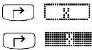 | Recalls value of variable to the stack. |
| Undefined all |  | Makes all variables not user-defined, but does not specify their values. |
| Solve for all |  | Creates variables if necessary and solves for all that are not user-defined (or as many as possible). |
Progress catalog  | |  | Shows information about the last solution. | |
| User-defined |  | Sets states touser-definedfor variable or list of variables on the stack. |
| Calculated |  | Sets states tonotuser-defined(calculated result) for variable or list of variables on the stack |
Meanings of Menu Labels
| Label Meaning | |
 | Value x0 is not defined by you and not used in the last solution. It can change with the next solution. |
 | Value x0 is not defined by you, but it was found in the last solution. It can change in the next solution. |
 | Value x0 is defined by you and not used in the last solution. It cannot change in the next solution (unless you solve only for this variable). |
 | Value x0 is defined by you and used in the last solution. It cannot change in the next solution (unless you solve only for this variable). |
Defining a set of equations
When you design a set of equations, you should do it with an understanding of how the Multiple-Equation Solver uses the equations to solve problems. The Multiple-Equation Solver uses the same process you'd use to solve for an unknown variable (assuming that you were not allowed to create additional variables). You'd look through the set of equations for one that has only one variable that you didn't know. You'd then use the root-finder to find its value. Then you would do this again until you've found the variable you want. You should choose your equations to allow likely unknown variables to occur individually in equations. You must avoid having two or more unknown variables in all equations. You can also specify equations in an order that's best for your problems. For example, the following three equations define initial velocity and acceleration based on two observed distances and times. The first two equations alone are mathematically sufficient for solving the problem, but each equation contains two unknown variables. Adding the third equation allows a successful solution because it contains only one of the unknown variables. x _ 1 = v _ 0 + a · t _ 1 x _ 2 = v _ 0 + a · t _ 2 ( x _ 2 amp; x _ 1 ) = a · (t _ 2 - t _ 1) - To create more robust equations, you can include functions that ensure proper and faster calculations—for example, CONST and TDELTA, UBASE, EXP, and IFTE. If your equations use any of the following functions, their variables won't necessarily be detected by the Multiple-Equation Solver: , , , | , QUOTE, APPLY, TVROOT, and CONST. The list of equations in EQ may contain menu definitions, but those definitions are ignored by MINIT when it creates Mpar. However, you can reorder the menu labels using MITM (described below).To create a set of equations for the Multiple-Equation Solver
1. Enter each equation in the set onto the stack. 2. Press ▲ to begin the Interactive Stack and then move the cursor up to the level containing the first equation you entered. 3. Press to combine them into a list. 4. Press ☐ ALPHA ☑ ALPHA ☐ STO to store the list into the EQ variable. 5. Press APPS ▲ ENTER 3910 3001 3123 to create Mpar and prepare the equation set for use with the Multiple-Equation Solver. 6. Press ☐ to launch the solver with the new set of equations.To change the title and menu for a set of equations
1. Make sure that the set of equations is the current set (as they are used when the Multiple-Equation Solver is launched). 2. Enter a text string containing the new title onto the stack. 3. Enter a list containing the variable names in the order you want them to appear on the menu. Use a "" to insert a blank label. You must include all variables in the original menu and no others, and you must match uppercase and lowercase characters. 4. Press APPS ▲ ENTERInterpreting results from the Multiple-Equation Solver
The Multiple-Equation Solver solves for variables by repeatedly looking through the set of equations for one that contains only one variable that's unknown (not user-defined and not found by the solver during this solution). It then uses the root-finder to find that value. It continues eliminating unknown variables until it solves for the variable you specified (or until it can't solve for any more variables). Each time the Multiple-Equation Solver starts solving for a variable, only the variables with black menu labels are known. During the solution process, the Multiple-Equation Solver shows the variable it is currently solving for. It also shows the type of root found (zero, sign-reversal, or extremum) or the problem if no root is found (bad guesses or constant). The following messages indicate errors in the problem setup: - Bad Guess(es). Units may be missing or inconsistent for a variable. For a list of guesses, at least one of the list elements must have consistent units. - Too Many Unknowns. The solver eventually encountered only equations having at least two unknowns. Either enter other known values, or change the set of equations. \- Constant? The initial value of a variable may be leading the root-finder in the wrong direction. Supply a guess in the opposite direction from a critical value. (If negative values are valid, try one.)Checking solutions
The variables having a ω mark in their menu labels are related for the most recent solution. They form a compatible set of values satisfying the equations used. The values of any variables without marks may not satisfy the equations because those variables were not involved in the solution process. If any solutions seem improper, check for the following problems: \- Wrong units. A known or found variable may have units different from those you assumed. These are global variables. If the variable existed before this calculation, then its unit system (SI or English) takes priority. To correct the units, either purge the variables before solving the equation, or enter the specific units you want. ■No units. If you are not using variables, your implied units may not be compatible among your variables or with the implied units of constants or functions. The current angle mode sets the implied units for angles. ■Multiple roots. An equation may have multiple roots, and the solver may have found an inappropriate one. Supple a guess for the variable to focus the search in the appropriate range. \- Wrong variable states. A known or unknown variable may not have the appropriate state. A known variable should have a black menu label, and an unknown variable should have a white label. \- Inconsistent conditions. If you enter values that are mathematically inconsistent for the equations, the application may give results that satisfy some equations but not all. This includes over-specifying the problem, where you enter values for more variables than are needed to define a physically realizable problem—the extra values may create an impossible or illogical problem. (The solutions satisfy the equations the solver used, but the solver doesn't try to verify that the solution satisfies all of the equations.) \- Not related. A variable may not be involved in the solution (no mark in the label), so it is not compatible with the variables that were involved. \- Wrong direction. The initial value of a variable may be leading the root-finder in the wrong direction. Supply a guess in the opposite direction from a critical value. (If negative values are valid, try one.)Appendix A Using input forms
This example of setting time and date illustrates the use of input forms in the calculator. Some general rules: \- Use the arrow keys (◀ ▶ ▼ ▲) to move from one field to the next in the input form. \- Use any the E100E soft menu key to see the options available for any given field in the input form. \- Use the arrow keys (◀ ▶ ▼ ▲) to select the preferred option for a given field, and press the 📄️ (F6) soft menu key to make the selection. \- In some instances, a check mark is required to select an option in an input form. In such case use the √≡≡ soft menu key to toggle the check mark on and off. \- Press the OFFC soft menu key to close an input form and return to the stack display. You can also press the ENTER key or the ON key to close the input form.Example - Using input forms in the NUM.SLV menu
Before discussing these items in detail we will present some of the characteristics of the input forms by using input forms from the financial calculation application in the numerical solver. Launch the numerical solver by using 7 NUM.SLV (associated with the 7 key). This produces a choose box that includes the following options:  To get started with financial calculations use the down arrow key (▼) to select item 5. Solve finance. Press 📄, to launch the application. The resulting screen is an input form with input fields for a number of variables (n, I%YR, PV, PMT, FV).  In this particular case we can give values to all but one of the variables, say, n = 10, I%YR = 8.5, PV = 10000, FV = 1000, and solve for variable PMT (the meaning of these variables will be presented later). Try the following: 10 Enter n = 10 8.5 Enter 1%YR = 8.5 10000 Enter PV = 10000  1000  Enter FV = 1000   Select and solve for PMT The resulting screen is:  In this input form you will notice the following soft menu key labels: Press to edit highlighted field Amortization menu - option specific to this application Press to solve for highlighted field Pressing NXT we see the following soft menu key labels:  Reset fields to default values Press to access the stack for calculations Press to determine the type of object in highlighted field Cancel operation Accept entry If you press 📄you will be asked to select between the two options:  If you select Reset value only the highlighted value will be reset to the default value. If, instead, you select Rest all, all the fields will be reset to their default values (typically, 0). At this point you can accept your choice (press 📄), or cancel the operation (press 📄). Press 📄 in this instance. Press 📄 to access the stack. The resulting screen is the following:  At this point, you have access to the stack, and the value last highlighted in the input form is provided for you. Suppose that you want to halve this value. The following screen follows in ALG mode after entering 1136.22/2:  (In RPN mode, we would have used 1136.22 ENTER 2 ENTER ÷). Press ☐ to enter this new value. The input form will now look like this:  Press 📄 to see the type of data in the PMT field (the highlighted field). As a result, you get the following specification:  This indicates that the value in the PMT field must be a real number. Press to return to the input form, and press L to recover the first menu. Next, press the ENTER key or the ON key to return to the stack. In this instance, the following values will be shown:  The top result is the value that was solved for PMT in the first part of the exercise. The second value is the calculation we made to redefine the value of PMT.Appendix B The calculator's keyboard
The figure below shows a diagram of the calculator's keyboard with the numbering of its rows and columns.  The figure shows 10 rows of keys combined with 3, 5, or 6 columns. Row 1 has 6 keys, rows 2 and 3 have 3 keys each, and rows 4 through 10 have 5 keys each. There are 4 arrow keys located on the right-hand side of the keyboard in the space occupied by rows 2 and 3. Each key has three, four, or five functions. The main key functions are shown in the figure below. To operate this main key functions simply press the corresponding key. We will refer to the keys by the row and column where they are located in the sketch above, thus, key (10, 1) is the ON key.  Main key functions in the calculator's keyboardMain key functions
Keys F1 through F6 keys are associated with the soft menu options that appear at the bottom of the calculator's display. Thus, these keys will activate a variety of functions that change according to the active menu. ■ The arrow keys, ▲ ▼ ◀ ▶ , are used to move one character at a time in the direction of the key pressed (i.e., up, down, left, or right). ■ The APPS function activates the applications menu. \- The MODE function activates the calculator's modes menu. \- The TOOL function activates a menu of tools useful for handling variables and getting help on the calculator. \- The VAR function shows the variables stored in the active directory, the STO function is used to store contents in variables. \- The NXT function is used to see additional soft menu options or variables in a directory. \- The HIST function allows you access to the algebraic-mode history, i.e., the collection of recent command entries in that mode. \- The EVAL key is used to evaluate algebraic and numeric expressions, the apostrophe key [ ' ] is used to enter a set of apostrophes for algebraic expressions. ■ The SYMB activates the symbolic operations menu. ■ The delete key ◀ is used to delete characters in a line. ■The y x key calculates the x power of y. ■The key calculates the square root of a number. ■ The SIN, COS, and TAN keys calculate the sine, cosine, and tangent, respectively, of a number. ■ The EEX key is used to enter power of tens (e.g., 5 × 10³ , is entered as 5, EEX, 3, which is shown as 5E3). \- The +/- key changes the sign of an entry, the X key enters the character X (upper case). ■ The 1/x key calculates the inverse of a number, the keys +, -, x, and ÷, are used for the fundamental arithmetic operations (addition, subtraction, multiplication, and division, respectively). ■ The ALPHA key is combined with other keys to enter alphabetic characters. - The left-shift key ← and the right-shift key → are combined with other keys to activate menus, enter characters, or calculate functions as described elsewhere. - The numerical keys (0 to 9) are used to enter the digits of the decimal number system. ■ There is a decimal point key (.) and a space key (SPC). - The ENTER key is used to enter a number, expression, or function in the display or stack, and ■ The ON key is used to turn the calculator on.Alternate key functions
The left-shift key, key (8,1), the right-shift key, key (9,1), and the ALPHA key, key (7,1), can be combined with some of the other keys to activate the alternative functions shown in the keyboard. For example, the SYMB key, key(4,4), has the following six functions associated with it: SYMB Main function, to activate the SYMBOLic menu ← MTH Left-shift function, to activate the MTH (Math) menu CAT Right-shift function, to activate the CATalog function ALPHA P ALPHA function, to enter the upper-case letter P ALPHA ← P ALPHA-Left-Shift function, to enter the lower-case letter p ALPHA → P ALPHA-Right-Shift function, to enter the symbol P Of the six functions associated with the key only the first four are shown in the keyboard itself. This is the way that the key looks in the keyboard:  Notice that the color and the position of the labels in the key, namely, SYMB, MTH, CAT and P, indicate which is the main function (SYMB), and which of the other three functions is associated with the left-shift ← (MTH), right-shift → (CAT), and ALPHA (P) keys. Diagrams showing the function or character resulting from combining the calculator keys with the left-shift ← , right-shift → , ALPHA ALPHA, ALPHA-left-shift ALPHA ← , and ALPHA-right-shift ALPHA → , are presented next. In these diagrams, the resulting character or function for each key combination is shown in white background. If the left-shift, right-shift or ALPHA keys are activated they are shown in a shaded background. Keys that do not get activated are shown in black background.Left-shift functions
The following sketch shows the functions, characters, or menus associated with the different calculator keys when the left-shift key ← is activated. \- The six left-shift functions associated with the F1 through F6 keys are associated with the setting up and production of graphics and tables. When using these functions in the calculator's Algebraic mode of operation, press the left-shift key ← first, and then any of the keys in Row 1. When using these functions in the calculator's RPN mode, you need to press the left-shift key ← simultaneously with the key in Row 1 of your choice. Function Y = is used to enter functions of the form y = f(x) for plotting, function WIN is used to set parameters of the plot window, function GRAPH is used to produce a graph, function 2D/3D is used to select the type of graph to be produced, function TBLSET is used to set parameters for a table of values of a function, function TABLE is used to generate a table of values of a function, - Function FILE activates the file browser in the calculator's memory. - The CUSTOM function activates the custom menu options, the i key is used to enter the unit imaginary number i into the stack (.)2 - ± i - The UPDIR function moves the memory location one level up in the calculator's file tree. ■ The RCL function is used to recall values of variables. - The PREV function shows the previous set of six menu options associated with the soft menu keys. \- The CMD function shows the most recent commands, the PRG function activates the programming menus, the MTRW function activates the Matrix Writer,  Left-shift ← functions of the calculator's keyboard ■ The CMD function shows the most recent commands. ■ The PRG function activates the programming menus. ■ The MTRW function activates the Matrix Writer. ■ The MTH function activates a menu of mathematical function. ■ The DEL key is used to delete variables. ■The e x key calculates the exponential function of x. ■The x2 key calculates the square of x (this is referred to as the SQ function). ■The ASIN, ACOS, and ATAN functions calculate the arcsine, arccosine, and arctangent functions, respectively. ■The 10 x function calculates the anti-logarithm of x. ■The keys ≠, ≤ and ≥, are used for comparing real numbers. ■ The ABS function calculates the absolute value of a real number, or the magnitude of a complex number or of a vector. ■ The USER function activates the user-defined keyboard menu. ■ The S.SLV function activates the symbolic solver menu. ■ The EXP&LN function activates the menu for substituting expressions in terms of the exponential and natural logarithm functions. ■ The FINANCE function activates a menu for financial calculations. ■ The CALC function activates a menu of calculus functions. ■ The MATRICES function activates a menu for creating and manipulation of matrices. \- The CONVERT function activates a menu for conversion of units and other expressions. ■ The ARITH function activates a menu of arithmetic functions. ■ The DEF key is used to define a simple function as a variable in the calculator menu. ■ The CONT key is used to continue a calculator operation. \- The ANS key recalls the last result when the calculator is in Algebraic operation mode. ■ The [ ], ( ), and {} keys are used to enter brackets, parentheses, or braces. \- The # key is used to enter numbers in other than the active number base. ■The infinity key ∞ is used to enter the infinite symbol in an expression. ■The pi key π is used to enter the value or symbol for π (the ratio of the length of a circumference to its diameter). ■The arrow keys, when combined with the left-shift key, move the cursor to the first character in the direction of the key pressed.  Right-shift → functions of the calculator's keyboardRight-shift functions
The sketch above shows the functions, characters, or menus associated with the different calculator keys when the right-shift key → is activated. ■ The functions BEGIN, END, COPY, CUT and PASTE are used for editing purposes. ■ The UNDO key is used to undo the last calculator operation. ■ The CHARS function activates the special characters menu. ■ The EQW function is used to start the Equation Writer. ■ The CAT function is used to activate the command catalog. ■ The CLEAR function clears the screen. ■ The LN function calculates the natural logarithm. ■ The √[x]y function calculates the x-th root of y. ■ The function is used to enter summations (or the upper case Greek letter sigma). ■ The function is used to calculate derivatives. ■ The ∫ function is used to calculate integrals. ■ The LOG function calculates the logarithm of base 10. ■ The ARG function calculates the argument of a complex number. ■ The ENTRY function is used to change entry mode in editing. ■ The NUM.SLV function launches the NUMerical SOLver menu. ■ The TRIG function activates the trigonometric substitution menu. ■ The TIME function activates the time menu. ■ The ALG function activates the algebra menu. ■The STAT function activates the statistical operations menu. ■ The UNITS function activates the menu for units of measurement. ■ The CMPLX function activates the complex number functions menu. ■ The LIB function activates the library functions. ■ The BASE function activates the numeric base conversion menu. \- The OFF key turns the calculator off, the → NUM key produces a numeric (or floating-point) value of an expression. \- The “” key enters a set of double-quotes used for entering text strings. ■ The _ key enters an underscore. ■ The << >> key enters the symbol for a program. ■The → key enters an arrow representing an input in a program. ■The ← key enters a return character in programs or text strings. ■ The comma (,) key enters a comma. ■The arrow keys, when combined with the right-shift key, move the cursor to the farthest character in the direction of the key pressed.ALPHA characters
The following sketch shows the characters associated with the different calculator keys when the ALPHA ALPHA is activated. Notice that the ALPHA function is used mainly to enter the upper-case letters of the English alphabet (A through Z). The numbers, mathematical symbols (-, +) , decimal point (.) , and the space (SPC) are the same as the main functions of these keys. The ALPHA function produces an asterisk (*) when combined with the times key, i.e., ALPHA ×.  Alpha ALPHA functions of the calculator's keyboardAlpha-left-shift characters
The following sketch shows the characters associated with the different calculator keys when the ALPHA (ALPHA) is combined with the left-shift key ← . Notice that the ALPHA ← combination is used mainly to enter the lower-case letters of the English alphabet (A through Z). The numbers, mathematical symbols (-, +, x) , decimal point (.), and the space (SPC) are the same as the main functions of these keys. The ENTER and CONT keys also work as their main function even when the ALPHA ← combination is used.  Alpha ALPHA ← functions of the calculator's keyboardAlpha-right-shift characters
The following sketch shows the characters associated with the different calculator keys when the ALPHA ALPHA is combined with the right-shift key ↗. Alpha ALPHA → functions of the calculator's keyboard
Notice that the ALPHA → combination is used mainly to enter a number of special characters from into the calculator stack. The CLEAR, OFF, →, ←, comma (, ), key enters and OFF keys also work as their main function even when the ALPHA → combination is used. The special characters generated by the ALPHA → combination include Greek letters (α, β, Δ, δ, ε, ρ, μ, λ, σ, θ, τ, ω, and Π), other characters generated by the ALPHA → combination are |, ', ^, =, <, >, /, ", \, _, \~, !, ?, << >>, and @.Appendix C CAS settings
CAS stands for Computer Algebraic System. This is the mathematical core of the calculator where the symbolic mathematical operations and functions are programmed. The CAS offers a number of settings can be adjusted according to the type of operation of interest. To see the optional CAS settings use the following: \- Press the MODE button to activate the CALCULATOR MODES input form.  At the bottom of the display you will find the following soft menu key options: Provides menus for manipulating calculator flags (*) Lets the user chose options in the different fields in the form Provides an input form to change CAS settings Provides an input form to change display settings Closes this input form and returns to normal display Use this key to accept settings (*) Flags are variables in the calculator, referred to by numbers, which can be "set" and "unset" to change certain calculator operating options. Pressing the NXT key shows the remaining options in the CALCULATOR MODES input form: Allows the user to reset a highlighted option Closes this input form and returns to normal display Use this key to accept settings \- To recover the original menu in the CALCULATOR MODES input box, press the NXT key. Of interest at this point is the changing of the CAS settings. This is accomplished by pressing the soft menu key. The default values of the CAS setting are shown below:  \- To navigate through the many options in the CAS MODES input form, use the arrow keys: ◀ ▶ ▼ ▲. \- To select or deselect any of the settings shown above, select the underline before the option of interest, and toggle the √≡≡ soft menu key until the right setting is achieved. When an option is selected, a check mark will be shown in the underline (e.g., the Rigorous and Simp Non-Rational options above). Unselected options will show no check mark in the underline preceding the option of interest (e.g., the _Numeric, _Approx, _Complex, _Verbose, _Step/Step, _Incr Pow options above). • After having selected and unselected all the options that you want in the CAS MODES input form, press the ☐ soft menu key. This will take you back to the CALCULATOR MODES input form. To return to normal calculator display at this point, press the ☐ soft menu key once more.Selecting the independent variable
Many of the functions provided by the CAS use a pre-determined independent variable. By default, such variable is chosen to be the letter X (upper case) as shown in the CAS MODES input box above. However, the user can change this variable to any other letter or combination of letters and numbers (a variable name must start with a letter) by editing the Indep var field in the CAS MODES input box. A variable called VX exists in the calculator's {HOME CASDIR} directory that takes, by default, the value of 'X'. This is the name of the preferred independent variable for algebraic and calculus applications. For that reason, most examples in this Chapter use X as the unknown variable. If you use other independent variable names, for example, with function HORNER, the CAS will not work properly. The variable VX is a permanent inhabitant of the {HOME CASDIR} directory. There are other CAS variables in the {HOME CASDIR}, e.g., REALASSUME (☐☐☐), MODULO (☐☐☐), CASINFO (☐☐☐), etc. You can change the value of VX by storing a new algebraic name in it, e.g., 'x', 'y', 'm', etc. Preferably, keep 'X' as your VX variable for the examples in this manual. Also, avoid using the variable VX in your programs or equations, so as to not get it confused with the CAS' VX. If you need to refer to the x-component of velocity, for example, you can use vx or Vx.Selecting the modulus
The Modulo option of the CAS MODES input box represents a number (default value = 13) used in modular arithmetic. More details about modular arithmetic are presented elsewhere.Numeric vs. symbolic CAS mode
When the Numeric CAS mode is selected, certain constants pre-defined in the calculator are displayed in their full floating-point value. By default, the _Numeric option is unselected, meaning that those pre-defined constants will be displayed as their symbol, rather than their value, in the calculator display. The following screen shows the values of the constant π (the ratio of the length of the circumference to its diameter) in symbolic format followed by the numeric, or floating-point, format. This example corresponds to the Algebraic operating mode.  The same example, corresponding to the RPN operating mode, is shown next: Approximate vs. Exact CAS mode
When the _Approx is selected, symbolic operations (e.g., definite integrals, square roots, etc.), will be calculated numerically. When the _Approx is unselected (Exact mode is active), symbolic operations will be calculated as closed-form algebraic expressions, whenever possible. The following screen shows a couple of symbolic expressions entered with an active exact mode in Algebraic operating mode:  In Algebraic mode, the object entered by the user is shown in the left-hand side of the screen, followed immediately by a result in the right-hand side of the screen. The results shown above show the symbolic expressions for (2) , i.e., the natural logarithm of 2, and √5 e., the square root of 5. If the _Numeric CAS option is selected, the corresponding results for these operations are as follows:  The keystrokes necessary for entering these values in Algebraic mode are the following: → LN 2 ENTER √5 ENTER The same calculations can be produced in RPN mode. Stack levels 3: and 4: show the case of Exact CAS setting (i.e., the _Numeric CAS option is unselected), while stack levels 1: and 2: show the case in which the Numeric CAS option is selected.  The required keystrokes are: 2 → LN 5 √X A keyboard short cut to toggle between APPROX and EXACT mode is by holding the right-shift key and pressing the ENTER key simultaneously, i.e., (hold) ENTER.Real numbers vs. integer numbers
CAS operations utilize integer numbers in order to keep full precision in the calculations. Real numbers are stored in the form of a mantissa and an exponent, and have limited precision. In APPROX mode, however, whenever you enter an integer number, it is automatically transformed into a real number, as illustrated next:  Whenever the calculator lists an integer value followed by a decimal dot, it is indicating that the integer number has been converted to a real representation. This will indicate that the number was entered while the CAS was set to APPROX mode. It is recommended that you select EXACT mode as default CAS mode, and change to APPROX mode if requested by the calculator in the performance of an operation. For additional information on real and integer numbers, as well as other calculator's objects, refer to Chapter 2.Complex vs. Real CAS mode
A complex number is a number of the form a+bi , where i, defined by 2-± i is the unit imaginary number (electrical engineers prefer to use the symbol j), and a and b are real numbers. For example, the number 2+3i is a complex number. Additional information on operations with complex numbers are presented in Chapter 4 of this guide. When the _Complex CAS option is selected, if an operation results in a complex number, then the result will be shown in the form a+bi or in the form of an ordered pair (a,b) . On the other hand, if the _Complex CAS option is unset (i.e., the Real CAS option is active), and an operation results in a complex number, you will be asked to switch to Complex mode. If you decline, the calculator will report an error. Please notice that, in COMPLEX mode the CAS is able to perform a wider range of operations than in REAL mode, but it will also be considerably slower. Thus, it is recommended that you use the REAL mode as default mode and switch to COMPLEX if requested by the calculator in the performance of an operation. The following example shows the calculation of the quantity 8 the Algebraic operating mode, first with the Real CAS option selected. In this case, you are asked if you want to change the mode to Complex:  If you press the OK soft menu key (), then the _Complex option is forced, and the result is the following:  The keystrokes used above are the following:  When asked to change to COMPLEX mode, use: F6. If you decide not to accept the change to COMPLEX mode, you get the following error message: Verbose vs. non-verbose CAS mode
When the _Verbose CAS option is selected, certain calculus applications are provided with comment lines in the main display. If the _Verbose CAS option is not selected, then those calculus applications will show no comment lines. The comment lines will appear momentarily in the top lines of the display while the operation is being calculated.Step-by-step CAS mode
When the _Step/step CAS option is selected, certain operations will be shown step at a time in the display. If the _Step/step CAS option is not selected, then intermediate steps will not be shown. For example, having selected the Step/step option, the following screens show the step-by-step division of two polynomials, namely, (X3-5X2+3X-2)/(X-2) . This is accomplished by using function DIV2 as shown below. Press ENTER to show the first step:  The screen inform us that the calculator is operating a division of polynomials A/B, so that A = BQ + R , where Q = quotient, and R = remainder. For the case under consideration, A = X3-5X2+3X-2 , and B = X-2. These polynomials are represented in the screen by lists of their coefficients. For example, the expression A: \1,-5,3,-2\ represents the polynomial A = X3-5X2+3X-2 , B: \1,-2\ represents the polynomial B = X-2, Q: \1\ represents the polynomial Q = X, and R: \-3,3,-2\ represents the polynomial R = -3X2+3X-2 . At this point, press, for example, the ENTER key. Continue pressing ENTER the key to produce additional steps:  Thus, the intermediate steps shown represent the coefficients of the quotient and residual of the step-by-step synthetic division as would have been performed by hand, i.e., X ^ 3 - 5 X ^ 2 + 3 X - 2X - 2 = X ^ 2 + - 3 X ^ 2 + 3 X - 2X - 2 = X ^ 2 - 3 X + - 3 X - 2/X - 2 = X ^ 2 - 3 X - 3 X - 8/X - 2.Increasing-power CAS mode
When the _Incr pow CAS option is selected, polynomials will be listed so that the terms will have increasing powers of the independent variable. If the _Incr pow CAS option is not selected (default value) then polynomials will be listed so that the terms will have decreasing powers of the independent variable. An example is shown next in Algebraic mode:  In the first case, the polynomial (X+3)5 is expanded in increasing order of the powers of X, while in the second case, the polynomial shows decreasing order of the powers of X. The keystrokes in both cases are the following: ← () X + 3 Y ^ X 5 ENTER In the first case the _lncr pow option was selected, while in the second it was not selected. The same example, in RPN notation, is shown below:  The same keystroke sequence was used to produce each of these results: 1 ← ( ) X + 3 Y ^ X 5 ENTER EVALRigorous CAS setting
When the _Rigorous CAS option is selected, the algebraic expression |X| , i.e., the absolute value, is not simplified to X . If the _Rigorous CAS option is not selected, the algebraic expression |X| is simplified to X . The CAS can solve a larger variety of problems if the rigorous mode is not set. However, the result, or the domain in which the result are applicable, might be more limited.Simplify non-rational CAS setting
When the _Simp Non-Rational CAS option is selected, non-rational expressions will be automatically simplified. On the other hand, if the _Simp Non-Rational CAS option is not selected, non-rational expressions will not be automatically simplified.Using the CAS HELP facility
Turn on the calculator, and press the TOOL key to activate the TOOL menu. Next, press the F2 soft menu key, followed by the ENTER key (the key in the lowest right corner of the keyboard), to activate the HELP facility. The display will look as follows:  At this point you will be provided with a list of all CAS commands in alphabetical order. You can use the down arrow key, ▼, to navigate through the list. To move upwards in the list use the up arrow key, ▲. The arrow keys are located on the right-hand side of the keyboard between the first and fourth rows of keys. Suppose that you want to find information on the command ATAN2S (ArcTANgent-to-Sine function). Press the down arrow key, ▼, until the command ATAN2S is highlighted in the list:  Notice that, in this instance, soft menu keys F5 and F6 are the only one with associated commands, namely: F5 CANCeL the help facility OK to activate help facility for the selected command If you press the ☐☐☐☐ F5 key, the HELP facility is skipped, and the calculator returns to normal display. To see the effect of using 📄 in the HELP facility, let's repeat the steps used above from to the selection of the command ATAN2S in the list of CAS commands: 📄F2 ENTER ▼ ▼ ...(10 times) Then, press the F6 key to obtain information about the command ATAN2S. The help facility indicates that the command, or function, ATAN2S replaces the value of atan(x), the arc tangent of a value x, by its equivalent in terms of the function asin (arcsine), i.e., The fourth and fifth lines in the display provide an example of application of the function ATAN2S. Line four, namely, ATAN2S(ATAN(X)), is the statement of the operation to be performed, while line five, namely, ASIN(X/√(X^2+1)), is the result. The bottom line in the display, starting with the particle See:, is a reference line listing other CAS commands related to the command ATAN2S. Notice that there are six commands associated with the soft menu keys in this case (you can check that there are only six commands because pressing the NXT produces no additional menu items). The soft menu key commands are the following: FI EXIT the help facility  In this case we want to ECHO the example into the stack by pressing F2. The resulting display is the following:  There are now four lines of the display occupied with output. The first two lines from the top correspond to the first exercise with the HELP facility in which we cancel the request for help. The third line from the top shows the most recent call to the HELP facility, while the last line shows the ECHO of the example command. To activate the command press the ENTER key. The result is:  Notice that, as new lines of output are produced, the display (or stack) pushes the existing lines upwards and fills the bottom of the screen with more output. The HELP facility, described in this section, will be very useful to refer to the definition of the many CAS commands available in the calculator. Each entry in the CAS help facility, whenever appropriate, will have an example of application of the command, as well as references as shown in this example. To navigate quickly to a particular command in the help facility list without having to use the arrow keys all the time, we can use a shortcut consisting of typing the first letter in the command's name. Suppose that we want to find information on the command IBP (Integration By Parts), once the help facility list is available, use the ALPHA key (first key in the fourth row from the bottom of the keyboard) followed by the key for the letter i (the same as the key TOOL), i.e., ALPHA 1. This will take you automatically to the first command that starts with an i, namely, IBASIS. Then, you can use the down arrow key ▼, twice, to find the command IBP. Pressing the F6 key, we activate the help facility for this command. Press F6 to recover the main list of commands, or exit to exit the facility.References for non-CAS commands
The help facility contains entries for all the commands developed for the CAS (Computer Algebraic System). There is a large number of other functions and commands that were originally developed for the HP 48G series calculators that are not included in the help facility. Good references for those commands are the HP 48G Series User's Guide (HP Part No. 00048-90126) and the HP 48G Series Advanced User's Reference Manual (HP Part No. 00048-90136) both published by Hewlett-Packard Company, Corvallis, Oregon, in 1993.CAS End User Term and Conditions
Use of the CAS Software requires from the user an appropriate mathematical knowledge. There is no warranty for the CAS Software, to the extent permitted by applicable law. Except when otherwise stated in writing the copyright holder provides the CAS Software "As Is" without warranty of any kind, either expressed or implied, including, but not limited to, the implied warranties of merchantability and fitness for a particular purpose. The entire risk as to the quality and performance of the CAS Software is with you. Should the CAS Software prove defective, you assume the cost of all necessary servicing, repair or correction. In no event unless required by applicable law will any copyright holder be liable to you for damages, including any general, special, incidental or consequential damages arising out of the use or inability to use the CAS Software (including but not limited to loss of data or data being rendered inaccurate or losses sustained by you or third parties or a failure of the CAS Software to operate with any other programs), even if such holder or other party has been advised of the possibility of such damages. If required by applicable law the maximum amount payable for damages by the copyright holder shall not exceed the royalty amount paid by Hewlett-Packard to the copyright holder for the CAS Software.Appendix D Additional character set
While you can use any of the upper-case and lower-case English letter from the keyboard, there are 255 characters usable in the calculator. Including special characters like θ , λ , etc., that that can be used in algebraic expressions. To access these characters we use the keystroke combination → CHARS (associated with the EVAL key). The result is the following screen:  By using the arrow keys, ◀ ▶ ▼ ▲, we can navigate through the collection of characters. For example, moving downwards in the screen produces more characters in the display:  Moving farther down, we see these characters:  There will be one character highlighted at all times. The lower line in the display will show the short cut for the highlighted character, as well as the ASCII character code (e.g., see the screen above: the short cut is α← Dα→9 , i.e., ALPHA ← D ALPHA → 9, and the code is 240). The display also shows three functions associated with the soft menu keys, f4, f5, and f6. These functions are: ☐: Opens a graphics screen where the user can modify highlighted character. Use this option carefully, since it will alter the modified character up to the next reset of the calculator. (Imagine the effect of changing the graphic of the character 1 to look like a 2!). ☐: Copies the highlighted character to the command line or equation writer (EQW) and exits the character set screen (i.e., echoes a single character to the stack). ☐: Copies the highlighted character to the command line or equation writer (EQW), but the cursor remains in the character set screen to allow the user to select additional characters (i.e., echoes a string of characters to the stack). To exit the character set screen press ENTER. For example, suppose you have to type the expression: λ2 + 2µ + 5 Here is a suggested approach, using the stack in either Algebraic or RPN mode: Use the keystrokes: 1 → CHARS to get to the characters screen. Next, use the arrow keys to highlight the character λ. Press (i.e., the F5 key), and continue with the keystrokes: + 2 × → CHARS. Next, use the arrow keys to highlight the character μ. Press (i.e., the F5 key), and finish the expression with the keystrokes: + 5 ENTER. Here is the result of this exercise in Algebraic and RPN modes, respectively:   Following, we list some of the most common ALPHA → keystroke combinations:Greek letters
α (alpha) ALPHA → A β (beta) ALPHA → B δ (delta) ALPHA → D ε (epsilon) ALPHA → E θ (theta) ALPHA → T λ (lambda) ALPHA → N μ (mu) ALPHA → M ρ (rho) ALPHA → F σ (sigma) ALPHA → S τ (tau) ALPHA → U ω (omega) ALPHA → V Δ (upper-case delta) ALPHA → C Π (upper-case pi) ALPHA → POther characters
\~ (tilde) ALPHA → I ! (factorial) ALPHA → 2 ? (question mark) ALPHA 3 \ (backward slash) ALPHA → 5 (angle symbol) ALPHA → 6 @ (at) ALPHA → ENTER Some characters commonly used that do not have simple keystroke shortcuts are: (x bar), γ (gamma), η (eta), Ω (upper-case omega). These characters can be “echoed” from the CHARS screen: → CHARS.Appendix E The Selection Tree in the Equation Writer
The expression tree is a diagram showing how the Equation Writer interprets an expression. The form of the expression tree is determined by a number of rules known as the hierarchy of operation. The rules are as follows: 1. Operations in parentheses are executed first, from the innermost to the outermost parentheses, and from left to right in the expression. 2. Arguments of functions are executed next, from left to right. 3. Functions are executed next, from left to right. 4. Powers of numbers are executed next, from left to right. 5. Multiplications and divisions are executed next, from left to right. 6. Additions and subtraction are executed last, from left to right. Execution from left to right means that, if two operations of the same hierarchy, say two multiplications, exist in an expression, the first multiplication to the left will be executed before the second, and so on. Consider, for example, the expression shown below in the equation writer:  The insertion cursor (◀) at this point is located to the right of the 2 in the argument of the SIN function in the denominator. Press the down arrow key ▼ to trigger the clear, editing cursor (□) around the 2 in the denominator. Next, press the left arrow key ◀, continuously, until the clear, editing cursor is around the y in the first factor in the denominator. Then, press the upper-arrow key to activate the selection cursor (■) around the y. By pressing the upper arrow key ▲, continuously, we can follow the expression tree that will take use from the y to the completion of the expression. Here is the sequence of operations highlighted by the upper arrow key ▲: Step A1 Step A2   Step A3 Step A4   Step A5 Step A6   We notice the application of the hierarchy-of-operation rules in this selection. First the y (Step A1). Then, y-3 (Step A2, parentheses). Then, (y-3)x (Step A3, multiplication). Then (y-3)x+5, (Step A4, addition). Then, ((y-3)x+5)(x 2 +4) (Step A5, multiplication), and finally, ((y-3)x+5)(x 2 +4)/SIN(4x-2) (Step A6, division). It is important to point out that the multiplication in Step A5 includes the first term, ((y-3)x+5) with a second term (x 2 +4), which is already calculated. To see the steps in calculating these second term, press the down arrow key ▼, continuously, until the clear, editing cursor is triggered around the y, once more. Then, press the right arrow key until these cursor is over the x in the second term in the numerator. Then, press the upper-arrow key to select this x. The steps in the evaluation of the expression, starting from this point, are shown below: Step B1 Step B2   Step B3 Step B4 = Step A5   Step B5 = Step A6  We can also follow the evaluation of the expression starting from the 4 in the argument of the SIN function in the denominator. Press the down arrow key ▼, continuously, until the clear, editing cursor is triggered around the y, once more. Then, press the right arrow key until these cursor is over the 4 in the denominator. Then, press the upper-arrow key ▲ to select this 4. The steps in the evaluation of the expression, starting from this point, are shown below: Step C1 Step C2   Step C3 Step C4   Step C5 = Step B5 = Step A6  The expression tree for the expression presented above is shown next:  The steps in the evaluation of the three terms (A1 through A6, B1 through B5, and C1 through C5) are shown next to the circle containing numbers, variables, or operators.Appendix F The Applications (APPS) menu
The Applications (APPS) menu is available through the APPS key (first key in second row from the keyboard's top). The APPS key shows the following applications:   The different applications are described next.Plot functions..
Selecting option 1. Plot functions.. in the APPS will produce the following menu list of graph-related options:  The six options shown are equivalent to the keystroke sequences listed below: Equation entry...  Plot window..  Graph display..  Plot setup..  Table setup..  Table display..  These applications are presented in detail in Chapter 12.I/O functions..
Selecting option 2. I/O functions.. in the APPS menu will produce the following menu list of input/output functions  These applications are described next: Send to Calculator Send data to another calculator (or to a PC with an infrared port) Get from Calculator Receive data from another calculator (or to a PC with an infrared port) Print display Send screen to printer Print.. Print selected object from calculator Transfer.. Transfer data to other device Start Server.. Calculator set as a server for communication with computers You can connect to another calculator or to a PC via infrared or via a cable. A USB cable is provided with the calculator for a USB connection. You can also use a serial cable to connect to the RS232 port on the calculator. (This cable is available as a separate accessory.)Constants lib..
Selecting option 3. Constants lib.. in the APPS menu opens the Constant Library application that provides values of standard physical constants:  The Constants Library is discussed in detail in Chapter 3.Numeric solver..
Selecting option 3. Constants lib.. in the APPS menu produces the numerical solver menu:  This operation is equivalent to the keystroke sequence → NUM.SLV. The numerical solver menu is presented in detail in Chapters 6 and 7.Time & date..
Selecting option 5.Time & date.. in the APPS menu produces the time and date menu:  This operation is equivalent to the keystroke sequence ↗ TIME . The time and date menu is presented in detail in Chapter 26.Equation writer..
Selecting option 6. Equation writer.. in the APPS menu opens the equation writer:  This operation is equivalent to the keystroke sequence _EQW. The equation writer is introduced in detail in Chapter 2. Examples that use the equation writer are available throughout this guide.File manager..
Selecting option 7.File manager.. in the APPS menu launches the file manager application:  This operation is equivalent to the keystroke sequence ← FILES .The file manager is introduced in Chapter 2.Matrix Writer..
Selecting option 8.Matrix Writer.. in the APPS menu launches the matrix writer:  This operation is equivalent to the keystroke sequence ← MTRW. The Matrix Writer is presented in detail in Chapter 10.Text editor..
Selecting option 9.Text editor.. in the APPS menu launches the line text editor:  The text editor can be started in many cases by pressing the down-arrow key ▼. If the object in the display is an algebraic object, pressing ▼ will most likely start the Equation Writer. The text editor is introduced in Chapter 2, and presented in detail in Appendix L.Math menu ..
Selecting option 10.Math menu.. in the APPS menu produces the MTH (mathematics) menu:   This operation is equivalent to the keystroke sequence ← MTH . The MTH menu is introduced in Chapter 3 (real numbers). Other functions from the MTH menu are presented in Chapters 4 (complex numbers), 8 (lists), 9 (vectors), 10 (matrix creation), 11 (matrix operation), 16 (fast Fourier transforms), 17 (probability applications), and 19 (numbers in different bases).CAS menu..
Selecting option 11.CAS menu.. in the APPS menu produces the CAS or SYMBOLIC menu:   This operation is also available by pressing the SYMB key. The CAS or SYMBOLIC menu is introduced in Chapter 5 (algebraic and arithmetic operations). Other functions from the CAS menu are presented in Chapters 4 (complex numbers), 6 (equations solutions), 10 (matrix creation), 11 (matrix operation), 13 (calculus), 14 (multivariate calculus), and 15 (vector analysis).Equation Library
Selecting option 12. Equation Library in the APPS men displays the EQ LIBRARY MENU. From here you can press 📄 and then 📄 to open the Equation Library:   Note that flag -117 should be set if you are going to use the Equation Library. Note too that the Equation Library will only appear on the APPS menu if the two Equation Library files are stored on the calculator. The Equation Library is explained in detail in chapter 27.Appendix G Useful shortcuts
Presented herein are a number of keyboard shortcuts commonly used in the calculator: - Adjust display contrast: ON (hold) +, or ON (hold) - - Toggle between RPN and ALG modes: MODE +/- or MODE +/- ENTER. - Set/clear system flag 95 (ALG vs. RPN operating mode)  • In ALG mode, CF(-95) selects RPN mode \- In RPN mode, 95 +/- ENTER SF selects ALG mode \- A keyboard short cut to toggle between APPROX and EXACT mode is by holding the right-shift key and pressing the ENTER key simultaneously, i.e., (hold) ENTER. \- Set/clear system flag 105 (EXACT vs. APPROX CAS mode)  \- In ALG mode, SF(-105) selects APPROX CAS mode CF(-105) selects EXACT CAS mode \- In RPN mode, 105 +/- ENTER SF selects APPROX CAS mode 105 +/- ENTER CF selects EXACT CAS mode \- Set/clear system flag 117 (CHOOSE boxes vs. SOFT menus):  \- In ALG mode, SF(-117) selects SOFT menus CF(-117) selects CHOOSE BOXES. \- In RPN mode, 117 +/- ENTER SF selects SOFT menus 117 +/- ENTER CF selects SOFT menus \- Change angular measure: o To degrees: ALPHA ALPHA D E G ENTER o To radian: ALPHA ALPHA R A D ENTER \- Special characters: ○ Angle symbol (∠): ALPHA → 6 ○ Factorial symbol (!): ALPHA → 2 ○ Degree symbol (°): ALPHA → (hold) 6 \- Lock/unlock alpha keyboard: - Lock alpha keyboard (upper case): ALPHA ALPHA ○ Unlock alpha keyboard (upper case): ALPHA ○ Lock alpha keyboard (lower case): ALPHA ALPHA ← ALPHA ○ Unlock alpha keyboard (lower case): ← ALPHA ALPHA \- Greek letters: Alpha (α): ALPHA → A DELTA (Δ): ALPHA → C Epsilon (ε): ALPHA → E Mu (μ): ALPHA → M PI ( ): ALPHA → P Theta (θ): ALPHA → T Omega (ω): ALPHA → V Beta (β): ALPHA → B Delta (d): ALPHA → D Rho (ρ): ALPHA → F Lambda ( λ ): ALPHA → N Sigma (σ): ALPHA → S Tau (t): ALPHA → U \- System-level operation (Hold ON, release it after entering second or third key): ○ ON (hold) FI F6 : "Cold" restart - all memory erased ○ ON (hold) F2 : Cancels keystroke ○ ON (hold) F3 : "Warm" restart - memory preserved ○ ON (hold) F4 : Starts interactive self-test ○ ON (hold) F5 : Starts continuous self-test ○ ON (hold) SPC : Deep-sleep shutdown - timer off ○ ON (hold) FI : Performs display screen dump ○ ON (hold) F4 : Cancels next repeating alarm \- Menus not accessible through keyboard: In RPN, enter menu_number, type MENU. In ALG mode, type MENU(menu_number). Menu_number is one of the following: o STAT soft menu: 96 o PLOT soft menu: 81 o SOLVE soft menu: 74, or use (hold) 7 - UTILITY soft menu: 113 \- Other menus: o MATHS menu: ALPHA ALPHA M A T H S ENTER o MAIN menu: ALPHA ALPHA M A I N ENTER \- Other keyboard short cuts: o (hold) 7 : SOLVE menu (menu 74) ○ ← (hold) MODE : PRG/MODES menu (Chapter 21) ○ ← (hold) ▼ : Starts text editor (Appendix L) ○ (hold) UPDIR : HOME(), go to HOME directory ○ (hold) PREV : Recover last active menu ○ (hold) : List contents of variables or menu entries o (hold) CHARS : PRG/CHAR menu (Chapter 21) ○ ALPHA → ENTRY : Changes insertion modeAppendix H The CAS help facility
The CAS help facility is available through the keystroke sequence TOOL NXT ENTER. The following screen shots show the first menu page in the listing of the CAS help facility.  The commands are listed in alphabetical order. Using the vertical arrow keys one can navigate through the help facility list. Some useful hints on navigating through this facility are shown next: \- You can hold down the down arrow key ▼ and watch the screen until the command you're looking for shows up in the screen. At this point, you can release the down arrow key. Most likely the command of interest will not be selected at this point (you may overshoot or undershoot it). However, you can use the vertical keys ▲ ▼ , one stroke at a time, to locate the command you want, and then press 📄. \- If, while holding down the down arrow key ▼ you overshoot the command of interest, you can hold down the up arrow key ▲ to move back towards that command. Refine the selection with the vertical keys ▲ ▼ , one stroke at a time. \- You can type the first letter of the command of interest, and then use the down arrow key ▼ to locate that particular command. For example, if you're looking for the command DERIV. After activating the help facility (TOOL NXT ENTER), type ALPHA D. This will select the first of the commands that start with D, i.e., DEGREE. To find DERIV, press ▼, twice. To activate the command, press 📄. \- You can type two or more letters of the command of interest, by locking the alphabetic keyboard. This will take you to the command of interest, or to its neighborhood. Afterwards, you need to unlock the alpha keyboard, and use the vertical arrow keys ▲ ▼ to locate the command, if needed. Press □ to locate the to activate the command. For example, to locate the command PROPFRAC, you can use, one of the following keystroke sequences:  See Appendix C for more information on the CAS (Computer Algebraic System). Appendix C includes other examples of application of the CAS help facility.Appendix I Command catalog list
This is a list of all commands in the command catalog (→ CAT). Those commands that belong to the CAS (Computer Algebraic System) are listed also in Appendix H. CAS help facility entries are available for a given command if the soft menu key 📄️ shows up when you highlight that particular command. Press this soft menu key to get the CAS help facility entry for the command. The first few screens of the catalog are shown below:         User-installed library commands would also appear on the command catalog list, using italic font. If the library includes a help item, then the soft menu key shows up when you highlight those user-created commands.Appendix J The MATHS menu
The MATHS menu, accessible through the command MATHS (available in the catalog CAT), contains the following sub-menus: The CMPLX sub-menu
 contains functions pertinent to operations with complex numbers:   These functions are described in Chapter 4.The CONSTANTS sub-menu
The CONSTANTS sub-menu provides access to the calculator mathematical constants. These are described in Chapter 3: The HYPERBOLIC sub-menu
 contains the hyperbolic functions and their inverses. These functions are described in Chapter 3. The INTEGER sub-menu
 provides functions for manipulating integer numbers and some polynomials. These functions are presented in Chapter 5:  The MODULAR sub-menu
 provides functions for modular arithmetic with numbers and polynomials. These functions are presented in Chapter 5:  The POLYNOMIAL sub-menu
 includes functions for generating and manipulating polynomials. These functions are presented in Chapter 5:  The TESTS sub-menu
 includes relational operators (e.g., ==, <, etc.), logical operators (e.g., AND, OR, etc.), the IFTE function, and the ASSUME and UNASSUME commands.   Relational and logical operators are presented in Chapter 21 in the context of programming the calculator in User RPL language. The IFTE function is introduced in Chapter 3. Functions ASSUME and UNASSUME are presented next, using their CAS help facility entries (see Appendix C).ASSUME UNASSUME
 Appendix K The MAIN menu
The MAIN menu is available in the command catalog. This menu include the following sub-menus:  The CASCFG command
This is the first entry in the MAIN menu. This command configures the CAS. For CAS configuration information see Appendix C.The ALGB sub-menu
The ALGB sub-menu includes the following commands:   These functions, except for 0.MAIN MENU and 11.UNASSIGN are available in the ALG keyboard menu (→_ALG). Detailed explanation of these functions can be found in Chapter 5. Function UNASSIGN is described in the following entry from the CAS menu: The DIFF sub-menu
 contains the following functions:   These functions are also available through the CALC/DIFF sub-menu (start with ← CALC). These functions are described in Chapters 13, 14, and 15, except for function TRUNC, which is described next using its CAS help facility entry: The MATHS sub-menu
The MATHS menu is described in detail in Appendix J.The TRIGO sub-menu
The TRIGO menu contains the following functions:    These functions are also available in the TRIG menu (→ TRIG). Description of these functions is included in Chapter 5.The SOLVER sub-menu
The SOLVER menu includes the following functions:  These functions are available in the CALC/SOLVE menu (start with ← CALC). The functions are described in Chapters 6, 11, and 16.The CMPLX sub-menu
The CMPLX menu includes the following functions:   The CMPLX menu is also available in the keyboard (→ CMPLX). Some of the functions in CMPLX are also available in the MTH/COMPLEX menu (start with ← MTH). Complex number functions are presented in Chapter 4.The ARIT sub-menu
The ARIT menu includes the following sub-menus:  The sub-menus INTEGER, MODULAR, and POLYNOMIAL are presented in detail in Appendix J.The EXP&LN sub-menu
The EXP&LN menu contains the following functions:  This menu is also accessible through the keyboard by using ← EXP&LN. The functions in this menu are presented in Chapter 5.The MATR sub-menu
The MATR menu contains the following functions:    These functions are also available through the MATRICES menu in the keyboard (← MATRICES). The functions are described in Chapters 10 and 11.The REWRITE sub-menu
The REWRITE menu contains the following functions:   These functions are available through the CONVERT/REWRITE menu (start with CONVERT). The functions are presented in Chapter 5, except for functions XNUM and XQ, which are described next using the corresponding entries in the CAS help facility (TOOL NXT REE):XNUM XQ
 Appendix L Line editor commands
When you trigger the line editor by using ← in the RPN stack or in ALG mode, the following soft menu functions are provided (press NXT to see the remaining functions):  The functions are briefly described as follows: ←SKIP: Skips characters to beginning of word. SKIP→: Skips characters to end of word. ←DEL: Delete characters to beginning of word. DEL→: Delete characters to end of word. DEL L: Delete characters in line. INS: When selected inserts characters at cursor location. If not selected, the cursor replaces characters (overwrites) instead of inserting characters. EDIT: Edits selection. →BEG: Move to beginning of word. →END: Mark end of selection. INFO: Provides information on Command Line editor, e.g.,  The items show in this screen are self-explanatory. For example, X and Y positions mean the position on a line (X) and the line number (Y). Stk Size means the number of objects in the ALG mode history or in the RPN stack. Mem(KB) means the amount of free memory. Clip Size is the number of characters in the clipboard. Sel Size is the number of characters in the current selection. EXEC: Execute command selected. HALT: Stop command execution. The line editor also provide the following sub-menus: SEARCH: Search characters or words in the command line. It includes the following functions:  GOTO: Move to a desired location in the command line. It includes the following functions:  Style: Text styles that can be used in the command line: The SEARCH sub-menu
The functions of the SEARCH sub-menu are: Find : Use this function to find a string in the command line. The input form provided with this command is shown next:  Replace: Use this command to find and replace a string. The input form provided for this command is:  Find next.: Finds the next search pattern as defined in Find Replace Selection: Replace selection with replacement pattern defined with Replace command. Replace/Find Next: Replace a pattern and search for another occurrence. The pattern is defined in Replace. Replace All: Replace all occurrence of a certain pattern. This command asks for confirmation from the user before replacing pattern. Fast Replace All: Replace all occurrences of a certain pattern without checking with the user.The GOTO sub-menu
The functions in the GOTO sub-menu are the following: Goto Line: to move to a specified line. The input form provided with this command is:  Goto Position: move to a specified position in the command line. The input form provided for this command is:  Labels: move to a specified label in the command line.The Style sub-menu
The Style sub-menu includes the following styles: BOL: Bold ITALI: Italics UNDE: Underline  : Inverse The command FONT allow the user to select the font for the command editor. Examples of the different styles are shown below:  Appendix M Table of Built-In Equations
The Equation Library consists of 15 subjects corresponding to the sections in the table below) and more than 100 titles. The numbers in parentheses below indicate the number of equations in the set and the number of variables in the set. There are 315 equations in total using 396 variable.Subjects and Titles
1: Columns and Beams (14, 20)
1: Elastic Buckling (4, 8) 6: Simple Sheer (1, 7) 2: Eccentric Columns (2, 11) 7: Cantilever Deflection (1, 10) 3: Simple Deflection (1, 9) 8: Cantilever Slope (1, 10) 4: Simple Slope (1, 10) 9: Cantilever Moment (1, 8) 5: Simple Moment (1, 8) 10: Cantilever Shear (1, 6)2: Electricity (42, 56)
1: Coulomb's Law (1, 5) 13: Capacitor Charge (1, 3) 2: Ohm's Law and Power (4, 4) 14: DC Inductor Voltage (3, 8) 3: Voltage Divider (1, 4) 15: RC transient (1, 6) 4: Current Divider (1, 4) 16: RL transient (1, 6) 5: Wire Resistance (1, 4) 17: Resonant Frequency (4, 7) 6: Series and Parallel R (2, 4) 18: Plate Capacitor (1, 4) 7: Series and Parallel C (2, 4) 19: Cylindrical Capacitor (1, 5) 8: Series and Parallel L (2, 4) 20: Solenoid Inductance (1, 5) 9: Capacitance Energy (1, 3) 21: Toroid Inductance (1, 6) 10: Inductive Energy (1, 3) 22: Sinusoidal Voltage (2, 6) 11: RLC Current Delay (5, 9) 23: Sinusoidal Current (2, 6) 12: DC Capacitor Current (3, 8)| 3: Fluids (29, 29)1: Pressure at Depth (1, 4) 3: Flow with Losses (10, 17)2: Bernoulli Equation (10, 15) 4: Flow in Full Pipes (8, 19) | |
| 4: Forces and Energy (31, 36)1: Linear Mechanics (8, 11) 5: ID Elastic Collisions (2, 5)2: Angular Mechanics (12, 15) 6: Drag Force (1, 5)3: Centripetal Force (4, 7) 7: Law of Gravitation (1, 4)4: Hooke’s Law (2, 4) 8: Mass–Energy Relation (4, 9) | |
| 5: Gases (18, 26)1: Ideal Gas Law (2, 6) 5: Isentropic Flow (4, 10)2: Ideal Gas State Change (1, 6) 6: Real Gas Law (2, 8)3: Isothermal Expansion (2, 7) 7: Real Gas State Change (1, 8)4: Polytropic Processes (2, 7) 8: Kinetic Theory (4, 9) | |
| 6: Heat Transfer (17, 31)1: Heat Capacity (2, 6) 5: Conduction and2: Thermal Expansion (2, 6) Convection (4, 14))3: Conduction (2, 7) 6: Black Body Radiation (5, 9)4: Convection (2, 6) | |
| 7: Magnetism (4, 14)1: Straight Wire (1,5) 3: B Field in Solenoid (1, 4)2: Force Between Wires (1, 6) 4: Field in Toroid (1, 6) | |
| 8: Motion (22, 24)1: Linear Motion (4, 6) 5: Circular Motion (3, 5)2: Object in Free Fall (4, 5) 6: Terminal Velocity (1, 5)3: Projectile Motion (5, 10) 7: Escape Velocity (1, 14)4: Angular Motion (4, 6) | |
| 9: Optics (11, 14) | |
| 1: Law of Refraction (1, 4) 4: Spherical Reflection (3, 5) | |
| 2: Critical Angle (1, 3) 5: Spherical Refraction (1, 5) | |
| 3: Brewster's Law (2, 4) 6: Thin Lens (3, 7) | |
| 10: Oscillations (17, 17) | |
| 1: Mass–Spring System (1, 4) 4: Torsional Pendulum (3, 7) | |
| 2: Simple Pendulum (3, 4) 5: Simple Harmonic (4, 8) | |
| 3: Conical Pendulum (4, 6) | |
| 11: Plane Geometry (31, 21) | |
| 1: Circle (5, 7) 4: Regular Polygon (6, 8) | |
| 2: Ellipse (5, 8) 5: Circular Ring (4,7) | |
| 3: Rectangle (5, 8) 6: Triangle (6, 107) | |
| 12: Solid Geometry (18, 12) | |
| 1: Cone (5, 9) 3: Parallelepiped (4, 9) | |
| 2: Cylinder (5, 9) | 4: Sphere (4, 7) |
| 13: Solid State Devices (33, 53) | |
| 1: PN Step Junctions (8, 19) | 3: Bipolar Transistors (8, 14) |
| 2: NMOS Transistors (10, 23) | 4: JFETs (7, 15) |
| 14: Stress Analysis (16, 28) | |
| 1: Normal Stress (3, 7) | 3: Stress on an Element (3, 7) |
| 2: Shear Stress (3, 8) | 4: Mohr's Circle (7, 10) |
| 15: Waves (12, 15) | |
| 1: transverse Waves (4, 9) | 3: Sound Waves (4,8) |
| 2: Longitudinal Waves (4, 9) | |
Appendix N Index
A
ABCUV 5-10 ABS 3-4, 4-6, 11-8 ACK 25-4 ACKALL 25-4 ACOS 3-6 ADD 8-9, 12-20 Additional character set D-1 ADDTMOD 5-11 Alarm functions 25-4 Alarms 25-2 ALG menu 5-3 Algebraic objects 5-1 ALOG 3-5 ALPHA characters B-9 ALPHA keyboard lock-unlock G-2 Alpha-left-shift characters B-10 Alpha-right-shift characters B-12 ALRM menu 25-3 AMORT 6-31 AMORTIZATION 6-10 AND 19-5 Angle between vectors 9-15 Angle Measure 1-23 Angle symbol (∠) G-2 Angle units 22-27, 22-29, 22-33 Angular measure G-2 ANIMATE 22-27 Animating graphics 22-26 Animation 22-26 Anti-derivatives 13-14 Approximate CAS mode C-4 Approximate vs. Exact CAS mode C-4 APPS menu F-1 ARC 22-21 AREA in plots 12-6 Area units 3-19 ARG 4-6 ARITHMETIC menu 5-9 ASIN 3-6 ASINH 3-9 ASN 20-6 ASR 19-6 ASSUME J-3 ATAN 3-6 ATANH 3-9 ATICK 22-7 Augmented matrix 11-32 AUTO 22-3 AXES 22-8, 22-13 AXL 9-24 AXM 11-16 AXQ 11-53B
B→R 19-3 Bar plots 12-29 BASE menu 19-1 Base units 3-22 Beep 1-25 BEG 6-31 BEGIN 2-27 Bessel's equation 16-52 Bessel's functions 16-53 Best data fitting 18-13, 18-62 Best polynomial fitting 18-62 Beta distribution 17-7 BIG 12-18 BIN 3-2 Binary numbers 19-1 Binary system 19-3 Binomial distribution 17-4 BIT menu 19-6 BLANK 22-32 BOL L-4 BOX 12-43, 12-45 BOXZ 12-48 Building a vector 9-12 BYTE menu 19-7C
C→PX 19-7 C→R 4-6 CALC/DIFF menu 16-3 Calculation with dates 25-3 Calculations with times 25-4 Calculator constants 3-16 CALCULATOR MODES input form C-1 Calculator restart G-3 Calculus 13-1 Cancel next repeating alarm G-3 Cartesian representation 4-1 CAS help facility listing H-1 CAS HELP facility C-10 CAS independent variable C-2 CAS menu.. F-6 CAS modulus C-3 CAS settings 1-26, C-1 CASDIR 2-35 CASE construct 21-51 CASINFO 2-37 Cauchy equation 16-51 CEIL 3-14 CENTR 22-7 Chain rule 13-6 Change sign 4-6 Character set D-1 Character strings 23-1 Characteristic polynomial 11-45 Characters list 23-3 CHARS menu 23-2 Chebyshev polynomials 16-55 CHINREM 5-10, 5-17 Chi-square distribution 17-11 CHOOSE 21-31 Choose box 21-31 CHOOSE boxes 1-4 CHR 23-1 CIRCL 12-45 Class boundaries 18-6 Class marks 18-5 Classes 18-5 CLKADJ 25-3 Clock display 1-30 CMD 2-62 CMDS 2-25 CMPLX menus 4-5 CNCT 22-13 CNTR 12-48 Coefficient of variation 18-5 COL+ 10-19 COL→10-19 "Cold" calculator restart G-3 COLLECT 5-4 Column norm 11-7 Column vectors 9-18 COL-10-20 COMB 17-2 Combinations 17-1 Command catalog list I-1 Complex CAS mode C-6 Complex Fourier series 16-26 COMPLEX mode 4-1 Complex numbers 2-2, 4-1 Complex vs. Real CAS mode C-6 Composing lists 8-2 CON 10-8 Concatenation operator 8-4 COND 11-10 Condition number 11-10 Confidence intervals for the variance 18-33 Confidence intervals in linear regression 18-52 Confidence intervals 18-22 Conic curves 12-20 CONJ 4-6 CONLIB 3-29 Constants lib F-2 Continuous self-test G-3 CONVERT 3-27 CONVERT Menu 5-26 Convolution 16-47 Coordinate System 1-24 Coordinate transformation 14-9 COPY 2-27 Correlation coefficient 18-11 COS 3-7 COSH 3-9 Covariance 18-11 CRDIR 2-41 Creating subdirectories 2-39 CROSS 9-11 Cross product 9-11 CST 20-1 CSWP 10-20 Cumulative distribution function 17-4 Cumulative frequency 18-8 Curl 15-5 CURS 2-20 CUT 2-27 CYCLOTOMIC 5-10 CYLIN 4-3D
D→R 3-14 DARCY 3-32 DATE 25-3 Date functions 25-1 Date setting 1-7 DATE+ 25-3 Dates calculations 25-4 DEBUG 21-35 DDAYS 25-3 Debugging programs 21-22 DEC 19-2 Decimal comma 1-22 Decimal numbers 19-4 decimal point 1-22 Decomposing a vector 9-11 Decomposing lists 8-2 Deep-sleep shutdown G-3 DEFINE 3-36 Definite integrals 13-15 DEFN 12-18 DEG 3-1 Degrees 1-23 DEL 12-46 DEL L L-1 DEL→L-1 DELALARM 25-4 Deleting subdirectories 2-43 DELKEYS 20-6 Delta function (Dirac's) 16-15 DEPND 22-6 DERIV 13-3 DERIV&INTEG menu 13-4 Derivative directional 15-1 Derivatives 13-1, 13-3 Derivatives extrema 13-12 Derivatives higher order 13-13 Derivatives implicit 13-7 Derivatives of equations 13-7 Derivatives partial 14-1 Derivatives step-by-step 13-16 Derivatives with 13-4 DERVX 13-3 DESOLVE 16-7 DET 11-12 De-tagging 21-33 Determinants 11-13, 11-40 DIAG→10-13 Diagonal matrix 10-13 DIFF menu 16-3 DIFFE sub-menu 6-29 Differential equation graph 12-26 Differential equations 16-1 differential equations 12-26 Differential equations, Fourier series 16-40 Differential equations, graphical solutions 16-57 Differential equations, Laplace transform 16-16 Differential equations, linear 16-4 Differential equations, non-linear 16-4 Differential equations, numerical solutions 16-57 Differential equations, slope fields 16-3 Differential equations, solutions 16-2 Differential, total 14-5 Differentials 13-19 Dirac's delta function 16-15 Directional derivative 15-1 Display adjustment 1-2 Display font 1-27 Display modes 1-27 Display screen dump G-3 DISTRIB 5-28 DIV 15-4 DIV2 5-10 DIV2MOD 5-11, 5-14 Divergence 15-4 DIVIS 5-9 DIVMOD 5-11, 5-14 DO construct 21-61 DOERR 21-64 DOLIST 8-11 DOMAIN 13-9 DOSUBS 8-11 DOT 9-11 Dot product 9-11 DOT+ DOT- 12-44 Double integrals 14-8 DRAW 12-20, 22-4 DRAW3DMATRIX 12-52 Drawing functions programs 22-22 DRAX 22-4 DROITE 4-9 DROP 9-20 DTAG 23-1E
e 3-16 EDIT L-1 Editor commands L-1 EGCD 5-18 EGDC 5-10 EGV 11-46 EGVL 11-46 Eigenvalues 11-45 eigenvalues 11-10 Eigenvectors 11-45 eigenvectors 11-10 Electric units 3-20 END 2-27 ENDSUB 8-11 Energy units 3-20 Engineering format 1-21 ENGL 3-30 Entering vectors 9-2 EPS 2-37 EPSX0 5-22 EQ 6-26 Equation Library F-6, M-1 Equation Library 27-1 Equation Writer (EQW) 2-10 Equation writer properties 1-29 Equation Writer, Selection Tree E-1 Equations, linear systems 11-17 Equations, solving 27-1 EQW BIG 2-11 CMDS 2-11 CURS 2-11 Derivatives 2-30 EDIT 2-11 EVAL 2-11 FACTOR 2-11 HELP 2-11 Integrals 2-32 SIMPLIFY 2-11 Summations 2-29 ERASE 12-20, 22-4 ERRO 21-65 ERRM 21-65 ERRN 21-65 Error trapping in programming 21-64 Errors in hypothesis testing 18-36 Errors in programming 21-64 EULER 5-10 Euler constant 16-54 Euler equation 16-51 Euler formula 4-1 EVAL 2-5 Exact CAS mode C-4 EXEC L-2 EXP 3-6 EXP2POW 5-28 EXPAND 5-4 EXPANDMOD 5-11 EXPLN 5-8, 5-28 EXPM 3-9 Exponential distribution 17-6 Extrema 13-12 Extreme points 13-12 EYEPT 22-10F
F distribution 17-12 FACTOR 2-11 Factorial 3-15 Factorial symbol (!) G-2 Factoring an expression 2-24 FACTORMOD 5-11 FACTORS 5-9 FANNING 3-32 Fast 3D plots 12-34 Fast Fourier transform 16-47 Fast Replace All L-3 FCOEF 5-11 FDISTRIB 5-28 FFT 16-47 Fields 15-1 File manager.. menu F-4 Financial calculations 6-9 Find next.. L-3 Finite arithmetic ring 5-13 Finite population 18-3 Fitting data 18-10 Fixed format 1-19 Flags 24-1 FLOOR 3-14 FOR construct 21-59 Force units 3-20 Format SD card 26-10 FOURIER 16-26 Fourier series 16-26 Fourier series and ODEs 16-41 Fourier series for square wave 16-38 Fourier series for triangular wave 16-34 Fourier series, complex 16-26 Fourier transforms 16-42 Fourier transforms, convolution 16-47 Fourier transforms, definitions 16-45 FP 3-14 Fractions 5-23 Frequency distribution 18-5 FROOTS 5-11, 5-24 Full pivoting 11-35 Function plot 12-2 FUNCTION plot operation 12-13 FUNCTION plots 12-5 Function, table of values 12-17, 12-25 Functions, multi-variate 14-1 Fundamental theorem of algebra 6-7G
GAMMA 3-15 Gamma distribution 17-6 GAUSS 11-54 Gaussian elimination 11-14, 11-29 Gauss-Jordan elimination 11-33, 11-38, 11-40, 11-43 GCD 5-11, 5-18 GCDMOD 5-11 Geometric mean 8-16, 18-3 GET 10-6 GETI 8-11 Global variable 21-2 Global variable scope 21-4 GOR 22-32 Goto Line L-4 GOTO menu L-2, L-4 Goto Position L-4 Grades 1-23 Gradient 15-1 Graphic objects 22-29 Graphical solution of ODEs 16-57 Graphics animation 22-26 Graphics options 12-1 Graphics programming 22-1 Graphs 12-1 Graphs bar plots 12-29 Graphs conic curves 12-20 Graphs differential equations 12-26 Graphs Fast 3D plots 12-34 Graphs Gridmap plots 12-40 Graphs histograms 12-29 Graphs parametric 12-22 Graphs polar 12-18 Graphs Pr-Surface plots 12-41 Graphs saving 12-7 Graphs scatterplots 12-31 Graphs slope fields 12-33 Graphs SYMBOLIC menu 12-49 Graphs truth plots 12-28 Graphs wireframe plots 12-36 Graphs Y-Slice plots 12-39 Graphs Zooming 12-47 GRD 3-1 Greek letters G-2 Greek letters D-3 Gridmap plots 12-40 GROB 22-29 GROB menu 22-31 GROB programming 22-33 GROBADD 12-50 Grouped data 8-18 Grouped data statistics 8-18 Grouped data variance 8-19 GXOR 22-32H
HADAMARD 11-5 HALT L-2 Harmonic mean 8-15 HEAD 8-11 Header size 1-30 Heaviside's step function 16-15 HELP 2-26 HERMITE 5-11, 5-18 HESS 15-2 Hessian matrix 15-2 HEX 3-2, 19-2 Hexadecimal numbers 19-7 Higher-order derivatives 13-13 Higher-order partial derivatives 14-3 HILBERT 10-14 Histograms 12-29 HMS-25-3 HMS+ 25-3 HMS→25-3 HORNER 5-11, 5-19 H-VIEW 12-19 Hyperbolic functions graphs 12-16 Hypothesis testing 18-35 Hypothesis testing errors 18-36 Hypothesis testing in linear regression 18-52 Hypothesis testing in the calculator 18-43 HZIN 12-48 HZOUT 12-48  i 3-16 I/O functions menu F-2 I→R 5-27 IABCUV 5-10 IBERNOULLI 5-10 ICHINREM 5-10 Identity matrix 11-6 identity matrix 10-1 IDIV2 5-10 IDN 10-9 IEGCD 5-10 IF...THEN..ELSE...END 21-48 IF...THEN..END 21-47 IFERR sub-menu 21-65 IFTE 3-36 ILAP 16-11 Illumination units 3-21 IM 4-6 IMAGE 11-55 Imaginary part 4-1 Improper integrals 13-20 Increasing-power CAS mode C-9 INDEP 22-6 Independent variable in CAS C-2 Infinite series 13-20 Infinite series 13-22 INFO 22-3 INPUT 21-22 Input forms programming 21-21 Input forms use of A-1 Input string prompt programming 21-21 Input-output functions menu F-2 INS L-1 INT 13-14 Integer numbers C-5 Integers 2-1 Integrals 13-14 Integrals definite 13-15 Integrals double 14-8 Integrals improper 13-20 Integrals multiple 14-8 Integrals step-by-step 13-16 Integration by partial fractions 13-20 Integration by parts 13-19 Integration change of variable 13-19 Integration substitution 13-18 Integration techniques 13-18 Interactive drawing 12-43 Interactive input programming 21-19 Interactive plots with PLOT menu 22-15 Interactive self-test G-3 INTVX 13-14 INV 4-5, L-4 Inverse cdf's 17-13 Inverse cumulative distribution functions 17-13 Inverse function graph 12-11 Inverse Laplace transforms 16-10 Inverse matrix 11-6 INVMOD 5-11 IP 3-14 IQUOT 5-10 IREMAINDER 5-10 Irrotational fields 15-5 ISECT in plots 12-6 ISOL 6-1 ISOM 11-55 ISPRIME? 5-10 ITALI L-4J
Jacobian 14-9 JORDAN 11-47K
KER 11-56 Key Click 1-25 Keyboard B-1 Keyboard ALPHA characters B-9 Keyboard ALPHA-left-shift characters B-10 Keyboard ALPHA-right-shift characters B-12 Keyboard alternate key functions B-4 Keyboard left-shift functions B-5 Keyboard main key functions B-2 Keyboard right-shift functions B-8 Kronecker's delta 10-1L
LABEL 12-45 Labels L-4 LAGRANGE 5-11, 5-19 Laguerre's equation 16-56 LAP 16-11 LAPL 15-4 Laplace transforms 16-10 Laplace transforms and ODEs 16-17 Laplace transforms inverse 16-10 Laplace transforms theorems 16-12 Laplace's equation 15-4 Laplacian 15-4 Last Stack 1-25 LCM 5-11, 5-20 LCXM 11-16 LDEC 16-4 Least-square function 11-22, 11-24 Least-square method 18-50 Left-shift functions B-5 LEGENDRE 5-11, 5-20 Legendre's equation 16-51 Length units 3-19 LGCD 5-10 lim 13-2 Limits 13-1 LIN 5-5 LINE 12-44 Line editor commands L-1 Line editor properties 1-28 Linear Algebra 11-1 Linear Applications 11-54 Linear differential equations 16-4 Linear regression additional notes 18-50 Linear regression confidence intervals 18-52 Linear regression hypothesis testing 18-52 Linear regression prediction error 18-52 Linear system of equations 11-18 Linearized relationships 18-12 LINSOLVE 11-41 LIST 2-34 LIST menu 8-8 List of CAS help facility H-1 List of command catalog I-1 Lists 8-1 LN 3-6 Ln(X) graph 12-8 LNCOLLECT 5-5 LNP1 3-9 Local variables 21-2 LOG 3-5 LOGIC menu 19-5 Logical operators 21-43 Lower-triangular matrix 11-50 LQ 11-49, 11-51 LQ decomposition 11-49 LSQ 11-24 LU 11-49 LU decomposition 11-49 LVARI 7-11M
Maclaurin series 13-23 MAD 11-48 Main diagonal 10-1 MAIN menu G-3 MAIN menu K-1 MAIN/ALGB menu K-1 MAIN/ARIT menu K-3 MAIN/CASCFG command K-1 MAIN/CMPLX menu K-3 MAIN/DIFF menu K-2 MAIN/EXP&LN menu K-4 MAIN/MATHS menu (MATHS menu) J-1 MAIN/MATR menu K-4 MAIN/REWRITE menu K-4 MAIN/SOLVER menu K-3 MAIN/TRIGO menu K-2 Manning's equation 21-15 MANT 3-14 MAP 8-12 MARK 12-44 Mass units 3-20 Math menu.. F-5 MATHS menu G-3, J-1 MATHS/CMPLX menu J-1 MATHS/CONSTANTS menu J-1 MATHS/HYPERBOLIC menu J-2 MATHS/INTEGER menu J-2 MATHS/MODULAR menu J-2 MATHS/POLYNOMIAL menu J-3 MATHS/TESTS menu J-3 matrices 10-1 Matrix "division" 11-27 Matrix augmented 11-32 Matrix factorization 11-49 Matrix Jordan-cycle decomposition 11-47 MATRIX menu 10-3 Matrix multiplication 11-2 Matrix operations 11-1 Matrix Quadratic Forms 11-52 Matrix raised to a power 11-5 Matrix term-by-term multiplication 11-4 Matrix transpose 10-1 Matrix writer 9-3 Matrix Writer 10-2 MATRIX/MAKE menu 10-3 Matrix-vector multiplication 11-2 MAX 3-13 Maximum 13-12, 14-5 MAXR 3-16 Mean 18-3 Measures of central tendency 18-3 Measures of spreading 18-3 Median 18-3 Memory 26-1 to 26-10 MENU 12-46 Menu numbers 20-2 Menus 1-3 Menus not accessible through keyboard G-3 MES 7-9 Message box programming 21-37 Method of least squares 18-50 MIN 3-13 Minimum 13-12, 14-5 MINIT 7-12 MINR 3-16 MITM 7-11 MKISOM 11-56 MOD 3-13 Mode 18-4 MODL 22-13 MODSTO 5-11 Modular arithmetic 5-12 Modular inverse 5-16 Modular programming 22-35 MODULO 2-37 Modulus in CAS C-3 Moment of a force 9-16 MSGBOX 21-31 MSLV 7-4 MSOLVR 7-12 MTH menu 3-7 MTH/LIST menu 8-8 MTH/PROBABILITY menu 17-1 MTH/VECTOR menu 9-10 MTRW 9-3 Multiple integrals 14-8 Multiple linear fitting 18-57 Multiple-Equation Solver 27-6 Multi-variate calculus 14-1 MULTMOD 5-11N
NDIST 17-10 NEG 4-6 Nested IF...THEN..ELSE..END 21-49 NEW 2-34 NEXTPRIME 5-10 Non-CAS commands C-13 Non-linear differential equations 16-4 Non-verbose CAS mode C-7 NORM menu 11-7 Normal distribution 17-10 Normal distribution cdf 17-10 Normal distribution standard 17-17 NOT 19-5 NSUB 8-11 NUM 23-1 NUM.SLV input forms A-1 NUM.SLV 6-13 Number Format 1-17 Number in bases 19-1 Numeric CAS mode C-3 Numeric solver menu F-3 Numeric vs. symbolic CAS mode C-3 Numerical solution of ODEs 16-57 Numerical solution to stiff ODEs 16-65 Numerical solver 6-5 NUMX 22-10 NUMY 22-10O
OBJ→9-19 Objects 2-1, 24-1 OCT 19-2 Octal numbers 3-2 ODEs (ordinary differential equations) 16-1 ODEs Graphical solution 16-57 ODEs Laplace transform applications 16-17 ODEs Numerical solution 16-57 ODETYPE 16-8 OFF 1-2 ON 1-2 OPER menu 11-15 Operations with units 3-25 Operators 3-7 OR 19-5 ORDER 2-34 Organizing data 2-33 Orthogonal matrices 11-50 Other characters D-3 Output tagging 21-33P
PA2B2 5-10 Paired sample tests 18-41 Parametric plots 12-22 PARTFRAC 5-5 Partial derivatives 14-1 Partial derivatives chain rule 14-4 Partial derivatives higher-order 14-3 Partial fractions integration 13-20 Partial pivoting 11-34 PASTE 2-27 PCAR 11-45 PCOEF 5-11, 5-21 PDIM 22-20 Percentiles 18-14 PERIOD 2-37, 16-34 PERM 17-2 Permutation matrix 11-50, 11-51 Permutations 17-1 PEVAL 5-22 PGDIR 2-44 Physical constants 3-29 PICT 12-8 Pivoting 11-34 PIX? 22-22 Pixel coordinates 22-25 Pixel references 19-7 PIXOFF 22-22 PIXON 22-22 Plane in space 9-17 PLOT 12-50 PLOT environment 12-3 Plot functions menu F-1 PLOT menu (menu 81) G-3 PLOT menu interactive plots 22-15 PLOT menu 22-1 PLOT operations 12-5 Plot setup 12-50 PLOT SETUP environment 12-3 PLOT WINDOW environment 12-4 PLOT/FLAG menu 22-13 PLOT/STAT menu 22-11 PLOT/STAT/DATA menu 22-12 PLOTADD 12-50 Plots program-generated 22-17 Poisson distribution 17-5 Polar coordinate plot 12-18 Polar coordinates double integrals 14-9 Polar plot 12-18 Polar representation 4-1, 4-3 POLY sub-menu 6-29 Polynomial Equations 6-6 Polynomial fitting 18-59 Polynomials 5-17 Population 18-3 POS 8-11 POTENTIAL 15-3 Potential function 15-3, 15-6 Potential of a gradient 15-3 Power units 3-20 POWEREXPAND 5-29 POWMOD 5-11 PPAR 12-3, 12-11 Prediction error linear regression 18-52 Pressure units 3-20 PREVPRIME 5-10 PRG menu shortcuts 21-9 PRG menu 21-5 PRG/MODES/KEYS sub-menu 20-5 PRG/MODES/MENU menu 20-1 PRIMIT 2-37 Probability 17-1 Probability density function 17-6 Probability distributions continuous 17-6 Probability distributions discrete 17-4 Probability distributions for statistical inference 17-9 Probability mass function 17-4 Program branching 21-46 Program loops 21-53 Program-generated plots 22-17 Programming 21-1 Programming choose box 21-31 Programming debugging 21-22 Programming drawing commands 22-19 Programming drawing functions 22-24 Programming error trapping 21-64 Programming graphics 22-1 Programming input forms 21-27 Programming input string prompt 21-21 Programming interactive input 21-19 Programming message box 21-37 Programming modular 22-35 Programming output 21-33 Programming plots 22-14 Programming sequential 21-19 Programming tagged output 21-34 Programming using units 21-37 Programming with GROBs 22-33 Programs with drawing functions 22-24 PROOT 5-21 PROPFRAC 5-10, 5-23 Pr-Surface plots 12-41 Ps-Contour plots 12-38 PSI 3-15 PTAYL 5-11, 5-21 PTYPE 22-4 Purging from SD card 26-11 PUT 8-10 PUTI 10-6 PVIEW 22-22 PX→C 19-7  QR 11-52 QR decomposition 11-52 QUADF 11-52 Quadratic form diagonal representation 11-53 QUOT 5-11, 5-21 QXA 11-53R
R→B 19-3 R→C 4-6 R→D 3-14 R→1 5-27 RAD 3-1 Radians 1-23 Radiation units 3-21 RAND 17-2 Random numbers 17-2 RANK 11-11 Rank of a matrix 11-9, 11-11 RANM 10-11 RCI 10-25 RCIJ 10-25 RCLKEYS 20-6 RCLMENU 20-1 RCWS 19-4 RDM 10-9 RDZ 17-3 RE 4-6 Real CAS mode C-6 Real numbers C-6 Real numbers vs. Integer numbers C-5 Real objects 2-1 Real part 4-1 RECT 4-3 REF. RREF, rref 11-43 Relational operators 21-43 REMAINDER 5-11, 5-21 RENAM 2-34 REPL 10-12 Replace L-3 Replace All L-3 Replace Selection L-3 Replace/Find Next L-3 RES 22-6 RESET 22-8 Restart calculator G-3 RESULTANT 5-11 Resultant of forces 9-15 REVLIST 8-9 REWRITE menu 5-27 Right-shift functions B-8 Rigorous CAS mode C-10 RISCH 13-14 RKF 16-67 RKFERR 16-71 RKFSTEP 16-69 RL 19-6 RLB 19-7 RND 3-14 RNRM 11-9 ROOT 6-26 ROOT in plots 12-5 ROOT sub-menu 6-26 Row norm 11-9 Row vectors 9-18 ROW+ 10-23 ROW→10-23 ROW-10-24 RR 19-6 RRB 19-7 RRK 16-68 RSBERR 16-71 RSD 11-44 RSWP 10-24 R∠Z 3-2S
Saddle point 14-5 Sample correlation coefficient 18-11 Sample covariance 18-11 Sample vs. population 18-5 Saving a graph 12-7 Scalar field 15-1 SCALE 22-7 SCALEH 22-7 SCALEW 22-7 Scatterplots 12-31 Scientific format 1-20 Scope global variable 21-4 SD cards 26-7 to 26-11 SEARCH menu L-2 Selection tree in Equation Writer E-1 SEND 2-34 SEQ 8-11 Sequential programming 21-15 Series Fourier 16-26 Series Maclaurin 13-23 Series Taylor 13-23 Setting time and date 25-2 SHADE in plots 12-6 Shortcuts G-1 SI 3-30 SIGMA 13-14 SIGMAVX 13-14 SIGN 3-14, 4-6 SIGNTAB 12-50, 13-10 SIMP2 5-10, 5-23 SIMPLIFY 5-29 Simplify non-rational CAS setting C-10 Simplifying an expression 2-24 SIN 3-7 Single-variable statistics 18-2 Singular value decomposition 11-9, 11-50 SINH 3-9 SIZE 8-10, 10-7 SKIP→L-1 SL 19-6 SLB 19-7 Slope fields 12-33 Slope fields for differential equations 16-3 SLOPE in plots 12-6 SNRM 11-8 SOFT menus 1-4 SOLVE 5-5, 6-2, 7-1, 27-1 SOLVE menu 6-26 SOLVE menu (menu 74) G-3 SOLVE/DIFF menu 16-67 SOLVEVX 6-3 SOLVR menu 6-26 SORT 2-34 Special characters G-2 Speed units 3-20 SPHERE 9-15 SQ 3-5 Square root 3-5 Square wave Fourier series 16-38 SR 19-6 SRAD 11-10 SRB 19-7 SREPL 23-3 SST 21-35 Stack properties 1-28 Standard deviation 18-4 Standard format 1-17 START ..STEP construct 21-58 START...NEXT construct 21-54 STAT menu 18-15 STAT menu (menu 96) G-3 Statistical inference probability distributions 17-9 Statistics 18-1 Step function (Heaviside's) 16-15 Step-by-step CAS mode C-7 Step-by-step integrals 13-16 STEQ 6-14 Stiff differential equations 16-67 Stiff ODE 16-66 Stiff ODEs numerical solution 16-67 STOALARM 25-4 STOKEYS 20-6 STREAM 8-11 String 23-1 String concatenation 23-2 Student t distribution 17-11 STURM 5-11 STURMAB 5-11 STWS 19-4 Style menu L-4 SUB 10-11 Subdirectories creating 2-39 Subdirectories deleting 2-43 SUBST 5-5 SUBTMOD 5-11, 5-15 Sum of squared errors (SSE) 18-63 Sum of squared totals (SST) 18-63 Summary statistics 18-13 SVD 11-50 SVL 11-51 SYLVESTER 11-54 SYMB/GRAPH menu 12-50 Symbolic CAS mode C-3 SYMBOLIC menu 12-49 Synthetic division 5-25 SYST2MAT 11-43 System flag (EXACT/APPROX) G-1 System flag 117 (CHOOSE/SOFT) 1-5, G-2 System flag 95 (ALG/RPN) G-1 System flags 24-3 System of equations 11-18 System-level operation G-3T
Table 12-17, 12-25 TABVAL 12-50, 13-9 TABVAR 12-50, 13-10 Tagged output programming 21-34 TAIL 8-11 TAN 3-7 TANH 3-9 Taylor polynomial 13-23 Taylor series 13-23 TAYLR 13-24 TAYLRO 13-24 TCHEBYCHEFF 5-22 Tchebycheff polynomials 16-55 TDELTA 3-33 Techniques of integration 13-18 Temperature units 3-20 TEXPAND 5-5 Text editor.. menu F-5 Three-dimensional plot programs 22-15 Three-dimensional vector 9-12 TICKS 25-3 TIME 25-3 Time & date... menu F-3 Time functions 25-1 TIME menu 25-1 Time setting 1-7, 25-2 TIME tools 25-2 Time units 3-19 Times calculations 25-4 TINC 3-34 TITLE 7-14 TLINE 12-45, 22-20 TMENU 20-1 TOOL menu CASCMD 1-7 CLEAR 1-7 EDIT 1-7 HELP 1-7 PURGE 1-7 RCL 1-7 VIEW 1-7 TOOL menu 1-7 Total differential 14-5 TPAR 12-17 TRACE 11-14 TRAN 11-15 Transforms Laplace 16-10 Transpose 10-1 Triangle solution 7-9 Triangular wave Fourier series 16-34 TRIG menu 5-8 Trigonometric functions graphs 12-16 TRN 10-7 TRNC 3-14 Truth plots 12-28 TSTR 25-3 TVM menu 6-30 TVMROOT 6-31 Two-dimensional plot programs 22-14 Two-dimensional vector 9-12 TYPE 24-2U
UBASE 3-22 UFACT 3-28 UNASSIGN K-1 UNASSUME J-3 UNDE L-4 UNDO 2-62 UNIT 3-30 Unit prefixes 3-24 Units 3-17 Units in programming 21-37 Upper-triangular matrix 11-29, 11-33 USB port P-2 User RPL language 21-1 User-defined keys 20-6 Using input forms A-1 UTILITY menu (menu 113) G-3 UTPC 17-12 UTPF 17-13 UTPN 17-10 UTPT 17-11 UVAL 3-27V
V→9-11 VALUE 3-30 VANDERMONDE 10-13 Variable scope 21-4 Variables 26-1 Variance 18-4 Variance confidence intervals 18-33 Variance inferences 18-47 Vector analysis 15-1 Vector building 9-11 Vector elements 9-7 Vector fields 15-1 Vector fields curl 15-5 Vector fields divergence 15-4 VECTOR menu 9-10 Vector potential 15-6 Vectors 9-1 Verbose CAS mode C-7 Verbose vs. non-verbose CAS mode C-7 VIEW in plots 12-6 Viscosity 3-21 Volume units 3-19 VPAR 12-42, 22-10 VPOTENTIAL 15-6 VTYPE 24-2 V-VIEW 12-19 VX 2-37, 5-19 VZIN 12-48W
"Warm" calculator restart G-3 Weber's equation 16-57 Weibull distribution 17-7 Weighted average 8-17 WHILE construct 21-63 Wireframe plots 12-36 Wordsize 19-4X
XCOL 22-13 XNUM K-5 XOR 19-5 XPON 3-14 XQ K-5 XRNG 22-6 XROOT 3-5 XSEND 2-34 XVOL 22-10 XXRNG 22-10 XYZ 3-2Y
YCOL 22-13 YRNG 22-6 Y-Slice plots 12-39 YVOL 22-10 YYRNG 22-10Z
ZAUTO 12-48 ZDECI 12-48 ZDFLT 12-48 ZEROS 6-4 ZFACT 12-47 ZFACTOR 3-32 ZIN 12-47 ZINTG 12-48 ZLAST 12-47 ZOOM 12-18, 12-47 ZOUT 12-48 ZSQR 12-49 ZTRIG 12-49 ZVOL 22-10Symbols
←DEL L-1 ! 17-2 % 3-12 %CH 3-12 %T 3-12 →ARRY 9-6, 9-20 →BEG L-1 →COL 10-18 →DATE 25-3 →DIAG 10-12 →END L-1 →GROB 22-31 →HMS 25-3 →LCD 22-32 →LIST 9-20 →ROW 10-22 →STK 3-30 →STR 23-1 →TAG 21-33, 23-1 →TIME 25-3 →UNIT 3-28 →V2 9-12 →V3 9-12 ΣDAT 18-7 ΔDLIST 8-9 ΣPAR 22-13 ΠPLIST 8-9 ΣSLIST 8-9Limited Warranty
HP 50g graphing calculator; Warranty period: 12 months 1. HP warrants to you, the end-user customer, that HP hardware, accessories and supplies will be free from defects in materials and workmanship after the date of purchase, for the period specified above. If HP receives notice of such defects during the warranty period, HP will, at its option, either repair or replace products which prove to be defective. Replacement products may be either new or like-new. 2. HP warrants to you that HP software will not fail to execute its programming instructions after the date of purchase, for the period specified above, due to defects in material and workmanship when properly installed and used. If HP receives notice of such defects during the warranty period, HP will replace software media which does not execute its programming instructions due to such defects. 3. HP does not warrant that the operation of HP products will be uninterrupted or error free. If HP is unable, within a reasonable time, to repair or replace any product to a condition as warranted, you will be entitled to a refund of the purchase price upon prompt return of the product with proof of purchase. 4. HP products may contain remanufactured parts equivalent to new in performance or may have been subject to incidental use. 5. Warranty does not apply to defects resulting from (a) improper or inadequate maintenance or calibration, (b) software, interfacing, parts or supplies not supplied by HP, (c) unauthorized modification or misuse, (d) operation outside of the published environmental specifications for the product, or (e) improper site preparation or maintenance. 6. HP MAKES NO OTHER EXPRESS WARRANTY OR CONDITION WHETHER WRITTEN OR ORAL. TO THE EXTENT ALLOWED BY LOCAL LAW, ANY IMPLIED WARRANTY OR CONDITION OF MERCHANTABILITY, SATISFACTORY QUALITY, OR FITNESS FOR A PARTICULAR PURPOSE IS LIMITED TO THE DURATION OF THE EXPRESS WARRANTY SET FORTH ABOVE. Some countries, states or provinces do not allow limitations on the duration of an implied warranty, so the above limitation or exclusion might not apply to you. This warranty gives you specific legal rights and you might also have other rights that vary from country to country, state to state, or province to province. 7. TO THE EXTENT ALLOWED BY LOCAL LAW, THE REMEDIES IN THIS WARRANTY STATEMENT ARE YOUR SOLE AND EXCLUSIVE REMEDIES. EXCEPT AS INDICATED ABOVE, IN NO EVENT WILL HP OR ITS SUPPLIERS BE LIABLE FOR LOSS OF DATA OR FOR DIRECT, SPECIAL, INCIDENTAL, CONSEQUENTIAL (INCLUDING LOST PROFIT OR DATA), OR OTHER DAMAGE, WHETHER BASED IN CONTRACT, TORT, OR OTHERWISE. Some countries, States or provinces do not allow the exclusion or limitation of incidental or consequential damages, so the above limitation or exclusion may not apply to you. 8. The only warranties for HP products and services are set forth in the express warranty statements accompanying such products and services. HP shall not be liable for technical or editorial errors or omissions contained herein. FOR CONSUMER TRANSACTIONS IN AUSTRALIA AND NEW ZEALAND: THE WARRANTY TERMS CONTAINED IN THIS STATEMENT, EXCEPT TO THE EXTENT LAWFULLY PERMITTED, DO NOT EXCLUDE, RESTRICT OR MODIFY AND ARE IN ADDITION TO THE MANDATORY STATUTORY RIGHTS APPLICABLE TO THE SALE OF THIS PRODUCT TO YOU.Service
Europe
| Country : Telephone numbers | |
| Austria +43-1-3602771203 | |
| Belgium +32-2-7126219 | |
| Denmark +45-8-2332844 | |
| Eastern Europe countries +420-5-41422523 | |
| Finland +358-9-640009 | |
| France +33-1-49939006 | |
| Germany +49-69-95307103 | |
| Greece +420-5-41422523 | |
| Holland +31-2-06545301 | |
| Italy +39-02-75419782 | |
| Norway | +47-63849309 |
| Portugal | +351-229570200 |
| Spain | +34-915-642095 |
| Sweden +46-851992065 | |
| +41-1-4395358 (German) | |
| Switzerland | +41-22-8278780 (French) |
| +39-02-75419782 (Italian) | |
| Turkey +420-5-41422523 | |
| UK +44-207-4580161 | |
| Czech Republic +420-5-41422523 | |
| South Africa +27-11-2376200 | |
| Luxembourg +32-2-7126219 | |
| Other European countries | +420-5-41422523 |
| Country : Telephone numbers |
| Australia +61-3-9841-5211Singapore +61-3-9841-5211 |
| Country : Telephone numbers | |
| Argentina 0-810-555-5520 | |
| Brazil | Sao Paulo 3747-7799; ROTC 0800-157751 |
| Mexico | Mx City 5258-9922; ROTC 01-800-472-6684 |
| Venezuela 0800-4746-8368 | |
| Chile | 800-360999 |
| Columbia | 9-800-114726 |
| Peru | 0-800-10111 |
| Central America & Caribbean | 1-800-711-2884 |
| Guatemala | 1-800-999-5105 |
| Puerto Rico | 1-877-232-0589 |
| Costa Rica | 0-800-011-0524 |
| Country : Telephone numbers | |
| U.S. | 1800-HP INVENT(905) 206-4663 or 800- HP |
| Canada | INVENT |
Regulatory information
Federal Communications Commission Notice
This equipment has been tested and found to comply with the limits for a Class B digital device, pursuant to Part 15 of the FCC Rules. These limits are designed to provide reasonable protection against harmful interference in a residential installation. This equipment generates, uses, and can radiate radio frequency energy and, if not installed and used in accordance with the instructions, may cause harmful interference to radio communications. However, there is no guarantee that interference will not occur in a particular installation. If this equipment does cause harmful interference to radio or television reception, which can be determined by turning the equipment off and on, the user is encouraged to try to correct the interference by one or more of the following measures: - Reorient or relocate the receiving antenna. - Increase the separation between the equipment and the receiver. - Connect the equipment into an outlet on a circuit different from that to which the receiver is connected. - Consult the dealer or an experienced radio or television technician for help.Modifications
The FCC requires the user to be notified that any changes or modifications made to this device that are not expressly approved by Hewlett-Packard Company may void the user's authority to operate the equipment.Cables
Connections to this device must be made with shielded cables with metallic RFI/EMI connector hoods to maintain compliance with FCC rules and regulations.Declaration of Conformity
for Products Marked with FCC Logo, United States Only This device complies with Part 15 of the FCC Rules. Operation is subject to the following two conditions: (1) this device may not cause harmful interference, and (2) this device must accept any interference received, including interference that may cause undesired operation. For questions regarding your product, contact: Hewlett-Packard Company P. O. Box 692000, Mail Stop 530113 Houston, Texas 77269-2000 Or, call 1-800-474-6836 For questions regarding this FCC declaration, contact: Hewlett-Packard Company P. O. Box 692000, Mail Stop 510101 Houston, Texas 77269-2000 Or, call 1-281-514-3333 To identify this product, refer to the part, series, or model number found on the product.Canadian Notice
This Class B digital apparatus meets all requirements of the Canadian Interference-Causing Equipment Regulations.Avis Canadien
Cet appareil numérique de la classe B respecte toutes les exigences du Règlement sur le matériel brouilleur du Canada.European Union Regulatory Notice
This product complies with the following EU Directives: - Low Voltage Directive 73/23/EEC • EMC Directive 89/336/EEC Compliance with these directives implies conformity to applicable harmonized European standards (European Norms) which are listed on the EU Declaration of Conformity issued by Hewlett-Packard for this product or product family. This compliance is indicated by the following conformity marking placed on the product:  This marking is valid for non-Telecom products and EU harmonized Telecom products (e.g. Bluetooth).  This marking is valid for EU non-harmonized Telecom products. *Notified body number (used only if applicable - refer to the product label)Japanese Notice
この装置は、情報処理装置等電波障害自主規制協議会 (VCCI) の基準に基づく第二情報技術装置です。この装置は、家庭環境で使用することとしていますが、この装置がラジオやテレビジョン受信機に近接しされると、受信障害を引き起こすことがあります。 取扱説明書に従って正しい取り扱いをしてください。Korean Notice
B급 기기(가정용 정보통신기기) 이 기기는 가정용으로 전자파적합등록을 한 기기로서 주거지역에서는 물론 모든지역에서 사용할 수 있습니다.Disposal of Waste Equipment by Users in Private Household in the European Union
 This symbol on the product or on its packaging indicates that this product must not be disposed of with your other household waste. Instead, it is your responsibility to dispose of your waste equipment by handing it over to a designated collection point for the recycling of waste electrical and electronic equipment. The separate collection and recycling of your waste equipment at the time of disposal will help to conserve natural resources and ensure that it is recycled in a manner that protects human health and the environment. For more information about where you can drop off your waste equipment for recycling, please contact your local city office, your household waste disposal service or the shop where you purchased the product.

- PREFACE
- TABLE OF CONTENTS
- CHAPTER 1 - GETTING STARTED ,1-1
- INTRODUCING THE CALCULATOR'S KEYBOARD, 1-11
- SELECTING CAS SETTINGS, 1-26
- CHAPTER 2 - INTRODUCING THE CALCULATOR ,2-1
- USING THE EQUATION WRITER (EQW) TO CREATE EXPRESSIONS ,2-10
- ORGANIZING DATA IN THE CALCULATOR, 2-33
- VARIABLES,2-47
- UNDO AND CMD FUNCTIONS ,2-62
- FLAGS,2-64
- CHAPTER 3 - CALCULATION WITH REAL NUMBERS ,3-1
- CHECKING CALCULATORS SETTINGS ,3-1
- CHECKING CALCULATOR MODE ,3-2
- REAL NUMBER CALCULATIONS,3-2
- REAL NUMBER FUNCTIONS IN THE MTH MENU ,3-7
- CALCULATOR CONSTANTS,3-16
- OPERATIONS WITH UNITS ,3-17
- OPERATIONS WITH TRANSCENDENTAL FUNCTIONS ,5-7
- FUNCTIONS IN THE ARITHMETIC MENU ,5-9
- APPLICATIONS OF THE ARITHMETIC MENU ,5-12
- POLYNOMIALS ,5-17
- FRACTIONS ,5-23
- THE CONVERT MENU AND ALGEBRAIC OPERATIONS ,5-26
- CHAPTER 6 - SOLUTION TO SINGLE EQUATIONS ,6-1
- SYMBOLIC SOLUTION OF ALGEBRAIC EQUATIONS ,6-1
- NUMERICAL SOLVER MENU ,6-5
- THE SOLVE SOFT MENU ,6-26
- CHAPTER 7 - SOLVING MULTIPLE EQUATIONS ,7-1
- RATIONAL EQUATION SYSTEMS ,7-1
- SOLUTION TO SIMULTANEOUS EQUATIONS WITH MSLV,7-4
- USING THE MULTIPLE EQUATION SOLVER (MES) ,7-9
- CHAPTER 8 - OPERATIONS WITH LISTS ,8-1
- DEFINITIONS,8-1
- DEFINING FUNCTIONS THAT USE LISTS ,8-13
- APPLICATIONS OF LISTS, 8-15
- CHAPTER 9 - VECTORS ,9-1
- DEFINITIONS,9-1
- ENTERING VECTORS,9-2
- IDENTIFYING, EXTRACTING, AND INSERTING VECTOR ELEMENTS, 9-7
- SIMPLE OPERATIONS WITH VECTORS ,9-9
- THE MTH/VECTOR MENU ,9-10
- APPLICATION OF VECTOR OPERATIONS,9-15
- ROW VECTORS, COLUMN VECTORS, AND LISTS ,9-18
- CHAPTER 10!- CREATING AND MANIPULATING MATRICES ,10-1 DEFINITIONS ,10-1
- ENTERING MATRICES IN THE STACK, 10-2
- CREATING MATRICES WITH CALCULATOR FUNCTIONS, 10-3
- A PROGRAM TO BUILD A MATRIX OUT OF A NUMBER OF LISTS, 10-14
- MANIPULATING MATRICES BY COLUMNS, 10-17
- MANIPULATING MATRICES BY ROWS, 10-21
- CHAPTER 11 - MATRIX OPERATIONS AND LINEAR ALGEBRA ,11-1 OPERATIONS WITH MATRICES ,11-1
- CHARACTERIZING A MATRIX (THE MATRIX NORM MENU), 11-7
- ADDITIONAL MATRIX OPERATIONS (THE MATRIX OPER MENU), 11-15
- SOLUTION OF LINEAR SYSTEMS, 11-17
- EIGENVALUES AND EIGENVECTORS, 11-45
- MATRIX FACTORIZATION, 11-49
- MATRIX QUADRATIC FORMS, 11-52
- CHAPTER 13 - CALCULUS APPLICATIONS ,13-1
- APPLICATION OF DERIVATIVES, 13-7
- ANTI-DERIVATIVES AND INTEGRALS, 13-14
- STEP-BY-STEP EVALUATION OF DERIVATIVES AND INTEGRALS, 13-16
- TECHNIQUES OF INTEGRATION, 13-18
- CHAPTER 14 - MULTI-VARIATE CALCULUS APPLICATIONS, 14-1 MULTI-VARIATE FUNCTIONS, 14-1
- CHAPTER 15 - VECTOR ANALYSIS APPLICATIONS, 15-1 DEFINITIONS, 15-1
- CHAPTER 16 - DIFFERENTIAL EQUATIONS ,16-1
- THE CALC/DIFF MENU, 16-3
- SOLUTION TO LINEAR AND NON-LINEAR EQUATIONS, 16-4
- LAPLACE TRANSFORMS, 16-10
- FOURIER SERIES, 16-26
- FOURIER TRANSFORMS, 16-42
- FAST FOURIER TRANSFORM (FFT) ,16-47
- SOLUTION TO SPECIFIC SECOND-ORDER DIFFERENTIAL EQUATIONS, 16-51
- NUMERICAL AND GRAPHICAL SOLUTIONS TO ODES, 16-57
- NUMERICAL SOLUTION TO ODES WITH THE SOLVE/DIFF MENU, 16-67
- CHAPTER 17 - PROBABILITY APPLICATIONS ,17-1
- THE MTH/PROBABILITY.. SUB-MENU - PART 1 ,17-1
- DISCRETE PROBABILITY DISTRIBUTIONS, 17-3
- CONTINUOUS PROBABILITY DISTRIBUTIONS, 17-6
- CONTINUOUS DISTRIBUTIONS FOR STATISTICAL INFERENCE ,17-9
- INVERSE CUMULATIVE DISTRIBUTION FUNCTIONS, 17-13
- CHAPTER 18 - STATISTICAL APPLICATIONS ,18-1
- THE STAT SOFT MENU, 18-15
- CONFIDENCE INTERVALS, 18-22
- DETERMINING CONFIDENCE INTERVALS, 18-27
- HYPOTHESIS TESTING, 18-35
- ADDITIONAL NOTES ON LINEAR REGRESSION, 18-50
- MULTIPLE LINEAR FITTING, 18-57
- POLYNOMIAL FITTING, 18-59
- CHAPTER 19 - NUMBERS IN DIFFERENT BASES ,19-1
- DEFINITIONS,19-1
- THE BASE MENU, 19-1
- THE LOGIC MENU, 19-5
- THE BIT MENU, 19-6
- THE BYTE MENU,19-7
- HEXADECIMAL NUMBERS FOR PIXEL REFERENCES, 19-7
- CHAPTER 20 - CUSTOMIZING MENUS AND KEYBOARD ,20-1
- CUSTOMIZING MENUS, 20-1
- CUSTOMIZING THE KEYBOARD, 20-5
- CHAPTER 21 - PROGRAMMING IN USER RPL LANGUAGE ,21-1
- AN EXAMPLE OF PROGRAMMING ,21-1
- THE PRG MENU,21-5
- PROGRAMS FOR GENERATING LISTS OF NUMBERS, 21-13
- EXAMPLES OF SEQUENTIAL PROGRAMMING, 21-15
- INTERACTIVE INPUT IN PROGRAMS, 21-19
- IDENTIFYING OUTPUT IN PROGRAMS, 21-33
- RELATIONAL AND LOGICAL OPERATORS, 21-43
- PROGRAM BRANCHING, 21-46
- PROGRAM LOOPS,21-53
- ERRORS AND ERROR TRAPPING, 21-64
- CHAPTER 22 - PROGRAMS FOR GRAPHICS MANIPULATION ,22-1
- THE PLOT MENU ,22-1
- GENERATING PLOTS WITH PROGRAMS, 22-14
- DRAWING COMMANDS FOR USE IN PROGRAMMING ,22-19
- ANIMATING GRAPHICS,22-26
- GRAPHIC OBJECTS (GROBS), 22-29
- A PROGRAM WITH PLOTTING AND DRAWING FUNCTIONS ,22-33
- AN INPUT FORM FOR THE MOHR'S CIRCLE PROGRAM, 22-40
- CHAPTER 23 - CHARACTER STRINGS ,23-1
- CHAPTER 24 - CALCULATOR OBJECTS AND FLAGS ,24-1
- CHAPTER 25 - DATE AND TIME FUNCTIONS ,25-1
- CHAPTER 26 - MANAGING MEMORY ,26-1
- USING LIBRARIES, 26-12
- BACKUP BATTERY,26-13
- CHAPTER 27 - THE EQUATION LIBRARY ,27-1
- SOLVING A PROBLEM WITH THE EQUATION LIBRARY, 27-1
- BROWSING IN THE EQUATION LIBRARY, 27-4
- USING THE MULTIPLE-EQUATION SOLVER,27-6
- APPENDICES
- APPENDIX A - USING INPUT FORMS ,A-1
- APPENDIX B - THE CALCULATOR'S KEYBOARD ,B-1
- APPENDIX C - CAS SETTINGS ,C-1
- APPENDIX D - ADDITIONAL CHARACTER SET ,D-1
- APPENDIX E - THE SELECTION TREE IN THE EQUATION WRITER ,E-1
- CHAPTER 1 GETTING STARTED
- BASIC OPERATIONS
- BATTERIES
- TO INSTALL THE MAIN BATTERIES
- TO INSTALL THE BACKUP BATTERY
- TURNING THE CALCULATOR ON AND OFF
- ADJUSTING THE DISPLAY CONTRAST
- CONTENTS OF THE CALCULATOR'S DISPLAY
- MENUS
- SOFT MENUS VS. CHOOSE BOXES
- SELECTING SOFT MENUS OR CHOOSE BOXES
- NOTES
- THE TOOL MENU
- SETTING TIME AND DATE
- SETTING THE TIME OF THE DAY
- SETTING THE DATE
- INTRODUCING THE CALCULATOR'S KEYBOARD
- SELECTING CALCULATOR MODES
- OPERATING MODE
- NUMBER FORMAT AND DECIMAL DOT OR COMMA
- STANDARD FORMAT
- FIXED FORMAT WITH DECIMALS
- SCIENTIFIC FORMAT
- ENGINEERING FORMAT
- DECIMAL COMMA VS. DECIMAL POINT
- ANGLE MEASURE
- COORDINATE SYSTEM
- BEEP, KEY CLICK, AND LAST STACK
- SELECTING CAS SETTINGS
- SELECTING DISPLAY MODES
- SELECTING THE DISPLAY FONT
- SELECTING PROPERTIES OF THE LINE EDITOR
- SELECTING PROPERTIES OF THE STACK
- SELECTING PROPERTIES OF THE EQUATION WRITER (EQW)
- SELECTING THE SIZE OF THE HEADER
- SELECTING THE CLOCK DISPLAY
- CHAPTER 2 INTRODUCING THE CALCULATOR
- CALCULATOR OBJECTS
- EDITING EXPRESSIONS ON THE SCREEN
- CREATING ARITHMETIC EXPRESSIONS
- EDITING ARITHMETIC EXPRESSIONS
- CREATING ALGEBRAIC EXPRESSIONS
- EDITING ALGEBRAIC EXPRESSIONS
- USING THE EQUATION WRITER (EQW) TO CREATE EXPRESSIONS
- SHOWING THE EXPRESSION IN SMALLER-SIZE
- EVALUATING THE EXPRESSION
- EVALUATING A SUB-EXPRESSION
- THE EXPRESSION TREE
- THE CURS FUNCTION
- SIMPLIFYING AN EXPRESSION
- FACTORING AN EXPRESSION
- USING THE CMDS MENU KEY
- USING THE HELP MENU
- USING THE EDITING FUNCTIONS BEGIN, END, COPY, CUT AND PASTE
- CREATING AND EDITING SUMMATIONS, DERIVATIVES, AND INTEGRALS
- SUMMATIONS
- DERIVATIVES
- DEFINITE INTEGRALS
- ORGANIZING DATA IN THE CALCULATOR
- FUNCTIONS FOR MANIPULATION OF VARIABLES
- THE HOME DIRECTORY
- SUBDIRECTORIES
- THE CASDIR SUB-DIRECTORY
- CASDIR VARIABLES IN THE STACK
- VARIABLES IN CASDIR
- TYPING DIRECTORY AND VARIABLE NAMES
- CREATING SUBDIRECTORIES
- USING THE FILES MENU
- USING THE COMMAND CRDIR
- COMMAND CRDIR IN ALGEBRAIC MODE
- COMMAND CRDIR IN RPN MODE
- MOVING AMONG SUBDIRECTORIES
- DELETING SUBDIRECTORIES
- USING THE COMMAND PGDIR
- COMMAND PGDIR IN ALGEBRAIC MODE
- COMMAND PGDIR IN RPN MODE
- USING THE PURGE COMMAND FROM THE TOOL MENU
- VARIABLES
- CREATING VARIABLES
- USING THE STO▶ COMMAND
- ALGEBRAIC MODE
- RPN MODE
- CHECKING VARIABLES CONTENTS
- PRESSING THE SOFT MENU KEY LABEL FOR THE VARIABLE
- USING THE RIGHT-SHIFT KEY → FOLLOWED BY SOFT MENU KEY LABELS
- LISTING THE CONTENTS OF ALL VARIABLES IN THE SCREEN
- REPLACING THE CONTENTS OF VARIABLES
- USING THE LEFT-SHIFT ← KEY FOLLOWED BY THE VARIABLE'S SOFT MENU KEY (RPN)
- USING THE ANS(1) VARIABLE (ALGEBRAIC MODE)
- COPYING VARIABLES
- USING THE HISTORY IN ALGEBRAIC MODE
- USING THE STACK IN RPN MODE
- COPYING TWO OR MORE VARIABLES USING THE STACK IN ALGEBRAIC MODE
- COPYING TWO OR MORE VARIABLES USING THE STACK IN RPN MODE
- REORDERING VARIABLES IN A DIRECTORY
- MOVING VARIABLES USING THE FILES MENU
- DELETING VARIABLES
- USING THE FILES COMMAND
- USING FUNCTION PURGE IN THE STACK IN ALGEBRAIC MODE
- USING FUNCTION PURGE IN THE STACK IN RPN MODE
- UNDO AND CMD FUNCTIONS
- FLAGS
- EXAMPLE OF FLAG SETTING: GENERAL SOLUTIONS VS. PRINCIPAL VALUE
- OTHER FLAGS OF INTEREST
- CHOOSE BOXES VS. SOFT MENU
- SELECTED CHOOSE BOXES
- CHAPTER 3
- CALCULATION WITH REAL NUMBERS
- CHECKING CALCULATORS SETTINGS
- CHECKING CALCULATOR MODE
- REAL NUMBER CALCULATIONS
- CHANGING SIGN OF A NUMBER, VARIABLE, OR EXPRESSION
- THE INVERSE FUNCTION
- ADDITION, SUBTRACTION, MULTIPLICATION, DIVISION
- USING PARENTHESES
- IN ALG MODE
- ABSOLUTE VALUE FUNCTION
- SQUARES AND SQUARE ROOTS
- POWERS AND ROOTS
- BASE-10 LOGARITHMS AND POWERS OF 10
- USING POWERS OF 10 IN ENTERING DATA
- NATURAL LOGARITHMS AND EXPONENTIAL FUNCTION
- TRIGONOMETRIC FUNCTIONS
- INVERSE TRIGONOMETRIC FUNCTIONS
- DIFFERENCES BETWEEN FUNCTIONS AND OPERATORS
- REAL NUMBER FUNCTIONS IN THE MTH MENU
- USING CALCULATOR MENUS
- HYPERBOLIC FUNCTIONS AND THEIR INVERSES
- REAL NUMBER FUNCTIONS
- PERCENTAGE FUNCTIONS
- MINIMUM AND MAXIMUM
- MODULO
- ABSOLUTE VALUE, SIGN, MANTISSA, EXPONENT, INTEGER AND FRACTIONAL PARTS
- ROUNDING, TRUNCATING, FLOOR, AND CEILING FUNCTIONS
- RADIANS-TO-DEGREES AND DEGREES-TO-RADIANS FUNCTIONS
- SPECIAL FUNCTIONS
- FACTORIAL OF A NUMBER
- CALCULATOR CONSTANTS
- OPERATIONS WITH UNITS
- THE UNITS MENU
- AVAILABLE UNITS
- LENGTH
- AREA
- VOLUME
- TIME
- SPEED
- MASS
- FORCE
- ENERGY
- POWER
- PRESSURE
- TEMPERATURE
- ELECTRIC CURRENT (ELECTRIC MEASUREMENTS)
- ANGLE (PLANAR AND SOLID ANGLE MEASUREMENTS)
- LIGHT (ILLUMINATION MEASUREMENTS)
- RADIATION
- VISCOSITY
- UNITS NOT LISTED
- CONVERTING TO BASE UNITS
- ATTACHING UNITS TO NUMBERS
- UNIT PREFIXES
- UNITS MANIPULATION TOOLS
- EXAMPLES OF CONVERT
- PHYSICAL CONSTANTS IN THE CALCULATOR
- SPECIAL PHYSICAL FUNCTIONS
- FUNCTION ZFACTOR
- FUNCTION FOΛ
- FUNCTION SIDENS
- FUNCTION TDELTA
- FUNCTION TINC
- DEFINING AND USING FUNCTIONS
- FUNCTIONS DEFINED BY MORE THAN ONE EXPRESSION
- THE IFTE FUNCTION
- COMBINED IFTE FUNCTIONS
- CHAPTER 4
- CALCULATIONS WITH COMPLEX NUMBERS
- DEFINITIONS
- SETTING THE CALCULATOR TO COMPLEX MODE
- ENTERING COMPLEX NUMBERS
- POLAR REPRESENTATION OF A COMPLEX NUMBER
- SIMPLE OPERATIONS WITH COMPLEX NUMBERS
- CHANGING SIGN OF A COMPLEX NUMBER
- ENTERING THE UNIT IMAGINARY NUMBER
- OTHER OPERATIONS
- THE CMPLX MENUS
- CMPLX MENU THROUGH THE MTH MENU
- CMPLX MENU IN KEYBOARD
- FUNCTIONS APPLIED TO COMPLEX NUMBERS
- FUNCTIONS FROM THE MTH MENU
- FUNCTION DROITE: EQUATION OF A STRAIGHT LINE
- CHAPTER 5
- ALGEBRAIC AND ARITHMETIC OPERATIONS
- ENTERING ALGEBRAIC OBJECTS
- SIMPLE OPERATIONS WITH ALGEBRAIC OBJECTS
- FUNCTIONS IN THE ALG MENU
- HELP FACILITY
- COLLECT: EXPAND
- FACTOR: LNCOLLECT
- LIN
- PARTFRAC
- SOLVE: SUBST
- TEXPAND
- OTHER FORMS OF SUBSTITUTION IN ALGEBRAIC EXPRESSIONS
- OPERATIONS WITH TRANSCENDENTAL FUNCTIONS
- EXPANSION AND FACTORING USING LOG-EXP FUNCTIONS
- EXPANSION AND FACTORING USING TRIGONOMETRIC FUNCTIONS
- FUNCTIONS IN THE ARITHMETIC MENU
- INTEGER MENU
- POLYNOMIAL MENU
- MODULO MENU
- APPLICATIONS OF THE ARITHMETIC MENU
- MODULAR ARITHMETIC
- OPERATIONS IN MODULAR ARITHMETIC
- FORMAL DEFINITION OF A FINITE ARITHMETIC RING
- FINITE ARITHMETIC RINGS IN THE CALCULATOR
- MODULAR ARITHMETIC IN THE CALCULATOR
- SETTING THE MODULUS (OR MODULO)
- MODULAR ARITHMETIC OPERATIONS WITH NUMBERS
- ADDTMOD EXAMPLES
- SUBTMOD EXAMPLES
- MULTMOD EXAMPLES
- DIVMOD EXAMPLES
- DIV2MOD EXAMPLES
- POWMOD EXAMPLES
- THE MODULAR INVERSE OF A NUMBER
- THE MOD OPERATOR
- POLYNOMIALS
- MODULAR ARITHMETIC WITH POLYNOMIALS
- THE CHINREM FUNCTION
- STATEMENT OF THE CHINESE REMAINDER THEOREM FOR INTEGERS
- THE EGCD FUNCTION
- THE GCD FUNCTION
- THE HERMITE FUNCTION
- THE HORNER FUNCTION
- THE VARIABLE VX
- THE LAGRANGE FUNCTION
- THE LCM FUNCTION
- THE LEGENDRE FUNCTION
- THE PCOEF FUNCTION
- THE PROOT FUNCTION
- THE PTAYL FUNCTION
- THE QUOT AND REMAINDER FUNCTIONS
- THE EPSX0 FUNCTION AND THE CAS VARIABLE EPS
- THE PEVAL FUNCTION
- THE TCHEBYCHEFF FUNCTION
- FRACTIONS
- THE SIMP2 FUNCTION
- THE PROPFRAC FUNCTION
- THE PARTFRAC FUNCTION
- THE FCOEF FUNCTION
- THE FROOTS FUNCTION
- STEP-BY-STEP OPERATIONS WITH POLYNOMIALS AND FRACTIONS
- THE CONVERT MENU AND ALGEBRAIC OPERATIONS
- UNITS CONVERT MENU (OPTION 1)
- BASE CONVERT MENU (OPTION 2)
- TRIGONOMETRIC CONVERT MENU (OPTION 3)
- MATRICES CONVERT MENU (OPTION 5)
- REWRITE CONVERT MENU (OPTION 4)
- DISTRIB EXPLN
- EXP2POW FDISTRIB
- LIN LNCOLLECT
- POWEREXPAND SIMPLIFY
- CHAPTER 6 SOLUTION TO SINGLE EQUATIONS
- SYMBOLIC SOLUTION OF ALGEBRAIC EQUATIONS
- FUNCTION ISOL
- FUNCTION SOLVE
- FUNCTION SOLVEVX
- FUNCTION ZEROS
- NUMERICAL SOLVER MENU
- POLYNOMIAL EQUATIONS
- FINDING THE SOLUTIONS TO A POLYNOMIAL EQUATION
- GENERATING POLYNOMIAL COEFFICIENTS GIVEN THE POLYNOMIAL'S ROOTS
- GENERATING AN ALGEBRAIC EXPRESSION FOR THE POLYNOMIAL
- FINANCIAL CALCULATIONS
- EXAMPLE 1 – CALCULATING PAYMENT ON A LOAN
- EXAMPLE 2 – CALCULATING AMORTIZATION OF A LOAN
- EXAMPLE 3 – CALCULATING PAYMENT WITH PAYMENTS AT BEGINNING OF PERIOD
- DELETING THE VARIABLES
- SOLVING EQUATIONS WITH ONE UNKNOWN THROUGH NUM.SLV
- FUNCTION STEQ
- SOLUTION PROCEDURE FOR EQUATION SOLVE
- EXAMPLE 1 – HOOKE'S LAW FOR STRESS AND STRAIN
- SPECIAL FUNCTION FOR PIPE FLOW: DARCY ( /DRRE )
- THE FUNCTION FANNING(Ε/D,RE)
- EXAMPLE 3 - FLOW IN A PIPE
- EXAMPLE 4 – UNIVERSAL GRAVITATION
- DIFFERENT WAYS TO ENTER EQUATIONS INTO EQ
- THE SOLVE SOFT MENU
- THE ROOT SUB-MENU
- FUNCTION ROOT
- VARIABLE EQ
- THE SOLVR SUB-MENU
- USING UNITS WITH THE SOLVR SUB-MENU
- THE DIFFE SUB-MENU
- THE POLY SUB-MENU
- FUNCTION PROOT
- FUNCTION PCOEF
- FUNCTION PEVAL
- THE SYS SUB-MENU
- THE TVM SUB-MENU
- FUNCTION TVMROOT
- FUNCTION AMORT
- FUNCTION BEG
- CHAPTER 7
- SOLVING MULTIPLE EQUATIONS
- RATIONAL EQUATION SYSTEMS
- EXAMPLE 1 – PROJECTILE MOTION
- EXAMPLE 2 – STRESSES IN A THICK WALL CYLINDER
- EXAMPLE 3 - SYSTEM OF POLYNOMIAL EQUATIONS
- SOLUTION TO SIMULTANEOUS EQUATIONS WITH MSLV
- EXAMPLE 1 - EXAMPLE FROM THE HELP FACILITY
- EXAMPLE 2 - ENTRANCE FROM A LAKE INTO AN OPEN CHANNEL
- USING THE MULTIPLE EQUATION SOLVER (MES)
- APPLICATION 1 - SOLUTION OF TRIANGLES
- TRIANGLE SOLUTION USING THE MULTIPLE EQUATION SOLVER (MES)
- CREATING A WORKING DIRECTORY
- ENTERING THE LIST OF EQUATIONS
- ENTERING A WINDOW TITLE
- CREATING A LIST OF VARIABLES
- PREPARING TO RUN THE MES
- 1500000 1993:4
- RUNNING THE MES INTERACTIVELY
- ORGANIZING THE VARIABLES IN THE SUB DIRECTORY
- PROGRAMMING THE MES TRIANGLE SOLUTION USING USER RPL
- RUNNING THE PROGRAM - SOLUTION EXAMPLES
- EXAMPLE 1 - RIGHT TRIANGLE
- ADDING AN INFO BUTTON TO YOUR DIRECTORY
- APPLICATION 2 - VELOCITY AND ACCELERATION IN POLAR COORDINATES
- CHAPTER 8 OPERATIONS WITH LISTS
- CREATING AND STORING LISTS
- COMPOSING AND DECOMPOSING LISTS
- OPERATIONS WITH LISTS OF NUMBERS
- CHANGING SIGN
- REAL NUMBER FUNCTIONS FROM THE KEYBOARD
- ABS EXP AND LN
- LOG AND ANTILOG SQ AND SQUARE ROOT
- SIN, ASIN COS, ACOS
- TAN, ATAN INVERSE (1/X)
- REAL NUMBER FUNCTIONS FROM THE MTH MENU
- SINH, ASINH COSH, ACOSH
- EXAMPLES OF FUNCTIONS THAT USE TWO ARGUMENTS
- LISTS OF COMPLEX NUMBERS
- LISTS OF ALGEBRAIC OBJECTS
- THE MTH/LIST MENU
- MANIPULATING ELEMENTS OF A LIST
- LIST SIZE
- EXTRACTING AND INSERTING ELEMENTS IN A LIST
- ELEMENT POSITION IN THE LIST
- HEAD AND TAIL FUNCTIONS
- THE SEQ FUNCTION
- THE MAP FUNCTION
- DEFINING FUNCTIONS THAT USE LISTS
- APPLICATIONS OF LISTS
- HARMONIC MEAN OF A LIST
- GEOMETRIC MEAN OF A LIST
- WEIGHTED AVERAGE
- STATISTICS OF GROUPED DATA
- CHAPTER 9 VECTORS
- ENTERING VECTORS
- TYPING VECTORS IN THE STACK
- STORING VECTORS INTO VARIABLES
- USING THE MATRIX WRITER (MTRW) TO ENTER VECTORS
- VECTORS VS. MATRICES
- MOVING TO THE RIGHT VS. MOVING DOWN IN THE MATRIX WRITER
- SUMMARY OF MATRIX WRITER USE FOR ENTERING VECTORS
- BUILDING A VECTOR WITH →ARRY
- IDENTIFYING, EXTRACTING, AND INSERTING VECTOR ELEMENTS
- SIMPLE OPERATIONS WITH VECTORS
- ADDITION, SUBTRACTION
- MULTIPLICATION BY A SCALAR, AND DIVISION BY A SCALAR
- THE MTH/VECTOR MENU
- MAGNITUDE
- DOT PRODUCT
- CROSS PRODUCT
- DECOMPOSING A VECTOR
- BUILDING A TWO-DIMENSIONAL VECTOR
- BUILDING A THREE-DIMENSIONAL VECTOR
- CHANGING COORDINATE SYSTEM
- APPLICATION OF VECTOR OPERATIONS
- RESULTANT OF FORCES
- ANGLE BETWEEN VECTORS
- MOMENT OF A FORCE
- EQUATION OF A PLANE IN SPACE
- ROW VECTORS, COLUMN VECTORS, AND LISTS
- FUNCTION OBJ→
- FUNCTION →LIST
- FUNCTION →ARRY
- FUNCTION DROP
- TRANSFORMING A ROW VECTOR INTO A COLUMN VECTOR
- TRANSFORMING A COLUMN VECTOR INTO A ROW VECTOR
- TRANSFORMING A LIST INTO A VECTOR
- TRANSFORMING A VECTOR (OR MATRIX) INTO A LIST
- CHAPTER 10
- CREATING AND MANIPULATING MATRICES
- ENTERING MATRICES IN THE STACK
- USING THE MATRIX WRITER
- TYPING IN THE MATRIX DIRECTLY INTO THE STACK
- CREATING MATRICES WITH CALCULATOR FUNCTIONS
- FUNCTIONS GET AND PUT
- FUNCTIONS GETI AND PUTI
- FUNCTION SIZE
- FUNCTION TRN
- FUNCTION CON
- FUNCTION IDN
- FUNCTION RDM
- RE-DIMENSIONING A VECTOR INTO A MATRIX
- RE-DIMENSIONING A MATRIX INTO ANOTHER MATRIX
- RE-DIMENSIONING A MATRIX INTO A VECTOR
- FUNCTION RANM
- FUNCTION SUB
- FUNCTION REPL
- FUNCTION →DIAG
- FUNCTION DIAG→
- FUNCTION VANDERMONDE
- FUNCTION HILBERT
- A PROGRAM TO BUILD A MATRIX OUT OF A NUMBER OF LISTS
- LISTS REPRESENT COLUMNS OF THE MATRIX
- KEYSTROKE SEQUENCE: PRODUCES
- LISTS REPRESENT ROWS OF THE MATRIX
- MANIPULATING MATRICES BY COLUMNS
- FUNCTION →COL
- FUNCTION COL→
- FUNCTION COL
- FUNCTION CSWP
- MANIPULATING MATRICES BY ROWS
- FUNCTION → ROW
- FUNCTION ROW→
- FUNCTION ROW
- FUNCTION RSWP
- FUNCTION RCI
- FUNCTION RCIJ
- CHAPTER 11
- MATRIX OPERATIONS AND LINEAR ALGEBRA
- OPERATIONS WITH MATRICES
- ADDITION AND SUBTRACTION
- MULTIPLICATION
- MULTIPLICATION BY A SCALAR
- MATRIX-VECTOR MULTIPLICATION
- MATRIX MULTIPLICATION
- TERM-BY-TERM MULTIPLICATION
- RAISING A MATRIX TO A REAL POWER
- THE IDENTITY MATRIX
- THE INVERSE MATRIX
- CHARACTERIZING A MATRIX (THE MATRIX NORM MENU)
- FUNCTION ABS
- FUNCTION SNRM
- SINGULAR VALUE DECOMPOSITION
- FUNCTIONS RNRM AND CNRM
- ROW NORM AND COLUMN NORM OF A MATRIX
- FUNCTION SRAD
- DEFINITION OF EIGENVALUES AND EIGENVECTORS OF A MATRIX
- FUNCTION COND
- CONDITION NUMBER OF A MATRIX
- FUNCTION RANK
- THE RANK OF A MATRIX
- FUNCTION DET
- THE DETERMINANT OF A MATRIX
- FUNCTION TRACE
- FUNCTION TRAN
- ADDITIONAL MATRIX OPERATIONS (THE MATRIX OPER MENU)
- FUNCTION AXL
- FUNCTION AXM
- FUNCTION LCXM
- SOLUTION OF LINEAR SYSTEMS
- USING THE NUMERICAL SOLVER FOR LINEAR SYSTEMS
- A SQUARE SYSTEM
- UNDER-DETERMINED SYSTEM
- OVER-DETERMINED SYSTEM
- LEAST-SQUARE SOLUTION (FUNCTION LSQ)
- SQUARE SYSTEM
- SOLUTION WITH THE INVERSE MATRIX
- SOLUTION BY "DIVISION" OF MATRICES
- SOLVING MULTIPLE SET OF EQUATIONS WITH THE SAME COEFFICIENT MATRIX
- GAUSSIAN AND GAUSS-JORDAN ELIMINATION
- EXAMPLE OF GAUSSIAN ELIMINATION USING EQUATIONS
- EXAMPLE OF GAUSSIAN ELIMINATION USING MATRICES
- GAUSS-JORDAN ELIMINATION USING MATRICES
- PIVOTING
- EXAMPLE OF GAUSS-JORDAN ELIMINATION WITH FULL PIVOTING
- STEP-BY-STEP CALCULATOR PROCEDURE FOR SOLVING LINEAR SYSTEMS
- CALCULATING THE INVERSE MATRIX STEP-BY-STEP
- INVERSE MATRICES AND DETERMINANTS
- SOLUTION TO LINEAR SYSTEMS USING CALCULATOR FUNCTIONS
- FUNCTION LINSOLVE
- FUNCTIONS REF, RREF, RREF
- FUNCTION SYST2MAT
- RESIDUAL ERRORS IN LINEAR SYSTEM SOLUTIONS (FUNCTION RSD)
- EIGENVALUES AND EIGENVECTORS
- FUNCTION PCAR
- FUNCTION EGVL
- FUNCTION EGV
- FUNCTION JORDAN
- FUNCTION MAD
- MATRIX FACTORIZATION
- FUNCTION LU
- ORTHOGONAL MATRICES AND SINGULAR VALUE DECOMPOSITION
- FUNCTION SVD
- FUNCTION SVL
- FUNCTION SCHUR
- FUNCTION LQ
- FUNCTION QR
- MATRIX QUADRATIC FORMS
- THE QUADF MENU
- FUNCTION AXQ
- FUNCTION QXA
- DIAGONAL REPRESENTATION OF A QUADRATIC FORM
- FUNCTION SYLVESTER
- FUNCTION GAUSS
- LINEAR APPLICATIONS
- FUNCTION IMAGE
- FUNCTION ISOM
- FUNCTION KER
- FUNCTION MKISOM
- CHAPTER 12 GRAPHICS
- GRAPHS OPTIONS IN THE CALCULATOR
- PLOTTING AN EXPRESSION OF THE FORM Y = F(X)
- SOME USEFUL PLOT OPERATIONS FOR FUNCTION PLOTS
- SAVING A GRAPH FOR FUTURE USE
- GRAPHICS OF TRANSCENDENTAL FUNCTIONS
- GRAPH OF LN(X)
- GRAPH OF THE EXPONENTIAL FUNCTION
- THE PPAR VARIABLE
- INVERSE FUNCTIONS AND THEIR GRAPHS
- SUMMARY OF FUNCTION PLOT OPERATION
- SETTINGS
- SOFT KEY MENU OPTIONS
- SOFT MENU KEY OPTIONS
- PLOTS OF TRIGONOMETRIC AND HYPERBOLIC FUNCTIONS
- GENERATING A TABLE OF VALUES FOR A FUNCTION
- THE TPAR VARIABLE
- PLOTS IN POLAR COORDINATES
- PLOTTING CONIC CURVES
- PARAMETRIC PLOTS
- GENERATING A TABLE FOR PARAMETRIC EQUATIONS
- PLOTTING THE SOLUTION TO SIMPLE DIFFERENTIAL EQUATIONS
- TRUTH PLOTS
- PLOTTING HISTOGRAMS, BAR PLOTS, AND SCATTER PLOTS
- BAR PLOTS
- TO PRODUCE THE GRAPH
- SCATTER PLOTS
- SLOPE FIELDS
- FAST 3D PLOTS
- WIREFRAME PLOTS
- PS-CONTOUR PLOTS
- Y-SLICE PLOTS
- GRIDMAP PLOTS
- PR-SURFACE PLOTS
- THE VPAR VARIABLE
- INTERACTIVE DRAWING
- DOT+ AND DOT
- MARK
- LINE
- TLINE
- BOX
- CIRCL
- LABEL
- DEL
- ERASE
- MENU
- SUB
- REPL
- PICT→
- X,Y→
- ZOOMING IN AND OUT IN THE GRAPHICS DISPLAY
- ZFACT, ZIN, ZOUT, AND ZLAST
- BOXZ
- ZDFLT, ZAUTO
- HZIN, HZOUT, VZIN AND VZOUT
- CNTR
- ZDECI
- ZINTG
- ZSQR
- ZTRIG
- THE SYMBOLIC MENU AND GRAPHS
- THE SYMB/GRAPH MENU
- FUNCTION DRAW3DMATRIX
- CHAPTER 13 CALCULUS APPLICATIONS
- THE CALC (CALCULUS) MENU
- LIMITS AND DERIVATIVES
- FUNCTION LIM
- FUNCTIONS DERIV AND DERVX
- THE DERIV&INTEG MENU
- CALCULATING DERIVATIVES WITH
- THE CHAIN RULE
- DERIVATIVES OF EQUATIONS
- IMPLICIT DERIVATIVES
- APPLICATION OF DERIVATIVES
- ANALYZING GRAPHICS OF FUNCTIONS
- FUNCTION DOMAIN
- FUNCTION TABVAL
- FUNCTION SIGNTAB
- FUNCTION TABVAR
- USING DERIVATIVES TO CALCULATE EXTREME POINTS
- HIGHER ORDER DERIVATIVES
- ANTI-DERIVATIVES AND INTEGRALS
- FUNCTIONS INT, INTVX, RISCH, SIGMA AND SIGMAVX
- STEP-BY-STEP EVALUATION OF DERIVATIVES AND INTEGRALS
- INTEGRATING AN EQUATION
- TECHNIQUES OF INTEGRATION
- SUBSTITUTION OR CHANGE OF VARIABLES
- INTEGRATION BY PARTS AND DIFFERENTIALS
- INTEGRATION BY PARTIAL FRACTIONS
- IMPROPER INTEGRALS
- INTEGRATION WITH UNITS
- INFINITE SERIES
- TAYLOR AND MACLAURIN'S SERIES
- TAYLOR POLYNOMIAL AND REMINDER
- FUNCTIONS TAYLR, TAYLRO, AND SERIES
- CHAPTER 14
- MULTI-VARIATE CALCULUS APPLICATIONS
- MULTI-VARIATE FUNCTIONS
- PARTIAL DERIVATIVES
- HIGHER-ORDER DERIVATIVES
- THE CHAIN RULE FOR PARTIAL DERIVATIVES
- TOTAL DIFFERENTIAL OF A FUNCTION Z = Z(X, Y)
- DETERMINING EXTREMA IN FUNCTIONS OF TWO VARIABLES
- USING FUNCTION HESS TO ANALYZE EXTREMA
- MULTIPLE INTEGRALS
- JACOBIAN OF COORDINATE TRANSFORMATION
- DOUBLE INTEGRAL IN POLAR COORDINATES
- CHAPTER 15 VECTOR ANALYSIS APPLICATIONS
- GRADIENT AND DIRECTIONAL DERIVATIVE
- A PROGRAM TO CALCULATE THE GRADIENT
- USING FUNCTION HESS TO OBTAIN THE GRADIENT
- POTENTIAL OF A GRADIENT
- DIVERGENCE
- LAPLACIAN
- CURL
- IRROTATIONAL FIELDS AND POTENTIAL FUNCTION
- VECTOR POTENTIAL
- CHAPTER 16 DIFFERENTIAL EQUATIONS
- BASIC OPERATIONS WITH DIFFERENTIAL EQUATIONS
- ENTERING DIFFERENTIAL EQUATIONS
- CHECKING SOLUTIONS IN THE CALCULATOR
- EVAL(ANS(1)) ENTER
- SLOPE FIELD VISUALIZATION OF SOLUTIONS
- THE CALC/DIFF MENU
- SOLUTION TO LINEAR AND NON-LINEAR EQUATIONS
- FUNCTION LDEC
- FUNCTION DESOLVE
- THE VARIABLE ODETYPE
- LAPLACE TRANSFORMS
- LAPLACE TRANSFORM AND INVERSES IN THE CALCULATOR
- LAPLACE TRANSFORM THEOREMS
- DIRAC'S DELTA FUNCTION AND HEAVISIDE'S STEP FUNCTION
- APPLICATIONS OF LAPLACE TRANSFORM IN THE SOLUTION OF LINEAR ODES
- DEFINING AND USING HEAVISIDE'S STEP FUNCTION IN THE CALCULATOR
- FOURIER SERIES
- FUNCTION FOURIER
- FOURIER SERIES FOR A QUADRATIC FUNCTION
- A GENERAL EXPRESSION FOR CN THE FUNCTION FOURIER CAN PROVIDE A GENERAL EXPRESSION FOR THE COEFFICIENT OF THE COMPLEX FOURIER SERIES EXPANSION. FOR EXAMPLE, USING THE SAME FUNCTION G(T) AS BEFORE, THE GENERAL TERM IS GIVEN BY (FIGURES SHOW NORMAL FONT AND SMALL FONT DISPLAYS):  TEXT_IMAGE :FOURIER(G(X),N) (N·Π+2·I)E 2·IN·Π +2·IN·Π 3 3 2·IN·Π N·Π·E 2 Q F  TEXT_IMAGE :FOURIER(G(X),N) (N:N+2:I)E^2\CDOT I:N\CDOT N+2\CDOT I:N^2\CDOT N^2+3\CDOT N:N-2\CDOT I N^3\CDOT N^3\CDOT E^2\CDOT I:N\CDOT N I:N+1 2:N^2 2 Q F THE GENERAL EXPRESSION TURNS OUT TO BE, AFTER SIMPLIFYING THE PREVIOUS RESULT, $$ C _ {N} = \FRAC {\LEFT( \BEGIN{ARRAY}{L L} \PI & 2 \END{ARRAY} \RIGHT) + ^ {I N \PI} + 2 ^ {2} \QUAD \PI^ {2 2 2} + 3 \PI - 2 I N N I E I N}{2 N ^ {3} \PI^ {3} \CDOT E ^ {2 I N \PI}} $$ WE CAN SIMPLIFY THIS EXPRESSION EVEN FURTHER BY USING EULER'S FORMULA FOR COMPLEX NUMBERS, NAMELY, E2INΠ = (2NΠ) + I · (2NΠ) = 1 + I · 0 = 1 , SINCE (2NΠ) = 1 , AND (2NΠ) = 0 , FOR N INTEGER. USING THE CALCULATOR YOU CAN SIMPLIFY THE EXPRESSION IN THE EQUATION WRITER (EQW) BY REPLACING E2INΠ = 1 . THE FIGURE SHOWS THE EXPRESSION AFTER SIMPLIFICATION:  TEXT_IMAGE I·N·Π+2 2 2 Π · Π EDIT CURS BIG ■ EVAL FACTO SIMP THE RESULT IS $$ C _ {N} = (I \CDOT N \CDOT \PI + 2) / (N ^ {2} \CDOT \PI^ {2}). $$ PUTTING TOGETHER THE COMPLEX FOURIER SERIES
- FOURIER SERIES FOR A TRIANGULAR WAVE
- FOURIER SERIES FOR A SQUARE WAVE
- FOURIER SERIES APPLICATIONS IN DIFFERENTIAL EQUATIONS
- FOURIER TRANSFORMS
- DEFINITION OF FOURIER TRANSFORMS
- PROPERTIES OF THE FOURIER TRANSFORM
- FAST FOURIER TRANSFORM (FFT)
- EXAMPLES OF FFT APPLICATIONS
- SOLUTION TO SPECIFIC SECOND-ORDER DIFFERENTIAL EQUATIONS
- THE CAUCHY OR EULER EQUATION
- LEGENDRE'S EQUATION
- BESSEL'S EQUATION
- CHEBYSHEV OR TCHEBYCHEFF POLYNOMIALS
- LAGUERRE'S EQUATION
- WEBER'S EQUATION AND HERMITE POLYNOMIALS
- NUMERICAL AND GRAPHICAL SOLUTIONS TO ODES
- NUMERICAL SOLUTION OF FIRST-ORDER ODE
- SOLUTION PRESENTED AS A TABLE OF VALUES
- GRAPHICAL SOLUTION OF FIRST-ORDER ODE
- NUMERICAL SOLUTION OF SECOND-ORDER ODE
- GRAPHICAL SOLUTION FOR A SECOND-ORDER ODE
- NUMERICAL SOLUTION FOR STIFF FIRST-ORDER ODE
- EXACT SOLUTION
- NUMERICAL SOLUTION
- NUMERICAL SOLUTION TO ODES WITH THE SOLVE/DIFF MENU
- FUNCTION RKF
- FUNCTION RRK
- FUNCTION RKFSTEP
- FUNCTION RRKSTEP
- FUNCTION RKFERR
- FUNCTION RSBERR
- CHAPTER 17 PROBABILITY APPLICATIONS
- THE MTH/PROBABILITY.. SUB-MENU - PART 1
- FACTORIALS, COMBINATIONS, AND PERMUTATIONS
- RANDOM NUMBERS
- DISCRETE PROBABILITY DISTRIBUTIONS
- BINOMIAL DISTRIBUTION
- POISSON DISTRIBUTION
- CONTINUOUS PROBABILITY DISTRIBUTIONS
- THE GAMMA DISTRIBUTION
- THE EXPONENTIAL DISTRIBUTION
- THE BETA DISTRIBUTION
- THE WEIBULL DISTRIBUTION
- FUNCTIONS FOR CONTINUOUS DISTRIBUTIONS
- CONTINUOUS DISTRIBUTIONS FOR STATISTICAL INFERENCE
- NORMAL DISTRIBUTION PDF
- NORMAL DISTRIBUTION CDF
- THE STUDENT-T DISTRIBUTION
- THE CHI-SQUARE DISTRIBUTION
- THE F DISTRIBUTION
- INVERSE CUMULATIVE DISTRIBUTION FUNCTIONS
- CHAPTER 18 STATISTICAL APPLICATIONS
- PRE-PROGRAMMED STATISTICAL FEATURES
- ENTERING DATA
- CALCULATING SINGLE-VARIABLE STATISTICS
- MEASURES OF CENTRAL TENDENCY
- MEASURES OF SPREAD
- COEFFICIENT OF VARIATION
- SAMPLE VS. POPULATION
- OBTAINING FREQUENCY DISTRIBUTIONS
- HISTOGRAMS
- FITTING DATA TO A FUNCTION Y = F(X)
- LINEARIZED RELATIONSHIPS
- BEST DATA FITTING
- OBTAINING ADDITIONAL SUMMARY STATISTICS
- CALCULATION OF PERCENTILES
- THE STAT SOFT MENU
- THE DATA SUB-MENU
- THE ΣPAR SUB-MENU
- THE MODL SUB-MENU WITHIN PAR
- THE 1VAR SUB MENU
- THE PLOT SUB-MENU
- THE FIT SUB-MENU
- THE SUMS SUB-MENU
- EXAMPLE OF STAT MENU OPERATIONS
- CONFIDENCE INTERVALS
- ESTIMATION OF CONFIDENCE INTERVALS
- CONFIDENCE INTERVALS FOR THE POPULATION MEAN WHEN THE POPULATION VARIANCE IS KNOWN
- CONFIDENCE INTERVALS FOR THE POPULATION MEAN WHEN THE POPULATION VARIANCE IS UNKNOWN LET AND S, RESPECTIVELY, BE THE MEAN AND STANDARD DEVIATION OF A RANDOM SAMPLE OF SIZE N, DRAWN FROM AN INFINITE POPULATION THAT FOLLOWS THE NORMAL DISTRIBUTION WITH UNKNOWN STANDARD DEVIATION Σ . THE 100·(1−Α) % [I.E., 99%, 95%, 90%, ETC.] CENTRAL TWO-SIDED CONFIDENCE INTERVAL FOR THE POPULATION MEAN Μ , IS ( -TN-1,Α/2· S/ , +TN-1,Α/2· S/ ), WHERE TN-1,Α/2 IS STUDENT'S T VARIATE WITH V = N-1 DEGREES OF FREEDOM AND PROBABILITY Α/2 OF EXCEEDENCE. THE ONE-SIDED UPPER AND LOWER 100·(1-Α) % CONFIDENCE LIMITS FOR THE POPULATION MEAN Μ ARE, RESPECTIVELY, $$ X + T _ {N - 1, \ALPHA / 2} \CDOT S / \SQRT {N}, \TEXT { AND } \OVERLINE {{X}} - T _ {N - 1, \ALPHA / 2} \CDOT S / \SQRT {N}. $$ SMALL SAMPLES AND LARGE SAMPLES
- CONFIDENCE INTERVAL FOR A PROPORTION
- SAMPLING DISTRIBUTION OF DIFFERENCES AND SUMS OF STATISTICS
- CONFIDENCE INTERVALS FOR SUMS AND DIFFERENCES OF MEAN VALUES
- DETERMINING CONFIDENCE INTERVALS
- MIN =-3.360241
- MAX =-1.039759
- CONFIDENCE INTERVALS FOR THE VARIANCE
- HYPOTHESIS TESTING
- PROCEDURE FOR TESTING HYPOTHESES
- ERRORS IN HYPOTHESIS TESTING
- SELECTING VALUES OF Α AND Β
- INFERENCES CONCERNING ONE MEAN
- TWO-SIDED HYPOTHESIS
- ONE-SIDED HYPOTHESIS
- INFERENCES CONCERNING TWO MEANS
- PAIRED SAMPLE TESTS
- INFERENCES CONCERNING ONE PROPORTION
- TWO-TAILED TEST
- ONE-TAILED TEST
- TESTING THE DIFFERENCE BETWEEN TWO PROPORTIONS SUPPOSE THAT WE WANT TO TEST THE NULL HYPOTHESIS, H0: P1-P2=P0 , WHERE THE P'S REPRESENTS THE PROBABILITY OF OBTAINING A SUCCESSFUL OUTCOME IN ANY GIVEN REPETITION OF A BERNOULLI TRIAL FOR TWO POPULATIONS 1 AND 2. TO TEST THE HYPOTHESIS, WE PERFORM N1 REPETITIONS OF THE EXPERIMENT FROM POPULATION 1, AND FIND THAT K1 SUCCESSFUL OUTCOMES ARE RECORDED. ALSO, WE FIND K2 SUCCESSFUL OUTCOMES OUT OF N2 TRIALS IN SAMPLE 2. THUS, ESTIMATES OF P1 AND P2 ARE GIVEN, RESPECTIVELY, BY P1' = K1/N1 , AND P2' = K2/N2 . THE VARIANCES FOR THE SAMPLES WILL BE ESTIMATED, RESPECTIVELY, AS $$ S _ {1} ^ {2} = P _ {1} ^ {\PRIME} (1 - P _ {1} ^ {\PRIME}) / N _ {1} = K _ {1} \CDOT (N _ {1} - K _ {1}) / N _ {1} ^ {3}, \TEXT {AND} S _ {2} ^ {2} = P _ {2} ^ {\PRIME} (1 - P _ {2} ^ {\PRIME}) / N _ {2} = K _ {2} \CDOT (N _ {2} - K _ {2}) / N _ {2} ^ {3}. $$ AND THE VARIANCE OF THE DIFFERENCE OF PROPORTIONS IS ESTIMATED FROM: SP2 = S12 + S22 . ASSUME THAT THE Z SCORE, Z = (P1 - P2 - P0) / SP , FOLLOWS THE STANDARD NORMAL DISTRIBUTION, I.E., Z N(0,1) . THE PARTICULAR VALUE OF THE STATISTIC TO TEST IS Z0 = (P1' - P2' - P0) / SP . TWO-TAILED TEST
- HYPOTHESIS TESTING USING PRE-PROGRAMMED FEATURES
- INFERENCES CONCERNING ONE VARIANCE
- INFERENCES CONCERNING TWO VARIANCES
- ADDITIONAL NOTES ON LINEAR REGRESSION
- THE METHOD OF LEAST SQUARES
- ADDITIONAL EQUATIONS FOR LINEAR REGRESSION
- PREDICTION ERROR
- CONFIDENCE INTERVALS AND HYPOTHESIS TESTING IN LINEAR REGRESSION
- PROCEDURE FOR INFERENCE STATISTICS FOR LINEAR REGRESSION USING THE CALCULATOR
- 1: COVARIANCE: 2.025
- MULTIPLE LINEAR FITTING
- POLYNOMIAL FITTING
- SELECTING THE BEST FITTING
- CHAPTER 19 NUMBERS IN DIFFERENT BASES
- THE BASE MENU
- FUNCTIONS HEX, DEC, OCT, AND BIN
- A2F0H
- 2BC10H
- 125H
- 41712C
- 179216C
- 293C
- 121360O
- 536020O
- 445O
- 1010001011110000B
- 101011110000010000B
- 100100101B
- CONVERSION BETWEEN NUMBER SYSTEMS
- 37B2H
- 310H
- 712C
- 30765C
- 101010B
- 1000001100B
- 1101001001B
- 147C
- 785C
- WORDSIZE
- OPERATIONS WITH BINARY INTEGERS
- THE LOGIC MENU
- 1100B
- 1010B
- 1000B
- 1110B
- 110B
- FFFFFFFFFFFFFF3H
- THE BIT MENU
- THE BYTE MENU
- HEXADECIMAL NUMBERS FOR PIXEL REFERENCES
- CHAPTER 20
- CUSTOMIZING MENUS AND KEYBOARD
- CUSTOMIZING MENUS
- THE PRG/MODES/MENU MENU
- MENU NUMBERS (RCLMENU AND MENU FUNCTIONS)
- CUSTOM MENUS (MENU AND TMENU FUNCTIONS)
- ENHANCED RPN MENU
- MENU SPECIFICATION AND CST VARIABLE
- CUSTOMIZING THE KEYBOARD
- THE PRG/MODES/KEYS SUB-MENU
- RECALL CURRENT USER-DEFINED KEY LIST
- ASSIGN AN OBJECT TO A USER-DEFINED KEY
- OPERATING USER-DEFINED KEYS
- UN-ASSIGNING A USER-DEFINED KEY
- ASSIGNING MULTIPLE USER-DEFINED KEYS
- CHAPTER 21
- PROGRAMMING IN USER RPL LANGUAGE
- AN EXAMPLE OF PROGRAMMING
- GLOBAL AND LOCAL VARIABLES AND SUBPROGRAMS
- GLOBAL VARIABLE SCOPE
- LOCAL VARIABLE SCOPE
- THE PRG MENU
- NAVIGATING THROUGH RPN SUB-MENUS
- FUNCTIONS LISTED BY SUB-MENU
- TIME ERROR RUN
- TIME/ALRM ERROR/IFERR
- SHORTCUTS IN THE PRG MENU
- KEYSTROKE SEQUENCE FOR COMMONLY USED COMMANDS
- [QR CODE]
- [UNREADABLE]
- 无法识别
- 10.2.10 10.2.11
- [QR CODE] [QR CODE]
- 1.00034 1:11:11:31
- 10153 11:00
- B:10
- PROGRAMS FOR GENERATING LISTS OF NUMBERS
- LISC
- CRLST
- CLIST
- EXAMPLES OF SEQUENTIAL PROGRAMMING
- PROGRAMS GENERATED BY DEFINING A FUNCTION
- PROGRAMS THAT SIMULATE A SEQUENCE OF STACK OPERATIONS
- INTERACTIVE INPUT IN PROGRAMS
- PROMPT WITH AN INPUT STRING
- A FUNCTION WITH AN INPUT STRING
- DEBUGGING THE PROGRAM
- FIXING THE PROGRAM
- INPUT STRING FOR TWO OR THREE INPUT VALUES
- INPUT STRING PROGRAM FOR TWO INPUT VALUES
- INPUT STRING PROGRAM FOR THREE INPUT VALUES
- APPLICATION: EVALUATING A FUNCTION OF THREE VARIABLES
- INPUT THROUGH INPUT FORMS
- CREATING A CHOOSE BOX
- IDENTIFYING OUTPUT IN PROGRAMS
- TAGGING A NUMERICAL RESULT
- DECOMPOSING A TAGGED NUMERICAL RESULT INTO A NUMBER AND A TAG
- DE-TAGGING" A TAGGED QUANTITY
- EXAMPLES OF TAGGED OUTPUT
- USING A MESSAGE BOX
- USING A MESSAGE BOX FOR PROGRAM OUTPUT
- INCLUDING INPUT AND OUTPUT IN A MESSAGE BOX
- INCORPORATING UNITS WITHIN A PROGRAM
- MESSAGE BOX OUTPUT WITHOUT UNITS
- RELATIONAL AND LOGICAL OPERATORS
- RELATIONAL OPERATORS
- LOGICAL OPERATORS
- PROGRAM BRANCHING
- BRANCHING WITH IF
- THE IF...THEN...END CONSTRUCT
- THE IF...THEN...ELSE...END CONSTRUCT
- NESTED IF...THEN...ELSE...END CONSTRUCTS
- THE CASE CONSTRUCT
- PROGRAM LOOPS
- THE START CONSTRUCT
- THE START...NEXT CONSTRUCT
- THE START...STEP CONSTRUCT
- EXAMPLE – GENERATING A LIST OF VALUES
- THE FOR CONSTRUCT
- THE FOR...NEXT CONSTRUCT
- THE FOR...STEP CONSTRUCT
- THE DO CONSTRUCT
- THE WHILE CONSTRUCT
- ERRORS AND ERROR TRAPPING THE FUNCTIONS OF THE PRG/ERROR SUB-MENU PROVIDE WAYS TO MANIPULATE ERRORS IN THE CALCULATOR, AND TRAP ERRORS IN PROGRAMS. THE PRG/ERROR SUB-MENU, AVAILABLE THROUGH ← PRG NXT NXT, CONTAINS THE FOLLOWING FUNCTIONS AND SUB-MENUS:  TEXT_IMAGE 2: 1: DOERR ERRN ERRN ERRO LASTA IFERR DOERR
- ERRN
- ERRM
- ERRO
- LASTARG
- SUB-MENU IFERR
- IF TRAP-CLAUSE THEN ERROR-CLAUSE END
- IF TRAP-CLAUSE THEN ERROR-CLAUSE ELSE NORMAL-CLAUSE END
- USER RPL PROGRAMMING IN ALGEBRAIC MODE
- CHAPTER 22
- PROGRAMS FOR GRAPHICS MANIPULATION
- THE PLOT MENU
- USER-DEFINED KEY FOR THE PLOT MENU
- DESCRIPTION OF THE PLOT MENU
- LABEL (10)
- AUTO (11)
- INFO (12)
- EQ (3)
- ERASE (4)
- DRAX (5)
- DRAW (6)
- THE PTYPE MENU UNDER PLOT (1)
- THE PPAR MENU (2)
- INFO (N) AND PPAR (M)
- INDEP (A)
- DEPND (B)
- XRNG (C) AND YRNG (D)
- RES (E)
- CENTR (G)
- SCALE (H)
- SCALEW (I)
- SCALEH (J)
- ATICK (I)
- AXES (K)
- RESET (F)
- THE 3D MENU WITHIN PLOT (7)
- THE PTYPE MENU WITHIN 3D (IV)
- THE VPAR MENU WITHIN 3D (V)
- INFO (S) AND VPAR (W)
- XVOL (N), YVOL (O), AND ZVOL (P)
- XXRNG (Q) AND YYRNG (R)
- EYEPT (T)
- NUMX(U) AND NUMY (V)
- VPAR (W)
- RESET (X)
- THE STAT MENU WITHIN PLOT
- THE PTYPE MENU WITHIN STAT (I)
- THE DATA MENU WITHIN STAT (II)
- THE PAR MENU WITHIN STAT (III)
- INFO (M) AND ΣPAR (K)
- XCOL (H)
- YCOL (I)
- MODL (J)
- ΣPAR (K)
- RESET (L)
- THE FLAG MENU WITHIN PLOT
- GENERATING PLOTS WITH PROGRAMS
- TWO-DIMENSIONAL GRAPHICS
- THREE-DIMENSIONAL GRAPHICS
- THE VARIABLE EQ
- EXAMPLES OF INTERACTIVE PLOTS USING THE PLOT MENU
- EXAMPLES OF PROGRAM-GENERATED PLOTS
- DRAWING COMMANDS FOR USE IN PROGRAMMING
- PICT
- PDIM
- PICT AND THE GRAPHICS SCREEN
- ARC
- PIX?, PIXON, AND PIXOFF
- PVIEW
- PX→C
- C→PX
- PROGRAMMING EXAMPLES USING DRAWING FUNCTIONS
- PIXEL COORDINATES
- ANIMATING GRAPHICS
- ANIMATING A COLLECTION OF GRAPHICS
- MORE INFORMATION ON THE ANIMATE FUNCTION
- GRAPHIC OBJECTS (GROBS)
- THE GROB MENU
- →GROB
- BLANK
- GOR
- GXOR
- →LCD
- LCD→
- SIZE
- AN EXAMPLE OF A PROGRAM USING GROB
- A PROGRAM WITH PLOTTING AND DRAWING FUNCTIONS
- MODULAR PROGRAMMING
- RUNNING THE PROGRAM
- A PROGRAM TO CALCULATE PRINCIPAL STRESSES
- PROGRAM PRNST
- ORDERING THE VARIABLES IN THE SUB-DIRECTORY
- A SECOND EXAMPLE OF MOHR'S CIRCLE CALCULATIONS
- AN INPUT FORM FOR THE MOHR'S CIRCLE PROGRAM
- CHAPTER 23 CHARACTER STRINGS
- STRING-RELATED FUNCTIONS IN THE TYPE SUB-MENU
- STRING CONCATENATION
- THE CHARS MENU
- THE CHARACTERS LIST
- CHAPTER 24
- CALCULATOR OBJECTS AND FLAGS
- DESCRIPTION OF CALCULATOR OBJECTS
- FUNCTION TYPE
- FUNCTION VTYPE
- CALCULATOR FLAGS
- SYSTEM FLAGS
- FUNCTIONS FOR SETTING AND CHANGING FLAGS
- USER FLAGS
- CHAPTER 25 DATE AND TIME FUNCTIONS
- THE TIME MENU
- SETTING AN ALARM
- BROWSING ALARMS
- TIME TOOLS
- CALCULATIONS WITH DATES
- 1D70B27722700H
- CALCULATING WITH TIMES
- ALARM FUNCTIONS
- CHAPTER 26 MANAGING MEMORY
- MEMORY STRUCTURE
- PORT MEMORY
- CHECKING OBJECTS IN MEMORY
- BACKUP OBJECTS
- BACKING UP OBJECTS IN PORT MEMORY
- BACKING UP AND RESTORING HOME
- BACKING UP THE HOME DIRECTORY
- RESTORING THE HOME DIRECTORY
- STORING, DELETING, AND RESTORING BACKUP OBJECTS
- USING DATA IN BACKUP OBJECTS
- USING SD CARDS
- INSERTING AND REMOVING AN SD CARD
- FORMATTING AN SD CARD
- ALTERNATIVE METHOD
- ACCESSING OBJECTS ON AN SD CARD
- STORING OBJECTS ON AN SD CARD
- RECALLING AN OBJECT FROM AN SD CARD
- EVALUATING AN OBJECT ON AN SD CARD
- PURGING AN OBJECT FROM THE SD CARD
- PURGING ALL OBJECTS ON THE SD CARD (BY REFORMATTING)
- SPECIFYING A DIRECTORY ON AN SD CARD
- 3:"DIR1/DIR2/DIR3/NAME
- USING LIBRARIES
- INSTALLING AND ATTACHING A LIBRARY
- LIBRARY NUMBERS
- DELETING A LIBRARY
- CREATING LIBRARIES
- BACKUP BATTERY
- CHAPTER 27 THE EQUATION LIBRARY
- SOLVING A PROBLEM WITH THE EQUATION LIBRARY
- USING THE SOLVER
- USING THE MENU KEYS
- BROWSING IN THE EQUATION LIBRARY
- VIEWING EQUATIONS
- VIEWING VARIABLES AND SELECTING UNITS
- VIEWING THE PICTURE
- USING THE MULTIPLE-EQUATION SOLVER
- MEANINGS OF MENU LABELS
- DEFINING A SET OF EQUATIONS
- TO CREATE A SET OF EQUATIONS FOR THE MULTIPLE-EQUATION SOLVER
- TO CHANGE THE TITLE AND MENU FOR A SET OF EQUATIONS
- INTERPRETING RESULTS FROM THE MULTIPLE-EQUATION SOLVER
- CHECKING SOLUTIONS
- APPENDIX A USING INPUT FORMS
- EXAMPLE - USING INPUT FORMS IN THE NUM.SLV MENU
- APPENDIX B THE CALCULATOR'S KEYBOARD
- MAIN KEY FUNCTIONS
- ALTERNATE KEY FUNCTIONS
- LEFT-SHIFT FUNCTIONS
- RIGHT-SHIFT FUNCTIONS
- ALPHA CHARACTERS
- ALPHA-LEFT-SHIFT CHARACTERS
- ALPHA-RIGHT-SHIFT CHARACTERS
- ALPHA ALPHA → FUNCTIONS OF THE CALCULATOR'S KEYBOARD
- APPENDIX C CAS SETTINGS
- SELECTING THE INDEPENDENT VARIABLE
- SELECTING THE MODULUS
- NUMERIC VS. SYMBOLIC CAS MODE
- APPROXIMATE VS. EXACT CAS MODE
- REAL NUMBERS VS. INTEGER NUMBERS
- COMPLEX VS. REAL CAS MODE
- VERBOSE VS. NON-VERBOSE CAS MODE
- STEP-BY-STEP CAS MODE
- INCREASING-POWER CAS MODE
- RIGOROUS CAS SETTING
- SIMPLIFY NON-RATIONAL CAS SETTING
- USING THE CAS HELP FACILITY
- REFERENCES FOR NON-CAS COMMANDS
- CAS END USER TERM AND CONDITIONS
- APPENDIX D ADDITIONAL CHARACTER SET
- GREEK LETTERS
- OTHER CHARACTERS
- APPENDIX E THE SELECTION TREE IN THE EQUATION WRITER
- APPENDIX F THE APPLICATIONS (APPS) MENU
- PLOT FUNCTIONS
- I/O FUNCTIONS
- CONSTANTS LIB
- NUMERIC SOLVER
- TIME & DATE
- EQUATION WRITER
- FILE MANAGER
- MATRIX WRITER
- TEXT EDITOR
- MATH MENU
- CAS MENU
- EQUATION LIBRARY
- APPENDIX G USEFUL SHORTCUTS
- APPENDIX H THE CAS HELP FACILITY
- APPENDIX I COMMAND CATALOG LIST
- APPENDIX J THE MATHS MENU
- THE CMPLX SUB-MENU
- THE CONSTANTS SUB-MENU
- THE HYPERBOLIC SUB-MENU
- THE INTEGER SUB-MENU
- THE MODULAR SUB-MENU
- THE POLYNOMIAL SUB-MENU
- THE TESTS SUB-MENU
- ASSUME UNASSUME
- APPENDIX K THE MAIN MENU
- THE CASCFG COMMAND
- THE ALGB SUB-MENU
- THE DIFF SUB-MENU
- THE MATHS SUB-MENU
- THE TRIGO SUB-MENU
- THE SOLVER SUB-MENU
- THE ARIT SUB-MENU
- THE EXP&LN SUB-MENU
- THE MATR SUB-MENU
- THE REWRITE SUB-MENU
- XNUM XQ
- APPENDIX L LINE EDITOR COMMANDS
- THE SEARCH SUB-MENU
- THE GOTO SUB-MENU
- THE STYLE SUB-MENU
- APPENDIX M TABLE OF BUILT-IN EQUATIONS
- SUBJECTS AND TITLES
- 1: COLUMNS AND BEAMS (14, 20)
- 2: ELECTRICITY (42, 56)
- APPENDIX N INDEX
- A
- B
- C
- D
- E
- F
- G
- H
- J
- K
- L
- M
- N
- O
- P
- R
- S
- T
- U
- V
- W
- X
- Y
- Z
- SYMBOLS
- LIMITED WARRANTY
- SERVICE
- EUROPE
- REGULATORY INFORMATION
- FEDERAL COMMUNICATIONS COMMISSION NOTICE
- MODIFICATIONS
- CABLES
- DECLARATION OF CONFORMITY
- CANADIAN NOTICE
- AVIS CANADIEN
- EUROPEAN UNION REGULATORY NOTICE
- JAPANESE NOTICE
- KOREAN NOTICE
- DISPOSAL OF WASTE EQUIPMENT BY USERS IN PRIVATE HOUSEHOLD IN THE EUROPEAN UNION
Brand : HP
Model : F2229AA 50g
Category : Calculator