
39gII - Calculator HP - Free user manual and instructions
Find the device manual for free 39gII HP in PDF.


| Product Type | Graphing Calculator |
| Brand | HP |
| Model | 39gII |
| Display | 131 x 64 pixels, monochrome LCD |
| Dimensions | 18.5 x 8.5 x 2.5 cm |
| Weight | 250 g (with batteries) |
| Power Source | 4 x AAA batteries |
| Battery Life | Approximately 100 hours of continuous use |
| Main Functions | Graphing, Scientific, Statistical, Matrix, Calculus, Programming (HP BASIC) |
| Memory | 256 KB Flash ROM, 32 KB RAM |
| Programming Language | HP BASIC |
| Connectivity | None (no USB or IR) |
| Languages | English, French, German, Spanish, Italian, Portuguese |
| Included Accessories | Batteries, Quick Start Guide |
| Maintenance | Clean with a soft, dry cloth. Do not use solvents. |
| Cleaning | Remove batteries before cleaning. Wipe exterior only. |
| Safety Warnings | Keep away from water and heat. Do not disassemble. |
| Repairability | Battery replacement only. No user-serviceable parts inside. |
| Certifications | CE, FCC |
| Warranty | 1 year limited warranty |
Frequently Asked Questions - 39gII HP
User questions about 39gII HP
0 question about this device. Answer the ones you know or ask your own.
Ask a new question about this device
Download the instructions for your Calculator in PDF format for free! Find your manual 39gII - HP and take your electronic device back in hand. On this page are published all the documents necessary for the use of your device. 39gII by HP.
USER MANUAL 39gII HP
THIS MANUAL AND ANY EXAMPLES CONTAINED HEREIN ARE PROVIDED "AS IS" AND ARE SUBJECT TO CHANGE WITHOUT NOTICE. HEWLETT-PACKARD COMPANY MAKES NO WARRANTY OF ANY KIND WITH REGARD TO THIS MANUAL, INCLUDING, BUT NOT LIMITED TO, THE IMPLIED WARRANTIES OF MERCHANTABILITY, NON-INFRINGEMENT AND FITNESS FOR A PARTICULAR PURPOSE.
HEWLETT-PACKARD CO. SHALL NOT BE LIABLE FOR ANY ERRORS OR FOR INCIDENTAL OR CONSEQUENTIAL DAMAGES IN CONNECTION WITH THE FURNISHING, PERFORMANCE, OR USE OF THIS MANUAL OR THE EXAMPLES CONTAINED HEREIN.
© Copyright 1994-1995, 1999-2000, 2003 Hewlett-Packard Development Company, L.P.
Reproduction, adaptation, or translation of this manual is prohibited without prior written permission of Hewlett-Packard Company, except as allowed under the copyright laws.
Hewlett-Packard Company
4995 Murphy Canyon Rd,
Suite 301
San Diego, CA 92123
Printing History
Edition 2 December 2003
Preface
Manual conventions P-1
Notice P-2
1 Getting started
On/off, cancel operations....1-1
The display 1-2
The keyboard 1-3
Menus 1-8
Input forms 1-9
Mode settings....1-10
Setting a mode....1-12
Aplets (E-lessons)....1-12
Aplet library 1-16
Aplet views....1-16
Aplet view configuration....1-18
Mathematical calculations....1-19
Using fractions....1-25
Complex numbers 1-29
Catalogs and editors 1-30
2 Aplets and their views
Aplet views 2-1
About the Symbolic view 2-1
Defining an expression (Symbolic view) 2-1
Evaluating expressions 2-3
About the Plot view....2-5
Setting up the plot (Plot view setup)....2-5
Exploring the graph....2-7
Other views for scaling and splitting the graph ......2-14
About the numeric view....2-16
Setting up the table (Numeric view setup) ......2-17
Exploring the table of numbers....2-18
Building your own table of numbers....2-19
"Build Your Own" menu keys....2-20
Example: plotting a circle 2-21
3 Function aplet
About the Function aplet.... 3-1
Getting started with the Function aplet 3-1
Function aplet interactive analysis.... 3-9
Plotting a piecewise-defined function 3-12
4 Parametric aplet
About the Parametric aplet 4-1
Getting started with the Parametric aplet.... 4-1
5 Polar aplet
Getting started with the Polar aplet 5-1
6 Sequence aplet
About the Sequence aplet.... 6-1
Getting started with the Sequence aplet 6-1
7 Solve aplet
About the Solve aplet.... 7-1
Getting started with the Solve aplet 7-2
Use an initial guess.... 7-5
Interpreting results 7-6
Plotting to find guesses.... 7-7
Using variables in equations 7-10
8 Statistics aplet
About the Statistics aplet.... 8-1
Getting started with the Statistics aplet.... 8-1
Entering and editing statistical data 8-6
Defining a regression model.... 8-12
Computed statistics 8-13
Plotting.... 8-15
Plot types 8-16
Fitting a curve to 2VAR data 8-17
Setting up the plot (Plot setup view) 8-18
Trouble-shooting a plot 8-18
Exploring the graph 8-19
Calculating predicted values 8-20
9 Inference aplet
About the Inference aplet 9-1
Getting started with the Inference aplet 9-1
Importing sample statistics from the Statistics aplet....9-4
Hypothesis tests 9-8
One-Sample Z-Test....9-8
Two-Sample Z-Test 9-9
One-Proportion Z-Test....9-10
Two-Proportion Z-Test 9-11
One-Sample T-Test 9-12
Two-Sample T-Test 9-14
Confidence intervals....9-15
One-Sample Z-Interval....9-15
Two-Sample Z-Interval 9-16
One-Proportion Z-Interval....9-17
Two-Proportion Z-Interval 9-17
One-Sample T-Interval 9-18
Two-Sample T-Interval....9-19
10 Using the Finance Solver
Calculating Amortizations....10-7
11 Using mathematical functions
Math functions....11-1
The MATH menu 11-1
Math functions by category 11-2
Keyboard functions....11-3
Calculus functions....11-6
Complex number functions....11-7
Constants 11-8
Hyperbolic trigonometry....11-8
List functions ......11-9
Loop functions....11-9
Matrix functions ......11-10
Polynomial functions 11-10
Probability functions....11-12
Real-number functions 11-13
Two-variable statistics....11-16
Symbolic functions....11-17
Test functions 11-18
Trigonometry functions 11-19
Symbolic calculations 11-20
Finding derivatives 11-21
12 Variables and memory management
Introduction 12-1
Storing and recalling variables.... 12-2
The VARS menu.... 12-4
Memory Manager 12-9
13 Matrices
Introduction 13-1
Creating and storing matrices 13-2
Working with matrices 13-4
Matrix arithmetic 13-6
Solving systems of linear equations 13-8
Matrix functions and commands.... 13-9
Argument conventions 13-10
Matrix functions.... 13-10
Examples.... 13-13
14 Lists
Displaying and editing lists 14-4
Deleting lists.... 14-6
Transmitting lists.... 14-6
List functions.... 14-6
Finding statistical values for list elements.... 14-9
15 Notes and sketches
Introduction 15-1
Aplet note view 15-1
Aplet sketch view.... 15-3
The notepad 15-6
16 Programming
Introduction 16-1
Program catalog 16-2
Creating and editing programs....16-4
Using programs 16-7
Customizing an aplet....16-9
Aplet naming convention....16-10
Example....16-10
Programming commands....16-13
Aplet commands 16-14
Branch commands....16-17
Drawing commands....16-19
Graphic commands 16-20
Loop commands 16-22
Matrix commands....16-23
Print commands....16-25
Prompt commands 16-25
Stat-One and Stat-Two commands 16-28
Stat-Two commands 16-29
Storing and retrieving variables in programs....16-30
Plot-view variables....16-30
Symbolic-view variables 16-37
Numeric-view variables....16-39
Note variables 16-42
Sketch variables 16-42
17 Extending aplets
Creating new aplets based on existing aplets 17-1
Using a customized aplet 17-3
Resetting an aplet....17-3
Annotating an aplet with notes 17-4
Annotating an aplet with sketches 17-4
Downloading e-lessons from the web....17-4
Sending and receiving aplets 17-4
Sorting items in the aplet library menu list 17-5
Reference information
Glossary.... R-1
Resetting the hp 39g+.... R-3
To erase all memory and reset defaults .... R-3
If the calculator does not turn on R-4
Operating details R-4
Batteries R-4
Variables.... R-6
Home variables R-6
Function aplet variables.... R-7
Parametric aplet variables.... R-8
Polar aplet variables R-9
Sequence aplet variables.... R-10
Solve aplet variables R-11
Statistics aplet variables.... R-12
MATH menu categories.... R-13
Math functions.... R-13
Program constants.... R-15
Program commands R-16
Status messages R-17
Limiting Warranty
Service W-3
Regulatory information......W-5
Index
The hp 39g+ is a feature-rich graphing calculator. It is also a powerful mathematics learning tool. The hp 39g+ is designed so that you can use it to explore mathematical functions and their properties.
You can get more information on the hp 39g+ from Hewlett-Packard's Calculators web site. You can download customized aplets from the web site and load them onto your calculator. Customized aplets are special applications developed to perform certain functions, and to demonstrate mathematical concepts.
Hewlett Packard's Calculators web site can be found at:
http://www.hp.com/calculators
Manual conventions
The following conventions are used in this manual to represent the keys that you press and the menu options that you choose to perform the described operations.
• Key presses are represented as follows:
SIN, COS, HOME, etc.
- Shift keys, that is the key functions that you access by pressing the key first, are represented as follows:
SHIFT CLEAR, SHIFT MODES, SHIFT ACOS, etc.
- Numbers and letters are represented normally, as follows:
5, 7, A, B, etc.
- Menu options, that is, the functions that you select using the menu keys at the top of the keypad are represented as follows:
STOP, CANCEL OK
- Input form fields and choose list items are represented as follows:
Function, Polar, Parametric
- Your entries as they appear on the command line or within input forms are represented as follows:
2*X2-3X+5
Notice
This manual and any examples contained herein are provided as-is and are subject to change without notice. Except to the extent prohibited by law, Hewlett-Packard Company makes no express or implied warranty of any kind with regard to this manual and specifically disclaims the implied warranties and conditions of merchantability and fitness for a particular purpose and Hewlett-Packard Company shall not be liable for any errors or for incidental or consequential damage in connection with the furnishing, performance or use of this manual and the examples herein.
© Copyright 2003 Hewlette-Packard Development Company, L.P.
The programs that control your hp 39g+ are copyrighted and all rights are reserved. Reproduction, adaptation, or translation of those programs without prior written permission from Hewlett-Packard Company is also prohibited.
Getting started
On/off, cancel operations
To turn on Press to turn on the calculator.
To cancel When the calculator is on, the key cancels then current operation.
To turn off
Press SHIFT OFF to turn the calculator off.
To save power, the calculator turns itself off after several minutes of inactivity. All stored and displayed information is saved.
If you see the ((•)) annunciator or the Low Bat message, then the calculator needs fresh batteries.
HOME is the calculator's home view and is common to all aplets. If you want to perform calculations, or you want to quit the current activity (such as an aplet, a program, or an editor), press All mathematical functions are available in the HOME. The name of the current aplet is displayed in the title of the home view.
The display
To adjust the contrast
Simultaneously press and (or to increase (or decrease) the contrast.
To clear the display
- Press CANCEL to clear the edit line.
- Press SHIFT CLEAR to clear the edit line and the display history.
Parts of the display
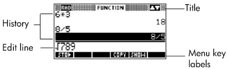
Menu key or soft key labels. The labels for the menu keys' current meanings. is the label for the first menu key in this picture. "Press means to press the first menu key, that is, the leftmost top-row key on the calculator keyboard.
Edit line. The line of current entry.
History. The HOME display ( ) shows up to four lines of history: the most recent input and output. Older lines scroll off the top of the display but are retained in memory.
Title. The name of the current aplet is displayed at the top of the HOME view. RAD, GRD, DEG specify whether Radians, Grads or Degrees angle mode is set for HOME. The ▼ and ▲ symbols indicate whether there is more history in the HOME display. Press the □ and to ▲ scroll in the HOME display.
NOTE
This user's guide contains images from the hp 39g+ and do not display the menu key label.
Annunciators. Annunciators are symbols that appear above the title bar and give you important status information.
| Annunciator Description | |
 | Shift in effect for next keystroke.To cancel, press again. |
| α Alpha in effect for next keystroke. | To cancel, press again. |
| ((•)) Low battery power. | |
| [25YZ] | Busy. |
 | Data is being transferred viainfrared or cable. |
The keyboard
Menu keys
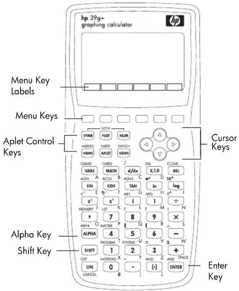
- On the calculator keyboard, the top row of keys are called menu keys. Their meanings depend on the context—that's why their tops are blank. The menu keys are sometimes called "soft keys".
- The bottom line of the display shows the labels for the menu keys' current meanings.
Aplet control keys
The aplet control keys are:
| Key Meaning | |
| SYMB | Displays the Symbolic view for the current aplet. See “Symbolic view” on page 1-16. |
| PLOT | Displays the Plot view for the current aplet. See “Plot view” on page 1-17. |
| NUM | Displays the Numeric view for the current aplet. See “Numeric view” on page 1-17. |
| HOME | Displays the HOME view. See “HOME is the calculator’s home view and is common to all aplets. If you want to perform calculations, or you want to quit the current activity (such as an aplet, a program, or an editor), press . All mathematical functions are available in the HOME. The name of the current aplet is displayed in the title of the home view.” on page 1-1. |
| APLET | Displays the Aplet Library menu. See “Aplet library” on page 1-16. |
| VIEWS | Displays the VIEWS menu. See “Aplet views” on page 1-16. |
Entry/Edit keys
The entry and edit keys are:
| Key Meaning | |
| ON (CANCEL) | Cancels the current operation if the calculator is on by pressing ONPressing SHIFT OFF turnsthen calculator off. |
| SHIFT | Accesses the function printed in blue above a key. |
| HOME | Returns to the HOME view, for performing calculations. |
| ALPHA | Accesses the alphabetical characters printed in orange below a key. Hold down to enter a string of characters. |
| ENTER | Enters an input or executes an operation. In calculations, ENTER acts like "=" . When OUT START is present as a menu key, ENTER acts the same as pressing OKSTART . |
| (-) | Enters a negative number. To enter -25, press 25 Note: this is not the same operation that the subtract button performs (-) . |
| X,T,θ | Enters the independent variable by inserting X, T, θ, or N into the edit line, depending on the current active aplet. |
| DEL | Deletes the character under the cursor. Acts as a backspace key if the cursor is at the end of the line. |
| SHIFT CLEAR | Clears all data on the screen. On a settings screen, for example Plot Setup, SHIFT CLEAR returns all settings to their default values. |
| ◀, ▶, ▲ | Moves the cursor around the display. Press first to move to the beginning, end, top or bottom. |
| Key Meaning (Continued) | |
| SHIFT CHARS Dis | plays a menu of all available characters. To type one, use the arrow keys to highlight it, and press OK . To select multiple characters, select each and press Fthen press OK . |
Shifted keystrokes
There are two shift keys that you use to access the operations and characters printed above the keys: SHIFT and ALPHA.
| Key Description | |
| SHIFT | Press thekeyto access the operations printed in blue above the keys. For instance, to access the Modes screen, pressSHthen pressHOME.(MODES is labeled in blue above thekey). You do not need to hold downwhen you press HOME. This action is depicted in this manual as “pressSHIFT MODES.”To cancel a shift, pressagain. |
| ALPHA | The alphabetic keys are also shifted keystrokes. For instance, to type Z, pressZL(The letters are printed in orange to the lower right of each key.)To cancel Alpha, pressALPHA again.For a lower case letter, pressSHIFTALPHA.For a string of letters, hold downALPHAwhile typing. |
HELPWITH
The hp 39g+ built-in help is available in HOME only. It provides syntax help for built-in math functions.
Access the HELPWITH command by pressing SHIFT SYNTAX and then the math key for which you require syntax help.
Example

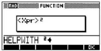
Note: Remove the left parenthesis from built-in functions such as sine, cosine, and tangent before invoking the HELPWITH command.
Math keys HOME () is the place to do calculations.
Keyboard keys. The most common operations are available from the keyboard, such as the arithmetic (like +) and trigonometric (like ) functions. Press ENTER to complete the operation: 256 √ ENTER displays 16.
MATH menu. Press MATH to open the MATH menu. The MATH menu is a comprehensive list of math functions that do not appear on the keyboard. It also

includes categories for all other functions and constants. The functions are grouped by category, ranging in alphabetical order from Calculus to Trigonometry.
- The arrow keys scroll through the list (, ▶ and move from the category list in the left column to the item list in the right column (◀). ▶
- Press to insert the selected command onto the edit line.
- Press to dismiss the MATH menu without selecting a command.
- Pressing CONE displays the list of Program Constants. You can use these in programs that you develop.
- Pressing takes you to the beginning of the MATH menu.
See "Math functions by category" on page 11-2 for details of the math functions.
HINT
When using the MATH menu, or any menu on the hp 39g+, pressing an alpha key takes you straight to the first menu option beginning with that alpha character. With this method, you do not need to press FirstJust press the key that corresponds to the command's beginning alpha character.
Program commands
Pressing SHIFT CMDS displays the list of Program Commands. See "Programming commands" on page 16-13.
Inactive keys If you press a key that does not operate in the current context, a warning symbol like this Appears. There is no beep.
Menus
A menu offers you a choice of items. Menus are displayed in one or two columns.
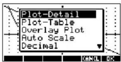
• The arrow in the display means more items below.
- The arrow in the display means more items above.

To search a menu
- Press ▼ or ▲ to scroll through the list. If you press SHIFT ▼, you'll go all the way to the end or the beginning of the list. Highlight the item you want to select, then press (or ). ENTER
- If there are two columns, the left column shows general categories and the right column shows specific contents within a category. Highlight a general category in the left column, then highlight an item in the right column. The list in the right column changes when a different category is highlighted.
Press OK ENTER when you have highlighted your selection.
- To speed-search a list, type the first letter of the word. For example, to find the Matrix category in MATH press ☐ the Alpha "M" key.
• To go up a page, you can press .STo go down a page, press SHIFT
To cancel a menu
Press ON (for CANCEL) or CANCEL. This cancels the current operation.
Input forms
An input form shows several fields of information for you to examine and specify. After highlighting the field to edit, you can enter or edit a number (or expression). You can also select options from a list (Some input forms include items to check (See below for examples input forms.
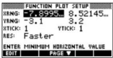

Reset input form values
To reset a field to its default values in an input form, move the cursor to that field and press .DTo reset all default field values in the input form, press SHIFT CLEAR.
Mode settings
You use the Modes input form to set the modes for HOME.
HINT
Although the numeric setting in Modes affects only HOME, the angle setting controls HOME and the current aplet. The angle setting selected in Modes is the angle setting used in both HOME and current aplet. To further configure an aplet, you use the SETUP keys (SHIFT PLOT and SHIFT NUM).
Press SHIFT MODES to access the HOME MODES input form.
| Setting Options | |
| Angle Measure | Angle values are:Degrees. 360 degrees in a circle.Radians. 2π radians in a circle.Grads. 400 grads in a circle.The angle mode you set is the angle setting used in both HOME and the current aplet. This is done to ensure that trigonometric calculations done in the current aplet and HOME give the same result. |
| Setting Options (Continued) | |
| Number Format | The number format mode you set is the number format used in both HOME and the current aplet.Standard. Full-precision display.Fixed. Displays results rounded to a number of decimal places. Example: 123.456789 becomes 123.46 in Fixed 2 format.Scientific. Displays results with an exponent, one digit to the left of the decimal point, and the specified number of decimal places. Example: 123.456789 becomes 1.23E2 in Scientific 2 format.Engineering. Displays result with an exponent that is a multiple of 3, and the specified number of significant digits beyond the first one. Example: 123.456E7 becomes 1.23E9 in Engineering 2 format.Fraction. Displays results as fractions based on the specified number of decimal places. Examples: 123.456789 becomes 123 in Fraction 2 format, and .333 becomes 1/3 and 0.142857 becomes 1/7. See “Using fractions” on page 1-25. |
| Decimal Mark | Dot or Comma. Displays a number as 12456.98 (Dot mode) or as 12456,98 (Comma mode). Dot mode uses commas to separate elements in lists and matrices, and to separate function arguments. Comma mode uses periods (dot) as separators in these contexts. |
Setting a mode
This example demonstrates how to change the angle measure from the default mode, radians, to degrees for the current aplet. The procedure is the same for changing number format and decimal mark modes.
- Press MODES to open the HOME MODES input form.
The cursor (highlight) is in the first field, Angle Measure.

- Press to display a list of choices.

- Press to select Degrees, and press OK. The angle measure changes to degrees.
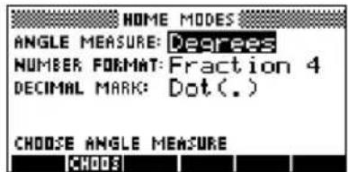
- Press to return to HOME.
HINT Whenever an input form has a list of choices for a field, you can press to cycle through them instead of using CHOOS.
Aplets (E-lessons)
Aplets are the application environments where you explore different classes of mathematical operations. You select the aplet that you want to work with.
Aplets come from a variety of sources:
• Built-in the hp 39g+ (initial purchase).
- Aplets created by saving existing aplets, which have been modified, with specific configurations. See "Creating new aplets based on existing aplets" on page 17-1.
- Downloaded from HP's Calculators web site.
• Copied from another calculator.
Aplets are stored in the Aplet library. See "Aplet library" on page 1-16 for further information.
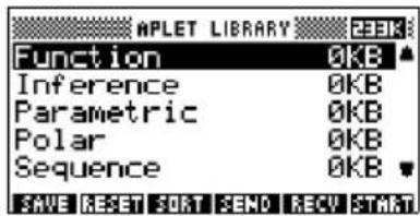
You can modify
configuration settings for the graphical, tabular, and symbolic views of the aplets in the following table. See "Aplet view configuration" on page 1-18 for further information.
| Aplet name | Use this aplet to explore: |
| Function Real-valued, rectangular functions y in terms of x. Example: y = 2x2 + 3x + 5 | |
| Inference Confidence intervals and Hypothesis tests based on the Normal and Students-t distributions. | |
| Parametric | Parametric relations x and y in terms of t. Example: x = (t) and y = (t) . |
| Polar | Polar functions r in terms of an angle θ. Example: r = 2(4θ) . |
| Sequence | Sequence functions U in terms of n, or in terms of previous terms in the same or another sequence, such as Un-1 and Un-2 . Example: U1 = 0 U2 = 1 and Un = Un-2 + Un-1 |
| Solve Equations in one or more real-valued variables. Example: x + 1 = x2 - x - 2 | |
| Statistics | One-variable (x) or two-variable (x and y) statistical data. |
In addition to these aplets, which can be used in a variety of applications, the hp 39g+ is supplied with two teaching aplets: Quad Explorer and Trig Explorer. You cannot modify configuration settings for these aplets.
A great many more teaching aplets can be found at HP's web site and other web sites created by educators, together with accompanying documentation, often with student work sheets. These can be downloaded free of charge and transferred to the hp 39g+ using the separately supplied Connectivity Kit.
Quad Explorer aplet
The Quad Explorer aplet is used to investigate the behaviour of y = a(x + h)2 + v as the values of a, h and v change, both by manipulating the equation and seeing the change in the graph, and by manipulating the graph and seeing the change in the equation.
HINT
More detailed documentation, and an accompanying student work sheet can be found at HP's web site.
Press APLET, select Explorer, and then press START. The Quad Explorer aplet opens in GRAPH mode, in which the arrow keys, the and keys, and the key are used to change the shape of the graph. This changing shape is reflected in the equation displayed at the top right corner of the screen, while the original graph is retained for comparison. In this mode the graph controls the equation.
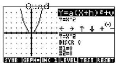
It is also possible to have the equation control the graph. Pressing SYME displays sub-expression of your equation.

Pressing the ▶ and key moves between sub-expressions, while pressing the ▲ and ▼ key changes their values.
Pressing follows the user to select whether all three sub-expressions will be explored at once or only one at a time.
A button is provided to evaluate the student's knowledge. Pressing TEST displays a target quadratic graph. The student must manipulate the equation's parameters to make the equation match the target graph. When a student feels that they have correctly chosen the parameters a CHECK button evaluates the answer and provide feedback. An ANSW button is provided for those who give up!

Trig Explorer aplet
The Trig Explorer aplet is used to investigate the behaviour of the graph of y as their (bx + c) + d values of a, b, c and d change, both by manipulating the equation and seeing the change in the graph, or by manipulating the graph and seeing the change in the equation.
Press APLET, select Explorer, and then press START to display the screen shown right.
In this mode, the graph controls the equation. Pressing the ▲ and ▼ ◀▶ keys transforms the graph, with these transformations reflected in


The button labelled 'a toggle between ORIG and EXTRA. When is chosen, the 'point of control' is at the origin (0,0) and the ▼ and ▶ keys control vertical and horizontal transformations. When E is chosen the 'point of control' is on the first extremum of the graph (i.e. for the sine graph at (π /2,1)
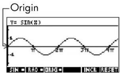
The arrow keys change the amplitude and frequency of the graph. This is most easily seen by experimenting.

Pressing displays the equation at the top of the screen. The equation is controlled by the graph. Pressing the ▶ and ▶ keys moves from parameter to parameter. Pressing the [parameter's values.
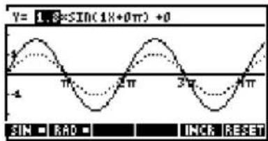
The default angle setting for this aplet is radians. The angle setting can be changed to degrees by pressing RAD.
Aplet library
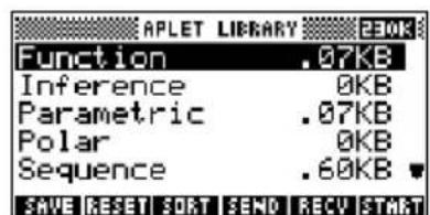
Aplets are stored in the Aplet library.
To open an aplet Press to display the Aplet library menu. Select the aplet and press START ENTER
From within an aplet, you can return to HOME any time by pressing HOME
Aplet views
When you have configured an aplet to define the relation or data that you want to explore, you can display it in different views. Here are illustrations of the three major aplet views (Symbolic, Plot, and Numeric), the six supporting aplet views (from the VIEWS menu), and the two user-defined views (Note and Sketch).
Symbolic view Press to display the aplet's Symbolic view.
You use this view to define the function(s) or equation(s) that you want to explore.
See "About the Symbolic view" on page 2-1 for further information.
Plot view Press to display the oplet's Plot view.
In this view, the functions that you have defined are displayed graphically.
See "About the Plot view" on page 2-5 for further information.

Numeric view
Press NUM to display the aplet's Numeric view.
In this view, the functions that you have defined are displayed in tabular format.
See "About the numeric view" on page 2-16 for further information.
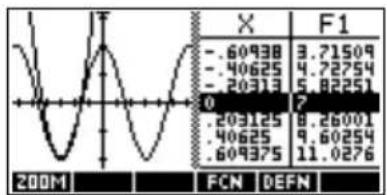
Plot-Table view The VIEWS menu contains the Plot-Table view.
VIEWS
Select Plot-Table OK
Splits the screen into the plot and the data table. See "Other views for scaling and splitting the graph" on page 2-14 for further informa
Plot-Detail view The VIEWS menu contains the Plot-Detail view.
VIEWS
Select Plot-Detail OK
Splits the screen into the plot and a close-up.
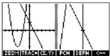
See "Other views for scaling and splitting the graph" on page 2-14 for further information.
Overlay Plot view
The VIEWS menu contains the Overlay Plot view.
VIEWS
Select Overlay Plot OK
Plots the current expression(s) without erasing any pre-existing plot(s).

See "Other views for scaling and splitting the graph" on page 2-14 for further information.
Note view
Press SHIFT NOTE to display the aplet's note view.
This note is transferred with the aplet if it is sent to another calculator or to a PC. A note view contains text to supplement an aplet.
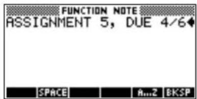
See "Notes and sketches" on page 15-1 for further information.
Sketch view
Press SHIFT SKETCH to display the aplet's sketch view.
Displays pictures to supplement an aplet.
See "Notes and sketches" on page 15-1 for further information.
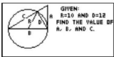
Aplet view configuration
You use the SETUP keys (SHIFT PLOT, and SHIFT NUM) to configure the aplet. For example, press SHIFT SETUP-PLOT (SHIFT PLOT) to display the input form for setting the aplet's plot settings. Angle measure is controlled using the MODES view.
Plot Setup
Press SHIFT SETUP-PLOT. Sets parameters to plot a graph.

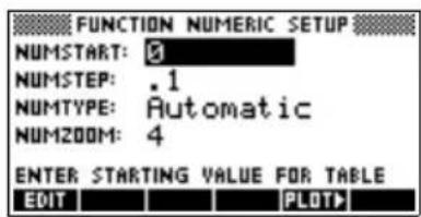
Numeric Setup
Press SHIFT SETUP-NUM. Sets parameters for building a table of numeric values.
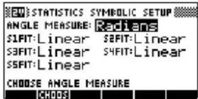
Symbolic Setup
This view is only available in the Statistics aplet in EUAR mode, where it plays an important role in choosing data models.
Press SHIFT SETUP-SYMB.
To change views Each view is a separate environment. To change a view, select a different view by pressing SYMB NUM PLOT keys or select a view from the VIEWS menu. To change to HOME, press -You do not explicitly close the current view, you just enter another one—like passing from one room into another in a house. Data that you enter is automatically saved as you enter it.
To save aplet configuration
You can save an aplet configuration that you have used, and transfer the aplet to other hp 39g+ calculators. See "Sending and receiving aplets" on page 17-4.
Mathematical calculations
The most commonly used math operations are available from the keyboard. Access to the rest of the math functions is via the MATH menu (MATH)
To access programming commands, press SHIFT CMDS. See "Programming commands" on page 16-13 for further information.
Where to start The home base for the calculator is the HOME view ( ) You can do all calculations here, and you can access all operations.
Entering expressions
- Enter an expression into the hp 39g+ in the same left-to-right order that you would write the expression. This is called algebraic entry.
• To enter functions, select the key or MATH menu item for that function. You can also enter a function by using the Alpha keys to spell out its name.
- Press to evaluate the expression you have in the edit line (where the blinking cursor is). An expression can contain numbers, functions, and variables.
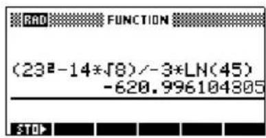
Example Calculate
2 3 ^ 2 - 1 4 √ 8- 3 (4 5)

Long results If the result is too long to fit on the display line, or if you want to see an expression in textbook format, press ▲ to highlight it and then press SHOW
Negative numbers
Type to start a negative number or to insert a negative sign.
To raise a negative number to a power, enclose it in parentheses. For example, (-5)2=25 , whereas -52=-25 .
Scientific notation (powers of 10)
A number like 5 or 104 written 1 in 10-7 scientific notation, that is, in terms of powers of ten. This is simpler to work with than 50000 or 0.000000321. To enter numbers like these, use EEX. (This is easier than using ×10Y .)
Example Calculate
(4 × 1 0 ^ - 1 3) (6 × 1 0 ^ 2 3)3 × 1 0 ^ - 5


Explicit and implicit multiplication
Implied multiplication takes place when two operands appear with no operator in between. If you enter AB, for example, the result is A*B.
However, for clarity, it is better to include the multiplication sign where you expect multiplication in an expression. It is clearest to enter AB as A*B.
HINT
Implied multiplication will not always work as expected. For example, entering A(B+4) will not give A*(B+4). Instead an error message is displayed: "Invalid User Function". This is because the calculator interprets A(B+4) as meaning 'evaluate function A at the value B+4', and function A does not exist. When in doubt, insert the * sign manually.
Parentheses You need to use parentheses to enclose arguments for functions, such as SIN(45). You can omit the final parenthesis at the end of an edit line. The calculator inserts it automatically.
Parentheses are also important in specifying the order of operation. Without parentheses, the hp 39g+ calculates according to the order of algebraic precedence (the next topic). Following are some examples using parentheses.
| Entering... Calculates... | |
| SIN 45 + SHIFT πSIN 45 π sin (45) + πSHIFT √ 85 9SHIFT √85 9 × ) | sin (45 + π)√88 9√88 9 |
Algebraic precedence order of evaluation
Functions within an expression are evaluated in the following order of precedence. Functions with the same precedence are evaluated in order from left to right.
- Expressions within parentheses. Nested parentheses are evaluated from inner to outer.
- Prefix functions, such as SIN and LOG.
- Postfix functions, such as !
- Power function, ^, NTHROOT.
- Negation, multiplication, and division.
- Addition and subtraction.
- AND and NOT.
- OR and XOR.
- Left argument of | (where).
10.Equals, =.
Largest and smallest numbers
The smallest number the hp 39g+ can represent is 1 × 10-499(1E-499) . A smaller result is displayed as zero. The largest number is 9.99999999999 × 10499(1E499) . A greater result is displayed as this number.
Clearing numbers
- clears the character under the cursor. When the cursor is positioned after the last character, DEL deletes the character to the left of the cursor, that is, it performs the same as a backspace key.
- CANCEL ( ) clears the edit line.
- SHIFT CLEAR clears all input and output in the display, including the display history.
Using previous results
The HOME display (HOME) shows you four lines of input/output history. An unlimited (except by memory) number of previous lines can be displayed by scrolling. You can retrieve and reuse any of these values or expressions.

When you highlight a previous input or result (by pressing ▲), the □ and menq labels appear.
![RAD FUNCTION 1+2+8 √2 99/76 5*77+99/70♦ STOP COPY [SHOW]](/content/2026/05/1017618/images/62f6288bd13bdf594fad74d47e4eabfe1ffd8966f43d59cb9e292cc0546f5550.jpg)
To copy a previous line
Highlight the line (press ▲ and press . TheFY number (or expression) is copied into the edit line.
To reuse the last result
Press SHIFT ANS (last answer) to put the last result from the HOME display into an expression. ANS is a variable that is updated each time you press ENTER
To repeat a previous line
To repeat the very last line, just press . Otherwise, highlight the line (press first, and then press . ENTER The highlighted expression or number is re-entered. If the previous line is an expression containing the ANS, the calculation is repeated iteratively.
Example See how
SHIFT ANS retrieves and reuses the last result (50), and updates ANS (from 50 to 75 to 100).
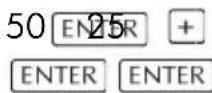
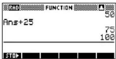
You can use the last result as the first expression in the edit line without pressing SHIFT ANS. Pressing -, ×, ÷, (or other operators that require a preceding argument) automatically enters ANS before the operator.
You can reuse any other expression or value in the HOME display by highlighting the expression (using the arrow keys), then pressing See "Using previous results" on page 1-22 for more details.
The variable ANS is different from the numbers in HOME's display history. A value in ANS is stored internally with the full precision of the calculated result, whereas the displayed numbers match the display mode.
HINT
When you retrieve a number from ANS, you obtain the result to its full precision. When you retrieve a number from the HOME's display history, you obtain exactly what was displayed.
Pressing evaluates (or re-evaluates) the last input, whereas pressing SHIFT ANS copies the last result (as ANS) into the edit line.
Storing a value in a variable
You can save an answer in a variable and use the variable in later calculations. There are 27 variables available for storing real values. These are A to Z and θ. See Chapter 12, "Variables and memory management" for more information on variables. For example:
- Perform a calculation.


- Store the result in the A variable.


- Perform another calculation using the A variable.

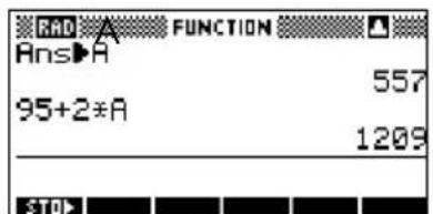
Accessing the display history
Pressing ▲ enables the highlight bar in the display history. While the highlight bar is active, the following menu and keyboard keys are very useful:
| Key Function | |
| ▲ , Scrolls | through the display history. |
| COPY | Copies the highlighted expression to the position of the cursor in the edit line. |
| SHOW | Displays the current expression in standard mathematical form. |
| DEL | Deletes the highlighted expression from the display history, unless there is a cursor in the edit line. |
| SHIFT | Clears all lines of display history and the edit line. |
| CLEAR |
Clearing the display history
It's a good habit to clear the display history (SHIFT CLEAR) whenever you have finished working in HOME. It saves calculator memory to clear the display history. Remember that all your previous inputs and results are saved until you clear them.
Using fractions
To work with fractions in HOME, you set the number format to Fractions, as follows:
Setting Fraction mode
- In HOME, open the HOME MODES input form.
SHIFT MODES

- Select Number Format, press to display the options, and highlight Fraction.
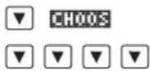

- Press to select the Number Format option, then move to the precision value field.


- Enter the precision value that you want to use, and press the set the precision. Press to return to HOME.
See "Setting fraction precision" below for more information.
Setting fraction precision
The fraction precision setting determines the precision in which the hp 39g+ converts a decimal value to a fraction. The greater the precision value that is set, the closer the fraction is to the decimal value.
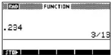
By choosing a precision of 1 you are saying that the fraction only has to match 0.234 to at least 1 decimal place (3/13 is 0.23076...).
The fractions used are found using the technique of continued fractions.
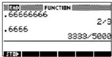
When converting recurring decimals this can be important. For example, at precision 6 the decimal 0.6666 becomes 3333/5000 (6666/10000) whereas at precision 3, 0.6666 becomes 2/3, which is probably what you would want.
For example, when converting .234 to a fraction, the precision value has the following effect:
- Precision set to 1:
- Precision set to 2:
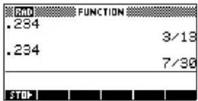
- Precision set to 3:
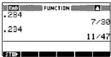
- Precision set to 4

Fraction calculations
When entering fractions:
- You use the key to separate the numerator part and the denominator part of the fraction.
- To enter a mixed fraction, for example, 1-1/2 , you enter it in the format (1 + 1/2) .
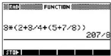
For example, to perform the following calculation:
3 (2 ^ 3 / _ 4 + 5 ^ 7 / _ 8)
- Set the Number format mode to Fraction and specify a precision value of 4. Select Fraction


- Enter the calculation.

Note: Ensure you are in the HOME view.

- Evaluate the calculation.
Converting decimals to fractions
To convert a decimal value to a fraction:
- Set the number format mode to Fraction.
- Either retrieve the value from the History, or enter the value on the command line.
- Press to convert the number to a fraction.
When converting a decimal to a fraction, keep the following points in mind:
- When converting a recurring decimal to a fraction, set the fraction precision to about 6, and ensure that you include more than six decimal places in the recurring decimal that you enter.
In this example, the fraction precision is set to 6. The top calculation returns the correct result. The bottom one does not.
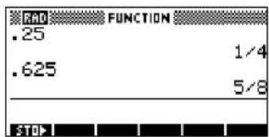
• To convert an exact decimal to a fraction, set the fraction precision to at least two more than the number of decimal places in the decimal.
In this example, the fraction precision is set to 6.
Complex numbers
Complex results
The hp 39g+ can return a complex number as a result for some math functions. A complex number appears as an ordered pair (x, y) , where x is the real part and y is the imaginary part. For example, entering returns (0,1).
To enter complex numbers
Enter the number in either of these forms, where x is the real part, y is the imaginary part, and i is the imaginary constant, √-1 :
• (x, y) or
• x + iy.
To enter i:
- press

or
- press MATH, ▲ or ▼ keys to select Constant, ▶ to move to the right column of the menu, ▼ to select i, and OK
Storing complex numbers
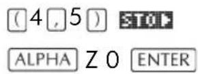
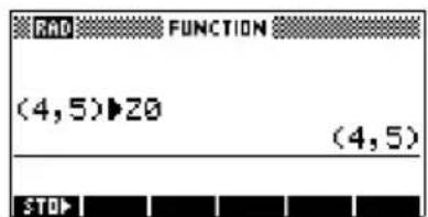
There are 10 variables available for storing complex numbers: Z0 to Z9. To store a complex number in a variable:
- Enter the complex number, press, enter the variable to store the number in, and press ENTER
Catalogs and editors
The hp 39g+ has several catalogs and editors. You use them to create and manipulate objects. They access features and stored values (numbers or text or other items) that are independent of aplets.
- A catalog lists items, which you can delete or transmit, for example an aplet.
- An editor lets you create or modify items and numbers, for example a note or a matrix.
| Catalog/Editor Contents | |
| Aplet library(APLET) | Aplets. |
| Sketch editor(SHIFT SKETCH) | Sketches and diagrams, See Chapter 15, “Notes and sketches”. |
| List (SHIFT LIST) | Lists. In HOME, lists are enclosed in {}. See Chapter 14, “Lists”. |
| Matrix (SHIFT MATRIX) | One- and two-dimensional arrays. In HOME, arrays are enclosed in []. See Chapter 13, “Matrices”. |
| Notepad (SHIFT NOTEPAD) | Notes (short text entries). See Chapter 15, “Notes and sketches”. |
| Program (SHIFT PROGRAM) | Programs that you create, or associated with user-defined aplets. See Chapter 16, “Programming”. |
Aplets and their views
Aplet views
This section examines the options and functionality of the three main views for the Function, Polar, Parametric, and Sequence aplets: Symbolic, Plot, and Numeric views.
About the Symbolic view
The Symbolic view is the defining view for the Function, Parametric, Polar, and Sequence aplets. The other views are derived from the symbolic expression.
You can create up to 10 different definitions for each Function, Parametric, Polar, and Sequence aplet. You can graph any of the relations (in the same aplet) simultaneously by selecting them.
Defining an expression (Symbolic view)
Choose the aplet from the Aplet Library.

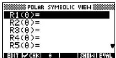
The Function, Parametric, Polar, and Sequence aplets start in the Symbolic view.
If the highlight is on an existing expression, scroll to an empty line—unless you don't mind writing over the expression—or, clear one line (□or all lines
(SHIFT CLEAR).
Expressions are selected (check marked) on entry. To deselect an expression, press 📂All selected expressions are plotted.
- For a Function definition, enter an expression to define F(X) . The only independent variable in the expression is X .

- For a Parametric definition, enter a pair of expressions to define X(T) and Y(T) . The only independent variable

- For a Polar definition, enter an expression to define R(θ) . The only independent variable in the expression is θ .
- For a Sequence definition, either: Enter the first and second terms for U ( U1 , or... U9 , or U0 ). Define the n th term of the

sequence in terms of N or of the prior terms, U(N-1) and U(N-2) . The expressions should produce real-valued sequences with integer domains. Or define the nth term as a non-recursive expression in terms of n only. In this case, the calculator inserts the first two terms based on the expression that you define.
Evaluating expressions
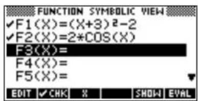
In aplets In the Symbolic view, a variable is a symbol only, and
does not represent one specific value. To evaluate a function in Symbolic view, press EURL function calls another function, then EIGSelves all references to other functions in terms of their independent variable.
- Choose the Function aplet.


- Enter the expressions in the Function aplet's Symbolic view.

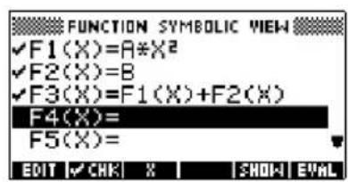
- Highlight F3(X).


- Press EVAL
Note how the values for F1(X) and F2(X) are substituted into F3(X).

In HOME You can also evaluate any expression in HOME by entering it into the edit line and pressing ENTER
For example, define F4 as below. In HOME, type F4 (9) and press This evaluates the expression, substituting 9 in place of X into F4.


SYMB view keys The following table details the menu keys that you use to work with the Symbolic view.
| Key Meaning | |
| EDIT | Copies the highlighted expression to the edit line for editing. Press OK when done. |
| CHK | Checks/ unchecks the current expression (or set of expressions). Only checked expression(s) are evaluated in the Plot and Numeric views. |
| X | Enters the independent variable in the Function aplet. Or, you can use the X,T,θ key on the keyboard. |
| T | Enters the independent variable in the Parametric aplet. Or, you can use the X,T,θ key on the keyboard. |
| θ | Enters the independent variable in the Polar aplet. Or, you can use the X,T,θ key on the keyboard. |
| N | Enters the independent variable in the Sequence aplet. Or, you can use the X,T,θ key on the keyboard. |
| SHOW | Displays the current expression in text book form. |
| EVAL | Resolves all references to other definitions in terms of variables and evaluates all arithmetic expressions. |
| VARS | Displays a menu for entering variable names or contents of variables. |
| Key | Meaning (Continued) |
| MATH | Displays the menu for entering math operations. |
| SHIFT CHARS | Displays special characters. To enter one, place the cursor on it and press OK. To remain in the CHARS menu and enter another special character, press ECHO. |
| DEL | Deletes the highlighted expression or the current character in the edit line. |
| SHIFT CLEAR | Deletes all expressions in the list or clears the edit line. |
About the Plot view
After entering and selecting (check marking) the expression in the Symbolic view, press Pilot adjust the appearance of the graph or the interval that is displayed, you can change the Plot view settings.
You can plot up to ten expressions at the same time. Select the expressions you want to be plotted together.
Setting up the plot (Plot view setup)
Press SHIFT SETUP-PLOT to define any of the settings shown in the next two tables.
- Highlight the field to edit.
- If there is a number to enter, type it in and press ENTER or OK
- If there is an option to choose, press , CHOOS highlight your choice, and press ENTER OK As a shortcut to CHOS highlight the field to change and press to cycle through the options.
- If there is an option to select or deselect, press ✓CHK to check or uncheck it.
-
Press to view more settings.
-
When done, press to view the new plot.
Plot view settings
The plot view settings are:
| Field Meaning | |
| XRNG, YRNG | Specifies the minimum and maximum horizontal (X) and vertical (Y) values for the plotting window. |
| RES For function plots: Resolution;“Faster” plots in alternate pixel columns; “Detail” plots in every pixel column. | |
| TRNG Parametric aplet: Specifies the t-values (T) for the graph. | |
| θRNG | Polar aplet: Specifies the angle (θ) value range for the graph. |
| NRNG Sequence aplet: Specifies the index (N) values for the graph. | |
| TSTEP For Parametric plots: the increment for the independent variable. | |
| θSTEP For Polar plots: the increment value for the independent variable. | |
| SEQPLOT For Sequence aplet: Stairstep or Cobweb types. | |
| XTICK Horizontal spacing for tickmarks. | |
| YTICK Vertical spacing for tickmarks. | |
Those items with space for a checkmark are settings you can turn on or off. Press FoE display the second page.
| Field Meaning | |
| SIMULT If more than one relation is being plotted, plots them simultaneously (otherwise sequentially).INV. CROSS Cursor crosshairs invert the status of the pixels they cover. | |
| Field Meaning (Continued) | |
| CONNECT Connect the plotted points. (The Sequence aplet always connects them.)LABELS Label the axes with XRNG and YRNG values.AXES Draw the axes.GRID Draw grid points using XTICK and YTICK spacing. | |
Reset plot settings
To reset the default values for all plot settings, press SHIFT CLEAR in the Plot Setup view. To reset the default value for a field, highlight the field, and press DEL
Exploring the graph
Plot view gives you a selection of keys and menu keys to explore a graph further. The options vary from aplet to aplet.
PLOT view keys The following table details the keys that you use to work with the graph.
| Key Meaning | |
 CLEAR Erases the plot and axes. CLEAR Erases the plot and axes. | |
 | Offers additional pre-defined views for splitting the screen and for scaling ("zooming") the axes. |
 | Moves cursor to far left or far right. |
 | Moves cursor between relations. |
 | |
 | |
 or Interrupts plotting. or Interrupts plotting. | |
 | |
 | Continues plotting if interrupted. |
| Key Meaning (Continued) | |
| MENU | Turns menu-key labels on and off.When the labels are off, pressingMENU turns them back on.Pressing oFEQ displays the full row of labels.Pressing oSECD time removes the row of labels to display only the graph.Pressing oFEQ time displays the coordinate mode. |
| 200M | Displays the ZOOM menu list. |
| TRACE | Turns trace mode on/off. A white box appears over the E on . TRACE |
| GOTO | Opens an input form for you to enter an X (or T or N or θ) value. Enter the value and press OK The cursor jumps to the point on the graph that you entered. |
| FCN | Function aplet only: turns on menu list for root-finding functions (see “Analyse graph with FCN functions” on page 3-4). |
| DEFN | Displays the current, defining expression. Press #K Store the menu. |
Trace a graph
You can trace along a function using the ◀ or ▶ key which moves the cursor along the graph. The display also shows the current coordinate position (x, y) of the cursor. Trace mode and the coordinate display are automatically set when a plot is drawn.
Note: Tracing might not appear to exactly follow your plot if the resolution (in Plot Setup view) is set to Faster. This is because RES: FASTER plots in only every other column, whereas tracing always uses every column.
In Function and Sequence Aplets: You can also scroll (move the cursor) left or right beyond the edge of the display window in trace mode, giving you a view of more of the plot.
To move between relations
If there is more than one relation displayed, press ▼ to move between relations.
To jump directly to a value
To jump straight to a value rather than using the Trace function, use the menu key. Press, therefore a value. Press is jump to the value.
To turn trace on/off
If the menu labels are not displayed, press MENU first.
- Turn off trace mode by pressing . TRAC
- Turn on trace mode by pressing . TRACE
• To turn the coordinate display off, press . MENU
Zoom within a graph
One of the menu key options is Zoming redraws the plot on a larger or smaller scale. It is a shortcut for changing the Plot Setup.
The Set Factors... option enables you to set the factors by which you zoom in or zoom out, and whether the zoom is centered about the cursor.
ZOOM options Press
select option, and press . (If is not displayed, press FIE not all available in all aplets.
OK
200M
| Option Meaning | |
| Center Re-centers the plot around the current position of the cursor without changing the scale. | |
| Box... Lets you draw a box to zoom in on.See “Other views for scaling and splitting the graph” on page 2-14. | |
| In Divides horizontal and vertical scales by the X-factor and Y-factor. For instance, if zoom factors are 4, then zooming in results in 1/4 as many units depicted per pixel. (see Set Factors...) | |
| Out | Multiplies horizontal and vertical scales by the X-factor and Y-factor (see Set Factors...). |
| X-Zoom In | Divides horizontal scale only, using X-factor. |
| X-Zoom Out | Multiplies horizontal scale, using X-factor. |
| Option Meaning | (Continued) |
| Y-Zoom In Divides vertical scale only, using Y-factor. | |
| Y-Zoom Out Multiplies vertical scale only, using Y-factor. | |
| Square Changes the vertical scale to match the horizontal scale. (Use this after doing a Box Zoom, X-Zoom, or Y-Zoom.) | |
| Set Factors... | Sets the X-Zoom and Y-Zoom factors for zooming in or zooming out.Includes option to recenter the plot before zooming. |
| Auto Scale Rescales the vertical axis so that the display shows a representative piece of the plot, for the supplied x axis settings. (For Sequence and Statistics aplets, autoscaling rescales both axes.)The autoscale process uses the first selected function only to determine the best scale to use. | |
| Decimal Rescales both axes so each pixel = 0.1 units. Resets default values for XRNG(-6.5 to 6.5) and YRNG (-3.1 to 3.2). (Not in Sequence or Statistics aplets.) | |
| Integer Rescales horizontal axis only,making each pixel =1 unit. (Not available in Sequence or Statistics aplets.) | |
| Trig Rescales horizontal axis so1 pixel = π/24 radians, 7.58, or 8 1/3 grads; rescales vertical axis so1 pixel = 0.1 unit.(Not in Sequence or Statistics aplets.) | |
| Un-zoom Returns | the display to the previous zoom, or if there has been only one zoom, un-zoom displays the graph with the original plot settings. |
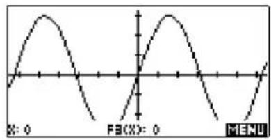
ZOOM examples The following screens show the effects of zooming options on a plot of 3 x sin
Plot of 3x
Zoom In:
MENU 200M OK

Un-zoom:
200M Un-zoom OK
Note: Press □ move to the bottom of the Zoom list.
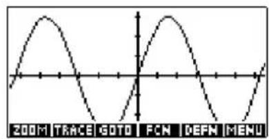
Zoom Out:
200H Out OK
Now un-zoom.
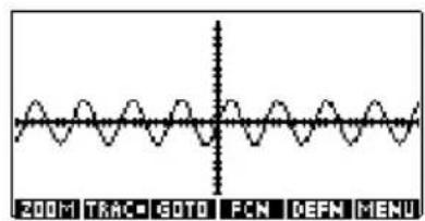
X-Zoom In:
200M X-Zoom In OK
Now un-zoom.
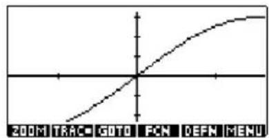
X-Zoom Out:
200M X-Zoom Out OK
Now un-zoom.

Y-Zoom In:
200M Y-Zoom In OK
Now un-zoom.

Y-Zoom Out:
2001 Y-Zoom Out OK
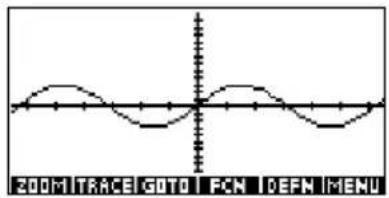
Zoom Square:
200M Square OK
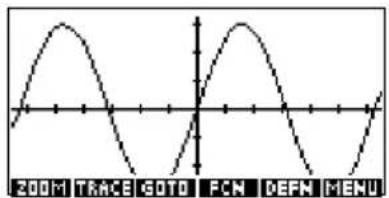
To box zoom The Box Zoom option lets you draw a box around the area you want to zoom in on by selecting the endpoints of one diagonal of the zoom rectangle.
- If necessary, press ☐NUM on the menu-key labels.
- Press outselect Box...
- Position the cursor on one corner of the rectangle. Press OK.
- Use the cursor keys (, etc.) to drag to the opposite corner.

- Press zoom in on the boxed area.

To set zoom factors 1. In the Plot view, press . MENU
-
Press
-
Select Set Factors... and press .OK
-
Enter the zoom factors. There is one zoom factor for the horizontal scale (XZOOM) and one for the vertical scale (YZOOM).
Zooming out multiplies the scale by the factor, so that a greater scale distance appears on the screen.
Zooming in divides the scale by the factor, so that a shorter scale distance appears on the screen.
Other views for scaling and splitting the graph
The preset viewing options menu ( ) contains options for drawing the plot using certain pre-defined configurations. This is a shortcut for changing Plot view settings. For instance, if you have defined a trigonometric function, then you could select Trig to plot your function on a trigonometric scale. It also contains split-screen options.
In certain aplets, for example those that you download from the world wide web, the preset viewing options menu can also contain options that relate to the aplet.
VIEWS menu options
Press ,select an option, and press .
OK
| Option Meaning | |
| Plot-Detail | Splits the screen into the plot and a close-up. |
| Plot-Table | Splits the screen into the plot and the data table. |
| Overlay Plot | Plots the current expression(s) without erasing any pre-existing plot(s). |
| Auto Scale | Rescales the vertical axis so that the display shows a representative piece of the plot, for the supplied x axis settings. (For Sequence and Statistics aplets, autoscaling rescales both axes.)The autoscale process uses the first selected function only to determine the best scale to use. |
| Decimal Rescales | both axes so each pixel = 0.1 unit. Resets default values for XRNG(-6.5 to 6.5) and YRNG (-3.1 to 3.2). (Not in Sequence or Statistics aplets.) |
| Integer Rescales | horizontal axis only,making each pixel=1 unit. (Not available in Sequence or Statistics aplets.) |
| Option | Meaning (Continued) |
| Trig | Rescales horizontal axis so 1 pixel=π/24 radian, 7.58, or 8 1/3 grads; rescales vertical axis so 1 pixel = 0.1 unit.(Not in Sequence or Statistics aplets.) |
Split the screen The Plot-Detail view can give you two simultaneous views of the plot.
-
Press . Select PlotDetail a The graph is plotted twice. You can now zoom in on the right side.
-
Press MENU 200M select the zoom method and press OK
ENTER. This zooms the right side. Here is an example of split screen
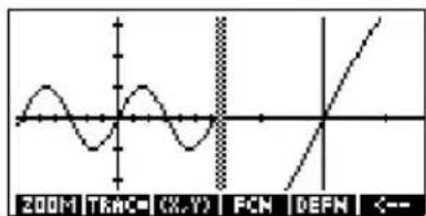
- The Plot menu keys are available as for the full plot (for tracing, coordinate display, equation display, and so on).
- moves the leftmost cursor to the screen's left edge and moves the rightmost cursor to the screen's right edge.
- The n<== key copies the right plot to the left plot.
- To un-split the screen, press PLOT . The left side takes over the whole screen.
The Plot-Table view gives you two simultaneous views of the plot.
- Press Plot-Table and press of the screen displays the plot on the left side and a table of numbers on the right side.
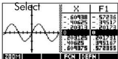
- To move up and down the table, use the and cursor keys. These keys move the trace point left or right along the plot, and in the table, the corresponding values are highlighted.
- To move between functions, use the and cursor keys to move the cursor from one graph to another.
- To return to a full Numeric (or Plot) view, press NUM (or PLOT).
Overlay plots
If you want to plot over an existing plot without erasing that plot, then use Overlay Plot instead of PLOT. Note that tracing follows only the current functions from the current aplet.
Decimal scaling Decimal scaling is the default scaling. If you have changed the scaling to Trig or Integer, you can change it back with Decimal.
Integer scaling Integer scaling compresses the axes so that each pixel is 1 and the origin is near the screen center.
Trigonometric scaling
Use trigonometric scaling whenever you are plotting an expression that includes trigonometric functions. Trigonometric plots are more likely to intersect the axis at points factored by π .
About the numeric view
After entering and selecting (check marking) the expression or expressions that you want to explore in the Symbolic view, press
NUM to view a table of data values for the independent variable (X, T, θ, or N) and dependent variables.
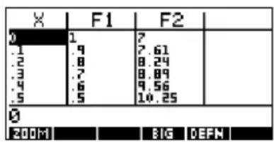
Setting up the table (Numeric view setup)
Press NUM to define any of the table settings. Use the Numeric Setup input form to configure the table.
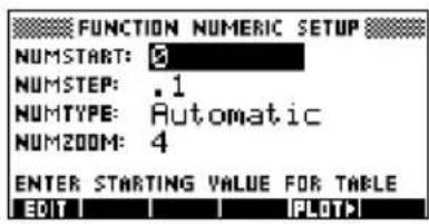
- Highlight the field to edit. Use the arrow keys to move from field to field.
- If there is a number to enter, type it in and press ENTER or OK. To modify an existing number, press EDIT.
- If there is an option to choose, press , CHOO'S highlight your choice, and press ENTER OK
- Shortcut: Press the key copy values from the Plot Setup into NUMSTART and NUMSTEP. Effectively, the PL034u key allows you to make the table match the pixel columns in the graph view.
- When done, press to view the table of numbers.
Numeric view settings
The following table details the fields on the Numeric Setup input form.
| Field Meaning | |
| NUMSTART The independent variable's starting value. | |
| NUMSTEP | The size of the increment from one independent variable value to the next. |
| NUMTYPE | Type of numeric table: Automatic or Build Your Own. To build your own table, you must type each independent value into the table yourself. |
| NUMZOOM | Allows you to zoom in or out on a selected value of the independent variable. |
Reset numeric settings
To reset the default values for all table settings, press
SHIFT CLEAR.
Exploring the table of numbers
NUM view menu keys
The following table details the menu keys that you use to work with the table of numbers.
| Key Meaning | |
| 200M | Displays ZOOM menu list. |
| BIG | Toggles between two character sizes. |
| DEFN | Displays the defining function expression for the highlighted column. To cancel this display, press DEF. |
Zoom within a table
Zooming redraws the table of numbers in greater or lesser detail.
ZOOM options The following table lists the zoom options:
| Option Meaning | |
| In Decreases the intervals for the independent variable so a narrower range is shown. Uses the NUMZOOM factor in Numeric Setup. | |
| Out Increases the intervals for the independent variable so that a wider range is shown. Uses the NUMZOOM factor in Numeric Setup. | |
| Decimal Changes intervals for the independent variable to 0.1 units. Starts at zero. (Shortcut to changing NUMSTART and NUMSTEP.) | |
| Integer Changes intervals for the independent variable to 1 unit. Starts at zero. (Shortcut to changing NUMSTEP.) | |
| Option Meaning | (Continued) |
| Trig Changes | intervals for independent variable to π/24 radian or 7.5 degrees or 81/3 grads. Starts at zero. |
| Un-zoom Returns | the display to the previous zoom. |
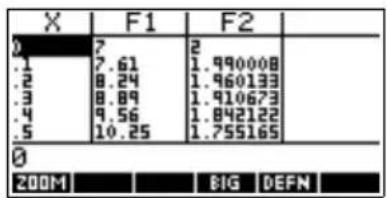
The display on the right is a Zoom In of the display on the left. The ZOOM factor is 4.


HINT
To jump to an independent variable value in the table, use the arrow keys to place the cursor in the independent variable column, then enter the value to jump to.
Automatic recalculation
You can enter any new value in the X column. When you press, The values for the dependent variables are recalculated, and the entire table is regenerated with the same interval between X values.
Building your own table of numbers
The default NUMTYPE is "Automatic", which fills the table with data for regular intervals of the independent (X, T, θ, or N) variable. With the NUMTYPE option set to "Build Your Own", you fill the table yourself by typing in the independent-variable values you want. The dependent values are then calculated and displayed.
Build a table 1. Start with an expression defined (in Symbolic view) in the aplet of your choice. Note: Function, Polar, Parametric, and Sequence aplets only.
-
In the Numeric Setup (SHIFT NUM), choose NUMTYPE: Build Your Own.
-
Open the Numeric view ( ) NUM
-
Clear existing data in the table (SHIFT CLEAR).
-
Enter the independent values in the left-hand column.
Type in a number and press [F] You do not have to enter them in order, because the function can rearrange them. To insert a number between two others, use INS

Clear data
Press SHIFT CLEAR, YES to erase the data from a table.
"Build Your Own" menu keys
| Key Meaning | |
| EDIT | Puts the highlighted independent value (X, T, θ, or N) into the edit line. Pressingreplacethis variable with its current value. |
| INS | Inserts a row of zero values at the position of the highlight. Replace a zero by typing the number you want and pressingENTER |
| SORT | Sorts the independent variable values into ascending or descending order. PressSORTand select the ascending or descending option from the menu, and pressOK |
| BIG | Toggles between two character sizes. |
| DEFN | Displays the defining function expression for the highlighted column. |
| DEL | Deletes the highlighted row. |
| SHIFT CLEAR | Clears all data from the table. |
Example: plotting a circle
Plot the circle, x2 + y2 = 9 . First rearrange it to read
y 9 x √ - ±^ 2.
To plot both the positive and negative y values, you need to define two equations as follows:
y 9 x √ - 2 and y 9 x - √ - 2
- In the Function aplet, specify the functions.


9
- Reset the graph setup to the default settings.
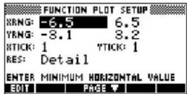
- Plot the two functions and hide the menu so that you can see all the circle.


- Reset the numeric setup to the default settings.

- Display the functions in numeric form.
NUM

Function aplet
About the Function aplet
The Function aplet enables you to explore up to 10 real-valued, rectangular functions y in terms of x. For example y 2x 3+= .
Once you have defined a function you can:
- create graphs to find roots, intercepts, slope, signed area, and extrema
- create tables to evaluate functions at particular values.
This chapter demonstrates the basic tools of the Function aplet by stepping you through an example. See “Aplet views” on page 2-1 for further information about the functionality of the Symbolic, Numeric, and Plot views.
Getting started with the Function aplet
The following example involves two functions: a linear function y and a quadratic equation
y = x 3 + (2.)
Open the Function aplet
- Open the Function aplet.

The Function aplet starts in the Symbolic view.
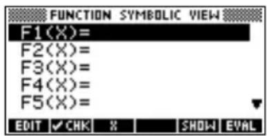
The Symbolic view is the defining view for Function, Parametric, Polar, and Sequence aplets. The other views are derived from the symbolic expression.
Define the expressions
- There are 10 function definition fields on the Function aplet's Symbolic view screen. They are labeled F1(X) to F0(X). Highlight the function definition field you want to use, and enter an expression. (You can press DEL to delete an existing line, or CLEAR to clear all lines.)

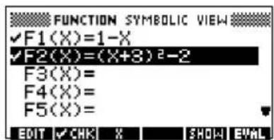
Set up the plot
You can change the scales of the x and y axes, graph resolution, and the spacing of the axis ticks.
- Display plot settings.
SHIFT SETUP-PLOT
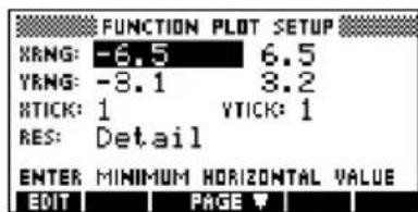
Note: For our example, you can leave the plot settings at their default values since we will be using the Auto Scale feature to choose an appropriate y axis for our x axis settings. If your settings do not match this example, press SHIFT CLEAR to restore the default values.
- Specify a grid for the graph.
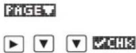

Plot the functions
- Plot the functions.
PLOT

Change the scale
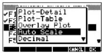
- You can change the scale to see more or less of your graphs. In this example, choose Auto Scale. (See "VIEWS menu options" on page 2-14 for a description of Auto Scale).


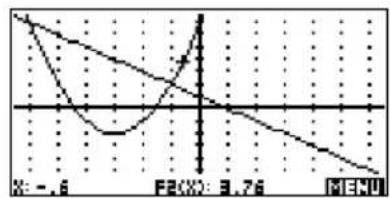
Trace a graph 7. Trace the linear function.

Note: By default, the tracer is active.
- Jump from the linear function to the quadratic function.

Analyse graph with FCN functions
- Display the Plot view menu.
MENU

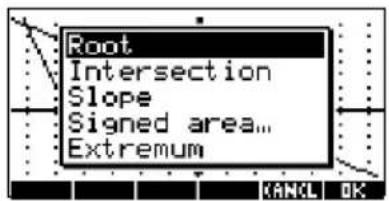
From the Plot view menu, you can use the functions on the FCN menu to find roots, intersections, slopes, and areas for a function defined in the Function aplet (and any Function-based aplets). The FCN functions act on the currently selected graph. See "FCN functions" on page 3-10 for further information.
To find a root of the quadratic function
- Move the cursor to the graph of the quadratic equation by pressing the ▲ or ▼ key. Then move the cursor so that it is near x 1—by pressing the ▶ or ▼ key.
FCN Select Root OK
The root value is displayed at the bottom of the screen.

Note: If there is more than one root (as in our example), the
coordinates of the root closest to the current cursor position are displayed.
To find the intersection of the two functions
- Find the intersection of the two functions.
MENU
FEN

08
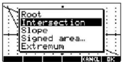
- Choose the linear function whose intersection with the quadratic function you wish to find.
OK
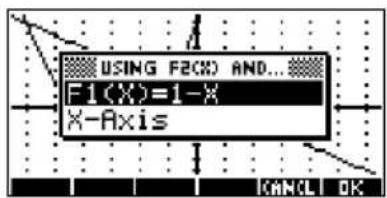
The coordinates of the intersection point are displayed at the bottom of the screen.
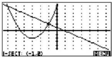
Note: If there is more than one intersection (as in our example), the coordinates of the intersection point closest to the current cursor position are displayed.
To find the slope of the quadratic function
- Find the slope of the quadratic function at the intersection point.
MENU FCN
Select slope
OK

The slope value is displayed at the bottom of the screen.
To find the signed area of the two functions
- To find the area between the two functions in the range -2 ≤ x ≤ -1 , first move the cursor to F1(x) = 1 - x and select the signed area option.
MENU FEN
Select Signed area
OK
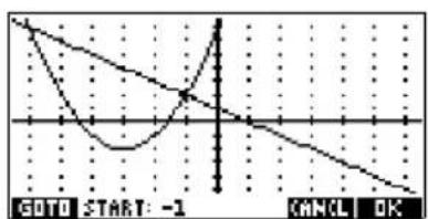
- Move the cursor to x by pressing the or

key.


-
Press of accept using F2(x) = (x + 3)2 - 2 as the other boundary for the integral.
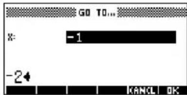
-
Choose the end value for x .


The cursor jumps to x = -2 on the linear function.
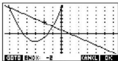
- Display the numerical value of the integral.

Note: See "Shading area" on page 3-11 for another method of calculating area.

To find the extremum of the quadratic
- Move the cursor to the quadratic equation and find the extremum of the quadratic.

Select Extremum OK
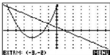
The coordinates of the extremum are displayed at the bottom of the screen.
HINT
The Root and Extremum functions return one value only even if the function has more than one root or extremum. The function finds the value closest to the position of the cursor. You need to re-locate the cursor to find other roots or extrema that may exist.
Display the numeric view
- Display the numeric view.
NUM

Set up the table 21. Display the numeric setup.
SHIFT SETUP-NUM

See "Setting up the table (Numeric view setup)" on page 2-17 for more information.
- Match the table settings to the pixel columns in the graph view.
FLOT OK

Explore the table
- Display the table of values.
NUM
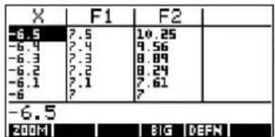
To navigate around a table
- Move to X = -5.9.
6 times
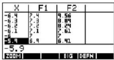
To go directly to a value
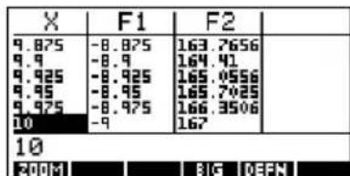
- Move directly to X = 10.
10 OK

To access the zoom options
- Zoom in on X = 10 by a factor of 4. Note: NUMZOOM has a setting of 4.
200M In
OK
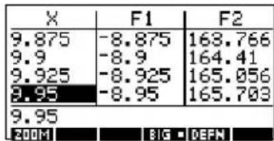
To change font size 27. Display table numbers in large font.
BIG
To display the symbolic definition of a column
- Display the symbolic definition for the F1 column.
DEFN

The symbolic definition of F1 is displayed at the bottom of the screen.
Function aplet interactive analysis
From the Plot view ( ), you can use the functions on the FCN menu to find roots, intersections, slopes, and areas for a function defined in the Function aplet (and any Function-based aplets). See "FCN functions" on page 3-10. The FCN operations act on the currently selected graph.
The results of the FCN functions are saved in the following variables:
- Area
- Extremum
- Isect
- Root
- Slope
For example, if you use the Root function to find the root of a plot, you can use the result in calculations in HOME.
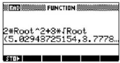
Access FCN variables
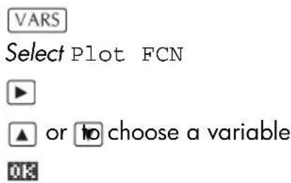
The FCN variables are contained on the VARS menu.
To access FCN variables in HOME:


To access FCN variable in the Function aplet's Symbolic view:
FCN functions The FCN functions are:
| Function Description | |
| Root | Select Root to find the root of the current function nearest the cursor. If no root is found, but only an extremum, then the result is labeled EXTR: instead of ROOT:. (The root-finder is also used in the Solve aplet. See also “Interpreting results” on page 7-6.) The cursor is moved to the root value on the x-axis and the resulting x-value is saved in a variable named ROOT. |
| Extremum Select | Extremum to find the maximum or minimum of the current function nearest the cursor. This displays the coordinate values and moves the cursor to the extremum. The resulting value is saved in a variable named EXTREMUM. |
| Slope Select Slope | to find the numeric derivative at the current position of the cursor. The result is saved in a variable named SLOPE. |
| Signed area | Select Signed area to find the numeric integral. (If there are two or more expressions checkmarked, then you will be asked to choose the second expression from a list that includes the x-axis.) Select a starting point, then move the cursor to selection ending point. The result is saved in a variable named AREA. |
| Function | Description (Continued) |
| Intersection | Select Intersection to find the intersection of two graphs nearest the cursor. (You need to have at least two selected expressions in Symbolic view.) Displays the coordinate values and moves the cursor to the intersection. (Uses Solve function.) The resulting x-value is saved in a variable named ISECT. |
Shading area
You can shade a selected area between functions. This process also gives you an approximate measurement of the area shaded.
- Open the Function aplet. The Function aplet opens in the Symbolic view.
- Select the expressions whose curves you want to study.
- Press to plot the functions.
-
Press or to position the cursor at the starting point of the area you want to shade.
-
Press
-
Press, then select Signed area on OK.
-
Press OK, choose the function that will act as the boundary of the shaded area, and press OK.
-
Press the ◀ or ▶ key to shade in the area.
-
Press OK to calculate the area. The area measurement is displayed near the bottom of the screen.
To remove the shading, press to re-draw the plot.
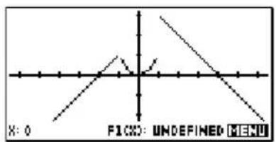
Plotting a piecewise-defined function
Suppose you wanted to plot the following piecewise-defined function.
f (x) = x + 2 amp; x ≤ - 1 x ^ 2 amp; - 1 lt; x ≤ 1 4 - x amp; x ≥ 1 .
- Open the Function aplet.
APLET Select
Function
START
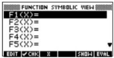
- Highlight the line you want to use, and enter the expression. (You can press to delete an existing line, or SHIFT CLEAR to clear all lines.)
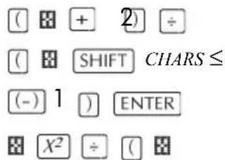
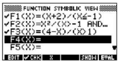
SHIFT CHARS > (-) 1
SHIFT AND SHIFT CHARS ≤ 1 ENTER
(4 - ) ÷ (
图
SHIFT CHARS > 1
ENTER
Note: You can use the menu key to assist in the entry of equations. It has the same effect as pressing ,T,θ .
Parametric aplet
About the Parametric aplet
The Parametric aplet allows you to explore parametric equations. These are equations in which both x and y are defined as functions of t . They take the forms x f t () = and y g .t () =
Getting started with the Parametric aplet
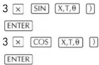
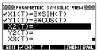
The following example uses the parametric equations
xt (⇒) Sin
y (t) = 3 t
Note: This example will produce a circle. For this example to work, the angle measure must be set to degrees.
Open the Parametric aplet
- Open the Parametric aplet.


Define the expressions
- Define the expressions.
Set angle measure
- Set the angle measure to degrees.


Set up the plot 4. Display the graphing options.
SHIFT PLOT

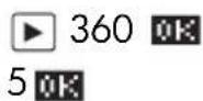
The Plot Setup input form has two fields not included in the Function aplet, TRNG and TSTEP. TRNG specifies the range of t values. TSTEP specifies the step value between t values.
- Set the TRNG and TSTEP so that t steps from 0° to 360° in 5° steps.

Plot the expression
- Plot the expression.
PLOT

- To see all the circle, press #vige.
MENU MENU

Overlay plot 8. Plot a triangle graph over the existing circle graph.


A triangle is displayed rather than a circle (without changing the equation) because the changed value of TSTEP ensures that points being plotted are 120° apart instead of nearly continuous.
You are able to explore the graph using trace, zoom, split screen, and scaling functionality available in the Function aplet. See "Exploring the graph" on page 2-7 for further information.
Display the numbers
- Display the table of values.

You can highlight a t-value, type in a replacement value, and see the table jump to that value. You can also zoom in or zoom out on any t-value in the table.
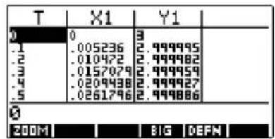
You are able to explore the table using ZOOM
GOTO, build your own table, and split screen functionality available in the Function aplet. See "Exploring the table of numbers" on page 2-18 for further information.
Getting started with the Polar aplet
Open the Polar aplet
- Open the Polar aplet.
APLET
Select PoI
RESET YES START
Like the Function aplet, the Polar aplet opens in the Symbolic view.

Define the expression
- Define the polar equation r = 2π (θ/2) (θ)2
2πSHIFT
COS
X,T,θ
2
)
COS
X,T,θ
)
x2
ENTER
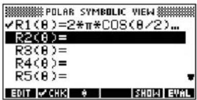
Specify plot settings
- Specify the plot settings. In this example, we will use the default settings, except for the θ RNG fields.
SHIFT
SETUP-PLOT
SHIFT
CLEAR
▶
4 πHIFT
013

Plot the expression
- Plot the expression.
PLOT
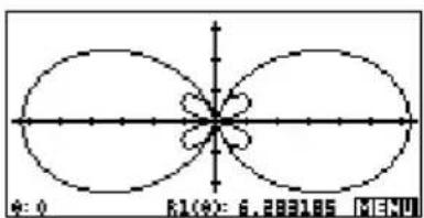
Explore the graph
- Display the Plot view menu key labels.
MENU
The Plot view options available are the same as those found in the Function aplet. See "Exploring the graph" on page 2-7 for further information.

Display the numbers
- Display the table of values for θ and R1.
NUM
The Numeric view options available are the same as those found in the Function aplet. See "Exploring the table of numbers" on page 2-18 for further information.
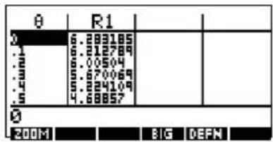
Sequence aplet
About the Sequence aplet
The Sequence aplet allows you to explore sequences.
You can define a sequence named, for example, U1:
- in terms of n
- in terms of U1(n-1)
• i n terms of U1(n-2)
• in terms of another sequence, for example, U2(n)
• in any combination of the above.
The Sequence aplet allows you to create two types of graphs:
- A Stairsteps graph plots n on the horizontal axis and Un on the vertical axis.
- A Cobweb graph plots Un-1 on the horizontal axis and Un on the vertical axis.
Getting started with the Sequence aplet
The following example defines and then plots an expression in the Sequence aplet.
Open the Sequence aplet
- Open the Sequence aplet.
The Sequence aplet starts in the Symbolic view.

Define the expression
- Define the Fibonacci sequence, in which each term (after the first two) is the sum of the preceding two terms:
U _ 1 = 1, U _ 2 = 1, U _ n = U _ n - 1 + U _ n - 2 n for 3
In the Symbolic view of the Sequence aplet, highlight the U1(1) field and begin defining your sequence.

Note: You can use the
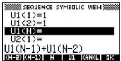
H, (N-2) (M-1) U1
and menu keys to assist in the entry of equations.
ENTER
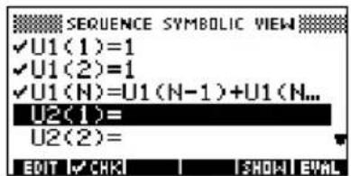
Specify plot settings
- In Plot Setup, first set the SEQPLOT option to Stairstep. Reset the default plot settings by clearing the Plot Setup view.
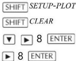

Plot the sequence
- Plot the Fibonacci sequence.
PLOT
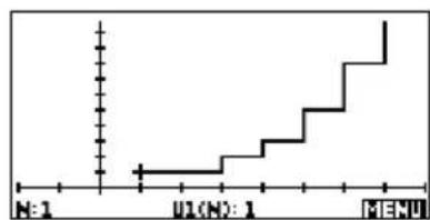
- In Plot Setup, set the SEQPLOT option to Cobweb.
SHIFT SETUP-PLOT
CHOOS Select Cobweb
OK
PLOT
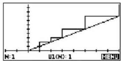
Display the table 6. Display the table of values for this example.
NUM
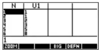
About the Solve aplet
The Solve aplet solves an equation or an expression for its unknown variable. You define an equation or expression in the symbolic view, then supply values for all the variables except one in the numeric view. Solve works only with real numbers.
Note the differences between an equation and an expression:
- An equation contains an equals sign. Its solution is a value for the unknown variable that makes both sides have the same value.
- An expression does not contain an equals sign. Its solution is a root, that is, a value for the unknown variable that makes the expression have a value of zero.
You can use the Solve aplet to solve an equation for any one of its variables.
When the Solve aplet is started, it opens in the Solve Symbolic view.
- In Symbolic view, you specify the expression or equation to solve. You can define up to ten equations (or expressions), named E0 to E9. Each equation can contain up to 27 real variables, named A to Z and θ .
- In Numeric view, you specify the values of the known variables, highlight the variable that you want to solve for, and press SOLUE
You can solve the equation as many times as you want, using new values for the knowns and highlighting a different unknown.
Note: It is not possible to solve for more than one variable at once. Simultaneous linear equations, for example,
should be solved using matrices or graphs in the Function aplet.
Getting started with the Solve aplet
Suppose you want to find the acceleration needed to increase the speed of a car from 16.67 m/sec (60 kph) to 27.78 m/sec (100 kph) in a distance of 100 m.
The equation to solve is:
V ^ 2 U ^ 2 2 AD + =
Open the Solve aplet
- Open the Solve aplet.
APLET Select Solve
START
The Solve aplet starts in the symbolic view.
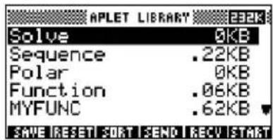
Define the equation
- Define the equation.
ALPHA V x2
E ALPHA X2
+ 2 ×
ALPHA A ×
ALPHA D ENTER

Note: You can use the ☐ menu key to assist in the entry of equations.
Enter known variables
- Display the Solve numeric view screen.
NUM

- Enter the values for the known variables.


HINT
If the Decimal Mark setting in the Modes input form (MODES) is set to Comma, use instead of .
Solve the unknown variable
- Solve for the unknown variable (A).


Therefore, the acceleration needed to increase the speed of a car from 16.67 m/sec (60 kph) to 27.78 m/sec (100 kph) in a distance of 100 m is approximately 2.47 m/s 2 .
Because the variable A in the equation is linear we know that we need not look for any other solutions.
Plot the equation
The Plot view shows one graph for each side of the selected equation. You can choose any of the variables to be the independent variable.
The current equation is V2 U2=2AD+
One of these is Y with V2 , that is V = 27.78 Y = 771.7284 . This graph will be a horizontal line.
The other graph will be Y with V2 = 2AD + U = 16.67 and D that is Y = 200A + 277.8889 . This graph is also a line. The desired solution is the value of A where these two lines intersect.
- Plot the equation for variable A .
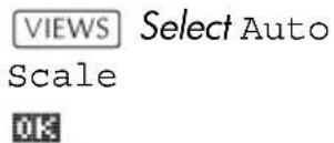
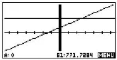
- Trace along the graph representing the left side of the equation until the cursor nears the intersection.
▶ ≈ 20 times

Note the value of A displayed near the bottom left corner of the screen.
The Plot view provides a convenient way to find an approximation to a solution instead of using the Numeric view Solve option. See "Plotting to find guesses" on page 7-7 for more information.
Solve aplet's NUM view keys
The Solve aplet's NUM view keys are:
| Key Meaning | |
| EDIT | Copies the highlighted value to the edit line for editing. Press when done. |
| INFO | Displays a message about the solution (see “Interpreting results” on page 7-6). |
| PAGE | Displays other pages of variables, if any. |
| DEFN | Displays the symbolic definition of the current expression. Press when done. |
| SOLVE | Finds a solution for the highlighted variable, based on the values of the other variables. |
| Key Meaning (Continued) | |
| DEL | Clears highlighted variable to zero or deletes current character in edit line, if edit line is active. |
| SHIFT CLEAR | Resets all variable values to zero or clears the edit line, if cursor is in edit line. |
Use an initial guess
You can usually obtain a faster and more accurate solution if you supply an estimated value for the unknown variable before pressing Solve starts looking for a solution at the initial guess.
Before plotting, make sure the unknown variable is highlighted in the numeric view. Plot the equation to help you select an initial guess when you don't know the range in which to look for the solution. See "Plotting to find guesses" on page 7-7 for further information.
HINT
An initial guess is especially important in the case of a curve that could have more than one solution. In this case, only the solution closest to the initial guess is returned.
Number format
You can change the number format for the Solve aplet in the Numeric Setup view. The options are the same as in HOME MODES: Standard, Fixed, Scientific, and Engineering. For the latter three, you also specify how many digits of accuracy you want. See "Mode settings" on page 1-10 for more information.
You might find it handy to set a different number format for the Solve aplet if, for example, you define equations to solve for the value of money. A number format of Fixed 2 would be appropriate in this case.
Interpreting results
After Solve has returned a solution, press in the Numeric view for more information. You will see one of the following three messages. Press to clear the message.
| Message Condition | |
| Zero The Solve aplet found a point wherethe value of the equation (or the rootof the expression) is zero within thecalculator’s 12-digit accuracy. | |
| Sign Reversal Solve found two points where thevalue of the equation has oppositesigns, but it cannot find a point inbetween where the value is zero.This might be becauseeitherthe twopoints are neighbours (they differ byone in the twelfth digit),ortheequation is not real-valued betweenthe two points. Solve returns thepoint where the value is closer tozero. If the value of the equation isa continuous real function, this pointis Solve’s best approximation of anactual root. | |
| Extremum Solve found a point where the valueof the equation approximates alocal minimum (for positive values)or maximum (for negative values).This point may or may not be a root.Or: Solve stopped searching at9.99999999999E499, the largestnumber the calculator canrepresent. |
If Solve could not find a solution, you will see one of the following two messages.
| Message Condition | |
| Bad Guess(es) The constant? The value of the equation is the same at every point sampled. | initial guess lies outside the domain of the equation.Therefore, the solution was not a real number or it caused an error. |
HINT
It is important to check the information relating to the solve process. For example, the solution that the Solve aplet finds is not a solution, but the closest that the function gets to zero. Only by checking the information will you know that this is the case.
The Root-Finder at work
You can watch the process of the root-finder calculating and searching for a root. Immediately after pressing SOLVE to start the root-finder, press any key except ON You will see two intermediate guesses and, to the left, the sign of the expression evaluated at each guess. For example:
- 2 2.219330555745
-121.31111111149
You can watch as the root-finder either finds a sign reversal or converges on a local extrema or does not converge at all. If there is no convergence in process, you might want to cancel the operation (press) and start over with a different initial guess.
Plotting to find guesses
The main reason for plotting in the Solve aplet is to help you find initial guesses and solutions for those equations that have difficult-to-find or multiple solutions.
Consider the equation of motion for an accelerating body:
_ 0 TVX AT ^ 2 2
where X is distance, V0 is initial velocity, T is time, and A is acceleration. This is actually two equations, Y = X and Y = V0 T + (AT2) / 2 .
Since this equation is quadratic for T, there can be both a positive and a negative solution. However, we are concerned only with positive solutions, since only positive distance makes sense.
- Select the Solve aplet and enter the equation.
APLET Select Solve START
ALPHA X
ALPHA V ×
ALPHA T +
ALPHA A
× TALP2A X2 ÷ OK
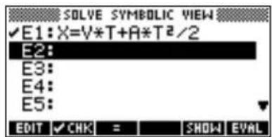
- Find the solution for T (time) when X = 30 , V = 2 , and A = 4 . Enter the values for X, V , and A ; then highlight the independent variable, T .
NUM
30 ENTER
2 ENTER
4 ENTER
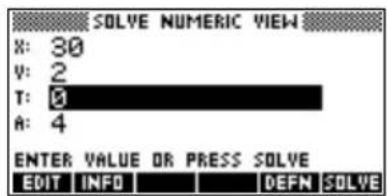
to highlight T
- Use the Plot view to find an initial guess for T . First set appropriate X and Y ranges in the Plot Setup. With equation X = V × T + A × T2 / 2 , the plot will produce two graphs: one for Y and X one for X = V × T + A × T2 / 2 . Since we have set X = 30 in this example, one of the graphs will be Y = 30 . Therefore, make the YRNG -5 to 35. Keep the XRNG default of -6.5 to 6.5.
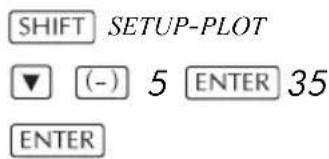
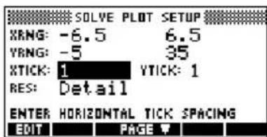
- Plot the graph.
PLOT
- Move the cursor near the positive (right-side) intersection. This cursor value will be an initial guess for T .
Press ▶ until the cursor is at the intersection.
The two points of intersection show that there are two solutions for this equation. However, only positive values for X make sense, so we want to find the solution for the intersection on the right side of the y-axis.

- Return to the Numeric view.
NUM

Note: the T-value is filled in with the position of the cursor from the Plot view.
- Ensure that the T value is highlighted, and solve the equation.
SOLUE
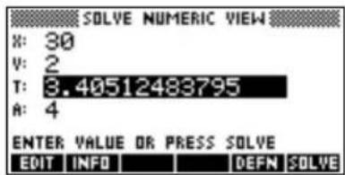
Use this equation to solve for another variable, such as velocity. How fast must a body's initial velocity be in order for it to travel 50 m within 3 seconds? Assume the same acceleration, 4 m/s 2 . Leave the last value of V as the initial guess.
3 ENTER ▲ ▲ ▲
50 ENTER
SOLUE

Using variables in equations
You can use any of the real variable names, A to Z and θ . Do not use variable names defined for other types, such as M1 (a matrix variable).
Home variables All home variables (other than those for aplet settings, like Xmin and Ytick) are global, which means they are shared throughout the different aplets of the calculator. A value that is assigned to a home variable anywhere remains with that variable wherever its name is used.
Therefore, if you have defined a value for T (as in the above example) in another aplet or even another Solve equation, that value shows up in the Numeric view for this Solve equation. When you then redefine the value for T in this Solve equation, that value is applied to T in all other contexts (until it is changed again).
This sharing allows you to work on the same problem in different places (such as HOME and the Solve aplet) without having to update the value whenever it is recalculated.
HINT As the Solve aplet uses existing variable values, be sure to check for existing variable values that may affect the solve process. (You can use SHIFT CLEAR to reset all values to zero in the Solve aplet's Numeric view if you wish.)
Aplet variables Functions defined in other aplets can also be referenced in the Solve aplet. For example, if, in the Function aplet, you define F1(X)=X2+10 , you can enter F1(X)=50 in the Solve aplet to solve the equation X2+10=50 .
Statistics aplet
About the Statistics aplet
The Statistics aplet can store up to ten data sets at one time. It can perform one-variable or two-variable statistical analysis of one or more sets of data.
The Statistics aplet starts with the Numeric view which is used to enter data. The Symbolic view is used to specify which columns contain data and which column contains frequencies.
You can also compute statistics values in HOME and recall the values of specific statistics variables.
The values computed in the Statistics aplet are saved in variables, and many of these variables are listed by the STATS function accessible from the Statistics aplet's Numeric view screen.
Getting started with the Statistics aplet
The following example asks you to enter and analyze the advertising and sales data (in the table below), compute statistics, fit a curve to the data, and predict the effect of more advertising on sales.
| Advertising minutes(independent, x) | Resulting Sales ($) (dependent, y) |
| 2 | 1 |
| 1 | 9 |
| 3 | 1 |
| 5 | 2 |
| 5 | 2 |
| 4 | 2 |
4
2
1
2
8
2
Open the Statistics aplet
- Open the Statistics aplet and clear existing data by pressing RESET.
APLET Select Statistics
RESET YES START
The Statistics aplet starts in the Numerical view.
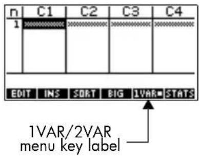
At any time the Statistics aplet is configured for only one of two types of statistical explorations: one-variable (.) One Two-variable (). The 5th menu key label in the Numeric view toggles between these two options and shows the current option.
2. Select
You need to select Eboxuse in this example we are analyzing a dataset comprising two variables: advertising minutes and resulting sales.
Enter data 3. Enter the data into the columns.


▶ to move to the next column
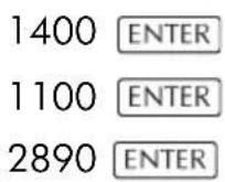

Choose fit and data columns
- Select a fit in the Symbolic setup view.


You can create up to five explorations of two-variable data, named S1 to S5. In this example, we will create just one: S1.
- Specify the columns that hold the data you want to analyze.
SYMB
You could have entered your data into columns other than C1 and C2.
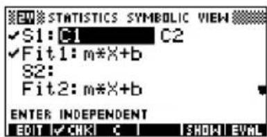
Explore statistics
- Find the mean advertising time (MEANX) and the mean sales (MEANY).
NUM STATS
MEANX is 3.3 minutes and MEANY is about \$1796.
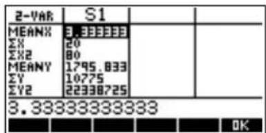
- Scroll down to display the value for the correlation coefficient (CORR). The CORR value indicates how well the linear model fits the data.
9 times
The value is .8995.
아름
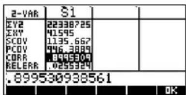
Setup plot 8. Change the plotting range to ensure all the data
points are plotted (and select a different point mark, if you wish).


Plot the graph 9. Plot the graph.
PLOT

Draw the regression curve
- Draw the regression curve (a curve to fit the data points).
MENU FIT
This draws the regression line for the best linear fit.
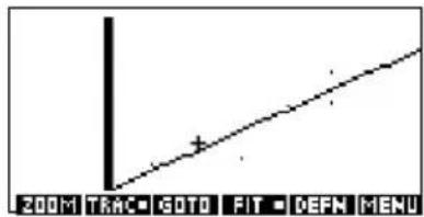
Display the equation for best linear fit
- Return to the Symbolic view.
SYMB
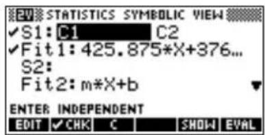
- Display the equation for the best linear fit.
▼ to move to the FIT1 field
SHOY
The full FIT1 expression is shown.
The slope (m) is 425.875. The y-intercept (b) is 376.25.

Predict values 13. To find the predicted sales figure if advertising were to go up to 6 minutes:
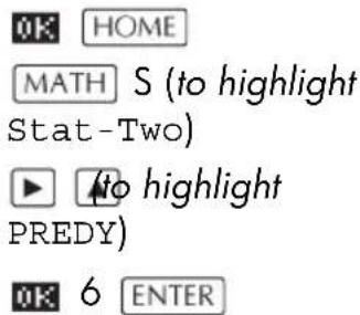
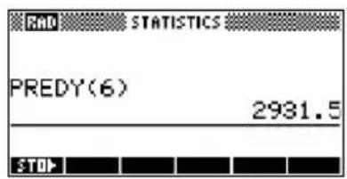
- Return to the Plot view.
PLOT

- Jump to the indicated point on the regression line.
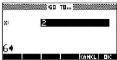
OK Observe the predicted y-value in the left bottom corner of the screen.
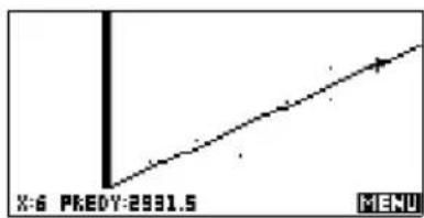
Entering and editing statistical data
The Numeric view (NISN) used to enter data into the Statistics aplet. Each column represents a variable named C0 to C9. After entering the data, you must define the data set in the Symbolic view (SYMB)
HINT
A data column must have at least four data points to provide valid two-variable statistics, or two data points for one-variable statistics.
You can also store statistical data values by copying lists from HOME into Statistics data columns. For example, in HOME, L1 STOP C1 stores a copy of the list L1 into the data-column variable C1.
Statistics aplet's NUM view keys
The Statistics aplet's Numeric view keys are:
| Key Meaning | |
| EDIT | Copies the highlighted item into the edit line. |
| INS | Inserts a zero value above the highlighted cell. |
| SORT | Sorts the specified independent data column in ascending or descending order, and rearranges a specified dependent (or frequency) data column accordingly. |
| BIG | Switches between larger and smaller font sizes. |
| 1VAR■2VAR■ | A toggle switch to select one-variable or two-variable statistics. This setting affects the statistical calculations and plots. The label indicates which setting is current. |
| STATS | Computes descriptive statistics for each data set specified in Symbolic view. |
| Key Meaning (Continued) | |
| DEL | Deletes the currently highlighted value. |
| SHIFT CLEAR | Clears the current column or all columns of data. Pregss SHIFT CLEAR to display a menu list, then select the current column or all columns option, and press OK |
| SHIFT cursor key | Moves to the first or last row, or first or last column. |
Example You are measuring the height of students in a classroom to find the mean height. The first five students have the following measurements 160cm, 165cm, 170cm, 175cm, 180cm.
- Open the Statistics aplet.


- Enter the measurement data.


- Find the mean of the sample.
Ensure the ZUAR
2VAR menu key label reads 1VAR. Press
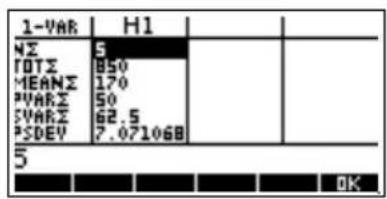
STATS to see the statistics calculated from the sample data in C1.
Note that the title of the column of statistics is H1. There are 5 data set definitions available for one-variable statistics: H1-H5. If
data is entered in C1, H1 is automatically set to use C1 for data, and the frequency of each data point is set to 1. You can select other columns of data from the Statistics Symbolic setup view.

- Press ☐: close the statistics window and press key to see the data set definitions.
The first column
indicates the associated column of data for each data set definition, and the second column indicates the constant frequency, or the column that holds the frequencies.
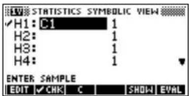
The keys you can use from this window are:
| Key Meaning | |
| EDIT | Copies the column variable (or variable expression) to the edit line for editing. Press when done. |
| CHK | Checks/unchecked the current data set. Only the checkmarked data set(s) are computed and plotted. |
| or Typing aid | for the column variables (or for the Fit expressions ( ) |
| Key Meaning (Continued) | |
| SHOW | Displays the current variable expression in standard mathematical form. Press when done. |
| EVAL | Evaluates the variables in the highlighted column (C1, etc.) expression. |
| VARS Displays the menu for entering variable names or contents of variables. | |
| MATH | Displays the menu for entering math operations. |
| DEL | Deletes the highlighted variable or the current character in the edit line. |
| SHIFT CLEAR Resets default specifications for the data sets or clears the edit line (if it was active).Note: If SHIFT CLEAR is used the data sets will need to be selected again before re-use. | |
To continue our example, suppose that the heights of the rest of the students in the class are measured, but each one is rounded to the nearest of the five values first recorded. Instead of entering all the new data in C1, we shall simply add another column, C2, that holds the frequencies of our five data points in C1.
| Height (cm) | Frequency |
| 160 5 | |
| 165 3 | |
| 170 8 | |
| 175 2 | |
| 180 1 |
- Move the highlight bar into the right column of the H1 definition and replace the frequency value of 1 with the name C2.
2
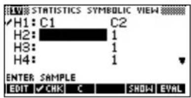
- Return to the numeric view.
NUM
- Enter the frequency data shown in the above table.
5 ENTER
3 ENTER
8 ENTER
2 ENTER
1 ENTER
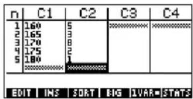
- Display the computed statistics.
STATE
The mean height is approximately 167.63cm.
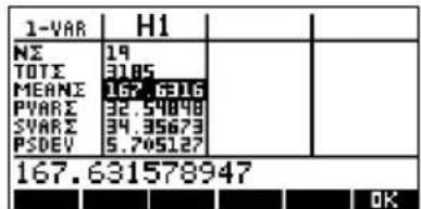
- Setup a histogram plot for the data.
OK SHIFT SETUP-PLOT
Enter set up information appropriate to your data.
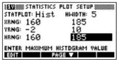
- Plot a histogram of the data.
PLOT

Save data The data that you enter is automatically saved. When you are finished entering data values, you can press a key for another Statistics view (like ,sonyou can switch to another aplet or HOME.
Edit a data set In the Numeric view of the Statistics aplet, highlight the data value to change. Type a new value and press Eore press to copy the value to the edit line for modification. Press after modifying the value on the edit line.
Delete data
- To delete a single data item, highlight it and press DEL. The values below the deleted cell will scroll up one row.
- To delete a column of data, highlight an entry in that column and press SHIFT CLEAR. Select the column name.
- To delete all columns of data, press SHIFT CLEAR. Select All columns.
Insert data
Highlight the entry following the point of insertion. Press INS, then enter a number. It will write over the zero that was inserted.
Sort data values
- In Numeric view, highlight the column you want to sort, and press SORT
- Specify the Sort Order. You can choose either Ascending or Descending.
-
Specify the INDEPENDENT and DEPENDENT data columns. Sorting is by the independent column. For instance, if Age is C1 and Income is C2 and you want to sort by Income, then you make C2 the independent column for the sorting and C1 the dependent column.
-
To sort just one column, choose None for the dependent column.
-
For one-variable statistics with two data columns, specify the frequency column as the dependent column.
-
Press
Defining a regression model
The Symbolic view includes an expression (Fit1 through Fit5) that defines the regression model, or "fit", to use for the regression analysis of each two-variable data set.
There are three ways to select a regression model:
- Accept the default option to fit the data to a straight line.
- Select one of the available fit options in Symbolic Setup view.
- Enter your own mathematical expression in Symbolic view. This expression will be plotted, but it will not be fitted to the data points.
Angle Setting
You can ignore the angle measurement mode unless your Fit definition (in Symbolic view) involves a trigonometric function. In this case, you should specify in the mode screen whether the trigonometric units are to be interpreted in degrees, radians, or grads.
To choose the fit 1. In Numeric view, make sure is
- Press SHIFT SETUP-SYMB to display the Symbolic Setup view. Highlight the Fit number (S1FIT to S5FIT) you want to define.
- Press choose from the list. Press when OK done. The regression formula for the fit is displayed in Symbolic view.
Fit models Eight fit models are available:
| Fit model | Meaning |
| Lineair | (Default.) Fits the data to a straight line, y = mx + b . Uses a least-squares fit. |
| Logaritmisch | Fits to a logarithmic curve, y = m x + b . |
| Macht | Fits to an exponential curve, y = bemx . |
| Power | Fits to a power curve, y = bxm . |
| Fit model Meaning (Continued) | |
| Quadratic Fits to a quadratic curve, y = ax2 + bx + c . Needs at least three points. | |
| Cubic Fits to a cubic curve, y = ax3 + bx2 + cx + d . Needs at least four points. | |
| Logistic Fits to a logistic curve, y = 1 dt e-bx(-t) where L is the saturation value for growth. You can store a positive real value in L , or—if L = 0 —let L be computed automatically. | |
| User Defined | Define your own expression (in Symbolic view.) |
To define your own fit
- In Numeric view, make sure
às set - Display the Symbolic view.
- Highlight the Fit expression (Fit1, etc.) for the desired data set.
- Type in an expression and press .ENTER
The independent variable must be X, and the expression must not contain any unknown variables.
Example: 1.5 × x + 0.3 × x
This automatically changes the Fit type (S1FIT, etc.) in the Symbolic Setup view to User Defined.
Computed statistics
One-variable
| Statistic | Definition |
| N | Number of data points. |
| TOT | Sum of data values (with their frequencies). |
| Statistic Definition | (Continued) |
| MEANΣ Mean value of data set. | |
| PVARΣ Population variance of data set. | |
| SVARΣ Sample variance of data set. | |
| PSDEV Population standard deviation of data set. | |
| SSDEV Sample standard deviation of data set. | |
| MINΣ Minimum data value in data set. | |
| Q1 First quartile: median of values to left of median. | |
| MEDIAN Median value of data set. | |
| Q3 Third quartile: median of values to right of median. | |
| MAXΣ Maximum data value in data set. | |
When the data set contains an odd number of values, the data set's median value is not used when calculating Q1 and Q3 in the table above. For example, for the following data set:
3, 5, 7, 8, 1 5, 1 6, 1 7
only the first three items, 3, 5, and 7 are used to calculate Q1, and only the last three terms, 15, 16, and 17 are used to calculate Q3.
Two-variable
| Statistic Definition | |
| MEANX | Mean of x- (independent) values. |
| ΣX | Sum of x-values. |
| ΣX2 Sum of x | 2 -values. |
| MEANY | Mean of y- (dependent) values. |
| ΣY | Sum of y-values. |
| Statistic | Definition (Continued) |
| Y2 Sum of y | 2 -values. |
| XY | Sum of each xy . |
| SCOV | Sample covariance of independent and dependent data columns. |
| PCOV | Population covariance of independent and dependent data columns |
| CORR | Correlation coefficient of the independent and dependent data columns for a linear fit only (regardless of the Fit chosen).Returns a value from 0 to 1, where 1 is the best fit. |
| RELERR | The relative error for the selected fit. Provides a measure of accuracy for the fit. |
Plotting You can plot:
- histograms ( ) IVAR
- box-and-whisker plots ( ) IVAR
- scatter plots (). 2VAR
Once you have entered your data ( ) defined your data set ( ) and defined your Fit model for two-variable statistics ( SHIFT SETUP-SYMB), you can plot your data. You can plot up to five scatter or box-and-whisker plots at a time. You can plot only one histogram at a time.
To plot statistical data
- In Symbolic view ( ) select () the dWCHK sets you want to plot.
-
For one-variable data ( ) select the plot type in Plot Setup (SHIFT SETUP-PLOT). Highlight STATPLOT, press CHOO'S, select either Histogram BoxWhisker, and press OK
-
For any plot, but especially for a histogram, adjust the plotting scale and range in the Plot Setup view. If you find histogram bars too fat or too thin, you can adjust them by adjusting the HWIDTH setting.
- Press. If you have not adjusted the Plot Setup PLOT yourself, you can try VIEWS select Auto Scale OK.
Auto Scale can be relied upon to give a good starting scale which can then be adjusted in the Plot Setup view.
Plot types
Histogram One-variable statistics.
The numbers below the plot mean that the current bar (where the cursor is) starts at 0 and ends at 2 (not including 2), and the
frequency for this column, (that is, the number of data elements that fall between 0 and 2) is 1. You can see information about the next bar by pressing the key.
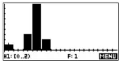
Box and Whisker Plot
One-variable statistics.
The left whisker marks the minimum data value. The box marks the first quartile, the median(where the cursor is), and the third quartile.
The right whisker marks the maximum data value. The numbers below the plot mean that this column has a median of 13.
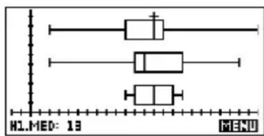
Scatter Plot Two-variable statistics.
The numbers below the plot indicate that the cursor is at the first data point for S2, at (1, 6). Press ☐to move to the next data point and display information about it.

To connect the data points as they are plotted, checkmark CONNECT in the second page of the Plot Setup. This is not a regression curve.
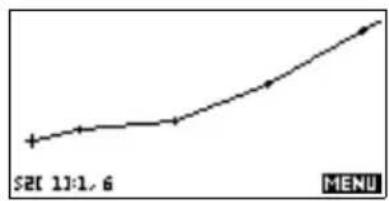
Fitting a curve to 2VAR data
In the Plot view, press Fit this draws a curve to fit the checked two-variable data set(s). See "To choose the fit" on page 8-12.
PLOT
MENU
FIT

SYMB
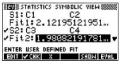
SHOW
The expression in Fit2 shows that the slope=1.98082191781 and the y-intercept=2.2657.

Correlation coefficient
The correlation coefficient is stored in the CORR variable. It is a measure of fit to a linear curve only. Regardless of the Fit model you have chosen, CORR relates to the linear model.
Relative Error The relative error is a measure of the error between predicted values and actual values based on the specified Fit. A smaller number means a better fit.
The relative error is stored in a variable named RELERR. The relative error provides a measure of fit accuracy for all fits, and it does depend on the Fit model you have chosen.
HINT
In order to access the CORR and RELERR variables after you plot a set of statistics, you must press to access the numeric view and then screen play the correlation values. The values are stored in the variables when you access the Symbolic view.
Setting up the plot (Plot setup view)
| The Plot Setup view (SHIFTSETUP-PLOT) sets most of the same plotting parameters as it does for the other built-in aplets.See “Setting up the plot (Plot view setup)” on page 2-5. Settings unique to the Statistics aplet are as follows: | |
| Plot type (1VAR) | STATPLOT enables you to specify either a histogram or a box-and-whisker plot for one-variable statistics (when IVAR is set). Press Closchange the highlighted setting |
| Histogram width | HWIDTH enables you to specify the width of a histogram bar. This determines how many bars will fit in the display, as well as how the data is distributed (how many values each bar represents). |
| Histogram range | HRNG enables you to specify the range of values for a set of histogram bars. The range runs from the left edge of the leftmost bar to the right edge of the rightmost bar. You can limit the range to exclude any values you suspect are outliers. |
| Plotting mark (2VAR) | S1MARK through S5MARK enables you to specify one of five symbols to use to plot each data set. Press c0003 change the highlighted setting. |
| Connected points (2VAR) | CONNECT (on the second page), when checkmarked, connects the data points as they are plotted. The resulting line is not the regression curve. The order of plotting is according to the ascending order of independent values. For instance, the data set (1,1), (3,9), (4,16), (2,4) would be plotted and traced in the order (1,1), (2,4), (3,9), (4,16). |
Trouble-shooting a plot
If you have problems plotting, check that you have the following:
- The correct o/lu/menu label on (Numeric view).
- The correct fit (regression model), if the data set is two-variable.
- Only the data sets to compute or plot are checkmarked (Symbolic view).
- The correct plotting range. Try using AvioNS Scale (instead of PLOR adjust the plotting parameters (in Plot Setup) for the ranges of the axes and the width of histogram bars (HWIDTH).
In EUGE, ensure that both paired columns contain data, and that they are the same length.
In mode, ensure that a paired column of frequency values is the same length as the data column that it refers to.
Exploring the graph
The Plot view has menu keys for zooming, tracing, and coordinate display. There are also scaling options under VIEWS. These options are described in "Exploring the graph" on page 2-7.
Statistics aplet's PLOT view keys
| Key Meaning | |
| SHIFT CLEAR Erases the plot. | |
| VIEWS | Offers additional pre-defined views for splitting the screen, overlaying plots, and autoscaling the axes. |
| SHIFT ◀ | Moves cursor to far left or far right. |
| SHIFT ▶ | |
| 200M | Displays ZOOM menu. |
| TRACE | Turns trace mode on/off. The white box appears next to the option when Trace mode is active. |
| Key Meaning (Continued) | |
| FIT | Turns fit mode on or off. Turning FIT on draws a curve to fit the data points according to the current regression model. |
| GOTO (2var statistics only) | Enables you to specify a value on the line of best fit to jump to or a data point number to jump to. |
| DEFN | Displays the equation of the regression curve. |
| MENU | Hides and displays the menu key labels. When the labels are hidden, any menu key displays the (x,y) coordinates. Pressing MENU redisplays the menu labels. |
Calculating predicted values
The functions PREDX and PREDY estimate (predict) values for X or Y given a hypothetical value for the other. The estimation is made based on the curve that has been calculated to fit the data according to the specified fit.
Find predicted values
- In Plot view, draw the regression curve for the data set.
- Press to move to the regression curve.
- Press GOTO and enter the value of X. The cursor jumps to the specified point on the curve and the coordinate display shows X and the predicted value of Y.
In HOME,
- Enter PREDX(y-value) ENTER to find the predicted value for the independent variable given a hypothetical dependent value.
- Enter PREDY(x-value) to find the predicted value of the dependent variable given a hypothetical independent variable.
You can type PREDX and PREDY into the edit line, or you can copy these function names from the MATH menu under the Stat-Two category.
HINT
In cases where more than one fit curve is displayed, the PREDY function uses the most recently calculated curve. In order to avoid errors with this function, uncheck all fits except the one that you want to work with, or use the Plot View method.
Inference aplet
About the Inference aplet
The Inference capabilities include calculation of confidence intervals and hypothesis tests based on the Normal Z-distribution or Student's t-distribution.
Based on the statistics from one or two samples, you can test hypotheses and find confidence intervals for the following quantities:
• mean
- proportion
• difference between two means
• difference between two proportions
Example data
When you first access an input form for an Inference test, by default, the input form contains example data. This example data is designed to return meaningful results that relate to the test. It is useful for gaining an understanding of what the test does, and for demonstrating the test. The calculator's on-line help provides a description of what the example data represents.
Getting started with the Inference aplet
This example describes the Inference aplet's options and functionality by stepping you through an example using the example data for the Z-Test on 1 mean.
Open the Inference aplet
- Open the Inference aplet.
The Inference aplet opens in the Symbolic view.
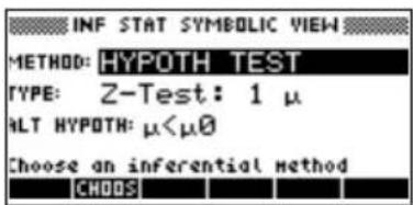
Inference aplet's SYMB view keys
The table below summarizes the options available in Symbolic view.
| Hypothesis Tests | Confidence Intervals |
| Z: 1 μ, the Z-Test on 1 mean | Z-Int: 1 μ, the confidence interval for 1 mean, based on the Normal distribution |
| Z: μ1 - μ2, the Z-Test on the difference of two means | Z-Int: μ1 - μ2, the confidence interval for the difference of two means, based on the Normal distribution |
| Z: 1 π, the Z-Test on 1 proportion | Z-Int: 1 π, the confidence interval for 1 proportion, based on the Normal distribution |
| Z: π1 - π2, the Z-Test on the difference in two proportions | Z-Int: π1 - π2, the confidence interval for the difference of two proportions, based on the Normal distribution |
| T: 1 μ, the T-Test on 1 mean | T-Int: 1 μ, the confidence interval for 1 mean, based on the Student's t-distribution |
| T: μ1 - μ2, the T-Test on the difference of two means | T-Int: μ1 - μ2, the confidence interval for the difference of two means, based on the Student's t-distribution |
If you choose one of the hypothesis tests, you can choose the alternative hypothesis to test against the null hypothesis. For each test, there are three possible choices for an alternative hypothesis based on a quantitative comparison of two quantities. The null hypothesis is always that the two quantities are equal. Thus, the alternative hypotheses cover the various cases for the two quantities being unequal: <, >, and ≠.
In this section, we will use the example data for the Z-Test on 1 mean to illustrate how the aplet works and what features the various views present.
Select the inferential method
- Select the Hypothesis Test inferential method.


- Define the type of test.
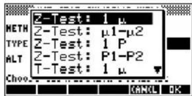
- Select an alternative hypothesis.


Enter data 5. Enter the sample statistics and population parameters.


The table below lists the fields in this view for our current Z-Test: 1 μ example.
| Field name | Definition |
| μ0 Assumed | population mean |
| σ Population | standard deviation |
| Sample mean | |
| n Sample size | |
| α Alpha level | for the test |
By default, each field already contains a value. These values constitute the example database and are explained in the feature of this aplet.
Display on-line help
-
To display the on-line help, press HELP
-
To close the on-line help, press OK.
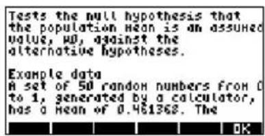
Display test results in numeric format
- Display the test results in numeric format.
NUM
The test distribution value and its associated probability are displayed, along with
the critical value(s) of the test and the associated critical value(s) of the statistic.

Note: You can access the on-line help in Numeric view.
Plot test results 9. Display a graphic view of the test results.
PLOT
Horizontal axes are presented for both the distribution variable and the test statistic. A
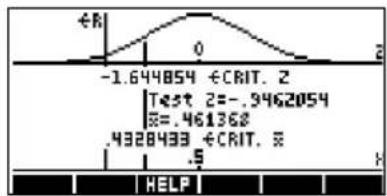
generic bell curve represents the probability distribution function. Vertical lines mark the critical value(s) of the test, as well as the value of the test statistic. The rejection region is marked and the test numeric results are displayed between the horizontal axes.
Importing sample statistics from the Statistics aplet
The Inference aplet supports the calculation of confidence intervals and the testing of hypotheses based on data in the Statistics aplet. Computed statistics for a sample of data in a column in any Statistics-based aplet can be imported for use in the Inference aplet. The following example illustrates the process.
A calculator produces the following 6 random numbers:
0.529, 0.295, 0.952, 0.259, 0.925, and 0.592
Open the Statistics aplet
- Open the Statistics aplet and reset the current settings.
APLET Select
Statistics
RESET YES
START
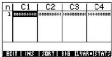
The Statistics aplet opens in the Numeric view.
Enter data 2. In the C1 column, enter the random numbers produced by the calculator.


HINT
If the Decimal Mark setting in the Modes input form (SHIFT modes) is set to Comma, use instead of .
- If necessary, select 1-variable statistics. Do this by pressing the fifth menu key until is displayed as its menu label.
Calculate statistics
- Calculate statistics.
STATE
The mean of 0.592 seems a little large compared to the
expected value of 0.5. To see if the difference is statistically significant, we will use the statistics computed here to construct a confidence interval for the true mean of the population of random numbers and see whether or not this interval contains 0.5.
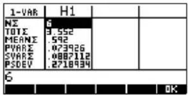
- Press to close the computed statistics window.
Open Inference aplet
- Open the Inference aplet and clear current settings.

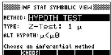
Select inference method and type
- Select an inference method.


- Select a distribution statistic type.
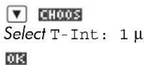
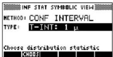
Set up the interval calculation
- Set up the interval calculation. Note: The default values are derived from sample data from the on-line help example.


Import the data
- Import the data from the Statistics aplet. Note: The data from C1 is displayed by default.
IMPRT
Note: Press ofc see the statistics before importing them into the Numeric Setup view.

Also, if there is more than one aplet based on the Statistics aplet, you are prompted to choose one.
OK
- Specify a 90%
confidence interval in the C: field.
![INF STAT NUMERIC SETUP x: .592 sx: .297844254603 n: 6 c: .99 Sample mean EDIT HELP [IMPORT]](/content/2026/05/1017618/images/a65df154e20dcc430fd2c98d0f794478758c1c57a74cf5b60f06984621e3375b.jpg)


the C: field
0.9
ENTER
to move

Display Numeric view
- Display the confidence interval in the Numeric view. Note: The interval setting is 0.5.
NUM
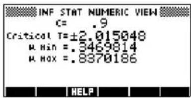
Display Plot view
- Display the confidence interval in the Plot view.
PLOT

You can see, from the second text row, that the mean is contained within interval (CI) of 0.34698
Note: The graph is a simple, generic bell-curve. It is not meant to accurately represent the t-distribution with 5 degrees of freedom.
Hypothesis tests
You use hypothesis tests to test the validity of hypotheses that relate to the statistical parameters of one or two populations. The tests are based on statistics of samples of the populations.
The hp 39g+ hypothesis tests use the Normal Z-distribution or Student's t-distribution to calculate probabilities.
One-Sample Z-Test
On the basis of statistics from a single sample, the One-Sample Z-Test measures the strength of the evidence for a selected hypothesis against the null hypothesis. The null hypothesis is that the population mean equals a specified value H0: µ = µ0 .
You select one of the following alternative hypotheses against which to test the null hypothesis:
H _ 1: µ_ 1 lt; µ_ 2
H _ 1: µ_ 1 gt; µ_ 2
H _ 1: µ_ 1 ≠ µ_ 2
Inputs The inputs are:
| Field name Definition | |
| Sample mean. | |
| n Sample size. | |
| µ0 | Hypothetical population mean. |
| σ Population standard deviation. | |
| α Significance level. | |
Results The results are:
| Result Description | |
| Test Z Z-test statistic. | |
| Prob Probability associated with the Z-Test statistic. | |
| Critical Z Boundary values of Z associated with the α level that you supplied. | |
| Critical | Boundary values of required by the α value that you supplied. |
Two-Sample Z-Test
Menu name
Z-Test: μ1−μ2
On the basis of two samples, each from a separate population, this test measures the strength of the evidence for a selected hypothesis against the null hypothesis. The null hypothesis is that the mean of the two populations are equal ( H0 : µ1 = µ2 ).
You select one of the following alternative hypotheses against which to test the null hypothesis:
H _ 1: µ_ 1 lt; µ_ 2
H _ 1: µ_ 1 gt; µ_ 2
H _ 1: µ_ 1 ≠ µ_ 2
Inputs The inputs are:
| Field name Definition | |
| 1 | Sample 1 mean. |
| 2 | Sample 2 mean. |
| n1 Sample 1 size. | |
| n2 Sample 2 size. | |
| σ1 Population 1 standard deviation. | |
| σ2 Population 2 standard deviation.α Significance level. | standard deviation. |
Results The results are:
| Result Description | |
| Test Z Z-Test statistic. | |
| Prob Probability associated with the Z-Test statistic. | |
| Critical Z Boundary value of Z associated with the α level that you supplied. |
One-Proportion Z-Test
On the basis of statistics from a single sample, this test measures the strength of the evidence for a selected hypothesis against the null hypothesis. The null hypothesis is that the proportion of successes in the two populations is equal: H0:π=π0
You select one of the following alternative hypotheses against which to test the null hypothesis:
H _ 1: πlt; π_ 0
H _ 1: πgt; π_ 0
H _ 1: π ≠ π_ 0
Inputs The inputs are:
| Field name Definition | |
| x Number of successes in the sample. | |
| n Sample size. | |
| π0 | Population proportion of successes. |
| α Significance level. | |
Results The results are:
| Result Description | |
| Test P Proportion of successes in the sample. | |
| Test Z Z-Test statistic. | |
| Prob Probability associated with the Z-Test statistic. | |
| Critical Z Boundary value of Z associated with the level you supplied. |
Two-Proportion Z-Test
Menu name
Z-Test: π 1 - π 2
On the basis of statistics from two samples, each from a different population, the Two-Proportion Z-Test measures the strength of the evidence for a selected hypothesis against the null hypothesis. The null hypothesis is that the proportion of successes in the two populations is equal H0 : π1 = π2 .
You select one of the following alternative hypotheses against which to test the null hypothesis:
H _ 1: π_ 1 lt; π_ 2
H _ 1: π_ 1 gt; π_ 2
H _ 1: π_ 1 ≠ π_ 2
Inputs The inputs are:
| Field name Definition | |
| X1 Sample 1 mean. | |
| X2 Sample 2 mean. | |
| n1 Sample 1 size. | |
| n2 Sample 2 size. | |
| α Significance level. | |
Results The results are:
| Result Description | |
| Test π1-π2 | Difference between the proportions of successes in the two samples. |
| Test Z Z-Test statistic. | |
| Prob Probability associated with the Z-Test statistic. | |
| Critical Z Boundary values of Z associated with the α level that you supplied. |
One-Sample T-Test
Menu name T-Test: 1 μ
The One-sample T-Test is used when the population standard deviation is not known. On the basis of statistics from a single sample, this test measures the strength of the evidence for a selected hypothesis against the null hypothesis. The null hypothesis is that the sample mean has some assumed value, H0:µ=µ0 You select one of the following alternative hypotheses against which to test the null hypothesis:
H _ 1: µlt; µ_ 0
H _ 1: µgt; µ_ 0
H _ 1: µ ≠ µ_ 0
Inputs The inputs are:
| Field name Definition | |
| Sample mean. | |
| Sx Sample standard deviation. | |
| n Sample size. | |
| µ 0 Hypothetical population mean. | |
| α Significance level. | |
Results The results are:
| Result Description | |
| Test T T-Test statistic. | |
| Prob Probability associated with the T-Test statistic. | |
| Critical T Boundary value of T associated with the α level that you supplied. | |
| Critical | Boundary value of required by the α value that you supplied. |
Two-Sample T-Test
Menu name
T-Test: μ1 - μ2
The Two-sample T-Test is used when the population standard deviation is not known. On the basis of statistics from two samples, each sample from a different population, this test measures the strength of the evidence for a selected hypothesis against the null hypothesis. The null hypothesis is that the two populations means are equal H0 : µ1 = µ2 .
You select one of the following alternative hypotheses against which to test the null hypothesis
H _ 1: µ_ 1 lt; µ_ 2
H _ 1: µ_ 1 gt; µ_ 2
H _ 1: µ_ 1 ≠ µ_ 2
Inputs The inputs are:
| Field name | Definition |
| 1 | Sample 1 mean. |
| 2 | Sample 2 mean. |
| S1 Sample 1 | standard deviation. |
| S2 Sample 2 | standard deviation. |
| n1 Sample 1 | size. |
| n2 Sample 2 | size. |
| α Significance level. | |
| _Pooled? | Check this option to pool samples based on their standard deviations. |
Results The results are:
| Result Description | |
| Test T T-Test statistic. | |
| Prob Probability associated with the T-Test statistic. | |
| Critical T Boundary values of T associated with the α level that you supplied. |
Confidence intervals
The confidence interval calculations that the hp 39g+ can perform are based on the Normal Z-distribution or Student's t-distribution.
One-Sample Z-Interval
Menu name Z-INT: μ 1
This option uses the Normal Z-distribution to calculate a confidence interval for m, the true mean of a population, when the true population standard deviation, s, is known.
Inputs TheT inputs are:
| Field name | Definition |
| Sample mean. | |
| σ Population | standard deviation. |
| n Sample size. | |
| c Confidence level. | |
Results The results are:
| Result Description | |
| Critical Z Critical value for Z.μ min Lower bound for μ.μ max Upper bound for μ. |
Two-Sample Z-Interval
Menu name
Z-INT: μ1–μ2
This option uses the Normal Z-distribution to calculate a confidence interval for the difference between the means of two populations, µ1-µ2 , when the population standard deviations, σ1 and σ2 , are known.
Inputs The inputs are:
| Field name | Definition |
| 1 | Sample 1 mean. |
| 2 | Sample 2 mean. |
| n1 Sample 1 size. | |
| n2 Sample 2 size. | |
| σ1 Population 1 standard deviation. | |
| σ2 Population 2 standard deviation. | |
| c Confidence level. | |
Results The results are:
| Result | Description |
| Critical Z Critical value for Z. | |
| Δ μ Min | Lower bound for µ1 - µ2 . |
| Δ μ Max | Upper bound for µ1 - µ2 . |
One-Proportion Z-Interval
Menu name Z-INT: 1 π
This option uses the Normal Z-distribution to calculate a confidence interval for the proportion of successes in a population for the case in which a sample of size, n, has a number of successes, x.
Inputs The inputs are:
| Field name | Definition |
| x Sample success count. | |
| n Sample size. | |
| c Confidence level. | |
Results The results are:
| Result Description | |
| Critical Z Critical value for Z.π Min Lower bound for π.π Max Upper bound for π. |
Two-Proportion Z-Interval
Menu name
Z-INT: π 1 - π 2
This option uses the Normal Z-distribution to calculate a confidence interval for the difference between the proportions of successes in two populations.
Inputs The inputs are:
| Field name | Definition |
| 1 | Sample 1 success count. |
| 2 | Sample 2 success count. |
| Field name | Definition (Continued) |
| n1 Sample 1 size. | |
| n2 Sample 2 size. | |
| c Confidence level. | |
Results The results are:
| Result | Description |
| Critical Z Critical value for Z. | |
| Δπ Min | Lower bound for the difference between the proportions of successes. |
| Δπ Max | Upper bound for the difference between the proportions of successes. |
One-Sample T-Interval
Menu name T-INT: 1 μ
This option uses the Student's t-distribution to calculate a confidence interval for m, the true mean of a population, for the case in which the true population standard deviation, s, is unknown.
Inputs The inputs are:
| Field name | Definition |
| 1 | Sample mean. |
| Sx Sample standard deviation. | |
| n Sample size. | |
| c Confidence level. | |
Results The results are:
| Result Description | |
| Critical T Critical value for T.μ Min Lower bound for μ.μ Max Upper bound for μ. |
Two-Sample T-Interval
Menu name
T-INT: µ1 - µ2
This option uses the Student's t-distribution to calculate a confidence interval for the difference between the means of two populations, µ 1 - µ 2 , when the population standard deviations, s1 and s2, are unknown.
Inputs The inputs are:
| Field name | Definition |
| 1 | Sample 1 mean. |
| 2 | Sample 2 mean. |
| s1 Sample 1 standard deviation. | |
| s2 Sample 2 standard deviation. | |
| n1 Sample 1 size. | |
| n2 Sample 2 size. | |
| C Confidence level. | |
| _Pooled Whether or not to pool the samples based on their standard deviations. | |
Results The results are:
| Result Description | |
| Critical T Critical value for T. | |
| Δ μ Min | Lower bound for μ1 - μ2. |
| Δ μ Max | Upper bound for μ1 - μ2. |
Using the Finance Solver
The Finance Solver, or Finance aplet, is available by using the APLET key in your calculator. Use the up and down arrow keys to select the Finance aplet. Your screen should look as follows:

Press the key or the soft menu key to activate the aplet. The resulting screen shows the different elements involved in the solution of financial problems with your hp 39g+ calculator.

Background information on and applications of financial calculations are provided next.
Background The Finance Solver application provides you with the ability of solving time-value-of-money (TVM) and amortization problems. These problems can be used for calculations involving compound interest applications as well as amortization tables.
Compound interest is the process by which earned interest on a given principal amount is added to the principal at specified compounding periods, and then the combined amount earns interest at a certain rate.
Financial calculations involving compound interest include savings accounts, mortgages, pension funds, leases, and annuities.
Time Value of Money (TVM) calculations, as the name implies, make use of the notion that a dollar today will be worth more than a dollar sometime in the future. A dollar today can be invested at a certain interest rate and generate a return that the same dollar in the future cannot. This TVM principle underlies the notion of interest rates, compound interest and rates of return.
TVM transactions can be represented by using cash flow diagrams. A cash flow diagram is a time line divided into equal segments representing the compounding periods. Arrows represent the cash flows, which could be positive (upward arrows) or negative (downward arrows), depending on the point of view of the lender or borrower. The following cash flow diagram shows a loan from a borrower's point of view:

On the other hand, the following cash flow diagram shows a load from the lender's point of view:
![graph TD A["Loan"] --> B["1"] B --> C["2"] C --> D["3"] D --> E["4"] E --> F["5"] F --> G["FV"] H["PV"] --> I["Equal periods"] J["Equal payments"] --> K["PMT PMT PMT PMT"] L["PMT"] --> M["PMT"]](/content/2026/05/1017618/images/a73ceab73e26312303efa88e443f3560d9900adca6bc30a21deefc4efb6b4437.jpg)
In addition, cash flow diagrams specify when payments occur relative to the compounding periods: at the beginning of each period or at the end. The Finance Solver application provides both of these payment
modes: Begin mode and End mode. The following cash flow diagram shows lease payments at the beginning of each period.

The following cash flow diagram shows deposits into an account at the end of each period.

As these cash-flow diagrams imply, there are five TVM variables:
| N The total | number of compounding periods or payments. |
| I%YR The nominal annual interest rate (or investment rate). This rate is divided by the number of payments per year (P/YR) to compute the nominal interest rate per compounding period – which is the interest rate actually used in TVM calculations. | |
| PV | The present value of the initial cash flow.To a lender or borrower, PV is the amount of the loan; to an investor, PV is the initial investment. PV always occurs at the beginning of the first period. |
| PMT | The periodic payment amount. The payments are the same amount each period and the TVM calculation assumes that no payments are skipped. Payments can occur at the beginning or the end of each compounding period -- an option you control by setting the Payment mode to Beg or End.The future value of the transaction: the amount of the final cash flow or the compounded value of the series of previous cash flows. For a loan, this is the size of the final balloon payment (beyond any regular payment due). For an investment this is the cash value of an investment at the end of the investment period. |
| FV | |
Performing TVM calculations
- Launch the Financial Solver as indicated at the beginning of this section.
- Use the arrow keys to highlight the different fields and enter the known variables in the TVM calculations, pressing the soft-menu key after entering each known value. Be sure that values are entered for at least four of the five TVM variables (namely, N, 1%YR, PV, PMT, and FV).
- If necessary, enter a different value for P/YR (default value is 12, i.e., monthly payments).
- Press the key to change the Payment mode (Beg or End) as required.
- Use the arrow keys to highlight the TVM variable you wish to solve for and press the -soft-monu key.
Example 1 - Loan calculations
Suppose you finance the purchase of a car with a 5-year loan at 5.5% annual interest, compounded monthly. The purchase price of the car is \19,500, and the down payment is \3,000. What are the required monthly payments? What is the largest loan you can afford if your maximum monthly payment is \$300? Assume that the payments start at the end of the first period.
Solution. The following cash flow diagram illustrates the loan calculations:
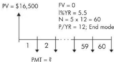
Start the Finance Solver, selecting P/YR = 12 and End payment option.
- Enter the known TVM variables as shown in the diagram above. Your input form should look as follows:

- Highlighting the PMT field, press the software menu key to obtain a payment of -315.17 (i.e., PMT = -\$315.17).
- To determine the maximum loan possible if the monthly payments are only \300, type the value - 300 in the PMT field, highlight the PV field, and press the soft menu key. The resulting value is PV = \15,705.85.
Example 2 - Mortgage with balloon payment
Suppose you have taken out a 30-year, \$150,000 house mortgage at 6.5% annual interest. You expect to sell the house in 10 years, repaying the loan in a balloon payment. Find the size of the balloon payment -- the value of the mortgage after 10 years of payment.
Solution. The following cash flow diagram illustrates the case of the mortgage with balloon payment:

- Start the Finance Solver, selecting P/YR = 12 and End payment option.
- Enter the known TVM variables as shown in the diagram above. Your input form, for calculating monthly payments for the 30-yr mortgage, should look as follows:

- Highlighting the PMT field, press the s p t L U E menu key to obtain a payment of -948.10 (i.e., PMT = -\$948.10)
- To determine the balloon payment or future value (FV) for the mortgage after 10 years, use N = 120, highlight the FV field, and press the -soft menu key. The resulting value is FV = -\127,164.19. The negative value indicates a payment from the homeowner. Check that the required balloon payments at the end of 20 years (N=240) and 25 years (N = 300) are -\83,497.92 and -\$48,456.24, respectively.
Calculating Amortizations
Amortization calculations, which also use the TVM variables, determine the amounts applied towards principal and interest in a payment or series of payments.
To calculate amortizations:
- Start the Finance Solver as indicated at the beginning of this section.
- Set the following TVM variables:
a Number of payments per year (P/YR)
b Payment at beginning or end of periods - Store values for the TVM variables I%YR, PV, PMT, and FV, which define the payment schedule.
- Press the 📄️ should be soft menu key and enter the number of payments to amortize in this batch.
- Press the soft menu key to amortize a batch of payments. The calculator will provide for you the amount applied to interest, to principal, and the remaining balance after this set of payments have been amortized.
Example 3 - Amortization for home mortgage
For the data of Example 2 above, find the amortization of the loan after the first 10 years (12x10 = 120 payments). Pressing the soft menu key produces the screen to the left. Enter 120 in the PAYMENTS field, and press the soft menu key to produce the results shown to the right.

To continue amortizing the loan:
- Press the soft menu key to store the new balance after the previous amortization as PV.
-
Enter the number of payments to amortize in the new batch.
-
Press the soft menu key to amortize the new batch of payments. Repeat steps 1 through 3 as often as needed.
Example 4 - Amortization for home mortgage
For the results of Example 3, show the amortization of the next 10 years of the mortgage loan. First, press the 2→ 7 soft menu key. Then, keeping 120 in the PAYMENTS field, press the soft menu key to produce the results shown below.
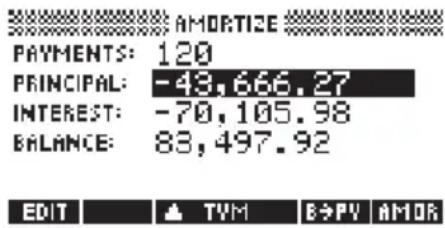
To amortize a series of future payments starting at payment p:
- Calculate the balance of the loan at payment p-1.
- Store the new balance in PV using the menu key.
- Amortize the series of payments starting at the new PV.
The amortization operation reads the values from the TVM variables, rounds the numbers it gets from PV and PMT to the current display mode, then calculates the amortization rounded to the same setting. The original variables are not changed, except for PV, which is updated by using after each amortization.
Using mathematical functions
Math functions
The hp 39g+ contains many math functions. The functions are grouped in categories. For example, the Matrix category contains functions for manipulating matrices. The Probability category (shown as Prob. on the MATH menu) contains functions for working with probability.
To use a math function, you enter the function onto the command line, and include the arguments in parentheses after the function. You can also select a math function from the MATH menu.
The MATH menu
The MATH menu provides access to math functions and programming constants.
The MATH menu is organized by category. For each category of functions on the left, there is a list of function names on the right. The highlighted category is the current category.

- When you press, you see the menu list of Math categories in the left column and the corresponding functions of the highlighted category in the right column. The menu key indicates that the MATH FUNCTIONS menu list is active.
To select a function 1. Press to display the MATH menu. The
categories appear in alphabetical order. Press ▲ to scroll through the categories. To skip directly to a category, press the first letter of the category's name. Note: You do not need to press FirstA
-
The list of functions (on the right) applies to the currently highlighted category (on the left). Use ▶ and ☐ switch between the category list and the function list.
-
Highlight the name of the function you want and press OFThis copies the function name (and an initial parenthesis, if appropriate) to the edit line.
Function categories
- Calculus
• Complex numbers - Constant
• Hyperbolic trigonometry (Hyperb.) - Lists
- Loop
• Matrices (Matrices)
• Polynomial (Polynom.)
• Probability (Prob.)
• Real numbers (Real) - Two-variable statistics (Stat-Two)
- Symbolic
- Tests
• Trigonometry (Trig)
Math functions by category
Syntax
Each function's definition includes its syntax, that is, the exact order and spelling of a function's name, its delimiters (punctuation), and its arguments. Note that the syntax for a function does not require spaces.
Functions common to keyboard and menus
These functions are common to the keyboard and MATH menu.
SHIFT π
For a description, see “ π ” on page 11-8.
SHIFT ARG
For a description, see "ARG" on page 11-7.
d/dx
For a description, see “ ” on page 11-7.
SHIFT AND
For a description, see "AND" on page 11-19.
| SHIFT ! | For a description, see “COMB(5,2) returns 10. That is, there are ten different ways that five things can be combined two at a time.!” on page 11-12. |
| SHIFT Σ | For a description, see “Σ” on page 11-10. |
| SHIFT EEX | For a description, see “Scientific notation (powers of 10)” on page 1-20. |
| SHIFT∫ | For a description, see “∫” on page 11-7. |
| SHIFT x-1 | The multiplicative inverse function finds the inverse of a square matrix, and the multiplicative inverse of a real or complex number. Also works on a list containing only these object types. |
Keyboard functions
The most frequently used functions are available directly from the keyboard. Many of the keyboard functions also accept complex numbers as arguments.

Add, Subtract, Multiply, Divide. Also accepts complex numbers, lists and matrices.
value1+ value2, etc.

Natural exponential. Also accepts complex numbers.
e^value
Example
e^5 returns 148.413159103

Natural logarithm. Also accepts complex numbers.
LN(value)
Example
LN(1) returns 0
SHIFT 10x
Exponential (antilogarithm). Also accepts complex numbers.
10^value
Example
103 returns 1000
log
Common logarithm. Also accepts complex numbers.
LOG(value)
Example
LOG(100) returns 2
SIN, COS, TAN
Sine, cosine, tangent. Inputs and outputs depend on the current angle format (Degrees, Radians, or Grads).
SIN(value)
COS(value)
TAN(value)
Example
TAN(45) returns 1 (Degrees mode).
SHIFT ASIN Arc sine: sin
-1 x. Output range is from -90° to 90° , -π/2 to π/2 , or -100 to 100 grads. Inputs and outputs depend on the current angle format. Also accepts complex numbers.
ASIN(value)
Example
ASIN(1) returns 90 (Degrees mode).
SHIFT ACOS Arc cosine: cos
os -1x . Output range is from 0° to 180° , 0 to π , or 0 to 200 grads. Inputs and outputs depend on the current angle format. Also accepts complex numbers. Output will be complex for values outside the normal COS domain of .1-x1≤≤
ACOS(value)
Example
ACOS (1) returns 0 (Degrees mode).
SHIFT ATAN Arc tangent: tan
-1x . Output range is from -90° to 90° ,
2π/2 to π/2 , or -100 to 100 grads. Inputs and outputs depend on the current angle format. Also accepts complex numbers.
ATAN(value)
Example
ATAN(1) returns 45 (Degrees mode).

Square. Also accepts complex numbers.
value 2
Example
182 returns 324
SHIFT Square root. Also accepts complex numbers.
√ value
Example
√324 returns 18

Negation. Also accepts complex numbers.
-value
Example
- (1, 2) returns (-1, -2)

Power (x raised to y). Also accepts complex numbers.
value^power
Example
2^8 returns 256
SHIFT ABS Absolute value. For a complex number, this is .
√ x ^ 2 + y ^ 2
ABS(value)
ABS((x, y))
Example
ABS (-1) returns 1
ABS((1,2)) returns 2.2360679775
Example
3 NTHROOT 8 returns 2
Calculus functions
The symbols for differentiation and integration are available directly form the keyboard—and S respectively—as well as from the MATH menu.
Differentiates expression with respect to the variable of differentiation. From the command line, use a formal name (S1, etc.) for a non-numeric result. See "Finding derivatives" on page 11-21.
variable(expression)
Example
_ s 1 (s 1 ^ 2 + 3 * s 1) returns 2 * s 1 + 3
∫
Integrates expression from lower to upper limits with respect to the variable of integration. To find the definite integral, both limits must have numeric values (that is, be numbers or real variables). To find the indefinite integral, one of the limits must be a formal variable (s1, etc).
∫ (lower, upper, expression, variable)
See "Using formal variables" on page 11-20 for further details.
Example
(0, s1, 2X + 3, X) ENTER ▲ COPY ENTER finds the indefinite result 3s1+2*(s12/2)
See "To find the indefinite integral using formal variables" on page 11-23 for more information on finding indefinite integrals.
TAYLOR
Calculates the nth order Taylor polynomial of expression at the point where the given variable = 0.
TAYLOR (expression, variable, n)
Example
TAYLOR(1 + sin(s1) 2 , s1, 5) with Radians angle measure and Fraction number format (set in MODES) returns 1+s1^2-1/3*s1^4.
Complex number functions
These functions are for complex numbers only. You can also use complex numbers with all trigonometric and hyperbolic functions, and with some real-number and keyboard functions. Enter complex numbers in the form (x,y) , where x is the real part and y is the imaginary part.
ARG
Argument. Finds the angle defined by a complex number. Inputs and outputs use the current angle format set in Modes.
ARG ((x, y))
Example
ARG((3,3)) returns 45 (Degrees mode)
CONJ Complex conjugate. Conjugation is the negation (sign reversal) of the imaginary part of a complex number. CONJ((x, y))
Example
CONJ((3,4)) returns (3,-4)
IM
Imaginary part, y, of a complex number, (x, y) . IM ((x, y))
Example
IM((3,4)) returns 4
RE
Real part x, of a complex number, (x, y) . RE((x, y))
Example
RE((3,4)) returns 3
Constants
The hp 39g+ has an internal numeric representation for these constants.
e Natural logarithm base. Internally represented as
2.71828182846.
e
i Imaginary value for, the complex number (0√1) .
i
MAXREAL Maximum real number. Internally represented as
9.999999999999 x 10 499 .
MAXREAL
MINREAL Minimum real number. Internally represented as
1 × 10-499
MINREAL
π Internally represented as 3.14159265359.
π
Hyperbolic trigonometry
The hyperbolic trigonometry functions can also take complex numbers as arguments.
ACOSH Inverse hyperbolic cosine : -1x .
ACOSH(value)
ASINH Inverse hyperbolic sine : sinh -1x .
ASINH(value)
ATANH Inverse hyperbolic tangent : tanh -1x .
ATANH(value)
COSH Hyperbolic cosine
COSH(value)
SINH Hyperbolic sine.
SINH(value)
TANH Hyperbolic tangent.
TANH(value)
ALOG
Antilogarithm (exponential). This is more accurate than 10x due to limitations of the power function.
ALOG(value)
EXP
Natural exponential. This is more accurate than ex due to limitations of the power function.
EXP(value)
EXPM1 Exponent minus 1 : . This is more accurate than
EXP when x is close to zero.
EXPM1(value)
LNP1
Natural log plus 1 : (x+1) . This is more accurate than the natural logarithm function when x is close to zero.
LNP1(value)
List functions
These functions work on list data. See "List functions" on page 14-6.
Loop functions
The loop functions display a result after evaluating an expression a given number of times.
ITERATE
Repeatedly for #times evaluates an expression in terms of variable. The value for variable is updated each time, starting with initialvalue.
ITERATE (expression, variable, initialvalue, #times)
Example
ITERATE (X2, X, 2, 3) returns 256
RECURSE
Provides a method of defining a sequence without using the Symbolic view of the Sequence aplet. If used with | ("where"), RECURSE will step through the evaluation.
RECURSE (sequencename, term n , term 1 , term 2 )
Example
RECURSE(U,U(N-1)*N,1,2) STOP U1(N)
Stores a factorial-calculating function named U1.
When you enter U1(5), for example, the function calculates 5! (120).
Σ
Summation. Finds the sum of expression with respect to variable from initialvalue to finalvalue.
(variable=initialvalue, finalvalue, expression)
Example
(C=1,5,C2) returns 55.
Matrix functions
These functions are for matrix data stored in matrix variables. See "Matrix functions and commands" on page 13-9.
Polynomial functions
Polynomials are products of constants (coefficients) and variables raised to powers (terms).
POLYCOEF
Polynomial coefficients. Returns the coefficients of the polynomial with the specified roots.
POLYCOEF ([roots])
Example
To find the polynomial with roots 2, -3, 4, -5:
POLYCOEF([2,-3,4,-5]) returns [1,2,-25,
-26,120] , representing x4 + 2x3 - 25x2 - 26x + 120 .
POLYEVAL Polynomial evaluation. Evaluates a polynomial with the specified coefficients for the value of x.
POLYEVAL ([coefficients], value)
Example
For x4+2x3-25x2-26x+120 :
POLYEVAL([1,2,-25,-26,120],8) returns 3432.
POLYFORM
Polynomial form. Creates a polynomial in variable 1 from expression.
POLYFORM(expression, variable 1)
Example
POLYFORM((X+1) 2 +1,X) returns X2 +2*X+2.
POLYROOT
Polynomial roots. Returns the roots for the nth-order polynomial with the specified n+1 coefficients.
POLYROOT([coefficients])
Example
For x4+2x3-25x2-26x+120 :
POLYROOT([1,2,-25,-26,120]) returns [2,-3,4,-5].
HINT
The results of POLYROOT will often not be easily seen in HOME due to the number of decimal places, especially if they are complex numbers. It is better to store the results of POLYROOT to a matrix.
For example, POLYROOT([1, 0, 0, -8] STOP M1 will store the three complex cube roots of 8 to matrix M1 as a complex vector. Then you can see them easily by going to the Matrix Catalog. and access them individually in calculations by referring to M1(1), M1(2) etc.
Probability functions
COMB
Number of combinations (without regard to order) of n things taken r at a time: n!/(r!(n-r)) .
COMB(n, r)
Example
COMB(5,2) returns 10. That is, there are ten different ways that five things can be combined two at a time.!
Factorial of a positive integer. For non-integers, ! = (x + 1) . This calculates the gamma function.
value!
PERM
Number of permutations (with regard to order) of n things taken r at a time: n!/(r!(n-r)!
PERM (n,r)
Example
PERM(5,2) returns 20. That is, there are 20 different permutations of five things taken two at a time.
RANDOM Random number (between zero and 1). Produced by a pseudo-random number sequence. The algorithm used in the RANDOM function uses a seed number to begin its sequence. To ensure that two calculators must produce different results for the RANDOM function, use the RANDSEED function to seed different starting values before using RANDOM to produce the numbers.
RANDOM
HINT
The setting of Time will be different for each calculator, so using RANDSEED(Time) is guaranteed to produce a set of numbers which are as close to random as possible. You can set the seed using the command RANDSEED.
UTPC
Upper-Tail Chi-Squared Probability given degrees of freedom, evaluated at value. Returns the probability that a 2 random variable is greater than value.
UTPC(degrees, value)
| UTPF | Upper-Tail Snedecor's F Probability given numerator degrees of freedom and denominator degrees of freedom (of the F distribution), evaluated at value. Returns the probability that a Snedecor's F random variable is greater than value.UTPF(numerator, denominator, value) |
| UTPN | Upper-Tail Normal Probability given mean and variance, evaluated at value. Returns the probability that a normal random variable is greater than value for a normal distribution. Note: The variance is the square of the standard deviation.UTPN(mean, variance, value) |
| UTPT | Upper-Tail Student's t-Probability given degrees of freedom, evaluated at value. Returns the probability that the Student's t- random variable is greater than value.UTPT(degrees, value) |
Real-number functions
Some real-number functions can also take complex arguments.
CEILING Smallest integer greater than or equal to value. CEILING(value)
Examples
CEILING(3.2) returns 4 CEILING(-3.2) returns -3
DEG→RAD Degrees to radians. Converts value from Degrees angle format to Radians angle format. DEG→RAD(value)
Example
DEG→RAD(180) returns 3.14159265359, the value of π.
FLOOR Greatest integer less than or equal to value. FLOOR(value)
Example
FLOOR (-3.2) returns -4
FNROOT
Function root-finder (like the Solve aplet). Finds the value for the given variable at which expression most nearly evaluates to zero. Uses guess as initial estimate.
FNROOT(expression, variable, guess)
Example
FNROOT(M*9.8/600-1,M,1) returns 61.2244897959.
FRAC Fractional part.
FRAC(value)
Example
FRAC (23.2) returns .2
HMS→
Hours-minutes-seconds to decimal. Converts a number or expression in H.MMSSs format (time or angle that can include fractions of a second) to x.x format (number of hours or degrees with a decimal fraction).
HMS → (H. MMSSs)
Example
HMS→(8.30) returns 8.5
→HMS
Decimal to hours-minutes-seconds. Converts a number or expression in x.x format (number of hours or degrees with a decimal fraction) to H.MMSSs format (time or angle up to fractions of a second).
→ HMS (x. x)
Example
→HMS (8.5) returns 8.3
INT Integer part.
INT(value)
Example
INT(23.2) returns 23
MANT
Mantissa (significant digits) of value.
MANT(value)
Example
MANT(21.2E34) returns 2.12
MAX Maximum. The greater of two values.
MAX(value1, value2)
Example
MAX(210,25) returns 210
MIN Minimum. The lesser of two values.
MIN(value1, value2)
Example
MIN(210, 25) returns 25
MOD
Modulo. The remainder of value1/value2.
value1 MOD value2
Example
9 MOD 4 returns 1
%
x percent of y; that is, x/100*y.
% (x, y)
Example
%(20,50) returns 10
%CHANGE
Percent change from x to y, that is, 100(y-x)/x .
%CHANGE(x, y)
Example
%CHANGE (20, 50) returns 150
%TOTAL
Percent total : (100)y/x. What percentage of x, is y.
%TOTAL(x, y)
Example
%TOTAL(20,50) returns 250
RAD→DEG
Radians to degrees. Converts value from radians to degrees.
RAD→DEG (value)
Example
RAD→DEG(π) returns 180
ROUND
Rounds value to decimal places. Accepts complex numbers.
ROUND(value, places)
Round can also round to a number of significant digits as showed in example 2.
Examples
ROUND (7.8676, 2) returns 7.68
ROUND (0.0036757,-3) returns 0.00368
SIGN
Sign of value. If positive, the result is 1. If negative, -1. If zero, result is zero. For a complex number, this is the unit vector in the direction of the number.
SIGN(value)
SIGN((x, y))
Examples
SIGN (-2) returns -1
SIGN((3,4)) returns (.6,.8)
TRUNCATE
Truncates value to decimal places. Accepts complex numbers.
TRUNCATE(value, places)
Example
TRUNCATE(2.3678,2) returns 2.36
XPON
Exponent of value.
XPON(value)
Example
XPON(123.4) returns 2
Two-variable statistics
These are functions for use with two-variable statistics.
See "Two-variable" on page 8-14.
Symbolic functions
The symbolic functions are used for symbolic manipulations of expressions. The variables can be formal or numeric, but the result is usually in symbolic form (not a number). You will find the symbols for the symbolic functions = and | (where) in the CHARS menu (SHIFT CHARS) as well as the MATH menu.
= (equals)
Sets an equality for an equation. This is not a logical operator and does not store values. (See "Test functions" on page 11-18.)
expression 1=expression2
ISOLATE
Isolates the first occurrence of variable in expression=0 and returns a new expression, where variable=newexpression. The result is a general solution that represents multiple solutions by including the (formal) variables S1 to represent any sign and n1 to represent any integer.
ISOLATE (expression, variable)
Examples
ISOLATE(2*X+8,X) returns -4 ISOLATE(A+B*X/C,X) returns -(A*C/B)
LINEAR?
Tests whether expression is linear for the specified variable. Returns 0 (false) or 1 (true).
LINEAR? (expression, variable)
Example
LINEAR? ((X^2-1) / (X+1), X) returns 0
QUAD
Solves quadratic expression=0 for variable and returns a new expression, where variable=newexpression. The result is a general solution that represents both positive and negative solutions by including the formal variable S1 to represent any sign: + or - .
QUAD (expression, variable)
Example
QUAD ( (X-1)2-7, X) returns (2+s1*5.29150262213)/2
QUOTE Encloses an expression that should not be evaluated numerically.
QUOTE (expression)
Examples
QUOTE(SIN(45)) STOCK) stores the expression SIN(45) rather than the value of SIN(45).
Another method is to enclose the expression in single quotes.
For example, X^3+2*X STOP F1(X) puts the expression X^3+2*X into F1(X) in the Function aplet.
| (where)
Evaluates expression where each given variable is set to the given value. Defines numeric evaluation of a symbolic expression.
expression | (variable1=value1, variable2=value2,...)
Example
3*(X+1) (X=3) returns 12.
Test functions
The test functions are logical operators that always return either a 1 (true) or a 0 (false).
< Less than. Returns 1 if true, 0 if false.
value1<value2
≤ Less than or equal to. Returns 1 if true, 0 if false.
value 1≤value2
== Equals (logical test). Returns 1 if true, 0 if false.
value1==value2
≠ Not equal to. Returns 1 if true, 0 if false.
value1≠value2
Greater than. Returns 1 if true, 0 if false.
value1>value2
≥ Greater than or equal to. Returns 1 if true, 0 if false.
value 1≥value2
AND
Compares value1 and value2. Returns 1 if they are both non-zero, otherwise returns 0.
value1 AND value2
IFTE
If expression is true, do the trueclause; if not, do the falseclause.
IFTE (expression, trueclause, falseclause)
Example
IFTE (X > 0, X2, X3)
NOT
Returns 1 if value is zero, otherwise returns 0.
NOT value
OR
Returns 1 if either value1 or value2 is non-zero, otherwise returns 0.
value1 OR value2
XOR
Exclusive OR. Returns 1 if either value1 or value2—but not both of them—is non-zero, otherwise returns 0.
value1 XOR value2
Trigonometry functions
The trigonometry functions can also take complex numbers as arguments. For SIN, COS, TAN, ASIN, ACOS, and ATAN, see the Keyboard category.
ACOT Arc cotangent.
ACOT(value)
ACSC Arc cosecant.
ACSC(value)
ASEC Arc secant.
ASEC(value)
COT
Cotangent: x/ x .
COT(value)
CSC Cosecant: 1/sinx
CSC(value)
SEC Secant: 1/cosx.
SEC(value)
Symbolic calculations
The hp 39g+ has the ability to perform symbolic calculations, for example, symbolic integration and differentiation. You can perform symbolic calculations in HOME and in the Function aplet.
In HOME When you perform calculations that contain normal variables, the calculator substitutes values for any variables. For example, if you enter A+B on the command line and press, the calculator retrieves the values for A and B from memory and substitutes them in the calculation.
Using formal variables
To perform symbolic calculations, for example symbolic differentiations and integrations, you need to use formal names. The hp 39g+ has six formal names available for use in symbolic calculations. These are S0 to S5. When you perform a calculation that contains a formal name, the hp 39g+ does not carry out any substitutions.
You can mix formal names and real variables. Evaluating (A+B+SI)2 will evaluate A+B, but not S1.
If you need to evaluate an expression that contains formal names numerically, you use the | (where) command, listed in the Math menu under the Symbolic category.
For example to evaluate (S1*S2)2 when S1=2 and S2=4, you would enter the calculation as follows:
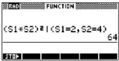
(The | symbol is in the CHARS menu: press SHIFT CHARS. The = sign is listed in the MATH menu under Symbolic functions.)
Symbolic calculations in the Function aplet
You can perform symbolic operations in the Function aplet's Symbolic view. For example, to find the derivative of a function in the Function aplet's Symbolic view, you define two functions and define the second function as a derivative of the first function. You then evaluate the second function. See "To find derivatives in the Function aplet's Symbolic view" on page 11-22 for an example.
Finding derivatives
The hp 39g+ can perform symbolic differentiation on some functions. There are two ways of using the hp 39g+ to find derivatives.
- You can perform differentiations in HOME by using the formal variables, S1 to S5.
- You can perform differentiations of functions of X in the Function aplet.
To find derivatives in HOME
To find the derivative of the function in HOME, use a formal variable in place of X. If you use X, the differentiation function substitutes the value that X holds, and returns a numeric result.
For example, consider the function:
dx ( s (n ^ 2) + 2 (x))
- Enter the differentiation function onto the command line, substituting S1 in place of X.

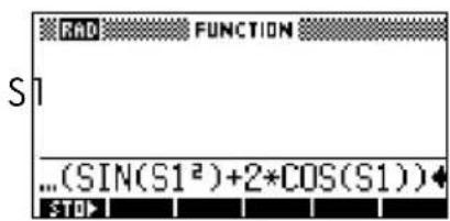
- Evaluate the function.
ENTER
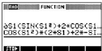
- Show the result.

SHOW

hp 39g+
To find derivatives in the Function aplet's Symbolic view
To find the derivative of the function in the Function aplet's Symbolic view, you define two functions and define the second function as a derivative of the first function. For example, to differentiate (x2) + 2 x
- Access the Function aplet's Symbolic view and define F1.
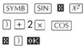

- Define F2(x) as the derivative of F(1) .


- Select F2(x) and evaluate it.


- Press to display the result. Note: Use the arrow keys to view the entire function.


You could also just define
F 1 (x) = dx ( (x ^ 2) + 2 (x)).
To find the indefinite integral using formal variables
For example, to find the indefinite integral of
3 x ^ 2 5 - dx use:
(0, S 1, 3 X ^ 2 - 5, X)
- Enter the function.


- Show the result format.

-
Press to close the show window.
-
Copy the result and evaluate.
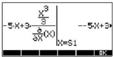
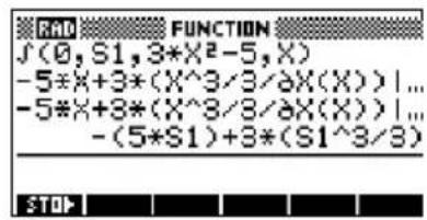
hp 39g+
Thus, substituting X for S1, it can be seen that:
3 x ^ 2 - 5 dx = - 5 x + 3 ( x ^ 33/ X (X))
This result is derived from substituting X=S1 and X=0 into the original expression found in step 1. However, substituting X=0 will not always evaluate to zero and may result in an unwanted constant.
To see this, consider: x(2-4dx)=(x2)55
The 'extra' constant of 6.4 results from the substitution of x into (x - 2)5 / 5 , and should be disregarded if an indefinite integral is required.

Variables and memory management
Introduction
The hp 39g+ has approximately 232K of user memory. The calculator uses this memory to store variables, perform computations, and store history.
A variable is an object that you create in memory to hold data. The hp 39g+ has two types of variables, home variables and aplet variables.
- Home variables are available in all aplets. For example, you can store real numbers in variables A to Z and complex numbers in variables Z0 to Z9. These can be numbers you have entered, or the results of calculations. These variables are available within all aplets and within any programs.
- Aplet variables apply only to a single aplet. Aplets have specific variables allocated to them which vary from aplet to aplet.
You use the calculator's memory to store the following objects:
- copies of aplets with specific configurations
- new aplets that you download
- aplet variables
- home variables
- variables created through a catalog or editor, for example a matrix or a text note
- programs that you create.
You can use the Memory Manager (SHIFT MEMORY) to view the amount of memory available. The catalog views, which are accessible via the Memory Manager, can be used to transfer variables such as lists or matrices between calculators.
Storing and recalling variables
You can store numbers or expressions from a previous input or result into variables.
Numeric Precision
A number stored in a variable is always stored as a 12-digit mantissa with a 3-digit exponent. Numeric precision in the display, however, depends on the display mode (Standard, Fixed, Scientific, Engineering, or Fraction). A displayed number has only the precision that is displayed. If you copy it from the HOME view display history, you obtain only the precision displayed, not the full internal precision. On the other hand, the variable Ans always contains the most recent result to full precision.
To store a value 1. On the command line, enter the value or the calculation for the result you wish to store.
- Press
STOP
- Enter a name for the variable.
4.
Press

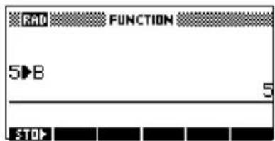
To store the results of a calculation
If the value you want to store is in the HOME view display history, for example the results of a previous calculation, you need to copy it to the command line, then store it.
- Perform the calculation for the result you want to store.
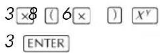

-
Move the highlight to the result you wish to store.
-
Press to copy the result to the command line.
-
Press
-
Enter a name for the variable.
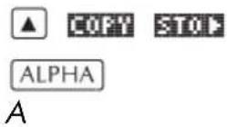
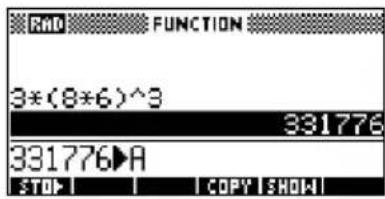
- Press to store the result.
The results of a calculation can also be stored directly to a variable. For example:


To recall a value To recall a variable's value, type the name of the variable and press ENTER

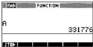
To use variables in calculations
You can use variables in calculations. The calculator substitutes the variable's value in the calculation:

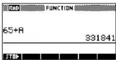
The VARS menu
You use the VARS menu to access all variables in the calculator. The VARS menu is organised by category. For each variable category in the left column, there is a list of variables in the right column. You select a variable category and then select a variable in the category.
- Open the VARS menu.
VARS
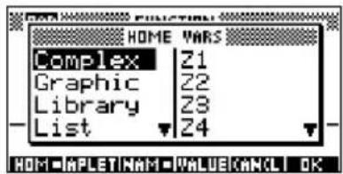
- Use the arrow keys or press the alpha key of the first letter in the category to select a variable category.
For example, to select the Matrix category, press ☐.
Note: In this instance, there is no need to press the ALPHA key.
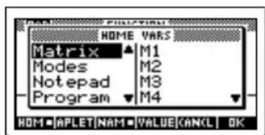
- Move the highlight to the variables column.
▶
- Use the arrow keys to select the variable that you want. For example, to select the M2 variable, press
↓
▼

- Choose whether to place the variable name or the variable value on the command line.
- Press to indicate that you want the variable's contents to appear on the command line.
- Press to indicate that you want the variable's name to appear on the command line.
- Press 108 place the value or name on the command line. The selected object appears on the command line.
OK

Note: The VARS menu can also be used to enter the names or values of variables into programs.
Example This example demonstrates how to use the VARS menu to add the contents of two list variables, and to store the result in another list variable.
- Display the List Catalog.
SHIFT LIST
to select L1
EOT
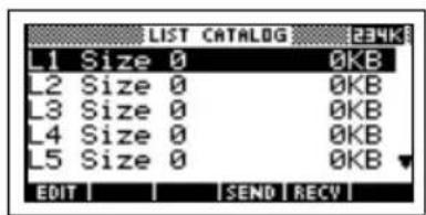
- Enter the data for L1.
88 OK 90 OK 89 OK
65 OK 70 OK
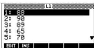
- Return to the List Catalog to create L2.
SHIFT LIST
to select L2
EDIT
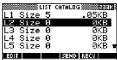
- Enter data for L2.


-
Press to access HOME.
-
Open the variable menu and select L1.


- Copy it to the command line. Note: Because the
NAME option is highlighted, the variable's name, rather than its contents, is copied to the command line.

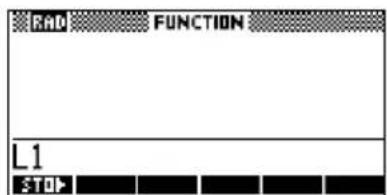
- Insert the + operator and select the L2 variable from the List variables.
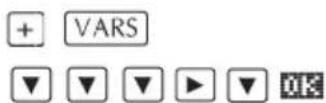
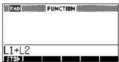
- Store the answer in the List catalog L3 variable.

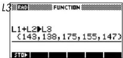
Note: You can also type list names directly from the keyboard.
Home variables
It is not possible to store data of one type in a variable of another type. For example, you use the Matrix catalog to create matrices. You can create up to ten matrices, and you can store these in variables M0 to M9. You cannot store matrices in variables other than M0 to M9.
| Category | Available names |
| Complex Z0 to Z9For example, (1,2)STOPZ0 or 2+3iSTOPZ1. You can enter a complex number by typing (r;i), where r represents the real part, and i represents the imaginary part. | |
| Graphic G0 to G9See “Graphic commands” on page 16-20 for more information on storing graphic objects via programming commands. See “To store into a graphics variable” on page 15-5 for more information on storing graphic object via the sketch view. | |
| Library Aplet library variables can store aplets that you have created, either by saving a copy of a standard aplet, or downloading an aplet from another source. | |
| List L0 to L9For example, {1,2,3}STOP | |
| Matrix M0 to M9 can store matrices or vectors.For example, [[1,2],[3,4]]MODE | |
| Modes Modes variables store the modes settings that you can configure usingSHIFTMODES. | |
| Notepad Notepad variables store notes. | |
| Program Program variables store programs. | |
| Real A to Z and θ.For example, 7.45ATOP | |
Aplet variables Aplet variables store values that are unique to a particular aplet. These include symbolic expressions and equations (see below), settings for the Plot and Numeric views, and the results of some calculations such as roots and intersections. See the Reference Information chapter for more information about aplet variables.
| Category | Available names |
| Function F0 to | F9 (Symbolic view). See “Function aplet variables” on page R-7. |
| Parametric X0, | Y0 to X9, Y9 (Symbolic view). See “Parametric aplet variables” on page R-8. |
| Polar R0 to R9 | (Symbolic view). See “Polar aplet variables” on page R-9. |
| Sequence U0 | to U9 (Symbolic view). See “Sequence aplet variables” on page R-10. |
| Solve | E0 to E9 (Symbolic view). See “Solve aplet variables” on page R-11. |
| Statistics | C0 to C9 (Numeric view). See “Statistics aplet variables” on page R-12. |
To access an aplet variable
- Open the aplet that contains the variable you want to recall.
- Press to display the VARS menu.
- Use the arrow keys to select a variable category in the left column, then press to access the variables in the right column.
- Use the arrow keys to select a variable in the right column.
-
To copy the name of the variable onto the edit line, press on is the default setting.)
-
To copy the value of the variable into the edit line, press pound press OK.

Memory Manager
You can use the Memory Manager to determine the amount of available memory on the calculator. You can also use Memory Manager to organize memory. For example, if the available memory is low, you can use the Memory Manager to determine which aplets or variables consume large amounts of memory. You can make deletions to free up memory.
Example 1. Start the Memory Manager. A list of variable categories is displayed.
SHIFT MEMORY
Free memory is displayed in the top right corner and the body of the screen lists
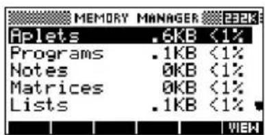
each category, the memory it uses, and the percentage of the total memory it uses.
- Select the category with which you want to work and press uMemory Manager displays memory details of variables within the category.


- To delete variables in a category:
- Press to delete the selected variable.
- Press SHIFT CLEAR to delete all variables in the selected category.
Introduction
You can perform matrix calculations in HOME and in programs. The matrix and each row of a matrix appear in brackets, and the elements and rows are separated by commas. For example, the following matrix:
[1 amp; 2 amp; 3 4 amp; 5 amp; 6 ]
is displayed in the history as:
[[1,2,3],[4,5,6]]
(If the Decimal Mark mode is set to Comma, then separate each element and each row with a period.)
You can enter matrices directly in the command line, or create them in the matrix editor.
Vectors
Vectors are one-dimensional arrays. They are composed of just one row. A vector is represented with single brackets; for example, [1,2,3] . A vector can be a real number vector or a complex number vector, for example [(1,2),(7,3)] .
Matrices Matrices are two-dimensional arrays. They are composed of more than one row and more than one column. Two-dimensional matrices are represented with nested brackets; for example, [[1,2,3],[4,5,6]]. You can create complex matrices, for example, [[(1,2), (3,4)], [(4,5), (6,7)]].
Matrix Variables There are ten matrix variables available, named M0 to M9. You can use them in calculations in HOME or in a program. You can retrieve the matrix names from the VARS menu, or just type their names from the keyboard.
Creating and storing matrices
You can create, edit, delete, send, and receive matrices in the Matrix catalog.

To open the Matrix catalog, press SHIFT MATRIX.
You can also create and store matrices—named or unnamed—in HOME. For example, the command:
POLYROOT([1,0,-1,0])▶M1
stores the root of the complex vector of length 3 into the M1 variable. M1 now contains the three roots of x3 x- 0 =
Matrix Catalog keys
The table below lists the operations of the menu keys in the Matrix Catalog, as well as the use of Delete (DEL) and Clear (CLEAR).
| Key Meaning | |
| EDIT | Opens the highlighted matrix for editing. |
| NEW | Prompts for a matrix type, then opens an empty matrix with the highlighted name. |
| SEND | Transmits the highlighted matrix to another hp 39g+ or a disk drive.See “Sending and receiving aplets” on page 17-4. |
| RECU | Receives a matrix from another hp 39g+ or a disk drive. See “Sending and receiving aplets” on page 17-4. |
| DEL | Clears the highlighted matrix. |
| SHIFT CLEAR | Clears all matrices. |
| SHIFT ▼ or ▲ | Moves to the end or the beginning of the catalog. |
To create a matrix in the Matrix Catalog
- Press MATRIX to open the Matrix Catalog. The Matrix catalog lists the 10 available matrix variables, M0 to M9.
- Highlight the matrix variable name you want to use and press NEW
- Select the type of matrix to create.
- For a vector (one-dimensional array), select Real vector or Complex vector. Certain operations (+, -, CROSS) do not recognize a one-dimensional matrix as a vector, so this selection is important.
- For a matrix (two-dimensional array), select Real matrix or Complex matrix.
- For each element in the matrix, type a number or an expression, and press EN(The expression may not contain symbolic variable names.)
For complex numbers, enter each number in complex form; that is, (a, b) , where a is the real part and b is the imaginary part. You must include the parentheses and the comma.
-
Use the cursor keys to move to a different row or column. You can change the direction of the highlight bar by pressing the menu key toggles between the following three options:
-
specifies that the cursor moves to the cell below the current cell when you press ENTER
- specifies that the cursor moves to the cell to the right of the current cell when you press ENTER.
-
specifies that the cursor stays in the current cell when you press ENTER
-
When done, press SHIFT MATRIX to see the Matrix catalog, or press return to HOME. The matrix entries are automatically stored.

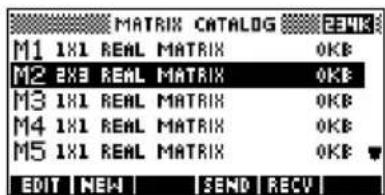
A matrix is listed with two dimensions, even if it is 3 × 1 . A vector is listed with the number of elements, such as 3.
To transmit a matrix
You can send matrices between calculators just as you can send aplets, programs, lists, and notes.
- Align the hp 39g+ calculators' infrared ports.
- Open the Matrix catalogs on both calculators.
-
Highlight the matrix to send.
-
Presso .
-
Press on the receiving calculator.
Working with matrices
To edit a matrix
In the Matrix catalog, highlight the name of the matrix you want to edit and press EDIT
Matrix edit keys
The following table lists the matrix edit key operations.
| Key Meaning | |
| EDIT | Copies the highlighted element to the edit line. |
| INS | Inserts a row of zeros above, or a column of zeros to the left, of the highlighted cell. (You are prompted to choose row or column.) |
| GO | A three-way toggle for cursor advancement in the Matrix editor. GO+ advances to the right, GO↓ advances downward, and GO does not advance at all. |
| BIG | Switches between larger and smaller font sizes. |
| DEL | Deletes the highlighted cells, row, or column (you are prompted to make a choice). |
| SHIFT CLEAR | Clears all elements from the matrix. |
| Key Meaning (Continued) | |
| Moves to the first row, last row, first column, or last column respectively. | |
To display a matrix
- In the Matrix catalog (SHIFT MATRIX), highlight the matrix name and press EDIT
- In HOME, enter the name of the matrix variable and press ENTER.
To display one element
In HOME, enter matrixname(row, column). For example, if M2 is [[3, 4], [5, 6]], then M2(1, 2) ENTER returns 4.
To create a matrix in HOME
-
Enter the matrix in the edit line. Start and end the matrix and each row with square brackets (the shifted 5 and keys).
-
Separate each element and each row with a comma. Example: [[1, 2], [3, 4]].
-
Press to enter and display the matrix.
The left screen below shows the matrix [[2.5,729], [16,2]] being stored into M5. The screen on the right shows the vector [66,33,11] being stored into M6. Note that you can enter an expression (like 5/2) for an element of the matrix, and it will be evaluated.
![[5/2,3^6],[16,2]]M5 [[2.5,729],[16,2]] STO](/content/2026/05/1017618/images/b31018190c97e57d4a572d151294e0ac1d8df61a406677b0372edb283428a5c5.jpg)
![RAD FUNCTION [66,33,11]M6 [66,33,11] STOP](/content/2026/05/1017618/images/517046bd9d7e08654fc01290379592cfd4307de7b00237d9d023ed0cfdf9cfbe.jpg)
To store one element
In HOME, enter, value STOP matrixname(row, column). For example, to change the element in the first row and second column of M5 to 728, then display the resulting matrix:
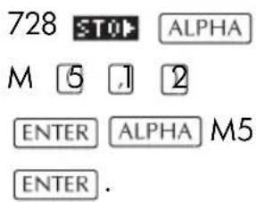
![R&D FUNCTION 728▶M5(1,2) 728 M5 [[2.5,728],[16,2]] STOP](/content/2026/05/1017618/images/978821614b4f52730317623250a376791a2ed4ec769d048130cee2eb6abd0a19.jpg)
An attempt to store an element to a row or column beyond the size of the matrix results in an error message.
Matrix arithmetic
You can use the arithmetic functions (+, -, ×, /) with matrix arguments. Division left-multiplies by the inverse of the divisor. You can enter the matrices themselves or enter the names of stored matrix variables. The matrices can be real or complex.
For the next four examples, store [[1,2],[3,4]] into M1 and [[5,6],[7,8]] into M2.
Example 1. Create the first matrix.
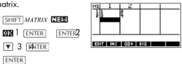
2. Create the second matrix.


- Add the matrices that you created.
HOME ALPHA
+ A12A
ENTER
![RAD FUNCTION M1+M2 M1 [[6,8],[10,12]] STOP](/content/2026/05/1017618/images/9185f8cd32630bac8339605efbdc407761bdbda6246764ad98b098c471a35738.jpg)
To multiply and divide by a scalar
For division by a scalar, enter the matrix first, then the operator, then the scalar. For multiplication, the order of the operands does not matter.
The matrix and the scalar can be real or complex. For example, to divide the result of the previous example by 2, press the following keys:
÷ 2 ENTER
![R&D FUNCTION M1+M2 [[6,8],[10,12]] Ans/2 [[3,4],[5,6]] STOP](/content/2026/05/1017618/images/c8ba7c4896ada63f83405537923ebd3e6dcf12f824edf87f0cc07776fde7ead4.jpg)
To multiply two matrices
To multiply the two matrices M1 and M2 that you created for the previous example, press the following keys:
ALPHA M1 × ALPHA M 2 ENTER
To multiply a matrix by a vector, enter the matrix first, then the vector. The
![ANS/2 [[3,4], [5,6]] M1*M2 [[19,22], [43,50]] STOP](/content/2026/05/1017618/images/aca94d75d21d247525d1889017f7957ae707f41d8001eaabfd2855c98cef3aee.jpg)
number of elements in the vector must equal the number of columns in the matrix.
To divide by a square matrix
For division of a matrix or a vector by a square matrix, the number of rows of the dividend (or the number of elements, if it is a vector) must equal the number of rows in the divisor.
This operation is not a mathematical division: it is a left-multiplication by the inverse of the divisor. M1/M2 is equivalent to M2-1 * M1 .
To divide the two matrices M1 and M2 that you created for the previous example, press the following keys:
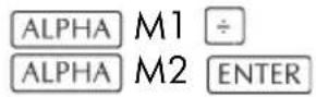
![M1*M2 [[19,22], [43,50]] M1/M2 [[5,4], [-4,-3]] STOP](/content/2026/05/1017618/images/05886e6a0b40fda190040406ab75682c61f098d60510bbaf5c773e9bfb9a953a.jpg)
To invert a matrix
You can invert a square matrix in HOME by typing the matrix (or its variable name) and pressing xHIFT -1 ENTER. Or you can use the matrix INVERSE command. Enter INVERSE(matrixname) in HOME and press ENTER.
To negate each element
You can change the sign of each element in a matrix by pressing before the matrix name.
Solving systems of linear equations
Example Solve the following linear system:
2 x 3 y 4 z + ≠ 5 x + y - z = 7 4 x - y + 2 z = 1
- Open the Matrix catalog and create a vector.
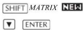

- Create the vector of the constants in the linear system.

- Return to the Matrix Catalog.

In this example, the vector you created is listed as M1.
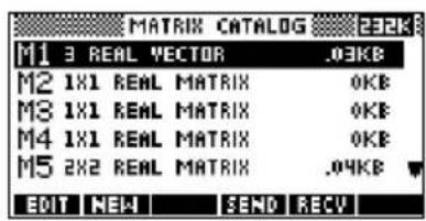
- Create a new matrix.

Select Real matrix

- Enter the equation coefficients.
2 ENTER 3 ENTER
4 ENTER ▼
1 ENTER 1 ENTER
(-) 1 ENTER ENTER4
(-) 1 ENTER 2 ENTER


In this example, the matrix you created is listed as M2.
- Return to HOME and enter the calculation to left-multiply the constants vector by the inverse of the coefficients matrix.

The result is a vector of the solutions:
![RND FUNCTION M2-1*M1 [2,3,-2] STOP](/content/2026/05/1017618/images/3a795878b886d5e773ea623b8f56d792faf993410deb94b94b53601f3276faff.jpg)
- x2 =
• y 3=
• z 2—
An alternative method, is to use the RREF function. See "RREF" on page 13-12.
Matrix functions and commands
About functions
- Functions can be used in any aplet or in HOME. They are listed in the MATH menu under the Matrix category. They can be used in mathematical expressions—primarily in HOME—as well as in programs.
- Functions always produce and display a result. They do not change any stored variables, such as a matrix variable.
- Functions have arguments that are enclosed in parentheses and separated by commas; for example, CROSS(vector1, vector2). The matrix input can be either a matrix variable name (such as M1) or the actual matrix data inside brackets. For example, CROSS(M1, [1, 2]).
About commands Matrix commands are listed in the CMDS menu (CMDS), in the matrix category.
SHIFT
See "Matrix commands" on page 16-23 for details of the matrix commands available for use in programming.
Functions differ from commands in that a function can be used in an expression. Commands cannot be used in an expression.
Argument conventions
- For row# or column#, supply the number of the row (counting from the top, starting with 1) or the number of the column (counting from the left, starting with 1).
- The argument matrix can refer to either a vector or a matrix.
Matrix functions
COLNORM Column Norm. Finds the maximum value (over all columns) of the sums of the absolute values of all elements in a column.
COLNORM(matrix)
COND Condition Number. Finds the 1-norm (column norm) of a square matrix.
COND(matrix)
CROSS Cross Product of vector1 with vector2.
CROSS (vector 1, vector 2)
| DET | Determinant of a square matrix. DET(matrix) |
| DOT | Dot Product of two arrays, matrix1 matrix2. DOT(matrix1, matrix2) |
| EIGENVAL | Displays the eigenvalues in vector form for matrix. EIGENVAL(matrix) |
| EIGENVV | Eigenvectors and Eigenvalues for a square matrix. Displays a list of two arrays. The first contains the eigenvectors and the second contains the eigenvalues. EIGENVV(matrix) |
| IDENMAT Identity matrix. Creates a square matrix of dimension size × size whose diagonal elements are 1 and off-diagonal elements are zero. IDENMAT(size) | |
| INVERSE Inverts a square matrix (real or complex). INVERSE(matrix) | |
| LQ | LQ Factorization. Factors an m × n matrix into three matrices: {{[m × n lowertrapezoidal]],[[n × n orthogonal]], [[m × m permutation]]}. LQ(matrix) |
| LSQ | Least Squares. Displays the minimum norm least squares matrix (or vector). LSQ(matrix1, matrix2) |
| LU | LU Decomposition. Factors a square matrix into three matrices: {{[lowertriangular]],[[uppertriangular]],[[permutation]]} The uppertriangular has ones on its diagonal. LU(matrix) |
| MAKEMAT | Make Matrix. Creates a matrix of dimension rows × columns, using expression to calculate each element. If expression contains the variables I and J, then the |
calculation for each element substitutes the current row number for I and the current column number for J.
MAKEMAT(expression, rows, columns)
Example
MAKEMAT(0,3,3) returns a 3 × 3 zero matrix, [[0,0,0], [0,0,0], [0,0,0]].
QR Factorization. Factors an m × n matrix into three matrices: {{[m×m orthogonal]], [[m×n uppertrapezoidal]], [[n×n permutation]]}.
QR(matrix)
RANK Rank of a rectangular matrix.
RANK(matrix)
ROWNORM Row Norm. Finds the maximum value (over all rows) for the sums of the absolute values of all elements in a row.
ROWNORM(matrix)
RREF Reduced-Row Echelon Form. Changes a rectangular matrix to its reduced row-echelon form.
RREF(matrix)
SCHUR Schur Decomposition. Factors a square matrix into two matrices. If matrix is real, then the result is {{[orthogonal]], [[upper-quasi triangular]]}. If matrix is complex, then the result is {{[unitary]], [[upper-triangular]]}.
SCHUR(matrix)
SIZE Dimensions of matrix. Returned as a list: {rows, columns}.
SIZE(matrix)
SPECNORM Spectral Norm of matrix.
SPECNORM(matrix)
SPECRAD Spectral Radius of a square matrix.
SPECRAD(matrix)
| SVD | Singular Value Decomposition. Factors an m × n matrix into two matrices and a vector: \[[m × m square orthogonal]],[[n × n square orthogonal]],[real]\. SVD(matrix) |
| SVL Singular Values. Returns a vector containing the singular values of matrix. | SVL(matrix) |
| TRACE | Finds the trace of a square matrix. The trace is equal to the sum of the diagonal elements. (It is also equal to the sum of the eigenvalues.)TRACE(matrix) |
| TRN | Transposes matrix. For a complex matrix, TRN finds the conjugate transpose.TRN(matrix) |
Examples
| Identity Matrix | You can create an identity matrix with the IDENMAT function. For example, IDENMAT(2) creates the 2×2 identity matrix [[1,0],[0,1]]. |
| You can also create an identity matrix using the MAKEMAT (make matrix) function. For example, entering MAKEMAT(I1⁄4J,4,4) creates a 4 × 4 matrix showing the numeral 1 for all elements except zeros on the diagonal. The logical operator 1⁄4 returns 0 when I (the row number) and J (the column number) are equal, and returns 1 when they are not equal. | |
| Transposing a Matrix | The TRN function swaps the row-column and column-row elements of a matrix. For instance, element 1,2 (row 1, column 2) is swapped with element 2,1; element 2,3 is swapped with element 3,2; and so on.For example, TRN ([ [1,2], [3,4]]) creates the matrix [[1,3], [2,4]]. |
Reduced-Row Echelon Form
The following set of equations x - 2y + 3z = 14
2 x y z = + 4 x - 2 y + 2 z = 1 4
3
can be written as the augmented matrix
[1 amp; 2 amp; - amp; 3 2 amp; 1 amp; 1 amp; - 4 amp; 2 amp; - amp; 2 ] 1 amp; 4 - 3 1 amp; 4
which can then stored as a 3 × 4 real matrix in any matrix variable. M1 is used in this example.
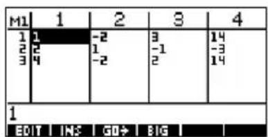
You can use the RREF function to change this to reduced row echelon form, storing it in any matrix variable. M2 is used in this example.
The reduced row echelon matrix gives the solution to the linear equation in the fourth column.
![RMO FUNCTION RREF(M1)▶M2 [[1,0,0,1], [0,1,0,-2]. STOP](/content/2026/05/1017618/images/d01c5756dc08a8ba2946c2473ec0ac3a9dbd30901698f1170bf67009adac159c.jpg)
An advantage of using the

RREF function is that it will also work with inconsistent matrices resulting from systems of equations which have no solution or infinite solutions.
For example, the following set of equations has an infinite number of solutions:
xyz = - + 5 2 x y = 7 x - 2 y + z = 2
The final row of zeros in the reduced-row echelon form of the augmented matrix indicates an inconsistency.
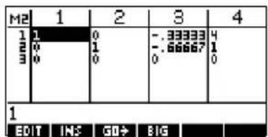
Lists
You can do list operations in HOME and in programs. A list consists of comma-separated real or complex numbers, expressions, or matrices, all enclosed in braces. A list may, for example, contain a sequence of real numbers such as 1, 2, 3 . (If the Decimal Mark mode is set to Comma, then the separators are periods.) Lists represent a convenient way to group related objects.
There are ten list variables available, named L0 to L9. You can use them in calculations or expressions in HOME or in a program. Retrieve the list names from the VARS menu, or just type their names from the keyboard.
You can create, edit, delete, send, and receive named lists in the List catalog (SHIFT LIST). You can also create and store lists—named or unnamed—in HOMEg lists
List variables are identical in behaviour to the columns C1.C0 in the Statistics aplet. You can store a statistics column to a list (or vice versa) and use any of the list functions on the statistics columns, or the statistics functions, on the list variables.
Create a list in the List Catalog
- Open the List catalog.
SHIFT LIST.

- Highlight the list name you want to assing to the new list (L1, etc.) and press EQT display the List editor.
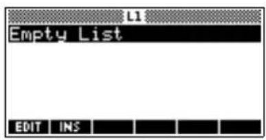
EDIT
- Enter the values you want in the list, pressing after each one.
ENTER
Values can be real or complex numbers (or an expression). If you enter a calculation, it is evaluated and the result is inserted in the list.

- When done, press SHIFT LIST to see the List catalog, or press to return to HOME.
List catalog keys The list catalog keys are:
| Key Meaning | |
| EDIT | Opens the highlighted list for editing. |
| SEND | Transmits the highlighted list to another hp 39g+ or a PC. See “Sending and receiving aplets” on page 17-4 for further information. |
| RECU | Receives a list from another hp 39g+ or a PC. See “Sending and receiving aplets” on page 17-4 for further information. |
| DEL | Clears the highlighted list. |
| SHIFT CLEAR | Clears all lists. |
| SHIFT Or Moves to the end or the beginning of the catalog. | |
List edit keys When you press to create exchange a list, the following keys are available to you:
| Key Meaning | |
| EDIT | Copies the highlighted list item into the edit line. |
| INS | Inserts a new value before the highlighted item. |
| DEL | Deletes the highlighted item from the list. |
| SHIFT CLEAR | Clears all elements from the list. |
| SHIFT ▼ or ▲ | Moves to the end or the beginning of the list. |
Create a list in HOME
-
Enter the list on the edit line. Start and end the list with braces (the shifted and keys) and separate each element with a comma.
-
Press to evaluate and display the list. Immediately after typing in the list, you can store it in a variable by pressing this name. The ENTER list variable names are L0 through L9.
This example stores the list {25,147,8} in L1. Note: You can omit the final brace when entering a list.
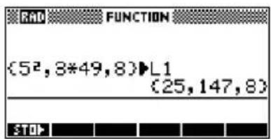
Displaying and editing lists
To display a list
- In the List catalog, highlight the list name and press EDIT.
- In HOME, enter the name of the list and press ENTER.
To display one element
In HOME, enter lastname(element#). For example, if L2 is {3,4,5,6}, then L2(2) ENTER returns 4.
To edit a list 1. Open the List catalog.
SHIFT LIST.

- Press ▲ or ▼ to highlight the name of the list you want to edit (L1, etc.) and press EDIT to display the list contents.
EDIT

- Press ▲ or ▼ to highlight the element you want to edit. In this example, edit the third element so that it has a value of 5.

- Press
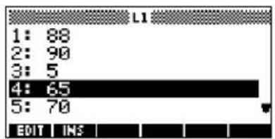
To insert an element in a list
- Open the List catalog.
SHIFT LIST.
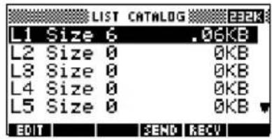
- Press ▲ or ▼ to highlight the name of the list you want to edit (L1, etc.) and press EDIT to display the list contents.

New elements are inserted above the highlighted position. In this example, an element, with the value of 9, is inserted between the first and second elements in the list.
- Press to the insertion position, then press and press 9.

- Press.
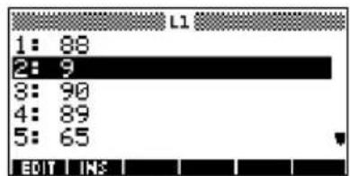
To store one element
In HOME, enter value STOP lastname(element). For example, to store 148 as the second element in L1, type 148 STOP(2) . ENTER
Deleting lists
To delete a list
In the List catalog, highlight the list name and press DEL. You are prompted to confirm that you want to delete the contents of the highlighted list variable. Press toTER delete the contents.
To delete all lists
In the List catalog, press SHIFT CLEAR.
Transmitting lists
You can send lists to calculators or PCs just as you can aplets, programs, matrices, and notes.
- Align the hp 39g+ calculators' infrared ports.
- Open the List catalogs on both calculators.
-
Highlight the list to send.
-
Press
-
Press on the receiving calculator.
List functions
List functions are found in the MATH menu. You can use them in HOME, as well as in programs.
You can type in the name of the function, or you can copy the name of the function from the List category of the MATH menu. Press (the)
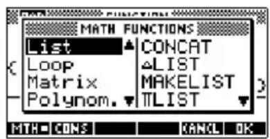
alpha L character key). This
highlights the List category in the left column. Press move the cursor to the right column which contain the List functions, select a function, and press OK
List functions have the following syntax:
- Functions have arguments that are enclosed in parentheses and separated by commas. Example: CONCAT(L1, L2). An argument can be either a list variable name (such as L1) or the actual list. For example, REVERSE( 1, 2, 3 ).
- If Decimal Mark in Modes is set to Comma, use periods to separate arguments. For example, CONCAT (L1.L2).
Common operators like +, -, ×, and / can take lists as arguments. If there are two arguments and both are lists, then the lists must have the same length, since the calculation pairs the elements. If there are two arguments and one is a real number, then the calculation pairs the number with each element of the list.
Example
5*1,2,3 returns 5,10,15 .
Besides the common operators that can take numbers, matrices, or lists as arguments, there are commands that can only operate on lists.
CONCAT Concatenates two lists into a new list.
CONCAT (list1, list2)
Example
CONCAT( 1,2,3,4 ) returns 1,2,3,4 .
ΔLIST
Creates a new list composed of the first differences, that is, the differences between the sequential elements in list1. The new list has one fewer elements than list1. The first differences for x1 x2 ... xn are x2-x1 ... xn-xn-1 .
ΔLIST(list1)
Example
In HOME, store 3,5,8,12,17,23 in L5 and find the first differences for the list.
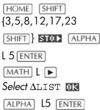
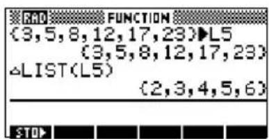
MAKELIST Calculates a sequence of elements for a new list.
Evaluates expression with variable from begin to end values, taken at increment steps.
MAKELIST (expression, variable, begin, end, increment)
The MAKELIST function generates a series by automatically producing a list from the repeated evaluation of an expression.
Example
In HOME, generate a series of squares from 23 to 27.
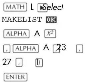

ΠLIST
Calculates the product of all elements in list.
LIST (list)
Example
LIST(2,3,4) returns 24.
POS Returns the position of an element within a list. The
element can be a value, a variable, or an expression. If there is more than one instance of the element, the position of the first occurrence is returned. A value of 0 is returned if there is no occurrence of the specified element.
POS (list, element)
Example
POS ( 3, 7, 12, 19, 12 ) returns 3
REVERSE Creates a list by reversing the order of the elements in a list.
REVERSE (list)
SIZE Calculates the number of elements in a list.
SIZE (list)
Also works with matrices.
ΣLIST Calculates the sum of all elements in list.
ΣLIST (list)
Example
LIST(2,3,4) returns 9.
SORT Sorts elements in ascending order.
SORT (list)
Finding statistical values for list elements
To find values such as the mean, median, maximum, and minimum values of the elements in a list, use the Statistics aplet.
Example In this example, use the Statistics aplet to find the mean,
median, maximum, and minimum values of the elements in the list, L1.
- Create L1 with values 88, 90, 89, 65, 70, and 89.
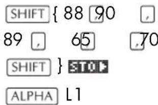
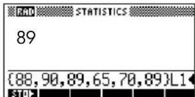
ENTER

- In HOME, store L1 into C1. You will then be able to see the list data in the Numeric view of the Statistics aplet.

- Start the Statistics aplet, and select 1-variable mode (press IF necessary, to display).

Note: Your list values are now in column 1 (C1).
- In the Symbolic view, define H1 (for example) as C1 (sample) and 1 (frequency).

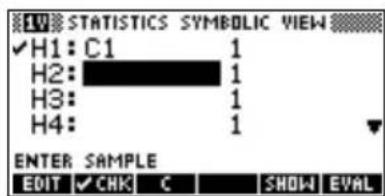
- Go to the Numeric view to display calculated statistics.


See "One-variable" on page 8-13 for the meaning of each computed statistic.
Notes and sketches
Introduction
The hp 39g+ has text and picture editors for entering notes and sketches.
- Each aplet has its own independent Note view and Sketch view. Notes and sketches that you create in these views are associated with the aplet. When you save the aplet, or send it to another calculator, the notes and sketches are saved or sent as well.
- The Notepad is a collection of notes independent of all aplets. These notes can also be sent to another calculator via the Notepad Catalog.
Aplet note view
You can attach text to an aplet in its Note view.
To write a note in Note view
- In an aplet, press NOTE for the Note view.
- Use the note editing keys shown in the table in the following section.
- Set Alpha lock ( )no.2 quick entry of letters. For lowercase Alpha lock, press SHIFT A...2.
- While Alpha lock is on:
- To type a single letter of the opposite case, press SHIFT letter. - To type a single non-alpha character (such as 5 or [ ), press first. (This turns off Alpha lock for one character.)
Your work is automatically saved. Press any view key (NUM, SYMBOL, PLOT, VIEWS) or HOME to exit the Notes view.
Note edit keys
| Key Meaning | |
| SPACE | Space key for text entry. |
| PAGE | Displays next page of a multi-page note. |
| A...2 | Alpha-lock for letter entry. |
| SHIFT A...2 | Lower-case alpha-lock for letter entry. |
| BKSF | Backspaces cursor and deletes character. |
| DEL | Deletes current character. |
| ENTER | Starts a new line. |
| SHIFT CLEAR Erases the entire note. | |
| VARS | Menu for entering variable names, and contents of variables. |
| MATH | Menu for entering math operations, and constants. |
| SHIFT CMDS | Menu for entering program commands. |
| SHIFT CHARS | Displays special characters. To type one, highlight it and press OK. To copy a character without closing the CHARS screen, press ECHO. |
Aplet sketch view
You can attach pictures to an aplet in its Sketch view (SKETCH). Your work is automatically saved with the aplet. Press any other view key or Hot exit the Sketch view
Sketch keys
| Key Meaning | |
| STOP | Stores the specified portion of the current sketch to a graphics variable (G1 through G0). |
| NEWP | Adds a new, blank page to the current sketch set. |
| PAGE | Displays next sketch in the sketch set. Animates if held down. |
| TEXT | Opens the edit line to type a text label. |
| DRAW | Displays the menu-key labels for drawing. |
| DEL | Deletes the current sketch. |
| SHIFT CLEAR | Erases the entire sketch set. |
| - | Toggles menu key labels on and off. If menu key labels are hidden,or any menu key, redisplays the menu key labels. |
To draw a line
- In an aplet, press SHIFT SKETCH for the Sketch view.
- In Sketch view, press [one] move the cursor to where you want to start the line
- Press 📁️ turns on line-drawing.
- Move the cursor in any direction to the end point of the line by pressing the ▲, ▼▶ keys.
- Press to finish the line.
To draw a box 1. In Sketch view, press and move the cursor to where you want any corner of the box to be.
- PressOH .
- Move the cursor to mark the opposite corner for the box. You can adjust the size of the box by moving the cursor.
- Press 7: finish the box.
To draw a circle 1. In Sketch view, press and move the cursor to where you want the center of the circle to be.
- Press This turns on circle drawing.
- Move the cursor the distance of the radius.
- Press to draw the circle.
DRAW keys
| Key Meaning | |
| DOT+ | Dot on. Turns pixels on as the cursor moves. |
| DOT- | Dot off. Turns pixels off as the cursor moves. |
| LINE | Draws a line from the cursor's starting position to the cursor's current position. Press when you have finished. You can draw a line at any angle. |
| BOX | Draws a box from the cursor's starting position to the cursor's current position. Press OK when you have finished. |
| CIRCL | Draws a circle with the cursor's starting position as the center. The radius is the distance between the cursor's starting and ending position. Press OK draw the circle. |
To label parts of a sketch
- Press type the text on the edit line. To lock the Alpha shift on, press up ( uppercase) or
SHIFT A...2
(for lowercase).
To make the label a smaller character size, turn off BIG before pressing A.2s a3 toggle between small and large font size). The smaller character size cannot display lowercase letters.
-
Press
-
Position the label where you want it by pressing the ▲, ▼, ▶ keys.
-
Press again to affix the label.
-
Press OFAL to continue drawing, or press HOME to exit the Sketch view.

To create a set of sketches
You can create a set of up to ten sketches. This allows for simple animation.
- After making a sketch, press NEWF to add a new, blank page. You can now make a new sketch, which becomes part of the current set of sketches.
- To view the next sketch in an existing set, press FAGE. Hold FAGE down for animation.
- To remove the current page in the current sketch series, press DEL.
To store into a graphics variable
You can define a portion of a sketch inside a box, and then store that graphic into a graphics variable.
- In the Sketch view, display the sketch you want to copy (store into a variable).
- Press
- Highlight the variable name you want to use and press OK.
- Draw a box around the portion you want to copy: move the cursor to one corner, press OK then move the cursor to the opposite corner, and press OK
To import a graphics variable
You can copy the contents of a graphics variable into the Sketch view of an aplet.
- Open the Sketch view of the aplet (SHIFT SKETCH). The graphic will be copied here.
- Press HOME
- Highlight Graphic, then press and highlight the name of the variable (G1, etc.).
- Press to recol the contents of the graphics variable.
- Move the box to where you would like to copy the graphic, then press OK
The notepad
Subject to available memory, you can store as many notes as you want in the Notepad (SHIFT NOTEPAD). These notes are independent of any aplet. The Notepad catalog lists the existing entries by name. It does not include notes that were created in aplets' Note views, but these can be imported. See "To import a note" on page 15-8.
To create a note in the Notepad
- Display the Notepad catalog.
SHIFT NOTEPAD
- Create a new note.
NEW

- Enter a name for your note.
A...2 MYNOTE OK
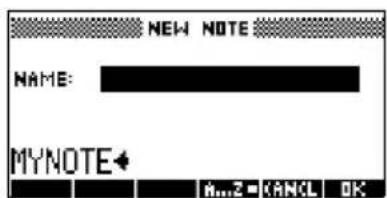
- Write your note.
See "Note edit keys" on page 15-2 for more information on the entry and editing of notes.

- When you are finished, press or am aplet key to exit Notepad. Your work is automatically saved.
Notepad Catalog keys
| Key Meaning | |
| EDIT | Opens the selected note for editing. |
| NEW | Begins a new note, and asks for a name. |
| SEND | Transmits the selected note to another hp 39g+ or PC. |
| RECU | Receives a note being transmitted from another hp 39g+ or PC. |
| DEL | Deletes the selected note. |
| SHIFT CLEAR Deletes | all notes in the catalog. |
To import a note You can import a note from the Notepad into an aplet's
Note view, and vice versa. Suppose you want to copy a note named "Assignments" from the Notepad into the Function Note view:
-
In the Function aplet, display the Note view (SHIFT NOTE).
-
Press HOME, highlight Notepad in the column, then highlight the name "Assignments" in the right column.
-
Press Ufclcopy: the contents of "Assignments" to the Function Note view.
Note: To recall the name instead of the contents, press HOME instead of .
Suppose you want to copy the Note view from the current aplet into the note, Assignments, in the Notepad.
-
In the Notepad (SHIFT NOTEPAD), open the note, "Assignments".
-
Press VARS AFLET, highlight Note in the left column, then press ▶ and highlight NoteText in the right column.
-
Press uricureck the contents of the Note view into the note "Assignments".
Programming
Introduction
| This chapter describes how to program using the hp 39g+. In this chapter you'll learn about:using the Program catalog to create and edit programsprogramming commandsstoring and retrieving variables in programsprogramming variables. | |
| HINT | More information on programming, including examples and special tools, can be found at HP's calculators web site:http://www.hp.com/calculators |
| The Contents of a Program | An hp 39g+ program contains a sequence of numbers, mathematical expressions, and commands that execute automatically to perform a task.These items are separated by a colon ( : ). Commands that take multiple arguments have those arguments separated by a semicolon ( ; ). For example,PIXON xposition; yposition: |
| Structured Programming | Inside a program you can use branching structures to control the execution flow. You can take advantage of structured programming by creating building-block programs. Each building-block program stands alone—and it can be called from other programs. Note:If a program has a space in its name then you have to put quotes around it when you want to run it. |
Example RUN GETVALUE: RUN CALCULATE: RUN
"SHOW ANSWER":
This program is separated into three main tasks, each an individual program. Within each program, the task can be simple—or it can be divided further into other programs that perform smaller tasks.
Program catalog
The Program catalog is where you create, edit, delete, send, receive, or run programs. This section describes how to
- open the Program catalog
- create a new program
- enter commands from the program commands menu
- enter functions from the MATH menu
- edit a program
- run and debug a program
- stop a program
- copy a program
- send and receive a program
- delete a program or its contents
- customize an aplet.
Open Program Catalog
1. Press PROGRAM.
The Program Catalog displays a list of program names. The Program Catalog contains a built-in entry called Editline.
Editline contains the last expression that you entered from the edit line in HOME, or the last data
you entered in an input form. (If you press ENTER from HOME without entering any data, the hp 39g+ runs the contents of Editline.)
Before starting to work with programs, you should take a few minutes to become familiar with the Program catalog menu keys. You can use any of the following keys (both menu and keyboard), to perform tasks in the Program catalog.
Program catalog keys
The program catalog keys are:
| Key Meaning | |
| EDIT | Opens the highlighted program for editing. |
| NEW | Prompts for a new program name, then opens an empty program. |
| SEND | Transmits the highlighted program to another hp 39g+ or to a disk drive. |
| RECU | Receives the highlighted program from another hp 39g+ or from a disk drive. |
| RUN | Runs the highlighted program. |
| SHIFT ▲ Moves to the beginning or end of the Program catalog.▼ | Deletes the highlighted program. |
| DEL | Deletes the highlighted program. |
| SHIFT CLEAR Deletes all programs in the program catalog. | |
Creating and editing programs
Create a new program
-
Press PROGRAM to open the Program catalog.
-
Press
The hp 39g+ prompts you for a name.
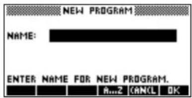
A program name can contain special characters, such as a space. However, if you use special characters and then run the program by typing it in HOME, you must enclose the program name in double quotes (""). Don't use the "symbol within your program name.
- Type your program name, then press OK When you press OK the Program Editor opens.

- Enter your program. When done, start any other activity. Your work is saved automatically.
Enter commands Until you become familiar with the hp 39g+ commands, the easiest way to enter commands is to select them from the Commands menu from the Program editor. You can also type in commands using alpha characters.
- From the Program editor, press SHIFT CMDS to open the Program Commands menu.
SHIFT CMDS

- On the left, use or to highlight a command category, then press to access the commands in the category. Select the command that you want.


- Press to paste the command into the program editor.

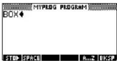
Edit a program
- Press SHIFT PROGRAM to open the Program catalog.

- Use the arrow keys to highlight the program you want to edit, and press The hp 39g+ opens the Program Editor. The name of your program appears in the title bar of the display. You can use the following keys to edit your program.
Editing keys The editing keys are:
| Key Meaning | |
| STOP | Inserts the character at the editing point. |
| SPACE | Inserts space into text. |
| PAGE | Displays previous page of the program. |
| PAGE | Displays next page of the program. |
| ▲ ▼ | Moves up or down one line. |
| ▶ ▶ | Moves right or left one character. |
| A...Z | Alpha-lock for letter entry. Press SHIFT A...Z to lock lower case. |
| BKSF | Backspaces cursor and deletes character. |
| DEL | Deletes current character. |
| ENTER | Starts a new line. |
| SHIFT CLEAR Erases the entire program. | |
| VARS Displays menus for selecting variable names, contents of variables, math functions, and program constants. | |
| MATH | |
| SHIFT CMDS Displays menus for selecting program commands. | |
| SHIFT CHARS Displays all characters. To type one, highlight it and press OK To enter several characters in a row, use the menu key while in the CHARS menu. | |
Using programs
Run a program
From HOME, type RUN program_name.
or
From the Program catalog, highlight the program you want to run and press RUN
Regardless of where you start the program, all programs run in HOME. What you see will differ slightly depending on where you started the program. If you start the program from HOME, the hp 39g+ displays the contents of Ans (Home variable containing the last result), when the program has finished. If you start the program from the Program catalog, the hp39g+ returns you to the Program catalog when the program ends.
Debug a program
If you run a program that contains errors, the program will stop and you will see an error message.

To debug the program:
- Press to edit the program.
The insert cursor appears in the program at the point where the error occurred.
- Edit the program to fix the error.
- Run the program.
- Repeat the process until you correct all errors.
Stop a program
You can stop the running of a program at any time by pressing CANCEL (the ON key). Note: You may have to press it a couple of times.
Copy a program You can use the following procedure if you want to make a copy of your work before editing—or if you want to use one program as a template for another.
- Press SHIFT PROGRM to open the Program catalog.
- Press
- Type a new file name, then choose OK The Program Editor opens with a new program.
- Press to open the variables menu.
- Press to quickly scroll to Program.
- Press , then highlight the program you want to copy.
- Press, then press.
The contents of the highlighted program are copied into the current program at the cursor location.
HINT If you use a programming routine often, save the routine under a different program name, then use the above method to copy it into your programs.
Transmit a program
You can send programs to, and receive programs from, other calculators just as you can send and receive aplets, matrices, lists, and notes.
After aligning the calculators' infrared ports, open the Program catalogs on both calculators. Highlight the program to send, then press SEND on the sending calculator and RECU on the receiving calculator.
You can also send programs to, and receive programs from, a remote storage device (aplet disk drive or computer). This takes place via a cable connection and requires an aplet disk drive or specialized software running on a PC (such as a connectivity kit).
Delete a program
To delete a program:
- Press PROGRAM to open the Program catalog.
- Highlight a program to delete, then press .DEL
Delete all programs
You can delete all programs at once.
- In the Program catalog, press SHIFT CLEAR.
- Press
Delete the contents of a program
You can clear the contents of a program without deleting the program name.
- Press SHIFT PROGRAM to open the Program catalog.
- Highlight a program, then press EDIT
- Press SHIFT CLEAR, then press WES
- The contents of the program are deleted, but the program name remains.
Customizing an aplet
You can customize an aplet and develop a set of programs to work with the aplet.
Use the SETVIEWS command to create a custom VIEWS menu which links specially written programs to the new aplet.
A useful method for customizing an aplet is illustrated below:
- Decide on the built-in aplet that you want to customize. For example you could customize the Function aplet or the Statistics aplet. The customized aplet inherits all the properties of the built-in aplet. Save the customized aplet with a unique name.
- Customize the new aplet if you need to, for example by presetting axes or angle measures.
-
Develop the programs to work with your customized aplet. When you develop the aplet's programs, use the standard aplet naming convention. This allows you to keep track of the programs in the Program catalog that belong to each aplet. See "Aplet naming convention" on page 16-10.
-
Develop a program that uses the SETVIEWS command to modify the aplet's VIEWS menu. The menu options provide links to associated programs. You can specify any other programs that you want transferred with the aplet. See "SETVIEWS" on page 16-14 for information on the command.
-
Ensure that the customized aplet is selected, then run the menu configuration program to configure the aplet's VIEWS menu.
-
Test the customized aplet and debug the associated programs. (Refer to "Debug a program" on page 16-7).
Aplet naming convention
To assist users in keeping track of aplets and associated programs, use the following naming convention when setting up an aplet's programs:
- Start all program names with an abbreviation of the aplet name. We will use APL in this example.
- Name programs called by menu entries in the VIEWS menu number, after the entry, for example:
- APL.ME1 for the program called by menu option 1
- APL.ME2 for the program called by menu option 2
- Name the program that configures the new VIEWS menu option APL.SV where SV stands for SETVIEWS.
For example, a customized aplet called "Differentiation" might call programs called DIFF.ME1, DIFF.ME2, and DIFF.SV.
Example
This example aplet is designed to demonstrate the process of customizing an aplet. The new aplet is based on the Function aplet. Note: This aplet is not intended to serve a serious use, merely to illustrate the process.
Save the aplet 1. Open the Function aplet and save it as
"EXPERIMENT". The new aplet appears in the Aplet library.
APLET Select
Function SAVE
ALPHA EXPERIMENT
013
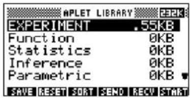
-
Create a program called EXP.ME1 with contents as shown. This program configures the plot ranges, then runs a program that allows you to set the angle format.
-
Create a program called EXP.ME2 with contents as shown. This program sets the numeric view options for the aplet, and runs the program that you can mode.
-
Create a program called EXP.ANG which the previous two programs call.
-
Create a program called EXP.S which runs when you start the aplet, as shown. This program sets the angle mode to degrees, and


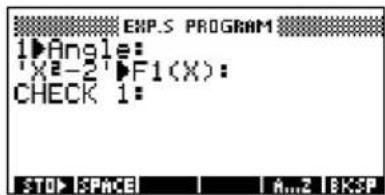
sets up the initial function that the aplet plots.
Configuring the Setviews menu option programs
In this section we will begin by configuring the VIEWS menu by using the SETVIEWS command. We will then create the "helper" programs called by the VIEWS menu which will do the actual work.
- Open the Program catalog and create a program named "EXP.SV". Include the following code in the program.
Each entry line after the command SETVIEWS is a trio that consists of a VIEWS menu text line (a space indicates none), a program
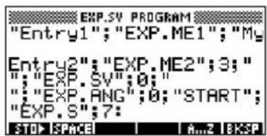
name, and a number that defines the view to go to after the program has run its course. All programs listed here will transfer with an aplet when the aplet is transferred.
SETVIEWS '' '' ; '' '' ; 18;
Sets the first menu option to be "Auto scale". This is the fourth standard Function aplet view menu option and the 18 "Auto scale", specifies that it is to be included in the new menu. The empty quotes will ensure that the old name of "Auto scale" appears on the new menu. See "SETVIEWS" on page 16-14.
'' My Entry1'';'' EXP.ME1'';1;
Sets the second menu option. This option runs program EXP.ME1, then returns to view 1, Plot view.
'' My Entry2'';'' EXP.ME2'';3;
Sets the third menu option. This option runs the program EXP.ME2, then returns to view 3, the NUM view.
' ' ' ' ; '' EXP.SV' ' ; 0 ;
This line specifies that the program to set the View menu (this program) is transferred with the aplet. The space character between the first set of quotes in the trio specifies that no menu option appears for the entry. You do not need to transfer this program with the aplet, but it allows users to modify the aplet's menu if they want to.
' ' ' ' ; '' EXP.ANG' ' ; 0 ;
The program EXP.ANG is a small routine that is called by other programs that the aplet uses. This entry specifies that the program EXP.ANG is transferred when the aplet is transferred, but the space in the first quotes ensures that no entry appears on the menu.
' ' START' '; '' EXP.S''; 7:
This specifies the Start menu option. The program that is associated with this entry, EXP.S, runs automatically when you start the aplet. Because this menu option specifies view 7, the VIEWS menu opens when you start the aplet.
You only need to run this program once to configure your aplet's VIEWS menu. Once the aplet's VIEWS menu is configured, it remains that way until you run SETVIEWS again.
You do not need to include this program for your aplet to work, but it is useful to specify that the program is attached to the aplet, and transmitted when the aplet is transmitted.
- Return to the program catalog. The programs that you created should appear as follows:

-
You must now the EDIT NEW I SEND RECY RUN program EXP.SV to execute the SETVIEWS command and create the modified VIEWS menu. Check that the name of the new aplet is highlighted in the Aplet view.
-
You can now return to the Aplet library and press START to run your new aplet.
Programming commands
This section describes the commands for programming with hp 39g+. You can enter these commands in your program by typing them or by accessing them from the Commands menu.
Aplet commands
CHECK
Checks (selects) the corresponding function in the current aplet. For example, Check 3 would check F3 if the current aplet is Function. Then a checkmark would appear next to F3 in Symbolic view, F3 would be plotted in Plot view, and evaluated in Numeric view.
CHECK n:
SELECT
Selects the named aplet and makes it the current aplet. Note: Quotes are needed if the name contains spaces or other special characters.
SELECT apletname:
SETVIEWS The SETVIEWS command is used to define entries in the
VIEWS menu for aplets that you customize. See "Customizing an aplet" on page 16-9 for an example of using the SETVIEWS command.
When you use the SETVIEWS command, the aplet's standard VIEWS menu is deleted and the customized menu is used in its place. You only need to apply the command to an aplet once. The VIEWS menu changes remain unless you apply the command again.
Typically, you develop a program that uses the SETVIEWS command only. The command contains a trio of arguments for each menu option to create, or program to attach. Keep the following points in mind when using this command:
- The SETVIEWS command deletes an aplet's standard Views menu options. If you want to use any of the standard options on your reconfigured VIEWS menu, you must include them in the configuration.
- When you invoke the SETVIEWS command, the changes to an aplet's VIEWS menu remain with the aplet. You need to invoke the command on the aplet again to change the VIEWS menu.
- All the programs that are called from the VIEWS menu are transferred when the aplet is transferred, for example to another calculator or to a PC.
- As part of the VIEWS menu configuration, you can specify programs that you want transferred with the aplet, but are not called as menu options. For example, these can be sub-programs that menu
options use, or the program that defines the aplet's VIEWS menu.
- You can include a "Start" option in the VIEWS menu to specify a program that you want to run automatically when the aplet starts. This program typically sets up the aplet's initial configuration. The START option on the menu is also useful for resetting the aplet.
Command syntax
The syntax for the command is as follows:
SETVIEWS
"Prompt1"; "ProgramName1"; ViewNumber1;
"Prompt2"; "ProgramName2"; ViewNumber2:
(You can repeat as many Prompt/ProgramName/
ViewNumber trios of arguments as you like.)
Within each Prompt/ProgramName/ViewNumber trio, you separate each item with a semi-colon.
Prompt
Prompt is the text that is displayed for the corresponding entry in the Views menu. Enclose the prompt text in double quotes.
Associating programs with your aplet
If Prompt consists of a single space, then no entry appears in the view menu. The program specified in the ProgramName item is associated with the aplet and transferred whenever the aplet is transmitted. Typically, you do this if you want to transfer the Setviews program with the aplet, or you want to transfer a sub-program that other menu programs use.
Auto-run programs
If the Prompt item is "Start", then the ProgramName program runs whenever you start the aplet. This is useful for setting up a program to configure the aplet. Users can select the Start item from the VIEWS menu to reset the aplet if they change configurations.
You can also define a menu item called "Reset" which is auto-run if the user chooses the button in the APLET view.
ProgramName
ProgramName is the name of the program that runs when the corresponding menu entry is selected. All programs that are identified in the aplet's SETVIEWS command are transferred when the aplet is transmitted.
ViewNumber
ViewNumber is the number of a view to start after the program finishes running. For example, if you want the menu option to display the Plot view when the associated program finishes, you would specify 1 as the ViewNumber value.
Including standard menu options
To include one of an aplet's standard VIEWS menu options in your customized menu, set up the arguments trio as follows:
- The first argument specifies the menu item name:
– Leave the argument empty to use the standard Views menu name for the item, or
- Enter a menu item name to replace the standard name.
- The second argument specifies the program to run:
- Leave the argument empty to run the standard menu option.
- Insert a program name to run the program before the standard menu option is selected.
- The third argument specifies the view and the menu number for the item. Determine the menu number from the View numbers table below.
Note: SETVIEWS with no arguments resets the views to default of the base aplet.
View numbers
The Function aplet views are numbered as follows:
| 0 | HOME | 11 | List Catalog |
| 1 | Plot | 12 | Matrix Catalog |
| 2 | Symbolic | 13 | Notepad Catalog |
| 3 | Numeric | 14 | Program Catalog |
| 4 | Plot-Setup | 15 | Plot-Detail |
| 5 | Symbolic-Setup | 16 | Plot-Table |
| 6 | Numeric-Setup | 17 | Overlay Plot |
| 7 | Views | 18 | Auto scale |
| 8 | Note | 19 | Decimal |
| 9 | Sketch view | 20 | Integer |
| 10 | Aplet Catalog | 21 | Trig |
UNCHECK Unchecks (unselects) the corresponding function in the current aplet. For example, Uncheck 3 would uncheck F3 if the current aplet is Function.
UNCHECK n:
Branch commands
Branch commands let a program make a decision based on the result of one or more tests. Unlike the other programming commands, the branch commands work in logical groups. Therefore, the commands are described together rather than each independently.
IF...THEN...END
Executes a sequence of commands in the true-clause only if the test-clause evaluates to true. Its syntax is:
IF test-clause
THEN true-clause END
Example
1▶A : IF A==1 THEN MSGBOX " A EQUALS 1" : END
IF... THEN... ELSE... END
Executes the true-clause sequence of commands if the test-clause is true, or the false-clause sequence of commands if the test-clause is false.
IF test-clause
THEN true-clause ELSE false-clause END
Example
1▶A :
IF A==1
    THEN MSGBOX "A EQUALS 1" :
    ELSE MSGBOX "A IS NOT EQUAL TO 1" :
END
CASE...END Executes a series of test-clause commands that execute the appropriate true-clause sequence of commands. Its syntax is:
CASE IF test-clause 1 THEN true-clause 1 END IF test-clause 2 THEN true-clause 2 END . . . IF test-clause n THEN true-clause n END END
When CASE is executed, test-clause1 is evaluated. If the test is true, true-clause1 is executed, and execution skips to END. If test-clause1 if false, execution proceeds to test-clause2 . Execution with the CASE structure continues until a true-clause is executed (or until all the test-clauses evaluate to false).
IFERR... THEN... END...
Many conditions are automatically recognized by the hp 39g+ as error conditions and are automatically treated as errors in programs.
IFERR...THEN...END allows a program to intercept error conditions that otherwise would cause the program to abort. Its syntax is:
IFERR trap-clause THEN error-clause END
RUN Runs the named program. If your program name contains
special characters, such as a space, then you must enclose the file name in double quotes ("").
RUN "program name": or RUN programname:
STOP Stops the current program.
STOP:
Drawing commands
The drawing commands act on the display. The scale of the display depends on the current aplet's Xmin, Xmax, Ymin, and Ymax values. The following examples assume the hp 39g+ default settings with the Function aplet as the current aplet.
ARC
Draws a circular arc, of given radians, whose centre is at (x,y) . The arc is drawn from start_angle_measurement, and end_angle_measurement.
ARC x;y;radius;start_angle_measurement; end_angle_measurement:
Example
ARC 0;0;2;0;360:
FREEZE:
Draws a circle centered at (0,0) of radius 2. The
FREEZE command causes the circle to
remain displayed on the screen until you press a key.
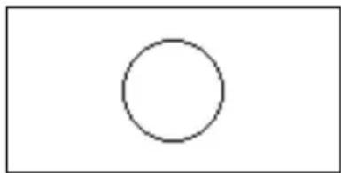
BOX
Draws a box with diagonally opposite corners (x1,y1) and (x2,y2) .
BOX x1; y1; x2; y2:
Example
BOX -1; -1; 1; 1:
FREEZE:
Draws a box, lower corner at (-1,-1) , upper corner at (1,1)
ERASE Clears the display
ERASE:
FREEZE
Halts the program, freezing the current display. Execution resumes when any key is pressed.
LINE
Draws a line from (x1, y1) to (x2, y2) .
LINE x1;y1;x2;y2:
PIXOFF
Turns off the pixel at the specified coordinates (x,y) .
PIXOFF x;y:
PIXON
Turns on the pixel at the specified coordinates (x,y) .
PIXON x;y:
TLINE
Toggles the pixels along the line from (x1, y1) to (x2, y2) on and off. Any pixel that was turned off, is turned on; any pixel that was turned on, is turned off. TLINE can be used to erase a line.
TLINE x1;y1;x2;y2:
Example
TLINE 0;0;3;3:
Erases previously drawn 45 degree line from (0,0) to (3,3), or draws that line if it doesn't already exist.
Graphic commands
The graphic commands use the graphics variables G0 through G9—or the Page variable from Sketch—as graphicname arguments. The position argument takes the form (x, y). Position coordinates depend on the current aplet's scale, which is specified by Xmin, Xmax, Ymin, and Ymax. The upper left corner of the target graphic (graphic2) is at (Xmin, Ymax).
You can capture the current display and store it in G0 by simultaneously pressing ON PLOT
DISPLAY→
Stores the current display in graphicname.
DISPLAY→ graphicname:
| →DISPLAY | Displays graphic from graphicname in the display.→DISPLAY graphicname: |
| →GROB | Creates a graphic from expression, using font_size, and stores the resulting graphic in graphicname. Font sizes are 1, 2, or 3. If the fontsize argument is 0, the hp 39g+ creates a graphic display like that created by the SHOW operation.→GROB graphicname; expression; fontsize: |
| GROBNOT | Replaces graphic in graphicname with bitwise-inverted graphic.GROBNOT graphicname: |
| GROBOR | Using the logical OR, superimposes graphicname2 onto graphicname1. The upper left corner of graphicname2 is placed at position.GROBOR graphicname1; position; graphicname2: |
| GROBXOR | Using the logical XOR, superimposes graphicname2 onto graphicname1. The upper left corner of graphicname2 is placed at position.GROBXOR graphicname1; position; graphicname2: |
| MAKEGROB Creates graphic with given width, height, and hexadecimal data, and stores it in graphicname.MAKEGROB graphicname; width; height; hexdata: | |
| PLOT→ | Stores the Plot view display as a graphic in graphicname.PLOT→graphicname: |
| PLOT→and DISPLAY→can be used to transfer a copy of the current PLOT view into the sketch view of the aplet for later use and editing.Example1 ▶PageNum:PLOT→Page:FREEZE:This program stores the current PLOT view to the first page in the sketch view of the current aplet and then displays the sketch as a graphic object until any key is pressed. | |
→PLOT
Puts graph from graphicname into the Plot view display.
→PLOT graphicname :
REPLACE
Replaces portion of graphic in graphicname1 with graphicname2, starting at position. REPLACE also works for lists and matrices.
REPLACE
Extracts a portion of the named graphic (or list or matrix), and stores it in a new variable, name. The portion is specified by position and positions.
Creates a blank graphic with given width and height, and stores it in graphicname.
ZEROGROB graphicname ; width ; height :
Loop commands
Loop hp allow a program to execute a routine repeatedly. The hp 39g+ has three loop structures. The example programs below illustrate each of these structures incrementing the variable A from 1 to 12.
DO...UNTIL ...END
Do ... Until ... End is a loop command that executes the loop-clause repeatedly until test-clause returns a true (nonzero) result. Because the test is executed after the loop-clause, the loop-clause is always executed at least once. Its syntax is:
DO loop-clause UNTIL test-clause END
1 ▶ A:
DO A + 1 ▶ A
UNTIL A == 12
END
WHILE... REPEAT... END
While ... Repeat ... End is a loop command that repeatedly evaluates test-clause and executes loop-clause sequence if the test is true. Because the test-clause is executed before the loop-clause, the loop-clause is not executed if the test is initially false. Its syntax is:
WHILE test-clause REPEAT loop-clause END
1 ▶ A:
WHILE A < 12
REPEAT A+1 ▶ A
END
FOR...TO...STEP ...END
FOR name=start-expression TO end-expression
[STEP increment];
loop-clause END
FOR A=1 TO 12 STEP 1;
DISP 3;A:
END
Note that the STEP parameter is optional. If it is omitted, a step value of 1 is assumed.
BREAK Terminates loop.
BREAK:
Matrix commands
The matrix commands take variables M0–M9 as arguments.
ADDCOL
Add Column. Inserts values into a column before column_number in the specified matrix. You enter the values as a vector. The values must be separated by commas and the number of values must be the same as the number of rows in the matrix name.
ADDCOL
name; [value 1,...,value n ]; column_number:
ADDROW
Add Row. Inserts values into a row before row_number in the specified matrix. You enter the values as a vector. The values must be separated by commas and the number of values must be the same as the number of columns in the matrix name.
ADDROW name; [value 1,..., value_n]; row_number:
DELCOL Delete Column. Deletes the specified column from the specified matrix.
DELCOL name;column_number:
DELROW Delete Row. Deletes the specified row from the specified matrix.
DELROW name; row_number:
EDITMAT Starts the Matrix Editor and displays the specified matrix. If used in programming, returns to the program when user presses OK.
EDITMAT name:
RANDMAT Creates random matrix with a specified number of rows and columns and stores the result in name (name must be M0...M9). The entries will be integers ranging from -9 to 9.
RANDMAT name ; rows ; columns :
REDIM Redimensions the specified matrix or vector to size. For a matrix, size is a list of two integers n1,n2 . For a vector, size is a list containing one integer n .
REDIM name ; size :
REPLACE Replaces portion of a matrix or vector stored in name with an object starting at position start. start for a matrix is a list containing two numbers; for a vector, it is a single number. Replace also works with lists and graphics.
SCALEADD Multiplies the row of the matrix name by value, then adds this result to the second specified row.
SCALEADD name ; value ; row1 ; row2 :
SUB
Extracts a sub-object—a portion of a list, matrix, or graphic from object—and stores it into name. start and end are each specified using a list with two numbers for a matrix, a number for vector or lists, or an ordered pair, (X, Y), for graphics.
Swap Rows. Exchanges row1 and row2 in the specified matrix.
SWAPROW name; row1; row2:
Print commands
These commands print to an HP infrared printer, for example the HP 82240B printer.
PRDISPLAY Prints the contents of the display.
PRDISPLAY:
PRHISTORY Prints all objects in the history.
PRHISTORY:
PRVAR
Prints name and contents of variablename.
PRVAR variablename:
You can also use the PRVAR command to print the contents of a program or a note.
PRVAR programname; PROG:
PRVAR notename; NOTE:
Prompt commands
BEEP
Beeps at the frequency and for the time you specify.
BEEP frequency ; seconds :
CHOOSE
Creates a choose box, which is a box containing a list of options from which the user chooses one. Each option is numbered, 1 through n. The result of the choose command is to store the number of the option chosen in a variable. The syntax is
CHOOSE default_option_number; title; option1;
option 2 ; ...option n :
where default_option_number is the number of the option that will be highlighted by default whenever the choose box is displayed, title is the text displayed in the title bar of the choose box, and option1...optionn are the options listed in the choose box.
Example
3 ▶ A: CHOOSE A;
"COMIC STRIPS";
"DILBERT";
"CALVIN&HOBBES";
"BLONDIE":

DISP
Displays textitem in a row of the display at the line_number. A text item consists of any number of expressions and quoted strings of text. The expressions are evaluated and turned into strings. Lines are numbered from the top of the screen, 1 being the top and 7 being the bottom.
DISP line_number; textitem:
Example
DISP 3; "A is" 2+2
Result: A is 4
(displayed on line 3)
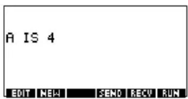
DISPTIME Displays the current date and time.
DISPTIME
To set the date and time, simply store the correct settings in the date and time variables. Use the following formats: M.DDYYYY for the date and H.MMSS for the time.
Examples
5.152000▶ DATE (sets the date to May 15, 2000).
10.1500▶ TIME (sets the time to 10:15 am).
EDITMAT Matrix Editor. Opens the Matrix editor for the specified matrix. Returns to the program when user presses OK
EDITMAT matrixname:
The EDITMAT command can also be used to create matrices.
-
Press SHIFT CMDS ) ▶ SIN OK
-
Press M Al, and then press . ENTER
The Matrix catalog opens with M1 available for editing.
EDITMAT matrixname is a shortcut to opening the matrix editor with matrixname.
FREEZE This command prevents the display from being updated after the program runs. This allows you to view the graphics created by the program. Cancel FREEZE by pressing any key.
FREEZE:
GETKEY Waits for a key, then stores the keycode rc.p in name, where r is row number, c is column number, and p is key-plane number. The key-planes numbers are: 1 for unshifted; 2 for shifted; 4 for alpha-shifted; and 5 for both alpha-shifted and shifted.
GETKEY name:
INPUT Creates an input form with a title bar and one field. The field has a label and a default value. There is text help at the bottom of the form. The user enters a value and presses the menu key. The value that the user enters is stored in the variable name. The title, label, and help items are text strings and need to be enclosed in double quotes.
Use SHIFT CHARS to type the quote marks " ".
INPUT name ; title , label ; help ; default :
Example
INPUT R; "Circular Area"; "Radius"; "Enter Number";1:
MSGBOX
Displays a message box containing textitem. A text item consists of any number of expressions and quoted strings of text. The expressions are evaluated and turned into strings of text.
For example, "AREA IS:" 2 + 2 becomes AREA IS: 4. Use CHARs to type the quote marks " ".
MSGBOX textitem:
Example
1 ▶ A: MSGBOX "AREA IS: "π*A^2:
You can also use the NoteText variable to provide text arguments. This can be used to insert line breaks. For example, press SHIFT NOTE and type AREA IS ENTER.
The position line
MSGBOX NoteText " " π*A^2:
will display the same message box as the previous example.
PROMPT
Displays an input box with name as the title, and prompts for a value for name. name can only be one character in length.
PROMPT name:
WAIT
Halts program execution for the specified number of seconds.
WAIT seconds:
Stat-One and Stat-Two commands
The following commands are used for analyzing one-variable and two-variable statistical data.
Stat-One commands
DO1VSTATS
Calculates STATS using datasetname and stores the results in the corresponding variables: NΣ, TotΣ, MeanΣ, PVarΣ, SVarΣ, PSDev, SSDev, MinΣ, Q1, Median, Q3, and MaxΣ. Datasetname can be H1, H2, ..., or H5. Datasetname must include at least two data points.
DO1VSTATS datasetname:
SETFREQ
Sets datasetname frequency according to column or value. Datasetname can be H1, H2,..., or H5, column can be C0–C9 and value can be any positive integer.
SETFREQ datasetname ; column :
or
SETFREQ definition ; value :
SETSAMPLE
Sets datasetname sample according to column. Datasetname can be H1–H5, and column can be CO–C9.
SETSAMPLE datasetname; column:
Stat-Two commands
DO2VSTATS
Calculates STATS using datasetname and stores the results in corresponding variables: MeanX, ΣX, ΣX2, MeanY, ΣY, ΣY2, ΣXY, Corr, PCov, SCov, and RELERR. Datasetname can be SI, S2,..., or S5. Datasetname must include at least two pairs of data points.
DO2VSTATS datasetname:
SETDEPEND
Sets datasetname dependent column. Datasetname can be S1, S2, ..., or S5 and column can be C0–C9.
SETDEPEND datasetname; column:
SETINDEP
Sets datasetname independent column. Datasetname can be S1, S2,..., or S5 and column can be C0–C9.
SETINDEP datasetname; column:
Storing and retrieving variables in programs
The hp 39g+ has both Home variables and Aplet variables. Home variables are used for real numbers, complex numbers, graphics, lists, and matrices. Home variables keep the same values in HOME and in aplets.
Aplet variables are those whose values depend on the current aplet. The aplet variables are used in programming to emulate the definitions and settings you make when working with aplets interactively.
You use the Variable menu ( ) to retrieve either Home variables or aplet variables. See "The VARS menu" on page 12-4. Not all variables are available in every aplet. S1fit-S5fit, for example, are only available in the Statistics aplet. Under each variable name is a list of the aplets where the variable can be used.
Plot-view variables
Area
Function
Contains the last value found by the Area function in Plot-FCN menu.
Axes
All Aplets
Turns axes on or off.
From Plot Setup, check (or uncheck) _AXES.
or
In a program, type:
1 ▶ Axes—to turn axes on (default).
0 ▶ Axes—to turn axes off.
Connect
Function
Parametric
Polar
Solve
Statistics
Draws lines between successively plotted points.
From Plot Setup, check (or uncheck) _CONNECT.
or
In a program, type
1 ▶ Connect—to connect plotted points (default, except in Statistics where the default is off).
0 ▶ Connect—not to connect plotted points.
Coord
Function
Parametric
Polar
Sequence
Solve
Statistics
Turns the coordinate-display mode in Plot view on or off.
From Plot view, use the Menu mean key to toggle coordinate display on an off.
In a program, type
1 ▶ Coord—to turn coordinate display on (default).
0 ▶ Coord—to turn coordinate display off.
Extremum
Function
Contains the last value found by the Extremum operation in the Plot-FCN menu.
FastRes
Function
Solve
Toggles resolution between plotting in every other column (faster), or plotting in every column (more detail).
From Plot Setup, choose Faster or More Detail.
or
In a program, type
1 ▶ FastRes—for faster (default).
0 ▶ FastRes—for more detail.
Grid
All Aplets
Turns the background grid in Plot view on or off. From Plot setup, check (or uncheck) _GRID.
or
In a program, type
1 ▶ Grid to turn the grid on.
0 ▶ Grid to turn the grid off (default).
Hmin/Hmax
Statistics
Defines minimum and maximum values for histogram bars.
From Plot Setup for one-variable statistics, set values for HRNG.
or
In a program, type
n1 Hmin
n2 ▶ Hmax
where n2 > n1
Hwidth
Statistics
Sets the width of histogram bars.
From Plot Setup in 1VAR stats set a value for Hwidth
or
In a program, type
n ▶ Hwidth
Indep
All Aplets
Defines the value of the independent variable used in tracing mode.
In a program, type
n ▶ Indep
InvCross
All Aplets
Toggles between solid crosshairs or inverted crosshairs. (Inverted is useful if the background is solid).
From Plot Setup, check (or uncheck) _InvCross or
In a program, type:
1 ▶ InvCross—to invert the crosshairs.
0 ▶ InvCross — for solid crosshairs (default).
lsect
Function
Contains the last value found by the Intersection function in the Plot-FCN menu.
Labels
All Aplets
Draws labels in Plot view showing X and Y ranges.
From Plot Setup, check (or uncheck) _Labels or
In a program, type
1 ▶Labels—to turn labels on.
0 ▶Labels—to turn labels off (default).
Nmin / Nmax
Sequence
Defines the minimum and maximum independent variable values. Appears as the NRNG fields in the Plot Setup input form.
From Plot Setup, enter values for NRNG.
or
In a program, type
n1 Nmin
n2 Nmax
where n2 > n1
Recenter
All Aplets
Recenters at the crosshairs locations when zooming.
From Plot-Zoom-Set Factors, check (or uncheck) _ Recenter
or
In a program, type
1 ▶ Recenter— to turn recenter on (default).
0 ▶ Recenter—to turn recenter off.
Root
Function
Contains the last value found by the Root function in the Plot-FCN menu.
S1mark-S5mark
Statistics
Sets the mark to use for scatter plots.
From Plot Setup for two-variable statistics, S1mark-S5mark, then choose a mark.
or
In a program, type
n ▶ S1mark
where n is 1, 2, 3, ... 5
SeqPlot
Sequence
Enables you to choose types of sequence plot: Stairstep or Cobweb.
From Plot Setup, select SeqPlot, then choose Stairstep or Cobweb.
or
In a program, type
1 ▶ SeqPlot—for Stairstep.
2 ▶ SeqPlot—for Cobweb.
Simult
Function
Parametric
Polar
Sequence
Enables you to choose between simultaneous and sequential graphing of all selected expressions.
From Plot Setup, check (or uncheck) _SIMULT
or
In a program, type
1 ▶ Simult—for simultaneous graphing.
0 ▶ Simult—for sequential graphing.
Slope
Function
Contains the last value found by the Slope function in the Plot-FCN menu.
StatPlot
Statistics
Enables you to choose types of 1-variable statistics plot between Histogram or Box-and-Whisker.
From Plot Setup, select StatPlot, then choose Histogram or BoxWhisker.
or
In a program, type
1▶ StatPlot—for Histogram.
2 ▶ StatPlot—for Box-and-Whisker.
Umin/Umax
Polar
Sets the minimum and maximum independent values. Appears as the URNG field in the Plot Setup input form.
From the Plot Setup input form, enter values for URNG.
or
In a program, type
n1 Umin
n2 Umax
where n2 > n1
Ustep
Polar
Sets the step size for an independent variable.
From the Plot Setup input form, enter values for USTEP.
or
In a program, type
n ▶ Ustep
where n 0>
Tmin / Tmax
Parametric
Sets the minimum and maximum independent variable values. Appears as the TRNG field in the Plot Setup input form.
From Plot Setup, enter values for TRNG.
or
In a program, type
n1 ▶ Tmin
n2 ▶ Tmax
where n2 > n1
Tracing
All Aplets
Turns the tracing mode on or off in Plot view.
In a program, type
1 ▶ Tracing—to turn Tracing mode on (default).
0 ▶ Tracing—to turn Tracing mode off.
Tstep
Parametric
Sets the step size for the independent variable.
From the Plot Setup input form, enter values for TSTEP.
or
In a program, type
n ▶ Tstep
where n 0>
Xcross
All Aplets
Sets the horizontal coordinate of the crosshairs. Only works with TRACE off.
In a program, type
n ▶ Xcross
Ycross
All Aplets
Sets the vertical coordinate of the crosshairs. Only works with TRACE off.
In a program, type
n ▶ Ycross
Xtick
All Aplets
Sets the distance between tick marks for the horizontal axis.
From the Plot Setup input form, enter a value for Xtick.
or
In a program, type
n ▶ Xtick where n 0>
Ytick
All Aplets
Sets the distance between tick marks for the vertical axis.
From the Plot Setup input form, enter a value for Ytick.
or
In a program, type
n ▶ Ytick where n 0>
Xmin / Xmax
All Aplets
Sets the minimum and maximum horizontal values of the plot screen. Appears as the XRNG fields (horizontal range) in the Plot Setup input form.
From Plot Setup, enter values for XRNG.
or
In a program, type
n1 Xmin
n2 Xmax
where n2 > n1
Ymin / Ymax
All Aplets
Sets the minimum and maximum vertical values of the plot screen. Appears as the YRNG fields (vertical range) in the Plot Setup input form.
From Plot Setup, enter the values for YRNG.
or
In a program, type
n1 Ymin
n2 Ymax
where n2 > n1
Xzoom
All Aplets
Sets the horizontal zoom factor.
From Plot-ZOOM-Set Factors, enter the value for XZOOM.
or
In a program, type
n ▶ XZOOM
where n 0>
Yzoom
All Aplets
Sets the vertical zoom factor.
From Plot-ZOOM-Set Factors, enter the value for YZOOM.
or
In a program, type
n ▶ YZOOM
Symbolic-view variables
Angle
All Aplets
Sets the angle mode.
From Symbolic Setup, choose Degrees, Radians, or Grads for angle measure.
or
In a program, type
1▶ Angle —for Degrees.
2 ▶ Angle —for Radians.
3 ▶ Angle—for Grads.
F1...F9, F0
Function
Can contain any expression. Independent variable is X.
Example
'SIN(X)' ▶ F1(X)
You must put single quotes around an expression to keep it from being evaluated before it is stored. Use
SHIFT CHARS to type the single quote mark.
X1, Y1...X9, Y9
X0,Y0
Parametric
Can contain any expression. Independent variable is T.
Example
'SIN(4*T)' ▶ Y1(T): '2*SIN(6*T)' ▶
X1 (T)
R1...R9, R0
Polar
Can contain any expression. Independent variable is θ .
Example
'2*SIN(2*θ)' ▶ R1(θ)
U1...U9, U0
Sequence
Can contain any expression. Independent variable is N.
Example
RECURSE (U, U(N-1) *N, 1, 2) ▶ U1(N)
E1...E9, E0
Solve
Can contain any equation or expression. Independent variable is selected by highlighting it in Numeric View.
Example
'X+Y*X-2=Y' ▶ E1
S1fit...S5fit
Statistics
Sets the type of fit to be used by the FIT operation in drawing the regression line.
From Symbolic Setup view, specify the fit in the field for S1FIT, S2FIT, etc.
or
In a program, store one of the following constant numbers or names into a variable S1fit, S2fit, etc.
1 Linear
2 LogFit
3 ExpFit
4 Power
5 QuadFit
6 Cubic
7 Logist
8 User defined
Example
Cubic ▶ S2fit
or
6 ▶ S2fit
Numeric-view variables
The following aplet variables control the Numeric view. The value of the variable applies to the current aplet only.
C1...C9, C0
Statistics
C0 through C9, for columns of data. Can contain lists.
Enter data in the Numeric view
or
In a program, type
LIST ▶Cn
where n = 0, 1, 2, 3 ... 9
Digits
All Aplets
Number of decimal places to use for Number format.
From Solve's Numeric Setup view, enter a value in the second field of Number Format.
or
In a program, type
n ▶ Digits
where 0 n 11< <
Except in the Solve aplet, the value of Digits takes effect only after the current aplet is saved with a new name. Until then, HDigit is in effect.
Format
All Aplets
Defines the number display format.
From Solve's Numeric Setup view, choose Standard, Fixed, Scientific, or Engineering in the Number Format field.
or
In a program, store the constant number (or its name) into the variable Format.
1 Standard
2 Fixed
3 Scientific
4 Engineering
Except in the Solve aplet, the value of Format takes effect only after the current aplet is saved with a new name. Until then, HFormat is in effect.
Example
Scientific ▶ Format
or
3 ▶ Format
NumCol
All Aplets except Statistics aplet
Sets the column to be highlighted in Numeric view.
In a program, type
n ▶ NumCol
where n can be 0, 1, 2, 3, 4, 5, 6, 7, 8, 9.
NumFont
Function
Parametric
Polar
Sequence
Statistics
Enables you to choose the font size in Numeric view.
Does not appear in the Num Setup input form.
Corresponds to the E key in Numeric view.
In a program, type
0 ▶ NumFont for small (default).
1 ▶ NumFont for big.
NumIndep
Function
Parametric
Polar
Sequence
Specifies the list of independent values to be used by Build Your Own Table.
In a program, type
LIST ▶ NumIndep
NumRow
All Aplets except
Statistics aplet
Sets the row to be highlighted in Numeric view.
In a program, type
n ▶ NumRow
where n 0>
NumStart
Function
Parametric
Polar
Sequence
Sets the starting value for a table in Numeric view.
From Num Setup, enter a value for NUMSTART.
or
In a program, type
n ▶ NumStart
NumStep
Function
Parametric
Polar
Sequence
Sets the step size (increment value) for an independent variable in Numeric view.
From Num Setup, enter a value for NUMSTEP.
or
In a program, type
n ▶ NumStep
where n 0>
NumType
Function
Parametric
Polar
Sequence
Sets the table format.
From Num Setup, choose Automatic or Build Your Own.
or
In a program, type
0 ▶ NumType for Build Your Own.
1 ▶ NumType for Automatic (default).
NumZoom
Function
Parametric
Polar
Sequence
Sets the zoom factor in the Numeric view.
From Num Setup, type in a value for NUMZOOM.
or
In a program, type
n ▶ NumZoom
where n 0>
StatMode
Statistics
Enables you to choose between 1-variable and 2-variable statistics in the Statistics aplet. Does not appear in the Plot Setup input form. Corresponds to the land menu keys in Numeric View.
In a program, store the constant name (or its number) into the variable StatMode. 1VAR=1, 2VAR=2.
Example
1VAR ▶ StatMode
or
1 ▶ StatMode
Note variables
The following aplet variable is available in Note view.
NoteText
All Aplets
Use NoteText to recall text previously entered in Note view.
Sketch variables
The following aplet variables are available in Sketch view.
Page
All Aplets
Sets a page in a sketch set. A sketch set can contain up to 10 graphics. The graphics can be viewed one at a time using the and key.
The Page variable refers to the currently displayed page of a sketch set.
In a program, type
graphicname ▶ Page
PageNum
All Aplets
Sets a number for referring to a particular page of the sketch set (in Sketch view).
In a program, type the page that is shown when SHIFT SKETCH is pressed.
n ▶ PageNum
Extending aplets
Aplets are the application environments where you explore different classes of mathematical operations.
You can extend the capability of the hp 39g+ in the following ways:
- Create new aplets, based on existing aplets, with specific configurations such as angle measure, graphical or tabular settings, and annotations.
- Transmit aplets between hp 39g+ calculators via an infra red link.
- Download e-lessons (teaching aplets) from Hewlett-Packard's Calculator web site.
- Program new aplets. See chapter 16, Programming, for further details.
Creating new aplets based on existing aplets
You can create a new aplet based on an existing aplet. To create a new aplet, save an existing aplet under a new name, then modify the aplet to add the configurations and the functionality that you want.
Information that defines an aplet is saved automatically as it is entered into the calculator.
To keep as much memory available for storage as possible, delete any aplets you no longer need.
Example This example demonstrates how to create a new aplet by saving a copy of the built-in Solve aplet. The new aplet is saved under the name “TRIANGLES” contains the formulas commonly used in calculations involving right-angled triangles.
- Open the Solve aplet and save it under the new name.


- Enter the four formulas:


- Decide whether you want the aplet to operate in Degrees, Radians, or Grads.

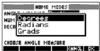
- View the Aplet Library. The "TRIANGLES" aplet is listed in the Aplet Library.
APLET
The Solve aplet can now be reset and used for other problems.
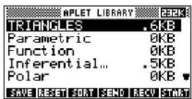
Using a customized aplet
To use the "Triangles" aplet, simply select the appropriate formula, change to the Numeric view and solve for the missing variable.
Find the length of a ladder leaning against a vertical wall if it forms an angle of 35° with the horizontal and extends 5 metres up the wall.
- Select the aplet.
APLET TRIANGLES
START

- Choose the sine formula in E1.


- Change to the Numeric view and enter the known values.
NUM
35 ENTER
5 ENTER

- Solve for the missing value.
SOLVE
The length of the ladder is approximately 8.72 metres
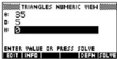
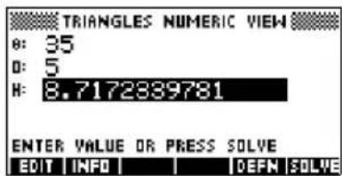
Resetting an aplet
Resetting an aplet clears all data and resets all default settings.
To reset an aplet, open the Library, select the aplet and press RESET.
You can only reset an aplet that is based on a built-in aplet if the programmer who created it has provided a Reset option.
Annotating an aplet with notes
The Note view (NOTE) attaches a note to the current aplet. See Chapter 15, "Notes and sketches".
Annotating an aplet with sketches
The Sketch view (SKETCH) attaches a picture to the current aplet. See chapter 15, "Notes and sketches".
HINT
Notes and sketches that you attach to an aplet become part of the aplet. When you transfer the aplet to another calculator, the associated note and sketch are transferred as well.
Downloading e-lessons from the web
In addition to the standard aplets that come with the calculator, you can download aplets from the world wide web. For example, Hewlett-Packard's Calculators web site contains aplets that demonstrate certain mathematical concepts. Note that you need the Graphing Calculator Connectivity Kit in order to load aplets from a PC.
Hewlett-Packard's Calculators web site can be found at:
http://www.hp.com/calculators
Sending and receiving aplets
A convenient way to distribute or share problems in class and to turn in homework is to transmit (copy) aplets directly from one hp 39g+ to another. This takes place via the infrared port.
You can also send aplets to, and receive aplets from, a remote storage device (aplet disk drive or computer). This takes place via a cable connection and requires an aplet disk drive or special software running on a PC (such as the PC Connectivity Kit).
To transmit an aplet
-
Connect the PC or aplet disk drive to the calculator by cable
or align the two calculators' infrared ports by matching up the triangle marks on the rims of the calculators.
Place the calculators no more than 2 inches (5 cm) apart. -
Sending calculator: Open the Library, highlight the aplet to send, and press SEND
- You have two options: another hp 39g+ or a disk drive on a PC. Highlight your selection and press OK.
- If transmitting to a disk drive, you have the options of sending to the current (default) directory or to another directory.
- Receiving calculator: Open the aplet library and press RECU.
- You have two options: another hp 39g+ or a disk drive (or computer). Highlight your selection and press OK.
The Transmit annunciator—» is displayed until transmission is complete.
If you are using the PC Connectivity Kit to download aplets from a PC, you will see a list of aplets in the PC's current directory. Check as many items as you would like to receive.
Sorting items in the aplet library menu list
Once you have entered information into an aplet, you have defined a new version of an aplet. The information is automatically saved under the current aplet name, such as "Function." To create additional aplets of the same type, you must give the current aplet a new name.
The advantage of storing an aplet is to allow you to keep a copy of a working environment for later use.
The aplet library is where you go to manage your aplets. Press A Highlight (using the arrow keys) the name of the aplet you want to act on.
To sort the aplet list
In the aplet library, press Select the sorting scheme and press .ENTER
- Chronologically produces a chronological order based on the date an aplet was last used. (The last-used aplet appears first, and so on.)
- Alphabetically produces an alphabetical order by aplet name.
To delete an aplet
You cannot delete a built-in aplet. You can only clear its data and reset its default settings.
To delete a customized aplet, open the aplet library, highlight the aplet to be deleted, and press DEto delete all custom aplets, press SHIFT CLEAR.
Glossary
aplet A small application, limited to one topic. The built-in aplet types are Function, Parametric, Polar, Sequence, Solve, and Statistics. An aplet can be filled with the data and solutions for a specific problem. It is reusable (like a program, but easier to use) and it records all your settings and definitions.
command An operation for use in programs. Commands can store results in variables, but do not display results. Arguments are separated by semi-colons, such as DISP expression; line#.
expression A number, variable, or algebraic expression (numbers plus functions) that produces a value.
function An operation, possibly with arguments, that returns a result. It does not store results in variables. The arguments must be enclosed in parentheses and separated with commas (or periods in Comma mode), such as CROSS(matrix1, matrix2).
HOME The basic starting point of the calculator. Go to HOME to do calculations.
Library For aplet management: to start, save, reset, send and receive aplets.
list A set of values separated by commas
(periods if the Decimal Mark mode is set to Comma) and enclosed in braces. Lists are commonly used to enter statistical data and to evaluate a function with multiple values.
Created and manipulated by the List editor and catalog.
matrix A two-dimensional array of values
separated by commas (periods if the Decimal Mark mode is set to Comma) and enclosed in nested brackets. Created and manipulated by the Matrix catalog and editor. Vectors are also handled by the Matrix catalog and editor.
menu A choice of options given in the
display. It can appear as a list or as a set of menu-key labels across the bottom of the display.
menu keys The top row of keys. Their operations
depend on the current context. The labels along the bottom of the display show the current meanings.
note Text that you write in the Notepad or
in the Note view for a specific aplet.
program A reusable set of instructions that you
record using the Program editor.
sketch A drawing that you make in the
Sketch view for a specific aplet.
variable The name of a number, list, matrix,
note, or graphic that is stored in memory. Use EGISore and use
VARS to retrieve.
vector A one-dimensional array of values
separated by commas (periods if the Decimal Mark mode is set to Comma) and enclosed in single brackets.
Created and manipulated by the Matrix catalog and editor.
views The possible contexts for an aplet:
Plot, Plot Setup, Numeric, Numeric
Setup, Symbolic, Symbolic Setup,
Sketch, Note, and special views like
split screens.
Resetting the hp 39g+
If the calculator "locks up" and seems to be stuck, you must reset it. This is much like resetting a PC. It cancels certain operations, restores certain conditions, and clears temporary memory locations. However, it does not clear stored data (variables, aplet databases, programs) unless you use the procedure, "To erase all memory and reset defaults".
To reset using the keyboard
Press and hold the key and the third menu key simultaneously, then release them.
If the calculator does not respond to the above key sequence, then:
- Turn the calculator over and locate the small hole in the back of the calculator.
- Insert the end of a straightened metal paper clip into the hole as far as it will go. Hold it there for 1 second, then remove it.
- Press If necessary, press and the first and last menu keys simultaneously.
To erase all memory and reset defaults
If the calculator does not respond to the above resetting procedures, you might need to restart it by erasing all of memory. You will lose everything you have stored. All factory-default settings are restored.
- Press and hold the key, the first menu key, and the last menu key simultaneously.
- Release all keys.
Note: To cancel this process, release only the top-row keys, then press the third menu key.
If the calculator does not turn on
If the hp 39g+ does not turn on follow the steps below until the calculator turns on. You may find that the calculator turns on before you have completed the procedure. If the calculator still does not turn on, please contact Customer Support for further information.
- Press and hold the key for 10 seconds.
- Press and hold the key and the third menu key simultaneously. Release the third menu key, then release the key.
- Press and hold the key, the first menu key, and the sixth menu key simultaneously. Release the sixth menu key, then release the first menu key, and then release the key.
- Locate the small hole in the back of the calculator. Insert the end of a straightened metal paper clip into the hole as far as it will go. Hold it there for 1 second, then remove it. Press the key.
- Remove the batteries (see "Batteries" on page R-4), press and hold the key for 10 seconds, and then put the batteries back in. Press the key.
Operating details
Operating temperature: 0° to 45°C (32° to 113°F).
Storage temperature: -20° to 65°C ( -4° to 149°F ).
Operating and storage humidity: 90% relative humidity at 40° C ( 104° F) maximum. Avoid getting the calculator wet.
Battery operates at 4.5V dc, 60mA maximum.
Batteries
The calculator uses 3 AAA(LR03) batteries as main power and a CR2032 lithium battery for memory backup.
Before using the calculator, please install the batteries according to the following procedure.
To install the main batteries
a. Slide up the battery compartment cover as illustrated. b. Insert 3 new AAA(LR03) batteries into the main compartment. Make sure each battery is inserted in the indicated direction.
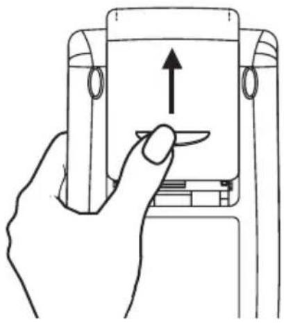
To install the backup battery
a. Press down the holder. Push the plate to the shown direction and lift it.

b. Insert a new CR2032 lithium battery. Make sure its positive (+) side is facing up.
c. Replace the plate and push it to the original place.
After installing the batteries, press to turn the power on.
Warning: When the low battery icon is displayed, you need to replace the batteries as soon as possible. However, avoid removing the backup battery and main batteries at the same time to avoid data lost.
Variables
Home variables
The home variables are:
| Category Available name | |
| Complex Z1...Z9, Z0 | |
| Graphic | G1...G9, G0 |
| Library Function | ParametricPolarSequenceSolveStatisticsUser-named |
| List | L1...L9, L0 |
| Matrix | M1...M9, M0 |
| Modes Ans | DateHAngleHDigitsHFormatIerrTime |
| Notepad User-named | |
| Program Editline | User-named |
| Real A...Z, 0 | |
Function aplet variables
The function aplet variables are:
| Category Available name | ||
| Plot Axes | Xcross | |
| Connect | Ycross | |
| Coord | Xtick | |
| FastRes | Ytick | |
| Grid | Xmin | |
| Indep | Xmax | |
| InvCross | Ymin | |
| Labels | Ymax | |
| Recenter | Xzoom | |
| Simult | Yxoom | |
| Tracing | ||
| Plot-FCN Area | Root | |
| Extremum | Slope | |
| Isect | ||
| Symbolic Angle | F6 | |
| F1 | F7 | |
| F2 | F8 | |
| F3 | F9 | |
| F4 | F0 | |
| F5 | ||
| Numeric Digits | NumRow | |
| Format | NumStart | |
| NumCol | NumStep | |
| NumFont | NumType | |
| NumIndep | NumZoom | |
| Note NoteText | ||
| Sketch Page PageNum | ||
Parametric aplet variables
The parametric aplet variables are:
| Category Available name | ||
| Plot Axes | Tracing | |
| Connect | Tstep | |
| Coord | Xcross | |
| Grid | Ycross | |
| Indep | Xtick | |
| InvCross | Ytick | |
| Labels | Xmin | |
| Recenter | Xmax | |
| Simult | Ymin | |
| Tmin | Ymax | |
| Tmax | Xzoom | |
| Yzoom | ||
| Symbolic Angle | Y5 | |
| X1 | X6 | |
| Y1 | Y6 | |
| X2 | X7 | |
| Y2 | Y7 | |
| X3 | X8 | |
| Y3 | Y8 | |
| X4 | X9 | |
| Y4 | Y9 | |
| X5 | X0 | |
| Y0 | ||
| Numeric Digits | NumRow | |
| Format | NumStart | |
| NumCol | NumStep | |
| NumFont | NumType | |
| NumIndep | NumZoom | |
| Note NoteText | ||
| Sketch Page PageNum | ||
Polar aplet variables
The polar aplet variables are:
| Category Available names | ||
| Plot Axes | ||
| Connect | Xcross | |
| Coord | Ycross | |
| Grid | Xtick | |
| Indep | Ytick | |
| InvCross | Xmin | |
| Labels | Xmax | |
| Recenter | Ymin | |
| Simult | Ymax | |
| Umin | Xzoom | |
| Umax | Yxoom | |
| θstep | ||
| Tracing | ||
| Symbolic Angle | R6 | |
| R1 | R7 | |
| R2 | R8 | |
| R3 | R9 | |
| R4 | R0 | |
| R5 | ||
| Numeric Digits | NumRow | |
| Format | NumStart | |
| NumCol | NumStep | |
| NumFont | NumType | |
| NumIndep | NumZoom | |
| Note NoteText | ||
| Sketch Page PageNum | ||
Sequence aplet variables
The sequence aplet variables are:
| Category Available name | ||
| Plot Axes | Tracing | |
| Coord | Xcross | |
| Grid | Ycross | |
| Indep | Xtick | |
| InvCross | Ytick | |
| Labels | Xmin | |
| Nmin | Xmax | |
| Nmax | Ymin | |
| Recenter | Ymax | |
| SeqPlot | Xzoom | |
| Simult | Yzoom | |
| Symbolic Angle | U6 | |
| U1 | U7 | |
| U2 | U8 | |
| U3 | U9 | |
| U4 | U0 | |
| U5 | ||
| Numeric Digits | NumRow | |
| Format | NumStart | |
| NumCol | NumStep | |
| NumFont | NumType | |
| NumIndep | NumZoom | |
| Note NoteText | ||
| Sketch Page PageNum | ||
Solve aplet variables
The solve aplet variables are:
| Category Available name | ||
| Plot Axes | Xcross | |
| Connect | Ycross | |
| Coord | Xtick | |
| FastRes | Ytick | |
| Grid | Xmin | |
| Indep | Xmax | |
| InvCross | Ymin | |
| Labels | Ymax | |
| Recenter | Xzoom | |
| Tracing | Yxoom | |
| Symbolic Angle | E6 | |
| E1 | E7 | |
| E2 | E8 | |
| E3 | E9 | |
| E4 | E0 | |
| E5 | ||
| Numeric Digits | NumCol | |
| Format | NumRow | |
| Note NoteText | ||
| Sketch Page PageNum | ||
Statistics aplet variables
The statistics aplet variables are:
| Category Available name | ||
| Plot Axes | S4mark | |
| Connect | S5mark | |
| Coord | StatPlot | |
| Grid | Tracing | |
| Hmin | Xcross | |
| Hmax | Ycross | |
| Hwidth | Xtick | |
| Indep | Ytick | |
| InvCross | Xmin | |
| Labels | Xmax | |
| Recenter | Ymin | |
| S1mark | Ymax | |
| S2mark | Xzoom | |
| S3mark | Yxoom | |
| Symbolic Angle | S3fit | |
| S1fit | S4fit | |
| S2fit | S5fit | |
| Numeric C0,.. | .C9 | NumFont |
| Digits | NumRow | |
| Format | StatMode | |
| NumCol | ||
| Stat-One MaxΣ | Q3 | |
| MeanΣ | PSDev | |
| Median | SSDev | |
| MinΣ | PVarΣ | |
| NΣ | SVarΣ | |
| Q1 | TotΣ | |
| Stat-Two Corr | ΣX | |
| Cov | ΣX2 | |
| Fit | ΣXY | |
| MeanX | ΣY | |
| MeanY | ΣY2 | |
| RelErr | ||
| Note NoteText | ||
| Sketch Page PageNum | ||
MATH menu categories
Math functions
The math functions are:
| Category Available name | ||
| Calculus | ||
| TAYLOR | ||
| Complex ARG | IM | |
| CONJ | RE | |
| Constant e | MAXREAL | |
| i | MINREAL | |
| π | ||
| Hyperb. ACOSH | TANH | |
| ASINH | ALOG | |
| ATANH | EXP | |
| COSH | EXPM1 | |
| SINH | LNP1 | |
| List CONCAT | REVERSE | |
| ΔLIST | SIZE | |
| MAKELIST | LIST | |
| πLIST | SORT | |
| POS | ||
| Loop ITERATE | ||
| RECURSE | ||
| Category Available name (Continued) | ||
| Matrix COLNORM | QR | |
| COND | RANK | |
| CROSS | ROWNORM | |
| DET | RREF | |
| DOT | SCHUR | |
| EIGENVAL | SIZE | |
| EIGENVV | SPECNORM | |
| IDENMAT | SPECRAD | |
| INVERSE | SVD | |
| LQ | SVL | |
| LSQ | TRACE | |
| LU | TRN | |
| MAKEMAT | ||
| Polynom. POLYCOEF | POLYFORM | |
| POLYEVAL | POLYROOT | |
| Prob. COMB | UTPC | |
| ! | UTPF | |
| PERM | UTPN | |
| RANDOM | UTPT | |
| Real CEILING | MIN | |
| DEG→RAD | MOD | |
| FLOOR | % | |
| FNROOT | %CHANGE | |
| FRAC | %TOTAL | |
| HMS→ | RAD→DEG | |
| →HMS | ROUND | |
| INT | SIGN | |
| MANT | TRUNCATE | |
| MAX | XPON | |
| Stat-Two PREDX | ||
| PREDY | ||
| Symbolic = | QUAD | |
| ISOLATE | QUOTE | |
| LINEAR? | | | |
| Tests | < ANDIFTE≤ NOT== OR≠>≥ | |
| Trig ACOT | ACSC COTCSCASEC SEC | |
Program constants
The program constants are:
| Category Available name | ||
| Angle Degrees | GradsRadians | |
| Format Standard | Fixed | SciEngFraction |
| SeqPlot Cobweb | Stairstep | |
| S1...5fit Linear | LogFitExpFitPower | QuadFitCubicLogistUser |
| StatMode Stat1Var | Stat2Var | |
| StatPlot Hist | BoxW | |
Program commands
The program commands are:
| Category Command | ||
| Aplet CHECK | ||
| SELECT | ||
| SETVIEWS | ||
| UNCHECK | ||
| Branch IF | CASE | |
| THEN | IFERR | |
| ELSE | RUN | |
| END | STOP | |
| Drawing ARC | LINE | |
| BOX | PIXOFF | |
| ERASE | PIXON | |
| FREEZE | TLINE | |
| Graphic DISPLAY→ | MAKEGROB | |
| →DISPLAY | PLOT→ | |
| →GROB | →PLOT | |
| GROBNOT | REPLACE | |
| GROBOR | SUB | |
| GROBXOR | ZEROGROB | |
| Loop FOR | UNTIL | |
| = | END | |
| TO | WHILE | |
| STEP | REPEAT | |
| END | END | |
| DO | BREAK | |
| Matrix ADDCOL | REDIM | |
| ADDROW | REPLACE | |
| DELCOL | SCALE | |
| DELROW | SCALEADD | |
| EDITMAT | SUB | |
| RANDMAT | SWAPCOL | |
| SWAPROW | ||
| Print PRDISPLAY | ||
| PRHISTORY | ||
| PRVAR | ||
| Prompt BEEP | GETKEY | |
| CHOOSE | INPUT | |
| DISP | MSGBOX | |
| DISPTIME | PROMPT | |
| EDITMAT | WAIT | |
| FREEZE | ||
| Stat-One DO1VSTATS | SETFREQ | |
| RANDSEED | SETSAMPLE | |
| Stat-Two DO2VSTATS | ||
| SETDEPEND | ||
| SETINDEP | ||
Status messages
| Message Meaning | |
| Bad Argument Type | Incorrect input for this operation. |
| Bad Argument Value | The value is out of range for this operation. |
| Infinite Result Math exception, such as 1/0. | |
| Insufficient Memory | You must recover some memory to continue operation. Delete one or more matrices, lists, notes, or programs (using catalogs), or custom (not built-in) aplets (using SHIFT MEMORY). |
| Insufficient Statistics Data | Not enough data points for the calculation. For two-variable statistics there must be two columns of data, and each column must have at least four numbers. |
| Invalid Dimension Array argument had wrong dimensions. | |
| Invalid Statistics Data | Need two columns with equal numbers of data values. |
| Invalid Syntax The function or command you entered does not include the proper arguments or order of arguments. The delimiters (parentheses, commas, periods, and semi-colons) must also be correct. Look up the function name in the index to find its proper syntax. | |
| Name Conflict The I | (where) function attempted to assign a value to the variable of integration or summation index. |
| Message Meaning (Continued) | |
| No Equations Checked | You must enter and check an equation (Symbolic view) before evaluating this function. |
| (OFF SCREEN) Function | tion value, root, extremum, or intersection is not visible in the current screen. |
| Receive Error Problem | m with data reception from another calculator. Re-send the data. |
| Too Few Arguments | The command requires more arguments than you supplied. |
| Undefined Name The | global variable named does not exist. |
| Undefined Result The | calculation has a mathematically undefined result (such as 0/0). |
| Out of Memory You | must recover a lot of memory to continue operation. Delete one or more matrices, lists, notes, or programs (using catalogs), or custom (not built-in) aplets (using SHIFT MEMORY). |
hp 39g+ Graphing Calculator; Warranty period: 12 months
-
HP warrants to you, the end-user customer, that HP hardware, accessories and supplies will be free from defects in materials and workmanship after the date of purchase, for the period specified above. If HP receives notice of such defects during the warranty period, HP will, at its option, either repair or replace products which prove to be defective. Replacement products may be either new or like-new.
-
HP warrants to you that HP software will not fail to execute its programming instructions after the date of purchase, for the period specified above, due to defects in material and workmanship when properly installed and used. If HP receives notice of such defects during the warranty period, HP will replace software media which does not execute its programming instructions due to such defects.
-
HP does not warrant that the operation of HP products will be uninterrupted or error free. If HP is unable, within a reasonable time, to repair or replace any product to a condition as warranted, you will be entitled to a refund of the purchase price upon prompt return of the product with proof of purchase.
-
HP products may contain remanufactured parts equivalent to new in performance or may have been subject to incidental use.
-
Warranty does not apply to defects resulting from (a) improper or inadequate maintenance or calibration, (b) software, interfacing, parts or supplies not supplied by HP, (c) unauthorized modification or misuse, (d) operation outside of the published environmental specifications for the product, or (e) improper site preparation or maintenance.
-
HP MAKES NO OTHER EXPRESS WARRANTY OR CONDITION WHETHER WRITTEN OR ORAL. TO THE EXTENT ALLOWED BY LOCAL LAW, ANY IMPLIED WARRANTY OR CONDITION OF MERCHANTABILITY, SATISFACTORY QUALITY, OR FITNESS FOR A PARTICULAR PURPOSE IS LIMITED TO THE DURATION OF THE EXPRESS WARRANTY SET FORTH ABOVE. Some countries, states or provinces do not allow limitations on the duration of an implied warranty, so the above limitation or exclusion might not apply to you. This warranty gives you specific legal rights and you might also have other rights that vary from country to country, state to state, or province to province.
-
TO THE EXTENT ALLOWED BY LOCAL LAW, THE REMEDIES IN THIS WARRANTY STATEMENT ARE YOUR SOLE AND EXCLUSIVE REMEDIES. EXCEPT AS INDICATED ABOVE, IN NO EVENT WILL HP OR ITS SUPPLIERS BE LIABLE FOR LOSS OF DATA OR FOR DIRECT, SPECIAL, INCIDENTAL, CONSEQUENTIAL (INCLUDING LOST PROFIT OR DATA), OR OTHER DAMAGE, WHETHER BASED IN CONTRACT, TORT, OR OTHERWISE. Some countries, States or provinces do not allow the exclusion or limitation of incidental or consequential damages, so the above limitation or exclusion may not apply to you.
-
The only warranties for HP products and services are set forth in the express warranty statements accompanying such products and services. HP shall not be liable for technical or editorial errors or omissions contained herein.
FOR CONSUMER TRANSACTIONS IN AUSTRALIA AND NEW ZEALAND: THE WARRANTY TERMS CONTAINED IN THIS STATEMENT, EXCEPT TO THE EXTENT LAWFULLY PERMITTED, DO NOT EXCLUDE, RESTRICT OR MODIFY AND ARE IN ADDITION TO THE MANDATORY STATUTORY RIGHTS APPLICABLE TO THE SALE OF THIS PRODUCT TO YOU.
Service
Europe Country : Telephone numbers
| Austria +43-1-3602771203 | |
| Belgium +32-2-7126219 | |
| Denmark +45-8-2332844 | |
| Eastern Europe countries | +420-5-41422523 |
| Finland +35-89640009 | |
| France +33-1-49939006 | |
| Germany +49-69-95307103 | |
| Greece +420-5-41422523 | |
| Holland +31-2-06545301 | |
| Italy +39-02-75419782 | |
| Norway +47-63849309 | |
| Portugal +351-229570200 | |
| Spain | +34-915-642095 |
| Sweden +46-851992065 | |
| Switzerland | +41-1-4395358(German) |
| +41-22-8278780(French) | |
| +39-02-75419782(Italian) | |
| Turkey | +420-5-41422523 |
| UK | +44-207-4580161 |
| Czech Republic | +420-5-41422523 |
| South Africa | +27-11-2376200 |
| Luxembourg | +32-2-7126219 |
| Other European countries | +420-5-41422523 |
| Asia Pacific Country : Telephone numbers | |
| Australia | +61-3-9841-5211 |
| Singapore | +61-3-9841-5211 |
L.America
Country : Telephone numbers
Argentina 0-810-555-5520 Brazil Sao Paulo 3747-7799; ROTC 0-800-157751 Mexico Mx City 5258-9922; ROTC 01-800-472-6684
Venezuela 0800-4746-8368
Chile 800-360999
Columbia 9-800-114726
Peru 0-800-10111
Central 1-800-711-2884
America &
Caribbean
Guatemala 1-800-999-5105
Puerto Rico 1-877-232-0589
Costa Rica 0-800-011-0524
N.America
Country : Telephone numbers
U.S. 1800-HP INVENT
Canada (905) 206-4663 or 800-HP INVENT
ROTC = Rest of the country
Please logon to http://www.hp.com for the latest service and support information.
Regulatory information
This section contains information that shows how the hp 39g+ graphing calculator complies with regulations in certain regions. Any modifications to the calculator not expressly approved by Hewlett-Packard could void the authority to operate the 39g+ in these regions.
USA This calculator generates, uses, and can radiate radio
frequency energy and may interfere with radio and television reception. The calculator complies with the limits for a Class B digital device, pursuant to Part 15 of the FCC Rules. These limits are designed to provide reasonable protection against harmful interference in a residential installation.
However, there is no guarantee that interference will not occur in a particular installation. In the unlikely event that there is interference to radio or television reception(which can be determined by turning the calculator off and on), the user is encouraged to try to correct the interference by one or more of the following measures:
■ Reorient or relocate the receiving antenna.
■ Relocate the calculator, with respect to the receiver.
Connections to Peripheral Devices
To maintain compliance with FCC rules and regulations, use only the cable accessories provided.
Canada This Class B digital apparatus complies with Canadian
Disposal of Waste Equipment by Users in Private Household in the European Union

This symbol on the product or on its packaging indicates that this product must not be disposed of with your other household waste. Instead, it is your responsibility to dispose of your waste equipment by handing it over to a designated collection point for the recycling of waste electrical and electronic equipment. The separate collection and recycling of your waste equipment at the time of disposal will help to conserve natural resources and ensure that it is recycled in a manner that protects human health and the environment. For more information about where you can drop off your waste equipment for recycling, please contact your local city office, your household waste disposal service or the shop where you purchased the product.
A
absolute value 11-5
add 11-3
algebraic entry 1-19
alpha characters typing 1-6
alphabetical sorting 17-6
angle measure 1-10
in statistics 8-12
setting 1-12
animation 15-5
creating 15-5
annunciators 1-3
Ans (last answer) 1-24
antilogarithm 11-4, 11-9
aplet
attaching notes 17-4
clearing 17-3
copying 17-4
definition of R-1
deleting 17-6
Function 11-21
Inference 9-1
key 1-4
library 17-5
opening 1-16
Parametric 4-1
Polar 5-1
receiving 17-5
resetting 17-3
sending 17-4, 17-5
Sketch view 15-1
Solve 7-1
sorting 17-6
statistics 8-1
transmitting 17-5
aplet commands
CHECK 16-14
SELECT 16-14
SETVIEWS 16-17
UNCHECK 16-17
aplet variables
definition 12-1, 12-8
in Plot view 16-30
new 12-1
aplet views
canceling operations in 1-1
changing 1-19
note 1-18
Numeric view 1-17
Plot view 1-17
sketch 1-18
split-screen 1-17
Symbolic view 1-16
arc cosecant 11-19
arc cosine 11-4
arc cotangent 11-19
arc secant 11-19
arc sine 11-4
arc tangent 11-5
area
graphical 3-10
interactive 3-10
variable 16-30
arguments
with matrices 13-10
attaching
a note to an aplet 15-1
a sketch to an aplet 15-3
auto scale 2-14
axes
plotting 2-7
variable 16-30
B
bad argument R-17
bad guesses error message 7-7
box-and-whisker plot 8-16
branch commands
CASE...END 16-18
IF...THEN...ELSE...END 16-18
IFERR...THEN...ELSE 16-18
branch structures 16-17
build your own table 2-19
C
calculus
operations 11-7
catalogs 1-30
chronological sorting 17-6
circle drawing 15-4
clearing
aplet 17-3
characters 1-22
display 1-22
display history 1-25
edit line 1-22
lists 14-6
plot 2-7
cobweb graph 6-1
coefficients
polynomial 11-10
columns
changing position 16-25
combinations 11-12
commands
aplet 16-14
branch 16-17
definition of R-1
drawing 16-19
graphic 16-20
loop 16-22
print 16-25
program 16-4, R-16
stat-one 16-28
stat-two 16-29
with matrices 13-10
complex number functions 11-5, 11-16
conjugate 11-7
imaginary part 11-7
real part 11-7
complex numbers 1-29
entering 1-29
maths functions 11-7
storing 1-29
confidence intervals 9-15
conjugate 11-7
connecting
data points 8-18
variable 16-30
connectivity kit 17-4
constant? error message 7-7
constants 11-8
e 11-8
i 11-8
maximum real number 11-8
minimum real number 11-8
program R-15
contrast
decreasing display 1-2
increasing display 1-2
coordinate display 2-9
copying
display 1-22
graphics 15-6
notes 15-8
programs 16-8
correlation
coefficient 8-17
CORR 8-17
statistical 8-15
cosecant 11-19
cosine 11-4
inverse hyperbolic 11-8
cotangent 11-19
covariance
statistical 8-15
creating
aplet 17-1
lists 14-1
matrices 13-3
notes in Notepad 15-6
programs 16-4
sketches 15-3
critical value(s) displayed 9-4
cross product
vector 13-10
curve fitting 8-12, 8-17
D
data set definition 8-8
date, setting 16-26
debugging programs 16-7
decimal
changing format 1-11
scaling 2-14, 2-16
decreasing display contrast 1-2
definite integral 11-6
deleting
aplet 17-6
lists 14-6
matrices 13-4
programs 16-9
statistical data 8-11
delimiters, programming 16-1
derivatives
definition of 11-6
in Function aplet 11-22
in Home 11-21
determinant
square matrix 13-11
differentiation 11-6
display 16-20
adjusting contrast 1-2
annunciator line 1-2
capture 16-20
clearing 1-2
date and time 16-26
element 13-5
elements 14-4
engineering 1-11
fixed 1-11
fraction 1-11
history 1-22
line 1-23
matrices 13-5
parts of 1-2
printing contents 16-25
rescaling 2-14
scientific 1-11
scrolling through history 1-25
soft key labels 1-2
standard 1-11
divide 11-3
drawing
circles 15-4
keys 15-4
lines and boxes 15-3
drawing commands
ARC 16-19
BOX 16-19
ERASE 16-20
FREEZE 16-20
LINE 16-20
PIXOFF 16-20
PIXON 16-20
TLINE 16-20
E
e 11-8
edit line 1-2
editing
matrices 13-4
notes 15-2
programs 16-5
Editline
Program catalog 16-2
editors 1-30
eigenvalues 13-11
eigenvectors 13-11
element
storing 13-6
E-lessons 1-12
engineering number format 1-11
equals
for equations 11-17
logical test 11-18
equations
solving 7-1
erasing a line in Sketch view 16-20
error messages
bad guesses 7-7
constant? 7-7
exclusive OR 11-19
exiting views 1-19
exponent
minus 1 11-9
of value 11-16
raising to 11-5
expression
defining 2-1, R-1
entering in HOME 1-19
evaluating in aplets 2-3
literal 11-18
plot 3-3
extremum 3-10
F
factorial 11-12
FastRes variable 16-31
fit
a curve to 2VAR data 8-17
choosing 8-12
defining your own 8-13
fixed number format 1-11
font size
change 3-8, 15-5
forecasting 8-20
fraction number format 1-11
full-precision display 1-11
function
analyse graph with FCN tools 3-4
definition 2-2, R-1
entering 1-19
gamma 11-12
intersection point 3-5
math menu R-13
slope 3-5
syntax 11-2
tracing 2-8
Function aplet 2-21, 3-1
function variables
area 16-30
axes 16-30
connect 16-30
fastres 16-31
grid 16-31
in menu map R-7
indep 16-32
isect 16-32
labels 16-33
Recenter 16-33
root 16-33
ycross 16-36
G
glossary R-1
graph
analyzing statistical data in 8-19
auto scale 2-14
box-and-whisker 8-16
capture current display 16-20
cobweb 6-1
comparing 2-5
connected points 8-17
defining the independent variable 16-35
drawing axes 2-7
expressions 3-3
grid points 2-7
histogram 8-15
in Solve aplet 7-7
one-variable statistics 8-18
overlaying 2-16
scatter 8-15, 8-16
split-screen view 2-15
splitting into plot and close-up 2-14
splitting into plot and table 2-14
stairsteps 6-1
statistical data 8-15
t values 2-6
tickmarks 2-6
tracing 2-8
two-variable statistics 8-18
Graphic commands
→GROB 16-21
DISPLAY→16-20
GROBNOT 16-21
GROBOR 16-21
GROBXOR 16-21
MAKEGROB 16-21
PLOT→16-21
REPLACE 16-22
SUB 16-22
ZEROGROB 16-22
graphics
copying 15-6
copying into Sketch view 15-6
storing and recalling 15-6, 16-20
H
histogram 8-15
adjusting 8-16
range 8-18
setting min/max values for bars
16-31
width 8-18
history 1-2, 16-25
Home 1-1
calculating in 1-19
display 1-2
evaluating expressions 2-4
reusing lines 1-23
variables 12-1, 12-7, R-6
horizontal zoom 16-37
hyperbolic
maths functions 11-9
hyperbolic trigonometry
ACOSH 11-8
ALOG 11-9
ASINH 11-8
ATANH 11-8
COSH 11-8
EXP 11-9
EXPM1 11-9
LNP1 11-9
SINH 11-8
TANH 11-9
hypothesis
alternative 9-2
inference tests 9-8
null 9-2
tests 9-2
|
i 11-8
implied multiplication 1-21
importing
graphics 15-6
notes 15-8
increasing display contrast 1-2
indefinite integral
using symbolic variables 11-23
independent values
adding to table 2-19
independent variable
defined for Tracing mode 16-32
inference
confidence intervals 9-15
hypothesis tests 9-8
One-Proportion Z-Interval 9-17
One-Sample Z-Interval 9-15
One-Sample Z-Test 9-8
Two-Proportion Z-Interval 9-17
Two-Proportion Z-Test 9-11
Two-Sample T-Interval 9-19
Two-Sample Z-Interval 9-16
infinite result R-17
infrared
transmission of aplets 17-5
initial guess 7-5
input forms
resetting default values 1-9
setting Modes 1-12
insufficient memory R-17
insufficient statistics data R-17
integer rank
matrix 13-12
integer scaling 2-14, 2-16
integral
definite 11-6
indefinite 11-23
integration 11-6
interpreting
intermediate guesses 7-7
intersection 3-11
invalid
dimension R-17
statistics data R-17
syntax R-17
inverse hyperbolic cosine 11-8
inverse hyperbolic functions 11-9
inverse hyperbolic sine 11-8
inverse hyperbolic tangent 11-8
inverting matrices 13-8
isect variable 16-32
K
keyboard
editing keys 1-5
entry keys 1-5
inactive keys 1-8
list keys 14-2
math functions 1-7
menu keys 1-4
Notepad keys 15-8
shifted keystrokes 1-6
L
labeling
axes 2-7
parts of a sketch 15-5
letters, typing 1-6
library, managing aplets in 17-5
linear fit 8-13
list
arithmetic with 14-7
calculate sequence of elements 14-8
calculating product of 14-8
composed from differences 14-7
concatenating 14-7
counting elements in 14-9
creating 14-1, 14-3, 14-4, 14-5
deleting 14-6
deleting list items 14-3
displaying 14-4
displaying list elements 14-4
editing 14-3
finding statistical values in list elements 14-9
generate a series 14-8
list function syntax 14-6
list variables 14-1
returning position of element in 14-8
reversing order in 14-8
sending and receiving 14-6
sorting elements 14-9
storing elements 14-1, 14-4, 14-5
storing one element 14-6
logarithm 11-4
logarithmic
fit 8-13
functions 11-3
logical operators
AND 11-19
equals (logical test) 11-18
greater than 11-18
greater than or equal to 11-19
IFTE 11-19
less than 11-18
less than or equal to 11-18
NOT 11-19
not equal to 11-18
OR 11-19
XOR 11-19
logistic fit 8-13
loop commands
BREAK 16-23
DO...UNTIL...END 16-22
FOR I= 16-23
WHILE...REPEAT...END 16-23
loop functions
ITERATE 11-9
RECURSE 11-10
summation 11-10
low battery 1-1
lowercase letters 1-6
M
mantissa 11-14
math functions
complex number 11-7
hyperbolic 11-9
in menu map R-13
keyboard 11-3
logical operators 11-18
menu 1-7
polynomial 11-10
probability 11-12
real-number 11-13
symbolic 11-17
trigonometry 11-19
MATH menu 11-1
math operations 1-19
enclosing arguments 1-21
in scientific notation 1-20
negative numbers in 1-20
matrices
adding rows 16-23
addition and subtraction 13-6
arguments 13-10
arithmetic operations in 13-6
assembly from vectors 13-1
changing row position 16-25
column norm 13-10
comma 14-7
commands 13-10
condition number 13-10
create identity 13-13
creating 13-3
creating in Home 13-5
deleting 13-4
deleting columns 16-24
deleting rows 16-24
determinant 13-11
display eigenvalues 13-11
displaying 13-5
displaying matrix elements 13-5
dividing by a square matrix 13-7
dot product 13-11
editing 13-4
extracting a portion 16-25
finding the trace of a square ma- trix 13-13
inverting 13-8
matrix calculations 13-1
multiplying and dividing by scalar 13-7
multiplying by vector 13-7
multiplying row by value and add-
ing result to second row 16-24
multiplying row number by value 16-24
negating elements 13-8
opening Matrix Editor 16-27
redimension 16-24
replacing portion of matrix or vec-
tor 16-24
sending or receiving 13-4
singular value decomposition
13-13
singular values 13-13
size 13-12
spectral norm 13-12
spectral radius 13-12
start Matrix Editor 16-24
storing elements 13-3, 13-5
storing matrix elements 13-6
swap column 16-25
swap row 16-25
transposing 13-13
variables 13-1
matrix functions 13-10
COLNORM 13-10
COND 13-10
CROSS 13-10
DET 13-11
DOT 13-11
EIGENVAL 13-11
EIGENVV 13-11
IDENMAT 13-11
INVERSE 13-11
LQ 13-11
LSQ 13-11
LU 13-11
MAKEMAT 13-11
QR 13-12
RANK 13-12
ROWNORM 13-12
RREF 13-12
SCHUR 13-12
SIZE 13-12
SPECNORM 13-12
SPECRAD 13-12
SVD 13-13
SVL 13-13
TRACE 13-13
TRN 13-13
maximum real number 1-22, 11-8
memory R-17
clearing all R-3
organizing 12-9
out of R-18
saving 1-25, 17-1
viewing 12-1
menu lists
searching 1-8
minimum real number 11-8
modes
angle measure 1-10
decimal mark 1-11
number format 1-11
multiple solutions
plotting to find 7-7
multiplication 11-3
implied 1-21
N
name conflict R-17
naming
programs 16-4
natural exponential 11-3, 11-9
natural log plus 1 11-9
natural logarithm 11-3
negation 11-5
negative numbers 1-20
no equations checked R-18
Normal Z-distribution, confidence in-
tervals 9-15
note
copying 15-8
editing 15-2
importing 15-8
printing 16-25
viewing 15-1
writing 15-1
Notepad 15-1
catalog keys 15-7
creating notes 15-6
writing in 15-6
nrng 2-6
nth root 11-6
null hypothesis 9-2
number format
engineering 1-11
fixed 1-11
fraction 1-11
in Solve aplet 7-5
scientific 1-11
Standard 1-11
numeric precision 12-9
Numeric view
adding values 2-19
automatic 2-17
build your own table 2-19
display defining function for col-
umn 2-18
recalculating 2-19
setup 2-17, 2-19
O
off
automatic 1-1
power 1-1
on/cancel 1-1
One-Proportion Z-Interval 9-17
One-Sample T-Interval 9-18
One-Sample T-Test 9-12
One-Sample Z-Interval 9-15
One-Sample Z-Test 9-8
order of precedence 1-21
overlaying plots 2-16, 4-3
P
π 11 - 8
paired columns 8-11
parametric variables
axes 16-30
connect 16-30
grid 16-31
in menu map R-8
indep 16-32
labels 16-33
recenter 16-33
ycross 16-36
parentheses
to close arguments 1-21
to specify order of operation 1-21
pause 16-28
permutations 11-12
pictures
attaching in Sketch view 15-3
plot
analyzing statistical data in 8-19
auto scale 2-14
box-and-whisker 8-16
cobweb 6-1
comparing 2-5
connected points 8-17, 8-18
decimal scaling 2-14
defining the independent variable 16-35
drawing axes 2-7
expressions 3-3
grid points 2-7
histogram 8-15
in Solve aplet 7-7
integer scaling 2-14
one-variable statistics 8-18
overlay plot 2-14
overlaying 2-16, 4-3
scaling 2-14
scatter 8-15, 8-16
sequence 2-6
setting up 2-5, 3-2
split-screen view 2-15
splitting 2-15
splitting into plot and close-up 2-14
splitting into plot and table 2-14
stairsteps 6-1
statistical data 8-15
statistics parameters 8-18
t values 2-6
tickmarks 2-6
to capture current display 16-20
tracing 2-8
trigonometric scaling 2-15
two-variable statistics 8-18
plotting resolution
and tracing 2-8
plot-view variables
area 16-30
connect 16-30
fastres 16-31
function 16-30
grid 16-31
hmin/hmax 16-31
hwidth 16-32
isect 16-32
labels 16-33
recenter 16-33
root 16-33
s1mark-s5mark 16-33
statplot 16-34
tracing 16-32
umin/umax 16-34
ustep 16-34
polar variables
axes 16-30
connect 16-30
grid 16-31
in menu map R-9
indep 16-32
labels 16-33
recenter 16-33
ycross 16-36
polynomial
coefficients 11-10
evaluation 11-11
form 11-11
roots 11-11
Taylor 11-7
polynomial functions
POLYCOEF 11-10
POLYEVAL 11-11
POLYFORM 11-11
POLYROOT 11-11
position argument 16-20
power (x raised to y) 11-5
precedence 1-22
predicted values statistical 8-20
contents of display 16-25
name and contents of variable 16-25
object in history 16-25
variables 16-25
probability functions ! 11-12
COMB 11-12
RANDOM 11-12
UTPC 11-12
UTPF 11-13
UTPN 11-13
UTPT 11-13
program
commands 16-4
copying 16-8
creating 16-4
debugging 16-7
deleting 16-9
delimiters 16-1
editing 16-5
naming 16-4
pausing 16-28
printing 16-25
sending and receiving 16-8
structured 16-1
prompt commands beep 16-25
create choose box 16-26
create input form 16-27
display item 16-26
display message box 16-28
halt program execution 16-28
insert line breaks 16-28
prevent screen display being up- dated 16-27
set date and time 16-26
store keycode 16-27
Q
quadratic
extremum 3-6
fit 8-13
function 3-4
quotes
in program names 16-4
R
random numbers 11-12
real number
maximum 11-8
minimum 11-8
real part 11-7
real-number functions 11-13 % 11-15
%CHANGE 11-15
%TOTAL 11-15
CEILING 11-13
DEGtoRAD 11-13
FNROOT 11-14
HMSto 11-14
INT 11-14
MANT 11-14
MAX 11-15
MIN 11-15
MOD 11-15
RADtoDEG 11-15
ROUND 11-16
SIGN 11-16
TRUNCATE 11-16
XPON 11-16
recalculation for table 2-19
receive error R-18
receiving
aplet 17-5
lists 14-6
matrices 13-4
programs 16-8
redrawing
table of numbers 2-18
reduced row echelon 13-12
regression
analysis 8-17
fit models 8-13
formula 8-12
user-defined fit 8-13
relative error
statistical 8-17
resetting
aplet 17-3
calculator R-3
memory R-3
result
copying to edit line 1-22
reusing 1-22
root
interactive 3-10
nth 11-6
variable 16-33
root-finding
displaying 7-7
interactive 3-9
operations 3-10
variables 3-10
S
S1mark-S5mark variables 16-33
scaling
automatic 2-14
decimal 2-10, 2-14
integer 2-10, 2-14, 2-16
options 2-14
resetting 2-14
trigonometric 2-15
scatter plot 8-15, 8-16
connected 8-17, 8-18
SCHUR decomposition 13-12
scientific number format 1-11, 1-20
scrolling
in Trace mode 2-8
searching
menu lists 1-8
speed searches 1-8
secant 11-20
sending
aplets 17-4
lists 14-6
programs 16-8
sequence
definition 2-2
sequence variables
Axes 16-30
Grid 16-31
in menu map R-10
Indep 16-32
Labels 16-33
Recenter 16-33
Ycross 16-36
setting
date 16-26
time 16-26
sign reversal 7-6
sine 11-4
inverse hyperbolic 11-8
singular value decomposition
matrix 13-13
singular values
matrix 13-13
sketches
creating 15-5
creating a blank graphic 16-22
creating a set of 15-5
erasing a line 16-20
labeling 15-5
opening view 15-3
sets 15-5
storing in graphics variable 15-5
slope 3-10
soft key labels 1-2
solve
error messages 7-7
initial guesses 7-5
interpreting intermediate guesses 7-7
interpreting results 7-6
plotting to find guesses 7-7
setting number format 7-5
solve variables
axes 16-30
connect 16-30
fastres 16-31
grid 16-31
in menu map R-11
indep 16-32
labels 16-33
recenter 16-33
ycross 16-36
sorting 17-6
aplets in alphabetic order 17-6
aplets in chronological order 17-6
elements in a list 14-9
spectral norm 13-12
spectral radius 13-12
square root 11-5
stack history
printing 16-25
stairsteps graph 6-1
standard number format 1-11
statistics
analysis 8-1
analyzing plots 8-19
angle mode 8-12
calculate one-variable 16-29
calculate two-variable 16-29
data set variables 16-39
data structure 16-39
define one-variable sample 16-29
define two-variable data set's dependent column 16-29
define two-variable data set's independent column 16-29
defining a fit 8-12
defining a regression model 8-12
deleting data 8-11
editing data 8-11
frequency 16-29
inserting data 8-11
plot type 8-18
plotting data 8-15
predicted values 8-20
regression curve (fit) models 8-12
saving data 8-10
sorting data 8-11
specifying angle setting 8-12
toggling between one-variable
and two-variable 8-12
tracing plots 8-19
troubleshooting with plots 8-18
zooming in plots 8-19
statistics variables
Axes 16-30
Connect 16-30
Grid 16-31
Hmin/Hmax 16-31
Hwidth 16-32
in menu map R-12
Indep 16-32
Labels 16-33
Recenter 16-33
S1mark-S5mark 16-33
Ycross 16-36
step size of independent variable 16-35
storing
list elements 14-1, 14-4, 14-5, 14-6
matrix elements 13-3, 13-5, 13-6
results of calculation 12-2
value 12-2
strings
literal in symbolic operations 11-18
subtract 11-3
summation function 11-10
symbolic
calculations in Function aplet 11-21
defining expressions 2-1
differentiation 11-21
displaying definitions 3-8
evaluating variables in view 2-3
setup view for statistics 8-12
symbolic functions
| (where) 11-18
equals 11-17
ISOLATE 11-17
LINEAR? 11-17
QUAD 11-17
QUOTE 11-18
Symbolic view
defining expressions 3-2
syntax 11-2
syntax errors 16-7
T
table
navigate around 3-8
numeric values 3-7
numeric view setup 2-17
tangent 11-4
inverse hyperbolic 11-8
Taylor polynomial 11-7
tickmarks for plotting 2-6
time 11-14
setting 16-26
time, converting 11-14
times sign 1-21
tmax 16-35
tmin 16-35
too few arguments R-18
tracing
functions 2-8
more than one curve 2-8
not matching plot 2-8
plots 2-8
transmitting
lists 14-6
matrices 13-4
programs 16-8
transposing a matrix 13-13
trigonometric
functions 11-19
scaling 2-10, 2-15, 2-16
trigonometry functions
ACOT 11-19
ACSC 11-19
ASEC 11-19
COT 11-19
CSC 11-19
SEC 11-20
trng 2-6
truncating values to decimal places 11-16
tstep 2-6, 16-35
Two-Proportion Z-Interval 9-17
Two-Proportion Z-Test 9-11
Two-Sample T-Interval 9-19
Two-Sample T-test 9-14
Two-Sample Z-Interval 9-16
typing letters 1-6
U
undefined
name R-18
result R-18
un-zoom 2-11
upper-tail chi-squared probability 11-12
upper-tail normal probability 11-13
upper-tail Snedecor's F 11-13
upper-tail student's t-probability 11-13
user defined
regression fit 8-13
V
value
recall 12-3
storing 12-2
variables
aplet 12-1
categories 12-7
definition 12-1, 12-7, R-2
in equations 7-10
in Symbolic view 2-3
independent 16-35
local 12-1
previous result (Ans) 1-23
printing 16-25
root 16-33
root-finding 3-10
step size of independent 16-35
types 12-1, 12-7
use in calculations 12-3
VARS menu 12-4, 12-5
vectors
column 13-1
cross product 13-10
definition of R-2
views 1-18
configuration 1-18
definition of R-3
W
warning symbol 1-8
where command ( | ) 11-18
X
Xcross variable 16-35
xrng 2-6
Y
Ycross variable 16-36
yrng 2-6
Z
Z-Interval 9-15
zoom 2-18
axes 2-12
box 2-9
center 2-9
examples of 2-11
factors 2-13
in 2-9
options 2-9, 3-8
options within a table 2-18
out 2-9
redrawing table of numbers op-
tions 2-18
square 2-10
un-zoom 2-11
within Numeric view 2-18
X-zoom 2-9
Y-zoom 2-10



- PREFACE
- 1 GETTING STARTED
- 2 APLETS AND THEIR VIEWS
- 3 FUNCTION APLET
- 4 PARAMETRIC APLET
- 5 POLAR APLET
- 6 SEQUENCE APLET
- 7 SOLVE APLET
- 8 STATISTICS APLET
- 9 INFERENCE APLET
- 10 USING THE FINANCE SOLVER
- 11 USING MATHEMATICAL FUNCTIONS
- 12 VARIABLES AND MEMORY MANAGEMENT
- 13 MATRICES
- 14 LISTS
- 15 NOTES AND SKETCHES
- 16 PROGRAMMING
- 17 EXTENDING APLETS
- REFERENCE INFORMATION
- LIMITING WARRANTY
- INDEX
- MANUAL CONVENTIONS
- NOTICE
- GETTING STARTED
- ON/OFF, CANCEL OPERATIONS
- TO TURN OFF
- THE DISPLAY
- TO ADJUST THE CONTRAST
- TO CLEAR THE DISPLAY
- PARTS OF THE DISPLAY
- NOTE
- THE KEYBOARD
- APLET CONTROL KEYS
- ENTRY/EDIT KEYS
- SHIFTED KEYSTROKES
- HELPWITH
- EXAMPLE
- HINT
- PROGRAM COMMANDS
- MENUS
- TO SEARCH A MENU
- TO CANCEL A MENU
- INPUT FORMS
- RESET INPUT FORM VALUES
- MODE SETTINGS
- SETTING A MODE
- APLETS (E-LESSONS)
- QUAD EXPLORER APLET
- TRIG EXPLORER APLET
- APLET LIBRARY
- APLET VIEWS
- NUMERIC VIEW
- OVERLAY PLOT VIEW
- NOTE VIEW
- SKETCH VIEW
- APLET VIEW CONFIGURATION
- PLOT SETUP
- NUMERIC SETUP
- SYMBOLIC SETUP
- TO SAVE APLET CONFIGURATION
- MATHEMATICAL CALCULATIONS
- ENTERING EXPRESSIONS
- NEGATIVE NUMBERS
- SCIENTIFIC NOTATION (POWERS OF 10)
- EXPLICIT AND IMPLICIT MULTIPLICATION
- ALGEBRAIC PRECEDENCE ORDER OF EVALUATION
- LARGEST AND SMALLEST NUMBERS
- CLEARING NUMBERS
- USING PREVIOUS RESULTS
- STORING A VALUE IN A VARIABLE
- ACCESSING THE DISPLAY HISTORY
- CLEARING THE DISPLAY HISTORY
- USING FRACTIONS
- SETTING FRACTION MODE
- SETTING FRACTION PRECISION
- FRACTION CALCULATIONS
- CONVERTING DECIMALS TO FRACTIONS
- COMPLEX NUMBERS
- COMPLEX RESULTS
- TO ENTER COMPLEX NUMBERS
- STORING COMPLEX NUMBERS
- CATALOGS AND EDITORS
- APLETS AND THEIR VIEWS
- ABOUT THE SYMBOLIC VIEW
- DEFINING AN EXPRESSION (SYMBOLIC VIEW)
- EVALUATING EXPRESSIONS
- ABOUT THE PLOT VIEW
- SETTING UP THE PLOT (PLOT VIEW SETUP)
- PLOT VIEW SETTINGS
- RESET PLOT SETTINGS
- EXPLORING THE GRAPH
- TRACE A GRAPH
- TO MOVE BETWEEN RELATIONS
- TO JUMP DIRECTLY TO A VALUE
- TO TURN TRACE ON/OFF
- ZOOM WITHIN A GRAPH
- ZOOM OPTIONS PRESS
- ZOOM IN
- UN-ZOOM
- ZOOM OUT
- X-ZOOM IN
- X-ZOOM OUT
- Y-ZOOM IN
- Y-ZOOM OUT
- ZOOM SQUARE
- OTHER VIEWS FOR SCALING AND SPLITTING THE GRAPH
- VIEWS MENU OPTIONS
- OVERLAY PLOTS
- TRIGONOMETRIC SCALING
- ABOUT THE NUMERIC VIEW
- SETTING UP THE TABLE (NUMERIC VIEW SETUP)
- NUMERIC VIEW SETTINGS
- RESET NUMERIC SETTINGS
- EXPLORING THE TABLE OF NUMBERS
- NUM VIEW MENU KEYS
- ZOOM WITHIN A TABLE
- AUTOMATIC RECALCULATION
- BUILDING YOUR OWN TABLE OF NUMBERS
- CLEAR DATA
- BUILD YOUR OWN" MENU KEYS
- EXAMPLE: PLOTTING A CIRCLE
- FUNCTION APLET
- ABOUT THE FUNCTION APLET
- GETTING STARTED WITH THE FUNCTION APLET
- OPEN THE FUNCTION APLET
- DEFINE THE EXPRESSIONS
- SET UP THE PLOT
- PLOT THE FUNCTIONS
- CHANGE THE SCALE
- ANALYSE GRAPH WITH FCN FUNCTIONS
- TO FIND A ROOT OF THE QUADRATIC FUNCTION
- TO FIND THE INTERSECTION OF THE TWO FUNCTIONS
- TO FIND THE SLOPE OF THE QUADRATIC FUNCTION
- TO FIND THE SIGNED AREA OF THE TWO FUNCTIONS
- DISPLAY THE NUMERIC VIEW
- EXPLORE THE TABLE
- TO NAVIGATE AROUND A TABLE
- TO GO DIRECTLY TO A VALUE
- TO ACCESS THE ZOOM OPTIONS
- TO DISPLAY THE SYMBOLIC DEFINITION OF A COLUMN
- FUNCTION APLET INTERACTIVE ANALYSIS
- ACCESS FCN VARIABLES
- FCN FUNCTIONS THE FCN FUNCTIONS ARE
- SHADING AREA
- PLOTTING A PIECEWISE-DEFINED FUNCTION
- PARAMETRIC APLET
- ABOUT THE PARAMETRIC APLET
- GETTING STARTED WITH THE PARAMETRIC APLET
- OPEN THE PARAMETRIC APLET
- SET ANGLE MEASURE
- PLOT THE EXPRESSION
- DISPLAY THE NUMBERS
- GETTING STARTED WITH THE POLAR APLET
- EXPLORE THE GRAPH
- MENU
- NUM
- SEQUENCE APLET
- ABOUT THE SEQUENCE APLET
- GETTING STARTED WITH THE SEQUENCE APLET
- OPEN THE SEQUENCE APLET
- DEFINE THE EXPRESSION
- SPECIFY PLOT SETTINGS
- PLOT THE SEQUENCE
- ABOUT THE SOLVE APLET
- GETTING STARTED WITH THE SOLVE APLET
- OPEN THE SOLVE APLET
- DEFINE THE EQUATION
- ENTER KNOWN VARIABLES
- SOLVE THE UNKNOWN VARIABLE
- PLOT THE EQUATION
- SOLVE APLET'S NUM VIEW KEYS
- USE AN INITIAL GUESS
- NUMBER FORMAT
- INTERPRETING RESULTS
- THE ROOT-FINDER AT WORK
- PLOTTING TO FIND GUESSES
- USING VARIABLES IN EQUATIONS
- STATISTICS APLET
- ABOUT THE STATISTICS APLET
- GETTING STARTED WITH THE STATISTICS APLET
- OPEN THE STATISTICS APLET
- SELECT
- CHOOSE FIT AND DATA COLUMNS
- SYMB
- EXPLORE STATISTICS
- NUM STATS
- 9 TIMES
- 아름
- SETUP PLOT 8. CHANGE THE PLOTTING RANGE TO ENSURE ALL THE DATA
- PLOT THE GRAPH 9. PLOT THE GRAPH
- DRAW THE REGRESSION CURVE
- DISPLAY THE EQUATION FOR BEST LINEAR FIT
- ENTERING AND EDITING STATISTICAL DATA
- STATISTICS APLET'S NUM VIEW KEYS
- DELETE DATA
- INSERT DATA
- SORT DATA VALUES
- DEFINING A REGRESSION MODEL
- ANGLE SETTING
- TO CHOOSE THE FIT 1. IN NUMERIC VIEW, MAKE SURE IS
- TO DEFINE YOUR OWN FIT
- COMPUTED STATISTICS
- ONE-VARIABLE
- TWO-VARIABLE
- PLOTTING YOU CAN PLOT
- TO PLOT STATISTICAL DATA
- PLOT TYPES
- HISTOGRAM ONE-VARIABLE STATISTICS
- BOX AND WHISKER PLOT
- ONE-VARIABLE STATISTICS
- SCATTER PLOT TWO-VARIABLE STATISTICS
- FITTING A CURVE TO 2VAR DATA
- CORRELATION COEFFICIENT
- SETTING UP THE PLOT (PLOT SETUP VIEW)
- TROUBLE-SHOOTING A PLOT
- CALCULATING PREDICTED VALUES
- FIND PREDICTED VALUES
- INFERENCE APLET
- ABOUT THE INFERENCE APLET
- EXAMPLE DATA
- GETTING STARTED WITH THE INFERENCE APLET
- OPEN THE INFERENCE APLET
- INFERENCE APLET'S SYMB VIEW KEYS
- SELECT THE INFERENTIAL METHOD
- DISPLAY ON-LINE HELP
- DISPLAY TEST RESULTS IN NUMERIC FORMAT
- PLOT
- IMPORTING SAMPLE STATISTICS FROM THE STATISTICS APLET
- CALCULATE STATISTICS
- STATE
- OPEN INFERENCE APLET
- SELECT INFERENCE METHOD AND TYPE
- SET UP THE INTERVAL CALCULATION
- IMPORT THE DATA
- IMPRT
- OK
- DISPLAY NUMERIC VIEW
- DISPLAY PLOT VIEW
- HYPOTHESIS TESTS
- ONE-SAMPLE Z-TEST
- TWO-SAMPLE Z-TEST
- MENU NAME
- ONE-PROPORTION Z-TEST
- TWO-PROPORTION Z-TEST
- ONE-SAMPLE T-TEST
- TWO-SAMPLE T-TEST
- CONFIDENCE INTERVALS
- ONE-SAMPLE Z-INTERVAL
- TWO-SAMPLE Z-INTERVAL
- ONE-PROPORTION Z-INTERVAL
- TWO-PROPORTION Z-INTERVAL
- ONE-SAMPLE T-INTERVAL
- TWO-SAMPLE T-INTERVAL
- USING THE FINANCE SOLVER
- PERFORMING TVM CALCULATIONS
- EXAMPLE 1 - LOAN CALCULATIONS
- EXAMPLE 2 - MORTGAGE WITH BALLOON PAYMENT
- CALCULATING AMORTIZATIONS
- TO CALCULATE AMORTIZATIONS
- EXAMPLE 3 - AMORTIZATION FOR HOME MORTGAGE
- TO CONTINUE AMORTIZING THE LOAN
- EXAMPLE 4 - AMORTIZATION FOR HOME MORTGAGE
- TO AMORTIZE A SERIES OF FUTURE PAYMENTS STARTING AT PAYMENT P
- USING MATHEMATICAL FUNCTIONS
- MATH FUNCTIONS
- THE MATH MENU
- FUNCTION CATEGORIES
- MATH FUNCTIONS BY CATEGORY
- SYNTAX
- FUNCTIONS COMMON TO KEYBOARD AND MENUS
- KEYBOARD FUNCTIONS
- CALCULUS FUNCTIONS
- TAYLOR
- COMPLEX NUMBER FUNCTIONS
- ARG
- IM
- RE
- CONSTANTS
- HYPERBOLIC TRIGONOMETRY
- ALOG
- EXP
- LNP1
- LIST FUNCTIONS
- LOOP FUNCTIONS
- ITERATE
- RECURSE
- Σ
- MATRIX FUNCTIONS
- POLYNOMIAL FUNCTIONS
- POLYCOEF
- POLYFORM
- POLYROOT
- PROBABILITY FUNCTIONS
- COMB
- PERM
- UTPC
- REAL-NUMBER FUNCTIONS
- EXAMPLES
- FNROOT
- HMS→
- →HMS
- MANT
- MOD
- CHANGE
- TOTAL
- RAD→DEG
- ROUND
- SIGN
- TRUNCATE
- XPON
- TWO-VARIABLE STATISTICS
- SYMBOLIC FUNCTIONS
- (EQUALS)
- ISOLATE
- LINEAR
- QUAD
- TEST FUNCTIONS
- AND
- IFTE
- NOT
- OR
- XOR
- TRIGONOMETRY FUNCTIONS
- ACOT ARC COTANGENT
- ACSC ARC COSECANT
- ASEC ARC SECANT
- COT
- CSC COSECANT: 1/SINX
- SYMBOLIC CALCULATIONS
- USING FORMAL VARIABLES
- SYMBOLIC CALCULATIONS IN THE FUNCTION APLET
- FINDING DERIVATIVES
- TO FIND DERIVATIVES IN HOME
- TO FIND DERIVATIVES IN THE FUNCTION APLET'S SYMBOLIC VIEW
- VARIABLES AND MEMORY MANAGEMENT
- INTRODUCTION
- STORING AND RECALLING VARIABLES
- NUMERIC PRECISION
- TO STORE THE RESULTS OF A CALCULATION
- THE VARS MENU
- HOME VARIABLES
- TO ACCESS AN APLET VARIABLE
- MEMORY MANAGER
- VECTORS
- CREATING AND STORING MATRICES
- MATRIX CATALOG KEYS
- TO CREATE A MATRIX IN THE MATRIX CATALOG
- TO TRANSMIT A MATRIX
- WORKING WITH MATRICES
- TO EDIT A MATRIX
- MATRIX EDIT KEYS
- TO DISPLAY A MATRIX
- TO DISPLAY ONE ELEMENT
- TO CREATE A MATRIX IN HOME
- TO STORE ONE ELEMENT
- MATRIX ARITHMETIC
- EXAMPLE 1. CREATE THE FIRST MATRIX
- CREATE THE SECOND MATRIX
- TO MULTIPLY AND DIVIDE BY A SCALAR
- TO MULTIPLY TWO MATRICES
- TO DIVIDE BY A SQUARE MATRIX
- TO INVERT A MATRIX
- TO NEGATE EACH ELEMENT
- SOLVING SYSTEMS OF LINEAR EQUATIONS
- MATRIX FUNCTIONS AND COMMANDS
- ABOUT FUNCTIONS
- ARGUMENT CONVENTIONS
- REDUCED-ROW ECHELON FORM
- LISTS
- CREATE A LIST IN THE LIST CATALOG
- CREATE A LIST IN HOME
- DISPLAYING AND EDITING LISTS
- TO DISPLAY A LIST
- TO INSERT AN ELEMENT IN A LIST
- DELETING LISTS
- TO DELETE A LIST
- TO DELETE ALL LISTS
- TRANSMITTING LISTS
- ΔLIST
- ΠLIST
- FINDING STATISTICAL VALUES FOR LIST ELEMENTS
- NOTES AND SKETCHES
- APLET NOTE VIEW
- TO WRITE A NOTE IN NOTE VIEW
- NOTE EDIT KEYS
- APLET SKETCH VIEW
- TO DRAW A LINE
- DRAW KEYS
- TO LABEL PARTS OF A SKETCH
- TO CREATE A SET OF SKETCHES
- TO STORE INTO A GRAPHICS VARIABLE
- TO IMPORT A GRAPHICS VARIABLE
- THE NOTEPAD
- TO CREATE A NOTE IN THE NOTEPAD
- NOTEPAD CATALOG KEYS
- PROGRAMMING
- PROGRAM CATALOG
- OPEN PROGRAM CATALOG
- PRESS PROGRAM
- PROGRAM CATALOG KEYS
- CREATING AND EDITING PROGRAMS
- CREATE A NEW PROGRAM
- EDIT A PROGRAM
- USING PROGRAMS
- RUN A PROGRAM
- DEBUG A PROGRAM
- STOP A PROGRAM
- TRANSMIT A PROGRAM
- DELETE A PROGRAM
- DELETE ALL PROGRAMS
- DELETE THE CONTENTS OF A PROGRAM
- CUSTOMIZING AN APLET
- APLET NAMING CONVENTION
- SAVE THE APLET 1. OPEN THE FUNCTION APLET AND SAVE IT AS
- CONFIGURING THE SETVIEWS MENU OPTION PROGRAMS
- PROGRAMMING COMMANDS
- APLET COMMANDS
- CHECK
- COMMAND SYNTAX
- PROMPT
- ASSOCIATING PROGRAMS WITH YOUR APLET
- AUTO-RUN PROGRAMS
- PROGRAMNAME
- VIEWNUMBER
- INCLUDING STANDARD MENU OPTIONS
- VIEW NUMBERS
- BRANCH COMMANDS
- IF...THEN...END
- IF... THEN... ELSE... END
- IFERR... THEN... END
- DRAWING COMMANDS
- ARC
- BOX
- ERASE CLEARS THE DISPLAY
- FREEZE
- LINE
- PIXOFF
- PIXON
- TLINE
- GRAPHIC COMMANDS
- DISPLAY→
- →PLOT
- REPLACE
- LOOP COMMANDS
- DO...UNTIL ...END
- WHILE... REPEAT... END
- FOR...TO...STEP ...END
- BREAK TERMINATES LOOP
- MATRIX COMMANDS
- ADDCOL
- ADDROW
- SUB
- PRINT COMMANDS
- PRVAR
- PROMPT COMMANDS
- BEEP
- CHOOSE
- DISP
- DISPTIME
- MSGBOX
- WAIT
- STAT-ONE AND STAT-TWO COMMANDS
- STAT-ONE COMMANDS
- DO1VSTATS
- SETFREQ
- SETSAMPLE
- STAT-TWO COMMANDS
- DO2VSTATS
- SETDEPEND
- SETINDEP
- STORING AND RETRIEVING VARIABLES IN PROGRAMS
- PLOT-VIEW VARIABLES
- AREA
- AXES
- CONNECT
- COORD
- EXTREMUM
- FASTRES
- GRID
- HMIN/HMAX
- HWIDTH
- STATISTICS
- INDEP
- ALL APLETS
- INVCROSS
- LSECT
- FUNCTION
- LABELS
- NMIN / NMAX
- SEQUENCE
- RECENTER
- ROOT
- S1MARK-S5MARK
- SEQPLOT
- SIMULT
- SLOPE
- STATPLOT
- UMIN/UMAX
- USTEP
- TMIN / TMAX
- PARAMETRIC
- TRACING
- TSTEP
- XCROSS
- YCROSS
- XTICK
- YTICK
- XMIN / XMAX
- YMIN / YMAX
- XZOOM
- YZOOM
- SYMBOLIC-VIEW VARIABLES
- ANGLE
- F1...F9, F0
- X1, Y1...X9, Y9
- X0,Y0
- R1...R9, R0
- U1...U9, U0
- E1...E9, E0
- S1FIT...S5FIT
- NUMERIC-VIEW VARIABLES
- C1...C9, C0
- DIGITS
- FORMAT
- NUMCOL
- NUMFONT
- NUMINDEP
- NUMROW
- NUMSTART
- NUMSTEP
- NUMTYPE
- NUMZOOM
- STATMODE
- NOTE VARIABLES
- NOTETEXT
- SKETCH VARIABLES
- PAGE
- PAGENUM
- EXTENDING APLETS
- CREATING NEW APLETS BASED ON EXISTING APLETS
- APLET
- USING A CUSTOMIZED APLET
- RESETTING AN APLET
- ANNOTATING AN APLET WITH NOTES
- ANNOTATING AN APLET WITH SKETCHES
- DOWNLOADING E-LESSONS FROM THE WEB
- SENDING AND RECEIVING APLETS
- TO TRANSMIT AN APLET
- SORTING ITEMS IN THE APLET LIBRARY MENU LIST
- TO SORT THE APLET LIST
- TO DELETE AN APLET
- GLOSSARY
- RESETTING THE HP 39G
- TO RESET USING THE KEYBOARD
- TO ERASE ALL MEMORY AND RESET DEFAULTS
- IF THE CALCULATOR DOES NOT TURN ON
- OPERATING DETAILS
- BATTERIES
- TO INSTALL THE MAIN BATTERIES
- TO INSTALL THE BACKUP BATTERY
- VARIABLES
- FUNCTION APLET VARIABLES
- PARAMETRIC APLET VARIABLES
- POLAR APLET VARIABLES
- SEQUENCE APLET VARIABLES
- SOLVE APLET VARIABLES
- STATISTICS APLET VARIABLES
- MATH MENU CATEGORIES
- PROGRAM CONSTANTS
- STATUS MESSAGES
- SERVICE
- L.AMERICA
- COUNTRY : TELEPHONE NUMBERS
- N.AMERICA
- REGULATORY INFORMATION
- CONNECTIONS TO PERIPHERAL DEVICES
- A
- B
- C
- D
- E
- F
- G
- H
- K
- L
- M
- N
- O
- P
- Q
- R
- S
- T
- U
- V
- W
- X
- Y
- Z
Brand : HP
Model : 39gII
Category : Calculator