17BII - Calculatrice HP - Notice d'utilisation et mode d'emploi gratuit

Type de produit	Calculatrice financière programmable
Marque et modèle	HP 17BII
Alimentation	2 piles CR2032 (3V)
Affichage	2 lignes, 12 caractères alphanumériques, menus et messages
Mémoire	6,5 Ko (environ 6 750 octets) pour données, listes et équations
Fonctions principales	Valeur temps de l'argent (TVM), flux de trésorerie (CFLO), obligations, amortissement, dépréciation, intérêts composés, pourcentages, statistiques, date et rendez-vous, solveur d'équations
Modes de calcul	Algébrique (ALG) ou Notation Polonaise Inverse (RPN)
Impression	Compatible avec l'imprimante infrarouge HP 82240 (optionnelle)
Dimensions (approx.)	15 × 8 × 1,5 cm
Poids (approx.)	120 g (sans piles)
Entretien et nettoyage	Chiffon doux sec ; ne pas utiliser de produits abrasifs
Sécurité	Mise hors tension automatique après 10 minutes d'inactivité
Pièces détachées et réparabilité	Piles remplaçables par l'utilisateur ; service après-vente HP
Informations générales	Manuel d'utilisation de 296 pages ; langues multiples

FOIRE AUX QUESTIONS - 17BII HP

Comment allumer et éteindre la calculatrice HP 17BII ?

Appuyez sur ON/C pour allumer. Pour éteindre, appuyez sur SHIFT puis sur ON/C. La calculatrice s'éteint automatiquement après 10 minutes d'inactivité.

Comment passer du mode algébrique (ALG) au mode RPN ?

Appuyez sur MODES, puis sélectionnez ALG ou RPN selon le mode souhaité.

Comment effacer toutes les données d'un menu ?

Appuyez sur CLEAR DATA une fois que le menu concerné est affiché. Cela efface toutes les valeurs des variables ou listes de ce menu.

Comment utiliser le solveur d'équations (SOLVE) ?

Depuis le menu principal, appuyez sur SOLVE puis NEW. Tapez votre équation en utilisant le menu ALPHA pour les lettres et symboles, puis validez avec INPUT. Appuyez sur CALC pour créer un menu personnalisé avec les variables de l'équation.

Comment changer le nombre de décimales affichées ?

Appuyez sur DSP, puis FIX, entrez le nombre de décimales (0 à 11) et appuyez sur INPUT. Pour voir tous les chiffres, sélectionnez ALL.

Comment effectuer un calcul d'amortissement ?

Saisissez les valeurs PV, I%YR et PMT dans le menu TVM. Appuyez sur OTHER, puis AMRT. Entrez le nombre de paiements à amortir via #P, puis consultez INT, PRIN et BAL pour les résultats.

La pile faible est indiquée par un symbole. Que faire ?

Remplacez les piles CR2032 dès que possible. Ouvrez le compartiment à piles, retirez les anciennes piles et insérez les nouvelles en respectant la polarité.

Comment transférer des valeurs entre menus ?

Lorsque vous changez de menu, le nombre affiché sur la ligne de calcul reste disponible. Pour transférer plusieurs valeurs, utilisez les registres de stockage STO et RCL (0 à 9).

Quelle est la capacité maximale de la mémoire ?

Environ 6,5 Ko (6 750 octets) de mémoire utilisable pour les listes de flux de trésorerie, listes de sommes, équations et rendez-vous. Les variables intégrées des menus n'utilisent pas cette mémoire.

Comment imprimer une table d'amortissement ?

Après avoir saisi les données du prêt dans TVM, allez dans OTHER puis AMRT. Appuyez sur TABLE, saisissez FIRST (premier paiement), LAST (dernier) et INCR (intervalle), puis appuyez sur GO pour imprimer via l'imprimante infrarouge HP 82240.

MODE D'EMPLOI 17BII HP

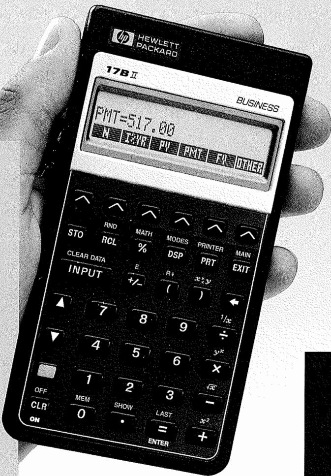
HP 17BII

Financial Calculator

Owner's Manual

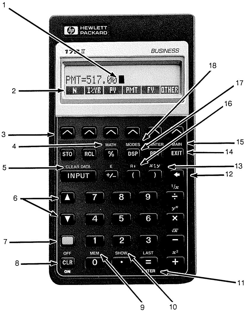
1. Cursor
2. Menu labels
3. Menu keys
4. More math
5. Clearing stored data
6. Moving through lists
7. Shift key (for colored functions)
8. On or display clear

9. User memory available

10. All decimal places

11. [ENTER] (RPN mode)
12. Backspace
13. Exchange RPN registers
14. Previous menu
15. Main menu
16. Roll down RPN stack
17. Display formats
18. Modes key

HP-17B II Business Calculator

Owner's Manual

Notice

For warranty and regulatory information for this calculator, see the owner's manual.

This manual and any examples contained herein are provided "as is" and are subject to change without notice. Hewlett-Packard Company makes no warranty of any kind with regard to this manual, including, but not limited to, the implied warranties of merchantability and fitness for a particular purpose. Hewlett-Packard Co. shall not be liable for any errors or for incidental or consequential damages in connection with the furnishing, performance, or use of this manual or the examples contained herein.

Hewlett-Packard Co. 1989. All rights reserved. Reproduction, adaptation, or translation of this manual is prohibited without prior written permission of Hewlett-Packard Company, except as allowed under the copyright laws.

The programs that control your calculator are copyrighted and all rights are reserved. Reproduction, adaptation, or translation of those programs without prior written permission of Hewlett-Packard Co. is also prohibited.

Corvallis Division

1000 N.E. Circle Blvd.

Corvallis, OR 97330, U.S.A.

Printing History

Edition 1

Edition 2

Edition 3

December 1989

April 1991

November 1994

9

110

Running Total and Statistics

111

The SUM Menu

112

Creating a SUM List

112

Entering Numbers and Viewing the TOTAL

113

Viewing and Correcting the List

115

Copying a Number from a List to the Calculator Line

115

Naming and Renaming a SUM List

116

Starting or GETting Another List

116

Clearing a SUM List and Its Name

116

Doing Statistical Calculations (CALC)

117

Calculations with One Variable

119

Calculations with Two Variables (FRCST)

122

Curve Fitting and Forecasting

126

Weighted Mean and Grouped Standard Deviation

129

129

Summation Statistics

129

Doing Other Calculations with SUM Data

10

130

Time, Appointments, and Date Arithmetic

130

Viewing the Time and Date

131

The Time Menu

132

Setting the Time and Date (SET)

133

Changing the Time and Date Formats (SET)

133

Adjusting the Clock Setting (ADJST)

133

Appointments (APPT)

134

Viewing or Setting an Appointment (APT1-APT10)

136

Acknowledging an Appointment

136

Unacknowledged Appointments

137

Clearing Appointments

138

Date Arithmetic (CALC)

139

Determining the Day of the Week for Any Date

139

Calculating the Number of Days between Dates

140

Calculating Past or Future Dates

11 141 The Equation Solver

141 An Example Using the Solver: Sales Forecasts

144 The SOLVE Menu

145 Entering Equations

146 Calculating Using Solver Menus (CALC)

149 Editing an Equation (EDIT)

149 Naming an Equation

150 Finding an Equation in the Solver List

150 Shared Variables

151 Clearing Variables

151 Deleting Variables and Equations

152 Deleting One Equation or Its Variables (DELET)

152 Deleting All Equations or All Variables in the Solver (CLEAR DATA)

153 Writing Equations

154 What Can Appear in an Equation

157 Solver Functions

161 Conditional Expressions with IF

163 The Summation Function ()

164 Accessing CFLO and SUM Lists from the Solver

165 Creating Menus for Multiple Equations (S Function)

166 How the Solver Works

168 Halting and Restarting the Numerical Search

168 Entering Guesses

12 171 Printing

172 The Printer's Power Source

172 Double-Space Printing

172 Printing the Display (PRT)

173 Printing Other Information (PRINTER)

174 Printing Variables, Lists, and Appointments (LIST)

175 Printing Descriptive Messages (MSG)

176 Trace Printing (TRACE)

177 How to Interrupt the Printer

13	178	Additional Examples
	178	Loans
	178	Simple Annual Interest
	179	Yield of a Discounted (or Premium) Mortgage
	181	Annual Percentage Rate for a Loan with Fees
	183	Loan with an Odd (Partial) First Period
	185	Canadian Mortgages
	187	Advance Payments (Leasing)
	189	Savings
	189	Value of a Fund with Regular Withdrawals
	191	Deposits Needed for a Child's College Account
	195	Value of a Tax-Free Account
	197	Value of a Taxable Retirement Account
	198	Modified Internal Rate of Return
	201	Price of an Insurance Policy
	203	Bonds
	205	Discounted Notes
	206	Statistics
	206	Moving Average
	208	Chi-Squared (x²) Statistics

A	211	Assistance, Batteries, Memory, and Service
	211	Obtaining Help in Operating the Calculator
	211	Answers to Common Questions
	213	Power and Batteries
	214	Low-Power Indications
	214	Installing Batteries
	216	Managing Calculator Memory
	217	Resetting the Calculator
	218	Erasing Continuous Memory
	218	Clock Accuracy
	219	Environmental Limits
	219	Determining If the Calculator Requires Service
	220	Confirming Calculator Operation: Self-Test

Limited One-Year Warranty
What is Covered
What Is Not Covered
Consumer Transactions in the United Kingdom
If the Calculator Requires Service
Obtaining Service
Service Charge
Shipping Instructions
Warranty on Service
Service Agreements
Regulatory Information
Radio Frequency Interference
Air Safety Notice (U.S.A.)

More About Calculations

IRR% Calculations

Possible Outcomes of Calculating IRR%
Halting and Restarting the IRR% Calculation
Storing a Guess for IRR%
Dolver Calculations
Direct Solutions
Iterative Solutions

Equations Used by Built-in Menus
Actuarial Functions
Percentage Calculations in Business (BUS)
Time Value of Money (TVM)
Amortization
Interest Rate Conversions
Cash-Flow Calculations
Bond Calculations
Depreciation Calculations
Sum and Statistics
Forecasting
Equations Used in (Chapter 13)
Canadian Mortgages
Odd-Period Calculations
Advance Payments
Modified Internal Rate of Return

Welcome to the HP-17B II

The HP-17B is part of Hewlett-Packard's new generation of calculators:

The two-line display has space for messages, prompts, and labels.
- Menu and messages show you options and guide you through problems.
Built-in applications solve these business and financial tasks:

Time Value of Money. For loans, savings, leasing, and amortization.
■ Interest Conversions. Between nominal and effective rates.
Cash Flows. Discounted cash flows for calculating net present value and internal rate of return.
Bonds. Price or yield on any date. Annual or semi-annual coupons; 30/360 or actual/actual calendar.
Depreciation. Using methods of straight line, declining balance, sum-of-the-years' digits, and accelerated cost recovery system.
Business Percentages. Percent change, percent total, markup.
Statistics. Mean, correlation coefficient, linear estimates, and other statistical calculations.
Clock. Time, date, and appointments.

Use the Solver for problems that aren't built in: type an equation and then solve for any unknown value. It's easier than programming!
There are 6.5K bytes of memory to store data, lists, and equations.
You can print information using the HP 82240 Infrared Printer.
■ You can choose either ALG (Algebraic) or RPN (Reverse Polish Notation) entry logic for your calculations.

Contents

12 List of Examples
15 Important Information

1 16 Getting Started

16 Power On and Off; Continuous Memory
16 Adjusting the Display Contrast
17 What You See in the Display
17 The Shift Key (■)
18 Backspacing and Clearing
19 Doing Arithmetic
20 Keying in Negative Numbers (+ - )
20 Using the Menu Keys
21 The MAIN Menu
22 Choosing Menus and Reading Menu Maps
23 Calculations Using Menus
25 Exiting Menus ( X I T)
25 Clearing Values in Menus
26 Solving Your Own Equations (SOLVE)
27 Typing Words and Characters: the ALPHAbetic Menu
28 Editing ALPHAbetic Text
29 Calculating the Answer (CALC)
30 Controlling the Display Format
31 Decimal Places
31 Internal Precision
31 Temporarily SHOWing ALL
31 Rounding a Number
32 Exchanging Periods and Commas in Numbers
33 Error Messages
33 Modes
34 Calculator Memory ( MEMI)

2

35 Arithmetic

35 The Calculator Line
35 Doing Calculations
36 Using Parentheses in Calculations
37 The Percent Key
38 The Mathematical Operations
38 The Power Function (Exponentiation)
39 The MATH Menu
40 Saving and Reusing Numbers
40 The History Stack of Numbers
41 Reusing the Last Result (LAST)
42 Storing and Recalling Numbers
43 Doing Arithmetic Inside Registers and Variables
44 Scientific Notation
44 Range of Numbers

3

45 Percentage Calculations in Business

46 Using the BUS Menus
46 Examples Using the BUS Menus
46 Percent Change (%CHG)
47 Percent of Total (%TOTL)
47 Markup as a Percent of Cost (MU%C)
48 Markup as a Percent of Price (MU%P)
48 Sharing Variables Between Menus

4

50 Time Value of Money

50 The TVM Menu
53 Cash Flow Diagrams and Signs of Numbers
55 Using the TVM Menu
56 Loan Calculations
60 Savings Calculations
63 Leasing Calculations
67 Amortization (AMRT)
68 Displaying an Amortization Table
71 Printing an Amortization Table

5	73	Interest Rate Conversions
	74	The ICNV Menu
	74	Converting Interest Rates
	77	Compounding Periods Different from Payment Periods.
6	80	Cash Flow Calculations
	81	The CFLO Menu
	82	Cash Flow Diagrams and Signs of Numbers
	83	Creating a Cash-Flow List
	84	Entering Cash Flows
	87	Viewing and Correcting the List
	87	Copying a Number from a List to the Calculator Line
	87	Naming and Renaming a Cash-Flow List
	88	Starting or GETting Another List
	89	Clearing a Cash-Flow List and Its Name
	89	Cash-Flow Calculations: IRR, NPV, NUS, NFV
	96	Doing Other Calculations with CFLO Data

7	97	Bonds
	97	The BOND Menu
	98	Doing Bond Calculations

8	103	Depreciation
	103	The DEPRC Menu
	105	Doing Depreciation Calculations
	105	DB, SOYD, and SL Methods
	107	The ACRS Method
	108	Partial-Year Depreciation

C 243 Menu Maps

D 249 RPN: Summary

249 About RPN
249 About RPN on the HP-17B II
250 Setting RPN Mode
251 Where the RPN Functions Are
252 Doing Calculations in RPN
252 Arithmetic Topics Affected by RPN Mode
252 Simple Arithmetic
254 Calculations With STO and RCL
255 Chain Calculations-No Parentheses!

E 256 RPN: The Stack

256 What the Stack Is
257 Reviewing the Stack (Roll Down)
257 Exchanging the X- and Y-Registers in the Stack
258 Arithmetic-How the Stack Does It
259 How ENTER Works
260 Clearing Numbers
261 The LAST X Register
261 Retrieving Numbers From LAST X
261 Reusing Numbers
262 Chain Calculations
263 Exercises

F 264 RPN: Selected Examples

271 Error Messages

276 Index

List of Examples

The following list groups the examples by category.

Getting Started

22 Using Menus
26 Using the Solver

Arithmetic

37 Calculating Simple Interest
166 Unit Conversions
178 Simple Interest at an Annual Rate (RPN example on page 264)

General Business Calculations

46 Percent Change
47 Percent of Total
47 Markup as a Percent of Cost
48 Markup as a Percent of Price
49 Using Shared Variables
147 Return on Equity

Time Value of Money

56 A Car Loan
57 A Home Mortgage
59 A Mortgage with a Balloon Payment
60 A Savings Account
62 An Individual Retirement Account
63 Calculating a Lease Payment
64 Present Value of a Lease with Advanced Payments and Option to Buy

69 Displaying an Amortization Schedule for a Home Mortgage
71 Printing an Amortization Schedule
160 Calculations for a Loan with an Odd First Period
179 Discounted Mortgage
181 APR for a Loan with Fees

(RPN example on page 264)

182 Loan from the Lender's Point of View
(RPN example on page 265)
184 Loan with an Odd First Period
185 Loan with an Odd First Period Plus Balloon
186 Canadian Mortgage
188 Leasing with Advance Payments
189 A Fund with Regular Withdrawals
191 Savings for College (RPN example on page 266)
195 Tax-Free Account (RPN example on page 268)
197 Taxable Retirement Account

(RPN example on page 269)

202 Insurance Policy

Interest Rate Conversions

75 Converting from a Nominal to an Effective Interest Rate
78 Balance of a Savings Account

Cash Flow Calculations

86 Entering Cash Flows
90 Calculating IRR and NPV of an Investment
93 An Investment with Grouped Cash Flows
95 An Investment with Quarterly Returns

199 Modified IRR

Bonds and Notes

100 Price and Yield of a Bond
101 A Bond with a Call Feature
102 A Zero-Coupon Bond
203 Yield to Maturity and Yield to Call
205 Price and Yield of a Discounted Note

Depreciation

105 Declining-Balance Depreciation
107 ACRS Deductions
109 Partial-Year Depreciation

Running Total and Statistical Calculations

114 Updating a Checkbook
118 Mean, Median, and Standard Deviation
124 Curve Fitting
127 Weighted Mean
207 A Moving Average in Manufacturing
209 Expected Throws of a Die (x^2)

Time, Alarms, and Date Arithmetic

132 Setting the Date and Time
137 Clearing and Setting an Appointment
139 Calculating the Number of Days between Two Dates
140 Determining a Future Date

How to Use the Equation Solver

142 Return on Equity
154 Sales Forecasts
160 Using a Solver Function (USPV)
163 Nested IF Functions
169 Using Guesses to Find a Solution Iteratively

Printing

176 Trace-Printing an Arithmetic Calculation

Important Information

Take the time to read chapter 1. It gives you an overview of how the calculator works, and introduces terms and concepts that are used throughout the manual. After reading chapter 1, you'll be ready to start using all of the calculator's features.
- You can choose either ALG (Algebraic) or RPN (Reverse Polish Notation) mode for your calculations. Throughout the manual, the "√" in the margin indicates that the examples or keystrokes must be performed differently in RPN. Appendixes D, E, and F explain how to use your calculator in RPN mode.
- Match the problem you need to solve with the calculator's capabilities and read the related topic. You can locate information about the calculator's features using the table of contents, the subject index, the list of examples, and the menu maps in appendix C (the gold-edged pages).
Before doing any time-value-of-money or cash-flow problems, refer to pages 53 and 82 to learn how the calculator uses positive and negative numbers in financial calculations.
■ For a deeper treatment of specific types of calculations, refer to chapter 13, "Additional Examples." If you especially like learning by example, this is a good reference spot for you.

Getting Started

Watch for this symbol in the margin. It identifies examples or keystrokes that are shown in ALG mode and must be performed differently in RPN mode. Appendixes D, E, and F explain how to use your calculator in RPN mode.

The mode affects only arithmetic calculations—all other operations, including the Solver, work the same in RPN and ALG modes.

Power On and Off; Continuous Memory

To turn on the calculator, press (clear) (note ON printed below the key). To turn it off, press and then . This shifted function is called (note OFF printed above the key). Since the calculator has Continuous Memory, turning it off does not affect the information you've stored there.

To conserve energy, the calculator turns itself off after 10 minutes of no use.

If you see the low battery symbol (□) at the top of the display, you should replace the batteries as soon as possible. Follow the instructions on page 214.

Adjusting the Display Contrast

The display's brightness depends on lighting, your viewing angle, and the display contrast setting. To change the display contrast, hold down the key and press + or - .

What You See in the Display

Menu Labels. The bottom line of the display shows the menu labels for each of the five major menus (work areas) in the calculator. More about these later in this chapter.

The Calculator Line. The calculator line is where you see numbers (or letters) that you enter, and the results of calculations.

Annunciators. The symbols shown here are called annihilators. Each one has a special significance.

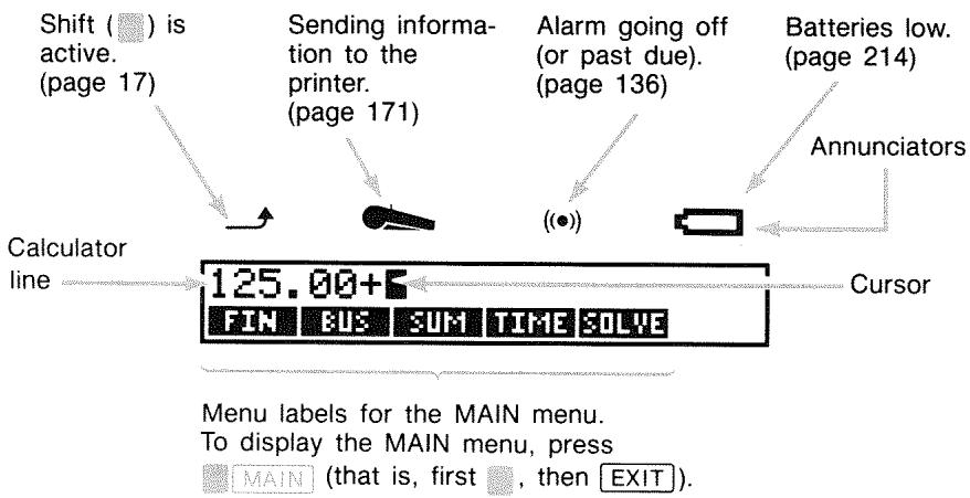
The Shift Key (

Some keys have a second, shifted function printed in color above the key. The colored shift key accesses these operations. For example, pressing and releasing , then pressing turns the calculator off. This is written OFF.

Pressing turns on the shift annunciator () . This symbol stays on until you press the next key. If you ever press by mistake, just press again to turn off the .

Backspacing and Clearing

The following keys erase typing mistakes, entire numbers, or even lists or sets of data.

Table 1-1. Keys for Clearing

Key	Description
CLR	Backspace; erases the character before the cursor. Clear; clears the calculator line. (When the calculator is off, this key turns the calculator on, but without clearing anything.)
CLEAR DATA	This clears all information in the current work area (menu). For example, it will erase all the numbers in a list if you are currently viewing a list (SUM or CFLO). In other menus (like TVM), CLEAR DATA clears all of the values that have been stored. In SOLVE, it can delete all equations.

The cursor () is visible while you are keying in a number or doing a calculation. When the cursor is visible, pressing deletes the last character you keyed in. When the cursor is not visible, pressing erases the last number.

Keys:	Display:	Description:
12345		Backspacing removes the 4 and 5.
.66	123.66	Calculates 1/123.66.
i/x	0.01
	0.00	C clears the calculator line.

In addition, there are more drastic clearing operations that erase more information at once. Refer to "Resetting the Calculator" on page 217 in appendix A.

Doing Arithmetic

The “ ” in the margin is a reminder that the example keystrokes are for ALG mode.

This is a brief introduction to doing arithmetic. More information on arithmetic is in chapter 2. Remember that you can erase errors by pressing or .

To calculate 21.1 + 23.8:

Keys:	Display:	Description:
21.1 +	21, 10+
23.8	21, 10+23, 8
=	44, 90	= completes calculation.

Once a calculation has been completed, pressing another digit key starts a new calculation. On the other hand, pressing an operator key continues the calculation:

77.35	77.35-	Calculates
		77.35 - 90.89.

90.89

-13.54

65 √x × 12	New calculation:
=	√65 × 12.

÷ 3.5

=

27.64

Calculates 96.75 ÷ 3.5.

You can also do long calculations without pressing = after each intermediate calculation—just press it at the end. The operators perform from left to right, in the order you enter them. Compare:

$$ \frac {6 5 + 1 2}{3 . 5} \quad \text {a n d} \quad 6 5 + \frac {1 2}{3 . 5} $$

65 + 12 ÷		Operations occur in the order you see them.
3.5 =	22.00

65	12	12
3.5	68.43

Keying in Negative Numbers (+/-)

The + key changes the sign of a number.

To key in a negative number, type that number, then press 7 .
To change the sign of an already displayed number (it must be the rightmost number), press +/- .

Keys:	Display:	Description:
75 +/-	-75	Changes the sign of 75.
× 7.1 =	-532.50	Multiplies -75 by 7.1.

Using the Menu Keys

The calculator usually displays a set of labels across the bottom of the display. The set is called a menu because it presents you with choices. The MAIN menu is the starting point for all other menus.

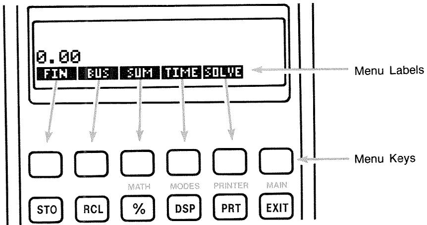
The top row of keys is related to the labels along the bottom of the display. The labels tell you what the keys do. The six keys are called menu keys; the labels are called menu labels.

The MAIN Menu

The MAIN menu is a set of primary choices leading to other menu options. No matter which menu you currently see, pressing main redistributes the MAIN menu. The menu structure is hierarchical.

Table 1-2. The MAIN Menu

Menu Label	Operations Done in This Category	Covered in:
FIN (Finance)	TVM: Time value of money: loans, savings, leasing, amortization.	Chapter 4
	ICNV: Interest conversions.	Chapter 5
	CFLO: Lists of cash flows for internal rate of return and net present value.	Chapter 6
	BOND: Yields and prices for bonds.	Chapter 7
	DEPRC: Depreciation using SL, DB, and SOYD methods, or ACRS.	Chapter 8
BUS (Business Percentages)	Percent of total, percent change, markup on cost, markup on price.	Chapter 3
SUM (Statistics)	Lists of numbers, running total, mean, weighted statistics, forecasting, summation statistics, and more.	Chapter 9
TIME (Time Manager)	Clock, calendar, appointments, date arithmetic.	Chapter 10
SOLVE (Equation Solver)	Creates customized menus from your own equations for calculations you do often.	Chapter 11

Choosing Menus and Reading Menu Maps

Below is a menu map illustrating one possible path through three levels of menus: from the MAIN menu to the BUS menu to the MU%C (markup as a percent of cost) menu. There are no menus that branch from the MU%C menu because the MU%C menu is a final destination—you use it to do calculations, rather than to choose another menu.

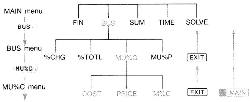
Press BUS to choose the BUS menu. Then press MU%C to choose the MU%C menu.
Press X I T to return to the previous menu. Pressing X I T enough times returns you to the MAIN menu.
Press MAIN to return to the MAIN menu directly.

When a menu has more than six labels, the label MORE appears at the far right. Use it to switch between sets of menu labels on the same "level".

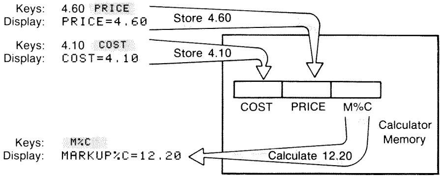
Example: Using Menus. Refer to the menu map for MU%C (above) along with this example. The example calculates the percent markup on cost of a crate of oranges that a grocer buys for 4.10 and sells for 4.60.

Step 1. Decide which menu you want to use. The MU%C (markup as a percent of cost) menu is our destination. If it's not obvious to you which menu you need, look up the topic in the subject index and examine the menu maps in appendix C.

Displaying the MU%C menu:

Step 2. To display the MAIN menu, press MAIN. This step lets you start from a known location on the menu map.

Step 3. Press BUS to display the BUS menu.

Step 4. Press Muzo to display the MU%C menu.

Using the MU%C menu:

Step 5. Key in the cost and press COST to store 4.10 as the COST.

Step 6. Key in the price and press PRICE to store 4.60 as the PRICE.

Step 7. Press MTC to calculate the markup as a percent of cost. The answer: MARKUP%C = 12.20 .

Step 8. To leave the MU%C menu, press EXIT twice (once to get back to the BUS menu, and again to get to the MAIN menu) or MAIN (to go directly to the MAIN menu).

Calculations Using Menus

Using menus to do calculations is easy. You don't have to remember in what order to enter numbers and in what order results come back. Instead, the menus guide you, as in the previous example. All the keys you need are together in the top row. The menu keys both store numbers for the calculations and start the calculations.

The MU%C menu can calculate M% C , the percent markup on cost, given COST and PRICE.

Then the same menu can calculate PRICE given COST and M% C

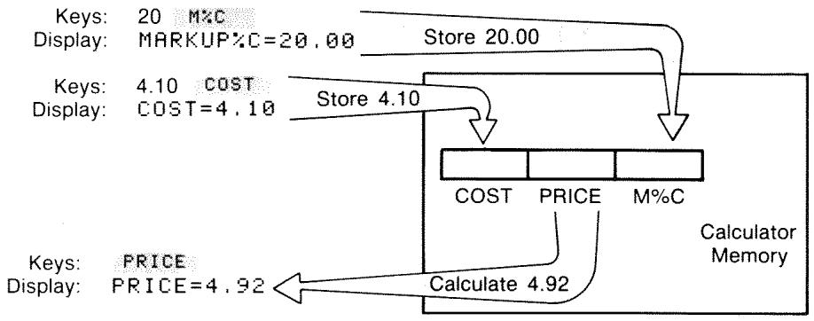
Notice that the two calculations use the same three variables; each variable can be used both to store and calculate values. These are called built-in variables, because they are permanently built into the calculator.

Many menus in this calculator work like the example above. The rules for using variables are:

To store a value, key in the number and press the menu key.* Arithmetic calculations, as well as single values, can be stored.
To calculate a value, press the menu key without first keying in a number. The calculator displays CALCULATING when a value is being calculated.
To verify a stored value, press RCL (recall) followed by the menu key. For example, RCL COST displays the value stored in COST.
To transfer a value to another menu, do nothing if it is displayed (that is, it is in the calculator line). A number in the calculator line remains there when you switch menus. To transfer more than one value from a menu, use storage registers. See page 42, "Storing and Recalling Numbers."

Exiting Menus (EXIT)

The key is used to leave the current menu and go back to the previously displayed menu (as shown in the previous example). This is true for menus you might pick by accident, too: gets you out.

Clearing Values in Menus

The Clear Data key is a powerful feature to clear all the data in the currently displayed menu, giving you a clean slate for new calculations.

If the current menu has variables (that is, if the display shows menu labels for variables, such as COST, PRICE, and M% C in the MU % C menu), pressing CLEAR DATA clears the values of those variables to zero.
If the current menu has a list (SUM, CFLO, or Solver), pressing CLEAR DATA clears the values in the list.

To see what value is currently stored in a variable, press RCL menu label.

Solving Your Own Equations (SOLVE)

This chapter has introduced some of the built-in menus the calculator offers. But if the solution to a problem is not built into HP-17B, you can turn to the most versatile feature of all: the Equation Solver. Here you define your own solution in terms of an equation. The Solver then creates a menu to go with your equation, which you can use over and over again, just like the other menus in the calculator.

The Solver is covered in chapter 11, but here is an introductory example. Because equations usually use letters of the alphabet, this section also explains how to type and edit letters and other characters that aren't on the keyboard.

Example: Using the Solver. Suppose you frequently buy carpet and must calculate how much it will cost. The price is quoted to you per square yard. Regardless of how you do the calculation (even if you do it longhand), you are using an equation.

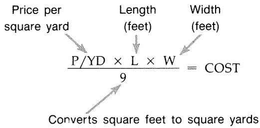
To type this equation into the Solver, use the ALPHA menu.

Typing Words and Characters: the ALPHAbetic Menu

The ALPHAbetic menu is automatically displayed when you need it to type letters and characters. The ALPHA menu also includes characters not found on the keyboard:

Uppercase letters.
Space.
■ Punctuation and special characters.
Non-English letters.

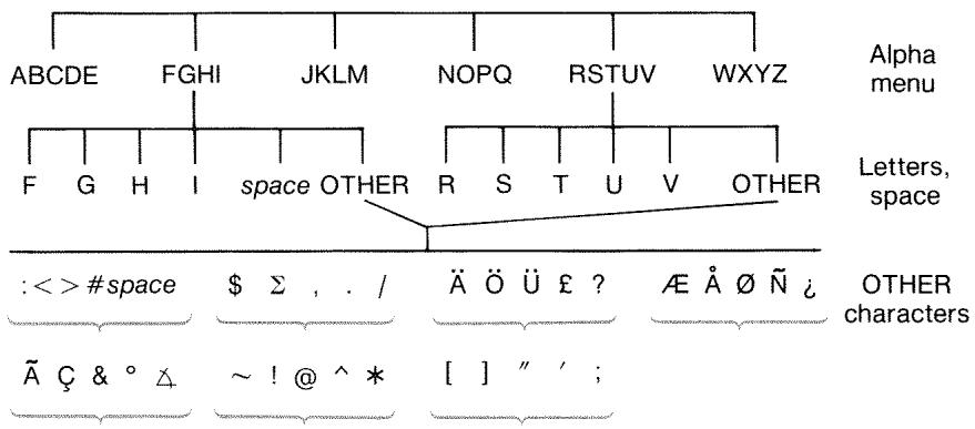
To type a letter you need to press two keys; for example, is produced by the keystrokes ABCDE R

Each letter menu has anOTHERkey for accessing punctuation and non-English characters. The letter menus with just four letters (for example, FGHI) include a space character (

To familiarize yourself with the ALPHA menu, type in the equation for the cost of carpeting. The necessary keystrokes are shown below. (Note the access to the special character, "/".) Use , if necessary, to make corrections. If you need to do further editing, refer to the next section, "Editing ALPHAbetic Text." When you're satisfied that the equation is correct, press INPUT to enter the equation into memory.

Keys

Characters

MAIN

SOLVE NEW

NOPQ

P

MORE

P

WXYZ

OTHER

MORE

P

WXYZ

Y

ABCOE

P/YD

JKLM

藻

图

P,YD×L×

WXYZ

H

P/YD×L×W÷9=

ABCDE

C

NOPQ

0

P/YD×L×W=9=CO

RSTUV

5

RSTUV

T

P/YD×L×W÷9=COST

INPUT

P,YD×L×W÷9=COST

Note that the is just a character, part of the variable's name. It is not an operator, which ÷ is.

Editing ALPHAbetic Text

The companion to the ALPHA menu is the ALPHA-Edit menu. To display the ALPHA-Edit menu, press EDIT in the SOLVE menu (or press EXIT in the ALPHA menu).

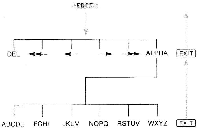
Table 1-3. Alphabetic Editing

Operation	Label or Key to Press
ALPHA-Edit Menu
Inserts character before the cursor.	Any character.
Deletes character at the cursor.	DEL
Moves the cursor far left, one display-width.	<<--
Moves the cursor left.	<--
Moves the cursor right.	-->
Moves the cursor far right, one display-width.	--->
Displays the ALPHA menu again.	ALPHA
Keyboard
Backspaces and erases the character before the cursor.	#
Clears the calculator line.	CLR

Calculating the Answer (CALC)

After an equation is input, pressing calc verifies it and creates a new, customized menu to go with the equation.

Menu labels for your variables

Each of the variables you typed into the equation now appears as a menu label. You can store and calculate values in this menu the same way you do in other menus.

Calculate the cost of carpet needed to cover a 9' by 12' room. The carpet costs $22.50 per square yard.

Starting from the MAIN menu (press MAIN):

Keys:	Display:	Description:
SOLVE	P/YD×L×W÷9=COST	Displays the SOLVE menu and the current equation.*
CALC		Displays the customized menu for carpeting.
22.5 P/YD	P/YD=22.50	Stores the price per square yard in P/YD.
12 L	L=12.00	Stores the length in L.
9 W	W=9.00	Stores the width in W.
COST	COST=270.00	Calculates the cost to cover a 9' × 12' room.

Now determine the most expensive carpet you can buy if the maximum amount you can pay is $300. Notice that all you need to do is enter the one value you are changing—there is no need to re-enter the other values.

300 COST COST=300.00 Stores $300 in COST.

P/YD P/YD=25.00 Calculate the maximum price per square yard you can pay.

EXIT EXIT Exits Solver.

Controlling the Display Format

The DSP menu (press DSP) gives you options for formatting numbers. You can pick the number of decimal places to be displayed, and whether to use a comma or a period to "punctuate" your numbers.

• If you entered this equation but don't see it now, press or until you do.

Decimal Places

To change the number of displayed decimal places, first press the DSP key. Then either:

Press FIX, type the number of decimal places you want (from 0 to 11), and press INPUT; or
Press ALL to see a number as precisely as possible at any time (12 digits maximum).

Internal Precision

Changing the number of displayed decimal places affects what you see, but does not affect the internal representation of numbers. The number inside the calculator always has 12 digits.

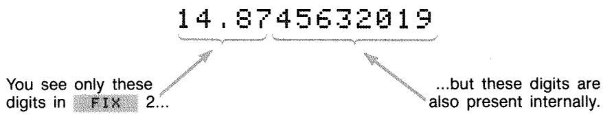
Temporarily SHOWing ALL

To temporarily see a number with full precision, press SHOW. This shows you the ALL format for as long as you hold down SHOW.

Rounding a Number

The RND function rounds the number in the calculator line to the number of displayed decimal places. Subsequent calculations use the rounded value.

Starting with two displayed decimal places:

Keys:	Display:	Description:
5.787	5.787■
DSP FIX4 [INPUT]	5.7870	Four decimal places are displayed.
DSP ALL	5.787	All significant digits; trailing zeros dropped.
DSP FIX2 [INPUT]	5.79	Two decimal places are displayed.
SHOW(hold)	FULL PRECISION IS:5.787	Temporarily shows full precision.
RNDSHOW (hold)	5.79	Rounds the number to two decimal places.

Exchanging Periods and Commas in Numbers

To exchange the periods and commas used for the decimal point and digit separators in a number:

1. Press DSP to access the DSP (display) menu.
2. Specify the decimal point by pressing or . Pressing sets a period as the decimal point and comma as the digit separator (U.S. mode). (For example, 1,000,000.00.) Pressing sets a comma as the decimal point and period as the digit separator (non-U.S. mode). (For example, 1.000.000.00.)

Error Messages

Sometimes the calculator cannot do what you "ask", such as when you press the wrong key or forget a number for a calculation. To help you correct the situation, the calculator beeps and displays a message.

Press CLR or to clear the error message.
Press any other key to clear the message and perform that key's function.

For more explanations, refer to the list of error messages just before the subject index.

Modes

Beeper. Beeping occurs when a wrong key is pressed, when an error occurs, and during alarms for appointments. You can suppress and re-activate the beeper in the MODES menu as follows:

1. Press MODES
2. Pressing BEEP will simultaneously change and display the current setting for the beeper:

BEEPER ON beeps for errors and appointments.
BEEPER ON: APPTS ONLY beeps only for appointments.
BEBPER OFF silences the beeper completely.

1. Press EXIT when done.

Print. Press MODES PRINT to specify whether or not the printer ac adapter is in use. Then press EXIT.

Double Space. Press MODES DEL to turn double-spaced printing on or off. Then press EXIT.

Algebraic. Press MODES FLG to select algebraic entry logic.

RPN. Press [MODES] RPH to select Reverse Polish Notation entry logic.

Calculator Memory (MEM)

The calculator stores many different types of information in its memory. Each piece of information requires a certain amount of storage space.* You can monitor the amount of available memory by pressing

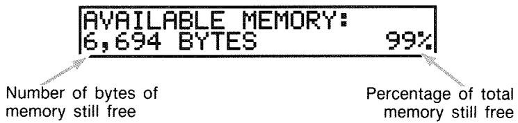
The amount of memory available for storing information and working problems is about 6,750 bytes. ^ (Units of memory space are called bytes.) The calculator gives you complete flexibility in how you use that available memory (such as for lists of numbers or equations). Use as much of the memory as you want for any task you want.

If you use nearly all of the calculator's memory, you'll encounter the message INSUFFICIENT MEMORY. To remedy this situation, you must erase some previously stored information. Refer to "Managing Calculator Memory" on page 216 in appendix A.

The calculator also allows you to erase at once all the information stored inside it. This procedure is covered in "Erasing Continuous Memory" on page 218.

• Storing numbers in menus like TVM (non-Solver menus) does not use any of your memory space.
  † There are 8,000 bytes total in RAM (random access memory): 6,750 bytes plus 1,250 bytes reserved by the system to store your values in built-in variables.

Arithmetic

If you prefer RPN to algebraic logic, please read appendix D before you read this chapter. The “ ” in the margin is a reminder that the example keystrokes are for ALG mode.

The Calculator Line

The calculator line is the part of the display where numbers appear and calculations take place. Sometimes this line includes labels for results, such as TOTAL = 124.60 . Even in this case you can use the number for a calculation. For example, pressing + 2 would calculate 124.60 plus 2, and the calculator would display the answer, 126.60.

There is always a number in the calculator line, even though sometimes the calculator line is hidden by a message (such as SELECT COMPOUNDING). To see the number in the calculator line, press 4 , which removes the message.

Doing Calculations

Simple calculating was introduced in chapter 1, page 19. Often longer calculations involve more than one operation. These are called chain calculations because several operations are "chained" together. To do a chain calculation, you don't need to press = after each operation, but only at the very end.

For instance, to calculate 750 × 12360 you can type either:

750 12 = 360

or

750 × 12 ÷ 360 =

In the second case, the ÷ key acts like the = key by displaying the result of 750 × 12 .

Here's a longer chain calculation.

$$ \frac {4 5 6 - 7 5}{1 8 . 5} \times \frac {6 8}{1 . 9} $$

This calculation can be written as: 456 - 75 ÷ 18.5 × 68 ÷ 1.9 .

Watch what happens in the display as you key it in:

Keys: Display:

456 75 381.00÷
18.5 20.59x
68 1,400,43÷
1.9 737.07

Using Parentheses in Calculations

Use parentheses when you want to postpone calculating an intermediate result until you've entered more numbers. For example, suppose you want to calculate:

$$ \frac {3 0}{8 5 - 1 2} \times 9 $$

If you were to key in 30 ÷ 85 , the calculator would calculate the intermediate result, 0.35. However, that's not what you want. To delay the division until you've subtracted 12 from 85, use parentheses:

Keys:	Display:	Description:
30÷85	30.00÷(85.00-	No calculation is done.
12	30.00÷73.00	Calculates 85 - 12.
×9	0.41×9	Calculates 30 / 73.
=	3.70	Calculates 0.41 × 9.

Note that you must include a for multiplication; parentheses do not imply multiplication.

The Percent Key

The % key has two functions:

Finding a Percentage. In most cases, % divides a number by 100. The one exception is when a plus or minus sign precedes the number. (See "Adding or Subtracting a Percentage," below.)

For instance, 25 % results in 0.25.

To find 25% of 200, press: 200 × 25 % . (Result is 50.00.)

Adding or Subtracting a Percentage. You can do this all in one calculation:

For instance, to decrease 200 by 25% , just enter 200 - 25% = 150.00 . (Result is 150.00 .)

Example: Calculating Simple Interest. You borrow $1,250 from a relative, and agree to repay the loan in a year with 7% simple interest. How much money will you owe?

Keys:	Display:	Description:
1250 + 7 %	1,250.00+87.50	Interest on the loan is $87.50.
	1,337.50	You must repay this amount at the end of one year.

The Mathematical Functions

Some of the math functions appear on the keyboard; others are in the MATH menu. Math functions act on the last number in the display.

Table 2-1. Shifted Math Functions

Key	Description
1/x	reciprocal
√x	square root
2/x	square

Keys:	Display:	Description:
4 1/x	0.25	Reciprocal of 4.
20 √x	4.47	Calculates √20.
+ 47.2 x	51.67x	Calculates 4.47 + 47.20.
1.1 x²	51.67x1.21	Calculates 1.1².
=	62.52	Completes calculation of (4.47 + 47.2) × 1.1².

The Power Function (Exponentiation)

The power function, ^x , raises the preceding number to the power of the following number.

Keys:	Display:	Description:
125 yx 3 =	1,953,125.00	Calculates 1253.
125 yx 3	5.00	Calculates the cube root of 125, which is the same as (125)1/3.

The MATH Menu

To display the MATH menu, press MATH (the shifted % key). Like the other mathematics functions, these functions operate on only the last number in the display.

Table 2-2. The MATH Menu Labels

Menu Label	Description
LOG	Common (base 10) logarithm of a positive number.
10^X	Common (base 10) antilogarithm; calculates 10^x.
LN	Natural (base e) logarithm of a positive number.
EXP	Natural antilogarithm; calculates ex.
N!	Factorial.
PI	Inserts the value for π into the display.

Keys:	Display:	Description:
2.5	MATH	Calculates 10^2.5.
10^X	316.23
4	N!	24.00
EXIT		Calculates the factorial of 4.
		Exits MATH menu.

You can access the MATH menu when another menu is displayed. For instance, while using SUM you might want to use a MATH function. Just press , then perform the calculation. Pressing returns you to SUM. The MATH result remains in the calculator line. Remember, however, that you must exit MATH before you resume using SUM.

Saving and Reusing Numbers

Sometimes you might want to include the result of a previous calculation in a new calculation. There are several ways to reuse numbers.

The History Stack of Numbers

When you start a new operation, the previous result moves out of the display but is still accessible. Up to four lines of numbers are saved: one in the display and three hidden. These lines make up the history stack.

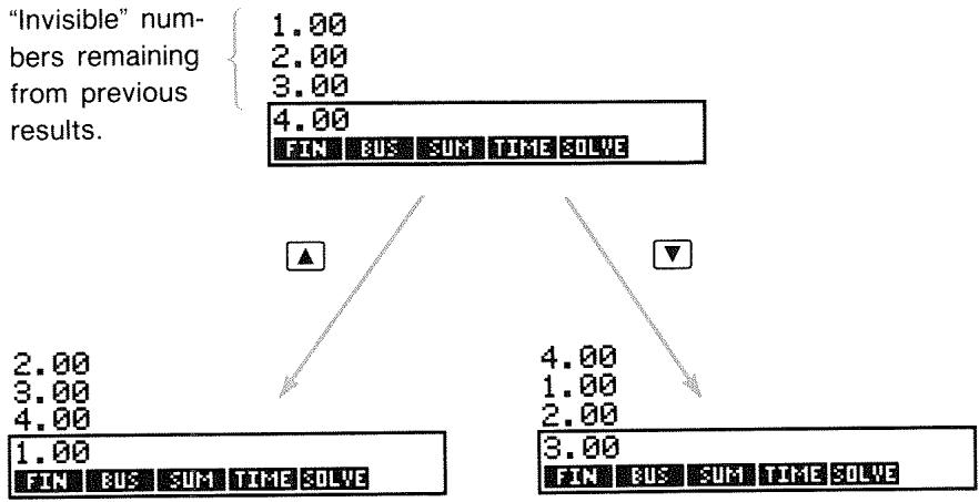
The , , and keys "roll" the history stack down or up one line, bringing the hidden results back into the display. If you hold down or , the history stack wraps around on itself. However, you cannot roll the history stack when an incomplete calculation is in the display. Also, you cannot gain access to the stack while using lists (SUM, CFLO) in ALG mode, or SOLVE in either ALG or RPN mode. All numbers in the history stack are retained when you switch menus.

Pressing exchanges the contents of the bottom two lines of the display.

Pressing CLEAR DATA clears the history stack. Be careful if a menu is active, because then CLEAR DATA also erases the data associated with that menu.

Keys:

Display:

Description:

75.55 32.63

42.92

150

21.43

42.92 moves out of display.

Now, suppose you want to multiply 42.92 × 11 . Using the history stack saves you time.

42.92

Moves 42.92 back to calculator line.

472.12

Reusing the Last Result (LAST)

The LAST key copies the last result—that is, the number just above the calculator line in the history stack—into a current calculation. This lets you reuse a number without retyping it and also lets you break up a complicated calculation.

$$ \frac {3 9 + 8}{\sqrt {1 2 3 + 1 7}} $$

Keys:

Display:

Description:

123 + 17 =

140.00

Calculates 123 + 17

11.83

Calculates 140 .

39 + 8 = ÷

47.00÷11.83

Copies 11.83 to the calculator line.

3.97

Completes the calculation.

An equivalent keystroke sequence for this problem would be:

39+8÷123+17

Storing and Recalling Numbers

The key copies a number from the calculator line into a designated storage area, called a storage register. There are ten storage registers in calculator memory, numbered 0 through 9. The key recalls stored numbers back to the calculator line.

√ If there is more than one number on the calculator line, STO stores only the last number in the display.

To store or recall a number:

1. Press STO or RCL. (To cancel this step, press .)
2. Key in the register number.

The following example uses two storage registers to do two calculations that use some of the same numbers.

$$ \frac {4 7 5 . 6}{3 9 . 1 5} $$

$$ \frac {5 6 0 . 1 + 4 7 5 . 6}{3 9 . 1 5} $$

✓ Keys:	Display:	Description:
475.6 STO 1	475.60	Stores 475.6 into register 1.
÷ 39.15 STO 2	475.60÷39.15	Stores 39.15 (rightmost number) into register 2.
=	12.15	Completes calculation.
560.1 + RCL 1	560.10+475.60	Recalls contents of regis-ter 1.
÷ RCL 2	1,035.70÷39.15	Recalls register 2.
=	26.45	Completes calculation.

The STO and RCL keys can also be used with variables. For example, STO MxC (in the MU%C menu) stores the rightmost number from the display into the variable M% C . RCL MxC copies the contents of M% C into the calculator line. If there is an expression in the display (such as 2 + 4 ), then the recalled number replaces only the last number.

You do not need to clear storage registers before using them. By storing a number into a register, you overwrite whatever existed there before.

Doing Arithmetic Inside Registers and Variables

You can also do arithmetic inside storage registers.

Keys:	Display:	Description:
45.7 STO 3	45.70	Stores 45.7 in reg. 3.
2.5 STO × 3	2.50	Multiplies contents of register 3 by 2.5 and stores result (114.25) back in register 3.
RCL 3	114.25	Displays register 3.

Table 2-3. Arithmetic in Registers

Keys	New Register Contents
STO +	old register contents + displayed number
STO -	old register contents - displayed number
STO ×	old register contents × displayed number
STO ÷	old register contents ÷ displayed number
STO ↕	old register contents ^ displayed number

You can also do arithmetic with the values stored in variables. For example, 2 × 2C (in the MU%C menu) multiplies the current contents of M% C by 2 and stores the product in M% C .

Scientific Notation

Scientific notation is useful when working with very large or very small numbers. Scientific notation shows a small number (less than 10) times 10 raised to a power. For example, the 1984 Gross National Product of the United States was 3,662,800,000,000 . In scientific notation, this is 3.6628 × 10^12 . For very small numbers the decimal point is moved to the right and 10 is raised to a negative power. For example, 0.00000752 can be written as 7.52 × 10^-6 .

When a calculation produces a result with more than 12 digits, the number is automatically displayed in scientific notation, using a capital E in place of “ × 10^".

Remember that + / - changes the sign of the entire number, and not of the exponent. Use - to make a negative exponent.

Type in the numbers 4.78 × 10^13 and -2.36 × 10^-15 .

Keys:	Display:	Description:
4.78 E 13	4.78E13	Pressing E starts the exponent.
CLEAR DATA	0.00	Clears number.
2.36 E - 15	2.36E-15	Pressing - before an exponent makes it negative.
+/-	-2.36E-15	Pressing +/− makes the entire number negative.
CLEAR DATA		C clears number.

Range of Numbers

The largest positive and negative numbers available on the calculator are ± 9.99999999999 × 10^499 ; the smallest positive and negative numbers available are ± 1 × 10^-499 .

Percentage Calculations in Business

The business percentages (BUS) menu is used to solve four types of problems. Each type of problem has its own menu.

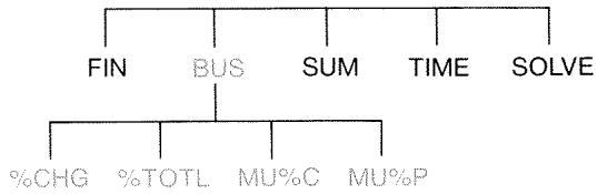
Table 3-1. The Business Percentages (BUS) Menus

Menu	Description
Percent change ( %CHG )	The difference between two numbers (OLD and NEW), expressed as a percentage (%CH) of OLD.
Percent of total ( %TOTAL )	The portion that one number (PART) is of another (TO-TAL), expressed as a percentage (%T).
Markup on cost ( MU×C )	The difference between price (PRICE) and cost (COST), expressed as a percentage of the cost (M%C).
Markup on price ( MU×P )	The difference between price (PRICE) and cost (COST), expressed as a percentage of the price (M%P).

The calculator retains the values of the BUS variables until you clear them by pressing CLEAR DATA. For example, pressing CLEAR DATA while in the %CHG menu clears OLD, NEW, and %CH.

To see what value is currently stored in a variable, press RCL menu label. This shows you the value without recalculating it.

Using the BUS Menus

Each of the four BUS menus has three variables. You can calculate any one of the three variables if you know the other two.

1. To display the %CHG, %TOTL, MU%C, or MU%P menu from the MAIN menu, press BUS, then the appropriate menu label. Pressing xchg, for example, displays:

1. Store each value you know by keying in the number and pressing the appropriate menu key.
2. Press the menu key for the value you want to calculate.

Examples Using the BUS Menus

Percent Change (%CHG)

Example. Total sales last year were 90,000. This year, sales were 95,000. What is the percent change between last year's sales and this year's?

Keys:	Display:	Description:
BUS		Displays %CHG menu.
%CHG
90000 OLD	OLD=90,000.00	Stores 90,000 in OLD.
95000 NEW	NEW=95,000.00	Stores 95,000 in NEW.
%CH	%CHANGE=5.56	Calculates percent change.

What would this year's sales have to be to show a 12% increase from last year? OLD remains 90,000, so you don't have to key it in again. Just enter % CH and ask for NEW.

12 :CH

% CHANGE = 12.00

Stores 12 in % CH

NEW

NEW=100,800.00

Calculates the value 12% greater than 90,000.

Percent of Total (%TOTL)

Example. Total assets for your company are 67,584. The firm has inventories of23,457. What percentage of total assets is inventory?

You will be supplying values for TOTAL and PART and calculating % T . This takes care of all three variables, so there is no need to use CLEAR DATA to remove old data.

Keys:		Display:		Description:
BUS	%TOTAL			Displays %TOTAL menu.
67584	TOTAL	TOTAL=67,584.00		Stores 67,584 in TOTAL.
23457	PART	PART=23,457.00		Stores23,457 in PART.
%T		%TOTAL=34.71		Calculates percent of total.

Markup as a Percent of Cost (MU%C)

Example. The standard markup on costume jewelry at Balkis's Boutique is 60% . The boutique just received a shipment of chokers costing $19.00 each. What is the retail price per choker?

Keys:	Display:	Description:
BUS		Displays MU%C menu.
MU%C
19 COST	COST=19.00	Stores cost in COST.
60 M%C	MARKUP%C=60.00	Stores 60% in M%C.
PRICE	PRICE=30.40	Calculates price.

Markup as a Percent of Price (MU%P)

Example. Kilowatt Electronics purchases televisions for 225, with a discount of 4%. The televisions are sold for300. What is the markup of the net cost as a percent of the selling price?

What is the markup as percent of price without the 4% discount?

Keys:	Display:	Description:
BUS		Displays MU%P menu.
MU%P
225 - 4 %		Calculates and stores net cost in COST.
COST	COST=216.00
300 PRICE	PRICE=300.00	Stores 300 in PRICE.
M%P	MARKUP%P=28.00	Calculates markup as a percent of price.

Use $225 for COST and leave PRICE alone.

225 COST COST = 225.00 Stores 225 in COST.

MARKUP: P = 25.00 Calculate markup.

Sharing Variables Between Menus

If you compare the MU%C menu and the MU%P menus, you'll see that they have two menu labels in common—cost and PRICE.

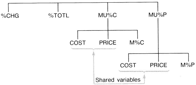
The calculator keeps track of the values you key in according to those labels. For example, if you key in COST and PRICE in the MU%C menu, exit to the BUS menu, and then display the MU%P menu, the calculator retains those values. In other words, the variables are shared between the two menus.

Example: Using Shared Variables. A food cooperative buys cases of canned soup with an invoice cost of (9.60 per case. If the co-op routinely uses a (15\%) markup on cost, for what price should it sell a case of soup?

Keys:	Display:	Description:
BUS		Displays MU%C menu.
MU%C
9.6 COST	COST=9.60	Stores 9.60 in COST.
15 M/C	MARKUP%C=15.00	Stores 15% in M%C.
PRICE	PRICE=11.04	Calculates retail price.

What is the markup on price? Switch menus but keep the same COST and PRICE.

EXIT MU.P

Exits MU%C menu and displays MU%P menu.

MARKUP%P=13.04

Calculates markup as a percent of price.

Time Value of Money

The phrase time value of money describes calculations based on money earning interest over a period of time. The TVM menu performs compound-interest calculations and calculates (and prints) amortization schedules.

In compound interest calculations, interest is added to the principal at specified compounding periods, thereby also earning interest. Savings accounts, mortgages, and leases are compound-interest calculations.
In simple interest calculations, the interest is a percent of the principal and is repaid in one lump sum. Simple interest calculations can be done using the % key (page 37). For an example that calculates simple interest using an annual interest rate, see page 178.

The TVM Menu

The time value of money (TVM) menu does many compound-interest calculations. Specifically, you can use the TVM menu for a series of cash flows (money received or money paid) when:

The dollar amount is the same for each payment.*
The payments occur at regular intervals.
The payment periods coincide with the compounding periods.

12 payments (or periods) per year

Payment mode: the end of each period

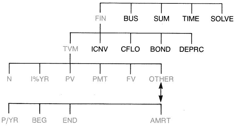
Figure 4-1. The First Level of TVM

To second level of TVM

The first level of the TVM menu has five menu labels for variables plus OTHER. The OTHER key accesses a second-level menu used to specify payment conditions (the payment mode) and to call up the AMRT (amortization) menu.

Figure 4-2. The Second Level of TVM

Table 4-1. TVM Menu Labels

Menu Label	Description
N	First Level Stores (or calculates) the total number of payments or compounding periods.*† (For a 30-year loan with monthly payments, N=12×30=360.)
N	Shortcut for N: Multiplies the number in the display by P/YR, and stores the result in N. (If P/YR were 12, then 30 would set N=360.)
I*YR	Stores (or calculates) the nominal annual interest rate as a percentage.
PV	Stores (or calculates) the present value—an initial cash flow or a discounted value of a series of future cash flows (PMTs + FV). To a lender or borrower, PV is the amount of the loan; to an investor, PV is the initial investment. If PV paid out, it is negative. PV always occurs at the beginning of the first period.
PMT	Stores (or calculates) the dollar amount of each periodic payment. All payments are equal, and no payments are skipped. (If the payments are unequal, use CFLO, not TVM.) Payments can occur at the beginning or end of each period. If PMT represents money paid out, it is negative.
FV	Stores (or calculates) the future value—a final cash flow or a compounded value of a series of previous cash flows (PV + PMTs). FV always occurs at the end of the last period. If FV is paid out, it is negative.
P/YR	specifies the number of payments or compounding periods per year.† (It must be an integer, 1 through 999.)
* When a non-integer N (an "odd period") is calculated, the answer must be interpreted carefully. See the savings account example on page 60. Calculations using a stored, non-integer N produce a mathematically correct result, but this result has no simple interpretation. The example on page 160 uses the Solver to do a partial-period (non-integer) calculation in which interest begins to accrue prior to the beginning of the first regular payment period. † The number of payment periods must equal the number of compounding periods. If this is not true, see page 77. For Canadian mortgages, see page 185.
BEG	Second Level (Continued)
	Sets Begin mode: payments occur at the beginning of each period. Typical for savings plans and leasing. (The Begin and End modes do not matter if PMT=0.)
END	Sets End mode: payments occur at the end of each period. Typical for loans and investments.
AMRT	Accesses the amortization menu. See page 67.

The calculator retains the values of the TVM variables until you clear them by pressing CLEAR DATA. When you see the first-level TVM menu, pressing CLEAR DATA clears N , I% YR, PV, PMT, and FV. When the second-level menu (OTHER) is displayed, pressing CLEAR DATA resets the payment conditions to 12 P/YR END MODE.

To see what value is currently stored in a variable, press RCL menu label. This shows you the value without recalculating it.

Cash Flow Diagrams and Signs of Numbers

It is helpful to illustrate TVM calculations with cash-flow diagrams. Cash-flow diagrams are time lines divided into equal segments called compounding (or payment) periods. Arrows show the occurrence of cash flows (payments in or out). Money received is a positive number (arrow up) and money paid out is a negative number (arrow down).

Note

The correct sign (positive or negative) for TVM numbers is essential. The calculations will make sense only if you consistently show payments out as negative and payments in (receipts) as positive. Perform a calculation from the

point of view of either the lender (investor) or the borrower, but not both!

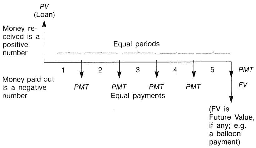
Figure 4-3. A Cash Flow Diagram for a Loan from Borrower's Point of View (End Mode)

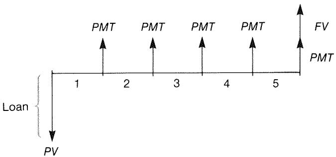
Figure 4-4. A Cash Flow Diagram for a Loan from Lender's Point of View (End Mode)

Payments occur at either the beginning of each period or the end of each period. End mode is shown in the last two figures; Begin mode is shown in the next figure.

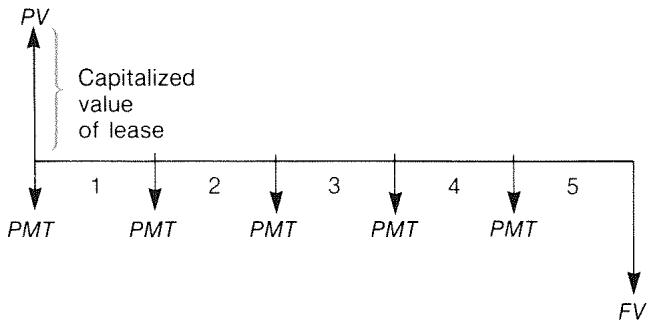
Figure 4-5. Lease Payments Made at the Beginning of Each Period (Begin Mode)

Using the TVM Menu

First draw a cash-flow diagram to match your problem. Then:

1.From the MAIN menu, press FIN TVM
2. To clear previous TVM values, press CLEAR DATA. (Note: You don't need to clear data if you enter new values for all five variables, or if you want to retain previous values.)
3. Read the message that describes the number of payments per year and the payment mode (Begin, End). If you need to change either of these settings, press OTHER.

To change the number of payments per year, key in the new value and press P/YR. (If the number of payments is different from the number of compounding periods, see "Compounding Periods Different from Payment Periods," page 77.)
To change the Begin/End mode, press BEG or END.
Press to return to the primary TVM menu.

1. Store the values you know. (Enter each number and press its menu key.)
2. To calculate a value, press the appropriate menu key.

You must give every variable—except the one you will calculate—a value, even if that value is zero. For example, FV must be set to zero when you are calculating the periodic payment (PMT) required to fully pay back a loan. There are two ways to set values to zero:

Before storing any TVM values, press CLEAR DATA to clear the previous TVM values.
Store zero; for example, pressing 0 FV sets FV to zero.

Loan Calculations

Three examples illustrate common loan calculations. (For amortization of loan payments, see page 67.) Loan calculations typically use End mode for payments.

Example: A Car Loan. You are financing the purchase of a new car with a 3-year loan at 10.5% annual interest, compounded monthly. The purchase price of the car is 7,250. Your down payment is1,500. What are your monthly payments? (Assume payments start one month after purchase—in other words, at the end of the first period.) What interest rate would reduce your monthly payment by $10?

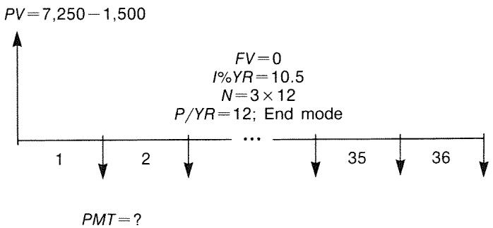
Keys:	Display:	Description:
FIN		Displays TVM menu.
TVM
CLEAR DATA	0.00	Cleared history stack and TVM variables.
OTHER		If needed: sets 12 pay-ment periods per year;End mode.
CLEAR DATA	12 P/YR END MODE
EXIT
3 × 12		Figures and stores num ber of payments.
N	N=36.00
10.5 I&YR	I%YR=10.50	Stores annual interest rate.
7250 - 1500		Stores amount of the loan.
PV	PV=5,750.00
PMT	PMT=-186.89	Calculates payment.Negative value means money to be paid out.

To calculate the interest rate that reduces the payment by (10, add 10 to reduce the negative PMT value.

+ 10 PMT	PMT=-176.89	Stores the reduced pay- ment amount.
I2YR	I2YR=6.75	Calculates the annual in- terest rate.

Example: A Home Mortgage. After careful consideration of your personal finances, you've decided that the maximum monthly mortgage payment you can afford is 630. You can make a12,000 down payment, and annual interest rates are currently 11.5%. If you take out a 30-year mortgage, what is the maximum purchase price you can afford?

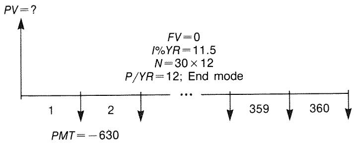
Keys:	Display:	Description:
FIN		Displays TVM menu.
TVM
CLEAR DATA	0.00	Cleared history stack and TVM variables.
OTHER		If needed: sets 12 pay-ment periods per year;
CLEAR DATA		End mode.
EXIT	12 P/YR END MODE
30 N	N=360.00	Pressing first multiplies 30 by 12, then stores this number of payments in N.
11.5 IZYR	IZYR=11.50	Stores annual interest rate.
630+/-		Stores a negative monthly payment.
PMT	PMT=-630.00
PV	PV=63,617.64	Calculates loan amount.
+12000=	75,617.64	Calculates total price of the house (loan plus down payment).

Example: A Mortgage with a Balloon Payment. You've taken out a 25-year, 75,250 mortgage at13.8\%$ annual interest. You anticipate that you will own the house for four years and then sell it, repaying the loan in a "balloon payment." What will be the size of your balloon payment?

The problem is done in two steps:

1. Calculate the monthly payment without the balloon (FV = 0) .
2. Calculate the balloon payment after 4 years.

Keys:	Display:	Description:
FIN		Displays TVM menu.
TVM
CLEAR DATA	0.00	Cleared history stack and TVM variables.
OTHER		If needed: sets 12 pay-ment periods per year;
CLEAR DATA
EXIT	12 P/YR END MODE	End mode.

Step 1. Calculate PMT for the mortgage.

25	N	N=300.00	Figures and stores the number of monthly payments in 25 years.
13.8	IXYR	IXYR=13.80	Stores annual interest rate.
75250	PV	PV=75,250.00	Stores amount of the loan.
PMT		PMT=-894.33	Calculates monthly payment.

Step 2. Calculate the balloon payment after 4 years.

894.33 +/− PMT	PMT=-894.33	Stores rounded PMT value for exact payment amount (no fractional cents).*
4 N	N=48.00	Figures and stores number of payments in 4 years.
FV	FV=-73,408.81	Calculates balloon payment after four years. This amount plus last monthly payment repays the loan.

Savings Calculations

Example: A Savings Account. You deposit 2,000 into a savings account that pays 7.2% annual interest, compounded annually. If you make no other deposits into the account, how long will it take for the account to grow to3,000? Since this account has no regular payments (PMT=0), the payment mode (End or Begin) is irrelevant.

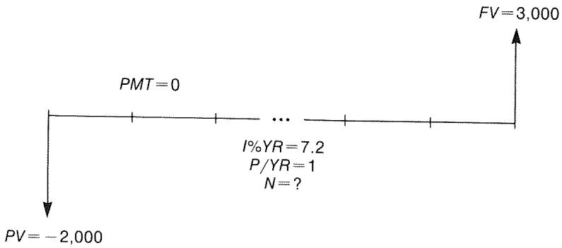
Keys:	Display:	Description
FIN		Displays TVM menu.
TVM
CLEAR DATA	0.00	Cleared history stack and TVM variables.
OTHER		Sets one compounding per./yr. (one interest pmt./yr). Payment mode does not matter.
1 P/YR
EXIT	1 P/YR
7.2 IXYR	IXYR=7.20	Stores annual interest rate.
2000 +/− PV	PV=-2,000.00	Stores amount of deposit.
3000 FV	FV=3,000.00	Stores future account balance in FV.
N	N=5.83	Calculates number of compounding periods (years) for the account to reach $3,000.

There is no conventional way to interpret results based on a non-integer value (5.83) of N . Since the calculated value of N is between 5 and 6, it will take 6 years of annual compounding to achieve a balance of at least $3,000. The actual balance at the end of 6 years can be calculated as follows:

6 N N = 6,00

Stores a whole number of years in N .

FV FV=3,035.28

Calculates account balance after six years.

Example: An Individual Retirement Account (IRA). You opened an IRA on April 15, 1985, with a deposit of 2,000. Thereafter, you deposit 80.00 into the account at the end of each half-month. The account pays 8.3% annual interest, compounded semimonthly. How much money will the account contain on April 15, 2000?

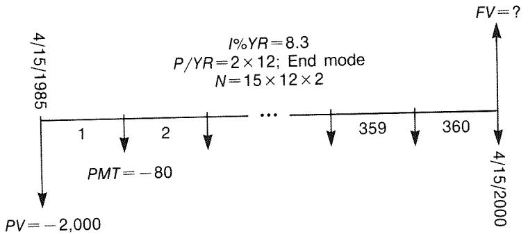
Keys: Display:

FIN

TVM

OTHER

24 P/YR

END

EXIT

Display:

24 P/YR END MODE

Description:

Displays TVM menu. It is not necessary to clear data because you do not need to set any of the values to zero.

Sets 24 payment periods per year, End mode.

15 N N = 360,00

Figures and stores number of deposits in N

8.3 IXYR IXYR=8.30

Stores annual interest rate.

2000 + PV = -2,000.00

Stores initial deposit.

80 + PMT PMT=-80.00

Stores semimonthly payment.

FV FV=63,963.84

Calculates balance in IRA after 15 years.

Leasing Calculations

Two common leasing calculations are 1) finding the lease payment necessary to achieve a specified yield, and 2) finding the present value (capitalized value) of a lease. Leasing calculations typically use "advance payments". For the calculator, this means Begin mode because all payments will be made at the beginning of the period. If there are two payments in advance, then one payment must be combined with the present value. For examples with two or more advance payments, see pages 64 and 187.

Example: Calculating a Lease Payment. A new car valued at 13,500 is to be leased for 3 years. The lessee has the option to purchase the car for 7,500 at the end of the leasing period. What monthly payments, with one payment in advance, are necessary to yield the lessor 14% annually? Calculate the payments from the lessor's point of view. Use Begin payment mode because the first payment is due at the inception of the lease.

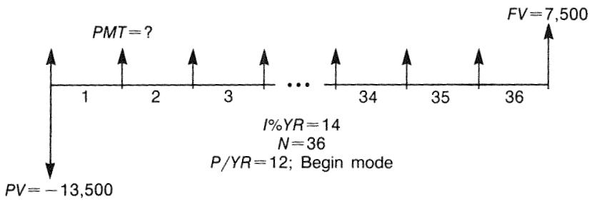
Keys:	Display:	Description:
FIN		Displays TVM menu.
TVM
OTHER		Sets 12 payment periods per year, Begin mode.
12 P/YR
BEG	12 P/YR BEGIN MODE
EXIT
36 N	N=36.00	Stores number of payments.
14 I.YR	I.YR=14.00	Stores annual interest rate.
13500+/-		Stores car's value in PV. (Money paid out by lessor.)
PV	PV=-13,500.00
7500 FV	FV=7,500.00	Stores purchase option value in FV. (Money received by lessor.)
PMT	PMT=289.19	Calculates monthly payment received.

Example: Present Value of a Lease with Advance Payments and Option to Buy. Your company is leasing a machine for 4 years. Monthly payments are 2,400 with two payments in advance. You have an option to buy the machine for 15,000 at the end of the leasing period. What is the capitalized value of the lease? The interest rate you pay to borrow funds is 18%, compounded monthly.

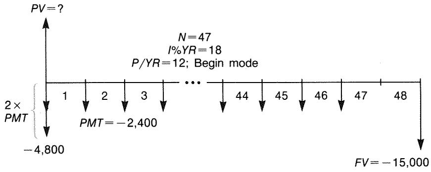
The problem is done in four steps:

1. Calculate the present value of 47 monthly payments in Begin mode. (Begin mode makes the first payment an advance payment.)
2. Add one additional payment to the calculated present value. This adds a second advance payment to the beginning of the leasing period, replacing what would have been the final (48th) payment.
3. Find the present value of the buy option.
4. Add the present values calculated in steps 2 and 3.

Keys:	Display:	Description:
FIN TVM		Displays TVM menu.
CLEAR DATA	0.00	Cleared history stack and TVM variables.
OTHER		Sets 12 payment periods per year; Begin mode.
12 P/YR
BEG
EXIT	12 P/YR BEGIN MODE

Step 1: Find the present value of the monthly payments.

47 N N = 47,00

Stores number of payments.

18 IxYR IxYR=18.00

Stores annual interest rate.

2400 + Stores monthly payment. PMT PMT=-2,400.00

PV PV=81,735.58

Calculates present (capitalized) value of the 47 monthly payments.

Step 2: Add the additional advance payment to PV . Store the answer.

2400 84,135.58

Calculates present value of all payments.

STO 0 84,135.58

Stores result in register 0.

Step 3: Find the present value of the buy option.

48 N N = 48,00

Stores number of payment periods.

15000 FV FV=-15,000.00

Stores amount of the buy option (money paid out).

0 PMT PMT=0.00

There are no payments.

PV PV=7,340.43

Calculates present value of the buy option.

Step 4: Add the results of step 2 and 3.

+0= 91,476.00

Calculates present, capitalized value of lease.

Amortization (AMRT)

The AMRT menu (press TVM OTHER AMRT) displays or prints the following values:

The loan balance after the payment(s) are made.
The amount of the payment(s) applied toward interest.
The amount of the payment(s) applied toward principal.

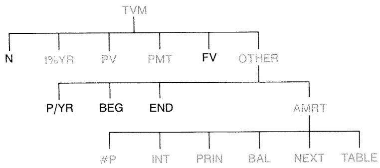
Table 4-2. AMRT Menu Labels

Menu Label	Description
#P	Stores the number of payments to be amortized, and calculates an amortization schedule for that many payments. Successive schedules start where the last schedule left off. #P can be an integer from 1 through 1,200.
INT	Displays the amount of the payments applied toward interest.
PRIN	Displays the amount of the payments applied toward principal.
BAL	Displays the balance of the loan.
NEXT	Calculates the next amortization schedule, which contains #P payments. The next set of payments starts where the previous set left off.
TABLE	Displays a menu for printing an amortization table (schedule).

Displaying an Amortization Schedule

For amortization calculations, you need to know PV , I% YR , and PMT . If you have just finished doing these calculations with the TVM menu, then skip to step 3.

To calculate and display an amortization schedule:\*

1. Press FIN TVM to display the TVM menu.
2. Store the values for I% YR , PV , and PMT . (Press +/- to make PMT a negative number.) If you need to calculate one of these values, follow the instructions under "Using the TVM Menu," on page 55. Then go on to step 3.
3. Press OTHER to display the rest of the TVM menu.
4. If necessary, change the number of payment periods per year stored in P/YR
5. If necessary, change the payment mode by pressing BEG or END. (Most loan calculations use End mode.)
6. Press AMRT. (If you want to print the amortization schedule, go to page 71 to continue.)
7. Key in the number of payments to be amortized at one time and press #P . For example, to see a year of monthly payments at one time, set #P to 12. To amortize the entire life of a loan at one time, set #P equal to the total number of payments (N). If #P = 12, the display would show:

Number of payments amortized at one time

Current set of payments to be amortized

Press to see results

1. To display the results, press INT, PRIN, and BAL (or press to view the results from the stack).
2. To continue calculating the schedule for subsequent payments, do a or b. To start the schedule over, do c.

a. To calculate the next successive amortization schedule, with the same number of payments, press NEXT.

Next successive set of payments authorized

b. To calculate a subsequent schedule with a different number of payments, key in that number and press #P
C. To start over from payment #1 (using the same loan information), press CLEAR DATA and proceed from step 7.

Example: Displaying an Amortization Schedule. To purchase your new home, you have taken out a 30-year, 65,000 mortgage at (12.5% annual interest. Your monthly payment is )693.72. Calculate the amount of the first year's and second year's payments that are applied toward principal and interest.

Then calculate the loan balance after 42 payments (3^1/2 years).

Keys:	Display:	Description:
FIN		Displays TVM menu.
TVM
12.5 IZYR	IZYR=12.50	Stores annual interest rate.
65000 PV	PV=65,000.00	Stores loan amount.
693.72 +/-		Stores monthly payment.
PMT	PMT=-693.72
OTHER		If needed: sets 12 pay-ment periods per year;End mode.
CLEAR DATA	12 P/YR END MODE
AMRT	KEY #PMTS; PRESS (#P)	Displays AMRT menu.
12 #P	#P=12 PMTS: 1-12	Calculates amortization schedule for first 12 pay- ments, but does not display it.
INT	INTEREST=-8,113.16	Displays interest paid in first year.
PRIN	PRINCIPAL=-211.48	Displays principal paid in first year.
BAL	BALANCE=64,788.52	Displays balance at end of first year.
NEXT	#P=12 PMTS: 13-24	Calculates amortization schedule for next 12 payments.
INT	INTEREST=-8,085.15	Displays results for sec- ond year.
PRIN	PRINCIPAL=-239.49
BAL	BALANCE=64,549.03

To calculate the balance after 42 payments (3½ years), amortize 18 additional payments (42 - 24 = 18) :

18	#P	#P=18 PMTS: 25-42	Calculates amortization schedule for next 18 months.
INT		INTEREST= -12,066.98	Displays results.
PRIN		PRINCIPAL=-419.98
BAL		BALANCE=64,129.05

Printing an Amortization Table (TABLE)

To print an amortization schedule (or "table") do steps 1 through 5 for displaying an amortization schedule (see page 68).

1. Press AMRT. Ignore the message KEY #PMTS; PRESS (#P).
2. Press TABLE .
3. Key in the payment number of the first payment in the schedule and press FIRST. (For instance, for the very first payment, FIRST = 1 .)
4. Key in the payment number of the last payment in the schedule and press LAST.
5. Key in the increment—the number of payments shown at one time—and press INCR. (For instance, for one year of monthly payments at a time, INCR=12.)
6. Press Go

Values are retained until you exit the TABLE menu, so you can print successive amortization schedules by re-entering only those TABLE values that change.

Example: Printing an Amortization Schedule. For the loan described in the previous example (page 69), print an amortization table with entries for the fifth and sixth years. You can continue from the AMRT menu in the previous example (step 7, above) or repeat steps 1 through 6.

Starting from the AMRT menu:

Keys:

TABLE

Display:

PRINT AMORT TABLE

Description:

Displays menu for printing amortization table.

4 12 + 1 FIRST

FIRST=49.00

The 49th is the first payment in year 5.

6 12 LAST

LAST=72.00

The 72nd is the last payment in year 6.

Each table entry represents 12 payments (1 year).

GO

Calculates and prints amortization schedule shown below.

I%YR=	12.50
PV=	65,000.00
PMT=	-693.72
P/YR=	12.00
END MODE
PMTS:49-60
INTEREST=	-7,976.87
PRINCIPAL=	-347.77
BALANCE=	63,622.94
PMTS:61-72
INTEREST=	-7,930.82
PRINCIPAL=	-393.82
BALANCE=	63,229.12

Interest Rate Conversions

The interest conversion (ICNV) menu converts between nominal and effective interest rates. To compare investments with different compounding periods, their nominal interest rates are converted to effective interest rates. This allows you, for example, to compare a savings account that pays interest quarterly with a bond that pays interest semiannually.

The nominal rate is the stated annual interest rate compounded periodically, such as 18% per year compounded monthly.
The effective rate is the rate that, compounded only once (that is, annually), would produce the same final value as the nominal rate. A nominal annual rate of 18% compounded monthly equals an effective annual rate of 19.56% .

When the compounding period for a given nominal rate is one year, then that nominal annual rate is the same as its effective annual rate.

The ICNV Menu

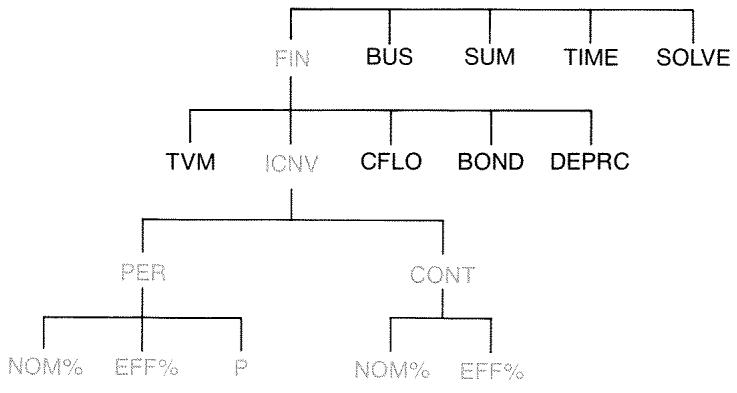
The ICNV menu converts between nominal and effective interest rates, using either:

Periodic compounding; for example, quarterly, monthly, or daily compounding.
Continuous compounding.

Converting Interest Rates

To convert between a nominal annual interest rate and an effective annual interest rate that is compounded periodically:

1. Press FIN ICNV to display the interest conversions menu.
2. Press PER for periodic.
3. Key in the number of compounding periods per year and press

4. To convert to the effective rate, first key in the nominal rate and press NOMX, then press EFFX.

5. To convert to the nominal rate, first key in the effective rate and press EFFX, then press NOMS.

To convert between a nominal annual interest rate and an effective annual interest rate that is compounded continuously:

1. Press FIN ICNV to get the interest conversions menu.
2. Press CONT for "continuous".
3. To convert to the effective rate, key in the nominal rate and press NOMx, then press EFFX.
4. To convert to the nominal rate, key in the effective rate and press EFFX, then press NOMX.

Values of EFF% and NOM% are shared between the PER and CONT menus. For example, an effective interest rate in CONT remains stored in EFF% when you exit the CONT menu and enter the PER menu. Pressing CLEAR DATA in either menu clears NOM% and EFF% in both.

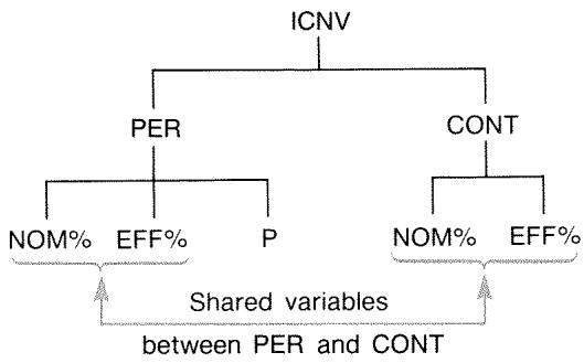
Example: Converting from a Nominal to an Effective Interest Rate. You are considering opening a savings account in one of three banks. Which bank has the most favorable interest rate?

Bank #1 6.7% annual interest, compounded quarterly.

Bank #2 6.65% annual interest, compounded monthly.

Bank #3 6.65% annual interest, compounded continuously.

Keys:	Display:	Description:
FIN		Displays ICNV menu.
ICNV
PER	COMPOUNDING P TIMES/YR	Displays PER menu.
4 P	P=4.00	Stores number of compounding periods per year for bank #1.
6.7 NOM:	NOM%=6.70	Stores nominal annual interest rate for bank #1.
EFF%	EFF%=6.87	Calculates effective interest rate for bank #1.
12 P	P=12.00	Stores number of compounding periods per year for bank #2.
6.65 NOM:	NOM%=6.65	Stores nominal annual interest rate for bank #2.
EFF%	EFF%=6.86	Calculates effective interest rate for bank #2.
EXIT CONT	CONTINUOUS COMPOUNDING	Displays CONT menu. Previous values of NOM% and EFF% are retained.
EFF%	EFF%=6.88	Calculates effective rate for bank #3.

The calculations show that bank #3 is offering the most favorable interest rate.

Compounding Periods Different from Payment Periods

The TVM menu assumes that the compounding periods and the payment periods are the same. However, regularly occurring savings-account deposits and withdrawals do not necessarily occur at the same time as the bank's compounding periods. If they are not the same, you can adjust the interest rate using the ICNV menu, and then use the adjusted interest rate in the TVM menu. (You can also use TVM if PMT = 0 , regardless of the compounding periods.)

1. Call up the periodic interest-rate conversion menu (FIN ICONV PER).
2. Calculate the effective annual interest rate from the nominal annual interest rate given by the bank.

a. Store annual interest rate in NOMX.
b. Store number of compounding periods per year in P
C. Press EFF:

1. Calculate the nominal annual interest rate that corresponds to your payment periods.

a. Store the number of regular payments or withdrawals you will be making per year in F
b. Press NOMX

1. Return to the TVM menu (EXIT EXIT TVM).
2. Store the just-calculated nominal interest rate in I% YR (press STO IXYR).
3. Store the number of payments or withdrawals per year in P Y R and set the appropriate payment mode.
4. Continue with the TVM calculation. (Remember that money paid out is negative; money received is positive.)

a. N is the total number of periodic deposits or withdrawals.
b. PV is the initial deposit.
c. PMT is the amount of the regular, periodic deposit or withdrawal.
d. FV is the future value.

When the interest rate is the unknown variable, first calculate I% YR in the TVM menu. This is the nominal annual rate that corresponds to your payment periods. Next, use the ICNV menu to convert this to the effective interest rate based on your payment periods. Last, convert the effective rate to the nominal rate based on the bank's compounding periods.

Example: Balance of a Savings Account. Starting today, you make monthly deposits of (25 into an account paying (5\%) interest compounded daily (365-day basis). At the end of 7 years, how much will you receive from the account?

Keys:	Display:	Description:
FIN
ICNV	SELECT COMPOUNDING
PER	COMPOUNDING P TIMES/YR	Periodic interest-rate conversion menu.
365 P	P=365.00	Stores bank's compound- ing periods.
5 NOM%	NOM%=5.00	Stores bank's nominal interest rate.
EFFF%	EFFF%=5.13	Calculates effective interest rate for daily compounding.
12 P	P=12.00	Stores number of deposits per year.
NOM%	NOM%=5.01	Calculates equivalent nominal interest rate for monthly compounding.
EXIT EXIT		Switches to TVM menu; NOM% value is still in calculator line.
TVM	5.01

STO IXYR IYR=5.01

Stores adjusted nominal interest rate in I% YR .

OTHER

12 P/YR

BEG EXIT 12 P/YR BEGIN MODE

Sets 12 payments per year; Begin mode.

7 N

25 + PMT

0 PV PV=0.00

Stores 84 deposit periods, $25 per deposit, and no money before the first regular deposit.

FV

FV=2,519.61

Value of account in 7 years.

If the interest rate were the unknown, you would first do the TVM calculation to get I% YR (5.01). Then, in the ICNV PER menu, store 5.01 as NOM% and 12 as P for monthly compounding. Calculate EFF% (5.13). Then change P to 365 for daily compounding and calculate NOM% (5.00). This is the bank's rate.

Cash Flow Calculations

The cash flow (CFLO) menu stores and analyzes cash flows (money received or paid out) of unequal (ungrouped) amounts that occur at regular intervals.* Once you've entered the cash flows into a list, you can calculate:

The total amount of the cash flows.
The internal rate of return (IRR%).
The net present value (NPV), net uniform series (NUS), and future value (NFV) for a specified periodic interest rate (1%) .

You can store many separate lists of cash flows, totaling up to about 700 different flows. The maximum number depends on the amount of available calculator memory.

The CFLO Menu

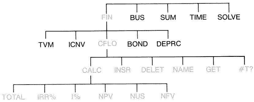
The CFLO menu creates cash-flow lists and performs calculations with a list of cash flows.

Table 6-1. CFLO Menu Labels

Menu Label	Description
CALC	Accesses the CALC menu to calculate TOTAL, IRR%, NPV, NUS, NFV.
INSR	Allows you to insert cash flows into a list.
DELETE	Deletes cash flows from a list.
NAME	Allows you to name a list.
GET	Allows you to switch from one list to another or create a new list.
#T?	Turns the prompting for #TIMES on and off.

To see the calculator line when this menu is in the display, press INPUT once. (This does not affect number entry.)

To see this menu when the calculator line is in the display, press EXIT.

Cash Flow Diagrams and Signs of Numbers

The sign conventions used for cash flow calculations are the same as those used in time-value-of-money calculations. A typical series of cash flows is one of two types:

■ Ungrouped cash flows. These occur in series of cash flows without "groups" of equal, consecutive flows.* Because each flow is different from the one before it, the number of times each flow occurs is one.

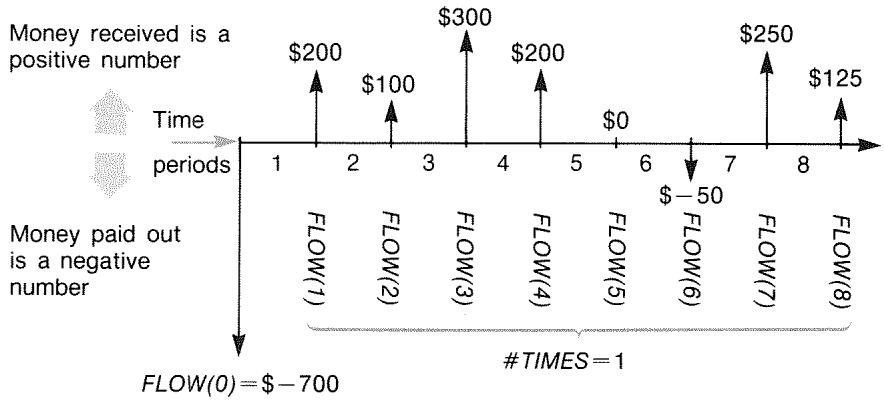
Figure 6-1. Cash Flows (Ungrouped)

The horizontal timeline is divided into equal compounding periods. The vertical lines represent the cash flows. For money received, the line points up (positive); for money paid out, the line points down (negative). In this case, the investor has invested ( \(700 ). This investment has generated a series of cash flows, starting at the end of the first period. Notice that there is no cash flow (a cash flow of zero) for period five, and that the investor pays a small amount in period six.

• Any cash flow series can be treated as an ungrouped one if you enter each flow individually.

• Grouped cash flows. These occur in a series containing "groups" of equal, consecutive flows. Consecutive, equal cash flows are called grouped cash flows. The series shown here is grouped into two sets of consecutive, equal cash flows:

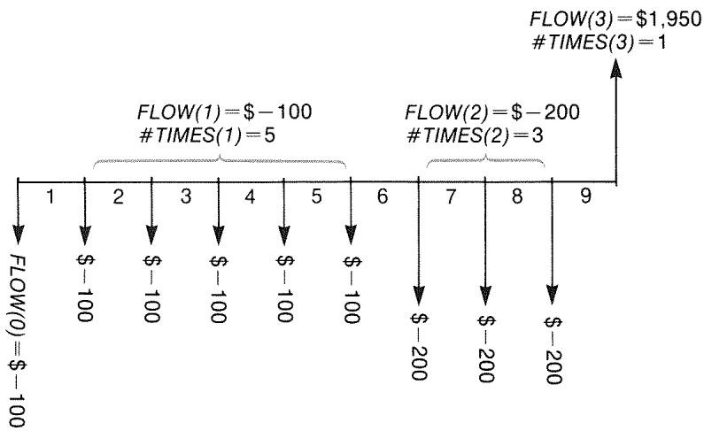
Figure 6-2. Grouped Cash Flows

After an initial payment of 100, the investor pays100 at the end of periods 1 through 5, and 200 at the end of periods 6 through 8. The investment returns1,950 at the end of period 9. For every cash flow you enter, the calculator prompts you to indicate how many times (#TIMES) it occurs.

Creating a Cash-Flow List

To use CFLO, be sure your cash flows are occurring at regular intervals and at the end of each period.* If a period is skipped, enter zero for its cash flow. If there are any grouped (consecutive and equal) cash flows, the #TIMES prompting makes entering the data easier.

• If the cash flows occur at the beginning of each period, then combine the first flow with the initial flow (which can increase or decrease the flow), and move each cash flow up one period. (Remember: a payment made at the beginning of period 2 is equivalent to the same payment made at the end of period 1, and so on. Refer to pages 53-55.)

Entering Cash Flows

To enter cash flows into a CFLO list:

1. Press FIN Cflo. You will see either FLOW(0) = ? if the current list is empty, or FLOW(1 or more) = ? if the list is not empty. This is the bottom of the current list.

1. If the list is not empty, you can do either a or b:

a. Clear the list by pressing CLEAR DATA YES (see also page 89.)
b. Get a new list by pressing GET *NEW. (The old list must be named first. Press NAME or see page 87.)

1. If the cash flows are ungrouped (that is, they are all different), then press #T? to turn #TIMES PROMPTING OFF. For grouped cash flows, leave this prompting on. (For more information, see "Prompting for #TIMES," next page.)
2. Key in the value of the initial cash flow, FLOW(0) (remember that money paid out is negative—use +/- to change the sign), and press INPUT.*

3. After briefly showing FLOW(0) , the display shows FLOW(1) = ? . (To view FLOW(0) longer, hold down INPUT before releasing it.) Key in the value for FLOW(1) and press INPUT . The prompt for the next item appears.

4. For grouped cash flows: The display now shows

TIMES(1)=1. If it does not, press EXIT #T? to turn the #TIMES prompting on. (See "Prompting for #TIMES," below.) #TIMES is the number of consecutive occurrences of FLOW(1). #TIMES has been automatically set to 1, and 1.00 is displayed on the calculator line. Do either a or b:

a. To retain the value 1 and go on to the next flow, press INPUT (or ).
b. To change #TIMES, key in the number and press INPUT.*

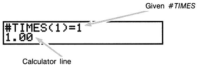
1. Continue entering each cash flow and, for grouped flows, the number of times it occurs. The calculator recognizes the end of the list when a flow is left blank (no value is entered).
2. Press EXIT to end the list and restore the CFLO menu. You can now proceed to correct the list, name the list, get another list, or do calculations with the values.

Use these same instructions to enter additional lists.

Prompting for #TIMES (#T?). When the calculator displays

TIMES(1)=1, it is prompting you for the number of times the current flow occurs. If all your cash flows are different (#TIMES always 1), then you don't need the #TIMES prompt. You can turn the prompting for #TIMES on and off by pressing #T? in the CFLO menu. This produces a brief message: either #TIMES

PROMPTING: OFF, or #TIMES PROMPTING: ON.

While prompting is off, all cash flows you enter will have #TIMES = 1.

When you are viewing a cash-flow list with the #TIMES prompting off, the calculator displays only those #TIMES values that are not 1.

The #TIMES prompting is usually on, because it is automatically turned on whenever you clear or get a cash-flow list.

Example: Entering Cash Flows. Enter the following ungrouped cash flows in a list and find the percentage internal rate of return (IRR).

0: —500 2: 275

1: 125 3: 200

Keys:	Display:	Description:
FIN
CFLO
CLEAR DATA	CLEAR THE LIST?	Asks for confirmation.
YES	FLOW(0)=?	Clears data from list and prompts for initial flow.
#T?	#TIMES PROMPTING: OFF	Sets prompting off be-cause it is not needed.
500+/- INPUT	FLOW(1)=? -500.00	Enters initial flow; then immediately prompts for next flow.
125 INPUT	FLOW(2)=? 125.00	Enters FLOW(1); prompts for next flow.
275 INPUT	FLOW(3)=? 275.00	Enters FLOW(2); prompts for next flow.
200 INPUT	FLOW(4)=? 200.00	Enters FLOW(3); prompts for next flow
EXIT CALC	NPV, NUS, NFV NEED I%	Ends list and displays CALC menu.
IRR%	IRR%=9.06	Calculates IRR.

Viewing and Correcting the List

To display a particular list, use GET (see page 88).

The and keys move up and down one number at a time. and display the beginning and end of the list.

Changing or Clearing a Number. To change a number after it's been entered: display the number, key in the new value, and press INPUT.

Use this same method to clear a number to zero. (Do not press CLR or , which clear the calculator line, not the cash-flow entry.)

Inserting Cash Flows into a List. Insertion occurs before (above) the current flow. Pressing INSR inserts a zero cash flow and renumbers the rest of the list. You can then enter a new cash flow and its #TIMES.

For example, if FLOW(6) is in the display, pressing INSR puts a new, zero flow between the previously numbered FLOW(5) and FLOW(6) .

Deleting Cash Flows from a List. Pressing DELETE deletes both the current flow and its #TIMES.

Copying a Number from a List to the Calculator Line

To copy a number from the list into the calculator line, use or to display the number, then press RCL INPUT.

Naming and Renaming a Cash-Flow List

A new list has no name. You may name it before or after filling the list, but you must name it in order to store another list.

To name a list:

1. Press NAME from the CFLO menu.

2. Use the ALPHA menu to type a name. (The ALPHA and ALPHA-Edit menus are covered on pages 27-29.) To clear a name, press CLR.

3. Press INPUT

The name can be up to 22 characters long and include any character except: + - × ÷ () < > : = space^*

But only the first three to five characters (depending on letter widths) of the name are used for a menu label. Avoid names with the same first characters, since their menu labels will look alike.

Viewing the Name of the Current List. Press NAME, then EXIT.

Starting or GETting Another List

When you press CFLO, the cash-flow list that appears is the same as the last one used.

To start a new list or switch to a different one, the current list must be named or cleared. If it is named, then:

1. Press GET. The GET menu contains a menu label for each named list plus *NEW.
2. Press the key for the desired list. (*NEW) brings up a new, empty list.)

Clearing a Cash-Flow List and Its Name

To clear a list's numbers and name:

1. Display the list you want to clear, then press CLEAR DATA YES . This removes the numbers.
2. If the list is named, you'll see ALSO CLEAR LIST NAME? Press YES to remove the name. Press NO to retain the name with an empty list.

To remove just one value at a time from a list, use DELETE.

Cash-Flow Calculations: IRR, NPV, NUS, NFV

Once you have entered a list of cash flows, you can calculate the following values in the CALC menu.

Sum (TOTAL).
- Internal rate of return (IRR%). This is a periodic rate of return. To calculate an annual nominal rate when the period is not a year, multiply the IRR% by the number of periods per year.

If you want the IRR% as an effective annual rate, then use the FIN ICNV menu to convert from the nominal annual rate to the effective annual rate.

Net present value (NPV), net uniform series (NUS), and net future value (NFV) for a specified, periodic interest rate, 1% .

Table 6-2. The CALC Menu for CFLO Lists

Menu Label	Description
TOTAL	Calculates the sum of the cash flows.
IRR*	Calculates the internal rate of return—the interest (discount) rate at which the net present value of the cash flows equals zero.
I%	Stores the periodic interest rate, expressed as a percentage (sometimes called cost of capital, discount rate, or required rate of return).
NPV	Given I%, calculates the net present value—the present value of a series of cash flows.
NUS	Given I%, calculates the net uniform series—the dollar amount of constant, equal cash flows having a present value equivalent to the net present value.
NFV	Given I%, calculates the net future value of a series of cash flows by finding the future value of the net present value.
* The calculations for internal rate of return are complex and may take a relatively long time. To interrupt the calculation, press any key. In certain cases, the calculator displays a message indicating that the calculation cannot continue without further information from you, or that there is no solution. Refer to appendix B for additional information about calculating IRR%.

About the Internal Rate of Return (IRR%). A "conventional investment" is considered attractive if IRR% exceeds the cost of capital. A conventional investment meets two criteria—(1) the sequence of cash flows changes sign only once, and (2) the sum (TOTAL) of the cash flows is positive.

Remember that the calculator determines a periodic IRR% . If the cash flows occur monthly, then IRR% is a monthly value, too. Multiply it by 12 for an annual value.

Example: Calculating IRR and NPV of an Investment. An investor makes an initial investment of $80,000, and expects returns over the next five years as illustrated below.

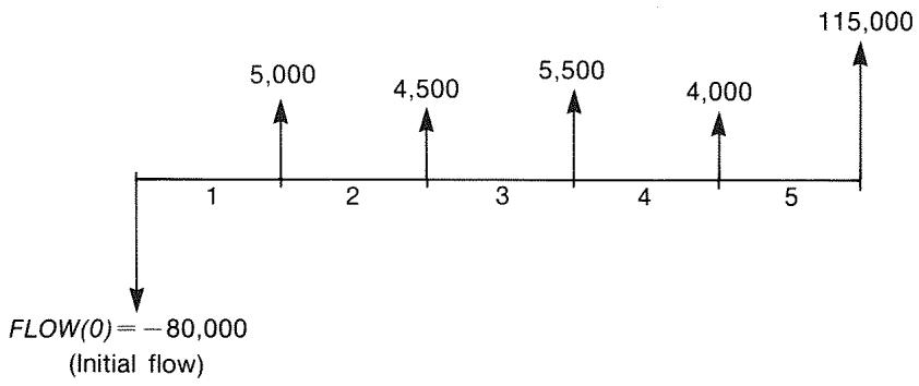
Calculate the total of the cash flows and the internal rate of return of the investment. In addition, calculate the net present value and net future value, assuming an annual interest rate of 10.5% .

Start the problem with an empty cash-flow list. Since the cash flows are ungrouped, each one occurs just once. Turn off the #TIMES prompt to make cash-flow entry faster.

Keys:	Display:	Description:
FIN		Displays current cash-flow list and CFLO menu keys.
CFLO
CLEAR DATA		Cleared current list or gets a new one. The empty list prompts for its initial cash flow.
YES
or
GET
*NEW	FLOW(0)=?
#T?	#TIMES PROMPTING: OFF	Briefly shows the status of #T, then returns to the list. With prompting off, all cash flows are assumed to occur just once.
80000 +/L INPUT	FLOW(1) =? -80,000.00	Prompts for next cash flow. Calculator line shows last number entered.
5000 INPUT	FLOW(2) =?	Stores $5,000 for FLOW(1), prompts for next flow.
4500 INPUT	FLOW(3) =?	Stores FLOW(2).
5500 INPUT	FLOW(4) =?	Stores FLOW(3).
4000 INPUT	FLOW(5) =?	Stores FLOW(4).
115000 INPUT	FLOW(6) =?	Stores final cash flow and shows end of list.
EXIT CALC TOTAL	TOTAL=54,000.00	Calculates sum of the cash flows.
IRR%	IRR% = 11.93	Calculates internal rate of return.
10.5 I%	I% = 10.50	Stores periodic interest rate.
NPV	NPV = 4,774.63	Calculates NPV.
NFV	NFV = 7,865.95	Calculates NFV.
Now calculate the net present value at an cash flow #4 is reduced to 1,000.		interest rate of 10.5% if
EXIT	FLOW(6) =?	Displays the bottom of the list.
▲▲	FLOW(4) = 4,000.00	Moves to cash flow #4.
1000 INPUT	FLOW(5) = 115,000.00	Changes cash flow #4 to1,000.
EXIT CALC NPV	NPV = 2,762.43	Calculates new NPV.

Example: An Investment with Grouped Cash Flows. You are considering an investment that requires a cash outlay of (9,000, with the promise of monthly cash flows as shown. Calculate IRR%. Also find NPV and NFV at an annual interest rate of (9\%).

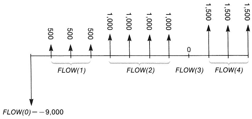
Since some of these cash flows are grouped (consecutive and equal), the #TIMES prompting must be on so you can specify a number other than 1.

Group Number	Amount	Number of Times
Initial	-9,000	—
1	500	3
2	1,000	4
3	0	1
4	1,500	3

Keys:	Display:	Description:
FIN		Current cash-flow list and CFLO menu.
CFLO
CLEAR DATA	FLOW(0)=?	Cleared current list. #TIMES prompting is turned on.
YES
9000+/-	FLOW(1)=?	Stores the initial cash flow.
INPUT
500 INPUT	#TIMES(1)=1	Stores FLOW(1) and prompts for #TIMES(1).
3 INPUT	FLOW(2)=?	FLOW(1) occurs 3 times; prompts for next cash flow.
1000 INPUT 4	FLOW(3)=?	Stores FLOW(2) four times.
INPUT
0 INPUT	FLOW(4)=?	Stores FLOW(3) one time (the 1 is automatically entered).
INPUT
1500 INPUT 3	FLOW(5)=?	Stores FLOW(4) three times.
INPUT
EXIT CALC		Displays the CALC menu.
IRR%	IRR%=1.53	Calculates monthly IRR%.
9÷12		Stores the periodic, monthly interest rate.
I%	I%=0.75
NPV	NPV=492.95	Calculates NPV.
NFV	NFV=535.18	Calculates NFV.

Example: An Investment with Quarterly Cash Returns. You have been offered an opportunity to invest (20,000. The investment returns quarterly payments over four years as follows:

Year 1 4 payments of $500

Year 2 4 payments of $1,000

Year 3 4 payments of $2,000

Year 4 4 payments of $3,000

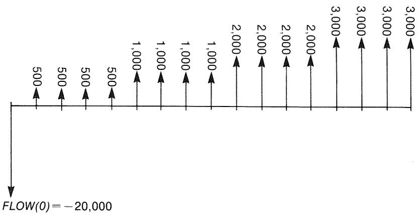
Calculate the annual rate of return for this investment. (The prompting for #TIMES should be on.)

Keys:

Display:

Description:

FIN

Current cash-flow list.

CFLQ

CLEAR DATA

YES

01

GET

NEW

FLOW（0）=？

Clears the current list or gets a new one. This sets the #TIMES prompting on.

20000

INPUT

FLOW（1）=？

500 INPUT

TIMES（1）=1

4 INPUT

FLOW（2）=？

1000 INPUT 4

INPUT

2000 INPUT 4

INPUT

3000 INPUT 4

INPUT

FLOW（5）=？

EXIT

IRX

IRR%=2.43

× 4

9.72

Stores the initial cash flow.

Stores FLOW(1) , then prompts for number of times this flow occurs.

FLOW(1) occurs four times.

Stores FLOW(2) , FLOW(3) and FLOW(4) , and the number of times each flow occurs.

Calculates quarterly rate of return.

Calculates nominal annual rate of return from quarterly rate.

Doing Other Calculations with CFLO Data

If you would like to do other calculations with cash flows besides those in the CALC menu, you can do so by writing your own Solver equations. There are Solver functions that can access data stored in CFLO lists, and there is a summation function that can combine all or part of the values stored in specific lists.

Refer to "Accessing CFLO and SUM Lists from the Solver" in chapter 11.

Bonds

The BOND menu calculates the yield to maturity or price of a bond. It also calculates yield to call on a coupon date and accrued interest. You can specify the:

Calendar basis: 30/360 or actual/actual (days per month/days per year). Municipal, state, and corporate bonds issued in the United States are typically 30/360. U.S. Treasury bonds are actual/actual.
- Coupon payments: semi-annual or annual. Most U.S. bonds are semi-annual.

The BOND Menu

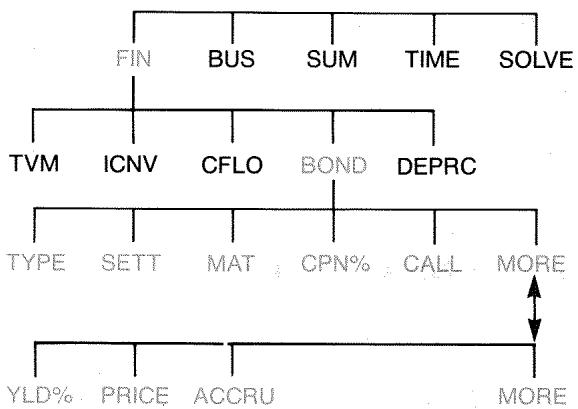
Pressing BOND shows you the BOND menu and the type of bond currently specified: 30/360 or A/A; SEMIANNUAL or ANNUAL.

Table 7-1. BOND Menu Labels

Menu Label	Description
TYPE	Displays a menu of bond types: 30/360 or actual/actual, semi-annual or annual.
SETT	Stores the settlement (purchase) date according to the current date format (MM.DDYYYY or DD.MMYYYY; see page 132).
MAT	Stores the maturity date or call date according to the current date format. The call date must coincide with a coupon date.
CPNX	Stores the annual coupon rate as a percentage.
CALL	Stores the call price per 100 face value. For a yield to maturity, make sure CALL equals 100. (A bond at maturity has a "call" value that is 100% of its face value.)
YLDX	Stores or calculates the yield (as an annual percentage) to maturity or yield to call date.
PRICE	Stores or calculates the price per100 face value.
ACCRU	Calculates the interest accrued from the last coupon-payment date until the settlement date, per $100 face value.

The calculator retains the values of the BOND variables until you clear them by pressing CLEAR DATA while the BOND menu is displayed. Clearing sets CALL to 100 and all other variables to zero.

To see the value currently stored in a variable, press RCL menu label.

Doing Bond Calculations

Remember that values in the BOND menu are expressed per 100 face value or as a percentage. A CALL value of 102 means that the bond will be worth102 for every $100 of face value when called. Some corporate bonds in the United States use the convention that the price of the bond is set to 100 if the coupon rate equals the yield, whether or not the settlement date is a coupon date. The BOND menu does not use this convention.

To calculate the price or yield of a bond:

1. Display the BOND menu: press FIN BOND
2. Press CLEAR DATA. This sets CALL = 100
3. Define the type of bond. If the message in the display does not match the type you want, press TYPE.

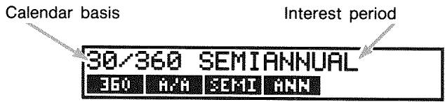
Pressing 360 sets the calendar basis to a 30-day month and a 360-day year.
Pressing n / n sets the calendar basis to the actual calendar month and to the actual calendar year.
■ Pressing SEMI sets semi-annual coupon payments.
Pressing ANN sets annual coupon payments.

Press EXIT to restore the BOND menu.

1. Key in the settlement date (MM.DDYYYY or DD.MMYYYY depending on the date format; see chapter 10) and press SETT.
2. Key in the maturity date or call date and press MAT
3. Key in the coupon rate as an annual percent and press CPN:
4. Key in the call value, if any, and press CALL. For a bond held to maturity, the CALL value must equal 100. (See step 3.)
5. To calculate a result, first press MORE to access the remaining menu labels. Do either a or b:

a. Key in the yield and press YLDX. Press PRICE to calculate the price.
b. Key in the price and press PRICE. Press YLDx to calculate the yield.

To calculate the accrued interest, press ACCRU. The total amount owed the seller is PRICE + ACCRU, that is: PRICE + ACCRU =

Calculating Fractional Values. When given a fractional value that must be entered in decimal form, do the arithmetic and then store the result directly into a variable. Do not clear the arithmetic and then re-type the result before storing it—this is an unnecessary step that can cause incorrect answers due to rounding. See how the following example stores 83% in YLD% .

Example: Price and Yield of a Bond. What price should you pay on August 10, 1987 for a 63/4% U.S. Treasury bond that matures on May 1, 2002 if you wish a yield of 83/8% ? The calendar basis is actual/actual and the coupon payments are semi-annual. (The example assumes MM.DDYYYY date format.)

Keys:	Display:	Description:
FIN BOND		Since there is no call on this bond, set CALL=100 by clearing variables.
CLEAR DATA
TYPE A/R		Sets bond type, if necessary.
SEMI EXIT	A/A SEMIANNUAL
8.101987		Stores settlement (pur-charge) date.
SETT	SETT=08/10/1987 MON
5.012002		Stores maturity date.
MAT	MAT=05/01/2002 WED
6.75 CPN%	CPN%=6.75	Stores annual coupon rate.
MORE		Stores desired yield (dis-played rounded to two decimal places).*
3÷8÷8
YLD%	YLD%=8.38

PRICE

PRICE=86.38

Result: price is 86.38 per100 face value.

ACCRU

86.38+1.85

Adds accrued interest owed the seller.

88.23

Net price.

Suppose that the market quote for the bond is 88 14 . What yield does it represent?

88.25 PRICE

PRICE=88.25

Stores quoted price.

YLDX

YLD%=8.13

Result: yield to maturity.

Example: A Bond with a Call Feature. What is the price of a 6% corporate bond maturing on March 3, 2007 and purchased on May 2, 1988 to yield 5.7% ? It is callable on March 3, 1991 (a coupon date), at a value of 102.75. What is the yield to the call date? Use a 30/360 calendar with semi-annual coupon payments.

Keys:	Display:	Description:
FIN		Displays BOND menu, clears variables.
BOND
CLEAR DATA
TYPE		Sets bond type, if necessary.
360
SEMI EXIT	30/360 SEMIANNUAL
5.021988		Stores purchase date (MM.DDYYYY format).
SETT	SETT= 05/02/1988 MON
3.032007		Stores maturity date.
MAT	MAT=03/03/2007 SAT
6 CPN:	CPN%=6.00	Stores annual coupon rate.
MORE		Stores yield.
5.7 YLD%	YLD%=5.70
PRICE	PRICE=103.43	Calculates price.
MORE		Changes maturity date to call date and stores a call value.
3.031991
MRT
102.75 CALL	CALL=102.75
MORE		Calculates yield to call.
YLD%	YLD%=5.58

Example: A Zero-Coupon Bond. Calculate the price of a zero-coupon, semi-annual bond using a 30/360 calendar basis. The bond was purchased on May 19, 1986 and will mature on June 30, 2000, and has a yield to maturity of 10% .

Keys:	Display:	Description:
FIN		Cleared BOND variables
BOND		setting CALL to 100.
CLEAR DATA
TYPE		Sets type if necessary
360		(check the display).
SEMI EXIT	30/360 SEMIANNUAL
5.191986		Purchase date
SETT	SETT=	(MM.DDYYYY format).
	05/19/1986 MON
6.302000		Maturity date.
MAT	MAT=06/30/2000 FRI
0 CPN%	CPN%=0.00	Coupon rate is zero.
MORE		Yield to maturity.
10 YLD%	YLD%=10.00
PRICE	PRICE=25.23	Calculates price.

Depreciation

The DEPRC (depreciation) menu calculates depreciation values and remaining depreciable values one year at a time. The methods available are:

Declining balance.
Sum-of-the-years' digits.
Straight line.
■ Accelerated Cost Recovery System.

The DEPRC Menu

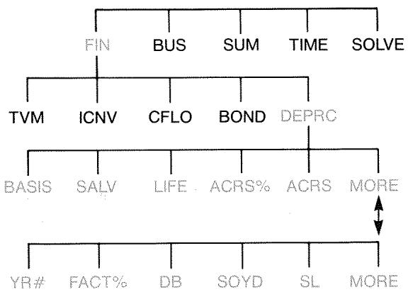
Pressing DEPRc displays the DEPRC menu.

Table 8-1. DEPRC Menu Labels

Menu Label or Key	Description
BASIS	Stores the depreciable cost basis of the asset at acquisition.
SALV	Stores the salvage value of the asset at the end of its useful life. If there is no salvage value, set SALV=0.
LIFE	Stores the expected useful life (in whole years) of the asset.
ACRS%	Stores the appropriate Accelerated Cost Recovery System percentage from the published ACRS tables.
ACRS	Calculates the ACRS deduction based on BASIS and ACRS%. (The values in SALV, LIFE, FACT%, and YR# do not matter.)
YR#	Stores the number of the year for which you want the depreciation (1, 2, etc.).
FACT%	Stores the declining-balance factor as a percentage of the straight-line rate. This is for the DB method only. For example, for a rate 11/4 times (125%) the straight-line rate, enter 125.
DB	Calculates the declining-balance depreciation for the year.
SOYD	Calculates the sum-of-the-years'-digits depreciation for the year.
SL	Calculates the straight-line depreciation for the year.
▼	Displays the remaining depreciable value, RDV, after you have pressed DB, SOYD, or SL.

The calculator retains the values of the DEPRC variables until you clear them by pressing Clear DATA while the DEPRC menu is displayed.

To see the value currently stored in a variable, press RCL menu label.

Doing Depreciation Calculations

DB, SOYD, and SL Methods

To calculate the depreciation for an asset:\*

1. Display the DEPRC menu: press FIN DEPRC.
2. Define the characteristics of the asset:

a. Key in the cost basis and press BAsIs
b. Key in the salvage value and press SALV. If there is no salvage value, enter zero.
C. Key in the useful life and press LIFE

1. Press MORE for the rest of the DEPRC menu.
2. Key in the number for the year of depreciation you want to calculate (1, 2, 3, etc.) and press YR#.
3. If you are using the declining-balance method, enter the DB factor (a percentage) and press FACTX.
4. Press DE, SoyD, or SL to calculate the appropriate depreciation.
5. To see the remaining depreciable value (basis - salvage value - accumulated depreciation), press .
6. To calculate the depreciation for another year, just change YR # and press DB, soYD, or SL again.

Example: Declining-Balance Depreciation. A metalworking machine, purchased for 10,000, is to be depreciated over 5 years. Its salvage value is estimated at 500. Find the depreciation and remaining depreciable value for each of the first 3 years of the machine's life using the double-declining-balance method (200% of the straight-line rate). For comparison, find the straight-line depreciation, as well.

Keys:	Display:	Description:
FIN		Displays DEPRC menu.
DEPRC
10000	BASIS=10,000.00	Cost basis.
500	SALV=500.00	Salvage value.
5	LIFE	Useful life.
MORE		First year of depreciation.
1	YR#	YR#=1.00
200	FACTX	FACT#=200.00
DB	DB=4,000.00	Depreciation in first year. (Salvage value ignored at this point.)
▼	RDV=5,500.00	Remaining depreciable value after first year (BASIS-SALV-4,000).
2	YR#
DB	DB=2,400.00	Depreciation in second year.
▼	RDV=3,100.00	Remaining depreciable value after second year.
3	YR#
DB	DB=1,440.00	Depreciation in third year.
▼	RDV=1,660.00	Remaining depreciable value after third year.
SL	SL=1,900.00	Straight-line depreciation for each year.
▼	RDV=3,800.00	Remaining depreciable value after third year using SL.

The ACRS Method

To calculate the amount of tax deduction under the U.S. Accelerated Cost Recovery System:

1. Display the DEPRC menu: press FIN DEPRC.
2. Enter the cost basis of the asset and press BASIS.
3. The Internal Revenue Service publishes tables that list the percentage of an asset's basis that can be deducted each year of its prescribed life. Look up that value, enter it, and press HCRS%.
4. Press ACRS to calculate the value of the deduction.

Example: ACRS Deductions. Use the ACRS method to find the income-tax deduction for a (25,000 asset over 3 years of a 5-year life. Use this hypothetical ACRS table:

Year	Percentage Deductible
1	15
2	25
3	20
4	20
5	20

Keys:

FIN DEPRC

25000 BASIS

15 ACRSx

ACRS

25 ACRS%

Display:

BASIS=25,000.00

ACRS%=15.00

ACRS=3,750,00

ACRS%=25.00

Description:

DEPRC menu.

Enters basis.

Tabular value, year 1.

Deduction in first year.

Tabular value, year 2.

ACRS

ACRS=6,250.00

Deduction in second year.

20 ACRS% ACRS%=20.00

Tabular value, year 3.

ACRS ACRS=5,000.00

Deduction in third year.

Partial-Year Depreciation

When the acquisition date of an asset does not coincide with the start of the tax or fiscal year, then the amounts of depreciation in the first and last years are computed as fractions of a full year's depreciation. Except in SL, the intermediate years are computed as sums of fractions. This does not apply to the ACRS method.

Suppose you acquired an asset in October and wanted to depreciate it for 3 years. (Your fiscal year begins January 1st.) The depreciation schedule would affect parts of 4 years, as shown in the illustration. The 3 months from October to December equal 14 year.

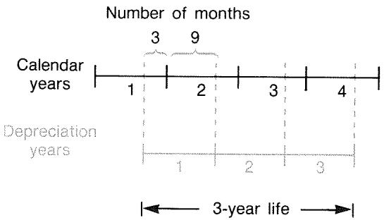
For SL depreciation, partial-year calculations are easy: calculate the SL value, then use 14 of that value for the first year, the full amount the second and third years, and 34 of that amount the fourth year.

For DB and SOYD depreciation, each year's depreciation value is different, as shown in the table:

Calendar Year	Depreciation Value
1 (Oct.-Dec.)	1/4 × year 1
2	(3/4 × year 1) + (1/4 × year 2)
3	(3/4 × year 2) + (1/4 × year 3)
4 (Jan.-Sept.)	3/4 × year 3

Example: Partial-Year Depreciation. A movie camera bought for 12,000 has a useful life of 10 years with a salvage value of 500. Using the sum-of-the-years'-digits method, find the amount of depreciation for the fourth year. Assume the first depreciation year was 11 months long.

Keys:	Display:	Description:
FIN DEPRC		Displays DEPRC menu.
12000 BASIS		Stores known values.
500 SALV
10 LIFE
MORE
3 YR#	YR#=3.00
SOYD	SOYD=1,672.72	Calculates depreciation for year 3.
÷12=STO 1	139.39	Stores 1 month's depreciation from year 3.
4 YR#		Calculates depreciation for year 4.
SOYD	SOYD=1,463.64
×11÷12=	1,341.67	Figures 11 months' depreciation from year 4.
+ RCL 1=	1,481.06	Figures total depreciation for year 4.

Running Total and Statistics

The SUM menu stores and statistically analyzes sets of numbers. As you enter the numbers, the calculator displays their running total. Once you've entered the numbers into a list, you can:

Calculate the mean, median, standard deviation, and range.
Display the largest and smallest number in the list.
Sort the list from smallest number to largest number.

With two lists of numbers, you can:

• Do curve-fitting and forecasting calculations using two SUM lists and one of four models—linear, exponential, logarithmic, and power. (Curve fitting for the linear model is called linear regression.)
  Calculate the weighted mean and grouped standard deviation.
  Find the summation statistics ( x, x^2, y, y^2, xy) .

You can store many separate lists of numbers in SUM, totaling up to about 840 items. The maximum number depends on the amount of available calculator memory.

The SUM Menu

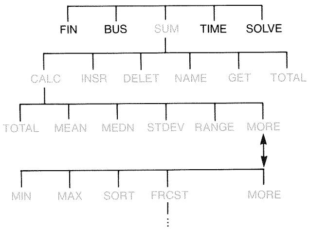
The SUM menu creates lists of numbers and performs calculations with a SUM list.

Table 9-1. SUM Menu Labels

Menu Label	Description
CALC	Accesses the CALC menu to calculate the total, mean, median, standard deviation, range, minimum, maximum, sorting, and linear regression (including weighted mean and summation statistics).
INSR	Allows you to insert numbers into the list.
DELETE	Deletes numbers from the list.
NAME	Allows you to name the list.
GET	Allows you to switch from one named list to another or to create a new list.
TOTAL	Displays the total of all the items in the list.

To see the calculator line when this menu is in the display, press INPUT once. (This does not affect number entry.)

To see this menu when the calculator line is in the display, press EXIT.

Creating a SUM List

To keep a running total of a list of numbers or do statistical calculations with sets of data, first create a SUM list of the values.

- Entering Numbers and Viewing the TOTAL

To enter numbers into a SUM list:

1. Press SUM. You'll see ITEM(1) = ? if the current list is empty, or ITEM(2 or more) = ? if the list is not empty. This is the bottom of the current list.

1. If the list is empty, start filling it (step 3). If the current list is not empty, you can do either a or b:

a. Clear the list by pressing CLEAR DATA YES page 116.)
b. Get a new list by pressing GET *NEW. (The old list must be named first. Press NAME or see page 115.)

1. Key in the value of the first item, ITEM(1) (press +/- for a negative number), and press INPUT.* (To view ITEM(1) longer, hold down INPUT before releasing it.)

2. Remember that you can do calculations with a number before entering it. This does not interfere with the list. Whenever you press INPUT, the number (or evaluated expression) in the calculator line is entered into the list. If you need to use the MATH menu, just press MATH, do the calculation, then press EXIT to return to where you were in SUM.

After briefly showing ITEM(1), the display shows

ITEM（2）=？

TOTAL = number

TOTAL is the updated, running TOTAL of all the numbers in the list (only one number, so far).

1. To enter ITEM(2), key in the value and press INPUT. The prompt for ITEM(3) and the new, updated total appear.
2. Continue entering values for ITEM(3), ITEM(4), etc. The calculator recognizes the end of the list when an item is left blank (no value is entered).
3. Press EXIT to end the list and restore the SUM menu. You can now proceed to correct the list, name the list, get another list, or do statistical calculations.

Use these same instructions to enter additional lists.

Viewing and Correcting the List

To display a particular list, use GET (see page 116).

The and keys move up and down the list one number at a time. and display the beginning and end of the list.

Changing or Clearing a Number. To change a number after it's been entered: display the number, key in the new value, and press INPUT.

Use the same method to clear a number to zero. (Do not press CLR or 4 , which clears the calculator line.)

Inserting Numbers into a List. Insertion occurs before (or above) the current entry. Pressing INSR inserts a zero item and renumbers the rest of the list. You can then enter a new value.

For example, if ITEM(6) is in the display, pressing INSR puts a new, zero item between the previously numbered ITEM(5) and ITEM(6).

Deleting Numbers from a List. Pressing DELETE deletes the current item.

Example: Updating a Checkbook. On May 31, your checking account balance was (267.82. The transactions for the first 10 days in June are:

Date	Transaction	Amount	Date	Transaction	Amount
6/1	Balance	267.82	6/3	Check	-128.90
6/1	Deposit	837.42	6/7	Check	- 65.35
6/1	Check	-368.23	6/10	Deposit	55.67
6/2	Check	- 45.36

Update the checkbook by calculating the running balance.

Keys:	Display:	Description:
SUM *
CLEAR DATA		Displays empty SUM list.
YES	ITEM(1)=?
267.82 INPUT	ITEM(2)=?	Enters beginning balance
	TOTAL=267.82	and shows running total.
837.42 INPUT	ITEM(3)=?	Enters deposit on 6/1.
	TOTAL=1,105.24

• If you want to preserve the current list, skip the next step (pressing CLEAR DATA). Instead, name the list and then press GET *NEW.

368.23

INPUT

45.36

INPUT

128.90

INPUT

65.35

INPUT

55.67 INPUT

ITEM（8）=？

TOTAL=553.07

EXIT

ITEM（8）=？

Enters remaining transactions.

Ends list and displays SUM menu again.

Copying a Number from a List to the Calculator Line

To copy a number from the list into the calculator line, use or to display the number, then press RCL INPUT.

Naming and Renaming a SUM List

A new list has no name. You may name it before or after filling the list, but you must name it in order to store another list.

To name a list:

1. Press NAME from the SUM menu.
2. Use the ALPHA menu to type in a name. (The ALPHA and ALPHA-Edit menus are covered on pages 27-29.) To clear a name, press CLR.
3. Press INPUT

The name can be up to 22 characters long and include any character except: + - × ÷ () < > : = space^*

But only the first three to five characters (depending on letter widths) of the name are used for a menu label. Avoid names with the same first characters, since their menu labels will look alike.

Viewing the Name of the Current List. Press NAME, then EXIT.

Starting or GETting Another List

When you press SUM, the SUM list that appears is the last one used.

To start a new list or switch to a different one, the current list must be named or cleared. If it is named, then:

1. Press GET. The GET menu contains a menu label for each named list plus KEN.
2. Press the key for the desired list. (*NEW) brings up a new, empty list.)

Clearing a SUM List and Its Name

To clear a list's numbers and name:

1. Display the list you want to clear, then press CLEAR DATA YES . This removes the numbers.
2. If the list is named, you'll see ALSO CLEAR LIST NAME? Press YES to remove the name. Press NO to retain the name with an empty list.

To remove just one value at a time from a list, use DELET.

Doing Statistical Calculations (CALC)

Once you have entered a list of numbers, you can calculate the following values.

For one variable: the total, mean, median, standard deviation, range, minimum, and maximum. You can also sort the numbers in order of increasing value.
For two variables: x -estimates and y -estimates (this is also called forecasting), the correlation coefficient for different types of curves (this is curve-fitting), the slope and y -intercept of the line, and summation statistics. You can also find the weighted mean and the grouped standard deviation.

Calculations with One Variable

The CALC menu calculates the following statistical values using one SUM list.

Table 9-2. The CALC Menu for SUM Lists

Menu Key	Description
TOTAL	Calculates the sum of the numbers in the list.
MEAN	Calculates the arithmetic mean (average).
MEDN	Calculates the median.
STDEV	Calculates the standard deviation.*
RANG	Calculates the difference between the largest and smallest number.
MIN	Finds the smallest (minimum) number in the list.
MAX	Finds the largest (maximum) number in the list.
SORT	Sorts the list in ascending order.
FRCST	Displays a series of menus for calculations with two variables for curve fitting, estimation, weighted mean and grouped standard deviation, and summation statistics.
* The calculator finds the sample standard deviation. The formula assumes that the list of numbers is a sampling of a larger, complete set of data. If the list is, in fact, the entire set of data, the true population standard deviation can be computed by calculating the mean of the original list, placing that value into the list, and then calculating the standard deviation.

Example: Mean, Median, and Standard Deviation. Suppose your shop had the following phone bills during the past six months:

Month	Phone Expense	Month	Phone Expense
1. May	340	4. August	780
2. June	175	5. September	245
3. July	450	6. October	625

Calculate the mean, median, and standard deviation of the monthly phone bills. Then display the smallest value in the list.

Keys:	Display:	Description:
SUM		Displays current SUM list and SUM menu keys.
CLEAR DATA		Clears current list or gets a new one.
YES
or
GET
*NEW	ITEM(1)=?
340 INPUT	ITEM(2)=?	Stores May's phone bill; shows total.
	TOTAL=340.00
175 INPUT	ITEM(3)=?	Stores June; updates total.
	TOTAL=515.00
450 INPUT		Stores phone bills for July-October and keeps a running total.
780 INPUT
245 INPUT
625 INPUT	ITEM(7)=?
	TOTAL=2,615.00
EXIT CALC	2,615.00	Displays CALC menu.
MEAN	MEAN=435.83	Calculates mean.
MEDN	MEDIAN=395.00	Calculates median.
STDEV	STDEV=231.55	Calculates standard deviation.
MORE		Displays rest of CALC menu.
MIN	MIN=175.00	Finds smallest number.

Calculations with Two Variables (FRCST)

The FRCST menu does the following two-variable calculations using two SUM lists:

Fits x - and y -data to a linear, logarithmic, exponential, or power curve.
Forecasts estimated values based on that curve.
Finds the weighted mean and grouped standard deviation.
■ Shows you the summation statistics ( x, x^2, y, y^2, xy, etc.)

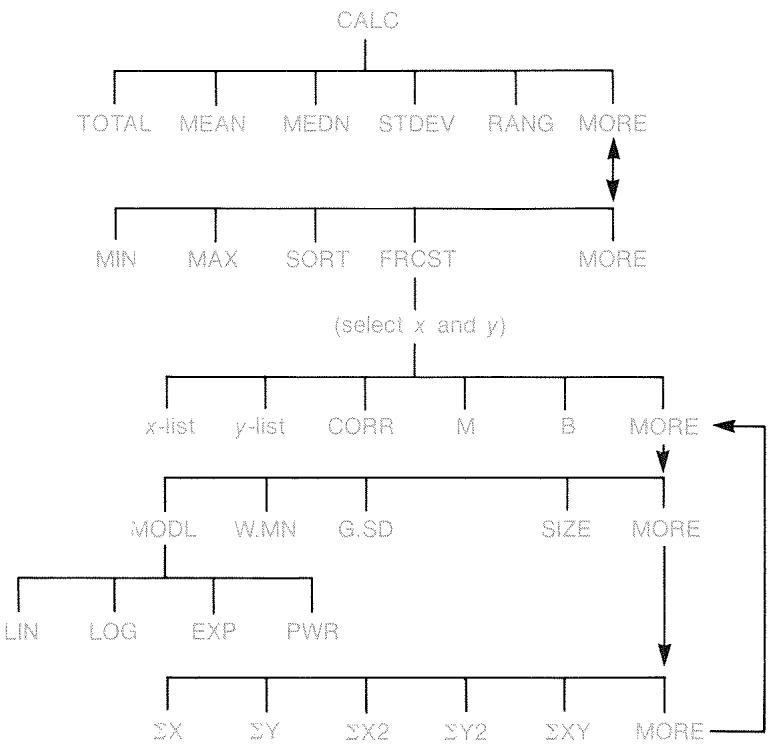
After pressing FRCST, you must specify two previously created lists—one for the x -variable and one for the y -variable. The two lists must have the same number of items.

Table 9-3. FRCST Menu Labels

Menu Label	Description
list name for x-variable	These specify the two lists of data to be com- pared. Also used for estimations: store x and estimate y, or vice-versa. *CURR is the menu la- bel for an unnamed current list.
list name for y-variable
CORR*	Calculates the correlation coefficient, a number between -1 and +1 that measures how closely the x,y data points match the calculated curve.
M*	Calculates M. For the linear model, this is the slope.
B*	Calculates B. For the linear model, this is the y- intercept.
MODL	Displays a choice of the four curve-fitting models: LIN, LOG, EXP, and PWR.
W.MN	Calculates the weighted mean of the x-values us- ing the weights in the y-list.
G.SD	Calculates the standard deviation of a set of x- values grouped by frequencies specified in the y- list.
SIZE	The number of items in either list.
ΣX	Sum of items in x-list.
ΣY	Sum of items in y-list.
ΣX2	Sum of squares of items in x-list.
ΣY2	Sum of squares of items in y-list.
ΣXY	Sum of products of items in x- and y-lists.
* For the non-linear models, the calculation uses the transformed data values.

Curve Fitting and Forecasting

Curve fitting is a statistical method for finding a relationship between two variables, x and y . Based on this relationship, you can estimate new values of y based on a given x -value, and vice-versa. Each SUM list holds the numbers (data values) for one variable. You can select one of four curve-fitting models:*

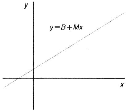
Linear Curve Fit
LIN

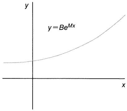
Exponential Curve Fit
EXP

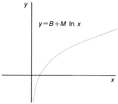
Logarithmic Curve Fit
LOG

Power Curve Fit
PWR

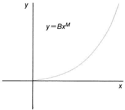
* The exponential, logarithmic, and power models are calculated using transformations that allow the data to be fitted by standard linear regression. The equations for these transformations appear in appendix B. The logarithmic model requires positive x -values; the exponential model requires positive y -values; and the power curve requires positive x - and y -values.

To do curve fitting and forecasting:

1. Enter the data into two SUM lists: one for the x -values and one for the y -values. Make sure each list has the same number of items so that the items are in matched pairs.
2. From the SUM menu, press CALC MORE FRCST to display a menu of SUM-list names. The current list is labeled *CURR unless named otherwise.
3. Press a menu key to select a list of x -values (independent variable).
4. Select a list of y -values (dependent variable).
5. Now you see the FRCST menu. Whichever curve-fitting model was used last is named in the display. If you want to select a different model, press MORE MODL, and then the menu key for the model.

1. To calculate the curve-fitting results, press CORR, M, and B

2. To forecast (estimate) a value:

3. Key in the known value and press the menu key for that variable.

4. Press the menu key for the variable whose value you want to forecast.

Example: Curve Fitting. BJ's Dahlia Garden advertises on a local radio station. For the past six weeks, the manager has kept records of the number of minutes of advertising that were purchased, and the sales for that week.

	Number of Minutes of Radio Advertising (x-values, MINUTES)	Dollar Sales (y-values, SALES)
Week 1	2	1,400
Week 2	1	920
Week 3	3	1,100
Week 4	5	2,265
Week 5	5	2,890
Week 6	4	2,200

BJ's wants to determine whether there is a linear relationship between the amount of radio advertising and the weekly sales. If a strong relationship exists, BJ's wants to use the relationship to forecast sales. A graph of the data looks like this:

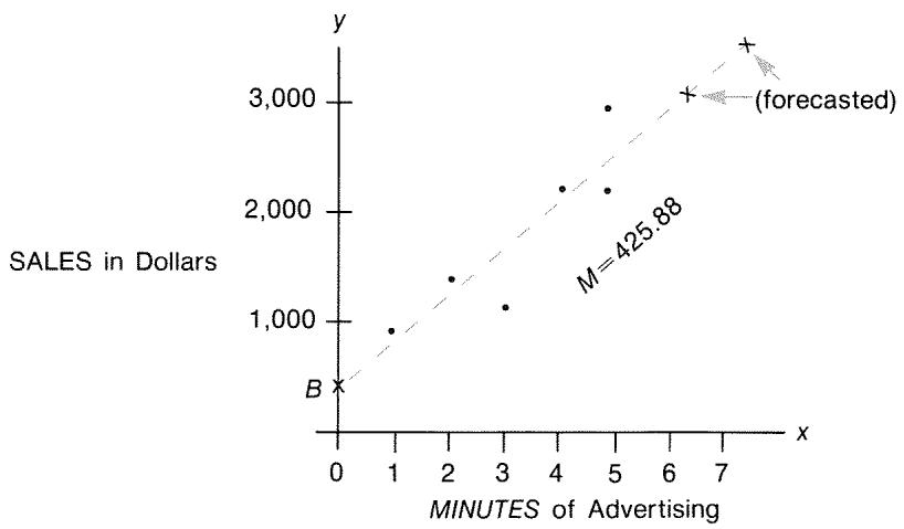
Keys:	Display:	Description:
SUM		Displays current SUM list and SUM menu keys.
CLEAR DATA		Clears current list.
YES	ITEM(1)=?
2 INPUT		Stores minutes of ad- vertising (x-values) into a SUM list.
1 INPUT
3 INPUT
5 INPUT
5 INPUT
4 INPUT	ITEM(7)=?
	TOTAL=20.00
EXIT NAME	TYPE NAME: [INPUT]
MINUTES		Names this list. (See page 27 to use the AL- PHA menu.)
INPUT	ITEM(7)=?
Now enter and name the second list.
GET *NEW	ITEM(1)=?	Gets a new, empty list.
1400 INPUT		Stores weekly sales (y- values) into a second SUM list.
920 INPUT
1100 INPUT
2265 INPUT
2890 INPUT
2200 INPUT	ITEM(7)=?
	TOTAL=10,775.00
EXIT NAME	TYPE NAME: [INPUT]
SALES INPUT	ITEM(7)=?	Names y-list.
CALC MORE		Identifies the lists for curve-fitting.
FRCST	SELECT x VARIABLE
MINU	SELECT Y VARIABLE	Selects MINUTES as x- list, SALES as y-list, indicates current curve- fitting model, and displays FRCST menu.
SALES	LINEAR *
CORR	CORR=0.90	Correlation coefficient for linear model.

The correlation coefficient calculated above is acceptable to BJ's. Using the linear model, estimate what the level of sales would be if the business purchased 7 minutes of advertising time per week.

7 MINU

MINUTES=7.00

Stores 7 in variable MINUTES.

SALES

SALES=3,357.38

Forecasts the sales resulting from 7 minutes of radio advertising.

How many minutes of advertising should BJ's buy if it wants to attain sales of $3,000?
3000 SALES

MINU

MINUTES=6.16

The business should buy about 6 minutes of advertising for sales of $3,000.†

Weighted Mean and Grouped Standard Deviation

Data in one list (x) can be weighted or grouped (by frequency) by data in another list (y) . To find the mean of weighted data and the standard deviation of grouped data:

1. Enter the data values—the x -variable—into a SUM list.

2. If the model named here is not the one you want to use, press MORE MODEL and select the one you want.
   This result is not the same as it would be if SALES were the independent (x) variable, and MINUTES were the dependent (y) variable.

3. Enter the corresponding weights or frequencies—the y -variables—into another list. (To calculate G.SD, the y -values should be integers.)

4. From the SUM menu, press CALC MORE FRCST to display a menu of SUM-list names. The current list is *CURR unless named otherwise.
5. Press the menu key for the list of x -values.
6. Now select the list with the weights (or frequencies) (y) .
7. To calculate the weighted mean, press MORE W.MN
8. To calculate the grouped standard deviation, press G.sD

Example: Weighted Mean. A survey of 266 one-bedroom rental apartments reveals that 54 of them rent for 200 per month, 32 for205, 88 for 210, and 92 for216. What is the average monthly rent and its standard deviation?

Create two SUM lists. The first, called RENT, should contain the numbers 200, 205, 210, and 216, in that order. The second can be unnamed and should contain the numbers 54, 32, 88, and 92, in that order.

Keys:	Display:	Description:
SUM
CLEAR DATA		Cleared current list or gets a new one.
YES
or
GET
*NEW	ITEM(1)=?
200 INPUT		Stores rents into a list.
205 INPUT
210 INPUT
216 INPUT	ITEM(5)=?
	TOTAL=831.00
EXIT NAME		Names this list RENT. (See page 27 to use the ALPHA menu.)
RENT INPUT	ITEM(5)=?
GET		Gets a new, empty list.
*NEW	ITEM(1)=?
54 INPUT		Stores frequencies into second list.
32 INPUT
88 INPUT
92 INPUT	ITEM(5)=$?
	TOTAL=266.00
EXIT CALC		Displays names of all SUM lists.
MORE
FRCST	SELECT X VARIABLE
RENT	SELECT Y VARIABLE	Specifies RENT as the x-list.
*CURR	LINEAR	Specifies the current, unnamed list as the y-list and then displays the FRCST menu. (Ignore model type.)
MORE		Average monthly rent.
M.MN	209.44
G.SD	5.97	Standard deviation of the rents.

Summation Statistics

The summation values are of interest if you want to perform other statistical calculations besides those provided by the calculator. To find x, x^2, y, y^2, (xy) , and n , the number of elements in either list:

1. Display the FRCST menu and select the x - and y -lists as explained in steps 1-4 of the instructions on page 123. To find the summation statistics for just one list of data, specify the same list for both x and y .
2. To see n , press MORE SIZE.
3. Press MORE again to display the summation menu, and press the menu label for the value you want.

Doing Other Calculations with SUM Data

If you would like to do other statistical calculations with SUM data besides those in the CALC menu, you can do so by writing your own Solver equation. There are Solver functions that can access data stored in SUM lists, and there is a summation function that can combine all or part of the values stored in specific lists.

Refer to "Accessing CFLO and SUM Lists from the Solver" in chapter 11.

Time, Appointments, and Date Arithmetic

The calculator contains a clock and calendar in the TIME menu. You can select a 12-hour or 24-hour clock, and a month-day-year or day-month-year calendar. You can:

■ Record appointments that set alarms with optional messages.
Determine the day of the week for a particular date.
Calculate the number of days between two dates using the 360-day, the 365-day, or the actual calendar.

Viewing the Time and Date

To view the time and date, press TIME in the MAIN menu.

If you overwrite the time and date, you can restore them to the display by pressing .

The TIME Menu

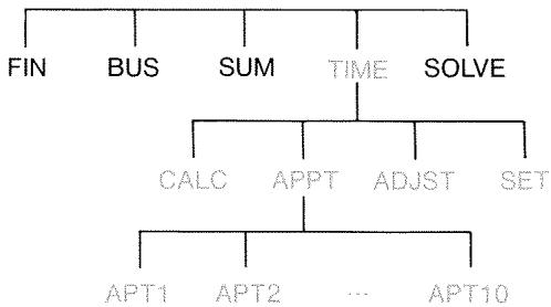
Table 10-1. The TIME Menu Labels

Menu Label	Description
CALC	Displays the CALC menu, for calculating the day of the week and other date arithmetic.
APPT	Displays the APPT menu for setting and viewing appointments.
ADJST	Displays the ADJST menu for adjusting the clock setting.
SET	Displays the SET menu for setting the time and date, and for selecting the time and date formats.

Setting the Time and Date (SET)

Table 10-2. The SET Menu Labels

Menu Label	Description
DATE	Sets the date to the displayed number (MM.DDYYYY or DD.MMYYYY).
TIME	Sets the time to the displayed number (HH.MMSS).
A/PM	Switches between AM and PM (12-hour clock).
M/D	Switches between month/day/year and day.month.year formats.
12/24	Switches between 12-hour and 24-hour clock formats.
HELP	Displays the formats for entering the clock's date and time.

To set the time:

1. Press TIME SET to display the SET menu.
2. Key in the correct time in the current format (A or P indicates the 12-hour clock). For example, for 9:08:30 p.m. enter 9.0830 in a 12-hour clock or 21.0830 in a 24-hour clock.
3. Press TIME to set the new time.
4. For 12-hour format: press H/PM to switch between AM and PM.

To set the date:

1. Key in the correct date in the current format. For example, for April 3, 1990 enter 4.031990 in month/day/year format or 3.041990 in day.month.year format.
2. Press DATE.

Example: Setting the Date and Time. Set the date and time to April 5, 1991, 4:07 p.m.

Keys:	Display:	Description:
SET		Displays SET menu.
4.051991		Sets date.
DATE	FRI 04/05/91 time
4.07 TIME		Sets time. Press A/PM if necessary.
A/PM	FRI
	04/05/91 04:07:xx P

Changing the Time and Date Formats (SET)

Use the SET menu to change the time and date formats. To switch between the 12- and 24-hour clocks, press 12/24 . To switch between the month/day/year and day.month.year calendars, press M/D.

Adjusting the Clock Setting (ADJST)

The ADJST menu adjusts the time setting forward or backward in increments of hours, minutes, or seconds.

1. Press TIME ADJST.
2. Press the appropriate menu key(s) until the correct time is displayed. For example, if the current time setting is 11:20:xx AM (ignoring seconds), pressing +HR twice changes the time to 1:20 PM. Then, pressing -MIN three times changes the time to 1:17 PM.

Appointments (APPT)

You can record up to ten appointments, each with an alarm. An appointment can contain a message. You can also create repeating appointments—appointments that recur at regular intervals.

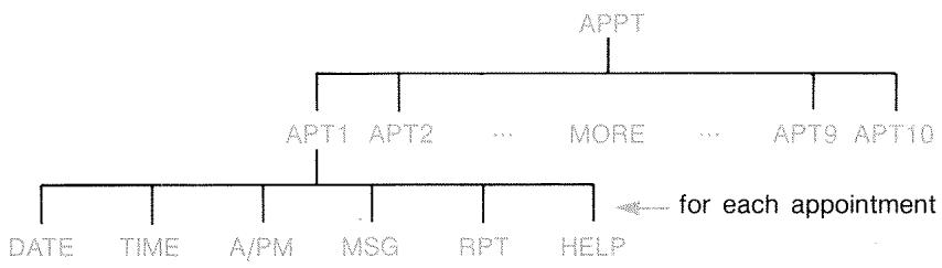
Viewing or Setting an Appointment (APT1-APT10)

Table 10-3. Menu Labels for Setting Appointments

Menu Label	Description
DATE	Sets the appointment date.
TIME	Sets the appointment time, and automatically enters the current date (if the existing appointment date was in the past).
A/PM	Sets AM or PM for 12-hour clock.
MSG	Displays the ALPHA menu and any existing message.
RPT	Displays the existing repeat interval and the menu for changing the repeat interval.
HELP	Displays the format for entering the date and time.

To set an appointment or view its current setting:

1. Press TIME, then APPT. The display tells you which appointments (numbered 1-10) are set and which are past due (expired with unacknowledged alarms).

Pressing MORE displays the status and menu labels for appointments 6 through 10.

1. Press a menu key—APT1 through APT10. The display shows the current appointment, if any, and the menu labels for setting appointments.
2. Optional: press CLEAR DATA to remove any old information.

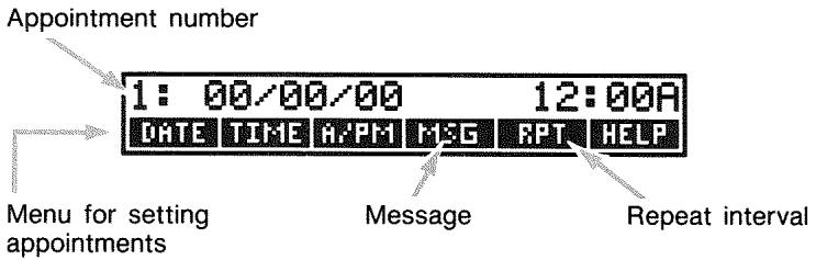
1. Setting the appointment time: Use 12-hour or 24-hour time, as appropriate. Key in the time as a number in the form HH.MM. For example, 2:25 p.m. would be 2.25 (12-hour format) or 14.25 (24-hour format). Press TIME. The date is automatically set to the current date if the existing date is in the past or was cleared. For 12-hour format: press R/PM to switch between AM and PM.
2. Setting the appointment date: Key in the date in the current date format. For example, enter October 4, 1990 as 10.041990 (month/day/year format) or 4.101990 (day.month.year format). Press DATE. If the appointment is within a year from today, you can omit the year.
3. The appointment message (optional): To set, change, or just view a message, press MSG. Type the message (refer to page 27 for using the ALPHA menu). Messages are limited to a maximum of 22 characters. Press INPUT when done. (Press EXIT to negate any changes and retain the original message.)

4. The repeat interval (optional): To set, view, or change a repeat interval, press RPT. Key in an integer and press the appropriate key. For example, 2 DAY causes the appointment to go off at the same time every other day; 90 MIN sets the repeat interval to 112 hours. NONE sets the appointment to nonrepeating. You can specify repeat intervals up to 104 weeks in length (728 days, 17,472 hours, etc.)

5. When done, press EXIT to return to the APPT menu. The appointment you just set will be recorded, such as SET:1. You can check an appointment by pressing its menu key (such as APT1).

restores an appointment's time and date to the display if it has been overwritten by other operations.

Acknowledging an Appointment

To acknowledge the appointment and clear the message, press any key (except ) during the beeping. Appointments not acknowledged within 20 seconds become past due.

When an appointment "comes due," the alarm starts beeping and the alarm annunciator (()) is displayed, even if the calculator was off.* The message (or, if none, the time and date) is displayed.

Unacknowledged Appointments

An appointment not acknowledged during its alarm becomes past due. The alarm annunciator remains on.

To acknowledge a past-due appointment:

1. Press TIME APPT.
2. Press the menu key for the past-due appointment.
3. Press to return to the APPT menu. The acknowledged appointment is no longer listed as past due.

A repeating appointment is deactivated while it is past due and will not go off subsequently until the past-due appointment has been acknowledged.

• If the calculator is in the middle of a complex calculation when an appointment comes due, the alarm annunciator comes on and the calculator beeps once. When the calculation is done, the alarm goes off.
  † The beeping can be suppressed or restricted to appointments. See "Beeper On and Off," page 33.

Clearing Appointments

To cancel an appointment or to get rid of a repeating appointment, you need to clear the appointment. Clearing changes the date and time to 00/00/00 , 12:00 AM, and removes the message and the repeat interval.

To clear an appointment, press the menu label for that appointment and press CLEAR DATA

To clear all ten appointments, display the APPT menu (the menu with APT1, APT2, etc.) and press CLEAR DATA YES.

Example: Clearing and Setting an Appointment. Today is Friday, April 20, 1990. You want to set appointment #4 to go off every Tuesday at 2:15 p.m. to remind you of a staff meeting. Assume 12-hour time format and month/day/year date format.

Keys:	Display:	Description:
TIME APPT		Displays setting for ap- pointment #4.
RPT4
CLEAR DATA	4: 00/00/00 12:00A	Cleared aptt. #4.
2.15 TIME	4: FRI 04/20/90 2:15A	Stores aptt. time and supplies current date.
A/PM	4: FRI 04/20/90 2:15P	Sets aptt. time to PM.
4.24 DATE	4: TUE 04/24/90 2:15P	Stores aptt. date.
MSG		Enters message: "staff".
STAFF INPUT	4: TUE 04/24/90 2:15P
RPT	RPT=NONE	Displays RPT menu.
1 WEEK	RPT=1 WEEK(S) 4: TUE 04/24/90 2:15P	Sets repeat interval.

Date Arithmetic (CALC)

The CALC menu performs date arithmetic:

Determines the day of the week for any date.
■ Determines the number of days between dates using one of three calendars—actual, 365-day, or 360-day.
- Adds or subtracts days from a date to determine a new date.

The calendar for date arithmetic runs from October 15, 1582 to December 31, 9999.

To display the CALC menu, press TIME, then CALC.

Table 10-4. CALC Menu Labels for Date Arithmetic

Menu Label	Description
DATE1	Stores or calculates a date. Also displays the day of the week. If you omit the year, the calculator uses the current year.
DATE2
DAYS	Stores or calculates the number of actual days between DATE1 and DATE2 , recognizing leap years.
360D	Calculates the number of days between DATE1 and DATE2 using the 360-day calendar (30-day months).
365D	Calculates the number of days between DATE1 and DATE2, using the 365-day calendar, ignoring leap years.
TODAY	A shortcut: recalls the current date, which can then be stored in DATE1 or DATE2.

The calculator retains the values for the TIME CALC variables DATE1, DATE2, DAYS until you clear them by pressing CLEAR DATA while the CALC menu is displayed.

To see what value is currently stored in a variable, press RCL menu label.

Determining the Day of the Week for Any Date

To find the day of the week for any date, key in the date and press DATE1 or DATE2.

Calculating the Number of Days between Dates

To calculate the number of days between two dates:

1. Key in the first date (for today's date, use TODAY) and press DATE1.
2. Key in the second date and press DATE2.
3. Press DAYS, 360D, or 365D to calculate the number of days using that calendar.

Example: Calculating the Number of Days between Two

Dates. Find the number of days between April 20, 1949 and August 2, 1986, using both the actual calendar and the 365-day calendar. Assume the date format is month/day/year.

Keys:	Display:	Description:
TIME		Displays CALC menu.
CALC
4.201949		Stores Apr. 20, 1949 as
DATE1	DATE1=04/20/1949 WED	first date and displays its day of the week.
8.021986		Stores Aug. 2, 1986 as
DATE2	DATE2=08/02/1986 SAT	second date.
DAYS	ACTUAL DAYS=13,618.00	Calculates actual number of intervening days.
365D	365 DAYS=13,609.00	Calculates number of intervening days by a 365-day calendar.

Calculating Past or Future Dates

To calculate a date a specified number of days from another date:

1. Key in the known date (for today's date, use TODAY) and press DATE1.
2. Key in the number of days. This number should be negative if the unknown date precedes the known date. Press DAYS.
3. Press DATE2 .

This calculation always uses the actual calendar.

Example: Determining a Future Date. On February 9, 1990, you purchase a 120-day option on a piece of land. Determine the expiration date. Assume the date format is month/day/year.

Keys:	Display:	Description:
TIME		Displays CALC menu.
CALC
2.091990	DATE1=	Stores Feb. 9, 1990.
DATE1	02/09/1990 FRI
120 DAYS	ACTUAL DAYS=120.00	Stores number of days into the future.
DATE2	DATE2=	Calculates expiration date (DATE2).
	06/09/1990 SAT

The Equation Solver

The Equation Solver (the SOLVE menu) stores equations that you enter and creates menus for them. You can then use those menus to do calculations. Enter Solver equations in algebraic form regardless of the calculation mode (ALG or RPN).

The Solver can store many equations—the number and length of equations is limited only by the amount of memory available. The equations are stored in a list.

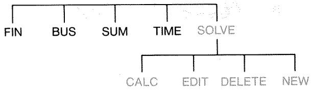
Solver Example: Sales Forecasts

Suppose part of your job includes making sales forecasts, and that these forecasts are revised based on new information. For instance,

A change in the price of the product will affect sales by a forecasted percentage, A% .
A change in sales-force training will affect sales by a forecasted percentage, B% .
A competitor's new product will affect sales by a forecasted percentage, C% .

Regardless of how you do this calculation (even if you do it long-hand), you are using an equation:

Next Forecast = Old Forecast + Change in Old Forecast
= Old Forecast + (Projected Percentage Changes × Old Forecast)

or:

$$ N E X T = O L D + \left(\left(A \% + B \% + C \%\right) \div 100 \times O L D\right) $$

Using the SOLVE and ALPHAbetic menus, you can type in this equation as

$$ N E X T = O L D + (A _ {2} + B _ {2} + C _ {2}) \div 1 0 0 \times O L D $$

and then automatically create this menu—which contains all the variables' labels—by pressing INPUT CALC :*

Each menu label represents a variable. You can use them to store and calculate values the same way you use other menus and their built-in variables.

Entering a Solver Equation. To type this equation, you must use the ALPHA menu. If you are not familiar with the ALPHA Abetic menu, refer to "Typing Words and Characters" on page 27.

Keys:

SOLVE

NEW

Display:

TYPE EQUATION;

[INPUT]

Description:

Displays SOLVE menu, then ALPHA menu.

NEXT = OLD

+ () A % +

B % + C %

) ÷ 100 ×

OLD	...D+(A%+B%+C%)
	÷100×OLD

INPUT

NEXT=0LD+ (R%+B%+C%)÷1...

Enters equation into list.

EDIT		Controls view of full equation.
--->
--->	...D+(A%+B%+C%)
	÷100×0LD

NEXT=OLD+ (A%+B%+C%)÷1...

Displays SOLVE menu.

Calculating with the Solver. Suppose last month's forecast for a product was 2,000 units. In the meantime, three market changes have occurred that affect this forecast. A) The price of the product has dropped, causing an expected 20% increase in sales. B) A major sales-force training program started, causing an expected 5% increase in sales. C) A competitor is introducing a new product, causing an expected 15% drop in sales. Calculate the new forecast for next month.

Keys:	Display:	Description:
CALC	VERIFYING EQUATION	Verifies that equation is valid; creates Solver menu with menu labels for this equation.
2000 OLD	OLD=2,000.00	Stores old forecast.
20 A%	A%=20.00	Stores effect of price drop on sales.
5 B%	B%=5.00	Stores effect of sales-force training on sales.
15 +/− C%	C%=-15.00	Stores effect of competitor's new product on sales.

Suppose your boss wants next month's forecast to be 2,300 units. You can't affect A% or C% , but you can affect B% through the sales training program. Determine what B% must be for NEXT to equal 2,300 units. All you need to do is re-enter the one value you are changing:

Keys:

Display:

Description:

2300

NEXT

NEXT=2,300,00

B%

B%=10.00

The training program would need to result in a 10% increase in sales to effect a new forecast of 2,300.

The SOLVE Menu

If the Solver list is empty, you will see an instruction for entering an equation when you press Solve:

If the Solver list is not empty, you will see the current equation—the last one entered or selected.

Pressing , , , and moves you through the list.

Table 11-1. The SOLVE Menu Labels

Menu Label	Description
CALC	Verifies the current equation and creates menu labels for it. This is necessary before doing any calculations.
EDIT	Accesses the ALPHA-Edit menu (page 28) so you can alter the current equation. The arrow keys move long equations across the display.
DELETE	Deletes the current equation or just its variables (that is, the space allotted in memory for the variables).
NEW	Allows you to enter a new equation.

While you're working with a specific equation in the Solver, the equation's own menu appears in the display. To retrieve the primary SOLVE menu, press EXIT.

Entering Equations

To make an entry into the Solver list:

1. Press SOLVE NEN. (To insert the new entry at the bottom of the list, press .)
2. Use the ALPHA menu to type in characters (see page 27), and use the regular keyboard to type in digits and arithmetic operators (+, =, y^x, etc.) . If you make a mistake, use to backspace or to start over. Or press to bring up the ALPHA-Edit menu.
3. Press INPUT to store the equation.
4. Press Calc to verify that the equation is valid, and to create its menu labels. You now can proceed with your calculations.

When you press calcc, the calculator displays:

VERIFYING EQUATION...

while the Solver checks that the equation is mathematically valid. (However, the Solver has no way of checking whether the equation is the right one for your problem.) If the equation cannot be solved, the calculator briefly displays:

INVALID EQUATION

and the cursor will blink at the first character that the Solver could not interpret. (It is possible that your mistake is somewhere else, but this is a good place to start looking, since this is where the Solver got stuck.) The ALPHA-Edit menu appears so you can make changes. Check to be sure you've made no typing mistakes, and that you've followed the rules for writing equations given on page 154 under "What Can Appear in an Equation."

An entry that is not an equation will be stored when you press INPUT, but it cannot be verified when you press calcc.

Calculating Using Solver Menus (CALC)

If pressing CRLF creates a Solver menu for your equation, then the equation is good (that is, mathematically valid).

If the equation contains more than six variables, the Solver uses the label MORE to switch between sets of menu labels.

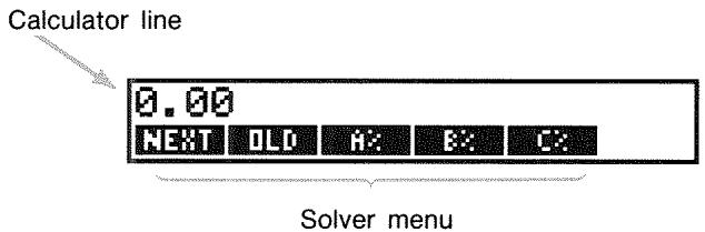
To test whether your equation is in fact correct, test it out by entering some values for which you already know the result, and see if the Solver's result is correct.

To do a calculation using a Solver menu:

1. Store values in all but one of the variables (for example, 2000 old, etc.). Remember that you can verify stored values by pressing RCL menu label.
2. To start the calculation, press the menu key for the variable you want to calculate.

In most cases, this is all you need to know about how the Solver works. However, certain types of equations are more difficult to solve. If, during the calculation, the display temporarily shows two lines of changing numbers, such as

$$ \begin{array}{l} A: 1. 5 0 0 0 0 0 0 0 0 0 - \ \text {A}: 1, 1 3 4 7 6 1 2 9 8 3 4 + \ \end{array} $$

then the Solver is searching for a result for the variable A . Read the section, "How the Solver Works," starting on page 166.

Example: Return on Equity. The Return on Equity of a business can be defined as:

$$ \mathrm {R O E} = \frac {\text {O p e r a t i n g i n c o m e - I n t e r s t - T a x e s}}{\text {C o m m o n e q u i t y}} $$

Find the ROE of a small firm with 2,000 in assets. The assets earned 10% while its debt cost it 8%. The assets were financed using500 of common equity and $1,500 of debt. The firm paid no taxes.

Operating income = assets × percentage earnings on assets

$$ = \text {A S S E T} \times \text {E R N} $$

Interest = debt × percentage interest paid on debt

$$ = D E B T \times \times I N T $$

Common equity = amount of common equity used for financing

$$ = E Q T Y $$

The Solver equation would be:

$$ R O E = (\text {A S S E T} \times \% \text {E R N} \div 1 0 0 - \text {D E B T} \times \% \text {I N T} \div 1 0 0 - \text {T R X}) \div \text {E Q T Y} \times 1 0 0 $$

Keys:	Display:	Description:
MAIN		Restores MAIN menu.
SOLVE		Displays ALPHA menu.
NEW	TYPE EQUATION; [CINPUT]
ROE = [ASSET × % ERN - DEBT × % INT - TAX ]		Entering the equation.
+ EQTY	...-DEBT×%INT-TAX) +EQTY
INPUT	ROE=(ASSET×%ERN - DEBT×...	Stores the equation.
CALC		Verifies the equation and displays the menu labels for ROE, ASSET, %ERN, DEBT, %INT, and (press MORE) TAX and EQTY.
2000 ASSET	ASST=2,000.00	Stores the values for the assets, the percentage earnings on assets, the amount of debt, the percentage interest paid on the debt, the taxes paid, and the common equity.
10 %ERN	%ERN=10.00
1500 DEBT	DEBT=1,500.00
8 %INT	%INT=8.00
MORE 0
TAX	TAX=0.00
500 EQTY	EQTY=500.00
MORE		The return on equity is 16%.
ROE	ROE=16.00

Editing an Equation (EDIT)

If you have an INVALID EQUATION, the cursor stops over the first character that the Solver could not logically interpret.

You can alter the current equation using the ALPHA-Edit menu:

1. Press EDIT to access the ALPHA-Edit menu. (See "Editing ALPHAbetic Text," page 28.) You can use (backspace) and (clear), as well.
2. To insert letters, press ALPHA and the appropriate letters. Press EXIT to bring back the editing menu.
3. Press INPUT to replace the previous version with the edited version.

Editing an equation clears its variables.

To abort an editing operation without saving any of the changes, press EXIT.

Naming an Equation

Naming equations helps you identify them later. The name precedes the equation, separated by a colon. If you don't name an equation initially, you can name it later using EDIT.

Type the name just as you type the rest of the equation. The calculator knows that whatever comes before the colon is not part of the equation. The name is for your visual aid only; the calculator cannot recognize it.

Names can be any length and contain any character except

$$ + - \times \div () < > ^ {\wedge}: = s p a c e $$

Finding an Equation in the Solver List

To display an entry in the Solver list, display the SOLVE menu and move through the list using the and keys. moves to and moves to .

Shared Variables

If two or more equations contain the same variable, that variable is shared among those equations. For example, suppose your Solver list of equations includes these two equations labeled RUG, which figures the cost of a carpet, and TOTAL, which figures the total cost of buying a carpet and installing it:

$$ R U G: P / Y D \times L \times W = 9 = C O S T $$

$$ T O T A L: C O S T + H O U R S \times 2 0, 5 0 = C H A R G E $$

COST is a shared variable. You can calculate a value for COST using the RUG equation, then switch to the TOTAL equation and calculate CHARGE after entering HOURS. Since the value for COST is shared, you do not need to store it again.

No sharing occurs between variables outside the Solver and those within the Solver. For example, this COST variable in the Solver is not shared with the COST variable in the MU%C and MU%P menus in BUS.

To transfer values between built-in variables and Solver variables, store them into storage registers. Recall them after switching menus. Remember that the value in the calculator line stays there when you switch menus.

Clearing Variables

You can clear the variables in a Solver equation just as you clear variables in other menus: press CLEAR DATA while the menu with those variables is displayed.

Make sure that the menu for the variables is in the display. (The equation itself should not be in the display. If it is, press CLEAR.) Pressing CLEAR DATA now sets NEXT, OLD, A% , B% , and C% to zero.

Variables are also cleared when their equation is edited.

If the SOLVE menu is displayed (rather than the SOLVE CALC menu), then pressing CLEAR DATA will prompt DELETE ALL VARIABLES?. Press NO, otherwise you will lose the variables in all the equations. (See "Deleting All Equations or Variables in the Solver," page 152.)

Deleting Variables and Equations

Each equation in the Solver list uses calculator memory to store 1) itself, and 2) its variables.*

Deleting a variable is quite different from clearing it:

• Clearing a variable sets it to zero; the variable retains its storage location in memory. This does not save memory space.

• An equation that has not been verified (CALC pressed) does not have any variables allocated to it. Therefore, it has no variables to be cleared or deleted.

• Deleting a variable erases its value and its storage location. This is a way to save memory space. If a variable is shared, its value is lost to all equations that share it. The memory space for a deleted variable is re-created the next time you use that equation.

Deleting One Equation or Its Variables (DELETE)

To delete an equation or its variables:

1. Display the equation.
2. Press DELETE in the SOLVE menu.
3. To delete the equation, respond YES to both questions:

DELETE THE VARIABLES?

DELETE THE EQUATION?

(If the entry has no variables allocated, then only the second question appears.)

1. To delete just the variables, respond NO to DELETE THE EQUATION?. This preserves the equation.

Deleting All Equations or All Variables in the Solver

（CLEARDATA）

To delete all the equations in the Solver, or just all the variables in all the equations:

1. Display the SOLVE menu. It doesn't matter which equation is displayed.
2. Press CLEAR DATA. To delete all equations, respond YES to both questions:

DELETE ALL VARIABLES?

DELETE ALL EQUATIONS?

1. To delete just the variables, respond NO to DELETE ALL EQUATIONS?. This preserves all equations.

Writing Equations

An equation in a book looks different from an equation in the Solver. A numerator and denominator might be separated by a bar, such as

$$ \frac {a + b + c}{d - e \times f} $$

Since a Solver equation appears all on one line, you must group the numerator and denominator separately by using parentheses, such as

$$ (R + B + C) \div (D - E \times F) $$

Order of Calculations. Operations occur from left to right but do:

Exponentiation first. For example, A × B 3 = C is interpreted as A × B^3 = C . B is raised to the 3rd power and then multiplied by A . To raise A × B to the 3rd power, write the equation as (A × B) 3 = C .
■ Multiplication and division before addition and subtraction. For example, A + B ÷ C = 12 is interpreted as A + (B / C) = 12 . To divide the sum of A + B by C , enter the equation as (A + B) ÷ C = 12 .

Parentheses. Parentheses override the above rules of priority. When in doubt, use parentheses. It never hurts to use parentheses—even multiple parentheses. (Do not use brackets or braces.)

For example, earlier (page 142) we used the equation

Next Forecast = Old Forecast + ( % + B% + C%100 × Old Forecast ) ,

which was entered into the calculator as

$$ N E X T = O L D + (A \% + B \% + C \%) = 100 \times O L D. $$

× C would be entered as ÷ (E × C)

[ A + \frac{B \times C}{D \times E} ] could be entered as R + E × C ÷ (D × E) .
A + × C(D + 5)× E could be entered as H + B× C÷ (D + 5)× E)

What Can Appear in an Equation

Long Equations. There is no limit on the length of an equation (or the number of variables it has) if there is enough memory to store it. An equation longer than one display line (22 characters) moves to the left and adds an ellipsis (...).

To view a long equation, move the cursor using the arrow keys on the ALPHA-Edit menu. For example:

TOTALCOST=LENGTH×WIDTH×HEIGHT÷12×UNIT×(1+MARKUP%÷100)

looks like

$$ T O T A L C O S T = L E N G T H \times W I D T \dots $$

when it is stored. Press EDIT -->> to view successive portions of the equation:

$$ \dots H \times H E I G H T \div 1 2 \times U N I T \times (1 + \dots $$

Spaces. You can use as many spaces as you like between variables, operators, and numbers.

Names of Variables. A variable's name can be up to 10 characters long, but cannot contain the characters + - × ÷ ^ ( ) < > = :space

The first three to five characters (depending on their widths) become the variable's menu label. Therefore, make sure no two variables in the same equation have the same first three to five characters.

Do not use AND, NOT, OR, XOR, or PI as variable names because they will be interpreted as functions.

Numbers (Constants). Do not put commas or other characters in numbers. For instance, type 10000 for ten thousand (not $10,000).

Parentheses. Do not use brackets or braces. Parentheses determine order, but do not imply multiplication. For example, the equation P_sn = P_s(1 - F) would be typed into the Solver as P_sn = P_S × (1 - F) . The × sign must be inserted between P_S and the parenthesis.

Functions and Conditional Expressions. An equation can contain any of the functions and conditional expressions given in the table on pages 157-159. Some of these functions also have typing aids.

Math Operators ("Typing Aids"). All of the math operators are located either on the keyboard (1x, 1x , etc.) or in the MATH menu (LN, EXP, etc.). Any of these operators except 1x can be included in an equation. (In the Solver, 1x is just a character.) You can call up the MATH menu from the Solver.

Many of these operators look different in an equation: pressing produces SQRT, for example. You then supply a number or variable followed by a closing parenthesis. The list of Solver functions on pages 157-159 shows the spelling of each function. Note that you supply the number after supplying the function.

You can also type these functions letter by letter using the ALPHA menu. However, it is faster to select math operators directly on the keyboard or in the MATH menu. This is called a typing aid.

For instance, these two methods of placing 25! (factorial) into an equation are equivalent. Starting after SOLVE NEW:

1. Using the ALPHA Menu

Keys:	Display:	Description:
FGHI
F	F
ABCDE
A	FA
ABCDE
C	FAC
RSTUV
T	FACT
25	FACT(25)=
ABCDE		This calculates 25!
A	FACT(25)=A	(factorial).

2. Using a Typing Aid

Keys:	Display:	Description:
MATH		MATH menu labels appear.
N!	FACT<	The ALPHA menu automatically returns after one MATH selection.
25	FACT(25)=
ABCDE		This also calculates 25!, and with fewer keystrokes.
A	FACT(25)=A

Solver Functions

Here is a complete list of functions that you can include in Solver equations. The items inside parentheses must be replaced by specific numbers, variables, or algebraic expressions.

In addition, you can use the arithmetic operators (+, -, ×, ÷, y^x) , but not % . (In the Solver, x is just a character, not an operator.)

Table 11-2. Solver Functions for Equations

Function	Description
ABS(x)	Absolute value of x.
ALOG(x)	Common (base 10) antilogarithm; 10x.
CDATE	Current date.
CTIME	Current time.
DATE(d1:n)	The date n days after (when n is positive) or before (when n is negative) date d1. The format for d1 is set in the TIME/SET menu.
DDAYS(d1:d2:cal)	Number of days between dates d1 and d2. Formats for d1 and d2 are set in the TIME menu; cal designates the calendar: ■ cal = 1 for the actual calendar, which recognizes leap years. ■ cal = 2 for the 365-day calendar, which ignores leap years. ■ cal = 3 for the 360-day calendar, which uses 12, 30-day months.
EXP(x)	Natural antilogarithm; ex.
EXPM1(x)	ex - 1.
FACT(x)	x!; factorial of a positive integer.
FLOW(CFLO-listname:flow#)	Value of the specified cash flow.
FP(x)	Fractional part of x.
HMS(time)	Converts time in decimal hours to HH.MMSS format.
HRS(time)	Converts time in HH.MMSS format to decimal hours.
IDIV(x:y)	Integer part of the quotient of x/y.
IF cond:expr1:expr2)	Conditional expression: if cond is true, use expr1; if cond is false, use expr2. See page 161.
INT(x)	Greatest integer less than or equal to x.
INV(x)	Inverse of x; 1/x.
IP(x)	Integer part of x.
ITEM(SUM-listname:item#)	Value of the specified SUM-list item.
LN(x)	Natural (base e) log of x.
LNP1(x)	In (1 + x)
LOG(x)	Common (base 10) log of x.
MAX(x:y)	Compares x and y, and returns the larger of the two.
MIN(x:y)	Compares x and y, and returns the smaller of the two.
MOD(x:y)	Remainder of the division x/y. MOD(x,y) = x - y × INT(x/y)
PI	π; 3.14159265359 (12 digits).
RND(x:y)	Rounds x to y decimal places if 0 ≤ y ≤ 11, or rounds x to y significant digits if -12 ≤ y ≤ -1. y must be an integer.
S(variable name)	Used in an IF function to test if solving for the variable named. Used to combine related equations into one Solver menu. See page 165.
SGN(x)	Sign of x (+1 if x > 0, 0 if x = 0, -1 if x < 0.
Σ(chr:c1:c2:s:expr)	Summation of the algebraic expression expr for values of the counter ctr, stepping from c1 to c2 at increments of s. See page 163.
SIZEC(CFLO-listname)	The number of the last flow in specified CFLO list.
SIZES(SUM-listname)	The number of items in specified SUM list.
SPFV(i%:n)	Future value of a single 1.00 payment; equivalent to (1 + i% ÷ 100)n. n is the number of compounding periods. i% is the interest rate per compounding period, expressed as a percentage.
SPPV(i%:n)	Present value of a single1.00 payment; equivalent to 1 ÷ SPFV(i%:n). n is the number of compounding periods. i% is the interest rate per compounding period, expressed as a percentage.
SQ(x)	Square of x; x2.
SQRT(x)	Square root of x; √x.
#T(CFLO-listname:flow#)	The number of times that specified cash flow occurs.
TRN(x:y)	Truncates x to y decimal places if 0 ≤ y ≤ 11, or truncates x to y significant digits if -12 ≤ y ≤ -1. y must be an integer.
USFV(i%:n)	Future value of a uniform series of 1.00 payments; equivalent to (SPFV(i%:n) -1) ÷ (i% ÷ 100). n is number of payments. i% is periodic interest rate, expressed as a percentage.
USPV(i%:n)	Present value of a uniform series of1.00 payments; equivalent to USFV(i%:n) ÷ SPFV(i%:n). n is number of payments. i% is periodic interest rate, expressed as a percentage.

Example Using a Solver Function (USPV): Calculations for a Loan with an Odd First Period. Suppose an auto purchase is financed with a $6,000 loan at 13.5% annual interest. There are 36 monthly payments starting in one month and five days. What is the payment amount?

Use the following formula when the time until the first payment is more than one month but less than two months. Interest for this odd (non-integer) period is calculated by multiplying the monthly interest by the number of days and dividing by 30.

The formula for this loan is:

$$ P V \left(1 + \frac {A N N I}{1 2 0 0} \times \frac {D A Y S}{3 0}\right) + P M T \left(\frac {1 - \left(1 + \frac {A N N I}{1 2 0 0}\right) ^ {- N}}{\frac {A N N I}{1 2 0 0}}\right) = 0 $$

where:

ANNI = the annual percentage interest rate.

N = the number of payment periods.

DAYS = the number of leftover, odd days (an integer from 0 through 30).

PV = the amount of the loan.

PMT = the monthly payment.

The formula can be rearranged and simplified using USPV, the Solver function for returning the present value of a uniform series of payments:

$$ P V \times (1 + A N N I \div 1 2 0 0 \times D A Y S \div 3 0) + $$

$$ P M T \times U S P V (A N N I \div 1 2; N) = 0 $$

The keystrokes are:

PV 1 + ANNII + 1200 DAYS + 30 + PMT USPV ANNI + 12:N = 0

Keys:	Display:	Description:
SOLVE	<Bottom OF LIST>	Displays SOLVE menu and bottom of Solver list.
NEW	TYPE EQUATION; [INPUT]	Displays ALPHA menu.
(type in equation as shown above)	...MT×USPV(ANNI÷12:N)=0	Remember that the colon is located after OTHER. (Press WXYZ OTHER : .)
INPUT CALC	0.00	Enters equation, verifies it, and creates menu.
6000 PV	PV=6,000.00	Stores loan amount in PV.
13.5 ANNI	ANNI=13.50	Stores annual percent interest in ANNI.
5 DAYS	DAYS=5.00	Stores number of odd days in DAYS.
36 N	N=36.00	Stores number of payments in N.
PMT	PMT=-203.99	Calculates monthly PMT of $203.99.

Conditional Expressions with IF

Equations can include conditional expressions using the function IF. The syntax of the IF function is:

IF(conditional expression : algebraic expression : algebraic expression) * then or else

• A conditional expression that contains within it an algebraic expression might cause the error INVALID EQUATION. If this happens, insert a + before the left parenthesis starting the algebraic expression. For example, change IF((A+2)÷5<12: ... to IF(+A+2)÷5<12: ...

For example, the Solver accepts the equation:

BONUS=IF(SALES>3000:，.02×SALES：.01×SALES)

According to this equation, if SALES is greater than 3000, then the BONUS equals .02 × SALES; otherwise ("or else"), BONUS equals .01 × SALES.

Logical Operators. Four logical operators can be used in conditional expressions: AND, OR, XOR, and NOT.

Relational Operators. Six relational operators are available for conditional expressions.

Operator	Keys
>	(ALPHA menu)
<	(ALPHA menu)
=	=
≥	> =
≤	< =
≠	< >

Examples of Conditional Equations.

B = IF (A>7 AND A<=15:2×A÷6:3×A+10) + C

Means: If A is greater than 7 and is less than or equal to 15, then B = 2 × A ÷ 6 + C . Otherwise, B = 3 × A + 10 + C .

VALUE = FIRST+IF(NOTFIRST 0:1÷FIRST:0）

Means: If FIRST is not equal to 0, then VALUE = FIRST + 1 ÷ FIRST. If FIRST = 0, then VALUE = FIRST.

T = W×IF(A=0 XOR B=0:A+B:A×B)

Means: If A or B , but not both, equals 0, then T = W × (A + B) . Otherwise, T = W × A × B . In other words,

When A = 0 and B 0 , T = W × B .

When A 0 and B = 0 , T = W × A .

When A = 0 and B = 0 , T = 0 .

When A 0 and B 0 , T = W × A × B .

Example: Nested IF Functions. An IF function can be used as the argument of another IF function. This is called nesting. Suppose a corporation uses a rating system to determine salary. Employees are rated on a scale from 1 through 3, and are given the following annual percent raise based on their rating:

Rating Percent Salary Increase

1	3%
2	6%
3	10%

The Solver equation to calculate an employee's new salary is based on his or her rating and old salary. What would be the new annual salary for an employee with a rating of 2 who currently earns $27,500 annually?

Press SOLVE NEW, then enter the equation:

$$ N E W = O L D \times (1 + I F (R = 1: . 0 3: I F (R = 2: . 0 6: . 1)) $$

To do the calculation:

Keys:	Display:	Description:
INPUT		Stores, verifies, and create menu labels for the equation.
CALC
27500 OLD	OLD=27,500.00	Stores old salary.
2 R	R=2.00	Stores rating.
NEW	NEW=29,150.00	Calculates new salary.

The Summation Function ()

The function does summation calculations in an equation:

(counter variable: starting value: ending value: step size: algebraic expression)

The counter variable takes on a series of values, beginning with the starting value, and incrementing according to the step size, until it passes the ending value. For each value of the counter, the algebraic expression is evaluated, and the value is added to the previous value. The function returns the final summation.

For example, when the equation:

$$ S E R I E S = \sum (I: 1: 6: 1: I \times X ^ {\wedge} I) $$

is solved for SERIES, the counter I runs from 1 through 6 in steps of one—that is, 1, 2, 3, 4, 5, 6. For each value I , the expression I × X I is calculated and added to the sum. Thus the stored value of X is used to calculate X + 2X^2 + 3X^3 + 4X^4 + 5X^5 + 6X^6 .

The following equation uses a variable as the ending value, 0 as the beginning value, and a step size of 2.

$$ S E R I E S = \sum (I: 0: L A S T: 2: I \times X ^ {\wedge} I) $$

If 8 is stored in LAST, I takes on values of 0, 2, 4, 6, and 8. Then the stored value of X will calculate 2X^2 + 4X^4 + 6X^6 + 8X^8 .

Accessing CFLO and SUM Lists from the Solver

You can use a Solver equation to perform calculations other than those in the CFLO and SUM menus using data stored in CFLO and SUM lists. The following Solver functions gain access to these lists.

SIZEC(CFLO-listname) returns the number of the last flow in the specified CFLO list. For example, if the last flow in the list INV were FLOW(6) = 5,000,00 , then SIZEC(INV) would equal 6.00.
■ FLOW(CFLO-listname:flow number) returns the value of the specified flow.
- #T(CFLO-listname : flow number) returns the number of times the specified flow occurs.
■ SIZES(SUM-listname) returns the number of items in the specified SUM list

ITEM(SUM-listname: item number) returns the value of the specified item.

Summation of List Data. The function can be used to sum calculations done with numbers in lists. For example, the following equation calculates x_1^2y_1^2 for values stored in two SUM lists named XVAR and YVAR, which must have the same number of items:

$$ S X 2 Y 2 = \sum (I: 1: S I Z E S (X V A R): 1: I T E M (X V A R: I) ^ {\wedge} 2 \times I T E M (Y V A R: I) ^ {\wedge} 2) $$

"Chi-Squared Statistics" in chapter 13 illustrates another use of the function with SUM lists.

Creating Menus for Multiple Equations (S Function)

The S (solving for) function is used in conjunction with the IF function to group related equations together and to specify the criteria for choosing one of them to solve.

S(name)

The advantage over two separate equations is that the single equation gives you a single menu with all possible variables. That way, if you are working with two different but related problems, you can keep the same Solver menu labels in the display all the time--you don't have to switch equations.

For example, consider these two equations for conversions:

$$ K G \times 2. 2 1 = L B \quad \text {a n d} \quad M \times 3. 2 8 = F T $$

The following, rearranged single equation can do either conversion:

$$ I F (S (K G) O R S (L B): K G \times 2, 2 1 - L B: M \times 3, 2 8 - F T) = 0 $$

This means: if you are solving for either KG or LB , then use KG × 2.21 - LB = 0 . Otherwise (that is, if you are solving for M or FT ), use M × 3.28 - FT = 0 . The two conversion equations are rewritten so that all the variables appear on one side of each equation, and the other side is set equal to zero.

The S function appears as part of the conditional expression of the IF function. You can leave out the " = 0 and it will be understood that the whole equation is set equal to zero.

Example: Unit Conversions. Use the above equation to convert between kilograms and pounds and between meters and feet.

Press SOLVE NEW, then enter the equation:

$$ I F (S (K G) O R S (L B): K G \times 2, 2 1 - L B: M \times 3, 2 8 - F T) $$

Press INPUT to store it, then CALC to verify it and create its menu:

1. Convert 225 pounds to kilograms.

Press 225 LB KG . Result is KG=101.81.

1. How many feet equal 100 meters?

Press 100 M FT. Result is FT=328.00.

Note that you do not have to clear variables between steps 1 and 2. The S function considers only those values in the part of the equation that it is solving.

How the Solver Works

The Solver has two ways of finding an answer. First, it tries to find a direct solution by rearranging the equation and then solving for the variable. If the Solver finds a direct solution, the calculator displays the result.

If the Solver is unable to find a direct solution, it tries to find the answer indirectly by iteration. It estimates a set of answers, sees how close they are to a solution, and then makes another set of estimates. The calculator displays the Solver's current estimates as the Solver searches for an answer. You should keep in mind that there might be more than one solution to an equation, and that it might be necessary for you to enter guesses to influence which solution the Solver finds. If the displayed estimates don't appear to be proceeding towards a number you judge to be a reasonable answer, you can stop this iterative process, enter your own guesses, and restart the search. (See "Halting and Restarting the Iterative Search" and "Entering Guesses," below.)

The process of finding a solution iteratively is very complex. There are four possible outcomes. Refer to "Solver Calculations" in appendix B for additional descriptions of these outcomes.

■ Case 1: The calculator displays a result. It is very likely that this is a solution to the equation. To check how good this result is, you can repeat the calculation by pressing the menu key for the variable you solved for. If the two sides of the equation have not been calculated to be exactly equal, the calculator displays a message with the values for the left and right sides of the equation. Read "Solver Calculations" in appendix B for an explanation of the meaning of this display.
■ Case 2: The calculator displays a message with the calculated, unequal values of the left and right sides of the equation. The Solver has found a possible solution, but you must interpret its validity. To see the questionable solution, press or . Refer to "Solver Calculations" in appendix B for more information.
■ Case 3: The calculator displays BAD GUESSES: PRESS [CLR] TO VIEW. The Solver cannot begin the search with the current guesses. Press or CLR to view the starting guesses. To supply new guesses, see "Entering Guesses," below.
■ Case 4: The calculator displays SOLUTION NOT FOUND. Check to see if your equation and stored values are correct. If the equation is correct, you might be able to find a solution by entering very good guesses.

Halting and Restarting the Iterative Search

When the Solver is iteratively searching for a solution (in other words, when the Solver is displaying sets of estimates), you can halt the calculation by pressing any key except . The calculator displays the message INTERRUPTED. To see the best estimate the Solver has found so far, press CLR or . You can restart the search from where it left off by pressing the menu key for the variable you are solving for. Or, you can restart the search using your own guesses (see "Entering Guesses," below).

Entering Guesses

Entering your own guesses serves two purposes. First, it can save time by telling the Solver where to start searching. Second, if more than one solution exists, entering guesses may lead the Solver to a solution in a specified range. The closer your guesses are to the desired solution, the better chance the Solver has of finding it.

You can enter guesses at these times:

Before beginning the calculation, after you've stored a value for every variable except the unknown variable. If you enter one guess, the Solver generates a second guess.
After you've halted the iterative search.
■ After the Solver has returned an answer, and you wish to begin searching for another answer.

You can enter one or two guesses. If you enter one guess, the Solver makes a second guess. If you enter two guesses, the Solver uses those two guesses to start searching for a solution. The Solver works most efficiently when the answer is between your two guesses. For example, if you know the answer is between 5 and 12, you should enter 5 and 12 as the starting guesses.

To enter one guess, key in the value and press the menu key twice. For example, 4.5 enters 4.5 as a guess for a Solver variable named A and starts the calculation.

To enter two guesses, key in the first guess and press the menu key. Then key in the second guess and press the menu key twice. For example, 0 A 100 A causes the Solver to search for A using 0 and 100.

Example: Using Guesses to Find a Solution Iteratively. One equation for calculating the profit from a manufacturing operation is:

$$ \begin{array}{l} \text {P r o f i t} = (\text {P r i c e} \times \text {Q u a n t i t y}) - (\text {V a r i a b l e c o s t s} \times \text {Q u a n t i t y}) \ \hskip 1 4. 2 2 6 3 7 8 p t - \text {F i x e d C o s t s} \end{array} $$

The C-Sharp Piano Corporation sells pianos for 6,000. Variable costs are4,100; fixed costs per year are 112,000. How many pianos must C-Sharp sell this year in order to earn a profit of130,000? (In past years, C-Sharp has had to sell between 100 and 200 pianos to make an acceptable profit. You can use this information as initial guesses.)

Press SOLVE NEW, then enter the equation:

$$ P R O F I T = P R I C E \times Q T Y - V A R C O S T \times Q T Y - F I X C O S T $$

Keys:	Display:	Description:
INPUT CALC		Stores, verifies, and cre-ates labels for the equation.
6000 PRICE	PRICE=6,000.00	Stores price.
4100 VARCO	VARCOST=4,100.00	Stores variable cost, fixed cost, and profit.
112000 FIXCO
130000 PROFI	FIXCOST=112,000
	PROFIT=130,000.00

The following steps enter guesses for QTY . If the Solver must search iteratively to solve for QTY , it will begin by using the estimates 100 and 200.

Keys:	Display:	Description:
100 QTY	QTY=100.00	The first guess for QTY.
200 QTY	QTY=200.00	The second guess for QTY.
QTY	QTY:200.00000000- QTY:100.00000000+ . . . QTY=127.37	Solves for QTY iteratively.

Printing

The calculator can print information using the HP 82240 Infrared Printer, which accepts the infrared signal from the printer port. This chapter describes information you can print. Operation of the printer is covered in the printer owner's manual.*

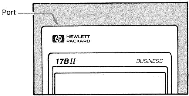
The print annunciator ( ) appears in the display whenever the calculator sends information through its printer port.

Because communication goes only one way—from calculator to printer—the calculator cannot determine whether the printer is receiving information. If a printing operation involves many lines of information, the calculator slows its transmission rate to allow the printer time to print.

• Since the HP-17B cannot send control characters to the printer, portions of the printer's manual pertaining to control codes and graphics characters do not apply.

To preserve battery power, the calculator will not transmit data to the printer when the low-power annunciator ( ) is on. If a low-power condition occurs after you've started a printing operation, printing stops and the calculator displays the message BATT TO LOW TO PRINT.

The Printer's Power Source

The speed of the printer depends on whether it is using its optional ac adapter. To optimize printing performance, set the printing speed mode in the calculator appropriately. To view or change the printing speed mode:

1. Press MODES
2. Press PRNT to change and display the new mode. If necessary, press PRNT again to set the desired mode:

PRINTER: AC ADAPTER
■ PRINTER: NO AC ADAPTER

1. Press .

For long printing operations, printing will be faster using the printer's ac adapter and the calculator's appropriate printing speed mode. When the printer is powered by batteries alone, be sure to change the mode to PRINTER: NO AC ADAPTER so that the calculator will not transmit data too rapidly.

Double-Space Printing

Press MODES DEL to turn double-space printing on or off. Then press EXIT.

Printing the Display (PRT)

To print whatever is in the calculator line, press . This prints numbers, expressions, single Solver equations, and messages. Menus cannot be printed.

Printing Other Information ( PRINTER)

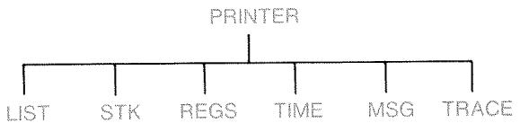
The PRINTER menu provides the ability to print most of the information you've stored, including the contents of variables, lists, appointments, the history stack, registers, and the current date and time. You can also transmit descriptive notes to label the output. (To print amortization schedules, see "Printing an Amortization Table," page 71.)

From within any menu you can press PRINTER to bring up the PRINTER menu. This table summarizes those printing activities.

Table 12-1. The PRINTER Menu Labels

Menu Label	Description
LIST	Prints data stored or calculated in the current menu. See "Printing Variables and Lists," below.
STK	Prints the contents of the history stack.
REGS	Prints the contents of registers 0 through 9.
TIME	Prints the current date and time.
MSG	Displays the ALPHA menu for typing a message up to 22 characters long. See page 175.
TRACE	Switches between Trace On and Trace Off modes. See "Trace Printing," page 176.

Upon completion, all of these functions except TRACE return the previous menu to the display.

Printing Variables, Lists, and Appointments (LIST)

You can list specific sets of information stored in menus by pressing PRINTER LIST while the relevant menu labels are displayed.

Printing the Values Stored in Variables. You can print a listing giving the values of all variables whose menu labels are displayed.* For example, if the calculator is in the FIN TVM menu, it displays the labels N IXYR PV PMT FV OTHER

Pressing PRINTER LIST now produces a print-out like this:

N=	360.00
I%YR=	12.50
PV=	65,000.00
PMT=	-693.00
FV=	0.00
P/YR=	12.00
END MODE

Printing Number Lists. To print out the contents of a particular SUM or CFLO list, that list must be the current list. Pressing PRINTER LIST while a SUM list named SALES is the current list produces labeled output like this:

NAME: SALES
ITEM#	VALUE
1	1,400.00
2	920.00
3	1,100.00
4	2,265.00
TOTAL=	5,685.00

• Except IRR% . Instead,press IRR% PRT to print the value for IRR% .

Printing Solver Equations. To print one or all Solver equations, display the main SOLVE menu (press SOLVE).

To print just the current equation, press [PRT].
To print out the entire list of equations, press PRINTER LIST

Printing Appointments. To print all stored appointments, display the APPT menu (press APPT), then press PRINTER LIST. This produces a listing like this for each appointment:

1: SAT 01/23/88 10:00  
DEMO FOR SMITH  
RPT=NONE 

Menu Not Associated with Stored Data. Remember that many menu labels do not represent data, but rather activities, such as FIN, BUS, DELET, and SET. They contain no information for printing. The calculator beeps if there is nothing to print when you press PRINTER LIST.

Printing Descriptive Messages (MSG)

You can include descriptive messages with your printed output by using msg. For example, suppose you wanted to print a number that represents the balance for September. You could start the output with the label "SEPTEMBER BALANCE".

1. Press PRINTER, then MSG. This brings up the ALPHA menu.
2. Type (and edit) the label or message.
3. Press INPUT to print out the label or message.

Now print out the number itself (if it's in the calculator line, press ).

Trace Printing (TRACE)

Trace printing produces a record of all the keys you've pressed and of calculated results. When tracing is off, use PRT and PRINTER to print what you want. When tracing is on, the calculator uses more power and operates more slowly.

To switch trace printing on and off:

1. Press PRINTER
2. Press TRACE to change the setting. A message informs you that tracing is on or off. If necessary, press TRACE again to display the desired message.
3. Press EXIT

Example: Trace-Printing an Arithmetic Calculation. Produce a record of the keystrokes you use to do the following calculation and store the result in the TVM variable PMT.

$$ { } ^ { 1 / 1 2 } \times 4 , 8 0 0 + 1 2 5 $$

Press PRINTER TRACE to set PRINT MODE: TRACE ON. If you see PRINT MODE: TRACE OFF, press TRACE again.

Keys:

EXIT

FIN

TVM

12

Print-out:

12.00

EXIT

FIN

TVM

1/8

0.08

***

4800

125

4,800.00

X

125.00

525.00

米米

PMT

PMT

PRINTER

PRINTER

TRACE

TRACE

EXIT

How to Interrupt the Printer

Pressing a calculator key during a printing operation will interrupt transmission, but not immediately stop the printing.

To stop the printer immediately, turn it off.

Additional Examples

Loans

Simple Annual Interest

See appendix F for RPN keystrokes for this example.

Example: Simple Interest at an Annual Rate. Your good friend needs a loan to start her latest enterprise and has requested that you lend her (450 for 60 days. You lend her the money at (7 \%) simple annual interest, to be calculated on a 365- day basis. How much interest will she owe you in 60 days, and what is the total amount owed?

$$ \text {The interest is :} (7 \% \text {of $450)} \times \frac {60 \text {days}}{365 \text {days}} $$

✓ Keys:	Display:	Description:
450 × 7 %	450.00 × .07	Annual interest.
× 60 ÷ 365		Actual interest for 60 days.
+	5.18+
450 =	455.18	Adds principal to get to-tal debt.

A Solver Equation for Simple Annual Interest:

$$ D E B T = L O A N + L O A N \times I \% \div 100 \times D A Y S = 365 $$

DEBT = the total owed at the end of the loan period.

LOAN = the original amount (principal) lent.

I% = the annual interest rate as a percent.

DAYS = the number of days in the loan.

For instructions on entering Solver equations, see "Solving Your Own Equations," on page 26.

If you know the dates for the course of the loan, rather than the number of days, use this for an actual-calendar basis:

$$ D E B T = L O A N + L O A N \times I \% \div 100 \times D D A Y S (D A T E 1: D A T E 2: 1) \div 365 $$

or use this for a 360-day basis:

$$ D E B T = L O A N + L O A N \times 1 \% \div 1 0 0 \times D D A Y S (D A T E 1: D A T E 2: 3) \div 3 6 0 $$

DATE1 = the date the loan commences.

DATE2 = the date the loan ends.

Yield of a Discounted (or Premium) Mortgage

The annual yield of a mortgage bought at a discount or premium can be calculated given the original mortgage amount (PV) , interest rate (I% YR) , periodic payment (PMT) , balloon payment amount (if any) (FV) , and the price paid for the mortgage (new PV ).

Remember the cash-flow sign convention: money paid out is negative, money received is positive.

Example: Discounted Mortgage. An investor wishes to purchase a 100,000 mortgage taken out at 9% for 20 years. Since the mortgage was issued, 42 monthly payments have been made. The loan is to be paid in full (a balloon payment) at the end of its fifth year. What is the yield if the purchase price of the mortgage is79,000?

1. Since the payment amount (PMT) is not given, calculate it first. To do this, first assume 20 years' amortization on the original mortgage with no balloon payment (so N = 20 × 12 , FV = 0 , PV = -100,000 , and I% YR = 9 ).

2. Since the balloon amount is not given, calculate it (FV) next. Use PMT from step 1, but change N to 5 years ( N = 5 × 12 ).

3. Finally enter current values for N (less number of payment periods already passed, or 5 × 12 - 42) and PV (proposed purchase price, $79,000); then calculate I%YR for the annual yield.

Step 1: Calculate PMT. Make sure FV = 0 .
Step 2: Enter the new value for N given a balloon in 5 years, then find FV , the amount of the balloon.

Keys:	Display:	Description:
FIN		Selects menu; sets 12
TVM		payments per year and
OTHER		End mode.
CLEAR DATA
EXIT	12 P/YR END MODE
20 N	N=240.00	Figures and stores total
9 IXYR		number of payments for
100000 +/−		a full 20-year loan with
FV	FV=-100,000.00	monthly payments.
0 FV	FV=0.00	Stores interest rate and
PMT	PMT=899.73	amount of original loan.
		(Money paid out is
		negative.)
		Sets FV to zero.
		Calculates monthly pay-
		ment received.

Keys:	Display:	Description:
5 N	N=60.00	Stores number of pay-ments for 5 years.
FV	FV=88,707.05	Calculates balloon due in 5 years.

Step 3: Enter actual, current values for N and PV ; then find new I% YR for discounted mortgage with balloon.

Keys:	Display:	Description:
RCL N - 42 N	N=18.00	Stores number of pay-ments remaining in 5-year loan.
79000 +/- PV	PV=-79,000	Stores proposed, dis-counted purchase price (new present value).
IXYR	IXYR=20.72	Calculates percent an-ual yield.

Annual Percentage Rate for a Loan with Fees

See appendix F for RPN keystrokes for the next two examples.

The annual percentage rate, APR, incorporates fees usually charged when a mortgage is issued, which effectively raises the interest rate. The actual amount received (the PV ) by the borrower is reduced, while the periodic payments remain the same. The APR can be calculated given the term of the mortgage ( N periods), the annual interest rate ( I% YR), the mortgage amount (new PV ), and the basis of the fee charged (how the fee is calculated).

Remember the cash-flow sign convention: money paid out is negative, money received is positive.

Example: APR for a Loan with Fees. A borrower is charged two points for the issuance of a mortgage. (One point is equal to 1% of the mortgage amount.) If the mortgage amount is $60,000 for 30 years and the interest rate is 11½% annually with monthly payments, what APR is the borrower paying?

1. Since the payment amount is not given, calculate it (PMT) first. Use the given mortgage amount ( (PV = \)60,000) ) and interest rate ( (I\% YR = 11^{1/2}\%) ).

2. To find the APR (the new I%YR), use the PMT calculated in step 1 and adjust the mortgage amount to reflect the points paid (PV = $60,000 - 2%). All other values remain the same (term is 30 years; no future value).

Keys:	Display:	Description:
FIN		If necessary, sets 12 pay-ments per year and End mode.
TUM
OTHER
CLEAR DATA
EXIT	12 P/YR END MODE
30 N	N=360.00	Figures and stores num-ber of payments.
11.5 I%YR		Stores interest rate and amount of loan.
60000 PV	PV=60,000.00
0 FV	FV=0.00	No balloon payment, so future value is zero.
PMT	PMT=-594.17	Borrower's monthly payment.
RCL PV		Stores actual amount of money received by bor-rower into PV.
-2 % PV	PV=58,800.00
I%YR	I%YR=11.76	Calculates APR.

Example: Loan from the Lender's Point of View. A 1,000,000, 10-year, 12% (annual interest) interest-only loan has an origination fee of 3 points. What is the yield to the lender? Assume that monthly payments of interest are made. (Before figuring the yield, you must calculate the monthly PMT = (loan × 12%) ÷ 12 mos.) When calculating the I%YR, the FV (a balloon payment) is the entire loan amount, or 1,000,000, while the PV is the loan amount minus the points.

Keys:	Display:	Description:
FIN		If necessary, sets 12 pay- ments per year and End mode.
TVM
OTHER
CLEAR DATA
EXIT	12 P/YR END MODE
10 N	N=120.00	Stores total number of payments.
1000000 x 12 % ÷	120,000.00÷	Calculates annual in- terest on $1,000,000 ...
12 PMT	PMT=10,000.00	...and calculates, then stores monthly payment.
1000000 FV	FV=1,000,000.00	Stores entire loan amount as balloon payment.
-3 % ÷ +/ PV	PV=-970,000.00	Calculates, then stores amount borrowed (total - points).
I%YR	I%YR=12.53	Calculates APR-the yield to lender.

Loan with an Odd (Partial) First Period

The TVM menu deals with financial transactions in which each payment period is the same length. However, situations exist in which the first payment period is not the same length as the remaining periods. This first period is sometimes called an odd or partial first period.

The following Solver equation calculates N , I% , PV , PMT , or FV for transactions involving an odd first period, using simple interest for the odd period. The formula is valid for 0 to 59 days from inception to first payment, and a 30-day month is assumed.*

A Solver Equation for Odd-Period Calculations:

$$ \begin{array}{l} O D D: P V \times (1 \div 1 0 0 \times F P (D A Y S \div 3 0) + 1) = - I F (D A Y S < 3 0; \ (1 + I x = 1 0 0) \times P M T: P M T) \times U S P V (I x: N) - F V \times S P P V (I x: N) \ \end{array} $$

(For the < character, pressWXYZ OTHER

PV = the loan amount.

I% = the periodic interest rate.

DAYS = the actual number of days until the first payment is made.

PMT = the periodic payment.

N = the total number of payment periods.

FV = the balloon payment. A balloon payment occurs at the end of the last (Nth) period and is in addition to any periodic payment.

The following examples assume that you have entered the equation named ODD, above, into the Solver. For instructions on entering Solver equations, see "Solving Your Own Equations," on page 26.

Example: Loan with an Odd First Period. A 36-month loan for $4,500 has an annual interest rate of 15%. If the first payment is made in 46 days, what is the monthly payment amount?

Select equation ODD in the Solver.

Keys:

Display:

Description:

CALC

Creates menu.

36 N N = 36.00

36 payment periods.

4500 PV PV=4,500.00

Stores loan amount.

15÷12		Stores periodic, monthly interest rate.
I%	I%=1.25
46 DAYS	DAYS=46.00	Stores days until first payment.
0 FV	FV=0.00	No balloon payment.
PMT	PMT=-157.03	Calculates payment.

Example: Loan with an Odd First Period Plus Balloon. A 10,000 loan has 24 monthly payments of400, plus a balloon payment of $3,000 at the end of the 24th month. If the payments begin in 8 days, what annual interest rate is being charged?

Select equation ODD.

Keys:	Display:	Description:
CALC		Creates menu.
10000 PV	PV=10,000.00	Stores known values.
24 N	N=24.00
400 +/-
PMT	PMT=-400.00
3000 +/-
FV	FV=-3,000.00
8 DAYS	DAYS=8.00
I%	I%=1.64	Calculates periodic (monthly) interest rate.
× 12 =	19.67	Annual interest rate.

Canadian Mortgages

In Canadian mortgages, the compounding and payment periods are not the same. Interest is compounded semi-annually while payments are made monthly. To use the TVM menu in the HP-17B, you need to calculate a Canadian mortgage factor to store as I% YR .

1. Set End mode and store 12 P/YR
2. Store 0 PMT, 6 N, and 200 FV
3. Add 200 to the annual interest rate, make the number negative, and store it in FV.
4. Press IXYR to calculate the Canadian mortgage factor.
5. Continue the problem by supplying the other mortgage values and solving for the unknown item. Do not change I% YR from step 4.

Example: Canadian Mortgage. What is the monthly payment required to fully amortize a 30-year, $30,000 Canadian mortgage if the interest rate is 12%?

Keys:	Display:	Description:
FIN		Displays TVM menu; sets 12 payments per year with End mode.
TVM
OTHER
CLEAR DATA
EXIT	12 P/YR END MODE
0 PMT	PMT=0.00
6 N	N=6.00
200 PV	PV=200.00
+ 12 = +/-
FV	FV=-212.00
IXYR	I%YR=11.71	Calculates I%YR for Canadian mortgage factor.
30 N	N=360.00	Stores other values.
30000 PV	PV=30,000.00
0 FV	FV=0.00
PMT	PMT=-301.92	Monthly payment.

A Solver Equation for Canadian Mortgages:

$$ \begin{array}{l} C A N: P V = - P M T \times U S P V ((1 + 1 \div 2 Y R \div 2 0 0) ^ {\wedge} (1 \div 6) - 1) \times 1 0 0; N) \ - F V \times S P P U ((1 + I X Y R \div 2 0 0) ^ {\wedge} (1 \div 6) - 1) \times 1 0 0; N) \ \end{array} $$

(For the operator, press y^ .)

PV = loan amount, or present value.

PMT = monthly payment amount.

I% YR = annual (Canadian) interest rate as a percent.

N = total number of payment periods for the life of the loan.

FV = remaining balance, or future value.

For instructions on entering Solver equations, see "Solving Your Own Equations," on page 26.

Advance Payments (Leasing)

Occasionally payments are made in advance, such as in leasing. Leasing agreements sometimes call for the extra payments to be made when the transaction is closed. A residual value (salvage value) can also exist at the end of the normal term.

The following equation calculates the monthly payment and the annual yield when one or more payments are made in advance. It can be modified to accommodate periods other than monthly by changing the number 12 to the appropriate number of payment periods per year.

Remember the cash-flow sign convention: money paid out is negative, money received is positive.

A Solver Equation for Advance Payments:

ADV: PMT = (-PV-FVx(SPPV(IYR÷12:N))+(USPV(IYR÷12:N-#ADV)+#ADV)

(For the # character, pressWXYZ OTHER #.)

PMT = the monthly payment amount.

PV = the value of the equipment.

FV = the residual value.

I% YR = the annual interest rate as a percent.

N = the total number of payments.

# ADV = the number of advance payments.

The following example assumes that you have entered the equation ADV, above, into the Solver. For instructions on entering Solver equations, see "Solving Your Own Equations," on page 26.

Example: Leasing with Advance Payments. Equipment worth (750 is leased to you for 12 months. The equipment is assumed to have no salvage value at the end of the lease. You agree to make three payments at the time of closing. What is the monthly payment if the annual interest rate is (10\%)?

Select the ADV equation in the Solver.

Keys:	Display:	Description:
CALC		Creates menu.
750 FV		Stores known values.
12 N
0 FV
3 #ADV
10 I*YR	I*YR=10.00
PMT	PMT=-64.45	Calculates payment.

Savings

Value of a Fund with Regular Withdrawals

Example: A Fund with Regular Withdrawals. What are the balances after 1, 10, and 20 years of a fund that starts at 750,000, has 20,000 withdrawn at the beginning of each quarter, and earns 10% annual interest compounded monthly?

1. Because the compounding periods and the withdrawal periods are not coincident, you must first convert the nominal interest rate to one in terms of the withdrawal periods. You can do this using the ICNV menu, as explained on page 77, "Compounding Periods Different from Payment Periods."
2. The rest of the calculation is a straightforward TVM problem. Remember that money deposited is paid out and therefore negative; money withdrawn is received and therefore positive.

Step 1: Find the adjusted nominal interest rate.

Keys:	Display:	Description:
FIN	ICNV	Displays periodic interest-rate conversion menu.
PER	COMPOUNDING P TIMES/YR
12	P=12.00	Stores number of compounding periods.
10	NOM%=10.00	Stores nominal interest rate.
EFFF%	EFF%=10.47	Calculates effective interest rate.
4	P=4.00	Stores number of withdrawal periods.
NOM%	NOM%=10.08	Calculates adjusted nominal interest rate.

Step 2: Calculate the future values.

Keys:	Display:	Description:
EXIT EXIT TVM		Switches to TVM menu.
◇	10.08	Clears message to show NOM% value still in cal-culator line.
STO IZYR	IZYR=10.08	Stores adjusted nominal interest rate in I%YR.
OTHER 4 P/YR BEG EXIT	4 P/YR BEGIN MODE	Sets 4 payments (with-drawals) per year and Begin mode.
750000 +/P V	PV=-750,000.00	Stores present (initial) value of fund.
20000 PMT	PMT=20,000.00	Stores withdrawal amount.
4 N	N=4.00	Stores number of with-drawals in 1 year.
FV	FV=743,364.31	Value of fund at end of year 1.
40 N	N=40.00	Stores number of with-drawals over 10 years.
FV	FV=641,824.41	Calculates value of fund at end of year 10.
20 N	N=80.00	Stores number of with-drawals after 20 years.
FV	FV=348,988.60	Calculates value of fund at end of year 20.

Deposits Needed for a Child's College Account

See appendix F for RPN keystrokes for this example.

Suppose you want to start saving now to accommodate a future series of cash outflows. An example of this is saving money for college. To determine how much you need to save each period, you must know when you'll need the money, how much you'll need, and at what interest rate you can invest your deposits.

Use a CFLO list to calculate the net uniform series (NUS) of the future withdrawals:

1. Store zero for all cash flows except the withdrawals. For those cash flows, store the amounts you will need to withdraw (since this is cash received, these cash flows will be positive).
2. Store the periodic interest rate in I% and calculate NUS. The NUS equals the amount of the monthly deposit you will need to make.

You can also calculate the equivalent present value of all the monthly deposits combined by calculating the net present value, NPV .

Example: Savings for College. Your daughter will be going to college in 12 years and you are starting a fund for her education. She will need $15,000 at the beginning of each year for four years. The fund earns 9% annually, compounded monthly, and you plan to make monthly deposits, starting at the end of the current month. How much should you deposit each month to meet her educational expenses?

The cash-flow diagram looks like this:

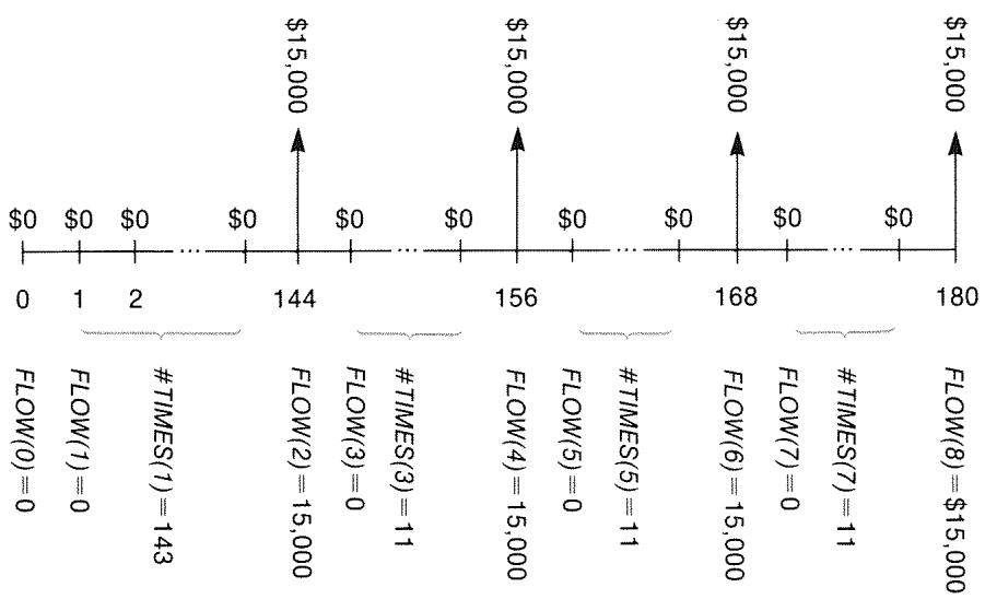
Figure 13-1. Flow of Withdrawals

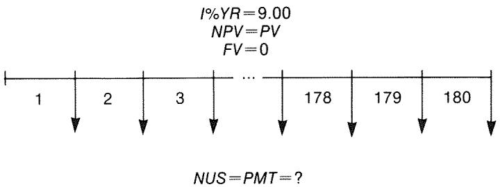
Figure 13-2. Flow of Deposits

Keys:	Display:	Description:
FIN		Displays current cash-flow list and CFLO menu keys.
CFLO
CLEAR DATA		Clears current list or gets a new one.
YES
or
GET
*NEW	FLOW(0)=?
Step 1: Set up a CFLO list.
0 INPUT	FLOW(1)=?	Sets initial cash flow, FLOW(0), to zero.
0 INPUT	#TIMES(1)=1	Stores zero in FLOW(1) and prompts for the number of times it occurs.
12 × 12 - 1 INPUT	FLOW(2)=?	Stores 143 (for 11 years, 11 months) in #TIMES(1) for FLOW(1).
15000 INPUT	#TIMES(2)=1	Stores amount of first withdrawal, at end of 12th year.
INPUT	FLOW(3)=?
0 INPUT	#TIMES(3)=1	Stores cash flows of zero...
11 INPUT	FLOW(4)=?	...for the next 11 months.
15000 INPUT	FLOW(5)=?	Stores second with-drawal, for sophomore year.
INPUT
0 INPUT		Stores cash flows of zero
11 INPUT	FLOW(6)=?	for the next 11 months.
15000 INPUT	FLOW(7)=?	Stores third withdrawal, for junior year.
INPUT
0 INPUT		Stores cash flows of zero
11 INPUT	FLOW(8)=?	for the next 11 months.
15000 INPUT	FLOW(9)=?	Stores fourth with-drawal, for senior year.
INPUT
EXIT CALC	NPV, NUS, NFV	Done entering cash
	NEED I%	flows; gets CALC menu.

Step 2: Calculate NUS for the monthly deposit.

Keys:	Display:	Description:
9÷12		Figures the periodic (monthly) interest rate and stores it in I%.
I%	I%=0.75
NUS	NUS=182.30	Amount of monthly de-posit needed to meet planned withdrawals.
NPV	NPV=17,973.48	Calculates the net present value of the monthly deposits, which is the same as the NPV of the four future withdrawals.

Value of a Tax-Free Account

See appendix F for RPN keystrokes for this example.

You can use the TVM menu to calculate the future value of a tax-free or tax-deferred account, such as an IRA or Keogh account. Remember that for calculations with cash flows, money paid out is negative and money received is positive. (Current tax law and your current income will determine whether just interest or also principal are tax-free, and for how long. You can solve for either case.)

N = the number of payments until retirement.

I% YR = the annual dividend rate.

PV = the present value of the retirement account.

PMT = the amount of your deposit. (It must be constant for the duration of the account.)

FV = the future value of the retirement account.

The purchasing power of that future value depends on the inflation rate and the duration of the account.

Example: Tax-Free Account. Consider opening an IRA account with a dividend rate of 8.175% . 1) If you invest \2,000at the beginning of each year for 35 years, how much will you have at retirement? 2) How much will you have paid into the IRA? 3) How much interest will you have earned? 4) If your post-retirement tax rate is15\%, what is the after-tax future value of the account? Assume only the interest will be taxed. (Assume the principal was taxed before deposit.) 5) What is the purchasing power of that amount, in today's dollars, assuming an8\%$ annual inflation rate?

Keys:	Display:	Description:
FIN		Sets 1 payment per year and Begin mode.
TVM
OTHER
1 P/YR
BEG EXIT	1 P/YR BEGIN MODE
35 N	N=35.00	Stores number of pay-ment periods until retirement (1 × 35).
8.175 I2YR	I2YR=8.18	Stores dividend rate.
0 PV	PV=0.00	Present value of account (before first payment).
2000 +/-		Annual payment (deposit).
PMT	PMT=-2,000.00
FV	FV=387,640.45	Calculates amount in ac-count at retirement.
RCL PMT		Calculates total amount paid into IRA by retirement.
× RCL
N =	-70,000.00
+ RCL		Calculates interest you will earn.
FV =	317,640.45
× 15 % =	47,646.07	Taxes at 15% of interest.
+/+ RCL		Subtracts taxes from total FV to calculate after-tax FV.
FV =	339,994.39
FV	FV=339,994.39	Stores after-tax future value in FV.
8 I2YR		Calculates present-value purchasing power of the above after-tax FV at 8% inflation rate.
0 PMT
PV	PV=-22,995.36

Value of a Taxable Retirement Account

See appendix F for RPN keystrokes for this example.

This problem uses the TVM menu to calculate the future value of a taxable retirement account that receives regular, annual payments beginning today (Begin mode). The annual tax on the interest is paid out of the account. (Assume the deposits have been taxed already.)

N = the number of years until retirement.

I% YR = the annual interest rate diminished by the tax rate: interest rate × (1 - tax rate) .

PV = the current amount in the retirement account.

PMT = the amount of the annual payment.

FV = the future value of the retirement account.

Example: Taxable Retirement Account. If you invest $3,000 each year for 35 years, with dividends taxed as ordinary income, how much will you have in the account at retirement? Assume an annual dividend rate of 8.175% and a tax rate of 28%, and that payments begin today. What will be the purchasing power of that amount in today's dollars, assuming 8% annual inflation?

Keys:	Display:	Description:
FIN		Displays TVM menu.
TVM
OTHER		Sets 1 payment per year and Begin mode.
1 P/YR
BEG EXIT	1 P/YR BEGIN MODE
35 N	N=35.00	Stores years until retirement.
8.175 - 28 %	8.18-2.29	Calculates and stores interest rate diminished by tax rate.
IXYZR	IXYZR=5.89
0 PV	PV=0.00	Stores no present value.
3000 +/− PMT	PMT=-3,000.00	Stores annual payment.

FV

FV=345,505.61

Calculates future value.

8 IYR
0 PMT

PV

PU=-23,368.11

Calculates present-value purchasing power of the above FV at 8% inflation.

Modified Internal Rate of Return

When there is more than one sign change (positive to negative or negative to positive) in a series of cash flows, there is a potential for more than one IRR% . For example, the cash-flow sequence in the following example has three sign changes and hence up to three potential internal rates of return. (This particular example has three positive real answers: 1.86, 14.35, and 29.02% monthly.)

The Modified Internal Rate of Return (MIRR) procedure is an alternative that can be used when your cash-flow situation has multiple sign changes. The procedure eliminates the sign change problem by utilizing reinvestment and borrowing rates that you specify. Negative cash flows are discounted at a safe rate that reflects the return on an investment in a liquid account. The figure generally used is a short-term security (T-bill) or bank passbook rate. Positive cash flows are reinvested at a reinvestment rate that reflects the return on an investment of comparable risk. An average return rate on recent market investments might be used.

1. In the CFLO menu, calculate the present value of the negative cash flows (NPV) at the safe rate and store the result in register 0. Enter zero for any cash flow that is positive.
2. Calculate the future value of the positive cash flows (NFV) at the reinvestment rate and store the result in register 1. Enter zero for any cash flow that is negative.
3. In the TVM menu, store the total number of periods in N , the NPV result in PV , and the NFV result in FV .
4. Press IXYR to calculate the periodic interest rate. This is the modified internal rate of return, MIRR.

Example: Modified IRR. An investor has an investment opportunity with the following cash flows:

Group (FLOW no.)	No. of Months (#TIMES)	Cash Flow, $
0	1	-180,000
1	5	100,000
2	5	-100,000
3	9	0
4	1	200,000

Calculate the MIRR using a safe rate of 8% and a reinvestment (risk) rate of 13% .

Keys:	Display:	Description:
FIN		Displays current cash-flow list.
CFLD
CLEAR DATA		Clears current list or gets a new one.
YES
or
GET
*NEW	FLOW(0)=?
180000+/-		Stores initial cash flow, FLOW(0).
INPUT	FLOW(1)=?
0 INPUT	#TIMES(1)=1	Stores FLOW(1) as zero since the flow amount is positive.
5 INPUT	FLOW(2)=?	Stores 5 for #TIMES(1).
100000+/-		Stores FLOW(2).
INPUT	#TIMES(2)=1
5 INPUT	FLOW(3)=?	Stores FLOW(2) 5 times. You can skip FLOW(3) and FLOW(4) because they are equal to zero for this part.

EXIT CALC NPV, NUS, NFV NEED Ix

1%=0.67

Stores monthly safe interest rate.

NPV

NPV=-654,136.81

Calculates NPV of negative cash flows.

NPV=-654,136.81

Stores NPV in register 0.

FLOW（3）=？

Returns to CFLO menu.

CLEAR DATA

YES

FLW（0）=？

Clearly list.

FLOW（1）=？

Stores zero as FLOW(0) . (Skip negative flows; store positive flows.)

FLOW（2）=？

Stores FLOW(1) 5 times.

FLOW（3）=？

Stores zero for FLOW(2) 5 times.

FLW（4）=？

Stores zero for FLOW(3) 9 times.

FLOW（5）=？

Stores FLOW(4) , 1 time.

CALC

NPV, NUS, NFV

NEED I%

1%

1x=1.08

NFV

NFV=800,582.75

Stores monthly reinvestment rate.

NFV=800,582.75

Calculates NFV of positive cash flows.

Stores NFV in register 1.

MAIN		Switches to TVM menu; sets 12 periods per year with End mode, if necessary.
FIN
TVM OTHER
CLEAR DATA
EXIT	12 P/YR END MODE
20 N	N=20.00	Stores total number of investment periods.
RCL 0 PV	PV=-654,136.81	Recalls present value of negative cash flows and stores in PV.
RCL 1 FV	FV=800,582.75	Recalls future value of positive cash flows and stores in FV.
0 PMT	PMT=0.00	Stores zero in PMT (no payments).
IZYR	IZYR=12.18	Calculates annual MIRR.

Price of an Insurance Policy

The price of an insurance policy, other than term life insurance, is rarely apparent at first glance. The price should include not only the premium payments, but also the interest that could have been earned on the cash value or savings portion of the policy.

The following equation calculates the price per $1,000 of protection for one policy year and the interest rate earned on the savings portion of the policy.

To calculate the price, assume some value for interest—for example, the interest rate you could earn on a one-year savings certificate after tax. Similarly, to calculate interest, assume a price per (1,000 per year for alternative insurance; for example, a low-cost term policy of the one-year renewable type.

Even complex policies like minimum-deposit plans can be analyzed with this procedure. Use policy surrender values for cash values and the actual (after-tax) amounts for payments (premiums) and dividends.

A Solver Equation for Insurance Price:

$$ \begin{array}{r l} \text {I N S} & = ((\text {P R E M} + \text {L V A L}) \times (1 + I x \div 1 0 0) - \text {V A L} - \text {D I V}) \div \ & (\cdot , 0 0 1 \times (\text {F A C E} - \text {V A L})) \end{array} $$

INS = the price per $1,000 of protection in one policy year.
PREM = the annual premium amount.

LVAL = the value of the policy at the end of last year.

I% = the rate of return, as a percent, on a savings account.

VAL = the value of the policy at the end of the current year.

DIV = the dollar value of the dividend for one year.

FACE = the face value of the policy for one year.

The following example assumes that you have entered the above equation into the Solver. For instructions on entering Solver equations, see "Solving Your Own Equations," on page 27.

Example: Insurance Policy. You are evaluating your 50,000 insurance policy. The premium of1,010 is due at the beginning of the year, and a dividend of 165 is received at the end of the policy year. The cash value of the policy is3,302 at the beginning of the year; it will grow to 4,104 by the end of the year. You can earn 6% on a savings account. What is the annual price per1,000 protection?

Select the correct equation in the Solver.

Keys:

Display:

CALC

1010

PREM

PREM=1,010.00

3302

LVAL

LVAL=3,302,00

Description:

Creates menu.

Stores annual premium.

Stores value of policy at end of last year.

6	1%	1%=6.00	Stores interest rate you could get elsewhere.
4104	VAL	VAL=4,104.00	Stores value of policy at end of this year.
MORE			Stores annual dividend.
165	DIV	DIV=165.00
50000	FACE	FACE=50,000.00	Stores face value of policy.
MORE			Your protection cost 6.57 per1,000 face (protection) value.
INS		INS=6.57

Insurance protection could be purchased for 3 per 1,000 face value. Calculate the rate of return on your savings.

Keys:	Display:	Description:
3 INS	INS=3.00	Stores price of alternate insurance.
1x	1x=2.20	Calculates rate of return.

Reference: Joseph M. Belth, Life Insurance—A Consumer's Handbook, Indiana University Press, 1973, p. 234.

Bonds

Example: Yield to Maturity and Yield to Call. On March 16, 1987 you consider the purchase of a 1,000 bond that was issued on January 1, 1985. It has a (10.5% semiannual coupon using a 30/360 calendar, and matures on January 1, 2015. The bond is callable on January 1, 1990 at 110 (that is, )1,100). The bond is now selling at 115.174 (that is, $1,151.74). Determine both the yield to maturity and the yield to call for this bond.

First, calculate the yield to maturity:

Keys:	Display:	Description:
FIN BOND		Displays BOND menu.
TYPE 360		Sets semiannual bond on 30/360 calendar.
SEMI EXIT	30/360 SEMIANNUAL
CLEAR DATA	30/360 SEMIANNUAL	Cleared variables; sets CALL to 100.
3.161987		Stores today as purchase date.
SETT	SETT=03/16/1987 MON
1.012015		Stores maturity date.
MAT	MAT=01/01/2015 THU
10.5 CPN%	CPN%=10.50	Stores coupon rate.
MORE		Stores price. Displays only two decimal places, but stores all three.
115.174 PRICE	PRICE=115.17
YLD%	YLD%=9.00	Calculates yield to maturity.

Second, calculate the yield to call:

Keys:	Display:	Description:
MORE	YLD%=9.00	Returns to first BOND menu.
1.011990		Changes maturity date to the call date.
MAT	MAT=01/01/1990 MON
110 CALL	CALL=110.00	Stores call value.
MORE YLD%	YLD%=7.63	Calculates a yield to call.

Discounted Notes

A note is a written agreement to pay to the buyer of the note a sum of money plus interest. Notes do not have periodic coupons, since all interest is paid at maturity. A discounted note is a note that is purchased below its face value. The following equations find the price or yield of a discounted note. The calendar basis is actual/360.

Solver Equations for Discounted Notes: To find the price given the discount rate:

$$ \text {N O T E : P R I C E} = \mathrm {R V} - (\mathrm {D I S C} \times \mathrm {R V} \times \mathrm {D D A Y S} (\mathrm {S E T T}: \mathrm {M A T}: 1) \div 3 6 0 0 0) $$

To find the yield given the price (or to find the price given the yield):

$$ \begin{array}{l} \text {N O T E : Y I E L D = (R V - P R I C E) \div P R I C E \times 3 6 0 0 0 \div} \ \text {D D A Y S (S E T T : M A T : 1)} \end{array} $$

PRICE = the purchase price per $100 face value.

YIELD = the yield as an annual percentage.

RV = the redemption value per $100.

DISC = the discount rate as a percent.

SETT = the settlement date (in current date format).

MAT = the maturity date (in current date format).

The following example assumes that you have entered the NOTE equations into the Solver. For instructions on entering Solver equations, see "Solving Your Own Equations," on page 27.

Example: Price and Yield of a Discounted Note. What are the price and yield of the following U.S. Treasury Bill: settlement date October 14, 1988; maturity date March 17, 1989; discount rate 8.7% ? (Assume month/day/year format.)

Select the NOTE:PRICE equation in the Solver.

Keys:	Display:	Description:
CALC		Creates menu.
10.141988		Stores known values.
SETT	SETT=10.14
3.171989
MAT	MAT=3.17
8.7 DISC	DISC=8.70
100 RV	RV=100.00
PRICE	PRICE=96.28	Calculates price.
EXIT▼		Displays NOTE:YIELD
CALC	NOTE:YIELD=(RV-PRICE)...	equation, then its menu.
YIELD	YIELD=9.04	Calculates yield.

Statistics

Moving Average

Moving averages are often useful in predicting trends in data taken over a period of time. In moving-average calculations, a specified number of points is averaged. Each time a new point is acquired, the oldest point is discarded. Thus, the same number of points is used in each calculation.

A Solver Equation for Moving Averages:

MAVG=∑（I：MAX（1：LAST-N+1）：LAST：1：ITEM(name：I））÷MIN(N：LAST)

N = the number of values averaged in each calculation.
LAST = the item number of the most recent value to be averaged.

name = the name of the SUM list whose data will be averaged. When you create and name the SUM list, make sure its name matches the name in the Solver equation.

The following example assumes that you have entered the equation MAVG into the Solver, using VOL for the SUM list's name. For instructions on entering Solver equations, see "Solving Your Own Equations," on page 27.

Example: A Moving Average in Manufacturing. Calculate a three-month moving average for the number of units manufactured during the first half of the year. Manufacturing volumes are:

January	February	March	April	May	June
4400	5360	2900	3670	4040	3200

Keys:

Display:

Description:

SUM

Displays SUM menu and current list.

CLEAR DATA

Clearscurrentlistorgets a newone.

YES

or

GET

NEW

ITEM（1）=？

4400 INPUT

Enters data.

5360 INPUT

2900 INPUT

3670 INPUT

4040 INPUT

3200 INPUT

ITEM（7）=？

TOTAL=23,570.00

EXIT NAME

VOL INPUT

ITEM（7）=？

Names the list VOL.

EXIT SOLVI

(use and

if necessary)

Displays the MAVG equation. Make sure name is VOL.

CALC		Displays menu.
3 N	N=3.00	Stores number of points.
3 LAST		Calculates average for months 1, 2, and 3.
MAVG	MAVG=4,220.00
4 LAST		Calculates average for months 2, 3, and 4.
MAVG	MAVG=3,976.67
5 LAST		Calculates average for months 3, 4, and 5.
MAVG	MAVG=3,536.67
6 LAST		Calculates average for months 4, 5, and 6.
MAVG	MAVG=3,636.67

Chi-Squared (^2) Statistics

The ^2 statistic is a measure of the goodness of fit between data and an assumed distribution.* It is used to test whether a set of observed frequencies differs from a set of expected frequencies sufficiently to reject the hypothesis under which the expected frequencies were obtained.

In other words, it tests whether discrepancies between the observed frequencies (O_i) and the expected frequencies (E_i) are significant, or whether they might reasonably result from chance. The equation is:

$$ \chi^ {2} = \sum_ {i = 1} ^ {n} \frac {\left(O _ {i} - E _ {i}\right) ^ {2}}{E _ {i}} $$

If there is a close agreement between the observed and expected frequencies, ^2 will be small. If the agreement is poor, ^2 will be large.

Solver Equations for ^2 Calculations:

If the expected value is a constant:

CHI=∑（I:1：SIZE（name1）：1：（ITEM(name1：I）-EXP）^2+EXP）

If the expected values vary:

CHI2=∑（I:1:SIZES(name1):1：（ITEM(name1:I)-ITEM(name2:I)）^2÷ITEM(name2:I)）

(To enter the character, press WXYZ OTHER MORE

CH12 = the final ^2 value for your data.

name1 = the name of the SUM list that contains the observed values.
name2 = the name of the SUM list that contains the expected values.
EXP = the expected value when it is a constant.

When you create and name the SUM list(s), make sure the name(s) match name1 (and name2, if applicable) in the Solver equation.

To solve the equation, press CH12 once or twice (until you see the message CALCULATING...).

The following example assumes that you have entered the CHI equation into the Solver, using OBS for name1. For instructions on entering Solver equations, see "Solving Your Own Equations," on page 27.

Example: Expected Throws of a Die. To determine whether a suspect die is biased, you toss it 120 times and observe the following results. (The expected frequency is the same for each number, 120 ÷ 6 , or 20.)

Number	1	2	3	4	5	6
Frequency Observed	25	17	15	23	24	16

Keystrokes:	Display:	Description:
SUM		Displays SUM menu and current list.
CLEAR DATA		Clears current list or gets a new one.
YES
or
GET
*NEW	ITEM(1)=?
25	INPUT	Enters observed values.
17	INPUT
15	INPUT
23	INPUT
24	INPUT
16	INPUT	ITEM(7)=?
		TOTAL=120.00
EXIT	NAME
OBS	INPUT	ITEM(7)=?
EXIT	SOLVE
(use ▲ and ▼)if necessary)		Displays the CHI equation. Make sure name1 is OBS.
CALC		Displays menu.
20	EXP	EXP=20.00
CHI	CHI=5.00	Stores expected value.
		Calculates χ2.

The number of degrees of freedom is (n - 1) = 5 . Consult statistical tables to find ^2 to a significance level of 0.05 with 5 degrees of freedom. The table shows that ^2_0.05,5 = 11.07 . Since the computed value (5.00) is less than 11.07, you can conclude that, to a 0.05 significance level (95% probability), the die is fair.

Assistance, Batteries, Memory, and Service

Obtaining Help in Operating the Calculator

Hewlett-Packard is committed to supporting users of HP calculators. You can obtain answers to your questions about using the calculator from our Calculator Support department. (Address and phone number are on the inside of the back cover.)

We suggest reading "Answers to Common questions," below, before contacting us. Past experience has shown that many of our customers have similar questions.

Answers to Common Questions

Q: I'm not sure if the calculator is malfunctioning or if I'm doing something incorrectly. How can I determine if the calculator is operating properly?

A: Refer to page 220, which describes the diagnostic self-test.

Q: My arithmetic keys don't work like I expect. I press 12 + 3 = and get 3.00.

A: You may be in the wrong mode. Press MODES RLG to set Algebraic mode.

Q: My numbers contain commas as decimal points. How do I restore the periods?

A:PressDISP

Q: How do I change the number of decimal places the calculator displays?

A: The procedure is described in "Decimal Places" on page 31.

Q: How do I clear all or portions of memory?
A: CLR clears the calculator line. CLEAR DATA clears the data lists or variables accessible from the current menu. Erasing the entire contents of memory is covered in "Erasing Continuous Memory" on page 218.
Q: Why am I getting the wrong answer using the TVM menu?
A: Be sure to enter a value for all five TVM variables, even if a value is zero (as FV is for a loan without a balloon). Clearing the variables before starting (CLEAR DATA) accomplishes the same thing. Check the appropriate payment mode (mortgages and loans are typically End mode calculations), and specify the number of payments per year ( P/YR ). Also check that all figures for money paid out are negative (the cash-flow sign convention).
Q: Can I access the TVM menu functions from the Solver?
A: No, but you can do the same functions by copying the appropriate financial formulas into the Solver. The formulas are given starting on page 157.
Q: Can I access the data stored in my CFLO and SUM lists from the Solver?
A: Yes. See "Accessing CFLO and SUM Lists from the Solver," page 164.
Q: How do I indicate multiplication in an equation typed into the Solver?
A: Use the multiplication key (×) . You cannot use the letter × in the ALPHA menu.
Q: What does an "E" in a number (for example, 2.51E - 13) mean?
A: Exponent of ten (for example, 2.51 × 10^-13 ). Refer to "Scientific Notation" on page 44.
Q: The calculator has displayed the message INSUFFICIENT MEMORY. What should I do?
A: Refer to "Managing Calculator Memory" on page 216 for instructions on how to reclaim memory for your use.

Q: The calculator is operating slowly, and the annunciator is blinking. Why?
A: The calculator is trace printing. Press PRINTER TRACE EXIT to turn off tracing.
Q: How can I change the sign of a number in a list without keying in the number again?
A:Press RCL INPUT +I INPUT.
Q: The beeper is not working.
A: Check the beeper mode by pressing MODES BEEP. See also page 33.
Q: The messages and the menu labels in the display are not in English. How do I restore the English?
A: Models of the HP-17B sold in many countries outside of the United States include a menu to select the language for messages and labels. To select the English language, press MODES INTL ENGL.

Power and Batteries

The HP 17B is powered by three 1.5-volt, button-cell batteries. Expected battery life depends on how the calculator is used and the chemical content of the batteries.

We recommend using either alkaline or silver-oxide type batteries. Do not use rechargeable batteries. Use batteries from the following list, or use another manufacturer's equivalent.

Alkaline

Silver Oxide

Panasonic LR44

Panasonic SR44W or SP357

Eveready A76

Eveready 357

Duracell LR44

RAY-O-VAC 357

Varta V13GA

Varta V357

Kodak KA76

Toshiba LR44

Low-Power Indications

When the low-battery annunciator (□) comes on, the calculator can continue normal operation for several hours. If the calculator is turned off, Continuous Memory will be preserved for approximately two weeks. To conserve battery power, printing does not function when the battery annunciator is on. Printing might halt during a printing operation due to a borderline low-battery condition. The calculator can detect that there is insufficient power for printing before the battery annunciator comes on.

If you continue to use the calculator after the battery annunciator comes on, power can eventually drop to a level at which the calculator stops powering the display and keyboard. The calculator will require fresh batteries before it can be turned back on. When you turn the calculator on after fresh batteries have been installed, the calculator displays MACHINE RESET if your stored data is intact. If data has been lost, the calculator displays MEMORY LOST. In either case, the clock's time might be incorrect.

Installing Batteries

Once the batteries are removed, you must replace the batteries within one minute to prevent loss of Continuous Memory.

To install batteries:

1. Have three fresh button-cell batteries at hand. Hold batteries by the edges. Do not touch the contacts. Wipe each battery with a clean, lint-free cloth to remove dirt and oil.

2. Make sure the calculator is off. Do not press again until the entire procedure for changing batteries is completed. Changing batteries with the calculator on can erase the contents of Continuous Memory. If you have set any appointments, make sure they will not come due while the batteries are out.

3. Hold the calculator as shown. To remove the battery-compartment door, press down and outward on the ribbed area until the door slides off.

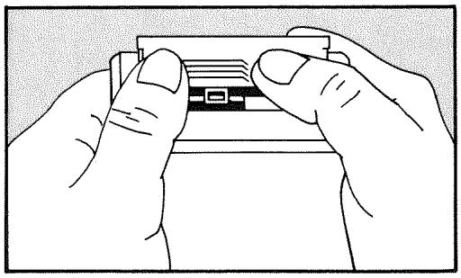
1. Turn the calculator over and shake the batteries out.

Do not mutilate, puncture, or dispose of batteries in fire. The batteries can burst or explode, releasing hazardous chemicals.

1. Hold the calculator as shown and stack the batteries, one at a time, in the battery compartment. Orient the batteries according to the diagram inside the battery compartment. Be sure the raised and flat ends match the diagram.

1. Slide the tab of the battery-compartment door into the slot in the calculator case, as shown.

Now turn the calculator back on. If it does not function, you might have taken too long to change the batteries or inadvertently turned the calculator on while the batteries were out. Remove the batteries again and lightly press a coin against both battery contacts in the calculator for a few seconds. Put the batteries back in and turn the calculator on. You should see MEMORY LOST.

Managing Calculator Memory

The calculator has approximately 6,750 units (or "bytes") of user memory available.* (This is separate from the system memory that stores all the unerasable information with which the calculator is manufactured.) The table below describes the memory requirements of stored user information.

The calculator displays INSUFFICIENT MEMORY if you attempt an operation that uses more memory than is currently available. If you see this message:

1. Complete any calculations in the calculator line (press or CLR). This frees the memory that was being used to store each of the numbers and operators.

2. To further increase the amount of available memory:

Rename the named SUM and CFLO lists with shorter names (see page 87), and clear any lists you no longer need (see page 89).

• Shorten or delete any messages with appointments (see page 135).
• Delete any Solver variables or equations you no longer need (see page 152).

Table A-1. Memory Requirements

Type of Information	Amount of Memory Used
CFLO number lists (excluding the list name)	101/2 bytes per list, + 91/2 bytes per flow entry (flow amount and #TIMES).
SUM number lists (excluding the list name)	16 bytes per list, + 8 bytes per item.
Names of lists	1 byte, + 1 byte per character.
Equations	101/2 bytes, + 1 byte per character (spaces are counted as characters), including the name.*
Solver variables	15 bytes per variable, + 1 byte per character in the variable's name.
Calculator line	Numbers: 8 bytes, + 1 byte per character.
Appointment messages	Operators: 31/2 bytes.
	41 bytes for the first message stored, + 1 byte per character in each message.
* The memory requirements of an equation substantially increase while its menu is displayed.

Resetting the Calculator

If the calculator doesn't respond to keystrokes or is behaving unusually, attempt to reset it. Resetting the calculator halts the current calculation, clears the calculator line, and displays the MAIN menu.

Continuous Memory is not affected. To reset the calculator, hold down while pressing the third menu key from the left. Repeat if necessary. The calculator displays MACHINE RESET.

The calculator can reset itself if it is dropped or if power is interrupted.

Erasing Continuous Memory

Erasing Continuous Memory erases all user-stored information except the current time and date. Specifically, it:

Clears the calculator line and history stack.
- Deletes all Solver equations and their variables, and clears all other variables in menus.
Cleared all CFLO and SUM lists and their names.
Cleared all appointments.
- Sets the calculator to certain "start-up" settings—month/day/year date format, 12-hour clock, 2 decimal places, period (.) decimal point, double-space printing off, printer tracing off, printer without the ac adapter, and beeper on.
Maintains the selected mode—ALG or RPN.

Erasing Continuous Memory does not affect the current time and date.

To erase Continuous Memory, press and hold down , the leftmost menu key, and the rightmost menu key. (Press three keys simultaneously). When the three keys are released, the calculator displays MEMORY LOST.

Continuous Memory can inadvertently be erased if the calculator is dropped or if power is interrupted.

Clock Accuracy

The clock is regulated by a quartz crystal accurate to within three minutes per month under normal conditions. The accuracy of the clock crystal is affected by temperature, physical shock, humidity, and aging. Optimum accuracy is maintained at 25^ (77^) .

Environmental Limits

In order to maintain product reliability, observe the following limits:

Operating temperature: 0^ to 45^ (32^ to 113^)
Storage temperature: -20^ to 65^ (-4^ to 149^)
- Operating and storage humidity: 90% relative humidity at 40^ (104^) maximum.

Determining If the Calculator Requires Service

Use these guidelines to determine if the calculator requires service. If it does, read "If the Calculator Requires Service" on page 222.

If the calculator won't turn on:

1. Attempt to reset the calculator (see page 217).
2. If the calculator fails to respond after step 1, replace the batteries (see page 214). If you have just replaced the batteries, see page 216.

If these steps do not help, the calculator requires service.

If the calculator doesn't respond to keystrokes:

1. Attempt to reset the calculator (see page 217).
2. If the calculator still fails to respond, attempt to erase Continuous Memory (see page 218). This will erase all the information you've stored.

If these steps do not help, the calculator requires service.

If the calculator responds to keystrokes but you suspect that it is malfunctioning:

1. Do the self-test (described below). If the calculator fails the self test, it requires service.

2. If the calculator passes the self-test, it is quite likely you've made a mistake in operating the calculator. Try rereading portions of the manual, and check "Answers to Common Questions" on page 211.

3. Contact the Calculator Support department. The address and phone number are listed on the inside back cover.

Confirming Calculator Operation: Self-Test

If the display can be turned on, but it appears that the calculator is not operating properly, you can do a diagnostic self-test. The self-test runs continuously, repeating until you halt it.

To run the self-test:

1. Turn the calculator on.
2. If you have the optional infrared printer, turn it on. Certain diagnostic information is printed during the test.
3. If possible, return to the MAIN menu (press MAIN).
4. To start the self-test, hold down while you press the fifth menu key from the left. Once the self-test has begun, do not press any keys until you are ready to halt the test.
5. During the test, the calculator beeps periodically and displays various patterns and characters. Watch for one of two messages that are displayed before the test automatically repeats:

If the calculator passes the self-test, the calculator displays OK-17B II-E.
If the calculator displays FAMIL followed by a five-digit number, the calculator requires service.

1. To halt the self-test, hold down while you press the third menu key from the left. The calculator displays MACHINE RESET. If you press any other key instead, the test halts and the calculator displays a FAIL message. This results from an incorrect key being pressed, and does not mean that the calculator requires service.

2. If the calculator failed the self-test, repeat steps 4 through 6 to verify the results. If you do not have a printer, write down the messages that are displayed in step 5.

Limited One-Year Warranty

What Is Covered

The calculator (except for the batteries, or damage caused by the batteries) is warranted by Hewlett-Packard against defects in materials and workmanship for one year from the date of original purchase. If you sell your unit or give it as a gift, the warranty is automatically transferred to the new owner and remains in effect for the original one-year period. During the warranty period, we will repair or, at our option, replace at no charge a product that proves to be defective, provided you return the product, shipping prepaid, to a Hewlett-Packard service center. (Replacement may be with a newer model of equivalent or better functionality.)

This warranty gives you specific legal rights, and you may also have other rights that vary from state to state, province to province, or country to country.

What Is Not Covered

Batteries, and damage caused by the batteries, are not covered by the Hewlett-Packard warranty. Check with the battery manufacturer about battery and battery leakage warranties.

This warranty does not apply if the product has been damaged by accident or misuse or as the result of service or modification by other than an authorized Hewlett-Packard service center.

No other express warranty is given. The repair or replacement of a product is your exclusive remedy. ANY OTHER IMPLIED WARRANTY OF MERCHANTABILITY OR FITNESS IS LIMITED TO THE ONE-YEAR DURATION OF THIS WRITTEN WARRANTY. Some states, provinces, or countries do not allow limitations on how long an implied warranty lasts, so the above limitation may not apply to you. IN NO EVENT SHALL HEWLETT-PACKARD COMPANY BE LIABLE FOR CONSEQUENTIAL DAMAGES. Some states, provinces, or countries do not allow the exclusion or limitation of incidental or consequential damages, so the above limitation or exclusion may not apply to you.

Products are sold on the basis of specifications applicable at the time of manufacture. Hewlett-Packard shall have no obligation to modify or update products once sold.

Consumer Transactions in the United Kingdom

This warranty shall not apply to consumer transactions and shall not affect the statutory rights of a consumer. In relation to such transactions, the rights and obligations of Seller and Buyer shall be determined by statute.

If the Calculator Requires Service

Hewlett-Packard maintains service centers in many countries. These centers will repair a calculator or replace it (with a equivalent or better model), whether it is under warranty or not. There is a charge for service after the warranty period. Calculators normally are serviced and reshipped within 5 working days of receipt.

Obtaining Service

In the United States: Send the calculator to the Corvallis Service Center listed on the inside of the back cover.

In Europe: Contact your HP sales office or dealer or HP's European headquarters for the location of the nearest service center. Do not ship the calculator for service without first contacting a Hewlett-Packard office.

Hewlett-Packard S.A.
150, Route du Nant-d'Avril
P.O. Box
CH 1217 Meyrin 2
Geneva, Switzerland
Telephone: [phone]

In other countries: Contact your HP sales office or dealer or write to the Corvallis Service Center (listed on the inside of the back cover) for the location of other service centers. If local service is unavailable, you can ship the calculator to the Corvallis Service Center for repair.

All shipping, reimportation arrangements, and customs costs are your responsibility.

Service Charge

There is a standard repair charge for out-of-warranty service. The Corvallis Service Center (listed on the inside of the back cover) can tell you how much this charge is. The full charge is subject to the customer's local sales or value-added tax wherever applicable.

Calculator products damaged by accident or misuse are not covered by the fixed service charges. In these cases, charges are individually determined based on time and material.

Shipping Instructions

If your calculator requires service, ship it to the nearest authorized service center or collection point. (You must pay the shipping charges for delivery to the service center, whether or not the calculator is under warranty.) Be sure to:

■ Include your return address and description of the problem.
■ Include proof of purchase date if the warranty has not expired.

• Include a purchase order, check, or credit card number plus expiration date (Visa or MasterCard) to cover the standard repair charge.
  ■ Ship the calculator in adequate protective packaging to prevent damage. Such damage is not covered by the warranty, so we recommend that you insure the shipment.
  Pay the shipping charges for delivery to the Hewlett-Packard service center, whether or not the calculator is under warranty.

Warranty on Service

Service is warranted against defects in materials and workmanship for 90 days from the date of service.

Service Agreements

In the U.S., a support agreement is available for repair and service. Refer to the form that was packaged with the manual. For additional information, contact the Calculator Service Center (see the inside of the back cover).

Regulatory Information

Radio Frequency Interference

U.S.A. The HP-17B generates and uses radio frequency energy and may interfere with radio and television reception. The calculator complies with the limits for a Class B computing device as specified in Subpart J of Part 15 of FCC Rules, which provide reasonable protection against such interference in a residential installation. In the unlikely event that there is interference to radio or television reception (which can be determined by turning the HP-17B off and on or by removing the batteries), try:

Reorienting the receiving antenna.
Relocating the calculator with respect to the receiver.

For more information, consult your dealer, an experienced radio/television technician, or the following booklet, prepared by the Federal Communications Commission: How to Identify and Resolve Radio-TV Interference Problems. This booklet is available from the U.S. Government Printing Office, Washington, D.C. 20402, Stock Number 004-000-00345-4. At the first printing of this manual, the telephone number was [phone].

West Germany. The HP-17B and the HP 82240 printer comply with VFG 1046/84, VDE 0871B, and similar non-interference standards.

If you use equipment that is not authorized by Hewlett-Packard, that system configuration has to comply with the requirements of Paragraph 2 of the German Federal Gazette, Order (VFG) 1046/84, dated December 14, 1984.

Air Safety Notice (U.S.A.)

The HP-17B and the HP 82240 printer comply with the requirements of RTCA (Radio Technical Commission for Aeronautics) Docket 160B, Section 21. Many airlines permit the use of calculators in flight based on such a qualification. However, before boarding a flight, check with an airline representative regarding use of calculators in flight.

Noise Declaration. In the operator position under normal operation (per ISO 7779): LpA < 70dB

More About Calculations

IRR% Calculations

The calculator determines IRR% for a set of cash flows using mathematical formulas that "search" for the answer. The process finds a solution by estimating an answer and then using that estimate to do another calculation—in mathematical terms, this is called an iterative process.

In most cases, the calculator finds the desired answer, since there is usually only one solution to the calculation. However, calculating IRR% for certain sets of cash flows is more complex. There may be more than one mathematical solution to the problem, or there may be no solution. In these cases, the calculator displays a message to help you interpret what has happened.

Possible Outcomes of Calculating IRR%

These are the possible outcomes of an IRR% calculation for which you have not stored a guess.

■ Case 1: The calculator displays a positive answer. This is the only positive answer. However, one or more negative answers may exist.
■ Case 2: The calculator finds a negative answer but a single positive solution also exists. It displays:

IRR% > 0 EXISTS; KEY IN GUESS; [STO] IRR%

To see the negative answer, press 4 . To search for that positive answer, you must input a guess. (Refer to "Storing a Guess for IRR% " below). There might also be additional negative answers.

Case 3: The calculator displays a negative answer and no message. This is the only answer.
Case 4: The calculator displays the message:

MANY/NO SOLUTIONS; KEY IN GUESS; [STO] (IRR%)

The calculation is very complex. It might involve more than one positive or negative answer, or there may be no solution. To continue the calculation, you must store a guess.

■ Case 5: The calculator displays: NO SOLUTION

There is no answer. This situation might be the result of an error, such as a mistake in keying in the cash flows. A common mistake is to put the wrong sign for a cash flow. A valid cash flow series must have at least one positive and one negative cash flow.

Halting and Restarting the IRR% Calculation

The search for IRR% may take a relatively long time. You can halt the calculation at any time by pressing any key. The calculator then displays the current estimate for IRR% . You can resume the calculation by:

■ Pressing STO IRR while the current estimate is displayed in the calculator line. This continues the calculation from where it left off.
Storing a guess for IRR% , discussed below.

Storing a Guess for IRR%

To enter a guess, key in an estimate of IRR% and then press STO IRR.

You can enter a guess for IRR% at these times:

Before beginning the calculation. This can reduce the time required to calculate an answer.
After you've halted the calculation.
After the calculator has halted the calculation due to any of the above cases. For cases 3 and 5, however, no (other) solutions will be found.

When calculating IRR% using a guess, the calculator displays the current estimate of IRR% and the calculated value of NPV for each iteration. The calculation halts when the calculator finds an answer. However, there may be additional positive or negative answers, or no true solution at all. You can continue searching for other solutions by halting the calculation and entering a different guess.

One way to obtain a good guess for IRR% is to calculate NPV for various interest rates ( I% ). Since IRR% is the interest rate at which NPV equals zero, the best estimate of IRR% is the interest rate that yields the value for NPV closest to zero.

To find a good estimate for IRR% , key in a guess for IRR% and press 1% . Then, press NPV to calculate NPV for that value. Repeat the calculation of NPV for several values of I% , and look for trends in the results. Choose as your guess for IRR% a value of I% that produces an NPV close to zero.

Solver Calculations

As noted in chapter 11, the Solver uses two methods to find solutions, depending on the complexity of the equation: direct and iterative (an indirect). To use all the calculating power included in the Solver, it would help to understand, in a general way, how it works.

Direct Solutions

When you start a calculation (by pressing a menu key), the Solver first tries to find a direct solution by "isolating" the variable you are solving for (the unknown). Isolating a variable involves rearranging the equation so that the unknown variable is by itself on the left-hand side of the equation. For example, suppose you enter the equation:

$$ P R O F I T = P R I C E - C O S T $$

If you've stored values for PROFIT and PRICE, pressing COST causes the Solver to internally rearrange the equation algebraically to solve for COST (COST is the unknown):

$$ C O S T = P R I C E - P R O F I T $$

Answers calculated this way are called direct solutions.

For certain equations, the unknown can be isolated, but an answer cannot be calculated with the values stored. Then the calculator displays: SOLUTION NOT FOUND

For example, if you enter an equation:

$$ A R E A = L \times W $$

and then enter values for AREA and W , the Solver rearranges the equation to:

$$ L = A R E A \div W $$

in order to calculate L . However, if you enter the value zero for W , the Solver cannot find an answer because division by zero is not allowed.

The Solver can isolate the unknown variable if the equation meets these conditions:

The unknown variable occurs only once in the equation.*

• The only functions in which the unknown variable appears are ALOG, DATE, DDAYS (actual calendar only), EXP, EXPM1, IF (in then and else clauses only), INV, LN, LNP1, LOG, S, SQ, and SQRT.

The only operators involving the unknown variable are +, -, ×, ÷ , and (power). If you are solving for a variable raised to a positive, even power (for example, A 2 = 4 ), there may be more than one solution. However, if the Solver can isolate the variable, it will find one of the solutions using the positive root. For example, the Solver rearranges A 2 = 4 to A = 4 and calculates the answer +2 .*

The unknown variable does not appear as an exponent.

Iterative Solutions

If the Solver is not able to isolate the unknown variable, it cannot provide a direct solution. In these cases, the Solver searches iteratively for a solution.†

In its iterative search for a solution, the Solver looks for a value that sets the left side of the equation equal to the right side. To do this, the Solver starts with two initial estimates of the answer, which we'll call estimate #1 and estimate #2. Using estimate #1, the Solver calculates values for the left and right side of the equation (LEFT and RIGHT) and calculates LEFT minus RIGHT (LEFT - RIGHT). Then, the Solver does the same calculations for estimate #2. If neither estimate produces a value of zero for LEFT - RIGHT, the Solver analyzes the results and produces two new estimates that it judges to be closer to the answer. By repeating this process many times, the Solver narrows in on the answer. During this search, the calculator displays the two current estimates and the sign of (LEFT - RIGHT) for each estimate, as shown.

Since calculators cannot do calculations with infinite precision (the HP-17B uses 12 digits in its calculations), sometimes the Solver will be unable to find an estimate where LEFT - RIGHT is exactly zero. However, the Solver can distinguish between situations where the current estimate could be a solution, and situations where no solution is found.

The iterative search for a solution sometimes takes several minutes. (You can halt the search at any time by pressing any key except.) There are four possible outcomes:

Case 1: The calculator displays an answer. This is very likely the true solution for the unknown variable.

There are two situations in which the Solver returns a case 1 answer:

Case 1a: LEFT - RIGHT is exactly zero.
- Case 1b: LEFT - RIGHT is not zero for either estimate. However, the Solver has found two estimates that cannot get any closer together. (Numbers that are as close together as possible are called neighbors.) Furthermore, LEFT - RIGHT is a positive value for one estimate and a negative value for the other estimate.

Case 1a: LEFT-RIGHT is exactly 0.

Case 1b: LEFT-RIGHT is not exactly 0. LEFT and RIGHT are relatively close together. The two estimates are "neighbors".

If you want to know whether LEFT - RIGHT is exactly zero, press the menu key for the unknown variable. If LEFT - RIGHT is not equal to zero, the calculator displays the values of LEFT and RIGHT.

The equation could have more than one iterative solution. If the answer does not seem reasonable, enter one or two guesses and restart the search.

• Case 2: The calculator displays the values of LEFT and RIGHT, which are unequal. To see the calculator's result, press or . If LEFT and RIGHT are relatively close to one another in value, the result is probably a true solution. Otherwise, the result is probably not a true solution.

If the result seems unreasonable, it could be because the equation has more than one solution. You might want to enter one or two guesses and restart the search.

If you want to obtain additional information about the answer, press and hold down the menu key for the unknown variable until the numbers in the display stop changing. At this point, the Solver is displaying the final estimates and the signs of LEFT - RIGHT for each estimate.

This information can be helpful:

Case 2a: If the signs of LEFT - RIGHT are opposite, and the two estimates are as close together as two 12-digit numbers can get (neighbors), the Solver found two estimates that "bracket" an ideal solution (a solution where LEFT - RIGHT equals zero). If LEFT and RIGHT are relatively close together, the answer is probably a solution.
Case 2b: If the signs of LEFT - RIGHT are opposite, and the two estimates are not neighbors, be very cautious about accepting the answer as a solution. If LEFT and RIGHT are relatively close together, the answer is probably a solution.
■ Case 2c: If LEFT - RIGHT for the two estimates have the same sign, the Solver has halted because it could find no estimates that further reduced the magnitude of LEFT - RIGHT. Be very cautious about accepting the answer. If the values of LEFT and RIGHT are not relatively close to one another, you should reject the answer.

Case 2a:

LEFT-RIGHT have opposite signs. The two estimates are "neighbors".

Case 2b:

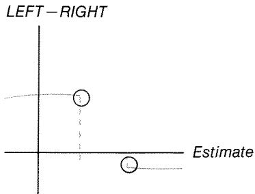
LEFT-RIGHT have opposite signs. The two estimates are far apart.

Case 2c:

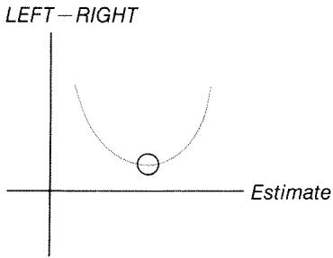
LEFT-RIGHT have the same sign.

Case 3: The calculator displays:

BAD GUESSES:

PRESS [CLR] TO VIEW

The Solver is unable to begin its iterative search for a solution using the current initial estimates (guesses). You might find a solution by entering different estimates. The closer you can estimate the answer, the more likely that the Solver will find a solution.

■ Case 4: The calculator displays: SOLUTION NOT FOUND

The Solver is unable to find a solution. Check your equation to make sure you have made no errors in entering it. Also check

the value of each known variable. If your equation and variables are correct, you might be able to find a solution by entering very good guesses.

Equations Used by Built-in Menus

Actuarial Functions

n = number of compounding periods.

i% = periodic interest rate, expressed as a percentage.

Single Payment Present Value Function

(Present value of a single $1.00 payment made after n periods.)

$$ SPPV (i\% :n) = \left(1 + \frac{i\%}{100}\right)^{-n} $$

Single Payment Future Value Function

(Future value after n periods of a single $1.00 payment.)

$$ SPFV (i\% :n) = \left(1 + \frac{i\%}{100}\right)^{n} $$

Uniform Series Present Value Function

(Present value of a $1.00 payment that occurs n times.)

$$ U S P V (i \% : n) = \frac {1 - \left(1 + \frac {i \%}{100}\right) ^ {- n}}{\frac {i \%}{100}} $$

Uniform Series Future Value Function

(Future value of a $1.00 payment that occurs n times.)

$$ U S F V (i \%; n) = \frac {\left(1 + \frac {i \%}{100}\right) ^ {n} - 1}{\frac {i \%}{100}} $$

Percentage Calculations in Business (BUS)

$$ \% \text{CHANGE} = \left(\frac {\text {NEW} - \text {OLD}}{\text {OLD}}\right) \times 100 $$

$$ \% \text {TOTAL} = \left(\frac {\text {PART}}{\text {TOTAL}}\right) \times 100 $$

$$ MARKUP\% C = \left(\frac{PRICE - COST}{COST}\right)\times 100 $$

$$ MARKUP\% P = \left(\frac{PRICE - COST}{PRICE}\right)\times 100 $$

Time Value of Money (TVM)

S = payment mode factor (0 for End mode; 1 for Begin mode).

$$ i\% = \frac{I\%\%YR}{P / YR} $$

$$ 0 = \mathrm{PV} + \left(1 + \frac{i\% \times S}{100}\right) \times PMT \times USPV (i\% :n) + FV \times SPPV (i\% :n) $$

Amortization

INT = accumulated interest

PRIN = accumulated principal

i = periodic interest rate

BAL is initially PV rounded to the current display setting.

PMT is initially PMT rounded to the current display setting.

$$ i = \frac{I\%YR}{P / YR\times 100} $$

For each payment amortized:

$$ I N T ^ {\prime} = B A L \times i (I N T ^ {\prime} \text {i s r o u n d e d t o t h e c u r r e n t d i s p l a y s e t t i n g}; $$

$$ I N T ^ {\prime} = 0 \text {f o r p e r i o d 0 i n B e g i n m o d e)} $$

$$ I N T = I N T ^ {\prime} \text {(w i t h s i g n o f P M T)} $$

$$ P R I N = P M T + I N T ^ {\prime} $$

$$ B A L _ {n e w} = B A L _ {o l d} + P R I N $$

$$ \Sigma I N T _ {n e w} = \Sigma I N T _ {o l d} + I N T $$

$$ \Sigma P R I N _ {n e w} = \Sigma P R I N _ {o l d} + P R I N $$

Conversions

Periodic compounding

$$ EFF\% = \left[\left(1 + \frac{NOM\%}{100\times P}\right)^{P} - 1\right]\times 100 $$

Continuous compounding

$$ EFF\% = \left(e^{\frac{NOM\%}{100}} - 1\right)\times 100 $$

Cash-Flow Calculations

j = the group number of the cash flow.

CF_j = amount of the cash flow for group j .

n_j = #TIMES the cash flow occurs for group j .

k^ = the group number of the last group of cash flows.

$$ N _ {j} = \sum_ {1 \leqslant l < j} n _ {l} = \text {t o t a l n u m b e r o f c a s h f l o w s p r i o r t o g r o u p} j $$

$$ N P V = C F _ {0} + \sum_ {j = 1} ^ {k} \left(C F _ {j} \times U S P V (i \%: n _ {j}) \times S P P V (i \%: N _ {j})\right) $$

When NPV = 0 , the solution for i% is IRR% .

$$ N F V = N P V \times S P F V (i \% : N) \text {where} N = \sum_ {j = 1} ^ {k} n _ {j} $$

$$ N U S = \frac {N P V}{U S P V (i \% : N)} $$

$$ T O T A L = \sum_ {j = 0} ^ {k} \left(n _ {j} \right. \times C F _ {j}) $$

Bond Calculations

Reference: Lynch, John J., Jr. and Jan H. Mayle, Standard Securities Calculation Methods, Securities Industry Association, New York, 1986.

A = accrued days, the number of days from beginning of coupon period to settlement date.

E = number of days in coupon period bracketing settlement date. By convention, E is 180 (or 360) if calendar basis is 30/360.

DSC = number of days from settlement date to next coupon date.

$$ (D S C = E - A). $$

M = coupon periods per year (1 = annual, 2 = semiannual).

N = number of coupon periods between settlement and redemption dates. If N has a fractional part (settlement not on coupon date), then round it to the next higher whole number.

Y = annual yield as a decimal fraction, YLD% / 100.

For one or fewer coupon period to redemption:

$$ P R I C E = \left[ \frac {C A L L + \frac {C P N \%}{M}}{1 + \left(\frac {D S C}{E} \times \frac {Y}{M}\right)} \right] - \left(\frac {A}{E} \times \frac {C P N \%}{M}\right) $$

For more than one coupon period to redemption:

$$ \begin{array}{l} P R I C E = \left[ \frac {C A L L}{\left(1 + \frac {Y}{M}\right) ^ {N - 1 + \frac {D S C}{E}}} \right] \ + \left[ \sum_ {K = 1} ^ {N} \frac {\frac {C P N \%}{M}}{\left(1 + \frac {Y}{M}\right) ^ {K - 1} + \frac {D S C}{E}} \right] - \left(\frac {A}{E} \times \frac {C P N \%}{M}\right) \ \end{array} $$

The "end-of-month" convention is used to determine coupon dates in the following exceptional situations. (This affects calculations for YLD% , PRICE , and ACCRU .)

If the maturity date falls on the last day of the month, then the coupon payments will also fall on the last day of the month. For example, a semiannual bond that matures on September 30 will have coupon payment dates on March 31 and September 30.
If the maturity date of a semiannual bond falls on August 29 or 30, then the February coupon payment dates will fall on the last day of February (28, or 29 in leap years).

Depreciation Calculations

For the given year, YR # :

$$ ACRS = \frac{ACRS\%}{100}\times BASIS $$

$$ S L = \frac {B A S I S - S A L V}{L I F E} $$

$$ S O Y D = \frac {B A S I S - S A L V}{L I F E \times \frac {(L I F E + 1)}{2}} \times (L I F E - Y R # + 1) $$

$$ D B = \frac {B A S I S \times F A C T \% / 100}{L I F E} \times \left(1 - \frac {(F A C T \% / 100)}{L I F E}\right) ^ {(Y R # - 1)} $$

For the last year of depreciation, DB equals the remaining depreciable value for the prior year.

Sum and Statistics

n = number of items in the list.

x^ = an element of the sorted list.

$$ T O T A L = \Sigma x _ {i} \quad M E A N = \bar {x} = \frac {\Sigma x _ {i}}{n} $$

$$ M E D I A N = x _ {j} ^ {\prime} \text {f o r o d d} n, \text {w h e r e} j = \frac {n + 1}{2} $$

$$ M E D I A N = \frac {\left(x _ {j} ^ {\prime} + x _ {j + 1} ^ {\prime}\right)}{2} \text {f o r e v e n} n, \text {w h e r e} j = \frac {n}{2} $$

$$ S T D E V = \sqrt {\frac {\Sigma \left(x _ {i} - \bar {x}\right) ^ {2}}{n - 1}} $$

$$ W. M N = \frac {\sum \left(y _ {i} x _ {i}\right)}{\sum y _ {i}} G. S D = \sqrt {\frac {\sum y _ {i} x _ {i} ^ {2} - \left(\sum y _ {i}\right) \bar {x} ^ {2}}{\left(\sum y _ {i}\right) - 1}} $$

$$ \text {R A N G E} = \text {M A X} - \text {M I N} $$

Forecasting

Model		Transformation	Xi	Yi
LIN	y = B + Mx	y = B + Mx	xi	yi
EXP	y = BeMx	ln y = ln B + Mx	xi	ln yi
LOG	y = B + M ln x	y = B + M ln x	ln xi	yi
PWR	y = BxM	ln y = ln B + M ln x	ln xi	ln yi

Let: = X_in = Y_in

$$ S X 2 = \Sigma \left(X _ {i} - \overline {{X}}\right) ^ {2} \quad S Y 2 = \Sigma \left(Y _ {i} - \overline {{Y}}\right) ^ {2} $$

$$ S X Y = \Sigma \left(X _ {i} - \bar {X}\right) \left(Y _ {i} - \bar {Y}\right) $$

Then:

$$ M = \frac {S X Y}{S X 2} $$

B = b for LIN and LOG models, and

B = e^b for EXP and PWR models,

where b = - M .

$$ \mathrm {C O R R} = \frac {\mathrm {S X Y}}{\sqrt {\mathrm {S X 2} \times \mathrm {S Y 2}}} $$

Equations Used in Chapter 13

Canadian Mortgages

$$ P V = - P M T \left[ \frac {1 - (1 + r) ^ {- N}}{r} \right] - F V (1 + r) ^ {- N} $$

where: r = [(1 + %YR200)^1 / 6 - 1]

N = total number of monthly payments

CI% YR = annual interest rate (as a percent)

PV = loan amount

PMT = monthly payment

FV = balloon payment

Odd-Period Calculations

$$ \begin{array}{l} P V \left[ 1 + i \times \frac {D A Y S}{3 0} \right] = \ - (1 + i \times S) \times P M T \times \left[ \frac {1 - (1 + i) ^ {- N}}{i} \right] - F V (1 + i) ^ {- N} \ \end{array} $$

where: PV = loan amount

i = periodic interest rate as a decimal

DAYS = actual number of days until the first payment

PMT = periodic payment amount

N = total number of payments

FV = balloon payment amount

$$ \begin{array}{l} S = 1 \text {i f} D A Y S < 3 0 \ S = 0 \text {i f} D A Y S \geqslant 3 0 \ \end{array} $$

Advance Payments

$$ P M T = \frac {- P V - F V (1 + i) ^ {- N}}{\left[ \frac {1 - (1 + i) ^ {- (N - # A D V)}}{i} + # A D V \right]} $$

where: PMT = payment amount

PV = loan amount

FV = balloon payment amount

i = periodic interest rate (as a decimal)

N = total number of payments

# ADV = number of payments made in advance

Modified Internal Rate of Return

$$ M I R R = 1 0 0 \left[ \left(\frac {N F V _ {P}}{- N P V _ {N}}\right) ^ {1 / n} - 1 \right] $$

where: n = total number of compounding periods

NFV_P = net future value of positive cash flows

NPV_N = net present value of negative cash flows

Menu Maps

The following maps show how to display each of the menus. There is a map for each menu label in the MAIN menu and for each menu found on the keyboard. The menu labels for variables are enclosed in boxes to illustrate how they are used:

Variable used to store and calculate values.
Variable used to calculate or display values; cannot be used to store values.
Variable used to store values; cannot be used to calculate values.

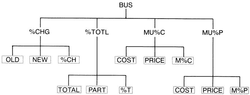
Figure C-1. BUS Menu

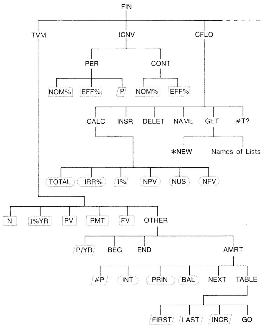
Figure C-2. FIN Menu

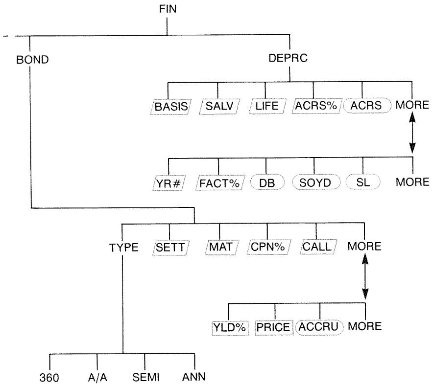
Figure C-2 (continued). FIN Menu

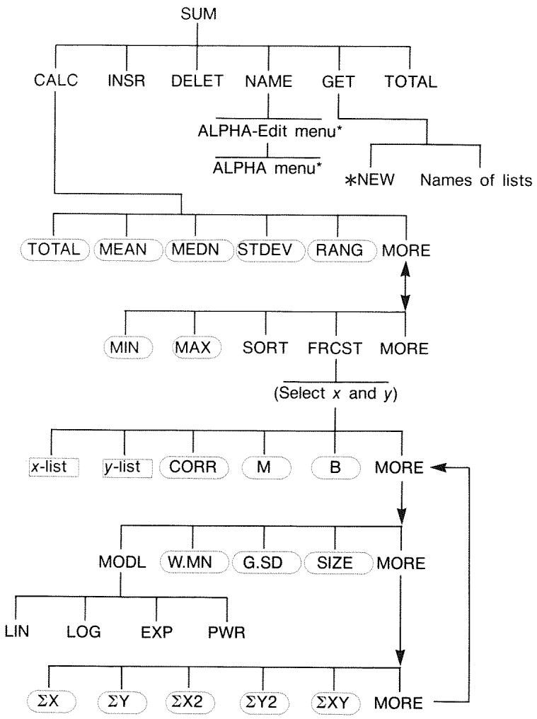
Figure C-3. SUM Menu

• For the complete menu, see pages 27-28.

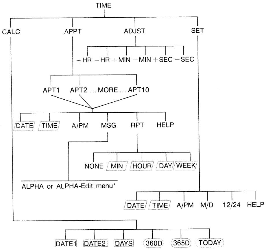
Figure C-4. TIME Menu

• For the complete menu, see pages 27-28.

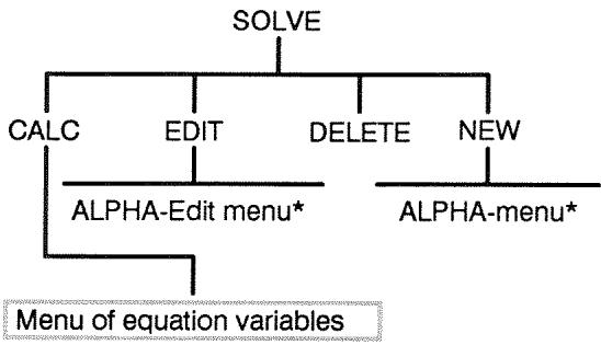
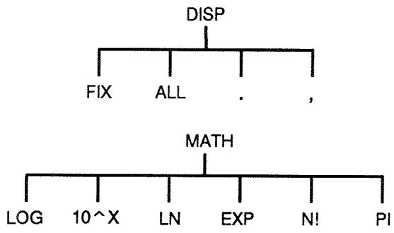
Figure C-5. SOLVE Menu

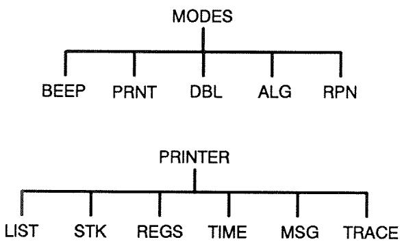
Figure C-6. DSP, MATH, MODES, and PRINTER Menus

• For the complete menu, see pages 27-28.

RPN: Summary

About RPN

The RPN appendix (D, E, and F) are especially for those of you who want to use or learn RPN — Hewlett-Packard's original Reverse Polish Notation for operating calculators. This calculator can use either RPN or algebraic logic for calculations — you choose which.

HP's RPN operating logic is based on an unambiguous, parentheses-free mathematical logic known as "Polish Notation," developed by the Polish logician Jan Lukasiewicz (1878-1956). While conventional algebraic notation places the operators between the relevant numbers or variables, Lukasiewicz's notation places them before the numbers or variables. For optimal efficiency of the stack, we have modified that notation to specify the operators after the numbers. Hence the term Reverse Polish Notation, or RPN.

Except for the RPN appendix, the examples and keystrokes in this manual are written entirely using Algebraic (ALG) mode.

About RPN on the HP-17B II

This appendix replaces much of chapter 2, "Arithmetic." It assumes that you already understand calculator operation as covered in chapter 1, "Getting Started." Only those features unique to RPN mode are summarized here:

RPN mode.
RPN functions.
RPN arithmetic, including percentages and and RCL arithmetic.

All other operations—including the Solver—work the same in RPN and ALG modes. (The Solver uses algebraic logic only.)

For more information about how RPN works, see appendix E, "RPN: The Stack." For RPN keystrokes of selected examples from chapter 13, see appendix F, "RPN: Selected Examples." Continue reading in chapter 2 to learn about the other functionality of your calculator.

Watch for this symbol in the margin earlier in the manual. It identifies keystrokes that are shown in ALG mode and must be performed differently in RPN mode. Appendixes D, E, and F explain how to use your calculator in RPN mode.

The mode affects only arithmetic calculations—all other operations, including the Solver, work the same in RPN and ALG modes.

Setting RPN Mode

The calculator operates in either RPN (Reverse Polish Notation) or ALG (Algebraic) mode. This mode determines the operating logic used for arithmetic calculations.

To select RPN mode: Press MODES RPN.

The calculator responds by displaying RPH MODE. This mode remains until you change it. The display shows the X register from the stack.

To select ALG mode: Press MODES ALG. The calculator displays ALGEBRATIC MODE.

Where the RPN Functions Are

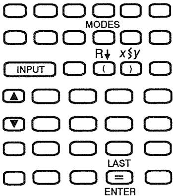
Function Name	Definition	Key to Use
ENTER	Enters and separates one number from the next.	=
LAST X	Recalls last number in X-register.	LAST
R↓	Rolls down stack contents.	R↓ (same as 0)
R↑	Rolls up stack contents.	▲ (except in lists)
X <> Y	X-register exchanges with Y-register.	x<>y (same as 0)
CHS	Changes sign.	+/-

Using INPUT for ENTER and for R . Except in CFLO and SUM lists, the INPUT key also performs the ENTER function and the key also performs the ^+ function.

In lists: INPUT stores numbers. Use to enter numbers into the stack during arithmetic calculations.
In lists: and move through lists. Use to roll through stack contents.

Doing Calculations in RPN

Arithmetic Topics Affected by RPN Mode

This discussion of arithmetic using RPN replaces those parts of chapter 2 that are affected by RPN mode. These operations are affected by RPN mode:

Two-number arithmetic (+,,-,,^*)
The percent function (%)
The LAST X function (LAST). See appendix E.

RPN mode does not affect the MATH menu, recalling and storing numbers, arithmetic done inside registers, scientific notation, numeric precision, or the range of numbers available on the calculator, all of which are covered in chapter 2.

Simple Arithmetic

Here are some examples of simple arithmetic. Notice that

ENTER separates numbers that you key in.
The operator (+,-,etc.) completes the calculation.
One-number functions (such as ) work the same in ALG and RPN modes.

To Calculate:	Press:	Display:
12 + 3	12 ENTER 3 +	15.00
12 - 3	12 ENTER 3 -	9.00
12 × 3	12 ENTER 3 ×	36.00
12 ÷ 3	12 ENTER 3 ÷	4.00
12²	12 x²	144.00
√12	12 √x	3.46
1/12	12 1/x	0.08

You do not need to use ENTER before an operator, only between keyed-in numbers. Key in both numbers (separated by ENTER) before pressing the operator key.

The Power Function (Exponentiation). The power function uses the keys.

To Calculate:	Press:	Display:
123	12 ENTER 3 yx	1,728.00
121/3 (cube root)	12 ENTER 3 1/x yx	2.29

The Percent Function. The % key calculates percentages without using the key. Combined with + or - , it adds or subtracts percentages.

To Calculate:	Press:	Display:
27% of 200	200 ENTER 27 %	54.00
200 less 27%	200 ENTER 27 % -	146.00
12% greater than 25	25 ENTER 12 % +	28.00

Compare these keystrokes in RPN and ALG modes:

RPN Mode

ALG Mode

27% of 200

200 ENTER 27 %

200× 27%

200 less 27%

200 ENTER 27 % -

200 27

Calculations with STO and RCL

The store () and recall () operations work identically in ALG and RPN modes (see "Storing and Recalling Numbers" and "Doing Arithmetic Inside Registers and Variables" in chapter 2). The keystrokes are the same for simple storing and recalling and for doing arithmetic inside registers and variables.

When doing arithmetic in the display with values from storage registers and variables, remember to use RPN. Compare these keystrokes in RPN and ALG modes:

RPN Mode

Store -2× 3 in register 5

2+/- ENTER 3 STO 5

ALG Mode

2+/-×3=STO5

Find PV - 2

FIN TVM RCL PV 2

FIN TVM RCL PV 2

Find PV less 2%

FIN TVM RCL PV 2%

FIN TVM RCL PV 2%

Find PMT × N

FIN TVM RCL PMT RCL H

FIN TVM RCL PMT RCL H

Chain Calculations—No Parentheses!

The speed and simplicity of calculating using RPN are apparent during chain calculations—longer calculations with more than one operation. The RPN memory stack (refer to appendix E) stores intermediate results until you need them, then inserts them into the calculation.

The cube root example and the percentage addition example (previous topics) are two simple examples of chain calculations.

For another example, calculate

$$ 7 \times (1 2 + 3) $$

Start the calculation inside the parentheses by finding 12 + 3 . Notice that you don't need to press ENTER to save this intermediate result (15) before proceeding. Since it is a calculated result, it is saved automatically—without using parentheses.

Keys:	Display:	Description:
12 ENTER 3	15.00	Intermediate result.
7	105.00	Pressing the function key produces the answer.

Now study these examples. Note the automatic storage and retrieval of intermediate results.

To Calculate:	Press:	Display:
(750 × 12) ÷ 360	750 ENTER 12 × 360 ÷	25.00
360 ÷ (750 × 12)	360 ENTER 750 ENTER 12 × ÷ or 750 ENTER 12 × 360x2y ÷	0.04
{ (456 - 75 ) ÷ 18.5} × (68 ÷ 1.9)	456 ENTER 75 ÷ 18.5 ÷ 68 ENTER 1.9 ÷ x	737.07
(3 + 4) × (5 + 6)	3 ENTER 4 ÷ 5 ENTER 6 ÷ x	77.00

RPN: The Stack

This appendix explains how calculations take place in the automatic memory stack and how this method minimizes keystrokes in complicated calculations.

What the Stack Is

Automatic storage of intermediate results is the reason that RPN mode easily processes complicated calculations—without using parentheses. The key to automatic storage is the automatic RPN memory stack.

The memory stack consists of up to four storage locations, called registers, which are "stacked" on top of each other. It is a work area for calculations. These registers—labeled X, Y, Z, and T—store and manipulate four current numbers. The "oldest" number is the one in the T-(top) register.

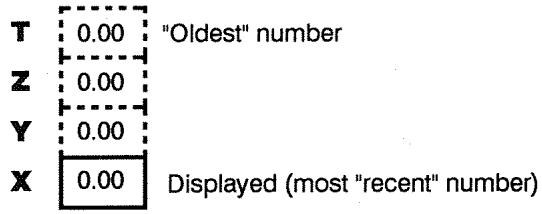
The most "recent" number is in the X-register: This is the number you see in the display.

Reviewing the Stack (Roll Down)

The (roll down) function (on the key) lets you review the entire contents of the stack by "rolling" the contents downward, one register at a time. While in RPN mode you don't need to press the shift key for .

The key has the same effect as + , except in a CFLO or SUM list, when affects the list and not the stack. Likewise, the key rolls the contents of the stack upward, except in lists.

Rolling a Full Stack. Suppose the stack is filled with 1, 2, 3, 4 (press 1 ENTER 2 ENTER 3 ENTER 4). Pressing four times rolls the numbers all the way around and back to where they started:

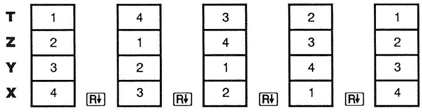
When you press , the value in the X-register rotates around into the T-register. Notice that the contents of the registers are rolled, while the registers themselves maintain their positions. The calculator displays only the X-register.

Variable Stack Size. Clearing the stack by pressing CLEAR DATA reduces the stack to one register (X) with a zero in it. As you enter numbers, the stack builds up again. The R and functions roll through as many registers as currently exist (one, two, three, or four).

Exchanging the X- and Y-Registers in the Stack

Another function that manipulates the stack contents is ( x exchange y ), located on the key. It swaps the contents of the X- and Y-registers without affecting the rest of the stack. Pressing again restores the original order of the contents. While in RPN mode you don't need to press the shift key for .

The ≥ y function is used primarily to swap the order of numbers in a calculation. For example, an easy way to calculate 9 ÷ (13 × 8) is to press 13 ENTER 8 × 9 ≥ y

Arithmetic—How the Stack Does It

The contents of the stack move up and down automatically as new numbers enter the X-register (lifting the stack), and as operators combine two numbers to produce one new number in the X-register (dropping the stack). See how a full stack drops, lifts, and drops its contents while calculating

$$ 3 + 4 - 9: $$

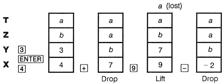
(a and b represent values already on the stack.)

• Notice that when the stack drops, it replicates the contents of the T-register and overwrites the X-register.
• When the stack lifts, it pushes the top contents out of the T-register, and that number is lost. This shows that the stack's memory is limited to four numbers for calculations.
• Because of the automatic movement of the stack, you do not need to clear the display before doing a new calculation.
• Most functions (except ENTER and CLR) prepare the stack to lift its contents when the next number enters the X -register.

How ENTER Works

You know that ENTER separates two numbers keyed in one after the other. In terms of the stack, how does it do this? Suppose the stack is filled with a , b , c , and d . Now enter and add two new numbers:

$$ 5 + 6: $$

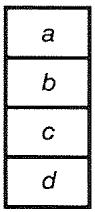
5

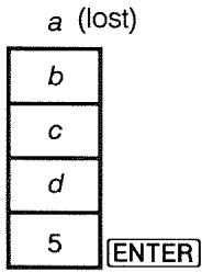
Lift

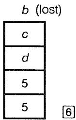
Lift
6

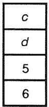
No lift

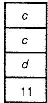
Drop

ENTER replicates the contents of the X-register into the Y-register. The next number you key in (or recall) writes over (instead of lifting) the copy of the first number left in the X-register. The effect is simply to separate two sequentially entered numbers.

Using a Number Twice in a Row. You can use the replicating feature of ENTER to other advantages. To add a number to itself, key in the number and press ENTER+

Filling the Stack with a Constant. The replicating effect of , together with the replicating effect (from T into Z) of stack drop, allows you to fill the stack with a numeric constant for calculations.

Example: Constant, Cumulative Growth. The annual sales of a small hardware company are projected to double each year for the next 3 years. If the current sales are (84,000, what are the annual sales for each of the next 3 years?

1. Fill the stack with the growth rate (2 ENTER ENTER ENTER).
2. Key in the current sales in thousands (84).
3. Calculate future sales by pressing for each of the next 3 years.

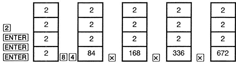
Sales for the next 3 years are projected to be 168,000; 336,000; and $672,000.

Clearing Numbers

Clearing One Number. Clearing the X-register puts a zero in it. The next number you key in (or recall) writes over this zero.

There are two ways to clear the number in the X-register:

Press +
Press CLR

For example, if you wanted to enter 1 and 3 but mistakenly entered 1 and 2, these keystrokes would correct it:

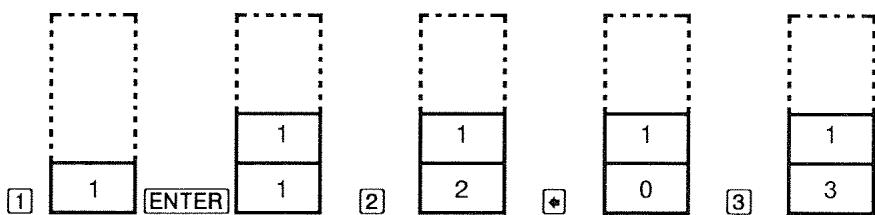
Clearing the Entire Stack. Pressing CLEAR DATA clears the X-register to zero and eliminates the Y-, Z-, and T-registers (reducing the size of the stack to one register). The stack expands again when you enter more numbers.

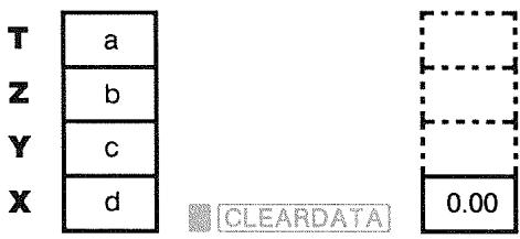
Because of the automatic movement of the stack, it is not necessary to clear the stack before starting a calculation. Note that if an application menu is currently displayed, pressing CLEAR DATA also clears the application's variables.

The LAST X Register

Retrieving Numbers from LAST X

The LAST X register is a companion to the stack: It stores the number that had been in the X-register just before the last numeric operation (such as a operation). Pressing LAST returns this value to the X-register. This ability to recall the "last x " value has two main uses:

• Correcting errors: retrieving a number that was in the X-register just before an incorrect calculation.
  Reusing a number in a calculation.

Reusing Numbers

You can use LAST to reuse a number (such as a constant) in a calculation. Remember to enter the constant second, just before executing the arithmetic operation, so that the constant is the last number in the X-register, and therefore can be saved and retrieved with LAST

Example: Calculate 96.74 + 52.3952.39 .

Keys:	Display:	Description:
96.74 ENTER	96.74
52.39 +	149.13	Intermediate result.
LAST	52.39	Retrieves the number before the + operation, saved in LAST X.
÷	2.85	Final result.

Chain Calculations

The automatic lifting and dropping of the stack's contents let you retain intermediate results without storing or reentering them, and without using parentheses. This is an advantage the RPN stack has over algebraic calculator logic. Other features of RPN include the following:

You never work with more than two numbers at a time.
ENTER separates two numbers keyed in sequentially.
- Pressing an operator key executes that operation immediately.
Intermediate results appear as they are calculated, so you can check each step as you go.
Intermediate results are automatically stored. They reappear automatically as they are needed for the calculation—the last result stored is the first to come back out.
- You can calculate in the same order as you would with pencil and paper—that is, from the innermost parentheses outward:

$$ 4 \div [ 1 4 + (7 \times 3) - 2 ] = 0. 1 2 $$

can be solved as 7 ENTER 3 + 14 + 2 - 4 xzy

Exercises

Here are some extra problems that you can do to practice using RPN.

Calculate: (14 + 12) × (18 - 12) ÷ (9 - 7) = 78.00

A Solution: 14 ENTER 12 + 18 ENTER 12 - x 9 ENTER 7 -

Calculate: 23^2 - (13 × 9) + 17 = 412.14

A Solution: 23 ^2 13 ENTER 9 -7 1 / x +

Calculate: (5.4 × 0.8) ÷ (12.5 - 0.7^3) = 0.60

A Solution: 5.4 ENTER .8 × .7 ENTER 3 y 12.5 xzy -

or

5.4 ENTER .8 × 12.5 ENTER .7 ENTER 3

Calculate: 8.33 × (4 - 5.2) ÷ [(8.33 - 7.46) × 0.32]4.3 × (3.15 - 2.75) - (1.71 × 2.01 = 4.57

A Solution: 4 ENTER 5.2 - 8.33 x LAST 7.46 - .32 x

3.15 ENTER 2.75 4.3 1.71 ENTER 2.01 x -

RPN: Selected Examples

The following examples selected from chapter 13 ("Additional Examples") have been converted to RPN keystrokes. These examples illustrate how to convert algebraic to RPN keystrokes in less common situations: with % ,with [] , and in a CFLO list.

Example: Simple Interest at an Annual Rate. Your good friend needs a loan to start her latest enterprise and has requested that you lend her (450 for 60 days. You lend her the money at (7 \%)simple annual interest, to be calculated on a 365- day basis. How much interest will she owe you in 60 days, and what is the total amount owed?

Keys:	Display:	Description:
450 ENTER 7 %	31.50	Annual interest.
60 × 365 ÷	5.18	Actual interest for 60 days.
450 ÷	455.18	Adds principal to get total debt.

Example: APR for a Loan with Fees. A borrower is charged two points for the issuance of a mortgage. (One point is equal to 1% of the mortgage amount.) If the mortgage amount is \60,000for 30 years and the interest rate is11^{1} / _{2}\%$ annually with monthly payments, what APR is the borrower paying?

1. Since the payment amount is not given, calculate it (PMT) first. Use the given mortgage amount (PV = 60,000) and interest rate (I%YR = 11^{1}$ /2%).
2. To find the APR (the new ( I\% YR )), use the PMT calculated in step 1 and adjust the mortgage amount to reflect the points paid (( PV = \)60,000 - 2\% )). All other values remain the same (term is 30 years; no future value).

Keys:	Display:	Description:
FIN TYM		If necessary, sets 12 payments per year and End mode.
OTHER
CLEAR DATA
EXIT	12 F/YR END MODE
30 H	N=360.00	Figures and stores number of payments.
11.5 I:YR		Stores interest rate and amount of loan.
60000 PV	PV=60,000.00
0 FV	FV=0.00	No balloon payment, so future value is zero.
PMT	PMT=-594.17	Borrower's monthly payment.
RCL PV		Stores actual amount of money received by borrower into PV.
2 % PV	PV=58,800.00
I:YR	I:YR=11.76	Calculates APR.

Example: Loan from the Lender's Point of View. A 1,000,000 10 -year, 12% (annual interest) interest-only loan has an origination fee of 3 points. What is the yield to the lender? Assume that monthly payments of interest are made. (Before figuring the yield, you must calculate the monthly PMT = (loan × 12% ) ÷ 12 mos.) When calculating the I% YR , the FV (a balloon payment) is the entire loan amount, or \1,000,000, while thePV$ is the loan amount minus the points.

Keys:	Display:	Description:
FIN	TVM	If necessary, sets 12
OTHER		payments per year and
CLEAR DATA		End mode.
EXIT	12 P/YR END MODE
10	N=120.00	Stores total number of
1000000 ENTER		Calculates annual interest on $1,000,000.
12 %	120,000.00
12 ÷ PMT	PMT=10,000.00	Calculates, then stores, monthly payment.
1000000 FV	FV=1,000,000.00	Stores entire loan amount as balloon payment.
3 % +/- FV	FV=-970,000.00	Calculates, then stores, amount borrowed (total - points).
IXYR	IXYR=12.53	Calculates APR - the yield to lender.

Example: Savings for College. Your daughter will be going to college in 12 years and you are starting a fund for her education. She will need (15,000 at the beginning of each year for four years. The fund earns (9\%) annually, compounded monthly. You plan to make monthly deposits, starting at the end of the current month. How much should you deposit each month to meet her educational expenses?

See figures 13-1 and 13-2 (chapter 13) for the cash-flow diagrams.

Remember to press the key for ENTER while working in a list. (Pressing INPUT will add data to the list, not perform an ENTER.)

Keys:	Display:	Description:
FIN CFLO		Displays current cash-flow list and CFLO menu keys.
CLEAR DATA		Cleared current list or gets a new one.
YES
or
GET *NEW	FLOW(B)=?

Step 1: Set up a CFLO list.

Keys:	Display:	Description:
0 INPUT	FLOW(1)=?	Sets initial cash flow, FLOW(0), to zero.
0 INPUT	#TIMES(1)=1	Stores zero in FLOW(1) and prompts for the number of times it occurs.
12 ENTER 12 × 1 - INPUT	FLOW(2)=?	For ENTER, press =, not INPUT. Stores 143 (for 11 years, 11 months) in #TIMES(1) for FLOW(1).
15000 INPUT	#TIMES(2)=1	Stores amount of first withdrawal, at end of 12th year.
INPUT	FLOW(3)=?
0 INPUT	#TIMES(3)=1	Stores cash flows of zero ...
11 INPUT	FLOW(4)=?	... for the next 11 months.
15000 INPUT	FLOW(5)=?	Stores second withdrawal, for sophomore year.
0 INPUT 11 INPUT	FLOW(6)=?	Stores cash flows of zero for the next 11 months.
15000 INPUT	FLOW(7)=?	Stores third withdrawal, for junior year.
0 INPUT 11 INPUT	FLOW(8)=?	Stores cash flows of zero for the next 11 months.
15000 INPUT	FLOW(9)=?	Stores fourth withdrawal, for senior year.
EXIT CALC	NPV, NUS, NFV	Done entering cash flows; gets CALC menu.

Step 2: Calculate NUS for the monthly deposit. Then calculate net present value.

Keys:	Display:	Description:
9 ENTER 12	IX=0.75	Figures the periodic (monthly) interest rate and stores it in I%.
HUS	HUS=182.30	Amount of monthly deposit needed to meet planned withdrawals.
NPV	NPV=17,973.48	Calculates the net present value of the monthly deposits, which is the same as the NPV of the four future withdrawals.

Example: Tax-Free Account. Consider opening an IRA account with a dividend rate of 8.175% . 1) If you invest \2,000at the beginning of each year for 35 years, how much will you have at retirement? 2) How much will you have paid into the IRA? 3) How much interest will you have earned? 4) If your post-retirement tax rate is15\%, what is the after-tax future value of the account? Assume only the interest will be taxed (the principal was taxed before deposit). 5) What is the purchasing power of that amount, in today's dollars, assuming an8\%$ annual inflation rate?

Keys:		Display:		Description:
FIN	TVM			Sets 1 payment per year and Begin mode.
OTHER	1 P/YR
BEG	EXIT	1 P/YR	BEGIN MODE
35	N	N=35.00		Stores number of payment periods until retirement (1×35).
8.175	I.ZYR	I.ZYR=8.18		Stores dividend rate.
0	PV	PV=0.00		Present value of account (before first payment).

2000 +/- PMT		PMT=-2,000.00	Annual payment (deposit).
FV		FV=387,640.45	Calculates amount in account at retirement.
RCL PMT RCL			Calculates total amount paid into IRA by retirement.
H ×		-70,000.00
RCL FV +		317,640.45	Calculates interest you will earn.
15 %		47,646.07	Taxes at 15% of interest.
+/- RCL FV			Subtracts taxes from total FV to calculate after-tax FV.
+		339,994.39
FV		FV=339,994.39	Stores after-tax future value in FV.
8 I:YR 0 PMT			Calculates present-value purchasing power of the above after-tax FV at 8% inflation rate.
FV		FV=-22,995.36

Example: Taxable Retirement Account. If you invest (3,000 each year for 35 years, with dividends taxed as ordinary income, how much will you have in the account at retirement? Assume an annual dividend rate of (8.175\%) and a tax rate of (28\%), and that payments begin today. What will be the purchasing power of that amount in today's dollars, assuming (8\%) annual inflation?

Keys:	Display:	Description:
FIN TVM		Displays TVM menu.
OTHER 1 P/YR		Sets 1 payment per year and Begin mode.
BEG EXIT	1 P/YR BEGIN MODE
35 N	N=35.00	Stores years until retirement.
8.175 ENTER 28 %	5.89	Calculates interest rate diminished by tax rate.

I:YR

IXYR=5.89

0 F

PV=0.80

3000 + / -

FMT

PMT=-3,000.00

FV

FV=345,505.61

8 I#R0

PV

PMT

PV=-23,368.11

Stores interest rate.

Stores no present value.

Stores annual payment.

Calculates future value.

Calculates present-value purchasing power of the above FV at 8% inflation.

Error Messages

The calculator beeps and displays an error message under certain circumstances—for example, when you attempt an operation that is not allowed.

The calculator distinguishes between math errors that occur on the calculator line and other types of messages by preceding math-error messages with the word ERROR:

Press CLR or to erase the message and restore the previous display.

BAD GUESSES:

PRESS [CLR] TO VIEW

The Solver cannot begin a numerical search using the initial estimates.

See pages 167 and 227.

BATTTOOLLOWTOPRINT

To conserve battery power, the calculator will not transmit data to the printer until fresh batteries have been installed.

CURRENT LIST UNNAMED;

NAME OR CLEAR THE LIST

Attempted to get another list without first clearing or naming the current list. Press CLEAR DATA to clear it or NAME to name it.

EMPTY LIST

Attempted a calculation using an empty CFLO or SUM list.

ERROR: LOGARITHM(NEG)

ERROR: LOGARITHM(0)

Attempted to take the base 10 or natural log of a negative number or zero. This can happen during curve-fitting calculations if you attempt to calculate:

A logarithmic forecasting model with a negative or zero x -value.
An exponential model with a negative or zero y -value.
A power model with a negative or zero x - or y -value.

ERROR: NEG^NONINTEGER

Attempted to raise a negative number to a non-integer power.

ERROR:OVERFLOW

An internal result in a calculation was too large for the calculator to handle.

ERROR: SQRT(NEG)

Attempted to take the square root of a negative number or calculate G.SD given any negative frequencies.

ERROR: UNDERFLOW

An internal result in a calculation was too small for the calculator to handle.

ERROR: 0^NEG

Attempted to raise zero to a negative power.

ERROR: 0÷0

Attempted to divide zero by zero.

ERROR: 0^0

Attempted to raise zero to the zero power.

ERROR: ÷ 0

Attempted to divide by zero.

INPUTSCAUSED-0

The numbers stored into built-in variables caused a division by zero in the calculation. You must change one or more stored values. (Refer to the equations in appendix B to see which variables appear in the divisor.)

INSUFFICIENT DATA

■ Attempted to calculate standard deviation with only one value in the list.
■ Attempted to do curve fitting using an x -variable list in which all the values are equal.
■ Attempted to do curve fitting using the logarithmic or power models with a list for which the transformed values of x ( x ) are equal.

INSUFFICIENT MEMORY

The calculator has insufficient memory available to do the operation you've specified. Refer to "Managing Calculator Memory" on page 216 for additional information.

INTEREST 一 = -100%

One of the following values for interest is less than or equal to -100 :

TVM menu: I% YR ÷ P/YR.
PER menu: NOM% ÷ P (calculating EFF% ); EFF% (calculating NOM% ).
CONT menu: EFF% .
■ CFLO menu: I% (calculating NPV, NUS, or NFV) or estimate of IRR%.

INTERRUPTED

Calculation of I% YR, IRR% , amortization results, a Solver variable, or a SUM-list sort was interrupted.

INVALID DATE

The number entered cannot be interpreted as a proper date. Check its format (page 132).

■ Attempted to set a date outside the range 1/1/1987 through 12/31/2086, or attempted date arithmetic outside the range 10/15/1582 through 12/31/9999.

INVALID EQUATION

The Solver cannot interpret the equation due to a syntax error. Refer to "What Can Appear in an Equation," page 154.
A variable's name is invalid. Refer to "Names of Variables," page 155.

INVALID INPUT

■ Attempted to store into a built-in variable a number that is outside the range of values permitted for that variable.
The number entered cannot be interpreted as a proper time.
The appointment's repeat interval is out of range.
■ Attempted to enter a non-integer, negative number when specifying the number of displayed decimal places (in DSP).

INVALID

Attempted to calculate I% YR with N ≤slant 0.99999 or N ≥slant 10^10 .

IRR% > 0 EXISTS; KEY

IN GUESS; [STO] (IRR%)

Calculation of IRR% produced a negative answer, but the calculator has determined that there is also a unique positive answer. (Refer to page 226.)

MACHINE RESET

The calculator has been reset (page 214, 217).

MANY OR NO SOLUTIONS

The calculator is unable to calculate I% YR. Check the values stored in PV, PMT, and FV. Make sure the signs of the numbers are correct. If the values of PV, PMT, and FV are correct, the calculation is too complex for the TVM menu. You may be able to perform the calculation using the CFLO menu to calculate IRR% .

MANY/NO SOLUTIONS; KEY

IN GUESS; [STO] (IRR%)

The calculation of IRR% is complex, and requires you to store a guess.

(Refer to page 227.)

MEMORY LOST

Continuous Memory has been erased (page 214, 218).

NAME ALREADY USED:

TYPE A NAME; [INPUT]

The list name name you've attempted to enter is already in use; type in a new name and press INPUT.

NO SOLUTION

No solution is possible using the values stored in the current built-in menu or list. This most commonly results from an incorrect sign for a cash flow or other monetary value. (Review page 53.)

N! N<0 OR N NONINTEGER

Attempted to calculate the factorial of a negative or non-integer value.

OVERFLOW

A warning—not an error—that the magnitude of a result is too large for the calculator to handle, so it returns ± 9.99999999999E499

rounded to the current display format. See page 44 for limits.

SOLUTION NOT FOUND

No solution was found for a Solver equation using the current values stored in its variables. Refer to page 234 in appendix B.

UNDERFLOW

A warning—not an error—that the magnitude of a result is too small for the calculator to handle, so it returns the value zero. See page 44 for limits.

UNEQUAL LIST LENGTHS

Attempted a two-list SUM calculation using lists of unequal lengths.

Special Characters

, 15, 16, 250

() alarmannunciator,136

low-batteryannunciator,16, 172,214

print annihilator, 171 shift annihilator, 17

10X,39

12×24,132

360D,138

365D,138

, 17

,32 1,32

= ,162

+/-, 20, 24

+HE,133

-MIN,133

- ,44

1/x,38

,38

%,37

CH,46

:CHG,45,46-47

:CHG menu

formula, 236

using, 46

TOTL,45,47

%TOTL menu

formula, 236

using, 47

*NEW,116

F,67

T? ,81,85-86

TIMES,85-86

,121,129,159,163-164,209

EXY,121,129

EX ,121,129

X82,121,129

,121,129

, 121, 129

l ,18,29,260

or 162

or , 40, 251, 257

with history stack, 40

in a list, 85, 150

editing a list, 87

， - > , < - 1<<-，29

A

ABS (absolute value) function, 157

ACCRU,98

Accrued interest, on bond, 98, 99

Accuracy of the clock, 218

Acknowledging appointments, 136

HCRS,104

ACRS,104

Actual calendar

actuarial equations, 235

for arithmetic, 138

for bonds, 98

Addition, 19

ADJST menu, 133

Advance payments, 63-66, 187-189, 242. See also

Leasing

HLG,33,250

Algebraic

mode, 33, 250

rules in equations, 153-154

HLL key, 31

ALOG,157

Alphabetic keys, 27-29

ALPHAbetic menu, 27

Amortization

calculations, 67-70

equations, 236-237

schedule, 68

schedule, printing, 71-72

AM/PM format, 132

AMRT menu, 67

AND operator, 155, 162

Annual percentage interest rate in TVM, 52

with fees, 181

with fees, RPN, 264

Annunciators, 16

definition, 17

printer, 171

Antilogarithms, 39, 157

H/PM, appointment-setting menu, 132

Appointment

menus, 131, 133-134

messages, 135

repeat interval, 135, 136

-setting menu, 134

Appointments

acknowledging, 136

clearing, 137

memory used by, 217

messages, 133

past due, 134

printing, 175

setting, 134-136

unacknowledged, 134, 136

APPT menu, 134

HFT1 through HPT10, 134

Arithmetic, 19-20, 35

in registers and variables, 43

in RPN, 253-255, 258

in RPN stack, 258

RPN examples, 263

Arithmetic priority, 142

Arrow keys

for changing current equation, 144

for editing, 29

for finding an equation, 150

for rolling the history stack, 40

for viewing long equations, 154

B

B,121

Backspace key, 18

BHL,67

Balance of loan, 69-70

Balloon payment, 54, 59-60

BHSIS,104

Batteries, changing, 214-216

Battery life, 214

annunciator, 214

Beeper, 136

Beeper on and off, 33

EEG,53

Begin payment mode, 53, 55

Beginning of list

in CFLO, 87

in SUM list, 113

BOND menu, 97-98

Bond calculations, 98-102

equations, 238

fractional values for, 100

price, 100

type, 98, 99

yield, 100

Bonds, 203-204

Bottom

of the current list, in CFLO, 84

of the Solver list, 150

Braces in equations, 155

Brackets in equations, 155

Brightness of the display, 16

Built-in variables. See Variables, built-in

BUS menu, 45, 243

Business variables, clearing, 45

Buy option, for a lease, 64-66

B -value,incurvefitting,121

C

, 15, 16, 250

CALC menu

in CFLO menu, 90

inSOLVE menu,146-147

in SUM menu, 117

in TIME menu, 138

CALC

in CFLO menu, 81

inSOLVE menu,145

in SUM menu, 111

in TIME menu, 131

Calculations, RPN

order of, 262

parenthesis in, 255, 262

Calculator line

arithmetic in, 35-44

definition, 17

displaying alphabetic information, 28-29

editing, 18

Calculator

not functioning, 219-220

resetting, 214, 217-218

Support, 211

Calendar basis, 97-98

Calendar. See also Date

360-day, 138

365-day, 138

actual, 138

range of, 138

Call, 98, 101

CALL,98

Canadian mortgage, 185-187, 241

Capitalized value, lease, 63-64

Cash flow

calculations, 80-96

equations, 237-238

list. See CFLO list

Cash flow diagrams

in cash flow calculations, 82-83

in TVM calculations, 53-55

Cash flows

equal. See Cash flows, grouped

grouped, 83, 93

initial, 83, 84

maximum number of, 80

sum of, 90

ungrouped, 82

zero,83,84

CDATE, 157

CFLO list

CALC menu, 90

clearing, 89

copying from, 87

correcting, 87

creating, 83

definition, 80

deleting numbers, 87

editing, 81, 87

entering numbers in, 84-86

GETing a new list, 88

inserting numbers, 87

name,clearing,89

naming, 87-88

printing, 174

signsofnumbers,82

starting a new list, 88

viewing name of current list, 88 viewing numbers, 87

Chain calculations, 19, 35-36 in RPN, 255, 262

Changing batteries, 213-216 the sign of a number, 20

Characters
for CFLO list, 87-88
for equation names, 149
in equations, 154-155
for SUM list, 115-116
inserting and deleting, 28-29

Checking calculator operation, 219-221

%CHG menu, 46 Chi-squared, 208-210

CLEAR DATA, 18, 25-26

Clearing, 18
AMRT variables, 69
appointments, 135, 137
BOND variables, 98
BUS variables, 45

calculator memory, 25-26
CFLO lists, 84, 89

%CHG variables, 45

ICONVvariables,75

menu variables, 25
menus, 25

MU%C variables, 45

MU%P variables, 45

numbers in RPN, 260

the history stack, 40

the RPN stack, 257, 261

Solver variables, 151
SUM lists, 112

% T variables, 45

TIMECALCvariables,138
TVMvariables,53

variables, 25-26

Clock. See Time

CLR, 16, 18, 29

Commas,in numbers,32

Compound interest calculations, 50

Compounding annual, 60 monthly, 56, 57, 59, 63, 64 periods, 50, 51, 52, 53 periods, vs. payment peric 77-79, 189 rates, 73 semimonthly, 62

Conditional expressions, 161-163

Constant numbers, RPN, 259, 261

Constants in equations, 155

CONT menu, 75

Continuous compounding, calculating interest for, 74

Continuous Memory, 34 erasing, 214, 218 using, 16

Contrast of display, changing, 16

Conventional investments, definition, 90

Converting interest rates, 74-76
CORR, 121

Correlation coefficient, 121
COST key, 48-49

Cost of capital, 90 markup on, 45, 47-48

Counter variable, in summation function, 163

Coupon basis, 97-98 payments, 97

CPN2,98

Creating a CFLO list, 83-86, 88

a new equation, in the Solver, 145-146

a SUM list, 112-113, 116

CTIME, 157

Cuberoot,38 inRPN,253

Current equation, 144 deleting, 151-152 printing, 175

Cursor, 17 movement keys, 29

Curve fitting, 110, 121-123 calculations, 123-126 equations, 240

Customer Support, 211

D

Date arithmetic, 138-140

Date format, 132, 133 for appointments, 133

DATE in appointment-setting menu, 134 in SET menu, 132

Date in the past or future, 140 setting, 132-133 viewing, 130

DATE, Solver, 157

DATE1,138

DATE2,138

Day of the week, determining, 138

Day.month.year format, 132, 133

DAYS,138

DE ,104DEL,33,

DDAYS,157

Decimal places, 31, 44

Decimal point, 32

Declining balance depreciation. See Depreciation

DEL ,29

DELET in CFLO menu, 81 in Solver menu, 145, 1 in SUM menu, 111, 11

Deleting all information, 214, 217-218

characters, 29 equations, 151-152

from a CFLO list, 87, 89

from a SUM list, 114, 116

variables in the Solver, 151-152

Dependent variable, 123

DEPRC menu, 103

Depreciation ACRS method, 103, 107-108

calculations, 103-109

declining balance method, 103, 105-106

equations, 239

partial year, 108-109

straight line, 103, 105

sum of the years' digits, 103, 105

Diagnostic self-test, 220-221

Diagrams, cash flow, 53-55, 82-83

Digit separator, 32

Direct solutions in Solver, 166, 228, 229-230

Discount rate, 90

Display

clearing, 18

contrast, 16

format, 30

in RPN, 256-261

messages, 33

organization, 17, 40

printing the contents of, 172

turning on and off, 16

Displayed messages, 271

Displaying

the contents of registers, 40-43

values assigned to variables, 25

Division, 35-37

Doublespace printing, 33, 172

[DSP], 30-32

DSP menu, 30-32, 248

E

Ekey,44

EDIT,145,149

Editing

alphabeticinformation,28-29

equations, 149

keys, 28-29

EFF: key, 77-75

Effective interest rate, 73-76, 89

E, in numbers, 44

Electronic interference, 224-225

End payment mode, 53, 54

END,53

Ending value, in summation function, 163

English language, setting, 213

ENTER,251,252-253,259,262

Entering

equations, 145-146

guesses in the Solver, 168-170

Entering numbers

in a SUM list, 112-113

into CFLO lists, 84-86

in RPN, 252, 259

Environmental limits, 219

Equals sign, used to complete calculations, 19, 35

Equation list. See Solver list

Equation Solver, 141-170, 228-235

clearing, 151

introduction, 26

Equations

algebraic rules, 153

characters in, 154-155

clearing, 151

deleting, 151-152

displaying, 150

editing, 149

entering, 145

erasing, 151

for built-in menus, 235-242

invalid, 146

length of, 141

long, viewing, 154

memory used by, 217

naming, 149

verifying, 145-146

writing, 153

Erasing. See also Clearing; Deleting

Erasing calculator memory, 214, 217-218

Error messages, 271, 33

Estimates, entering in the Solver, 168-170

Examples, 178

in RPN, 264-270

Exchanging registers, RPN, 257

X I T ,22,25,81,85,112,135,149

EXP, 157

EXP,39

EXPM1, 157

Exponential model, 119, 121, 122

Exponential numbers, 44

Exponentiation, 38-39, 253

in equations, 153

F

Face value, bond, 98

FACTx,104

FACT,157

Factorial, 39, 157

FIN menu, 244-245

FIX key,31

FLOW, Solver, 157

Forecasting

calculations, 119-126

equations, 240-241

values, 110, 121-123

Foreign languages, 213

Formating numbers, 30

FP, 157

Fractional part, 157

FRCST menu, 119, 121

FRCST,117

Functions in equations, 155, 157-159

Future date, calculating, 140

Future value of a series of payments

equation, 235

Solver function, 159

FV key, 52

G

General business

calculations, 45-49

equations, 236

GET, in CFLO, 88

GET, in SUM, 116

GO,71

Grouped standard deviation, 126-128

G.SD,121

Guesses

entering in the Solver, 168-170

IRR%, entering, 226-228

Solver, 234

H

Halting a numerical search, 168

Hierarchy of menus, 21

HELP

in the appointment-setting

menu, 134

in the SET menu, 132

Hierarchy of operations, in equations, 153

History stack, 40. See also Stack, RPN

printing, 173

HMS, 158

HP Solve. See Solver

HRS, 158

Humidity requirements, 219

题

1%, 89

I,90

ICNV

equations, 237

menu, 73-74

variables,clearing,75

IDIV, 158

IF, 158, 161-162

nested, 163

Independent variable, 123

Individual Retirement Account, 62-63

INPUT,87

for storing equations, 27

in CFLO menu, 81

in RPN, 252

in the Solver list, 145-146

in SUM list, 112

Inserting characters, 29

INSR

in CFLO list, 81, 87

in SUM list, 111, 113

Installing batteries, 214-216

Insufficient memory, 34, 216

Insurance policy, price, 201-203

INT, 158

INT ,67

Intermediate results, RPN, 256, 262

Interest

compound, 50, 73

equations, 237

on loan, amount of PMT applied toward, 69-70

simple, 50

Interest rate conversions, 73-79, 189, 237

effective and nominal, 73

Internal rate of return. See also

IRR% calculations, 80, 86, 89-90 Interrupting an IRR% calculation, 227

Interrupting the Solver, 168

INT, rounded in amortization calculations, 68

INV, 158

Invalid equation, 146

Inverse, 253

Investments calculating IRR% and NPV of, 90-92

with grouped cash flows, 93-95

IP, 158

IRA, 62-63, 195

IRR%, 89, 90, 198

IFR,90

IRR% calculations, 226-228 halting, 227

IRR% estimate

making, 227-228

seeing current, 227

IRR% solutions, types of, 226-227

ITEM, 158

Iteration in Solver, 167-170, 228, 230-235

IXYR key, 52

L

Language, setting, 213

Large numbers, keying in and displaying, 44

Largest number available, 44

in a list, 117

Last result, copying, 41

LAST,41 in RPN,261

LAST X register, RPN, 261

Leasing, 63-66, 187-189

LEFT-RIGHT, interpreting,

230-233

Letter keys, 27

LIFE,104

LIN,121

Linear estimation, 110, 121-123

Linear model, 119, 122

Linear regression, 110

List. See CFLO list; SUM list; Solver list

List, RPN, 252

rolling the stack, 257

LIST,173

LN, 158

LH,39

LNP1, 158

Loan

amortizing, 67-72

APR for, with fees, 181

APR for, with fees, RPN, 264

calculations, 56-60

interest-only, 182

interest-only,RPN,265

odd-period, 183, 184-185

LOG,39

LOG, 158

Logarithms, 39, 157

Logarithmic model, 119, 121, 122

Logical operators, 162

Low memory, 216-217

Low power, 214

and printing, 172

annunciator, 172

M

M,121

MAIN menu, 17, 20-21

MAIN, 20-23

Manual, organization of, 15

Markup

on cost, 45, 47-48

on price, 45, 48

MAT,98

Math in equations, 153, 155

MATH menu, 39, 248

MAX,117

MAX, 158

MxO,48

M.P,48

M/D,48

MEAN,117

Mean, 239

calculating, 117-119

weighted, 126-128

Median, 239-240

calculating, 117-119

MEDN,117

MEM key, 34

Memory. See also Continuous Memory

Memory

freeing, 216-217

insufficient, 216

losing, 214, 218

requirements, 218

size, 216

using and reusing, 34

Menu

keys, 20

labels, 17

maps, 22, 243-248

Menus

calculations with, 23-25

changing, 22, 25

exiting, 25

names of, 149

printing values stored in, 174-175

sharingvariables,48-49

using, 20-26

Messages for appointments, 135

memory used by, 217

Messages, error, 271

MIN,117

MIN, Solver, 158

MOD, 158

Mode of payments (Begin and End), 53

Models, curve-fitting, 121, 122

Modes

FLG,33,249,250

beeper, 33

double-space printing, 33, 172

menu map, 248

MODES,172

printracapapter,33

RPN,33,249-250,253

Modified IRR, 198-201, 242

MODL,121

Month/day/year format, 132-133

MOREkey,22

Mortgage, 57, 59. See also Loan

calculations, 56-60, 67-69

discounted or premium, 179

Moving average, 206-208

MSO

in appointment setting menu, 134

in printer menu, 173

MU%C, 46

equation, 236

Multiple equations, linking, 165

Multiplication

in arithmetic, 19, 35-37

in equations, 153

MU%P, 46

equation, 236

N

H , 52

H ,52

H! ,39

NAME

in CFLO list, 87-88

in SUM list, 115-116

Names

of equations, 149

of lists,clearing,89

ofvariables,155

Negative numbers in arithmetic calculations, 20 in cash-flow calculations, 82-83 in TVM calculations, 53

Neighbors in Solver, 231

Nested IF function, in the Solver, 163

Net future value, 80, 90

Net present value, 80, 90

Net uniform series, 80, 90

NEW key,8
NEW ,145
NEXT,67

NFV calculating, 80, 90 equation, 237 NFV, 90

N, non-integer, 52, 62
HOM: , 74-75

Nominal interest rate, 73-76, 89
Non-integer period, 160

NOT, 162

Notes, discounted, 205-206

NPV,90

NPV calculating, 89-90 equation, 89, 237

Number of days between dates, 138-139 of decimal points, 44 lists. See CFLO list; SUM list; Solver list of payments, in TVM, 52 range, 44

Numbers. See also Values entering, RPN, 252, 259 with exponents, 44

Numerical solutions, 166-169
NUS, 89, 237
NUS, 90

0

Odd-period calculations, 160-161, 183, 242

OFF,16-17 OLD,46

ON,16

Operators, in equations, 153-155 in RPN, 255, 256, 262

Option to buy, for a lease, 63-64 OR, 162

Order of calculation, in the Solver, 153

OTHER menu, 52-53

Overdue appointments. See Past-due appointments

Overview, 3

P

P,67-68,71 F,74

Parentheses inarithmetic calculations, 36-37

in equations, 153, 155

in RPN, 255, 256, 262

PART,47

Partial period. See also Odd period payments, 52

Past dates, calculating, 140

Past due appointments, 136 definition, 134

Payment mode, 51 changing, 52 definition, 54-5

resetting, 53

Payment periods, 51, 52, 53 compounding, 50-53 in cash flow calculations, 82

vs. compounding periods, 77-79, 189

Payments

amortization of, 67-70

lease, 63-66

number per year, in TVM, 52

TVM, 52

Percent, 37

change,45-47

key for simple interest, 37, 50

of cost, 45, 47-48

of total, 45, 47

Percentage calculations, 45-49

in RPN, 253

Periodic compounding, calculating

interest rates for, 74-75

Periodic interest rate, 90

Periodic rate of return, 89

Periods. See also Payment periods

in numbers, 32

PI, 39, 158

F I ,39

PMT. See also Payments

in TVM, 52

rounded amortization

calculations, 68

PMT,52

Positive numbers

in cash flow calculations, 82-83

in TVM, 53

Power

function, 38, 253

raising a number to, 38

Power curve, 119, 121, 122

Power on and off, 16

Power. See also Low power;

Batteries

Precision of numbers, internal, 31

Present value

definition, 52

of a lease, 63-66

of a series of payments, 159, 235

of a single payment, 159, 235

Previous menu, displaying, 25

PRICE,48,98

PRICE, as a shared variable, 48-49

Price, markup on, 45, 48

PRIN,67

Principal of loan, amount of PMT applied toward, 69-70

PRINTER menu, 173, 248

Printer port, 171

PRINTER,173

Printer

power for, 172

using, 171

Printing

amortization table, 71-72

appointments, 175

display, 172

double space, 33, 172

equations, 175

history stack, 173

interrupting, 177

messages, 175

number lists, 174

slow, 171

Solver list, 175

speed, 172

statistical values, 174

time and date, 173

variables, 174

withtracing,176

Prompting for #TIMES, 85

[PRT], 172

Purchase date, bond, 98

Purchase price, in mortgage

calculations, 57-58

PV , rounded in amortization

calculations, 68

FWE,110,121

F/YR,52

Q, R

Questions, common, 211-213

R↓,40,251

R†, 251

Radio frequency interference, 224-225

Radix (decimal point), 31
RANG, 117

Range calculating, 117 of numbers, 44

Rate of return, periodic, 89

RCL,42-43,87 in RPN calculations, 254 with variables, 25

Recalling numbers, 42-43 from variables, 25 in RPN, 252, 254 with LAST, 41

Reciprocal key, 38
Register storage, 42-43
Registers arithmetic in, 43
in RPN, 256-261
printing the contents of, 173
REGS, 173

Regulatory information, 224-225

Relational operators, 162

Remaining depreciable value, 104, 105

Renaming lists. See CFLO list; SUM list; the Solver list

Repeating appointments past-due, 136 setting, 135

Replacing batteries, 214-216

Required rate of return, 90

Resetting the calculator, 217

Reusing a number, RPN, 259, 261 calculator memory, 34, 218
Reverse Polish Notation, 249

RND, 158

IRND,31

Root of a number, 38

Rounding a PMT, 60

Rounding numbers, 31

RPN. See appendix D, E, and F, or individual entries

RPN,33

RPT,134

Running total, 112-113

S

S (function), 158

SALV,104

Sample standard deviation, 117

Saving numbers, 40

Savings account, 60-62 college, 191-194 college, RPN, 266

regular,189-190

retirement, 197

retirement,RPN,269
taxfree,195-198

tax free, RPN, 268

Savings calculations, 60-63

Scientific notation, 44

Self-test, 220-221

Service charge for, 223

contracts, 224

determining if necessary, 219-220

obtaining, 222-224

warranty on, 221-222

SET menu, 132

SET,131

SETT,98

Setting an appointment, 134-136

Settings, default start-up, 218

Settlement date, 98

SGN, 158

Shared variables

in BUS, 48-49

in ICNV, 75

in equations, 150

Shift, 17

Shipping instructions, for service, 223-224

SHOW,31

Sign of numbers

in cash-flow calculations, 82

in TVM calculations, 53

Simple interest, 37

with annual rate, 178

with annual rate, RPN, 264

SIZE,121

SL ,104

Slope, in curve-fitting, 121, 123

Small numbers, keying in and displaying, 44

Smallest number

available, 44

in a list, 117

SOLVE menu, 247

Solver, 141-170. See also Equations

Solver calculations, 143, 146-147

creating custom menus, 141-142

how it works, 166-170

multiple solutions in, 167

technical discussion of, 228-235

using, 141-156

Solver estimates, seeing current, 228-235

Solver functions, 157-159

Solver list

clearing, 151-152

current equation, 144

definition, 141

deleting equations, 145, 151-152

deletingvariablesfrom, 151-152

editing an equation, 145

empty, 144

entering equations, 145-146

printing, 175

Solver menu, 144-145

for multiple equations, 165

Solver solutions, types of, 231-235

Solver variables. See Variables, Solver

SORT,117

Sorting numbers, 117

SOYD,104

Spaces in equations, 154

Specifying the number of decimal places, 31

SPFV, 159, 235

SPPV, 159, 235

SQ, 159

SQRT, 159

Square root calculating, 38, 253

Solver, 159

Square, Solver, 159

Squaring a number, 38, 253

Stack. See History stack

Stack, RPN, 256-261

automatic movement of, 258, 262

clearing, 257, 261

dropping, 258

lifting, 258

losing contents off the top, 258

replicating contents in, 258, 257

rollingcontents;258,259

size, 257

Standard deviation, 100, 118-119

calculating, 117-119

grouped, 126-128

Starting value, in summation function, 163

Statistical calculations, 116-129

Statistical equations, 239-241

Statistical variables, 117, 119-123

Statistics, x and y , 119-123

STDEV,117

Step size, in summation function, 163

STK,173

STO, 42-43

calculations with, RPN, 254

Storage registers, 42-43

arithmetic in, 43

printing the contents of, 173

Storing numbers, 41, 42-43

in built-in variables, 25

in RPN, 252, 254

Subtraction, 19, 35-37

SUM equations, 239-240

SUM items, maximum number of, 110

SUM list

CALC menu, 117

clearing, 116

clearing numbers, 113

copying a number from, 115

correcting, 113

creating, 112-113

definition, 110-111

deleting numbers, 114

editing, 111, 113-114

entering numbers in, 112-113

FRCST menu, 121

GETing a new list, 116

inserting numbers, 113

largest number in, 117

name, deleting, 116

naming, 115

printing, 174

smallest number in, 117

sorting, 110, 117

starting a new list, 116

viewing numbers, 113

viewing the name of the current list, 116

SUM menu, 111-112, 246

Sum of cash flows, 90

Summation, 121, 129, 159,

163-164

function, in the Solver,

163-165,209

of lists, 165

values, 121, 129

Switching menus, 22-23

T

T, 159

：T，47

T? ,84

TABLE,67

Temperature requirements, 219

Testing the calculator, 219-222

Text, printing (MSG), 173

TIME menu, 130-131

Time value of money

calculations, 50-72

equations, 236

Time

accuracy, 218

and date, printing, 173

changing, 132-133

format, 133, 134-135

of day, viewing, 130

setting, 132-133

TIME

in appointment-setting menu, 134

in PRINTER menu, 173

in SET menu, 132

TIMES, prompting, 85-86

TODAY, 138

Top of the equation list, in the Solver, 150

TOTAL, 47

of a SUM list, 111, 117

Total, percent of, 47

TOTAL, sum of cash flows, 90

%TOTL, 45, 47

TRACE,173

Trace-printing, 176

TRN, 159

Troubleshooting, 211-213, 219-222

True population standard deviation, 117

Truncating function, in Solver, 159

Turning calculator on and off, 16

TVM

calculations, 50-72

equation, 236

instructions, 55-56

menu, 50-53, 55

variables,clearing,53

TYPE,98

Typing aids, 155

Typing alphabetic characters, 27

U

Unacknowledged appointments, 136-134

Unit conversions, in the Solver, 166

Unknown variables in Solver, 229, 230

Up-arrow key, 40

USFV, 159, 235

USPV,159,235

V

Values

clearing, 25-26. See also

CLEAR DATA

recalling, 25, 42-43

storing, 25, 42-43

transferring between menus, 25

Variable,

dependent, 123

independent, 123

Variables,

built-in, 24

printing, 174

shared, 48-49

statistical, 117, 119-123

Variables, Solver, 142

clearing, 151

deleting, 152

names of, 155

shared, 150

Verifying equations, 145-146

Viewing lists. See CFLO list; SUM list; Solver list

W

Warranty information, 221-222

Weighted mean, 121, 126-128

W.MH,121

X

≥ y ,40

in RPN, 257

XOR, 162

x -values, in forecasting, 122-123

Y,Z

Yield

of lease, 63-64

to call, bonds, 97

tomaturity,bonds,97

y -intercept, in curve-fitting, 121, 123

YLDx,98

YF# , 104

y -values, in forecasting, 122-123

^ ,38,253

Zero-coupon bond, 102

This regulation applies only to The Netherlands

Batteries are delivered with this product, when empty do not throw them away but collect as small chemical waste.

Bij dit produit zichen batterijnen geleverd.
Wannerde zeleeg,zoen,moet u zeniet weggoolen maar inlevenen als KCA.

Contacting Hewlett-Packard

For Information about Using the Calculator. If you have questions about how to use the calculator that are not covered in this guide, first check the table of contents, the subject index, and "Answers to Common Questions" in appendix A. If you can't find an answer in the manual, you can contact the Calculator Support Department:

Hewlett-Packard

Calculator Support

1000 N.E. Circle Blvd.

Corballis, OR 97330, U.S.A.

[phone] (Mon.-Fri., 8:00am-3:00pm Pacific time)

[phone] FAX

For Hardware Service. See appendix A for diagnostic instructions and information on obtaining service. But, before you send your unit for service, please call HP Calculator Support at the number listed below.

Hewlett-Packard

Corvallis Service Center

1030 N.E. Circle Blvd., Bldg. 11

Corvallis, OR 97330, U.S.A.

[phone] (HP Calculator Support)

If you are outside the United States, see appendix A for information on locating the nearest service centre.

Page

3 Welcome to the HP-17B II
12 List of Examples
15 Important Information
16 1:Getting Started
35 2: Arithmetic
45 3: Percentage Calculations in Business
50 4: Time Value of Money
73 5: Interest Rate Conversions
80 6: Cash Flow Calculations
97 7:Bonds
103 8:Depreciation
110 9: Running Total and Statistics
130 10: Time, Appointments, and Date Arithmetic
141 11: The Equation Solver
171 12: Printing
178 13: Additional Examples
211 A: Assistance, Batteries, Memory, and Service
226 B: More About Calculations
243 C: Menu Maps
249 D: RPN: Summary
256 E: RPN: The Stack
264 F: RPN: Selected Examples
271 Error Messages
276 Index