
Accuvix XQ - Ultrasonic cleaner SAMSUNG - Free user manual and instructions
Find the device manual for free Accuvix XQ SAMSUNG in PDF.


| Product Type | Diagnostic Ultrasound System (ACCUVIX XQ) |
| Manufacturer | MEDISON (Samsung Medison) |
| Dimensions (with monitor) | Height: 1499.3 mm, Width: 657.1 mm, Depth: 1102 mm |
| Weight | 134 kg (fully configured) |
| Power Supply | 100-120 VAC / 200-240 VAC, 15 A / 8 A, 50/60 Hz |
| Imaging Modes | 2D, M-mode, Color Doppler, Power Doppler, PW Doppler, CW Doppler, 3D, Harmonic Imaging, Dual Live, Panoramic Imaging |
| Display | 15-inch high-resolution non-interlaced color monitor, 800x600 pixels, 24-bit color |
| Probe Connectors | 5 (including CW probe connector) |
| Supported Applications | General, Gynecology, Abdomen, OB, Renal, Urology, Pediatric, Vascular, Small Parts, Fetal Heart, Cardiac, Breast, Neonatal, TCD, Musculoskeletal, Contrast Agent |
| Measurement Packages | Obstetrics, Gynecology, Cardiology, Fetal Echo, Vascular, Urology, Radiology |
| Image Storage | Cine loop (up to 2048 frames), Loop imaging (4096 lines), SonoView image filing, DICOM |
| Control Panel | Touch screen, dedicated keyboard, knobs, trackball, footswitch |
| Safety Classification | Class I, Type BF applied parts, continuous operation, not suitable for flammable anesthetics |
| EMC Compliance | IEC/EN 60601-1-2, CISPR 11 Group 1 Class A |
| Operating Environment | Temperature: 10°C to 35°C, Humidity: 30% to 75%, Pressure: 700 hPa to 1060 hPa |
| Storage Environment | Temperature: -25°C to 60°C, Humidity: 20% to 95%, Pressure: 700 hPa to 1060 hPa |
| Cleaning and Disinfection | Use approved disinfectants; clean probes after each use; refer to Chapter 7 (Maintenance) |
| Warranty | 1 year from installation; covers workmanship and materials; excludes damage from misuse, accidents, or modification |
| Spare Parts/Repair | Contact MEDISON Customer Service; circuit diagrams available upon request to qualified personnel |
Frequently Asked Questions - Accuvix XQ SAMSUNG
User questions about Accuvix XQ SAMSUNG
0 question about this device. Answer the ones you know or ask your own.
Ask a new question about this device
Download the instructions for your Ultrasonic cleaner in PDF format for free! Find your manual Accuvix XQ - SAMSUNG and take your electronic device back in hand. On this page are published all the documents necessary for the use of your device. Accuvix XQ by SAMSUNG.
USER MANUAL Accuvix XQ SAMSUNG
(Empty Page)
WARRANTY
MEDISON provides the following warranty to the purchaser of this system. This warranty is valid for a period of one year from the date of installation and covers all problems caused by faulty workmanship or faulty material. MEDISON will, as sole and exclusive remedy and at no charge, replace any such defective unit returned to MEDISON within the designated warranty period.
The warranty does not cover damages and loss caused by outside factors including, but not limited to fire, flood, storm, tidal wave, lightening, earthquake, theft, abnormal conditions of operation, and intentional destruction of the equipment. Damage caused by equipment relocation is not covered.
The warranty is void in cases where the equipment has been damaged as a result of an accident, misuse, abuse, dropping, or when attempts to modify or alter any part or assembly of the equipment have taken place.
Parts with cosmetic defects or deterioration will not be replaced.
Replacement of batteries, training materials, and supplies are not covered.
MEDISON will not be responsible for incidental or consequential damages of any kind arising from or connected with the use of the equipment.
MEDISON will not be responsible for any loss, damage, or injury resulting from a delay in services rendered under the warranty.
This limited warranty is in lieu of all other warranties expressed or implied, including warranties of merchant ability or fitness for any particular use. No representative or other person is authorized to represent or assume for MEDISON any warranty liability beyond that set forth herein.
Defective equipment shipped from you to MEDISON must be packed in the replacement cartons. Shipping and insurance costs are the responsibility of the customer. To return defective material to MEDISON, contact the MEDISON Customer Service Department.
MEDISON or a local distributor will make available, upon request, circuit diagrams, component parts lists, descriptions, calibration instructions and other information which will assist your appropriately qualified technical personnel to repair those parts of the equipment which are designated by MEDISON as repairable.
CAUTION: United States federal law restricts this device to sale by or on the order of a physician.
MEDISON
MANUFACTURED BY MEDISON CO., LTD
1003, Daechi-dong, Gangnam-Gu, SEOUL, 135-280 KOREA
MEDISON Customer Service Department
TEL: 82-2-2194-1234 FAX: 82-2-2194-1071 International World Wide Web: www.medison.com
EC Representative
The Customer shall keep confidential all proprietary information furnished or disclosed to the Customer by MEDISON, unless such information has become part of the public domain through no fault of the Customer. The Customer shall not use such proprietary information, without the prior written consent of MEDISON, for any purpose other than the maintenance, repair or operation of the goods.
MEDISON's systems contain MEDISON's proprietary software in machine-readable form. MEDISON retains all its rights, title and interest in the software except that purchase of this product includes a license to use the machine-readable software contained in it. The Customer shall not copy, trace, disassemble or modify the software. Transfer of this product by the Customer shall constitute a transfer of this license that shall not be otherwise transferable. Upon cancellation or termination of this contract or return of the goods for reasons other than repair or modification, the Customer shall return to MEDISON all such proprietary information.
Declarations

This is CSA symbol for Canada and United States of America
This is manufacturer's declaration of product compliance with applicable EEC directive(s) and the European notified body.

This is manufacturer's declaration of product compliance with applicable EEC directive(s).
Safety Requirements
* Classifications:
- Type of protection against electrical shock: Class I
- Degree of protection against electrical shock (Patient connection): Type BF equipment
- Degree of protection against harmful ingress of water: Ordinary equipment
- Degree of safety of application in the presence of a flammable anesthetic material with air or with oxygen or nitrous oxide: Equipment not suitable for use in the presence of a flammable anesthetic mixture with air or with oxygen or nitrous oxide.
- Mode of operation: Continuous operation
* Electromechanical safety standards met:
- IEC/EN 60601-1 Medical Electrical Equipment, Part 1, General Requirements for Safety.
- IEC/EN 60601-1-1 Safety requirements for medical electrical systems.
- IEC/EN 60601-1-2 Electromagnetic compatibility -Requirements and tests.
- IEC 61157 Declaration of acoustic output parameters.
- ISO 10993-1 Biological evaluation of medical devices.
- UL 2601-1 Medical Electrical Equipment, Part 1, General Requirements for Safety.
- CSA 22.2, 601.1 Medical Electrical Equipment, Part 1, General Requirements for Safety.
READ THIS FIRST
How to Use Your Manual
This manual addresses the reader who is familiar with ultrasound techniques. Only medical doctors or persons supervised by medical doctors should use this system. Sonography training and clinical procedures are not included here. This manual is not intended to be used as training material for the principles of ultrasound, anatomy, scanning techniques, or applications. You should be familiar with all of these areas before attempting to use this manual or your ultrasound system.
This manual does not include diagnosis results or opinions. Also, check the measurement reference for each application's result measurement before the final diagnosis.
It is useless to make constant or complex adjustments to the equipment controls. The system has been preset at the factory to produce an optimum image in the majority of patients. User adjustments are not usually required. If the user wishes to change image settings, the variables may be set as desired. Optimal images are obtained with little difficulty.
We are not responsible for errors that occur when the system is run on a user's PC.
Please keep this user guide close to the product as a reference when using the system.
For safe use of this product, you should read ‘Chapter1. Safety’ in this manual, prior to starting to use this system.
NOTE
Some features are not available in some countries. The features with options, and specifications that this manual present can be changed without notice. Government approval is still pending in some nations.
Conventions Used in This Manual
| DANGER | Describes precautions necessary to prevent user hazards of great urgency. Ignoring a DANGER warning will risk life-threatening injury. |
| WARNING | Used to indicate the presence of a hazard that can cause serious personal injury, or substantial property damage. |
| CAUTION | Indicates the presence of a hazard that can cause equipment damage. |
| NOTE | A piece of information useful for installing, operating and maintaining a system. Not related to any hazard. |
System Upgrades and Manual Set Updates
MEDISON Ultrasound is committed to innovation and continued improvement. Upgrades may be announced that consist of hardware or software improvements. Updated manuals will accompany those system upgrades.
Verify that this version of the manual is correct for the system version. If not, please contact the Customer Service Department.
If You Need Assistance
If you need any assistance with the equipment, please contact the MEDISON Customer Service Department or one of their worldwide customer service representatives, immediately.
TABLE OF CONTENTS
CHAPTER 1. SAFETY
SAFETY SIGNS....1-2
SAFETY SYMBOLS 1-2
LABELS....1-4
ELECTRICAL SAFETY 1-5
PREVENTION OF ELECTRIC SHOCK.... 1-5
ECG-RELATED INFORMATION 1-6
ESD....1-7
EMI....1-7
EMC 1-8
MECHANICAL SAFETY 1-14
MOVING THE EQUIPMENT.... 1-14
SAFETY NOTE 1-14
BIOLOGICAL SAFETY 1-15
ALARA PRINCIPLE....1-15
ENVIRONMENTAL PROTECTION 1-26
CHAPTER 2. INTRODUCTION AND INSTALLATION
WHAT IS ACCUVIX XQ? 2-2
FEATURES AND ADVANTAGES OF ACCUVIX XQ 2-2
SPECIFICATIONS.... 2-3
PRODUCT CONFIGURATION AND INSTALLATION.... 2-7
MONITOR....2-7
CONTROL PANEL 2-9
CONSOLE 2-17
PERIPHERALS 2-21
PROBES 2-23
ACCESSORIES....2-24
OPTIONS 2-25
CHAPTER 3. SETTINGS
SELECTING PROBE AND APPLICATION 3-3
SELECTING PROBE, APPLICATION AND PRESET VALUES 3-3
EDITING PROBE PRESET VALUES....3-4
ENTERING PATIENT INFORMATION ....3-5
REGISTERING NEW PATIENT 3-5
SEARCHING PATIENT INFORMATION....3-6
EDITING PATIENT INFORMATION 3-8
MODIFYING MEASURE DATA 3-8
GENERAL SETUP 3-11
TITLE 3-11
DISPLAY 3-12
PERIPHERALS SETUP 3-13
OPTION SETUP....3-16
INFORMATION SETUP 3-17
MISCELLANEOUS SETUP....3-18
3D SETUP 3-21
LIVE 3D SETUP ....3-22
DICOM SETUP 3-24
DICOM SETUP PROCEDURES....3-24
DICOM DEVICE SETUP 3-25
SERVICE DIAGNOSTICS SETUP....3-26
AUTO CALC SETUP....3-27
STRESS ECHO SETUP....3-28
GENERAL SETTINGS FOR STRESS ECHO....3-28
ADVANCED SETTINGS FOR STRESS ECHO 3-30
MEASUREMENT SETUP 3-31
GENERAL 3-32
OBSTETRICS (OB) MEASUREMENT SETTINGS 3-36
CARDIAC MEASUREMENT SETTINGS 3-41
VASCULAR MEASUREMENT SETTINGS....3-42
UROLOGY MEASUREMENT SETTINGS....3-43
UTILITY SETUP 3-44
B/W POST 3-44
COLOR POST 3-47
IMAGE PRESET.... 3-48
PANORAMIC IMAGING.... 3-49
ECG 3-51
ETC 3-52
VCR PLAY 3-54
DYNAMICMR 3-55
STRESS ECHO 3-57
BIOPSY 3-72
IMAGE STORE 3-73
CHAPTER 4. DIAGNOSIS MODES
DIAGNOSIS MODE TYPES AND CONTROL 4-3
DIAGNOSIS MODES 4-3
DIAGNOSIS MODE SCREENS AND IMAGE INFORMATION.... 4-3
CHANGING DIAGNOSIS MODE FORMATS 4-4
OPTIMIZING DIAGNOSIS MODE 4-5
BASIC MODES 4-7
2D MODE 4-7
M MODE 4-13
COLOR DOPPLER MODE 4-16
POWER DOPPLER MODE 4-19
PW (PULSE WAVE) SPECTRAL DOPPLER MODE.... 4-21
CW (CONTINUOUS WAVE) SPECTRAL DOPPLER MODE 4-26
AUTOMATIC CALCULATOR 4-28
COMBINED MODES 4-29
2D/C/PW MODE 4-29
2D/PD/PW MODE 4-29
2D/C/CW MODE 4-30
2D/PD/CW MODE 4-30
2D/C/M MODE....4-31
DUAL LIVE MODE 4-31
MULTI-IMAGE MODES....4-32
DUAL-2D MODE 4-32
DUAL-2D/C MODE 4-32
DUAL-2D/PD MODE 4-33
MULTI-DIMENSIONAL MODES 4-34
MULTI-DIMENSIONAL....4-34
ACQUIRING 3D IMAGES....4-35
3D VIEW 4-37
OPTIMIZING 3D IMAGES 4-55
3D XI TM MODE 4-64
XI STIC (OPTIONAL) 4-76
CHAPTER 5. MEASUREMENTS AND CALCULATIONS
MEASUREMENT RANGE AND ACCURACY 5-2
BASIC MEASUREMENTS....5-4
ACTIVATING BASIC MEASUREMENT MODE 5-4
BASIC MEASUREMENT MENU....5-5
DISTANCE MEASUREMENT 5-7
CIRCUMFERENCE AND AREA MEASUREMENT 5-8
VOLUME MEASUREMENT....5-9
MEASUREMENT IN M MODE....5-11
MEASUREMENT IN SPECTRAL DOPPLER MODE 5-11
CALCULATIONS BY APPLICATION....5-13
BASICS OF CALCULATIONS BY APPLICATION 5-13
OB CALCULATIONS 5-19
FETAL ECHO CALCULATIONS 5-25
GYN CALCULATIONS....5-30
UROLOGY CALCULATIONS....5-32
VASCULAR CALCULATIONS 5-36
CARDIAC CALCULATIONS 5-40
RADIOLOGY CALCULATION....5-49
REPORT 5-51
REPORT FUNCTIONS ....5-51
GRAPH FUNCTION....5-52
CHAPTER 6. IMAGE MANAGEMENT
REVIEWING IMAGES 6-2
SAVING AND VIEWING CINE IMAGES....6-2
REVIEWING CINE IMAGES IN DUAL LIVE MODE 6-3
CINE IMAGE FUNCTION IN MULTI-IMAGE....6-3
SAVING AND VIEWING LOOP IMAGES....6-4
ANNOTATING IMAGES 6-5
TYPING TEXT 6-5
DISPLAYING BODY MARKER 6-8
DISPLAYING INDICATOR....6-9
SAVING AND TRANSFERRING IMAGES 6-11
SAVING IMAGES 6-11
TRANSFERRING IMAGES 6-11
PRINTING AND RECORDING IMAGES 6-12
PRINTING IMAGES 6-12
RECORDING IMAGES 6-12
SONOVIEW 6-14
USING SONOVIEW....6-14
PATIENT EXAM LIST 6-15
VIEWING IMAGES – VIEW MODE 6-20
TOOLS....6-22
CHAPTER 7. MAINTENANCE
SYSTEM MAINTENANCE....7-2
INSTALLATION REQUIREMENTS 7-2
CLEANING AND DISINFECTION....7-2
FUSE REPLACEMENT....7-3
ADMINISTRATION OF INFORMATION 7-5
USER SETTING BACK UP....7-5
PATIENT INFORMATION BACK-UP....7-5
SOFTWARE....7-5
CHAPTER 8. PROBES
PROBES 8-2
DETERGENT, DISINFECTANT, AND ULTRASOUND GEL....8-4
SHEATHS....8-5
PROBE PRECAUTIONS....8-6
CLEANING AND DISINFECTING THE PROBE....8-7
BIOPSY 8-12
BIOPSY KIT COMPONENTS....8-12
USING THE BIOPSY KIT 8-13
CLEANING AND DISINFECTING BIOPSY KIT 8-14
ASSEMBLING THE BIOPSY KIT 8-15
REFERENCE MANUAL
MEDISON IS PROVIDING AN ADDITIONAL ACCUVIX XQ REFERENCE MANUAL. GA TABLES AND REFERENCES FOR EACH APPLICATION ARE INCLUDED IN THE REFERENCE MANUAL.
OB REFERENCE 4
VASCULAR REFERENCE....155
UROLOGY REFERENCE 157
FETAL ECHO REFERENCE....159
CARDIOLOGY REFERENCE 162
ACOUSTIC POWER TABLES 177
Chapter 1
Safety
SAFETY SIGNS 2
Safety Symbols 2
Labels 4
ELECTRICAL SAFETY 5
Prevention of Electric Shock....5
ECG-Related Information 6
ESD....7
EMI....7
EMC 8
MECHANICAL SAFETY 14
Moving the Equipment.... 14
Safety Note 14
BIOLOGICAL SAFETY 15
ALARA Principle 15
ENVIRONMENTAL PROTECTION 26
Safety Signs
Please read this chapter before using the MEDISON ultrasound system. It is relevant to the ultrasound system, the probes, the recording devices, and any of the optional equipment.
ACCUVIX XQ is intended for use by, or by the order of, and under the supervision of, a licensed physician who is qualified for direct use of the device.
Safety Symbols
The International Electro Technical Commission (IEC) has established a set of symbols for medical electronic equipment, which classify a connection or warn of potential hazards. The classifications and symbols are shown below.
| Symbols | Description |
 | AC (alternating current) voltage source |
 | Indicates a caution for risk of electric shock. |
 | Isolated patient connection (Type BF applied part). |
 | Power switch (Supplies/cuts the power for product) |
 | Refer to the User Manual. |
 | Identifies an equipotential ground. |
 | Indicates dangerous voltages over 1000V AC or over 1500V DC. |
 | Identifies the point where the system safety ground is fastened to the chassis. Protective earth connected to conductive parts of Class I equipment for safety purposes. |
 | Output port |
 | Input port | |
 | Input/Output (I/O) port | |
 | Left and right Audio / Video input | |
 | Left and right Audio / Video output | |
 | Remote print output | |
 | Foot switch connector | |
 | ECG connector | |
 | Protection against the effects of immersion. | |
 | Protection against dripping water. | |
 | Probe connector |
Labels
To protect the system, you may see 'Warning' or 'Caution' marked on the surface of the product.
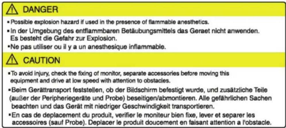
[Label 1. Marked on the sides of the product]
CAUTION
- To avoid any injury from improper use, read and understand all instructions in the User's Manual before attempting to use this system.
- Vor der Inbetriebnahme die Bedienungsanleitung unbedingt lesen, weil die Fehlanwendung des Gerätes zur Beschädigung führen kann.
•Lire attentivement le manuel avant utiliser le produit. Il y aurait le risque de se blesser a cause de l'usage abusif.
275-K-A026A
[Label 2. Marked on the bottom of the product]
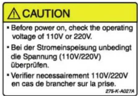
[Label 3. Marked below OUTLET]
Electrical Safety
This equipment has been verified as a Class I device with Type BF applied parts.
CAUTION
As for US requirement, the LEAKAGE CURRENT might be measured from a center-tapped circuit when the equipment connects in the United States to 240V supply system.
■ To help assure grounding reliability, connect to a “hospital grade” or “hospital only” grounded power outlet.
Prevention of Electric Shock
In a hospital, dangerous currents are due to the potential differences between connected equipment and touchable conducting parts found in medical rooms. The solution to the problem is consistent equipotential bonding. Medical equipment is connected with connecting leads made up of angled sockets to the equipotential bonding network in medical rooms.
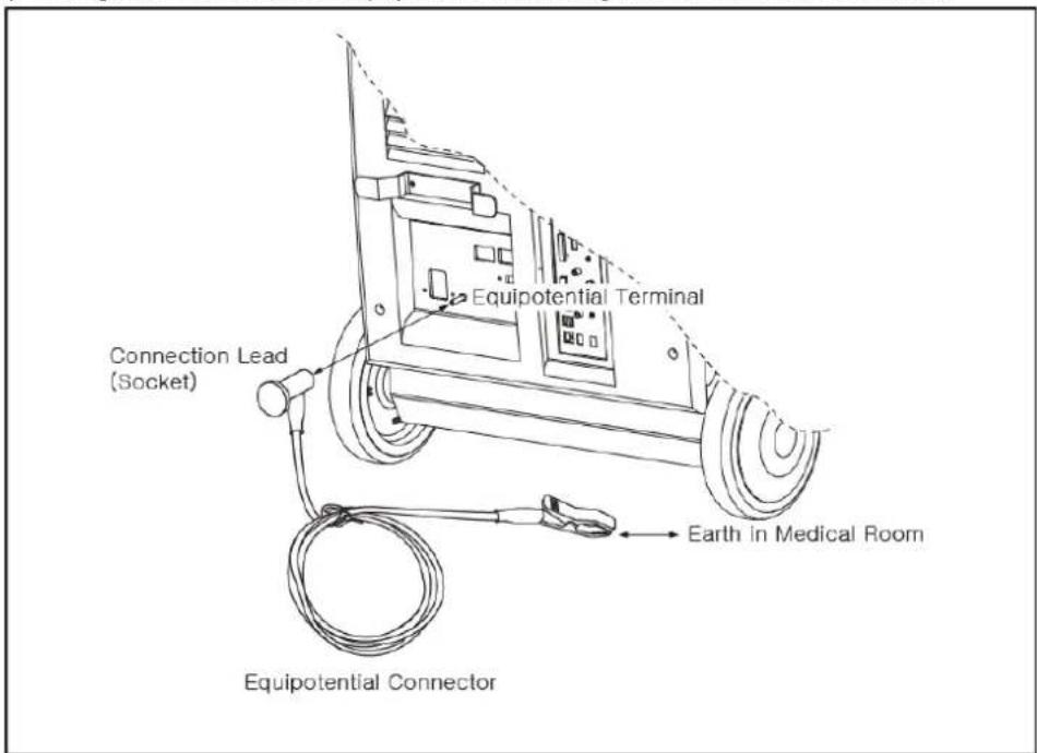
[Figure 1.1 Equipotential bonding]
All accessory equipment connected to the digital interfaces must be certified according to the representative IEC standards (i.e. IEC60950/EN60950 for data processing equipment and IEC60601-1/EN60601-1 for medical equipment). Furthermore all configurations should comply with the system standard IEC60601-1-1/EN60601-1-1. Anybody who connects additional equipment to the signal input part or signal output part configurations of a medical system is therefore responsible for the system complying with the requirements of IEC60601-1-1/EN60601-1-1.
| WARNING | ■ Electric shock may exist result if this system, including and all of its externally mounted recording and monitoring devices, is not properly grounded.■ Do not remove the covers on the system; hazardous voltages are present inside. Cabinet panels must be in place while the system is in use. All internal adjustments and replacements must be made by a qualified MEDISON Customer Service Department.■ Check the face, housing, and cable before use. Do not use, if the face is cracked, chipped, or torn, the housing is damaged, or if the cable is abraded.■ Always disconnect the system from the wall outlet prior to cleaning the system.■ All patient contact devices, such as probes and ECG leads, must be removed from the patient prior to application of a high voltage defibrillation pulse.■ Do not touch patient and the SIP/SOP on the rear panel simultaneously. Doing so may cause a leakage current exceeding the maximum allowable values.■ The use of flammable anesthetic gas or oxidizing gases (N20) should be avoided. |
| CAUITON | ■ The system has been designed for 100-120VAC and 200-240VAC; you should select the input voltage of monitor, printer and VCR. Prior to connecting an OEM power cord, verify that the voltage indicated on the power cord matches the voltage rating of the OEM device.■ An isolation transformer protects the system from power surges. The isolation transformer continues to operate when the system is in standby.■ Do not immerse the cable in liquids. Cables are not waterproof. |
ECG-Related Information
| WARNING | This device is not intended to provide a primary ECG monitoring function, and therefore does not have means of indicating an inoperative electrocardiograph.Do not use ECG electrodes of HF surgical equipment. Any malfunctions in the HF surgical equipment may result in burns to the patient.Do not use ECG electrodes during cardiac pacemaker procedures or other electrical stimulators.Do not use ECG leads and electrodes in an operating room. |
ESD
Electrostatic discharge (ESD), commonly referred to as a static shock, is a naturally occurring phenomenon. ESD is most prevalent during conditions of low humidity, which can be caused by heating or air conditioning. During low humidity conditions, electrical charges naturally build up on individuals, creating static electricity. An ESD occurs when an individual with an electrical energy build-up comes in contact with conductive objects such as metal doorknobs, file cabinets, computer equipment, and even other individuals. The static shock or ESD is a discharge of the electrical energy build-up from a charged individual to a lesser or non-charged individual or object.
CAUITON
■ The level of electrical energy discharged from a system user or patient to an ultrasound system can be significant enough to cause damage to the system or probes.
■ The following precautions can help to reduce ESD:
- Anti-static spray on carpets or linoleum
- Anti-static mats
- A ground wire connection between the system and the patient table or bed.
EMI
Although this system has been manufactured in compliance with existing Electromagnetic Interference (EMI) requirements, use of this system in the presence of an electromagnetic field can cause momentary degradation of the ultrasound image.
If this occurs often, MEDISON suggests a review of the environment in which the system is being used, to identify possible sources of radiated emissions. These emissions could be from other electrical devices used within the same room or an adjacent room. Communication devices such as cellular phones and pagers can cause these emissions. The existence of radios, TVs, or microwave transmission equipment nearby can also cause interference.
CAUTION
In cases where EMI is causing disturbances, it may be necessary to relocate this system.
EMC
The testing for EMC((Electromagnetic Compatibility)) of this system has been performed according to the international standard for EMC with medical devices (IEC60601-1-2). This IEC standard was adopted in Europe as the European norm (EN60601-1-2).
Guidance and manufacturer's declaration - electromagnetic emission
This product is intended for use in the electromagnetic environment specified below.
The customer or the user of this product should assure that it is used in such an environment.
| Emission test Compliance Electromagnetic environment -guidance | ||
| RF EmissionCISPR 11 | Group 1 | The Ultrasound System uses RF energy only for its internal function. Therefore, its RF emissions are very low and are not likely to cause any interference in nearby electronic equipment. |
| RF EmissionCISPR 11 | Class A | The Ultrasound System is suitable for use in all establishments, other than domestic and those directly connected to the public low-voltage power supply network that supplies buildings used for domestic purpose. |
| Harmonic EmissionIEC 61000-3-2 | Class A | |
| Flicker EmissionIEC 61000-3-3 | Complies | |
Approved Cables, Transducers and Accessories for EMC
1. Approved Cable for Electromagnetic Compliance
Cables connected to this product may affect its emissions; Use only the cable types and lengths listed below table.
| Cable | Type | Length |
| VGA | Shielded | Normal |
| Parallel | Shielded | Normal |
| RS232C | Shielded | |
| USB | Shielded | Normal |
| LAN(RJ45) | Twisted | pair |
| S-Video | Shielded | |
| Foot Switch Shielded 2.5m | ||
| B/W Printer Unshielded Coaxial Normal | ||
| MIC | Unshielded | Any |
| Printer Remote | Unshielded | Any |
| Audio R.L | Shielded | Normal |
| VHS | Shielded | Normal |
| ECG AUX input | Shielded < 3m | |
Normal
Normal
Any
2. Approved Transducer for Electromagnetic Compliance
The image transducer used with the ACCUVIX XQ Ultrasound System may affect its emission. The transducer listed in 'Chapter 8. Probes' when used with this product, have been tested to comply with the group1 class A emission as required by International Standard CISPR 11.
3. Approved Accessories for Electromagnetic Compliance
Accessories used with the ACCUVIX XQ Ultrasound System may effect its emissions.
| CAUTION | When connecting other customer-supplied accessories to the system, such as a remote printer or VCR, it is the user's responsibility to ensure the electromagnetic compatibility of the system. Use only CISPR 11 or CISPR 22, CLASS B compliant devices. | ||
| WARNING | The use of cables, transducers, and accessories other than those specified may result in increased emission or decreased Immunity of the Ultrasound System. | ||
| Immunity test IEC 60601 Test level Compliance level | Electromagnetic environment -guidance | ||
| Electrotatic discharge (ESD)IEC 61000-4-2 | ±6 KV Contact±8KV air | ±6KV Contact±8KV air | Floors should be wood, concrete or ceramic tile. If floors are covered with synthetic material, the relative humidity should be at least 30%. |
| Electrical fast transient/burstIEC 61000-4-4 | ±2 KV for power supply lines ±1 KV for input/output lines | ±2KV for power supply lines ±1 KV for input/output lines | Mains power quality should be that of a typical commercial or hospital environment. |
| SurgeIEC 61000-4-5 | ±1 KV differential mode±2KV common mode | ±1KV differential mode±2KV common mode | Mains power quality should be that of a typical commercial or hospital environment. |
| Voltage dips, short interruptions and voltage variations on power supply input linesIEC 61000-4-11 | <5% UT for 0.5cycle (>95% dip in UT)40% UT for 5 cycle (60% dip in UT)70% UT for 25 cycle (30% dip in UT)<5% UT for 5 s (<95% dip in UT) | <5% UT for 0.5cycle (>95% dip in UT)40% UT for 5 cycle (60% dip in UT)70% UT for 25 cycle (30% dip in UT)<5% UT for 5 s (<95% dip in UT) | Mains power quality should be that of a typical commercial or hospital environment. If the user of this product requires continued operation during power mains interruptions, it is recommended that this product is powered from an uninterruptible power supply or a battery. |
| Power frequency (50/60Hz) magnetic fieldIEC 61000-4-8 | 3 A/m 3 A/m | Power frequency magnetic fields should be at levels characteristic of a typical location in a typical commercial or hospital environment. | |
| NOTE UT is the a.c. mains voltage prior to application of the test level. | |||
| Immunity test | IEC 60601 Test level | Compliance level | Electromagnetic environment - guidance |
| Conducted RF IEC 61000-4-6 | 3 Vrms150 kHz to 80MHz | 0.01V | Portable and mobile RF communications equipment should be used no closer to any part of the Ultrasound System, including cables, than the recommended separation distance calculated from the equation applicable to the frequency of the transmitter.Recommended separation distance d = [ 3,5/V1 ] d = [ 3,5/E1 ] 80MHz to 800MHZ d = [ 7/E1 ] 800MHz to 2.5GHzwhere P is the maximum output power rating of the transmitter in watts (W) according to the transmitter manufacturer and d is the recommended separation distance in meters (m).Field strengths from fixed RF transmitters, as determined by an electromagnetic site survey, a should be less than the compliance level in each frequency range. b Interference may occur in the vicinity of equipment marked with the following symbol :(( ) ) |
| Radiated RF IEC 61000-4-3 | 3 V/m80 MHz to 2.5GHz | 3V/m | |
| NOTE 1) At 80MHz and 800MHz, the higher frequency range applies.NOTE 2) These guidelines may not apply in all situations. Electromagnetic propagation is affected by absorption and reflection from structures, objects and people. | |||
| a Field strengths from fixed transmitters, such as base stations for radio (cellular/cordless) telephones and land mobile radios, amateur radio, AM and FM radio broadcast and TV broadcast cannot be predicted theoretically with accuracy. To assess the electromagnetic environment due to fixed RF transmitters, an electromagnetic site survey should be considered. If the measured field strength in the location in which the Ultrasound System is used exceeds the applicable RF compliance level above, the Ultrasound System should be observed to verify normal operation. If abnormal performance is observed, additional measures may be necessary, such as re-orienting or relocating the Ultrasound System or using a shielded location with a higher RF shielding effectiveness and filter attenuation. b Over the frequency range 150kHz to 80MHz, field strengths should be less than [V 1 ] V/m. | |||
Recommended separation distances between portable and mobile RF communications equipment and the ACCUVIX XQ
This product is intended for use in an electromagnetic environment in which radiated RF disturbances are controlled. The customer or the user of the this product can help Prevent electromagnetic interference by maintaining a minimum distance between portable and mobile RF communications equipment (transmitters) and this product as recommended below, according to the maximum output power of the communications equipment.
| Rated maximum output power of transmitter [W] | Separation distance according to frequency of transmitter [m] | ||
| 150kHz to 80MHz d = [ 3,5/V1 ] | 80MHz to 800MHz d = [ 3,5/E1 ] | 800MHz to 2.5GHz d = [ 7/E1 ] | |
| V1=0.01Vrms | E1=3 V/m E | 1=3V/m | |
| 0.01 | 35.00 | 0.11 | |
| 0.1 | 110.68 | 0.36 | |
| 1 | 350.00 | 1.16 | 2.33 |
| 10 | 1106.80 | 3.68 | |
| 100 | 3500.00 | 11.66 | |
| For transmitters rated at a maximum output power not listed above, the recommended separation distance d in meters (m) can be estimated using the equation applicable to the frequency of the transmitter, where p is the maximum output power rating of the transmitter in watts (W) according to the transmitter manufacturer.NOTE 1) At 80MHz and 800MHz, the separation distance for the higher frequency range applies.NOTE 2) These guidelines may not apply in all situations. Electromagnetic propagation is affected by absorption and reflection from structures, objects and people. | |||
Electromagnetic environment – guidance
The Ultrasound System must be used only in a shielded location with a minimum RF shielding effectiveness and, for each cable that enters the shielded location. Field strengths outside the shielded location from fixed RF transmitters, as determined by an electromagnetic site survey, should be less than 3V/m.
It is essential that the actual shielding effectiveness and filter attenuation of the shielded location be verified to assure that they meet the minimum specification.
| CAUTION | If the system is connected to other customer-supplied equipment, such as a local area network (LAN) or a remote printer, Medison cannot guarantee that the remote equipment will work correctly in the presence of electromagnetic phenomena. |
Avoiding Electromagnetic Interference
A medical device can either generate or receive electromagnetic interference.
The EMC standards describe tests for both emitted and received interference.
Medison Ultrasound System do not generate interference in excess of the referenced standards.
An Ultrasound System is designed to receive signals at radio frequency and is therefore susceptible to interference generated by RF energy sources. Examples of other source of interference are medical device, information technology products, and radio and television transmission towers. Tracing the source of radiated interference can be a difficult task.
Customers should consider the following in an attempt to locate the source:
■ Is the interference intermittent or constant?
■ Does the interference show up only with one transducers operating at the same frequency or with several transducer?
■ Do two different transducer operating at the same frequency have the same problem?
Is the interference present if the system is moved to a different location in the facility?
The answers to these questions will help determine if the problem reside with the system or the scanning environment. After you answer the question, contact your Medison service representative.
Mechanical Safety
Moving the Equipment
Only the front wheels of the system can be used for steering. Therefore to maneuver the system in tight spaces, use repeated back-and-forth movements to position the system into the desired space. On rare occasions a component may become disconnected inside the system.
The components are installed securely and can withstand considerable shock, but excessive shock may cause system failure.
If the system operates abnormally after repositioning, please contact the MEDISON Customer Service Department.
The brakes are on the front wheels of the console. Press the brakes with your feet to lock or release them. You can use the brakes to control the movement of the product such as by preventing its movement while scanning.
| WARNING | ■ The system can weigh approximately 101kg (202lb), depending upon configuration, and could cause injury should it topple over.■ Be aware of the castors, especially when moving the system. MEDISON recommends that you exercise caution when moving the product up or down ramps.■ The monitor can be separated and easily removed from the unit if necessary. |
Safety Note
| CAUTION | ■ Never attempt to modify the product in any way.■ Please wait at least 10 seconds before rebooting the product. Otherwise, it may not function properly.■ Check the operational safety when using the product after a prolonged break in service.■ Make sure that other objects, such as metal pieces, do not enter the system.■ Do not block the ventilation slots.■ To prevent damage to the power cord, be sure to grip the plug head – not the cord – when unplugging.■ Excessive bending or twisting of cables on patient-applied parts may cause failure or intermittent operation of the system.■ Improper cleaning or sterilization of a patient-applied part may cause permanent damage. |
Please refer to "Chapter 7. Maintenance" for detailed information on protecting, cleaning and disinfecting the equipment.
Biological Safety
Verify the alignment of the biopsy guide before use. See the “Chapter 8. Probes” section of this manual.
WARNING
■ Ultrasound waves may have damaging effects on cells and, therefore, may be harmful to the patient. If there is no medical benefit, minimize the exposure time and maintain the ultrasound wave output level at low. Please refer to the ALARA principle.
- Do not use the system if an error message appears on the video display indicating that a hazardous condition exists. Note the error code, turn off the power to the system, and call your local MEDISON Customer Service Department.
- Do not use a system that exhibits erratic or inconsistent updating. Discontinuities in the scanning sequence are indicative of a hardware failure that should be corrected before use.
■ The system limits the maximum contact temperature to 43 degree Celsius, and the ultrasonic waves output observes American FDA regulations.
ALARA Principle
Guidance for the use of diagnostic ultrasound is defined by the “as low as reasonably achievable” (ALARA) principle. The decision as to what is reasonable has been left to the judgment and insight of qualified personnel. No set of rules can be formulated that would be sufficiently complete to dictate the correct response for every circumstance. By keeping ultrasound exposure as low as possible, while obtaining diagnostic images, users can minimize ultrasonic bioeffects.
Since the threshold for diagnostic ultrasound bioeffects is undetermined, it is the sonographer's responsibility to control the total energy transmitted into the patient. The sonographer must reconcile exposure time with diagnostic image quality. To ensure diagnostic image quality and limit exposure time, the ultrasound system provides controls that can be manipulated during the exam to optimize the results of the exam.
The ability of the user to abide by the ALARA principle is important. Advances in diagnostic ultrasound not only in the technology but also in the applications of the technology, have resulted in the need for more and better information to guide the user. The output indices are designed to provide that important information
There are a number of variables, which affect the way in which the output display indices can be used to implement the ALARA principle. These variables include mass, body size, location of the bone relative to the focal point, attenuation in the body, and ultrasound exposure time. Exposure time is an especially useful variable, because the user controls it. The ability to limit the index values over time support the ALARA principle.
| Applying ALARA
The system-imaging mode used depends upon the information needed. 2D-mode and M-mode imaging provide anatomical information, while Doppler, Power, and Color imaging provide information about blood flow. Scanned modes, like 2D-mode, Power, or Color, disperse or scatter the ultrasonic energy over an area, while an unscanned mode, like M-mode or Doppler, concentrates ultrasonic energy. Understanding the nature of the imaging mode being used allows the sonographer to apply the ALARA principle with informed judgment. The probe frequency, system set-up values, scanning techniques, and operator experience aid the sonographer in meeting the definition of the ALARA principle.
The decision as to the amount of acoustic output is, in the final analysis, up to the system operator. This decision must be based on the following factors: type of patient, type of exam, patient history, ease or difficulty of obtaining diagnostically useful information, and the potential localized heating of the patient due to probe surface temperatures. Prudent use of the system occurs when patient exposure is limited to the lowest index reading for the shortest amount of time necessary to achieve acceptable diagnostic results.
Although a high index reading does not mean that a bioeffect is actually occurring, a high index reading should be taken seriously. Every effort should be made to reduce the possible effects of a high index reading. Limiting exposure time is an effective way to accomplish this goal.
There are several system controls that the operator can use to adjust the image quality and limit the acoustic intensity. These controls are related to the techniques that an operator might use to implement ALARA. These controls can be divided into three categories: direct, indirect, and receiver control.
Direct Controls
Application selection and the output intensity control directly affect acoustic intensity. There are different ranges of allowable intensity or output based on your selection. Selecting the correct range of acoustic intensity for the application is one of the first things required during any exam. For example, peripheral vascular intensity levels are not recommended for fetal exams. Some systems automatically select the proper range for a particular procedure, while others require manual selection. Ultimately, the user bears the responsibility for proper clinical use. The MEDISON system provides both automatic and user-definable settings.
Output has direct impact on acoustic intensity. Once the application has been established, the output control can be used to increase or decrease the intensity output. The output control allows you to select intensity levels less than the defined maximum. Prudent use dictates that you select the lowest output intensity consistent with good image quality.
Indirect Controls
The indirect controls are those that have an indirect effect on acoustic intensity. These controls affect imaging mode, pulse repetition frequency, focus depth, pulse length, and probe selection.
The choice of imaging mode determines the nature of the ultrasound beam. 2D-mode is a scanning mode,
Doppler is a stationary or unscanned mode. A stationary ultrasound beam concentrates energy on a single location. A moving or scanned ultrasound beam disperses the energy over a wide area and the beam is only concentrated on a given area for a fraction of the time necessary in unscanned mode.
Pulse repetition frequency or rate refers to the number of ultrasound bursts of energy over a specific period of time. The higher the pulse repetition frequency, the more pulses of energy in a given period of time. Several controls affect pulse repetition frequency: focal depth, display depth, sample volume depth, color sensitivity, number of focal zones, and sector width controls.
Focus of the ultrasound beam affects the image resolution. To maintain or increase resolution at a different focus requires a variation in output over the focal zone. This variation of output is a function of system optimization. Different exams require different focal depths. Setting the focus to the proper depth improves the resolution of the structure of interest.
Pulse length is the time during which the ultrasonic burst is turned on. The longer the pulse, the greater the time-average intensity value. The greater the time-average intensity, the greater the likelihood of temperature increase and cavitations. Pulse length or burst length or pulse duration is the output pulse duration in pulsed Doppler. Increasing the Doppler sample volume increases the pulse length.
Probe selection affects intensity indirectly. Tissue attenuation changes with frequency. The higher the probe operating frequency, the greater the attenuation of the ultrasonic energy. Higher probe operating frequencies require higher output intensity to scan at a deeper depth. To scan deeper at the same output intensity, a lower probe frequency is required. Using more gain and output beyond a point, without corresponding increases in image quality, can mean that a lower frequency probe is needed.
Receiver Controls
Receiver controls are used by the operator to improve image quality. These controls have no effect on output. Receiver controls only affect how the ultrasound echo is received. These controls include gain, TGC, dynamic range, and image processing. The important thing to remember, relative to output, is that receiver controls should be optimized before increasing output. For example; before increasing output, optimize gain to improve image quality.
Additional Considerations
Ensure that scanning time is kept to a minimum, and ensure that only medically required scanning is performed. Never compromise quality by rushing through an exam. A poor exam will require a follow-up, which ultimately increases the time. Diagnostic ultrasound is an important tool in medicine, and, like any tool, should be used efficiently and effectively.
Output Display Features
The system output display comprises two basic indices: a mechanical index and a thermal index. The thermal index consists of the following indices: soft tissue (TIs), cranial bone (Tic) and bone (Tlb). One of these three thermal indices will be displayed at all times. Which one depends upon the system preset or user choice, depending upon the application at hand.
The mechanical index is continuously displayed over the range of 0.0 to 1.9, in increments of 0.1.
The thermal index consists of the three indices, and only one of these is displayed at any one time. Each probe application has a default selection that is appropriate for that combination. The Tlb or Tls is continuously displayed over the range of 0.0 to maximum output, based on the probe and application, in increments of 0.1.
The application-specific nature of the default setting is also an important factor of index behavior. A default setting is a system control state which is preset by the manufacturer or the operator. The system has default index settings for the probe application. The default settings are invoked automatically by the ultrasound system when power is turned on, new patient data is entered into the system database, or a change in application takes place.
The decision as to which of the three thermal indices to display should be based on the following criteria:
Appropriate index for the application: TIs is used for imaging soft tissue; and Tlb for a focus at or near bone.
Some factors might create artificially high or low thermal index readings e.g. presence of fluid or bone, or the flow of blood. A highly attenuating tissue path, for example, will cause the potential for local zone heating to be less than the thermal index displays.
Scanned modes versus unscanned modes of operation affect the thermal index. For scanned modes, heating tends to be near the surface; for unscanned modes, the potential for heating tends to be deeper in the focal zone.
Always limit ultrasound exposure time. Do not rush the exam. Ensure that the indices are kept to a minimum and that exposure time is limited without compromising diagnostic sensitivity.
Mechanical Index (MI) Display
Mechanical bioeffects are threshold phenomena that occur when a certain level of output is exceeded. The threshold level varies, however, with the type of tissue. The potential for mechanical bioeffects varies with peak pressure and ultrasound frequency. The MI accounts for these two factors. The higher the MI value, the greater the likelihood of mechanical bioeffects occurring but there is no specific MI value that means that a mechanical effect will actually occur. The MI should be used as a guide for implementing the ALARA principle.
Thermal Index (TI) Display
The TI informs the user about the potential for temperature increase occurring at the body surface, within body tissue, or at the point of focus of the ultrasound beam on bone. The TI is an estimate of the temperature increase in specific body tissues. The actual amount of any temperature rise is influenced by factors such as tissue type, vascularity, and mode of operation etc. The TI should be used as a guide for implementing the ALARA principle.
The bone thermal index (Tlb) informs the user about potential heating at or near the focus after the ultrasound beam has passed through soft tissue or fluid, for example, at or near second or third trimester fetal bone.
The cranial bone thermal index (Tlc) informs the user about the potential heating of bone at or near the surface, for example, cranial bone.
The soft tissue thermal index (TIs) informs the user about the potential for heating within soft homogeneous tissue.
You can select either TIs or Tlb using the TIs/Tlb selection on the Miscellaneous system setups. Tlc is displayed when you select a trans-cranial application.
Mechanical and Thermal indices Display Precision and Accuracy
The Mechanical and Thermal Indices on the system are precise to 0.1 units.
The MI and TI display accuracy estimates for the system are given in the Acoustic Output Tables manual. These accuracy estimates are based on the variability range of probes and systems, inherent acoustic output modeling errors and measurement variability, as described below.
The displayed values should be interpreted as relative information to help the system operator achieve the ALARA principle through prudent use of the system. The values should not be interpreted as actual physical values investigated tissue or organs. The initial data that is used to support the output display is derived from laboratory measurements based on the AIUM measurement standard. The measurements are then put into algorithms for calculating the displayed output values.
Many of the assumptions used in the process of measurement and calculation are conservative in nature. Over-estimation of actual in situ exposure, for the vast majority of tissue paths, is built into the measurement and calculation process. For example:
The measured water tank values are de-rated using a conservative, industry standard, attenuation coefficient of 0.3dB/cm-MHz.
Conservative values for tissue characteristics were selected for use in the TI models. Conservative values for tissue or bone absorption rates, blood perfusion rates, blood heat capacity, and tissue thermal conductivity were selected.
Steady state temperature rise is assumed in the industry standard TI models, and the assumption is made that the ultrasound probe is held steady in one position long enough for steady state to be reached.
A number of factors are considered when estimating the accuracy of display values: hardware variations, algorithm accuracy estimation and measurement variability. Variability among probes and systems is a significant factor. Probe variability results from piezoelectric crystal efficiencies, process-related impedance differences, and sensitive lens focusing parameter variations. Differences in the system pulse voltage control and efficiencies are also a contributor to variability. There are inherent uncertainties in the algorithms used for estimating acoustic output values over the range of possible system operating conditions and pulse voltages. Inaccuracies in laboratory measurements are related to differences in hydrophone calibration and performance, positioning, alignment and digitization tolerances, and variability among test operators.
The conservative assumptions of the output estimation algorithms of linear propagation, at all depths, through a 0.3dB/cm-MHz attenuated medium are not taken into account in calculation of the accuracy estimate displayed. Neither linear propagation, nor uniform attenuation at the 0.3dB/cm-MHz rate, occur in water tank measurements or in most tissue paths in the body. In the body, different tissues and organs have dissimilar attenuation characteristics. In water, there is almost no attenuation. In the body, and particularly in water tank measurements, non-linear propagation and saturation losses occur as pulse voltages increase.
The display accuracy estimates take into account the variability ranges of probes and systems, inherent acoustic output modeling errors, and measurement variability. Display accuracy estimates are not based on errors in, or caused by measuring according to, the AIUM measurement standards. They are also independent of the effects of non-linear loss on the measured values.
Control affecting the indices
As various system controls are adjusted, the TI and MI values may change. This will be most apparent as the POWER control is adjusted; however, other system controls will affect the on-screen output values.
Power
Power controls the system acoustic output. Two real-time output values are on the screen: a TI and a MI. They change as the system responds to POWER adjustments.
In combined modes, such as simultaneous Color, 2D-mode and pulsed Doppler, the individual modes each add to the total TI. One mode will be the dominant contributor to this total. The displayed MI will be from the mode with the largest peak pressure.
2D mode Controls
2D-mode size
Narrowing the sector angle may increase the frame rate. This action will increase the TI. Pulse voltage may be automatically adjusted down with software controls to keep the TI below the system maximums. A decrease in pulse voltage will decrease MI.
Zoom
Increasing the zoom magnification may increase frame rate. This action will increase the TI. The number of focal zones may also increase automatically to improve resolution. This action may change MI since the peak intensity can occur at a different depth.
Persistence
A lower persistence will decrease the TI. Pulse voltage may be automatically increased. An increase in pulse voltage will increase MI.
Focal no.
More focal zones may change both the TI and MI by changing frame rate or focal depth automatically. Lower frame rates decrease the TI. MI displayed will correspond to the zone with the largest peak intensity.
Focus
Changing the focal depth will change the MI. Generally, higher MI values will occur when the focal depth is near the natural focus of the transducer.
Color and Power Controls
Color Sensitivity
Increasing the color sensitivity may increase the TI. More time is spent scanning for color images.
Color pulses are the dominant pulse type in this mode.
Color Sector Width
Narrower color sector width will increase color frame rate and the TI will increase. The system may automatically decrease pulse voltage to stay below the system maximum. A decrease in pulse voltage will decrease the MI. If pulsed Doppler is also enabled then pulsed Doppler will remain the dominant mode and the TI change will be small.
Color Sector Depth
Deeper color sector depth may automatically decrease color frame rate or select a new color focal zone or color pulse length. The TI will change due to the combination of these effects. Generally, the TI will decrease with increased color sector depth. MI will correspond to the peak intensity of the dominant pulse type, which is a color pulse. However, if pulsed Doppler is also enabled then pulsed Doppler will remain the dominant mode and the TI change will be small.
Scale
Using the SCALE control to increase the color velocity range may increase the TI. The system will automatically adjust pulse voltage to stay below the system maximums. A decrease in pulse voltage will also decrease MI.
Sec Width
A narrower 2D-mode sector width in Color imaging will increase color frame rate. The TI will increase. MI will not change. If pulsed Doppler is also enabled, then pulsed Doppler will remain as the primary mode and the TI change will be small.
M-mode and Doppler Controls
Speed
M-mode and Doppler sweep speed adjustments will not affect the MI. When M-mode sweep speed changes, TI changes.
Simultaneous and Update Methods
Use of combination modes affects both the TI and MI through the combination of pulse types. During simultaneous mode, the TI is additive. During auto-update and duplex, the TI will display the dominant pulse type. The displayed MI will be from the mode with the largest peak pressure.
Sample Volume Depth
When Doppler sample volume depth is increased the Doppler PRF may automatically decrease. A decrease in PRF will decrease the TI. The system may also automatically decrease the pulse voltage to remain below the system maximum. A decrease in pulse voltage will decrease MI.
Doppler, CW, M-mode, and Color Imaging Controls
When a new imaging mode is selected, both the TI and the MI will change to default settings. Each mode has a corresponding pulse repetition frequency and maximum intensity point. In combined or simultaneous modes, the TI is the sum of the contribution from the modes enabled and MI is the MI for the focal zone and mode with the largest derated intensity. If a mode is turned off and then reselected, the system will return to the previously selected settings.
Probe
Each probe model available has unique specifications for contact area, beam shape, and center frequency. Defaults are initialized when you select a probe. MEDISON factory defaults vary with probe, application, and selected mode. Defaults have been chosen below the FDA limits for intended use.
Depth
An increase in 2D-mode depth will automatically decrease the 2D-mode frame rate. This would decrease the TI. The system may also automatically choose a deeper 2D-mode focal depth. A change of focal depth may change the MI. The MI displayed is that of the zone with the largest peak intensity.
Application
Acoustic output defaults are set when you select an application. MEDISON factory defaults vary with probe, application, and mode. Defaults have been chosen below the FDA limits for intended use.
Related Guidance Documents
For more information about ultrasonic bioeffects and related topics refer to the following;
AIUM Report, January 28, 1993, "Bioeffects and Safety of Diagnostic Ultrasound"
■ Bioeffects Considerations for the Safety of Diagnostic Ultrasound, J Ultrasound Med., Sept. 1998: Vol. 7, No. 9 Supplement
■ Acoustic Output Measurement Standard for Diagnostic Ultrasound Equipment. (AIUM, NEMA. 1998)
■ Acoustic Output Labeling Standard for Diagnostic Ultrasound Equipment (AIUM, 1998)
■ Second Edition of the AIUM Output Display Standard Brochure, Dated March 10, 1994. (A copy of this document is shipped with each system.)
■ Information for Manufacturer Seeking Marketing Clearance of Diagnostic Ultrasound Systems and Transducers. FDA. September 1997. FDA.
■ Standard for Real-Time Display of Thermal and Mechanical Acoustic Output Indices on Diagnostic Ultrasound Equipment. (Revision 1, AIUM, NEMA. 1998)
■ WFUMB. Symposium on Safety of Ultrasound in Medicine: Conclusions and Recommendations on Thermal and Non-Thermal Mechanisms for Biological Effects of Ultrasound, Ultrasound in Medicine and Biology, 1998: Vol. 24, Supplement1.
Acoustic Output and Measurement
Since the first usage of diagnostic ultrasound, the possible human biological effects (bioeffects) of ultrasound exposure have been studied by various scientific and medical institutions. In October 1987, the American Institute of Ultrasound in Medicine(AIUM) ratified a report prepared by its Bioeffects Committee (Bioeffects Considerations for the Safety of Diagnostic Ultrasound, J Ultrasound Med., Sept. 1988: Vol.7, No.9 Supplement), sometimes referred to as the Stowe Report, which reviewed available data on possible effects of ultrasound exposure. Another report “Bioeffects and Safety of Diagnostic Ultrasound,” dated January 28, 1993 provides more up to date information.
The acoustic output for this system has been measured and calculated in accordance with the December 1985 "510(K) Guide for Measuring and Reporting Acoustic Output of Diagnostic Ultrasound Medical Devices," except that the hydrophone meets the requirements of "Acoustic Output Measurement Standard for Diagnostic Ultrasound Equipment" (NEMA UD 2-1992)
In Situ, Derated, and Water Value Intensities
All intensity parameters are measured in water. Since water does not absorb acoustic energy, these water measurements represent a worst case value. Biological tissue does absorb acoustic energy. The true value of the intensity at any point depends on the amount and type of tissue and the frequency of the ultrasound that passes through the tissue. The intensity value in the tissue, In Situ, has been estimated using the following formula:
In Situ = Water [e-]23.0(alf) where: In Situ = In Situ Intensity Value
Water = Water Value Intensity
e = 2.7183
a = Attenuation Factor
Tissue a(dB/cm-MHz)
Brain .53
Heart .66
Kidney .79
Liver .43
Muscle .55
I = skin line to measurement depth (cm)
f = Center frequency of the transducer/system/mode combination(MHz)
Since the ultrasonic path during an examination is likely to pass through varying lengths and types of tissue, it is difficult to estimate the true In Situ intensity. An attenuation factor of 0.3 is used for general reporting purpose; therefore, the In Situ value which is commonly reported uses the formula:
In Situ (derated) = Water [e ^ - ] ^ 0 6 9. 0 (lf
Since this value is not the true In Situ intensity, the term "derated" is used.
The maximum derated and the maximum water values do not always occur at the same operating condition; therefore, the reported maximum water and derated values may not be related to the In Situ (derated) formula. Take for example a multi-zone array transducer that has maximum water value intensities in its deepest zone: the same transducer may have its largest derated intensity in one if its shallowest focal zones.
Acoustic Output and Measurement
The terms and symbols used in the acoustic output tables are defined in the following paragraphs.
ISPTA.3 The derated spatial-peak temporal-average intensity (milliwatts per square centimeter).
ISPPA.3 The derated spatial-peak pulse-average intensity (watts per square centimeter). The value of IPA.3 at the position of global maximum MI (IPA.3@MI) may be reported instead of ISPPA.3 if the global maximum MI is reported.
MI The Mechanical Index. The value of MI at the position of ISPPA.3, (MI@ISPPA.3) may be reported instead of MI (global maximum value) if ISPPA.3 is 190W/cm 2
Pr.3 The derated peak rarefactional pressure (megapascals) associated with the transmit pattern giving rise to the reported MI value.
WO The ultrasonic power (milliwatts). For the operating condition giving rise to ISPTA.3, WO is the total time-average power;. For operating conditions subject to reporting under ISPPA.3, WO is the ultrasonic power associated with the transmit pattern giving rise to the value reported under ISPPA.3
fc The center frequency (MHz). For MI and ISPPA.3, Fc is the center frequency associated with the transmit pattern giving rise to the global maximum value of the respective parameter. For ISPTA.3, for combined modes involving beam types of unequal center frequency, Fc is defined as the overall range of center frequencies of the respective transmit patterns.
ZSP The axial distance at which the reported parameter is measured (centimeters).
x-6,y-6 are respectively the in-plane (azimuth) and out-of-plane (elevation) -6 dimensions in the x-y plane where ZSP is found (centimeters).
| PD | The pulse duration (microseconds) associated with the transmit pattern giving rise to the reported value of the respective parameter. |
| PRF | The pulse repetition frequency (Hz) associated with the transmit pattern giving rise to the reported value of the respective parameter. |
| EBD | The entrance beam dimensions for the azimuth and elevation planes (centimeters). |
| EDS | The entrance dimensions of the scan for the azimuth and elevation planes (centimeters). |
Acoustic Measurement Precision and Uncertainty
The Acoustic Measurement Precision and Acoustic Measurement Uncertainty are described below.
| Quantity | Precision | Total Uncertainty |
| PII.3 (derated pulse intensity integral) 3.2 % +21 % to - 24 % | ||
| Wo (acoustic power) 6.2 % +/- 19 % | ||
| Pr.3 (derated rarefaction pressure) 5.4 % +/- 15 % | ||
| Fc (center frequency) < 1 % | +/- 4.5 % |
Systematic Uncertainties.
For the pulse intensity integral, derated rarefaction pressure Pr.3, center frequency and pulse duration, the analysis includes considerations of the effects on accuracy of:
Hydrophone calibration drift or errors.
Hydrophone / Amp frequency response.
Spatial averaging.
Alignment errors.
Voltage measurement accuracy, including.
- Oscilloscope vertical accuracy.
- Oscilloscope offset accuracy.
- Oscilloscope clock accuracy.
- Oscilloscope Digitization rates.
- Noise.
The systematic uncertainties Acoustic power measurements using a Radiation Force are measured through the use of calibrated NIST acoustic power sources.
We also refer to a September 1993 analysis done by a working group of the IEC technical committee 87 and prepared by K. Beissner, as a first supplement to IEC publication 1161.
The document includes analysis and discussion of the sources of error / measurement effects due to:
Balance system calibration.
Absorbing (or reflecting) target suspension mechanisms.
Linearity of the balance system.
Extrapolation to the moment of switching the ultrasonic transducer (compensation for ringing and thermal drift).
Target imperfections.
Absorbing (reflecting) target geometry and finite target size.
Target misalignment.
Ultrasonic transducer misalignment.
Water temperature.
Ultrasonic attenuation and acoustic streaming.
Coupling or shielding foil properties.
Plane-wave assumption.
Environmental influences.
Excitation voltage measurement.
Ultrasonic transducer temperature.
Effects due to nonlinear propagation and saturation loss.
The overall findings of the analysis give a rough Acoustic Power accuracy figure of +/- 10% for the frequency range of 1 - 10 MHz.
Environmental Protection
CAUTION
■ The console and peripherals could be sent back to manufacturers for recycling or proper disposal after their useful lives.
■ Disposal of waste shall be disposed in accordance with national laws.
■ The waste sheaths are to be disposed of safely and national regulations must be observed.
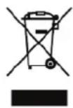
Waste Electrical and Electronic Equipment
This symbol is applied in the European Union and other European countries.
This symbol on the product indicates that this product shall not be treated as household waste. Instead it shall be handed over to the applicable collection point for the recycling of electrical and electronic equipment. By ensuring this product is disposed of correctly, you will help prevent potential negative consequences for the environment and human health, which could otherwise be caused by inappropriate waste handling of this product. The recycling of materials will help to conserve natural resources. For more detailed information about recycling of this product, please contact your local city office, your electrical and electronic waste disposal service or the shop where you purchased the product.
Chapter 2
Introduction and Installation
What is ACCUVIX XQ? 2
FEATURES AND ADVANTAGES OF ACCUVIX XQ 2
Specifications ....3
Product Configuration and Installation ....7
MONITOR 7
CONTROL PANEL 9
CONSOLE 17
PERIPHERALS 21
PROBES 23
ACCESSORIES 24
OPTIONS 25
What is ACCUVIX XQ?
ACCUVIX XQ is color ultrasonic diagnostic equipment with high resolution and high penetration. It provides a wide variety of easy-to-use measurement functions.
Features and Advantages of ACCUVIX XQ
- Cutting-Edge Digital Beam Forming Technology – ACCUVIX XQ leverages on MEDISON's independently developed technology.
- Various Applications – ACCUVIX XQ can be used in a wide variety of applications, including in the abdomen, obstetrics, gynecology, the vascular system, cardiology, and urology.
- Various Diagnosis Modes – ACCUVIX XQ provides various diagnosis modes, including 2D mode, M mode, Color Doppler mode, Power Doppler mode, PW Spectral Doppler mode, and CW Spectral Doppler mode.
■ 3D Imaging Function – ACCUVIX XQ is capable of acquiring three-dimensional images of superior quality by using the mechanical scan type 3D probe for its 3D imaging function.
■ VOCAL (Virtual Organ Computer Aided anaLysis) - ACCUVIX XQ can express internal organs in 3D images.
■ Measurement and Reporting Function – ACCUVIX XQ provides not only the basic measurement functions such as distance, area, circumference, and volume but a wide variety of different measurement functions for each application. Also, a reporting function based on measurement results is available.
■ Scanned Image Examination Function - ACCUVIX XQ provides 2,048 frames of Cine memory, and 4,096 lines of Loop imaging.
■ SonoView Function - SonoView is an integrated image filing program that enables users to store, load and share images
■ DICOM (Digital Imaging and Communication in Medicine) Function – Images can be saved, transmitted, and printed out over the network.
■ Good connectivity - ACCUVIX XQ provides good connectivity to Peripheral Devices
Specifications
| Physical Dimensions | Height: 1499.3mm (with monitor)Width: 657.1mmDepth: 1102mmWeight: 134kg for fully configured system | |
| Imaging modes | 2D real-timeDual 2D real-time2D/M modeColor DopplerPulsed Wave DopplerContinuous Wave DopplerPower Doppler3D modeFree Angle M modeDual Live modeSimultaneousReal-time zoom | |
| Focusing | Dynamic transmit focusing, maximum of eight points (four points simultaneously selectable)Digital dynamic receive focusing (continuous) | |
| Displayed Levels of Gray and Color | 256 shades of gray, 8 bits16,777,216 colors, 8 bits for each RGB component | |
| Probes | Curved Linear Array | C3-7IMC2-6ICC5-2EL (Domestic market only)C4-9EDC1-4EC |
| Endocavity Curved Linear Array | EC4-9ISEC4-9ES | |
| Linear Array | L5-12IML6-12ISL8-15ISL5-9EEL4-7EL | |
| Volume Probe | VAW3-5VAW4-7VNA6-12VDW5-8B3D3-5EK3D4-7EK3D4-8ET3D5-8EK3D2-6ET | |
| Phased Array | P2-4ACP3-5ACP3-7AC | |
| Static CW | CW2.0CW4.0 | |
| Probe connections | 5 probe connectors (including CW probe connector) | |
| Control Panel | - Dedicated keyboard controls and Touch panel soft-keys- Central home position controls- Shortcuts for many functions- Functional grouping of keys- Positive feedback on control actuation- Indicator lights identify activated keys- Lighting of control panel labels- Peripherals controlled through the system keyboard- 2-button footswitch- Audio volume control- Side access to system power On/Off button | |
| Monitor | - 15 inch high resolution non-interlaced color monitor- Resolution: 800 x 600 x 24bit- Brightness control with quick return to a pre-set calibrated level- Contrast control with quick return to a pre-set calibrated level- Degauss control- High brightness & contrast | |
| Application | General, Gynecology, Abdomen, OB, Renal, Urology, Pediatric, Vascular, Small Parts, Fetal Heart, Cardiac, Breast, Neonatal, OB Early, TCD, Musculoskeletal, Pediatric Cardiology, Pediatric Abdomen, Contrast Agent | |
| Signal processing (Pre-processing) | TGC controlMode-independent gain controlAcoustic power control (adjustable)Dynamic apertureDynamic apodizationDynamic range control (adjustable)Image view area controlM-mode sweep speed control | |
| Signal processing (Post-processing) | Frame averageGamma-scale windowingHistogramImage orientation (left/right and up/down)White on black / Black on whiteReal-time zoom | |
| Measurement Packages | ObstetricsGynecologyCardiologyFetal EchoVascular (Carotid, Upper Extremity, Lower Extremity, Varicose)UrologyRadiology* Refer the Chapter 5 for additional information | |
| Calipers and General Measurements | Trackball operation of multiple cursors2D: Linear measurements and area measurements using elliptical approximation or traceM-mode: Continuous readout of distance, time, and slope rateDoppler: Velocity and trace | |
| Image Storage | Cineloop memory (maximum 2048 frames)Image filing system | |
| Volume Mode | - Live 3D, Static 3D, Freehand 3D- System Maximum Volume Frame Rate: 18Hz- Multi-planar view display- VolumeCT, VOCAL, SHELL, Magicut plus, 3D Measure- Optimum volume resolution- Various 3D rendering algorithm- Gray & Color mode- 3D Smart Controller (to be updated)- 3D XI TM - STIC (Optional) | |
| Ultrasound Workstation | Pentium IV, Hard Drive: 40GB or 80GB, RAM size: max.2GB, Windows 2000, 1.3GB magneto-optical disc drive | |
| Optional Devices | - VCR: Panasonic AG-MD835 SVHC (NTSC & PAL), SONY SVO-9500MD (NTSC & PAL)- Video Page Printer: Mitsubishi M90E B/W page printer (120V/240V, NTSC & PAL, 3" x 4" format)- Color Video Page Printer: Mitsubishi CP700U color page printer (120V NTSC), Mitsubishi CP700E color page printer (240V PAL)- Foot Switch: The functions of Left & Right Foot Pedals can be selected in Setup Mode. Freeze, Update, Record, Print, Store, Volume Start | |
| Peripheral Signals | RGB Sync, S-VHS and VHS, Video Patient Monitor, Audio left & right, VGA, RS-232C, Parallel port, DICOM, USB port, Microphone, Patient Monitor 9V dc power, Printer B/W and Print Remote | |
| Electrical Parameters | 100-120VAC/200-240VAC, 15A/8A, 50/60Hz | |
| Pressure Limits | Operating: 700hPa to 1060hPaStorage: 700hPa to 1060hPa | |
| Humidity Limits | Operating: 30% to 75%Storage & Shipping: 20% to 95% | |
| Temperature Limits | Operating: 10°C ~ 35°CStorage & Shipping: -25 °C ~ 60°C | |
Product Configuration and Installation
This product consists of the monitor, control panel, console, peripheral devices, and probes.
Monitor
The VGA monitor displays ultrasound images and other related information. The monitor is connected to the console by an arm so that it can be moved to any desired position.
Monitor Display
The monitor displays ultrasound images, related information, and menu items that allow the user to control the system. The screen consists of the title, the image area, and the feedback area as illustrated below.
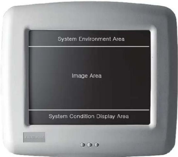
[Figure 2.1 Monitor Display]
Title
The title displays the logo, patient information, institution name, application, frame rate, frame depth, probe information, acoustic output information, and date and time.

[Figure 2.2 Title]
Image Area
The image area displays the ultrasound image, image information, annotation, and measurement information.
![[2D] G50 / 90dB FA10 / P90 FS10 * PG : 0](/content/2026/05/955519/images/0c8dfcb7f8b5345bfbe9b72a52cdbdba3e10170ba4f3be90822cca178e577126.jpg)
[Figure 2.3 Image Area]
Feedback Area
The feedback area displays the currently selected mode, the status of the trackball function, and the image freeze indication.
■ Feedback Information: Displays a variety of system information, such as the current system status, available items, and body marker, while using the system.

[Figure 2.4 Body Marker Feedback]
Control Panel
The user controls the system by using the control panel. The control panel includes the touch screen and the keyboard for added convenience.
The touch screen, in particular, allows easy setting of menu values for each mode.
NOTE
When installing the product or using it for the first time, please make sure that the alpha-numeric keyboard cover is removed before use.
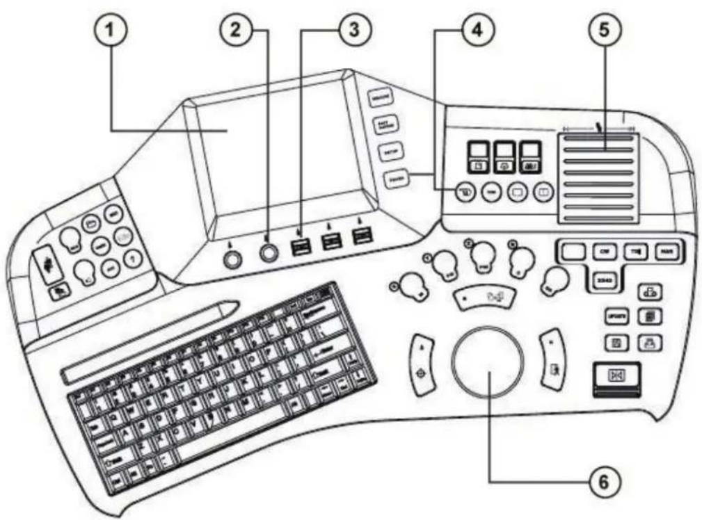
[Figure 2.5 Control Panel]
The user can manipulate the control panel using ① Touch Screen, ② Knob-Button, ③ Up down Switch, ④ Button, ⑤ Slide and ⑥ Track Ball.
NOTE
Knob-buttons can not only be turned clockwise and counterclockwise to change values but can also be pressed to perform certain functions.
Using Touch Screen
The touch screen displays the image adjustment menu, measurement menu and utility menu. The user can make necessary adjustments by pressing the menu items on the touch screen.
Values for the menu items across the bottom of the touch screen can be adjusted using the Knob-buttons and the Up-down switches on the control panel.
SonoView and other functions displayed on the monitor screen can be selected by using the touch screen or by using the Trackball and the Set button.
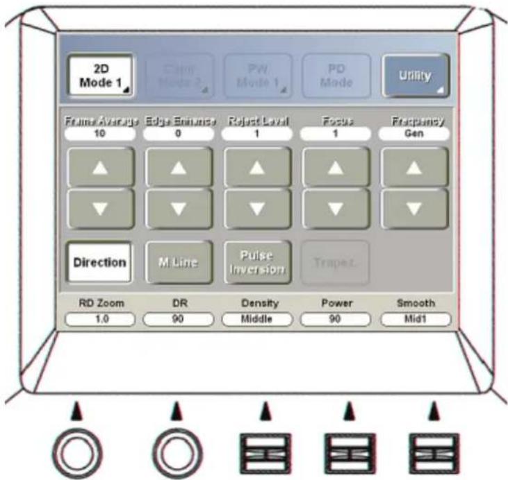
[Figure 2.6 Control Panel]
Control Panel Functions
The following are descriptions and usage instructions for the controls on the control panel. For detailed information on controls with multiple functions, please refer to "Chapter 3" and later parts of this manual.
Saving and Printing
 | Freeze | Press this to freeze the image being scanned.Frozen images can be saved, printed, measured, or used in the Cine function. Press the button again to return to Scan mode.This button is used as the Volume Start button in 3D View mode. |
 | Save | Press this to save the report for the current image and measurement results into the database. Saved images and reports are easily managed by SonoView. |
 | Echo Print | Press this to print the current image using the echo printer configured. |
 | Update | Press this to perform the available option for the current diagnosis mode. For example, this button selects the image to activate in Dual mode. In this case, pressing the button once activates the image on the right, and pressing it once again freezes the image on the right and activates the image on the left.This button holds the 2D image and releases it in Spectral Doppler mode. |
 | Report | Press this to activate the Report program that shows measurement results, etc. for the selected application. |
 | Record | Press this to record the currently displayed images onto the VCR. Press the button once again stop recording. |
Selecting Diagnosis Mode and Adjusting Gain
NOTE
For detailed information on modes, please refer to "Chapter 4. Diagnosis Modes."
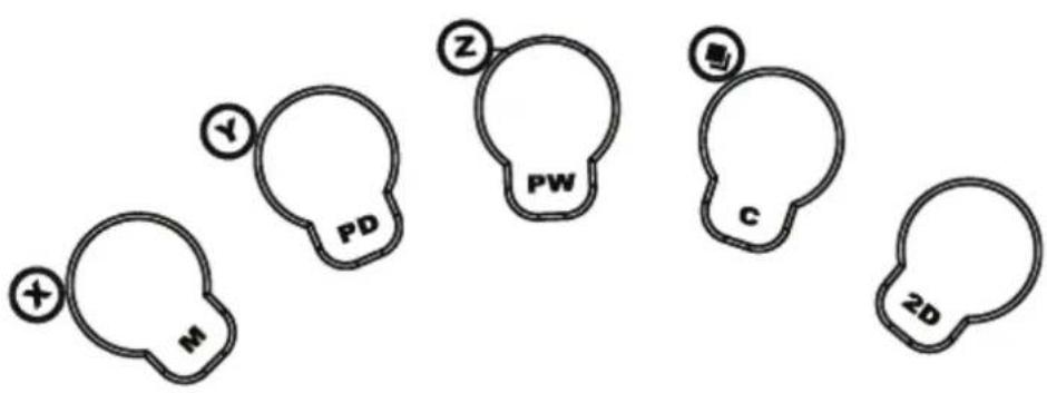
| 2D & 2D Gain | Use this to observe the anatomy by real-time images in the depth direction of the scanned surface.Once the 2D knob-button is set to On, it cannot be set to Off by pressing it again. You can return from any image mode to 2D mode by pressing the 2D button.Turn the knob-button to adjust 2D Gain. | |
| M & 2D Gain | This is used for M mode. It specifies the observation line on the 2D image and shows the changes on the line as time passes. Press the button again to set it to Off.Turn the knob-button to adjust 2D Gain.This button is used to rotate the image by the X-axis in 3D View mode. | |
| C & C Gain | This is used for Color mode. It shows the real-time blood flow pattern on 2D images. Press the button again to set it to Off.Turn the knob-button to adjust Color Doppler Gain.This button is used to move the reference image forward/backward in 3D View mode. | |
| PW & PW Gain | This is used for PW Spectral Doppler mode. It shows the blood flow in vessels or in the heart. This is very useful as it can be used simultaneously with 2D mode. Press the button again to set it to Off.Turn the knob-button to adjust PW Spectral Doppler Gain.This button is used to rotate the image by the Z-axis in 3D View mode. | |
| PD & PD Gain | This is used for Power Doppler mode. It shows the presence of blood flow and information on the blood flow amount on the 2D screen.Press the button again to set it to Off.Turn the knob-button to adjust Power Doppler Gain.This button is used to rotate the image by the Y-axis in 3D View mode. | |
 | Dual | This is used for Dual mode. Two 2D images can be compared against each other. The Set button, the Dual button and the Update button can be used to select the left image or the right image in Dual mode. Press the 2D button again to set it to Off. |
 | Dual Live | This is used for 2D mode, Color mode, and Power Doppler mode. Press the button to display the mode image on the left/right-hand side of the screen.Selecting it in 2D mode or Color mode displays a 2D image or Color Doppler image on the screen, and selecting it in Power Doppler mode displays a Power Doppler image and 2D image on the screen.Press the button again to set it to Off. |
 | Harmonic | This is used for Harmonic Imaging mode.Press the button again to set it to Off. Functionality of this button is optional. |
 | CW | This is used for CW Spectral Doppler mode. This is available only for Phased Array probe and Static CW probe.Press the button again to set it to Off. |
 | TDI | Press this to execute the Tissue Doppler Image function.This is used for Color mode, Power Doppler mode, and PW Spectral Doppler mode. This is available only for the Phased Array probe under the Cardiac or Pediatric Cardiology applications.Press the button again to set it to Off. |
 | 3D/4D | This is used for 3D mode. This is available in 2D mode. 3D is not available while in Cine status. Press the button again to set it to Off. |
Image Adjustments
 | Focus | Use this to move the focal point to the target position. Lift the switch to move the focal point up and depress the switch to move the focal point down. |
 | Depth | Use this to adjust the depth of the image being observed. Lift the switch to decrease the depth of the image and depress the switch to increase the depth of the image. |
 | Zoom | Lifting the switch brings up the Zoom box. Use the Change button and the Trackball to resize the Zoom box, and then press the Set button to apply the size. To quit Zoom mode, press the Exit button or adjust the Depth up-down switch. Use the Trackball to move around the zoomed area. |
TGC (Time Gain Control)
 | TGC(Time Gain Control) | The 8 slides are used to adjust TGC for each depth level. |
CAUTION
Take note that the image may show lines if the Gain values for adjacent slides are set at too great a difference.
Measurements and Annotations
 | Measurement | Press this to display on the touch screen the available measurement menu items for each application and diagnosis mode. You can select a menu item and take relevant measurements.Press the Caliper button on the touch screen to take basic measurements such as distance and circumference. For detailed information, please refer to “Chapter 5. Measurements.” |
 | Body Marker | Press this to display the Body Marker list on the touch screen. This function draws specified Body Markers on the image. |
 | Indicator | Press this to display arrow-shaped Indicators on the image. |
 | Text | Use this function to place text on the image. |
 | Clear | Press this to delete the text, indicators, body markers and measurement results from the image. |
NOTE
For detailed information, please refer to "Chapter 6. Image Management."
Trackball and Its Controls
 | Trackball | Use this to move the cursor around the screen.In Cine Display mode, the Trackball can be used for Navigating around images. |
 | Change | Press this to change the current Trackball function.For example, when specifying two pointsfor measurements, this button can be used to modify the previously selected point. |
 | Exit | Press this to quit the current function and returns to the previous state. |
 | Set | Press this to select the items or values specified by the Trackball. |
Utility
 | SonoView | Press this to execute the image filing program, SonoView. | |
 | Sound | Press the knob-button to set Sound On/Off, or turn the knob-button to adjust the volume.This is used for Spectral Doppler mode and other similar modes. | |
 | ECG | Press the knob-button to execute ECG. Pressing the knob-button while ECG is running sets the Trigger On/Off.When the Trigger is On, turn the knob-button to adjust Trigger Time, and when the Trigger is Off, turn the knob-button to adjust ECG Position.ECG-related setting values can be specified through the touch screen. | |
 | User | Press this to execute the function assigned to the User button. The User value can be specified through the touch screen. | |
 | The last saved image is transmitted to the e-mail address specified in the patient information. An alert message will appear if there is a problem in the network configuration or connection.If the e-mail information has not been entered, pressing the E-Mail button brings up the patient information screen. | ||
 | AIO | This button is used for 2D mode and Spectral Doppler mode. The Auto Image Optimization function will be executed to provide optimized images to the user. |
 | FSI | The Full Spectrum Image function will be executed to provide a sharper display of images being scanned. There are three levels of FSI, which is indicated on the screen as “FSI 0” and so on. |
Setup
 | Probe | Press this to display on the touch screen the screen where the probe or the application can be selected or changed. |
 | Setup | Press this to display the Setting screen where system preset values can be changed. The values can also be selected from the touch screen. |
 | Patient | Press this to display the screen where an existing patient ID can be selected from the list or information for a new patient can be entered. The values can also be selected from the touch screen. |
 | End Exam | Press this to end the examination for the current patient and resets all related data. |
Alpha-numeric Keyboard
The keyboard is used for entering text and other functions. Press the F1 key to execute the Help Manual. Press the F1 key again or press the Exit button on the touch screen to exit. For more detailed help on specific functions, please refer to the instructions on the functions in this manual.
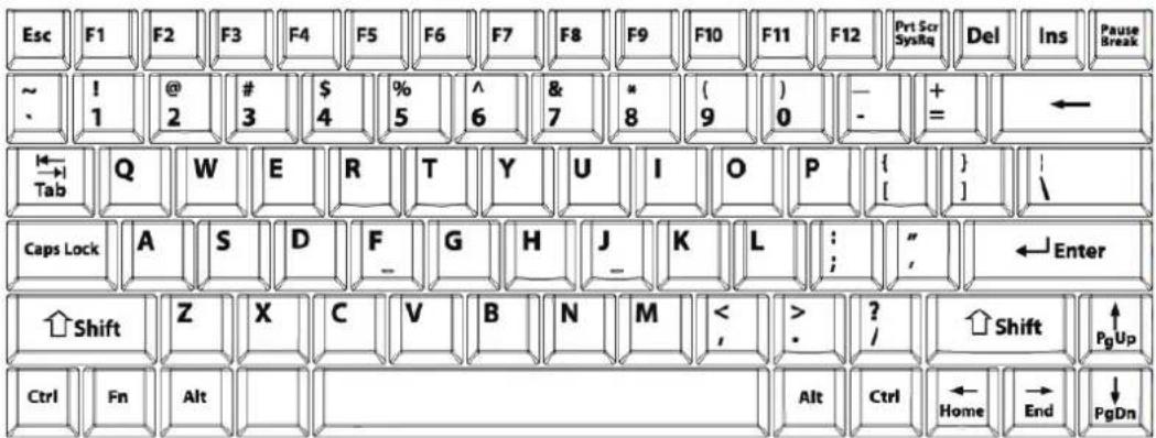
[Figure 2.7 Alpha-numeric Keyboard]
Console
The console consists of internal devices that acquire and process ultrasound images and external devices that facilitate connection and installation of peripheral devices. External devices include the probe connectors, ports for monitor and other peripheral devices, input and output devices such as a HDD, probe holders, wheels for portability, space for peripheral devices, and the system power switch.
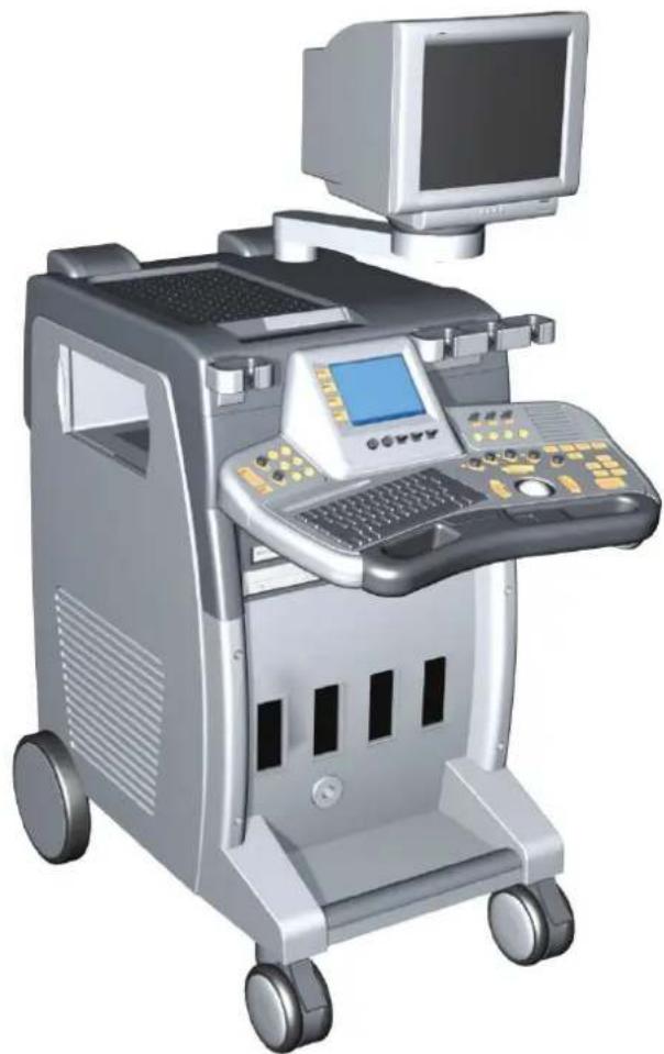
[Figure 2.8 Console]
Rear Panel
A monitor, printer, VCR and other devices can be connected to the rear panel of the product.
A monitor, printer, VCR and other devices can be connected to the rear panel of the product.
![graph TD A["1 VGA"] --> B["2"] B --> C["3 VGA"] C --> D["4 VGA"] D --> E["5 VGA"] E --> F["6 VGA"] F --> G["7 VGA"] G --> H["8 VGA"] H --> I["9 VGA"] I --> J["10 VGA"] J --> K["11 VGA"] K --> L["12 VGA"] L --> M["13 VGA"] M --> N["14 VGA"] N --> O["15 VGA"] O --> P["16 VGA"] P --> Q["17 VGA"] Q -->…](/content/2026/05/955519/images/7397ca569f454ed7b11d25e7ef417386139c53724f3810a42f3232f59beb4881.jpg)
[Figure 2.9 Rear Panel]
VGA1 / VGA2 (Output)
The VGA output signal is sent to the monitor through this port.
PARALLEL (Output)
Normal PC printers can be connected on the parallel port.
RS-232C (Input/Output)
This is an RS-232C input/output port. RS-232C allows VCR controls, Open Line Transfer and so on.
LINE (Input/Output)
The modem can be connected on this port. (Reserved)
USB (Input/Output)
USB (Universal Serial Bus) devices can be connected on this port. (Reserved)
DICOM (Input/Output)
DICOM can be connected on this port. Patient information can be transmitted to other servers over the DICOM network.
AUDIO (Input/Output)
Audio devices can be connected on this port.
| NOTE | Audio Input on the rear panel and Audio Input on the front panel may not be used simultaneously. Only Output on both panels may be used simultaneously. |
VHS (Input/Output)
VHS type VCRs can be connected on this port.
| NOTE | VHS Input on the rear panel and VHS Input on the front panel may not be used simultaneously. Only Output on both panels may be used simultaneously. |
S-VHS (Input/Output)
S-VHS type VCRs can be connected on this port.
| NOTE | S-VHS Input on the rear panel and S-VHS Input on the front panel may not be used simultaneously. Only Output on both panels may be used simultaneously. |
PATIENT MONITOR (Output)
A separate monitor for the patient can be connected on this port. It supports external power of 9V.
PRINTER (Output)
Echo printers can be connected on this port.
PRINT REMOTE (Output)
Echo printers for remote printing can be connected on this port.
INTERLACE RGB (Output)
This port sends Interlace RGB signals. Color video printer, etc .can be connected here.
MIC (Input)
The microphone can be connected on this port.
DVD (Input)
The DVD can be connected on this port. (Reserved)
Microsoft Windows Printer
Microsoft Windows 2000 compatible printers can be used. Connect the printer to the Printer port on the rear panel.
CAUTION
For information on installing printer drivers, please direct your inquiries to the MEDISON Customer Service Center.
When connecting the printer, make sure that the printer model matches the printer specified on the Windows or system settings screen.
Probe Holder
The front part of the console features holders where probes can be rested.
Peripherals
These are the devices that can be used in conjunction with the console. Common peripherals include VCR, echo printer, microphone, foot switch, and lamp.
Lamp
The lamp illuminates the keyboard in dark rooms or other dark places. The lamp connector is located under the control panel. Use the switch on the lamp housing to power the lamp On/Off.
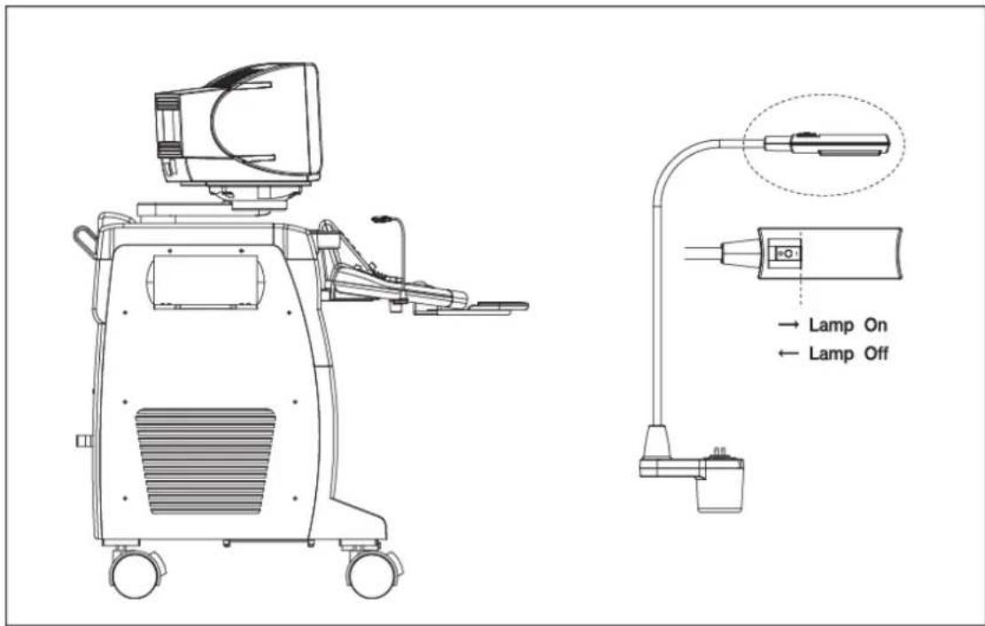
[Figure 2.10 Lamp Switch On/Off]
| WARNING | Using the product in wet or high-humidity places may result in electric shock. |
| CAUTION | Assembling or disassembling the lamp while the power is on may result in abnormal operation of the product. Be careful not to damage the lamp by dropping it or applying excessive force to it. |
Foot Switch
The user can press the left and right pedals with a foot to control simple functions. The foot switch connector is located at the front of the base of the product.
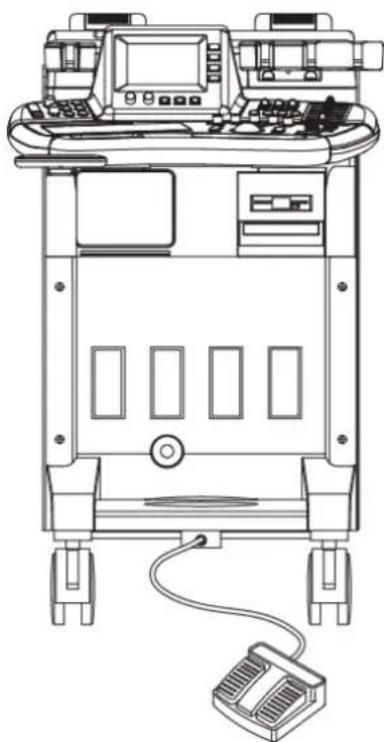
[Figure 2.11 Foot Switch]
Probes
Probes are devices that transmit ultrasound and collect data for generating ultrasound images.
NOTE
For detailed information, please refer to "Chapter 8. Probes."
Connecting Probes
Installation or removal of probes to or from the probe connectors must be performed only when the system power is OFF.
- Connect probes to the probe connectors on the front panel of the console. Including the Static CW probe, a maximum of 5 probes can be connected to the console.
- After connecting the probe to the connector, turn the dial on the connector clockwise to secure it.
- When the system restarts, the probe used before the last shut down will be activated again.
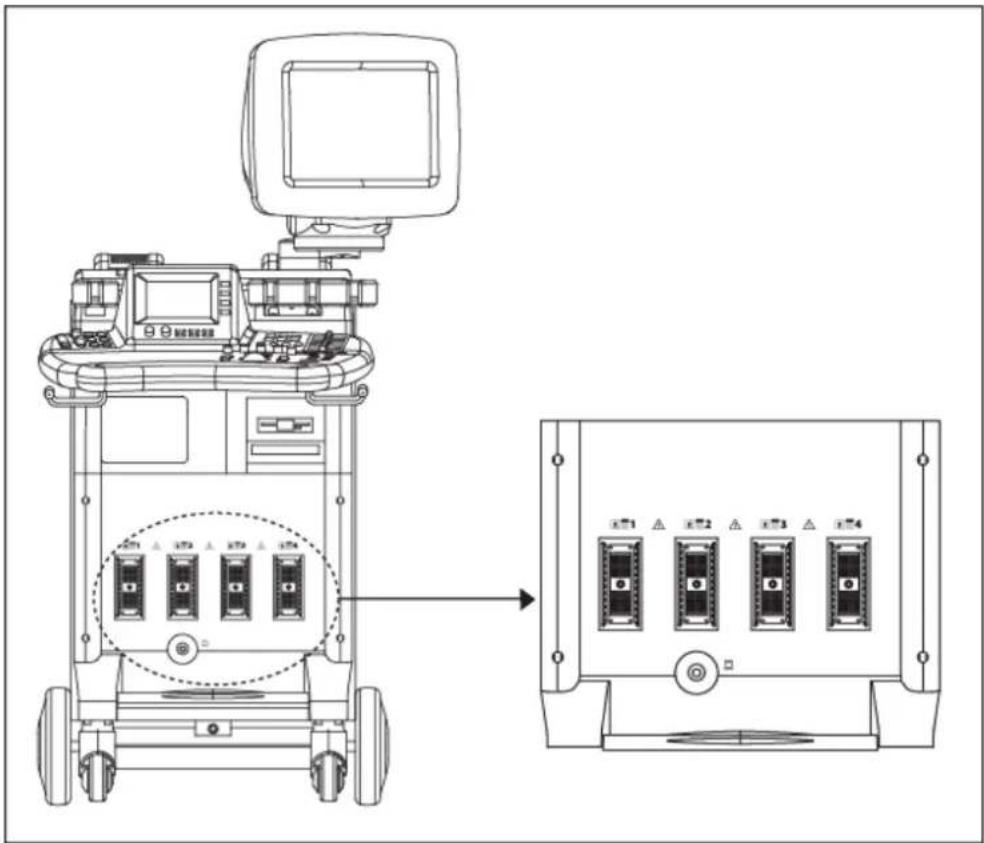
[Figure 2.12 Probe Connectors]
Accessories
The following accessories are provided with this product.
CAUTION
Main cord set, separately certified according to the relevant standards, is to be used when supplied to EU and USA/CAN.
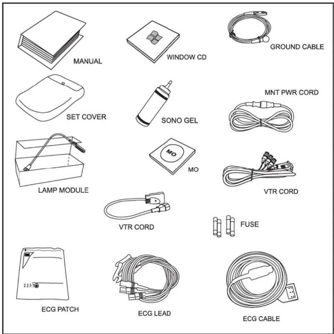
[Figure 2.13 Accessories]
NOTE
Accessories can be different according to the country.
Options
ACCUVIX XQ provides the following options. These options are available only when selected by the user.
■ Live 3D
■ DICOM
■ SONOATLAS
■ 3D XI TM
■ Stress Echo
■ Panoramic Imaging
■ DynamicMR
■ SCI (Spatial Compound Image)
■ STIC (Spatio-Temporal Image Correlation)
XI STIC
XI VOCAL
■ DICOM SR
For more information on the options above, please refer to the respective sections in this manual.
Chapter 3
Settings
SELECTING PROBE AND APPLICATION 3
Selecting Probe, Application and Preset Values 3
Editing Probe Preset Values.... 4
ENTERING PATIENT INFORMATION....5
Registering New Patient....5
Searching Patient Information 6
Editing Patient Information....8
Modifying Measure Data....8
GENERAL SETUP 11
Title 11
Display 12
PERIPHERALS SETUP 13
OPTION SETUP.... 16
INFORMATION SETUP 17
MISCELLANEOUS SETUP 18
3D SETUP 21
LIVE 3D SETUP 22
DICOM SETUP....24
DICOM Setup Procedures....24
DICOM Device Setup 25
SERVICE DIAGNOSTICS SETUP 26
AUTO CALC SETUP 27
STRESS ECHO SETUP ....28
General Settings for Stress Echo....28
Advanced Settings for Stress Echo....30
MEASUREMENT SETUP 31
General....32
Obstetrics (OB) Measurement Settings 36
Cardiac Measurement Settings....41
Vascular Measurement Settings 42
Urology Measurement Settings....43
UTILITY SETUP....44
B/W Post....44
Color Post....47
Image Preset 48
Panoramic Imaging 49
ECG....51
ETC 52
VCR Play....54
DynamicMR....55
Stress Echo 57
Biopsy....72
Image Store....73
Selecting Probe and Application
Before scanning, select a probe and an application. For information on the probes and applications supported by this system, please refer to "Chapter 8. Probes". Trackball
A set of different applications is pre-assigned to each probe type, and the probe settings are optimized for each application. The user may change the settings as needed.
Press the Probe button on the control panel and the Probe Selection screen will appear on the touch screen. You can select or change probes and applications, and edit probe preset values at this screen.
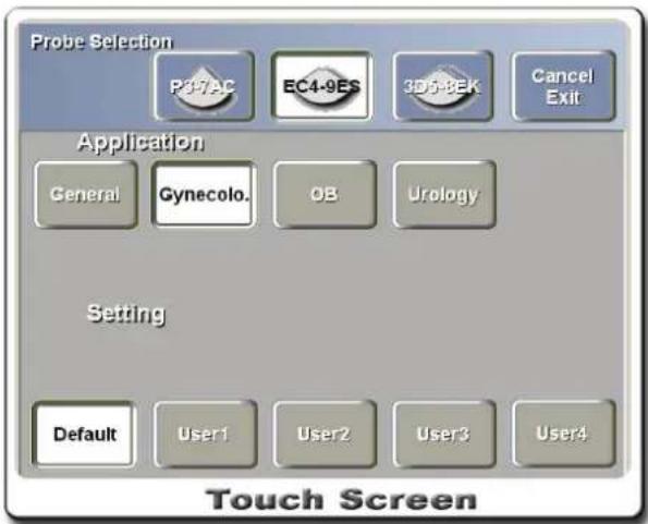
[Figure 3.1 Probe Selection Screen]
Selecting Probe, Application and Preset Values
Selecting a probe displays the list of applications supported by the probe, and selecting an application displays the current preset values.
- Select a probe.
- Verify the probe selection and select an application.
-
Select appropriate preset values according to the probe and application selected.
-
Exit the Probe Selection screen. Press the Cancel/Exit button to cancel any changes made.
Editing Probe Preset Values
While probes settings are optimized for each application, the user may change the settings as needed. For information on editing probe preset values, please refer to the "Utility Settings" section of this chapter.
Probe preset values are optimized for probes and applications as shown below.
■ For L5-12IM, L6-12IS, L8-12IS, L5-9EE, and VN6-12:
Breast – 'Breast1'
Small Parts – ‘Thyroid’, ‘Testicle’, ‘Bowel’
Musculoskeletal – 'Shoulder Knee', 'Hand Foot'
Vascular – ‘Cerebr.Carotid’, ‘Periph.Arterial’, ‘Periph.Venous’
■ For C2-6IC: Fetal Heart – ‘Fetal Heart1’
Entering Patient Information
You can enter the patient's information before scanning. Patient information includes basic information such as the patient ID, name, DOB, and gender and additional information for applications. Diag. Physician, Ref. The Diag. Physician, Ref. Physician, and Sonographer fields contain up to four recent data entries each.
NOTE
You must enter both the ID and the name when registering a patient for the first time.
All patient data is identified by the patient ID. The ID must be entered at all times, and other information can be entered additional as needed. The OK button remains disabled if the ID has not been entered.
Press the Patient button on the control panel and the Patient Information screen will appear on the touch screen.
You can register information for a new patient or edit information for an existing patient at this screen. You can also use the touch screen. Press the menu button on the touch screen to move the input cursor on the Patient Information screen to the selected position.
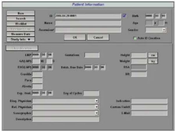
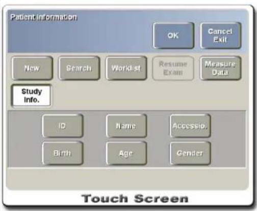
[Figure 3.2 Patient Information]
Registering New Patient
-
Press the New button on the Patient Information screen and then use the Trackball, the Set button and the keyboard to enter the patient's name, ID and other information.
-
Press the New button while "Auto ID Creation" is selected to automatically assign a new patient ID.
- If a duplicate ID is entered, the icon next to the ID input field changes to .
- Press the Study Info. button to enter detailed information required for examination.
- Press the OK button when you have finished entering the patient information. Press Cancel to cancel the process.
Searching Patient Information
Searching by ID
Enter the ID of the patient to search and the patient information will be displayed on the screen.
Using the Search Function
- Press the Search button at the Patient Information screen and the patient search screen will appear.
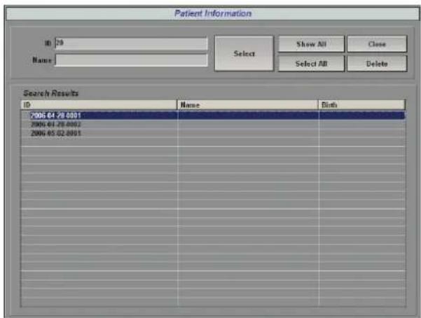
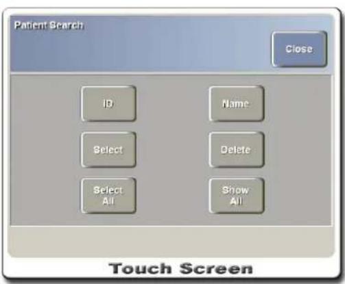
[Figure 3.3 Patient Search Screen]
- Enter a patient ID or name on the Patient Search screen and the list of registered patients will appear, sorted by the ID.
- The Select button and the OK button remain disabled if no patient matches the search condition.
- Press the Show All button to search all patients without specifying the ID or name.
- Press the Select All button to select all the patients on the list.
- Select a patient and press the Delete button to delete the ID and information for a registered patient.
- Press the Close button to quit searching patients and close the Patient Search window.
WARNING
Deleting a patient ID results in deletion of all the saved images in SonoView and as well as all the relevant data for the patient.
Using the Worklist button
- Press the Worklist button at the Modality Worklist screen and the patient search screen will appear.
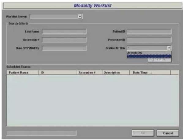
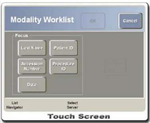
[Figure 3.4 Modality Worklist Screen]
- Select Worklist Server, enter the patient's information in one or more input fields, and then press the Search button. Scheduled patients that match the search conditions will appear. Searching without entering any patient information displays the entire list of scheduled patients.
- Select a patient to examine and press the OK button. The Patient Information screen will appear.
- Press the Close button to quit searching patients and close the Modality Worklist window.
Worklist Server is configured under DICOM Setup and it connects to the institution's DICOM Modality Worklist Server and retrieves information on scheduled patients and examinations. Selecting a patient on Worklist automatically enters the patient information.
Station AE Title shows the AE (Application Entity) Title value as specified under DICOM Setup. When no value has been entered, this field shows the model number of the ultrasonic equipment. Selecting “* (asterisk)” displays information for all patients registered in Worklist Server.
Editing Patient Information
You can add or edit desired information at the Patient Information screen.
- Use the Trackball, the Set button and the keyboard to add or edit desired information.
- Press the OK button when you have finished adding or editing the patient information. Press Cancel to cancel any changes.
If you open the Patient Information screen to enter the patient ID after obtaining Measure values, the Resume Exam button will be activated. Here, enter the patient ID and press the Resume Exam button to add the measurement results to the patient ID entered. Pressing the OK button instead of the Resume Exam button discards the measurement results.
The Resume Exam button is activated only when there are calculated results. When the patient information has not yet been entered, use this button to add the calculated results to the information for another patient or a new patient.
NOTE
For information on backing up patient information, please refer to "Chapter 6. Image Management."
Modifying Measure Data
This function is used for entering the patient's obstetrics measurement values or viewing measurement values. It is accessible by pressing the Measure Data button at the Patient Information screen. The Measure Data button is activated only when the patient ID has been entered for adding or modifying the patient information.
The Measure Data screen consists of the Insert screen, where measurement values can be entered, and the View screen, where the measurement values entered can be viewed.
Insert Screen
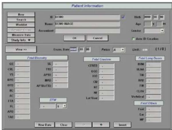
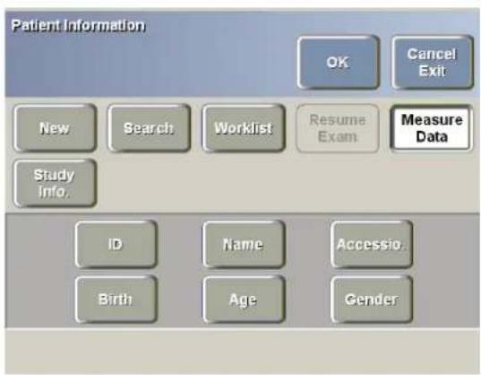
[Figure 3.5 Measure Data – Insert]
- Press the Measure Data button. The Insert screen will appear where you can enter obstetrics measurement values. Maximum of 8 sets of measurement values (8 examinations) can be entered per date.
- Press the Cancel button to cancel entering measurement values. Press the New Data button to cancel measurement values for other examinations.
- Press the Insert button at the bottom of the screen after entering the measurement values. You can view the measurement values entered at the View screen of the Measure Data screen.
- Press the view>> button on the left-hand side of the Insert screen. The View screen will appear where you can view the measure data or save it as an Excel file.
View Screen
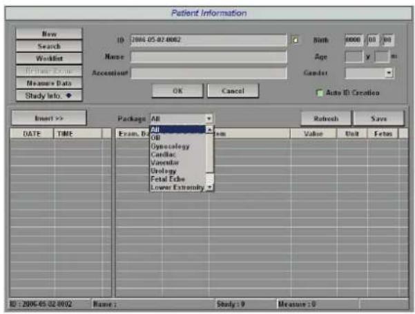
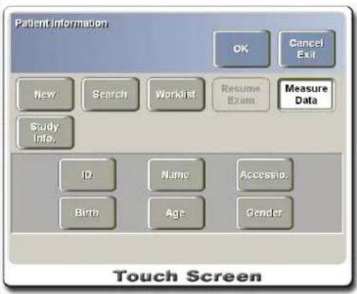
[Figure 3.6 Measure Data – View]
- At the View screen you can select the "Package" item and view measurement values entered by applications.
- The exam date marked with an asterisk (*), such as 2005/05/15 *, indicates the current measurement data.
- Press the Refresh button to refresh the screen with measurement values that have newly been measured or entered.
- Press the Save button. The View screen will appear where you can save the information on the screen as an Excel file. The patient ID will be used as the file name, which can be modified.
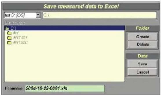
- You can use the buttons on the Save measured data to Excel window to create or delete folders for saving the file, save file or cancel the process.
- Press the Insert>> button on the left-hand side of the screen to move to the Insert screen.
General Setup
This section includes instructions on general system settings and their verification. Settings can be changed to suit various needs and preferences of the user.
- Press the Setup button on the control panel and the setting screen grouped by functional categories will appear. Buttons for the categories will appear on the touch screen.
- You can select a category from the monitor or the touch screen, or select it by turning the Select Setting knob-button below the touch screen.
- Select the General tab at the Setting screen. Make adequate settings for each item.
- To close the screen, select the Close button or press the Exit button on the touch screen.
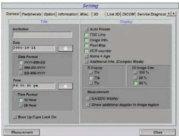
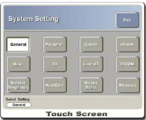
[Figure 3.7 Setting – General]
Title
Sets the institution name, date and time which are displayed on the title area of the screen.
■ Institution:
Enter the hospital/institution name.
■ Date
Set the current date and display format.
■ Time Set the current time and display format.
■ Boot up caps lock status
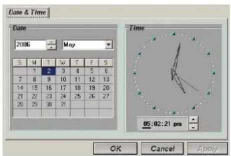
This menu sets the initial status of Caps Lock
after system boot-up. This Caps Lock enables capital letter entry without the need to press the Shift key.
Display
Sets display-related options. Pressing the checkbox toggles the corresponding option on or off.
■ Auto Freeze
If turned on, scan mode automatically freezes after 5 minutes. This setting does not apply to Live 3D Scan mode, where automatic freeze occurs after 20 minutes.
■ TGC Line
If turned on, TGC Line is displayed on the screen at all times. If turned off, TGC Line appears briefly when adjusting TGC.
■ Image Info
Sets whether to display the image information in the image zone.
■ Post Map
Sets whether to display Post Map in the feedback area.
■ VCR Counter
By default, VCR Counter is displayed at all times when Panasonic MD835 is connected on Serial Port. Turning this option off displays the counter only while recording.
■ Name + Age
If turned on, the patient's age is displayed in the title area in the format of "23y 3m."
■ Additional Info. (Complex Mode)
If turned on, six recently saved images in SonoView are displayed on the left-hand side of the screen.
■ TI (Thermal Index) Display
Sets whether to display TIs, Tib or Tic as TI in the title area. The TI value is set automatically and does not require user settings.
■ 2D Image Size
Selects 100%, 95% or 90% as the display size of the 2D image. New setting takes effect after the system restarts.
■ Measurement
If the GA/EDD Display checkbox is selected, the GA and EDD values entered in the patient's information are displayed as measurement values on the screen.
If the Show additional Doppler in image region checkbox is selected, Doppler-related measurement results are displayed in the image zone. If the checkbox is not selected, the measurement results are displayed in the feedback area.
Peripherals Setup
You can make settings for VCR, printer, foot switch, etc. that are connected to the system. Select the Peripherals tab at the Setting screen.
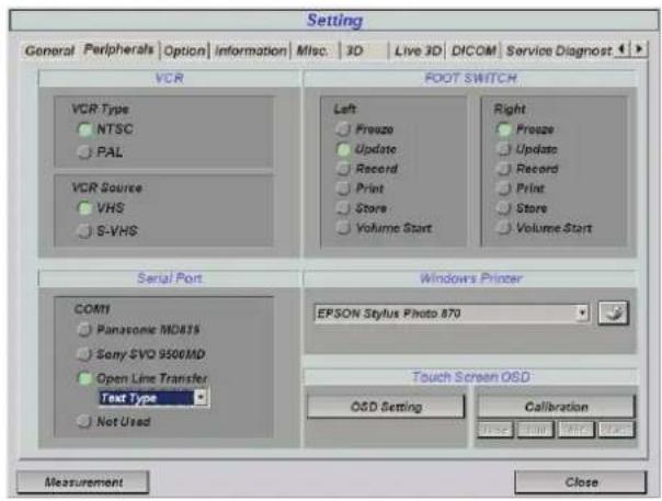
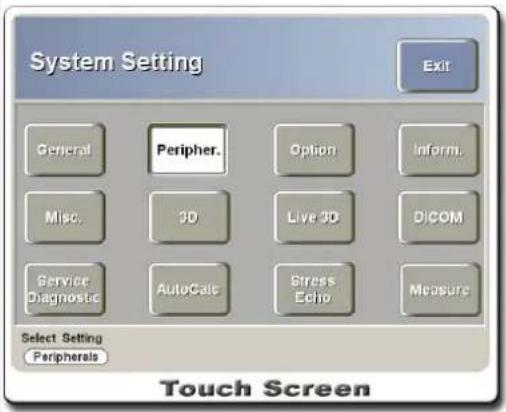
[Figure 3.8 Setting – Peripherals]
■ VCR Type
Sets the output type of VCR Port as NTSC or PAL. This setting cannot be changed by the user.
■ VCR Source
Sets the input type of VCR Port as VHS or S-VHS.
■ Foot Switch
Sets the left/right pedal of the foot switch for Freeze, Update, Record, Print, Store, or Volume Start.
Serial Port
Selects a device connected to Serial Port. Available options include Panasonic MD835, Sony SVO 9500MD, Open Line Transfer, etc. Open Line Transfer allows you to specify the transfer method for report data.
■ Windows Printer
Selects the printer to use.
■ Touch Screen OSD
This is the environment configuration menu for the touch screen. Press the OSD Setting button and the OSD Menu, Select, and Up/Down menus will appear on the touch screen. Each menu can be selected using the knob-button or up-down switch below the touch screen.
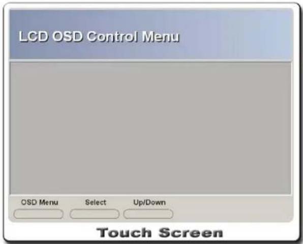
[Figure 3.9 LCD OSD Control Menu]
- Press the OSD Menu knob-button and the menu will appear. To change the menu, use the Up/Down up-down switch and the Select knob-button to make selections.
- After selecting a menu, use the Up/Down up-down switch to change the value. When necessary changes are made, press the Select knob-button to finish settings.
- Once the touch screen settings are complete, the Information window will appear as illustrated below. Press the OK button.
■ Touch Screen Calibration
This is the menu for calibrating coordinates on the touch screen. The touch screen needs to be calibrated if its button selection is out of range. The possible range of error for calibration is between 2.032 mm and 4.572 mm.
Press the Calibration button on the monitor screen. The Base, End, Init., and Exit buttons will become active and the Calibration screen will appear on the touch screen.
To calibrate coordinates for the touch screen:
- Press the Init. button to reset the coordinates.
-
Press the Base button. When the "+" sign appears at the upper left-hand corner of the touch screen, press the "+" sign to set its position.
-
Press the End button. When the "+" sign appears at the lower right-hand corner of the touch screen, press the "+" sign to set its position.
- Use a blunt object to press the "+" signs. Take note that using sharp objects may damage the touch screen.
- If you wish to re-calibrate, press the Init. button and repeat the procedures above.
- When setting is complete, press the Exit button to finish. New settings will not be saved if you do not press the Exit button.
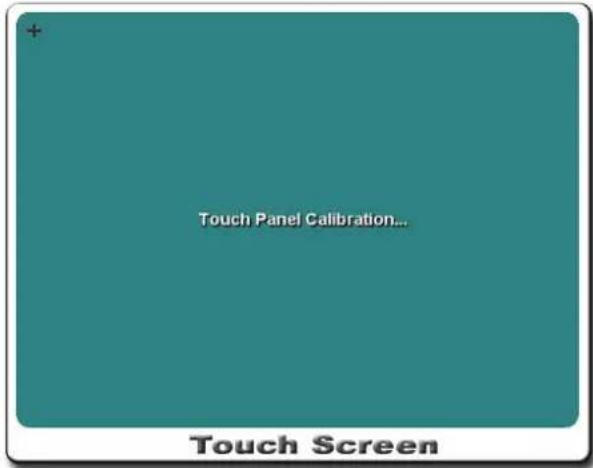
[Figure 3.10 Touch Screen Calibration]
| WARNING | System error(s) may occur if you do not follow the instructions above. In case of system error(s), perform the calibration again by pressing Init. > Exit > Calibration. If the problem is not resolved, please contact the customer service center. |
| CAUTION | Do not use sharp or metallic objects when calibrating coordinates for the touch screen. This may damage the touch screen when setting the “+” points. If possible, use a stylus pen specially designed for PDAs or touch screens. |
Option Setup
This screen displays the serial number of the system software and the list of optional software items. Only the software items with "Password" displayed on the right-hand column are available for use. Optional software items cannot be installed or removed by the user.
Select the Option tab at the Setting screen.
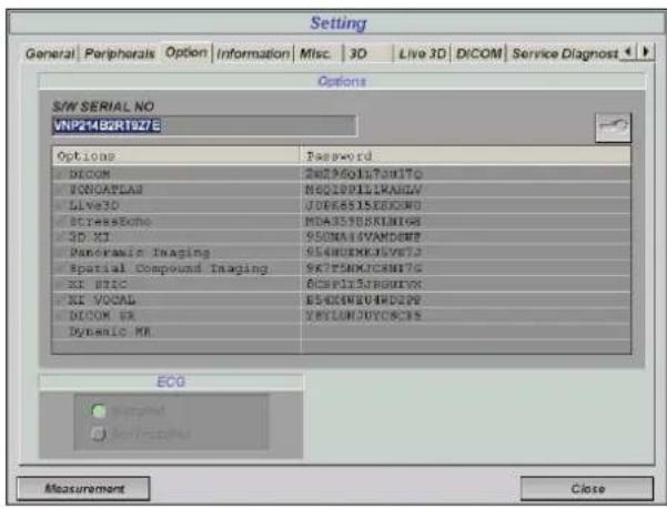
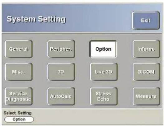
[Figure 3.11 Setting – Option]
* The actual options may be different from the ones shown in this illustration.
Information Setup
This function displays the version information of the system software. Select the Information tab at the Setting screen. Press the Detail button to view the system version.
![Setting General | Peripherals | Option | Information | Misc. | 3D | Live 3D | DICOM | Service Diagnost | Version Information Detail Version : 1,85,80,0426 Name : 1015,25288 CPU vec [40] BFO vec [AD] BPI vec [AD] BPS vec [AD] BPS vec [AD] DBP vec [55] DBC vec [64] VM vec [64] DC vec [38] NETR vec [60…](/content/2026/05/955519/images/dc1366316f13fadea1cc1b9c6a3f90820d6ccb75a9e1e6b05f59a48fc9d30867.jpg)
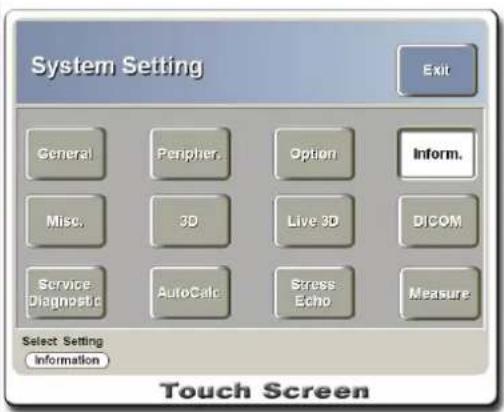
[Figure 3.12 Setting – Information]
* The actual system version may be different from the version information shown in this illustration.
Miscellaneous Setup
Select the Misc. tab on the Setting screen.
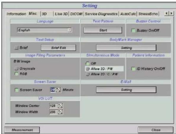
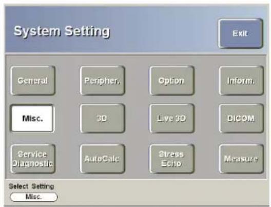
[Figure 3.13 Setting – Misc.]
Language
Languages supported by the system include English, German, Spanish, French, Italian and Russian. Language cannot be changed by the user.
■ Test Pattern
Press the Start button to display the images that demonstrate the monitor display.
■ Buzzer Control
Toggles on/off the buzzer that sounds when buttons on the control panel and the touch screen are pressed.
■ Text Setup
You can set the text starting position and Brief mode (abbreviated words function).
To set the text starting position, move the cursor to the position where the text will appear for the first time when entering text, and then press the Set button on the control panel to specify the position.
Brief mode is the function that automatically enters the terms used in the system. Select "Brief" under Text Setup.
For editing Brief mode, press the Brief Edit button to add or delete the terms used in the system. For detailed information on this function, please refer to "Chapter 6. Image Management."
■ Bodymark Manager
You can set, delete or reorder commonly used Bodymarkers.
Pressing the Bodymarker button in the control panel displays Bodymarkers.
Pressing the Setting button displays the Bodymarker Manager screen, bringing up the
Bodymark-Preview screen on the touch screen.
In the Bodymark Manager screen, all bodymarkers are displayed by probe, application and group. In this screen, you can search for a bodymarker to use, based on criteria such as probe, and set it.
The Bodymark -Preview screen on the touch screen shows bodymarkers set by the user. When the list of bodymarkers spans more than one page, use the Up/Down switch below Page to select a desired page. In this screen, you can delete or reorder bodymarkers.
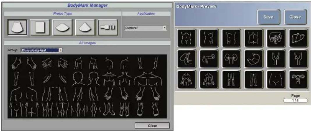
[Figure 3.14 Bodymark Manager]
- Adding a bodymarker
In the Bodymark Manager screen, search for bodymarker-based criteria such as probe and select a desired bodymarker with the trackball in the control panel. Pressing the Setting button adds the bodymarker to the Bodymark -Preview screen on the touch screen.
- Deleting a bodymarker
In the Bodymark -Preview screen in the control panel, select a bodymarker and press the Up/Down switch below Delete. The selected bodymarker will be deleted.
- Reordering bodymarkers
In the Bodymark-Preview screen in the control panel, select a bodymarker and press the knob-button below Image Move. The selected bodymarker will be moved forward or backward.
- Saving a bodymarker
The Bodymark-Preview screen on the touch screen, press Save. The selected bodymarker will be saved. Pressing the Bodymarker button in the control panel displays the list of bodymarkers. Press Cancel to cancel any settings.
■ Image Filing Parameters
B/W (Black & White) images can be saved either as Grayscale or as RGB (color).
Color images are saved as RGB regardless of this setting.
■ Simultaneous Mode
Determines whether to activate simultaneous functions in Spectral Doppler Mode.
- Off: Select this if not using simultaneous mode.
- Allow 2D/PW: Select this if using simultaneous mode for 2D/PW but not for 2D/C/PW.
- Allow 2D/C/PW: Select this if using simultaneous mode both for 2D/PW and for 2D/C/PW.
■ Patient Information
Checking the box of 'ID History On/Off' shows ID lists for auto complete in the Patient Information screen.
■ Screen Saver
This function starts after a certain period of time to protect the screen. You can set Screen Saver to start automatically when the system is not in use. The idle time for starting Screen Saver can be set anywhere between 20 minutes and 60 minutes.
■ E-mail Setting
Configures the mail server settings.
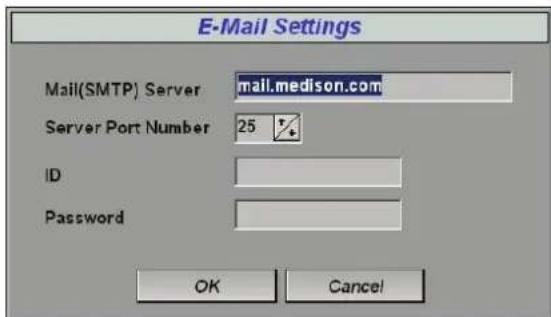
■ VOI LUT
When saving DICOM images, adjust the brightness and contrast values for gray images by changing the "Window Center" and "Window Width" values. Adjusted images can be viewed on PACS devices that use DICOM-standard VOI LUT.
- Window Center: For gray images, if its value is greater than 128, the brightness increases and, otherwise, the brightness decreases.
- Window Width: For gray images, if its value is greater than 256, the contrast decreases and, otherwise, the contrast increases.
■ Clip Save
Determines how clips are saved. Clips can be saved by beat only when ECG is running; clips will not be saved when ECG beats do not appear even if the setting is selected for clips to be saved by beat. When Low MI is activated, clips are saved by time only. Available setting range is 1 beat - 4 beat or 1 sec - 10 sec, respectively.
3D Setup
This sets the initial screen for 3D View and 3D XI View. Select the 3D tab at the Setting screen.
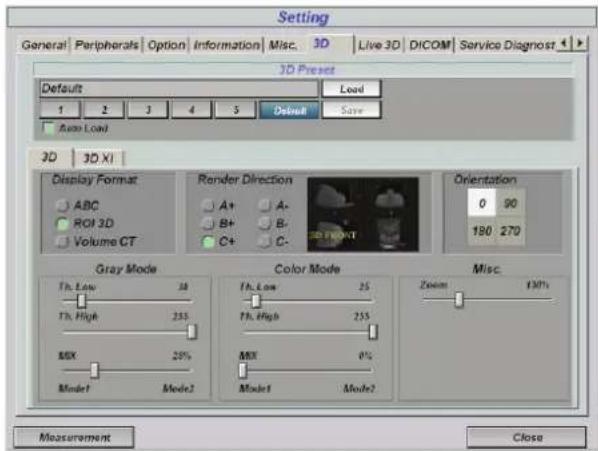
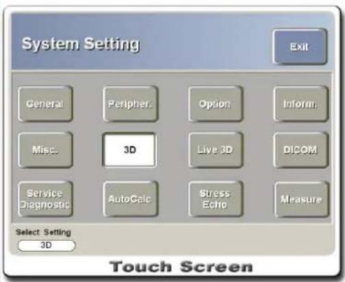
[Figure 3.15 Setting - 3D (3D)]
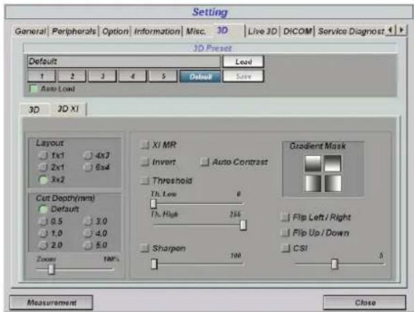
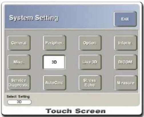
[Figure 3.16 Setting - 3D (3D XI)]
3D: You can change Display Format, Render Direction, Orientation, Misc., Gray Mode, Color Mode, etc. for 3D View.
3D XI: You can change Layout, Cut Depth, Threshold, Sharpen, Gradient mask, etc. for 3D XI View.
Select User1, User2, etc. under Preset, enter the user-specific values and press the Save button to save the preset values. To load the preset values assigned to each User button, select a User button and press the Load button. If "Auto Load" is selected, preset values are loaded as soon as a User button is pressed. Press the Default button to revert to the initial preset values.
Live 3D Setup
This sets the initial screen for Live 3D View and Live 3D XI View. Select the Live 3D tab at the Setting screen.
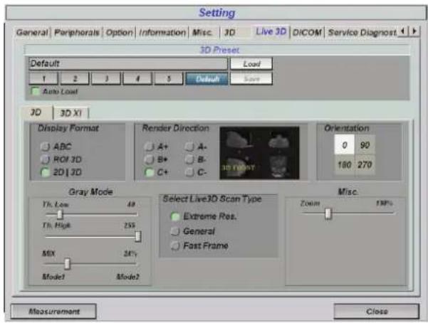
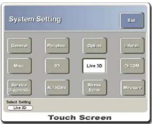
[Figure 3.17 Setting – Live 3D (3D)]
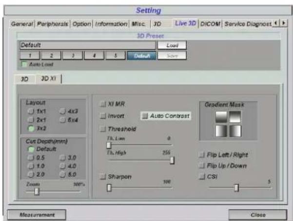
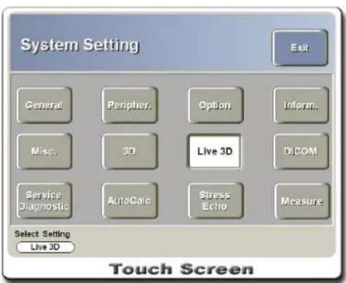
[Figure 3.18 Setting – Live 3D (3D XI)]
3D: You can change Display Format, Render Direction, Orientation, Gray Mode, Misc., Live 3D Scan, etc. under the Live 3D tab.
3D XI: You can change Layout, Cut Depth, Threshold, Sharpen, Gradient mask, etc. under the Live 3D XI tab.
Select User1, User2, etc. under Preset, enter the user-specific values and press the Save button to save the preset values. To load the preset values assigned to each User button, select a User button and press the Load button. If "Auto Load" is selected, preset values are loaded
as soon as a User button is pressed. Press the Default button to revert to the initial preset values.
■ Setting Live 3D Scan Type
The scan type for Live 3D is set as "Extreme Res." by default. Other scan types can be set using User1 through User5 settings.
- Extreme Res.: This scan type has priority over image quality in Mid / High / Extreme mode of scan quality. While achieving high image quality, the frame rate is low.
- General: This scan type has priority over frame rate in Low / Mid mode of scan quality and priority over image quality in High / Extreme mode of scan quality.
- Fast Frame: This scan type has priority over frame rate in Low / Mid / High mode of scan quality. While achieving high frame rate, the image quality is low. (Extreme mode excluded)
NOTE
Probes that support Live 3D Scan Type settings are "3D3-5EK" and "3D4-7EK."
Since the Live 3D Scan Type value is not reflected when changing preset in Live 3D View mode of 3D mode, please acquire images after selecting a desired preset in image scan mode.
DICOM Setup
This section contains instructions for operating DICOM (Digital Imaging and Communication in Medicine) and setting DICOM servers. Select the DICOM tab at the Setting screen.
| NOTE | For detailed information, refer to the user manual of the server equipment or the DICOM Conformance Statement. |
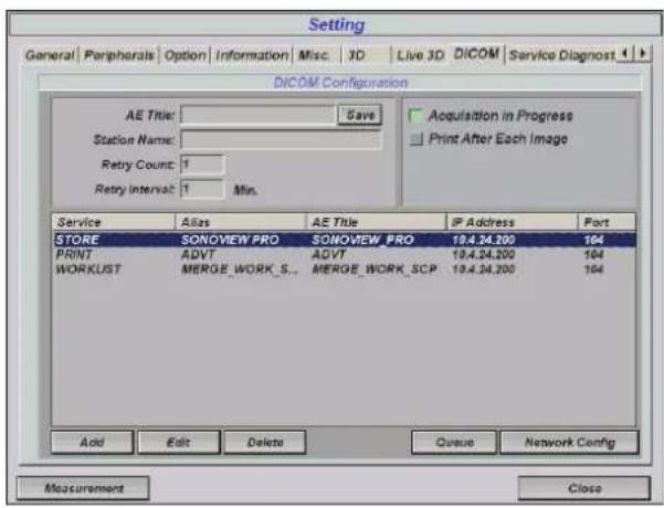
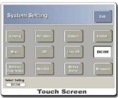
[Figure 3.19 Setting – DICOM]
DICOM Setup Procedures
Configure the DICOM information for the system. After entering information for the items below, select "Acquisition in Progress" for automatically transmitting the DICOM information. Also, select "Print After Each Image" for automatic printing.
- AE Title: Enter the DICOM AE (Application Entity) title.
- Station Name: Enter a unique name for the system (e.g. US1, US2, etc.).
- Retry Count: Enter the number of transmission retries in case of transmission failures.
- Retry Interval: Enter the length of time (unit: minutes) during which the transmission will be retried in case of transmission failures.
DICOM Device Setup
Press the Add button to configure information on DICOM, PRINT, WORKLIST, and STORE SR servers. Press the Edit button to edit the current server information, or press the Delete button to delete the current server information.
- Service: Enter the name of the server to configure.
- Alias: Enter the name of the server to use.
- AE Title: Enter AE Title for the server to use.
- IP Address: Enter the IP address for the server to use.
- Port: Enter the port number for the server to use.
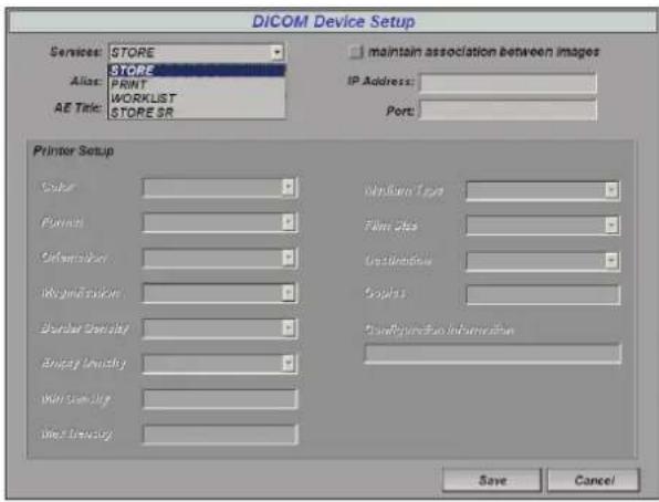
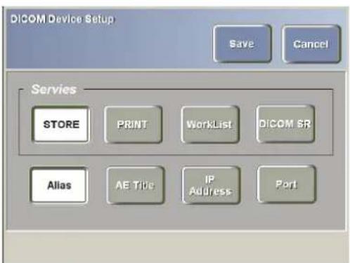
[Figure 3.20 Setting – DICOM Device Setup]
Service Diagnostics Setup
Select the Service Diagnostics tab at the Setting screen.
Provided for inspecting the system status, Remote Service is a function designed for use by the Medison Customer Service Center for after-sales service purposes. Related settings are inaccessible to the user.
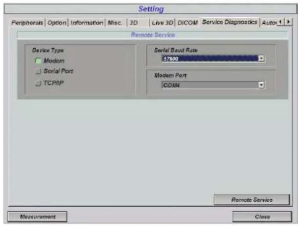
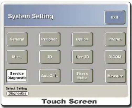
[Figure 3.21 Setting – Service Diagnostics]
Auto Calc Setup
Here, you can select measurement result menus that are displayed on the screen in Spectral Doppler Mode.
Please note that the menu items here are displayed only when the Automatic Calculator function in Spectral Doppler Mode is in use. Select the AutoCalc tab at the Setting screen.
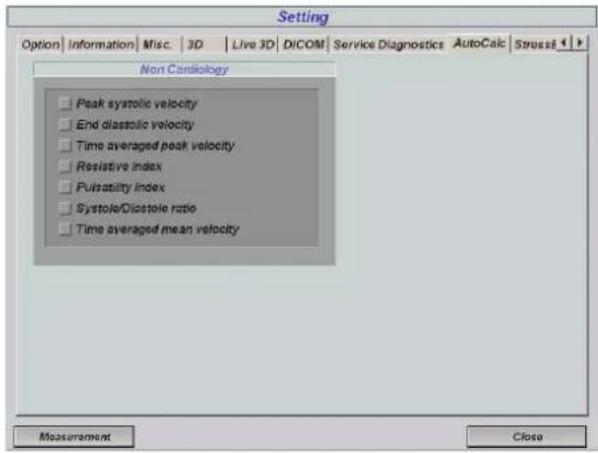
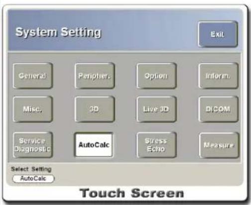
[Figure 3.22 Setting - AutoCalc]
Maximum of 6 menus can be selected. When the Mean Trace menu is turned off under the Automatic Calculator function, the TAM (time averaged mean velocity) menu will not be displayed on the screen.
Also, when the PSA (peak systolic velocity) and EDV (end diastolic velocity) values are 0, results of all menus will not be displayed on the screen.
Stress Echo Setup
Set the Stress Echo measurement method and its menu. Select the StressEcho tab at the Setting screen.
Stress Echo settings consist of General settings and Advanced settings.
General Settings for Stress Echo
Shows the Protocol, Stage, and View lists registered on the system. Press the General>> button at the Advanced screen, and the General screen will appear.
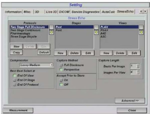
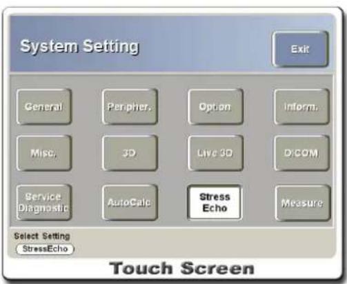
[Figure 3.23 Setting – Stress Echo (General)]
Protocols
- Basic protocols supported include Two Stage Full Disclosure, Two Stage Continuous, Pharmacologic, and Three Stage Bicycle, and the user may create custom Protocols.
- Press the Up/Down arrows on the right to change the order of the Stages on the list.
- Select a Protocol to view the "Compression" and "Best Beat Select at" values for the Protocol.
- New: Protocols with the same names cannot be created. A new protocol does not have any Stage value. By default, the "Compression" value is set as "Uncompressed" and the "Best Beat Select at" value as "End of View."
-
Delete & Edit: Protocols can be deleted or renamed. Note that default protocols cannot be deleted or renamed.
-
Copy: An existing Protocol can be copied for use. Note that the copied protocol may not use the same name.
- Default: Resets the 4 default Protocols with the initial system preset values (Stage, View, etc.).
■ Stages
- Maximum of 5 Stages can be created for each Protocol. Press the Up/Down arrows on the right to change the order of the Stages on the list.
- New: Stages with the same names cannot be created. A new Stage is initialized with "PLAX, PSAX, A4C, and A2C" as Views. By default, "Capture Method" is set as "Perspective" and "Accept Prior to Store" as "On."
- Delete & Edit: Stages can be deleted or renamed.
Views
- Maximum of 8 Views can be created for each Stage. Press the Up/Down arrows on the right to change the order of the Views on the list.
- New: Views with the same names cannot be created. The default values for a new View are "1" for "Beats Per Image" and "1" for "Images Per View."
- Delete & Edit: Views can be deleted or renamed.
■ Compression
This function is responsible for compressing images. It controls the file size of the images used in Stress Exam in SonoView.
■ Best Beat Select at
Sets the stage for selecting images for inspection from the images acquired.
■ Capture Method
This is the method for acquiring images. "Full Disclosure" acquires images and then allocates them in each View, and "Perspective" selects Views and then acquires images.
■ Accept Prior to Store
This menu sets whether to confirm the acquired images before proceeding to the next View. This option becomes available if it is set to "On" and "Capture Method" is set to "Perspective."
■ Capture Length
This menu sets the range for image acquisition. "Beats Per Image" sets the number of heart beats for the images acquired, and "Image Per View" sets the number of images contained in a View.
Advanced Settings for Stress Echo
Press the Advanced>> button at the General screen, and the Advanced screen will appear.
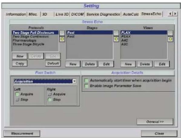
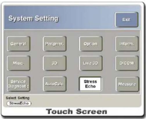
[Figure 3.24 Setting – Stress Echo (Advanced)]
■ Foot Switch
Sets the Foot Switch functions at each stage when performing Stress Echo. Foot Switch functions can be set for three stages: Acquisition, Accept Prior to Store, and Best Beat Select.
■ Acquisition Details
If "Automatically start timer when acquisition begin" is selected, timer starts automatically when acquisition begins. If "Enable Image Parameter Save" is selected, image parameters are saved in a selected View.
Measurement Setup
Select the Measurement button at the Setting screen, or press the Measure button on the touch screen. Measurement menus will appear on the monitor and the touch screen.
Turn the knob-buttons below the touch screen to select Select Pkg. and Select Page.
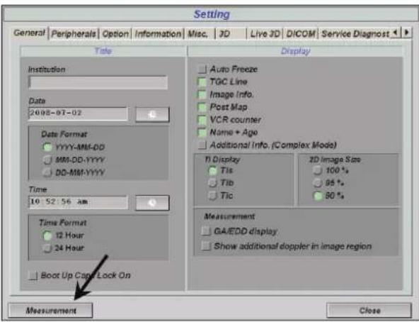
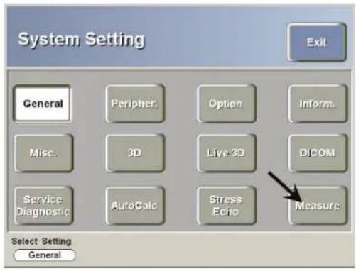
[Figure 3.25 Measure Setup]
Select Pkg. at the bottom of the touch screen is for selecting general measurement settings, and OB (obstetrics), cardiac, vascular, and urology measurement settings.
Select Page is for selecting the setup menu categories for each measurement setting.
General
General: Basic Measurement Settings
■ 2D Circumference and Area Method
Sets the method for measuring circumference and area.
■ Measurement Unit
Sets the basic measurement unit (velocity, distance or area) used in screen displays and reports. Make sure you press the Clear button before changing this setting as this affects all previous measurement results.
■ Doppler Mode Y-Axis Unit
Sets the unit to display on the Y-axis in Spectral Doppler Mode.
■ Caliper Ratio, Average Display
Specify whether to display addition information such as ratios and average as well as measurement data during basic measurements.
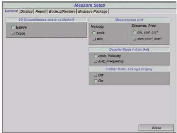
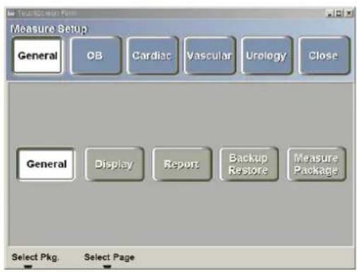
[Figure 3.26 Measure Setup – General]
Display: Measurement Screen Settings
■ Caliper Line Type
Sets Caliper Line displayed on the screen. The dotted line can be set to show always or hide. It can also be set to hide when the cursor position has been confirmed.
■ Caliper Line Marker Type
Sets the shape of the caliper cursor displayed on the screen. Either "Cross Hair" or "Arrow Head" can be selected.
■ Doppler Trace Direction Type
When Auto Trace / Limited Trace functions are used in Spectral Doppler Mode, this menu sets the range of the measurement values.
■ Mean Trace Line
Determines whether to apply Mean Trace Line on the screen when Automatic Calculator is in use.
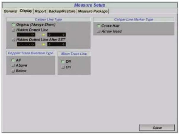
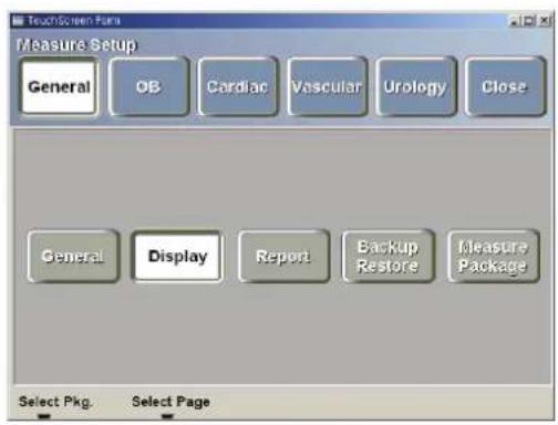
[Figure 3.27 Measure Setup - Display]
Report
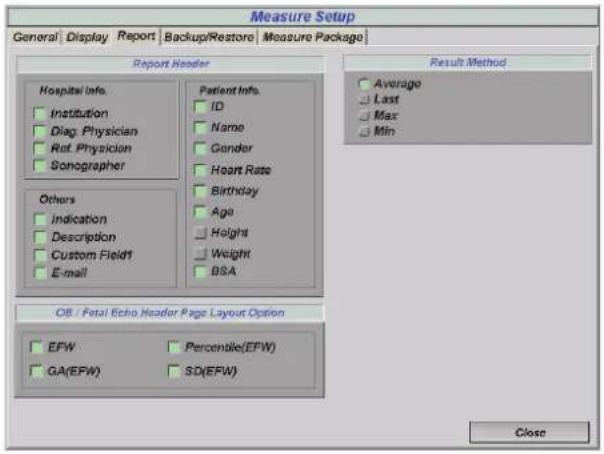
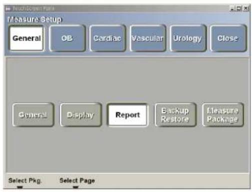
[Figure 3.28 Measure Setup – Report]
■ Report Header / OB, Fetal Echo Header Page Layout Option
You can select what kind of information is displayed on the report screen (Report Header).
■ Result Method
Sets the calculation method for the measurement result value displayed on the report. When Average Value is selected, the average value of the last three measurement results is displayed. When Last Measured Value is selected, the last measurement value is shown.
- Average: Shows the average of the last three measurement values.
- Last: Shows the last measurement value.
- Max: Shows the largest measurement value.
- Min: Shows the smallest measurement value.
Backs up or restores user tables set by the user. Press the Backup button to save OB Table Reference in the selected media, or press the Restore button to load Reference from the selected media.
Checking the Measured Data checkbox backs up or restores measurement results for a specified period.
■ Measured Data
This menu is for backing up measurement results. If "Write to File" is selected, measurement results can be backed up by pressing the Transfer button on the report screen.
Measurement results are backed up in a text file. You can specify whether to overwrite or append to the existing file of the same name. The backup file name can be specified by the user or else the system assigns it a name automatically.
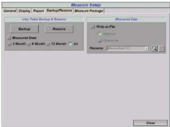
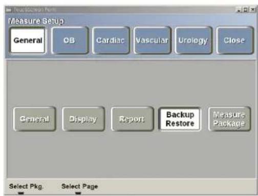
[Figure 3.29 Measure Setup – Backup/Restore]
Measure Package
■ Item Customize
Set items using on the measurement menu and report. 'Factory Items' applies factory setting, and 'Custom Items' applies user-designed setting in the system.
Custom Items
- Select the application in 'Selection', and items will show up in the 'Group Order'.
-
Select the check box in 'Group Order'. The selected items are showed in the 'Menu' and 'Report' on the right side of the screen.
-
Use the up-down arrow to arrange the order. It applies to the 'Menu' and 'Report'.
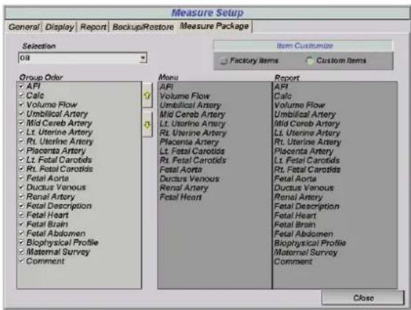
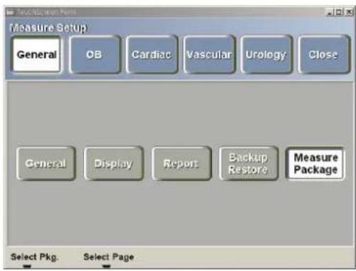
[Figure 3.30 Measure Setup – Measure Package]
NOTE
■ When switch Velocity mode and Frequency mode, applications except Cardiac, Gynecology, OB, and Urology can set group spartely.
■ All changes are applied to the system after rebooting.
Obstetrics (OB) Measurement Settings
General Settings for Obstetrics Measurement
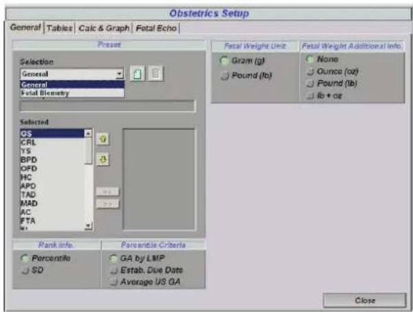
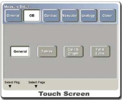
[Figure 3.31 Obstetrics Setup – General]
■ Preset
Sets obstetrics measurement menus used in examination. Select desired Presets from "Selection." If General is selected, all items can be used. If Fetal Biometry is selected, only Fetal Biometry-related items can be used.
■ User Preset
Press the button next to the Selection field to set a new Preset. Enter a title in the Preset Name field and a brief explanation in the Description field. Press the OK button to create a new Preset.
Once the Preset is created, select menu items to use in obstetrics measurement.
Select items from the entire list on the right and press the << button to move them to the list on the left. This specifies the items to use in User Preset.
To remove them from the list on the left, select items and then press the >> button.
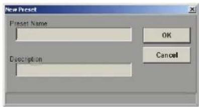
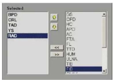
To delete User Preset, select User Preset and then press the button. General and Fetal Biometry cannot be deleted because they are default Presets.
Rank Info.
Select SD or Percentile for displaying Growth Range in the Result Display area. This is displayed as both SD and Percentile in reports.
■ Percentile Criteria
Select a value to use for percentile calculation.
■ Fetal Weight Unit Selection
Sets the unit for Fetal Weight used in obstetrics measurement. Select gram (g) or pound (lb).
■ Fetal Weight Additional Info. Unit Selection
Use this to select the basic unit and to display additional information for EFW. Select None, Gram (g), Ounce (oz), Pound (lb) or lb+oz.
Table Settings for Obstetrics Measurement
Sets Tables and Equations used in the measurement menu.
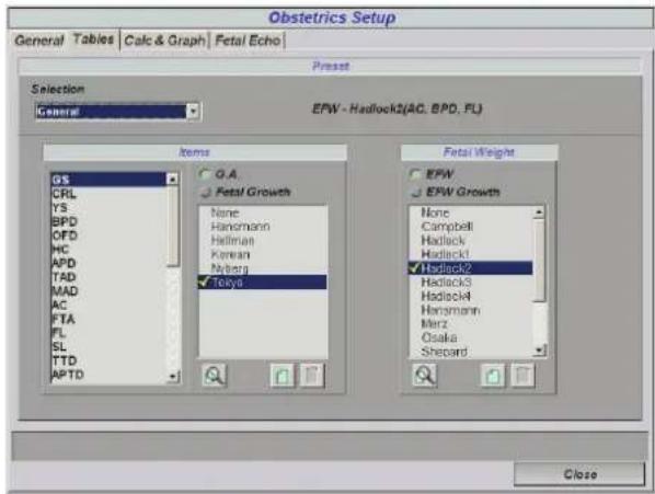
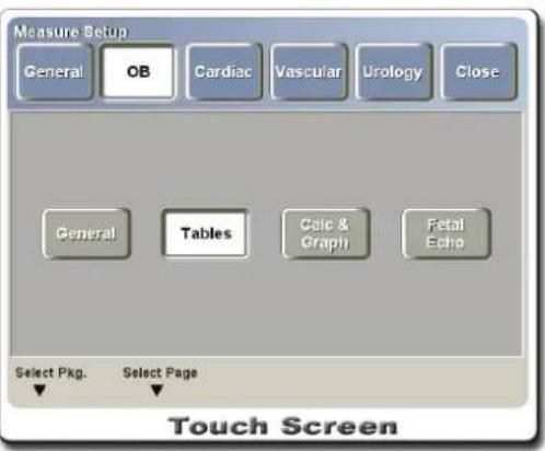
[Figure 3.32 Obstetrics Setup – Tables]
Table & Equation
Press the 🔒 button to view the details for Table or Equation.
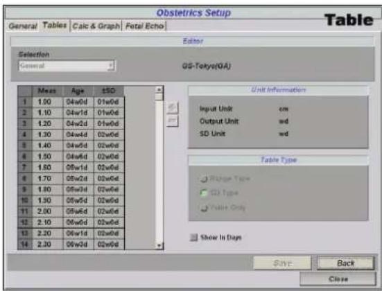
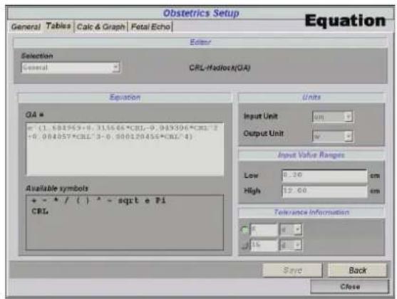
[Figure 3.33 Obstetrics Setup – Table 보기]
- GA Table and Fetal Growth Table are displayed on the screen as below.
HC-Hadlock(GA)
BPD-Hansmann(Growth)
- Press the "Show in Days" checkbox to display Output in d (days) instead of wd (week and days).
| Meas | Age | ±SD | |
| 1 | 1.00 | 04w0d | 01w0d |
| 2 | 1.10 | 04w1d | 01w0d |
| 3 | 1.20 | 04w2d | 01w0d |
| 4 | 1.30 | 04w4d | 02w0d |
| 5 | 1.40 | 04w5d | 02w0d |
| 6 | 1.50 | 04w6d | 02w0d |
| 7 | 1.60 | 05w1d | 02w0d |
| 8 | 1.70 | 05w2d | 02w0d |
| 9 | 1.80 | 05w3d | 02w0d |
| Meas | Age | +-SD | |
| 1 | 00.60 | 035d | 005d |
| 2 | 01.00 | 042d | 006d |
| 3 | 01.60 | 049d | 007d |
| 4 | 02.40 | 056d | 008d |
| 5 | 03.40 | 063d | 009d |
| 6 | 04.40 | 070d | 010d |
| 7 | 05.00 | 077d | 011d |
| 8 | 05.80 | 084d | 012d |
| 9 | 06.40 | 091d | 013d |
- The numeric units in Table are displayed under Unit Information, and Table format is displayed under Table Type. Fetal Growth Table displays the SD (Standard Deviation) information. SD information can also be entered when adding User Tables.
- Equation Table shows Value Ranges and the Tolerance information.
■ User Table & User Equation
Press the button to set a new Table or a new Equation. Enter the name and brief description in the "Name" and "Description" fields and then select the type of Table. Press the OK button, and User Table will appear.
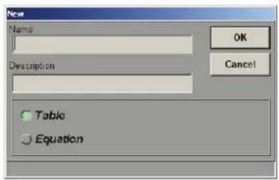
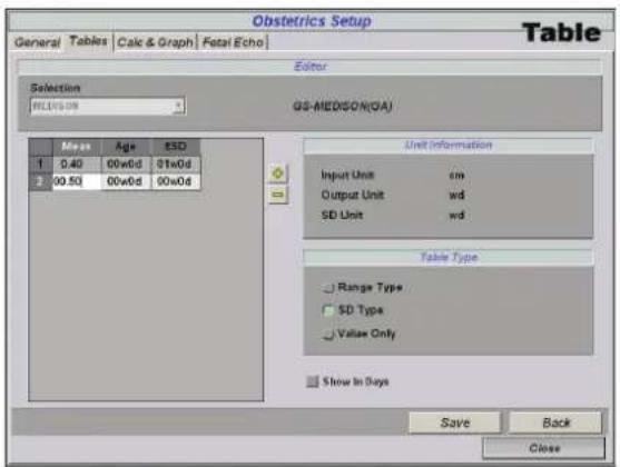
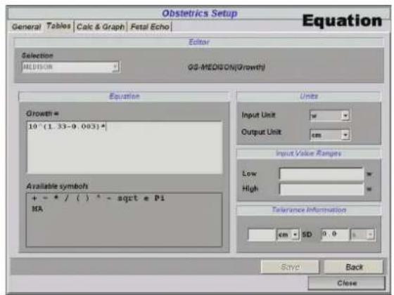
[Figure 3.34 Obstetrics Setup – User Table]
Press the + button to add a row to Table, or press the - button to delete a row.
To enter a value, click the input box with the Trackball. After entering a value, press the Tab key or the Enter key on the keyboard to save it.
Select Table Type to display the input screen according to the table type. "Range Type" allows input for Min/Max values, "SD Type" allows input for SD value, and "Value Only" allows input for Measure and Age values.
Press the Save button to save the Table content, or press the Back button to return to the previous screen.
| Meas | Age | Min | Max | |
| 1 | 0.40 | 04w0d | 00w0d | 00w0d |
| Meas | Age | ±SD | ||
| 1 | 0.40 | 00w0d | 01w0d | |
| 2 | 00.50 | 00w0d | 00w0d | |
| Meas | Age | |||
| 1 | 0.40 | 00w0d | ||
| 2 | 0.50 | 04w2d | ||
| 3 | 0.60 | 04w3d | ||

Press the button to delete User Table.
Calc & Graph Settings
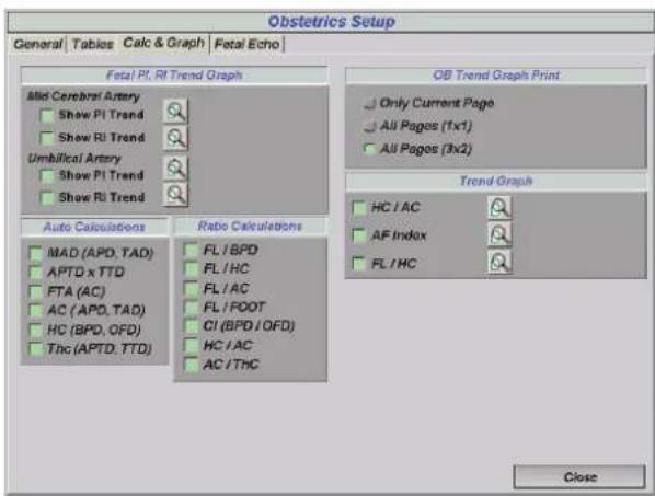
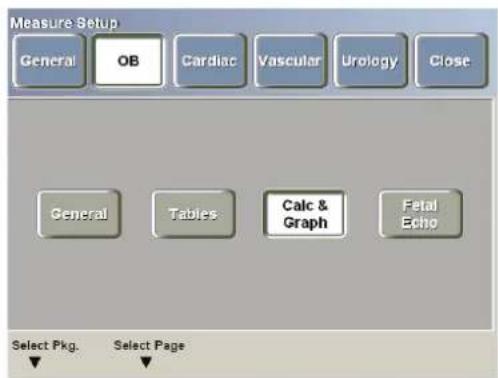
[Figure 3.35 Obstetrics Setup – Clac & Graph]
■ Fetal PI, RI Trend Graph
In obstetrics measurement, PI and RI can be measured from the fetal blood flow to check state of the fetus. Select Fetal PI or RI Trend as the reference table for measurement.
■ Auto calculations
Specify an item that will be calculated automatically. For example, if the MAD checkbox is selected as shown below, when APD and TAD are measured, the measurements are used to calculate MAD automatically and display the result on the screen. The results of automatic calculation may affect GA and EDD information.
■ Ratio calculations
Specify a measurement item for which a ratio will be calculated. For example, if the FL/BPD checkbox is selected, when FL and BPD are measured, the ratio between them is calculated and displayed on the screen. This ratio also appears in a report.
■ OB Trend Graph Print
Sets the print format for report screen with graphs as follows:
- Only Current Page: Only the current screen is printed.
- All Pages (1x1): The printable graphs from the list on the left-hand side of the report screen are printed one per page.
- All Pages (3x2): The printable graphs from the list on the left-hand side of the report screen are printed six per page.
■ Trend Graph
Specify whether to include a graph for a certain item or ratio in an obstetrics report.
Press 📄 and the Editor screen for the selected graph will appear.
Fetal Echo Measurement Setup
During obstetrics measurement, the LV (Left Ventricle) volume of the fetus is measured. Here, the volume is calculated using the option under "LV Volume Calculation Method."
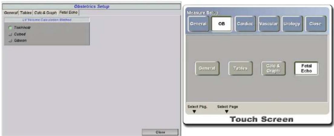
[Figure 3.36 Obstetrics Setup – Fetal Echo]
Cardiac Measurement Settings
Select the Cardiac button at the Measure Setup screen to set cardiac measurement settings.
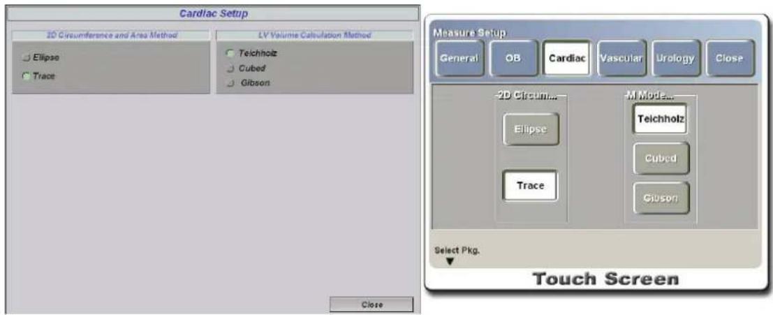
[Figure 3.37 Measure Setup – Cardiac]
■ 2D Circumference and Area Method
Select either the Ellipse or Trace as the measurement method for measuring 2D circumference and area in cardiac measurement.
■ LV Volume Calculation Method
Select the method for calculating the LV volume in M mode.
Vascular Measurement Settings
Select the Vascular button at the Measure Setup screen to set vascular measurement settings.
At the Vascular Setup screen below, you can set the Peak Velocity item used in automatic calculation of the "A/B Ratio" or "ICA/CCA Ratio".
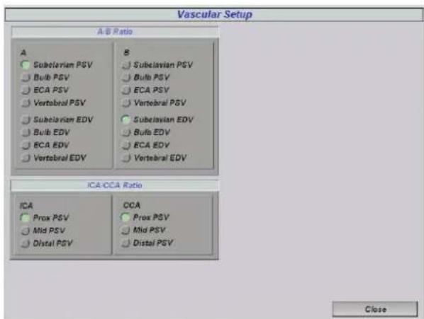
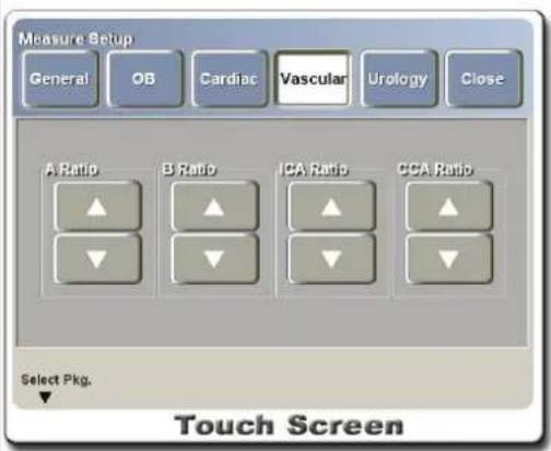
[Figure 3.38 Measure Setup – Vascular]
Urology Measurement Settings
Select the Urology button at the Measure Setup screen to configure the settings related to urology measurements. Set the equations used for calculating volumes in urology measurements.
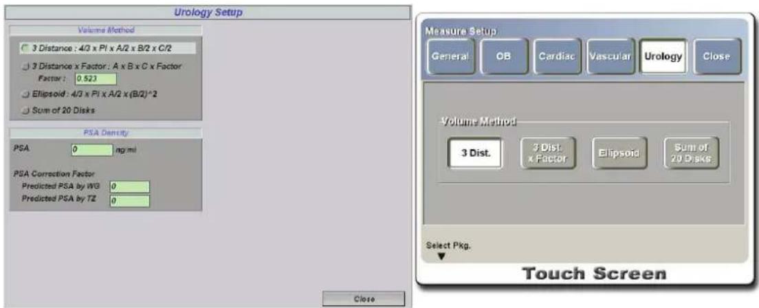
[Figure 3.39 Measure Setup – Urology]
Volume Method
- 3 Distance: The volume value is calculated using three diameters in the longitudinal and transverse planes. (4 / 3 x 3.14 x A x B x C / 8)
- 3 Distance x Factor: The volume value is calculated using three diameters from the longitudinal plane and transversal plane and a factor (F) value entered by a user. (A x B x C x F)
- Ellipsoid: The volume value is calculated using the length of the main axis and the length of the beside axis on 2D plane. (4 / 3 x 3.14 x Main / 2 x (Beside / 2) 2 )
- Sum of 20 Disks: The volume value is calculated by adding the areas on the 20 parallel planes. (d / 20 x (A1 + A2 + ... A20), d : the sum of distances between disks)
| NOTE | 3 Distances: A = 1st Dia. ; B = 2nd Dia. ; C = 3rd Dia.Ellipsoid: A = Main Dia. ; B = Beside Dia.The factor value is set as “0.523” by default. When changing the value it must be within the range of “0 < factor < 1.” |
■ PSA Density
Enter values for measuring Prostate Spec. Antigen Density (PSAD), Predicted PSA by WG and Predicted PSA by T-Zone.
- PSA: Enter the PSA value for measuring Prostate Spec. Antigen Density (PSAD).
- PSA Correction Factor: Enter PSA Correction Factor for measuring Predicted PSA by WG and Predicted PSA by T-Zone.
Utility Setup
Various utilities are provided for facilitate optimal use of the system.
Touch the Utility button on the touch screen and the Utility menu will appear.
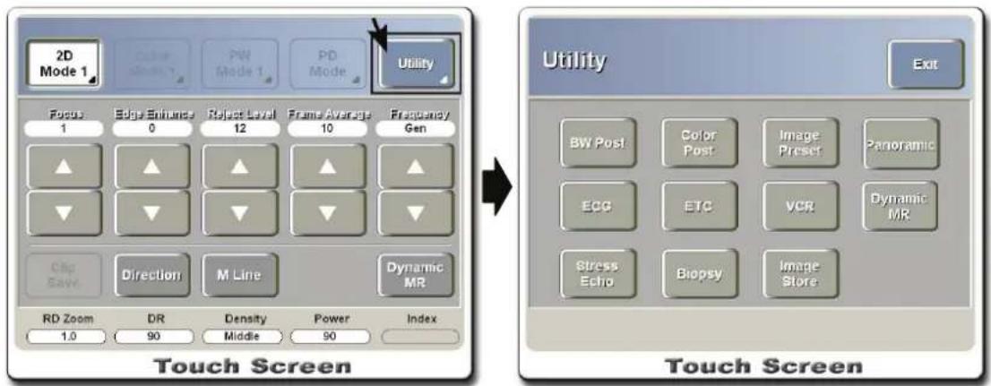
[Figure 3.40 Utility Menu]
B/W Post
Post map is a function that shows gray scale in separated areas of low echo, mid echo and high echo. It enhances or suppresses the discriminating power for each area.
Gray scale curves available for selection in post map are as follows.
 | This curve suppresses the overall echo while enhancing the discriminating power for the high echo area. |
 | This curve enhances the discriminating power for the low echo area. |
 | This curve softens the screen. |
 | This curve improves distinction for the low echo and high echo areas. |
 | This curve contains no changes. |
Use the BW Post button at the Utility menu to set post maps and their Gamma settings. There are 5 Type Curves and 2 User Curves that can be set for post maps.
Press the Exit button on the touch screen to close BW Post settings.
Please refer to the post map setup information displayed in the feedback area.
- TB: Pos – Use the Trackball to adjust the position of the curve.
- CHG: Point – Press the CHANGE button to select a Point to move.
- SET: Apply – Press the SET button to apply the preset values to the screen.
- S: Save curve – Press the S key on the keyboard to save the preset values.
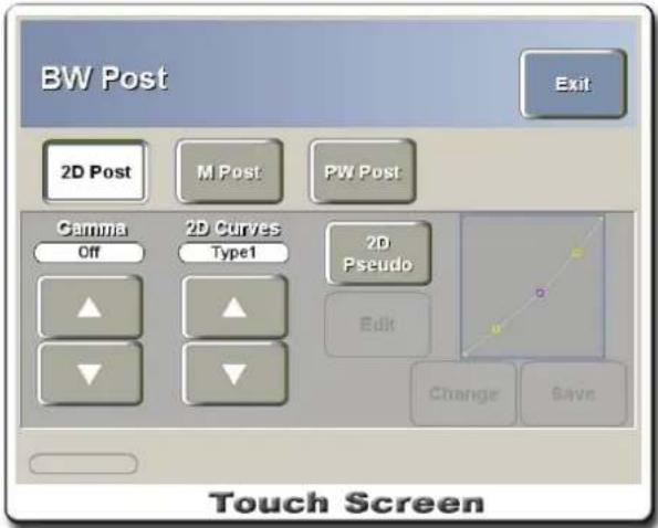
[Figure 3.41 Utility – B/W Post(2D Post)]
2D Post Map Settings
Press the 2D Post button and press the up/down buttons on the touch screen to select a desired curve.
If a User Curve is selected, you can select the Edit button to make a custom curve.
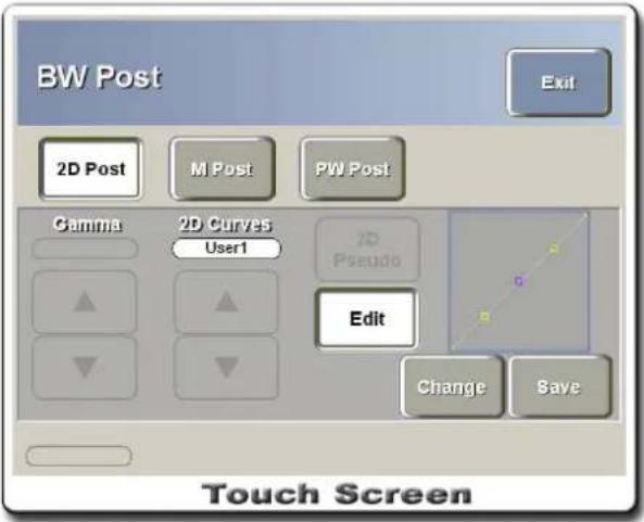
[Figure 3.42 Utility – B/W Post(Edit)]
■ Press the Change button, select points on the curve, and then use the Trackball and the Set button to change the shape.
■ Press the Save button and then save the changed curve.
■ Press the 2D Pseudo button to change the color of the screen. The screen color is changed by turning the knob-button below the touch screen.
M Post Map Settings
Press the M Post button.
Curve and Pseudo settings are performed in the same way as 2D Post Map settings.
PW Post Map Settings
Press the PW Post button.
Curve and Pseudo settings are performed in the same way as 2D Post Map settings.
Gamma Setting
At 2D post map setup, use the Gamma up/down buttons to set the brightness and contrast settings for the image.
Color Post
Press the Color Post button at the Utility menu to set C Post Map, PD Post Map, the Color Capture function, and the Color Tag function. There are 12 Type Curves and 4 User Curves that can be set for post maps.
Press the Exit button on the touch screen to close Color Post settings.
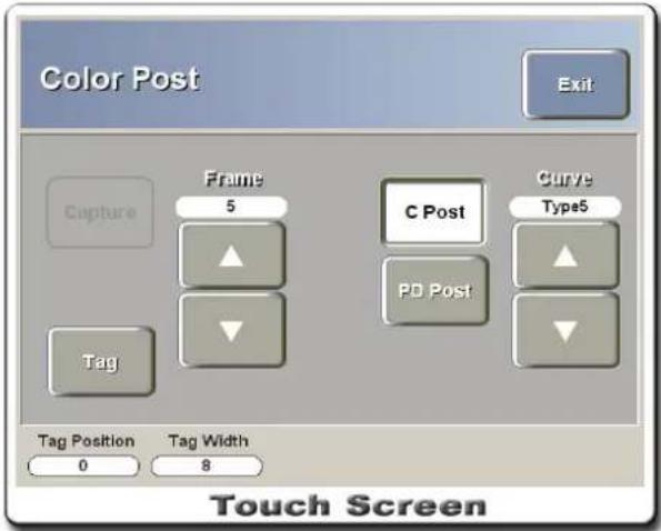
[Figure 3.43 Utility – Color Post]
C Post Map Setting
Press the C Post button and set the curve.
Note that C Post Map cannot be set when Directional Power Doppler Mode is in use.
PD Post Map Setting
Press the PD Post button and set the curve.
Note that PD Post Map cannot be set when Directional Power Doppler Mode is in use.
Setting color capture function
Press the Capture button to toggle the Capture function on/off, and then use the touch screen to set the Frame value.
Setting color tag function
Press the Tag button to toggle the Tag function on/off, and then use the knob-buttons below the touch screen to set the Tag Position and Tag Width values.
Image Preset
Preset allows the user to adjust Image Settings and select a saved setting to apply to the system.
Press the Image Preset button at the Utility menu.
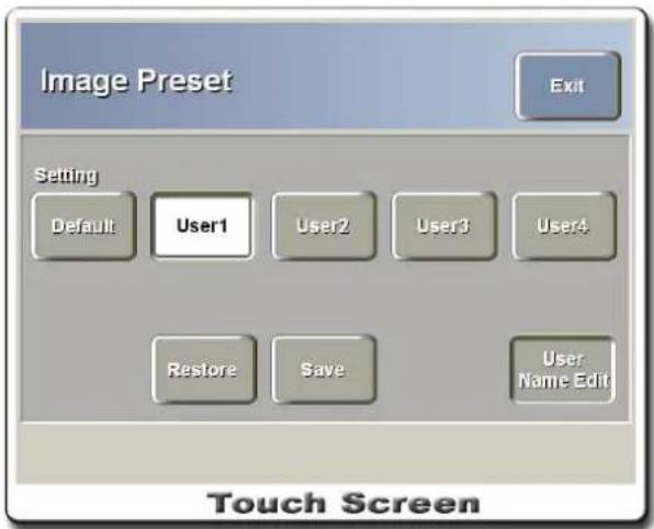
[Figure 3.44 Utility – Image Preset]
Settings
Default is the default system image setting, and User 1 through User 4 are custom preset values that can be saved by the user.
Restore
Press the Restore button to apply the selected preset values to the current screen.
Save
Press the Save button to save the preset values applied to the current screen.
User Name Edit
Select the User Name Edit button to rename the User settings. Press the corresponding User button to activate the setting.
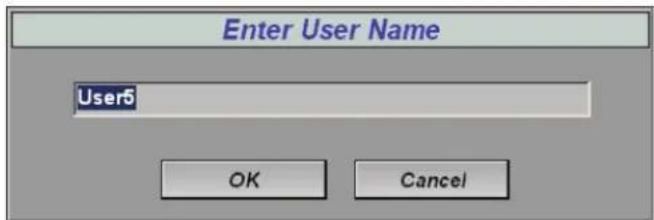
Panoramic Imaging
Panoramic Imaging is the function that acquires images for a wider range by using continuous ultrasonographic images. This function is available in 2D mode for L5-12IM, L6-12IS, and L8-15IS probes only. Up to 1,000 frames of images can be acquired. The function automatically stops when it exceeds 1,000 frames.
CAUTION
Panoramic images can be viewed on VCR. The Measure function can also be used on Panoramic images. Please note that measurements of Panoramic image on VCR recordings may not be accurate.
Running Panoramic Imaging
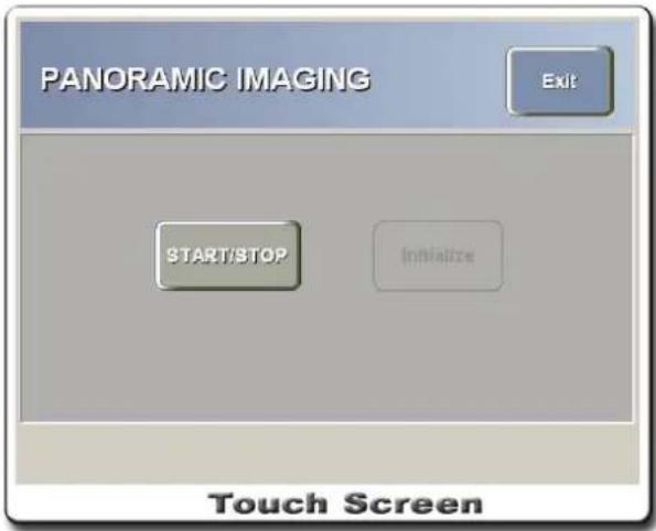
[Figure 3.45 Utility – Panoramic Imaging]
- Select the Panoramic button at the Utility menu.
-
Press the START/STOP button on the touch screen or the SET button on the control panel. Panoramic Imaging will begin.
-
When scanning a curved surface, ensure that the scan surface and the contact surface of the probe are always at a right angle.
- Moving in the opposite direction while acquiring images erases the previous frames and saves new frames.
- To exit Panoramic Imaging, press the START/STOP button or the SET button.
NOTE
■ The image quality may deteriorate if the contact surface of the probe loses contact with the scan surface while acquiring images.
■ Artifacts may also occur if scanning is done too rapidly or there are changes in the angle of the contact surface.
Review State
When get the panoramic image, the touch screen will be changed as 'Review State'.
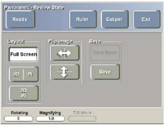
[Figure 3.46 Panoramic-Review State]
■ Ready: It returns to the first step of Panoramic Imaging.
■ Ruler: A ruler will show up or off on the panoramic image.
■ Caliper: A simple measurement menu will show up or off.
■ Exit: It terminates Panoramic Imaging.
Layout
- Full Screen: It displays only panoramic image.
- Flip Image: It will show up on the touch screen when you select the layout as 'Full Screen'.

■ Save: It saves the image according to selected layout.
NOTE
When you select the layout as 'Full Screen', you cannot use 'Cine Save'.
■ Rotating: It rotates 2D image from0 to 340°by 20°.
■ Magnifying: It magnifies 2D image from 1.0\~2.8 times by 0.2 times. This button will be showed up when you select the layout as 'Full Screen'.
■ T/B Move: Review the Cine of the panoramic image using the trackball. You cannot use this function when you select the layout as 'Full Screen'.
ECG
Shows the image of heart beat. This is available when the application is Cardiac. In Dual mode, the ECG Cine function can be used for both the images.
To turn ECG on:
- Select the ECG button at the Utility menu or press the ECG knob-button on the control panel. The ECG function will start.
- Adjust ECG menus on the touch screen.
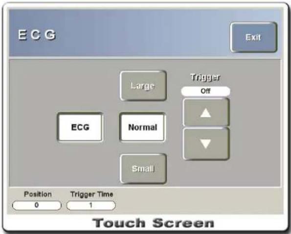
[Figure 3.47 Utility – ECG]
■ ECG: Set ECG on or off.
■ Large, Normal, Small: Select the ECG size.
■ Trigger: Set a numeric value for the Trigger interval or turn it off. The function can be toggled on/off also by pressing the ECG knob-button on the control panel.
■ Position: Turn the knob-button below the touch screen to adjust the ECG position. ECG moves toward the top as the number increases. This can be adjusted also by turning the ECG knob-button on the control panel while Trigger is turned off. Pressing the knob-button toggles the value between 0 and 300.
■ Trigger Time: Turn the knob-button below the touch screen while Trigger is turned on to adjust the time for showing Trigger. This can be adjusted also by turning the ECG knob-button on the control panel.
CAUTION
If the ECG is less then 30Hz, the Heart Rate (HR) function may not operate properly.
The error rate for the Heart Rate (HR) value in CW mode when ECG is in use is within 2%.
ETC
Select the ETC button at the Utility menu.
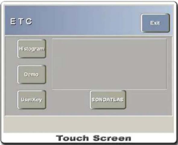
[Figure 3. 48 Utility – ETC]
Histogram
Histogram is the function that shows the gray level histogram for the selected area. This is based on the notion that symptoms of a certain condition can be expressed by observing echo distribution.
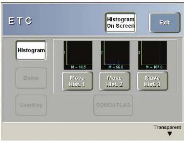
[Figure 3.49 Utility – ETC(Histogram)]
■ Select Histogram and the point for selecting area will appear on the screen.
■ Select area by using the Trackball and the Set button. The graph will appear on the touch screen showing the echo distribution for the selected area.
■ Press the Histogram On Screen button on the touch screen and the graph on the
touch screen will also appear on the monitor.
■ Press the Transparent to delete the background of the histogram.
NOTE
Transparent function is not available when the histogram moved on the area like measurement data.
■ Use the Move Hist. 1, Move Hist. 2 and Move Hist. 3 buttons on the touch screen to move the graphs on the screen.
■ Press the Change button on the control panel to change the area shape to ellipse.
Demo
Displays Demo images saved in SonoView.
Menu is displayed on the touch screen. You can use the buttons to navigate through desired Demo images.
![Accumix XO MISIGN OB #175 / 14.0cm MI 1.0 VA4-7 / Gen Tlb0.2 02:46:45 pm [20] GSb / 90/81 FA2 / P90 IMR Fetal Head (24wks)](/content/2026/05/955519/images/1bfe813024388f34a6e7f7d2b90403a826bb3d6f1279bf3c65bb52ef0fd3ca22.jpg)
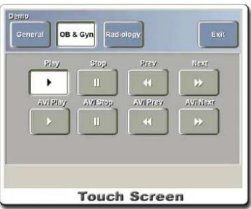
[Figure 3.50 Utility – ETC(Demo)]
UserKey
Sequences of frequently used functions can be recorded to User Keys. The sequences can be performed by pressing the corresponding User Key.
To record a sequence to a User Key:
■ Select the User Key button at the ETC menu or press the User button on the control panel.
■ Select a desired button from User 1 Record... through User 4 Record...
■ When the message below appears, perform the desired functions in a sequence.
User key Recording
■ Once the recording is complete, press the User Key button at the ETC menu or press the User button on the control panel to finish.
User key registration success
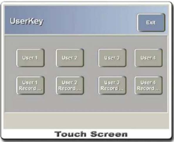
[Figure 3.51 Utility – ETC (UserKey)]
SONOATLAS
This is an ultrasound training program (option menu) with instructions on scan methods and pathology.
Press the Med button or the Ob&Gyn button on the touch screen and the program will appear on the screen.
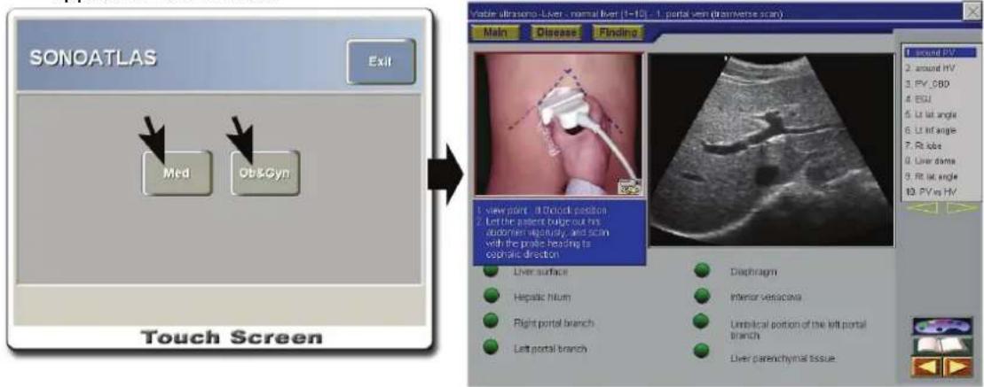
[Figure 3.52 Utility – ETC (SONOATLAS)]
VCR Play
This function is for playing back recorded video. Before using the VCR Play function, make sure that the VCR is properly connected to the system.
For more information on the VCR function, refer to "Chapter 6. Image Management."
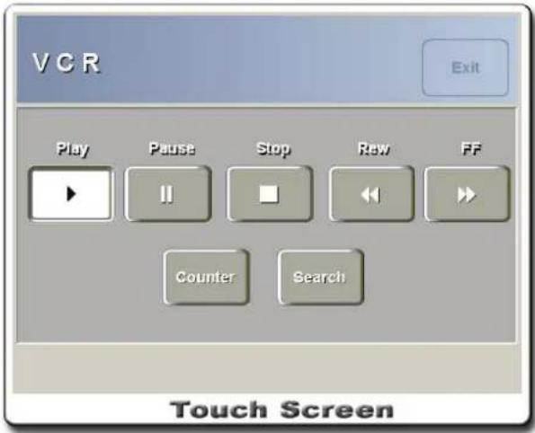
[Figure 3.53 Utility - VCR]
DynamicMR
DynamicMR is the function that removes speckle noise and strengthens edges for 2D images for higher image accuracy. This optional function is available in 2D modes only. It cannot be used when the Phased Array probe is in use.
The function consists of 6 presets. The index value can be specified for each preset for acquiring desired images.
Press the DynamicMR button at the Utility menu and the screen below will appear on the touch screen.
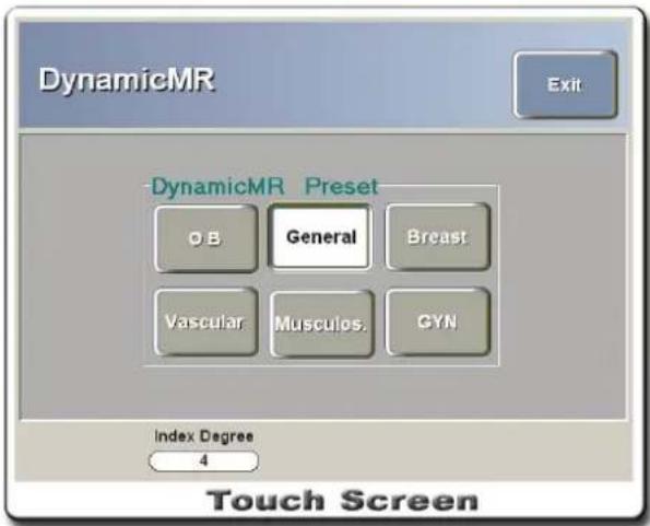
[Figure 3.54 Utility – DynamicMR]
DynamicMR Preset
■ Press the button for the DynamicMR Preset to setup. Each of the following 6 Presets have different DynamicMR properties.
- OB: Expresses amniotic fluid as black, bones (spine, head, etc.) as thin, boundary of the brain as clear, and placenta/fetal organs as soft.
- General: Removes noise and expresses soft images when examining liver, thyroid, prostate, etc.
- Breast: Clearly expresses the distinction between fat tissues and breast tissues.
- Vascular: Expresses the inside of vessels as black so that the vascular walls are seen clearly.
- Musculos. (Musculoskeletal): Clearly expresses muscles, ligaments, etc.
- GYN: Clearly expresses the boundaries of outside of uterus, endometrium, and ovaries.
■ Turn the knob-button below Index Degree to set the Index value for the selected Preset. The saved Index value is kept until the next setup.
■ Press the Exit button to exit the DynamicMR setup function.
■ You can press the DynamicMR button at the 2D menu to select or deselect the settings.
■ Default Index for DunicMR Presets.
| DynamicMR Preset Default Index (1~5) | |
| OB | 5 |
| General | 3 |
| Breast | 4 |
| Vascular | 4 |
| Musculos. | 4 |
| GYN | 3 |
■ Default DynamicMR Presets for Probe Applications.
| Probe Application DynamicMR Preset | |
| OB, OB Early, Fetal heart OB | |
| General, Abdomen, Renal, Small part, Pediatric General | |
| Breast | Breast |
| Vascular | Vascular |
| Musculoskeletal | Musculos. |
| Gynecology, Urology GYN | |
■ The following functions are not available while DynamicMR is in use.
- StressEcho
- Histogram
- User Key
-
BW post, Color post
-
Panoramic Imaging
- Setup
- Screen Saver
- Auto Freeze
- Text in Real state
- Read Zoom in Freeze state
- PGC (Post Gain Control) in Freeze state
- Spacebar function in Freeze state: On/Off toggle for Image Information and Gray Scale Bar
- Patient, Report, Email, VCR, Image Preset, Demo, SONOATLAS: DynamicMR stops automatically when any of these functions are performed.
■ The following 2D functions are available while DynamicMR is in use.
- Gain, TGC, Focus position, Depth, Zoom, Read Zoom, Direction, M-line
Stress Echo
Stress Echo is conducted for examining heart failures. There are two methods: exercise stress test and pharmacological stress test.
By default, this system supports Two Stage Full Disclosure, Two Stage Continuous, Pharmacologic, and Three Stage Bicycle. The user may also create custom protocols as needed.
This function works only with Phase Array Probe and ECG must be turned on.
Stress Echo measurement is measuring a protocol on the patient. Protocols to use in Stress Echo measurement can be selected at the Settings screen.
→ Default protocols supported by the system
| Protocol type | Stage | View sequence | Loops view |
| Two Stage Full Disclosure | RestPost | PLAX,PSAX,A4C,A2CPLAX,PSAX,A4C,A2C | 1 or 4 |
| Two Stage Continuous | RestPost | PLAX,PSAX,A4C,A2CA4C,A2C,PLAX,PSAX | 1 or 4 |
| Pharmacologic | Stage1Stage2Stage3Stage4 | PLAX,PSAX,A4C,A2CPLAX,PSAX,A4C,A2CPLAX,PSAX,A4C,A2CPLAX,PSAX,A4C,A2C | 1 or 4 |
| Three Stage Bicycle | RestPeakPost | PLAX,PSAX,A4C,A2CA4C,A2CA4C,A2C,PLAX,PSAX | 1 or 4 |
Exercise Stress Echo Program
This method conducts examination while the patient is exercising. Follow the procedures below.
■ Press the Stress Echo button at the Utility menu.
■ The Stress Echo Protocol selection screen will appear on the touch screen. If the patient information has not been entered, the Patient Information screen will appear.
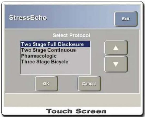
[Figure 3.55 Selecting Stress Echo Protocols]
■ Use the up/down buttons on the touch screen to select the protocol to use and then press the OK button.
■ Press the Cancel or the Exit button to cancel measurement.
■ The system will return to the Acquisition screen, where ROI box and ECG waveform will appear. While the ROI box cannot be resized, you can use the Trackball to move it around.
■ Image acquisition menu items will vary depending on the protocol selected.
■ Pharmacologic: This method injects medication instead of using exercise stress. The method involves using Exercise Stress Echo Program and acquiring images. Pharmacologic is same with other protocols except for Stages. Pharmacologic has 4 Stages.
![graph TD A["Three Stage Bicycle"] --> B["Three Stage Bicycle"] B --> C["Two Stage Full Disclosure / Two Stage Continuous"] C --> D["Pharmacologic"] D --> E["Three Stage Bicycle"] style A fill:#f9f,stroke:#333 style B fill:#f9f,stroke:#333 style C fill:#ccf,stroke:#333 style D fill:#cfc,stroke:#333](/content/2026/05/955519/images/2afd7f282ba491091bc27c7b42c33da2aa19d3fe20f2c741b37c9e5607bf7231.jpg)
[Figure 3.56 Acquisition Screen]
Image Acquisition
Acquisition Ready
■ Select Stages and Views for acquiring images on the touch screen. Stages and Views with acquired images are marked by checks.
■ Press the Acquire button after acquiring the desired images to save them to View. Examination cannot be carried out if heart rate is below 20 or above 300.
CAUTION
Do not repeatedly press the Acquire button while "Acquisition in Progress" is progressing toward 100%. This may result in system error(s).
■ Select Stages and Views for acquiring images on the touch screen. Stages and Views with acquired images are marked by checks.
■ Press the Review button to run Stress Exam of SonoView and view acquired images.
■ Press the Stage button to move on to the next Stage without acquiring images for the current Stage.
■ Press the Suspend button to return to the 2D screen, where Stress Echo can be rerun so that the examination can continue from the previous Stage.
■ Press the Exit button to exit Stress Echo measurement.
■ The method for acquiring images for View of each Stage varies depending on the Capture Method selected at the Setting screen.
- Full Disclosure
Allocates images to each View after acquiring images.
Heart Beat Counter appears in Full Disclosure to indicate the number of "Beats" acquired.
- Perspective
Selects desired Views and then acquires appropriate images for each View.
- Image acquisition stops when Heart Beat Counter reaches 320 since pressing the Acquire button or when the Exit button is pressed. The Stop button and the Pause button are also available during the examination. The ROI box can be moved when paused.
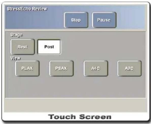
[Figure 3.57 Stress Echo Review]
■ Select "Enable Image Parameter Save" at the Setting screen, and the "Change Image Param" menu will appear on the touch screen. This menu is available when there are 3 or more Stages.
- Preset values for the View images acquired in the previous Stage are applied to the View images to be acquired in the next Stage. Preset values saved are "Gain, Depth, ROI Position, Sector Size, and Sector Invert (L/R)."
- This function is not available for the first Stage and the last Stage. The menu items appear only for the second or third Stage. Start Acquire after selecting the menu.
Accept Prior to Store
The Accept Prior to Store function allows the user to confirm acquired images before proceeding to the next View. This function id available only when the Capture Method at the Setting screen is set to Perspective and Accept Prior to Store is set to on.
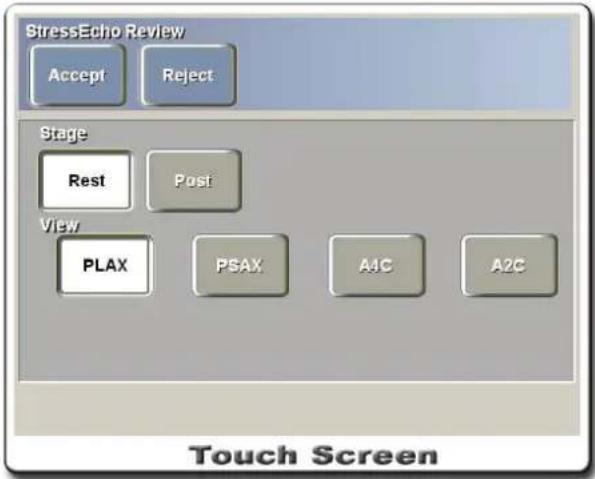
[Figure 3.58 Stress Echo Review]
■ Selecting the Accept button accepts the acquired images as candidates and proceeds to the next stage, Best Beat Select.
■ To cancel the acquired images and return to the previous Acquisition Ready state, select the Reject button.
Best Beat Select
Once image acquisition is complete, the next stage is Best Beat Select. This stage is for selecting optimal beat images for examination.
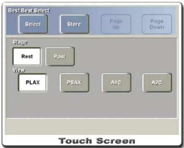
[Figure 3.59 Best Beat Select]
■ Use the Trackball to select desired images on the screen and then press the Select button.
■ Press the Store button to save the selected images. The screen moves to a View with images yet to be saved. Use the Page Up and Page Down buttons to view the images not shown on the current screen.
■ You may not select images saved in other Views.
End of Protocol
Once the image acquisition and image selection are complete, press the Review button to move to Stress Exam. Or, select the Exit button to exit Stress Echo Program.
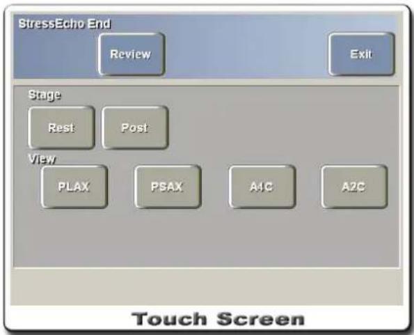
[Figure 3.60 Stress Echo End]
SonoView Stress Exam Screen
This program retrieves and manages the images saved during Stress Echo examinations.
After all examinations are complete, press the Review button on the touch screen to move to the screen where you can view Stages and Views of the patient examined.
Alternatively, exit Stress Echo Program and press the SonoView button on the control panel to run SonoView.
In SonoView, press the Stress Exam button to view the patient list. Selecting a patient moves to Review mode where you can retrieve the patient's Stress Echo examination images.
Review Mode Monitor Display
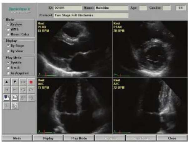
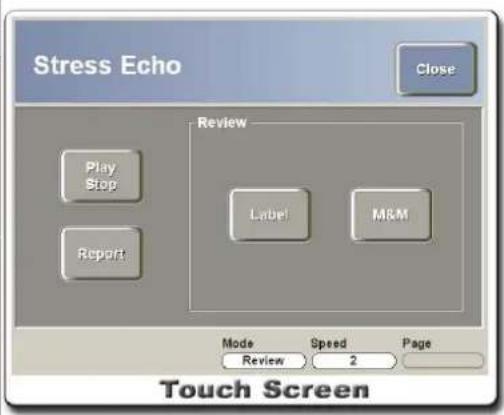
[Figure 3.61 Stress Exam – Review Mode]
■ Patient information such as ID, name, Age, Gender, Protocol, and Page are displayed across the top of the screen.
■ Image Information
Stage Name, View Name, and Heart Rate are displayed at the upper left-hand corner of the screen, and ECG and Frame position information is displayed at the lower left-hand corner of the screen.
The number of the current frame is displayed if you stop the image while viewing it.
■ Selecting Image
Use the Trackball and the Set button to select or deselect images. To select multiple images, select images while pressing the CTRL key on the keyboard.
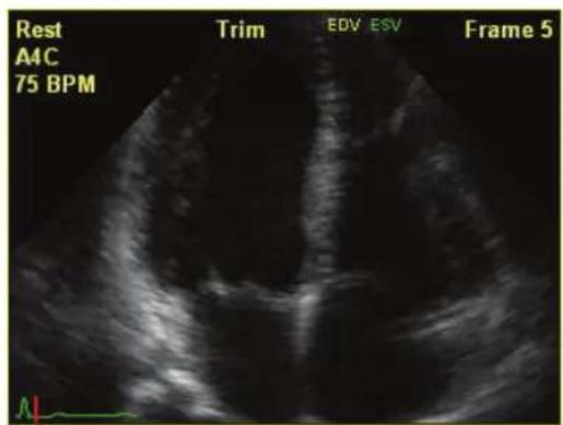
Selecting Menu
Use the Trackball and the Set button to select the menu on the left-hand side of the screen.
■ Mode: Repeatedly press the Mode button at the bottom of the screen or use the up-down switch below the touch screen to select modes.
- Review: This reviewing mode displays 4 images at a time.
- WMS: Wall Motion Scoring function is available. Two images are displayed at the top and Wall Motion Diagrams matching the images at the top are displayed at the bottom. WMS is available only for 4 Views (PLAX, PSAX, A4C and A2C).
- Meas/Calc: 2D Measure (Distance, Area, Trace) and Calculation (Simpson Method) functions are available.
■ Display: Repeatedly press the Display button to sort images by Stage or View.
■ Play Mode: Repeatedly press the Play Mode button to select Play Mode for the image. Depending on the mode selected, certain zones are repeated when playing save images.
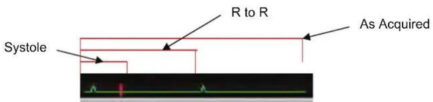
■ Functionality:
 | Speed Control | Image playback speed can be controlled in 5 steps. Playback speed can also be selected using the up-down switch below the touch screen. This applies to all images. |
 | Trace Shuttle | Stop image playback, select the image, and then select the Shuttle function. This allows you to use the Trackball to scroll back and forth the image frames. The Trackball cursor disappears when using the Trace Shuttle function. Press the button again to deactivate it. |
 | Play / Stop | Plays or stops the image. This is also accessible through the Play / Stop button on the touch screen. This applies to all images. |
 | Beat Navigation | An “R to R” section is counted as 1 Beat. This function is used for skipping certain Beats in images with multiple Beats. This applies to selected images only. |
 | Image Navigation | This is used for navigating to other images when there are multiple images in the same Stage or the same View. Index of the image is displayed at the lower right-hand corner of the image. This applies to selected images only. |
 | Comments | This opens the screen for entering comments. |
 | Report | This shows Patient Info, WMS, Calculation, and Comments on the screen. This is also accessible through the Report button on the touch screen. |
 | Trim | Use this to remove the first or the last frame for an image clip. Frames removed vary depending on Play Mode. Changing Play Mode after performing Trim restores the setting. This applies to selected images only. |
 | Change Label | Select an image and press the Change Label button to change Stage and View for the image. Label can also be changed by using the Label button on the touch screen. |
 | Mix & Match | Select multiple images and then select the Mix & Match function to view selected images only. Select it again to return to the previous state. Mode or Display cannot be changed while the Mix & Match function is in use. This is also accessible through the M&M button on the touch screen. |
■ Change Page: When there are more than 4 images, they cannot fit into one page. In this case, press the Page Up button and the Page Down button to navigate through pages to view different images. Pages can also be selected using the up-down switch below the touch screen.
Index of the current page is displayed at the upper right-hand corner of the screen.
WMS (Wall Motion Scoring) Mode
WMS Mode performs color mapping on the various parts of the heart suspected of muscle failures for Wall Motion Scoring.
The image clips appear at the top, and WMS Diagrams matching the image clips appear at the bottom.
Select a desired Score button from the menu on the left or on the touch screen, and then click the WMS Diagram area to perform WMS.
WMS Diagrams are available only for 4 Views (PLAX, PSAX, A4C and A2C).
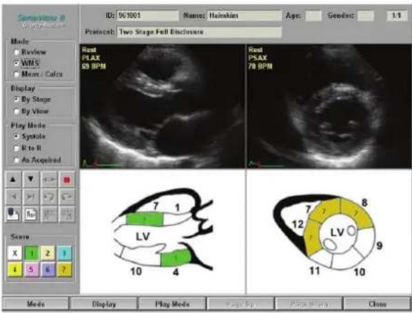
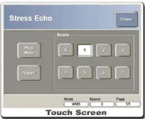
[Figure 3.62 Stress Exam – WMS Mode]
■ Score Definition
| Description | Numeric | Score |
| Not Scored X White | ||
| Normal | 1 | Green |
| Hypokinetic | 2 | Brown |
| Akinetic | 3 | Cyan |
| Dyskinetic | 4 | Yellow |
| Aneurysmal | 5 | Magenta |
| Akinetic with Scar 6 Blue | ||
| Dyskinetic with Scar 7 Mustard |
Color
■ Segment Definition
| Left Ventricular Segment Segment # | |
| Basal Anterior Septum 1 | |
| Basal Anterior | 2 |
| Basal Lateral | 3 |
| Basal Posterior | 4 |
| Basal Inferior | 5 |
| Basal Septum | 6 |
| Mid Anterior Septum | 7 |
| Mid Anterior | 8 |
| Mid Lateral | 9 |
| Mid Posterior | 10 |
| Mid Inferior | 11 |
| Mid Septum | 12 |
| Apical Septum | 13 |
| Apical Anterior | 14 |
| Apical Lateral | 15 |
| Apical Inferior | 16 |
Meas/Calc Mode
■ 2D Measure
- 2D Distance: This method measures the distance between two points on the image. Press the Distance button, and then use the Trackball and the Set button to select the start point and the end point and measure their distance. Press the Change button again to reposition the start point and the end point.
- Ellipse: This method draws an ellipse on the image and measures its circumference and area. Press the Ellipse button, and then use the Trackball and the Set button to select the start point and the end point. Use the Trackball to adjust the size of the ellipse and measure its circumference and area. Press the Change button again to reposition the start point and the end point.
- Trace: This method draws a closed curve on the image and measures its circumference and area. Press the Trace button, and then use the Trackball and the Set button to draw a freehand curve in desired area. Draw a closed line that links the start point with the end point and measure its circumference and area.
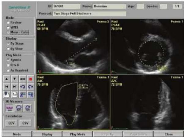
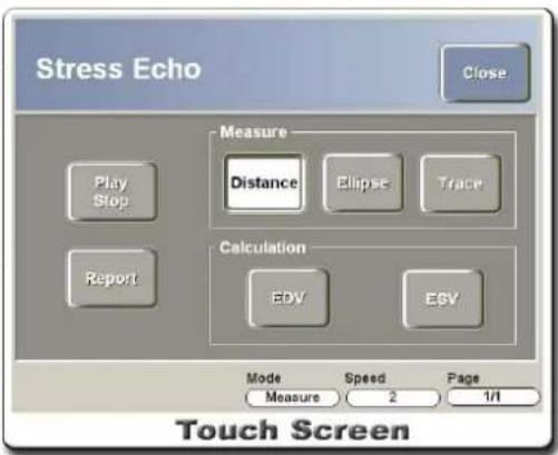
[Figure 3.63 Stress Exam – 2D Measure Mode]
- In 2D Measure, you can press the Exit button to cancel measurement, or use the Clear button to erase the results.
- There are two methods for displaying Measure Data. The first is to display measure data in all frames. This allows viewing of measure data from all frames. The second is to display measure data only in the frames measured. You can view measured frames one by one by pressing the R key on the keyboard. Press Space Bar on the keyboard to select between the two display methods.
■ Calculation
- EDV: This method calculates Diastolic Volume on image. The measurement method is the same as Trace.
- ESV: This method calculates Systolic Volume on image. The measurement method is the same as Trace.
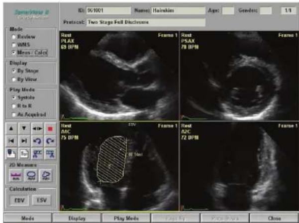
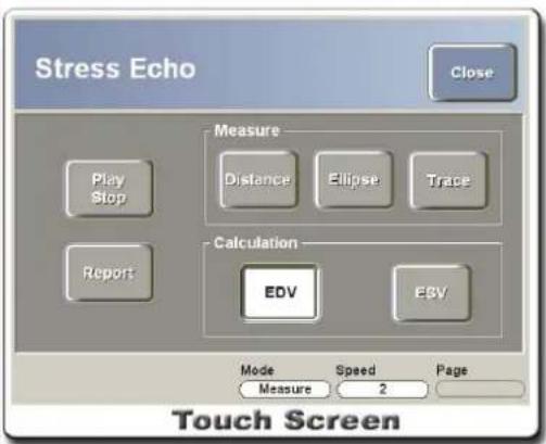
[Figure 3.64 Stress Exam – Calculation Mode]
- You can press the Exit button to cancel calculation, or use the Clear button to erase the results.
- Calculation can be performed for A2C and A4C Views only. Each View can contain one EDV and one ESV measurements.
- There are two modes for displaying Calculation Data. Mode1 displays Calculation on all calculated frames, and Mode2 displays Calculation only in the frames where calculations were performed.
Press Space Bar to toggle the modes.
Report
Select the “(Comments)” button or the “(Report)” button, and the menu will appear on the monitor and the touch screen.
■ Patient Info: Displays the information of the patient receiving the Stress Echo examination.
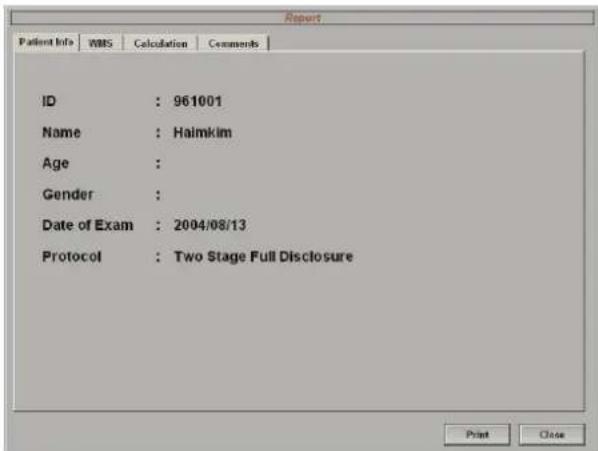
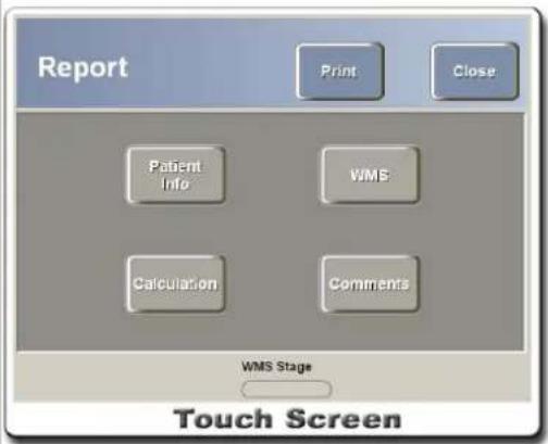
[Figure 3.65 Report – Patient Info]
■ WMS: Displays Wall Motion Score and Diagram for each Stage.
- Select the Overall tab at the bottom of the screen to view Wall Motion Score for the entire Stage.
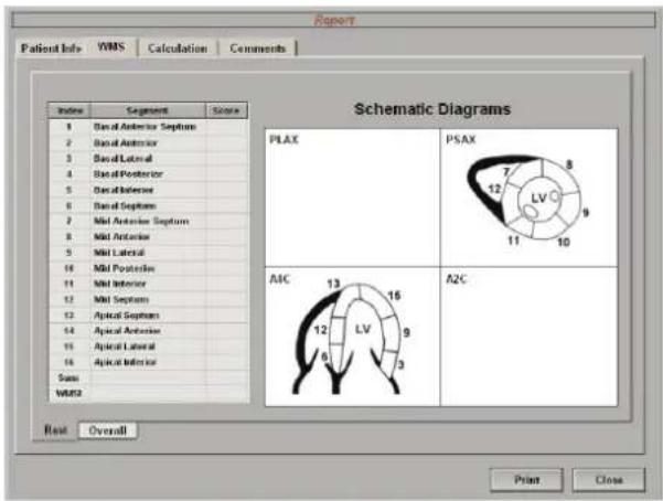
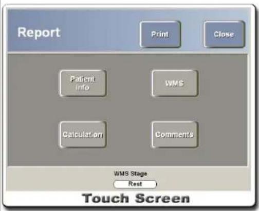
[Figure 3.66 Report – WMS]
- Diagrams can be modified at the WMS Report screen. Place the cursor over the segment to modify and double-click the Set button. At the Score selection window as illustrated below, select a desired Score.
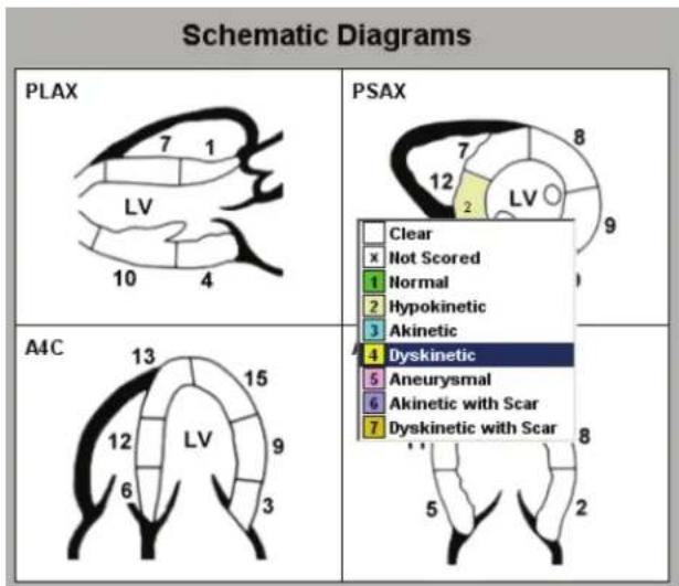
■ Calculation: Displays EDV and ESV measurement values for each Stage.
- Stroke Volume, Cardiac output and EF for A2C and A4C can be calculated only if Dias Vol and Sys Vol values have been measured before and if the Dias Vol value is greater than the Sys Vol value. Dias Vol of Bi Plane can be calculated only if Dias Vol of A2C and A4C is measured before, and Sys Vol can be calculated only if Sys Vol of A2C and A4C is measured before.
- Calculation equations are as follows.
| Diastolic Volume | EDV = π/4 i=1n ai2 · L/n cc(ml) where n = 20 |
| Systolic Volume | EDV = π/4 i=1n ai2 · L/n cc(ml) where n = 20 |
| Stroke Volume | SV = EDV - ESV cc(ml) |
| Cardiac Output | CO = (SV × HR) / 1000 m./min |
| Ejection Fraction | EF = (EDV - ESV) / EDV × 100 % |
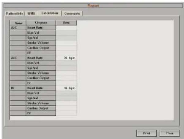
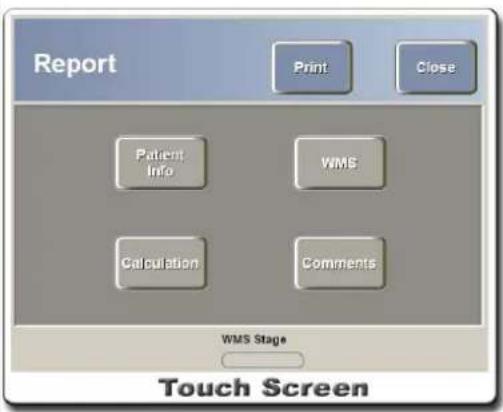
[Figure 3.67 Report – Calculation]
- Calculation values can be modified at the Calculation Report screen. Place the cursor over the item to modify and double-click the Set button. Enter the new value and press the Enter key on the keyboard to save the new Calculation value.
| Dias Vol | [50.21 ml] |
| Sys Vol | 30.73 ml |
| Stroke Volume | 19.48 ml |
| Cardiac Output | 1.40 l/m |
| EF | 38.79 % |
- Editable values are "Dias Vol" and "Sys Vol." Values modified at the Report screen are marked with " ." Once the volume values are changed, "Stroke Volume", "Cardiac output" and "EF" values are automatically re-calculated. Note that the volume value for Bi-plane retains the original value even if the A4C and A2C volumes are modified. Re-performing measurement in Meas/Calc mode discards the modified values at the Report screen.
■ Comments: You can enter comments or descriptions for the Stress Echo examination.
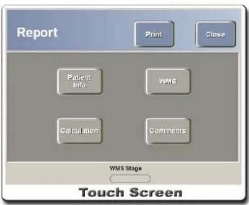
[Figure 3.68 Report – Comments]
- Press the Print button on the monitor or the touch screen, and the Print Setup window will appear.
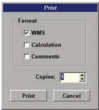
- WMS, Calculation, and Comments can be selected for printing and the number of print copies can be specified.
Biopsy
Biopsy is the method used for acquiring cells of abnormal tissue by Biopsy Needle. Press the Biopsy button at the Utility menu.
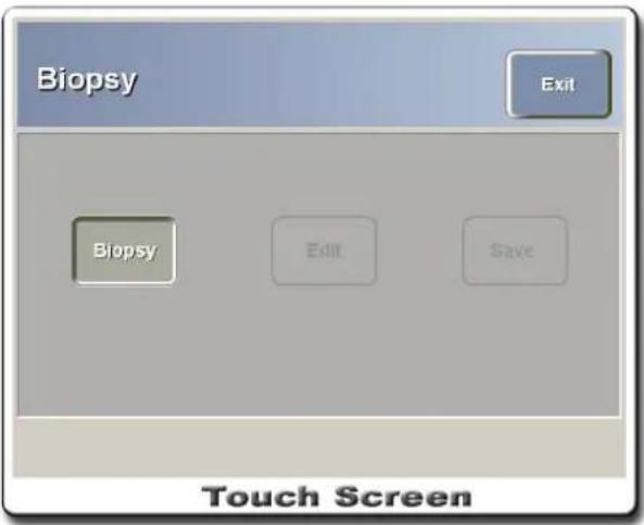
[Figure 3.69 Utility – Biopsy]
Displaying Biopsy Guideline
- Press the Biopsy button to toggle on/off the Biopsy Guideline displayed on the screen. Turn Biopsy on and the following message will appear.
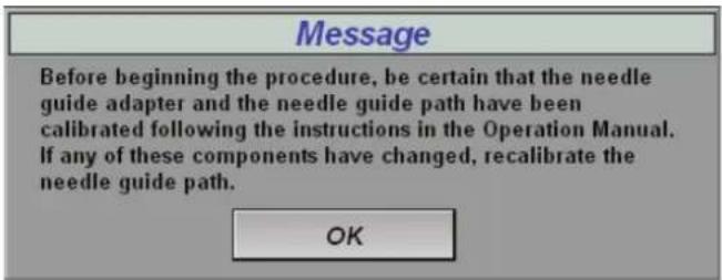
- Check the needle path by referring to the Biopsy Guideline on the screen. If the needle path is correct, click the OK button. If it is not correct, adjust the Biopsy Guideline.
Biopsy Guideline Setup
- Press the Edit button to edit the Biopsy Guideline. The following message will appear on the screen.
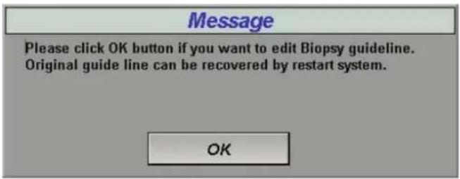
-
If you press the OK button, the Biopsy Edit screen will appear. Or, press the Cancel button to close the Biopsy menu. To restore the settings while editing the Biopsy Guideline, reboot the system.
-
Press the Save button when editing is complete. The following message will appear on the screen.
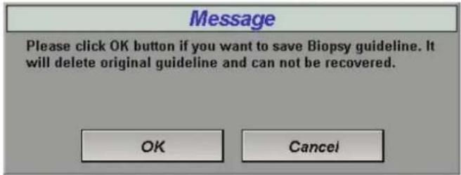
- Press the OK button to save the edited Biopsy Guideline. Note that the previous Biopsy Guideline is deleted and it cannot be recovered.
Image Store
Pressing the Image Store button on the touch screen saves the scan mode images on the system. The last save image can be sent by e-mail.
Chapter 4
Diagnosis Modes
DIAGNOSIS MODE TYPES AND CONTROL....3
DIAGNOSIS MODES....3
DIAGNOSIS MODE SCREENS AND IMAGE INFORMATION....3
CHANGING DIAGNOSIS MODE FORMATS....4
OPTIMIZING DIAGNOSIS MODE....5
BASIC MODES....7
2D MODE....7
M MODE....13
COLOR DOPPLER MODE 16
POWER DOPPLER MODE 19
PW (PULSE WAVE) SPECTRAL DOPPLER MODE....21
CW (CONTINUOUS WAVE) SPECTRAL DOPPLER MODE 26
AUTOMATIC CALCULATOR....28
COMBINED MODES 29
2D/C/PWMODE....29
2D/PD/PW MODE 29
2D/C/CWMODE 30
2D/PD/CWMODE 30
2D/CMMODE 31
DUAL LIVE MODE....31
MULTI-IMAGE MODES.... 32
DUAL-2DMODE 32
4 - 2 ACCUVIX XQ Operation Manual
DUAL-2D/C MODE 32
DUAL-2D/PDMODE....33
MULTI-DIMENSIONAL MODES 34
MULTI-DIMENSIONAL....34
ACQUIRING3D IMAGES....35
3D VIEW 37
OPTIMIZING 3D IMAGES....55
3D XI™ MODE 64
XISTIC MODE (OPTIONAL)....76
Diagnosis Mode Types and Control
Diagnosis Modes
This product supports a variety of diagnosis modes including Basic modes, Combined modes, Multi-Image modes, and 3D modes.
■ Basic Modes: Include 2D Mode, Color Doppler Mode, Power Doppler Mode, M Mode, PW Spectral Doppler Mode, and CW Spectral Doppler Mode.
■ Combined Modes: These modes are Color Doppler Mode or Power Doppler Mode combined with M Mode, PW Spectral Doppler Mode, or CW Spectral Doppler Mode. Dual Live Mode, which features Color Doppler Mode and 2D Mode in single screen, is also one of the Combined Modes.
■ Multi-Image Modes: In Dual Modes you can view two images side by side simultaneously and compare them.
■ 3D Modes: These modes provide 3D images.
Functionalities for each mode are restricted by the probes selected. For example, Freehand 3D Mode supports all probes except for Static CW probe, and Volume 3D Mode supports 3D probe only.
Diagnosis Mode Screens and Image Information
The following table shows the information appearing on different diagnosis mode screens.
| Monitor Display | 2D Mode | M Mode | C Mode | PD Mode | PW Mode | 3D Mode |
| 2D Image and Image Information | ● | ● | ● | ● | ● | ● |
| M Image and Image Information | ● | |||||
| Color Doppler Image and Image Information | ● | |||||
| Power Doppler Image and Image Information | ● | |||||
| Spectral Doppler Image and Image Information | ● | |||||
| M Line | ● | |||||
| D Line and Sample Volume | ● | |||||
| ROI (Region of Interest) Box | ● ● | ● | ||||
| Title Bar | ● | ● | ● | ● | ● | ● |
| Depth Marker | ● | ● | ● | ● | ● | ● |
| Focusing Point & Number | ● | ● | ● | ● | ● | ● |
| Gray Scale Bar | ● | ● | ● | ● | ● | ● |
| Color Bar | ● ● | |||||
| TGC Curve | ● | ● | ● | ● | ● | ● |
The following table shows the image information appearing for each mode. Note that image information for 2D mode appears in all modes.
| Image Information | 2D Mode | M Mode | C Mode | PD Mode | PW Mode | |
| Gain | ● | ● | ● | ● | ● | |
| Dynamic Range | ● ● | |||||
| Frame Average | ● ● ● ● | |||||
| Power | ● ● | |||||
| PRF (Pulse Repetition Frequency) | ● ● ● | |||||
| Wall Filter | ● ● ● | |||||
| Sensitivity | ● ● | |||||
| Sample Volume Depth | ● | |||||
| Sample Volume Size | ● | |||||
| Angle | ● | |||||
Image information and gray scale bar disappear from the screen by pressing Spacebar.
Changing Diagnosis Mode Formats
The following section explains how to change the display format that is common to all diagnosis modes.
Changing Active Image Mode
All diagnosis modes except for 2D mode provide two or more modes simultaneously. You can press the button for each mode on the touch screen to select the active image mode and control its menus.
Changing Active Image in Multi-Image Modes
Use the Update button, the Set button and the Dual button on the control panel to change the active image. For example, press the Update button, the Set button or the Dual button in Dual-2D mode to freeze the image being scanned on the left-hand side of the screen and show the image being scanned on the right.
Freezing 2D Image in Spectral Doppler Mode
When the simultaneous function is turned on and 2D image and spectral Doppler image are displayed real-time, you can freeze the 2D image to view more accurate spectral Doppler image.
Press the Update button on the control panel to freeze the 2D image. Press the button again to display the 2D image again.
If the simultaneous function is turned off, the current image mode is indicated as "PW Only" or "2D Only" at the upper right-hand corner of the screen.
You can determine the use of simultaneous modes by setting "Simultaneous Mode" under the Misc. tab on the Settings screen. If this option is set to "Off", the Simultaneous button on the PW Spectral Doppler menu remains inactive.
You can also freezing 2D image by the Update button in 2D/C/PW Mode, 2D/PD/PW Mode, 2D/C/CW Mode, 2D/PD/CW Mode, and 2D/C/M Mode.
Image Depth Control
Use the Depth switch on the control panel. Raise the Depth switch to decrease view depth, or lower the Depth switch to increase the view depth. Maximum depth and minimum depth vary depending on the probe.
Zooming Image
Use the Zoom switch on the control panel to zoom the image. Raise the Zoom switch and the Zoom box will appear. Use the Change button and the Trackball to move and resize the Zoom box. Repeatedly pressing the Change button toggles the "Zoom Pos." and "Zoom size" indication on the screen.
■ Zoom position: Press the Change button to make the HD Zoom box appear with solid lines. Use the Trackball to move the box to any desired position.
■ Zoom size: Press the Change button to make the HD Zoom box appear with dotted lines. Use the Trackball to resize the HD Zoom box.
Adjust the size and the position of the Zoom box and then press the Set button to zoom the image. The Zoom Navigation box on the screen shows the relative position of the zoomed area.
When using the Zoom function, press the Z button on the control panel to hide the Zoom Navigation box and deactivate Zoom Position. Press the Z button again and the Zoom Navigation box will appear.
Change Depth or press the Exit button on the control panel to cancel the image zoom.
Read Zoom
This function is for zooming the image saved in the memory. Note that this is not available in Dual mode or Loop mode.
The RD Zoom menu appears on the touch screen when the image is frozen by pressing the Freeze button or when adjusting the Zoom switch on the control panel.
Turn the knob-button below the RD Zoom menu to run the Read Zoom function and zoom the image. When Read Zoom is activated, the Zoom switch will not work. (Write Zoom cannot be activated.)
Optimizing Diagnosis Mode
The following are instructions for optimizing images in all diagnosis modes.
Gain Control
Use the mode knob-button on the control panel to adjust the brightness of the image. Turn it clockwise to increase Gain or turn it counter-clockwise to decrease Gain.
Adjusting Post Gain
When the image is frozen by pressing the Freeze button on the control panel, you can adjust the mode knob-button to adjust Gain. Turn it clockwise to increase Gain or turn it counter-clockwise to decrease Gain.
Post Gain can be adjusted to any values between +10 and -10. The Post Gain value is displayed on the screen in the format of “*PG:0.” The Gain value is restored to the value before freezing when the image becomes active again.
TGC Control
When ultrasound is transmitted through the human body, the lucency of ultrasound weakens as it travels deeper into the body. TGC (Time Gain Compensation) can be used to supplement this. For obtaining the best image quality, TGC is divided into 8 regions which can be used to adjust Gain by different depths.
Move the TGC slide to the right (+) to increase Gain (brightening the image) or move the TGC slide to the left (-) to decrease Gain (darkening the image).
Harmonic Function
This product provides the OHI (Optimal Harmonic Imaging) function. In 2D mode, press the HAR button on the control panel to activate the function.
Focus Position Control
Use the Focus switch on the control panel to focus on specific regions for clearer view. Raise the switch to move the focus position up and lower the switch to move the focus position down.
Focus Number Control
Press the Focus up/down button on the touch screen to adjust the number of focusing points. Check on the screen as focusing points are added or removed.
Frequency Change
Each probe provides a wide range of frequencies for obtaining images of best quality. Use the Frequency up/down button on the touch screen to change the probe frequency.
This function is available for linear probes (L5-12IM, L6-12IS) only.
Power Control
Power is the intensity of the acoustic output.
Use the up-down switch below Power on the touch screen to adjust the value.
Basic Modes
2D Mode
This basic mode, also referred to as B Mode (Brightness mode), provides scan planes of organs.
![MEDISON General #511 /4.0cm MI 1.3/2006-05-03 L0-15S / Gen Tis 0.2/11:34:51 am [20] 0.57/10 dB T240/P90 FSM * P5 : 0](/content/2026/05/955519/images/af731de6a6863ffeb8053ea81670562727b0e01279a2124747f815132805a281.jpg)
[Figure 4.1 2D Mode]
2D Mode Selection
Since 2D mode is always turned on except for special cases, the 2D button does not function as a toggle. In any diagnosis mode, just press the 2D button to switch to 2D mode which is the basic diagnosis mode.
2D Menu
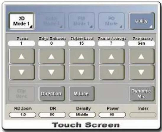
![2D Mode 2 Candle abcate 1 PIV Mode 1 PD Mode Utility Tissue Cystic Pulse Intervention Trapex Steer Apex Reset AIO Scan Area Scan Angle Frame Rate 100 % 0 [Deg] Fact Touch Screen](/content/2026/05/955519/images/3384fe2af8f99103d3987d08ac4bb394a74cfbff6fe65e78f969c29bc25d436a.jpg)
[Figure 4.2 2D Menu]
Changing 2D Image Format
Changing Image Direction
- Changing Left/Right Orientation (Horizontal Orientation, Direction): Press the Direction button on the touch screen.
- Changing Up/down Direction (Vertical Orientation, Apex): Press the Apex button on the touch screen.
- Changing View Area
Turn the knob-button below Scan Area on the touch screen to adjust the size of the Area to be anywhere between 60% and 100%. After changing the view area, turn the knob-button below Scan Angle left/right to move View Area left/right and view other regions. Scan Angle is unavailable for linear probes.
The frame rate (FPS) drops as the view area becomes larger and the frame rate increases as the view area becomes smaller.
Showing M Line
M Line indicates the relative position of the M Mode image or the Spectral Doppler Mode image in the 2D image.
Press the M line button on the touch screen to show M Line, and press the M line button again to hide M Line.
Optimizing 2D Images
Adjusting Frame Average
The Frame Average function obtains the average for the previous frame and the current frame and displays it on the screen in order to reduce speckles on continuous images on the same examination regions. Adjusting this function to High will result in a relatively smooth display of the image, but the user may get the impression that the display is slower (the actual frame rate does not drop). It is recommended that this function be turned off when examining OB, cardiac and other movement-intense organs. It is useful to set this function to High when examining internal medicine and organs with little movements.
Use the Frame Average up/down button on the touch screen to make adjustments.
This clearly displays the boundaries between tissues or organs. Edges appear clearer if the Edge Enhance value is set high. Use the Edge Enhance up/down button on the touch screen to make adjustments.
Adjusting Reject Level
This function is used to eliminate noise or low level echoes for clearer signals. Use the Reject Level up/down button on the touch screen to make adjustments.
Adjusting Tissue Property
You can select the ultrasound velocity according to the patient's physique. Physique menu contains Cystic, Adipose, Normal and Solid. Use the Tissue up/down button on the touch screen to make adjustments.
Smooth Function
This is available for Convex probe. It shows smoother 2D images by eliminating noise. Use the up-down switch below Smooth on the touch screen to make adjustments.
Pulsed Inversion Function
When Harmonic mode is in use, press the Pulsed Inversion button on the touch screen to activate this function. This shows sharp images with clear edges. This function is not available for L5-12IM, VNA6-12, L6-12IS, and L8-15IS probes.
Trapezoid Function
When using Linear probe, you can stretch the 2D image into a trapezoid and examine it in a larger area. Press the Trapez. button on the touch screen to run this function.
When adjusting the image depth, the Trapezoid function may not be available at certain depth values. Note that using the Zoom function turns the Trapezoid function off.
DynamicMR Function
This optional function removes speckle noise and strengthens edges for 2D images for higher image accuracy.
Press the DynamicMR button on the touch screen to run it. The previous configuration will be applied to the image.
NOTE
DynamicMR has 6 Presets, each of which has 5 Indexes. To select new values or make other settings, press the DynamicMR button on the Utility menu and make the settings.
Steer Function
This function adjusts the angle of the ultrasound beam in order to prevent loss of ultrasound information. This function is available for Linear probe only. Use the Steer button on the touch screen to run this function.
Adjusting Dynamic Range
You can adjust the minimum value and maximum ratio of the input signal and display images by changes in contrast. Images appear soft at higher ratios and coarse at lower ratios.
Turn the knob-button below DR on the touch screen to make adjustments.
Adjusting Density
Use the up-down switch below Density on the touch screen to adjust the image scan line. This is useful for quickly examining images with low values.
While density can be adjusted to Low, Middle, or High, it is available in 4 steps — Low, Middle1, Middle2 and High — for Color Doppler Mode.
Adjusting Frame Rate
Frame rate is the number of images generated per second. Frame rate should be set to high when viewing fast moving organs.
Use the up-down switch below Frame Rate on the touch screen to make adjustments.
AIO (Auto Image Optimization) Function
This function optimizes 2D images by adjusting 2D Gain, Dynamic Range and TGC automatically.
Press the AIO button on the control panel to activate it and the Reset AIO button on the touch screen to deactivate it. It deactivates when Harmonic Mode or Pulse Inversion is activated.
Pressing and holding the AIO button executes the AIO function repeatedly.
The probes and applications in the following table are applied with the new AIO function to obtain more optimized images.
| Abdomen | OB | SmallPart | Vascular | Cardiac | |
| L6-12IS | ● ● | ||||
| C5-2EL | ● | ||||
| C2-6IC | ● | ||||
| 3D4-7EK | ● | ||||
| P2-4AC | ● |
Clip Save Function
This function saves the screen image into a clip. It is provided for Cardiac application with Phased Array probe or Contrast Agent application with C5-2EL or C1-4EC probe (only Low MI).
Press the Clip Save button on the touch screen to activate it. Specify the unit and value(s) to be used for saving a clip under the Misc. tab on the Setting screen.
While saving a clip, press the Set button on the control panel to complete the saving process or the Exit button to cancel the saving process.
NOTE
Clips can be saved by beat only when ECG is running; clips will not be saved when ECG beats do not appear even if the setting is selected for clips to be saved by beat.
If 10 seconds of a color image are saved, the screen will be updated 3 seconds after saving is completed.
Spatial Compound Image (SCI) Function
This function displays more smooth 2D images by eliminating speckle noises and is available only in 2D Mode for the L6-12IS probe.
Press the SCI button on the touch screen to activate it. Its value(s) can be adjusted with the SCI Filter up/down button that appears when it is running.
When the SCI function is in use, Frame Average, ECG Trigger, AIO and Write Zoom functions become unavailable.
The SCI function deactivates when 3D Mode, M Mode, C Mode, PD Mode, PW Mode, Pulse Inversion or Trapezoid is activated.
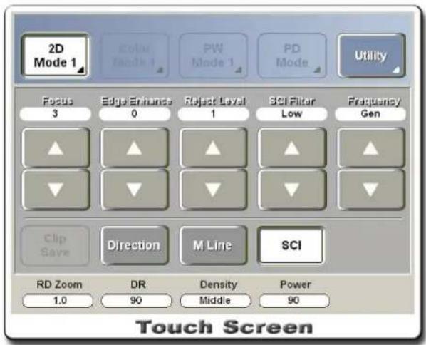
[Figure 4.3 Spatial Compound Image]
Low MI Function
This function displays clearer contrast images and is available for Contrast Agent application with the C5-2EL or C1-4EC probe.
Press the Low MI button on the touch screen to activate it. Images can be adjusted via the menu displayed on the touch screen. Press the Low MI Off button to deactivate Low MI and switch to 2D Mode. Press the 2D Menu button to keep Low MI activated and switch to 2D Mode.
Use of the Low MI menu is similar to that of the 2D Mode Menu.
![2D Mode 2 Color Mode 1 PW Mode 1 PD Mode Utility Tiscus Normal Smooth Mid1 Pulse Inversion Trapies Stress Apex Low MI Reset AIO Scan Area Scan Angle Frame Rate 100% 0 [Deg] Fast Touch Screen](/content/2026/05/955519/images/d89e118a6624b87f6b14b24fd7b927d17c32bd20ab5b5b4bbfc3fbc803e65fb4.jpg)

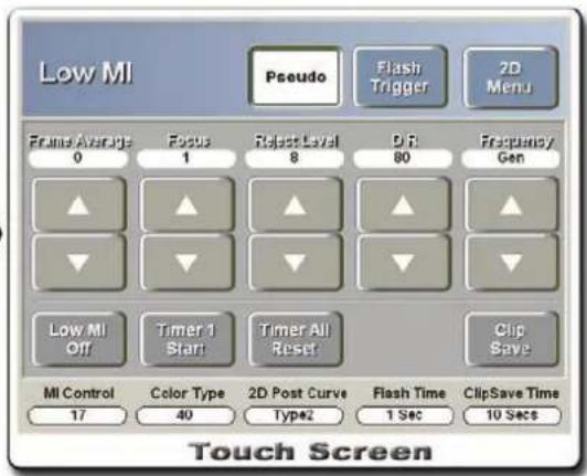
[Figure 4.4 Low MI]
- Pressing the Timer 1 Start button resets and activates Timer. The elapsed time after an agent is injected can be measured with a counter displayed on the screen. If an image becomes frozen, Timer 2 is activated to show the time for which it is frozen. Press the Return Low MI button to return to the Low MI function.
![[2D] G60 / 80dB FAO / P90 INV / FSIO LowMI T1: 00:00:10 T2: 00:00:10](/content/2026/05/955519/images/344a42f9bcc087d153e6f98d28963f472a3eba5aac884eff2602b6dee18ff6df.jpg)
- Pressing the Timer All Reset button resets both Timer 1 & 2.
- Flash Trigger is a function that breaks the agent bubbles injected by bursting flashes at the maximum MI Power of the system and probe for the specified Flash Time. Flash Time can be specified with the up/down switch under Flash Time on the touch screen.
- Use the knob-button under MI Control to adjust the MI Power value. Available setting ranges are between 0 – 100.
- Color Type and 2D Post Curve change the color of the image applied with Pseudo.
NOTE
While Low MI is in use, you may not switch to any mode other than Dual Mode.
Trying to activate Low MI in Harmonic Mode results in activation of Pulse Inversion.
M Mode
This mode provides images that change over time at certain regions of 2D mode scan planes, such as the movement of a heart valve. A 2D image is also displayed to indicate the relative position of the selected region and allow the user to change the position.
![MEDISON General M1300 / 4.0cm MI 1.3/2006-05-03 L0-1SIS / Gen TIs 0.3 / TC6:35 nm [2006] GSS / 8988 FA10 / P90 FSIB PG:0 Loop Pos Freeze](/content/2026/05/955519/images/dac5d12e4c94321535b237590cd9f9ec69ebb03c8e1008aa434012869c753835.jpg)
[Figure 4.4 M Mode]
M Mode Selection
Press the M button on the control panel. Press it again to return to 2D mode.
2D/M Menu
M Mode and 2D Mode have the same menus for image optimization.
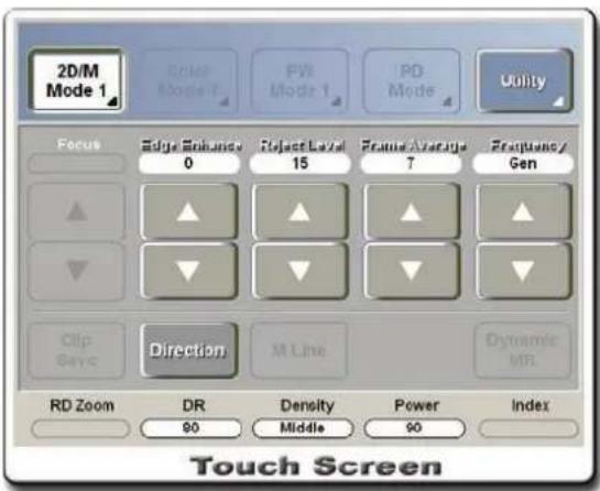
![2D/M Mode 2 Color Mode 1 PW Mode 1 PD Mode Utility Tissue Cystic Speed 180 Pulse Inversion Trapsc Steel Apex Reset AIO Scan Area 100 % Scan Angle 0 [Deg] Frame Rate Fast LoopFormat Top Down DispFormat 50/50 Touch Screen](/content/2026/05/955519/images/dd900586af2c6d6c44cf3588d63bb52757a1c216c38fb8f3c1245412c6aef90b.jpg)
[Figure 4.5 2D/M Menu]
Changing M Mode Format
Adjusting M Line
M Line indicates the relative position of the M Mode image in the 2D image. Use the Trackball on the control panel to move M Line left and right and view different regions.
Adjusting Sweep Speed
Use the Speed up/down button on the touch screen to adjust the sweep speed of M image in steps.
Changing Loop Format
Use the up-down switch below LoopFormat on the touch screen to change the position where 2D image and M image appear. Top Down Format places 2D image and M image at the top and the bottom, and Side by Side Format places them on the left and the right.
Changing M Image Size
Use the up-down switch below Disp Format on the touch screen to change the size of 2D image and M image. Available options are "50/50", "40/60", and "60/40" which indicate the image size ratio between 2D image and M image.
Free Angle M Mode
This mode allows the user to rotate or move M Line—which normally moves horizontally—for viewing 2D images. Adjusting the depth for 2D image initializes M Line.
NOTE
This mode is available for Phased Array probe. It is unavailable in Color Doppler Mode or Zoom Mode.
Starting and Adjusting Free Angle M Mode
Press the Free Angle button on the touch screen to run it. The menu is illustrated in the figure below.
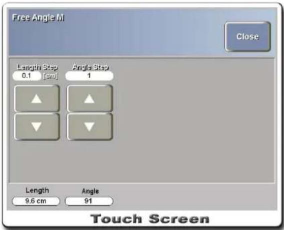
[Figure 4.6 Free Angle M Mode]
Turn the knob-buttons below Length and Angle on the touch screen to adjust the length and angle of M Line.
Use the Length Step and Angle Step up/down buttons on the touch screen to adjust the steps for "Length" and "Angle." If Step is set to "3," the value can be adjusted in multiples of 3.
Position of M Line can be adjusted by moving the Trackball. Start point and end point of M Line cannot be outside the 2D image.
Things to Consider When Using Free Angle M Mode
Selecting another mode (2D Mode, etc.) while using Free Angle M Mode exists Free Angle M Mode and activates the selected mode.
The Patient, End Exam, Indicator, Text, Body marker, and Measure buttons function normally in Free Angle M Mode.
If you selecting the User, E-mail, Mic or SonoView button in Free Angle M Mode, the selected button functions after shifting to the normal M Mode.
The buttons on the control panel other than those mentioned above (those with LED off) do not function.
NOTE
For information on optimizing M image, refer to "2D Mode."
Color Doppler Mode
In this mode you can obtain a variety of information about blood flow within the 2D Image such as the existence of blood flow, its average speed and its direction within the ROI (Region of Interest).
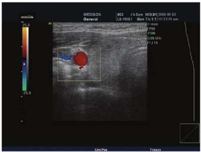
[Figure 4.7 Color Doppler Mode]
Color Doppler Mode Selection
Press the C button on the control panel. Press it again to return to 2D mode.
C Menu
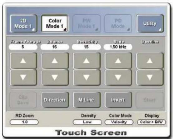
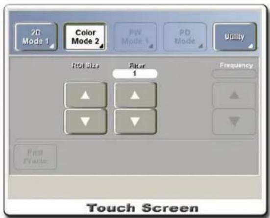
[Figure 4.8 C Menu]
Changing Color Image Format
NOTE
Color Bar is a color map that shows the direction and velocity of blood flow. Colors above the baseline across the center of the color bar indicate blood flowing toward the probe and colors below the baseline indicate blood flowing away from the probe.
Adjusting Color Bar Baseline
Press the Baseline up/down button on the touch screen. Press the up button to move the baseline up on the color bar, or press the down button to move the baseline down.
Baseline can be adjusted only when Color Mode is set to "Velocity."
Inverting Color Bar
Press the Invert button on the touch screen. Inverting the color bar also inverts the colors displayed on the image.
Changing Color Display Information
Use the up-down switch below Color Mode on the touch screen to select Velocity, Power, Variance, or Vel + Var. If "Velocity" or "Vel + Var" is selected, numbers will be displayed above and below the color bar indicating the color scale values. If "Variance" is selected, +1 and -1 will be displayed. If "Power" is selected, no numbers will be displayed.
Color Image Optimization
Adjusting Balance
Adjust the range of color image display by comparing Gray Level of the 2D image with Doppler signal values of the color image. As the Balance value increases, color image appears even in regions with high Gray Level in 2D image (bright regions), expanding the range of color image.
Use the Balance up/down button on the touch screen to make adjustments.
Adjusting Sensitivity
Use the Sensitivity up/down button on the touch screen to make adjustments.
Increasing the Sensitivity value increases Sensitivity, and decreasing the Sensitivity value decreases Sensitivity. As color sensitivity increases, frame rate drops.
Adjusting Scale (PRF)
Use the Scale up/down button on the touch screen to make adjustments. Increasing the Scale value increases PRF (Pulse Repetition Frequency), expanding the range of blood flow velocity displayed, and decreasing the value decreases PRF, narrowing the range of blood flow velocity displayed.
Changing ROI Box
Color Pos: ROI (Region Of Interest) indicates the area of the 2D image where color (blood flow) information is displayed in Color Doppler Mode. Use the Trackball to change the
position of the box.
Color Size: Press the ROI Size up/down button on the touch screen. Alternatively, repeatedly press the Change button on the control panel to change the function of the Trackball and use the Trackball when its appropriate function is displayed on the screen.
Adjusting Wall Filter
Wall Filter is an electric filter that removes low-frequency Doppler signals from movement of the vessel wall. Adjust Cutoff Frequency to remove from the screen Doppler signals with frequencies that are lower than the Cutoff Frequency.
Use the Filter up/down button on the touch screen to make adjustments. Increasing the Filter value increases the Cutoff Frequency for Wall Filter, and decreasing the value decreases the Cutoff Frequency for Wall Filter.
Fast Frame Function
This function increases the frame rate when the application is set to Fetal Heart. The image moves approximately 70% faster than the actual speed.
Press the Fast Frame button on the touch screen to run this function.
Steer Function
When using Linear probe, this function adjusts the ultrasound beam angle to prevent the loss of color information caused by the ultrasound beam angle.
Use the Steer button on the touch screen to make adjustments.
Display Function
Use the up-down switch below Display on the touch screen to select the Display format. Color Doppler Mode supports Color + B/W Image, Color Only, and B/W Only display.
TDI (Tissue Doppler Image) Function
When the application Cardiac or Pediatric Cardiology and the Phased Array probe is in use, movements of cardiac tissues can be viewed in Doppler modes.
Cardiac tissues can be viewed by color information in Color Doppler Mode and Power Doppler Mode, and time-dependent changes of cardiac tissues can be viewed by spectral Doppler images in PW Spectral Doppler mode.
Press the TDI button on the control panel. "TDI on" will be indicated on the screen.
NOTE
For information on other menu items, refer to "2D Mode."
Power Doppler Mode
Instead of the speed or direction of blood flow, Power Doppler Mode displays the overall strength of blood flow, thereby showing information about the existence and amount of blood flow in the sample area.
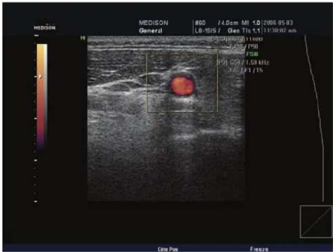
[Figure 4.9 Power Doppler Mode]
Power Doppler Mode Selection
Press the PD button on the control panel. Press it again to return to 2D mode.
PD Menu
Use of the Power Doppler Mode menu is similar to the Color Doppler Mode menu.
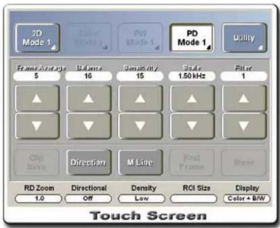
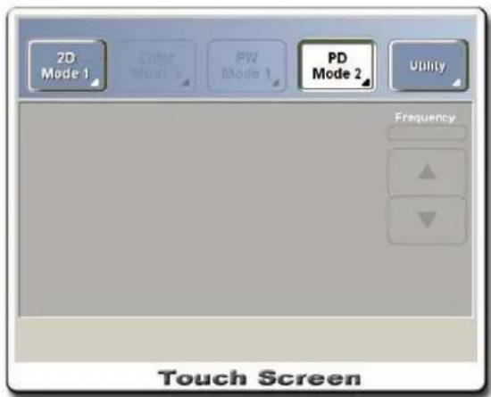
[Figure 4.10 PD Menu]
Optimizing Power Doppler Image
Directional Function
This function displays the amount (power) of blood flow and direction of blood flow. Press the Directional button on the touch screen to activate it.
NOTE
■ Color Bar is a color map that displays the existence of blood flow and its amount. Brighter colors on the color bar indicate high amount of blood flow.
■ For information on other menu items, refer to "Color Doppler Mode."
PW (Pulse Wave) Spectral Doppler Mode
This mode shows the velocity of blood flow at a specific position within blood vessel. Distance (depth) information can be obtained by transmitting pulses over time frames. This mode is useful for measuring low-speed blood flow such as in abdomen and peripheral vessels. A 2D image is also displayed to indicate the relative position of the selected region in blood vessel and allow the user to change the position.
On the PW Spectral Doppler Mode image, the horizontal axis represents time, and the vertical axis represents speed (or frequency).
![MEDISON General #1850 /4.0pm M10.45 2006-05-03 L6-ISIS / Gen TIs 0,1 /15:55:05 am [FW] S70 FT /4.80 kHz Depth 10 Size 2.00 Angle 0 * PG: 0 pDJ GS3 /11:00 FA2 /P10 FSM SV Pos](/content/2026/05/955519/images/f52e1416e09e7c389122f56ce5f04d73abd890d866747ae0ddd08c24f0bc2c3a.jpg)
[Figure 4.11 PW Spectral Doppler Mode]
PW Spectral Doppler Mode Selection
Press the PD button on the control panel. Press it again to return to 2D mode.
D Menu
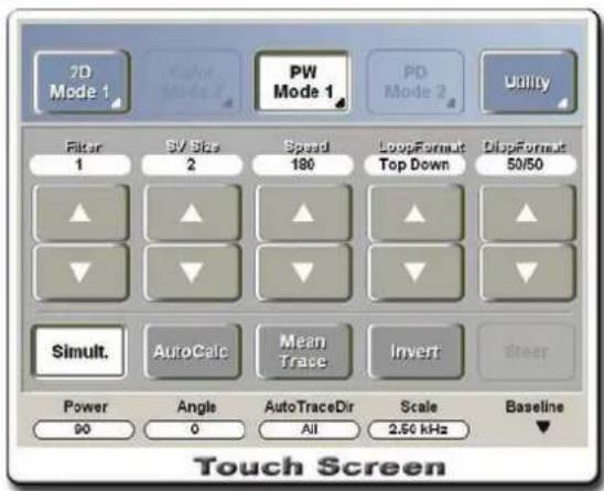
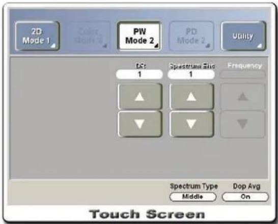
[Figure 4.12 PW Menu]
PW Spectral Doppler Mode Format Change
Adjusting Sweep Speed
Use the Speed up/down button on the touch screen to adjust the sweep speed of Spectral Doppler image in steps.
Adjusting Doppler Baseline
Use the up-down switch below Baseline on the touch screen. Raise the switch button to move the baseline up, or lower the switch to move the baseline down.
Changing Loop Format
Use the up-down switch below Loop Format on the touch screen to change the position where 2D image and Spectral Doppler image appear. Top Down Format places 2D image and Spectral Doppler image at the top and the bottom, and Side by Side Format places them on the left and the right.
Changing Spectral Doppler Image Size
Use the up/down button Disp Format on the touch screen to change the size of 2D image and Spectral Doppler image. Available options are "50/50", "40/60", and "60/40" which indicate the image size ratio between 2D image and Spectral Doppler image.
Activating Simultaneous Mode
The PW Spectral Doppler image and 2D image can be displayed simultaneously or separately.
Press the Simult. button on the touch screen to activate Simultaneous Mode. When Simultaneous Mode is on, selecting the button again to deactivate Simultaneous Mode.
Simultaneous Mode decreases Doppler PRF, thus decreasing the measurable speed range. Activate the Simultaneous Mode option by setting Simultaneous Mode as "Allow 2D/PW" or "Allow 2D/C/PW" in the Misc. tab at the Setting screen.
Inverting Doppler Axis
Press the Invert button on the touch screen. Positions of the + and - speed indications will be inverted.
Optimizing PW Spectral Doppler Image
Sample Volume
Located on the 2D image, it indicates the position of the Spectral Doppler image. Displayed in the format of xx.x@yy.y mm, it indicates that the size of the sample volume is "xx.x mm" and the depth is "yy.y mm." For example, 2.0@16.7 mm means that the Sample Volume of 2.0mm size is located at a depth of 16.7mm.
Changing Position: Use the Trackball on the control panel.
Changing Size: Press the SV Size up/down button on the touch screen. Alternatively, repeatedly press the Change button on the control panel to change the function of the Trackball. "SV Pos" and "SV Size" will appear on the screen in one after another.
Changing Angle: Use the knob-button below Angle on the touch screen to make
adjustments. Turn the knob-button to change the angle by 1° , or press it to change the angle to -60° , 0° , or 60° . Adjusting the sample volume angle allows more accurate measurement of velocity.
Adjusting Doppler Sound Volume
Use the Sound knob-button on the control panel. Pressing the knob-button toggles sound on/off. Turn it clockwise to increase the volume and turn it counter-clockwise to decrease the volume.
Adjusting Spectrum Enhancement
This function enhances sensitivity of Spectral Doppler images by adjusting brightness and sensitivity of Spectral Doppler images. Press the Spectrum Enh. up/down button on the touch screen to make adjustments.
Adjusting Spectrum Type
Use the Spectrum Type up/down button on the touch screen to adjust the Spectral Doppler image to a desired type. You can obtain soft spectral Doppler images.
Adjusting Doppler Average
This function determines availability (on/off) of FDRP (Fast DRP). It can enhance expression of Spectral Doppler images. Press the Dop Avg up/down button on the touch screen to make adjustments.
HPRF (High PRF) Function
This function measures blood flow beyond the speed limit at specific depths. It doubles or triples the original scale. This function is available only in PW Spectral Doppler Mode.
Starting HPRF
Continuously increase the scale value at a specific depth to start HPRF. Phantom Gate will appear on D Line at the position higher than the sample volume. Once HPRF starts, PRF does not increase even if you increase the scale value.
Finishing HPRF
While HPRF is in use, decrease the scale value by one step to finish HPRF. The PRF value will be the maximum value for the current PW Spectral Doppler Mode.
Adjusting Sample Volume Position
If you adjust the sample volume in PW only state, the system calculates the PRF value and the Phantom Gate position and updates them on the Spectral Doppler image. If HPRF cannot start, HPRF will terminate.
If you adjust the sample volume in 2D only state, the PRF value does not change.
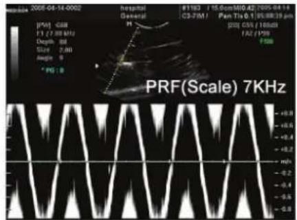
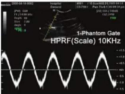
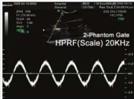
[Figure 4.13 Starting HPRF]
NOTE
HPRF is not available in Simultaneous Mode. Also, if the twice the PRF value is 23kHz or above before starting HPRF, HPRF will not start.
CAUTION
■ The Phantom Gate position can be located outside the 2D image area in Zoom Mode.
■ Make sure that sample volume and Phantom Gate are not placed together in the measuring area. If there are two or more sample volumes placed on vessels, the Spectral Doppler image may have excessive noise due to the unwanted Doppler substances.
AIO (Auto Image Optimization) Function
This function allows increasing of the scale and/or automatic change of the baseline for unaliasing of Spectral Doppler images. Press the AIO button on the control panel.
NOTE
When AIO is in use, scale can increase by twofold at maximum. If the current scale is at the maximum, the AIO function will not start.
Things to Consider for Auto Image Optimization
This algorithm manipulates Automatic Calculator (Real Time Automatic Doppler Trace). Please refer to "Things to Consider for Real Time Automatic Doppler Trace."
AIO can function properly if the Spectral Doppler image repeats for 2 cycles or more.
Spectral Doppler images that are not aliased may be recognized as optimal images and the AIO function may not be available. If the Spectral Doppler image is small because the scale
value is high (even though not aliased), the AIO function automatically adjusts the scale value and displays the optimal Spectral Doppler image.
NOTE
For information on Wall Filter, Scale, Dynamic Range, Steer, Frequency, and TDI Adjustment, refer to "2D Mode" and "Color Doppler Mode." Methods for using the menus may be different, but the functions are identical.
CW (Continuous Wave) Spectral Doppler Mode
This mode shows the velocity of blood flow within blood vessel. It can measure high-speed blood flow by continuously transmitting pulses. However, this is not useful for viewing information for specific areas.
A 2D image is also displayed to indicate the relative position of the vessel and allow the user to change the position. Note that 2D image is not displayed when using Static CW probes (CW2.0, CW4.0).
Steered CW Spectral Doppler Mode
When using Phased Array probe, press the CW button on the control panel to activate the function. Press it again to return to 2D mode.
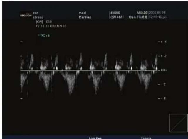
[Figure 4.14 Steered CW Spectral Doppler Mode]
Static CW Spectral Doppler Mode
This mode is available only for Static CW probes. At the Probe Selection screen, select Static CW probe on the touch screen to activate the mode.
![MEDISON CAR stress [CW] GGS F1 / 14.29 kHz / P100 Depth 73 *PG:8 med Cardiac P1 8944 / 12.0cmM19.09 2006-06-28 P3-SAC1 Gen Tis 16 12:05:40 µm [70] 550 / 10dB FA4 / P100 100A / PS10 -4 H12 -4 JIR = 0 Loop Pos Freeze](/content/2026/05/955519/images/26df0b0080b1d58527154a9c719c1b00aeb9fce10d0160ca68b6bf7e8935d0ad.jpg)
[Figure 4.15 Static CW Spectral Doppler Mode]
CW Menu
Methods for using the menu are the same as in PW Spectral Doppler Mode.
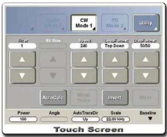
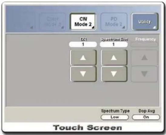
[Figure 4.16 CW Menu]
NOTE
For information on optimizing CW images, refer to "PW Spectral Doppler Mode."
Automatic Calculator
Adjusting Frequency
The Automatic Calculator function, also called Real Time Automatic Doppler Trace, can be activated by selecting the AutoCalc button on the touch screen. When Automatic Calculator is in use, peak trace on the Spectral Doppler image is highlighted in green.
Real-time Doppler signals are traced and their measurement values are displayed. PSA, EDV, TAP, RI, PI, S/D, VTI, Gpeak, Gmean, and Vmean values can be obtained in Cardiac Package, and PSA, EDV, TAP, TAM, RI, PI, S/D, and Vmean values can be obtained in Non-Cardiac Packages.
Press the Mean Trace button on the touch screen to run the Mean Trace function. Mean Trace is highlighted in black on the Spectral Doppler image. This is not available when the application is Cardiac.
| CAUTION | Auto Trace measurement values in measurement mode and Automatic Calculator measurement values may not be identical. This is because each function uses different algorithms. For more accurate measurement, use Auto Trace in measurement mode. |
Auto Trace Direction
This function selects the areas that are traced by Doppler signals. Use the up-down switch below Auto Trace Dir on the touch screen to select All, Up, or Down. You can select either Up or Down when the application is Cardiac.
Things to Consider for Automatic Calculator
Results will not be displayed if the function is run against inaccurate values.
Trace and/or results may not be accurate in the following situations.
- Aliasing occurs because PRF is too low in comparison to the image speed, or the Spectral Doppler image is clustered around the baseline because PRF is too high.
- Peak is indistinctive or intermittent such as in Spectral Doppler images for veins.
- It is difficult to identify the Spectral Doppler image because Doppler Gain Setting is too high or too low.
- Index Display immediately after moving the sample volume with the Trackball.
- Certain portions of major Spectral Doppler image signals are cut off because the Wall Filter value is too high.
- Peak Trace is interfered with abnormal noise or artefact of Doppler signals.
- Heart rate is 140bpm or above.
Combined Modes
2D/C/PW Mode
Color Doppler Mode and PW Spectral Doppler Mode are displayed simultaneously. To use the 2D/C/PW Mode, under the Misc. tab on the Setting screen, set Simultaneous Mode to "Allow 2D/C/PW."
In Color Doppler Mode, press the M button on the control panel. Or, in PW Spectral Doppler Mode, press the C button on the control panel.
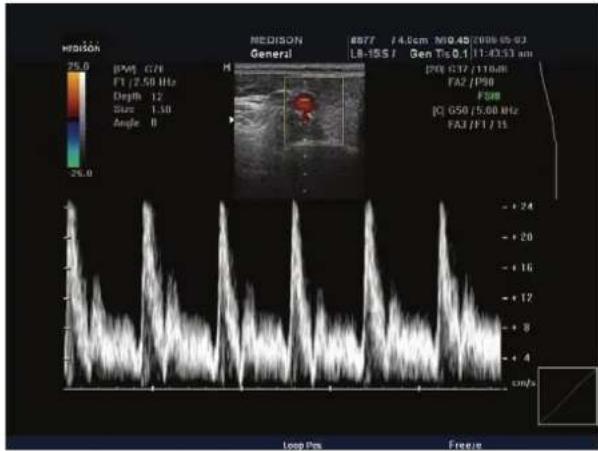
[Figure 4.17 2D/C/PW Mode]
2D/PD/PW Mode
Power Doppler Mode and PW Spectral Doppler Mode are displayed simultaneously. To use the 2D/C/PW Mode, under the Misc. tab on the Setting screen, set Simultaneous Mode to "Allow 2D/C/PW."
In Power Doppler Mode, press the M button on the control panel. Or, in PW Spectral Doppler Mode, press the PD button on the control panel.
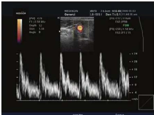
[Figure 4.18 2D/PD/PW Mode]
2D/C/CW Mode
Color Doppler Mode and CW Spectral Doppler Mode are displayed simultaneously. Note that this mode is available for Phased Array probe only.
In Color Doppler Mode, press the CW button on the control panel. Or, in CW Spectral Doppler Mode, press the C button on the control panel.
![M0103 car stress 70.0 (CM) GOS F1 /14.29 kHz /P100 Depth 78 med Cardiac #1023 / 12.0cm/MID 09/2006-16-28 P3-SAC / Gen Tls 1& 12:06:53 pm [20] GSO / 9048 FA4 /P30 HA1 /FSB [C] GSO / 4.80 kHz FA2 /F2 /B HR = II Loop Pos Freeze](/content/2026/05/955519/images/6853002b33c2d53c61fe21d2a1adc100aa5b319a1c39688425143de67318dde8.jpg)
[Figure 4.19 2D/C/CW Mode]
2D/PD/CW Mode
Power Doppler Mode and CW Spectral Doppler Mode are displayed simultaneously. Note that this mode is available for Phased Array probe only.
In Power Doppler Mode, press the CW button on the control panel. Or, in CW Spectral Doppler Mode, press the PD button on the control panel.
![MOHOS car stress med Cardiac #1020 / 12.0cm NID 08/2006-06-28 P3-SAC / Gen Tis 1.6 / 12:06:53 pm [CV] GSB F1 / 14.29 kHz / P100 Depth 78 [CQ] GSB / 90dB FAM / P30 HAN / FSB [C] GSO / 4.80 Hz FA2 / F2 / B HR = 3 Loop Nex Freeze](/content/2026/05/955519/images/fa21d52e43bcc6cbfb5263694c42a3a743f621e1fda8c41901b9f8497df365d9.jpg)
[Figure 4.20 2D/PD/CW Mode]
2D/C/M Mode
Color Doppler Mode and M Mode are displayed simultaneously. Note that this mode is available only when the application is “Fetal Heart” or when the application is “Cardiac”, “General” or “Pediatric” for Phased Array probe.
In Color Doppler Mode, press the M button on the control panel. Or, in M Mode, press the C button on the control panel.
![MEDISON Cardias #2050 / 16.0cmM10.82/2008-06-20 P3-7AC I Pen Tis 0.6 03:56:10 pm [2004] G30/95aB FA2 /P90 FSB [Q] G70/4.58 MHz FA4 /F2 / B Loop Pan Freeze](/content/2026/05/955519/images/c4c9437729f7ee79570327a80277e818b48a2501a783bc80e81394af5e15a80d.jpg)
[Figure 4.21 2D/C/M Mode]
Dual Live Mode
This mode displays 2D Mode and Color Doppler Mode simultaneously. 2D image is displayed on the right and Color Doppler image is displayed on the left. If run in Power Doppler Mode, it displays 2D image and Power Doppler image.
Press the DUAL LIVE button on the control panel to activate it, and use the Color Doppler menu to optimize the image. Use the Cine Save function for more effective viewing.
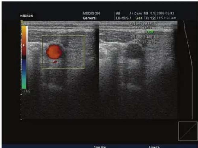
[Figure 4.22 Dual Live Mode]
Multi-Image Modes
The multi-image viewing function is only available when the images and conditions on both sides are identical.
Dual-2D Mode
This mode allows you to compare 2D images side by side.
In 2D Mode, 3D Mode, or Spectral Doppler Mode, press the Dual button on the control panel to select the function. Press the Dual button to close Dual-2D Mode and return to 2D Mode which is the default mode.
Use the Dual button, the Update button and the Set button to change the left/right images.
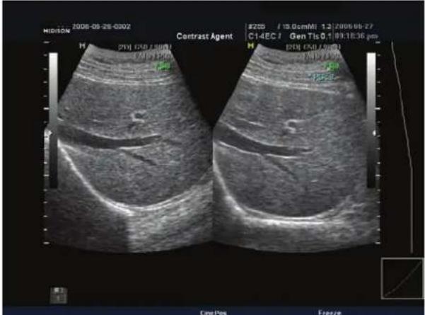
[Figure 4.23 Dual-2D Mode]
Dual-2D/C Mode
This mode allows you to compare Color Doppler Mode images side by side.
In Color Doppler Mode, press the Dual button on the control panel. Or, in Dual-2D Mode, press the C button on the control panel.
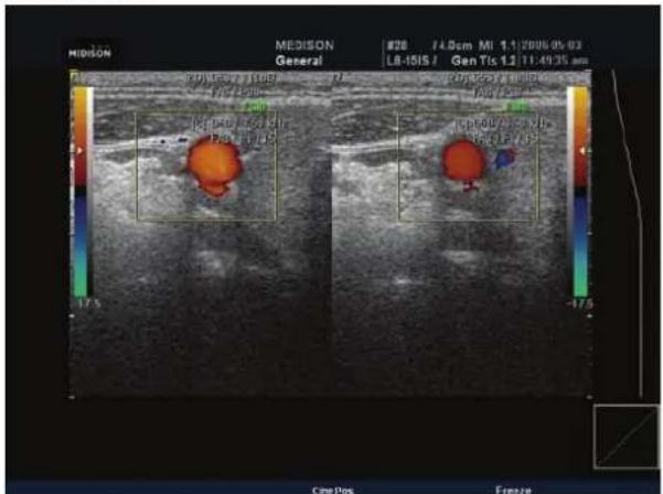
[Figure 4.24 Dual-2D / Color Doppler Mode]
Dual-2D/PD Mode
This mode allows you to compare PD Mode images side by side.
In PD Mode, press the Dual button on the control panel. Or, in Dual-2D Mode, press the PD button on the control panel.
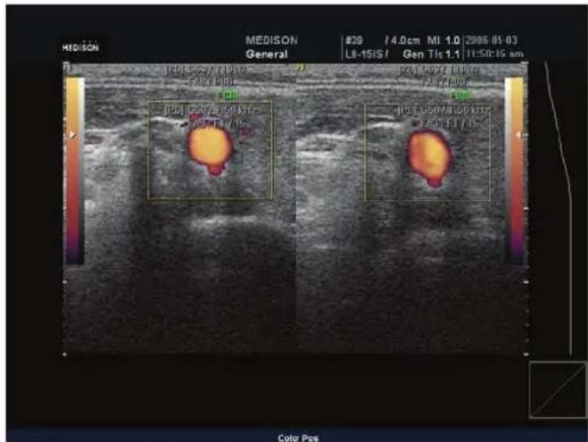
[Figure 4.25 Dual-2D/PD Mode]
Multi-Dimensional Modes
Multi-Dimensional
Multi-Dimensional Modes display tissues or organs as 3-dimensional images. Multi-Dimensional Modes continuously obtain 2-dimensional surface images from the probe and render the volume data for displaying 3-dimensional images.
Multi-Dimensional Mode Types
Types by Image Information
- 3D Mode: This is the default 3D Mode. Press the 3D/4D button in 2D Mode to access it.
- 3D Color Doppler Mode: This mode displays blood flow velocity and direction information on 3D image by color. Press the 3D/4D button in Color Doppler Mode to access it.
- 3D Power Doppler Mode: This mode displays existence of blood flow and its amount information on 3D image by color. Press the 3D/4D button in Power Doppler Mode to access it.
Types by Scan Methods
- Static 3D Mode: This mode obtains a 3-dimensional image by rendering continuous 2D images once. 3D probes obtain volume data by mechanical scanning, and 2D probes obtain volume data by freehand scanning.
Live 3D Mode: This mode obtains a 3-dimensional image by rendering continuous 2D images multiple times. It processes volume data real-time and it is available for 3D probes only. - XI STIC Mode: Use a 3D probe to obtain the fetal cardiac cycle and STIC volume data
How to Improve 3D Image Quality
- Consider the direction, division and size of the viewpoint, as well as the visibility of an object.
■ Before 3D scanning, adjust the contrast of the specific textures in 2D Mode.
■ The ROI (Region of Interest) box determines the image being rendered. Portions of image outside the ROI box are not included in the rendering process.
■ Bigger the ROI box, slower is the rendering speed. Therefore, set an appropriate ROI box size.
■ To determine the contour of objects, surface of objects should be insulated with hypoechoic tissues—such as amniotic fluid—which do not generate echoes.
■ To obtain a high quality 3D surface, adjust the low-threshold value.
■ Set the noise gray value lower than the surface value in order to obtain clearer images from edges of the ROI box to the surface of the objects.
In general, do not adjust High-Threshold; set it to the maximum value of 255. If the surface render algorithm is higher than the Threshold value, this value indicates the boundary of the surface. Therefore, use High-Threshold to adjust the boundary manually.
Acquiring 3D Images
Image Scan Mode
This mode allows acquisition of 3D and Live 3D images. Press the 3D/4D button on the control panel to access it. Set the menu items and then press the Freeze button to start scanning.
Press the Exit button or the 3D/4D button on the control panel to exit Image Scan Mode. You may also select a button for another mode to exit.
If 3D image is acquired by changing the left/right direction (by selecting the Direction menu), it is displayed on View Mode. But if 3D image is acquired by changing the up/down direction (by selecting the Apex menu), it is not displayed on View Mode.
Volume Box
Multi-Dimensional Modes contain two volume boxes. The volume box with cyan lines indicates the scanning area on the 2D image, and the volume box with yellow lines indicates the area of the rendered 3D image. The yellow box is also called the ROI box.
- Changing Position: Use the Trackball to change the position of the volume box. Press the Change button on the control panel to change the function of the Trackball to "Move" and then change the position. The function of the Trackball is displayed in the feedback area.
- Changing Size: Turn the knob-buttons below ROI Width and ROI Height on the touch screen to make adjustments. Alternatively, press the Change button on the control panel to change the function of the Trackball to "Resize" and then change the size.
Setting Auto Calc
This function is available when the application is OB. It automatically sets up the volume box.
Press the Auto ROI Off button on the touch screen to change it to Auto ROI On. The volume box will appear in the desired area of the image.
This is not available in 3D Color Doppler Mode or 3D Power Doppler Mode.
NOTE
The Auto ROI function is available only when the fetal body is displayed on the screen. This function manipulates brightness and contrast of the image.
Adjusting Vol. Angle
Use the up-down switch below Vol. Angle on the touch screen to adjust the scanning angle of the 3D probe.
Adjusting Scan Quality
Use the up-down switch below Scan quality on the touch screen to adjust the quality of the 3D image.
Low: The image quality is low but the 3D image speed (or rendering speed) is fast.
Mid: The image quality is better than Low Quality but the speed is slower than Low Quality.
High: The image quality and expression are good. Speed is slower than Mid Quality.
Extreme: The image quality is excellent. Use this to obtain detailed images regardless of the speed.
Image Acquisition Procedures
Static 3D Image Acquisition Procedures
- Press the 3D/4D button on the control panel to move to Image Scan Mode, and then select the 3D button on the touch screen.
- Adjust "Scan Quality" and "Vol. Angle" on the touch screen.
- Use the volume box on the screen to set the position and size of the 3D image to acquire.
- Press the Freeze button on the control panel. A 3D image will be acquired for the area within the volume box and then View Mode will appear.
![2008-07-17-0091 FPS27 / 14.0cm M10.63 2008-07-20 3D3-BEK / Gen Tlb0.1 06:52:05 pm [2D] C65 / 90dB FA10 / P90 FS10 * PG : 0](/content/2026/05/955519/images/5ff5c9a4d9cb238d99813c2d39a537a79531bda2d554ed40ae5ef515254c3f2b.jpg)
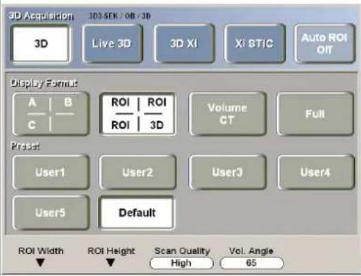
[Figure 4.26 3D Acquisition - 3D]
Live 3D Image Acquisition Procedures
- Press the 3D/4D button on the control panel to move to Image Scan Mode, and then select the Live 3D button on the touch screen.
- Adjust "Scan Quality" and "Vol. Angle" on the touch screen.
- Use the volume box on the screen to set the position and size of the 3D image to acquire.
- Press the Freeze button on the control panel. A Live 3D image will be acquired for the area within the volume box and then View Mode will appear.
![2008-07-17-0001 OB FPSZ7 / 14.DemMI0.63 2008-07-20 3D3-SEK / Gen Tlb0.1 06:52:05 pm [2D] G65 / 90dB FA10 / P90 FS10 * PG : 0](/content/2026/05/955519/images/c010e0451ec8ac259eb1d59cb2340c9dbd93d8fe613fb822ab0123707e169dd6.jpg)
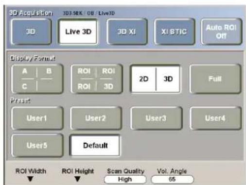
[Figure 4.27 3D Acquisition – Live 3D]
NOTE
■ To obtain a direct view of the face of the fetus on the screen when acquiring the 3D image, place the head of the fetus in the direction of the Direction Mark, put the fetus in the Coronal Plane, and then scan the fetus from the back toward the abdomen.
■ The 3D image of the fetal face is more easily found in the coronal plane than in the sagittal plane.
3D View
3D View Mode
This mode allows adjusting and/or viewing of the 3D or Live 3D image that was acquired in Image Scan Mode.
In 3D View Mode, press the Exit button or the 3D/4D button on the control panel to move to Image Scan Mode. Press the 2D button to completely exit 3D Mode. Note that pressing the Exit button on the control panel in Live 3D View Mode switches to Live Cine Mode.
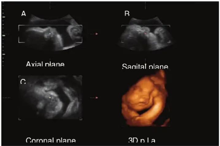
[Figure 4.28 Static 3D View]
The default 3D View screen consists of Axial Section, Sagital Section and Coronal Section surface images—which are volume data cut by anatomical positions—and 3D images.
Figure 4.28 illustrates a screen displaying Axial Section as "A plane," Sagital Section as "B plane," and Coronal Section as "C plane."
In ABC-ROI 3D Mode, the ROI box displayed in each section can be adjusted for obtaining desired 3D images.
View Mode Control Menu
Control menus for 3D or Live 3D images appear on the touch screen depending on the characteristics of each mode.
When operating images, the “icon” icon and the Trackball function icon appear at the bottom of the screen.
The following icons are available.
- Icons in 3D View Mode:
- Icons in 3D XI Mode:

Selecting 3D View Mode
Static 3D View Mode
For better viewing of 3D images, view modes are categorized into 2D Mode and 3D Mode depending on rendering methods.
At the View Mode Control menu, press a button on the touch screen to access the corresponding view mode.
To exit the selected view mode or return to the previous menu, press the Exit button on the touch screen or the Exit button on the control panel.
2D Mode for Static 3D View
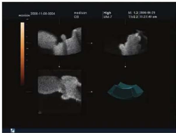
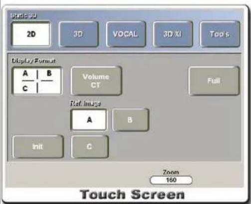
[Figure 4.29 Static 3D - 2D]
| Menu | Description |
 ABC Mode Selection ABC Mode Selection | ABC Mode does not display 3D image; it displays multi-planar images only. Use Full Mode for a more detailed view. |
 Volume CT Mode Selection Volume CT Mode Selection | Volume CT Mode displays a 3D view of the plane position of the examination image.Hold down the Change button on the control panel for a few seconds and the mouse pointer will appear. Use the Trackball and the Set button to adjust the 3D space. Use the Niche Zoom menu on the touch screen to zoom in or zoom out the Volume CT image. Use the Zoom menu to zoom in or zoom out the surface image and apply it on the Volume CT image. |
OH (Orientation Help) Function
OH (Orientation Help) image displays the relative position of the currently selected reference image in regards to the volume data.
The A, B, and C buttons of the reference image move the plane of OH, and rotating each reference image also rotates the plane of OH. OH image is shown only in 2D Mode for Static 3D.
NOTE
If the plane of OH is not properly expressed for the volume data, press the Init button.
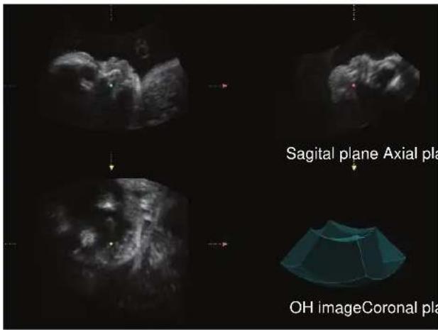
[Figure 4.30 OH Screen]
[A plane]
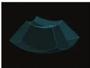
[B plane]
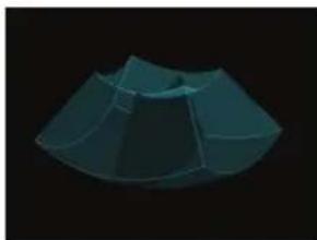
[C plane]
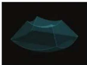
3D Mode for Static 3D View
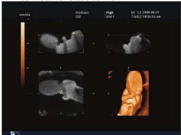
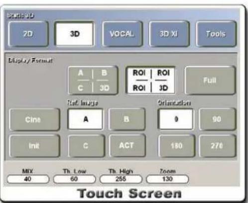
[Figure 4.31 Static 3D - 3D]
| Menu | Description |
 ABC-3D Mode Selection ABC-3D Mode Selection | ABC-3D Mode projects a 3D image on the Volume data plane without setting an ROI. Detailed examination is possible as 3D image is projected without using an ROI. |
 ABC-ROI 3D Mode Selection ABC-ROI 3D Mode Selection | In ABC-ROI 3D Mode, desired 3D images can be examined by adjusting the surface images and the ROI box on 3D images. |
 Full Screen View (Full Mode) Full Screen View (Full Mode) | Fits the 3D image on the entire screen in View Modes. |
 Reset to Initial Position Reset to Initial Position | Initializes the current image back to the state it was at the beginning of 3D View Mode or to the Preset state. |
 Change Reference Plane (Reference Plane Selection) Change Reference Plane (Reference Plane Selection) | Each multi-planar has its own standard coordinate system and rotates or moves according to the coordinate system. The image selected as a reference image rotates or moves according to the reference image coordinate system, and other images rotate or move according to their own standard coordinate systems.Press a desired button to change the reference image. |
 3D Orientation 3D Orientation | Rotates the 3D image against the Z-axis in the 3D standard coordinate system by the rotation value selected. |
| Rotate Image by X-axis (↓↑) | Turn the X knob-button to rotate the selected reference image in the direction of the X-axis. In Full Mode where the reference image is not shown, the selected image acts as the reference image and the Full Mode image rotates by the X-axis.The M knob-button on the control panel acts as the X knob-button. |
| Rotate Image by Y-axis (⇐) | Turn the Y knob-button to rotate the selected reference image or the Full Mode image in the direction of the Y-axis. The PD knob-button on the control panel acts as the Y knob-button. |
| Rotate Image by Z-axis (∪∪) | Turn the Z knob-button to rotate the selected reference image or the Full Mode image in the direction of the Z-axis. The PW knob-button on the control panel acts as the Z knob-button. |
| Move and Resize Image (ROI Box Adjustment) | Press the Change button on the control panel and use the Trackball to move the selected reference image or the Full Mode image up/down/left/right. Press the Change button again to resize the ROI box.Here, hold down the Change button for 2 seconds to change the function of the Trackball.Press the Set button and theicon will appear on the screen. Move the Trackball while holding down the Set button to rotate the image. Also, press the Exit button and theicon will appear on the screen. This function is for moving the image. |
| Image Zoom | To zoom the selected reference image in ABC-ROI 3D Mode, adjust the Zoom value on the touch screen. Use the up-down switch below Zoom to adjust the value. |
Auto Contour (ACT) Function
This function locates the fetal face area automatically in a fetus image scanned in Sagital plane. In the ROI box on A Plane, a contour line appears and a 3D image is contoured.
Press ACT Edit button to edit the contour line. Adjust it with the Set button on the control panel and the Trackball.
NOTE
Except in the 3D Convex probe, a contour line appears as a straight line.
This function is available only in Static 3D Mode where Render Direction is 'C+'.
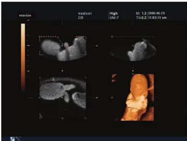
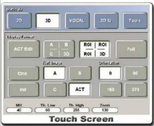
[Figure 4.32 Static 3D - ACT]
Live 3D View Mode
For more detailed viewing of Live 3D images, the modes are divided according to rendering methods.
At the View Mode Control menu, press a button on the touch screen to access the corresponding view mode.
To exit the selected view mode or return to the previous menu, press the Exit button on the touch screen or the Exit button on the control panel.
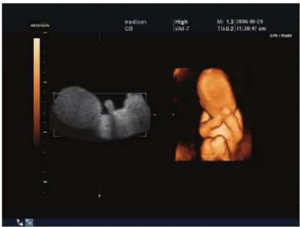
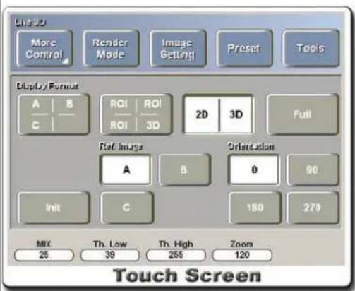
[Figure 4.33 Live 3D - 2D-3D Mode]
| Menu | Description |
 2D-3D Mode Selection 2D-3D Mode Selection | Plane of the image and Live 3D image can be examined.In 2D-3D Mode, adjust the ROI box to view a desired 3D image. The selected reference image is displayed in 2D image. |
NOTE
For information on other menu items, refer to "Static 3D View."
* 3D Coordinate System
- Multi-planar Standard Coordinate Systems
A Standard Coordinate System
B Standard Coordinate System
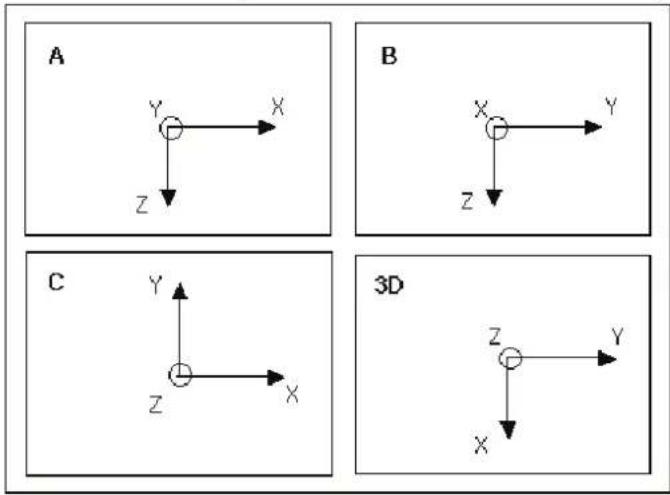
C Standard Coordinate System
3D Standard Coordinate System
- Full Mode Coordinate System
![graph TD A["Full"] --> B["X"] B --> C["Y"] C --> D["Z"]](/content/2026/05/955519/images/8ed5880b79ed0ccde1f0463e477bdd06e849d2a589d9926ce0d2a298b8b465e9.jpg)
- Reference Image Coordinate System
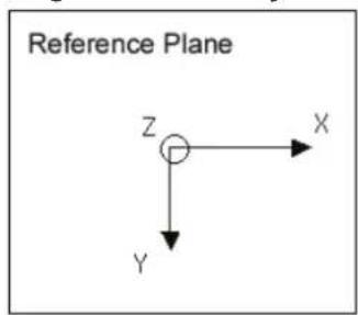
Cine Mode
3D Cine Mode
This mode provides Cine function for examining the rendered 3D image. Press the Cine button on the touch screen. The menu illustrated below will appear and the 3D Cine Mode will start.
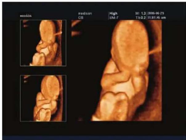
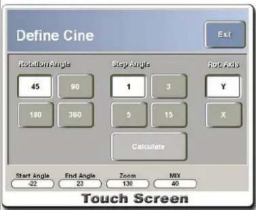
[Figure 4.34 3D Cine Mode]
- Cine Settings: Before viewing images by Cine, make appropriate settings for viewing images on the touch screen.
| Menu | Description |
| Rotation Angle | Set ranges for 3D Cine rotation. |
| Step Angle | Selected Rotation Angle rotates by the Step Angle value. If the Step Angle is set to 15° , the 3D Cine set to 360° rotates in 25 steps, and the 3D Cine set to 90° rotates in 7 steps. |
| Rotation Axis | Select the rotation axis for 3D Cine. |
| Start, End Angle | Set the start and end angle values for the rotation range. |
| Zoom | Zoom the 3D Cine image by 25% - 400%. Use the up-down switch below the touch screen to adjust the value. |
| Mix | Use the up-down switch below the touch screen to adjust the Mix value. |
- Running Cine: Press the Calculate button on the touch screen to run 3D Cine. The Cine image generation process will be displayed on the screen and then 3D Cine will start. The menu below will appear on the touch screen. ▶ ▶ ▶ Press the button to stop or start 3D Cine.
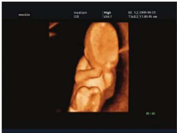
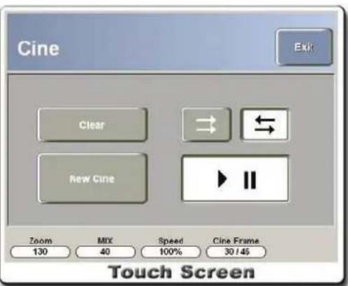
[Figure 4.35 3D Cine]
| Menu | Description |
| New Cine | While 3D Cine is in use, press the New Cine button to acquire a new Cine image. |
| Rotate |  Select the button to continuously rotate in one direction, or Select the button to continuously rotate in one direction, or  select the button to rotate in one direction and then rotate in the opposite direction. select the button to rotate in one direction and then rotate in the opposite direction. |
| Speed | Adjust the Speed value to adjust the rotation speed of the 3D Cine image. Use the up-down switch below Speed. |
| Cine Frame | Adjust the Cine Frame value on the touch screen to view the 3D Cine image by each desired frame. |
| Zoom | Adjust the Zoom value on the touch screen to zoom the image. Turn the knob-button below Zoom to adjust the value. |
| Mix | Adjust the MIX value below the touch screen to adjust the mix of Render Mode. Use the knob-button below MIX. |
Live 3D Cine Mode
Live 3D Mode provides the Cine function for saving or viewing the recently scanned 3D images. Up to 128 Live 3D images can be saved.
- Running Cine: While scanning Live 3D image, press the Freeze button or the Exit button on the control panel to start Live 3D Cine Mode. Or, press the Tools button on the touch screen to move to the Tool menu and select the Live Cine button. When Live 3D Cine starts, the menu below will appear on the touch screen.
Press the button to stop or start Live 3D Cine.
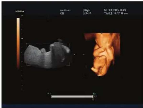
[Figure 4.36 Live 3D Cine]
| Menu | Description |
| New Cine | While 3D Cine is in use, press the Freeze button to acquire a new Cine image. |
| Save | When saving Live Cine images, you can specify the save range for Cine images in the same way as in 2D Mode.Adjust the First Frame and the Last Frame values on the touch screen to adjust the Cine image save range. The progress bar indicating the save range will appear on the screen. Use the up-down switches below the menus to adjust the menus.After selecting the save range, press the Save button on the control panel.When the Save Volume screen appears on the touch screen, select the Save button to save Live Cine image. |
NOTE
For information on other menu items, refer to "3D Cine Mode."
VOCAL (Virtual Organ Computer Aided anaLysis) Mode
Select the VOCAL button on the touch screen to start VOCAL Mode. VOCAL is a very useful tool for measuring volumes of tissues within the human body.
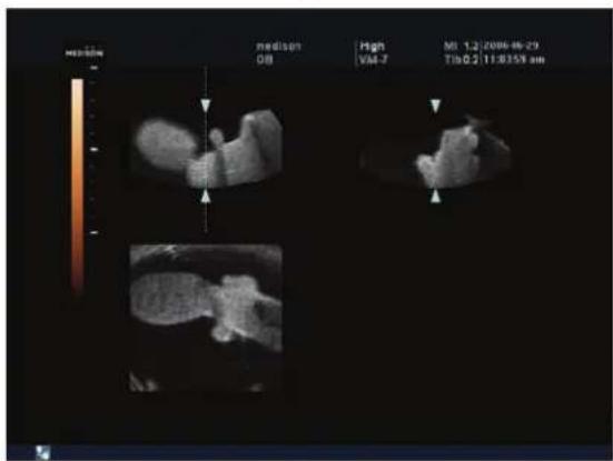
[Figure 4.37 VOCAL Mode]
Setting Reference Image
A reference image must be set up in order to obtain the volume of a desired object. Press a button on the touch screen to specify which plane should be used for contouring.
Note that contouring is done as the image rotates by the vertical axis in A Plane and B Plane and as the image rotates by the horizontal axis in C Plane.
Setting VOCAL Parameter (Rotation Step)
You can set the step angle for image rotation. Available ranges are 12° , 18° and 30° . Press the corresponding button on the touch screen to select the range.
15 contour images are generated for 12° , 10 images for 18° , and 6 images for 30° . The default rotation angle is 30° .
Setting Range
Adjust the Pole1 and Pole2 values on the touch screen to set the contour range. Use the knob-buttons below Pole1 and Pole2 to set the position of the arrow. Turn the knob-button to position the arrow at the vertical or horizontal edge of the object to measure.
VOCAL Automatic Start
Select Contour Type on the touch screen to automatically generate the object for acquiring volume value.
| Menu | Description |
| Solid Type | Press the Solid button to contour when there are many echoes within the object. |
| Cystic Type | Press the Cystic button to contour when there are few echoes within the object. |
| Prostate Type | Press the Prostate button to contour when using prostate-related objects. |
| General Type | Press the General button to contour according to characteristics of general objects. General Type is faster than other automatic Contour Types but is slightly less accurate. |
| Sphere Type | Press the Sphere button to automatically generate a basic spheric object. After making the spheric object, modify the contour image to make it into a desired shape. |
VOCAL Manual Start (Manual Type)
Press the Manual button on the touch screen and you can manually contour frame by frame. The menu below will appear on the touch screen when you press the Manual button.
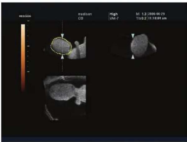
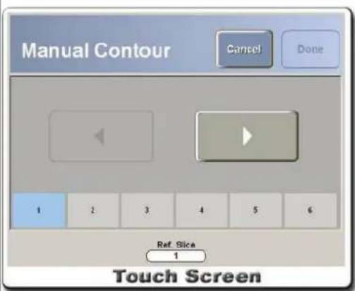
[Figure 4.38 VOCAL Mode – Manual Type]
- Move the Trackball while holding down the Set button to determine the shape of the object. After determining the shape of the object, press the Set button again to complete frame generation.
- Press the ▶ button or press the number button on the touch screen to move to the next frame and determine the shape of the object.
- To determine the shape of the object again, press the ◀ button or press the number button on the touch screen to move to the previous frame.
- Use the up-down switch below Ref. Slice to move to different frames.
- To cancel contour, press the Cancel button on the touch screen.
- Repeat the steps above to contour all the frames and then press the Done button.
Edit Contour
When contour is complete, the system switches to Edit Contour Mode. In this mode, use the up-down switch below Ref. Slice to select contour obtained in the previous step.
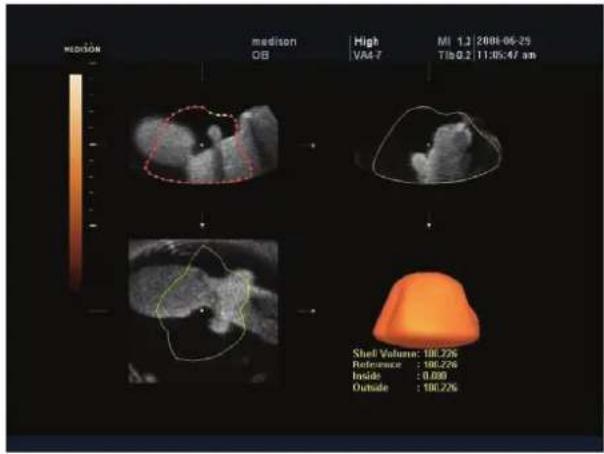
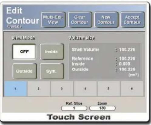
[Figure 4.39 VOCAL Mode – Edit Contour]
- Shell Mode
| Menu | Description |
| Off | Shell Thickness is not applied. |
| Inside | Shell is drawn inside the contour generated by Shell Thickness specified. |
| Outside | Shell is drawn outside the contour generated by Shell Thickness specified. |
| Symmetric | Half the shell is drawn inside the contour by half the Shell Thickness specified and the other half of the shell is drawn outside the contour by half the Shell Thickness specified. |
- Ref. Slice
Use the up-down switch below the touch screen to move to different frames and re-contour the object.
- Zoom
Use the up-down switch below Zoom to adjust the value for zooming image.
- Shell Thickness
Adjust the Thickness value to set the thickness of the shell. Use the up-down switch below Thickness to adjust the value. Note that the value cannot be adjusted when Shell Mode is OFF.
- Multi-Edit View
Draw a line to edit up to 6 slices at a time.
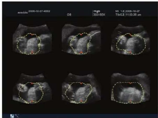
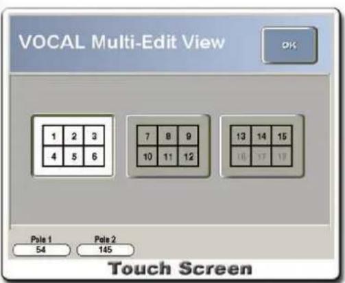
[Figure 4.40 Multi Edit View]
- Select a slice to edit.
- Change the position of pole points.
Every slice in the screen has two pole points indicated with red dots at the same positions as each other. Use the Pole 1 and Pole 2 knob-buttons on the touch screen. Changing the position of a pole point simultaneously changes the position of the pole points in all slices.
- Edit a contour line.
A contour line is shown in yellow. Use the Set button and the trackball to edit the left or right portion around a notional vertical line connecting pole points 1 and 2. Here, you may not edit it so that it crosses the notional vertical line connecting pole points 1 and 2. A contour line being edited is shown in red.
- Press Ok on the touch screen to finish editing. The changes are applied and displayed on the screen.
NOTE
■ The Slice buttons activated on the touch screen vary depending on the number of slices. The number of slices is determined based on the slice angle. For example, when 6 slices have been created through a 30° rotation, only slice buttons 1–6 are activated. However, for example, when 15 slices have been created through a 12° rotation, slice buttons 1–6, 7-12 and 13-15 are activated.
■ When Multi-Edit View is in use, Zoom and Rotation functions are not available.
- Clear Contour
Press the Clear Contour button to cancel the currently set contour, exit VOCAL Mode and return to 3D View Mode.
- New Contour
Press the New Contour button to cancel the currently set contour, return to the VOCAL Mode screen and generate new contour.
- Accept Contour
Press the Accept Contour button to apply the contour specified.
- Result Display
Volume information will be displayed at the lower right-hand corner of the monitor and on the touch screen.
| Menu | Description |
| Shell Volume size | Outside Shell Volume – Inside Shell Volume |
| Reference Volume size | Volume size of the generated object using the initial contour. |
| Inside Volume size | Volume size inside the generated object when Shell Mode is Inside. |
| Outside Volume size | Volume size outside the generated object when Shell Mode is Outside. |
VOCAL – Volume CT Mode
After generating the VOCAL object, press the Volume CT button in VOCAL Mode to insert the A, B, and C Plane images in the VOCAL object for examination.
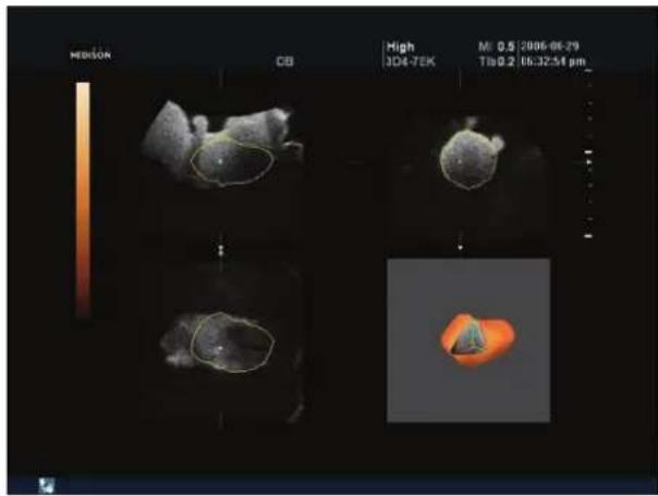
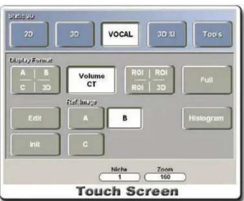
[Figure 4.40 VOCAL – Volume CT]
VOCAL – Volume CT View Mode Settings
Adjust the Niche menu on the touch screen to set up View Mode for Volume CT. There are eight (1-8) Volume CT View Modes, each of which shows one-eighth of the VOCAL object.
The eighth View Mode is not shown in the illustration above because it is located at the back.
* VOCAL object has been removed from the illustration above for demonstration purposes.
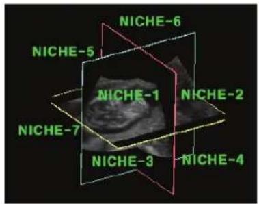
VOCAL – Volume CT Operation
VOCAL – Volume CT Mode allows object rotation and axis movement.
- Object Rotation: Object rotation involves VOCAL rotation and Volume CT rotation. VOCAL rotation is rotating the VOCAL object along with the Volume data with the center of the VOCAL object as the rotation axis. Volume CT rotation is rotating only the VOCAL object but not A, B, or C planes. To perform the Volume CT rotation function, hold down the Change button on the control panel for a few seconds. When the mouse pointer appears on the screen, use the Trackball and the Set button to rotate the object.
- Axis Movement: Turn the C knob-button on the control panel to move the rotation axis for the selected reference image. For example, if the A button is selected in the reference image, the central axis moves toward the depth direction of A plane.
VOCAL Histogram
VOCAL Histogram shows distribution of the gray value of the black and white image within the VOCAL object and the gray value of the Power Doppler image, and the relevant MG (Mean Gray), VI (Vascularization Index), FI (Flow Index), and VFI (Vascularization-Flow Index).
VOCAL Histogram is only available for 3D images and Power Doppler 3D images that are in black and white.
Equations used are as follows.
- MG: average value of gray voxel brightness (gray)
= total brightness (gray) / all voxel number - VI: ratio of color voxels against all voxels within the shell
= color voxel number / all voxel number - FI: average value of brightness (color) for color voxels within the shell
= total brightness (color) / color voxel number - VFI: average value of brightness (color) for all voxels within the shell
= total brightness (color) / all voxel number
VOCAL ABC-3D Mode
After accepting the contour in VOCAL Mode, press the ABC-3D button on the touch screen to view images in VOCAL ABC-3D Mode.
ABC-3D in VOCAL Mode cuts out the contoured surface images and reconstructs a 3D image based on them. 3D image is displayed in the position of the contour image shown on A plane. This mode allows viewing of organs in their actual images. In particular, SeeThru Mode is useful for clinical purposes as it provides color position and distribution of organs.
3D Measure
In 3D View Mode, you can press the Measure button on the control panel to perform 3D Measure functions (Caliper, Slice, and Calculation).
Since 3D Measure involves measurements on 3D images that are constructed with 2D images, measurement menu items supported by M Mode or Spectral Doppler Mode are not available here. Also, measurements that require multiple images such as the AFI menu under OB measurement are not available.
3D Measure has an error rate of 5% in addition to the measurement error rate in 2D Mode. Press the Close button on the touch screen to exit the 3D Measure function. You can also exit by pressing the Measure button or the Exit button on the control panel.
Caliper 3D / Calc 3D
Caliper 3D and Calc 3D measurement menus are identical to 2D Mode and use the same measurement methods in 2D Mode. For detailed information on measurement methods, refer to "Basic Measurements" and "Application Measurements" sections in this manual.
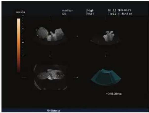
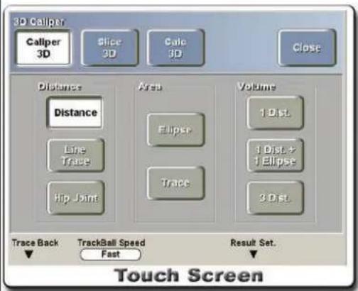
[Figure 4.41 3D Measure – Caliper 3D]
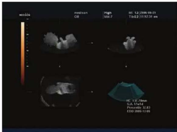
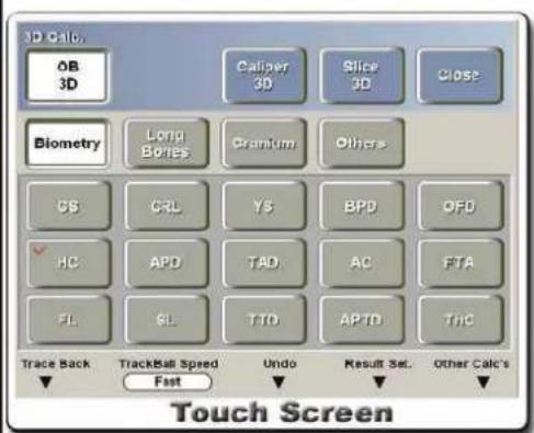
[Figure 4.42 3D Measure – Calc 3D]
Slice 3D
Press the Slice 3D button on the touch screen and the menu below will appear on the touch screen.
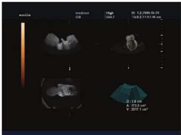
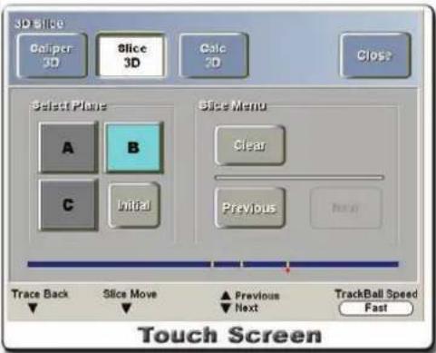
[Figure 4.43 3D Measure – Slice 3D]
Slice 3D slices a single Volume into multiple planes and measures them.
Under Select Plane, select a measure plane to measure and use the knob-button below Slice Move to move to the slice image to measure.
Use the trace method to measure. To cancel a part of the measuring line while tracing, press the Delete button or turn the knob-button below Trace Back. Press the Clear button on the touch screen to delete the measurement result.
If measuring multiple slice images, the measured slices are displayed on the bar on the touch screen. To move to different slice images, use the Previous button and the Next button, or use the up-down switch below Previous/Next.
To return to the initial image before measuring, select the Initial button on the touch screen.
Trace Back
To delete a part of the measuring line while using Trace, use the Trace Back function. Turn the knob-button below Trace Back left or right to delete the Trace measuring line.
Trackball Speed
The Trackball Speed function adjusts the speed of the Trackball on the control panel. Turn the knob-button below Trackball Speed to select Slow, Normal or Fast.
3D Notation
Text Input
Press the Text button on the control panel to input texts on the screen. The Text Brief function is not supported.
Press the Clear button on the control panel or on the touch screen to clear all texts on the screen.
Indicator Input
Press the Indicator button on the control panel to input indicators on the screen. Use the Set button and the Trackball to place indicators.
Press the Clear button on the control panel or on the touch screen to clear all indicators. Press the Undo button on the touch screen to delete indicators one by one in the order they are placed.
Indicators in Live 3D View and Live 3D XI TM can be moved within the screen only.
[Figure 4.44 3D Notation]
Optimizing 3D Images
To set the image parameters in View Mode, select the Tools button on the touch screen. The screen below will appear on the touch screen.
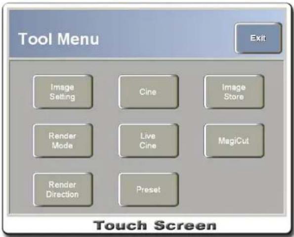
[Figure 4.45 Tool Menu]
Image Setting
Press the Image Setting button on the touch screen to set the Gamma value and Chroma Map for images. Used Chroma Map preset values can be saved in Preset.
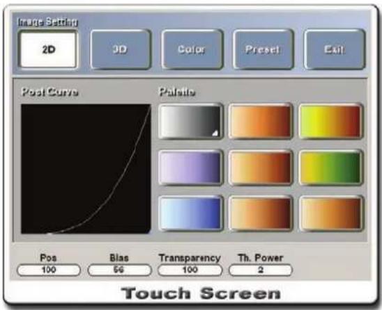
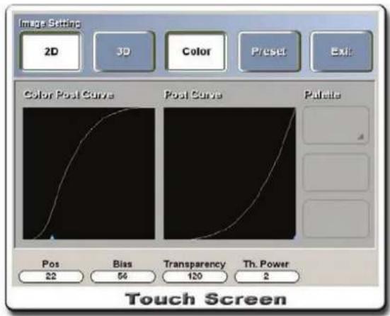
[Figure 4.46 Tool Menu – Image Setting (2D & Color)]
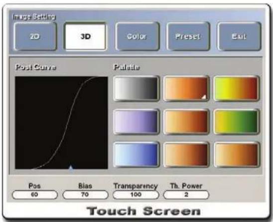
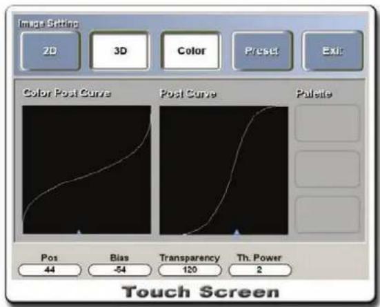
[Figure 4.47 Tool Menu – Image Setting (3D & Color)]
Select the 2D button on the touch screen to set the Gamma value, etc. for 2D images. Select the 3D button to make settings for 3D images.
Adjusting Post Curve
To adjust Post Curve, adjust the Pos value and the Bias value at the bottom of the touch screen. Use the knob-buttons below Pos and Bias.
Setting Palette
Select a desired color button on the touch screen.
Setting Transparency
Adjust the Transparency value to adjust the transparency of 3D images. Use the up-down switch below Transparency on the touch screen. The value range is from 20 to 250.
The lowest Transparency value (20) is for complete transparency, and the highest Transparency value (250) is for complete opacity. The default Transparency value is 100.
Setting Preset
Use this function to set up Post Curve, Palette, current Threshold value, and other parameters for the current image and save them as user preset values.
Select a button from User 1 through User 5 and press the Save button to save the user preset values under the selected button.
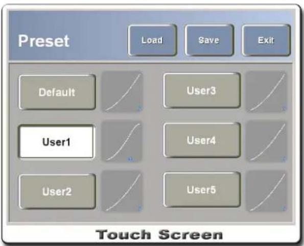
[Figure 4.48 Tool Menu – Image Setting (Preset)]
Setting Render Mode
Press the Render Mode button on the touch screen to set Render Mode. The last used Render Mode preset values are automatically saved.
Render Mode includes four modes: Gray, Color, SeeThru and VOCAL.
Gray Render Mode
This mode shows volume data acquired by gray method as a 3D rendering image.
Rendering values can be set for Mode1 and Mode2. A total of 11 combinations are available.
| Menu | Description |
| Surface Mode | This is the default mode. It displays a 3D image by ray-casting. |
| Surface Smooth Mode | This is similar to the default mode. It displays a 3D image by ray-casting softer than Surface Mode. |
| Max Mode | This mode displays the maximum value of intensity. This is useful for viewing bones within the body. |
| Min Mode | This mode displays the minimum value of intensity. This is useful for viewing vessels and hollow parts within the body. |
| Light Mode | This mode displays the depth information of 3D image by brightness. |
| X-Ray Mode | This mode displays the average value of intensity. It has the same effect as X-ray images. |
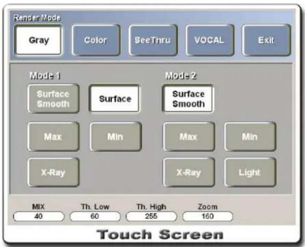
[Figure 4.49 Tool Menu – Render Mode (Gray)]
Color Render Mode
This mode shows volume data acquired by Angio/CFM method as a 3D rendering image. It supports three combinations: Surface-Light, Surface-Max, and Surface-X-Ray.
The modes are accessed in the same way as Gray Render Mode.
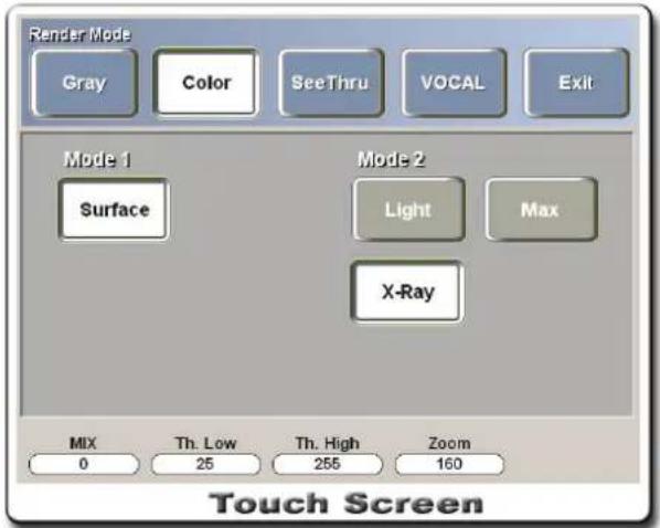
[Figure 4.50 Tool Menu – Render Mode (Color)]
SeeThru Render Mode
This mode shows Gray + Angio or Gray + CFM combination of data as a 3D rendering image. It supports four combinations: Transp-Surface, Transp-Transp, Max-Surface, and Max-Transp. When you survey color data, the system runs SeeThru Render mode as default.
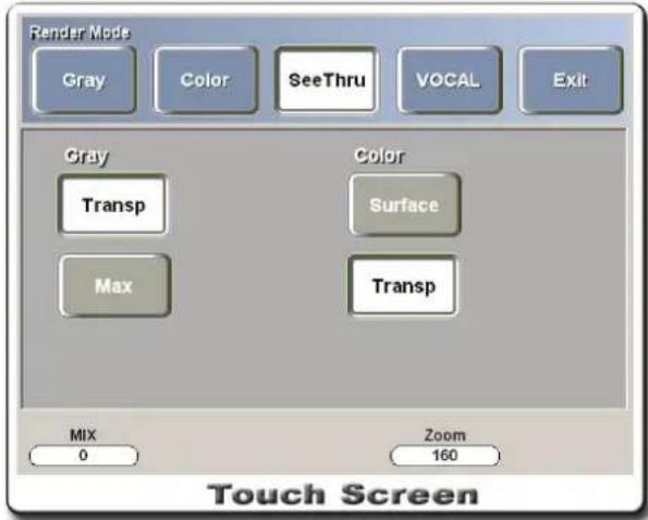
[Figure 4.51 Tool Menu – Render Mode (SeeThru)]
| Menu | Description |
| Transp+Surface Combination | View the color data within the gray data while adjusting the transparency of the gray data (use the MIX knob-button). Parts hidden by the gray data may appear slightly darker. |
| Transp+Transp Combination | View the color data within the gray data while adjusting the transparency of the gray data and the color data (use the MIX knob-button). Parts hidden by the gray data may appear slightly darker. |
| Max+Surface Combination | View the color data according to the MIX ratio of the gray data in Max Mode and the color data from Surface Mode (use the MIX knob-button). Parts hidden by the gray data may appear slightly brighter. |
| Max+Transp Combination | View the color data according to the MIX ratio of the gray data in Max Mode and the color data from Transp Mode (use the MIX knob-button). Parts hidden by the gray data may appear slightly brighter. |
VOCAL Render Mode
You can set the color of the object shown in VOCAL Mode. Select desired colors for Surface and Wire.
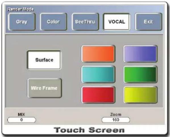
[Figure 4.52 Tool Menu – Render Mode (VOCAL)]
Adjusting Rendering Mode Mix
Adjust the Mix value below the touch screen to adjust the mix of Render Mode. Use the knob-button below MIX.
Adjusting Threshold (Low, High)
Adjust the Th.Low and Th.High values at the bottom of the touch screen to adjust the Threshold values. Use the knob-buttons or the up-down switches below the menus.
Adjust the Th.Low value and the Th.High value to hide information below and above the values from the 3D image. Only the information between the Th.Low value and the Th.High value is shown as the 3D image.
Image Zoom
To zoom the image, adjust the Zoom value at the bottom of the touch screen. Use the up-down switch below Zoom.
MagiCut Mode
This function cuts out a desired portion from the entire image for viewing. Press the MagiCut button on the touch screen.
Setting Cut Mode
Select the Cut Mode type on the touch screen.
- Inside Contour: Cuts the inside of the selected area.
- Outside Contour: Cuts the outside of the selected area.
-
Inside Box: Cuts the inside of the box.
-
Outside Box: Cuts the outside of the box.
- Small Eraser: Cuts using a small eraser.
- Big Eraser: Cuts using a big eraser.
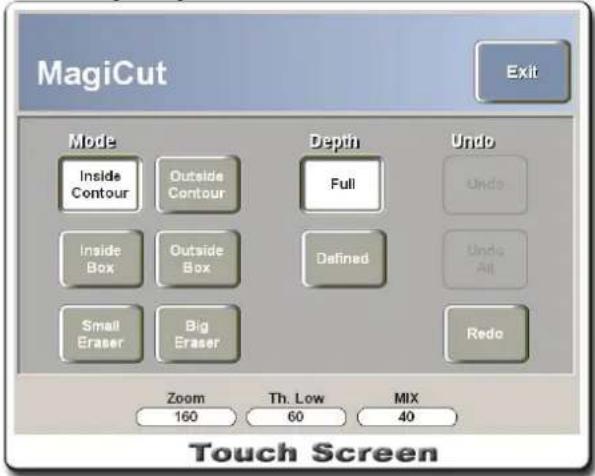
[Figure 4.53 Tool Menu – MagiCut]
Setting Cutting Area
To set the cutting area in MagiCut Mode, use the Trackball and the Set button on the control panel.
You may also cut the image by adjusting the depth of the cutting area. Select the Full button on the touch screen delete the entire area selected, or select the Defined button to delete by the value specified. Press the Define button and the Cut Depth menu will appear. Use the knob-button below Cut Depth to specify the depth for the area to delete.
Canceling MagiCut
To restore the cut area from the full image, select the Undo button on the touch screen. Press the Undo button to restore the last cut area. Press the Undo All button to restore the entire image.
After restoring the image by pressing the Undo button or the Undo All button, select the Redo button to cut the same area again.
Render Direction Settings
To change the camera position for viewing 3D images, select the Render Direction button on the touch screen.
Standard coordinate systems change according to the changes in position (refer to the section on changing reference image).
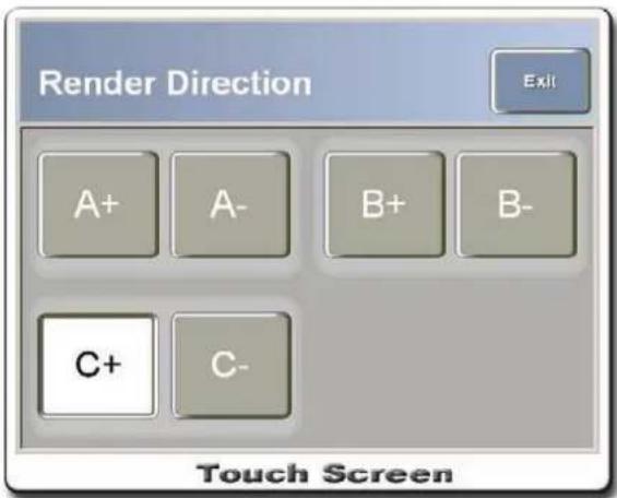
[Figure 4.54 Tool Menu – Render Direction]
A + : Moves to the direction currently looking at A plane.
A – : Moves to the back of the direction currently looking at A plane.
B + : Moves to the direction currently looking at B plane.
B – : Moves to the back of the direction currently looking at B plane.
C + : Moves to the direction currently looking at C plane.
C-: Moves to the back of the direction currently looking at C plane.
Image Store
Pressing the Image Store button on the touch screen saves the 3D image on the system. The last saved image can be sent by using the E-Mail function.
Saving Images
Press the Save button on the control panel to save 3D images in View Mode. Saved images are managed by SonoView.
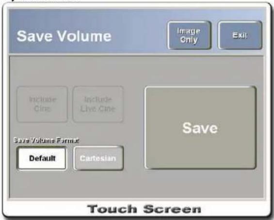
[Figure 4.55 Tool Menu – Image Store]
| Menu | Description |
| Save | Saves 3D image including volume data. If volume data and Cine images are saved together, new 3D rendering images and Cine/Live images can be reproduced at a later time. |
| Image Only Saves only the image displayed on the screen. | |
| Include Cine | This is available when 3D Cine images are generated. Select the Include Cine button and press the Save button to save Cine images and volume data. If the Include Cine button is not selected, only the volume data is saved. |
| Include Live Cine | This is available when Live 3D Cine images are generated. The function is the same as Include Cine. |
| Save Volume Format - Default | Coordinate systems for 3D data saved in this system are different from coordinate systems for 3D data used in CT or MRI. Save by selecting the Default button if you plan to use the data in SonoView only. |
| Save Volume Format - Cartesian | Save the 3D image by selecting the Cartesian button if you plan to use it in other 3D programs such as CT or MRI. If the Cartesian format is selected only the A plane image is saved. Because data format cannot be verified in SonoView, you must indicate the format in the save name when saving a SonoView image. |
| Setting Save Range | When saving Live 3D Cine images, you can specify the save range for Cine images in the same way as in 2D Mode. Refer to “Live 3D Cine Mode.” |
Printing Image
Press the Echo Print button on the control panel to print 3D images in View Mode.
3D XI TM Mode
Procedures for acquiring images in 3D XI TM is the same for Static 3D images.
Press the 3D XI button on the touch screen to switch to 3D XI TM , or press the 3D button to scan and then press the 3D XI button at the 3D View screen to switch to 3D XI TM .
3D XI TM supports three modes: Multi Slice View, Volume CT, and Oblique View.
![2008-07-17-0001 MEDISON OB H FPS27 / 14.0cmM10.63 / 2008-07-20 3D3-5EK / Gen Tlb 0.1 / 06:52:05 pm [20] GS5 / 90dB FA10 / P90 FS10 * PG : 0](/content/2026/05/955519/images/629b63f2d109a5e2b3ff37710771f5a79421cc7177f25247dafdac351d4d2cd8.jpg)
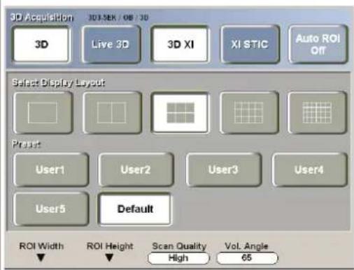
[Figure 4.56 3D Acquisition - 3D XI™]
In Live 3D XI ™ , press the Live 3D button and the 3D XI button simultaneously to acquire image. Live 3D XI ™ provides Multi Slice View Mode only.
![2008-07-17-0001 MEDISON OB H FPS27 / 14.0cmMl0.63 2009-07-20 3D3-5EK / Gen Tlb0.1 06:52:05 pm [2D] G65 / 90dB FA10 / P90 FS10 * PG : 0](/content/2026/05/955519/images/2f257a4ef0c50e1fb7f7bf4c88610b2de71a803be4f8d5378f284a7e5fb058aa.jpg)
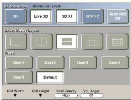
[Figure 4.57 3D Acquisition – Live 3D XI™]
Multi Slice View
This function enhances usefulness of examination by using neighboring multi slice images. To use the functions related to Multi Slice View, press the Multi Slice View button on the touch screen and use the menu displayed.
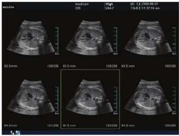
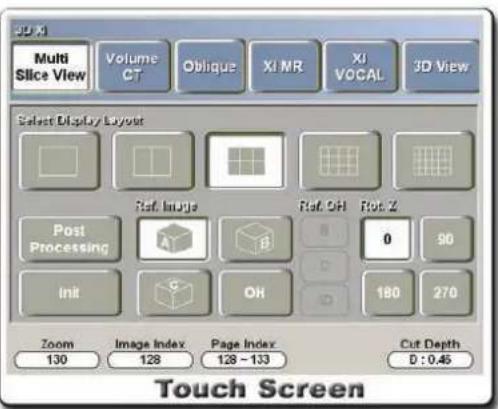
[Figure 4.58 Multi Slice View]
Init: Resets all settings for Multi Slice View.
Display Layout (1 × 1, 2 × 1, 3 × 2, 4 × 3, 6 × 4)
This function sets the display layout. You can select one from the five layouts. 1 x 1 supports large image size but does not show slice images. 6 x 4 has small images but supports slice images. The default display layout is 3 x 2.
Each time a new layout is selected, the currently selected image moves to the first position on the screen.
Ref. Image (A/B/C Plane)
Shows the selected reference image in Multi Slice View.
Rot. Z (0/90/180/270)
To rotate Multi Slice image, press the button for the desired rotation value. Here, the coordinate system rotate by the Z-axis in the "3D standard coordinate system."
Each time the mode changes or the reference plane changes, the current Rot. Z is reset to 0.
OH (Orientation Help) Function
Like the OH function in 3D view, this function shows the relative position of the currently selected slice image in volume data for Multi Slice View images.
Press the OH button on the touch screen to activate or deactivate it.
- Reference Plane: Shows the relative position of the slices displayed in other sections. In this image, a scout marker appears indicating the position of each slice image.
- Pressing the Set button on the control panel zooms the selected slice image to the 1 X
1 layout to enable more detailed observation.
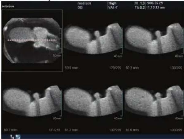
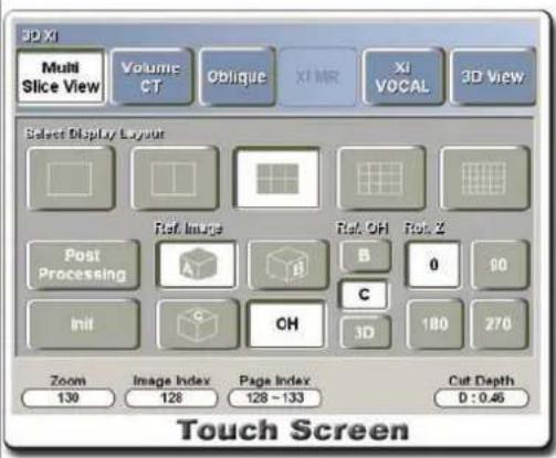
[Figure 4.59 Multi Slice View - OH]
Rotation
Turn the X, Y, and Z knob-buttons to freely rotate the Multi Slice image. When the selected reference image is rotated, the results are reflected in all planes.
Translation
Move the Multi Slice image to a new position. Use the Change button on the control panel and the Trackball to move the image. The image moves along the X-axis and the Y-axis.
Zoom (x1.0 \~ x4.0)
The Multi Slice image can be zoomed by 4 times. Use the knob-button below Zoom on the touch screen to make adjustments.
Image Index
Shows the index of the currently selected image. The selected image is highlighted with yellow borders. Use the knob-button below Image Index on the touch screen or the Trackball to select an image. If the image index is outside the range of the current page, the screen moves to the previous or next index as the page index changes accordingly.
Magnification
Press the Set button at the selected image index to magnify the selected image as in the 1 x 1 layout. Press the Exit button to return to the original layout. Here, the position of Image Index is restored to the previously selected position. Images are not saved in the Magnification state.
Page Index
Shows the range of the current page index according to the display layout. Use the up-down switch below Page Index on the touch screen to adjust the value.
Cut Depth
Set the gap between Multi Slice images. The gap between Slice images can be set by the user. It is marked as an internal calculation value by default. The unit is mm. Use the up-down switch below Cut Depth on the touch screen to adjust the value.
Here, Cut Depth indicates the gap between the slices for the volume data. It does not refer to the actual anatomical position of the scanned objects.
Post Processing
This function is responsible for post-processing Multi Slice images. You can produce various images using this function. Post-processed images are not applied in Volume CT. The table below lists the functions provided. Each function can be repeated or used in combination with other functions. Note that only the Flip Image function may be repeated in the color display area (image acquired in 3D/C or 3D/PD Mode).
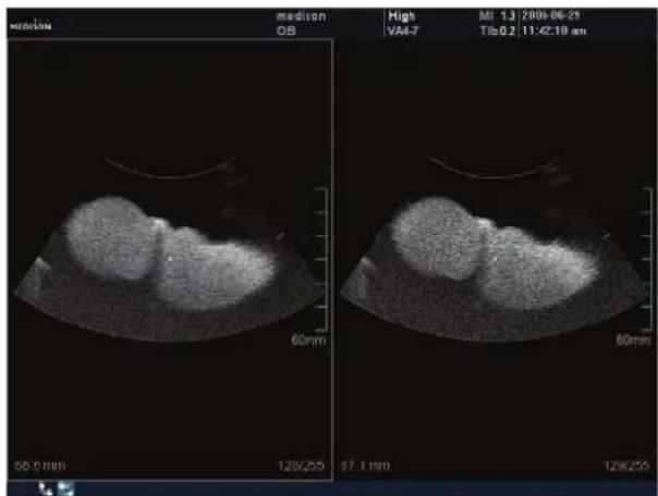
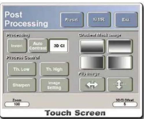
| Menu | Description |
| Invert | Inverts the brightness of Multi Slice images. |
| Auto Contrast | Automatically adjusts the brightness of Multi Slice images. This function calculates the histogram of the image and stretches the contrast distribution. The change may be marginal if the image already has well-spread contrast. |
| Compound Imaging (3D CI) | Eliminates noises and enhances image quality by compounding images. Set the distance between images to be used for 3D CI by using 3D CI Offset on the touch screen. |
| Image Setting | Sets the Gamma value for the image. Use the knob-buttons below Pos and Bias to adjust Post Curve. The Gamma value and Chroma map are reset if a new scan is performed or Multi Slice View is reset. |
| Sharpen | Sharpens the boundary of Multi Slice images. Higher the preset value, clearer the boundary becomes. Use the knob-button below Sharpen on the touch screen to make adjustments. When the function overlaps with the Th.Low and Th.High functions, you can press the knob-buttons to change the control state.Operation by Button State:When button is not pressed: The Sharpen value is not applied on the image.When button is pressed and check mark is present: The Sharpen value is applied, and the value can be adjusted by the knob-button.When button is pressed and check mark is not present: The Sharpen value is applied, and the value cannot be adjusted by the knob-button. |
| Th.Low / Th.High | Set the threshold for Multi Slice images. This removes the brightness of levels that are not wanted in images. Use the knob-buttons below Th.Low and Th.High on the touch screen to make adjustments. When the function overlaps with the Sharpen function, you can press the knob-buttons to change the control state. Button controls are the same as Sharpen. |
| Gradient Mask Image | Set the brightness of Multi Slice images. You may select up/down/left/right or none for Gradient Mask. Bright areas on buttons represent image areas that will be processed as bright and dark areas on buttons represent image areas that will be processed as dark. Button selection determines the image brightness adjustment. |
| Flip Image | Flips the position of Multi Slice images vertically or horizontally. |
Setting Preset
Use this function to set up Post Curve, Palette, current Threshold value, and other parameters for the current image and save them as user preset values.
Select a button from User 1 through User 5 and press the Save button to save the user preset values under the selected button.
XI MR
This function improves the image quality by stressing the contrast and edges of Multi Slice images. The function is applied only to the selected images with yellow borders.
Measurement
Like 3D Measure in 3D View, simple measurements can be performed in Multi Slice View. Refer to the section on "3D Measure." (The volume value can be measured using 1
Distance.)
This function is not available in Volume CT and Oblique of 3D XI TM Mode, and the Slice 3D function remains inactive.
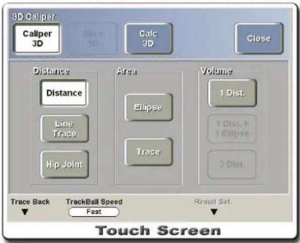
[Figure 4.61 3D Measure]
Notation
Like 3D Notation in 3D View, texts and indicators can be entered 3D XI ™ also. For more information, refer to the section on “3D Notation.”
Volume CT
This function provides relational view of surface images by expressing coronal, sagittal and axial images in appropriate positions in the 3D space. Volume CT supports two modes: Cube Volume CT and Cross Volume CT. Press the Volume CT button on the touch screen.
Cube Volume CT
Provides information of external surface images neighboring the cube.
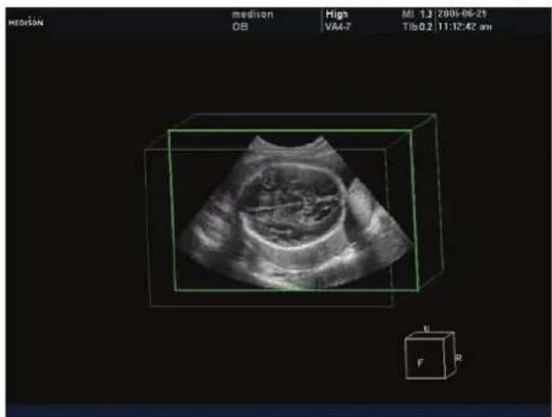
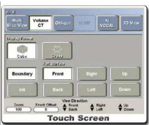
[Figure 4.62 Cube Volume CT]
| Menu | Description |
| Default Setting | Shows the selected surface according to the position of the image selected in Multi Slice View. If the position is close to the front/top/left direction of the volume, the image is shown in the same direction as the multi slice image because the image is shown from the selected position. If the position is close to the back/bottom/right direction of the volume, the image is then shown in the opposite direction as the multi slice image because the image is shown from the selected position. The position of the selected slice is shown with the image slightly slanting. This is for showing other plane images simultaneously when looking at them from different directions. |
| Ref. Surface | Sets Reference Surface. You can select any of the six surfaces. |
| View Direction | When the user selects one of the six surfaces as the desired view direction, the selected surface is placed toward the front. |
| Ref. Surface Offset | Moves the offset position of the selected Reference Surface. Use the knob-button below Surface Offset on the touch screen to make adjustments. |
| Rotation | Use the X/Y/Z knob-button on the control panel to rotate Cube Volume CT image by the X/Y/X-axis. |
| Zoom | Zooms in/out the Cube Volume CT image. Use the knob-button below Zoom on the touch screen to make adjustments. |
| Boundary | Sets or clears the additional boundary lines for Cube Volume CT. Additional boundary lines indicate the external area for the entire volume. |
Cross Volume CT
Provides information of images inside the planes crossing over each other.
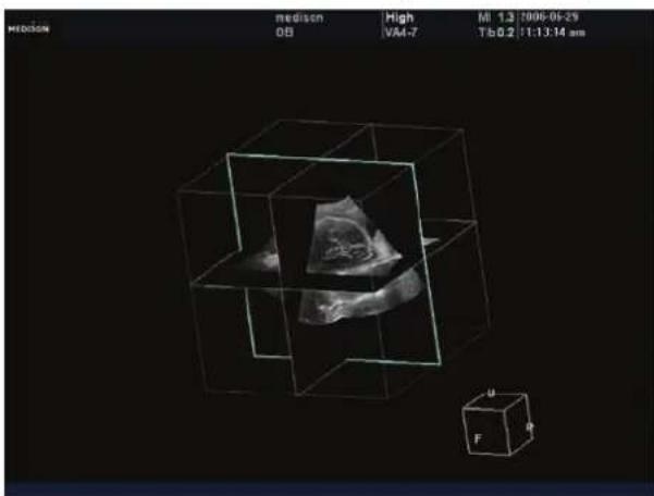
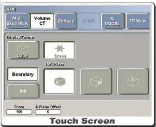
[Figure 4.63 Cross Volume CT]
| Menu | Description |
| Ref. Plane | Sets Reference Plane. |
| Ref. Plane Offset | Moves Reference Plane. Use the knob-button belowPlane Offseton the touch screen to make adjustments. |
| Rotation | Use the X/Y/Z knob-button on the control panel to rotate Cross Volume CT image by the X/Y/X-axis. |
| Zoom | Zooms in/out the Cross Volume CT image. Use the knob-button belowZoomon the touch screen to make adjustments. |
| Boundary | Sets or clears the additional boundary line for Cross Volume CT.Additional boundary lines indicate the external area for the entire volume. |
Oblique View
Surface images can be viewed by applying line/contour on desired surfaces in anatomical positions of coronal/sagittal/axial images. Press the Oblique button on the touch screen.
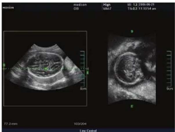
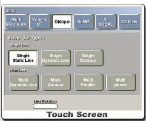
[Figure 4.64 Oblique View]
Select Cut Type
Provides the following Cut Types:
i) Single Line: Applies a single line to an image for a surface view. A reference image and a line are displayed on the left side of the screen and an oblique image for the line on the right side of the screen.
| Menu | Description |
| Single Static Line | Obtains information for a vertical surface image using the default line. Use the knob-button belowLine Rotationon the touch screen to rotate thedefault line. |
| Single Dynamic Line | Obtains information for a vertical surface image by editing a line. Press the Single Dynamic Line button and then use the trackball and the Set button to specify a start point. Then, draw a line and press the Set button again to specify an end point. A surface image perpendicular to the line will be shown. Use the knob-button below Line Rotation on the touch screen to rotate the line and press the Change button on the control panel to move it. |
| Single Contour (Edit) | Obtains information for a vertical surface image by editing a contour. Press the Single Contour button and then use the trackball and the Set button to specify a start point. Then draw a contour and press the Set button again to specify an end point. A surface image perpendicular to the contour will be shown. Because there is a restriction on the volume of data with contours, a surface image cannot be viewed if the volume of data has exceeded its limit. |
ii) Multi Line: Applies up to 5 lines to a reference image for a surface view. Lines are shown in different colors for easier identification.
A reference image is shown at the upper left-hand corner of the screen, containing all lines.
The oblique image of a line is shown by color in the screen. However, If the reference image is changed, all of the existing lines will disappear.
| Menu | Description |
| Multi Dynamic Line | Applies five lines to a reference image and displays an oblique image for these. Press the Multi Dynamic Line button and then use the trackball and the Set button to draw a line. Then a surface image perpendicular to the line will appear separated with line colours. Five dynamic lines can be drawn. Use the Rotation knob-button to rotate a line. |
| Multi Contour | Applies five random contour lines to a reference image and displays an oblique image for these. Press the Multi Contour button and then use the trackball and the Set button to draw a curve. Then an oblique image will appear separated with curve colours. Five curves can be drawn. |
| Multi Parallel | Applies lines parallel with a random line to a reference image and displays an oblique image for these. Press the Multi Parallel button and then use the trackball and the Set button to draw a reference line. Then a parallel line will be drawn automatically. An oblique image for each line is displayed. Use the Line Rotation knob-button to rotate a reference line. The changes are applied to all parallel lines. Use the Line Offset knob-button to adjust the spacing between parallel lines. |
| Multi Plumb | Applies lines perpendicular to a random dynamic line to a reference image and displays oblique image for these. Press the Multi Plumb button and then use the trackball and the Set button to draw a reference line. Then a perpendicular line will be drawn automatically. An oblique image for each line is displayed. Use the Line Rotation knob-button to rotate a reference line. The changes are applied to all perpendicular lines. Use the Line Offset knob-button to adjust the spacing between perpendicular lines. |
View direction of Vertical Surface Image
As illustrated below, the view direction is perpendicular to the cutting direction of the volume data.
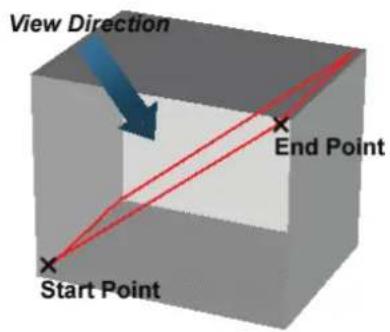
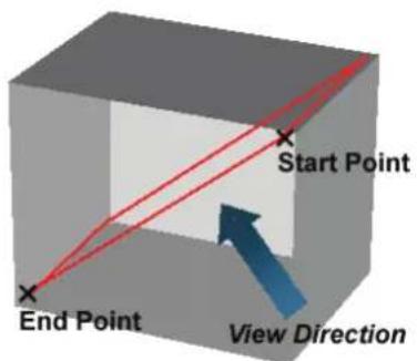
[Figure 4.23 3D View]
3D DMR
In 3D, Live 3D or 3D XI Mode, you can apply Dynamic MR to enhance images.
■ 3D DMR in 3D / Live 3D Modes
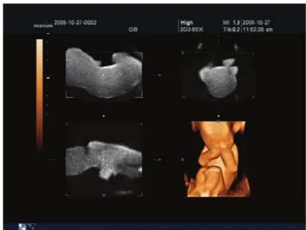
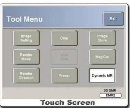
[Figure 4.65 3D DMR in 3D / Live 3D Modes]
-
Press the Tools button on the touch screen. The Tool Menu screen will appear.
-
Press Dynamic MR.
- With the 3D DMR switch at the bottom of the touch screen, set the DMR type to DMR 1-4. The DMR type set is immediately applied.
■ 3D DMR in 3D XI TM Mode
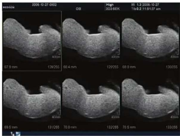
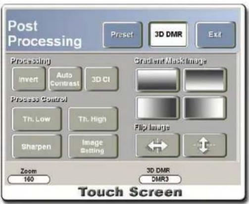
[Figure 4.66 3D DMR in 3D XI™ Mode]
- In the Multi Slice View screen on the touch screen, press 3D DMR. Dynamic MR is applied.
- Press Post Processing to change the DMR type. The Post Processing screen will appear.
- With the 3D DMR switch at the bottom of the touch screen, set the DMR type to DMR 1-4. Press Exit to complete the changes.
NOTE
■ Because Dynamic MR is optional, it becomes available only when a dongle for Dynamic MR is attached.
■ When the dongle is not attached, the 3D DMR button on the touch screen is shown as XI MR in 3D XI Mode and does the same job as XI MR in Post Processing.
If an image is saved after Dynamic MR is applied and it is viewed without the dongle attached, it appears without the effect of Dynamic MR.
XI VOCAL
Unlike in VOCAL, which uses the rotation surface method, XI VOCAL slices an object using a parallel surface method to calculate its volume. Press XI VOCAL on the touch screen for 3D XI.
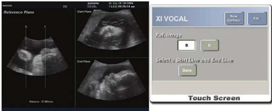
[Figure 4.67 XI VOCAL]
The reference image specified in Multi Slice View appears in the screen. When the Rotation or Zoom function has been used with the reference image in Multi Slice View, the effects still remains with the reference image for XI VOCAL.
Perform XI VOCAL by following the steps below. In each step, pressing Exit on the touch screen aborts XI VOCAL and returns to Multi Slice View for 3D XI.
- Select an image to use as a reference on the touch screen.
- Specify Start and End Lines. Use the Set button and the trackball on the control panel. The distance between two lines along with Start and End Planes are displayed in the screen. Once the lines are specified, press Done.
- A message appears on the touch screen, asking whether to contour the reference image. Press Done to proceed.
-
Specify Contour Type. Solid, Cystic and General allows you to retrieve a contour automatically and Manual allows you to retrieve a contour manually. For more information, refer to 'VOCAL.'
-
Specify the number of images to contour. Press Make to move to the next step.
-
Specify the position of Seed Point in the screen.
- When automatic contour retrieval is selected, two Pole Points appear in different positions in all slices and the contour of an object is retrieved based on them. The position of the Pole Points for each slice can be moved independently. To change the position of Pole Points, use the Pole 1 and Pole 2 buttons or the Set button and trackball on the control panel.
- When manual contour retrieval is selected, draw a contour line manually to retrieve a contour. When finished, press Done.
-
Contour is executed. A progress bar appears at the bottom of the screen, indicating the progress. Press Stop to finish contour and execute the same contour for the others.
-
When Contour is completed, you can press All Slice Show to review the completed slices. To edit a contour, press Edit Contour and use the Set button and the trackball on the control panel to edit a contour line.
Press Exit to finish XI VOCAL. To create a new contour, press New Contour and repeat the above steps.
Live 3D XI™ Mode
Live 3D XI TM supports Multi Slice View only.
Procedures for running Multi Slice View for Live 3D XI TM are the same as running Multi Slice View for 3D XI TM .
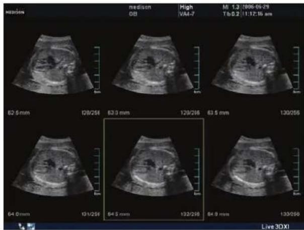
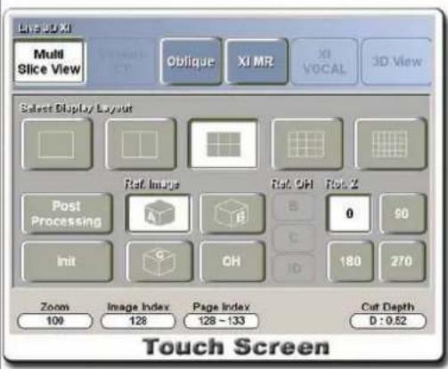
[Figure 4.68 Live 3D XI™ - Multi Slice View]
XI STIC Mode (Optional)
STIC stands for Spatio-Temporal Image Correlation. It calculates a heartbeat cycle with the volume data for a fetal cardiac area, and reconstructs and displays the volume data.
STC is divided into regular STIC and XI STIC depending on whether 3D XI TM is used.
| NOTE | ■ XI STIC Mode is available only with a 3D Probe. |
| ■ XI STIC Mode is available in 3D Color Doppler mode and 3D Power Doppler mode. | |
| ■ XI STIC Mode is not available in Live 3D Mode. |
- In Image Scan Mode, press 3D and XI STIC. To access in 3D XI Mode, press 3D, 3D XI and XI STIC.
-
Specify each menu on the touch screen.
-
For settings in STIC Mode, refer to Live 3D.
-
For settings in XI STIC Mode, refer to 3D XI.
-
Specify Scan Time, STIC Angle and Trimester.
-
Scan Time: Specify the scan time between 7 – 20 seconds in 1 second increments.
- STIC Angle: Specify an angle between 15 - 60° in 5° increments.
- Trimester: Specify the pregnancy trimester to 1st , 2nd , 3rd or User Set. If it is set to 1st - 3rd , the Scan Time and STIC Angle for that trimester are automatically set. Please refer to the following table:
| 1st | 2nd | 3rd | |
| Scan Time 10 sec. 12 sec. 15 sec. | |||
| STIC Angle | 20° | 25° | 30° |
If Scan Time or STIC Angle is set out of the specified range, Trimester appears as User Set.
- Press the Freeze button on the control panel. The system begins to acquire the STIC volume data.
- The number of heartbeats for a fetus is calculated and displayed on the touch screen. Press Yes to proceed. Press No to cancel and scan again.
NOTE
When the number of heartbeats cannot be calculated due to severe Motion Artifact or no heartbeat cycle, the system returns to the Acquire STIC Volume Data screen.
- Once volume data scan is completed, a STIC image appears. Adjust the image with the touch screen.
- With STIC Speed, the image playback speed can be adjusted. Available options are All CINE, 25%, 33%, 50% and 100%. If it is set to All CINE, all Volume CINE saved are reviewed regardless of the speed. If it is set to a percentage, an image is played at the speed of the specified percentage to the number of fetal heartbeats (100%).
- Press the 3D/4D button on the control panel to finish. Press Exit to return to the previous step.
※ Tip! To obtain good STIC volume data:
- STIC Angle: For smaller fetal hearts, specify a smaller Scan Angle.
- Scan Position: Make sure that the centers of the specified Scan Angle and the fetal heart are aligned with each other.
- Volume Box: Adjust it to match the size of a fetal heart.
※ To obtain good Color STIC volume data:
- Control the fps at least 15 during scanning.
- Set the application with Fetal Heart.
- During Cine, control the gain for good color view.
STIC
This is STIC Mode without 3D XI ™ . STIC information such as Image Angle, Vol.Angle, Scan Time, Heart Rate and Cine are displayed in the right hand side of the screen.
NOTE
The touch screen menus for STIC Mode can be used in the same way as in Live 3D View.
In STIC Mode, STIC Volume CINE performs tasks by default. Pressing the Yoyo button on the touch screen changes the CINE play type from Loop to Yoyo.
Pressing the Freeze button on the touch screen stops CINE play and switches to Static 3D Mode. In the Static 3D screen, you can use Vol.Index to move to the volume data for the corresponding index. Pressing the Freeze button again returns to STIC Mode and enables CINE play.
To run 3D View or 3D XI, or save a STIC image, press the corresponding button after stopping CINE Play.
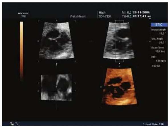
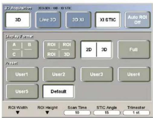
[Figure 4.69 STIC]
XI STIC
This is STIC Mode with 3D XI™. The XI STIC logo appears at the lower right corner of the screen.
NOTE
The touch screen menus for XI STIC Mode can be used in the same way as in 3D XI Mode.
In XI STIC Mode, you can review slice images. However, features such as Volume CT, XI VOCAL or 3D View are not available in this mode. Press the Freeze button on the touch screen to switch to 3D XI Mode. In the 3D XI screen, you can use Vol.Index to move to the volume data for the corresponding index. Pressing the Freeze button again returns to XI STIC Mode.
To run 3D View or save a XI STIC image, press the corresponding button after switching to 3D XI Mode.
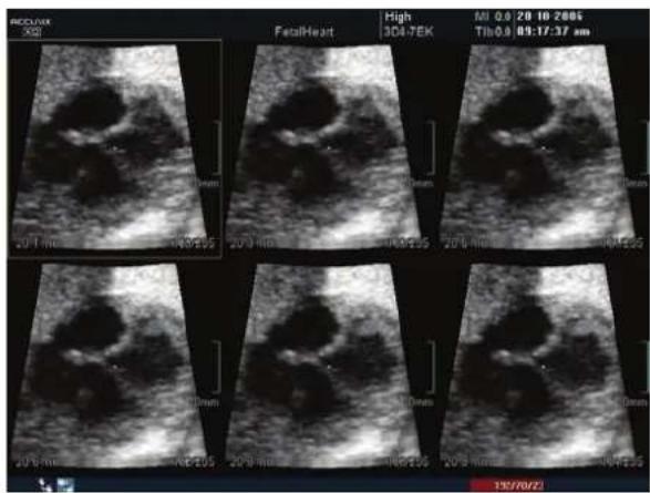
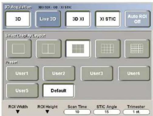
[Figure 4.70 XI STIC]
Chapter 4
Diagnosis Modes
DIAGNOSIS MODE TYPES AND CONTROL.... 3
DIAGNOSIS MODES....3
DIAGNOSIS MODE SCREENS AND IMAGE INFORMATION....3
CHANGING DIAGNOSIS MODE FORMATS....4
OPTIMIZING DIAGNOSIS MODE....5
BASIC MODES....7
2D MODE....7
M MODE....13
COLOR DOPPLER MODE 16
POWER DOPPLER MODE 19
PW (PULSE WAVE) SPECTRAL DOPPLER MODE....21
CW(CONTINUOUS WAVE) SPECTRAL DOPPLER MODE 26
AUTOMATIC CALCULATOR....28
COMBINED MODES 29
2D/C/PWMODE....29
2D/PD/PW MODE 29
2D/C/CW/MODE 30
2D/PD/CW MODE 30
2D/C/M MODE 31
DUAL LIVE MODE....31
MULTI-IMAGE MODES 32
DUAL-2DMODE 32
4 - 2 ACCUVIX XQ Operation Manual
DUAL-2D/C MODE 32
DUAL-2D/PDMODE 33
MULTI-DIMENSIONAL MODES 34
MULTI-DIMENSIONAL....34
ACQUIRING 3D IMAGES....35
3D VIEW 37
OPTIMIZING 3D IMAGES....55
3D XI TM MODE 64
XISTIC MODE (OPTIONAL)....76
Diagnosis Mode Types and Control
Diagnosis Modes
This product supports a variety of diagnosis modes including Basic modes, Combined modes, Multi-Image modes, and 3D modes.
■ Basic Modes: Include 2D Mode, Color Doppler Mode, Power Doppler Mode, M Mode, PW Spectral Doppler Mode, and CW Spectral Doppler Mode.
■ Combined Modes: These modes are Color Doppler Mode or Power Doppler Mode combined with M Mode, PW Spectral Doppler Mode, or CW Spectral Doppler Mode. Dual Live Mode, which features Color Doppler Mode and 2D Mode in single screen, is also one of the Combined Modes.
■ Multi-Image Modes: In Dual Modes you can view two images side by side simultaneously and compare them.
■ 3D Modes: These modes provide 3D images.
Functionalities for each mode are restricted by the probes selected. For example, Freehand 3D Mode supports all probes except for Static CW probe, and Volume 3D Mode supports 3D probe only.
Diagnosis Mode Screens and Image Information
The following table shows the information appearing on different diagnosis mode screens.
| Monitor Display | 2D Mode | M Mode | C Mode | PD Mode | PW Mode | 3D Mode |
| 2D Image and Image Information | ● | ● | ● | ● | ● | ● |
| M Image and Image Information | ● | |||||
| Color Doppler Image and Image Information | ● | |||||
| Power Doppler Image and Image Information | ● | |||||
| Spectral Doppler Image and Image Information | ● | |||||
| M Line | ● | |||||
| D Line and Sample Volume | ● | |||||
| ROI (Region of Interest) Box | ● ● | ● | ||||
| Title Bar | ● | ● | ● | ● | ● | ● |
| Depth Marker | ● | ● | ● | ● | ● | ● |
| Focusing Point & Number | ● | ● | ● | ● | ● | ● |
| Gray Scale Bar | ● | ● | ● | ● | ● | ● |
| Color Bar | ● ● | |||||
| TGC Curve | ● | ● | ● | ● | ● | ● |
The following table shows the image information appearing for each mode. Note that image information for 2D mode appears in all modes.
| Image Information | 2D Mode | M Mode | C Mode | PD Mode | PW Mode | |
| Gain | ● | ● | ● | ● | ● | |
| Dynamic Range | ● ● | |||||
| Frame Average | ● ● ● ● | |||||
| Power | ● ● | |||||
| PRF (Pulse Repetition Frequency) | ● ● ● | |||||
| Wall Filter | ● ● ● | |||||
| Sensitivity | ● ● | |||||
| Sample Volume Depth | ● | |||||
| Sample Volume Size | ● | |||||
| Angle | ● | |||||
Image information and gray scale bar disappear from the screen by pressing Spacebar.
Changing Diagnosis Mode Formats
The following section explains how to change the display format that is common to all diagnosis modes.
Changing Active Image Mode
All diagnosis modes except for 2D mode provide two or more modes simultaneously. You can press the button for each mode on the touch screen to select the active image mode and control its menus.
Changing Active Image in Multi-Image Modes
Use the Update button, the Set button and the Dual button on the control panel to change the active image. For example, press the Update button, the Set button or the Dual button in Dual-2D mode to freeze the image being scanned on the left-hand side of the screen and show the image being scanned on the right.
Freezing 2D Image in Spectral Doppler Mode
When the simultaneous function is turned on and 2D image and spectral Doppler image are displayed real-time, you can freeze the 2D image to view more accurate spectral Doppler image.
Press the Update button on the control panel to freeze the 2D image. Press the button again to display the 2D image again.
If the simultaneous function is turned off, the current image mode is indicated as "PW Only" or "2D Only" at the upper right-hand corner of the screen.
You can determine the use of simultaneous modes by setting "Simultaneous Mode" under the Misc. tab on the Settings screen. If this option is set to "Off", the Simultaneous button on the PW Spectral Doppler menu remains inactive.
You can also freezing 2D image by the Update button in 2D/C/PW Mode, 2D/PD/PW Mode, 2D/C/CW Mode, 2D/PD/CW Mode, and 2D/C/M Mode.
Image Depth Control
Use the Depth switch on the control panel. Raise the Depth switch to decrease view depth, or lower the Depth switch to increase the view depth. Maximum depth and minimum depth vary depending on the probe.
Zooming Image
Use the Zoom switch on the control panel to zoom the image. Raise the Zoom switch and the Zoom box will appear. Use the Change button and the Trackball to move and resize the Zoom box. Repeatedly pressing the Change button toggles the "Zoom Pos." and "Zoom size" indication on the screen.
■ Zoom position: Press the Change button to make the HD Zoom box appear with solid lines. Use the Trackball to move the box to any desired position.
■ Zoom size: Press the Change button to make the HD Zoom box appear with dotted lines. Use the Trackball to resize the HD Zoom box.
Adjust the size and the position of the Zoom box and then press the Set button to zoom the image. The Zoom Navigation box on the screen shows the relative position of the zoomed area.
When using the Zoom function, press the Z button on the control panel to hide the Zoom Navigation box and deactivate Zoom Position. Press the Z button again and the Zoom Navigation box will appear.
Change Depth or press the Exit button on the control panel to cancel the image zoom.
Read Zoom
This function is for zooming the image saved in the memory. Note that this is not available in Dual mode or Loop mode.
The RD Zoom menu appears on the touch screen when the image is frozen by pressing the Freeze button or when adjusting the Zoom switch on the control panel.
Turn the knob-button below the RD Zoom menu to run the Read Zoom function and zoom the image. When Read Zoom is activated, the Zoom switch will not work. (Write Zoom cannot be activated.)
Optimizing Diagnosis Mode
The following are instructions for optimizing images in all diagnosis modes.
Gain Control
Use the mode knob-button on the control panel to adjust the brightness of the image. Turn it clockwise to increase Gain or turn it counter-clockwise to decrease Gain.
Adjusting Post Gain
When the image is frozen by pressing the Freeze button on the control panel, you can adjust the mode knob-button to adjust Gain. Turn it clockwise to increase Gain or turn it counter-clockwise to decrease Gain.
Post Gain can be adjusted to any values between +10 and -10. The Post Gain value is displayed on the screen in the format of “*PG:0.” The Gain value is restored to the value before freezing when the image becomes active again.
TGC Control
When ultrasound is transmitted through the human body, the lucency of ultrasound weakens as it travels deeper into the body. TGC (Time Gain Compensation) can be used to supplement this. For obtaining the best image quality, TGC is divided into 8 regions which can be used to adjust Gain by different depths.
Move the TGC slide to the right (+) to increase Gain (brightening the image) or move the TGC slide to the left (-) to decrease Gain (darkening the image).
Harmonic Function
This product provides the OHI (Optimal Harmonic Imaging) function. In 2D mode, press the HAR button on the control panel to activate the function.
Focus Position Control
Use the Focus switch on the control panel to focus on specific regions for clearer view. Raise the switch to move the focus position up and lower the switch to move the focus position down.
Focus Number Control
Press the Focus up/down button on the touch screen to adjust the number of focusing points. Check on the screen as focusing points are added or removed.
Frequency Change
Each probe provides a wide range of frequencies for obtaining images of best quality. Use the Frequency up/down button on the touch screen to change the probe frequency.
This function is available for linear probes (L5-12IM, L6-12IS) only.
Power Control
Power is the intensity of the acoustic output.
Use the up-down switch below Power on the touch screen to adjust the value.
Basic Modes
2D Mode
This basic mode, also referred to as B Mode (Brightness mode), provides scan planes of organs.
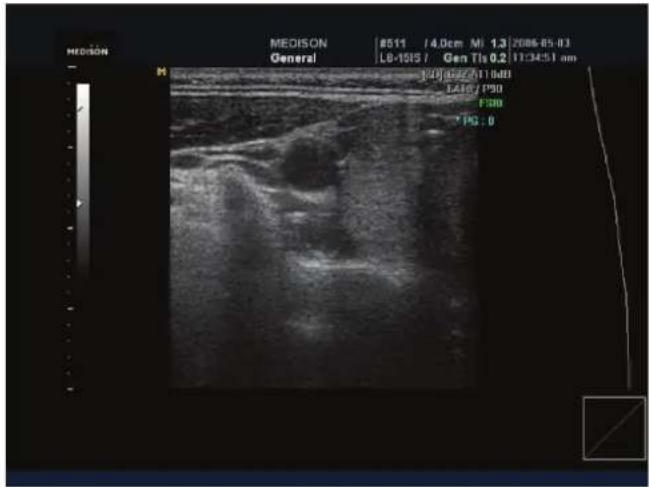
[Figure 4.1 2D Mode]
2D Mode Selection
Since 2D mode is always turned on except for special cases, the 2D button does not function as a toggle. In any diagnosis mode, just press the 2D button to switch to 2D mode which is the basic diagnosis mode.
2D Menu
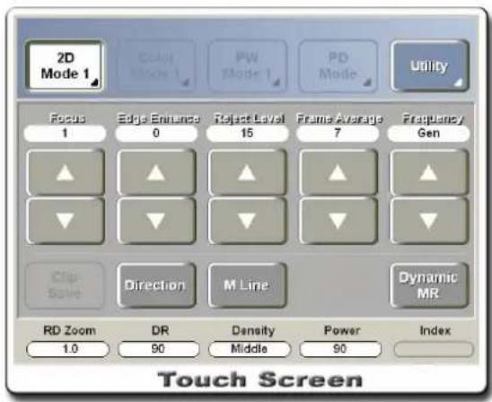
![2D Mode 2 Color Mode 1 PW Mode 1 PD Mode Utility Tissue Cystic Pulse Inversion Trapez Steer Apex Reset AIO Scan Area Scan Angle Frame Rate 100 % 0 [Deg] Fast Touch Screen](/content/2026/05/955519/images/0fd031f43f8838efa1b60bc5847dc34633937163e993e66b9585c29db47b1bd2.jpg)
[Figure 4.2 2D Menu]
Changing 2D Image Format
Changing Image Direction
- Changing Left/Right Orientation (Horizontal Orientation, Direction): Press the Direction button on the touch screen.
- Changing Up/down Direction (Vertical Orientation, Apex): Press the Apex button on the touch screen.
- Changing View Area
Turn the knob-button below Scan Area on the touch screen to adjust the size of the Area to be anywhere between 60% and 100%. After changing the view area, turn the knob-button below Scan Angle left/right to move View Area left/right and view other regions. Scan Angle is unavailable for linear probes.
The frame rate (FPS) drops as the view area becomes larger and the frame rate increases as the view area becomes smaller.
Showing M Line
M Line indicates the relative position of the M Mode image or the Spectral Doppler Mode image in the 2D image.
Press the M line button on the touch screen to show M Line, and press the M line button again to hide M Line.
Optimizing 2D Images
Adjusting Frame Average
The Frame Average function obtains the average for the previous frame and the current frame and displays it on the screen in order to reduce speckles on continuous images on the same examination regions. Adjusting this function to High will result in a relatively smooth display of the image, but the user may get the impression that the display is slower (the actual frame rate does not drop). It is recommended that this function be turned off when examining OB, cardiac and other movement-intense organs. It is useful to set this function to High when examining internal medicine and organs with little movements.
Use the Frame Average up/down button on the touch screen to make adjustments.
This clearly displays the boundaries between tissues or organs. Edges appear clearer if the Edge Enhance value is set high. Use the Edge Enhance up/down button on the touch screen to make adjustments.
Adjusting Reject Level
This function is used to eliminate noise or low level echoes for clearer signals. Use the Reject Level up/down button on the touch screen to make adjustments.
Adjusting Tissue Property
You can select the ultrasound velocity according to the patient's physique. Physique menu contains Cystic, Adipose, Normal and Solid. Use the Tissue up/down button on the touch screen to make adjustments.
Smooth Function
This is available for Convex probe. It shows smoother 2D images by eliminating noise. Use the up-down switch below Smooth on the touch screen to make adjustments.
Pulsed Inversion Function
When Harmonic mode is in use, press the Pulsed Inversion button on the touch screen to activate this function. This shows sharp images with clear edges. This function is not available for L5-12IM, VNA6-12, L6-12IS, and L8-15IS probes.
Trapezoid Function
When using Linear probe, you can stretch the 2D image into a trapezoid and examine it in a larger area. Press the Trapez. button on the touch screen to run this function.
When adjusting the image depth, the Trapezoid function may not be available at certain depth values. Note that using the Zoom function turns the Trapezoid function off.
DynamicMR Function
This optional function removes speckle noise and strengthens edges for 2D images for higher image accuracy.
Press the DynamicMR button on the touch screen to run it. The previous configuration will be applied to the image.
NOTE
DynamicMR has 6 Presets, each of which has 5 Indexes. To select new values or make other settings, press the DynamicMR button on the Utility menu and make the settings.
Steer Function
This function adjusts the angle of the ultrasound beam in order to prevent loss of ultrasound information. This function is available for Linear probe only. Use the Steer button on the touch screen to run this function.
Adjusting Dynamic Range
You can adjust the minimum value and maximum ratio of the input signal and display images by changes in contrast. Images appear soft at higher ratios and coarse at lower ratios.
Turn the knob-button below DR on the touch screen to make adjustments.
Adjusting Density
Use the up-down switch below Density on the touch screen to adjust the image scan line. This is useful for quickly examining images with low values.
While density can be adjusted to Low, Middle, or High, it is available in 4 steps — Low, Middle1, Middle2 and High — for Color Doppler Mode.
Adjusting Frame Rate
Frame rate is the number of images generated per second. Frame rate should be set to high when viewing fast moving organs.
Use the up-down switch below Frame Rate on the touch screen to make adjustments.
AIO (Auto Image Optimization) Function
This function optimizes 2D images by adjusting 2D Gain, Dynamic Range and TGC automatically.
Press the AIO button on the control panel to activate it and the Reset AIO button on the touch screen to deactivate it. It deactivates when Harmonic Mode or Pulse Inversion is activated.
Pressing and holding the AIO button executes the AIO function repeatedly.
The probes and applications in the following table are applied with the new AIO function to obtain more optimized images.
| Abdomen | OB | Small Part | Vascular | Cardiac | |
| L6-12IS | ● ● | ||||
| C5-2EL | ● | ||||
| C2-6IC | ● | ||||
| 3D4-7EK | ● | ||||
| P2-4AC | ● |
Clip Save Function
This function saves the screen image into a clip. It is provided for Cardiac application with Phased Array probe or Contrast Agent application with C5-2EL or C1-4EC probe (only Low MI).
Press the Clip Save button on the touch screen to activate it. Specify the unit and value(s) to be used for saving a clip under the Misc. tab on the Setting screen.
While saving a clip, press the Set button on the control panel to complete the saving process or the Exit button to cancel the saving process.
NOTE
Clips can be saved by beat only when ECG is running; clips will not be saved when ECG beats do not appear even if the setting is selected for clips to be saved by beat.
If 10 seconds of a color image are saved, the screen will be updated 3 seconds after saving is completed.
Spatial Compound Image (SCI) Function
This function displays more smooth 2D images by eliminating speckle noises and is available only in 2D Mode for the L6-12IS probe.
Press the SCI button on the touch screen to activate it. Its value(s) can be adjusted with the SCI Filter up/down button that appears when it is running.
When the SCI function is in use, Frame Average, ECG Trigger, AIO and Write Zoom functions become unavailable.
The SCI function deactivates when 3D Mode, M Mode, C Mode, PD Mode, PW Mode, Pulse Inversion or Trapezoid is activated.
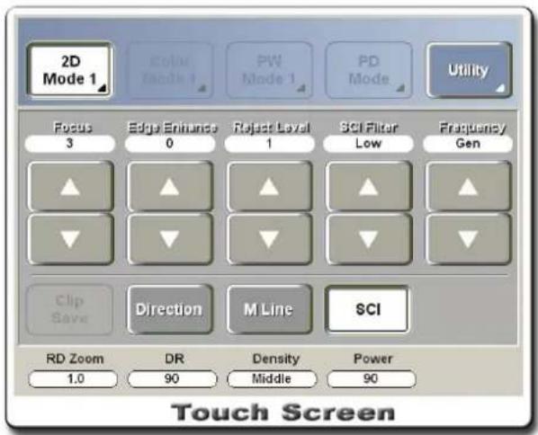
[Figure 4.3 Spatial Compound Image]
Low MI Function
This function displays clearer contrast images and is available for Contrast Agent application with the C5-2EL or C1-4EC probe.
Press the Low MI button on the touch screen to activate it. Images can be adjusted via the menu displayed on the touch screen. Press the Low MI Off button to deactivate Low MI and switch to 2D Mode. Press the 2D Menu button to keep Low MI activated and switch to 2D Mode.
Use of the Low MI menu is similar to that of the 2D Mode Menu.
![2D Mode 2 Color Mode 3 PW Mode 4 PD Mode Utility Tripsis Normal Smoothi Mid1 Pulse Inversion Traperz Usher Apex Low MI Reset AIO Scan Area Scan Angle Frame Rate 100 % 0 [Deg] Fast Touch Screen](/content/2026/05/955519/images/4d2e4e0d42c86b0b4d27df0d4e233531684438ed8ca6a227cf82512c06696ccd.jpg)

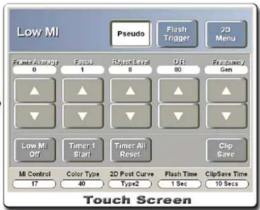
[Figure 4.4 Low MI]
- Pressing the Timer 1 Start button resets and activates Timer. The elapsed time after an agent is injected can be measured with a counter displayed on the screen. If an image becomes frozen, Timer 2 is activated to show the time for which it is frozen. Press the Return Low MI button to return to the Low MI function.
![[2D] G60 / 80dB FA0 / P90 INV / FS10 LowMI T1: 00:00:10 T2: 00:00:10](/content/2026/05/955519/images/32411d3813b66216e99ada3d94cacd7783975cd86599fcfc8cc7ac06ba797a7c.jpg)
- Pressing the Timer All Reset button resets both Timer 1 & 2.
- Flash Trigger is a function that breaks the agent bubbles injected by bursting flashes at the maximum MI Power of the system and probe for the specified Flash Time. Flash Time can be specified with the up/down switch under Flash Time on the touch screen.
- Use the knob-button under MI Control to adjust the MI Power value. Available setting ranges are between 0 – 100.
- Color Type and 2D Post Curve change the color of the image applied with Pseudo.
NOTE
While Low MI is in use, you may not switch to any mode other than Dual Mode.
Trying to activate Low MI in Harmonic Mode results in activation of Pulse Inversion.
M Mode
This mode provides images that change over time at certain regions of 2D mode scan planes, such as the movement of a heart valve. A 2D image is also displayed to indicate the relative position of the selected region and allow the user to change the position.
![MEDISON General M1 MEDISON #1398 / 4.0cm MI 1.3 2006-05-03 LB-1915 / Gan Tls 0,3 11:30:35 am [20/M] G39 / 85dB FA10 / P30 FSBD * PC : 0 Loop Pos Freeze](/content/2026/05/955519/images/9a79e2e82f779321ebee790f7b0504c1358b9e9b94018c3f9ecfb2a515bab3ce.jpg)
[Figure 4.4 M Mode]
M Mode Selection
Press the M button on the control panel. Press it again to return to 2D mode.
2D/M Menu
M Mode and 2D Mode have the same menus for image optimization.
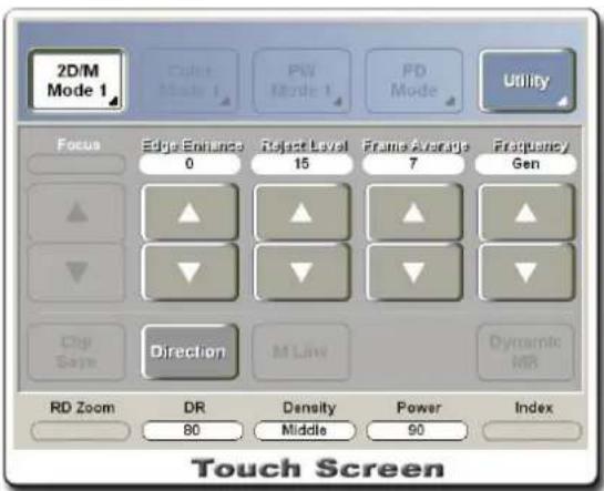
![2D/M Mode 2 Color Single 1 PV Mode 1 PD Mode Utility Tissue Cystic Speed 180 Pulse Inversion Trapez. Street Apex Reset AIO Scan Area 100 % Scan Angle 0 [Deg] Frame Rate Fast LoopFormat Top Down DispFormat 50/50 Touch Screen](/content/2026/05/955519/images/038e6f116726298bed72d08c2a2eb6997de1d01d8c2b5a4a6ad9113c7ffaec6f.jpg)
[Figure 4.5 2D/M Menu]
Changing M Mode Format
Adjusting M Line
M Line indicates the relative position of the M Mode image in the 2D image. Use the Trackball on the control panel to move M Line left and right and view different regions.
Adjusting Sweep Speed
Use the Speed up/down button on the touch screen to adjust the sweep speed of M image in steps.
Changing Loop Format
Use the up-down switch below LoopFormat on the touch screen to change the position where 2D image and M image appear. Top Down Format places 2D image and M image at the top and the bottom, and Side by Side Format places them on the left and the right.
Changing M Image Size
Use the up-down switch below Disp Format on the touch screen to change the size of 2D image and M image. Available options are "50/50", "40/60", and "60/40" which indicate the image size ratio between 2D image and M image.
Free Angle M Mode
This mode allows the user to rotate or move M Line—which normally moves horizontally—for viewing 2D images. Adjusting the depth for 2D image initializes M Line.
NOTE
This mode is available for Phased Array probe. It is unavailable in Color Doppler Mode or Zoom Mode.
Starting and Adjusting Free Angle M Mode
Press the Free Angle button on the touch screen to run it. The menu is illustrated in the figure below.
![Free Angle M Close Length Step 0.1 [cm] Angle Step 1 Length 9.6 cm Angle 91 Touch Screen](/content/2026/05/955519/images/aad9e5ab14109e24b2c83403040da27c236f7bcff40ff3859668daadb939d386.jpg)
[Figure 4.6 Free Angle M Mode]
Turn the knob-buttons below Length and Angle on the touch screen to adjust the length and angle of M Line.
Use the Length Step and Angle Step up/down buttons on the touch screen to adjust the steps for "Length" and "Angle." If Step is set to "3," the value can be adjusted in multiples of 3.
Position of M Line can be adjusted by moving the Trackball. Start point and end point of M Line cannot be outside the 2D image.
Things to Consider When Using Free Angle M Mode
Selecting another mode (2D Mode, etc.) while using Free Angle M Mode exists Free Angle M Mode and activates the selected mode.
The Patient, End Exam, Indicator, Text, Body marker, and Measure buttons function normally in Free Angle M Mode.
If you selecting the User, E-mail, Mic or SonoView button in Free Angle M Mode, the selected button functions after shifting to the normal M Mode.
The buttons on the control panel other than those mentioned above (those with LED off) do not function.
NOTE
For information on optimizing M image, refer to "2D Mode."
Color Doppler Mode
In this mode you can obtain a variety of information about blood flow within the 2D Image such as the existence of blood flow, its average speed and its direction within the ROI (Region of Interest).
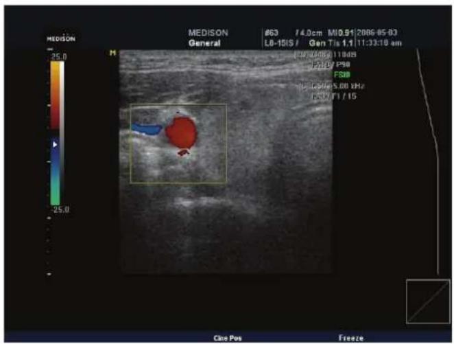
[Figure 4.7 Color Doppler Mode]
Color Doppler Mode Selection
Press the C button on the control panel. Press it again to return to 2D mode.
C Menu
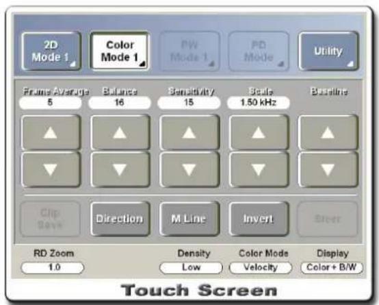
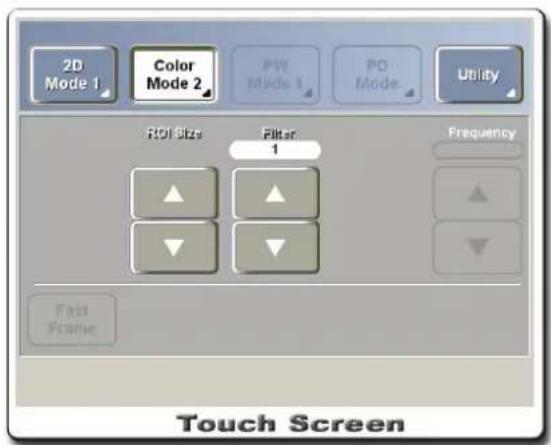
[Figure 4.8 C Menu]
Changing Color Image Format
NOTE
Color Bar is a color map that shows the direction and velocity of blood flow. Colors above the baseline across the center of the color bar indicate blood flowing toward the probe and colors below the baseline indicate blood flowing away from the probe.
Adjusting Color Bar Baseline
Press the Baseline up/down button on the touch screen. Press the up button to move the baseline up on the color bar, or press the down button to move the baseline down.
Baseline can be adjusted only when Color Mode is set to "Velocity."
Inverting Color Bar
Press the Invert button on the touch screen. Inverting the color bar also inverts the colors displayed on the image.
Changing Color Display Information
Use the up-down switch below Color Mode on the touch screen to select Velocity, Power, Variance, or Vel + Var. If "Velocity" or "Vel + Var" is selected, numbers will be displayed above and below the color bar indicating the color scale values. If "Variance" is selected, +1 and -1 will be displayed. If "Power" is selected, no numbers will be displayed.
Color Image Optimization
Adjusting Balance
Adjust the range of color image display by comparing Gray Level of the 2D image with Doppler signal values of the color image. As the Balance value increases, color image appears even in regions with high Gray Level in 2D image (bright regions), expanding the range of color image.
Use the Balance up/down button on the touch screen to make adjustments.
Adjusting Sensitivity
Use the Sensitivity up/down button on the touch screen to make adjustments.
Increasing the Sensitivity value increases Sensitivity, and decreasing the Sensitivity value decreases Sensitivity. As color sensitivity increases, frame rate drops.
Adjusting Scale (PRF)
Use the Scale up/down button on the touch screen to make adjustments. Increasing the Scale value increases PRF (Pulse Repetition Frequency), expanding the range of blood flow velocity displayed, and decreasing the value decreases PRF, narrowing the range of blood flow velocity displayed.
Changing ROI Box
Color Pos: ROI (Region Of Interest) indicates the area of the 2D image where color (blood flow) information is displayed in Color Doppler Mode. Use the Trackball to change the
position of the box.
Color Size: Press the ROI Size up/down button on the touch screen. Alternatively, repeatedly press the Change button on the control panel to change the function of the Trackball and use the Trackball when its appropriate function is displayed on the screen.
Adjusting Wall Filter
Wall Filter is an electric filter that removes low-frequency Doppler signals from movement of the vessel wall. Adjust Cutoff Frequency to remove from the screen Doppler signals with frequencies that are lower than the Cutoff Frequency.
Use the Filter up/down button on the touch screen to make adjustments. Increasing the Filter value increases the Cutoff Frequency for Wall Filter, and decreasing the value decreases the Cutoff Frequency for Wall Filter.
Fast Frame Function
This function increases the frame rate when the application is set to Fetal Heart. The image moves approximately 70% faster than the actual speed.
Press the Fast Frame button on the touch screen to run this function.
Steer Function
When using Linear probe, this function adjusts the ultrasound beam angle to prevent the loss of color information caused by the ultrasound beam angle.
Use the Steer button on the touch screen to make adjustments.
Display Function
Use the up-down switch below Display on the touch screen to select the Display format. Color Doppler Mode supports Color + B/W Image, Color Only, and B/W Only display.
TDI (Tissue Doppler Image) Function
When the application Cardiac or Pediatric Cardiology and the Phased Array probe is in use, movements of cardiac tissues can be viewed in Doppler modes.
Cardiac tissues can be viewed by color information in Color Doppler Mode and Power Doppler Mode, and time-dependent changes of cardiac tissues can be viewed by spectral Doppler images in PW Spectral Doppler mode.
Press the TDI button on the control panel. "TDI on" will be indicated on the screen.
NOTE
For information on other menu items, refer to "2D Mode."
Power Doppler Mode
Instead of the speed or direction of blood flow, Power Doppler Mode displays the overall strength of blood flow, thereby showing information about the existence and amount of blood flow in the sample area.
![MEDISON General M MEDISON #GO /4.0pm MI 1.0/2006-05-03 LB-1515 / Gen Tis 1,1/11:39.02 am [24] GB/T 110dB FSTJ/P90 FS10 T90 GB/T 1.58 kHz FAJ/T1/15 Close Pos Freeze](/content/2026/05/955519/images/39b90f658144af2fe80129d1d5d581c68bd61d8320fe8fb209183bc7cbe2292c.jpg)
[Figure 4.9 Power Doppler Mode]
Power Doppler Mode Selection
Press the PD button on the control panel. Press it again to return to 2D mode.
PD Menu
Use of the Power Doppler Mode menu is similar to the Color Doppler Mode menu.
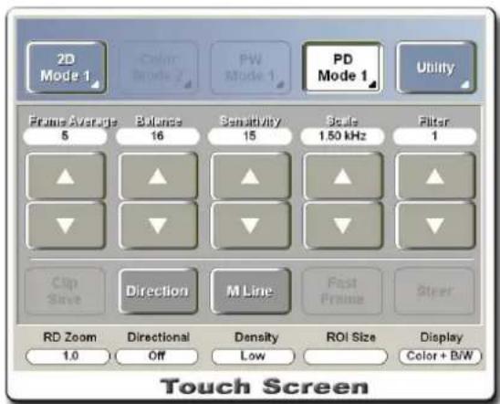
[Figure 4.10 PD Menu]
Optimizing Power Doppler Image
Directional Function
This function displays the amount (power) of blood flow and direction of blood flow. Press the Directional button on the touch screen to activate it.
NOTE
■ Color Bar is a color map that displays the existence of blood flow and its amount. Brighter colors on the color bar indicate high amount of blood flow.
■ For information on other menu items, refer to "Color Doppler Mode."
PW (Pulse Wave) Spectral Doppler Mode
This mode shows the velocity of blood flow at a specific position within blood vessel. Distance (depth) information can be obtained by transmitting pulses over time frames. This mode is useful for measuring low-speed blood flow such as in abdomen and peripheral vessels. A 2D image is also displayed to indicate the relative position of the selected region in blood vessel and allow the user to change the position.
On the PW Spectral Doppler Mode image, the horizontal axis represents time, and the vertical axis represents speed (or frequency).
![MEDISON [PM] G70 F1 /4.00 kHz Depth 10 Size 2.00 Angle 8 * PG : 0 MEDISON General H #185D /4.0zm MI0.45/2006-05-03 LB-191S / Gen Tis 0.1/11:55:05 am [20] G53 / 110dB FA2 / P30 FSBD + 35 - 30 + 25 - 20 + 15 - 10 + 5 cm/s SV Pm](/content/2026/05/955519/images/58ca4904870718cce2720accac103f91250b9628b508e3bf99684398c02a33b6.jpg)
[Figure 4.11 PW Spectral Doppler Mode]
PW Spectral Doppler Mode Selection
Press the PD button on the control panel. Press it again to return to 2D mode.
D Menu
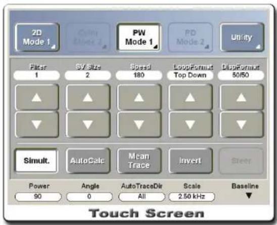
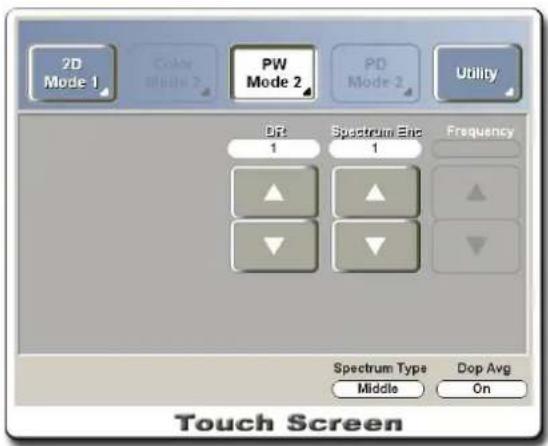
[Figure 4.12 PW Menu]
PW Spectral Doppler Mode Format Change
Adjusting Sweep Speed
Use the Speed up/down button on the touch screen to adjust the sweep speed of Spectral Doppler image in steps.
Adjusting Doppler Baseline
Use the up-down switch below Baseline on the touch screen. Raise the switch button to move the baseline up, or lower the switch to move the baseline down.
Changing Loop Format
Use the up-down switch below Loop Format on the touch screen to change the position where 2D image and Spectral Doppler image appear. Top Down Format places 2D image and Spectral Doppler image at the top and the bottom, and Side by Side Format places them on the left and the right.
Changing Spectral Doppler Image Size
Use the up/down button Disp Format on the touch screen to change the size of 2D image and Spectral Doppler image. Available options are "50/50", "40/60", and "60/40" which indicate the image size ratio between 2D image and Spectral Doppler image.
Activating Simultaneous Mode
The PW Spectral Doppler image and 2D image can be displayed simultaneously or separately.
Press the Simult. button on the touch screen to activate Simultaneous Mode. When Simultaneous Mode is on, selecting the button again to deactivate Simultaneous Mode.
Simultaneous Mode decreases Doppler PRF, thus decreasing the measurable speed range. Activate the Simultaneous Mode option by setting Simultaneous Mode as "Allow 2D/PW" or "Allow 2D/C/PW" in the Misc. tab at the Setting screen.
Inverting Doppler Axis
Press the Invert button on the touch screen. Positions of the + and - speed indications will be inverted.
Optimizing PW Spectral Doppler Image
Sample Volume
Located on the 2D image, it indicates the position of the Spectral Doppler image. Displayed in the format of xx.x@yy.y mm, it indicates that the size of the sample volume is "xx.x mm" and the depth is "yy.y mm." For example, 2.0@16.7 mm means that the Sample Volume of 2.0mm size is located at a depth of 16.7mm.
Changing Position: Use the Trackball on the control panel.
Changing Size: Press the SV Size up/down button on the touch screen. Alternatively, repeatedly press the Change button on the control panel to change the function of the Trackball. "SV Pos" and "SV Size" will appear on the screen in one after another.
Changing Angle: Use the knob-button below Angle on the touch screen to make
adjustments. Turn the knob-button to change the angle by 1° , or press it to change the angle to -60° , 0° , or 60° . Adjusting the sample volume angle allows more accurate measurement of velocity.
Adjusting Doppler Sound Volume
Use the Sound knob-button on the control panel. Pressing the knob-button toggles sound on/off. Turn it clockwise to increase the volume and turn it counter-clockwise to decrease the volume.
Adjusting Spectrum Enhancement
This function enhances sensitivity of Spectral Doppler images by adjusting brightness and sensitivity of Spectral Doppler images. Press the Spectrum Enh. up/down button on the touch screen to make adjustments.
Adjusting Spectrum Type
Use the Spectrum Type up/down button on the touch screen to adjust the Spectral Doppler image to a desired type. You can obtain soft spectral Doppler images.
Adjusting Doppler Average
This function determines availability (on/off) of FDRP (Fast DRP). It can enhance expression of Spectral Doppler images. Press the Dop Avg up/down button on the touch screen to make adjustments.
HPRF (High PRF) Function
This function measures blood flow beyond the speed limit at specific depths. It doubles or triples the original scale. This function is available only in PW Spectral Doppler Mode.
Starting HPRF
Continuously increase the scale value at a specific depth to start HPRF. Phantom Gate will appear on D Line at the position higher than the sample volume. Once HPRF starts, PRF does not increase even if you increase the scale value.
Finishing HPRF
While HPRF is in use, decrease the scale value by one step to finish HPRF. The PRF value will be the maximum value for the current PW Spectral Doppler Mode.
Adjusting Sample Volume Position
If you adjust the sample volume in PW only state, the system calculates the PRF value and the Phantom Gate position and updates them on the Spectral Doppler image. If HPRF cannot start, HPRF will terminate.
If you adjust the sample volume in 2D only state, the PRF value does not change.
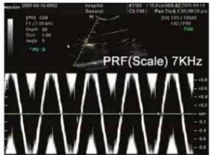
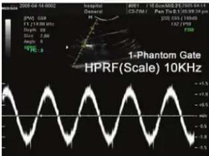
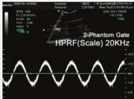
[Figure 4.13 Starting HPRF]
NOTE
HPRF is not available in Simultaneous Mode. Also, if the twice the PRF value is 23kHz or above before starting HPRF, HPRF will not start.
CAUTION
■ The Phantom Gate position can be located outside the 2D image area in Zoom Mode.
■ Make sure that sample volume and Phantom Gate are not placed together in the measuring area. If there are two or more sample volumes placed on vessels, the Spectral Doppler image may have excessive noise due to the unwanted Doppler substances.
AIO (Auto Image Optimization) Function
This function allows increasing of the scale and/or automatic change of the baseline for unaliasing of Spectral Doppler images. Press the AIO button on the control panel.
NOTE
When AIO is in use, scale can increase by twofold at maximum. If the current scale is at the maximum, the AIO function will not start.
Things to Consider for Auto Image Optimization
This algorithm manipulates Automatic Calculator (Real Time Automatic Doppler Trace). Please refer to "Things to Consider for Real Time Automatic Doppler Trace."
AIO can function properly if the Spectral Doppler image repeats for 2 cycles or more.
Spectral Doppler images that are not aliased may be recognized as optimal images and the AIO function may not be available. If the Spectral Doppler image is small because the scale
value is high (even though not aliased), the AIO function automatically adjusts the scale value and displays the optimal Spectral Doppler image.
NOTE
For information on Wall Filter, Scale, Dynamic Range, Steer, Frequency, and TDI Adjustment, refer to "2D Mode" and "Color Doppler Mode." Methods for using the menus may be different, but the functions are identical.
CW (Continuous Wave) Spectral Doppler Mode
This mode shows the velocity of blood flow within blood vessel. It can measure high-speed blood flow by continuously transmitting pulses. However, this is not useful for viewing information for specific areas.
A 2D image is also displayed to indicate the relative position of the vessel and allow the user to change the position. Note that 2D image is not displayed when using Static CW probes (CW2.0, CW4.0).
Steered CW Spectral Doppler Mode
When using Phased Array probe, press the CW button on the control panel to activate the function. Press it again to return to 2D mode.
![MEDISON CAR stress [CW] GGB F2 /8.33 kHz / P100 * PG : 0 MEDISON CAR stress med Cardize #4096 MID.00 2005-06-28 CW 4M/ Gen Tis 0.0 12:02:16 pm - + 4 - + 2 - - 1 - - 2 - - 4 Loop Pos Freeze](/content/2026/05/955519/images/a77fbe6cc93fffa6c19d0fc7dd9dd731799933be25493a7253759b20a4d67a50.jpg)
[Figure 4.14 Steered CW Spectral Doppler Mode]
Static CW Spectral Doppler Mode
This mode is available only for Static CW probes. At the Probe Selection screen, select Static CW probe on the touch screen to activate the mode.
![Mccosin Ear stress med Cardize 0944 / 12.0cm M10.05 2005-06-26 P3-SAC / Gen Tis 18 / 12:05:40 pm [GW] 0.05 F1 / 14.29 kHz / F100 Depth: 73 * PG : 8 [20] GSIB / SIBIB FM4 / F100 HAR / FSIB - + 4 - Hz - - 4 HR = 0 Loop Pos Freeze](/content/2026/05/955519/images/b6a001fc31245097f0b9b8411ca4a3c5a855612fdfe7e1b16b581ff81061bded.jpg)
[Figure 4.15 Static CW Spectral Doppler Mode]
CW Menu
Methods for using the menu are the same as in PW Spectral Doppler Mode.
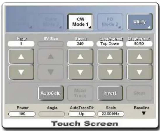
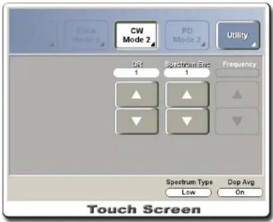
[Figure 4.16 CW Menu]
NOTE
For information on optimizing CW images, refer to "PW Spectral Doppler Mode."
Automatic Calculator
Adjusting Frequency
The Automatic Calculator function, also called Real Time Automatic Doppler Trace, can be activated by selecting the AutoCalc button on the touch screen. When Automatic Calculator is in use, peak trace on the Spectral Doppler image is highlighted in green.
Real-time Doppler signals are traced and their measurement values are displayed. PSA, EDV, TAP, RI, PI, S/D, VTI, Gpeak, Gmean, and Vmean values can be obtained in Cardiac Package, and PSA, EDV, TAP, TAM, RI, PI, S/D, and Vmean values can be obtained in Non-Cardiac Packages.
Press the Mean Trace button on the touch screen to run the Mean Trace function. Mean Trace is highlighted in black on the Spectral Doppler image. This is not available when the application is Cardiac.
| CAUTION | Auto Trace measurement values in measurement mode and Automatic Calculator measurement values may not be identical. This is because each function uses different algorithms. For more accurate measurement, use Auto Trace in measurement mode. |
Auto Trace Direction
This function selects the areas that are traced by Doppler signals. Use the up-down switch below Auto Trace Dir on the touch screen to select All, Up, or Down. You can select either Up or Down when the application is Cardiac.
Things to Consider for Automatic Calculator
Results will not be displayed if the function is run against inaccurate values.
Trace and/or results may not be accurate in the following situations.
- Aliasing occurs because PRF is too low in comparison to the image speed, or the Spectral Doppler image is clustered around the baseline because PRF is too high.
- Peak is indistinctive or intermittent such as in Spectral Doppler images for veins.
- It is difficult to identify the Spectral Doppler image because Doppler Gain Setting is too high or too low.
- Index Display immediately after moving the sample volume with the Trackball.
- Certain portions of major Spectral Doppler image signals are cut off because the Wall Filter value is too high.
- Peak Trace is interfered with abnormal noise or artefact of Doppler signals.
- Heart rate is 140bpm or above.
Combined Modes
2D/C/PW Mode
Color Doppler Mode and PW Spectral Doppler Mode are displayed simultaneously. To use the 2D/C/PW Mode, under the Misc. tab on the Setting screen, set Simultaneous Mode to "Allow 2D/C/PW."
In Color Doppler Mode, press the M button on the control panel. Or, in PW Spectral Doppler Mode, press the C button on the control panel.
![MEDISON 25.0 [FW] G76 F1 / 2.59 MHz Depth 12 Size 1.50 Angle 0 MEDISON General 4877 / 4.0cm M10.45 7006-85-63 L6-16S / Gen Tis 0,1 11:43:53 am [20] G37 / T18dB FA2 / P90 FAB [Q] G50 / 5.00 Hz FA3 / F1 / 15 - + 24 - + 26 - + 16 - + 12 - + 8 - + 4 cm/s Loop Pos Freeze](/content/2026/05/955519/images/7cf6342e1a6f9bbdad59349729a6ce5667fccfe354618fef580886ce2c172088.jpg)
[Figure 4.17 2D/C/PW Mode]
2D/PD/PW Mode
Power Doppler Mode and PW Spectral Doppler Mode are displayed simultaneously. To use the 2D/C/PW Mode, under the Misc. tab on the Setting screen, set Simultaneous Mode to "Allow 2D/C/PW."
In Power Doppler Mode, press the M button on the control panel. Or, in PW Spectral Doppler Mode, press the PD button on the control panel.
![MEDISON [FW] G78 F1 / 2.59 MHz Depth 12 Skee 1.50 Angular 0 MEDISON General #970 / 4.0cm M10.45 2006-05-03 LB-15IS / Gen Tls 0,1/11:4638 am [20] G37 / 11963 FA2 / P90 FDB [PO] G50 / 1.58 Hz FA3 / F1 / 15 - + 24 - + 26 - + 16 - + 12 - + 8 - + 4 cm/s Loop Pos Freeze](/content/2026/05/955519/images/1a427e1b3b09ffb9b041c2a4ae42ebc31208b78f1621a4894195fc494310a337.jpg)
[Figure 4.18 2D/PD/PW Mode]
2D/C/CW Mode
Color Doppler Mode and CW Spectral Doppler Mode are displayed simultaneously. Note that this mode is available for Phased Array probe only.
In Color Doppler Mode, press the CW button on the control panel. Or, in CW Spectral Doppler Mode, press the C button on the control panel.
![MEDITION CAR stress 70.0 [CW] GE5 F1 / 14.29 kHz / P188 Depth /8 med Cardiac #1023 / 12.0cm M10.09/ 2006-06-28 P3-GAC / Gen Tis 1.8 U20653 µm [20] GS0 / 90dB FA4 / PS0 IHP / FSB [C] GS0 / 4.00 kHz FA2 / F2 / 8 HR = 0 Loop Pos Freeze](/content/2026/05/955519/images/24b82e71d05c8540ab92b68401b66a6abad248588ba3e809bf8d86c159ac2508.jpg)
[Figure 4.19 2D/C/CW Mode]
2D/PD/CW Mode
Power Doppler Mode and CW Spectral Doppler Mode are displayed simultaneously. Note that this mode is available for Phased Array probe only.
In Power Doppler Mode, press the CW button on the control panel. Or, in CW Spectral Doppler Mode, press the PD button on the control panel.
![M1023 / 12.0cm M10.09/2006-06-28 P3-DAC / Gen Tis 1.8 12:06:53 pm [CW] G65 F1 / 14.29 kHz / P100 Depth 78 HR = 0 Cardiac - + 4 Hz - - 4 Loop Pos Freeze](/content/2026/05/955519/images/22517d9dd779afda857df5890a7b56b94152ae8c206d9bddf7d1f0580506d0ef.jpg)
[Figure 4.20 2D/PD/CW Mode]
2D/C/M Mode
Color Doppler Mode and M Mode are displayed simultaneously. Note that this mode is available only when the application is "Fetal Heart" or when the application is "Cardiac", "General" or "Pediatric" for Phased Array probe.
In Color Doppler Mode, press the M button on the control panel. Or, in M Mode, press the C button on the control panel.
![MEDISON Cardiac #2055 / 16.0cm M10.62/ 2086-05-28 P3-7AC / Pen Tis 0.6 / E3SE:30 pm [20MJ G60 / 35sD] FA2 / P90 FSB [C] G70 / 4.50 kHz FA4 / F2 / 0 Loop Pos Freeze](/content/2026/05/955519/images/c413fa5703c12670973dc7c1c3879c40beb0e6937126af6f292b48677a75b8aa.jpg)
[Figure 4.21 2D/C/M Mode]
Dual Live Mode
This mode displays 2D Mode and Color Doppler Mode simultaneously. 2D image is displayed on the right and Color Doppler image is displayed on the left. If run in Power Doppler Mode, it displays 2D image and Power Doppler image.
Press the DUAL LIVE button on the control panel to activate it, and use the Color Doppler menu to optimize the image. Use the Cine Save function for more effective viewing.
![MEDISON GENERAL MB 74.0cm MT 1.1 2006-05-03 LB-1SIS / Gen Tis 1.2 11:51:28 am [0] 3.5V / 3.5V 3.5V / 3.5V [0] 2.5V / 3.5V 7.5V / 3.5V Cine Pos Freeze](/content/2026/05/955519/images/f6de32b5ece384630cb43151a699984b0c756b86c3e101f11e5813d84035b196.jpg)
[Figure 4.22 Dual Live Mode]
Multi-Image Modes
The multi-image viewing function is only available when the images and conditions on both sides are identical.
Dual-2D Mode
This mode allows you to compare 2D images side by side.
In 2D Mode, 3D Mode, or Spectral Doppler Mode, press the Dual button on the control panel to select the function. Press the Dual button to close Dual-2D Mode and return to 2D Mode which is the default mode.
Use the Dual button, the Update button and the Set button to change the left/right images.
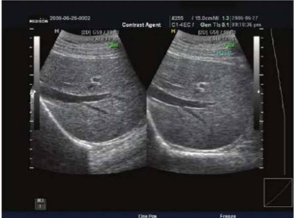
[Figure 4.23 Dual-2D Mode]
Dual-2D/C Mode
This mode allows you to compare Color Doppler Mode images side by side.
In Color Doppler Mode, press the Dual button on the control panel. Or, in Dual-2D Mode, press the C button on the control panel.
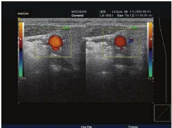
[Figure 4.24 Dual-2D / Color Doppler Mode]
Dual-2D/PD Mode
This mode allows you to compare PD Mode images side by side.
In PD Mode, press the Dual button on the control panel. Or, in Dual-2D Mode, press the PD button on the control panel.
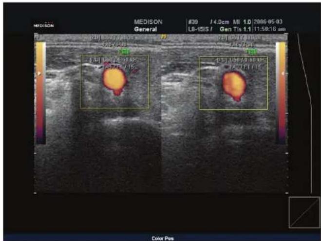
[Figure 4.25 Dual-2D/PD Mode]
Multi-Dimensional Modes
Multi-Dimensional
Multi-Dimensional Modes display tissues or organs as 3-dimensional images. Multi-Dimensional Modes continuously obtain 2-dimensional surface images from the probe and render the volume data for displaying 3-dimensional images.
Multi-Dimensional Mode Types
Types by Image Information
- 3D Mode: This is the default 3D Mode. Press the 3D/4D button in 2D Mode to access it.
- 3D Color Doppler Mode: This mode displays blood flow velocity and direction information on 3D image by color. Press the 3D/4D button in Color Doppler Mode to access it.
- 3D Power Doppler Mode: This mode displays existence of blood flow and its amount information on 3D image by color. Press the 3D/4D button in Power Doppler Mode to access it.
Types by Scan Methods
- Static 3D Mode: This mode obtains a 3-dimensional image by rendering continuous 2D images once. 3D probes obtain volume data by mechanical scanning, and 2D probes obtain volume data by freehand scanning.
- Live 3D Mode: This mode obtains a 3-dimensional image by rendering continuous 2D images multiple times. It processes volume data real-time and it is available for 3D probes only.
- XI STIC Mode: Use a 3D probe to obtain the fetal cardiac cycle and STIC volume data
How to Improve 3D Image Quality
- Consider the direction, division and size of the viewpoint, as well as the visibility of an object.
■ Before 3D scanning, adjust the contrast of the specific textures in 2D Mode.
■ The ROI (Region of Interest) box determines the image being rendered. Portions of image outside the ROI box are not included in the rendering process.
■ Bigger the ROI box, slower is the rendering speed. Therefore, set an appropriate ROI box size.
■ To determine the contour of objects, surface of objects should be insulated with hypoechoic tissues—such as amniotic fluid—which do not generate echoes.
■ To obtain a high quality 3D surface, adjust the low-threshold value.
■ Set the noise gray value lower than the surface value in order to obtain clearer images from edges of the ROI box to the surface of the objects.
In general, do not adjust High-Threshold; set it to the maximum value of 255. If the surface render algorithm is higher than the Threshold value, this value indicates the boundary of the surface. Therefore, use High-Threshold to adjust the boundary manually.
Acquiring 3D Images
Image Scan Mode
This mode allows acquisition of 3D and Live 3D images. Press the 3D/4D button on the control panel to access it. Set the menu items and then press the Freeze button to start scanning.
Press the Exit button or the 3D/4D button on the control panel to exit Image Scan Mode. You may also select a button for another mode to exit.
If 3D image is acquired by changing the left/right direction (by selecting the Direction menu), it is displayed on View Mode. But if 3D image is acquired by changing the up/down direction (by selecting the Apex menu), it is not displayed on View Mode.
Volume Box
Multi-Dimensional Modes contain two volume boxes. The volume box with cyan lines indicates the scanning area on the 2D image, and the volume box with yellow lines indicates the area of the rendered 3D image. The yellow box is also called the ROI box.
- Changing Position: Use the Trackball to change the position of the volume box. Press the Change button on the control panel to change the function of the Trackball to "Move" and then change the position. The function of the Trackball is displayed in the feedback area.
- Changing Size: Turn the knob-buttons below ROI Width and ROI Height on the touch screen to make adjustments. Alternatively, press the Change button on the control panel to change the function of the Trackball to "Resize" and then change the size.
Setting Auto Calc
This function is available when the application is OB. It automatically sets up the volume box.
Press the Auto ROI Off button on the touch screen to change it to Auto ROI On. The volume box will appear in the desired area of the image.
This is not available in 3D Color Doppler Mode or 3D Power Doppler Mode.
NOTE
The Auto ROI function is available only when the fetal body is displayed on the screen. This function manipulates brightness and contrast of the image.
Adjusting Vol. Angle
Use the up-down switch below Vol. Angle on the touch screen to adjust the scanning angle of the 3D probe.
Adjusting Scan Quality
Use the up-down switch below Scan quality on the touch screen to adjust the quality of the 3D image.
Low: The image quality is low but the 3D image speed (or rendering speed) is fast.
Mid: The image quality is better than Low Quality but the speed is slower than Low Quality.
High: The image quality and expression are good. Speed is slower than Mid Quality.
Extreme: The image quality is excellent. Use this to obtain detailed images regardless of the speed.
Image Acquisition Procedures
Static 3D Image Acquisition Procedures
- Press the 3D/4D button on the control panel to move to Image Scan Mode, and then select the 3D button on the touch screen.
- Adjust "Scan Quality" and "Vol. Angle" on the touch screen.
- Use the volume box on the screen to set the position and size of the 3D image to acquire.
- Press the Freeze button on the control panel. A 3D image will be acquired for the area within the volume box and then View Mode will appear.
![2008-07-17-0091 OB FPS27 / 14.0cm MI0.63 2008-07-20 3D3-BEK / Gen Tlb0.1 06:52:05 pm [2D] C65 / 90dB FA10 / P90 FS10 * PG : 0](/content/2026/05/955519/images/bcac643ddee63360907bc8726d87bb88c4f940d49c79acee15a366a2b958c659.jpg)
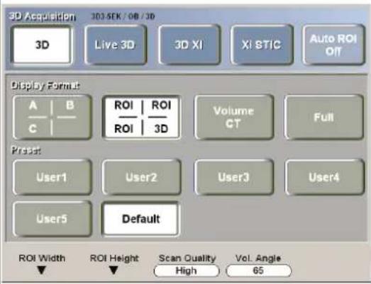
[Figure 4.26 3D Acquisition - 3D]
Live 3D Image Acquisition Procedures
- Press the 3D/4D button on the control panel to move to Image Scan Mode, and then select the Live 3D button on the touch screen.
- Adjust "Scan Quality" and "Vol. Angle" on the touch screen.
- Use the volume box on the screen to set the position and size of the 3D image to acquire.
- Press the Freeze button on the control panel. A Live 3D image will be acquired for the area within the volume box and then View Mode will appear.
![MEDISON 2008-07-17-0001 OB FPS27 / 14.0emMI0.63 2008-07-20 3D3-5EK / Gen Tib0.1 06:52:05 pm [2D] G65 / 90dB FA10 / P90 FS10 * PG : 0](/content/2026/05/955519/images/9773cd1cdab045aaacff381baaa366a2f514e39d5715c81fa25598da09570b03.jpg)
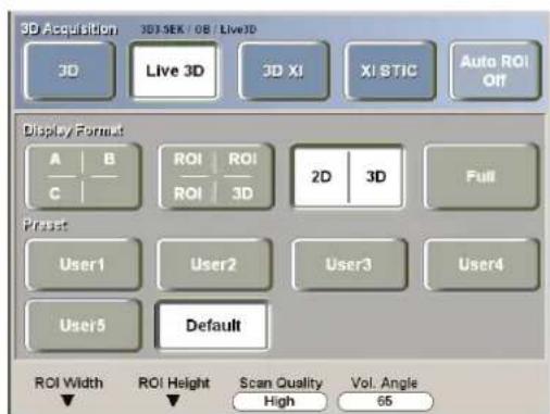
[Figure 4.27 3D Acquisition – Live 3D]
NOTE
■ To obtain a direct view of the face of the fetus on the screen when acquiring the 3D image, place the head of the fetus in the direction of the Direction Mark, put the fetus in the Coronal Plane, and then scan the fetus from the back toward the abdomen.
■ The 3D image of the fetal face is more easily found in the coronal plane than in the sagittal plane.
3D View
3D View Mode
This mode allows adjusting and/or viewing of the 3D or Live 3D image that was acquired in Image Scan Mode.
In 3D View Mode, press the Exit button or the 3D/4D button on the control panel to move to Image Scan Mode. Press the 2D button to completely exit 3D Mode. Note that pressing the Exit button on the control panel in Live 3D View Mode switches to Live Cine Mode.
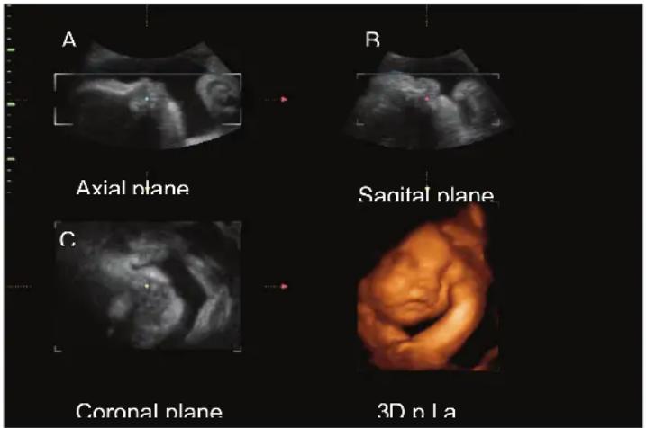
[Figure 4.28 Static 3D View]
The default 3D View screen consists of Axial Section, Sagital Section and Coronal Section surface images—which are volume data cut by anatomical positions—and 3D images.
Figure 4.28 illustrates a screen displaying Axial Section as “A plane,” Sagital Section as “B plane,” and Coronal Section as “C plane.”
In ABC-ROI 3D Mode, the ROI box displayed in each section can be adjusted for obtaining desired 3D images.
View Mode Control Menu
Control menus for 3D or Live 3D images appear on the touch screen depending on the characteristics of each mode.
When operating images, the “icon” icon and the Trackball function icon appear at the bottom of the screen.
The following icons are available.
- Icons in 3D View Mode:
- Icons in 3D XI Mode:

Selecting 3D View Mode
Static 3D View Mode
For better viewing of 3D images, view modes are categorized into 2D Mode and 3D Mode depending on rendering methods.
At the View Mode Control menu, press a button on the touch screen to access the corresponding view mode.
To exit the selected view mode or return to the previous menu, press the Exit button on the touch screen or the Exit button on the control panel.
2D Mode for Static 3D View
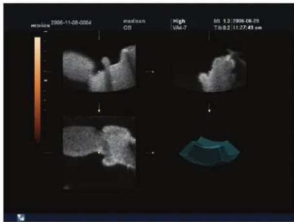
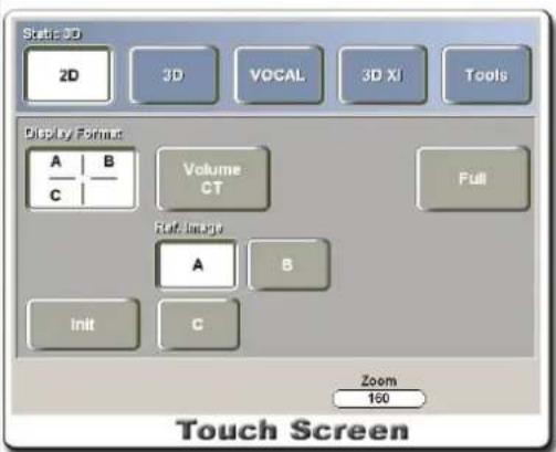
[Figure 4.29 Static 3D - 2D]
| Menu | Description |
 ABC Mode Selection ABC Mode Selection | ABC Mode does not display 3D image; it displays multi-planar images only. Use Full Mode for a more detailed view. |
 Volume CT Mode Selection Volume CT Mode Selection | Volume CT Mode displays a 3D view of the plane position of the examination image.Hold down the Change button on the control panel for a few seconds and the mouse pointer will appear. Use the Trackball and the Set button to adjust the 3D space. Use the Niche Zoom menu on the touch screen to zoom in or zoom out the Volume CT image. Use the Zoom menu to zoom in or zoom out the surface image and apply it on the Volume CT image. |
OH (Orientation Help) Function
OH (Orientation Help) image displays the relative position of the currently selected reference image in regards to the volume data.
The A, B, and C buttons of the reference image move the plane of OH, and rotating each reference image also rotates the plane of OH. OH image is shown only in 2D Mode for Static 3D.
NOTE
If the plane of OH is not properly expressed for the volume data, press the Init button.
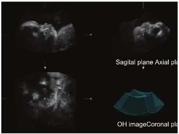
[Figure 4.30 OH Screen]
[A plane]
[B plane]
[C plane]
3D Mode for Static 3D View
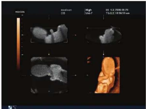
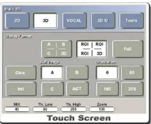
[Figure 4.31 Static 3D - 3D]
| Menu | Description |
 ABC-3D Mode Selection ABC-3D Mode Selection | ABC-3D Mode projects a 3D image on the Volume data plane without setting an ROI. Detailed examination is possible as 3D image is projected without using an ROI. |
| ABC-ROI 3D Mode Selection | In ABC-ROI 3D Mode, desired 3D images can be examined by adjusting the surface images and the ROI box on 3D images. |
| Full Screen View (Full Mode) | Fits the 3D image on the entire screen in View Modes. |
| Reset to Initial Position | Initializes the current image back to the state it was at the beginning of 3D View Mode or to the Preset state. |
| Change Reference Plane(Reference Plane Selection) | Each multi-planar has its own standard coordinate system and rotates or moves according to the coordinate system. The image selected as a reference image rotates or moves according to the reference image coordinate system, and other images rotate or move according to their own standard coordinate systems.Press a desired button to change the reference image. |
 3D Orientation 3D Orientation | Rotates the 3D image against the Z-axis in the 3D standard coordinate system by the rotation value selected. |
| Rotate Image by X-axis (↓↑) | Turn the X knob-button to rotate the selected reference image in the direction of the X-axis. In Full Mode where the reference image is not shown, the selected image acts as the reference image and the Full Mode image rotates by the X-axis.The M knob-button on the control panel acts as the X knob-button. |
| Rotate Image by Y-axis (⇌) | Turn the Y knob-button to rotate the selected reference image or the Full Mode image in the direction of the Y-axis. The PD knob-button on the control panel acts as the Y knob-button. |
| Rotate Image by Z-axis (∪∪) | Turn the Z knob-button to rotate the selected reference image or the Full Mode image in the direction of the Z-axis. The PW knob-button on the control panel acts as the Z knob-button. |
| Move and Resize Image (ROI Box Adjustment) | Press the Change button on the control panel and use the Trackball to move the selected reference image or the Full Mode image up/down/left/right. Press the Change button again to resize the ROI box.Here, hold down the Change button for 2 seconds to change the function of the Trackball.Press the Set button and theicon will appear on the screen. Move the Trackball while holding down the Set button to rotate the image. Also, press the Exit button and theicon will appear on the screen. This function is for moving the image. |
| Image Zoom | To zoom the selected reference image in ABC-ROI 3D Mode, adjust the Zoom value on the touch screen. Use the up-down switch below Zoom to adjust the value. |
Auto Contour (ACT) Function
This function locates the fetal face area automatically in a fetus image scanned in Sagital plane. In the ROI box on A Plane, a contour line appears and a 3D image is contoured.
Press ACT Edit button to edit the contour line. Adjust it with the Set button on the control panel and the Trackball.
NOTE
Except in the 3D Convex probe, a contour line appears as a straight line.
This function is available only in Static 3D Mode where Render Direction is 'C+'.
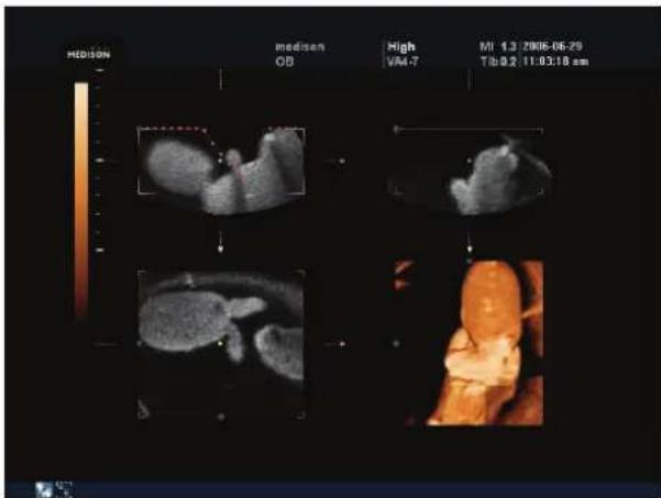
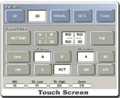
[Figure 4.32 Static 3D - ACT]
Live 3D View Mode
For more detailed viewing of Live 3D images, the modes are divided according to rendering methods.
At the View Mode Control menu, press a button on the touch screen to access the corresponding view mode.
To exit the selected view mode or return to the previous menu, press the Exit button on the touch screen or the Exit button on the control panel.
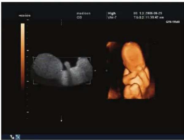
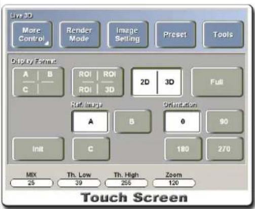
[Figure 4.33 Live 3D - 2D-3D Mode]
| Menu | Description |
 2D-3D Mode Selection 2D-3D Mode Selection | Plane of the image and Live 3D image can be examined.In 2D-3D Mode, adjust the ROI box to view a desired 3D image. The selected reference image is displayed in 2D image. |
NOTE
For information on other menu items, refer to "Static 3D View."
* 3D Coordinate System
- Multi-planar Standard Coordinate Systems
A Standard Coordinate System
B Standard Coordinate System
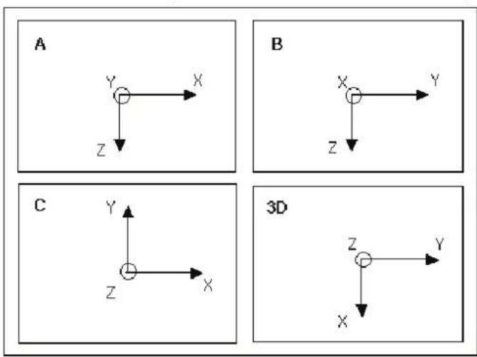
C Standard Coordinate System
3D Standard Coordinate System
- Full Mode Coordinate System
![graph TD A["Full"] --> B["X"] B --> C["Y"] C --> D["Z"]](/content/2026/05/955519/images/12586ae9a4a6c70e175b426bd37866388719591ef13e92618ab79631bde9cf16.jpg)
- Reference Image Coordinate System
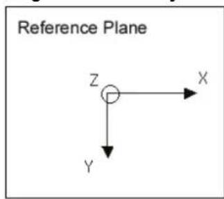
Cine Mode
3D Cine Mode
This mode provides Cine function for examining the rendered 3D image. Press the Cine button on the touch screen. The menu illustrated below will appear and the 3D Cine Mode will start.
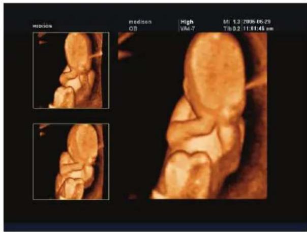
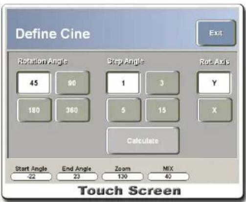
[Figure 4.34 3D Cine Mode]
- Cine Settings: Before viewing images by Cine, make appropriate settings for viewing images on the touch screen.
| Menu | Description |
| Rotation Angle | Set ranges for 3D Cine rotation. |
| Step Angle | Selected Rotation Angle rotates by the Step Angle value. If the Step Angle is set to 15° , the 3D Cine set to 360° rotates in 25 steps, and the 3D Cine set to 90° rotates in 7 steps. |
| Rotation Axis | Select the rotation axis for 3D Cine. |
| Start, End Angle | Set the start and end angle values for the rotation range. |
| Zoom | Zoom the 3D Cine image by 25% - 400%. Use the up-down switch below the touch screen to adjust the value. |
| Mix | Use the up-down switch below the touch screen to adjust the Mix value. |
- Running Cine: Press the Calculate button on the touch screen to run 3D Cine. The Cine image generation process will be displayed on the screen and then 3D Cine will start. The menu below will appear on the touch screen. ▶ ▶ ▶ Press the button to stop or start 3D Cine.
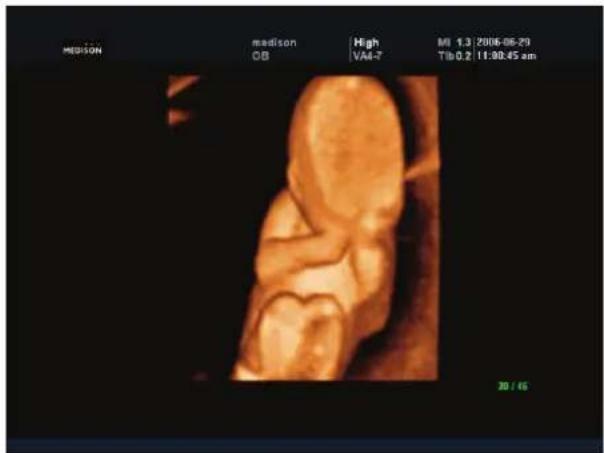
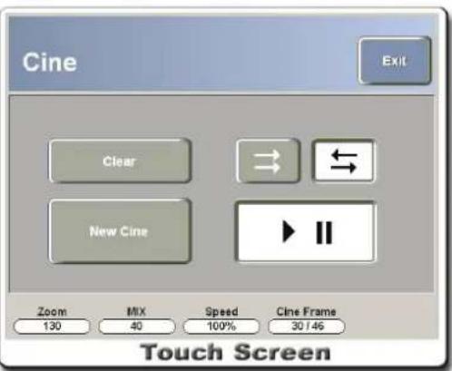
[Figure 4.35 3D Cine]
| Menu | Description |
| New Cine | While 3D Cine is in use, press the New Cine button to acquire a new Cine image. |
| Rotate |  Select the button to continuously rotate in one direction, or Select the button to continuously rotate in one direction, or  select the to rotate in one direction and then rotate in the opposite direction. select the to rotate in one direction and then rotate in the opposite direction. |
| Speed | Adjust the Speed value to adjust the rotation speed of the 3D Cine image. Use the up-down switch below Speed. |
| Cine Frame | Adjust the Cine Frame value on the touch screen to view the 3D Cine image by each desired frame. |
| Zoom | Adjust the Zoom value on the touch screen to zoom the image. Turn the knob-button below Zoom to adjust the value. |
| Mix | Adjust the MIX value below the touch screen to adjust the mix of Render Mode. Use the knob-button below MIX. |
Select the button to continuously rotate in one direction, or
Live 3D Cine Mode
Live 3D Mode provides the Cine function for saving or viewing the recently scanned 3D images. Up to 128 Live 3D images can be saved.
- Running Cine: While scanning Live 3D image, press the Freeze button or the Exit button on the control panel to start Live 3D Cine Mode. Or, press the Tools button on the touch screen to move to the Tool menu and select the Live Cine button. When Live 3D Cine starts, the menu below will appear on the touch screen.
Press the button to stop or start Live 3D Cine.
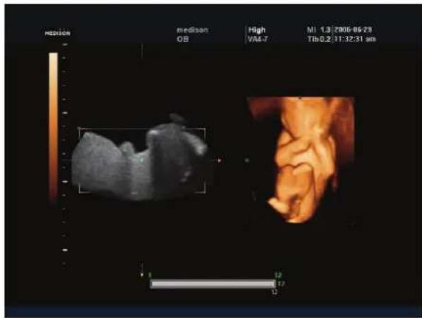
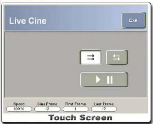
[Figure 4.36 Live 3D Cine]
| Menu | Description |
| New Cine | While 3D Cine is in use, press the Freeze button to acquire a new Cine image. |
| Save | When saving Live Cine images, you can specify the save range for Cine images in the same way as in 2D Mode.Adjust the First Frame and the Last Frame values on the touch screen to adjust the Cine image save range. The progress bar indicating the save range will appear on the screen. Use the up-down switches below the menus to adjust the menus.After selecting the save range, press the Save button on the control panel.When the Save Volume screen appears on the touch screen, select the Save button to save Live Cine image. |
NOTE
For information on other menu items, refer to "3D Cine Mode."
VOCAL (Virtual Organ Computer Aided anaLysis) Mode
Select the VOCAL button on the touch screen to start VOCAL Mode. VOCAL is a very useful tool for measuring volumes of tissues within the human body.
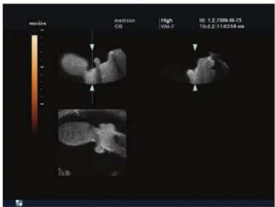
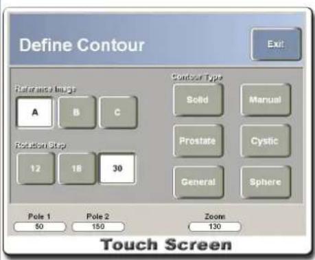
[Figure 4.37 VOCAL Mode]
Setting Reference Image
A reference image must be set up in order to obtain the volume of a desired object. Press a button on the touch screen to specify which plane should be used for contouring.
Note that contouring is done as the image rotates by the vertical axis in A Plane and B Plane and as the image rotates by the horizontal axis in C Plane.
Setting VOCAL Parameter (Rotation Step)
You can set the step angle for image rotation. Available ranges are 12° , 18° and 30° . Press the corresponding button on the touch screen to select the range.
15 contour images are generated for 12° , 10 images for 18° , and 6 images for 30° . The default rotation angle is 30° .
Setting Range
Adjust the Pole1 and Pole2 values on the touch screen to set the contour range. Use the knob-buttons below Pole1 and Pole2 to set the position of the arrow. Turn the knob-button to position the arrow at the vertical or horizontal edge of the object to measure.
VOCAL Automatic Start
Select Contour Type on the touch screen to automatically generate the object for acquiring volume value.
| Menu | Description |
| Solid Type | Press the Solid button to contour when there are many echoes within the object. |
| Cystic Type | Press the Cystic button to contour when there are few echoes within the object. |
| Prostate Type | Press the Prostate button to contour when using prostate-related objects. |
| General Type | Press the General button to contour according to characteristics of general objects. General Type is faster than other automatic Contour Types but is slightly less accurate. |
| Sphere Type | Press the Sphere button to automatically generate a basic spheric object. After making the spheric object, modify the contour image to make it into a desired shape. |
VOCAL Manual Start (Manual Type)
Press the Manual button on the touch screen and you can manually contour frame by frame. The menu below will appear on the touch screen when you press the Manual button.
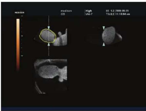
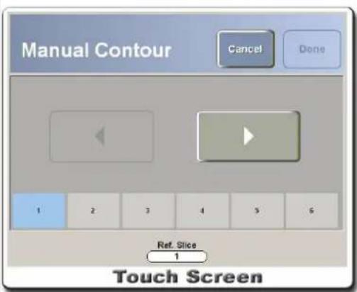
[Figure 4.38 VOCAL Mode – Manual Type]
- Move the Trackball while holding down the Set button to determine the shape of the object. After determining the shape of the object, press the Set button again to complete frame generation.
- Press the ▶ button or press the number button on the touch screen to move to the next frame and determine the shape of the object.
- To determine the shape of the object again, press the ◀ button or press the number button on the touch screen to move to the previous frame.
- Use the up-down switch below Ref. Slice to move to different frames.
- To cancel contour, press the Cancel button on the touch screen.
- Repeat the steps above to contour all the frames and then press the Done button.
Edit Contour
When contour is complete, the system switches to Edit Contour Mode. In this mode, use the up-down switch below Ref. Slice to select contour obtained in the previous step.
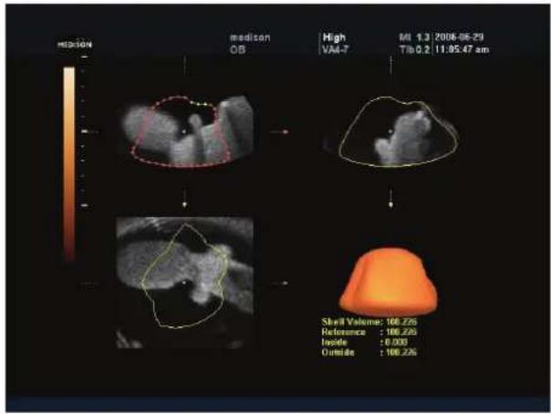
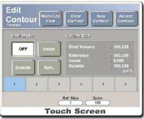
[Figure 4.39 VOCAL Mode – Edit Contour]
- Shell Mode
| Menu | Description |
| Off | Shell Thickness is not applied. |
| Inside | Shell is drawn inside the contour generated by Shell Thickness specified. |
| Outside | Shell is drawn outside the contour generated by Shell Thickness specified. |
| Symmetric | Half the shell is drawn inside the contour by half the Shell Thickness specified and the other half of the shell is drawn outside the contour by half the Shell Thickness specified. |
- Ref. Slice
Use the up-down switch below the touch screen to move to different frames and re-contour the object.
- Zoom
Use the up-down switch below Zoom to adjust the value for zooming image.
- Shell Thickness
Adjust the Thickness value to set the thickness of the shell. Use the up-down switch below Thickness to adjust the value. Note that the value cannot be adjusted when Shell Mode is OFF.
- Multi-Edit View
Draw a line to edit up to 6 slices at a time.
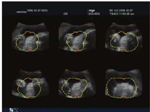
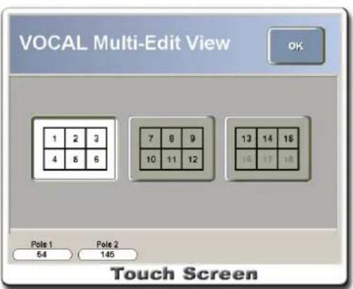
[Figure 4.40 Multi Edit View]
- Select a slice to edit.
- Change the position of pole points.
Every slice in the screen has two pole points indicated with red dots at the same positions as each other. Use the Pole 1 and Pole 2 knob-buttons on the touch screen. Changing the position of a pole point simultaneously changes the position of the pole points in all slices.
- Edit a contour line.
A contour line is shown in yellow. Use the Set button and the trackball to edit the left or right portion around a notional vertical line connecting pole points 1 and 2. Here, you may not edit it so that it crosses the notional vertical line connecting pole points 1 and 2. A contour line being edited is shown in red.
- Press Ok on the touch screen to finish editing. The changes are applied and displayed on the screen.
NOTE
■ The Slice buttons activated on the touch screen vary depending on the number of slices. The number of slices is determined based on the slice angle. For example, when 6 slices have been created through a 30° rotation, only slice buttons 1–6 are activated. However, for example, when 15 slices have been created through a 12° rotation, slice buttons 1–6, 7-12 and 13-15 are activated.
■ When Multi-Edit View is in use, Zoom and Rotation functions are not available.
- Clear Contour
Press the Clear Contour button to cancel the currently set contour, exit VOCAL Mode and return to 3D View Mode.
- New Contour
Press the New Contour button to cancel the currently set contour, return to the VOCAL Mode screen and generate new contour.
- Accept Contour
Press the Accept Contour button to apply the contour specified.
- Result Display
Volume information will be displayed at the lower right-hand corner of the monitor and on the touch screen.
| Menu | Description |
| Shell Volume size | Outside Shell Volume – Inside Shell Volume |
| Reference Volume size | Volume size of the generated object using the initial contour. |
| Inside Volume size | Volume size inside the generated object when Shell Mode is Inside. |
| Outside Volume size | Volume size outside the generated object when Shell Mode is Outside. |
VOCAL – Volume CT Mode
After generating the VOCAL object, press the Volume CT button in VOCAL Mode to insert the A, B, and C Plane images in the VOCAL object for examination.
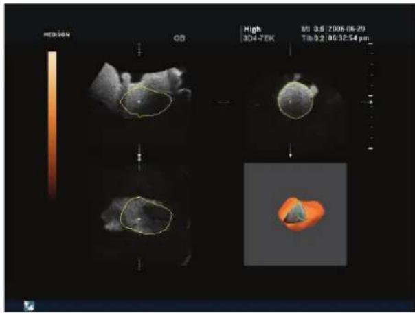
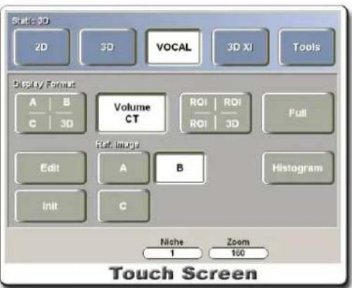
[Figure 4.40 VOCAL – Volume CT]
VOCAL – Volume CT View Mode Settings
Adjust the Niche menu on the touch screen to set up View Mode for Volume CT. There are eight (1-8) Volume CT View Modes, each of which shows one-eighth of the VOCAL object.
The eighth View Mode is not shown in the illustration above because it is located at the back.
* VOCAL object has been removed from the illustration above for demonstration purposes.
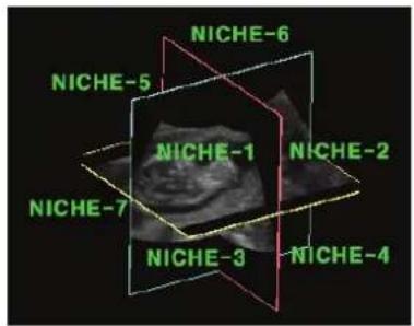
VOCAL – Volume CT Operation
VOCAL – Volume CT Mode allows object rotation and axis movement.
- Object Rotation: Object rotation involves VOCAL rotation and Volume CT rotation. VOCAL rotation is rotating the VOCAL object along with the Volume data with the center of the VOCAL object as the rotation axis. Volume CT rotation is rotating only the VOCAL object but not A, B, or C planes. To perform the Volume CT rotation function, hold down the Change button on the control panel for a few seconds. When the mouse pointer appears on the screen, use the Trackball and the Set button to rotate the object.
- Axis Movement: Turn the C knob-button on the control panel to move the rotation axis for the selected reference image. For example, if the A button is selected in the reference image, the central axis moves toward the depth direction of A plane.
VOCAL Histogram
VOCAL Histogram shows distribution of the gray value of the black and white image within the VOCAL object and the gray value of the Power Doppler image, and the relevant MG (Mean Gray), VI (Vascularization Index), FI (Flow Index), and VFI (Vascularization-Flow Index).
VOCAL Histogram is only available for 3D images and Power Doppler 3D images that are in black and white.
Equations used are as follows.
- MG: average value of gray voxel brightness (gray)
= total brightness (gray) / all voxel number - VI: ratio of color voxels against all voxels within the shell
= color voxel number / all voxel number - FI: average value of brightness (color) for color voxels within the shell
= total brightness (color) / color voxel number - VFI: average value of brightness (color) for all voxels within the shell
= total brightness (color) / all voxel number
VOCAL ABC-3D Mode
After accepting the contour in VOCAL Mode, press the ABC-3D button on the touch screen to view images in VOCAL ABC-3D Mode.
ABC-3D in VOCAL Mode cuts out the contoured surface images and reconstructs a 3D image based on them. 3D image is displayed in the position of the contour image shown on A plane. This mode allows viewing of organs in their actual images. In particular, SeeThru Mode is useful for clinical purposes as it provides color position and distribution of organs.
3D Measure
In 3D View Mode, you can press the Measure button on the control panel to perform 3D Measure functions (Caliper, Slice, and Calculation).
Since 3D Measure involves measurements on 3D images that are constructed with 2D images, measurement menu items supported by M Mode or Spectral Doppler Mode are not available here. Also, measurements that require multiple images such as the AFI menu under OB measurement are not available.
3D Measure has an error rate of 5% in addition to the measurement error rate in 2D Mode. Press the Close button on the touch screen to exit the 3D Measure function. You can also exit by pressing the Measure button or the Exit button on the control panel.
Caliper 3D / Calc 3D
Caliper 3D and Calc 3D measurement menus are identical to 2D Mode and use the same measurement methods in 2D Mode. For detailed information on measurement methods, refer to "Basic Measurements" and "Application Measurements" sections in this manual.
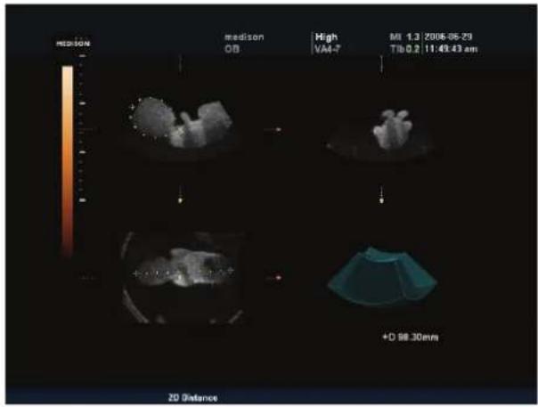
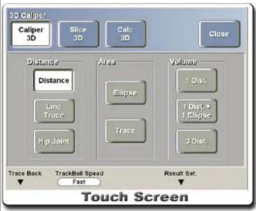
[Figure 4.41 3D Measure – Caliper 3D]
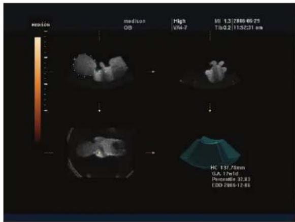
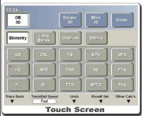
[Figure 4.42 3D Measure – Calc 3D]
Slice 3D
Press the Slice 3D button on the touch screen and the menu below will appear on the touch screen.
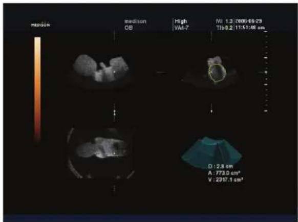
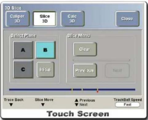
[Figure 4.43 3D Measure – Slice 3D]
Slice 3D slices a single Volume into multiple planes and measures them.
Under Select Plane, select a measure plane to measure and use the knob-button below Slice Move to move to the slice image to measure.
Use the trace method to measure. To cancel a part of the measuring line while tracing, press the Delete button or turn the knob-button below Trace Back. Press the Clear button on the touch screen to delete the measurement result.
If measuring multiple slice images, the measured slices are displayed on the bar on the touch screen. To move to different slice images, use the Previous button and the Next button, or use the up-down switch below Previous/Next.
To return to the initial image before measuring, select the Initial button on the touch screen.
Trace Back
To delete a part of the measuring line while using Trace, use the Trace Back function. Turn the knob-button below Trace Back left or right to delete the Trace measuring line.
Trackball Speed
The Trackball Speed function adjusts the speed of the Trackball on the control panel. Turn the knob-button below Trackball Speed to select Slow, Normal or Fast.
3D Notation
Text Input
Press the Text button on the control panel to input texts on the screen. The Text Brief function is not supported.
Press the Clear button on the control panel or on the touch screen to clear all texts on the screen.
Indicator Input
Press the Indicator button on the control panel to input indicators on the screen. Use the Set button and the Trackball to place indicators.
Press the Clear button on the control panel or on the touch screen to clear all indicators. Press the Undo button on the touch screen to delete indicators one by one in the order they are placed.
Indicators in Live 3D View and Live 3D XI™ can be moved within the screen only.
[Figure 4.44 3D Notation]
Optimizing 3D Images
To set the image parameters in View Mode, select the Tools button on the touch screen. The screen below will appear on the touch screen.
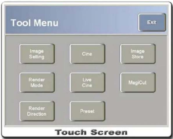
[Figure 4.45 Tool Menu]
Image Setting
Press the Image Setting button on the touch screen to set the Gamma value and Chroma Map for images. Used Chroma Map preset values can be saved in Preset.
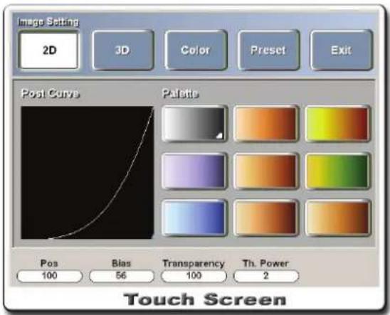
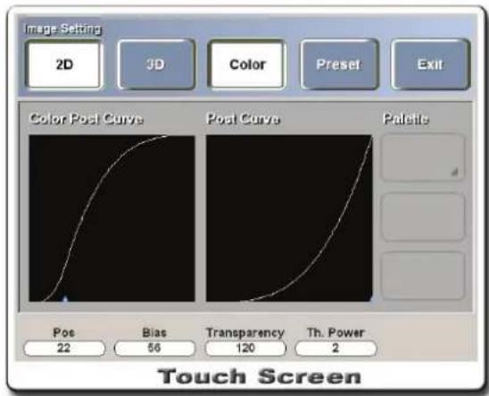
[Figure 4.46 Tool Menu – Image Setting (2D & Color)]
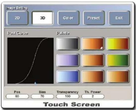
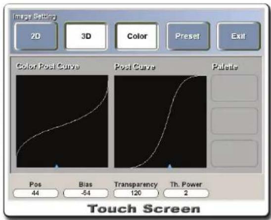
[Figure 4.47 Tool Menu – Image Setting (3D & Color)]
Select the 2D button on the touch screen to set the Gamma value, etc. for 2D images. Select the 3D button to make settings for 3D images.
Adjusting Post Curve
To adjust Post Curve, adjust the Pos value and the Bias value at the bottom of the touch screen. Use the knob-buttons below Pos and Bias.
Setting Palette
Select a desired color button on the touch screen.
Setting Transparency
Adjust the Transparency value to adjust the transparency of 3D images. Use the up-down switch below Transparency on the touch screen. The value range is from 20 to 250.
The lowest Transparency value (20) is for complete transparency, and the highest Transparency value (250) is for complete opacity. The default Transparency value is 100.
Setting Preset
Use this function to set up Post Curve, Palette, current Threshold value, and other parameters for the current image and save them as user preset values.
Select a button from User 1 through User 5 and press the Save button to save the user preset values under the selected button.
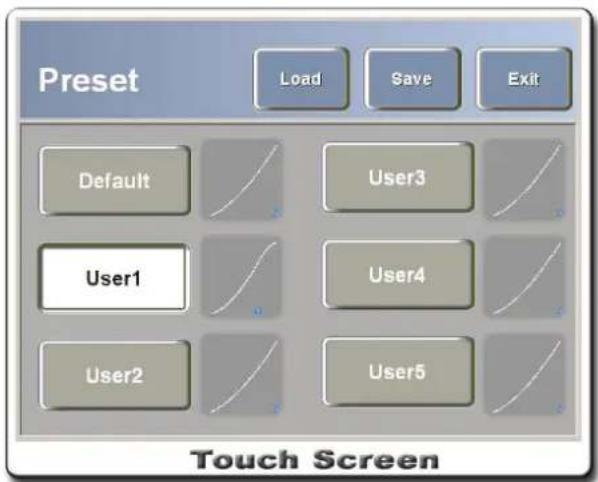
[Figure 4.48 Tool Menu – Image Setting (Preset)]
Setting Render Mode
Press the Render Mode button on the touch screen to set Render Mode. The last used Render Mode preset values are automatically saved.
Render Mode includes four modes: Gray, Color, SeeThru and VOCAL.
Gray Render Mode
This mode shows volume data acquired by gray method as a 3D rendering image.
Rendering values can be set for Mode1 and Mode2. A total of 11 combinations are available.
| Menu | Description |
| Surface Mode | This is the default mode. It displays a 3D image by ray-casting. |
| Surface Smooth Mode | This is similar to the default mode. It displays a 3D image by ray-casting softer than Surface Mode. |
| Max Mode | This mode displays the maximum value of intensity. This is useful for viewing bones within the body. |
| Min Mode | This mode displays the minimum value of intensity. This is useful for viewing vessels and hollow parts within the body. |
| Light Mode | This mode displays the depth information of 3D image by brightness. |
| X-Ray Mode | This mode displays the average value of intensity. It has the same effect as X-ray images. |
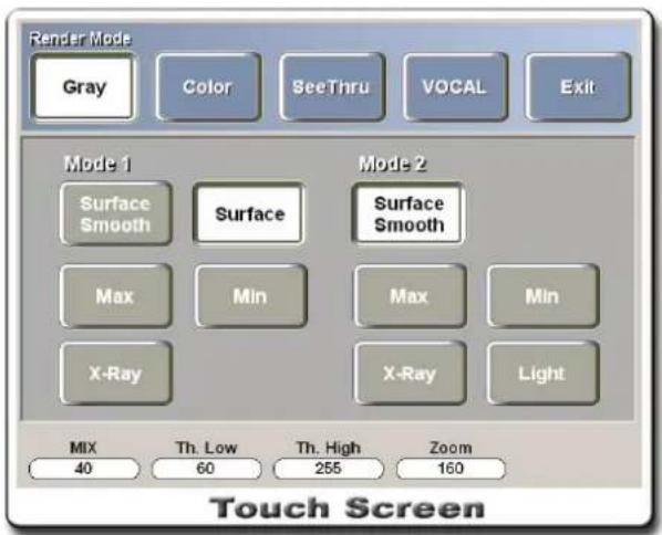
[Figure 4.49 Tool Menu – Render Mode (Gray)]
Color Render Mode
This mode shows volume data acquired by Angio/CFM method as a 3D rendering image. It supports three combinations: Surface-Light, Surface-Max, and Surface-X-Ray.
The modes are accessed in the same way as Gray Render Mode.
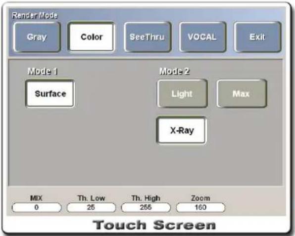
[Figure 4.50 Tool Menu – Render Mode (Color)]
SeeThru Render Mode
This mode shows Gray + Angio or Gray + CFM combination of data as a 3D rendering image. It supports four combinations: Transp-Surface, Transp-Transp, Max-Surface, and Max-Transp. When you survey color data, the system runs SeeThru Render mode as default.
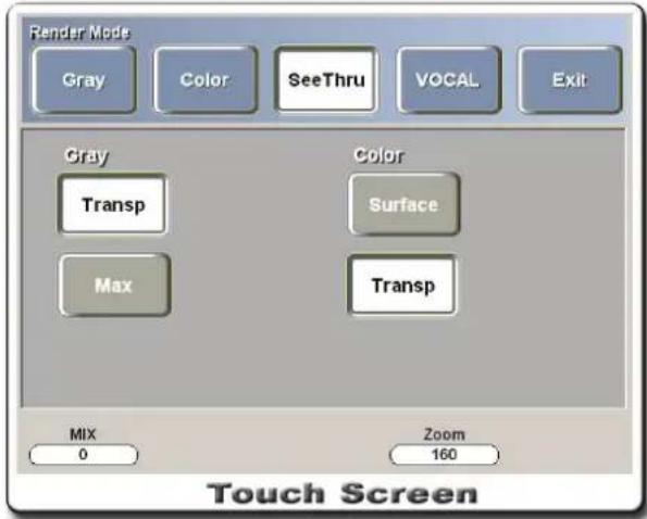
[Figure 4.51 Tool Menu – Render Mode (SeeThru)]
| Menu | Description |
| Transp+Surface Combination | View the color data within the gray data while adjusting the transparency of the gray data (use the MIX knob-button). Parts hidden by the gray data may appear slightly darker. |
| Transp+Transp Combination | View the color data within the gray data while adjusting the transparency of the gray data and the color data (use the MIX knob-button). Parts hidden by the gray data may appear slightly darker. |
| Max+Surface Combination | View the color data according to the MIX ratio of the gray data in Max Mode and the color data from Surface Mode (use the MIX knob-button). Parts hidden by the gray data may appear slightly brighter. |
| Max+Transp Combination | View the color data according to the MIX ratio of the gray data in Max Mode and the color data from Transp Mode (use the MIX knob-button). Parts hidden by the gray data may appear slightly brighter. |
VOCAL Render Mode
You can set the color of the object shown in VOCAL Mode. Select desired colors for Surface and Wire.
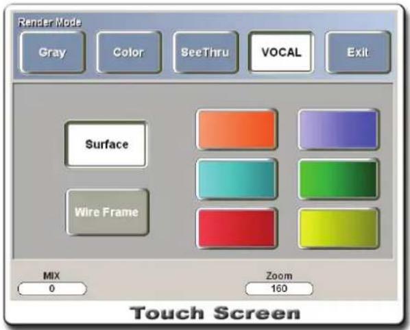
[Figure 4.52 Tool Menu – Render Mode (VOCAL)]
Adjusting Rendering Mode Mix
Adjust the Mix value below the touch screen to adjust the mix of Render Mode. Use the knob-button below MIX.
Adjusting Threshold (Low, High)
Adjust the Th.Low and Th.High values at the bottom of the touch screen to adjust the Threshold values. Use the knob-buttons or the up-down switches below the menus.
Adjust the Th.Low value and the Th.High value to hide information below and above the values from the 3D image. Only the information between the Th.Low value and the Th.High value is shown as the 3D image.
Image Zoom
To zoom the image, adjust the Zoom value at the bottom of the touch screen. Use the up-down switch below Zoom.
MagiCut Mode
This function cuts out a desired portion from the entire image for viewing. Press the MagiCut button on the touch screen.
Setting Cut Mode
Select the Cut Mode type on the touch screen.
- Inside Contour: Cuts the inside of the selected area.
- Outside Contour: Cuts the outside of the selected area.
-
Inside Box: Cuts the inside of the box.
-
Outside Box: Cuts the outside of the box.
- Small Eraser: Cuts using a small eraser.
- Big Eraser: Cuts using a big eraser.
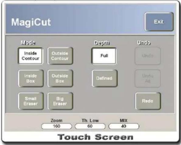
[Figure 4.53 Tool Menu – MagiCut]
Setting Cutting Area
To set the cutting area in MagiCut Mode, use the Trackball and the Set button on the control panel.
You may also cut the image by adjusting the depth of the cutting area. Select the Full button on the touch screen delete the entire area selected, or select the Defined button to delete by the value specified. Press the Define button and the Cut Depth menu will appear. Use the knob-button below Cut Depth to specify the depth for the area to delete.
Canceling MagiCut
To restore the cut area from the full image, select the Undo button on the touch screen. Press the Undo button to restore the last cut area. Press the Undo All button to restore the entire image.
After restoring the image by pressing the Undo button or the Undo All button, select the Redo button to cut the same area again.
Render Direction Settings
To change the camera position for viewing 3D images, select the Render Direction button on the touch screen.
Standard coordinate systems change according to the changes in position (refer to the section on changing reference image).
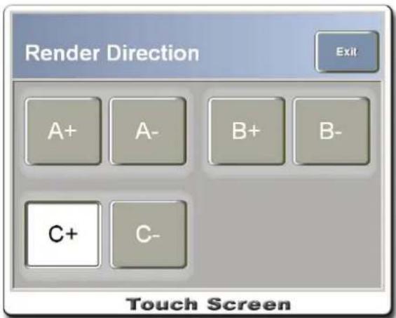
[Figure 4.54 Tool Menu – Render Direction]
A + : Moves to the direction currently looking at A plane.
A-: Moves to the back of the direction currently looking at A plane.
B + : Moves to the direction currently looking at B plane.
B – : Moves to the back of the direction currently looking at B plane.
C + : Moves to the direction currently looking at C plane.
C-: Moves to the back of the direction currently looking at C plane.
Image Store
Pressing the Image Store button on the touch screen saves the 3D image on the system. The last saved image can be sent by using the E-Mail function.
Saving Images
Press the Save button on the control panel to save 3D images in View Mode. Saved images are managed by SonoView.
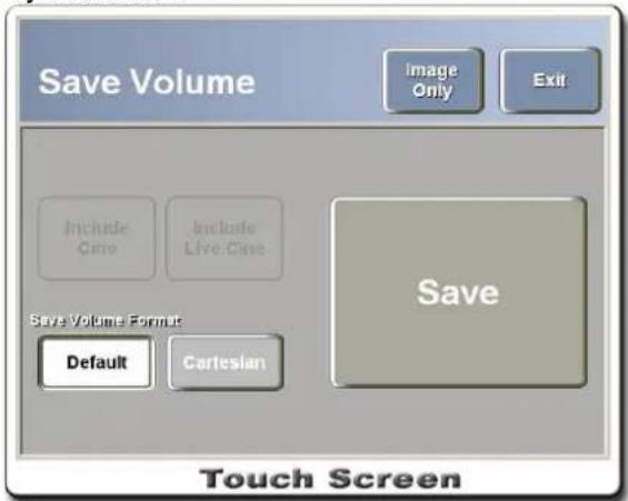
[Figure 4.55 Tool Menu – Image Store]
| Menu | Description |
| Save | Saves 3D image including volume data. If volume data and Cine images are saved together, new 3D rendering images and Cine/Live images can be reproduced at a later time. |
| Image Only Saves only the image displayed on the screen. | |
| Include Cine | This is available when 3D Cine images are generated. Select the Include Cine button and press the Save button to save Cine images and volume data. If the Include Cine button is not selected, only the volume data is saved. |
| Include Live Cine | This is available when Live 3D Cine images are generated. The function is the same as Include Cine. |
| Save Volume Format - Default | Coordinate systems for 3D data saved in this system are different from coordinate systems for 3D data used in CT or MRI. Save by selecting the Default button if you plan to use the data in SonoView only. |
| Save Volume Format - Cartesian | Save the 3D image by selecting the Cartesian button if you plan to use it in other 3D programs such as CT or MRI. If the Cartesian format is selected only the A plane image is saved. Because data format cannot be verified in SonoView, you must indicate the format in the save name when saving a SonoView image. |
| Setting Save Range | When saving Live 3D Cine images, you can specify the save range for Cine images in the same way as in 2D Mode. Refer to “Live 3D Cine Mode.” |
Printing Image
Press the Echo Print button on the control panel to print 3D images in View Mode.
3D XI TM Mode
Procedures for acquiring images in 3D XI ™ is the same for Static 3D images.
Press the 3D XI button on the touch screen to switch to 3D XI TM , or press the 3D button to scan and then press the 3D XI button at the 3D View screen to switch to 3D XI TM .
3D XI ™ supports three modes: Multi Slice View, Volume CT, and Oblique View.
![2008-07-17-0001 MEDISON OB M FPS27 / 14.0cmM10.63 | 2000-07-20 3D3-5EK / Gen Tlb 0.1 | 06:52:05 pm [20] G65 / 90dB FA10 / P90 FS10 * PG : 0](/content/2026/05/955519/images/58edd1a993dd824457668e95ce5dd4657de42b1764c8bb0df3d6b03b2bc69aaa.jpg)
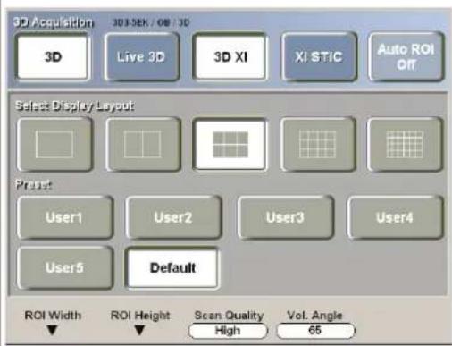
[Figure 4.56 3D Acquisition - 3D XI™]
In Live 3D XI ™ , press the Live 3D button and the 3D XI button simultaneously to acquire image. Live 3D XI ™ provides Multi Slice View Mode only.
![2008-07-17-0001 MEDISON OB H FPS27 / 14.0cmM10.63 2008-07-20 3D3-5EK / Gen Tlb 0.1 06:52:05 pm [2D] G65 / 90dB FA10 / P90 FSII * PG : 0](/content/2026/05/955519/images/46bf73b78dff343d6bdb93bbd5f646f5a8184b4d1a7519422dec7fec0da0d6cc.jpg)
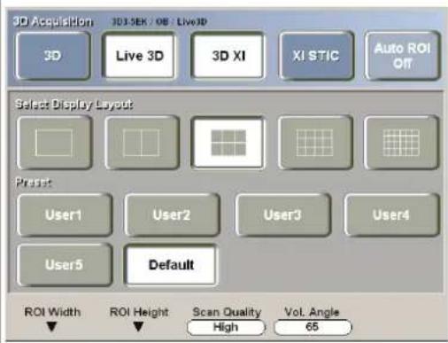
[Figure 4.57 3D Acquisition – Live 3D XI TM ]
Multi Slice View
This function enhances usefulness of examination by using neighboring multi slice images. To use the functions related to Multi Slice View, press the Multi Slice View button on the touch screen and use the menu displayed.
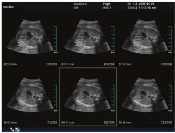
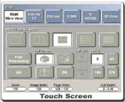
[Figure 4.58 Multi Slice View]
Init: Resets all settings for Multi Slice View.
Display Layout (1 × 1, 2 × 1, 3 × 2, 4 × 3, 6 × 4)
This function sets the display layout. You can select one from the five layouts. 1 x 1 supports large image size but does not show slice images. 6 x 4 has small images but supports slice images. The default display layout is 3 x 2.
Each time a new layout is selected, the currently selected image moves to the first position on the screen.
Ref. Image (A/B/C Plane)
Shows the selected reference image in Multi Slice View.
Rot. Z (0/90/180/270)
To rotate Multi Slice image, press the button for the desired rotation value. Here, the coordinate system rotate by the Z-axis in the "3D standard coordinate system."
Each time the mode changes or the reference plane changes, the current Rot. Z is reset to 0.
OH (Orientation Help) Function
Like the OH function in 3D view, this function shows the relative position of the currently selected slice image in volume data for Multi Slice View images.
Press the OH button on the touch screen to activate or deactivate it.
- Reference Plane: Shows the relative position of the slices displayed in other sections. In this image, a scout marker appears indicating the position of each slice image.
- Pressing the Set button on the control panel zooms the selected slice image to the 1 X
1 layout to enable more detailed observation.
[Figure 4.59 Multi Slice View – OH]
Rotation
Turn the X, Y, and Z knob-buttons to freely rotate the Multi Slice image. When the selected reference image is rotated, the results are reflected in all planes.
Translation
Move the Multi Slice image to a new position. Use the Change button on the control panel and the Trackball to move the image. The image moves along the X-axis and the Y-axis.
Zoom (x1.0 \~ x4.0)
The Multi Slice image can be zoomed by 4 times. Use the knob-button below Zoom on the touch screen to make adjustments.
Image Index
Shows the index of the currently selected image. The selected image is highlighted with yellow borders. Use the knob-button below Image Index on the touch screen or the Trackball to select an image. If the image index is outside the range of the current page, the screen moves to the previous or next index as the page index changes accordingly.
Magnification
Press the Set button at the selected image index to magnify the selected image as in the 1 x 1 layout. Press the Exit button to return to the original layout. Here, the position of Image Index is restored to the previously selected position. Images are not saved in the Magnification state.
Page Index
Shows the range of the current page index according to the display layout. Use the up-down switch below Page Index on the touch screen to adjust the value.
Cut Depth
Set the gap between Multi Slice images. The gap between Slice images can be set by the user. It is marked as an internal calculation value by default. The unit is mm. Use the up-down switch below Cut Depth on the touch screen to adjust the value.
Here, Cut Depth indicates the gap between the slices for the volume data. It does not refer to the actual anatomical position of the scanned objects.
Post Processing
This function is responsible for post-processing Multi Slice images. You can produce various images using this function. Post-processed images are not applied in Volume CT. The table below lists the functions provided. Each function can be repeated or used in combination with other functions. Note that only the Flip Image function may be repeated in the color display area (image acquired in 3D/C or 3D/PD Mode).
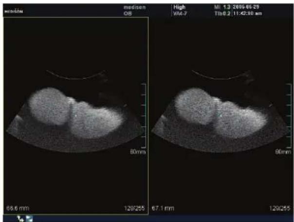
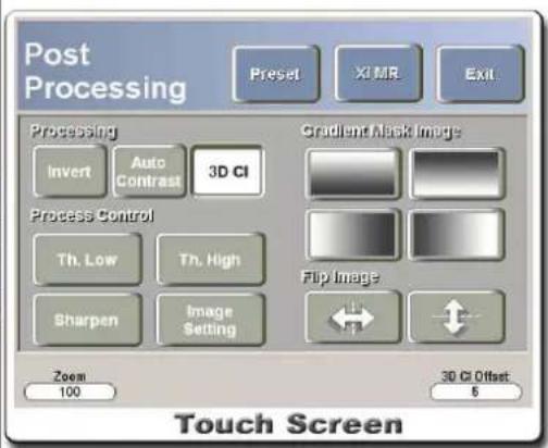
| Menu | Description |
| Invert | Inverts the brightness of Multi Slice images. |
| Auto Contrast | Automatically adjusts the brightness of Multi Slice images. This function calculates the histogram of the image and stretches the contrast distribution. The change may be marginal if the image already has well-spread contrast. |
| Compound Imaging (3D CI) | Eliminates noises and enhances image quality by compounding images. Set the distance between images to be used for 3D CI by using 3D CI Offset on the touch screen. |
| Image Setting | Sets the Gamma value for the image. Use the knob-buttons below Pos and Bias to adjust Post Curve. The Gamma value and Chroma map are reset if a new scan is performed or Multi Slice View is reset. |
| Sharpen | Sharpens the boundary of Multi Slice images. Higher the preset value, clearer the boundary becomes. Use the knob-button below Sharpen on the touch screen to make adjustments. When the function overlaps with the Th.Low and Th.High functions, you can press the knob-buttons to change the control state.Operation by Button State:When button is not pressed: The Sharpen value is not applied on the image.When button is pressed and check mark is present: The Sharpen value is applied, and the value can be adjusted by the knob-button.When button is pressed and check mark is not present: The Sharpen value is applied, and the value cannot be adjusted by the knob-button. |
| Th.Low / Th.High | Set the threshold for Multi Slice images. This removes the brightness of levels that are not wanted in images. Use the knob-buttons below Th.Low and Th.High on the touch screen to make adjustments. When the function overlaps with the Sharpen function, you can press the knob-buttons to change the control state. Button controls are the same as Sharpen. |
| Gradient Mask Image | Set the brightness of Multi Slice images. You may select up/down/left/right or none for Gradient Mask. Bright areas on buttons represent image areas that will be processed as bright and dark areas on buttons represent image areas that will be processed as dark. Button selection determines the image brightness adjustment. |
| Flip Image | Flips the position of Multi Slice images vertically or horizontally. |
Setting Preset
Use this function to set up Post Curve, Palette, current Threshold value, and other parameters for the current image and save them as user preset values.
Select a button from User 1 through User 5 and press the Save button to save the user preset values under the selected button.
XI MR
This function improves the image quality by stressing the contrast and edges of Multi Slice images. The function is applied only to the selected images with yellow borders.
Measurement
Like 3D Measure in 3D View, simple measurements can be performed in Multi Slice View. Refer to the section on "3D Measure." (The volume value can be measured using 1
Distance.)
This function is not available in Volume CT and Oblique of 3D XI™ Mode, and the Slice 3D function remains inactive.
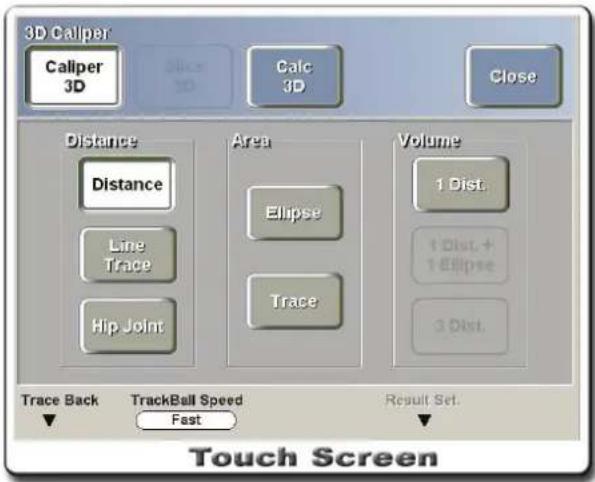
[Figure 4.61 3D Measure]
Notation
Like 3D Notation in 3D View, texts and indicators can be entered 3D XI™ also. For more information, refer to the section on "3D Notation."
Volume CT
This function provides relational view of surface images by expressing coronal, sagittal and axial images in appropriate positions in the 3D space. Volume CT supports two modes: Cube Volume CT and Cross Volume CT. Press the Volume CT button on the touch screen.
Cube Volume CT
Provides information of external surface images neighboring the cube.
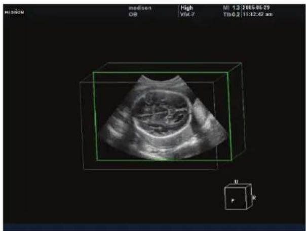
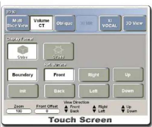
[Figure 4.62 Cube Volume CT]
| Menu | Description |
| Default Setting | Shows the selected surface according to the position of the image selected in Multi Slice View. If the position is close to the front/top/left direction of the volume, the image is shown in the same direction as the multi slice image because the image is shown from the selected position. If the position is close to the back/bottom/right direction of the volume, the image is then shown in the opposite direction as the multi slice image because the image is shown from the selected position. The position of the selected slice is shown with the image slightly slanting. This is for showing other plane images simultaneously when looking at them from different directions. |
| Ref. Surface | Sets Reference Surface. You can select any of the six surfaces. |
| View Direction | When the user selects one of the six surfaces as the desired view direction, the selected surface is placed toward the front. |
| Ref. Surface Offset | Moves the offset position of the selected Reference Surface. Use the knob-button below Surface Offset on the touch screen to make adjustments. |
| Rotation | Use the X/Y/Z knob-button on the control panel to rotate Cube Volume CT image by the X/Y/X-axis. |
| Zoom | Zooms in/out the Cube Volume CT image. Use the knob-button below Zoom on the touch screen to make adjustments. |
| Boundary | Sets or clears the additional boundary lines for Cube Volume CT. Additional boundary lines indicate the external area for the entire volume. |
Cross Volume CT
Provides information of images inside the planes crossing over each other.
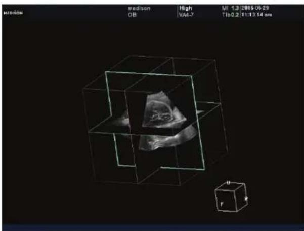
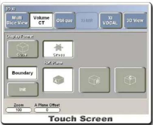
[Figure 4.63 Cross Volume CT]
| Menu | Description |
| Ref. Plane | Sets Reference Plane. |
| Ref. Plane Offset | Moves Reference Plane. Use the knob-button belowPlane Offseton the touch screen to make adjustments. |
| Rotation | Use the X/Y/Z knob-button on the control panel to rotate Cross Volume CT image by the X/Y/X-axis. |
| Zoom | Zooms in/out the Cross Volume CT image. Use the knob-button belowZoomon the touch screen to make adjustments. |
| Boundary | Sets or clears the additional boundary line for Cross Volume CT.Additional boundary lines indicate the external area for the entire volume. |
Oblique View
Surface images can be viewed by applying line/contour on desired surfaces in anatomical positions of coronal/sagittal/axial images. Press the Oblique button on the touch screen.
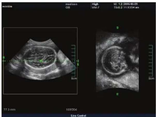
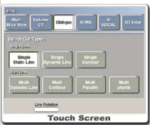
[Figure 4.64 Oblique View]
Select Cut Type
Provides the following Cut Types:
i) Single Line: Applies a single line to an image for a surface view. A reference image and a line are displayed on the left side of the screen and an oblique image for the line on the right side of the screen.
| Menu | Description |
| Single Static Line | Obtains information for a vertical surface image using the default line. Use the knob-button belowLine Rotationon the touch screen to rotate thedefault line. |
| Single Dynamic Line | Obtains information for a vertical surface image by editing a line. Press the Single Dynamic Line button and then use the trackball and the Set button to specify a start point. Then, draw a line and press the Set button again to specify an end point. A surface image perpendicular to the line will be shown. Use the knob-button below Line Rotation on the touch screen to rotate the line and press the Change button on the control panel to move it. |
| Single Contour (Edit) | Obtains information for a vertical surface image by editing a contour. Press the Single Contour button and then use the trackball and the Set button to specify a start point. Then draw a contour and press the Set button again to specify an end point. A surface image perpendicular to the contour will be shown. Because there is a restriction on the volume of data with contours, a surface image cannot be viewed if the volume of data has exceeded its limit. |
ii) Multi Line: Applies up to 5 lines to a reference image for a surface view. Lines are shown in different colors for easier identification.
A reference image is shown at the upper left-hand corner of the screen, containing all lines.
The oblique image of a line is shown by color in the screen. However, If the reference image is changed, all of the existing lines will disappear.
| Menu | Description |
| Multi Dynamic Line | Applies five lines to a reference image and displays an oblique image for these. Press the Multi Dynamic Line button and then use the trackball and the Set button to draw a line. Then a surface image perpendicular to the line will appear separated with line colours. Five dynamic lines can be drawn. Use the Rotation knob-button to rotate a line. |
| Multi Contour | Applies five random contour lines to a reference image and displays an oblique image for these. Press the Multi Contour button and then use the trackball and the Set button to draw a curve. Then an oblique image will appear separated with curve colours. Five curves can be drawn. |
| Multi Parallel | Applies lines parallel with a random line to a reference image and displays an oblique image for these. Press the Multi Parallel button and then use the trackball and the Set button to draw a reference line. Then a parallel line will be drawn automatically. An oblique image for each line is displayed. Use the Line Rotation knob-button to rotate a reference line. The changes are applied to all parallel lines. Use the Line Offset knob-button to adjust the spacing between parallel lines. |
| Multi Plumb | Applies lines perpendicular to a random dynamic line to a reference image and displays oblique image for these. Press the Multi Plumb button and then use the trackball and the Set button to draw a reference line. Then a perpendicular line will be drawn automatically. An oblique image for each line is displayed. Use the Line Rotation knob-button to rotate a reference line. The changes are applied to all perpendicular lines. Use the Line Offset knob-button to adjust the spacing between perpendicular lines. |
View direction of Vertical Surface Image
As illustrated below, the view direction is perpendicular to the cutting direction of the volume data.
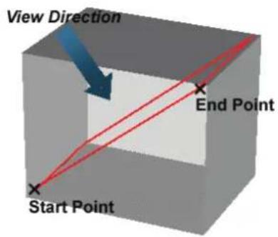
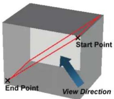
[Figure 4.23 3D View]
3D DMR
In 3D, Live 3D or 3D XI Mode, you can apply Dynamic MR to enhance images.
■ 3D DMR in 3D / Live 3D Modes
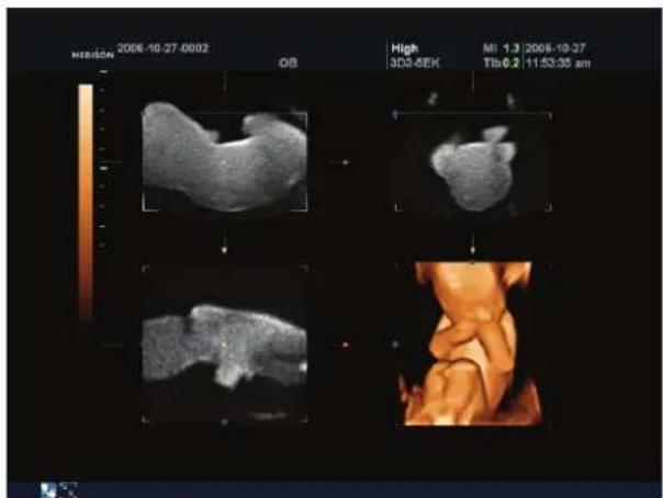
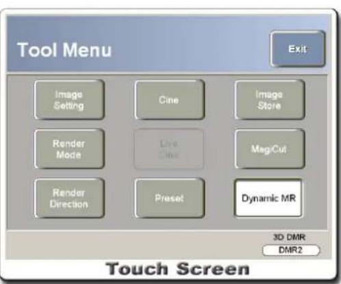
[Figure 4.65 3D DMR in 3D / Live 3D Modes]
-
Press the Tools button on the touch screen. The Tool Menu screen will appear.
-
Press Dynamic MR.
- With the 3D DMR switch at the bottom of the touch screen, set the DMR type to DMR 1-4. The DMR type set is immediately applied.
■ 3D DMR in 3D XI TM Mode
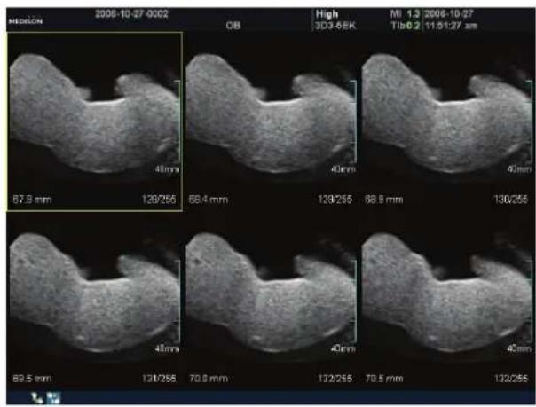
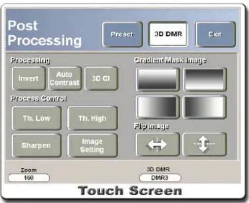
[Figure 4.66 3D DMR in 3D XI™ Mode]
- In the Multi Slice View screen on the touch screen, press 3D DMR. Dynamic MR is applied.
- Press Post Processing to change the DMR type. The Post Processing screen will appear.
- With the 3D DMR switch at the bottom of the touch screen, set the DMR type to DMR 1-4. Press Exit to complete the changes.
NOTE
■ Because Dynamic MR is optional, it becomes available only when a dongle for Dynamic MR is attached.
■ When the dongle is not attached, the 3D DMR button on the touch screen is shown as XI MR in 3D XI Mode and does the same job as XI MR in Post Processing.
If an image is saved after Dynamic MR is applied and it is viewed without the dongle attached, it appears without the effect of Dynamic MR.
XI VOCAL
Unlike in VOCAL, which uses the rotation surface method, XI VOCAL slices an object using a parallel surface method to calculate its volume. Press XI VOCAL on the touch screen for 3D XI.
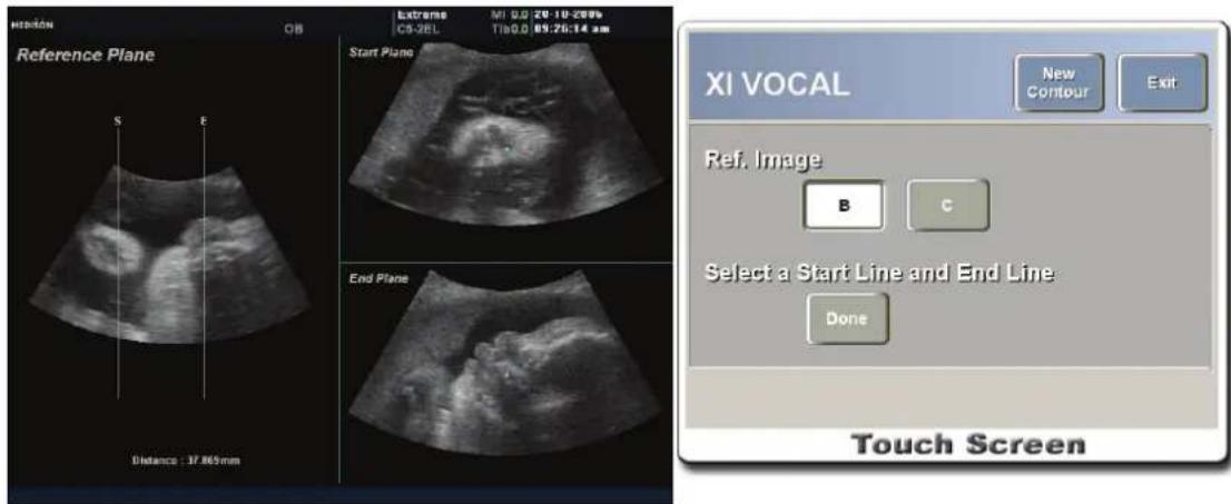
[Figure 4.67 XI VOCAL]
The reference image specified in Multi Slice View appears in the screen. When the Rotation or Zoom function has been used with the reference image in Multi Slice View, the effects still remains with the reference image for XI VOCAL.
Perform XI VOCAL by following the steps below. In each step, pressing Exit on the touch screen aborts XI VOCAL and returns to Multi Slice View for 3D XI.
- Select an image to use as a reference on the touch screen.
- Specify Start and End Lines. Use the Set button and the trackball on the control panel. The distance between two lines along with Start and End Planes are displayed in the screen. Once the lines are specified, press Done.
- A message appears on the touch screen, asking whether to contour the reference image. Press Done to proceed.
-
Specify Contour Type. Solid, Cystic and General allows you to retrieve a contour automatically and Manual allows you to retrieve a contour manually. For more information, refer to 'VOCAL.'
-
Specify the number of images to contour. Press Make to move to the next step.
-
Specify the position of Seed Point in the screen.
- When automatic contour retrieval is selected, two Pole Points appear in different positions in all slices and the contour of an object is retrieved based on them. The position of the Pole Points for each slice can be moved independently. To change the position of Pole Points, use the Pole 1 and Pole 2 buttons or the Set button and trackball on the control panel.
- When manual contour retrieval is selected, draw a contour line manually to retrieve a contour. When finished, press Done.
-
Contour is executed. A progress bar appears at the bottom of the screen, indicating the progress. Press Stop to finish contour and execute the same contour for the others.
-
When Contour is completed, you can press All Slice Show to review the completed slices. To edit a contour, press Edit Contour and use the Set button and the trackball on the control panel to edit a contour line.
Press Exit to finish XI VOCAL. To create a new contour, press New Contour and repeat the above steps.
Live 3D XI™ Mode
Live 3D XI TM supports Multi Slice View only.
Procedures for running Multi Slice View for Live 3D XI TM are the same as running Multi Slice View for 3D XI TM .
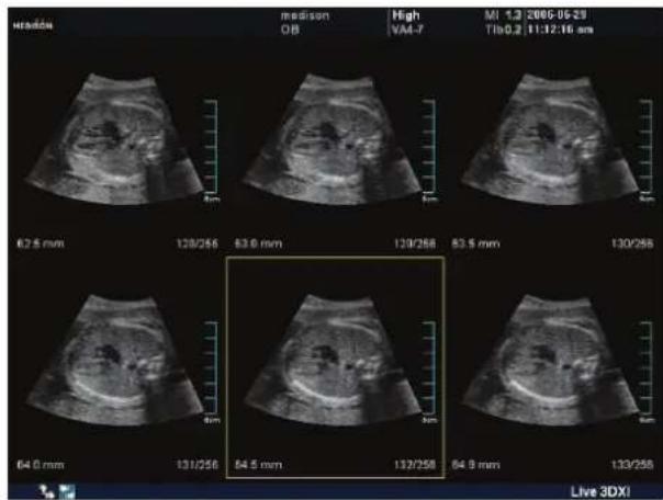
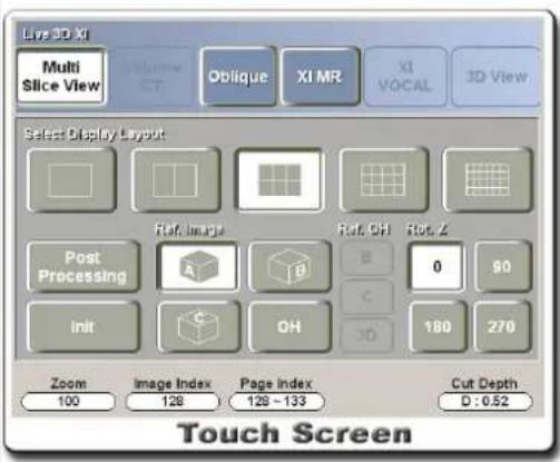
[Figure 4.68 Live 3D XI™ - Multi Slice View]
XI STIC Mode (Optional)
STIC stands for Spatio-Temporal Image Correlation. It calculates a heartbeat cycle with the volume data for a fetal cardiac area, and reconstructs and displays the volume data.
STC is divided into regular STIC and XI STIC depending on whether 3D XI ™ is used.
| NOTE | ■ XI STIC Mode is available only with a 3D Probe. |
| ■ XI STIC Mode is available in 3D Color Doppler mode and 3D Power Doppler mode. | |
| ■ XI STIC Mode is not available in Live 3D Mode. |
- In Image Scan Mode, press 3D and XI STIC. To access in 3D XI Mode, press 3D, 3D XI and XI STIC.
-
Specify each menu on the touch screen.
-
For settings in STIC Mode, refer to Live 3D.
-
For settings in XI STIC Mode, refer to 3D XI.
-
Specify Scan Time, STIC Angle and Trimester.
-
Scan Time: Specify the scan time between 7 – 20 seconds in 1 second increments.
- STIC Angle: Specify an angle between 15 - 60° in 5° increments.
- Trimester: Specify the pregnancy trimester to 1st , 2nd , 3rd or User Set. If it is set to 1st
- 3 rd , the Scan Time and STIC Angle for that trimester are automatically set. Please refer to the following table:
| 1st | 2nd | 3rd | |
| Scan Time 10 | sec. 12 sec. 15 sec. | ||
| STIC Angle | 20° | 25° | 30° |
If Scan Time or STIC Angle is set out of the specified range, Trimester appears as User Set.
- Press the Freeze button on the control panel. The system begins to acquire the STIC volume data.
- The number of heartbeats for a fetus is calculated and displayed on the touch screen. Press Yes to proceed. Press No to cancel and scan again.
| NOTE | When the number of heartbeats cannot be calculated due to severe Motion Artifact or no heartbeat cycle, the system returns to the Acquire STIC Volume Data screen. |
- Once volume data scan is completed, a STIC image appears. Adjust the image with the touch screen.
- With STIC Speed, the image playback speed can be adjusted. Available options are All CINE, 25%, 33%, 50% and 100%. If it is set to All CINE, all Volume CINE saved are reviewed regardless of the speed. If it is set to a percentage, an image is played at the speed of the specified percentage to the number of fetal heartbeats (100%).
- Press the 3D/4D button on the control panel to finish. Press Exit to return to the previous step.
※ Tip! To obtain good STIC volume data:
- STIC Angle: For smaller fetal hearts, specify a smaller Scan Angle.
- Scan Position: Make sure that the centers of the specified Scan Angle and the fetal heart are aligned with each other.
- Volume Box: Adjust it to match the size of a fetal heart.
※ To obtain good Color STIC volume data:
- Control the fps at least 15 during scanning.
- Set the application with Fetal Heart.
- During Cine, control the gain for good color view.
STIC
This is STIC Mode without 3D XI™. STIC information such as Image Angle, Vol.Angle, Scan Time, Heart Rate and Cine are displayed in the right hand side of the screen.
NOTE
The touch screen menus for STIC Mode can be used in the same way as in Live 3D View.
In STIC Mode, STIC Volume CINE performs tasks by default. Pressing the Yoyo button on the touch screen changes the CINE play type from Loop to Yoyo.
Pressing the Freeze button on the touch screen stops CINE play and switches to Static 3D Mode. In the Static 3D screen, you can use Vol.Index to move to the volume data for the corresponding index. Pressing the Freeze button again returns to STIC Mode and enables CINE play.
To run 3D View or 3D XI, or save a STIC image, press the corresponding button after stopping CINE Play.
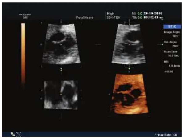
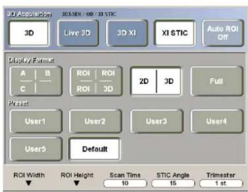
[Figure 4.69 STIC]
XI STIC
This is STIC Mode with 3D XI™. The XI STIC logo appears at the lower right corner of the screen.
NOTE
The touch screen menus for XI STIC Mode can be used in the same way as in 3D XI Mode.
In XI STIC Mode, you can review slice images. However, features such as Volume CT, XI VOCAL or 3D View are not available in this mode. Press the Freeze button on the touch screen to switch to 3D XI Mode. In the 3D XI screen, you can use Vol.Index to move to the volume data for the corresponding index. Pressing the Freeze button again returns to XI STIC Mode.
To run 3D View or save a XI STIC image, press the corresponding button after switching to 3D XI Mode.
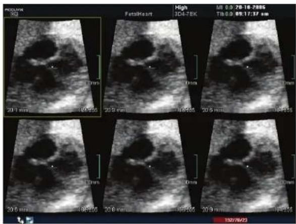
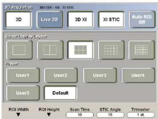
[Figure 4.70 XI STIC]
Chapter 5
Measurements and Calculations
MEASUREMENT RANGE AND ACCURACY 2
BASIC MEASUREMENTS 4
ACTIVATING BASIC MEASUREMENT MODE 4
BASIC MEASUREMENT MENU 5
DISTANCE MEASUREMENT 7
CIRCUMFERENCE AND AREA MEASUREMENT 8
VOLUME MEASUREMENT 9
MEASUREMENT IN M MODE 11
MEASUREMENT IN SPECTRAL DOPPLER MODE 11
CALCULATIONS BY APPLICATION 13
BASICS OF CALCULATIONS BY APPLICATION....13
OB CALCULATIONS 19
FETAL ECHO CALCULATIONS....25
GYN CALCULATIONS....30
UROLOGY CALCULATIONS....32
VASCULAR CALCULATIONS....36
CARDIAC CALCULATIONS 40
RADIOLOGY CALCULATION....49
REPORT....51
REPORT FUNCTIONS 51
GRAPH FUNCTION 52
Measurement Range and Accuracy
The measurements provided by the system do not define a specific physiological or anatomic parameter. Rather, what is provided is a measurement of a physical property such as distance or velocity for evaluation by the clinician.
For each of the measurements available on the system, the measurement accuracy and range over which that accuracy is valid is shown in the following tables. Measurement accuracy is also constrained by the caliper placement capability limit. Unless specified by a probe or an application, all linear distance measurements have the following accuracy requirements.
The RMI413 phantom is used for all 2D and M-mode measurement accuracy tests.
The RMI1425A phantom is used for the Doppler measurement accuracy tests.
Unless specified otherwise by a probe or application, all linear distance movements have the following accuracy limits.

2D Mode
| Measurement Type Range Accuracy Notes | |||
| Axial Distance 0.01-24.91 cm +/- 2% or +/- 2 mm | |||
| Lateral Distance 0.01-30.37 cm +/- 2% or +/- 2 mm | |||
| Diagonal Distance 0.01-39.28 cm +/- 2% or +/- 2 mm | |||
| Area | 0.01-756.52 2 | cm +/- | 4% |
| Circumstance 0.03-1 | 10.56 cm +/- 3% or +/- 5 mm | ||
| Volume | 0.01-60601.51 3 | cm +/- | 8% |
NOTE
- The accuracies are calculated using the following equations:
Distance error (2% or 2mm) = Image Pixel error (1% or 1mm) + Hardware error (1% or 1mm)
Area error (4%)= Distance 1 x Distance 2
Volume error (8%)= Distance 1 x Distance 2 x Distance 3
Circumference error (3% or 5mm)= Distance error (2% or 2mm) + Calculation precision (1% or 3mm)
- The phantom used is Multi-purpose phantom, RMI 413, from GAMMAX, Inc. USA.
M Mode
| Measurement Type Range Accuracy Notes | |||
| Depth | 0.01-24.00 cm +/- 2% or +/- 2 mm | ||
| Time | 0.01-4.26 sec +/- 2% or 0.2 sec | ||
| Velocity | 0.01-2400.00 cm /sec +/- 4 % | ||
NOTE
- The accuracies are calculated using following equations:
Distance error (2% or 2mm) = Image Pixel error (1% or 1mm) + Hardware error (1% or 1mm)
Time error (2% or 0.2 sec) = Image Pixel error (1% or 0.1 sec) + Hardware error (1% or 0.1 sec)
Velocity error (4%) = Distance / Time
- The phantom used is Multi-purpose phantom, RMI 413, from GAMMAX, Inc. USA
Doppler Mode
| Measurement Type Range Accuracy Notes | |||
| Time | 0.01-4.26 sec +/- 2% or 0.2 sec | ||
| Velocity | 0.15-200.00 cm /sec +/- 15 % | ||
NOTE
- The phantom used is Doppler phantom, RMI 1425A, from GAMMAX, Inc., USA.
- The accuracies cited in the above table arise from the positioning of the cursors on the Doppler display and subsequent measurements made. The velocity tests can therefore be used to check these values since these are not indicators of the underlying absolute velocity assurance. The absolute velocity accuracy is tested using a series of phantom measurements.
Absolute Doppler Velocity Accuracy:
Accuracy is defined as the difference between a calibrated phantom velocity and that annotated as the time-e-averaged mean by the system. The time-averaged mean is calculated as the average over a determined period of time of the intensity-weighted mean of the spectrum. All probes have been tested to ensure that the time-averaged mean velocity falls within +/- 15% of that annotated on the phantom. Due to Doppler phantom constraints, these tests have been conducted in the range 15 cm/sec to 110 cm/sec .
Basic Measurements
A specific distance, area, etc. can be measured by using scanned images or Freeze Mode. Measurement methods may differ depending on the mode used.
| Measurements | Measurement Methods |
| Distance Measurement | 2D Distance (Line)2D Distance (Trace)2D Hip JointM DistanceDoppler VelocityDoppler Velocity (A/B)Doppler Trace |
| Circumference and Area Measurement | 2D Ellipse2D Trace |
| Volume Measurement | 3D Volume: 3 Distance3D Volume: 1 Distance3D Volume: Distance + Ellipse |
Activating Basic Measurement Mode
Pressing the Measure button or the Freeze button on the control panel and the Measurement by Application Menu will appear. Press the Caliper button on the touch screen to run the basic measurement mode.
| How to Activate | Touch Screen Menu |
| Press theMeasurebutton. When theMeasurement byApplication Menuappears press theCaliperbutton. | 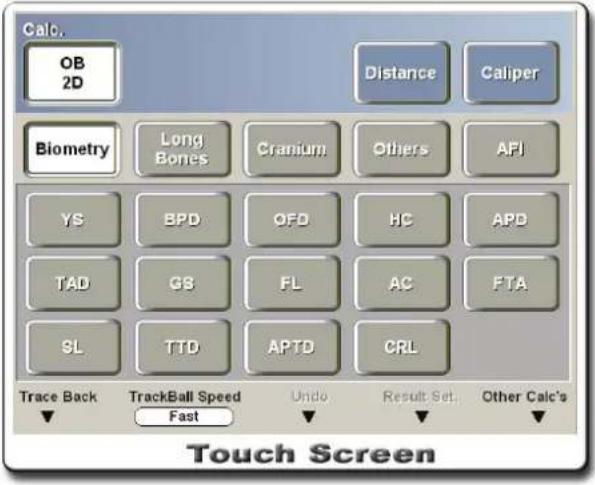 |
| Press the Freeze button. When the Cine menu or the Loop menu appears press the Set button on the control panel. | 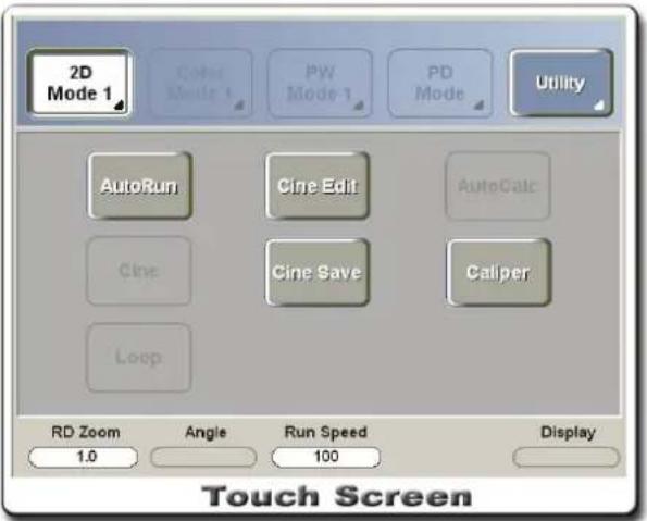 |
| Press the Caliper button, and the basic measurement mode menu will appear. | 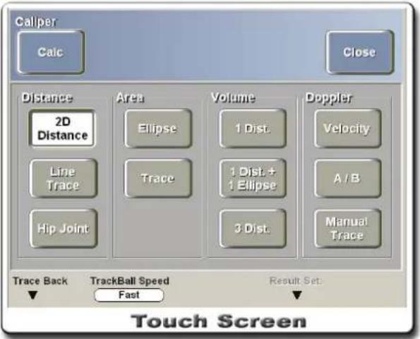 |
Basic Measurement Menu
You can change configurations regarding basic measurements. For more information, refer to "Chapter 3 Settings" in this manual.
Trace Back
To delete a part of the measuring line while using Trace, use the Trace Back function. Turn the knob-button below Trace Back left or right to delete the Trace measuring line.
When using the Manual Trace menu in Spectral Doppler Mode, you can perform the same function by turning the Trackball to the left.
Trackball Speed
The Trackball Speed menu is used for adjusting the speed of the Trackball on the control panel.
Turn the knob-button below Trackball Speed to select Slow, Normal or Fast.
Exiting Measurement Mode
To finish measuring and return to diagnosis mode, press the Exit button on the control panel or the Close button on the touch screen.
Measurement Results
Printing Measurement Results
Press the Echo Print button on the control panel to print the results via an echo-printer.
Displaying Measurement Results
To move the measurement results, select the Result Set. up-down switch below the touch screen in Measurement by Application Mode or Basic Measurement Mode.
[Figure 5.1 Displaying Measurement Results]
- Move Result
Moves the measurement results. Press the Set button to confirm the position.
- Save Settings
Saves the changed position of the measurement results. All subsequent measurement results will appear in the saved position.
- Restore Default
Resets to the system default position.
Deleting Measurement Results
Press the Clear button on the control panel.
Distance Measurement
2D Distance: Measures the distance between two points
This measurement function can be performed in all diagnosis modes. The results are displayed in cm (or mm). A maximum of four sets of measurements can be displayed simultaneously.
- Press the Caliper button and then press the 2D Distance button on the touch screen.
- Use the Trackball to place the cursor at the start point of the area to measure and then press the Set button. Use the same method to assign the end point.
- You can reset the position of the measurement area by pressing the Change button before pressing the Set button.
- After position setup, distance and average are displayed on the screen.
- A new cursor will appear for a new measurement. If measuring distances more than four times, the oldest distance measurement results will be replaced first.
The ratio of the first distance to the second, and the ratio of the third to the fourth are calculated and displayed as percentages.
Line Trace: Measures a non-straight distance between two points
This measurement function can be performed in all diagnosis modes. The results are displayed in cm (or mm). A maximum of four sets of measurements can be displayed simultaneously.
- Press the Caliper button and then press the Line Trace button on the touch screen.
- Use the Trackball to place the cursor at a point on the contour of the area to measure and then press the Set button. Use the Trackball to draw the contour and then press the Set button.
- You can reset the position of the measurement area by pressing the Change button before pressing the Set button. You can erase parts of the trace line by pressing the Del key on the keyboard before pressing the Set button or by using Trace Back on the touch screen.
- After position setup, distance and average are displayed on the screen.
- A new cursor will appear for a new measurement. If measuring distances more than four times, the oldest distance measurement results will be replaced first.
The ratio of the first distance to the second, and the ratio of the third to the fourth are calculated and displayed as percentages.
2D Hip Joint Measurement
This measurement is available in all diagnosis modes.
-
Press the Caliper button and then press the Hip Joint button on the touch screen.
-
Use the Trackball to place the cursor at the start point of the area to measure and then press the Set button. Use the same method to assign the end point.
- You can reset the position of the measurement area by pressing the Change button before pressing the Set button.
- Set the second and third lines of the Hip Joint in the same way.
- After position setup, the measurement results are displayed on the screen.
- A new cursor will appear for a new volume measurement. If measuring lines more than four times, the oldest line measurement results will be recalculated first.
Apply the alpha angle ( α ) between the first line and the second line, and the beta angle ( β ) between the first and the third to the table shown below, and calculate the type. Refer to the table below for Hip Joint measurement results.
| TYPE | α β | |
| 1a | 60 ≤ α < 90 | 0 < β < 55 |
| 1b | 60 ≤ α < 90 | 55 ≤ β < 90 |
| 2a/b | 50 ≤ α < 60 | 0 < β < 90 |
| 2c | 43 ≤ α < 50 | 77 ≤ β < 90 |
| d | 43 ≤ α < 50 | 0 < β < 77 |
| 3/4 | 0 < α < 43 |
Circumference and Area Measurement
Ellipse: Measures elliptical objects
This measurement function is available in all diagnosis modes. The measurement results are displayed in cm or mm (circumference) or cm2 or mm2 (area). A maximum of four sets of measurements can be displayed at one time. Average circumference and average area are shown together. This tool is especially useful for bladder and prostate measurement. The following shows the measurement formula and procedures.
Circ = 2 π · √ 1/2 · (A/2) ^ 2 + (B/2) ^ 2 , (A: Longaxis, B: Shortaxis)
Area = π × a × b, (a, b: Axis)
-
Press the Caliper button and then press the Ellipse button on the touch screen.
-
Use the Trackball to place the cursor at the start point of the area to measure and then press the Set button. Use the same method to assign the end point.
- You can reset the position of the measurement area by pressing the Change button before pressing the Set button.
-
After the ellipse appears with the two points as an axis, adjust the shape (or another axis) of the ellipse using the Trackball. Then, press the Set button.
-
After position setup, the measurement results are displayed on the screen.
- A new cursor will appear for a new circumference or area measurement.
Trace: Measures objects with irregular shapes
This measurement function is available in all diagnosis modes. The measurement results are displayed in cm or mm (circumference) or cm2 or mm2 (area). A maximum of four sets of measurements can be displayed at one time. Average circumference and average area are shown together. The following shows the measurement formula and procedures.
Circ = sum √ X (n) - X (n - 1) ^ 3 + Yn - Yn - 1 ^ - 2, (N = 1, 2 ... last point) (
Area = sum √ X (n - 1) × Y (n) - X (n) × Y (n - 1) , (N=1,2...lastpoint)
- Press the Caliper button and then press the Trace button on the touch screen.
- Use the Trackball to place the cursor at a point on the contour of the area to measure and then press the Set button. Use the Trackball to draw the contour and then press the Set button.
- You can reset the position of the measurement area by pressing the Change button before pressing the Set button. You can erase parts of the trace line by pressing the Del key on the keyboard before pressing the Set button or by using Trace Back on the touch screen.
- Trace ends when the cursor returns to the start point or when the Set button is pressed. The measurement results will be displayed on the screen.
- A new cursor will appear for a new circumference or area measurement.
Volume Measurement
3D Volume: 3 Distance: Measures using three distances (axes)
This measurement function is available in all diagnosis modes. The measurement results are displayed in cm 3 (or mm 3 ). The following shows the measurement formula and procedures.
Vol = 4/3 π · D _ 12 · D _ 22 · D _ 32, (D: distance)
- Press the Caliper button and then press the 3 Dist button on the touch screen.
- Use the Trackball and Set button to measure three lines. Method for measuring a line is the same as in "2D Distance Measurement."
- After measuring the length of the three lines, the measurement results are shown on the screen.
- A new cursor will appear for a new volume measurement.
3D Volume: 1 Distance: Measures using one distance (diameter)
This measurement function is available in all diagnosis modes. The measurement results are displayed in cm3 (or mm3 ). A maximum of four sets of measurements can be displayed simultaneously. The following shows the measurement formula and procedures.
Vol = 4/3 π · (D/2) ^ 3, (D: distance)
- Press the Caliper button and then press the 1 Dist button on the touch screen.
- Use the Trackball and Set button to measure one line. Method for measuring a line is the same as in "2D Distance Measurement."
- Based on the line measured, the volume will be calculated and then be displayed.
- A new cursor will appear for a new volume measurement.
3D Volume: Distance + Ellipse: Measures using one ellipse and one distance
This measurement function is available in all diagnosis modes. The measurement results are displayed in cm3 (or mm3 ). A maximum of two sets of measurements can be displayed simultaneously. The following shows the measurement formula and procedures.
π/6 dba ( short - axis , b: Long axis , d: Distance )
- Press the Caliper button and then press the 1 Dist + 1 Ellipse button on the touch screen.
- Use the Trackball and Set button to measure one line. Method for measuring a line is the same as in "2D Distance Measurement."
- After measuring one line, draw one ellipse. Method for drawing an ellipse is the same as in "Ellipse Measurement."
- Based on the line and ellipse measured, the volume of the ellipse will be calculated and then be displayed.
- A new cursor will appear for a new volume measurement.
-
To measure the line and the ellipse from different perspectives,
-
After measuring the line, press the Freeze button on the control panel to return to diagnosis mode.
- Scan a new image and then press the Freeze button again to return to measurement mode.
- When a new cursor appears on the screen, measure the ellipse.
- When in Dual Mode, which simultaneously displays two images on the screen, the user can measure the volume without having to return to the diagnosis mode.
Measurement in M Mode
M Distance: Measures the distance, time interval, speed between two points
Method for measuring distance in M Mode is the same as in "2D Mode."
M Mode shows the changes occurring in the image according to time. If the distance (cm or mm) between two points is measured, the time interval (sec), speed (cm/s or mm/s), etc. can be checked. A maximum of four sets of measurements can be displayed simultaneously.
- Press the Caliper button and then press the M Distance button on the touch screen.
- Use the Trackball and the Set button to measure the distance. Method for measuring distance is the same as in "2D Distance (Line) Measurement."
- After position setup, the measurement results are displayed on the screen.
- A new cursor will appear for a new measurement.
Measurement in Spectral Doppler Mode
NOTE
Since a Spectral Doppler image is displayed in terms of time (X-axis) and velocity (Y-axis), setting one point above the image will allow the velocity to be checked.
Also, an additional line will appear to help more accurate positioning when measuring a point.
Method for measuring distance in Spectral Doppler Mode is the same as in "2D Mode."
Doppler Velocity: Measures acceleration using the distance between two points
The velocity (cm/s or mm/s), RI (Resistivity Index), velocity ratio (V1/V2), velocity change (dV: cm/s or mm/s), time interval between two points (sec), and acceleration (Acc: cm/s 2 or mm/s 2 ) are displayed.
A maximum of four sets of measurements can be displayed simultaneously. The following shows the measurement formula and procedures.
RI = V _ 1 - V _ 2V _ 1
dV = V _ 2 - V _ 1
on Acceleration = dV(T _ 2 - T _ 1) on Acceleration = dV/dT
- Press the Caliper button and then press the Velocity button on the touch screen.
- Use the Trackball and the Set button to measure the distance. Method for measuring
distance is the same as in "2D Distance Measurement."
- After position setup, the measurement results are displayed on the screen.
- A new cursor will appear for a velocity measurement.
Doppler Velocity (A/B): Measures velocity ratio between two points
The velocity (cm/s or mm/s), the RI (Resistivity Index), and the velocity ratio between two points (A/B) are displayed.
A maximum of four sets of measurements can be displayed simultaneously. The following shows the measurement method.
- Press the Caliper button and then press the A/B button on the touch screen.
- Use the Trackball to place the cursor at the start point of the area to measure and then press the Set button. Use the same method to assign the end point.
- You can reset the position of the measurement area by pressing the Change button before pressing the Set button. Here, the names of Point A and Point B may be changed.
- After the position setup, the velocity at each point and the velocity ratio between the two points are displayed on the screen.
- A new cursor will appear for a velocity measurement.
Manual Trace: Measures average velocity using trace
The time duration value (dT: sec), integration value of blood flow velocity (VTI: cm or mm), maximum velocity (Peak V: cm/s or mm/s), Mean G (mmHg), average velocity (Mean V: cm/s or mm/s) are displayed.
A maximum of four sets of measurements can be displayed simultaneously. The following shows the measurement formula and procedures.
_ 2 TTdT = VTI = v × dt, (VTI: VelocityTimeIntegral)
Mean V = VTI/ Duration of flow
- Press the Caliper button and then press the Manual Trace button on the touch screen.
- Use the Trackball to place the cursor at the start point of the area to measure velocity and then press the Set button. Use the Trackball to draw the contour on waveform to measure velocity and then press the Set button.
- You can erase parts of the trace line by turning the Trackball to the left before pressing the Set button or by using Trace Back on the touch screen.
- After position setup, the measurement results are displayed on the screen.
- A new cursor will appear for a new measurement.
Calculations by Application
This product provides measurement packages according to each application such as Obstetrics, Gynecology, Cardiology, Vascular, Urology and Fetal Echo.
Basics of Calculations by Application
Before Taking Measurements
- Check that the patient information has been entered. If not entered, press the Patient button and enter the patient data.
- Check that correct application and probe are selected for measurement. To change the settings, press the Probe button to change the probe or application.
NOTE
The calculation range of each measurement package varies with the selected probe and application, so the correct probe and application must be selected.
Selecting Measurement Items
Use the up-down switch below Other Calc's on the touch screen to change the application and measurement item.
Press the button for the application to measure and then press the Return button or the Return up-down switch to change the measurement item.
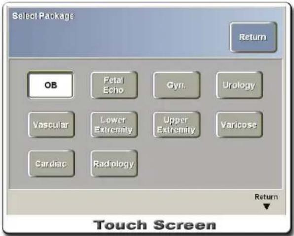
[Figure 5.2 Selecting Measurement Items]
NOTE
Press the Set button on the control panel to select the obstetrics measurement item or the fetal echo measurement item. Note that this function is not available while taking measurements.
Measurement Results
Printing Measurement Results
Press the Echo Print button on the control panel to print the results via an echo-printer.
Displaying Measurement Results
To move the measurement results, select the Result Set. up-down switch below the touch screen in Measurement by Application Mode or Basic Measurement Mode.
[Figure 5.3 Displaying Measurement Results]
- Move Result
Moves the measurement results. Press the Set button to confirm the position.
- Save Settings
Saves the changed position of the measurement results. All subsequent measurement results will appear in the saved position.
- Restore Default
Resets to the system default position.
Deleting Measurement Results
Press the Clear button on the control panel.
Closing Measurement Menu
■ Press the Exit button on the control panel to exit the measurement menu.
■ Press the End Exam button and complete the measurement to save the results for data management. Search for and select the information of the next patient. To register a new patient and continue taking measurements for the patient, finish the current measurements and then register a new patient.
Trace Back
To delete a part of the measuring line while using Trace, use the Trace Back function. Turn the knob-button below Trace Back on the touch screen left or right to delete the Trace measuring line.
Trackball Speed
The Trackball Speed function adjusts the speed of the Trackball on the control panel. Turn the knob-button below Trackball Speed on the touch screen to select Slow, Normal or Fast.
Undo
While taking measurements, press the Exit button on the control panel to cancel the measurement process. To cancel a completed measurement process, select the up-down switch below Undo on the touch screen. The last measured item will be deleted from the screen.
Distance Measurement
While using the Measure function, you can measure the distance between two points on scanned images at any time. This function is identical to "2D Distance" in "Basic Measurement Mode." Press the Distance button on the touch screen to access it.
Heart Rate Calculations
This can be measured in M Mode or Spectral Doppler Mode.
■ Press the Heart Rate button on the touch screen menu in measurement mode to calculate the heart rate.
■ When the first baseline appears, place it at the starting position of the waveform and press the Set button.
■ Turn the knob-button below HR Cycle to adjust the Cycle value. The Cycle value is used for calculating the average value of the heart rate; the result becomes more accurate for higher Cycle values.
■ When the second baseline appears, place it at the ending position of the waveform and press the Set button.
■ The result will be calculated and be displayed on the screen.
Measuring Doppler Spectrum
Trace the spectral waveform to measure PSV (Peak Systolic Velocity), EDV (End Diastolic Velocity), Vmean, Gmean, Gpeak, S/D, PI (Pulsatility Index), RI (Resistivity Index), etc. in Spectral Doppler Mode.
Methods for tracing spectral waveforms include Auto Trace, Limited Trace, and Manual Trace. The value can also be obtained through itemized measurements.
Auto Trace: Automatically calculates Doppler Spectrum Cycle
- Press the Measure button on the control panel after obtaining a desired image.
- Press the Auto Trace button in the measurement menu. The spectral waveform will be traced automatically and the measurement value will be calculated.
- Various values such as PSV, EDV, TAM, Vmean, Gmean, Gpeak, S/D, PI, and RI will be measured and be displayed on the screen.
Things to Consider for Frozen Doppler Spectrum Auto Trace
Under "Doppler trace mode" in Measure Setup, select All, Above or Below to specify the direction of the spectrum to trace.
Take the following precautions when using the Frozen Automatic Doppler Trace function.
- If aliasing occurs because the PRF is too low in comparison to the velocity of the area examined, the aliasing spectrum can be traced. Note that the distinction from non-aliased spectrums must be clear.
- If peaks are uncertain or intermittent as in the spectral waveform in veins, tracing for the waveform is possible, but peak values such as PSV cannot be obtained.
In this case, Max Velocity will be shown as the PSV and the “Doppler Spectrum Trace Failed!” message will appear on the screen. - If Doppler Gain is set too high or too low, meaningful spectrum distinction becomes difficult and errors may occur in measurement results.
- If the spectrum is interfered by abnormal Doppler noise or artifact, tracing may fail. Adjust the Threshold value on the touch screen to obtain appropriate contour.
- If PW Gain is changed for an image in the Freeze state, tracing may fail. Adjust the Threshold value on the touch screen to obtain appropriate contour.
- If the CW 4M or CW 2M probe is in use, error(s) may occur in the results.
- When the application is set to Cardiac, Auto Trace is not supported for two-peak spectrums such as Mitral Valve Inflow and Tricuspid Valve Inflow.
Limited Trace: Calculates Doppler Spectrum Cycle in Designated Range
- Press the Measure button on the control panel after obtaining a desired image.
- Press the Limited Trace button in the measurement menu. The baseline will appear on the spectral waveform.
- Use the Trackball to place the baseline at the start point of the area to measure, and press the Set button.
- When the second baseline appears, place it at the ending position of the measurement range and press the Set button.
- To move the baseline, press the Change button to select the baseline. Reposition it and then press the Set button.
- "Limited Trace" will finish and the measurement value will be calculated.
- Various values such as PSV, EDV, TAM, Vmean, Gmean, Gpeak, S/D, PI, and RI will
be measured and be displayed on the screen.
Manual Trace: Manually calculates Doppler Spectrum Cycle
- Press the Measure button on the control panel after obtaining a desired image.
- Press the Manual Trace button in the measurement menu, and a + cursor will appear on the spectral waveform.
- Place the cursor at the start point of the spectrum to measure. Press the Set button and then use the Trackball to trace the spectral waveform.
- Press the Set button to finish Manual Trace. You can erase parts of the trace line by turning the Trackball to the left before pressing the Set button or by using Trace Back on the touch screen.
- Various values such as PSV, EDV, Vmean, Gmean, Gpeak, S/D, PI, and RI will be measured and be displayed on the screen.
Itemized Measurement: Calculates Doppler Spectrum Cycle by measuring PSV and EDV
- Press the Measure button on the control panel after obtaining a desired image.
- Select the PSV and EDV items in the measurement menu, and a + cursor will appear on the spectral waveform.
- Move the cursor to the systolic velocity point, and press Set button. Then, another + cursor will appear.
- Move the + cursor to the diastolic velocity point and press Set button.
- Various values such as PSV, EDV, S/D and RI will be measured and be displayed on the screen.
Doppler Measurement Items
| Result | Calculation | Date | Equation |
| PSV (Peak Systolic Velocity) | Velocity | cm/s | |
| EDV (End Diastolic Velocity) | Velocity | cm/s | |
| Vmean (Mean Velocity) | Velocity Calculated | cm/s | |
| Gmean (Mean Gradient) | Gradient | mmHg | |
| Gpeak (Peak Gradient) | Calculation | mmHg | 4 × PSV × PSV |
| RI (Resistively Index) | Calculation | Ratio | (PSV – EDV) / PSV |
| S/D (PSV/EDV) | Calculation | Ratio | PSV / EDV |
| PI (Pulsatility Index) | Calculation | Ratio | (PSV – EDV) / Vmean |
| TAM(Time Average Mean) | Velocity | cm/s | |
| Fetal HR | HR | BPM | HR = #beats × 60 / Time |
Volume Flow Measurement Method
■ Select Volume Flow in the measurement menu to measure related items and calculate the volume flow value. The Volume Flow value can also be calculated by measuring other items.
■ The following are formula for measuring Volume Flow.
- ( ) ×= TAMABeaAVolumeFlow
- (D) π × d24 × 60
■ Vessel Area and TAM values are used for calculating Volume Flow.
- There are two ways to measure Vessel Area: one uses the circumference (Vessel Area) and the other uses the distance (Vessel Dist). For more information on measurements, refer to "Basic Measurements."
- The TAM (Time Avg. Mean Velocity) value is automatically calculated only when using Auto trace or Limited trace. For more information on measurements, refer to "Measuring Doppler Spectrum."
Measuring Stenosis %
■ There are two ways to obtain Stenosis %: %StA using the area and %StD using the distance.
-%Stenosis Area. : Calculates stenosis ratio using the area of vessel.
- Press the %StA button and the first cursor will appear in 2D Mode.
- Measure the area of the vessel outer wall using the Circ/Area measurement method.
- When the second cursor appears, measure the area of the vessel inner wall under stenosis.
- %Stenosis Area. = (Outer Area - Inner Area) / Outer Area × 100
- %Stenosis Dist.: Calculates stenosis ratio using the diameter of vessel
- Press the %StD button and the first cursor will appear in 2D Mode.
- Measure the total diameter of the vessel using the Distance measurement method.
- When the second cursor appears, measure the diameter of the vessel inner wall under stenosis.
- %Stenosis Dist. = (Outer Distance - Inner Distance) / Outer Distance × 100
OB Calculations
Before Obtaining OB Calculations
Entering Basic OB Information
Enter the information required for OB diagnosis in the Patient Information screen. The basic OB information include LMP (Last Menstrual Period) and Gestations.
■ Once LMP is entered, EDD (Estimated Delivery Date) and GA (Gestational Age) are calculated automatically. LMP is required for the calculation of values such as EDD and SD in obstetrics measurement.
- EDD(LMP) = LMP + 280days
- GA(LMP) = Current System Date - LMP
A maximum of four fetuses can be entered in the Gestations menu. The default value is '1'. In the case of twins, enter '2'.
For more information on the patient information menu items and method for entering patient information, refer to “Entering Patient Information” in “Chapter 3 Settings” in this manual.
OB Measurement Menu Setup
Set up GA Equation, GA Table and OB measurement menus that are used in obstetrics measurements. The user can manually write, back up and restore GA Tables. For more information on GA Equation and Table, refer to the Reference Manual.
For more information on other measurement menu items and setup methods, refer to 'Setting Measurements' in "Chapter 3. Settings" in this manual.
Measurement Items
Measurement items include Fetal Biometry, Fetal Cranium, Fetal Long Bones, AFI, etc.
■ Fetal Biometry includes GS, CRL, YS, BPD, OFD, HC, APD, TAD, MAD, AC, FTA, FL, SL, TTD, APTD, and APTD * TTD, ThC.
■ Fetal Long Bones includes HUM, ULNA, TIB, RAD, FIB, CLAV, Vertebral and NB.
■ Fetal Cranium includes CEREB, OOD, IOD, CM, NF, NT, and Lateral Ventricle.
■ Fetal Others includes FOOT, EAR, MP, Left Kidney, Right Kidney, and Pelvis.
■ Doppler includes Umbilical Artery, MCA (Mid Cerebral Artery), Placenta Artery, Left Uterine Artery, Right Uterine Artery, Left Fetal Carotids, Right Fetal Carotids, Fetal Aorta, Ductus Venous, Volume Flow, and Fetal HR. Measurement items also include PSV, EDV, Trace, Vmean, S/D, PI, RI, Gpeak, and Gmean. The Fetal HR item is also included.
■ Measurement methods are the same as the basic measurement methods.
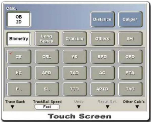
[Figure 5.4 OB Measurement Menu]
Pregnancy Calculation
- Press the Manual button on the control panel and the obstetrics measurement menu will appear on the touch screen.
- Select the group for the desired measurement item or the measurement item itself. For example, to measure BPD, select Biometry and then press the BPD button on the sub-menu that appears.
- Use the Trackball and the Set button on the control panel to take measurements.
Fetal Biometry and Fetal Long Bones extensively make use of distance measurements. HC and AC utilize circumference measurements and FTA utilizes area measurements.
Measured items are automatically recorded in the report. The report contains the mean value for the new GA value, and the recently measured values (up to separate 3 values). (The value may not be accurate if the measurements were taken less than three times.) The mean values are used for GA and EDD calculation, and are displayed on graphs.
Measuring Distance Measurement Item
■ BPD: Measures the maximum transverse diameter value when the thalamus appears symmetrical against the midline.
■ OFD: Measures the distance between the front and the back of the head in the same condition as in BPD.
■ CRL: Measures the long axis of the embryo from the head to the rump.
■ FL: Measures the length of the femur; measures the long axis of the femur closer to the probe.
■ MAD: Calculates the average values of transverse and anterior-posterior lengths of the fetal abdomen.
MAD = (APD + TAD) / 2
Measuring Circumference Measurement Items
■ HC: Measures the circumference of the head when in the same condition as in BPD. The HC measurement value is calculated automatically when the BPD and OFD items are measured.
π √ 2 OFDBPD / NC + =
However, when Merz Reference is used, the following formula is used for calculation.
HC = 2. 3 2 5 × √ BPD ^ 2 + OFD ^ 2
■ AC: Calculates abdominal circumference on the fetal transverse image when the stomach and the DV (ductus venosus) are shown clearly. The AC measurement value is calculated automatically when the APD and TAD items are measured. At this time, position the cursor on the outside including the skin.
AC = π √ AP (D ^ 2 + TAD ^ 2 2 /)
However, when Merz Reference is used, the following formula is used for calculation. AC = π × (APD + TAD) / 2
■ FTA: Measures the fetal trunk area (chest or abdomen) on the fetal transverse image. This value is calculated automatically when a circle is drawn using trace or ellipse. FTA = AC2 4π
NOTE
For more information on measuring methods, refer to "Basic Measurements."
Measurement Points
BPD, OFD, HC –fetal head
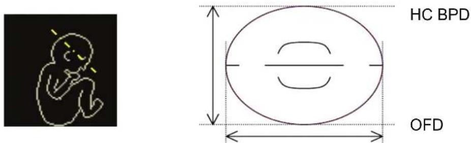
APD, TAD, APTD, TTD – fetal abdomen or fetal trunk
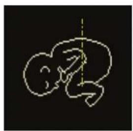
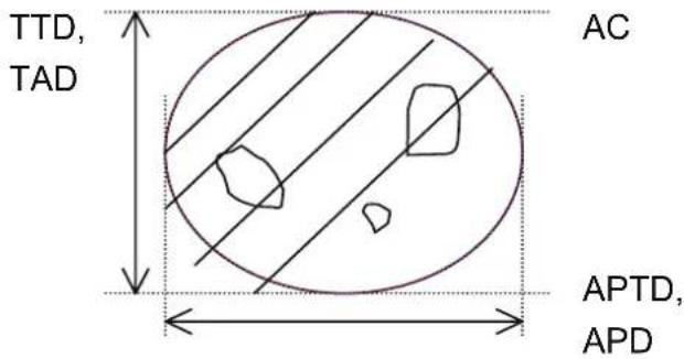
FTA –fetal trunk
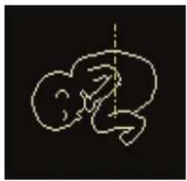
FL – fetal femur
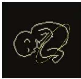
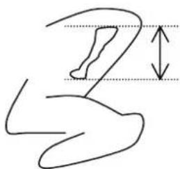
Vertebral – fetal vertebrae
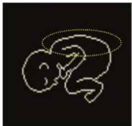
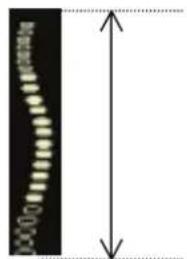
Calculating Fetal Weight
■ The fetal weight is shown in units of g (Gram), oz (ounce) or lb (pound) in 2D Mode and Dual Mode.
The user can calculate the fetal weight by measuring one set from (BPD, AC), (BPD, FL, FTA), (BPD, APTD, TTD, FL), (BPD, APTD, TTD, SL), (BPD, TTD), (AC, FL), (BPD, AC, FL), (HC, AC, FL), (BPD, HC, AC, FL), (AC) or (BPD, APTD, TTD). For example, if Obstetrics Setup (at the Measure Setup screen) is set to the Tokyo1 University method, measuring BPD, APTD and TTD displays the fetal weight on the screen. For your information, the Osaka University and Tokyo University methods are generally used in Asia, the Merz method in Europe, and the Shepard and Hadlock methods in Americas.
■ Once all the GA values are measured, the fetal weight is automatically calculated and displayed on the report. For information on formula for calculating the fetal weight,
refer to 'Estimated Fetal Weight Formula' in the Reference Manual.
AFI Calculation Method
■ AFI is calculated by measuring each quadrant (Q1, Q2, Q3, Q4) from four images.
- Measurements are performed by dividing the pregnant woman's abdomen into four quadrants. The distance between the fetus and the farthest point of each area is measured.
- Select and measure each quadrant, or press the All button to measure all the quadrants in one instance.
- To obtain the specific image from each quadrant plane, press the Freeze button to go to the diagnosis mode. After obtaining the image, press Freeze button again to return to the measurement mode.
- The measurement values taken from each plane are added and displayed on the screen.
■ MVP (Maximum Vertical Pocket) measures the diameter of an Amniotic Fluid Pocket.
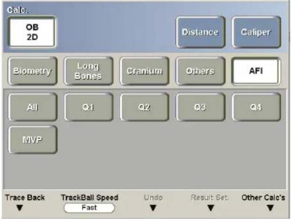
[Figure 5.5 OB Measurement Menu – AFI]
OB Measurements in Spectral Doppler Mode
Measurements can be obtained by tracing or marking points over spectral waveforms in Spectral Doppler images.
All of the measurement items are measured using the same method. The Volume Flow and Stenosis of each area can be obtained. For more information on measurement methods, refer to "Measuring Volume Flow."
| Menu | Sub | menu |
| Volume Flow | Trace – Auto, Limited, Manual Doppler Waveform Trace | |
| PSV | Velocity | |
| EDV | Velocity | |
| %StA | Calculation | |
| %StD | Calculation | |
| Vessel Area Area | ||
| Vessel Distance Distance | ||
| Umbilical Artery Same as | above Same as above | |
| MCA(Mid Cereb Artery) Same | as above Same as above | |
| Placenta Artery Same as | above Same as above | |
| Rt. / Lt. Uterine Artery Same | as above Same as above | |
| Renal Artery Same as | above Same as above | |
| Rt. / Lt. Fetal Carotids Same | as above Same as above | |
| Fetal Aorta Same as | above Same as above | |
| Ductus Venous Same as | above Same as above | |
Result
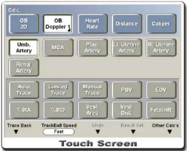
[Figure 5.6 OB Measurement Menu – Spectral Doppler Mode]
Fetal HR Calculation
This can be measured in M Mode or Spectral Doppler Mode.
■ Press the Fetal HR button to calculate the heart rate.
■ When the first baseline appears, place it at the starting position of the waveform and press the Set button on the control panel.
■ Turn the knob-button below HR Cycle on the touch screen to adjust the Cycle value. The Cycle value is used for calculating the average value of the heart rate; the result becomes more accurate for higher Cycle values.
■ When the second baseline appears, place it at the ending position of the waveform and press the Set button.
■ The result will be calculated and be displayed on the screen.
| Menu | Sub menu | Result |
| Fetal HR | Fetal Heart Rate | Time interval & No. of beats |
Fetal Echo Calculations
Before Obtaining Fetal Echo Calculations
For easier calculation processes, the method for calculating the volume of the fetus in M Mode can be configured.
For more information on other measurement menu items and setup methods, refer to 'Setting Measurements' in "Chapter 3. Settings" in this manual.
Measurement Items
This measurement examines the fetal heart. Measurement methods are the same as the basic measurement methods.
| 2D Mode | 2D Echo, CTAR (Cardio-Thorax Area Ratio) |
| M Mode | Fetal M Mode |
| PW Spectral Doppler Mode | MPA (Main Pulmonary Artery), Duct.Art (Ductus Arteriosus), IVC (Inferior Vena Cava), Duct.Vein (Ductus Venosus), Ascending Aorta, Descending Aorta, MV Inflow, MV Regurg, TV Inflow, TV Regurg, PLI (Preload Index) |
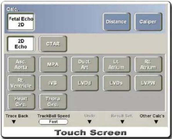
[Figure 5.7 Fetal Echo Measurement Menu]
Fetal Echo Measurements in 2D Mode
- Press the Manual button on the control panel and the fetal echo measurement menu will appear on the touch screen.
- Select the menu to measure, and a cursor appears on the screen.
- Use the Trackball and the Set button on the control panel to take measurements.
The measurement methods of each menu are shown in the table below.
| Menu | Sub menu | Input Meas. |
| 2D Echo | Asc. Aorta (Ascending Aorta) Distance | |
| MPA (Main Pulmonary Artery) Distance | ||
| Duct. Art (Ductus Arteriosus) Distance | ||
| Left Atrium Distance | ||
| Right Atrium Distance | ||
| Right Ventricle Distance | ||
| Inter Ventricular Septum Distance | ||
| Lt. Ventricle Dia.(Diastole) | Distance | |
| Lt. Ventricle Sys.(Systole) Distance | ||
| LVPW (Left Ventricle Posterior Wall) Distance | ||
| Heart Circ. (Circumference) | Circ/Area | |
| Thoracic Circ. (Circumference) Circ/Area | ||
| CTAR (Cardio-Thorax Area Ratio) | All (Distance) | |
| ThAPD (Thorax Anteroposterior Diameter) Distance | ||
| ThTD (Thorax Transverse Diameter) | Distance | |
| HAPD (Heart AP Diameter) | Distance | |
| HTD (Heart Transverse Diameter) | Distance | |
| All (Area) | ||
| ThA (Thorax Area) Area | ||
| HrtA (Heart Area) | Area | |
| CTAR (A) (Cardio-Thorax Area Ratio by Area) | Area |
■ Asc. Aorta (Ascending Aorta), MPA (Main Pulmonary Artery), Duct. Art (Ductus Arteriosus), Lt. Atrium (Left Atrium), Rt. Atrium (Right Atrium), Rt. Ventricle (Right Ventricle), IVS (Inter Ventricular Septum), LVDd (Left Ventricle Diameter Diastole), LVDs (Left Ventricle Diameter Systole), and LVPW (Left Ventricle Posterior Wall) use distance measuring methods.
■ Heart Circ. (Heart Circumference), and Thora Circ. (Thoracic Circumference) use Circ/Area measuring methods.
■ The CTAR menu measures and compares the size of the fetal chest and heart. You can obtain the comparison values by obtaining the Thorax AP Diameter, Thorax Transverse Diameter, Heart AP Diameter, Heart Transverse Diameter values.
Fetal Echo Measurements in M Mode
- Press the Manual button on the control panel and the fetal echo measurement menu will appear on the touch screen.
- Select the menu to measure, and a cursor appears on the screen.
- Use the Trackball and the Set button on the control panel to take measurements. The user can measure all items in one instance or select and measure the specific items in M Mode.
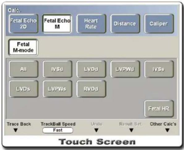
[Figure 5.8 Fetal Echo Measurement Menu – M Mode]
The table below shows measurement methods for menu items.
| Menu | Sub menu | Input Meas. |
| Fetal M Mode | IVSd (Inter Ventricular Septal Thickness Diastolic) | Distance (Thickness) |
| LVDd (Left Ventricle Diameter Diastolic) | Distance (Thickness) | |
| LVPWd (Left Ventricle Posterior Wall Dimension Diastolic) | Distance (Thickness) | |
| IVSs (Inter Ventricular Septal Thickness Systolic) | Distance (Thickness) | |
| LVDs (Left Ventricle Diameter Systolic) | Distance (Thickness) | |
| LVPWs (Left Ventricle Posterior Wall Dimension Systolic) | Distance (Thickness) | |
| RVDd (Right Ventricle Diameter Diastolic) | Distance (Thickness) | |
| All (IVSd, LVDd, LVPWd, IVSs, LVDs, LVPWs) | Same as above |
■ The sub-menus of Fetal M-mode are measured as shown below.
- IVSd and IVSs measure AIVS and PIVS at the diastolic and systolic phases respectively.
-
LVDd and LVDs measure ENDO at the diastolic and systolic phases respectively.
-
LVPWd and LVPWs measure EPI at the diastolic and systolic phases respectively.
- AIVS: Anterior Interventricular Septum
PIVS: Posterior Interventricular Septum
ENDO: End cardinal Surface of Left Ventricular Wall
EPI: Epicardial Surface of Left Ventricular Wall - RVDd is measured in the same way as in LVDd.
Fetal Echo Measurements in Spectral Doppler Mode
- Press the Manual button on the control panel and the fetal echo measurement menu will appear on the touch screen.
- Select the menu to measure, and a cursor appears on the screen.
- Use the Trackball and the Set button on the control panel to take measurements.
- There are four measurement methods to measure MPA, Duct.Art, IVC, Duct.Vein, Asc.Aorta, and Dsc.Aorta: Auto Trace, Limited Trace, Manual Trace, and Measurement Each Item One by One.
The table below shows measurement methods for menu items.
| Menu | Sub menu | Input Meas. |
| MPA (Main Pulmonary Artery) | Trace – Auto, Limited, Manual | Doppler Waveform Trace |
| PSV Velocity | ||
| EDV Velocity | ||
| Ductua Arteriosus | Same as above | Same as above |
| Inferior Vena Cava | Same as above | Same as above |
| Ductus Venosus | Same as above | Same as above |
| Ascending Aorta | Same as above | Same as above |
| Descending Aorta | Same as above | Same as above |
| MV (Mitral Valve) Inflow | Peak E Velocity | |
| Peak A Velocity | ||
| MV (Mitral Valve) Regurgitation | Velocity | Velocity |
| Tricuspid Valve Inflow | Peak E Velocity | |
| Peak A Velocity | ||
| Tricuspid Valve Regurgitation | Velocity | Velocity |
| PLI (PreLoad Index) | Systolic Flow | Velocity |
| Diastolic Flow | Velocity | |
| Atrial Reversal Flow | Velocity |
■ Select Auto Trace to trace the image and calculate the measurement values automatically.
■ Select Limited Trace, and the baseline will appear on the image. Set the start and end
points of the spectral waveform using the baseline, and the measurement value is calculated automatically. The user can reposition the baseline by pressing the Change button.
■ Select Manual Trace, and a cursor will appear on the image. Trace the Doppler waveform, and the measurement value is calculated automatically.
■ The user can select and measure each item manually.
- PSV measures the Peak Systolic velocity.
- EDV measures the End Diastolic velocity.
- Peak E measures the Ventricular Systolic peak.
- Peak A measures the Atrial Systolic peak.
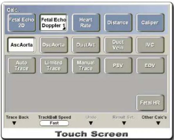
[Figure 5.9 Fetal Echo Measurement Menu – Spectral Doppler Mode]
Fetal HR Calculation
This can be measured in M Mode or Spectral Doppler Mode.
■ Press the Fetal HR button to calculate the heart rate.
■ When the first baseline appears, place it at the starting position of the waveform and press the Set button on the control panel.
■ Turn the knob-button below HR Cycle on the touch screen to adjust the Cycle value. The Cycle value is used for calculating the average value of the heart rate; the result becomes more accurate for higher Cycle values.
■ When the second baseline appears, place it at the ending position of the waveform and press the Set button.
■ The result will be calculated and be displayed on the screen.
| Menu | Sub menu | Result |
| Fetal HR | Fetal Heart Rate | Time interval & No. of beats |
GYN Calculations
Before Obtaining GYN Calculations
Enter the information required for GYN diagnosis in the Patient Information screen. Basic Information for gynecology includes GRAVIDA, PARA, ABORTA, Exp. Ovul. and Day of Cycle.
Measurement Items
Measurement items include Uterus, Lt. Ovary, Rt. Ovary, Lt. Follicles, Rt. Follicles, Lt. Ovarian A., Rt. Ovarian A., Lt. Uterine Artery, Rt. Uterine Artery, Cyst, and Mass. Lt. Ovarian A., Rt. Ovarian A., Lt. Uterine Artery, Rt. Uterine Artery items are measured in Spectral Doppler Mode and other items are measured in 2D Mode.
Measurement methods are the same as the basic measurement methods.
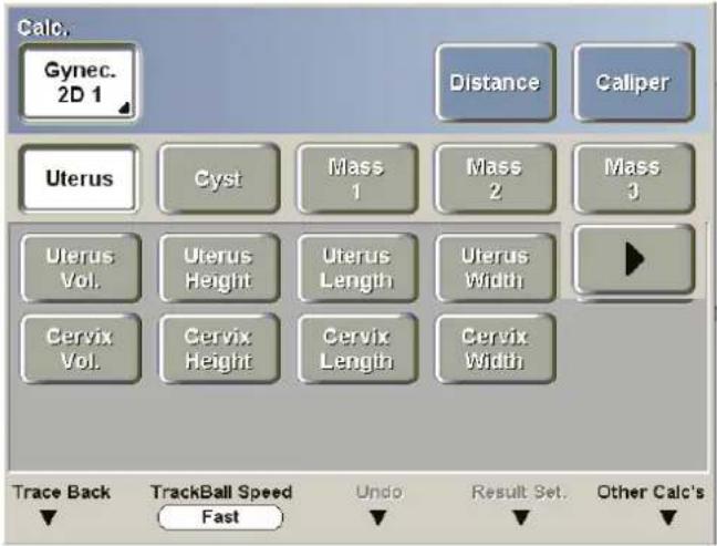
[Figure 5.10 GYN Measurement Menu]
GYN Measurements
- Press the Manual button on the control panel and the gynecology measurement menu will appear on the touch screen.
- Select the menu to measure, and a cursor appears on the screen.
- Use the Trackball and the Set button on the control panel to take measurements.
Measurements can be obtained by tracing or marking points over spectral waveforms in Spectral Doppler images.
The user can obtain various values such as PSV, EDV, Vmean, Gmean, Gpeak, S/D, PI and RI from the spectral waveform. For more information on measurement methods, refer to "Measuring Doppler Spectrum".
The table below shows measurement methods for menu items.
| Menu Sub menu Input Meas. | ||
| Uterus | Uterus Length, Height, Width 3 Distance Volume Meas. | |
| Uterus Volume 3 Distance Volume Meas. | ||
| Endo. Thickness Distance | ||
| Cervix Length, Height, Width 3 Distance Volume Meas. | ||
| Cervix Volume 3 Distance Volume Meas. | ||
| Cyst | Length, Height, Width 3 Distance Volume Meas. | |
| Volume 3 Distance Volume Meas. | ||
| Right / Left Ovary Same as above Same as above | ||
| Right / Left Follicle Required for One to 12 Follicles Distance | ||
| Mass 1/2/3 | Length, Height, Width 3 Distance Volume Meas. | |
| Trace – Auto, Limited, Manual Doppler | Waveform Trace | |
| PSV | Velocity | |
| EDV | Velocity | |
| Endometrial Polyp Same as above Same as above | ||
| Right / Left Ovarian Tumor | Same as above Same as above | |
| Uterine Tumor 1/2/3 | Same as above Same as above | |
| Cervical Tumor Same as above Same as above | ||
| Ectopic Pregnancy | Same as above Same as above | |
| Right / Left Ovarian Artery | Trace – Auto, Limited, Manual Doppler | Waveform Trace |
| PSV | Velocity | |
| EDV | Velocity | |
| Right / Left Uterine Artery | Same as above Same as above | |
| Pericystic Flow | Same as above Same as above | |
| Endometrial Flow | Same as above Same as above | |
When the Long axis image and Transverse axis image of the uterus are needed for measuring volume, press the Freeze button on the control panel to return to scan mode and obtain an image from another perspective.
Urology Calculations
Before Obtaining Urology Calculations
For easier calculation processes, set Volume Method for use in calculations.
There are four Volume Methods, and the user can set the factor value for formulae that require factor values.
For more information on other measurement menu items and setup methods, refer to 'Setting Measurements' in "Chapter 3. Settings" in this manual.
Measurement Items
■ Measures BLVOL (Bladder Volume), WGVOL (Whole Gland Prostate Volume), TZVOL (Transitional Zone Prostate Volume), Residual Volume, Lt. Kidney Vol. and Rt. Kidney Vol. in 2D Mode.
Also measures Vessel Area and Vessel Distance for calculating Volume Flow.
■ Residual Pre/Post and PSA Density Volume can be measured.
■ Measurement items in Spectral Doppler Mode are divided into Auto Trace, Limited Trace and Manual Trace depending on the measurement method.
■ Measurement methods are the same as the basic measurement methods.
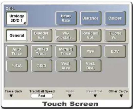
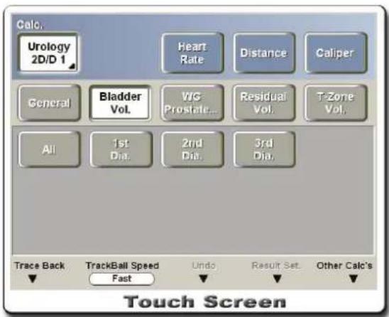
[Figure 5.11 Urology Measurement Menu]
Volume Measurements
- Press the Manual button on the control panel and the urology measurement menu will appear on the touch screen.
- Select the required measurement item and menu, and a cursor appears on the screen.
- Use the Trackball and the Set button on the control panel to take measurements.
There are two ways to measure in each menu: one is measuring the item values from one image, and the other is measuring the item values from several images. The measurement
methods of each menu vary with the Volume Method set at the Setting screen.
If 3Distance or 3Distance * Factor is set in Urology Setup, three diameter values can be obtained in order.
| Menu | Sub menu | Result |
| Bladder Volume | All | |
| 1st Dia. (Diameter) Distance | ||
| 2nd Dia. (Diameter) Distance | ||
| 3rd Dia (Diameter) Distance | ||
| Whole Gland Prostate Volume | All | |
| 1st Dia. (Diameter) Distance | ||
| 2nd Dia. (Diameter) Distance | ||
| 3rd Dia (Diameter) Distance | ||
| Residual Volume | Pre All | |
| Pre 1st Dia. (Diameter) Distance | ||
| Pre 2nd Dia. (Diameter) Distance | ||
| Pre 3rd Dia (Diameter) Distance | ||
| Post All | ||
| Post 1st Dia. (Diameter) Distance | ||
| Post 2nd Dia. (Diameter) Distance | ||
| Post 3rd Dia (Diameter) Distance | ||
| Transitional Zone Prostate Volume | All | |
| 1st Dia. (Diameter) Distance | ||
| 2nd Dia. (Diameter) Distance | ||
| 3rd Dia (Diameter) Distance | ||
| Left (Right) Kidney Volume | All | |
| 1st Dia. (Diameter) Distance | ||
| 2nd Dia. (Diameter) Distance | ||
| 3rd Dia (Diameter) Distance | ||
| Renal Pelvis Distance |
■ If Ellipsoid is set in Urology Setup, Main Diameter and Beside Diameter values can be obtained in order.
| Menu | Sub menu | Result |
| Bladder Volume | All | |
| Main Dia. (Diameter) Distance | ||
| Beside Dia. (Diameter) Distance | ||
| Whole Gland Prostate Volume | All | |
| Main Dia. (Diameter) Distance | ||
| Beside Dia. (Diameter) Distance | ||
| Residual Volume | Pre All | |
| Pre Main Dia. (Diameter) Distance | ||
| Pre Beside Dia. (Diameter) Distance | ||
| Post All | ||
| Post Main Dia. (Diameter) Distance | ||
| Post Beside Dia. (Diameter) Distance | ||
| Transitional Zone Prostate Volume | All | |
| Main Dia. (Diameter) Distance | ||
| Beside Dia. (Diameter) Distance | ||
| Left (Right) Kidney Volume | All | |
| Main Dia. (Diameter) Distance | ||
| Beside Dia. (Diameter) Distance | ||
| Renal Pelvis Distance |
If Sum of 20 Disks is set in Urology Setup, the user can calculate the measurement values below by using the Trackball and the Set button to measure the prostate axis after measuring the prostate circumference.
| Menu | Sub menu | Result |
| Bladder Volume | Bladder Vol. | 20 Diameter & Area |
| Whole Gland Prostate Volume | Whole Gland Prostate Vol. | 20 Diameter & Area |
| Residual Volume | Pre Vol. | 20 Diameter & Area |
| Post Vol. | 20 Diameter & Area | |
| Transitional Zone Prostate Volume | Transitional Zone Prostate Vol. | 20 Diameter & Area |
| Left (Right) Kidney Volume | Left (Right) Kidney Vol. | 20 Diameter & Area |
| Renal Pelvis | Distance |
Volume Flow Measurements
The Volume Flow menu is shown below. For more information, refer to “Measuring Volume Flow.”
| Menu | Sub menu | Result |
| Volume Flow | Trace – Auto, Limited, Manual | Doppler Waveform Trace |
| PSV | Velocity | |
| EDV | Velocity | |
| %StA | Calculation | |
| %StD | Calculation | |
| Vessel Area | Area | |
| Vessel Distance | Distance |
Measurements in Reports
Items such as Predicted PSA by WG, Predicted PSA by T-Zone, and Prostate Spec. Antigen Density can be measured by entering PSA (Prostate Specific Antigen). PSA and other values can be entered at "urology measurement settings" also.
Each measurement item can be measured while editing a report by pressing the Edit button at a urology report.
Measuring Predicted PSA by WG
In the Predicted PSA by WG menu, enter the "PSA Correction factor" value.
■ PREDPSA will be calculated and be displayed on the screen.
■ PREDPSA = PSA correction factor × WGVOL
| Predicted PSA by WG | 1 | 2 | 3 | Avg. |
| PSA Correction factor | ||||
| PREDPSA |
Measuring Predicted PSA by T-Zone
In the Predicted PSA by T-Zone menu, enter the "PSA Correction factor" value.
■ TZPSA will be calculated and be displayed on the screen.
■ TZPSA = PSA correction factor × TZVOL
| Predicted PSA by T-Zone | 1 | 2 | 3 | Avg. |
| PSA Correction factor | ||||
| TZPSA |
Measuring Prostate Spec. Antigen Density
In the Prostate Spec. Antigen Density menu, enter the "PSA" value.
■ PSAD will be calculated and be displayed on the screen.
■ PSAD = PSA / WGVOL
| Prostate Spec. Antigen | 1 | 2 | 3 | Avg. |
| PSA | ng/ml | |||
| PSAD |
Vascular Calculations
Before Obtaining Vascular Calculations
For easier calculation processes, you can also set the Peak Velocity used in calculating 'A/B Ratio' and 'ICA/CCA Ratio'.
For more information on other measurement menu items and setup methods, refer to 'Setting Measurements' in "Chapter 3. Settings" in this manual.
Measurement Items
The vascular measure package contains measurement items for each measurement area.
Vascular / Carotid Artery Measurement Menu
The Carotid Artery vascular measurement menu contains Subclavian, Proximal CCA, Mid CCA, Distal CCA, Bulb, Proximal ICA, Mid ICA, Distal ICA, ECA, Vertebral, Volume Flow, Heart Rate, etc.
Lower Extremities Measurement Menu
The Lower Extremities vascular measurement menu provides a measure package that examines CIA (common iliac artery), IIA (internal iliac artery), EIA (external iliac artery), CFA (common femoral artery), SFA (superficial femoral artery), DFA (deep femoral artery), POP A (poplitieal artery), ATA (anterior tibial artery), PTA (posterior tibial artery), PA (peroneal artery), DPA (dorsalis pedis artery), General, Volume Flow, Heart Rate, etc.
Upper Extremities Measurement Menu
The Upper Extremities vascular measurement menu provides a measure package that examines Subclavian, Cephalic, Auxiliary, Brachial, Basilic, Radial, Ulnar, SPA, General, Volume Flow, Heart Rate, etc.
Varicose Measurement Menu
The Varicose vascular measurement menu provides a measure package that examines FV (Femoral vein), GSV (Great saphenous vein), POPV (poplitiear vein), General, SSV (Small saphenous vein), etc.
All vascular measurements are taken using the same methods, which are identical to the basic measurement methods. It is convenient to calculate each measurement value on the Spectral Doppler image.
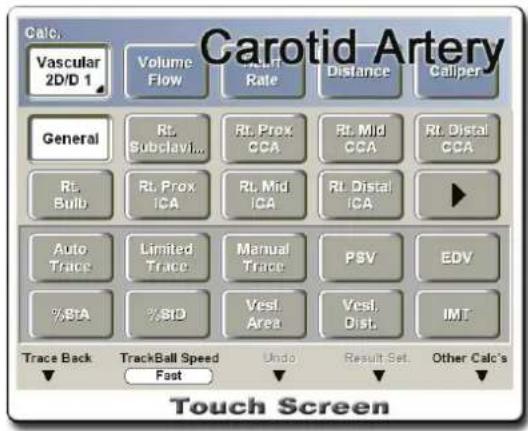
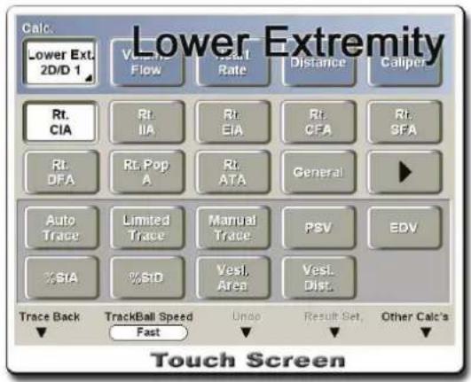
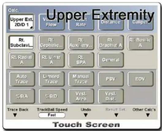
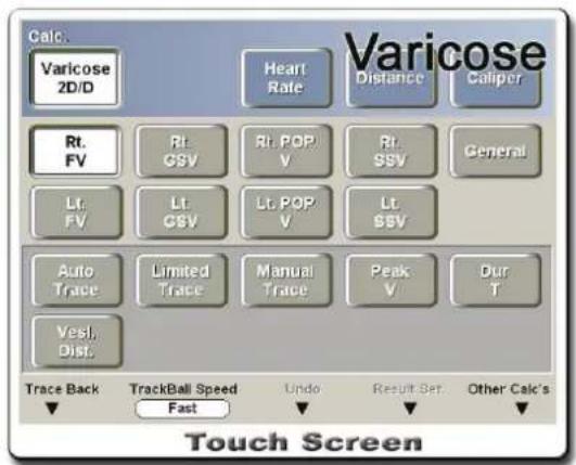
[Figure 5.12 Vascular Measurement Menu]
Vascular Measurements
- Press the Manual button on the control panel and the vascular measurement menu will appear on the touch screen.
- Select the menu to measure and a cursor appears on the screen.
- Use the Trackball and the Set button on the control panel to take measurements.
The table below shows measurement methods for menu items.
| Menu Sub menu Input Meas. | |||
| Vascular(Carotid Artery) | General | Trace –Auto, Limited, Manual Doppler Waveform Trace | |
| PSV | Velocity | ||
| EDV | Velocity | ||
| %StA | Calculation | ||
| %StD | Calculation | ||
| Vessel Area Area | |||
| Vessel Distance Distance | |||
| IMT (Intima Media Thickness) | Distance | ||
| Menu Sub menu | Input Meas. | ||
| Vascular(Carotid Artery) | Rt./Lt. Subclavian | Same as above Same as above | |
| Rt./Lt. Prox CCA(Proximal Common Carotid Artery) | Same as above Same as above | ||
| Rt./Lt. Mid CCA | Same as above Same as above | ||
| Rt./Lt. Distal CCA | Same as above Same as above | ||
| Rt./Lt. Bulb | Same as above Same as above | ||
| Rt./Lt. Prox ICA(Proximal Internal Carotid Artery) | Same as above Same as above | ||
| Rt./Lt. Mid ICA | Same as above Same as above | ||
| Rt./Lt. Distal ICA | Same as above Same as above | ||
| Rt./Lt. ECA(External Carotid Artery) | Same as above Same as above | ||
| Rt./Lt. Vertebral | Same as above Same as above | ||
| Lower Extremity | Rt./Lt. CIA (Common Iliac Artery | Same as above Same as above | |
| Rt./Lt. IIA (Internal IA) | Same as above Same as above | ||
| Rt./Lt. EIA (External IA) | Same as above Same as above | ||
| Rt./Lt. CFA(Common Femoral Artery) | Same as above Same as above | ||
| Rt./Lt. SFA (Superficial FA) | Same as above Same as above | ||
| Rt./Lt. DFA (Deep FA) | Same as above Same as above | ||
| Rt./Lt. POPA (Popliteal Artery) | Same as above Same as above | ||
| Rt./Lt. ATA (Anterior Tibial Artery) | Same as above Same as above | ||
| Rt./Lt. PTA (Posterior Tibial Artery) | Same as above Same as above | ||
| Rt./Lt. Peroneal A(Peroneal Artery) | Same as above Same as above | ||
| Rt./Lt. DPA (Dorsalis Pedis Artery) | Same as above Same as above | ||
| General | Same as above Same as above | ||
| Upper Extremity | Rt./Lt. Subclavian A | Same as above Same as above | |
| Rt./Lt. Cephalic A | Same as above Same as above | ||
| Rt./Lt. Auxiliary A | Same as above Same as above | ||
| Rt./Lt. Brachial A | Same as above Same as above | ||
| Rt./Lt. Basilic A | Same as above Same as above | ||
| Rt./Lt. Radial A | Same as above Same as above | ||
| Rt./Lt. Ulnar A | Same as above Same as above | ||
| Rt./Lt. SPA(Superficial Palmar Arches)Menu Sub menu Input Meas. | Same as above Same as above | ||
| General | Same as above Same as above | ||
| Varicose | Rt./Lt. FV (Femoral Vein) | Trace –Auto, Limited, Manual Doppler Waveform Trace | |
| Peak V Velocity | |||
| Dur T Time | |||
| Vessel Distance Distance | |||
| Rt./Lt. GSV (Great Saphenous Vein) | Same as above Same as above | ||
| Rt./Lt. POPV (Poplitiear Vein) Same as above Same as above | |||
| Rt./Lt. SSV(Small Saphenous Vein) | Same as above Same as above | ||
| General Same as above Same as above | |||
■ The user can obtain various values such as PSV, EDV, Vmean, Gmean, Gpeak, S/D, PI and RI from the spectral waveform in a Spectral Doppler image. For more information on measurement methods, refer to "Measuring Doppler Spectrum".
■ The Volume Flow and Stenosis % values for each measurement area can be obtained. For more information on measurement methods, refer to "Measuring Volume Flow" and "Measuring Stenosis%." The user can obtain the Volume Flow value using the TAM (Time Average Mean Velocity) value obtained from the spectral waveform.
Cardiac Calculations
Before Obtaining Cardiac Calculations
Enter the information required for cardiac diagnosis in the Patient Information screen. Basic Information for cardiac includes Height, Weight and HR (Heart Rate). When the patient's height and weight are entered, BSA (Body Surface Area) is automatically calculated and displayed.
For more information on the patient information menu items and method for entering patient information, refer to "Entering Patient Information" in "Chapter 3 Settings" in this manual.
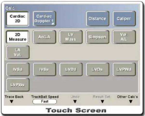
[Figure 5.13 Cardiac Measurement Menu]
Measurement Items
Measurement methods are the same as the basic measurement methods.
| 2D Mode | 2D Measure, Ao/LA (Aorta/Left Atrium), LV (Left Ventricle) mass, Simpson, Vol A/L (Area Length), LA (Left Atrial) Volume |
| Color Doppler Mode | AoV (Aortic Valve) Regurgitation, MV (Mitral Valve) Regurgitation, TV (Tricuspid Valve) Regurgitation, PV (Pulmonary Valve) Regurgitation |
| M Mode | Ao/LA (Aorta/Left Atrium), Lt. (Left) Ventricle, MV (Mitral Valve), Heart Rate |
| Spectral Doppler Mode | AoV (Aortic Valve) Systolic, AoV (Aortic Valve) Regurgitation, LVOT Doppler, MV (Mitral Valve) Inflow, MV (Mitral Valve) Regurgitation, TV (Tri - cuspid Valve) Inflow, TV (Tricuspid Valve) Regurgitation, PV (Pulmonary Valve) Systolic, PV (Pulmonary Valve) Regurgitation, Tei Index, Tissue Doppler, Pulmonary Veins, Qp:Qs, Hepatic Vein, Heart Rate |
Cardiac Measurements in 2D Mode
- Press the Manual button on the control panel and the cardiac measurement menu will appear on the touch screen.
- Select the menu to measure, and a cursor appears on the screen.
- Use the Trackball and the Set button on the control panel to take measurements.
The table below shows measurement methods for menu items.
| Menu Sub | menu Input Meas. | |
| 2D Measure | IVSd (Inter Ventricular Septal thickness Diastolic) Distance (Thickness) | |
| IVSs (Inter Ventricular Septal thickness Systolic) Distance (Thickness) | ||
| LVDd (Left Ventricle Diameter Diastolic) Distance (Thickness) | ||
| LVDs (Left Ventricle Diameter Systolic) Distance (Thickness) | ||
| LVPWd (Left Ventricle Posterior Wall Dimension Diastolic) Distance (Thickness) | ||
| LVPWs (Left Ventricle Posterior Wall Dimension Systolic) Distance (Thickness) | ||
| Ao/LA (Aorta/Left Atrium) | Ao-LA (Aorta-Left Atrium) Length | |
| LVOT Dia (Left Ventricle Outflow Tract Diameter) Length | ||
| Ao Root Dia (Aorta Root Diameter) Length | ||
| LA Dia (Left Atrium Dimension) Length | ||
| LV (Left Ventricle) Mass | Epi. Area (Epicardial) Area | |
| Endo. Area (Endocardial) | Area | |
| LV Length (Left Ventricle Length) | Distance | |
| Simpson | A4C Diastole | 20 Diameter & Length |
| A4C Systole | 20 Diameter & Length | |
| A2C Diastole | 20 Diameter & Length | |
| A2C Systole | 20 Diameter & Length | |
| Vol. A/L (Volume Area/Length) | LV Vol. Diastole | Area & Length |
| LV Vol. Systole | Area & Length | |
| LA (Left Atrium) Vol. | A-P | Distance |
| S-I | Distance | |
| M-L | Distance |
[2D Measure]
Take measurements for 2D Measure sub-menu items.
- IVSd and IVSs measure AIVS and PIVS at the diastolic and systolic phases respectively.
- LVDd and LVDs measure ENDO at the diastolic and systolic phases respectively.
- LVPWd and LVPWs measure EPI at the diastolic and systolic phases respectively.
NOTE
AIVS: Anterior Interventricular Septum
PIVS: Posterior Interventricular Septum
ENDO: Endocardinal Surface of Left Ventricular Wall
EPI: Epicardial Surface of Left Ventricular Wall
[Ao/LA]
The sub-menus of Ao/LA are measured as shown below.
- The Ao-LA menu measures Ao Root Dia and LA Dia.
- LVOT Dia measures the point of Aortic Valve Annulus.
- Ao Root Dia measures the distance between the Anterior Aortic Wall and Posterior Aortic Wall.
- LA Dia measures the distance between the Posterior Aortic Wall and Left Arterial Wall.
[LV Mass]
When measuring LV Mass, the user can obtain the images at different angles needed for the sub-menus by using the Freeze button on the control panel. Dual Mode is useful for measuring LV Mass as it shows two images simultaneously.
- LV (Left Ventricle) is used only when measuring mass. It can be measured only in the case of the diastole of Left Ventricle.
- Myocardial thickness = SQRT(Dia.A / Pi) - SQRT(Sys.A / Pi)
[Simpson] and [Vol. A/L]
Measures the cardiac circumference and axis.
- 20 Diameter & Length: Trace the cardiac circumference when the cursor for tracing area appears, and draw the cardiac axis when the cursor for measuring length appears. The heart is divided in 20 sections from the axis for calculation.
- [LA Vol.]
Measures the left arterial volume. The sub-menus Diam1, Diam2 and Diam3 measure anterior-posterior, inferior-superior and lateral-medial distances for the left atrium, respectively.
Cardiac Measurements in M Mode
- Press the Manual button on the control panel and the cardiac measurement menu will appear on the touch screen.
- Select the menu to measure, and a cursor appears on the screen.
- Use the Trackball and the Set button on the control panel to take measurements. The user can measure all items in one instance or select and measure the specific items in M Mode.
The table below shows measurement methods for menu items.
| Menu Sub | menu Input Meas. | |
| Ao/LA(Aorta/Left Atrium) | Ao Root Dia (Aortic Root Dimension) Distance | |
| AoV Cusp Sep. (Aortic Valve Cusp Separation) Distance | ||
| LA Dia (Left Atrial Dimension) Distance | ||
| LV PET (Left Ventricle Pre Eject Time) Time | ||
| LV ET (Left Ventricle Eject Time) Time | ||
| All Same as above | ||
| Lt. Ventricle | IVSd (Inter Ventricular Septal thickness Diastolic) Distance (Thickness) | |
| LVDd (Left Ventricle Diameter Diastolic) Distance (Thickness) | ||
| LVPWd (Left Ventricle Posterior Wall Dimension Diastolic) Distance (Thickness) | ||
| IVSs (Inter Ventricular Septal thickness Systolic) Distance (Thickness) | ||
| LVDs (Left Ventricle Diameter Systolic) Distance (Thickness) | ||
| LVPWs (Left Ventricle Posterior Wall Dimension Systolic) Distance (Thickness) | ||
| RVDd (Right Ventricle Diameter Diastolic) | Distance (Thickness) | |
| All Same as above | ||
| MV (Mitral Valve) | A-C Interval Time interval | |
| D-E (D – E Excursion) | Distance | |
| E-F Slope | Slope (Velocity) | |
| EPSS (E Point Septal Separation) | Distance (Thickness) | |
| All Points | Same as above | |
| Heart Rate | Heart Rate | Time interval & No. of beats |
[Ao/LA]
- Ao Root Dia measures the distance between the Anterior Aortic Wall and Posterior Aortic Wall.
- AoV Cusp Sep. measures the distance between the Coronary Cusp and Non Coronary Cusp.
- LA Dia measures the distance between the Posterior Aortic Wall and Left Arterial Wall.
- LV PET measures the distance between the ECG's Q Wave and Aortic Valve Opening.
- LV ET measures the distance between the Aortic Valve Opening and Aortic Valve Closing.
[Lt. Ventricle]
- The Lt. Ventricle sub-menus are measured in the same way as in 2D Measure.
- RVDd is measured in the same way as in LVDd.
[MV]
- A-C Interval calculates the time duration by measuring the distance between the A point and C point in the Mitral Valve measurement screen.
- D-E measures the distance between the E point of the Anterior Mitral Valve and the D
point of the Mitral Valve Opening.
- E-F Slope calculates the velocity by measuring the distance between the E point and F point in the Mitral Valve measurement screen.
- EPSS measures the distance between the E point in the Mitral Valve and Posterior Interventricular Septum. The user can measure only in the upper direction of the E point, and only in the lower direction in Apex.
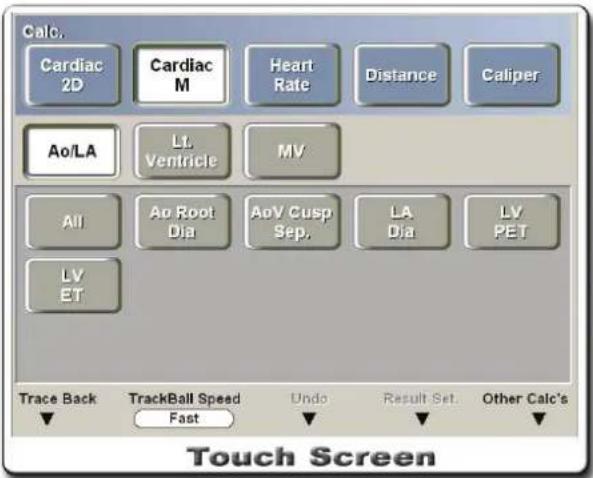
[Figure 5.14 Cardiac Measurement Menu – M Mode]
Cardiac Measurements in Color Doppler Mode
- Press the Manual button on the control panel and the cardiac measurement menu will appear on the touch screen.
- Select the menu to measure, and a cursor appears on the screen.
- Use the Trackball and the Set button on the control panel to take measurements.
The table below shows measurement methods for menu items.
| Menu Sub menu Input Meas. | ||
| AoV (Aortic Valve) Regurg | PISA (Proximal Isovelocity Surface Area) Radius Distance | |
| PISA-Alias Vel. Velocity | ||
| MV (Mitral Valve) Regurg | PISA-Radius | Distance |
| PISA-Alias Vel. Velocity | ||
| TV (Tricuspid Valve) Regurg | PISA Radius Distance | |
| PISA-Alias Vel. Velocity | ||
| PV (Pulmonary Valve) Regurg | PISA Radius Distance | |
| PISA-Alias Vel. Velocity | ||
[PISA-Radius]
Measures the distance between Valve and First Isovelocity.
[PISA-Alias Vel.]
Multiplies the result value of PISA-Radius by the regurgitated peak velocity.
The velocity value is needed to measure the items above. So select Velocity or Vel + Var as the color display. For more information on settings, refer to "Changing Color Image Format" in "Chapter 4. Diagnosis Modes" in this manual.
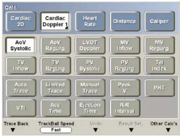
[Figure 5.15 Cardiac Measurement Menu – Color Doppler Mode]
Cardiac Measurements in Spectral Doppler Mode
- Press the Manual button on the control panel and the cardiac measurement menu will appear on the touch screen.
- Select the menu to measure, and a cursor appears on the screen.
- Use the Trackball and the Set button on the control panel to take measurements.
The table below shows measurement methods for menu items.
| Menu Sub menu Input Meas. | ||
| AoV (Aortic Valve) Systolic | Trace – Auto, Limited, Manual Doppler Waveform Trace | |
| Peak V (Velocity) Velocity | ||
| PHT (Pressure Half Time) Time or Calculated from Trace | ||
| VTI (Velocity Time Integral) Calculated | ||
| Acc (Acceleration) Time Time or Calculated from Trace | ||
| Ejection (Ejection) Time Time | ||
| R-R Interval (Rate-Rate Interval) Time Interval & No. of beats | ||
| AoV (Aortic Valve) Regurg | Trace –Limited, Manual Doppler Waveform Trace | |
| Peak V (Velocity) Velocity | ||
| VTI (Velocity Time Integral) Calculated | ||
| PHT (Pressure Half Time) Time or Calculated from Trace | ||
| LVOT (Left Ventricular Outflow Tract) Doppler | Trace – Auto, Limited, Manual Doppler Waveform Trace | |
| Peak V (Velocity) Velocity | ||
| VTI (Velocity Time Integral) Calculated | ||
| Dia (Diameter) Distance | ||
| MV (Mitral Valve) Inflow | Trace -Limited, Manual Doppler Waveform Trace | |
| Peak E Velocity | ||
| Peak A Velocity | ||
| E (Peak) - DT (Dec Time) - A (Peak) Velocity & Time | ||
| Acc (Acceleration Time) Time or Calculated from Trace | ||
| Dec (Deceleration Time) Time or Calculated from Trace | ||
| PHT (Pressure Half Time) Time or Calculated from Trace | ||
| IVRT (IsoVolumic Relaxation Time) Time | ||
| R-R Interval (Rate-Rate Interval) Time Interval & No. of beats | ||
| MV (Mitral Valve) Regurg | Trace - Auto, Limited, Manual Doppler Waveform Trace | |
| Peak V (Velocity) Velocity | ||
| VTI (Velocity Time Integral) Calculated | ||
| TV (Tricuspid Valve) Inflow | Trace -Limited, Manual Doppler Waveform Trace | |
| Peak E Velocity | ||
| Peak A Velocity | ||
| Acc (Acceleration Time) Time or Calculated from Trace | ||
| Dec (Deceleration Time) Time or Calculated from Trace | ||
| PHT (Pressure Half Time) Time or Calculated from Trace | ||
| R-R Interval (Rate-Rate Interval) Time Interval & No. of beats | ||
| TV (Tricuspid Valve) Regurg | Trace - Auto, Limited, Manual Doppler Waveform Trace | |
| Peak V (Velocity) Velocity | ||
| VTI (Velocity Time Integral) Calculated | ||
| PV Systolic | Trace - Auto, Limited, Manual Doppler Waveform Trace | |
| Peak V (Velocity) Velocity | ||
| PHT (Pressure Half Time) Time or Calculated from Trace | ||
| Acc (Acceleration Time) Time or Calculated from Trace | ||
| R-R Interval (Rate-Rate Interval) Time Interval & No. of beats | ||
| PV Regurg | Trace - Auto, Limited, Manual Doppler Waveform Trace | |
| Peak V (Velocity) Velocity | ||
| VTI (Velocity Time Integral) Calculated | ||
| PHT (Pressure Half Time) Time or Calculated from Trace | ||
| Tei Index | MCO | Time |
| Ejection Time Time | ||
| All | Time | |
| Tissue Doppler | Peak E' | Velocity |
| Tissue Doppler | Peak A' | Velocity |
| Peak S Velocity | ||
| Acc (Acceleration Time) Time or Calculated from Trace | ||
| Dec (Deceleration Time) Time or Calculated from Trace | ||
| IVCT (IsoVolume Contraction Time) Time or Calculated from Trace | ||
| IVRT (IsoVolume Relaxation Time) Time or Calculated from Trace | ||
| Plum. Veins(Pulmonary Veins) | Dias Vel. (Diastolic Velocity) Velocity | |
| Sys Vel. (Systolic Velocity) Velocity | ||
| A. Rev Vel. (Artery Reversal Velocity) Velocity | ||
| A. Rev Dur. (Artery Reversal Duration) Time | ||
| Qp:Qs | Sys. VTI ([Systemic] Flow Area Trace) Calculated | |
| Sys. HR ([Systemic] Heart Rate) Heart Rate | ||
| Sys. Dia ([Systemic] Outflow Tract Diameter) Diameter | ||
| Pulm. VTI ([Pulmonic] Flow Area Trace) Calculated | ||
| Pulm. HR ([Pulmonic] Heart Rate) Heart Rate | ||
| Pulm. Dia ([Pulmonic] Outflow Tract Diameter) Diameter | ||
| Hepatic Vein | All | Diastolic, Systolic, Reversal |
| Diastolic | Velocity | |
| Systolic | Velocity | |
| Reversal | Velocity | |
| Heart Rate | Heart Rate | Time interval & No. of beats |
NOTE The Auto Trace function is not provided in MV Inflow and TV Inflow.
■ There are four ways to measure LVOT Doppler, MV Inflow / MV Regurgitation, AoV Systolic / AoV Regurgitation, TV Inflow / TV Regurgitation, PV Systolic / PV Regurgitation: Auto Trace, Limited Trace, Manual Trace, Measurement Each Item One by One.
■ The user can obtain various values such as PSV, EDV, Vmean, Gmean, Gpeak, S/D, PI, RI, SV and CO. For more information on measurement methods, refer to "Measuring Doppler Spectrum".
■ Peak values, Acc Time, Dec Time, Ejection Time, VTI, PHT, R-R Interval, etc. are automatically measured by tracing the PW Spectral Doppler image. Each item can also be selectively measured.
- E-DT-A measures Peak E, Dec Time, and Peak A in one instance.
- Peak V: Measures the Higher Velocity value.
- Peak E: Measures the Ventricular Systolic peak.
- Peak A: Measures the Atrial Systolic peak.
- Acc Time measures the time duration when blood flow is accelerated and Dec Time measures the time duration when blood flow is decelerated.
- Ejection: Measures the time duration by measuring the distance between the Aortic Valve Opening and Aortic Valve Closing.
- VTI: Calculates the value using the formula of VTI = Sum of Vi (t after tracing
the Spectral Doppler image.
- PHT: Calculates Half-Time using the Pressure gradient value obtained between the E point of Valve and the baseline.
- R-R Interval: Measures the distance between consecutive R waves on the ECG.
■ [LVOT Doppler]
Measure Left Ventricular Outflow. Its sub-menu Dia measures the Aortic Valve Annulus point in the 2D image.
In the sub-menus of [Tei Index], [MCO] measures the mitral valve closed-open time, and [ET] measures the ejection time.
In the sub-menu of Tissue Doppler, Peak S measures the systolic peak, and IVCT and IVRT measure Isovolumic Contraction and Isovolumic Relaxation phases, respectively.
■ The sub-menus of Plum. Veins are measured as shown below:
- Dias Vel. and Sys Vel. measure the velocity at the diastole and systolic phases.
- A. Rev Vel. measures the Peak Velocity at Atrial Reversal.
- A. Rev Dur. measures the time duration by measuring the distance between the Mitral Valve Closing and the heart diastole phase.
■ The sub-menus of Qp:Qs are measured as shown below.
- Sys. VTI and Pulm. VTI measure the VTI by tracing LVOT Flow and RVOT Flow respectively.
- Sys. HR and Plum. HR measure the heart rate by measuring the diastole phase and systolic phase respectively in LVOT Flow and RVOT Flow.
- Sys. Dia and Plum. Dia measures the Outflow Tract distance in the 2D images of LVOT Flow and RVOT Flow, respectively.
■ Hepatic Vein is the menu used for measuring hepatic vein.
- Diastolic, Systolic and Reversal measure the peak velocity at diastolic phase, systolic phase, and reversal phase respectively.
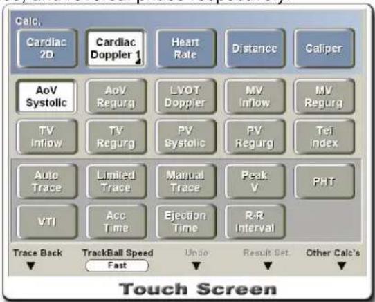
[Figure 5.16 Cardiac Measurement Menu – Spectral Doppler Mode]
Radiology Calculation
Measurement Items
Aorta, Celiac Artery, Hepatic Artery, Splenic Artery, Spleen Volume, SMA (Superior Mesenteric Artery), IMA (Inferior Mesenteric Artery), IVC (Inferior Vena Cave), Lt. Kidney Volume, Rt. Kidney Volume, Lt. Renal Artery, Rt. Renal Artery, Lt. Arcuate Artery, Rt. Arcuate Artery, Heart Rate
All measurements are taken using the same methods, which are identical to the basic measurement methods.
It is convenient to calculate each measurement value on the Spectral Doppler image.
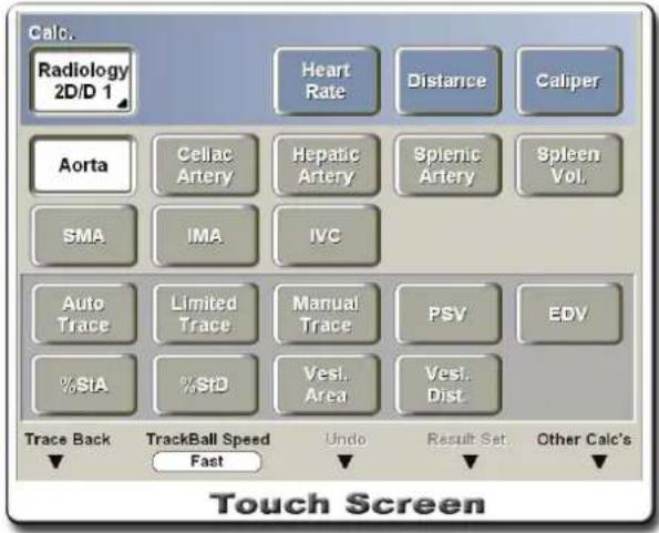
[Figure 5.17 Radiology Measurement Menu]
Radiology Measurements
-
Press the Manual button on the control panel and the radiology measurement menu will appear on the touch screen.
-
Select the menu to measure, and a cursor appears on the screen.
-
Use the Trackball and the Set button on the control panel to take measurements.
The table below shows measurement methods for menu items.
| Menu | Sub menu | Result |
| Aorta | Trace – Auto, Limited, Manual | Doppler Waveform Trace |
| PSV Velocity | ||
| EDV Velocity | ||
| %StA Calculation | ||
| %StD Calculation | ||
| Vessel Area Area | ||
| Vessel Distance Distance | ||
| Celiac Artery | Same as above | Same as above |
| Hepatic Artery | Same as above | Same as above |
| Splenic Artery | Same as above | Same as above |
| SMA (Superior Mesenteric Artery) | Same as above | Same as above |
| IMA (Inferior Mesenteric Artery) | Same as above | Same as above |
| IVC (Inferior Mesenteric Artery) | Same as above | Same as above |
| Right / Left Renal Artery | Same as above | Same as above |
| Right / Left Arcuate Artery | Same as above | Same as above |
| Spleen Volume | All | |
| Height Distance | ||
| Width Distance | ||
| Length Distance | ||
| Right / Left Kidney Volume | Same as above | Same as above |
The user can obtain various values such as PSV, EDV, Vmean, Gmean, Gpeak, S/D, PI and RI from the spectral waveform in a Spectral Doppler image. For more information on measurement methods, refer to "Measuring Doppler Spectrum".
The Volume Flow and Stenosis % values for each measurement area can be obtained. For more information on measurement methods, refer to "Measuring Volume Flow" and "Measuring Stenosis%." The user can obtain the Volume Flow value using the TAM (Time Average Mean Velocity) value obtained from the spectral waveform.
Report
Measurement and calculation results can be viewed in the report for each application.
■ Press the Report button on the control panel to check the report of a specific application.
■ Select Next App. on the touch screen to search/view reports for other applications. Reports for applications that have not been measured will not be shown.
■ Select Exit on the main screen to close the report and return to diagnosis mode. Alternatively, press the Exit button on the control panel or the Exit button on the touch screen.
■ The following figure shows a report example.
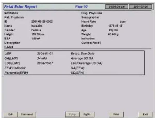
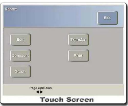
[Figure 5.18 Report Screen]
Report Functions
Viewing Report
The measurement items and their calculation results are displayed.
When the report screen has two or more pages, use PgUp and PgDn at the bottom of the report screen to navigate through the pages.
Editing Report
Select Edit at the report screen or on the touch screen and then edit desired information. After editing, press OK to return to the original report screen, and the edited values will be shown in the [ ] brackets in the report.
Adding Comments on Report
Press the Comment button at the report screen or on the touch screen to enter additional information on the values shown in the report. After entering the information, press OK to return to the report screen.
Printing out Report
Select Print at the report screen or the touch screen.
Transferring Report
■ This command transfers the report data over the RS232C communication cable. Press the Transfer button at the report screen or on the touch screen after finishing measurements.
■ Under the Peripherals tab at the Setting screen, select Open Line Transfer for Serial Port, and then connect the RS232C cable to the port.
NOTE
If the operating system of the PC connected to this system via the RS-232C Cable is Windows XP TM , errors may be caused during transferring.
Saving Report
Select the Save button on the control panel. You can view and manage saved reports in SonoView.
Graph Function
■ Press the Graph button at the report screen or on the touch screen to view Graph, History, or SD information.
In order to view the information, patient ID and LMP must be entered in patient information and range values must be set for GA table, Fetal Growth table, and Fetal Growth table.
■ This function is used for displaying GA values such as BPD, HC, AC and FL, allowing the user to diagnose fetal growth.
■ This function can be used only in OB reports.
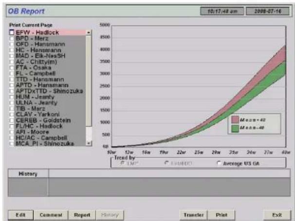
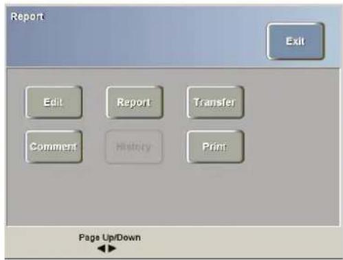
[Figure 5.19 Graph]
NOTE
Patient name, ID and LMP must be entered in order for graphs and reports to be saved in the HDD automatically.
Viewing Graph
- Recently measured values are displayed as graphs. Graphs are drawn against gestation period (week) or fetal size (mm).
- G.A. values, including the fetal weight, are displayed at the bottom of the screen. Use the Trackball and the Set button to select a desired item and its graph will appear.
- Press the Report button to return to the report screen.
- Press the Exit button at the graph screen or the Exit button on the control panel to return to diagnosis mode.
※ Standard Deviation & Percentile
Among OB information, the Growth Table and the typical fetal distribution for the same number of weeks are used to determine the following information:
- The normal distribution curve.
- The measurements for an actual fetus or a position in EFW distribution.
- Whether a distribution point is within the normal range.
The reference number of weeks for the Growth Table can be set to LMP, Estab. DD or Average US GA under [Pctl.Criteria]. The typical setting is LMP.
When LMP is not known or uncertain, or when the difference between LMP and Average US GA is substantial, care must be taken, as selecting different [Pctl.Criteria] can result in a significant difference.
When represented by SD, a point near the average indicates a value closer to ±0 SD and a point away from the average indicates a value closer to the maximum or minimum value. The greater part of the range falls within ±3 SD, and ±1 SD represents 68.3% of the entire range. Thus it can be seen that most fetal measurements are tightly clustered around the average value.
The Percentile represents a point in distribution from between 0 and 100 inclusive. Therefore, the average point is represented as 50 Percentile.
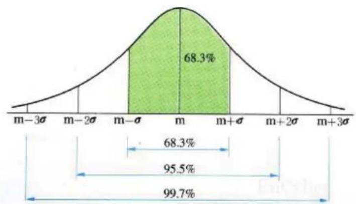
[Figure 5.20 The distribution of the Growth Table for the selected number of weeks (m: Average, σ: Standard Deviation)]
As shown in the figure, the average point corresponds to 0 SD (that is, 50 Percentile). If a point is in the range between -1 SD and +1 SD, it falls within 68.3% of the entire range. This means that at the point falls within the range between 16 and 84.
Further, if a point is in the range between -2 SD and +2 SD, it falls within 95.5% of the entire range. Thus, the point falls in the range between 3 and 97.
SD and Percentile are interchangeable. Percentile can be used when a fetal measurement ranking is desired, and SD can be used when the distance between actual fetal measurements and the average measurement is sought.
While the range of Growth Table references that are primarily used with OB measurement data varies depending on the user, the typical range accepted by most users is as below:
1) When references are created based on SD:
-2.0 SD - +2.0 SD (when converted to Percentile: 2.28 Percentile - 97.72 Percentile)
-1.5 SD - +1.5 SD (when converted to Percentile: 6.68 Percentile - 93.32 Percentile)
-1.0 SD - +1.0 SD (when converted to Percentile: 15.87 Percentile - 84.13 Percentile)
2) When references are created based on Percentile:
2.5 Percentile - 97.5 Percentile (when converted to SD: -1.96 SD - 1.96 SD)
5.0 Percentile - 95.0 Percentile (when converted to SD: -1.645 SD - 1.645 SD)
10.0 Percentile - 90.0 Percentile (when converted to SD: -1.288 SD - 1.288 SD)
Chapter 6
Image Management
REVIEWING IMAGES 2
Saving and Viewing Cine Images.... 2
Reviewing Cine Images in Dual Live Mode 3
Cine Image Function in Multi-Image 4
Saving and Viewing Loop Images 4
ANNOTATING IMAGES....5
Typing Text 5
Displaying Body Marker 8
Displaying Indicator 9
SAVING AND TRANSFERRING IMAGES 11
Saving Images 11
Transferring Images.... 11
PRINTING AND RECORDING IMAGES.... 12
Printing Images....12
Recording Images....12
SONOVIEW....14
Using SonoView 14
Patient Exam List.... 15
Viewing Images – View Mode.... 20
Tools 22
Reviewing Images
2D Mode screens, M Mode screens, ECG information and other images can be saved on the system automatically and be retrieved by the user whenever necessary.
Saving and Viewing Cine Images
Press the Freeze button after diagnosis to change to the Cine Memory function. Turn the Trackball left/right at the frozen screen to navigate the previous images back/forward. Numbers and locations of images saved so far are indicated across the top of the screen.
The Cine Image menu screen is illustrated below.
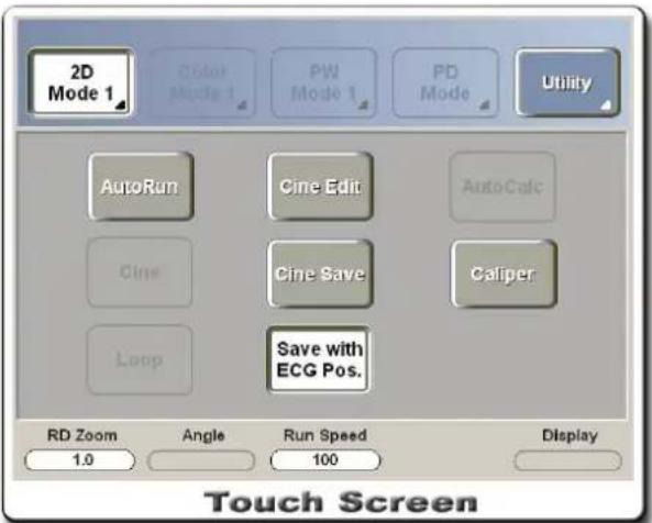
[Figure 6.1 Cine Image]
Reviewing Cine Images
Manual Image Examination
Use the Trackball to review images manually. Turn the Trackball left/right to display the images saved in Cine Memory frame by frame.
Automatic Image Examination
Press the Auto Run button on the touch screen to automatically review the images saved in Cine Memory. The saved Cine images are displayed automatically.
Press the Auto Run button again to stop the automatic image examination.
Use the up-down switch below Run Speed on the touch screen to adjust the time for each frame.
Saving Cine Images
Press the Cine Save button on the touch screen to save Cine images. You can use SonoView to search and/or manage Cine images.
The number of saved images is 256, including the currently frozen image.
Setting Range for Saving Cine Images
When saving Cine images, pres the Cine Edit button on the touch screen to set the save range.
The progress bar indicating the save range will appear on the screen. Use the Trackball and the Set button on the control panel to set the save range.
Use the Change button to select "Start Pos" and "End Pos" and then use the knob-buttons below Start Pos and End Pos to set the save range.
To search Cine images easily and conveniently, use Position Step on the touch screen. Set the step, and Cine image jumps according to the value of the step between start position and end position.
Maximum of 2,048 images can be saved. Note that the saving process will take longer when there are many images to save.
Saving ECG Position
If the Save with ECG Pos. button is selected, the ECG Cine mark will also be saved when saving Cine images with ECG. The ECG Cine mark indicates the relative position of the Cine image on the screen on the ECG wave.
RD Zoom Function
Read Zoom is one of the image zooming functions. It works in 2D Mode, Color Doppler Mode, and Power Doppler Mode but not in Dual Mode and Loop Mode.
Turn the knob-button below the menu to run the Read Zoom function and zoom the image in Scan Mode.
Display Function
When reviewing Cine images in Color Doppler Mode or Power Doppler Mode, you can set the images displayed as Color or B/W.
You can select Color + B/W, Color Only, or B/W Only for the display type.
Use the up-down switch below Display on the touch screen to change the display format.
Reviewing Cine Images in Dual Live Mode
You can use the same methods as in basic modes to review Cine images in Dual Live Mode. You cannot review the image on the left and the image on the right individually because they are identical to each other.
Cine Image Function in Multi-Image
In Dual Mode, both active and frozen images are displayed simultaneously on the screen. The frozen image is displayed on the left in Dual Mode. Press the Freeze button while scanning the image on the right. The image on the right will stop and the Cine image will be applied to the image on the right. To apply the Cine image on the image on the left, press the Update button, the Set button or the Dual button on the control panel to activate the image on the left.
Saving and Viewing Loop Images
Images examined in M Mode or PW Spectral Doppler Mode are saved as Loop images. Press the Freeze button on the control panel to freeze the image being scanned and view the Loop image. Press the Change button on the control panel select the Cine image function and the Loop image function. The current function will be indicated at the upper left-hand corner of the screen. Alternatively, you can select the functions by using the Cine button or the Loop button on the touch screen.
The Loop Image menu screen is illustrated below.
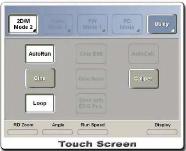
[Figure 6.2 Loop Image]
Reviewing Loop Images
Manual Image Examination
Use the Trackball to review images manually. Turn the Trackball left/right to display the images saved in Loop Memory along the time axis.
Automatic Image Examination
Press the Auto Run button on the touch screen to automatically review the images saved in Loop Memory. The saved Loop images are displayed automatically.
Press the Auto Run button again to stop the automatic image examination.
Annotating Images
Typing Text
Press the Text button on the control panel to enter Annotation Mode.
Use the alphanumeric keyboard on the control panel to input text and use the Trackball to move the cursor.
After entering text, press the Exit button or the Text button on the control panel to exit Annotation Mode.
![2005-07-03-0004 MEASURE General #31 /4.5cm MI0.02 2006-07-03 LS-12/M/ Res Ts:0.4 BIC:41:31 pm P0.050 / 118dB FAS/P5B FSIB PG:0 TEXT TEST TEXT SIZE 17 [SCT] - Select, [CLEAR] - Delete Word - Freeze](/content/2026/05/955519/images/94475c550861f8daa6efd42d1d72f8ab93d2b447205b0f3a3844e451e7e7ca8c.jpg)
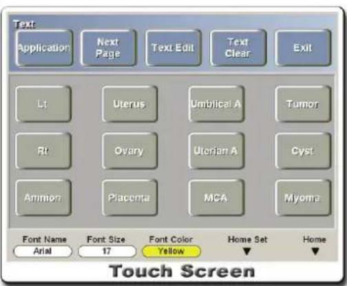
[Figure 6.3 Annotation Mode]
Positioning the Cursor
Functions of the arrow keys on the keyboard in Annotation Mode are listed below.
| [↑] Key | Moves the cursor position up by one row on the same column of the current cursor. |
| [↓] Key | Moves the cursor position down by one row on the same column of the current cursor. |
| [←] Key | Moves the cursor position to the left by one column on the same row of the current cursor. |
| [→] Key | Moves the cursor position to the right by one column on the same row of the current cursor. |
- Use the up-down switch below Home Set to save the current position. The saved position will remain unchanged after the system restarts.
- Use the up-down switch below Home to move the cursor to the saved position.
- You can select a text block and move it with the Trackball.
Selecting Font
- Selecting Font: Use the knob-button below Font Name. The available fonts are Arial, Comic Sans MS, Courier New, Georgia, Impact, Lucida Console, Microsoft Sans Serif Regular, Palatino Linotype, Tahoma, Times New Roman, Trebuchet MS and Verdana.
- Changing Font Size: Use the knob-button below Font Size. The available font sizes are 11pt - 30pt.
- Changing Font Color: Use the up-down switch below Font Color. The available font colors are Black, Green, Olive, Navy, Purple, Teal, Gray, Silver, Red, Lime, Yellow, Blue, Aqua and White.
Deleting Text
Press the Text Clear button on the touch screen to delete text on the screen.
- When waiting for text input, all text on the screen is deleted.
- While text is being typed in, only the word with the cursor on it is deleted.
- When a text block is selected, only the selected text is deleted.
Pressing the Clear button on the control panel deletes all text on the screen.
Annotating from Touch Screen
You can enter a frequently used word via the touch screen without having to type it.
Press one of the buttons displayed on the touch screen to enter a desired word.
Each measurement category has its own set of words as shown in the table below. These words can also be user-edited.
| Abdomen | Lt | Rt | Liver |
| GB | Pancreas | Spleen | |
| Kidney | Aorta | ||
| CBD | Mass | Cirrhosis | |
| OB & GYN | Lt | Rt | Amnion |
| Uterus | Ovary | Placenta | |
| Umblical A Uterian A MCA | |||
| Tumor | Cyst | Myoma | |
| Small Part | Lt | Rt | Thyroid |
| Breast | Testis | Scrotum | |
| Muscle | Ligament | Tendon | |
| Mass | Cyst | Nodule | |
| Vascular | Lt | Rt | Vertebral |
| CCA | ECA | ICA | |
| Artery | Vein | IMT | |
| Aneurysm | Varicosis | Stenosis | |
| 3D | Lt | Rt | Hand |
| Face | Lip | Foot | |
| Heart | Bladder | Spine | |
| Cord | Eye | Ear | |
IVC
Editing Touch Screen Word List
- Press the Application button on the touch screen to select the exam category that contains the word to edit.
- The words provided for each application appear on the screen.
- Select the button for the word to edit and press the Text Edit button.
- After editing the word, press the OK button to save the change.
Editing the name of application on the Touch Screen
- Press the Application button on the touch screen. Text Application screen is appeared on the touch screen.
- Press the Name Edit and select the application to change its name.
- The window of Enter Application Name is showed up on the monitor. Change or Edit the name of application.
- Press the Ok to save and finish the change. Or press the Cancel to cancel and exit the editing name.
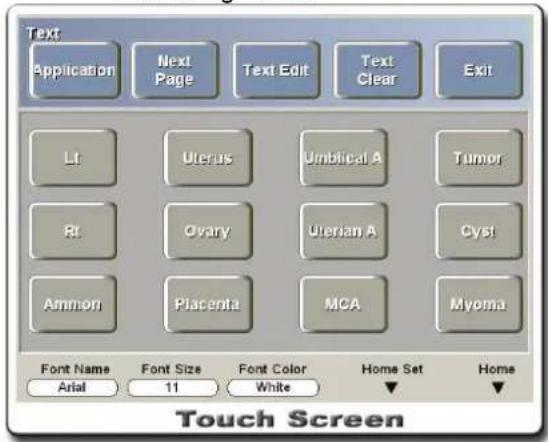
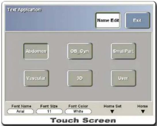
[Figure 6.4 Text Edit]
Annotating with Brief Word Function
The Brief Word function is provided to facilitate easier annotation task. This function allows you to enter texts faster and easier.
For example, if using the Brief Word function to entering the text "Tumor," you only need to enter "Tu" and the system will automatically search for the word "Tumor" from the brief word list and enter it.
To use the Brief Word function in Annotation Mode, select Brief under the Misc. tab on the Setting screen.
If the Brief Word function is in use, the brief word window shown below will appear on the screen.
| SVC | Superior Vena Cava |
| A | Transabdominal |
| TES | Testicle |
Editing Brief Word List
You can add, modify or delete the default brief word list provided with the system.
- To edit the brief word list, press the Brief Edit button below the Misc. tab on the Setting screen.
- Press the New button to add a new brief word, or press the Delete button to delete a brief word.
- Select a brief word to modify and modify the word at the input field at the bottom of the screen. Changes will be applied immediately.
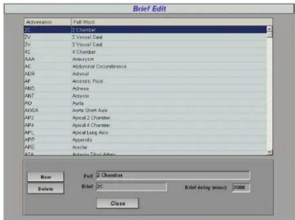
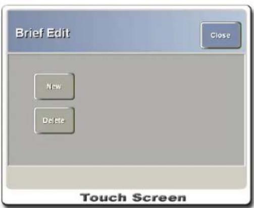
[Figure 6.5 Brief Edit Dialog Box]
Displaying Body Marker
Press the Body Marker button on the control panel to switch to Body Marker Input Mode.
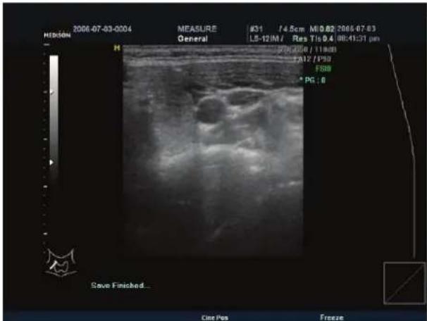
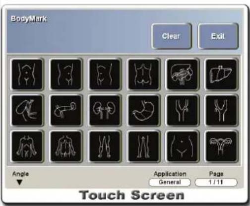
[Figure 6.6 Body Marker Input Mode]
NOTE
Refer to ‘Chapter 3. Settings’ for how to setup the body marker.
Body markers will appear on the touch screen. When the number of body markers is over one page, you can change the page of the body marker by using the up-down switch below the Page.
The types of body markers displayed on the touch screen will vary depending on the application selected. Change the application with the up-down switch below the Application, and the types of body markers on the touch screen will be changed.
Press the Body Marker button and the body marker will be placed on the image.
- Use the Trackball to move the probe cursor to the position where body marker will be placed.
- Use the Angle knob-button on the control panel to adjust the angle of the probe cursor.
- Press the Set button or the Exit button on the control panel to exit Body Marker Mode.
Changing Body Marker Position
Press the Change button on the control panel.
Use the Trackball to move the body marker to a desired position.
Press the Change button on the control panel again to confirm the new position.
Deleting Body Marker
Press the Clear button on the control panel or the touch screen.
Displaying Indicator
Press the Indicator button on the control panel and the arrow-shaped indicator will appear.
- To change the shape of the indicator, select a desired cursor on the touch screen.
- Use the knob-button below Rotate on the touch screen to adjust the indicator direction.
- Press the Exit button or the Indicator button on the control panel to exit Indicator Mode.
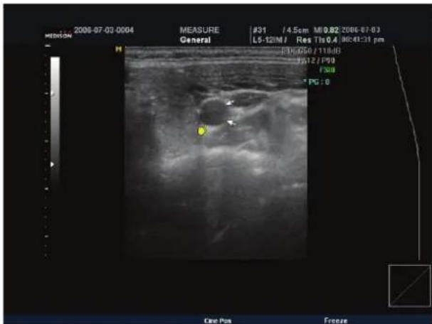
[Figure 6.7 Indicator]
| Deleting Indicator
To delete all indicators on the screen, press the Clear button on the control panel or the Indicator Clear button on the touch screen.
To delete indicators one by one, use the up-down switch below Undo on the touch screen.
Flip the up-down switch up and down to delete recently entered indicators one by one in order.
Once deleted, indicators cannot be restored.
Saving and Transferring Images
Saving Images
Images are saved and managed independently for each patient. If you press the Save button on the control panel without having entered the basic patient information, the Patient Information screen will appear. Normal images and 3D images can be saved. You can edit and/or manage the images from SonoView.
Saving an Image with Text
For more information on entering text on images, refer to “Annotating Images” in this chapter.
NOTE
Saving images with descriptions can make the retrieving process much easier and faster.
Transferring Images
There are two methods for transferring images using DICOM. One is to transferring the scanned images one by one immediately after they are scanned, and the other is to scan all the images first and then to transfer the selected ones only. For more information on DICOM server settings and DICOM operation, refer to the section "DICOM Settings" in "Chapter 3. Settings."
Transferring Images in Real Scan Mode
Press the Save button on the control panel to save the image and at the same time transfer it to the server via DICOM. Note that the image will be transferred automatically only when "Acquisition in progress" is selected under the DICOM tab at the Setting screen.
Transferring Images from SonoView
Select Exam at Exam List to transfer all the images in Exam. In View Mode, select and transfer images one by one.
Printing and Recording Images
Printing Images
Press the Echo Print button on the control panel to print the scanned images via an echo-printer. For more information on printer settings, refer to "Chapter 3. Settings."
Recording Images
To record images with the VCR during scanning, press the recording button on the VCR connected. Alternatively, press the VCR button on the control panel.
If Panasonic MD830 (or Sony SVO 9500MD) is connected on Serial Port, the VCR Counter value will appear on the screen.
For more information on VCR settings and Serial Port settings, refer to "Chapter 3. Settings."
VCR Function
The VCR function allows the user to review recorded images on the system. Before using the VCR function, make sure that the VCR is properly connected to the system.
To enter VCR Mode, select the VCR button in the Utility menu. Alternatively, press the VCR button on the control panel.
The VCR menu below will appear on the touch screen.
[Figure 6.8 VCR Menu]
- To view the VCR playback screen on this system, select the Play button on the touch screen and then press the Play button the VCR.
-
To stop the VCR playback, press the Stop button on the VCR and then press the Stop button on the touch screen.
-
If Panasonic MD830 (or Sony SVO 9500MD) is connected on Serial Port, press the Play, Stop, Pause, Rew, and FF buttons to control the VCR.
- Press the Counter button on the touch screen to adjust the VCR Counter value. Press the Counter button and the window below will appear on the screen.
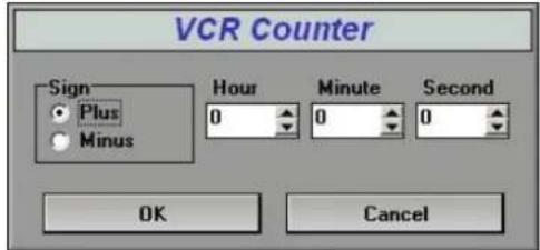
- Press the Search button on the touch screen to move to a specific position using the search dialog box.
Measuring in VCR Images
Basic measurements can be taken on VCR images. During the VCR image playback, press the Freeze button on the control panel and you will be able to take various measurements using the buttons on the touch screen.
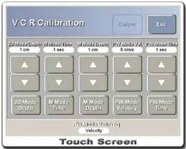
[Figure 6.9 VCR Calibration]
- Use the up/down buttons on the touch screen to adjust the factor for each menu value.
- Set factors for 2D Mode Depth, M Mode Time, M Mode Depth, PW Mode Velocity (Frequency), and PW Mode Time, and then press the Caliper button on the touch screen to take basic measurements such as distance, area and volume.
- If taking measurements again, factors must be set again.
- Press the Freeze button to finish taking measurements and return to the VCR image.
SonoView
SonoView is a total image management system which provides saving/filing, previewing and deleting of images, as well as exporting of data for data exchange with standard PCs.
The image format used in this system complies with the international standard DICOM (Digital Imaging and Communication in Medicine) image format. Therefore, PACS (Picture Archiving Communication System) can be implemented with no extra costs, allowing image data exchange with other institutes and other devices.
* DICOM and PACS are well established in advanced countries but are currently in an introductory stage in Korea.
This system supports the Bitmap file format (*.bmp files), which is the most commonly used on standard PCs, for maximum image data exchange.
It is therefore possible to use SonoView in systematic management and research of patient medical history.
NOTE
All images containing patient information are identified by patient IDs. For efficient management, it is recommended that you use the patient's chart number or a part of the social security number as the patient ID.
Using SonoView
 | SonoView | Starts SonoView. |
 | Store Saves the image in SonoView. | |
* Exams are identified with the patient ID. If the patient information has not been entered, the Patient Information screen will appear.
WARNING
You must enter the patient ID because all images are saved according to the patient ID entered.
Failure to enter the patient ID may result in loss and/or critical error(s) on previously saved images.
NOTE
Images are saved on HDD (Hard Disk Drive), MO (Magneto Optical), or ODD (Optical Disk Drive). The term ODD refers to drives that can access CD-R (Compact Disc Recordable), CD-RW (Compact Disc Rewritable), or DVD-R (Digital Versatile Disc Recordable). Such media are collectively referred to as Optical Discs.
Once SonoView starts, the screen will appear where SonoView settings can be edited and Exam List can be accessed. Use the Trackball and the Set button on the control panel or use the menu on the touch screen to select the menu.
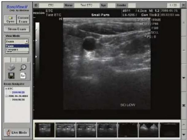
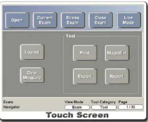
[Figure 6.10 SonoView]
Patient Exam List
Exam List Execution

Press the Open button to view Exam List saved in SonoView.
The Exam List screen shows patient ID, name, recent examination date, etc. Displayed on the upper right-hand corner of the screen are the total number of exams, the number of exams currently selected, and the number and size of images contained in them.
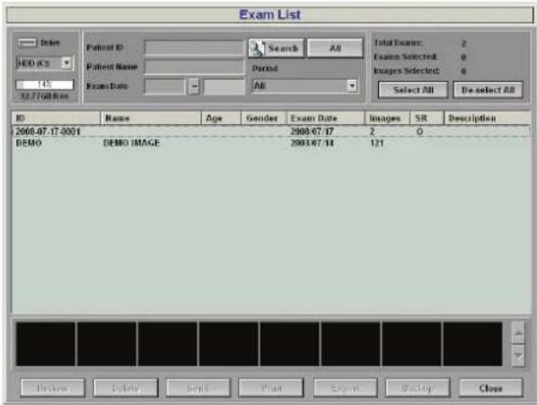
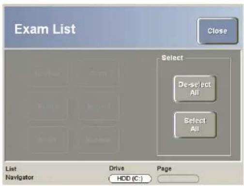
[Figure 6.11 Exam List Screen]
Selecting Patient Exam
Use the Trackball and the Set button to select a desired exam. Multiple exams can be selected at one time. Press the Set button again to deselect exams. Press the Select All button to select all exams in one instance, or press the Deselect All button to deselect all exams.
Displayed on the upper left-hand corner of the Exam List screen is the free space on each storage drive. Select HDD, MO, or ODD to check the free space and saved exams on the selected medium. Use the up-down switch below the touch screen to change the drive.
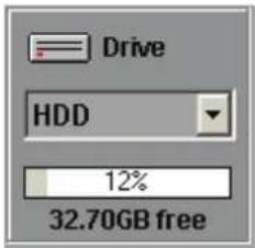
Sorting Patient Exam
Press a column header on Exam List to sort exams by the column. For example, press ID to sort the list by ID.
Searching Patient Exam
You can perform a search by entering the patient ID or name at the Exam List screen.
* Enter one or more letter/number to search.
After entering the search condition in the patient ID, name, and date fields, press the Search button to display exams that are identical or similar to the condition entered.
Press the All button to show all saved exams.
You can specify a period and search for exams for the period specified. "All" shows exams for all dates.
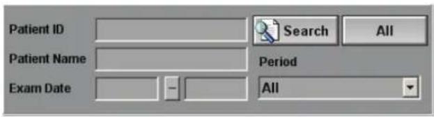
Viewing Patient Exam
Select an exam to view and press the Review button. While images are displayed in a 640 x 480 area on the screen, the full 800 x 600 area will be used if the exam list or a message window is displayed on the screen.
Deleting Patient Exam
Delete
Select an exam to delete and press the Delete button. Once deleted, exams cannot be restored. To delete some of the images, select the images to delete in View Mode and then press the Del key on the keyboard.
To select more than one image, select the images while holding down the Ctrl key on the keyboard.
Transferring Patient Exam
Send
You can transfer patient exams over the DICOM network to a DICOM server. Note that the Send button will not be activated if the DICOM function has not been configured. Select an exam to transfer and press the Send button.
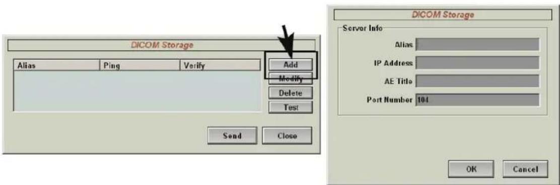
[Figure 6.12 DICOM Storage Setup Screen]
- To add a new server after selecting an exam, press the Add button at the DICOM Send window. Enter the required information and then press the OK button.
- To check or modify the server information after selecting an exam, press the Modify button.
- To delete a server after selecting an exam, press the Delete button. To check the connection between the Server and DICOM, press the Test button.
- After finishing all tasks, press the Send button to transfer the selected exams to the desired server.
Printing Patient Exam
This function uses a printer connected on the DICOM network. Note that the Print button will not be activated if the DICOM function has not been configured. Select an exam to and press the Print button.
Procedures for setting and printing exams are the same as for transferring exams.
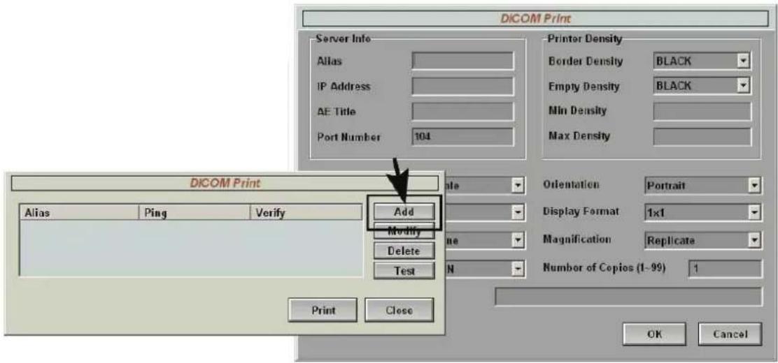
[Figure 6.13 DICOM Print Setup Screen]
Exporting Patient Exam
Export
After selecting an exam, press the Export button to save the images contained in the exam as BMP, JPEG, TIFF, DICOM or AVI files in the selected medium.
Multiple exams can be selected and exported in one instance.
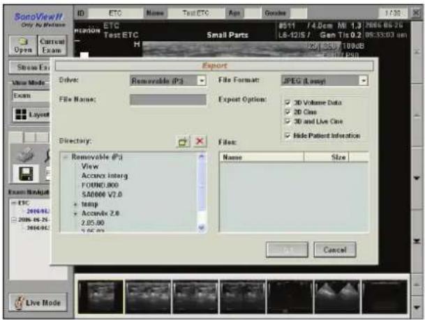
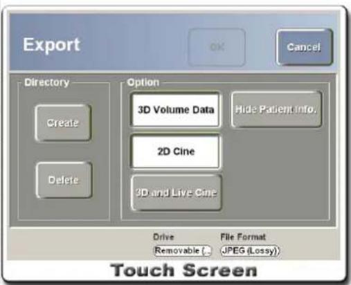
[Figure 6.14 Exam Export]
All the images in the same exam are given the same file name. If there are several images in one exam, serial numbers are attached to the back of the file names.
The Directory box displays the directory structure of the selected drive. Press the Create button to create a new folder on the drive, or press the Delete button to delete the selected folder.
Selecting Export Options
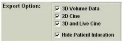
- 3D Volume Data transfers 3D images along with 3D Volume Data.
- 2D Cine converts the saved Cine images into AVI files and transfers them.
- 3D and Live Cine converts 3D Cine or Live Cine images into AVI files and transfers them.
- Hide Patient Information removes patient ID, patient name, institute name and other patient information from the images being transferred.
Patient Exam Backup
Backup
You can use MO Drive or ODD to back up the images in DICOMDIR in accordance to the DICOM 3.0 standard.
- Select an exam and press the Backup button. Insert the backup medium in the drive and wait until the LED goes off.
- At the media selection window, press the MO button or the ODD button.
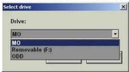
- Select whether to delete the exam after the backup. Once deleted, images cannot be restored.
- Images can be appended additionally to CR-R and CD-RW media because they support multi-session. CD-RW media can be reused over and over by deleting images on them.
- For optical discs, backup images must not use more than 95% of the medium capacity because additional files with backup information are saved on them.
Restoring Patient Exam
Restore
- Insert the medium with backup information in the drive and wait until the LED goes off.
- Use the drive selection function at the upper left-hand corner of the screen to select MO or ODD.
- When the list of exams saved on the medium appears, select a desired image and perform various functions such as Review, Delete, Send, Restore, and Print. Note that
DVD and CD-R medium do not support the Delete function.
- To transfer the exams saved in the medium to the system hard disk, select the exams and press the Restore button.
Viewing Images – View Mode
View Mode
Exam Mode
View all images of the selected exam in the order they were saved.
- Select an exam in View Mode using the combo box on the left side of the screen.
- In the preview window at the bottom of the screen, use the Trackball and the Set button to select images and the images will be displayed according to the layout of the image selection window.
- In some modes, the currently displayed image is highlighted with yellow borders in the preview window across the bottom of the screen.
Compare Mode
Several images are compared.
- Select Compare using the combo box at the left side of the screen in View Mode.
- Select an image in the preview window across the bottom of the screen and its border will blink.
- Assign the image display location in the image selection window and the selected image will be displayed.
- Maximum of 4 images can be compared. (2 x 2)
Exam navigator
You can use Exam Navigator to search exams and images faster and easier. For example, select two exams from Exam List and load them, and their ID and other information will be displayed Exam Navigator.
You can also make selections by using the knob-button below the touch screen.
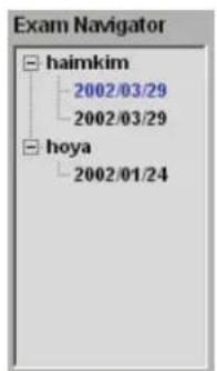
Preview Function
Preview images of the selected exam are displayed across the bottom of the screen. If there are more than 7 images in the selected exam, press the ▽ button on the right-hand side of the screen to view next images. Press the △ button to view previous images.

Layout
You can set the layout for View Mode.
Press the Layout button to adjust the number of images displayed on the screen. Select "User Defined" to set the number of columns and rows for the layout. Maximum of 4 columns and 4 rows can be used.
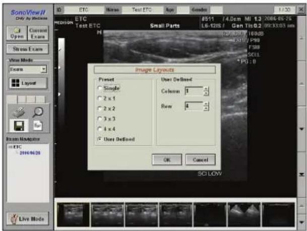
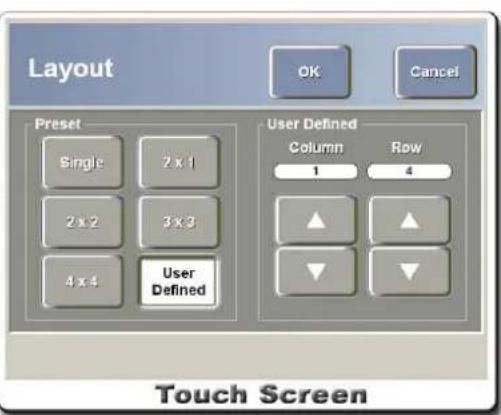
[Figure 6.15 Image Layouts]
Viewing Full Screen Image
You can zoom images full screen.
Place the cursor on the image and press the Set button twice to zoom the image. Press the Set button twice again to return to the previous state.

/ Use the / buttons to view previous/next images.
3D Mode
When viewing 3D images, the 3D button will appear at the lower right-hand corner of the image. Press the 3D button to start 3D Mode.
Cine Mode
When viewing Cine images, the Cine playback and search buttons will appear at the lower left-hand corner of the image. Press the play button to play the Cine image. When paused, you can use the search button to move frame by frame.
Deleting Images
Select the images to delete in View Mode and press the Del key on the keyboard. To select multiple images, select the images while holding down the Ctrl key on the keyboard. Note that images for the current exam cannot be deleted.
Viewing Current Exam

Press the Current Exam button at the upper left-hand corner of the SonoView screen or the Current Exam button on the touch screen to view the images saved for the current exam.
Tools
Various functions in SonoView are displayed with icons. Use the up-down switch below Tool Category on the touch screen to select tool groups.
Tool
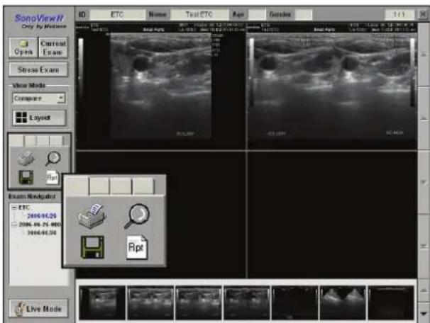
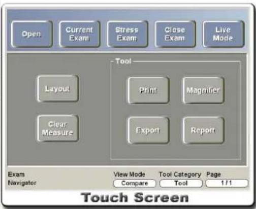
[Figure 6.16 Tool]

- You can perform the print setup in the Print Layouts window.
-
Ink Save Mode inverts the dark background color and prints images.
-
Press the OK button, and the image will appear with a brief report.
- Press the Echo Print button on the control panel to print the image.
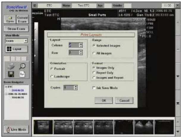
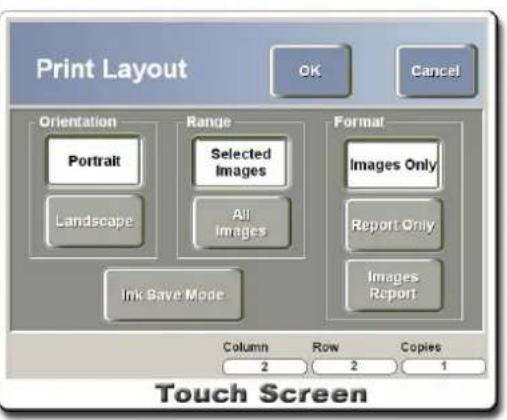
[Figure 6.17 Print Setup]

Magnifier
- Select the magnifier function and the cursor will change to the magnifier icon. Place the magnifier at a desired position and press the Set button to magnify the selected part of the image. Move the Trackball while holding down the Set button to magnify other parts of the image.
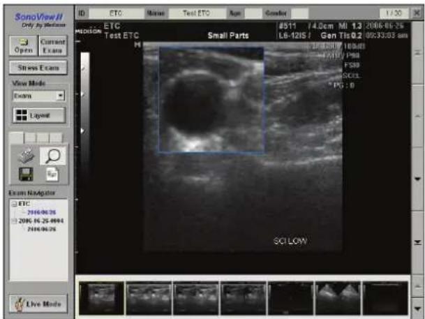
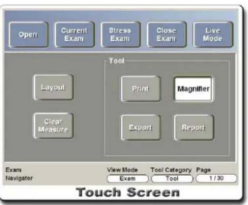
[Figure 6.18 Using Magnifier on Image]
- This function cannot be performed in full screen mode or when the layout is set as Single.

Export
- Select the Export function and the cursor will change to the floppy disk icon. Place the cursor over a desired image and press the Set button.
- After entering the folder name and the file names for the images, press the Export button to convert and save the images as BMP, JPEG, TIFF, DICOM and AVI files.
- To save multiple images in one instance, press the Set button while holding down the Ctrl key on the keyboard to select multiple images.
NOTE
The Export function will not be activated if file name and folder name are not entered.

Report
- You can compose reports containing various information about exams.
- Press the OK button to save. Press the Cancel button to cancel saving.
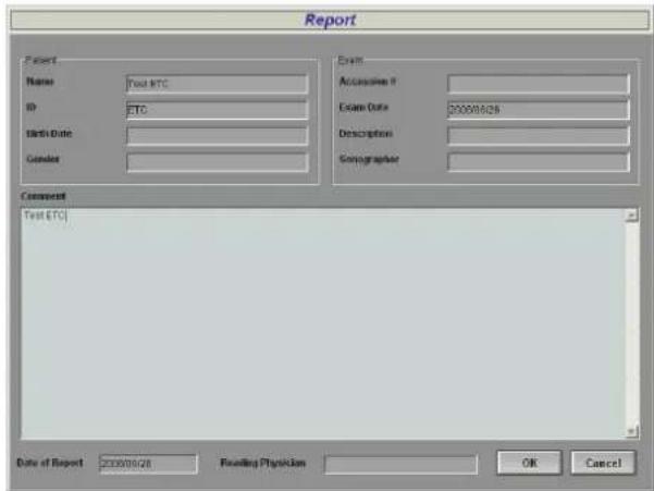
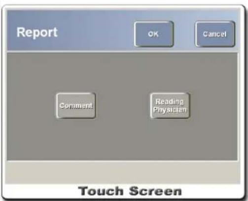
[Figure 6.19 Report]
Measure
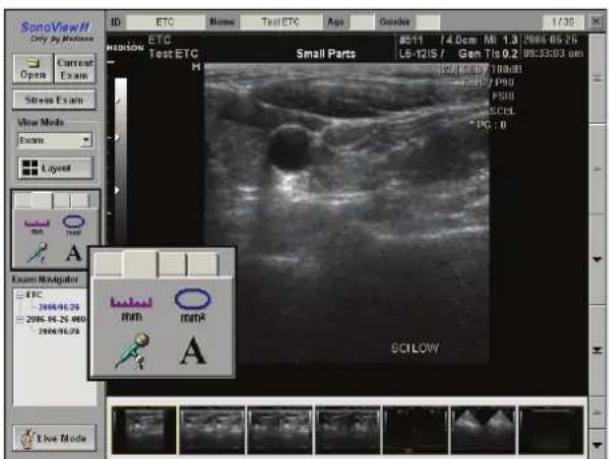
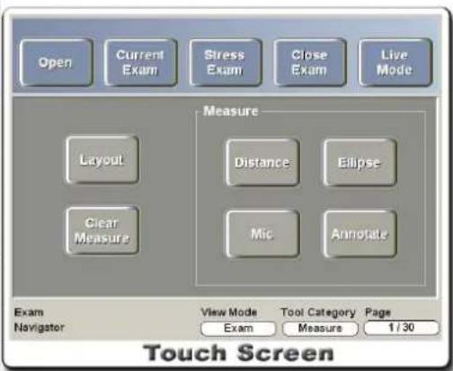
[Figure 6.20 Measure]

Distance
- This function measures the distance between two points on a saved image.
- Press the Distance button and place the cursor on a desired image to zoom the image full screen.
- Place the cursor at the start point and the end point of the distance measurement and then press the Set button. You can reset the position of the measurement area by pressing the Change button before pressing the Set button. Once the points are assigned, the distance between the two points is displayed on the screen.
- Repeat the process to measure multiple distances.
- Press the Exit button to finish measurements. Measurement results are not saved.

Ellipse
- This function measures the circumference and area of desired areas on a saved image.
- Press the Ellipse button and place the cursor on a desired image to zoom the image full screen.
- Place the cursor at the start point and the end point of the distance measurement and then press the Ellipse button. Pressing the Change button before pressing the Set button allows the position of the measurement area to be reset. Use the Trackball to adjust the shape and size of the ellipse and press the Set button. The circumference and area of the ellipse will be displayed on the screen.
- Repeat the process to measure multiple ellipses.
- Press the Exit button to finish measurements. Measurement results are not saved.

Annotate
- This function allows entering of texts on the image.
- Press the Annotate button and capital A will appear on the image. Select an image to zoom it full screen. A cursor will appear on the image.
- Position the cursor on a desired area and enter text.
- Press the Set button to confirm the text. Press the Exit button to finish entering texts.
Network
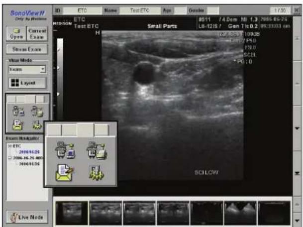
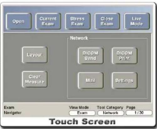
[Figure 6.21 Network]

DICOM Selective Send (Option)
- You can use the DICOM network to transfer selected images to other servers. This button will not be activated if the DICOM function has not been configured for the system.
- Use the Ctrl key on the keyboard and the Set button on the control panel to select images to transfer, and then press the DICOM Send button. The DICOM settings screen will appear.
- Press the Send button to transfer images to the server. Images can be transferred to maximum of 4 servers simultaneously.

DICOM Selective Print (Option)
- You can use printers connected on the DICOM network to print selected images. This button will not be activated if the DICOM function has not been configured for the system.
- Use the Ctrl key on the keyboard and the Set button on the control panel to select images to print, and then press the DICOM Print button. The number of images selected will be displayed on the screen for confirmation. The DICOM settings screen will appear after that.
- Press the Print button to print images via the DICOM printer.
- For more information on DICOM printers, refer to the respective printer manual or the DICOM Conformance Statement.

- This function sends images as e-mail attachments.
- Use the Ctrl key on the keyboard and the Set button on the control panel to select images to
send as e-mail attachments, and then press the Email button. Enter the user name, e-mail address, recipient's e-mail address, subject, and message.
- Press the Send button after entering all the necessary information. Use the Set button to select images at the Email composition screen and view the images attached.
- To use the email function, you must specify Email (SMTP) Server under Setting Tool (SonoView) and the user must have a valid e-mail account on the server selected.
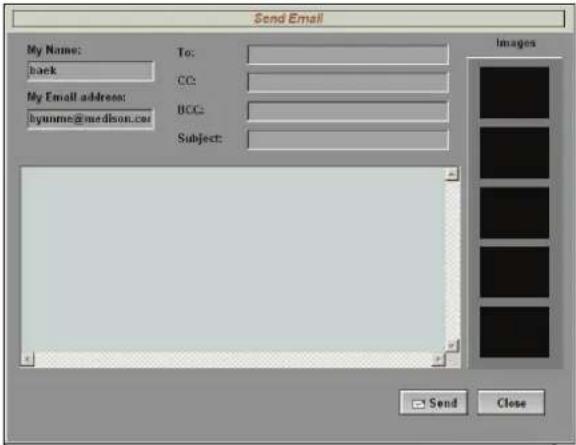
[Figure 6.22.Email Composition Screen]
NOTE
If the mail server is working but e-mails cannot be sent:
- Make sure that the LAN cable is properly connected.
- Check the IP settings under peripheral devices settings at the Setting screen.
- Check that ICMP (ping) is open for the selected mail server. If ICMP (ping) is closed, the e-mail function may not work correctly.

Settings
- The Text Annotation tab contains settings for text color, font, and size. (Previously entered texts are not changed)
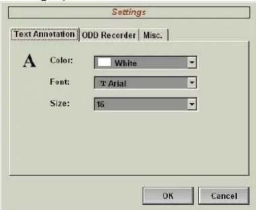
[Figure 6.23 Setting – Text Annotation]
- The ODD Recorder tab shows information for the Optical Disc Drive installed.
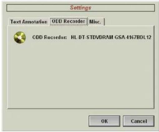
[Figure 6.24 Settings – ODD Recorder]
- The Misc. tab contains settings for sorting Exam Navigator. Patient ID or Patient's Name can be used for sorting.
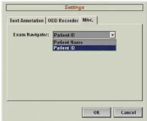
[Figure 6.25 Setting – Misc.]
Media Format
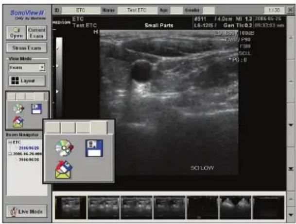
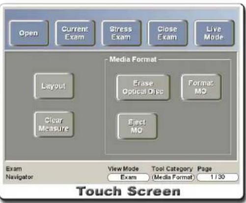
[Figure 6.26 Media Format]

Erase Optical Disc
This function erases all data saved in the optical disc.
Data on DVD or CD-R media cannot be erased. In general, a CD-RW medium can be erased and reused about 1,000 times.

Format MO
This function formats MO disks.

Eject MO
This function ejects the MO disk from the MO drive.
Chapter 7
Maintenance
SYSTEM MAINTENANCE....2
Installation Requirements ....2
Cleaning and disinfection....2
Fuse Replacement....3
ADMINISTRATION OF INFORMATION......5
User Setting Back up 5
Patient information Back-up....5
SOFTWARE....5
System Maintenance
NOTE
The user must ensure that the safety inspections are performed every 2 years according to the requirements of safety standard EN 60601-1. Only trained persons are allowed to perform the safety inspections mentioned above.
Installation Requirements
When installing:
■ Optimal conditions for the system are temperatures of 10° 35° C and humidity of 30% \~ 75%.
■ Avoid humidity.
■ Avoid direct sunlight.
■ Avoid places with extreme temperature variations.
■ Avoid heat sources.
■ Avoid dusty and unventilated areas.
■ Avoid places where the system is likely to be exposed to vibration or impacts.
■ Avoid places where the system is likely to be exposed to chemical substances or gases.
CAUTION
Placing the system near generators, X-Ray machines, or broadcast cables may result in screen noise and abnormal visual images. Using the power source with other electric devices may also induce noise.
Cleaning and disinfection
Cleaning
WARNING
Always use protective eyewear and gloves when cleaning and disinfecting the equipment.
- Turn off the system and disconnect the system power cord from the wall outlet.
- Use a soft cloth lightly dampened in a mild soap or detergent solution to clean exterior surfaces on the system.
Disinfection
CAUTION
Use only recommended disinfectants on system surfaces.
- Turn off the system and disconnect the system power cord from the wall outlet.
- The following disinfectants are recommended because of both their biological effectiveness (as qualified through the FDA 510(k) process) and their chemical compatibility with MEDISON ultrasound product materials. Mix the disinfection solution compatible with your system according to label instructions for solution strength. A disinfectant qualified by the FDA 510(k) process is recommended.
| Solutions | Country | Type | Active | Ingredient | FDA |
| Cidex | USA | Liquid | Gluteraldehyde | K924434 | |
| Cidex Plus USA | Liquid Gluteraldehyde | K923744 |
510(k)
- Wipe the system surfaces with the disinfectant solution, following the disinfectant label instructions for wipe durations, solution strength, and disinfectant contact duration.
- Air dry or towel dry with a sterile cloth according to the instructions on the disinfectant label.
Fuse Replacement
The power protection fuse protects the product from excess current. If the power monitoring protection circuit detects excess current, it shuts off the current to the equipment in order to prevent overheating and to restrict the ultrasound power output.
If the fuse blows, replace it as shown below.
DANGER
To avoid risk of electric shock, always disconnect the plug from the system prior to fuse replacement.
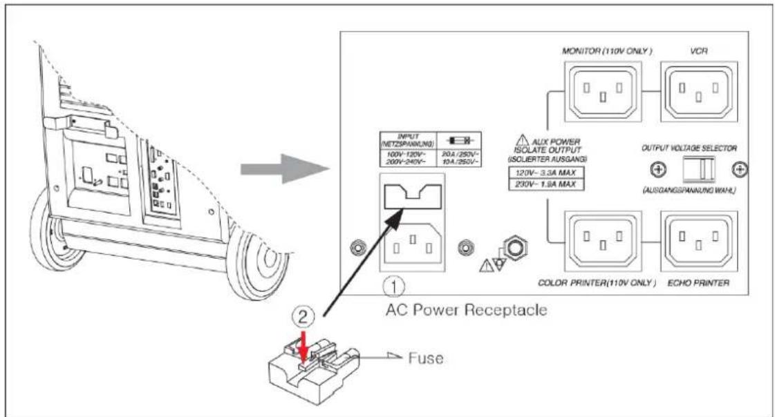
[Figure 7.1 Fuse replacement]
- Disconnect the power cord from the system. (See ①)
- Take the fuse out by pressing the middle of fuse. (See ②)
- Insert the fuse holder into the appliance inlet.
- After installing the new fuse, connect the power cord to the system.
Fuse information is shown in the following table.
| Input Ratings Fuse Ratings Company Order No. | |||
| 100-120VAC | 12.5A/250V | Schurter | 0001.2515 |
| 200-240VAC | 10A/250V | Orisel | 55T210000 |
Administration of Information
CAUTION
You may lose information files on user settings or patients, because of shock on the product or internal error. Thus, back-up on a regular basis.
User Setting Back up
- Always keep a backup copy of all information related to the user settings in case of data loss.
- Clients cannot back-up the user settings of the product. Contact the MEDISON Customer Service Department to attain support for back-up.
- However, clients may back up the user setting on GA Table used in obstetrics diagnosis. For further information please refer to "Chapter 3. Settings".
Patient information Back-up
The SonoView program can be used for backing up patients' basic information and scanned images. The user can choose to save the data, and the data is also saved in the system by default. If the system needs to be reinstalled due to product failure, etc., the MEDISON customer support staff will restore the patients' basic information and scanned images that are saved in the system. For more information on this, see "Chapter 6 Image Managements."
SOFTWARE
The product software may be updated to enhance performance. The user cannot make any changes to the software. Please contact the MEDISON customer service representative for help in software changes.
CAUTION
Minor software updates may be carried out without the prior notice from the manufacturer.
Should errors occur in the operating system (Linux), and should you desire to upgrade the operating system, please follow the instructions of the operating system manufacturer.
Chapter 8
Probes
PROBES 2
Detergent, Disinfectant, and Ultrasound Gel 4
Sheaths....5
Probe Precautions....6
Cleaning and Disinfecting the Probe ....7
BIOPSY 12
Biopsy KIT Components 12
Using the Biopsy Kit....13
Cleaning and Disinfecting Biopsy Kit....14
Assembling the Biopsy Kit....15
Probes
The probe is a device that sends and receives ultrasound for acquiring image data. It is also called a Transducer or Scanhead.
The system limits patient contact temperature to 43 degrees Celsius, and acoustic power values to their respective U.S. FDA limits. A power protection fuse circuit protects against over-current conditions. If the power monitor protection circuit senses an over-current condition, then the drive current to the probe is shut off immediately, preventing overheating of the probe surfaces and limiting acoustic output. Validation of the power protection fuse circuit is performed under normal system operation. For invasive probes, additional protections are designed to keep patient contact surface temperature under 43 degrees Celsius in the event of a single fault failure.
The ultrasonographic image scanner uses the image data received by the probe to display the images of each organ on the screen. For best quality images, select the appropriate probe for the each application.
The applications for each probe are shown below.
| Probe | Applications |
| L5-12IM | General, Vascular (Cerebr. Carotid, Periph. Arterial, Periph. Venous), Small Parts (Thyroid, Testicle, Bowel), Breast (Breast1), Pediatric, Musculoskeletal (Shoulder Knee, Hand Foot) |
| L6-12IS | General, Vascular (Cerebr. Carotid, Periph. Arterial, Periph. Venous), Small Parts (Thyroid, Testicle, Bowel), Breast (Breast1), Pediatric, Musculoskeletal (Shoulder Knee, Hand Foot) |
| L8-15IS | General, Vascular (Cerebr. Carotid, Periph. Arterial, Periph. Venous), Small Parts (Thyroid, Testicle, Bowel), Breast (Breast1), Pediatric, Musculoskeletal (Shoulder Knee, Hand Foot) |
| L5-9EE | General, Vascular (Cerebr. Carotid, Periph. Arterial, Periph. Venous), Small Parts (Thyroid, Testicle, Bowel), Breast (Breast1), Pediatric, Musculoskeletal (Shoulder Knee, Hand Foot) |
| L4-7EL | General, Vascular (Cerebr. Carotid, Periph. Arterial, Periph. Venous), Small Parts (Thyroid, Testicle, Bowel), Breast (Breast1), Pediatric, Musculoskeletal (Shoulder Knee, Hand Foot) |
| C3-7IM | General, Gynecology, Abdomen, OB, Renal, Fetal Heart, OB Early |
| C2-6IC | General, Gynecology, Abdomen, OB, Renal, Fetal Heart (Fetal Heart1), OB Early |
| C5-2EL | General, Gynecology, Abdomen, OB, Renal, Fetal Heart, OB Early, Contrast Agent |
| C1-4EC | General, Gynecology, Abdomen, OB, Renal, Fetal heart, OB Early, Contrast Agent |
| C4-9ED | General, Abdomen, Pediatric, Vascular (Cerebr. Carotid, Periph. Arterial, Periph. Venous), Neonatal |
| EC4-9ES | General, Gynecology, OB, Urology |
| EC4-9IS | General, Gynecology, OB, Urology |
| VAW3-5 | General, Gynecology, Abdomen, OB, Renal, Fetal Heart, OB Early |
| VAW4-7 | General, Gynecology, Abdomen, OB, Renal, Fetal Heart, OB Early |
| VNA6-12 | General, Vascular (Cerebr. Carotid, Periph. Arterial, Periph. Venous), Small Parts (Thyroid, Testicle, Bowel), Breast (Breast1), Pediatric, Musculoskeletal (Shoulder Knee, Hand Foot) |
| VDW5-8 | General, Gynecology, OB, Urology |
| 3D3-5EK | General, Gynecology, Abdomen, OB, Renal, Fetal Heart, OB Early |
| 3D4-7EK | General, Gynecology, Abdomen, OB, Renal, Fetal Heart, OB Early |
| 3D4-8ET | General, Gynecology, Abdomen, OB, Renal, Fetal Heart, OB Early |
| 3D5-8EK | General, Gynecology, OB, Urology |
| 3D2-6ET | General, Gynecology, Abdomen, OB, Renal, FetalHeart, OB Early |
| P2-4AC | General, Abdomen, Cardiac, TCD, Pediatric Cardiology |
| P3-5AC | General, Abdomen, Cardiac, TCD, Pediatric Cardiology |
| P3-7AC | General, Cardiac, Neonatal, Pediatric Cardiology, Pediatric Abdomen |
| CW2.0 | General, Cardiac |
| CW4.0 | General, Pediatric, Cardiac |
TI Table
The TI (Thermal Index) information on the screen varies depending on the probe and application.
The preset TI information is as follows: Tis (Soft tissue): ○ Tib (Bone) : ● Tic (Cranial bone): ◎.
Detergent, Disinfectant, and Ultrasound Gel
Using an inappropriate ultrasound gel may damage the probe. For proper transmission of the acoustic beam, only use ultrasound transmission gel only approved by MEDISON.
| WARNING | ■ Do not use mineral oil, oil-based solutions, or other non-approved material as they may cause damage to the probe.■ Do not use gels that contain any of the following agents:- Acetone- Methanol- Denatured Ethyl Alcohol- Mineral Oil- lodine- Lanoline- Any lotions or gels containing perfume |
Sheaths
Sheaths are recommended for clinical applications of an invasive nature, including intraoperative, transrectal, transvaginal, and biopsy procedures. MEDISON does not supply sheaths so that you should purchase appropriate ones on your own.
| WARNING | ■ Always keep sheaths in a sterile state.■ Sheaths are disposable. Do not reuse them.■ If sheaths are torn or soiled after use, wash and disinfect the probe.■ In neurosurgical applications, a disinfected probe must be used with sterile gel and a sterile pyrogen-free sheath.■ If the sterile sheath becomes compromised during neurosurgical applications involving a patient with Creutzfeldt-Jakob disease, the probe cannot be successfully sterilized by any disinfection method.■ Some sheaths contain natural rubber latex and talc, which can cause allergic reactions in some individuals. Please refer to the FDA Medical Alert released on March 29, 1991. |
Installing the Sheath
- Use sterile gloves.
- Unpack the sheath and fill it with acoustic coupling gel.
- Insert the probe into the sheath and pull the latex tip to cover the probe completely. If possible, cover the probe cable as well.
- Ensure that there is no air bubble within the ultrasound gel.
- If necessary, secure the sheath to the probe and the probe cable.
- Dispose of the sheath after use.
Probe Precautions
The probe can easily be damaged by improper use or by contacting certain chemical substances. Always follow the instructions in the user manual to inspect the probe cable, case and lens before and after each use.
Check for cracks, broken parts, leaks and sharp edges. If there is any damage, immediately stop using the probe and contact the MEDISON Customer Support Department. Using damaged probes may result in electric shocks and other hazards to the patients and/or users.
CAUTION
■ Do not apply mechanical shock to the probe.
- Do not place the probe cable on the floor where the cable can be run over by equipment wheels, etc. Do not apply excessive force to bend or pull the cable.
■ Do not immerse the probe into any inappropriate substances such as alcohol, bleach, ammonium chloride, and hydrogen peroxide.
■ Do not expose the probe to temperatures of +50°C or higher.
Use and Infection Control of the Probe
The ultrasonographic image scanner uses ultrasound, and it makes direct contact with the patient when in use. Depending on the types of examinations, such contact can be made to a wide variety of locations including the ordinary skin or the location of blood transfusion during a surgery.
The most effective method to prevent infection among patients is to use each probe only once. However, probes may need to be re-used as they are complex in design and expensive. Consequently, protective devices such as sheaths must be used, and the safety instructions must be followed carefully in order to minimize the risk of infection among patients.
WARNING
No neurosurgical treatments or examinations should be carried out on a patient with Creutzfeldt-Jakob disease (critical brain disease caused by virus). If the probe has been used on such a patient, it cannot be sterilized by any method whatsoever.
CAUTION
Sufficient washing and disinfecting must be carried out for preventing infection. This is the responsibility of the user who manages and maintains the disinfection procedures for the equipment. Always use legally approved detergents and sheaths.
Electric Shocks
The probe uses electrical energy. If it touches conductive materials, there are risks of electric shocks to the patient or the user.
WARNING
■ Regularly receive short-circuit examination from the MEDISON Customer Support Department. Do not immerse the probe into liquid.
■ Do not immerse the probe into liquid
■ Do not drop the probe or apply mechanical shocks.
■ Inspect the housing, strain relief, lens and seal for damage, and check for any functional problem before and after each use.
■ Do not apply excessive force to twist, pull or bend the probe cable. It may result in a short circuit.
■ The power protection fuse protects the probe and the product from excess current. If the power monitoring protection circuit detects excess current, it immediately shuts off the current to the probe in order to prevent the probe surface from overheating and to restrict the ultrasound power output.
■ The temperature of the product for making contact with patients is limited under 43°C. The ultrasound power output (AP&I) is in compliance with US FDA standards.
Cleaning and Disinfecting the Probe
Using an inappropriate detergent or disinfectant may damage the probe.
WARNING
Always use protective eyewear and gloves when cleaning and disinfecting probes.
Information of Detergent, Disinfectant and Ultrasound Gel
Use an appropriate one with following tables. The information is also listed on the Medison web site. (http://www.medison.com)
NOTE
The information on the website is prior to the information in this manual.
| Names | Disinfectants | ||||||||||||||
| T-Spray II | T-Spray | Sani-Cloth | Cidex\ OPA2,3) | Cidex\ Plus2) | Metricide2) | Omnicide | Nuclear | Wavicide-013) | Sekusept Extra | Sporox II | Gigasept AF3) | Gigasept FF | |||
| Type | Spray | Spray | Wipe | Liquid | Liquid | Liquid | Liquid | Liquid | Liquid | Liquid | Liquid | Liquid | Liquid | ||
| Active Ingredient | Quaternary Ammonium(N-Alkyl) | Glutaraldehyde | Hydrogen Peroxide | Succindialdeh-yde, formaldehyde | Bersteinsaure | ||||||||||
| 3D | 3D3-5EK | X | X | X | ● | X | X | X | X | X | X | X | |||
| 3D4-7EK | X | X | X | ● | X | X | X | X | X | X | X | ||||
| 3D4-8ET | X | X | X | ● | X | X | X | X | ● | ||||||
| 3D5-8EK | X | X | X | ● | X | X | X | X | X | X | X | ||||
| VA3-5 | X | X | ● | X | X | X | X | X | X | X | |||||
| VA4-7 | X | X | ● | X | X | X | X | X | X | X | |||||
| VN6-12 | X | X | X | ● | X | X | X | X | X | X | X | ||||
| VD5-8B | X | X | X | ● | X | X | X | X | X | X | X | ||||
| CA | C1-4EC | ● | ● | ● | ★ | ★ | ● | ● | ● | ● | ●● | ||||
| C5-2EL | ● | ● | ● | ● | ● | ● | ● | ● | ● | ● | ● | ● | ● | ||
| C2-6IC | ● | ● | ● | ★ | ● | ● | ● | ● | ● | X | X | ★ | |||
| C3-7IM | ●● | ● | ● | X | ● | X | |||||||||
| C4-9ED | ●● | ●● | ● | ●● | X | ||||||||||
| EC | EC4-9ES | ●●●★● | X | X | ● | ||||||||||
| EC4-9IS | ●●●★● | X | X | ● | |||||||||||
| LA | L4-7EL | ● | ●●● | ● | ● | ● | ● | ● | ●● | ||||||
| L5-9EE | ●● | ||||||||||||||
| L5-12IM | ●● | ● | ● | X | ● | X | |||||||||
| L6-12IS | ●●●★● | ● | X | X | ● | ||||||||||
| L8-15IS | ●●●★● | ● | X | X | ● | ||||||||||
| PA | P2-4AC | ● | ● | ● | ★ | ● | ● | ● | ● | ● | X | X | ★ | ||
| P3-5AC | ● | ● | ● | ★ | ● | ● | ● | ● | ● | X | X | ★ | |||
| P3-7AC | ●●●★ | X | ● | ● | ★ | ● | X | X | ★ | ||||||
| CW | CW 2.0 | ●●●★● | ● | X | X | ● | |||||||||
| Names | Cleaner | Gel | ||||
| Enzol | Klenzyme | Isopropyl alcohol(70%) | Metrizyme | Aquasonics 1003) | ||
| Type | NA | Liquid | Liquid | Gel | ||
| Active Ingredient | Dodecylphenole -thoxylate, Sodium Xylene Sulfonate | Proteolytic Enzymes | Alcohol | Propylene Glycol | ||
| 3D | 3D3-5EK | ● | ||||
| 3D4-7EK | ● | |||||
| 3D4-8ET | ● | ● ● | ||||
| 3D5-8EK | ● | |||||
| VA3-5 | ● | |||||
| VA4-7 | ● | |||||
| VN6-12 | ● | |||||
| VD5-8B | ● | |||||
| CA | C1-4EC | ● ● | ● ● | |||
| C5-2EL | ● | ● | ● | ● | ● | |
| C2-6IC | ● ● | x | ● ● | |||
| C3-7IM | x | ● | x | ● ● | ||
| C4-9ED | ● ● | x | ● ● | |||
| EC | EC4-9ES | ● ● | x | ● ● | ||
| EC4-9IS | ● ● | x | ● ● | |||
| LA | L4-7EL | ● | ● | ● | ● | ● |
| L5-9EE | ● | |||||
| L5-12IM | x | ● | x | ● ● | ||
| L6-12IS | ● ● | x | ● ● | |||
| L8-15IS | ● ● | x | ● ● | |||
| PA | P2-4AC | ● ● | x | ● ● | ||
| P3-5AC | ● ● | x | ● ● | |||
| CW | CW 2.0 | ● ● | x | ● ● | ||
NOTE
x = Not compatible(DO NOT USE)
● = Compatible
Blank = Untested (DO NOT USE)
★ = Staining may occur on housing parts; however, the acoustic performance and image quality are not affected.
(1) Compatible but no EPA Registration
(2) FDA 510(k) qualified
(3) Has CE mark
(4) Discontinued
(5) Under Development
Information about manufacturer(or Distributor) of Detergent,
Disinfectant and Ultrasound Gel
| Product Manufacturer or Distributor Telephone number | ||
| Aquasonics | Packer Co. | +1-800-631-8888(USA) |
| Cidex | CIVCO Co. | +1-800-445-6741(USA)+1-319-656-4447(Worldwide) |
| Enzol | CIVCO Co. | +1-800-445-6741(USA)+1-319-656-4447(Worldwide) |
| Glgasept AF S&M(Schulke&mayr) Co. +44-114-254-3500(UK) | ||
| Gigasept FF S&M(Schulke&mayr) Co. +44-114-254-3500(UK) | ||
| Isopropyl alcohol (70%) Local drugstore None | ||
| Klenzyme | Steris Co. | +1-800-548-4873(USA) |
| Metricide | CIVCO Co. | +1-800-445-6741(USA)+1-319-656-4447(Worldwide) |
| Metrizyme Metrex Research Corp. +1-800-841-1428(USA) | ||
| Milton | Product & Gamble Australia Pty. Ltd. | +61-1800-028-280(Australia) |
| Nuclear | Nation Diagonostics Co. | +1-800-526-3867(USA)+44(0)-148-264-6020(UK) |
| Omnicide | Cottrell Ltd. | +1-800-THE-EDGE(USA) |
| Sani-cloth | PDI Nice/Pak Products Co. | +1-914-365-1602(USA) |
| Sekusept Extra | Henkel Hygiene GmbH. | +49-0211-797-0(Germany) |
| Sporox II | Sultan Chemist Inc. | +1-800-637-8582(USA) |
| T-Spray | CIVCO Co. | +1-800-445-6741(USA)+1-319-656-4447(Worldwide) |
| Virkon | Antec International LTD. | +1-403-286-1771(USA) |
| Wavicide | Wave Energy System Inc. | +1-800-252-1125(USA) |
Cleaning
Cleaning is an important procedure that is carried out before disinfecting the probe. The probe must be cleaned after each use.
CAUTION
-
Do not use a surgical brush when cleaning probes. The use of even soft brushes can damage the probe.
■ During cleaning and disinfection, keep the parts of the probe that must remain dry higher than the other parts during wetting until all parts are dry. This will help prevent liquid from entering non-liquid-tight areas of the probe. -
Disconnect the probe from the system.
-
Remove any biopsy adapters or biopsy needle guides. (Biopsy adapters are re-usable and can be disinfected).
-
Discard sheaths. (Sheaths are single-use items).
- Use a soft cloth lightly dampened with mild soap or compatible cleaning solution to remove any particulate matter and body fluid that remain on the probe or cable.
- To remove remaining particulates, rinse with water up to the immersion point.
- Wipe with a dry cloth.
- If necessary, wipe first with a water-dampened clothe to remove soap residue.
Disinfection
Only disinfect vaginal and rectal probes. A 106 reduction in pathogens should be reached following the disinfection procedures in this Manual and using the following MEDISON recommended solutions. The following disinfectants are recommended because of both their biological effectiveness (as qualified through the FDA 510(k) process) and their chemical compatibility with MEDISON ultrasound product materials.
CAUTION
If a pre-mixed solution is used, be sure to observe the solution expiration date.
■ The type of tissue it will contact during use dictates the level of disinfection required for a device. Ensure that the solution strength and duration of contact are appropriate for disinfection.
■ Using a non-recommended disinfectant or not following the recommended disinfection method can damage and/or discolor the probe and will void the probe warranty.
■ Do not immerse probes for longer than one hour, unless they are sterilizable.
■ Only sterilize probes using liquid solutions. Avoid using autoclave, gas (EtO), or other non-MEDISON-approved methods.
CAUTION
- Follow the instructions on the disinfectant label for storage, use and disposition of the disinfectant. We recommend the use of disinfectants that are FDA 510(k) approved.
- Mix the disinfectant compatible with your probe according to level instructions for solution strength.
- Immerse the probe into the disinfectant as shown in the illustration below.
- Using the instructions on the disinfectant, rinse the probe after the immersion process is complete.
- Air dry the probe or towel it dry with a clean cloth.
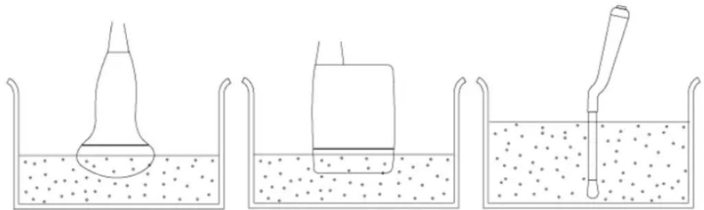
[Figure 8.1 Disinfection]
Biopsy
A biopsy is an examination method that surgically extracts tissue from the patient for examination. The probe and the biopsy kit are used together when conducting a biopsy with the ultrasonographic image scanner.
The ultrasound system shows the needle, which penetrates through the skin surface and veins, along with the examination location, minimizing the risk to the patient.
Biopsy KIT Components
The biopsy kit consists of the adaptor, needle guide and needle. The components vary depending on the probe type. The components and accessories can be purchased from MEDISON.
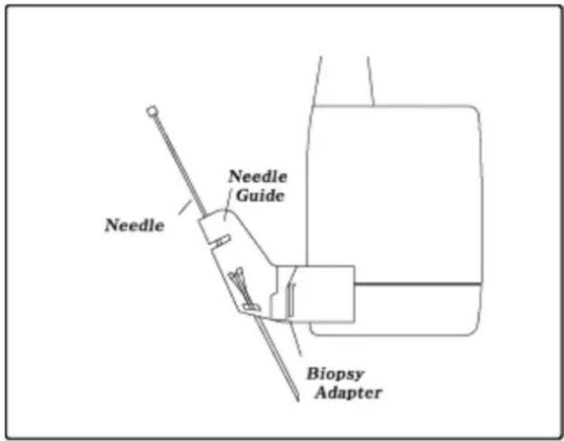
[Figure 8.2 Biopsy Kit Components]
- Adaptor: Secures the needle guide to the probe tightly.
- Needle Guide: Guides the angle (direction) of the needle so that it can reach the examination location accurately. It also secures the needle so that the needle is not loose.
- Needle: This is the needle that is inserted into the patient's body.
- Sheath: Prevents the probe and adaptor from getting soiled by any unwanted substances during the examination (blood and other body fluids).
- Ultrasound Gel: The space between the probe and the sheath is filled with the ultrasound gel to obtain images of the best quality.
Using the Biopsy Kit
WARNING
■ Verify the condition of the biopsy needle before use. Do not use a bent biopsy needle.
■ The biopsy needle may bend during tissue penetration. The precise location of the needle must be checked by monitoring the echo generated from the needle.
■ Never use the biopsy kit to biopsy prostate tissue.
■ Verify the condition of the biopsy needle before use. Do not use a bent biopsy needle.
Before Using Biopsy Kit
Ultrasonographic scanning using the biopsy kit must be conducted by medical doctors or experienced medical staff with appropriate qualifications. Always, without fail, verify all safety prevention procedures and disinfection.
Use only MEDISON-approved biopsy kits. Other bands may not properly fit MEDISON probes. Improper installation may result in patient discomfort.
Inspect all components. Ensure that the biopsy kit you are using is the correct one for the probe, the system, and system software.
WARNING
■ Do not attempt to use the biopsy until you read the instructions for installing the sheath and verifying alignment of the needle guide.
■ Always ensure that the probe and the needle guide are secured on both the left and the right.
■ Do not use in IVF, CVS, or PUBS procedures.
Biopsy Procedure
The system generates a needle guideline though the displayed real-time ultrasound images to indicate the anticipated path of the needle. You can use this guideline to ensure that the needle or instrument is following the correct path.
- Ready the patient according to the procedure appropriate for the examination objectives.
- Install the sheath and the biopsy kit.
- Set the system controls for the biopsy procedure.
- If necessary, apply acoustic gel to the patient.
- Begin scanning the patient. Adjust the patient so that the location for examination fits into the needle guideline on the screen.
-
Insert the needle into the needle guide.
-
Perform the puncture by sliding the needle through the groove in the guide until the needle intercepts the target.
-
To keep the needle securely in the needle guide, press down on the top of the biopsy adapter with your index finger.
-
When the examination location is reached, take the needle out of the needle guide.
- Detach the needle guide, adapter and sheath from the probe.
- Dispose of the components that are not designed for reuse.
Needle Guide Alignment
Alignment of the needle guide displayed on the system is for the purpose of verifying whether the needle and the needle guide are properly installed. This must be done prior to the biopsy examination. Do not use the needle guide if the needle is not following the intended path. Contact MEDISON Customer Service Department for service.
Reverberation or other tissue artifacts may produce false needle images which can cause confusion. Ensure the needle path is along the guideline, and that you are not using a false needle image to locate the needle.
WARNING
■ The needle used for this alignment verification must not be used for the actual procedure. Always use a new, sterile needle for each biopsy procedure.
■ To assist in accurate projection of the needle, use a straight, new needle for each alignment procedure.
- Attach the biopsy kit.
- Set the system depth for the procedure to be performed and select the Biopsy menu.
- Immerse the probe into the water bath, and insert the needle into the needle guide.
- Confirm that the needle image is on the needle guidelines. If so, the needle guide is properly aligned.
- If the needle image is out of the needle guideline, check the needle guide or the probe adapter.
Cleaning and Disinfecting Biopsy Kit
Wash and disinfect the biopsy kit to reduce pathogens to the level of 106 . Some components of the biopsy kit may be disposable. Please read the biopsy kit user manual carefully before use.
Only disinfect vaginal and rectal probes. A 10-6 reduction in pathogens should be reached following the disinfection procedures in this manual and using the following MEDISON recommended solutions. The following disinfectants are recommended because of both their biological effectiveness (as qualified through the FDA 510(k) process) and their chemical compatibility with MEDISON ultrasound product materials.
WARNING
Always use protective eyewear and gloves when cleaning and disinfecting biopsy kit.
Cleaning and disinfection of stainless steel biopsy kit
Cleaning
- After use, remove the biopsy kit from the probe.
- Disassemble the biopsy kit into its component parts, if applicable.
- Using a small brush and water, scrub each part to remove trapped material from the biopsy kit.
- Rinse with water to remove remaining particulates.
Disinfection
- Disinfect the adapter by autoclaving (Steam) or using gas (Ethylene Oxide).
- After disinfection, follow the proper post-disinfection procedure for the disinfection method used. (Please refer to the disinfection user manual, etc.)
- Inspect the biopsy kit for damage such as cracks, rust or breakage. If damage is evident, discontinue use of the biopsy kit and contact MEDISON Customer Service Department.
Cleaning and Disinfection of plastic biopsy kit
Cleaning
- After use, remove the biopsy kit from the probe.
- Disassemble the biopsy kit into its component parts, if applicable. Discard the single-use parts. These parts cannot be disinfected.
- Using a small brush and water, scrub each part to remove trapped material from the reusable components.
- Rinse with water to remove remaining particulates.
Disinfection
- Check the disinfection duration (generally 10 hours) and temperature of the disinfectant.
- After disinfection, follow the proper post-disinfection procedure for the disinfection method used.
- Inspect the components for damage such as cracks, rust or breakage. If damage is evident, discontinue use of the biopsy kit and contact MEDISON Customer Service Department.
CAUTION
Always use protective eyewear and gloves when cleaning and disinfecting biopsy kit.
Assembling the Biopsy Kit
C3-7IM Biopsy guide
■ Specification
| Model name BP-C | 3-7IM | |
| Component | Adapter | 1EA |
| Box | 1 EA | |
| Material | Stainless (non-disposable) | |
| Available Gauges 15 | G, 16G, 17G, 18G, 19G, 20G, 21G, 22G | |
■ Biopsy Kit Configuration
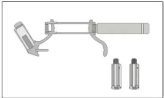
■ Installation
1. Fill the sheath with the ultrasound gel.
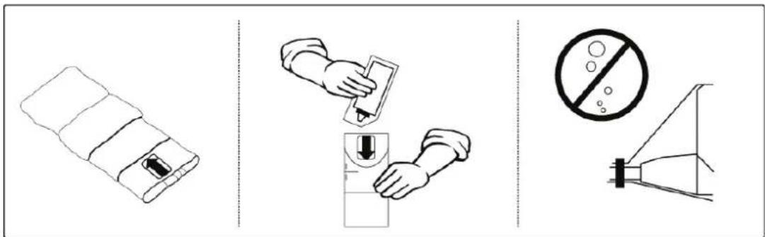
Sheath
Gel inside Sheath
- Mount the Adapter onto the probe.
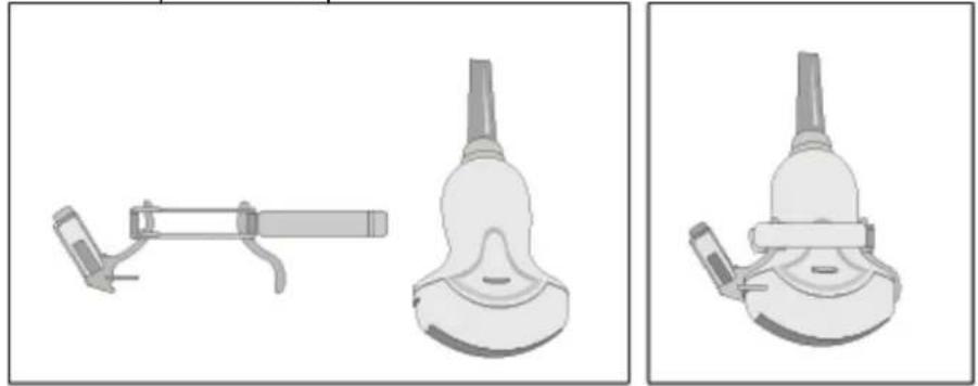
-
Install the needle guide onto the adapter.
-
Place the sheath on the adapter and insert the needle into the needle guide.
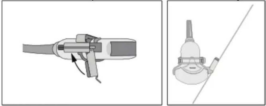
VAW3-5 / VAW4-7 / 3D3-5EK / 3D4-7EK Biopsy guide
■ Specification
| Model name | PEC-51 | |
| Component | Biopsy KIT(Adapter&Guide) | 1EA |
| Case | 1 EA | |
| User Manual | 1 EA | |
| Material | Stainless (non-disposable) | |
| Available Gauges | 16G, 18G, 22G | |
■ Biopsy Kit Configuration
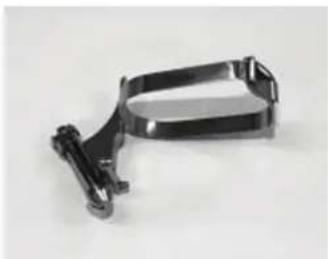
■ Installation
- Mount the Adapter onto the probe.
- Install the needle guide onto the adapter.
- Insert the needle into the needle guide.
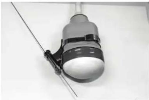
VNW6-12 Biopsy guide
■ Specification
| Model name | PEC-54 |
| Inner diameters | 1.0mm, 1.4mm, 2.2mm |
■ Biopsy Kit Configuration
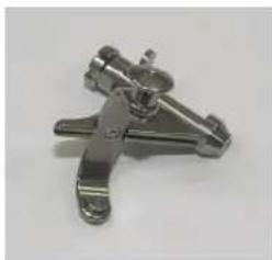
■ Installation
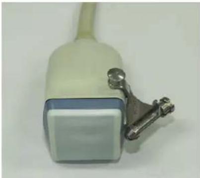
VDW5-8B / 3D5-8EK Biopsy guide
■ Specification
| Model name | PEC-47 | |
| Component | Biopsy KIT(Adapter&Guide) | 1EA |
| Case | 1 EA | |
| User Manual | 1 EA | |
| Material | Stainless (non-disposable) | |
| Available Gauges | 16G, 18G, 22G | |
■ Biopsy Kit Configuration
■ Installation
- Mount the Adapter onto the probe.
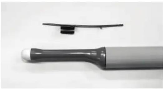
- Fix the biopsy adapter to the probe turning the knob.
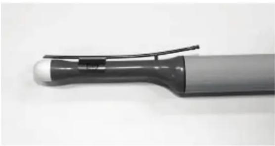
- Insert the needle into the needle guide.
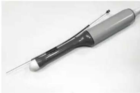
EC4-9ES / EC4-9IS Biopsy guide
■ Specification
| Model name | BPKIT-003 |
| Component | Adapter 1EABox 1 EA |
| Material | PUR 2160 |
| Available Gauges | 17G |
■ Biopsy Kit Configuration

Biopsy Adapter Needle Guide
■ Installation
- Mount the Adapter onto the probe.
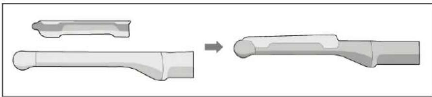
- Place the cover supplied with the kit all the way down to the adapter and then secure the guide.
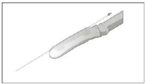
L5-12IM Biopsy guide
■ Specification
| Model name | BP-L5-12IM | |
| Component | Adapter | 1EA |
| Box | 1 EA | |
| Material | Stainless (non-disposable) | |
| Available Gauges | 15G, 16G, 17G, 18G, 19G, 20G, 21G, 22G | |
■ Biopsy Kit Configuration
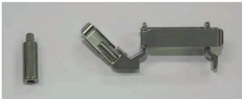
■ Installation
- Mount the biopsy adaptor onto the probe as shown below.
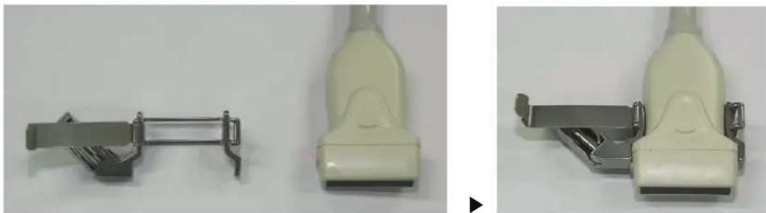
- Fill the sheath with sterile acoustic coupling gel and pulling the sheath to completely cover the adaptor.
- Mount the needle guide & clip onto the adaptor and insert the needle into the needle guide as shown below.
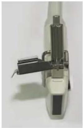
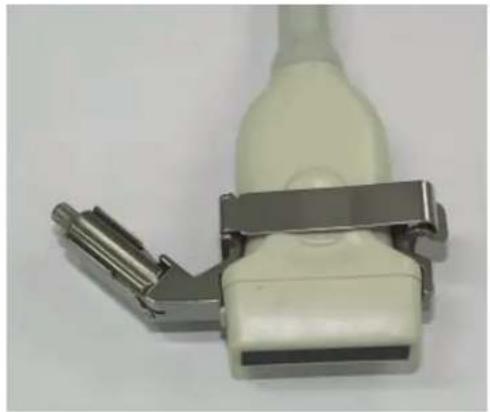
C5-2EL Biopsy guide
■ Specification
| Model name | BPK-C2-5EL |
| Component | Biopsy Adapter 1EABox 1EA |
| Material | Acetal Copolymer |
| Available Gauges | 14G, 16G, 18G, 20G, 22G |
■ Biopsy Kit Configuration
Biopsy Adapter
Needle Guide
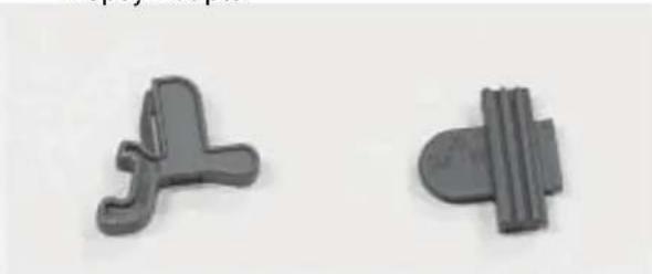
Clip (Left)
Clip (Right)
■ Installation
- Mount the Adapter onto the probe.
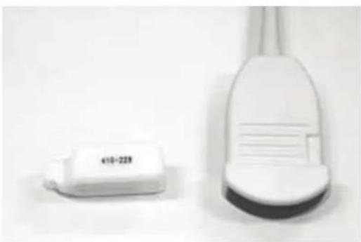
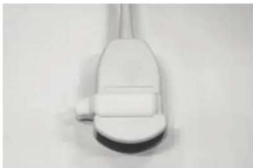
- Fill the sheath with the ultrasound gel.
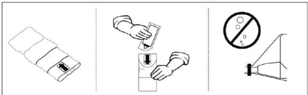
- Install the needle guide onto the adapter.
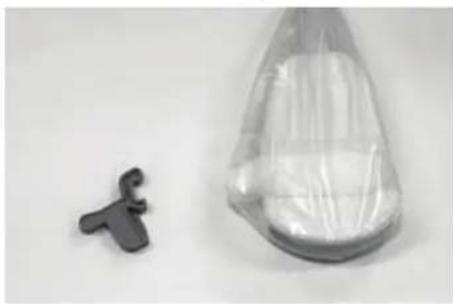
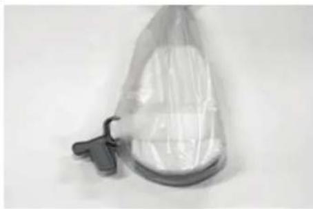
- Installing the Needle Guide Clip.
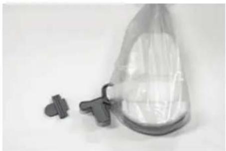
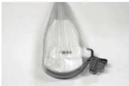
- Insert the needle into the needle guide.
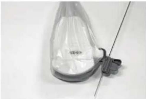
C2-6IC Biopsy guide
■ Specification
| Model name | BPK-C2-6IC | |
| Component | Adapter | 1EA |
| Box | 1 EA | |
| Available Gauges | 14G, 15G, 16G, 17G, 18G, 19G, 20G, 21G, 22G, 23G | |
■ Biopsy Kit Configuration
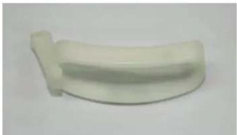
Biopsy
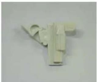
Adapter
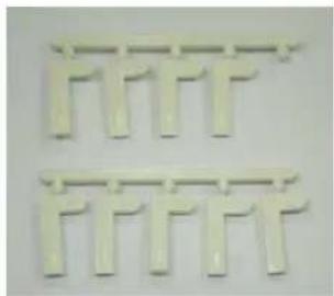
Needle
Guide
Clip
■ Installation
- Mount the biopsy adaptor onto the probe as shown below.
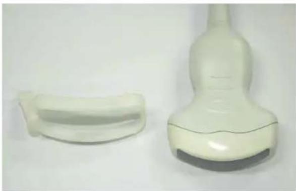
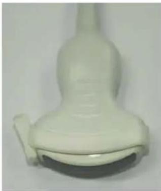
- Insert gel into probe cover. And cover it.
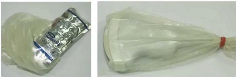
- Install the needle guide onto the adapter.
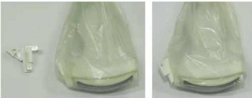
- Installing the Needle Guide Clip.
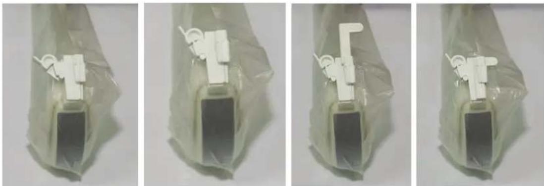
- Insert the needle into the needle guide.
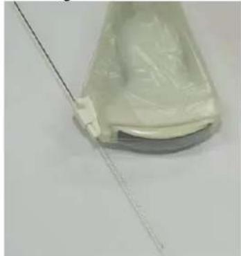
L6-12IS / L8-15IS Biopsy guide
■ Specification
| Model name | BP-KIT-012 | |
| Component | Adapter | 1EA |
| Box | 1 EA | |
| Needle Guide Pack | 24 EA | |
| Available Gauges | 14G, 15G, 16G, 17G, 18G, 19G, 20G, 21G, 22G, 23G | |
■ Biopsy Kit Configuration
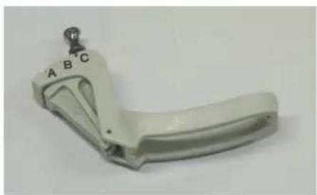
Biopsy
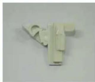
Adapter
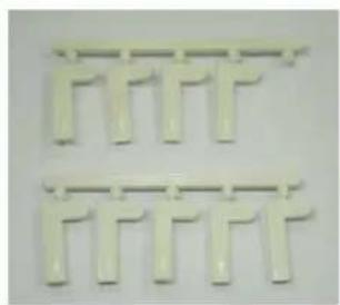
Needle
Guide
Clip
■ Installation
- Mount the biopsy adaptor onto the probe as shown below.
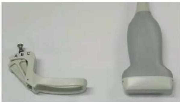
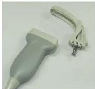
- Selecting Bracket Angle (& Locking).
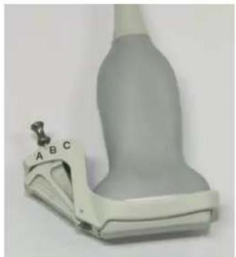
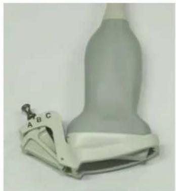
- Insert gel into probe cover. And cover it.
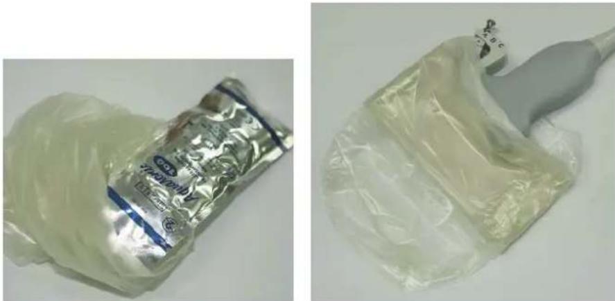
- Installing the Needle Guide and Clip.
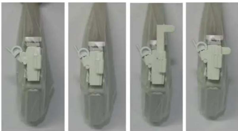
- Insert the needle into the needle guide.
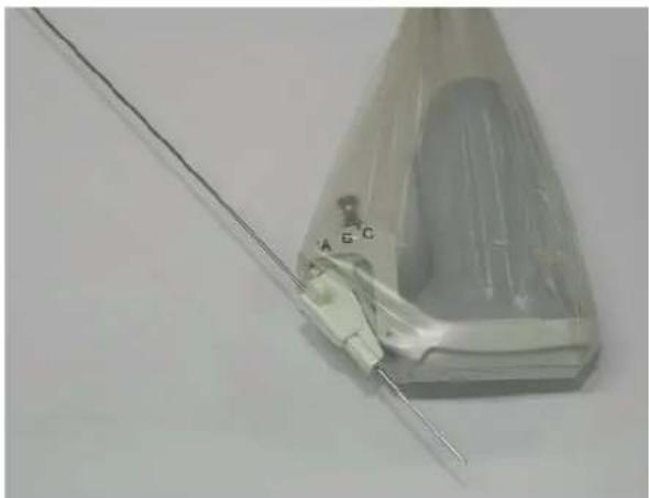
L5-9EE Biopsy guide
■ Specification
| Model name | BP-KIT-013 | |
| Component | Biopsy KIT(Adapter&Guide)CaseUser Manual | 1EA1EA1EA |
| Material | Acetal Copolymer | |
| Available Gauges | 16G, 18G, 20G | |
■ Biopsy Kit Configuration
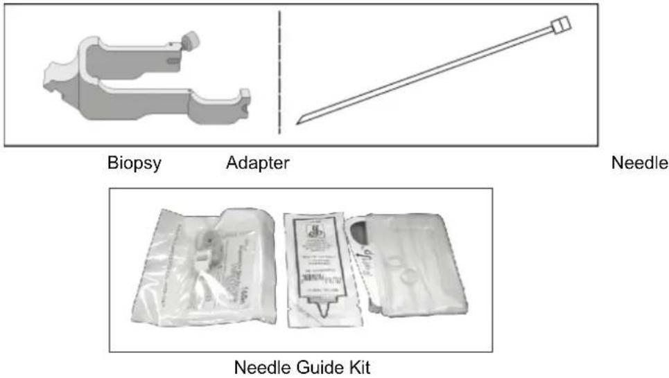
■ Installation
- Mount the Adapter onto the probe.
![graph LR A["Initial Clip"] --> B["Force Application"] B --> C["Load Adjustment"] C --> D["Final Load Adjustment"]](/content/2026/05/955519/images/7cf56a08048ec16eb8b896e5a6a03b7c44ae1b9733262f8f33fcfe3da9de3097.jpg)
- Insert gel into probe cover. And cover it.
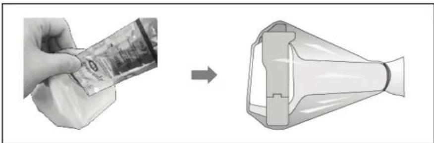
- Install the needle guide onto the adapter.
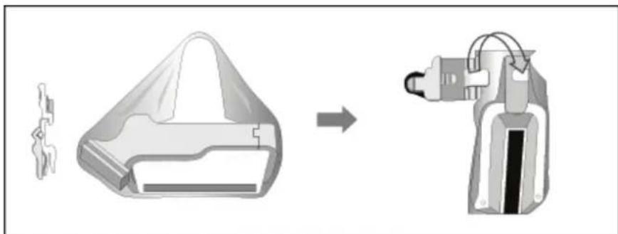
- Lock the needle guide.
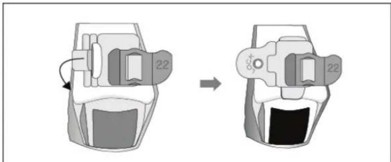
- Press the needle guide and install the needle into the needle guide.
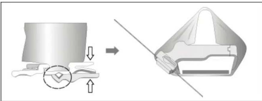
C1-4EC Biopsy guide
■ Specification
| Model name | BP-KIT-016 |
| Component | Biopsy KIT(Adapter&Guide) 1EACase 1EAUser Manual 1EA |
| Material | Polyphenolsulfone |
| Available Gauges | 14G, 15G, 16G, 17G, 18G, 20G, 21G, 22G, 23G |
■ Installation
- Mount the Adapter onto the probe.
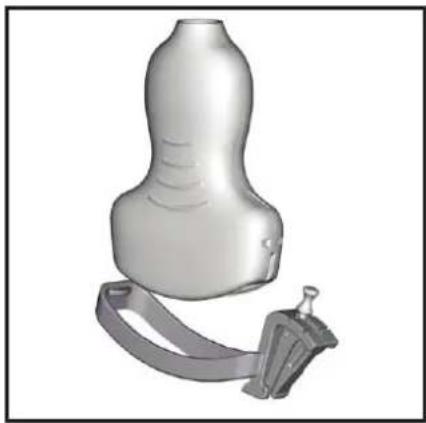
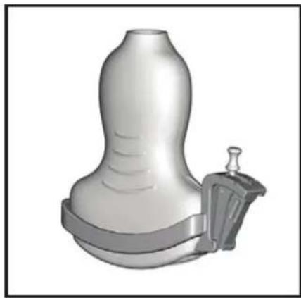
- Insert gel into the cover for the Kit and cover the adaptor completely.
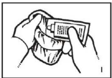
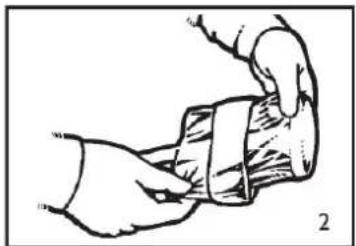
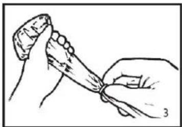
- Mount the needle guide for the desired gauge onto the adaptor along the groove.
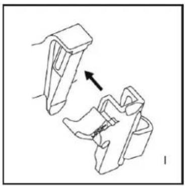
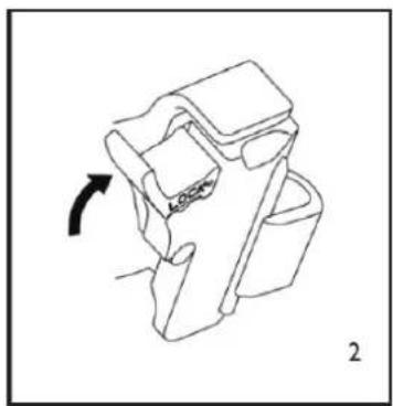
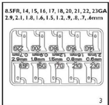
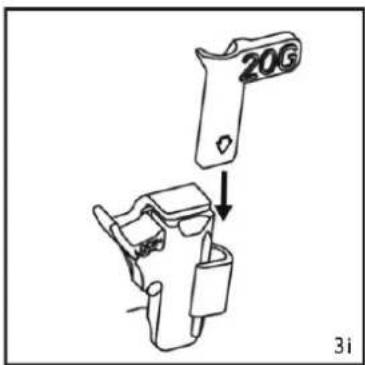
C4-7EL Biopsy guide
■ Specification
| Model name | BP-KIT-014 | |
| Component | Biopsy KIT(Adapter&Guide)BOX | 1EA1EA |
| Material | Polyurethane | |
| Available Gauges | 14G, 16G, 18G, 20G, 22G, 25G | |
■ Biopsy Kit Configuration
Biopsy Adapter
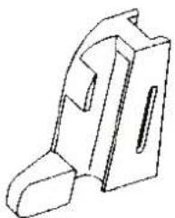
Needle Guide
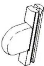
Clip
■ Installation
- Mount the Adapter onto the probe.
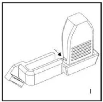
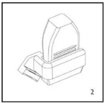
- Insert gel into the cover for the Kit and cover the adaptor completely.
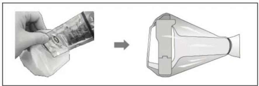
- Mount the needle guide onto the adaptor.
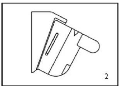
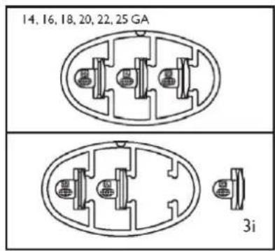
- Mount the needle guide for the desired gauge onto the adaptor.
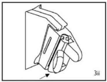
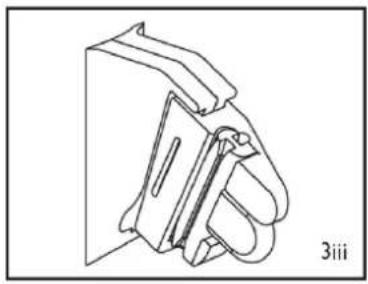
- Insert a needle into the needle guide and start using it.
3D2-6ET Biopsy guide
■ Specification
| Model name BP-KIT-015 | |
| Component | Biopsy Adapter 1 EANeedle Guide PackBox 1 EA |
| Material | Polyurethane |
| Available Gauges | 16 G, 18G, 22G |
■ Biopsy Kit Configuration
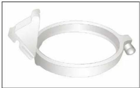
Biopsy Adapter
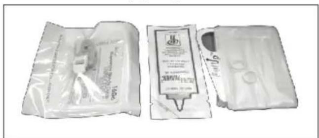
Needle Guide Kit
■ Installation
- Mount the Adapter onto the probe.
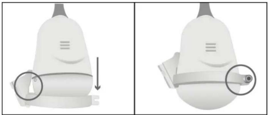
- Insert gel into the cover for the Kit and cover the adaptor completely.
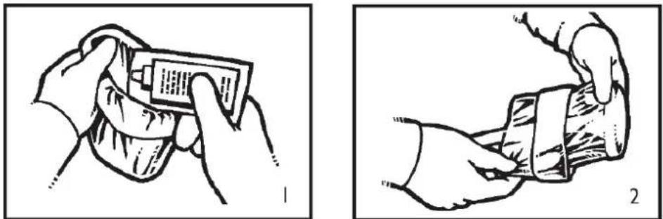
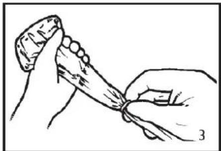
- Mount the needle guide for the desired gauge onto the adaptor.
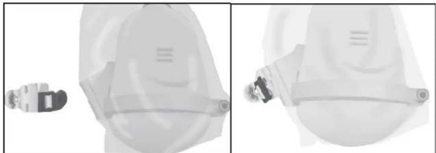
- Lock the needle guide.
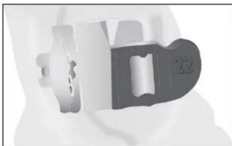
(a)
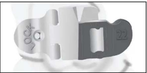
(b)
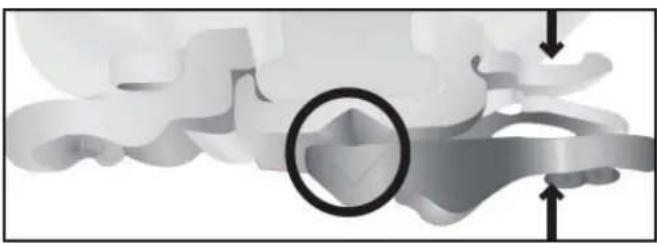
(c)
- Press the needle guide like figure (c) and install the needle into the needle guide.
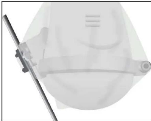
Table of Contents
OB REFERENCE......5
ESTIMATED FETAL WEIGHT FORMULA 5
Method using (BPD, AC) 5
Method using (BPD, FL, FTA) 6
Method using (BPD, APTD, TTD, FL) 6
Method using (BPD, APTD, TTD, SL)....6
Method using (BPD, TTD)....6
Method using (AC, FL) 7
Method using (BPD, AC, FL) 7
Method using (HC, AC, FL) 8
Method using (BPD, HC, AC, FL) 9
Method using (AC) 9
Method using (BPD, AC) 9
Method using (AC, HC) 10
Method using (BPD, APTD, TTD) 10
GESTATIONAL AGE FORMULA AND TABLE LIST 11
Abdominal Circumference(AC) : KOREAN 11
Abdominal Circumference (AC) : HADLOCK.... 12
Abdominal Circumference (AC) : HANSMANN.... 13
Abdominal Circumference (AC) : MERZ 15
Abdominal Circumference (AC) : JEANTY 19
Abdominal Circumference (AC) : TOKYO 20
Abdominal Circumference (AC) : CHITTY (D) 22
Abdominal Circumference (AC) : CHITTY (M) 23
Abdominal Circumference (AC) : CAMPBELL 24
Abdominal Circumference (AC) : ASUM(SCW) 26
Abdominal Circumference (AC) : CFEF 27
Biparietal Diameter (BPD) : KOREAN.... 28
Biparietal Diameter (BPD) : HANSMANN 29
Biparietal Diameter (BPD) : HADLOCK 31
Biparietal Diameter (BPD) : MERZ.... 32
Biparietal Diameter (BPD) : JEANTY 35
Biparietal Diameter (BPD) : SABBAGHA 37
Biparietal Diameter (BPD) : TOKYO 38
Biparietal Diameter (BPD) : OSAKA 40
Biparietal Diameter (BPD) : CHITTY (OUT-IN) 45
Biparietal Diameter (BPD) : CHITTY (OUT-OUT) 47
Biparietal Diameter (BPD) : CAMPBELL.... 49
Biparietal Diameter (BPD) : KURTZ 50
Biparietal Diameter (BPD) : ASUM(SCW).... 52
Biparietal Diameter (BPD) : BESSIS 53
Biparietal Diameter (BPD) : CFEF.... 54
Crown-Rump Length (CRL) : KOREAN 55
Crown-Rump Length (CRL) : ROBINSON....56
Crown-Rump Length (CRL) : HANSMANN 57
Crown-Rump Length (CRL) : TOKYO 60
Crown-Rump Length (CRL) : NELSON....62
Crown-Rump Length (CRL) : HADLOCK....63
Crown-Rump Length (CRL) : OSAKA....65
Crown-Rump Length (CRL) : ASUM(SCW)....67
Crown-Rump Length (CRL) : REMPEN....68
Femur Length (FL) : KOREAN....70
Femur Length (FL) : HADLOCK 71
Femur Length (FL) : MERZ 72
Femur Length (FL) : HANSMANN 74
Femur Length (FL) : HOHLER....76
Femur Length (FL) : JEANTY 77
Femur Length (FL) : TOKYO 79
Femur Length (FL) : OSAKA....81
Femur Length (FL) : CHITTY 85
Femur Length (FL) : CAMPBELL 87
Femur Length (FL) : ASUM(SCW)....89
Femur Length (FL) : DOUBILET 90
Femur Length (FL) : BESSIS....91
Femur Length (FL) : CFEF 92
Anterior Posterior Thoracic Diameter (APTD) : HANSMANN....93
Anterior Posterior Thoracic Diameter (APTD) and Thorax Transverse Diameter (TTD):
SHINOZUKA 95
Thorax Transverse Diameter (TTD) : HANSMANN....97
Gestational Sac (GS) : KOREAN....99
Gestational Sac (GS) : HANSMANN 100
Gestational Sac (GS) : HELLMAN....101
Gestational Sac (GS) : NYBERG.... 102
Gestational Sac (GS) : TOKYO 103
Occipital Frontal Diameter (OFD) : HANSMANN....104
Occipital Frontal Diameter (OFD) : KOREAN 106
Occipital Frontal Diameter (OFD) : ASUM(SCW)....107
Occipital Frontal Diameter (OFD) : MERZ 108
Inner Ocular Distance (IOD) : HASNMANN....110
Outer Ocular Distance (OOD) : JENATY 111
Outer Ocular Distance (OOD) : HANSMANN 112
Humerus (HUM) : JENATY 113
Humerus (HUM) : KOREAN.... 115
Humerus (HUM) : MERZ....116
Humerus (HUM) : OSAKA 118
Humerus (HUM) : ASUM(SCW)....120
Tibia (TIB) : JENATY 121
Tibia (TIB) : MERZ 123
Tibia (TIB) : HANSMANN....125
Cerebellum : HILL 126
Cerebellum: CHITTY 127
Cerebellum : GOLDSTEIN 128
Ulna:JEANTY 129
Ulna : MERZ 131
Ulna : HANSMANN 132
Head Circumference (HC) : KOREAN 133
Head Circumference (HC) : HANSMANN 134
Head Circumference (HC) : HADLOCK 136
Head Circumference (HC) : MERZ 137
Head Circumference (HC) : CHITTY (D).... 141
Head Circumference (HC) : CHITTY (M) 143
Head Circumference (HC) : CAMPBELL 145
Head Circumference (HC) : ASUM(SCW) 146
Head Circumference (HC) : CFEF 147
Fetal Age Table (FTA) : OSAKA 148
Clavicle (CLAV) : YARKONI 152
Length of Vertebral (Vertebral) : TOKYO 154
Radius Length (RAD) : MERZ 155
Radius Length (RAD) : JEANTY 156
Radius Length (RAD) : HANSMANN 157
Mean Abdominal Diameter (MAD) : EIK-NESSH.... 158
Mid Cerebral Artery(MCA)-Resistance Index(RI) : SHINOZUKA 160
Mid Cerebral Artery(MCA)-Pulsatility Index(PI) : SHINOZUKA 161
Umbilical Artery(UmA)-Resistance Index(RI) : SHINOZUKA 162
Umbilical Artery(UmA)- Pulsatility Index(PI) : SHINOZUKA 163
Anterior Posterior Abdominal Diameter (APD): BESSIS.... 164
Transverse Abdominal Diameter (TAD) : CFEF 165
Thoracic Circumference (ThC): CHITKARA.... 166
Fibula Length (FIB): JEANTY 167
Fibula Length (FIB): HANSMANN 168
Nuchal Thickness (NT) : YAGEL 169
Amniotic Fluid Index (AFI) : MOORE 170
Head Circumference(HC) / Abdominal Circumference(AC): Campbell 171
Femur Length/Head Circumference (FL/HC) : HADLOCK 172
ESTIMATED FETAL WEIGHT GROWTH REFERENCE.... 173
Estimate Fetal Weight (EFW) : BRENNER 173
Estimate Fetal Weight (EFW) : DOUBILET 174
Estimate Fetal Weight (EFW) : OSAKA 175
Estimate Fetal Weight (EFW) : HADLOCK 178
Estimate Fetal Weight (EFW) : TOKYO 179
Estimate Fetal Weight (EFW) : WILLIAMS 180
Estimate Fetal Weight (EFW) : YARKONI (TWINS) 181
Estimate Fetal Weight (EFW) : HANSMANN 182
VASCULAR REFERENCE 183
UROLOGY REFERENCE 185
FETAL ECHO REFERENCE....187
CARDIOLOGY REFERENCE ...... 190
CARDIOLOGY 2D....190
CARDIOLOGY C MODE....195
CARDIOLOGY M MODE....197
CARDIOLOGY DOPPLER....201
ACOUSTIC POWER TABLES 205
OB Reference
Estimated Fetal Weight Formula
Method using (BPD, AC)
Shepard Method [grams]
[Equation]
1000 × 10(-1.7492 + 0.166 × (BPD) + 0.046 × (AC) - 0.002646 × (AC) × (BPD))
[Input Range]
AC :15.5\~40.0 cm
BPD : 3.1\~10.0 cm
EFW:224\~4925 g
[Reference]
Shepard MJ, et al, “An Evaluation of Two Equations for Predicting Fetal Weight by Ultrasound,” American Journal of Ob & Gyn, January 1982; 142(1):47-54
Hadlock Method [grams]
[Equation]
10(1.11 + (0.05845 × AC) - (0.000604 × AC2) - (0.007365 × BPD2) + (0.000595 × BPD × AC) + (0.1694 × BPD))
[Reference]
Hadlock F, et al, "Sonographic Estimated of Fetal Weight," Radiology 1984:150:535-540
Merz Method [grams]
[Equation]
EFW = (157.07 × AC) + (15.9 × BPD2) - 3200.4
[Reference]
E. Merz, W. Goldhofer, E. Timor-Tritsch "Ultrasound in Gynecology and Obstetrics" Textbook and Atlas, 1991, Georg Thieme Verlag, 308-338
Method using (BPD, FL, FTA)
Osaka university [grams]
[Equation]
EFW = (1. 2 5 6 4 7 (BPD ^ 3) + (3. 5 0 6 6 5 (FTA (FL) + 6. 3
[Reference]
Mineo Aoki. "The Diagnosis and Treatment of IUGR" Perineitaru Kea (Japanese Journal of Perinatal Care), 1990; Vol.9 NO.5, p407-422 (in Japanese)
Method using (BPD, APTD, TTD, FL)
Tokyo 2 university Method [grams]
[Equation]
1.07*BPD 3 +3.42*APTD*TTD*FL
[Reference]
Jpn J Med Ultrasonics Vol.23. No.12 (1996)
Method using (BPD, APTD, TTD, SL)
Shinozuka 2 Method [grams]
[Equation]
1.07*BPD 3 +2.91*APTD*TTD*SL
[Reference]
Shinozuka, N et, al, Am J Obstet Gynecol 157:1140, 1987
Method using (BPD, TTD)
Hansmann's fetal weight [grams]
[Equation]
((- 1. 0 5 7 7 5 × BPD) + (0. 6 4 9 1 4 5 × TTD) + (0. 0 9 3 0 7 0 7 × BPD ^ 2) - (0. 0 2 0 5 6 2 × TTD ^ 2) + (0. 5 1 5 2 6 3)) × 1 0 0 0. 0
[Low Range]
BPD : 5.9cm \~ ∞
TTD : 5.6cm \~ ∞
EFW: 500g \~ ∞
[Reference]
Hansmann, Hackeloer, Staudach, Wittman, "Ultrasound Diagnosis in Obstetrics and Gynecology," Springer-Verlag, New York, 1986
Method using (AC, FL)
Hadlock 1 Method [grams]
[Equation]
Log10 (EFW) = (0. 0 5 2 8 1 × AC) + (0. 1 9 3 8 × FL) - (0. 0 0 4 × AC × FL) + 1. 3 0 4
± 2SD = 16%
[Reference]
Frank P. Hadlock, R. B. Harrist, Ralph S. Sharman, Russell L. Deter, Seung K. Park. "Estimation of fetal weight with the use of head, body, and femur measurement-A prospective study" American Journal of Obstetrics and Gynaecology, Vol 151. No.3:333-337, February 1, 1985
Ferrero [grams]
[Equation]
Log10 (EFW) = (0. 1 3 2 4 4 × AC) - (0. 1 2 9 9 6 × FL) - (0. 0 0 1 7 3 5 8 8 × AC 2)
+ (0. 0 0 3 0 9 2 1 2 × FL × AC) + (2. 1 8 9 8 4 × FL / AC) + 0. 7 7 1 2 5
[Reference]
Ferrero A, Maggi E, Giancotti A, et al: Regression formula for estimation of fetal weight with use of abdominal circumference and femur length: A prospective study. J Ultrasound Med 13:823, 1994
Method using (BPD, AC, FL)
Hadlock 2 Method [grams]
[Equation]
Log10 (EFW) = (0. 0 3 1 6 × BPD) + (0. 0 4 5 7 × AC) + (0. 1 6 2 3 × FL) - (0. 0 0 3 4 × AC × FL) + 1. 3 3 5
± 2SD = 15%
[Reference]
Frank P. Hadlock, R. B. Harrist, Ralph S. Sharman, Russell L. Deter, Seung K. Park.
"Estimation of fetal weight with the use of head, body, and femur measurement-A prospective study" American Journal of Obstetrics and Gynaecology, Vol 151. No.3:333-337, February 1, 1985
Shinozuka 1 Method [grams]
[Equation]
1. 0 7 × BPD ^ 3 + 0. 3 0 × AC ^ 2 × FL
[Reference]
Shinozuka, N et, al, Am J Obstet Gynecol 157:1140, 1987
Woo [grams]
[Equation]
Log _ 1 0 (EFW) = (0. 1 5 5 4 9 × BPD) + (0. 0 4 8 6 4 × AC) - (0. 0 0 2 7 9 6 8 2 × BPD × AC)
+ (0. 0 3 7 7 6 9 × FL) - (0. 0 0 0 4 9 4 5 2 9 × AC × FL) + 1. 1 3 7 0 5
[Reference]
Woo JS, Wan CW, Cho KM: Computer-assisted evaluation of ultrasonic fetal weight prediction using multiple regression equations with and without the fetal femur length, J Ultrasound Med 4:65, 1985
Method using (HC, AC, FL)
Hadlock 3 Method [grams]
[Equation]
Log _ 1 0 (EFW) = (0. 0 1 0 7 × HC) + (0. 0 4 3 8 × AC) + (0. 1 5 8 × FL) - (0. 0 0 3 2 6 × AC × FL) + 1. 3 2 6
± 2 SD = 15 %
[Reference]
Frank P. Hadlock, R. B. Harrist, Ralph S. Sharman, Russell L. Deter, Seung K. Park. "Estimation of fetal weight with the use of head, body, and femur measurement-A prospective study" American Journal of Obstetrics and Gynaecology, Vol 151. No.3:333-337, February 1, 1985
Weiner2 [grams]
[Equation]
Log _ 1 0 (EFW) = (0. 0 2 2 5 3 × HC) + (0. 0 1 6 4 5 × AC) + (0. 0 6 4 3 9 × FL) + 1. 6 9 6 1
[Reference]
Weiner CP, Sabbagha RE, Vaisrub N, et al: Ultrasonic fetal weight prediction: Role of head circumference and femur length. Obstet Gynecol 65:812, 1985
Method using (BPD, HC, AC, FL)
Hadlock 4 Method [grams]
[Equation]
Log _ 1 0 (EFW) = (0. 0 0 6 4 × HC) + (0. 0 4 2 4 × AC) + (0. 0 0 0 6 1 × BPD × AC)
+ (0. 1 7 4 × FL) - (0. 0 0 3 8 6 × AC × FL) + 1. 3 5 9 6
± 2SD = 14.8%
[Reference]
Frank P. Hadlock, R. B. Harrist, Ralph S. Sharman, Russell L. Deter, Seung K. Park. "Estimation of fetal weight with the use of head, body, and femur measurement-A prospective study" American Journal of Obstetrics and Gynaecology, Vol 151. No.3:333-337, February 1, 1985
Method using (AC)
Campbell's fetal weight [grams]
[Equation]
1 0 0 0 × 1 0 ^ (0. 2 8 2 × AC - 0. 0 0 3 3 1 × AC 2 - 4. 5 6 4)
[Input Range]
AC:21.0\~40.0cm
EFW:903\~4137g
[Reference]
Campbell, S., Wilkin, D. "Ultrasonic Measurement of Fetal Abdomen Circumference in the Estimation of Fetal Weight." British Journal of OB & GYN, 82, 9: 689-697, September 1975
Higginbottom [grams]
[Equation]
EFW = AC ^ 3 × 0. 0 8 1 6
[Reference]
Higginbottom J, Slater J. Porter G, et al: Estimation of fetal weight from ultrasonic measurement of trunk circumference. Br J Obstet Gynecol 82:698, 1975
Method using (BPD, AC)
Thurnau [grams]
[Equation]
EFW = (9. 3 3 7 × BPD × AC) - 2 2 9
[Reference]
Thurnau GR, Tamura RK, Sabbagha R, et al: A simple estimated fetal weight equation based on real-time ultrasound measurements of fetuses less than thirty-four weeks' gestation. Am J Obstet Gynecol 145:557, 1983
Warsof [grams]
[Equation]
Log _ 1 0 (EFW) = (0. 1 4 4 × BPD) + (0. 0 3 2 × AC) - (0. 0 0 0 1 1 1 × AC × BPD ^ 2) - 1. 5 9 9) × 1 0 0 0
[Reference]
Warsof SL, Gohari P, Berkowitz RL, et al: The estimation of fetal weight by computer-assisted analysis. Am J Obstet Gynecol 120:881, 1977
Method using (AC, HC)
Weiner1 [grams]
[Equation]
Log _ 1 0 (EFW) = (0. 0 4 0 3 5 × HC) + (0. 0 1 2 8 5 × AC) + 1. 6 5 7 5
[Reference]
Weiner CP, Sabbagha RE, Vaisrub N, et al: Ultrasonic fetal weight prediction: Role of head circumference and femur length. Obstet Gynecol 65:812, 1985
Method using (BPD, APTD, TTD)
Tokyo 1 university Method [grams]
[Equation]
1. 7 3 × BPD ^ 3 + 2 8 × APTD × TTD - 2 1 7
[Reference]
Jpn J Med Ultrasonics Vol.23. No.12 (1996)
Gestational Age Formula and Table List
Abdominal Circumference(AC) : KOREAN
GA Table
Y.G Park." The Standardization of Fetal body parts according to the normal Korean Gestational Age in Ultrasound" Korean Ultrasound Institute, Vol. 14, No.2, 1995
GA = 7. 4 0 3 5 0 6 + 0. 7 6 1 9 1 × AC + 0. 0 0 4 4 9 2 3 0 4 × AC ^ 2
Output Unit : w(weeks)
Input Unit : cm
Min Range : 5.9 cm
Max Range : 35.2 cm
Fetal Growth Table
Y.G Park. "The Standardization of Fetal body parts according to the normal Korean Gestational Age in Ultrasound" Korean Ultrasound Institute, Vol. 14, No.2, 1995
AC = 1 3. 5 5 4 0 8 5 × MA - 0. 0 5 9 9 7 3 × MA ^ 2 - 9 4. 5 8 8 1 6 8
Output Unit : cm
Input Unit : w(week)
Min Range : 12cm
Max Range : 40cm
| Age (W) | Growth (cm) | ±SD (cm) |
| 12 | 5.932 | 0.794 |
| 16 | 10.793 | 0.728 |
| 20 | 15.086 | 0.742 |
| 24 | 19.300 | 1.258 |
| 28 | 23.988 | 0.870 |
| 32 | 27.738 | 0.799 |
| 34 | 29.578 | 0.771 |
| 36 | 31.731 | 0.583 |
| 38 | 33.514 | 0.370 |
| 40 | 34.490 | 1.608 |
Abdominal Circumference (AC) : HADLOCK
GA Table
Frank P. Hadlock, Russell L. Deter, Ronald B. Harrist, Seung K. Park., "Estimating Fetal Age: Computer-Assisted Analysis of Multiple Fetal Growth Parameters" Radiology, 1984; 152:497-501.
GA = 8. 1 4 + 0. 7 5 3 × AC + 0. 0 0 3 6 × AC ^ 2
Output Unit : w(weeks)
Input Unit : cm
Min Range : 4.83cm
Max Range : 38.04 cm
Standard Deviation :
| Min (w) Max (w) ±2SD | ||
| 12 | 18 | 1.66 |
| 18 | 24 | 2.06 |
| 24 | 30 | 2.18 |
| 30 | 36 | 2.96 |
| 36 | 42 | 3.04 |
Fetal Growth Table
Hadlock, F., Deter, R.L., Harrist, R.B., Park, S.K. "Estimating Fetal Age: Computer-Assisted Analysis of Multiple Fetal Growth Parameters" Radiology, 1984, 152: 497-501. (Biometric Age and Growth Equations)
Graph = 1. 6 1 × MA - 0. 0 0 9 9 8 × MA ^ 2 - 1 3. 3
Output Unit : cm
Input Unit : w(weeks)
Min Range : 12 cm
Max Range : 40 cm
Standard Deviation : 2SD = 2.68 cm
| Min Range(w) | Max Range(w) | SD(w) |
| 0 | 100 | 2.68 |
Abdominal Circumference (AC) : HANSMANN
GA Table
Hansmann, Hackeloer, Staudach, Wittman "Ultrasound Diagnosis in Obstetrics and Gynecology" Springer-Verlag, New York, 1986, p.431.
| AC (cm) | GA (wd) |
| 5.3 | 12w0d |
| 6.3 | 13w0d |
| 7.5 | 14w0d |
| 8.5 | 15w0d |
| 9.7 | 16w0d |
| 10.7 | 17w0d |
| 11.6 | 18w0d |
| 12.6 | 19w0d |
| 13.5 | 20w0d |
| 14.5 | 21w0d |
| 15.5 | 22w0d |
| 16.5 | 23w0d |
| 17.3 | 24w0d |
| 18.3 | 25w0d |
| 19.1 | 26w0d |
| 20.2 | 27w0d |
| 21.1 | 28w0d |
| 22.2 | 29w0d |
| 23.0 | 30w0d |
| 24.0 | 31w0d |
| 24.9 | 32w0d |
| 25.8 | 33w0d |
| 26.8 | 34w0d |
| 27.7 | 35w0d |
| 28.7 | 36w0d |
| 29.6 | 37w0d |
| 30.6 | 38w0d |
| 31.5 | 39w0d |
| 32.0 | 40w0d |
Fetal Growth Table
Hansmann, Hackeloer, Staudach, Wittman "Ultrasound Diagnosis in Obstetrics and Gynecology" Springer-Verlag, New York, 1986, p.431.
| GA(W) | Growth(cm) |
| 12 | 5.30 |
| 13 | 6.30 |
| 14 | 7.50 |
| 15 | 8.50 |
| 16 | 9.70 |
| 17 | 10.70 |
| 18 | 11.60 |
| 19 | 12.60 |
| 20 | 13.50 |
| 21 | 14.50 |
| 22 | 15.50 |
| 23 | 16.50 |
| 24 | 17.30 |
| 25 | 18.30 |
| 26 | 19.10 |
| 27 | 20.20 |
| 28 | 21.10 |
| 29 | 22.20 |
| 30 | 23.00 |
| 31 | 24.00 |
| 32 | 24.90 |
| 33 | 25.80 |
| 34 | 26.80 |
| 35 | 27.70 |
| 36 | 28.70 |
| 37 | 29.60 |
| 38 | 30.60 |
| 39 | 31.50 |
| 40 | 32.00 |
Abdominal Circumference (AC) : MERZ
GA Table
E. Merz, W. Goldhofer, E. Timor-Tritsch "Ultrasound in Gynecology and Obstetrics" Text book and Atlas, 1991 Georg Thieme Verlag, 308-338
| AC (cm) | GA (wd) | 5% (wd) | 95% (wd) |
| 5.6 | 12w1d | 10w6d | 13w2d |
| 5.8 | 12w2d | 11w1d | 13w4d |
| 6.0 | 12w4d | 11w2d | 13w5d |
| 6.2 | 12w5d | 11w4d | 13w6d |
| 6.4 | 12w6d | 11w5d | 14w1d |
| 6.6 | 13w1d | 11w6d | 14w2d |
| 6.8 | 13w2d | 12w0d | 14w4d |
| 7.0 | 13w4d | 12w1d | 14w5d |
| 7.2 | 13w4d | 12w3d | 14w6d |
| 7.4 | 13w6d | 12w4d | 15w1d |
| 7.6 | 14w0d | 12w6d | 15w2d |
| 7.8 | 14w1d | 12w6d | 15w4d |
| 8.0 | 14w3d | 13w1d | 15w5d |
| 8.2 | 14w4d | 13w2d | 15w6d |
| 8.4 | 14w6d | 13w4d | 16w1d |
| 8.6 | 15w0d | 13w5d | 16w2d |
| 8.8 | 15w1d | 13w6d | 16w4d |
| 9.0 | 15w3d | 14w0d | 16w5d |
| 9.2 | 15w4d | 14w1d | 16w6d |
| 9.4 | 15w5d | 14w3d | 17w1d |
| 9.6 | 15w6d | 14w4d | 17w2d |
| 9.8 | 16w1d | 14w6d | 17w4d |
| 10.0 | 16w2d | 14w6d | 17w5d |
| 10.2 | 16w4d | 15w1d | 17w6d |
| 10.4 | 16w5d | 15w2d | 18w1d |
| 10.6 | 16w6d | 15w4d | 18w2d |
| 10.8 | 17w1d | 15w5d | 18w3d |
| 11.0 | 17w2d | 15w6d | 18w4d |
| 11.2 | 17w3d | 16w0d | 18w6d |
| 11.4 | 17w4d | 16w1d | 19w0d |
| 11.6 | 17w6d | 16w3d | 19w1d |
| 11.8 | 18w0d | 16w4d | 19w3d |
| 12.0 | 18w1d | 16w6d | 19w4d |
| 12.2 | 18w3d | 17w0d | 19w6d |
| 12.4 | 18w4d | 17w1d | 20w0d |
| 12.6 | 18w6d | 17w2d | 20w1d |
| 12.8 | 19w0d | 17w4d | 20w3d |
| 13.0 | 19w1d | 17w5d | 20w4d |
| 13.2 | 19w2d | 17w6d | 20w6d |
| 13.4 | 19w4d | 18w0d | 21w0d |
| 13.6 | 19w5d | 18w1d | 21w1d |
| 13.8 | 19w6d | 18w3d | 21w3d |
| 14.0 | 20w1d | 18w4d | 21w4d |
| 14.2 | 20w2d | 18w6d | 21w6d |
| 14.4 | 20w4d | 19w0d | 22w0d |
| 14.6 | 20w5d | 19w1d | 22w1d |
| 14.8 | 20w6d | 19w2d | 22w3d |
| 15.0 | 21w1d | 19w4d | 22w4d |
| 15.2 | 21w1d | 19w5d | 22w6d |
| 15.4 | 21w3d | 19w6d | 23w0d |
| 15.6 | 21w4d | 20w1d | 23w1d |
| 15.8 | 21w6d | 20w1d | 23w3d |
| 16.0 | 22w0d | 20w3d | 23w4d |
| 16.2 | 22w1d | 20w4d | 23w6d |
| 16.4 | 22w3d | 20w6d | 24w0d |
| 16.6 | 22w4d | 21w0d | 24w1d |
| 16.8 | 22w6d | 21w1d | 24w3d |
| 17.0 | 23w0d | 21w2d | 24w4d |
| 17.2 | 23w1d | 21w4d | 24w6d |
| 17.4 | 23w2d | 21w5d | 25w0d |
| 17.6 | 23w4d | 21w6d | 25w1d |
| 17.8 | 23w5d | 22w1d | 25w3d |
| 18.0 | 23w6d | 22w1d | 25w4d |
| 18.2 | 24w1d | 22w3d | 25w6d |
| 18.4 | 24w2d | 22w4d | 26w0d |
| 18.6 | 24w4d | 22w6d | 26w1d |
| 18.8 | 24w5d | 23w0d | 26w3d |
| 19.0 | 24w6d | 23w1d | 26w4d |
| 19.2 | 25w0d | 23w2d | 26w6d |
| 19.4 | 25w1d | 23w4d | 27w0d |
| 19.6 | 25w3d | 23w5d | 27w1d |
| 19.8 | 25w4d | 23w6d | 27w3d |
| 20.0 | 25w6d | 24w1d | 27w4d |
| 20.2 | 26w0d | 24w2d | 27w6d |
| 20.4 | 26w1d | 24w3d | 27w6d |
| 20.6 | 26w3d | 24w4d | 28w1d |
| 20.8 | 26w4d | 24w6d | 28w2d |
| 21.0 | 26w6d | 25w0d | 28w4d |
| 21.2 | 27w0d | 25w1d | 28w5d |
| 21.4 | 27w1d | 25w2d | 28w6d |
| 21.6 | 27w2d | 25w4d | 29w1d |
| 21.8 | 27w4d | 25w5d | 29w2d |
| 22.0 | 27w5d | 25w6d | 29w4d |
| 22.2 | 27w6d | 26w1d | 29w5d |
| 22.4 | 28w1d | 26w2d | 29w6d |
| 22.6 | 28w2d | 26w3d | 30w1d |
| 22.8 | 28w4d | 26w4d | 30w2d |
| 23.0 | 28w5d | 26w6d | 30w4d |
| 23.2 | 28w6d | 27w0d | 30w5d |
| 23.4 | 29w0d | 27w1d | 30w6d |
| 23.6 | 29w1d | 27w3d | 31w1d |
| 23.8 | 29w3d | 27w4d | 31w2d |
| 24.0 | 29w4d | 27w5d | 31w4d |
| 24.2 | 29w6d | 27w6d | 31w5d |
| 24.4 | 30w0d | 28w1d | 31w6d |
| 24.6 | 30w1d | 28w2d | 32w1d |
| 24.8 | 30w3d | 28w3d | 32w2d |
| 25.0 | 30w4d | 28w4d | 32w4d |
| 25.2 | 30w6d | 28w6d | 32w5d |
| 25.4 | 30w6d | 29w0d | 32w6d |
| 25.6 | 31w1d | 29w1d | 33w1d |
| 25.8 | 31w2d | 29w3d | 33w2d |
| 26.0 | 31w4d | 29w4d | 33w4d |
| 26.2 | 31w5d | 29w5d | 33w5d |
| 26.4 | 31w6d | 29w6d | 33w6d |
| 26.6 | 32w1d | 30w1d | 34w1d |
| 26.8 | 32w2d | 30w2d | 34w2d |
| 27.0 | 32w4d | 30w4d | 34w4d |
| 27.2 | 32w5d | 30w4d | 34w5d |
| 27.4 | 32w6d | 30w6d | 34w6d |
| 27.6 | 33w0d | 31w0d | 35w1d |
| 27.8 | 33w1d | 31w1d | 35w2d |
| 28.0 | 33w3d | 31w3d | 35w4d |
| 28.2 | 33w4d | 31w4d | 35w5d |
| 28.4 | 33w6d | 31w5d | 35w6d |
| 28.6 | 34w0d | 31w6d | 36w1d |
| 28.8 | 34w1d | 32w1d | 36w2d |
| 29.0 | 34w3d | 32w2d | 36w4d |
| 29.2 | 34w4d | 32w4d | 36w5d |
| 29.4 | 34w5d | 32w4d | 36w6d |
| 29.6 | 34w6d | 32w6d | 37w1d |
| 29.8 | 35w1d | 33w0d | 37w1d |
| 30.0 | 35w2d | 33w1d | 37w3d |
| 30.2 | 35w4d | 33w3d | 37w4d |
| 30.4 | 35w5d | 33w4d | 37w6d |
| 30.6 | 35w6d | 33w5d | 38w0d |
| 30.8 | 36w1d | 33w6d | 38w1d |
| 31.0 | 36w2d | 34w1d | 38w3d |
| 31.2 | 36w4d | 34w2d | 38w4d |
| 31.4 | 36w4d | 34w4d | 38w6d |
| 31.6 | 36w6d | 34w4d | 39w0d |
| 31.8 | 37w0d | 34w6d | 39w1d |
| 32.0 | 37w1d | 35w0d | 39w3d |
| 32.2 | 37w3d | 35w1d | 39w4d |
| 32.4 | 37w4d | 35w3d | 39w6d |
| 32.6 | 37w6d | 35w4d | 40w0d |
| 32.8 | 38w0d | 35w5d | 40w1d |
| 33.0 | 38w1d | 35w6d | 40w3d |
| 33.2 | 38w3d | 36w1d | 40w4d |
| 33.4 | 38w4d | 36w2d | 40w6d |
| 33.6 | 38w5d | 36w4d | 41w0d |
| 33.8 | 38w6d | 36w5d | 41w1d |
| 34.0 | 39w1d | 36w6d | 41w3d |
| 34.2 | 39w2d | 37w0d | 41w4d |
| 34.4 | 39w4d | 37w1d | 41w6d |
| 34.6 | 39w5d | 37w3d | 42w0d |
| 34.8 | 39w6d | 37w4d | 42w1d |
Fetal Growth Table
E. Merz, W. Goldhofer, E. Timor-Tritsch "Ultrasound in Gynecology and Obstetrics" Textbook and Atlas, 1991 Georg Thieme Verlag, 308-338
| Age (W) | Growth (cm) | 5% (cm) | 95% (cm) |
| 12 | 5.8 | 4 | |
| 13 | 6.8 | 5 | |
| 14 | 7.9 | 6 | |
| 15 | 8.9 | 6.9 | |
| 16 | 9.9 | 7.9 | |
| 17 | 11 | 8.9 | |
| 18 | 12 | 9.9 | |
| 19 | 13 | 10.8 | 15.2 |
| 20 | 14 | 11.8 | 16.2 |
| 21 | 15.1 | 12.8 | 17.3 |
| 22 | 16.1 | 13.8 | 18.4 |
| 23 | 17.1 | 14.8 | 19.5 |
| 24 | 18.2 | 15.8 | 20.5 |
| 25 | 19.2 | 16.7 | 21.6 |
10.9 11.9 13 14.1
| 26 | 20.2 | 17.7 | 22.7 |
| 27 | 21.2 | 18.7 | 23.8 |
| 7.6 28 | 22.3 | 19.7 | 24.8 |
| 8.7 29 | 23.3 | 20.7 | 25.9 |
| 9.8 30 | 24.3 | 21.7 | 27 |
| 31 | 25.3 | 22.7 | 28 |
| 32 | 26.4 | 23.7 | 29.1 |
| 33 | 27.4 | 24.6 | 30.2 |
| 34 | 28.4 | 25.6 | 31.2 |
| 35 | 29.5 | 26.6 | 32.3 |
| 36 | 30.5 | 27.6 | 33.4 |
| 37 | 31.5 | 28.6 | 34.4 |
| 38 | 32.5 | 29.6 | 35.5 |
| 39 | 33.6 | 30.6 | 36.5 |
| 40 | 34.6 | 31.6 | 37.6 |
Abdominal Circumference (AC) : JEANTY
Fetal Growth Table
Jeanty, P., Cousaert, E., Cantraine, F., "Normal Growth of the Abdominal Perimeter" American Journal of Perinatology, 1:129, 1984
| Age (W) | Growth (cm) | Min (cm) | Max (cm) |
| 12 | 5.70 | 3.50 | 8.00 |
| 13 | 6.70 | 4.50 | 9.00 |
| 14 | 7.70 | 5.50 | 10.00 |
| 15 | 8.80 | 6.50 | 11.00 |
| 16 | 9.80 | 7.60 | 12.00 |
| 17 | 10.90 | 8.60 | 13.10 |
| 18 | 11.90 | 9.70 | 14.20 |
| 19 | 13.00 | 10.80 | 15.20 |
| 20 | 14.10 | 11.90 | 16.30 |
| 21 | 15.20 | 12.90 | 17.40 |
| 22 | 16.30 | 14.00 | 18.50 |
| 23 | 17.30 | 15.10 | 19.60 |
| 24 | 18.40 | 16.20 | 20.60 |
| 25 | 19.50 | 17.20 | 21.70 |
| 26 | 20.50 | 18.30 | 22.70 |
| 27 | 21.50 | 19.30 | 23.80 |
| 28 | 22.50 | 20.30 | 24.80 |
| 29 | 23.50 | 21.30 | 25.70 |
| 30 | 24.40 | 22.20 | 26.70 |
| 31 | 25.40 | 23.10 | 27.60 |
| 32 | 26.20 | 24.00 | 28.50 |
| 33 | 27.10 | 24.80 | 29.30 |
| 34 | 27.90 | 25.60 | 30.10 |
| 35 | 28.60 | 26.40 | 30.90 |
| 36 | 29.30 | 27.10 | 31.60 |
| 37 | 30.00 | 27.80 | 32.20 |
| 38 | 30.60 | 28.30 | 32.80 |
| 39 | 31.10 | 28.90 | 33.30 |
| 40 | 31.60 | 29.40 | 33.80 |
Abdominal Circumference (AC) : TOKYO
GA Table
Jpn J Med Ultrasonics Vol. 23. No. 12 (1996)
| AC (cm) | GA (wd) | Min (wd) | Max (wd) |
| 10.00 | 15w3d | 14w2d | 16w4d |
| 10.50 | 16w0d | 14w6d | 17w1d |
| 11.00 | 16w4d | 15w3d | 17w5d |
| 11.50 | 17w0d | 15w6d | 18w1d |
| 12.00 | 17w4d | 16w2d | 18w6d |
| 12.50 | 18w0d | 16w5d | 19w2d |
| 13.00 | 18w4d | 17w2d | 19w6d |
| 13.50 | 19w0d | 17w5d | 20w2d |
| 14.00 | 19w4d | 18w2d | 20w6d |
| 14.50 | 20w0d | 18w5d | 21w2d |
| 15.00 | 20w3d | 19w0d | 21w6d |
| 15.50 | 21w0d | 19w4d | 22w3d |
| 16.00 | 21w3d | 20w0d | 22w6d |
| 16.50 | 22w0d | 20w4d | 23w3d |
| 17.00 | 22w3d | 21w0d | 23w6d |
| 17.50 | 22w6d | 21w3d | 24w2d |
| 18.00 | 23w3d | 21w6d | 25w0d |
| 18.50 | 23w6d | 22w2d | 25w3d |
| 19.00 | 24w3d | 22w6d | 26w0d |
| 19.50 | 24w6d | 23w2d | 26w3d |
| 20.00 | 25w3d | 23w6d | 27w0d |
| 20.50 | 25w6d | 24w2d | 27w3d |
| 21.00 | 26w3d | 24w5d | 28w1d |
| 21.50 | 27w0d | 25w2d | 28w5d |
| 22.00 | 27w3d | 25w5d | 29w1d |
| 22.50 | 28w0d | 26w2d | 29w5d |
| 23.00 | 28w4d | 26w6d | 30w2d |
| 23.50 | 29w0d | 27w2d | 30w5d |
| 24.00 | 29w4d | 27w5d | 31w3d |
| 24.50 | 30w1d | 28w2d | 32w0d |
| 25.00 | 30w5d | 28w6d | 32w4d |
| 25.50 | 31w2d | 29w3d | 33w1d |
| 26.00 | 31w6d | 30w0d | 33w5d |
| 26.50 | 32w3d | 30w4d | 34w2d |
| 27.00 | 33w1d | 31w2d | 35w0d |
| 27.50 | 33w5d | 31w5d | 35w5d |
| 28.00 | 34w2d | 32w2d | 36w2d |
| 28.50 | 35w0d | 33w0d | 37w0d |
| 29.00 | 35w4d | 33w4d | 37w4d |
| 29.50 | 36w2d | 34w2d | 38w2d |
| 30.00 | 37w0d | 35w0d | 39w0d |
| 30.50 | 37w5d | 35w5d | 39w5d |
| 31.00 | 38w2d | 36w1d | 40w3d |
| 31.50 | 39w0d | 36w6d | 41w1d |
| 32.00 | 39w6d | 37w5d | 42w0d |
| 32.50 | 40w4d | 38w3d | 42w5d |
| 33.00 | 41w2d | 39w1d | 43w3d |
Fetal Growth Table
Jpn J Med Ultrasonics Vol. 23. No. 12 (1996)
| Age (W) | Growth (cm) | Min (cm) | Max (cm) |
| 16 | 10.90 | 9.50 | 12.40 |
| 17 | 12.00 | 10.40 | 13.50 |
| 18 | 13.00 | 11.40 | 14.60 |
| 19 | 14.00 | 12.30 | 15.70 |
| 20 | 15.10 | 13.30 | 16.80 |
| 21 | 16.10 | 14.20 | 17.80 |
| 22 | 17.10 | 15.10 | 18.90 |
| 23 | 18.10 | 16.10 | 20.00 |
| 24 | 19.10 | 17.00 | 21.10 |
| 25 | 20.10 | 17.90 | 22.10 |
| 26 | 21.00 | 18.80 | 23.10 |
| 27 | 22.00 | 19.70 | 24.20 |
| 28 | 22.90 | 20.50 | 25.20 |
| 29 | 23.80 | 21.40 | 26.10 |
| 30 | 24.70 | 22.20 | 27.10 |
| 31 | 25.60 | 23.00 | 28.10 |
| 32 | 26.50 | 23.80 | 29.00 |
| 33 | 27.30 | 24.50 | 29.90 |
| 34 | 28.10 | 25.30 | 30.70 |
| 35 | 28.90 | 26.00 | 31.60 |
| 36 | 29.70 | 26.60 | 32.40 |
| 37 | 30.40 | 27.30 | 33.20 |
| 38 | 31.10 | 27.90 | 34.00 |
| 39 | 31.80 | 28.50 | 34.70 |
| 40 | 32.40 | 29.10 | 35.40 |
| 41 | 33.00 | 29.60 | 36.10 |
| 42 | 33.60 | 30.10 | 36.70 |
Abdominal Circumference (AC) : CHITTY (D)
Fetal Growth Table
L.S. Chitty, D.G. Altman, S. Campbell, "Charts of Fetal Size: 3. Abdominal Measurement"
British Journal of Obstetrics and Gynaecology, February 1994. Vol 101. Pp125-131
| Age (W) | Growth (cm) | Min (cm) | Max (cm) |
| 12 | 5.58 | 5.05 | |
| 13 | 6.74 | 6.13 | |
| 14 | 7.89 | 7.2 | |
| 15 | 9.03 | 8.27 | |
| 16 | 10.16 | 9.33 | |
| 17 | 11.29 | 10.38 | 12.21 |
| 18 | 12.41 | 11.42 | 13.4 |
| 19 | 13.52 | 12.45 | 14.59 |
| 20 | 14.62 | 13.48 | 15.77 |
| 21 | 15.71 | 14.49 | 16.94 |
| 22 | 16.8 | 15.5 | |
| 23 | 17.87 | 16.49 | 19.25 |
| 24 | 18.93 | 17.48 | 20.38 |
| 25 | 19.98 | 18.45 | 21.51 |
| 26 | 21.02 | 19.41 | 22.63 |
| 27 | 22.04 | 20.36 | 23.73 |
| 28 | 23.06 | 21.29 | 24.82 |
| 6.29 | 24.05 | 22.22 | 25.89 |
| 7.30 | 25.04 | 23.12 | 26.96 |
| 8.531 | 26.01 | 24.02 | 28.01 |
| 9.39 | 26.97 | 24.9 | |
| 11 33 | 27.91 | 25.76 | 30.06 |
| 34 | 28.84 | 26.61 | 31.06 |
| 35 | 29.75 | 27.44 | 32.05 |
| 36 | 30.64 | 28.26 | 33.02 |
| 37 | 31.51 | 29.06 | 33.97 |
| 38 | 32.37 | 29.84 | 34.91 |
| 18.9 | 33.21 | 30.6 | |
| 40 | 34.04 | 31.35 | 36.72 |
| 41 | 34.84 | 32.08 | 37.6 |
| 42 | 35.62 | 32.78 | 38.46 |
Abdominal Circumference (AC) : CHITTY (M)
Fetal Growth Table
L.S. Chitty, D.G. Altman, S. Campbell, "Charts of Fetal Size: 3. Abdominal Measurement" British Journal of Obstetrics and Gynaecology, February 1994. Vol 101. Pp125-131
| Age (W) | Growth (cm) | Min (cm) | Max (cm) |
| 12 | 5.89 | 5.13 | |
| 13 | 7.09 | 6.26 | |
| 14 | 8.27 | 7.39 | |
| 15 | 9.45 | 8.5 | |
| 16 | 10.62 | 9.62 | |
| 17 | 11.78 | 10.72 | 12.84 |
| 18 | 12.93 | 11.82 | 14.05 |
| 19 | 14.08 | 12.9 | |
| 20 | 15.21 | 13.98 | 16.45 |
| 21 | 16.34 | 15.05 | 17.63 |
| 22 | 17.46 | 16.1 | |
| 23 | 18.56 | 17.15 | 19.97 |
| 24 | 19.66 | 18.19 | 21.12 |
| 25 | 20.74 | 19.21 | 22.27 |
| 26 | 21.81 | 20.22 | 23.39 |
| 27 | 22.87 | 21.22 | 24.51 |
| 28 | 23.91 | 22.21 | 25.61 |
| 6.68 | 24.94 | 23.18 | 26.7 |
| 7.90 | 25.96 | 24.14 | 27.78 |
| 9.35 | 26.96 | 25.08 | 28.84 |
| 10.39 | 27.95 | 26.01 | 29.89 |
| 11.62 | 28.92 | 26.93 | 30.92 |
| 34 | 29.88 | 27.82 | 31.93 |
| 35 | 30.82 | 28.7 | |
| 15.26 | 31.74 | 29.57 | 33.91 |
| 37 | 32.64 | 30.41 | 34.88 |
| 38 | 33.53 | 31.24 | 35.82 |
| 18.39 | 34.4 | 32.05 | 36.75 |
| 40 | 35.25 | 32.84 | 37.66 |
| 41 | 36.08 | 33.62 | 38.54 |
| 42 | 36.89 | 34.37 | 39.41 |
Abdominal Circumference (AC) : CAMPBELL
GA Table
Campbell Professor Campbell's Group at Harris Birthright Centre, King's College Hospital
| AC (cm) | GA (wd) | ±SD (wd) |
| 9.00 | 14w0d | 02w0d |
| 10.10 | 15w0d | 02w1d |
| 11.20 | 16w0d | 02w1d |
| 12.30 | 17w0d | 02w1d |
| 13.40 | 18w0d | 02w1d |
| 14.50 | 19w0d | 02w1d |
| 15.60 | 20w0d | 02w2d |
| 16.70 | 21w0d | 02w2d |
| 17.80 | 22w0d | 02w2d |
| 18.80 | 23w0d | 02w3d |
| 19.90 | 24w0d | 02w4d |
| 21.00 | 25w0d | 02w5d |
| 22.10 | 26w0d | 02w5d |
| 23.10 | 27w0d | 02w6d |
| 24.20 | 28w0d | 02w6d |
| 25.30 | 29w0d | 02w6d |
| 26.40 | 30w0d | 03w0d |
| 27.50 | 31w0d | 03w1d |
| 28.60 | 32w0d | 03w1d |
| 29.70 | 33w0d | 03w4d |
| 30.80 | 34w0d | 04w0d |
| 31.70 | 35w0d | 04w2d |
| 32.50 | 36w0d | 04w2d |
| 33.10 | 37w0d | 04w2d |
| 33.80 | 38w0d | 04w2d |
| 34.40 | 39w0d | 0w0d |
| 35.00 | 40w0d | 0w0d |
Fetal Growth Table
Chitty, L., Campbell, S., "Charts of Fetal Size: Abdominal measurements,"
British J of OB and Gyn., February 1994, vol. 101, ppl 125-131, Table1.
| Age (wd) | Growth (cm) |
| 12w0d | 6.00 |
| 13 w0d 7.02 | |
| 14 w0d 8.43 | |
| 15 w0d 9.43 | |
| 16 w0d 10.96 | |
| 17 w0d 11.75 | |
| 18 w0d 13.06 | |
| 19 w0d 14.44 | |
| 20 w0d 15.20 | |
| 21 w0d 16.53 | |
| 22 w0d 17.03 | |
| 23 w0d 18.51 | |
| 24 w0d 19.54 | |
| 25 w0d 20.46 | |
| 26 w0d 21.54 |
| 27 w0d 22.62 |
| 28 w0d 24.12 |
| 29 w0d 25.35 |
| 30 w0d 26.22 |
| 31 w0d 27.30 |
| 32 w0d 27.98 |
| 33 w0d 29.21 |
| 34 w0d 30.14 |
| 35 w0d 31.09 |
| 36 w0d 31.85 |
| 37 w0d 32.94 |
| 38 w0d 33.10 |
| 39 w0d 34.26 |
| 40 w0d 36.04 |
| 41 w0d 36.89 |
Abdominal Circumference (AC) : ASUM(SCW)
Fetal Growth Table
Australasian Society for Ultrasound in Medicine
Policies and Statements - [D7] Statement On Normal Ultrasonic Fetal Measurements (Revised May 2001)
| Age (w) | Growth (mm) | ±SD (mm) |
| 11 | 52.00 | 10.00 |
| 12 | 63.00 | 10.00 |
| 13 | 74.00 | 10.00 |
| 14 | 84.00 | 10.00 |
| 15 | 96.00 | 10.00 |
| 16 | 106.00 | 10.00 |
| 17 | 120.00 | 15.00 |
| 18 | 131.00 | 15.00 |
| 19 | 140.00 | 15.00 |
| 20 | 151.00 | 15.00 |
| 21 | 164.00 | 20.00 |
| 22 | 176.00 | 20.00 |
| 23 | 186.00 | 20.00 |
| 24 | 201.00 | 20.00 |
| 25 | 212.00 | 20.00 |
| 26 | 223.00 | 25.00 |
| 27 | 230.00 | 25.00 |
| 28 | 242.00 | 25.00 |
| 29 | 259.00 | 25.00 |
| 30 | 262.00 | 25.00 |
| 31 | 272.00 | 30.00 |
| 32 | 283.00 | 30.00 |
| 33 | 294.00 | 30.00 |
| 34 | 305.00 | 30.00 |
| 35 | 315.00 | 30.00 |
| 36 | 325.00 | 35.00 |
| 37 | 333.00 | 35.00 |
| 38 | 342.00 | 35.00 |
| 39 | 356.00 | 35.00 |
| 40 | 362.00 | 35.00 |
| 41 | 367.00 | 35.00 |
Abdominal Circumference (AC) : CFEF
Fetal Growth Table
J.Créquat, M. Duyme, G. Brodaty
Y.G Park. "The Standardization of Fetal body parts according to the normal Korean Gestational Age in Ultrasound" Korean Ultrasound Institute, Vol. 14, No.2, 1995
GA = 1. 2 0 0 0 7 × BPD + 0. 2 0 7 6 × BPD ^ 2 + 9. 2 0 9 2 1 6
Output Unit : w(weeks)
Input Unit : cm
Min Range : 1.9 cm
Max Range : 9.4 cm
Fetal Growth Table
Y.G Park. "The Standardization of Fetal body parts according to the normal Korean Gestational Age in Ultrasound" Korean Ultrasound Institute, Vol. 14, No.2, 1995
BPD = 5. 1 0 6 1 0 4 × MA - 0. 0 4 6 7 1 9 × MA ^ 2 - 3 5. 0 5 3 3 3 4
Output Unit : cm
Input Unit : w(week)
Min Range : 12cm
Max Range : 40cm
| Age (W) | Growth (cm) | ±SD (cm) |
| 12 | 1.970 | 0.219 |
| 16 | 3.483 | 0.213 |
| 20 | 4.783 | 0.231 |
| 24 | 5.978 | 0.287 |
| 28 | 7.164 | 0.256 |
| 32 | 8.122 | 0.263 |
| 34 | 8.496 | 0.244 |
| 36 | 8.849 | 0.225 |
| 38 | 9.093 | 0.121 |
| 40 | 9.401 | 0.188 |
Biparietal Diameter (BPD) : HANSMANN
GA Table
Hansmann, Hackeloer, Staudach, Wittman. "Ultrasound Diagnosis in Obstetrics and Gynecology." Springer-Verlag, New York, 1986, p.440-441.
| BPD (cm) | GA (wd) | Min (wd) | Max (wd) |
| 2.9 | 13w3d | 12w2d | 14w3d |
| 3.0 | 13w5d | 12w5d | 14w5d |
| 3.1 | 14w0d | 12w6d | 15w1d |
| 3.2 | 14w2d | 13w2d | 15w3d |
| 3.3 | 14w4d | 13w3d | 15w6d |
| 3.4 | 15w0d | 13w5d | 16w2d |
| 3.5 | 15w2d | 14w1d | 16w3d |
| 3.6 | 15w4d | 14w3d | 16w6d |
| 3.7 | 16w0d | 14w6d | 17w1d |
| 3.8 | 16w2d | 15w0d | 17w4d |
| 3.9 | 16w4d | 15w3d | 17w6d |
| 4.0 | 17w0d | 15w5d | 18w1d |
| 4.1 | 17w2d | 16w0d | 18w4d |
| 4.2 | 17w4d | 16w3d | 18w6d |
| 4.3 | 17w6d | 16w4d | 19w1d |
| 4.4 | 18w1d | 16w6d | 19w3d |
| 4.5 | 18w4d | 17w2d | 19w6d |
| 4.6 | 18w6d | 17w4d | 20w1d |
| 4.7 | 19w1d | 17w6d | 20w4d |
| 4.8 | 19w3d | 18w0d | 20w6d |
| 4.9 | 19w5d | 18w1d | 21w1d |
| 5.0 | 20w0d | 18w4d | 21w1d |
| 5.1 | 20w3d | 19w0d | 21w6d |
| 5.2 | 20w5d | 19w2d | 22w1d |
| 5.3 | 21w0d | 19w3d | 22w4d |
| 5.4 | 21w3d | 20w0d | 22w6d |
| 5.5 | 21w5d | 20w2d | 23w0d |
| 5.6 | 22w0d | 20w5d | 23w2d |
| 5.7 | 22w2d | 21w0d | 23w4d |
| 5.8 | 22w5d | 21w3d | 23w6d |
| 5.9 | 23w0d | 21w4d | 24w3d |
| 6.0 | 23w2d | 21w6d | 24w4d |
| 6.1 | 23w4d | 22w1d | 25w0d |
| 6.2 | 24w0d | 22w4d | 25w3d |
| 6.3 | 24w2d | 22w6d | 25w4d |
| 6.4 | 24w4d | 23w1d | 26w0d |
| 6.5 | 24w6d | 23w4d | 26w2d |
| 6.6 | 25w1d | 23w6d | 26w5d |
| 6.7 | 25w3d | 24w1d | 27w1d |
| 6.8 | 25w6d | 24w3d | 27w2d |
| 6.9 | 26w1d | 24w6d | 27w4d |
| 7.0 | 26w3d | 25w0d | 27w6d |
| 7.1 | 26w5d | 25w2d | 28w3d |
| 7.2 | 27w1d | 25w4d | 28w4d |
| 7.3 | 27w3d | 26w0d | 29w2d |
| 7.4 | 27w6d | 26w1d | 29w4d |
| 7.5 | 28w1d | 26w3d | 29w6d |
| 7.6 | 28w4d | 26w5d | 30w2d |
| 7.7 | 28w6d | 27w1d | 30w5d |
| 7.8 | 29w2d | 27w2d | 31w3d |
| 7.9 | 29w5d | 27w3d | 32w0d |
| 8.0 | 30w0d | 27w6d | 32w1d |
| 8.1 | 30w3d | 28w2d | 32w4d |
| 8.2 | 31w0d | 28w6d | 33w1d |
| 8.3 | 31w2d | 29w0d | 33w5d |
| 8.4 | 31w6d | 29w3d | 34w2d |
| 8.5 | 32w2d | 29w6d | 34w4d |
| 8.6 | 32w5d | 30w1d | 35w1d |
| 8.7 | 33w2d | 30w2d | 36w1d |
| 8.8 | 33w5d | 31w0d | 36w3d |
| 8.9 | 34w2d | 31w4d | 37w0d |
| 9.0 | 34w5d | 32w0d | 37w3d |
| 9.1 | 35w1d | 32w1d | 38w5d |
| 9.2 | 35w6d | 33w2d | 39w2d |
| 9.3 | 36w5d | 33w5d | 39w5d |
| 9.4 | 37w3d | 34w5d | 40w1d |
| 9.5 | 38w3d | 35w2d | 41w0d |
| 9.6 | 38w6d | 35w2d | 41w3d |
| 9.7 | 39w0d | 35w6d | 42w0d |
| 9.8 | 39w2d | 36w3d | 42w0d |
| 9.9 | 39w3d | 36w4d | 42w4d |
| 10.0 | 39w4d | 36w5d | 42w2d |
| 10.1 | 39w5d | 37w1d | 42w4d |
| 10.2 | 39w6d | 37w1d | 42w2d |
| 10.3 | 40w0d | 37w2d | 42w2d |
| 10.4 | 40w1d | 37w3d | 42w2d |
| 10.5 | 40w2d | 37w6d | 42w2d |
Fetal Growth Table
Hansmann, Hackeloer, Stauch, Wittman "Ultrasound Diagnosis in Obstetrics and Gynecology" Springer-Verlag, New York, 1986. p.176
| Age (W) | Growth (cm) | Min (cm) | Max (cm) |
| 10 | 1.40 | 0.90 | 1.80 |
| 11 | 1.70 | 1.30 | 2.20 |
| 12 | 2.10 | 1.60 | 2.50 |
| 13 | 2.40 | 2.00 | 2.90 |
| 14 | 2.80 | 2.30 | 3.20 |
| 15 | 3.10 | 2.70 | 3.60 |
| 16 | 3.50 | 3.00 | 3.90 |
| 17 | 3.80 | 3.40 | 4.30 |
| 18 | 4.20 | 3.70 | 4.60 |
| 19 | 4.50 | 4.00 | 4.90 |
| 20 | 4.80 | 4.40 | 5.30 |
| 21 | 5.10 | 4.70 | 5.60 |
| 22 | 5.50 | 5.00 | 5.90 |
| 23 | 5.80 | 5.30 | 6.20 |
| 24 | 6.10 | 5.60 | 6.50 |
| 25 | 6.40 | 5.90 | 6.80 |
| 26 | 6.70 | 6.20 | 7.10 |
| 27 | 7.00 | 6.50 | 7.40 |
| 28 | 7.20 | 6.80 | 7.70 |
| 29 | 7.50 | 7.00 | 7.90 |
| 30 | 7.70 | 7.30 | 8.20 |
| 31 | 7.90 | 7.50 | 8.40 |
| 32 | 8.20 | 7.70 | 8.60 |
| 33 | 8.40 | 7.90 | 8.80 |
| 34 | 8.60 | 8.10 | 9.00 |
| 35 | 8.70 | 8.30 | 9.20 |
| 36 | 8.90 | 8.40 | 9.30 |
| 37 | 9.00 | 8.60 | 9.50 |
| 38 | 9.10 | 8.70 | 9.60 |
| 39 | 9.30 | 8.80 | 9.70 |
| 40 | 9.30 | 8.90 | 9.80 |
Biparietal Diameter (BPD) : HADLOCK
GA Table
Hadlock, F., Deter, R.L., Harrist, R.B., Park, S.K. "Estimating Fetal Age: Computer-Assisted Analysis of Multiple Fetal Growth Parameters" Radiology, 1984, 152: 497-501. (Biometric Age and Growth Equations)
GA = 9. 5 4 + 1. 4 8 2 × BPD + 0. 1 6 7 6 × BPD ^ 2
Output Unit : w(weeks)
Input Unit : cm
Min Range : 1.36 cm
Max Range : 10.18 cm
Standard Deviation :
| Min Range(w) | Max Range(w) ±2SD(w) | |
| 12 | 18 | 1.19 |
| 18 | 24 | 1.73 |
| 24 | 30 | 2.18 |
| 30 | 36 | 3.08 |
| 36 | 42 | 3.20 |
Fetal Growth Table
Hadlock, F., Deter, R.L., Harrist, R.B., Park, S.K. "Estimating Fetal Age: Computer-Assisted Analysis of Multiple Fetal Growth Parameters" Radiology, 1984, 152: 497-501.
E q u a t i o n = 0. 4 1 × MA - 0. 0 0 0 0 6 1 × MA ^ 3 - 3. 0 8
Output Unit : cm
Input Unit : w(weeks)
Min Range : 12 cm
Max Range : 40 cm
Standard Deviation : 2SD = 0.6 cm
| Min Range(cm) | Max Range(cm) | SD(cm) |
| 0 | 100 | 0.6 |
Biparietal Diameter (BPD) : MERZ
GA Table
E. Merz, W. Goldhofer, E. Timor-Tritsch "Ultrasound in Gynecology and Obstetrics" Textbook and Atlas, 1991 Georg Thieme Verlag, 308-338
| BPD (cm) | GA (wd) | 5% (wd) | 95% (wd) |
| 2.1 | 12w1d | 10w5d | 13w5d |
| 2.2 | 12w3d | 10w6d | 13w6d |
| 2.3 | 12w5d | 11w1d | 14w1d |
| 2.4 | 13w0d | 11w4d | 14w4d |
| 2.5 | 13w1d | 11w5d | 14w5d |
| 2.6 | 13w4d | 12w0d | 15w0d |
| 2.7 | 13w6d | 12w1d | 15w3d |
| 2.8 | 14w1d | 12w4d | 15w5d |
| 2.9 | 14w2d | 12w5d | 15w6d |
| 3.0 | 14w4d | 13w0d | 16w1d |
| 3.1 | 14w6d | 13w2d | 16w4d |
| 3.2 | 15w1d | 13w4d | 16w6d |
| 3.3 | 15w3d | 13w6d | 17w0d |
| 3.4 | 15w5d | 14w0d | 17w3d |
| 3.5 | 16w0d | 14w2d | 17w5d |
| 3.6 | 16w2d | 14w4d | 18w0d |
| 3.7 | 16w4d | 14w6d | 18w1d |
| 3.8 | 16w6d | 15w1d | 18w4d |
| 3.9 | 17w1d | 15w3d | 18w6d |
| 4.0 | 17w3d | 15w5d | 19w1d |
| 4.1 | 17w5d | 15w6d | 19w4d |
| 4.2 | 18w0d | 16w1d | 19w6d |
| 4.3 | 18w2d | 16w4d | 20w1d |
| 4.4 | 18w4d | 16w6d | 20w3d |
| 4.5 | 18w6d | 17w1d | 20w5d |
| 4.6 | 19w1d | 17w3d | 21w0d |
| 4.7 | 19w3d | 17w4d | 21w1d |
| 4.8 | 19w5d | 17w6d | 21w4d |
| 4.9 | 20w0d | 18w1d | 21w6d |
| 5.0 | 20w3d | 18w4d | 22w1d |
| 5.1 | 20w5d | 18w6d | 22w4d |
| 5.2 | 21w0d | 19w1d | 22w6d |
| 5.3 | 21w2d | 19w3d | 23w1d |
| 5.4 | 21w4d | 19w5d | 23w4d |
| 5.5 | 21w6d | 20w0d | 23w6d |
| 5.6 | 22w1d | 20w2d | 24w1d |
| 5.7 | 22w4d | 20w4d | 24w3d |
| 5.8 | 22w6d | 20w6d | 24w5d |
| 5.9 | 23w1d | 21w1d | 25w1d |
| 6.0 | 23w4d | 21w4d | 25w4d |
| 6.1 | 23w6d | 21w6d | 25w6d |
| 6.2 | 24w1d | 22w1d | 26w1d |
| 6.3 | 24w4d | 22w4d | 26w4d |
| 6.4 | 24w6d | 22w6d | 26w6d |
| 6.5 | 25w1d | 23w1d | 27w1d |
| 6.6 | 25w4d | 23w4d | 27w4d |
| 6.7 | 25w6d | 23w6d | 27w6d |
| 6.8 | 26w1d | 24w1d | 28w2d |
| 6.9 | 26w4d | 24w3d | 28w4d |
| 7.0 | 26w6d | 24w5d | 28w6d |
| 7.1 | 27w1d | 25w1d | 29w2d |
| 7.2 | 27w4d | 25w4d | 29w5d |
| 7.3 | 27w6d | 25w6d | 30w0d |
| 7.4 | 28w2d | 26w1d | 30w3d |
| 7.5 | 28w4d | 26w4d | 30w5d |
| 7.6 | 29w0d | 26w6d | 31w1d |
| 7.7 | 29w3d | 27w1d | 31w4d |
| 7.8 | 29w6d | 27w4d | 32w0d |
| 7.9 | 30w1d | 27w6d | 32w2d |
| 8.0 | 30w4d | 28w2d | 32w5d |
| 8.1 | 30w6d | 28w5d | 33w1d |
| 8.2 | 31w2d | 29w1d | 33w4d |
| 8.3 | 31w5d | 29w4d | 33w6d |
| 8.4 | 32w1d | 29w6d | 34w2d |
| 8.5 | 32w4d | 30w2d | 34w5d |
| 8.6 | 32w6d | 30w5d | 35w1d |
| 8.7 | 33w2d | 31w0d | 35w4d |
| 8.8 | 33w6d | 31w4d | 36w1d |
| 8.9 | 34w1d | 31w6d | 36w4d |
| 9.0 | 34w4d | 32w2d | 36w6d |
| 9.1 | 35w1d | 32w6d | 37w3d |
| 9.2 | 35w4d | 33w1d | 37w6d |
| 9.3 | 35w6d | 33w4d | 38w1d |
| 9.4 | 36w3d | 34w0d | 38w6d |
| 9.5 | 36w6d | 34w4d | 39w2d |
| 9.6 | 37w2d | 34w6d | 39w5d |
| 9.7 | 37w6d | 35w3d | 40w1d |
| 9.8 | 38w2d | 35w6d | 40w5d |
| 9.9 | 38w6d | 36w3d | 41w1d |
| 10.0 | 39w2d | 36w6d | 41w6d |
| 10.1 | 39w6d | 37w2d | 42w2d |
| 10.2 | 40w2d | 37w6d | 42w6d |
Fetal Growth Table
E. Merz, W. Goldhofer, E. Timor-Tritsch "Ultrasound in Gynecology and Obstetrics" Textbook and Atlas, 1991 Georg Thieme Verlag, 308-338
| Age (W) | Growth (cm) | 5% (cm) | 95% (cm) |
| 12 | 2 | 1.5 | |
| 13 | 2.4 | 1.9 | |
| 14 | 2.8 | 2.3 | |
| 15 | 3.1 | 2.7 | |
| 16 | 3.5 | 3 | |
| 17 | 3.9 | 3.4 | |
| 18 | 4.3 | 3.8 | |
| 19 | 4.6 | 4.1 | |
| 20 | 5 | 4.5 | |
| 21 | 5.3 | 4.8 | |
| 22 | 5.6 | 5.1 | |
| 23 | 6 | 5.4 | |
| 24 | 6.3 | 5.7 | |
| 25 | 6.6 | 6 |
| 26 | 6.9 | 6.3 | 7.4 | |
| 27 | 7.2 | 6.6 | 7.7 | |
| 28 | 7.4 | 6.9 | 8 | |
| 29 | 7.7 | 7.1 | 8.3 | |
| 30 | 7.9 | 7.4 | 8.5 | |
| 31 | 8.2 | 7.6 | 8.8 | |
| 4 32 | 8.4 | 7.8 | 9 | |
| 33 | 8.6 | 8 | 9.2 | |
| 34 | 8.9 | 8.2 | 9.5 | |
| 35 | 9.1 | 8.4 | 9.7 | |
| 36 | 9.3 | 8.6 | 9.9 | |
| 37 | 9.4 | 8.8 | 10.1 | |
| 38 | 9.6 | 9 | 10.3 | |
| 39 | 9.8 | 9.1 | 10.4 | |
| 40 | 9.9 | 9.3 | 10.6 |
7.1
Biparietal Diameter (BPD) : JEANTY
GA Table
Jeanty, P., Romero, R. "Obstetrical Ultrasound" McGraw-Hill Book Company, pages 57-61, 1984.
| BPD (cm) | GA (wd) | Min (wd) | Max (wd) |
| 1.00 | 09w1d | 06w4d | 11w6d |
| 1.10 | 09w4d | 06w6d | 12w1d |
| 1.20 | 09w5d | 07w0d | 12w3d |
| 1.30 | 10w0d | 07w2d | 12w5d |
| 1.40 | 10w2d | 07w4d | 12w6d |
| 1.50 | 10w4d | 07w6d | 13w1d |
| 1.60 | 10w6d | 08w1d | 13w3d |
| 1.70 | 11w1d | 08w3d | 13w5d |
| 1.80 | 11w2d | 08w4d | 14w0d |
| 1.90 | 11w4d | 08w6d | 14w1d |
| 2.00 | 11w6d | 09w1d | 14w4d |
| 2.10 | 12w1d | 09w3d | 14w6d |
| 2.20 | 12w3d | 09w5d | 15w0d |
| 2.30 | 12w4d | 09w6d | 15w2d |
| 2.40 | 12w6d | 10w1d | 15w4d |
| 2.50 | 13w1d | 10w4d | 15w6d |
| 2.60 | 13w3d | 10w5d | 16w1d |
| 2.70 | 13w5d | 11w0d | 16w3d |
| 2.80 | 14w0d | 11w2d | 16w4d |
| 2.90 | 14w1d | 11w4d | 16w6d |
| 3.00 | 14w4d | 11w6d | 17w1d |
| 3.10 | 14w6d | 12w1d | 17w3d |
| 3.20 | 15w1d | 12w2d | 17w5d |
| 3.30 | 15w2d | 12w4d | 18w0d |
| 3.40 | 15w4d | 12w6d | 18w2d |
| 3.50 | 15w6d | 13w1d | 18w4d |
| 3.60 | 16w1d | 13w4d | 18w6d |
| 3.70 | 16w3d | 13w5d | 19w1d |
| 3.80 | 16w5d | 14w0d | 19w3d |
| 3.90 | 17w0d | 14w2d | 19w5d |
| 4.00 | 17w2d | 14w4d | 19w6d |
| 4.10 | 17w4d | 14w6d | 20w1d |
| 4.20 | 17w6d | 15w1d | 20w4d |
| 4.30 | 18w1d | 15w3d | 20w6d |
| 4.40 | 18w3d | 15w5d | 21w1d |
| 4.50 | 18w5d | 16w0d | 21w3d |
| 4.60 | 19w0d | 16w2d | 21w5d |
| 4.70 | 19w2d | 16w4d | 22w0d |
| 4.80 | 19w4d | 16w6d | 22w2d |
| 4.90 | 19w6d | 17w1d | 22w4d |
| 5.00 | 20w2d | 17w4d | 22w6d |
| 5.10 | 20w4d | 17w6d | 23w1d |
| 5.20 | 20w6d | 18w1d | 23w4d |
| 5.30 | 21w1d | 18w4d | 23w6d |
| 5.40 | 21w4d | 18w6d | 24w1d |
| 5.50 | 21w6d | 19w1d | 24w4d |
| 5.60 | 22w1d | 19w4d | 24w6d |
| 5.70 | 22w4d | 19w6d | 25w1d |
| 5.80 | 22w6d | 20w1d | 25w4d |
| 5.90 | 23w1d | 20w4d | 25w6d |
| 6.00 | 23w4d | 20w6d | 26w1d |
| 6.10 | 23w6d | 21w1d | 26w4d |
| 6.20 | 24w1d | 21w4d | 26w6d |
| 6.30 | 24w4d | 21w6d | 27w1d |
| 6.40 | 24w6d | 22w1d | 27w4d |
| 6.50 | 25w2d | 22w4d | 27w6d |
| 6.60 | 25w4d | 22w6d | 28w2d |
| 6.70 | 26w0d | 23w2d | 28w4d |
| 6.80 | 26w3d | 23w5d | 29w0d |
| 6.90 | 26w5d | 24w0d | 29w3d |
| 7.00 | 27w1d | 24w3d | 29w6d |
| 7.10 | 27w4d | 24w6d | 30w1d |
| 7.20 | 27w6d | 25w1d | 30w4d |
| 7.30 | 28w2d | 25w4d | 30w6d |
| 7.40 | 28w5d | 26w0d | 31w2d |
| 7.50 | 29w1d | 26w3d | 31w5d |
| 7.60 | 29w4d | 26w6d | 32w1d |
| 7.70 | 29w6d | 27w1d | 32w4d |
| 7.80 | 30w2d | 27w4d | 33w0d |
| 7.90 | 30w5d | 28w0d | 33w3d |
| 8.00 | 31w1d | 28w4d | 33w6d |
| 8.10 | 31w4d | 28w6d | 34w2d |
| 8.20 | 32w0d | 29w2d | 34w5d |
| 8.30 | 32w4d | 29w6d | 35w1d |
| 8.40 | 32w6d | 30w1d | 35w4d |
| 8.50 | 33w3d | 30w5d | 36w0d |
| 8.60 | 33w6d | 31w1d | 36w4d |
| 8.70 | 34w2d | 31w4d | 37w0d |
| 8.80 | 34w6d | 32w1d | 37w3d |
| 8.90 | 35w2d | 32w4d | 37w6d |
| 9.00 | 35w5d | 33w0d | 38w3d |
| 9.10 | 36w1d | 33w4d | 38w6d |
| 9.20 | 36w5d | 34w0d | 39w3d |
| 9.30 | 37w1d | 34w4d | 39w6d |
| 9.40 | 37w5d | 35w0d | 40w3d |
| 9.50 | 38w2d | 35w4d | 40w6d |
Biparietal Diameter (BPD) : SABBAGHA
GA Table
Sabbagha, R.E., et. al. "Standardization of Sonar Cephalometry and Gestational Age" Obstetrics and Gynecology, Vol. 52, No.4: 403, October, 1978
| BPD (cm) | GA (wd) | ±SD (wd) |
| 3.70 | 16w0d | 1w0d |
| 4.00 | 17w0d | 1w3d |
| 4.30 | 18w0d | 1w3d |
| 4.50 | 19w0d | 1w3d |
| 4.70 | 20w0d | 1w3d |
| 5.00 | 21w0d | 1w3d |
| 5.30 | 22w0d | 1w3d |
| 5.60 | 23w0d | 1w3d |
| 5.90 | 24w0d | 1w3d |
| 6.20 | 25w0d | 1w3d |
| 6.60 | 26w0d | 1w3d |
| 6.90 | 27w0d | 2w0d |
| 7.20 | 28w0d | 2w0d |
| 7.50 | 29w0d | 3w0d |
| 7.80 | 30w0d | 3w0d |
| 8.00 | 31w0d | 3w0d |
| 8.30 | 32w0d | 3w0d |
| 8.50 | 33w0d | 3w0d |
| 8.70 | 34w0d | 3w0d |
| 8.80 | 35w0d | 3w0d |
| 9.00 | 36w0d | 3w0d |
| 9.20 | 37w0d | 3w0d |
| 9.30 | 38w0d | 3w0d |
| 9.40 | 39w0d | 3w0d |
| 9.50 | 40w0d | 3w0d |
Biparietal Diameter (BPD) : TOKYO
GA Table
Jpn J Med Ultrasonics Vol. 23 No. 12 (1996)
| BPD (cm) | GA (wd) | Min (wd) | Max (wd) |
| 1.30 | 10w1d | 09w4d | 10w5d |
| 1.40 | 10w3d | 09w6d | 11w0d |
| 1.50 | 10w5d | 10w1d | 11w2d |
| 1.60 | 11w0d | 10w3d | 11w4d |
| 1.70 | 11w2d | 10w5d | 11w6d |
| 1.80 | 11w4d | 11w0d | 12w1d |
| 1.90 | 11w6d | 11w2d | 12w3d |
| 2.00 | 12w1d | 11w4d | 12w5d |
| 2.10 | 12w3d | 11w6d | 13w0d |
| 2.20 | 12w6d | 12w2d | 13w3d |
| 2.30 | 13w1d | 12w3d | 13w6d |
| 2.40 | 13w3d | 12w5d | 14w1d |
| 2.50 | 13w5d | 13w0d | 14w3d |
| 2.60 | 14w0d | 13w2d | 14w5d |
| 2.70 | 14w2d | 13w4d | 15w0d |
| 2.80 | 14w4d | 13w6d | 15w2d |
| 2.90 | 14w6d | 14w1d | 15w4d |
| 3.00 | 15w1d | 14w3d | 15w6d |
| 3.10 | 15w3d | 14w5d | 16w1d |
| 3.20 | 15w5d | 15w0d | 16w3d |
| 3.30 | 16w0d | 15w2d | 16w5d |
| 3.40 | 16w2d | 15w4d | 17w0d |
| 3.50 | 16w4d | 15w6d | 17w2d |
| 3.60 | 16w6d | 16w0d | 17w5d |
| 3.70 | 17w1d | 16w2d | 18w0d |
| 3.80 | 17w4d | 16w5d | 18w3d |
| 3.90 | 17w6d | 17w0d | 18w5d |
| 4.00 | 18w1d | 17w2d | 19w0d |
| 4.10 | 18w3d | 17w4d | 19w2d |
| 4.20 | 18w5d | 17w6d | 19w4d |
| 4.30 | 19w0d | 18w1d | 19w6d |
| 4.40 | 19w2d | 18w3d | 20w1d |
| 4.50 | 19w4d | 18w5d | 20w3d |
| 4.60 | 20w0d | 19w0d | 21w0d |
| 4.70 | 20w2d | 19w2d | 21w2d |
| 4.80 | 20w4d | 19w4d | 21w4d |
| 4.90 | 20w6d | 19w6d | 21w6d |
| 5.00 | 21w1d | 20w1d | 22w1d |
| 5.10 | 21w3d | 20w3d | 22w3d |
| 5.20 | 21w6d | 20w6d | 22w6d |
| 5.30 | 22w1d | 21w0d | 23w2d |
| 5.40 | 22w3d | 21w2d | 23w4d |
| 5.50 | 22w5d | 21w4d | 23w6d |
| 5.60 | 23w1d | 22w0d | 24w2d |
| 5.70 | 23w3d | 22w2d | 24w4d |
| 5.80 | 23w5d | 22w4d | 24w6d |
| 5.90 | 24w1d | 23w0d | 25w2d |
| 6.00 | 24w3d | 23w1d | 25w5d |
| 6.10 | 24w5d | 23w3d | 26w0d |
| 6.20 | 25w1d | 23w6d | 26w3d |
| 6.30 | 25w3d | 24w1d | 26w5d |
| 6.40 | 25w5d | 24w3d | 27w0d |
| 6.50 | 26w1d | 24w6d | 27w3d |
| 6.60 | 26w3d | 25w0d | 27w6d |
| 6.70 | 26w6d | 25w3d | 28w2d |
| 6.80 | 27w2d | 25w6d | 28w5d |
| 6.90 | 27w4d | 26w1d | 29w0d |
| 7.00 | 28w0d | 26w4d | 29w3d |
| 7.10 | 28w3d | 27w0d | 29w6d |
| 7.20 | 28w5d | 27w1d | 30w2d |
| 7.30 | 29w1d | 27w4d | 30w5d |
| 7.40 | 29w4d | 28w0d | 31w1d |
| 7.50 | 30w0d | 28w3d | 31w4d |
| 7.60 | 30w3d | 28w6d | 32w0d |
| 7.70 | 30w6d | 29w1d | 32w4d |
| 7.80 | 31w2d | 29w4d | 33w0d |
| 7.90 | 31w5d | 30w0d | 33w3d |
| 8.00 | 32w1d | 30w3d | 33w6d |
| 8.10 | 32w5d | 31w0d | 34w3d |
| 8.20 | 33w1d | 31w2d | 35w0d |
| 8.30 | 33w5d | 31w6d | 35w4d |
| 8.40 | 34w2d | 32w3d | 36w1d |
| 8.50 | 34w6d | 33w0d | 36w5d |
| 8.60 | 35w3d | 33w3d | 37w3d |
| 8.70 | 36w0d | 34w0d | 38w0d |
| 8.80 | 36w5d | 34w5d | 38w5d |
| 8.90 | 37w4d | 35w4d | 39w4d |
| 9.00 | 38w3d | 36w2d | 40w4d |
Fetal Growth Table
Jpn J Med Ultrasonics Vol. 23 No. 12 (1996)
| Age (W) | Growth (cm) | Min (cm) | Max (cm) |
| 10 | 1.43 | 1.08 | 1.77 |
| 11 | 1.76 | 1.41 | 2.12 |
| 12 | 2.10 | 1.74 | 2.47 |
| 13 | 2.44 | 2.07 | 2.82 |
| 14 | 2.78 | 2.40 | 3.16 |
| 15 | 3.12 | 2.73 | 3.51 |
| 16 | 3.46 | 3.06 | 3.86 |
| 17 | 3.80 | 3.39 | 4.20 |
| 18 | 4.13 | 3.72 | 4.55 |
| 19 | 4.46 | 4.04 | 4.88 |
| 20 | 4.79 | 4.36 | 5.22 |
| 21 | 5.11 | 4.67 | 5.55 |
| 22 | 5.42 | 4.97 | 5.87 |
| 23 | 5.73 | 5.27 | 6.18 |
| 24 | 6.03 | 5.56 | 6.49 |
| 25 | 6.32 | 5.85 | 6.79 |
| 26 | 6.60 | 6.12 | 7.08 |
| 27 | 6.87 | 6.38 | 7.36 |
| 28 | 7.14 | 6.64 | 7.63 |
| 29 | 7.39 | 6.88 | 7.89 |
| 30 | 7.63 | 7.11 | 8.14 |
| 31 | 7.85 | 7.33 | 8.38 |
| 32 | 8.06 | 7.53 | 8.60 |
| 33 | 8.26 | 7.72 | 8.80 |
| 34 | 8.45 | 7.90 | 8.99 |
| 35 | 8.61 | 8.06 | 9.17 |
| 36 | 8.76 | 8.20 | 9.33 |
| 37 | 8.90 | 8.32 | 9.47 |
| 38 | 9.01 | 8.43 | 9.59 |
| 39 | 9.11 | 8.52 | 9.70 |
| 40 | 9.18 | 8.59 | 9.78 |
| 41 | 9.24 | 8.63 | 9.85 |
| 42 | 9.28 | 8.66 | 9.89 |
Biparietal Diameter (BPD) : OSAKA
GA Table
Osaka University Method 1989, 3 by Univ. Of Osaka
| BPD (cm) | G.A (wd) |
| 1.30 | 10w0d |
| 1.40 | 10w1d |
| 1.50 | 10w3d |
| 1.60 | 10w5d |
| 1.70 | 11w0d |
| 1.80 | 11w1d |
| 1.90 | 11w3d |
| 2.00 | 11w5d |
| 2.10 | 12w0d |
| 2.20 | 12w2d |
| 2.30 | 12w4d |
| 2.40 | 12w6d |
| 2.50 | 13w1d |
| 2.60 | 13w3d |
| 2.70 | 13w5d |
| 2.80 | 14w0d |
| 2.90 | 14w1d |
| 3.00 | 14w3d |
| 3.10 | 14w5d |
| 3.20 | 15w0d |
| 3.30 | 15w2d |
| 3.40 | 15w4d |
| 3.50 | 16w0d |
| 3.60 | 16w2d |
| 3.70 | 16w4d |
| 3.80 | 16w6d |
| 3.90 | 17w1d |
| 4.00 | 17w3d |
| 4.10 | 17w5d |
| 4.20 | 18w0d |
| 4.30 | 18w2d |
| 4.40 | 18w4d |
| 4.50 | 18w6d |
| 4.60 | 19w2d |
| 4.70 | 19w4d |
| 4.80 | 19w6d |
| 4.90 | 20w1d |
| 5.00 | 20w3d |
| 5.10 | 20w5d |
| 5.20 | 21w1d |
| 5.30 | 21w3d |
| 5.40 | 21w5d |
| 5.50 | 22w0d |
| 5.60 | 22w3d |
| 5.70 | 22w5d |
| 5.80 | 23w0d |
| 5.90 | 23w3d |
| 6.00 | 23w5d |
| 6.10 | 24w0d |
| 6.20 | 24w3d |
| 6.30 | 24w5d |
| 6.40 | 25w0d |
| 6.50 | 25w3d |
| 6.60 | 25w5d |
| 6.70 | 26w0d |
| 6.80 | 26w3d |
| 6.90 | 26w5d |
| 7.00 | 27w1d |
| 7.10 | 27w4d |
| 7.20 | 27w6d |
| 7.30 | 28w2d |
| 7.40 | 28w4d |
| 7.50 | 29w0d |
| 7.60 | 29w3d |
| 7.70 | 29w6d |
| 7.80 | 30w2d |
| 7.90 | 30w4d |
| 8.00 | 31w0d |
| 8.10 | 31w3d |
| 8.20 | 32w0d |
| 8.30 | 32w3d |
| 8.40 | 32w6d |
| 8.50 | 33w3d |
| 8.60 | 33w6d |
| 8.70 | 34w0d |
| 8.80 | 35w0d |
| 8.90 | 35w4d |
| 9.00 | 36w2d |
| 9.10 | 37w0d |
| 9.20 | 37w6d |
| 9.30 | 39w0d |
| 9.40 | 40w0d |
Fetal Growth Table
Osaka University Method 1989, 3 by Univ. Of Osaka
| GA(wd) | Growth(cm) | ±SD(cm) |
| 10w0d | 1.33 | 0.19 |
| 10w1d | 1.38 | 0.19 |
| 10w2d | 1.44 | 0.19 |
| 10w3d | 1.50 | 0.19 |
| 10w4d | 1.55 | 0.19 |
| 10w5d | 1.61 | 0.19 |
| 10w6d | 1.66 | 0.20 |
| 11w0d | 1.72 | 0.20 |
| 11w1d | 1.77 | 0.20 |
| 11w2d | 1.83 | 0.20 |
| 11w3d | 1.88 | 0.20 |
| 11w4d | 1.93 | 0.20 |
| 11w5d | 1.99 | 0.21 |
| 11w6d | 2.04 | 0.21 |
| 12w0d | 2.09 | 0.21 |
| 12w1d | 2.15 | 0.21 |
| 12w2d | 2.20 | 0.21 |
| 12w3d | 2.25 | 0.21 |
| 12w4d | 2.31 | 0.21 |
| 12w5d | 2.36 | 0.22 |
| 12w6d | 2.41 | 0.22 |
| 13w0d | 2.46 | 0.22 |
| 13w1d | 2.52 | 0.22 |
| 13w2d | 2.57 | 0.22 |
| 13w3d | 2.62 | 0.22 |
| 13w4d | 2.67 | 0.23 |
| 13w5d | 2.72 | 0.23 |
| 13w6d | 2.77 | 0.23 |
| 14w0d | 2.82 | 0.23 | |
| 14w1d | 2.87 | 0.23 | |
| 14w2d | 2.93 | 0.23 | |
| 14w3d | 2.98 | 0.23 | |
| 14w4d | 3.03 | 0.24 | |
| 14w5d | 3.08 | 0.24 | |
| 14w6d | 3.13 | 0.24 | |
| 15w0d | 3.18 | 0.24 | |
| 15w1d | 3.23 | 0.24 | |
| 15w2d | 3.28 | 0.24 | |
| 15w3d | 3.33 | 0.24 | |
| 15w4d | 3.38 | 0.25 | |
| 15w5d | 3.42 | 0.25 | |
| 15w6d | 3.47 | 0.25 | |
| 16w0d | 3.52 | 0.25 | |
| 16w1d | 3.57 | 0.25 | |
| 16w2d | 3.62 | 0.25 | |
| 16w3d | 3.67 | 0.25 | |
| 16w4d | 3.72 | 0.25 | |
| 16w5d | 3.77 | 0.26 | |
| 16w6d | 3.81 | 0.26 | |
| 17w0d | 3.86 | 0.26 | |
| 17w1d | 3.91 | 0.26 | |
| 17w2d | 3.96 | 0.26 | |
| 17w3d | 4.01 | 0.26 | |
| 17w4d | 4.05 | 0.26 | |
| 17w5d | 4.10 | 0.27 | |
| 17w6d | 4.15 | 0.27 | |
| 18w0d | 4.20 | 0.27 | |
| 18w1d | 4.24 | 0.27 |
| 18w2d | 4.29 | 0.27 |
| 18w3d | 4.34 | 0.27 |
| 18w4d | 4.39 | 0.27 |
| 18w5d | 4.43 | 0.27 |
| 18w6d | 4.48 | 0.28 |
| 19w0d | 4.53 | 0.28 |
| 19w1d | 4.57 | 0.28 |
| 19w2d | 4.62 | 0.28 |
| 19w3d | 4.67 | 0.28 |
| 19w4d | 4.71 | 0.28 |
| 19w5d | 4.76 | 0.28 |
| 19w6d | 4.80 | 0.28 |
| 20w0d | 4.85 | 0.29 |
| 20w1d | 4.90 | 0.29 |
| 20w2d | 4.94 | 0.29 |
| 20w3d | 4.99 | 0.29 |
| 20w4d | 5.03 | 0.29 |
| 20w5d | 5.08 | 0.29 |
| 20w6d | 5.12 | 0.29 |
| 21w0d | 5.17 | 0.29 |
| 21w1d | 5.21 | 0.29 |
| 21w2d | 5.26 | 0.30 |
| 21w3d | 5.30 | 0.30 |
| 21w4d | 5.35 | 0.30 |
| 21w5d | 5.39 | 0.30 |
| 21w6d | 5.44 | 0.30 |
| 22w0d | 5.48 | 0.30 |
| 22w1d | 5.52 | 0.30 |
| 22w2d | 5.57 | 0.30 |
| 22w3d | 5.61 | 0.30 |
| 22w4d | 5.66 | 0.31 |
| 22w5d | 5.70 | 0.31 |
| 22w6d | 5.74 | 0.31 |
| 23w0d | 5.79 | 0.31 |
| 23w1d | 5.83 | 0.31 |
| 23w2d | 5.87 | 0.31 |
| 23w3d | 5.92 | 0.31 |
| 23w4d | 5.96 | 0.31 |
| 23w5d | 6.00 | 0.31 |
| 23w6d | 6.05 | 0.32 |
| 24w0d | 6.09 | 0.32 |
| 24w1d | 6.13 | 0.32 |
| 24w2d | 6.17 | 0.32 |
| 24w3d | 6.22 | 0.32 |
| 24w4d | 6.26 | 0.32 |
| 24w5d | 6.30 | 0.32 |
| 24w6d | 6.34 | 0.32 |
| 25w0d | 6.39 | 0.32 |
| 25w1d | 6.43 | 0.32 |
| 25w2d | 6.47 | 0.33 |
| 25w3d | 6.51 | 0.33 |
| 25w4d | 6.55 | 0.33 |
| 25w5d | 6.59 | 0.33 |
| 25w6d | 6.63 | 0.33 |
| 26w0d | 6.67 | 0.33 |
| 26w1d | 6.71 | 0.33 |
| 26w2d | 6.75 | 0.33 |
| 26w3d | 6.80 | 0.33 |
| 26w4d | 6.84 | 0.33 |
| 26w5d | 6.88 | 0.33 |
| 26w6d | 6.92 | 0.34 |
| 27w0d | 6.95 | 0.34 |
| 27w1d | 6.99 | 0.34 |
| 27w2d | 7.03 | 0.34 |
| 27w3d | 7.07 | 0.34 |
| 27w4d | 7.11 | 0.34 |
| 27w5d | 7.15 | 0.34 |
| 27w6d | 7.19 | 0.34 |
| 28w0d | 7.23 | 0.34 |
| 28w1d | 7.27 | 0.34 |
| 28w2d | 7.30 | 0.34 |
| 28w3d | 7.34 | 0.34 |
| 28w4d | 7.38 | 0.35 |
| 28w5d | 7.42 | 0.35 |
| 28w6d | 7.45 | 0.35 |
| 29w0d | 7.49 | 0.35 |
| 29w1d | 7.53 | 0.35 |
| 29w2d | 7.56 | 0.35 |
| 29w3d | 7.60 | 0.35 |
| 29w4d | 7.64 | 0.35 |
| 29w5d | 7.67 | 0.35 |
| 29w6d | 7.71 | 0.35 |
| 30w0d | 7.74 | 0.35 |
| 30w1d | 7.78 | 0.35 |
| 30w2d | 7.81 | 0.35 |
| 30w3d | 7.85 | 0.36 |
| 30w4d | 7.88 | 0.36 |
| 30w5d | 7.92 | 0.36 |
| 30w6d | 7.95 | 0.36 |
| 31w0d | 7.98 | 0.36 |
| 31w1d | 8.02 | 0.36 |
| 31w2d | 8.05 | 0.36 |
| 31w3d | 8.08 | 0.36 |
| 31w4d | 8.12 | 0.36 |
| 31w5d | 8.15 | 0.36 |
| 31w6d | 8.18 | 0.36 |
| 32w0d | 8.21 | 0.36 |
| 32w1d | 8.24 | 0.36 |
| 32w2d | 8.27 | 0.36 |
| 32w3d | 8.31 | 0.36 |
| 32w4d | 8.34 | 0.37 |
| 32w5d | 8.37 | 0.37 |
| 32w6d | 8.40 | 0.37 |
| 33w0d | 8.43 | 0.37 |
| 33w1d | 8.46 | 0.37 |
| 33w2d | 8.48 | 0.37 |
| 33w3d | 8.51 | 0.37 |
| 33w4d | 8.54 | 0.37 |
| 33w5d | 8.57 | 0.37 |
| 33w6d | 8.60 | 0.37 |
| 34w0d | 8.62 | 0.37 |
| 34w1d | 8.65 | 0.37 |
| 34w2d | 8.68 | 0.37 |
| 34w3d | 8.70 | 0.37 |
| 34w4d | 8.73 | 0.37 |
| 34w5d | 8.75 | 0.37 |
| 34w6d | 8.78 | 0.37 |
| 35w0d | 8.80 | 0.37 |
| 35w1d | 8.83 | 0.38 |
| 35w2d | 8.85 | 0.38 |
| 35w3d | 8.87 | 0.38 |
| 35w4d | 8.90 | 0.38 |
| 35w5d | 8.92 | 0.38 |
| 35w6d | 8.94 | 0.38 |
| 36w0d | 8.96 | 0.38 |
| 36w1d | 8.98 | 0.38 |
| 36w2d | 9.00 | 0.38 |
| 36w3d | 9.02 | 0.38 |
| 36w4d | 9.04 | 0.38 |
| 36w5d | 9.06 | 0.38 |
| 36w6d | 9.08 | 0.38 |
| 37w0d | 9.10 | 0.38 |
| 37w1d | 9.12 | 0.38 |
| 37w2d | 9.14 | 0.38 |
| 37w3d | 9.15 | 0.38 |
| 37w4d | 9.17 | 0.38 |
| 37w5d | 9.18 | 0.38 |
| 37w6d | 9.20 | 0.38 |
| 38w0d | 9.21 | 0.38 |
| 38w1d | 9.23 | 0.38 |
| 38w2d | 9.24 | 0.38 |
| 38w3d | 9.26 | 0.39 |
| 38w4d | 9.27 | 0.39 |
| 38w5d | 9.28 | 0.39 |
| 38w6d | 9.29 | 0.39 |
| 39w0d | 9.30 | 0.39 |
| 39w1d | 9.31 | 0.39 |
| 39w2d | 9.32 | 0.39 |
| 39w3d | 9.33 | 0.39 |
| 39w4d | 9.34 | 0.39 |
| 39w5d | 9.35 | 0.39 |
| 39w6d | 9.36 | 0.39 |
| 40w0d | 9.36 | 0.39 |
Biparietal Diameter (BPD) : CHITTY (OUT-IN)
GA Table
Altman DG, Chitty LS: New Charts for ultrasound dating of pregnancy. Ultrasound in Obstetrics and Gynecology, Vol. 10: 174-191, 1997
| BPD (cm) | G.A (wd) | Min (wd) | Max (wd) |
| 2.10 | 12w5d | 11w6d | 13w5d |
| 2.20 | 13w0d | 12w1d | 14w0d |
| 2.30 | 13w2d | 12w3d | 14w2d |
| 2.40 | 13w4d | 12w4d | 14w4d |
| 2.50 | 13w6d | 12w6d | 14w6d |
| 2.60 | 14w1d | 13w1d | 15w1d |
| 2.70 | 14w3d | 13w3d | 15w3d |
| 2.80 | 14w5d | 13w4d | 15w5d |
| 2.90 | 14w6d | 13w6d | 16w0d |
| 3.00 | 15w1d | 14w1d | 16w2d |
| 3.10 | 15w3d | 14w3d | 16w5d |
| 3.20 | 15w5d | 14w4d | 17w0d |
| 3.30 | 16w0d | 14w6d | 17w2d |
| 3.40 | 16w2d | 15w1d | 17w4d |
| 3.50 | 16w4d | 15w3d | 17w6d |
| 3.60 | 16w6d | 15w5d | 18w2d |
| 3.70 | 17w1d | 15w6d | 18w4d |
| 3.80 | 17w3d | 16w1d | 18w6d |
| 3.90 | 17w6d | 16w3d | 19w2d |
| 4.00 | 18w1d | 16w5d | 19w4d |
| 4.10 | 18w3d | 17w0d | 19w6d |
| 4.20 | 18w5d | 17w2d | 20w2d |
| 4.30 | 19w0d | 17w4d | 20w4d |
| 4.40 | 19w2d | 17w6d | 20w6d |
| 4.50 | 19w4d | 18w1d | 21w2d |
| 4.60 | 19w6d | 18w3d | 21w4d |
| 4.70 | 20w2d | 18w5d | 22w0d |
| 4.80 | 20w4d | 19w0d | 22w2d |
| 4.90 | 20w6d | 19w2d | 22w5d |
| 5.00 | 21w1d | 19w4d | 23w0d |
| 5.10 | 21w4d | 19w6d | 23w3d |
| 5.20 | 21w6d | 20w1d | 23w5d |
| 5.30 | 22w1d | 20w3d | 24w1d |
| 5.40 | 22w4d | 20w5d | 24w4d |
| 5.50 | 22w6d | 21w0d | 24w6d |
| 5.60 | 23w1d | 21w2d | 25w2d |
| 5.70 | 23w4d | 21w4d | 25w4d |
| 5.80 | 23w6d | 21w6d | 26w0d |
| 5.90 | 24w1d | 22w1d | 26w3d |
| 6.00 | 24w4d | 22w3d | 26w6d |
| 6.10 | 24w6d | 22w5d | 27w1d |
| 6.20 | 25w2d | 23w1d | 27w4d |
| 6.30 | 25w4d | 23w3d | 28w0d |
| 6.40 | 26w0d | 23w5d | 28w3d |
| 6.50 | 26w2d | 24w0d | 28w6d |
| 6.60 | 26w5d | 24w2d | 29w1d |
| 6.70 | 27w0d | 24w4d | 29w4d |
| 6.80 | 27w3d | 25w0d | 30w0d |
| 6.90 | 27w5d | 25w2d | 30w3d |
| 7.00 | 28w1d | 25w4d | 30w6d |
| 7.10 | 28w3d | 25w6d | 31w2d |
| 7.20 | 28w6d | 26w2d | 31w5d |
| 7.30 | 29w2d | 26w4d | 32w1d |
| 7.40 | 29w4d | 26w6d | 32w4d |
| 7.50 | 30w0d | 27w2d | 33w0d |
| 7.60 | 30w2d | 27w4d | 33w3d |
| 7.70 | 30w5d | 27w6d | 33w6d |
| 7.80 | 31w1d | 28w2d | 34w2d |
| 7.90 | 31w4d | 28w4d | 34w5d |
| 8.00 | 31w6d | 28w6d | 35w1d |
| 8.10 | 32w2d | 29w2d | 35w5d |
| 8.20 | 32w5d | 29w4d | 36w1d |
| 8.30 | 33w1d | 30w0d | 36w4d |
| 8.40 | 33w3d | 30w2d | 37w0d |
| 8.50 | 33w6d | 30w5d | 37w3d |
| 8.60 | 34w2d | 31w0d | 38w0d |
| 8.70 | 34w5d | 31w2d | 38w3d |
| 8.80 | 35w1d | 31w5d | 38w6d |
| 8.90 | 35w4d | 32w0d | 39w3d |
Fetal Growth Table
L.S. Chitty, D.G. Altman, S. Campbell. "Charts of Fetal Size: 2. Head Measurement" British Journal of Obstetrics and Gynaecology, January 1994. Vol 101. Pp35-43
| Age (W) | Growth (cm) | Min (cm) | Max (cm) |
| 12 | 1.83 | 1.57 | 2.09 |
| 13 | 2.2 | 1.93 | 2.47 |
| 14 | 2.56 | 2.28 | 2.84 |
| 15 | 2.93 | 2.64 | 3.22 |
| 16 | 3.28 | 2.99 | 3.58 |
| 17 | 3.63 | 3.33 | 3.94 |
| 18 | 3.98 | 3.66 | 4.30 |
| 19 | 4.32 | 4.00 | 4.64 |
| 20 | 4.65 | 4.32 | 4.99 |
| 21 | 4.98 | 4.64 | 5.32 |
| 22 | 5.3 | 4.95 | 5.65 |
| 23 | 5.61 | 5.25 | 5.97 |
| 24 | 5.92 | 5.55 | 6.29 |
| 25 | 6.21 | 5.84 | 6.59 |
| 26 | 6.50 | 6.12 | 6.89 |
| 27 | 6.78 | 6.39 | 7.18 |
| 28 | 7.05 | 6.65 | 7.46 |
| 29 | 7.31 | 6.90 | 7.73 |
| 30 | 7.57 | 7.15 | 7.99 |
| 31 | 7.81 | 7.38 | 8.24 |
| 32 | 8.04 | 7.60 | 8.48 |
| 33 | 8.26 | 7.81 | 8.71 |
| 34 | 8.47 | 8.02 | 8.93 |
| 35 | 8.67 | 8.21 | 9.14 |
| 36 | 8.86 | 8.38 | 9.33 |
| 37 | 9.03 | 8.55 | 9.52 |
| 38 | 9.20 | 8.70 | 9.69 |
| 39 | 9.35 | 8.85 | 9.85 |
| 40 | 9.48 | 8.97 | 9.99 |
| 41 | 9.61 | 9.09 | 10.12 |
| 42 | 9.72 | 9.19 | 10.24 |
Biparietal Diameter (BPD) : CHITTY (OUT-OUT)
GA Table
D.G. Altman, L.S. Chitty. "New Charts for Ultrasound Dating of Pregnancy" Ultrasound in Obstetrics and Gynecology, Vol.10, p174-191, 1997
| BPD (cm) | G.A (wd) | Min (wd) | Max (wd) |
| 2.20 | 12w4d | 11w5d | 13w4d |
| 2.30 | 12w6d | 12w0d | 13w6d |
| 2.40 | 13w1d | 12w1d | 14w1d |
| 2.50 | 13w3d | 12w3d | 14w3d |
| 2.60 | 13w4d | 12w5d | 14w5d |
| 2.70 | 13w6d | 12w6d | 15w0d |
| 2.80 | 14w1d | 13w1d | 15w2d |
| 2.90 | 14w3d | 13w3d | 15w4d |
| 3.00 | 14w5d | 13w4d | 15w6d |
| 3.10 | 15w0d | 13w6d | 16w1d |
| 3.20 | 15w2d | 14w1d | 16w3d |
| 3.30 | 15w4d | 14w3d | 16w5d |
| 3.40 | 15w5d | 14w4d | 17w0d |
| 3.50 | 16w0d | 14w6d | 17w2d |
| 3.60 | 16w2d | 15w1d | 17w5d |
| 3.70 | 16w4d | 15w3d | 18w0d |
| 3.80 | 16w6d | 15w4d | 18w2d |
| 3.90 | 17w1d | 15w6d | 18w4d |
| 4.00 | 17w3d | 16w1d | 19w0d |
| 4.10 | 17w5d | 16w3d | 19w2d |
| 4.20 | 18w0d | 16w4d | 19w4d |
| 4.30 | 18w2d | 16w6d | 19w6d |
| 4.40 | 18w4d | 17w1d | 20w2d |
| 4.50 | 19w0d | 17w3d | 20w4d |
| 4.60 | 19w2d | 17w5d | 20w6d |
| 4.70 | 19w4d | 18w0d | 21w2d |
| 4.80 | 19w6d | 18w2d | 21w4d |
| 4.90 | 20w1d | 18w4d | 22w0d |
| 5.00 | 20w3d | 18w5d | 22w2d |
| 5.10 | 20w5d | 19w0d | 22w4d |
| 5.20 | 21w1d | 19w2d | 23w0d |
| 5.30 | 21w3d | 19w4d | 23w2d |
| 5.40 | 21w5d | 19w6d | 23w5d |
| 5.50 | 22w0d | 20w1d | 24w0d |
| 5.60 | 22w2d | 20w3d | 24w3d |
| 5.70 | 22w5d | 20w5d | 24w5d |
| 5.80 | 23w0d | 21w0d | 25w1d |
| 5.90 | 23w2d | 21w2d | 25w4d |
| 6.00 | 23w5d | 21w4d | 25w6d |
| 6.10 | 24w0d | 21w6d | 26w2d |
| 6.20 | 24w2d | 22w1d | 26w5d |
| 6.30 | 24w5d | 22w4d | 27w0d |
| 6.40 | 25w0d | 22w6d | 27w3d |
| 6.50 | 25w2d | 23w1d | 27w6d |
| 6.60 | 25w5d | 23w3d | 28w2d |
| 6.70 | 26w0d | 23w5d | 28w4d |
| 6.80 | 26w3d | 24w0d | 29w0d |
| 6.90 | 26w5d | 24w2d | 29w3d |
| 7.00 | 27w1d | 24w4d | 29w6d |
| 7.10 | 27w3d | 25w0d | 30w2d |
| 7.20 | 27w6d | 25w2d | 30w4d |
| 7.30 | 28w1d | 25w4d | 31w0d |
| 7.40 | 28w4d | 25w6d | 31w3d |
| 7.50 | 28w6d | 26w2d | 31w6d |
| 7.60 | 29w2d | 26w4d | 32w2d |
| 7.70 | 29w5d | 26w6d | 32w5d |
| 7.80 | 30w0d | 27w1d | 33w1d |
| 7.90 | 30w3d | 27w4d | 33w4d |
| 8.00 | 30w5d | 27w6d | 34w0d |
| 8.10 | 31w1d | 28w1d | 34w3d |
| 8.20 | 31w4d | 28w3d | 34w6d |
| 8.30 | 31w6d | 28w6d | 35w2d |
| 8.40 | 32w2d | 29w1d | 35w6d |
| 8.50 | 32w5d | 29w4d | 36w2d |
| 8.60 | 33w1d | 29w6d | 36w5d |
| 8.70 | 33w3d | 30w1d | 37w1d |
| 8.80 | 33w6d | 30w4d | 37w4d |
| 8.90 | 34w2d | 30w6d | 38w1d |
| 9.00 | 34w5d | 31w1d | 38w4d |
| 9.10 | 35w1d | 31w4d | 39w0d |
Fetal Growth Table
L.S. Chitty, D.G. Altman, S. Campbell, "Charts of Fetal Size: 2. Head Measurement" British Journal of Obstetrics and Gynaecology, January 1994. Vol 101. Pp35-43
| Age (W) | Growth (cm) | Min (cm) | Max (cm) |
| 12 | 1.97 | 1.68 | 2.25 |
| 13 | 2.35 | 2.06 | 2.65 |
| 14 | 2.73 | 2.43 | 3.03 |
| 15 | 3.10 | 2.80 | 3.41 |
| 16 | 3.47 | 3.16 | 3.79 |
| 17 | 3.83 | 3.51 | 4.16 |
| 18 | 4.19 | 3.86 | 4.52 |
| 19 | 4.54 | 4.2 | 4.88 |
| 20 | 4.88 | 4.54 | 5.23 |
| 21 | 5.22 | 4.86 | 5.57 |
| 22 | 5.55 | 5.19 | 5.91 |
| 23 | 5.87 | 5.5 | 6.23 |
| 24 | 6.18 | 5.80 | 6.55 |
| 25 | 6.48 | 6.10 | 6.86 |
| 26 | 6.78 | 6.38 | 7.17 |
| 27 | 7.06 | 6.66 | 7.46 |
| 28 | 7.34 | 6.93 | 7.74 |
| 29 | 7.60 | 7.19 | 8.01 |
| 30 | 7.86 | 7.43 | 8.28 |
| 31 | 8.10 | 7.67 | 8.53 |
| 32 | 8.33 | 7.90 | 8.77 |
| 33 | 8.55 | 8.11 | 9.00 |
| 34 | 8.76 | 8.31 | 9.21 |
| 35 | 8.96 | 8.5 | 9.42 |
| 36 | 9.15 | 8.68 | 9.61 |
| 37 | 9.32 | 8.84 | 9.79 |
| 38 | 9.48 | 8.99 | 9.96 |
| 39 | 9.62 | 9.13 | 10.11 |
| 40 | 9.75 | 9.26 | 10.25 |
| 41 | 9.87 | 9.36 | 10.37 |
| 42 | 9.97 | 9.46 | 10.48 |
Biparietal Diameter (BPD) : CAMPBELL
GA Table
Professor Campbell's Group at Harris birthright Centre, King's College Hospital
| BPD (cm) | GA (wd) | ±SD (wd) |
| 2.40 | 13w0d | 0w0d |
| 2.80 | 14w0d | 01w0d |
| 3.20 | 15w0d | 01w0d |
| 3.70 | 16w0d | 01w0d |
| 4.10 | 17w0d | 01w0d |
| 4.40 | 18w0d | 01w0d |
| 4.70 | 19w0d | 01w1d |
| 5.10 | 20w0d | 01w1d |
| 5.40 | 21w0d | 01w1d |
| 5.80 | 22w0d | 01w1d |
| 6.10 | 23w0d | 01w2d |
| 6.40 | 24w0d | 01w2d |
| 6.70 | 25w0d | 01w2d |
| 7.00 | 26w0d | 01w3d |
| 7.30 | 27w0d | 01w3d |
| 7.50 | 28w0d | 01w4d |
| 7.80 | 29w0d | 01w4d |
| 8.00 | 30w0d | 01w5d |
| 8.30 | 31w0d | 01w6d |
| 8.50 | 32w0d | 02w0d |
| 8.70 | 33w0d | 02w1d |
| 8.90 | 34w0d | 02w3d |
| 9.10 | 35w0d | 02w5d |
| 9.30 | 36w0d | 02w6d |
| 9.50 | 37w0d | 03w0d |
| 9.70 | 38w0d | 0w0d |
| 9.90 | 39w0d | 0w0d |
| 10.00 | 40w0d | 0w0d |
Biparietal Diameter (BPD) : KURTZ
GA Table
Kurtz AB, et al., "Analysis of biparietal diameter as an accurate indicator of gestational age" Journal of Clinical Ultrasound, 8:319-326, August 1980
| BPD (cm) | GA (wd) | ±SD (wd) |
| 2.00 | 12w0d | 0w0d |
| 2.10 | 12w0d | 0w0d |
| 2.20 | 12w5d | 0w4d |
| 2.30 | 13w0d | 0w4d |
| 2.40 | 13w1d | 0w4d |
| 2.50 | 13w4d | 0w4d |
| 2.60 | 13w5d | 0w4d |
| 2.70 | 14w0d | 0w4d |
| 2.80 | 14w2d | 0w5d |
| 2.90 | 14w4d | 0w5d |
| 3.00 | 14w6d | 0w5d |
| 3.10 | 15w1d | 0w6d |
| 3.20 | 15w2d | 0w6d |
| 3.30 | 15w4d | 0w6d |
| 3.40 | 15w6d | 0w6d |
| 3.50 | 16w1d | 1w0d |
| 3.60 | 16w3d | 1w0d |
| 3.70 | 16w5d | 1w1d |
| 3.80 | 17w0d | 1w1d |
| 3.90 | 17w2d | 1w1d |
| 4.00 | 17w4d | 1w1d |
| 4.10 | 17w6d | 1w3d |
| 4.20 | 18w1d | 1w4d |
| 4.30 | 18w3d | 1w6d |
| 4.40 | 18w6d | 1w6d |
| 4.50 | 19w1d | 2w1d |
| 4.60 | 19w3d | 2w0d |
| 4.70 | 19w5d | 1w6d |
| 4.80 | 20w0d | 1w6d |
| 4.90 | 20w2d | 1w5d |
| 5.00 | 20w4d | 1w4d |
| 5.10 | 20w6d | 1w4d |
| 5.20 | 21w1d | 1w5d |
| 5.30 | 21w4d | 1w5d |
| 5.40 | 21w6d | 1w6d |
| 5.50 | 22w1d | 1w6d |
| 5.60 | 22w4d | 1w6d |
| 5.70 | 22w6d | 1w5d |
| 5.80 | 23w1d | 1w5d |
| 5.90 | 23w4d | 1w4d |
| 6.00 | 23w6d | 1w5d |
| 6.10 | 24w1d | 1w5d |
| 6.20 | 24w4d | 1w4d |
| 6.30 | 24w6d | 1w4d |
| 6.40 | 25w2d | 1w4d |
| 6.50 | 25w4d | 1w4d |
| 6.60 | 26w0d | 1w4d |
| 6.70 | 26w3d | 1w3d |
| 6.80 | 26w5d | 1w3d |
| 6.90 | 27w1d | 1w2d |
| 7.00 | 27w4d | 1w1d |
| 7.10 | 27w6d | 1w1d |
| 7.20 | 28w2d | 1w1d |
| 7.30 | 28w5d | 1w1d |
| 7.40 | 29w1d | 1w0d |
| 7.50 | 29w4d | 1w0d |
| 7.60 | 30w0d | 1w0d |
| 7.70 | 30w2d | 1w2d |
| 7.80 | 30w4d | 1w2d |
| 7.90 | 31w1d | 1w3d |
| 8.00 | 31w4d | 1w3d |
| 8.10 | 32w1d | 1w3d |
| 8.20 | 32w4d | 1w3d |
| 8.30 | 33w0d | 1w4d |
| 8.40 | 33w3d | 1w5d |
| 8.50 | 34w0d | 1w5d |
| 8.60 | 34w2d | 1w6d |
| 8.70 | 35w0d | 1w4d |
| 8.80 | 35w3d | 1w5d |
| 8.90 | 36w1d | 1w5d |
| 9.00 | 36w4d | 1w5d |
| 9.10 | 37w1d | 1w2d |
| 9.20 | 37w6d | 1w1d |
| 9.30 | 38w2d | 1w0d |
| 9.40 | 39w0d | 1w1d |
| 9.50 | 39w5d | 1w1d |
| 9.60 | 40w2d | 1w1d |
| 9.70 | 41w0d | 1w1d |
| 9.80 | 41w6d | 1w2d |
Biparietal Diameter (BPD) : ASUM(SCW)
Fetal Growth Table
Australasian Society for Ultrasound in Medicine
Policies and Statements - [D7] Statement On Normal Ultrasonic Fetal Measurements (Revised May 2001)
| Age (W) | Growth (mm) | ±SD (mm) |
| 11 | 16.00 | 2.00 |
| 12 | 20.00 | 4.00 |
| 13 | 24.00 | 4.00 |
| 14 | 28.00 | 4.00 |
| 15 | 31.00 | 4.00 |
| 16 | 36.00 | 5.00 |
| 17 | 39.00 | 5.00 |
| 18 | 42.00 | 4.00 |
| 19 | 45.00 | 5.00 |
| 20 | 47.00 | 4.00 |
| 21 | 49.00 | 4.00 |
| 22 | 52.00 | 5.00 |
| 23 | 57.00 | 5.00 |
| 24 | 60.00 | 6.00 |
| 25 | 64.00 | 6.00 |
| 26 | 67.00 | 4.00 |
| 27 | 68.00 | 5.00 |
| 28 | 72.00 | 4.00 |
| 29 | 75.00 | 4.00 |
| 30 | 76.00 | 4.00 |
| 31 | 80.00 | 6.00 |
| 32 | 81.00 | 4.00 |
| 33 | 84.00 | 6.00 |
| 34 | 86.00 | 6.00 |
| 35 | 88.00 | 6.50 |
| 36 | 90.00 | 6.00 |
| 37 | 92.00 | 6.50 |
| 38 | 93.00 | 6.00 |
| 39 | 95.00 | 8.00 |
| 40 | 96.00 | 8.00 |
| 41 | 98.00 | 8.00 |
Biparietal Diameter (BPD) : BESSIS
GA Table
The data are those provided by Dr. Bessis to M. Le Bel.(Same as SIGMA 20, see memo from Ch. Gahwiler dated, June 23, 1983)
| BPD (cm) | GA (wd) | ±SD (wd) |
| 1.90 | 11w4d | 0w6d |
| 2.35 | 13w0d | 0w6d |
| 3.65 | 17w0d | 0w6d |
| 4.90 | 21w0d | 1w0d |
| 6.05 | 25w0d | 1w2d |
| 7.20 | 29w0d | 1w5d |
| 8.15 | 33w0d | 2w4d |
| 8.75 | 37w0d | 4w4d |
| 9.70 | 39w6d | 4w4d |
Biparietal Diameter (BPD) : CFEF
Fetal Growth Table
J. Créquat, M. Duyme, G. Brodaty
Y.G Park." The Standardization of Fetal body parts according to the normal Korean Gestational Age in Ultrasound" Korean Ultrasound Institute, Vol. 14, No.2, 1995
GA = CRL × 1. 0 8 8 1 5 + 6. 3 2 1 9 8 8
Output Unit : w(weeks)
Input Unit : cm
Min Range : 0.9 cm
Max Range : 5.4 cm
Fetal Growth Table
Y.G Park. "The Standardization of Fetal body parts according to the normal Korean Gestational Age in Ultrasound" Korean Ultrasound Institute, Vol. 14, No.2, 1995
Output Unit : cm
Input Unit : w(week)
Min Range : 7w
Max Range : 11w
| Age (W) | Growth (cm) | ±SD (cm) |
| 7 | 1.045 | 0.287 |
| 8 | 1.589 | 0.304 |
| 9 | 2.339 | 0.291 |
| 10 | 3.307 | 0.297 |
| 11 | 4.286 | 0.346 |
Crown-Rump Length (CRL) : ROBINSON
GA Table
Robinson HP, Fleming JEE British Journal of Obstetrics and Gynecology 82:702-710, September 1975
GA = 8. 0 5 2 × √ CRL + 2 3. 7 3
Output Unit : d(days)
Input Unit : mm
Min Range : 0.70 cm
Max Range : 7.96 cm
Crown-Rump Length (CRL) : HANSMANN
GA Table
Hansmann, Hackeloer, Staudach, Wittman. "Ultrasound Diagnosis in Obstetrics and Gynecology." Springer-Verlag, New York, 1986, p.439.
| CRL (cm) | GA (wd) | Min (wd) | Max (wd) |
| 0.60 | 06w1d | 05w1d | 07w0d |
| 0.70 | 06w2d | 05w3d | 07w2d |
| 0.80 | 06w4d | 05w4d | 07w3d |
| 0.90 | 06w6d | 05w6d | 07w6d |
| 1.00 | 07w0d | 06w1d | 08w0d |
| 1.10 | 07w2d | 06w2d | 08w1d |
| 1.20 | 07w3d | 06w3d | 08w3d |
| 1.30 | 07w4d | 06w5d | 08w4d |
| 1.40 | 07w6d | 06w6d | 08w6d |
| 1.50 | 08w0d | 07w0d | 09w0d |
| 1.60 | 08w2d | 07w2d | 09w1d |
| 1.70 | 08w3d | 07w3d | 09w2d |
| 1.80 | 08w4d | 07w4d | 09w4d |
| 1.90 | 08w5d | 07w5d | 09w5d |
| 2.00 | 08w6d | 07w6d | 09w6d |
| 2.10 | 09w0d | 08w0d | 10w0d |
| 2.20 | 09w1d | 08w1d | 10w1d |
| 2.30 | 09w2d | 08w2d | 10w2d |
| 2.40 | 09w3d | 08w3d | 10w3d |
| 2.60 | 09w5d | 08w5d | 10w5d |
| 2.80 | 10w0d | 08w6d | 11w1d |
| 3.00 | 10w2d | 09w1d | 11w2d |
| 3.20 | 10w3d | 09w2d | 11w4d |
| 3.40 | 10w5d | 09w4d | 11w5d |
| 3.60 | 10w6d | 09w5d | 12w0d |
| 3.80 | 11w1d | 09w6d | 12w2d |
| 4.00 | 11w2d | 10w1d | 12w3d |
| 4.20 | 11w3d | 10w2d | 12w4d |
| 4.40 | 11w4d | 10w3d | 12w6d |
| 4.60 | 11w6d | 10w5d | 13w0d |
| 4.80 | 12w0d | 10w6d | 13w2d |
| 5.00 | 12w1d | 10w6d | 13w3d |
| 5.20 | 12w2d | 11w0d | 13w4d |
| 5.40 | 12w3d | 11w0d | 13w5d |
| 5.60 | 12w4d | 11w1d | 13w6d |
| 5.80 | 12w5d | 11w2d | 14w0d |
| 6.00 | 12w6d | 11w3d | 14w1d |
| 6.30 | 13w0d | 11w4d | 14w3d |
| 6.60 | 13w2d | 11w5d | 14w5d |
| 7.00 | 13w3d | 12w0d | 15w0d |
| 7.30 | 13w5d | 12w1d | 15w1d |
| 7.60 | 13w6d | 12w2d | 15w3d |
| 8.00 | 14w1d | 12w4d | 15w5d |
| 8.30 | 14w2d | 12w5d | 16w0d |
| 8.60 | 14w4d | 12w6d | 16w2d |
| 9.00 | 14w6d | 13w1d | 16w4d |
| 9.30 | 15w1d | 13w3d | 16w6d |
| 9.60 | 15w3d | 13w4d | 17w1d |
| 10.00 | 15w5d | 13w6d | 17w3d |
| 10.30 | 16w0d | 14w1d | 17w6d |
| 10.60 | 16w2d | 14w3d | 18w1d |
| 11.00 | 16w4d | 14w5d | 18w4d |
| 11.30 | 17w0d | 15w0d | 19w0d |
| 11.60 | 17w2d | 15w2d | 19w2d |
| 12.00 | 17w4d | 15w4d | 19w4d |
| 12.30 | 18w0d | 16w0d | 20w0d |
| 12.60 | 18w2d | 16w2d | 20w3d |
| 13.00 | 18w6d | 16w5d | 20w6d |
| 13.30 | 19w1d | 17w0d | 21w2d |
| 13.60 | 19w4d | 17w3d | 21w6d |
| 14.00 | 20w0d | 17w6d | 22w2d |
| 14.30 | 20w3d | 18w1d | 22w5d |
| 14.60 | 20w6d | 18w4d | 23w1d |
| 15.00 | 21w3d | 19w0d | 23w5d |
Fetal Growth Table
Hansmann, Hackeloer, Staudach, Wittmann. "Ultrasound Diagnosis in Obstetrics and Gynecology." Springer-Verlag, New York, 1986
| Age (wd) | Growth (cm) | Min (cm) | Max (cm) | ||
| 06w1d 0.69 | 0.23 | 1.15 | |||
| 06w2d 0.76 | 0.28 | 1.25 | |||
| 06w3d 0.83 | 0.32 | 1.34 | |||
| 06w4d 0.90 | 0.36 | 1.43 | |||
| 06w5d 0.96 | 0.39 | 1.52 | |||
| 06w6d 1.02 | 0.43 | 1.61 | |||
| 07w0d 1.08 | 0.47 | 1.69 | |||
| 07w1d 1.14 | 0.50 | 1.78 | |||
| 07w2d 1.21 | 0.54 | 1.87 | |||
| 07w3d 1.27 | 0.58 | 1.96 | |||
| 07w4d 1.33 | 0.62 | 2.05 | |||
| 07w5d 1.40 | 0.66 | 2.14 | |||
| 07w6d 1.47 | 0.70 | 2.24 | |||
| 08w0d 1.54 | 0.75 | 2.34 | |||
| 08w1d 1.62 | 0.80 | 2.44 | |||
| 08w3d 1.78 | 0.91 | 2.65 | |||
| 08w5d 1.96 | 1.03 | 2.88 | |||
| 09w0d 2.15 | 1.17 | 3.12 | |||
| 09w2d 2.36 | 1.33 | 3.39 | |||
| 09w4d 2.59 | 1.51 | 3.66 | |||
| 09w6d 2.83 | 1.70 | 3.96 | |||
| 10w2d 3.24 | 2.03 | 4.44 | |||
| 10w4d 3.53 | 2.27 | 4.79 | |||
| 10w6d 3.83 | 2.52 | 5.14 | |||
| 11w2d 4.32 | 2.93 | 5.71 | |||
| 11w4d 4.66 | 3.22 | 6.13 | |||
| 11w6d 5.02 | 3.53 | 6.51 | |||
| 12w2d | 5.56 | 4.00 | 7.13 | |
| 12w4d | 5.94 | 4.32 | 7.55 | |
| 12w6d | 6.31 | 4.64 | 7.98 | |
| 13w2d | 6.88 | 5.13 | 8.63 | |
| 13w4d | 7.26 | 5.56 | 9.06 | |
| 13w6d | 7.63 | 5.78 | 9.48 | |
| 14w2d | 8.18 | 6.25 | 10.11 | |
| 14w4d | 8.54 | 6.56 | 10.52 | |
| 14w6d | 8.89 | 6.86 | 10.92 | |
| 15w2d | 9.39 | 7.28 | 11.50 | |
| 15w4d | 9.71 | 7.55 | 11.87 | |
| 15w6d | 10.01 | 7.80 | 12.22 | |
| 16w2d | 10.44 | 8.15 | 12.73 | |
| 16w4d | 10.70 | 8.36 | 13.04 | |
| 16w6d | 10.95 | 8.56 | 13.34 | |
| 17w2d | 11.30 | 8.83 | 13.77 | |
| 17w4d | 11.51 | 8.99 | 14.04 | |
| 17w6d | 11.72 | 9.15 | 14.29 | |
| 18w2d | 12.00 | 9.35 | 14.65 | |
| 18w4d | 12.19 | 9.48 | 14.89 | |
| 18w6d | 12.37 | 9.62 | 15.12 | |
| 19w1d | 12.55 | 9.75 | 15.36 | |
| 19w3d | 12.74 | 9.89 | 15.60 | |
| 19w5d | 12.94 | 10.03 | 15.85 | |
| 20w0d | 13.16 | 10.20 | 16.12 | |
| 20w1d | 13.28 | 10.29 | 16.26 | |
| 20w2d | 13.40 | 10.40 | 16.41 |
Crown-Rump Length (CRL) : TOKYO
GA Table
Jpn J Med Ultrasonics Vol. 23 No. 12 (1996)
| CRL (cm) | Age (wd) | ±SD (wd) |
| 0.50 | 06w3d | 00w3d |
| 1.00 | 07w3d | 00w4d |
| 1.50 | 08w1d | 00w5d |
| 2.00 | 08w6d | 00w6d |
| 2.50 | 09w4d | 00w6d |
| 3.00 | 10w2d | 01w0d |
| 3.50 | 10w6d | 01w1d |
| 4.00 | 11w3d | 01w1d |
| 4.50 | 11w6d | 01w2d |
| 5.00 | 12w2d | 01w3d |
Fetal Growth Table
Jpn J Med Ultrasonics Vol. 23 No. 12 (1996)
| Age (wd) | Growth (cm) | Min (cm) | Max (cm) |
| 07w0d | 0.79 | 0.51 | |
| 07w1d | 0.86 | 0.55 | |
| 07w2d | 0.93 | 0.60 | |
| 07w3d | 1.01 | 0.65 | |
| 07w4d | 1.09 | 0.71 | |
| 07w5d | 1.17 | 0.76 | |
| 07w6d | 1.25 | 0.82 | |
| 08w0d | 1.34 | 0.88 | |
| 08w1d | 1.43 | 0.95 | |
| 08w2d | 1.52 | 1.01 | |
| 08w3d | 1.61 | 1.08 | |
| 08w4d | 1.71 | 1.15 | |
| 08w5d | 1.81 | 1.22 | |
| 08w6d | 1.91 | 1.30 | |
| 09w0d | 2.01 | 1.38 | |
| 09w1d | 2.12 | 1.46 | |
| 09w2d | 2.23 | 1.54 | |
| 09w3d | 2.34 | 1.63 | |
| 09w4d | 2.45 | 1.72 | |
| 09w5d | 2.57 | 1.81 | |
| 09w6d | 2.68 | 1.90 |
| 10w0d | 2.80 | 1.99 | 3.61 | |
| 10w1d | 2.93 | 2.09 | 3.76 | |
| 1.07 | 10w2d | 3.05 | 2.19 | 3.91 |
| 1.17 | 10w3d | 3.18 | 2.29 | 4.06 |
| 1.27 | 10w4d | 3.31 | 2.40 | 4.22 |
| 1.37 | 10w5d | 3.44 | 2.51 | 4.38 |
| 1.47 | 10w6d | 3.58 | 2.62 | 4.54 |
| 1.58 | 11w0d | 3.71 | 2.73 | 4.70 |
| 1.69 | 11w1d | 3.85 | 2.84 | 4.86 |
| 1.80 | 11w2d | 4.00 | 2.96 | 5.03 |
| 1.91 | 11w3d | 4.14 | 3.08 | 5.20 |
| 2.03 | 11w4d | 4.29 | 3.20 | 5.37 |
| 2.15 | 11w5d | 4.44 | 3.33 | 5.55 |
| 2.27 | 11w6d | 4.59 | 3.45 | 5.73 |
| 2.39 | 12w0d | 4.74 | 3.58 | 5.91 |
| 2.52 | 12w1d | 4.90 | 3.72 | 6.09 |
| 2.65 | 12w2d | 5.06 | 3.85 | 6.27 |
| 2.78 | 12w3d | 5.22 | 3.99 | 6.46 |
| 2.91 | 12w4d | 5.39 | 4.13 | 6.65 |
| 3.05 | 12w5d | 5.55 | 4.27 | 6.84 |
| 3.18 | 12w6d | 5.72 | 4.41 | 7.03 |
| 3.32 | 13w0d | 5.89 | 4.56 | 7.23 |
Crown-Rump Length (CRL) : NELSON
GA Table
Nelson, L. "Comparison of Methods for Determining Crown-Rump Measurement by Real-Time Ultrasound." Journal of Clinical Ultrasound, 9:67-70, February, 1981.
GA _ days = 5 1. 0 0 0 8 + 0. 6 × CRL _ mm
Output Unit : d(days)
Input Unit : mm
Min Range : 0.67 cm
Max Range : 8.24 cm
Crown-Rump Length (CRL) : HADLOCK
GA Table
Frank P. Hadlock, Yogesh P. Shah, Donna J. Kanon, Joshua V. Lindsey, "Fetal Crown-Rump Length: Reevaluation of Relation to Menstrual Age(5-18 weeks) with High-Resolution Real-Time US" Radiology, 1992; 182:501-505
| CRL (cm) | GA (wd) | Min (wd) | Max (wd) |
| 0.2 | 5w5d | 5w2d | 6w1d |
| 0.3 | 5w6d | 5w3d | 6w3d |
| 0.4 | 6w1d | 5w4d | 6w4d |
| 0.5 | 6w1d | 5w5d | 6w5d |
| 0.6 | 6w3d | 5w6d | 6w6d |
| 0.7 | 6w4d | 6w1d | 7w1d |
| 0.8 | 6w5d | 6w1d | 7w2d |
| 0.9 | 6w6d | 6w2d | 7w3d |
| 1.0 | 7w1d | 6w4d | 7w5d |
| 1.1 | 7w1d | 6w4d | 7w5d |
| 1.2 | 7w3d | 6w6d | 8w0d |
| 1.3 | 7w4d | 6w6d | 8w1d |
| 1.4 | 7w5d | 7w1d | 8w2d |
| 1.5 | 7w6d | 7w2d | 8w4d |
| 1.6 | 8w0d | 7w3d | 8w4d |
| 1.7 | 8w1d | 7w3d | 8w5d |
| 1.8 | 8w2d | 7w4d | 9w0d |
| 1.9 | 8w3d | 7w5d | 9w1d |
| 2.0 | 8w4d | 7w6d | 9w2d |
| 2.1 | 8w5d | 8w0d | 9w3d |
| 2.2 | 8w6d | 8w1d | 9w4d |
| 2.3 | 9w0d | 8w2d | 9w5d |
| 2.4 | 9w1d | 8w3d | 9w6d |
| 2.5 | 9w1d | 8w3d | 10w0d |
| 2.6 | 9w3d | 8w5d | 10w1d |
| 2.7 | 9w4d | 8w5d | 10w2d |
| 2.8 | 9w4d | 8w6d | 10w3d |
| 2.9 | 9w5d | 8w6d | 10w3d |
| 3.0 | 9w6d | 9w1d | 10w5d |
| 3.1 | 10w0d | 9w1d | 10w6d |
| 3.2 | 10w1d | 9w2d | 10w6d |
| 3.3 | 10w1d | 9w3d | 11w0d |
| 3.4 | 10w2d | 9w3d | 11w1d |
| 3.5 | 10w3d | 9w4d | 11w2d |
| 3.6 | 10w4d | 9w5d | 11w2d |
| 3.7 | 10w4d | 9w5d | 11w3d |
| 3.8 | 10w5d | 9w6d | 11w4d |
| 3.9 | 10w6d | 10w0d | 11w5d |
| 4.0 | 10w6d | 10w0d | 11w5d |
| 4.1 | 11w0d | 10w1d | 11w6d |
| 4.2 | 11w1d | 10w1d | 12w0d |
| 4.3 | 11w1d | 10w2d | 12w1d |
| 4.4 | 11w1d | 10w2d | 12w1d |
| 4.5 | 11w2d | 10w3d | 12w1d |
| 4.6 | 11w3d | 10w3d | 12w2d |
| 4.7 | 11w4d | 10w4d | 12w3d |
| 4.8 | 11w4d | 10w5d | 12w4d |
| 4.9 | 11w5d | 10w5d | 12w4d |
| 5.0 | 11w5d | 10w5d | 12w4d |
| 5.1 | 11w6d | 10w6d | 12w5d |
| 5.2 | 11w6d | 11w0d | 12w6d |
| 5.3 | 12w0d | 11w0d | 13w0d |
| 5.4 | 12w0d | 11w0d | 13w0d |
| 5.5 | 12w1d | 11w1d | 13w0d |
| 5.6 | 12w1d | 11w2d | 13w1d |
| 5.7 | 12w2d | 11w2d | 13w2d |
| 5.8 | 12w2d | 11w2d | 13w2d |
| 5.9 | 12w3d | 11w3d | 13w3d |
| 6.0 | 12w4d | 11w4d | 13w4d |
| 6.1 | 12w4d | 11w4d | 13w4d |
| 6.2 | 12w4d | 11w4d | 13w4d |
| 6.3 | 12w5d | 11w5d | 13w5d |
| 6.4 | 12w6d | 11w5d | 13w6d |
| 6.5 | 12w6d | 11w5d | 13w6d |
| 6.6 | 12w6d | 11w6d | 14w0d |
| 6.7 | 13w0d | 12w0d | 14w0d |
| 6.8 | 13w1d | 12w0d | 14w1d |
| 6.9 | 13w1d | 12w0d | 14w1d |
| 7.0 | 13w1d | 12w1d | 14w2d |
| 7.1 | 13w2d | 12w2d | 14w3d |
| 7.2 | 13w3d | 12w2d | 14w3d |
| 7.3 | 13w3d | 12w2d | 14w3d |
| 7.4 | 13w4d | 12w3d | 14w4d |
| 7.5 | 13w4d | 12w4d | 14w5d |
| 7.6 | 13w5d | 12w4d | 14w6d |
| 7.7 | 13w6d | 12w5d | 14w6d |
| 7.8 | 13w6d | 12w5d | 14w6d |
| 7.9 | 13w6d | 12w6d | 15w0d |
| 8.0 | 14w0d | 12w6d | 15w1d |
| 8.1 | 14w1d | 13w0d | 15w2d |
| 8.2 | 14w1d | 13w0d | 15w2d |
| 8.3 | 14w1d | 13w0d | 15w2d |
| 8.4 | 14w2d | 13w1d | 15w3d |
| 8.5 | 14w3d | 13w2d | 15w4d |
| 8.6 | 14w4d | 13w2d | 15w5d |
| 8.7 | 14w4d | 13w3d | 15w5d |
| 8.8 | 14w5d | 13w4d | 15w6d |
| 8.9 | 14w6d | 13w4d | 16w0d |
| 9.0 | 14w6d | 13w5d | 16w1d |
| 9.1 | 15w0d | 13w6d | 16w1d |
| 9.2 | 15w1d | 13w6d | 16w2d |
| 9.3 | 15w1d | 14w0d | 16w3d |
| 9.4 | 15w2d | 14w1d | 16w4d |
| 9.5 | 15w2d | 14w1d | 16w4d |
| 9.6 | 15w3d | 14w1d | 16w4d |
| 9.7 | 15w4d | 14w2d | 16w5d |
| 9.8 | 15w4d | 14w2d | 16w6d |
| 9.9 | 15w5d | 14w3d | 17w0d |
| 10.0 | 15w6d | 14w4d | 17w1d |
| 10.1 | 16w0d | 14w5d | 17w2d |
| 10.2 | 16w1d | 14w6d | 17w3d |
| 10.3 | 16w1d | 14w6d | 17w3d |
| 10.4 | 16w2d | 15w0d | 17w4d |
| 10.5 | 16w3d | 15w1d | 17w5d |
| 10.6 | 16w4d | 15w1d | 17w6d |
| 10.7 | 16w4d | 15w2d | 17w6d |
| 10.8 | 16w5d | 15w3d | 18w0d |
| 10.9 | 16w6d | 15w3d | 18w1d |
| 11.0 | 16w6d | 15w4d | 18w2d |
| 11.1 | 17w0d | 15w4d | 18w3d |
| 11.2 | 17w1d | 15w5d | 18w3d |
| 11.3 | 17w1d | 15w6d | 18w4d |
| 11.4 | 17w2d | 15w6d | 18w5d |
| 11.5 | 17w3d | 16w0d | 18w6d |
| 11.6 | 17w4d | 16w1d | 18w6d |
| 11.7 | 17w4d | 16w1d | 19w0d |
| 11.8 | 17w5d | 16w2d | 19w1d |
| 11.9 | 17w6d | 16w3d | 19w2d |
| 12.0 | 17w6d | 16w3d | 19w2d |
| 12.1 | 18w0d | 16w4d | 19w3d |
Crown-Rump Length (CRL) : OSAKA
GA Table
Osaka University Method 1989, 3 by Univ. Of Osaka
| CRL (cm) | GA (wd) |
| 0.90 | 07w1d |
| 1.00 | 07w3d |
| 1.10 | 07w4d |
| 1.20 | 07w6d |
| 1.30 | 08w0d |
| 1.40 | 08w1d |
| 1.50 | 08w2d |
| 1.60 | 08w3d |
| 1.70 | 08w4d |
| 1.80 | 08w5d |
| 1.90 | 08w6d |
| 2.00 | 09w0d |
| 2.10 | 09w0d |
| 2.20 | 09w1d |
| 2.30 | 09w2d |
| 2.40 | 09w3d |
| 2.50 | 09w3d |
| 2.60 | 09w4d |
| 2.70 | 09w5d |
| 2.80 | 09w6d |
| 2.90 | 09w6d |
| 3.00 | 10w0d |
| 3.10 | 10w1d |
| 3.20 | 10w1d |
| 3.30 | 10w2d |
| 3.40 | 10w3d |
| 3.50 | 10w3d |
| 3.60 | 10w4d |
| 3.70 | 10w4d |
| 3.80 | 10w5d |
| 3.90 | 10w6d |
| 4.00 | 10w6d |
| 4.10 | 11w0d |
| 4.20 | 11w0d |
| 4.30 | 11w1d |
| 4.40 | 11w2d |
| 4.50 | 11w2d |
| 4.60 | 11w3d |
| 4.70 | 11w3d |
| 4.80 | 11w4d |
| 4.90 | 11w5d |
| 5.00 | 11w6d |
| 5.10 | 11w6d |
| 5.20 | 11w6d |
| 5.30 | 12w0d |
| 5.40 | 12w1d |
| 5.50 | 12w1d |
| 5.60 | 12w2d |
| 5.70 | 12w2d |
| 5.80 | 12w3d |
| 5.90 | 12w3d |
| 6.00 | 12w4d |
| 6.10 | 12w5d |
| 6.20 | 12w5d |
| 6.30 | 12w6d |
Fetal Growth Table
Osaka University Method 1989, 3 by Univ. Of Osaka
| Age (W) | Growth (cm) | ±SD (cm) |
| 6 | 0.52 | 0.10 |
| 7 | 0.90 | 0.14 |
| 8 | 1.41 | 0.19 |
| 9 | 2.11 | 0.24 |
| 10 | 2.99 | 0.28 |
| 11 | 4.06 | 0.31 |
| 12 | 5.32 | 0.31 |
Crown-Rump Length (CRL) : ASUM(SCW)
Fetal Growth Table
Australasian Society for Ultrasound in Medicine
Policies and Statements - [D7] Statement On Normal Ultrasonic Fetal Measurements (Revised May 2001)
| Age (wd) | Growth (mm) |
| 05w2d | 1.00 |
| 05w3d | 2.00 |
| 05w4d | 3.00 |
| 05w5d | 3.00 |
| 05w6d | 4.00 |
| 06w0d | 4.00 |
| 06w1d | 5.00 |
| 06w2d | 6.00 |
| 06w3d | 7.00 |
| 06w4d | 8.00 |
| 06w5d | 9.00 |
| 06w6d | 10.00 |
| 07w0d | 11.00 |
| 07w1d | 11.00 |
| 07w2d | 12.00 |
| 07w3d | 12.00 |
| 07w4d | 13.00 |
| 07w5d | 14.00 |
| 07w6d | 15.00 |
| 08w0d | 17.00 |
| 08w1d | 18.00 |
| 08w2d | 19.00 |
| 08w3d | 20.00 |
| 08w4d | 21.00 |
| 08w5d | 22.00 |
| 08w6d | 22.00 |
| 09w0d | 23.00 |
| 09w1d | 24.00 |
| 09w2d | 26.00 |
| 09w3d | 27.00 |
| 09w4d | 28.00 |
| 09w5d | 29.00 |
| 09w6d | 31.00 |
| 10w0d | 34.00 |
| 10w1d | 36.00 |
| 10w2d | 37.00 |
| 10w3d | 38.00 |
| 10w4d | 39.00 |
| 10w5d | 39.00 |
| 10w6d | 40.00 |
| 11w0d | 44.00 |
| 11w1d | 45.00 |
| 11w2d | 47.00 |
| 11w3d | 48.00 |
| 11w4d | 52.00 |
| 11w5d | 55.00 |
| 11w6d | 56.00 |
| 12w0d | 57.00 |
| 12w1d | 58.00 |
| 12w2d | 60.00 |
| 12w3d | 61.00 |
| 12w4d | 63.00 |
| 12w5d | 64.00 |
| 12w6d | 65.00 |
| 13w0d | 68.00 |
| 13w1d | 70.00 |
| 13w2d | 72.00 |
| 13w3d | 74.00 |
| 13w4d | 76.00 |
| 13w5d | 77.00 |
| 13w6d | 80.00 |
| 14w0d | 81.00 |
| 14w1d | 84.00 |
| 14w2d | 85.00 |
| 14w3d | 86.00 |
| 14w4d | 87.00 |
Crown-Rump Length (CRL) : REMPEN
GA Table
Rempen A. "Biometrie in der Fruhgraviditat (I. Trimenon)" Der Frauenarzt, 32:425, 1991
| CRL (cm) | GA (wd) | Min (wd) | Max (wd) |
| 0.2 | 6w0d | 5w1d | 6w6d |
| 0.3 | 6w1d | 5w2d | 7w0d |
| 0.4 | 6w2d | 5w3d | 7w1d |
| 0.5 | 6w3d | 5w4d | 7w2d |
| 0.6 | 6w4d | 5w5d | 7w3d |
| 0.7 | 6w5d | 5w6d | 7w4d |
| 0.8 | 6w6d | 6w0d | 7w5d |
| 0.9 | 7w0d | 6w1d | 7w6d |
| 1.0 | 7w1d | 6w2d | 8w0d |
| 1.1 | 7w2d | 6w3d | 8w1d |
| 1.2 | 7w3d | 6w4d | 8w2d |
| 1.3 | 7w4d | 6w5d | 8w3d |
| 1.4 | 7w5d | 6w6d | 8w4d |
| 1.5 | 7w6d | 7w0d | 8w5d |
| 1.6 | 7w6d | 7w0d | 8w5d |
| 1.7 | 8w0d | 7w1d | 8w6d |
| 1.8 | 8w1d | 7w2d | 9w0d |
| 1.9 | 8w2d | 7w3d | 9w1d |
| 2.0 | 8w3d | 7w4d | 9w2d |
| 2.1 | 8w4d | 7w5d | 9w3d |
| 2.2 | 8w5d | 7w6d | 9w4d |
| 2.3 | 8w5d | 7w6d | 9w4d |
| 2.4 | 8w6d | 8w0d | 9w5d |
| 2.5 | 9w0d | 8w1d | 9w6d |
| 2.6 | 9w1d | 8w2d | 10w0d |
| 5.4 | 12w0d | 11w1d | 12w6d |
| 5.5 | 12w0d | 11w1d | 12w6d |
| 5.6 | 12w1d | 11w2d | 13w0d |
| 5.7 | 12w1d | 11w2d | 13w0d |
| 5.8 | 12w2d | 11w3d | 13w1d |
| 5.9 | 12w3d | 11w4d | 13w2d |
| 6.0 | 12w3d | 11w4d | 13w2d |
| 6.1 | 12w4d | 11w5d | 13w3d |
| 6.2 | 12w4d | 11w5d | 13w3d |
| 6.3 | 12w5d | 11w6d | 13w4d |
| 6.4 | 12w5d | 11w6d | 13w4d |
| 6.5 | 12w6d | 12w0d | 13w5d |
| 6.6 | 12w6d | 12w0d | 13w5d |
| 6.7 | 13w0d | 12w1d | 13w6d |
| 6.8 | 13w0d | 12w1d | 13w6d |
| 6.9 | 13w1d | 12w2d | 14w0d |
| 7.0 | 13w1d | 12w2d | 14w0d |
| 7.1 | 13w2d | 12w3d | 14w1d |
| 7.2 | 13w2d | 12w3d | 14w1d |
| 7.3 | 13w3d | 12w4d | 14w2d |
| 7.4 | 13w3d | 12w4d | 14w2d |
| 7.5 | 13w4d | 12w5d | 14w3d |
| 7.6 | 13w4d | 12w5d | 14w3d |
| 7.7 | 13w4d | 12w5d | 14w3d |
| 7.8 | 13w5d | 12w6d | 14w4d |
Femur Length (FL) : KOREAN
GA Table
Y.G Park. "The Standardization of Fetal body parts according to the normal Korean Gestational Age in Ultrasound" Korean Ultrasound Institute, Vol. 14, No.2, 1995
GA = FL × 2. 3 6 8 5 5 + 0. 2 0 8 9 × FL ^ 2 + 1 0. 5 1 3 2 4 2
Output Unit : w(weeks)
Input Unit : cm
Min Range : 0.7 cm
Max Range : 7.3 cm
Fetal Growth Table
Y.G Park. "The Standardization of Fetal body parts according to the normal Korean Gestational Age in Ultrasound" Korean Ultrasound Institute, Vol. 14, No.2, 1995
FL = 4. 2 2 1 5 1 3 × MA - 0. 0 3 5 3 1 4 × MA ^ 2 - 3 8. 9 2 9 9 9 3
Output Unit : cm
Input Unit : w(week)
Min Range : 12cm
Max Range : 40cm
| Age (W) | Growth (cm) | ±SD (cm) |
| 12 | 0.790 | 0.142 |
| 16 | 1.900 | 0.133 |
| 20 | 3.000 | 0.204 |
| 24 | 4.100 | 0.198 |
| 28 | 5.100 | 0.209 |
| 32 | 6.100 | 0.205 |
| 34 | 6.461 | 0.226 |
| 36 | 6.710 | 0.222 |
| 38 | 7.013 | 0.245 |
| 40 | 7.287 | 0.216 |
Femur Length (FL) : HADLOCK
GA Table
Hadlock, F., Deter, R.L., Harrist, R.B., Park, S.K. "Estimating Fetal Age: Computer-Assisted Analysis of Multiple Fetal Growth Parameters" Radiology, 1984, 152: 497-501. (Biometric Age and Growth Equations)
GA = 1 0. 3 5 + 2. 4 6 0 × FL + 0. 1 7 0 × FL ^ 2
Output Unit : w(weeks)
Input Unit : cm
Min Range : 0.64 cm
Max Range : 8.20 cm
Standard Deviation :
| Min Range(w) | Max Range(w) | ±2SD(w) |
| 12 | 18 | 1.38 |
| 18 | 24 | 1.80 |
| 24 | 30 | 2.08 |
| 30 | 36 | 2.96 |
| 36 | 42 | 3.12 |
Fetal Growth Table
Hadlock, F., Deter, R.L., Harrist, R.B., Park, S.K. "Estimating Fetal Age: Computer-Assisted Analysis of Multiple Fetal Growth Parameters" Radiology, 1984, 152: 497-501. (Biometric Age and Growth Equations)
Equation = 0. 4 2 7 × MA - 0. 0 0 3 4 × MA ^ 2 - 3. 9 1
Output Unit : cm
Input Unit : w(weeks)
Min Range : 12 cm
Max Range : 40 cm
Standard Deviation : 2SD = 0.6 cm
| Min Range(cm) | Max Range(cm) | SD(cm) |
| 0 | 100 | 0.6 |
Femur Length (FL) : MERZ
GA Table
E. Merz, W. Goldhofer, E. Timor-Tritsch "Ultrasound in Gynecology and Obstetrics" Textbook and Atlas, 1991 Georg Thieme Verlag, 308-338
| FL (cm) | GA (wd) | Min (wd) | Max (wd) |
| 1.0 | 12w2d | 11w1d | 13w4d |
| 1.1 | 12w5d | 11w4d | 13w6d |
| 1.2 | 13w0d | 11w6d | 14w1d |
| 1.3 | 13w2d | 12w1d | 14w4d |
| 1.4 | 13w5d | 12w3d | 15w0d |
| 1.5 | 14w0d | 12w5d | 15w2d |
| 1.6 | 14w3d | 13w1d | 15w5d |
| 1.7 | 14w5d | 13w3d | 16w0d |
| 1.8 | 15w1d | 13w6d | 16w3d |
| 1.9 | 15w3d | 14w1d | 16w5d |
| 2.0 | 15w6d | 14w4d | 17w1d |
| 2.1 | 16w1d | 14w6d | 17w3d |
| 2.2 | 16w4d | 15w1d | 17w6d |
| 2.3 | 16w6d | 15w3d | 18w1d |
| 2.4 | 17w1d | 15w6d | 18w4d |
| 2.5 | 17w4d | 16w1d | 19w1d |
| 2.6 | 17w6d | 16w3d | 19w3d |
| 2.7 | 18w2d | 16w6d | 19w6d |
| 2.8 | 18w4d | 17w1d | 20w1d |
| 2.9 | 19w0d | 17w4d | 20w4d |
| 3.0 | 19w3d | 17w6d | 20w6d |
| 3.1 | 19w5d | 18w1d | 21w1d |
| 3.2 | 20w1d | 18w4d | 21w4d |
| 3.3 | 20w4d | 18w6d | 22w1d |
| 3.4 | 20w6d | 19w1d | 22w3d |
| 3.5 | 21w1d | 19w4d | 22w6d |
| 3.6 | 21w4d | 20w0d | 23w1d |
| 3.7 | 21w6d | 20w2d | 23w4d |
| 3.8 | 22w2d | 20w5d | 23w6d |
| 3.9 | 22w5d | 21w0d | 24w3d |
| 4.0 | 23w1d | 21w3d | 24w6d |
| 4.1 | 23w3d | 21w5d | 25w1d |
| 4.2 | 23w6d | 22w1d | 25w4d |
| 4.3 | 24w1d | 22w4d | 25w6d |
| 4.4 | 24w4d | 22w6d | 26w3d |
| 4.5 | 25w0d | 23w1d | 26w6d |
| 4.6 | 25w3d | 23w4d | 27w1d |
| 4.7 | 25w6d | 24w0d | 27w4d |
| 4.8 | 26w1d | 24w3d | 28w0d |
| 4.9 | 26w4d | 24w5d | 28w2d |
| 5.0 | 26w6d | 25w1d | 28w5d |
| 5.1 | 27w2d | 25w4d | 29w1d |
| 5.2 | 27w5d | 25w6d | 29w4d |
| 5.3 | 28w1d | 26w1d | 30w0d |
| 5.4 | 28w4d | 26w4d | 30w4d |
| 5.5 | 29w0d | 27w0d | 31w0d |
| 5.6 | 29w3d | 27w3d | 31w3d |
| 5.7 | 29w6d | 27w6d | 31w6d |
| 5.8 | 30w1d | 28w1d | 32w1d |
| 5.9 | 30w4d | 28w4d | 32w4d |
| 6.0 | 31w0d | 29w0d | 33w0d |
| 6.1 | 31w4d | 29w4d | 33w4d |
| 6.2 | 31w6d | 29w6d | 33w6d |
| 6.3 | 32w2d | 30w2d | 34w2d |
| 6.4 | 32w6d | 30w6d | 34w6d |
| 6.5 | 33w1d | 31w1d | 35w1d |
| 6.6 | 33w4d | 31w4d | 35w4d |
| 6.7 | 34w1d | 32w0d | 36w1d |
| 6.8 | 34w4d | 32w3d | 36w4d |
| 6.9 | 35w0d | 32w6d | 37w1d |
| 7.0 | 35w3d | 33w2d | 37w4d |
| 7.1 | 35w6d | 33w6d | 38w0d |
| 7.2 | 36w2d | 34w1d | 38w3d |
| 7.3 | 36w6d | 34w4d | 39w0d |
| 7.4 | 37w2d | 35w1d | 39w4d |
| 7.5 | 37w5d | 35w4d | 39w6d |
| 7.6 | 38w1d | 36w0d | 40w3d |
| 7.7 | 38w5d | 36w4d | 40w6d |
| 7.8 | 39w1d | 37w0d | 41w3d |
| 7.9 | 39w4d | 37w3d | 41w6d |
| 8.0 | 40w1d | 37w6d | 42w2d |
Fetal Growth Table
Merz, E., Grupner, A., Kern, F. "Mathematical Modeling of Fetal Limb Growth." Journal of Clinical Ultrasound. 17: 179-185, March/April, 1989
| Age (W) | Growth (cm) | Min (cm) | Max (cm) |
| 12 | 0.90 | 0.50 | 1.30 |
| 13 | 1.20 | 0.80 | 1.60 |
| 14 | 1.50 | 1.10 | 1.90 |
| 15 | 1.80 | 1.40 | 2.20 |
| 16 | 2.10 | 1.70 | 2.50 |
| 17 | 2.40 | 2.00 | 2.80 |
| 18 | 2.70 | 2.20 | 3.10 |
| 19 | 3.00 | 2.50 | 3.40 |
| 20 | 3.20 | 2.80 | 3.70 |
| 21 | 3.50 | 3.10 | 4.00 |
| 22 | 3.80 | 3.40 | 4.20 |
| 23 | 4.10 | 3.60 | 4.50 |
| 24 | 4.30 | 3.90 | 4.80 |
| 25 | 4.60 | 4.10 | 5.10 |
| 26 | 4.90 | 4.40 | 5.30 |
| 27 | 5.10 | 4.60 | 5.60 |
| 28 | 5.30 | 4.90 | 5.80 |
| 29 | 5.60 | 5.10 | 6.10 |
| 30 | 5.80 | 5.30 | 6.30 |
| 31 | 6.00 | 5.60 | 6.50 |
| 32 | 6.30 | 5.80 | 6.80 |
| 33 | 6.50 | 6.00 | 7.00 |
| 34 | 6.70 | 6.20 | 7.20 |
| 35 | 6.90 | 6.40 | 7.40 |
| 36 | 7.10 | 6.60 | 7.60 |
| 37 | 7.30 | 6.80 | 7.80 |
| 38 | 7.50 | 6.90 | 8.00 |
| 39 | 7.60 | 7.10 | 8.20 |
| 40 | 7.80 | 7.30 | 8.40 |
Femur Length (FL) : HANSMANN
GA Table
Hansmann, Hackeloer, Staudach, Wittman. "Ultrasound Diagnosis in Obstetrics and Gynecology." Springer-Verlag, New York, 1986, p431.
| FL(cm) | GA(wd) |
| 1.0 13w0d | |
| 1.2 14w0d | |
| 1.6 15w0d | |
| 1.8 16w0d | |
| 2.2 17w0d | |
| 2.5 18w0d | |
| 2.8 19w0d | |
| 3.1 20w0d | |
| 3.4 21w0d | |
| 3.6 22w0d | |
| 3.9 23w0d | |
| 4.1 24w0d | |
| 4.4 25w0d | |
| 4.7 | 26w0d |
| 4.9 | 27w0d |
| 5.1 | 28w0d |
| 5.4 | 29w0d |
| 5.6 | 30w0d |
| 5.9 | 31w0d |
| 6.1 | 32w0d |
| 6.3 | 33w0d |
| 6.5 | 34w0d |
| 6.7 | 35w0d |
| 6.9 | 36w0d |
| 7.1 | 37w0d |
| 7.3 | 38w0d |
| 7.4 | 39w0d |
| 7.5 | 40w0d |
Fetal Growth Table
Hansmann, Hackeloer, Staudach, Wittman "Ultrasound Diagnosis in Obstetrics and Gynecology" Springer-Verlag, New York, 1986, p.182.
| Age (W) | Growth (cm) | Min (cm) | Max (cm) |
| 12 | 0.80 | 0.40 | 1.30 |
| 13 | 1.10 | 0.60 | 1.60 |
| 14 | 1.40 | 0.90 | 1.80 |
| 15 | 1.70 | 1.20 | 2.10 |
| 16 | 2.00 | 1.50 | 2.40 |
| 17 | 2.30 | 1.80 | 2.70 |
| 18 | 2.50 | 2.10 | 3.00 |
| 19 | 2.80 | 2.40 | 3.30 |
| 20 | 3.10 | 2.60 | 3.60 |
| 21 | 3.40 | 2.90 | 3.80 |
| 22 | 3.60 | 3.20 | 4.10 |
| 23 | 3.90 | 3.50 | 4.40 |
| 24 | 4.20 | 3.70 | 4.60 |
| 25 | 4.40 | 4.00 | 4.90 |
| 26 | 4.70 | 4.20 | 5.10 |
| 27 | 4.90 | 4.50 | 5.40 |
| 28 | 5.20 | 4.70 | 5.60 |
| 29 | 5.40 | 5.00 | 5.90 |
| 30 | 5.60 | 5.20 | 6.10 |
| 31 | 5.90 | 5.40 | 6.30 |
| 32 | 6.10 | 5.60 | 6.50 |
| 33 | 6.30 | 5.80 | 6.70 |
| 34 | 6.50 | 6.00 | 6.90 |
| 35 | 6.70 | 6.20 | 7.10 |
| 36 | 6.80 | 6.40 | 7.30 |
| 37 | 7.00 | 6.50 | 7.40 |
| 38 | 7.10 | 6.70 | 7.60 |
| 39 | 7.30 | 6.80 | 7.70 |
| 40 | 7.40 | 7.00 | 7.90 |
Femur Length (FL) : HOHLER
GA Table
Hohler, C.W., Quetel, T.A. "Fetal Femur Length: Equations for Computer Calculation of Gestational Age from Ultrasound Measurements." American Journal of Obstetrics and Gynecology, Vol. 143, No. 4: 479-481, June 15, 1982
GA = 9. 1 8 + 2. 6 7 × FL + 0. 1 6 × FL ^ 2
Output Unit : w(weeks)
Input Unit : cm
Min Range : 1.0 cm
Max Range : 8.0 cm
Femur Length (FL) : JEANTY
GA Table
Jeanty et al., "Estimation of Gestational Age from Measurements of Fetal Long Bones" Journal of Ultrasound in Medicine, February 1984. Vol 3. Pp75-79
| FL (cm) | GA (wd) | Min (wd) | Max (wd) |
| 1.0 | 12w4d | 10w3d | 14w6d |
| 1.1 | 12w6d | 10w5d | 15w1d |
| 1.2 | 13w2d | 11w1d | 15w4d |
| 1.3 | 13w4d | 11w3d | 15w6d |
| 1.4 | 13w6d | 11w5d | 16w1d |
| 1.5 | 14w1d | 12w0d | 16w3d |
| 1.6 | 14w4d | 12w3d | 16w6d |
| 1.7 | 14w6d | 12w5d | 17w1d |
| 1.8 | 15w1d | 13w0d | 17w3d |
| 1.9 | 15w4d | 13w3d | 17w6d |
| 2.0 | 15w6d | 13w5d | 18w1d |
| 2.1 | 16w2d | 14w1d | 18w4d |
| 2.2 | 16w4d | 14w3d | 18w6d |
| 2.3 | 16w6d | 14w5d | 19w1d |
| 2.4 | 17w2d | 15w1d | 19w4d |
| 2.5 | 17w4d | 15w3d | 19w6d |
| 2.6 | 18w0d | 15w6d | 20w1d |
| 2.7 | 18w2d | 16w1d | 20w4d |
| 2.8 | 18w5d | 16w4d | 20w6d |
| 2.9 | 19w0d | 16w6d | 21w1d |
| 3.0 | 19w3d | 17w1d | 21w4d |
| 3.1 | 19w6d | 17w4d | 22w0d |
| 3.2 | 20w1d | 17w6d | 22w2d |
| 3.3 | 20w4d | 18w2d | 22w5d |
| 3.4 | 20w6d | 18w5d | 23w1d |
| 3.5 | 21w1d | 19w0d | 23w3d |
| 3.6 | 21w4d | 19w3d | 23w6d |
| 3.7 | 22w0d | 19w6d | 24w1d |
| 3.8 | 22w3d | 20w1d | 24w4d |
| 3.9 | 22w5d | 20w4d | 24w6d |
| 4.0 | 23w1d | 20w6d | 25w2d |
| 4.1 | 23w4d | 21w2d | 25w5d |
| 4.2 | 23w6d | 21w5d | 26w1d |
| 4.3 | 24w2d | 22w1d | 26w4d |
| 4.4 | 24w5d | 22w4d | 26w6d |
| 4.5 | 25w0d | 22w6d | 27w1d |
| 4.6 | 25w3d | 23w1d | 27w4d |
| 4.7 | 25w6d | 23w4d | 28w0d |
| 4.8 | 26w1d | 24w0d | 28w3d |
| 4.9 | 26w4d | 24w3d | 29w6d |
| 5.0 | 27w0d | 24w6d | 29w1d |
| 5.1 | 27w3d | 25w1d | 29w4d |
| 5.2 | 27w6d | 25w4d | 30w0d |
| 5.3 | 28w1d | 26w0d | 30w3d |
| 5.4 | 28w4d | 26w3d | 30w6d |
| 5.5 | 29w1d | 26w6d | 31w2d |
| 5.6 | 29w4d | 27w2d | 31w5d |
| 5.7 | 29w6d | 27w5d | 32w1d |
| 5.8 | 30w2d | 28w1d | 32w4d |
| 5.9 | 30w5d | 28w4d | 32w6d |
| 6.0 | 31w1d | 28w6d | 33w2d |
| 6.1 | 31w4d | 29w3d | 33w6d |
| 6.2 | 32w0d | 29w6d | 34w1d |
| 6.3 | 32w3d | 30w1d | 34w4d |
| 6.4 | 32w6d | 30w5d | 35w1d |
| 6.5 | 33w2d | 31w1d | 35w4d |
| 6.6 | 33w5d | 31w4d | 35w6d |
| 6.7 | 34w1d | 32w0d | 36w3d |
| 6.8 | 34w4d | 32w3d | 36w6d |
| 6.9 | 35w0d | 32w6d | 37w1d |
| 7.0 | 35w4d | 33w2d | 37w5d |
| 7.1 | 35w6d | 33w5d | 38w1d |
| 7.2 | 36w3d | 34w1d | 38w4d |
| 7.3 | 36w6d | 34w4d | 39w0d |
| 7.4 | 37w2d | 35w1d | 39w4d |
| 7.5 | 37w5d | 35w4d | 39w6d |
| 7.6 | 38w1d | 36w0d | 40w3d |
| 7.7 | 38w4d | 36w3d | 40w6d |
| 7.8 | 39w1d | 36w6d | 41w2d |
| 7.9 | 39w4d | 37w2d | 41w5d |
| 8.0 | 40w0d | 37w6d | 42w1d |
Fetal Growth Table
Jeanty, P. "Fetal Limb Biometry" (Letter) Radiology, 147:602, 1983
| Age (W) | Growth (cm) | Min (cm) | Max (cm) |
| 11 | 0.60 | 0.60 | 0.60 |
| 12 | 0.90 | 0.90 | 0.90 |
| 13 | 1.20 | 0.60 | 1.90 |
| 14 | 1.50 | 0.50 | 1.90 |
| 15 | 1.90 | 1.10 | 2.60 |
| 16 | 2.20 | 1.30 | 2.40 |
| 17 | 2.50 | 2.00 | 2.90 |
| 18 | 2.80 | 1.90 | 3.10 |
| 19 | 3.10 | 2.30 | 3.80 |
| 20 | 3.30 | 2.20 | 3.90 |
| 21 | 3.60 | 2.70 | 4.50 |
| 22 | 3.90 | 2.90 | 4.400 |
| 23 | 4.10 | 3.50 | 4.80 |
| 24 | 4.40 | 3.40 | 4.90 |
| 25 | 4.60 | 3.80 | 5.40 |
| 26 | 4.90 | 3.90 | 5.30 |
| 27 | 5.10 | 4.50 | 5.70 |
| 28 | 5.30 | 4.50 | 5.70 |
| 29 | 5.60 | 4.90 | 6.20 |
| 30 | 5.80 | 4.90 | 6.20 |
| 31 | 6.00 | 5.30 | 6.70 |
| 32 | 6.20 | 5.30 | 6.70 |
| 33 | 6.40 | 5.60 | 7.10 |
| 34 | 6.50 | 5.70 | 7.00 |
| 35 | 6.70 | 6.10 | 7.30 |
| 36 | 6.90 | 6.10 | 7.40 |
| 37 | 7.10 | 6.40 | 7.70 |
| 38 | 7.20 | 6.20 | 7.90 |
| 39 | 7.40 | 6.40 | 8.30 |
| 40 | 7.50 | 6.60 | 8.10 |
Femur Length (FL) : TOKYO
GA Table
Jpn J Med Ultrasonics Vol. 23. No. 12 (1996)
| FL (cm) | GA (wd) | Min (wd) | Max (wd) |
| 2.00 | 16w1d | 15w2d | 17w0d |
| 2.10 | 16w3d | 15w4d | 17w2d |
| 2.20 | 16w6d | 16w0d | 17w5d |
| 2.30 | 17w1d | 16w1d | 18w1d |
| 2.40 | 17w3d | 16w3d | 18w3d |
| 2.50 | 17w6d | 16w6d | 18w6d |
| 2.60 | 18w1d | 17w1d | 19w1d |
| 2.70 | 18w3d | 17w3d | 19w3d |
| 2.80 | 18w6d | 17w6d | 19w6d |
| 2.90 | 19w1d | 18w1d | 20w1d |
| 3.00 | 19w4d | 18w3d | 20w5d |
| 3.10 | 20w0d | 18w6d | 21w1d |
| 3.20 | 20w2d | 19w1d | 21w3d |
| 3.30 | 20w5d | 19w4d | 21w6d |
| 3.40 | 21w1d | 20w0d | 22w2d |
| 3.50 | 21w3d | 20w2d | 22w4d |
| 3.60 | 21w6d | 20w5d | 23w0d |
| 3.70 | 22w2d | 21w0d | 23w4d |
| 3.80 | 22w5d | 21w3d | 24w0d |
| 3.90 | 23w1d | 21w6d | 24w3d |
| 4.00 | 23w3d | 22w1d | 24w5d |
| 4.10 | 24w0d | 22w5d | 25w2d |
| 4.20 | 24w3d | 23w1d | 25w5d |
| 4.30 | 24w6d | 23w4d | 26w1d |
| 4.40 | 25w3d | 24w1d | 26w5d |
| 4.50 | 25w6d | 24w3d | 27w2d |
| 4.60 | 26w2d | 24w6d | 27w5d |
| 4.70 | 26w5d | 25w2d | 28w1d |
| 4.80 | 27w2d | 25w6d | 28w5d |
| 4.90 | 27w5d | 26w2d | 29w1d |
| 5.00 | 28w2d | 26w6d | 29w5d |
| 5.10 | 28w5d | 27w2d | 30w1d |
| 5.20 | 29w2d | 27w5d | 30w6d |
| 5.30 | 29w5d | 28w1d | 31w2d |
| 5.40 | 30w2d | 28w5d | 31w6d |
| 5.50 | 30w5d | 29w1d | 32w2d |
| 5.60 | 31w2d | 29w5d | 32w6d |
| 5.70 | 31w6d | 30w2d | 33w3d |
| 5.80 | 32w3d | 30w6d | 34w0d |
| 5.90 | 33w0d | 31w2d | 34w5d |
| 6.00 | 33w3d | 31w5d | 35w1d |
| 6.10 | 34w0d | 32w2d | 35w5d |
| 6.20 | 34w4d | 32w6d | 36w2d |
| 6.30 | 35w1d | 33w3d | 36w6d |
| 6.40 | 35w5d | 34w0d | 37w3d |
| 6.50 | 36w2d | 34w4d | 38w0d |
| 6.60 | 37w0d | 35w2d | 38w5d |
| 6.70 | 37w4d | 35w5d | 39w3d |
| 6.80 | 38w1d | 36w2d | 40w0d |
| 6.90 | 38w5d | 36w6d | 40w4d |
| 7.00 | 39w3d | 37w4d | 41w2d |
Fetal Growth Table
Jpn J Med Ultrasonics Vol. 23. No. 12 (1996)
| Age (W) | Growth (cm) | Min (cm) | Max (cm) |
| 16 | 2.14 | 1.74 | 2.54 |
| 17 | 2.40 | 1.99 | 2.80 |
| 18 | 2.65 | 2.25 | 3.06 |
| 19 | 2.91 | 2.50 | 3.32 |
| 20 | 3.16 | 2.74 | 3.58 |
| 21 | 3.41 | 2.99 | 3.84 |
| 22 | 3.66 | 3.23 | 4.09 |
| 23 | 3.91 | 3.47 | 4.34 |
| 24 | 4.15 | 3.71 | 4.59 |
| 25 | 4.39 | 3.94 | 4.83 |
| 26 | 4.62 | 4.17 | 5.07 |
| 27 | 4.84 | 4.39 | 5.30 |
| 28 | 5.06 | 4.61 | 5.52 |
| 29 | 5.28 | 4.81 | 5.74 |
| 30 | 5.48 | 5.01 | 5.95 |
| 31 | 5.68 | 5.21 | 6.16 |
| 32 | 5.87 | 5.39 | 6.35 |
| 33 | 6.05 | 5.57 | 6.54 |
| 34 | 6.22 | 5.73 | 6.71 |
| 35 | 6.38 | 5.89 | 6.88 |
| 36 | 6.53 | 6.03 | 7.03 |
| 37 | 6.67 | 6.17 | 7.18 |
| 38 | 6.80 | 6.29 | 7.31 |
| 39 | 6.91 | 6.40 | 7.43 |
| 40 | 7.01 | 6.49 | 7.53 |
| 41 | 7.10 | 6.57 | 7.62 |
| 42 | 7.17 | 6.64 | 7.70 |
Femur Length (FL) : OSAKA
GA Table
Osaka University Method 1989, 3 by Univ. Of Osaka
| FL (cm) | GA (wd) |
| 0.90 | 13w0d |
| 1.00 | 13w2d |
| 1.10 | 13w4d |
| 1.20 | 13w6d |
| 1.30 | 14w1d |
| 1.40 | 14w4d |
| 1.50 | 14w6d |
| 1.60 | 15w1d |
| 1.70 | 15w3d |
| 1.80 | 15w5d |
| 1.90 | 16w1d |
| 2.00 | 16w3d |
| 2.10 | 16w6d |
| 2.20 | 17w1d |
| 2.30 | 17w3d |
| 2.40 | 18w0d |
| 2.50 | 18w1d |
| 2.60 | 18w4d |
| 2.70 | 18w6d |
| 2.80 | 19w2d |
| 2.90 | 19w4d |
| 3.00 | 20w0d |
| 3.10 | 20w2d |
| 3.20 | 20w5d |
| 3.30 | 21w0d |
| 3.40 | 21w3d |
| 3.50 | 21w5d |
| 3.60 | 22w1d |
| 3.70 | 22w4d |
| 3.80 | 23w1d |
| 3.90 | 23w2d |
| 4.00 | 23w5d |
| 4.10 | 24w1d |
| 4.20 | 24w4d |
| 4.30 | 25w0d |
| 4.40 | 25w3d |
| 4.50 | 25w6d |
| 4.60 | 26w2d |
| 4.70 | 26w4d |
| 4.80 | 27w1d |
| 4.90 | 27w4d |
| 5.00 | 28w0d |
| 5.10 | 28w3d |
| 5.20 | 28w6d |
| 5.30 | 29w2d |
| 5.40 | 29w6d |
| 5.50 | 30w2d |
| 5.60 | 30w6d |
| 5.70 | 31w3d |
| 5.80 | 31w6d |
| 5.90 | 32w3d |
| 6.00 | 32w6d |
| 6.10 | 33w4d |
| 6.20 | 34w1d |
| 6.30 | 34w4d |
| 6.40 | 35w2d |
| 6.50 | 35w5d |
| 6.60 | 36w3d |
| 6.70 | 36w6d |
| 6.80 | 37w1d |
| 6.90 | 38w3d |
| 7.00 | 39w1d |
| 7.10 | 39w6d |
Fetal Growth Table
Osaka University Method 1989, 3 by Univ. Of Osaka
| Age (wd) | Growth (cm) | ±SD (cm) |
| 13w0d | 0.94 | 0.21 |
| 13w1d | 0.98 | 0.21 |
| 13w2d | 1.03 | 0.21 |
| 13w3d | 1.07 | 0.21 |
| 13w4d | 1.12 | 0.21 |
| 13w5d | 1.17 | 0.21 |
| 13w6d | 1.21 | 0.22 |
| 14w0d | 1.26 | 0.22 |
| 14w1d | 1.30 | 0.22 |
| 14w2d | 1.35 | 0.22 |
| 14w3d | 1.39 | 0.22 |
| 14w4d | 1.44 | 0.22 |
| 14w5d | 1.48 | 0.22 |
| 14w6d | 1.53 | 0.22 |
| 15w0d | 1.57 | 0.22 |
| 15w1d | 1.61 | 0.22 |
| 15w2d | 1.66 | 0.22 |
| 15w3d | 1.70 | 0.22 |
| 15w4d | 1.75 | 0.22 |
| 15w5d | 1.79 | 0.22 |
| 15w6d | 1.83 | 0.22 |
| 16w0d | 1.88 | 0.22 |
| 16w1d | 1.92 | 0.22 |
| 16w2d | 1.96 | 0.22 |
| 16w3d | 2.01 | 0.23 |
| 16w4d | 2.05 | 0.23 |
| 16w5d | 2.09 | 0.23 |
| 16w6d | 2.13 | 0.23 |
| 17w0d | 2.18 | 0.23 |
| 17w1d | 2.22 | 0.23 |
| 17w2d | 2.26 | 0.23 |
| 17w3d | 2.30 | 0.23 |
| 17w4d | 2.34 | 0.23 |
| 17w5d | 2.39 | 0.23 |
| 17w6d | 2.43 | 0.23 |
| 18w0d | 2.47 | 0.23 |
| 18w1d | 2.51 | 0.23 |
| 18w2d | 2.55 | 0.23 |
| 18w3d | 2.59 | 0.23 |
| 18w4d | 2.63 | 0.23 |
| 18w5d | 2.67 | 0.23 |
| 18w6d | 2.71 | 0.23 |
| 19w0d | 2.75 | 0.24 |
| 19w1d | 2.79 | 0.24 |
| 19w2d | 2.83 | 0.24 |
| 19w3d | 2.87 | 0.24 |
| 19w4d | 2.91 | 0.24 |
| 19w5d | 2.95 | 0.24 |
| 19w6d | 2.99 | 0.24 |
| 20w0d | 3.03 | 0.24 |
| 20w1d | 3.07 | 0.24 |
| 20w2d | 3.11 | 0.24 |
| 20w3d | 3.15 | 0.24 |
| 20w4d | 3.19 | 0.24 |
| 20w5d | 3.23 | 0.24 |
| 20w6d | 3.27 | 0.24 |
| 21w0d | 3.30 | 0.24 |
| 21w1d | 3.34 | 0.24 |
| 21w2d | 3.38 | 0.24 |
| 21w3d | 3.42 | 0.24 |
| 21w4d | 3.46 | 0.25 |
| 21w5d | 3.49 | 0.25 |
| 21w6d | 3.53 | 0.25 |
| 22w0d | 3.57 | 0.25 |
| 22w1d | 3.61 | 0.25 |
| 22w2d | 3.64 | 0.25 |
| 22w3d | 3.68 | 0.25 |
| 22w4d | 3.72 | 0.25 |
| 22w5d | 3.75 | 0.25 |
| 22w6d | 3.79 | 0.25 |
| 23w0d | 3.83 | 0.25 |
| 23w1d | 3.86 | 0.25 |
| 23w2d | 3.90 | 0.25 |
| 23w3d | 3.93 | 0.25 |
| 23w4d | 3.97 | 0.25 |
| 23w5d | 4.01 | 0.25 |
| 23w6d | 4.04 | 0.25 |
| 24w0d | 4.08 | 0.25 |
| 24w1d | 4.11 | 0.26 |
| 24w2d | 4.15 | 0.26 |
| 24w3d | 4.18 | 0.26 |
| 24w4d | 4.22 | 0.26 |
| 24w5d | 4.25 | 0.26 |
| 24w6d | 4.28 | 0.26 |
| 25w0d | 4.32 | 0.26 |
| 25w1d | 4.35 | 0.26 |
| 25w2d | 4.39 | 0.26 |
| 25w3d | 4.42 | 0.26 |
| 25w4d | 4.45 | 0.26 |
| 25w5d | 4.49 | 0.26 |
| 25w6d | 4.52 | 0.26 |
| 26w0d | 4.56 | 0.26 |
| 26w1d | 4.59 | 0.26 |
| 26w2d | 4.62 | 0.26 |
| 26w3d | 4.65 | 0.26 |
| 26w4d | 4.69 | 0.26 |
| 26w5d | 4.72 | 0.27 |
| 26w6d | 4.75 | 0.27 |
| 27w0d | 4.78 | 0.27 |
| 27w1d | 4.82 | 0.27 |
| 27w2d | 4.85 | 0.27 |
| 27w3d | 4.88 | 0.27 |
| 27w4d | 4.91 | 0.27 |
| 27w5d | 4.91 | 0.27 |
| 27w6d | 4.97 | 0.27 |
| 28w0d | 5.01 | 0.27 |
| 28w1d | 5.04 | 0.27 |
| 28w2d | 5.07 | 0.27 |
| 28w3d | 5.10 | 0.27 |
| 28w4d | 5.13 | 0.27 |
| 28w5d | 5.16 | 0.27 |
| 28w6d | 5.19 | 0.27 |
| 29w0d | 5.22 | 0.27 |
| 29w1d | 5.25 | 0.27 |
| 29w2d | 5.28 | 0.28 |
| 29w3d | 5.31 | 0.28 |
| 29w4d | 5.34 | 0.28 |
| 29w5d | 5.37 | 0.28 |
| 29w6d | 5.40 | 0.28 |
| 30w0d | 5.43 | 0.28 |
| 30w1d | 5.46 | 0.28 |
| 30w2d | 5.49 | 0.28 |
| 30w3d | 5.52 | 0.28 |
| 30w4d | 5.54 | 0.28 |
| 30w5d | 5.57 | 0.28 |
| 30w6d | 5.60 | 0.28 |
| 31w0d | 5.63 | 0.28 |
| 31w1d | 5.66 | 0.28 |
| 31w2d | 5.69 | 0.28 |
| 31w3d | 5.71 | 0.28 |
| 31w4d | 5.74 | 0.28 |
| 31w5d | 5.77 | 0.28 |
| 31w6d | 5.80 | 0.29 |
| 32w0d | 5.82 | 0.29 |
| 32w1d | 5.85 | 0.29 |
| 32w2d | 5.88 | 0.29 |
| 32w3d | 5.90 | 0.29 |
| 32w4d | 5.93 | 0.29 |
| 32w5d | 5.96 | 0.29 |
| 32w6d | 5.98 | 0.29 |
| 33w0d | 6.01 | 0.29 |
| 33w1d | 6.04 | 0.29 |
| 33w2d | 6.06 | 0.29 |
| 33w3d | 6.09 | 0.29 |
| 33w4d | 6.11 | 0.29 |
| 33w5d | 6.14 | 0.29 |
| 33w6d | 6.16 | 0.29 |
| 34w0d | 6.19 | 0.29 |
| 34w1d | 6.21 | 0.29 |
| 34w2d | 6.24 | 0.29 |
| 34w3d | 6.26 | 0.30 |
| 34w4d | 6.29 | 0.30 |
| 34w5d | 6.31 | 0.30 |
| 34w6d | 6.34 | 0.30 |
| 35w0d | 6.36 | 0.30 |
| 35w1d | 6.39 | 0.30 |
| 35w2d | 6.41 | 0.30 |
| 35w3d | 6.43 | 0.30 |
| 35w4d | 6.46 | 0.30 |
| 35w5d | 6.48 | 0.30 |
| 35w6d | 6.50 | 0.30 |
| 36w0d | 6.53 | 0.30 |
| 36w1d | 6.55 | 0.30 |
| 36w2d | 6.57 | 0.30 |
| 36w3d | 6.60 | 0.30 |
| 36w4d | 6.62 | 0.30 |
| 36w5d | 6.64 | 0.30 |
| 36w6d | 6.66 | 0.30 |
| 37w0d | 6.69 | 0.31 |
| 37w1d | 6.71 | 0.31 |
| 37w2d | 6.73 | 0.31 |
| 37w3d | 6.75 | 0.31 |
| 37w4d | 6.77 | 0.31 |
| 37w5d | 6.79 | 0.31 |
| 37w6d | 6.82 | 0.31 |
| 38w0d | 6.84 | 0.31 |
| 38w1d | 6.86 | 0.31 |
| 38w2d | 6.88 | 0.31 |
| 38w3d | 6.90 | 0.31 |
| 38w4d | 6.92 | 0.31 |
| 38w5d | 6.94 | 0.31 |
| 38w6d | 6.96 | 0.31 |
| 39w0d | 6.98 | 0.31 |
| 39w1d | 7.00 | 0.31 |
| 39w2d | 7.02 | 0.31 |
| 39w3d | 7.04 | 0.31 |
| 39w4d | 7.06 | 0.32 |
| 39w5d | 7.08 | 0.32 |
| 39w6d | 7.10 | 0.32 |
| 40w0d | 7.12 | 0.32 |
Femur Length (FL) : CHITTY
GA Table
D.G. Altman, L.S. Chitty, "New Charts for Ultrasound Dating of Pregnancy" Ultrasound in Obstetrics and Gynecology, Vol.10, p174-191, 1997
| FL (cm) | GA (wd) | Min (wd) | Max (wd) |
| 1.00 | 13w0d | 12w1d | 13w6d |
| 1.10 | 13w2d | 12w3d | 14w1d |
| 1.20 | 13w4d | 12w5d | 14w4d |
| 1.30 | 13w6d | 13w0d | 14w6d |
| 1.40 | 14w1d | 13w1d | 15w1d |
| 1.50 | 14w3d | 13w3d | 15w3d |
| 1.60 | 14w5d | 13w5d | 15w6d |
| 1.70 | 15w0d | 14w0d | 16w1d |
| 1.80 | 15w2d | 14w2d | 16w3d |
| 1.90 | 15w5d | 14w4d | 16w6d |
| 2.00 | 16w0d | 14w6d | 17w1d |
| 2.10 | 16w2d | 15w1d | 17w3d |
| 2.20 | 16w4d | 15w3d | 17w6d |
| 2.30 | 16w6d | 15w5d | 18w1d |
| 2.40 | 17w2d | 16w0d | 18w4d |
| 2.50 | 17w4d | 16w2d | 18w6d |
| 2.60 | 17w6d | 16w4d | 19w2d |
| 2.70 | 18w2d | 16w6d | 19w5d |
| 2.80 | 18w4d | 17w1d | 20w0d |
| 2.90 | 18w6d | 17w4d | 20w3d |
| 3.00 | 19w2d | 17w6d | 20w5d |
| 3.10 | 19w4d | 18w1d | 21w1d |
| 3.20 | 20w0d | 18w3d | 21w4d |
| 3.30 | 20w2d | 18w5d | 22w0d |
| 3.40 | 20w5d | 19w1d | 22w2d |
| 3.50 | 21w0d | 19w3d | 22w5d |
| 3.60 | 21w3d | 19w5d | 23w1d |
| 3.70 | 21w5d | 20w1d | 23w4d |
| 3.80 | 22w1d | 20w3d | 24w0d |
| 3.90 | 22w4d | 20w5d | 24w3d |
| 4.00 | 22w6d | 21w1d | 24w6d |
| 4.10 | 23w2d | 21w3d | 25w2d |
| 4.20 | 23w5d | 21w6d | 25w5d |
| 4.30 | 24w1d | 22w1d | 26w1d |
| 4.40 | 24w3d | 22w4d | 26w4d |
| 4.50 | 24w6d | 22w6d | 27w1d |
| 4.60 | 25w2d | 23w2d | 27w4d |
| 4.70 | 25w5d | 23w4d | 28w0d |
| 4.80 | 26w1d | 24w0d | 28w3d |
| 4.90 | 26w4d | 24w3d | 29w0d |
| 5.00 | 27w0d | 24w5d | 29w3d |
| 5.10 | 27w3d | 25w1d | 30w0d |
| 5.20 | 27w6d | 25w4d | 30w3d |
| 5.30 | 28w2d | 26w0d | 31w0d |
| 5.40 | 28w5d | 26w2d | 31w3d |
| 5.50 | 29w2d | 26w5d | 32w0d |
| 5.60 | 29w5d | 27w1d | 32w3d |
| 5.70 | 30w1d | 27w4d | 33w0d |
| 5.80 | 30w4d | 28w0d | 33w4d |
| 5.90 | 31w1d | 28w3d | 34w1d |
| 6.00 | 31w4d | 28w6d | 34w4d |
| 6.10 | 32w1d | 29w2d | 35w1d |
| 6.20 | 32w4d | 29w5d | 35w5d |
| 6.30 | 33w1d | 30w1d | 36w2d |
| 6.40 | 33w4d | 30w4d | 36w6d |
| 6.50 | 34w1d | 31w0d | 37w3d |
| 6.60 | 34w4d | 31w3d | 38w0d |
| 6.70 | 35w1d | 32w0d | 38w5d |
Fetal Growth Table
L.S. Chitty, D.G. Altman, S. Campbell, "Charts of Fetal Size: 4. Femur Length" British Journal of Obstetrics and Gynaecology, February 1994. Vol 101. Pp132-135
| Age (W) | Growth (cm) | Min (cm) | Max (cm) |
| 12 | 0.77 | 0.55 | 1.00 |
| 13 | 1.09 | 0.86 | 1.33 |
| 14 | 1.41 | 1.17 | 1.65 |
| 15 | 1.72 | 1.47 | 1.97 |
| 16 | 2.03 | 1.77 | 2.28 |
| 17 | 2.33 | 2.07 | 2.59 |
| 18 | 2.63 | 2.36 | 2.90 |
| 19 | 2.92 | 2.64 | 3.20 |
| 20 | 3.21 | 2.92 | 3.49 |
| 21 | 3.49 | 3.20 | 3.78 |
| 22 | 3.76 | 3.46 | 4.06 |
| 23 | 4.03 | 3.72 | 4.34 |
| 24 | 4.29 | 3.98 | 4.61 |
| 25 | 4.55 | 4.23 | 4.87 |
| 26 | 4.80 | 4.47 | 5.13 |
| 27 | 5.04 | 4.70 | 5.38 |
| 28 | 5.27 | 4.93 | 5.62 |
| 29 | 5.50 | 5.14 | 5.85 |
| 30 | 5.71 | 5.35 | 6.07 |
| 31 | 5.92 | 5.55 | 6.29 |
| 32 | 6.12 | 5.74 | 6.49 |
| 33 | 6.31 | 5.93 | 6.69 |
| 34 | 6.49 | 6.10 | 6.88 |
| 35 | 6.66 | 6.26 | 7.06 |
| 36 | 6.82 | 6.42 | 7.23 |
| 37 | 6.97 | 6.56 | 7.38 |
| 38 | 7.11 | 6.69 | 7.53 |
| 39 | 7.24 | 6.81 | 7.67 |
| 40 | 7.36 | 6.92 | 7.79 |
| 41 | 7.46 | 7.02 | 7.90 |
| 42 | 7.56 | 7.11 | 8.01 |
Femur Length (FL) : CAMPBELL
GA Table
Professor Campbell's Group at Harris birthright Centre, King's College Hospital
| FL (cm) | GA (wd) | ±SD (wd) |
| 1.80 | 15w0d | 00w6d |
| 2.20 | 16w0d | 00w6d |
| 2.50 | 17w0d | 00w6d |
| 2.80 | 18w0d | 01w0d |
| 3.00 | 19w0d | 01w0d |
| 3.30 | 20w0d | 01w0d |
| 3.60 | 21w0d | 01w0d |
| 3.90 | 22w0d | 01w1d |
| 4.20 | 23w0d | 01w1d |
| 4.40 | 24w0d | 01w1d |
| 4.70 | 25w0d | 01w2d |
| 4.90 | 26w0d | 01w3d |
| 5.20 | 27w0d | 01w3d |
| 5.40 | 28w0d | 01w4d |
| 5.60 | 29w0d | 01w5d |
| 5.80 | 30w0d | 01w6d |
| 6.10 | 31w0d | 02w0d |
| 6.30 | 32w0d | 02w1d |
| 6.50 | 33w0d | 02w3d |
| 6.60 | 34w0d | 02w4d |
| 6.80 | 35w0d | 02w6d |
| 6.90 | 36w0d | 03w1d |
| 7.10 | 37w0d | 00w0d |
| 7.20 | 38w0d | 00w0d |
| 7.40 | 39w0d | 00w0d |
| 7.50 | 40w0d | 00w0d |
Fetal Growth Table
Chitty, I., Campbell, Stuart, "Charts of Fetal Size: 4 Femur Length,"
British J of OB and Gyn., February 1994, Vol. 101, pp. 132-135, Table1.
| Age (wd) | Growth (cm) |
| 12w0d | 0.85 |
| 13w0d | 1.10 |
| 14w0d | 1.41 |
| 15w0d | 1.71 |
| 16w0d | 2.05 |
| 17w0d | 2.27 |
| 18w0d | 2.69 |
| 19w0d | 2.98 |
| 20w0d | 3.22 |
| 21w0d | 3.54 |
| 22w0d | 3.72 |
| 23w0d | 4.06 |
| 24w0d | 4.35 |
| 25w0d | 4.61 |
| 26w0d | 4.69 |
| 27w0d | 5.02 |
| 28w0d | 5.24 |
| 29w0d | 5.63 |
| 30w0d | 5.80 |
| 31w0d | 5.97 |
| 32w0d | 6.13 |
| 33w0d | 6.28 |
| 34w0d | 6.43 |
| 35w0d | 6.62 |
| 36w0d | 6.83 |
| 37w0d | 6.99 |
| 38w0d | 7.08 |
| 39w0d | 7.17 |
| 40w0d | 7.47 |
| 41w0d | 7.48 |
| 42w0d | 7.60 |
Femur Length (FL) : ASUM(SCW)
Fetal Growth Table
Australasian Society for Ultrasound in Medicine
Policies and Statements - [D7] Statement On Normal Ultrasonic Fetal Measurements (Revised May 2001)
| Age (W) | Growth (mm) | ±SD (mm) |
| 11 | 8.00 | 2.00 |
| 12 | 10.00 | 2.50 |
| 13 | 11.00 | 2.50 |
| 14 | 15.00 | 3.00 |
| 15 | 17.00 | 3.50 |
| 16 | 22.00 | 4.00 |
| 17 | 25.00 | 4.00 |
| 18 | 28.00 | 5.00 |
| 19 | 30.00 | 5.00 |
| 20 | 32.00 | 6.00 |
| 21 | 34.00 | 6.00 |
| 22 | 37.00 | 5.00 |
| 23 | 43.00 | 5.00 |
| 24 | 45.00 | 4.00 |
| 25 | 48.00 | 5.00 |
| 26 | 49.00 | 5.00 |
| 27 | 50.00 | 5.00 |
| 28 | 54.00 | 4.00 |
| 29 | 55.00 | 5.50 |
| 30 | 58.00 | 6.00 |
| 31 | 59.00 | 5.50 |
| 32 | 62.00 | 6.00 |
| 33 | 65.00 | 4.00 |
| 34 | 66.00 | 4.00 |
| 35 | 67.00 | 6.00 |
| 36 | 69.00 | 6.00 |
| 37 | 72.00 | 5.00 |
| 38 | 73.00 | 5.50 |
| 39 | 75.00 | 6.00 |
| 40 | 76.00 | 4.00 |
| 41 | 77.00 | 5.00 |
Femur Length (FL) : DOUBILET
GA Table
Doubilet PM, Benson CB. "Improved Prediction of Gestational Age in the Late Third Trimester" Journal of Ultrasound in Medicine, 12;647-653, 1993
| FL(cm) | GA(wd) | |
| 1.00 | 13w5d | |
| 1.10 | 13w6d | |
| 1.20 | 14w1d | |
| 1.30 | 14w3d | |
| 1.40 | 14w4d | |
| 1.50 | 14w6d | |
| 1.60 | 15w1d | |
| 1.70 | 15w3d | |
| 1.80 | 15w4d | |
| 1.90 | 15w6d | |
| 2.00 | 16w1d | |
| 2.10 | 16w3d | |
| 2.20 | 16w5d | |
| 2.30 | 17w0d | |
| 2.40 | 17w2d | |
| 2.50 | 17w4d | |
| 2.60 | 17w6d | |
| 2.70 | 18w1d | |
| 2.80 | 18w4d | |
| 2.90 | 18w6d | |
| 3.00 | 19w1d | |
| 3.10 | 19w3d | |
| 3.20 | 19w5d |
| 3.30 | 20w1d |
| 3.40 | 20w3d |
| 3.50 | 20w5d |
| 3.60 | 21w1d |
| 3.70 | 21w3d |
| 3.80 | 21w6d |
| 3.90 | 22w1d |
| 4.00 | 22w4d |
| 4.10 | 22w6d |
| 4.20 | 23w2d |
| 4.30 | 23w5d |
| 4.40 | 24w1d |
| 4.50 | 24w4d |
| 4.60 | 24w6d |
| 4.70 | 25w2d |
| 4.80 | 25w5d |
| 4.90 | 26w1d |
| 5.00 | 26w4d |
| 5.10 | 27w0d |
| 5.20 | 27w4d |
| 5.30 | 28w0d |
| 5.40 | 28w3d |
| 5.50 | 28w6d |
| 5.60 | 29w3d |
| 5.70 | 29w6d |
| 5.80 | 30w3d |
| 5.90 | 30w6d |
| 6.00 | 31w3d |
| 6.10 | 31w6d |
| 6.20 | 32w4d |
| 6.30 | 33w0d |
| 6.40 | 33w4d |
| 6.50 | 34w1d |
| 6.60 | 34w5d |
| 6.70 | 35w2d |
| 6.80 | 35w6d |
| 6.90 | 36w4d |
| 7.00 | 37w1d |
| 7.10 | 37w5d |
| 7.20 | 38w2d |
| 7.30 | 39w0d |
| 7.40 | 39w4d |
| 7.50 | 40w2d |
| 7.60 | 40w6d |
| 7.70 | 41w4d |
| 7.80 | 42w0d |
Femur Length (FL) : BESSIS
GA Table
The data are those provided by Dr. Bessis to M. Le Bel.(Same as SIGMA 20, see memo from Ch. Gahwiler dated, June 23, 1983)
| FL (cm) | GA (wd) | ±SD (wd) |
| 1.04 | 13w0d | 1w0d |
| 2.22 | 17w0d | 1w1d |
| 3.37 | 21w0d | 1w1d |
| 4.45 | 25w0d | 1w3d |
| 5.42 | 29w0d | 1w4d |
| 6.42 | 33w0d | 2w1d |
| 6.90 | 37w0d | 2w6d |
| 7.34 | 41w0d | 4w0d |
Femur Length (FL) : CFEF
Fetal Growth Table
J. Créquat, M. Duyme, G. Brodaty
Hansmann, Hackeloer, Staudach, Wittman "Ultrasound Diagnosis in Obstetrics and Gynecology" Springer-Verlag, New York, 1986
| APTD(cm) | GA(W) |
| 2.25 14w | |
| 2.58 15w | |
| 2.85 16w | |
| 3.11 17w | |
| 3.46 18w | |
| 3.75 19w | |
| 4.00 20w | |
| 4.34 21w | |
| 4.65 22w | |
| 4.90 23w | |
| 5.15 24w | |
| 5.48 25w | |
| 5.80 26w | |
| 6.15 27w |
| 6.39 | 28w |
| 6.70 | 29w |
| 7.01 | 30w |
| 7.25 | 31w |
| 7.62 | 32w |
| 7.93 | 33w |
| 8.15 | 34w |
| 8.40 | 35w |
| 8.75 | 36w |
| 9.02 | 37w |
| 9.30 | 38w |
| 9.53 | 39w |
| 9.68 | 40w |
| 9.84 | 41w |
| 9.91 | 42w |
Fetal Growth Table
Hansmann, Hackeloer, Staudach, Wittman "Ultrasound Diagnosis in Obstetrics and Gynecology" Springer-Verlag, New York, 1986
| Age (W) | Growth (cm) | Min (cm) | Max (cm) |
| 14 | 2.25 | 2.25 | 2.25 |
| 15 | 2.58 | 2.21 | 2.95 |
| 16 | 2.85 | 2.45 | 3.25 |
| 17 | 3.11 | 2.61 | 3.61 |
| 18 | 3.46 | 3.02 | 3.90 |
| 19 | 3.75 | 3.25 | 4.25 |
| 20 | 4.00 | 3.40 | 4.60 |
| 21 | 4.34 | 3.76 | 4.92 |
| 22 | 4.65 | 4.04 | 5.26 |
| 23 | 4.90 | 4.20 | 5.60 |
| 24 | 5.15 | 4.35 | 5.95 |
| 25 | 5.48 | 4.68 | 6.28 |
| 26 | 5.80 | 4.95 | 6.65 |
| 27 | 6.15 | 5.30 | 7.00 |
| 28 | 6.39 | 5.43 | 7.35 |
| 29 | 6.70 | 5.70 | 7.70 |
| 30 | 7.01 | 6.01 | 8.01 |
| 31 | 7.25 | 6.10 | 8.40 |
| 32 | 7.62 | 6.52 | 8.72 |
| 33 | 7.93 | 6.81 | 9.05 |
| 34 | 8.15 | 6.90 | 9.40 |
| 35 | 8.40 | 7.08 | 9.72 |
| 36 | 8.75 | 7.40 | 10.10 |
| 37 | 9.02 | 7.62 | 10.42 |
| 38 | 9.30 | 7.90 | 10.70 |
| 39 | 9.53 | 8.06 | 11.00 |
| 40 | 9.68 | 8.16 | 11.20 |
| 41 | 9.84 | 8.32 | 11.35 |
| 42 | 9.91 | 8.41 | 11.40 |
Anterior Posterior Thoracic Diameter (APTD) and Thorax Transverse Diameter (TTD) : SHINOZUKA
GA Table
Norio Shinozuka, Haruo Masuda, Hideyuki Kagawa, and Yuji Taketani. Department of Obstetrics and Gynecology, Faculty of Medicine, University of Tokyo. Jpn J Med Ultrasonics 23(12) 877-888, 1996
| APTD x TTD (cm2) | GA (wd) | ±SD (wd) |
| 10.00 | 16w1d | 01w1d |
| 12.00 | 17w0d | 01w1d |
| 14.00 | 17w6d | 01w1d |
| 16.00 | 18w4d | 01w1d |
| 18.00 | 19w3d | 01w1d |
| 20.00 | 20w1d | 01w1d |
| 22.00 | 20w6d | 01w2d |
| 24.00 | 21w4d | 01w2d |
| 26.00 | 22w2d | 01w2d |
| 28.00 | 22w6d | 01w2d |
| 30.00 | 23w4d | 01w2d |
| 32.00 | 24w1d | 01w3d |
| 34.00 | 24w5d | 01w3d |
| 36.00 | 25w2d | 01w3d |
| 38.00 | 25w6d | 01w3d |
| 40.00 | 26w3d | 01w4d |
| 42.00 | 27w0d | 01w4d |
| 44.00 | 27w3d | 01w4d |
| 46.00 | 28w0d | 01w5d |
| 48.00 | 28w4d | 01w5d |
| 50.00 | 29w0d | 01w5d |
| 52.00 | 29w3d | 01w6d |
| 54.00 | 30w0d | 01w6d |
| 56.00 | 30w3d | 01w6d |
| 58.00 | 31w0d | 02w0d |
| 60.00 | 31w3d | 02w0d |
| 62.00 | 31w6d | 02w0d |
| 64.00 | 32w3d | 02w1d |
| 66.00 | 32w6d | 02w1d |
| 68.00 | 33w3d | 02w1d |
| 70.00 | 33w6d | 02w2d |
| 72.00 | 34w2d | 02w2d |
| 74.00 | 34w6d | 02w3d |
| 76.00 | 35w3d | 02w3d |
| 78.00 | 35w6d | 02w3d |
| 80.00 | 36w3d | 02w4d |
| 82.00 | 37w0d | 02w4d |
| 84.00 | 37w4d | 02w4d |
| 86.00 | 38w1d | 02w4d |
| 88.00 | 38w5d | 02w5d |
| 90.00 | 39w2d | 02w5d |
Fetal Growth Table
Norio Shinozuka, Haruo Masuda, Hideyuki Kagawa, and Yuji Taketani. Department of Obstetrics and Gynecology, Faculty of Medicine, University of Tokyo. Jpn J Med Ultrasonics 23(12) 877-888, 1996
| Age (W) | Growth (cm) | Min (cm) | Max (cm) |
| 16 | 11.20 | 7.90 | 14.60 |
| 17 | 13.30 | 9.70 | 17.00 |
| 18 | 15.60 | 11.60 | 19.60 |
| 19 | 18.10 | 13.70 | 22.40 |
| 20 | 20.80 | 16.10 | 25.50 |
| 21 | 23.60 | 18.50 | 28.80 |
| 22 | 26.70 | 21.20 | 32.20 |
| 23 | 29.90 | 23.90 | 35.90 |
| 24 | 33.20 | 26.80 | 39.70 |
| 25 | 36.70 | 29.80 | 43.60 |
| 26 | 40.30 | 33.00 | 47.70 |
| 27 | 44.10 | 36.20 | 52.00 |
| 28 | 47.90 | 39.40 | 56.30 |
| 29 | 51.80 | 42.80 | 60.80 |
| 30 | 55.70 | 46.20 | 65.30 |
| 31 | 59.70 | 49.60 | 69.90 |
| 32 | 63.80 | 53.00 | 74.50 |
| 33 | 67.80 | 56.50 | 79.20 |
| 34 | 71.90 | 59.90 | 83.90 |
| 35 | 75.90 | 63.30 | 88.60 |
| 36 | 79.90 | 66.60 | 93.30 |
| 37 | 83.90 | 69.80 | 97.90 |
| 38 | 87.70 | 72.90 | 102.50 |
| 39 | 91.50 | 76.00 | 107.00 |
| 40 | 95.10 | 78.90 | 111.40 |
| 41 | 98.60 | 81.60 | 115.70 |
| 42 | 102.00 | 84.10 | 119.80 |
Thorax Transverse Diameter (TTD) : HANSMANN
GA Table
| TTD (cm) | GA (wd) |
| 1.7 | 12w0d |
| 2.0 | 13w0d |
| 2.4 | 14w0d |
| 2.7 | 15w0d |
| 3.1 | 16w0d |
| 3.4 | 17w0d |
| 3.7 | 18w0d |
| 4.0 | 19w0d |
| 4.4 | 20w0d |
| 4.7 | 21w0d |
| 5.0 | 22w0d |
| 5.3 | 23w0d |
| 5.6 | 24w0d |
| 5.9 | 25w0d |
| 6.2 | 26w0d |
| 6.5 | 27w0d |
| 6.9 | 28w0d |
| 7.2 | 29w0d |
| 7.4 | 30w0d |
| 7.8 | 31w0d |
| 8.1 | 32w0d |
| 8.3 | 33w0d |
| 8.6 | 34w0d |
| 8.9 | 35w0d |
| 9.2 | 36w0d |
| 9.4 | 37w0d |
| 9.7 | 38w0d |
| 9.9 | 39w0d |
| 10.1 | 40w0d |
Fetal Growth Table
Hansmann, Hackeloer, Staudach, Wittman "Ultrasound Diagnosis in Obstetrics and Gynecology" Springer-Verlag, New York, 1986
| Age (W) | Growth (cm) | Min (cm) | Max (cm) |
| 12 | 1.70 | 1.70 | 1.70 |
| 13 | 2.00 | 2.00 | 2.00 |
| 14 | 2.40 | 2.00 | 2.80 |
| 15 | 2.70 | 2.30 | 3.10 |
| 16 | 3.10 | 2.70 | 3.50 |
| 17 | 3.40 | 3.00 | 3.80 |
| 18 | 3.70 | 3.30 | 4.20 |
| 19 | 4.00 | 3.60 | 4.60 |
| 20 | 4.40 | 3.90 | 4.90 |
| 21 | 4.70 | 4.20 | 5.30 |
| 22 | 5.00 | 4.50 | 5.60 |
| 23 | 5.30 | 4.80 | 6.00 |
| 24 | 5.60 | 5.00 | 6.30 |
| 25 | 5.90 | 5.30 | 6.70 |
| 26 | 6.20 | 5.60 | 7.00 |
| 27 | 6.50 | 5.90 | 7.30 |
| 28 | 6.90 | 6.20 | 7.70 |
| 29 | 7.20 | 6.40 | 8.00 |
| 30 | 7.40 | 6.70 | 8.30 |
| 31 | 7.80 | 7.00 | 8.60 |
| 32 | 8.10 | 7.30 | 8.90 |
| 33 | 8.30 | 7.50 | 9.30 |
| 34 | 8.60 | 7.80 | 9.60 |
| 35 | 8.90 | 8.00 | 9.90 |
| 36 | 9.20 | 8.30 | 10.20 |
| 37 | 9.40 | 8.50 | 10.50 |
| 38 | 9.70 | 8.70 | 10.80 |
| 39 | 9.90 | 8.90 | 11.10 |
| 40 | 10.10 | 9.10 | 11.40 |
| 41 | 10.20 | 9.20 | 11.70 |
Gestational Sac (GS) : KOREAN
GA Table
Y.G Park. "The Standardization of Fetal body parts according to the normal Korean Gestational Age in Ultrasound" Korean Ultrasound Institute, Vol. 14, No.2, 1995
GA = GS × 0. 7 1 8 8 7 + 6. 1 5 6 0 0 4
Output Unit : w(weeks)
Input Unit : cm
Min Range : 2.5 cm
Max Range : 6.1 cm
Gestational Sac (GS) : HANSMANN
GA Table
Hansmann, Hackeloer, Staudach and Wittman. "Ultrasound Diagnosis in Obstetrics and Gynecology" Springer-Verlag, New York, 1986; P.36
| GS (cm) | Age (wd) |
| 0.7 | 4w6d |
| 0.9 | 5w5d |
| 1.0 | 6w0d |
| 1.3 | 6w2d |
| 1.5 | 6w5d |
| 2.4 | 7w3d |
| 2.8 | 8w2d |
| 3.4 | 9w0d |
Gestational Sac (GS) : HELLMAN
GA Table
Hellman LM, Kobayashi M, Fillisti L, et al, "Growth and development of the human fetus prior to the twentieth week of gestation" American Journal of Obstetrics and Gynecology, 103:789-800, 1969
| .GS (cm) | Age (wd) |
| 1.0 | 5w0d |
| 1.1 | 5w1d |
| 1.2 | 5w2d |
| 1.3 | 5w3d |
| 1.4 | 5w4d |
| 1.5 | 5w5d |
| 1.6 | 5w6d |
| 1.7 | 6w0d |
| 1.8 | 6w1d |
| 1.9 | 6w2d |
| 2.0 | 6w3d |
| 2.1 | 6w4d |
| 2.2 | 6w5d |
| 2.3 | 6w6d |
| 2.4 | 7w0d |
| 2.5 | 7w1d |
| 2.6 | 7w2d |
| 2.7 | 7w3d |
| 2.8 | 7w4d |
| 2.9 | 7w5d |
| 3.0 | 7w6d |
| 3.1 | 8w0d |
| 3.2 | 8w1d |
| 3.3 | 8w2d |
| 3.4 | 8w3d |
| 3.5 | 8w4d |
| 3.6 | 8w5d |
| 3.7 | 8w6d |
| 3.8 | 9w0d |
| 3.9 | 9w1d |
| 4.0 | 9w2d |
| 4.1 | 9w3d |
| 4.2 | 9w4d |
| 4.3 | 9w5d |
| 4.4 | 9w6d |
| 4.5 | 10w0d |
| 4.6 | 10w1d |
| 4.7 | 10w2d |
| 4.8 | 10w3d |
| 4.9 | 10w4d |
| 5.0 | 10w5d |
| 5.1 | 10w6d |
| 5.2 | 11w0d |
| 5.3 | 11w1d |
| 5.4 | 11w2d |
| 5.5 | 11w3d |
| 5.6 | 11w4d |
| 5.7 | 11w5d |
| 5.8 | 11w6d |
| 5.9 | 12w0d |
| 6.0 | 12w1d |
Gestational Sac (GS) : NYBERG
GA Table
Nyberg, David, A., Hill, Lyndon, M., Bohm-Vele, Marcela., Mendelson, Ellen, B. "Transvaginal Ultrasound." Mosby Yearbook, 76. 1992
GA = 0. 1 3 2 × GS _ mm + 4. 2 9 9
Output Unit : w(weeks)
Input Unit : mm
Min Range : 0.14 cm
Max Range : 5.54 cm
Gestational Sac (GS) : TOKYO
GA Table
Tokyo University Takashi Okai, et al. Japan Society of Obstetrics and Gynecology, Vol.38, No.8
| GS(W) | GA(wd) | ±SD(wd) |
| 1.0 | 4w0d | 1w0d |
| 1.6 | 5w0d | 1w1d |
| 2.2 | 6w0d | 1w4d |
| 2.7 | 7w0d | 1w5d |
| 3.4 | 8w0d | 1w6d |
| 4.1 | 9w0d | 2w0d |
| 4.8 | 10w0d | 2w1d |
| 5.7 | 11w0d | 2w2d |
| 6.7 | 12w0d | 2w3d |
Occipital Frontal Diameter (OFD) : HANSMANN
GA Table
Hansmann, Hackeloer, Staudach, Wittman. "Ultrasound Diagnosis in Obstetrics and Gynecology." Springer-Verlag, New York, 1986, p.431.
| OFD (cm) | GA (wd) | |
| 3.1 | 14w0d | |
| 3.8 | 15w0d | |
| 4.1 | 16w0d | |
| 4.6 | 17w0d | |
| 5.0 | 18w0d | |
| 5.4 | 19w0d | |
| 5.8 | 20w0d | |
| 6.3 | 21w0d | |
| 6.7 | 22w0d | |
| 7.2 | 23w0d | |
| 7.6 | 24w0d | |
| 8.0 | 25w0d | |
| 8.4 | 26w0d | |
| 8.8 | 27w0d |
| 9.1 | 28w0d |
| 9.5 | 29w0d |
| 9.8 | 30w0d |
| 10.0 | 31w0d |
| 10.3 | 32w0d |
| 10.5 | 33w0d |
| 10.7 | 34w0d |
| 10.9 | 35w0d |
| 11.1 | 36w0d |
| 11.2 | 37w0d |
| 11.3 | 38w0d |
| 11.4 | 39w0d |
| 11.5 | 40w0d |
Fetal Growth Table
Hansmann, Hackeloer, Staudach, Wittman "Ultrasound Diagnosis in Obstetrics and Gynecology" Springer-Verlag, New York, 1986, p.176.
| Age (W) | Growth (cm) | Min (cm) | Max (cm) |
| 10 | 1.40 | 0.70 | 2.10 |
| 11 | 1.80 | 1.10 | 2.50 |
| 12 | 2.30 | 1.60 | 3.00 |
| 13 | 2.70 | 2.00 | 3.40 |
| 14 | 3.10 | 2.40 | 3.80 |
| 15 | 3.60 | 2.90 | 4.30 |
| 16 | 4.00 | 3.30 | 4.70 |
| 17 | 4.40 | 3.70 | 5.10 |
| 18 | 4.80 | 4.10 | 5.50 |
| 19 | 5.30 | 4.60 | 6.00 |
| 20 | 5.70 | 5.00 | 6.40 |
| 21 | 6.10 | 5.40 | 6.80 |
| 22 | 6.50 | 5.80 | 7.20 |
| 23 | 6.90 | 6.20 | 7.60 |
| 24 | 7.20 | 6.50 | 7.90 |
| 25 | 7.60 | 6.90 | 8.30 |
| 26 | 8.00 | 7.30 | 8.70 |
| 27 | 8.30 | 7.60 | 9.00 |
| 28 | 8.70 | 8.00 | 9.40 |
| 29 | 9.00 | 8.30 | 9.70 |
| 30 | 9.30 | 8.60 | 10.00 |
| 31 | 9.60 | 8.90 | 10.30 |
| 32 | 9.90 | 9.20 | 10.60 |
| 33 | 10.20 | 9.50 | 10.80 |
| 34 | 10.40 | 9.70 | 11.10 |
| 35 | 10.60 | 9.90 | 11.30 |
| 36 | 10.90 | 10.20 | 11.60 |
| 37 | 11.10 | 10.40 | 11.80 |
| 38 | 11.20 | 10.50 | 11.90 |
| 39 | 11.40 | 10.70 | 12.10 |
| 40 | 11.50 | 10.80 | 12.20 |
Occipital Frontal Diameter (OFD) : KOREAN
GA Table
Y.G Park. "The Standardization of Fetal body parts according to the normal Korean Gestational Age in Ultrasound" Korean Ultrasound Institute, Vol. 14, No.2, 1995
GA = OFD × 1. 5 5 9 4 1 + 0. 0 7 7 3 0 5 8 0 × OFD ^ 2 + 7. 9 3 7 3 9 1
Output Unit : w(weeks)
Input Unit : cm
Min Range : 2.4 cm
Max Range : 12.4 cm
Fetal Growth Table
Y.G Park. "The Standardization of Fetal body parts according to the normal Korean Gestational Age in Ultrasound" Korean Ultrasound Institute, Vol. 14, No.2, 1995
OFD = 5. 9 5 6 6 5 8 × MA - 0. 0 4 5 8 7 4 × MA ^ 2 - 4 0. 7 0 7 3 3 1
Output Unit : cm
Input Unit : w(week)
Min Range : 12cm
Max Range : 40cm
| Age (W) | Growth (cm) | ±SD (cm) |
| 12 | 2.503 | 0.391 |
| 16 | 4.250 | 0.269 |
| 20 | 5.918 | 0.303 |
| 24 | 7.479 | 0.564 |
| 28 | 9.173 | 0.393 |
| 32 | 10.283 | 0.357 |
| 34 | 10.716 | 0.390 |
| 36 | 11.553 | 0.365 |
| 38 | 12.053 | 0.233 |
| 40 | 12.059 | 0.598 |
Occipital Frontal Diameter (OFD) : ASUM(SCW)
Fetal Growth Table
Australasian Society for Ultrasound in Medicine
Policies and Statements - [D7] Statement On Normal Ultrasonic Fetal Measurements (Revised May 2001)
| Age (W) | Growth (mm) | ±SD (mm) |
| 11 | 21.00 | 2.00 |
| 12 | 24.00 | 2.00 |
| 13 | 29.00 | 3.00 |
| 14 | 34.00 | 3.00 |
| 15 | 38.00 | 3.00 |
| 16 | 46.00 | 3.00 |
| 17 | 50.00 | 3.00 |
| 18 | 54.00 | 3.50 |
| 19 | 57.00 | 3.50 |
| 20 | 61.00 | 3.50 |
| 21 | 63.00 | 4.00 |
| 22 | 68.00 | 3.50 |
| 23 | 76.00 | 4.00 |
| 24 | 79.00 | 4.00 |
| 25 | 82.00 | 4.50 |
| 26 | 84.00 | 4.50 |
| 27 | 86.00 | 4.50 |
| 28 | 95.00 | 5.00 |
| 29 | 97.00 | 5.50 |
| 30 | 98.00 | 5.50 |
| 31 | 101.00 | 5.00 |
| 32 | 102.00 | 5.00 |
| 33 | 107.00 | 5.50 |
| 34 | 108.00 | 5.50 |
| 35 | 109.00 | 5.50 |
| 36 | 112.00 | 5.50 |
| 37 | 113.00 | 6.00 |
| 38 | 116.00 | 5.50 |
| 39 | 119.00 | 6.00 |
| 40 | 120.00 | 6.00 |
| 41 | 122.00 | 6.00 |
Occipital Frontal Diameter (OFD) : MERZ
GA Table
| OFD (cm) | G.A (wd) |
| 3.00 | 12w5d |
| 3.20 | 13w0d |
| 3.40 | 13w5d |
| 3.50 | 14w0d |
| 3.70 | 14w5d |
| 3.90 | 15w0d |
| 4.10 | 15w5d |
| 4.30 | 16w0d |
| 4.50 | 16w5d |
| 4.70 | 17w0d |
| 5.00 | 17w5d |
| 5.20 | 18w0d |
| 5.40 | 18w5d |
| 5.60 | 19w0d |
| 5.80 | 19w5d |
| 6.00 | 20w0d |
| 6.30 | 20w5d |
| 6.50 | 21w0d |
| 6.70 | 21w5d |
| 6.90 | 22w0d |
| 7.10 | 22w5d |
| 7.30 | 23w0d |
| 7.50 | 23w5d |
| 7.70 | 24w0d |
| 7.90 | 24w5d |
| 8.10 | 25w0d |
| 8.20 | 25w5d |
| 8.40 | 26w0d |
| 8.60 | 26w5d |
| 8.80 | 27w0d |
| 9.00 | 27w5d |
| 9.10 | 28w0d |
| 9.30 | 28w5d |
| 9.40 | 29w0d |
| 9.60 | 29w5d |
| 9.70 | 30w0d |
| 9.90 | 30w5d |
| 10.00 | 31w0d |
| 10.10 | 31w5d |
| 10.20 | 32w0d |
| 10.40 | 32w5d |
| 10.50 | 33w0d |
| 10.60 | 33w5d |
| 10.70 | 34w0d |
| 10.80 | 34w5d |
| 10.90 | 35w0d |
| 11.00 | 35w5d |
| 11.10 | 36w5d |
| 11.20 | 37w0d |
| 11.30 | 38w0d |
| 11.40 | 39w0d |
| 11.50 | 41w5d |
Fetal Growth Table
| Age (W) | Growth (cm) | 5% (cm) | 95% (cm) |
| 13 | 3.2 | 2.8 3.6 | |
| 14 | 3.5 | 3.1 4.0 | |
| 15 | 3.9 | 3.5 4.3 | |
| 16 | 4.3 | 3.9 4.8 | |
| 17 | 4.7 | 4.3 5.2 | |
| 18 | 5.2 | 4.7 5.6 | |
| 19 | 5.6 | 5.1 6.1 | |
| 20 | 6.0 | 5.6 6.5 | |
| 21 | 6.5 | 6.0 6.9 | |
| 22 | 6.9 | 6.4 7.4 | |
| 23 | 7.3 | 6.8 7.8 | |
| 24 | 7.7 | 7.2 8.2 | |
| 25 | 8.1 | 7.5 8.6 | |
| 26 | 8.4 | 7.9 9.0 |
| 27 | 8.8 | 8.2 | 9.3 | |
| 28 | 9.1 | 8.6 | 9.7 | |
| 29 | 9.4 | 8.9 | 10.0 | |
| 30 | 9.7 | 9.2 | 10.3 | |
| 31 | 10.0 | 9.4 | 10.6 | |
| 32 | 10.2 | 9.7 | 10.8 | |
| 33 | 10.5 | 9.9 | 11.1 | |
| 34 | 10.7 | 10.1 | 11.3 | |
| 35 | 10.9 | 10.3 | 11.5 | |
| 36 | 11.0 | 10.4 | 11.6 | |
| 37 | 11.2 | 10.5 | 11.8 | |
| 38 | 11.3 | 10.6 | 11.9 | |
| 39 | 11.4 | 10.7 | 12.0 | |
| 40 | 11.4 | 10.8 | 12.1 | |
| 41 | 11.5 | 10.8 | 12.1 |
Inner Ocular Distance (IOD) : HASNMANN
Fetal Growth Table
Hansmann, Hackeloer, Staudach, Wittman. "Ultrasound Diagnosis in Obstetrics and Gynecology." Springer-Verlag, New York, 1986, p.177
| Age (W) | Growth (cm) | Min (cm) | Max (cm) |
| 12 | 0.80 | 0.40 | 1.10 |
| 13 | 0.80 | 0.50 | 1.10 |
| 14 | 0.90 | 0.60 | 1.20 |
| 15 | 1.00 | 0.60 | 1.30 |
| 16 | 1.00 | 0.70 | 1.30 |
| 17 | 1.10 | 0.80 | 1.40 |
| 18 | 1.10 | 0.80 | 1.50 |
| 19 | 1.20 | 0.90 | 1.50 |
| 20 | 1.30 | 1.00 | 1.60 |
| 21 | 1.30 | 1.00 | 1.60 |
| 22 | 1.40 | 1.10 | 1.70 |
| 23 | 1.40 | 1.10 | 1.70 |
| 24 | 1.50 | 1.20 | 1.80 |
| 25 | 1.50 | 1.20 | 1.90 |
| 26 | 1.60 | 1.30 | 1.90 |
| 27 | 1.60 | 1.30 | 1.90 |
| 28 | 1.70 | 1.40 | 2.00 |
| 29 | 1.70 | 1.40 | 2.00 |
| 30 | 1.80 | 1.50 | 2.10 |
| 31 | 1.80 | 1.50 | 2.10 |
| 32 | 1.90 | 1.50 | 2.20 |
| 33 | 1.90 | 1.60 | 2.20 |
| 34 | 1.90 | 1.60 | 2.20 |
| 35 | 2.00 | 1.60 | 2.30 |
| 36 | 2.00 | 1.70 | 2.30 |
| 37 | 2.00 | 1.70 | 2.30 |
| 38 | 2.10 | 1.70 | 2.40 |
| 39 | 2.10 | 1.80 | 2.40 |
| 40 | 2.10 | 1.80 | 2.40 |
Outer Ocular Distance (OOD) : JENATY
GA Table
Jeanty, P., Rodesch, F., Delbeke, D., Dumont, J. "Estimation of Gestational Age from
Measurements of Fetal Long Bones" Journal of Ultrasound Medicine, 3: 75-79, February, 1984
| OOD (cm) | GA (wd) | Min (wd) | Max (wd) |
| 1.50 | 10w3d | 07w1d | 13w6d |
| 1.60 | 11w0d | 07w5d | 14w3d |
| 1.70 | 11w4d | 08w2d | 15w0d |
| 1.80 | 12w1d | 08w6d | 15w4d |
| 1.90 | 12w6d | 09w4d | 16w1d |
| 2.00 | 13w3d | 10w1d | 16w5d |
| 2.10 | 14w0d | 10w5d | 17w2d |
| 2.20 | 14w4d | 11w2d | 17w6d |
| 2.30 | 15w1d | 11w6d | 18w4d |
| 2.40 | 15w6d | 12w4d | 19w1d |
| 2.50 | 16w3d | 13w1d | 19w5d |
| 2.60 | 17w0d | 13w5d | 20w2d |
| 2.70 | 17w4d | 14w2d | 20w6d |
| 2.80 | 18w1d | 14w6d | 21w4d |
| 2.90 | 18w6d | 15w4d | 22w1d |
| 3.00 | 19w3d | 16w1d | 22w5d |
| 3.10 | 20w0d | 16w4d | 23w2d |
| 3.20 | 20w4d | 17w1d | 23w6d |
| 3.30 | 21w1d | 17w6d | 24w4d |
| 3.40 | 21w5d | 18w3d | 25w1d |
| 3.50 | 22w2d | 19w0d | 25w5d |
| 3.60 | 22w6d | 19w4d | 26w2d |
| 3.70 | 23w4d | 20w1d | 26w6d |
| 3.80 | 24w1d | 20w6d | 27w3d |
| 3.90 | 24w5d | 21w3d | 28w0d |
| 4.00 | 25w2d | 22w0d | 28w4d |
| 4.10 | 25w6d | 23w1d | 29w1d |
| 4.20 | 26w4d | 23w4d | 29w6d |
| 4.30 | 27w1d | 23w6d | 30w3d |
| 4.40 | 27w5d | 24w3d | 31w0d |
| 4.50 | 28w2d | 25w0d | 31w4d |
| 4.60 | 28w6d | 25w4d | 32w1d |
| 4.70 | 29w4d | 26w1d | 32w6d |
| 4.80 | 30w1d | 26w6d | 33w3d |
| 4.90 | 30w5d | 27w2d | 34w0d |
| 5.00 | 31w2d | 27w6d | 34w4d |
| 5.10 | 31w6d | 28w4d | 35w1d |
| 5.20 | 32w4d | 29w1d | 35w6d |
| 5.30 | 33w0d | 29w5d | 36w3d |
| 5.40 | 33w4d | 30w2d | 37w0d |
| 5.50 | 34w1d | 30w6d | 37w4d |
| 5.60 | 34w6d | 31w4d | 38w1d |
| 5.70 | 35w3d | 32w1d | 38w5d |
| 5.80 | 36w0d | 32w5d | 39w2d |
| 5.90 | 36w4d | 33w2d | 39w6d |
| 6.00 | 37w1d | 33w6d | 40w4d |
| 6.10 | 37w6d | 34w4d | 41w1d |
| 6.20 | 38w3d | 35w1d | 41w4d |
| 6.30 | 39w0d | 35w5d | 42w2d |
| 6.40 | 39w4d | 36w2d | 42w6d |
| 6.50 | 40w1d | 36w6d | 43w4d |
Outer Ocular Distance (OOD) : HANSMANN
Fetal Growth Table
Hansmann, Hackeloer, Staudach and Wittman. "Ultrasound Diagnosis in Obstetrics and Gynecology" Springer-Verlag, New York, 1986; P.177
| Age (W) | Growth (cm) | Min (cm) | Max (cm) |
| 12 | 1.60 | 1.10 | 2.00 |
| 13 | 1.80 | 1.40 | 2.30 |
| 14 | 2.00 | 1.60 | 2.50 |
| 15 | 2.30 | 1.80 | 2.70 |
| 16 | 2.50 | 2.00 | 2.90 |
| 17 | 2.70 | 2.20 | 3.10 |
| 18 | 2.90 | 2.40 | 3.30 |
| 19 | 3.10 | 2.60 | 3.50 |
| 20 | 3.30 | 2.80 | 3.70 |
| 21 | 3.50 | 3.00 | 3.90 |
| 22 | 3.60 | 3.20 | 4.10 |
| 23 | 3.80 | 3.40 | 4.30 |
| 24 | 4.00 | 3.50 | 4.40 |
| 25 | 4.20 | 3.70 | 4.60 |
| 26 | 4.30 | 3.90 | 4.70 |
| 27 | 4.50 | 4.00 | 4.90 |
| 28 | 4.60 | 4.20 | 5.10 |
| 29 | 4.80 | 4.30 | 5.20 |
| 30 | 4.90 | 4.50 | 5.30 |
| 31 | 5.00 | 4.60 | 5.50 |
| 32 | 5.20 | 4.70 | 5.60 |
| 33 | 5.30 | 4.90 | 5.70 |
| 34 | 5.40 | 5.00 | 5.80 |
| 35 | 5.50 | 5.10 | 6.00 |
| 36 | 5.60 | 5.20 | 6.10 |
| 37 | 5.70 | 5.30 | 6.20 |
| 38 | 5.80 | 5.40 | 6.30 |
| 39 | 5.90 | 5.50 | 6.40 |
| 40 | 6.00 | 5.60 | 6.40 |
Humerus (HUM) : JENATY
GA Table
Jeanty et al., "Estimation of Gestational Age from Measurements of Fetal Long Bones" Journal of Ultrasound in Medicine, February 1984. Vol 3. Pp75-79
| HUM (cm) | GA (wd) | Min (wd) | Max (wd) |
| 1.0 | 12w4d | 9w6d | 15w2d |
| 1.1 | 12w6d | 10w1d | 15w4d |
| 1.2 | 13w1d | 10w3d | 15w6d |
| 1.3 | 13w4d | 10w6d | 16w1d |
| 1.4 | 13w6d | 11w1d | 16w4d |
| 1.5 | 14w1d | 11w3d | 16w6d |
| 1.6 | 14w4d | 11w6d | 17w2d |
| 1.7 | 14w6d | 12w1d | 17w4d |
| 1.8 | 15w1d | 12w4d | 18w0d |
| 1.9 | 15w4d | 12w6d | 18w2d |
| 2.0 | 15w6d | 13w1d | 18w5d |
| 2.1 | 16w2d | 13w4d | 19w1d |
| 2.2 | 16w5d | 13w6d | 19w3d |
| 2.3 | 17w1d | 14w2d | 19w6d |
| 2.4 | 17w3d | 14w5d | 20w1d |
| 2.5 | 17w6d | 15w1d | 20w4d |
| 2.6 | 18w1d | 15w4d | 21w0d |
| 2.7 | 18w4d | 15w6d | 21w3d |
| 2.8 | 19w0d | 16w2d | 21w6d |
| 2.9 | 19w3d | 16w5d | 22w1d |
| 3.0 | 19w6d | 17w1d | 22w4d |
| 3.1 | 20w2d | 17w4d | 23w0d |
| 3.2 | 20w5d | 18w0d | 23w4d |
| 3.3 | 21w1d | 18w3d | 23w6d |
| 3.4 | 21w4d | 18w6d | 24w2d |
| 3.5 | 22w0d | 19w2d | 24w6d |
| 3.6 | 22w4d | 19w5d | 25w1d |
| 3.7 | 22w6d | 20w1d | 25w5d |
| 3.8 | 23w3d | 20w4d | 26w1d |
| 3.9 | 23w6d | 21w1d | 26w4d |
| 4.0 | 24w2d | 21w4d | 27w1d |
| 4.1 | 24w6d | 22w0d | 27w4d |
| 4.2 | 25w2d | 22w4d | 28w0d |
| 4.3 | 25w5d | 23w0d | 28w4d |
| 4.4 | 26w1d | 23w4d | 29w0d |
| 4.5 | 26w5d | 24w0d | 29w4d |
| 4.6 | 27w1d | 24w4d | 30w0d |
| 4.7 | 27w5d | 25w0d | 30w4d |
| 4.8 | 28w1d | 25w4d | 31w0d |
| 4.9 | 28w6d | 26w0d | 31w4d |
| 5.0 | 29w2d | 26w4d | 32w0d |
| 5.1 | 29w6d | 27w1d | 32w4d |
| 5.2 | 30w2d | 27w4d | 33w1d |
| 5.3 | 30w6d | 28w1d | 33w4d |
| 5.4 | 31w3d | 28w5d | 34w1d |
| 5.5 | 32w0d | 29w1d | 34w5d |
| 5.6 | 32w4d | 29w6d | 35w2d |
| 5.7 | 33w1d | 30w2d | 35w6d |
| 5.8 | 33w4d | 30w6d | 36w3d |
| 5.9 | 34w1d | 31w3d | 36w6d |
| 6.0 | 34w6d | 32w0d | 37w4d |
| 6.1 | 35w2d | 32w4d | 38w1d |
| 6.2 | 35w6d | 33w1d | 38w5d |
| 6.3 | 36w4d | 33w6d | 39w2d |
| 6.4 | 37w1d | 34w3d | 39w6d |
| 6.5 | 37w5d | 35w0d | 40w4d |
| 6.6 | 38w2d | 35w4d | 41w1d |
| 6.7 | 38w6d | 36w1d | 41w5d |
| 6.8 | 39w4d | 36w6d | 42w2d |
| 6.9 | 40w1d | 37w3d | 42w6d |
Fetal Growth Table
Jeanty, P. "Fetal Limb Biometry" (Letter) Radiology, 147:602, 1983
| Age (W) | Growth (cm) | Min (cm) | Max (cm) |
| 11 | 0.60 | 0.60 | 0.60 |
| 12 | 0.90 | 0.30 | 1.00 |
| 13 | 1.30 | 0.50 | 2.00 |
| 14 | 1.60 | 0.50 | 2.00 |
| 15 | 1.80 | 1.10 | 2.60 |
| 16 | 2.10 | 1.20 | 2.50 |
| 17 | 2.40 | 1.90 | 2.90 |
| 18 | 2.70 | 1.80 | 3.00 |
| 19 | 2.90 | 2.20 | 3.60 |
| 20 | 3.20 | 2.30 | 3.60 |
| 21 | 3.40 | 2.80 | 4.00 |
| 22 | 3.60 | 2.80 | 4.00 |
| 23 | 3.80 | 3.20 | 4.50 |
| 24 | 4.10 | 3.10 | 4.60 |
| 25 | 4.30 | 3.50 | 5.10 |
| 26 | 4.50 | 3.6 | |
| 27 | 4.60 | 4.20 | 5.10 |
| 28 | 4.80 | 4.10 | 5.20 |
| 29 | 5.00 | 4.40 | 5.60 |
| 30 | 5.20 | 4.40 | 5.60 |
| 31 | 5.30 | 4.70 | 5.90 |
| 32 | 5.50 | 4.70 | 5.90 |
| 33 | 5.60 | 5.00 | 6.20 |
| 34 | 5.70 | 5.00 | 6.20 |
| 35 | 5.80 | 5.20 | 6.50 |
| 36 | 6.00 | 5.30 | 6.30 |
| 37 | 6.10 | 5.70 | 6.40 |
| 38 | 6.10 | 5.50 | 6.60 |
| 39 | 6.20 | 5.60 | 6.90 |
| 40 | 6.30 | 5.60 | 6.90 |
Humerus (HUM) : KOREAN
GA Table
Y.G Park. "The Standardization of Fetal body parts according to the normal Korean Gestational Age in Ultrasound" Korean Ultrasound Institute, Vol. 14, No.2, 1995
GA = HUM × 3. 0 2 7 1 8 + 0. 2 0 0 5 × HUM ^ 2 + 9. 9 0 7 5 2 2
Output Unit : w(weeks)
Input Unit : cm
Min Range : 0.7 cm
Max Range : 7.3 cm
Fetal Growth Table
Y.G Park. "The Standardization of Fetal body parts according to the normal Korean Gestational Age in Ultrasound" Korean Ultrasound Institute, Vol. 14, No.2, 1995
HUM = 3. 6 7 9 9 4 8 × MA - 0. 0 2 9 3 5 9 × MA ^ 2 - 3 3. 4 1 3 6 6 0
Output Unit : cm
Input Unit : w(week)
Min Range : 12cm
Max Range : 40cm
| Age (W) | Growth (cm) | ±SD (cm) |
| 12 | 0.690 | 0.118 |
| 16 | 1.796 | 0.122 |
| 20 | 2.803 | 0.129 |
| 24 | 3.802 | 0.169 |
| 28 | 4.605 | 0.178 |
| 32 | 5.495 | 0.212 |
| 34 | 5.800 | 0.253 |
| 36 | 6.114 | 0.249 |
| 38 | 6.396 | 0.256 |
| 40 | 6.579 | 0.316 |
Humerus (HUM) : MERZ
GA Table
Merz, Eberband, "Ultrasonic Mensuration of Fetal Limb Bones in the Second and Third Trimesters." J Clin Ultrasound 15: 175-183, Table 1, March/April 1987
| Humerus (cm) | G.A (wd) |
| 1.00 | 13w0d |
| 1.20 | 14w0d |
| 1.40 | 15w0d |
| 1.70 | 16w0d |
| 2.00 | 17w0d |
| 2.30 | 18w0d |
| 2.60 | 19w0d |
| 2.90 | 20w0d |
| 3.20 | 21w0d |
| 3.30 | 22w0d |
| 3.70 | 23w0d |
| 3.80 | 24w0d |
| 4.20 | 25w0d |
| 4.30 | 26w0d |
| 4.50 | 27w0d |
| 4.70 | 28w0d |
| 4.80 | 29w0d |
| 5.00 | 30w0d |
| 5.30 | 31w0d |
| 5.40 | 32w0d |
| 5.60 | 33w0d |
| 5.80 | 34w0d |
| 5.90 | 35w0d |
| 6.00 | 36w0d |
| 6.10 | 37w0d |
| 6.40 | 38w0d |
| 6.50 | 39w0d |
| 6.60 | 40w0d |
Fetal Growth Table
Merz, Eberband, "Ultrasonic Mensuration of Fetal Limb Bones in the Second and Third Trimesters." J Clin Ultrasound 15: 175-183, Table 1, March/April 1987
| Age (W) | Growth (cm) | Min (cm) | Max (cm) |
| 12 | 0.80 | 0.40 | 1.10 |
| 13 | 1.10 | 0.70 | 1.40 |
| 14 | 1.40 | 1.00 | 1.70 |
| 15 | 1.60 | 1.30 | 2.00 |
| 16 | 1.90 | 1.60 | 2.30 |
| 17 | 2.20 | 1.80 | 2.60 |
| 18 | 2.50 | 2.10 | 2.80 |
| 19 | 2.70 | 2.40 | 3.10 |
| 20 | 3.00 | 2.60 | 3.40 |
| 21 | 3.20 | 2.90 | 3.60 |
| 22 | 3.50 | 3.10 | 3.90 |
| 23 | 3.70 | 3.30 | 4.10 |
| 24 | 4.00 | 3.60 | 4.40 |
| 25 | 4.20 | 3.80 | 4.60 |
| 26 | 4.40 | 4.00 | 4.80 |
| 27 | 4.60 | 4.20 | 5.00 |
| 28 | 4.80 | 4.40 | 5.20 |
| 29 | 5.00 | 4.60 | 5.40 |
| 30 | 5.20 | 4.80 | 5.60 |
| 31 | 5.40 | 4.90 | 5.80 |
| 32 | 5.50 | 5.10 | 6.00 |
| 33 | 5.70 | 5.30 | 6.20 |
| 34 | 5.90 | 5.40 | 6.30 |
| 35 | 6.00 | 5.50 | 6.50 |
| 36 | 6.10 | 5.70 | 6.60 |
| 37 | 6.30 | 5.80 | 6.70 |
| 38 | 6.40 | 5.90 | 6.90 |
| 39 | 6.50 | 6.00 | 7.00 |
| 40 | 6.60 | 6.20 | 7.10 |
Humerus (HUM) : OSAKA
GA Table
Osaka University Method 1989, 3 by Univ. Of Osaka
| Humerus (cm) | G.A (wd) |
| 1.00 | 13w0d |
| 1.10 | 13w2d |
| 1.20 | 13w5d |
| 1.30 | 14w0d |
| 1.40 | 14w2d |
| 1.50 | 14w5d |
| 1.60 | 15w0d |
| 1.70 | 15w3d |
| 1.80 | 15w5d |
| 1.90 | 16w1d |
| 2.00 | 16w3d |
| 2.10 | 16w5d |
| 2.20 | 17w2d |
| 2.30 | 17w4d |
| 2.40 | 18w0d |
| 2.50 | 18w3d |
| 2.60 | 18w6d |
| 2.70 | 19w1d |
| 2.80 | 19w4d |
| 2.90 | 20w0d |
| 3.00 | 20w3d |
| 3.10 | 20w5d |
| 3.20 | 21w2d |
| 3.30 | 21w4d |
| 3.40 | 22w1d |
| 3.50 | 22w4d |
| 3.60 | 23w0d |
| 3.70 | 23w3d |
| 3.80 | 23w6d |
| 3.90 | 24w2d |
| 4.00 | 24w6d |
| 4.10 | 25w3d |
| 4.20 | 26w0d |
| 4.30 | 26w3d |
| 4.40 | 26w6d |
| 4.50 | 27w3d |
| 4.60 | 28w0d |
| 4.70 | 28w4d |
| 4.80 | 29w1d |
| 4.90 | 29w5d |
| 5.00 | 30w3d |
| 5.10 | 31w0d |
| 5.20 | 31w5d |
| 5.30 | 32w3d |
| 5.40 | 33w1d |
| 5.50 | 33w6d |
| 5.60 | 34w4d |
| 5.70 | 35w3d |
| 5.80 | 36w2d |
| 5.90 | 37w1d |
| 6.00 | 38w1d |
| 6.10 | 39w2d |
| 6.20 | 40w0d |
Fetal Growth Table
Osaka University Method 1989, 3 by Univ. Of Osaka
| Age (W) | Growth (cm) | ±SD (cm) |
| 13 | 1.12 | 0.21 |
| 14 | 1.33 | 0.24 |
| 15 | 1.56 | 0.27 |
| 16 | 1.81 | 0.30 |
| 17 | 2.06 | 0.33 |
| 18 | 2.32 | 0.36 |
| 19 | 2.57 | 0.38 |
| 20 | 2.83 | 0.40 |
| 21 | 3.09 | 0.41 |
| 22 | 3.34 | 0.42 |
| 23 | 3.59 | 0.43 |
| 24 | 3.83 | 0.43 |
| 25 | 4.05 | 0.43 |
| 26 | 4.27 | 0.47 |
| 27 | 4.48 | 0.42 |
| 28 | 4.67 | 0.41 |
| 29 | 4.86 | 0.40 |
| 30 | 5.03 | 0.39 |
| 31 | 5.19 | 0.38 |
| 32 | 5.34 | 0.37 |
| 33 | 5.48 | 0.36 |
| 34 | 5.61 | 0.34 |
| 35 | 5.72 | 0.33 |
| 36 | 5.83 | 0.32 |
| 37 | 5.93 | 0.31 |
| 38 | 6.03 | 0.29 |
| 39 | 6.11 | 0.28 |
| 40 | 6.19 | 0.28 |
Humerus (HUM) : ASUM(SCW)
Fetal Growth Table
Australasian Society for Ultrasound in Medicine
Policies and Statements - [D7] Statement On Normal Ultrasonic Fetal Measurements (Revised May 2001)
| Age (W) | Growth (mm) | ±SD (mm) |
| 11 | 8.00 | 3.00 |
| 12 | 9.00 | 2.00 |
| 13 | 11.00 | 3.00 |
| 14 | 14.00 | 4.00 |
| 15 | 17.00 | 5.50 |
| 16 | 21.00 | 4.00 |
| 17 | 25.00 | 5.00 |
| 18 | 27.00 | 5.50 |
| 19 | 29.00 | 5.00 |
| 20 | 31.00 | 5.00 |
| 21 | 32.00 | 6.00 |
| 22 | 35.00 | 6.00 |
| 23 | 38.00 | 4.00 |
| 24 | 40.00 | 6.00 |
| 25 | 43.00 | 5.00 |
| 26 | 44.00 | 4.00 |
| 27 | 47.00 | 4.00 |
| 28 | 50.00 | 5.00 |
| 29 | 51.00 | 5.00 |
| 30 | 52.00 | 5.00 |
| 31 | 54.00 | 5.00 |
| 32 | 56.00 | 5.00 |
| 33 | 57.00 | 6.00 |
| 34 | 59.00 | 5.50 |
| 35 | 60.00 | 6.00 |
| 36 | 62.00 | 5.00 |
| 37 | 63.00 | 6.00 |
| 38 | 64.00 | 6.00 |
| 39 | 65.00 | 5.50 |
| 40 | 66.00 | 6.00 |
| 41 | 68.00 | 6.00 |
Tibia (TIB) : JENATY
GA Table
Jeanty et al., "Estimation of Gestational Age from Measurements of Fetal Long Bones" Journal of Ultrasound in Medicine, February 1984. Vol 3. Pp75-79
| Tibia (cm) | G.A (wd) | Min (wd) | Max (wd) |
| 1.00 | 13w3d | 10w4d | 16w2d |
| 1.10 | 13w5d | 10w6d | 16w4d |
| 1.20 | 14w1d | 11w1d | 17w0d |
| 1.30 | 14w3d | 11w4d | 17w2d |
| 1.40 | 14w6d | 11w6d | 17w5d |
| 1.50 | 15w1d | 12w1d | 18w0d |
| 1.60 | 15w4d | 12w4d | 18w3d |
| 1.70 | 15w6d | 13w0d | 18w6d |
| 1.80 | 16w1d | 13w2d | 19w1d |
| 1.90 | 16w4d | 13w5d | 19w4d |
| 2.00 | 17w0d | 14w1d | 19w6d |
| 2.10 | 17w3d | 14w4d | 20w2d |
| 2.20 | 17w6d | 14w6d | 20w5d |
| 2.30 | 18w1d | 15w1d | 21w1d |
| 2.40 | 18w4d | 15w4d | 21w3d |
| 2.50 | 18w6d | 16w0d | 21w6d |
| 2.60 | 19w2d | 16w3d | 22w1d |
| 2.70 | 19w5d | 16w6d | 22w4d |
| 2.80 | 20w1d | 17w1d | 23w0d |
| 2.90 | 20w4d | 17w4d | 23w4d |
| 3.00 | 21w0d | 18w1d | 23w6d |
| 3.10 | 21w3d | 18w4d | 24w2d |
| 3.20 | 21w6d | 18w6d | 24w5d |
| 3.30 | 22w1d | 19w2d | 25w1d |
| 3.40 | 22w4d | 19w5d | 25w4d |
| 3.50 | 23w1d | 20w1d | 26w0d |
| 3.60 | 23w4d | 20w4d | 26w3d |
| 3.70 | 23w6d | 21w0d | 26w6d |
| 3.80 | 24w3d | 21w4d | 27w2d |
| 3.90 | 24w6d | 21w6d | 27w5d |
| 4.00 | 25w2d | 22w3d | 28w1d |
| 4.10 | 25w5d | 22w6d | 28w4d |
| 4.20 | 26w1d | 23w2d | 29w1d |
| 4.30 | 26w4d | 23w5d | 29w4d |
| 4.40 | 27w1d | 24w1d | 30w0d |
| 4.50 | 27w4d | 24w4d | 30w4d |
| 4.60 | 28w0d | 25w1d | 30w6d |
| 4.70 | 28w4d | 25w4d | 31w3d |
| 4.80 | 29w0d | 26w1d | 31w6d |
| 4.90 | 29w3d | 26w4d | 32w2d |
| 5.00 | 29w6d | 27w0d | 32w6d |
| 5.10 | 30w3d | 27w4d | 33w2d |
| 5.20 | 30w6d | 28w0d | 33w6d |
| 5.30 | 31w3d | 28w4d | 34w2d |
| 5.40 | 31w6d | 29w0d | 34w6d |
| 5.50 | 32w3d | 29w4d | 35w2d |
| 5.60 | 32w6d | 30w0d | 35w6d |
| 5.70 | 33w3d | 30w4d | 36w2d |
| 5.80 | 33w6d | 31w0d | 36w6d |
| 5.90 | 34w3d | 31w4d | 37w2d |
| 6.00 | 34w6d | 32w0d | 37w6d |
| 6.10 | 35w3d | 32w4d | 38w2d |
| 6.20 | 35w6d | 33w0d | 38w6d |
| 6.30 | 36w4d | 33w4d | 39w3d |
| 6.40 | 37w0d | 34w1d | 39w6d |
| 6.50 | 37w4d | 34w4d | 40w3d |
| 6.60 | 38w0d | 35w1d | 41w0d |
| 6.70 | 38w4d | 35w5d | 41w4d |
| 6.80 | 39w1d | 36w1d | 42w0d |
| 6.90 | 39w5d | 36w6d | 42w4d |
Fetal Growth Table
Jeanty, P. "Fetal Limb Biometry" (Letter) Radiology, 147:602, 1983
| Age (W) | Growth (cm) | Min (cm) | Max (cm) |
| 11 | 0.40 | 0.40 | 0.40 |
| 12 | 0.70 | 0.70 | 0.70 |
| 13 | 1.00 | 0.40 | 1.70 |
| 14 | 1.30 | 0.20 | 1.90 |
| 15 | 1.60 | 0.50 | 2.70 |
| 16 | 1.90 | 0.70 | 2.50 |
| 17 | 2.20 | 1.50 | 2.90 |
| 18 | 2.40 | 1.40 | 2.90 |
| 19 | 2.70 | 1.90 | 3.50 |
| 20 | 2.90 | 1.90 | 3.50 |
| 21 | 3.20 | 2.40 | 3.90 |
| 22 | 3.40 | 2.50 | 3.90 |
| 23 | 3.60 | 3.00 | 4.30 |
| 24 | 3.90 | 2.80 | 4.50 |
| 25 | 4.10 | 3.10 | 5.00 |
| 26 | 4.30 | 3.30 | 4.90 |
| 27 | 4.50 | 3.90 | 5.10 |
| 28 | 4.70 | 3.80 | 5.20 |
| 29 | 4.90 | 4.00 | 5.70 |
| 30 | 5.10 | 4.10 | 5.60 |
| 31 | 5.20 | 4.60 | 5.80 |
| 32 | 5.40 | 4.60 | 5.90 |
| 33 | 5.60 | 4.90 | 6.20 |
| 34 | 5.70 | 4.70 | 6.40 |
| 35 | 5.90 | 4.80 | 6.90 |
| 36 | 6.00 | 4.90 | 6.80 |
| 37 | 6.10 | 5.20 | 7.10 |
| 38 | 6.20 | 5.40 | 6.90 |
| 39 | 6.40 | 5.80 | 6.90 |
| 40 | 6.50 | 5.80 | 6.90 |
Tibia (TIB) : MERZ
GA Table
Merz, E., et al. "Ultrasonic Mensuration of Fetal Limb Bones in the Second and Third Trimesters." J Clin Ultrasound 15: 175-183, Table 1, March/April 1987
| Tibia (cm) | GA (wd) |
| 0.90 | 13w0d |
| 1.00 | 14w0d |
| 1.30 | 15w0d |
| 1.60 | 16w0d |
| 1.80 | 17w0d |
| 2.20 | 18w0d |
| 2.50 | 19w0d |
| 2.70 | 20w0d |
| 3.00 | 21w0d |
| 3.20 | 22w0d |
| 3.60 | 23w0d |
| 3.70 | 24w0d |
| 4.00 | 25w0d |
| 4.20 | 26w0d |
| 4.40 | 27w0d |
| 4.50 | 28w0d |
| 4.60 | 29w0d |
| 4.80 | 30w0d |
| 5.10 | 31w0d |
| 5.20 | 32w0d |
| 5.40 | 33w0d |
| 5.70 | 34w0d |
| 5.80 | 35w0d |
| 6.00 | 36w0d |
| 6.10 | 37w0d |
| 6.20 | 38w0d |
| 6.40 | 39w0d |
| 6.50 | 40w0d |
| 6.60 | 41w0d |
| 6.80 | 42w0d |
Fetal Growth Table
Merz, E., Grupner, A., Kern, F. "Mathematical Modeling of Fetal Limb Growth." Journal of Clinical Ultrasound. 17: 179-185, March/April, 1989.
| Age (W) | Growth (cm) | Min (cm) | Max (cm) |
| 12 | 0.70 | 0.40 | 1.00 |
| 13 | 1.00 | 0.60 | 1.30 |
| 14 | 1.20 | 0.90 | 1.60 |
| 15 | 1.50 | 1.20 | 1.90 |
| 16 | 1.80 | 1.40 | 2.10 |
| 17 | 2.10 | 1.70 | 2.40 |
| 18 | 2.30 | 2.00 | 2.70 |
| 19 | 2.60 | 2.20 | 3.00 |
| 20 | 2.80 | 2.50 | 3.20 |
| 21 | 3.10 | 2.70 | 3.50 |
| 22 | 3.30 | 2.90 | 3.70 |
| 23 | 3.60 | 3.20 | 4.00 |
| 24 | 3.80 | 3.40 | 4.20 |
| 25 | 4.00 | 3.60 | 4.40 |
| 26 | 4.20 | 3.80 | 4.60 |
| 27 | 4.50 | 4.00 | 4.90 |
| 28 | 4.70 | 4.20 | 5.10 |
| 29 | 4.90 | 4.40 | 5.30 |
| 30 | 5.00 | 4.60 | 5.50 |
| 31 | 5.20 | 4.80 | 5.70 |
| 32 | 5.40 | 5.00 | 5.80 |
| 33 | 5.60 | 5.10 | 6.00 |
| 34 | 5.70 | 5.30 | 6.20 |
| 35 | 5.90 | 5.40 | 6.30 |
| 36 | 6.00 | 5.60 | 6.50 |
| 37 | 6.20 | 5.70 | 6.60 |
| 38 | 6.30 | 5.90 | 6.80 |
| 39 | 6.40 | 6.00 | 6.90 |
| 40 | 6.60 | 6.10 | 7.00 |
Tibia (TIB) : HANSMANN
Fetal Growth Table
Hansmann, Hackeloer, Staudach and Wittman. "Ultrasound Diagnosis in Obstetrics and Gynecology" Springer-Verlag, New York, 1986; P.182
| Age(W) | Growth(cm) | Min(cm) | Max(cm) |
| 12 | 0.70 | 0.70 | |
| 13 | 1.00 | 1.00 | |
| 14 1.20 | 0.70 1.70 | ||
| 15 1.50 | 0.90 2.00 | ||
| 16 1.70 | 1.20 2.20 | ||
| 17 2.00 | 1.50 2.50 | ||
| 18 2.20 | 1.70 2.70 | ||
| 19 2.50 | 2.00 3.00 | ||
| 20 2.70 | 2.20 3.30 | ||
| 21 3.00 | 2.50 3.50 | ||
| 22 3.20 | 2.70 3.80 | ||
| 23 3.50 | 3.00 4.00 | ||
| 24 3.70 | 3.20 4.20 | ||
| 25 4.00 | 3.40 4.50 |
| 26 | 4.20 | 3.70 | 4.70 | ||
| 27 | 4.40 | 3.90 | 4.90 | ||
| 28 | 4.60 | 4.10 | 5.10 | ||
| 29 | 4.80 | 4.30 | 5.30 | ||
| 30 | 5.00 | 4.50 | 5.50 | ||
| 31 | 5.20 | 4.70 | 5.70 | ||
| 32 | 5.40 | 4.80 | 5.90 | ||
| 33 | 5.50 | 5.00 | 6.00 | ||
| 34 | 5.70 | 5.20 | 6.20 | ||
| 35 | 5.80 | 5.30 | 6.40 | ||
| 36 | 6.00 | 5.50 | 6.50 | ||
| 37 | 6.10 | 5.60 | 6.70 | ||
| 38 | 6.30 | 5.80 | 6.80 | ||
| 39 | 6.40 | 5.90 | 6.90 | ||
| 40 | 6.60 | 6.10 | 7.10 |
Cerebellum : HILL
GA Table
Hill LM, David G, Fries J, Hixson J, Dawn R. "The Transverse Cerebellar Diameter in Estimating Gestational Age in the Large for Gestational Age Fetus" Obstetrics and Gynecology, 75:981-985, June 1990
| CEREB (cm) | G.A (wd) | ±SD (wd) |
| 1.40 | 15w1d | 1w0d |
| 1.50 | 15w6d | 1w0d |
| 1.60 | 16w4d | 1w0d |
| 1.70 | 17w1d | 1w0d |
| 1.80 | 17w6d | 1w0d |
| 1.90 | 18w4d | 1w6d |
| 2.00 | 19w2d | 1w6d |
| 2.10 | 20w0d | 1w6d |
| 2.20 | 20w5d | 1w6d |
| 2.30 | 21w3d | 1w6d |
| 2.40 | 22w1d | 1w6d |
| 2.50 | 22w6d | 1w6d |
| 2.60 | 23w4d | 1w6d |
| 2.70 | 24w1d | 2w0d |
| 2.80 | 24w6d | 2w0d |
| 2.90 | 25w4d | 2w0d |
| 3.00 | 26w1d | 2w0d |
| 3.10 | 26w6d | 2w0d |
| 3.20 | 27w4d | 2w0d |
| 3.30 | 28w1d | 2w0d |
| 3.40 | 28w6d | 2w0d |
| 3.50 | 29w3d | 2w0d |
| 3.60 | 30w0d | 2w3d |
| 3.70 | 30w4d | 2w3d |
| 3.80 | 31w1d | 2w3d |
| 3.90 | 31w6d | 2w3d |
| 4.00 | 32w2d | 2w3d |
| 4.10 | 32w6d | 2w3d |
| 4.20 | 33w3d | 2w3d |
| 4.30 | 33w6d | 2w3d |
| 4.40 | 34w3d | 2w3d |
| 4.50 | 34w6d | 2w3d |
| 4.60 | 35w2d | 2w3d |
| 4.70 | 35w5d | 2w3d |
| 4.80 | 36w1d | 3w1d |
| 4.90 | 36w4d | 3w1d |
| 5.00 | 36w6d | 3w1d |
| 5.10 | 37w1d | 3w1d |
| 5.20 | 37w4d | 3w1d |
| 5.40 | 38w0d | 3w1d |
| 5.50 | 38w2d | 3w1d |
| 5.60 | 38w4d | 3w1d |
Cerebellum : CHITTY
GA Table
D.G. Altman, L.S. Chitty. "New Charts for Ultrasound Dating of Pregnancy" Ultrasound in Obstetrics and Gynecology, Vol.10, p174-191, 1997
| CEREB (cm) | GA (wd) | Min (wd) | Max (wd) |
| 1.30 | 14w3d | 13w1d | 16w0d |
| 1.40 | 15w2d | 14w0d | 16w6d |
| 1.50 | 16w2d | 14w6d | 17w5d |
| 1.60 | 17w0d | 15w4d | 18w4d |
| 1.70 | 17w6d | 16w3d | 19w3d |
| 1.80 | 18w5d | 17w2d | 20w2d |
| 1.90 | 19w4d | 18w0d | 21w1d |
| 2.00 | 20w3d | 18w6d | 22w0d |
| 2.10 | 21w1d | 19w4d | 22w6d |
| 2.20 | 22w0d | 20w2d | 23w5d |
| 2.30 | 22w5d | 21w0d | 24w4d |
| 2.40 | 23w4d | 21w5d | 25w4d |
| 2.50 | 24w2d | 22w2d | 26w3d |
| 2.60 | 25w0d | 23w0d | 27w3d |
| 2.70 | 25w6d | 23w4d | 28w2d |
| 2.80 | 26w4d | 24w1d | 29w2d |
| 2.90 | 27w2d | 24w5d | 30w2d |
| 3.00 | 28w0d | 25w1d | 31w2d |
| 3.10 | 28w6d | 25w5d | 32w2d |
| 3.20 | 29w4d | 26w1d | 33w3d |
| 3.30 | 30w2d | 26w4d | 34w4d |
| 3.40 | 31w0d | 26w6d | 35w5d |
| 3.50 | 31w5d | 27w2d | 36w6d |
| 3.60 | 32w3d | 27w4d | 38w1d |
Cerebellum : GOLDSTEIN
Fetal Growth Table
Cerebellar measurements with ultrasonography in the evaluation of fetal growth and development
AM J. Obstet. Gynecol. 156:1065-1069, 1987
| Age (W) | Growth (cm) | Min (cm) | Max (cm) |
| 15 | 1.40 | 1.00 | 1.60 |
| 16 | 1.60 | 1.40 | 1.70 |
| 17 | 1.70 | 1.60 | 1.80 |
| 18 | 1.80 | 1.70 | 1.90 |
| 19 | 1.90 | 1.80 | 2.20 |
| 20 | 2.00 | 1.80 | 2.20 |
| 21 | 2.20 | 1.90 | 2.40 |
| 22 | 2.30 | 2.10 | 2.40 |
| 23 | 2.40 | 2.20 | 2.60 |
| 24 | 2.50 | 2.20 | 2.80 |
| 25 | 2.80 | 2.30 | 2.90 |
| 26 | 2.90 | 2.50 | 3.20 |
| 27 | 3.00 | 2.60 | 3.20 |
| 28 | 3.10 | 2.70 | 3.40 |
| 29 | 3.40 | 2.90 | 3.80 |
| 30 | 3.50 | 3.10 | 4.00 |
| 31 | 3.80 | 3.20 | 4.30 |
| 32 | 3.80 | 3.30 | 4.20 |
| 33 | 4.00 | 3.20 | 4.40 |
| 34 | 4.00 | 3.30 | 4.40 |
| 35 | 4.05 | 3.10 | 4.70 |
| 36 | 4.30 | 3.60 | 5.50 |
| 37 | 4.50 | 3.70 | 5.50 |
| 38 | 4.85 | 4.00 | 5.50 |
| 39 | 5.20 | 5.20 | 5.50 |
Ulna : JEANTY
GA Table
Jeanty P, Rodesch F, Delbeke D, Mumont J, "Estimation of Gestational Age from Measurements of Fetal Long Bones." J Ultrasound Med 3:75-79, 1984
| Ulna (cm) | GA (wd) | Min (wd) | Max (wd) |
| 1.00 | 13w1d | 10w1d | 16w1d |
| 1.10 | 13w4d | 10w4d | 16w4d |
| 1.20 | 13w6d | 10w6d | 16w6d |
| 1.30 | 14w1d | 11w1d | 17w2d |
| 1.40 | 14w4d | 11w4d | 17w5d |
| 1.50 | 15w0d | 11w6d | 18w0d |
| 1.60 | 15w3d | 12w2d | 18w3d |
| 1.70 | 15w5d | 12w5d | 18w6d |
| 1.80 | 16w1d | 13w1d | 19w1d |
| 1.90 | 16w4d | 13w4d | 19w4d |
| 2.00 | 16w6d | 13w6d | 20w0d |
| 2.10 | 17w2d | 14w2d | 20w3d |
| 2.20 | 17w5d | 14w5d | 20w6d |
| 2.30 | 18w1d | 15w1d | 21w1d |
| 2.40 | 18w4d | 15w4d | 21w4d |
| 2.50 | 19w0d | 16w0d | 22w1d |
| 2.60 | 19w3d | 16w3d | 22w4d |
| 2.70 | 19w6d | 16w6d | 22w6d |
| 2.80 | 20w2d | 17w2d | 23w2d |
| 2.90 | 20w6d | 17w5d | 23w6d |
| 3.00 | 21w1d | 18w1d | 24w2d |
| 3.10 | 21w5d | 18w4d | 24w6d |
| 3.20 | 22w1d | 19w1d | 25w1d |
| 3.30 | 22w5d | 19w4d | 25w5d |
| 3.40 | 23w1d | 20w1d | 26w1d |
| 3.50 | 23w4d | 20w4d | 26w5d |
| 3.60 | 24w1d | 21w1d | 27w1d |
| 3.70 | 24w4d | 21w4d | 27w5d |
| 3.80 | 25w1d | 22w1d | 28w1d |
| 3.90 | 25w4d | 22w4d | 28w5d |
| 4.00 | 26w1d | 23w1d | 29w1d |
| 4.10 | 26w5d | 23w4d | 29w5d |
| 4.20 | 27w1d | 24w1d | 30w2d |
| 4.30 | 27w5d | 24w5d | 30w6d |
| 4.40 | 28w2d | 25w1d | 31w2d |
| 4.50 | 28w6d | 25w6d | 31w6d |
| 4.60 | 29w3d | 26w2d | 32w3d |
| 4.70 | 29w6d | 26w6d | 33w0d |
| 4.80 | 30w4d | 27w3d | 33w4d |
| 4.90 | 31w1d | 28w0d | 34w1d |
| 5.00 | 31w4d | 28w4d | 34w5d |
| 5.10 | 32w1d | 29w1d | 35w2d |
| 5.20 | 32w6d | 29w5d | 35w6d |
| 5.30 | 33w3d | 30w2d | 36w2d |
| 5.40 | 34w0d | 30w6d | 37w0d |
| 5.50 | 34w4d | 31w4d | 37w5d |
| 5.60 | 35w1d | 32w1d | 38w2d |
| 5.70 | 35w6d | 32w6d | 38w6d |
| 5.80 | 36w3d | 33w3d | 39w4d |
| 5.90 | 37w1d | 34w0d | 40w1d |
| 6.00 | 37w5d | 34w4d | 40w6d |
| 6.10 | 38w2d | 35w2d | 41w3d |
| 6.20 | 39w0d | 35w6d | 42w0d |
| 6.30 | 39w4d | 36w4d | 42w5d |
| 6.40 | 40w2d | 37w1d | 43w2d |
Fetal Growth Table
Jeanty, P. "Fetal Limb Biometry" (Letter) Radiology, 147:602, 1983
| Age (W) | Growth (cm) | Min (cm) | Max (cm) |
| 11 | 0.50 | 0.50 | 0.50 |
| 12 | 0.80 | 0.80 | 0.80 |
| 13 | 1.10 | 0.30 | 1.80 |
| 14 | 1.30 | 0.40 | 1.70 |
| 15 | 1.60 | 1.00 | 2.20 |
| 16 | 1.90 | 0.80 | 2.40 |
| 17 | 2.10 | 1.10 | 3.20 |
| 18 | 2.40 | 1.30 | 3.00 |
| 19 | 2.60 | 2.00 | 3.20 |
| 20 | 2.90 | 2.10 | 3.20 |
| 21 | 3.10 | 2.50 | 3.60 |
| 22 | 3.30 | 2.40 | 3.70 |
| 23 | 3.50 | 2.70 | 4.30 |
| 24 | 3.70 | 2.90 | 4.10 |
| 25 | 3.90 | 3.40 | 4.40 |
| 26 | 4.10 | 3.40 | 4.40 |
| 27 | 4.30 | 3.70 | 4.80 |
| 28 | 4.40 | 3.70 | 4.80 |
| 29 | 4.60 | 4.00 | 5.10 |
| 30 | 4.70 | 3.80 | 5.40 |
| 31 | 4.90 | 3.90 | 5.90 |
| 32 | 5.00 | 4.00 | 5.80 |
| 33 | 5.20 | 4.30 | 6.00 |
| 34 | 5.30 | 4.40 | 5.90 |
| 35 | 5.40 | 4.70 | 6.10 |
| 36 | 5.50 | 4.70 | 6.10 |
| 37 | 5.60 | 4.90 | 6.20 |
| 38 | 5.70 | 4.80 | 6.30 |
| 39 | 5.70 | 4.90 | 6.60 |
| 40 | 5.80 | 5.00 | 6.50 |
Ulna : MERZ
Fetal Growth Table
E. Merz, W. Goldhofer, E. Timor-Tritsch "Ultrasound in Gynecology and Obstetrics" Textbook and Atlas, 1991 Georg Thieme Verlag, 308-338
| Age (W) | Growth (cm) | Min (cm) | Max (cm) |
| 12 | 0.60 | 0.30 | 0.90 |
| 13 | 0.90 | 0.50 | 1.20 |
| 14 | 1.20 | 0.80 | 1.50 |
| 15 | 1.40 | 1.10 | 1.80 |
| 16 | 1.70 | 1.40 | 2.10 |
| 17 | 2.00 | 1.70 | 2.30 |
| 18 | 2.30 | 1.90 | 2.60 |
| 19 | 2.50 | 2.20 | 2.90 |
| 20 | 2.80 | 2.40 | 3.10 |
| 21 | 3.00 | 2.70 | 3.40 |
| 22 | 3.30 | 2.90 | 3.60 |
| 23 | 3.50 | 3.100 | 3.90 |
| 24 | 3.70 | 3.30 | 4.10 |
| 25 | 3.90 | 3.50 | 4.30 |
| 26 | 4.10 | 3.70 | 4.50 |
| 27 | 4.30 | 3.90 | 4.70 |
| 28 | 4.50 | 4.10 | 4.90 |
| 29 | 4.70 | 4.30 | 5.10 |
| 30 | 4.80 | 4.40 | 5.20 |
| 31 | 5.00 | 4.60 | 5.40 |
| 32 | 5.10 | 4.70 | 5.50 |
| 33 | 5.30 | 4.90 | 5.70 |
| 34 | 5.40 | 5.00 | 5.80 |
| 35 | 5.50 | 5.10 | 6.00 |
| 36 | 5.60 | 5.20 | 6.10 |
| 37 | 5.70 | 5.30 | 6.20 |
| 38 | 5.80 | 5.40 | 6.30 |
| 39 | 5.90 | 5.50 | 6.40 |
| 40 | 6.00 | 5.60 | 6.50 |
Ulna : HANSMANN
Fetal Growth Table
Hansmann, Hackeloer, Staudach and Wittman. "Ultrasound Diagnosis in Obstetrics and Gynecology" Springer-Verlag, New York, 1986; P.183
| Age(W) | Growth(cm) | Min(cm) | Max(cm) |
| 12 | 0.70 | 0.70 | |
| 13 1.00 | 0.50 1.50 | ||
| 14 1.30 | 0.80 1.80 | ||
| 15 1.60 | 1.10 2.10 | ||
| 16 1.80 | 1.30 2.30 | ||
| 17 2.10 | 1.60 2.60 | ||
| 18 2.40 | 1.90 2.90 | ||
| 19 2.60 | 2.10 3.10 | ||
| 20 2.90 | 2.40 3.40 | ||
| 21 3.10 | 2.60 3.60 | ||
| 22 3.30 | 2.80 3.80 | ||
| 23 3.60 | 3.10 4.10 | ||
| 24 3.80 | 3.30 4.30 | ||
| 25 4.00 | 3.50 4.50 |
0.70
| 26 | 4.20 | 3.70 | 4.70 | ||
| 27 | 4.40 | 3.90 | 4.90 | ||
| 28 | 4.60 | 4.10 | 5.10 | ||
| 29 | 4.80 | 4.30 | 5.30 | ||
| 30 | 4.90 | 4.40 | 5.40 | ||
| 31 | 5.10 | 4.60 | 5.60 | ||
| 32 | 5.30 | 4.80 | 5.80 | ||
| 33 | 5.40 | 4.90 | 5.90 | ||
| 34 | 5.60 | 5.10 | 6.10 | ||
| 35 | 5.70 | 5.20 | 6.20 | ||
| 36 | 5.80 | 5.30 | 6.30 | ||
| 37 | 6.00 | 5.50 | 6.50 | ||
| 38 | 6.10 | 5.60 | 6.60 | ||
| 39 | 6.20 | 5.70 | 6.70 | ||
| 40 | 6.30 | 5.80 | 6.80 |
Head Circumference (HC) : KOREAN
GA Table
Y.G Park. "The Standardization of Fetal body parts according to the normal Korean Gestational Age in Ultrasound" Korean Ultrasound Institute, Vol. 14, No.2, 1995
GA = HC × 1. 4 3 2 4 5 - 0. 0 1 0 2 0 8 × HC ^ 2 - 0. 3 4 2 0 1 5
Output Unit : w(weeks)
Input Unit : cm
Min Range : 7.4 cm
Max Range : 35.4 cm
Fetal Growth Table
Y.G Park. "The Standardization of Fetal body parts according to the normal Korean Gestational Age in Ultrasound" Korean Ultrasound Institute, Vol. 14, No.2, 1995
HC = 1 5. 8 4 3 9 5 5 × MA - 0. 1 1 2 1 4 9 × MA ^ 2 - 9 9. 9 2 4 7 2 7
Output Unit : cm
Input Unit : w(week)
Min Range : 12cm
Max Range : 40cm
| Age (W) | Growth (cm) | ±SD (cm) |
| 12 | 7.246 | 0.791 |
| 16 | 12.505 | 0.746 |
| 20 | 17.188 | 0.743 |
| 24 | 21.522 | 1.250 |
| 28 | 25.989 | 0.870 |
| 32 | 29.231 | 0.798 |
| 34 | 30.578 | 0.771 |
| 36 | 32.239 | 0.577 |
| 38 | 33.522 | 0.297 |
| 40 | 37.283 | 1.389 |
Head Circumference (HC) : HANSMANN
GA Table
Hansmann, Hackeloer, Staudach, Wittman. "Ultrasound Diagnosis in Obstetrics and Gynecology." Springer-Verlag, New York, 1986, p431.
| HC(cm) | GA(wd) |
| 10.6 | 14w0d |
| 11.5 | 15w0d |
| 12.7 | 16w0d |
| 14.0 | 17w0d |
| 15.2 | 18w0d |
| 16.4 | 19w0d |
| 17.6 | 20w0d |
| 19.0 | 21w0d |
| 20.3 | 22w0d |
| 21.5 | 23w0d |
| 22.6 | 24w0d |
| 24.0 | 25w0d |
| 25.1 | 26w0d |
| 26.3 | 27w0d |
| 27.4 | 28w0d |
| 28.4 | 29w0d |
| 29.3 | 30w0d |
| 30.3 | 31w0d |
| 31.1 | 32w0d |
| 31.8 | 33w0d |
| 32.5 | 34w0d |
| 33.2 | 35w0d |
| 33.7 | 36w0d |
| 34.0 | 37w0d |
| 34.4 | 38w0d |
| 34.7 | 39w0d |
| 34.9 | 40w0d |
Fetal Growth Table
Hansmann, Hackeloer, Staudach, Wittman "Ultrasound Diagnosis in Obstetrics and Gynecology" Springer-Verlag, New York, 1986, p.176.
| Age (W) | Growth (cm) | Min (cm) | Max (cm) |
| 10 | 5.00 | 2.60 | 7.40 |
| 11 | 6.30 | 3.80 | 8.70 |
| 12 | 7.50 | 5.10 | 10.00 |
| 13 | 8.80 | 6.40 | 11.20 |
| 14 | 10.10 | 7.60 | 12.50 |
| 15 | 11.30 | 8.90 | 13.80 |
| 16 | 12.60 | 10.10 | 15.00 |
| 17 | 13.80 | 11.40 | 16.30 |
| 18 | 15.10 | 12.60 | 17.50 |
| 19 | 16.30 | 13.80 | 18.70 |
| 20 | 17.50 | 15.00 | 19.90 |
| 21 | 18.70 | 16.20 | 21.10 |
| 22 | 19.80 | 17.40 | 22.30 |
| 23 | 21.00 | 18.50 | 23.40 |
| 24 | 22.10 | 19.60 | 24.50 |
| 25 | 23.20 | 20.70 | 25.60 |
| 26 | 24.20 | 21.80 | 26.60 |
| 27 | 25.20 | 22.80 | 27.70 |
| 28 | 26.20 | 23.80 | 28.60 |
| 29 | 27.10 | 24.70 | 29.60 |
| 30 | 28.10 | 25.60 | 30.50 |
| 31 | 28.90 | 26.50 | 31.30 |
| 32 | 29.70 | 27.30 | 32.20 |
| 33 | 30.50 | 28.10 | 32.90 |
| 34 | 31.20 | 28.80 | 33.60 |
| 35 | 31.90 | 29.40 | 34.30 |
| 36 | 32.50 | 30.00 | 34.90 |
| 37 | 33.00 | 30.60 | 35.50 |
| 38 | 33.50 | 31.10 | 35.90 |
| 39 | 33.90 | 31.50 | 36.40 |
| 40 | 34.30 | 31.90 | 36.70 |
Head Circumference (HC) : HADLOCK
GA Table
Hadlock, F., Deter, R.L., Harrist, R.B., Park, S.K. "Estimating Fetal Age: Computer-Assisted Analysis of Multiple Fetal Growth Parameters" Radiology, 1984, 152: 497-501. (Biometric Age and Growth Equations)
GA = 8. 9 6 + 0. 5 4 × HC + 0. 0 0 0 3 × HC ^ 3
Output Unit : w(weeks)
Input Unit : cm
Min Range : 5.5 cm
Max Range : 35.7 cm
Standard Deviation :
| Min Range(w) | Max Range(w) | SD(w) |
| 12 | 18 | 1.19 |
| 18 | 24 | 1.48 |
| 24 | 30 | 2.06 |
| 30 | 36 | 2.98 |
| 36 | 42 | 2.70 |
Fetal Growth Table
Hadlock, F., Deter, R.L., Harrist, R.B., Park, S.K. "Estimating Fetal Age: Computer-Assisted Analysis of Multiple Fetal Growth Parameters" Radiology, 1984, 152: 497-501.
Equation = 1. 5 6 × MA - 0. 0 0 0 2 5 4 8 × MA ^ 3 - 1 1. 4 8
Output Unit : cm
Input Unit : w(weeks)
Min Range : 12 cm
Max Range : 40 cm
Standard Deviation : 2SD=2.00cm
| Min Range(cm) | Max Range(cm) | SD(cm) |
| 0 | 100 | 2.00 |
Head Circumference (HC) : MERZ
GA Table
E. Merz, W. Goldhofer, E. Timor-Tritsch "Ultrasound in Gynecology and Obstetrics" Text book and Atlas, 1991 Georg Thieme Verlag, 308-338
| HC (cm) | GA (wd) | 5% (wd) | 95% (wd) |
| 7.2 | 12w1d | 11w0d | 13w1d |
| 7.4 | 12w2d | 11w1d | 13w4d |
| 7.6 | 12w3d | 11w1d | 13w4d |
| 7.8 | 12w4d | 11w2d | 13w5d |
| 8.0 | 12w5d | 11w4d | 13w6d |
| 8.2 | 12w6d | 11w4d | 14w0d |
| 8.4 | 12w6d | 11w5d | 14w1d |
| 8.6 | 13w1d | 11w6d | 14w2d |
| 8.8 | 13w1d | 12w0d | 14w3d |
| 9.0 | 13w2d | 12w1d | 14w4d |
| 9.2 | 13w4d | 12w2d | 14w5d |
| 9.4 | 13w4d | 12w3d | 14w6d |
| 9.6 | 13w5d | 12w4d | 14w6d |
| 9.8 | 13w6d | 12w5d | 15w1d |
| 10.0 | 14w0d | 12w6d | 15w1d |
| 10.2 | 14w1d | 12w6d | 15w4d |
| 10.4 | 14w2d | 13w0d | 15w4d |
| 10.6 | 14w3d | 13w1d | 15w5d |
| 10.8 | 14w4d | 13w2d | 15w6d |
| 11.0 | 14w5d | 13w3d | 16w0d |
| 11.2 | 14w6d | 13w4d | 16w1d |
| 11.4 | 15w0d | 13w5d | 16w2d |
| 11.6 | 15w1d | 13w6d | 16w3d |
| 11.8 | 15w2d | 14w0d | 16w4d |
| 12.0 | 15w3d | 14w1d | 16w5d |
| 12.2 | 15w4d | 14w1d | 17w0d |
| 12.4 | 15w5d | 14w2d | 17w1d |
| 12.6 | 15w6d | 14w3d | 17w1d |
| 12.8 | 16w0d | 14w4d | 17w3d |
| 13.0 | 16w1d | 14w5d | 17w4d |
| 13.2 | 16w2d | 14w6d | 17w5d |
| 13.4 | 16w3d | 15w0d | 17w6d |
| 13.6 | 16w4d | 15w1d | 18w0d |
| 13.8 | 16w5d | 15w2d | 18w1d |
| 14.0 | 16w6d | 15w4d | 18w2d |
| 14.2 | 17w0d | 15w4d | 18w3d |
| 14.4 | 17w1d | 15w6d | 18w4d |
| 14.6 | 17w2d | 15w6d | 18w5d |
| 14.8 | 17w4d | 16w0d | 19w0d |
| 15.0 | 17w4d | 16w1d | 19w1d |
| 15.2 | 17w6d | 16w2d | 19w2d |
| 15.4 | 17w6d | 16w3d | 19w3d |
| 15.6 | 18w1d | 16w4d | 19w4d |
| 15.8 | 18w1d | 16w5d | 19w5d |
| 16.0 | 18w3d | 16w6d | 19w6d |
| 16.2 | 18w4d | 17w0d | 20w0d |
| 16.4 | 18w5d | 17w1d | 20w1d |
| 16.6 | 18w6d | 17w2d | 20w2d |
| 16.8 | 19w0d | 17w4d | 20w4d |
| 17.0 | 19w1d | 17w4d | 20w4d |
| 17.2 | 19w2d | 17w6d | 20w6d |
| 17.4 | 19w3d | 17w6d | 20w6d |
| 17.6 | 19w4d | 18w0d | 21w1d |
| 17.8 | 19w6d | 18w1d | 21w3d |
| 18.0 | 19w6d | 18w2d | 21w4d |
| 18.2 | 20w1d | 18w4d | 21w5d |
| 18.4 | 20w1d | 18w4d | 21w6d |
| 18.6 | 20w3d | 18w6d | 22w0d |
| 18.8 | 20w4d | 19w0d | 22w1d |
| 19.0 | 20w5d | 19w1d | 22w2d |
| 19.2 | 20w6d | 19w2d | 22w4d |
| 19.4 | 21w1d | 19w4d | 22w5d |
| 19.6 | 21w1d | 19w4d | 22w6d |
| 19.8 | 21w3d | 19w5d | 23w0d |
| 20.0 | 21w4d | 19w6d | 23w2d |
| 20.2 | 21w5d | 20w0d | 23w3d |
| 20.4 | 21w6d | 20w1d | 23w4d |
| 20.6 | 22w1d | 20w3d | 23w6d |
| 20.8 | 22w1d | 20w4d | 23w6d |
| 21.0 | 22w3d | 20w5d | 24w1d |
| 21.2 | 22w4d | 20w6d | 24w2d |
| 21.4 | 22w5d | 21w0d | 24w3d |
| 21.6 | 22w6d | 21w1d | 24w4d |
| 21.8 | 23w1d | 21w3d | 24w6d |
| 22.0 | 23w2d | 21w4d | 25w0d |
| 22.2 | 23w4d | 21w6d | 25w1d |
| 22.4 | 23w4d | 21w6d | 25w2d |
| 22.6 | 23w6d | 22w1d | 25w4d |
| 22.8 | 24w0d | 22w1d | 25w6d |
| 23.0 | 24w1d | 22w3d | 26w0d |
| 23.2 | 24w3d | 22w4d | 26w1d |
| 23.4 | 24w4d | 22w5d | 26w2d |
| 23.6 | 24w5d | 22w6d | 26w4d |
| 23.8 | 24w6d | 23w1d | 26w5d |
| 24.0 | 25w1d | 23w2d | 26w6d |
| 24.2 | 25w2d | 23w4d | 27w1d |
| 24.4 | 25w4d | 23w5d | 27w2d |
| 24.6 | 25w5d | 23w6d | 27w4d |
| 24.8 | 25w6d | 24w1d | 27w5d |
| 25.0 | 26w0d | 24w1d | 27w6d |
| 25.2 | 26w1d | 24w3d | 28w0d |
| 25.4 | 26w3d | 24w4d | 28w1d |
| 25.6 | 26w4d | 24w6d | 28w3d |
| 25.8 | 26w6d | 25w0d | 28w4d |
| 26.0 | 27w0d | 25w1d | 28w6d |
| 26.2 | 27w1d | 25w3d | 29w0d |
| 26.4 | 27w3d | 25w4d | 29w1d |
| 26.6 | 27w4d | 25w6d | 29w3d |
| 26.8 | 27w6d | 26w0d | 29w4d |
| 27.0 | 28w1d | 26w1d | 30w0d |
| 27.2 | 28w2d | 26w3d | 30w1d |
| 27.4 | 28w4d | 26w4d | 30w3d |
| 27.6 | 28w5d | 26w6d | 30w4d |
| 27.8 | 28w6d | 27w0d | 30w6d |
| 28.0 | 29w1d | 27w1d | 31w0d |
| 28.2 | 29w2d | 27w3d | 31w1d |
| 28.4 | 29w4d | 27w5d | 31w4d |
| 28.6 | 29w6d | 27w6d | 31w5d |
| 28.8 | 30w0d | 28w1d | 31w6d |
| 29.0 | 30w1d | 28w2d | 32w1d |
| 29.2 | 30w4d | 28w4d | 32w3d |
| 29.4 | 30w5d | 28w6d | 32w4d |
| 29.6 | 30w6d | 29w0d | 32w6d |
| 29.8 | 31w1d | 29w1d | 33w0d |
| 30.0 | 31w3d | 29w3d | 33w3d |
| 30.2 | 31w4d | 29w4d | 33w4d |
| 30.4 | 31w6d | 29w6d | 33w6d |
| 30.6 | 32w1d | 30w1d | 34w1d |
| 30.8 | 32w2d | 30w2d | 34w2d |
| 31.0 | 32w4d | 30w4d | 34w4d |
| 31.2 | 32w6d | 30w6d | 34w6d |
| 31.4 | 33w1d | 31w1d | 35w1d |
| 31.6 | 33w3d | 31w3d | 35w3d |
| 31.8 | 33w4d | 31w4d | 35w4d |
| 32.0 | 33w6d | 31w6d | 36w0d |
| 32.2 | 34w1d | 32w0d | 36w1d |
| 32.4 | 34w3d | 32w2d | 36w4d |
| 32.6 | 34w5d | 32w4d | 36w6d |
| 32.8 | 34w6d | 32w6d | 37w0d |
| 33.0 | 35w1d | 33w1d | 37w2d |
| 33.2 | 35w4d | 33w2d | 37w5d |
| 33.4 | 35w6d | 33w4d | 38w0d |
| 33.6 | 36w1d | 33w6d | 38w2d |
| 33.8 | 36w3d | 34w1d | 38w4d |
| 34.0 | 36w4d | 34w3d | 38w6d |
| 34.2 | 36w6d | 34w5d | 39w1d |
| 34.4 | 37w1d | 35w0d | 39w3d |
| 34.6 | 37w4d | 35w2d | 39w5d |
| 34.8 | 37w6d | 35w4d | 40w1d |
| 35.0 | 38w1d | 35w6d | 40w4d |
| 35.2 | 38w4d | 36w1d | 40w6d |
| 35.4 | 38w6d | 36w4d | 41w1d |
| 35.6 | 39w1d | 36w6d | 41w3d |
| 35.8 | 39w4d | 37w1d | 41w6d |
| 36.0 | 39w6d | 37w4d | 42w1d |
| 36.2 | 40w1d | 37w6d | 42w3d |
| 36.4 | 40w4d | 38w1d | 42w6d |
Fetal Growth Table
E. Merz, W. Goldhofer, E. Timor-Tritsch "Ultrasound in Gynecology and Obstetrics" Textbook and Atlas, 1991 Georg Thieme Verlag, 308-338
| Age (W) | Growth (cm) | 5% (cm) | 95% (cm) |
| 12 | 7.6 | 6.3 | |
| 13 | 9.0 | 7.7 | |
| 14 | 10.4 | 9.0 | |
| 15 | 11.7 | 10.4 | 13.2 |
| 16 | 13.1 | 11.7 | 14.6 |
| 17 | 14.4 | 13.0 | 15.9 |
| 18 | 15.7 | 14.2 | 17.2 |
| 19 | 16.9 | 15.5 | 18.5 |
| 20 | 18.2 | 16.7 | 19.7 |
| 21 | 19.4 | 17.9 | 21 |
| 22 | 20.5 | 19.0 | 22.2 |
| 23 | 21.7 | 20.1 | 23.3 |
| 24 | 22.8 | 21.2 | 24.5 |
| 25 | 23.9 | 22.3 | 25.6 |
| 26 | 24.9 | 23.3 | 26.6 |
| 27 | 25.9 | 24.3 | 27.7 |
| 28 | 26.9 | 25.3 | 28.7 |
| 29 | 27.9 | 26.2 | 29.6 |
| 30 | 28.8 | 27.1 | 30.6 |
| 31 | 29.6 | 27.9 | 31.5 |
| 32 | 30.5 | 28.8 | 32.3 |
| 33 | 31.3 | 29.6 | 33.2 |
| 34 | 32.1 | 30.3 | 34.0 |
| 35 | 32.8 | 31.1 | 34.7 |
| 36 | 33.6 | 31.8 | 35.5 |
| 37 | 34.2 | 32.4 | 36.2 |
| 38 | 34.9 | 33.1 | 36.8 |
| 39 | 35.5 | 33.7 | 37.5 |
| 40 | 36.1 | 34.3 | 38.1 |
Head Circumference (HC) : CHITTY (D)
GA Table
D.G. Altman, L.S. Chitty. "New Charts for Ultrasound Dating of Pregnancy" Ultrasound in Obstetrics and Gynecology, Vol.10, p174-191, 1997
| HC (cm) | GA (wd) | Min (wd) | Max (wd) |
| 8.00 | 12w4d | 11w3d | 13w5d |
| 8.50 | 12w6d | 11w6d | 14w1d |
| 9.00 | 13w2d | 12w2d | 14w4d |
| 9.50 | 13w5d | 12w4d | 15w0d |
| 10.00 | 14w1d | 13w0d | 15w3d |
| 10.50 | 14w4d | 13w3d | 15w5d |
| 11.00 | 15w0d | 13w6d | 16w1d |
| 11.50 | 15w3d | 14w2d | 16w4d |
| 12.00 | 15w6d | 14w5d | 17w0d |
| 12.50 | 16w2d | 15w1d | 17w3d |
| 13.00 | 16w4d | 15w4d | 17w6d |
| 13.50 | 17w0d | 15w6d | 18w2d |
| 14.00 | 17w3d | 16w2d | 18w5d |
| 14.50 | 17w6d | 16w5d | 19w1d |
| 15.00 | 18w2d | 17w1d | 19w3d |
| 15.50 | 18w5d | 17w4d | 19w6d |
| 16.00 | 19w1d | 17w6d | 20w2d |
| 16.50 | 19w3d | 18w2d | 20w5d |
| 17.00 | 19w6d | 18w5d | 21w1d |
| 17.50 | 20w2d | 19w1d | 21w4d |
| 18.00 | 20w5d | 19w3d | 22w0d |
| 18.50 | 21w1d | 19w6d | 22w3d |
| 19.00 | 21w4d | 20w2d | 22w6d |
| 19.50 | 22w0d | 20w4d | 23w2d |
| 20.00 | 22w2d | 21w0d | 23w5d |
| 20.50 | 22w5d | 21w3d | 24w2d |
| 21.00 | 23w1d | 21w5d | 24w5d |
| 21.50 | 23w4d | 22w1d | 25w1d |
| 22.00 | 24w0d | 22w4d | 25w5d |
| 22.50 | 24w3d | 22w6d | 26w1d |
| 23.00 | 24w6d | 23w2d | 26w5d |
| 23.50 | 25w3d | 23w5d | 27w1d |
| 24.00 | 25w6d | 24w1d | 27w5d |
| 24.50 | 26w2d | 24w3d | 28w2d |
| 25.00 | 26w5d | 24w6d | 28w6d |
| 25.50 | 27w2d | 25w2d | 29w3d |
| 26.00 | 27w5d | 25w5d | 30w0d |
| 26.50 | 28w2d | 26w1d | 30w4d |
| 27.00 | 28w6d | 26w4d | 31w2d |
| 27.50 | 29w3d | 27w0d | 32w0d |
| 28.00 | 30w0d | 27w3d | 32w4d |
| 28.50 | 30w4d | 27w6d | 33w3d |
| 29.00 | 31w1d | 28w3d | 34w1d |
| 29.50 | 31w5d | 28w6d | 35w0d |
| 30.00 | 32w3d | 29w3d | 35w6d |
| 30.50 | 33w1d | 30w0d | 36w5d |
| 31.00 | 33w6d | 30w3d | 37w4d |
| 31.50 | 34w4d | 31w0d | 38w4d |
| 32.00 | 35w3d | 31w5d | 39w4d |
Fetal Growth Table
L.S. Chitty, D.G. Altman, S. Campbell, "Charts of Fetal Size: 2. Head Measurement" British Journal of Obstetrics and Gynaecology, January 1994. Vol 101. Pp35-43
| Age (W) | Growth (cm) | Min (cm) | Max (cm) |
| 12 | 6.81 | 5.96 | 7.67 |
| 13 | 8.22 | 7.33 | 9.11 |
| 14 | 9.60 | 8.69 | 10.52 |
| 15 | 10.97 | 10.02 | 11.92 |
| 16 | 12.31 | 11.34 | 13.29 |
| 17 | 13.64 | 12.63 | 14.64 |
| 18 | 14.93 | 13.89 | 15.97 |
| 19 | 16.20 | 15.14 | 17.27 |
| 20 | 17.45 | 16.35 | 18.54 |
| 21 | 18.66 | 17.54 | 19.79 |
| 22 | 19.85 | 18.69 | 21.00 |
| 23 | 21.00 | 19.81 | 22.19 |
| 24 | 22.12 | 20.91 | 23.34 |
| 25 | 23.21 | 21.96 | 24.45 |
| 26 | 24.26 | 22.98 | 25.53 |
| 27 | 25.27 | 23.97 | 26.58 |
| 28 | 26.25 | 24.91 | 27.58 |
| 29 | 27.18 | 25.82 | 28.55 |
| 30 | 28.07 | 26.68 | 29.47 |
| 31 | 28.92 | 27.50 | 30.35 |
| 32 | 29.73 | 28.27 | 31.18 |
| 33 | 30.49 | 29.00 | 31.97 |
| 34 | 31.20 | 29.69 | 32.72 |
| 35 | 31.87 | 30.32 | 33.41 |
| 36 | 32.48 | 30.90 | 34.05 |
| 37 | 33.04 | 31.44 | 34.64 |
| 38 | 33.55 | 31.92 | 35.18 |
| 39 | 34.00 | 32.34 | 35.67 |
| 40 | 34.40 | 32.71 | 36.10 |
| 41 | 34.74 | 33.02 | 36.47 |
| 42 | 35.03 | 33.27 | 36.78 |
Head Circumference (HC) : CHITTY (M)
GA Table
D.G. Altman, L.S. Chitty. "New Charts for Ultrasound Dating of Pregnancy" Ultrasound in Obstetrics and Gynecology, Vol.10, p174-191, 1997
| HC (cm) | GA (wd) | Min (wd) | Max (wd) |
| 8.50 | 12w6d | 12w1d | 13w4d |
| 9.00 | 13w2d | 12w4d | 14w0d |
| 9.50 | 13w5d | 12w6d | 14w3d |
| 10.00 | 14w0d | 13w2d | 14w6d |
| 10.50 | 14w3d | 13w4d | 15w2d |
| 11.00 | 14w6d | 14w0d | 15w6d |
| 11.50 | 15w2d | 14w3d | 16w2d |
| 12.00 | 15w5d | 14w5d | 16w5d |
| 12.50 | 16w1d | 15w1d | 17w1d |
| 13.00 | 16w3d | 15w3d | 17w4d |
| 13.50 | 16w6d | 15w6d | 18w0d |
| 14.00 | 17w2d | 16w1d | 18w3d |
| 14.50 | 17w5d | 16w4d | 18w6d |
| 15.00 | 18w1d | 17w0d | 19w2d |
| 15.50 | 18w3d | 17w2d | 19w5d |
| 16.00 | 18w6d | 17w5d | 20w1d |
| 16.50 | 19w2d | 18w0d | 20w4d |
| 17.00 | 19w5d | 18w3d | 21w0d |
| 17.50 | 20w0d | 18w5d | 21w3d |
| 18.00 | 20w3d | 19w1d | 21w6d |
| 18.50 | 20w6d | 19w3d | 22w2d |
| 19.00 | 21w2d | 19w6d | 22w6d |
| 19.50 | 21w5d | 20w1d | 23w2d |
| 20.00 | 22w0d | 20w4d | 23w5d |
| 20.50 | 22w3d | 20w6d | 24w1d |
| 21.00 | 22w6d | 21w2d | 24w4d |
| 21.50 | 23w2d | 21w5d | 25w0d |
| 22.00 | 23w5d | 22w0d | 25w4d |
| 22.50 | 24w1d | 22w3d | 26w0d |
| 23.00 | 24w4d | 22w6d | 26w3d |
| 23.50 | 25w0d | 23w1d | 27w0d |
| 24.00 | 25w3d | 23w4d | 27w3d |
| 24.50 | 25w6d | 24w0d | 28w0d |
| 25.00 | 26w3d | 24w3d | 28w3d |
| 25.50 | 26w6d | 24w6d | 29w0d |
| 26.00 | 27w3d | 25w2d | 29w4d |
| 26.50 | 27w6d | 25w5d | 30w1d |
| 27.00 | 28w3d | 26w2d | 30w5d |
| 27.50 | 29w0d | 26w5d | 31w2d |
| 28.00 | 29w4d | 27w2d | 32w0d |
| 28.50 | 30w1d | 27w5d | 32w4d |
| 29.00 | 30w5d | 28w2d | 33w2d |
| 29.50 | 31w2d | 28w6d | 34w0d |
| 30.00 | 32w0d | 29w3d | 34w5d |
| 30.50 | 32w5d | 30w0d | 35w3d |
| 31.00 | 33w3d | 30w5d | 36w2d |
| 31.50 | 34w1d | 31w2d | 37w1d |
| 32.00 | 34w6d | 32w0d | 38w0d |
| 32.50 | 35w5d | 32w5d | 38w6d |
Fetal Growth Table
L.S. Chitty, D.G. Altman, S. Campbell, "Charts of Fetal Size: 2. Head Measurement" British Journal of Obstetrics and Gynaecology, January 1994. Vol 101. Pp35-43
| Age (W) | Growth (cm) | Min (cm) | Max (cm) |
| 12 | 6.96 | 6.13 | 7.78 |
| 13 | 8.37 | 7.52 | 9.22 |
| 14 | 9.77 | 8.89 | 10.65 |
| 15 | 11.15 | 10.24 | 12.06 |
| 16 | 12.51 | 11.57 | 13.45 |
| 17 | 13.85 | 12.88 | 14.81 |
| 18 | 15.16 | 14.16 | 16.15 |
| 19 | 16.44 | 15.41 | 17.47 |
| 20 | 17.70 | 16.64 | 18.76 |
| 21 | 18.93 | 17.84 | 20.02 |
| 22 | 20.13 | 19.01 | 21.25 |
| 23 | 21.30 | 20.15 | 22.44 |
| 24 | 22.43 | 21.26 | 23.61 |
| 25 | 23.53 | 22.33 | 24.74 |
| 26 | 24.60 | 23.36 | 25.83 |
| 27 | 25.63 | 24.36 | 26.89 |
| 28 | 26.62 | 25.32 | 27.91 |
| 29 | 27.57 | 26.24 | 28.89 |
| 30 | 28.48 | 27.12 | 29.83 |
| 31 | 29.34 | 27.96 | 30.73 |
| 32 | 30.16 | 28.75 | 31.58 |
| 33 | 30.94 | 29.50 | 32.38 |
| 34 | 31.67 | 30.20 | 33.14 |
| 35 | 32.35 | 30.85 | 33.85 |
| 36 | 32.98 | 31.45 | 34.51 |
| 37 | 33.56 | 32.00 | 35.12 |
| 38 | 34.08 | 32.49 | 35.68 |
| 39 | 34.56 | 32.94 | 36.18 |
| 40 | 34.97 | 33.32 | 36.62 |
| 41 | 35.33 | 33.65 | 37.01 |
| 42 | 35.63 | 33.93 | 37.34 |
Head Circumference (HC) : CAMPBELL
GA Table
Professor Campbell's Group at Harris birthright Centre, King's College Hospital
| HC (cm) | GA (wd) | ±SD (wd) |
| 11.50 | 14w0d | 01w3d |
| 12.60 | 15w0d | 01w3d |
| 13.70 | 16w0d | 01w4d |
| 14.80 | 17w0d | 01w5d |
| 15.90 | 18w0d | 01w6d |
| 17.00 | 19w0d | 02w0d |
| 18.10 | 20w0d | 02w1d |
| 19.20 | 21w0d | 02w2d |
| 20.40 | 22w0d | 02w3d |
| 21.50 | 23w0d | 02w3d |
| 22.70 | 24w0d | 02w3d |
| 23.80 | 25w0d | 02w3d |
| 24.90 | 26w0d | 02w4d |
| 26.00 | 27w0d | 02w5d |
| 27.10 | 28w0d | 02w5d |
| 28.10 | 29w0d | 02w6d |
| 29.00 | 30w0d | 03w0d |
| 29.90 | 31w0d | 03w1d |
| 30.80 | 32w0d | 03w4d |
| 31.50 | 33w0d | 03w6d |
| 32.00 | 34w0d | 04w1d |
| 32.50 | 35w0d | 04w1d |
| 33.00 | 36w0d | 04w2d |
| 33.50 | 37w0d | 04w2d |
| 34.00 | 38w0d | 05w0d |
| 34.30 | 39w0d | 00w0d |
| 34.50 | 40w0d | 00w0d |
Head Circumference (HC) : ASUM(SCW)
Fetal Growth Table
Australasian Society for Ultrasound in Medicine
Policies and Statements - [D7] Statement On Normal Ultrasonic Fetal Measurements (Revised May 2001)
| Age (W) | Growth (mm) | ±SD (mm) |
| 11 | 59.00 | 15.00 |
| 12 | 70.00 | 15.00 |
| 13 | 84.00 | 15.00 |
| 14 | 96.00 | 15.00 |
| 15 | 108.00 | 15.00 |
| 16 | 128.00 | 15.00 |
| 17 | 141.00 | 15.00 |
| 18 | 151.00 | 20.00 |
| 19 | 160.00 | 20.00 |
| 20 | 170.00 | 20.00 |
| 21 | 176.00 | 20.00 |
| 22 | 188.00 | 20.00 |
| 23 | 210.00 | 20.00 |
| 24 | 220.00 | 20.00 |
| 25 | 231.00 | 20.00 |
| 26 | 238.00 | 20.00 |
| 27 | 250.00 | 20.00 |
| 28 | 263.00 | 20.00 |
| 29 | 269.00 | 25.00 |
| 30 | 274.00 | 25.00 |
| 31 | 284.00 | 25.00 |
| 32 | 288.00 | 25.00 |
| 33 | 300.00 | 25.00 |
| 34 | 305.00 | 25.00 |
| 35 | 310.00 | 25.00 |
| 36 | 317.00 | 25.00 |
| 37 | 321.00 | 25.00 |
| 38 | 328.00 | 25.00 |
| 39 | 336.00 | 25.00 |
| 40 | 340.00 | 25.00 |
| 41 | 344.00 | 25.00 |
Head Circumference (HC) : CFEF
Fetal Growth Table
J. Créquat, M. Duyme, G. Brodaty
Osaka University Method 1989, 3 by Univ. Of Osaka
| FTA (cm2) | GA(wd) |
| 5.60 | 14w0d |
| 6.00 | 14w2d |
| 7.00 | 14w5d |
| 8.00 | 15w3d |
| 9.00 | 16w1d |
| 10.00 | 16w3d |
| 11.00 | 16w5d |
| 12.00 | 17w3d |
| 13.00 | 17w6d |
| 14.00 | 18w2d |
| 15.00 | 18w4d |
| 16.00 | 19w1d |
| 17.00 | 19w4d |
| 18.00 | 19w6d |
| 19.00 | 20w2d |
| 20.00 | 20w5d |
| 21.00 | 21w0d |
| 22.00 | 21w3d |
| 23.00 | 21w5d |
| 24.00 | 22w1d |
| 25.00 | 22w3d |
| 26.00 | 22w5d |
| 27.00 | 23w1d |
| 28.00 | 23w3d |
| 29.00 | 23w5d |
| 30.00 | 24w0d |
| 31.00 | 24w2d |
| 32.00 | 24w5d |
| 33.00 | 25w0d |
| 34.00 | 25w2d |
| 35.00 | 25w4d |
| 36.00 | 25w6d |
| 37.00 | 26w1d |
| 38.00 | 26w3d |
| 39.00 | 26w5d |
| 40.00 | 27w0d |
| 41.00 | 27w2d |
| 42.00 | 27w4d |
| 43.00 | 27w6d |
| 44.00 | 28w1d |
| 45.00 | 28w3d |
| 46.00 | 28w5d |
| 47.00 | 29w0d |
| 48.00 | 29w2d |
| 49.00 | 29w4d |
| 50.00 | 29w6d |
| 51.00 | 30w1d |
| 52.00 | 30w3d |
| 53.00 | 30w5d |
| 54.00 | 30w6d |
| 55.00 | 31w1d |
| 56.00 | 31w3d |
| 57.00 | 31w5d |
| 58.00 | 32w0d |
| 59.00 | 32w2d |
| 60.00 | 32w3d |
| 61.00 | 32w5d |
| 62.00 | 33w0d |
| 63.00 | 33w2d |
| 64.00 | 33w4d |
| 65.00 | 33w6d |
| 66.00 | 34w0d |
| 67.00 | 34w2d |
| 68.00 | 34w4d |
| 69.00 | 34w6d |
| 70.00 | 35w1d |
| 71.00 | 35w3d |
| 72.00 | 35w5d |
| 73.00 | 36w0d |
| 74.00 | 36w2d |
| 75.00 | 36w4d |
| 76.00 | 36w6d |
| 77.00 | 37w1d |
| 78.00 | 37w3d |
| 79.00 | 37w5d |
| 80.00 | 37w6d |
| 81.00 | 38w2d |
| 82.00 | 38w4d |
| 83.00 | 39w0d |
| 84.00 | 39w1d |
| 85.00 | 39w3d |
| 86.00 | 39w6d |
| 86.60 | 40w0d |
Fetal Growth Table
Osaka University Method 1989, 3 by Univ. Of Osaka
| Age (wd) | Growth (cm2) | ±SD (cm2) |
| 14w0d | 5.60 | 1.20 |
| 14w1d | 5.80 | 1.20 |
| 14w2d | 6.00 | 1.20 |
| 14w3d | 6.30 | 1.30 |
| 14w4d | 6.50 | 1.30 |
| 14w5d | 6.80 | 1.30 |
| 14w6d | 7.10 | 1.30 |
| 15w0d | 7.30 | 1.40 |
| 15w1d | 7.60 | 1.40 |
| 15w2d | 7.80 | 1.40 |
| 15w3d | 8.10 | 1.50 |
| 15w4d | 8.40 | 1.50 |
| 15w5d | 8.70 | 1.50 |
| 15w6d | 8.90 | 1.50 |
| 16w0d | 9.20 | 1.60 |
| 16w1d | 9.50 | 1.60 |
| 16w2d | 9.80 | 1.60 |
| 16w3d | 10.10 | 1.70 |
| 16w4d | 10.40 | 1.70 |
| 16w5d | 10.70 | 1.70 |
| 16w6d | 11.00 | 1.80 |
| 17w0d | 11.30 | 1.80 |
| 17w1d | 11.60 | 1.80 |
| 17w2d | 11.90 | 1.90 |
| 17w3d | 12.20 | 1.90 |
| 17w4d | 12.50 | 1.90 |
| 17w5d | 12.80 | 2.00 |
| 17w6d | 13.20 | 2.00 |
| 18w0d | 13.50 | 2.00 |
| 18w1d | 13.80 | 2.10 |
| 18w2d | 14.10 | 2.10 |
| 18w3d | 14.50 | 2.10 |
| 18w4d | 14.80 | 2.20 |
| 18w5d | 15.20 | 2.20 |
| 18w6d | 15.50 | 2.20 |
| 19w0d | 15.80 | 2.30 |
| 19w1d | 16.20 | 2.30 |
| 19w2d | 16.60 | 2.30 |
| 19w3d | 16.90 | 2.40 |
| 19w4d | 17.30 | 2.40 |
| 19w5d | 17.60 | 2.50 |
| 19w6d | 18.00 | 2.50 |
| 20w0d | 18.40 | 2.50 |
| 20w1d | 18.70 | 2.60 |
| 20w2d | 19.10 | 2.60 |
| 20w3d | 19.50 | 2.60 |
| 20w4d | 19.90 | 2.70 |
| 20w5d | 20.20 | 2.70 |
| 20w6d | 20.60 | 2.80 |
| 21w0d | 21.00 | 2.80 |
| 21w1d | 21.40 | 2.80 |
| 21w2d | 21.80 | 2.90 |
| 21w3d | 22.20 | 2.90 |
| 21w4d | 22.60 | 3.00 |
| 21w5d | 23.00 | 3.00 |
| 21w6d | 23.40 | 3.00 |
| 22w0d | 23.80 | 3.10 |
| 22w1d | 24.20 | 3.10 |
| 22w2d | 24.70 | 3.20 |
| 22w3d | 25.10 | 3.20 |
| 22w4d | 25.50 | 3.30 |
| 22w5d | 25.90 | 3.30 |
| 22w6d | 26.40 | 3.30 |
| 23w0d | 26.80 | 3.40 |
| 23w1d | 27.20 | 3.40 |
| 23w2d | 27.70 | 3.50 |
| 23w3d | 28.10 | 3.50 |
| 23w4d | 28.50 | 3.60 |
| 23w5d | 29.00 | 3.60 |
| 23w6d | 29.40 | 3.70 |
| 24w0d | 29.90 | 3.70 |
| 24w1d | 30.30 | 3.70 |
| 24w2d | 30.80 | 3.80 |
| 24w3d | 31.30 | 3.80 |
| 24w4d | 31.70 | 3.90 |
| 24w5d | 32.20 | 3.90 |
| 24w6d | 32.60 | 4.00 |
| 25w0d | 33.10 | 4.00 |
| 25w1d | 33.60 | 4.10 |
| 25w2d | 34.10 | 4.10 |
| 25w3d | 34.50 | 4.20 |
| 25w4d | 35.00 | 4.20 |
| 25w5d | 35.50 | 4.30 |
| 25w6d | 36.00 | 4.30 |
| 26w0d | 36.50 | 4.40 |
| 26w1d | 36.90 | 4.40 |
| 26w2d | 37.40 | 4.50 |
| 26w3d | 37.90 | 4.50 |
| 26w4d | 38.40 | 4.60 |
| 26w5d | 38.90 | 4.60 |
| 26w6d | 39.40 | 4.70 |
| 27w0d | 39.90 | 4.70 |
| 27w1d | 40.40 | 4.80 |
| 27w2d | 40.90 | 4.80 |
| 27w3d | 41.40 | 4.90 |
| 27w4d | 41.90 | 4.90 |
| 27w5d | 42.40 | 5.00 |
| 27w6d | 42.90 | 5.00 |
| 28w0d | 43.40 | 5.10 |
| 28w1d | 44.00 | 5.10 |
| 28w2d | 44.50 | 5.20 |
| 28w3d | 45.00 | 5.20 |
| 28w4d | 45.50 | 5.30 |
| 28w5d | 46.00 | 5.30 |
| 28w6d | 46.60 | 5.40 |
| 29w0d | 47.10 | 5.40 |
| 29w1d | 47.60 | 5.50 |
| 29w2d | 48.10 | 5.60 |
| 29w3d | 48.70 | 5.60 |
| 29w4d | 49.20 | 5.70 |
| 29w5d | 49.70 | 5.70 |
| 29w6d | 50.20 | 5.80 |
| 30w0d | 50.80 | 5.80 |
| 30w1d | 51.30 | 5.90 |
| 30w2d | 51.80 | 5.90 |
| 30w3d | 52.40 | 6.00 |
| 30w4d | 52.90 | 6.10 |
| 30w5d | 53.40 | 6.10 |
| 30w6d | 54.00 | 6.20 |
| 31w0d | 54.50 | 6.20 |
| 31w1d | 55.00 | 6.30 |
| 31w2d | 55.60 | 6.40 |
| 31w3d | 56.10 | 6.40 |
| 31w4d | 56.70 | 6.50 |
| 31w5d | 57.20 | 6.50 |
| 31w6d | 57.70 | 6.60 |
| 32w0d | 58.30 | 6.70 |
| 32w1d | 58.80 | 6.70 |
| 32w2d | 59.40 | 6.80 |
| 32w3d | 59.90 | 6.80 |
| 32w4d | 60.40 | 6.90 |
| 32w5d | 61.00 | 7.00 |
| 32w6d | 61.50 | 7.00 |
| 33w0d | 62.10 | 7.10 |
| 33w1d | 62.60 | 7.10 |
| 33w2d | 63.10 | 7.20 |
| 33w3d | 63.70 | 7.30 |
| 33w4d | 64.20 | 7.30 |
| 33w5d | 64.70 | 7.40 |
| 33w6d | 65.30 | 7.50 |
| 34w0d | 65.80 | 7.50 |
| 34w1d | 66.40 | 7.60 |
| 34w2d | 66.90 | 7.60 |
| 34w3d | 67.40 | 7.70 |
| 34w4d | 67.90 | 7.80 |
| 34w5d | 68.50 | 7.80 |
| 34w6d | 69.00 | 7.90 |
| 35w0d | 69.50 | 8.00 |
| 35w1d | 70.10 | 8.00 |
| 35w2d | 70.60 | 8.10 |
| 35w3d | 71.10 | 8.20 |
| 35w4d | 71.60 | 8.20 |
| 35w5d | 72.20 | 8.30 |
| 35w6d | 72.70 | 8.40 |
| 36w0d | 73.20 | 8.40 |
| 36w1d | 73.70 | 8.50 |
| 36w2d | 74.20 | 8.60 |
| 36w3d | 74.70 | 8.60 |
| 36w4d | 75.20 | 8.70 |
| 36w5d | 75.70 | 8.80 |
| 36w6d | 76.20 | 8.80 |
| 37w0d | 76.80 | 8.90 |
| 37w1d | 77.30 | 9.00 |
| 37w2d | 77.70 | 9.10 |
| 37w3d | 78.20 | 9.10 |
| 37w4d | 78.70 | 9.20 |
| 37w5d | 79.20 | 9.30 |
| 37w6d | 79.70 | 9.30 |
| 38w0d | 80.20 | 9.40 |
| 38w1d | 80.70 | 9.50 |
| 38w2d | 81.10 | 9.60 |
| 38w3d | 81.60 | 9.60 |
| 38w4d | 82.10 | 9.70 |
| 38w5d | 82.60 | 9.80 |
| 38w6d | 83.00 | 9.80 |
| 39w0d | 83.50 | 9.90 |
| 39w1d | 83.90 | 10.00 |
| 39w2d | 84.40 | 10.10 |
| 39w3d | 84.80 | 10.10 |
| 39w4d | 85.30 | 10.20 |
| 39w5d | 85.70 | 10.30 |
| 39w6d | 86.10 | 10.40 |
| 40w0d | 86.60 | 10.40 |
Clavicle (CLAV) : YARKONI
GA Table
Yarkoni, S., et. al. "Clavicular Measurement: A New Biometric Parameter for Fetal Evaluation." Journal of Ultrasound in Medicine 4:467-470, September, 1985.
| CLAV (cm) | Growth (wd) | Min (wd) | Max (wd) |
| 1.10 | 13w6d | 8w3d | 17w2d |
| 1.20 | 14w4d | 9w1d | 18w1d |
| 1.30 | 14w3d | 10w0d | 19w6d |
| 1.40 | 15w2d | 11w6d | 20w5d |
| 1.50 | 16w1d | 12w5d | 21w4d |
| 1.60 | 18w0d | 12w3d | 21w3d |
| 1.70 | 18w5d | 13w2d | 22w2d |
| 1.80 | 19w4d | 14w1d | 23w0d |
| 1.90 | 19w3d | 16w0d | 24w6d |
| 2.00 | 20w2d | 16w6d | 25w5d |
| 2.10 | 21w1d | 17w4d | 26w4d |
| 2.20 | 22w6d | 17w3d | 26w2d |
| 2.30 | 23w5d | 18w2d | 27w1d |
| 2.40 | 24w4d | 19w1d | 28w0d |
| 2.50 | 24w3d | 21w0d | 29w6d |
| 2.60 | 25w1d | 21w5d | 30w5d |
| 2.70 | 26w0d | 22w4d | 30w3d |
| 2.80 | 27w6d | 22w3d | 31w2d |
| 2.90 | 28w5d | 23w2d | 32w1d |
| 3.00 | 29w4d | 24w0d | 34w0d |
| 3.10 | 29w2d | 25w6d | 34w6d |
| 3.20 | 30w1d | 26w5d | 35w4d |
| 3.30 | 31w0d | 27w4d | 35w3d |
| 3.40 | 32w6d | 27w3d | 36w2d |
| 3.50 | 33w5d | 28w1d | 37w1d |
| 3.60 | 33w3d | 29w0d | 39w0d |
| 3.70 | 34w2d | 30w6d | 39w5d |
| 3.80 | 35w1d | 31w5d | 40w4d |
| 3.90 | 37w0d | 32w4d | 40w3d |
| 4.00 | 37w6d | 32w2d | 41w2d |
| 4.10 | 38w4d | 33w1d | 42w0d |
| 4.20 | 38w3d | 35w0d | 43w6d |
| 4.30 | 39w2d | 35w6d | 44w5d |
| 4.40 | 40w1d | 36w5d | 45w4d |
| 4.50 | 41w6d | 36w3d | 45w3d |
Fetal Growth Table
Yarkoni, S., Schmidt, W., Jeanty, P. et. al. (1985) Clavicle measurement: A new biometric parameter for fetal evaluation. J. Ultrasound Med., 4, 467-470
| Age (W) | Growth (cm) | Min (cm) | Max (cm) |
| 15 | 1.60 | 1.10 | 2.10 |
| 16 | 1.70 | 1.20 | 2.20 |
| 17 | 1.80 | 1.30 | 2.30 |
| 18 | 1.90 | 1.40 | 2.40 |
| 19 | 2.00 | 1.50 | 2.50 |
| 20 | 2.10 | 1.60 | 2.60 |
| 21 | 2.20 | 1.70 | 2.70 |
| 22 | 2.30 | 1.80 | 2.80 |
| 23 | 2.40 | 1.90 | 2.90 |
| 24 | 2.50 | 2.00 | 3.00 |
| 25 | 2.60 | 2.10 | 3.10 |
| 26 | 2.70 | 2.20 | 3.20 |
| 27 | 2.80 | 2.30 | 3.30 |
| 28 | 2.90 | 2.40 | 3.40 |
| 29 | 3.00 | 2.50 | 3.50 |
| 30 | 3.10 | 2.60 | 3.60 |
| 31 | 3.20 | 2.70 | 3.70 |
| 32 | 3.30 | 2.80 | 3.80 |
| 33 | 3.40 | 2.90 | 3.90 |
| 34 | 3.50 | 3.00 | 4.00 |
| 35 | 3.60 | 3.10 | 4.10 |
| 36 | 3.70 | 3.20 | 4.20 |
| 37 | 3.80 | 3.30 | 4.30 |
| 38 | 3.90 | 3.40 | 4.40 |
| 39 | 4.00 | 3.50 | 4.50 |
| 40 | 4.10 | 3.60 | 4.60 |
Length of Vertebral (Vertebral) : TOKYO
GA Table
Tokyo University Takashi Okai, et al. Japan Society of Obstetrics and Gynecology, Vol.38, No.8
| Vertebral (cm) | Age (wd) | ±SD (wd) |
| 4.05 | 21w0d | 01w0d |
| 4.39 | 22w0d | 01w2d |
| 4.71 | 23w0d | 01w4d |
| 5.01 | 24w0d | 01w5d |
| 5.30 | 25w0d | 02w0d |
| 5.57 | 26w0d | 02w3d |
| 5.82 | 27w0d | 02w5d |
| 6.06 | 28w0d | 03w0d |
| 6.30 | 29w0d | 03w3d |
| 6.51 | 30w0d | 03w4d |
| 6.72 | 31w0d | 04w0d |
| 6.93 | 32w0d | 04w3d |
| 7.13 | 33w0d | 04w6d |
| 7.32 | 34w0d | 05w0d |
| 7.51 | 35w0d | 05w3d |
| 7.70 | 36w0d | 05w5d |
| 7.89 | 37w0d | 06w0d |
| 8.08 | 38w0d | 06w2d |
| 8.27 | 39w0d | 06w4d |
| 8.47 | 40w0d | 06w6d |
Radius Length (RAD) : MERZ
Fetal Growth Table
E. Merz, W. Goldhofer, E. Timor-Tritsch "Ultrasound in Gynecology and Obstetrics" Textbook and Atlas, 1991 Georg Thieme Verlag, 308-338
| Age (W) | Growth (cm) | Min (cm) | Max (cm) |
| 12 | 0.50 | 0.10 | 0.80 |
| 13 | 0.70 | 0.40 | 1.10 |
| 14 | 1.00 | 0.70 | 1.40 |
| 15 | 1.30 | 0.90 | 1.60 |
| 16 | 1.50 | 1.20 | 1.90 |
| 17 | 1.80 | 1.40 | 2.10 |
| 18 | 2.00 | 1.60 | 2.40 |
| 19 | 2.20 | 1.90 | 2.60 |
| 20 | 2.50 | 2.10 | 2.90 |
| 21 | 2.70 | 2.30 | 3.10 |
| 22 | 2.90 | 2.50 | 3.30 |
| 23 | 3.10 | 2.70 | 3.50 |
| 24 | 3.30 | 2.90 | 3.70 |
| 25 | 3.50 | 3.10 | 3.90 |
| 26 | 3.70 | 3.20 | 4.10 |
| 27 | 3.80 | 3.40 | 4.30 |
| 28 | 4.00 | 3.60 | 4.40 |
| 29 | 4.10 | 3.70 | 4.60 |
| 30 | 4.30 | 3.80 | 4.70 |
| 31 | 4.40 | 4.00 | 4.90 |
| 32 | 4.50 | 4.10 | 5.00 |
| 33 | 4.70 | 4.20 | 5.10 |
| 34 | 4.80 | 4.30 | 5.20 |
| 35 | 4.90 | 4.40 | 5.30 |
| 36 | 5.00 | 4.50 | 5.40 |
| 37 | 5.10 | 4.60 | 5.50 |
| 38 | 5.10 | 4.70 | 5.60 |
| 39 | 5.20 | 4.70 | 5.70 |
| 40 | 5.30 | 4.80 | 5.80 |
Radius Length (RAD) : JEANTY
Fetal Growth Table
Jeanty, P. "Fetal Limb Biometry" (Letter) Radiology, 147:602, 1983
| Age (W) | Growth (cm) | Min (cm) | Max (cm) |
| 11 | 0.50 | 0.50 | 0.50 |
| 12 | 0.70 | 0.70 | 0.70 |
| 13 | 1.00 | 1.00 | 1.00 |
| 14 | 1.30 | 0.80 | 1.30 |
| 15 | 1.50 | 1.20 | 1.90 |
| 16 | 1.80 | 0.90 | 2.10 |
| 17 | 2.00 | 1.10 | 2.90 |
| 18 | 2.20 | 1.40 | 2.60 |
| 19 | 2.40 | 2.00 | 2.90 |
| 20 | 2.70 | 2.10 | 2.80 |
| 21 | 2.90 | 2.50 | 3.20 |
| 22 | 3.10 | 2.40 | 3.40 |
| 23 | 3.20 | 2.60 | 3.90 |
| 24 | 3.40 | 2.70 | 3.80 |
| 25 | 3.60 | 3.10 | 4.00 |
| 26 | 3.70 | 3.00 | 4.10 |
| 27 | 3.90 | 3.30 | 4.50 |
| 28 | 4.00 | 3.30 | 4.50 |
| 29 | 4.20 | 3.60 | 4.70 |
| 30 | 4.30 | 3.40 | 4.90 |
| 31 | 4.40 | 3.40 | 5.30 |
| 32 | 4.50 | 3.70 | 5.10 |
| 33 | 4.60 | 4.10 | 5.10 |
| 34 | 4.70 | 3.90 | 5.30 |
| 35 | 4.80 | 3.80 | 5.70 |
| 36 | 4.80 | 4.10 | 5.40 |
| 37 | 4.90 | 4.50 | 5.30 |
| 38 | 4.90 | 4.50 | 5.30 |
| 39 | 5.00 | 4.60 | 5.40 |
| 40 | 5.00 | 4.60 | 5.40 |
Radius Length (RAD) : HANSMANN
Fetal Growth Table
Hansmann, Hackeloer, Staudach and Wittman. "Ultrasound Diagnosis in Obstetrics and Gynecology" Springer-Verlag, New York, 1986; P.183
| Age(W) | Growth(cm) | Min(cm) | Max(cm) |
| 12 | 0.70 | 0.70 | |
| 13 1.00 | 0.60 1.40 | ||
| 14 1.30 | 0.80 1.70 | ||
| 15 1.50 | 1.10 2.00 | ||
| 16 1.80 | 1.30 2.20 | ||
| 17 2.00 | 1.40 2.60 | ||
| 18 2.20 | 1.50 2.90 | ||
| 19 2.40 | 2.00 2.90 | ||
| 20 2.70 | 2.20 3.20 | ||
| 21 2.90 | 2.40 3.30 | ||
| 22 3.10 | 2.70 3.40 | ||
| 23 3.20 | 2.60 3.90 | ||
| 24 3.40 | 2.60 4.20 | ||
| 25 3.60 | 3.10 4.10 |
0.70
| 26 | 3.70 | 3.20 | 4.30 | ||
| 27 | 3.90 | 3.30 | 4.50 | ||
| 28 | 4.00 | 3.30 | 4.80 | ||
| 29 | 4.20 | 3.60 | 4.70 | ||
| 30 | 4.30 | 3.60 | 4.90 | ||
| 31 | 4.40 | 3.80 | 5.00 | ||
| 32 | 4.50 | 3.70 | 5.30 | ||
| 33 | 4.60 | 4.10 | 5.10 | ||
| 34 | 4.70 | 4.00 | 5.30 | ||
| 35 | 4.80 | 4.10 | 5.40 | ||
| 36 | 4.80 | 4.90 | 5.70 | ||
| 37 | 4.90 | 4.50 | 5.30 | ||
| 38 | 4.90 | 4.50 | 5.40 | ||
| 39 | 5.00 | 4.50 | 5.40 | ||
| 40 | 5.00 | 4.60 | 5.50 |
Mean Abdominal Diameter (MAD) : EIK-NESSH
GA Table
Eik-Nes SH, Jorgensen NP, Grottum P, Lokvik B. Normal range curves for the intrauterine growth of the fetal abdominal diameters, Submitted JCU.
MAD = (APD + TAD) / 2
| MAD (cm) | G.A (wd) |
| 3.60 | 16w0d |
| 3.70 | 16w3d |
| 3.80 | 16w6d |
| 3.90 | 17w3d |
| 4.00 | 17w6d |
| 4.10 | 18w2d |
| 4.20 | 18w4d |
| 4.30 | 19w0d |
| 4.40 | 19w3d |
| 4.50 | 19w5d |
| 4.60 | 20w1d |
| 4.70 | 20w3d |
| 4.80 | 20w5d |
| 4.90 | 21w1d |
| 5.00 | 21w3d |
| 5.10 | 21w5d |
| 5.20 | 22w0d |
| 5.30 | 22w2d |
| 5.40 | 22w5d |
| 5.50 | 23w0d |
| 5.60 | 23w2d |
| 5.70 | 23w4d |
| 5.80 | 23w6d |
| 5.90 | 24w1d |
| 6.00 | 24w3d |
| 6.10 | 24w5d |
| 6.20 | 25w0d |
| 6.30 | 25w2d |
| 6.40 | 25w4d |
| 6.50 | 25w6d |
| 6.60 | 26w1d |
| 6.70 | 26w3d |
| 6.80 | 26w5d |
| 6.90 | 27w0d |
| 7.00 | 27w2d |
| 7.10 | 27w3d |
| 7.20 | 27w5d |
| 7.30 | 28w0d |
| 7.40 | 28w2d |
| 7.50 | 28w4d |
| 7.60 | 28w6d |
| 7.70 | 29w1d |
| 7.80 | 29w3d |
| 7.90 | 29w5d |
| 8.00 | 30w0d |
| 8.10 | 30w2d |
| 8.20 | 30w4d |
| 8.30 | 30w6d |
| 8.40 | 31w1d |
| 8.50 | 31w3d |
| 8.60 | 31w5d |
| 8.70 | 32w0d |
| 8.80 | 32w2d |
| 8.90 | 32w4d |
| 9.00 | 32w6d |
| 9.10 | 33w1d |
| 9.20 | 33w4d |
| 9.30 | 33w6d |
| 9.40 | 34w1d |
| 9.50 | 34w3d |
| 9.60 | 34w6d |
| 9.70 | 35w1d |
| 9.80 | 35w3d |
| 9.90 | 35w6d |
| 10.00 | 36w1d |
| 10.10 | 36w4d |
| 10.20 | 37w0d |
| 10.30 | 37w3d |
| 10.40 | 37w6d |
| 10.50 | 38w2d |
| 10.60 | 38w5d |
| 10.70 | 39w1d |
| 10.80 | 39w5d |
Fetal Growth Table
Eik-Nes SH, Jorgensen NP, Grottum P, Lokvik B. Normal range curves for the intrauterine growth of the fetal abdominal diameters, Submitted JCU.
MAD = (APD + TAD) / 2
| Age (wd) | Growth (cm) |
| 16w0d | 3.60 |
| 16w3d | 3.70 |
| 16w6d | 3.80 |
| 17w3d | 3.90 |
| 17w6d | 4.00 |
| 18w2d | 4.10 |
| 18w4d | 4.20 |
| 19w0d | 4.30 |
| 19w3d | 4.40 |
| 19w5d | 4.50 |
| 20w1d | 4.60 |
| 20w3d | 4.70 |
| 20w5d | 4.80 |
| 21w1d | 4.90 |
| 21w3d | 5.00 |
| 21w5d | 5.10 |
| 22w0d | 5.20 |
| 22w2d | 5.30 |
| 22w5d | 5.40 |
| 23w0d | 5.50 |
| 23w2d | 5.60 |
| 23w4d | 5.70 |
| 23w6d | 5.80 |
| 24w1d | 5.90 |
| 24w3d | 6.00 |
| 24w5d | 6.10 |
| 25w0d | 6.20 |
| 25w2d | 6.30 |
| 25w4d | 6.40 |
| 25w6d | 6.50 |
| 26w1d | 6.60 |
| 26w3d | 6.70 |
| 26w5d | 6.80 |
| 27w0d | 6.90 |
| 27w2d | 7.00 |
| 27w3d | 7.10 |
| 27w5d | 7.20 |
| 28w0d | 7.30 |
| 28w2d | 7.40 |
| 28w4d | 7.50 |
| 28w6d | 7.60 |
| 29w1d | 7.70 |
| 29w3d | 7.80 |
| 29w5d | 7.90 |
| 30w0d | 8.00 |
| 30w2d | 8.10 |
| 30w4d | 8.20 |
| 30w6d | 8.30 |
| 31w1d | 8.40 |
| 31w3d | 8.50 |
| 31w5d | 8.60 |
| 32w0d | 8.70 |
| 32w2d | 8.80 |
| 32w4d | 8.90 |
| 32w6d | 9.00 |
| 33w1d | 9.10 |
| 33w4d | 9.20 |
| 33w6d | 9.30 |
| 34w1d | 9.40 |
| 34w3d | 9.50 |
| 34w6d | 9.60 |
| 35w1d | 9.70 |
| 35w3d | 9.80 |
| 35w6d | 9.90 |
| 36w1d | 10.00 |
| 36w4d | 10.10 |
| 37w0d | 10.20 |
| 37w3d | 10.30 |
| 37w6d | 10.40 |
| 38w2d | 10.50 |
| 38w5d | 10.60 |
| 39w1d | 10.70 |
| 39w5d | 10.80 |
Mid Cerebral Artery(MCA)-Resistance Index(RI) : SHINOZUKA
Fetal Growth Table
N.Shinozuka & H.Kagawa 1996. http://www.shinozuka.com
| Age (W) | 10% 90% | |
| 21 | 0.77 | 0.86 |
| 22 | 0.78 | 0.89 |
| 23 | 0.79 | 0.91 |
| 24 | 0.80 | 0.92 |
| 25 | 0.80 | 0.93 |
| 26 | 0.80 | 0.94 |
| 27 | 0.80 | 0.94 |
| 28 | 0.80 | 0.95 |
| 29 | 0.80 | 0.94 |
| 30 | 0.79 | 0.94 |
| 31 | 0.79 | 0.93 |
| 32 | 0.78 | 0.92 |
| 33 | 0.77 | 0.91 |
| 34 | 0.76 | 0.90 |
| 35 | 0.75 | 0.89 |
| 36 | 0.73 | 0.88 |
| 37 | 0.72 | 0.87 |
| 38 | 0.70 | 0.86 |
| 39 | 0.68 | 0.85 |
| 40 | 0.66 | 0.84 |
| 41 | 0.64 | 0.83 |
Mid Cerebral Artery(MCA)-Pulsatility Index(PI) : SHINOZUKA
Fetal Growth Table
N.Shinozuka & H.Kagawa 1996. http://www.shinozuka.com
| Age (W) | 10% 90% | |
| 21 | 1.51 | 2.02 |
| 22 | 1.56 | 2.19 |
| 23 | 1.59 | 2.34 |
| 24 | 1.62 | 2.46 |
| 25 | 1.64 | 2.54 |
| 26 | 1.65 | 2.60 |
| 27 | 1.65 | 2.63 |
| 28 | 1.65 | 2.63 |
| 29 | 1.63 | 2.61 |
| 30 | 1.61 | 2.57 |
| 31 | 1.58 | 2.52 |
| 32 | 1.54 | 2.45 |
| 33 | 1.49 | 2.38 |
| 34 | 1.44 | 2.30 |
| 35 | 1.38 | 2.21 |
| 36 | 1.32 | 2.13 |
| 37 | 1.25 | 2.05 |
| 38 | 1.19 | 1.98 |
| 39 | 1.12 | 1.92 |
| 40 | 1.05 | 1.87 |
| 41 | 0.99 | 1.83 |
Umbilical Artery(UmA)-Resistance Index(RI) : SHINOZUKA
Fetal Growth Table
N.Shinozuka & H.Kagawa 1996. http://www.shinozuka.com
| Age (W) | 10% 90% | |
| 13 | 0.76 | 0.96 |
| 14 | 0.73 | 0.92 |
| 15 | 0.71 | 0.89 |
| 16 | 0.69 | 0.86 |
| 17 | 0.67 | 0.84 |
| 18 | 0.66 | 0.83 |
| 19 | 0.65 | 0.81 |
| 20 | 0.64 | 0.80 |
| 21 | 0.64 | 0.79 |
| 22 | 0.63 | 0.78 |
| 23 | 0.62 | 0.78 |
| 24 | 0.62 | 0.77 |
| 25 | 0.61 | 0.77 |
| 26 | 0.61 | 0.76 |
| 27 | 0.60 | 0.75 |
| 28 | 0.59 | 0.75 |
| 29 | 0.58 | 0.74 |
| 30 | 0.57 | 0.74 |
| 31 | 0.56 | 0.73 |
| 32 | 0.55 | 0.72 |
| 33 | 0.54 | 0.71 |
| 34 | 0.53 | 0.70 |
| 35 | 0.52 | 0.70 |
| 36 | 0.51 | 0.69 |
| 37 | 0.50 | 0.68 |
| 38 | 0.50 | 0.67 |
| 39 | 0.50 | 0.67 |
| 40 | 0.50 | 0.67 |
| 41 | 0.50 | 0.67 |
Umbilical Artery(UmA)- Pulsatility Index(PI) : SHINOZUKA
Fetal Growth Table
N.Shinozuka & H.Kagawa 1996. http://www.shinozuka.com
| Age (W) | 10% 90% | |
| 13 | 1.29 | 2.58 |
| 14 | 1.20 | 2.22 |
| 15 | 1.13 | 1.97 |
| 16 | 1.08 | 1.79 |
| 17 | 1.05 | 1.66 |
| 18 | 1.02 | 1.57 |
| 19 | 1.00 | 1.50 |
| 20 | 0.99 | 1.45 |
| 21 | 0.97 | 1.41 |
| 22 | 0.96 | 1.37 |
| 23 | 0.95 | 1.35 |
| 24 | 0.94 | 1.33 |
| 25 | 0.92 | 1.31 |
| 26 | 0.91 | 1.29 |
| 27 | 0.90 | 1.27 |
| 28 | 0.88 | 1.25 |
| 29 | 0.87 | 1.23 |
| 30 | 0.85 | 1.21 |
| 31 | 0.82 | 1.19 |
| 32 | 0.80 | 1.16 |
| 33 | 0.78 | 1.14 |
| 34 | 0.75 | 1.12 |
| 35 | 0.73 | 1.10 |
| 36 | 0.70 | 1.08 |
| 37 | 0.68 | 1.06 |
| 38 | 0.67 | 1.05 |
| 39 | 0.66 | 1.04 |
| 40 | 0.66 | 1.03 |
| 41 | 0.67 | 1.03 |
Anterior Posterior Abdominal Diameter (APD): BESSIS
GA Table
The data are those provided by Dr. Bessis to M. Le Bel.(Same as SIGMA 20, see memo from Ch. Gahwiler dated, June 23, 1983)
| APD (cm) | GA (wd) | ±SD (wd) |
| 2.50 | 14w0d | 01w1d |
| 7.00 | 28w5d | 02w1d |
| 7.50 | 30w5d | 02w3d |
| 8.00 | 32w4d | 03w1d |
| 8.20 | 33w4d | 03w1d |
| 8.40 | 34w3d | 03w4d |
| 8.60 | 35w5d | 04w1d |
| 8.80 | 37w1d | 04w6d |
Transverse Abdominal Diameter (TAD) : CFEF
Fetal Growth Table
J.Créquat, M. Duyme, G. Brodaty
Thoracic Circumference (ThC): CHITKARA
Fetal Growth Table
Chitkara U, Rosenberg J, Chervenak FA, et al. "Prenatal Sonographic Assessment of the Fetal Thorax: Normal Values" American Journal of Obstetrics and Gynecology, 156:1069, 1987
| Age (W) | Growth (cm) | Min (cm) | Max (cm) |
| 16 | 9.10 | 6.40 | 1 |
| 17 | 10.00 | 7.30 | |
| 18 | 11.00 | 8.20 | |
| 19 | 11.90 | 9.10 | |
| 20 | 12.80 | 10.00 | 15.50 |
| 21 | 13.70 | 11.00 | 16.40 |
| 22 | 14.60 | 11.90 | 17.30 |
| 23 | 15.50 | 12.80 | 18.20 |
| 24 | 16.40 | 13.70 | 19.10 |
| 25 | 17.30 | 14.60 | 20.00 |
| 26 | 18.20 | 15.50 | 21.00 |
| 27 | 19.10 | 16.40 | 21.90 |
11.90
| 28 | 20.00 | 17.30 | 22.80 |
| 29 | 21.00 | 18.20 | 23.70 |
| 30 | 21.90 | 19.10 | 24.60 |
| 12.801 | 22.80 | 20.00 | 25.50 |
| 13.782 | 23.70 | 20.90 | 26.40 |
| 14.608 | 24.60 | 21.80 | 27.30 |
| 34 | 25.50 | 22.80 | 28.20 |
| 35 | 26.40 | 23.70 | 29.10 |
| 36 | 27.30 | 24.60 | 30.00 |
| 37 | 28.20 | 25.50 | 30.90 |
| 38 | 29.10 | 26.40 | 31.90 |
| 39 | 30.00 | 27.30 | 32.80 |
| 40 | 30.90 | 28.20 | 33.70 |
Fibula Length (FIB): JEANTY
Fetal Growth Table
Jeanty, P. "Fetal Limb Biometry" (Letter) Radiology, 147:602, 1983
| Age (W) | Growth (cm) | Min (cm) | Max (cm) |
| 11 | 0.20 | 0.20 | |
| 12 | 0.50 | 0.50 | |
| 13 | 0.80 | 0.80 | |
| 14 | 1.10 | 0.60 | |
| 15 | 1.40 | 1.00 | |
| 16 | 1.70 | 0.60 | |
| 17 | 1.90 | 0.70 | |
| 18 | 2.20 | 1.00 | |
| 19 | 2.40 | 1.80 | |
| 20 | 2.70 | 1.80 | |
| 21 | 2.90 | 2.40 | |
| 22 | 3.10 | 2.10 | |
| 23 | 3.30 | 2.30 | |
| 24 | 3.50 | 2.60 | |
| 25 | 3.70 | 3.30 |
| 26 | 3.90 | 3.20 |
| 27 | 4.10 | 3.50 |
| 0.28 | 4.30 | 3.60 |
| 0.38 | 4.50 | 4.00 |
| 0.38 | 4.70 | 3.80 |
| 1.30 | 4.80 | 4.00 |
| 1.38 | 5.00 | 4.00 |
| 2.28 | 5.10 | 4.30 |
| 3.36 | 5.20 | 4.60 |
| 2.38 | 5.40 | 5.10 |
| 3.36 | 5.50 | 5.10 |
| 3.07 | 5.60 | 5.50 |
| 3.38 | 5.70 | 5.40 |
| 3.38 | 5.80 | 5.50 |
| 4.48 | 5.90 | 5.40 |
Fibula Length (FIB): HANSMANN
Fetal Growth Table
Hansmann, Hackeloer, Staudach and Wittman. "Ultrasound Diagnosis in Obstetrics and Gynecology" Springer-Verlag, New York, 1986; P.182
| Age (W) | Growth (cm) | Min (cm) | Max (cm) |
| 12 | 0.60 | 0.60 | |
| 13 | 0.90 | 0.90 | |
| 14 | 1.20 | 0.60 | |
| 15 | 1.50 | 0.90 | |
| 16 | 1.80 | 1.30 | |
| 17 | 2.10 | 1.30 | |
| 18 | 2.30 | 1.50 | |
| 19 | 2.60 | 1.90 | |
| 20 | 2.80 | 2.10 | |
| 21 | 3.10 | 2.40 | |
| 22 | 3.30 | 2.70 | |
| 23 | 3.50 | 2.80 | |
| 24 | 3.70 | 2.90 | |
| 25 | 4.00 | 3.40 |
| 26 | 4.20 | 3.60 | 4.70 |
| 27 | 4.40 | 3.70 | 5.00 |
| 0.80 | 4.50 | 3.80 | 5.30 |
| 0.90 | 4.70 | 4.10 | 5.40 |
| 1.90 | 4.90 | 4.30 | 5.60 |
| 2.30 | 5.10 | 4.20 | 5.90 |
| 2.30 | 5.20 | 4.20 | 6.30 |
| 2.90 | 5.40 | 4.60 | 6.20 |
| 3.30 | 5.50 | 4.60 | 6.50 |
| 3.30 | 5.70 | 5.10 | 6.20 |
| 3.30 | 5.80 | 5.40 | 6.30 |
| 3.30 | 5.90 | 5.40 | 6.50 |
| 3.30 | 6.10 | 5.60 | 6.50 |
| 4.20 | 6.20 | 5.60 | 6.70 |
| 4.50 | 6.30 | 5.90 | 6.70 |
4.50
Nuchal Thickness (NT) : YAGEL
Fetal Growth Table
Yagel S, Anteby EY, Rosen L, et al: Assessment of first tirmester nuchal translucency by daily reference intervals. Ultrasound Obstet Gynecol 11:262, 1998
Moore TR, Cayle JE: The amniotic fluid index in normal human pregnancy. Am J Obstet Gynecol 162:1168, 1990
| Age(W) | Meas(cm) | Min(cm) | Max(cm) | ||
| 16 12 | 10 | 7.90 | 18.50 | ||
| 17 12 | 70 | 8.30 | 19.40 | ||
| 18 13 | 30 | 8.70 | 20.20 | ||
| 19 13 | 70 | 9.00 | 20.70 | ||
| 20 14 | 10 | 9.30 | 21.20 | ||
| 21 14 | 30 | 9.50 | 21.40 | ||
| 22 14 | 50 | 9.70 | 21.60 | ||
| 23 14 | 60 | 9.80 | 21.80 | ||
| 24 14 | 70 | 9.80 | 21.90 | ||
| 25 14 | 70 | 9.70 | 22.10 | ||
| 26 14 | 70 | 9.70 | 22.30 | ||
| 27 14 | 60 | 9.50 | 22.60 | ||
| 28 14 | 60 | 9.40 | 22.80 | ||
| 29 | 14 | .50 | 9.20 | 23.10 | |
| 30 | 14 | .50 | 9.00 | 23.40 | |
| 31 | 14 | .40 | 8.80 | 23.80 | |
| 32 | 14 | .40 | 8.60 | 24.20 | |
| 33 | 14 | .30 | 8.30 | 24.50 | |
| 34 | 14 | .20 | 8.10 | 24.80 | |
| 35 | 14 | .00 | 7.90 | 24.90 | |
| 36 | 13 | .80 | 7.70 | 24.90 | |
| 37 | 13 | .50 | 7.50 | 24.40 | |
| 38 | 13 | .20 | 7.30 | 23.90 | |
| 39 | 12 | .70 | 7.20 | 22.60 | |
| 40 | 12 | .30 | 7.10 | 21.40 | |
| 41 | 11 | .60 | 7.00 | 19.40 | |
| 42 | 11 | .00 | 6.90 | 17.50 |
Head Circumference(HC) / Abdominal Circumference(AC): Campbell
Fetal Growth Table
Campbell HC/AC Fetal Growth Tabel for Uranus
Campbell, s. "Ultrasound Measurement of the Fetal Head to Abdomen Circumference Ratio in the Assessment of Growth Retardation." Br J Obstetrics and Gynecology, Vol. 84. 165-174. March 1977.
| Age (W) | HC /AC (None) | Min (None) | Max (None) |
| 13 | 1.23 | 1.14 | 1.31 |
| 14 | 1.23 | 1.14 | 1.31 |
| 15 | 1.22 | 1.05 | 1.39 |
| 16 | 1.22 | 1.05 | 1.39 |
| 17 | 1.18 | 1.07 | 1.29 |
| 18 | 1.18 | 1.07 | 1.29 |
| 19 | 1.18 | 1.09 | 1.26 |
| 20 | 1.18 | 1.09 | 1.26 |
| 21 | 1.15 | 1.06 | 1.25 |
| 22 | 1.15 | 1.06 | 1.25 |
| 23 | 1.13 | 1.05 | 1.21 |
| 24 | 1.13 | 1.05 | 1.21 |
| 25 | 1.13 | 1.04 | 1.22 |
| 26 | 1.13 | 1.04 | 1.22 |
| 27 | 1.13 | 1.05 | 1.22 |
| 28 | 1.13 | 1.05 | 1.22 |
| 29 | 1.10 | 0.99 | 1.21 |
| 30 | 1.10 | 0.99 | 1.21 |
| 31 | 1.07 | 0.96 | 1.17 |
| 32 | 1.07 | 0.96 | 1.17 |
| 33 | 1.04 | 0.96 | 1.11 |
| 34 | 1.04 | 0.96 | 1.11 |
| 35 | 1.02 | 0.93 | 1.11 |
| 36 | 1.02 | 0.93 | 1.11 |
| 37 | 0.98 | 0.92 | 1.05 |
| 38 | 0.98 | 0.92 | 1.05 |
| 39 | 0.97 | 0.87 | 1.06 |
| 40 | 0.97 | 0.87 | 1.06 |
| 41 | 0.96 | 0.93 | 1.00 |
| 42 | 0.96 | 0.93 | 1.00 |
Femur Length/Head Circumference (FL/HC) : HADLOCK
Fetal Growth Table
Hadlock FP, Harrist RB, Shah Y, Park SK. "The Femur Length/Head Circumference Relation in Obstetric Sonography" Journal of Ultrasound in Medicine, 3(10), October 1984, Pp.439-442
| Age (W) | FL/HC (%) | ±SD (%) |
| 15 | 16.2 | 1.8 |
| 16 | 14.9 | 3.2 |
| 17 | 16.1 | 3.0 |
| 18 | 16.9 | 2.2 |
| 19 | 17.2 | 2.2 |
| 20 | 18.3 | 3.0 |
| 21 | 18.1 | 4.4 |
| 22 | 19.3 | 1.8 |
| 23 | 20.0 | 1.6 |
| 24 | 19.8 | 2.2 |
| 25 | 19.5 | 1.6 |
| 26 | 19.5 | 1.8 |
| 27 | 19.5 | 1.8 |
| 28 | 19.7 | 1.8 |
| 29 | 20.2 | 1.2 | |
| 30 | 20.3 | 2.2 | |
| 31 | 20.3 | 2.0 | |
| 32 | 20.2 | 2.2 | |
| 33 | 20.7 | 1.6 | |
| 34 | 20.6 | 2.4 | |
| 35 | 21.2 | 2.2 | |
| 36 | 21.1 | 2.0 | |
| 37 | 21.7 | 1.8 | |
| 38 | 21.8 | 1.8 | |
| 39 | 22.0 | 2.8 | |
| 40 | 21.6 | 1.8 | |
| 41 | 22.4 | 1.6 | |
| 42 | 22.0 | 3.8 |
Estimated Fetal Weight Growth Reference
Estimate Fetal Weight (EFW) : BRENNER
Fetal Growth Table
A Standard of Fetal Growth for the United States of America. Brenner WE, Edelman DA, Hendricks CH. American Journal of Obstetrics and Gynecology 126;555-564, November 1976
| Age (W) | Growth (g) | Min (g) | Max (g) |
| 21 | 410 | 280 | 860 |
| 22 | 480 | 320 | 920 |
| 23 | 550 | 370 | 990 |
| 24 | 640 | 420 | 1080 |
| 25 | 740 | 490 | 1180 |
| 26 | 860 | 570 | 1320 |
| 27 | 990 | 660 | 1470 |
| 28 | 1150 | 770 | 1660 |
| 29 | 1310 | 890 | 1890 |
| 30 | 1460 | 1030 | 2100 |
| 31 | 1630 | 1180 | 2290 |
| 32 | 1810 | 1310 | 2500 |
| 33 | 2010 | 1480 | 2690 |
| 34 | 2220 | 1670 | 2880 |
| 35 | 2430 | 1870 | 3090 |
| 36 | 2650 | 2190 | 3290 |
| 37 | 2870 | 2310 | 3470 |
| 38 | 3030 | 2510 | 3610 |
| 39 | 3170 | 2680 | 3750 |
| 40 | 3280 | 2750 | 3870 |
| 41 | 3360 | 2800 | 3980 |
| 42 | 3410 | 2830 | 4060 |
| 43 | 3420 | 2840 | 4100 |
| 44 | 3390 | 2790 | 4110 |
Estimate Fetal Weight (EFW) : DOUBILET
Fetal Growth Table
Improved Birth Weight Table for Neonates Developed from Gestations Dated by Early Ultrasonography. Peter M. Doubilet, MD, PhD, Carol B. Benson, MD, Allan S. Nadel, MD, Steven A. Ringer, MD, PhD. by the American Institute of Ultrasound in Medicine J Ultrasound Med 16:241-249, 1997
| Age (W) | Growth (g) | Min (g) | Max (g) |
| 25 | 660 | 490 | 889 |
| 26 | 760 | 568 | 1016 |
| 27 | 875 | 660 | 1160 |
| 28 | 1005 | 765 | 1322 |
| 29 | 1153 | 884 | 1504 |
| 30 | 1319 | 1020 | 1706 |
| 31 | 1502 | 1171 | 1928 |
| 32 | 1702 | 1338 | 2167 |
| 33 | 1918 | 1519 | 2421 |
| 34 | 2146 | 1714 | 2687 |
| 35 | 2383 | 1919 | 2959 |
| 36 | 2622 | 2129 | 3230 |
| 37 | 2859 | 2340 | 3493 |
| 38 | 3083 | 2544 | 3736 |
| 39 | 3288 | 2735 | 3952 |
| 40 | 3462 | 2904 | 4127 |
| 41 | 3597 | 3042 | 4254 |
| 42 | 3685 | 3142 | 4322 |
| 43 | 3717 | 3195 | 4324 |
Estimate Fetal Weight (EFW) : OSAKA
Fetal Growth Table
Osaka University Method 1989, 3 by Univ. Of Osaka
| Age(W) | Growth(g) | ±SD(g) |
| 16w0d | 137 | 29 |
| 16w1d | 142 | 29 |
| 16w2d | 147 | 29 |
| 16w3d | 153 | 29 |
| 16w4d | 158 | 30 |
| 16w5d | 164 | 30 |
| 16w6d | 170 | 30 |
| 17w0d | 176 | 31 |
| 17w1d | 182 | 31 |
| 17w2d | 188 | 32 |
| 17w3d | 195 | 33 |
| 17w4d | 202 | 33 |
| 17w5d | 209 | 34 |
| 17w6d | 216 | 35 |
| 18w0d | 223 | 35 |
| 18w1d | 231 | 36 |
| 18w2d | 238 | 37 |
| 18w3d | 246 | 38 |
| 18w4d | 254 | 39 |
| 18w5d | 263 | 40 |
| 18w6d | 271 | 41 |
| 19w0d | 280 | 42 |
| 19w1d | 289 | 43 |
| 19w2d | 298 | 44 |
| 19w3d | 308 | 45 |
| 19w4d | 317 | 46 |
| 19w5d | 327 | 48 |
| 19w6d | 337 | 49 |
| 20w0d | 347 | 50 |
| 20w1d | 358 | 51 |
| 20w2d | 368 | 53 |
| 20w3d | 379 | 54 |
| 20w4d | 390 | 56 |
| 20w5d | 401 | 57 |
| 20w6d | 413 | 58 |
| 21w0d | 425 | 60 |
| 21w1d | 436 | 61 |
| 21w2d | 449 | 63 |
| 21w3d | 461 | 65 |
| 21w4d | 474 | 66 |
| 21w5d | 486 | 68 |
| 21w6d | 499 | 69 |
| 22w0d | 513 | 71 |
| 22w1d | 526 | 73 |
| 22w2d | 540 | 74 |
| 22w3d | 553 | 76 |
| 22w4d | 568 | 78 |
| 22w5d | 582 | 80 |
| 22w6d | 596 | 81 |
| 23w0d | 611 | 83 |
| 23w1d | 626 | 85 |
| 23w2d | 641 | 87 |
| 23w3d | 656 | 89 |
| 23w4d | 672 | 91 |
| 23w5d | 688 | 92 |
| 23w6d | 704 | 94 |
| 24w0d | 720 | 96 |
| 24w1d | 736 | 98 |
| 24w2d | 753 | 100 |
| 24w3d | 770 | 102 |
| 24w4d | 787 | 104 |
| 24w5d | 804 | 106 |
| 24w6d | 822 | 108 |
| 25w0d | 839 | 110 |
| 25w1d | 857 | 112 |
| 25w2d | 875 | 114 |
| 25w3d | 893 | 116 |
| 25w4d | 912 | 118 |
| 25w5d | 930 | 120 |
| 25w6d | 949 | 123 |
| 26w0d | 968 | 125 |
| 26w1d | 987 | 127 |
| 26w2d | 1007 | 129 |
| 26w3d | 1026 | 131 |
| 26w4d | 1046 | 133 |
| 26w5d | 1066 | 135 |
| 26w6d | 1086 | 138 |
| 27w0d | 1106 | 140 |
| 27w1d | 1127 | 142 |
| 27w2d | 1147 | 144 |
| 27w3d | 1168 | 146 |
| 27w4d | 1189 | 149 |
| 27w5d | 1210 | 151 |
| 27w6d | 1232 | 153 |
| 28w0d | 1253 | 155 |
| 28w1d | 1275 | 158 |
| 28w2d | 1296 | 160 |
| 28w3d | 1318 | 162 |
| 28w4d | 1340 | 164 |
| 28w5d | 1363 | 167 |
| 28w6d | 1385 | 169 |
| 29w0d | 1407 | 171 |
| 29w1d | 1430 | 174 |
| 29w2d | 1453 | 176 |
| 29w3d | 1476 | 178 |
| 29w4d | 1499 | 181 |
| 29w5d | 1522 | 183 |
| 29w6d | 1545 | 185 |
| 30w0d | 1568 | 188 |
| 30w1d | 1592 | 190 |
| 30w2d | 1615 | 192 |
| 30w3d | 1639 | 195 |
| 30w4d | 1663 | 197 |
| 30w5d | 1687 | 200 |
| 30w6d | 1711 | 202 |
| 31w0d | 1735 | 204 |
| 31w1d | 1759 | 207 |
| 31w2d | 1783 | 209 |
| 31w3d | 1808 | 212 |
| 31w4d | 1832 | 214 |
| 31w5d | 1857 | 217 |
| 31w6d | 1881 | 219 |
| 32w0d | 1906 | 222 |
| 32w1d | 1930 | 224 |
| 32w2d | 1955 | 227 |
| 32w3d | 1980 | 229 |
| 32w4d | 2005 | 232 |
| 32w5d | 2029 | 234 |
| 32w6d | 2054 | 237 |
| 33w0d | 2079 | 239 |
| 33w1d | 2104 | 242 |
| 33w2d | 2129 | 244 |
| 33w3d | 2154 | 247 |
| 33w4d | 2179 | 250 |
| 33w5d | 2204 | 252 |
| 33w6d | 2229 | 255 |
| 34w0d | 2254 | 257 |
| 34w1d | 2279 | 260 |
| 34w2d | 2304 | 263 |
| 34w3d | 2329 | 265 |
| 34w4d | 2354 | 268 |
| 34w5d | 2379 | 271 |
| 34w6d | 2403 | 274 |
| 35w0d | 2428 | 276 |
| 35w1d | 2453 | 279 |
| 35w2d | 2478 | 282 |
| 35w3d | 2502 | 285 |
| 35w4d | 2527 | 288 |
| 35w5d | 2551 | 290 |
| 35w6d | 2576 | 293 |
| 36w0d | 2600 | 296 |
| 36w1d | 2624 | 299 |
| 36w2d | 2648 | 302 |
| 36w3d | 2672 | 305 |
| 36w4d | 2696 | 308 |
| 36w5d | 2720 | 311 |
| 36w6d | 2744 | 314 |
| 37w0d | 2767 | 317 |
| 37w1d | 2791 | 320 |
| 37w2d | 2814 | 323 |
| 37w3d | 2837 | 326 |
| 37w4d | 2860 | 329 |
| 37w5d | 2883 | 332 |
| 37w6d | 2906 | 335 |
| 38w0d | 2928 | 339 |
| 38w1d | 2950 | 342 |
| 38w2d | 2973 | 345 |
| 38w3d | 2995 | 348 |
| 38w4d | 3016 | 352 |
| 38w5d | 3038 | 355 |
| 38w6d | 3059 | 358 |
| 39w0d | 3080 | 362 |
| 39w1d | 3101 | 365 |
| 39w2d | 3121 | 369 |
| 39w3d | 3142 | 372 |
| 39w4d | 3162 | 376 |
| 39w5d | 3182 | 379 |
| 39w6d | 3201 | 383 |
| 40w0d | 3220 | 387 |
Estimate Fetal Weight (EFW) : HADLOCK
Fetal Growth Table
Hadlock, F., Harrist, R.B., Martinez-Poyer, J. "In-utero Analysis of Fetal Growth: A Sonographic Weight Standard" Radiology. 1991, 181: 129-133.
| Age(W) | Growth(g) | Min(g) | Max(g) |
| 10 | 35 | 29 | |
| 11 | 45 | 37 | |
| 12 | 58 | 48 | |
| 13 | 73 | 61 | |
| 14 | 93 | 77 | |
| 15 | 117 | 97 | |
| 16 | 146 | 121 | 171 |
| 17 | 181 | 150 | 212 |
| 18 | 223 | 185 | 261 |
| 19 | 273 | 227 | 319 |
| 20 | 331 | 275 | 387 |
| 21 | 399 | 331 | 467 |
| 22 | 478 | 398 | 559 |
| 23 | 568 | 471 | 665 |
| 24 | 670 | 556 | 784 |
| 25 | 785 | 652 | 918 |
| 26 | 913 | 758 | 1068 |
| 27 | 1055 | 876 | 1234 |
| 28 | 1210 | 1004 | 1416 |
| 29 | 1379 | 1145 | 1613 |
| 30 | 1559 | 1294 | 1824 |
| 31 | 1751 | 1453 | 2049 |
| 32 | 1953 | 1621 | 2285 |
| 33 | 2162 | 1794 | 2530 |
| 34 | 2377 | 1973 | 2781 |
| 35 | 2595 | 2154 | 3036 |
| 36 | 2813 | 2335 | 3291 |
| 37 | 3028 | 2513 | 3543 |
| 38 | 3236 | 2686 | 3786 |
| 39 | 3435 | 2851 | 4019 |
| 40 | 3619 | 3004 | 4234 |
Estimate Fetal Weight (EFW) : TOKYO
Fetal Growth Table
Jpn J Med Ultrasonics Vol. 23. No. 12 (1996)
| Age (W) | Growth (g) | Min (g) | Max (g) |
| 18 | 216 | 163 | 269 |
| 19 | 279 | 211 | 348 |
| 20 | 349 | 264 | 434 |
| 21 | 427 | 324 | 529 |
| 22 | 513 | 392 | 634 |
| 23 | 609 | 469 | 748 |
| 24 | 714 | 555 | 873 |
| 25 | 830 | 651 | 1009 |
| 26 | 956 | 756 | 1156 |
| 27 | 1092 | 870 | 1313 |
| 28 | 1237 | 993 | 1481 |
| 29 | 1391 | 1123 | 1658 |
| 30 | 1552 | 1261 | 1843 |
| 31 | 1720 | 1404 | 2035 |
| 32 | 1892 | 1551 | 2233 |
| 33 | 2068 | 1701 | 2434 |
| 34 | 2244 | 1851 | 2638 |
| 35 | 2420 | 1999 | 2841 |
| 36 | 2592 | 2143 | 3041 |
| 37 | 2758 | 2280 | 3236 |
| 38 | 2915 | 2407 | 3422 |
| 39 | 3059 | 2521 | 3596 |
| 40 | 3187 | 2618 | 3756 |
| 41 | 3296 | 2695 | 3896 |
Estimate Fetal Weight (EFW) : WILLIAMS
Fetal Growth Table
Williams RL, Creasy RK, Cunningham GC, et al: Fetal growth and perinatal viability in California. Obstet Gynecol 1982 May; 59(5): 624-32
| Age (W) | Growth (g) | Min (g) | Max (g) |
| 22 | 513 | 320 | 746 |
| 23 | 589 | 365 | 861 |
| 24 | 675 | 417 | 989 |
| 25 | 773 | 477 | 1132 |
| 26 | 882 | 546 | 1289 |
| 27 | 1005 | 627 | 1463 |
| 28 | 1143 | 720 | 1653 |
| 29 | 1298 | 829 | 1859 |
| 30 | 1484 | 955 | 2136 |
| 31 | 1695 | 1100 | 2402 |
| 32 | 1920 | 1284 | 2673 |
| 33 | 2155 | 1499 | 2910 |
| 34 | 2394 | 1728 | 3132 |
| 35 | 2628 | 1974 | 3333 |
| 36 | 2849 | 2224 | 3521 |
| 37 | 3052 | 2455 | 3706 |
| 38 | 3227 | 2642 | 3867 |
| 39 | 3364 | 2790 | 3994 |
| 40 | 3462 | 2881 | 4080 |
| 41 | 3524 | 2946 | 4127 |
| 42 | 3589 | 3011 | 4185 |
| 43 | 3626 | 3044 | 4221 |
| 44 | 3633 | 3043 | 4233 |
Estimate Fetal Weight (EFW) : YARKONI (TWINS)
Fetal Growth Table
Yarkoni S, Reece EA, Holford T, et al: Estimated fetal weight in the evaluation of growth in twin gestations: A prospective longitudinal study. Obstet Gynecol 69:636, 1987.
| Age(W) | Growth(g) | Min(g) | Max(g) |
| 16 154 | 132 207 | ||
| 17 215 | 173 249 | ||
| 18 276 | 214 291 | ||
| 19 300 | 223 412 | ||
| 20 324 | 232 534 | ||
| 21 432 | 275 705 | ||
| 22 540 | 319 876 | ||
| 23 598 | 347 880 | ||
| 24 656 | 376 885 | ||
| 25 793 | 549 1118 | ||
| 26 931 | 722 1352 |
| 27 | 1087 | 755 | 1563 | |
| 28 | 1244 | 789 | 1774 | |
| 29 | 1395 | 900 | 1883 | |
| 30 | 1546 | 1011 | 1992 | |
| 31 | 1693 | 1198 | 2392 | |
| 32 | 1840 | 1385 | 2793 | |
| 33 | 2032 | 1491 | 3000 | |
| 34 | 2224 | 1597 | 3208 | |
| 35 | 2427 | 1703 | 3336 | |
| 36 | 2631 | 1809 | 3465 | |
| 37 | 2824 | 2239 | 3679 | |
| 38 | 3017 | 2669 | 3894 |
Estimate Fetal Weight (EFW) : HANSMANN
Fetal Growth Table
Hansmann, Hackeloer, Staudach and Wittman. "Ultrasound Diagnosis in Obstetrics and Gynecology" Springer-Verlag, New York, 1986; P.186
| Age(W) | Growth(g) | Min(g) | Max(g) |
| 9 45 | 44 46 | ||
| 10 48 | 45 51 | ||
| 11 54 | 48 60 | ||
| 12 63 | 54 72 | ||
| 13 77 | 63 91 | ||
| 14 96 | 74 118 | ||
| 15 122 | 90 154 | ||
| 16 155 | 111 199 | ||
| 17 197 | 136 258 | ||
| 18 247 | 166 328 | ||
| 19 307 | 203 411 | ||
| 20 377 | 246 508 | ||
| 21 456 | 294 618 | ||
| 22 545 | 348 742 | ||
| 23 644 | 409 879 | ||
| 24 753 | 475 1031 |
| 25 871 547 1195 | |
| 26 1000 626 1374 | |
| 27 1139 711 1567 | |
| 28 1288 802 1774 | |
| 29 1448 899 1997 | |
| 30 1618 1003 2233 | |
| 31 1798 1113 2483 | |
| 32 1984 1226 2742 | |
| 33 2176 1342 3010 | |
| 34 2369 1460 3278 | |
| 35 2557 1575 3539 | |
| 36 2734 1682 3786 | |
| 37 2890 1776 4004 | |
| 38 3016 1849 4183 | |
| 39 3099 1888 4310 | |
| 40 3131 1887 4375 |
Vascular Reference
Resistivity Index
RI = VsystolicVdiastolic/Vsystolic
Reference : Burns, Peter N., “The Physical principles of Doppler Spectral Analysis,” Journal of Clinical Ultrasound, Nov./Dec. 1987, Vol.15, No.9,p.586
Pulsatility Index
PI = VsystolicVdiastolic/Vmean
Reference : Burns, Peter N., “The Physical principles of Doppler Spectral Analysis,” Journal of Clinical Ultrasound, Nov./Dec. 1987, Vol.15, No.9,p.585
SD (systolic, diastolic ratio)
SD = V _ systoic V _ diastolic × 1 0 0 (%)
Reference : Ameriso S, et al., "Pulseless Transcranial Doppler Finding in Takayasu's Arteritis," J Clin Ultrasound, September 1990; 18:592-6
Gradient
P = × V ^ 2 4 (mmHg)
where, P : pressure gradient V : the maximum instantaneous velocity(m/sec)
%STA
% STA = StenosisArea/BloodVesselArea × 100
Reference : Jacob, Normaan M et, al., “Duplex Carotid Sonography : Crieteria for Stenosis, Accuracy, and Pitfalls,” Radiology 154: 385\~391, 1985.
%STD
STD (%) stStenosisDi/lDistBloodVesse 100 % × =
Reference : Taylor K. J. W., Burns P. N., Breslau P., “Clinical Applications of Doppler Ultrasound”, Raven Press, N.Y., pages 130-136.
Volume Flow(Area)
6 0 × × = TAMAreaVolumeFlow (ml / min)
Volume Flow(Dist.)
VolumeFlow = π × d ^ 24 × TAM × 6 0 (ml/min)
Urology Reference
Resistivity Index
RI = VsystolicVdiastolic/Vsystolic
Reference : Burns, Peter N., “The Physical principles of Doppler Spectral Analysis,” Journal of Clinical Ultrasound, Nov./Dec. 1987, Vol.15, No.9, p.586
Pulsatility Index
PI = VsystolicVdiastolic/Vmean
Reference : Burns, Peter N., "The Physical principles of Doppler Spectral Analysis," Journal of Clinical Ultrasound, Nov./Dec. 1987, Vol.15, No.9, p.585
S/D (systolic, diastolic ratio)
/ DS = Vsystolic/Vdiastolic
Reference : Ameriso S, et al., "Pulseless Transcranial Doppler Finding in Takayasu's Arteritis," J Clin Ultrasound, September 1990; 18:592-6
Gradient
4 × PSV ^ 2 (mmHg)
Where, P: pressure gradient V: the maximum instantaneous velocity (m/sec)
Volume Flow (Area)
= × TAMA × (dV ( phal / min ) low
Volume Flow (Dist.)
VolumeFlow = π × d ^ 2TAM × × 6 0 (ml / min)
Prostate Vloume (3 Distances)
4/3 π · 1/2 · 2/2 · 3 rdDiandDiastDia/2 (ml)
Prostate Vloume (3 Distances x Factor)
.. 321 ·FactorrdDiandDiastDia
Prostate Vloume (Ellipsoid)
4/3 π · /2 · ( BesideDia /2) ^ 2 MainDia
Prostate Vloume (Sum of 20 Disks)
Vol. = π/4 _ i = 1 ^ n a _ i ^ 2 · L/n where n = 2 0
Prostate Spec. Antigen
PSAD = PSA / ProstateVolume
Residual Volume
V _ res = V _ post - V _ pre
%STA
% STA = StenosisArea/BloodVesselArea × 100 (%)
Reference : Jacob, Normaan M et, al., “Duplex Carotid Sonography : Criteria for Stenosis, Accuracy, and Pitfalls,” Radiology 154: 385\~391, 1985.
%STD
% STD = StenosisDist/BloodVesselDist × 100 (%)
Reference : Taylor K. J. W., Burns P. N., Breslau P., "Clinical Applications of Doppler
Fetal Echo Reference
Stroke Volume (SV)
SVED (VESV = ) (ml)
where, EDV : End Diastolic Volume ESV : End Systolic Volume
Cardiac Output (CO)
CO = (SVPR)/1 0 0 0 l / min
Ejection Fraction (EF)
EF = (EDVESV)/EDV * 100%
where, EDV : End Diastolic Volume ESV : End Systolic Volume
Reference : Oh, J.K., Seward, J.B., Tajik, A.J. "The Echo Manual" Boston: Little, Brown and Company, 1994; 43
Cardio-Thorax Area Ratio (CTAR)
CTAR=(HAPDHTD)/(ThAPDThTD)*100%
LV Vol. d (LV Volume Diastolic)
Teichholz EDV=7.0/2.4+LVDd\ LVDd3
Reference : Teichholz, L.E., Kreulen, T., Herman, M.V., et. al. "Problems in echocardiographic volume determinations: echocardiographic-angiographic correlations in the presence or absence of asynergy." American Journal of Cardiology, 1976, 37:7.
Cubed LVDd=
Reference : Pombo, J.F., et. al. "Left Ventricular Volumes and Ejection Fractioin by Echocardiography." Circulation, Vol. XLIII, 482, April, 1971.
Gibson *)90.5*98.0(*52.0 LVDdLVDdEDV+=
Reference : "Basic Echocardiography" Iowa Heart Center, Mark J. Harry R.D.C.S., R.V.T. Jan, 1997 p. 30
LV Vol. s (LV Volume Systolic)
Teichholz ESV = 7.0/2.4 + LVDs LVDs3
Reference : Teichholz, L.E., Kreulen, T., Herman, M.V., et. al. "Problems in echocardiographic volume determinations: echocardiographic-angiographic correlations in the presence or absence of asynergy." American Journal of Cardiology, 1976, 37:7.
Cubed LVDs =
Reference : Pombo, J.F., et. al. "Left Ventricular Volumes and Ejection Fractioin by Echocardiography." Circulation, Vol. XLIII, 482, April, 1971.
Gibson EDV = 0.52(1.14LVDs + 4.18)*LVDs2
Reference : "Basic Echocardiography" Iowa Heart Center, Mark J. Harry R.D.C.S., R.V.T. Jan, 1997 p. 30
LV Mass
LV _ mass ( grams ) = 1. 0 4 · [(LVDd + LVPWd + IVSd) ^ 3 - LVDd ^ 3 ] * 0. 8 + 0. 6
Reference : Oh, J.K., Seward, J.B. The Echo Manual. Boston: Little, Brown and company, 1994, p.43.
Fractional Shortening of Left Ventricle Internal diameter
A percent change in LV cavity dimension with systolic contraction
FS = LVDd - LVDs/LVDd * 1 0 0 (%)
Harvey Feigenbaum, "Echocardiography", 1995 fifth edition
Resistivity Index
RI = VsystolicVdiastolic/Vsystolic
Reference : Burns, Peter N., “The Physical principles of Doppler Spectral Analysis,” Journal of Clinical Ultrasound, Nov./Dec. 1987, Vol.15, No.9,p.586
Pulsatility Index
PI = VsystolicVdiastolic/Vmean
Reference : Burns, Peter N., “The Physical principles of Doppler Spectral Analysis,” Journal of Clinical Ultrasound, Nov./Dec. 1987, Vol.15, No.9,p.585
SD (systolic, diastolic ratio)
SD = V _ systoic V _ diastolic × 1 0 0 (%)
Reference : Ameriso S, et al., "Pulseless Transcranial Doppler Finding in Takayasu's Arteritis," J Clin Ultrasound, September 1990; 18:592-6
Preload Index
Atrial Reversal Flow/Systolic Flow
Cardiology Reference
Cardiology 2D
BSA(Body Surface Area)
BSA can be calculated by entering patient's weight and height in New Patient Input Screen.
BSA = H ^ 0. 7 2 5 * W ^ 0. 4 2 5 * 0. 0 0 7 1 8 4 (m ^ 2)
where, H : centimeters W : kilograms
Reference : Grossman, W. "Cardiac Catheterization and Angiography." Blood Flow Measurement : Hemodynamic Principles, 1980. Chapter 8, page 90.
Simpson's method
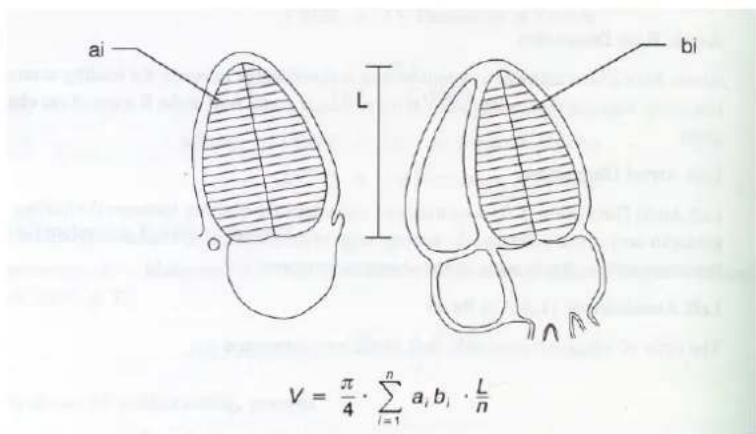
Simpson's protocol is used for calculation left ventricular volume from measurements taken in two scan planes. The calculation of volume for both methods (2-chamber or the 4-chamber view) results from summation of areas from diameters of 20 cylinders or discs of equal height, apportioned over the left ventricular length
LV Vol. A/L
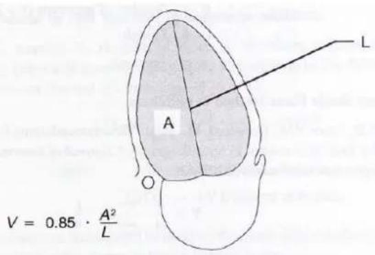
LV Volume: Single Plane Area Length
Stroke Volume (SV)
SVED (VESV = ) (ml)
where, EDV : End Diastolic Volume ESV : End Systolic Volume
Stroke Volume Index(SI)
SI = SV / BSA
Cardiac Output (CO)
CO = (SVPR)/1 0 0 0 l / min
Cardiac Index (CI)
CI = CO / BSA
Ejection Fraction (EF)
EF = (EDVESV)/EDV * 100%
where, EDV : End Diastolic Volume ESV : End Systolic Volume
Reference : Harvey Feigenbaum, "Echocardiography", 1995 fifth edition Chapter3 p 144, Lea&Febiger
2D Measure
LV Vol. d (LV Volume Diastolic)
Teichholz EDV·=7.0/2.4+LVDd\ LVDd3
Reference : Teichholz, L.E., Kreulen, T., Herman, M.V., et. al. "Problems in echocardiographic volume determinations: echocardiographic-angiographic correlations in the presence or absence of asynergy." American Journal of Cardiology, 1976, 37:7.
Cubed LVDdÊDV=
Reference : Pombo, J.F., et. al. "Left Ventricular Volumes and Ejection Fractioin by Echocardiography." Circulation, Vol. XLIII, 482, April, 1971.
Gibson EDV = 0.52 * (0.98 * LVDd + 5.90) * LVDd2
Reference : "Basic Echocardiography" Iowa Heart Center, Mark J. Harry R.D.C.S., R.V.T. Jan, 1997 p. 30
LV Vol. s (LV Volume Systolic)
Teichholz ESV = 7.0/2.4 + LVDs· LVDs3
Reference : Teichholz, L.E., Kreulen, T., Herman, M.V., et. al. "Problems in echocardiographic volume determinations: echocardiographic-angiographic correlations in the presence or absence of asynergy." American Journal of Cardiology, 1976, 37:7.
Cubed EDV = LVDs3
Reference : Pombo, J.F., et. al. "Left Ventricular Volumes and Ejection Fractioin by Echocardiography." Circulation, Vol. XLIII, 482, April, 1971.
Gibson EDV = 0.52 * (1.14 * LVDs + 4.18) * LVDs2
Reference : "Basic Echocardiography" Iowa Heart Center, Mark J. Harry R.D.C.S., R.V.T. Jan, 1997 p. 30
LV Mass
Lvmass (grams) = 1. 0 4 · [(LVDd + LVPWDd + IVSd) ^ 3 - LVDd ^ 3] * 0. 8 + 0. 6
LVDd : Left Ventricle Dimension Diastole
LVPWd : Left Ventricle Posterior Wall Dimension Diastole
LVSd : Interventricular Septal Thickness Diastole
Stroke Volume (SV)
SVED (VESV = ) (ml)
where, EDV : End Diastolic Volume ESV : End Systolic Volume
Stroke Volume Index(SI)
SI = SV / BSA (ml / m ^ 2)
Cardiac Output (CO)
CO = (SVPR)/1 0 0 0 l / min
Cardiac Index (CI)
CI = CO / BSA (l / m / m ^ 2)
Ejection Fraction (EF)
EF = (% - ESVEDV)/EDV * 1 0 0
where, EDV : End Diastolic Volume ESV : End Systolic Volume
Reference : Harvey Feigenbaum, “ Echocardiography”, 1995 fifth edition Chapter3 p 144 ,Lea&Febiger
Fraction Shortening (FS)
FS = (%)/LVDd - LVDsLVDd/1 0 0
LV MASS
![A₁ A₂ b = √(A₂/π) t = √(A₁/π) - b Aₘ A₁ A₂ Aₘ = A₁ - A₂ LV Mass in grams = 1.05 · [[5/6 · A₁ · (a + d + t)] - [5/6 · A₂ · (a + d)]]](/content/2026/05/955519/images/be1adfb3166224e21ba4983eaa06ce1820ffc4c2e25f6849f92d75d2ae9129c6.jpg)
LVmassAL105= [(5/611)-(5/622)] grams * * * * *
where, A1 : short axis area, Epicardinal (cm 2 ) A2 : short axis area, Endocardinal (cm 2 )
L1 : long axis Epicardinal length (cm) L2 : long axis Endocardinal length (cm)
Epicardial Volume
Epi. V = 5 / 6 × A 1 × L 1 (ml)
Endocardial Volume
Endo. V = 5/6 * A 2 * L 2 (ml)
Reference : Harvey Feigenbaum, “ Echocardiography”, 1995 fifth edition Chapter3 p 158, Lea&Febiger
Myocardial Thickness
√ π √ / π. AreaEndoAreaEpiTmy - = (cm)
LV Mass Index
LV Mass Index = LV Mass / BSA (g / m ^ 2)
Cardiology C mode
PISA(Proximal Isovelocity Surface Area) Radius
Reference : Oh, J.K., Seward, J.B., Tajik, A.J. The Echo Manual. Boston: Little, Brown and Company, 1994, p.106.
Schmailzl, K., Omerod, O., Editors. Ultrasound in Cardiology. Blackwell Science, 1994, p.125.
PISA-Radios is the radial distance of the isovelocity shell from the orifice (Figure - Regurgitant Flow-PISA Radius)
PISA = 2 πr ^ 2
where : PISA = Proximal Isovelocity surface area in cm 2
r = Radial distance of the isovelocity shell from the orifice in cm
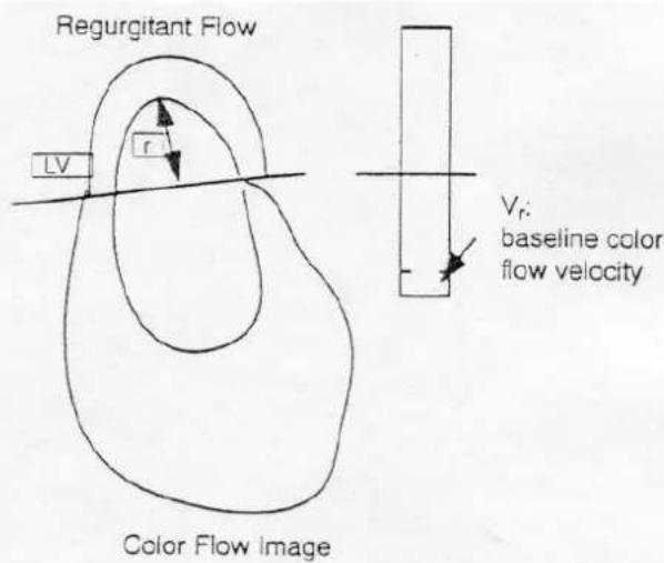
Figure - Regurgitant Flow-PISA Radius
PISA(Proximal Isovelocity Surface Area) Alias Velocity
Reference : Schmailzl. K., Omerod, O., Editors. Ultrasound in Cardiology. Blackwell
Science, 1994, p.125.
PISA-Alias Velocity is the peak velocity of the regurgitant jet on the Doppler display (Figure – Regurgitant Flow-PISA Alias Velocity)
Figure - Regurgitant Flow-PISA Alias Velocity
Regurgitant Volume Flow Rate (Rate)
Reference : Oh, J.K., Seward, J.B., Tajik, A.J. The Echo Manual. Boston: Little, Brown and Company, 1994, p. 106
Rate is calculated in milliliters/sec.
Rate = PISA*Vr
Where: PISA = Proximal isovelocity surface area in cm^2
Vr = Color flow velocity at radius r in cm/sec measured at the mitral orifice on the Color display
Effective Regurgitant Orifice(ERO)
Reference : Oh, J.K., Seward, J.B., Tajik, A.J. The Echo Manual. Boston: Little, Brown and Company, 1994, pp. 108-109
Vmr is the peak velocity of the mitral regurgitant jet measured on the Doppler display.
ERO = Rate/Vmr
Regurgitant Volume (Vol)
Reference : Oh, J.K., Seward, J.B., Tajik, A.J. The Echo Manual. Boston: Little, Brown and Company, 1994, pp. 108-109
Vol = ERO*VTImr
Where: Vol = Regurgitant volume in milliliters
ERO = Effective Regurgitant area in cm^2
VTImr = Velocity integral of the Regurgitant flow measured on the Doppler display
Cardiology M mode
Left Ventricle
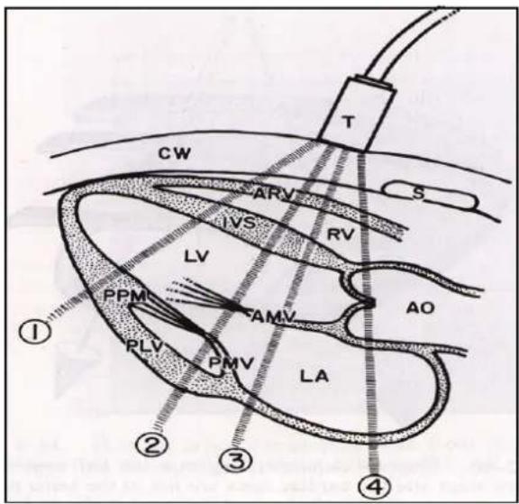
Reference : Harvey Feigenbaum, "Echocardiography", 1995 fifth edition
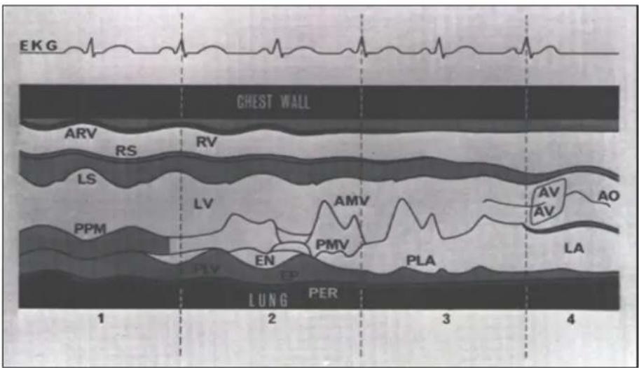
Reference : Harvey Feigenbaum, "Echocardiography", 1995 fifth edition
LV Vol. d (LV Volume Diastolic)
Teichholz EDV=7.0/2.4+LVDd LVDd3
Reference : Teichholz, L.E., Kreulen, T., Herman, M.V., et. al. "Problems in echocardiographic volume determinations: echocardiographic-angiographic correlations in the presence or absence of asynergy." American Journal of Cardiology, 1976, 37:7.
Cubed LVDd=
Reference : Pombo, J.F., et. al. "Left Ventricular Volumes and Ejection Fractioin by Echocardiography." Circulation, Vol. XLIII, 482, April, 1971.
Gibson EDV = 0.52 * (0.98 * LVDd + 5.90) * LVDd2
Reference : "Basic Echocardiography" Iowa Heart Center, Mark J. Harry R.D.C.S., R.V.T. Jan, 1997 p. 30
LV Vol. s (LV Volume Systolic)
Teichholz ESV = 7.0/2.4 + LVDs · LVDs3
Reference : Teichholz, L.E., Kreulen, T., Herman, M.V., et. al. "Problems in echocardiographic volume determinations: echocardiographic-angiographic correlations in the presence or absence of asynergy." American Journal of Cardiology, 1976, 37:7.
Cubed EDV = LVDs3
Reference : Pombo, J.F., et. al. "Left Ventricular Volumes and Ejection Fractioin by Echocardiography." Circulation, Vol. XLIII, 482, April, 1971.
Gibson EDV = 0.52(1.14LVDs + 4.18)*LVDs2
Reference : "Basic Echocardiography" Iowa Heart Center, Mark J. Harry R.D.C.S., R.V.T. Jan, 1997 p. 30
Stroke Volume (SV)
SV = (EDV - ESV) (ml)
where, EDV : End Diastolic Volume
ESV : End Systolic Volume
Stroke Volume Index(SI)
SI = SV / BSA (ml / m ^ 2)
Cardiac Output (CO)
CO = (SVPR)/1 0 0 0 l / min
Cardiac Index (CI)
CI = CO / BSA (l / m / m ^ 2)
Ejection Fraction (EF)
EF = (% - ESVEDV/EDV * 100
where, EDV : End Diastolic Volume ESV : End Systolic Volume
Reference : Harvey Feigenbaum, “ Echocardiography”, 1995 fifth edition Chapter3 p 144 ,Lea&Febiger
Fraction Shortening (FS)
FS = (%)/LVDd - LVDsLVDd/1 0 0
LV Mass
LV _ mass ( grams ) = 1. 0 4 · [(LVDd + LVPWDd + IVSd) ^ 3 - LVDd ^ 3 ] * 0. 8 + 0. 6
Reference : Oh, J.K., Seward, J.B. The Echo Manual. Boston: Little, Brown and company, 1994, p.43.
LV Mass Index
LV Mass Index = LV Mass / BSA (g / m ^ 2)
MV (Mitral Valve)
Definition for the Mitral Valve
D : end of systolic, immediately before the opening of the Mitral Valve
E : the arterial leaflet of the Mitral valve open, it peaks at E
F : lowest point of the initial diastolic closing
A : In atrial systole, blood is propelled through the Mitral orifice and the Mitral leaflets reopen
the peak of this phase of Mitral valve motion is indicated as A
C : complete closure occurs after the onset of ventricular systole
Mitral Valve D-E Excursion (unit : cm)
Distance between the onset of the opening of the Mitral valve at D and the maximum opening of the anterior Mitral valve leaflet at E
Mitral Valve D-E Slope (unit : cm/sec)
Automatically calculated from the D - E excursion the rate of change that exists between two point (D,E)
Mitral Valve E-F Slope (unit : cm/sec)
The rate of change that exists between two point(E, F)
EPSS ( Mitral Valve E Point Septal Separation ) ( unit : cm)
Distance between the Mitral Valve E point and posterior edge of the interventricular septum at the same point in time
A-C interval (unit : msec)
The distance between the A point and the C point
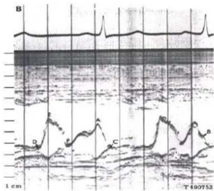
Figure - Mitral Valve M mode Waveform
Ao/LA
Aortic Root Diameter (unit:cm) : Ao Root Dia.
The distance between the leading echo of the anterior aortic wall and the leading echo of the posterior aortic wall at R wave of the electrocardiogram
Aortic Valve Cusp Separation (Ao Cusp Sep.)
The distance between the trailing echo of the anterior aortic valve leaflet and the leading echo of
the posterior aortic valve leaflet in early diastole
Left Atrial Diameter (unit:cm) : LA Dia.
The distance between the trailing edge of the posterior aortic wall echo and the leading edge of the posterior left atrial wall echo at the level of aortic wall at the R wave of the electrocardiogram.
Cardiology Doppler
Mitral Valve, Tricuspid Valve
Pressure Gradient
PgV = × ^ 2 4 (mmHg)
where, V : Velocity (m/sec)
PHT ; Pressure Half Time
Reference : Oh, J.K., Seward, J.B., Tajik, A.J. The Echo Manual. Boston: Little, Brown and Company, 1994, p.59-60
Pressure half-time (PHT) is the time it takes for the peak pressure gradient to fall to half to half of its peak value. DT is deceleration time in centimeters per second form the peak velocity to the baseline.
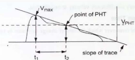
V _ PHT = V _ · √ 2 = V _ 1 . 4 PHT = t _ 2 - t _ 1
slope = (t _ 2 - t _ 1)(V _ PHT - V _ ) = PHT V _ 1 . 4 - V _
PHT = slope × V _ × (- 0. 2 9)
Mitral Valve area
MVA = 2 2 0 / PHT (cm ^ 2)
where ; PHT is Pressure Half Time (milliseconds)
Reference : John H. Phillipse, “ Practical Quantitative Doppler Echocardiography”, p47, chapter6, CRC press, 1991
VTI(Velocity Time Integral)
VTI = Mean velocity(cm/sec) * Ejection time(sec) = L (cm)
ACC(Acceleration), DEC(Deceleration)
V 2 - V 1 / _ T 2 - T 1 (m / ^ 2)
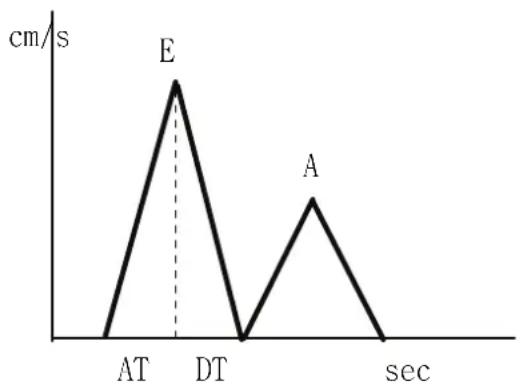
AT :Acceleration Time, DT : Deceleration Time
E point : Early Diastolic Flow, A point : Atrial contraction
Aortic Valve, LVOT Doppler
HR(Heart Rate)
HR = #beats*60 /time (bpm : bit/minute)
CONT(Continuity Equation)
When there is a constant flow in a flow channel with a Stenosis, the flow volume at the Stenosis portion equals that at nonstenotic portions.
This equation is valid not only in a constant flow, but also in a pulsality flow channel.
SV 1 = SV 2
where, SV1 : stroke volume in the nonstenotic area
SV2: stroke volume in the stenotic area
AVAEVOTareaX V 1/V 2 cm ^ 2
where, AVA(1): Aortic Valve Area by Velocity
AVA(2): Aortic Valve Area by VTI
LVOTarea: π*DiaLVOT2/4
VTI1 : Left Ventricle output track VTI
VTI2 : Aortic valve VTI
V1 : Left Ventricle output track velocity
V2: Aortic valve velocity
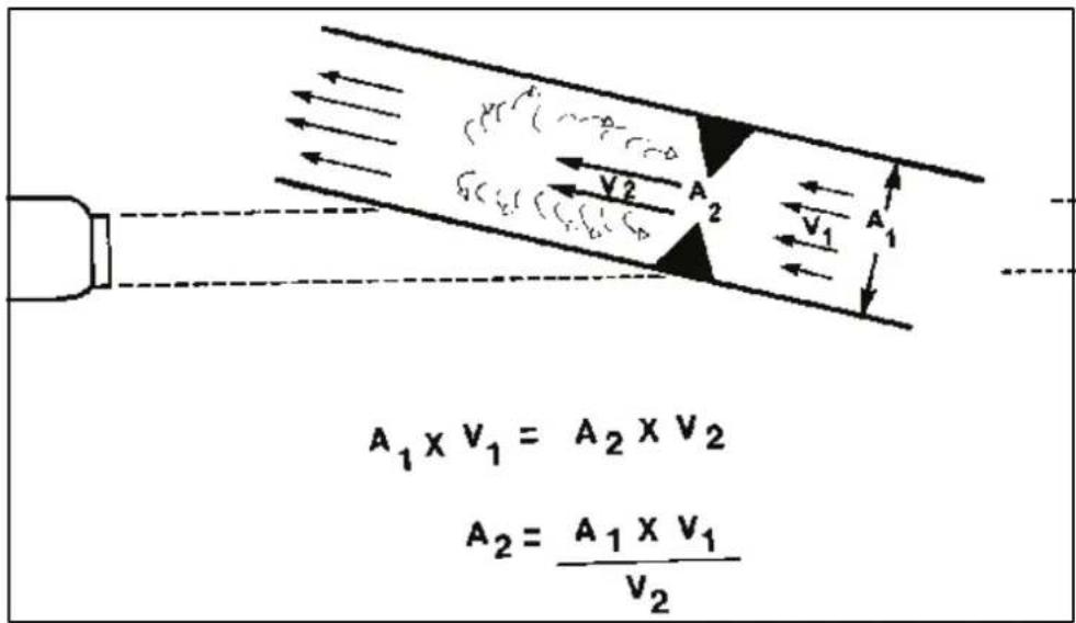
Figure - Continuity Equation
Reference : Harvey Feigenbaum, “ Echocardiography”, 1995 fifth edition
CSA(Cross Sectional Area)
Area = π × (D/2) ^ 2
where, D: diameter
Pulmonic Veins
Reference : Oh, J.K., Seward, J.B., Tajik, A.J. The Echo Manual. Boston: Little, Brown and Company, 1994, p.48
Diastolic Velocity
Velocity measured at diastole.
Systolic Velocity
Velocity measured at systole.
Artrial Reversal Velocity (A. Rev Vel)
Atrial reversal velocity is the peak velocity of the atrial reversal component.
Pulmonary Atrial Reversal Duration (A. Rev Dur)
Pulmonary atrial flow reversal duration is the time between the diastolic component of pulmonary venous flow and the closure of the mitral valve.
Sys/Dia (Systole/Diastole)
Ratio of the velocity measured at systole and the velocity measured at diastole.
Shunt Ratio QP : QS
The equations that follows area derivee dfrom the following source:
Oh, J.K., Seward, J.B., Tajik, A.J. The Echo Manual, Boston: Little, Brown, and Company, 1994.
QP : QS = Pulmonic Cardiac Output / Systemic Cardiac Output
CO = Pulm SV * Pulm HR / 1000
Outflow Trace Area = π * (Pulm Dia / 2)²
Dim of Aaprt the -12 dB OUTPUT BEAM DIMENSIONS. The active
apertu-re dimensions in the azimuthal and elevational
directions. (centimeters). For scanned modes, the 'X_dim' is
the length of the entire scanned aperture.
fawf the ACOUSTIC WORKING FREQUENCY. Center frequency.
(megahertz)
Focal Length The nominal focal points, azimuthal (FL x) and elevational (FLy),
for the operating condition. (centimeters).
Ipa,α at max. MI the ATTENUATED PULSE-AVERAGE INTENSITY at the
depth of reported MI, Zat_max_Ipi, a · (watts per square
centimeter).
Ila,α(z) the ATTENUATED TEMPORAL-AVERAGE INTENSITY at
axial distance z. (milliwatts per square centimeter)
MI the displayed parameter representing potential cavitation bio-
effects. (unit-less)
P the time-average ultrasonic OUTPUT POWER radiated by the
transducer for the transmit pattern(s) associated with the
report-ed Index. For TIS_non_scan and TIB_non_scan this is
the total acoustic power of the non-scanned beam(s). For TIC
it is the total acoustic power of the contributing modes (which
will be list-ed separately, for the reader to sum). The reported
maximum TIS_scan value may (likely) come from a
combinational mode. In this case, P = P1 + P1 × 1 . P1 is the
BOUNDED OUTPUT POWER (the maximum power emitted
from a one cm width of the active (scanned) transmit aperture
of the transducer in the scan plane direction) of each the
scanned transmit modes. For instance in 2D color mode
P1_2D and P1_Col will be listed. P1× 1 is the ma-ximum
contribution from any one square centimeter of the non-
scanned transmit mode(s) active aperture. (milliwatts).
Acoustic Power Tables
IEC Tables
Symbols and Definitions
Standard 60601-2-37 published by the International Electrotechnical Commission (IEC) requires the declaration of acoustic output information. The definitions and units of the symbols in those tables are listed below, and are consistent with IEC 60601-2-37 and IEC 62359. Definitions for CAPITALIZED parameters, if not found here, can be found in the reference documents.
All table entries have been obtained at the operating conditions that give rise to
the Maximum Index Value (shown in the second row of the table). Due to the
complexities of the system user interface, it may be difficult to exactly replicate
the declared condition. Contact Medison for further information as needed.
Note that Medison provides information for both of the TIS non-scanned columns.
The ‘Aaprt≤1’ (cm 2 ) column is an ‘at_surface’ TIS value and the ‘Aaprt>1’ (cm 2 )
column is a 'below surface' TIS value. The tables will provide additional
informational flags ( ** ) in the event that the largest TIS non-scanned value is an
'at_surface' value with Aaprt > 1 cm 2 , or if the largest TIS non-scanned value is a
'below_surface' value with Aaprt ≤ 1 cm² case (very rare).
Aaprt the -12 dB OUTPUT BEAM AREA, or transmit aperture area,
of the ultrasonic beam. Derived from the -12 dB OUTPUT
BEAM DIMENSIONS. (centimeters squared)
deq at max. lpi the EQUIVALENT BEAM DIAMETER at the point where the
free-field (non-attenuated), PULSE INTENSITY INTEGRAL is a
maximum (centimeters).
b
Equal to [(4 / n)(Pa(zb) / Ita,a(zb))]0.5 . (centimeters)
206 Acoustic Power Tables
| Po(z) the (ultrasonic) ATTENUATED OUTPUT POWER at axial distance zs , for the non-scanned modes or TRANSMIT PATTERNS. (milliwatts) | zb the distance where TIB_non-scan is determined. For non-scanned modes, Distance along the beam axis to the plane where the product of the ATTENUATED OUTPUT POWER and ATTENUATED TEMPORAL-AVERAGE INTENSITY ( Pa(z) × Ita,a(z) ) maximizes. (centimeters) |
| Pr,u the ATTENUATED PEAK-RAREFACTIONAL ACOUSTIC PRESSURE associated with the transmit pattern giving rise to the reported value of MI. (megapascals) | zbp value equal to 1.5 times the EQUIVALENT APERTURE DIAMETER ( Deq ). Also equals 1.69 * aprt . (centimeters) |
| Pr at max. Ipi the PEAK-RAREFACTIONAL ACOUSTIC PRESSURE at the point where the free-field (non-attenuated), PULSE INTENSITY INTEGRAL is a maximum (megapascals). | zs the distance where TIS_non-scan is determined. The axial distance corresponding to the location of max[min( Pa(z) , Ita,a(z) × 1 cm2 ), where z >= zbp . (centimeters) |
| prr the PULSE REPETITION RATE associated with the transmit pattern giving rise to the reported value of MI (pulses per second). | |
| TIB the BONE THERMAL INDEX for applications, such as fetal (second and third trimester) or neonatal cephalic (through the fontanelle), in which the ultrasound beam passes through soft tissue and a focal region is in the immediate vicinity of bone. (unit-less) | ■ Explanatory Notes(a) This index is not required to this operating mode.(b) This probe is not intended for adult transcranial uses.(c) This formulation for TIS is less than that for an alternate formulation in this mode.(d) The maximum index value is less than 1.0* If the MI comes from a scanning mode Transmit Pattern (pulse), the 'prr' listed is the average per second for the 'worst case' scan line. 'prr' for scanning modes is the product of the frame rate and the number of pulse per line of the Transmit Pattern.** The max TIS unscanned value is an 'at_surface' value and occurs for aperture > 1.0 cm^2, OR The max TIS unscanned value is a 'below_surface' value and occurs for aperture <= 1.0 cm^2.+ The max TIB for this combinational mode = the at_surface TIS_scanned value. The non-scanned_TIB value indicated is the below_surface max. A "+" is used when the TIB value is less than the TIS_scanned value for the operating condition. |
| TIC the CRANIAL BONE THERMAL INDEX. | |
| TISscan the SOFT TISSUE THERMAL INDEX in a scanning mode. (unit-less) | |
| TISnon-scan the SOFT TISSUE THERMAL INDEX in a non-auto scanning mode. (unit-less) | |
| td the PULSE DURATION associated with the TRANSMIT PATTERN giving rise to the reported value of MI. (microseconds) | |
| Zatmaxlpi the axial distance from the transducer where the |
C1-4EC
C1-4EC: 2D& 2D+M mode
C1-4EC: 2D+Color, Triple, CPA & Triple CPA
| Index Label | M.I. | TIS | TIB | TIC | |||
| scan | non- scan | non- | |||||
| Aaprt ≤ 1 | Aaprt >1\ scan | ||||||
| Maximum Index Value | 1.55 | 1.59 | 0.76** | 1.46 | 4.09 | (b) | |
| Associated Acoustic Parameters | Pro (MPa) | 2.52 | - | - | - | - | - |
| P(mW) | - | 2D P1:8.33Col P1:120 | PDP1x1:58.4 | PDP:238 | (b) | ||
| Min.of |Pa(zs)|Ipa,x(zj × 1cm21) (mW) | - | - | - | 150 | - | - | |
| zs (cm) | - | - | - | 3.84 | - | - | |
| zbp (cm) | - | - | - | 3.77 | - | - | |
| zb (cm) | - | - | - | - | 4.74 | - | |
| zatmaxlpi,α (cm) | 2.04 | - | - | - | - | - | |
| deqzb (cm) | - | - | - | - | 0.67 | - | |
| fsurf (MHz) | 2.66 | 2D:1.94 Col:2.65 | 2.72 | 2.04 | 2.04 | (b) | |
| Dim of Aaprt X (cm)Y (cm) | 2D:4.27 Col:2.74 | 0.86 | 3.55 | 2.69 | (b) | ||
| 1.40 | 1.40 | 1.40 | 1.40 | (b) | |||
| Other Information | t (μsec) | 0.90 | - | - | - | - | - |
| prr (pulses/sec) | 65.7* | - | - | - | - | - | |
| Pr at max. Ipi (MPa) | 2.85 | - | - | - | - | - | |
| dep at max. Ipi (cm) | - | - | - | - | 0.56 | - | |
| Ipe,a at max. MI (W/cm2) | 266 | ||||||
| Focal Length FLx (cm)FLy (cm) | - | - | 3.50 | 14.5 | - | - | |
| - | - | 5.00 | 5.00 | - | - | ||
| - | - | ||||||
| Operating Control Conditions | Control 1 | MI | |||||
| Control 2 | TIS_as | ||||||
| Control 3 | TIS_as_U | ||||||
| Control 4 | TIS_bs | ||||||
| Control 5 | TIB_bs | ||||||
Control 1: 2D mode, 2D:2.2Mhz, Focus:5.0Cm, FR:58.18
Control 2: 2D mode, 2D:2.2Mhz, Focus:5.0Cm, FR:103.0
Control 3: 2D+M mode, 2D:2.2Mhz, Focus:3.5Cm, FR:31.10
Control 3: Triple mode, 2D:1.8Mhz, PD:2.8Mhz, Col:2.0Mhz, Focus:3.5Cm, FR:1.81
Control 5: 2D+M mode, 2D:2.2Mhz, Focus:6.8Cm, FR:28.20
Control 1: 2D+Color mode, 2D:1.8Mhz, Col:2.8Mhz, Focus:3.5Cm, FR:6.57
Control 2: 2D+Color mode, 2D:1.8Mhz, Col:2.8Mhz, Focus:5.0Cm, FR:6.89
Control 3: Triple mode, 2D:1.8Mhz, PD:2.8Mhz, Col:2.0Mhz, Focus:3.5Cm, FR:1.81
Control 4: Triple mode, 2D:1.8Mhz, PD:2.0Mhz, Col:2.0Mhz, Focus:14.5Cm, FR:1.69
Control 5: Triple mode, 2D:1.8Mhz, PD:2.0Mhz, Col:2.0Mhz, Focus:11.0Cm, FR:1.69
C1-4EC: Pulsed Doppler &2D+Pulsed Doppler
C2-6IC
C2-6IC: 2D& 2D+M mode
| Index Label | M.I. | TIS | TIB TIC | |||||
| scan | non- scan | non- scan | ||||||
| Aaprt ≤ 1 | Aaprt >1 | |||||||
| Maximum Index Value | 1.44 | 1.77 | 0.06 | 0.09 | 0.15+ | (b) | ||
| Associated Acoustic Parameters | Pro (MPa) | 2.31 | - | - | - | - | - | |
| P (mW) | - | 2D P1:132 | M P1x1:4.57 | M P:4.47 | (b) | |||
| Min.of [ Po(zs),Ilo, o ( zs )x1cm^2] (mW) | - | - | - | 6.97 | - | - | ||
| za (cm) | - | - | - | 3.20 | - | - | ||
| Zbp (cm) | - | - | - | 3.14 | - | - | ||
| Zb (cm) | - | - | - | - | 3.50 | - | ||
| z_at_max_lpl,α (cm) | 3.50 | - | - | - | - | - | ||
| deq(z0) (cm) | - | - | - | - | 0.33 | - | ||
| fswf (MHz) | 2.57 | 2.82 | 2.81 | 2.79 | 2.69 | |||
| Dim of Aaprt | X (cm) | 2.31 | 0.81 | 2.87 | 0.94 | (b) | ||
| Y (cm) | 1.20 | 1.20 | 1.20 | 1.20 | (b) | |||
| Other Information | tu (μsec) | 0.68 | - | - | - | - | - | |
| prr (pulses/sec) | 58.7^ | - | - | - | - | - | ||
| Pi at max. Ipi (MPa) | 3.17 | - | - | - | - | - | ||
| dsq at max. Ipi (cm) | - | - | - | - | 0.32 | - | ||
| Ilo, o at max. MI (W/cm2) | 313 | |||||||
| Focal Length | FLx (cm) | - | - | 5.00 | 17.5 | - | - | |
| FLy (cm) | - | - | 7.00 | 7.00 | - | - | ||
| - | - | |||||||
| Operating Control | Control 1 | MI | ||||||
| Control 2 | TIS_as | |||||||
| Control 3 | TIS_as_U | |||||||
| Control 4 | TIS_bs | |||||||
| Control 5 | TIB_bs | |||||||
Control 1: 2D mode, 2D:2.4Mhz, Focus:5.0Cm, FR:58.68
Control 2: 2D mode, 2D:2.8Mhz, Focus:5.0Cm, FR:103.9
Control 3: 2D+M mode, 2D:2.8Mhz, Focus:5.0Cm, FR:31.37
Control 4: 2D+M mode , 2D:2.8Mhz , Focus:17.5Cm , FR:13.89
Control 5: 2D+M mode, 2D:2.6Mhz, Focus:5.0Cm, FR:31.37
Control 1: Pulsed Doppler mode, PD:2.0Mhz, Focus:3.5Cm
Control 2: 2D+Pulsed Doppler mode, 2D:1.8Mhz, PD:2.8Mhz, Focus:3.5Cm, FR:7.27
Control 3: Pulsed Doppler mode, PD:2.8Mhz, Focus:8.8Cm
Control 4: Pulsed Doppler mode, PD:2.0Mhz, Focus:14.5Cm
C2-6IC: 2D+Color, Triple, CPA & Triple CPA
C2-6IC: Pulsed Doppler & 2D + Pulsed Doppler
| Index Label | M.I. | TIS | TIB | TIC | ||||
| scan | non- scan | non- scan | ||||||
| Aaprt ≤ 1 | Aaprt > 1 | |||||||
| Maximum Index Value | 1.38 | 1.03 | 1.04 | 1.64 | 3.83 | (b) | ||
| Associated Acoustic Parameters | Pi.o (MPa) | 2.24 | - | - | - | - | - | |
| P (mW) | 2D P1:5.46PD P1x1:93.9 | PDP1x1:83.6 | PD P:221 | (b) | ||||
| Min.of [Pe(zs), Its,a(zs)x1cm2] (mW) | - | - | - | 134 | - | - | ||
| Zs (cm) | - | - | - | 2.80 | - | - | ||
| Zbp (cm) | - | - | - | 2.74 | - | - | ||
| Zb (cm) | - | - | - | - | 4.40 | - | ||
| z_at_max_lpi,a (cm) | 0.90 | - | - | - | - | - | ||
| deq(Z0) (cm) | - | - | - | - | 0.58 | - | ||
| fout (MHz) | 2.61 | 2D:2.49PD:2.58 | 2.61 | 2.57 | 2.57 | (b) | ||
| Dim of Aaprt X (cm)Y(cm) | 2D:5.99PD:1.75 | 0.69 | 2.18 | 2.18 | (b) | |||
| 1.20 | 1.20 | 1.20 | 1.20 | (b) | ||||
| Other Information | tc (μsec) | 1.42 | - | - | - | - | - | |
| prr (pulses/sec) | 999 | - | - | - | - | - | ||
| Pr at max. Ipi (MPa) | 2.48 | - | - | - | - | - | ||
| deq at max. Ipi (cm) | - | - | - | - | 0.56 | - | ||
| Ips,a at max. MI ( W/cm2 ) | 183 | |||||||
| Focal FLx (cm)Length FLy (cm) | - | - | 3.50 | 11.0 | - | - | ||
| - | - | 7.00 | 7.00 | - | - | |||
| - | - | |||||||
| Operating Control Conditions | Control 1 | MI | ||||||
| Control 2 | TIS_as | |||||||
| Control 3 | TIS_as_U | |||||||
| Control 4 | TIS_bs | TIB_bs | ||||||
Control 1: Pulsed Doppler mode, PD:2.6Mhz, Focus:2.0Cm
Control 2: 2D+Pulsed Doppler mode, 2D:2.2Mhz, PD:2.6Mhz, Focus:8.8Cm, FR:5.58
Control 3: Pulsed Doppler mode, PD:2.6Mhz, Focus:3.5Cm
Control 4: Pulsed Doppler mode, PD:2.6Mhz, Focus:11.0Cm
| Index Label | TIS M.I. | TIB TIC | ||||||
| scan | non- scan | non- scan | ||||||
| aprt≤1 | aprt>1 | |||||||
| Maximum Index Value | 1.42 | 1.67 | 0.88 | 1.06 | 2.90 | (b) | ||
| Associated Acoustic Parameters | Pi,a (MPa) | 2.30 | - | - | - | - | - | |
| P(mW) | - | 2D P1:3.44Col P1:130 | PDP1x1:70.9 | PDP:70.9 | (b) | |||
| Min.of [P0(zs),Ia,s (zs)x1cm2] (mW) | - | - | - | 86.3 | - | - | ||
| Zs (cm) | - | - | - | 2.80 | - | - | ||
| Zbp (cm) | - | - | - | 2.74 | - | - | ||
| Zb (cm) | - | - | - | - | 1.30 | - | ||
| z_at_max_lpi,a(cm) | 1.40 | - | - | - | - | - | ||
| deqZb1 (cm) | - | - | - | - | 0.42 | - | ||
| fawt (MHz) | 2.62 | 2D:2.51Col:2.63 | 2.60 | 2.58 | 2.60 | (b) | ||
| Dim of Aaprt X (cm)Y (cm) | 2D:3.96Col:2.22 | 0.50 | 2.18 | 0.50 | (b) | |||
| 1.20 | 1.20 | 1.20 | 1.20 | (b) | ||||
| Other Information | td (μsec) | 1.01 | - | - | - | - | - | |
| prr (pulses/sec) | 76.0* | - | - | - | - | - | ||
| Pr at max. Ip (MPa) | 2.28 | - | - | - | - | - | ||
| deqat max. Ip (cm) | - | - | - | - | 0.42 | - | ||
| Ipa,s at max. MI ( W/cm2 ) | 210 | |||||||
| Focal Length FLx (cm)FLy (cm) | - | - | 2.00 | 11.0 | - | - | ||
| - | - | 7.00 | 7.00 | - | - | |||
| - | - | |||||||
| Operating Control | Control 1 | MI | ||||||
| Control 2 | TIS_as | |||||||
| Control 3 | TIS_as_U | TIB_bs | ||||||
| Control 4 | TIS_bs | |||||||
Control 1: 2D+Color mode, 2D:2.2Mhz, Col:2.6Mhz, Focus:3.5Cm, FR:5.85
Control 2: 2D+Color mode, 2D:2.2Mhz, Col:2.6Mhz, Focus:5.0Cm, FR:6.38
Control 3: Triple mode, 2D:2.2Mhz, PD:2.6Mhz, Col:2.6Mhz, Focus:11.0Cm, FR:1.55
Control 4: Triple mode, 2D:2.2Mhz, PD:2.6Mhz, Col:2.6Mhz, Focus:2.0Cm, FR:1.55
C3-7IM
C3-7IM: 2D& 2D+M mode
C3-7IM:: 2D+Color, Triple, CPA & Triple CPA
| Index Label | M.I. | TIS | TIB | TIC | ||||
| scan | non- scan | non- scan | ||||||
| Aaprt ≤ 1 | Aaprt > 1 | |||||||
| Maximum Index Value | 1.20 | 1.25 | 0.80** | 0.71 | 2.41 | (b) | ||
| Associated Acoustic Parameters | Pi,a (MPa) | 1.98 | - | - | - | - | - | |
| P(mW) | - | 2D P1:4.11Col P1:89.0 | PDP1x1:59.6 | PDP:56.5 | (b) | |||
| Min_of [Pit(zit)la, o(zit)x1cm2] (mW) | - | - | - | 53.4 | - | - | ||
| Zit (cm) | - | - | - | 1.94 | - | - | ||
| Zbp (cm) | - | - | - | 2.33 | - | - | ||
| Zb (cm) | - | - | - | - | 1.56 | - | ||
| z_at_max_lpi,α(cm) | 0.60 | - | - | - | - | - | ||
| deq(Z0) (cm) | - | - | - | - | 0.38 | - | ||
| fazr (MHz) | 2.71 | 2D:2.56Col:2.82 | 2.81 | 2.81 | 2.84 | (b) | ||
| Dim of Aaprt X (cm)Y (cm) | 2D:6.91Col:4.68 | 1.01 | 1.73 | 0.65 | (b) | |||
| 1.10 | 1.10 | 1.10 | 1.10 | (b) | ||||
| Other Information | tc (μsec) | 0.69 | - | - | - | - | - | |
| prr(pulses/sec) | 4.37* | - | - | - | - | - | ||
| Pr at max. Ip (MPa) | 2.09 | - | - | - | - | - | ||
| deq at max. Ip (cm) | - | - | - | - | 0.37 | - | ||
| Ipe,a at max. MI (W/cm2) | 112 | - | ||||||
| Focal LengthFLx (cm)FLy (cm) | - | - | 5.00 | 8.80 | - | - | ||
| - | - | 7.50 | 7.50 | - | - | |||
| - | - | - | ||||||
| Operating Control | Control 1 | MI | ||||||
| Control 2 | TIS_as | |||||||
| Control 3 | TIS_as_U | |||||||
| Control 4 | TIS_bs | |||||||
| Control 5 | TIB_bs | |||||||
Control 1: 2D+Color mode, 2D:2.6MHz, Col:2.8MHz, Focus:2.0GHz, TR:4.37
Control 2: ZD+Color Mode, ZD:2.6MHz, Col:2.6MHz, Focus:14.0CM, FR:2.00
Control 3: Triple mode, 3D:2.6MHz, RD:2.8MHz, Col:2.8MHz, Focus:5.0CM, FR:
Control 3: Pulsed Doppler mode, PD:2.8Mhz, Focus:5.0Cm
Control 4. Triple mode, ZD.2.0MHz, PD.2.0MHz, QoI.2.0MHz, Focus.0.0GHz, PK.1.47
Control 5: Triple mode, 2D:2.6Mhz, PD:2.8Mhz, Col:2.8Mhz, Focus:3.5Cm, FR:1.47
| Index Label | TIS M.I. | TIB TIC | ||||||
| scan | non- scan | non- scan | ||||||
| Aaprt ≤ 1A | aprt>1 | |||||||
| Maximum Index Value 1.27 0.90 1.36** | 1.32 | 2.89 (b) | ||||||
| Associated Acoustic Parameters | Pr,a | (MPa) | 2.14 | - | - | - | - | - |
| P | (mW) | - | 2D P1:3.36PD P1x1:70.5 | PD P1x1:102 | PD P:94.3 | (b) | ||
| Min.of [Pa(Zs),Ib,a(Zs)x1cm2] | (mW) | - | - | - | 99.0 | - | - | |
| Zc | (cm) | - | - | - | 1.58 | - | - | |
| Zbp | (cm) | - | - | - | 2.08 | - | - | |
| Zb | (cm) | - | - | - | - | 1.44 | - | |
| z_at_max_lpi,a | (cm) | 1.44 | - | - | - | - | - | |
| deq(Zt) | (cm) | - | - | - | - | 0.52 | - | |
| fam | (MHz) | 2.83 | 2D:2.71 PD:2.81 | 2.80 | 2.80 | 2.83 | (b) | |
| Dim of Aaprt | X (cm) | 2D:6.91 PD:1.01 | 1.01 | 1.37 | 0.65 | (b) | ||
| Y (cm) | 1.10 | 1.10 | 1.10 | 1.10 | (b) | |||
| Other Information | td | (μsec) | 1.24 | - | - | - | - | - |
| prr | (pulses/sec) | 999 | - | - | - | - | - | |
| Pr at max. Ip | (MPa) | 2.46 | - | - | - | - | - | |
| deq at max. Ipi | (cm) | - | - | - | - | 0.52 | - | |
| Ipa,a at max. MI | (W/cm2) | 200 | ||||||
| Focal Length | FLx (cm) | - | - | 5.00 | 6.80 | - | - | |
| FLy (cm) | - | - | 7.50 | 7.50 | - | - | ||
| - | - | |||||||
| Operating Control | Control 1 | MI | ||||||
| Control 2 | TIS_as | |||||||
| Control 3 | TIS_as_U | |||||||
| Control 4 | TIS_bs | |||||||
| Control 5 | TIB_bs | |||||||
Control 1: Pulsed Doppler mode, PD:2.8Mhz, Focus:3.5Cm
Control 2: 2D+Pulsed Doppler mode, 2D:2.6Mhz, PD:2.8Mhz, Focus:5.0Cm, FR:7.27
Control 3: Pulsed Doppler mode, PD:2.8Mhz, Focus:5.0Cm
Control 4: Pulsed Doppler mode, PD:2.8Mhz, Focus:6.8Cm
Control 5: Pulsed Doppler mode, PD:2.8Mhz, Focus:3.5Cm
C4-9ED
C4-9ED: 2D& 2D+M mode
| Index Label | M.I. | TIS | TIB | TIC | ||||
| scan | non- scan | non- | ||||||
| Aaprt ≤ 1 | Aaprt >1 scan | |||||||
| Maximum Index Value | 1.52 | 1.17 | 0.02 | 0.01** | 0.05+ | 1.34 | ||
| Associated Acoustic Parameters | Pf,a | (MPa) | 3.39 | - | - | - | - | - |
| P | (mW) | - | 2D P1:50.1 | M P1x1:0.80 | MP:0.79 | MP:52.2 | ||
| Min.of [Pa(zs),Ita,a(zs)× 1cm2] | (mW) | - | - | - | 0.55 | - | - | |
| zs | (cm) | - | - | - | 1.08 | - | - | |
| zbp | (cm) | - | - | - | 1.01 | - | - | |
| zb | (cm) | - | - | - | - | 1.24 | - | |
| z_at_max_lpi,α | (cm) | 1.32 | - | - | - | - | - | |
| deq(z0) | (cm) | - | - | - | - | 0.23 | - | |
| fsvt | (MHz) | 4.96 | 4.92 | 4.96 | 4.96 | 4.91 | 4.92 | |
| Dim of Aaprt | X (cm) | 1.24 | 0.59 | 0.59 | 0.59 | 1.24 | ||
| Y (cm) | 0.60 | 0.60 | 0.60 | 0.60 | 0.60 | |||
| Other Information | tc | (μsec) | 0.20 | - | - | - | - | - |
| prr | (pulses/sec) | 35.8* | - | - | - | - | - | |
| Pr at max. Ipi | (MPa) | 4.13 | - | - | - | - | - | |
| deq at max. Ipi | (cm) | - | - | - | - | 0.22 | - | |
| Ipa,a at max. MI | (W/cm2) | 526 | - | |||||
| Focal Length | FLx (cm) | - | - | 1.50 | 1.50 | - | - | |
| FLy (cm) | - | - | 3.80 | 3.80 | - | - | ||
| - | - | - | ||||||
| Operating Control | Control 1 | MI | ||||||
| Control 2 | TIS_as | TIC_as | ||||||
| Control 3 | TIS_as_U | TIS_bs | ||||||
| Control 4 | TIB_bs | |||||||
Control 1: 2D mode, 2D:7.7Mhz, Focus:1.5Cm, FR:35.76
Control 2: 2D mode, 2D:6.2Mhz, Focus:1.5Cm, FR:66.48
Control 3: 2D+M mode, 2D:7.7Mhz, Focus:1.5Cm, FR:35.76
Control 4: 2D+M mode, 2D:6.2Mhz, Focus:1.5Cm, FR:35.76
C3-7IM:: Pulsed Doppler & 2D + Pulsed Doppler
| Index Label | TIS M.I. | TIB TIC | ||||||
| scan | non- scan | non- scan | ||||||
| Aapr ≤ 1 A | aprt>1 | |||||||
| Maximum Index Value 1.27 0.90 1.36** | 1.32 | 2.89 (b) | ||||||
| Associated Acoustic Parameters | Pi,x (MPa) | 2.14 | - | - | - | - | - | |
| P(mW) | - | 2D P1:3.36PD P1x1:70.5 | PD P1x1:102 | PD P: 94.3 | (b) | |||
| Min.of [ Pa(zs),Iba,α ( za × 1cm2 ] (mW) | - | - | - | 99.0 | - | - | ||
| Zs (cm) | - | - | - | 1.58 | - | - | ||
| Zbp (cm) | - | - | - | 2.08 | - | - | ||
| Zb (cm) | - | - | - | - | 1.44 | - | ||
| z_at_max_lpi,α (cm) | 1.44 | - | - | - | - | - | ||
| deqZb (cm) | - | - | - | - | 0.52 | - | ||
| fout (MHz) | 2.83 | 2D:2.71PD:2.81 | 2.80 | 2.80 | 2.83 | (b) | ||
| Dim of Aaprt X (cm) | - | 2D:6.91PD:1.01 | 1.01 | 1.37 | 0.65 | (b) | ||
| Y(cm) | - | 1.10 | 1.10 | 1.10 | (b) | |||
| Other Information | td (μsec) | 1.24 | - | - | - | - | - | |
| prr (pulses/sec) | 999 | - | - | - | - | - | ||
| Pr at max. Ipi (MPa) | 2.46 | - | - | - | - | - | ||
| deq at max. Ipi (cm) | - | - | - | - | 0.52 | - | ||
| Ipa,x at max. MI ( W/cm2 ) | 200 | - | ||||||
| Focal FLx (cm) | - | - | 5.00 | 6.80 | - | - | ||
| Length FLy (cm) | - | - | 7.50 | 7.50 | - | - | ||
| - | - | - | ||||||
| Operating Control Conditions | Control 1 | MI | ||||||
| Control 2 | TIS_as | |||||||
| Control 3 | TIS_as_U | |||||||
| Control 4 | TIS_bs | |||||||
| Control 5 | TIB bs | |||||||
Control 1: Pulsed Doppler mode, PD:2.8Mhz, Focus:3.5Cm
Control 2: 2D+Pulsed Doppler mode, 2D:2.6Mhz, PD:2.8Mhz, Focus:5.0Cm, FR:7.27
Control 3: Pulsed Doppler mode, PD:2.8Mhz, Focus:5.0Cm
Control 4: Pulsed Doppler mode, PD:2.8Mhz, Focus:6.8Cm
Control 5: Pulsed Doppler mode, PD:2.8Mhz, Focus:3.5Cm
C4-9ED 2D+Color, Triple, CPA & Triple CPA
C4-9ED: Pulsed Doppler & 2D + Pulsed Doppler
| Index Label | M.I. | TIS | TIB | TIC | ||||
| scan | non- scan | non- scan | ||||||
| Aaprt ≤ 1 A | aprt > 1 | |||||||
| Maximum Index Value | 1.62 | 1.03 | 1.16 | 0.72** | 1.85 | 1.19 | ||
| Associated Acoustic Parameters | Pi,a (MPa) | 3.43 | - | - | - | - | - | |
| P (mW) | - | 2D P1:1.52PD P1x1:26.3 | PDP1x1:49.0 | PD P:27.7 | PDP:45.2 | |||
| Min.of [Pa(zs),Ila,c(zs)x1cm2] (mW) | - | - | - | 30.3 | - | - | ||
| Za (cm) | - | - | - | 1.40 | - | - | ||
| Zbp (cm) | - | - | - | 1.66 | - | - | ||
| Zb (cm) | - | - | - | - | 1.48 | - | ||
| z_at_max_lpi,q (cm) | 1.24 | - | - | - | - | - | ||
| deq(zo) (cm) | - | - | - | - | 0.21 | - | ||
| favt (MHz) | 4.46 | 2D:4.68PD:5.03 | 4.96 | 4.96 | 4.43 | 4.96 | ||
| Dim of Aaprt X (cm) | 2D:2.69PD:1.60 | 1.60 | 1.60 | 0.60 | 1.18 | |||
| 0.60 | 0.60 | 0.60 | 0.60 | 0.60 | ||||
| Other Information | tc (μsec) | 0.80 | - | - | - | - | - | |
| prr (pulses/sec) | 999 | - | - | - | - | - | ||
| Pr at max. Ipi (MPa) | 4.04 | - | - | - | - | - | ||
| deq at max. Ipi (cm) | - | - | - | - | 0.18 | - | ||
| Ips,u at max. MI (W/cm2) | 562 | - | ||||||
| Focal FLx (cm) | - | - | 4.00 | 4.00 | - | - | ||
| Length FLy (cm) | - | - | 3.80 | 3.80 | - | - | ||
| - | - | - | ||||||
| Operating Control Conditions | Control 1 | MI | ||||||
| Control 2 | TIS_as | |||||||
| Control 3 | TIS_as_U | TIS_bs | ||||||
| Control 4 | TIB_bs | |||||||
| Control 5 | TIC as | |||||||
Control 1: Pulsed Doppler mode, PD:4.4Mhz, Focus:1.5Cm
Control 2: 2D+Pulsed Doppler mode, 2D:4.4Mhz, PD:5.1Mhz, Focus:4.0Cm, FR:7.33
Control 3: Pulsed Doppler mode, PD:5.1Mhz, Focus:4.0Cm
Control 4: 2D+Pulsed Doppler mode, 2D:4.4Mhz, PD:4.4Mhz, Focus:2.0Cm, FR:7.22
Control 5: Pulsed Doppler mode, PD:5.1Mhz, Focus:3.0Cm
| Index Label | TIS M.I. | TIB TIC | ||||||
| scan | non- scan | non- scan | ||||||
| aprt≤1 A | aprt>1 | |||||||
| Maximum Index Value | 1.40 | 1.41 | 0.77 | 0.46** | 1.94 | 1.68 | ||
| Associated Acoustic Parameters | Prs (MPa) | 3.14 | ||||||
| P (mW) | 2D P1:1.25 Col P1:57.2 | PD P1x1:32.2 | PD P:29.3 | 2D P1:2.06 Col P1:94.4 | ||||
| Min.of [Pa(zs),Its u(zs)x1cm2] (mW) | 19.3 | |||||||
| Ze (cm) | 1.48 | |||||||
| Zbp (cm) | 1.42 | |||||||
| Zb (cm) | 1.48 | |||||||
| z_at_max_lpi,a (cm) | 1.32 | |||||||
| deqZb1 (cm) | 0.21 | |||||||
| fawt (MHz) | 2D:4.93 5.05 Col:5.08 | 5.04 | 5.04 | 4.42 | 2D:4.93 Col:5.05 | |||
| Dim of Aaprt X (cm) | 2D:1.91 Col:1.93 | 1.18 | 1.18 | 0.80 | 2.69 | |||
| 0.60 | 0.60 | 0.60 | 0.60 | 0.60 | ||||
| Other Information | td (μsec) | 0.50 | ||||||
| prr (pulses/sec) | 64.1* | |||||||
| Pr at max. Ip (MPa) | 3.88 | |||||||
| deq at max. Iµ (cm) | 0.18 | |||||||
| Ipa,ix at max. MI (W/cm2) | 487 | |||||||
| Focal Length FLx (cm) | 3.00 | 3.00 | ||||||
| 3.80 | 3.80 | |||||||
| Operating Control Conditions | Control 1 | MI | TIC_as | |||||
| Control 2 | TIS_as | |||||||
| Control 3 | TIS_as_U | TIS_bs | ||||||
| Control 4 | TIB_bs | |||||||
Control 1: 2D+Color mode, 2D:4.4Mhz, Col:5.1Mhz, Focus:1.5Cm, FR:4.93
Control 2: 2D+Color mode, 2D:4.4Mhz, Col:5.1Mhz, Focus:1.5Cm, FR:7.94
Control 3: Triple mode, 2D:4.4Mhz, PD:5.1Mhz, Col:4.4Mhz, Focus:3.0Cm, FR:1.50
Control 4: Triple mode. 2D:4.4Mhz. PD:4.4Mhz. Col:4.4Mhz. Focus:2.0Cm. FR:1.52
C5-2EL: 2D+Color, Triple, CPA & Triple CPA
| Index Label | M.I. | TIS | TIB | TIC | ||||
| scan | non- scan | non- scan | ||||||
| Aaprt≤1 | Aaprt>1 | |||||||
| Maximum Index Value | 1.43 | 1.81 | 0.87** | 1.40 | 2.89 | (b) | ||
| Associated Acoustic Parameters | Pra | (MPa) | 2.29 | - | - | - | - | - |
| P | (mW) | - | 2D P1:4.77Col P1:146 | PDP1x1:72.2 | PD P:162 | (b) | ||
| Min.of [Pa(zs),Ib,a(z4)x1cm2] | (mW) | - | - | - | 117 | - | - | |
| zs | (cm) | - | - | - | 1.90 | - | - | |
| 4bp | (cm) | - | - | - | 2.60 | - | - | |
| 7b | (cm) | - | - | - | - | 3.60 | - | |
| z_at_max_lpi,α | (cm) | 1.60 | - | - | - | - | - | |
| dadjZij | (cm) | - | - | - | - | 0.68 | - | |
| fadv | (MHz) | 2D:2.25Col:2.53 | 2.55 | 2.52 | 2.52 | (b) | ||
| Dim of A_aprt | X (cm) | 2D:4.00Col:2.64 | 0.82 | 1.81 | 1.81 | (b) | ||
| Y (cm) | 1.30 | 1.30 | 1.30 | 1.30 | (b) | |||
| Other Information | tc | (μsec) | 0.98 | - | - | - | - | - |
| prr | (pulses/sec) | 67.6* | - | - | - | - | - | |
| Pr at max. Ipi | (MPa) | 2.62 | - | - | - | - | - | |
| dadj at max. Isj | (cm) | - | - | - | - | 0.48 | - | |
| Ips,a at max. MI | (W/cm2) | 196 | ||||||
| Focal Length | FLx (cm) | - | - | 5.00 | 11.0 | - | - | |
| FLy (cm) | - | - | 8.00 | 8.00 | - | - | ||
| - | - | |||||||
| Operating Control Conditions | Control 1 | MI | ||||||
| Control 2 | TIS_as | |||||||
| Control 3 | TIS_as_U | |||||||
| Control 4 | TIS_bs | TIB_bs | ||||||
Control 1: 2D mode, 2D:2.4Mhz, Focus:5.0Cm, FR:58.18
Control 2: 2D mode, 2D:2.5Mhz, Focus:5.0Cm, FR:103.0
Control 3: 2D+M mode, 2D:5.1Mhz, Focus:5.0Cm, FR:31.1
Control 4: Triple mode, 2D:2.0Mhz, PD:2.6Mhz, Col:2.6Mhz, Focus:11.0Cm, FR:1.55
C5-2EL
C5-2EL: 2D& 2D+M mode
| Index Label | TIS M.I. | TIB TIC | ||||||
| scan | non- scan | non- scan | ||||||
| April ≤1 A | aprt >1 | |||||||
| Maximum Index Value 1.54 2.24 0.02** 0 | 04 0.06+ (b) | |||||||
| Associated Acoustic Parameters | Pr,a (MPa) | 2.37 | - | - | - | - | - | |
| P (mW) | - | 2D P1:191 | M P1x1:1.68 | M P:2.92 | (b) | |||
| Min.of [Pa(za),Ia,a(za)x1cm2] (mW) | - | - | - | 2.67 | - | - | ||
| za (cm) | - | - | - | 3.50 | - | - | ||
| zbp (cm) | - | - | - | 3.28 | - | - | ||
| zb (cm) | - | - | - | - | 5.20 | - | ||
| zatmaxlpl,α (cm) | 3.60 | - | - | - | - | - | ||
| depiZtj (cm) | - | - | - | - | 0.40 | - | ||
| fawf (MHz) | 2.38 | 2.46 | 2.87 | 2.75 | 2.74 | (b) | ||
| Dim of Aaprt X (cm) | 2.14 | 0.82 | 2.88 | 1.40 | (b) | |||
| 1.30 | 1.30 | 1.30 | 1.30 | (b) | ||||
| Other Information | td (μsec) | 0.85 | - | - | - | - | - | |
| prr (pulses/sec) | 58.2* | - | - | - | - | - | ||
| Pr at max. Ip (MPa) | 3.13 | - | - | - | - | - | ||
| depi at max. Ip (cm) | - | - | - | - | 0.38 | - | ||
| Ipa,a at max. MI (W/cm2) | 201 | |||||||
| Focal Length FLx (cm) | - | - | 5.00 | 17.5 | - | - | ||
| FLy (cm) | - | - | 8.00 | 8.00 | - | |||
| - | - | |||||||
| Operating Control Conditions | Control 1 | MI | ||||||
| Control 2 | TIS_as | |||||||
| Control 3 | TIS_as_U | |||||||
| Control 4 | TIS_bs | |||||||
| Control 5 | TIB_bs | |||||||
Control 1: 2D+Color mode, 2D:2.0Mhz, Col:2.6Mhz, Focus:2.0Cm, FR:5.2
Control 2: 2D+Color mode, 2D:2.0Mhz, Col:2.6Mhz, Focus:6.8Cm, FR:4.73
Control 3: Triple mode, 2D:2.0Mhz, PD:2.6Mhz, Col:2.6Mhz, Focus:5.0Cm, FR:1.55
Control 4: 2D+M mode , 2D:5.1Mhz , Focus:17.5Cm , FR:13.83Control 5: 2D+M mode , 2D:5.1Mhz , Focus:8.8Cm , FR:22.01
C5-2EL: Pulsed Doppler &2D+Pulsed Doppler
EC4-9ES
EC4-9ES: 2D& 2D+M mode
| Index Label | M.I. | TIS | TIB | TIC | ||||
| scan | non- scan | non- scan | ||||||
| Aaprt ≤ 1 | Aaprt >1 | |||||||
| Maximum Index Value | 1.34 | 1.41 | 0.03 | 0.02** | 0.07+ | (b) | ||
| Associated Acoustic Parameters | Pra (MPa) | 3.16 | - | - | - | - | - | |
| P(mW) | - | 2D P1:47.1 M P1x1:0.99 | M P:0.98 | (b) | ||||
| Min.of [ Po(Zs),Ita,u (Zs)x1cm2 ] (mW) | - | - | - | 0.64 | - | - | ||
| Zs (cm) | - | - | - | 1.02 | - | - | ||
| Zbp (cm) | - | - | - | 0.98 | - | - | ||
| Zb (cm) | - | - | - | - | 1.32 | - | ||
| z_at_max_Ipi,a (cm) | 1.32 | - | - | - | - | - | ||
| deq(Zs) (cm) | - | - | - | - | 0.20 | - | ||
| faxt (MHz) | 5.55 | 6.30 | 6.30 | 6.30 | 5.24 | (b) | ||
| Dim of Aaprt | X (cm) | 1.18 | 0.56 | 0.56 | 0.56 | (b) | ||
| Y (cm) | 0.60 | 0.60 | 0.60 | 0.60 | (b) | |||
| Other Information | Id (μsec) | 0.24 | - | - | - | - | - | |
| prr (pulses/sec) | 34.9* | - | - | - | - | - | ||
| Pr at max. Ipi (MPa) | 3.97 | - | - | - | - | - | ||
| deq at max. Ipi (cm) | - | - | - | - | 0.20 | - | ||
| Ipa,a at max. MI ( W/cm2 ) | 409 | - | ||||||
| Focal Length FLx (cm) | - | - | 1.50 | 1.50 | - | - | ||
| - | - | 3.00 | 3.00 | - | - | |||
| - | - | - | ||||||
| Operating Control Conditions | Control 1 | MI | ||||||
| Control 2 | TIS_as | |||||||
| Control 3 | TIS_as_U | TIS_bs | ||||||
| Control 4 | TIB_bs | |||||||
Control 1: 2D mode, 2D:6.2Mhz, Focus:1.5Cm, FR:34.89
Control 2: 2D mode , 2D:8.8Mhz , Focus:1.5Cm , FR:64.87
Control 3: 2D+M mode , 2D:8.8Mhz , Focus:1.5Cm , FR:34.89
Control 4: 2D+M mode, 2D:5.1Mhz, Focus:1.5Cm, FR:34.89
Control 1: Pulsed Doppler mode, PD:2.6Mhz, Focus:2.0Cm
Control 2: 2D+Pulsed Doppler mode, 2D:2.0Mhz, PD:2.6Mhz, Focus:11.0Cm, FR:5.62
Control 3: Pulsed Doppler mode, PD:2.6Mhz, Focus:3.5Cm
Control 4: Pulsed Doppler mode, PD:2.6Mhz, Focus:11.0Cm
EC4-9ES: Pulsed Doppler & 2D + Pulsed Doppler
| Index Label | M.I. | TIS | TIB TIC | |||||
| scan | non- scan | non- scan | ||||||
| Aaprt ≤ 1 A | aprt >1 | |||||||
| Maximum Index Value | 1.49 | 0.95 | 0.97 | 0.56 | 1.83 | (b) | ||
| Associated Acoustic Parameters | Pra (MPa) | 3.14 | - | - | - | - | - | |
| P (mW) | - | 2D P1:1.35PD P1x1:32.5 | PDP1x1:40.4 | PD P: 37.8 | (b) | |||
| Min.of [Pa(zs),Ita,a(zs)× 1cm2] (mW) | - | - | - | 23.4 | - | - | ||
| zs (cm) | - | - | - | 1.47 | - | - | ||
| zbp (cm) | - | - | - | 1.93 | - | - | ||
| zb (cm) | - | - | - | - | 1.47 | - | ||
| z_at_max_lpl,α (cm) | 1.26 | - | - | - | - | - | ||
| deq(z0) (cm) | - | - | - | - | 0.28 | - | ||
| favf (MHz) | 4.43 | 2D:5.11PD:5.08 | 5.03 | 5.04 | 5.08 | (b) | ||
| Dim of Aaprt X (cm) | 2D:2.56PD:1.16 | 1.56 | 2.16 | 1.16 | (b) | |||
Control 1: Pulsed Doppler mode, PD:4.4Mhz, Focus:5.5Cm
Control 2: 2D+Pulsed Doppler mode, 2D:4.4Mhz, PD:5.1Mhz, Focus:3.0Cm, FR:7.27
Control 3: Pulsed Doppler mode, PD:5.1Mhz, Focus:4.0Cm
Control 4: Pulsed Doppler mode, PD:5.1Mhz, Focus:5.5Cm
EC4-9ES: 2D+Color, Triple, CPA & Triple CPA
| Index Label | TIS M.I. | TIB TIC | ||||||
| scan | non- scan | non- scan | ||||||
| Aaprt ≤ 1 A | aprt >1 | |||||||
| Maximum Index Value 1.43 1.31 0.64 0.34 | ** | 1.39 (b) | ||||||
| Associated Acoustic Parameters | Pr,a (MPa) | 3.22 | - | - | - | - | - | |
| P(mW) | - | 2D P1:1.09 Col P1:52.4 | PD P1x1:26.3 | PD P:26.3 | (b) | |||
| Min.of [Po(zs),Ita,α (zs) × 1cm2] (mW) | - | - | - | 15.6 | - | - | ||
| Zs (cm) | - | - | - | 1.47 | - | - | ||
| Zbp (cm) | - | - | - | 1.41 | - | - | ||
| Zb (cm) | - | - | - | - | 1.61 | - | ||
| zatmaxlpl,α (cm) | 1.32 | - | - | - | - | - | ||
| dopzp (cm) | - | - | - | - | 0.24 | - | ||
| faw' (MHz) | 5.10 | 2D:5.36 Col:5.14 | 5.10 | 5.10 | 5.10 | (b) | ||
| Dim of Aaprt | X (cm) | 2D:1.82 Col:1.84 | 1.16 | 1.16 | 1.16 | (b) | ||
| Y (cm) | 0.60 | 0.60 | 0.60 | 0.60 | (b) | |||
| Other Information | td (μsec) | 0.50 | - | - | - | - | - | |
| prr (pulses/sec) | 63.8* | - | - | - | - | - | ||
| Pr at max. Ip (MPa) | 4.04 | - | - | - | - | - | ||
| dop at max. Ip (cm) | - | - | - | - | 0.21 | - | ||
| Ipa,c at max. MI ( W/cm2 ) | 446 | - | ||||||
| Focal Length | FLx (cm) | - | - | 3.00 | 3.00 | - | - | |
| FLy (cm) | - | - | 3.00 | 3.00 | - | - | ||
| - | - | |||||||
| Operating Control Conditions | Control 1 | MI | ||||||
| Control 2 | TIS as | |||||||
| Control 3 | TIS_as_U | TIS_bs | TIB_bs | |||||
Control 1: 2D+Color mode, 2D:4.4Mhz, Col:5.1Mhz, Focus:1.5Cm, FR:4.91
Control 2: 2D+Color mode, 2D:4.4Mhz, Col:5.1Mhz, Focus:1.5Cm, FR:7.84
Control 3: Triple mode, 2D:4.4Mhz, PD:5.1Mhz, Col:4.4Mhz, Focus:3.0Cm, FR:1.85
EC4-9IS
EC4-9IS: 2D& 2D+M mode
EC4-9IS: 2D+Color, Triple, CPA & Triple CPA
| Index Label | M.I. | TIS | TIB | TIC | ||||
| scan | non- scan | non- scan | ||||||
| Aaprt ≤ 1 | Aaprt > 1 | |||||||
| Maximum Index Value | 1.51 | 1.15 | 0.59 | 0.36** | 1.23 | (b) | ||
| Associated Acoustic Parameters | Pi,a | (MPa) | 3.33 | - | - | - | - | - |
| P | (mW) | - | 2D P1:2.15Col P1:48.0 | PDP1x1:25.8 | PDP:19.1 | (b) | ||
| Min.of [Pa(zs),Ib,a(zs) × 1cm2] | (mW) | - | - | - | 15.7 | - | - | |
| Zs | (cm) | - | - | - | 1.50 | - | - | |
| Zbp | (cm) | - | - | - | 1.49 | - | - | |
| Zb | (cm) | - | - | - | - | 2.20 | - | |
| z_at_max_lpi,α | (cm) | 1.50 | - | - | - | - | - | |
| deqZ0 | (cm) | - | - | - | - | 0.17 | - | |
| fout | (MHz) | 4.86 | 2D:4.60Col:4.85 | 4.81 | 4.81 | 4.85 | (b) | |
| Dim of Aaprt | X (cm) | 2D:1.85Col:1.22 | 1.30 | 1.30 | 0.97 | (b) | ||
| Y (cm) | 0.60 | 0.60 | 0.60 | 0.60 | (b) | |||
| Other Information | tc | (μsec) | 0.60 | - | - | - | - | - |
| prr | (pulses/sec) | 82.8* | - | - | - | - | - | |
| Pr at max. Ipi | (MPa) | 4.19 | - | - | - | - | - | |
| deq at max. Ipi | (cm) | - | - | - | - | 0.16 | - | |
| Ipe,a at max. MI | (W/cm2) | 531 | - | |||||
| Focal Length | FLx (cm) | - | - | 4.00 | 4.00 | - | - | |
| FLy (cm) | - | - | 3.50 | 3.50 | - | - | ||
| - | - | - | ||||||
| Control 1 | MI | |||||||
| Control 2 | TIS as | TIS as U | TIS bs | |||||
| Control 3 | TIB_bs | |||||||
Control 1: 2D+Color mode, 2D:4.1Mhz, Col:4.7Mhz, Focus:2.0Cm, FR:6.37
Control 2: 2D+Color mode, 2D:4.1Mhz, Col:4.7Mhz, Focus:1.5Cm, FR:7.55
Control 3: Triple mode, 2D:4.1Mhz, PD:4.7Mhz, Col:4.7Mhz, Focus:4.0Cm, FR:2.51
Control 4: Triple mode, 2D:4.1Mhz, PD:4.7Mhz, Col:4.7Mhz, Focus:3.0Cm, FR:2.43
Control 1: 2D mode, 2D:4.4Mhz, Focus:1.5Cm, FR:37.40
Control 2: 2D mode, 2D:6.8Mhz, Focus:2.0Cm, FR:69.17
Control 3: 2D+M mode, 2D:6.8Mhz, Focus:2.0Cm, FR:37.40
Control 4: 2D+M mode, 2D:4.4Mhz, Focus:1.5Cm, FR:37.40
| Index Label | TISM.I. | TIB TIC | ||||||
| scan | non- scan | non- scan | ||||||
| aprt≤1 | aprt>1 | |||||||
| Maximum Index Value 1.49 1.02 0.05 0.03 | * | 0.10+ | (b) | |||||
| Associated Acoustic Parameters | Pr,a (MPa) | 3.21 | - | - | - | - | - | |
| P (mW) | - | 2D P1:36.8 | M P1x1:1.67 | M P:1.29 | (b) | |||
| Min.of [Pa(Zs),Ib,a(Zs)x1cm2] (mW) | - | - | - | 1.13 | - | - | ||
| Zs (cm) | - | - | - | 1.00 | - | - | ||
| Zbp (cm) | - | - | - | 0.96 | - | - | ||
| Zb (cm) | - | - | - | - | 0.90 | - | ||
| z_at_max_lpi,a (cm) | 1.20 | - | - | - | - | - | ||
| deq(Zt) (cm) | - | - | - | - | 0.21 | - | ||
| femf (MHz) | 4.66 | 5.81 | 5.70 | 5.70 | 4.66 | (b) | ||
| Dim of Aaprt | X (cm) | - | 1.26 | 0.54 | 0.54 | 0.41 | (b) | |
| Y (cm) | - | 0.60 | 0.60 | 0.60 | 0.60 | (b) | ||
| Other Information | td (μsec) | 0.38 | - | - | - | - | - | |
| prr (pulses/sec) | 37.4* | - | - | - | - | - | ||
| Pr at max. Ip (MPa) | 3.79 | - | - | - | - | - | ||
| deq at max. Ipi (cm) | - | - | - | - | 0.19 | - | ||
| Ipa,a at max. MI (W/cm2) | 414 | - | ||||||
| Focal Length | FLx (cm) | - | - | 2.00 | 2.00 | - | - | |
| FLy (cm) | - | - | 3.50 | 3.50 | - | - | ||
| - | - | - | ||||||
| Operating Control | Control 1 | MI | ||||||
| Control 2 | TIS_as | |||||||
| Control 3 | TIS_as_U | TIS_bs | ||||||
| Control 4 | TIB_bs | |||||||
L4-7EL
L4-7EL: 2D& 2D+M mode
| Index Label | M.I. | TIS | TIB | TIC | ||||
| scan | non- scan | non- scan | ||||||
| Aaprt ≤ 1 | Aaprt >1 | |||||||
| Maximum Index Value | 1.35 | 0.54 | 0.03 | 0.02** | 0.04+ | (b) | ||
| Associated Acoustic Parameters | Pr,a | (MPa) | 2.82 | - | - | - | - | - |
| P | (mW) | - | 2D P1:25.6 M P1x1:0.94 | M P1x1:1.54 | M P:1.54 | (b) | ||
| Min.of [ Pa(zs),Ila,x ( zs )×1cm^2] | (mW) | - | - | - | 0.94 | - | - | |
| Zs | (cm) | - | - | - | 1.70 | - | - | |
| Zbp | (cm) | - | - | - | 1.67 | - | - | |
| Zb | (cm) | - | - | - | - | 1.70 | - | |
| z_at_max_lpl,q | (cm) | 2.20 | - | - | - | - | - | |
| deqzb | (cm) | - | - | - | - | 0.49 | - | |
| fzwf | (MHz) | 4.39 | 4.21 | 4.21 | 4.21 | 4.21 | (b) | |
| Dim of Aaprt | X (cm) | 2D:3.84 M:1.62 | 1.62 | 1.62 | 1.62 | (b) | ||
| Y (cm) | 0.60 | 0.60 | 0.60 | 0.60 | (b) | |||
| Other Information | Id | (μsec) | 0.28 | - | - | - | - | - |
| prr | (pulses/sec) | 167* | - | - | - | - | - | |
| Pr at max. Ip | (MPa) | 3.89 | - | - | - | - | - | |
| deq at max. Ip | (cm) | - | - | - | - | 0.45 | - | |
| Ipa,a at max. MI | (W/cm2) | 313 | - | |||||
| Focal Length | FLx (cm) | - | - | 6.50 | 6.50 | - | - | |
| FLy (cm) | - | - | 1.70 | 1.70 | - | - | ||
| - | ||||||||
| Operating Control Conditions | Control 1 | MI | TIS_bs | TIB_bs | ||||
| Control 2 | TIS_as | TIS_as_U | ||||||
Control 1: 2D+M mode, 2D:8.8Mhz, Focus:3.2Cm, FR:47.27
Control 1: Pulsed Doppler mode, PD:4.7Mhz, Focus:3.0Cm
Control 2: 2D+Pulsed Doppler mode, 2D:4.1Mhz, PD:4.7Mhz, Focus:4.0Cm, FR:9.57
Control 3: Pulsed Doppler mode, PD:4.7Mhz, Focus:4.0Cm
Control 4: Pulsed Doppler mode, PD:4.7Mhz, Focus:4.0Cm
EC4-9IS: Pulsed Doppler & 2D + Pulsed Doppler
| Index Label | TIS M.I. | TIB TIC | ||||||
| scan | non- scan | non- scan | ||||||
| Aapr ≤ 1 A | aprt>1 | |||||||
| Maximum Index Value 1.52 0.80 0.95 | 0.58↑ | 1.84 (b) | ||||||
| Associated Acoustic Parameters | Pi,x (MPa) | 3.32 | - | - | - | - | - | |
| P(mW) | - | 2D P1:2.04PD P1x1:25.6 | PD P1x1:41.6 | PD P:39.6 | (b) | |||
| Min.of [ Pa(zs),Iba,α ( za × 1cm2 ] (mW) | - | - | - | 25.4 | - | - | ||
| Zs (cm) | - | - | - | 1.50 | - | - | ||
| Zbp (cm) | - | - | - | 1.49 | - | - | ||
| Zb (cm) | - | - | - | - | 2.00 | - | ||
| z_at_max_lpi,α (cm) | 2.10 | - | - | - | - | - | ||
| deqZb (cm) | - | - | - | - | 0.24 | - | ||
| fout (MHz) | 4.75 | 2D:4.56PD:4.78 | 4.78 | 4.78 | 4.83 | (b) | ||
| Dim of Aaprt X (cm)Y(cm) | 2D:2.59PD:1.30 | 1.30 | 1.30 | 1.30 | (b) | |||
| 0.60 | 0.60 | 0.60 | 0.60 | (b) | ||||
| Other Information | td (μsec) | 0.80 | - | - | - | - | - | |
| prr (pulses/sec) | 999 | - | - | - | - | - | ||
| Pr at max. Ipi (MPa) | 4.59 | - | - | - | - | - | ||
| deq at max. Ipi (cm) | - | - | - | - | 0.20 | - | ||
| Ipa,x at max. MI ( W/cm2 ) | 480 | - | ||||||
| Focal FLx (cm)Length FLy (cm) | - | - | 4.00 | 4.00 | - | - | ||
| - | - | 3.50 | 3.50 | - | - | |||
| - | - | - | ||||||
| Operating Control Conditions | Control 1 | MI | ||||||
| Control 2 | TIS_as | |||||||
| Control 3 | TIS_as_U | TIS_bs | ||||||
| Control 4 | TIB_bs | |||||||
L4-7EL: 2D+Color, Triple, CPA & Triple CPA
L4-7EL: Pulsed Doppler & 2D + Pulsed Doppler
| Index Label | M.I. | TIS | TIB | TIC | |||
| scan | non- scan | non- scan | |||||
| Apr ≤ 1 A | aprt>1 | ||||||
| Maximum Index Value | 1.40 | 1.34 | 1.29** | 0.93 | 2.69 | (b) | |
| Associated Acoustic Parameters | Pr,a (MPa) | 2.67 | - | - | - | - | - |
| P(mW) | 2D P1:2.18PD P1x1:30.4 | PDP1x1:51.2 | PD P:72.2 | (b) | |||
| Min.of [Pa(zs),Isa, α (zs) × 1cm2] (mW) | - | - | - | 36.9 | - | - | |
| Zs (cm) | - | - | - | 1.60 | - | - | |
| Zbp (cm) | - | - | - | 1.93 | - | - | |
| Zb (cm) | - | - | - | - | 1.64 | - | |
| Z_at_max_lpi,α(cm) | 2.28 | - | - | - | - | - | |
| deqzb (cm) | - | - | - | - | 0.39 | - | |
| Iswf (MHz) | 3.63 | 2D:4.01 PD:5.31 | 5.31 | 5.31 | 3.60 | (b) | |
| Dim of Aaprt X(cm) | 2D:3.84 PD:2.16 | 2.16 | 2.16 | 1.56 | (b) | ||
| 0.60 | 0.60 | 0.60 | 0.60 | (b) | |||
| Other Information | tg (μsec) | 1.02 | - | - | - | - | - |
| prr(pulses/sec) | 999 | - | - | - | - | - | |
| Pi at max. Ipi (MPa) | 3.56 | - | - | - | - | - | |
| deq at max. Ipi (cm) | - | - | - | - | 0.32 | - | |
| Isa,a at max. MI(W/cm2) | 391 | - | |||||
| Focal LengthFLx(cm) | - | - | 6.50 | 6.50 | - | - | |
| - | - | 1.70 | 1.70 | - | - | ||
| - | - | - | |||||
| Operating Control Conditions | Control 1 | MI | |||||
| Control 2 | TIS_as | TIS_as_U | TIS_bs | ||||
| Control 3 | TIB_bs | ||||||
Control 1: Pulsed Doppler mode, PD:3.6Mhz, Focus:3.2Cm
Control 2: 2D+Pulsed Doppler mode, 2D:4.7Mhz, PD:5.6Mhz, Focus:6.5Cm, FR:7.33
Control 3: 2D+Pulsed Doppler mode, 2D:8.8Mhz, PD:3.6Mhz, Focus:4.7Cm, FR:7.17
Control 1: 2D+Color mode, 2D:8.8Mhz, Col:3.6Mhz, Focus:2.5Cm, FR:5.41
Control 2: Triple mode, 2D:4.7Mhz, PD:4.7Mhz, Col:4.7Mhz, Focus:4.7Cm, FR:2.78
Control 3: Triple mode, 2D:4.7Mhz, PD:4.7Mhz, Col:4.7Mhz, Focus:6.5Cm, FR:2.78
L5-9EE
L5-9EE: 2D& 2D+M mode
L5-9EE: 2D+Color, Triple, CPA & Triple CPA
| Index Label | M.I. | TIS | TIB TIC | |||||
| scan | non- scan | non- scan | ||||||
| a & rt≤1 A | aprt>1 | |||||||
| Maximum Index Value | 1.52 | 0.91 | 0.74 | 0.46** | 1.27 | (b) | ||
| Associated Acoustic Parameters | Pra | (MPa) | 3.37 | - | - | - | - | - |
| P | (mW) | - | 2D P1:0.17PD P1x1:20.5Col P1:7.14 | PDP1x1:31.5 | PDP:26.2 | (b) | ||
| Min.of [Pa(zs),Iia,(zs)x1cm2] | (mW) | - | - | - | 19.6 | - | - | |
| Zs | (cm) | - | - | - | 1.40 | - | - | |
| Zbp | (cm) | - | - | - | 1.34 | - | - | |
| Zb | (cm) | - | - | - | - | 1.40 | - | |
| z_at_max_Ipi,a | (cm) | 0.80 | - | - | - | - | - | |
| deq(Zb) | (cm) | - | - | - | - | 0.29 | - | |
| femt | (MHz) | 2D:5.04PD4:902Col:4.89 | 4.92 | 4.92 | 4.93 | (b) | ||
| Dim of Aaprt | X (cm) | 2D:4.99PD:1.56Col:3.90 | 1.56 | 1.56 | 1.01 | (b) | ||
| Y (cm) | 0.40 | 0.40 | 0.40 | 0.40 | (b) | |||
| Other Information | tc | (μsec) | 0.43 | - | - | - | - | - |
| prr | (pulses/sec) | 76.5* | - | - | - | - | - | |
| Pr at max. Ipi | (MPa) | 3.54 | - | - | - | - | - | |
| deq at max. Ipi | (cm) | - | - | - | - | 0.20 | - | |
| Ips,a at max. MI | (W/cm2) | 510 | - | |||||
| Focal Length | FLx (cm) | - | - | 4.70 | 4.70 | - | - | |
| FLy (cm) | - | - | 1.80 | 1.80 | - | - | ||
| - | - | - | ||||||
| Operating Control Conditions | Control 1 | MI | ||||||
| Control 2 | TIS_as | TIS_as_U | TIS_bs | |||||
| Control 3 | TIB_bs | |||||||
Control 1: 2D+Color mode, 2D:6.8Mhz, Col:5.1Mhz, Focus:1.0Cm, FR:4.78
Control 2: Triple mode, 2D:6.8Mhz, PD:5.1Mhz, Col:5.1Mhz, Focus:4.7Cm, FR:1.85
Control 3: Triple mode, 2D:6.8Mhz, PD:5.1Mhz, Col:5.1Mhz, Focus:3.2Cm, FR:1.85
| Index Label | TIS M.I. | TIB TIC | ||||||
| scan | non- scan | non- scan | ||||||
| Aaprt ≤ 1 A | aaprt >1 | |||||||
| Maximum Index Value 1.31 0.71 0.02 0.01** 0.03 + (b) | ||||||||
| Associated Acoustic Parameters | Pr,a (MPa) | 2.95 | - | - | - | - | - | |
| P (mW) | - | 2D P1:27.0 | M P1x1:0.97 | M P:0.53 | (b) | |||
| Min.of [Pa(zs),Iba,α(zs)x1cm2] (mW) | - | - | - | 0.62 | - | - | ||
| zs (cm) | - | - | - | 1.60 | - | - | ||
| zbp (cm) | - | - | - | 1.55 | - | - | ||
| zb (cm) | - | - | - | - | 1.90 | - | ||
| zatmaxlpi,α (cm) | 1.40 | - | - | - | - | - | ||
| deff(zfi) (cm) | - | - | - | - | 0.19 | - | ||
| fzwf (MHz) | 5.08 | 5.52 | 4.15 | 4.15 | 4.75 | (b) | ||
| Dim of Aaprt X (cm) | 1.75 | 2.11 | 2.11 | 0.78 | (b) | |||
| 0.40 | 0.40 | 0.40 | 0.40 | (b) | ||||
| Other Information | ti (μsec) | 0.23 | - | - | - | - | - | |
| prr (pulses/sec) | 63.4* | - | - | - | - | - | ||
| Pi at max. Ibi (MPa) | 3.69 | - | - | - | - | - | ||
| deq at max. Ifi (cm) | - | - | - | - | 0.19 | - | ||
| Ipa,x at max. MI (W/cm2) | 395 | - | ||||||
| Focal Length FLx (cm) | - | - | 6.50 | 6.50 | - | - | ||
| - | - | 1.80 | 1.80 | - | - | |||
| - | - | - | ||||||
| Operating Control Conditions | Control 1 | MI | ||||||
| Control 2 | TIS_as | |||||||
| Control 3 | TIS as U | TIS_bs | ||||||
| Control 4 | TIB_bs | |||||||
Control 1: 2D mode, 2D:7.7Mhz, Focus:1.7Cm, FR:63.39
Control 2: 2D mode, 2D:8.8Mhz, Focus:1.7Cm, FR:111.9
Control 3: 2D+M mode, 2D:7.7Mhz, Focus:6.5Cm, FR:30.94
Control 4: 2D+M mode, 2D:7.7Mhz, Focus:2.5Cm, FR:52.43
L5-9EE: Pulsed Doppler & 2D + Pulsed Doppler
| Index Label | TISM.I. | TIB TIC | |||||
| scan | non- scan | non- scan | |||||
| aprt≤1 A | aprt>1 | ||||||
| Maximum Index Value 1.45 0.97 | 1.07 0 | 69** 1.63 (b) | |||||
| Associated Acoustic Parameters | Pr,a(MPa) | 3.23 | - | - | - | - | - |
| P(mW) | - | 2D P1:1.10PD P1x1:26.4 | PDP1x1:45.5 | PD P:33.5 | (b) | ||
| Min.of [Po(zs),Ita,a(zs)x1cm^2] (mW) | - | - | - | 29.3 | - | - | |
| Zs(cm) | - | - | - | 1.30 | - | - | |
| Zbp(cm) | - | - | - | 1.55 | - | - | |
| Zb(cm) | - | - | - | - | 1.40 | - | |
| z_at_max_lpi,a(cm) | 0.90 | - | - | - | - | - | |
| dqj(Zj)(cm) | - | - | - | - | 0.29 | - | |
| fswf(MHz) | 4.92 | 2D:4.78 PD:4.88 | 4.92 | 4.92 | 4.91 | (b) | |
| Dim of Aaprt X (cm) | 2D:4.99 PD:1.56 | 2.11 | 2.11 | 1.01 | (b) | ||
| 0.40 | 0.40 | 0.40 | 0.40 | (b) | |||
| Other Information | td(μsec) | 0.61 | - | - | - | - | - |
| prr(pulses/sec) | 999 | - | - | - | - | - | |
| Pr at max. lpi(MPa) | 3.55 | - | - | - | - | - | |
| dcq at max. lpi(cm) | - | - | - | - | 0.21 | - | |
| Ipe,a at max. MI (W/cm2) | 485 | - | |||||
| Focal Length FLx (cm) | - | - | 6.50 | 6.50 | - | - | |
| - | - | 1.80 | 1.80 | - | - | ||
| - | - | - | |||||
| Operating Control Conditions | Control 1 | MI | |||||
| Control 2 | TIS_as | ||||||
| Control 3 | TIS_as_U | TIS_bs | |||||
| Control 4 | TIB_bs | ||||||
L5-12IM
| Index Label | M.I. | TIS | TIB | TIC | ||||
| scan | non- scan | non- scan | ||||||
| Aaprt ≤ 1 A | aprt > 1 | |||||||
| Maximum Index Value | 1.56 | 2.48 | 0.07 | 0.04** | 0.08+ | (b) | ||
| Associated Acoustic Parameters | Pi,a (MPa) | 3.82 | - | - | - | - | - | |
| P(mW) | - | 2D P1:86.3 | M P1x1:2.20 | M P:0.86 | (b) | |||
| Min.of [ Pci(zs),Ibi,c (zs)x1cm2 ] (mW) | - | - | - | 1.43 | - | - | ||
| Zs (cm) | - | - | - | 1.00 | - | - | ||
| Zbp (cm) | - | - | - | 1.57 | - | - | ||
| Zb (cm) | - | - | - | - | 1.10 | - | ||
| z_at_max_lpi,α (cm) | 0.70 | - | - | - | - | - | ||
| deqzpi (cm) | - | - | - | - | 0.17 | - | ||
| fswt (MHz) | 6.03 | 6.03 | 6.24 | 6.24 | 5.23 | (b) | ||
| Dim of Aaprt X (cm) | 1.26 | 2.16 | 2.16 | 0.56 | (b) | |||
| 0.40 | 0.40 | 0.40 | 0.40 | (b) | ||||
| Other Information | tg (μsec) | 0.26 | - | - | - | - | - | |
| prr (pulses/sec) | 64.0* | - | - | - | - | - | ||
| Pi at max. Ipi (MPa) | 4.44 | - | - | - | - | - | ||
| deq at max. Ipi (cm) | - | - | - | - | 0.17 | - | ||
| Iia,a at max. MI (W/cm2) | 793 | - | - | |||||
| Focal FLx (cm) | - | - | 6.50 | 6.50 | - | - | ||
| Length FLy (cm) | - | - | 1.80 | 1.80 | - | - | ||
| - | - | |||||||
| Operating Control Conditions | Control 1 | MI | ||||||
| Control 2 | TIS_as | |||||||
| Control 3 | TIS_as_U | TIS_bs | ||||||
| Control 4 | TIB_bs | |||||||
Control 1: 2D mode, 2D:6.8Mhz, Focus:1.0Cm, FR:63.99
Control 2: 2D mode, 2D:6.8Mhz, Focus:1.0Cm, FR:113.0
Control 3: 2D+M mode, 2D:6.8Mhz, Focus:6.5Cm, FR:31.07
Control 4: 2D+M mode, 2D:5.6Mhz, Focus:1.7Cm, FR:63.99
Control 1: Pulsed Doppler mode, PD:5.1Mhz, Focus:1.0Cm
Control 2: 2D+Pulsed Doppler mode, 2D:6.8Mhz, PD:5.1Mhz, Focus:4.7Cm, FR:7.17
Control 3: Pulsed Doppler mode, PD:5.1Mhz, Focus:6.5Cm
Control 4: 2D+Pulsed Doppler mode, 2D:6.8Mhz, PD:5.1Mhz, Focus:3.2Cm, FR:8.77
L5-12IM: Pulsed Doppler & 2D + Pulsed Doppler
| Index Label | M.I. | TIS | TIB TC | |||||
| scan | non- scan | non- scan | ||||||
| Aaprt ≤ 1 A | aprt>1 | |||||||
| Maximum Index Value | 1.45 | 1.82 | 2.26 | 1.67** | 2.56 | (b) | ||
| Associated Acoustic Parameters | Pia | (MPa) | 3.23 | - | - | - | - | - |
| P | (mW) | - | 2D P1:6.91PD P1x1:32.2 | PDP1x1:94.1 | PD P:67.6 | (b) | ||
| Min.of [Po(zs),Ita,x(zs)x1cm2] | (mW) | - | - | - | 69.9 | - | - | |
| Zs | (cm) | - | - | - | 0.80 | - | - | |
| Zbp | (cm) | - | - | - | 1.57 | - | - | |
| Zb | (cm) | - | - | - | - | 1.00 | - | |
| z_at_max_lpi,a | (cm) | 1.10 | - | - | - | - | - | |
| deqzs | (cm) | - | - | - | - | 0.40 | - | |
| fevt | (MHz) | 4.97 | 2D:4.60 PD:5.02 | 5.04 | 5.01 | 4.97 | (b) | |
| Dim of Aaprt | X (cm) | - | 2D:3.84 PD:2.16 | 2.16 | 2.16 | 1.04 | (b) | |
| Y (cm) | - | 0.40 | 0.40 | 0.40 | 0.40 | (b) | ||
| Other Information | Ic | (μsec) | 0.75 | - | - | - | - | - |
| prr | (pulses/sec) | 999 | - | - | - | - | - | |
| Pr at max. Ipi | (MPa) | 3.88 | - | - | - | - | - | |
| deq at max. Ipi | (cm) | - | - | - | - | 0.32 | - | |
| Isa,a at max. MI | (W/cm2) | 612 | - | - | ||||
| Focal Length | FLx (cm) | - | - | 6.50 | 6.50 | - | - | |
| FLy (cm) | - | - | 1.80 | 1.80 | - | - | ||
| - | - | |||||||
| Operating Control Conditions | Control 1 | MI | ||||||
| Control 2 | TIS as | |||||||
| Control 3 | TIS_as_U | |||||||
| Control 4 | TIS bs | |||||||
| Control 5 | TIB bs | |||||||
Control 1: Pulsed Doppler mode, PD:5.1Mhz, Focus:1.7Cm
Control 2: 2D+Pulsed Doppler mode, 2D:5.1Mhz, PD:5.1Mhz, Focus:6.5Cm, FR:7.33
Control 3: Pulsed Doppler mode, PD:5.1Mhz, Focus:6.5Cm
Control 4: Pulsed Doppler mode, PD:5.1Mhz, Focus:6.5Cm
Control 5: Pulsed Doppler mode, PD:5.1Mhz, Focus:3.2Cm
L5-12IM: 2D+Color, Triple, CPA & Triple CPA
| Index Label | TIS M.I. | TIB TIC | ||||||
| scan | non- scan | non- scan | ||||||
| Aaprt ≤ 1 A | aprt >1 | |||||||
| Maximum Index Value 1.58 1.72 1.40 0.96** | 1.91 (b) | |||||||
| Associated Acoustic Parameters | Pi,x (MPa) | 3.39 | - | - | - | - | - | |
| P (mW) | 2D P1:6.45Col P1:66.0 | PDP1x1:60.0 | PD P:30.7 | (b) | ||||
| Min.of [Po(zs),Iba,c (z d )x1cm^2] (mW) | - | - | - | 41.3 | - | - | ||
| zs (cm) | - | - | - | 1.10 | - | - | ||
| zbp (cm) | - | - | - | 1.57 | - | - | ||
| zb (cm) | - | - | - | - | 0.90 | - | ||
| z_at_max_lpi,α (cm) | 1.10 | - | - | - | - | - | ||
| deqZb1 (cm) | - | - | - | - | 0.26 | - | ||
| fzat (MHz) | 2D:4.964.63Col:5.00 | 4.91 | 4.91 | 4.98 | (b) | |||
| Dim of Aaprt X (cm) | 2D:2.22Col:1.18 | 2.16 | 2.16 | 0.80 | (b) | |||
| 0.40 | 0.40 | 0.40 | 0.40 | (b) | ||||
| Other Information | td (μsec) | 0.55 | - | - | - | - | - | |
| prr (pulses/sec) | 74.6* | - | - | - | - | - | ||
| Pr at max. Ipi (MPa) | 4.08 | - | - | - | - | - | ||
| deq at max. Ipi (cm) | - | - | - | - | 0.20 | - | ||
| Ips,u at max. MI (W/cm2) | 733 | - | - | |||||
| Focal Length FLx (cm) | - | - | 6.50 | 6.50 | - | - | ||
| - | - | 1.80 | 1.80 | - | - | |||
| - | - | |||||||
| Operating Control Conditions | Control 1 | MI | ||||||
| Control 2 | TIS_as | |||||||
| Control 3 | TIS_as_U | TIS_bs | ||||||
| Control 4 | TIB_bs | |||||||
Control 1: 2D+Color mode, 2D:5.1Mhz, Col:4.7Mhz, Focus:1.7Cm, FR:5.74
Control 2: 2D+Color mode, 2D:5.1Mhz, Col:5.1Mhz, Focus:1.0Cm, FR:11.73
Control 3: Triple mode, 2D:5.1Mhz, PD:5.1Mhz, Col:4.7Mhz, Focus:6.5Cm, FR:2.15
Control 4: Triple mode, 2D:5.1Mhz, PD:5.1Mhz, Col:4.7Mhz, Focus:2.5Cm, FR:2.15
L6-12IS
L6-12IS: 2D& 2D+M mode
L6-12IS: 2D+Color, Triple, CPA & Triple CPA
| Index Label | M.I. | TIS | TIB TC | |||||
| scan | non- scan | non- | ||||||
| aprt≤1 | Aaprt>1 scan | |||||||
| Maximum Index Value | 1.53 | 2.99 | 2.66 | 1.73** | 2.73+ | (b) | ||
| Associated Acoustic Parameters | Pi,a (MPa) | 3.78 | - | - | - | - | - | |
| P (mW) | 2D P1:1.99PD P1x1:42.3Col P1:10.9 | PD P1x1:89.6 | PD P:89.6 | (b) | ||||
| Min.of [Pa(z2),Ib,a(zs)x1cm2] (mW) | - | - | - | 58.3 | - | - | ||
| zs (cm) | - | - | - | 1.00 | - | - | ||
| zbp (cm) | - | - | - | 1.57 | - | - | ||
| zb (cm) | - | - | - | - | 1.00 | - | ||
| Z_at_max_lpl,d (cm) | 0.60 | - | - | - | - | - | ||
| deqzo (cm) | - | - | - | - | 0.49 | - | ||
| fcw (MHz) | 2D:5.46PD:6@88Col:5.31 | 6.23 | 6.23 | 6.23 | (b) | |||
| Dim of Aaprt X (cm) | 2D:3.80PD:2.14Col:3.80 | 2.14 | 2.14 | 2.14 | (b) | |||
| 0.40 | 0.40 | 0.40 | 0.40 | (b) | ||||
| Other Information | te (μsec) | 0.41 | - | - | - | - | - | |
| prr (pulses/sec) | 72.5* | - | - | - | - | - | ||
| Pr at max. IFi (MPa) | 4.29 | - | - | - | - | - | ||
| deq at max. Ipl (cm) | - | - | - | - | 0.47 | - | ||
| Igs,a at max. MI (W/cm 2 ) | 516 | - | - | |||||
| Focal Length FLx (cm) | - | - | 6.50 | 6.50 | - | - | ||
| - | - | 2.00 | 2.00 | - | - | |||
| - | - | |||||||
| Operating Control Conditions | Control 1 | MI | ||||||
| Control 2 | TIS_as | TIS_as_U | TIS_bs | TIB_bs | ||||
Control 1: 2D+Color mode, 2D:5.1Mhz, Col:6.2Mhz, Focus:3.2Cm, FR:5.58 Control 2: Triple mode, 2D:5.1Mhz, PD:6.2Mhz, Col:5.1Mhz, Focus:6.5Cm, FR:6.67
| Index Label | TIS M.I. | TIB TIC | ||||||
| scan | non- scan | non- scan | ||||||
| aprt≤1 A | aprt>1 | |||||||
| Maximum Index Value | 1.52 | 2.61 | 0.11 | 0 | 07** 0 | 10+ | ||
| Associated Acoustic Parameters | Pr,a (MPa) | 4.22 | - | - | - | - | - | |
| P (mW) | - | 2D P1:83.1 | M P1x1:3.29 | M P:3.12 | (b) | |||
| Min.of [Pa(zs),Ia,a (zs)x1cm2] (mW) | - | - | - | 2.32 | - | - | ||
| zs (cm) | - | - | - | 0.70 | - | - | ||
| Zbp (cm) | - | - | - | 1.36 | - | - | ||
| Zb (cm) | - | - | - | - | 0.80 | - | ||
| z_at_max_lpi,α (cm) | 0.60 | - | - | - | - | - | ||
| deq(zt) (cm) | - | - | - | - | 0.48 | - | ||
| faw' (MHz) | 7.71 | 6.60 | 6.78 | 6 | 71 5.90 | (b) | ||
| Dim of Aaprt X (cm) | 1.72 | 2.14 | 1 | 62 1.62 | (b) | |||
| 0.40 | 0.40 | 0 | 40 0.40 | (b) | ||||
| Other Information | td (μsec) | 0.17 | - | - | - | - | - | |
| prr (pulses/sec) | 64.6* | - | - | - | - | - | ||
| Pr at max. Ip (MPa) | 4.89 | - | - | - | - | - | ||
| deq at max. Ip (cm) | - | - | - | - | 0.48 | - | ||
| Ipa,a at max. MI (W/cm2) | 772 | - | - | |||||
| Focal Length FLx (cm) | - | - | 6.50 | 6.50 | - | - | ||
| - | - | 2.00 | 2.00 | - | - | |||
| - | - | |||||||
| Operating Control Conditions | Control 1 | MI | ||||||
| Control 2 | TIS_as | |||||||
| Control 3 | TIS_as_U | |||||||
| Control 4 | TIS_bs | |||||||
| Control 5 | TIB_bs | |||||||
Control 1: 2D mode, 2D:8.8Mhz, Focus:1.0Cm, FR:64.60
Control 2: 2D mode, 2D:6.8Mhz, Focus:3.2Cm, FR:88.52
Control 3: 2D+M mode, 2D:6.8Mhz, Focus:6.5Cm, FR:30.97
Control 4: 2D+M mode, 2D:6.8Mhz, Focus:6.5Cm, FR:30.97
Control 5: 2D+M mode, 2D:5.6Mhz, Focus:6.5Cm, FR:30.97
L8-15IS
L8-15IS: 2D& 2D+M mode
| b) Index Label | M.I. | TIS | TIB | TIC | ||||
| scan | non- scan | non- scan | ||||||
| Aaprt ≤ 1 | Aaprt >1 | |||||||
| Maximum Index Value | 1.51 | 2.59 | 0.10 | 0.06** | 0.06+ | (b) | ||
| Associated Acoustic Parameters | Pr,a | (MPa) | 4.23 | - | - | - | - | - |
| P | (mW) | - | 2D P1:61.7 | M P1x1:2.21 | M P:2.01 | (b) | ||
| Min.of [Pa(zs),Ita,a(zs)× 1cm2] | (mW) | - | - | - | 1.28 | - | - | |
| Zs | (cm) | - | - | - | 0.87 | - | - | |
| Zbp | (cm) | - | - | - | 1.57 | - | - | |
| Zb | (cm) | - | - | - | - | 0.87 | - | |
| z_al_max_lpl,d | (cm) | 1.23 | - | - | - | - | - | |
| deq(za) | (cm) | - | - | - | - | 0.45 | - | |
| fzwf | (MHz) | 7.83 | 8.81 | 9.05 | 9.05 | 8.25 | (b) | |
| Dim of Aaprt | X (cm) | 1.74 | 2.16 | 2.16 | 2.16 | (b) | ||
| Y (cm) | 0.40 | 0.40 | 0.40 | 0.40 | (b) | |||
| Other Information | td | (μsec) | 0.17 | - | - | - | - | - |
| prr | (pulses/sec) | 64.6* | - | - | - | - | - | |
| Pi at max. Ipi | (MPa) | 5.78 | - | - | - | - | - | |
| deq at max. Ipi | (cm) | - | - | - | - | 0.45 | - | |
| Ipa,x at max. MI | (W/cm2) | 1266 | - | |||||
| Focal Length | FLx (cm) | - | - | 6.50 | 6.50 | - | - | |
| FLy (cm) | - | - | 1.50 | 1.50 | - | - | ||
| - | - | |||||||
| Operating Control Conditions | Control 1 | MI | ||||||
| Control 2 | TIS_as | |||||||
| Control 3 | TIS_as_U | TIS_bs | ||||||
| Control 4 | TIB_bs | |||||||
Control 1: 2D mode, 2D:10.3Mhz, Focus:1.7Cm, FR:64.60
Control 2: 2D mode, 2D:12.3Mhz, Focus:2.5Cm, FR:96.08
Control 3: 2D+M mode, 2D:12.3Mhz, Focus:6.5Cm, FR:30.97
Control 4: 2D+M mode, 2D:10.3Mhz, Focus:6.5Cm, FR:30.97
L6-12IS: Pulsed Doppler & 2D + Pulsed Doppler
| Index Label | TIS M.I. | TIB TIC | ||||||
| scan | non- scan | non- scan | ||||||
| Aaprt ≤ 1 A | aprt >1 | |||||||
| Maximum Index Value | 1.66 | 2.90 | 3 | 32 | 2.58** | 3.39 | ||
| Associated Acoustic Parameters | Pi,a (MPa) | 4.11 | - | - | - | - | - | |
| P (mW) | - | 2D P1:9.31PD P1x1:42.3 | PD P1x1:114 | PD P: 109 | (b) | |||
| Min_of [Pa(zs),Ia, α (zs)× 1cm2] (mW) | - | - | - | 88.4 | - | - | ||
| zs (cm) | - | - | - | 0.60 | - | - | ||
| Zbp (cm) | - | - | - | 1.57 | - | - | ||
| Zb (cm) | - | - | - | - | 1.10 | - | ||
| Z_at_max_lpi,α (cm) | 0.60 | - | - | - | - | - | ||
| deqzt,i (cm) | - | - | - | - | 0.48 | - | ||
| Ian' (MHz) | 6.14 | 2D:5.46 PD:6.23 | 6.12 | 6.12 | 5.25 | (b) | ||
| Dim of Aaprt X (cm)Y (cm) | 2D:3.80 PD:2.14 | 2.14 | 2.14 | 2.14 | (b) | |||
| 0.40 | 0.40 | 0.40 | 0.40 | (b) | ||||
| Other Information | td (μsec) | 0.57 | - | - | - | - | - | |
| prr (pulses/sec) | 999 | - | - | - | - | - | ||
| Pr at max. Ip (MPa) | 4.63 | - | - | - | - | - | ||
| deq at max. Ip (cm) | - | - | - | - | 0.47 | - | ||
| Ipa,u at max. MI (W/cm2) | 623 | - | - | |||||
| Focal Length FLx (cm)FLy (cm) | - | - | 6.50 | 6.50 | - | - | ||
| - | - | 2.00 | 2.00 | - | - | |||
| - | - | |||||||
| Operating Control Conditions | Control 1 | MI | ||||||
| Control 2 | TIS_as | |||||||
| Control 3 | TIS_as_U | TIS_bs | ||||||
| Control 4 | TIB_bs | |||||||
Control 1: Pulsed Doppler mode, PD:6.2Mhz, Focus:3.2Cm
Control 2: 2D+Pulsed Doppler mode, 2D:5.1Mhz, PD:6.2Mhz, Focus:6.5Cm, FR:30.97
Control 3: Pulsed Doppler mode, PD:6.2Mhz, Focus:6.5Cm
Control 4: Pulsed Doppler mode, PD:5.1Mhz, Focus:6.5Cm
L8-15IS: 2D+Color, Triple, CPA & Triple CPA
L8-15IS: Pulsed Doppler & 2D + Pulsed Doppler
| Index Label | M.I. | TIS | TIB | TIC | ||||
| scan | non- scan | non- scan | ||||||
| Aaprt<1 | Aaprt>1 | |||||||
| Maximum Index Value | 1.32 | 2.18 | 2.17 | 1.38** | 2.47 | (b) | ||
| Associated Acoustic Parameters | Pi,a | (MPa) | 3.64 | - | - | - | - | - |
| P | (mW) | - | 2D P1:0.51PD P1x1:27.6 | PDP1x1:59.9 | PD P:59.6 | (b) | ||
| Min.of [Pa(zs),Isa,(zs)× 1cm2] | (mW) | - | - | - | 38.0 | - | - | |
| Zs | (cm) | - | - | - | 0.87 | - | - | |
| Zbp | (cm) | - | - | - | 1.57 | - | - | |
| Zb | (cm) | - | - | - | - | 0.87 | - | |
| z_at_max_lpi,d | (cm) | 0.87 | - | - | - | - | - | |
| d_eq Z5 | (cm) | - | - | - | - | 0.34 | - | |
| fswf | (MHz) | 7.57 | 2D:7.68PD:7.63 | 7.62 | 7.60 | 7.63 | (b) | |
| Dim of Aaprt | X (cm) | 2D:2.56PD:2.16 | 2.16 | 2.16 | 2.16 | (b) | ||
| Y (cm) | 0.40 | 0.40 | 0.40 | 0.40 | (b) | |||
| Other Information | tg | (μsec) | 0.58 | - | - | - | - | - |
| prr | (pulses/sec) | 999 | - | - | - | - | - | |
| Pi at max. Ipi | (MPa) | 4.40 | - | - | - | - | - | |
| deq at max. Ipi | (cm) | - | - | - | - | 0.34 | - | |
| Isa,a at max. MI | (W/cm2) | 780 | - | |||||
| Focal Length | FLx (cm) | - | - | 6.50 | 6.50 | - | - | |
| FLy (cm) | - | - | 1.50 | 1.50 | - | - | ||
| - | - | |||||||
| Operating Control Conditions | Control 1 | MI | ||||||
| Control 2 | TIS_as | TIB_bs | ||||||
| Control 3 | TIS_as_U | |||||||
| Control 4 | TIS_bs | |||||||
Control 1: Pulsed Doppler mode, PD:7.7Mhz, Focus:4.7Cm
Control 2: 2D+Pulsed Doppler mode, 2D:7.7Mhz, PD:7.7Mhz, Focus:6.5Cm, FR:7.27
Control 3: Pulsed Doppler mode, PD:7.7Mhz, Focus:6.5Cm
Control 4: Pulsed Doppler mode, PD:7.7Mhz, Focus:6.5Cm
| Index Label | TIS M.I. | TIB TIC | |||||
| scan | non- scan | non- scan | |||||
| aprt≤1 A | aprt>1 | ||||||
| Maximum Index Value | 1.52 | 1.80 | 1.47 | 0.93** | 1.65+ | (b) | |
| Associated Acoustic Parameters | Pi,a (MPa) | 4.14 | - | - | - | - | - |
| P(mW) | - | 2D P1:0.32 Col P1:49.9 | PD P1x1:40.5 | PD P:40.5 | (b) | ||
| Min.of [Po(zs),Ia,a (zs)× 1cm2] (mW) | - | - | - | 25.6 | - | - | |
| zs (cm) | - | - | - | 0.87 | - | - | |
| zbp (cm) | - | - | - | 1.57 | - | - | |
| zb (cm) | - | - | - | - | 0.87 | - | |
| z_at_max_lpi,a(cm) | 1.14 | - | - | - | - | - | |
| deqzbj (cm) | - | - | - | - | 0.35 | - | |
| faw' (MHz) | 2D:7.32 7.47 Col:7.52 | 7.64 | 7.64 | 7.64 | (b) | ||
| Dim of Aaprt X(cm) | 2.56 | 2.16 | 2.16 | 2.16 | (b) | ||
| 0.40 | 0.40 | 0.40 | 0.40 | (b) | |||
| Other Information | td (μsec) | 0.34 | - | - | - | - | - |
| prr(pulses/sec) | 76.8* | - | - | - | - | - | |
| Pr at max. Ip (MPa) | 5.56 | - | - | - | - | - | |
| deq at max. Ip (cm) | - | - | - | - | 0.35 | - | |
| Ipa,c at max. MI(W/cm2) | 1608 | - | |||||
| Focal Length FLx(cm) | - | - | 6.50 | 6.50 | - | - | |
| - | - | 1.50 | 1.50 | - | - | ||
| - | - | ||||||
| Operating Control Conditions | Control 1 | MI | |||||
| Control 2 | TIS_as | ||||||
| Control 3 | TIS as U | TIS bs | TIB bs | ||||
Control 1: 2D+Color mode, 2D:7.7Mhz, Col:7.7Mhz, Focus:1.7Cm, FR:4.80
Control 2: 2D+Color mode, 2D:7.7Mhz, Col:7.7Mhz, Focus:3.2Cm, FR:4.68
Control 3: Triple mode, 2D:7.7Mhz, PD:7.7Mhz, Col:7.7Mhz, Focus:6.5Cm, FR:1.04
P2-4AC
P2-4AC: 2D& 2D+M mode
P2-4AC: 2D+Color, Triple, CPA & Triple CPA
| Index Label | M.I. | TIS | TIB | TIC | ||||
| scan | non- scan | non- scan | ||||||
| Aaprt ≤ 1 | Aaprt >1 | |||||||
| Maximum Index Value | 1.09 | 1.01 | 0.74 | 0.77 | 2.64 | 2.24 | ||
| Associated Acoustic Parameters | Pro (MPa) | 1.71 | - | - | - | - | - | |
| P (mW) | - | 2D P1:2.75PD P1x1:66.7Col P1:27.3 | PDP1x1:63.6 | PDP:63.6 | 2D P1:2.15PD P1x1:48.4Col P1:28.8 | |||
| Min.of [Pd(zs),Ilo,c(zs) × 1cm2] (mW) | - | - | - | 66.7 | - | - | ||
| Zs (cm) | - | - | - | 2.10 | - | - | ||
| Zbp (cm) | - | - | - | 2.78 | - | - | ||
| Zb (cm) | - | - | - | - | 1.20 | - | ||
| z_at_max_lpl, a (cm) | 1.20 | - | - | - | - | - | ||
| deq(z0) (cm) | - | - | - | - | 0.44 | - | ||
| fswt (MHz) | 2.45 | 2D:1.90PD:2.44Col:2.08 | 2.45 | 2.44 | 2.45 | 2D:1.90PD:2.45Col:2.08 | ||
| Dim of Aaprt X (cm) | 2D:0.78PD:0.78Col:1.32 | 0.66 | 1.92 | 0.66 | 2D:0.36PD:0.36Col:0.66 | |||
| 1.40 | 1.40 | 1.40 | 1.40 | 1.40 | ||||
| Other Information | Ic (μsec) | 1.49 | - | - | - | - | - | |
| prr (pulses/sec) | 1874* | - | - | - | - | - | ||
| Pr at max. Ipi (MPa) | 1.88 | - | - | - | - | - | ||
| deq at max. Ipi (cm) | - | - | - | - | 0.44 | - | ||
| Ipe,u at max. MI (W/cm2) | 122 | - | ||||||
| Focal Length FLx (cm) | - | - | 2.00 | 12.0 | - | - | ||
| - | - | 8.50 | 8.50 | - | - | |||
| - | - | |||||||
| Operating Control Conditions | Control 1 | MI | TIS_as_U | TIB_bs | ||||
| Control 2 | TIS_as | |||||||
| Control 3 | TIS_bs | |||||||
| Control 4 | TIC_as | |||||||
Control 1: 2D mode, 2D:2.0Mhz, Focus:6.0Cm, FR:198.5
Control 1: Triple mode, 2D:1.7Mhz, PD:2.5Mhz, Col:2.0Mhz, Focus:2.0Cm, FR:4.93
Control 3: 2D+M mode, 2D:4.1Mhz, Focus:10.0Cm, FR:51.34
Control 3: Triple mode, 2D:1.7Mhz, PD:2.5Mhz, Col:2.0Mhz, Focus:12.0Cm, FR:4.93
Control 4: Triple mode, 2D:1.7Mhz, PD:2.5Mhz, Col:2.0Mhz, Focus:2.0Cm, FR:4.93
| Index Label | TIS M.I. | TIB TIC | ||||||
| scan | non- scan | non- scan | ||||||
| Apr ≤ 1 A | aprt >1 | |||||||
| Maximum Index Value 1.22 1.86 0.05* | 0.08 0. | 7+ 2.91 | ||||||
| Associated Acoustic Parameters | Pr,a (MPa) | 1.78 | - | - | - | - | - | |
| P (mW) | - | 2D P1:125M P1x1:4.09 | MP1x1:3.75 | M P:5.80 | 2D P:90.6M P:2.62 | |||
| Min.of [Pa(Zs),Ia,a(Zs)× 1cm2] (mW) | - | - | - | 5.62 | - | - | ||
| Zs (cm) | - | - | - | 2.40 | - | - | ||
| Zbp (cm) | - | - | - | 2.78 | - | - | ||
| Zb (cm) | - | - | - | - | 5.10 | - | ||
| z_at_max_lpi,α (cm) | 5.40 | - | - | - | - | - | ||
| deq(Ze) (cm) | - | - | - | - | 0.32 | - | ||
| faw' (MHz) | 2.14 | 3.05 | 3.05 | 2.88 | 2.54 | 2.56 | ||
| Dim of Aaprt X (cm)Y (cm) | 0.78 | 0.78 | 1.92 | 1.92 | 0.36 | |||
| 1.40 | 1.40 | 1.40 | 1.40 | 1.40 | ||||
| Other Information | td (μsec) | 0.72 | - | - | - | - | - | |
| prr (pulses/sec) | 199 A | - | - | - | - | - | ||
| Pi at max. Ip (MPa) | 2.42 | - | - | - | - | - | ||
| deq at max. Ip (cm) | - | - | - | - | 0.30 | - | ||
| Ipa,c at max. MI (W/cm 2 ) | 273 | - | ||||||
| Focal Length FLx (cm)FLy (cm) | - | - | 4.00 | 10.0 | - | - | ||
| - | - | 8.50 | 8.50 | - | - | |||
| - | - | |||||||
| Operating Control Conditions | Control 1 | MI | ||||||
| Control 2 | TIS_as | TIS_as_U | ||||||
| Control 3 | TIS_bs | |||||||
| Control 4 | TIB_bs | |||||||
| Control 5 | TIC_as | |||||||
P2-4AC: Pulsed Doppler & 2D + Pulsed Doppler
P2-4AC: CW
| Index Label | M.I. | TIS | TIB | TIC | ||||
| scan | non- scan | non- scan | ||||||
| Aaprt ≤ 1 | Aaprt >1 | |||||||
| Maximum Index Value | 0.06 | (a) | 0.70** | 0.67 | 2.70 | |||
| Associated Acoustic Parameters | Pi,a (MPa) | 0.09 | - | - | - | - | - | |
| P (mW) | - | (a) | 67.2 | 82.4 | 90.3 | |||
| Min.of [Pd(zs),Ib,a ( zs )x1cm^2] (mW) | - | - | - | 63.6 | - | - | ||
| zs (cm) | - | - | - | 1.70 | - | - | ||
| Zbp (cm) | - | - | - | 1.96 | - | - | ||
| Zb (cm) | - | - | - | - | 1.70 | - | ||
| z_at_max_lpi,α (cm) | 1.70 | - | - | - | - | - | ||
| deqzej (cm) | - | - | - | - | 0.53 | - | ||
| fswf (MHz) | 2.20 | (a) | 2.20 | 2.20 | 2.20 | 2.20 | ||
| Dim of Aaprt X (cm)Y (cm) | (a) | 0.96 | 0.96 | 0.96 | 0.96 | |||
| (a) | 1.40 | 1.40 | 1.40 | 1.40 | ||||
| Other Information | tc (μsec) | cw | - | - | - | - | - | |
| prr (pulses/sec) | cw | - | - | - | - | - | ||
| Pr at max. Ipi (MPa) | 0.10 | - | - | - | - | - | ||
| deq at max. Ipi (cm) | - | - | - | - | 0.53 | - | ||
| Ip2,a at max. MI (W/cm2) | 0.28 | - | ||||||
| Focal Length FLx (cm)FLy (cm) | - | - | 16.0 | 2.00 | - | - | ||
| - | - | 8.50 | 8.50 | - | - | |||
| - | - | |||||||
| Operating Control Conditions | Control 1 | MI | TIS_bs | TIB_bs | TIC_as | |||
| Control 2 | TIS_as_U | |||||||
Control 1: CW mode, CW:2.2Mhz, Focus:2.0Cm
Control 2: CW mode, CW:2.2Mhz , Focus:16.0Cm
Control 1: Pulsed Doppler mode, PD:5.1Mhz, Focus:2.0Cm
Control 2: 2D+Pulsed Doppler mode, 2D:5.1Mhz, PD:5.1Mhz, Focus:6.5Cm, FR:7.27
Control 3: Pulsed Doppler mode, PD:5.1Mhz, Focus:6.5Cm
P3-5AC
P3-5AC: 2D& 2D+M mode
P3-5AC: 2D+Color, Triple, CPA & Triple CPA
| Index Label | TIS M.I. | TIB TIC | ||||||
| scan | non- scan | non- scan | ||||||
| Aaprt ≤ 1 | Aaprt >1 | |||||||
| Maximum Index Value | 1.36 | 1.36 | 1.01** | 1.12 | 2.74 | 2.65 | ||
| Associated Acoustic Parameters | Pro (MPa) | 2.04 | - | - | - | - | - | |
| P (mW) | 2D P1:3.46PD P1x1:78.1Col P1:27.8 | PDP1x1:65.8 | PDP:55.6 | 2D P1:4.92PD P1x1:111Col P1:39.6 | ||||
| Min.of |Pn(zs),Ita,a(zs)× 1cm2 (mW) | - | - | - | 72.5 | - | - | ||
| Zs (cm) | - | - | - | 1.90 | - | - | ||
| Zbp (cm) | - | - | - | 2.20 | - | - | ||
| Zb (cm) | - | - | - | - | 1.40 | - | ||
| Z_at_max_lpi, a (cm) | 1.40 | - | - | - | - | - | ||
| deq(Z0) (cm) | - | - | - | - | 0.36 | - | ||
| favt (MHz) | 2.27 | 2D:2.27PD:3.24Col:2.33 | 3.24 | 3.23 | 2.27 | 2D:2.27PD:3.24Col:2.33 | ||
| Dim of Aaprt X (cm) | 1.41 | 1.41 | 1.41 | 0.66 | 1.41 | |||
| 1.20 | 1.20 | 1.20 | 1.20 | 1.20 | ||||
| Other Information | tb (μsec) | 1.53 | - | - | - | - | - | |
| prr (pulses/sec) | 1874 | - | - | - | - | - | ||
| Pr at max. Ipi (MPa) | 2.27 | - | - | - | - | - | ||
| deq at max. Ipi (cm) | - | - | - | - | 0.36 | - | ||
| Ipa,u at max. MI ( W/cm2 ) | 146 | - | ||||||
| Focal Length FLX (cm) | - | - | 10.0 | 12.0 | - | - | ||
| - | - | 7.00 | 7.00 | - | - | |||
| - | - | |||||||
| Operating Control Conditions | Control 1 | MI | TIB_bs | |||||
| Control 2 | TIS_as | TIS_as_U | TIC_as | |||||
| Control 3 | TIS_bs | |||||||
Control 1: 2D mode, 2D:3.1Mhz, Focus:4.0Cm, FR:139.1
Control 2: 2D+M mode, 2D:3.1Mhz, Focus:4.0Cm, FR:82.09
Control 1: Triple mode, 2D:1.9Mhz, PD:2.2Mhz, Col:2.2Mhz, Focus:2.0Cm, FR:4.93
Control 4: 2D mode, 2D:3.1Mhz, Focus:2.0Cm, FR:139.1
Control 3: Triple mode, 2D:1.9Mhz, PD:2.2Mhz, Col:2.2Mhz, Focus:2.0Cm, FR:4.93
P3-5AC: Pulsed Doppler & 2D + Pulsed Doppler
P3-5AC: CW
| Index Label | M.I. | TIS | TIB TIC | |||||
| scan | non- scan | non- scan | ||||||
| Aaprt ≤ 1 | Aaprt >1 | |||||||
| Maximum Index Value | 0.07 | (a) | 1.83 | 1.20** | 4.09 | 3.60 | ||
| Associated Acoustic Parameters | Pi,x | (MPa) | 0.12 | - | - | - | - | - |
| P | (mW) | - | (a) | 150 | 135 | 150 | ||
| Min.of [Pd(zs),Ito,n(zs)× 1cm2] | (mW) | - | - | - | 98.2 | - | - | |
| zs | (cm) | - | - | - | 1.80 | - | - | |
| Zbp | (cm) | - | - | - | 1.56 | - | - | |
| Zb | (cm) | - | - | - | - | 2.40 | - | |
| z_at_max_lpi,a | (cm) | 4.30 | - | - | - | - | - | |
| deq(zt) | (cm) | - | - | - | - | 0.49 | - | |
| fswf | (MHz) | 2.57 | (a) | 2.57 | 2.57 | 2.57 | 2.57 | |
| Dim of Aaprt | X (cm) | (a) | 0.70 | 0.70 | 0.70 | 0.70 | ||
| Y (cm) | (a) | 1.20 | 1.20 | 1.20 | 1.20 | |||
| Other Information | tc | (μsec) | cw | - | - | - | - | - |
| prr | (pulses/sec) | cw | - | - | - | - | - | |
| Pr at max. Ipi | (MPa) | 0.17 | - | - | - | - | - | |
| deq at max. Ipi | (cm) | - | - | - | - | 0.47 | - | |
| Ipa,a at max. MI | (W/cm 2 ) | 0.47 | - | |||||
| Focal Length | FLx (cm) | - | - | 14.0 | 2.00 | - | - | |
| FLy (cm) | - | - | 7.00 | 7.00 | - | - | ||
| - | - | |||||||
| Operating Control Conditions | Control 1 | MI | TIC as | |||||
| Control 2 | TIS_as_U | |||||||
| Control 3 | TIS_bs | TIB_bs | ||||||
Control 1: Pulsed Doppler mode, PD:3.4Mhz, Focus:6.0Cm
Control 1: CW mode, CW:2.6Mhz, Focus:4.0Cm
Control 2: CW mode, CW:2.6Mhz, Focus:14.0Cm
Control 3: CW mode, CW:2.6Mhz, Focus:2.0Cm
Control 2: 2D+Pulsed Doppler mode, 2D:1.9Mhz, PD:3.4Mhz, Focus:14.0Cm, FR:9.35
Control 3: Pulsed Doppler mode, PD:3.4Mhz, Focus:10.0Cm
Control 4: Pulsed Doppler mode, PD:3.4Mhz, Focus:12.0Cm
Control 5: 2D+Pulsed Doppler mode, 2D:1.9Mhz, PD:2.2Mhz, Focus:2.0Cm, FR:17.09
P3-7AC
P3-7AC: 2D& 2D+M mode
P3-7AC: 2D+Color, Triple, CPA & Triple CPA
| Index Label | M.I. | TIS | TIB TC | |||||
| scan | non- scan | non- scan | ||||||
| Aaprt ≤ 1 | Aaprt >1 | |||||||
| Maximum Index Value | 1.16 | 1.28 | 0.97 | 0.69** | 1.53 | 1.59 | ||
| Associated Acoustic Parameters | Pf,a | (MPa) | 2.49 | - | - | - | - | - |
| P | (mW) | - | 2D P1:4.85 Col P1:56.9 | PD P1x1:45.1 | PD P:43.2 | 2D P1:4.75 Col P1:46.8 | ||
| Min_of PG( Zs) ,Ita,o. (z, x1cm^2) | (mW) | - | - | - | 32.2 | - | - | |
| Zs | (cm) | - | - | - | 1.08 | - | - | |
| Zbp | (cm) | - | - | - | 1.53 | - | - | |
| Zb | (cm) | - | - | - | - | 2.52 | - | |
| z_at_max_lpi, a | (cm) | 1.20 | - | - | - | - | - | |
| davg zu | (cm) | - | - | - | - | 0.28 | - | |
| favg | (MHz) | 4.58 | 2D:3.79 Col:4.40 | 4.53 | 4.53 | 4.58 | 2D:3.78 Col:3.69 | |
| Dim of Aaprt | X (cm) | 1.02 | 1.02 | 1.02 | 1.02 | 0.64 | ||
| Y (cm) | 0.80 | 0.80 | 0.80 | 0.80 | 0.80 | |||
| Other Information | t0 | (μsec) | 0.54 | - | - | - | - | - |
| prr | (pulses/sec) | 129* | - | - | - | - | - | |
| Pr at max. Ipi | (MPa) | 3.01 | - | - | - | - | - | |
| deq at max. Ipi | (cm) | - | - | - | - | 0.26 | - | |
| Ips,o at max. MI | (W/cm2) | 223 | - | |||||
| Focal Length | FLx (cm) | - | - | 16.0 | 16.0 | - | - | |
| FLy (cm) | - | - | 5.00 | 5.00 | - | - | ||
| - | - | |||||||
| Operating Control Conditions | Control 1 | MI | ||||||
| Control 2 | TIS_as | |||||||
| Control 3 | TIS_as_U | TIS_bs | ||||||
| Control 4 | TIB_bs | |||||||
| Control 5 | TIC as | |||||||
Control 1: 2D mode, 2D:5.1Mhz, Focus:2.0Cm, FR:142.5
Control 2: 2D+M mode, 2D:6.2Mhz, Focus:4.0Cm, FR:45.49
Control 3: 2D+M mode, 2D:6.2Mhz, Focus:16.0Cm, FR:23.76
Control 1: 2D+Color mode, 2D:3.6Mhz, Col:4.7Mhz, Focus:2.0Cm, FR:14.38
Control 2: 2D+Color mode, 2D:3.6Mhz, Col:4.7Mhz, Focus:12.0Cm, FR:8.06
Control 3: Triple mode, 2D:3.6Mhz, PD:4.7Mhz, Col:3.6Mhz, Focus:16.0Cm, FR:3.05
Control 4: Triple mode, 2D:3.6Mhz, PD:4.7Mhz, Col:3.6Mhz, Focus:4.0Cm, FR:3.80
Control 5: 2D+Color mode, 2D:3.6Mhz, Col:3.6Mhz, Focus:2.0Cm, FR:14.38
| Index Label | TIS M.I. | TIB TIC | ||||||
| scan | non- scan | non- scan | ||||||
| Apr ≤ 1 A | aprr >1 | |||||||
| Maximum Index Value | 1.46 | 1.75 | 0.12 | 0.09** | 0.14+ | 2.17 | ||
| Associated Acoustic Parameters | Pr,a (MPa) | 3.04 | - | - | - | - | - | |
| P (mW) | - | 2D P1:82.7M P1x1:3.09 | MP1x1:5.94 | M P:5.94 | 2D P:85.3M P:3.19 | |||
| Min.of [Pa(Zs),Ia,a(Zs)× 1cm2] (mW) | - | - | - | 4.68 | - | - | ||
| zs (cm) | - | - | - | 0.84 | - | - | ||
| zbp (cm) | - | - | - | 1.53 | - | - | ||
| zb (cm) | - | - | - | - | 0.84 | - | ||
| z_at_max_lpi, α (cm) | 1.20 | - | - | - | - | - | ||
| deq(Zc) (cm) | - | - | - | - | 0.76 | - | ||
| faw' (MHz) | 4.32 | 4.28 | 4.11 | 4.11 | 4.11 | 4.28 | ||
| Dim of Aaprt | X (cm) | 1.02 | 1.02 | 1.02 | 1.02 | 1.02 | ||
| Y (cm) | 0.80 | 0.80 | 0.80 | 0.80 | 0.80 | |||
| Other Information | td (μsec) | 0.28 | - | - | - | - | - | |
| prr (pulses/sec) | 143* | - | - | - | - | - | ||
| Pr at max. Ip (MPa) | 3.61 | - | - | - | - | - | ||
| deq at max. Ipi (cm) | - | - | - | - | 0.61 | - | ||
| Ipa,a at max. MI (W/cm2) | 386 | - | ||||||
| Focal Length | FLx (cm) | - | - | 16.0 | 16.0 | - | - | |
| FLy (cm) | - | - | 5.00 | 5.00 | - | - | ||
| - | - | |||||||
| Operating Control Conditions | Control 1 | MI | ||||||
| Control 2 | TIS_as | TIC_as | ||||||
| Control 3 | TIS_as_U | TIS_bs | TIB_bs | |||||
P3-7AC: Pulsed Doppler & 2D + Pulsed Doppler
P3-7AC: CW
| Index Label | M.I. | TIS | TIB | TIC | ||||
| scan | non- scan | non- scan | ||||||
| Aaprt ≤ 1 | Aaprt >1 | |||||||
| Maximum Index Value | 0.04 | (a) | 1.21 | 0.60** | 1.34 | 2.36 | ||
| Associated Acoustic Parameters | Pi,a (MPa) | 0.07 | - | - | - | - | - | |
| P (mW) | - | (a) | 66.1 | 57.2 | 66.1 | |||
| Min.of [Pd(zs),Ib,n ( zs )x1cm^2] (mW) | - | - | - | 32.8 | - | - | ||
| Zs (cm) | - | - | - | 2.10 | - | - | ||
| Zbp (cm) | - | - | - | 1.05 | - | - | ||
| Zb (cm) | - | - | - | - | 2.70 | - | ||
| z_at_max_lpi,α (cm) | 2.80 | - | - | - | - | - | ||
| deq(zo) (cm) | - | - | - | - | 0.46 | - | ||
| fswf (MHz) | 3.85 | (a) | 3.85 | 3.85 | 3.85 | 3.85 | ||
| Dim of Aaprt X (cm)Y (cm) | (a) | 0.48 | 0.48 | 0.48 | 0.48 | |||
| (a) | 0.80 | 0.80 | 0.80 | 0.80 | ||||
| Other Information | tc (μsec) | cw | - | - | - | - | - | |
| prr (pulses/sec) | cw | - | - | - | - | - | ||
| Pr at max. Ipi (MPa) | 0.10 | - | - | - | - | - | ||
| deq at max. Ipi (cm) | - | - | - | - | 0.45 | - | ||
| Ipa,a at max. MI (W/cm2) | 0.16 | - | ||||||
| Focal Length FLx (cm)FLy (cm) | - | - | 14.0 | 2.00 | - | - | ||
| - | - | 5.00 | 5.00 | - | - | |||
| - | - | |||||||
| Operating Control Conditions | Control 1 | MI | TIS_bs | TIB_bs | TIC_as | |||
| Control 3 | TIS_as_U | |||||||
Control 1: CW mode, CW:3.9Mhz, Focus:2.0Cm
Control 2: CW mode, CW:3.9Mhz, Focus:14.0Cm
Control 1: Pulsed Doppler mode, PD:4.7Mhz, Focus:2.0Cm
Control 2: 2D+Pulsed Doppler mode,2D:3.6Mhz, PD:4.7Mhz, Focus:12.0Cm, FR:10.95
Control 3: Pulsed Doppler mode, PD:4.7Mhz, Focus:16.0Cm
Control 4: Pulsed Doppler mode, PD:3.6Mhz, Focus:8.0Cm
Control 5: Pulsed Doppler mode, PD:3.6Mhz, Focus:10.0Cm
3D2-6ET
3D2-6ET: 2D& 2D+M mode
3D2-6ET: 2D+Color, Triple, CPA & Triple CPA
| Index Label | M.I. | TIS | TIB | TIC | ||||
| scan | non- scan | non- | ||||||
| aprt≤1 | Aaprt>1 scan | |||||||
| Maximum Index Value | 1.08 | 0.96 | 0.62 | 0.60 | 1.94 | (b) | ||
| Associated Acoustic Parameters | Pi,a (MPa) | 1.66 | - | - | - | - | - | |
| P (mW) | 2D P1:2.67Col P1:68.7 | PDP1x1:45.3 | PDP:58.3 | (b) | ||||
| Min.of [Pa(zs),Ib,a(zs)× 1cm2] (mW) | - | - | - | 44.0 | - | - | ||
| zs (cm) | - | - | - | 1.60 | - | - | ||
| zbp (cm) | - | - | - | 2.49 | - | - | ||
| zb (cm) | - | - | - | - | 1.30 | - | ||
| z_at_max_lpl,α (cm) | 1.20 | - | - | - | - | - | ||
| deqzs (cm) | - | - | - | - | 0.54 | - | ||
| fawf (MHz) | 2D:2.21Col:2.84 | 2.88 | 2.86 | 2.37 | (b) | |||
| Dim of Aaprt | X (cm) | 2D:3.88Col:1.76 | 0.46 | 1.66 | 0.83 | (b) | ||
| Y (cm) | 1.30 | 1.30 | 1.30 | 1.30 | (b) | |||
| Other Information | tc (μsec) | 1.09 | - | - | - | - | - | |
| prr (pulses/sec) | 27.9* | - | - | - | - | - | ||
| Pr at max. lpi (MPa) | 1.74 | - | - | - | - | - | ||
| deq at max. lpi (cm) | - | - | - | - | 0.40 | - | ||
| Ipa,a at max. MI (W/cm2) | 89.0 | |||||||
| Focal Length | FLx (cm) | - | - | 2.00 | 6.80 | - | - | |
| FLy (cm) | - | - | 8.00 | 8.00 | - | - | ||
| - | - | |||||||
| Operating Control Conditions | Control 1 | MI | TIS_as_U | |||||
| Control 2 | TIS_as | |||||||
| Control 3 | TIS_bs | |||||||
| Control 4 | TIB_bs | |||||||
(b)
| Index Label | TISM.I. | TIB TIC | |||||
| scan | non- scan | non- scan | |||||
| aprt≤1 A | aprt>1 | ||||||
| Maximum Index Value | 1.49 | 1.51 | 0.05** | 0.06 0 | 18+ | ||
| Associated Acoustic Parameters | Pr,a (MPa) | 2.29 | -- | - | - | - | |
| P (mW) | - | 2D P1:139 | M P1x1:4.37 | M P:5.94 | (b) | ||
| Min.of [Pa(Zs),Ita,α(Zs)×1cm2] (mW) | -- | 5.80 | - | - | |||
| Zs (cm) | - | - | - | 3.20 | - | - | |
| Zbp (cm) | - | - | - | 3.16 | - | - | |
| Zb (cm) | - | - | - | - | 4.40 | - | |
| z_at_max_lpi,α (cm) | 3.60 | - | - | - | - | - | |
| deqZe1 (cm) | - | - | - | - | 0.37 | - | |
| faxc (MHz) | 2.37 | 2.28 | 2.28 | 2.15 | 2.22 | ||
| Dim of Aaprt X (cm) | - | 2.36 | 0.83 | 2.68 | 1.66 | (b) | |
| - | 1.30 | 1.30 | 1.30 | 1.30 | (b) | ||
| Other Information | td (μsec) | 0.64 | - | - | - | - | - |
| prr (pulses/sec) | 39.4* | - | - | - | - | - | |
| Pr at max. Ip (MPa) | 2.92 | - | - | - | - | - | |
| deq at max. Ip (cm) | - | - | - | - | 0.36 | - | |
| Ips,c at max. MI (W/cm2) | 356 | ||||||
| Focal Length FLx (cm) | - | - | 3.50 | 11.0 | - | - | |
| - | - | 8.00 | 8.00 | - | - | ||
| - | - | ||||||
| Operating Control Conditions | Control 1 | MI | |||||
| Control 2 | TIS_as | ||||||
| Control 3 | TIS_as_U | ||||||
| Control 4 | TIS_bs | ||||||
| Control 5 | TIB_bs | ||||||
Control 1: 2D mode, 2D:2.3Mhz, Focus:5.0Cm, FR:39.43
Control 2: 2D mode, 2D:2.1Mhz, Focus:3.5Cm, FR:72.77
Control 3: 2D+M mode, 2D:2.1Mhz, Focus:3.5Cm, FR:20.58
Control 4: 2D+M mode, 2D:2.0Mhz, Focus:11.0Cm, FR:12.87
Control 5: 2D+M mode, 2D:2.0Mhz, Focus:6.8Cm, FR:18.74
Control 1: Triple mode, 2D:2.0Mhz, PD:2.9Mhz, Col:2.4Mhz, Focus:2.0Cm, FR:1.99
Control 2: 2D+Color mode, 2D:2.0Mhz, Col:2.9Mhz, Focus:3.5Cm, FR:5.55
Control 3: Triple mode, 2D:2.0Mhz, PD:2.9Mhz, Col:2.4Mhz, Focus:6.8Cm, FR:1.99
Control 4: Triple mode, 2D:2.0Mhz, PD:2.4Mhz, Col:2.4Mhz, Focus:3.5Cm, FR:1.86
3D2-6ET: Pulsed Doppler & 2D + Pulsed Doppler
3D3-5EK: 2D& 2D+M mode
| Index Label | M.I. | TIS | TIB TIC | |||||
| scan | non- scan | non- scan | ||||||
| Aabrt ≤ 1A | aprt >1 | |||||||
| Maximum Index Value | 1.49 | 1.06 | 0.04 | 0.05 | 0.13+ | (b) | ||
| Associated Acoustic Parameters | Pra | (MPa) | 2.24 | - | - | - | - | - |
| P | (mW) | - | 2D P1:96.0 | M P1x1:3.26 | M P:2.67 | (b) | ||
| Min.of [Pa(zs),Ita,a(Zs)x1cm2] | (mW) | - | - | - | 4.57 | - | - | |
| Zs | (cm) | - | - | - | 3.60 | - | - | |
| Zbp | (cm) | - | - | - | 3.58 | - | - | |
| Zb | (cm) | - | - | - | - | 0.60 | - | |
| zatmaxlpi,a | (cm) | 3.50 | - | - | - | - | - | |
| deqZb | (cm) | - | - | - | - | 0.42 | - | |
| fcwf | (MHz) | 2.27 | 2.31 | 2.46 | 2.14 | 2.36 | ||
| Dim of Aaprt | X (cm) | 2.14 | 0.65 | 3.44 | 0.37 | (b) | ||
| Y (cm) | 1.30 | 1.30 | 1.30 | 1.30 | (b) | |||
| Other Information | tc | (μsec) | 0.77 | - | - | - | - | - |
| prr | (pulses/sec) | 39.8* | - | - | - | - | - | |
| Pr at max. Ipi | (MPa) | 2.83 | - | - | - | - | - | |
| deq at max. Ipi | (cm) | - | - | - | - | 0.42 | - | |
| Isa,a at max. MI | (W/cm2) | 222 | - | |||||
| Focal Length | FLx (cm) | - | - | 3.50 | 17.5 | - | - | |
| FLy (cm) | - | - | 8.00 | 8.00 | - | - | ||
| - | - | |||||||
| Operating Control Conditions | Control 1 | MI | ||||||
| Control 2 | TIS_as | |||||||
| Control 3 | TIS_as_U | |||||||
| Control 4 | TIS_bs | |||||||
| Control 5 | TIB_bs | |||||||
Control 1: Pulsed Doppler mode, PD:2.9Mhz, Focus:5.0Cm
Control 2: 2D+Pulsed Doppler mode, 2D:2.0Mhz, PD:2.9Mhz, Focus:2.0Cm, FR:3.86
Control 3: Pulsed Doppler mode, PD:2.9Mhz, Focus:2.0Cm
Control 4: Pulsed Doppler mode, PD:2.9Mhz, Focus:6.8Cm
Control 5: Pulsed Doppler mode, PD:2.9Mhz, Focus:2.0Cm
Control 1: 2D mode, 2D:2.4Mhz, Focus:5.0Cm, FR:39.75
Control 2: 2D mode , 2D:2.4Mhz , Focus:3.5Cm , FR:73.36
Control 3: 2D+M mode, 2D:2.6Mhz, Focus:3.5Cm, FR:20.74
Control 4: 2D+M mode, 2D:2.2Mhz, Focus:17.5Cm, FR:9.38
Control 5: 2D+M mode, 2D:2.4Mhz, Focus:2.0Cm, ER:20.74
3D3-5EK: 2D+Color, Triple, CPA & Triple CPA
3D3-5EK: Pulsed Doppler & 2D + Pulsed Doppler
| Index Label | M.I. | TIS | TIB | TIC | ||||
| scan | non- scan | non- scan | ||||||
| Aaprt ≤ 1 | Aaprt > 1 | |||||||
| Maximum Index Value | 1.49 | 0.87 | 0.84 | 1.15 | 3.09 | (b) | ||
| Associated Acoustic Parameters | Pr,a | (MPa) | 2.35 | - | - | - | - | - |
| P | (mW) | 2D P1:3.11PD P1x1:71.4 | PDP1x1:71.4 | PD P:61.6 | (b) | |||
| Min.of [ Pa(zs),Ib,a ( zs )x1cm^2] | (mW) | - | - | - | 98.3 | - | - | |
| Za | (cm) | - | - | - | 3.10 | - | - | |
| Zbp | (cm) | - | - | - | 3.00 | - | - | |
| Zb | (cm) | - | - | - | - | 0.60 | - | |
| z_at_max_lpi,a | (cm) | 0.60 | - | - | - | - | - | |
| deqZb | (cm) | - | - | - | - | 0.42 | - | |
| fawf | (MHz) | 2D:2.21PD:2.47 | 2.47 | 2.45 | 2.48 | (b) | ||
| Dim of Aaprt | X (cm) | 2D:5.95PD:0.74 | 0.74 | 2.42 | 0.37 | (b) | ||
| Y (cm) | 1.30 | 1.30 | 1.30 | 1.30 | (b) | |||
| Other Information | Id | (μsec) | 1.36 | - | - | - | - | - |
| prr | (pulses/sec) | 999 | - | - | - | - | - | |
| Pr at max. Ip | (MPa) | 2.40 | - | - | - | - | - | |
| deq at max. Ipi | (cm) | - | - | - | - | 0.42 | - | |
| Ipa,a at max. MI | (W/cm2) | 187 | - | |||||
| Focal Length | FLx (cm) | - | - | 3.50 | 11.0 | - | - | |
| FLy (cm) | - | - | 8.00 | 8.00 | - | - | ||
| - | - | |||||||
| Control 1 | MI | |||||||
| Operating Control Conditions | Control 2 | TIS_as | ||||||
| Control 3 | TIS_as_U | |||||||
| Control 4 | TIS_bs | |||||||
| Control 5 | TIB_bs | |||||||
Control 1: 2D+Color mode, 2D:2.2Mhz, Col:2.6Mhz, Focus:2.0Cm, FR:6.98
Control 2: 2D+Color mode, 2D:2.2Mhz, Col:2.6Mhz, Focus:3.5Cm, FR:5.56
Control 3: Triple mode, 2D:2.2Mhz, PD:2.6Mhz, Col:2.6Mhz, Focus:3.5Cm, FR:1.99
Control 4: Triple mode. 2D:2.2Mhz. PD:2.6Mhz. Col:2.6Mhz. Focus:11.0Cm. FR:1.99 | Control 4: Pulsed Doppler mode. PD:2.6Mhz. Focus:11.0Cm
Control 5: Pulsed Doppler mode, PD:2.6Mhz, Focus:2.0Cm
Control 1: Pulsed Doppler mode, PD:2.6Mhz, Focus:2.0Cm
Control 2: 2D+Pulsed Doppler mode, 2D:2.2Mhz, PD:2.6Mhz, Focus:3.5Cm, FR:5.14
Control 3: Pulsed Doppler mode, PD:2.6Mhz, Focus:3.5Cm
Control 4: Pulsed Doppler mode, PD:2.6Mhz, Focus:11.0Cm
Control 1: Pulsed Doppler mode, PD:2.6Mhz, Focus:2.0Cm
Control 2: 2D+Pulsed Doppler mode, 2D:2.2Mhz, PD:2.6Mhz, Focus:3.5Cm, FR:5.14
Control 3: Pulsed Doppler mode, PD:2.6Mhz, Focus:3.5Cm
Control 4: Pulsed Doppler mode, PD:2.6Mhz, Focus:11.0Cm
Control 5: Pulsed Doppler mode, PD:2.6Mhz, Focus:2.0Cm
3D4-7EK
3D4-7EK: 2D& 2D+M mode
3D4-7EK: 2D+Color, Triple, CPA & Triple CPA
| Index Label | M.I. | TIS | TIB | TIC | ||||
| scan | non- scan | non- scan | ||||||
| Aaprt ≤ 1 | Aaprt >1 | |||||||
| Maximum Index Value | 1.50 | 2.39 | 1.25 | 1.01** | 3.19 | (b) | ||
| Associated Acoustic Parameters | Pr,a (MPa) | 2.50 | - | - | - | - | - | |
| P (mW) | 2D P1:8.34Col P1:173 | PDP1x1:94.1 | PDP:94.1 | (b) | ||||
| Min.of [Pd(Zs),Ib,α (Zs) × 1cm2] (mW) | - | - | - | 76.1 | - | - | ||
| Za (cm) | - | - | - | 1.10 | - | - | ||
| Zbp (cm) | - | - | - | 1.15 | - | - | ||
| Zb (cm) | - | - | - | - | 1.10 | - | ||
| z_at_max_lpl,α (cm) | 2.90 | - | - | - | - | - | ||
| deqZo (cm) | - | - | - | - | 0.54 | - | ||
| fswi (MHz) | 2.77 | 2D:2.62Col:2.77 | 2.79 | 2.79 | 2.79 | (b) | ||
| Dim of Aaprt X (cm) | 2D:3.55Col:1.80 | 0.38 | 0.38 | 0.38 | (b) | |||
| 1.20 | 1.20 | 1.20 | 1.20 | (b) | ||||
| Other Information | Ic (μsec) | 0.91 | - | - | - | - | - | |
| prr (pulses/sec) | 75.9* | - | - | - | - | - | ||
| Pr at max. Ipl (MPa) | 3.15 | - | - | - | - | - | ||
| deq at max. Ipl (cm) | - | - | - | - | 0.51 | - | ||
| Ipa,a at max. MI (W/cm2) | 291 | - | ||||||
| Focal Length FLx (cm) | - | - | 2.00 | 2.00 | - | - | ||
| - | - | 6.00 | 6.00 | - | - | |||
| - | - | |||||||
| Operating Control Conditions | Control 1 | MI | ||||||
| Control 2 | TIS_as | |||||||
| Control 3 | TIS_as_U | TIS_bs | TIB_bs | |||||
Control 1: 2D mode, 2D:2.5Mhz, Focus:2.0Cm, FR:57.03
Control 1. 2D+Color mode , 2D.2.5MHz , Col.2.6MHz , Focus.3.5CM , FR.5.84
Control 3: 2D+M mode, 2D:3.1Mhz, Focus:3.5Cm, FR:30.29
Control 3: Triple mode, 2D:2.5Mhz, PD:2.8Mhz, Col:2.8Mhz, Focus:2.0Cm, FR:1.55
Control 1: 2D+Color mode, 2D:2.5Mhz, Col:2.8Mhz, Focus:3.5Cm, FR:5.84
Control 2: 2D+Color mode, 2D:2.5Mhz, Col:2.8Mhz, Focus:5.0Cm, FR:6.35
Control 4: 2D+M mode, 2D:3.1MHz, Focus:11.0Cm, EP:18.84
Control: P.2B - InMode | E2.6/1MHz | P.6ac4.90GHz | P.11Hb5
3D4-8ET 3D4-8ET: 2D& 2D+M mode
| Index Label | M.I. | TIS | TIB | TIC | ||||
| scan | non- scan | non- scan | ||||||
| Aaprt ≤ 1 | Aaprt >1 | |||||||
| Maximum Index Value | 1.31 | 0.95 | 0.03 | 0.03 | 0.08+ | (b) | ||
| Associated Acoustic Parameters | Pr,a | (MPa) | 2.39 | - | - | - | - | - |
| P | (mW) | - | 2D P1: 53.3 | M P1x1: 1.62 | M P:1.62 | (b) | ||
| Min.of [Pc(zs),Ib,a, c (zs) × 1cm2] | (mW) | - | - | - | 2.01 | - | - | |
| Zs | (cm) | - | - | - | 4.00 | - | - | |
| Zbp | (cm) | - | - | - | 4.03 | - | - | |
| Zb | (cm) | - | - | - | - | 0.80 | - | |
| z_at_max_lpi,α | (cm) | 3.50 | - | - | - | - | - | |
| deqzb | (cm) | - | - | - | - | 0.34 | - | |
| fswf | (MHz) | 3.35 | 3.74 | 3.69 | 3.41 | 3.69 | (b) | |
| Dim of Aaprt | X (cm) | - | 1.65 | 0.45 | 4.35 | 0.45 | (b) | |
| Y (cm) | - | 1.30 | 1.30 | 1.30 | 1.30 | (b) | ||
| Other Information | tc | (μsec) | 0.41 | - | - | - | - | - |
| prr | (pulses/sec) | 40.3* | - | - | - | - | - | |
| Pr at max. Ipl | (MPa) | 3.30 | - | - | - | - | - | |
| deq at max. Ipi | (cm) | - | - | - | - | 0.34 | - | |
| Ips,a at max. MI | (W/cm2) | 479 | ||||||
| Focal Length | FLx (cm) | - | - | 2.00 | 17.5 | - | - | |
| FLy (cm) | - | - | 6.00 | 6.00 | - | - | ||
| - | - | |||||||
| Operating Control Conditions | Control 1 | MI | ||||||
| Control 2 | TIS_as | |||||||
| Control 3 | TIS_as_U | |||||||
| Control 4 | TIS_bs | |||||||
| Control 5 | TIB_bs | |||||||
Control 1: 2D mode, 3.6MHz, Focus:5cm, FR:40.34
Control 2: 2D mode, 4.4MHz, Focus:2cm, FR:74.50
Control 3: 2D + M mode, 4.4MHz, Focus:2cm, FR:21.04
Control 4: 2D + M mode, 3.9MHz, Focus:17.5cm, FR:9.38
Control 5: 2D + M mode, 4.4MHz, Focus:2cm, FR:21.04
3D4-7EK: Pulsed Doppler & 2D + Pulsed Doppler
| Index Label | TIS M.I. | TIB TIC | ||||||
| scan | non- scan | non- scan | ||||||
| Δ 1 | Δ aprt>1 | |||||||
| Maximum Index Value 1.42 1.39 1.48 | 1.20** | 3.82 (b) | ||||||
| Associated Acoustic Parameters | Pi,a | (MPa) | 2.37 | - | - | - | - | - |
| P | (mW) | - | 2D P1:5.26PD P1x1:99.9 | PDP1x1:112 | PD P:112 | (b) | ||
| Min.of [Pa(zs),Itc,c(zs)× 1cm2] | (mW) | - | - | - | 90.4 | - | - | |
| zs | (cm) | - | - | - | 1.10 | - | - | |
| Zbp | (cm) | - | - | - | 1.15 | - | - | |
| Zb | (cm) | - | - | - | - | 1.10 | - | |
| Z_at_max_lpl,α | (cm) | 3.40 | - | - | - | - | - | |
| daq,Zb | (cm) | - | - | - | - | 0.53 | - | |
| fat | (MHz) | 2D:2.652.78PD:2.79 | 2.78 | 2.78 | 2.78 | (b) | ||
| Dim of Aaprt | X (cm) | 2D:4.89PD:0.38 | 0.38 | 0.38 | 0.38 | (b) | ||
| Y (cm) | 1.20 | 1.20 | 1.20 | 1.20 | (b) | |||
| Other Information | td | (μsec) | 1.17 | - | - | - | - | - |
| prr | (pulses/sec) | 999 | - | - | - | - | - | |
| Pi at max. Ipi | (MPa) | 3.22 | - | - | - | - | - | |
| deq at max. Ip | (cm) | - | - | - | - | 0.50 | - | |
| Ipa,s at max. MI | (W/cm2) | 312 | - | |||||
| Focal Length | FLx (cm) | - | - | 2.00 | 2.00 | - | - | |
| FLy (cm) | - | - | 6.00 | 6.00 | - | - | ||
| - | - | |||||||
| Operating Control Conditions | Control 1 | MI | ||||||
| Control 2 | TIS_as | |||||||
| Control 3 | TIS_as_U | TIS_bs | TIB_bs | |||||
Control 1: Pulsed Doppler mode, PD:2.8Mhz, Focus:5.0Cm
Control 2: 2D+Pulsed Doppler mode, 2D:2.5Mhz, PD:2.8Mhz, Focus:2.0Cm, FR:7.33
Control 3: Pulsed Doppler mode, PD:2.8Mhz, Focus:2.0Cm
3D4-8ET: 2D+Color, Triple, CPA & Triple CPA
3D4-8ET: Pulsed Doppler & 2D + Pulsed Doppler
| Index Label | M.I. | TIS | TIB | TIC | ||||
| scan | non- scan | non- scan | ||||||
| Aaprt ≤ 1 | Aaprt >1 | |||||||
| Maximum Index Value | 1.13 | 0.62 | 0.67 | 0.55 | 1.68 | (b) | ||
| Associated Acoustic Parameters | Pr,x | (MPa) | 2.27 | - | - | - | - | - |
| P | (mW) | - | 2D P1:9.21PD P1x1:26.7 | PD P1x1:35.3 | PD P:32.9 | (b) | ||
| Min.of [Pa(zs),Ib,a(zs)× 1cm2] | (mW) | - | - | - | 29.2 | - | - | |
| zs | (cm) | - | - | - | 1.40 | - | - | |
| Zbp | (cm) | - | - | - | 2.11 | - | - | |
| Zb | (cm) | - | - | - | - | 1.40 | - | |
| z_at_max_lpl,q | (cm) | 1.40 | - | - | - | - | - | |
| deqzb | (cm) | - | - | - | - | 0.29 | - | |
| fzwf | (MHz) | 4.05 | 2D:3.20 PD:4.03 | 4.00 | 4.00 | 4.07 | (b) | |
| Dim of Aaprt | X (cm) | - | 2D:4.80PD:0.825 | 0.825 | 1.20 | 0.45 | (b) | |
| Y (cm) | - | 1.30 | 1.30 | 1.30 | 1.30 | (b) | ||
| Other Information | tc | (μsec) | 0.94 | - | - | - | - | - |
| prr | (pulses/sec) | 999 | - | - | - | - | - | |
| Pt at max. Ipi | (MPa) | 2.54 | - | - | - | - | - | |
| deq at max. Ipi | (cm) | - | - | - | - | 0.29 | - | |
| Ipe,a at max. MI | (W/cm2) | 305 | ||||||
| Focal Length | FLx (cm) | - | - | 3.50 | 5.00 | - | - | |
| FLy (cm) | - | - | 6.00 | 6.00 | - | - | ||
| - | - | |||||||
| Operating Control Conditions | Control 1 | MI | TIB_bs | |||||
| Control 2 | TIS_as | |||||||
| Control 3 | TIS_as_U | |||||||
| Control 4 | TIS_bs | |||||||
Control 1: PD mode, 4.1MHz, Focus:2cm
Control 2: 2D + PD mode, 2D 3.2MHz, PD 4.1MHz, Focus:3.5cm, FR:21.04
Control 3: PD mode, 4.1MHz, Focus:3.5cm
Control 4: PD mode, 4.1MHz, Focus:5cm
| Index Label | TIS M.I. | TIB TIC | ||||||
| scan | non- scan | non- scan | ||||||
| Aprt ≤ 1 | aprt >1 | |||||||
| Maximum Index Value 1.44 0.80 0.47 | 0.33 1.2 | 1 (b) | ||||||
| Associated Acoustic Parameters | Pr,a | (MPa) | 2.52 | - | - | - | - | - |
| P | (mW) | 2D P1:6.53Col P1:37.9 | PD P1x1:24.0 | PD P:24.0 | (b) | |||
| Min.of [Pa(za),Isa,a(zs)x1cm2] | (mW) | - | - | - | 17.3 | - | - | |
| za | (cm) | - | - | - | 3.70 | - | - | |
| zbp | (cm) | - | - | - | 3.66 | - | - | |
| zb | (cm) | - | - | - | - | 1.40 | - | |
| Z_at_max_lpl,a | (cm) | 3.10 | - | - | - | - | - | |
| daq[zj] | (cm) | - | - | - | - | 0.30 | - | |
| faw | (MHz) | 3.05 | 2D:3.13Col:3.9 | 4.07 | 4.01 | 4.06 | (b) | |
| Dim of Aaprt | X (cm) | 2D:3.64Col:3.38 | 0.45 | 3.60 | 0.45 | (b) | ||
| Y (cm) | 1.30 | 1.30 | 1.30 | 1.30 | (b) | |||
| Other Information | td | (μsec) | 0.46 | - | - | - | - | - |
| prr | (pulses/sec) | 7.43* | - | - | - | - | - | |
| Pr at max. Ip | (MPa) | 3.25 | - | - | - | - | - | |
| daq at max. Iµ | (cm) | - | - | - | - | 0.29 | - | |
| Ipa,c at max. MI | (W/cm2) | 480 | ||||||
| Focal Length | FLx (cm) | - | - | 2.00 | 14.5 | - | - | |
| FLy (cm) | - | - | 6.00 | 6.00 | - | - | ||
| - | - | |||||||
| Operating Control Conditions | Control 1 | MI | ||||||
| Control 2 | TIS_as | |||||||
| Control 3 | TIS_as_U | TIB_bs | ||||||
| Control 4 | TIS_bs | |||||||
Control 1: 2D + Color mode, 2D 3.2MHz, Col 5.6MHz, Focus:3.5cm, FR:7.43
Control 2: 2D + Color mode, 2D 3.2MHz, Col 4.1MHz, Focus:5cm, FR:5.90
Control 3: Tripple mode, 2D 3.2MHz, PD 4.1MHz, Col 4.1MHz, Focus:2cm, FR:8.85
Control 4: Tripple mode,2D 3.2MHz, PD 4.1MHz, Col 4.1MHz, Focus:14.5cm,FR:4.50
3D5-8EK: 2D+Color, Triple, CPA & Triple CPA
| Index Label | M.I. | TIS | TIB TIC | |||||
| scan | non- scan | non- scan | ||||||
| Aaprt ≤ 1 A | aprt >1 | |||||||
| Maximum Index Value | 0.97 | 1.10 | 0.56 | 0.41** | 1.50 | (b) | ||
| Associated Acoustic Parameters | Pr,a | (MPa) | 2.11 | - | - | - | - | - |
| P | (mW) | - | 2D P1:2.67Col P1:47.0 | PDP1x1:25.2 | PDP:25.2 | (b) | ||
| Min.of [Pa(zs),Ita,a(zs)x1cm2] | (mW) | - | - | - | 18.2 | - | - | |
| zs | (cm) | - | - | - | 1.00 | - | - | |
| zbp | (cm) | - | - | - | 0.91 | - | - | |
| zb | (cm) | - | - | - | - | 1.60 | - | |
| z_at_max_lpl,α | (cm) | 1.80 | - | - | - | - | - | |
| deq(zs) | (cm) | - | - | - | - | 0.22 | - | |
| fawl | (MHz) | 4.68 | 2D:4.28Col:4.67 | 4.70 | 4.70 | 4.70 | (b) | |
| Dim of Aaprt | X (cm) | 2D:2.56Col:1.44 | 0.48 | 0.48 | 0.48 | (b) | ||
| Y (cm) | 0.60 | 0.60 | 0.60 | 0.60 | (b) | |||
| Other Information | Id | (μsec) | 0.67 | - | - | - | - | - |
| prr | (pulses/sec) | 70.7* | - | - | - | - | - | |
| Pr at max. Ipi | (MPa) | 2.77 | - | - | - | - | - | |
| deqat max. Ipt | (cm) | - | - | - | - | 0.22 | - | |
| Ipa,a at max. MI | (W/cm2) | 272 | - | |||||
| Focal Length | FLx (cm) | - | - | 1.50 | 1.50 | - | - | |
| FLy (cm) | - | - | 3.00 | 3.00 | - | - | ||
| - | - | |||||||
| Operating Control Conditions | Control 1 | MI | ||||||
| Control 2 | TIS as | |||||||
| Control 3 | TIS_as_U | TIS_bs | TIB_bs | |||||
Control 1: 2D+Color mode, 2D:4.1Mhz, Col:4.7Mhz, Focus:3.0Cm, FR:4.42 Control 2: 2D+Color mode, 2D:4.1Mhz, Col:4.7Mhz, Focus:2.0Cm, FR:4.55 Control 3: Triple mode, 2D:4.1Mhz, PD:4.7Mhz, Col:4.7Mhz, Focus:1.5Cm, FR:1.75
3D5-8EK
3D5-8EK: 2D& 2D+M mode
| Index Label | TIS M.I. | TIB TIC | ||||||
| scan | non- scan | non- scan | ||||||
| Aprt ≤ 1 A | aprt >1 | |||||||
| Maximum Index Value 1.05 0.86 0.03 0.02* | 0.07 | +(b) | ||||||
| Associated Acoustic Parameters | Pr,a (MPa) | 2.21 | - | - | - | - | - | |
| P (mW) | - | 2D P1:38.6 | M P1x1:1.24 | M P:1.19 | (b) | |||
| Min.of [Po(zs),Ia,a (zs)x1cm2] (mW) | - | - | - | 1.02 | - | - | ||
| zs (cm) | - | - | - | 0.60 | - | - | ||
| Zbp (cm) | - | - | - | 0.74 | - | - | ||
| Zb (cm) | - | - | - | - | 1.80 | - | ||
| z_at_max_lpi,a (cm) | 1.90 | - | - | - | - | - | ||
| dap(zt) (cm) | - | - | - | - | 0.21 | - | ||
| fawt (MHz) | 4.43 | 4.69 | 4.67 | 4.67 | 4.43 | (b) | ||
| Dim of Aaprt X (cm) | 0.96 | 0.32 | 0.32 | 0.64 | (b) | |||
| 0.60 | 0.60 | 0.60 | 0.60 | (b) | ||||
| Other Information | td (μsec) | 0.49 | - | - | - | - | - | |
| prr (pulses/sec) | 207* | - | - | - | - | - | ||
| Pi at max. Ip (MPa) | 2.73 | - | - | - | - | - | ||
| dcg at max. Ip (cm) | - | - | - | - | 0.20 | - | ||
| Ipa,c at max. MI (W/cm2) | 226 | - | ||||||
| Focal Length FLx (cm) | - | - | 1.50 | 1.50 | - | - | ||
| - | - | 3.00 | 3.00 | - | - | |||
| - | - | |||||||
| Operating Control Conditions | Control 1 | MI | TIB_bs | |||||
| Control 2 | TIS_as | |||||||
| Control 3 | TIS_as_U | TIS_bs | ||||||
Control 1: 2D+M mode, 2D:4.4Mhz, Focus:3.0Cm, FR:26.66
Control 2: 2D mode, 2D:4.7Mhz, Focus:1.5Cm, FR:60.49
Control 3: 2D+M mode, 2D:4.7Mhz, Focus:1.5Cm, FR:32.33
3D5-8EK: Pulsed Doppler & 2D + Pulsed Doppler
VAW3-5
VAW3-5: 2D& 2D+M mode
| Index Label | M.I. | TIS | TIB | TIC | ||||
| scan | non- scan | non- scan | ||||||
| Aaprt ≤ 1 | Aaprt >1 | |||||||
| Maximum Index Value | 0.99 | 0.29 | 0.03 | 0.04 | 0.07+ | (b) | ||
| Associated Acoustic Parameters | Pr.o (MPa) | 1.49 | ||||||
| P (mW) | 2D P1:27.0 | M P1x1:2.06 | M P:3.93 | (b) | ||||
| Min.of [ Po(zs)Ib,s ( zs )x1cm^2] (mW) | - | - | - | 2.68 | - | - | ||
| Zs (cm) | - | - | - | 5.00 | - | - | ||
| Zbp (cm) | - | - | - | 3.45 | - | - | ||
| Zb (cm) | - | - | - | - | 5.20 | - | ||
| z_at_max_lpi, a (cm) | 5.00 | - | - | - | - | - | ||
| deqzb (cm) | - | - | - | 0.47 | - | |||
| fswf (MHz) | 2.25 | 2.22 | 3.05 | 2.76 | 2.75 | (b) | ||
| Dim of Aaprt X (cm) | 6.02 | 0.75 | 3.20 | 1.50 | (b) | |||
| 1.30 | 1.30 | 1.30 | 1.30 | (b) | ||||
| Other Information | td (μsec) | 0.63 | - | - | - | - | - | |
| prr (pulses/sec) | 45.8* | - | - | - | - | - | ||
| Pi at max. Ipi (MPa) | 1.97 | - | - | - | - | - | ||
| deq at max. Ipi (cm) | - | - | - | 0.47 | - | |||
| Ibs,c at max. MI (W/cm2) | 140 | |||||||
| Focal Length FLx (cm) | - | - | 3.50 | 14.5 | - | - | ||
| - | - | 8.00 | 8.00 | - | - | |||
| - | - | |||||||
| Operating Control Conditions | Control 1 | MI | ||||||
| Control 2 | TIS_as | |||||||
| Control 3 | TIS_as_U | |||||||
| Control 4 | TIS_bs | |||||||
| Control 5 | TIB_bs | |||||||
Control 1: Pulsed Doppler mode, PD:4.7Mhz, Focus:2.0Cm
Control 2: 2D+Pulsed Doppler mode, 2D:4.1Mhz, PD:4.7Mhz, Focus:3.0Cm, FR:7.38
Control 3: 2D+Pulsed Doppler mode, 2D:4.1Mhz, PD:4.7Mhz, Focus:1.5Cm, FR:7.27
Control 1: 2D mode, 2D:2.2Mhz, Focus:6.8Cm, FR:45.78
Control 2: 2D mode, 2D:2.2Mhz, Focus:11.0Cm, FR:32.72
Control 3: 2D+M mode, 2D:3.9Mhz, Focus:3.5Cm, FR:26.00
Control 4: 2D+M mode, 2D:3.9Mhz, Focus:14.5Cm, FR:14.58
Control 5: 2D+M mode, 2D:3.9Mhz, Focus:6.8Cm, FR:24.00
VAW3-5: Pulsed Doppler & 2D + Pulsed Doppler
| Index Label | M.I. | TIS | TIB | TIC | ||||
| scan | non- scan | non- scan | ||||||
| Apr≤1 | Apr>1 | |||||||
| Maximum Index Value | 0.94 | 0.69 | 0.70** | 1.00 | 2.55 | (b) | ||
| Associated Acoustic Parameters | PLα | (MPa) | 1.48 | |||||
| P | (mW) | 2D P1:0.78PD P1x1:72.2 | PDP1x1:58.0 | PD P:110 | (b) | |||
| Min.of [Pa(zs),Iα , α (zg)x1cm2] | (mW) | - | - | - | 82.7 | - | - | |
| zs | (cm) | - | - | - | 1.80 | - | - | |
| zbp | (cm) | - | - | - | 2.37 | - | - | |
| zb | (cm) | - | - | - | 5.20 | - | ||
| z_at_max_lpi,α | (cm) | 1.60 | - | - | - | - | - | |
| deq(zb) | (cm) | - | - | 0.40 | - | |||
| fswf | (MHz) | 2.51 | 2D:3.38PD:2.51 | 2.54 | 2.54 | 2.51 | (b) | |
| Dim of Aaprt | X (cm) | 2D:6.02PD:1.50 | 1.50 | 1.50 | 1.50 | (b) | ||
| Y (cm) | 1.30 | 1.30 | 1.30 | 1.30 | (b) | |||
| Other Information | Id | (μsec) | 1.23 | - | - | - | - | - |
| prr | (pulses/sec) | 999 | - | - | - | - | - | |
| Pr at max. Ipl | (MPa) | 1.39 | - | - | - | - | ||
| dq at max. Ipl | (cm) | - | - | - | 0.38 | - | ||
| Iss,a at max. MI | (W/cm2) | 81.9 | - | |||||
| Focal Length | FLx (cm) | - | - | 6.80 | 6.80 | - | - | |
| FLy (cm) | - | - | 8.00 | 8.00 | - | - | ||
| - | - | |||||||
| Operating Control Conditions | Control 1 | MI | ||||||
| Control 2 | TIS_as | TIB_bs | ||||||
| Control 3 | TIS_as_U | TIS_bs | ||||||
Control 1: Pulsed Doppler mode, PD:2.6Mhz, Focus:3.5Cm
Control 2: 2D+Pulsed Doppler mode, 2D:4.4Mhz, PD:2.6Mhz, Focus:6.8Cm, FR:24.82
Control 3: Pulsed Doppler mode, PD:2.6Mhz, Focus:6.8Cm
Control 3: Triple+CPA mode,2D:4.4Mhz,PD:2.6Mhz,Col:2.6Mhz,Focus:11.0Cm,FR:1.72
Control 4: Triple+CPA mode,2D:4.4Mhz,PD:2.6Mhz,Col:2.6Mhz, Focus:3.5Cm, FR:1.72
VAW3-5: 2D+Color, Triple, CPA & Triple CPA
| Index Label | TIS M.I. | TIB TIC | ||||||
| scan | non- scan | non- scan | ||||||
| A abrt≤1 A | aprt>1 | |||||||
| Maximum Index Value 1.01 1.16 0.55 0.56 | 1.90 (b) | |||||||
| Associated Acoustic Parameters | Prs | (MPa) | 1.55 | |||||
| P | (mW) | 2D P1:0.68 Col P1:100 | PD P1x1:45.6 | PD P:45.6 | (b) | |||
| Min.of [Pa(zs),Its, c(zs)× 1cm2] | (mW) | - | - | - | 42.4 | - | - | |
| Zs | (cm) | - | - | - | 4.00 | - | - | |
| Zbp | (cm) | - | - | - | 3.02 | - | - | |
| Zb | (cm) | - | - | - | 1.60 | - | ||
| z_at_max_lpi,α | (cm) | 4.80 | - | - | - | - | - | |
| deq(Zc) | (cm) | - | - | 0.52 | - | |||
| faxr | (MHz) | 2.32 | 2D:3.14 Col:2.41 | 2.51 | 2.49 | 2.51 | (b) | |
| Dim of Aaprt | X (cm) | 2D:6.02 Col:4.32 | 0.75 | 2.44 | 0.75 | (b) | ||
| Y (cm) | 1.30 | 1.30 | 1.30 | 1.30 | (b) | |||
| Other Information | td | (μsec) | 1.05 | - | - | - | - | - |
| prr | (pulses/sec) | 19.8* | - | - | - | - | - | |
| Pr at max. Ip | (MPa) | 2.19 | - | - | - | - | - | |
| deq at max. Ip | (cm) | - | - | - | 0.48 | |||
| Ipa,a at max. MI | (W/cm2) | 135 | - | |||||
| Focal Length | FLx (cm) | - | - | 3.50 | 11.0 | - | - | |
| FLy (cm) | - | - | 8.00 | 8.00 | - | - | ||
| - | - | |||||||
| Operating Control Conditions | Control 1 | MI | ||||||
| Control 2 | TIS_as | |||||||
| Control 3 | TIS_as_U | TIB_bs | ||||||
| Control 4 | TIS_bs | |||||||
VAW4-7
VAW4-7: 2D& 2D+M mode
VAW4-7: 2D+Color, Triple, CPA & Triple CPA
| Index Label | M.I. | TIS | TIB | TIC | ||||
| scan | non- scan | non- scan | ||||||
| Aaprt ≤ 1 | Aaprt >1 | |||||||
| Maximum Index Value | 1.38 | 1.46 | 0.74 | 1.04 | 2.36 | (b) | ||
| Associated Acoustic Parameters | Pt,a | (MPa) | 2.30 | |||||
| P | (mW) | 2D P1:1.13Col P1:110 | PDP1x1:56.1 | PD P:140 | (b) | |||
| Min.of [Pd(zs),Is,a(zj)x1cm2] | (mW) | - | - | - | 79.2 | - | - | |
| Zs | (cm) | - | - | - | 3.00 | - | - | |
| Zbp | (cm) | - | - | - | 2.85 | - | - | |
| Zb | (cm) | - | - | - | 4.00 | - | ||
| z_at_max_lpi,d | (cm) | 3.80 | - | - | - | - | ||
| dextz0 | (cm) | - | - | 0.61 | - | |||
| faw | (MHz) | 2.76 | 2D:3.98Col:2.74 | 2.77 | 2.75 | 2.75 | (b) | |
| Dim of Aaprt | X (cm) | 2D:4.86Col:3.42 | 0.76 | 2.36 | 2.36 | (b) | ||
| Y (cm) | 1.20 | 1.20 | 1.20 | 1.20 | (b) | |||
| Other Information | te | (μsec) | 0.94 | - | - | - | - | - |
| prr | (pulses/sec) | 40.3* | - | - | - | - | - | |
| Pi at max. Ipi | (MPa) | 3.23 | - | - | - | - | - | |
| deq at max. Ipi | (cm) | - | - | 0.56 | ||||
| Ipa,a at max. MI | (W/cm2) | 267 | ||||||
| Focal Length | FLx (cm) | - | - | 3.50 | 11.0 | - | - | |
| FLy (cm) | - | - | 6.00 | 6.00 | - | - | ||
| - | - | |||||||
| Operating Control Conditions | Control 1 | MI | ||||||
| Control 2 | TIS_as | |||||||
| Control 3 | TIS_as_U | |||||||
| Control 4 | TIS_bs | TIB_bs | ||||||
Control 1: 2D mode, 2D: 2.9Mhz, Focus: 5.0Cm, FR: 19.72
Control 2: 2D mode, 2D:4.7Mhz, Focus:17.5Cm, FR:37.11
Control 2:CPA mode, 2D:4.7MHz, Col:2.8MHz, Focus:6.6GHz, PR:15.78
Control 3:Triple+CPA mode, 3D:4.7MHz, DP:8.8MHz, Col:8.8MHz, Focus:3.5GHz, DP:3.56
Control 4: 2D+M mode, 2D:3.6Mhz, Focus:8.8Cm, FR:19.32
Control 1:2D+Color mode, 2D:4.7Mhz, Col:2.8Mhz, Focus:6.8Cm, FR:2.52
Control 2:CPA mode, 2D:4.7Mhz, Col:2.8Mhz, Focus:8.8Cm, FR:13.78
Control 3: Triple+CPA mode, 2D: 4.7Mhz, PD: 2.8Mhz, Col: 2.8Mhz, Focus: 3.5Cm, FR: 3.56
Control 4:Triple+CPA mode,2D:4.7Mhz,PD:2.8Mhz,Col:2.8Mhz,Focus:11.0Cm,FR:3.56
VNA6-12
VNA6-12: 2D& 2D+M mode
| Index Label | M.I. | TIS | TIB | TIC | ||||
| scan | non- scan | non- scan | ||||||
| Aaprt≤1 | Aaprt>1 | |||||||
| Maximum Index Value | 1.62 | 1.84 | 0.09 | 0.07* * | 0.10+ | (b) | ||
| Associated Acoustic Parameters | Pra (MPa) | 3.85 | - | - | - | - | - | |
| P (mW) | 2D P1:63.1 M P1x1:1.76 | M P1x1:3.33 | M P:3.34 | (b) | ||||
| Min.of Pc( za) .Ila,a. (zs)x1cm^2 (mW) | - | - | - | 2.50 | - | - | ||
| Zs (cm) | - | - | - | 0.70 | - | - | ||
| Zbp (cm) | - | - | - | 1.57 | - | - | ||
| Zb (cm) | - | - | - | - | 0.70 | - | ||
| z_at_max_lpi, a (cm) | 0.70 | - | - | - | - | - | ||
| deq( Zb) (cm) | - | - | - | - | 0.54 | - | ||
| femt (MHz) | 5.65 | 5.88 | 5.94 | 5.94 | 5.32 | (b) | ||
| Dim of Aaprt X (cm) | 2D:3.84 M:1.44 | 2.16 | 2.16 | 2.16 | (b) | |||
| 0.40 | 0.40 | 0.40 | 0.40 | (b) | ||||
| Other Information | td (μsec) | 0.27 | - | - | - | - | - | |
| prr (pulses/sec) | 55.0* | - | - | - | - | - | ||
| Pr at max. Ipi (MPa) | 4.28 | - | - | - | - | - | ||
| deq at max. Ipl (cm) | - | - | - | - | 0.53 | - | ||
| Ips,a at max. MI (W/cm2) | 463 | - | ||||||
| Focal Length FLx (cm) | - | - | 6.50 | 6.50 | - | - | ||
| - | - | 2.00 | 2.00 | - | - | |||
| - | - | |||||||
| Operating Control Conditions | Control 1 | MI | ||||||
| Control 2 | TIS_as | |||||||
| Control 3 | TIS_as_U | TIS_bs | ||||||
| Control 4 | TIB_bs | |||||||
Control 1: Pulsed Doppler mode, PD:2.8Mhz, Focus:5.0Cm
Control 2: 2D+Pulsed Doppler mode, 2D:4.1Mhz, PD:2.8Mhz, Focus:3.5Cm, FR:24.48
Control 3: 2D+Pulsed Doppler mode, 2D:4.7Mhz, PD:2.8Mhz, Focus:3.5Cm, FR:24.48
Control 4: Pulsed Doppler mode, PD:2.8Mhz, Focus:11.0Cm
Control 1: 2D mode, 2D:6.8Mhz, Focus:2.8Cm, FR:54.96
Control 2: 2D+M mode, 2D:6.8Mhz, Focus:4.4Cm, FR:43.17
Control 3: 2D+M mode, 2D:6.8Mhz, Focus:6.5Cm, FR:31.65
Control 4: 2D+M mode, 2D:5.6Mhz, Focus:6.5Cm, FR:31.65
VAW4-7: Pulsed Doppler & 2D + Pulsed Doppler
| Index Label | TIS M.I. | TIB TIC | ||||||
| scan | non- scan | non- scan | ||||||
| Aabrt ≤ 1 | aaprt >1 | |||||||
| Maximum Index Value 1.22 0.95 0.93 | 1.45 3 | 22 (b) | ||||||
| Associated Acoustic Parameters | Pr,a | (MPa) | 2.03 | |||||
| P | (mW) | 2D P1:1.13PD P1x1:69.9 | PDP1x1:69.9 | PD P: 195 | (b) | |||
| Min.of [Pa(zs),Ila a(zs)x1cm2] | (mW) | - | - | - | 110 | - | - | |
| Zs | (cm) | - | - | - | 3.00 | - | - | |
| Zbp | (cm) | - | - | - | 2.85 | - | - | |
| Zb | (cm) | - | - | - | 4.60 | - | ||
| Z_al_max_lpi,α | (cm) | 3.40 | - | - | - | - | ||
| deq(zb) | (cm) | - | - | 0.57 | - | |||
| faxi | (MHz) | 2.77 | 2D:3.99PD:2.79 | 2.79 | 2.78 | 2.78 | (b) | |
| Dim of Aaprt | X (cm) | 2D:4.86PD:0.76 | 0.76 | 2.36 | 2.36 | (b) | ||
| Y (cm) | 1.20 | 1.20 | 1.20 | 1.20 | (b) | |||
| Other Information | td | (μsec) | 1.32 | - | - | - | - | - |
| prr | (pulses/sec) | 999 | - | - | - | - | - | |
| Pr at max. Ip | (MPa) | 2.73 | - | - | - | - | ||
| deq at max. Ip | (cm) | - | - | - | 0.50 | |||
| Ipa,a at max. MI | (W/cm 2 ) | 222 | ||||||
| Focal Length | FLx (cm) | - | - | 3.50 | 11.0 | - | - | |
| FLy (cm) | - | - | 6.00 | 6.00 | - | - | ||
| - | - | |||||||
| Operating Control Conditions | Control 1 | MI | ||||||
| Control 2 | TIS_as | |||||||
| Control 3 | TIS_as_U | |||||||
| Control 4 | TIS_bs | TIB_bs | ||||||
VNA6-12: Pulsed Doppler & 2D + Pulsed Doppler
| Index Label | TIS M.I. | TIB TIC | ||||||
| scan | non- scan | non- scan | ||||||
| Aaprt ≤ 1 | Aaprt >1 | |||||||
| Maximum Index Value | 1.44 | 2.22 | 2.43 | 1.91** | 3.59 | (b) | ||
| Associated Acoustic Parameters | Pi,a | (MPa) | 3.23 | - | - | - | - | - |
| P | (mW) | - | 2D P1:8.34PD P1x1:39.0 | PDP1x1:101 | PD P:101 | (b) | ||
| Min.of [ Pd(zs),Iia,a(zj)x1cm2 ] | (mW) | - | - | - | 79.2 | - | - | |
| Zs | (cm) | - | - | - | 0.70 | - | - | |
| Zbp | (cm) | - | - | - | 1.57 | - | - | |
| Zb | (cm) | - | - | - | - | 0.70 | - | |
| z_at_max_lpi,α | (cm) | 1.10 | - | - | - | - | - | |
| deq(zb) | (cm) | - | - | - | - | 0.50 | - | |
| fswf | (MHz) | 5.05 | 2D:5.00PD:5.04 | 5.05 | 5.05 | 5.05 | (b) | |
| Dim of Aaprt | X (cm) | 2D:3.84PD:2.16 | 2.16 | 2.16 | 2.16 | (b) | ||
| Y (cm) | 0.40 | 0.40 | 0.40 | 0.40 | (b) | |||
| Other Information | td | (μsec) | 0.73 | - | - | - | - | - |
| prr | (pulses/sec) | 999 | - | - | - | - | - | |
| Pr at max. Ipi | (MPa) | 3.89 | - | - | - | - | - | |
| deq at max. Ipi | (cm) | - | - | - | - | 0.49 | - | |
| Ipa,a at max. MI | (W/cm2) | 454 | - | |||||
| Focal Length | FLx (cm) | - | - | 6.50 | 6.50 | - | - | |
| FLy (cm) | - | - | 2.00 | 2.00 | - | - | ||
| - | - | |||||||
| Operating Control Conditions | Control 1 | MI | ||||||
| Control 2 | TIS_as | |||||||
| Control 3 | TIS_as_U | TIS_bs | TIB_bs | |||||
Control 1: Pulsed Doppler mode, PD:5.1Mhz, Focus:2.0Cm
Control 2: 2D+Pulsed Doppler mode, 2D:5.1Mhz, PD:5.1Mhz, Focus:6.5Cm, FR:7.27
Control 3: Pulsed Doppler mode, PD:5.1Mhz, Focus:6.5Cm
VNA6-12: 2D+Color, Triple, CPA & Triple CPA
| Index Label | TIS M.I. | TIB TIC | ||||||
| scan | non- scan | non- scan | ||||||
| Aaprt ≤ 1 A | aaprt >1 | |||||||
| Maximum Index Value 1.50 1.54 0.51 0.39** 0 81+ (b) | ||||||||
| Associated Acoustic Parameters | Pr,a | (MPa) | 3.37 | - | - | - | - | - |
| P | (mW) | - | 2D P1:4.77Col P1:60.2 | PD P1x1:21.4 | PDP:14.8 | (b) | ||
| Min.of [Pa(zs),Its,c(zs)x1cm2] | (mW) | - | - | - | 16.2 | - | - | |
| Zs | (cm) | - | - | - | 0.80 | - | - | |
| Zbp | (cm) | - | - | - | 1.57 | - | - | |
| Zb | (cm) | - | - | - | - | 0.90 | - | |
| z_at_max_lpi,α | (cm) | 0.60 | - | - | - | - | - | |
| dq(lZt,l | (cm) | - | - | - | - | 0.30 | - | |
| fax,t | (MHz) | 5.05 | 2D:5.00Col:4.99 | 5.00 | 5.00 | 5.04 | (b) | |
| Dim of Aaprt | X (cm) | 2D:3.84Col:2.74 | 2.16 | 2.16 | 1.16 | (b) | ||
| Y (cm) | 0.40 | 0.40 | 0.40 | 0.40 | (b) | |||
| Other Information | td | (μsec) | 0.52 | - | - | - | - | - |
| prr | (pulses/sec) | 75.0* | - | - | - | - | - | |
| Pr at max. Ip | (MPa) | 3.78 | - | - | - | - | - | |
| deq at max. Ip | (cm) | - | - | - | - | 0.22 | - | |
| Ipa,s at max. MI (W/cm 2) | 499 | - | ||||||
| Focal Length | FLx (cm) | - | - | 6.50 | 6.50 | - | - | |
| FLy (cm) | - | - | 2.00 | 2.00 | - | - | ||
| - | - | |||||||
| Operating Control Conditions | Control 1 | MI | ||||||
| Control 2 | TIS_as | |||||||
| Control 3 | TIS_as_U | TIS_bs | ||||||
| Control 4 | TIB_bs | |||||||
Control 1: 2D+Color mode, 2D:5.1Mhz, Col:5.1Mhz, Focus:0.9Cm, FR:5.77
Control 2: 2D+Color mode, 2D:5.1Mhz, Col:5.1Mhz, Focus:3.6Cm, FR:5.71
Control 3: Triple mode, 2D:5.1Mhz, PD:5.1Mhz, Col:5.1Mhz, Focus:6.5Cm, FR:2.15
Control 4: Triple mode, 2D:5.1Mhz, PD:5.1Mhz, Col:5.1Mhz, Focus:3.6Cm, FR:2.15
VDW5-8B
VDW5-8B: 2D& 2D+M mode
VDW5-8B: 2D+Color, Triple, CPA & Triple CPA
| Index Label | M.I. | TIS | TIB TIC | |||||
| scan | non- scan | non- scan | ||||||
| Aaprt ≤ 1 | Aaprt >1 | |||||||
| Maximum Index Value | 0.91 | 1.08 | 0.48 | 0.37** | 1.13 | (b) | ||
| Associated Acoustic Parameters | Pi,a | (MPa) | 1.98 | - | - | - | - | - |
| P | (mW) | - | 2D P1:2.62 Col P1:45.6 | PD P1x1:21.1 | PD P:21.0 | (b) | ||
| Min.of [Pa(Zs),Is,a(zs)× 1cm2] | (mW) | - | - | - | 16.2 | - | - | |
| Zs | (cm) | - | - | - | 0.80 | - | - | |
| Zbp | (cm) | - | - | - | 0.90 | - | - | |
| Zb | (cm) | - | - | - | - | 1.60 | - | |
| z_at_max_lpi,d | (cm) | 1.80 | - | - | - | - | - | |
| deq(Zs) | (cm) | - | - | - | - | 0.24 | - | |
| Iswf | (MHz) | 4.74 | 2D:4.02 Col:4.74 | 4.76 | 4.76 | 4.76 | (b) | |
| Dim of Aaprt | X (cm) | 2D:2.50 Col:1.48 | 0.47 | 0.47 | 0.66 | (b) | ||
| Y (cm) | 0.60 | 0.60 | 0.60 | 0.60 | (b) | |||
| Other Information | tc | (μsec) | 0.61 | - | - | - | - | - |
| prr | (pulses/sec) | 63.5* | - | - | - | - | - | |
| Pi at max. Ipi | (MPa) | 2.66 | - | - | - | - | - | |
| deq at max. Ipi | (cm) | - | - | - | - | 0.23 | - | |
| Isa,a at max. MI | (W/cm2) | 168 | - | |||||
| Focal Length | FLx (cm) | - | - | 1.50 | 1.50 | - | - | |
| FLy (cm) | - | - | 3.00 | 3.00 | - | - | ||
| - | - | |||||||
| Operating Control Conditions | Control 1 | MI | ||||||
| Control 2 | TIS_as | |||||||
| Control 3 | TIS_as_U | TIS_bs | ||||||
| Control 4 | TIB_bs | |||||||
Control 1: 2D mode, 2D:6.8Mhz, Focus:3.0Cm, FR:26.66
Control 2: 2D mode, 2D:6.8Mhz, Focus:1.5Cm, FR:60.49
Control 3: 2D+M mode, 2D:6.8Mhz, Focus:3.0Cm, FR:26.66
Control 4: 2D+M mode, 2D:4.7Mhz, Focus:1.5Cm, FR:32.33
Control 1: 2D+Color mode , 2D:4.1Mhz , Col:4.7Mhz , Focus:3.0Cm , FR:3.97
Control 2: 2D+Color mode, 2D:4.1Mhz, Col:4.7Mhz, Focus:1.5Cm, FR:4.07
Control 3: Triple mode, 2D:4.1Mhz, PD:4.7Mhz, Col:4.7Mhz, Focus:1.5Cm, FR:1.72
Control 4: Triple mode, 2D:4.1Mhz, PD:4.7Mhz, Col:4.7Mhz, Focus:2.0Cm, FR:1.72
CW2.0
CW2.0: CW mode
| Index Label | M.I. | TIS | TIB | TIC | ||||
| scan | non- scan | non- | ||||||
| aprt≤1 | Aaprt>1 scan | |||||||
| Maximum Index Value | 0.04 | (a) | 0.32 | (c) | 1.20 | (b) | ||
| Associated Acoustic Parameters | Pi,a | (MPa) | 0.05 | - | - | - | - | - |
| P | (mW) | - | (a) | 34.3 | 34.3 | (b) | ||
| Min.of [Pu(zs),Its, (zs)x1cm2] | (mW) | - | - | - | (c) | - | - | |
| zs | (cm) | - | - | - | (c) | - | - | |
| zbp | (cm) | - | - | - | (c) | - | - | |
| zb | (cm) | - | - | - | - | 1.30 | - | |
| z_at_max_lpi,α | (cm) | 1.90 | - | - | - | - | - | |
| deqzb | (cm) | - | - | - | - | 0.57 | - | |
| famf | (MHz) | 1.92 | (a) | 1.92 | (c) | 1.92 | (b) | |
| Dim of Aaprt | X (cm) | (a) | 0.90 | c) | 0.90 | |||
| Y (cm) | (a) | 0.65 | c) | 0.65 | ||||
| Other Information | td | (μsec) | CW | - | - | - | - | - |
| prr | (pulses/sec) | CW | - | - | - | - | - | |
| Pi at max. Ipi | (MPa) | 0.07 | - | - | - | - | - | |
| deq at max. Ipi | (cm) | - | - | - | - | 0.52 | - | |
| Ips,a at max. MI | (W/cm2) | 0.11 | ||||||
| Focal Length | FLx (cm) | - | - | 5.50 | (c) | - | - | |
| FLy (cm) | - | - | 5.50 | (c) | - | - | ||
| - | - | |||||||
| Operating Control Conditions | Control 1 | MI | TIS_as_U | TIB_bs | ||||
Control 1: Set Output to Maximum.
VDW5-8B: Pulsed Doppler & 2D + Pulsed Doppler
| Index Label | TIS M.I. | TIB TIC | ||||||
| scan | non- scan | non- scan | ||||||
| aprt≤1 A | aprt>1 | |||||||
| Maximum Index Value 1.23 0.66 0.66 | 0.48** | 1.44 (b) | ||||||
| Associated Acoustic Parameters | Pr,a | (MPa) | 2.69 | - | - | - | - | - |
| P | (mW) | - | 2D P1:2.44PD P1x1:27.0 | PDP1x1:29.4 | PD P:27.0 | (b) | ||
| Min.of [Pa(zs),Ila a(zs)x1cm2] | (mW) | - | - | - | 21.1 | - | - | |
| Zs | (cm) | - | - | - | 0.80 | - | - | |
| Zbp | (cm) | - | - | - | 0.90 | - | - | |
| Zb | (cm) | - | - | - | - | 1.60 | - | |
| z_al_max_lpi,α | (cm) | 1.60 | - | - | - | - | - | |
| deq(Zb) | (cm) | - | - | - | - | 0.24 | - | |
| faxi | (MHz) | 4.73 | 2D:4.06PD:4.76 | 4.74 | 4.76 | 4.76 | (b) | |
| Dim of Aaprt | X (cm) | 2D:2.50PD:0.66 | 0.97 | 0.47 | 0.66 | (b) | ||
| Y (cm) | 0.60 | 0.60 | 0.60 | 0.60 | (b) | |||
| Other Information | td | (μsec) | 0.81 | - | - | - | - | - |
| prr | (pulses/sec) | 999 | - | - | - | - | - | |
| Pr at max. Ip | (MPa) | 3.41 | - | - | - | - | - | |
| deq at max. Ip | (cm) | - | - | - | - | 0.23 | - | |
| Ipa,a at max. MI | (W/cm2) | 304 | - | |||||
| Focal Length | FLx (cm) | - | - | 3.00 | 1.50 | - | - | |
| FLy (cm) | - | - | 3.00 | 3.00 | - | - | ||
| - | - | |||||||
| Operating Control Conditions | Control 1 | MI | ||||||
| Control 2 | TIS_as | TIB_bs | ||||||
| Control 3 | TIS_as_U | |||||||
| Control 4 | TIS_bs | |||||||
Control 1: Pulsed Doppler mode, PD:4.7Mhz, Focus:2.0Cm
Control 2: 2D+Pulsed Doppler mode, 2D:4.1Mhz, PD:4.7Mhz, Focus:2.0Cm, FR:7.27
Control 3: Pulsed Doppler mode, PD:4.7Mhz, Focus:3.0Cm
Control 4: Pulsed Doppler mode, PD:4.7Mhz, Focus:1.5Cm
(b) (b)
FDA Tables
Explanatory Notes
(a) This index is not required to this operating mode.
(b) This probe is not intended for adult transcranial uses.
(c) This formulation for TIS is less than that for an alternate formulation in
this mode.
(d) The maximum index value is less than 1.0
* PRF for scanning modes is the product of the frame rate and the number of pulse per line
Notes
- The following system Control settings are all at the maximum allowable
transmit voltages for those settings.
- The transmit focal zone (FZ) for the ACCUVIX XQ is designated as FZ 0,
tightest and nearest, through to FZ 7, the deepest and furthest zone.
- The units for PRF (Pulse Repetition Frequency) and FR (Frame Rate) are in Hertz.
- Generally, the tables for 2D (B) mode and 2D + M simultaneous mode are
reported on one table. The 2D Color mode, Triple mode, CPA mode, Triple
mode with CPA mode, and Color M mode indices are reported together on
one table. The Pulse Doppler mode and 2D + Pulse Doppler mode indices
are reported on one table. The CW mode is reported on one table.
- The values reported in the tables for Wo are more definitively (Wo1+Wo1x1)
for TIS-scan, Wo1x1 for TIS-non-scan, and Wo for TIB and TIC respectively.
CW4.0
CW4.0: CW mode
| Index Label | TIS M.I. | TIB TIC | ||||||
| scan | non- scan | non- | ||||||
| aprt≤1 A | aprt>1 scan | |||||||
| Maximum Index Value 0.02 (a) 0.11 (c) | 0.38 (b) | |||||||
| Associated Acoustic Parameters | Pi,a (MPa) | 0.05 | - | - | - | - | - | |
| P(mW) | - | (a) | 6.35 | 6.35 | (b) | |||
| Min.of [Pd(Zs),Itx,(Zs)× 1cm22] (mW) | - | - | - | (c) | - | - | ||
| Zs (cm) | - | - | - | (c) | - | - | ||
| Zbp (cm) | - | - | - | (c) | - | - | ||
| Zb (cm) | - | - | - | - | 1.20 | - | ||
| z_at_max_lpi,α (cm) | 1.20 | - | - | - | - | - | ||
| deqZb (cm) | - | - | - | - | 0.29 | - | ||
| fawt (MHz) | 3.85 | (a) | 3.85 | (c) | 3.85 | (b) | ||
| Dim of Aaprt | X (cm) | (a) | 0.90 | (c) | 0.90 | (b) | ||
| Y (cm) | (a) | 0.65 | (c) | 0.65 | (b) | |||
| Other Information | ta (μsec) | CW | - | - | - | - | - | |
| prr (pulses/sec) | CW | - | - | - | - | - | ||
| Pr at max. Ip (MPa) | 0.06 | - | - | - | - | - | ||
| deq at max. Ipi (cm) | - | - | - | - | 0.29 | - | ||
| Ipa,c at max. MI (W/cm2) | 0.07 | |||||||
| Focal Length | FLx (cm) | - | - | 3.50 | (c) | - | - | |
| FLy (cm) | - | - | 3.50 | (c) | - | - | ||
| - | - | |||||||
| Operating Control Conditions | Control 1 | MI | TIS_as_U | TIB_bs | ||||
Symbols and Definitions
| All table entries have been obtained at the same operating conditions that give rise to the maximum Index Value in the second row. Due to the complexities of the system user interface, it may be difficult to exactly replicate the declared condition. Contact Medison for further information. |
| Symbols used in the table are described below. |
| MI the Mechanical Index.TISscanthe Soft Tissue Thermal Index in an auto-scanning mode.TISnon-scanthe Soft Tissue Thermal Index in a non-auto-scanning mode. |
| TIB the Bone Thermal Index. |
| TIC the Cranial Thermal Index.Aaprithe area of the active aperture (square centimeters). |
| pr,3the derated peak rarefactional pressure associated with the transmit pattern giving rise to the value reported under MI (megapascals). |
| W0For TIB and TIC: time average acoustic power at the source, in milliwatts. (Also see the definitions for W01and W01x1that follow.)For TIS scan, W0=W01+W01x1For TIS non-scan, W0=W01x1W01: F or scanning modes and/or scanning components of combinational modes: time average acoustic power at the source, per cm, in milliwatts. This is the acoustic power emitted from the central 1-cm length, in the scan direction, of the aperture corresponding to the scanned pulses.W01x1:For non-scanning modes and/or non-scanning components of combinational modes: time average acoustic power at the source, per cm2, in milliwatts. This is the acoustic power emitted from the central 1 cm2of the active non-scanned aperture through which the highest acoustic power is being transmitted. |
| W.3(z1) the derated ultrasonic power at axial distance z1 (milliwatts). | |
| ITA.3(z1) the derated spatial-peak, temporal-average intensity at axial distance z1 (milliwatts per square centimeter). | |
| z1 the axial distance corresponding to the location of max[min( W.3(z) , ITA.3(z) × 1 cm2 )], where z = zhp (centimeters). | |
| zbp | 1.69aprt (centimeters). |
| zsp | For MI, the axial distance at which p.3 is measured for TIB, the axial distance at which TIB is a maximum (i.e., zsp = zB.3 )(centimeters). |
| deq(z) | the equivalent beam diameter as a function of axial distance z , and is equal to [(4/ )( Wo/ITA(z) )]0.5where ITA(z) is the temporal-average intensity as a function of z (centimeters). |
| fc | is the center frequency (MHz). For MI, fc is the center frequency associated with the transmit pattern giving rise to the maximum reported value of MI. For TI, for combined modes involving transmit patterns of unequal center frequency, fc is defined as the overall range of center frequencies of the respective transmit patterns. |
| Dim. of Aaprt | the active aperture dimensions for the azimuthal and elevational planes (centimeters). |
| PD | the pulse duration (microseconds) associated with the transmit pattern giving rise to the reported value of MI. |
| PRF | the pulse repetition frequency associated with the transmit pattern giving rise to the reported value of MI (Hz). |
| pr@PIImax | the peak rarefactional pressure at the point where the freefield, spatial-peak pulse intensity integral is a maximum (megapascals). See Section 6.2.4.1 of the Output Display Standard, entitled "Measurement Methodology for Mechanical and Thermal Indices". |
| deq@PIImax | the equivalent beam diameter at the point where the freefield, |
C1-4EC
C1-4EC: 2D& 2D+M mode
| Index Label | TIS M.I. | TIB TIC | ||||||
| scan | non- scan | non- scan | ||||||
| Aaprt ≤ 1 | Aaprt >1 | |||||||
| Maximum Index Value | 1.56 | 1.43 | 0.04** | 0.08 | 0.19+ | |||
| Assoc Acoustic Parameter | Pr,3 (MPa) | 2.29 | ||||||
| Wo (mW) | 2D P1:140 | M P1x1:4.37 | M P:6.23 | (b) | ||||
| min of [W_3( Z1 ),ITA_3( Z1 )] (mW) | 8.18 | |||||||
| Z1 (cm) | 4.20 | |||||||
| Zbp (cm) | 4.16 | |||||||
| Zsp (cm) | 4.02 | 4.74 | ||||||
| deq(Zsp) (cm) | 0.37 | |||||||
| fc (MHz) | 2.15 | 2.15 | 2.14 | 2.12 | 2.14 | |||
| Dim of Aaprt | X(cm) | 2.74 | 0.86 | 4.32 | 1.63 | |||
| Y(cm) | 1.40 | 1.40 | 1.40 | 1.40 | ||||
| Other Information | PD (μsec) | 0.80 | ||||||
| PRF (Hz) | 58.2* | |||||||
| Pr@PIImax (MPa) | 2.81 | |||||||
| deq@PIImax (cm) | 0.36 | |||||||
| Focal Length | FLx(cm) | 5.00 | 3.50 | 17.5 | (b) | |||
| FLy(cm) | 5.00 | 5.00 | 5.00 | (b) | ||||
| lpa,3@MImax (W/cm2) | 288 | |||||||
| Operating Control Conditions | Control 1 | MI | ||||||
| Control 2 | TIS_as | |||||||
| Control 3 | TIS_as_U | |||||||
| Control 4 | TIS_bs | |||||||
| Control 5 | TIB_bs | |||||||
Control 1: 2D mode, 2D:2.2Mhz, Focus:5.0Cm, FR:58.18
Control 2: 2D mode, 2D:2.2Mhz, Focus:5.0Cm, FR:103.0
Control 3: 2D+M mode, 2D:2.2Mhz, Focus:3.5Cm, FR:31.10
Control 4: 2D+M mode, 2D:2.2Mhz, Focus:17.5Cm, FR:13.83
Control 5: 2D+M mode , 2D:2.2Mhz , Focus:6.8Cm , FR:28.20
spatial-peak pulse intensity integral is a maximum
(centimeters). See Section 6.2.5.1 of the Output Display
Standard, entitled "Measurement Methodology for Mechanical and Thermal Indices".
FL the focal length, or azimuthal and elevational lengths, if
different (centimeters).
IPA.3@MImax the derated pulse average intensity at the point of maximum
reported MI (Watts per square centimeter).
Measurement uncertainties for acoustic quantities (power, pressure, intensities and center frequency) should be provided.
Explanatory Notes
(e) This index is not required to this operating mode.
(f) This probe is not intended for adult transcranial uses.
(g) This formulation for TIS is less than that for an alternate formulation in this
mode.
(h) The maximum index value is less than 1.0
* If the MI comes from a scanning mode Transmit Pattern (pulse), the 'prr'
listed is the average per second for the 'worst case' scan line. 'prr' for
scanning modes is the product of the frame rate and the number of pulse
per line of the Transmit Pattern.
** The max TIS unscanned value is an 'at_surface' value and occurs for
aperture > 1.0 cm^2, OR The max TIS unscanned value is a
'below_surface' value and occurs for aperture <= 1.0 cm^2.
+ The max TIB for this combinational mode = the at_surface TIS_scanned
value. The non-scanned_TIB value indicated is the below_surface max. A "+" is used when the TIB value is less than the TIS_scanned value for the operating condition.
C1-4EC: 2D+Color, Triple, CPA & Triple CPA
C1-4EC: Pulsed Doppler &2D+Pulsed Doppler
| Index Label | TIS M.I. | TIB TIC | ||||||
| scan | non- scan | non- scan | ||||||
| Aaprt ≤ 1 | Aaprt >1 | |||||||
| Maximum Index Value | 1.53 | 0.85 | 0.94** | 2.13 | 4.97 | (b) | ||
| Assoc Acoustic Parameter | Pr.3 (MPa) | 2.18 | ||||||
| Wo (mW) | 2D P1:5.33PD P1x1:75.1 | PDP1x1:73.3 | PD P: 376 (p) | |||||
| min of [W .3(z1), ITA .3(z1)] (mW) | - | - | - | 218 | - | |||
| Z1 (cm) | - | - | - | 3.84 | - | |||
| Zbp (cm) | - | - | - | 3.77 | - | |||
| Zsp (cm) | 3.66 | 4.02 | ||||||
| deq(Zsp) (cm) | 0.96 | |||||||
| fc (MHz) | 2.05 | 2D:1.93PD:2.72 | 2.68 | 2.05 | 2.05 | (b) | ||
| Dim of Aaprt | X(cm) | 2D:6.14PD:0.86 | 2.11 | 3.55 | 3.55 | (b) | ||
| Y(cm) | 1.40 | 1.40 | 1.40 | 1.40 | (b) | |||
| Other Information | PD (μsec) | 1.59 | - | - | - | - | ||
| PRF (Hz) | 999 | - | - | - | - | |||
| Pr@PIImax (MPa) | 2.49 | - | - | - | - | |||
| deq@PIImax (cm) | 0.82 | |||||||
| Focal Length | FLx(cm) | 3.50 | 8.80 | 14.5 | (b) | |||
| FLy(cm) | 5.00 | 5.00 | 5.00 | (b) | ||||
| Ipa.3@MImax (W/cm2) | 240 | |||||||
| Operating Control Conditions | Control 1 | MI | ||||||
| Control 2 | TIS_as | |||||||
| Control 3 | TIS_as_U | |||||||
| Control 4 | TIS_bs | TIB_bs | ||||||
Control 1: 2D+Color mode, 2D:1.8Mhz, Col:2.8Mhz, Focus:3.5Cm, FR:6.57
Control 2: 2D+Color mode, 2D:1.8Mhz, Col:2.8Mhz, Focus:5.0Cm, FR:6.89
Control 3: Triple mode, 2D:1.8Mhz, PD:2.8Mhz, Col:2.0Mhz, Focus:3.5Cm, FR:1.81
Control 4: Triple mode, 2D:1.8Mhz, PD:2.0Mhz, Col:2.0Mhz, Focus:14.5Cm, FR:1.69
Control 5: Triple mode, 2D:1.8Mhz, PD:2.0Mhz, Col:2.0Mhz, Focus:11.0Cm, FR:1.69
Control 1: Pulsed Doppler mode, PD:2.0Mhz, Focus:3.5Cm
Control 2: 2D+Pulsed Doppler mode, 2D:1.8Mhz, PD:2.8Mhz, Focus:3.5Cm, FR:7.27
Control 3: Pulsed Doppler mode, PD:2.8Mhz, Focus:8.8Cm
Control 4: Pulsed Doppler mode, PD:2.0Mhz, Focus:14.5Cm
C2-6IC
C2-6IC: 2D& 2D+M mode
C2-6IC: 2D+Color, Triple, CPA & Triple CPA
| Index Label | TIS M.I. | TIB TIC | ||||||
| scan | non- scan | non- scan | ||||||
| Aaprt ≤ 1 | Aaprt >1 | |||||||
| Maximum Index Value | 1.42 | 1.67 | 0.88 | 1.06 | 2.90 | (b) | ||
| Assoc Acoustic Parameter (b) (b) (b) | Pr,3 (MPa) | 2.30 | ||||||
| Wo (mW) | 2D P1:3.44 Col P1:130 | PD P1x1:70.9 | PD P:70.9 | (b) | ||||
| min of [W .3(z1),ITA.3(z1)] (mW) | 86.3 | - | ||||||
| Z1 (cm) | 2.80 | - | ||||||
| Zbp (cm) | 2.74 | - | ||||||
| Zsp (cm) | 1.40 | 1.30 | ||||||
| deq(Zsp) (cm) | 0.42 | |||||||
| fc (MHz) | 2.62 | 2D:2.51 Col:2.63 | 2.60 | 2.58 | 2.60 | (b) | ||
| Dim of Aaprt | X(cm) | 2D:3.96 Col:2.22 | 0.50 | 2.18 | 0.50 | (b) | ||
| Y(cm) | 1.20 | 1.20 | 1.20 | 1.20 | (b) | |||
| Other Information | PD (μsec) | 1.01 | - | |||||
| PRF (Hz) | 76.0* | - | ||||||
| Pr@PIImax (MPa) | 2.28 | - | ||||||
| deq@PIImax (cm) | 0.42 | |||||||
| Focal Length | FLx(cm) | 5.00 | 2.00 | 11.0 | (b) | |||
| FLy(cm) | 7.00 | 7.00 | 7.00 | (b) | ||||
| |pa3 @MI|max (W/cm2) | 210 | |||||||
| Operating Control Conditions | Control 1 | MI | ||||||
| Control 2 | TIS_as | |||||||
| Control 3 | TIS_as_U | TIB_bs | ||||||
| Control 4 | TIS_bs | |||||||
Control 1: 2D mode, 2D:2.4Mhz, Focus:5.0Cm, FR:58.68
Control 2: 2D mode, 2D:2.8Mhz, Focus:5.0Cm, FR:103.9
Control 3: 2D+M mode, 2D:2.8Mhz, Focus:5.0Cm, FR:31.37
Control 4: 2D+M mode, 2D:2.8Mhz, Focus:17.5Cm, FR:13.89
Control 5: 2D+M mode, 2D:2.6Mhz, Focus:5.0Cm, FR:31.37
Control 1: 2D+Color mode, 2D:2.2Mhz, Col:2.6Mhz, Focus:3.5Cm, FR:5.85
Control 2: 2D+Color mode, 2D:2.2Mhz, Col:2.6Mhz, Focus:5.0Cm, FR:6.38
Control 3: Triple mode, 2D:2.2Mhz, PD:2.6Mhz, Col:2.6Mhz, Focus:11.0Cm, FR:1.55 Control 4: Triple mode, 2D:2.2Mhz, PD:2.6Mhz, Col:2.6Mhz, Focus:2.0Cm, FR:1.55
Control 1: 2D+Color mode, 2D:2.2Mhz, Col:2.6Mhz, Focus:3.5Cm, FR:5.85
Control 2: 2D+Color mode, 2D:2.2Mhz, Col:2.6Mhz, Focus:5.0Cm, FR:6.38
Control 3: Triple mode, 2D:2.2Mhz, PD:2.6Mhz, Col:2.6Mhz, Focus:11.0Cm, FR:1.55
Control 4: Triple mode, 2D:2.2Mhz, PD:2.6Mhz, Col:2.6Mhz, Focus:2.0Cm, FR:1.55
| Index Label | TISM.I. | TIB TIC | ||||||
| scan | non- scan | non- scan | ||||||
| Aprt ≤ 1 A | aprt >1 | |||||||
| Maximum Index Value | 1.44 | 1.77 | 0.06 | 0.09 | 0.15+ | b | ||
| Assoc Acoustic Parameter | Pr,3 (MPa) | 2.31 | ||||||
| W0 (mW) | 2D P1:132 | M P1x1:4.57 | M P:4.47 | (b) | ||||
| min of [W..3( Z1 ),ITA..3( Z1 )] (mW) | 6.97 | |||||||
| Z1 (cm) | 3.20 | |||||||
| Zbp (cm) | 3.14 | |||||||
| Zsp (cm) | 3.50 | 3.50 | ||||||
| deq(Zsp) (cm) | 0.33 | |||||||
| fc (MHz) | 2.57 | 2.82 | 2.81 | 2.79 | 2.69 | |||
| Dim of Aaprt | X(cm) | 2.31 | 0.81 | 2.87 | 0.94 | |||
| Y(cm) | 1.20 | 1.20 | 1.20 | 1.20 | ||||
| Other Information | PD (μsec) | 0.68 | ||||||
| PRF (Hz) | 58.7* | |||||||
| Pr@PIImax (MPa) | 3.17 | |||||||
| deq@PIImax (cm) | 0.32 | |||||||
| Focal Length | FLx(cm) | 5.00 | 5.00 | 17.5 | (b) | |||
| FLy(cm) | 7.00 | 7.00 | 7.00 | (b) | ||||
| Ipa,3@MImax | (W/cm2) | 313 | ||||||
| Operating Control Conditions | Control 1 | MI | ||||||
| Control 2 | TIS_as | |||||||
| Control 3 | TIS_as_U | |||||||
| Control 4 | TIS_bs | |||||||
| Control 5 | TIB_bs | |||||||
C2-6IC: Pulsed Doppler & 2D + Pulsed Doppler
C3-7IM: 2D& 2D+M mode
| Index Label | TISM.I. | TIB TIC | ||||||
| scan | non- scan | non- scan | ||||||
| Aaprt ≤ 1 | Aaprt >1 | |||||||
| Maximum Index Value | 1.21 | 1.41 | 0.05** | 0.04 | 0.06+ | (b) | ||
| Assoc Acoustic Parameter | Pr.3 (MPa) | 2.38 | ||||||
| Wo (mW) | 2D P1:76.2 | M P1x1:2.45 | M P:1.78 | (b) | ||||
| min of [W.3(z1),ITA.3(z1)] (mW) | 2.55 | |||||||
| z1 (cm) | 2.33 | |||||||
| Zbp (cm) | 2.33 | |||||||
| Zsp (cm) | 1.81 | 1.68 | ||||||
| deq(Zsp) (cm) | 0.45 | |||||||
| fc (MHz) | 3.91 | 3.88 | 3.88 | 3.58 | 3.91 | (b) | ||
| Dim of Aaprt | X(cm) | 2.95 | 1.01 | 1.73 | 0.65 | (b) | ||
| Y(cm) | 1.10 | 1.10 | 1.10 | 1.10 | (b) | |||
| Other Information | PD (μsec) | 0.17 | ||||||
| PRF (Hz) | 152* | |||||||
| Pr@PII max (MPa) | 2.92 | |||||||
| d @PII eq max (cm) | 0.43 | |||||||
| Focal Length | FLx(cm) | 3.50 | 5.00 | 8.80 | (b) | |||
| FLy(cm) | 7.50 | 7.50 | 7.50 | (b) | ||||
| pa.3 @MI max | (W/cm2) | 366 | ||||||
| Operating Control Conditions | Control 1 | MI | TIB_bs | |||||
| Control 2 | TIS_as | |||||||
| Control 3 | TIS_as_U | |||||||
| Control 4 | TIS_bs | |||||||
Control 1: Pulsed Doppler mode. PD:2.6Mhz, Focus:2.0Cm
Control 2: 2D+Pulsed Doppler mode, 2D:2.2Mhz, PD:2.6Mhz, Focus:8.8Cm, FR:5.58
Control 3: Pulsed Doppler mode, PD:2.6Mhz, Focus:3.5Cm
Control 4: Pulsed Doppler mode, PD:2.6Mhz, Focus:11.0Cm
Control 1: 2D+M mode, 2D:5.1Mhz, Focus:3.5Cm, FR:31.5
Control 2: 2D mode, 2D:5.1Mhz, Focus:3.5Cm, FR:104.3
Control 3: 2D+M mode, 2D:5.1Mhz, Focus:8.8Cm, FR:22.21
Control 4: 2D+M mode, 2D:5.1Mhz, Focus:3.5Cm, FR:31.5
C3-7IM:: 2D+Color, Triple, CPA & Triple CPA
C3-7IM:: Pulsed Doppler & 2D + Pulsed Doppler
(b)
| Index Label | M.I. | TIS | TIB | TIC | ||||
| scan | non- scan | non- scan | ||||||
| aprt≤1 A | aprt>1 | |||||||
| Maximum Index Value | 1.27 | 0.90 | 1 | 36** | 1.32 | 2.89 | ||
| Assoc Acoustic Parameter | Pr.3 (MPa) | 2.14 | ||||||
| Wo (mW) | 2D P1:3.36PD P1x1:70.5 | PD P1x1:102 | PD P: 94.3 | (b) | ||||
| min of [W.3(z1),ITA.3(z1)] (mW) | - | - | - | 99.0 | - | |||
| Z1 (cm) | - | - | - | 1.58 | - | |||
| Zbp (cm) | - | - | - | 2.08 | - | |||
| Zsp (cm) | 1.44 | 1.44 | ||||||
| deq(Zsp) (cm) | 0.52 | |||||||
| fc (MHz) | 2.83 | 2D:2.71PD:2.81 | 2.80 | 2.80 | 2.83 | (b) | ||
| Dim of Aaprt | X(cm) | 2D:6.91PD:1.01 | 1.01 | 1.37 | 0.65 | (b) | ||
| Y(cm) | 1.10 | 1.10 | 1.10 | 1.10 | (b) | |||
| Other Information | PD (μsec) | 1.24 | - | - | - | - | ||
| PRF (Hz) | 999 | - | - | - | - | |||
| Pr@Pll max (MPa) | 2.46 | - | - | - | - | |||
| deq@Pll max (cm) | 0.52 | |||||||
| Focal Length | FLx(cm) | 5.00 | 5.00 | 6.80 | (b) | |||
| FLy(cm) | 7.50 | 7.50 | 7.50 | (b) | ||||
| pa.3 @MI max | (W/cm2) | 200 | ||||||
| Operating Control Conditions | Control 1 | MI | ||||||
| Control 2 | TIS_as | |||||||
| Control 3 | TIS_as_U | |||||||
| Control 4 | TIS_bs | |||||||
| Control 5 | TIB_bs | |||||||
Control 1: Pulsed Doppler mode, PD:2.8Mhz, Focus:3.5Cm
Control 2: 2D+Pulsed Doppler mode, 2D:2.6Mhz, PD:2.8Mhz, Focus:5.0Cm, FR:7.27
Control 3: Pulsed Doppler mode, PD:2.8Mhz, Focus:5.0Cm
Control 4: Pulsed Doppler mode, PD:2.8Mhz, Focus:6.8Cm
Control 5: Pulsed Doppler mode, PD:2.8Mhz, Focus:3.5Cm
Control 1: 2D+Color mode, 2D:2.6Mhz, Col:2.8Mhz, Focus:2.0Cm, FR:4.37
Control 2: 2D+Color mode, 2D:2.6Mhz, Col:2.8Mhz, Focus:14.5Cm, FR:2.66
Control 3: Triple mode, 2D:2.6Mhz, PD:2.8Mhz, Col:2.8Mhz, Focus:5.0Cm, FR:1.47
Control 4: Triple mode, 2D:2.6Mhz, PD:2.8Mhz, Col:2.8Mhz, Focus:8.8Cm, FR:1.47
Control 5: Triple mode, 2D:2.6Mhz, PD:2.8Mhz, Col:2.8Mhz, Focus:3.5Cm, FR:1.47
C4-9ED
C4-9ED: 2D& 2D+M mode
C4-9ED 2D+Color, Triple, CPA & Triple CPA
| Index Label | M.I. | TIS | TIB | TIC | ||||
| scan | non- scan | non- scan | ||||||
| Aaprt ≤ 1 | Aaprt >1 | |||||||
| Maximum Index Value | 1.40 | 1.41 | 0.77 | 0.46** | 1.94 | 1.68 | ||
| Assoc Acoustic Parameter | Pr.3 (MPa) | 3.14 | ||||||
| Wo (mW) | 2D P1:1.25Col P1:57.2 | PDP1x1:32.2 | PD P:29.3 | 2D P1:2.06Col P1:94.4 | ||||
| min of [W_3(z1),ITA_3(z1)] (mW) | 19.3 | - | ||||||
| Z1 (cm) | 1.48 | - | ||||||
| Zbp (cm) | 1.42 | - | ||||||
| Zsp (cm) | 1.32 | 1.48 | ||||||
| deq(Zsp) (cm) | 0.21 | |||||||
| fc (MHz) | 5.05 | 2D:4.93Col:5.08 | 5.04 | 5.04 | 4.42 | 2D:4.93Col:5.05 | ||
| Dim of Aaprt | X(cm) | 2D:1.91Col:1.93 | 1.18 | 1.18 | 0.80 | 2.69 | ||
| Y(cm) | 0.60 | 0.60 | 0.60 | 0.60 | 0.60 | |||
| Other Information | PD (μsec) | 0.50 | - | |||||
| PRF (Hz) | 64.1* | - | ||||||
| Pr@PIImax (MPa) | 3.88 | - | ||||||
| deq@PIImax (cm) | 0.18 | |||||||
| Focal Length | FLx(cm) | 1.50 | 3.00 | 3.00 | 1.50 | |||
| FLy(cm) | 3.80 | 3.80 | 3.80 | 3.80 | ||||
| pa.3 @MI max | (W/cm2) | 487 | ||||||
| Operating Control Conditions | Control 1 | MI | TIC_as | |||||
| Control 2 | TIS_as | |||||||
| Control 3 | TIS_as_U | TIS_bs | ||||||
| Control 4 | TIB_bs | |||||||
Control 1: 2D mode, 2D:7.7Mhz, Focus:1.5Cm, FR:35.76
Control 2: 2D mode . 2D:6.2Mhz . Focus:1.5Cm . FR:66.48
Control 3: 2D+M mode, 2D:7.7Mhz, Focus:1.5Cm, FR:35.76
Control 4: 2D+M mode, 2D:6.2Mhz, Focus:1.5Cm, FR:35.76
Control 1: 2D+Color mode, 2D:4.4Mhz, Col:5.1Mhz, Focus:1.5Cm, FR:4.93
Control 2: 2D+Color mode, 2D:4.4Mhz, Col:5.1Mhz, Focus:1.5Cm, FR:7.94
Control 3: Triple mode, 2D:4.4Mhz, PD:5.1Mhz, Col:4.4Mhz, Focus:3.0Cm, FR:1.50
Control 4: Triple mode, 2D:4.4Mhz, PD:4.4Mhz, Col:4.4Mhz, Focus:2.0Cm, FR:1.52
C5-2EL
C5-2EL: 2D& 2D+M mode
| Index Label | TIS M.I. | TIB TIC | ||||||
| scan | non- scan | non- scan | ||||||
| aprt≤1 A | aprt>1 | |||||||
| Maximum Index Value | 1.54 | 2.24 | 0 | 02** | 0.04 | 0.06+ | ||
| Assoc Acoustic Parameter | Pr.3 (MPa) | 2.37 | ||||||
| Wo (mW) | 2D P1:191 | M P1x1:1.68 | M P:2.92 | (b) | ||||
| min of [W.3(Z1),ITA.3(Z1)] (mW) | 2.67 | |||||||
| Z1 (cm) | 3.50 | |||||||
| Zbp (cm) | 3.28 | |||||||
| Zsp (cm) | 3.60 | 5.20 | ||||||
| deq(Zsp) (cm) | 0.40 | |||||||
| fc (MHz) | 2.38 | 2.46 | 2 | 87 | 2.75 | 2.74 | ||
| Dim of Aaprt | X(cm) | 2.14 | 0.82 | 2.88 | 1.40 | (b) | ||
| Y(cm) | 1.30 | 1.30 | 1.30 | 1.30 | (b) | |||
| Other Information | PD (μsec) | 0.85 | ||||||
| PRF (Hz) | 58.2* | |||||||
| Pr@PII max (MPa) | 3.13 | |||||||
| deq@PII max (cm) | 0.38 | |||||||
| Focal Length | FLx(cm) | 5.00 | 5.00 | 17.5 | (b) | |||
| FLy(cm) | 8.00 | 8.00 | 8.00 | (b) | ||||
| Ipa.3 @MI max (W/cm 2) | 201 | |||||||
| Operating Control Conditions | Control 1 | MI | ||||||
| Control 2 | TIS_as | |||||||
| Control 3 | TIS_as_U | |||||||
| Control 4 | TIS_bs | |||||||
| Control 5 | TIB_bs | |||||||
Control 1: Pulsed Doppler mode, PD:4.4Mhz, Focus:1.5Cm
Control 2: 2D+Pulsed Doppler mode, 2D:4.4Mhz, PD:5.1Mhz, Focus:4.0Cm, FR:7.33
Control 3: Pulsed Doppler mode, PD:5.1Mhz, Focus:4.0Cm
Control 4: 2D+Pulsed Doppler mode, 2D:4.4Mhz, PD:4.4Mhz, Focus:2.0Cm, FR:7.22
Control 5: Pulsed Doppler mode, PD:5.1Mhz, Focus:3.0Cm
Control 1: 2D mode, 2D:2.4Mhz, Focus:5.0Cm, FR:58.18
Control 2: 2D mode, 2D:2.5Mhz, Focus:5.0Cm, FR:103.0
Control 3: 2D+M mode, 2D:5.1Mhz, Focus:5.0Cm, FR:31.1
Control 4: 2D+M mode, 2D:5.1Mhz, Focus:17.5Cm, FR:13.83
Control 1: 2D mode, 2D:2.4Mhz, Focus:5.0Cm, FR:58.18
Control 2: 2D mode, 2D:2.5Mhz, Focus:5.0Cm, FR:103.0
Control 3: 2D+M mode, 2D:5.1Mhz, Focus:5.0Cm, FR:31.1
Control 1: 2D mode, 2D:2.4Mhz, Focus:5.0Cm, FR:58.18
Control 2: 2D mode, 2D:2.5Mhz, Focus:5.0Cm, FR:103.0
Control 3: 2D+M mode, 2D:5.1Mhz, Focus:5.0Cm, FR:31.1
Control 4: 2D+M mode, 2D:5.1Mhz, Focus:17.5Cm, FR:13.83
Control 1: 2D mode, 2D:2.4Mhz, Focus:5.0Cm, FR:58.18
Control 2: 2D mode, 2D:2.5Mhz, Focus:5.0Cm, FR:103.0
| Assoc Acoustic Parameter | Pr.3 (MPa) | 2.37 | |||
| Wo (mW) | 2D P1:191 | M P1x1:1.68 | |||
| min of [W.3(z1),ITA.3(z1)] (mW) | |||||
| z1 (cm) | |||||
| Zbp (cm) | |||||
| Zsp (cm) | 3.60 | ||||
| deq(Zsp) (cm) | |||||
| fc (MHz) | 2.38 | 2.46 | 2 | ||
| Dim of Aaprt | X(cm) | 2.14 | 0.82 | ||
| Y(cm) | 1.30 | 1.30 | |||
| Other Information | PD (μsec) | 0.85 | |||
| PRF (Hz) | 58.2* | ||||
| Pr@PII max (MPa) | 3.13 | ||||
| deq@PII max (cm) | |||||
| Focal Length | FLx(cm) | 5.00 | 5.00 | ||
| FLy(cm) | 8.00 | 8.00 | |||
| Ipa.3 @MI max (W/cm 2) | 201 | ||||
| Operating Control Conditions | Control 1 | MI | |||
| Control 2 | TIS_as | ||||
| Control 3 | TIS_as_U | ||||
| Control 4 | |||||
| Control 5 | |||||
C4-9ED: Pulsed Doppler & 2D + Pulsed Doppler
| Index Label | TIS M.I. | TIB TIC | ||||||
| scan | non- scan | non- scan | ||||||
| aprt≤1 A | aprt>1 | |||||||
| Maximum Index Value | 1.62 | 1.03 | 1 | 16 | 0.72** | 1.85 | ||
| Assoc Acoustic Parameter | Pr.3 (MPa) | 3.43 | ||||||
| Wo (mW) | 2D P1:1.52PD P1x1:26.3 | PDP1x1:49.0 | PD P:27.7 | PDP:45.2 | ||||
| min of [W.3(z1).ITA.3(z1)] (mW) | - | - | - | 30.3 | - | |||
| z1 (cm) | - | - | - | 1.40 | - | |||
| Zbp (cm) | - | - | - | 1.66 | - | |||
| Zsp (cm) | 1.24 | 1.48 | ||||||
| deq(Zsp) (cm) | 0.21 | |||||||
| fc (MHz) | 4.46 | 2D:4.68 PD:5.03 | 4.96 | 4.96 | 4.43 | 4.96 | ||
| Dim of Aaprt | X(cm) | 2D:2.69 PD:1.60 | 1.60 | 1.60 | 0.80 | 1.18 | ||
| Y(cm) | 0.60 | 0.60 | 0.60 | 0.60 | 0.60 | |||
| Other Information | PD (μsec) | 0.80 | - | - | - | - | ||
| PRF (Hz) | 999 | - | - | - | - | |||
| Pr@PII max (MPa) | 4.04 | - | - | - | - | |||
| deq@PII max (cm) | 0.18 | |||||||
| Focal Length | FLx(cm) | 4.00 | 4.00 | 4.00 | 3.00 | |||
| FLy(cm) | 3.80 | 3.80 | 3.80 | 3.80 | ||||
| Ipa.3 @MI max | (W/cm2) | 562 | ||||||
| Operating Control Conditions | Control 1 | MI | ||||||
| Control 2 | TIS_as | |||||||
| Control 3 | TIS_as_U | TIS_bs | ||||||
| Control 4 | TIB_bs | |||||||
| Control 5 | TIC_as | |||||||
(1) (2) (3) (4) (5)
2.4.14.01.1.2.1.3.1.4.1.5.1.6.1.7.1.8.1.9.2.
Control 1: Pulsed Doppler mode, PD:4.4Mhz, Focus:1.5Cm
Control 2: 2D+Pulsed Doppler mode, 2D:4.4Mhz, PD:5.1Mhz, Focus:4.0Cm, FR:7.33
Control 3: Pulsed Doppler mode, PD:5.1Mhz, Focus:4.0Cm
Control 4: 2D+Pulsed Doppler mode, 2D:4.4Mhz, PD:4.4Mhz, Focus:2.0Cm, FR:7.22
C5-2EL: 2D+Color, Triple, CPA & Triple CPA
C5-2EL: Pulsed Doppler &2D+Pulsed Doppler
| Index Label | TIS M.I. | TIB TIC | ||||||
| scan | non- scan | non- scan | ||||||
| A ≤ 1 | aprt >1 | |||||||
| Maximum Index Value | 1.37 | 1.16 | 1.32 | 1.85 | 3.61 | (b) | ||
| Assoc Acoustic Parameter | Pr.3 (MPa) | 2.18 | ||||||
| Wo (mW) | 2D P1:10.6PD P1x1:113 | PDP1x1:108 | PD P: 207 | (b) | ||||
| min of [W.3(Z1),ITA.3(Z1)] (mW) | - | - | - | 155 | - | |||
| Z1 (cm) | - | - | - | 3.00 | - | |||
| Zbp (cm) | - | - | - | 2.60 | - | |||
| Zsp (cm) | 1.60 | 3.60 | ||||||
| deq(Zsp) (cm) | 0.69 | |||||||
| fc (MHz) | 2.54 | 2D:2.19PD:2.51 | 2.55 | 2.51 | 2.51 | (b) | ||
| Dim of Aaprt | X(cm) | 2D:5.27PD:1.81 | 0.66 | 1.81 | 1.81 | (b) | ||
| Y(cm) | 1.30 | 1.30 | 1.30 | 1.30 | (b) | |||
| Other Information | PD (μsec) | 1.27 | - | - | - | - | ||
| PRF (Hz) | 999 | - | - | - | - | |||
| Pr@PIImax (MPa) | 2.51 | - | - | - | - | |||
| deq@PIImax (cm) | 0.54 | |||||||
| Focal Length | FLx(cm) | 11.0 | 3.50 | 11.0 | (b) | |||
| FLy(cm) | 8.00 | 8.00 | 8.00 | (b) | ||||
| Ipa.3@MImax (W/cm2) | 202 | |||||||
| Operating Control Conditions | Control 1 | MI | ||||||
| Control 2 | TIS_as | TIB_bs | ||||||
| Control 3 | TIS_as_U | |||||||
| Control 4 | TIS_bs | |||||||
Control 1: Pulsed Doppler mode, PD:2.6Mhz, Focus:2.0Cm
Control 2: 2D+Pulsed Doppler mode, 2D:2.0Mhz, PD:2.6Mhz, Focus:11.0Cm, FR:5.62
Control 3: Pulsed Doppler mode, PD:2.6Mhz, Focus:3.5Cm
Control 4: Pulsed Doppler mode, PD:2.6Mhz, Focus:11.0Cm
| Index Label | TISM.I. | TIB TIC | ||||||
| scan | non- scan | non- scan | ||||||
| aprt≤1 | aprt>1 | |||||||
| Maximum Index Value | 1.43 | 1.81 | 0.87** | 1.40 | 2.89 | |||
| Assoc Acoustic Parameter | Pr.3 (MPa) | 2.29 | ||||||
| Wo (mW) | 2D P1:4.77Col P1:146 | PDP1x1:72.2 | PD P:162 | (b) | ||||
| min of [W..3(Z1),ITA..3(Z1)] (mW) | 117 | - | ||||||
| Z1 (cm) | 1.90 | - | ||||||
| Zbp (cm) | 2.60 | - | ||||||
| Zsp (cm) | 1.60 | 3.60 | ||||||
| deq(Zsp) (cm) | 0.68 | |||||||
| fc (MHz) | 2.54 | 2D:2.25Col:2.53 | 2.55 | 2.52 | 2.52 | (b) | ||
| Dim of Aaprt | X(cm) | 2D:4.00Col:2.64 | 0.82 | 1.81 | 1.81 | (b) | ||
| Y(cm) | 1.30 | 1.30 | 1.30 | 1.30 | (b) | |||
| Other Information | PD (μsec) | 0.98 | - | |||||
| PRF (Hz) | 67.6* | - | ||||||
| Pr@PII max (MPa) | 2.62 | - | ||||||
| deq@PII max (cm) | 0.48 | |||||||
| Focal Length | FLx(cm) | 6.80 | 5.00 | 11.0 | (b) | |||
| FLy(cm) | 8.00 | 8.00 | 8.00 | (b) | ||||
| Ipa.3 @MI max | (W/cm2) | 196 | ||||||
| Operating Control Conditions | Control 1 | MI | ||||||
| Control 2 | TIS_as | |||||||
| Control 3 | TIS_as_U | |||||||
| Control 4 | TIS_bs | TIB_bs | ||||||
Control 1: 2D+Color mode, 2D:2.0Mhz, Col:2.6Mhz, Focus:2.0Cm, FR:5.2
Control 2: 2D+Color mode, 2D:2.0Mhz, Col:2.6Mhz, Focus:6.8Cm, FR:4.73
Control 3: Triple mode, 2D:2.0Mhz, PD:2.6Mhz, Col:2.6Mhz, Focus:5.0Cm, FR:1.55
Control 4: Triple mode, 2D:2.0Mhz, PD:2.6Mhz, Col:2.6Mhz, Focus:11.0Cm, FR:1.55
EC4-9ES
EC4-9ES: 2D& 2D+M mode
EC4-9ES: 2D+Color, Triple, CPA & Triple CPA
| Index Label | M.I. | TIS | TIB | TIC | ||||
| scan | non- scan | non- scan | ||||||
| Aaprt ≤ 1 | aprt >1 | |||||||
| Maximum Index Value | 1.43 | 1.31 | 0.64 | 0.38** | 1.39 | |||
| Assoc Acoustic Parameter | Pr,3 (MPa) | 3.22 | ||||||
| Wo (mW) | 2D P1:1.09Col P1:52.4 | PD P1x1:26.3 | PD P:26.3 | (b) | ||||
| min of [W_3( Z1 ),ITA_3( z1 )] (mW) | 15.6 | - | ||||||
| Z1 (cm) | 1.47 | - | ||||||
| Zbp (cm) | 1.41 | - | ||||||
| Zsp (cm) | 1.32 | 1.61 | ||||||
| deq(Zsp) (cm) | 0.24 | |||||||
| fc (MHz) | 5.10 | 2D:5.36Col:5.14 | 5.10 | 5.10 | 5.10 | (b) | ||
| Dim of Aaprt | X(cm) | 2D:1.82Col:1.84 | 1.16 | 1.16 | 1.16 | (b) | ||
| Y(cm) | 0.60 | 0.60 | 0.60 | 0.60 | (b) | |||
| Other Information | PD (μsec) | 0.50 | - | |||||
| PRF (Hz) | 63.8* | - | ||||||
| Pr@PIImax (MPa) | 4.04 | - | ||||||
| deq@PIImax (cm) | 0.21 | |||||||
| Focal Length | FLx(cm) | 1.50 | 3.00 | 3.00 | (b) | |||
| FLy(cm) | 3.00 | 3.00 | 3.00 | (b) | ||||
| lpa,3@MImax(W/cm2) | 446 | |||||||
| Operating Control Conditions | Control 1 | MI | ||||||
| Control 2 | TIS_as | |||||||
| Control 3 | TIS_as_U | TIS_bs | TIB_bs | |||||
Control 1: 2D mode, 2D:6.2Mhz, Focus:1.5Cm, FR:34.89
Control 2: 2D mode . 2D:8.8Mhz . Focus:1.5Cm . FR:64.87
Control 3: 2D+M mode, 2D:8.8Mhz, Focus:1.5Cm, FR:34.89
Control 3: Triple mode, 2D:4.4Mhz, PD:5.1Mhz, Col:4.4Mhz, Focus:3.0Cm, FR:1.85
| Index Label | TIS M.I. | TIB TIC | ||||||
| scan | non- scan | non- scan | ||||||
| aprt≤1 A | aprt>1 | |||||||
| Maximum Index Value | 1.34 | 1.41 | 0.03 | 0.02** | 0.07+ | (b) | ||
| Assoc Acoustic Parameter | Pr.3 (MPa) | 3.16 | ||||||
| W0 (mW) | 2D P1:47.1 | M P1x1:0.99 | M P:0.98 | (b) | ||||
| min of [W.3(z1),ITA.3(z1)] (mW) | 0.64 | |||||||
| z1 (cm) | 1.02 | |||||||
| Zbp (cm) | 0.98 | |||||||
| Zsp (cm) | 1.32 | 1.32 | ||||||
| deq(Zsp) (cm) | 0.20 | |||||||
| fc (MHz) | 5.55 | 6.30 | 6.30 | 6.30 | 5.24 | (b) | ||
| Dim of Aaprt | X(cm) | 1.18 | 0.56 | 0.56 | 0.56 | (b) | ||
| Y(cm) | 0.60 | 0.60 | 0.60 | 0.60 | (b) | |||
| Other Information | PD (μsec) | 0.24 | ||||||
| PRF (Hz) | 34.9* | |||||||
| Pr@PII max (MPa) | 3.97 | |||||||
| deq@PII max (cm) | 0.20 | |||||||
| Focal Length | FLx(cm) | 1.50 | 1.50 | 1.50 | (b) | |||
| FLy(cm) | 3.00 | 3.00 | 3.00 | (b) | ||||
| Ipa.3 @MI max | (W/cm2) | 409 | ||||||
| Operating Control Conditions | Control 1 | MI | ||||||
| Control 2 | TIS_as | |||||||
| Control 3 | TIS_as_U | TIS_bs | ||||||
| Control 4 | TIB_bs | |||||||
EC4-9IS
EC4-9IS: 2D& 2D+M mode
| Index Label | M.I. | TIS | TIB | TIC | ||||
| scan | non- scan | non- scan | ||||||
| Aaprt<1 | Aaprt>1 | |||||||
| Maximum Index Value | 1.49 | 1.02 | 0.05 | 0.03** | 0.10+ | (b) | ||
| Assoc Acoustic Parameter | Pr.3 (MPa) | 3.21 | ||||||
| Wo (mW) | 2D P1:36.8 | M P1x1:1.67 | M P:1.29 | (b) | ||||
| min of [W .3( Z1 ,ITA .3( Z1 )] (mW) | 1.13 | |||||||
| Z1 (cm) | 1.00 | |||||||
| Zbp (cm) | 0.96 | |||||||
| Zsp (cm) | 1.20 | 0.90 | ||||||
| deq(Zsp) (cm) | 0.21 | |||||||
| fc (MHz) | 4.66 | 5.81 | 5.70 | 6.70 4.66 | ||||
| Dim of Aaprt | X(cm) | 1.26 | 0.54 | 0.54 | 0.41 | |||
| Y(cm) | 0.60 | 0.60 | 0.60 | 0.60 | ||||
| Other Information | PD (μsec) | 0.38 | ||||||
| PRF (Hz) | 37.4* | |||||||
| Pr@PIImax (MPa) | 3.79 | |||||||
| deq@PIImax (cm) | 0.19 | |||||||
| Focal Length | FLx(cm) | 2.00 | 2.00 | 2.00 | (b) | |||
| FLy(cm) | 3.50 | 3.50 | 3.50 | (b) | ||||
| Ipa.3@MImax (W/cm 2 ) | 414 | |||||||
| Operating Control Conditions | Control 1 | MI | ||||||
| Control 2 | TIS_as | |||||||
| Control 3 | TIS_as_U | TIS_bs | ||||||
| Control 4 | TIB_bs | |||||||
Control 1: 2D mode, 2D:4.4Mhz, Focus:1.5Cm, FR:37.40
Control 2: 2D mode, 2D:6.8Mhz, Focus:2.0Cm, FR:69.17
Control 3: 2D+M mode, 2D:6.8Mhz, Focus:2.0Cm, FR:37.40
Control 1: Pulsed Doppler mode , PD:4.4Mhz , Focus:5.3CM Control 2: 3D+Pulsed Doppler mode, 3D:4.4Mhz, RD:5.1Mhz
Control 2. 2D+Pulsed Doppler mode, 2D:4.4MHz, FD:3.1MHz, Focus:3.0CM, FR:7.27
Control 3: Pulsed Doppler mode, RR:5.1MHz, Focus:4.0CM
Control 3: Pulsed Doppler mode , PD.5.1MHz , Focus.4.0CM Control 4: Pulsed Doppler mode , RD:5.1MHz , Focus:5.5GHz
Control 4. Pulsed Doppler mode , PD.5.1MHz , Focus.5.5CM
EC4-9ES: Pulsed Doppler & 2D + Pulsed Doppler
| Index Label | TIS M.I. | TIB TIC | ||||||
| scan | non- scan | non- scan | ||||||
| aprt≤1 | aprt>1 | |||||||
| Maximum Index Value | 1.49 | 0.95 | 0.97 | 0.56 | .83 | |||
| Assoc Acoustic Parameter | Pr.3 (MPa) | 3.14 | ||||||
| Wo (mW) | 2D P1:1.35PD P1x1:32.5 | PDP1x1:40.4 | PD P: 37.8 | (b) | ||||
| min of [W.3(Z1),ITA.3(Z1)] (mW) | - | - | - | 23.4 | - | |||
| Z1 (cm) | - | - | - | 1.47 | - | |||
| Zbp (cm) | - | - | - | 1.93 | - | |||
| Zsp (cm) | 1.28 | 1.47 | ||||||
| deq(Zsp) (cm) | 0.28 | |||||||
| fc (MHz) | 4.43 | 2D:5.11PD:5.08 | 5.03 | 5.04 | 5.08 | (b) | ||
| Dim of Aaprt | X(cm) | 2D:2.56PD:1.16 | 1.56 | 2.16 | 1.16 | (b) | ||
| Y(cm) | 0.60 | 0.60 | 0.60 | .60 | ||||
| Other Information | PD (μsec) | 0.83 | - | - | - | - | ||
| PRF (Hz) | 999 | - | - | - | - | |||
| Pr@PIImax (MPa) | 3.76 | - | - | - | - | |||
| deq@PIImax (cm) | 0.24 | |||||||
| Focal Length | FLx(cm) | 3.00 | 4.00 | 5.50 | (b) | |||
| FLy(cm) | 3.00 | 3.00 | 3.00 | (b) | ||||
| Ipa.3 @MI max | (W/cm2) | 310 | ||||||
| Operating Control Conditions | Control 1 | MI | ||||||
| Control 2 | TIS_as | TIB_bs | ||||||
| Control 3 | TIS_as_U | |||||||
| Control 4 | TIS_bs | |||||||
EC4-9IS: Pulsed Doppler & 2D + Pulsed Doppler
| Index Label | TIS M.I. | TIB TIC | ||||||
| scan | non- scan | non- scan | ||||||
| aprt≤1 | aprt>1 | |||||||
| Maximum Index Value | 1.52 | 0.80 | 0.95 | 0.58** | 1.84 | |||
| Assoc Acoustic Parameter | Pr.3 (MPa) | 3.32 | ||||||
| Wo (mW) | 2D P1:2.04PD P1x1:25.6 | PDP1x1:41.6 | PD P: 39.6 | (b) | ||||
| min of [W.3(z1),ITA.3(z1)] (mW) | - | - | - | 25.4 | - | |||
| z1 (cm) | - | - | - | 1.50 | - | |||
| Zbp (cm) | - | - | - | 1.49 | - | |||
| Zsp (cm) | 2.10 | 2.00 | ||||||
| deq(Zsp) (cm) | 0.24 | |||||||
| fc (MHz) | 4.75 | 2D:4.56PD:4.78 | 4.78 | 4.78 | 4.83 | (b) | ||
| Dim of Aaprt | X(cm) | 2D:2.59PD:1.30 | 1.30 | 1.30 | 1.30 | (b) | ||
| Y(cm) | 0.60 | 0.60 | 0.60 | 0.60 | (b) | |||
| Other Information | PD (μsec) | 0.80 | - | - | - | - | ||
| PRF (Hz) | 999 | - | - | - | - | |||
| Pr@PII max (MPa) | 4.59 | - | - | - | - | |||
| deq@PII max (cm) | 0.20 | |||||||
| Focal Length | FLx(cm) | 4.00 | 4.00 | 4.00 | (b) | |||
| FLy(cm) | 3.50 | 3.50 | 3.50 | (b) | ||||
| pa.3 @MI max | (W/cm2) | 480 | ||||||
| Operating Control Conditions | Control 1 | MI | ||||||
| Control 2 | TIS_as | |||||||
| Control 3 | TIS_as_U | TIS_bs | ||||||
| Control 4 | TIB_bs | |||||||
Control 1: Pulsed Doppler mode, PD:4.7Mhz, Focus:3.0Cm
Control 2: 2D+Pulsed Doppler mode, 2D:4.1Mhz, PD:4.7Mhz, Focus:4.0Cm, FR:9.57
Control 3: Pulsed Doppler mode, PD:4.7Mhz, Focus:4.0Cm
Control 4: Pulsed Doppler mode, PD:4.7Mhz, Focus:4.0Cm
EC4-9IS: 2D+Color, Triple, CPA & Triple CPA
| Index Label | TIS M.I. | TIB TIC | ||||||
| scan | non- scan | non- scan | ||||||
| A ≤ 1 | aprt >1 | |||||||
| Maximum Index Value | 1.51 | 1.15 | 0.59 | 0.36** | 1.23 | |||
| Assoc Acoustic Parameter | Pr.3 (MPa) | 3.33 | ||||||
| Wo (mW) | 2D P1:2.15 Col P1:48.0 | PD P1x1:25.8 | PD P:19.1 (b) | |||||
| min of [W .3(z1).ITA .3(z1)] (mW) | 15.7 | - | ||||||
| Z1 (cm) | 1.50 | - | ||||||
| Zbp (cm) | 1.49 | - | ||||||
| Zsp (cm) | 1.50 | 2.20 | ||||||
| deq(Zsp) (cm) | 0.17 | |||||||
| fc (MHz) | 4.86 | 2D:4.60 Col:4.85 | 4.81 | 4.81 | 4.85 | (b) | ||
| Dim of Aaprt | X(cm) | 2D:1.85 Col:1.22 | 1.30 | 1.30 | 0.97 | (b) | ||
| Y(cm) | 0.60 | 0.60 | 0.60 | 0.60 | (b) | |||
| Other Information | PD (μsec) | 0.60 | - | |||||
| PRF (Hz) | 82.8* | - | ||||||
| Pr@PIImax (MPa) | 4.19 | - | ||||||
| deq@PIImax (cm) | 0.16 | |||||||
| Focal Length | FLx(cm) | 1.50 | 4.00 | 4.00 | (b) | |||
| FLy(cm) | 3.50 | 3.50 | 3.50 | (b) | ||||
| Ipa.3@MImax (W/cm2) | 531 | |||||||
| Operating Control Conditions | Control 1 | MI | ||||||
| Control 2 | TIS_as | |||||||
| Control 3 | TIS_as_U | TIS_bs | ||||||
| Control 4 | TIB_bs | |||||||
Control 1: 2D+Color mode, 2D:4.1Mhz, Col:4.7Mhz, Focus:2.0Cm, FR:6.37
Control 2: 2D+Color mode, 2D:4.1Mhz, Col:4.7Mhz, Focus:1.5Cm, FR:7.55
Control 3: Triple mode, 2D:4.1Mhz, PD:4.7Mhz, Col:4.7Mhz, Focus:4.0Cm, FR:2.51
Control 4: Triple mode, 2D:4.1Mhz, PD:4.7Mhz, Col:4.7Mhz, Focus:3.0Cm, FR:2.43
L4-7EL
L4-7EL: 2D& 2D+M mode
L4-7EL: 2D+Color, Triple, CPA & Triple CPA
| Index Label | M.I. | TIS | TIB | TIC | ||||
| scan | non- scan | non- scan | ||||||
| Aaprt ≤ 1 | Aaprt >1 | |||||||
| Maximum Index Value | 1.50 | 1.90 | 1.52 | 0.99 | 2.09 | |||
| Assoc Acoustic Parameter | Pr.3 (MPa) | 2.86 | ||||||
| Wo (mW) | 2D P1:0.38PD P1x1:44.0Col P1:17.4 | PDP1x1:69.3 | PD P:69.3 (b) | |||||
| min of [W.3(z1),ITA.3(z1)] (mW) | 45.5 | - | ||||||
| Z1 (cm) | 2.00 | - | ||||||
| Zbp (cm) | 1.93 | - | ||||||
| Zsp (cm) | 1.72 | 2.00 | ||||||
| deq(sp) (cm) | 0.39 | |||||||
| fc (MHz) | 3.65 | 2D:4.29PD:4.61Col:4.55 | 4.61 | 4.58 | 4.61 | |||
| Dim of Aaprt | X(cm) | 2D:3.84PD:1.56Col:3.39 | 1.56 | 2.16 | 1.56 | |||
| Y(cm) | 0.60 | 0.50 | 0.60 | 0.60 | ||||
| Other Information | PD (μsec) | 0.70 | - | |||||
| PRF (Hz) | 64.9* | - | ||||||
| Pr@PIImax (MPa) | 3.57 | - | ||||||
| deq@PIImax (cm) | 0.29 | |||||||
| Focal Length | FLx(cm) | 4.70 | 4.70 | 6.50 | (b) | |||
| FLy(cm) | 1.70 | 1.70 | 1.70 | (b) | ||||
| |pa.3@MImax| | (W/cm2) | 428 | ||||||
| Operating Control Conditions | Control 1 | MI | ||||||
| Control 2 | TIS_as | TIS_as_U | TIB_bs | |||||
| Control 3 | TIS_bs | |||||||
Control 1: 2D+M mode, 2D:8.8Mhz, Focus:3.2Cm, FR:47.27
Control 2: 2D+M mode, 2D:8.8Mhz, Focus:6.5Cm, FR:30.47
Control 1: 2D+Color mode, 2D:8.8Mhz, Col:3.6Mhz, Focus:2.5Cm, FR:5.41
Control 2: Triple mode, 2D:4.7Mhz, PD:4.7Mhz, Col:4.7Mhz, Focus:4.7Cm, FR:2.78
Control 3: Triple mode, 2D:4.7Mhz, PD:4.7Mhz, Col:4.7Mhz, Focus:6.5Cm, FR:2.78
L4-7EL: Pulsed Doppler & 2D + Pulsed Doppler
L5-9EE: 2D& 2D+M mode
| Index Label | M.I. | TIS | TIB | TIC | ||||
| scan | non- scan | non- scan | ||||||
| aprt≤1 A | aprt>1 | |||||||
| Maximum Index Value | 1.31 | 0.71 | 0.02 | 0.01** | 0.03+ | (b) | ||
| Assoc Acoustic Parameter | Pr.3 (MPa) | 2.95 | ||||||
| Wo (mW) | 2D P1:27.0 | M P1x1:0.97 | M P:0.53 | (b) | ||||
| min of [W.3(z1),ITA.3(z1)] (mW) | 0.62 | |||||||
| Z1 (cm) | 1.60 | |||||||
| Zbp (cm) | 1.55 | |||||||
| Zsp (cm) | 1.40 | 1.90 | ||||||
| deq(Zsp) (cm) | 0.19 | |||||||
| fc (MHz) | 5.08 | 5.52 | 4.15 | 4.15 | 4.75 | (b) | ||
| Dim of Aaprt | X(cm) | 1.75 | 2.11 | 2.11 | 0.78 | (b) | ||
| Y(cm) | 0.40 | 0.40 | 0.40 | 0.40 | (b) | |||
| Other Information | PD (μsec) | 0.23 | ||||||
| PRF (Hz) | 63.4* | |||||||
| Pr@PII max (MPa) | 3.69 | |||||||
| deq@PII max (cm) | 0.19 | |||||||
| Focal Length | FLx(cm) | 1.70 | 6.50 | 6.50 | (b) | |||
| FLy(cm) | 1.80 | 1.80 | 1.80 | (b) | ||||
| Ipa.3 @MI max (W/cm 2) | 395 | |||||||
| Operating Control Conditions | Control 1 | MI | ||||||
| Control 2 | TIS_as | |||||||
| Control 3 | TIS_as_U | TIS_bs | ||||||
| Control 4 | TIB_bs | |||||||
Control 1: 2D mode , 2D:7.7Mhz , Focus:1.7Cm , FR:63.39Control 2: 2D mode , 2D:8.8Mhz , Focus:1.7Cm , FR:111.9
Control 3: 2D+M mode, 2D:7.7Mhz, Focus:6.5Cm, FR:30.94
Control 4: 2D+M mode, 2D:7.7Mhz, Focus:2.5Cm, FR:52.43
Control 1: Pulsed Doppler mode, PD:3.6Mhz, Focus:3.2Cm
Control 2: 2D+Pulsed Doppler mode, 2D:4.7Mhz, PD:5.6Mhz, Focus:6.5Cm, FR:7.33
Control 3: 2D+Pulsed Doppler mode, 2D:8.8Mhz, PD:3.6Mhz, Focus:4.7Cm, FR:7.17
L5-9EE
| Index Label | TIS M.I. | TIB TIC | ||||||
| scan | non- scan | non- scan | ||||||
| Aaprt ≤ 1A | aprt >1 | |||||||
| Maximum Index Value | 1.40 | 1.34 | 1.29** | 0.93 | 2.69 | |||
| Assoc Acoustic Parameter | Pr.3 (MPa) | 2.67 | ||||||
| W0 (mW) | 2D P1:2.18PD P1x1:30.4 | PDP1x1:51.2 | PD P: 72.2 | (b) | ||||
| min of [W.3(Z1),ITA.3(Z1)] (mW) | - | - | - | 36.9 | - | |||
| Z1 (cm) | - | - | - | 1.60 | - | |||
| Zbp (cm) | - | - | - | 1.93 | - | |||
| Zsp (cm) | 2.28 | 1.64 | ||||||
| deq(Zsp) (cm) | 0.39 | |||||||
| fc (MHz) | 3.63 | 2D:4.01PD:5.31 | 5.31 | 5.31 | 3.60 | (b) | ||
| Dim of Aaprt | X(cm) | 2D:3.84PD:2.16 | 2.16 | 2.16 | 1.56 | (b) | ||
| Y(cm) | 0.60 | 0.60 | 0.60 | 0.60 | (b) | |||
| Other Information | PD(μsec) | 1.02 | - | - | - | - | ||
| PRF(Hz) | 999 | - | - | - | - | |||
| Pr@PIImax (MPa) | 3.56 | - | - | - | - | |||
| deq@PIImax (cm) | 0.32 | |||||||
| Focal Length | FLx(cm) | 6.50 | 6.50 | 6.50 | (b) | |||
| FLy(cm) | 1.70 | 1.70 | 1.70 | (b) | ||||
| Ipa.3@MImax ( W/cm2 ) | 391 | |||||||
| Operating Control Conditions | Control 1 | MI | ||||||
| Control 2 | TIS_as | TIS_as_U | TIS_bs | |||||
| Control 3 | TIB_bs | |||||||
L5-9EE: 2D+Color, Triple, CPA & Triple CPA
L5-9EE: Pulsed Doppler & 2D + Pulsed Doppler
| Index Label | M.I. | TIS | TIB | TIC | ||||
| scan | non- scan | non- scan | ||||||
| aprt≤1 A | aprt>1 | |||||||
| Maximum Index Value | 1.45 | 0.97 | 1.07 | 0.69** | 1.63 | |||
| Assoc Acoustic Parameter | Pr.3 (MPa) | 3.23 | ||||||
| Wo (mW) | 2D P1:1.10PD P1x1:26.4 | PDP1x1:45.5 | PD P:33.5 | (b) | ||||
| min of [W,3(z1),ITA,3(z1)] (mW) | - | - | - | 29.3 | - | |||
| z1 (cm) | - | - | - | 1.30 | - | |||
| Zbp (cm) | - | - | - | 1.55 | - | |||
| Zsp (cm) | 0.90 | 1.40 | ||||||
| deq(Zsp) (cm) | 0.29 | |||||||
| fc (MHz) | 4.92 | 2D:4.78 PD:4.88 | 4.92 | 4.92 | 4.91 | (b) | ||
| Dim of Aaprt | X(cm) | 2D:4.99 PD:1.56 | 2.11 | 2.11 | 1.01 | (b) | ||
| Y(cm) | 0.40 | 0.40 | 0.40 | 0.40 | (b) | |||
| Other Information | PD (μsec) | 0.61 | - | - | - | - | ||
| PRF (Hz) | 999 | - | - | - | - | |||
| Pr@PII max (MPa) | 3.55 | - | - | - | - | |||
| deq@PII max (cm) | 0.21 | |||||||
| Focal Length | FLx(cm) | 4.70 | 6.50 | 6.50 | (b) | |||
| FLy(cm) | 1.80 | 1.80 | 1.80 | (b) | ||||
| pa.3 @MI max (W/cm 2) | 485 | |||||||
| Operating Control Conditions | Control 1 | MI | ||||||
| Control 2 | TIS_as | |||||||
| Control 3 | TIS_as_U | TIS_bs | ||||||
| Control 4 | TIB_bs | |||||||
Control 1: Pulsed Doppler mode, PD:5.1Mhz, Focus:1.0Cm
Control 2: 2D+Pulsed Doppler mode, 2D:6.8Mhz, PD:5.1Mhz, Focus:4.7Cm, FR:7.17
Control 3: Pulsed Doppler mode, PD:5.1Mhz, Focus:6.5Cm
Control 4: 2D+Pulsed Doppler mode, 2D:6.8Mhz, PD:5.1Mhz, Focus:3.2Cm, FR:8.77
| Index Label | TIS M.I. | TIB TIC | ||||||
| scan | non- scan | non- scan | ||||||
| Aaprt ≤ 1A | aprt >1 | |||||||
| Maximum Index Value | 1.52 | 0.91 | 0.74 | 0.46** | 1.27 | |||
| Assoc Acoustic Parameter | Pr,3 (MPa) | 3.37 | ||||||
| W0 (mW) | 2D P1:0.17PD P1x1:20.5Col P1:7.14 | PDP1x1:31.5 | PD P:26.2 | (b) | ||||
| min of [W.3(Z1),ITA.3(Z1)] (mW) | 19.6 | - | ||||||
| Z1 (cm) | 1.40 | - | ||||||
| Zbp (cm) | 1.34 | - | ||||||
| Zsp (cm) | 0.80 | 1.40 | ||||||
| deq(Zsp) (cm) | 0.29 | |||||||
| Ic (MHz) | 4.90 | 2D:5.04PD:4.92Col:4.89 | 4.92 | 4.92 | 4.93 | (b) | ||
| Dim of Aaprt | X(cm) | 2D:4.99PD:1.56Col:3.90 | 1.56 | 1.56 | 1.01 | (b) | ||
| Y(cm) | 0.40 | 0.40 | 0.40 | 0.40 | (b) | |||
| Other Information | PD(μsec) | 0.43 | - | |||||
| PRF(Hz) | 76.5* | - | ||||||
| Pr@PIImax (MPa) | 3.54 | - | ||||||
| deq@PIImax (cm) | 0.20 | |||||||
| Focal Length | FLx(cm) | 4.70 | 4.70 | 4.70 | (b) | |||
| FLy(cm) | 1.80 | 1.80 | 1.80 | (b) | ||||
| Ipa,3@MImax (W/cm2) | 510 | |||||||
| Operating Control Conditions | Control 1 | MI | ||||||
| Control 2 | TIS_as | TIS_as_U | TIS_bs | |||||
| Control 3 | TIB_bs | |||||||
Control 1: 2D+Color mode, 2D:6.8Mhz, Col:5.1Mhz, Focus:1.0Cm, FR:4.78
Control 2: Triple mode, 2D:6.8Mhz, PD:5.1Mhz, Col:5.1Mhz, Focus:4.7Cm, FR:1.85
Control 3: Triple mode, 2D:6.8Mhz, PD:5.1Mhz, Col:5.1Mhz, Focus:3.2Cm, FR:1.85
L5-12IM
L5-12IM: 2D& 2D+M mode
L5-12IM: 2D+Color, Triple, CPA & Triple CPA
| Index Label | TIS M.I. | TIB TIC | ||||||
| scan | non- scan | non- scan | ||||||
| Aaprt ≤ 1 | Aaprt >1 | |||||||
| Maximum Index Value | 1.58 | 1.72 | 1.40 | 0.96* | 1 | 91(b) | ||
| (b)Assoc Acoustic Parameter | Pr,3 (MPa) | 3.39 | ||||||
| Wo (mW) | 2D P1:6.45Col P1:66.0 | PDP1x1:60.0 | PDP:30.7 | (b) | ||||
| min of [W_3(z1),ITA_3(z1)] (mW) | 41.3 | - | ||||||
| z1 (cm) | 1.10 | - | ||||||
| Zbp (cm) | 1.57 | - | ||||||
| Zsp (cm) | 1.10 | 0.90 | ||||||
| deq(Zsp) (cm) | 0.26 | |||||||
| fc (MHz) | 4.63 | 2D:4.96Col:5.00 | 4.91 | 4.91 | 4.98 | (b) | ||
| Dim of Aaprt | X(cm) | 2D:2.22Col:1.18 | 2.16 | 2.16 | 0.80 | (b) | ||
| Y(cm) | 0.40 | 0.40 | 0.40 | 0.40 | (b) | |||
| Other Information | PD (μsec) | 0.55 | - | |||||
| PRF (Hz) | 74.6* | - | ||||||
| Pr@PIImax (MPa) | 4.08 | - | ||||||
| deq@PIImax (cm) | 0.20 | |||||||
| Focal Length | FLx(cm) | 1.00 | 6.50 | 6.50 | (b) | |||
| FLy(cm) | 1.80 | 1.80 | 1.80 | (b) | ||||
| Ipa,3@MImax (W/cm2) | 733 | |||||||
| Operating Control Conditions | Control 1 | MI | ||||||
| Control 2 | TIS_as | |||||||
| Control 3 | TIS_as_U | TIS_bs | ||||||
| Control 4 | TIB_bs | |||||||
Control 1: 2D mode, 2D:6.8Mhz, Focus:1.0Cm, FR:63.99
Control 2: 2D mode, 2D:6.8Mhz, Focus:1.0Cm, FR:113.0
Control 3: 2D+M mode, 2D:6.8Mhz, Focus:6.5Cm, FR:31.07
Control 4: 2D+M mode, 2D:5.6Mhz, Focus:1.7Cm, FR:63.99
Control 1: 2D+Color mode, 2D:5.1Mhz, Col:4.7Mhz, Focus:1.7Cm, FR:5.74
Control 2: 2D+Color mode, 2D:5.1Mhz, Col:5.1Mhz, Focus:1.0Cm, FR:11.73
Control 3: Triple mode, 2D:5.1Mhz, PD:5.1Mhz, Col:4.7Mhz, Focus:6.5Cm, FR:2.15 Control 4: Triple mode, 2D:5.1Mhz, PD:5.1Mhz, Col:4.7Mhz, Focus:2.5Cm, FR:2.15
| Index Label | TIS M.I. | TIB TIC | ||||||
| scan | non- scan | non- | ||||||
| aprt≤1 A | aprt>1 scan | |||||||
| Maximum Index Value | 1.56 | 2.48 | 0.07 | 0.04** | 0.06+ | |||
| Assoc Acoustic Parameter | Pr,3 (MPa) | 3.82 | ||||||
| Wo (mW) | 2D P1:86.3 | M P1x1:2.20 | M P:0.86 | (b) | ||||
| min of [W.3(z1),ITA.3(z1)] (mW) | 1.43 | |||||||
| z1 (cm) | 1.00 | |||||||
| Zbp (cm) | 1.57 | |||||||
| Zsp (cm) | 0.70 | 1.10 | ||||||
| deq(Zsp) (cm) | 0.17 | |||||||
| fc (MHz) | 6.03 | 6.03 | 6.24 | 6.24 | 5.23 | (b) | ||
| Dim of Aaprt | X(cm) | 1.26 | 2.16 | 2.16 | 0.56 | (b) | ||
| Y(cm) | 0.40 | 0.40 | 0.40 | 0.40 | (b) | |||
| Other Information | PD (μsec) | 0.26 | ||||||
| PRF (Hz) | 64.0* | |||||||
| Pr@PII max (MPa) | 4.44 | |||||||
| deq@PII max (cm) | 0.17 | |||||||
| Focal Length | FLx(cm) | 1.00 | 6.50 | 6.50 | (b) | |||
| FLy(cm) | 1.80 | 1.80 | 1.80 | (b) | ||||
| Ipa.3@MI max | (W/cm2) | 793 | ||||||
| Operating Control Conditions | Control 1 | MI | ||||||
| Control 2 | TIS_as | |||||||
| Control 3 | TIS_as_U | TIS_bs | ||||||
| Control 4 | TIB_bs | |||||||
L5-12IM: Pulsed Doppler & 2D + Pulsed Doppler
| Index Label | TIS M.I. | TIB TIC | ||||||
| scan | non- scan | non- scan | ||||||
| Aaprt ≤ 1 A | aprt >1 | |||||||
| Maximum Index Value | 1.45 | 1.82 | 2 | 26 | 1.67** | 2.56 | ||
| Assoc Acoustic Parameter | Pr.3 (MPa) | 3.23 | ||||||
| W0 (mW) | 2D P1:6.91PD P1x1:32.2 | PDP1x1:94.1 | PD P:67.6 | (b) | ||||
| min of [W.3(Z1),ITA.3(Z1)] (mW) | - | - | - | 69.9 | - | |||
| Z1 (cm) | - | - | - | 0.80 | - | |||
| Zbp (cm) | - | - | - | 1.57 | - | |||
| Zsp (cm) | 1.10 | 1.00 | ||||||
| deq(Zsp) (cm) | 0.40 | |||||||
| fc (MHz) | 4.97 | 2D:4.60PD:5.02 | 5.04 | 5.01 | 4.97 | (b) | ||
| Dim of Aaprt | X(cm) | 2D:3.84PD:2.16 | 2.16 | 2.16 | 1.04 | (b) | ||
| Y(cm) | 0.40 | 0.40 | 0.40 | 0.40 | (b) | |||
| Other Information | PD (μsec) | 0.75 | - | - | - | - | ||
| PRF (Hz) | 999 | - | - | - | - | |||
| Pr@PII max (MPa) | 3.88 | - | - | - | - | |||
| deq@PII max (cm) | 0.32 | |||||||
| Focal Length | FLx(cm) | 6.50 | 6.50 | 6.50 | (b) | |||
| FLy(cm) | 1.80 | 1.80 | 1.80 | (b) | ||||
| Ipa.3 @MI max | (W/cm2) | 612 | ||||||
| Operating Control Conditions | Control 1 | MI | ||||||
| Control 2 | TIS_as | |||||||
| Control 3 | TIS_as_U | |||||||
| Control 4 | TIS_bs | |||||||
| Control 5 | TIB_bs | |||||||
L6-12IS
L6-12IS: 2D& 2D+M mode
| Index Label | TIS M.I. | TIB TIC | ||||||
| scan | non- scan | non- scan | ||||||
| aprt≤1 A | aprt>1 | |||||||
| Maximum Index Value | 1.52 | 2.61 | 0 | 11 | 0.07** | 0.10+ | ||
| Assoc Acoustic Parameter | Pr.3 (MPa) | 4.22 | ||||||
| Wo (mW) | 2D P1:83.1 | M P1x1:3.29 | M P:3.12 | (b) | ||||
| min of [W .3(z1),ITA .3(z1)] (mW) | 2.32 | |||||||
| Z1 (cm) | 0.70 | |||||||
| Zbp (cm) | 1.36 | |||||||
| Zsp (cm) | 0.60 | 0.80 | ||||||
| deq(Zsp) (cm) | 0.48 | |||||||
| fc (MHz) | 7.71 | 6.60 | 6 | 78 | 6.71 | 5.90 | ||
| Dim of Aaprt | X(cm) | 1.72 | 2.14 | 1.62 | 1.62 | (b) | ||
| Y(cm) | 0.40 | 0.40 | 0.40 | 0.40 | (b) | |||
| Other Information | PD (μsec) | 0.17 | ||||||
| PRF (Hz) | 64.6* | |||||||
| Pr@PII max (MPa) | 4.89 | |||||||
| deq@PII max (cm) | 0.48 | |||||||
| Focal Length | FLx(cm) | 3.20 | 6.50 | 6.50 | (b) | |||
| FLy(cm) | 2.00 | 2.00 | 2.00 | (b) | ||||
| Ipa.3 @MI max (W/cm 2) | 772 | |||||||
| Operating Control Conditions | Control 1 | MI | ||||||
| Control 2 | TIS_as | |||||||
| Control 3 | TIS_as_U | |||||||
| Control 4 | TIS_bs | |||||||
| Control 5 | TIB_bs | |||||||
Control 1: 2D mode, 2D:8.8Mhz, Focus:1.0Cm, FR:64.60
Control 2: 2D mode, 2D:6.8Mhz, Focus:3.2Cm, FR:88.52
Control 3: 2D+M mode, 2D:6.8Mhz, Focus:6.5Cm, FR:30.97
Control 4: 2D+M mode, 2D:6.8Mhz, Focus:6.5Cm, FR:30.97
Control 5: 2D+M mode, 2D:5.6Mhz, Focus:6.5Cm, FR:30.97
Control 1: Pulsed Doppler mode, PD:5.1Mhz, Focus:1.7Cm
Control 2: 2D+Pulsed Doppler mode, 2D:5.1Mhz, PD:5.1Mhz, Focus:6.5Cm, FR:7.33
Control 3: Pulsed Doppler mode, PD:5.1Mhz, Focus:6.5Cm
Control 4: Pulsed Doppler mode, PD:5.1Mhz, Focus:6.5Cm
Control 5: Pulsed Doppler mode, PD:5.1Mhz, Focus:3.2Cm
L6-12IS: Pulsed Doppler & 2D + Pulsed Doppler
| Index Label | M.I. | TIS | TIB | TIC | ||||
| scan | non- scan | non- scan | ||||||
| aprt≤1 | Aaprt>1 | |||||||
| Maximum Index Value | 1.66 | 2.90 | 3.32 | 2.58** | 3.39 | (b) | ||
| Assoc Acoustic Parameter | Pr.3 (MPa) | 4.11 | ||||||
| Wo (mW) | 2D P1:9.31PD P1x1:42.3 | PD P1x1:114 | PD P: 109 | (b) | ||||
| min of [W.3(z1),ITA.3(z1)] (mW) | - | - | - | 88.4 | - | |||
| Z1 (cm) | - | - | - | 0.60 | - | |||
| Zbp (cm) | - | - | - | 1.57 | - | |||
| Zsp (cm) | 0.60 | 1.10 | ||||||
| deq(Zsp) (cm) | 0.48 | |||||||
| fc (MHz) | 6.14 | 2D:5.46PD:6.23 | 6.12 | 6.12 | 5.25 | (b) | ||
| Dim of Aaprt | X(cm) | 2D:3.80PD:2.14 | 2.14 | 2.14 | 2.14 | (b) | ||
| Y(cm) | 0.40 | 0.40 | 0.40 | 0.40 | (b) | |||
| Other Information | PD (μsec) | 0.57 | - | - | - | - | ||
| PRF (Hz) | 999 | - | - | - | - | |||
| Pr@Pll max (MPa) | 4.63 | - | - | - | - | |||
| d @Pll eq max (cm) | 0.47 | |||||||
| Focal Length | FL x(cm) | 6.50 | 6.50 | 6.50 | (b) | |||
| FL y(cm) | 2.00 | 2.00 | 2.00 | (b) | ||||
| pa.3 @MI max | (W/cm2) | 623 | ||||||
| Operating Control Conditions | Control 1 | MI | ||||||
| Control 2 | TIS_as | |||||||
| Control 3 | TIS_as_U | TIS_bs | ||||||
| Control 4 | TIB_bs | |||||||
Control 1: Pulsed Doppler mode, PD:6.2Mhz, Focus:3.2Cm
Control 2: 2D+Pulsed Doppler mode, 2D:5.1Mhz, PD:6.2Mhz, Focus:6.5Cm, FR:30.97
Control 3: Pulsed Doppler mode, PD:6.2Mhz, Focus:6.5Cm
Control 4: Pulsed Doppler mode, PD:5.1Mhz, Focus:6.5Cm
L6-12IS: 2D+Color, Triple, CPA & Triple CPA
| Index Label | TIB M.I. | TIB TIC | ||||||
| scan | non- scan | non- scan | ||||||
| aprt≤1 | aprt>1 | |||||||
| Maximum Index Value | 1.53 | 2.99 | 2.66 | 1.73** | 2.73+ | (b) | ||
| Assoc Acoustic Parameter | Pr.3 (MPa) | 3.78 | ||||||
| Wo (mW) | 2D P1:1.99PD P1x1:42.3Col P1:10.9 | PDP1x1:89.6 | PD P:89.6 | (b) | ||||
| min of [W.3(z1),ITA.3(z1)] (mW) | 58.3 | - | ||||||
| z1 (cm) | 1.00 | - | ||||||
| Zbp (cm) | 1.57 | - | ||||||
| Zsp (cm) | 0.60 | 1.00 | ||||||
| deq(Zsp) (cm) | 0.49 | |||||||
| fc (MHz) | 6.08 | 2D:5.46PD:6.23Col:5.31 | 6.23 | 6.23 | 6.23 | (b) | ||
| Dim of Aaprt | X(cm) | 2D:3.80PD:2.14Col:3.80 | 2.14 | 2.14 | 2.14 | (b) | ||
| Y(cm) | 0.40 | 0.40 | 0.40 | 0.40 | (b) | |||
| Other Information | PD (μsec) | 0.41 | - | |||||
| PRF (Hz) | 72.5* | - | ||||||
| Pr@PIImax (MPa) | 4.29 | - | ||||||
| deq@PIImax (cm) | 0.47 | |||||||
| Focal Length | FLx(cm) | 6.50 | 6.50 | 6.50 | (b) | |||
| FLy(cm) | 2.00 | 2.00 | 2.00 | (b) | ||||
| Ipa.3 @MI max | (W/cm2) | 516 | ||||||
| Operating Control Conditions | Control 1 | MI | ||||||
| Control 2 | TIS_as | TIS_as_U | TIS_bs | TIB_bs | ||||
Control 1: 2D+Color mode, 2D:5.1Mhz, Col:6.2Mhz, Focus:3.2Cm, FR:5.58 Control 2: Triple mode, 2D:5.1Mhz, PD:6.2Mhz, Col:5.1Mhz, Focus:6.5Cm, FR:6.67
L8-15IS
L8-15IS: 2D& 2D+M mode
L8-15IS: 2D+Color, Triple, CPA & Triple CPA
| Index Label | M.I. | TIS | TIB | TIC | ||||
| scan | non- scan | non- scan | ||||||
| Aaprt ≤ 1 | Aaprt >1 | |||||||
| Maximum Index Value | 1.52 | 1.80 | 1.47 | 0.93** | 1.65+ | (b) | ||
| Assoc Acoustic Parameter | Pr.3 (MPa) | 4.14 | ||||||
| Wo (mW) | 2D P1:0.32Col P1:49.9 | PDP1x1:40.5 | PD P:40.5 | (b) | ||||
| min of [W.3(z1),ITA.3(z1)] (mW) | 25.6 | - | ||||||
| z1 (cm) | 0.87 | - | ||||||
| Zbp (cm) | 1.57 | - | ||||||
| Zsp (cm) | 1.14 | 0.87 | ||||||
| deq(zsp) (cm) | 0.35 | |||||||
| fc (MHz) | 7.47 | 2D:7.32Col:7.52 | 7.64 | 7.64 | 7.64 | (b) | ||
| Dim of Aaprt | X(cm) | 2.56 | 2.16 | 2.16 | 2.16 | (b) | ||
| Y(cm) | 0.40 | 0.40 | 0.40 | 0.40 | (b) | |||
| Other Information | PD (μsec) | 0.34 | - | |||||
| PRF (Hz) | 76.8* | - | ||||||
| P @PII max (MPa) | 5.56 | - | ||||||
| deq@PIImax (cm) | 0.35 | |||||||
| Focal Length | FLx(cm) | 3.20 | 6.50 | 6.50 | (b) | |||
| FLy(cm) | 1.50 | 1.50 | 1.50 | (b) | ||||
| pa.3 @MI max | (W/cm2) | 1608 | ||||||
| Operating Control Conditions | Control 1 | MI | ||||||
| Control 2 | TIS_as | |||||||
| Control 3 | TIS_as_U | TIS_bs | TIB_bs | |||||
Control 1: 2D+Color mode, 2D:7.7Mhz, Col:7.7Mhz, Focus:1.7Cm, FR:4.80
Control 2: 2D+Color mode, 2D:7.7Mhz, Col:7.7Mhz, Focus:3.2Cm, FR:4.68
Control 3: Triple mode, 2D:7.7Mhz, PD:7.7Mhz, Col:7.7Mhz, Focus:6.5Cm, FR:1.04
| Index Label | TIS M.I. | TIB TIC | ||||||
| scan | non- scan | non- scan | ||||||
| aprt≤1 A | aprt>1 s | |||||||
| Maximum Index Value | 1.51 | 2.59 | 0.10 | 0.06** | 0.06+ | |||
| Assoc Acoustic Parameter | Pr,3 (MPa) | 4.23 | ||||||
| W0 (mW) | 2D P1:61.7 | M P1x1:2.21 | M P:2.01 | (b) | ||||
| min of [W.3(21),ITA.3(z1)] (mW) | 1.28 | |||||||
| z1 (cm) | 0.87 | |||||||
| Zbp (cm) | 1.57 | |||||||
| Zsp (cm) | 1.23 | 0.87 | ||||||
| deq(Zsp) (cm) | 0.45 | |||||||
| fc (MHz) | 7.83 | 8.81 | 9.05 | 9.06 | 8 | 25 | ||
| Dim of Aaprt | X(cm) | 1.74 | 2.16 | 2.16 | 2.16 | (b) | ||
| Y(cm) | 0.40 | 0.40 | 0.40 | 0.40 | (b) | |||
| Other Information | PD (μsec) | 0.17 | ||||||
| PRF (Hz) | 64.6* | |||||||
| Pr@PII max (MPa) | 5.78 | |||||||
| deq@PII max (cm) | 0.45 | |||||||
| Focal Length | FLx(cm) | 2.50 | 6.50 | 6.50 | (b) | |||
| FLy(cm) | 1.50 | 1.50 | 1.50 | (b) | ||||
| Ipa.3@MI max | (W/cm2) | 1266 | ||||||
| Operating Control Conditions | Control 1 | MI | ||||||
| Control 2 | TIS_as | |||||||
| Control 3 | TIS_as_U | TIS_bs | ||||||
| Control 4 | TIB_bs | |||||||
Control 1: 2D mode, 2D:10.3Mhz, Focus:1.7Cm, FR:64.60
Control 2: 2D mode, 2D:12.3Mhz, Focus:2.5Cm, FR:96.08
Control 3: 2D+M mode , 2D:12.3Mhz , Focus:6.5Cm , FR:30.97Control 4: 2D+M mode , 2D:10.3Mhz , Focus:6.5Cm , FR:30.97
L8-15IS: Pulsed Doppler & 2D + Pulsed Doppler
| Index Label | TIS M.I. | TIB TIC | ||||||
| scan | non- scan | non- | ||||||
| aprt<1 A | aprt>1 scan | |||||||
| Maximum Index Value | 1.32 | 2.18 | 2 | 17 | 1.38** | 2.47 | ||
| Assoc Acoustic Parameter | Pr.3 (MPa) | 3.64 | ||||||
| Wo (mW) | 2D P1:0.51PD P1x1:27.6 | PDP1x1:59.9 | PD P:59.6 | (b) | ||||
| min of [W.3(z1),ITA.3(z1)] (mW) | - | - | - | 38.0 | - | |||
| z1 (cm) | - | - | - | 0.87 | - | |||
| Zbp (cm) | - | - | - | 1.57 | - | |||
| Zsp (cm) | 0.87 | 0.87 | ||||||
| deq(zsp) (cm) | 0.34 | |||||||
| fc (MHz) | 7.57 | 2D:7.68PD:7.63 | 7.62 | 7.60 | 7.63 | (b) | ||
| Dim of Aaprt | X(cm) | 2D:2.56PD:2.16 | 2.16 | 2.16 | 2.16 | (b) | ||
| Y(cm) | 0.40 | 0.40 | 0.40 | 0.40 | (b) | |||
| Other Information | PD (μsec) | 0.58 | - | - | - | - | ||
| PRF (Hz) | 999 | - | - | - | - | |||
| Pr@PII max (MPa) | 4.40 | - | - | - | - | |||
| deq@PII max (cm) | 0.34 | |||||||
| Focal Length | FLx(cm) | 6.50 | 6.50 | 6.50 | (b) | |||
| FLy(cm) | 1.50 | 1.50 | 1.50 | (b) | ||||
| Ipa.3 @MI max | (W/cm2) | 780 | ||||||
| Operating Control Conditions | Control 1 | MI | ||||||
| Control 2 | TIS_as | TIB_bs | ||||||
| Control 3 | TIS_as_U | |||||||
| Control 4 | TIS_bs | |||||||
P2-4AC
| P2-4AC: 2D& 2D+M mode | ||||||||
| Index Label | M.I. | TIS | TIB | TIC | ||||
| scan | non- scan | non- scan | ||||||
| Aaprt ≤ 1 | Aaprt>1 | |||||||
| (b) Maximum Index Value | 1.22 | 1.86 | 0.05** | 0.08 | 0.17+ 2.81 | |||
| Assoc Acoustic Parameter | Pr.3 (MPa) | 1.78 | ||||||
| Wo (mW) | 2D P1:125 M P1x1:4.09 | M P1x1:3.75 | M P:5.80 | 2D P:90.6 M P:2.62 | ||||
| min of [W .3(Z1),ITA .3(Z1)] (mW) | 5.62 | |||||||
| Z1 (cm) | 2.40 | |||||||
| Zbp (cm) | 2.78 | |||||||
| Zsp (cm) | 5.40 | 5.10 | ||||||
| deq(Zsp) (cm) | 0.32 | |||||||
| fc (MHz) | 2.14 | 3.05 | 3.05 | 2.88 | 2.54 | 2.56 | ||
| Dim of Aaprt | X(cm) | 0.78 | 0.78 | 1.92 | 1.92 | 0.36 | ||
| Y(cm) | 1.40 | 1.40 | 1.40 | 1.40 | 1.40 | |||
| Other Information | PD (μsec) | 0.72 | ||||||
| PRF (Hz) | 199* | |||||||
| Pr@PII max (MPa) | 2.42 | |||||||
| deq@PII max (cm) | 0.30 | |||||||
| Focal Length | FLx(cm) | 4.00 | 4.00 | 10.0 | 2.00 | |||
| FLy(cm) | 8.50 | 8.50 | 8.50 | 8.50 | ||||
| Ipa.3 @MI max | (W/cm2) | 273 | ||||||
| Operating Control Conditions | Control 1 | MI | ||||||
| Control 2 | TIS_as | TIS_as_U | ||||||
| Control 3 | TIS_bs | |||||||
| Control 4 | TIB_bs | |||||||
| Control 5 | TIC_as | |||||||
Control 1: 2D mode, 2D:2.0Mhz, Focus:6.0Cm, FR:198.5
Control 2: 2D+M mode , 2D:4.1Mhz , Focus:4.0Cm , FR:82.09
Control 3: 2D+M mode, 2D:4.1Mhz, Focus:10.0Cm, FR:51.34
Control 4: 2D+M mode, 2D:2.5Mhz, Focus:6.0Cm, FR:74.25
Control 5: 2D+M mode, 2D:2.5Mhz, Focus:2.0Cm, FR:82.09
Control 1: Pulsed Doppler mode, PD:7.7Mhz, Focus:4.7Cm
Control 2: 2D+Pulsed Doppler mode, 2D:7.7Mhz, PD:7.7Mhz, Focus:6.5Cm, FR:7.27
Control 3: Pulsed Doppler mode, PD:7.7Mhz, Focus:6.5Cm
Control 4: Pulsed Doppler mode, PD:7.7Mhz, Focus:6.5Cm
P2-4AC: 2D+Color, Triple, CPA & Triple CPA
P2-4AC: Pulsed Doppler & 2D + Pulsed Doppler
| Index Label | M.I. | TIS | TIB | TIC | ||||
| scan | non- scan | non- scan | ||||||
| aprt≤1 A | aprt>1 | |||||||
| Maximum Index Value | 1.38 | 0.95 | 0.95** | 1.24 | 3.06 | 2.32 | ||
| Assoc Acoustic Parameter | Pr.3 (MPa) | 2.16 | ||||||
| Wo (mW) | 2D P1:11.2PD P1x1:79.7 | PDP1x1:81.9 | PD P:89.4 | 2D P:9.09PD P:65.3 | ||||
| min of [W .3(z1), [TA .3(z1)] (mW) | - | - | - | 107 | - | |||
| Z1 (cm) | - | - | - | 2.10 | - | |||
| Zbp (cm) | - | - | - | 2.78 | - | |||
| Zsp (cm) | 2.10 | 2.00 | ||||||
| deq(Zsp) (cm) | 0.46 | |||||||
| Tc (MHz) | 2.45 | 2D:1.90PD:2.44 | 2.44 | 2.44 | 2.44 | 2D:1.91PD:2.45 | ||
| Dim of Aaprt | X(cm) | 0.78 | 0.78 | 1.92 | 0.78 | 0.36 | ||
| Y(cm) | 1.40 | 1.40 | 1.40 | 1.40 | 1.40 | |||
| Other Information | PD (μsec) | 1.51 | - | - | - | - | ||
| PRF (Hz) | 999 | - | - | - | - | |||
| Pr@PIImax (MPa) | 2.44 | - | - | - | - | |||
| deq@PIImax (cm) | 0.43 | |||||||
| Focal Length | FLx(cm) | 4.00 | 4.00 | 12.0 | 2.00 | |||
| FLy(cm) | 8.50 | 8.50 | 8.50 | 8.50 | ||||
| Ipa.3 @MI max (W/cm 2) | 224 | |||||||
| Operating Control Conditions | Control 1 | MI | ||||||
| Control 2 | TIS_as | |||||||
| Control 3 | TIS_as_U | TIB_bs | ||||||
| Control 4 | TIS_bs | |||||||
| Control 5 | TIC_as | |||||||
Control 1: Pulsed Doppler mode, PD:2.5Mhz, Focus:4.0Cm
Control 2: 2D+Pulsed Doppler mode, 2D:1.7Mhz, PD:2.5Mhz, Focus:4.0Cm, FR:17.09
Control 3: Pulsed Doppler mode, PD:2.5Mhz, Focus:12.0Cm
Control 4: Pulsed Doppler mode, PD:2.5Mhz, Focus:4.0Cm
Control 5: 2D+Pulsed Doppler mode, 2D:1.7Mhz, PD:2.5Mhz, Focus:2.0Cm, FR:17.09
Control 1: Triple mode, 2D:1.7Mhz, PD:2.5Mhz, Col:2.0Mhz, Focus:2.0Cm, FR:4.93
Control 2: Triple mode, 2D:1.7Mhz, PD:2.5Mhz, Col:2.0Mhz, Focus:4.0Cm, FR:4.80
Control 3: Triple mode, 2D:1.7Mhz, PD:2.5Mhz, Col:2.0Mhz, Focus:12.0Cm, FR:4.93
Control 4: Triple mode , 2D:1.7Mhz, PD:2.5Mhz, Col:2.0Mhz, Focus:2.0Cm, FR:4.93
P2-4AC: CW
P3-5AC: 2D& 2D+M mode
| Index Label | M.I. | TIS | TIB | TIC | ||||
| scan | non- scan | non- scan | ||||||
| Aaprt ≤ 1 | Aaprt > 1 | |||||||
| Maximum Index Value | 1.38 | 1.86 | 0.07** | 0.08 | 0.20+ | 3.33 | ||
| Assoc Acoustic 2.20 Parameter | Pr.3 (MPa) | 2.35 | ||||||
| Wo (mW) | 2D P1:132 M P1x1:3.91 | M P1x1:5.40 | M P:5.21 | M P:134 | ||||
| min of [W_3(z1),ITA_3(z1)] (mW) | 6.34 | |||||||
| Z1 (cm) | 1.90 | |||||||
| Zbp (cm) | 2.20 | |||||||
| Zsp (cm) | 3.80 | 3.60 | ||||||
| deq(zsp) (cm) | 0.29 | |||||||
| fc (MHz) | 2.89 | 2.89 | 2.78 | 2.78 | 2.89 | 2.90 | ||
| Dim of Aaprt | X(cm) | 1.32 | 1.41 | 1.41 | 1.32 | 0.66 | ||
| Y(cm) | 1.20 | 1.20 | 1.20 | 1.20 | 1.20 | |||
| Other Information | PD (μsec) | 0.43 | ||||||
| PRF (Hz) | 139* | |||||||
| Pr@PIImax (MPa) | 2.75 | |||||||
| deq@PIImax (cm) | 0.28 | |||||||
| Focal Length | FLx(cm) | 4.00 | 16.0 | 16.0 | 2.00 | |||
| FLy(cm) | 7.00 | 7.00 | 7.00 | 7.00 | ||||
| lpa,3@MImax (W/cm2) | 388 | |||||||
| Operating Control Conditions | Control 1 | MI | ||||||
| Control 2 | TIS_as | TIB_bs | ||||||
| Control 3 | TIS_as_U | TIS_bs | ||||||
| Control 4 | TIC_as | |||||||
Control 1: CW mode, CW:2.2Mhz, Focus:2.0Cm
Control 2: CW mode, CW:2.2Mhz, Focus:16.0Cm
Control 1: 2D mode, 2D:3.1Mhz, Focus:4.0Cm, FR:139.1
Control 2: 2D+M mode, 2D:3.1Mhz, Focus:4.0Cm, FR:82.09
Control 3: 2D+M mode, 2D:3.1Mhz, Focus:16.0Cm, FR:36.63
Control 4: 2D mode, 2D:3.1Mhz, Focus:2.0Cm, FR:139.1
P3-5AC: 2D+Color, Triple, CPA & Triple CPA
P3-5AC: Pulsed Doppler & 2D + Pulsed Doppler
| Index Label | M.I. | TIS | TIB TIC | |||||
| scan | non- scan | non- scan | ||||||
| Aaprt ≤ 1 | Aaprt >1 | |||||||
| Maximum Index Value | 1.59 | 1.35 | 1.33** | 1.47 | 2.92 | 2.63 | ||
| Assoc Acoustic Parameter | Pr,3 (MPa) | 2.86 | ||||||
| Wo (mW) | 2D P1:16.9PD P1x1:91.5 | PDP1x1:86.5 | PD P:59.6 | 2D P:24.0PD P:130 | ||||
| min of [W .3(z1), [TA .3(z1)] (mW) | - | - | - | 96.6 | - | |||
| Z1 (cm) | - | - | - | 1.80 | - | |||
| Zbp (cm) | - | - | - | 2.20 | - | |||
| Zsp (cm) | 4.30 | 1.40 | ||||||
| deq(Zsp) (cm) | 0.36 | |||||||
| fc (MHz) | 3.23 | 2D:2.23PD:3.21 | 3.23 | 3.21 | 2.27 | 2D:2.23PD:3.21 | ||
| Dim of Aaprt | X(cm) | 1.41 | 1.41 | 1.41 | 0.66 | 1.41 | ||
| Y(cm) | 1.20 | 1.20 | 1.20 | 1.20 | 1.20 | |||
| Other Information | PD (μsec) | 1.17 | - | - | - | - | ||
| PRF (Hz) | 999 | - | - | - | - | |||
| Pr@PII max (MPa) | 4.10 | - | - | - | - | |||
| deq@PII max (cm) | 0.36 | |||||||
| Focal Length | FLx(cm) | 14.0 | 10.0 | 12.0 | 14.0 | |||
| FLy(cm) | 7.00 | 7.00 | 7.00 | 7.00 | ||||
| Ipa.3 @MI max | (W/cm2) | 373 | ||||||
| Operating Control Conditions | Control 1 | MI | ||||||
| Control 2 | TIS_as | TIC_as | ||||||
| Control 3 | TIS_as_U | |||||||
| Control 4 | TIS_bs | |||||||
| Control 5 | TIB_bs | |||||||
Control 1: Pulsed Doppler mode, PD:3.4Mhz, Focus:6.0Cm
Control 2: 2D+Pulsed Doppler mode, 2D:1.9Mhz, PD:3.4Mhz, Focus:14.0Cm, FR:9.35
Control 3: Pulsed Doppler mode, PD:3.4Mhz, Focus:10.0Cm
Control 4: Pulsed Doppler mode, PD:3.4Mhz, Focus:12.0Cm
Control 5: 2D+Pulsed Doppler mode, 2D:1.9Mhz, PD:2.2Mhz, Focus:2.0Cm, FR:17.09
| Index Label | TIS M.I. | TIB TIC | ||||||
| scan | non- scan | non- scan | ||||||
| apr≤1 A | apr>1 | |||||||
| Maximum Index Value | 1.36 | 1.36 | 1.01** | 1.12 | 2.74 2.65 | |||
| Assoc Acoustic Parameter | Pr.3 (MPa) | 2.04 | ||||||
| W0 (mW) | 2D P1:3.46PD P1x1:78.1Col P1:27.8 | PDP1x1:65.8 | PDP:55.6 | 2D P1:4.92PD P1x1:111Col P1:39.6 | ||||
| min of [W.3(z1),ITA.3(z1)] (mW) | 72.5 | - | ||||||
| Z1 (cm) | 1.90 | - | ||||||
| Zbp (cm) | 2.20 | - | ||||||
| Zsp (cm) | 1.40 | 1.40 | ||||||
| deq(Zsp) (cm) | 0.36 | |||||||
| fc (MHz) | 2.27 | 2D:2.27PD:3.24Col:2.33 | 3.24 | 3.23 | 2.27 | 2D:2.27PD:3.24Col:2.33 | ||
| Dim of Aaprt | X(cm) | 1.41 | 1.41 | 1.41 | 0.66 | 1.41 | ||
| Y(cm) | 1.20 | 1.20 | 1.20 | 1.20 | 1.20 | |||
| Other Information | PD (μsec) | 1.53 | - | |||||
| PRF (Hz) | 1874* | - | ||||||
| Pr@PII max (MPa) | 2.27 | - | ||||||
| deq@PII max (cm) | 0.36 | |||||||
| Focal Length | FLx(cm) | 10.0 | 10.0 | 12.0 | 10.0 | |||
| FLy(cm) | 7.00 | 7.00 | 7.00 | 7.00 | ||||
| Ipa.3 @MI max | (W/cm2) | 146 | ||||||
| Operating Control Conditions | Control 1 | MI | TIB_bs | |||||
| Control 2 | TIS_as | TIS_as_U | TIC_as | |||||
| Control 3 | TIS_bs | |||||||
Control 1: Triple mode, 2D:1.9Mhz, PD:2.2Mhz, Col:2.2Mhz, Focus:2.0Cm, FR:4.93
Control 2: Triple mode, 2D:1.9Mhz, PD:3.4Mhz, Col:2.2Mhz, Focus:10.0Cm, FR:4.8
Control 3: Triple mode, 2D:1.9Mhz, PD:2.2Mhz, Col:2.2Mhz, Focus:2.0Cm, FR:4.93
P3-7AC
P3-7AC: 2D& 2D+M mode
| Index Label | TIS M.I. | TIB TIC | ||||||
| scan | non- scan | non- scan | ||||||
| aprt≤1 A | aprt>1 | |||||||
| Maximum Index Value | 1.46 | 1.75 | 0.12 | 0.09** | 0.14+ | 2.17 | ||
| Assoc Acoustic Parameter | Pr.3 (MPa) | 3.04 | ||||||
| Wo (mW) | 2D P1:82.7M P1x1:3.09 | M P1x1:5.94 | M P:5.94 | 2D P:85.3 M P:3.19 | ||||
| min of [W.3(z1),ITA.3(z1)] (mW) | 4.68 | |||||||
| Z1 (cm) | 0.84 | |||||||
| Zbp (cm) | 1.53 | |||||||
| Zsp (cm) | 1.20 | 0.84 | ||||||
| deq(Zsp) (cm) | 0.76 | |||||||
| fc (MHz) | 4.32 | 4.28 | 4.11 | 4.11 | 4.11 | 4.28 | ||
| Dim of Aaprt | X(cm) | 1.02 | 1.02 | 1.02 | 1.02 | 1.02 | ||
| Y(cm) | 0.80 | 0.80 | 0.80 | 0.80 | 0.80 | |||
| Other Information | PD (μsec) | 0.28 | ||||||
| PRF (Hz) | 143* | |||||||
| Pr@PII max (MPa) | 3.61 | |||||||
| deq@PII max (cm) | 0.61 | |||||||
| Focal Length | FLx(cm) | 4.00 | 16.0 | 16.0 | 4.00 | |||
| FLy(cm) | 5.00 | 5.00 | 5.00 | 5.00 | ||||
| Ipa.3 @MI max (W/cm 2) | 388 | |||||||
| Operating Control Conditions | Control 1 | MI | ||||||
| Control 2 | TIS_as | TIC_as | ||||||
| Control 3 | TIS_as_U | TIS_bs | TIB_bs | |||||
Control 1: CW mode, CW:2.6Mhz, Focus:4.0Cm
Control 2: CW mode, CW:2.6Mhz, Focus:14.0Cm
Control 3: CW mode, CW:2.6Mhz, Focus:2.0Cm
Control 2: 2D+M mode , 2D:6.2Mhz , Focus:4.0Cm , FR:45.49Control 3: 2D+M mode , 2D:6.2Mhz , Focus:16.0Cm , FR:23.76
P3-5AC: CW
| Index Label | TIS M.I. | TIB TIC | ||||||
| scan | non- scan | non- scan | ||||||
| Aaprt ≤ 1A | aprt >1 | |||||||
| Maximum Index Value | 0.07 | (a) | 1.83 | 1.20** | 4.09 | |||
| Assoc Acoustic Parameter | Pr.3 (MPa) | 0.12 | ||||||
| Wo (mW) | (a) | 150 | 135 | 150 | ||||
| min of [W .3(z1), ITA .3(z1)] (mW) | - | - | - | 98.2 | - | |||
| Z1 (cm) | - | - | - | 1.80 | - | |||
| Zbp (cm) | - | - | - | 1.56 | - | |||
| Zsp (cm) | 4.30 | 2.40 | ||||||
| deq(Zsp) (cm) | 0.49 | |||||||
| fc (MHz) | 2.57 | (a) | 2.57 | 2.57 | 2.57 | 2.57 | ||
| Dim of Aaprt | X(cm) | (a) | 0.70 | 0.70 | 0.70 | 0.70 | ||
| Y(cm) | (a) | 1.20 | 1.20 | 1.20 | 1.20 | |||
| Other Information | PD (μsec) | cw | - | - | - | - | ||
| PRF (Hz) | cw | - | - | - | - | |||
| Pr@PIImax (MPa) | 0.17 | - | - | - | - | |||
| deq@PIImax (cm) | 0.47 | |||||||
| Focal Length | FLx(cm) | (a) | 14.0 | 2.00 | 14.0 | |||
| FLy(cm) | (a) | 7.00 | 7.00 | 7.00 | ||||
| Ipa.3@MImax (W/cm2) | 0.47 | |||||||
| Operating Control Conditions | Control 1 | MI | TIC_as | |||||
| Control 2 | TIS_as_U | |||||||
| Control 3 | TIS_bs | TIB_bs | ||||||
P3-7AC: 2D+Color, Triple, CPA & Triple CPA
P3-7AC: Pulsed Doppler & 2D + Pulsed Doppler
| Index Label | M.I. | TIS | TIB | TIC | ||||
| scan | non- scan | non- scan | ||||||
| Aaprt ≤ 1 | Aaprt > 1 | |||||||
| Maximum Index Value | 1.53 | 1.31 | 1.34 | 0.95** | 2.00 | 1.59 | ||
| Assoc Acoustic Parameter | Pr,3 (MPa) | 3.29 | ||||||
| Wo (mW) | 2D P1:11.9PD P1x1:49.1 | PDP1x1:62.0 | PD P:63.0 | PDP:65.1 | ||||
| min of [W,3(z1),|TA,3(z1)] (mW) | - | - | - | 44.2 | - | |||
| Z1 (cm) | - | - | - | 1.08 | - | |||
| Zbp (cm) | - | - | - | 1.53 | - | |||
| Zsp (cm) | 1.20 | 3.00 | ||||||
| deq(Zsp) (cm) | 0.33 | |||||||
| fc (MHz) | 4.61 | 2D:3.80PD:4.53 | 4.53 | 4.53 | 3.66 | 3.62 | ||
| Dim of Aaprt | X(cm) | 1.02 | 1.02 | 1.02 | 1.02 | 1.02 | ||
| Y(cm) | 0.80 | 0.80 | 0.80 | 0.80 | 0.80 | |||
| Other Information | PD (μsec) | 0.78 | - | - | - | - | ||
| PRF (Hz) | 999 | - | - | - | - | |||
| Pr@PII max (MPa) | 3.98 | - | - | - | - | |||
| deq@PII max (cm) | 0.31 | |||||||
| Focal Length | FLx(cm) | 12.0 | 16.0 | 16.0 | 10.0 | |||
| FLy(cm) | 5.00 | 5.00 | 5.00 | 5.00 | ||||
| Ipa,3 @MI max (W/cm 2) | 386 | |||||||
| Operating Control Conditions | Control 1 | MI | ||||||
| Control 2 | TIS_as | |||||||
| Control 3 | TIS_as_U | TIS_bs | ||||||
| Control 4 | TIB_bs | |||||||
| Control 5 | TIC_as | |||||||
Control 1: 2D+Color mode, 2D:3.6Mhz, Col:4.7Mhz, Focus:2.0Cm, FR:14.38
Control 2: 2D+Color mode, 2D:3.6Mhz, Col:4.7Mhz, Focus:12.0Cm, FR:8.06
Control 3: Triple mode, 2D:3.6Mhz, PD:4.7Mhz, Col:3.6Mhz, Focus:16.0Cm, FR:3.05
Control 4: Triple mode, 2D:3.6Mhz, PD:4.7Mhz, Col:3.6Mhz, Focus:4.0Cm, FR:3.80
Control 5: 2D+Color mode, 2D:3.6Mhz, Col:3.6Mhz, Focus:2.0Cm, FR:14.38
Control 1: Pulsed Doppler mode, PD:4.7Mhz, Focus:2.0Cm
Control 2: 2D+Pulsed Doppler mode, 2D:3.6Mhz, PD:4.7Mhz, Focus:12.0Cm, FR:10.95
Control 3: Pulsed Doppler mode, PD:4.7Mhz, Focus:16.0Cm
Control 4: Pulsed Doppler mode, PD:3.6Mhz, Focus:8.0Cm
Control 5: Pulsed Doppler mode, PD:3.6Mhz, Focus:10.0Cm
3D2-6ET 3D2-6ET: 2D& 2D+M mode
| Index Label | M.I. | TIS | TIB | TIC | ||||
| scan | non- scan | non- scan | ||||||
| Aaprt ≤ 1 | Aaprt > 1 | |||||||
| 2.30Maximum Index Value | 1.49 | 1.51 | 0 | 05** | 0.06 | 0.18+ | ||
| Assoc Acoustic Parameter 3.85 | Pr.3 (MPa) | 2.29 | ||||||
| Wo (mW) | 2D P1:139 | M P1x1:4.37 | M P:5.94 | (b) | ||||
| min of [W .3(z1), [TA .3(z1)] (mW) | 5.80 | |||||||
| Z1 (cm) | 3.20 | |||||||
| Zbp (cm) | 3.16 | |||||||
| Zsp (cm) | 3.60 | 4.40 | ||||||
| deq(Zsp) (cm) | 0.37 | |||||||
| fc (MHz) | 2.37 | 2.28 | 2.28 | 2.15 | 2.22 | (b) | ||
| Dim of Aaprt | X(cm) | 2.36 | 0.83 | 2.68 | 1.66 | (b) | ||
| Y(cm) | 1.30 | 1.30 | 1.30 | 1.30 | (b) | |||
| Other Information | PD (μsec) | 0.64 | ||||||
| PRF (Hz) | 39.4* | |||||||
| Pr@PII max (MPa) | 2.92 | |||||||
| deq@PII max (cm) | 0.36 | |||||||
| Focal Length | FLx(cm) | 3.50 | 3.50 | 11.0 | (b) | |||
| FLy(cm) | 8.00 | 8.00 | 8.00 | (b) | ||||
| Ipa.3 @MI max | (W/cm2) | 356 | ||||||
| Operating Control Conditions | Control 1 | MI | ||||||
| Control 2 | TIS_as | |||||||
| Control 3 | TIS_as_U | |||||||
| Control 4 | TIS_bs | |||||||
| Control 5 | TIB_bs | |||||||
Control 1: CW mode, CW:3.9Mhz, Focus:2.0Cm
Control 2: CW mode, CW:3.9Mhz, Focus:14.0Cm
P3-7AC: CW
| Index Label | TIS M.I. | TIB TIC | ||||||
| scan | non- scan | non- scan | ||||||
| aprt≤1 | aprt>1 | |||||||
| Maximum Index Value | 0.04 | (a) | 1.21 | 0.60** | 1.34 | |||
| Assoc Acoustic Parameter | Pr.3 (MPa) | 0.07 | ||||||
| Wo (mW) | (a) | 66.1 | 57.2 | 66.1 | ||||
| min of [W.3(z1),ITA.3(z1)] (mW) | - | - | - | 32.8 | - | |||
| Z1 (cm) | - | - | - | 2.10 | - | |||
| Zbp (cm) | - | - | - | 1.05 | - | |||
| Zsp (cm) | 2.80 | 2.70 | ||||||
| deq(Zsp) (cm) | 0.46 | |||||||
| fc (MHz) | 3.85 | (a) | 3.85 | 3.85 | 3.85 | |||
| Dim of Aaprt | X(cm) | (a) | 0.48 | 0.48 | 0.48 | 0.48 | ||
| Y(cm) | (a) | 0.80 | 0.80 | 0.80 | 0.80 | |||
| Other Information | PD (μsec) | cw | - | - | - | - | ||
| PRF (Hz) | cw | - | - | - | - | |||
| Pr@PII max (MPa) | 0.10 | - | - | - | - | |||
| deq@PII max (cm) | 0.45 | |||||||
| Focal Length | FLx(cm) | (a) | 14.0 | 2.00 | 14.0 | |||
| FLy(cm) | (a) | 5.00 | 5.00 | 5.00 | ||||
| Ipa.3 @MI max | (W/cm2) | 0.16 | ||||||
| Operating Control Conditions | Control 1 | MI | TIS_bs | TIB_bs | TIC_as | |||
| Control 2 | TIS_as_U | |||||||
Control 1: 2D mode, 2D:2.3Mhz, Focus:5.0Cm, FR:39.43
Control 2: 2D mode, 2D:2.1Mhz, Focus:3.5Cm, FR:72.77
Control 3: 2D+M mode, 2D:2.1Mhz, Focus:3.5Cm, FR:20.58
Control 4: 2D+M mode, 2D:2.0Mhz, Focus:11.0Cm, FR:12.87
Control 5: 2D+M mode, 2D:2.0Mhz, Focus:6.8Cm, FR:18.74
3D2-6ET: 2D+Color, Triple, CPA & Triple CPA
3D2-6ET: Pulsed Doppler & 2D + Pulsed Doppler
| Index Label | M.I. | TIS | TIB | TIC | ||||
| scan | non- scan | non- scan | ||||||
| aprt≤1 | Aaprt>1 | |||||||
| Maximum Index Value | 1.33 | 0.94 | 0 | 96 | 0.89 | 2.68 | ||
| Assoc Acoustic Parameter | Pr.3 (MPa) | 2.25 | ||||||
| Wo (mW) | 2D P1:3.54PD P1x1:65.5 | PDP1x1:69.5 | PD P:69.6 | (b) | ||||
| min of [W.3(z1),ITA.3(z1)] (mW) | - | - | - | 65.5 | - | |||
| Z1 (cm) | - | - | - | 1.60 | - | |||
| Zbp (cm) | - | - | - | 2.49 | - | |||
| Zsp (cm) | 3.90 | 1.50 | ||||||
| deq(Zsp) (cm) | 0.44 | |||||||
| fc (MHz) | 2.84 | 2D:2.21PD:2.89 | 2.90 | 2.86 | 2.87 | (b) | ||
| Dim of Aaprt | X(cm) | 2D:5.91PD:0.46 | 0.46 | 1.66 | 0.46 | (b) | ||
| Y(cm) | 1.30 | 1.30 | 1.30 | 1.30 | (b) | |||
| Other Information | PD (μsec) | 1.31 | - | - | - | - | ||
| PRF (Hz) | 999 | - | - | - | - | |||
| Pr@PII max (MPa) | 3.18 | - | - | - | - | |||
| deq@PII max (cm) | 0.44 | |||||||
| Focal Length | FLx(cm) | 2.00 | 2.00 | 6.80 | (b) | |||
| FLy(cm) | 8.00 | 8.00 | 8.00 | (b) | ||||
| Ipa.3 @MI max (W/cm2) | 257 | |||||||
| Operating Control Conditions | Control 1 | MI | ||||||
| Control 2 | TIS_as | |||||||
| Control 3 | TIS_as_U | |||||||
| Control 4 | TIS_bs | |||||||
| Control 5 | TIB_bs | |||||||
Control 1: Triple mode, 2D:2.0Mhz, PD:2.9Mhz, Col:2.4Mhz, Focus:2.0Cm, FR:1.99
Control 2: 2D+Color mode, 2D:2.0Mhz, Col:2.9Mhz, Focus:3.5Cm, FR:5.55
Control 3: Triple mode, 2D:2.0Mhz, PD:2.9Mhz, Col:2.4Mhz, Focus:6.8Cm, FR:1.99
Control 4: Triple mode, 2D:2.0Mhz, PD:2.4Mhz, Col:2.4Mhz, Focus:3.5Cm, FR:1.86
Control 1: Pulsed Doppler mode, PD:2.9Mhz, Focus:5.0Cm
Control 2: 2D+Pulsed Doppler mode, 2D:2.0Mhz, PD:2.9Mhz, Focus:2.0Cm, FR:3.86
Control 3: Pulsed Doppler mode, PD:2.9Mhz, Focus:2.0Cm
Control 4: Pulsed Doppler mode, PD:2.9Mhz, Focus:6.8Cm
Control 5: Pulsed Doppler mode, PD:2.9Mhz, Focus:2.0Cm
3D3-5EK: 2D+Color, Triple, CPA & Triple CPA
3D3-5EK: 2D& 2D+M mode
| Index Label | TIS M.I. | TIB TIC | ||||||
| scan | non- scan | non- scan | ||||||
| aprt≤1 A | aprt>1 | |||||||
| Maximum Index Value | 1.45 | 1.27 | 0 | 79 | 0.83 | 2.84 | ||
| (b) Assoc Acoustic Parameter | Pr.3 (MPa) | 2.30 | ||||||
| Wo (mW) | 2D P1:4.35 Col P1:103 | PD P1x1:67.4 | PD P:57.2 | (b) | ||||
| min of [W3(21),ITA3(z1)] (mW) | 71.4 | - | ||||||
| Z1 (cm) | 3.10 | - | ||||||
| Zbp (cm) | 3.00 | - | ||||||
| Zsp (cm) | 0.60 | 0.60 | ||||||
| deq(Zsp) (cm) | 0.42 | |||||||
| fc (MHz) | 2.50 | 2D:2.20 Col:2.49 | 2.47 | 2.45 | 2.50 | (b) | ||
| Dim of Aaprt | X(cm) | 2D:3.67 Col:1.53 | 0.74 | 2.42 | 0.37 | (b) | ||
| Y(cm) | 1.30 | 1.30 | 1.30 | 1.30 | (b) | |||
| Other Information | PD (μsec) | 0.96 | - | |||||
| PRF (Hz) | 97.7* | - | ||||||
| Pr@PII max (MPa) | 2.36 | - | ||||||
| deq@PII max (cm) | 0.42 | |||||||
| Focal Length | FLx(cm) | 3.50 | 3.50 | 11.0 | (b) | |||
| FLy(cm) | 8.00 | 8.00 | 8.00 | (b) | ||||
| Ipa.3@Mmax(W/cm2) | 180 | |||||||
| Operating Control Conditions | Control 1 | MI | ||||||
| Control 2 | TIS_as | |||||||
| Control 3 | TIS_as_U | |||||||
| Control 4 | TIS_bs | |||||||
| Control 5 | TIB_bs | |||||||
Control 1: 2D mode, 2D:2.4Mhz, Focus:5.0Cm, FR:39.75
Control 1: 2D+Color mode, 2D:2.2Mhz, Col:2.6Mhz, Focus:2.0Cm, FR:6.98
Control 2: 2D+Color mode, 2D:2.2Mhz, Col:2.6Mhz, Focus:3.5Cm, FR:5.56
Control 4: 2D+M mode, 2D:2.2Mhz, Focus:17.5Cm, FR:9.38
Control 4: Triple mode, 2D:2.2Mhz, PD:2.6Mhz, Col:2.6Mhz, Focus:11.0Cm, FR:1.99
Control 5: Triple mode, 2D:2.2Mhz, PD:2.6Mhz, Col:2.6Mhz, Focus:2.0Cm, FR:1.99
| Index Label | TIS M.I. | TIB TIC | ||||||
| scan | non- scan | non- scan | ||||||
| Aaprt ≤ 1 A | aprt>1 | |||||||
| Maximum Index Value | 1.49 | 1.06 | 0 | 04 | 0.05 | 0.13 | ||
| Assoc Acoustic Parameter | Pr,3 (MPa) | 2.24 | ||||||
| wo (mW) | 2D P1:96.0 | M P1x1:3.26 | M P:2.67 | (b) | ||||
| min of [W.3(Z1),ITA.3(Z1)] (mW) | 4.57 | |||||||
| z1 (cm) | 3.60 | |||||||
| Zbp (cm) | 3.58 | |||||||
| Zsp (cm) | 3.50 | 0.60 | ||||||
| deq(Zsp) (cm) | 0.42 | |||||||
| fc (MHz) | 2.27 | 2.31 | 2 | 46 | 2.14 | 2.36 | ||
| Dim of Aaprt | X(cm) | 2.14 | 0.65 | 3.44 | 0.37 | (b) | ||
| Y(cm) | 1.30 | 1.30 | 1.30 | 1.30 | (b) | |||
| Other Information | PD (μsec) | 0.77 | ||||||
| PRF (Hz) | 39.8* | |||||||
| Pr@PIImax (MPa) | 2.83 | |||||||
| deq@PIImax (cm) | 0.42 | |||||||
| Focal Length | FLx(cm) | 3.50 | 3.50 | 17.5 | (b) | |||
| FLy(cm) | 8.00 | 8.00 | 8.00 | (b) | ||||
| Ipa,3@MImax (W/cm2) | 222 | |||||||
| Operating Control Conditions | Control 1 | MI | ||||||
| Control 2 | TIS_as | |||||||
| Control 3 | TIS_as_U | |||||||
| Control 4 | TIS_bs | |||||||
| Control 5 | TIB_bs | |||||||
3D3-5EK: Pulsed Doppler & 2D + Pulsed Doppler
| Index Label | TIS M.I. | TIB TIC | ||||||
| scan | non- scan | non- scan | ||||||
| Aaprt ≤ 1 A | aprt >1 | |||||||
| Maximum Index Value | 1.49 | 0.87 | 0 | 84 | 1.15 | 3.09 | ||
| Assoc Acoustic Parameter | Pr.3 (MPa) | 2.35 | ||||||
| W0 (mW) | 2D P1:3.11PD P1x1:71.4 | PDP1x1:71.4 | PD P:61.6 | (b) | ||||
| min of [W.3(z1),ITA.3(z1)] (mW) | - | - | - | 98.3 | - | |||
| z1 (cm) | - | - | - | 3.10 | - | |||
| Zbp (cm) | - | - | - | 3.00 | - | |||
| Zsp (cm) | 0.60 | 0.60 | ||||||
| deq(Zsp) (cm) | 0.42 | |||||||
| fc (MHz) | 2.50 | 2D:2.21PD:2.47 | 2.47 | 2.45 | 2.48 | (b) | ||
| Dim of Aaprt | X(cm) | 2D:5.95PD:0.74 | 0.74 | 2.42 | 0.37 | (b) | ||
| Y(cm) | 1.30 | 1.30 | 1.30 | 1.30 | (b) | |||
| Other Information | PD (μsec) | 1.36 | - | - | - | - | ||
| PRF (Hz) | 999 | - | - | - | - | |||
| Pr@PIImax (MPa) | 2.40 | - | - | - | - | |||
| deq@PIImax (cm) | 0.42 | |||||||
| Focal Length | FLx(cm) | 3.50 | 3.50 | 11.0 | (b) | |||
| FLy(cm) | 8.00 | 8.00 | 8.00 | (b) | ||||
| Ipa.3@MImax (W/cm2) | 187 | |||||||
| Operating Control Conditions | Control 1 | MI | ||||||
| Control 2 | TIS_as | |||||||
| Control 3 | TIS_as_U | |||||||
| Control 4 | TIS_bs | |||||||
| Control 5 | TIB_bs | |||||||
3D4-7EK
3D4-7EK: 2D& 2D+M mode
| Index Label | TISM.I. | TIB TIC | ||||||
| scan | non- scan | non- scan | ||||||
| A ≤1 Aaprt | aprt >1 | |||||||
| Maximum Index Value | 1.43 | 2.13 | 0 | 06 | 0.04 | 0.13+ | ||
| Assoc Acoustic Parameter | Pr.3 (MPa) | 2.32 | ||||||
| Wo (mW) | 2D P1:153 | M P1x1:4.00 | M P:4.89 | (b) | ||||
| min of [W .3(z1), [TA .3(z1)] (mW) | 3.16 | |||||||
| Z1 (cm) | 2.90 | |||||||
| Zbp (cm) | 2.85 | |||||||
| Zsp (cm) | 0.60 | 3.70 | ||||||
| deq(Zsp) (cm) | 0.43 | |||||||
| fc (MHz) | 2.62 | 2.92 | 2 | 92 | 2.89 | 2.57 | ||
| Dim of Aaprt | X(cm) | 1.99 | 0.76 | 2.37 | 1.91 | (b) | ||
| Y(cm) | 1.20 | 1.20 | 1.20 | 1.20 | (b) | |||
| Other Information | PD (μsec) | 0.62 | ||||||
| PRF (Hz) | 57.0* | |||||||
| Pr@PII max (MPa) | 2.19 | |||||||
| deq@PII max (cm) | 0.42 | |||||||
| Focal Length | FLx(cm) | 3.50 | 3.50 | 11.0 | (b) | |||
| FLy(cm) | 6.00 | 6.00 | 6.00 | (b) | ||||
| pa.3 @MI max (W/cm 2) | 167 | |||||||
| Operating Control Conditions | Control 1 | MI | ||||||
| Control 2 | TIS_as | |||||||
| Control 3 | TIS_as_U | |||||||
| Control 4 | TIS_bs | |||||||
| Control 5 | TIB_bs | |||||||
(b)
(b)
Control 1: 2D mode, 2D:2.5Mhz, Focus:2.0Cm, FR:57.03
Control 2: 2D mode, 2D:3.1Mhz, Focus:3.5Cm, FR:102.1
Control 3: 2D+M mode, 2D:3.1Mhz, Focus:3.5Cm, FR:30.29
Control 4: 2D+M mode, 2D:3.1Mhz, Focus:11.0Cm, FR:18.84
Control 5: 2D+M mode, 2D:2.5Mhz, Focus:8.8Cm, FR:21.50
Control 1: Pulsed Doppler mode, PD:2.6Mhz, Focus:2.0Cm
Control 2: 2D+Pulsed Doppler mode, 2D:2.2Mhz, PD:2.6Mhz, Focus:3.5Cm, FR:5.14
Control 3: Pulsed Doppler mode, PD:2.6Mhz, Focus:3.5Cm
Control 4: Pulsed Doppler mode, PD:2.6Mhz, Focus:11.0Cm
Control 5: Pulsed Doppler mode, PD:2.6Mhz, Focus:2.0Cm
3D4-7EK: Pulsed Doppler & 2D + Pulsed Doppler
(b)
| Index Label | TIS M.I. | TIB TIC | ||||||
| scan | non- scan | non- scan | ||||||
| aprt≤1 A | aprt>1 | |||||||
| Maximum Index Value | 1.42 | 1.39 | 1.48 | .20** | 3.82 | |||
| Assoc Acoustic Parameter | Pr,3 (MPa) | 2.37 | ||||||
| Wo (mW) | 2D P1:5.26 PD P1x1:99.9 | PD P1x1:112 | PD P: 112 | (b) | ||||
| min of [W .3(z1),ITA .3(z1)] (mW) | - | - | - | 90.4 | - | |||
| Z1 (cm) | - | - | - | 1.10 | - | |||
| Zbp (cm) | - | - | - | 1.15 | - | |||
| Zsp (cm) | 3.40 | 1.10 | ||||||
| deq(Zsp) (cm) | 0.53 | |||||||
| fc (MHz) | 2.78 | 2D:2.65 PD:2.79 | 2.78 | 2.78 | 2.78 | (b) | ||
| Dim of Aaprt | X(cm) | 2D:4.89 PD:0.38 | 0.38 | 0.38 | 0.38 | (b) | ||
| Y(cm) | 1.20 | 1.20 | 1.20 | 1.20 | (b) | |||
| Other Information | PD (μsec) | 1.17 | - | - | - | - | ||
| PRF (Hz) | 999 | - | - | - | - | |||
| Pr@PII max (MPa) | 3.22 | - | - | - | - | |||
| deq@PII max (cm) | 0.50 | |||||||
| Focal Length | FLx(cm) | 2.00 | 2.00 | 2.00 | (b) | |||
| FLy(cm) | 6.00 | 6.00 | 6.00 | (b) | ||||
| Ipa.3 @MI max (W/cm 2) | 312 | |||||||
| Operating Control Conditions | Control 1 | MI | ||||||
| Control 2 | TIS_as | |||||||
| Control 3 | TIS_as_U | TIS_bs | TIB_bs | |||||
Control 1: Pulsed Doppler mode, PD:2.8Mhz, Focus:5.0Cm
Control 2: 2D+Pulsed Doppler mode, 2D:2.5Mhz, PD:2.8Mhz, Focus:2.0Cm, FR:7.33
Control 3: Pulsed Doppler mode, PD:2.8Mhz, Focus:2.0Cm
3D4-7EK: 2D+Color, Triple, CPA & Triple CPA
| Index Label | TIS M.I. | TIB TIC | ||||||
| scan | non- scan | non- scan | ||||||
| Aaprt ≤ 1 A | aprt >1 | |||||||
| Maximum Index Value | 1.50 | 2.39 | 1.25 | .01** | 3.19 | |||
| Assoc Acoustic Parameter | Pr.3 (MPa) | 2.50 | ||||||
| Wo (mW) | 2D P1:8.34 Col P1:173 | PD P1x1:94.1 | PD P:94.1 | (b) | ||||
| min of [W .3( Z1 ), ITA .3( Z1 )] (mW) | 76.1 | - | ||||||
| Z1 (cm) | 1.10 | - | ||||||
| Zbp (cm) | 1.15 | - | ||||||
| Zsp (cm) | 2.90 | 1.10 | ||||||
| deq(Zsp) (cm) | 0.54 | |||||||
| fc (MHz) | 2.77 | 2D:2.62 Col:2.77 | 2.79 | 2.79 | 2.79 | (b) | ||
| Dim of Aaprt | X(cm) | 2D:3.55 Col:1.80 | 0.38 | 0.38 | 0.38 | (b) | ||
| Y(cm) | 1.20 | 1.20 | 1.20 | 1.20 | (b) | |||
| Other Information | PD (μsec) | 0.91 | - | |||||
| PRF (Hz) | 75.9* | - | ||||||
| Pr@PIImax (MPa) | 3.15 | - | ||||||
| deq@PIImax (cm) | 0.51 | |||||||
| Focal Length | FLx(cm) | 5.00 | 2.00 | 2.00 | (b) | |||
| FLy(cm) | 6.00 | 6.00 | 6.00 | (b) | ||||
| Ipa.3@MImax (W/cm 2 ) | 291 | |||||||
| Operating Control Conditions | Control 1 | MI | ||||||
| Control 2 | TIS_as | |||||||
| Control 3 | TIS_as_U | TIS_bs | TIB_bs | |||||
Control 1: 2D+Color mode, 2D:2.5Mhz, Col:2.8Mhz, Focus:3.5Cm, FR:5.84
Control 2: 2D+Color mode, 2D:2.5Mhz, Col:2.8Mhz, Focus:5.0Cm, FR:6.35
Control 3: Triple mode, 2D:2.5Mhz, PD:2.8Mhz, Col:2.8Mhz, Focus:2.0Cm, FR:1.55
3D4-8ET
3D4-8ET: 2D& 2D+M mode
| Index Label | M.I. | TIS | TIB | TIC | ||||
| scan | non- scan | non- scan | ||||||
| Aaprt ≤ 1 | Aaprt >1 | |||||||
| Maximum Index Value | 1.44 | 0.80 | 0.47 | 0.33 | 1 | 21 | ||
| b) Assoc Acoustic Parameter | Pr,3 (MPa) | 2.52 | ||||||
| Wo (mW) | 2D P1:6.53Col P1:37.9 | PD P1x1:24.0 | PDP:24.0 | (b) | ||||
| min of [W.3(z1),ITA.3(z1)] (mW) | 17.3 | - | ||||||
| Z1 (cm) | 3.70 | - | ||||||
| Zbp (cm) | 3.66 | - | ||||||
| Zsp (cm) | 3.10 | 1.40 | ||||||
| deq(Zsp) (cm) | 0.30 | |||||||
| fc (MHz) | 3.05 | 2D:3.13Col:3.9 | 4.07 | 4.01 | 4.08 | (b) | ||
| Dim of Aaprt | X(cm) | 2D:3.64Col:3.38 | 0.45 | 3.60 | 0.45 | (b) | ||
| Y(cm) | 1.30 | 1.30 | 1.30 | 1.30 | (b) | |||
| Other Information | PD (μsec) | 0.46 | - | |||||
| PRF (Hz) | 7.43* | - | ||||||
| Pr@PIImax (MPa) | 3.25 | - | ||||||
| deq@PIImax (cm) | 0.29 | |||||||
| Focal Length | FLx(cm) | 2.00 | 2.00 | 14.5 | (b) | |||
| FLy(cm) | 6.00 | 6.00 | 6.00 | (b) | ||||
| |pa.3 @MImax (W/cm2) | 480 | |||||||
| Operating Control Conditions | Control 1 | MI | ||||||
| Control 2 | TIS_as | |||||||
| Control 3 | TIS_as_U | TIB_bs | ||||||
| Control 4 | TIS_bs | |||||||
Control 1: 2D mode, 3.6MHz, Focus:5cm, FR:40.34
Control 1: 2D + Color mode, 2D 3.2MHz, Col 5.6MHz, Focus:3.5cm, FR:7.43
Control 3: 2D + M mode, 4.4MHz, Focus:2cm, FR:21.04
Control 4: 2D + M mode, 3.9MHz, Focus:17.5cm, FR:9.38
Control 5: 2D + M mode, 4.4MHz, Focus:2cm, FR:21.04
Control 1: 2D + Color mode, 2D 3.2MHz, Col 5.6MHz, Focus:3.5cm, FR:7.43
Control 2: 2D + Color mode, 2D 3.2MHz, Col 4.1MHz, Focus:5cm, FR:5.90
Control 3: Tripple mode, 2D 3.2MHz, PD 4.1MHz, Col 4.1MHz, Focus:2cm, FR:8.85
Control 4: Tripple mode,2D 3.2MHz, PD 4.1MHz, Col 4.1MHz, Focus:14.5cm,FR:4.50
3D5-8EK
3D5-8EK: 2D& 2D+M mode
| Index Label | M.I. | TIS | TIB TIC | |||||
| scan | non- scan | non- scan | ||||||
| Aaprt ≤ 1 | Aaprt >1 | |||||||
| Maximum Index Value | 1.05 | 0.86 | 0.03 | 0.02** | 0.07+ | (b) | ||
| Assoc Acoustic Parameter | Pr.3 (MPa) | 2.21 | ||||||
| Wo (mW) | 2D P1:38.6 | M P1x1:1.24 | M P:1.19 | (b) | ||||
| min of [W .3(z1),ITA .3(z1)] (mW) | 1.02 | |||||||
| z1 (cm) | 0.60 | |||||||
| Zbp (cm) | 0.74 | |||||||
| Zsp (cm) | 1.90 | 1.80 | ||||||
| deq(zsp) (cm) | 0.21 | |||||||
| fc (MHz) | 4.43 | 4.69 | 4.67 | 4.67 | 4.43 | (b) | ||
| Dim of Aaprt | X(cm) | 0.96 | 0.32 | 0.32 | 0.64 | (b) | ||
| Y(cm) | 0.60 | 0.60 | 0.60 | 0.60 | (b) | |||
| Other Information | PD (μsec) | 0.49 | ||||||
| PRF (Hz) | 207* | |||||||
| Pr@PIImax (MPa) | 2.73 | |||||||
| deq@PIImax (cm) | 0.20 | |||||||
| Focal Length | FLx(cm) | 1.50 | 1.50 | 1.50 | (b) | |||
| FLy(cm) | 3.00 | 3.00 | 3.00 | (b) | ||||
| Ipa.3 @MI max | (W/cm2) | 226 | ||||||
| Operating Control Conditions | Control 1 | MI | TIB_bs | |||||
| Control 2 | TIS_as | |||||||
| Control 3 | TIS_as_U | TIS_bs | ||||||
Control 1: 2D+M mode, 2D:4.4Mhz, Focus:3.0Cm, FR:26.66
Control 2: 2D mode, 2D:4.7Mhz, Focus:1.5Cm, FR:60.49
Control 3: 2D+M mode, 2D:4.7Mhz, Focus:1.5Cm, FR:32.33
3D4-8ET: Pulsed Doppler & 2D + Pulsed Doppler
| Index Label | TIS M.I. | TIB TIC | ||||||
| scan | non- scan | non- scan | ||||||
| aprt≤1 A | aprt>1 | |||||||
| Maximum Index Value | 1.13 | 0.62 | 0.67 | 0.55 | 1.68 | |||
| Assoc Acoustic Parameter | Pr.3 (MPa) | 2.27 | ||||||
| Wo (mW) | 2D P1:9.21PD P1x1:26.7 | PD P1x1:35.3 | PD P:32.9 | (b) | ||||
| min of [W.3(z1),ITA.3(z1)] (mW) | - | - | - | 29.2 | - | |||
| Z1 (cm) | - | - | - | 1.40 | - | |||
| Zbp (cm) | - | - | - | 2.11 | - | |||
| Zsp (cm) | 1.40 | 1.40 | ||||||
| deq(Zsp) (cm) | 0.29 | |||||||
| fc (MHz) | 4.05 | 2D:3.20PD:4.03 | 4.00 | 4.00 | 4.07 | (b) | ||
| Dim of Aaprt | X(cm) | - | 2D:4.80PD:0.825 | 0.825 | 1.20 | 0.45 | (b) | |
| Y(cm) | - | 1.30 | 1.30 | 1.30 | 1.30 | (b) | ||
| Other Information | PD (μsec) | 0.94 | - | - | - | - | ||
| PRF (Hz) | 999 | - | - | - | - | |||
| Pr@PIImax (MPa) | 2.54 | - | - | - | - | |||
| deq@PIImax (cm) | 0.29 | |||||||
| Focal Length | FLx(cm) | 3.50 | 3.50 | 5.00 | (b) | |||
| FLy(cm) | 6.00 | 6.00 | 6.00 | (b) | ||||
| pa.3 @MImax | (W/cm2) | 305 | ||||||
| Operating Control Conditions | Control 1 | MI | TIB_bs | |||||
| Control 2 | TIS_as | |||||||
| Control 3 | TIS_as_U | |||||||
| Control 4 | TIS_bs | |||||||
Control 1: PD mode, 4.1MHz, Focus:2cm
Control 2: 2D + PD mode, 2D 3.2MHz, PD 4.1MHz, Focus:3.5cm, FR:21.04
Control 3: PD mode, 4.1MHz, Focus:3.5cm
Control 4: PD mode, 4.1MHz, Focus:5cm
3D5-8EK: 2D+Color, Triple, CPA & Triple CPA
3D5-8EK: Pulsed Doppler & 2D + Pulsed Doppler
| Index Label | TIS M.I. | TIB TIC | ||||||
| scan | non- scan | non- scan | ||||||
| aprt≤1 A | aprt>1 | |||||||
| Maximum Index Value | 1.32 | 0.66 | 0.61 | 0.44** | 1.65 | |||
| Assoc Acoustic Parameter | Pr.3 (MPa) | 2.87 | ||||||
| Wo (mW) | 2D P1:2.92PD P1x1:26.7 | PDP1x1:27.3 | PD P: 27.3 | (b) | ||||
| min of [W.3(Z1),ITA.3(Z1)] (mW) | - | - | - | 19.7 | - | |||
| Z1 (cm) | - | - | - | 1.00 | - | |||
| Zbp (cm) | - | - | - | 0.91 | - | |||
| Zsp (cm) | 1.70 | 1.50 | ||||||
| deq(Zsp) (cm) | 0.23 | |||||||
| fc (MHz) | 4.68 | 2D:4.32PD:4.70 | 4.69 | 4.69 | 4.69 | (b) | ||
| Dim of Aaprt | X(cm) | 2D:2.56PD:0.96 | 0.48 | 0.48 | 0.48 | (b) | ||
| Y(cm) | 0.60 | 0.60 | 0.60 | 0.60 | (b) | |||
| Other Information | PD (μsec) | 0.80 | - | - | - | - | ||
| PRF (Hz) | 999 | - | - | - | - | |||
| Pr@PII max (MPa) | 3.49 | - | - | - | - | |||
| deq@PII max (cm) | 0.22 | |||||||
| Focal Length | FLx(cm) | 3.00 | 1.50 | 1.50 | (b) | |||
| FLy(cm) | 3.00 | 3.00 | 3.00 | (b) | ||||
| pa.3 @MI max (W/cm 2) | 510 | |||||||
| Operating Control Conditions | Control 1 | MI | ||||||
| Control 2 | TIS_as | |||||||
| Control 3 | TIS_as_U | TIS_bs | TIB_bs | |||||
(b)
Control 1: 2D+Color mode, 2D:4.1Mhz, Col:4.7Mhz, Focus:3.0Cm, FR:4.42
Control 2: 2D+Color mode, 2D:4.1Mhz, Col:4.7Mhz, Focus:2.0Cm, FR:4.55
Control 3: Triple mode, 2D:4.1Mhz, PD:4.7Mhz, Col:4.7Mhz, Focus:1.5Cm, FR:1.75
Control 1: Pulsed Doppler mode, PD:4.7Mhz, Focus:2.0Cm
Control 2: 2D+Pulsed Doppler mode, 2D:4.1Mhz, PD:4.7Mhz, Focus:3.0Cm, FR:7.38
Control 3: 2D+Pulsed Doppler mode, 2D:4.1Mhz, PD:4.7Mhz, Focus:1.5Cm, FR:7.27
FR:1.75
VAW3-5
VAW3-5: 2D& 2D+M mode
VAW3-5: 2D+Color, Triple, CPA & Triple CPA
| Index Label | M.I. | TIS | TIB | TIC | ||||
| scan | non- scan | non- scan | ||||||
| aprt≤1 | Aaprt>1 | |||||||
| Maximum Index Value | 1.01 | 1.16 | 0.55 | 0.56 | 1 | 50 | ||
| Assoc Acoustic Parameter | Pr.3 (MPa) | 1.55 | ||||||
| Wo (mW) | 2D P1:0.68Col P1:100 | PDP1x1:45.6 | PDP:45.6 | (b) | ||||
| min of [W.3(Z1),ITA.3(Z1)] (mW) | 42.4 | - | ||||||
| Z1 (cm) | 4.00 | - | ||||||
| Zbp (cm) | 3.02 | - | ||||||
| Zsp (cm) | 4.80 | 1.60 | ||||||
| deq(Zsp) (cm) | 0.52 | |||||||
| fc (MHz) | 2.32 | 2D:3.14Col:2.41 | 2.51 | 2.49 | 2.51 | (b) | ||
| Dim of Aaprt | X(cm) | 2D:6.02Col:4.32 | 0.75 | 2.44 | 0.75 | (b) | ||
| Y(cm) | 1.30 | 1.30 | 1.30 | 1.30 | (b) | |||
| Other Information | PD (μsec) | 1.05 | - | |||||
| PRF (Hz) | 19.8* | - | ||||||
| Pr@PIImax (MPa) | 2.19 | - | ||||||
| deq@PIImax (cm) | 0.48 | |||||||
| Focal Length | FLx(cm) | 11.0 | 3.50 | 11.0 | (b) | |||
| FLy(cm) | 8.00 | 8.00 | 8.00 | (b) | ||||
| Ipa.3 @MI max (W/cm 2) | 135 | |||||||
| Operating Control Conditions | Control 1 | MI | ||||||
| Control 2 | TIS_as | |||||||
| Control 3 | TIS_as_U | TIB_bs | ||||||
| Control 4 | TIS_bs | |||||||
Control 1: 2D mode, 2D:2.2Mhz, Focus:6.8Cm, FR:45.78
Control 1: 2D+Color mode, 2D:4.4Mhz, Col:2.4Mhz, Focus:6.8Cm, FR:1.24
Control 2: CPA mode , 2D:4.4Mhz , Col:2.6Mhz , Focus:11.0Cm , FR:12.89
Control 3: Triple+CPA mode,2D:4.4Mhz,PD:2.6Mhz,Col:2.6Mhz,Focus:11.0Cm,FR:1.72 Control 4: Triple+CPA mode,2D:4.4Mhz,PD:2.6Mhz,Col:2.6Mhz, Focus:3.5Cm, FR:1.72
| Index Label | TIS M.I. | TIB TIC | ||||||
| scan | non- scan | non- scan | ||||||
| aprt≤1 A | aprt>1 | |||||||
| Maximum Index Value | 0.99 | 0.29 | 0 | 03 | 0.04 | 0.07 | ||
| Assoc Acoustic Parameter | Pr.3 (MPa) | 1.49 | ||||||
| W0 (mW) | 2D P1:27.0 | M P1x1:2.06 | M P:3.93 | (b) | ||||
| min of [W .3(z1), ITA .3(z1)] (mW) | 2.68 | |||||||
| Z1 (cm) | 5.00 | |||||||
| Zbp (cm) | 3.45 | |||||||
| Zsp (cm) | 5.00 | 5.20 | ||||||
| deq(Zsp) (cm) | 0.47 | |||||||
| fc (MHz) | 2.25 | 2.22 | 3 | 05 | 2.76 | 2.75 | ||
| Dim of Aaprt | X(cm) | 6.02 | 0.75 | 3.20 | 1.50 | (b) | ||
| Y(cm) | 1.30 | 1.30 | 1.30 | 1.30 | (b) | |||
| Other Information | PD (μsec) | 0.63 | ||||||
| PRF (Hz) | 45.8* | |||||||
| Pr@PII max (MPa) | 1.97 | |||||||
| deq@PII max (cm) | 0.47 | |||||||
| Focal Length | FLx(cm) | 11.0 | 3.50 | 14.5 | (b) | |||
| FLy(cm) | 8.00 | 8.00 | 8.00 | (b) | ||||
| Ipa.3 @MI max | (W/cm2) | 140 | ||||||
| Operating Control Conditions | Control 1 | MI | ||||||
| Control 2 | TIS_as | |||||||
| Control 3 | TIS_as_U | |||||||
| Control 4 | TIS_bs | |||||||
| Control 5 | TIB_bs | |||||||
VAW4-7
VAW4-7: 2D& 2D+M mode
| Index Label | M.I. | TIS | TIB | TIC | ||||
| scan | non- scan | non- scan | ||||||
| aprt≤1 | Aaprt>1 | |||||||
| Maximum Index Value | 1.34 | 0.55 | 0.07 | 0.10 | 0.12+ | (b) | ||
| Assoc Acoustic Parameter | Pr.3 (MPa) | 2.28 | ||||||
| Wo (mW) | 2D P1:29.0 | M P1x1:3.74 | M P:8.41 | (b) | ||||
| min of [W .3( z 1), ITA .3( z 1)] (mW) | 6.14 | |||||||
| z1 (cm) | 1.40 | |||||||
| Zbp (cm) | 2.56 | |||||||
| Zsp (cm) | 3.40 | 1.40 | ||||||
| deq(Zsp) (cm) | 1.10 | |||||||
| fc (MHz) | 2.89 | 4.00 | 3.89 | 3.26 | 3.26 | (b) | ||
| Dim of Aaprt | X(cm) | 4.86 | 0.76 | 1.90 | 1.90 | (b) | ||
| Y(cm) | 1.20 | 1.20 | 1.20 | 1.20 | (b) | |||
| Other Information | PD (μsec) | 0.50 | ||||||
| PRF (Hz) | 19.7* | |||||||
| Pr@PII max (MPa) | 3.18 | |||||||
| deq@PII max (cm) | 0.62 | |||||||
| Focal Length | FLx(cm) | 17.5 | 3.50 | 8.80 | (b) | |||
| FLy(cm) | 6.00 | 6.00 | 6.00 | (b) | ||||
| pa.3 @MI max (W/cm 2) | 315 | |||||||
| Operating Control Conditions | Control 1 | MI | ||||||
| Control 2 | TIS_as | |||||||
| Control 3 | TIS_as_U | |||||||
| Control 4 | TIS_bs | TIB_bs | ||||||
Control 1: 2D mode, 2D:2.9Mhz, Focus:5.0Cm, FR:19.72
Control 2: 2D mode, 2D:4.7Mhz, Focus:17.5Cm, FR:37.11
Control 3: 2D+M mode, 2D:3.6Mhz, Focus:3.5Cm, FR:26.00
Control 4: 2D+M mode, 2D:3.6Mhz, Focus:8.8Cm, FR:19.32
VAW3-5: Pulsed Doppler & 2D + Pulsed Doppler
| Index Label | TIS M.I. | TIB TIC | ||||||
| scan | non- scan | non- scan | ||||||
| aprt≤1 A | aprt>1 | |||||||
| Maximum Index Value | 0.94 | 0.69 | 0.70** | 1.00 | 2.55 | |||
| Assoc Acoustic Parameter | Pr.3 (MPa) | 1.48 | ||||||
| W0 (mW) | 2D P1:0.78PD P1x1:72.2 | PDP1x1:58.0 | PD P: 110 | (b) | ||||
| min of [W .3(Z1), ITA .3(Z1)] (mW) | - | - | - | 82.7 | - | |||
| Z1 (cm) | - | - | - | 1.80 | - | |||
| Zbp (cm) | - | - | - | 2.37 | - | |||
| Zsp (cm) | 1.60 | 5.20 | ||||||
| deq(Zsp) (cm) | 0.40 | |||||||
| fc (MHz) | 2.51 | 2D:3.38PD:2.51 | 2.54 | 2.54 | 2.51 | (b) | ||
| Dim of Aaprt | X(cm) | 2D:6.02PD:1.50 | 1.50 | 1.50 | 1.50 | (b) | ||
| Y(cm) | 1.30 | 1.30 | 1.30 | 1.30 | (b) | |||
| Other Information | PD (μsec) | 1.23 | - | - | - | - | ||
| PRF (Hz) | 999 | - | - | - | - | |||
| Pr@PIImax (MPa) | 1.39 | - | - | - | - | |||
| deq@PIImax (cm) | 0.38 | |||||||
| Focal Length | FLx(cm) | 6.80 | 6.80 | 6.80 | (b) | |||
| FLy(cm) | 8.00 | 8.00 | 8.00 | (b) | ||||
| Ipa.3 @MI max | (W/cm2) | 81.9 | ||||||
| Operating Control Conditions | Control 1 | MI | ||||||
| Control 2 | TIS_as | TIB_bs | ||||||
| Control 3 | TIS_as_U | TIS_bs | ||||||
Control 1: Pulsed Doppler mode, PD:2.6Mhz, Focus:3.5Cm
Control 2: 2D+Pulsed Doppler mode, 2D:4.4Mhz, PD:2.6Mhz, Focus:6.8Cm, FR:24.82
Control 3: Pulsed Doppler mode, PD:2.6Mhz, Focus:6.8Cm
VAW4-7: Pulsed Doppler & 2D + Pulsed Doppler
| Index Label | TIS M.I. | TIB TIC | ||||||
| scan | non- scan | non- | ||||||
| Aaprt ≤ 1 A | aprt >1 scan | |||||||
| Maximum Index Value | 1.22 | 0.95 | 0.93 | 1.45 | 3.22 | (b) | ||
| Assoc Acoustic Parameter | Pr,3 (MPa) | 2.03 | ||||||
| Wo (mW) | 2D P1:1.13PD P1x1:69.9 | PDP1x1:69.9 | PD P:195 | (b) | ||||
| min of [W_3( Z1 ),ITA_3( Z1 )] (mW) | - | - | - | 110 | - | |||
| Z1 (cm) | - | - | - | 3.00 | - | |||
| Zbp (cm) | - | - | - | 2.85 | - | |||
| Zsp (cm) | 3.40 | 4.60 | ||||||
| deq(Zsp) (cm) | 0.57 | |||||||
| fc (MHz) | 2.77 | 2D:3.99PD:2.79 | 2.79 | 2.78 | 2.78 | (b) | ||
| Dim of Aaprt | X(cm) | 2D:4.86PD:0.76 | 0.76 | 2.36 | 2.36 | (b) | ||
| Y(cm) | 1.20 | 1.20 | 1.20 | 1.20 | (b) | |||
| Other Information | PD (μsec) | 1.32 | - | - | - | - | ||
| PRF (Hz) | 999 | - | - | - | - | |||
| Pr@PIImax (MPa) | 2.73 | - | - | - | - | |||
| deq@PIImax (cm) | 0.50 | |||||||
| Focal Length | FLx(cm) | 3.50 | 3.50 | 11.0 | (b) | |||
| FLy(cm) | 6.00 | 6.00 | 6.00 | (b) | ||||
| lpa,3@MImax (W/cm2) | 222 | |||||||
| Operating Control Conditions | Control 1 | MI | ||||||
| Control 2 | TIS_as | |||||||
| Control 3 | TIS_as_U | |||||||
| Control 4 | TIS_bs | TIB_bs | ||||||
Control 1: Pulsed Doppler mode, PD:2.8Mhz, Focus:5.0Cm
Control 2: 2D+Pulsed Doppler mode, 2D:4.1Mhz, PD:2.8Mhz, Focus:3.5Cm, FR:24.48
Control 3: 2D+Pulsed Doppler mode, 2D:4.7Mhz, PD:2.8Mhz, Focus:3.5Cm, FR:24.48
Control 4: Pulsed Doppler mode, PD:2.8Mhz, Focus:11.0Cm
VAW4-7: 2D+Color, Triple, CPA & Triple CPA
| Index Label | TIS M.I. | TIB TIC | ||||||
| scan | non- scan | non- | ||||||
| aprt≤1 A | aprt>1 scan | |||||||
| Maximum Index Value | 1.38 | 1.46 | 0.74 | 1.04 | 2.36 | (b) | ||
| Assoc Acoustic Parameter | Pr.3 (MPa) | 2.30 | ||||||
| W0 (mW) | 2D P1:1.13 Col P1:110 | PD P1x1:56.1 | PD P:140 | (b) | ||||
| min of [W.3(z1),ITA.3(z1)] (mW) | 79.2 | - | ||||||
| z1 (cm) | 3.00 | - | ||||||
| Zbp (cm) | 2.85 | - | ||||||
| Zsp (cm) | 3.80 | 4.00 | ||||||
| deq(Zsp) (cm) | 0.61 | |||||||
| fc (MHz) | 2.76 | 2D:3.98 Col:2.74 | 2.77 | 2.75 | 2.75 | (b) | ||
| Dim of Aaprt | X(cm) | 2D:4.86 Col:3.42 | 0.76 | 2.36 | 2.36 | (b) | ||
| Y(cm) | 1.20 | 1.20 | 1.20 | 1.20 | (b) | |||
| Other Information | PD (μsec) | 0.94 | - | |||||
| PRF (Hz) | 40.3* | - | ||||||
| Pr@PII max (MPa) | 3.23 | - | ||||||
| deq@PII max (cm) | 0.56 | |||||||
| Focal Length | FLx(cm) | 8.80 | 3.50 | 11.0 | (b) | |||
| FLy(cm) | 6.00 | 6.00 | 6.00 | (b) | ||||
| 'pa.3 @MI max | (W/cm2) | 267 | ||||||
| Operating Control Conditions | Control 1 | MI | ||||||
| Control 2 | TIS_as | |||||||
| Control 3 | TIS_as_U | |||||||
| Control 4 | TIS_bs | TIB_bs | ||||||
Control 1:2D+Color mode, 2D:4.7Mhz, Col:2.8Mhz, Focus:6.8Cm, FR:2.52
Control 2:CPA mode, 2D:4.7Mhz, Col:2.8Mhz, Focus:8.8Cm, FR:13.78
Control 3: Triple+CPA mode,2D:4.7Mhz,PD:2.8Mhz,Col:2.8Mhz,Focus:3.5Cm,FR:3.56
Control 4: Triple+CPA mode,2D:4.7Mhz,PD:2.8Mhz,Col:2.8Mhz,Focus:11.0Cm,FR:3.56
VNA6-12
VNA6-12: 2D+Color, Triple, CPA & Triple CPA
| Index Label | TISM.I. | TIB TIC | ||||||
| scan | non- scan | non- scan | ||||||
| aprt≤1 A | aprt>1 scan | |||||||
| Maximum Index Value | 1.50 | 1.54 | 0.51 | 0.39* | 0.31+ | |||
| Assoc Acoustic Parameter | Pr.3 (MPa) | 3.37 | ||||||
| Wo (mW) | 2D P1:4.77Col P1:60.2 | PDP1x1:21.4 | PDP:14.8 | (b) | ||||
| min of [W.3(z1),[TA.3(z1)] (mW) | 16.2 | - | ||||||
| z1 (cm) | 0.80 | - | ||||||
| Zbp (cm) | 1.57 | - | ||||||
| Zsp (cm) | 1.80 | 1.60 | ||||||
| deq(Zsp) (cm) | 0.24 | |||||||
| fc (MHz) | 5.05 | 2D:5.00Col:4.99 | 5.00 | 5.00 | 5.04 | (b) | ||
| Dim of Aaprt | X(cm) | 2D:3.84Col:2.74 | 2.16 | 2.16 | 1.16 | (b) | ||
| Y(cm) | 0.40 | 0.40 | 0.40 | 0.40 | (b) | |||
| Other Information | PD (μsec) | 0.52 | - | |||||
| PRF (Hz) | 75.0* | - | ||||||
| Pr@PIImax (MPa) | 3.78 | - | ||||||
| deq@PIImax (cm) | 0.22 | |||||||
| Focal Length | FLx(cm) | 3.60 | 6.50 | 6.50 | (b) | |||
| FLy(cm) | 2.00 | 2.00 | 2.00 | (b) | ||||
| pa.3 @MI max | (W/cm2) | 499 | ||||||
| Operating Control Conditions | Control 1 | MI | ||||||
| Control 2 | TIS_as | |||||||
| Control 3 | TIS_as_U | TIS_bs | ||||||
| Control 4 | TIB_bs | |||||||
Control 1: 2D mode, 2D:6.8Mhz, Focus:2.8Cm, FR:54.96
Control 2: 2D+M mode, 2D:6.8Mhz, Focus:4.4Cm, FR:43.17
Control 3: 2D+M mode, 2D:6.8Mhz, Focus:6.5Cm, FR:31.65
Control 4: 2D+M mode, 2D:5.6Mhz, Focus:6.5Cm, FR:31.65
Control 1: 2D+Color mode, 2D:5.1Mhz, Col:5.1Mhz, Focus:0.9Cm, FR:5.77
Control 2: 2D+Color mode, 2D:5.1Mhz, Col:5.1Mhz, Focus:3.6Cm, FR:5.71
Control 3: Triple mode, 2D:5.1Mhz, PD:5.1Mhz, Col:5.1Mhz, Focus:6.5Cm, FR:2.15
Control 4: Triple mode, 2D:5.1Mhz, PD:5.1Mhz, Col:5.1Mhz, Focus:3.6Cm, FR:2.15
VDW5-8B
VDW5-8B: 2D& 2D+M mode
| Index Label | M.I. | TIS | TIB | TIC | ||||
| scan | non- scan | non- scan | ||||||
| aprt≤1 | Aaprt>1 | |||||||
| Maximum Index Value | 1.34 | 1.12 | 0.03 | 0.03* | 0.08+ | (b) | ||
| Assoc Acoustic Parameter | Pr.3 (MPa) | 2.95 | ||||||
| Wo (mW) | 2D P1:45.0 | M P1x1:1.50 | M P:1.40 | (b) | ||||
| min of [W.3(z1), .3(z1)] (mW) | 1.15 | |||||||
| Z1 (cm) | 0.60 | |||||||
| Zbp (cm) | 0.73 | |||||||
| Zsp (cm) | 1.80 | 0.60 | ||||||
| deq(Zsp) (cm) | 0.33 | |||||||
| fc (MHz) | 4.80 | 5.22 | 4.80 | 4.80 | 4.80 | (b) | ||
| Dim of Aaprt | X(cm) | 0.92 | 0.66 | 0.31 | 0.31 | (b) | ||
| Y(cm) | 0.60 | 0.60 | 0.60 | 0.60 | (b) | |||
| Other Information | PD (μsec) | 0.28 | ||||||
| PRF (Hz) | 26.7* | |||||||
| Pr@PII max (MPa) | 4.09 | |||||||
| deq@PII max (cm) | 0.33 | |||||||
| Focal Length | FLx(cm) | 1.50 | 3.00 | 1.50 | (b) | |||
| FLy(cm) | 3.00 | 3.00 | 3.00 | (b) | ||||
| pa.3 @MI max (W/cm 2) | 282 | |||||||
| Operating Control Conditions | Control 1 | MI | ||||||
| Control 2 | TIS_as | |||||||
| Control 3 | TIS_as_U | |||||||
| Control 4 | TIS_bs | TIB_bs | ||||||
Control 1: 2D mode, 2D:6.8Mhz, Focus:3.0Cm, FR:26.66
Control Z: 2D mode, 2D:6.8MHz, Focus:1.5Cm, FR:60.49
Control 3: 2D+M mode , 2D:6.8Mhz , Focus:3.0Cm , FR:26.66
Control 4: 2D+M mode, 2D:4.7Mhz, Focus:1.5Cm, FR:32.33
VNA6-12: Pulsed Doppler & 2D + Pulsed Doppler
| Index Label | TIS M.I. | TIB TIC | ||||||
| scan | non- scan | non- scan | ||||||
| aprt≤1 A | aprt>1 | |||||||
| Maximum Index Value | 1.44 | 2.22 | 2.43 | .91** | 3.59 | |||
| Assoc Acoustic Parameter | Pr.3 (MPa) | 3.23 | ||||||
| W0 (mW) | 2D P1:8.34PD P1x1:39.0 | PD P1x1:101 | PD P: 101 | (b) | ||||
| min of [W .3(Z1), ITA .3(Z1)] (mW) | - | - | - | 79.2 | - | |||
| Z1 (cm) | - | - | - | 0.70 | - | |||
| Zbp (cm) | - | - | - | 1.57 | - | |||
| Zsp (cm) | 1.10 | 0.70 | ||||||
| deq(Zsp) (cm) | 0.50 | |||||||
| fc (MHz) | 5.05 | 2D:5.00PD:5.04 | 5.05 | 5.05 | 5.05 | (b) | ||
| Dim of Aaprt | X(cm) | 2D:3.84PD:2.16 | 2.16 | 2.16 | 2.16 | (b) | ||
| Y(cm) | 0.40 | 0.40 | 0.40 | 0.40 | (b) | |||
| Other Information | PD (μsec) | 0.73 | - | - | - | - | ||
| PRF (Hz) | 999 | - | - | - | - | |||
| Pr@PIImax (MPa) | 3.89 | - | - | - | - | |||
| deq@PIImax (cm) | 0.49 | |||||||
| Focal Length | FLx(cm) | 6.50 | 6.50 | 6.50 | (b) | |||
| FLy(cm) | 2.00 | 2.00 | 2.00 | (b) | ||||
| Ipa.3 @MI max | (W/cm2) | 454 | ||||||
| Operating Control Conditions | Control 1 | MI | ||||||
| Control 2 | TIS_as | |||||||
| Control 3 | TIS_as_U | TIS_bs | TIB_bs | |||||
Control 1: Pulsed Doppler mode, PD:5.1Mhz, Focus:2.0Cm
Control 2: 2D+Pulsed Doppler mode, 2D:5.1Mhz, PD:5.1Mhz, Focus:6.5Cm, FR:7.27
Control 3: Pulsed Doppler mode, PD:5.1Mhz, Focus:6.5Cm
VDW5-8B: 2D+Color, Triple, CPA & Triple CPA
| VDW5-8B: Pulsed Doppler & 2D + Pulsed Doppler | ||||||||
| Index Label | TIS M.I. | TIB TIC | ||||||
| scan | non- scan | non- scan | ||||||
| aprt≤1 | Aaprt>1 | |||||||
| Maximum Index Value | 1.23 | 0.66 | 0 | 66 | 0.48** | 1.44 | ||
| Assoc Acoustic Parameter | Pr.3 (MPa) | 2.69 | ||||||
| Wo (mW) | 2D P1:2.44PD P1x1:27.0 | PDP1x1:29.4 | PD P:27.0 | (b) | ||||
| min of [W.3(Z1),ITA.3(Z1)] (mW) | - | - | - | 21.1 | - | |||
| Z1 (cm) | - | - | - | 0.80 | - | |||
| Zbp (cm) | - | - | - | 0.90 | - | |||
| Zsp (cm) | 1.60 | 1.60 | ||||||
| deq(Zsp) (cm) | 0.24 | |||||||
| fc (MHz) | 4.73 | 2D:4.06PD:4.76 | 4.74 | 4.76 | 4.76 | (b) | ||
| Dim of Aaprt | X(cm) | 2D:2.50PD:0.66 | 0.97 | 0.47 | 0.66 | (b) | ||
| Y(cm) | 0.60 | 0.60 | 0.60 | 0.60 | (b) | |||
| Other Information | PD (μsec) | 0.81 | - | - | - | - | ||
| PRF (Hz) | 999 | - | - | - | - | |||
| Pr@PII max (MPa) | 3.41 | - | - | - | - | |||
| deq@PII max (cm) | 0.23 | |||||||
| Focal Length | FLx(cm) | 2.00 | 3.00 | 1.50 | (b) | |||
| FLy(cm) | 3.00 | 3.00 | 3.00 | (b) | ||||
| Ipa.3 @MI max | (W/cm2) | 304 | ||||||
| Operating Control Conditions | Control 1 | MI | ||||||
| Control 2 | TIS_as | TIB_bs | ||||||
| Control 3 | TIS_as_U | |||||||
| Control 4 | TIS_bs | |||||||
| VDW5-8B: Pulsed Doppler & 2D + Pulsed Doppler | ||||||||
| Index Label | TISM.I. | TIB TIC | ||||||
| scan | non- scan | non- scan | ||||||
| Aaprt ≤ 1 | Aaprt >1 | |||||||
| Maximum Index Value | 1.23 | 0.66 | 0 | 66 | 48** | 1.44 | ||
| Assoc Acoustic Parameter | Pr.3 (MPa) | 2.69 | ||||||
| Wo (mW) | 2D P1:2.44PD P1x1:27.0 | PDP1x1:29.4 | PD P:27.0 | (b) | ||||
| min of [W.3(z1),ITA.3(z1)] (mW) | - | - | - | 21.1 | - | |||
| z1 (cm) | - | - | - | 0.80 | - | |||
| Zbp (cm) | - | - | - | 0.90 | - | |||
| Zsp (cm) | 1.60 | 1.60 | ||||||
| deq(zsp) (cm) | 0.24 | |||||||
| fc (MHz) | 4.73 | 2D:4.06PD:4.76 | 4.74 | 4.76 | 4.76 | (b) | ||
| Dim of Aaprt | X(cm) | 2D:2.50PD:0.66 | 0.97 | 0.47 | 0.66 | (b) | ||
| Y(cm) | 0.60 | 0.60 | 0.60 | 0.60 | (b) | |||
| Other Information | PD (μsec) | 0.81 | - | - | - | - | ||
| PRF (Hz) | 999 | - | - | - | - | |||
| Pr@PIImax (MPa) | 3.41 | - | - | - | - | |||
| deq@PIImax (cm) | 0.23 | |||||||
| Focal Length | FLx(cm) | 2.00 | 3.00 | 1.50 | (b) | |||
| FLy(cm) | 3.00 | 3.00 | 3.00 | (b) | ||||
| 1pa.3 @MImax | (W/cm2) | 304 | ||||||
| Operating Control Conditions | Control 1 | MI | ||||||
| Control 2 | TIS_as | TIB_bs | ||||||
| Control 3 | TIS_as_U | |||||||
| Control 4 | TIS_bs | |||||||
| Index Label | TIS M.I. | TIB TIC | ||||||
| scan | non- scan | non- scan | ||||||
| aprt≤1 A | aprt>1 scan | |||||||
| Maximum Index Value | 0.91 | 1.08 | 0.48 | 0.37* | 1 | 13(b) | ||
| Assoc Acoustic Parameter | Pr.3 (MPa) | 1.98 | ||||||
| Wo (mW) | 2D P1:2.62 Col P1:45.6 | PD P1x1:21.1 | PD P:21.0 | (b) | ||||
| min of [W .3(z1),ITA .3(z1)] (mW) | 16.2 | - | ||||||
| Z1 (cm) | 0.80 | - | ||||||
| Zbp (cm) | 0.90 | - | ||||||
| Zsp (cm) | 1.80 | 1.60 | ||||||
| deq(Zsp) (cm) | 0.24 | |||||||
| fc (MHz) | 4.74 | 2D:4.02 Col:4.74 | 4.76 | 4.76 | 4.76 | (b) | ||
| Dim of Aaprt | X(cm) | 2D:2.50 Col:1.48 | 0.47 | 0.47 | 0.66 | (b) | ||
| Y(cm) | 0.60 | 0.60 | 0.60 | 0.60 | (b) | |||
| Other Information | PD (μsec) | 0.61 | - | |||||
| PRF (Hz) | 63.5* | - | ||||||
| Pr@PII max (MPa) | 2.66 | - | ||||||
| deq@PII max (cm) | 0.23 | |||||||
| Focal Length | FLx(cm) | 1.50 | 1.50 | 1.50 | (b) | |||
| FLy(cm) | 3.00 | 3.00 | 3.00 | (b) | ||||
| pa.3 @MI max | (W/cm2) | 168 | ||||||
| Operating Control Conditions | Control 1 | MI | ||||||
| Control 2 | TIS_as | |||||||
| Control 3 | TIS_as_U | TIS_bs | ||||||
| Control 4 | TIB_bs | |||||||
Control 1: 2D+Color mode, 2D:4.1Mhz, Col:4.7Mhz, Focus:3.0Cm, FR:3.97
Control 2: 2D+Color mode, 2D:4.1Mhz, Col:4.7Mhz, Focus:1.5Cm, FR:4.07
Control 3: Triple mode, 2D:4.1Mhz, PD:4.7Mhz, Col:4.7Mhz, Focus:1.5Cm, FR:1.72
Control 4: Triple mode, 2D:4.1Mhz, PD:4.7Mhz, Col:4.7Mhz, Focus:2.0Cm, FR:1.72
CW4.0
CW4.0: CW mode
| Index Label | TIS M.I. | TIB TIC | ||||||
| scan | non- scan | non- scan | ||||||
| Aaprt ≤ 1A | aprt >1 | |||||||
| Maximum Index Value | 0.02 | (a) | 0.11 | (c) | 0.38 | (b) | ||
| Assoc Acoustic Parameter | Pr.3 (MPa) | 0.05 | - | - | - | - | - | |
| Wo (mW) | - | (a) | 6.35 | 6.35 | (b) | |||
| min of [W.3(z1),ITA3(z1)] (mW) | (c) | |||||||
| z1 (cm) | (c) | |||||||
| Zbp (cm) | (c) | |||||||
| Zsp (cm) | 1.20 | 1.20 | ||||||
| deq(zsp) (cm) | 0.29 | |||||||
| fc (MHz) | 3.85 | (a) | 3.85 | (c) | 3.85 | (b) | ||
| Dim of Aaprt | X(cm) | (a) | 0.90 | (c) | 0.90 | (b) | ||
| Y(cm) | (a) | 0.65 | (c) | 0.65 | (b) | |||
| Other Information | PD (μsec) | CW | ||||||
| PRF (Hz) | CW | |||||||
| Pr@PIImax (MPa) | 0.06 | |||||||
| deq@PIImax (cm) | 0.29 | |||||||
| Focal Length | FLx(cm) | 3.50 | 3.50 | (c) | (b) | |||
| FLy(cm) | 3.50 | 3.50 | (c) | (b) | ||||
| Ipa.3@MImax | (W/cm2) | 0.07 | ||||||
| Operating Control Conditions | Control 1 | MI | TIS_as_U | TIB_bs | ||||
Control 1: Set Output to Maximum.
CW2.0
CW2.0: CW mode
| Index Label | TIS M.I. | TIB TIC | ||||||
| scan | non- scan | non- scan | ||||||
| Aaprt ≤ 1A | aprt >1 | |||||||
| Maximum Index Value | 0.04 | (a) | 0.32 | (c) | 1.20 | |||
| Assoc Acoustic Parameter | Pr,3 (MPa) | 0.05 | - | - | - | - | - | |
| Wo (mW) | - | (a) | 34.3 | 34.3 | (b) | |||
| min of [W.3(z1),ITA.3(z1)] (mW) | (c) | |||||||
| z1 (cm) | (c) | |||||||
| Zbp (cm) | (c) | |||||||
| Zsp (cm) | 1.90 | 1.30 | ||||||
| deq(Zsp) (cm) | 0.57 | |||||||
| fc (MHz) | 1.92 | (a) | .92 | (c) | 1.92 | |||
| Dim of Aaprt | X(cm) | (a) | 0.90 | (c) | 0.90 | (b) | ||
| Y(cm) | (a) | 0.65 | (c) | 0.65 | (b) | |||
| Other Information | PD (μsec) | CW | ||||||
| PRF (Hz) | CW | |||||||
| Pr@PIImax (MPa) | 0.07 | |||||||
| deq@PIImax (cm) | 0.52 | |||||||
| Focal Length | FLx(cm) | 5.50 | 5.50 | (c) | (b) | |||
| FLy(cm) | 5.50 | 5.50 | (c) | (b) | ||||
| Ipa,3@MImax | (W/cm2) | 0.11 | ||||||
| Operating Control Conditions | Control 1 | MI | TIS_as_U | TIB_bs | ||||
Control 1: Set Output to Maximum.

- WARRANTY
- MEDISON
- DECLARATIONS
- SAFETY REQUIREMENTS
- CLASSIFICATIONS
- ELECTROMECHANICAL SAFETY STANDARDS MET
- READ THIS FIRST
- HOW TO USE YOUR MANUAL
- NOTE
- CONVENTIONS USED IN THIS MANUAL
- SYSTEM UPGRADES AND MANUAL SET UPDATES
- IF YOU NEED ASSISTANCE
- TABLE OF CONTENTS
- CHAPTER 1. SAFETY
- CHAPTER 2. INTRODUCTION AND INSTALLATION
- CHAPTER 3. SETTINGS
- SELECTING PROBE AND APPLICATION
- ENTERING PATIENT INFORMATION
- GENERAL SETUP
- PERIPHERALS SETUP
- OPTION SETUP
- INFORMATION SETUP
- MISCELLANEOUS SETUP
- D SETUP
- LIVE 3D SETUP
- DICOM SETUP
- SERVICE DIAGNOSTICS SETUP
- AUTO CALC SETUP
- STRESS ECHO SETUP
- MEASUREMENT SETUP
- UTILITY SETUP
- CHAPTER 4. DIAGNOSIS MODES
- DIAGNOSIS MODE TYPES AND CONTROL
- BASIC MODES
- COMBINED MODES
- CHAPTER 5. MEASUREMENTS AND CALCULATIONS
- CHAPTER 6. IMAGE MANAGEMENT
- REVIEWING IMAGES
- ANNOTATING IMAGES
- SAVING AND TRANSFERRING IMAGES
- PRINTING AND RECORDING IMAGES
- SONOVIEW
- CHAPTER 7. MAINTENANCE
- SYSTEM MAINTENANCE
- ADMINISTRATION OF INFORMATION
- CHAPTER 8. PROBES
- REFERENCE MANUAL
- CHAPTER
- SAFETY
- SAFETY SIGNS
- SAFETY SYMBOLS
- LABELS
- CAUTION
- ELECTRICAL SAFETY
- PREVENTION OF ELECTRIC SHOCK
- ECG-RELATED INFORMATION
- ESD
- CAUITON
- EMI
- EMC
- GUIDANCE AND MANUFACTURER'S DECLARATION - ELECTROMAGNETIC EMISSION
- APPROVED CABLES, TRANSDUCERS AND ACCESSORIES FOR EMC
- APPROVED CABLE FOR ELECTROMAGNETIC COMPLIANCE
- APPROVED TRANSDUCER FOR ELECTROMAGNETIC COMPLIANCE
- APPROVED ACCESSORIES FOR ELECTROMAGNETIC COMPLIANCE
- RECOMMENDED SEPARATION DISTANCES BETWEEN PORTABLE AND MOBILE RF COMMUNICATIONS EQUIPMENT AND THE ACCUVIX XQ
- ELECTROMAGNETIC ENVIRONMENT – GUIDANCE
- AVOIDING ELECTROMAGNETIC INTERFERENCE
- MECHANICAL SAFETY
- MOVING THE EQUIPMENT
- SAFETY NOTE
- BIOLOGICAL SAFETY
- WARNING
- ALARA PRINCIPLE
- APPLYING ALARA
- DIRECT CONTROLS
- INDIRECT CONTROLS
- RECEIVER CONTROLS
- ADDITIONAL CONSIDERATIONS
- OUTPUT DISPLAY FEATURES
- MECHANICAL INDEX (MI) DISPLAY
- THERMAL INDEX (TI) DISPLAY
- CONTROL AFFECTING THE INDICES
- POWER
- D MODE CONTROLS
- D-MODE SIZE
- ZOOM
- PERSISTENCE
- FOCAL NO
- FOCUS
- COLOR AND POWER CONTROLS
- COLOR SENSITIVITY
- COLOR SECTOR WIDTH
- COLOR SECTOR DEPTH
- SCALE
- SEC WIDTH
- M-MODE AND DOPPLER CONTROLS
- SPEED
- SIMULTANEOUS AND UPDATE METHODS
- SAMPLE VOLUME DEPTH
- DOPPLER, CW, M-MODE, AND COLOR IMAGING CONTROLS
- PROBE
- DEPTH
- APPLICATION
- RELATED GUIDANCE DOCUMENTS
- ACOUSTIC OUTPUT AND MEASUREMENT
- IN SITU, DERATED, AND WATER VALUE INTENSITIES
- ACOUSTIC MEASUREMENT PRECISION AND UNCERTAINTY
- SYSTEMATIC UNCERTAINTIES
- ENVIRONMENTAL PROTECTION
- WASTE ELECTRICAL AND ELECTRONIC EQUIPMENT
- INTRODUCTION AND INSTALLATION
- WHAT IS ACCUVIX XQ
- FEATURES AND ADVANTAGES OF ACCUVIX XQ
- PRODUCT CONFIGURATION AND INSTALLATION
- MONITOR
- MONITOR DISPLAY
- TITLE
- FEEDBACK AREA
- CONTROL PANEL
- USING TOUCH SCREEN
- CONTROL PANEL FUNCTIONS
- SELECTING DIAGNOSIS MODE AND ADJUSTING GAIN
- ALPHA-NUMERIC KEYBOARD
- CONSOLE
- REAR PANEL
- VGA1 / VGA2 (OUTPUT)
- PARALLEL (OUTPUT)
- RS-232C (INPUT/OUTPUT)
- LINE (INPUT/OUTPUT)
- USB (INPUT/OUTPUT)
- DICOM (INPUT/OUTPUT)
- AUDIO (INPUT/OUTPUT)
- VHS (INPUT/OUTPUT)
- S-VHS (INPUT/OUTPUT)
- PATIENT MONITOR (OUTPUT)
- PRINTER (OUTPUT)
- PRINT REMOTE (OUTPUT)
- INTERLACE RGB (OUTPUT)
- MIC (INPUT)
- DVD (INPUT)
- MICROSOFT WINDOWS PRINTER
- PROBE HOLDER
- PERIPHERALS
- LAMP
- FOOT SWITCH
- PROBES
- CONNECTING PROBES
- ACCESSORIES
- OPTIONS
- SETTINGS
- SELECTING PROBE, APPLICATION AND PRESET VALUES
- EDITING PROBE PRESET VALUES
- REGISTERING NEW PATIENT
- SEARCHING PATIENT INFORMATION
- SEARCHING BY ID
- USING THE SEARCH FUNCTION
- USING THE WORKLIST BUTTON
- EDITING PATIENT INFORMATION
- MODIFYING MEASURE DATA
- DISPLAY
- AUTO FREEZE
- TGC LINE
- IMAGE INFO
- POST MAP
- VCR COUNTER
- NAME + AGE
- ADDITIONAL INFO. (COMPLEX MODE)
- TI (THERMAL INDEX) DISPLAY
- D IMAGE SIZE
- MEASUREMENT
- VCR TYPE
- VCR SOURCE
- SERIAL PORT
- WINDOWS PRINTER
- TOUCH SCREEN OSD
- TOUCH SCREEN CALIBRATION
- LANGUAGE
- TEST PATTERN
- BUZZER CONTROL
- TEXT SETUP
- BODYMARK MANAGER
- ADDING A BODYMARKER
- DELETING A BODYMARKER
- REORDERING BODYMARKERS
- SAVING A BODYMARKER
- IMAGE FILING PARAMETERS
- SIMULTANEOUS MODE
- PATIENT INFORMATION
- SCREEN SAVER
- E-MAIL SETTING
- VOI LUT
- CLIP SAVE
- SETTING LIVE 3D SCAN TYPE
- DICOM SETUP PROCEDURES
- DICOM DEVICE SETUP
- GENERAL SETTINGS FOR STRESS ECHO
- PROTOCOLS
- STAGES
- VIEWS
- COMPRESSION
- BEST BEAT SELECT AT
- CAPTURE METHOD
- ACCEPT PRIOR TO STORE
- CAPTURE LENGTH
- ADVANCED SETTINGS FOR STRESS ECHO
- ACQUISITION DETAILS
- GENERAL
- GENERAL: BASIC MEASUREMENT SETTINGS
- D CIRCUMFERENCE AND AREA METHOD
- MEASUREMENT UNIT
- DOPPLER MODE Y-AXIS UNIT
- CALIPER RATIO, AVERAGE DISPLAY
- DISPLAY: MEASUREMENT SCREEN SETTINGS
- CALIPER LINE TYPE
- CALIPER LINE MARKER TYPE
- DOPPLER TRACE DIRECTION TYPE
- MEAN TRACE LINE
- REPORT
- REPORT HEADER / OB, FETAL ECHO HEADER PAGE LAYOUT OPTION
- RESULT METHOD
- MEASURED DATA
- MEASURE PACKAGE
- ITEM CUSTOMIZE
- CUSTOM ITEMS
- OBSTETRICS (OB) MEASUREMENT SETTINGS
- GENERAL SETTINGS FOR OBSTETRICS MEASUREMENT
- PRESET
- USER PRESET
- RANK INFO
- PERCENTILE CRITERIA
- FETAL WEIGHT UNIT SELECTION
- FETAL WEIGHT ADDITIONAL INFO. UNIT SELECTION
- TABLE SETTINGS FOR OBSTETRICS MEASUREMENT
- TABLE & EQUATION
- USER TABLE & USER EQUATION
- CALC & GRAPH SETTINGS
- FETAL PI, RI TREND GRAPH
- AUTO CALCULATIONS
- RATIO CALCULATIONS
- OB TREND GRAPH PRINT
- TREND GRAPH
- FETAL ECHO MEASUREMENT SETUP
- CARDIAC MEASUREMENT SETTINGS
- LV VOLUME CALCULATION METHOD
- VASCULAR MEASUREMENT SETTINGS
- UROLOGY MEASUREMENT SETTINGS
- VOLUME METHOD
- PSA DENSITY
- B/W POST
- D POST MAP SETTINGS
- M POST MAP SETTINGS
- PW POST MAP SETTINGS
- GAMMA SETTING
- COLOR POST
- C POST MAP SETTING
- PD POST MAP SETTING
- SETTING COLOR CAPTURE FUNCTION
- SETTING COLOR TAG FUNCTION
- IMAGE PRESET
- RESTORE
- SAVE
- USER NAME EDIT
- PANORAMIC IMAGING
- RUNNING PANORAMIC IMAGING
- REVIEW STATE
- ECG
- TO TURN ECG ON
- ETC
- HISTOGRAM
- DEMO
- USERKEY
- SONOATLAS
- VCR PLAY
- DYNAMICMR
- DYNAMICMR PRESET
- STRESS ECHO
- EXERCISE STRESS ECHO PROGRAM
- IMAGE ACQUISITION
- ACQUISITION READY
- FULL DISCLOSURE
- PERSPECTIVE
- BEST BEAT SELECT
- END OF PROTOCOL
- SONOVIEW STRESS EXAM SCREEN
- SELECTING MENU
- WMS (WALL MOTION SCORING) MODE
- MEAS/CALC MODE
- D MEASURE
- CALCULATION
- BIOPSY
- DISPLAYING BIOPSY GUIDELINE
- BIOPSY GUIDELINE SETUP
- IMAGE STORE
- DIAGNOSIS MODES
- MULTI-IMAGE MODES
- ACCUVIX XQ OPERATION MANUAL
- MULTI-DIMENSIONAL MODES
- DIAGNOSIS MODE SCREENS AND IMAGE INFORMATION
- CHANGING DIAGNOSIS MODE FORMATS
- CHANGING ACTIVE IMAGE MODE
- CHANGING ACTIVE IMAGE IN MULTI-IMAGE MODES
- FREEZING 2D IMAGE IN SPECTRAL DOPPLER MODE
- IMAGE DEPTH CONTROL
- ZOOMING IMAGE
- READ ZOOM
- OPTIMIZING DIAGNOSIS MODE
- GAIN CONTROL
- ADJUSTING POST GAIN
- TGC CONTROL
- HARMONIC FUNCTION
- FOCUS POSITION CONTROL
- FOCUS NUMBER CONTROL
- FREQUENCY CHANGE
- POWER CONTROL
- D MODE
- D MODE SELECTION
- D MENU
- CHANGING 2D IMAGE FORMAT
- CHANGING IMAGE DIRECTION
- SHOWING M LINE
- OPTIMIZING 2D IMAGES
- ADJUSTING FRAME AVERAGE
- ADJUSTING REJECT LEVEL
- ADJUSTING TISSUE PROPERTY
- SMOOTH FUNCTION
- PULSED INVERSION FUNCTION
- TRAPEZOID FUNCTION
- DYNAMICMR FUNCTION
- STEER FUNCTION
- ADJUSTING DYNAMIC RANGE
- ADJUSTING DENSITY
- ADJUSTING FRAME RATE
- AIO (AUTO IMAGE OPTIMIZATION) FUNCTION
- CLIP SAVE FUNCTION
- SPATIAL COMPOUND IMAGE (SCI) FUNCTION
- LOW MI FUNCTION
- M MODE
- M MODE SELECTION
- D/M MENU
- CHANGING M MODE FORMAT
- ADJUSTING M LINE
- ADJUSTING SWEEP SPEED
- CHANGING LOOP FORMAT
- CHANGING M IMAGE SIZE
- FREE ANGLE M MODE
- STARTING AND ADJUSTING FREE ANGLE M MODE
- THINGS TO CONSIDER WHEN USING FREE ANGLE M MODE
- COLOR DOPPLER MODE
- COLOR DOPPLER MODE SELECTION
- C MENU
- CHANGING COLOR IMAGE FORMAT
- ADJUSTING COLOR BAR BASELINE
- INVERTING COLOR BAR
- CHANGING COLOR DISPLAY INFORMATION
- COLOR IMAGE OPTIMIZATION
- ADJUSTING BALANCE
- ADJUSTING SENSITIVITY
- ADJUSTING SCALE (PRF)
- CHANGING ROI BOX
- ADJUSTING WALL FILTER
- FAST FRAME FUNCTION
- DISPLAY FUNCTION
- TDI (TISSUE DOPPLER IMAGE) FUNCTION
- POWER DOPPLER MODE
- POWER DOPPLER MODE SELECTION
- PD MENU
- OPTIMIZING POWER DOPPLER IMAGE
- DIRECTIONAL FUNCTION
- PW (PULSE WAVE) SPECTRAL DOPPLER MODE
- PW SPECTRAL DOPPLER MODE SELECTION
- PW SPECTRAL DOPPLER MODE FORMAT CHANGE
- ADJUSTING DOPPLER BASELINE
- CHANGING SPECTRAL DOPPLER IMAGE SIZE
- ACTIVATING SIMULTANEOUS MODE
- INVERTING DOPPLER AXIS
- OPTIMIZING PW SPECTRAL DOPPLER IMAGE
- SAMPLE VOLUME
- ADJUSTING DOPPLER SOUND VOLUME
- ADJUSTING SPECTRUM ENHANCEMENT
- ADJUSTING SPECTRUM TYPE
- ADJUSTING DOPPLER AVERAGE
- HPRF (HIGH PRF) FUNCTION
- STARTING HPRF
- FINISHING HPRF
- ADJUSTING SAMPLE VOLUME POSITION
- THINGS TO CONSIDER FOR AUTO IMAGE OPTIMIZATION
- CW (CONTINUOUS WAVE) SPECTRAL DOPPLER MODE
- STEERED CW SPECTRAL DOPPLER MODE
- STATIC CW SPECTRAL DOPPLER MODE
- CW MENU
- AUTOMATIC CALCULATOR
- ADJUSTING FREQUENCY
- AUTO TRACE DIRECTION
- THINGS TO CONSIDER FOR AUTOMATIC CALCULATOR
- D/C/PW MODE
- D/PD/PW MODE
- D/C/CW MODE
- D/PD/CW MODE
- D/C/M MODE
- DUAL LIVE MODE
- DUAL-2D MODE
- DUAL-2D/C MODE
- DUAL-2D/PD MODE
- MULTI-DIMENSIONAL
- MULTI-DIMENSIONAL MODE TYPES
- TYPES BY IMAGE INFORMATION
- TYPES BY SCAN METHODS
- HOW TO IMPROVE 3D IMAGE QUALITY
- ACQUIRING 3D IMAGES
- IMAGE SCAN MODE
- VOLUME BOX
- SETTING AUTO CALC
- ADJUSTING VOL. ANGLE
- ADJUSTING SCAN QUALITY
- IMAGE ACQUISITION PROCEDURES
- STATIC 3D IMAGE ACQUISITION PROCEDURES
- LIVE 3D IMAGE ACQUISITION PROCEDURES
- D VIEW
- D VIEW MODE
- VIEW MODE CONTROL MENU
- SELECTING 3D VIEW MODE
- STATIC 3D VIEW MODE
- OH (ORIENTATION HELP) FUNCTION
- AUTO CONTOUR (ACT) FUNCTION
- LIVE 3D VIEW MODE
- CINE MODE
- D CINE MODE
- LIVE 3D CINE MODE
- VOCAL (VIRTUAL ORGAN COMPUTER AIDED ANALYSIS) MODE
- SETTING REFERENCE IMAGE
- SETTING VOCAL PARAMETER (ROTATION STEP)
- SETTING RANGE
- VOCAL AUTOMATIC START
- VOCAL MANUAL START (MANUAL TYPE)
- EDIT CONTOUR
- REF. SLICE
- SHELL THICKNESS
- MULTI-EDIT VIEW
- CLEAR CONTOUR
- NEW CONTOUR
- ACCEPT CONTOUR
- RESULT DISPLAY
- VOCAL – VOLUME CT MODE
- VOCAL – VOLUME CT VIEW MODE SETTINGS
- VOCAL – VOLUME CT OPERATION
- VOCAL HISTOGRAM
- VOCAL ABC-3D MODE
- CALIPER 3D / CALC 3D
- SLICE 3D
- TRACE BACK
- TRACKBALL SPEED
- D NOTATION
- TEXT INPUT
- INDICATOR INPUT
- OPTIMIZING 3D IMAGES
- IMAGE SETTING
- ADJUSTING POST CURVE
- SETTING PALETTE
- SETTING TRANSPARENCY
- SETTING PRESET
- SETTING RENDER MODE
- GRAY RENDER MODE
- COLOR RENDER MODE
- SEETHRU RENDER MODE
- VOCAL RENDER MODE
- ADJUSTING RENDERING MODE MIX
- ADJUSTING THRESHOLD (LOW, HIGH)
- IMAGE ZOOM
- MAGICUT MODE
- SETTING CUT MODE
- SETTING CUTTING AREA
- CANCELING MAGICUT
- RENDER DIRECTION SETTINGS
- SAVING IMAGES
- PRINTING IMAGE
- D XI TM MODE
- MULTI SLICE VIEW
- REF. IMAGE (A/B/C PLANE)
- ROT. Z (0/90/180/270)
- ROTATION
- TRANSLATION
- ZOOM (X1.0 \~ X4.0)
- IMAGE INDEX
- MAGNIFICATION
- PAGE INDEX
- CUT DEPTH
- POST PROCESSING
- XI MR
- DISTANCE.)
- NOTATION
- VOLUME CT
- CUBE VOLUME CT
- CROSS VOLUME CT
- OBLIQUE VIEW
- SELECT CUT TYPE
- VIEW DIRECTION OF VERTICAL SURFACE IMAGE
- D DMR
- XI VOCAL
- LIVE 3D XI™ MODE
- XI STIC MODE (OPTIONAL)
- ※ TIP! TO OBTAIN GOOD STIC VOLUME DATA
- ※ TO OBTAIN GOOD COLOR STIC VOLUME DATA
- STIC
- XI STIC
- D COORDINATE SYSTEM
- MULTI-PLANAR STANDARD COORDINATE SYSTEMS
- FULL MODE COORDINATE SYSTEM
- REFERENCE IMAGE COORDINATE SYSTEM
- [FIGURE 4.59 MULTI SLICE VIEW – OH]
- MEASUREMENTS AND CALCULATIONS
- MEASUREMENT RANGE AND ACCURACY
- ABSOLUTE DOPPLER VELOCITY ACCURACY
- BASIC MEASUREMENTS
- ACTIVATING BASIC MEASUREMENT MODE
- BASIC MEASUREMENT MENU
- EXITING MEASUREMENT MODE
- MEASUREMENT RESULTS
- PRINTING MEASUREMENT RESULTS
- DISPLAYING MEASUREMENT RESULTS
- MOVE RESULT
- SAVE SETTINGS
- RESTORE DEFAULT
- DELETING MEASUREMENT RESULTS
- DISTANCE MEASUREMENT
- D DISTANCE: MEASURES THE DISTANCE BETWEEN TWO POINTS
- LINE TRACE: MEASURES A NON-STRAIGHT DISTANCE BETWEEN TWO POINTS
- D HIP JOINT MEASUREMENT
- CIRCUMFERENCE AND AREA MEASUREMENT
- ELLIPSE: MEASURES ELLIPTICAL OBJECTS
- TRACE: MEASURES OBJECTS WITH IRREGULAR SHAPES
- VOLUME MEASUREMENT
- D VOLUME: 3 DISTANCE: MEASURES USING THREE DISTANCES (AXES)
- D VOLUME: 1 DISTANCE: MEASURES USING ONE DISTANCE (DIAMETER)
- D VOLUME: DISTANCE + ELLIPSE: MEASURES USING ONE ELLIPSE AND ONE DISTANCE
- MEASUREMENT IN M MODE
- M DISTANCE: MEASURES THE DISTANCE, TIME INTERVAL, SPEED BETWEEN TWO POINTS
- MEASUREMENT IN SPECTRAL DOPPLER MODE
- DOPPLER VELOCITY: MEASURES ACCELERATION USING THE DISTANCE BETWEEN TWO POINTS
- DOPPLER VELOCITY (A/B): MEASURES VELOCITY RATIO BETWEEN TWO POINTS
- MANUAL TRACE: MEASURES AVERAGE VELOCITY USING TRACE
- CALCULATIONS BY APPLICATION
- BASICS OF CALCULATIONS BY APPLICATION
- BEFORE TAKING MEASUREMENTS
- SELECTING MEASUREMENT ITEMS
- CLOSING MEASUREMENT MENU
- UNDO
- HEART RATE CALCULATIONS
- MEASURING DOPPLER SPECTRUM
- AUTO TRACE: AUTOMATICALLY CALCULATES DOPPLER SPECTRUM CYCLE
- THINGS TO CONSIDER FOR FROZEN DOPPLER SPECTRUM AUTO TRACE
- LIMITED TRACE: CALCULATES DOPPLER SPECTRUM CYCLE IN DESIGNATED RANGE
- MANUAL TRACE: MANUALLY CALCULATES DOPPLER SPECTRUM CYCLE
- ITEMIZED MEASUREMENT: CALCULATES DOPPLER SPECTRUM CYCLE BY MEASURING PSV AND EDV
- VOLUME FLOW MEASUREMENT METHOD
- MEASURING STENOSIS
- OB CALCULATIONS
- BEFORE OBTAINING OB CALCULATIONS
- ENTERING BASIC OB INFORMATION
- OB MEASUREMENT MENU SETUP
- MEASUREMENT ITEMS
- PREGNANCY CALCULATION
- MEASURING DISTANCE MEASUREMENT ITEM
- MEASURING CIRCUMFERENCE MEASUREMENT ITEMS
- MEASUREMENT POINTS
- CALCULATING FETAL WEIGHT
- AFI CALCULATION METHOD
- OB MEASUREMENTS IN SPECTRAL DOPPLER MODE
- FETAL HR CALCULATION
- FETAL ECHO CALCULATIONS
- BEFORE OBTAINING FETAL ECHO CALCULATIONS
- FETAL ECHO MEASUREMENTS IN 2D MODE
- FETAL ECHO MEASUREMENTS IN M MODE
- FETAL ECHO MEASUREMENTS IN SPECTRAL DOPPLER MODE
- GYN CALCULATIONS
- BEFORE OBTAINING GYN CALCULATIONS
- GYN MEASUREMENTS
- UROLOGY CALCULATIONS
- BEFORE OBTAINING UROLOGY CALCULATIONS
- VOLUME MEASUREMENTS
- VOLUME FLOW MEASUREMENTS
- MEASUREMENTS IN REPORTS
- MEASURING PREDICTED PSA BY WG
- MEASURING PREDICTED PSA BY T-ZONE
- MEASURING PROSTATE SPEC. ANTIGEN DENSITY
- VASCULAR CALCULATIONS
- BEFORE OBTAINING VASCULAR CALCULATIONS
- VASCULAR / CAROTID ARTERY MEASUREMENT MENU
- LOWER EXTREMITIES MEASUREMENT MENU
- UPPER EXTREMITIES MEASUREMENT MENU
- VARICOSE MEASUREMENT MENU
- VASCULAR MEASUREMENTS
- CARDIAC CALCULATIONS
- BEFORE OBTAINING CARDIAC CALCULATIONS
- CARDIAC MEASUREMENTS IN 2D MODE
- [2D MEASURE]
- [AO/LA]
- [LV MASS]
- [SIMPSON] AND [VOL. A/L]
- CARDIAC MEASUREMENTS IN M MODE
- [LT. VENTRICLE]
- [MV]
- CARDIAC MEASUREMENTS IN COLOR DOPPLER MODE
- [PISA-RADIUS]
- [PISA-ALIAS VEL.]
- CARDIAC MEASUREMENTS IN SPECTRAL DOPPLER MODE
- NOTE THE AUTO TRACE FUNCTION IS NOT PROVIDED IN MV INFLOW AND TV INFLOW
- [LVOT DOPPLER]
- RADIOLOGY CALCULATION
- RADIOLOGY MEASUREMENTS
- REPORT FUNCTIONS
- VIEWING REPORT
- EDITING REPORT
- ADDING COMMENTS ON REPORT
- PRINTING OUT REPORT
- TRANSFERRING REPORT
- SAVING REPORT
- GRAPH FUNCTION
- VIEWING GRAPH
- ※ STANDARD DEVIATION & PERCENTILE
- IMAGE MANAGEMENT
- SAVING AND VIEWING CINE IMAGES
- REVIEWING CINE IMAGES
- MANUAL IMAGE EXAMINATION
- AUTOMATIC IMAGE EXAMINATION
- SAVING CINE IMAGES
- SETTING RANGE FOR SAVING CINE IMAGES
- SAVING ECG POSITION
- RD ZOOM FUNCTION
- REVIEWING CINE IMAGES IN DUAL LIVE MODE
- CINE IMAGE FUNCTION IN MULTI-IMAGE
- SAVING AND VIEWING LOOP IMAGES
- REVIEWING LOOP IMAGES
- TYPING TEXT
- POSITIONING THE CURSOR
- SELECTING FONT
- DELETING TEXT
- ANNOTATING FROM TOUCH SCREEN
- EDITING TOUCH SCREEN WORD LIST
- EDITING THE NAME OF APPLICATION ON THE TOUCH SCREEN
- ANNOTATING WITH BRIEF WORD FUNCTION
- EDITING BRIEF WORD LIST
- DISPLAYING BODY MARKER
- CHANGING BODY MARKER POSITION
- DELETING BODY MARKER
- DISPLAYING INDICATOR
- DELETING INDICATOR
- SAVING AN IMAGE WITH TEXT
- TRANSFERRING IMAGES
- TRANSFERRING IMAGES IN REAL SCAN MODE
- TRANSFERRING IMAGES FROM SONOVIEW
- PRINTING IMAGES
- RECORDING IMAGES
- VCR FUNCTION
- MEASURING IN VCR IMAGES
- USING SONOVIEW
- PATIENT EXAM LIST
- EXAM LIST EXECUTION
- SELECTING PATIENT EXAM
- SORTING PATIENT EXAM
- SEARCHING PATIENT EXAM
- VIEWING PATIENT EXAM
- DELETING PATIENT EXAM
- DELETE
- TRANSFERRING PATIENT EXAM
- SEND
- PRINTING PATIENT EXAM
- EXPORTING PATIENT EXAM
- EXPORT
- SELECTING EXPORT OPTIONS
- PATIENT EXAM BACKUP
- BACKUP
- RESTORING PATIENT EXAM
- VIEWING IMAGES – VIEW MODE
- VIEW MODE
- EXAM MODE
- COMPARE MODE
- EXAM NAVIGATOR
- PREVIEW FUNCTION
- LAYOUT
- VIEWING FULL SCREEN IMAGE
- DELETING IMAGES
- VIEWING CURRENT EXAM
- TOOLS
- TOOL
- MAGNIFIER
- MEASURE
- DISTANCE
- ELLIPSE
- ANNOTATE
- NETWORK
- DICOM SELECTIVE SEND (OPTION)
- DICOM SELECTIVE PRINT (OPTION)
- MEDIA FORMAT
- ERASE OPTICAL DISC
- FORMAT MO
- EJECT MO
- MAINTENANCE
- INSTALLATION REQUIREMENTS
- WHEN INSTALLING
- CLEANING AND DISINFECTION
- CLEANING
- DISINFECTION
- FUSE REPLACEMENT
- DANGER
- USER SETTING BACK UP
- PATIENT INFORMATION BACK-UP
- SOFTWARE
- TI TABLE
- DETERGENT, DISINFECTANT, AND ULTRASOUND GEL
- SHEATHS
- INSTALLING THE SHEATH
- PROBE PRECAUTIONS
- USE AND INFECTION CONTROL OF THE PROBE
- ELECTRIC SHOCKS
- CLEANING AND DISINFECTING THE PROBE
- INFORMATION OF DETERGENT, DISINFECTANT AND ULTRASOUND GEL
- INFORMATION ABOUT MANUFACTURER(OR DISTRIBUTOR) OF DETERGENT
- DISINFECTANT AND ULTRASOUND GEL
- BIOPSY KIT COMPONENTS
- USING THE BIOPSY KIT
- BEFORE USING BIOPSY KIT
- BIOPSY PROCEDURE
- NEEDLE GUIDE ALIGNMENT
- CLEANING AND DISINFECTING BIOPSY KIT
- CLEANING AND DISINFECTION OF STAINLESS STEEL BIOPSY KIT
- CLEANING AND DISINFECTION OF PLASTIC BIOPSY KIT
- ASSEMBLING THE BIOPSY KIT
- C3-7IM BIOPSY GUIDE
- SPECIFICATION
- BIOPSY KIT CONFIGURATION
- INSTALLATION
- FILL THE SHEATH WITH THE ULTRASOUND GEL
- VAW3-5 / VAW4-7 / 3D3-5EK / 3D4-7EK BIOPSY GUIDE
- VNW6-12 BIOPSY GUIDE
- VDW5-8B / 3D5-8EK BIOPSY GUIDE
- EC4-9ES / EC4-9IS BIOPSY GUIDE
- L5-12IM BIOPSY GUIDE
- C5-2EL BIOPSY GUIDE
- C2-6IC BIOPSY GUIDE
- L6-12IS / L8-15IS BIOPSY GUIDE
- L5-9EE BIOPSY GUIDE
- C1-4EC BIOPSY GUIDE
- C4-7EL BIOPSY GUIDE
- D2-6ET BIOPSY GUIDE
- OB REFERENCE
- ESTIMATED FETAL WEIGHT FORMULA
- GESTATIONAL AGE FORMULA AND TABLE LIST
- METHOD USING (BPD, AC)
- HADLOCK METHOD [GRAMS]
- MERZ METHOD [GRAMS]
- METHOD USING (BPD, FL, FTA)
- METHOD USING (BPD, APTD, TTD, FL)
- METHOD USING (BPD, APTD, TTD, SL)
- METHOD USING (BPD, TTD)
- METHOD USING (AC, FL)
- HADLOCK 1 METHOD [GRAMS]
- FERRERO [GRAMS]
- METHOD USING (BPD, AC, FL)
- HADLOCK 2 METHOD [GRAMS]
- SHINOZUKA 1 METHOD [GRAMS]
- WOO [GRAMS]
- METHOD USING (HC, AC, FL)
- HADLOCK 3 METHOD [GRAMS]
- WEINER2 [GRAMS]
- METHOD USING (BPD, HC, AC, FL)
- HADLOCK 4 METHOD [GRAMS]
- METHOD USING (AC)
- CAMPBELL'S FETAL WEIGHT [GRAMS]
- HIGGINBOTTOM [GRAMS]
- THURNAU [GRAMS]
- METHOD USING (AC, HC)
- METHOD USING (BPD, APTD, TTD)
- ABDOMINAL CIRCUMFERENCE(AC) : KOREAN
- GA TABLE
- FETAL GROWTH TABLE
- ABDOMINAL CIRCUMFERENCE (AC) : HADLOCK
- ABDOMINAL CIRCUMFERENCE (AC) : HANSMANN
- ABDOMINAL CIRCUMFERENCE (AC) : MERZ
- ABDOMINAL CIRCUMFERENCE (AC) : JEANTY
- ABDOMINAL CIRCUMFERENCE (AC) : TOKYO
- ABDOMINAL CIRCUMFERENCE (AC) : CHITTY (D)
- ABDOMINAL CIRCUMFERENCE (AC) : CHITTY (M)
- ABDOMINAL CIRCUMFERENCE (AC) : CAMPBELL
- ABDOMINAL CIRCUMFERENCE (AC) : ASUM(SCW)
- ABDOMINAL CIRCUMFERENCE (AC) : CFEF
- BIPARIETAL DIAMETER (BPD) : HANSMANN
- BIPARIETAL DIAMETER (BPD) : HADLOCK
- BIPARIETAL DIAMETER (BPD) : MERZ
- BIPARIETAL DIAMETER (BPD) : JEANTY
- BIPARIETAL DIAMETER (BPD) : SABBAGHA
- BIPARIETAL DIAMETER (BPD) : TOKYO
- BIPARIETAL DIAMETER (BPD) : OSAKA
- BIPARIETAL DIAMETER (BPD) : CHITTY (OUT-IN)
- BIPARIETAL DIAMETER (BPD) : CHITTY (OUT-OUT)
- BIPARIETAL DIAMETER (BPD) : CAMPBELL
- BIPARIETAL DIAMETER (BPD) : KURTZ
- BIPARIETAL DIAMETER (BPD) : ASUM(SCW)
- BIPARIETAL DIAMETER (BPD) : BESSIS
- BIPARIETAL DIAMETER (BPD) : CFEF
- CROWN-RUMP LENGTH (CRL) : ROBINSON
- CROWN-RUMP LENGTH (CRL) : HANSMANN
- CROWN-RUMP LENGTH (CRL) : TOKYO
- CROWN-RUMP LENGTH (CRL) : NELSON
- CROWN-RUMP LENGTH (CRL) : HADLOCK
- CROWN-RUMP LENGTH (CRL) : OSAKA
- CROWN-RUMP LENGTH (CRL) : ASUM(SCW)
- CROWN-RUMP LENGTH (CRL) : REMPEN
- FEMUR LENGTH (FL) : KOREAN
- FEMUR LENGTH (FL) : HADLOCK
- FEMUR LENGTH (FL) : MERZ
- FEMUR LENGTH (FL) : HANSMANN
- FEMUR LENGTH (FL) : HOHLER
- FEMUR LENGTH (FL) : JEANTY
- FEMUR LENGTH (FL) : TOKYO
- FEMUR LENGTH (FL) : OSAKA
- FEMUR LENGTH (FL) : CHITTY
- FEMUR LENGTH (FL) : CAMPBELL
- FEMUR LENGTH (FL) : ASUM(SCW)
- FEMUR LENGTH (FL) : DOUBILET
- FEMUR LENGTH (FL) : BESSIS
- FEMUR LENGTH (FL) : CFEF
- ANTERIOR POSTERIOR THORACIC DIAMETER (APTD) AND THORAX TRANSVERSE DIAMETER (TTD) : SHINOZUKA
- THORAX TRANSVERSE DIAMETER (TTD) : HANSMANN
- GESTATIONAL SAC (GS) : KOREAN
- GESTATIONAL SAC (GS) : HANSMANN
- GESTATIONAL SAC (GS) : HELLMAN
- GESTATIONAL SAC (GS) : NYBERG
- GESTATIONAL SAC (GS) : TOKYO
- OCCIPITAL FRONTAL DIAMETER (OFD) : HANSMANN
- OCCIPITAL FRONTAL DIAMETER (OFD) : KOREAN
- OCCIPITAL FRONTAL DIAMETER (OFD) : ASUM(SCW)
- OCCIPITAL FRONTAL DIAMETER (OFD) : MERZ
- INNER OCULAR DISTANCE (IOD) : HASNMANN
- OUTER OCULAR DISTANCE (OOD) : JENATY
- OUTER OCULAR DISTANCE (OOD) : HANSMANN
- HUMERUS (HUM) : JENATY
- HUMERUS (HUM) : KOREAN
- HUMERUS (HUM) : MERZ
- HUMERUS (HUM) : OSAKA
- HUMERUS (HUM) : ASUM(SCW)
- TIBIA (TIB) : JENATY
- TIBIA (TIB) : MERZ
- TIBIA (TIB) : HANSMANN
- CEREBELLUM : HILL
- CEREBELLUM : CHITTY
- CEREBELLUM : GOLDSTEIN
- ULNA : JEANTY
- ULNA : MERZ
- ULNA : HANSMANN
- HEAD CIRCUMFERENCE (HC) : KOREAN
- HEAD CIRCUMFERENCE (HC) : HANSMANN
- HEAD CIRCUMFERENCE (HC) : HADLOCK
- HEAD CIRCUMFERENCE (HC) : MERZ
- HEAD CIRCUMFERENCE (HC) : CHITTY (D)
- HEAD CIRCUMFERENCE (HC) : CHITTY (M)
- HEAD CIRCUMFERENCE (HC) : CAMPBELL
- HEAD CIRCUMFERENCE (HC) : ASUM(SCW)
- HEAD CIRCUMFERENCE (HC) : CFEF
- CLAVICLE (CLAV) : YARKONI
- LENGTH OF VERTEBRAL (VERTEBRAL) : TOKYO
- RADIUS LENGTH (RAD) : MERZ
- RADIUS LENGTH (RAD) : JEANTY
- RADIUS LENGTH (RAD) : HANSMANN
- MEAN ABDOMINAL DIAMETER (MAD) : EIK-NESSH
- MID CEREBRAL ARTERY(MCA)-RESISTANCE INDEX(RI) : SHINOZUKA
- MID CEREBRAL ARTERY(MCA)-PULSATILITY INDEX(PI) : SHINOZUKA
- UMBILICAL ARTERY(UMA)-RESISTANCE INDEX(RI) : SHINOZUKA
- UMBILICAL ARTERY(UMA)- PULSATILITY INDEX(PI) : SHINOZUKA
- ANTERIOR POSTERIOR ABDOMINAL DIAMETER (APD): BESSIS
- TRANSVERSE ABDOMINAL DIAMETER (TAD) : CFEF
- THORACIC CIRCUMFERENCE (THC): CHITKARA
- FIBULA LENGTH (FIB): JEANTY
- FIBULA LENGTH (FIB): HANSMANN
- NUCHAL THICKNESS (NT) : YAGEL
- HEAD CIRCUMFERENCE(HC) / ABDOMINAL CIRCUMFERENCE(AC): CAMPBELL
- FEMUR LENGTH/HEAD CIRCUMFERENCE (FL/HC) : HADLOCK
- ESTIMATED FETAL WEIGHT GROWTH REFERENCE
- ESTIMATE FETAL WEIGHT (EFW) : BRENNER
- ESTIMATE FETAL WEIGHT (EFW) : DOUBILET
- ESTIMATE FETAL WEIGHT (EFW) : OSAKA
- ESTIMATE FETAL WEIGHT (EFW) : HADLOCK
- ESTIMATE FETAL WEIGHT (EFW) : TOKYO
- ESTIMATE FETAL WEIGHT (EFW) : WILLIAMS
- ESTIMATE FETAL WEIGHT (EFW) : YARKONI (TWINS)
- ESTIMATE FETAL WEIGHT (EFW) : HANSMANN
- VASCULAR REFERENCE
- RESISTIVITY INDEX
- PULSATILITY INDEX
- SD (SYSTOLIC, DIASTOLIC RATIO)
- GRADIENT
- STA
- STD
- VOLUME FLOW(AREA)
- VOLUME FLOW(DIST.)
- UROLOGY REFERENCE
- S/D (SYSTOLIC, DIASTOLIC RATIO)
- VOLUME FLOW (AREA)
- VOLUME FLOW (DIST.)
- PROSTATE VLOUME (3 DISTANCES)
- PROSTATE VLOUME (3 DISTANCES X FACTOR)
- PROSTATE VLOUME (ELLIPSOID)
- PROSTATE VLOUME (SUM OF 20 DISKS)
- PROSTATE SPEC. ANTIGEN
- RESIDUAL VOLUME
- FETAL ECHO REFERENCE
- STROKE VOLUME (SV)
- CARDIAC OUTPUT (CO)
- EJECTION FRACTION (EF)
- CARDIO-THORAX AREA RATIO (CTAR)
- LV VOL. D (LV VOLUME DIASTOLIC)
- LV VOL. S (LV VOLUME SYSTOLIC)
- LV MASS
- FRACTIONAL SHORTENING OF LEFT VENTRICLE INTERNAL DIAMETER
- PRELOAD INDEX
- CARDIOLOGY REFERENCE
- CARDIOLOGY 2D
- BSA(BODY SURFACE AREA)
- SIMPSON'S METHOD
- LV VOL. A/L
- STROKE VOLUME INDEX(SI)
- CARDIAC INDEX (CI)
- FRACTION SHORTENING (FS)
- EPICARDIAL VOLUME
- ENDOCARDIAL VOLUME
- MYOCARDIAL THICKNESS
- CARDIOLOGY C MODE
- PISA(PROXIMAL ISOVELOCITY SURFACE AREA) RADIUS
- PISA(PROXIMAL ISOVELOCITY SURFACE AREA) ALIAS VELOCITY
- FIGURE - REGURGITANT FLOW-PISA ALIAS VELOCITY
- REGURGITANT VOLUME FLOW RATE (RATE)
- EFFECTIVE REGURGITANT ORIFICE(ERO)
- REGURGITANT VOLUME (VOL)
- CARDIOLOGY M MODE
- LEFT VENTRICLE
- LV MASS INDEX
- MV (MITRAL VALVE)
- DEFINITION FOR THE MITRAL VALVE
- MITRAL VALVE D-E EXCURSION (UNIT : CM)
- MITRAL VALVE D-E SLOPE (UNIT : CM/SEC)
- MITRAL VALVE E-F SLOPE (UNIT : CM/SEC)
- EPSS ( MITRAL VALVE E POINT SEPTAL SEPARATION ) ( UNIT : CM)
- A-C INTERVAL (UNIT : MSEC)
- AO/LA
- AORTIC ROOT DIAMETER (UNIT:CM) : AO ROOT DIA
- AORTIC VALVE CUSP SEPARATION (AO CUSP SEP.)
- CARDIOLOGY DOPPLER
- MITRAL VALVE, TRICUSPID VALVE
- MITRAL VALVE AREA
- VTI(VELOCITY TIME INTEGRAL)
- ACC(ACCELERATION), DEC(DECELERATION)
- AORTIC VALVE, LVOT DOPPLER
- HR(HEART RATE)
- CONT(CONTINUITY EQUATION)
- DIASTOLIC VELOCITY
- SYSTOLIC VELOCITY
- ARTRIAL REVERSAL VELOCITY (A. REV VEL)
- PULMONARY ATRIAL REVERSAL DURATION (A. REV DUR)
- SYS/DIA (SYSTOLE/DIASTOLE)
- SHUNT RATIO QP : QS
- QP : QS = PULMONIC CARDIAC OUTPUT / SYSTEMIC CARDIAC OUTPUT
- ACOUSTIC POWER TABLES
- IEC TABLES
- SYMBOLS AND DEFINITIONS
- FDA TABLES
- EXPLANATORY NOTES
- NOTES
- CW
- CW4.0: CW MODE
Brand : SAMSUNG
Model : Accuvix XQ
Category : Ultrasonic cleaner