
SPSS 19 - Desktop software IBM - Free user manual and instructions
Find the device manual for free SPSS 19 IBM in PDF.


| Product Type | Statistical Analysis Software |
| Brand | IBM |
| Model | SPSS 19 |
| Version | 19.0 |
| Platform | Windows, macOS, Linux |
| System Requirements - RAM | 1 GB minimum (2 GB recommended) |
| System Requirements - Disk Space | 500 MB minimum |
| System Requirements - Processor | x86-compatible processor (1.5 GHz or faster) |
| Key Functions | Descriptive statistics, regression, factor analysis, data management, graphical presentation |
| Data Formats Supported | IBM SPSS (.sav), Excel, CSV, SAS, Stata, and more |
| License Type | Commercial, academic, and trial versions available |
| Language Support | Multilingual (including English, French, Spanish, German, etc.) |
| Maintenance | Updates and patches available via IBM Support Portal |
| Security | User authentication, role-based access, data encryption options |
| Documentation | User manual (46 pages) and online help system |
| Spare Parts & Repairability | Software is not repairable; reinstallation via original media or download |
Frequently Asked Questions - SPSS 19 IBM
User questions about SPSS 19 IBM
0 question about this device. Answer the ones you know or ask your own.
Ask a new question about this device
Download the instructions for your Desktop software in PDF format for free! Find your manual SPSS 19 - IBM and take your electronic device back in hand. On this page are published all the documents necessary for the use of your device. SPSS 19 by IBM.
USER MANUAL SPSS 19 IBM
Descriptive Statistics
SPSS Help. SPSS has a good online help system. Once SPSS is up and running, you can find it by going to Help>Topics in the menu bar, i.e., click Help in the menu bar and then click Topics in the drop window that opens.
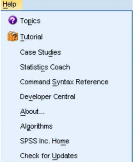
You will now be in the help contents window. Click Tutorial.

You can then open any of the books comprising the tutorial by clicking on the + to get to the various subtopics. Once in a subtopic is open, you can just keep clicking on the right and left arrows to move through it page by page. I suggest going through the entire Overview booklet. Once you are working with a data set, and have an idea of what you want to do with the data, you can also use the Statistics Coach under the Help menu to help get the information you wish. It will lead you through the SPSS process.
Using the SPSS Data Editor. When you begin SPSS, you open up to the Data Editor. For our purposes right now, you can learn how to do this by going to Help>Tutorial>Using the Data Editor, and then working your way through the subtopics. The data we will use is given in the table below, with the numbers indicating total protein ( g/ml).
| 76.33 | 77.63 149 | 49 54.38 | 55.47 51.70 | |
| 78.15 | 85.40 41.9 | 8 69.91 1 | 28.40 88.17 | |
| 58.50 | 84.70 44.4 | 0 57.73 8 | 8.78 86.24 | |
| 54.07 | 95.06 114 | 79 53.07 | 72.30 59.36 | |
| 76.33 | 77.63 149 | 49 54.38 | 55.47 51.70 | |
| 59.20 | 67.10 109 | 30 82.60 | 62.80 61.90 | |
| 74.78 | 77.40 57.9 | 0 91.47 7 | 1.50 61.70 | |
| 106.00 | 61.10 63.9 | 6 54.41 8 | 8.82 79.55 | |
| 153.56 | 70.17 55.0 | 5 100.36 | 51.16 72.10 | |
| 62.32 | 73.53 47.2 | 3 35.90 7 | 2.20 66.60 | |
| 59.76 | 95.33 73.5 | 0 62.20 6 | 7.20 44.73 | |
| 57.68 |
For our data, double click on the var at the top of the first column or click on the Variable View tab at the bottom of the page, type in ``protein'' in the Name column, and hit Enter. Under the assumption that you are going to enter numerical data, the rest of the row is filled in.
Changes in the type and display of the variable can be made by clicking in the appropriate cells and using any
| Name | Type | Width | Decimals | Label | Values | Missing | Columns | Align | Measure | Role | |
| 1 | protein | Numeric | 8 | 2 | None | None | 8 | Right | Scale | None |
buttons given. Then hit the Data View tab and type in the data values, following each by Enter.
| 1 : protein | 35.90 | |
| protein | var | |
| 1 | 35.90 | |
| 2 | 41.98 | |
| 3 | 44.40 | |
| 4 | 44.73 | |
Save the file as usual where you wish under the name protein.sav. You just need type protein. The suffix is attached automatically.
Sorting the Data. From the menu, choose Data>Sort Cases..., click the right arrow to move protein to the Sort by box, make sure Ascending is chosen, and click OK. Our data column is now in ascending order. However, the first thing that come up is an output page telling you what has happened. Click the table with the Star on it to get back to the Data Editor.

Obtaining the Descriptive Statistics. Go to Analyze>Descriptive Statistics>Explore...,
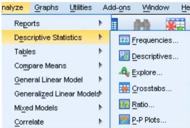
select protein from the box on the left, and then click the arrow for Dependent List:. Make sure Both is checked under Display.

Click the Statistics... button, then make sure Descriptives and Percentiles are checked. We will use 95% for Confidence Interval for Mean. Click Continue.

Then click Plots.... Under Boxplots, select Factor levels together, and under Descriptive, choose both Stem-and-leaf and Histogram. Then click Continue.
Then click OK. This opens an output window with two frames. The frame on the left contains an outline of the data on the right.
Clicking an item in either frame selects it, and allows you to copy it (and paste into a word processor), for instance. Double clicking an item in the left frame either shows or hides that item in the right frame. Clicking on Descriptives in the left frame brings up the following:
Descriptives
| Statistic | Std. Error | |||
| protein | Mean | 73.3292 | 2.99984 | |
| 95% Confidence Interval for Mean | Lower Bound | 67.3286 | ||
| Upper Bound | 79.3298 | |||
| 5% Trimmed Mean | 71.2454 | |||
| Median | 69.9100 | |||
| Variance | 548.943 | |||
| Std. Deviation | 23.42953 | |||
| Minimum | 35.90 | |||
| Maximum | 153.56 | |||
| Range | 117.66 | |||
| Interquartile Range | 26.44 | |||
| Skewness | 1.468 | .306 | ||
| Kurtosis | 2.821 | .604 | ||
The Standard Error of the Mean is a measure of how much the value of the mean may vary from repeated samples of the same size taken from the same distribution. The 95% Confidence Interval for Mean are two numbers that we would expect 95% of the means from repeated samples of the same size to fall between. The 5% Trimmed Mean is the mean after the highest and lowest 2.5% of the values have been removed. Skewness measures the degree and direction of asymmetry. A symmetric distribution such as a normal distribution has a skewness of 0, a distribution that is skewed to the left, when the mean is less than the median, has a negative skewness, and a distribution that is skewed to the right, when the mean is greater than the median, has a positive skewness. Kurtosis is a measure of the heaviness of the tails of a distribution. A normal distribution has kurtosis 0. Extremely nonnormal distributions may have high positive or negative kurtosis values, while nearly normal distributions will have kurtosis values close to 0. Kurtosis is positive if the tails are “heavier” than for a normal distribution and negative if the tails are “lighter” than for a normal distribution.
Double clicking an item in the right frame opens it's editor, if it has one. Double click on the histogram, shown on the next page, to open the Chart Editor. To learn about the Chart Editor, visit Building Charts and Editing Charts under Help>Core System. Once the chart editor opens, choose Edit>Properties from the Chart Editor Menus, click on a number on the vertical axis (which highlights all such numbers), and then click on Scale. From the left diagram at the bottom of the next page, we see a minimum and a maximum for the vertical axis and a major increment of 5. This corresponds to the tick marks and labels on the vertical axis. Now click on Labels & Ticks, check Display Ticks under Minor Ticks, and enter 5 for Number of minor ticks per major ticks:. The Properties window should now look like the rightmost diagram at the bottom of the next page. Click Apply to see the results of this change.

histogram
| Range | Frequency | | --------- | --------- | | 40.00-50.00 | 1 | | 50.00-60.00 | 4 | | 60.00-70.00 | 15 | | 70.00-80.00 | 11 | | 80.00-90.00 | 13 | | 90.00-100.00 | 7 | | 100.00-110.00 | 3 | | 110.00-120.00 | 3 | | 120.00-130.00 | 1 | | 130.00-140.00 | 1 | | 140.00-150.00 | 1 | | 150.00-160.00 | 1 |

Now click on a number on the horizontal axis and then click on Number Format. In the diagram to the left below, we see that we have 2 decimal places. The values in this window can be changed as desired. Next, click on one of the bars and then Binning in the Properties window. Suppose we want bars of width 20 beginning at 30. Check Custom, Interval width:, and enter 20 in the value box. Check Custom value for anchor:, followed by 30 in the value box. Your window should look like the one on the right below.
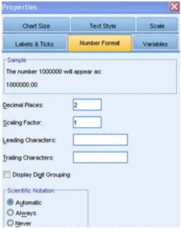

Finally, click Apply and close the Chart Editor to get the histogram below.

histogram
| protein range | Frequency | | ------------- | --------- | | 40.00 - 60.00 | 5 | | 60.00 - 80.00 | 26 | | 80.00 - 100.00 | 20 | | 100.00 - 120.00 | 6 | | 120.00 - 140.00 | 2 | | 140.00 - 160.00 | 1 |Next choose Percentiles from either output frame. The following comes up.
Percentiles
| Percentiles | ||||||||
| 5 | 10 | 25 | 50 | 75 | 90 | 95 | ||
| Weighted Average (Definition 1) | protein | 44.4330 | 51.2680 | 57.8150 | 69.9100 | 84.2600 | 104.8720 | 127.0390 |
| Tukey's Hinges | protein | 57.9000 | 69.9100 | 83.8200 | ||||
Obviously, there are two different methods at work here. The formulas are given in the SPSS Algorithms Manual. Typically, use the Weighed Average. Tukey's Hinges was designed by Tukey for use with the boxplot.

boxplot
| protein | value | | ------- | ----- | | | 61 | | | 060 | | | 59 |The box covers the Interquartile range (IQR) = Q 75 - Q 25 , with the line being Q _50 , the median. In all three cases, the Tukey's Hinges is used. The whiskers extend a maximum of 1.5 IQR from the box. Data points between 1.5 and 3 IQR from the box are indicted by circles and are known as outliers, while those more than 3 IQR from the box are indicated by asterisks and are known as extremes. In this boxplot, the outliers are the 59th, 60th, and 61st elements of the data list.
Copying Output to Word (for instance). You can easily copy a selection of output or the entire output window to Word and other programs in the usual fashion. Just select what you wish to copy, choose Edit>Copy, switch to a Word or other document and choose Edit>Paste. After saving the output, you can also export it as a Word, Powerpoint, Excel, text, or PDF document from File>Export. For information on this, see Help>Tutorial>Working with Output or Help>Core System>Working with Output.
Probability Distributions
Binomial Distribution. We shall assume n=15 and p=.75. We will first find P(X ≤ x | 15, .75) for x = 0, ..., 15, i.e., the cumulative probabilities. First put the numbers 0 through 15 in a column of a worksheet. (Actually, you only need to enter the numbers whose cumulative probability you desire.) Then click Variable View, type in number (the name you choose is optional) under Name, and I suggest putting in 0 for Decimal. Still in Variable View, put the names cum_bin and bin_prob in new rows under Name, and set Width to 12, Decimal to 10, and Columns to 12 for each of these.
| Name | Type | Width | Decimals | Label | Values | Missing | Columns | Align | Measure | Role | |
| 1 | number | Numeric | 8 | 0 | None | None | 8 | Right | Scale | None | |
| 2 | cum_bin | Numeric | 12 | 10 | None | None | 12 | Right | Scale | None | |
| 3 | bin_prob | Numeric | 12 | 10 | None | None | 12 | Right | Scale | None |
Then click back to Data View. From the menu, choose Transform>Compute Variable.... When the Compute Variable window comes up, click Reset, and type cum_bin in the box labeled Target Variable. Scroll down the Function group: window to CDF & Noncentral CDF to select it, then scroll to and select Cdf.Binom in the Functions and Special Variables: window. Then press the up arrow. We need to fill in the three arguments indicated by question marks. The first is the x. This is given by the number column. At this point, the first question mark should be highlighted. Click on number in the box on the left to highlight it, then hit the right arrow to the right of that box. Now highlight the second question mark and type in 15 (our n), and then highlight the third question mark and type in .75 (our p). Hit OK. If you get a message about changing the existing variable, hit OK for that too.
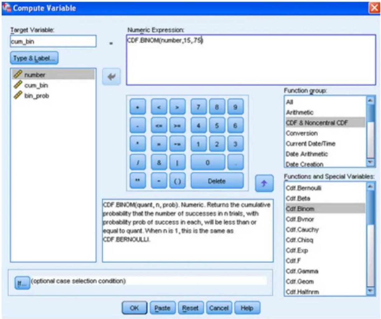
The cumulative binomial probabilities are now found in the column cum_bin. Now we want to put the individual binomial probabilities into the column bin_prob. Do basically the same as the above, except make the Target Variable "bin_prob," and the Numeric Expression "CDF.BINOM(number,15,.75) - CDF.BINOM(number-1,15,.75)." The Data View now looks like the table at the top of the next page, with the cumulative binomial probabilities in the second column and the individual binomial probabilities in the third coloumn.
| cum_bin | bin_prob | |
| 1 | 9E-10 | 9E-10 |
| 2 | 4.28E-8 | 4.19E-8 |
| 3 | 9.229E-7 | 8.801E-7 |
| 4 | .0000123642 | .0000114413 |
| 5 | .0001153359 | .0001029717 |
| 6 | .0007949490 | .0006796131 |
| 7 | .0041930145 | .0033980655 |
| 8 | .0172998384 | .0131068239 |
| 9 | .0566203101 | .0393204717 |
| 10 | .1483680774 | .0917477673 |
| 11 | .3135140585 | .1651459811 |
| 12 | .5387131236 | .2251990652 |
| 13 | .7639121888 | .2251990652 |
| 14 | .9198192339 | .1559070451 |
| 15 | .9866365390 | .0668173051 |
| 16 | 1.0000000000 | .0133634610 |
Poisson Distribution. Let us assume that = .5 . We will first find P(X ≤ x .5) for x = 0, , 15 , i.e., the cumulative probabilities. First put the numbers 0 through 15 in a column of a worksheet. (We have already done this above. Again, you only need to enter the numbers whose cumulative probability you desire.) Then click Variable View, type in number (we have done this above and the name you choose is optional) under Name, and I suggest putting in 0 for Decimal. Still in Variable View, put the names cum_pois and pois_pro in new rows under Name, and set Width to 12, Decimal to 10, and Columns to 12 for each of these.
| Name | Type | Width | Decimals | Label | Values | Missing | Columns | Align | Measure | Role | |
| 1 | number | Numeric | 8 | 0 | None | None | 8 | Right | Scale | None | |
| 2 | cum_bin | Numeric | 12 | 10 | None | None | 12 | Right | Scale | None | |
| 3 | bin_prob | Numeric | 12 | 10 | None | None | 12 | Right | Scale | None | |
| 4 | cum_pois | Numeric | 12 | 10 | None | None | 12 | Right | Scale | None | |
| 5 | Pois_pro | Numeric | 12 | 10 | None | None | 12 | Right | Scale | None |
Then click back to Data View. From the menu, choose Transform>Compute Variable.... When the Compute Variable window comes up, click Reset, and type cum_pois in the box labeled Target Variable. Scroll down the Function group: window to CDF & Noncentral CDF to select it, then scroll to and select Cdf.Poisson in the Functions and Special Variables: window. Then press the up arrow. We need to fill in the two arguments indicated by question marks. The first is the x. That is given by the number column. At this point, the first question mark should be highlighted. Click on number in the box on the left to highlight it, then hit the right arrow to the right of that box. Now highlight the second question mark and type in .5 (our λ). Then hit OK. If you get a message about changing the existing variable, hit OK for that too. The
cumulative Poisson probabilities are now found in the column cum_pois.
Now we want to put the individual Poisson probabilities into the column pois_pro. Do basically the same as above, except make the Target Variable “pois_pro,” and the Numeric Expression “CDF.POISSON(number,.5) - CDF.POISSON(number-1,.5).” The Data View now looks like the table below, with the cumulative Poisson probabilities in the fourth column and the individual Poisson probabilities in the fifth coloumn.
| cum_bin | bin_prob | cum_pois | pois_pro | |
| 1 | 9E-10 | 9E-10 | .6065306597 | .6065306597 |
| 2 | 4.28E-8 | 4.19E-8 | .9097959896 | .3032653299 |
| 3 | 9.229E-7 | 8.801E-7 | .9856123220 | .0758163325 |
| 4 | .0000123642 | .0000114413 | .9982483774 | .0126360554 |
| 5 | .0001153359 | .0001029717 | .9998278844 | .0015795069 |
| 6 | .0007949490 | .0006796131 | .9999858351 | .0001579507 |
| 7 | .0041930145 | .0033980655 | .9999989976 | .0000131626 |
| 8 | .0172998384 | .0131068239 | .9999999378 | 9.402E-7 |
| 9 | .0566203101 | .0393204717 | .9999999966 | 5.88E-8 |
| 10 | .1483680774 | .0917477673 | .9999999998 | 3.3E-9 |
| 11 | .3135140585 | .1651459811 | 1.0000000000 | 2E-10 |
| 12 | .5387131236 | .2251990652 | 1.0000000000 | 0E-10 |
| 13 | .7639121888 | .2251990652 | 1.0000000000 | 0E-10 |
| 14 | .9198192339 | .1559070451 | 1.0000000000 | 0E-10 |
| 15 | .9866365390 | .0668173051 | 1.0000000000 | 0E-10 |
| 16 | 1.0000000000 | .0133634610 | 1.0000000000 | 0E-10 |
Normal Distribution. Suppose we are using a normal distribution with mean 100 and standard deviation 20 and we wish to find P(X ≤ 135). Start a new Data Editor sheet, and just type 0 in the first row of the first column and then hit Enter. Then click Variable View, put the names cum_norm, int_norm, and inv_norm in new rows under Name, and set Decimal to 4 for each of these.
| Name | Type | Width | Decimals | Label | Values | Missing | Columns | Align | Measure | Role | |
| 1 | cum_norm | Numeric | 8 | 4 | None | None | 8 | Right | Scale | None | |
| 2 | int_norm | Numeric | 8 | 4 | None | None | 8 | Right | Scale | None | |
| 3 | inv_norm | Numeric | 8 | 4 | None | None | 8 | Right | Scale | None |
Then click back to Data View. From the menu, choose Transform>Compute Variable.... When the Compute Variable window comes up, click Reset, and type cum_norm in the box labeled Target Variable. Scroll down the Function group: window to CDF & Noncentral CDF to select it, then scroll to and select Cdf.Normal in the Functions and Special Variables: window. We need to fill in the three arguments indicated by question marks to get CDF.NORMAL(135,100,20) under Numeric Expression: as in the diagram at the top of the next page.

The probability is now found in the column cum_norm.
Staying with the normal distribution with mean 100 and standard deviation 20, suppose we with to find P(90 ≤ X ≤135). Do as above except make the Target Variable “int_norm,” and the Numeric Expression “CDF.NORMAL(135,100,20) - CDF.NORMAL(90,100,20).” The probability is now found in the column int_norm.
Continuing to use a normal distribution with mean 100 and standard deviation 20, suppose we wish to find x such that P(X ≤ x) = .6523. Again, do as above except make the Target Variable “inv_norm,” and the Numeric Expression “IDF.NORMAL(.6523,100,20)” by choosing Inverse DF under Function Group: and Idf.Normal under Functions and Special Variables:. The x-value is now found in the column inv_norm. From the table below we see that for the normal distribution with mean 100 and standard deviation 20, P(X ≤ 135) = .9599 and P(90 ≤ X ≤ 135) = .6514\$. Finally, if P(X ≤ x) = .6523, then x=107.8307.
| cum_norm | int_norm | inv_norm | |
| 1 | .9599 | .6514 | 107.8307 |
Confidence Intervals and Hypothesis Testing Using t
A Single Population Mean. We found earlier that the sample mean of the data given on page 2, which you may have saved under the name protein.sav, is 73.3292 to four decimal places. We wish to test whether the mean of the population from which the sample came is 70 as opposed to a true mean greater than 70. We test
$$ H _ {0}: \mu = 7 0 $$
$$ H _ {\mathrm{a}}: \mu > 7 0. $$
From the menu, choose Analyze>Compare Means>One-Sample T Test. Select protein from the left-hand window and click the right arrow to move it to the Test Variable(s) window. Set the Test Value to 70.

Click on Options. Set the Confidence Interval to 95% (or any other value you desire).
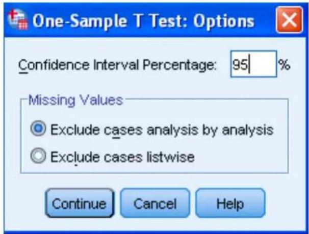
Then click Continue followed by OK. You get the following output.
One-Sample Statistics
| N | Mean | Std. Deviation | Std. Error Mean | |
| protein | 61 | 73.3292 | 23.42953 | 2.99984 |
One-Sample Test
| Test Value = 70 | ||||||
| t | df | Sig. (2-tailed) | Mean Difference | 95% Confidence Interval of the Difference | ||
| Lower | Upper | |||||
| protein | 1.110 | 60 | .272 | 3.32918 | -2.6714 | 9.3298 |
SPSS gives us the basic descriptives in the first table. In the second table, we are given that the t-value for our test is 1.110. The p-value (or Sig. (2-tailed)) is given as .272. Thus the p-value for our one-tailed test is one-half of that or .136. Based on this test statistic, we would not reject the null hypothesis, for instance, for a value of =.05 . SPSS also gives us the 95% Confidence Interval of the Difference between our data scores and the hypothesized mean of 70, namely (-2.6714, 9.3298). Adding the hypothesized value of 70 to both numbers gives us a 95% confidence interval for the mean of (67.3286, 79.3298). If you are only interested in the confidence interval from the beginning, you can just set the Test Value to 0 instead of 70.
The Difference Between Two Population means. For a data set, we are going to look at a distribution of 32 cadmium level readings from the placenta tissue of mothers, 14 of whom were smokers. The scores are as follows:
non-smokers
10.0 8.4 12.8 25.0 11.8 9.8 12.5 15.4 23.5 9.4 25.1 19.5 25.5 9.8 7.5 11.8 12.2 15.0
smokers
30.0 30.1 15.0 24.1 30.5 17.8 16.8 14.8 13.4 28.5 17.5 14.4 12.5 20.4
We enter this data in two columns of the Data Editor. The first column, which is labeled s_ns, contains a 1 for each non-smoking score and a 2 for each smoking score. The scores are contained in the second column, which is labeled cadmium. Clicking Variable View, we put s_ns for the name of the first column, change Decimals to 0, and type in Smoker for Label. Double-click on the three dots following None,
| Name | Type | Width | Decimals | Label | Values | Missing | Columns | Align | Measure | Role | |
| 1 | s_ns | Numeric | 8 | 0 | Smoker | None ... | None | 8 | Right | Scale | Input |
and in the window that opens, type 1 for Value, Non-Smoker for Value Label, and then press Add. Then type 2 for Value, Smoker for Value Label,
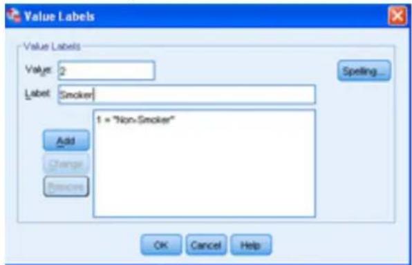
and again press Add. Then hit OK and complete the Variable View as follows.
| Name | Type | Width | Decimals | Label | Values | Missing | Columns | Align | Measure | Role | |
| 1 | s_ns | Numeric | 8 | 0 | Smoker | Smoker)... | None | 8 | Right | Scale | Input |
| 2 | cadmium | Numeric | 8 | 1 | None | None | 8 | Right | Scale | Input |
Returning to Data View gives a window whose beginning looks like that below.
| s_ns | cadmium | |
| 1 | 1 | 10.0 |
| 2 | 1 | 8.4 |
| 3 | 1 | 12.8 |
Now we wish to test the hypotheses
$$ H _ {0}: \mu_ {1} - \mu_ {2} = 0 $$
$$ H _ {\mathrm{a}}: \mu_ {1} - \mu_ {2} \neq 0 $$
where _1 refers to the population mean for the non-smokers and _2 refers to the population mean for the smokers. From the menu, choose Analyze>Compare Means>Independent-Samples T Test, and in the window that comes up, move cadmium to the Test Variable(s) window, and s_ns into the Grouping Variable window.

Notice the two questions marks that appear. Click on Define Groups..., put in 1 for Group 1 and 2 for Group 2.

Then click Continue. As before, click Options..., enter 95 (or any other number) for Confidence Interval, and again click Continue followed by OK. The first table of output gives the descriptives.
Group Statistics
| Smoker | N | Mean | Std. Deviation | Std. Error Mean | |
| cadmium | Non-Smoker | 18 | 14.722 | 6.1986 | 1.4610 |
| Smoker | 14 | 20.414 | 6.8141 | 1.8211 |
To get the second table as it appears here, I first double-clicked on the Independent Samples Test table, giving it a fuzzy border and bringing us into the table editor, and then chose Pivot>Transpose Rows and Columns from the menu.
Independent Samples Test
| cadmium | |||
| Equal variances assumed | Equal variances not assumed | ||
| Levene's Test for Equality of Variances | F | .461 | |
| Sig. | .502 | ||
| t-test for Equality of Means | t | -2.468 | -2.438 |
| df | 30 | 26.671 | |
| Sig. (2-tailed) | .020 | .022 | |
| Mean Difference | -5.6921 | -5.6921 | |
| Std. Error Difference | 2.3065 | 2.3348 | |
| 95% Confidence Interval Lower of the Difference Upper | -10.4025 | -10.4854 | |
| -.9816 | -.8987 | ||
In interpreting the data, the first thing we need to determine is whether we are assuming equal variances. Levene's Test for Equality of Variances is an aid in this regard. Since the p-value of Levine's test is p=.502 for a null hypothesis of all variances equal, in the absence of other information we have no strong evidence to
discount this hypothesis, so we will take our results from the Equal Variances Assumed column. We see that, with 30 degrees of freedom, we have t=-2.468 and p=.020, so we reject the null hypothesis H_0 : _1-_2=0 at the =.05 level of significance. That we would reject this null hypothesis can also be seen in that the 95% Confidence Interval of the Difference of (-10.4025, -.9816) does not contain 0. However, we would not reject the null hypothesis at the =.01 level of significance and, correspondingly, the 99% Confidence Interval of the Difference, had we chosen that level, would contain 0.
Paired Comparisons. We consider the weights (in kg) of 9 women before and after 12 weeks on a special diet, with the goal of determining whether the diet aids in weight reduction. The paired data is given below.
| Before | 117.3 | 111.4 | 98.6 | 104.3 | 105.4 | 100.4 | 81.7 | 89.5 | 78.2 |
| After | 83.3 | 85.9 | 75.8 | 82.9 | 82.3 | 77.7 | 62.7 | 69.0 | 63.9 |
We place the Before data in the first column of our worksheet and the After data in the second column. We wish to test the hypotheses
$$ H _ {0}: \mu_ {\mathrm{B-A}} = 0 $$
$$ H _ {\mathrm{a}}: \mu_ {\mathrm{B-A}} > 0 $$
with one-sided alternative. From the menu, choose Analyze>CompareMeans>Paire-Samples T Test. In the window that opens, first click Before followed by the right arrow to make it Variable 1 and then After followed by the right arrow to make it Variable 2.
![Paired-Samples T Test Before After Paired Variables: Pair Variable1 Variable2 1 [Before] [After] 2 Options... OK Paste Reset Cancel Help](/content/2026/05/944397/images/401c52dad0f1a0591d36019bd924938563e3f0fbf4771d142f8efb0462ccbe64.jpg)
Next, click Options... to set Confidence Interval to 99%. Then click Continue to close the Options... window followed by OK to get the output.
Paired Samples Statistics
| Mean | N | Std. Deviation | Std. Error Mean | ||
| Pair 1 | Before | 98.533 | 9 | 13.1341 | 4.3780 |
| After | 75.944 | 9 | 8.7593 | 2.9198 | |
The first output table gives the descriptives and a second (not shown here) gives a correlation coefficient. From the third table, which has been pivoted to interchange rows and columns,
Paired Samples Test
| Pair 1 | ||
| Before - After | ||
| Paired Differences | Mean | 22.5889 |
| Std. Deviation | 5.3194 | |
| Std. Error Mean | 1.7731 | |
| 99% Confidence Interval of the Difference | Lower 16.6393 | |
| Upper 28.5384 | ||
| t | 12.740 | |
| df | 8 | |
| Sig. (2-tailed) | .000 | |
we see that we have a t-score of 12.740. The fact that Sig.(2-tailed) is given as .000 really means that it is less than .001. Thus, for our one-sided test, we can conclude that p < .0005, so that in almost any situation we would reject the null hypothesis. We also see that the mean of the weight losses for the sample is 22.5889, with a 99% Confidence Interval of the Difference (the mean weight loss for the population from which the sample was drawn) being (16.6393, 28.5384).
One-Way ANOVA
For data, we will use percent predicted residual volume measurements as categorized by smoking history.
Never 35,120,90,109,82,40,68,84,124,77,140,127,58,110,42,57,93
Former 62, 73, 60, 77, 52, 115, 82, 52, 105, 143, 80, 78, 47, 85, 105, 46, 66, 95, 82, 141, 64, 124, 65, 42, 53, 67, 95, 99, 69, 118, 131, 76, 69, 69
Current 96,107,63,134,140,103,158
We will place the volume measurements in the first column and the second column will be coded by 1 = "Never," 2 = "Former," and 3 = "Current." The Variable View looks as below.
| Name | Type | Width | Decimals | Label | Values | Missing | Columns | Align | Measure | Role | |
| 1 | volume | Numeric | 8 | 1 | None | None | 8 | Right | Scale | Input | |
| 2 | smoking | Numeric | 8 | 0 | Smoker | {1, Never)... | None | 8 | Right | Scale | Input |
We test to see if there is a difference among the population means from which the samples have been drawn. We use the hypotheses
$$ H _ {0}: \mu_ {\mathrm{N}} = \mu_ {\mathrm{F}} = \mu_ {\mathrm{C}} $$
H_a : Not all of _N , _F , and C are equal.
From the menu we choose Analyze>Compare Means>One-Way ANOVA.... In the window that opens, place volume under Dependent List and Smoker[smoking] under Factor.
![One-Way ANOVA Dependent List: volume Factor: Smoker [smoking] Contrasts... Post_Hoc... Options... OK Paste Reset Cancel Help](/content/2026/05/944397/images/23ee62061f2689ab2bda02ab554f0fd69509f91533948b3c4d77852e087c13da.jpg)
Then click Post Hoc... For a post-hoc test, we will only choose Tukey (Tukey's HSD test) with Significance Level .05, and then click Continue.
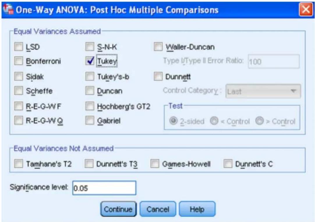
Then we click options and choose Descriptive, Homogeneity of variance test, and Means plot. The Homogeneity of variance test calculates the Levene statistic to test for the equality of group variances. This test is not dependent on the assumption of normality. The Brown-Forsythe and Welch statistics are better than the F statistic if the assumption of equal variable does not hold.

Then we click Continue followed by OK to get our output.
Descriptives
volume
| Never | Former | Current | Total | ||
| N | 21 | 44 | 7 | 72 | |
| Mean | 82.143 | 84.250 | 114.429 | 86.569 | |
| Std. Deviation | 30.4356 | 29.2981 | 31.9001 | 30.8617 | |
| Std. Error | 6.6416 | 4.4169 | 12.0571 | 3.6371 | |
| 95% Confidence Interval for Mean | Lower Bound | 68.289 | 75.343 | 84.926 | 79.317 |
| Upper Bound | 95.997 | 93.157 | 143.931 | 93.822 | |
| Minimum | 35.0 | 40.0 | 63.0 | 35.0 | |
| Maximum | 140.0 | 151.0 | 158.0 | 158.0 | |
A first impression from the Descriptives is that the mean of the Current smokers differs significantly from those who Never smoked and the Former smokers, the latter two means being pretty much the same.
Test of Homogeneity of Variances
volume
| Levene Statistic | df1 | df2 | Sig. |
| .026 | 2 | 69 | .974 |
The results of the Test of Homogeneity of Variances is nonsignificant since we have a p value of .974, showing that there is no reason to believe that the variances of the three groups are different from one another. This is reassuring since both ANOVA and Tukey's HSD have equal variance assumptions. Without this reassurance, interpretation of the results would be difficult, and we would likely remain the data with the Brown-Forsythe and Welch statistics.
ANOVA
volume
| Sum of Squares | df | Mean Square | F | Sig. | |
| Between Groups | 6081.117 | 2 | 3040.559 | 3.409 | .039 |
| Within Groups | 61542.536 | 69 | 891.921 | ||
| Total | 67623.653 | 71 |
Now we look at the results of the ANOVA itself. The Sum of Squares Between Groups is the SSA, the Sum of Squares Within Groups is the SSW, the Total Sum of Squares is the SST, the Mean Square Between Groups is the MSA, the Mean Square Within Groups is the MSW, and the F value of 3.409 is the Variance Ratio. Since the p value is .039, we will reject the null hypothesis at the = .05 level of significance, concluding that all three population means are not the same, but would not reject it at the = .01 level.
So now the question becomes which of the means significantly differ from the others. For this we look to post-hoc tests. One option which was not chosen was LSD (least significant difference) since this simply does a t test on each pair. Here, with three groups we would test three pairs. But if you have 7 groups, for instance, that is 21 separate t tests, and at an = .05 level of significance, even if all the means are the same, you can expect on the average to get one Type I error where you reject a true null hypothesis for every 20 tests. In other words, while the t test is useful in testing whether two means are the same, it is not the test to use for checking multiple means. That is why we chose ANOVA in the first place. We have chosen Tukey's HSD because it offers adequate protection from Type I errors and is widely used.
Multiple Comparisons
volume
Tukey HSD
| (I) Smoke r | (J) Smoke r | Mean Difference (I-J) | Std. Error | Sig. | 95% Confidence Interval | |
| Lower Bound | Upper Bound | |||||
| Never | Former | -2.1071 | 7.9211 | .962 | -21.081 | 16.866 |
| Current | -32.2857* | 13.0342 | .041 | -63.507 | -1.065 | |
| Former | Never | 2.1071 | 7.9211 | .962 | -16.866 | 21.081 |
| Current | -30.1786* | 12.1527 | .040 | -59.288 | -1.069 | |
| Current | Never | 32.2857* | 13.0342 | .041 | 1.065 | 63.507 |
| Former | 30.1786* | 12.1527 | .040 | 1.069 | 59.288 | |
*. The mean difference is significant at the 0.05 level.
Looking at all of the p values (Sig.) in the Multiple Comparisons table, we see that Current differs significantly ( = .05 ) from Never and Former, with no significant difference detected between Never and Former. The second table for Tukey's HSD, seen below, divides the groups into homogeneous subsets and gives the mean for each group.
Tukey HSD
| Smoker | N | Subset for alpha = 0.05 | |
| 1 | 2 | ||
| Never | 21 | 82.143 | |
| Former | 44 | 84.250 | |
| Current | 7 | 114.429 | |
| Sig. | .981 | 1.000 | |
Means for groups in homogeneous subsets are displayed.
Simple Linear Regression and Correlation
We will use the following 109 x-y data pairs for simple linear regression and correlation.
| x | y | x | y | x | y | x | y | x | y | |||||
| 1 | 74.75 | 25.72 | 23 | 79.90 | 35.43 | 45 | 83.00 | 96.54 | 67 | 96.50 | 144.00 | 89 | 121.00 | 245.00 |
| 2 | 72.60 | 25.89 | 24 | 89.20 | 60.09 | 46 | 107.10 | 118.00 | 68 | 105.50 | 121.00 | 90 | 109.00 | 137.00 |
| 3 | 81.80 | 42.60 | 25 | 82.00 | 45.84 | 47 | 94.30 | 107.00 | 69 | 105.00 | 97.13 | 91 | 97.50 | 165.00 |
| 4 | 83.95 | 42.80 | 26 | 92.00 | 70.40 | 48 | 94.50 | 123.00 | 70 | 107.00 | 166.00 | 92 | 105.50 | 152.00 |
| 5 | 74.65 | 29.84 | 27 | 86.60 | 83.45 | 49 | 79.70 | 65.92 | 71 | 107.00 | 87.99 | 93 | 98.00 | 181.00 |
| 6 | 71.85 | 21.68 | 28 | 80.50 | 84.30 | 50 | 79.30 | 81.29 | 72 | 101.00 | 154.00 | 94 | 94.50 | 80.95 |
| 7 | 80.90 | 29.08 | 29 | 86.00 | 78.89 | 51 | 89.80 | 111.00 | 73 | 97.00 | 100.00 | 95 | 97.00 | 137.00 |
| 8 | 83.40 | 32.98 | 30 | 82.50 | 64.75 | 52 | 83.80 | 90.73 | 74 | 100.00 | 123.00 | 96 | 105.00 | 125.00 |
| 9 | 63.50 | 11.44 | 31 | 83.50 | 72.56 | 53 | 85.20 | 133.00 | 75 | 108.00 | 217.00 | 97 | 106.00 | 241.00 |
| 10 | 73.20 | 32.22 | 32 | 88.10 | 89.31 | 54 | 75.50 | 41.90 | 76 | 100.00 | 140.00 | 98 | 99.00 | 134.00 |
| 11 | 71.90 | 28.32 | 33 | 90.80 | 78.94 | 55 | 78.40 | 41.71 | 77 | 103.00 | 109.00 | 99 | 91.00 | 150.00 |
| 12 | 75.00 | 43.86 | 34 | 89.40 | 83.55 | 56 | 78.60 | 58.16 | 78 | 104.00 | 127.00 | 100 | 102.50 | 198.00 |
| 13 | 73.10 | 38.21 | 35 | 102.00 | 127.00 | 57 | 87.80 | 88.85 | 79 | 106.00 | 112.00 | 101 | 106.00 | 151.00 |
| 14 | 79.00 | 42.48 | 36 | 94.50 | 121.00 | 58 | 86.30 | 155.00 | 80 | 109.00 | 192.00 | 102 | 109.10 | 229.00 |
| 15 | 77.00 | 30.96 | 37 | 91.00 | 107.00 | 59 | 85.50 | 70.77 | 81 | 103.50 | 132.00 | 103 | 115.00 | 253.00 |
| 16 | 68.85 | 55.78 | 38 | 103.00 | 129.00 | 60 | 83.70 | 75.08 | 82 | 110.00 | 126.00 | 104 | 101.00 | 188.00 |
| 17 | 75.95 | 43.78 | 39 | 80.00 | 74.02 | 61 | 77.60 | 57.05 | 83 | 110.00 | 153.00 | 105 | 100.10 | 124.00 |
| 18 | 74.15 | 33.41 | 40 | 79.00 | 55.48 | 62 | 84.90 | 99.73 | 84 | 112.00 | 158.00 | 106 | 93.30 | 62.20 |
| 19 | 73.80 | 43.35 | 41 | 83.50 | 73.13 | 63 | 79.80 | 27.96 | 85 | 108.50 | 183.00 | 107 | 101.80 | 133.00 |
| 20 | 75.90 | 29.31 | 42 | 76.00 | 50.50 | 64 | 108.30 | 123.00 | 86 | 104.00 | 184.00 | 108 | 107.90 | 208.00 |
| 21 | 76.85 | 36.60 | 43 | 80.50 | 50.88 | 65 | 119.60 | 90.41 | 87 | 111.00 | 121.00 | 109 | 108.50 | 208.00 |
| 22 | 80.90 | 40.25 | 44 | 86.50 | 140.00 | 66 | 119.90 | 106.00 | 88 | 108.50 | 159.00 |
The x's are waist circumferences (cm) and the y's are measurements of deep abdominal adipose tissue gathered by CAT scans. Since CAT scans are expensive, the goal is to find a predictive equation. First we wish to take a look at the scatter plot of the data, so we choose Graphs>Legacy Dialogs>Scatter/Dot from the menu. In the window that opens, click on Simple Scatter, and then Define. In the Simple Scatterplot window that opens, drag x and y to the boxes shown.

Then click OK to get the following scatter plot, which leads us to suspect that there is a significant linear relationship.

scatter
| x | y | |-------|-------| | 60.00 | 10.00 | | 65.00 | 30.00 | | 70.00 | 40.00 | | 75.00 | 50.00 | | 80.00 | 60.00 | | 85.00 | 70.00 | | 90.00 | 80.00 | | 95.00 | 90.00 | | 100.00| 100.00| | 105.00| 110.00| | 110.00| 120.00| | 115.00| 130.00| | 120.00| 140.00| | 125.00| 150.00| | 130.00| 160.00| | 135.00| 170.00| | 140.00| 180.00| | 145.00| 190.00| | 150.00| 200.00| | 155.00| 210.00| | 160.00| 220.00| | 165.00| 230.00| | 170.00| 240.00| | 175.00| 250.00| | 180.00| 260.00| | 185.00| 270.00| | 190.00| 280.00| | 195.00| 290.00| | 200.00| 300.00| | 205.00| 310.00| | 210.00| 320.00| | 215.00| 330.00| | 220.00| 340.00| | 225.00| 350.00| | 230.00| 360.00| | 235.00| 370.00| | 240.00| 380.00| | 245.00| 390.00| | 250.00| 400.00| | 255.00| 410.00| | 260.00| 420.00| | 265.00| 430.00| | 270.00| 440.00| | 275.00| 450.00| | 280.00| 460.00| | 285.00| 470.00| | 290.00| 480.00| | 295.00| 490.00| | 300.0 |Regression. To explore this relationship, choose Analyze>Regression>Linear... from the menu, select and move y under Dependent and x under Independent(s).

Then click Statistics..., and in the window that opens with Estimates and Model fit already checked, also check Confidence intervals and Descriptives.

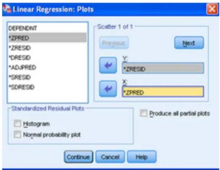
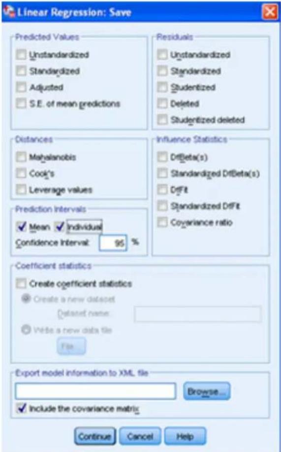
Then click Continue. Next click Plots.... In the window that opens, enter *ZRESID for Y and *ZPRED for X to get a graph of the standardized residuals as a function of the standardized predicted values. After clicking Continue, next click Save.... In the window that opens, check Mean and Individual under Prediction Intervals with 95% for Confidence Intervals. This will add four columns to our data window that give the 95% confidence intervals for the mean values _y1x and individual values y_1 for each x in our set of data pairs.
Then click Continue followed by OK to get the output.
Descriptive Statistics
| Mean | Std. Deviation | N | |
| y | 101.8940 | 57.29476 | 109 |
| x | 91.9018 | 13.55912 | 109 |
We first see the mean and the standard deviation for the two variables in the Descriptive Statistics.
Model Summary ^b
| Mode I | R | R Square | Adjusted R Square | Std. Error of the Estimate |
| 1 | .819a | .670 | .667 | 33.06493 |
a. Predictors: (Constant), x
b. Dependent Variable: y
In the Model Summary, we see that the bivariate correlation coefficient r (R) is .819, indicating a strong positive linear relationship between the two variables. The coefficient of determination r^2 (R Square) of .670 indicates that, for the sample, 67% of the variation of y can be explained by the variation in x. But this may be an overestimate for the population from which the sample is drawn, so we use the Adjusted R Square as a better estimate for the population. Finally, the Standard Error of the Estimate is 33.0649.
Coefficients ^a
| Model | |||
| 1 | |||
| (Constant) | x | ||
| Unstandardized Coefficients | B | -215.981 | 3.459 |
| Std. Error | 21.796 | .235 | |
| Standardized Coefficients | Beta | .819 | |
| t | -9.909 | 14.740 | |
| Sig. | .000 | .000 | |
| 95% Confidence Interval for B | Lower Bound | -259.190 | 2.994 |
| Upper Bound | -172.773 | 3.924 | |
a. Dependent Variable: y
We use the sample regression (least squares) equation =a+bx to approximate the population regression equation _ylx=+ x . From the Coefficients table, is -215.981 and is 3.459 from the first row of numbers (rows and columns transposed from the output), so the sample regression equation is =-215.981+3.459x . From the last two rows of numbers in the table, one gets that 95% confidence intervals for and are (-259.190, -172.773) and (2.994, 3.924), respectively.
The t test is used for testing the null hypothesis =0 , for if =0 , the sample regression equation will have little value for prediction and estimation. It can be used similarly to test the null hypothesis =0 , but this is of much less interest. In this case, we read from the above table that for H_0:=0 , H_a:0 , we have t=14.740. Since the p-value (Sig.=.000) for that t test is less than .001 (the meaning of Sig.=.000), we can reject the null hypothesis of =0 .
Although the ANOVA table is more properly used in multiple regression for testing the null hypothesis _1 = _2 = = _n = 0 with an alternative hypothesis of not all _i = 0 , it can also be used to test = 0 in simple linear regression. In the table below, the Regression Sum of Squares (SSR) is the variation expained by regression, and the Residual Sum of Squares} (SSE) is the variation not explained by regression (the ``E'' stands for error). The Mean Square Regression and the Mean Square Residual are MSR and MSE respectively, with the F value of 217.279 being their quotient. Since the p -value ( Sig. = .000 ) is less than .001, we can
reject the null hypothesis of = 0 .
ANOVA ^b
| Model | Sum of Squares | df | Mean Square | F | Sig. | |
| 1 | Regression | 237548.516 | 1 | 237548.516 | 217.279 | .000^a |
| Residual | 116981.986 | 107 | 1093.290 | |||
| Total | 354530.502 | 108 | ||||
a. Predictors: (Constant), x
b. Dependent Variable: y
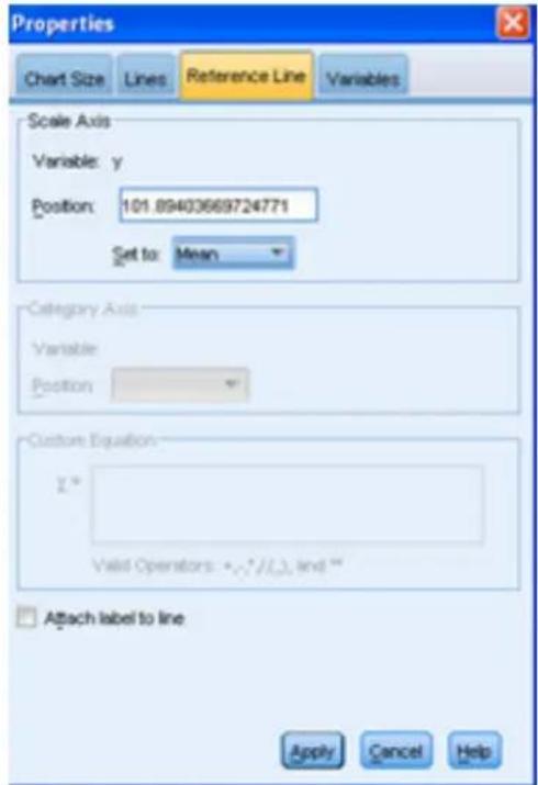
We now return to the scatter plot. Double click on the plot to bring up the Chart Editor and choose Options>Y Axis Reference Line from the menu. In the window that opens, select Reference Line and, from the dropdown menue for Set to:, choose Mean and then click Apply.

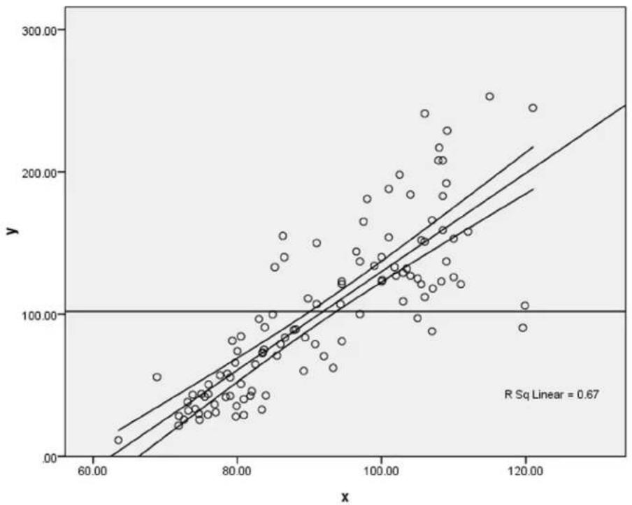
Next, from the Chart Editor menu, choose Elements>Fit Line at Total. In the window that opens, with Fit Line highlighted at the top, make sure Linear is chosen for Fit Method, and Mean with 95% for Confidence Intervals. Then click Apply. You get the first graph at the top of the next page. In this graph, the horizontal line shows the mean of the y-values, 101.894. We see that the scatter about the regression line is much less than the scatter about the mean line, which is as it should be when the null hypothesis β=0 has been rejected. The bands about the regression line give the 95% confidence interval for the mean values μ ylx for each x, or from another point of view, the probability is .95 that the population regression line μ ylx =α+βx lies within these bands.
Finally, go back to the same menu and choose Individual instead of Mean, followed again by Apply. After some editing as discussed earlier in this manual, you get the second graph on the next page. Here, for each x-value, the outer bands give the 95% confidence interval for the individual y_1 for each value of x.
The confidence bands in the scatter plots relate to the four new columns in our data window, a portion of which is shown at the bottom of the next page. We interpret the first row of data. For x = 74.5 , the 95% confidence interval
scatter
| x | y | |-------|-------| | 60.00 | 0.00 | | 70.00 | 50.00 | | 80.00 | 100.00| | 90.00 | 150.00| | 100.00| 200.00| | 110.00| 250.00| | 120.00| 300.00|
scatter
| x | y | | --- | --- | | 60 | 10 | | 70 | 30 | | 80 | 50 | | 90 | 70 | | 100 | 100 | | 110 | 120 | | 120 | 150 | | 130 | 200 || x | y | LMCI_1 | UMCI_1 | LICI_1 | UICI_1 | |
| 1 | 74.75 | 25.72 | 32.41572 | 52.72078 | -23.7607 | 108.8972 |
| 2 | 72.60 | 25.89 | 24.17575 | 46.08766 | -31.3250 | 101.5884 |
| 3 | 81.80 | 42.60 | 59.11112 | 74.79530 | .93840 | 132.9680 |
| 4 | 83.95 | 42.80 | 67.10283 | 81.67669 | 8.43859 | 140.3409 |
for the mean value _y_174.5 is (32.41572, 52.72078), corresponding to the limits of the inner bands at x=74.5 in the scatter plot, and the 95% confidence interval for the individual value y_i(74.5) is (-23.7607, 108.8972), corresponding to the limits of the outer bands at x=74.5. The first pair of acronyms lmci and umci stand for “lower mean confidence interval” and “upper mean confidence interval,” respectively, with the i in the second pair standing for “individual.”
Finally, consider the residual plot below. On the horizontal axis are the standardized y values from the data pairs, and on the vertical axis are the standardized residuals for each such y. If all the regression assumptions were met for our data set, we would expect to see random scattering about the horizontal line at level 0 with no noticeable patterns. However, here we see more spread for the larger values of y, bringing into question whether the assumption regarding equal standard deviations for each y population is met.

scatter
| Regression Standardized Predicted Value | Regression Standardized Residual | | --------------------------------------- | --------------------------------- | | -2.0 | 0.5 | | -1.5 | 0.8 | | -1.0 | 0.3 | | -0.5 | 0.6 | | 0.0 | 0.4 | | 0.5 | 0.7 | | 1.0 | 1.2 | | 1.5 | 1.5 | | 2.0 | 2.0 | | 2.5 | 1.8 | | 3.0 | 1.5 |Correlation. Choose Analyze>Correlate>Bivariate... from the menu to study the correlation of the two variables x and y.
![Bivariate Correlations 95% L CI for y mean [...] 95% U CI for y mean [...] 95% L CI for y individu... 95% U CI for y individu... Variables: x y Correlation Coefficients Pearson: Kendall's tau-b Spearman Test of Significance Two-tailed One-tailed Flag significant correlations OK Paste Reset Cancel Help](/content/2026/05/944397/images/eb53e3298c78be8ad1033cb33ed4f49a8c04477efacf0e29567c9f40f276763c.jpg)
In the window that opens, move both x and y to the Variables window and make sure Pearson is selected. The other two choices are for nonparametric correlations. We will choose Two-tailed here since we already have the results of the One-tailed option in the Correlation table in the regression output. In general, you choose One-tailed if you know the direction of correlation (positive or negative), and Two-tailed if you do not. Clicking OK gives the results.
Correlations
| x | |||
| x | Pearson Correlation | 1.000 | |
| Sig. (2-tailed) | |||
| N | 109.000 | ||
| y | Pearson Correlation | .819** | |
| Sig. (2-tailed) | .000 | ||
| N | 109 | 10 | |
**. Correlation is significant at the 0.01 level (
We see again that the Pearson Correlation r is .819, and from the Sig. of .000, we know that the p -value is less than .001 and so we would reject a null hypothesis of r = 0 .
Multiple Regression
We will use the following data set for multiple linear regression. In this data set, required ram, amount of input, and amount of output, all in kilobytes, are used to predict minutes of processing time for a given task. From left to right, we will use the variables y, x_1, x_2 , and x_3 . Overall, the process used parallels that of simple linear regression.
| minutes | ram | input | output | |
| 1 | 5.2 | 19 | 5 | 1 |
| 2 | 17.3 | 105 | 10 | 2 |
| 3 | 15.5 | 70 | 15 | 5 |
| 4 | 23.4 | 80 | 20 | 8 |
| 5 | 15.4 | 24 | 12 | 10 |
| 6 | 9.5 | 15 | 2 | 5 |
| 7 | 6.2 | 22 | 3 | 4 |
| 8 | 10.0 | 35 | 10 | 3 |
| 9 | 7.7 | 42 | 5 | 2 |
| 10 | 6.3 | 15 | 2 | 2 |
| 11 | 7.2 | 8 | 4 | 5 |
| 12 | 8.5 | 7 | 5 | 6 |
| 13 | 8.9 | 12 | 10 | 3 |
| 14 | 5.6 | 15 | 7 | 2 |
| 15 | 4.1 | 17 | 4 | 1 |
| 16 | 9.7 | 18 | 3 | 6 |
| 17 | 13.4 | 24 | 8 | 5 |
| 18 | 11.7 | 25 | 8 | 4 |
| 19 | 8.4 | 32 | 10 | 3 |
| 20 | 12.1 | 79 | 12 | 2 |
Choose Analyze>Regression>Linear... from the menu, select and move minutes under Dependent and ram, input, and output, in that order, under Independent(s). Then fill in the options for Statistics, Plots, and Save exactly as you did for simple linear regression.

Finally, click OK to get the output.
Descriptive Statistics
| Mean | Std. Deviation | N | |
| minutes | 10.305 | 4.7798 | 20 |
| ram | 33.20 | 27.816 | 20 |
| input | 7.75 | 4.711 | 20 |
| output | 3.95 | 2.350 | 20 |
We first see the mean and the standard deviation for all of the variables in the Descriptive Statistics.
Model Summary ^b
| Mode I | R | R Square | Adjusted R Square | Std. Error of the Estimate |
| 1 | .959a | .920 | .904 | 1.4773 |
a. Predictors: (Constant), output, ram, input
b. Dependent Variable: minutes
In the Model Summary, we see that the coefficient of multiple correlation r (R) is .959, indicating a strong positive linear relationship between the predictors and the dependent variable. The coefficient of determination r_2 (R Square) of .920 indicates that, for the sample, 92% of the variation of minutes can be explained by the variation in ram, input, and output. But this may be an overestimate for the population from which the sample is drawn, so we use the Adjusted R Square as a better estimate for the population. Finally, the Standard Error of the Estimate is 1.4773.
Letting y=minutes, x_1=ram , x_2=input , and x_2=output , we use the sample regression (least squares) equation =a+b_1x_1+b_2x_2+b_3x_3 to approximate the population regression equation _y|(x_1,x_2,x_3)=+_1x_1+_2x_2+_3x_3 . From the Coefficients table on the next page, a=.975, b_1=.09937 , b_2=.243 , and b_3=1.049 from the first row of numbers (rows and columns transposed from the output), so the sample regression equation is =.975+.09937x_1+.243x_2+
Coefficients ^a
| Model | |||||
| 1 | |||||
| (Constant) | ram | input | output | ||
| Unstandardized Coefficients | B | .975 | .099 | .243 | 1.049 |
| Std. Error | .787 | .018 | .115 | .169 | |
| Standardized Coefficients | Beta | .578 | .240 | .516 | |
| t | 1.239 | 5.469 | 2.116 | 6.221 | |
| Sig. | .233 | .000 | .050 | .000 | |
| 95% Confidence Interval for B | Lower Bound | -.694 | .061 | .000 | .692 |
| Upper Bound | 2.645 | .138 | .487 | 1.407 | |
a. Dependent Variable: minutes
1.049x_3 . From the last two rows of numbers in the table, one gets that 95% confidence intervals are (- .694,2.645) for , (.061,.138) for _1 , (.000,.487) for _2 , and (.692,1.407) for _3 ,
The t test is used for testing the various null hypotheses _i=0 . It can be used similarly to test the null hypothesis =0 , but this is of much less interest. In this case, we read from the above table that, as an example, for H_0:_1=0 , H_a:_10 , we have t=5.469. Since the p-value (Sig. = .000) for that t test is less than .001, we can reject the null hypothesis of _1=0 . Notice that at the =.05 level, we would accept the null hypothesis _2=0 since p=.05. Also, notice that 0 is in the 95% confidence interval for _2 (barely). But if using these t tests, keep in mind the dangers of using multiple hypothesis tests and/or finding multiple confidence intervals on the same set of data.
ANOVA ^b
| Model | Sum of Squares | df | Mean Square | F | Sig. | |
| 1 | Regression | 399.169 | 3 | 133.056 | 60.965 | .000^a |
| Residual | 34.920 | 16 | 2.183 | |||
| Total | 434.090 | 19 | ||||
a. Predictors: (Constant), output, ram, input
b. Dependent Variable: minutes
Preferably, we use the ANOVA table for testing the null hypothesis _1=_2=_3=0 with an alternative hypothesis of not all _1=0 . In the ANOVA table, the Regression Sum of Squares (SSR) is the variation expained by regression, and the Residual Sum of Squares (SSE) is the variation not explained by regression (the "E" stands for error). The Mean Square Regression and the Mean Square Residual are MSR and MSE respectively, with the F value of 60.965 being their quotient. Since the p-value (Sig. = .000) is less than .001, we can reject the null hypothesis of _1=_2=_3=0 , inferring indeed that there is a regression effect.
The mean value _y_1(x_1,x_2,x_3) and individual y_1 confidence intervals for each data point relate to the four new columns in our data window, a portion of which is shown below. We interpret the first row of data. For the predictor triple (x_1,x_2,x_3)=(19,5,1) , the 95% confidence interval for the mean value _y_1(19,5,1) is (3.88934, 6.36905) and the 95% confidence interval for the individual value y_1(19,5,1) is (1.76090,8.49749). The first pair of acronyms lmci and umci stand for “lower mean confidence interval” and “upper mean confidence interval,” respectively, with the i in the second pair standing for “individual.”
| minutes | ram | input | output | LMCI_1 | UMCI_1 | LICI_1 | UICI_1 | |
| 1 | 5.2 | 19 | 5 | 1 | 3.88934 | 6.36905 | 1.76090 | 8.49749 |
| 2 | 17.3 | 105 | 10 | 2 | 13.58944 | 18.29218 | 12.02455 | 19.85707 |
| 3 | 15.5 | 70 | 15 | 5 | 15.49101 | 18.16387 | 13.42241 | 20.23247 |
Finally, consider the residual plot below. On the horizontal axis are the standardized y values from the data points, and on the vertical axis are the standardized residuals for each such y. If all the regression assumptions were met for our data set, we would expect to see random scattering about the horizontal line at level 0 with no noticeable patterns. In fact, that is exactly what we see here.
Dependent Variable: minutes

scatter
| Regression Standardized Predicted Value | Regression Standardized Residual | | --------------------------------------- | --------------------------------- | | -1.2 | 0.8 | | -1.0 | 0.1 | | -0.8 | -0.3 | | -0.6 | -0.5 | | -0.4 | -0.7 | | -0.2 | -0.9 | | 0.0 | 1.4 | | 0.2 | 1.9 | | 0.4 | 0.0 | | 0.6 | -1.2 | | 0.8 | -1.4 | | 1.0 | 0.9 | | 1.2 | -0.9 | | 1.4 | 0.8 | | 1.6 | 0.8 | | 1.8 | 0.8 | | 2.0 | 0.8 | | 2.2 | 0.8 | | 2.4 | 0.8 | | 2.6 | 0.8 | | 2.8 | 0.8 | | 3.0 | 0.8 |Nonlinear Regression
We will use the data set below for nonlinear regression. The fact that the data is nonlinear is made clear by the scatter plot, which was obtained by methods indicated in the section on Simple Linear Regression and Correlation.

scatter
| x | y | | ---- | --- | | 5.0 | 0 | | 1.0 | 0 | | 1.5 | 0 | | 2.0 | 100 | | 2.5 | 300 | | 3.0 | 1000 |Transformation of Variables to Get a Linear Relationship. In this case we take the natural logarithm of the dependent variable y to see if x and y are linearly related. First return to Variable View in the Data Editor, and in the third row enter y under Name and 4 for Decimals, as shown at the top of the next page.
| Name | Type | Width | Decimals | |
| 1 | x | Numeric | 8 | 1 |
| 2 | y | Numeric | 8 | 1 |
| 3 | Iny | Numeric | 8 | 4 |
Then click back to Data View. From the menu, choose Transform>Compute Variable.... When the Compute Variable window comes up, click Reset, then type Iny in the box labeled Target Variable. Then scroll down the Function Group window to Arithmetic and then down the Functions and Special Variables window to Ln to select it and press the up arrow.

To fill in the argument indicated by question mark, click on y in the box on the left to highlight it, then hit the right arrow to the right of that box. Then hit OK. If you get a message about changing the existing variable, hit OK for that too. The natural logarithm for each y are now found in the column lny, as seen below.
| x | y | lny | |
| 1 | .5 | 3.2 | 1.1632 |
| 2 | 1.0 | 9.8 | 2.2824 |
| 3 | 1.5 | 31.8 | 3.4595 |
| 4 | 2.0 | 98.8 | 4.5931 |
| 5 | 2.5 | 321.5 | 5.7730 |
| 6 | 3.0 | 995.0 | 6.9027 |
From the scatter plot that follows at the top of the next page, it seems clear that x and ln y are linearly related. Doing a linear regression with x as the independent variable and ln y as the dependent variable as described in the section Simple Linear Regression and Correlation, we get the regression equation ln y=-.001371+2.303054 x with a Standard Error of the Estimate of .0159804. This is equivalent to the exponential regression equation =.99863(10.0047)^x .

scatter
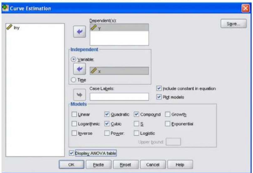
| x | y | | ---- | ------ | | 1.0 | 2.2500 | | 1.5 | 3.4500 | | 2.0 | 4.6000 | | 2.5 | 5.8000 | | 3.0 | 7.0000 |Choosing a Model using Curve Estimation. To find an appropriate model for a given data set, such as the one in the previous section, choose Analyze>Regression>Curve Estimation.... In the Curve Estimation window that opens, enter y under Dependent(s), x under Independent with Variable selected, and make sure Include constant in equation, Plot models, and Display ANOVA table are all checked. Under Models, for this example check Quadratic, Cubic, and Compound.
The following table from the help menu describes the various models.
Linear. Model whose equation is Y = b0 + (b1 * t) . The series values are modeled as a linear function of time.
Logarithmic. Model whose equation is Y = b0 + (b1 * (t)) .
Inverse. Model whose equation is Y = b0 + (b1 / t).
Quadratic. Model whose equation is Y = b0 + (b1 * t) + (b2 * t^**2) . The quadratic model can be used to model a series that "takes off" or a series that dampens.
Cubic. Model that is defined by the equation Y = b0 + (b1 * t) + (b2 * t2) + (b3 * t3) .
Power. Model whose equation is Y = b0 * (t**b1) or ln(Y) = ln(b0) + (b1 * ln(t)).
Compound. Model whose equation is Y = b0 * (b1**t) or ln(Y) = ln(b0) + (ln(b1) * t).
S-curve. Model whose equation is Y = e^**(b0 + (b1/t)) or (Y) = b0 + (b1/t) .
Logistic. Model whose equation is Y = 1 / (1/u + (b0 * (b1**t))) or (1/y - 1/u) = (b0) + ((b1) * t) where u is the upper boundary value. After selecting Logistic, specify the upper boundary value to use in the regression equation. The value must be a positive number that is greater than the largest dependent variable value.
Growth. Model whose equation is Y = e^**(b0 + (b1 * t)) or (Y) = b0 + (b1 * t) .
Exponential. Model whose equation is Y = b0 * (e**(b1 * t)) or ln(Y) = ln(b0) + (b1 * t).
Finally, click OK. We show below the output for the Quadratic model. The regression equation is =336.790-693.691x+295.521x^2 . The other data, although arranged differently, is similar to that for linear and multiple regression. We do note that the Standard Error is 111.856.
Quadratic
Model Summary
| R | R Square | Adjusted R Square | Std. Error of the Estimate |
| .975 | .950 | .916 | 111.856 |
The independent variable is x.
ANOVA
| Sum of Squares | df | Mean Square | F | Sig. | |
| Regression | 711415.561 | 2 | 355707.781 | 28.430 | .011 |
| Residual | 37535.314 | 3 | 12511.771 | ||
| Total | 748950.875 | 5 |
The independent variable is x.
Coefficients
| Unstandardized Coefficients | Standardized Coefficients | t | Sig. | ||
| B | Std. Error | Beta | |||
| x | -693.691 | 261.814 | -1.677 | -2.650 | .077 |
| x** 2 | 295.521 | 73.227 | 2.554 | 4.036 | .027 |
| (Constant) | 336.790 | 200.094 | 1.683 | .191 | |
Although they are not shown here, the regression equation for the Cubic model is = -248.667 + 779.244x - 680.240x^2 +185.859x^3 with a Standard Error of 35.776 and the regression equation for the Compound model is = .999(10.005)^x with a Standard Error of .016. The results of the Compound equation are seen to be similar to those of the previous section, as expected. From a comparison of standard errors, it appears that Compound is the best model of the three examined. We are also given a plot with the observed points along with the graphs of the models selected. We again see that Compound provides the best model of the three considered.

line
| x | Observed | Quadratic | Cubic | Compound | | ---- | -------- | --------- | ----- | -------- | | 0.5 | 0 | 0 | 0 | 0 | | 1.0 | 0 | 0 | 0 | 0 | | 1.5 | 0 | 0 | 0 | 0 | | 2.0 | 100 | 100 | 100 | 100 | | 2.5 | 400 | 400 | 400 | 400 | | 3.0 | 1000 | 1000 | 1000 | 1000 |Chi-Square Test of Independence
For data, we will use a survey of a sample of 300 adults in a certain metropolitan area where they indicated which of three policies they favored with respect to smoking in public places.
| Highest education level | Policy Favored | Total | |||
| No restrictions on smoking | Smoking allowed in designated areas only | No smoking at all | No opinion | ||
| College graduate | 5 | 44 | 23 | 3 | 75 |
| High school graduate | 15 | 100 | 30 | 5 | 150 |
| Grade school graduate | 15 | 40 | 10 | 10 | 75 |
| Total | 35 | 184 | 63 | 18 | 300 |
We wish to test if there is a relationship between education level and attitude toward smoking in public places. We test the hypotheses
H_0 : Education level and policy favored are independent H_a : The two variables are not independent
Ignoring the Total row and column, we enter the data from the table into the first column of the Data View, reading across the rows from left to right. In the second column we list the row the data came from, and in the third column the column the data came from. This is seen to the right.
In the Variable View below, across from “educ,” enter “Education” for “Label,” and for “Values” enter 1 = “College,” 2 = “High School,” and 3 = “Grade School.” Across from “policy,” enter Policy for “Label,” and for “Values” enter 1 = “No restrictions,” 2 = “Designated areas,” 3 = “No smoking,” and 4 = “No opinion.”
| count | educ | policy | |
| 1 | 5 | 1 | 1 |
| 2 | 44 | 1 | 2 |
| 3 | 23 | 1 | 3 |
| 4 | 3 | 1 | 4 |
| 5 | 15 | 2 | 1 |
| 6 | 100 | 2 | 2 |
| 7 | 30 | 2 | 3 |
| 8 | 5 | 2 | 4 |
| 9 | 15 | 3 | 1 |
| 10 | 40 | 3 | 2 |
| 11 | 10 | 3 | 3 |
| 12 | 10 | 3 | 4 |
| Name | Type | Width | Decimals | Label | Values | |
| 1 | count | Numeric | 8 | 0 | None | |
| 2 | educ | Numeric | 8 | 0 | Education | {1, College}... |
| 3 | policy | Numeric | 8 | 0 | Policy | {1, No restri... |
This is not very well documented, but the first thing we need to do for ^2 is to tell SPSS which column contains the frequency counts. Choose Data>Weight Cases... from the menu, and in the window that opens,
![Weight Cases Education [educ] Policy [policy] Do not weight cases Weight cases by Frequency Variable: count Current Status: Weight cases by count OK Paste Reset Cancel Help](/content/2026/05/944397/images/24ad1d4b61eea9f1e211275dab8a7b4c0dab313800b2e311b896db21902fb907.jpg)
choose Weight cases by and move the variable count under Frequency Variable. Then click OK. Now choose Analyze>Descriptive Statistics>Crosstabs... from the menu.
![Crosstabs count Row(s): Education [educ] Column(s): Policy [policy] Layer 1 of 1 Previous Next Display clustered bar charts Suppress tables OK Paste Reset Cancel Help Statistics... Cells... Format...](/content/2026/05/944397/images/922765f3d7d53d59590e6f5caa484cf201066d5db53991d2a5a38c9b67b978b6.jpg)
In the window that opens, move Education[educ] under Row(s) and Policy[policy] under Column(s). Next click Statistics..., and in the window that opens, check only Chi-square, and then click Continue. Next click Cells....
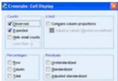
Check Observed and Expected under Counts, followed by Continue and OK.
Education * Policy Crosstabulation
| Policy | |||||||
| No restrictions | Designated areas | No smoking | No opinion | Total | |||
| Education | College | Count | 5 | 44 | 23 | 3 | 75 |
| Expected Count | 8.8 | 46.0 | 15.8 | 4.5 | 75.0 | ||
| High School | Count | 15 | 100 | 30 | 5 | 150 | |
| Expected Count | 17.5 | 92.0 | 31.5 | 9.0 | 150.0 | ||
| Grade School | Count | 15 | 40 | 10 | 10 | 75 | |
| Expected Count | 8.8 | 46.0 | 15.8 | 4.5 | 75.0 | ||
| Total | Count | 35 | 184 | 63 | 18 | 300 | |
| Expected Count | 35.0 | 184.0 | 63.0 | 18.0 | 300.0 | ||
The first table of output simply provides a table of the Counts and the Expected Counts if the variables are independent.
Chi-Square Tests
| Value | df | Asymp. Sig.(2-sided) | |
| Pearson Chi-Square | 22.502^a | 6 | .001 |
| Likelihood Ratio | 20.598 | 6 | .002 |
| Linear-by-Linear Association | 1.033 | 1 | .310 |
| N of Valid Cases | 300 |
a. 2 cells (16.7%) have expected count less than 5. The minimum expected count is 4.50.
From the second table, the Pearson Chi-Square statistic is 22.502 with a p-value (Asymp. Sig. (2-sided)) of .001. Thus, for instance, we would reject the null hypothesis at the =.01 level of significance. Notice the note that 16.7% of the cells have expected counts less than 5 and the minimum expected count is 4.5. Typically, we need no more than 20% of the expected counts less than 5 with a minimum expected count of at least 1.
Nonparametric Tests
The Wilcoxon Matched-Pairs Signed-Rank Test. For data, we use cardiac output (liters/minute) of 15 postcardiac surgical patients. The data is as follows:
4.91 4.10 6.74 7.27 7.42 7.50 6.56 4.64
5.98 3.14 3.23 5.80 6.17 5.39 5.77
We want to test the hypotheses
H_0 : = 5.05
H_a:5.05
We enter the data by putting the numbers above in the first column, labeled output. Because we are using a matched-pairs test, we create the matched pairs by entering the test value 5.05 fifteen times in the second column, labeled constant. The Data View looks as at the top of the next page.
| output | constant | |
| 1 | 4.91 | 5.05 |
| 2 | 5.98 | 5.05 |
| 3 | 4.10 | 5.05 |
| 4 | 3.14 | 5.05 |
| 5 | 6.74 | 5.05 |
| 6 | 3.23 | 5.05 |
From the menu, choose Analyze>Nonparametric Tests>Legacy Dialogs>2 Related Samples....
![Two Related Samples Tests Output constant Test Pairs: Pair Variable1 Variable2 1 [OUTPUT] [CONSTANT] 2 Test Type ✓ Wliccawon □ Sign □ McNemar ■ Marginal Homogeneity OK Paste Reset Cancel Help Options](/content/2026/05/944397/images/d8f8050f64527edc82708815b86a4eec84d0f6debf0c3dfbef2f567d21f4cc50.jpg)
In the window that opens, first click output followed by the arrow to make it Variable 1 for Pair 1, then constant followed by the arrow to make it Variable 2. Make sure Wilcoxon is checked. If you want descriptive statistics and/or quartiles, you can choose those under Options.... Then click OK to get the output.
Wilcoxon Signed Ranks Test
Ranks
| N | Mean Rank | Sum of Ranks | ||
| constant - output | Negative Ranks | 10^a | 8.60 | 86.00 |
| Positive Ranks | 5^b | 6.80 | 34.00 | |
| Ties | 0^c | |||
| Total | 15 | |||
a. constant < output
b. constant > output
c. constant = output
The first table of output gives the number of the 15 comparisons that are Negative (rank of constant
Test Statistics ^b
| constant-output | |
| Z | -1.477a |
| Asymp. Sig. (2-tailed) | .140 |
a. Based on positive ranks.
The Z in the second table is the standardized normal approximation to the test statistic, and the Asymp. Sig (2-tailed) of .140, which we will use as our p-value, is estimated from the normal approximation. Because of the size of this p-value, we will not reject the null hypothesis at any of the usual levels of significance.
The Mann-Whitney Rank-Sum Test. For data, we will look at hemoglobin determination (grams) for 25 laboratory animals, 15 of whom have been exposed to prolonged inhalation of cadmium oxide.
Exposed 14.4, 14.2, 13.8, 16.5, 14.1, 16.6, 15.9, 15.6, 14.1, 15.2, 15.7, 16.7, 13.7, 15.3, 14.0
Unexposed 17.4, 16.2, 17.1, 17.5, 15.0, 16.0, 16.9, 15.0, 16.3, 16.8,
We want to test the hypotheses
$$ \begin{array}{l} \mathrm{H} _ {0}: \mu_ {\text { exposed }} = \mu_ {\text { unexposed }} \ \mathrm{H} _ {\mathrm{a}}: \mu_ {\text { exposed }} > \mu_ {\text { unexposed }} \end{array} $$
As for the t test earlier, we enter the 25 hemoglobin readings in column one of the Data View and label the column hemoglobin. In the second column, labeled status, we use 1="Exposed" and 2="Unexposed", which are also listed under Values for status in the Variable View.
To do the test, choose Analyze>Nonparametric Tests>Legacy Dialogs>Two Independent Samples... from the menu.
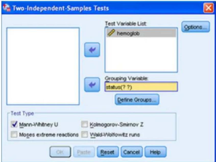
In the window that opens, first check Mann-Whitney U under Test Type, then move the variable hemoglobin to the Test Variable List box and the variable status to the Grouping Variable box. Then click Define Groups....
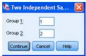
Put 1 in the box for Group 1 and 2 in the box for Group 2. Then click Continue. You may click Options... if you want the output to include descriptive statistics and/or quartiles. Finally, click OK to get the output.
Mann-Whitney Test
Ranks
| status | N | Mean Rank | Sum of Ranks | |
| hemoglobin | Exposed | 15 | 9.67 | 145.00 |
| Unexposed | 10 | 18.00 | 180.00 | |
| Total | 25 | |||
We see from the first table, after ranking the hemoglobin values from least to greatest, the Mean Rank and Sum of Ranks for each status category.
Test Statistics ^b
| hemoglobin | |
| Mann-Whitney U | 25.000 |
| Wilcoxon W | 145.000 |
| Z | -2.775 |
| Asymp. Sig. (2-tailed) | .006 |
| Exact Sig. [2+(1-tailed Sig.)] | .004 ^a |
a. Not corrected for ties.
b. Grouping Variable: status
The Mann-Whitney U, calculated by counting the number of times a value from the smaller group (here Unexposed) is less than a value from the larger group (here Exposed), is 25.000. This is equivalent to the Wilcoxon W, which is the Sum of Ranks of the smaller group. The Z in the second table is again the standardized normal approximation to the test statistic, and the Asymp. Sig (2-tailed) of .006 is estimated from the normal approximation. Because we are using a 1-tailed test, we will take one-half of this number, .003 as our p-value, causing us to reject the null hypothesis at all of the usual levels of significance.
Control Charts
Control Charts for the Mean. To illustrate control charts for the mean, we use the following sample yield data in grams/liter which have been obtained for each of five successive days, with all samples of size 7. Let us also assume that the process has a specified mean _0=50 and specified standard deviation _0=1 .
| Day 1: 49.5 | 49.9 | 50.5 | 50.2 | 50.5 | 49.8 | 51.1 |
| Day 2: 48.5 | 52.3 | 48.2 | 51.2 | 50.1 | 49.3 | 50.0 |
| Day 3: 50.5 | 51.7 | 49.5 | 51.2 | 48.3 | 50.2 | 50.4 |
| Day 4: 49.8 | 49.7 | 50.2 | 50.6 | 50.3 | 49.4 | 49.3 |
| Day 5: 50.5 | 50.9 | 49.5 | 50.2 | 49.8 | 49.8 | 50.3 |
In entering the data in the Data Editor, put the 35 sample values in the first column, labeled g_per_l, with 1 decimal place, and put the day number in the second column, labeled day, with no decimal places. A portion of this Data Editor window is shown at the top of the next page.
| g_per_l | day | |
| 1 | 49.5 | 1 |
| 2 | 49.9 | 1 |
| 3 | 50.5 | 1 |
| 4 | 50.2 | 1 |
| 5 | 50.5 | 1 |
| 6 | 49.8 | 1 |
| 7 | 51.1 | 1 |
| 8 | 48.5 | 2 |
| 9 | 52.3 | 2 |
To create the control chart(s), click Analyze>Quality Control>Control Charts... from the menu bar, and in the window that opens, select X-Bar, R, s under Variable Charts and make sure Cases are units is checked under Data Organization.

Then click Define, and in the new window that opens, move g_per_l under Process Measurement and day under Subgroups Defined by. Under Charts, we will select X-Bar using standard deviation and check the box for Display s chart.

Click Options, and enter 2 for Number of Sigmas. After clicking Continue, since we have specifications for the mean, we click Statistics..., and in the window that opens, based on our specified mean and standard deviation, enter 50.756 for Upper and 49.244, Lower for Specification Limits, and 50 for Target. Then select Estimate using S-Bar under Capability Sigma. Finally, click Continue followed by OK to get the control charts.
The first control chart given as output is the chart for the mean. This chart, which is pretty much self-explanatory, clearly shows the daily means along with the unspecified (UCL and LCL) and specified (USpec and LSpec) control limits. It is clear that the process is always in control.

line
| Sigma level | g_per_I | UCL | U Spec | Average | L Spec | LCL | | ----------- | ------- | ------ | ------ | ------- | ------ | ------ | | 1 | 50.2 | 50.733 | 50.756 | 50.091 | 49.244 | 49.450 | | 2 | 49.95 | | | | | | | 3 | 50.25 | | | | | | | 4 | 49.9 | | | | | | | 5 | 50.15 | | | | | |The second control chart is for the standard deviation, and it is clear that, as far as standard deviation is concerned, the process is out of control on Day 2.

line
| Sigma level | Standard Deviation | | ----------- | ------------------ | | 1 | 0.55 | | 2 | 1.45 | | 3 | 1.10 | | 4 | 0.48 | | 5 | 0.48 |In the event X-Bar using range had been chosen, the second chart would be a range chart.
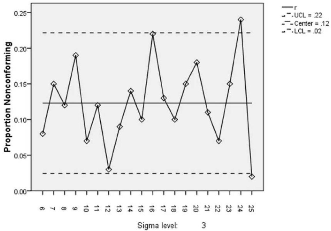
Control Charts for the Proportion. To illustrate control charts for the proportion, we use the number of defectives in samples of size 100 from a production process for twenty days in August.
August: 6 7 8 9 10 11 12 13 14 15
Defectives: 8 15 12 19 7 12 3 9 14 10
August: 16 17 18 19 20 21 22 23 24 25
Defectives: 22 13 10 15 18 11 7 15 24 2
In entering the data in the Data Editor, put the 20 numbers of defectives (from each sample of size 100) in the first column, labeled r, and put the corresponding date in August in the second column, labeled August, both with no decimal places, as shown below.
| r | august | |
| 1 | 8 | 6 |
| 2 | 15 | 7 |
| 3 | 12 | 8 |
| 4 | 19 | 9 |
| 5 | 7 | 10 |
To create the control chart, click Analyze>Quality Control>Control Charts... from the menu bar, and in the window that opens, select p, np under Attribute Charts and make sure Cases are subgroups is checked under Data Organization.

Then click Define, and in the new window that opens, move r under Number Nonconforming, move August under Subgroups Labeled by, select Constant for Sample Size, and enter 100 in the following box. Under Chart, we will select p (Proportion nonconforming).
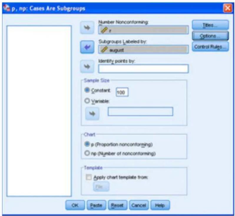
Now click Options, and enter 3 for Number of Sigmas. Then click Continue followed by OK to get the control chart, which is again pretty much self-explanatory. We see that the process is out of control on August 24 and 25, although it is hard to call too few defectives out of control.
Control Chart: r
line
| Sigma level | Proportion Nonconforming | | ----------- | ------------------------ | | 6 | 0.08 | | 7 | 0.15 | | 8 | 0.12 | | 9 | 0.19 | | 10 | 0.07 | | 11 | 0.12 | | 12 | 0.03 | | 13 | 0.09 | | 14 | 0.14 | | 15 | 0.10 | | 16 | 0.22 | | 17 | 0.13 | | 18 | 0.10 | | 19 | 0.15 | | 20 | 0.18 | | 21 | 0.11 | | 22 | 0.07 | | 23 | 0.15 | | 24 | 0.24 | | 25 | 0.02 |- Descriptive Statistics
- Probability Distributions
- Confidence Intervals and Hypothesis Testing Using t
- non-smokers
- smokers
- One-Way ANOVA
- Descriptives
- Test of Homogeneity of Variances
- ANOVA
- Multiple Comparisons
- Simple Linear Regression and Correlation
- Multiple Regression
- Nonlinear Regression
- Quadratic
- Chi-Square Test of Independence
- Nonparametric Tests
- Wilcoxon Signed Ranks Test
- Mann-Whitney Test
- Control Charts
Brand : IBM
Model : SPSS 19
Category : Desktop software