Display 2.3 - Uncategorized Martin Audio - Free user manual and instructions
Find the device manual for free Display 2.3 Martin Audio in PDF.


User questions about Display 2.3 Martin Audio
0 question about this device. Answer the ones you know or ask your own.
Ask a new question about this device
Download the instructions for your Uncategorized in PDF format for free! Find your manual Display 2.3 - Martin Audio and take your electronic device back in hand. On this page are published all the documents necessary for the use of your device. Display 2.3 by Martin Audio.
USER MANUAL Display 2.3 Martin Audio
natural_image
Partial view of a curved white line on black background, resembling a crescent or arc (no text or symbols)DISPLAY™
2.3
A guide to Martin Audio's DISPLAY
System Optimisation Software for
MLA and Wavefront Precision systems.
Contents
Version History 4
Installation....4
System requirements ....4
Introduction....5
Latest Version....5
Numerical Optimisation 6
Index Plots....7
Opening the Program 18
User Interface Mode 18
Quick start 19
Application menu 26
Preferences 28
Add an Array....30
Slice Tab....39
Slice Setup 39
Draw a Shell 40
Edit the shell 41
Using Survey 42
Position the Array....44
Add the Audience Region 45
Editing the Audience Region ....45
Express Tab....47
Set Box Resolution....48
Optimise All 49
Coverage Tab 58
Saving Files 58
Help 59
Audience Offsets 59
Changing Line Properties....61
Target Profile Selection 62
Target Refinement....65
Splay Angle Tab....66
Splay Angles....66
Array Diagram 67
Coverage / Current Best Optimised Output 68
Current Acoustic Output 69
Calculation....69
Optimisation....70
Rig Tab 73
MLA 73
MLA Compact 79
MLA Mini 82
Wavefront Precision 91
O-Line 98
EQ Tab 101
Basic View....101
Expert Mode....107
SPL Tab....112
Individual Graph Windows 114
Adding additional arrays....117
Deleting an array 118
Exporting the Optimisation 119
Exporting D2P Files....119
Exporting to DXF 120
Printable Reports....122
Export 3D Data ....125
Version History
Manual Version 1.5- WPS Added
Display Version: 2.3.3. b11
Installation
MLA and MLA Compact touring system owners will have a Tablet PC as part of their system package which will be pre-loaded with all necessary software including the latest version of Vu-Net. For owners of Multicellular or Wavefront Precision systems or anyone else requiring the software, Display 2.3 can be downloaded from the Martin Audio website.
Note that Display 2.3.3 is a 64-bit application and it will not run on a 32-bit PC
It is essential that the PC has an internet connection when running the installation as the latest version of MatLab components will automatically be downloaded as part of the installation.
System requirements
Display2.3 requires a Windows PC running either Windows 7, Windows 8 or Windows 10; no other operating systems are supported. We would recommend a 64-bit i7 processor running at 2.6GHz minimum with a minimum of 8GB of RAM. File sizes are not particularly huge so a high-capacity Hard Drive is not necessary but an SSD drive will be faster and more reliable. The mathematical calculations involved in creating optimisations use an application called MatLab Components and when running this uses a great deal of computational power so it is best not to scrimp on CPU power and speed when specifying a PC to run the application.
Users have reported that Display2.3 works perfectly well on an Apple Mac using Bootcamp or under a virtual platform such as VM Ware Fusion or Parallels, (these options still require a copy of Windows 7, 8 or 10 to be installed) however this is not supported by Martin Audio.
Introduction
Display 2.3 is the application that is used in conjunction with Vu-Net and a Martin Audio Multicellular System, either MLA, MLA Compact, MLA Mini, Wavefront Precision; WPL, WPC and WPM, O-Line or a combination of any of these systems to generate the inter-cabinet angles and the DSP optimisation parameters which can then be quickly and easily uploaded to the hardware over the U-Net system network or in the case of MLA Mini directly using a USB connection. It also shows accurate analysis of the system response in the venue.
The application has an entirely straightforward, logical workflow; in fact it does not allow jumping to advance stages of the design, it is necessary to complete each stage in a logical order.
Display 2.3 uses numerical optimisation to arrive at the resulting cabinet angles and DSP coefficients. Taking the cabinet angles as an example, to explain the process in slightly crude manner this means that it tries a great many combinations of possible angles, checks the result using the computer model of the array response and compares it to the desired response. It continues to check through a huge number of possible combinations until it arrives at the closest match to what has been asked of it. In the case of the cabinet angles, it has the facility to “polish” the array which means it does a second pass having arrived at a set of angles to fine tune the array angles. This process although highly complex, actually only takes a few minutes, certainly no longer than a conventional line-array prediction application.
Having specified the cabinet angles the array can be rigged and whilst that is being done the second stage of the optimisation process is done. This also uses numerical optimisation, but this time addresses the EQ, FIR, gain and phase parameters available in the DSP, going through the hundreds of thousands of possible combinations possible until the output is as close as possible to the desired response. With a large array and complex venue this could take up to ten minutes to complete however this will be far quicker than the time it takes to rig all arrays so in no way slows down the show build-up. To actually try every possible combination of DSP would take months even on the most powerful computer- there are millions of possible combinations and that is where the unique digital algorithm comes into play, examining batches of results to see if certain parameter changes are taking you closer or further from your desired performance characteristics. It will reject a series of parameter changes that are heading towards a "dead end" and instead will focus on those which get you closer to the desired result, gradually honing all parameters until it reaches a result which is a close as possible to the specifications that the technician has requested. This method allows phenomenal accuracy in a highly realistic and practical length of time. The accuracy of the resulting design hinges on the computer model which predicts how the array will perform for a given set of cabinet angles and DSP coefficients. The computer model devised for Display 2.3 is one of the most sophisticated and accurate ever devised for an audio system and is capable of achieving results to closer than +/-1dB of actual measured parameters.
A Display design can easily be done prior to arriving at the venue in the comfort of your office. If you have drawings of the space and details of the flying position and the trim height of the arrays you can complete the rigging and DSP design which makes set-up on site extremely quick and efficient. It is possible to try several different DSP optimisations with priority given to a variety of performance characteristics. These can be uploaded to the array and stored in snapshots to be recalled in a few seconds.
Latest Version
Version 2.3.3 incorporates the entire family of Wavefront Precision products and O-Line and has an enhanced layout to maximise the graphical content. New help functions are also available for anyone with limited experience of using the application.
From version 2.2 onwards there is greater interaction with Vu-Net v2.0 so it is important to use that version or later to get the best performance from one of our multicellular systems. It is perfectly ok to use older versions of Display2 with Vu-Net v2.0, or optimisations created in Display 2.3 with Vu-Net v1.2.5, there is complete cross compatibility, but the best results will definitely be obtained using the latest versions of both applications.
One particular step forward is a lowering of the frequencies at which the optimisation is effective. This is always difficult as part of the optimisation process involves attempting to contain the audio distribution within areas you have specified which is very difficult to do with lower frequencies as they become less directional the lower the frequency. The Martin Audio R&D team have however continued to research methods to extend the low frequency control and we learnt a great deal developing the MLA Mini system which has always had LF included in the optimisation. Version 2.3 now optimises lower frequencies using FIR filtering but without increasing latency which is a remarkable achievement. Note that your multicellular system MUST be running the latest firmware for the optimisations to be effective at low frequencies. MLA and MLA Compact must be running 2.3.57 and 2.12.44 respectively. These were released in 2015 so all system should be running them as a matter of course.
Note that if opening .mat files created in Display version prior to version 2.3, the low frequency optimisation will not be used. If you wish to re-optimise older projects, the best option is to import the venue shell and then add the array manually to create a new project with all the latest benefits.
Numerical Optimisation
At this point it is worth taking a moment to explain in detail one of the concepts behind how Display operates; Numerical Optimisation is an easily misunderstood concept, a few people make the incorrect assumption that it is some sort of “averaging” system meaning that the result is a compromise which couldn’t be further from the truth.
What made multicellular systems possible was the development of a phenomenally accurate computer model of the system which works hand in hand with the precision acoustic design of the cabinets. There are a colossal number of factors that affect an array performance; the performance of individual drivers, the horn design, the angle between enclosures, the number of enclosures et cetera. Martin Audio have taken the analysis of array performance to the most advanced level ever attempted, including boundary effect modelling which includes the effect that all other cabinets in an array have on a single driver; essentially each individual cabinet has a baffle extending above and below it formed by the other enclosures in the array. For cabinets in the middle of the array this is fairly symmetrical but for cabinets towards the top and bottom it becomes more and more asymmetrical which has a highly significant effect on the individual module performance and therefore the overall array performance.
The diagrams below show the response of a single array element which is the second box down in a six-box array. The first picture ignores the effect of its neighbouring enclosures. The second picture shows the dramatic effect that the enclosure above and the four below have on the response. Ignoring this effect will clearly compromise the ability to accurately predict how the array will perform, in fact measurements show that ignoring the boundary effect can result in inaccuracies of up to 8dB which fairly obviously would make the system unusable.
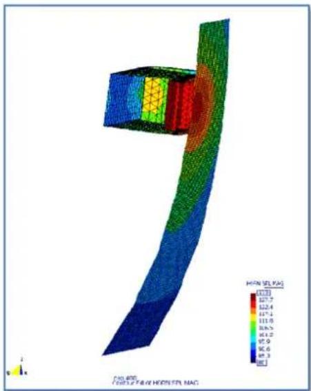
heatmap
| HOMIN SEL PAG | Value | | ------------- | ----- | | 1.0 | 127.7 | | 2.0 | 122.4 | | 3.0 | 117.4 | | 4.0 | 111.6 | | 5.0 | 98.6 | | 6.0 | 91.2 | | 7.0 | 87.9 | | 8.0 | 85.6 | | 9.0 | 81.3 | | 10.0 | 78.1 |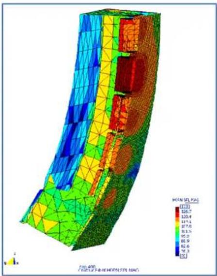
heatmap
| MHN SEL RAG | Value | |-------------|-------| | 13.7 | 126.7 | | 12.4 | 120.4 | | 11.1 | 115.1 | | 9.8 | 117.9 | | 8.5 | 11.5 | | 7.2 | 9.2 | | 6.0 | 8.9 | | 4.7 | 8.2 | | 3.3 | 8.6 | | 2.0 | 9.3 |Martin Audio have perfected the computer model for our Multicellular systems to such a degree that the predicted performance can reach accuracy of as close as 1dB of measured results which has made the whole system not only possible but extremely accurate.
Numerical optimisation uses the computer model to check the performance for a given mechanical orientation or DSP configuration, and compares the result on the venue slice to what you have asked the system to achieve. It will then try an alternative option to see if it is getting closer or further from the desired result. If it is further from what you want it to achieve it will ignore that configuration and pursue the more successful angles or EQ curves, trying configuration after configuration before it has attempted close to every possible combination and has got as close as possible to the desired result.
If you consider the first optimisation which calculates the splay angles, for an MLA system there are eight possible angles available between each cabinet; 0.5, 1, 2, 3, 4, 5, 6 and 7.5^ If you have a reasonable size array of say 16 enclosures that means a total of 8 × 8 × 8 × × 8 , (fifteen 8's! ) or 35,184,372,088,832 possible combinations of angles between all cabinets. Clearly analysing each of these combinations involves a substantial amount of processing but pales into insignificance compared to the hundreds of
thousands of calculations required when running numerical optimisation for the DSP; every band of EQ frequency, bandwidth and gain, phase and FIR filters for every one of the cells of every cabinet. This is why a powerful PC is required and the EQ optimisation can take up to fifteen minutes or so for a large array in a complex arena. Even the most powerful PC available today couldn't try every possible combination in a reasonable time scale so complex algorithms are used so that when a certain sequence of filter parameters are consistently demonstrating results further from the goals that have been set, the system will abandon those avenues and try others. With this system highly accurate parameters can be produced that are as close as possible to the desired goals in a reasonable time frame. This is a very basic explanation, in fact it is Martin Audio's development of the revolutionary but phenomenally complex digital algorithm that the application uses to refine the optimisation which give the best possible results in a reasonable time frame. Not only that but key parts of the optimisation process are multithreaded which means that the system is able to exploit the latest 64-bit, quad core processors to speed up the entire process.
Whilst this system is processor hungry clearly it is a very realistic and practical method to obtain the best possible results from an array where so many variables are at your disposal. Trying to manually adjust several thousand DSP parameters is obviously not going to be realistic however good a system technician believes his ears might be.
Index Plots
The other concept which Martin Audio developed as part of the MLA system is the index plot. We needed a method to display the results of the system optimisation that was clear and easy to interpret. Because the whole basis of the system is that the radiated signal is coherent where it arrives at all parts of the audience as opposed to when it leaves the array we needed a method of displaying the frequency response at dozens of positions simultaneously. There are a few methods in existence for achieving this, 3D graphs for example but they don't really meet the brief of being quick and easy to interpret. The Index plot solves this problem.
As we will see when we look at the application in more detail, we draw a two dimensional slice of the venue in which we are deploying our array. It then gets presented in Display like so; -
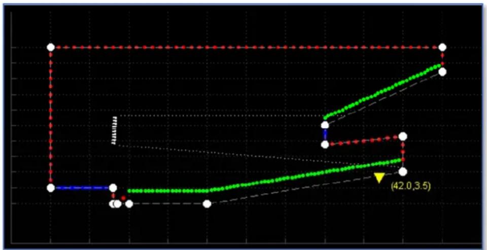
line
| Point | Value | |-------|-------| | Start | 0.0 | | Mid | 0.0 | | End | 3.5 |The colours represent the three types of plane; the audience area are green, non-audience, areas around the venue which we are not concerned about are red, and finally areas where we would like the system to actively steer sound away from known as hard avoid are blue. By default the hard avoid is the stage but this could also be reflective back walls or balcony fronts, or noise sensitive areas beyond an arena at an outdoor event. The planes are represented by a series of dots. These are spaced closer together in the audience region where we need the most detail. Ideally we would like to be able to view the frequency response at each of these dots so each becomes a sort of virtual measurement mic.
The normal way to present a graph of frequency response is of course for the horizontal 'x' axis to be frequency, usually from 20Hz to 20KHz, and for the vertical 'y' axis to display magnitude, usually in dB. If however we display magnitude with colours we can easily show many response plots simultaneously. If we make red the highest magnitude- the loudest- and blue the quietest, by running through the colours in the spectrum we can very easily identify the peaks and troughs in a response. This frees up the vertical axis which we can use for all of our "virtual mics"; -
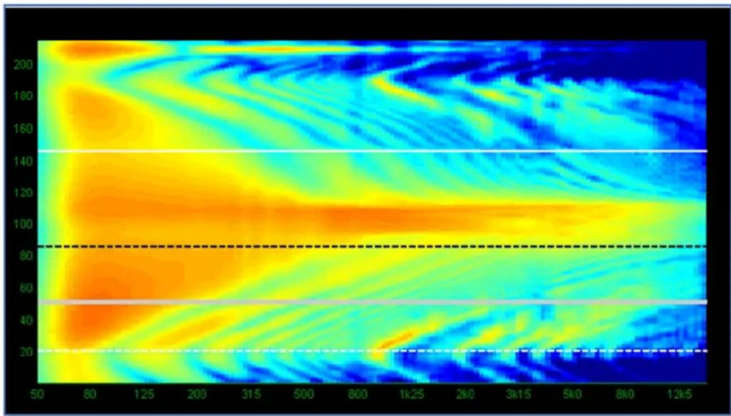
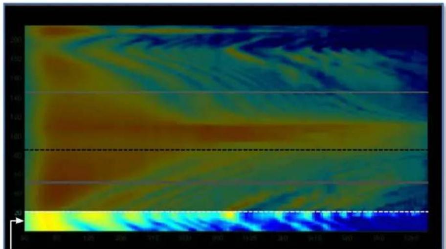
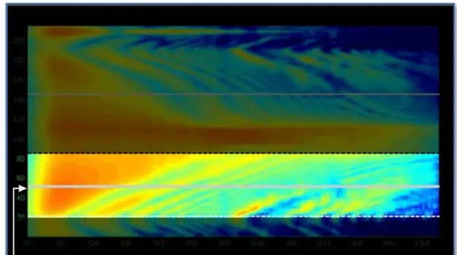
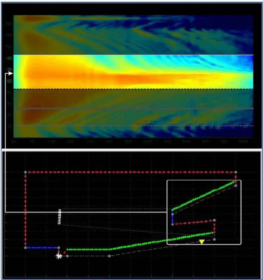
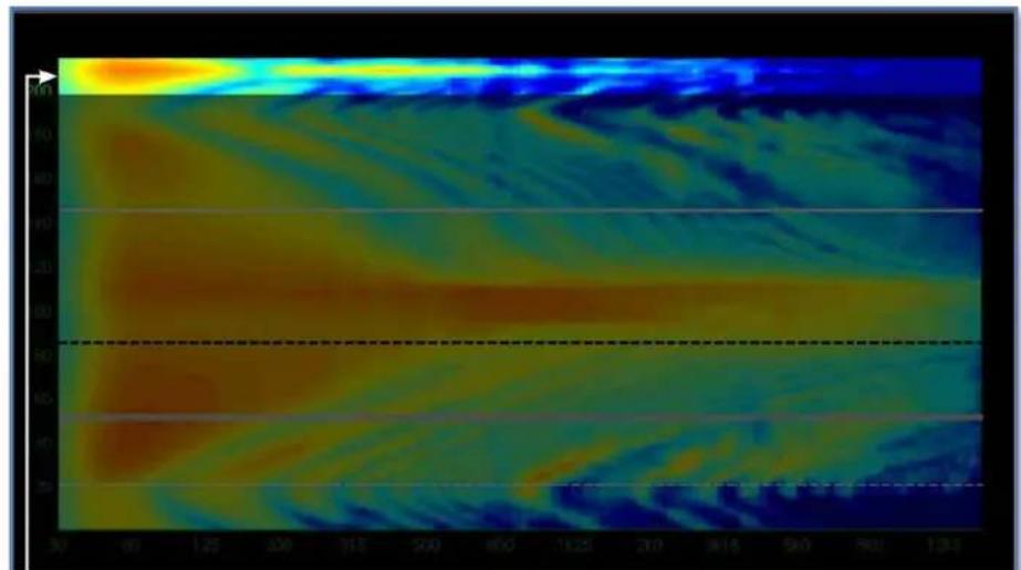
This is the Index plot of a completely un-optimised system. The horizontal axis as mentioned is frequency. As we cannot optimise very low frequencies the graph starts at 50Hz going all the way up to 20kHz. The vertical axis is now the 2D slice of the venue "unravelled". At the bottom is the starting point for our 2D slice at the back of the stage then move vertically upward and at point 20 we see a dashed white line which represents the audience start point that we identify on our venue slice. We continue upwards moving back through the audience, the thick grey line is where we have placed our cursor which gives us the facility to obtain a standard frequency response graph. Continuing up the axis going further back in the venue we find a dashed black line which is a reference point which we also determine. The solid white line is where the audience coverage finishes. Just above this is the back wall and then up to the number 200 is the venue ceiling and the last section of the graph is the back of the venue behind the array; -
heatmap
| Time | Value | |------|-------| | 94 | 0 | | 95 | 10 | | 125 | 20 | | 200 | 30 | | 315 | 40 | | 400 | 50 | | 600 | 60 | | 915 | 70 | | 1125 | 80 | | 200 | 90 | | 315 | 100 | | 407 | 110 | | 600 | 120 | | 915 | 130 | | 1295 | 140 | | 1295 | 150 | | 1295 | 160 | | 1295 | 170 | | 1295 | 180 | | 1295 | 190 | | 1295 | 200 |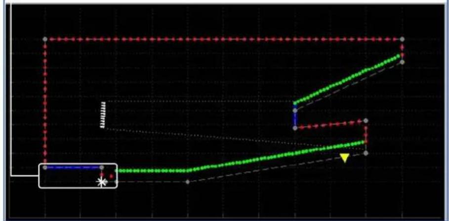
flowchart
graph TD
    A["Start"] --> B["Red Path"]
    B --> C["Green Path"]
    C --> D["Blue Path"]
    D --> E["Yellow Arrow"]
    style A fill:#f9f,stroke:#333
    style B fill:#ccf,stroke:#333
    style C fill:#cfc,stroke:#333
    style D fill:#fcc,stroke:#333
    style E fill:#ffc,stroke:#333
This shows the bottom portion of the index plot corresponds to the stage and "pit" leading up to the start of the audience coverage.
heatmap
| Angle | Value | |-------|-------| | 190° | 26 | | 180° | 40 | | 170° | 60 | | 160° | 80 | | 150° | 100 | | 140° | 120 | | 130° | 140 | | 120° | 160 | | 110° | 180 | | 100° | 200 | | 90° | 180 | | 80° | 160 | | 70° | 140 | | 60° | 120 | | 50° | 100 | | 40° | 80 | | 30° | 60 | | 20° | 40 | | 10° | 20 | | 0° | 10 | | -10° | 5 | | -20° | 3 | | -30° | 2 | | -40° | 1 | | -50° | 0.5 | | -60° | 0.3 | | -70° | 0.2 | | -80° | 0.1 | | -90° | 0.05 | | -100° | 0.03 | | -110° | 0.02 | | -120° | 0.01 | | -130° | 0.005 | | -140° | 0.003 | | -150° | 0.002 | | -160° | 0.001 | | -170° | 0.0005| | -180° | 0.0003| | -190° | 0.0002| | -200° | 0.0001| | -210° | 0.00005| | -220° | 0.00003| | -230° | 0.00002| | -240° | 0.00001| | -250° | 0.000005| | -260° | 0.000003| | -270° | 0.000002| | -280° | 0.000001| | -290° | 0.0000005| | -300° | 0.0000003| | -310° | 0.0000002| | -320° | 0.0000001| | -330° | 0.00000005| | -340° | 0.00000003| | -350° | 0.00000002| | -360° | 0.00000001| | -370° | 0.000000005| | -380° | 0.000000003| | -390° | 0.000000002| | -400° | 0.5 | | -415° | 1 | | -435° | 2 | | -455° | 3 | | -475° | 4 | | -495° | 5 | | -515° | 6 | | -535° | 7 | | -555° | 8 | | -575° | 9 | | -595° | 1 | | -615° | 1 | | -635° | 1 | | -655° | 1 | | -675° | 1 | | -695° | 1 | | -715° | 1 | | -735° | 1 | | -755° | 1 | | -775° | 1 | | -795° | 1 | | -815° | 1 | | -835° | 1 | | -855° | 1 | | -875° | 1 | | -895° | 1 | | -915° | 1 | | -935° | 1 | | -955° | 1 | | -975° | 1 | | -995° | 1 | | -128° | 1 |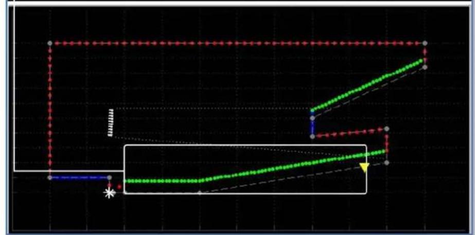
flowchart
graph TD
    A["Start"] --> B["Red Path"]
    B --> C["Green Path"]
    C --> D["Red Path"]
    D --> E["Green Path"]
    E --> F["Red Path"]
    F --> G["Green Path"]
    G --> H["Red Path"]
    H --> I["Green Path"]
    I --> J["Red Path"]
    J --> K["Green Path"]
    K --> L["Red Path"]
    L --> M["Green Path"]
    M --> N["Red Path"]
    N --> O["Green Path"]
    O --> P["Red Path"]
    P --> Q["Green Path"]
    Q --> R["Red Path"]
    R --> S["Green Path"]
    S --> T["Red Path"]
    T --> U["Green Path"]
    U --> V["Red Path"]
    V --> W["Green Path"]
    W --> X["Red Path"]
    X --> Y["Green Path"]
    Y --> Z["Red Path"]
    Z --> AA["Green Path"]
    AA --> AB["Red Path"]
    AB --> AC["Green Path"]
    AC --> AD["Red Path"]
    AD --> AE["Green Path"]
    AE --> AF["Red Path"]
    AF --> AG["Green Path"]
    AG --> AH["Red Path"]
    AH --> AI["Green Path"]
    AI --> AJ["Red Path"]
    AJ --> AK["Green Path"]
    AK --> AL["Red Path"]
    AL --> AM["Green Path"]
    AM --> AN["Red Path"]
This section of the index plot corresponds to the first portion of the audience plane up to the reference point.
text_image
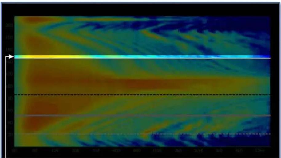
Scientific visualization with top: 3D color gradient and bottom: technical diagram showing trajectory paths, zoomed-in section, and annotated points with annotations.This is the section from the reference point to the back of the audience area. The strong band of red indicated the front of the balcony which is getting a great deal of direct sound prior to optimising the system.
heatmap
| Time | Value | |-------|-------| | 18:00 | -21 | | 18:30 | -19 | | 18:60 | -17 | | 18:90 | -15 | | 19:20 | -13 | | 19:50 | -11 | | 19:80 | -9 | | 20:10 | -7 | | 20:40 | -5 | | 20:70 | -3 | | 21:00 | -1 | | 21:30 | 1 | | 21:60 | 3 | | 21:90 | 5 | | 22:20 | 7 | | 22:50 | 9 | | 22:80 | 11 | | 23:10 | 13 | | 23:40 | 15 | | 23:70 | 17 | | 24:00 | 19 | | 24:30 | 21 | | 24:60 | 23 | | 24:90 | 25 | | 25:20 | 27 | | 25:50 | 29 | | 25:80 | 31 | | 26:10 | 33 | | 26:40 | 35 | | 26:70 | 37 | | 27:00 | 39 | | 27:30 | 41 | | 27:60 | 43 | | 27:90 | 45 | | 28:20 | 47 | | 28:50 | 49 | | 28:80 | 51 | | 29:10 | 53 | | 29:40 | 55 | | 29:70 | 57 | | 30:00 | 59 | | 30:30 | 61 | | 30:60 | 63 | | 30:90 | 65 | | 31:20 | 67 | | 31:50 | 69 | | 31:80 | 71 | | 32:10 | 73 | | 32:40 | 75 | | 32:70 | 77 | | 33:00 | 79 | | 33:30 | 81 | | 33:60 | 83 | | 33:90 | 85 | | 34:20 | 87 | | 34:50 | 89 | | 34:80 | 91 | | 35:10 | 93 | | 35:40 | 95 | | 35:70 | 97 | | 36:00 | 99 | | 36:30 | 101 | | 36:60 | 103 | | 36:90 | 105 | | 37:20 | 107 | | 37:50 | 109 | | 37:80 | 111 | | 38:10 | 113 | | 38:40 | 115 | | 38:70 | 117 | | 39:00 | 119 | | 39:30 | 121 | | 39:60 | 123 | | 39:90 | 125 | | 40:20 | 127 | | 40:50 | 129 | | 40:80 | 131 | | 41:10 | 133 | | 41:40 | 135 | | 41:70 | 137 | | 42:00 | 139 | | 42:30 | 141 | | 42:60 | 143 | | 42:90 | 145 | | 43:20 | 147 | | 43:50 | 149 | | 43:80 | 151 | | 44:10 | 153 | | 44:40 | 155 | | 44:70 | 157 | | 45:00 | 159 | | 45:30 | 161 | | 45:60 | 163 | | 45:90 | 165 | | 46:20 | 167 | | 46:50 | 169 | | 46:80 | 171 | | 47:10 | 173 | | 47:40 | 175 | | 47:70 | 177 | | 48:00 | 179 | | 48:30 | 181 | | 48:60 | 183 | | 48:90 | 185 | | 49:20 | 187 | | 49:50 | 189 | | 49:80 | 191 | | 50:10 | 193 | | ... | ... |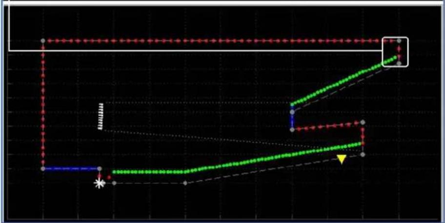
flowchart
graph TD
    A["Start"] --> B["Path 1"]
    B --> C["Path 2"]
    C --> D["End"]
    style A fill:#f9f,stroke:#333
    style B fill:#ccf,stroke:#333
    style C fill:#cfc,stroke:#333
    style D fill:#fcc,stroke:#333
This is the narrow section corresponding to the rear wall.
heatmap
| Time | Value | |-------|-------| | 200 | 200 | | 180 | 180 | | 160 | 160 | | 140 | 140 | | 120 | 120 | | 100 | 100 | | 80 | 80 | | 60 | 60 | | 40 | 40 | | 20 | 20 | | 0 | 0 |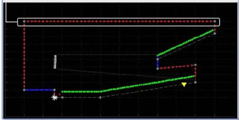
flowchart
graph TD
    A["Start"] --> B["Path 1"]
    B --> C["Path 2"]
    C --> D["End"]
    style A fill:#f9f,stroke:#333
    style B fill:#bbf,stroke:#333
    style C fill:#bfb,stroke:#333
    style D fill:#ffb,stroke:#333
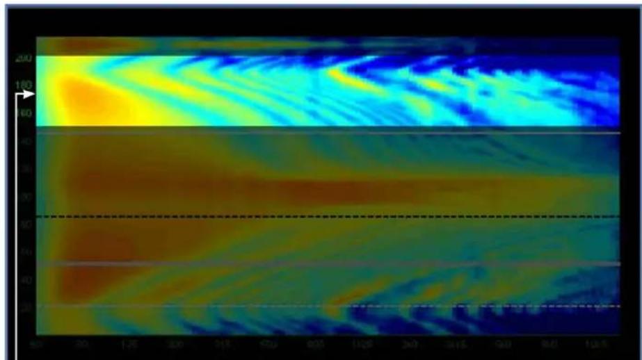
This is the response on the ceiling
heatmap
| X Range | Y Range | Value | |---------|---------|-------| | 30-60 | 30-60 | Low | | 60-120 | 30-60 | Medium| | 120-240 | 30-60 | High | | 240-480 | 30-60 | Medium| | 480-720 | 30-60 | Low | | 720-960 | 30-60 | Medium| | 960-1200| 30-60 | High |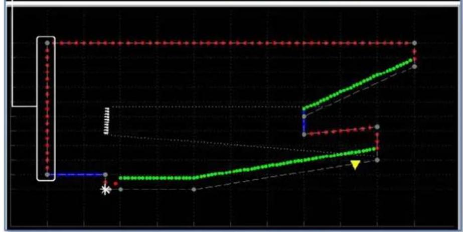
flowchart
graph TD
    A["Start"] --> B["Path 1"]
    B --> C["Path 2"]
    C --> D["End"]
    style A fill:#f9f,stroke:#333
    style B fill:#ccf,stroke:#333
    style C fill:#cfc,stroke:#333
    style D fill:#fcc,stroke:#333
And finally, the rear wall.
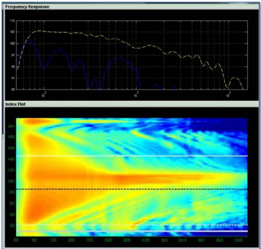
We can also take a look at the actual frequency response on a conventional graph at any specific point on the plot to better understand what we are looking at. Just to re-emphasis, these plots are prior to any system optimisation; they show the response of an array flown with all angles at 0.5^ !
line
| X Value | Frequency Response | Index Plot | |---------|--------------------|----------| | 50 | ~90 | ~20 | | 60 | ~105 | ~40 | | 125 | ~95 | ~60 | | 200 | ~90 | ~80 | | 315 | ~95 | ~100 | | 500 | ~90 | ~120 | | 800 | ~95 | ~140 | | 1k25 | ~90 | ~160 | | 2k0 | ~95 | ~180 | | 3k15 | ~90 | ~20 | | 5k0 | ~95 | ~20 | | 8k0 | ~90 | ~20 | | 12k5 | ~95 | ~20 |The plot at the bottom now has the thick solid white line at the bottom indicating that the curser is over the stage area. The frequency response graph at the top shows two traces. The dashed yellow line is the response at the reference position indicated by the dashed black line on the index plot. The blue response is on stage where our curser position has been placed. It is easy to see from these how the colours respond to the peaks and troughs on the graph. The on-stage response for example has little or no high frequency, it is not even registering anything above around 2.5KHz, on the index plot it is an even band of blue in this region. The response at the reference position is reasonably flat in the low frequencies, gradually tapering off as the frequencies increase. On the index plot we see a block of orange which gradually fades through yellow, green and indigo to blue at the highest frequencies.
We can now look at an optimised system, this is what a perfect system would look like if it wasn't for little inconveniences such as the laws of physics, the impossible dream of perfect coverage at all frequencies for the entire audience with no spill whatsoever anywhere else; -
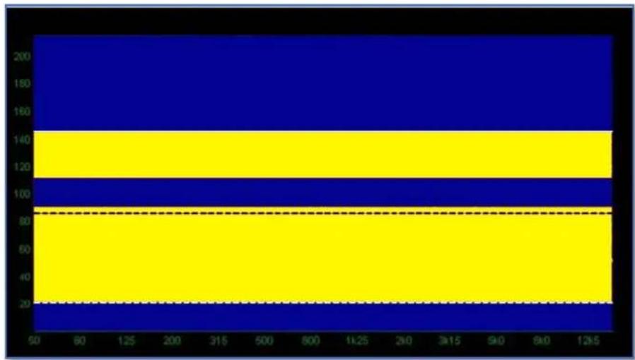
bar_stacked
| Category | Blue Segment | Yellow Segment | Dark Blue Segment | |---|---|---|---| | Top Row | 200 | 0 | 0 | | Middle Row | 140 | 0 | 0 | | Bottom Row | 100 | 0 | 0 | | Total | 80 | 0 | 0 |Here we have a real-world optimisation with a 10-box system; -
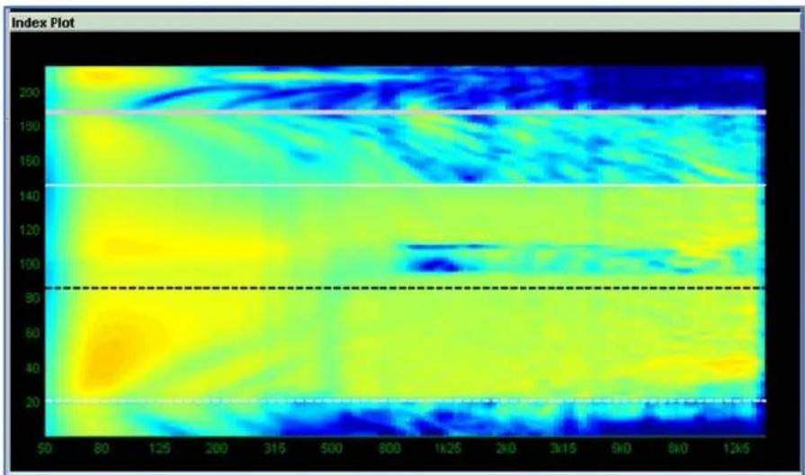
heatmap
| Index | Value | |-------|-------| | 200 | 20 | | 130 | 40 | | 140 | 60 | | 100 | 80 | | 90 | 100 | | 12k5 | 12k5 |And to demonstrate how close the system can get to the perfect coverage, here is the same venue with an array consisting of 16 MLA plus 1 MLD optimised to obtain a front to back differential of 0dB- exactly the same spl everywhere. The audience target has been given maximum priority ignoring non-audience and hard avoid areas; -
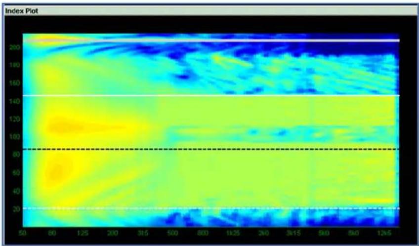
heatmap
| Index | Value | |-------|-------| | 200 | High | | 180 | Medium| | 160 | Low | | 140 | Medium| | 120 | High | | 100 | Medium| | 80 | Low | | 60 | Medium| | 40 | High | | 20 | Low |As you can see the vast bulk of the audience region is a consistent yellow/green with a band of blue indicating the underneath and front of the balcony. Quite a respectable result.
Note that using the hard avoid feature whilst extremely useful does have some limitations, whilst superb at rejecting sound behind the array on stage, if used for a balcony front for example it relies on the array being physically positioned exactly as it is depicted in the software to a fraction of a degree, not easy to achieve with standard electric hoists, plus if the array is not directly in front of the balcony the hard avoid region which will form an arc from the array, may miss the balcony at the extremes of the horizontal coverage giving some members of the audience a very poor experience.
Opening the Program
When run for the first time, Display 2.3 will open with the following window; -

text_image
DISPLAY 2.3 - Dashboard Enter Password OKThe password is available once you have watched the Display introduced video which will give you a good overview of how to use the application. Enter the password and click OK and the Dashboard will open so you can start using the application.
Note that the password is only required the first time you run Display 2.3. Subsequent uses will open straight to the program Dashboard.
User Interface Mode
Display is set to Basic mode by default. We strongly advise any users new to the application to stay in this mode as it will make the program very much more straightforward to navigate. For existing system owners and trained M-Techs you can access Expert mode via the Preferences option in the Help Menu; -
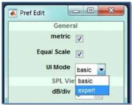
text_image
Pref Edit General metric Equal Scale UI Mode basic SPL Vie basic dB/div expertClick on the drop-down next to UI Mode and select expert. This will change the view in the tabs as you work through a project design. The features that you are used to seeing if you are an experienced Display user will be visible by default.
Note that the User Interface Mode is retained when Display is closed, it will be in the same mode when re-opened until such time as you return to Preferences to change it.
Quick start
Excellent results are available from Display 2.3 without necessarily refining each step of the process. The default settings have been established following a great deal of research and use in the field so are perfectly acceptable for a majority of applications. These are the steps necessary to deploy a system using the system defaults; -
1. Open Display; -

text_image
DISPLAY 2.3.3 - Dashboard b11 File Add Export Help2. Click on the icon to add your array
text_image
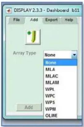
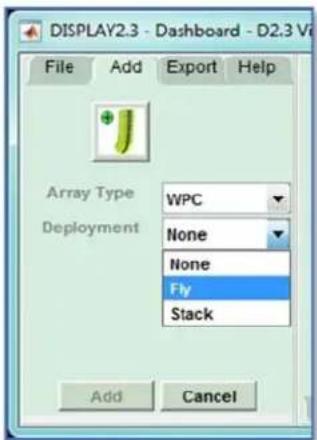
DISPLAY 2.3.3 - Dashboard b11 File Add Export Help Array Type None None MLA MLAC MLAM WPL WPC WPS WPM OLINE Add- Select how the array is to be deployed- flown, ground stacked, pole mounted (the available options depend on the system type selected), enter the quantity of cabinets and name your array.
text_image
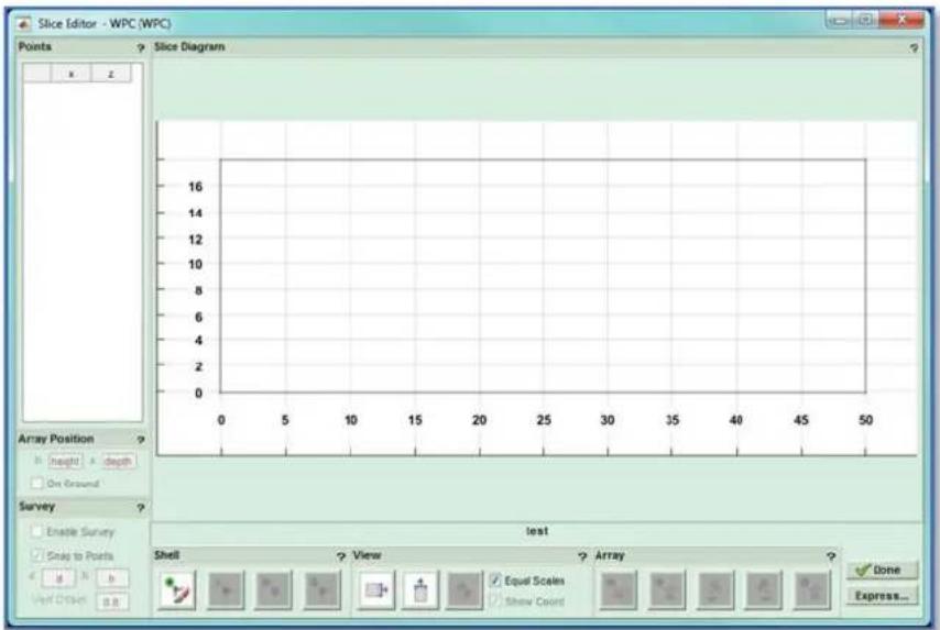
DISPLAY2.3 - Dashboard - D2.3 V File Add Export Help Array Type WPC Deployment None None Fly Stack Add Cancel- Click on the Slice Tab, enter an approximate maximum height and length and click OK; -
text_image
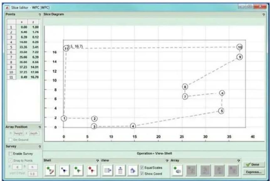
Slice Editor - WPC (WPC) Points Slice Diagram Array Position Height depth On Ground Survey Enable Survey Snap to Posts Test Shell View Array Equal Scales Show Count Done Express...- Click on 'Shell' and draw an approximate side view of the venue starting with the stage in the bottom left corner and working round the venue anticlockwise clicking each time you need to define each plane in the slice
line
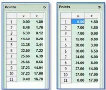
| Point | X | Y | |---|---|---| | 1 | 0 | 2 | | 2 | 6 | 2 | | 3 | 7 | 0 | | 4 | 15 | 0 | | 5 | 33.56 | 0 | | 6 | 33.68 | 0 | | 7 | 25.66 | 7 | | 8 | 26.66 | 9 | | 9 | 34 | 8 | | 10 | 37 | 15 | Table: Slice Diagram; X-axis: Position; Y-axis: Height; Legend: Array Position; Data Points; Values shown in the table; Source: Open Ground; Legend: Operation=View-Shell; View: Shell; Array: EqualScales; Show Coord: Show Coord; Done: Done; Express...- In the points section click on each point tabbing between them in turn and editing the values to accurate positions taken from either measurements you have taken yourself or from architects plans
other
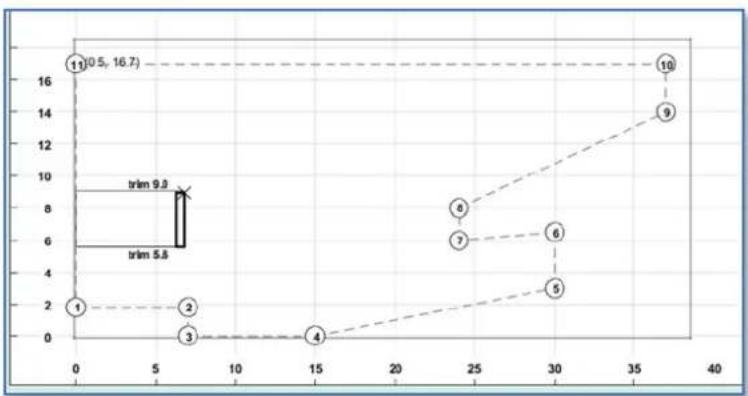
| Points | x | z | |---|---|---| | 1 | 0.00 | 1.80 | | 2 | 6.46 | 1.76 | | 3 | 6.39 | 0.12 | | 4 | 14.60 | 0.20 | | 5 | 33.35 | 3.41 | | 6 | 33.50 | 7.22 | | 7 | 25.66 | 6.39 | | 8 | 25.66 | 8.66 | | 9 | 37.23 | 14.91 | | 10 | 37.23 | 17.00 | | 11 | 0.49 | 16.70 | The table is a separate data table with two columns: 'x' and 'z'. The first row contains the absolute values of the numbers in the table (e.g., 1 = 0.00). The second row contains the corresponding values of the numbers in the table (e.g., 1 = 0.00). The table is colored differently to indicate different values.- Click on 'Array' and position the array within the venue as close as possible to the position at which it will be rigged;
line
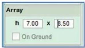
| Point | X-axis | Y-axis | |---|---|---| | 1 | 0 | 2 | | 2 | 7 | 0 | | 3 | 7 | 0 | | 4 | 15 | 0 | | 5 | 30 | 3 | | 6 | 30 | 6 | | 7 | 24 | 6 | | 8 | 24 | 8 | | 9 | 37 | 14 | | 10 | 37 | 16.7 | (1) (0.5, 16.7) (11) (2) trim 9.0 (3) trim 5.8 (4)The position can be trimmed in the Array Window; -
text_image
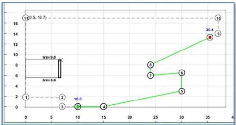
Array h 7.00 x 8.50 On Ground- Define the audience by clicking on the Add Audience region' button. Click on the position for the front row of the audience, move the cursor to the position of the rear seats and click again; -
line
| Point | X | Y | |---|---|---| | 1 | 0 | 2 | | 2 | 7 | 2 | | 3 | 8 | 0 | | 4 | 15 | 0 | | 5 | 30 | 3 | | 6 | 30 | 6 | | 7 | 24 | 6 | | 8 | 24 | 8 | | 9 | 37 | 14 | | 10 | 37 | 16.7 | | trim 9.0 (top) | 7 | 9.0 | | trim 5.6 (bottom) | 7 | 5.6 | | Trim 11 (top) | 0.5 | 16.7 | | Trim 10 (top) | 37 | 16.7 | The chart displays a single green line with circular markers indicating specific data points along the X-axis. The Y-axis is unlabeled but represents a numerical value for each point. The chart includes a dashed horizontal line at Y=16 and a vertical line at X=0. The label 'trim' in the top-left corner indicates a specific data point or condition.- Click 'Express' to open the Window to refine the coverage and create the optimisation; -
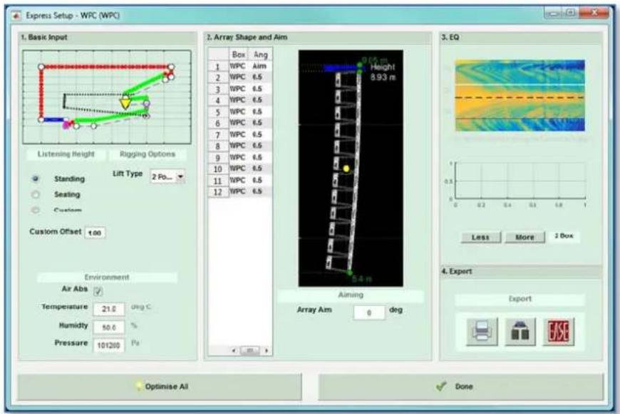
text_image
Express Setup - WPC (WPC) 1. Basic Input Listening Height Rigging Options Lift Type 2 Po... Standing Seating Custom Custom Offset 1.00 Environment Air Abs ✓ Temperature 21.6 Deg C Humidity 50.6 % Pressure 101200 Pu 2. Array Shape and Aim Box Ang 1 WPC Aim 2 WPC 6.5 3 WPC 6.5 4 WPC 6.5 5 WPC 6.5 6 WPC 6.5 7 WPC 6.5 8 WPC 6.5 9 WPC 6.5 10 WPC 6.5 11 WPC 6.5 12 WPC 6.5 3. EQ Height 8.93 m 0.05 m Aiming Array Arm 0 deg Less More 2 Box 4. Expert Export Optimise All Done- Select Standing, seated or a custom offset for the audience position and select the rigging option for a flown system this is single or 2 point; -
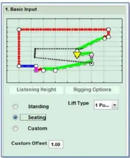
text_image
1. Basic Input Listening Height Rigging Options Lift Type 1 Po... Standing Seating Custom Custom Offset 1.00- Enter the temperature in the venue (or predicted temperature for when the show will take place) and the Humidity and Atmospheric Pressure if available
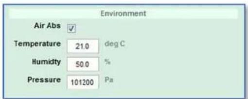
text_image
Environment Air Abs ✓ Temperature 21.0 deg C Humidity 50.0 % Pressure 101200 Pa- For WPL, WPC and WPM systems adjust the resolution in the EQ Window; -
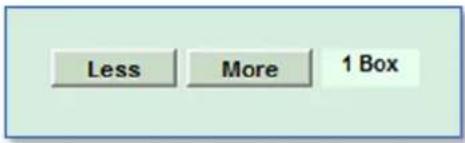
text_image
Less More 1 BoxFor WPL and WPS the resolution can be 1 to 2 box, for WPC 1 to 3 and for WPM the choices are 1 to 4 box.
- Click 'Optimise All'

text_image
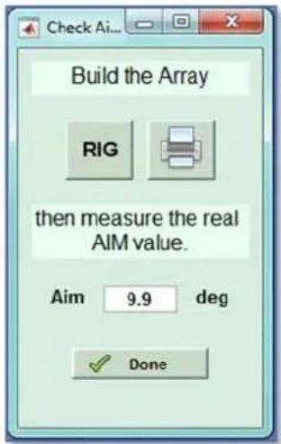
Optimise All- Once the Array splay angle optimisation is finished, click on 'Rig' on the 'Build the Array Window; -
text_image
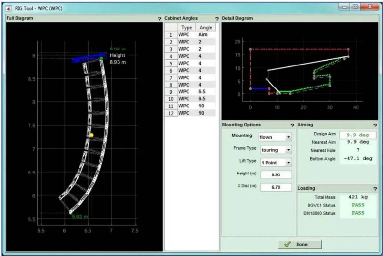
Check Ai... Build the Array RIG then measure the real AIM value. Aim 9.9 deg Done- Use the detail in the Rigging window to fly the array using the inter cabinet splay angles and overall array angle as listed in the rigging detail; -

text_image
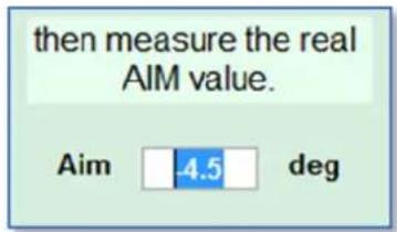
RIG Tool - WPC (WPC) Full Diagram Cabinet Angles Detail Diagram 1 WPC Aim 2 WPC 2 3 WPC 2 4 WPC 4 5 WPC 4 6 WPC 4 7 WPC 4 8 WPC 4 9 WPC 6.5 10 WPC 6.5 11 WPC 10 12 WPC 10 Height 8.93 m Mounting Options Aiming Mounting flown Design Aim 9.9 deg Frame Type touring Nearest Aim 9.9 deg Lift Type 1 Point Nearest Hole 7 Height (m) 8.93 Bottom Angle -47.1 deg X Dist (m) 6.78 Loading Total Mass 421 kg BGVC1 Status PASS DN10000 Status PASS Done- Check the actual angle at which the array is angled using an inclinometer and if different from the calculated angle, enter the accurate angle in the Build the Array Window; -
text_image
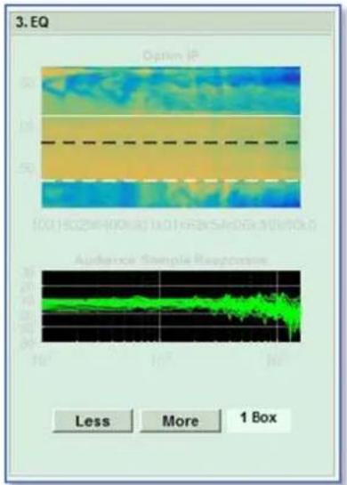
then measure the real AIM value. Aim -4.5 deg- Click 'Done' and the EQ Optimisation starts
text_image
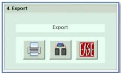
3. EQ Optim IP 100150254(00x8) 100165x5x05x10x00x Aperture Sample Response Less More 1 Box- Click on the 'Export to Vu-Net' button (middle button) to Export the optimised file
text_image
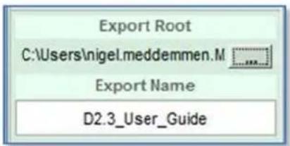
4. Export Export- Click on 'Export Root' and navigate to a file location in which to store the optimisation file. Rename the file if required;
text_image
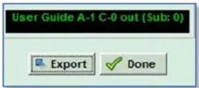
Export Root C:\Users\nigel.meddemmen.M Export Name D2.3_User_Guide- Click on 'Export' to upload the optimisation coefficients into the d2p file that has been created.
text_image
User Guide A-1 C-0 out (Sub: 0) Export Done- When the Export has finished, click 'Done'. You have finished the project. Save the file so you can return to it to edit the parameters if anything requires further refinement once the file has been uploaded to the array using Vu-Net and you have had a chance to listen to the system and evaluate how well the coverage is meeting your expectations.
Application menu
When Display 2.3 is first launched, the Dashboard below is shown. This remains visible at all stages of the project design and as will be seen; tabs will appear in a logical order to prompt you to enter the required data at each stage of the design process.

text_image
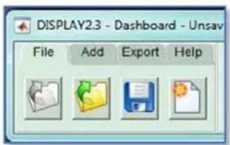
DISPLAY 2.33 - Dashboard b11 File Add Export HelpAs you can see, the application prompts you to enter the details of your array as the first step however it is worth taking a look at the options available under each menu item first. The file menu offers four options, Open Recent Files, Open files, Save and New.
text_image
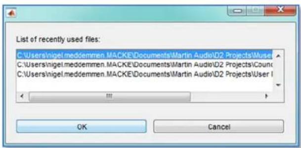
DISPLAY2.3 - Dashboard - Unsav File Add Export HelpThe first option is to load recent projects you have been working on (if running Display for the first time this option does not appear as there are no recent projects), clicking this option will bring up a list of recent projects; -
text_image
List of recently used files: C:\Users\nigel.meddemmen.MACKE\Documents\Martin Audio\D2 Projects\Muser C:\Users\nigel.meddemmen.MACKE\Documents\Martin Audio\D2 Projects\Cound C:\Users\nigel.meddemmen.MACKE\Documents\Martin Audio\D2 Projects\UserIf the project hasn't been opened recently you can select 'Load' to open an existing project to continue working on it. Next you can save the current project and finally you can start a new project. Note that until you have actually started on a project and saved it, the 'create new project' option will have no effect.
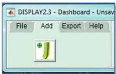
The Add menu prompts you to add the details of your Multicellular array.
text_image
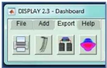
DISPLAY2.3 - Dashboard - Unsav File Add Export HelpThe Export menu is where the finished optimisation(s) and 3D models are uploaded to a file. This is the final stage of the design process and we will look at this process later in this guide.
text_image
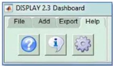
DISPLAY 2.3 - Dashboard File Add Export HelpThe Help menu brings up a set of options for the project which can be selected to suit the design you are working on
text_image
DISPLAY 2.3 Dashboard File Add Export HelpThe first icon is a link direct to the Display 2.3 User Guide. Note that internet access is required for this to work as it links to the URL for the User guide on the Martin Audio website.
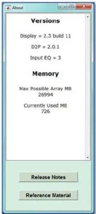
The next icon is the about function which gives details about Display 2.3 with links to some useful documents. It opens the following window; -
text_image
Versions Display = 2.3 build 11 D2P = 2.0.1 Input EQ = 3 Memory Max Possible Array MB 26994 Currently Used MB 726 Release Notes Reference MaterialRelease notes opens an HTML document with full details of the Display 2.3 content and the changes and improvements from Display 2.2.
Reference Material links to a Reference folder which is installed with the application and contains three pdf documents; -
■ Drive Granularity for Straight and Curved Loudspeaker Arrays
■ Improved Methods for Controlling Touring Loudspeaker Arrays
Numerically Optimised Touring Loudspeaker Arrays – Practical Applications
Preferences
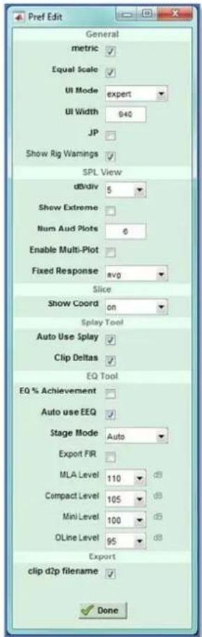
The final option in the Help menu is the Preferences enabling you to tailor the application to how you would like to work for a given project. Clicking on the icon in the help menu brings up this window, the options selected are the defaults for all new Display 2.3 installations; -
text_image
Pref Edit General metric ✓ Equal Scale ✓ UI Mode expert UI Width 940 JP Show Rig Warnings ✓ SPL View db/div 5 Show Extreme Num Aud Plots 0 Enable Multi-Plot Fixed Response avg Slice Show Coord on Splay Tool Auto Use Splay ✓ Clip Deltas ✓ EQ Tool EQ % Achievement Auto use EEQ ✓ Stage Mode Auto Export FIR MLA Level 110 db Compact Level 105 db Mini Level 100 db OLine Level 95 db Export clip d2p filename ✓ DoneGeneral
Metric allows you to select metric in place of imperial measurements.
Equal scale refers to the x and y scales for the 2D slice drawing required of the venue. For a venue with say a very long x axis and very little height, it may be easier to depict the layout with unequal scales.
UI Mode allows selection of either basic, advanced or expert views. This changes which parameters are visible for editing in each of the tabs. On most cases the same functions are available but may require an extra click to expand the view to use them. Display 2.3 will be in Basic mode by default. It will remain in whatever mode is active when the application is closed and reopened.
SPL View
dB/div allows selection of the Decibel per division on the optimisation of either 5 or 10.
Show extreme is active when Multi-plot has been enabled. The response at the start and finish of the audience region will be highlighted in green and red respectively so they are easy to pick out particularly when large numbers of audience plots have been selected.
Num Aud Plots dictates the number of audience plots to show if the Multi-plot option has been enabled. This can be as many plots are there green "virtual microphone" dots, the display would however look very confused so not more than around 12 is a more practical number.
Enable Multi-Plot when checked will display the number of response graphs specified in the Audience Plots window.
Fixed response allows you to select the fixed responses displayed when in Multi Plot is enabled. With Multi-plot disabled the spl window will show the response at the reference position as a dashed yellow line, plus the average response over the entire
audience region as a dashed white line. In Multi Plot mode you have the option to display simultaneously with the audience plots you have specified, either the reference response, still with a yellow line, the average audience response or neither.
Slice
Show Coord allows you to turn off the display of the coordinate number for each node on the drawing. This might be useful for a very complex drawing where the numbers would clutter the view but for the vast majority of projects this should be left on.
Splay Tool
Auto Use Splay will instantly apply the optimised angles to the array model. With this disabled you can review the array shape before applying the angles to the project. In most cases this can be left enabled.
EQ Tool
EQ% Achievement will display the percentage achievement that the optimisation has produced related to the goals that you have set. With this disabled it will display raw figures for equalisation.
Auto use EEQ acts in the same way as the auto function for optimised splay angles, it will instantly apply them to the project as soon as the optimisation is complete. If you wish to review the optimisation before applying the filters you can leave this disabled and an additional 'Apply' button will appear when the optimisation is complete.
Stage Mode. There are two modes for the hard avoid function, either mean or peak level or the default which is Auto. Display will calculate the best option depending on the available system resources.
Export FIR allows you to export just the FIR filter calculations in the optimisation as a txt file.
Levels The next four lines determine the default spl level at which the optimisation is calculated. These can be changed in an individual project however is all of your projects require the default to be changed; for example extreme spl is a priority or at the other end of the scale, the lowest possible noise floor is important, the default values can be changed here for MLA and O-Line systems.
Export
Clip d2p filename ensures that the exported filename matches the array name making it easier to identify which optimisation corresponds to a given Display optimisation when uploading to the system via Vu-Net.
Add an Array
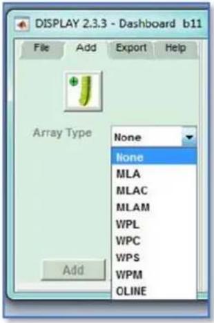
One you have selected the preferences that you wish to use, the first step is to add an array. Go to the 'Add' tab and click on the array icon. The following window will appear; -
text_image
DISPLAY 2.3.3 - Dashboard b11 File Add Export Help Array Type None None MLA MLAC MLAM WPL WPC WPS WPM OLINE AddIn the first drop-down you must select the type of array, either 'None', then three options from the Multicellular range; MLA, MLAC (MLA Compact) or MLAM meaning MLA Mini, the three systems from the Wavefront Precision range; WPM, WPC and WPL, and finally O-Line. "None" has very limited use (perhaps for silent discos?).
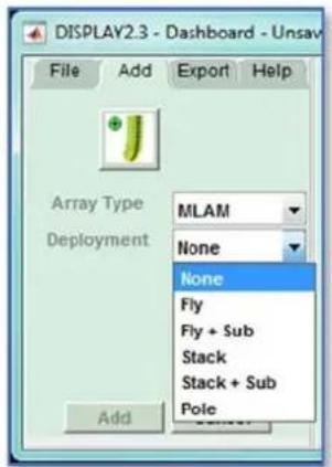
Next you need to select your method of deployment which will in turn determine a number of other factors in how the design process operates. The options are; -
■ MLA, MLA Compact, WPS and WPC flown or stack,
■ WPL may be flown, flown with sub or stacked
- MLA Mini and WPM, flown with sub, ground stacked, ground stacked on sub and pole mount,
■ O-Line may be flown or wall mounted; -
text_image
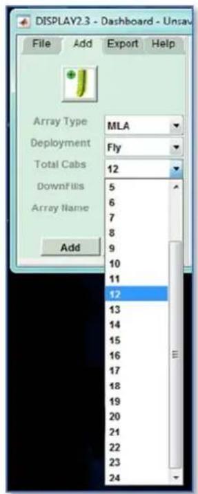
DISPLAY2.3 - Dashboard - Unsav File Add Export Help Array Type MLAM Deployment None None Fly Fly + Sub Stack Stack + Sub Pole AddNext you need to select the total number of cabs. The options change according to the maximum number for each type of deployment. For MLA, MLA Compact, WPL and WPS you can fly up to 24 cabinets; -
text_image
DISPLAY2.3 - Dashboard - Unsav File Add Export Help Array Type MLA Deployment Fly Total Cabs 12 DownFills 5 Array Name 6 Add 7 8 9 10 11 12 13 14 15 16 17 18 19 20 21 22 23 24And ground stack up to six; -
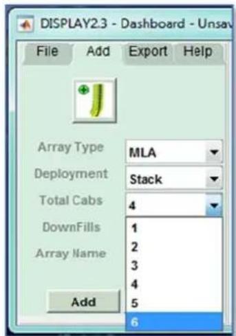
text_image
DISPLAY2.3 - Dashboard - Unsav File Add Export Help Array Type MLA Deployment Stack Total Cabs 4 DownFills 1 Array Name 2 Add 3 4 5 6For WPL you can fly up to 12 cabinets when fly with sub is selected; -
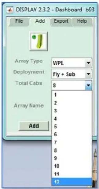
text_image
DISPLAY 2.3.2 - Dashboard b93 File Add Export Help Array Type WPL Deployment Fly + Sub Total Cabs 8 Array Name Add 1 2 3 4 5 6 7 8 9 10 11 12For MLA Mini there are more variations, for a flown system with the MSX ground stacked or rack mount amplifier modules you can fly from 2 to 16 in increments of one cabinet; -
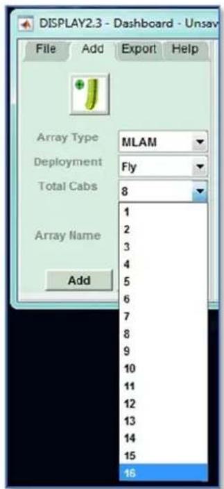
text_image
DISPLAY2.3 - Dashboard - Unsay File Add Export Help Array Type MLAM Deployment Fly Total Cabs 8 Array Name Add 1 2 3 4 5 6 7 8 9 10 11 12 13 14 15 16When flying with subs the maximum is 12 MLA Mini; -
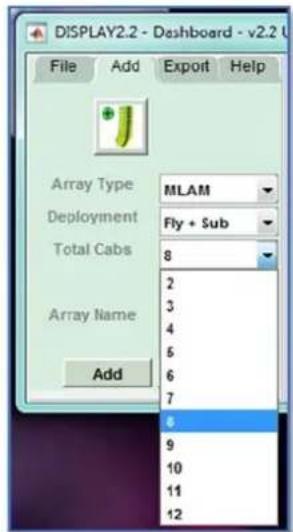
text_image
DISPLAY2.2 - Dashboard - v2.2 U File Add Export Help Array Type MLAM Deployment Fly + Sub Total Cabs 8 Array Name Add 9 10 11 12For ground stacked systems either on the floor or on top of the MSX, the maximum is 8 cabinets; -
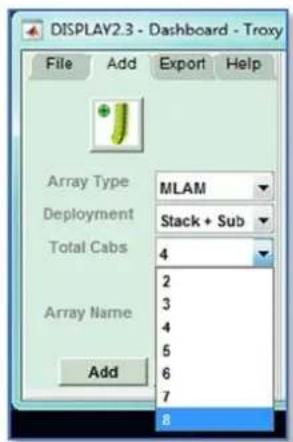
text_image
DISPLAY2.3 - Dashboard - Troxy File Add Export Help Array Type MLAM Deployment Stack + Sub Total Cabs 4 Array Name 2 Add 8And finally for a pole mount system the maximum is 4 cabinets; -
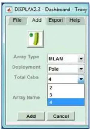
text_image
DISPLAY2.3 - Dashboard - Troxy File Add Export Help Array Type MLAM Deployment Pole Total Cabs 4 Array Name 2 3 4 Add CancelFor WPM or WPC the maximum is 16 for a flown system
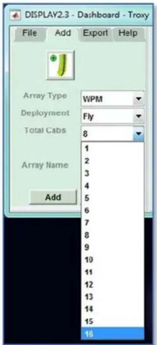
text_image
DISPLAY2.3 - Dashboard - Troxy File Add Export Help Array Type WPM Deployment Fly Total Cabs 8 1 2 3 4 5 6 7 8 9 10 11 12 13 14 15 16 AddSix Boxes for a ground stacked system
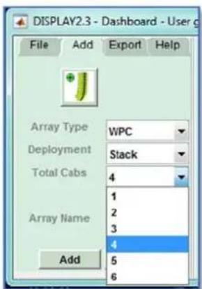
text_image
DISPLAY2.3 - Dashboard - User File Add Export Help Array Type WPC Deployment Stack Total Cabs 4 Array Name 1 Add 5 4 6For WPM you can fly up to 16 boxes; -
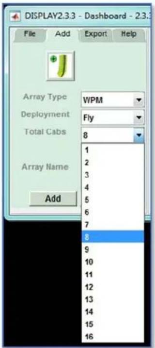
text_image
DISPLAY2.3.3 - Dashboard - 2.3.3 File Add Export Help Array Type WPM Deployment Fly Total Cabs 8 Array Name Add 8 9 10 11 12 13 14 15 16WPM Flown with Sub can be up to 12 boxes; -
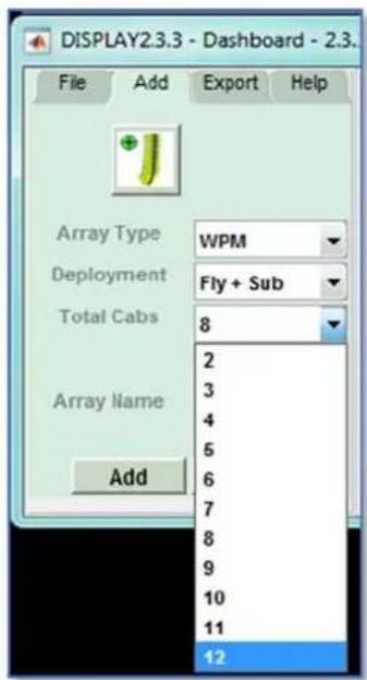
text_image
DISPLAY2.3.3 - Dashboard - 2.3. File Add Export Help Array Type WPM Deployment Fly + Sub Total Cabs 8 Array Name Add 2 2 3 4 5 6 7 8 9 10 11 12WPM Ground stacked as with all other WP Systems is up to six enclosures; -
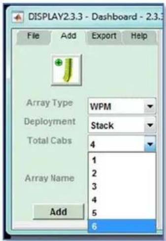
text_image
DISPLAY2.3.3 - Dashboard - 2.3.3 File Add Export Help Array Type WPM Deployment Stack Total Cabs 4 Array Name 1 Add 6Finally a pole mount system duplicates the MLA Mini option of four boxes; -
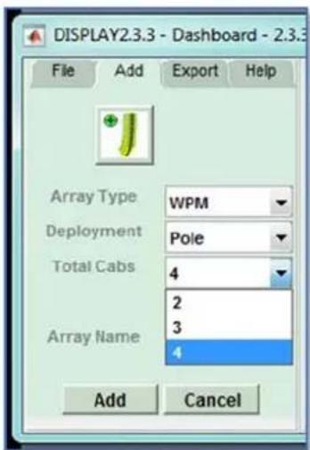
text_image
DISPLAY2.3.3 - Dashboard - 2.3.3 File Add Export Help Array Type WPM Deployment Pole Total Cabs 4 Array Name 2 3 4 Add CancelFor O-line you can select up to 24 for a flown system; -
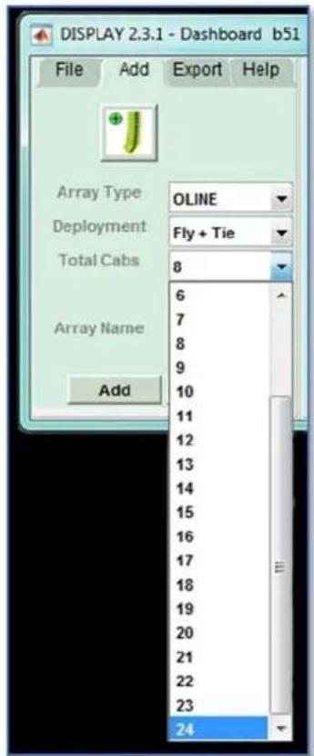
text_image
DISPLAY 2.3.1 - Dashboard b51 File Add Export Help Array Type OLINE Deployment Fly + Tie Total Cabs 8 6 7 8 9 10 11 12 13 14 15 16 17 18 19 20 21 22 23 24Or 16 for a wall mounted system; -
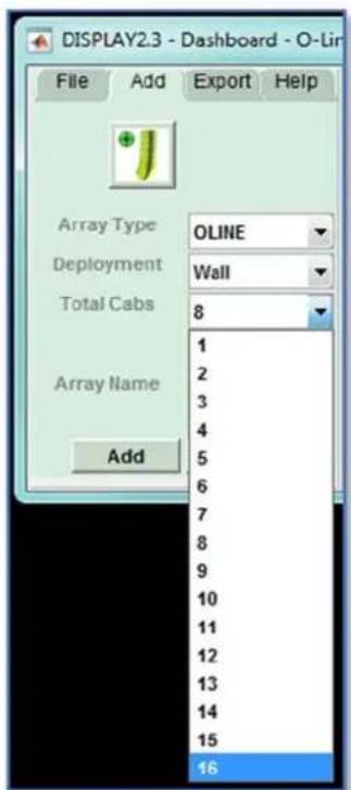
text_image
DISPLAY2.3 - Dashboard - O-Lin File Add Export Help Array Type OLINE Deployment Wall Total Cabs 8 Array Name Add 1 2 3 4 5 6 7 8 9 10 11 12 13 14 15 16Note that it is essential that the array design in Display 2.3 matches the physical array being used. The optimisation files that Display creates can only be uploaded to an array that exactly matches the file. The option to create arrays that are not multiples of four for MLA Mini is allow powering arrays using IKON amplifiers.
Finally you need to give the array a name. This is important as the D2P file created with the optimisation for that array will have the name that you assign at this point. If you wish to try several optimisations one method is to duplicate the design adding another array and entering the same venue and array properties but to give the array a different name that is appropriate to the optimisation that you are attempting.
Once you have entered the array details the dashboard will change, the array details section will turn green and the design process tabs will appear; -

text_image
DISPLAY2.3 - Dashboard - User Guide.mat File Add Export Help Slice Cover Splay Rig EQ SPL Rename MLA L&RYou will notice on the right-hand side the 'Rename' box. This gives you the opportunity to rename your array. Simply click in the box, type in the new name and press return. The Rename box will briefly turn green and the array name will change on the tab.
Next try clicking on any of the icons other than the 'Slice'. You will find that a window appears as shown; -
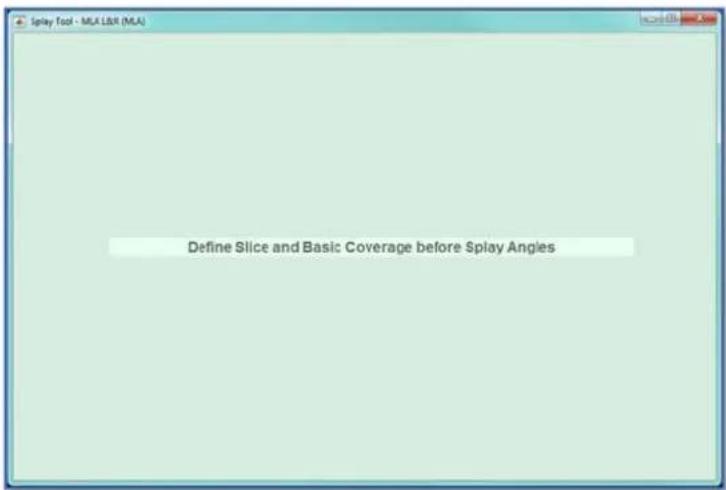
text_image
Splay Tool - MLA L&R (MLA) Define Slice and Basic Coverage before Splay AnglesThis window will appear if you attempt to access any of the process icons out of sequence, meaning before the preceding process has been completed. This feature forces you to complete the project design process in the correct, logical order. Once you have completed each section you are then able to go back and access any of the completed parts of the design.
Slice Tab
Slice Setup
The first stage of a Display project using any system is to draw a 2D slice of the venue. For most cases with a conventional stereo pair of arrays this can be a slice down the centre of the venue and many venue architects' plans will include a suitable side view.
Clicking on the 2D Slice icon will initially bring up a window prompting you to enter the basic length and height of the venue. This only needs to be approximate; enter a figure larger than the biggest dimension (but it's not a problem if you don't know the dimensions at this stage and the initial figures are too small).
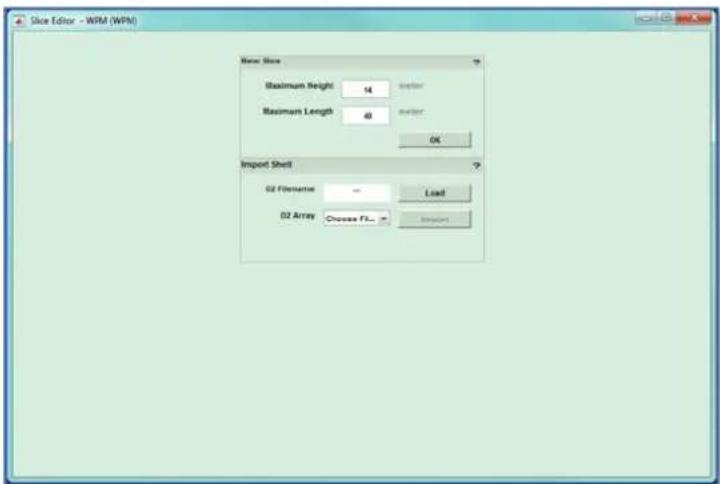
text_image
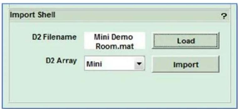
Slice Editor - WPM (WPM) New Slot Maximum Height 14 Maximum Length 48 Import Shell D2 Dimensions Load D2 Array Choose File... ImportThe other option is to import a Shell from an existing D2 file, this is extremely useful when creating designs for venues in which you have already deployed a multicellular system and still have the designs. It is also very useful when you wish to try several optimisations in a project as we will see later.
To load a Shell simply click on the 'Load' button, navigate to the file containing the shell you wish to use and click on it. The filename will appear in the D2 Filename box. A drop-down box will appear next to the 'D2 Array' which will contain a list of all the arrays in the project you have selected. Choose the one which has the shell you wish to use. Note that only the shell data is imported, the array and other optimisation parameters are ignored;
text_image
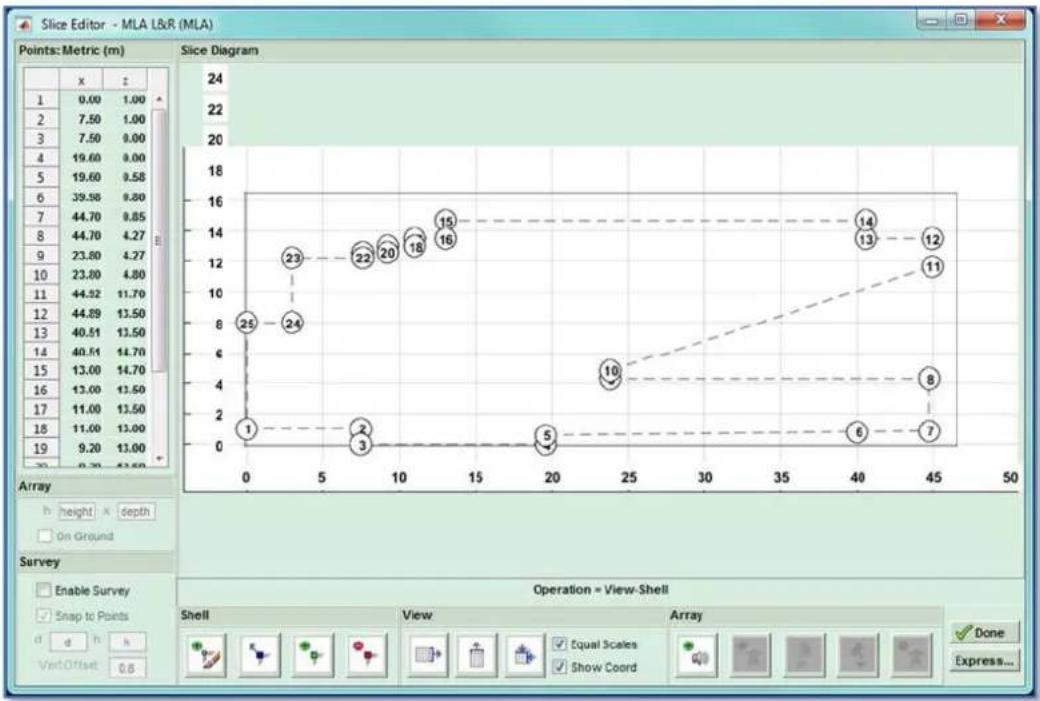
Import Shell D2 Filename Mini Demo Room.mat Load D2 Array Mini ImportClick import and the Slice Editor window appears with the shell already drawn;
line
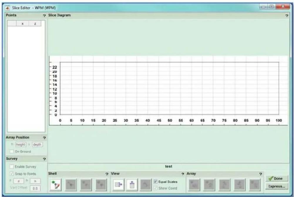
| Point | x (m) | y (m) | |---|---|---| | 1 | 0.00 | 1 | | 2 | 7.50 | 1.00 | | 3 | 7.50 | 0.00 | | 4 | 19.60 | 0.00 | | 5 | 19.60 | 0.58 | | 6 | 39.98 | 0.80 | | 7 | 44.70 | 0.85 | | 8 | 44.70 | 4.27 | | 9 | 23.80 | 4.27 | | 10 | 23.80 | 4.80 | | 11 | 44.92 | 11.70 | | 12 | 44.89 | 13.50 | | 13 | 40.51 | 13.50 | | 14 | 40.51 | 14.70 | | 15 | 13.00 | 14.70 | | 16 | 13.00 | 13.50 | | 17 | 11.00 | 13.00 | | 18 | 11.00 | 13.00 | | 19 | 9.20 | 13.00 | | Array height x depth on Ground Survey Enable Survey Snap to Points d d h h Var:Offset 0.6 Operation = View-Shell Shell View Array Equal Scales Show Coord Done Express...However, if we assume that we have to draw a shell from scratch, ignore the 'Import Shell' section, enter very approximate maximum dimensions for the length and height of the venue and click OK, the 2D Slice window will appear; -
text_image
Slice Editor - WPM (WPM) Points Slice Diagram X Z 22 20 18 16 14 12 10 8 4 2 0 0 5 10 15 20 25 20 25 30 35 40 45 50 55 60 65 70 75 80 85 90 95 100 Array Position height x depth On Ground Survey Enable Survey Snap to Points d h h Vert Offset 0.0 test Shell View Array Done Equal Scales Show Coord Express...Draw a Shell
Note that the window opens as a floating window and can be enlarged or maximised as any standard Windows application, this is obviously worth doing if you are working on a notebook PC or Tablet PC with a small screen. As you can see, most of the controls are greyed out and remain so until you have drawn the venue slice. To do this click on the Shell icon and move your mouse over to the drawing grid. A starting node is added at the zero point on the x axis but at 1.8 metres on the y axis to represent the back of a stage that is 1.8 metres high (this can be edited once you have completed the drawing). Next move the mouse in an anticlockwise direction moving the cursor to the approximate position of each node and click to add the node. You MUST
draw the shell anticlockwise; the optimisation will be completely wrong if the venue is drawn clockwise. The stage MUST also be on the LEFT of the slice diagram. When you arrive at the final node double click which will complete the drawing.
Note that you do not need to spend time or effort positioning the nodes in exactly the right position as it is extremely quick and easy to edit the precise node coordinates to match your measurements.
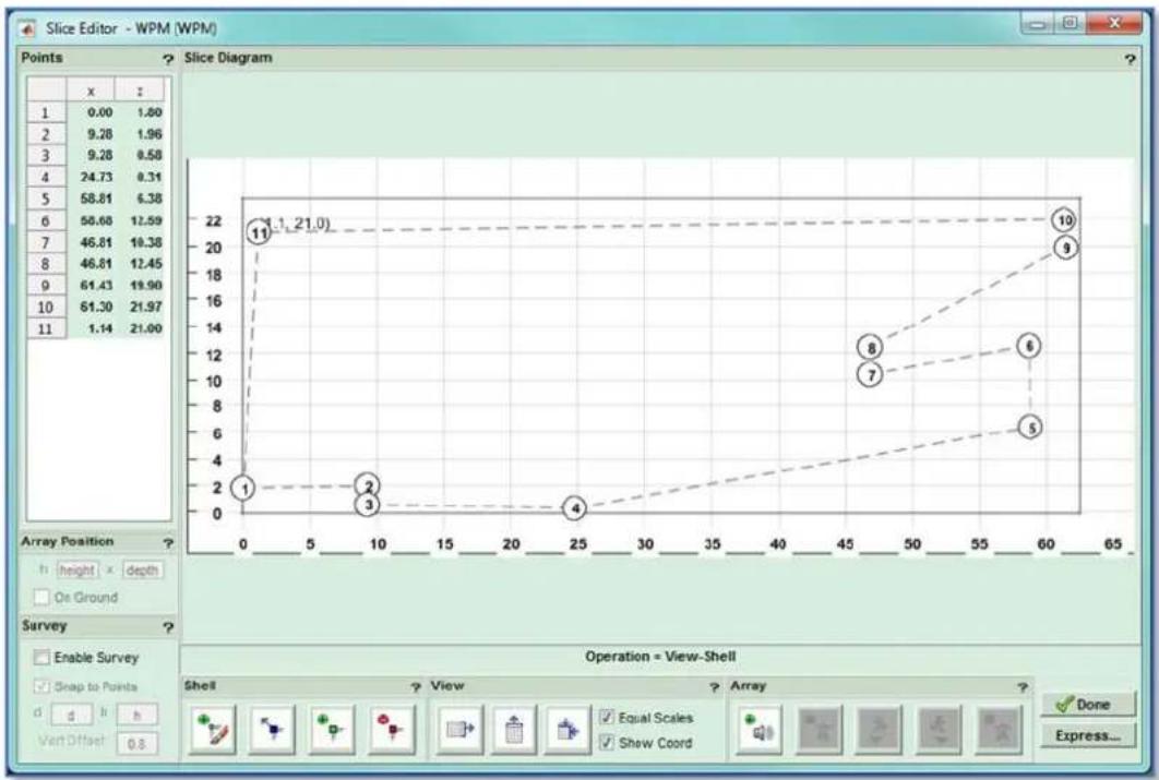
line
| Point | X | Y | |-------|------|------| | 1 | 0 | 2 | | 2 | 10 | 2 | | 3 | 10 | 2 | | 4 | 25 | 0 | | 5 | 45 | 4 | | 6 | 55 | 6 | | 7 | 45 | 10 | | 8 | 45 | 12 | | 9 | 60 | 18 | | 10 | 60 | 20 | | 11 | 60 | 22 |You will now see that a number of additional buttons are active and these can be used to perfect the venue drawing. Edit the shell
text_image
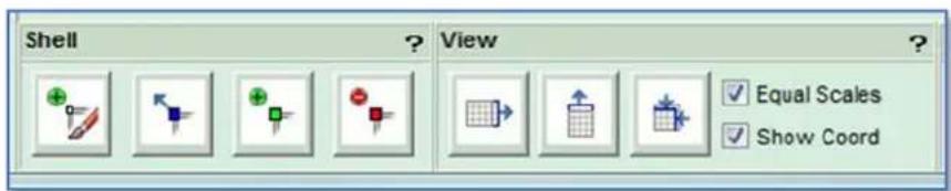
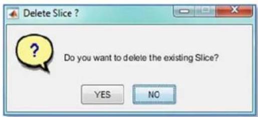
Shell View Equal Scales Show CoordThe first button is the shell entry that you have already used. If you have completely messed up the venue drawing you can click on this and start again, the initial drawing will be completely replaced. Note that if the shell has more than four nodes you will see a warning Window appear; -
text_image
Delete Slice ? Do you want to delete the existing Slice? YES NOThis is to prevent you from accidentally deleting a complex venue slice diagram.
The next button enables you to move any of the nodes. Click on the button and move your cursor over to the drawing. You will find that the cursor changes to a cross over the drawing area and when you hover over one of the nodes the circle around the node number will turn green. Click on the node that you need to move and drag and drop it to its new position.
The next button gives you the opportunity to add nodes if you missed any out in your initial pass. Click on the button and move your cursor over the drawing, as you move over the dashed lines between nodes you will see a small green circle appear. When
you have the circle in the desired position single-click and a new node is added and the numbering shifts to accommodate the new node. If necessary, you can use the move node button to reposition the new node however there is a much quicker way to precisely position the nodes as we will mention shortly.
If it's not entirely obvious the red button is for removing unwanted nodes than can easily appear if you accidentally clicked whilst drawing the slice. As with the 'move' button, click on the Delete button then move your cursor over the offending node and left click to consign it to history.
The View buttons help to maximise the drawing, to either the width of the slice, the height, or to fit the drawing into the extents of the available window. There are also two check boxes, the first by default makes the horizontal and vertical scales equal so you get a good proportional view of the venue shape hover if you have a situation where this makes it difficult to place the array for example a very long venue with a low ceiling, uncheck this box and the vertical and horizontal scales will maximise to the window to allow the maximum detail to be visible. Finally, you can uncheck the Show Coordinates button which removes the numbering from all nodes.
As mentioned, there is no need whatsoever to enter the nodes accurately when first drawing the slice, it is time consuming, particularly on a small screen, and inaccurate. Instead, you can edit all points shown on the top left list of nodes; -
| x | z | |
| 1 | 0.00 | 1.80 |
| 2 | 9.28 | 1.96 |
| 3 | 9.28 | 0.58 |
| 4 | 24.73 | 0.31 |
| 5 | 58.81 | 6.38 |
| 6 | 58.68 | 12.59 |
| 7 | 46.81 | 10.38 |
| 8 | 46.81 | 12.45 |
| 9 | 61.43 | 19.90 |
| 10 | 61.30 | 21.97 |
| 11 | 1.14 | 21.00 |
Click on the x coordinate for node 1, in most cases this is likely to be 0.00 but if not type the correct value and hit the Tab key. The z coordinate for the node 1 is highlighted and you can type the correct value. Tab again and the x figure for node 2 is highlighted and so on. You will get very quick at tabbing through all the coordinates entering the correct values to give you a perfectly accurate 2D slice drawing. This obviously is a far quicker method of working.
Using Survey
The process of drawing a shell as described above is fine particularly if you have architects drawings of a venue and are able to create a Display 2.3 project in advance of arriving on site, but in a touring situation this luxury is rarely available and therefore you may need to measure the venue when you get to site. The best method is to use a laser measure such as the Leica Disto D510 which is supplied as part of full MLA and MLA Compact systems and is available from Martin Audio as an optional accessory. The Distos have been in widespread use for accurately measuring venues for line array software so most technicians are familiar with their operation and accuracy. The D510 is one of the most advanced models and has a host of functions to make getting an accurate interpretation of the venue as quick and easy as possible.
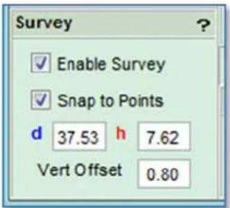
Display 2.3 allows entry of points using a Survey method instead of entering points as distances on the x and y axis which may be impossible or at least very difficult to measure on site; -
text_image
Survey Enable Survey Snap to Points d 37.53 h 7.62 Vert Offset 0.80Survey allows you to enter the distance to a specific point and the angle from where you are taking the measurement. This means that you can stand say directly under where the array points are and measure from there to all of the nodes in the venue taking note of the distance and angle which the Disto can display by selecting the angle display option. (See the guide supplied with the D510 for more details).
To enter the measurements, you first need to enter an approximate 2D slice with the correct number of nodes as described above. Now click in the Enable Survey check box. By default, leave the Snap to Points box checked. You will notice that the points list has now changed to Distance and Angle for each node; -
| Dist | Angle | |
| 1 | 0.80 | -90.00 |
| 2 | 9.30 | -3.93 |
| 3 | 9.50 | -12.26 |
| 4 | 24.84 | -5.30 |
| 5 | 58.93 | 3.68 |
| 6 | 59.52 | 9.66 |
| 7 | 47.45 | 9.44 |
| 8 | 47.83 | 11.88 |
| 9 | 63.82 | 15.73 |
| 10 | 64.28 | 17.54 |
| 11 | 18.44 | 86.46 |
You now need to enter the vertical offset from which you are taking your measurements, a tripod is strongly recommended to keep things accurate, the only other way to keep a constant accurate figure is to measure from the floor in which case enter zero for your vertical offset but sitting around on cold venue floors is an over-rated pastime so invest in a good quality tripod and the job becomes far more civilised. Measure from the ground to the tripod height you have set up and enter this figure into the Vertical Offset box. Now click on whichever point you intend to take your measurements from, you will see the measurement point selected shown as a yellow diamond. Having checked the Snap to Points box you can select any position on the slice and drag along it but when you get close to the nodes the measurement diamond will jump directly onto the node, without it you can select any point along the venue without the snap action close to the nodes.
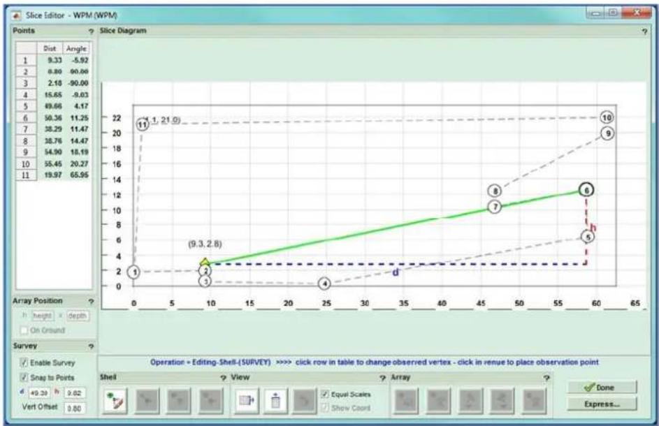
Now click on one of the positions on the list of points top left that you wish to enter the dimensions, in the following picture, the stage is 2 metres high and 8 metres deep with the flying points 0.5 metres off stage. All points were entered very quickly and using the method described above, the first 4 nodes were corrected. Enable Survey was then selected and the array flying point node 4 was selected. We want to measure to node 8 at the bottom of the front of the balcony so we click on the distance figure for that node; -
line
| Array Position | Height (m) | Depth (m) | View | Array | |---|---|---|---|---| | 1 | 2 | 0 | 2 | 11 | | 2 | 3 | 0 | 3 | 1 | | 3 | 4 | 0 | 4 | 21 | | 4 | 5 | 0 | 5 | 21 | | 5 | 6 | 0 | 6 | 21 | | 6 | 7 | 0 | 7 | 21 | | 7 | 8 | 0 | 8 | 21 | | 8 | 9 | 0 | 9 | 21 | | 9 | 10 | 0 | 10 | 21 | | 10 | 11 | 0 | 11 | 21 | | 11 | 12 | 0 | 12 | 21 | | 12 | 13 | 0 | 13 | 21 | | 13 | 14 | 0 | 14 | 21 | | 14 | 15 | 0 | 15 | 21 | | 15 | 16 | 0 | 16 | 21 | | 16 | 17 | 0 | 17 | 21 | | 17 | 18 | 0 | 18 | 21 | | 18 | 19 | 0 | 19 | 21 | | 19 | 20 | 0 | 20 | 21 | | 20 | 21 | 0 | 21 | 21 | | 21 | 22 | 0 | 22 | 21 | | 22 | 23 | 0 | 23 | 21 | | 23 | 24 | 0 | 24 | 21 | | 24 | 25 | 0 | 25 | 21 | | 25 | 26 | 0 | 26 | 21 | | 26 | 27 | 0 | 27 | 21 | | 27 | 28 | 0 | 28 | 21 | | 28 | 29 | 0 | 29 | 21 | | 29 | 30 | 0 | 30 | 21 | | 30+ (Note: The chart displays a single data point at x=9 for the 'Value' column in the table to change observed vertex. The 'Value' column contains the number of rows in the table to change observed vertex. There is no additional data series in this view. The 'Value' column contains the number of rows in the table to change observed vertex. The 'Value' column contains the number of rows in the table to change observed vertex. The 'Value' column contains the number of rows in the table to change observed vertex. The 'Value' column contains the number of rows in the table to change observed vertex. The 'Value' column contains the number of rows in the table to change observed vertex. The 'Value' column contains the number of rows in the table to change observed vertex. The 'Value' column contains the number in the table to change observed vertex. The 'Value' column contains the number in the table to change observed vertex. The 'Value' column contains the number in the table to change observed vertex. The 'Value' column contains the number in the table to change observed vertex. The 'Value' column contains the number in the table to change observed vertex. The 'Value' column contains the number in the table to change observed vertex. The 'Value' column contains the number in the table, but it is not explicitly labeled on the chart. The 'Value' column contains the number of rows in the table to change observed vertex, click in venue to place observation point. The 'Value' column contains the number of rows in the table to change observed vertex, click in venue to place observation point. The 'Value' column contains the number of rows in the table to change observed vertex, click in venue to place observation point. The 'Value' column contains the number of rows in the table to change observed vertex, click in venue to place observation point. The 'Value' column contains the number of rows in the table to change observed vertex, click in venues to place observation point. The 'Value' column contains the number of rows in the table to change observed vertex, click in venues to place observation point. The 'Value' column contains the number of rows in the table to change observed vertex, click in venues to place observation point. The 'Value' column contains the number of rows in the table to change observed vertex, click in venues to place observation point. The 'Value' column contains the number of rows in the table to change observed vehicle, click in venues to place observation point, click in venues to place observation point. The 'Value' column contains the number of vehicles, click in venues to place observation point, click in venues to place observation point, click in venues to place observation point. The 'Value' column contains vehicles, click in venues to place observation point, click in venues to place observation point, click in venues to place observation point, click in venues to place observation point. The 'Value' column contains vehicles, click in venues to place observation point, click in venues to place observation point, click in venues to place observation point, click in venues to place observation point, click in venues to place observation point, click in venues to place observation point, click in venues to place observation point, click in venues to place observation point, click in venues to place observation point, click in venues to place observation point, click in venues to place observation point, click in venues to place observation point, click in venues to place observation point, click in venue to place observation point, click in venue to place observation point, click in venue to place observation point, click in venue to place observation point, click in venue to place observation point, click in venue to place observation point, click in venue to place observation point, click in venue to place observation point, click in venue to place observation point, click in venue to place observation point, click in venue to place observation point, click in venue to place observation point, click in venue to place observation points, click in venue to place observations.You can now enter the distance figure that the Laser measure has measure from that point to the bottom of the balcony, hit Tab and enter the angle. You will see the drawing adjust to your figures and in the Survey box you will see the distance and height coordinates from your measurement position to what you are measuring calculated from the diagonal distance and angle you have entered. If desired you can enter figures into these boxes if you do not have the facility to measure angles. This makes it more convenient than measuring from the back of the stage if that area is crowded with lighting techs or backline crew etc. As before you can quickly tab between node figures to enter all of the measurements first typing the Distance figure followed by the angle. Once you have finished entering all figures you can un-check Enable Survey to return to standard mode and you will be able to add the array. Once your drawing is perfectly accurate, click on the Fit drawing to Extents button to maximise it in your window.
Position the Array
Now click on the array button and move your cursor into the drawing window. You will see a rough rectangular representation of the array showing the x coordinates and the top and bottom trim heights. Once again, there is no need to worry about being 100% accurate when placing the array, put it in an approximate position and left click to drop it in place. If for any reason you want to start again just click on the array button again and have another go. Once positioned you will see over on the left the array position coordinates.
text_image
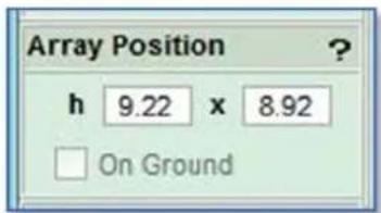
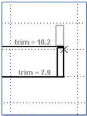
Array Position h 9.22 x 8.92 On GroundThis is where you can accurately correct the position of the array. Note that the height figure is to the centre of the upper flying pin on the top cabinet in the array, what is shown in the slice drawing is the figure for the trim height to the top of the flying hardware and the lower trim from the lowest point on the array, so effectively the maximum and minimum rigging positions. The 'On Ground' option is available for any array that has been specified as a ground stack. This will ignore the figure for the height and lock the array to the lowest point on the slice according to where the x position is specified. If for example the stage is 5 metres deep and the x figure is 3m the array will be positioned on stage, if the x position were 6m the array would be on the floor. For MLA Mini systems a grey box will appear above the array if flown with sub has been selected;
text_image
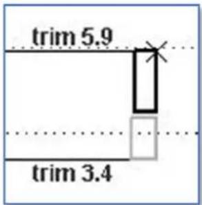
trim = 10.2 trim = 7.9Or below the array if stack with sub has been selected; -
text_image
trim 5.9 trim 3.4It shows the space occupied by the subs. The size of the rectangle expands depending on how many may possibly be above the array. The rigging tab allows accurate calculations when this mode is selected as we will see.
Add the Audience Region
Now you need to determine the audience area that we need to cover. Click on the Add Audience button; -
Then hover over the slice drawing. You will see a green inverted triangle moving left and right along the slice outline corresponding to the left and right movement of your cursor. Position the triangle where the audience position starts and click once. Now move the cursor to the right tracing the slice along the audience area and you will see a green line following your movement with a red inverted triangle at the end of the line. When the red triangle is over the furthest point of the audience region click again and the audience area is defined. Don't worry at this point that it includes underneath and on the front of balconies et cetera that is corrected at the next stage.
Editing the Audience Region
If you didn't get either the start or finish points correct it is easy to adjust them by using the Move Coverage Marker buttons, either the green one for the start position or the red one for the stop position.
Just click on either of the buttons and move the cursor to the correct position, the triangle marker will move for whichever point you are adjusting without disturbing the other. When you have the point in the correct new position click again to finalise it.
You can also delete the audience region entirely but clicking on the 'Add Audience' button again automatically deletes what you have already entered allowing you to start again, or click on the Delete Audience button which removes the audience region you have drawn but you have the option to re-draw a new region at a later time.
Assuming you have drawn an accurate representation of the venue (and remember that the more accurate the D2 project, the better the audible results), you have now finished entering the venue slice and can click on 'Done' to close the window.
Express Tab
In the bottom right corner of the Slice tab is an "Express" button which opens window allowing a quick set-up which uses default setting for all but the most essential functions and can very quickly produce excellent results more rapidly than stepping through the Cover, Splay, Rig and EQ tabs.
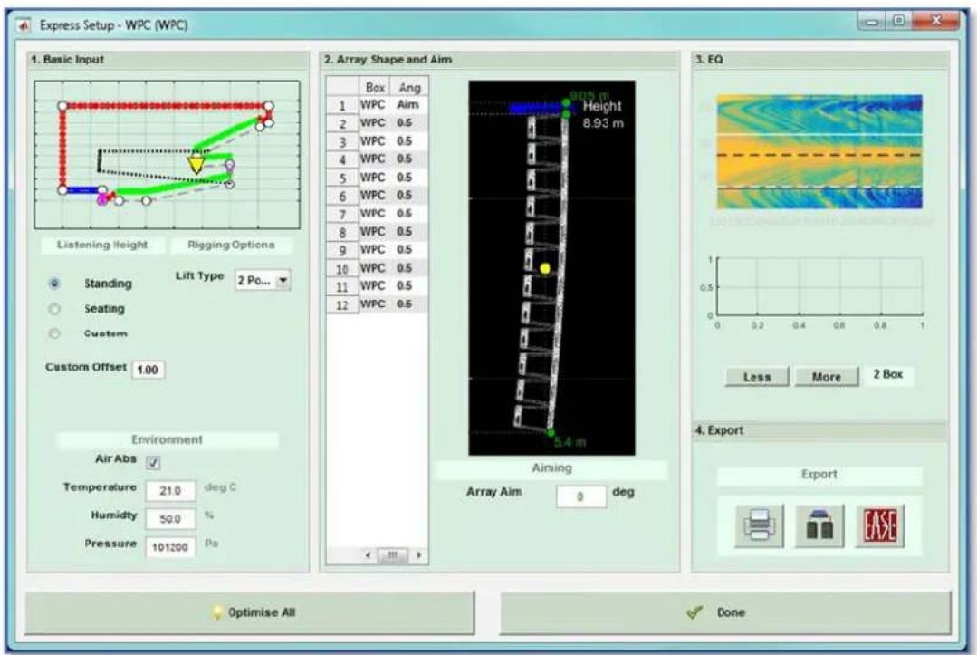
text_image
Express Setup - WPC (WPC) 1. Basic Input Listening Height Rigging Options Standing Lift Type 2 Po... Seating Custom Custom Offset 1.00 Environment Air Abs ✓ Temperature 210 deg C Humidity 50.0 % Pressure 101200 Pa 2. Array Shape and Aim Box Ang 1 WPC Aim 2 WPC 0.5 3 WPC 0.5 4 WPC 0.5 5 WPC 0.5 6 WPC 0.5 7 WPC 0.5 8 WPC 0.5 9 WPC 0.5 10 WPC 0.5 11 WPC 0.5 12 WPC 0.5 905 m Height 8.93 m 5.4 m Aiming Array Aim 0 deg Optimise All Done 1. EQ Less More 2 Box 4. Export ExportThere are 4 sections to the window. 1. is Basic input and it is necessary to enter the options in this window first; -
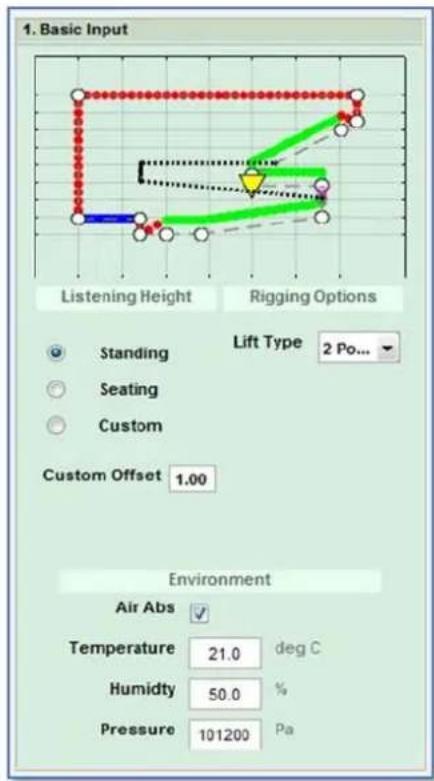
text_image
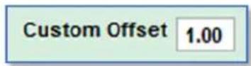
1. Basic Input Listening Height Rigging Options Lift Type 2 Po... Standing Seating Custom Custom Offset 1.00 Environment Air Abs Temperature 21.0 deg C Humidity 50.0 % Pressure 101200 PaAt the top of this section you will see a thumbnail of the venue slice with the coverage shown. Green areas are the audience region, red areas are non-audience and Blue areas are Hard-Avoid where the system will actively cancel signal to minimise spill into unwanted areas. By default this is on stage. The first option to select is the listening height of the audience which can be Standing, Seated, or a custom offset entered in the box towards the bottom of the Listening Height section; -
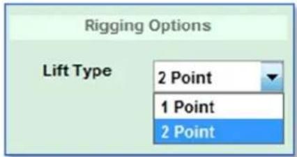
The next option is to select how the system is to be rigged. For a standard flown system this is a single or 2 point rigging; -
text_image
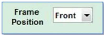
Rigging Options Lift Type 2 Point 1 Point 2 PointYou also need to determine the flying frame position, either front of rear.
text_image
Frame Position FrontOn most circumstances this will be front, you may need to use rear if the array is likely to have an extreme up-tilt.
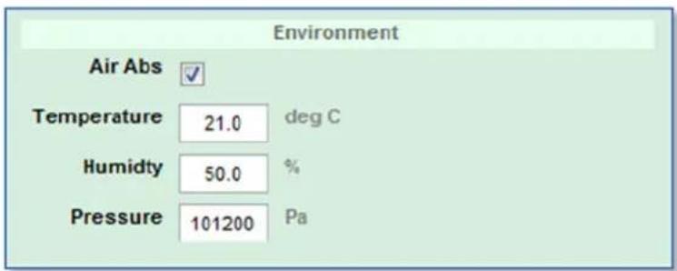
The final detail that is required before commencing with the optimisation is to decide whether to include the Environment parameters which will be incorporated into the calculations. The Air Absorbsion will be compensated for based on the figures for Temperature, Humidity and atmospheric pressure entered in this section; -
text_image
Environment Air Abs ✓ Temperature 21.0 deg C Humidity 50.0 % Pressure 101200 PaThese can be obtained from local weather forecasts, Smart Phone apps, or compact hand-held environmental measurement devices are readily available and are fairly inexpensive. The air absorption can make a huge difference to how sound is propagated, particularly at high frequencies so we would strongly recommend entering accurate figures for the environmental conditions where possible. If you do not need to use this feature it can be bypassed by clicking on the "Air Abs" box and un-checking it.
Set Box Resolution
For Wavefront Precision cabinets it is necessary to select the box resolution prior to optimising the array. This determines how many channels of amplification are used to power the array and therefore how many cells are available to achieve the goals that you have selected. The lowest resolution for WPM for example is 4-box which means four cabinets paralleled and driven from a single amplifier channel. For a 12-box array this would require three channels of amplification making it a very economical system but effectively it only has three cells with which to optimise the system and try to achieve the coverage that you have selected. Box resolution is therefore always a balance between budget and performance.
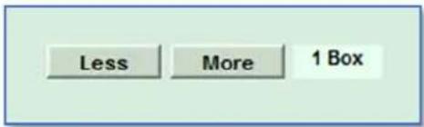
Resolution adjustment is made in the EQ section; -
text_image
Less More 1 BoxWPM can be changed from 1-box to 4 box, WPS 1 or 2 box, WPC from 1-box to 3 box and WPL 1 or 2 box.
Note that the resolution option is only available for Wavefront Precision systems, it is not present for any of the Multicellular products; MLA, MLA Compact or MLA Mini.
You can now start to optimise the array using the Optimise All which will do both the Splay angle optimisation followed by the EQ optimisation.
Optimise All
The quickest option to optimise all aspects of the system is to use the "Optimise All" Button; -

text_image
Optimise AllClicking this will start the splay angle optimisation immediately. The array will go through hundreds of combinations of angles with the internal computer model comparing the array performance in the venue you have drawn to see if the angles are helping to get results closer to what you have specified. You will see the array thumbnail in the Array Shape and Aim section turn green and move as it tries the many angle options; -
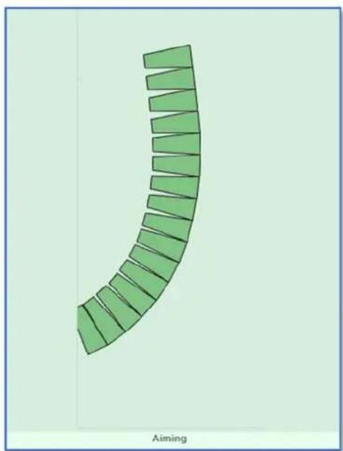
text_image
Aiming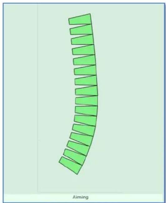
text_image
AimingOnce completed, the array will return to the default appearance but with the array shape shown as calculated; -

line
| Point | Height (m) | |-------|------------| | 1 | 8.36 | | 2 | 8.31 | | 3 | 5.52 |You will see the following Window appear; -
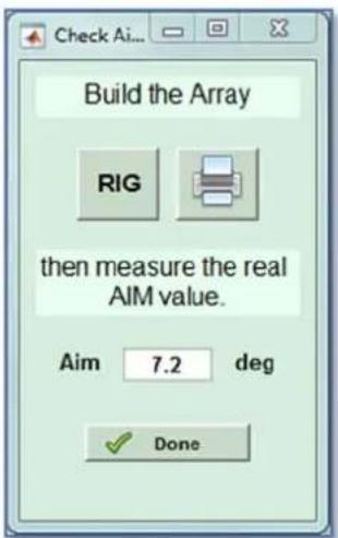
text_image
Check Ai... Build the Array RIG then measure the real AIM value. Aim 7.2 deg DoneThis prompts you to start physically rigging the system. Clicking on rig; -
Will bring up the full rigging page with all details of the array deployment; -
line
| Mounting Options | Aiming | | ---------------- | ------ | | Design Aim | 9.9 deg | | Nearest Aim | 9.9 deg | | Nearest Hole | 7 | | Bottom Angle | -47.1 deg | | Loading | ? | | Total Mass | 421 kg | | BGVC1 Status | PASS | | DW18800 Status | PASS |You can also select Print if you have a printer connected to your PC; -
Whilst this is unlikely if you are working on site, it is very useful if you are lucky enough to be able to complete a Display design prior to the event perhaps working from architects drawings of the venue. The print option produces a rigging report in HTML format rather than sending a file direct to a printer. You will see this window appear; -
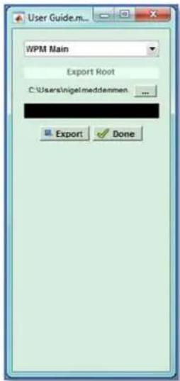
text_image
WPM Main Export Root C:\Users\nigel\meddammen Export DoneFirst you need to select a file location using the Export Root button; -
Then click on Export and the file will be created and the window will show that the Export is completed; -

The HTML report will open in your default browser; -
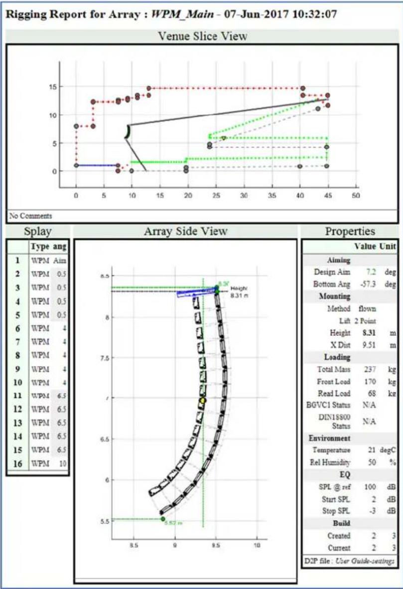
line
Rigging Report for Array : WPM_Main - 07-Jun-2017 10:32:07 Venue Slice View | X-axis | Height (m) | |---|---| | 0 | 8.5 | | 5 | 8.5 | | 10 | 8.5 | | 15 | 8.5 | | 20 | 8.5 | | 25 | 8.5 | | 30 | 8.5 | | 35 | 8.5 | | 40 | 8.5 | | 45 | 8.5 | | 50 | 8.5 | Value Unit Aiming Design Aim 7.2 deg Bottom Ang -57.3 deg Mounting Method flown Lift 2 Point Height 8.31 m X Dirt 9.51 m Loading Total Mass 237 kg Front Load 170 kg Read Load 68 kg BGVC1 Status N/A DIN18800 Status N/A Environment Temperature 21 degC Rel Humidity 50 % EQ SPL @ ref 100 dB Start SPL 2 dB Stop SPL -3 dB Build Created 2 3 Current 2 3 D2P file : User Guide-settingsThis contains all the details for the array deployment and can be printed and handed to the system technicians to fly the system. You can click 'Done' on the export window to return to the optimisation process.
You can now start the EQ optimisation however if you have time you have the option to change the array aim angle from the optimised value to the angle at which the array is actually hanging by taking a measurement from the inclinometer on the flying frame (if fitted). It is often very difficult to precisely match the calculated angle due to the limitations of chain hoists and other rigging hardware. The great thing about the optimisation process is that by entering the angle at which the array is actually flying, the EQ optimisation will compensate to ensure that the coverage is exactly as you specified.
Once you have amended the aim angle if required, click the 'Done' button; -
And the EQ optimisation will start; -

line
| Parameter | Value | | --------- | ----- | | Options IP | 0.6 | | Audience Sample Response | 0.2 - 0.8 |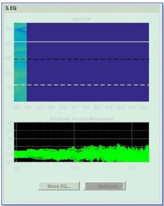
bar
| Time | Value | |------|-------| | 0K | 100 | | 3K | 100 | | 2ND | 100 | | 1ND | 100 | | 1K | 100 | | 2ND | 100 | | -1ND | 100 | | -2ND | 100 | | -3ND | 100 | | -4ND | 100 | | -5ND | 100 | | -6ND | 100 | | -7ND | 100 | | -8ND | 100 | | -9ND | 100 | | -10ND| 100 |The Window shows the blank index plot at the top with the white dashed line the audience start position, the black dashed line the reference point position and the solid white line the audience stop. The lower graph shows the frequency response at every virtual mic position in the audience region (the green dots). At the start of the optimisation the response varies enormously particularly as you move up into the mid and high frequency bands. The optimisation starts at low frequencies and you will see the index plot start to appear and the response in the lower graph start to even out with just the difference in front to back spl that was specified in the coverage tab evident.
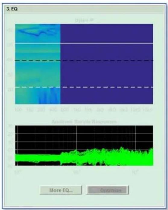
text_image
3. EQ Options IP Audience Sample Responses More EQ... Optimize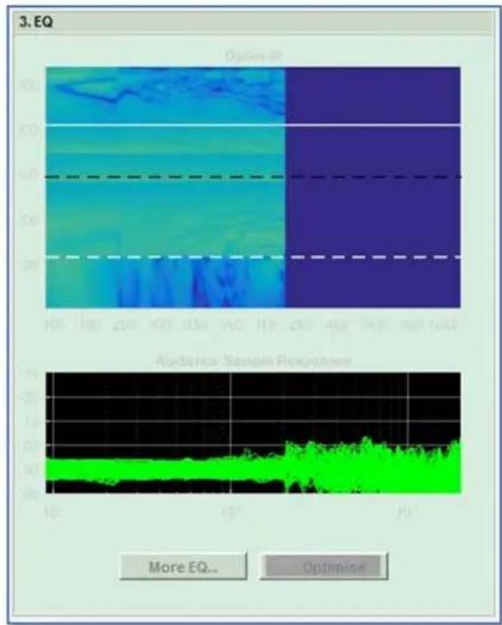
text_image
3. EQ Option IP 00 100 200 300 400 500 600 700 800 900 1000 1100 1200 1300 1400 1500 1600 1700 1800 1900 2000 2100 2200 2300 2400 2500 2600 2700 2800 2900 3000 3100 3200 3300 3400 3500 3600 3700 3800 3900 4000 4100 4200 4300 4400 4500 4600 4700 4800 4900 5000 5100 5200 5300 5400 5500 5600 5700 5800 5900 6000 6100 6200 6300 6400 6500 6600 6700 6800 6900 7000 7100 7200 7300 7400 7500 7600 7700 7800 7900 8000 8100 8200 8300 8400 8500 8600 8700 8800 8900 9000 9100 9200 9300 9400 9500 9600 9700 9800 9900 1000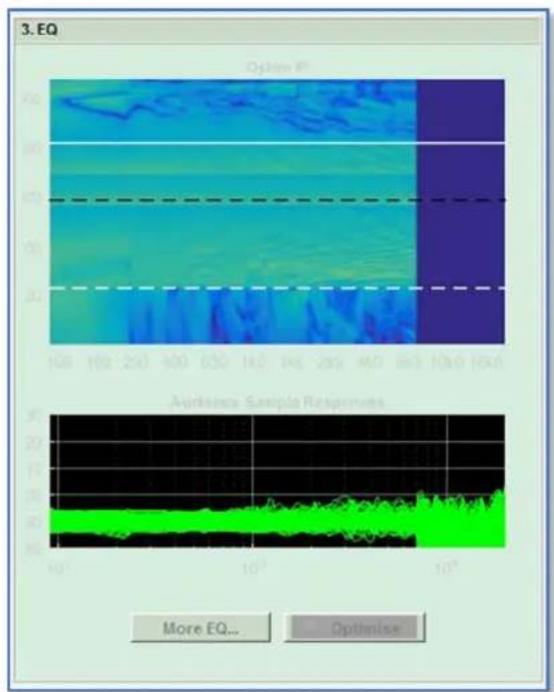
text_image
3. EQ Option Pi Avõrdince Sample Responnets More EQ... Optimise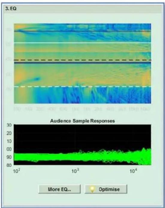
text_image
3. EQ Audience Sample Responses More EQ... OptimiseThe process continues working its way up through the audio band, the improvement in the consistency of the audience response very obvious. Once completed the final index plot will be displayed and shows a good even spread of green/yellow over the audience region. The solid blue line is under the balcony in our example where the coverage is shadowed. The blue shading above the reference point is under the balcony and you can clearly see above that how consistent the response is right to the back of the audience seated up in the balcony. All areas outside of the audience region are significantly bluer in colour demonstrating how well the system has reduced spl spill in these areas, a highly satisfactory result. Remember that this graphical representation will be within +/- 1dB of measurable results.
Once we are satisfied with the results we can move on to Export the settings.
The Export section has three options.
text_image
4. Export ExportThe first option is a second opportunity to export the rigging report as was available after the splay optimisation completed.
The second option; -
Exports the EQ optimisation as a d2p file suitable for uploading to the iKon amplifiers using Martin Audio's Vu-Net application. Click on this button and a similar window to the rigging report opens; -
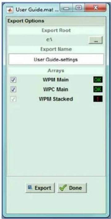
text_image
User Guide.mat ... Export Options Export Root c:\ ... Export Name User Guide-settings Arrays WPM Main OK WPC Main OK WPM Stacked Export DoneAs with the rigging report, the first step is to create a file in the location of your choice by clicking on the Export root button; -
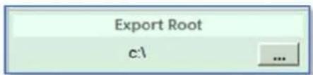
text_image
Export Root c:\The file name will default to the name of your Display project but can be edited to any name of your choice. Next you need to select which optimisations you wish to export; -
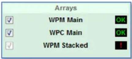
text_image
Arrays ✓ WPM Main OK ✓ WPC Main OK ✓ WPM Stacked !If your project only has a single array there will only be a single option here and it will be automatically checked ready to export. You can however add several arrays to a project (see the chapter Adding Additional Arrays) and all optimised arrays will be available in the Export window. In the example above, the WPM Main array has been optimised, as has WPC Main. WPM Stacked has been added to the project but the EQ Optimisation hasn't been completed which is why there is the exclamation mark in the box to the right of the name instead of an "OK";
Fairly obviously this cannot be exported until an optimisation has been done so the box to the left cannot be checked.
All checked arrays will be exported into the same file and when uploaded into a system can be dropped into the appropriate array. You may have some arrays that were experiments to see the results of alternative deployments and which may not be required for use with a system so you can un-check any which you won't need.
Once you are happy with your choice of arrays to export click 'Export' and you will see the export process taking place going through all the EQ parameters for the arrays selected; -
text_image
WPM Main A-1 C-5 out (Sub: 9.4)When this display disappears the Export is complete and you can click 'Done' to close the Export Window.
The EASE export offers the facility to create an XGLC file for the array which when used with the EASE GLL for array means you can import an array design into an EASE project. The EASE button also opens an Export Window requiring the file location to be selected; -
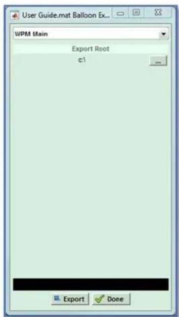
text_image
WPM Main Export Root c:1 ... Export DoneArrays in the project have to have their EASE files exported individually so the drop-down at the top is used to select which array you wish to Export; -
text_image
WPM Main WPM Main WPC Main WPM StackedClick on 'Export', you will again see a progress display showing the export as it completes; -

text_image
Exporting WPM Box 4The display will show when the export is complete; -
| Finished Export |
You can click 'Done' to close the Export Window.
This completes the Setup process and we can click on 'Done' to close the Setup Window; -

text_image
DoneNext step for WPM and WPC Systems is to view the spl of the completed design. See the SPL Tab Chapter for full details.
Coverage Tab
The next step is to precisely define the coverage but as with any application it is very good practice to save your project as you go along. Click on File on the Dashboard if it is not visible and click on the Save icon. Choose a suitable file location, you might with to create a dedicated folder for a given show to hold all files in one place, then name the file and click save.
Saving Files
Note that the save function in Display 2.3 is slightly unusual so needs a little explanation. Save does not automatically save the file you are working on. It will open a window giving you the opportunity to give the file a new name and to choose the location in which to store the saves file. If you wish to save the file you are working on you will need to navigate to the file and select it. You will be prompted for confirmation that you wish to replace the old file; -
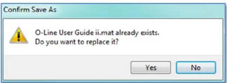
text_image
Confirm Save As O-Line User Guide ii.mat already exists. Do you want to replace it? Yes NoThis is a system which we introduced with the original incarnation of Display when it was launched for our original line array systems. This enables you to easily save copies of your work at each stage of the design process so you can easily revert back to an earlier version if you need to- perhaps you make a mistake and don't get the results you are hoping for you can easily go back to a stage where you were happy with the results rather than having to start from scratch.
Having completed the venue slice, the Coverage ("Cover") tab will now be active. A single mouse click will open the Coverage Editor window. The appearance will vary depending on the settings in the Options section. This is Basic View;

text_image
Coverage Editor - MLA L&R (MLA) Venue Diagram Audience Offsets Uniform Offset Standing Seating Custom Custom Offset 1.00 Line Properties Non Audience Audience Hard Avoid Reset 269,58 DoseThis is Expert; -
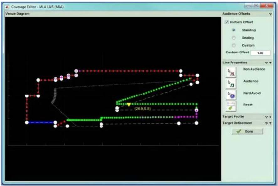
text_image
Coverage Editor - MLA L&R (MIA) Venue Diagram Audience Offsets Uniform Offset Standing Seating Custom Custom Offset 1.00 Line Properties Non Audience Audience Hard Avoid Reset Target Profile Target Refinement DoneHelp
On all sections you will see a '?' in the top right corner; -
Clicking on this brings up a Window with a detailed explanation of that section of Display. This is the Audience Offsets Help window; -
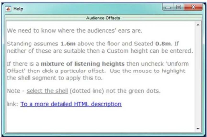
text_image
We need to know where the audiences' ears are. Standing assumes 1.6m above the floor and Seated 0.8m. If neither of these are suitable then a Custom height can be entered. If there is a mixture of listening heights then uncheck 'Uniform Offset' then click a particular offset. Use the mouse to highlight the shell segment to apply this to. Note - select the shell (dotted line) not the green dots. link: To a more detailed HTML descriptionAudience Offsets
The first step is to define the Audience Offsets, the height above the venue floor at which the audience ears are found. You will notice that the green lines showing the audience area are hovering above the planes which is to represent the offset of the position of the audience members' ears. By default this will be a uniform offset for all audience areas set to standing. Changes are made using the Audience Offsets panel; -
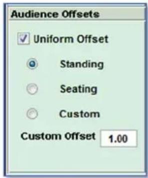
text_image
Audience Offsets ✓ Uniform Offset ○ Standing ○ Seating ○ Custom Custom Offset 1.00If for example the entire audience is seated, you can simply click the seating button and you will see the green audience line drop accordingly. The Standing offset is 1.6m and the Seating is 1.2. If you have a particularly unusual audience, very tall standing or perhaps very low seats, you can use the Custom offset to define the offset height in metres.
You will often encounter venues where you have a non-uniform offset, for example a room with a seated balcony but standing downstairs in the stalls. In these instances you need to un-check the Uniform Offset button and define the offset for each plane individually. When you uncheck the box, the controls change and look like this; -
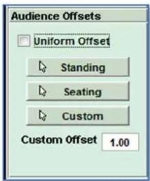
text_image
Audience Offsets Uniform Offset Standing Seating Custom Custom Offset 1.00In a similar fashion to changing Plane properties, you click on the Offset type first, and then hover over the required audience plane and click when the correct plane is highlighted with the same bold white dashed line. Note that all planes have to be defined individually, in our example for instance, the stalls audience area comprises two planes, the flat section at the front, and the raked section rising towards the back. Both of these will have to be changed to whatever the desired offset is. This can be useful as there are plenty of venues with a standing area down at the front and seating towards the back. When you are using Custom offsets, you can define a different custom height for each plane if required, you are not restricted to a single global figure.
Our example now has a standing audience downstairs and a seated upstairs; -
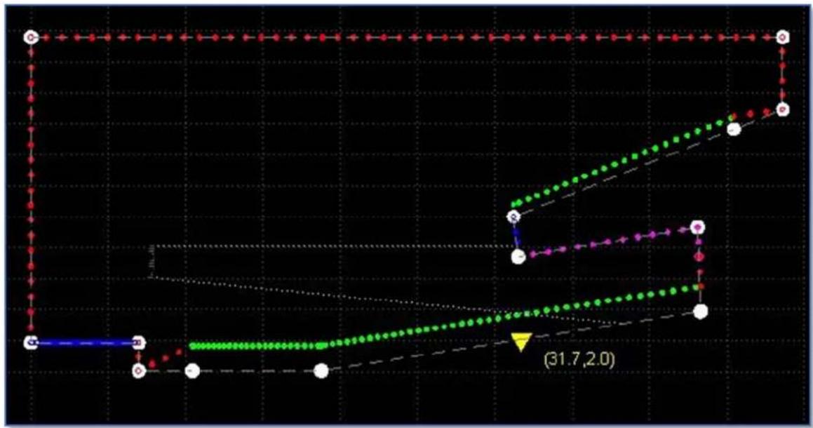
line
| Point | Value | |-------|-------| | 1 | 1.0 | | 2 | 1.0 | | 3 | 1.0 | | 4 | 1.0 | | 5 | 1.0 | | 6 | 1.0 | | 7 | 1.0 | | 8 | 1.0 | | 9 | 1.0 | | 10 | 1.0 | | 11 | 1.0 | | 12 | 1.0 | | 13 | 1.0 | | 14 | 1.0 | | 15 | 1.0 | | 16 | 1.0 | | 17 | 1.0 | | 18 | 1.0 | | 19 | 1.0 | | 20 | 1.0 | | 21 | 1.0 | | 22 | 1.0 | | 23 | 1.0 | | 24 | 1.0 | | 25 | 1.0 | | 26 | 1.0 | | 27 | 1.0 | | 28 | 1.0 | | 29 | 1.0 | | 30 | 1.0 | | 31 | 1.0 | | 32 | 1.0 | | 33 | 1.0 | | 34 | 1.0 | | 35 | 1.0 | | 36 | 1.0 | | 37 | 1.0 | | 38 | 1.0 | | 39 | 1.0 | | 40 | 1.0 | | 41 | 1.0 | | 42 | 1.0 | | 43 | 1.0 | | 44 | 1.0 | | 45 | 1.0 | | 46 | 1.0 | | 47 | 1.0 | | 48 | 1.0 | | 49 | 1.0 | | 50 | 1.0 | | 51 | 1.0 | | 52 | 1.0 | | 53 | 1.0 | | 54 | 1.0 | | 55 | 1.0 | | 56 | 1.0 | | 57 | 1.0 | | 58 | 1.0 | | 59 | 1.0 | | 60 | 1.0 | | 61 | 1.0 | | 62 | 1.0 | | 63 | 1.0 | | 64 | 1.0 | | 65 | 1.0 | | 66 | 1.0 | | 67 | 1.0 | | 68 | 1.0 | | 69 | 1.0 | | 70 | 1.0 | | 71 | 1.0 | | 72 | 1.0 | | 73 | 1.0 | | 74 | 1.0 | | 75 | 1.0 | | 76 | 1.0 | | 77 | 1.0 | | 78 | 1.0 | | 79 | 1.0 | | 80 | 1.0 | | 81 | 1.0 | | 82 | 1.0 | | 83 | 1.0 | | 84 | 1.0 | | 85 | 1.0 | | 86 | 1.0 | | 87 | 1.0 | | 88 | 1.0 | | 89 | 1.0 | | 90 | 1.0 | | 91 | 1.0 | | 92 | 1.0 | | 93 | 1.0 | | 94 | 1.0 | | 95 | 1.0 | | 96 | 1.0 | | 97 | 1.0 | | 98 | 1.0 | | 99 | 1.0 | | Note: The values in the 'Value' column are estimated based on the provided code snippet in the code editor's annotation 'P'. The text 'P' is not explicitly labeled in the image.Changing Line Properties
Next is the section for adjusting the plane line properties; -

text_image
Line Properties Non Audience Audience Hard Avoid ResetEach node entered in your Venue slice is shown as a white circle with each plane now allocated a colour between the nodes. There are three types of plane, Audience which is shown green, non-audience which is red and hard avoid which is blue. The system by default makes the stage hard avoid, the coverage planes from where specified in the venue slice start to finish will be audience and all other planes non-audience. The first step is to edit these to reflect exactly how you need the system to react to the venue.
In the example above, the audience area includes the stalls, the wall at the back of the stalls, under the balcony, the front of the balcony and the balcony itself. Clearly this is not correct and we need to change some of these planes.
At this stage we have to make a decision on where our priorities lie. There is a temptation to make all areas other than the genuine audience planes hard avoid to try and make the system reduce spill onto anywhere other than the audience, however we have to be realistic about what can be achieved. Whilst we have a tremendous amount of processing power available, we cannot change the laws of physics so there is a limit to just how much we can get the system to do. We are more likely to get good results if we are sensible with how much demand we put on the DSP. In the example we have shown, we are obviously not going to get any direct sound arriving under the balcony, it is essentially in "shadow" so there is little point in making this area hard avoid, likewise it clearly shouldn't be defined as audience or the system will waste DSP attempting coverage over an area it cannot reach so it should definitely be non audience. With a little experience you will learn what works well and what not to attempt. In our example I would keep the stage as hard avoid, perhaps also have a hard avoid on the balcony front which could give problems with a slap-back echo on stage and make all other areas non audience. The default setting usually has the stage hard avoid also including the stage front and the "pit" between the stage and audience start as hard avoid. This is not only
unnecessary but trying to get the DSP to get the signal from hard avoid immediately to audience is expecting far too much, it is much more realistic to keep the stage floor as hard avoid and the front of the stage and pit non audience.
You will also notice a pink area at the back of the stalls in our example. This indicates any part of the venue plane that is not in line of site of the array, essentially in "shadow". In many venues, particularly theatre style rooms with one or more balcony, this is very common and additional under-balcony fills may need to be deployed. You can of course close the Cover tab and return to the Slice tab to try alternative array positions to try and minimise any such shaded areas if audience areas are affected. In our example it is only under the balcony and on the rear wall at the back of the stalls that are not in line of site and so there is no need for any remedial action.
Each plane between nodes needs to be adjusted individually, to do this, click on the required plane property first, and then select the line you wish to change. For example, on our example, we want to make the balcony from hard avoid and under the balcony non audience. As it's the top button, let's do the non audience first. Click on the Non audience button and then hover over the planes, as you hover over each line you will see the feint dashed lines turn a bright white, thick dashed line. When you are over the plane you need to change, under the balcony in this case, a single mouse click changes the plane colour to red. Now we can do the same for the balcony front, click the Hard Avoid button and then select the small vertical balcony front which will change to blue to show it is now hard avoid.
You can click on the Audience button to change any planes to audience but this is rarely required as long as you initially defined the audience areas correctly in the Venue slice, you are more likely to have too many audience planes rather than not enough although you may need to change a plane back to audience if you have accidentally changed it to something else. If you get several wrong you can click on the Reset which returns all planes to the default that you started with.
Here is our example with all planes changed to what we need; -
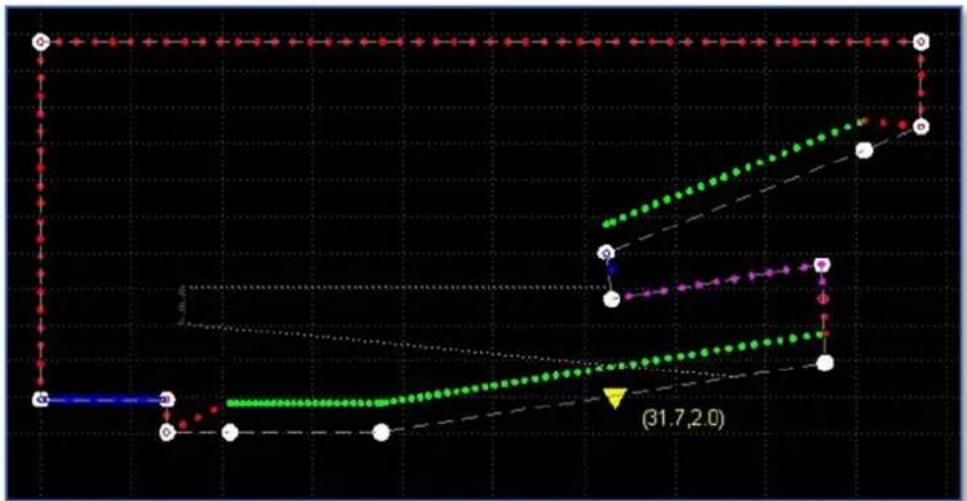
line
| Point | Value | |-------|-------| | 1 | 31.7 | | 2 | 2.0 |Target Profile Selection
If you have selected Advanced or Expert Mode you will see the Target Profile section which is minimised by default; -

To expand the window click on the icon on the extreme right; -
The window expands (simultaneously closing the Line Properties) and appears like this; -
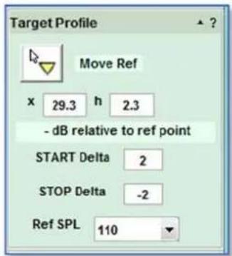
text_image
Target Profile Move Ref x 29.3 h 2.3 - dB relative to ref point START Delta 2 STOP Delta -2 Ref SPL 110This unassuming little box is one of the most powerful features of Martin Audio multicellular systems, whilst all other systems on the market are trying desperately to achieve a 3dB drop in level for every doubling of distance away from their arrays, Display 2.3 and one of Martin Audio's Multicellular or Wavefront Precision systems you can simply specify the precise loudness contour you desire across the venue. If you want the back row to be as loud as the front then you simply type "0" in both the start and stop delta positions and the system will give you exactly that. It can even make it louder at the back than the front if that is what you want.
The start and finish deltas are referenced to the yellow triangle which by default is placed in the middle of the audience region when you enter the coverage area in the venue slice. You have the opportunity to move it and if you didn't do so in the venue slice you can click on the 'Move Ref' button and move your cursor around the venue planes. The triangle will follow your cursor sticking to the planes until you are happy with its position and a further mouse click with cement it in its new position. Alternatively you can enter either an x or h figure to specify the horizontal position or height of the reference point and it will jump to the closest position on the venue shell that corresponds to the coordinates you have entered.
It is tempting to automatically position the reference position wherever front of house is positioned but this is not in the least bit necessary. The reference is used to adjust the contour so its position should be dictated by how you want the volume to change from the start to the finish of the audience region. Take a look at the following diagrams;
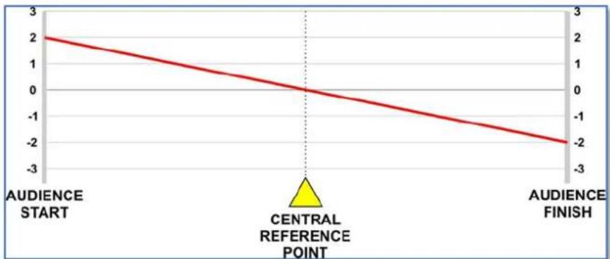
line
| Time Point | Value | | ------------------ | ----- | | AUDIENCE START | 2 | | CENTRAL REFERENCE POINT | 0 | | AUDIENCE FINISH | -2 |This shows a system that has been set up with the reference point in the centre of the audience region and a start and finish delta of + and - 2dB respectively. Because the reference point is central, the SPL drops evenly from start to finish, down 4dB from the loudest point at the start of the coverage.
The next diagram shows a system where the front of house position is around three-quarters of the way back from the front but the start and stop deltas are still at +/-2dB; -
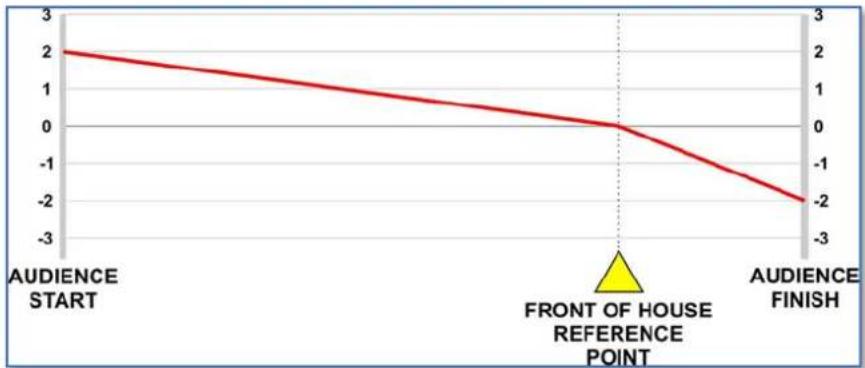
line
| Point | Value | | ------------------ | ----- | | AUDIENCE START | 2 | | FRONT OF HOUSE REFERENCE POINT | 0 | | AUDIENCE FINISH | -2 |As you can see, the level drops gradually over three quarters of the venue back to front of house and then drops rapidly back to the audience finish. Slightly strange and in most (but not necessarily all) circumstance, unwanted. To get the same smooth 4dB drop you should enter the start delta as +3dB and the finish at -1dB. But that only works if front of house is exactly three quarters of the way back! In the majority of cases you are far better of leaving the reference at the halfway point to make it easier to easily calculate how the loudness contour will flow from start to finish.
Of course they are many applications when it may be desirable to have the spl rapidly drop off behind the reference point, at outdoor events where noise pollution is an issue, the ability to move the reference point to dictate the contour in front and behind it individually is another very useful tool at the system technicians disposal to create the ideal coverage for difficult environmental conditions.
The default setting is +2/-3dB for Multicellular and +/-3 for Wavefront Precision with the reference point in the centre, these have been proved to work extremely well in practical tests so are unquestionably a very good place to start and works very well, unless you have a very large array or need to try something slightly unusual it is advisable to stick with these settings.
As mentioned, setting the start and stop delta is simply a case of entering the required figure in dB. As with entering hard avoid regions, it is prudent to be mindful of how hard your DSP is going to have to work to achieve the results you have requested. With a huge array of 22 MLA enclosures, it was possible to achieve a 0dB start/stop delta in the Tokyo Dome, the furthest seat being around 550 feet from the array. It would however be very difficult to get such an astonishing result from say an eight box WPM array. The height of the array also has a significant effect, a ground stacked system will not be able to achieve low figures for start and stop as a flown array.
In actual fact, a 0dB start/stop sounds very unnatural and because you are used to hearing an array get louder as you get closer, you actually get the distinct impression that it is getting quieter as you get closer to the array. The other issue is that multicellular optimisation is only effective down to approximately 150Hz, low and sub frequencies will still behave as you would expect reducing in SPL by 6dB for every doubling of distance. If the optimisation from front to back is set to a target of as little as a few dB this will obviously differ drastically from the behaviour of low frequencies meaning that the will be a very noticeable difference in tonal balance across the audience coverage with the loss of low frequencies being very apparent as you go towards the back as the mid and high frequencies hardly drop in level. It is recommended therefore that unless you have specific reasons to do otherwise, that you use the default figures. For most medium to large sized array this should be easily achievable and will leave plenty of DSP power for other tasks and will retain a far more natural and subtle change of tonal balance throughout the audience.
The final option is to set the reference SPL at which Display 2 will attempt to achieve the smoothest coverage as close as possible to the targets that you have specified. If you select 85dB you stand a better chance of achieving the system goals as it gives the option to allow great cancellation or gain shading to reduce levels in areas closer to the array thus making the coverage as even as possible and potentially closer to your SPL deltas. If however you need as much SPL as possible and have set your SPL deltas to allow a greater variation from start to stop you can select a higher SPL, 100 or 105dB and you will achieve a higher output from the system. The trade-off however is that Choosing SPL levels that are very low means that a high input signal level will be necessary to drive the arrays to high SPL's. In some instances this could cause the input to the cabinets to limit, as MLA series can accept a maximum of +18dBu peak input level. Choosing levels that are higher than the default will increase the noise floor. The default levels are set to provide a compromise between noise floor vs input level required to drive the system to high SPL's. So unless you have a very good reason to choose otherwise we would strongly recommend using the default figures. These are 110dB for MLA, 105dB for MLA Compact, WPS and WPC and 100dB for MLA Mini and WPM.
From version 2.2 onwards the reference figure is calibrated so that you will measure that figure at the reference position with 0dBu applied to the array input. With the array gain structure now calibrated it was necessary to look at the subwoofer gains to maintain a good balance. Vu-Net v2.0 will detect the optimisation reference figure in the Display d2p file and will automatically trim the sub input gain. For an MLA system or other system optimised at 110dB or higher, the sub gain will be increased to +10dB, for MLA Compact or other system optimised at 105dB the input gain will be set to +5dB and for MLA Mini or other system optimised at 100dB or less the gain will remain at 0dB
Target Refinement
The final adjustment in the Coverage tab is to refine the Target to compensate for air absorption. The window is also minimised by default; -

The effects of air absorption can have a very significant effect on the upper frequency bands. The compensation is edited in this window; -
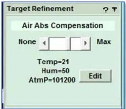
text_image
Target Refinement Air Abs Compensation None Max Temp=21 Hum=50 AtmP=101200 EditThe fader bar adjusts the amount of compensation from zero to a maximum level. This is best used for higher amounts where weather conditions are extreme or where you have particularly long throws as the compensation will help ensure that higher frequencies are not lost. However, be careful not to overdo it if not really necessary as you could run the risk of running out of headroom in the upper frequency bands.
The Edit button brings up the window into which you can enter the necessary environmental conditions; -
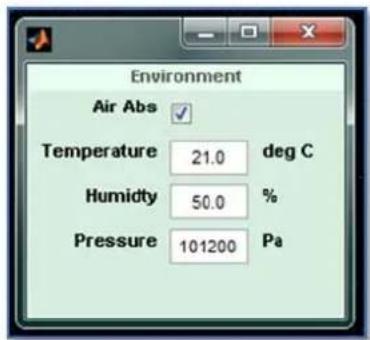
text_image
Environment Air Abs Temperature 21.0 deg C Humidity 50.0 % Pressure 101200 PaIf you un-check the air absorption there will be no compensation applied to the optimisation, you can still enter the Temperature, Humidity and Pressure so if you need to create a new optimisation including air absorption it is as quick and easy as checking the box. Be aware that environmental conditions change drastically throughout the day! A 6.00 am load-in is going to give very, very different readings compared to a packed, 8.00pm show with all lighting, smoke machines and pyrotechnics going full tilt!
Once you have determined your Start and Stop Deltas you can click on Done to close the Coverage window and you can move on to the Splay tab.
Splay Angle Tab
Having completed the Coverage, you will be able to open the Splay tab and the default window in Basic Mode will appear as follows; -
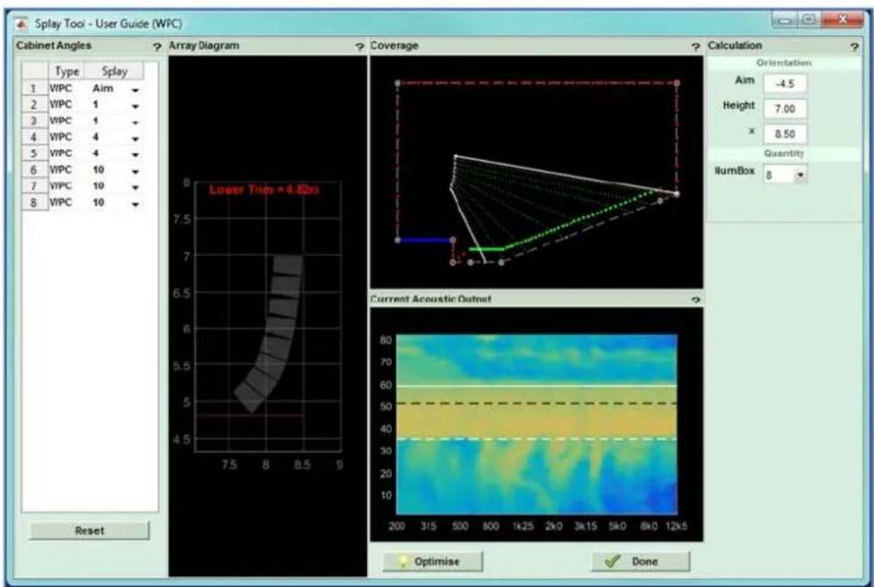
text_image
Splay Tool - User Guide (WPC) Cabinet Angles Type Splay 1 WPC Aim 2 WPC 1 3 WPC 1 4 WPC 4 5 WPC 4 6 WPC 10 7 WPC 10 8 WPC 10 Array Diagram Coverage Calculation Orientation Aim -4.5 Height 7.00 x 8.50 Quantity NumBox 8 Lower Trim = 4.82m Current Acoustic Output Reset Optimize DoneAnd Expert mode looks like this; -
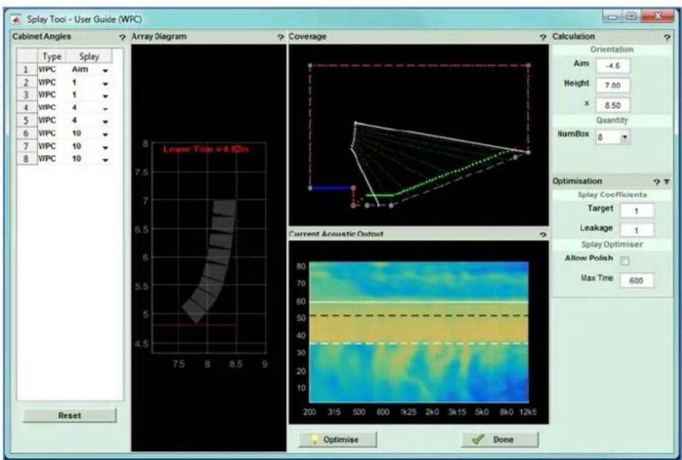
text_image
Splay Tool - User Guide (WPC) Cabinet Angles Type Splay 1 WPC Aim 2 WPC 1 3 WPC 1 4 WPC 4 5 WPC 4 6 WPC 10 7 WPC 10 8 WPC 10 Array Diagram Coverage Calculation Orientation Aim -4.5 Height 7.00 x 8.50 Quantity NumBox 8 Lower Trim = 4.0m Reset Current Acoustic Output Optimise Done Splay Coefficients Target 1 Leakage 1 Splay Optimiser Allow Polish Max Time 600There are a number of sections to the window, these are; - Cabinet angles, Array Diagram, Current Acoustic Output, Coverage, Current Acoustic Output, Calculation, and in Advanced and Expert modes Optimisation
Splay Angles
This shows a list of all cabinets in the array and initially this will show all angles between cabinets at the default of 0.5^ ;
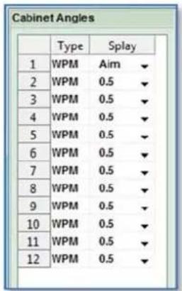
text_image
Cabinet Angles Type Splay 1 WPM Aim 2 WPM 0.5 3 WPM 0.5 4 WPM 0.5 5 WPM 0.5 6 WPM 0.5 7 WPM 0.5 8 WPM 0.5 9 WPM 0.5 10 WPM 0.5 11 WPM 0.5 12 WPM 0.5There is a drop-down arrow next to each cabinet allowing you to manually select a cabinet angle. We will discuss this option later. At the bottom of the list is a rest button which will return all angles to 0.5^ .
text_image
ResetArray Diagram
The Array diagram shows a representation of the array and most importantly for flown arrays shows the lower trim point, the distance from the lowest point on the array to the ground. The diagram will adjust in real time when the optimisation is taking place and the lower trim will change accordingly. In most instances the lower trim at the start will be lower than when the optimisation is complete. This is because the array starting point is with an almost straight array with all angles at 0.5^ , once the optimisation is complete some of the angles will inevitably be higher thus reducing the overall height of the array and raising the lower trim height
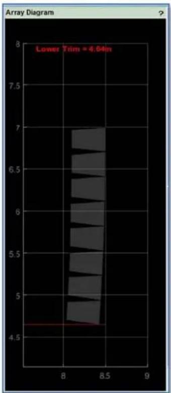
bar
Array Diagram | X-axis | Value | |---|---| | 8.0 | 7.0 | | 8.1 | 6.9 | | 8.2 | 6.8 | | 8.3 | 6.7 | | 8.4 | 6.6 | | 8.5 | 6.5 | | 8.6 | 6.4 | | 8.7 | 6.3 | | 8.8 | 6.2 | | 8.9 | 6.1 | | 9.0 | 6.0 | | 9.1 | 5.9 | | 9.2 | 5.8 | | 9.3 | 5.7 | | 9.4 | 5.6 | | 9.5 | 5.5 | | 9.6 | 5.4 | | 9.7 | 5.3 | | 9.8 | 5.2 | | 9.9 | 5.1 | | Lower Trim = 4.64mCoverage / Current Best Optimised Output
Prior to starting the optimisation this shows the coverage diagram with the array shown with all angles at the default 0.5^ . Note that the white lines from the top and bottom of the array are the acoustic centres of the top and bottom cabinets, NOT the furthest points of the coverage which will be 3.25^ beyond the upper line and 3.25^ lower than the bottom line for MLA or 10^ lower if MLD are used at the bottom of the array. For MLA Compact and MLA Mini it will be 5^ higher and 5^ lower. The lines are not intended to show the vertical coverage, just where the array is actually mechanically pointing by default. Similarly the dotted lines show the acoustic centres of all cabinets in the array.
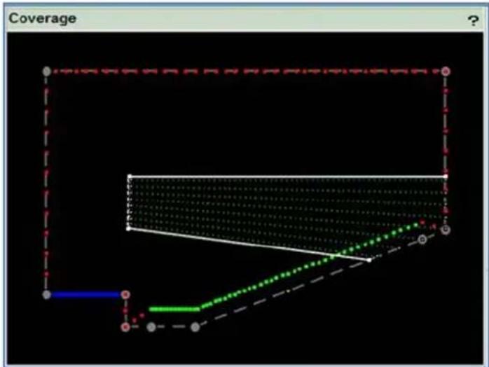
flowchart
graph TD
    A["Start"] --> B{Decision}
    B -->|Yes| C["Path 1"]
    B -->|No| D["Path 2"]
    C --> E["End"]
    D --> F["End"]
When you start the optimisation process which window switches to an index plot showing in real time the acoustic performance as different inter cabinet angles are tried; -
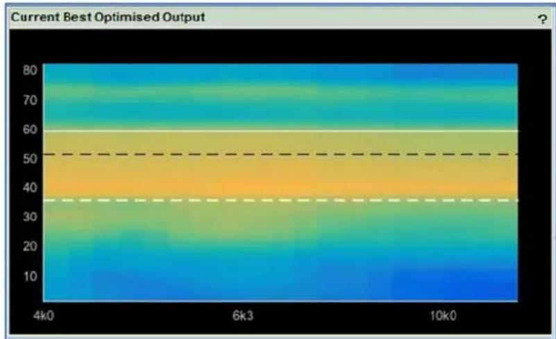
heatmap
| | 4k0 | 6k3 | 10k0 | | ------ | ---- | ---- | ---- | | 80 | | | | | 70 | | | | | 60 | | | | | 50 | | | | | 40 | | | | | 30 | | | | | 20 | | | | | 10 | | | |This gives you an instant comparison to the Current Acoustic Output; essentially a "before" and "after" to see how manually articulating the array has improved the coverage.
One completed the window reverts to the coverage diagram showing the articulated array with the white lines from the centre of the upper and lower cabinets again showing where the acoustic centres are pointing; -
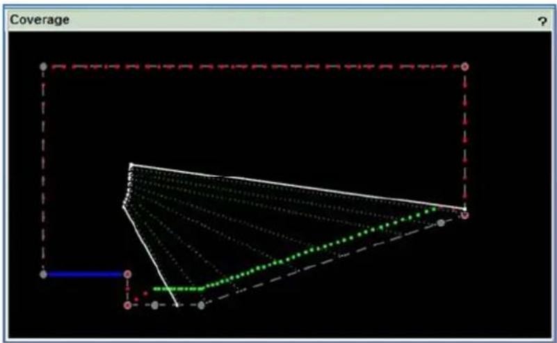
text_image
Coverage ?Current Acoustic Output
This shows an Index Plot of the system prior to the optimisation process.
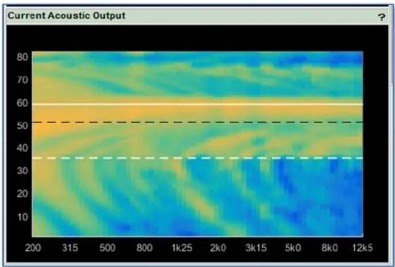
heatmap
| X Range | Y Range | Value | |---------|---------|-------| | 200-315 | 10-20 | ~30 | | 200-315 | 20-30 | ~40 | | 200-315 | 30-40 | ~50 | | 200-315 | 40-50 | ~60 | | 200-315 | 50-60 | ~70 | | 200-315 | 60-80 | ~80 | | 315-500 | 10-20 | ~30 | | 315-500 | 20-30 | ~40 | | 315-500 | 30-40 | ~50 | | 315-500 | 40-50 | ~60 | | 315-500 | 50-60 | ~70 | | 315-500 | 60-80 | ~80 | | 500-800 | 10-20 | ~30 | | 500-800 | 20-30 | ~40 | | 500-800 | 30-40 | ~50 | | 500-800 | 40-50 | ~60 | | 500-800 | 50-60 | ~70 | | 500-800 | 60-80 | ~80 | | 800-1k25 | 10-20 | ~30 | | 800-1k25 | 20-30 | ~40 | | 800-1k25 | 30-40 | ~50 | | 800-1k25 | 40-50 | ~60 | | 800-1k25 | 50-60 | ~70 | | 800-1k25 | 60-80 | ~80 | | 1k25 | 10-20 | ~30 | | 1k25 | 20-30 | ~40 | | 1k25 | 30-40 | ~50 | | 1k25 | 40-50 | ~60 | | 1k25 | 50-60 | ~70 | | 1k25 | 60-80 | ~80 | | 2k2 | 10-20 | ~30 | | 2k2 | 20-30 | ~40 | | 2k2 | 30-40 | ~50 | | 2k2 | 40-50 | ~60 | | 2k2 | 50-60 | ~70 | | 2k2 | 60-80 | ~80 | | 3k2 | 10-20 | ~30 | | 3k2 | 20-30 | ~40 | | 3k2 | 30-40 | ~50 | | 3k2 | 40-50 | ~60 | | 3k2 | 50-60 | ~70 | | 3k2 | 60-80 | ~80 | | 5k2 | 10-20 | ~30 | | 5k2 | 20-30 | ~40 | | 5k2 | 30-40 | ~50 | | 5k2 | 40-50 | ~60 | | 5k2 | 50-60 | ~70 | | 5k2 | 60-80 | ~80 | | 8k2 | 10-20 | ~30 | | 8k2 | 20-30 | ~40 | | 8k2 | 30-40 | ~50 | | 8k2 | 40-50 | ~60 | | 8k2 | 50-60 | ~70 | | 8k2 | 60-80 | ~80 | | 12k5 | 10-20 | ~30 | | 12k5 | 20-30 | ~40 | | 12k5 | 30-40 | ~50 | | 12k5 | 40-50 | ~60 | | 12k5 | 50-60 | ~70 | | 12k5 | 60-80 | ~80 |Calculation
The Calculation section shows the physical orientation of the overall array. From here the number of boxes is defined and can be changed if for any reason the initial array size was incorrect. You have the option to change the number of cabinets. You can however only change the number to a quantity that is appropriate to the deployment method selected so a maximum of 6 for ground stacked MLA or MLA Compact, 8 for ground stacked MLA Mini 12 for MLA Mini flown with MSX.
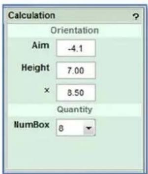
text_image
Calculation Orientation Aim -4.1 Height 7.00 x 8.50 Quantity NumBox 8The height to the top of the array and distance from the origin is also shown and can be edited to match the physical deployment of the system, very useful if for example it wasn't possible to fly the array exactly where you planned, perhaps the points couldn't be placed as high as you wanted.
The tilt of the entire array is shown and will be automatically generated as part of the optimisation process. It is also possible to overwrite this if necessary to match the actual tilt of the array, given the resolution of most chain hoists it is frequently difficult to exactly match a given tilt angle even with front and back motors.
The number of enclosures can also be edited at this stage. Perhaps a cabinet has been damaged in transit and won't physically attach to the array or perhaps you decide to add MLD cabinets to the bottom of an MLA array you can over-type the number shown to the maximum number allowed.
Optimisation
The Optimisation section is available in Advanced and Expert modes. In Advanced mode it is closed by default; -

The window is expanded as before by clicking on the icon in the right-hand corner; -

This window is where the optimisation characteristics are refined. The splay coefficients determine the priority given to either the target response or the leakage. The actual numbers entered are not important, it is the ratio between them that determine how much priority is given to each coefficient so if you want the Target coefficient to be twice as important as Leakage you can enter '2' in Target and leave leakage as '1' or you could leave Target as '1' and change Leakage to '0.5' the result would be exactly the same.
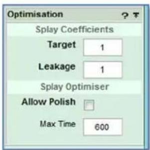
text_image
Optimisation Splay Coefficients Target 1 Leakage 1 Splay Optimiser Allow Polish Max Time 600Allow Polish lets the software take a second run at refining the inter-cabinet angles after it has completed the first pass. It re-starts the optimisation when it has completed the first attempt with the angles it has already calculated as a starting point and further refines them to get the best possible result. If you are in a rush you may want to disable this feature, particularly for very large arrays which may take some time to optimise.
The Max Time is the time in seconds that the system will allow for the optimisation to run. For the vast majority of systems the default setting of 600 seconds (10 minutes) will be more than adequate, particularly when Display 2.3 is run on a high spec PC. With very large arrays in complex venues you may need to increase this time to get the best optimisation assuming you have the time at your disposal. If you don't have sufficient time the optimisation will time out and you will see a warning suggesting that you increase the Maximum Time. You can however, accept the angles it has calculated at any stage or even enter your own angles manually and the Equalisation optimisation will work from these angles albeit with a slight compromise on the system performance. Whilst some array angles may look strange to those used to working with conventional line arrays, always trust the software! Multicellular systems are NOT line arrays so don't try and use them in the same way.
Run the optimisation
Click on the Optimise button; -
The system will run through all possibly array angle configurations. The drawing will show the array moving through the various positions and will be green; -
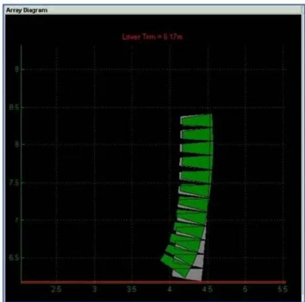
bar
Array Diagram | X-Axis (Value) | Y-Axis (Value) | | :--- | :--- | | 4.0 | 6.5 | | 4.1 | 6.6 | | 4.2 | 6.7 | | 4.3 | 6.8 | | 4.4 | 6.9 | | 4.5 | 7.0 | | 4.6 | 7.1 | | 4.7 | 7.2 | | 4.8 | 7.3 | | 4.9 | 7.4 | | 5.0 | 7.5 | | 5.1 | 7.6 | | 5.2 | 7.7 | | 5.3 | 7.8 | | 5.4 | 7.9 | | 5.5 | 8.0 | Lower Tim = 6.17mWhen it has completed its first pass it will start again on its polish cycle if you have checked this option. The array will change colour to yellow. When the optimisation is finished you will see the array diagram with the array now stationary. The yellow polished version will be superimposed above the green un-polished version. The final lower trim height is also displayed;

line
| x | y | | ---- | ----- | | 8.0 | 7.5 | | 8.2 | 8.0 | | 8.4 | 8.5 | | 8.6 | 9.0 | | 8.8 | 9.5 | | 9.0 | 10.0 | | 9.2 | 10.5 | | 9.4 | 11.0 |If you have de-selected the 'Auto Use Splay' option in preferences, a new button will appear on the bottom right of the window;

text_image
Optimise Use DoneIf we click on 'Use' the angles calculated will be imposed onto the Splay Angles list. With the Auto Use Splay enabled we will see the calculated angles immediately applied to the array. Here we see a "before" and "after"; -
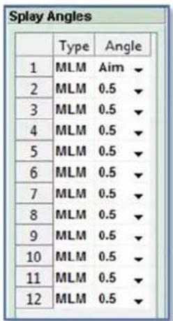
text_image
Splay Angles Type Angle 1 MLM Aim 2 MLM 0.5 3 MLM 0.5 4 MLM 0.5 5 MLM 0.5 6 MLM 0.5 7 MLM 0.5 8 MLM 0.5 9 MLM 0.5 10 MLM 0.5 11 MLM 0.5 12 MLM 0.5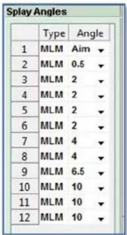
text_image
Splay Angles Type Angle 1 MLM Aim 2 MLM 0.5 3 MLM 2 4 MLM 2 5 MLM 2 6 MLM 2 7 MLM 4 8 MLM 4 9 MLM 6.5 10 MLM 10 11 MLM 10 12 MLM 10We also have the Calculation window showing the complete mechanical articulation of the array including the array tilt; -
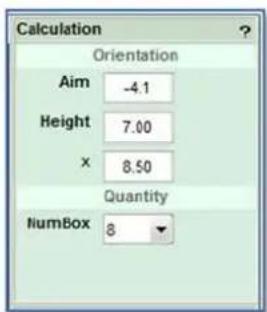
text_image
Calculation Orientation Aim -4.1 Height 7.00 x 8.50 Quantity numBox 8The tilt figure is reasonably logical; a positive figure means the array is tilting up at the top, a negative figure means the array is tilting down. The touring array grids feature an integral inclinometer system so these figures can be matched when the system is flow. The Inclinometer system is an optional accessory on Wavefront Precision systems
One major advantage of the MLA and Wavefront Precision family of systems optimised with D2.3 is that real-world figures for the rigging can be entered if they don't actually exactly match what the system has recommended. If for example there are constraints on the curvature of the array you can click on the down arrow for each of the intercabinet angles you need to change and select the angle you would like to use from the drop down. It is always best to accept the splay optimisation results wherever possible (always trust the software!) but there will always be a few venues where there are physical limitations on exactly how you can deploy the system.
Likewise, with the enclosure quantities and orientation. Most common is perhaps array height; it is very common for flying points to end up lower than you have originally been told. It is vital to make any changes in Display 2.3 to match as closely as possible the actual physical deployment of the system. The EQ optimisation will use the data on this page regardless whether it was entered automatically by the splay optimisation or manually by you. Simply overwrite the number for tilt, height, 'x' position or box quantities and press enter. If the number entered is a valid entry the box will briefly flash green and your new value will be displayed. If you enter an invalid number, for example if you try and enter more than 16 MLA Mini, the box will briefly flash red and will default to the maximum value.
We have completed the Splay optimisation so can click 'Done' to close the window and move to the next stage.
Rig Tab
The rigging tab displays all the mechanical information required for rigging a system including the array height, lower trim, mass and all splay angles. This tab is identical in both UI options, Basic and Expert.
As the rigging hardware is different for each of the Systems there are variations in how the Rig Tab appears so we will look at the types of system individually starting with MLA
MLA
The left-hand section shows the system flown by default using the flying frame from a single point.
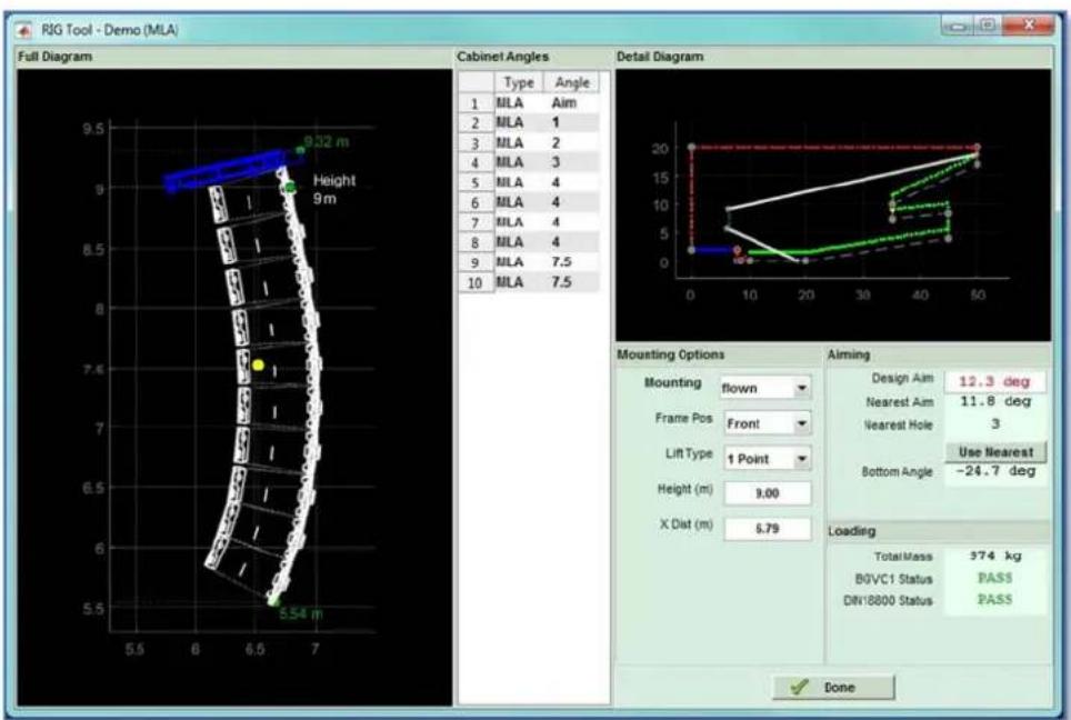
text_image
RJG Tool - Demo (MLA) Full Diagram Cabinet Angles Type Angle 1 MLA Aim 2 MLA 1 3 MLA 2 4 MLA 3 5 MLA 4 6 MLA 4 7 MLA 4 8 MLA 4 9 MLA 7.5 10 MLA 7.5 Detail Diagram 20 15 10 5 4 3 2 1 0 Mounting Options Aiming Mounting flown Beforeing Frame Pos Front Design Aim 12.3 deg Nearest Aim 11.8 deg Nearest Hole 3 Lift Type 1 Point Use Nearest Bottom Angle -24.7 deg Height(m) 9.00 X Dist(m) 5.79 Loading Total Mass 574 kg B0VC1 Status PASS DIN18800 Status PASS DoneThere are a number of important sections to the screen. First is the array diagram showing a scale picture of the flown array accurately displaying the physical deployment of the array; -
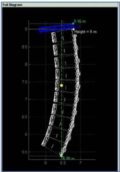
other
| Height (m) | Base Width (m) | |------------|----------------| | 9.16 | 6.58 |This is useful so you can quickly see if there are any mechanical issues with the array that might make flying in a particular venue difficult; perhaps the rear of the array is hanging back further than you initially thought and might impede something else that is flown close to it such as lighting or scenery. The lower trim point is also displayed so the array can be accurately flown to the correct height. It can be measured either by the time-honoured method of attaching a tape measure or using a laser measure such as the Leica Disto D8. The green cross with dotted lines shows the centre of gravity of the array.
Next is a list of the splay angles; -
| Cabinet Angles | ||
| Type | Angle | |
| 1 | MLA | Aim |
| 2 | MLA | 0.5 |
| 3 | MLA | 1 |
| 4 | MLA | 4 |
| 5 | MLA | 5 |
| 6 | MLA | 4 |
| 7 | MLA | 2 |
| 8 | MLA | 4 |
| 9 | MLA | 4 |
| 10 | MLA | 7.5 |
This gives you all the information you need to set the inter-cabinet angles when you are flying the system.
There is a thumbnail diagram of the entire venue which will update as you make changes to the rigging; -
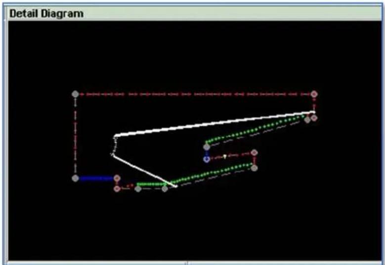
flowchart
graph TD
    A["Start"] --> B["Path 1"]
    B --> C["Path 2"]
    C --> D["End"]
    style A fill:#f9f,stroke:#333
    style B fill:#ccf,stroke:#333
    style C fill:#cfc,stroke:#333
    style D fill:#fcc,stroke:#333
Note that the examples shown are for an array which is possible to fly. If the optimisation creates an array that is impossible to realise within the capabilities of the flying frame the array diagram will show a warning flag as shown here; -
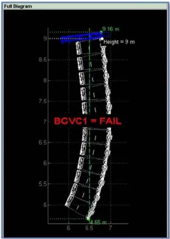
text_image
Full Diagram 9 16 m Height = 9 m 7 6.5 m 4.65 m BGVC1 = FAILIn this case it is necessary to chance the height and possibly coverage area of the array until a "legal" array shape is produced or in the case above, reduce the number of cabinets or switch to a two point hang.
The final section shows the mounting option and results; -
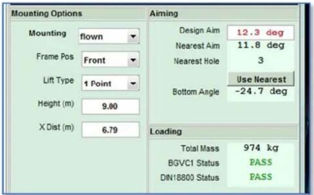
text_image
Mounting Options Aiming Mounting flown Design Aim 12.3 deg Nearest Aim 11.8 deg Nearest Hole 3 Lift Type 1 Point Use Nearest Height (m) 9.00 Bottom Angle -24.7 deg X Dist (m) 6.79 Loading Total Mass 974 kg BGVC1 Status PASS DIN18800 Status PASSThe first option for mounting determines how the array is to be deployed Using the Mounting drop-down; -
text_image
Mounting flownFor MLA there are only two options, flown or ground stacked. Ground stack is only available for an array of six boxes or less, if the array is larger than six you will see this message; -
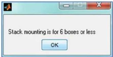
text_image
Stack mounting is for 6 boxes or less OKThere are options for the flying of systems, when flying MLA there are two positions on the flying grid from which they can be fitted; front and rear. This gives different angle options depending on whether the array has a steep upward or downward tilt. Front and rear can be selected using the Frame Pos. drop-down; -
text_image
Frame Pos. FrontThe 'Lift Type' refers to the number of hoists used to fly the array which can either be one using one of the holes along the spine of the flying frame, or two attaching one to the front-most point and the second to the rear-most point. This is selected with the drop-down; -

text_image
Lift Type 1 PointThe Aiming and Loading sections will change depending on the various options selected. Here we have the results for a single point hang of three MSX and twelve MLA Mini; -
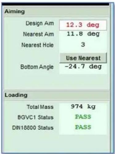
text_image
Aiming Design Aim 12.3 deg Nearest Aim 11.8 deg Nearest Hole 3 Use Nearest Bottom Angle -24.7 deg Loading Total Mass 974 kg BGVC1 Status PASS DIN18800 Status PASSThis shows the total mass of the array including the flying frame to be 974Kg (Note that the Rig tool does not yet show imperial measurements even if Metric is un-checked in preferences). It shows that the optimisation specified an upwards tilt (a down tilt will be signified with a minus number) of 12.3°, by using the Nearest Hole as displayed, in this example hole 3, the actual tilt created is 11.8°. If we click on the 'Use Nearest' button the array tilt will be changed to match what the actual flying grid will achieve. This means that when you proceed to the next stage of optimising the equalisation, Display 2.3 will optimise for the array positioned exactly as it will be in the real world giving the most accurate optimisation possible. When you click 'Use Nearest', the Design Aim will change to match the actual Aim angle and will turn green;
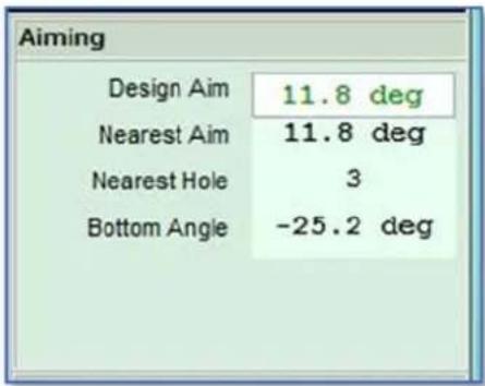
text_image
Aiming Design Aim 11.8 deg Nearest Aim 11.8 deg Nearest Hole 3 Bottom Angle -25.2 degNote that if by a happy coincidence the 'Nearest Hole' gives an angle which happens to match the Design angle the identical angles will automatically be green.
The Aiming section also displays the angle of the bottom cabinet making it easy to check the angle of the array before it is flown out using a portable inclinometer, or the inclinometer option on a Disto laser measure.
The Loading box displays the total array mass including the flying grid and cables and weather the flying system meets BGVC1 or DIN18800; -
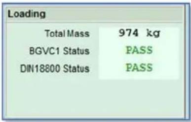
text_image
Loading Total Mass 974 kg BGVC1 Status PASS DIN18800 Status PASSIf you select the 2 Point option the Aiming changes to simply show the required aim and the Bottom cabinet angle as you can adjust the array tilt by raising and lowering front or rear hoists; -
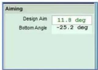
text_image
Aiming Design Aim 11.8 deg Bottom Angle -25.2 degThe loading section will also change to show how the total array mass is distributed between the points; -
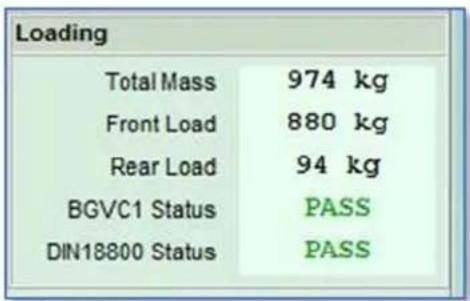
text_image
Loading Total Mass 974 kg Front Load 880 kg Rear Load 94 kg BGVC1 Status PASS DIN18800 Status PASSThis shows the mass that each point will see, in this example 830Kg for the front point and 94Kg for the rear point.
Ground Stacking
Assuming you have 6 MLA or less you have the option of ground stacking.
If you select 'On Ground' you will first see a warning that the array height may change and that it is advisable to re-calculate the splay angles back in the splay tab; -
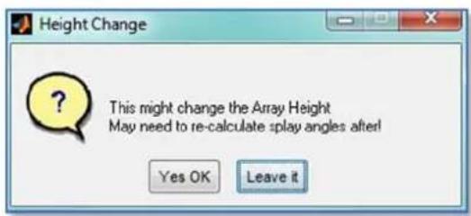
text_image
Height Change This might change the Array Height May need to re-calculate splay angles after! Yes OK Leave itClick 'Yes OK to proceed and the array diagram will update accordingly; -
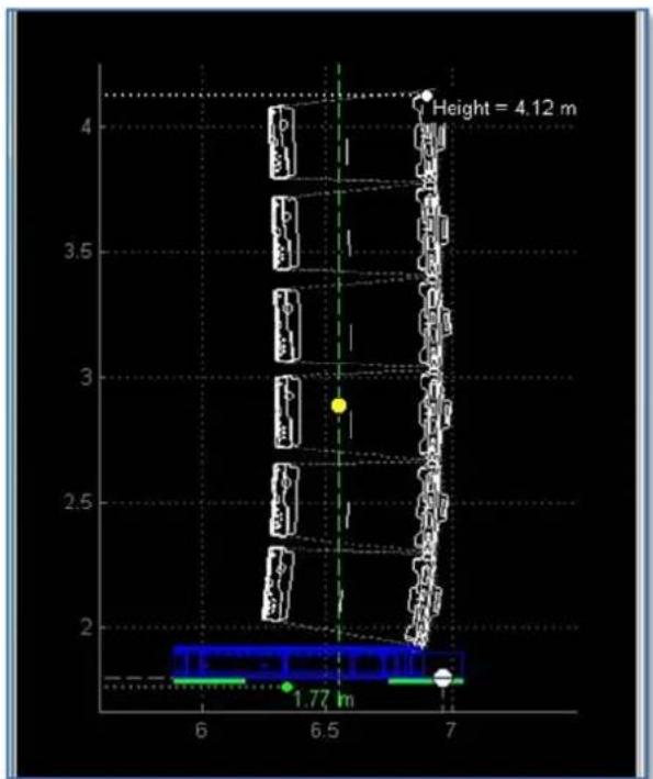
scatter
| Height (m) | X | Y | | ---------- | ---- | ---- | | 4.12 | 7.0 | 1.77 |'On Ground' refers to the lowest point on the venue slice available for the horizontal (front to back) position for the array. If for example the array is placed on a stage, selecting 'On Ground' will result in a Lower trim equal to the stage.
For either option the results section will also update showing the total array mass and the required ground stack bar and number to use to get the closest angle to the design figure; -
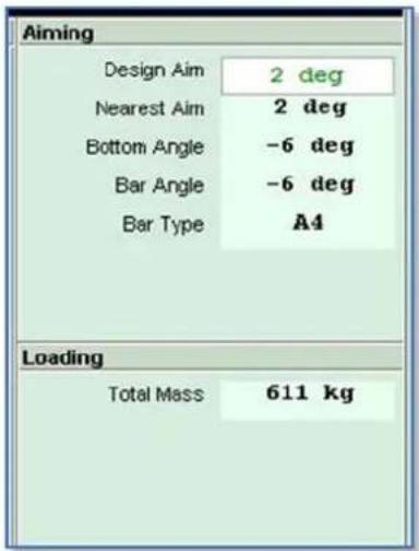
text_image
Aiming Design Aim 2 deg Nearest Aim 2 deg Bottom Angle -6 deg Bar Angle -6 deg Bar Type A4 Loading Total Mass 611 kgThe MLA ground stack bar has three holes, one which locates in the flying frame and two holes labelled 'A' and 'B' which are used in the rear rigging bracket holes to achieve the desired up or down tilt. In this this example hole A is used in the 4° hole to achieve the aim angle of 2°. The bottom angle is also shown, clearly in most ground stack applications you could easily check the angle of the top cabinet but you have the option of checking the bottom cabinet if for some reason the top cabinet cannot be easily or safely reached, a system stacked on top of several subs or a high piece of staging for example.
In the above example the nearest aim matches what is achievable with the ground stack bar in the appropriate hole therefore the Design Aim is automatically green. If this was not the case there would be exactly the same option available as with a flown system of using the nearest angle available which will adjust the array angle ready for the EQ optimisation
MLA Compact
The rigging options for MLA Compact are almost identical to MLA as it has exactly the same constraints; a maximum of 24 flown cabinets and 6 ground stacked. The rigging windows therefore look pretty much the same. A flown system appears like this; -
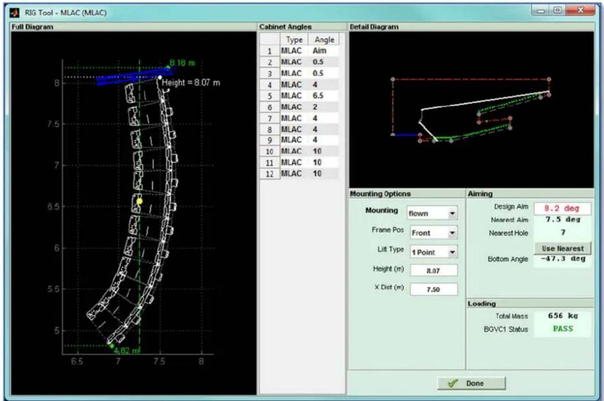
text_image
RIG Tool - MLAC (MLAC) Full Diagram Cabinet Angles Detail Diagram 1 Type Angle MLAC Aim 2 MLAC 0.5 MLAC 0.5 4 MLAC 4 MLAC 6.5 MLAC 2 7 MLAC 4 8 MLAC 4 9 MLAC 4 10 MLAC 10 11 MLAC 10 12 MLAC 10 Mounting Options Aiming Design Aim 8.2 deg Nearest Aim 7.5 deg Nearest Hole 7 Litt Type 1 Point Use Nearest Bottom Angle -47.3 deg Height (m) 8.07 X Dist (m) 7.50 Loading Total Mass 656 kg BGVC1 Status PASS DoneAnd a ground stack system like this; -
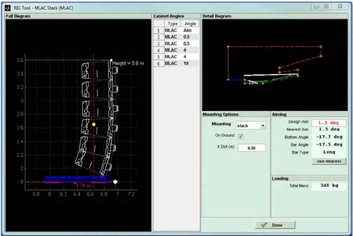
text_image
RIG Tool - MLAC Stack (MLAC) Full Diagram Cabinet Angles Detail Diagram Type Angle 1 MLAC Aim 2 MLAC 0.5 3 MLAC 0.5 4 MLAC 4 5 MLAC 4 6 MLAC 10 Height = 3.6 m Mounting Options Aiming Mounting stack Design Aim 1.3 deg On Ground Nearest Aim 1.5 deg X Dist (m) Bottom Angle -17.7 deg 6.90 Bar Angle -17.5 deg Bar Type Long use nearest Loading Total Mass 340 kg DoneThe principal difference is how the ground stack information is displayed. MLA Compact has two versions of ground stack bar, a long bar for arrays requiring a down-tilt as shown in the example above, and a short bar for arrays that require an up-tilt. As the example above shows, the Aiming panel shows which type of bar; -
text_image
Aiming Design Aim 1.5 deg Nearest Aim 1.5 deg Bottom Angle -17.5 deg Bar Angle -17.5 deg Bar Type LongRather than specifying which hole in the bar is shows the bar angle as the bar itself has a label with shows which holes to use to achieve the desired angle. Once again where there is a difference in the design aim to that which can be achieved with the ground stack bar the design aim is shown in red with the 'Use Nearest' option available. If clicked the design aim and array diagram will be updated; -
text_image
Aiming Design Aim 1.5 deg Nearest Aim 1.5 deg Bottom Angle -17.5 deg Bar Angle -17.5 deg Bar Type LongHere we see a ground stack array which has an up-tilt; -
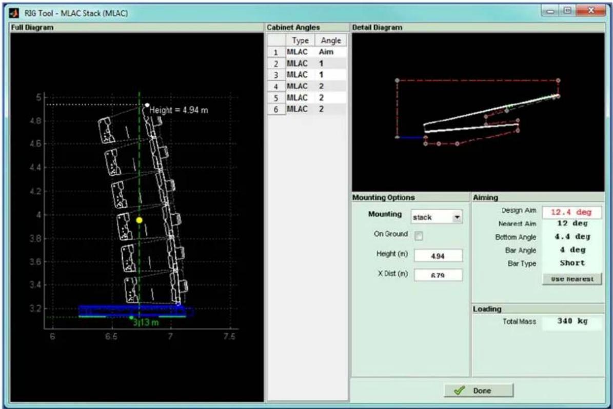
text_image
RIG Tool - MLAC Stack (MLAC) Full Diagram Cabinet Angles Detail Diagram 1 MLAC Aim 2 MLAC 1 3 MLAC 1 4 MLAC 2 5 MLAC 2 6 MLAC 2 Height = 4.94 m Mounting Options Aiming Design Aim 12.4 deg Nearest Aim 12 deg Bottom Angle 4.4 deg Bar Angle 4 deg Bar Type Short Use nearest Loading Total Mass 340 kg DoneThe aiming panel looks similar but is specifying the short ground stack bar; -
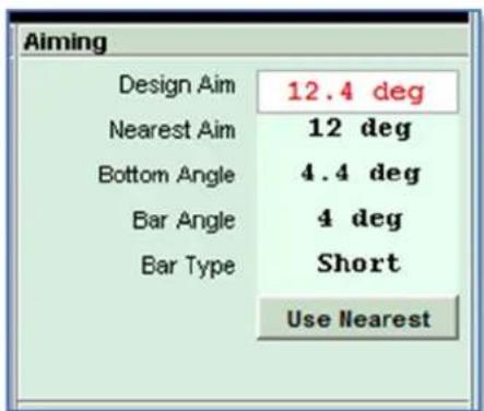
text_image
Aiming Design Aim 12.4 deg Nearest Aim 12 deg Bottom Angle 4.4 deg Bar Angle 4 deg Bar Type Short Use NearestMLA Mini
MLA Mini has several deployment option for both flown and ground stacked systems. This changes the options and information in the rigging panel
Flown system
The Window for a flown MLA mini system appears like this; -
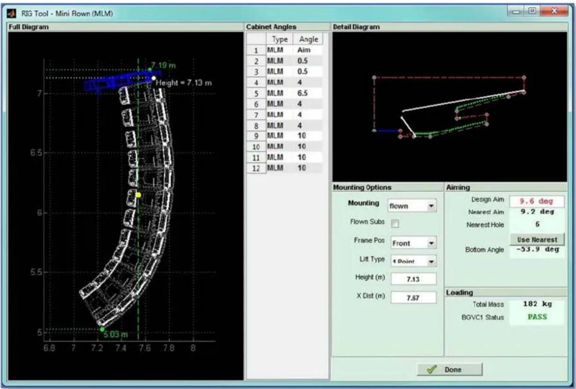
text_image
RIG Tool - Mini Frown (MLM) Full Diagram Cabinet Angles Detail Diagram 1 MLM Aim 2 MLM 0.5 3 MLM 0.5 4 MLM 4 5 MLM 6.5 6 MLM 4 7 MLM 4 8 MLM 4 9 MLM 10 10 MLM 10 11 MLM 10 12 MLM 10 Mounting Options Aiming Mounting flown Design Aim 9.6 deg Flown Subs Nearest Aim 9.2 deg Frame Pos Front Nearest Hole 6 Lift Type 4 Point Bottom Angle Use Nearest -53.9 deg Height (m) 7.13 X Dist (m) 7.67 Loading Total Mass 182 kg BGVC1 Status PASS DoneIf we look first at the Mounting panel we have a number of options; -
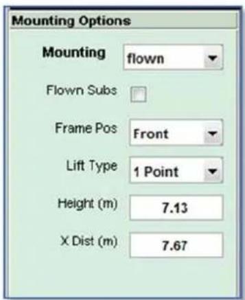
text_image
Mounting Options Mounting flown Flown Subs Frame Pos Front Lift Type 1 Point Height (m) 7.13 X Dist (m) 7.67First we have the 'Mounting' drop-down which gives us the option of flown, stacked or pole mount. Availability of these modes is dependent on the number of boxes. Flown can be the full complement of 16, ground stacked up to 8 and pole mount up to 4. As the array in the example has 12 enclosures we cannot select stacked or pole mount, if we try we will see the following windows; -
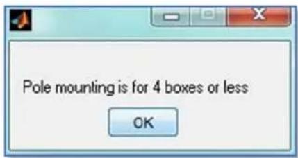
text_image
Pole mounting is for 4 boxes or less OK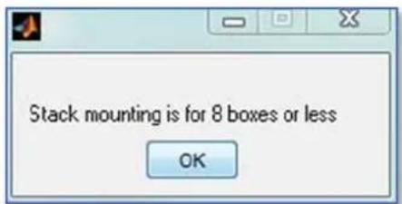
text_image
Stack mounting is for 8 boxes or less OKNext we have the option to fly the MSX subs with the arrays if this wasn't selected when the array was initially added to the project. This again has the limitation that it is only available for up to 12 enclosures, if the array is more than 12 cabinets the flown subs option will not appear.
Here is the system above with flown subs; -
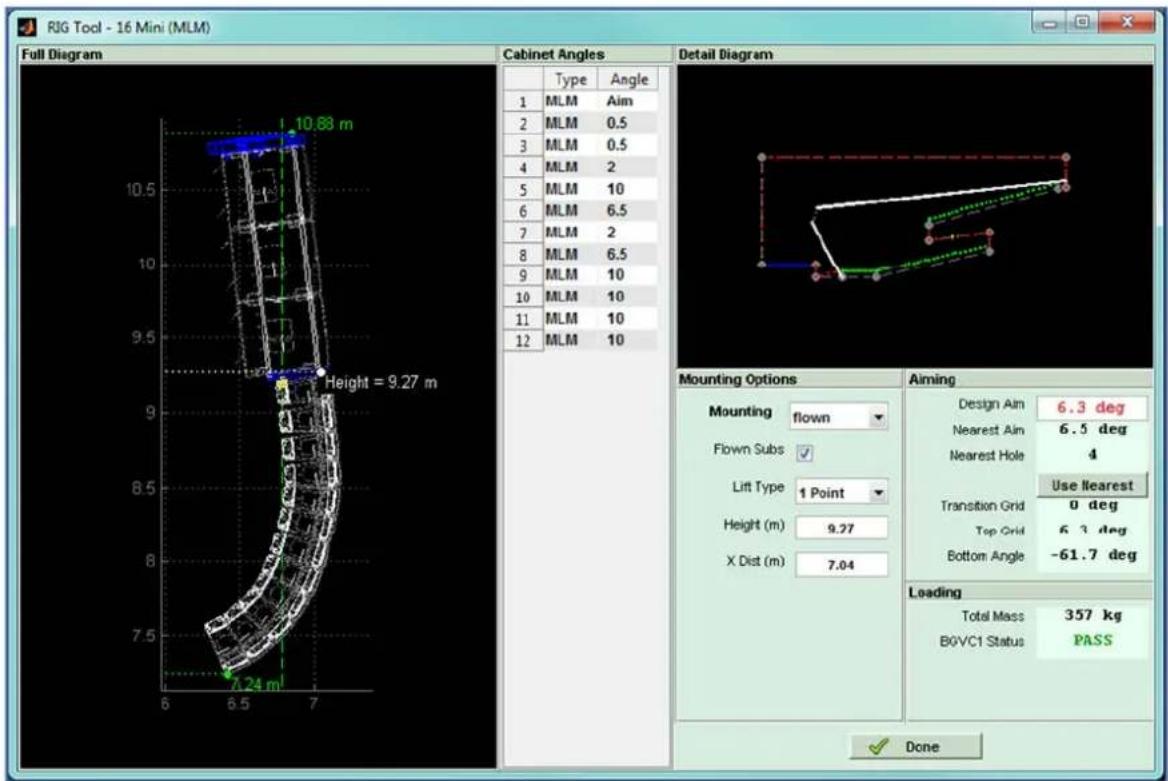
text_image
RIG Tool - 16 Mini (MLM) Full Diagram Cabinet Angles Detail Diagram 1 Type Angle MLM Aim 2 MLM 0.5 3 MLM 0.5 4 MLM 2 5 MLM 10 6 MLM 6.5 7 MLM 2 8 MLM 6.5 9 MLM 10 10 MLM 10 11 MLM 10 12 MLM 10 Height = 9.27 m Mounting Options Aiming Flown Subs Lift Type 1 Point Height (m) 9.27 X Dist (m) 7.04 Design Aim 6.3 deg Nearest Aim 6.5 deg Nearest Hole 4 Use Ilearest Transition Grid 0 deg Top Grid 6.3 deg Bottom Angle -61.7 deg Leading Total Mass 357 kg BGVC1 Status PASS DoneAs with MLA and MLA Compact systems you can select 1 or 2 point hangs, the difference is that even with the maximum flown MLA Mini, either 16 alone or 12 with 3 MSX, they will still be within BGVC1 limits from a single point. 2 point does of course give you the flexibility of trimming the array angle by fine adjustment of one or other hoists.
As with MLA and MLA Compact the Aiming panel shows the array design angle and what is achievable with the nearest hole on the flying grid; -
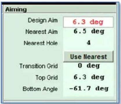
text_image
Aiming Design Aim 6.3 deg Nearest Aim 6.5 deg Nearest Hole 4 Use Nearest Transition Grid 0 deg Top Grid 6.3 deg Bottom Angle -61.7 degAgain by clicking on 'Use Nearest' the Design Aim will change to match the available angle and will turn green; -
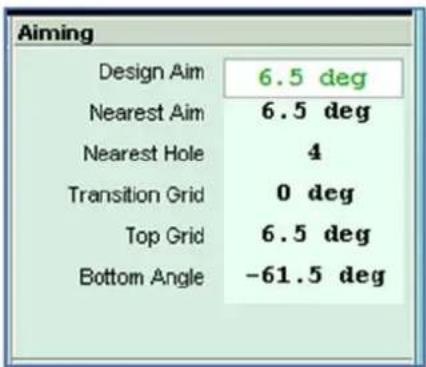
text_image
Aiming Design Aim 6.5 deg Nearest Aim 6.5 deg Nearest Hole 4 Transition Grid 0 deg Top Grid 6.5 deg Bottom Angle -61.5 degNote that there are two angles that need to be defined when flying with MSX subs. The main array angle set by using the appropriate hole in the flying grid, and the angle between the MSX and the MLA Mini which is set using the rear rigging bracket on the MLA Mini Transition frame. There are three positions, the angle will be shown in the aiming panel. The example above is zero degrees but Display will attempt to keep the MSX subs as close to horizontal as possible so will add the additional tilt that may be required by using the extra angles that are available from the transition frame.
Ground Stacking
Here we see an eight box MLA Mini ground stack; -
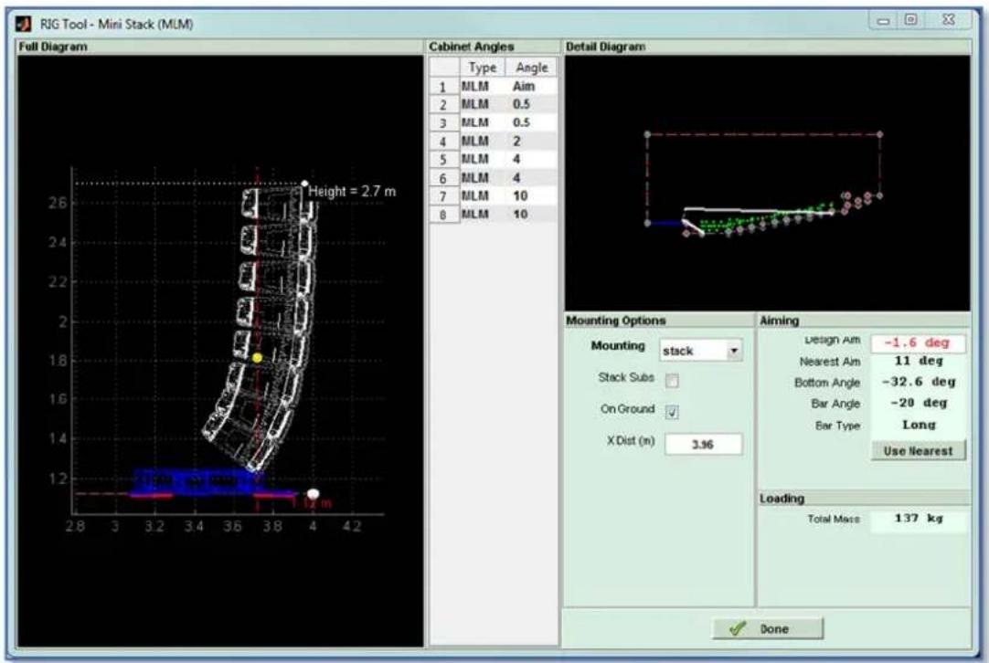
text_image
RIG Tool - Mini Stack (MLM) Full Diagram Height = 2.7 m Cabinet Angles Detail Diagram Type Angle 1 MLM Aim 2 MLM 0.5 3 MLM 0.5 4 MLM 2 5 MLM 4 6 MLM 4 7 MLM 10 8 MLM 10 Mounting Options Aiming Mounting stacks Stack Subs On Ground X Dist (n) 3.36 Design Aim -1.6 deg Nearest Aim 11 deg Bottom Angle -32.6 deg Bar Angle -20 deg Bar Type Long Use Nearest Loading Total Mass 137 kg DoneThe principal difference with MLA Mini is in the Mounting Options; -
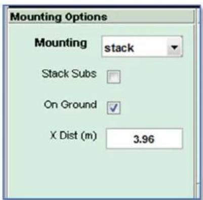
text_image
Mounting Options Mounting stack Stack Subs On Ground ✓ X Dist (m) 3.96We now have the option to stack on top of the subs. This option will add the MSX subs below the array, a single sub for 1 to 4 cabinets and two MSX for 5 to 8 cabinets. This will naturally change the height of the array so you will see this window to prompt you to recalculate splay angles in the splay Tab.
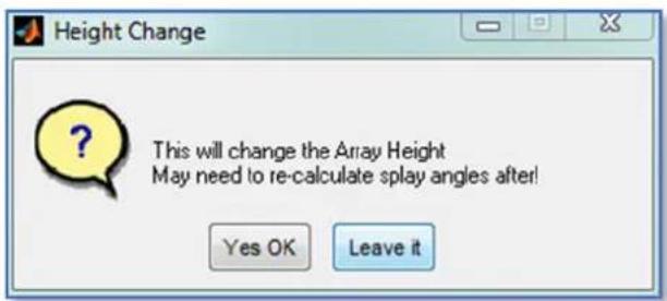
text_image
Height Change This will change the Array Height May need to re-calculate splay angles after! Yes OK Leave itThe Array Diagram will update to show the Subs; -
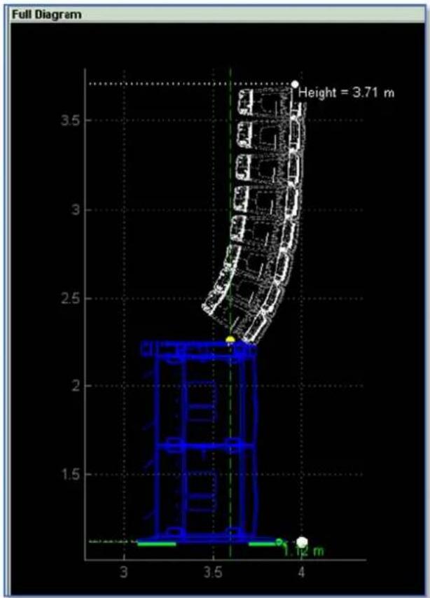
text_image
Full Diagram Height = 3.71 m 1.12 mAs with ground stacked MLA and MLA Compact ground stacked systems, if the array is not already locked to the ground using the option in the Slice tab, you can select it here; -
text_image
Stock Subs ✓ On Ground ✓ X Diet (m)As this may change the array height you will see the same pop-up window prompting you to re-calculate splay angles.
The Aiming panel is virtually identical to the MLA Compact; -
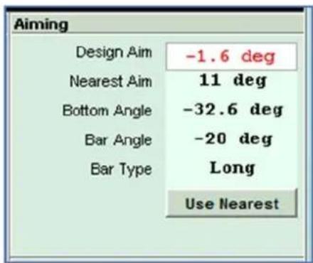
text_image
Aiming Design Aim -1.6 deg Nearest Aim 11 deg Bottom Angle -32.6 deg Bar Angle -20 deg Bar Type Long Use NearestAs with Compact, Display will calculate the closest angle available using the ground stack bar and if this doesn't match the Design aim it will be displayed in red with the option to 'Use Nearest'. Once again this option will change the Design angle to match the actual angle of the array so the EQ optimisation will be based on exactly where how the array is angled; -
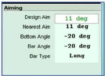
text_image
Aiming Design Aim 11 deg Nearest Aim 11 deg Bottom Angle -20 deg Bar Angle -20 deg Bar Type LongAs with Compact there are two types of ground stack bar, a long and a short. For ground stack arrays which require a down-tilt on the bottom enclosure the long bar is used as in the above example, for array which require an up-tilt the short bar is used; -
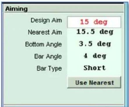
text_image
Aiming Design Aim 15 deg Nearest Aim 15.5 deg Bottom Angle 3.5 deg Bar Angle 4 deg Bar Type Short Use NearestAlso in common with MLA Compact, the ground stack bars are labelled with the angles that they can produce so that is shown in the Aiming panel rather than which particular holes in the bar and cabinet to use.
Pole Mount
The final option for rigging is pole mount available for two to four MLA Mini on top of a single MSX using the ASF20071 wind-up distance pole which is supplied with either the fixed or adjustable pole mount assemblies or can be purchased as an accessory and used with the MLA Mini Universal Bracket (ASF20051) and the Pole Mount Adaptor (ASF20045).
Here is an initial Rig Tool Window for a pole mount system following a 4 cabinet optimisation; -
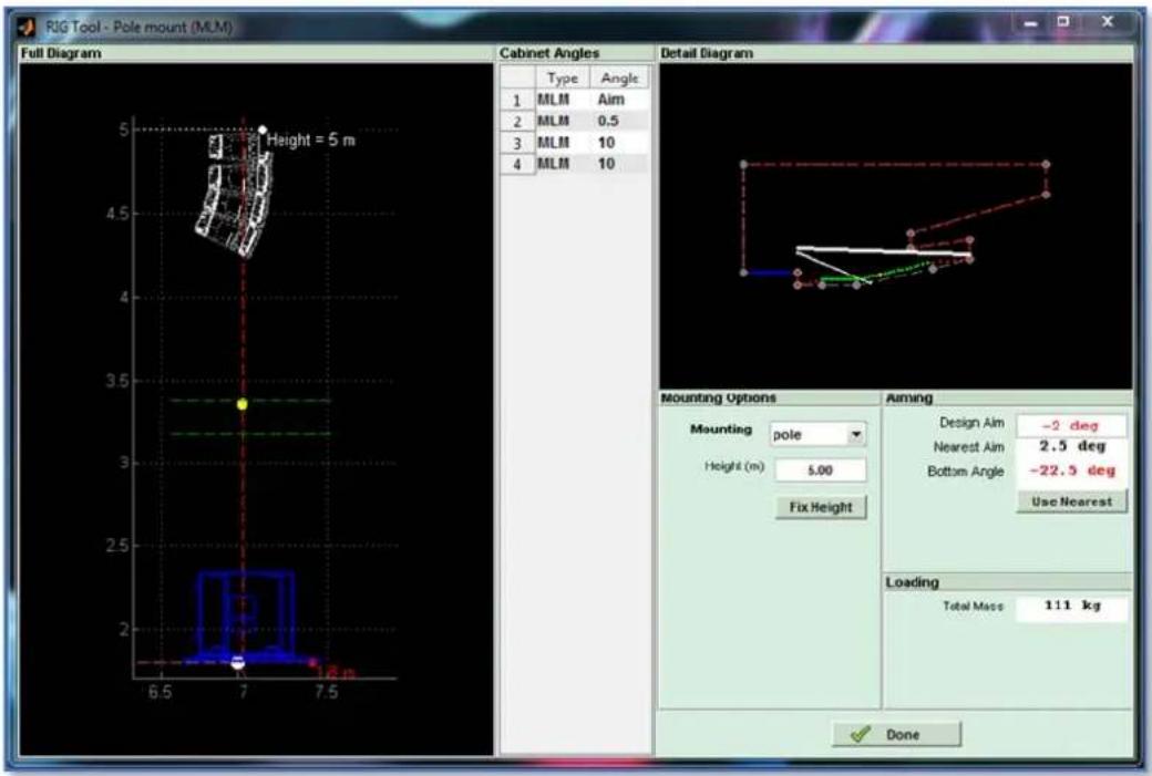
text_image
RIG Tool - Pole mount (MLM) Full Diagram Cabinet Angles Detail Diagram Type Angle 1 MLM Aim 2 MLM 0.5 3 MLM 10 4 MLM 10 Height = 5 m Mounting Options Aiming Mounting pole Design Aim -2 deg Height(m) 5.00 Nearest Aim 2.5 deg Fix Height Bottom Angle -22.5 deg Loading Total Mass 111 kg DoneWe can see that the array is far too high to fit on the standard pole so the first job is to correct the height to something that is usable in the real world. This is provided for pole mount deployment by the 'Fix Height' button; -
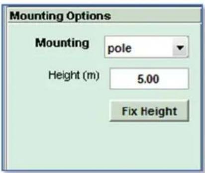
text_image
Mounting Options Mounting pole Height (m) 5.00 Fix HeightClicking this will lower the array, again showing the warning pop-up that the array height will change; -
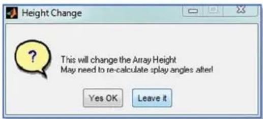
text_image
Height Change This will change the Array Height May need to re-calculate splay angles after! Yes OK Leave itThe array is now at a sensible height above the MSX; -
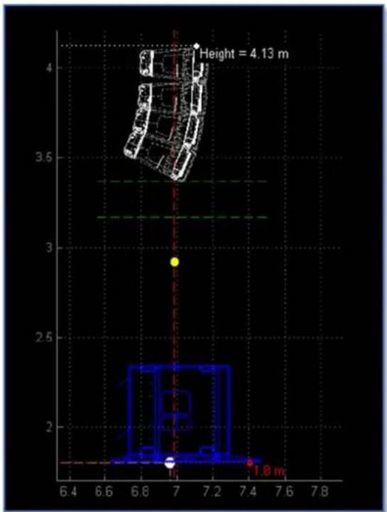
text_image
Height = 4.13 m 1.8 mNote that the array height displayed is the height from the ground NOT above the MSX. You can see that the MSX is at 1.8m, perhaps on a stage so the top trim of the array is at 4.13 - 1.8 = 2.33m above the surface on which the MSX is placed.
The next issue is the array angle. The Universal bracket allows for a tilt from 0 to -18° (18° down) if the optimisation has created an angle greater than -18° the angle will be displayed in red with the option to 'Use Nearest';

text_image
Aiming Design Aim -2 deg Nearest Aim 2.5 deg Bottom Angle -22.5 deg Use NearestBy clicking 'Use Nearest' the angle will revert to -18^ the array diagram will update and the design aim will update and turn green;
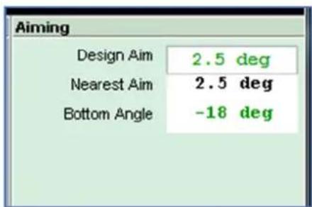
text_image
Aiming Design Aim 2.5 deg Nearest Aim 2.5 deg Bottom Angle -18 degThe same applies in the unlikely event of the optimisation arriving at an array angle that requires the bottom cabinet to have an angle greater than 0^ , an up-tilt in other words; -
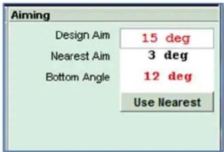
text_image
Aiming Design Aim 15 deg Nearest Aim 3 deg Bottom Angle 12 deg Use NearestClicking on 'Use Nearest' will change the Bottom angle to zero and update the diagram and Design Aim; -
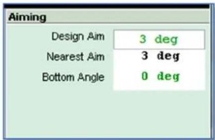
text_image
Aiming Design Aim 3 deg Nearest Aim 3 deg Bottom Angle 0 degOnce you have finished with the Rig Tool, click '√Done' to close the window so you can advance to the Equalisation optimisation using the EQ tab.
Wavefront Precision
All Wavefront Precision systems may be flown or ground stacked. Flown arrays up to 16 cabinets are possible and ground stacked array of up to 6 cabinets. WPL may be flown with or without subs, 24 cabinets without sub, 12 with sub, or ground stacked up to 6. WPS arrays may be up to 24 cabinets. WPM may also be pole mounted driven by a preset on the iK81 amplifier driving the array, rigging details for this option are not available as there is no benefit in optimising pole mounted arrays.
Flown System
A flown WPL, WPC, WPS or WPM array appears like this; -
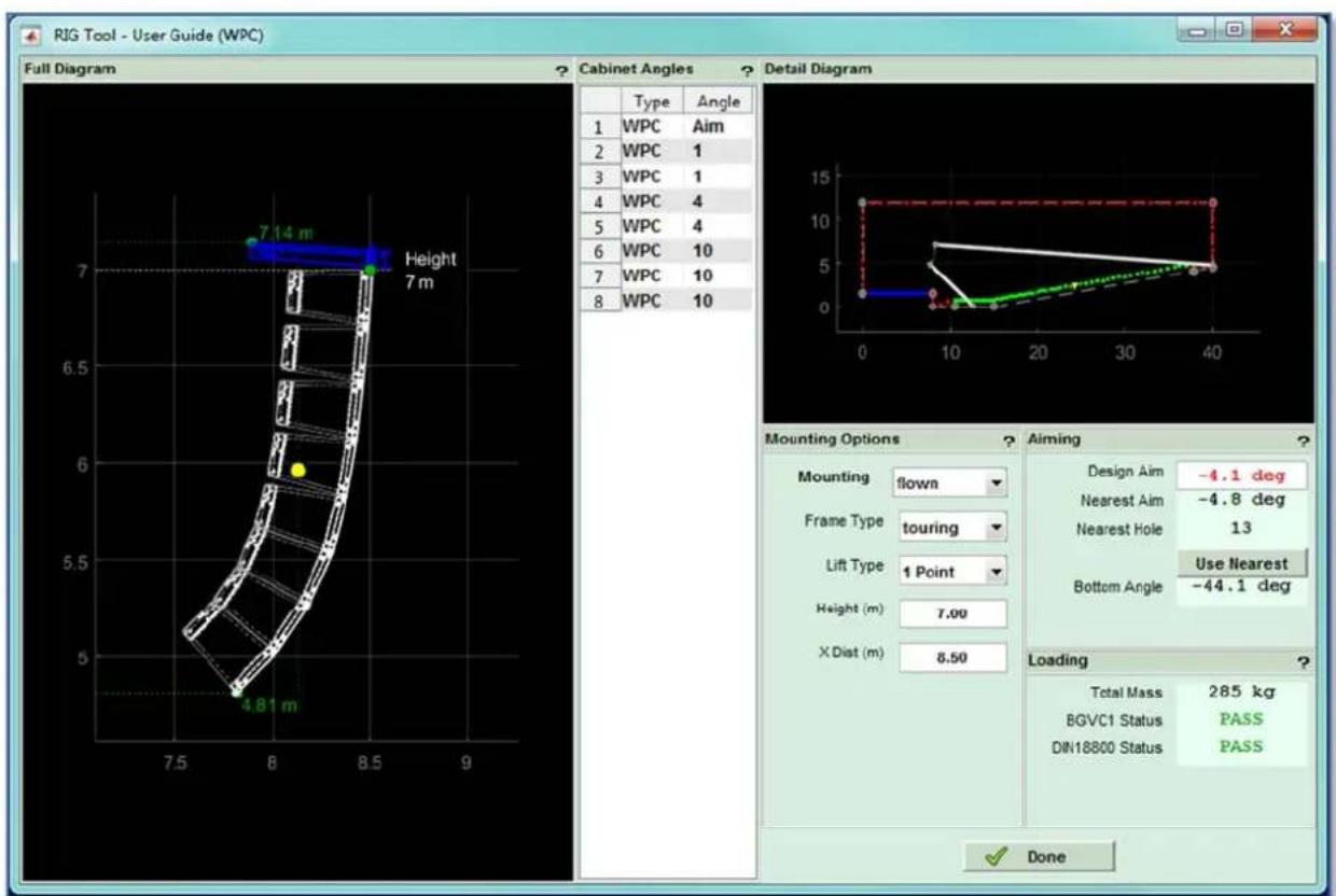
text_image
RIG Tool - User Guide (WPC) Full Diagram Cabinet Angles Detail Diagram Type Angle 1 WPC Aim 2 WPC 1 3 WPC 1 4 WPC 4 5 WPC 4 6 WPC 10 7 WPC 10 8 WPC 10 Height 7 m 7.14 m 4.81 m Mounting Options ? Aiming Mounting flown Frame Type touring Lift Type 1 Point Height(m) 7.00 X Dist(m) 8.50 Design Aim -4.1 deg Nearest Aim -4.8 deg Nearest Hole 13 Use Nearest Bottom Angle -44.1 deg Loading Total Mass 285 kg BGVC1 Status PASS DN18800 Status PASS DoneThere are a couple of options in the mounting panel; -
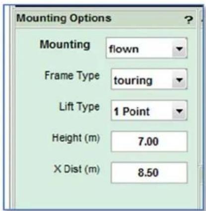
text_image
Mounting Options Mounting flown Frame Type touring Lift Type 1 Point Height (m) 7.00 X Dist (m) 8.50The mounting drop-down gives us the option to select flown or stacked (ground stacked). Flown arrays can be up to 16 boxes, ground stacked up to 6. If you attempt to change a flown array greater than 6 boxes to stacked you will see the following window;
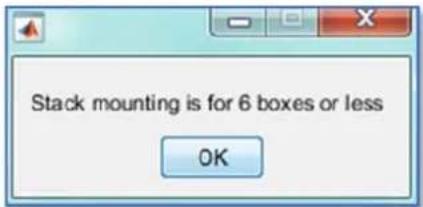
text_image
Stack mounting is for 6 boxes or less OKNext you may select from the full-spec Touring Frame or the lower cost basic Installation frame (WPC and WPM only). The geometry is slightly different so some of the rigging details will update if the frame type is changed.
Lift Type allows you to select between a single point list and two point. Height and x Dist allow you to modify the array position if this has changed from earlier in the project design.
The Aiming section gives details of the array angle. This will change depending on whether single or two point hang has been selected. This is how the window appears with 2 point flying selected; -
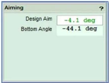
text_image
Aiming Design Aim -4.1 deg Bottom Angle -44.1 degThe Design Aim is confirming the array angle calculated by the splay angle optimisation, the Bottom Angle shows the angle of the bottom cabinet in the array enabling you to check the array angle a little easier than measuring the flying grid. This is particularly useful if the flying grid is the install version without an inclinometer fitted.
Switch to Single point and the section appears as follows; -
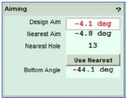
text_image
Aiming Design Aim -4.1 deg Nearest Aim -4.8 deg Nearest Hole 13 Use Nearest Bottom Angle -44.1 degThis shows the nearest hole on the flying grid to get as close as possible to the Design Aim. The Angle for the hole shown is displayed and if this differs from the design aim- as is quite likely- the Design aim will be displayed in red. If you are fortunate and there is a hole on the grid which will give the exact angle that you require the Design aim figure will be green. You have the option to select Use Nearest which will modify the Design Aim to match the actual physical angle at which the array will hang. The advantage of this is that Display will compensate for this angle when it does the EQ optimisation to obtain the coverage area exactly as you requested. When Use Nearest is selected the section changes to appear as follows; -
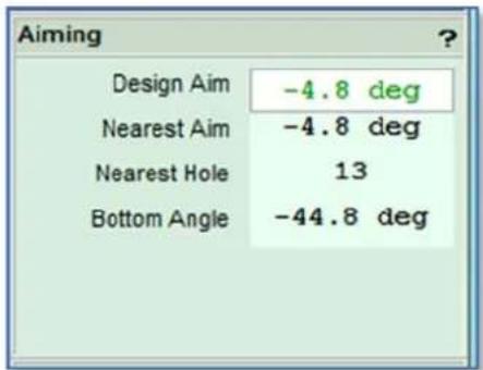
text_image
Aiming Design Aim -4.8 deg Nearest Aim -4.8 deg Nearest Hole 13 Bottom Angle -44.8 degAs you can see, the Design Aim and Nearest Aim now match with the Design Aim in green.
The final section is the Loading; -
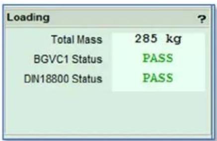
text_image
Loading Total Mass 285 kg BGVC1 Status PASS DIN18800 Status PASSFor a single point hang the total array mass is shown which includes the flying frame and all cabinets. This section also displays whether the array meets BGVC1 and DIN18800 safety standards. For a two point hang the load on each point is also displayed;
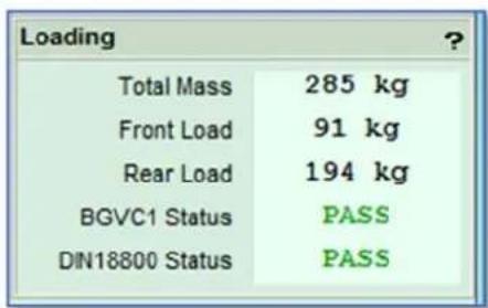
text_image
Loading Total Mass 285 kg Front Load 91 kg Rear Load 194 kg BGVC1 Status PASS DIN18800 Status PASSWPL Flown with Sub
The rigging page for a WPL system flown with sub is slightly different; -
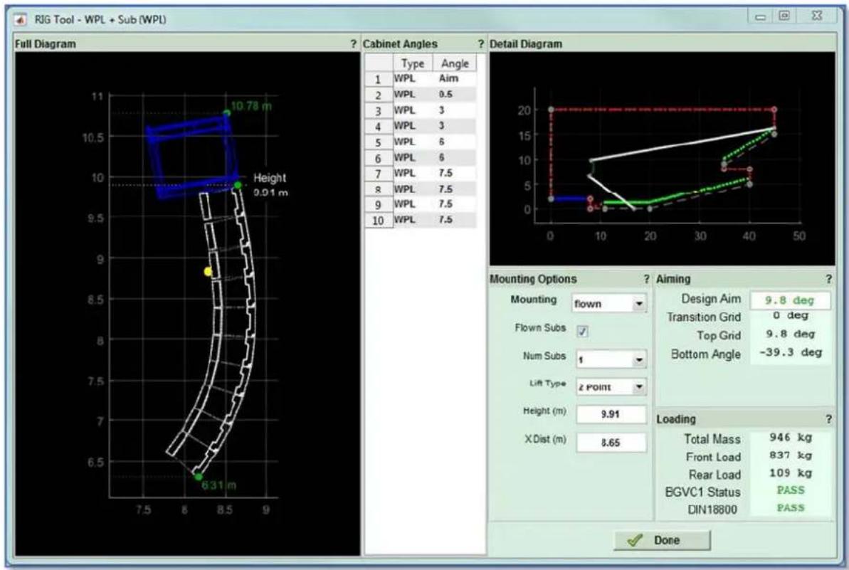
text_image
RIG Tool - WPL + Sub (WPL) Full Diagram Cabinet Angles Detail Diagram Type Angle 1 WPL Aim 2 WPL 0.5 3 WPL 3 4 WPL 3 5 WPL 6 6 WPL 6 7 WPL 7.5 8 WPL 7.5 9 WPL 7.5 10 WPL 7.5 Mounting Options ? Aiming Mounting flown Flown Subs Num Subs 1 Lift Type 2 POINT Height(m) 9.91 X Dist(m) 8.65 Design Aim 9.8 deg Transition Grid 0 deg Top Grid 9.8 deg Bottom Angle -39.3 deg Loading Total Mass 946 kg Front Load 837 kg Rear Load 109 kg BGVC1 Status PASS DIN18800 PASS DoneThe page has an additional selection for the number of flown subs. This defaults to 1 but up to 3 can be selected; -
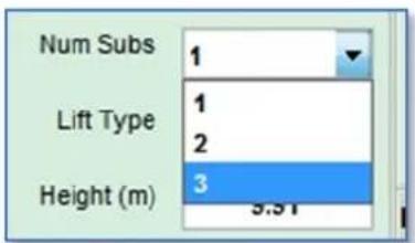
text_image
Num Subs 1 Lift Type 1 2 Height (m) 3 5.51The rigging image and all details will change accordingly; -
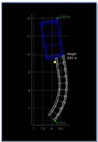
other
| Dimension | Value | | --------- | --------- | | Height | 9.91 m | | Height | 11.97 m | | Width | 6.31 m |All other aspects of the rigging are identical to a standard flown array.
Ground Stacked arrays
Arrays of up to 6 boxes of any Wavefront Precision system may be ground stacked; -
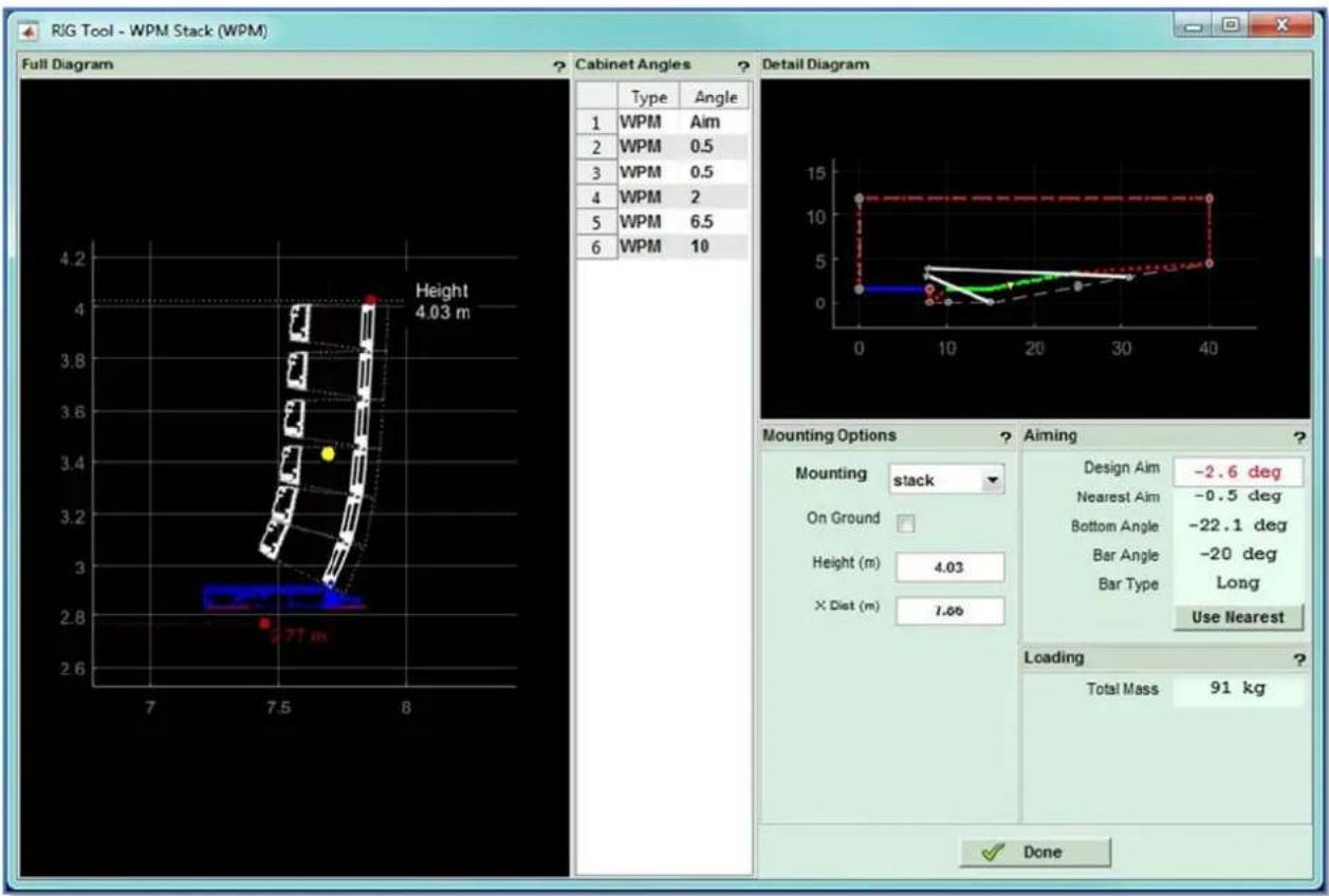
text_image
RIG Tool - WPM Stack (WPM) Full Diagram Cabinet Angles Detail Diagram Type Angle 1 WPM Aim 2 WPM 0.5 3 WPM 0.5 4 WPM 2 5 WPM 6.5 6 WPM 10 Height 4.03 m Mounting Options ? Aiming Mounting stacks On Ground Height (m) 4.03 × Dist (m) 1.69 Design Aim -2.6 deg Nearest Aim -0.5 deg Bottom Angle -22.1 deg Bar Angle -20 deg Bar Type Long Use Nearest Loading Total Mass 91 kg DoneThis can be selected at the beginning of you project design or a flown array can be converted to ground stacked by selecting the Stacked option in the Mounting sections; -
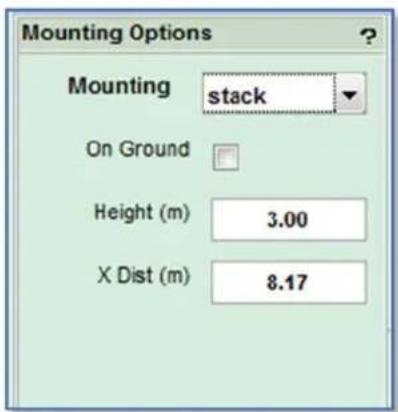
text_image
Mounting Options Mounting stack On Ground Height (m) 3.00 X Dist (m) 8.17You now have the option to anchor the stack onto the ground which will automatically update the array height. You will see a warning window; -
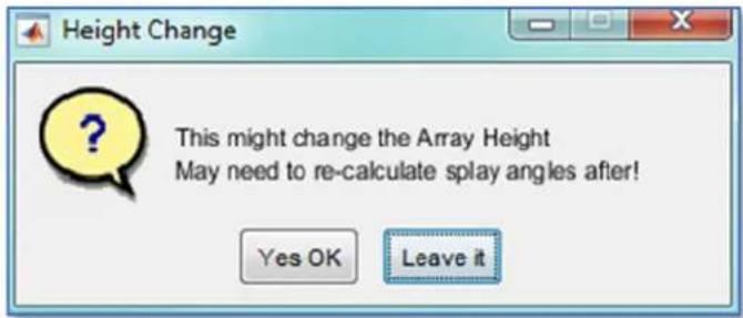
text_image
Height Change This might change the Array Height May need to re-calculate splay angles after! Yes OK Leave itAssuming you are happy to proceed click Yes OK and the height and Stack diagram will update; -
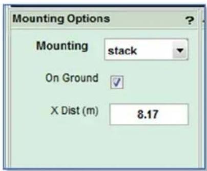
text_image
Mounting Options Mounting stack On Ground ✓ X Dist (m) 8.17Note that the option to select frame type is gone as only the touring frame is suitable for ground stacked arrays. Height is also removed as we have selected to stack on the ground.
The Aiming Section appears like this; -
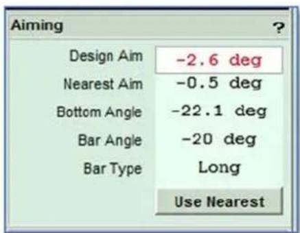
text_image
Aiming Design Aim -2.6 deg Nearest Aim -0.5 deg Bottom Angle -22.1 deg Bar Angle -20 deg Bar Type Long Use NearestThis shows the design aim which is in red as the nearest aim possible with the ground stack bar differs from the ideal angle. The Bar type is shown which will be either long or short. Generally arrays with a down tilt will require the long bar and those with an up-tilt the short bar. Bar Angle refers to the holes in the bar which are labelled to show which to use. As with a flown array using a single point you can select Use Nearest which will update the angles; -
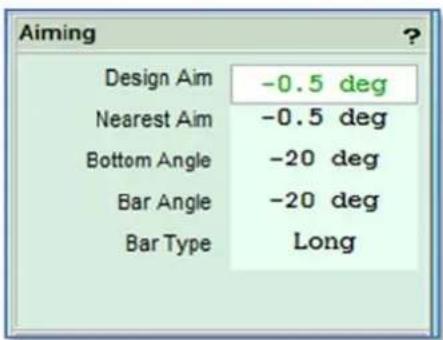
text_image
Aiming Design Aim -0.5 deg Nearest Aim -0.5 deg Bottom Angle -20 deg Bar Angle -20 deg Bar Type LongAs the array is not flown there are no safety standard to be met therefore the Loading section just displays the array mass; -
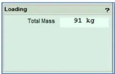
text_image
Loading Total Mass 91 kgAs long as the floor can support the array mass you won't have any problems!
O-Line
O-Line may be flown or wall mounted. Flown systems can be up to 24 modules. There are two options for wall mounting, a smaller bracket which cater for up to 4 modules or a larger bracket which will hold up to 16.
Flown arrays
A flown system will appear like this; -
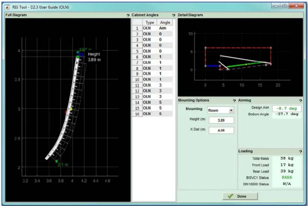
text_image
RIG Tool - D2.3 User Guide (OLN) Full Diagram Cabinet Angles Detail Diagram Type Angle 1 OLN Aim 2 OLN 0 3 OLN 0 4 OLN 0 5 OLN 0 6 OLN 1 7 OLN 1 8 OLN 1 9 OLN 1 10 OLN 1 11 OLN 3 12 OLN 3 13 OLN 3 14 OLN 5 15 OLN 5 16 OLN 5 Mounting Options ? Aiming Mounting flown Height (m) 3.89 X Dist (m) 4.09 Design Aim -8.7 deg Bottom Angle -37.7 deg Loading Total Mass 58 kg Front Load 17 kg Rear Load 39 kg BGVC1 Status PASS DN18000 Status N/A DoneYou have the option to switch to Wall mount using the drop-down box should you need to change the deployment.
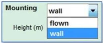
text_image
Mounting wall Height (m) flown wallThis can only be done for arrays up to 16 modules, any larger and flying is the only option.
There are no options for single or two point hang and the design aim will need to be matched by adjusting the length of the tie on the rear of the array. The angle of the bottom cabinet is shown which may be easier to measure when adjusting the array to get the correct angle

text_image
Aiming Design Aim -8.7 deg Bottom Angle -27.7 degFinally the loading is shown so you ensure that the points for the principal hang and the tie-back are sufficient and that the array is safe; -
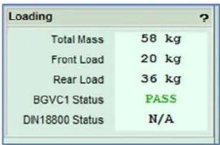
text_image
Loading Total Mass 58 kg Front Load 20 kg Rear Load 36 kg BGVC1 Status PASS DIN18800 Status N/AWall Mount
A wall mount system of 5 to 16 modules will appear like this; -
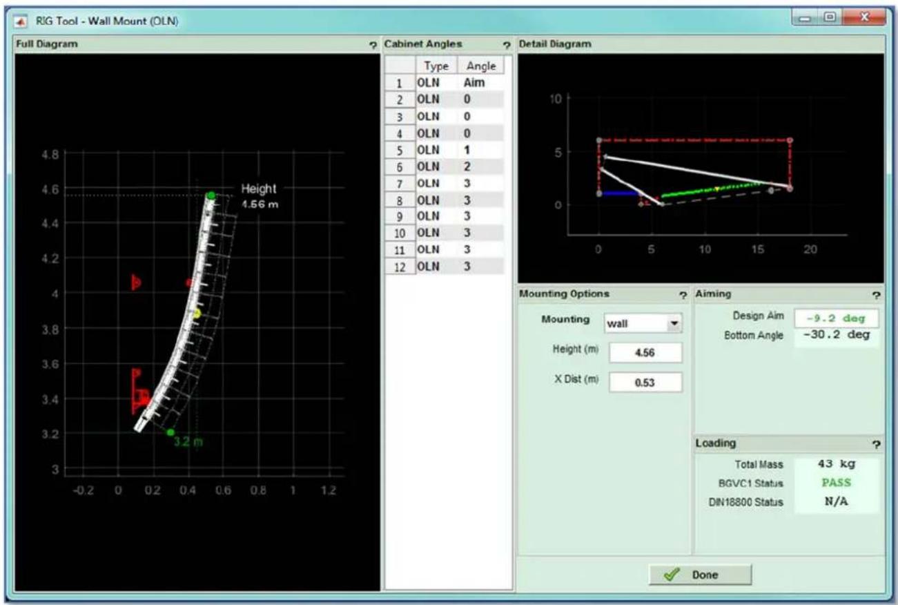
text_image
RIG Tool - Wall Mount (OLN) Full Diagram Cabinet Angles Detail Diagram Type Angle 1 OLN Aim 2 OLN 0 3 OLN 0 4 OLN 0 5 OLN 1 6 OLN 2 7 OLN 3 8 OLN 3 9 OLN 3 10 OLN 3 11 OLN 3 12 OLN 3 Height 4.56 m Mounting Options ? Aiming Mounting wall Design Aim -9.2 deg Height(m) Bottom Angle -30.2 deg X Dist(m) Loading Total Mass 43 kg BGVC1 Status PASS DIN18800 Status N/A DoneThe 4-16 wall bracket includes an additional tie which in the example above is fitted on module 5 and attaches to a second wall fixing. The length of this tie is adjusted to obtain the correct array angle. The array diagram shows the positions required for the wall fittings; -
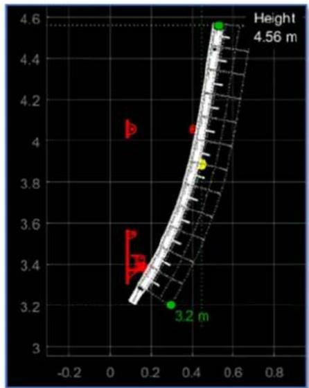
scatter
| X | Y | |------|------| | 0.1 | 4.1 | | 0.4 | 4.0 | | 0.5 | 4.56 |Small arrays of 4 or less modules use the 4-box wall bracket and appear like this; -
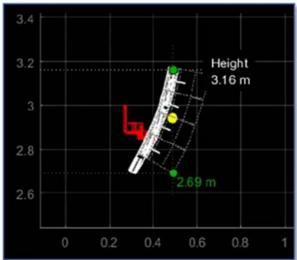
scatter
| Point | X | Y | |-------|------|------| | Green | 0.5 | 3.2 | | Yellow| 0.5 | 2.9 | | Red | 0.3 | 2.9 | | Green | 0.5 | 2.69 |There is no additional tie, just a single wall bracket, the array angle is adjusted with a screw in the base of the bracket
EQ Tab
The EQ tab is where we make the decision on how we want the system to perform. In a perfect world we could get the system to achieve an even coverage over the audience area with absolutely no spill whatsoever outside of this. Of course the laws of physics dictate that this is impossible to achieve even with the colossal processing power available in a multicellular system. We therefore have to balance our requirements between the three principal objective functions; our audience target, the spill into non audience areas and spill onto areas defined as hard avoid.
Basic View
This is the EQ Window for MLA, MLA Compact and MLA Mini; -
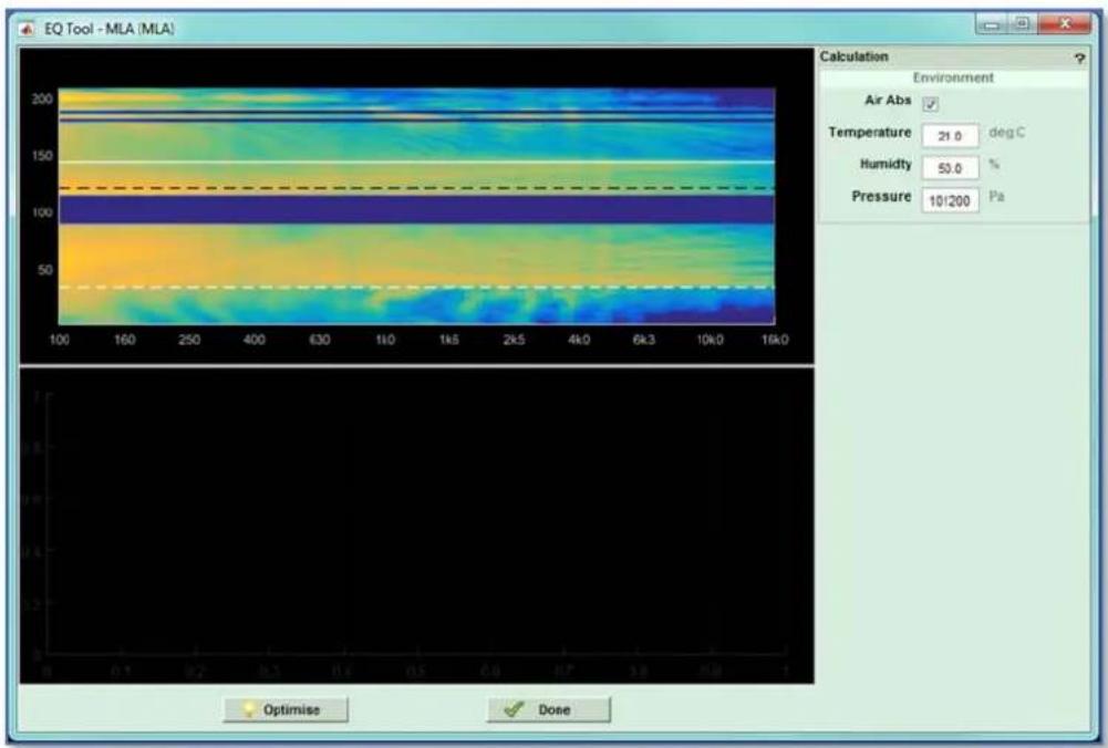
text_image
EQ Tool - MLA (MLA) Calculation Environment Air Abs Temperature 21.0 deg C Humidity 53.0 % Pressure 10/200 Pa Optimise DoneAnd for WPL, WPC, WPS & WPM; -
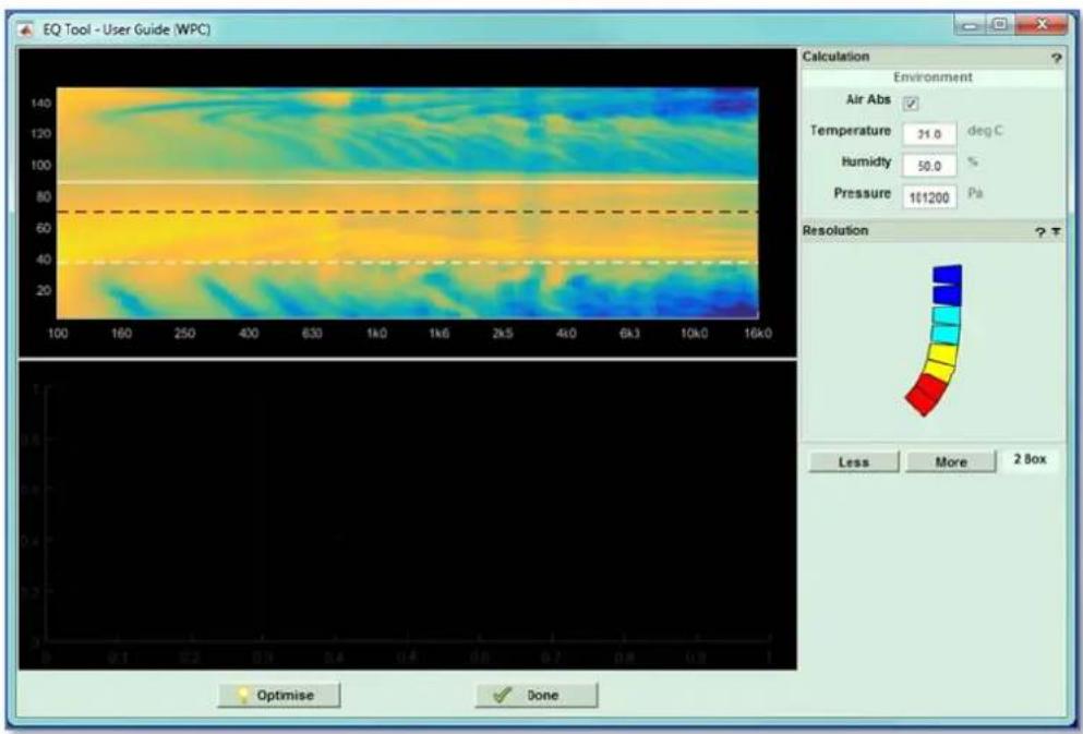
text_image
EQ Tool - User Guide (WPC) Calculation Environment Air Abs ✓ Temperature 31.0 deg C Humidity 50.0 % Pressure 161200 Pa Resolution Less More 2 Box Optimise DoneAnd for O-Line
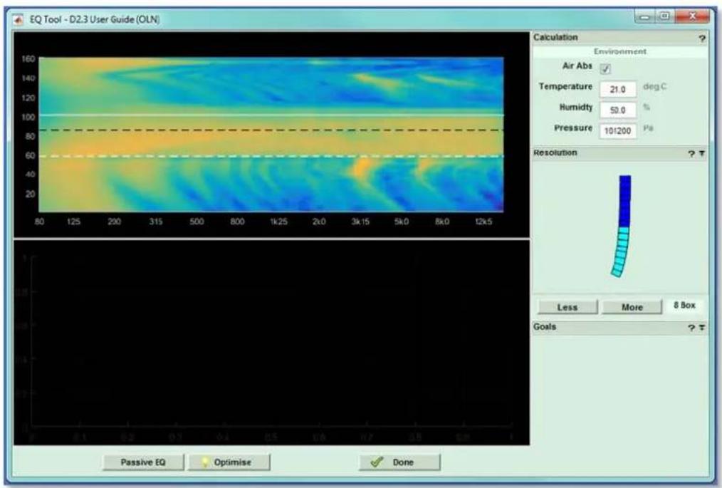
text_image
EQ Tool - D2.3 User Guide (OLN) Calculation Environment Air Abs Temperature 21.0 deg C Humidity 50.0 % Pressure 101200 Pa Resolution Less More 8 Box Goals Passive EQ Optimise DoneAir Absorption
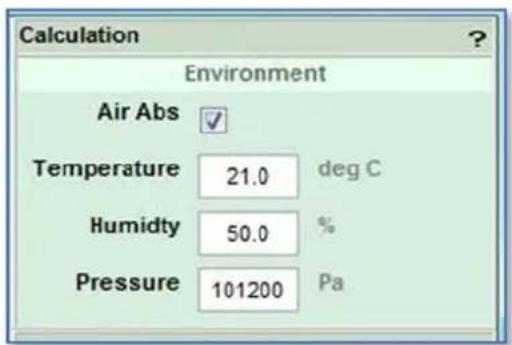
text_image
Calculation Environment Air Abs Temperature 21.0 deg C Humidity 50.0 % Pressure 101200 PaThe Environment window allows you to activate the air absorption system which will compensate for the environmental conditions in the same way as the system did for the splay angles. The temperature, humidity and pressure can be entered into this window
Resolution
The Resolution window is where the level of cellular control is calculated for Wavefront Precision and O-Line arrays. The highest setting is 1 box where each cabinet is treated as an individual cell in the optimisation process. 2 box means that the cabinets are connected in parallel and the optimisation treats a pair of boxes as one cell. WPM can have a resolution of 1, 2, 3 and 4 boxes, WPC can be 1, 2 or 3, WPS and WPL can be 1 or 2. The level is selected using the 'Less' and 'More' buttons. O-Line can be 1, 2, 3, 4, 5, 6, 7, 8 or "Array". Array will optimise the array with one channel of amplification regardless of the array length, essentially matching the function of the original O-Line software application. The text to the right of the buttons displays the resolution level that has been set. You will notice that at 1 box resolution, all of the cabinets in the array thumbnail have a different colour; -
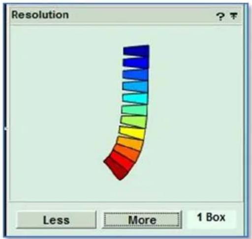
text_image
Resolution ? ? Less More 1 BoxIf we select 2 box the cabinets are paired and each pair now shares a colour; -
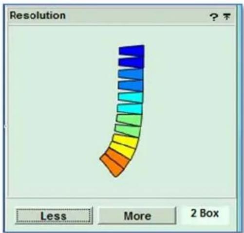
text_image
Resolution ? ? Less More 2 BoxThree box looks like this; -
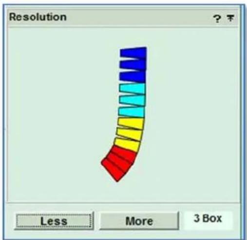
text_image
Resolution ? ? Less More 3 BoxAnd 4-box which is available for WPM or O-Line; -
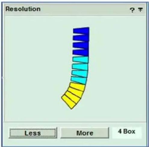
text_image
Resolution ? ? Less More 4 BoxFor O-line we can go up to 8-box resolution; -
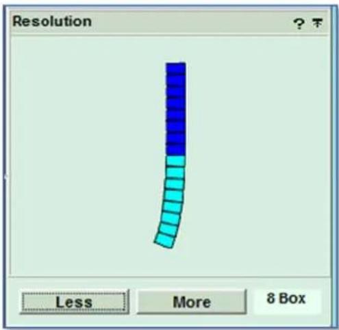
text_image
Resolution ? ? Less More 8 BoxAnd if "Array" is selected the array will appear like this with a single colour, irrespective of its length; -
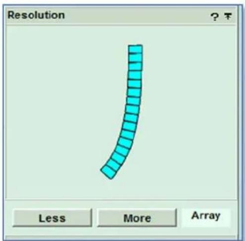
text_image
Resolution ? T Less More ArrayThis makes is very obvious how the array is configured and the degree of control we are able to obtain obviously depends on how high the resolution is set.
Once the Environment settings have been edited and in the case of Wavefront Precision and O-Line the desired Resolution is selected, click on Optimise; -
text_image
OptimiseThe EQ optimisation process will start. The lower section of the window now shows a frequency response graph with the response at all audience positions (the green dots in the Coverage view) displayed. The optimisation process works from the lowest frequencies upwards, calculating the Equalisation parameters required to active the required performance, displaying the calculated response on the graph. You will see the varied responses which are widely scattered, particularly at higher frequencies, gradually flatten and draw in together showing that the optimisation is making huge improvements to the response for all audience positions. Here is the response with the optimisation just started; -
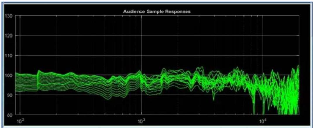
line
| x | y | | -------- | ---- | | 100 | 100 | | 1000 | 95 | | 10000 | 85 |Just the bottom half an octave has been processed, you can see the huge variation in response from around 8KHz and above prior to optimisation.
Here the process has reached around 1KHz, the lower frequencies are looking very nicely consistent; -
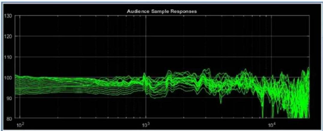
line
| X (log scale) | Y (line 1) | Y (line 2) | Y (line 3) | Y (line 4) | Y (line 5) | Y (line 6) | Y (line 7) | Y (line 8) | Y (line 9) | Y (line 10) | | ------------- | ---------- | ---------- | ---------- | ---------- | ---------- | ---------- | ---------- | ---------- | ---------- | ----------- | | 10^2 | ~100 | ~100 | ~100 | ~100 | ~100 | ~100 | ~100 | ~100 | ~100 | ~100 | | 10^3 | ~100 | ~100 | ~100 | ~100 | ~100 | ~100 | ~100 | ~100 | ~100 | ~100 | | 10^4 | ~85 | ~85 | ~85 | ~85 | ~85 | ~85 | ~85 | ~85 | ~85 | ~85 | | >10^4 | ~105 | ~105 | ~105 | ~105 | ~105 | ~105 | ~105 | ~105 | ~105 | ~105 |Up to 7KHz and the optimisation is looking extremely impressive
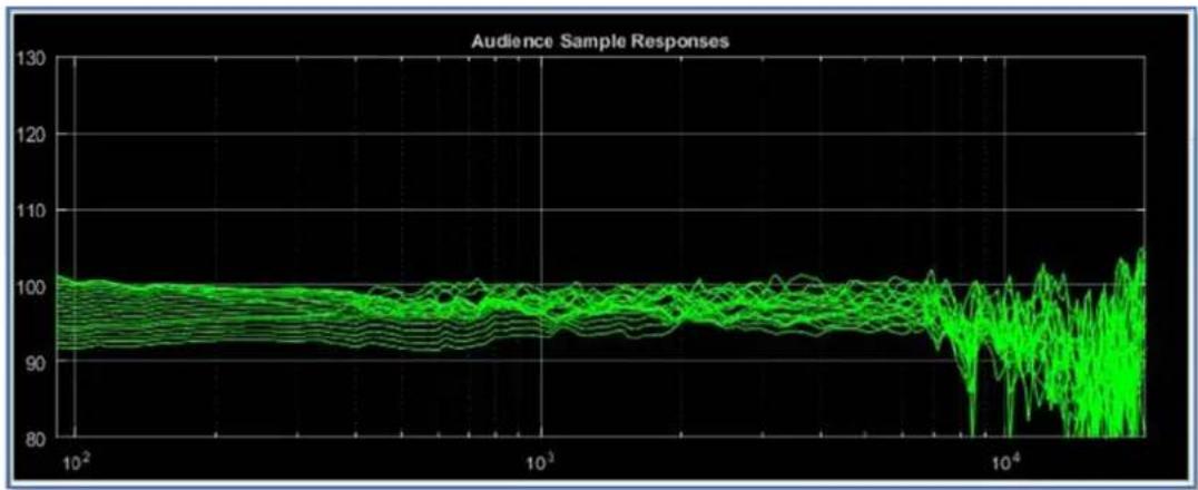
line
| x | y | | -------- | ---- | | 10^2 | ~100 | | 10^3 | ~98 | | 10^4 | ~85 |The finished optimisation shows a remarkable improvement on the response at the start; -

line
| x | y | | -------- | ---- | | 10^2 | ~100 | | 10^3 | ~98 | | 10^4 | ~105 |The optimisation is complete and you can click 'Done' to close the window.
With O-Line there is the option to view Passive EQ Parameters not projects that are not using an iKon amplifier to power the array and therefore just require basic IIR (standard) parametric parameters which can be programmed into any digital system processor. This is designed to be used in place of the Optimisation (not as well as). Click on the Passive EQ button; -
This opens the following window; -
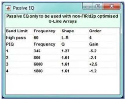
text_image
Passive EQ only to be used with non-FIR/d2p optimised 0-Line Arrays Band Limit Frequency Shape Order high pass 60 L-R 4 PEQ Frequency Q Gain 1 345 1.27 -5.2 2 800 1.61 -2.1 3 6000 1.61 +2.5 4 1800 1.61 -1.2Use these parameters to program the processor of your choice. There is no need to use the Optimise function.
Expert Mode
In Expert mode Multicellular Arrays appear like this; -
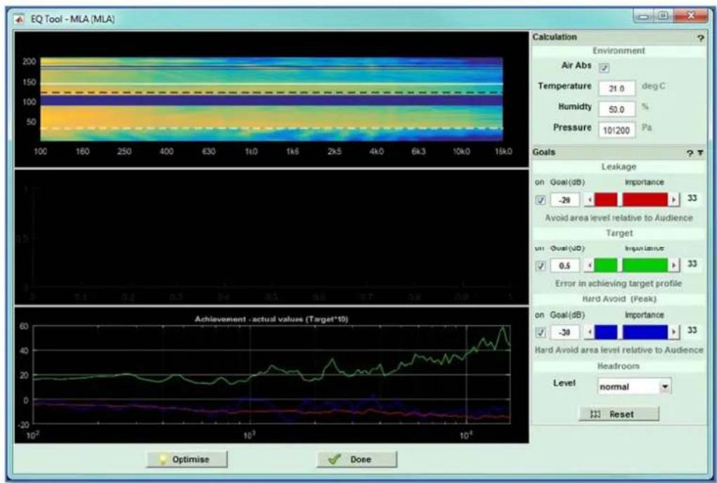
text_image
EQ Tool - MLA (MLA) Calculation Environment Air Abs Temperature 21.0 deg C Humidity 50.0 % Pressure 10/200 Pa Goals Leakage on Goal(dB) Importance ✓ -28 ▼ 33 Avoid area level relative to Audience Target on Goal(dB) Impian Latute ✓ 0.5 ▼ 33 Error in achieving target profile Hard Avoid (Peak) on Goal(dB) Importance ✓ -38 ▼ 33 Hard Avoid area level relative to Audience Headroom Level normal Reset Achievement - actual values (Target*10) Optimise DoseAnd Wavefront Precision; -
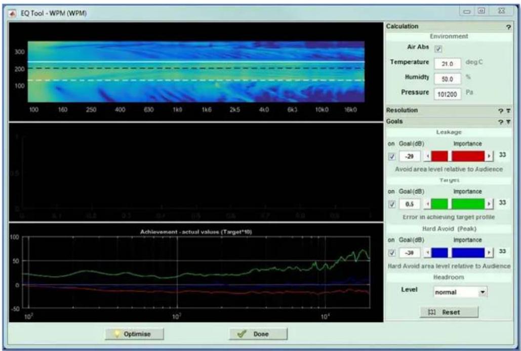
text_image
EQ Tool - WPM (WPM) Calculation Environment Air Abs Temperature 21.0 deg C Humidity 50.0 % Pressure 101200 Pa Resolution Goals Leakage on Goal(dB) Importance 33 Avoid area level relative to Audience Targets on Goal(dB) Importance 33 Error in achieving target profile Hard Avoid (Peak) on Goal(dB) Importance 33 Hard Avoid area level relative to Audience Headroom Level normal Reset Optimise DoneAnd O-Line
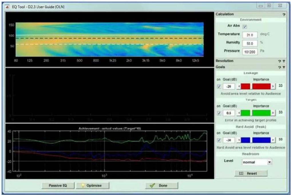
text_image
EQ Tool - D2.3 User Guide (OLN) Calculation Environment Air Abs Temperature 21.0 deg C Humidity 50.0 % Pressure 10/200 Pa Resolution Goals Leakage on Goal(dB) Importance 33 Avoid area level relative to Audience Target on Goal(dB) Importance 33 Error in achieving target profile Hard Avoid (Peak) on Goal(dB) Importance 33 Hard Avoid area level relative to Audience Headroom Level normal [...] Reset Passive EQ Optimise DoneThe Goals Window is now available so the Resolution window will need to be opened by clicking on the expand icon if you are optimising WPL, WPC, WPS, WPM or O-Line.
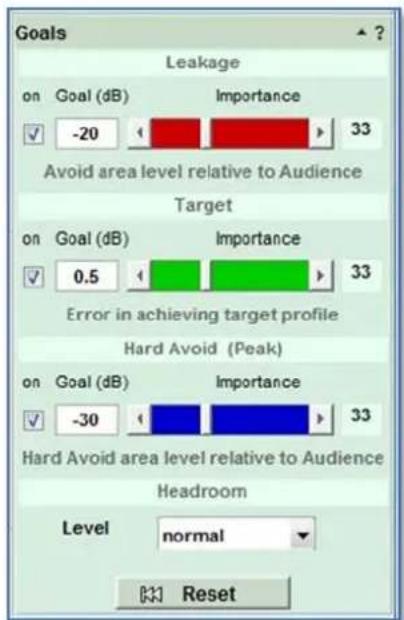
text_image
Goals Leakage on Goal (dB) Importance ✓ -20 33 Avoid area level relative to Audience Target on Goal (dB) Importance ✓ 0.5 33 Error in achieving target profile Hard Avoid (Peak) on Goal (dB) Importance ✓ -30 33 Hard Avoid area level relative to Audience Headroom Level normal ResetThe three goals are Leakage, Target and Hard Avoid. The relative balance for each of these is controlled by the horizontal faders with the numeric percentage value of each showing to the right. The default starting position is each with equal importance so a level of 33% for all three (yes that equals 99% not 100, get over it...). These are the settings that are used for the optimisation when using Basic view which doesn't have access to the Goals window to edit the relative balance of the three targets.
'Leakage' is the spill onto non-audience areas the importance slider is coloured red to match the red non-audience planes in the Coverage tab. It can be deactivated by un-checking the 'on' box. The default value is -20 which means that the system will attempt to achieve a level at least 20dB below the audience level.
'Target' controls the audience level, as with the other goals it can be deactivated. The option is primarily there for consistency, it would be highly unusual not to want to optimise the audience area but not impossible, for example, if you had an area off site
where it was crucial to keep levels to an absolute minimum you would make the area hard avoid and give maximum priority to the Hard Avoid goal by deactivating Leakage and Target. Target is shown with a green slider also to match the green audience region in the Coverage tab. The goal figure is 0.5dB by default so the optimisation will attempt to match the magnitude contour set in the Coverage Tab to within 0.5dB.
'Hard Avoid' also has an 'on' check box and a blue importance slider. The default Goal is 30dB lower than the audience level for any plane selected as hard avoid.
The importance sliders allow you to set the relative importance of each of the three goals, two if you have one of the goals switched off. If you have two switched off the fader for the remaining function will automatically go to 100% and will no longer be adjustable. If you attempt to switch off all three goals the system will automatically turn Target back on (see, it's not so easy to break it!). When you adjust any of the three sliders, the other two will automatically compensate for example if you move target to the right towards the maximum, both Leakage and Hard Avoid will move down. If you think in percentage terms, all three start with equal precedence at 33%. If you move Target up to say 70%, Leakage and Hard Avoid will decrease equally to 15%. Now if we move Hard Avoid up to 35% both Leakage and Target will move down an equal amount from their previous position so will end up at 5% and 60%. The actual figures are not particularly vital, what the sliders give you is a quick, easy way of balancing the relative importance of the three goals to achieve the results you want at a glance. There is a reset function which will turn on all three goals and return all three faders to the default, 33% position. It will not however reset the figures for the goals, if you have changed these you will need to change them back manually.
The final selection is to set the expected spl so that the optimisation can calculate the parameters to allow the best possible headroom. The options are extreme, high, normal and low.
To show the optimisation results, we have set the faders as follows; -
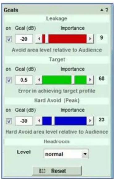
text_image
Goals Leakage on Goal (dB) Importance 9 ✓ -20 Avoid area level relative to Audience Target on Goal (dB) Importance 68 ✓ 0.5 Error in achieving target profile Hard Avoid (Peak) on Goal (dB) Importance 23 ✓ -30 Hard Avoid area level relative to Audience Headroom Level normal ResetWe have given the target the greatest importance, hard avoid comes second with little importance to leakage. We want to get the best coverage for our audience whilst minimising sound on stage and reflections from the balcony. The rest of our venue is not too reverberant so we are not too concerned about spill onto non audience areas.
If we now click on Optimise for an MLA System the Window will once again show the initial frequency response in the audience region with a green trace for all virtual microphone positions which will gradually improve as the optimisation moves through the frequency range. You will also see a second graph which shows how well the optimisation has achieved the targets that you have set Here we see the progress which has reached 500Hz;
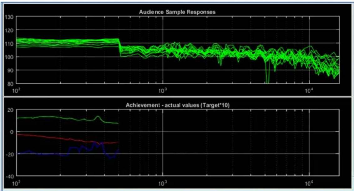
Here it is up to 5KHz; -
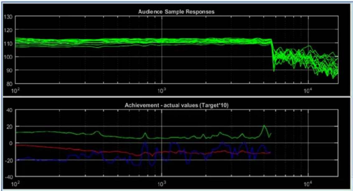
And the completed optimisation; -
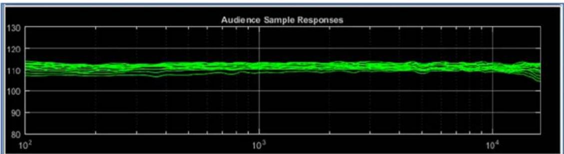
line
| x | y | | ------ | ---- | | 100 | 112 | | 1000 | 112 | | 10000 | 112 |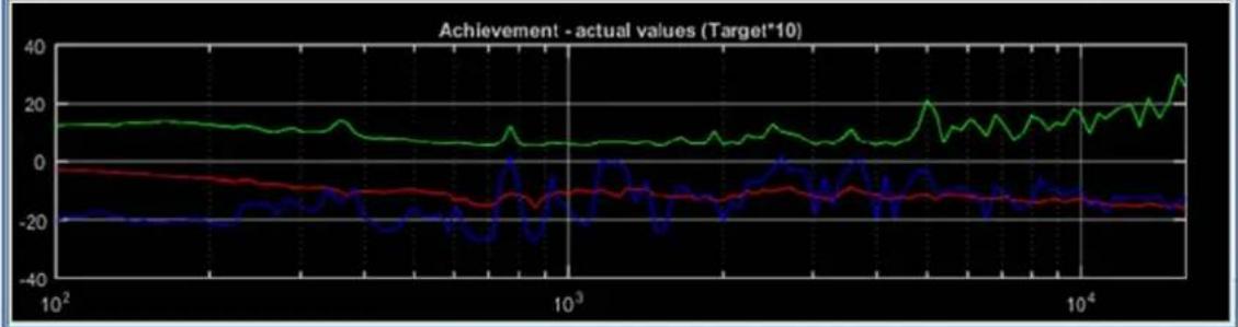
line
| x | Green Line | Red Line | Blue Line | | ------ | ---------- | -------- | --------- | | 100 | 15 | -5 | -20 | | 1000 | 10 | -10 | -25 | | 10000 | 25 | -15 | -15 |This shows the quite astonishing results achievable with MLA, the frequency response is remarkably flat at almost every position in the audience which is what we would hope for given that we gave the target a higher priority. You will notice that the target for the hard avoid is looking a little ragged which is to be expected as it was only given a target of 23%. If we try a new optimisation with a hard avoid percentage of 90%, target of only 10% with non-audience switched off, this is the result;

line
| X (log scale) | Y (approx) | | ------------- | ---------- | | 10² | ~110 | | 10³ | ~110 | | 10⁴ | ~110 |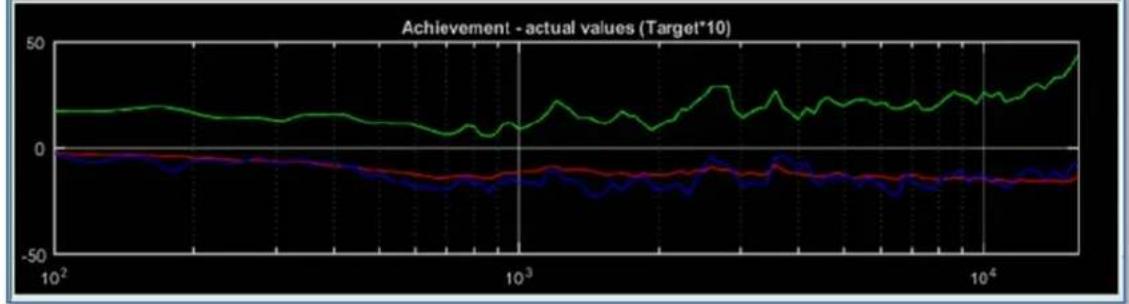
line
| X Value | Green Line | Red Line | Blue Line | |---------|------------|----------|-----------| | 100 | ~15 | ~0 | ~-5 | | 1000 | ~10 | ~-5 | ~-10 | | 10000 | ~30 | ~-5 | ~-10 |The audience response is not quite as flat or consistent although is still a huge improvement on where it started, the Achievement for hard avoid however has improved quite significantly. This demonstrates how you have the tools at your disposal to maximise the performance of your system depending on what is most important in the environment in which your system is employed. This is completely unique to systems optimised using Display.
SPL Tab
The final tab is the SPL View which gives us the opportunity to view the optimised result in more detail. This is identical in both Basic and Expert UI modes. Here is our test venue; -
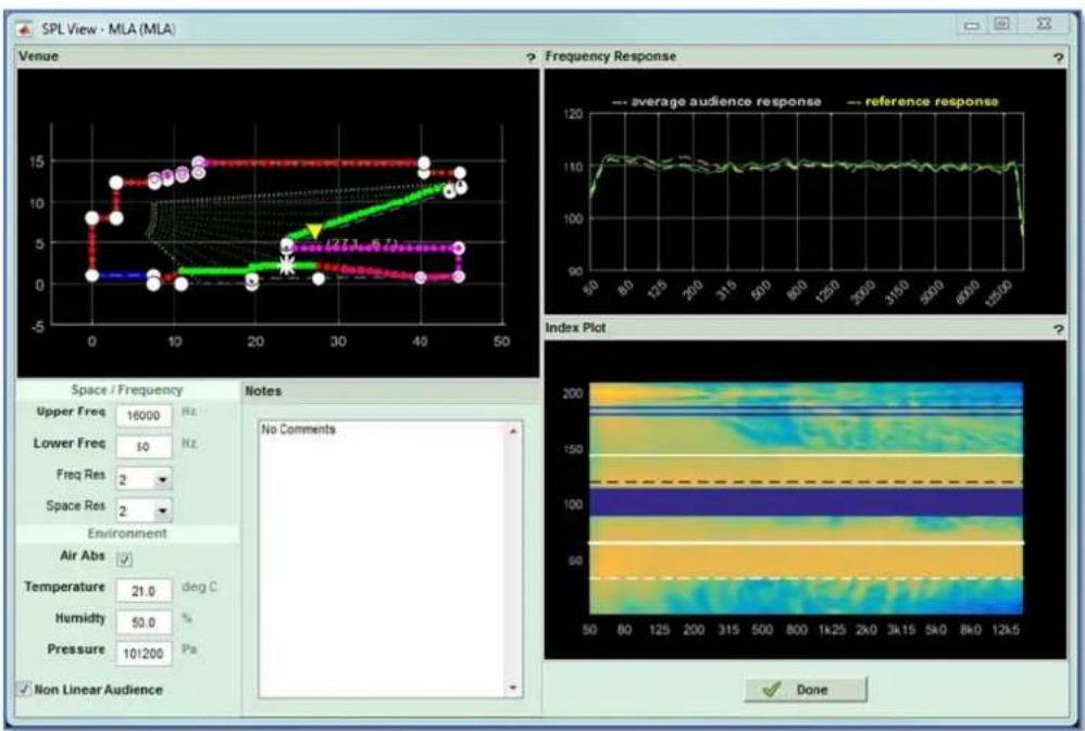
line
| Frequency | Average Audience Response | Reference Response | | --------- | ------------------------- | ------------------ | | 0 | 16000 | 110 | | 10 | 16000 | 110 | | 20 | 16000 | 110 | | 30 | 16000 | 110 | | 40 | 16000 | 110 | | 50 | 16000 | 110 |On the top left we see our coverage slice, the bottom right is the index plot and the top right shows the frequency where our cursor is placed on the index plot which will show green when the curser is over an audience area, red when it is over a non-audience area and blue when over a hard avoid area. The response at the reference position is also shown as a dashed yellow line and the average repose over the entire audience region as a dashed white line.
The cursor is shown as a thicker white line on the Index plot. The cursor position is also shown on the venue slice as a white asterix. As you move your cursor position on the index plot the white asterix moves on the Venue diagram and the frequency response plot updates instantaneously.
The performance looks very good, even lower frequencies are looking remarkably consistent benefitting from the LF optimisation in version 2.3. Let's take a look at the results in other positions; -
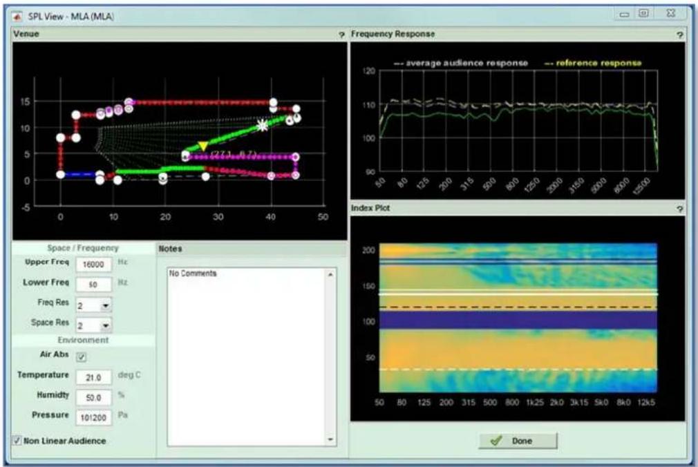
text_image
SPL View - MLA (MLA) Venue Frequency Response average audience response reference response Space / Frequency Upper Freq 16000 Hz Lower Freq 50 Hz Freq Res 2 Space Res 2 Environment Air Abs ✓ Temperature 21.0 deg C Humidity 50.0 % Pressure 101200 Pa Non Linear Audience Notes No Comments Index Plot DoneHere we see the response right at the back of the balcony which is still quite astonishingly flat. We can be very satisfied that we have achieved an extremely good even coverage for all audience members in this venue. It is also worth taking a look at how well we have avoided the stage; -
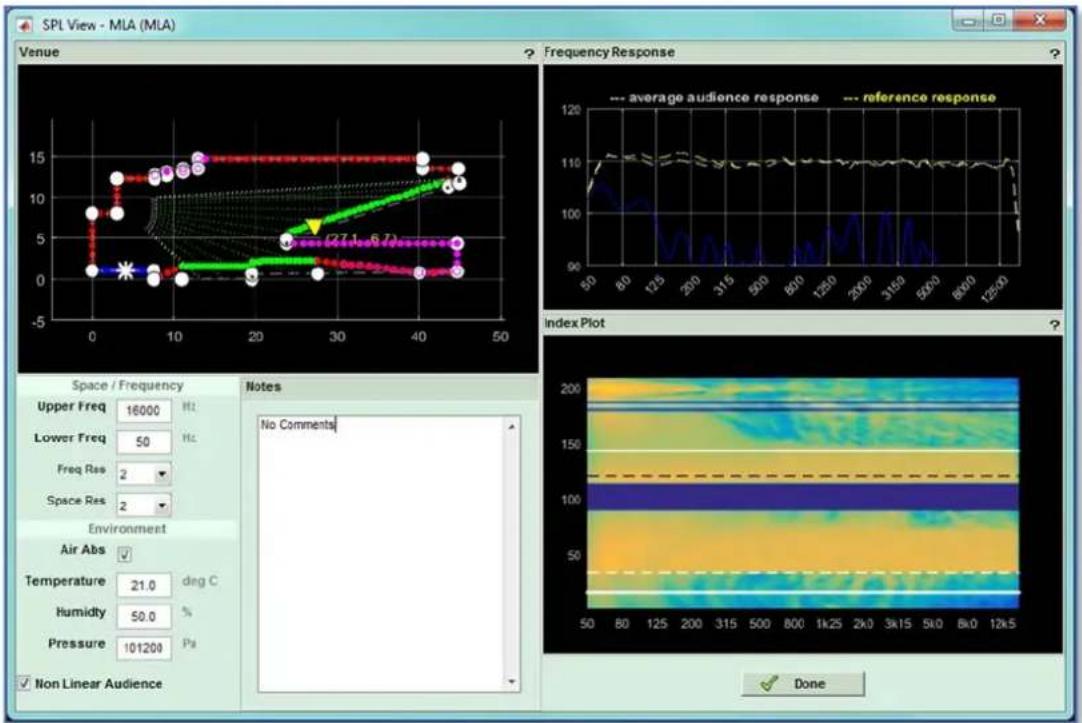
text_image
SPL View - MLA (MLA) Venue Frequency Response --- average audience response --- reference response 120 90 110 120 110 100 100 100 100 100 100 100 100 100 100 100 100 100 100 100 100 100 100 100 100 100 100 100 100 100 12500 Space / Frequency Upper Freq 16000 Ht. Lower Freq 50 Hz Freq Res 2 Space Res 2 Environment Air Abs ✓ Temperature 21.0 deg C Humidity 50.0 % Pressure 101200 Pa ✓ Non Linear Audience Notes No Comments Index Plot DoneThis shows the response on stage and the hard avoid here has done an astonishing job of reducing levels on stage, the attenuation is dramatic, it is fair to say that the array will be almost inaudible on stage.
Individual Graph Windows
Many of the graphical views produced in Display 2 can be opened in an independent floating Window and the file saved as a file. This includes the following views; -
Coverage Tab Venue Diagram Target Coverage Diagram
Splay Tab Current Acoustic Output Graph Array Diagram
Rigging Tab Full Array Diagram
EQ Tab Current EQ Index Plot Optimised EQ Index Plot Audience Sample Responses Graph Non-Audience Sample Response Graph Goal Achievement Graph
View SPL Tab Venue Diagram Frequency Response Graph Index Plot
The Window can be very useful for comparing graphs from different optimisations, storing them for future use or looking at them in more detail. The window is opened by right clicking on the horizontal or vertical scale in any of the views listed above, this is an example of a Venue Diagram from the Coverage Tab; -
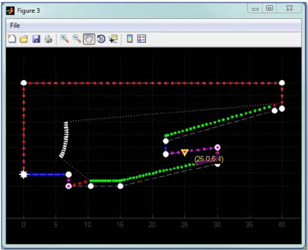
line
| x | y | |----|------| | 0 | 1 | | 7 | 0 | | 22 | 0 | | 30 | 0.5 | | 40 | 1 |The Window has the following menu bar which is the same regardless of which view is opened; -
text_image
FileThis offers a host of extra functions for further manipulation of the graph. The first icon is for creating a new figure as they are referred to, this obviously has little use within Display 2; -

Next you have the option for opening a file, this would be used for opening a figure you have saved previously.

The save function allows you to store the current figure in a file location of your choice. Navigate to a suitable location, the name will default to a highlighted "untitled" prompting you to give it an appropriate name before clicking 'Save' to store the file.
Print will open the Print dialog for your default printer.

The the zoom function, as you would expect the + allows zooming in, click on the + symbol then click on the graph and you will zoom in 100% (double the original size), further clicks will zoom in by another 100%. Clicking on the – has the reverse effect, each click will reduce the size by half (-100%). A more useful zoom function is available using click and hold. This function is available by selecting either the + or – zoom buttons. If you click and hold and move the mouse forward you will gradually zoom in, move the mouse backward you will zoom out.
The Pan icon allows you to click and drag the graph to a new position, useful for examining areas of the graph once it has been enlarged using the zoom command.

The Rotate 3D command is extremely powerful for certain types of graph. In particular an Index plot quite literally has an extra dimension when viewed using this command.

By clicking on the graph and dragging you can manipulate the 3D view to give a very helpful view to assist in visualising the system performance. The 3D view below is one of our sample venues. The spl colours now also correspond to the vertical axis "z" axis of the graph so you can very easily identify peaks and troughs in the spl profile.
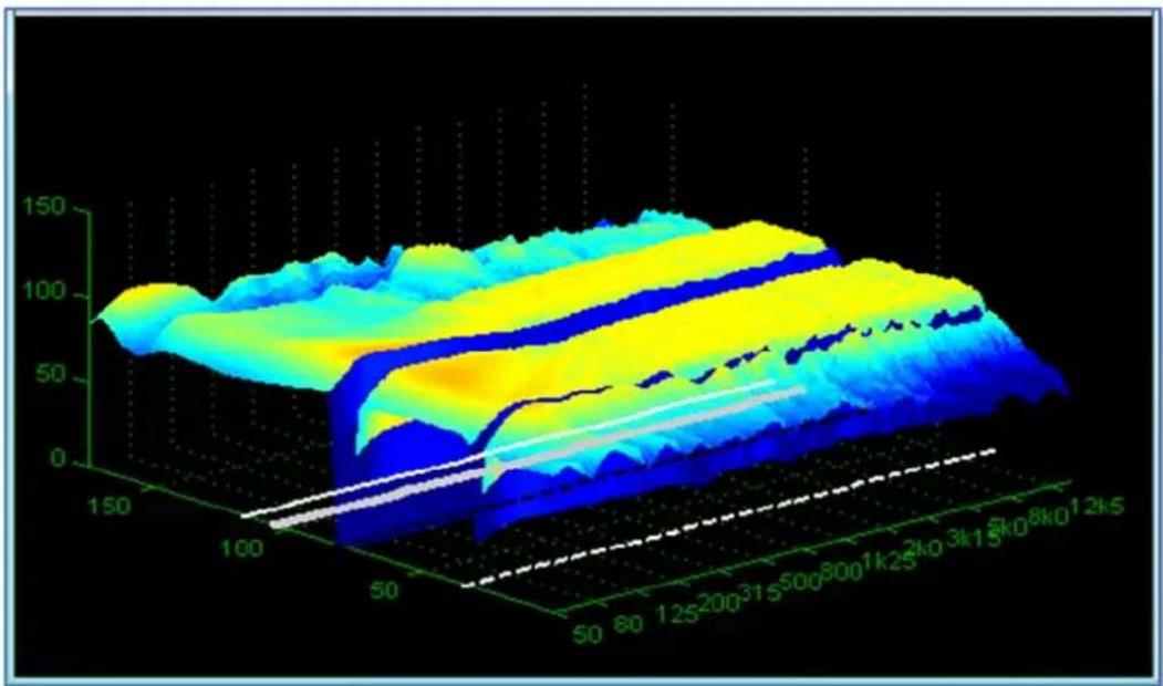
surface_3d
| Depth (k) | X-Coordinate | Y-Coordinate | |-----------|--------------|--------------| | 50 | 100 | 0 | | 60 | 125 | 25 | | 70 | 150 | 50 | | 80 | 125 | 75 | | 90 | 100 | 100 | | 100 | 75 | 125 | | 110 | 50 | 150 | | 120 | 25 | 175 | | 130 | 10 | 200 | | 140 | 5 | 225 | | 150 | 0 | 250 |The Data Cursor is useful on graphs such as the frequency response as you can click on any point of the graph and see a value for both x and y positions; -

You can continue to click on new positions on the graph to obtain readings for as long as the Data Cursor button is selected.
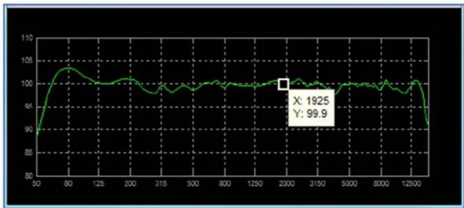
line
| X | Y | | ---- | --- | | 1925 | 99.9 |Insert Colorbar adds a reference bar to the graph; -

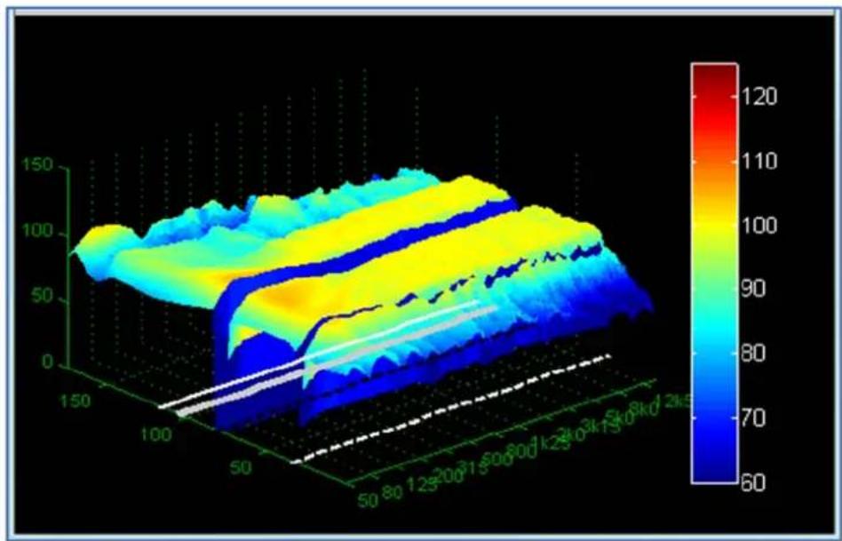
heatmap
| X Range | Y Range | Value | |---------|---------|-------| | 50-80 | 0-150 | ~60 | | 80-125 | 0-150 | ~70 | | 125-200 | 0-150 | ~80 | | 200-300 | 0-150 | ~90 | | 300-400 | 0-150 | ~100 | | 400-500 | 0-150 | ~110 | | 500-600 | 0-150 | ~120 | | 600-700 | 0-150 | ~115 | | 700-800 | 0-150 | ~110 | | 800-900 | 0-150 | ~105 | | 900-1000| 0-150 | ~100 | | 1000-1100| 0-150 | ~95 | | 1100-1200| 0-150 | ~90 | | 1200-1300| 0-150 | ~85 | | 1300-1400| 0-150 | ~80 | | 1400-1500| 0-150 | ~75 |Insert Legend is a function to add a key to the graph but this has not been adopted in Display 2.3
Adding additional arrays
It is very common to have additional arrays deployed at a venue, particularly side hangs in venues where the stage projects out into the arena and there is perhaps banked seating either side of stage. With MLA Mini having a horizontal dispersion of 100^ it is obviously impossible to achieve coverage right round the sides of a stage so side hangs are often essential. You may also have to deploy delay hangs larger auditoriums. These can all be catered for in the same Display 2.3 Mini project by adding the extra arrays as required and going through the same design process we have already used for each array.
If we select the Add tab and click on the add array button, we will see the same dialog window open that we used when we created the original array. You will notice however that the tab for the first array is still present; -
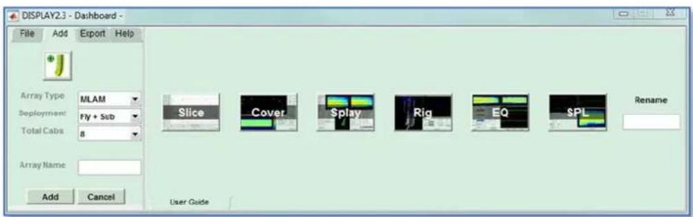
text_image
DISPLAY2.3 - Dashboard - File Add Export Help Array Type MLAM Deployment Fly + Sub Total Cabs 8 Array Name Add Cancel Slice Cover Splay Rig EQ SPL Rename User GuideWe will add a second array of eight MLA Mini to be used as side hangs so will name them "Sides". Once you have entered the name, click on Add and a new tab will be created; -

text_image
DISPLAY2.3 - Dashboard - File Add Export Help Slice Cover Splay Rig EQ SPL Rename User Guide SidesYou can now go through the same design process defining the 2D slice, array position, audience planes and optimisation coefficients exactly as we did for the main array, we can return to edit the main array at any time by clicking on the tab. As mentioned previously, we can rename either of the arrays by selecting the correct tab, typing the new name in the Rename box and pressing enter.
You can enter dozens of arrays, only seven will be visible at any one time as the dashboard cannot be expended on the present version. Arrays added above seven cannot be accessed until you delete one of the visible arrays.
Deleting an array
To keep your Display project tidy and the file size reasonable you may need to delete arrays that are no longer required. This is very simple, select the array by clicking on its tab and type 'delete' in the Rename box and press Return. The array tab will disappear. Note that you must type 'delete' or 'Delete', if you or type the whole word in upper case you will simply rename the array "DELETE".
Exporting the Optimisation
Once you have completed your array designs you need to export the file so it can be uploaded into the system via Vu-Net. On the Dashboard select the 'Export' tab, you will see four options, the first is to generate a printable rigging report file, the next will produce a DXF wireframe model of the array, the third will export D2P files of your optimisation which can be uploaded into the system via Vu-Net, and finally the EASE option will export an XGLC file which when used with the GLL for the cabinet type can be used to import an array directly into EASE with all deployment details- array and inter-cabinet angles et cetera.

text_image
DISPLAY2.3 - Dashboard - User guide QS.mat File Add Export Help Slice Cover Splay Rig EQ SPL Rename User Guide NLA WPMExporting D2P Files
First we will look at Exporting D2P files of your EQ Optimisations, this is likely to be the most common Export function you will use. Click the Export to VUNET button
You will see the export window open; -
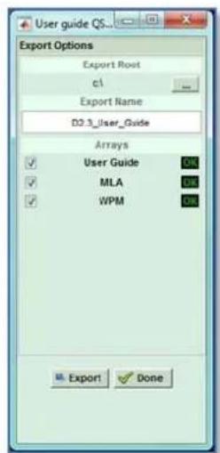
text_image
User guide QS... Export Options Export Root c1 Export Name D2.3_User_Guide Arrays User Guide MLA WPM Export DoneThe First step is to create a file into which the D2P optimisations will be loaded. The Export Root defaults to your PC C: drive but it is good practice to save your files to a dedicated folder which can be used to store all files created for a particular project. Click on the small box on the right of the Export Root section, navigate to a convenient file location, and if necessary create a new folder first to drop the file into. The Export Root will show the file location; -
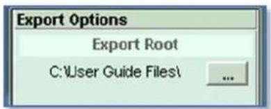
text_image
Export Options Export Root C:\User Guide Files\ ...You have now created a file but until you run the next stage there will not be any optimisation files present! You will see a list of all the arrays you have created which will have a green OK symbol if the optimisation files were saved by pressing 'Use' when the optimisation was completed. If the design process was incomplete for any reason there will be a red exclamation mark showing; -
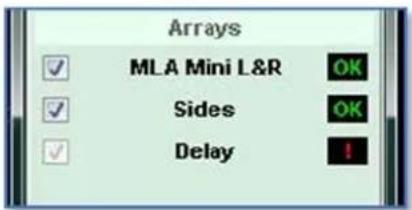
text_image
Arrays MLA Mini L&R Sides DelayIf this is an array that is not required you can continue, if it is one that is needed you should click 'Done' to close the Export window and return to the array to complete the optimisation process.
If you have all the required arrays present you can select them for export using the check box on the left. By default this will be all completed arrays but if there are some which were unsuccessful attempts you can un-check them so they cannot accidentally get used.
Click Export and a line of text in green appears at the bottom of the window showing the export process taking place. Once this disappears the export is complete and you can click done to close the window.
Exporting to DXF
The final button on the Export section allows the exporting of a wireframe model of the array for use with AutoCad; -

Clicking on the button brings up the following Window; -
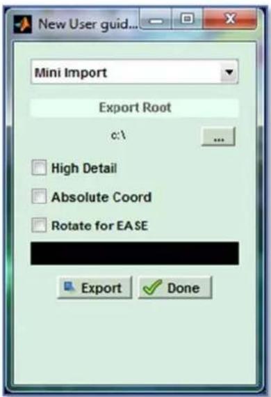
text_image
New User guid... Mini Import Export Root c:\ High Detail Absolute Coord Rotate for EASE Export DoneAs with Balloon Exports the first stage is to select which of the arrays in your project you wish to Export using the drop-down at the top of the window; -
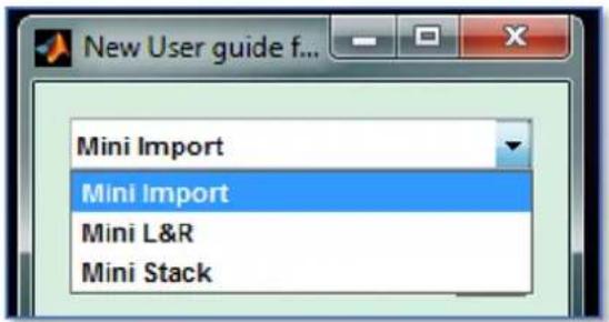
text_image
New User guide f... Mini Import Mini Import Mini L&R Mini StackNext click on the box on the right to navigate to a suitable file location in which to save the exported file; -
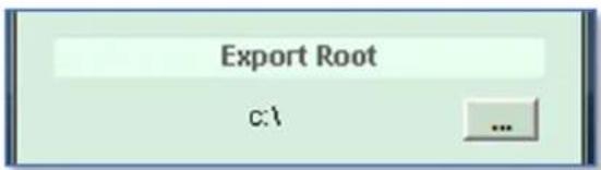
text_image
Export Root c:1 ...Next you have three options to adjust the parameters of the exported DXF; -
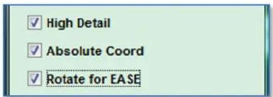
text_image
✓ High Detail ✓ Absolute Coord ✓ Rotate for EASEHigh detail will produce the best quality of drawing but with a larger file size, with large arrays it may be necessary to select standard detail to keep the files size manageable.
Absolute coordinates will position the model according to its position within the venue. With this un-checked the model will not have any location parameters specified, it will essentially be free-floating.
Finally, if you intend to import the DXF into EASE you need to click the Rotate for EASE option to ensure that the model will be correctly orientated which used with EASE.
When you are happy with your choice of parameters, click the Export button. The black window will show the progress of the Export; -

text_image
Exporting box 3When the Export is finished you will see an indication in the widow; -

text_image
Finished ExportClick the √Done button to close the Export window. Here is an example of a DXF export viewed in AutoCad; -
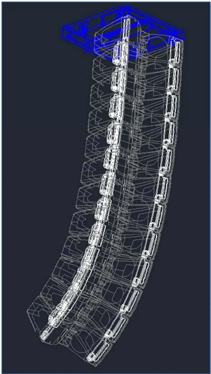
natural_image
3D wireframe model of a multi-level building structure with blue structural framework (no text or symbols)Printable Reports
A new feature for Display 2.3 is the ability to export a report which can be filed or printed.

Clicking on the icon brings up the following window; -
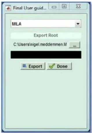
text_image
Final User guid... MLA Export Root C:\Users\nigel.meddemmen.M Export DoneIn similar fashion to the optimisation files, the first step is to select the directory to wish you would like to export the report, note that the report will generate information for just the currently selected array, if you have several arrays in the project you will have to use the Export Report function individually for all those for which you need a report. Click 'Export' and a new folder will be created in the selected file location and three files will be uploaded, a png image of the array; -
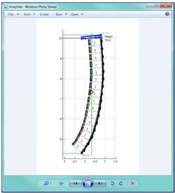
text_image
ArraySide - Windows Photo Viewer File Print E-mail Burn Open Height 10 m 4.3 m 5.0 6.0 7.0 8.0 9.0 10.0 10.15 mA png image of the venue slice; -
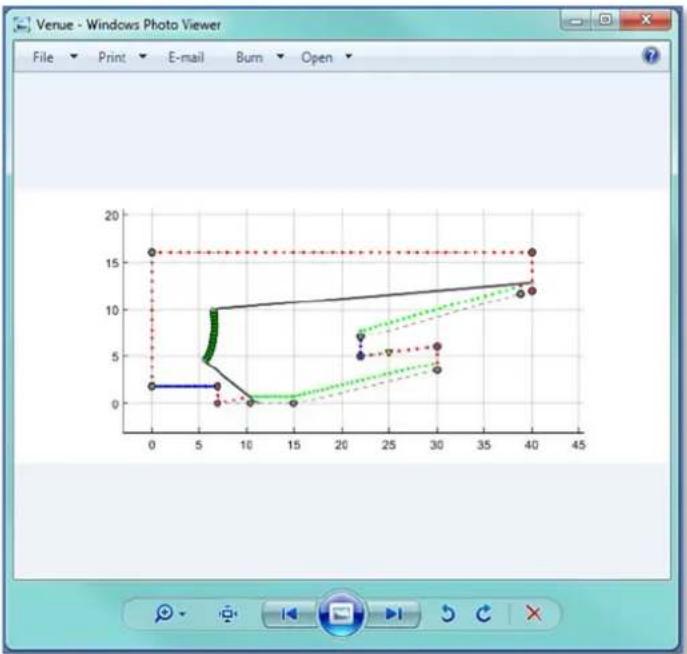
text_image
Venue - Windows Photo Viewer File Print E-mail Burn Open 16 10 10 10 10 10 10 10 10 10 10 10 10 10 10 10 10 10 10 10 10 10 10 10 10 10 10 10 10 10 10 10 10 10 10And an HTML file which contains both images plus a full rigging report; -
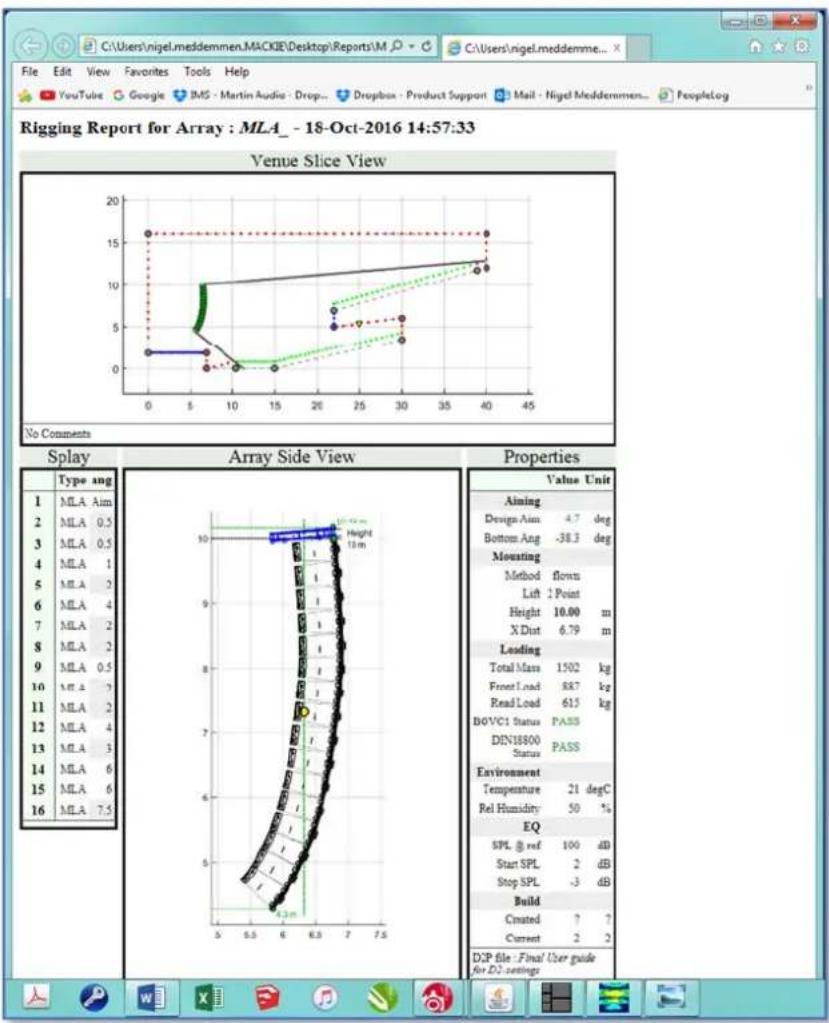
text_image
Rigging Report for Array : MLA_ - 18-Oct-2016 14:57:33 Venue Slice View No Comments Splay Array Side View Properties Type ang 1 MLA Aim 2 MLA 0.5 3 MLA 0.5 4 MLA 1 5 MLA 2 6 MLA 4 7 MLA 2 8 MLA 2 9 MLA 0.5 10 M.T.A 7 11 MLA 2 12 MLA 4 13 MLA 3 14 MLA 6 15 MLA 6 16 MLA 7.5 10 Height 10 m 8 6 5 4.3m 5.5 6.5 7.5 10 10 9 8 7 6 5 4.3m 5.5 6.5 7.5 15 16 17 18 19 20 10 11 12 13 14 15 16 Aiming Design Aim 4.7 deg Bottom Ang -38.3 deg Mounting Method flows Lift Point Height 10.00 m X Dist 6.79 m Leading Total Mass 1502 kg Front Load 887 kg Read Load 615 kg BOVC1 Status PASS DIN18800 Status PASS Environment Temperature 21 degC Rel Humidity 50 % EQ SPL @ ref 100 dB Start SPL 2 dB Stop SPL -3 dB Build Created ? ? Current 2 ? DXP file : Final User guide for D2 settingsExport 3D Data
Display 2.3 features the option to export an XGLC file which when combined with the GLL for the cabinet type enables the optimised array to be imported into an EASE project.
The EASE button also opens an Export Window requiring the file location to be selected; -
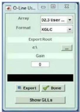
text_image
O-Line Us... Array D2.3 User ... Format XGLC Export Root c:\ Gain 0 Export Done Show GLLsArrays in the project have to have their EASE files exported individually so the drop-down at the top is used to select which array you wish to Export; -
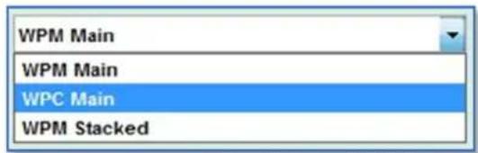
text_image
WPM Main WPM Main WPC Main WPM StackedNext Select which 3D format you would like to export, either EASE XGLC or CLF Text; -
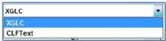
text_image
XGLC XGLC CLFTextSelect a file location in which to place the exported file and click on 'Export', you will again see a progress display showing the export as it completes; -

text_image
Exporting WPM Box 4The display will show when the export is complete; -

text_image
Finished ExportYou can click on Show GLLs; -
Which will show the file location for all array EASE GII files
You can click 'Done' to close the Export Window.