MTurboReverb - Audio software MeldaProduction - Free user manual and instructions
Find the device manual for free MTurboReverb MeldaProduction in PDF.


| Product Type | Audio Software (Reverb Plugin) |
| Version | MTurboReverb |
| Developer | MeldaProduction |
| Platform | Windows, macOS |
| Plugin Formats | VST, VST3, AU, AAX |
| Bit Depth | 32-bit and 64-bit |
| Sample Rate | Up to 192 kHz |
| Reverb Algorithms | Convolution, Algorithmic, and Hybrid |
| Presets | Over 1000 factory presets |
| CPU Usage | Optimized for low latency |
| Installation | Download from MeldaProduction website |
| Activation | License key required |
| User Interface | Resizable GUI with dark theme |
| Memory Usage | Approximately 50 MB RAM |
| Disk Space | 200 MB free space |
| Maintenance | Regular updates via MeldaProduction installer |
| Safety | No special safety precautions; standard computer use |
| Spare Parts | Not applicable (software) |
| General Info | Professional reverb plugin with comprehensive controls |
Frequently Asked Questions - MTurboReverb MeldaProduction
User questions about MTurboReverb MeldaProduction
0 question about this device. Answer the ones you know or ask your own.
Ask a new question about this device
Download the instructions for your Audio software in PDF format for free! Find your manual MTurboReverb - MeldaProduction and take your electronic device back in hand. On this page are published all the documents necessary for the use of your device. MTurboReverb by MeldaProduction.
USER MANUAL MTurboReverb MeldaProduction
Overview
MTurboReverb is probably the most powerful algorithmic reverb ever made. Most reverbs are based around a single algorithm, for which you can change certain properties, such as reverb length. That makes them very limited in terms of use and sound. MTurboReverb comes with currently about 100 reverb designs (based on different, often multiple, algorithms), complex and simple, realistic and creative, large and small, featuring all kinds of advanced factors such as pitch shifting or frequency shifting. So in a way it serves as 100 different reverb plugins (or hardware units) and more are being created.
All these reverbs are available by selecting one of the devices on the main screen (called Easy screen). All of them share a very similar GUI, so that you in fact instantly learn to use all of these reverbs just by learning one. You can browse the available reverbs simply by clicking on them on the left side of the Easy screen. Use the Display locks button on top of the list to show locks next to most parameters, which let you lock them so they stay the same while browsing the reverbs. For instance, if you are using the reverb as a send, which was quite common mainly to save CPU, you will want to set the Dry/Wet to 100%. To do that, just click the lock button next to the Dry/Wet control and it will stay at that value while changing reverbs.
Most of the reverbs feature everything you'd usually need, from Dry/Wet and Length controls through to parameters of early and late reflections and advanced dynamics processing, all available instantly from the Easy screen and documented below.
Under the hood
MTurboReverb does all that magic by providing a simple programming language that lets you actually define the algorithm that powers the reverb. It has been designed in such a way that creating these algorithms is actually very simple. In fact, each algorithm is defined by a single line! Despite all the versatility the engine is actually extremely CPU efficient. Anyway do not worry; you don't need to do any programming yourself, unless you feel especially creative. The devices will probably keep you busy for a long time.
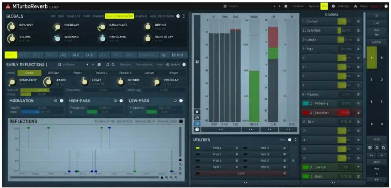
The Edit screen provides access to the underlying functionality and contains several modules. First there are 4 ER (Early Reflection) sections. These are more graphical and let you define the early reflections directly via a tapped delay line. Presets for these sections are available and there are hundreds of predefined ERs. Besides the classic tapped delay line, traditionally used for producing early reflections, each ER sections actually provides additional algorithms such as Diffuser or Room, so that you can actually design the whole reverb just using the ER sections. But that would exploit only a small part of the plugin's potential.
The main power lies in the 6 LR (Late Reflection) sections. So in a way there are up to 6 reverbs running in parallel, and that's not including the ERs, you can only imagine how big the potential is. Each LR section provides an Algorithm field, which lets you design the actual processing unit, and define several parameters that apply to the algorithm automatically. These include dampening, size, length and other basic parameters as well as advanced controls defining the underlying system of delays and other structures.
Finally there is a fully-featured dynamics section, that can process the reverb input or output, and 2 dynamic equalizers, one processing standard left/right channels and the other processing mid/side channels. Finally there are modulators at your disposal, if you really aim at being extra creative. And the huge set of multiparameters let you build Easy screen GUIs for your own reverb designs (they have been used to create all the predefined reverbs).
MTurboReverb vs. MTurboReverbLE
MTurboReverb comes in 2 licence editions - MTurboReverb is the full licence, which gives you access to all features of the plugin and also to the multiband version MTurboReverbMB. This full licence is also part of the MTotalFXBundle and MCompleteBundle.
MTurboReverbLE is a limited licence, which provides all the devices on the Easy screen. It doesn't let you use the multiband version or the Edit screen, hence you cannot design your own reverbs. It should however be far more than enough for everyday mixing/mastering/production, it's like 100 reverbs after all.
Easy screen vs. Edit screen
The plugin provides 2 user interfaces - an easy screen and an edit screen. Use the Edit button to switch between the two.
By default most plugins open on the easy screen (edit button released). This screen is a simplified view of the plugin which provides just a few controls. On the left hand side of the plugin you can see the list of available devices / instruments (previously called 'active presets'), that is, presets with controls. These controls are actually nothing more than multiparameters (single knobs that can control one or more of the plug-in's parameters and sometimes known as Macro controls in other plug-ins) and are described in more detail later. Each device may provide different controls and usually is intended for a specific purpose. The easy screen is designed for you to be able to perform common tasks, quickly and easily, without the need to use the advanced settings (that is, those available on the Edit screen).
In most cases the devices are highlighted using different text colors. In some cases the colors only mark different types of processing, but in most cases the general rule is that black/white devices are the essential ones designed for general use. Green devices are designed for a specific task or audio materials, e.g. de-essing or processing vocals in a compressor plugin. Red devices usually provide some very special processing or some extreme or creative settings. In a distortion plugin, for example, these may produce an extremely distorted output. Blue devices require an additional input, a side-chain or MIDI input usually. Without these additional inputs these Blue presets usually do not function as intended. Please check your host's documentation about routing side-chain and MIDI into an effect plugin.
To the right of the controls are the meters or time-graphs for the plugin; the standard plugin Toolbar may be to the right of these or at the bottom of the plugin.
By clicking the Edit button you can switch the plugin to edit mode (edit button pushed). This mode provides all the features that the plugin offers. You lose no settings by toggling between edit mode and the easy screen unless you actually change something. This way you can easily check what is "under the hood" for each device, or start with an device and then tweak the plugin settings further.
Devices are factory specified and cannot be modified directly by users, however you can still make your own and store them as normal presets. To do so, configure the plugin as desired, then define each multiparameter and specify its name in its settings. You can then switch to the easy screen and check the user interface that you have created. Once you are satisfied with it, save it as a normal preset while you are on the easy screen. Although your preset will not be displayed or selected in the list of available devices, the functionality will be exactly the same. For more information about multiparameters and devices please check the online video tutorials.
If you are an advanced designer, you can also view both the easy and edit screens at the same time. To do that, hold Ctrl key and press the Edit button.

Presets
Presets
Presets button shows a window with all available presets. A preset can be loaded from the preset window by double-clicking on it, selecting via the buttons or by using your keyboard. You can also manage the directory structure, store new presets, replace existing ones etc. Presets are global, so a preset saved from one project, can easily be used in another. The arrow buttons next to the preset button can be used to switch between presets easily.
Holding Ctrl while pressing the button loads a random preset. There must be some presets for this feature to work of course.
Presets can be backed up by 3 different methods:
A) Using "Backup" and "Restore" buttons in each preset window, which produces a single archive of all presets on the computer.
B) Using "Export/Import" buttons, which export a single folder of presets for one plugin.
C) By saving the actual preset files, which are found in the following directories (not recommended):
Windows: C:\Users{username}\AppData\Roaming\MeldaProduction
Mac OS X: /Library/Application support/MeldaProduction
Files are named based on the name of the plugin like this: " {pluginname}.presets", so for example MAutopan.presets or MDynamics.presets. If the directory cannot be found on your computer for some reason, you can just search for the particular file.
Please note that prior to version 16 a different format was used and the naming was " {pluginname}presets.xml". The plugin also supports an online preset exchange. If the computer is connected to the internet, the plugin connects to our server once a week, submits your presets and downloads new ones if available. This feature is manually maintained in order to remove generally unusable presets, so it may take some time before any submitted presets become available. This feature relies on each user so we strongly advise that any submitted presets be named and organised in the same way as the factory presets, otherwise they will be removed.

Left arrow
Left arrow button loads the previous preset.

Right arrow
Right arrow button loads the next preset.
Randomize button loads a random preset.
Randomize
Randomize button (with the text 'Random') generates random settings. Generally, randomization in plug-ins works by selecting random values for all parameters, but rarely achieves satisfactory results, as the more parameters that change the more likely one will cause an unwanted effect. Our plugins employ a smart randomization engine that learns which settings are suitable for randomization (using the existing presets) and so is much more likely to create successful changes.
In addition, there are some mouse modifiers that assist this process. The smart randomization engine is used by default if no modifier keys are held.
Holding Ctrl while clicking the button constrains the randomization engine so that parameters are only modified slightly rather than completely randomized. This is suitable to create small variations of existing interesting settings.
Holding Alt while clicking the button will force the engine to use full randomization, which sets random values for all reasonable automatable parameters. This can often result in "extreme" settings. Please note that some parameters cannot be randomized this way.

Panic
Panic button resets the plugin state. You can use it to force the plugin to report latency to the host again and to avoid any audio problems. For example, some plugins, having a look-ahead feature, report the size of the look-ahead delay as latency, but it is inconvenient to do that every time the look-ahead changes as it usually causes the playback to stop. After you tweak the latency to the correct value, just click this button to sync the track in time with the others, minimizing phasing artifacts caused by the look-ahead delay mixing with undelayed audio signals in your host. It may also be necessary to restart playback in your host.
Another example is if some malfunctioning plugin generates extremely high values for the input of this plugin. A potential filter may start generating very high values as well and as a result the playback will stop. You can just click this button to reset the plugin and the playback will start again.
Settings
Settings button shows a menu with additional settings of the plugin. Here is a brief description of the separate items.
Licence manager lets you activate/deactivate the plugins and manage subscriptions. While you can simply drag & drop a licence file onto the plugin, in some cases there may be a faster way. For instance, you can enter your user account name and password and the plugin will do all the activating for you.
There are 4 groups of settings, each section has its own detailed help information: GUI & Style enables you to pick the GUI style for the plug-in and the main colours used for the background, the title bars of the windows and panels, the text and graphs area and the highlighting (used for enabled buttons, sliders, knobs etc).
Advanced settings configures several processing options for the plug-in.
Global system settings contains some settings for all MeldaProduction plugins. Once you change any of them, restart your DAW if needed, and it will affect all MeldaProduction plugins.
Dry/Wet affects determines, for Multiband plug-ins, which multiband parameters are affected by the Global dry/wet control.
Smart interpolation adjusts the interpolation algorithm used when changing parameter values; the higher the setting the higher the audio quality and the lower the chance of zippering noise, but more CPU will be used.

WWW
WWW button shows a menu with additional information about the plugin. You can check for updates, get easy access to support, MeldaProduction web page, video tutorials, Facebook/Twitter/YouTube channels and more.
Sleep indicator
Sleep indicator informs whether the plugin is currently active or in sleep mode. The plugin can automatically switch itself off to save CPU, when there is no input signal and the plugin knows it cannot produce any signal on its own and it generally makes sense. You can disable this in Settings / Intelligent sleep on silence both for individual instances and globally for all plugins on the system.
Plugin toolbar

Plugin toolbar provides some global features, A-H presets and more.

Oversampling
Oversampling can potentially improve sound quality by processing at a higher sample rate. Processors such as compressors, saturators, distortions etc., which employ nonlinear processing generate higher harmonics of the existing frequencies. If these frequencies exceed the Nyquist rate, which equals half of the sampling rate, they get mirrored back under the Nyquist rate. This is known as aliasing and is almost always considered an artifact. This is because the mirrored frequencies are no longer harmonic and sound as digital noise as this effect does not physically occur in nature. Oversampling reduces the problem by temporarily increasing the sampling rate. This moves the Nyquist frequency which in turn, diminishes the level of the aliased harmonics. Note that the point of oversampling is not to remove harmonics, we usually add them intentionally to make the signal richer, but to reduce or attenuate the harmonics with frequencies so high, that they just cannot be represented within the sampling rate.
To understand aliasing, try this experiment: Set the sampling rate in your host to 44100 Hz. Open MOscillator and select a "rectangle" or "full saw" waveform. These simple waveforms have lots of harmonics and without oversampling even they become highly aliased. Now select 16x oversampling and listen to the difference. If you again select 1x oversampling, you can hear that the audio signal gets extensively "dirty". If you use an analyzer (MAnalyzer or MEqualizer for example), you will clearly see how, without oversampling, the plugin generates lots of inharmonic frequencies, some of them which are even below the fundamental frequency. Here is another, very extreme example to demonstrate the result of aliasing. Choose a "sine" shape and activate 16x oversampling. Now use a distortion or some saturation to process the signal. It is very probable that you will be able to hear (or at least see in the analyzer) the aliased frequencies.
The plugin implements a high-quality oversampling algorithm, which essentially works like this: First the audio material is upsampled to a higher sampling rate using a very complicated filter. It is then processed by the plugin. Further filtering is performed in order to remove any frequencies above the Nyquist rate to prevent aliasing from occurring, and then the audio gets downsampled to the original sampling rate.
Oversampling also has several disadvantages of which you should be aware before you start using it. Firstly, upsampled processing induces latency (at least in high-quality mode, although you can select low-quality directly in this popup), which is not very usable in real time applications. Secondly, oversampling also takes much more CPU power, due to both the processing being performed at a higher sampling rate (for 16x oversampling at 44100 Hz, this equates to 706 kHz!), and the complex filtering. Finally, and most
importantly, oversampling creates some artifacts of its own and for some algorithms processing at higher sampling rates can actually lower the audio quality, or at least change the sound character. Your ears should always be the final judge.
As always, use this feature ONLY if you can actually hear the difference. It is a common misconception that oversampling is a miraculous cure all that makes your audio sound better. That is absolutely not the case. Ideally, you should work in a higher sampling rate (96kHz is almost always enough), while limiting the use of oversampling to some heavily distorting processors.
L+R
Channel mode
Channel mode button shows the current processing channel mode, e.g. Left+Right (L+R) indicates the processing of left and right channels. This is the default mode for mono and stereo audio material and effectively processes the incoming signal as expected. However the plugin also provides additional modes, of which you may take advantage as described below. Mastering this feature will give you unbelievable options for controlling the stereo field.
Note that this is not relevant for mono audio tracks, because the host supplies only one input and output channel.
Left (L) mode and Right (R) mode allow the plugin to process just one channel, only the left or only the right. This feature has a number of simple uses. Equalizing only one channel allows you to fix spectral inconsistencies, when mids are lower in one channel for example. A kind of stereo expander can be produced by equalizing each side differently. Stereo expansion could also be produced by using a modulation effect, such as a vibrato or flanger, on one of these channels. Note however that the results would not be fully mono compatible.
Left and right channels can be processed separately with different settings, by creating two instances of the plugin in series, one set to 'L' mode and the other to 'R' mode. The instance in 'L' mode will not touch the right channel and vice versa. This approach is perfectly safe and is even advantageous, as both sides can be configured completely independently with both settings visible next to each other.
Mid (M) mode allows the plugin to process the so-called mid (or mono) signal. Any stereo signal can be transformed from left and right, to mid and side, and back again, with minimal CPU usage and no loss of audio quality. The mid channel contains the mono sum (or centre), which is the signal present in both left and right channels (in phase). The side channel contains the difference between the left and right channels, which is the "stereo" part. In 'M mode' the plugin performs the conversion into mid and side channels, processes mid, leaves side intact and converts the results back into the left and right channels expected by the host.
To understand what a mid signal is, consider using a simple gain feature, available in many plugins. Setting the plugin to M mode and decreasing gain, will actually lower or attenuate the mono content and the signal will appear "wider". There must be some stereo content present, this will not work for monophonic audio material placed in stereo tracks of course. Similarly amplifying the mono content by increasing the gain, will make the mono content dominant and the stereo image will become "narrower".
As well as a simple gain control there are various creative uses for this channel mode.
Using a compressor on the mid channel can widen the stereo image, because in louder parts the mid part gets attenuated and the stereo becomes more prominent. This is a good trick to make the listener focus on an instrument whenever it is louder, because a wider stereo image makes the listener feel that the origin of the sound is closer to, or even around them.
A reverb on the mid part makes the room appear thin and distant. It is a good way to make the track wide due to the existing stereo content, yet spacey and centered at the same time. Note that since this effect does not occur naturally, the result may sound artificial on its own, however it may help you fit a dominant track into a mix.
An equalizer gives many possibilities - for example, the removal of frequencies that are colliding with those on another track. By processing only the mid channel you can keep the problematic frequencies in the stereo channel. This way it is possible to actually fit both tracks into the same part of the spectrum - one occupying the mid (centre) part of the signal, physically appearing further away from the listener, the other occupying the side part of the signal, appearing closer to the listener.
Using various modulation effects can vary the mid signal, to make the stereo signal less correlated. This creates a wider stereo image and makes the audio appear closer to the listener.
Side (S) mode is complementary to M mode, and allows processing of only the side (stereo) part of the signal leaving the mid intact. The same techniques as described for M mode can also be applied here, giving the opposite results.
Using a gain control with positive gain will increase the width of the stereo image.
A compressor can attenuate the side part in louder sections making it more monophonic and centered, placing the origin a little further away and in front of the listener.
A reverb may extend the stereo width and provide some natural space without affecting the mid content. This creates an interesting side-effect - the reverb gets completely cancelled out when played on a monophonic device (on a mono radio for example). With stereo processing you have much more space to place different sounds in the mix. However when the audio is played on a monophonic system it becomes too crowded, because what was originally in two channels is now in just one and mono has a very limited capability for 2D placement. Therefore getting rid of the reverb in mono may be advantageous, because it frees some space for other instruments.
An equalizer can amplify some frequencies in the stereo content making them more apparent and since they psycho acoustically become closer to the listener, the listener will be focused on them. Conversely, frequencies can be removed to free space for other instruments in stereo.
A saturator / exciter may make the stereo richer and more appealing by creating higher harmonics without affecting the mid channel, which could otherwise become crowded.
Modulation effects can achieve the same results as in mid mode, but this will vary a lot depending on the effect and the audio material. It can be used in a wide variety of creative ways.
Mid+Side (M+S) lets the plugin process both mid and side channels together using the same settings. In many cases there is no difference to L+R mode, but there are exceptions.
A reverb applied in M+S mode will result in minimal changes to the width of the stereo field (unless it is true-stereo, in which case mid will affect side and vice versa), it can be used therefore, to add depth without altering the width.
A compressor in M+S mode can be a little harder to understand. It basically stabilizes the levels of the mid and side channels. When channel linking is disabled in the compressor, you can expect some variations in the sound field, because the compressor will attenuate the louder channel (usually the mid), changing the stereo width depending on the audio level. When channel linking is enabled, a
compressor will usually react similarly to the L+R channel mode.
Exciters or saturators are both nonlinear processors, their outputs depend on the level of the input, so the dominant channel (usually mid) will be saturated more. This will usually make the stereo image slightly thinner and can be used as a creative effect.
How to modify mid and side with different settings? The answer is the same as for the L and R channels. Use two instances of the plugin one after another, one in M mode, the other in S mode. The instance in M mode will not change the side channel and vice versa.
Left+Right(neg) (L+R-) mode is the same as L+R mode, but the right channel's phase will be inverted. This may come in handy if the L and R channels seem out of phase. When used on a normal track, it will force the channels out of phase. This may sound like an extreme stereo expansion, but is usually extremely fatiguing on the ears. It is also not mono compatible - on a mono device the track will probably become almost silent. Therefore be advised to use this only if the channels are actually out of phase or if you have some creative intent.
There are also 4 subsidiary modes: Left & zero Right (L(R0)), Right & zero Left (R(L0)), Mid & zero Side (M(S0)) and Side & zero Mid (S(M0)). Each of these processes one channel and silences the other.
Surround mode is not related to stereo processing but lets the plugin process up to 8 channels, depending on how many the host supplies. For VST2 plugins you have to first activate surround processing using the Activate surround item in the bottom. This is a global switch for all MeldaProduction plugins, which configures them to report 8in-8out capabilities to the host, on loading. It is disabled by default, because some hosts have trouble dealing with such plugins. After activation, restart your host to start using the surround capabilities of the plugins. Deactivation is done in the same way. Please note that all input and output busses will be multi-channel, that includes side-chain for example. For VST3/AU/AAX plugins the activation is not necessary.
First place the plugin on a surround track - a track that has more than 2 channels. Then select Surround from the plug-in's Channel Mode menu. The plugins will regard this mode as a natural extension of 2 channel processing. For example, a compressor will process each channel separately or measure the level by combining the levels of all of the inputs provided. Further surround processing properties, to enable/disable each channel or adjust its level, can be accessed via the Surround settings in the menu.
Ambisonics mode provides support for the modern 3D systems (mostly cinema and VR) with up to 64 channels (ambisonics 7th order). Support for this is still quite rare among the DAWs, so this needs to be activated in all DAWs using the Activate ambisonics item in the bottom. This is a global switch for all MeldaProduction plugins, which configures them to report 64in-64out capabilities to the host, on loading. After activation, restart your host to start using the ambisonics capabilities of the plugins. Deactivation is done in the same way. Please note that all input and output busses will be multi-channel, that includes side-chain for example.
First place the plugin on an ambisonics track, supported are all orders from 1st (4 channels) to 7th (64 channels). Then select
Ambisonics from the plug-in's Channel Mode menu. Finally select the Ambisonics settings in the menu and configure the Ambisonics order and other settings if needed. The plugins will regard this mode as a natural extension of 2 channel processing. For example, a compressor will process each channel separately or measure the level by combining the levels of all of the inputs provided.
AGC
AGC button enables or disables the automatic gain control - the automatic adjustment of the output volume such that it matches the input volume. Human hearing is very adaptable. In fact differences in loudness, for example when loading a preset, may go unnoticed and instead be perceived by the listener as "better sounding", leading to a misjudgement. This feature should prevent this effect, thus allowing the listener to focus on the sonic qualities only.
AGC works by measuring input and output loudness, and then compensating for the difference while also taking into account any induced latency. The loudness measurement follows the ITU and EBU specifications with an RMS of 400ms, meaning that the reaction time is 400ms. This is very important, as you should be aware that AGC needs time to properly adjust after any change of settings. Also note that this is a nonlinear operation. It may cause some distortion due to the long measurement time. It should be negligible though.
AGC makes sense in most applications including reverberation and equalization for example. However, in some cases it can work against the plugin. A simple example of this is a tremolo, where the plugin manipulates output volume. If the tremolo rate is slow enough, say 1Hz, it makes the period longer than the actual AGC measurement time. So whenever the tremolo changes audio level, the AGC starts compensating for it. This can of course be used creatively, since AGC will always be a little "late", but it is definitely not a desired outcome in normal use.
Another example of this is compression. When used with short attack and release times, AGC can effectively compensate for the attenuation of the compressor. However when the attack and release times are higher than 100ms, the compressor's reaction time becomes too slow, and in conjunction with AGC, severe pumping can occur.
As a general rule of thumb as for all audio processing tasks, use it only if you know you need it. AGC is a powerful tool that can make your workflow easier, but it can also be damaging.

Set
Set button uses the AGC (automatic gain compensation) processor to calculate the ideal output gain to ensure that the output audio loudness is equal to the input level. To use it, simply enable playback in your host and click the button. The plugin's output gain will be adjusted to match the input and output levels as closely as possible.
If the AGC is already enabled, the change will be instant and you can disable the AGC afterwards. Typically you will browse presets, generate random settings etc. During the entire time you will have AGC enabled to prevent you from experiencing different output loudness levels. When you find a sonically ideal setup, you simply click the Set button to set the output gain automatically and disable the AGC as you won't need it anymore.
If the AGC is not already enabled, clicking the Set button displays a window with progress bar for a few seconds, while the plugin
temporarily enables AGC and analyses input and output of the plugin. After that the AGC is disabled again.
To get the best results, you should feed the plugin with some "universal" signal. If you are processing a specific instrument, play a typical part, a chorus in case of vocals for example. If you are creating presets designed for general use, white/pink noise may be the best signal to use.
Limiter
Limiter
Limiter button enables or disables the safety limiter. Its purpose is to protect you from peaks above 0dB, which can have damaging effects to your processing chain, your monitors and even your hearing.
It is generally advised to keep your audio below 0dB at all times in all stages of your processing chain. However, several plugins may cause high level outputs with certain settings, often due to unprevented resonances with specific audio materials. The safety limiter prevents that.
Note that it is NOT wise to enable this "just in case". As with any processing, the limiter requires additional processing power and modifies the output signal. It is a transparent single-band brickwall limiter, but you still need to be careful when using it.
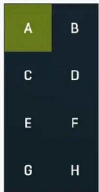
A-H presets selector
A-H presets selector controls the current A-H preset. This allows the plugin to store up to 8 sets of settings, including those parameters that cannot be automated or modulated. However it does not include channel mode, oversampling and potentially some other global controls available from the Settings/Settings menu.
For example, this feature can be used to keep multiple settings, when you are not sure about the ideal configuration When you change any parameter, only the currently selected preset is modified.
The four buttons below enable you to switch between the last 2 selected sets using the A/B button, morph between the first 4 sets using the morphing button and copy & paste settings from one preset to another (via the clipboard).
It is also possible to switch between the presets using MIDI program change messages sent from your host. The set selected depends on the Program Change number: 0 selects A, 7 selects H, 8 selects A, 15 selects H and so on.
A/B
A/B
A/B button switches between the active and previously active A-H preset (not necessarily the A and B presets themselves). To compare any 2 of the A-H presets, select one and then the other. Clicking this button will then switch between these two. You can do the same thing by clicking on the particular presets, but this makes it easier, letting you close your eyes and just listen.
88
Morph
Morph button lets you morph between the A, B, C and D settings. Morphing only affects those parameters that can be automated or modulated; that does include most of the parameters however. When you click this button, an X/Y graph is shown allowing you to drag the position indicator to any position between the letters A, B, C and D. The closer you drag the indicator to one of the letters, the closer the actual settings are to that preset.
Please note that this will overwrite and change the preset that is currently selected, so it is best to select a new preset e.g. 'E', then use the morphing method. This way you will define the settings for A, B, C and D, morph between them, and store the result in 'E' without any modification of the original A, B, C and D presets.
Please note that the ABCD morphing itself cannot be automated and that, while morphing, the changes to the underlying parameters are not notified to the host (there may be hundreds of change events).
→
Copy
Copy button copies the current settings to the system clipboard. Other presets, oversampling, channel mode and other global settings are not copied.
Hold Ctrl to save the settings as a file instead. That may be necessary for complex settings, which may be too long for system clipboard to handle. It may also be advantageous when you want to send the settings via email. You can load the settings by drag & dropping them to a plugin or holding Ctrl and clicking Paste.

Paste
Paste button pastes settings from the system clipboard into the current preset. Hold Ctrl to load the settings from a file instead. Hold Shift to paste the settings to all of the A-H slots at once.

Undo
Undo button reverts the last change. Only changes to automatable or modulatable parameters and global settings (load/randomize) are stored.
Redo
Redo button reverts the last undo operation.

WAV
WAV button lets you process a file using the plugin with current settings. You can either click the button and select a file, or drag & drop the file (or multiple files) onto the button. If you let the plugin process WAV files, these will be saved with the original settings. If you use a different file type (such as MP3), the plugin will create WAV files with 32-bit bits-per-sample floating point.
Please note that the files will be overwritten, so make a copy first if you want to keep the original.

IR
IR button lets you generate impulse response file, which approximates what the plugin does. You can use that in various IR players, including some hardware. Please note that any dynamic/modulated/somehow changing in time behaviour cannot be captured by an IR file. Also note that the IR will be generated as 24-bit WAV file ONLY if it is actually possible - if the output exceeds 0dBFS (or goes below -40dBFS), this cannot be accurately produced, so a 32-bit floating point WAV file will be generated. Some HW devices are known to have problems importing such files.
Collapse
Collapse button minimizes or enlarges the panel to release space for other editors.
Reload
Reload
Reload button reloads the device and sets all non-locked controls in the current device to their default values. It may be useful, since the plugin stores current settings when switching between the devices, hence this button is a quick and easy way to get the defaults for the devices, before you changed them. If you want to reload all parameters for the device, you must unlock the Easy screen locks or disable them all by turning off the On/Off button in the Global Locking panel in Edit mode.
Small spaces
Living room
Mojo
Bedroom
Ambience
Percussive space
Small room
Bunker
Cookies and milk
Room
Studio
Booth
Antovo studio
Bathroom
Wine cellar
Rice beads
Concrete room
Recording room
Dirty room
Character room
Large spaces
Huge spaces
Plates & springs
Creative
Special
2D positioning
Device selector
Device selector lets you choose from the predefined devices (previous 'active presets'). These are different from normal presets as they can actually have Easy-mode controls available via knobs or buttons. Click on an device to load it. Check out our video tutorials for information about creating your own devices. Although you cannot put your own devices into this selector, you can still save them as normal presets and on loading they will work in the exactly same way.
When browsing the devices, the plugin stores the control values (multiparameters). It doesn't store the full settings, only the multiparameters, so that if you switch between the devices, your settings will be kept intact, unless you switch to edit screen and perform some advanced editing, in which case it is recommended to use the A-H presets to store your work.
< >
Collapse
Collapse button minimizes or enlarges the panel to release space for other editors.

Comp
Comp controls the threshold for the compressor processing the input or reverberation signals (selected using the Pre button in the panel), the minimal signal level, when the effect is applied. Above this level the signal is being compressed. Please note that by 'level' we are talking about the level that the attack/release detector produces, not the peak level for instance. When this parameter is set to its maximum, the compressor is effectively disabled.
Gate
Gate controls the threshold for the gate processing the input or reverberation signals (selected using the Pre button in the panel), that is, the minimal signal level below which the effect is applied. Below this level the signal is being gated; with high ratios this essentially means the signal is silenced. Please note that by 'level' we are talking about the level that the attack/release detector produces, not the peak signal level for instance. When this parameter is set to minimum, the gate is effectively disabled.

Pre
Pre switch makes the dynamics module process the input signal as opposed to processing the reverberation signal. Please note that this switch does NOT change the dry input signal being mixed using the global Dry/Wet knob, that is the dynamics processing is applied AFTER the signal is tapped for the dry component fed into that knob.

Dynamics panel
Dynamics panel controls the dynamics processing applied to the input or the reverberation signal (selected using the Pre button in the Dynamic Globals panel). This includes gating and compression, both of which are very useful on both signals.
Gating applied to the input signal is a classic technique that lets you reverberate only loud parts of the signal. It is typically used on drums to produce a reverb tail for snare drums for example.
Compressing the input signal lowers the dynamic range creating a "flatter" sound, which creates more stable reverberation without actually flattening the input signal itself.
Gating the reverberation signal is a rather specific effect which lets you abruptly terminate the reverberation signal when its level goes below the threshold. When a long reverb is used, it can often muddy the mix during the parts where the particular instrument isn't playing anymore, or create long endings when used on master, which then need to be faded-out by some other method. Using a gate with threshold low enough can provide an automatic solution which stops the reverb tail sooner than it normally would, removing the muddiness / tail.
Compressing the reverberation signal flattens the reverberation signal and when overused can introduce the typical compression character many are seeking on the tracks themselves, but on the reverberation signal instead. It is mainly useful as a creative tool.

Focus
Focus controls the frequency that the dynamics module is listening to the most. This works as a band-pass filter removing unwanted frequencies from the detector. By default the focus is set to the maximum value and the filter is disabled. Lower the value to enable the filter and let the processor focus on the specified frequency. For example, when you want to produce areverberation tail for snare drums in mixed drums, enable the dynamics module, activate the gate (which is activated by default) and set the focus to the fundamental frequency of the snare drum (around 200-500Hz).
RMS length
RMS length smoothes out the values of the input levels (not the input itself), such that the level detector receives the pre-processed signal without so many fluctuations. When set to its minimum value the detector becomes a so-called "peak detector", otherwise it is an "RMS detector".
When you look at a typical waveform in any editor, you can see that the signal is constantly changing and contains various transient bursts and separate peaks. This is especially noticeable with rhythmical signals, such as drums. Trying to imagine how a typical attack/release detector works with such a wild signal may be complex, at least. RMS essentially takes the surrounding samples and averages them. The result is a much smoother signal with fewer individual peaks and short noise bursts.
RMS length controls how many samples are taken to calculate the average. It stabilizes the levels, but it also causes a slower response time. As such it is great for mastering, when you want to lower the dynamic range in a very subtle way without any instabilities. However, it is not really desirable for processing drums, for example, where the transient bursts may actually be individual drum hits, hence it is usually recommended to use peak detectors for percussive instruments.
Note that the RMS detector has 2 modes - a simplified approximation is used by default, and a true RMS is processor can be enabled from the advanced settings (if provided). Both respond differently, neither of them is better than the other, they are simply different.

Release
Release defines the release time, that is how quickly the level detector decreases the measured input level. The shorter the release time, the faster the response is. Once the attack stage has been completed, when the input peak level is lower than the current level measured by the detector, the detector moves into the release mode, in which the measured level is decreased depending on the input signal. The lower the input signal, or the shorter the release time, the faster the measured level drops. Once the measured level falls under the Threshold then the dynamics processing (compression, limiting, gating) will stop.
There must be a reasonable balance between attack and release times. If the attack is too long compared to release, the detector would tend to keep the level low, because release would cause the level to fall too quickly. Hence in most cases you may expect the attack time to be shorter than the release time.
To understand the working of a level detector, it is best to cover the typical cases:
In a compressor the release time controls how quickly the measured level falls below the threshold and the compression stops. As a result a very short release time makes the compressor stop quickly, for example, leaving the sustain of a snare drum intact. On the other hand, a very long release keeps the compression working longer, hence it is useful to stabilize the levels.
In a limiter the release time keeps the measured level above the limiter threshold causing the gain reduction. Having a very long release time in this case doesn't make sense as the limiter would be working continuously and the effect would be more or less the same as simply decreasing the input gain manually. However too short a release time lets the limiter stop too quickly, which usually causes distortion as the peaks through the limiter to the subsequent in-built clipper or saturator. Hence release time is used to avoid distortion at the expense of decreasing the output level.
In a gate the situation is similar to a compressor - the release time controls how quickly the measured level can fall below the threshold at which point the gate closes. Having a longer release time in a gate is a perfectly acceptable option. The release time will basically control how much of the sound's sustain will pass.
In a modulator, the detector is driving other parameters, a filter cut-off frequency for example, and the situation really depends on the target. If you want the detector to react quickly on the input level falling, use a shorter release time; if you want it to follow the flow of the input signal slowly, use longer attack and release times.
Attack
Attack defines the attack time, that is how quickly the level detector increases the measured input level. When the input peak level is higher than the current level measured by the detector, the detector moves into the attack mode, in which the measured level is increased depending on the input signal. The higher the input signal, or the shorter the attack time, the faster the measured level rises. Once the measured level exceeds the Threshold then the dynamics processing (compression, limiting, gating) will start.
There must be a reasonable balance between attack and release times. If the attack is too long compared to the release, the detector will tend to keep the measured level low, because the release would cause that level to fall too quickly. In most cases you may expect the attack time to be shorter than the release time.
To understand the working of a level detector, it is best to cover the typical cases:
In a compressor the attack time controls how quickly the measured level moves above the threshold and the processor begins compressing. As a result, a very short attack time will compress even the beginning transient of a snare drum for example, hence it would remove the punch. With a very long attack time the measured level may not even reach the threshold, so the compressor may not do anything.
In a limiter the attack becomes a very sensitive control, defining how much of the signal is limited and how much of it becomes saturated/clipped. If the attack time is very short, limiting starts very quickly and the limiter catches most peaks itself and reduces them, providing lower distortion, but can cause pumping. On the other hand, a higher attack setting (typically above 1ms) will let most peaks through the limiter to the subsequent in-built clipper or saturator, which causes more distortion of the initial transient, but less pumping.
In a gate the situation is similar to a compressor - the attack time controls how quickly the measured level can rise above the threshold at which point the gate opens. In this case you will usually need very low attack times, so that the gate reacts quickly enough. The inevitable distortion can then be avoided using look-ahead and hold parameters.
In a modulator, the detector is driving other parameters, a filter cut-off frequency for example, and the situation really depends on the target. If you want the detector to react quickly on the input level rising, use a shorter attack time; if you want it to follow the flow of the input signal slowly, use longer attack and release times.

Comp ratio
Comp ratio controls the ratio for the compressor. The higher the ratio, the stronger the effect is, above the threshold.

Gate ratio
Gate ratio controls the ratio for the gate. The higher the ratio is, the stronger the effect is, below the threshold.
Type
Type lets you choose from several predefined types. These change the sound of the reverb by changing some of the algorithm properties. For instance, a Room device uses Type to choose between several rooms, each of them with more or less different character. Sometimes the differences between types may be huge, sometimes it only changes the stereo field for example; it all depends on the particular device. In some rare cases the control has a different meaning - it is marked Presets and serves as a set of predefined presets, which change several controls of the device. In these cases you need to be careful, since changing the preset changes other parameters, even those you might have already changed yourself.
Treble
Treble controls the high-shelf filter which processes the reverberation signal amplifying or attenuating the high frequency content, giving it more or less "shine". This control is mainly useful for controlling the tone of the reverb. Higher values generally make the reverb brighter, lower values make it darker.
High-cut
High-cut lets you remove highest frequencies using a low-pass filter. This is sometimes useful to clean up the treble, so that the mix doesn't become crowded. In most cases bass and mids are more problematic though.
High-cut mid
High-cut mid lets you filter out highest frequencies using a low-pass filter similarly to High-cut, however it only affects the mids, the center signal. Hence it leaves the side signal intact. It is useful during mixing to clean up the treble, without actually removing the treble, since these highest frequencies will stay intact in the sides, where they contribute on the wide reverberation tail. It is usually better to try this control first before using the High-cut, which kills the high-end completely.
Length
Length controls the reverb decay time. This parameter affects the late reflections only since the early reflection length is constant and each echo is generated separately. Late reflections are generated in a very different way similar to how it happens in nature - using a system of delays and feedback lines more and more echoes are produced in time with their levels constantly lowering. Mathematically speaking the reverb decay never ends, so in a way an algorithmic reverb is infinite, and the reverb time is defined as the time after which the echoes decay to approximately -60dB, which makes it virtually inaudible in the context of a full scale signal.
Please note that in physical spaces the reverb length naturally relates to the size of the space, which is not true for algorithmic reverbs, which let you specify length and size separately. For that, look at the Size parameter in the Late Reflections panel, if provided.
Early/late
Early/late defines the ratio between early and late reflections. Generally early reflections characterize the space and position of the source object and late reflections (reverberation) indicate the room properties. Usually the more audible the early reflections, the closer the dry signal seems and conversely the more late reverberation that is present, the further away it sounds.
Early reflections represent only the initial portion of the reverb tail, when the first few reflections of the sound from the nearest walls reach the ears/head. After some time the sound reflects so many times from various walls that the echo density (the number of echoes per second) becomes very high and the reverb in fact decays into noise (if designed that way). And this is the part known as the late reflections, which usually sounds smooth and can potentially be extremely long, while early reflections only last up to a few hundred milliseconds.
Predelay
Predelay defines the initial delay before the actual response, which simulates the space between the sound source and the listener. The longer the predelay is, the further away the source seems. At some point (around say 100ms) the brain stops understanding that that the reverberation belongs to the dry signal and starts interpreting them separately, and then the dry signal becomes close to the listener again. Predelay can therefore be used to control the distance from the source to the destination, but detaching the 2 signals can also be useful for instance to fill up a mix that isn't full enough without smearing the signal with the reverb itself.

Size
Size controls the size of the virtual space. It is usually implemented by increasing the echo delay size. Please note that unlike real spaces, where higher size usually means longer reverb time, the algorithmic reverberation provides these parameters separately. In effect the size parameter controls mainly how the echoes build up. Higher sizes make the echoes build up mosre slowly (since the distance for the sound to travel from one wall to another is higher). Conversely lower sizes provide faster echo build up, often to the point where the room becomes so small that multiple walls are similar in distance and additional modes start to form and the reverb starts sounding like a small resonant box. In most devices the range for this parameter is intentionally kept large enough for both natural reverberation and the extreme creative effects.

Widening
Widening controls the stereo width of the reverberation signal. The algorithm is fully mono-compatible as it only extends the existing stereo field and no new signal is added. The default 0% means no processing at all. Lowering the value produces narrower results, eventually leading to a monophonic reverb. Higher values produce wider results, however although the width may initially sound pleasing, it may be quite fatiguing, so use it with caution.
It may be of a great help when mixing however, as in these cases it is often advantageous to provide a different width for each instrument in order to provide better separation for the listener.

Bass
Bass controls the low-shelf filter which processes the reverberation signal amplifying or attenuating the low frequency content, giving it more or less "boom". This control is mainly useful for controlling the tone of the reverb.
It is often useful to amplify the bass content in orchestral and contemporary epic music for example, partly to make the reverb sound darker (it might be better to lower the Treble though), but always be careful not to muddy the bass content too much. Attenuating the bass content helps during mixing to free the low-end part of the spectrum, however it is usually better to use the Low-cut or Low-cut side controls instead.

Gain
Gain controls the power amplification applied on the reverberation signal. In most cases the devices are designed so that the reverberation level is similar to the input signal already and hence the Dry/Wet control works well.
To check if everything is ideal, set the dry/wet control to 0% and listen / measure the loudness (using the LU meter). Then set the dry/wet to 100%, so that you are auditioning only the reverberation signal and the loudness should be similar. If not, use the gain control to make it similar. When the reverberation signal is similar in loudness to the input signal, the dry/wet control will work better more effectively, since it will avoid the loudness deception, which would normally make you think that the louder signal sound better, even if it that is actually not true.

Saturation
Saturation controls the amount of saturation applied to the reverberation signal. It is an effect that has no equivalent in natural reverberation, but it can highly enhance the output, especially when it comes to the high-end content and brightness. It is recommended to use it with caution however, since analog saturation is technically a smooth distortion and as such may not be very suitable for acoustic music for instance.
Low-cut side
Low-cut side lets you filter out low frequencies using a high-pass filter similarly to Low-cut, however it only affects the side signal and keeps the center (mids) intact. This is very useful during mixing to keep the bass content clean. By filtering only the sides you can keep the bass content centred and clean yet still provide some reverberation. It is usually better to try this control first before using the Low-cut, which kills the low-end completely.
Low-cut
Low-cut lets you remove lowest frequencies using a high-pass filter. This is often useful for cleaning up the bass content, so that the mix doesn't become crowded / muddy. In fact it is nearly always useful to use either low-cut or Low-cut side to clean up the low-end to 100-200Hz, where the reverb only creates mud. In some cases it is even useful to filter out everything below say 500-800Hz, especially for vocals, where the reverb then provides nice smooth high-end, but doesn't interfere with either the bass and mids and keeps the intelligibility of the vocals.
Dry/Wet
Dry/Wet defines the ratio between the dry signal and the produced reverberation signal. If you use the reverb as a send effect, keep this at 100% and put the reverb on a dedicated bus in your host to which you send all the tracks to be processed. This way you control the amount of reverberation by adjusting the levels of the tracks that you send to the bus. If you use the reverb as an insert, use this parameter to control the amount of ambience versus the direct signal. Usually the higher the dry/wet value is, the more distant the audio seems.
Diffusion
Diffusion increases the number of echoes in the early reflection signal providing a smoother early stage of the reverberation signal. It is often useful to increase diffusion for percussive materials, otherwise the initial attack of each hit could sound like "many hits" when the diffusion is too low. However when processing vocals for example, high diffusion is known to reduce the intelligibility; hence it may be useful to turn it down.

Widening
Widening lets you change the stereo width of the early reflections. Early reflections often follow the input signal very closely, so that the brain may not even be able to distinguish between the input signal and these echoes. In most cases they are also rather wide, which may or may not be desired.
If the input signal is mono, you may enjoy the fact that the early reflections produce a nice phattening stereoizing effect. However you may want the initial part of the reverb to have a similar width as the input signal, so that they blend together well.
Also, when mixing it is often desirable for some instruments to be located in the center, so that the mix doesn't become crowded and muddy. This control lets you make the early reflections more centered (or the other way around - more spread out) without changing the late reflections in any way. That way you can make the reverb fit well to the input signal without affecting the nicely wide smooth late reverberation tail.

Modulation
Modulation controls the amount of modulation, which usually varies the input signal pitch and as such changes the reverberation response in time. It often provides a pleasing evolving character at the expense of additional CPU requirements. It also effectively diminishes the possibility of comb filtering resulting in metallic resonances.

Cross
Cross controls how each input channel affects each output channel. When this is set to 0%, then the left output is generated from the left input only and the right output is generated from the right input only. At 50% the left output is generated 67% from the left input and 33% from the right input. And the right output is generated 67% from the right input and 33% from the left input. When this is 100%, both left and right channels contribute equally (50:50) to both left and right outputs. And when you set this to 200%, the channels are exchanged, hence the left output is generated solely from the right input and vice versa.
0.2000 Hz
Modulation rate
Modulation rate controls the speed of the input modulation. The faster it is, the more pronounced is the effect. It can sound very artificial when overused, which can however be exploited for creative effects.
Damp High
Damp High controls the amount of high frequency dampening for the late reflections generator. In nature the air continuously absorbs the higher frequencies and so the signal continuously gets darker and darker. This control defines how quickly that happens.
Dampening is usually implemented as a feedback high-shelf or low-pass filter and the units are presented as decibels or cut-off frequency, depending on what the control changes - the filter's gain, frequency or both. In any case, maximum usually disables the dampening completely, minimum provides maximum dampening.
Damp Low
Damp Low controls the amount of low frequency dampening for the late reflections generator. Low frequencies are often absorbed by various obstacles and so the signal continuously gets weaker and weaker. This control defines how quickly that happens. Although low frequency dampening doesn't happen in nature as much as high frequency dampening, it is very useful for making the mix cleaner.
Dampening is usually implemented as a feedback low-shelf or high-pass filter and the units are presented as decibels or cut-off frequency, depending on what the control changes - the filter's gain, frequency or both. In any case, minimum usually disables the dampening completely, maximum provides maximum dampening.

Complexity
Complexity controls the complexity of the late reflection generator algorithm. It may have very different meaning and effect for different algorithms (devices), in most cases it controls the number of internal delays and feedback paths and as a result it controls the echo density. Therefore usually the higher the complexity, the smoother and denser is the reverberation signal. at the expense of higher CPU consumption. Higher complexity can also avoid metallic resonances (modes).

Cross
Cross controls how each input channel affects each output channel. When this is set to 0%, then the left output is generated from the left input only and the right output is generated from the right input only. At 50% the left output is generated 67% from the left input and 33% from the right input. And the right output is generated 67% from the right input and 33% from the left input. When this is 100%, both left and right channels contribute equally (50:50) to both left and right outputs. And when you set this to 200%, the channels are exchanged, hence the left output is generated solely from the right input and vice versa.

Predelay
Predelay controls additional delay processing only the late reflections. You can use it to control the delay between the early reflections and the late reflections.
One reason to use it is to avoid cancellation between them - since early and late reflection generators are traditionally separate modules, there is a chance they will produce echoes at the same times, which may potentially cancel each other, which significantly lowers the signal punch. This predelay control lets you delay the onset of the late reflections ensuring they won't overlap. In other cases you may however want the late reflections to start as soon as possible (set predelay to 0ms), so that the echoes build up quickly.
The parameter also lets you completely detach the late reflections from the input signal and the early reflections by using very high predelay. These settings however serve mostly for creative purposes.
0.2000 Hz
Modulation rate
Modulation rate controls the speed of the input modulation. The faster it is, the more pronounced is the effect. It can sound very artificial when overused, which can however be exploited for creative effects.

Modulation
Modulation controls the amount of modulation, which usually varies the input signal pitch and as such changes the reverberation response in time. It often provides a pleasing evolving character at the expense of additional CPU requirements. It also effectively diminishes the
possibility of comb filtering resulting in metallic resonances.

natural_image
Vertical dark blue rectangle with a small white square in the top right corner (no text or symbols)Time graph
Time graph button switches between the metering view and the time-graphs. The metering view provides an immediate view of the current values including a text representation. The time-graphs provide the same information over a period of time. Since different time-graphs often need different units, only the most important units are provided.

Pause
Pause button pauses the processing.

Popup
Popup button shows a pop-up window and moves the whole metering / time-graph system into it. This is especially useful in cases where you cannot enlarge the meters within the main window or such a task is too complicated. The pop-up window can be arbitrarily resized. In metering mode it is useful for easier reading from a distance for example. In time-graph mode it is useful for getting higher accuracy and a longer time perspective.

Enable
Enable button enables or disables the metering system. You can disable it to save system resources.

Collapse
Collapse button minimizes or enlarges the panel to release space for other editors.

Collapse
Collapse button minimizes or enlarges the panel to release space for other editors.
Collapse
Collapse button minimizes or enlarges the panel to release space for other editors.
Collapse
Collapse button minimizes or enlarges the panel to release space for other editors.

Collapse
Collapse button minimizes or enlarges the panel to release space for other editors.
Edit mode

Presets
Presets
Presets button shows a window with all available presets. A preset can be loaded from the preset window by double-clicking on it, selecting via the buttons or by using your keyboard. You can also manage the directory structure, store new presets, replace existing ones etc. Presets are global, so a preset saved from one project, can easily be used in another. The arrow buttons next to the preset button can be used to switch between presets easily.
Holding Ctrl while pressing the button loads a random preset. There must be some presets for this feature to work of course.
Presets can be backed up by 3 different methods:
A) Using "Backup" and "Restore" buttons in each preset window, which produces a single archive of all presets on the computer.
B) Using "Export/Import" buttons, which export a single folder of presets for one plugin.
C) By saving the actual preset files, which are found in the following directories (not recommended):
Windows: C:\Users{username}\AppData\Roaming\MeldaProduction
Mac OS X: /Library/Application support/MeldaProduction
Files are named based on the name of the plugin like this: " {pluginname}.presets", so for example MAutopan.presets or MDynamics.presets. If the directory cannot be found on your computer for some reason, you can just search for the particular file.
Please note that prior to version 16 a different format was used and the naming was " {pluginname}presets.xml". The plugin also supports an online preset exchange. If the computer is connected to the internet, the plugin connects to our server once a week, submits your presets and downloads new ones if available. This feature is manually maintained in order to remove generally unusable presets, so it may take some time before any submitted presets become available. This feature relies on each user so we strongly advise that any submitted presets be named and organised in the same way as the factory presets, otherwise they will be removed.

Left arrow
Left arrow button loads the previous preset.

Right arrow
Right arrow button loads the next preset.

Randomize
Randomize button loads a random preset.
Random
Randomize
Randomize button (with the text 'Random') generates random settings. Generally, randomization in plug-ins works by selecting random values for all parameters, but rarely achieves satisfactory results, as the more parameters that change the more likely one will cause an unwanted effect. Our plugins employ a smart randomization engine that learns which settings are suitable for randomization (using the existing presets) and so is much more likely to create successful changes.
In addition, there are some mouse modifiers that assist this process. The smart randomization engine is used by default if no modifier keys
are held.
Holding Ctrl while clicking the button constrains the randomization engine so that parameters are only modified slightly rather than completely randomized. This is suitable to create small variations of existing interesting settings.
Holding Alt while clicking the button will force the engine to use full randomization, which sets random values for all reasonable automatable parameters. This can often result in "extreme" settings. Please note that some parameters cannot be randomized this way.

Panic
Panic button resets the plugin state. You can use it to force the plugin to report latency to the host again and to avoid any audio problems. For example, some plugins, having a look-ahead feature, report the size of the look-ahead delay as latency, but it is inconvenient to do that every time the look-ahead changes as it usually causes the playback to stop. After you tweak the latency to the correct value, just click this button to sync the track in time with the others, minimizing phasing artifacts caused by the look-ahead delay mixing with undelayed audio signals in your host. It may also be necessary to restart playback in your host.
Another example is if some malfunctioning plugin generates extremely high values for the input of this plugin. A potential filter may start generating very high values as well and as a result the playback will stop. You can just click this button to reset the plugin and the playback will start again.
Settings
Settings button shows a menu with additional settings of the plugin. Here is a brief description of the separate items.
Licence manager lets you activate/deactivate the plugins and manage subscriptions. While you can simply drag & drop a licence file onto the plugin, in some cases there may be a faster way. For instance, you can enter your user account name and password and the plugin will do all the activating for you.
There are 4 groups of settings, each section has its own detailed help information: GUI & Style enables you to pick the GUI style for the plug-in and the main colours used for the background, the title bars of the windows and panels, the text and graphs area and the highlighting (used for enabled buttons, sliders, knobs etc).
Advanced settings configures several processing options for the plug-in.
Global system settings contains some settings for all MeldaProduction plugins. Once you change any of them, restart your DAW if needed, and it will affect all MeldaProduction plugins.
Dry/Wet affects determines, for Multiband plug-ins, which multiband parameters are affected by the Global dry/wet control.
Smart interpolation adjusts the interpolation algorithm used when changing parameter values; the higher the setting the higher the audio quality and the lower the chance of zippering noise, but more CPU will be used.

WWW
WWW button shows a menu with additional information about the plugin. You can check for updates, get easy access to support, MeldaProduction web page, video tutorials, Facebook/Twitter/YouTube channels and more.
Sleep indicator
Sleep indicator informs whether the plugin is currently active or in sleep mode. The plugin can automatically switch itself off to save CPU, when there is no input signal and the plugin knows it cannot produce any signal on its own and it generally makes sense. You can disable this in Settings / Intelligent sleep on silence both for individual instances and globally for all plugins on the system.
Plugin toolbar

Plugin toolbar provides some global features, A-H presets and more.
1x
Oversampling
Oversampling can potentially improve sound quality by processing at a higher sample rate. Processors such as compressors, saturators, distortions etc., which employ nonlinear processing generate higher harmonics of the existing frequencies. If these frequencies exceed the Nyquist rate, which equals half of the sampling rate, they get mirrored back under the Nyquist rate. This is known as aliasing and is almost always considered an artifact. This is because the mirrored frequencies are no longer harmonic and sound as digital noise as this effect does not physically occur in nature. Oversampling reduces the problem by temporarily increasing the sampling rate. This moves the Nyquist frequency which in turn, diminishes the level of the aliased harmonics. Note that the point of oversampling is not to remove harmonics, we usually add them intentionally to make the signal richer, but to reduce or attenuate the harmonics with frequencies so high, that they just cannot be represented within the sampling rate.
To understand aliasing, try this experiment: Set the sampling rate in your host to 44100 Hz. Open MOscillator and select a "rectangle" or
"full saw" waveform. These simple waveforms have lots of harmonics and without oversampling even they become highly aliased. Now select 16x oversampling and listen to the difference. If you again select 1x oversampling, you can hear that the audio signal gets extensively "dirty". If you use an analyzer (MAnalyzer or MEqualizer for example), you will clearly see how, without oversampling, the plugin generates lots of inharmonic frequencies, some of them which are even below the fundamental frequency. Here is another, very extreme example to demonstrate the result of aliasing. Choose a "sine" shape and activate 16x oversampling. Now use a distortion or some saturation to process the signal. It is very probable that you will be able to hear (or at least see in the analyzer) the aliased frequencies.
The plugin implements a high-quality oversampling algorithm, which essentially works like this: First the audio material is upsampled to a higher sampling rate using a very complicated filter. It is then processed by the plugin. Further filtering is performed in order to remove any frequencies above the Nyquist rate to prevent aliasing from occurring, and then the audio gets downsampled to the original sampling rate.
Oversampling also has several disadvantages of which you should be aware before you start using it. Firstly, upsampled processing induces latency (at least in high-quality mode, although you can select low-quality directly in this popup), which is not very usable in real time applications. Secondly, oversampling also takes much more CPU power, due to both the processing being performed at a higher sampling rate (for 16x oversampling at 44100 Hz, this equates to 706 kHz!), and the complex filtering. Finally, and most importantly, oversampling creates some artifacts of its own and for some algorithms processing at higher sampling rates can actually lower the audio quality, or at least change the sound character. Your ears should always be the final judge.
As always, use this feature ONLY if you can actually hear the difference. It is a common misconception that oversampling is a miraculous cure all that makes your audio sound better. That is absolutely not the case. Ideally, you should work in a higher sampling rate (96kHz is almost always enough), while limiting the use of oversampling to some heavily distorting processors.
L+R
Channel mode
Channel mode button shows the current processing channel mode, e.g. Left+Right (L+R) indicates the processing of left and right channels. This is the default mode for mono and stereo audio material and effectively processes the incoming signal as expected. However the plugin also provides additional modes, of which you may take advantage as described below. Mastering this feature will give you unbelievable options for controlling the stereo field.
Note that this is not relevant for mono audio tracks, because the host supplies only one input and output channel.
Left (L) mode and Right (R) mode allow the plugin to process just one channel, only the left or only the right. This feature has a number of simple uses. Equalizing only one channel allows you to fix spectral inconsistencies, when mids are lower in one channel for example. A kind of stereo expander can be produced by equalizing each side differently. Stereo expansion could also be produced by using a modulation effect, such as a vibrato or flanger, on one of these channels. Note however that the results would not be fully mono compatible.
Left and right channels can be processed separately with different settings, by creating two instances of the plugin in series, one set to 'L' mode and the other to 'R' mode. The instance in 'L' mode will not touch the right channel and vice versa. This approach is perfectly safe and is even advantageous, as both sides can be configured completely independently with both settings visible next to each other.
Mid (M) mode allows the plugin to process the so-called mid (or mono) signal. Any stereo signal can be transformed from left and right, to mid and side, and back again, with minimal CPU usage and no loss of audio quality. The mid channel contains the mono sum (or centre), which is the signal present in both left and right channels (in phase). The side channel contains the difference between the left and right channels, which is the "stereo" part. In 'M mode' the plugin performs the conversion into mid and side channels, processes mid, leaves side intact and converts the results back into the left and right channels expected by the host.
To understand what a mid signal is, consider using a simple gain feature, available in many plugins. Setting the plugin to M mode and decreasing gain, will actually lower or attenuate the mono content and the signal will appear "wider". There must be some stereo content present, this will not work for monophonic audio material placed in stereo tracks of course. Similarly amplifying the mono content by increasing the gain, will make the mono content dominant and the stereo image will become "narrower".
As well as a simple gain control there are various creative uses for this channel mode.
Using a compressor on the mid channel can widen the stereo image, because in louder parts the mid part gets attenuated and the stereo becomes more prominent. This is a good trick to make the listener focus on an instrument whenever it is louder, because a wider stereo image makes the listener feel that the origin of the sound is closer to, or even around them.
A reverb on the mid part makes the room appear thin and distant. It is a good way to make the track wide due to the existing stereo content, yet spacey and centered at the same time. Note that since this effect does not occur naturally, the result may sound artificial on its own, however it may help you fit a dominant track into a mix.
An equalizer gives many possibilities - for example, the removal of frequencies that are colliding with those on another track. By processing only the mid channel you can keep the problematic frequencies in the stereo channel. This way it is possible to actually fit both tracks into the same part of the spectrum - one occupying the mid (centre) part of the signal, physically appearing further away from the listener, the other occupying the side part of the signal, appearing closer to the listener.
Using various modulation effects can vary the mid signal, to make the stereo signal less correlated. This creates a wider stereo image and makes the audio appear closer to the listener.
Side (S) mode is complementary to M mode, and allows processing of only the side (stereo) part of the signal leaving the mid intact. The same techniques as described for M mode can also be applied here, giving the opposite results.
Using a gain control with positive gain will increase the width of the stereo image.
A compressor can attenuate the side part in louder sections making it more monophonic and centered, placing the origin a little further away and in front of the listener.
A reverb may extend the stereo width and provide some natural space without affecting the mid content. This creates an interesting side-effect - the reverb gets completely cancelled out when played on a monophonic device (on a mono radio for example). With stereo processing you have much more space to place different sounds in the mix. However when the audio is played on a monophonic system
it becomes too crowded, because what was originally in two channels is now in just one and mono has a very limited capability for 2D placement. Therefore getting rid of the reverb in mono may be advantageous, because it frees some space for other instruments.
An equalizer can amplify some frequencies in the stereo content making them more apparent and since they psycho acoustically become closer to the listener, the listener will be focused on them. Conversely, frequencies can be removed to free space for other instruments in stereo.
A saturator / exciter may make the stereo richer and more appealing by creating higher harmonics without affecting the mid channel, which could otherwise become crowded.
Modulation effects can achieve the same results as in mid mode, but this will vary a lot depending on the effect and the audio material. It can be used in a wide variety of creative ways.
Mid+Side (M+S) lets the plugin process both mid and side channels together using the same settings. In many cases there is no difference to L+R mode, but there are exceptions.
A reverb applied in M+S mode will result in minimal changes to the width of the stereo field (unless it is true-stereo, in which case mid will affect side and vice versa), it can be used therefore, to add depth without altering the width.
A compressor in M+S mode can be a little harder to understand. It basically stabilizes the levels of the mid and side channels. When channel linking is disabled in the compressor, you can expect some variations in the sound field, because the compressor will attenuate the louder channel (usually the mid), changing the stereo width depending on the audio level. When channel linking is enabled, a compressor will usually react similarly to the L+R channel mode.
Exciters or saturators are both nonlinear processors, their outputs depend on the level of the input, so the dominant channel (usually mid) will be saturated more. This will usually make the stereo image slightly thinner and can be used as a creative effect.
How to modify mid and side with different settings? The answer is the same as for the L and R channels. Use two instances of the plugin one after another, one in M mode, the other in S mode. The instance in M mode will not change the side channel and vice versa.
Left+Right(neg) (L+R-) mode is the same as L+R mode, but the right channel's phase will be inverted. This may come in handy if the L and R channels seem out of phase. When used on a normal track, it will force the channels out of phase. This may sound like an extreme stereo expansion, but is usually extremely fatiguing on the ears. It is also not mono compatible - on a mono device the track will probably become almost silent. Therefore be advised to use this only if the channels are actually out of phase or if you have some creative intent.
There are also 4 subsidiary modes: Left & zero Right (L(R0)), Right & zero Left (R(L0)), Mid & zero Side (M(S0)) and Side & zero Mid (S(M0)). Each of these processes one channel and silences the other.
Surround mode is not related to stereo processing but lets the plugin process up to 8 channels, depending on how many the host supplies. For VST2 plugins you have to first activate surround processing using the Activate surround item in the bottom. This is a global switch for all MeldaProduction plugins, which configures them to report 8in-8out capabilities to the host, on loading. It is disabled by default, because some hosts have trouble dealing with such plugins. After activation, restart your host to start using the surround capabilities of the plugins. Deactivation is done in the same way. Please note that all input and output busses will be multi-channel, that includes side-chain for example. For VST3/AU/AAX plugins the activation is not necessary.
First place the plugin on a surround track - a track that has more than 2 channels. Then select Surround from the plug-in's Channel Mode menu. The plugins will regard this mode as a natural extension of 2 channel processing. For example, a compressor will process each channel separately or measure the level by combining the levels of all of the inputs provided. Further surround processing properties, to enable/disable each channel or adjust its level, can be accessed via the Surround settings in the menu.
Ambisonics mode provides support for the modern 3D systems (mostly cinema and VR) with up to 64 channels (ambisonics 7th order). Support for this is still quite rare among the DAWs, so this needs to be activated in all DAWs using the Activate ambisonics item in the bottom. This is a global switch for all MeldaProduction plugins, which configures them to report 64in-64out capabilities to the host, on loading. After activation, restart your host to start using the ambisonics capabilities of the plugins. Deactivation is done in the same way. Please note that all input and output busses will be multi-channel, that includes side-chain for example.
First place the plugin on an ambisonics track, supported are all orders from 1st (4 channels) to 7th (64 channels). Then select
Ambisonics from the plug-in's Channel Mode menu. Finally select the Ambisonics settings in the menu and configure the Ambisonics order and other settings if needed. The plugins will regard this mode as a natural extension of 2 channel processing. For example, a compressor will process each channel separately or measure the level by combining the levels of all of the inputs provided.
AGC
Set
AGC
AGC button enables or disables the automatic gain control - the automatic adjustment of the output volume such that it matches the input volume. Human hearing is very adaptable. In fact differences in loudness, for example when loading a preset, may go unnoticed and instead be perceived by the listener as "better sounding", leading to a misjudgement. This feature should prevent this effect, thus allowing the listener to focus on the sonic qualities only.
AGC works by measuring input and output loudness, and then compensating for the difference while also taking into account any induced latency. The loudness measurement follows the ITU and EBU specifications with an RMS of 400ms, meaning that the reaction time is 400ms. This is very important, as you should be aware that AGC needs time to properly adjust after any change of settings. Also note that this is a nonlinear operation. It may cause some distortion due to the long measurement time. It should be negligible though.
AGC makes sense in most applications including reverberation and equalization for example. However, in some cases it can work against the plugin. A simple example of this is a tremolo, where the plugin manipulates output volume. If the tremolo rate is slow enough, say 1Hz, it makes the period longer than the actual AGC measurement time. So whenever the tremolo changes audio level, the AGC starts compensating for it. This can of course be used creatively, since AGC will always be a little "late", but it is definitely not a desired outcome in normal use.
Another example of this is compression. When used with short attack and release times, AGC can effectively compensate for the attenuation of the compressor. However when the attack and release times are higher than 100ms, the compressor's reaction time becomes too slow, and in conjunction with AGC, severe pumping can occur.
As a general rule of thumb as for all audio processing tasks, use it only if you know you need it. AGC is a powerful tool that can make your workflow easier, but it can also be damaging.
Set
Set
Set button uses the AGC (automatic gain compensation) processor to calculate the ideal output gain to ensure that the output audio loudness is equal to the input level. To use it, simply enable playback in your host and click the button. The plugin's output gain will be adjusted to match the input and output levels as closely as possible.
If the AGC is already enabled, the change will be instant and you can disable the AGC afterwards. Typically you will browse presets, generate random settings etc. During the entire time you will have AGC enabled to prevent you from experiencing different output loudness levels. When you find a sonically ideal setup, you simply click the Set button to set the output gain automatically and disable the AGC as you won't need it anymore.
If the AGC is not already enabled, clicking the Set button displays a window with progress bar for a few seconds, while the plugin temporarily enables AGC and analyses input and output of the plugin. After that the AGC is disabled again.
To get the best results, you should feed the plugin with some "universal" signal. If you are processing a specific instrument, play a typical part, a chorus in case of vocals for example. If you are creating presets designed for general use, white/pink noise may be the best signal to use.
Limiter
Limiter
Limiter button enables or disables the safety limiter. Its purpose is to protect you from peaks above 0dB, which can have damaging effects to your processing chain, your monitors and even your hearing.
It is generally advised to keep your audio below 0dB at all times in all stages of your processing chain. However, several plugins may cause high level outputs with certain settings, often due to unprevented resonances with specific audio materials. The safety limiter prevents that.
Note that it is NOT wise to enable this "just in case". As with any processing, the limiter requires additional processing power and modifies the output signal. It is a transparent single-band brickwall limiter, but you still need to be careful when using it.
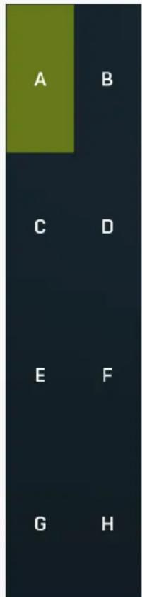
A-H presets selector
A-H presets selector controls the current A-H preset. This allows the plugin to store up to 8 sets of settings, including those parameters that cannot be automated or modulated. However it does not include channel mode, oversampling and potentially some other global controls available from the Settings/Settings menu.
For example, this feature can be used to keep multiple settings, when you are not sure about the ideal configuration When you change any parameter, only the currently selected preset is modified.
The four buttons below enable you to switch between the last 2 selected sets using the A/B button, morph between the first 4 sets using the morphing button and copy & paste settings from one preset to another (via the clipboard).
It is also possible to switch between the presets using MIDI program change messages sent from your host. The set selected depends on the Program Change number: 0 selects A, 7 selects H, 8 selects A, 15 selects H and so on.
A/B
A/B button switches between the active and previously active A-H preset (not necessarily the A and B presets themselves). To compare any 2 of the A-H presets, select one and then the other. Clicking this button will then switch between these two. You can do the same thing by clicking on the particular presets, but this makes it easier, letting you close your eyes and just listen.

Morph
Morph button lets you morph between the A, B, C and D settings. Morphing only affects those parameters that can be automated or modulated; that does include most of the parameters however. When you click this button, an X/Y graph is shown allowing you to drag the position indicator to any position between the letters A, B, C and D. The closer you drag the indicator to one of the letters, the closer the actual settings are to that preset.
Please note that this will overwrite and change the preset that is currently selected, so it is best to select a new preset e.g. 'E', then use the morphing method. This way you will define the settings for A, B, C and D, morph between them, and store the result in 'E' without any modification of the original A, B, C and D presets.
Please note that the ABCD morphing itself cannot be automated and that, while morphing, the changes to the underlying parameters are not notified to the host (there may be hundreds of change events).

Copy
Copy button copies the current settings to the system clipboard. Other presets, oversampling, channel mode and other global settings are not copied.
Hold Ctrl to save the settings as a file instead. That may be necessary for complex settings, which may be too long for system clipboard to handle. It may also be advantageous when you want to send the settings via email. You can load the settings by drag & dropping them to a plugin or holding Ctrl and clicking Paste.

Paste
Paste button pastes settings from the system clipboard into the current preset. Hold Ctrl to load the settings from a file instead. Hold Shift to paste the settings to all of the A-H slots at once.

Undo
Undo button reverts the last change. Only changes to automatable or modulatable parameters and global settings (load/randomize) are stored.

Redo
Redo button reverts the last undo operation.

WAV
WAV button lets you process a file using the plugin with current settings. You can either click the button and select a file, or drag & drop the file (or multiple files) onto the button. If you let the plugin process WAV files, these will be saved with the original settings. If you use a different file type (such as MP3), the plugin will create WAV files with 32-bit bits-per-sample floating point.
Please note that the files will be overwritten, so make a copy first if you want to keep the original.
IR
IR button lets you generate impulse response file, which approximates what the plugin does. You can use that in various IR players, including some hardware. Please note that any dynamic/modulated/somehow changing in time behaviour cannot be captured by an IR file. Also note that the IR will be generated as 24-bit WAV file ONLY if it is actually possible - if the output exceeds 0dBFS (or goes below -40dBFS), this cannot be accurately produced, so a 32-bit floating point WAV file will be generated. Some HW devices are known to have problems importing such files.

Collapse
Collapse button minimizes or enlarges the panel to release space for other editors.

Globals panel contains basic audio processing features.
Mid
Mid
Mid button lets you audition the mid (mono) from the reverberation signal only, that is the mono part of the output. You can use it to check for potential phase cancellations and to get your ears adjusted to the actual center.
Side
Side
Side button lets you audition the side from the reverberation signal only, that is the stereo part of the output.
Swap L/R
Swap L/R
Swap L/R button swaps the left and right output channels in the reverberation signal, so it lets you check for stereo field correctness.
Invert
Invert
Invert switch inverts the phase of the final reverberation signal. This can be handy when you experience phase cancellation problems when mixing the signal with the input signal using Dry/Wet knob for example.
Parallel
Parallel
Parallel switch defines how the reverb processes individual ER and LR modules and creates the output signal from them. By default this is disabled meaning that the reverb actually works like a hybrid between serial and parallel processing - the signal is taken from the first module to the next one etc. and each of them has Input and Output parameters, while let you control from where the module takes the signal and how it affects the current output. This eventually lets you create partially serial or parallel processing. However due to the level compensation involved, you may want to disable this, in which case all the modules will be processing the dry input signal and just mixed together to form the final output.
Gain compensation
Gain compensation
Gain compensation switch activates the gain compensation, which reduces the level when multiple modules are used to maintain approximately constant level. It is enabled by default, since it speeds up the workflow, but in some more complex situations you may want to turn it off, in which case you will have to do all the level handling manually.
Analysis
Analysis
Analysis button displays a powerful analyzer, which extracts impulse response from the current settings and shows its waveform, spectrum and echo density analysis.
Impulse response analysis
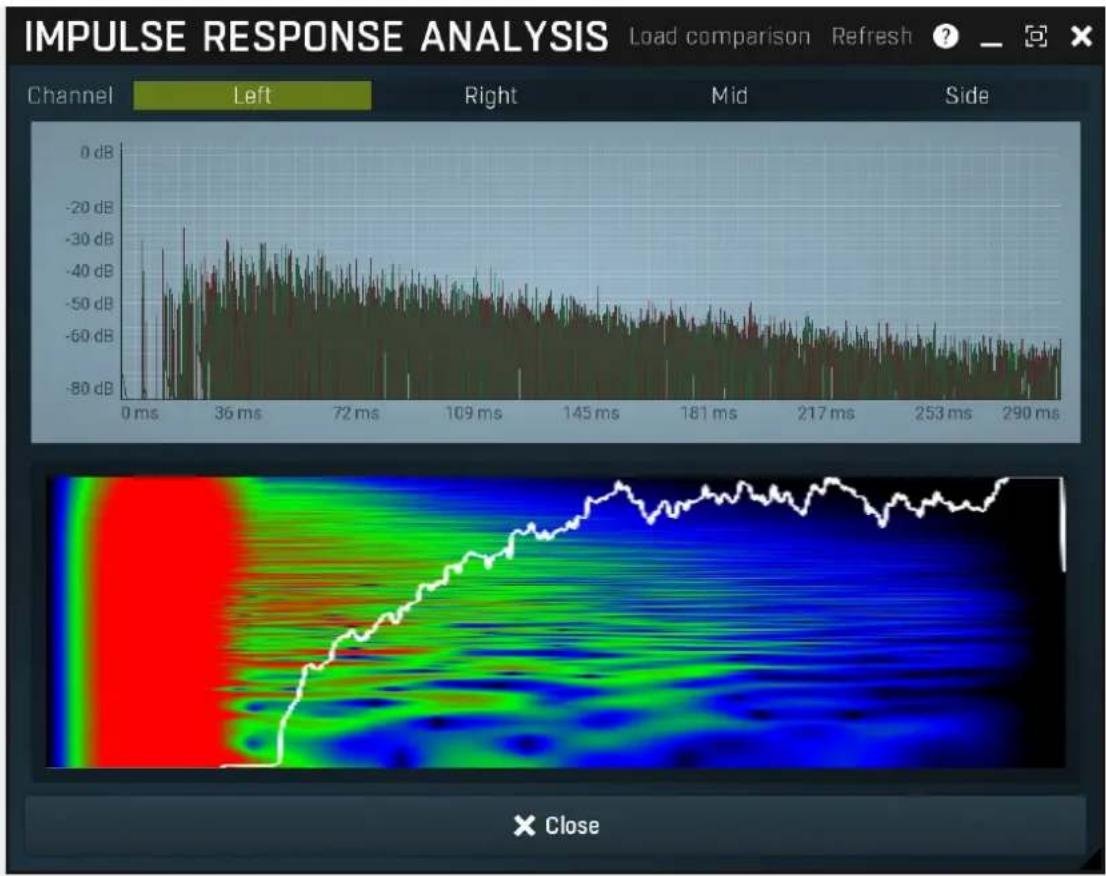
line
| Time (ms) | Value (dB) | |-----------|------------| | 0 | -80 | | 36 | -30 | | 72 | -40 | | 109 | -50 | | 145 | -60 | | 181 | -65 | | 217 | -70 | | 253 | -75 | | 290 | -80 |Impulse response analysis provides comprehensive analysis of current reverb settings. It displays the impulse response itself on top. Below you can see the spectrum profile in time and echo density. The analysis automatically updates whenever you change anything related to late reflections, but it doesn't react to all graphs. Note, that in order to sample the impulse response required for the analysis, the main audio processing is temporarily bypassed, so when the analyzer is displayed, actual auditioning may not be very comfortable. However it is very powerful tool for reverb design.
Load comparison
Load comparison
Load comparison button lets you select an external impulse response file and display its analysis next to current analysis view. This can be very helpful when trying to match a different reverb.
Refresh
Refresh
Refresh button samples the impulse response of current settings and updates the analysis. This is normally done automatically, but several parameters do not trigger analysis, so you can force the plugin to update using this button.
| Channel | Left | Right | Mid | Side | Channel |
Channel lets you choose, which channel is analyzed in the bottom analysis view.
Generate impulse
Generate impulse
Generate impulse button makes the reverb produce and process one impulse. It is useful when designing new reverbs.

DRY/WET
50.0%
Dry/Wet
Dry/Wet defines the ratio between the dry signal and the produced reverberation signal. If you use the reverb as a send effect, keep this at 100% and put the reverb on a dedicated bus in your host to which you send all the tracks to be processed. This way you control the amount of reverberation by adjusting the levels of the tracks that you send to the bus. If you use the reverb as an insert, use this parameter to control the amount of ambience versus the direct signal. Usually the higher the dry/wet value is, the more distant the audio seems.
Range: 0.00% to 100.0%, default 50.0%

PREDELAY
0 ms
Predelay
Predelay defines the initial delay before the actual response, which simulates the space between the sound source and the listener. The longer the predelay is, the further away the source seems. At some point (around say 100ms) the brain stops understanding that that the reverberation belongs to the dry signal and starts interpreting them separately, and then the dry signal becomes close to the listener
again. Predelay can therefore be used to control the distance from the source to the destination, but detaching the 2 signals can also be useful for instance to fill up a mix that isn't full enough without smearing the signal with the reverb itself.
Range: 0 ms to 1000 ms, default 0 ms
EARLY/LATE
20.0%
Early/late
Early/late defines the ratio between early and late reflections. Generally early reflections characterize the space and position of the source object and late reflections (reverberation) indicate the room properties. Usually the more audible the early reflections, the closer the dry signal seems and conversely the more late reverberation that is present, the further away it sounds.
Early reflections represent only the initial portion of the reverb tail, when the first few reflections of the sound from the nearest walls reach the ears/head. After some time the sound reflects so many times from various walls that the echo density (the number of echoes per second) becomes very high and the reverb in fact decays into noise (if designed that way). And this is the part known as the late reflections, which usually sounds smooth and can potentially be extremely long, while early reflections only last up to a few hundred milliseconds.
Range: 0.00% to 100.0%, default 50.0%
OUTPUT
0.00 dB
Output gain
Output gain defines the gain performed on the reverberation signal. You can use it to match the input level, so that Dry/Wet becomes easy to use and won't fool your ears by changing the output loudness.
Range: -24.00 dB to +24.00 dB, default 0.00 dB
VOLUME
0.00 dB
Volume
Volume defines the gain performed on the reverberation signal. It's similar to Output gain, but has a different range, which is compatible with the volume parameters of all ER and LR modules. This compatibility can be exploited for some very advanced techniques involving automatic loudness compensation in multiparameter banks.
Range: silence to 12.0 dB, default 0.00 dB

WIDENING
0.00%
Widening
Widening defines the broad-band stereo field widening depth. The algorithm is fully mono-compatible as it only extends the existing stereo field and no new signal is added. This parameter should only be used to control the existing stereo field.
Widening converts the audio into its mid (mono) and side channels, leaving the mid intact and applying a gain to the side channel, then converts the signal back to left and right channels. As a result the stereo image becomes wider (for widening above 0%) or narrower (for widening below 0%). This method of widening the stereo image may initially sound pleasing, however it can quickly become fatiguing on the ear and often sounds unnatural, especially for larger amounts of widening. Use this parameter to control the existing stereo field and as a special effect. Use it to increase width only with caution.
Please note that this algorithm is applied to the reverberation signal only. This is one of the ways to push the audio further away (lower values) or closer (higher values). The advantage is that the original signal's width is kept intact, yet the brain is often able to understand the distance clues.
Range: Mono to 200.0%, default 0.00%
PANORAMA
center
Panorama
Panorama defines the panorama applied to the reverberation signal.
Range: 100% left to 100% right, default center
RIGHT DELAY
0 ms
Right delay
Right delay lets you delay the right channel reverberation signal against the left channel or vice versa. It can be handy for improving the natural stereo field. If the value is positive, right signal is delayed. If it is negative, left channel is delayed instead.
Range: -100 ms to 100 ms, default 0 ms
| ER 1 | ER 2 | ER 3 | ER 4 | LR 1 | LR 2 | LR 3 | LR 4 | LR 5 | LR 6 | DYNAMICS | EQ | EQ M/S |
selector
Tab selector switches between subsections.
Early panel
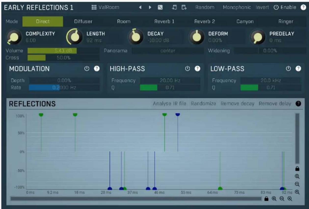
bar
| Time | Reflection | |--------|------------| | 0 ms | 100% | | 9.2 ms | 100% | | 18 ms | 100% | | 28 ms | -100% | | 37 ms | -100% | | 46 ms | -100% | | 55 ms | 100% | | 64 ms | -100% | | 73 ms | -100% | | 83 ms | -100% | | 92 ms | -100% |Early panel contains parameters of the Early reflections generator. It is based on a complex delay system, which you can access directly, or you can let the plugin generate the features automatically, analyzer an impulse response file etc. Early reflections describe the room properties and their purpose is usually to give some initial punch and width to the sound. It is often complicated to set them up manually, as the taps need to follow specific rules, otherwise strong artifacts, typically comb-filtering, may occur, therefore it is often advantageous to let the plugin generate them automatically.

ValRoom
Presets
Presets button displays a window where you can load and manage available presets. Hold Ctrl when clicking to load a random preset instead.

Left arrow
Left arrow button loads the previous preset.

Right arrow
Right arrow button loads the next preset.

Randomize
Randomize button loads a random preset.

Copy
Copy button copies the settings onto the system clipboard.

Paste
Paste button loads the settings from the system clipboard.
Random
Random
Random button generates random settings using the existing presets.
Monophonic
Monophonic
Monophonic button switches to/from single channel mode, where the reflections graph contains only one set of taps and these are used for all channels. In such mode no stereo expansion will occur and usually the stereo width is actually lowered.
Invert
Invert
Invert switch inverts the phase of the signal from this module. This can be handy when you experience phase cancellation problems when mixing the signal with the input signal using Dry/Wet knob for example.
| Mode | Direct | Diffuser | Room | Reverb 1 | Reverb 2 | Canyon | Ringer |
Mode
Mode defines the algorithm of the Early Reflections (ER) generator. The whole ER section is generally designed for use in the default Direct mode, but the other modes may be useful creatively.
Direct is the typical algorithm which most reverbs use and that is a tapped delay. The effect of this mode is the least prominent as there is no feedback whatsoever and hence it is also the safest (less likely to produce unwanted muddiness). It is also the least CPU demanding. However, a common problem is that if you want to provide some sort of diffusion even for the early reflections, you may need a lot of reflections to do that, in which case lots of CPU power may be necessary. In these cases it is useful to combine multiple ER generators; for example, one in the Direct mode and another one in Diffuser mode.
Diffuser mode usually requires just a few reflections and the internal feedback can provide the typical diffusive results without any coloration of the sound spectrum. It is characterized by the long initial attack and ringing if either the length is too low or too many reflections are used. Hence it is usually recommended to use short Length (e.g. 20ms) and small Complexity (say 3-5) values. The diffuser mode is usually used in conjunction with other modes to get a higher density.
Room, Reverb 1 and Reverb 2 modes implement some basic reverberation algorithms, which actually sound more like late reflections, so in a way this may be all that you need to design a full reverb. These algorithms usually suffer from low echo density and there's no direct way to control the reverberation time. They may be well used creatively though.
Canyon is rather creative and its decay times are often extremely long.
Ringer implements a serial comb filter system, which has a very characteristic metallic sound character; it is available only for the sake of completeness as it can be useful creatively.
Complexity
Complexity controls the number of early reflections. The more reflections, the more CPU it requires, but the more dense the early reflections can be. With modes other than Direct it is often enough to have just a few reflections.
Range: 1.00 to 64.00, default 30.00
Length
Length controls the length of the early reflection interval, basically the time until the last early reflection arises to the listener. It generally controls the room size, which is especially advantageous since it is independent on the late reflection time, hence you can create a big room with short ambience for example.
Range: 1.0 ms to 1000 ms, default 100 ms
Decay
Decay controls the level of the reflections with increasing time. By lowering the decay you can make the reflections, which arrive later, sound less prominent, which is natural, however it also shortens them early reverberation section. By increasing the decay towards 0dB you can make all reflections similar in loudness, providing less natural sound, which can however provide some sort of tightness often useful when mixing.
Range: -60.00 dB to +60.00 dB, default -10.00 dB
Deform
Deform skews the delay times, which in effect changes the character/shape of the virtual room.
Range: -100.0% to 100.0%, default 0.00%

Predelay
Predelay defines the initial delay before the generator response, which simulates the space between the sound source and the listener. There is also a global predelay, which delays the whole output of the plugin generated signal. This one delays only the output of this early reflections generator however and can be used to control the timing of each generator.
Range: 0 ms to 1000 ms, default 0 ms
Volume 5.43 dB Volume
Volume defines the level of the output for this Early reflections generator.
Range: silence to 12.0 dB, default 0.00 dB
Panorama defines the panorama applied to the Early reflections generator output.
Range: 100% left to 100% right, default center
Widening
0.00%
Widening
Widening defines the broad-band stereo field widening depth. The algorithm is fully mono-compatible as it only extends the existing stereo field and no new signal is added. This parameter should only be used to control the existing stereo field.
Widening converts the audio into its mid (mono) and side channels, leaving the mid intact and applying a gain to the side channel, then converts the signal back to left and right channels. As a result the stereo image becomes wider (for widening above 0%) or narrower (for widening below 0%). This method of widening the stereo image may initially sound pleasing, however it can quickly become fatiguing on the ear and often sounds unnatural, especially for larger amounts of widening. Use this parameter to control the existing stereo field and as a special effect. Use it to increase width only with caution.
Range: Mono to 200.0%, default 0.00%
Cross
50.0%
Cross
Cross controls how each input channel affects each output channel. When this is set to 0%, then the left output is generated from the left input only and the right output is generated from the right input only. At 50% the left output is generated 67% from the left input and 33% from the right input. And the right output is generated 67% from the right input and 33% from the left input. When this is 100%, both left and right channels contribute equally (50:50) to both left and right outputs. And when you set this to 200%, the channels are exchanged, hence the left output is generated solely from the right input and vice versa.
Range: 0.00% to 200.0%, default 0.00%
Modulation panel
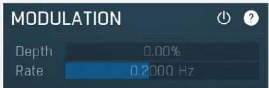
Modulation panel contains the modulation parameters for this generator. When this is disabled, the processor is taking the input signal directly. If you enable it, the input signal is modulated first, which often provides a pleasing evolving character at the expense of additional CPU requirements. It also effectively diminishes the possibility of comb filtering.
Depth
0.00%
Depth
Depth controls the depth of the input modulation useful to further improve the realisticity of the produced reverberation. It can sound very artificial when overused.
Range: 0.00% to 100.0%, default 50.0%
Rate
0.2000 Hz
Rate
Rate controls the speed of the input modulation. The faster it is, the more pronounced the effect is. It can sound very artificial when overused.
Range: 0.0100 Hz to 10.00 Hz, default 0.2000 Hz
High-pass panel
High-pass panel contains parameters of the optional high-pass filter processing the output of this generator.
Frequency
20.00 Hz
Frequency
Frequency defines the filter cut-off frequency.
Range: 20.00 Hz to 20.0 kHz, default 20.00 Hz
Q
0.71
Q
Q defines resonance of the filter.
Range: 0.05 to 100.00, default 0.71
Low-pass panel
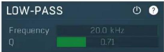
Low-pass panel contains parameters of the optional low-pass filter processing the output of this generator.
Frequency 20.0 kHz Frequency
Frequency defines the filter cut-off frequency.
Range: 20.00 Hz to 20.0 kHz, default 20.0 kHz

Q defines resonance of the filter.
Range: 0.05 to 100.00, default 0.71
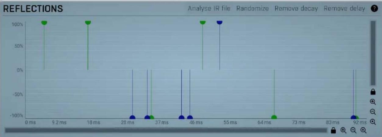
line
| Time (ms) | Reflection (%) | | --------- | -------------- | | 0 | 100 | | 9.2 | 100 | | 18 | 100 | | 28 | -100 | | 37 | -100 | | 46 | -100 | | 55 | 100 | | 64 | -100 | | 73 | -100 | | 83 | -100 | | 92 | -100 |Reflections editor
Reflections editor contains all the reflections the generator is based on. Each point defined one reflection. Only used reflections are displayed, hence the graph depends on the Complexity parameter. Horizontal axis defines time, left being zero delay, right being maximum delay controller by Length parameter. Vertical axis contains the reflection level, its meaning depends on the current Mode. In the default Direct mode it controls the level or loudness of the reflection.
Analyse IR file
Analyse IR file
Analyse IR file lets you select an impulse response file to load and analyze. The plugin will set the reflections according to the prominent reflections in the beginning of that file.
Randomize
Randomize
Randomize generates a new set of reflections using a specially designed randomization algorithm. Hold ctrl to randomly change the current values slightly instead of a full randomization.
Remove decay
Remove decay
Remove decay readjusts the taps to minimize the decay. It is often useful after analyzing an IR file, since despite the results may be convincingly reproducing the original, one cannot really use Decay parameter well anymore, since there is already some decay in the taps. Also, early reflections without too much decay are often quite advantageous to disperse and tighten the audio.
Remove delay
Remove delay
Remove delay removes the empty space in front of the first tap and sets the Length and Predelay appropriately.
Late panel
![LATE REFLECTIONS 1 Living room Random Early Invert Enable ? LENGTH 100 ms COMPLEXITY 24 SIZE 50.0% PREDELAY 0 ms Volume 5.57 dB Panorama center Widening 0.00% Cross 50.0% input 0% prev, 100% dry Output 100% out, 100% prev MODULATION Depth 0.00% Rate 0.2000 Hz HIGH-PASS Frequency 358.9 Hz Q 0.71 LOW-PASS Frequency 10.3 kHz Q 0.31 DAMPENING LOW Gain 0.00 dB Frequency 100.2 Hz Q 0.40 Sparse 4 DAMPENING HIGH Gain -3.00 dB Frequency 6000 Hz Q 0.40 Sparse 2 DESIGNER Randomize parameters Randomize algorithm Smart seed generator ? Algorithm ca[#an[a;fh;b[swap]]) Status: Ok Param 1 1.00 Param 2 1.00 Param 3 1.00 Delay min 5.0% Delay max 18.6% Pitch shift 0 Delay order Random Delay focus -306.4% Delay width 100.0% Input order Random Input focus 400.0% Input width 0.00% Output order Random Output focus 400.0% Output width 0.00% Panic Channels unrelated Channel seeds unrelated](/content/2026/05/983866/images/b81ee7b5e1cb49006543cc0fb7f26d911d46f8bbfd9449a7d0ffd2164ef51bd8.jpg)
Late panel contains parameters of the late reflections generator. It implements a state of the art algorithmic generator system, which you can actually program yourself, but in most cases it is best to start from presets. It lets you define your own reverberation algorithm from the several predefined modules. As all algorithmic reverberators it is based on a very complex feedback delay system and instead of providing direct access to the many parameters it has, it is controlled using a set of pseudorandom number of generators, which configure these parameters automatically. This way you can simply focus on the sound while clicking the randomizer buttons.
Living room
Presets
Presets button displays a window where you can load and manage available presets. Hold Ctrl when clicking to load a random preset instead.

Left arrow
Left arrow button loads the previous preset.

Right arrow
Right arrow button loads the next preset.

Randomize
Randomize button loads a random preset.

Copy
Copy button copies the settings onto the system clipboard.

Paste
Paste button loads the settings from the system clipboard.
Random
Random
Random button generates random settings using the existing presets.
Early
Early
Early switch makes the plugin think this LR is actually an early reflections generator. It makes it work well with the Early/late parameter. Without it you could still use a multiparameter to simulate proper early/late mix, but this option makes it much easier.
Invert
Invert
Invert switch inverts the phase of the signal from this module. This can be handy when you experience phase cancellation problems when mixing the signal with the input signal using Dry/Wet knob for example.

Length
Length controls the decay length, an approximate time until the reverb decays to -60dB. Note that the actual decay time may vary with several other settings. Also the Algorithm may highly affect the decay length.
Range: 100 ms to 60000 ms, default 2000 ms

Complexity
Complexity controls the structure of this late reflections generator. Its meaning depends on the Algorithm, but in most cases the higher the value is, the more complex and likely more natural the output will be, however the CPU requirements will increase as well. Range: 1 to 64, default 8

Size
Size controls the virtual room size. It controls the delay lengths used in the generator. The actual meaning depends on the Algorithm. Range: 0.00% to 100.0%, default 50.0%

Predelay
Predelay defines the initial delay before the generator response, which simulates the space between the sound source and the listener. The longer the predelay is, the further away the source seems. There is also a global predelay, which delays the whole output of the plugin generated signal. This one delays only the output of this generator however.
Range: 0 ms to 1000 ms, default 0 ms
Volume 5.57 dB Volume
Volume defines the level of the output for this late reflections generator.
Range: silence to 12.0 dB, default 0.00 dB
Panorama center
Panorama
Panorama defines the panorama applied to the late reflections generator output. Range: 100% left to 100% right, default center
Widening 0.00%
Widening
Widening defines the broad-band stereo field widening depth. The algorithm is fully mono-compatible as it only extends the existing stereo field and no new signal is added. This parameter should only be used to control the existing stereo field.
Widening converts the audio into its mid (mono) and side channels, leaving the mid intact and applying a gain to the side channel, then converts the signal back to left and right channels. As a result the stereo image becomes wider (for widening above 0%) or narrower (for widening below 0%). This method of widening the stereo image may initially sound pleasing, however it can quickly become fatiguing on the ear and often sounds unnatural, especially for larger amounts of widening. Use this parameter to control the existing stereo field and as a special effect. Use it to increase width only with caution.
Range: Mono to 200.0%, default 0.00%
Cross 50.0% Cross
Cross controls how each input channel affects each output channel. When this is set to 0%, then the left output is generated from the left input only and the right output is generated from the right input only. At 50% the left output is generated 67% from the left input and 33% from the right input. And the right output is generated 67% from the right input and 33% from the left input. When this is 100%, both left and right channels contribute equally (50:50) to both left and right outputs. And when you set this to 200%, the channels are exchanged, hence the left output is generated solely from the right input and vice versa.
Range: 0.00% to 200.0%, default 0.00%
Input 0% prev, 100% dry
Input
Input controls how much of the original (dry) input and how much of the signal from the previous generators is mixed to form the input for this generator.
If you set this to 0% prev, 100% dry, the generator will be processing the dry input, hence it will be working in parallel with the previous generators.
If you set this to 100% prev, 100% dry, then this generator will process an equal mix of both the dry input and the output from the previous section.
If you set this to 100% prev, 0% dry, then this generator will work in series with the previous generator. Serial processing can produce high density, however it will also increase the risk of comb filtering, which is usually not desired.
Range: 0% prev, 100% dry to 100% prev, 0% dry, default 0% prev, 100% dry
Output 100% out, 100% prev
Output
Output controls the mix ratio between current signal produced by previous generators and output from this one. It is often useful in conjunction with Input as in this way you can place all generators serially after each other, as opposed to parallel processing, which is the default.
If you set this to 0% out, 100% prev, the generator will be effectively doing nothing.
If you set this to 100% out, 100% prev, then this generator will be fully mixed with the previous output, hence it will be working in parallel with other generators.
If you set this to 100% out, 0% prev, then this generator's output will replace the current reverberation signal, hence it will work in series with the previous generators. Serial processing can provide high density, however it will also increase the risk of comb filtering, which is usually not desired.
Range: 0% out, 100% prev to 100% out, 0% prev, default 100% out, 100% prev
Modulation panel
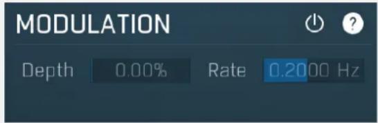
Modulation panel contains the modulation parameters for this generator. When this is disabled, the processor is taking the input signal directly. If you enable it, the input signal is modulated first, which often provides a pleasing evolving character at the expense of additional CPU requirements. It also effectively diminishes the possibility of comb filtering. Note that you can perform additional modulations within the actual Algorithm.
Depth 0.00%
Depth
Depth controls the depth of the input modulation useful to further improve the realisticity of the produced reverberation. It can sound very artificial when overused.
Range: 0.00% to 100.0%, default 50.0%
Rate 0.2000 Hz
Rate
Rate controls the speed of the input modulation. The faster it is, the more pronounced the effect is. It can sound very artificial when overused.
Range: 0.0100 Hz to 10.00 Hz, default 0.2000 Hz
High-pass panel
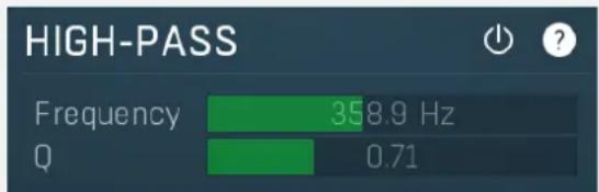
bar
| Metric | Value | |--------|-------| | Frequency | 358.9 Hz | | Q | 0.71 |High-pass panel contains parameters of the optional high-pass filter processing the output of this generator.
Frequency
358.9 Hz
Frequency
Frequency defines the filter cut-off frequency.
Range: 20.00 Hz to 20.0 kHz, default 20.00 Hz


Q defines resonance of the filter.
Range: 0.05 to 100.00, default 0.71
Low-pass panel
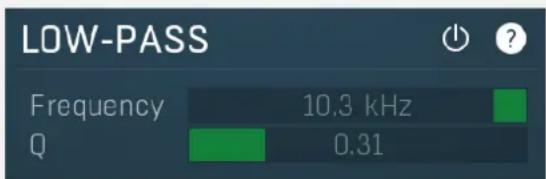
Low-pass panel contains parameters of the optional low-pass filter processing the output of this generator.
Frequency
10.3 kHz
Frequency
Frequency defines the filter cut-off frequency.
Range: 20.00 Hz to 20.0 kHz, default 20.0 kHz

Q defines resonance of the filter.
Range: 0.05 to 100.00, default 0.71
Dampening Low panel
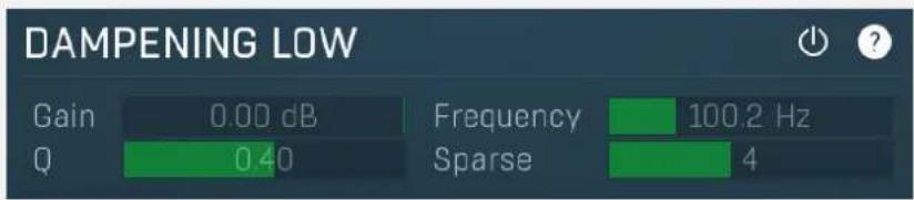
Dampening Low panel contains parameters of the low frequency dampening filter. Its purpose is to simulate absorption by air and walls. If and how is this feature used depends on the Algorithm.
Gain 0.00 dB Gain
Gain controls the filter gain, hence amount of the dampening. The lower it is, the more of the bass content is removed and less muffled the sound will be.
Range: -20.00 dB to 0.00 dB, default -3.00 dB
Frequency 100.2 Hz Frequency
Frequency controls the filter frequency. The higher it is, the more of the bass content is removed and less muffled the sound will be. Range: 20.00 Hz to 20.0 kHz, default 200.0 Hz
Q 0.40 Q
Q controls the filter Q. The lower it is the smoother the effect will be, but it will also be less focused the low frequencies desired to attenuate.
Range: 0.05 to 0.71, default 0.40
Sparse 4 Sparse
Sparse lets you avoid filtering all internal delaylines and save CPU. The effect of dampening is lowered this way, but it is in fact more natural as it sort-of simulates different reflection surfaces. Value 1 means that every delay is filtered and provides highest dampening and highest CPU usage. Value 2 that every second delay is filtered etc. Note that this parameter is supported only by R and RD algorithm modules.
Range: 1 to 8, default 4
Dampening High panel
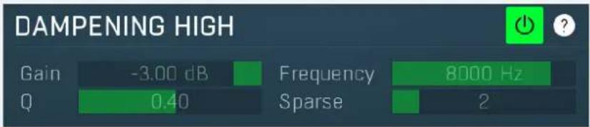
Dampening High panel contains parameters of the high frequency dampening filter. Its purpose is to simulate absorption by air and walls. If and how is this feature used depends on the Algorithm.
Gain -3.00 dB Gain
Gain controls the filter gain, hence amount of the dampening. The lower it is, the darker the sound will be.
Range: -20.00 dB to 0.00 dB, default -3.00 dB
Frequency 8000 Hz Frequency
Frequency controls the filter frequency. The lower it is, the darker the sound will be.
Range: 20.00 Hz to 20.0 kHz, default 8000 Hz
Q 0.40 Q
Q controls the filter Q. The lower it is the smoother the effect will be, but it will also be less focused the high frequencies desired to attenuate.
Range: 0.05 to 0.71, default 0.40
Sparse 2 Sparse
Sparse lets you avoid filtering all internal delaylines and save CPU. The effect of dampening is lowered this way, but it is in fact more natural as it sort-of simulates different reflection surfaces. Value 1 means that every delay is filtered and provides highest dampening and highest CPU usage. Value 2 that every second delay is filtered etc. Note that this parameter is supported only by R and RD algorithm modules.
Range: 1 to 8, default 2
Designer panel
![DESIGNER Randomize parameters Randomize algorithm Smart seed generator ? Algorithm ca[#an[a;fh;b[swap]] Status: Ok Param 1 1.00 Param 2 1.00 Param 3 1.00 Delay min 5.0% Delay max 18.6% Pitch shift Ø Delay order Random ▶ Delay focus -306.4% Delay width 100.0% Input order Random ▶ Input focus 400.0% Input width 0.00% Output order Random ▶ Output focus 400.0% Output width 0.00% ■ Panic Channel unrelated Channel seeds unrelated](/content/2026/05/983866/images/219722cdf63c1c6b2c19ee4e8ff38968b64c0408cf7888f18a58cb7e6410e461.jpg)
Designer panel controls the algorithm used in the late reflections generator and its parameters.
Randomize parameters
Randomize parameters
Randomize parameters button randomizes all parameters of the algorithm except for the algorithm itself and Complexity. It is useful for testing the algorithm. It doesn't always change all parameters, it just changes them somehow. If you hold Ctrl, the parameters will only be slightly modified rather than completely randomized.
Randomize algorithm
Randomize algorithm
Randomize algorithm button is an experimental algorithm generator. When using this feature, it is highly recommended to keep safety limiter enabled.
Smart seed generator
Smart seed generator
Smart seed generator button lets you explore thousands of seeds and qualify them automatically, so that you can browse only the best ones. Instead of listening to the sound each seed produces, the engine can 'listen' for you and let you choose from the best ones according to requested criteria.
Smart seed generator
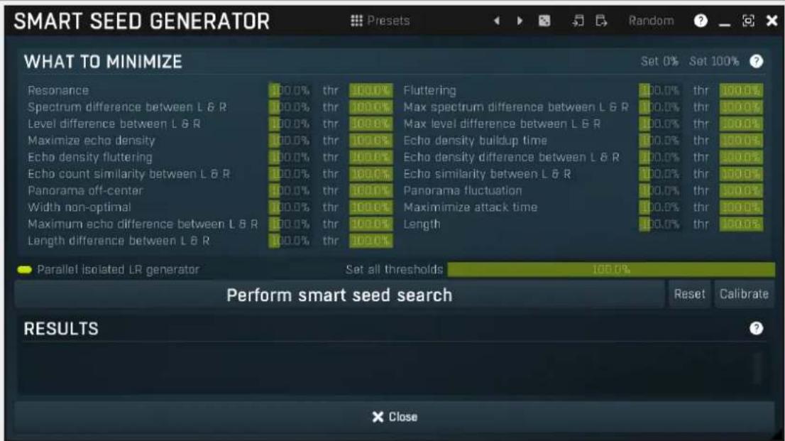
Smart seed generator is an extremely powerful statistical tool that makes the plugin try several different seeds, analyse them and extract several perceptual factors, based on which it can decide whether each seed is good or not. It then sorts them based on these factors. You can browse the seeds simply by selecting them in the listbox containing the results. The best seeds are at the top of the list.
The generator is parallelized by default, which lets it exploit the computational capabilities of your computer and analyzes the LR module separately. When the parallelization is disabled, it analyzes the global output of the plugin by sampling its impulse response. This can be used to combine multiple LR modules for instance.
Stereo field, the biggest challenge in audio ever?
One of the reasons we are employing reverbs in the first place is to create a virtual stereo field with depth and space, for audio materials that are otherwise clean or boring or both. While creating depth is simple enough, just providing reasonable evolving echo density and stereo field is a completely different story and currently nearly all reverbs out there perform very badly in this respect. The main problem is that the psychoacoustics here are extremely complex. Since birth our brains learn to analyze different factors of what we hear and associate them with what we see so that we can feel the place even when we do not actually see it at that moment. We can also detect where the sound originates from, potential obstacles close to us etc.
The problem here is that algorithmic reverbs do not care about that at all, but they still generate these clues, which often cause our brains to be confused. But brains are amazing devices and they adjust so quickly that, if you are designing a reverb, they actually work against you, fooling you into believing that your reverb actually "sounds good". And it just might sound good on its own, but in the context of a mix, or other tracks it may be actually quite bad. And pretty much all reverbs on the market that we have tried are.
What are the symptoms of a problematic stereo field?
Well, first of all, to spot the problems, you will have to train your ears. And it's not going to be easy. In fact, it's probably the hardest thing I have ever tried to teach my ears, well, my brain. But after you do that, you will be changed, as I am right now :).
First put your headphones on, get a monophonic recording that you are used to. Just a short loop is all that is needed. Always use the same loop, because sooner or later you'll know everything about it. This loop should contain both drums (being a source of noise-like signals) and melodic instruments (being a source of signals with harmonic relationships), but both should be percussive, so that you can always "feel" the reverb tail. Enable the reverb, ideally with dry/wet at 100% wet, but audition only the "mid" signal (mono). To do that you can for example add MStereoScope and use the mid/side selector. Or even better use MCompare, which has a Mid switch, since switching this way is much easier, and it is useful for comparing different reverbs anyway. Now, listen to the loop for as long as you need, until you feel that your ears hear the same thing spectrally each time and you feel as if everything is in front of you, far away, in some sort of tunnel. That's how mono sounds.
Now disable the Mid switch, and the sound will expand to stereo. Please note that you must NOT allow any pause in-between, you need a sudden change from mono to stereo. How you do that depends on the capabilities of your DAW. Listen for a few seconds and switch back to Mid. Try that with a few different reverbs, just to learn the differences. After a few attempts your ears should have some knowledge of the process, and now when you switch to stereo, a few things may happen:
A) Everything is fine, the sound expands around you, both ears seem to hear the full spectrum of frequencies, all instruments sound in both ears, and when you disable the reverb, it nicely decays to the center in front of you.
B) Something is wrong, and right now you are probably just confused and not sure what it is. Some classic problems that you may encounter are:
- The sound feels as if it is coming from one side. This is usually caused by the first echoes coming in one channel sooner than in the other. The delays need to be different, otherwise it would all sound mono again, but if there are many echoes coming from say the left channel ahead of the right channel, then it would seem as if the audio originated on the left. Or there may actually be more echoes on the left altogether. And there are plenty of other things that may go wrong.
- It seems like something is missing in one channel, as if one of your ears suddenly became partially deaf. The echoes together change the spectrum in some way and in many cases they cause an attenuation of an interval in the spectrum, just like an equalizer. The good thing is that brain will quickly compensate, because it just needs you to hear properly, that's a necessary survival skill. But it's actually a bad thing, because after a few seconds you feel as if everything is fine, so you need to switch to mono and let your ears adjust again.
- It seems that the bass drum (or another instrument) originates on the left. This is actually sort of a combination of both the previous cases. Your brain just really tries to make sense of all that, so it can actually group the frequencies that predominate in each channel into the instruments it can find there, and make you feel as if the bass drum is slightly on the left, the snare is on the right etc. The reverb basically causes fluctuations of the spectrum in time; that's what echoes do when they are close to each other. And in our case it means that in the beginning of the reverb tail most of the bass drum frequencies are present in the left channel and vice versa, so it seems like the bass drum is on the left. It's especially noticeable in the beginning of the reverb tail, where the echo density is quite low.
- After you stop the playback, the reverb tail decays, somewhere, but definitely not in the center. There are many things the reverb tail can do depending on the algorithm. Sometimes it goes from left to right and back again like an autopan. You might have even used an autopan, which would explain a lot :). But in most cases it just feels like the sound is running away to the left or right. Just a little. But if you are aiming for natural space reverberation, the sound should ideally
stay as close to the center as possible. But again, to judge the center, you need to hit the mono switch, otherwise you just cannot be sure the brain is not deceiving you.
These things may actually be wanted for some creative purposes in some cases, but not in general. When mixing with such reverbs, you may get fooled and at one point you may just start asking yourself what is wrong, but in the context of multitrack mixing it will be pretty much impossible to detect that the reverb is the problem and why. You can always pan a nicely balanced reverb, but if its stereo field is muddled in the first place, as it is with most reverbs, there's just nothing you can do afterwards. And the difference is unbelievable, once you understand what to listen to.
It's also worth noting that the Room type control that most devices have is great for detecting these stereo field irregularities, because when quickly changing the settings, it's quite easy to perceive that the audio is jumping from one place to another in the stereo field. While it is just fine if the audio is changing distance - close and far - it's not so good when it is jumping from left to right and vice versa. This method works very well in detecting which settings are not ideal.
Ear fatigue
It's possible that after say 30 minutes you will feel as if it doesn't make sense at all anymore. What seemed fine to you sounds really bad now, and in a few minutes it may all change, so you cannot trust yourself anymore. That's normal. Your brain has been overloaded. It's as if you are teleporting from one place to another every few seconds and your brain needs to adjust all the time and at some point it just got tired. So take some rest, do something completely different and try again in an hour or so. After all, this is a good practice for all audio processing jobs. Our brain just likes to trick us; in this case it is just a little extreme.
How to balance the stereo field
The answer is the seed. It defines the delays, coefficients, everything under the hood, which is hidden from you as it is too technical and would be way too hard and clumsy to manipulate directly. But there are more than 2 billion seeds, so going through all of them to find the best one isn't really an option. The smart seed generator can cover thousands of seeds in just a few minutes and cannot be fooled that easily. On the other hand its ability to detect these psychoacoustic clues is highly limited, so at the end of the day your ears will have to be the final judge anyway. But the generator can still remove the seeds which have too many resonances, low echo density, or which don't seem to be centered or wide enough, saving a lot of drudgery.
The usual problem is that these factors often work against each other. For example, the higher the echo density, the higher the probability of resonances. That's why the smart seed generator may look a little scary. It lets you choose those factors that you want to be considered more important.
So to make your life easier, just start like this: First of all, set up your algorithm properly, including the settings in the Designer panel. Then open the smart seed generator and let it start searching for seeds. Give it at least 1000. The more the better, sometimes 100 is enough, sometimes not, depending on the algorithm. Stop the search, click the Set 100% button to make all factors equally important, then click the Calibrate button to let the engine make some statistical adjustments. And finally use the Set all thresholds value to set it as low as needed so all that os left is just a few dozen seeds. This will basically filter out the bad seeds, those which do not qualify in some of the factors. But do not set it too low, it's a computer, not an artificial intelligence; it may not know what you really want. And then try different seeds. Just click on each while listening. And when you feel that it is great, do not forget to do the "mono test", you may be very unpleasantly surprised.
Stereo width
One particular problem is that we expect reverbs to sound wide. But the width is caused by differences between the left and right channels, whether these are caused by different spectra, echoes or something else. And settings with a non-centered stereo field may also appear wider, initially. So do not be fooled by the impression of width. After all, the widest signal ever is out-of-phase and that's what we try to avoid at all costs. And as demonstrated by MStereoSpread, it is actually possible to have a stereo field that is centered, yet extremely wide. A good seed can provide great width and still a balanced stereo field, but it may be a little hard to find one.
Presets
Presets
Presets button displays a window where you can load and manage available presets. Hold Ctrl when clicking to load a random preset instead.

Left arrow
Left arrow button loads the previous preset.

Right arrow
Right arrow button loads the next preset.

Randomize
Randomize button loads a random preset.

Copy
Copy button copies the settings onto the system clipboard.

Paste
Paste button loads the settings from the system clipboard.
Random
Random button generates random settings using the existing presets.
What to minimize panel
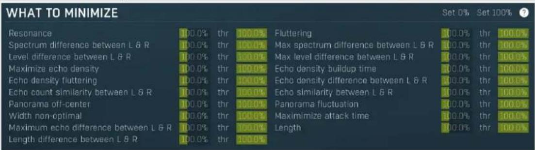
What to minimize panel controls which factors the seed generator should focus on. Each factor has a weight, which defines how important it is. If you set all weights to 0%, the list of results won't be sorted at all. If you set all weights to the same number (probably 100%), each factor will be considered equally important. Whenever you change any of the weights, the list of results gets sorted again to provide the correct order.
All factors are defined to be ideally as small as possible; hence the generator tries to minimize all values. For instance Resonance factor defines how much the IR seems to be resonating at some frequencies. Resonating usually sounds metallic and is rarely considered a good quality of a reverb, hence if you want focus on seeds that have minimum resonance, simply increase the weight for this factor.
Note that most factors are perceptual and as such as it is extremely hard (if possible at all) to quantify them well, as that means simulating human auditory system. The generator performs a complex analysis of the impulse responses produced by the plugin, but the quality of the approximations may still vary a lot. Also note that since the analysis is based on impulse responses, it doesn't notice any kind of modulation, which varies in time (that is variations over time).
Next to each factor there is also a threshold slider, named thr. This lets you filter out results, that don't fit certain parameter at all. This lets you solve more complex situations, such as when you want to minimize all factors at the same time, but you do not want any resonance at all. Such a wish wouldn't be possible with just the weights, because that would make you increase the weight for the resonance to maximum, so the list would be ordered mostly by resonance, nearly ignoring other parameters. Please note that in order to make this work well, calibration needs to be performed. The threshold represents the maximum allowed value for the factor.
Set 0%
Set 0%
Set 0% button sets 0% weight for all factors, which effectively disables any sorting. It is useful when you want to focus on just a few factors and disabling all of them manually would be tedious.
Set 100%
Set 100%
Set 100% button sets 100% weight for all factors, which effectively enables them all and makes them equally important, which is default.

Parallel isolated LR generator
Parallel isolated LR generator
Parallel isolated LR generator button activates a special processing mode which uses multiple cores of your CPU and isolates the processing to only the single LR generator, ignoring all other modules and advanced options. In fact it only cares about the settings in the Designer panel. As such it cannot be used to combine multiple LR modules together for example, but it is several times faster and it lets you get ideal settings for individual LR modules.
Perform smart seed search
Perform smart seed search
Perform smart seed search button starts or stops the processing. During the processing the plugin cannot be used as the sampling requires exclusive access to the processing engine. You can stop the processing and continue at any time. The generator automatically detects the reverberation length and the longer it is, the slower the analysis works.
Reset
Reset
Reset button deletes all results.
Calibrate
Results
Results contains the list of tested seeds. The list is sorted by the first number, which is the total 'quality', which depends on the factors and the weights you selected for them. The lower this value is, the better. But always note that scientific measurements may produce quite different results than human perception. The quality value is followed by the actual seed and all the factors.
Algorithm ca[#an[a;fh;b[swap]]
![MeldaProduction MTurboReverb - Algorithm ca[#an[a;fh;b[swap]] - 1](/content/2026/05/983866/images/f9f98f550dfedb14db01727d3e5e3f7c14c5d95d65e0230a860cacb56e6ff849.jpg)
Algorithm
Algorithm controls how the Late Reflections generator actually works and you can program it completely using a single formula exploiting the many modules that the software provides. If you have reached this stage, it probably means that you are ready to get seriously creative and this is exactly what it is all about.
For decades scientists have been trying various "reverb topologies" to mimic the sound of real rooms (or just to get creative) without convolution, which is extremely CPU demanding and very limited when it comes to modulation and adjustment. Topology is, simply put, a set of basic building blocks connected in some way, each of which carries out a particular operation. Most reverbs on the market are usually a product of one such topology. When designing MTurboReverb we originally wanted to include just one single topology like everyone else, but as we were comparing it to different reverbs on the market, it turned out that a far bigger picture is actually possible. So we came up with the (almost) ultimate reverb modular system, which is not only particularly versatile, but also easy and quick to use, and extremely CPU efficient.
Instead of providing a complex graphical interface to define a topology, the algorithm is entirely constructed from a single line expression. The coefficients and delay lengths are some sort of pseudorandom numbers generated automatically (via the Seed and other parameters in this panel). The coefficients are order, focus and width for each of delay, input and output and are displayed in the Designer panel. Their usage depends on the algorithms. They are mainly relevant for the R, RD, CC and CA modules.
The algorithm only controls what modules are used and how they are connected (that is, it defines the topology) and the parameters are generated making it simple to set up the whole thing. The engine knows how many parameters and delays are used and how quickly the reverb should decay (please note though that a proper compensation is not always possible, especially with nested modules, see below). All modules are designed such that they compensate for gain change etc., so the hard work has already been done, and now the only thing for you to do is to experiment, use your ears, and be creative.
Introduction
Before you start programming your own reverberation algorithms it is highly recommended to check out the presets. You will learn a lot from a close inspection of them. Also you should enable the safety limiter button (on the right-hand side of the plugin), since infinite feedback is quite common when dealing with complex feedback systems. In most cases the engine will compensate for everything, but sometimes it just cannot be done. If you are ready for some programming, here's how it works. First a few examples, so that you can see how easy it actually is:
parallel[comb;comb;comb;comb];allpass;allpass = 4 combs in parallel followed by 2 allpasses in series. Those two modules types, and many others, are described below. This is actually one of the first reverbs ever designed, called Schroeder's reverb. It has many variations, but this is pretty much the basic one.
p[4c];2a = this is the same thing! It's just presented in a more compact syntax, it all depends on which you prefer.
reverb or r is a full reverb implementation. It's actually the topology that we originally wanted to include as the only one.
Syntax
The syntax defining the topology consists of several modules, placed one by one and separated by a semicolon ';'. Some modules can have parameters, placed in round brackets '(parameter1;parameter2;...)', and some may have submodules, placed in square brackets '[submodule1;submodule2;...]'.
In front of each module you can specify the number of occurrences, 100 is the maximum for safety reasons. The number only serves as a shortcut, so that you don't need to specify the same module multiple times, for example 3a is exactly the same thing as a;a;a. Instead of a number you can use a hashtag '#', which will be replaced by the value of the Complexity parameter. This way the user can change the topology without editing the algorithm formula itself at all, by changing the Complexity value.
You can insert spaces anywhere; these have no meaning, but they can make the algorithm easier to look at. You can also mix uppercase and lowercase letters. Most modules have a short name and a long name, it doesn't matter which you use.
For some modules there are parameters that you can either specify or they will be randomized. By randomizing we mean a controlled pseudo-randomizing based on the seed value, which means that it will be the same every time, until you click Seed
again. The Seed is just a very long number, from which the whole pseudo-random sequence of numbers starts. The seed is stored in the same way as any other parameter, it can be attached to a multiparameter etc., so there's no black magic, it's just a very long ugly number :). Please note that whenever we talk about random numbers below, we actually mean these seed-based pseudo-random numbers.
To summarise, the syntax looks like this (the elements in italics are optional): count/# module (parameter1; parameter2; ...) [submodule1; submodule2; ...];
User parameters and expressions
Most modules are designed in such a way that they don't need any further control. They calculate all the internal variables to maintain the desired reverb length, compensate for output level changes etc. But in some specific cases you may need to change the algorithm in some way, without actually accessing the text.
For that, the plugin provides 3 user parameters below the algorithm field, named Param 1, Param 2 and Param 3. You can then implant those parameters anywhere you want in the algorithm by writing \1, \2 or \3. These values are inserted as text, which means that the algorithm must make sense after replacing the \1, \2 and \3 literals by the values. In most cases you'd use these to alter the feedback coefficients, levels etc., where the available range of -1 to +1 is sufficient.
It is also possible to insert mathematical expressions featuring the parameters. These need to be delimited by {expression}. The expression evaluator will process the parameters, numbers and most of the useful mathematical functions. As an example, you can write 1 * 10 + (2) in the algorithm, whatever the purpose of such equation would be. Note that expression evaluation certainly requires a little more CPU when evaluating the algorithm, however there is no difference when it comes to actual audio processing afterwards.
Need to know information about reverb design
Feel free to design your reverbs just using your ears. You can just take some presets and use the randomizers to change how it sounds. But if you are willing to dig further, there is some more information you might need to know.
Frequency response is one of the big concerns. For example, try this as the algorithm: 3c. It's 3 comb filters in series and it sounds horrible (if you are aiming at realistic reverberation). The problem is in the metallic resonances - a very specific frequency response. Actually it's sort of possible to get such a response in nature, well, it is if you are willing to sit in a small metal cube :). In any case it's not exactly how great ambiences sound. It completely kills some frequencies, while resonating at others. The problem is that it cannot be completely avoided. But one of the characteristics of good reverbs is that they do not resonate much, in other words their frequency response is reasonably flat.
Room modes are sort of the same thing as the frequency response. Each mode is a resonance. A little experiment - go to your toilet/bathroom and clap with your hands. And just listen. What you will probably hear is almost an alien-like sound. Well, these are the resonances. Now go to your nearest church, and I mean a real old church, a Gothic one ideally. And do the same thing - people may look at you as if you are weird, just tell them that it's for science! I do that every time I visit a church, because it's awesome! Your clap will slowly decay to a slightly filtered white noise, in a very very natural way. It's almost addictive. And guess what, there are still modes / resonances! But there are so many of them that you cannot hear them anymore, they just sort of cancel each other out. And that's more or less what we want to achieve. Sadly, it's probably not possible for short ambiences, since each echo is like a single resonance, so we need lots of echoes. That's not always possible, but we want to get close.
Echo density sounds like a fancy mathematical term, but is actually pretty simple - it just says how many echoes there are per second. After all, reverberation is nothing else than producing lots and lots of echoes. There are many theories about what the echo density should be, but in general in the beginning there's just one "direct signal" and then the echo density should ideally increase in time. Imagine a simple cubic room. You make a directional sound (not possible I know, but just imagine it), it reflects from a wall in all directions, so from one wave of sound you have several, and that happens every time a sound wave hits a wall. So at the end the number of echoes grows exponentially in time. And that's a problem, because the basic elements used in reverb design don't change the echo density over time, so to build a realistic reverb, we'll need some more complex topologies.
So these are the scientific properties for reverb realism. That said, it's absolutely not true that a reverb has to sound realistic to sound good. Just look at plate reverbs, they are commonly used these days despite they are everything but realistic. There are no limits to creativity!
Helper modules
The first set of modules doesn't do anything directly to the sound, but these are necessary for managing other modules.
S / Serial [submodule1;submodule2;...]
Executes submodule1, submodule2 etc. in series, one by one. Since this is a basic module it is the default and you can omit its name. Thus ([4c] is the same as s[4c]).
Example: [3c;2a]=3 combs and 2 allpasses in series, the first comb receives the dry signal and the other 4 receive the audio from the previous stage, so the output = comb1->comb2->comb3->allpass1->allpass2
P / Parallel [submodule1;submodule2;...]
Executes submodule1, submodule2 etc. in parallel and mixes their outputs together.
Example: p[3c;2a] = 3 combs and 2 allpasses in parallel, each receiving the dry audio signal, so the output = comb1 + comb2 + comb3 + allpass1 + allpass2
PW / ParallelW (w1;w2...) [submodule1;submodule2;...]
Executes submodule1, submodule2 etc. in parallel and mixes their outputs with the specified/randomized weights. A weight is just a mathematical term for a multiplier or level, so, for example, 0.5 halves the signal level, -1 inverts it.
Instead of writing the weights themselves, you can just enter "c", which stands for coefficients. In that case the module uses the input coefficients for the weights. It is not enabled by default, because we usually want a completely random sequence independent of the input coefficient system, which can process and sort them.
Example: pw(1;-1;0.5)[3c;2a] = 3 combs and 2 allpasses in parallel, where the weights for the first 3 combs are specified in the brackets and for the allpasses the weights are randomized.
Example: pw(c)[#a] = several allpasses in parallel, the number of allpasses depends on the Complexity parameter, and the weights are defined using input coefficients. This algorithm sounds more like an effect than a reverb, but it's behaviour depends a lot on the input coefficients and you can variously modify/sort them using the input coefficient parameters. That way you can for example make allpasses with longer delays more prominent.
B / Bypass (probability) [submodule1;submodule2;...]
Executes submodules serially, so it's similar to serial, but it may bypass the whole chain based on the probability in the range 0..1 (default 0.5, which means 50% probability). For example, 0.1 means 10% probability that the modules will be bypassed. This simple module is great for randomizing topologies and also for saving resources - some modules may be quite CPU hungry and you may not need all of them, so this is an elegant way to enable only some of them. If the bypass is active, all resources from the submodules are freed, so you don't need to worry about efficiency.
Example: 4b[a] = 0-4 allpasses in series, how many? Depends on the seed;)
Example: b(0.1)[10a] = 0-10 allpasses in series, but with a probability of bypass 10%, it is more likely that there will be 10 of them;
Example: 10b(0.1)[a]=0-10 allpasses in series, each with some random chance of being active, hence 10 bypass modules, each with one allpass.
L / Level (gain in dB)
Level module performs a simple gain. When there is no gain specified, it does nothing, literally. That way it can be used as a dummy module which is sometimes useful for more complex algorithms. Instead of gain in dB you can also specify one of the keywords 'in' or 'out', which lets the module allocate and use an input or output coefficient instead. This way you can perform a random level change and control the sequence using input or output coefficient parameters.
Example: p[l;4c]= a level module and 4 comb filters in parallel, each receiving the incoming signal itself, and mixed together.
Example: I(-3) = a simple -3dB gain.
Example: p[l(-3);4c] = a level module (reducing the level by 3dB) and 4 comb filters in parallel, each receiving the incoming signal itself, and mixed together.
Example: p[#[c;l(in)]] = parallel comb filters, each with a random gain depending on the input coefficients.
LC / LevelC (gain as multiplier)
LevelC does exactly the same job as Level, but its parameter is specified as a multiplier instead of a gain in decibels. So the module simply multiplies the input signal by the specified value. It is mainly useful in conjunction with the user parameters, so that you can for example tweak the feedback coefficients.
Example: an[lc(\$1)]=an allpass diffuser with a level module in its feedback path, controlled by the Param 1 value, which can be used to lower the feedback level.
ST / SerialTap [submodule1;submodule2;...]
Executes submodules serially, so it's similar to serial, but the output is taken by mixing the outputs from each of them as opposed to normal serial processing which takes only the output of the last submodule.
Example: st[#d] = a simple tapped delay having # taps.
Example: st[3a]=3 allpasses in series with their outputs mixed, so it's like the output = (a1) + (a1->a2) + (a1->a2->a3). While the serial tap has been used a lot for reverb design in the past, I personally feel it is quite obsolete, because of one danger - (a1->a2) is just a modified (a1), so there's a strong chance of comb filtering, leading to some sort of metallic result. So if you're heading in this direction, it will probably be useful to perform some kind of modulation in each stage.
STW / SerialTapW (w1;w2...)[submodule1;submodule2;...]
Similar to serialtap, but weights the outputs being mixed. You can, again, use "c" instead of the actual weights to make the engine use input coefficients.
Example: stw(1;-1)[3a]=3 allpasses in series with their outputs mixed, where the weights for the first 2 of them are specified, the 3rd weight is randomized.
Example: stw(c)[#d]=a tapped delay having # taps (defined by the Complexity parameter), but the output from each tap is weighted using the input coefficients. By sorting the input coefficients into ascending order you can create a reverse delay for example - sorting the weights into ascending order makes each tap a little louder than the previous one.
Basic modules
These are the basic building blocks of all reverb design. All of them are based on delays, sometimes with a feedback, sometimes without.
D / Delay (time)
A simple delay, which shifts everything in time. On its own it doesn't provide any kind of reverberation, but it can be useful with other modules. The delay time is specified in milliseconds. If not specified, it's randomized.
Example: p[c;[d;c]] = 2 comb filters in parallel, but the second one is delayed by a random amount.
C / Comb (decay; time)
Comb filter, a delay with feedback, which is basically just an infinite echo. It is called a comb filter because its frequency response looks like a comb, literally. It produces resonances at multiples of the base frequency (depending on the delay length), hence if the base is say 100Hz, then there will be resonances at 100Hz, 200Hz, 300Hz etc. And that's not good, because it sounds metallic. It's like listening through a metal pipe. If the delay length is long enough, above say 40ms, then mathematically it's still a comb filter, but the brain recognizes each echo separately and you don't hear the metallic behaviour any more, but for reverberation one usually needs far shorter delays, so that's not a solution. However the metallic effect can be diminished to a large extent by placing comb filters in parallel, so that statistically their resonances will counteract each other.
Decay controls the decay coefficient, which is 1 by default, which means that the comb filter's decay follows the Length parameter - by definition the reverb length is the time period until the impulse response decays below -60dBFS. Using this parameter you can speed up the decay, or invert it using -1, or if you specify 0, the decay factor will be randomized. Time is the length of the comb filter's delay specified in milliseconds and, as always, randomized if it is not defined.
Example: p[#c]=comb filters in parallel , the number depends on the Complexity parameter. This can actually sound like a reverb, not a very good one though.
Example: c(0.5;10) = a comb filter with extra fast decay and delay of 10ms.
CB / CombB (decay;time)
This is an alternative to the Comb module, which lets the direct signal pass as well, unlike the previous comb, which produces only the echoes.
X / XComb (decay;time) and XB / XCombB (decay;time)
This is another alternative to the Comb, with a different kind of level compensation. The normal comb compensates for the gain in such a way that the overall level stays the same. This is usually the best way to go, however since the comb filter changes the frequency response, some frequencies are attenuated and others are amplified. That means that if you place such a comb filter into a feedback path, the level of frequencies that are amplified would rise with each echo and there you have it - an infinite feedback.
xcomb compensates in a different way - it makes sure that no frequency gets amplified. As such it is lower in level, so it may be a little too silent for normal use, but it is the solution in those cases where you want to use it inside some feedback path.
A / Allpass (decay;time)
Allpass is a more complex comb filter, which doesn't alter the spectrum, mathematically speaking. In practice it highly limits the metallic resonances, but as it usually is, it's not perfect either. Its response is a bit unnatural, as the decay first builds up and then goes down in a way, and so it sounds good only for small delays. As such, allpasses are mainly used as diffusers; a comb filter (or something else) produces somewhat sparse echoes and an allpass then creates additional reflections in between - the diffusion. As such, allpass filters usually employ small delays, shorter decay and are used in series.
With higher decay coefficients allpasses can sound sort of metallic too and since the usual usage is as diffusers, we defined the default decay as 2/3 = 0.6666... If you want it to react similarly to Comb and have the decay according to the Length parameter, specify the decay parameter as 1 (or -1).
We call this module just allpass or allpass diffuser, to avoid confusion with allpass filters, which will be mentioned later too.
Example: p[# c];3a = classic reverb design featuring several comb filters in parallel followed by a diffusion section made by 3 allpasses in series.
Filtering and modulation
Most problems in reverberation algorithms are caused by the fact that the original signal being delayed and summed back is always the same. This behaviour itself is also very unnatural. Filtering and modulation modules are essential to get more realistic reverberation and dampening and to avoid the metallic resonances caused by summing these exact same signals.
V | Vibrato (length; lfo frequency)
Vibrato is a classic modulation processor, which varies the pitch coming through it, while also delaying it a little. In fact, the global
modulation panel in the LR tab does exactly this, but on the input signal. The Vibrato module lets you perform this pitch variation anywhere and is especially useful for feedback processing, which will be discussed later.
Length controls the delay line size and can be specified in milliseconds, the default is 1ms and maximum is 10ms. LFO frequency controls how quickly the pitch is modulated, in Hz. If it is not specified, a random value is used. If both values are too high, the resulting effect can be very unnatural, kind of "honky tonky". If any of the values is too low, the effect may not be noticeable at all.
Example: p[#[c;v]] = parallel comb filters, each with a vibrato modulating its output. It's a basic, but powerful, technique to make the outputs of each comb filter different enough to minimize the metallic resonances.
Example: p[#v]= parallel vibratos. This is actually a simple chorus effect.
FL / FilterL (frequency diff; Q diff)
Filter low implements a low-shelf filter controlled by the Dampening Low panel. Without this module (or some complex module, which implements it internally) the dampening panel will not have any effect. By default it follows the settings in the panel strictly, however you can change the frequency and Q values randomly. Frequency diff controls the maximum number of octaves that the actual filter frequency may differ from the settings. Q diff controls the maximum difference in Q specified by a 2^x multiplier - if you set it to 0, which is the default, no randomization will take place. Set it to 1, and the actual Q may go from 50% (1/2x) to 200% (2x) compared with the settings in the Dampening Low panel.
Example: p[# [c;fl(1;0.1)]] = parallel comb filters, each with a low-shelf filter (if the dampening is enabled), where the frequency of each filter may go from 1 octave below the value in the Dampening Low panel to 1 octave above, and Q may be a little different as well (about +/- 0.7%) .
FH / FilterH (frequency diff; Q diff)
Filter high implements the high-shelf filter controlled by the Dampening High panel. It works in the same way as FilterL.
FA / FilterA (frequency; Q)
Filter allpass implements a second order allpass filter with its center and its Q value both either random or specified. It is important to understand the difference from the Allpass module, which is based on a longer delay line and should produce distinct echoes. FilterA has no delay (well, strictly, it has 2 single sample delays) and its purpose is not to produce any kind of echo, but to change the phase of some frequencies in the signal while keeping their levels intact. It provides a way to make a signal different from the original without actually causing very noticeable changes to it when played on its own. That way it is an alternative to the Vibrato module.
Example: p[#[c;fa]] = parallel comb filters, each with an allpass filter modulating its output. It's another powerful technique to make the outputs of each comb filter different enough to lower the metallic resonances.
FAM / FilterAMod (modf;modq;modLFOFrequency;center frequency;center Q)
Filter allpass modulated is an extension to the FilterA module, where the frequency and Q of the filter are modulated by an internal LFO. ModF then defines the modulation range of the filter frequency in octaves and defaults to 1, which means the actual filter frequency is oscillating 1 octave up and down around the center frequency (which may be specified or randomized). ModQ defines the modulation range of the filter Q as 2^x and defaults to 0, as described for the FilterL module. Hence if this is 1, the Q will go from 0.5x to 2x around the center Q (which may be specified or randomized). ModLFOFrequency specifies the frequency of the LFO in Hz.
Example: p[#[c;fam(0;1)]] = parallel comb filters, each with an allpass filter modulating its output. The frequency of the each filter does not change (as modf is 0), but the Q is changing from half the random center to double that value.
F / Filter (frequency; type; Q; gain)
Filter lets you create a classic filter as used in most equalizers. You should specify all of the required parameters, otherwise these will default to frequency=8000Hz, Q=0.7071 (neutral Q), gain=-6dB and type=lowpass6. The filter type parameter is self-explanatory can have one of following values: Peak, PeakAnalog, LowShelf, HighShelf, LowPass, HighPass, LowPass6, HighPass6, BandPass, Notch (case-insensitive).
Example: f(1000) = a 6dB/octave lowpass filter at 1000Hz. 6dB/octave filters don't have a resonance nor gain, so the 2 parameters, which haven't been specified are ignored.
Example: f(2000;highshelf;2;-8)=a highshelf filter at 2kHz with Q=2 and gain -8dB.
Sat / Saturation (drywet;mode)
Saturation implements exactly the same algorithm as the one used in other plugins from MeldaProduction, e.g. MSaturator. You can control its dry/wet ratio or it will be randomized and mode sets the kind of the saturation, currently from 0 to 8 (defaulting to 0).
Please note that saturation is a property of analog components and it does not occur in natural reverberation systems, but it's a common way to phatten up the signal, that's the reason for providing this module.
And that since we assumed that this module could be used in feedback, we couldn't allow it to increase the level of the signal, otherwise an infinite feedback would occur. So instead it lowers the level, which would speed up the decay when used in feedback paths. It's not technically a bad thing, but it is important to be aware of that.
Example: p[#[c;sat]] = parallel comb filters, each with a saturation phattening its output. Please note that this will not help avoid metallic resonances very much, if at all.
Nested modules
Nesting is an essential method for designing reverbs with more complex feedback. So far we have described 2 modules featuring a feedback - Comb and Allpass. In both cases the feedback created from the delayed signal and the input signal is not processed in any way. Nesting lets you process the feedback line which is coming from the delay output back into the delay input.
There's an interesting problem with the nesting - the reverberation length. Currently the modules are able to actually find out what delay the submodules cause and to compensate for it appropriately. However note that for example putting an allpass diffuser inside a feedback loop of a comb filter will actually make its response longer, because the tails of both modules will interact and there's no way to compensate for such a complex behaviour. You can manually compensate using the Level module in the feedback path.
CN / CombN (decay;time) [submodule1;submodule2;...] and CNB / CombNB (decay;time) [submodule1;submodule2;...] Nested comb filter is an extension to the Comb module, which lets you process the feedback path with specified submodules, executed in series.
Example: cn[fh;fl] = a comb filter with both dampening filters in the feedback path, which is a classic approach used to dampen the reverberation tail continuously.
Example: cn[a] = a comb filter with an allpass diffuser in its feedback path. Please note that such a processor may not follow the reverb Length any more.
XN / XCombN (decay;time) [submodule1;submodule2;...] and XNB / XCombNB (decay;time) [submodule1;submodule2;...] This is an alternative to the CombN, with a level compensation that prevents any frequencies being amplified by the comb itself. Please refer to XComb for more information.
Example: cn[xn[xn[fh;fl]]] = a comb filter with another comb filter in its feedback path, which also has a comb filter in its path. The innermost comb filter contains dampening filters in its feedback path. The inner combs need to be XN and not CN, as CN keeps the level intact, but amplifies the resonance frequencies, so you would get an infinite feedback with multiple CNs.
CNI / CombNI (decay;time) [submodule1;submodule2;...] and XNI / XCombNI (decay;time) [submodule1;submodule2;...] This is an extension to the CN and XN modules. It executes submodule1 on the delay output (being the output of this module). The remaining submodules are executed on the feedback path the same way as with CN/XN.
Example: cni[[2a];fn;fl] = a comb filter, where the output is processed with 2 allpass diffusers in series, and that is fed back through dampening filters.
AN / AllpassN (decay;time) [submodule1;submodule2;...]
Nested allpass diffuser is an extension to the Allpass module, which lets you process the feedback path with the specified submodules, executed in series. Unlike CombN it doesn't alter the levels of the frequencies in the signal, so it usually sounds less metallic and is more suitable for execution in series.
Example: 2an[2a;fh;fl] = 2 allpass diffusers in series, each with 2 allpass diffusers and both dampening filters in the feedback path. It actually works as a nice simple reverb.
Example: p[#an[a;fh;fl]] = several parallel allpass diffusers, each with another allpass and dampening filters in the feedback path. It is already a nice reverb but it is not very dense.
STFB / SerialTapFB (w1;w2...) [submodule1;submodule2;...;submoduleN]
Serial tap with feedback is an extension to SerialTapW, which processes all submodules up to the last one summing them into the output, but then it uses the submoduleN to process the output from the previous submodule and sends it back into the input. This is like a complex extension to CN and CNI modules. Please note that since the outputs from the submodules are mixed, again there's the problem with comb filtering. If you specify only one submodule, there won't be any feedback processing and the module will actually work like CNI.
The weights will be constructed the same way as with SerialTapW module - either they will be randomized or you'll specify some, or you write "c", in which case input coefficients will be used.
Example: stfb[4d;v] = serial delay with 4 taps summed together and a vibrato in the feedback to minimize metallic sound caused by the feedback.
Example: stfb(c)[#d;a]= a tapped delay having # taps, but the output from each tap is weighted using the input coefficients. The feedback is processed using an allpass diffuser. By sorting the input coefficients up you can create a reverse delay for example - sorting the weights up makes each tap a little louder than the previous one.
Complex modules
There have been decades of investigation into the field of artificial reverberation with the twin goals of providing good echo density and avoiding the metallic resonances. The Following modules pretty much cover the latest inventions.
CC / CircularComb [outmodule1;...;outmoduleN;fbmodule1;...;fbmoduleN]
You can view a circular comb as a set of comb filters that are executed in parallel, where the feedback from the 1st comb goes to the 2nd comb, feedback from the 2nd comb goes to the 3rd comb etc. This can successfully remove the metallic resonances, because there are no short equally-spaced echoes as in the traditional comb filter. The complex feedback system makes the signal "travel" through the whole system until it circulates back to the beginning, which is usually late enough so that the brain no longer hears equally spaced echoes.
This module will probably form a basis for most of your realistic reverberation experiments, so it is essential to know how to use it. It has no parameters, and for now it is the first module that makes use of both the input & output coefficients and delay lines, so it exploits the whole randomizing system of MTurboReverb. It expects an even number of submodules, 2 times N of them. The First N modules are processing the output of each delay, the last N modules are processing the feedback lines. The number of submodules therefore determine the number of the delays in the system, which is N. So with say 16 submodules, there will be 8 delay lines. If there were say 17 submodules, then the last one is "alone" and hence will be ignored and the number of the delay lines will still be 8.
Example: cc[#l;#[fl;fh]] = comb filter system where the number of delays equals the Complexity value and if you make it high enough, it actually sounds like a nice reverb. Level (L) modules are used as dummy modules doing nothing, hence the output from the delays is not processed at all. The feedback is processed using the dampening filters though.
Example: cc[v;#a;#[fl;fh];fa] = a more complex reverb, where the number of delay lines is Complexity + 1. It is + 1 as the very first module, a vibrato, and the very last, an allpass filter, are always present - the number of modules is 1 + # + # + 1, and the number of lines is (1 + # + # + 1)/2. The output of each delay line is processed using an allpass diffuser (to increase the echo density over time), except for the first one, which is modulated using a vibrato. The feedback lines are processed using the dampening filters, except for the last one, which uses an allpass filter, just for some modulation.
Example: cc[#b[a];#b[a];#b[fl;fh];#b[fl;fh]] = an even more complex reverb, where the number of delay lines is 2 * Complexity - the number of modules is #++#++, and the number of lines is (#+#+#++)/2. The output of some of the delay lines is processed using an allpass diffuser, and the feedback lines of some of them are processed using the dampening filters. This example nicely show the advantages of the Bypass module, which lets you randomly process each of the delay lines.
XC / XCircularComb [outmodule1;...;outmoduleN;fbmodule1;..;fbmoduleN]
Circular comb with compensated feedback, so that no frequency is amplified. This is needed when placing the circular comb inside a feedback path, because a CC module would most likely cause an infinite feedback.
CA / XCircularAllPass [outmodule1;...;outmoduleN;fbmodule1;..;fbmoduleN]
Circular allpass is similar to circular comb, but instead of comb filters it consists of several allpass diffusers with interconnected feedback lines. As such it doesn't produce an actual flat response even from a mathematical point of view. However in many cases it can indeed sound far less metallic than circular comb.
FDN4 and FDN4D
4x4 feedback delay network (FDN) of 2 types. Imagine 4 comb filters in parallel, where the feedback lines are interconnected, so that the output of each comb is actually sent to the other 3 comb filter feedback lines. FDNs provide a nice way to increase the echo density and diffuse the output, because while the echo density of a single comb filter is constant, it just creates evenly-spaced echoes, multiple comb filters affecting each other make the echo density rise in time, which is natural for physical spaces.
FDNs provide a mathematical apparatus to generalize other reverb topologies, but their design is very complex and they are rarely very effective, especially for the larger sizes needed to implement realistic reverberation. Therefore they are used mainly for theoretical research. We include 2 types of 4x4 FDN (FDN4D provides higher diffusion), which are useful along with other modules.
Example: p[#fdn4] = several 4x4 FDNs executed in parallel. You can view this as an extension to parallel comb filters, where FDNs provide more natural echo density, however there is still the problem with metallic resonances, hence the need to execute them in parallel.
XFDN4 and XFDN4D
Similarly to Comb and XComb, these are special versions of FDN4 and FDN4D, which compensate the level in such a way that no frequency gets amplified. Hence these should be safe to use inside feedback loops.
FDN (size) [submodule1;submodule2...submoduleN]
Generalized feedback delay network of specified size or controlled by Complexity. It is a complex version of FDN4 with size ranging from 1 to 256. In theory an appropriately-sized FDN can do the job of any other topology, unfortunately designing a proper matrix for that task could be extremely complex and the CPU consumption of such a module may be huge. This module implements a generalized class of matrices, which can provide a huge variety of ambiences, however it is imperative to watch the CPU meter when utilizing it. Since there is hypothetically an infinite number of matrices that the module can produce and these are one of the main factors controlling the output sound, you may need to try several Seeds to get the sound that you are searching for.
You may specify submodules to process the feedback lines. If you specify too many of them, the remaining ones will be ignored.
Example: fdn[#[fl;fh]] = a fully featured FDN based reverb of size # (that is, determined by the Complexity value), where each feedback is processed using the dampening filters.
XFDN
Similarly to FDN4 and XFDN4, this is a special version of FDN, which compensates the level in such a way, that no frequency gets amplified. Hence this should be safe to use inside feedback loops.
Example: fdn[#[xfdn;fh;fl]] = FDN, where each feedback line is processed with another FDN and dampening filters. This is one of the structures nobody normally even dared to explore as it is immensely complex, so its creative potential hasn't really been discovered yet.
R / Reverb and RD / ReverbD
Reverb modules are similar to CircularComb, but instead of single comb filters they use 4x4 FDNs, so they are even more complex. The ReverbD version provides higher diffusion. These are actually the modules that were originally intended to be the only 2 topologies in MTurboReverb. They have no parameters or submodules and everything is completely randomized. They exploit full
randomizer potential, follow the Complexity parameter (the actual number of delay lines is 4 * complexity) and implement the dampening filters internally including the Sparse parameter.
Example: r = yes, that's the only thing you need to write to make a good reverb in MTurboReverb :).
RP / ReverbP [submodule1;submodule2...] and RPD / ReverbPD [submodule1;submodule2...]
Reverb with processing extends the Reverb modules by allowing you to process the feedback lines in some way. Please note that the number of delay lines is 4 * complexity, hence there are also that many feedback lines. The modules make use of as many submodules as they can. For example, if the complexity is 4, there will be 16 delay lines and 16 feedback lines. In this case you can therefore specify up to 16 submodules. If you specify more, the remaining ones will be ignored. If you specify less, some of the feedback lines won't be processed.
Example: rp[#b[v(0.5)];#b[v(0.3)]] = a reverb with 4 * Complexity delay lines, where the feedback of the first half may or may not be modulated using a vibrato with slightly delayed delay lines (just not to over-process the signals, since there will probably be many vibratos).
CROSS / Crossover (slope; frequency1; frequency2..) [band1; band2...]
Crossover module splits the input signal into multiple bands (depending on the number of submodules you specify) and makes the first one process band 1, The 2nd one process band 2 etc. After that it mixes everything back to generate the final output. The maximum number of bands is 32; any further submodules would be ignored.
By default the bands are uniformly split through the spectrum from 20Hz to 20kHz, but you can specify the band split frequencies (in Hz) manually. Slope parameter controls the crossover separation between bands as dB per octave and can be 6, 12, 24 (default), 48, 72, 96 or 120. If you specify a different number, the nearest lower number (or the smallest if below the minimum) is chosen.
Example: cross(48)[l(-30);r;[5a]] = splits the spectrum into 3 bands using 48dB/octave crossover. The lowest band (bass) is simply attenuated by 30dB, mid band is processed using a fully featured reverb, and the highest band (treble) is processed with 5 allpasses in series. Such a construction doesn't really make much sense, so it is for demonstration/creative purposes only.
Example: cross[8v] = 8-band vibrato.
Example: cross[#[p[#c]]] = splits the input into # bands and in each of them # parallel comb filters are processed in parallel. This actually sounds sort of like a spring reverb, depending on the parameters.
CROSSLP / CrossoverLP (slope;tapcount;frequency1;frequency2..) [band1;band2...]
Crossover LP module is similar for Crossover module, however it uses a linear-phase crossover. Please note that as such it introduces latency which can NOT be compensated within the plugin. Tapcount parameter controls this latency in samples (defined for 44,100 Hz sampling rate, it is adjusted for other sampling rates). The higher it is, the more accurate the crossover is, but the more delayed the output is. The default value is 512, which actually isn't a very high accuracy, but it is an optimal quality/latency ratio for 24dB/octave crossovers. You can specify values from 64 to 8,192.
Multi-channel modules
Most reverbs out there work in single-channel mode. That means that the input channels are merged in some way according to the Cross parameter (many reverbs actually don't have even that and simply mix all channels to mono) and after that they are processed independently. Usually that's just fine and speeds up processing, however some topologies require the channels to react to each other. It's especially noticeable if you feed the reverb with a very wide (or fully panned to either side) audio signal.
Please note that if you use any of the following modules, MTurboReverb will switch into multi-channel mode, which may consume additional CPU power. Also, the following modules do nothing when used to process monophonic audio.
Swap
Swaps the left and right channels. If used in surround mode, it swaps channels 1 & 2, then 3 & 4 etc. Swapping is the most used interchannel processing; as -it doesn't mix anything it lowers the risk of metallic resonances and it provides maximum interchannel width.
Example: cc[#l;l;#[fh;fl];swap] = simple, but nice reverb featuring #+1 interconnected delay lines with dampening filters in the feedback paths of all of them except for the last one, which swaps the channels creating a nice spatial effect for stereo audio materials.
Mono
Mixes all input channels to mono. It is the opposite of Swap as it narrows the stereo field. It is not useful too often, but it can be used to simulate narrow spaces and to make the stereo image more controlled.
Widening (depth)
Performs the classic mid/side width processing to control the stereo width. Depth is either randomized or can be specified, in the range -1 to +4. -1 means collapse to mono (but it is more effective to use the Mono module directly), 0 means no width processing, +1 means 2x bigger stereo width. Please note that even though the module compensates for level changes, placing it inside a feedback loop increases the likelihood of infinite feedback.
LRtoMS and MStoLR
LRtoMS converts the input signal to mid/side format and MStoLR converts it back to the traditional left/right format. In order for this to work properly you should always use them in pairs, like this: LRtoMS;{some processing};MStoLR. This can be useful to control
the stereo field more accurately.
Example: Irtoms;r;mstolr = reverb processed in mid/side format. Please note that since most signals are pretty thin (that is, have a low width), monophonic in many cases, the Mid channel is usually far more dominant, hence processing in Mid/Side mode often leads to lower the output stereo width.
Example: p[r;[lrtoms;r;mstolr]] = 2 reverbs in parallel, one processing the input directly, the other processing it in mid/side format. It's like a compromise between the direct reverberation, which often leads to the stereo field being aimed slightly to the left or right side, and the mid/side being too thin.
Advanced modules
We decided to include more advanced modulation and helper algorithms, which you usually use as normal effects for processing your mixes. These turn out to be very effective for more creative purposes.
Tremolo (depth; frequency)
Tremolo is a classic volume modulation effect and is mainly useful for creative effects. Depth controls the dry/wet ratio from 0 to 1. Frequency is specified in Hz. Both parameters are randomized if not specified.
Autopan (depth; frequency)
Automatic panner can be helpful in providing additional stereo width and is mainly useful for creative effects. Depth controls the dry/wet ratio from 0 to 1. Frequency is specified in Hz. Both parameters are randomized if not specified.
Pitch (fftsize; pitch shift; formant shift; keep formants)
Pitch shifter is a powerful, but CPU-consuming, module, hence you need to be careful when using it. It also introduces latency, which cannot be compensated within the plugin, so technically it causes an additional delay. It can be used for various creative effects, usually in feedback paths.
fftsize controls the size of the processing buffer, hence also the latency. The higher it is, the higher the frequency resolution will be, but the lower the time resolution will be. So it's always a compromise. This value needs to be a power of 2 from 64 to 16,384, default value is 1,024, and the ideal values usually are 1024, 2048 or 4096. Please note that these values correspond to sampling rates around 48kHz and are recalculated for higher sampling rates. If you specify a value which is not a power of 2, it will be rounded up to the nearest higher power of 2.
Pitch shift value follows the global Pitch shift parameter or you can specify it, in semitones, in the range -12 to +12. You may specify value 'c', which makes it follow the pitch shift parameter and may get useful if you want to specify any parameters after this one, but do not want to specify the actual pitch shift. Formant shift is randomized or you can specify it in semitones as well, in the range -12 to +12. Keep formants must be in the range 0 to 1 and controls how much the formants will be kept intact. It defaults to 1 (that is, keep the formants fully intact).
Example: cc[#a;#l;l;pitch(1024;-1)]= a powerful circular comb system, which has a diffuser in the output of each comb filter to gradually increase the echo density, but the last one has a pitch shifter in the feedback path instead. Since the pitch shifter has a latency, the last comb filter uses a longer delay than it actually should, so it sounds like the pitch shifting is in some global feedback. It is shifting the pitch down by 1 semitone. For more typical "shimmer" effect use -12 or +12, meaning one octave up or down.
FreqShift (maximum; shift; override)
Frequency shifter shifts all frequencies up/down by the specified number of Hz, ranging from -10,000Hz to +10,000Hz. If the shift is not specified, the value is randomized in the range -maximum to +maximum, where the maximum defaults to 1000.
It's similar to pitch shifting, but it doesn't keep the harmonic relationship, so the higher the shift, the less natural is the output sound. With a very small shift, say below 10Hz, it can sound similar to pitch shifting, so it can be used like a less CPU-consuming method without latency. For higher shift values it can be used for creative purposes. Since it can modify the signal without changing its character too much, it is an efficient way to fight the metallic resonances.
Override parameter lets you use the \1 parameters. For example, freqshift(100;0;\1) makes the engine use parameter 1 to get shift from -100Hz to +100Hz.
Example: cc[#b[freqshift(100)];#a] = a very creative circular comb system, which gradually increases the echo density using the allpass diffusers, but also performs random frequency shifting at random places, hence it can provide all sorts of effects from quite natural reverberation to extremely creative stuff. Change the shift value of 100 to something higher to make the effect more creative.
Noise
Produces white noise. Useful for extremely creative ideas.
Mul (drywet) [submodule1;submodule2...]
Processes the input signal using the submodules and then multiplies the results by the input. Drywet parameter (in range 0..1, 1 by default) controls how much of the dry input signal is mixed with this to form the final output.
Example: mul[noise] = multiplies the input by the white noise level.
Spectral (fftsize;attack;hold)
Experimental spectral domain reverb, which is by no means realistic, but can sound nicely ethereal. It follows the reverb length and dampening automatically.
fftsize controls the size of the processing buffer, hence also the latency. The higher it is, the higher the frequency resolution will be, but the lower the time resolution will be. So it's always a compromise. This value needs to be a power of 2 from 64 to 16,384, default value is 1,024, and the ideal values usually are 1024, 2048 or 4096. Please note that these values correspond to sampling rates around 48kHz and are recalculated for higher sampling rates. If you specify a value which is not a power of 2, it will be rounded up to the nearest higher power of 2.
Both attack and hold values are specified in 10 seconds units, which is a little nonstandard, but it is done this way so that you can use the parameters, which have range -1..+1, well with them. Hence you can easily parametrize up to 10 seconds attack & hold, which seems to be a reasonable maximum. Attack defaults to 0.1 seconds (hence 0.01 if you use the parameter) and hold defaults to 0.
Example: spectral(4096; \$1; 0.1) = spectral reverb with higher resolution, attack controlled by parameter 1 (in range 0 to 10 seconds) and hold 1 second.
ConvoNoise (shape:length;hpshape;hpq;hpf;lpshape;lpq;lpf)
Convolution with white noise is a classic approach for generating impulse response for convolution reverbs. This one provides a noise generator with dampening. It produces in a way an ideal reverberation, without resonances and with optimal decay. However please note that it is technically not algorithmic, so it makes MTurboReverb a sort of hybrid between convolution and algorithmic reverbs. Also note that it may require significant CPU to process and its parameters cannot be automated, since it requires considerable amount of time to update the processing structures.
Shape controls the shape of the decay (in -1 to +1, but bigger numbers are permitted too). Shape 0 provides normal exponential decay, higher values makes the decay stay longer on higher values making it sound longer, lower values make the decay go down faster making it sound shorter and more percussive.
Length lets you override the reverb length. If you don't specify it or enter a negative number, it will follow the global reverb length parameter.
HPShape parameter controls the shape of the frequency of the low-pass filter in time, which simulates high-dampening. It ranges from -1 to +1, but bigger numbers are permitted too. Shape 0 provides the classic linear decay (meaning in the logarithmic spectral profile), so that the frequency of the filter naturally goes down. Higher values makes the frequency stay longer on higher values making it sound brighter. Lower values make the frequency of the filter go down quicker making it sound darker. HPF and HPQ values let you override the filter minimum frequency and Q. By default these are taken from the Dampening high panel. Specify -1 if you do not want to override them.
Similarly LPShape controls the shape of the frequency of the high-pass filter, which simulates low-dampening. It's meaning is the same and the LPF and LPQ let you override its maximum frequency and Q.
Example: convonoise(0;-1; 1;0.2;-1; 2)/example> = convolution reverb with quick decay (shape -1) following the reverb length. The shape of high-dampening filter is controlled by parameter 1 ( 1 ), frequency is not overridden, but Q is set to 0.2. Low-dampening filter shape is controlled by parameter 2 ( 2 ), no other parameters are overridden.
Transient (attackdb; release; resolution; link)
A fully featured transient processor is useful to smoothen the transients in the reverberation signal. It implements the same algorithm as the level independent processing from MTransient plugin. Attackdb controls the attack shaping and is represented as (x * 20)dB. This is for convenience when using the parameters. Therefore specifying -1 means -20dB gain for attack, 0 means no processing at all, +1 means +20dB attack gain.
Release lets you manually prolong the attack section and smoothen the transients even more. It is specified in seconds, default value is 0. Resolution controls the transient detector resolution in seconds, in a way how long the transient needs to be to be detected. You can use it experimentally to adjust the detector to work well with certain signals. The default value of 0.02 (20ms) fits most cases.
Link defines whether the same processing should be applied on all channels. By default it is on (1), so that the plugin keeps stereo coherence.
Example: transient(-2) = ultrahard attack attenuation of -40dB (-2 * 20dB).

Seed
Seed
Seed controls the pseudorandom value generator for the delays and input/output coefficients. When the seed is the same, the generator always produces the same results, hence also the coefficients are the same. By clicking the button you can create a completely new sequence, hence it is an easy way to randomly change the results without messing with complicated parameters the generator is based on. There are billions of combinations the generator can produce.
Range: 0 to 2147483647, default 12345678
Param 1
1.00
Param 1
Param 1 controls the user defined parameter, which you can implant into the Algorithm via '\$1'. Note that processing changes to this parameter requires an additional CPU power.
Range: -1.00 to 1.00, default 1.00
Param 2
1.00
Param 2
Param 2 controls the user defined parameter, which you can implant into the Algorithm via '\$2'. Note that processing changes to this parameter requires an additional CPU power.
Range: -1.00 to 1.00, default 1.00
Param 3
1.00
Param 3
Param 3 controls the user defined parameter, which you can implant into the Algorithm via '\$3'. Note that processing changes to this parameter requires an additional CPU power.
Range: -1.00 to 1.00, default 1.00
Delay min
5.0%
Delay min
Delay min controls the minimum for the delay length used in the generator. This way you can make sparser or denser reflections and control the algorithm in general. If and how are these delay size actually used depends on the Algorithm.
Range: 0.00% to 100.0%, default 5.0%
Delay max
18.6%
Delay max
Delay max controls the maximum for the delay length used in the generator. This way you can make sparser or denser reflections and control the algorithm in general. If and how are these delay size actually used depends on the Algorithm.
Range: 0.00% to 100.0%, default 50.0%
Pitch shift
0
Pitch shift
Pitch shift controls the amount of pitch shifting in semitones used in Pitch modules. If pitch modules are not used, the parameter will have no effect.
Range: -12.00 to +12.00, default 0
Delay order
Random
◀ ▶
Delay order
Delay order controls the order of the delay lengths. On its own it doesn't make much sense, but along with other order settings it lets you set lowest coefficients for smallest delays for example. It also lets you control which parts of the algorithm get which delay lengths. Its effect depends a lot on the algorithm, but think about it this way: an algorithmic reverb is always based on some form of complex delay system. For starters you can think of several delays in series, one after the other. Now if the first delay is short, while the next delays are longer, the first echo will occur very quickly and then the density will get lower. Conversely if the first delay is long, the first echo will arrive sooner and the density will increase afterwards. If they are not sorted, anything is possible. In practice the situation is always far more complex, but the classic advice is try both options and see what suits you best. In most cases sorting provides tighter results, while no sorting results in more ambient results. If and how are these delay size actually used depends on the Algorithm.
Delay focus
-306.4%
Delay focus
Delay focus controls the tendency of the pseudorandom value generator for the delay system coefficients. Lower values tend to produce shorter delays, which in effect causes quicker increase in the reflection density over time. Conversely, higher values tend to produce longer delays, which then slow down the density. However the output can still become very dense, just in longer time. If and how are the delay sizes actually used depends on the Algorithm.
Range: -400.0% to 400.0%, default -100.0%
Delay width
100.0%
Delay width
Delay width controls the tendency to produce different delay lengths for different channels, hence to provide wider stereo spectrum as a result of different processing in each channel. It is extended to surround as well. If and how are the delay lengths actually used depends on the Algorithm.
Range: 0.00% to 100.0%, default 20.0%
Input order
Random
◀ ▶
Input order
Input order controls the order of the input coefficients. On its own it doesn't make much sense, but along with other order settings it lets you set lowest coefficients for smallest delays for example. It also lets you control which parts of the algorithm get which coefficients. If and how are these coefficients actually used depends on the Algorithm.
Input focus
400.0%
Input focus
Input focus controls the tendency of the pseudorandom value generator for the input coefficients. Lower values tend to produce lower input coefficients, which in effect usually produces less dense output. If and how are these coefficients actually used depends on the Algorithm.
Range: -400.0% to 400.0%, default 400.0%
Input width
0.00%
Input width
Input width controls the tendency to produce different coefficients for different channels, hence to provide wider stereo spectrum as a result of different processing in each channel. It is extended to surround as well. If and how are these coefficients actually used depends on the Algorithm.
Range: 0.00% to 100.0%, default 0.00%
Output order
Random
◀ ▶
Output order
Output order controls the order of the output coefficients. On its own it doesn't make much sense, but along with other order settings it lets you set lowest coefficients for smallest delays for example. It also lets you control which parts of the algorithm get which coefficients. If and how are these coefficients actually used depends on the Algorithm.
Output focus
400.0%
Output focus
Output focus controls the tendency of the pseudorandom value generator for the output coefficients. Lower values tend to produce lower output coefficients, which in effect usually produces less dense output. If and how are these coefficients actually used depends on the Algorithm.
Range: -400.0% to 400.0%, default 400.0%
Output width
0.00%
Output width
Output width controls the tendency to produce different coefficients for different channels, hence to provide wider stereo spectrum as a result of different processing in each channel. It is extended to surround as well. If and how are these coefficients actually used depends on the Algorithm.
Range: 0.00% to 100.0%, default 0.00%

Panic
Panic
Panic parameter has no direct meaning, but whenever it is changed, the LR module is reset. This may get handy when changing multiple controls via a multiparameter, where each change may cause various audio artifacts due to the delay lines being changed.
You can then map this parameter to the same multiparameter, with completely random values, so that it is changed as well and as a result the whole engine is reset and no audio artifacts will occur. The drawback is that it then takes time before the reverb starts sounding the way it should since the delays are empty. Range: 0 to 2147483647, default 12345678
Channels unrelated
Channels unrelated
Channels unrelated selects a different algorithm for generating delays for different channels. It will provide different stereo width results, depending on the algorithm and seed.
Channel seeds unrelated
Channel seeds unrelated
Channel seeds unrelated starts randomization for each channel with a different seed. This helps providing a wider image, since different channels will be processed differently. Note that this option does not affect generating delays and input & output coefficients.
Dynamics panel
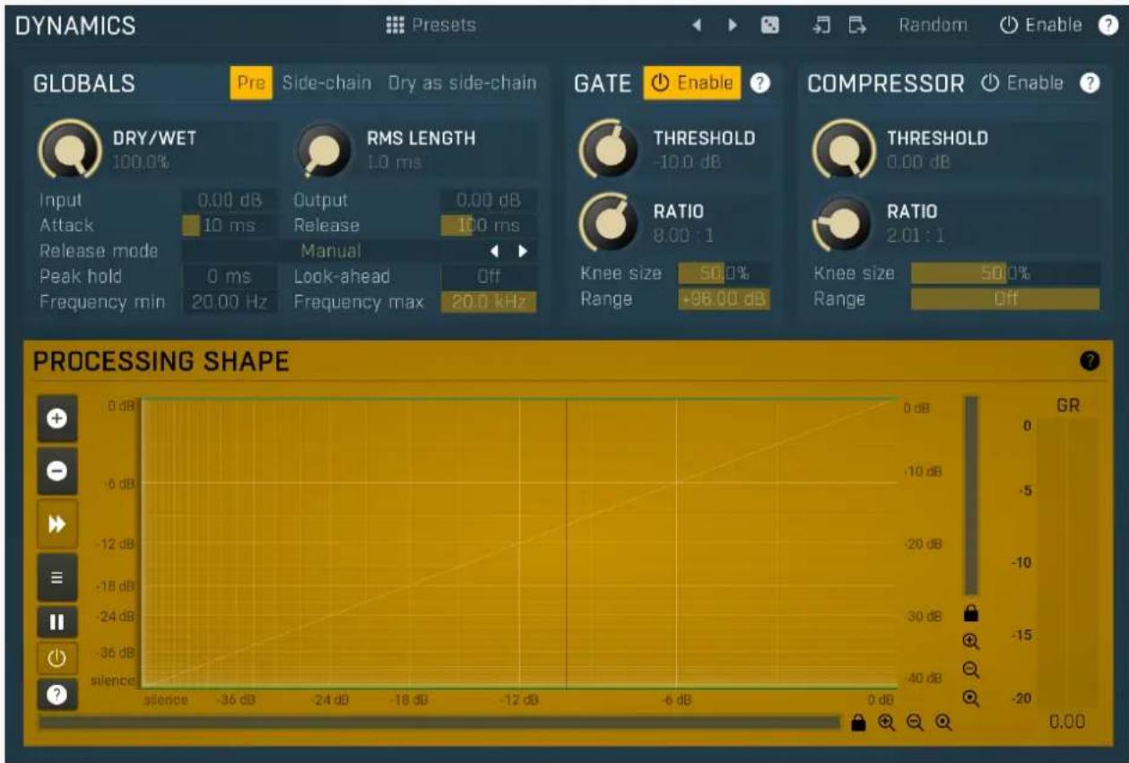
Dynamics panel controls the dynamics processing applied to the input or the reverberation signal (selected using the Pre button in the Dynamic Globals panel). This includes gating and compression, both of which are very useful on both signals.
Gating applied to the input signal is a classic technique that lets you reverberate only loud parts of the signal. It is typically used on drums to produce a reverb tail for snare drums for example.
Compressing the input signal lowers the dynamic range creating a "flatter" sound, which creates more stable reverberation without actually flattening the input signal itself.
Gating the reverberation signal is a rather specific effect which lets you abruptly terminate the reverberation signal when its level goes below the threshold. When a long reverb is used, it can often muddy the mix during the parts where the particular instrument isn't playing anymore, or create long endings when used on master, which then need to be faded-out by some other method. Using a gate with threshold low enough can provide an automatic solution which stops the reverb tail sooner than it normally would, removing the muddiness / tail.
Compressing the reverberation signal flattens the reverberation signal and when overused can introduce the typical compression character many are seeking on the tracks themselves, but on the reverberation signal instead. It is mainly useful as a creative tool.
Presets button displays a window where you can load and manage available presets. Hold Ctrl when clicking to load a random preset instead.

Left arrow
Left arrow button loads the previous preset.

Right arrow
Right arrow button loads the next preset.

Randomize
Randomize button loads a random preset.

Copy
Copy button copies the settings onto the system clipboard.

Paste
Paste button loads the settings from the system clipboard.

Random
Random button generates random settings using the existing presets.
Globals
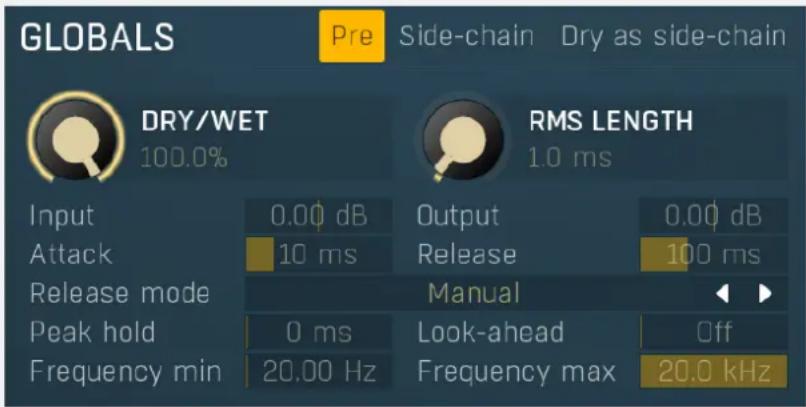

Pre
Pre switches between processing the input or reverberation signal. By default it is on, so that the dynamics section is processing the input signal allowing you to produce reveberation only to loud snare hits for example.

Side-chain
Side-chain button activates the side-chain input as a source for dynamics.
Dry as side-chain
Dry as side-chain
Dry as side-chain button makes the plugin send the dry signal to the side-chain. When Side-chain switch is enabled, the dynamics module is listening to whatever you send to the side-chain. When it is disabled however, the dynamics processes the same signal it is listening to. So either it is directly processing the dry input or the reverberation signal. Enabling this option makes the plugin always listen to the dry signal. While that makes no difference when Pre is enabled, when it is disabled, the dynamics will be processing the reverberation signal, but listening to the dry input. This can be useful to duck the reverberation while the input audio is loud enough, hence avoiding the 2 signals to collide and let the reverb fill the gaps in the actual performance.

DRY/WET
100.0%
Dry/Wet
Dry/Wet defines the ratio between dry and wet signals. 100% means fully processed, 0% means no processing at all. This feature essentially provides a modern way to do so-called parallel (or 'New York') compression. Essentially there are main 2 approaches to compression - A) set the threshold high, so that it affects everything above it, B) set the threshold low and use the dry/wet ratio control to reduce the effect of compression, which provides an easy way to control the amount of compression without too much editing of the more advanced parameters. Please note that lowering the ratio does NOT have the same effect as lowering dry/wet in most cases.
Range: 0.00% to 100.0%, default 100.0%

RMS LENGTH
1.0ms
RMS length
RMS length smoothes out the values of the input levels (not the input itself), such that the level detector receives the pre-processed signal without so many fluctuations. When set to its minimum value the detector becomes a so-called "peak detector", otherwise it is an "RMS detector".
When you look at a typical waveform in any editor, you can see that the signal is constantly changing and contains various transient bursts and separate peaks. This is especially noticeable with rhythmical signals, such as drums. Trying to imagine how a typical attack/release detector works with such a wild signal may be complex, at least. RMS essentially takes the surrounding samples and averages them. The result is a much smoother signal with fewer individual peaks and short noise bursts.
RMS length controls how many samples are taken to calculate the average. It stabilizes the levels, but it also causes a slower response time. As such it is great for mastering, when you want to lower the dynamic range in a very subtle way without any instabilities. However, it is not really desirable for processing drums, for example, where the transient bursts may actually be individual drum hits, hence it is usually recommended to use peak detectors for percussive instruments.
Note that the RMS detector has 2 modes - a simplified approximation is used by default, and a true RMS is processor can be enabled from the advanced settings (if provided). Both respond differently, neither of them is better than the other, they are simply different.
Range: Peak to 1000 ms, default 1.00 ms
Input
0.00 dB
Input gain
Input gain defines gain applied to the incoming signal.
Range: -24.00 dB to +24.00 dB, default 0.00 dB
Output
0.00 dB
Input gain
Input gain defines gain applied to the output signal.
Range: -24.00 dB to +24.00 dB, default 0.00 dB
Attack
10ms
Attack
Attack defines the attack time, that is how quickly the level detector increases the measured input level. When the input peak level is higher than the current level measured by the detector, the detector moves into the attack mode, in which the measured level is increased depending on the input signal. The higher the input signal, or the shorter the attack time, the faster the measured level rises. Once the measured level exceeds the Threshold then the dynamics processing (compression, limiting, gating) will start.
There must be a reasonable balance between attack and release times. If the attack is too long compared to the release, the detector will tend to keep the measured level low, because the release would cause that level to fall too quickly. In most cases you may expect the attack time to be shorter than the release time.
To understand the working of a level detector, it is best to cover the typical cases:
In a compressor the attack time controls how quickly the measured level moves above the threshold and the processor begins compressing. As a result, a very short attack time will compress even the beginning transient of a snare drum for example, hence it would remove the punch. With a very long attack time the measured level may not even reach the threshold, so the compressor may not do anything.
In a limiter the attack becomes a very sensitive control, defining how much of the signal is limited and how much of it becomes saturated/clipped. If the attack time is very short, limiting starts very quickly and the limiter catches most peaks itself and reduces them, providing lower distortion, but can cause pumping. On the other hand, a higher attack setting (typically above 1ms) will let most peaks through the limiter to the subsequent in-built clipper or saturator, which causes more distortion of the initial transient, but less pumping.
In a gate the situation is similar to a compressor - the attack time controls how quickly the measured level can rise above the threshold at which point the gate opens. In this case you will usually need very low attack times, so that the gate reacts quickly enough. The inevitable distortion can then be avoided using look-ahead and hold parameters.
In a modulator, the detector is driving other parameters, a filter cut-off frequency for example, and the situation really depends on the target. If you want the detector to react quickly on the input level rising, use a shorter attack time; if you want it to follow the flow of the input signal slowly, use longer attack and release times.
Range: 0 ms to 10000 ms, default 10.0 ms
Release
100ms
Release
Release defines the release time, that is how quickly the level detector decreases the measured input level. The shorter the release time, the faster the response is. Once the attack stage has been completed, when the input peak level is lower than the current level measured by the detector, the detector moves into the release mode, in which the measured level is decreased depending on the input signal. The lower the input signal, or the shorter the release time, the faster the measured level drops. Once the measured level falls under the Threshold then the dynamics processing (compression, limiting, gating) will stop.
There must be a reasonable balance between attack and release times. If the attack is too long compared to release, the detector would tend to keep the level low, because release would cause the level to fall too quickly. Hence in most cases you may expect the attack time to be shorter than the release time.
To understand the working of a level detector, it is best to cover the typical cases:
In a compressor the release time controls how quickly the measured level falls below the threshold and the compression stops. As a result a very short release time makes the compressor stop quickly, for example, leaving the sustain of a snare drum intact. On the other hand, a very long release keeps the compression working longer, hence it is useful to stabilize the levels.
In a limiter the release time keeps the measured level above the limiter threshold causing the gain reduction. Having a very long release time in this case doesn't make sense as the limiter would be working continuously and the effect would be more or less the same as simply decreasing the input gain manually. However too short a release time lets the limiter stop too quickly, which usually causes distortion as the peaks through the limiter to the subsequent in-built clipper or saturator. Hence release time is used to avoid distortion at the expense of decreasing the output level.
In a gate the situation is similar to a compressor - the release time controls how quickly the measured level can fall below the threshold at which point the gate closes. Having a longer release time in a gate is a perfectly acceptable option. The release time will basically control how much of the sound's sustain will pass.
In a modulator, the detector is driving other parameters, a filter cut-off frequency for example, and the situation really depends on the target. If you want the detector to react quickly on the input level falling, use a shorter release time; if you want it to follow the flow of the input signal slowly, use longer attack and release times.
Range: 0 ms to 10000 ms, default 100 ms
Release mode
Manual

Release mode
Release mode defines how the plug-in performs when decreasing level. In manual mode this is based only on the release time, which is suitable for most cases when the signal has constant characteristics. Automatic release modes can adapt to signals with unstable characteristics.
Automatic and Automatic fast modes: the longer the level stays above the threshold, the longer the release time will be and thus, the longer it will take to move below the threshold and end the release stage. The idea is that if the input is loud for some time, it will most likely stay that way for some more time, hence it should be stabilized to avoid unnecessary temporary fluctuations, which could result in pumping.
Both automatic modes increase the release time when the input signal is above the threshold and vice versa. The speed of the increase depends on the Auto speed parameter. Automatic fast mode uses full speed immediately after crossing the threshold, automatic mode varies the speed according to the current signal level.
For example, when a guitarist plays softly, the level is low and fluctuates around the threshold and the release time gets slower. So the processor quickly responds to sudden changes. However, when the guitarist starts playing a solo, the level rises and, the longer the solo is, the longer the release time becomes, hence the response becomes slower avoiding unnecessary fluctuations (pumping) when the solo contains small silent sections.
Linear 1 and Linear 2 modes: the higher the level is, the longer the release. The idea is that if the input is very loud, it will probably stay that way for some time, so it is wise to keep the levels up too. This is similar to the automatic modes, however the main factor is not how long the level is high, but how high it is.
Below the threshold the release time is the same as the attack time, above the threshold the release time rises from the attack time up to the specified release time parameter. Linear 1 mode usually provides higher release times than does Linear 2.
Opto mode: the higher the level is, the shorter the release. So this is kind of the opposite of linear modes. The idea is, that you are expecting short transients, which you wish to deal with. Normally the higher the level would get in such a transient, the longer it would take to get the level below the threshold, so, when used in a compressor for example, these transients would cause unnecessary compression in the sustain stage. The opto detector lowers the level quickly, minimizing the amount of compression in the sustain stage.
For example, let's say you are compressing a full drumset, but there is a very dominant sharp and short hi-hat sound, so it is appropriate to have short release times. You would use Opto mode. But the rest of the drumset deserves a softer treatment, so you want to keep longer release times. Use one of the other modes.
Peak hold
0 ms
Peak hold
Peak hold defines the time that signal level detector holds its maximum before the release stage is allowed to start. As an example, you can imagine that when an attack stage ends there can be an additional peak hold stage and the level is not yet falling, before the release stage starts. This is true only when true peak mode is enabled (check the advanced detector settings if available).
It is often used in gates to avoid the gated level falling below the threshold too quickly, while having short release times. If you want the gate to close quickly, you need a short release time. But in that case the ending may be too abrupt and even cause some distortion. So you use the peak hold to delay the release stage.
It is also used along with look-ahead to avoid distortion in limiters and compressors. If you need a very short attack, the attack stage may be too quick and cause distortions. In limiters this attack time is often 0ms, in which case it becomes a clipper. Setting look-ahead and peak hold to the same value will make the detector move ahead in time, so that it can react to attack stages before they actually occur and yet hold the levels for the actual signal to come.
Range: 0 ms to 1000 ms, default 0 ms
Look-ahead
Off
Look-ahead
Look-ahead delays the actual signal being processed, but keeps the detector signal intact. This makes the processor use a signal that has not actually arrived for dynamic calculation. This allows the processor to respond even faster, in fact, ahead of time. This feature is useful for mastering, however it naturally induces latency.
Look-ahead can be available in milliseconds (with obvious meaning) or in percentages. In percentages the look-ahead delay is computed automatically based on the attack and hold times. For example, if look-ahead is 100%, attack time 2ms and peak hold
10ms, then the look-ahead is 10ms; 60% look-ahead would be 7.2ms. If the look-ahead is simply an on/off switch, then it is toggling between 0% and 100% values.
Before using look-ahead, you should understand what such a feature does exactly as the results can potentially be damaging to your audio. Look-ahead basically moves the signal back in time, in other words its signal detector measures the input levels ahead of time. This means that when the detector is in the attack stage, the level is rising, the actual signal is not rising yet, but it will do so soon. However, the same applies to the release stage! When the detector moves to the release stage, the actual signal is not falling yet. This can lead to very strange artifacts (which can be used creatively of course).
The common way to fix this is to set the release time considerably higher than the attack time. In this way, the level will rise ahead of time in the attack stage, and same will happen for the release stage and the level will go down, however, since the level is falling slowly, the look-ahead will not be that relevant.
Another option is to use the peak hold feature. It is highly recommended to enable true hold in the advanced detector settings if available. Essentially this feature maximizes the input level over a certain period of time. So for example, if you set look-ahead to 5ms and peak hold to 5ms as well, the actual signal will arrive 5ms later than the detector signal, however the peak hold feature will ensure that the detector holds the highest peaks for 5ms, so the attack stage will be ahead of time, but the release will not! You can consider it a form of latency compensation for the release stage.
Look-ahead is commonly used in limiters along with very low (often 0ms) attack times to avoid distortion. With 0ms attack time the limiter is immediately following the input and when the level gets above 0dB, it turns it down to 0dB, so the attack stage is effectively being clipped. To avoid distortion produced by this effect, you can increase look-ahead and peak hold to the same value, say 1ms. As a result the attack stage occurs before it actually occurs, so the distortion is still present, but in much lower levels and usually is masked by the forthcoming transient.
Range: Off to 1000 ms, default Off
Frequency min 20.00 Hz Frequency min
Frequency min defines the cut-off frequency for the detector's high pass filter - minimal frequency.
Range: 20.00 Hz to 20.0 kHz, default 20.00 Hz
Frequency max 20.0 kHz Frequency max
Frequency max defines the cut-off frequency for the detector's low pass filter - maximal frequency.
Range: 20.00 Hz to 20.0 kHz, default 20.0 kHz
Gate panel
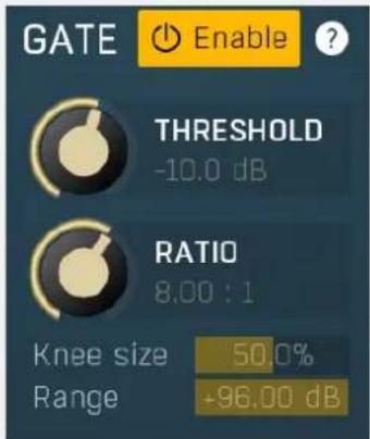
Gate panel contains the controls of the gate processor.
THRESHOLD
-10.0 dB
Threshold
Threshold determines the maximum signal level below which the effect starts to apply.
Range: -80.0 dB to 0.00 dB, default -15.9 dB

RATIO
800:1
Ratio
Ratio defines the gating ratio of the input signal below the threshold. The higher the ratio, the more brutal the gate will be.
Range: 1.00 : 1 to Infinity, default 8.00 : 1
Knee size 50.0%
Knee size
Knee size defines size of the knee.
Range: 0.00% to 100.0%, default 50.0%
Processor 2 panel
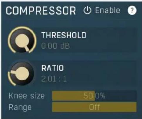
Processor 2 panel contains parameters of the secondary processor, which can behave like a compressor or expander.

THRESHOLD
0.00 dB
Threshold
Threshold determines the minimum signal level above which the compression effect starts to apply.
Range: -80.0 dB to 0.00 dB, default -12.0 dB
RATIO
2.01:1
Ratio
Ratio defines the compression ratio of the input signal above the threshold. The higher the ratio, the more compression you get.
Range: 1.00 : 1 to Infinity, default 2.00 : 1
Knee size
50.0%
Knee size
Knee size defines size of the knee.
Range: 0.00% to 100.0%, default 50.0%
Range
Off
Range
Range defines size of the interval above the threshold after which the original signal ratio is restored.
Range: +1.00 dB to Off, default Off
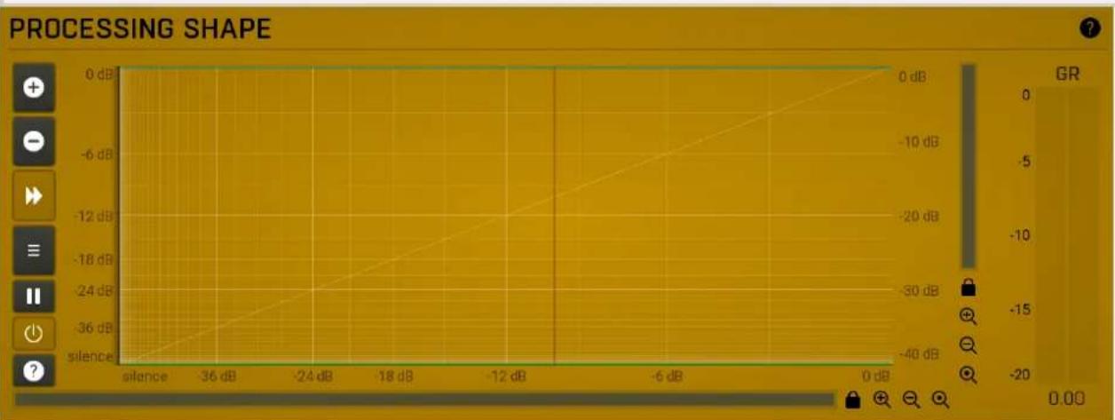
Level shape graph
Level shape graph displays the dynamic processing transformation shape. The X axis represents the input signal level, Y axis defines the output level.
Please note that this display is not logarithmic. This can lead to confusion, as, for example, a moving expander's threshold changes the graph's slope while the ratio stays the same. This is however necessary, because a logarithmic display can never contain silence, as it is minus infinity decibels, and the silence point is essential for gates for example. The display is therefore a compromise between usability
and accuracy.
The moving vertical line shows the current detected level. It may be moving extremely quickly depending on the settings. It may also be invisible if the input level is silence or above 0dB (which is not recommended unless you are using the processor as a limiter). There may be other graphs available, such as input & output waveform and gain reduction time graphs.
Meters
Meters display gain-reduction for each channel being processed. Also it contains controls to manipulate time-graphs shown in the transformation shape graph above.

Plus
Plus button increases the time-graph speed (reduces the period that is displayed).

Minus
Minus button decreases the time-graph speed (increases the period that is displayed).

Rewind
Rewind button enables or disables the time-graph static mode. In static mode the graphs are fixed and the current position cycles from left to right; otherwise the graphs move from right to left and the current position is fixed (at the right-hand side).

Menu
Menu button displays the time-graph settings. In this window you can control which graphs are displayed, the speed and other relevant parameters.
Time-graph settings
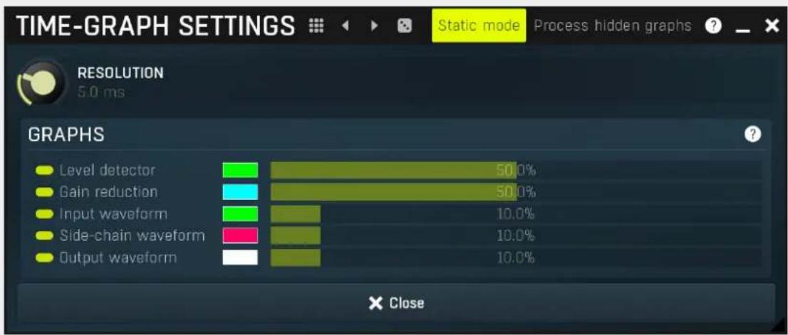

Presets
Presets button displays a window where you can load and manage available presets. Hold Ctrl when clicking to load a random preset instead.

Left arrow
Left arrow button loads the previous preset.

Right arrow
Right arrow button loads the next preset.

Randomize
Randomize button loads a random preset.
Static mode
Static mode
Static mode stops the graph from scrolling to the left and makes the graph refresh from left to right instead.
When this is disabled, the entire graph is moving from right to left as the incoming audio is processed. This may make it hard to spot the actual details, which is where the static mode comes to the rescue. Static mode is the default state and in most cases is more practical.
Process hidden graphs
Process hidden graphs
Process hidden graphs enables measurement of graphs which are actually disabled in the view. This may come handy if you need to repeatedly show and hide several graphs. With this mode disabled, which it is by default, the processor saves CPU resources by computing only those measurements that are actually visible. However, when you show a currently hidden graph, no measurements are available, so you will need to wait for the graph to be generated from the incoming signal. If you enable this option, the graph will be available immediately after you make it visible.

RESOLUTION
50ms
Resolution
Resolution controls the time it takes for the graph to move one pixel. Therefore this actually controls the display speed.
Graphs panel
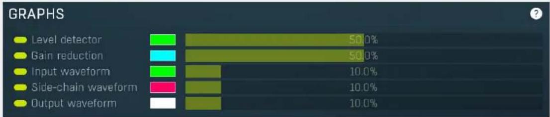
bar
GRAPHS | Category | Value (%) | |---|---| | Level detector | 50.0 | | Gain reduction | 50.0 | | Input waveform | 10.0 | | Side-chain waveform | 10.0 | | Output waveform | 10.0 |Graphs panel contains all available graphs and lets you show or hide each of them, and change their visual properties.

Pause
Pause button pauses the processing.

Enable
Enable button enables or disables the metering system. You can disable it to save system resources.
Envelope graph menu
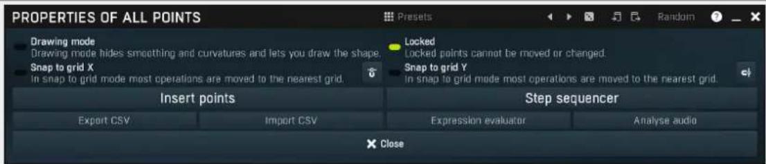
Envelope graph menu provides additional features which are used to edit the graph. Open the menu using right mouse button in the graph. Please note that if you select some points in the graph, or click on a point for example, the menu will be different and will cover only those features related to the selected set of points.

Presets
Presets
Presets button displays a window where you can load and manage available presets. Hold Ctrl when clicking to load a random preset instead.

Left arrow
Left arrow button loads the previous preset.

Right arrow
Right arrow button loads the next preset.

Randomize
Randomize button loads a random preset.

Copy
Copy button copies the settings onto the system clipboard.

Paste
Paste button loads the settings from the system clipboard.
Random
Random
Random button generates random settings using the existing presets.

Snap to grid X
In snap to grid mode most operations are moved to the nearest grid.

Snap to grid
X
Snap to grid X activates the snap to grid feature. Alternatively you can press Alt while dragging a point or selection.

Snap to grid Y
In snap to grid mode most operations are moved to the nearest grid.

Snap
Snap button activates the snap to grid feature. Alternatively you can press Alt while dragging a point or selection.
Insert points
Insert point button creates a point at mouse position.
Step sequencer
Insert point
sequencer
Step sequencer button generates the envelope from step sequencer.
Export CSV
Export CSV
Export CSV feature lets you export the graph to a CSV file. CSV file is a simple text format, which has multiple lines with X and Y coordinates delimited by ';' For example:
0.275;0.2
0.438;0.5
0.775;0.67
Import CSV
Import CSV
Import CSV feature lets you select a CSV file and imports the graph points from it. CSV file is a simple text format, which has multiple lines with X and Y coordinates delimited by ';'. For example:
0.275;0.2
0.438;0.5
0.775;0.67
Expression evaluator
Expression evaluator
Expression evaluator lets you generate points based on a mathematic formula. The only input variable is 'x', so as an example you may write 'ln(x^3 + 1) - sin(x*x)'.
Expression evaluator uses traditional C/C++ style formatting, which is natural for most people. It provides arithmetics, logical and conditional operators. Following terms are supported:
Constants: pi, e, sqrt2, ln2
Arithmetic operators:
-a inverts the sign, e.g. "-x" produces +2 for x=-2
a+b = addition
a-b = subtraction
a*b = multiplication
a/b = division
a%b = modulo, remainder after division
a^b = power, e.g. "2^3" produces 2*2*2 = 8
Arithmetic functions:
min(a,b) = minimum of both values
max(a,b) = maximum of both values
limit(a,min,max) = a limited into the interval min..max
to01(a,min,max) = converts "a" as min..max to 0..1
from01(a,min,max) = converts "a" as 0..1 to min..max
tom11(a,min,max) = converts "a" as min..max to -1..1
fromm11(a,min,max) = converts "a" as -1..1 to min..max
Basic mathematic functions: abs(x) = absolute value , e.g. abs(-3) = 3 sqr(x) = xx sqrt(x) = square root exp(x) = natural exponential e^ ln(x) = natural logarithm log10(x) = logarithm with base 10 log(x, base) = logarithm with specified base inv(x) = 1/x sgn(x) = sign of x, -1 or 0 or +1 depending on xx round(x) = rounding to the nearest value floor(x) = rounding to the nearest lower value, e.g. floor(-2.3) = -3 ceil(x) = rounding to the nearest higher value, e.g. ceil(-2.3) = -2 rand(x) = random value from 0 to x
Functions for specific units:
f01(a) = converts "a" as frequency from 20...20000 into log scale 0..1
ffrom01(a) = converts "a" as 0..1 (log scale) to frequency from 20...20000
todb(a) = converts "a" as multiplier to dB value by calculating "20*log10(a)"
fromdb(a) = converts "a" as dB value to multiplier by calculating "10^(a/20)"
Trigonometric functions: (x) , (x) , (x) , (x) , (x) , (x) , (x) , (x) , (x)
Logical operators:
a==b = comparison producing 1 if "a" and "b" are equal, 0 otherwise
a!=b = comparison producing 1 if "a" and "b" are NOT equal, 0 otherwise
a<b = comparison producing 1 if "a" is lower than "b", 0 otherwise
a<=b = comparison producing 1 if "a" is lower or equal to "b", 0 otherwise
a>b = comparison producing 1 if "a" is greater than "b", 0 otherwise
a>=b = comparison producing 1 if "a" is greater or equal to "b", 0 otherwise
!a = logical negation, 0 produces 1, 0 otherwise
a&&b = logical AND, produces 1 if both "a" and "b" are nonzero
a||b = logical OR, produces 1 if any of "a" and "b" are nonzero
a^^b = logical XOR, produces 1 if "a" and "b" are logically different
a ? b : c = if a is nonzero, then the result is b, otherwise it is c
Analyse audio
Analyse audio
Analyse audio lets you analyse a portion of an audio file at specified intervals, extract its level envelope and use those levels to construct the graph's curve.
Equalizer panel
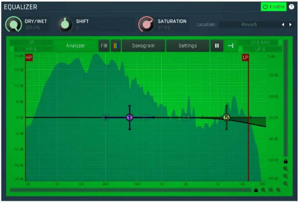
line
| Frequency | Power Level (dB) | | --------- | ---------------- | | 20 | -24 | | 50 | 18 | | 100 | 24 | | 500 | 18 | | 1k | 6 | | 2k | 0 | | 5k | -6 | | 10k | -12 | | 20k | -24 |Equalizer panel contains the integrated dynamic equalizer you can use to pre-process the input or post-process the output. There are 2 independent equalizers, one processing the standard input channels (depending on the channel configuration, typically left and right, etc.), the other one is processing the mid/side channels, which are transformed from the left and right channels.

DRY/WET
100.0%
Dry/Wet
Dry/Wet defines ratio between dry and wet signals. 100% means fully processed, 0% means no processing at all. In normal mode only peak and shelf filters are affected correctly, other filters are left at 100% unless the ratio is set to 0%, in which case the equalizer is bypassed.
Range: 0.00% to 100.0%, default 100.0%
SHIFT
0
Shift
Shift lets you pitch shift all bands by specified number of semitones. It doesn't change the actual band points, but changes the resulting EQ shape appropriately.
Range: -24.00 to +24.00, default 0

SATURATION
67.8%
Soft saturation
Soft saturation defines amount of saturation simulating analog equalizers.
Range: 0.00% to 100.0%, default 0.00%
Location
Reverb
◀ ▶
Location
Location controls exactly where in the signal processing chain the EQ will be performed. In most cases the differences will probably be subtle, but bigger differences may occur with more complex settings featuring dynamics processing for example. By default the processing chain is like this:
Input -> Dynamics (if Pre) -> Early & Late Reflections -> Dynamics (if not Pre) -> Widening etc. -> Dry/Wet -> Output
Input mode performs the EQ on the input signal. Hence everything in the reverb is then affected, including dynamics. For example, if you want to trigger the reverb by a bass drum, you would use the Dynamics tab as a gate and filter everything above say 100Hz. But if you locate the EQ in front of the dynamics and set it to filter out everything below say 200Hz, which is a common practice, there would be almost no signal left to trigger the reverb.
Input after dynamics mode performs the EQ on the input signal after the dynamics (if located at that stage). Therefore the input dynamic processing would not be affected by the EQ. In the example with the bass drum the reverb input would have filtered frequencies below 200Hz, but the gate would still follow the bass drum.
Reverb mode performs the EQ on the reverberation signal, on the mixed early and late reflections. In most cases the results will
actually be the same as the previous mode. The output may be slightly different if you use some kind of nonlinear processing or modulation in the reverb engine.
Reverb after dynamics mode performs the EQ on the reverberation signal after the dynamics (if located at that stage) has processed the reverberation signal, which is the case only if the Pre is disabled.
Output mode performs the EQ on the final output signal; in particular, after the global Dry/Wet. This means that the dry signal allowed to pass through the reverb would be equalized too.
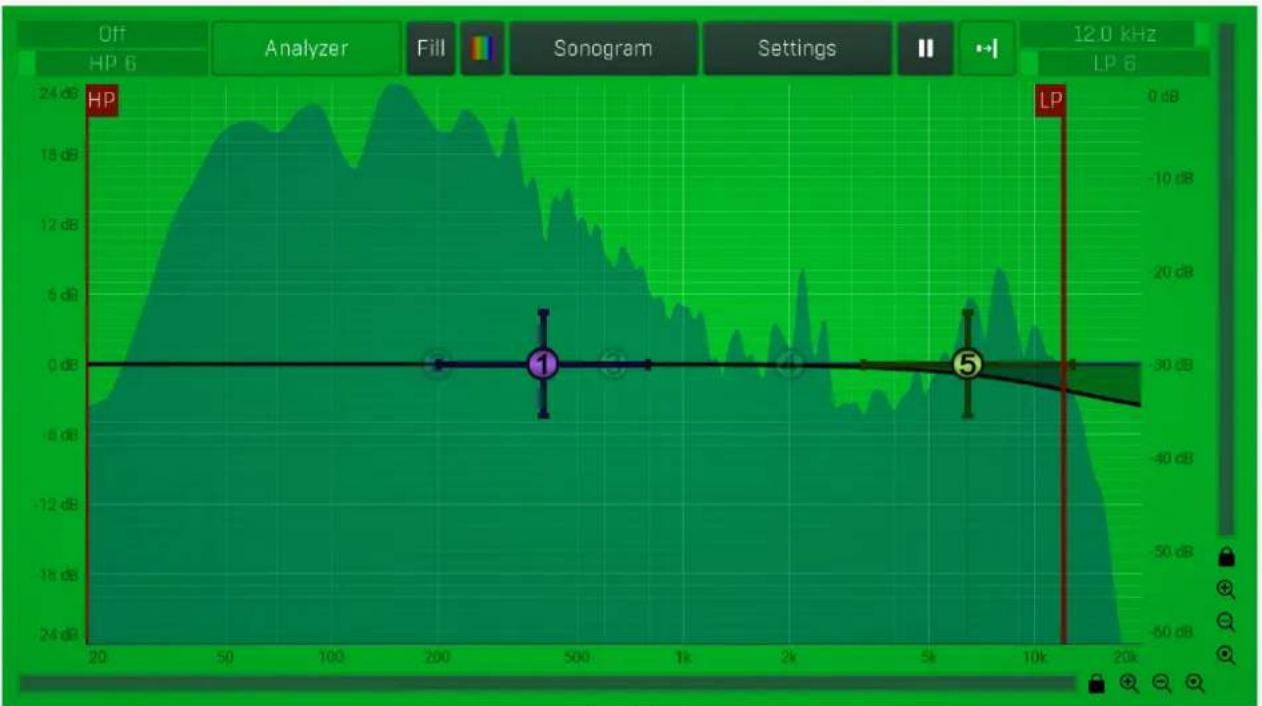
line
| Frequency | Power (dB) | | --------- | ---------- | | 200 | 0 | | 500 | 0 | | 1000 | 0 | | 5000 | -30 | | 10000 | -35 | | 20000 | -45 |Equalizer shape graph
Equalizer shape graph controls and displays the frequency response. There are several bands available, each of them can be enabled/disabled, can be set to a different filter, can have different frequency, Q and other parameters.
Double-click on a band point to enable or disable a band. Drag it to change its frequency and gain. Drag the horizontal nodes to change its Q. Hold ctrl key for fine tuning. Click using the right mouse button on it to open a window with additional settings.
Analyzer
Analyzer
Analyzer button enables or disables the spectrum analyzer, which shows the levels of individual frequencies. In most practical cases it is more convenient to use the sonogram, which shows the frequencies in time, but provides a lower level resolution as the levels are differentiated by color. The spectrum analyzer also provides a micro-sonogram (shown in the bottom of the panel) which uses the same color-based view as the sonogram.
Fill
Fill
Fill button enables or disables the full-sized analyzer micro-sonogram. This means that the micro-sonogram at the bottom of the equalizer graph will fill the whole analyzer view. Color differentiation is often easier to understand than the classical spectrum analyzer, so this might help you better understand the spectrum of your audio material.
An alternative is to use the spectrum sonogram.

Analyzer Rainbow Colors
Analyzer Rainbow Colors lets you see the analyzed sound spectrum in beautiful colors, following the same style as visible light. It ranges from infra-red colors for the lowest frequencies to ultra-violet colors for the highest frequencies in the analyzed audio. If rainbow colors are disabled, the analyzer and graph will be single-colored, following the setup from Settings/Graphs.
Sonogram
Sonogram
Sonogram button enables or disables the spectrum sonogram, which shows levels of individual frequencies in time. Levels are differentiated by color, so the accuracy is not as good as when using the spectrum analyzer. However, the time axis improves the visual orientation in the spectrum for typical audio signals. In contrast, the spectrum analyzer is more of a scientific tool.
Settings
Settings
Settings button shows the settings of the spectrum analyzer and the spectrum sonogram.
Analyzer settings
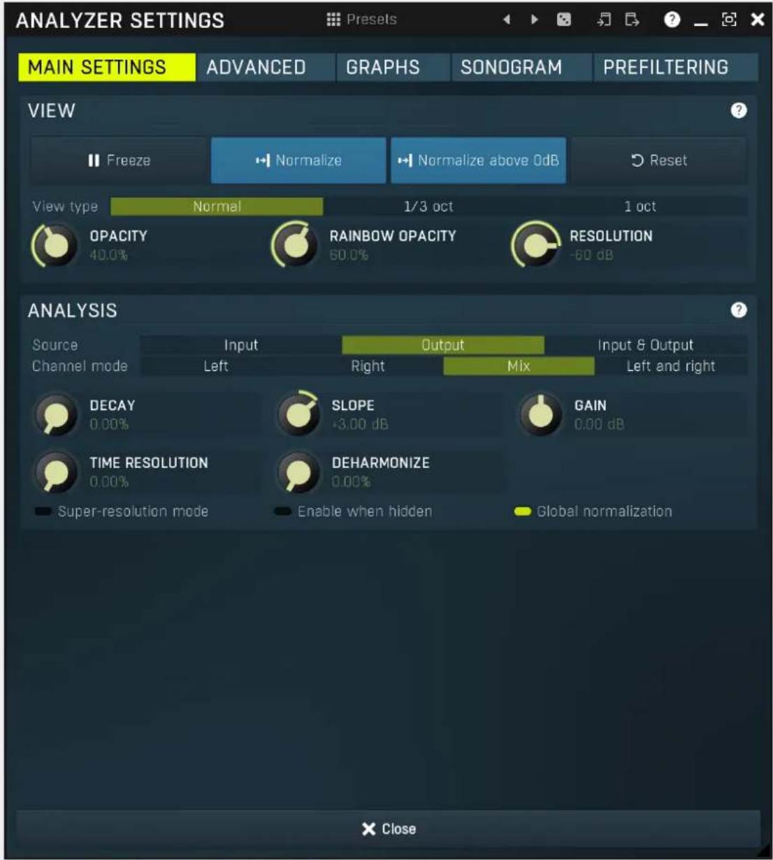

Presets
Presets
Presets button displays a window where you can load and manage available presets. Hold Ctrl when clicking to load a random preset instead.

Left arrow
Left arrow button loads the previous preset.

Right arrow
Right arrow button loads the next preset.

Randomize
Randomize button loads a random preset.

Copy
Copy button copies the settings onto the system clipboard.

Paste
Paste button loads the settings from the system clipboard.
selector
Tab selector switches between subsections.
Main settings panel
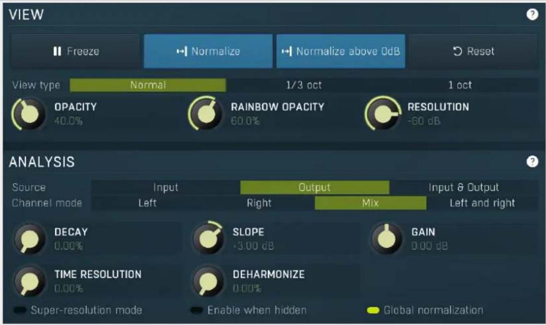
Main settings panel contains the most useful settings controlling the analyzer behaviour and view.
View
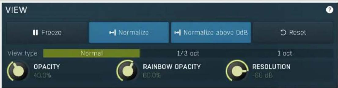
II Freeze
Freeze
Freeze button stops processing temporarily.
→ | Normalize
Normalize
Normalize button enables or disables the visual normalization, which makes the loudest frequency be displayed at the top of the analyser area (0dB); it does not normalise the sound. This is very useful for comparing frequency levels, however it does hide the actual level.
When comparing 2 spectrums you are usually interested mainly in the frequency level differences. In most cases both audio materials will have different overall levels, which would mean that one of the graphs would be "lower" than the other, making the comparison quite difficult. Normalize fixes this and makes the most prominent frequencies of the spectrum reach the top of the analyzer area (or have the most highlighted color in case of sonogram).
Reset
Reset
Reset button resets the analyzer state. This is particularly useful when analyzing infinite average and maximum values.
View type Normal 1/3 oct 1 oct View type
View type controls the way the spectrum is displayed. By default a smooth curve is presented. This view provides the best resolution and detail, but other modes (1/3 octave, 1 octave) may be easier to read.

OPACITY
40.0%
Opacity
Opacity controls the opacity of all analyzer graphs.

RAINBOW OPACITY
60.0%
Rainbow opacity
Rainbow opacity controls the opacity of the rainbow graph, if enabled.
RESOLUTION
-60 dB
Resolution
Resolution defines the vertical range on the display. The human auditory system has a resolution of about 90dB and the relevant range is usually less than 60dB. However you may want to use a higher resolution to check for technical problems - aliasing, distortion etc.
Analysis
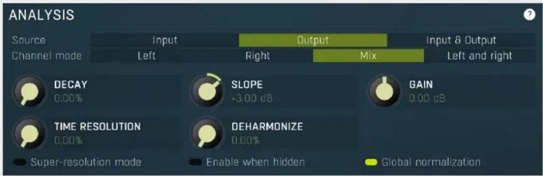
Source
Input
Output
Input & Output
Source
mode
Source mode defines which audio stages are to be analyzed. By default both input & output are selected and analyzed. However you may want to analyze only the input, or the output (or the external side-chain, where available, on its own or with the input or output).
Channel mode
Left
Right
Mix
Left and right
Channel
mode
Channel mode defines which channels are to be analyzed. By default all channels are merged into a mono sum (Mix mode), which is then analyzed. However you may want to analyze separate channels or display both the left and right channels separately. Please note that if two channels (for example: input & output, or input & side-chain) are displayed at the same time then mix mode is used instead of left & right mode. Similarly, when the plug-in is in Surround mode then Mix mode is used.
Also please note that when the plug-in is in one of the Mid / Side modes of operation, then you should read 'Left' as 'Mid' and 'Right' as 'Side'.
Different analyser combinations can, of course, be saved as different named presets.

DECAY
0.00%
Decay
Decay controls the speed at which the magnitudes return to the minimum value (silence). It is an alternative to averaging, which affects the speed that the frequencies both gain and lose their magnitudes. With a decay of 0% the magnitude goes to the minimum immediately. With 100% it stays the same forever, so it makes it display the maximum.

SLOPE
+3.00 dB
Slope
Slope makes the analyser increase the magnitude of higher frequencies, since they are typically lower in energy. 3dB per octave is a typical value, which makes pink noise horizontal as pink noise contains equal energy in each octave. Therefore if you set slope to 3dB, the response would be the same for the FFT and 1/3 octave graphs.
GAIN
0.00 dB
Gain
Gain makes all frequencies change magnitude by the specified amount. This has no meaning when normalization is enabled.

TIME RESOLUTION
0.00%
Time resolution
Time resolution improves the time resolution, but lowers the spectral resolution. This is typically useful for more scientific analyses, where the signal is moving quickly and you need to follow its movements quickly. This is often advantageous for sonograms with very high FFT sizes.

DEHARMONIZE
0.00%
Deharmonize
Deharmonize tries to remove harmonics in the content and leave only fundamentals. This may help you find the dominant frequencies in the signal.
Super-resolution mode
Super-resolution mode
Super-resolution mode activates a special processing algorithm, which provides high resolution even in the low frequency spectrum. Using standard FFT algorithms you can increase the FFT size to get better bass resolution, but this also slows down the response. Super-resolution mode keeps the quick response in high frequencies as they are naturally quicker, but also highly enhances the bass spectrum resolution. It requires additional CPU power.
Enable when hidden
Enable when hidden
Enable when hidden causes the analysis engine to continue processing the signal even when the GUI is hidden. Otherwise the sonogram is stopped, therefore will not be immediately available when the GUI is shown again.
Global normalization
Global normalization
Global normalization makes the normalization work based on the maximum of all graphs visible at the time. This means that the levels between the graphs will stay the same, but the maximum level will be 0dB. This is useful for comparing relative levels. If you disable this, all graphs will be normalized separately and will touch 0dB unless they are silent; and this is useful for comparing spectra.
Advanced panel
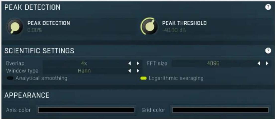
Advanced panel contains more advanced settings controlling the scientific parameters of the audio analysis.
Peak detection


PEAK DETECTION
0.00%
Peak detection
Peak detection tries to the remove skirts of separate sinusoids letting you view the frequencies contained in your audio material. This may be handy when performing more scientific analyses.

PEAK THRESHOLD
-40.00 dB
Peak threshold
Peak threshold defines the level below the maximum which is used for peak detection. You can use this to control which peaks get through and to get rid of small insignificant ones.
Scientific settings

Overlap
4x

Overlapping
Overlapping makes the analyser perform multiple FFT processing on the same data which results in better precision at the cost of higher CPU impact. With higher overlapping the response also speeds up.
FFT size
4096

FFT size
FFT size defines FFT processing block size. It basically controls the resolution. However for higher resolution in bass content it is recommended to use super-resolution mode instead as it keeps the quick response in higher frequencies.
Window type
Hann

Window type
Window type defines the type of window used to pre-process the source samples. This has several consequences for the frequency response, but it is a little scientific parameter. If you do not have specific requirements you can just leave this set to its default.

Analytical smoothing
Analytical smoothing
Analytical smoothing switch activates a more complicated smoothing algorithm, which provides more accurate results, however it may require much more CPU power. Unlike normal smoothing this method doesn't change the proportions of frequencies with higher magnitudes. It is useful mostly for technical analysis and for most musical signals it is often better to use the default smoothing method.

Logarithmic averaging
Logarithmic averaging
Logarithmic averaging switch activates averaging in logarithmic mode, hence decibels. If you disable it, linear averaging will be used.
Graphs panel
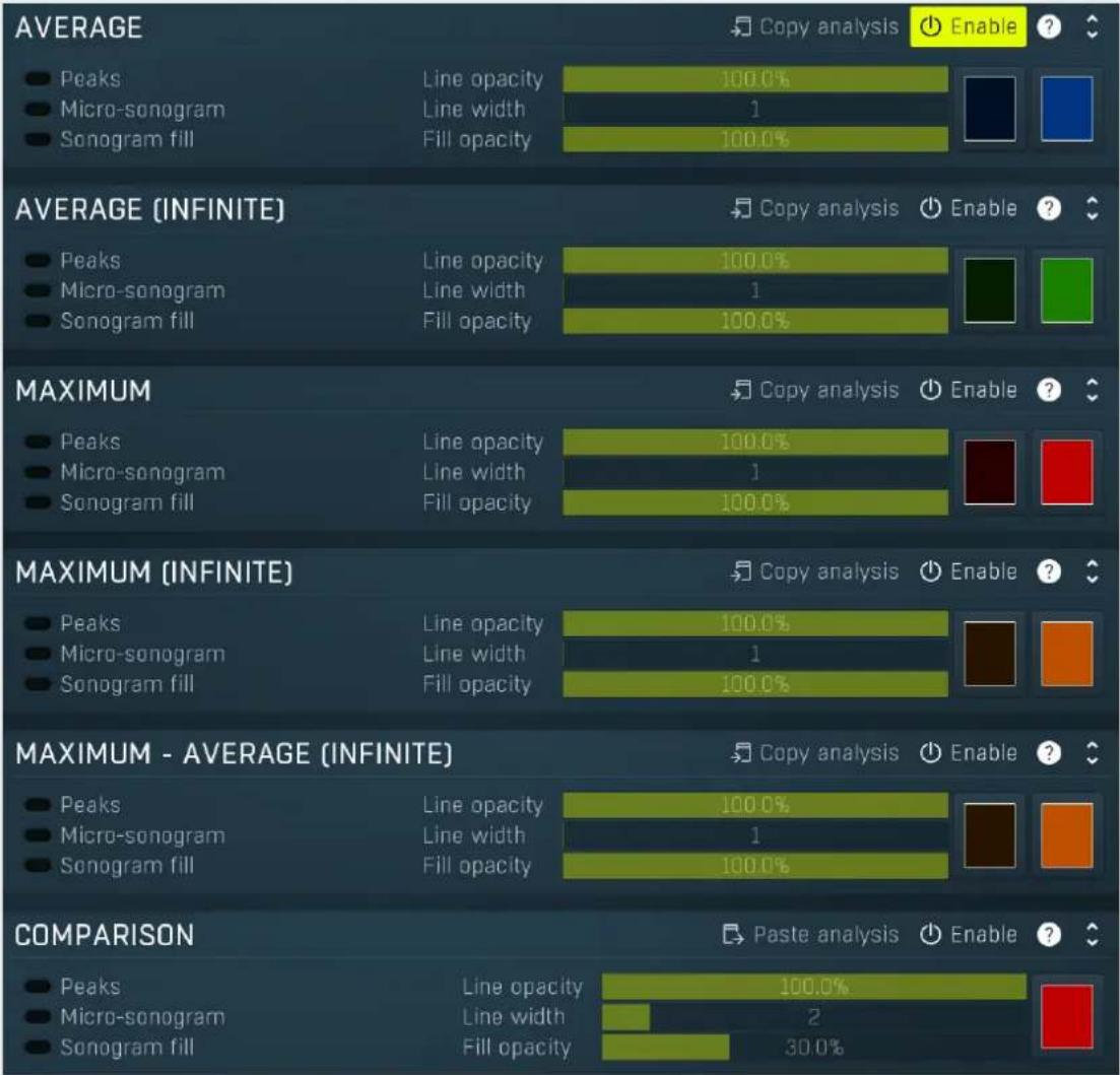
Graphs panel contains visual settings for the different graphs that you can show in the analyzer.
Average


Copy analysis
Copy analysis
Copy analysis button copies the current state of the analysis into the system clipboard so that you can paste it into another analyzer for comparison. Hold ctrl to export the analysis into a CSV file.

Analyzer Fill and Line Color - All Channels
Analyzer Fill and Line Color - All Channels defines the fill and line colors of the analyzer graph when Rainbow analyzer colors are disabled. This setting is used to set colors in all channel modes - see channel mode help in the Main Settings tab.

Analyzer Fill and Line Color - Left Channel
Analyzer Fill and Line Color - Left Channel defines the fill and line colors of the analyzer graph when Rainbow analyzer colors are disabled. This setting is used to set colors in the left channel mode only - see channel mode help in the Main Settings tab.

Peaks
Peaks
Peaks enables detection of frequencies with the highest magnitudes. Frequencies which are at most 20dB lower than the maximum are displayed, and there may be at most 8 of them. Please note that this feature requires additional CPU power.
Line opacity
100.0%
Line opacity
Line opacity controls the opacity of the graph outline.

Micro-sonogram
Micro-sonogram
Micro-sonogram displays a small single-state sonogram at the bottom of the graph. This may help you compare relevant frequencies, because it is usually easier to compare colors than graph values.
Line width

Line width
Line width controls the width of the graph online.

Sonogram fill
Fill
Fill makes the sonogram (enabled by Show sonogram) fill the whole area.
Fill opacity
100.0%
Fill opacity
Fill opacity controls the opacity of the graph interior fill.
Average (infinite)


Copy analysis
Copy analysis
Copy analysis button copies the current state of the analysis into the system clipboard so that you can paste it into another analyzer for comparison. Hold ctrl to export the analysis into a CSV file.

Analyzer Fill and Line Color - All Channels
Analyzer Fill and Line Color - All Channels defines the fill and line colors of the analyzer graph when Rainbow analyzer colors are disabled. This setting is used to set colors in all channel modes - see channel mode help in the Main Settings tab.

Analyzer Fill and Line Color - Left Channel
Analyzer Fill and Line Color - Left Channel defines the fill and line colors of the analyzer graph when Rainbow analyzer colors are disabled. This setting is used to set colors in the left channel mode only - see channel mode help in the Main Settings tab.
Maximum


Copy analysis
Copy analysis
Copy analysis button copies the current state of the analysis into the system clipboard so that you can paste it into another analyzer for comparison. Hold ctrl to export the analysis into a CSV file.
Analyzer Fill and Line Color - All Channels
Analyzer Fill and Line Color - All Channels defines the fill and line colors of the analyzer graph when Rainbow analyzer colors are disabled. This setting is used to set colors in all channel modes - see channel mode help in the Main Settings tab.

Analyzer Fill and Line Color - Left Channel
Analyzer Fill and Line Color - Left Channel defines the fill and line colors of the analyzer graph when Rainbow analyzer colors are disabled. This setting is used to set colors in the left channel mode only - see channel mode help in the Main Settings tab.
Maximum (infinite)


Copy analysis
Copy analysis
Copy analysis button copies the current state of the analysis into the system clipboard so that you can paste it into another analyzer for comparison. Hold ctrl to export the analysis into a CSV file.
Analyzer Fill and Line Color - All Channels
Analyzer Fill and Line Color - All Channels defines the fill and line colors of the analyzer graph when Rainbow analyzer colors are disabled. This setting is used to set colors in all channel modes - see channel mode help in the Main Settings tab.

Analyzer Fill and Line Color - Left Channel
Analyzer Fill and Line Color - Left Channel defines the fill and line colors of the analyzer graph when Rainbow analyzer colors are disabled. This setting is used to set colors in the left channel mode only - see channel mode help in the Main Settings tab.
Maximum - Average (infinite)


Copy analysis
Copy analysis
Copy analysis button copies the current state of the analysis into the system clipboard so that you can paste it into another
analyzer for comparison. Hold ctrl to export the analysis into a CSV file.
Analyzer Fill and Line Color - All Channels
Analyzer Fill and Line Color - All Channels defines the fill and line colors of the analyzer graph when Rainbow analyzer colors are disabled. This setting is used to set colors in all channel modes - see channel mode help in the Main Settings tab.

Analyzer Fill and Line Color - Left Channel
Analyzer Fill and Line Color - Left Channel defines the fill and line colors of the analyzer graph when Rainbow analyzer colors are disabled. This setting is used to set colors in the left channel mode only - see channel mode help in the Main Settings tab.
Comparison

bar
COMPARISON | Metric | Value (%) | | :--- | :--- | | Peaks | Line opacity | | Micro-sonogram | Line width | | Sonogram fill | Fill opacity | | Paste analysis | Enable ?
Paste analysis
Paste analysis
Paste analysis button pastes an analysis from the system clipboard and displays it as a comparison. This way you can compare your analysis to any other analysis from MeldaProduction plugins.

Analyzer Fill and Line Color - Left Channel
Analyzer Fill and Line Color - Left Channel defines the fill and line colors of the analyzer graph when Rainbow analyzer colors are disabled. This setting is used to set colors in the left channel mode only - see channel mode help in the Main Settings tab.
Sonogram panel
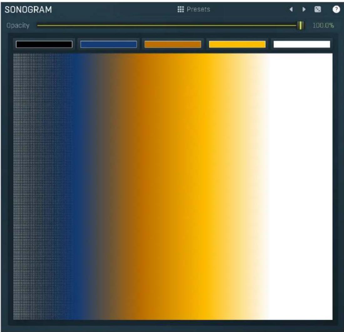
Sonogram panel contains visual settings of the sonogram, mainly the sonogram colors. A sonogram uses a set of colors. When the particular frequency's level is at the minimum, the first color is used. When it is at the maximum, the last color is used. Otherwise it interpolates the colors in-between.

Presets
Presets
Presets button displays a window where you can load and manage available presets. Hold Ctrl when clicking to load a random preset instead.

Left arrow
Left arrow button loads the previous preset.

Right arrow
Right arrow button loads the next preset.

Randomize
Randomize button loads a random preset.
Opacity
100.0%
Opacity
Opacity controls the opacity of the sonogram.
Prefiltering panel
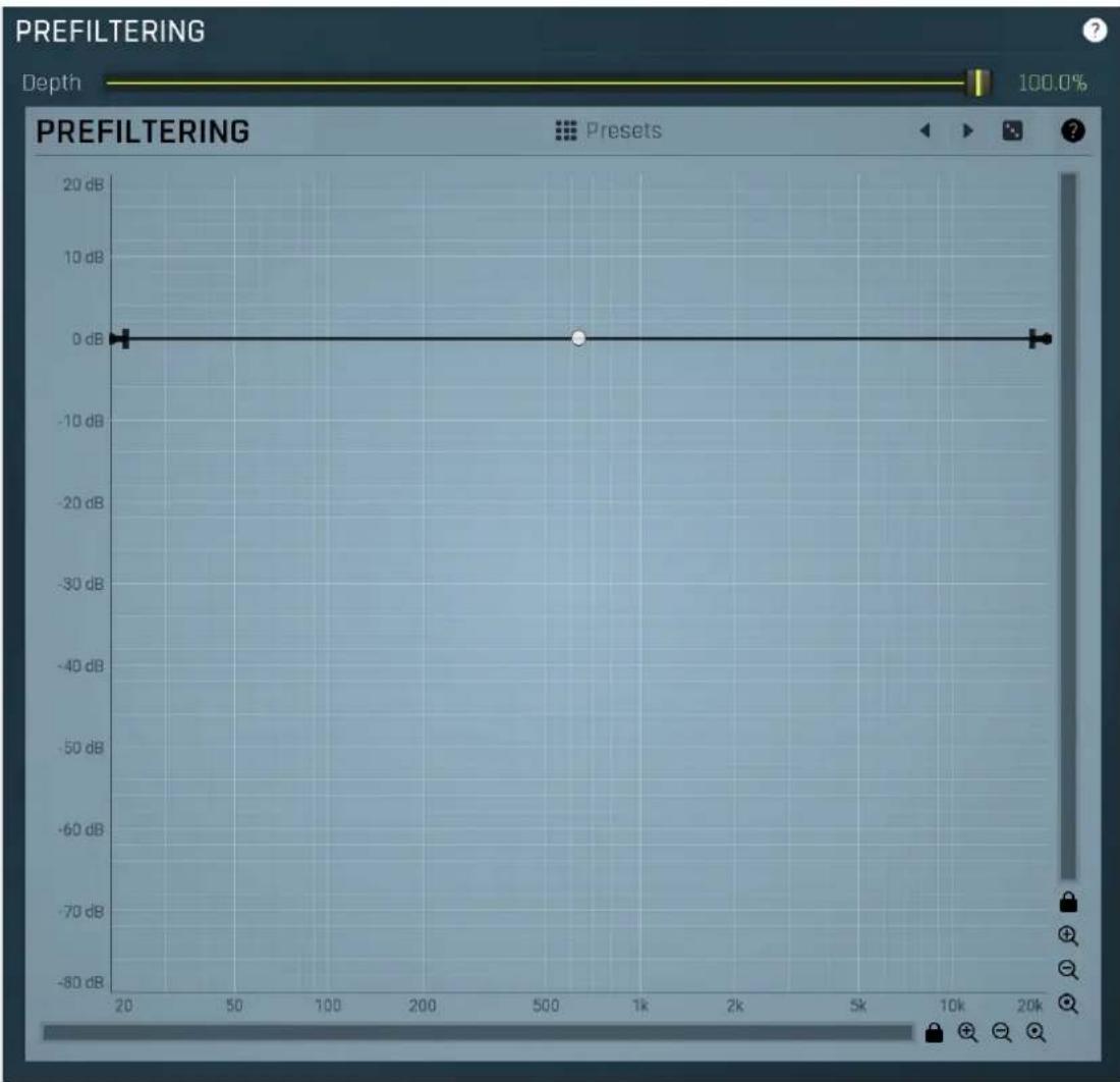
line
| X | Y | |-------|-------| | 20 | 0 dB | | 100 | 0 dB | | 500 | 0 dB | | 2000 | 0 dB |Prefiltering panel provides the optional prefiltering, which means that level of each frequency is either increased or decreased before analysis. Normally the analyzer shows scientific levels of each frequency. However you can for example use the predefined loudness curves, which makes the analyzer show how the human auditory system responds to the frequencies, so it in fact provides more accurate analysis taking into account the fact that human hearing is more complicated than the mathematical model.
Depth 100.0% Depth
Depth controls the amount of prefiltering. 100% makes the analyzer follow the prefiltering graph precisely, 0% essentially disables this feature.
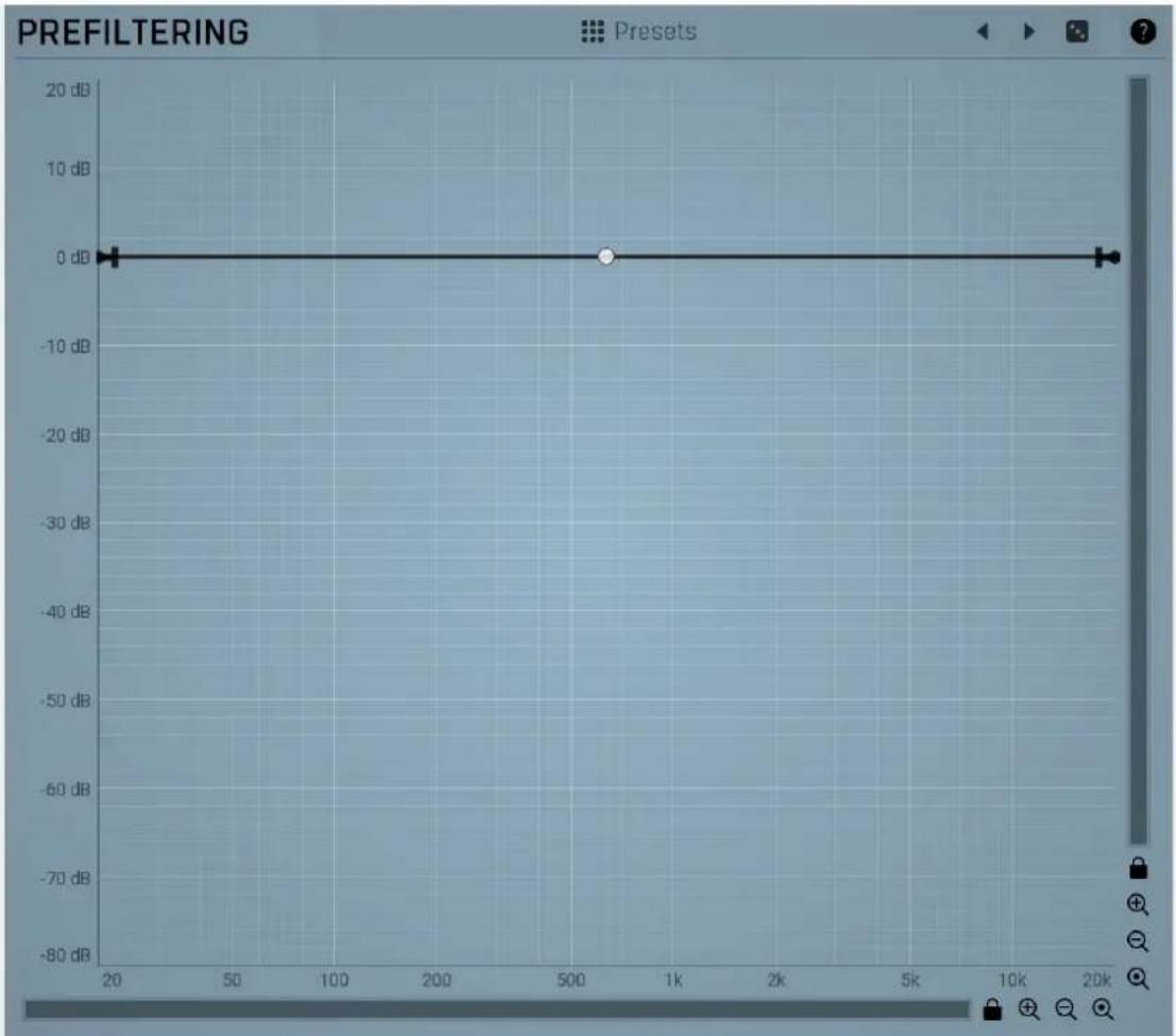
line
| x | y | | ---- | ----- | | 20 | 0 dB | | 500 | 0 dB | | 20k | 0 dB |Prefiltering
Envelope graph
Envelope graph provides an extremely advanced way to edit any kind of shape that you can imagine. An envelope has a potentially unlimited number of points, connected by several types of curves with adjustable curvature (drag the dot in the middle of each arc) and the surroundings of each point can also be automatically smoothed using the smoothness (horizontal pull rod) control. You can also literally draw the shape in drawing mode (available via the main context menu).
- Left mouse button can be used to select points. If there is a point, you can move it (or the entire selection) by dragging it. If there is a curvature circle, you can set up its tension by dragging it. If there is a line, you can drag both edge points of it. If there is a smoothing controller, you can drag its size. Hold Shift to drag more precisely. Hold Ctrl to create a new point and to remove any points above or below.
- Left mouse button double click can be used to create a new point. If there is a point, it will be removed instead. If there is a curvature circle, zero tension will be set. If there is a smoothing controller, zero size will be set.
- Right mouse button shows a context menu relevant to the object under the cursor or to the entire selection. Hold Ctrl to create or remove any points above or below.
- Middle mouse button drag creates a new point and removes any points above or below. It is the same as holding Ctrl and dragging using left mouse button.
- Mouse wheel over a point modifies its smoothing controller. If no point is selected, then all points are modified.
- Ctrl+A selects all points. Delete deletes all selected points.

Presets
Presets
Presets button displays a window where you can load and manage available presets. Hold Ctrl when clicking to load a random preset instead.

Left arrow
Left arrow button loads the previous preset.

Right arrow
Right arrow button loads the next preset.

Randomize

Pause
Pause button stops the analyzer temporarily.

Normalize
Normalize button enables or disables the visual normalization, which makes the loudest frequency be displayed at the top of the analyser area (0dB); it does not normalise the sound. This is very useful for comparing frequency levels, however it does hide the actual level.
When comparing 2 spectrums you are usually interested mainly in the frequency level differences. In most cases both audio materials will have different overall levels, which would mean that one of the graphs would be "lower" than the other, making the comparison quite difficult. Normalize fixes this and makes the most prominent frequencies of the spectrum reach the top of the analyzer area (or have the most highlighted color in case of sonogram).
Band settings window
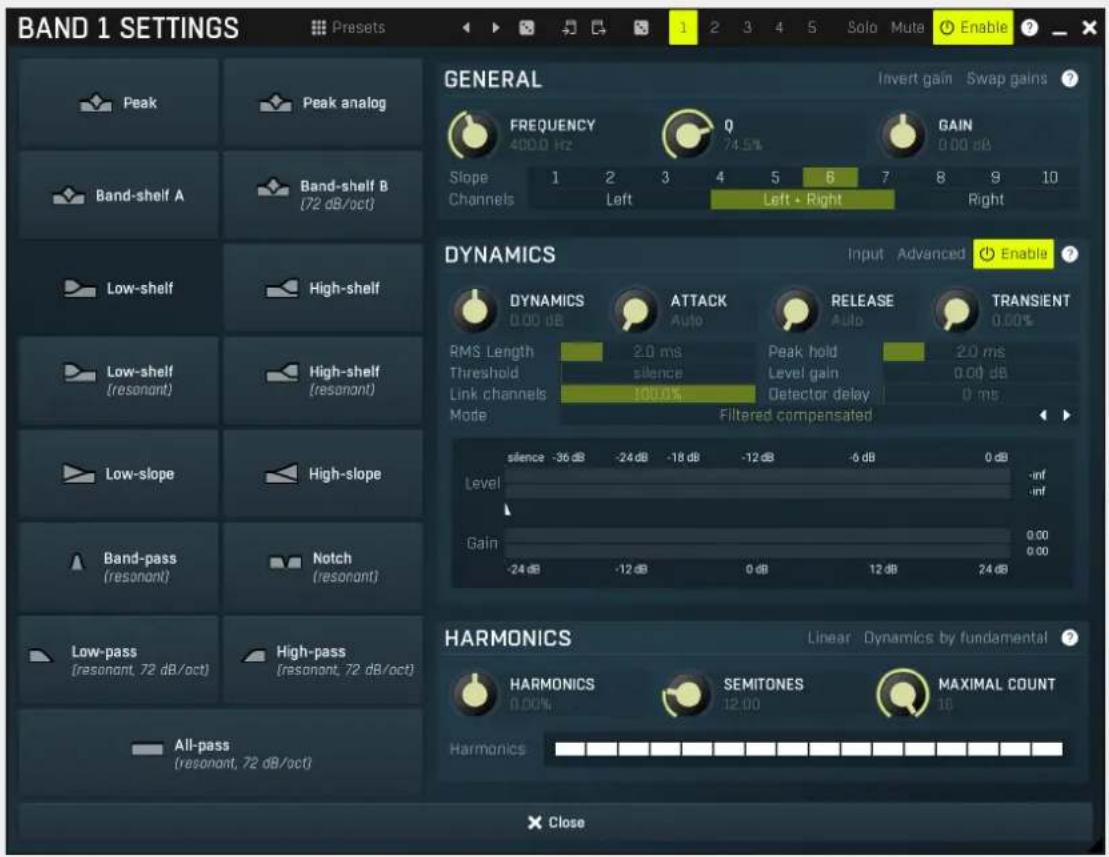
Band settings window contains settings for the particular band and can be displayed by right-clicking on a band or from a band list (if provided). On the left side you can see list of available filters, click on one to select it. On the right side, additional options and features are available.

Presets
Presets
Presets button displays a window where you can load and manage available presets. Hold Ctrl when clicking to load a random preset instead.

Left arrow
Left arrow button loads the previous preset.

Right arrow
Right arrow button loads the next preset.

Randomize
Randomize button loads a random preset.

Copy
Copy button copies the settings onto the system clipboard.

Paste
Paste button loads the settings from the system clipboard.

Random
Random button generates random settings using the existing presets.
General panel
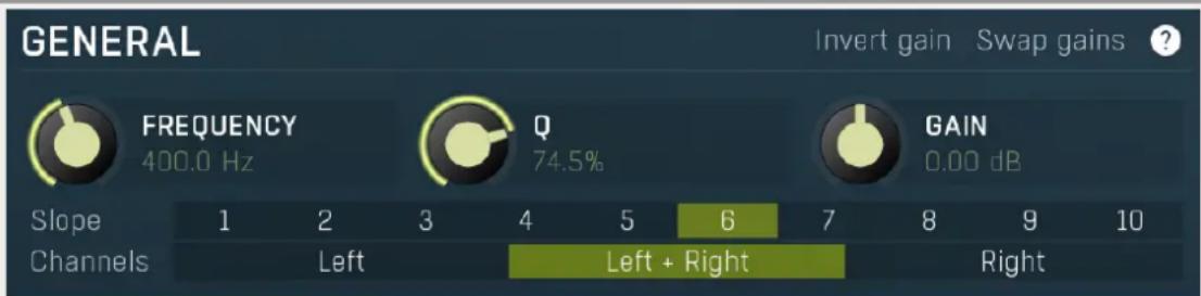
General panel contains standard filter settings such as frequency or Q. Most of these values are available directly from the band graph, but it may be necessary to use these controls for more accurate or textual access.
Invert gain
Invert gain
Invert gain inverts the gain of the band, e.g. makes -6dB from +6dB.
Swap gains
Swap gains
Swap gains button swaps values between gain and dynamics gain.
FREQUENCY
400.0 Hz
Frequency
Frequency defines the band's central frequency, which has different meaning depending of filter type.

Q
74.5%
Q
Q defines bandwidth. Please note that Q is an engineering term and the higher it is, the lower the bandwidth. Our implementation is trying to be more user-friendly, and by increasing the value (thus to the right), the bandwidth is increased as well. The editor still displays the Q value correctly.
GAIN
0.00 dB
Gain
Gain defines how the particular frequencies are amplified or attenuated. This parameter is used only by peak and shelf filters.
Slope
1
2
3
4
5
6
7
8
9
10
Slope
Slope can potentially duplicate some of the filters creating steeper ones. By default, the slope is 1 and this usually means 2-pole 12 dB/octave filters. By specifying 2 you can make the plugin uses 4-pole 24 dB/octave filters instead etc. To see the actual slope of each filter look into the filter type list on the left.
Channels
Left
Left + Right
Right
Channels
Channels controls which channels the band processes. If the input is stereo (left and right channels, L+R, selected on the toolbar Channel mode button), then you can make a band process only the left, only the right, or both channels. Similarly when the plugin is set to M/S channel mode, you can choose between mid, side or both channels.
When one of more bands are set to process a single channel, then 2 EQ curves are displayed, in red for the Left or Mid and in green for the Right or Side. If these are not distinct, then we recommend using a style with a light background for these graphs.
You cannot process left with one band and side with the other, because these are working in different encoding modes. In this case you can easily use 2 instances of the plugin in series, one in L/R mode and the other in M/S.
Dynamics panel
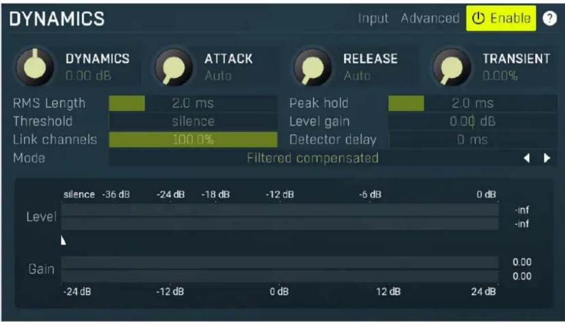
Dynamics panel contains settings of the dynamics processing which control how the filter behaves depending on input signal. Normal filters are static, meaning they don't change any features depending on the input signal. If you enable dynamic properties, by making the dynamic gain nonzero, the filter will start listening to the level of the input signal. This requires more CPU of course, as such a band is essentially an extremely complex generalized compressor, but the algorithms used are as efficient as it is technically possible.
A dynamic band varies the gain according to the input level. It can listen to the whole spectrum or to just part of it. By default it is driven by the partial spectrum, which it modifies itself, so, for example, when you have a high shelf, it is essentially listening to a high part of the spectrum. You can do many things with such a dynamic processor, but essentially it can work as a compressor or expander. There are many more advanced ideas that you can do and the full power hasn't really been explored yet.
Input
Input
Input switch makes the band measure the input level instead of current level in the chain of bands. When this is disabled (default) and the equalizer is processing the bands serially, which means that each band is processing the output from the previous stage, including level measurement. If you enable this switch however, the dynamic processing will be driven by the original input signal instead.
Please note that when Side-chain is on, this switch has no meaning, since side-chain has priority.
Advanced
Advanced
Advanced button displays additional settings for this band. These contain some more esoteric features, such as a dynamic transformation shape.

Enable
Enable
Enable button enables the dynamic processing. You can use it to switch between enabled and disabled dynamic processing to check the differences.
DYNAMICS
0.00 dB
Dynamics
Dynamics defines the maximum gain of the filter that could be caused by the input signal. For example, if you set it to -24dB and the input signal contained in the band were very strong, the band will be set to an additional -24dB. This would work similarly to a compressor in that band.

ATTACK
Auto
Attack
Attack defines the attack time, that is how quickly the level detector increases the measured input level. When the input peak level is higher than the current level measured by the detector, the detector moves into the attack mode, in which the measured level is increased depending on the input signal. The higher the input signal, or the shorter the attack time, the faster the measured level rises. Once the measured level exceeds the Threshold then the dynamics processing (compression, limiting, gating) will start.
There must be a reasonable balance between attack and release times. If the attack is too long compared to the release, the detector will tend to keep the measured level low, because the release would cause that level to fall too quickly. In most cases you may expect the attack time to be shorter than the release time.
To understand the working of a level detector, it is best to cover the typical cases:
In a compressor the attack time controls how quickly the measured level moves above the threshold and the processor begins
compressing. As a result, a very short attack time will compress even the beginning transient of a snare drum for example, hence it would remove the punch. With a very long attack time the measured level may not even reach the threshold, so the compressor may not do anything.
In a limiter the attack becomes a very sensitive control, defining how much of the signal is limited and how much of it becomes saturated/clipped. If the attack time is very short, limiting starts very quickly and the limiter catches most peaks itself and reduces them, providing lower distortion, but can cause pumping. On the other hand, a higher attack setting (typically above 1ms) will let most peaks through the limiter to the subsequent in-built clipper or saturator, which causes more distortion of the initial transient, but less pumping.
In a gate the situation is similar to a compressor - the attack time controls how quickly the measured level can rise above the threshold at which point the gate opens. In this case you will usually need very low attack times, so that the gate reacts quickly enough. The inevitable distortion can then be avoided using look-ahead and hold parameters.
In a modulator, the detector is driving other parameters, a filter cut-off frequency for example, and the situation really depends on the target. If you want the detector to react quickly on the input level rising, use a shorter attack time; if you want it to follow the flow of the input signal slowly, use longer attack and release times.

RELEASE
Auto
Release
Release defines the release time, that is how quickly the level detector decreases the measured input level. The shorter the release time, the faster the response is. Once the attack stage has been completed, when the input peak level is lower than the current level measured by the detector, the detector moves into the release mode, in which the measured level is decreased depending on the input signal. The lower the input signal, or the shorter the release time, the faster the measured level drops. Once the measured level falls under the Threshold then the dynamics processing (compression, limiting, gating) will stop.
There must be a reasonable balance between attack and release times. If the attack is too long compared to release, the detector would tend to keep the level low, because release would cause the level to fall too quickly. Hence in most cases you may expect the attack time to be shorter than the release time.
To understand the working of a level detector, it is best to cover the typical cases:
In a compressor the release time controls how quickly the measured level falls below the threshold and the compression stops. As a result a very short release time makes the compressor stop quickly, for example, leaving the sustain of a snare drum intact. On the other hand, a very long release keeps the compression working longer, hence it is useful to stabilize the levels.
In a limiter the release time keeps the measured level above the limiter threshold causing the gain reduction. Having a very long release time in this case doesn't make sense as the limiter would be working continuously and the effect would be more or less the same as simply decreasing the input gain manually. However too short a release time lets the limiter stop too quickly, which usually causes distortion as the peaks through the limiter to the subsequent in-built clipper or saturator. Hence release time is used to avoid distortion at the expense of decreasing the output level.
In a gate the situation is similar to a compressor - the release time controls how quickly the measured level can fall below the threshold at which point the gate closes. Having a longer release time in a gate is a perfectly acceptable option. The release time will basically control how much of the sound's sustain will pass.
In a modulator, the detector is driving other parameters, a filter cut-off frequency for example, and the situation really depends on the target. If you want the detector to react quickly on the input level falling, use a shorter release time; if you want it to follow the flow of the input signal slowly, use longer attack and release times.

TRANSIENT
0.00%
Transient
Transient lets you mix the level follower output with a transient detector output. This lets you follow signal level, transients or both. Note that since transient level is usually lower than level detector's output, Level gain is only applied on the level detector's signal, so you can use this to compensate for the difference in level.
RMS Length
2.0ms
RMS length
RMS length smoothes out the values of the input levels (not the input itself), such that the level detector receives the pre-processed signal without so many fluctuations. When set to its minimum value the detector becomes a so-called "peak detector", otherwise it is an "RMS detector".
When you look at a typical waveform in any editor, you can see that the signal is constantly changing and contains various transient bursts and separate peaks. This is especially noticeable with rhythmical signals, such as drums. Trying to imagine how a typical attack/release detector works with such a wild signal may be complex, at least. RMS essentially takes the surrounding samples and averages them. The result is a much smoother signal with fewer individual peaks and short noise bursts.
RMS length controls how many samples are taken to calculate the average. It stabilizes the levels, but it also causes a slower response time. As such it is great for mastering, when you want to lower the dynamic range in a very subtle way without any instabilities. However, it is not really desirable for processing drums, for example, where the transient bursts may actually be individual drum hits, hence it is usually recommended to use peak detectors for percussive instruments.
Note that the RMS detector has 2 modes - a simplified approximation is used by default, and a true RMS is processor can be
enabled from the advanced settings (if provided). Both respond differently, neither of them is better than the other, they are simply different.
Peak hold
2.0 ms
Peak hold
Peak hold defines the time that signal level detector holds its maximum before the release stage is allowed to start. As an example, you can imagine that when an attack stage ends there can be an additional peak hold stage and the level is not yet falling, before the release stage starts. This is true only when true peak mode is enabled (check the advanced detector settings if available).
It is often used in gates to avoid the gated level falling below the threshold too quickly, while having short release times. If you want the gate to close quickly, you need a short release time. But in that case the ending may be too abrupt and even cause some distortion. So you use the peak hold to delay the release stage.
It is also used along with look-ahead to avoid distortion in limiters and compressors. If you need a very short attack, the attack stage may be too quick and cause distortions. In limiters this attack time is often 0ms, in which case it becomes a clipper. Setting look-ahead and peak hold to the same value will make the detector move ahead in time, so that it can react to attack stages before they actually occur and yet hold the levels for the actual signal to come.
Threshold
silence
Threshold
Threshold controls the minimum level above which the dynamic gain actually starts working.
Level gain
0.00 dB
Level gain
Level gain controls the gain applied to the detector, which can be used for example when the input level is too low, so that dynamic processing would be negligible, unless the level is boosted.
Link channels
100.0%
Link channels
Link channels controls how much the signal level for each channel is controlled by the other channels. With 0% the link is disabled and each channel is not affected by the other channels at all. This is suitable to balance stereo channels, for example. With 100% the link is enabled and all channels are controlled by levels of all channels equally (that is the average level of those channels), therefore the processor will apply the same amount of processing on all channels. This is the default in most cases as it preserves relative levels between the channels.
Detector delay
0 ms
Detector delay
Detector delay lets you delay the detector input, hence the band will react later than the actual input signal.
Mode
Filtered compensated

Mode
Mode controls the way the band reacts to the input signal. It has no meaning if the dynamic gain is 0dB. Filtered compensated mode is default and it means that the source for measuring input level is a filtered signal with additional compensation. For example, when using a low-shelf filter, the signal is low-passed with a filter with the same settings as the low-shelf, therefore the low-shelf filter is affected only by the signal the low-shelf is actually amplifying or attenuating. Since a low-passed signal with cut-off at 100Hz has usually a much lower level than the one filtered with cut-off at 10 kHz, additional compensation is performed to diminish these differences. Filtered mode is similar, but the compensation is not performed. This may be advantageous for audio materials that do not contain the full spectrum, e.g. a bass line, where the compensation may make things complicated. Entire spectrum mode is the simplest - it simply takes the input signal without any further processing. This may be useful for example to attenuate selected frequencies when the input level gets too high.
meters
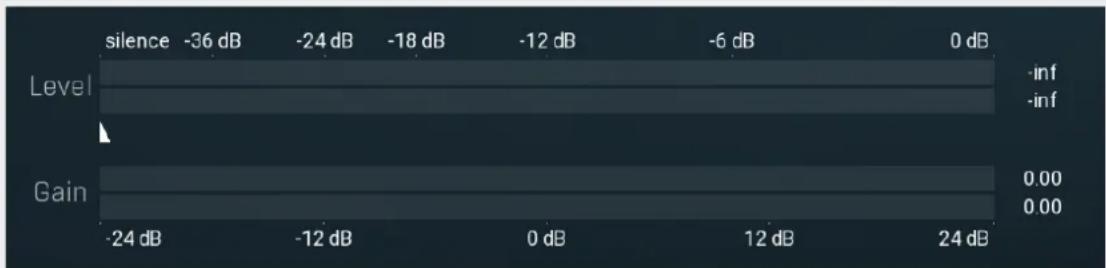
bar
| Level | -36 dB | -24 dB | -18 dB | -12 dB | -6 dB | 0 dB | |---|---|---|---|---|---|---| | Gain | -24 dB | -12 dB | 0 dB | 12 dB | 24 dB | 0.00 | | Level | -inf | -inf | -inf | -inf | -inf | -inf |Threshold
Threshold controls minimum level at which the dynamic gain actually starts working.
Harmonics panel
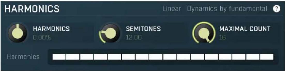
Harmonics panel contains parameters of the harmonics - clones of the main band created at higher frequencies derived from the frequency of the main band. This is often useful for removing natural noises, which usually bring some harmonics with them etc.
Linear
Linear
Linear button enables the linear harmonics spacing. When the main band frequency is say 100Hz and the Semitones value is 12, then in the default logarithmic mode the harmonics are 200Hz, 400Hz, 800Hz etc., increasing by 12 semitones (1 octave) each time. This is suitable because the filters themselves are logarithmic. However harmonics generated by physical instruments are not spaced in this way. Rather, for a Semitones value of 12, they increase by a multiple of 12/12 of the main frequency each time. For example, for a base frequency of 100Hz, they will be at 200Hz, 300Hz, 400Hz, 500Hz etc. In linear mode the harmonics work in this way, but please note that then there is only a limited set of harmonics and Q is modified to approximate a reasonable behaviour, which is not always possible.
Dynamics by fundamental
Dynamics by fundamental
Dynamics by fundamental switch causes each harmonic to be driven by the same detector settings as set for the main band. It is disabled by default, which means that each harmonic is literally a clone of the original filter and has its own dynamics detector depending on its own frequency. Please note that if you want each harmonic to behave in exactly the same way as the main band, you also need to switch on the Input (at the top of the Dynamics panel), otherwise the harmonics would be measuring the signal processed by the main band.
HARMONICS
0.00%
Harmonics
Harmonics defines the gain of the created harmonics. With maximum value (+/- 100%), all harmonics will have the same gain as the main band. A lower value makes the higher harmonics have lower gain. A negative depth will make alternate harmonics have positive and negative gains and is particularly useful for creative effects.

SEMITONES
12.00
Semitones
Semitones defines the frequency interval of the harmonics. For example, if the band is at 100Hz and the number of semitones is 12 (default), then the first harmonic will be at 200Hz (12 semitones higher), second at 400Hz etc., increasing by 12 semitones (1 octave) each time. Thus they are logarithmically-spaced harmonics. When linearly-spaced harmonics are enabled, this merely changes the ratio between them. In this mode, 100Hz is followed by 200Hz, 300Hz, 400Hz, 500Hz etc, that is, increasing by a multiple of 12/12 of the main frequency each time.
For a value of 7 (a perfect fifth), the logarithmic harmonics would be at 150Hz, 225Hz, 337.5Hz, 506.25Hz etc, increasing by 7 semitones (= 50%, as 1.05946 ^ 7 = 1.498) each time and the linear harmonics would be at 158Hz, 251Hz, 397Hz, 628Hz etc, increasing by 7/12 each time.

MAXIMAL COUNT
16
Maximal count
Maximal count defines the maximum number of harmonics that could be created. The harmonics that are created depends on them being activated in the Harmonics grid.
Harmonics grid

Harmonics grid is useful to turn on/off particular harmonics manually. Click any one to enable / disable it.
Band advanced settings
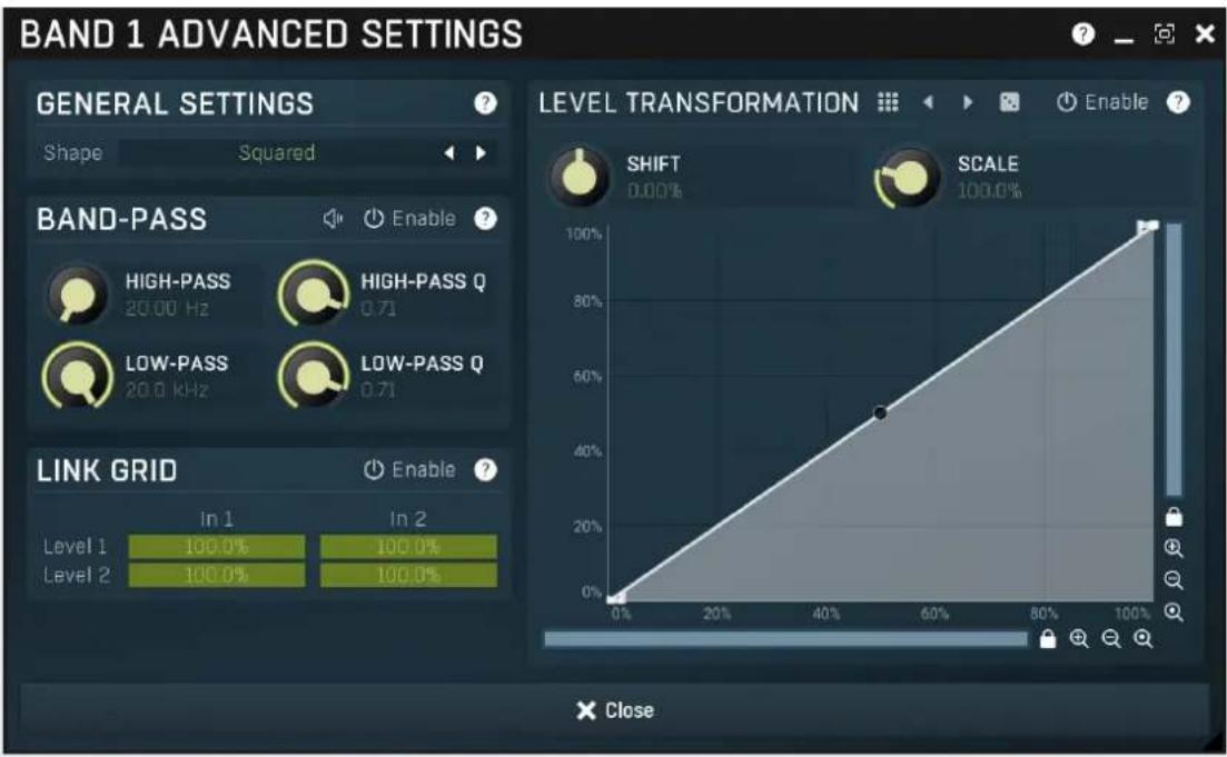
Band advanced settings contains additional settings for the band. These contain some more esoteric features, such as a dynamic transformation shape. It can be displayed by clicking the right mouse button on a band while holding Ctrl, from the basic band settings window, or from the band list if provided.
General settings panel
GENERAL SETTINGS
Shape
Squared

General settings panel contains additional parameters, which are too scientific to be available from the main band settings.
Shape Squared Shape
Shape affects the processing shape. The plug-in features specific non-linear transfer shapes which affect the way the level are interpreted. Logarithmic mode is the most physical one, increase from, say, -90dB to -80dB and from -10dB to 0dB produces the same difference in the output dynamic gain. However from the nature of it is tends to generate high gains and usually setting a threshold is needed. Linear mode on the other hand tends to stay near minimum gains and usually is the most aggressive. Squared mode is a compromise between these two. Comparing the three modes, Linear mode requires the least amount of CPU power and Logarithmic requires the most.
Band-pass panel
BAND-PASS

HIGH-PASS
20.00 Hz

Enable


HIGH-PASS Q
0.71

LOW-PASS
20.0 kHz

LOW-PASS Q
0.71
Band-pass panel contains parameters of the band pass, which you can use to process the signal that is used measure level of the band additionally. For example, you may want a band at high frequencies to react to bass content; you can do this by placing the band anywhere on the high frequencies and set the low-pass at say 200Hz.

Play
Play button enables the band-pass monitoring and hence could be useful to tweak the band pass.

Enable
Enable
Enable button enables the band-pass module. It is off by default to save CPU resources.
Level transformation
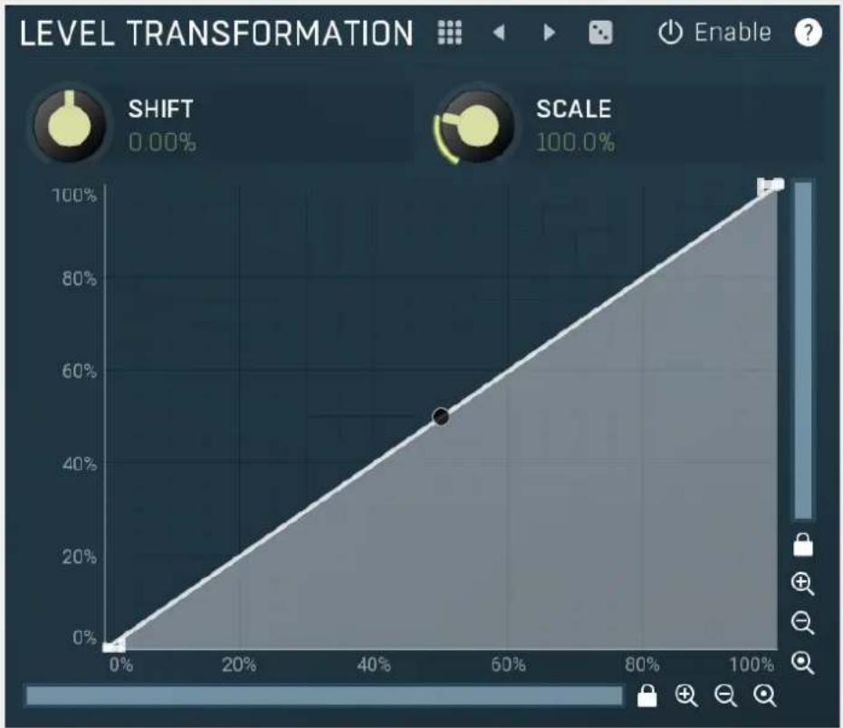
line
| Level | Transformation | |-------|-----------------| | 0% | 0% | | 50% | 50% | | 100% | 100% |Level transformation graph lets you transform the dynamic gain according to the input level. The X axis contains the input level; the Y axis controls the output level, which is then used to set the dynamic gain.

Presets
Presets button displays a window where you can load and manage available presets. Hold Ctrl when clicking to load a random preset instead.

Left arrow
Left arrow button loads the previous preset.

Right arrow
Right arrow button loads the next preset.

Randomize
Randomize button loads a random preset.

Enable
Enable
Enable button enables the level transformation module. It is off by default to save CPU resources.
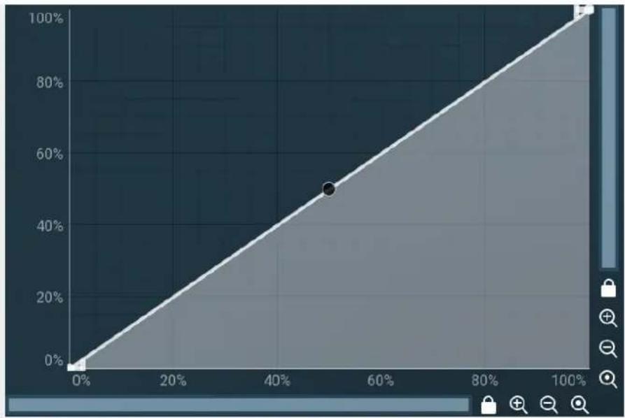
line
| X | Y | | ---- | --- | | 0% | 0% | | 50% | 50% |EnvelopeEditorGraph
Envelope graph
Envelope graph provides an extremely advanced way to edit any kind of shape that you can imagine. An envelope has a potentially unlimited number of points, connected by several types of curves with adjustable curvature (drag the dot in the middle of each arc) and the surroundings of each point can also be automatically smoothed using the smoothness (horizontal pull rod) control. You can also literally draw the shape in drawing mode (available via the main context menu).
- Left mouse button can be used to select points. If there is a point, you can move it (or the entire selection) by dragging it. If there is a curvature circle, you can set up its tension by dragging it. If there is a line, you can drag both edge points of it. If there is a smoothing controller, you can drag its size. Hold Shift to drag more precisely. Hold Ctrl to create a new point and to remove any points above or below.
- Left mouse button double click can be used to create a new point. If there is a point, it will be removed instead. If there is a curvature circle, zero tension will be set. If there is a smoothing controller, zero size will be set.
- Right mouse button shows a context menu relevant to the object under the cursor or to the entire selection. Hold Ctrl to create or remove any points above or below.
- Middle mouse button drag creates a new point and removes any points above or below. It is the same as holding Ctrl and dragging using left mouse button.
- Mouse wheel over a point modifies its smoothing controller. If no point is selected, then all points are modified.
- Ctrl+A selects all points. Delete deletes all selected points.
SHIFT
0.00%
Shift
Shift lets you virtually shift the whole graph vertically. This basically shifts the dynamic gain.

SCALE
100.0%
Scale
Scale lets you virtually scale the whole graph vertically. This basically scales the dynamic gain.
Link grid panel
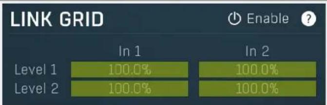
Link grid panel controls the linking between the channels; that is, how the input level in each channel affects the levels in the other channels. By default the way channels affect processing in other channels depends solely on the Link channels parameter.
Here you can set up a more complicated relationship. For example, you can make the left channel (1) respond to the right channel (2) only and vice versa. Each column in the grid is an input and each row is an output. Each output level is a mix of the factored input levels. For that example above, the values for "Level 1" would be 0% and 100%, and for "Level 2" they would be 100% and 0%.
Equalizer panel
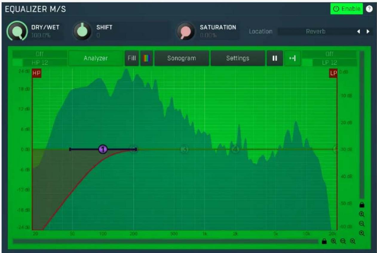
line
| Frequency | Power (dB) | | --------- | ---------- | | 20 | -24.0 | | 50 | -12.0 | | 100 | -6.0 | | 200 | 0.0 | | 500 | 6.0 | | 1k | 12.0 | | 2k | 18.0 | | 5k | 24.0 | | 10k | 20.0 | | 20k | 10.0 |Equalizer panel contains the integrated dynamic equalizer you can use to pre-process the input or post-process the output. There are 2 independent equalizers, one processing the standard input channels (depending on the channel configuration, typically left and right, etc.), the other one is processing the mid/side channels, which are transformed from the left and right channels.

DRY/WET
100.0%
Dry/Wet
Dry/Wet defines ratio between dry and wet signals. 100% means fully processed, 0% means no processing at all. In normal mode only peak and shelf filters are affected correctly, other filters are left at 100% unless the ratio is set to 0%, in which case the equalizer is bypassed.
Range: 0.00% to 100.0%, default 100.0%

SHIFT
0
Shift
Shift lets you pitch shift all bands by specified number of semitones. It doesn't change the actual band points, but changes the resulting EQ shape appropriately.
Range: -24.00 to +24.00, default 0

SATURATION
0.00%
Soft saturation
Soft saturation defines amount of saturation simulating analog equalizers.
Range: 0.00% to 100.0%, default 0.00%
Location
Reverb

Location
Location controls exactly where in the signal processing chain the EQ will be performed. In most cases the differences will probably be
subtle, but bigger differences may occur with more complex settings featuring dynamics processing for example. By default the processing chain is like this:
Input -> Dynamics (if Pre) -> Early & Late Reflections -> Dynamics (if not Pre) -> Widening etc. -> Dry/Wet -> Output
Input mode performs the EQ on the input signal. Hence everything in the reverb is then affected, including dynamics. For example, if you want to trigger the reverb by a bass drum, you would use the Dynamics tab as a gate and filter everything above say 100Hz. But if you locate the EQ in front of the dynamics and set it to filter out everything below say 200Hz, which is a common practice, there would be almost no signal left to trigger the reverb.
Input after dynamics mode performs the EQ on the input signal after the dynamics (if located at that stage). Therefore the input dynamic processing would not be affected by the EQ. In the example with the bass drum the reverb input would have filtered frequencies below 200Hz, but the gate would still follow the bass drum.
Reverb mode performs the EQ on the reverberation signal, on the mixed early and late reflections. In most cases the results will actually be the same as the previous mode. The output may be slightly different if you use some kind of nonlinear processing or modulation in the reverb engine.
Reverb after dynamics mode performs the EQ on the reverberation signal after the dynamics (if located at that stage) has processed the reverberation signal, which is the case only if the Pre is disabled.
Output mode performs the EQ on the final output signal; in particular, after the global Dry/Wet. This means that the dry signal allowed to pass through the reverb would be equalized too.
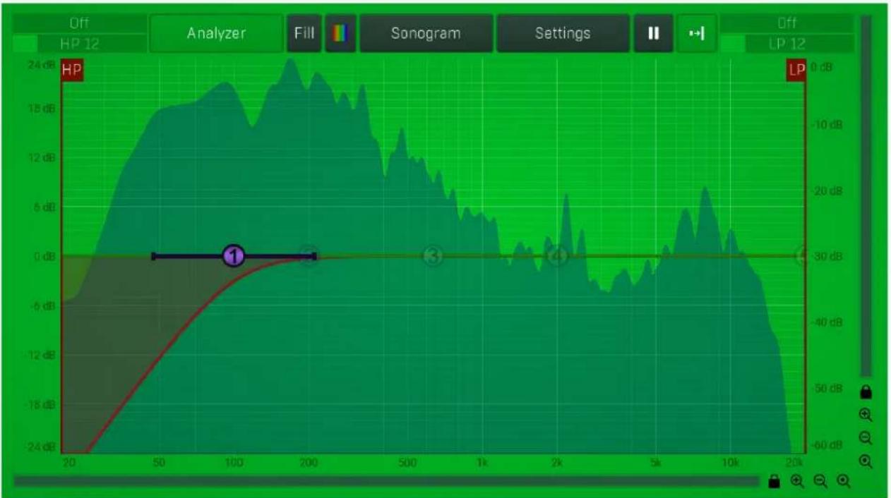
line
| Frequency (Hz) | Power (dB) | | -------------- | ---------- | | 20 | -24 | | 50 | -12 | | 100 | 0 | | 200 | 30 | | 500 | 0 | | 1k | -12 | | 2k | -40 | | 5k | -60 | | 10k | -60 | | 20k | -60 |Equalizer shape graph
Equalizer shape graph controls and displays the frequency response. There are several bands available, each of them can be enabled/disabled, can be set to a different filter, can have different frequency, Q and other parameters.
Double-click on a band point to enable or disable a band. Drag it to change its frequency and gain. Drag the horizontal nodes to change its Q. Hold ctrl key for fine tuning. Click using the right mouse button on it to open a window with additional settings.
Analyzer
Analyzer
Analyzer button enables or disables the spectrum analyzer, which shows the levels of individual frequencies. In most practical cases it is more convenient to use the sonogram, which shows the frequencies in time, but provides a lower level resolution as the levels are differentiated by color. The spectrum analyzer also provides a micro-sonogram (shown in the bottom of the panel) which uses the same color-based view as the sonogram.
Fill
Fill
Fill button enables or disables the full-sized analyzer micro-sonogram. This means that the micro-sonogram at the bottom of the equalizer graph will fill the whole analyzer view. Color differentiation is often easier to understand than the classical spectrum analyzer, so this might help you better understand the spectrum of your audio material.
An alternative is to use the spectrum sonogram.

Analyzer Rainbow Colors
Analyzer Rainbow Colors lets you see the analyzed sound spectrum in beautiful colors, following the same style as visible light. It ranges
from infra-red colors for the lowest frequencies to ultra-violet colors for the highest frequencies in the analyzed audio. If rainbow colors are disabled, the analyzer and graph will be single-colored, following the setup from Settings/Graphs.
Sonogram
Sonogram
Sonogram button enables or disables the spectrum sonogram, which shows levels of individual frequencies in time. Levels are differentiated by color, so the accuracy is not as good as when using the spectrum analyzer. However, the time axis improves the visual orientation in the spectrum for typical audio signals. In contrast, the spectrum analyzer is more of a scientific tool.
Settings
Settings
Settings button shows the settings of the spectrum analyzer and the spectrum sonogram.
||
Pause
Pause button stops the analyzer temporarily.
|→|
Normalize
Normalize button enables or disables the visual normalization, which makes the loudest frequency be displayed at the top of the analyser area (0dB); it does not normalise the sound. This is very useful for comparing frequency levels, however it does hide the actual level.
When comparing 2 spectrums you are usually interested mainly in the frequency level differences. In most cases both audio materials will have different overall levels, which would mean that one of the graphs would be "lower" than the other, making the comparison quite difficult. Normalize fixes this and makes the most prominent frequencies of the spectrum reach the top of the analyzer area (or have the most highlighted color in case of sonogram).
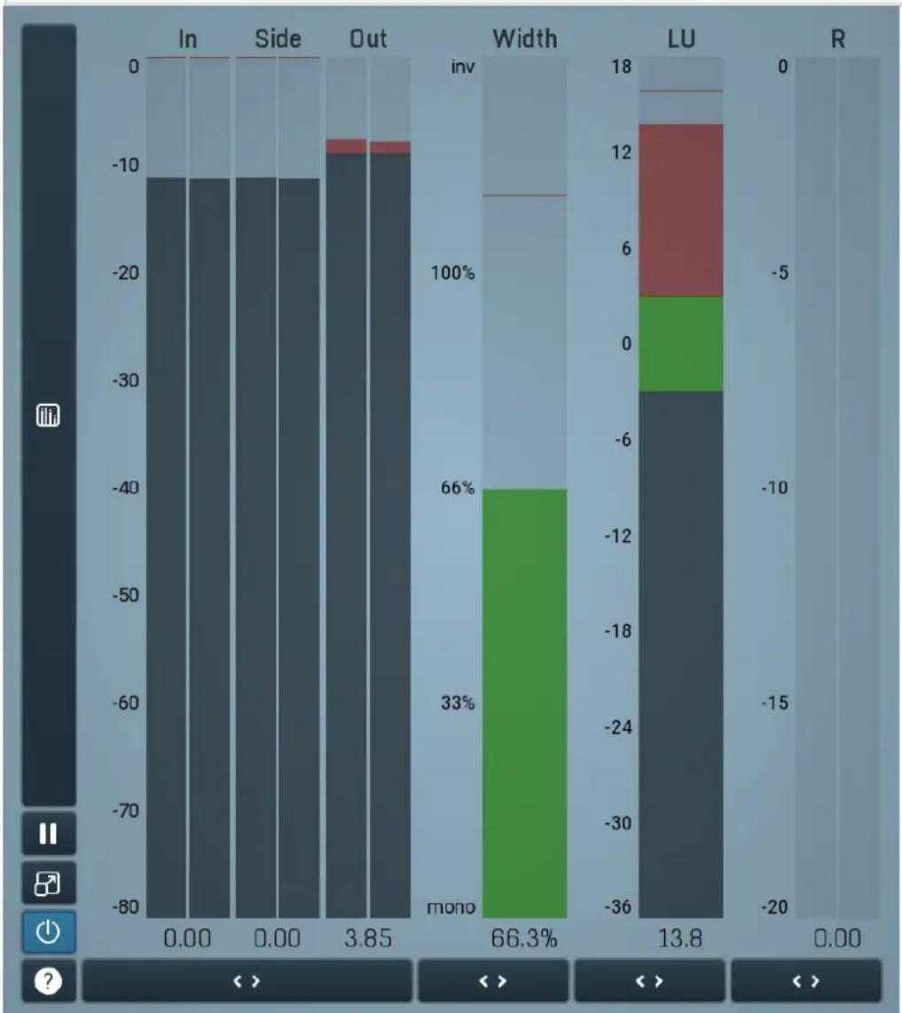
bar_stacked
| Category | In (%) | Side (%) | Out (%) | | :--- | :--- | :--- | :--- | | In | -12 | -12 | -12 | | Side | -12 | -12 | -12 | | Out | -12 | -4 | -9 | | Width | 0 | 0 | 100 | | LU | 0 | 0 | 18 | | R | 0 | 0 | 0 |Global meter view
Global meter view provides a powerful metering system. If you do not see it in the plug-in, click the Meters or Meters & Utilities button to the right of the main controls. The display can work as either a classical level indicator or, in time graph mode, show one or more values in time. Use the first button to the left of the display to switch between the 2 modes and to control additional settings, including pause, disable
and pop up the display into a floating window. The meter always shows the actual channels being processed, thus in M/S mode, it shows mid and side channels.
In the classical level indicators mode each of the meters also shows the recent maximum value. Click on any one of these values boxes to reset them all.
In meter indicates the total input level. The input meter shows the audio level before any specific processing (except potential oversampling and other pre-processing). It is always recommended to keep the input level under 0dB. You may need to adjust the previous processing plugins, track levels or gain stages to ensure that it is achieved.
As the levels approach 0dB, that part of the meters is displayed with red bars. And recent peak levels are indicated by single bars.
Out meter indicates the total output level. The output meter is the last item in the processing chain (except potential downsampling and other post-processing). It is always recommended to keep the output under 0dB.
As the levels approach 0dB, that part of the meters is displayed with red bars. And recent peak levels are indicated by single bars.
R meter shows gain reduction for each channel. Negative values, running down from the top, mean that compression or limiting is occurring. The lower the value, the stronger the effect. For maximum transparency you should try to achieve the least amount of gain reduction. Expansion is not indicated in this meter.
Width meter shows the stereo width at the output stage. This meter requires at least 2 channels and therefore does not work in mono mode. Stereo width meter basically shows the difference between the mid and side channels.
When the value is 0%, the output is monophonic. From 0% to 66% there is a green range, where most audio materials should remain.
From 66% to 100% the audio is very stereophonic and the phase coherence may start causing problems. This range is colored blue. You may still want to use this range for wide materials, such as background pads. It is pretty common for mastered tracks to lie on the edge of green and blue zones.
Above 100% the side signal exceeds the mid signal, therefore it is too monophonic or the signal is out of phase. This is marked using red color. In this case you should consider rotating the phase of the left or right channels or lowering the side signal, otherwise the audio will be highly mono-incompatible and can cause fatigue even when played back in stereo.
For most audio sources the width is fluctuating quickly, so the meter shows a 400ms average. It also shows the temporary maximum above it as a single coloured bar.
If you right click on the meter, you can enable/disable loudness pre-filtering, which uses EBU standard filters to simulate human perception. This may be useful to get a more realistic idea about stereo width. However, since humans perceive the bass spectrum as lower than the treble, this may hide phase problems in that bass spectrum.
LU meter shows the output loudness in EBU-18 scale. The loudness metering follows the ITU-R BS.1770-3 and EBU 3341 specifications.
The metering units used are LU (Loudness Units) with 0 LU defined as -23 LUFS (LU Full Scale) and you should consider the LU values to be relative - using them to compare the loudness values between different signals. If the difference in loudness between 2 signals is 10 LU, it is approximately 10 dB as well.
Please note that you should still use your ears to judge loudness properly as there is still no accurate model of human loudness perception and every measurement is only an approximation. Loudness perception is also individual.
If you right click on the meter, additional settings will be displayed. Maximum value displays the maximum since the analysis started, rather than the recent maximum. Loudness pre-filtering uses EBU standard filters to simulate human perception. However, you may want to disable this to get more technical measurements.
There are 3 types of loudness measurements, all following the EBU specifications.
Momentary loudness uses an RMS sliding analysis window of 400 milliseconds; therefore it shows quick fluctuations in loudness.
Short-term loudness works in the same way, but uses a window of 3 seconds, therefore it provides more stable loudness measurements. Integrated loudness shows the overall loudness, hence it is affected by the whole track from the beginning of the playback until you reset it by clicking on the value field. The host may reset it too; it depends on your host.
Please note that the Integrated loudness is NOT the same as an averaged loudness, as it ignores quiet passages. Imagine a track which is generally quiet but has a few loud sections. The averaged loudness will be less than the Integrated loudness. Its calculation uses gating to ignore those quiet passages (levels less than 10 LU less than the current ungated level) of the track. Essentially, Integrated loudness is a measure of the loudest sections of the track.

Time graph
Time graph button switches between the metering view and the time-graphs. The metering view provides an immediate view of the current values including a text representation. The time-graphs provide the same information over a period of time. Since different time-graphs often need different units, only the most important units are provided.

Pause
Pause button pauses the processing.

Popup
Popup button shows a pop-up window and moves the whole metering / time-graph system into it. This is especially useful in cases where you cannot enlarge the meters within the main window or such a task is too complicated. The pop-up window can be arbitrarily resized. In metering mode it is useful for easier reading from a distance for example. In time-graph mode it is useful for getting higher accuracy and a longer time perspective.

Enable
Enable button enables or disables the metering system. You can disable it to save system resources.

Collapse
Collapse button minimizes or enlarges the panel to release space for other editors.

Collapse
Collapse button minimizes or enlarges the panel to release space for other editors.

Collapse
Collapse button minimizes or enlarges the panel to release space for other editors.

Collapse
Collapse button minimizes or enlarges the panel to release space for other editors.
Utilities
Modulator button displays settings of the modulator. It also contains a checkbox, to the left, which you can use to enable or disable the modulator. Click on it using your right mouse button or use the menu button to display an additional menu with learning capabilities - as described below.

Menu
Menu button shows the smart learn menu. You can also use the right mouse button anywhere on the modulator button.
Learn activates the learning mode and displays "REC" on the button as a reminder, Clear & Learn deletes all parameters currently associated with the modulator, then activates the learning mode as above. After that every parameter you touch will be associated to the modulator along with the range that the parameter was changed. Learning mode is ended by clicking the button again.
In smart learn mode the modulator does not operate but rather records your actions. You can still adjust every automatable parameter and use it normally. When you change a parameter, the plugin associates that parameter with the modulator and also records the range of values that you set.
For example, to associate a frequency slider and make a modulator control it from 100Hz to 1KHz, just enable the smart learn mode, click the slider then move it from 100Hz to 1KHz (you can also edit the range later in the modulator window too). Then disable the learning mode by clicking on the button.

Menu
Menu button displays additional menu containing features for modulator presets and randomization.

Lock
Lock button displays the settings of the global parameter lock. Click on it using your left mouse button to open the Global Parameter Lock window, listing all those parameters that are currently able to be locked.
Click on it using your right mouse button or use the menu button to display the menu with learning capabilities - Learn activates the learning mode, Clear & Learn deletes all currently-lockable parameters and then activates the learning mode. After that, every parameter you touch will be added to the lock. Learning mode is ended by clicking the button again.
The On/Off button built into the Lock button enables or disables the active locks.

Collapse
Collapse button minimizes or enlarges the panel to release space for other editors.

Multiparameter
Multiparameter button displays settings of the multiparameter. The multiparameter value can be adjusted by dragging it or by pressing Shift and clicking it to enter a new value from the virtual keyboard or from your computer keyboard.
Click on the button using your left mouse button to open the Multiparameter window where all the details of the multiparameter can be set. Click on it using your right mouse button or click on the menu button to the right to display an additional menu with learning
capabilities - as described below.

Menu
Menu button shows the smart learn menu. You can also use the right mouse button anywhere on the multiparameter button.
Learn attaches any parameters, including ranges. Click this, then move any parameters through the ranges that you want and click the multiparameter button again to finish. While learning is active, "REC" is displayed on the multiparameter button and learning mode is ended by clicking the button again.
Clear & Learn clears any parameters currently in the list then attaches any parameters, including ranges. Click this, then move any parameters through the ranges that you want and click the multiparameter button again to finish. While learning is active, "REC" is displayed on the multiparameter button and learning mode is ended by clicking the button again.
Reset resets all multiparameter settings to defaults.
Quick Learn clears any parameters currently in the list, attaches one parameter, including its range and assigns its name to the multiparameter. Click this, then move one parameter through the range that you want.
Attach MIDI Controller opens the MIDI Settings window, selects a unused parameter and activates MIDI learn. Click this then move the MIDI controller that you want to assign.
Reorder to ... lets you change the order of the multiparameters. This can be useful when creating active-presets. Please note that this feature can cause problems when one multiparameter controls other multiparameters, as these associations will not be preserved and they will need to be rebuilt.
In learning mode the multiparameter does not operate but rather records your actions. You can still adjust every automatable parameter and use it normally. When you change a parameter, the plugin associates that parameter with the multiparameter and also records the range of values that you set.
For example, to associate a frequency slider and make a multiparameter control it from 100Hz to 1KHz, just enable the smart learn mode, click the slider then move it from 100Hz to 1KHz (you can also edit the range later in the Multiparameter window too). Then disable the learning mode by clicking on the button.
< >
Collapse
Collapse button minimizes or enlarges the panel to release space for other editors.
Preset selector
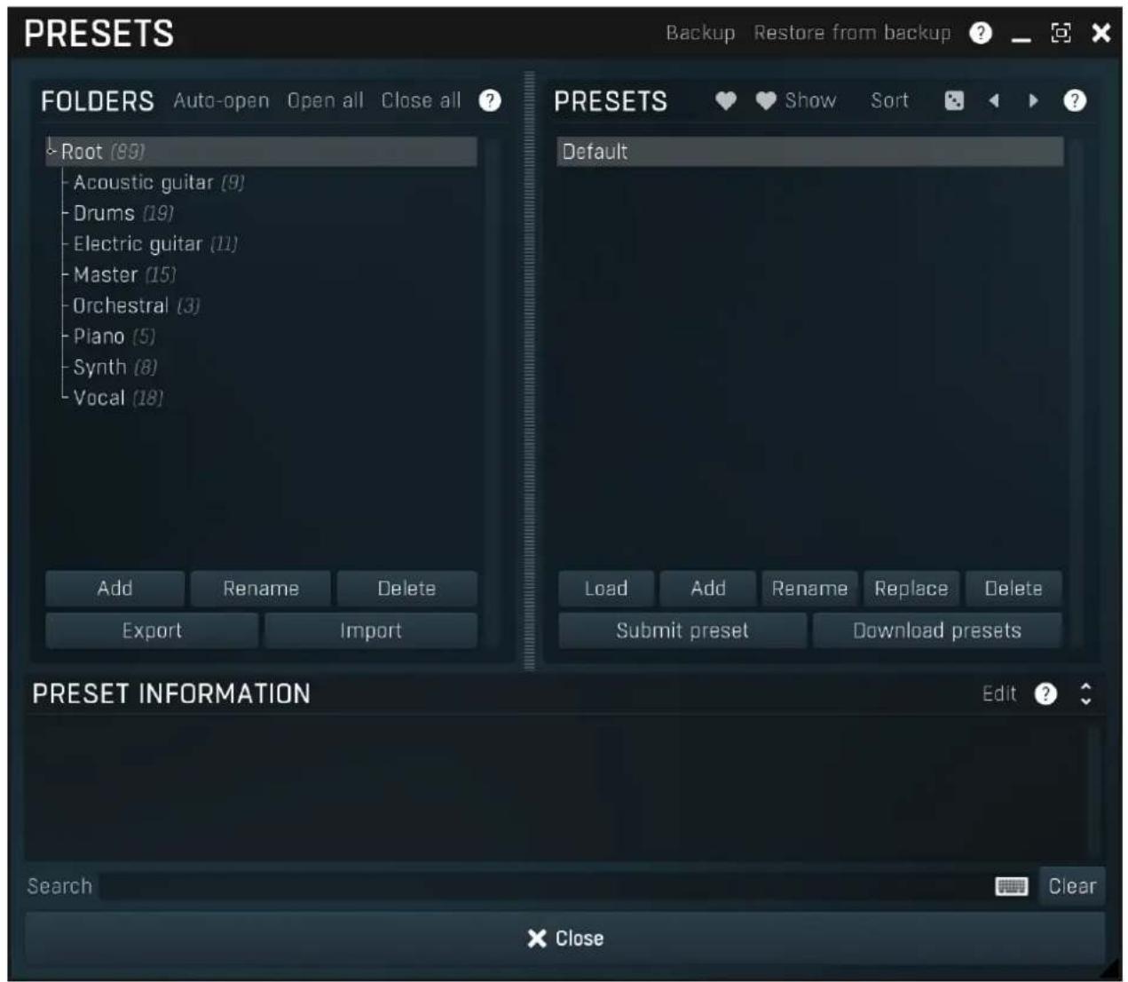
Preset management window provides management for your presets.
Backup
Backup
Backup button lets you backup presets for all MeldaProduction software into a single file, so you can transfer it to a different machine and restore the presets there for example.
Restore from backup
Restore from backup
Restore from backup button lets you restore presets for all MeldaProduction software from a single file created by the Backup button.
Folders tree
![FOLDERS Auto-open Open all Close all ? Root [89] Acoustic guitar [9] Drums [19] Electric guitar [11] Master [15] Orchestral [3] Piano [5] Synth [8] Vocal [18] Add Rename Delete Export Import](/content/2026/05/983866/images/a67aa9e9327f6b200c84fe22983b7795f7089124c1f0f76afbef9b07a759bdc1.jpg)
Folders tree lets you organize your presets into any number of folders. Use the buttons at the bottom of the window to create, rename or delete sub-folders. Note that these are not actual files & folders on disk, but are records in the preset database.
Auto-open
Auto-open
Auto-open switch makes the tree automatically open selected items, so that all sub-folders are visible, whenever you select one. This makes it easier to browse through large structures containing many folders. The switch also makes the browser show all presets available in the selected folder including all sub-folders (except when you select the root folder).
Open all
Open all
Open all button expands the whole tree, so you can see all of the folders. This may be handy when editing large preset structures.
Close all
Close all
Close all button collapses the whole tree except for the root folder. This may be handy when editing large preset structures.
Add
Add
Add button creates a new folder in the tree
Rename
Rename
Rename button lets you rename the selected folder.
Delete
Delete
Delete button deletes the folder including all the presets and subfolders in it.
Export
Export
Export button lets you export the selected folder including all presets and sub-folders into a file, which you can then transfer to any computer. Or just use as a back-up.
Import
Import
Import button lets you import a file containing presets and sub-folders and add it to the selected folder. The importer will ask you whether to destroy the original contents, so that the new presets replace previous ones, or to keep both.
Presets list
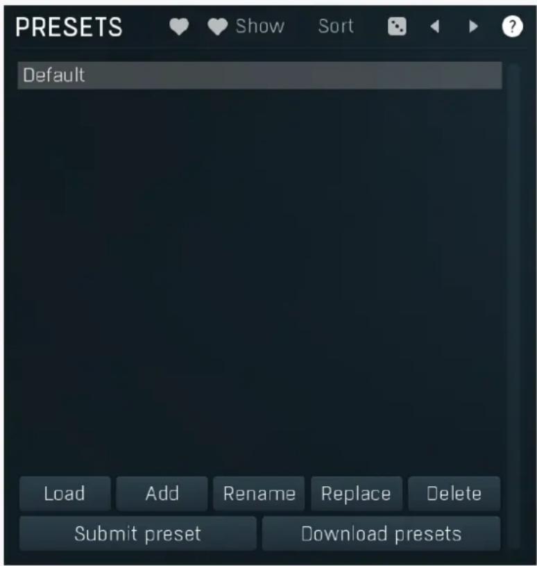
Presets list contains all presets available in the selected folder. Double-click on a preset or use Load button to load a preset. Use the buttons at the bottom of the list to perform additional changes. Please note that these are not actual files & folders on disk, but are records in the preset database.

Favourite
Favourite button toggles the 'favourite' indicator for the selected preset.

Show
Show
Show button shows only the favourite presets and hides the others.

Sort
Sort button shows the presets sorted alphabetically.

Random
Random button selects and loads a random preset from the current folder. This way you can quickly browse the presets in the folder in a completely random order.

Previous
Previous button selects and loads the previous preset from the current folder.

Next
Next button selects and loads the next preset from the current folder.
Submit preset
Submit preset
Submit preset button submits the selected preset to the online exchange servers and retrieves all the presets currently in the database. This feature serves as an online database of presets available for all the user community. Please do not submit garbage presets.
Download presets
Download presets
Download presets button retrieves all the presets currently in the database. This feature serves as an online database of presets available for all the user community. Please consider participating by submitting your presets as well.
Load
Load
Load button loads the specified preset. Please note that you can do the same thing by double-clicking the preset itself or pressing the Enter key.
Add
Add
Add button creates a new preset using the current settings.
Rename
Rename
Rename button lets you rename the selected preset.
Replace
Replace
Replace button replaces the selected preset by one with current settings.
Delete
Delete
Delete button deletes the selected preset.
Search

Search
Search filters the list of available presets to those containing the keywords in name or information.
Clear
Clear
Clear button deletes all text in the search field.

information
Preset information field contains optional information about the preset, which you can edit when creating or renaming the preset.
Plugin settings
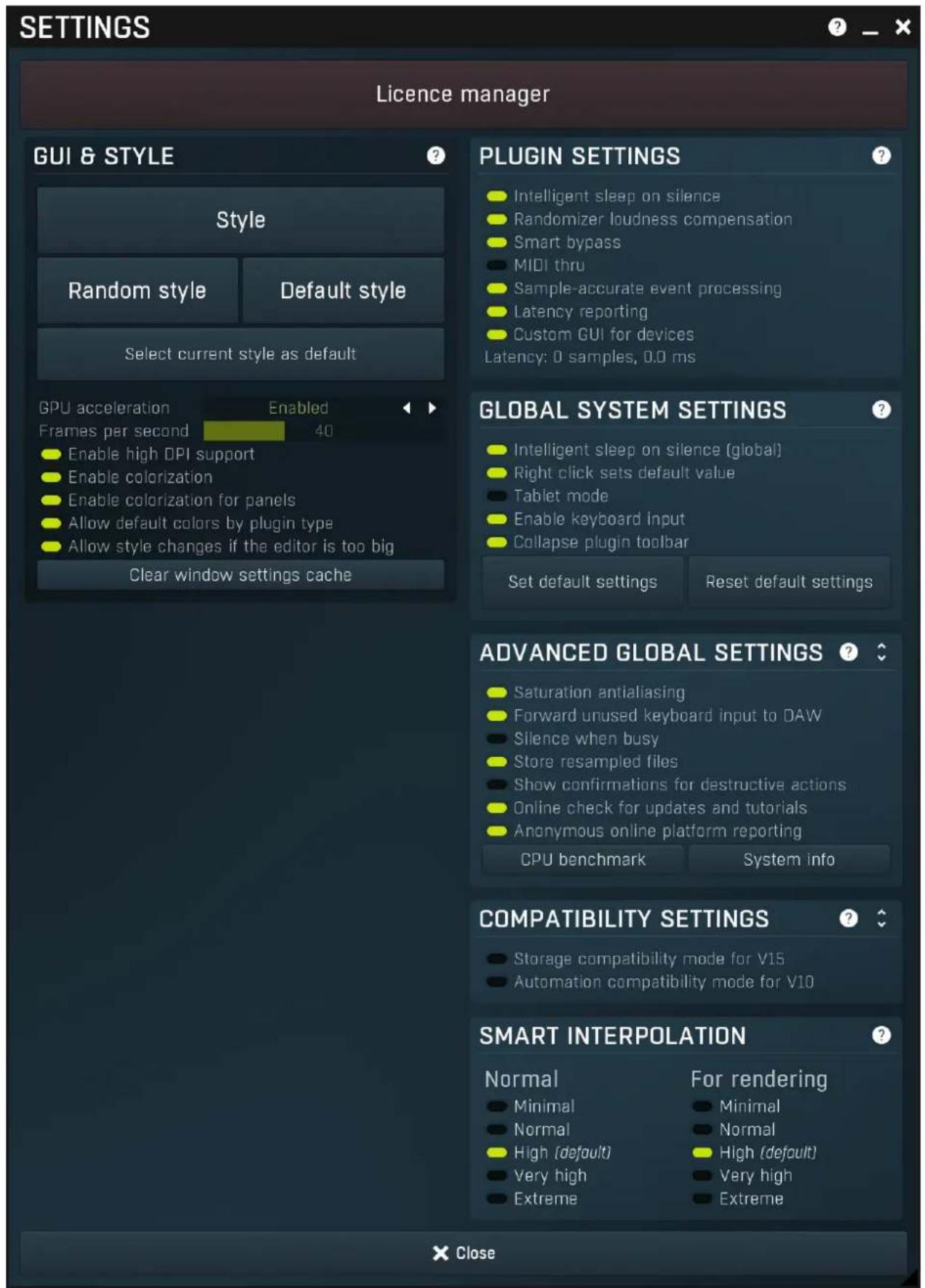
Plugin settings window offers more advanced settings and is available via the Settings button.
Licence panel
Licence manager
Licence panel lets you manage licences on this computer.
Licence manager
Activate
Activate button lets you activate your licence for the plugin on this computer.
GUI & Style panel
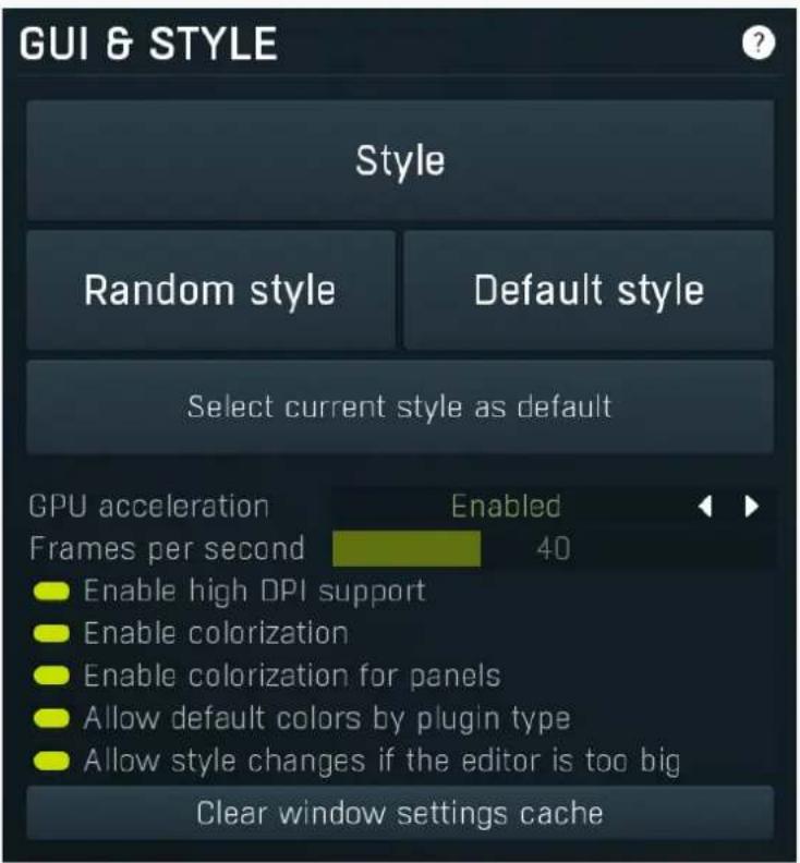
GUI & Style panel lets you configure the plugin's style (and potentially styles of other plugins) and other GUI properties.
Style
Style
Style button lets you change the style for this particular plugin.
Random style
Random style
Random style button selects a random style with random editor mode.
Default style
Default style
Default style button reverts to the default style and default size of the GUI. Hold the Ctrl key while clicking to revert all MeldaProduction
software products, not just the current plugin.
Select current style as default
Select current style as default
Select current style as default button stores the current style as the default for all MeldaProduction software. This is used for the other plugins that are currently using the default style; that is, those plugins for which you have NOT selected a specific style. Please note that if you have already selected a specific style for a particular plugin, then it won't be changed until you use the Default style button.
GPU acceleration
Enabled

GPU acceleration
GPU acceleration controls how much the GPU is used for visual rendering to save CPU power.
Enabled mode provides maximum speed and lets the GPU perform as many drawing operations as possible.
Compatibility mode uses the GPU for drawing, but doesn't use modern technologies for maximum performance. Use it if you experience occasional problems with drawing, the usual case for older ATI graphics cards. With Pro Tools on OSX this mode is always used instead of Enabled mode due to compatibility problems with this host.
Disabled mode disables GPU acceleration completely, drawing is then performed by the CPU. Use only if you experience technical difficulties.
A known problem may occur when using multiple displays with multiple graphical interfaces. When moving the plugin window from one display to another, it may stop displaying correctly until you move it back to the original display.
Frames per second
40
Frames per second
Frames per second controls the refresh rate of the visual engine. The higher the number is the smoother everything is, but the more CPU it requires. You might want to lower this value if your computer is running out of CPU power.
Enable high DPI support
Enable high DPI / retina support
Enable high DPI / retina support enables the plugin to use the high resolution on high DPI (Windows) and retina (OSX) devices. It is enabled by default and detected automatically, if the host allows it. If you run into any problems, you can disable it using this option. It may be desired if you use multiple displays where only some of them feature the high resolution making the image on the low resolution ones look ugly.
If you disable this option, on Windows the high DPI device detection will be ignored and the plugin will probably appear very small. You can manually compensate for it by using a bigger style. On OSX disabling this option will disable the high DPI rendering, resulting in the classic blurry look of non-compliant applications. Changes take effect after you restart the host.
Enable colorization
Enable colorization
Enable colorization enables the plugin to change the colors of certain elements overriding your style settings. Plugins use that to highlight different parts of the graphics interface for easier workflow. You may want to disable it if you just feel it's not for you. This particular option is relevant only for controls - knobs, sliders, checkboxes etc.
Enable colorization for panels
Enable colorization for panels
Enable colorization for panels enables the plugin to change the colors of certain elements overriding your style settings. Plugins use that to highlight different parts of the graphics interface for easier workflow. You may want to disable it if you just feel it's not for you. This particular option is relevant only for containers - panels, graphs etc.
Allow default colors by plugin type
Allow default colors by plugin type
Allow default colors by plugin type is on by default and makes the plugin select its default colors depending on the type of the Plugin. Hence for instance equalizer will always be green. This is done by selecting one of the first 8 color presets for the current style, so the actual colors depend on selected style and its presets. You may want to disable this if you for example want all plugins to look the same including the style and colors. It is necessary to restart your host for a change to this option to take effect.
Allow style changes if the editor is too big
Allow style changes if the editor is too big
Allow style changes if the editor is too big is on by default and makes the plugin change its style, editor mode and other settings if it finds out it is too big to fit the current screen resolution.
Clear window settings cache
Clear window settings cache
Clear window settings cache button deletes stored states of all popup windows on all MeldaProduction software. The window settings mostly contain positions and sizes, but in some cases also the data inside the popup windows. You can use this feature if something goes wrong, a window doesn't appear at all, problems like that. While this shouldn't happen and it's generally better to contract our support, this button provides a potential quick fix.
Plugin settings panel
PLUGIN SETTINGS

- Intelligent sleep on silence
- Randomizer loudness compensation
Smart bypass
MIDI thru
Sample-accurate event processing
Latency reporting
Custom GUI for devices
Latency: 0 samples, 0.0 ms
Plugin settings panel contains settings that control the behaviour of this plugin instance. These are properties that rarely need to be changed, so they have been moved here.
- Intelligent sleep on silence
Intelligent sleep on silence
Intelligent sleep on silence option provides a huge CPU saver by automatically disabling the plugin processing if the input is silent and if the plugin doesn't generate some signal on its own. This makes the plugins take virtually no CPU if there is no need for them to actually process anything. Disable this if you run into any problems with them.
Randomizer loudness compensation
Randomizer loudness compensation
Randomizer loudness compensation enables the automatic detection of loudness after new settings have been generated using the main Random button and using the output gain of the plugin to get some predefined level. This is useful in most cases since normally randomized settings can produce various output levels, so this can mitigate the problem.
Smart bypass
Smart bypass
Smart bypass enables the high quality crossfading bypass system, which ensures a smooth transition between the processed and dry signals. You may want to disable it if you are using settings with latency on a plugin, which demands lots of CPU power, which would otherwise need to perform processing even when bypassed, which is pretty much the only downside of the smart bypassing algorithm.
MIDI thru
MIDI thru
MIDI thru makes the plugin pass all input MIDI through to its MIDI output. That is often advantageous in DAWs such as Reaper, which naturally pass MIDI from one plugin to the next.
Sample-accurate event processing
Sample-accurate event processing
Sample-accurate event processing makes the plugin schedule every event such as MIDI or automation to their accurate locations with sample accuracy, if the host allows it.
For example, if the block size in your host's audio settings is 1024 samples, this means the plugin is probably processing blocks of 1024 samples, in 44100 Hz sampling rate it is about 23ms. If this setting is disabled, any change in automation, MIDI, modulation etc. may then be granularized to 23ms (once per block), which means that you will not be able to recognize events that occur say 10ms apart from each other. When this setting is enabled however, the plugin divides processing blocks to sub-blocks and processes the events at their correct positions. This may, of course, require more CPU power.
Latency reporting
Latency reporting
Latency reporting makes the plugin report latency to the DAW, if any. Normally this is enabled, but in certain live situations you may want to disable this, so that the DAW stops compensating the latency on other tracks. It has no effect if the plugin is placed on master track.
Custom GUI for devices
Custom GUI for devices
Custom GUI for devices enables displaying custom GUIs for the easy screen devices. You can disable it if you like the generic GUI better.
Global system settings panel
GLOBAL SYSTEM SETTINGS

- Intelligent sleep on silence (global)
Right click sets default value
Tablet mode
Enable keyboard input
Collapse plugin toolbar
Set default settings
Reset default settings
Global system settings panel contains settings which are applied to all plugins on this computer.
- Intelligent sleep on silence (global)
Intelligent sleep on silence (global)
Intelligent sleep on silence (global) is a global switch, which disables the Auto disable on silence feature in all plugins on the system. It is provided "just in case" something goes wrong.
Right click sets default value
Right click sets default value
Right click sets default value makes the engine set default value to a parameter when you right click on it. By default, a menu is displayed instead, with an option to set the default value, but potentially with more features. When this is disabled, you can still set a default value by holding ctrl/cmd when right clicking the control.
Tablet mode
Tablet mode
Tablet mode enables better support for tablets at the expense of the mouse. Enable this if you are using a tablet to control the plugins and it is behaving incorrectly.
Enable keyboard input
Enable keyboard input
Enable keyboard input enables the keyboard input for the main plugin window. You may want to disable if the plugin intercepts spacebar key (often used by the host for playback enable/disable and your host doesn't allow for the problem itself.
Collapse plugin toolbar
Collapse plugin toolbar
Collapse plugin toolbar makes all plugins collapse the plugin toolbar containing more advanced features such as channel modes, A-H presets, oversampling, safety limiter etc. It is enabled by default to make the user interfaces cleaner and easier to grasp for beginners.
Set default settings
Set default settings
Set default settings button stores the current plugin settings as the defaults, so that when you open a new instance of the plugin, these settings will be loaded automatically.
Reset default settings
Reset default settings
Reset default settings button removes the defaults that you set using Set default settings button, so that when you open a new instance of the plugin, the factory defaults will be loaded.
Advanced global settings panel
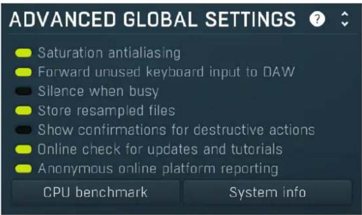
Advanced global settings panel contains advanced settings which are applied to all plugins on this computer.
Saturation antialiasing
Saturation antialiasing
Saturation antialiasing enables a global support for antialiasing in saturation algorithms available in many of the plugins. These require additional CPU processing, however significantly reduce aliasing artifacts without a need for oversampling.
Forward unused keyboard input to DAW
Forward unused keyboard input to DAW
Forward unused keyboard input to DAW makes the plugin forward unused keyboard events to the DAW from its popups. If this is disabled, pressing say spacebar commonly used to start/stop playback won't work if a popup window is active. Enabling this makes this work and it is optional just in case your DAW does something unexpected.
Silence when busy
Silence when busy
Silence when busy makes all plugins silence the output when something time consuming is being performed in background and the plugin needs to wait for it. For instance, in modular plugins such as MXXX, adding a module requires lots of changes in the entire engine, so it is performed in background and while the plugin is inconsistent state, it is temporarily bypassed. Sometimes however, when performing live, bypassing makes the dry signal go through and that may not be wanted. So you can enable this option, and the plugin will silence the output instead.
Store resampled files
Store resampled files
Store resampled files allows the plugins create audio files for sampling rates being used if they differ from the original file sampling rate. It is used only by a few plugins, but it can improve the loading performance a lot at the cost of some additional storage on the hard drive. Disable this option if you are short on free space.
Show confirmations for destructive actions
Show confirmations for destructive actions
Show confirmations for destructive actions makes the plugin display a confirmation window whenever you are going to change the plugin settings irreversibly when using a feature, for example: when resetting your settings.
Online check for updates and tutorials
Online check for updates and tutorials
Online check for updates and tutorials lets the plugin ask about once a week if there is a new version or tutorial available so you can be easily kept up to date.
Anonymous online platform reporting
Anonymous online platform reporting
Anonymous online platform reporting helps us maximize compatibility with your operating system and host. If enabled, our plugins will send information about the system and host that you are using. We can use this information to find out which plugins and platforms are used the most and maximize testing and support there. Platform reporting is completely anonymous and requires only minimal internet connection time (a few kB once a week).
CPU benchmark
CPU benchmark
CPU benchmark button calculates the performance of the plugin with the current settings.
System info
System info
System info button displays some technical information about the build and the machine.
Compatibility settings panel
COMPATIBILITY SETTINGS


Storage compatibility mode for V15
Automation compatibility mode for V10
Compatibility settings panel contains advanced settings you rarely need unless you run into some problems when using multiple versions or old projects.
Storage compatibility mode for V15
Storage compatibility mode for V15
Storage compatibility mode for V15 reverts to the older and much slower storage system used by version 15 and older. Use this if you want to open your projects or presets on older version of MeldaProduction plugins.
Automation compatibility mode for V10
Automation compatibility mode for V10
Automation compatibility mode for V10 reverts the set of automation parameters back to version 10 and earlier. Use this if you need the plugins to work with projects, which contain automation, made using version 10 or older. In version 11 the list of automatable parameters have been highly simplified and reorganized and multiparameters are provided for the vast number of hidden parameters. This should speed up loading, improve workflow with the plugins and improve compatibility with various hosts.
Smart interpolation panel
SMART INTERPOLATION

Normal
Minimal
Normal
High (default)
Very high
Extreme
For rendering
Minimal
Normal
High (default)
Very high
Extreme
Smart interpolation panel controls the depth of the smart interpolation algorithm, which controls the parameters in order to provide maximum audio quality and lower the chance of zipper noise. Smart interpolation is engaged whenever you change any parameter via the GUI, modulators, multiparameters, MIDI or automation.
Many parameters can be automated easily and the plugin responds with sample-accurate results. However, several parameters need exhaustive pre-processing when changed. In these cases, the parameters are not updated every sample, but, for example, once every 32 samples. This highly reduces CPU usage, but affects the output quality.
With modulators the situation is more complicated. Besides the updating issue, the modulator itself can perform some pretty advanced processing, hence it is better to perform the processing in blocks. However, the bigger the block, the less often the modulator updates those parameters associated with it and the resulting modulation is less accurate. In a way you can say that the modulator is slower and lazier. This may actually be wanted, so when it comes to modulators it is not true that a better mode always means better output quality.
The smart interpolation mode controls the maximum number of samples being processed before the parameters are updated. Minimal mode uses 2048 samples and rarely will do anything unless processing offline. Normal mode uses 256 samples and usually is enough to achieve good quality results. High mode uses 32 samples and provides perfect quality for most cases. It is also a good compromise between CPU usage and audio quality, so it is the default. Very high mode uses 4 samples and you will rarely need it. Extreme mode uses 1 sample, which means that everything is updated after every single sample. This provides the highest possible accuracy and quality you can ever achieve, however it requires lots of CPU and it is very unlikely that you will ever need it. If you use this mode and still hear audio artifacts, then either what you are hearing is actually CPU overload, or you are doing something that is not physically possible.
The higher the mode, the quicker the parameter updates, but the more the CPU load.
Please note that modulating certain parameters without artifacts is impossible. For example, when modulating a delay very quickly, the physics of such a process just cannot occur in the natural world and the results are appropriately unnatural. These physically impossible processes usually manifest themselves as distortion or zipper noise.
Modulator editor
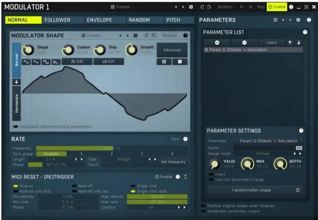
Modulator is an extremely advanced feature, which lets you change parameters automatically depending on various inputs. You can use this to add movement to your sound, respond to some plugins differently for louder sections, or even follow the pitch of the input.
The modulator edit window has two parts: on the left side you can configure the mode of the modulator (the way the modulator works) and on the right side there is a list of parameters to modulate. A modulator can control all automatable parameters (and often more than that) including the parameters of other modulators. Each modulator can control as many parameters as is needed and each of the parameters has its own range and transformation shape. The values and ranges of the first 4 parameters associated with the other modulators can also be modulated/automated. The following modulator modes are available:
Normal mode makes the modulator behave like an ordinary low-frequency oscillator (LFO). There are various ways to control its shape as with all oscillators in our plugins. Each modulator can synchronize to the host in the Synchronization panel. Modulators can also synchronize with each other using the Sync groups. Using MIDI reset you can reset the oscillator to any phase using MIDI notes, but obviously to-host synchronization must be disabled in order for this to work.
Note that the settings in this mode are used even if the modulator is actually in a different mode by using "LFO modulation". This basically blends between the actual mode, which may for example detect the input signal level, and give it some additional movement using the LFO depending on the LFO modulation parameter available for each of the remaining modes.
Follower mode makes the modulator detect the input signal level. It contains an extremely advanced and accurate level detector taken from our MDynamics plugin. The level follower is an immensely useful feature, yet it may be a little difficult for beginners to comprehend, so we will cover it here in more detail.
It is often necessary to adjust the follower slightly for new material. First, it has the standard parameters - attack, release, hold and RMS length. These are fairly standard features and help is available for each of them. Level min and max controls the range of input levels. When the input level is equal to or below the min level, the modulated parameters' values will be minimal. Similarly, when it reaches the max level, the modulated parameters' values will be at their maximum. This allows for adjustments to the range of input levels, which are certainly different for any audio material and settings. It can be used creatively too - for example, by using very low values for both limits we can differentiate between silent and non-silent parts, similar to the way a gate effect works.
Advanced detector settings provide some extraordinary features, such as psycho-acoustic pre-filtering, which forces the modulator to detect loudness instead of raw input levels, custom input signal pre-filtering using a fully featured 6-band equalizer, and custom attack and release shapes. Band-pass panel pre-filters the level detection signal using a band-pass filter, so this is like a very simplified version of the equalizer from the advanced detector settings. Side-chain makes the modulator measure side-chain input if the plugin has one. For modular plugins the modulator can also be driven by a feedback signal. The advanced panel provides some further level processing features that you can take advantage of creatively or to further adjust to your actual audio material.
Project onto LFO shape is a more advanced concept, which is available for other modulator modes too. You can easily imagine, that the
modulator in any mode generates values for each parameter, we can say it is between 0 and 1, where 0 sets minimum parameter value, and 1 sets the maximum. Project onto LFO shape forces the modulator to use this range in the oscillator shape, which can then be configured in normal mode. The value is basically transformed by the oscillator shape, where the values generated by the modulator are on the horizontal axis (phase) and the output is the actual oscillator value. This feature has no physical meaning and can only be used creatively - to transform the more or less linear results of the level follower into a much more complicated curve.
Let us demonstrate the follower mode with an example - the idea is to apply a delay to a snare drum within a previously mixed drumset. This is commonly used on reggae/dub rhythms for example, however in these cases the snare track is usually available separately. Using the modulators you can get somewhat interesting results even with an already mixed drumset. The idea is to increase the input gain whenever the snare is playing, so that only the snare drum (and potentially other instruments playing at the same moment) are passed into the delay. So first teach the modulator to control input gain parameter of the delay and set it to follower mode, potentially configure some of the parameters to get the desired response. Now the louder the input is, the more delay you get. To make it respond only to snare drum, enable the band-pass and set the filter limits accordingly, e.g. 500Hz to 1k. This makes the input gain increased depending on the input level in this part of the spectrum, which contains the snare drum.
Envelope mode causes the modulator to generate an arbitrary envelope, similar to those from synthesizers. It can either follow MIDI - the envelope starts when a key is pressed, goes though the attack and decay stages, then holds in sustain stage until the key is released when the release stage begins, or it can follow audio - when the audio level exceeds Threshold on it behaves the same way as when a note is pressed in MIDI mode, and then when the input level drops below Threshold off it behaves like a key release. As with most modes there is LFO modulation and LFO projection and the input level can be driven by the side-chain or feedback if available. The envelope shape can be adjusted using several controls (lengths of each stage etc.) and you can even draw your own shape.
Random mode is a smooth random generator. It is very handy if you want some parameters to change over time, but do not actually want them to be periodic like LFOs. A modulator in random mode does not actually generate random values, the results will always be the same at each position in your arrangement in the host. This allows a pseudo synchronization with the host and ensures a "what you hear is what you get" performance. Speed parameter controls the speed of change and any slight change to this parameter will change the whole stream.
Pitch detects the pitch of the input signal assuming it is not polyphonic (here it can work too and will probably detect the lowest note, however it is definitely not suitable for percussive signals, which do not have a pitch). It is very useful, enabling you to tune an oscillator to follow your singing, or allow an equalizer to control separate harmonics of a vocal, use a distortion to get more drive for higher notes in a guitar solo and much more. The pitch detection may be a little tricky to understand, so we will discuss it in more detail.
A pitch detector takes the input signal and tries to approximate the pitch of the fundamental frequency in it. It is physically impossible to detect pitch instantly, as an extreme example, 20Hz takes 50ms for the signal to evolve enough to detect that there is actually a 20Hz frequency in the signal. For this and many other reasons any pitch detector employs several limitations. These are available in the Detector panel. The defaults will work well for most audio material, however, it is useful to understand the parameters, so that you can let the detector adapt better to your particular audio materials if necessary, and also in order to be more creative.
Min and max frequency parameters in the Detector panel control the limits of the frequencies you expect in the input. For example, a female voice is unlikely to sing below 100Hz, so it is customary to set the minimum frequency to 100Hz or even higher. Voice signals contain several artifacts, blows and pops, all of which can temporarily create frequencies below the actual pitch of the voice, so setting these limits is preferable to avoid "jumps" to incorrect pitches. Stabilization and Speed also prevent these jumps by restricting how quickly the pitch can change. These can also be used creatively. Threshold controls the minimum level of the input signal to be considered "not-silent and probably having pitch". This acts as a form of gate, which prevents the detector from analyzing irrelevant rumble in between actual performances. Shift panel allows the detected pitch to be shifted up or down and Auto-tune panel moves it to the closest note - similar to the automatic pitch changing function from MAutoPitch, except no pitch shifting is actually done and the results are used purely to control some parameters.
Min and max frequency parameters in the top of the editor have a very different meaning than the parameters of the same name in the detector panel. From now on we will assume that the pitch has been detected successfully and are now considering what to do with the results. Again, we may assume the modulator generates values from 0 to 1, where at 0 the modulated parameters' values become minimal and reach maximum at 1. When the input pitch is equal or below the min frequency parameter, the modulator's value is 0, hence modulated parameters will have a minimal value as well. Similarly when the pitch reaches max frequency, the modulated parameters will get to the maximum.
Now you may say this makes no sense, because the detected pitch cannot exceed the limits specified in the Detector panel anyway. The reason for this is that most "frequency" parameters of all plugins are limited from 20Hz to 20kHz, whether it is the frequency of a band in an equalizer, or a high-pass frequency in a phaser for example. It is a reasonable solution since physiologically speaking these figures are on or around the range of our hearing limits.
Let us explain the concept with an example. We want to modulate a band of an equalizer, so that it always follows the fundamental frequency, the pitch, of our audio material. All we need to do is to switch the modulator to pitch mode, allow it to control the band frequency parameter and set the range for this parameter to the full range, from 20Hz to 20kHz. The pitch detector may then detect frequencies from 50Hz to 2kHz, but the modulator takes it that the actual limits (converted to 0..1) are 20Hz to 20kHz and that exactly the same range is configured for the band frequency parameter, so you could say that "they understand each other". We did not need to touch the min and max frequency parameters at all.
Here is one more example, where we would actually want to adjust the min and max frequency parameters. We want to control a drive parameter of a distortion for a guitar so that the higher the guitarist plays the more distortion he gets. Again, we teach a modulator to control the drive parameter, for any range we want, and switch the modulator to pitch mode. Now the modulator will move the drive parameter, but only slightly, because it assumes the pitch can vary from 20Hz to 20kHz, but the guitar may actually only play from about 100Hz to 1kHz. So we can use the min and max frequency parameters to say "what is high and what is low", to limit the frequency range. There are no general rules here, you have to experiment, because every instrument and parameter is different.
To sum things up, the difference between controlling a frequency parameter and a drive parameter is simply the fact that a frequency
parameter is compatible with the pitch. After all, pitch is nothing more than a frequency (strictly speaking it is a logarithmic representation of frequency).

Presets
Presets
Presets button displays a window where you can load and manage available presets. Hold Ctrl when clicking to load a random preset instead.

Left arrow
Left arrow button loads the previous preset.

Right arrow
Right arrow button loads the next preset.

Randomize
Randomize button loads a random preset.

Copy
Copy button copies the settings onto the system clipboard.

Paste
Paste button loads the settings from the system clipboard.

Random
Random button generates random settings. Note that unlike copy & paste, presets & randomization do NOT affect the set of parameters being modified, hence it serves to optimize adjustment of the modulator behaviour assuming that you already specified the set of parameters to control.
If you hold Shift, the plugin will undo previous randomization.

R
R button enables automation read. This way you can actually automate the modulation value. First you use W button to record the modulator values over time. After that you can modify it in some way and enable automation read to override the normal modulator behaviour. Note that the results may be different when automation is used with potentially lower audio quality and slower response.

W
W button enables automation write. This way you can actually automate the modulation value. Use the button to record the modulator values over time. After that you can modify it in some way and enable automation read to override the normal modulator behaviour. Note that the results may be different when automation is used with potentially lower audio quality and slower response.

Map
Map button displays all current mappings of modulators, multiparameters and MIDI (whichever subsystems the plugin provides).
Parameters panel
![PARAMETERS PARAMETER LIST Learn Param 11 [Globals -> Saturation] PARAMETER SETTINGS Parameter Param 11 [Globals -> Saturation] Name Range mode Interval VALUE MAX DEPTH 0.00% 100.0% 100.0% Invert Use first parameter's range Transformation shape Restore original values when disabled Assignable parameter ranges](/content/2026/05/983866/images/1a1014595ec9dbb0ad989b884dbf2e609006948c8cc0d1cdffa68d4f172246ed.jpg)
Parameters panel contains the list of the parameters that the modulator is controlling, their ranges etc.

Presets
Presets button displays a window where you can load and manage available presets. Hold Ctrl when clicking to load a random preset instead.

Left arrow
Left arrow button loads the previous preset.

Right arrow
Right arrow button loads the next preset.

Randomize
Randomize button loads a random preset.
Parameter list
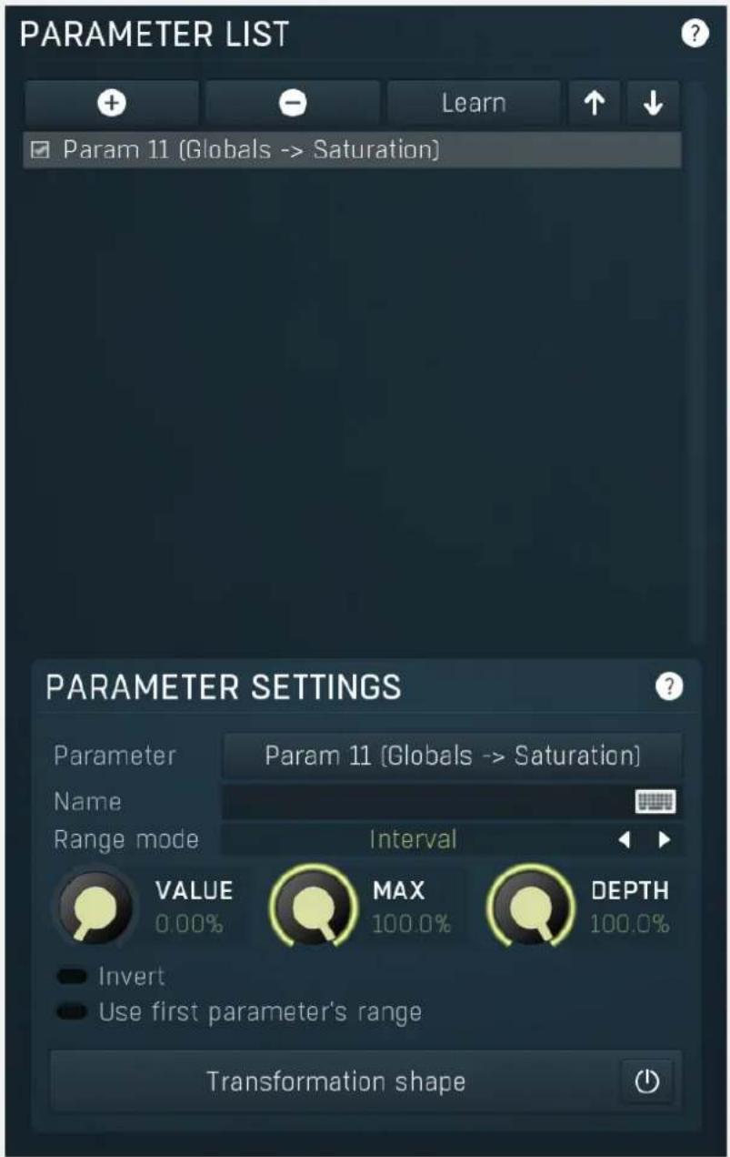

Add
Add button adds a parameter to the list of controlled parameters. Alternatively you can use the learn feature available by right-clicking the modulator button.

Delete
Delete button deletes the selected parameter from the list of controlled parameters.

Learn
Learn button starts or stops the learning. Click it, then move some parameters in the plugin, then click it again. Learning can also be accessed from the global modulator menu.

Up
Up button moves the selected parameter up one item, if possible. This may be useful when keeping things organized, but please note that if you have some other multiparameter, modulator or another subsystem access the ranges of individual parameters, this function will reorder them, so these connections will no longer be correct.

Down
Down button moves the selected parameter down one item, if possible. This may be useful when keeping things organized, but please note that if you have some other multiparameter, modulator or another subsystem access the ranges of individual
parameters, this function will reorder them, so these connections will no longer be correct.
Parameter Settings
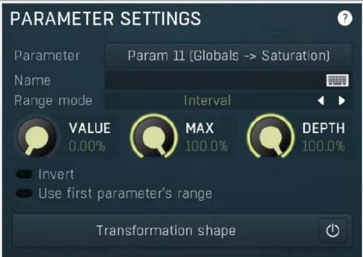
Parameter Param 11 [Globals -> Saturation]
Parameter
Parameter defines the target parameter which is being modulated. The set contains all automatable parameters.
Name
Name
Name lets you name the parameter somehow and may be helpful in situations, where there are many parameters being edited without obvious meanings.
Range mode Interval
Range mode
Range mode defines how the parameter range is selected. While sometimes it is better to specify minimum and maximum, other times it is better to use a nominal center and depth (\% of full scale). This control allows you to define which one it will be.
Up and down mode makes the values go above and below the selected Value, which is considered the center. The interval is made smaller if necessary.
Full range mode is similar, except the range is symmetrically constrained, so the selected Value may not be the center anymore.
Up/down only modes goes from the selected value up/down only.
Let's compare these 4 modes. Taking a value of -12dB value, with a depth of 75% and a scale of +/- 24dB. The nominal range is therefore = +/-24 dB * 75% = 36dB. With values of 0%, 50% and 100% the outputs are:
Up and down: -24, -12, 0 (range constrained to 12 dB either side)
Full range: -24, -6, 12 (range limited to minimum, but not constrained)
Up only: -12, 6, 24 (range not constrained = +/-24 dB * 75% = 36dB)
Down only: -12, -18, -24 (range limited to minimum)
Interval mode is the most simple one and goes from Value to Maximal value.
Value
Value defines the center of the target parameter's range or the minimum if the Range mode is set to Interval.
Maximal value
Maximal value defines the upper limit of the target parameter's range. It is available only if the Range mode is set to Interval. This value can be lower than Value. 0% is always mapped to reference>Value and 100% to reference>Maximal value.
Depth
Depth defines size of the target parameter's range. It is used only if the Range mode is not set to Interval.
Invert
Invert
Invert checkbox inverts the target parameter's range, so that minimum becomes maximum and vice versa.
Use first parameter's range
Use first parameter's range
Use first parameter's range makes the parameter display use the same range as the first parameter in the list. This is often useful if want to control the range in some way and apply the range to multiple parameters.
Transformation shape

Transformation shape
Transformation shape button displays the graph editor, which lets you tweak the shape of the curve used to control the selected parameter. The X axis shows the original values, the Y axis defines the results. Note that this takes some CPU, therefore you have to enable it using the enable button in the title.
Restore original values when disabled
Restore original values when
disabled
Restore original values when disabled makes the modulator restore the original parameter values when it is disabled by automation or modulation. Normally when you manually disable the modulator, the original values are restored as that is usually desired. However when you control the modulator enable state by automation or modulation, you may or may not want this to happen.
Assignable parameter ranges
Assignable parameter ranges
Assignable parameter ranges allows you to assign parameter ranges of several first parameters to other subsystems such as multiparameters or modulators. By default it is disabled, which removes all the relevant parameters to save valuable resources. This feature is available only if automation compatibility mode for V10 is disabled.
NORMAL
FOLLOWER
ENVELOPE
RANDOM
PITCH
Mode
Mode defines the way in which the modulator works. The modulator is like a black box that generates one number in range 0% to 100% at each moment and then assigns the appropriate value to each of the target parameters. The mode defines what this number will be. Select the particular tab to control the modulator's behaviour.
Normal mode uses a standard low-frequency oscillator (LFO) to drive the parameters.
Follower mode uses the level of the input signal.
Envelope generates an envelope using MIDI notes or by following input signal level.
Random generates randomized output which is however the same every time you render the song.
Pitch detects and follows the pitch of the input signal.
Normal mode
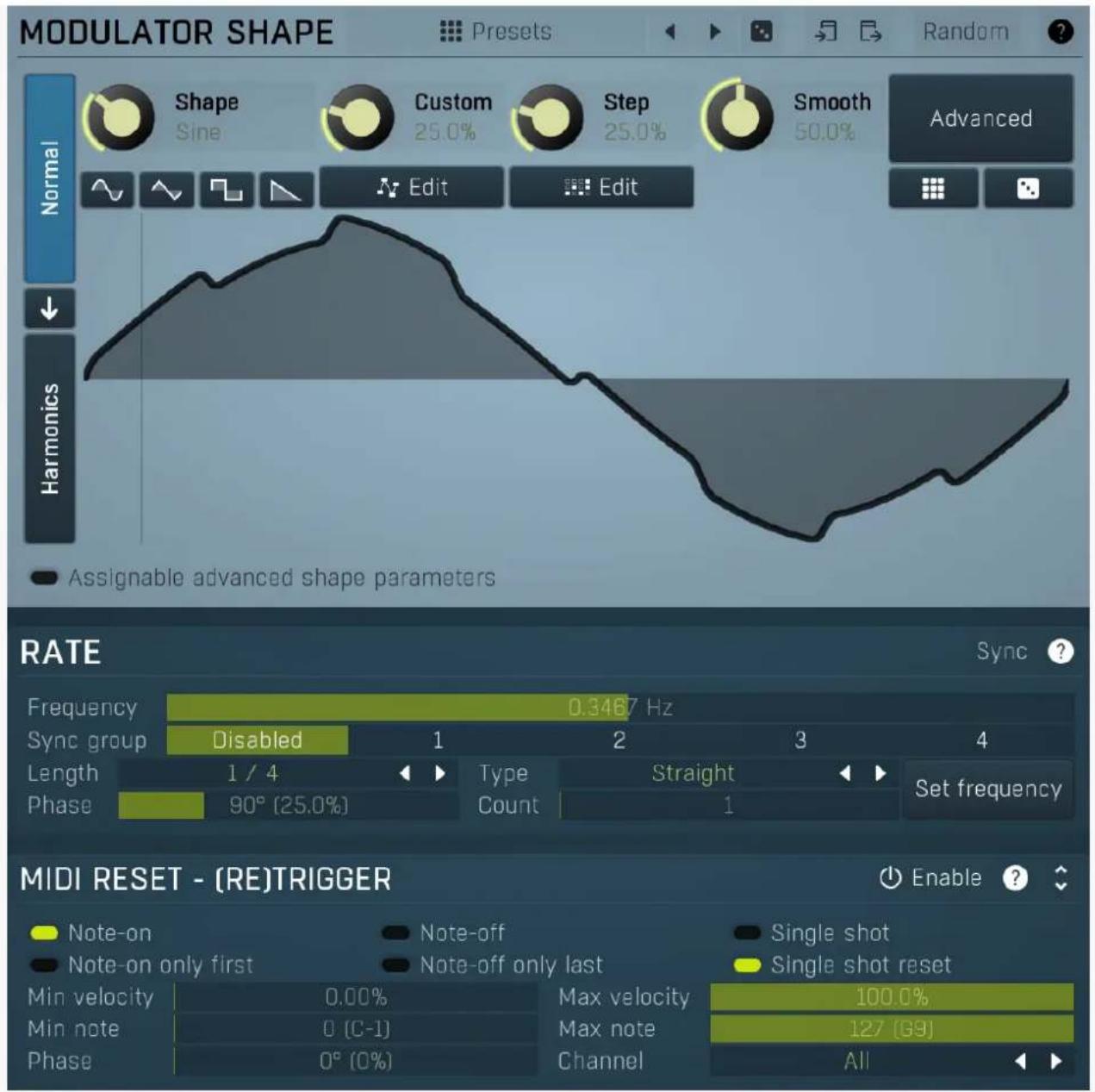
line
| Parameter | Value | |-------------------------|-----------| | Frequency | 0.3467 Hz | | Sync group | Disabled | | Length | 1 / 4 | | Phase | 90° (25.0%) | | Type | Count | | Straight | 1 | | Set frequency | - | | Note-on | - | | Note-on only first | - | | Note-off | - | | Note-off only last | - | | Single shot | - | | Single shot reset | - | | Min velocity | 0.00% | | Min note | 0 (C-1) | | Max velocity | 100.0% | | Max note | 127 (G9) | | Phase | 0° (0%) | | Channel | All |Normal mode makes the modulator work as a traditional low-frequency oscillator (LFO). Note that even if the modulator itself is running in a different mode, you can still blend this LFO using the LFO modulation parameter available on each tabbed page. The LFO parameters themselves are available on the first tabbed page only though.
Signal generator
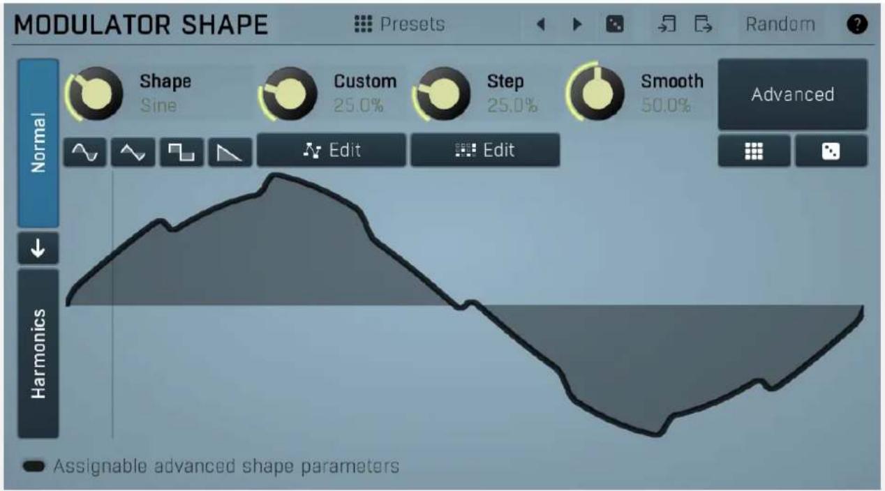
Signal generator defines the modulation LFO shape. It is used by the LFO generator, but also for the Project feature. Signal-generator is an incredibly versatile generator of low & high frequency signals. It offers 2 distinct modes - Normal and Harmonics. Normal mode is appropriate for low-frequency oscillators, where the graphical shape is relevant and is used to drive some form of modulation. For example, a tremolo uses this modulation to change the actual signal level in time. Frequencies for such oscillators usually do not exceed 20Hz as this is a sort of limit above which the frequencies become audible.
Harmonics mode is designed for high-frequency oscillators, where the actual shape is not as important as the harmonic content of the resulting signal, hence it is especially useful for actual audio signals. Please note that since a shape can contain more harmonics than those available from the harmonic generator, the results may not be exactly the same. As an example, a rectangular wave in normal mode may sound fuller than when converted to the harmonic mode.
Use the arrow-down button to switch from normal mode to harmonics mode or click the Normal and Harmonics buttons
Normal mode
The generator first uses a set of predefined signal shapes (sine, triangle, rectangle...), which you can select directly by right-clicking on the editor and choosing the requested shape from the menu. This menu also provides a link to the modulator shapes preset manager, normalization and randomization. You can also use the Main shape parameter, which generates a combination of adjacent signals to provide a nearly inexhaustible number of basic shapes.
The engine then combines the predefined shape with a Custom shape, which may be anything you can draw using the advanced envelope engine, depending on the level set by the Custom shape control. Use the Edit button to edit the custom shape.
You can also combine those results with a fully featured step sequencer, with variable number of steps and several shapes for each of them, depending on the level set by the Step sequencer control. Use the lower Edit button to edit the step sequence.
Those results may be mixed with a custom sample, which is available from the advanced settings, accessed by clicking the Advanced button.
Smoothness softens any abrupt edges, generated by the step sequencer for example.
Finally there are Advanced features providing more complex transformations, adding harmonics etc. or you can click the Randomize button in the top-left corner to generate a random, but reasonable, modulator shape.
Harmonics mode
Harmonics mode represents the signal as a series of harmonics (that is, multiples of the base frequency). For example, when your oscillator has a frequency of 2Hz (set in the Rate panel), then the harmonics are 2Hz, 4Hz, 6Hz, 8Hz etc. In theory, any signal can be created by mixing a potentially infinite number of these harmonics.
The harmonics mode lets you control the levels and phases of each harmonic. The top graph controls the levels of individual harmonics, while the bottom one controls their phases. Use the left-mouse button to change the values in each graph, the right-mouse button sets the default for the harmonics - 0% level and 0% phase. In both graphs the harmonics of power 2 (that is octaves) are highlighted. Other harmonics may actually sound disharmonic, despite their names.
For example, if you reset all harmonics to the defaults and increase only the first one, you will get a simple sine wave. By adding further harmonics you make the output signal more complex.
Harmonics controls the number of generated harmonics. The higher the number is, the richer the output signal is (unless the levels are 0% of course). This is useful to make the sound cleaner. For example, if you transform a saw-tooth wave to harmonics, it would not sound like a typical saw-tooth wave anymore, but more like a low-passed version of one. The more harmonics you use, the closer you get to the original saw-tooth wave.
Generator is a powerful tool for generating the harmonics, which are otherwise rather clumsy to edit. The generator provides several parameters based upon which it creates the entire series of harmonic levels and phases. These parameters are usually easier to understand than the harmonics themselves. Part of the generator is the randomizer available via the Random seed button, which smartly generates random settings for the generator. This makes the process of getting new sounds as simple as possible.
Signal generation fundamentals
The signal generator produces a periodic signal with specified wave shape. This means that the signal is repeating over and over again. As a result it can only contain multiples of the fundamental frequency. For example, if the generator is producing 100Hz signal, then it can contain 100Hz (fundamental or 1st harmonic), 200Hz (2nd harmonic), 300Hz (3rd harmonic), 400Hz (4th harmonic) etc. However, it can never produce 110Hz. You can then control the level of each harmonic and their relative phases. It does not matter whether you use the normal mode using oscillator shapes, or harmonics mode where you can control the harmonics directly. If both modes result in the same wave shape (such as sine wave vs. 1st harmonic only), then the result is exactly the same.
Sine wave is the simplest of all as it contains the fundamental frequency only. The "sharper" the signal shape is, the more harmonics it contains. The biggest source of higher harmonics is a "discontinuity", which you can see in both rectangle and saw waves. In theory, these signals have an infinite number of harmonics. However since our hearing is highly limited to less than 20kHz, the number of harmonics which are relevant is actually pretty small. If you generate a 50Hz signal, which is very low, and assuming that you have extremely good ears and you actually hear 20kHz, then the number of harmonics audible for you is 20000 / 50 = 400.
What happens above 20kHz?
Consider the example above again, what happens with harmonics above 400? These either stay there and simply are not audible, disappear if anti-aliasing is used, or get aliased back under 20kHz in which case you get the typical digital dirt.
When you convert a rectangle wave to harmonics mode, only the first 256 harmonics are used, so it basically works like an infinitely steep low-pass filter. What is the limit then? 50 Hz * 256 = 12.8kHz. The harmonic mode will not produce anything above this limit if you are generating a 50Hz signal. Most people do not hear anything above 15kHz, so this is usually enough, but if not, you may need to use the normal mode where you get the "infinite" number of harmonics.
What you see is not always what you get!
Say you want a rectangle wave and play a 440Hz tone(A4). You would expect the output signal to be a really quick rectangle wave, right? Wrong! If you would do that, and actually most synthesizers on the market do that, you would get the infinite number of harmonics. And, since you are working in say 48kHz sampling rate, the maximum frequency that can actually exist in your signal is 24kHz. So everything above it would get aliased below 24kHz, and there would be a lot of aliased dirt.
The "good" synthesizers perform a so-called anti-aliasing. There are several methods, most of them require quite a lot of CPU or have other limitations. The goal is to remove all frequencies above the 24kHz in our case or in reality, it is more about removing all aliased frequencies above 20kHz - this means, that we do not care about frequencies above 20kHz, because we do not hear them anyway. But we will keep it simple. Let's say we remove everything above 20kHz. You already know that the rectangle wave can be created using an infinite number of harmonics or sine waves. We removed everything above the 45th harmonic (20000 / 440) so our rectangle wave is trying to be formed using just 45 harmonics, so it will not really look like a rectangle wave.
After some additional filtering (like DC removal), the rectangle wave may look completely different than a true rectangle wave, yet it would sound the same! Does it matter? Not really. You simply edit the shape as a rectangle wave and let the synthesizer do the ugly stuff for you. But do not check the output, because it may be very different than what you would expect );).
How can I generate non-harmonic frequencies?
Ok, so now you are playing a 440Hz (A4) saw wave, it contains 440Hz, 880Hz, 1320Hz etc. Anything generated using the signal generator can contain only these frequencies, the only difference is the levels and phases of each of them. What if you want to make the signal dirty by adding say 500Hz? Well, that is not that simple! Here we are getting into audio synthesizer stuff, so let us just give you a few hints.
The traditional way is to use modulation. One particular method is called frequency modulation (FM). Instead of generating a 440Hz saw wave with your generator, you change the pitch, up and down. You are modulating the frequency, that's why FM. It is basically a vibrato, but as you increase the speed of the vibrato, it gets so quick that you stop noticing the pitch changes (that's very simplified but it serves the purpose) and instead it starts producing a very complex spectrum. Will the 500Hz be there? Well, if setup correctly, yes, but there will also be lots of other non-harmonic frequencies.
Another way is possible without any other tools. Let's say you do not want 440Hz, but 660Hz. Then you may generate 220Hz instead of 440Hz (which is one octave below it) and voila, 660Hz is the 3rd harmonic (3 x 220 is 660)! But you need to shift the saw wave one octave above. Fortunately it is not that hard here - go to the normal mode, select saw tooth, click advanced, and use the harmonics panel to remove the fundamental and leave just the 2nd harmonic, then convert it to harmonic mode. Well, it's not that
hard, but it's not exactly simple either...
The only way is, of course, additive synthesis. In that case you do not use one oscillator, but many of them. It lets you generate just about anything. But there is a catch, actually many of them. First, you need to say "ok I want this frequency and that frequency...", the setup is actually infinitely hard as there may be an infinite number of frequencies :). And the second is, of course, CPU requirements.
So is there some ultimate solution? Nope, sorry. The good thing is, you will not probably need it, because while what you see is not always what you get, also what you want is often not what you really want to hear :).
Presets
Presets
Presets button displays a window where you can load and manage available presets. Hold Ctrl when clicking to load a random preset instead.

Left arrow
Left arrow button loads the previous preset.

Right arrow
Right arrow button loads the next preset.

Randomize
Randomize button loads a random preset.

Copy
Copy button copies the settings onto the system clipboard.

Paste
Paste button loads the settings from the system clipboard.
Random
Random
Random button generates random settings using the existing presets.
Normal
Normal
Normal button switches the generator into the normal mode, which lets you edit the shape of the oscillator. This is especially advantageous for low-frequency oscillators, where the shape matters even though it doesn't have any physical meaning.

Convert
Convert button converts the current shape into harmonic-based representation. Please note that since the number of harmonics is limited, the result will not perfectly resemble the original shape.
Harmonics
Harmonics
Harmonics button switches the generator into the harmonics mode, which lets you edit the levels and phases of individual harmonics. This is especially advantageous for high-frequency oscillators, hence sound generators.
Signal generator in Normal mode
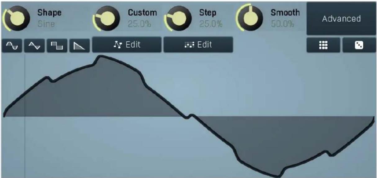
Signal generator in Normal mode works by generating the oscillator shape using a combination of several curves - a predefined set of standard curves, custom shape, step sequencer and custom sample. It also post-processes the shape using several filters including smoothing to custom transformations. This is especially useful when using the oscillator as an LFO (low-frequency-oscillator), where the harmonic contents does not really matter, but the shape does.

Shape
Sine
Shape
Shape controls the main shape used by the signal generator. There are several predefined shapes: exponential, triangle, sine power 8, sine power 4, sine square, sine, harmonics, more harmonics, disharmonics, sine square root, sine 4 root, rectangle, rect-saw, saw, noise and mess. You can choose any of them or interpolate between any 2 adjacent shapes using this control.
Custom
25.0%
Custom
Custom controls the amount of the custom shape that is blended into the main shape.

Edit
Edit button shows the custom shape editor.
Signal generator custom shape editor
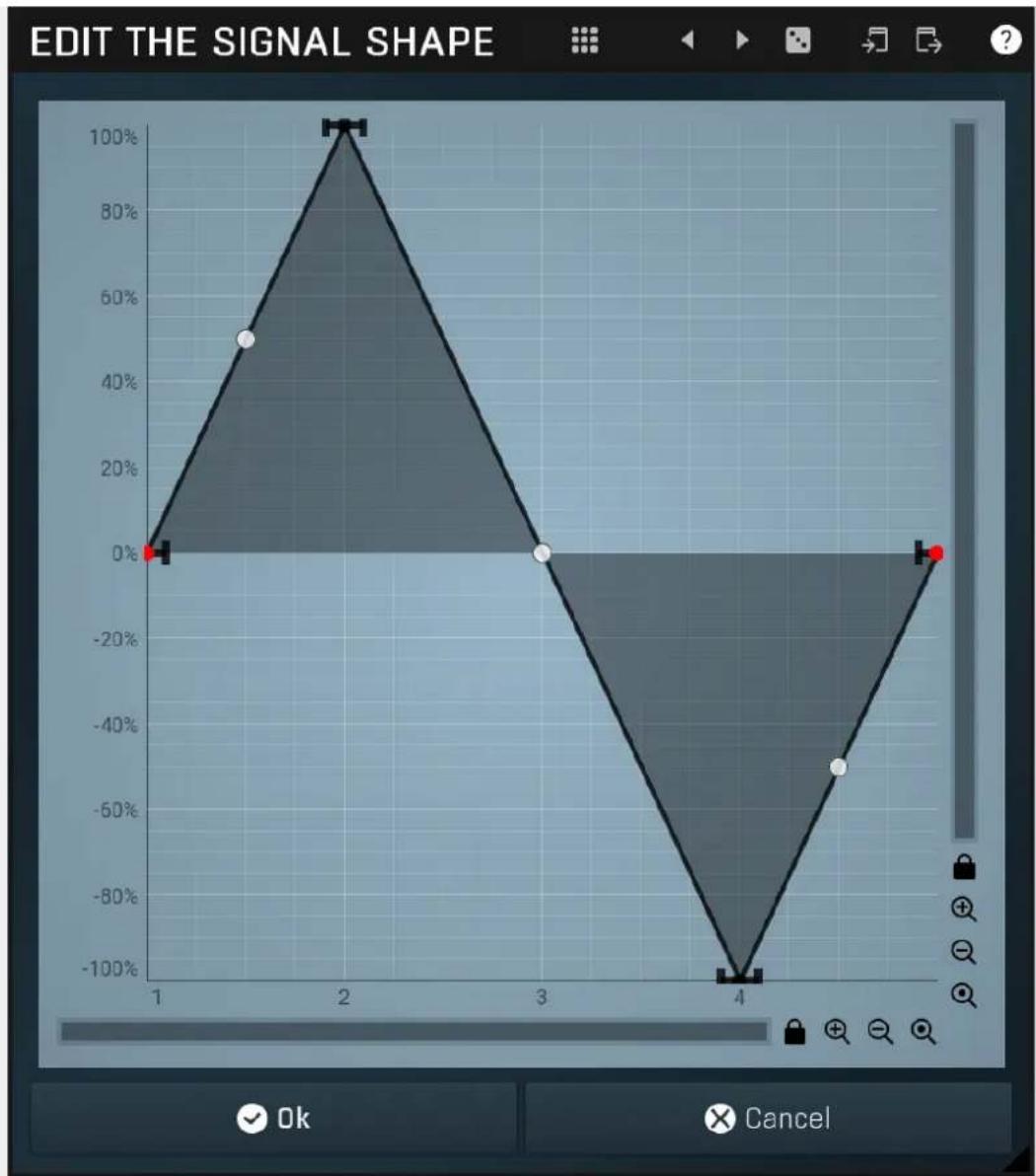
line
| Time | Signal Value | |------|--------------| | 1 | 0% | | 2 | 100% | | 3 | 0% | | 4 | -100% | | 5 | 0% |Signal generator custom shape editor controls the custom shape. You can edit virtually any shape that you can imagine and then blend it with the standard shapes, the step sequencer etc.

Presets
Presets button displays a window where you can load and manage available presets. Hold Ctrl when clicking to load a random preset instead.

Left arrow
Left arrow button loads the previous preset.

Right arrow
Right arrow button loads the next preset.

Randomize
Randomize button loads a random preset.

Copy
Copy button copies the settings onto the system clipboard.

Paste
Paste button loads the settings from the system clipboard.
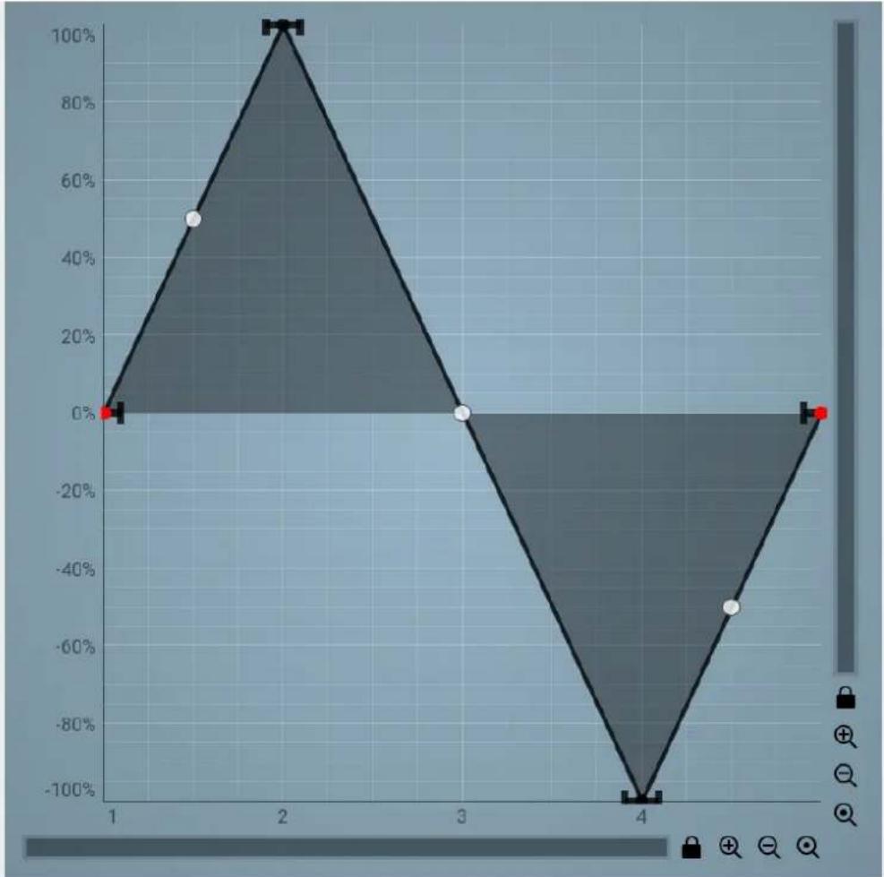
area
| X-Axis | Y-Axis (%) | |---|---| | 1 | 0 | | 2 | 100 | | 3 | 0 | | 4 | -100 |Graph editor
Graph editor lets you edit the envelope graph.
Envelope graph
Envelope graph provides an extremely advanced way to edit any kind of shape that you can imagine. An envelope has a potentially unlimited number of points, connected by several types of curves with adjustable curvature (drag the dot in the middle of each arc) and the surroundings of each point can also be automatically smoothed using the smoothness (horizontal pull rod) control. You can also literally draw the shape in drawing mode (available via the main context menu).
- Left mouse button can be used to select points. If there is a point, you can move it (or the entire selection) by dragging it. If there is a curvature circle, you can set up its tension by dragging it. If there is a line, you can drag both edge points of it. If there is a smoothing controller, you can drag its size. Hold Shift to drag more precisely. Hold Ctrl to create a new point and to remove any points above or below.
- Left mouse button double click can be used to create a new point. If there is a point, it will be removed instead. If there is a curvature circle, zero tension will be set. If there is a smoothing controller, zero size will be set.
- Right mouse button shows a context menu relevant to the object under the cursor or to the entire selection. Hold Ctrl to create or remove any points above or below.
- Middle mouse button drag creates a new point and removes any points above or below. It is the same as holding Ctrl and dragging using left mouse button.
- Mouse wheel over a point modifies its smoothing controller. If no point is selected, then all points are modified.
- Ctrl+A selects all points. Delete deletes all selected points.
Step 25.0%
Step
Step controls the amount of the step sequencer shape that is blended into the main shape (which has already been blended with the custom shape).

Edit
Edit button shows the step sequencer editor.
Signal generator step sequencer editor
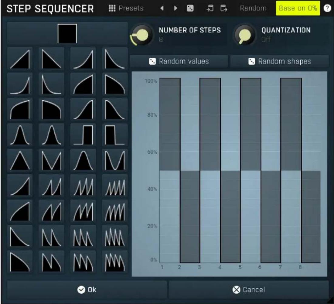
bar
| Step | Random values (%) | Random shapes (%) | |---|---|---| | 1 | 100 | 50 | | 2 | 100 | 50 | | 3 | 100 | 50 | | 4 | 100 | 50 | | 5 | 100 | 50 | | 6 | 100 | 50 | | 7 | 100 | 50 | | 8 | 100 | 50 |Signal generator step sequencer editor controls the step sequencer shape. You can have various numbers of steps each with a different value and shape. Note that for classic rectangular shapes the output can be very rough, hence it may be worth considering using Smoothness parameter to smooth out the resulting shape. This will use additional CPU power of course, but that should be negligible unless you modulate any of the signal generator parameters.

Presets
Presets
Presets button displays a window where you can load and manage available presets. Hold Ctrl when clicking to load a random preset instead.

Left arrow
Left arrow button loads the previous preset.

Right arrow
Right arrow button loads the next preset.

Randomize
Randomize button loads a random preset.

Copy
Copy button copies the settings onto the system clipboard.

Paste
Paste button loads the settings from the system clipboard.
Random
Random button generates random settings using the existing presets.

Random values
Random values
Random values button generates random sequence of values, but keeps the shape of each step.

Random shapes
Random shapes
Random shapes button generates random sequence of shapes, but keeps the values of each step.

Smooth
50.0%
Smooth
Smooth controls the amount of smoothing. Many shapes, especially those produced by the step sequencer, have rough jagged edges, which may be advantageous, but when used to modulate certain parameters, the output may be clicking or causing other artifacts. Smoothness helps it by smoothing the whole signal shape out and removing these rough edges.
Advanced
Advanced
Advanced button displays an additional window with more advanced settings for post-processing the signal shape, such as harmonics or custom transformations.
Advanced settings
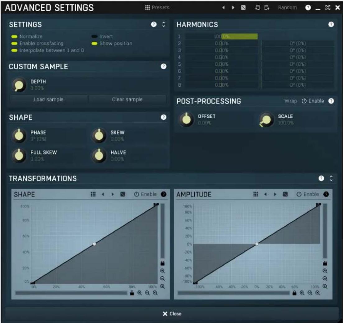

Presets
Presets
Presets button displays a window where you can load and manage available presets. Hold Ctrl when clicking to load a random preset instead.

Left arrow
Left arrow button loads the previous preset.

Right arrow
Right arrow button loads the next preset.

Randomize
Randomize button loads a random preset.

Copy
Copy button copies the settings onto the system clipboard.

Paste
Paste button loads the settings from the system clipboard.
Random
Random
Random button generates random settings using the existing presets.
Settings panel
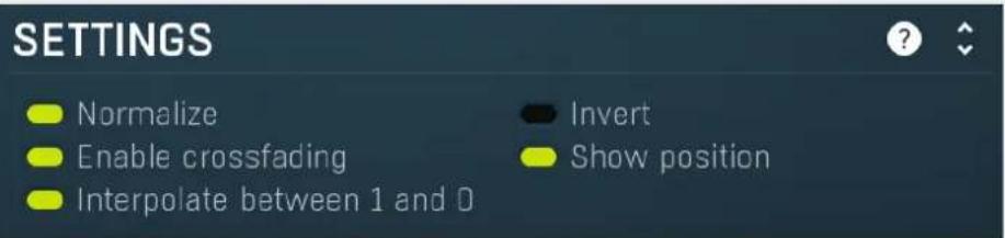
Settings panel contains some global settings of the oscillator.

Normalize
Normalize
Normalize switch enables normalization to -1..+1. It is generally desirable since even if you draw a custom shape, you usually want it to have the full range. You may want to disable it if you want to create some custom shapes, where the level actually matters.

Invert
Invert
Invert switch simply inverts the output shape vertically.

Enable crossfading
Enable crossfading
Enable crossfading enables interpolation between shapes when the shape is changing. This requires more CPU, but can avoid zipper noise when the shape is being modulated for example.

Show position
Show position
Show position makes the editor display a position indicator.

Interpolate between 1 and 0
Interpolate between 1 and 0
Interpolate between 1 and 0 smoothens the discontinuity between 1 and 0 values, which is inevitable for shapes such as saw or rect for example. However when this is a high frequency oscillator (HFO), this discontinuity is what creates the highest frequencies, so it is actually desirable. When using it as an LFO, you may also want the discontinuity in some extreme cases.
Custom sample panel
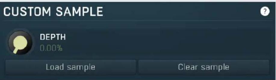
Custom sample panel contains parameters of the custom sample that you can load and mix with the other sources. Do NOT confuse this with a sampler, the custom sample is taken as one period of the waveform. It can be used for creative effects and it can be used to import a custom waveform. The custom sample is then stored with limited precision within the settings, so the sample does not need to be kept on the system, but note that these settings may be quite large. To limit the space required by the settings, the sample is stored only if the depth is not 0%, meaning only if the sample is actually used.

DEPTH
0.00%
Depth
Depth controls the amount of custom sample mix. 0% means the sample is not used even if there actually is one loaded. 100% means the sample completely overrides the basic shape, custom shape, step sequencer... However, transformations are still performed on the sample.
Load sample
Load sample
Load sample button displays a file selection window, which lets you select the custom sample file.
Clear sample
Clear sample
Clear sample button removes the custom sample if it has been loaded.
Shape panel
![SHAPE PHASE 0° [0%] SKEW 0.00% FULL SKEW 0.00% HALVE 0.00%](/content/2026/05/983866/images/6d6f62bae4431ae5f85bdc47ad4598812b6b4de6b337fa39384c18b5d5cb6d9c.jpg)
Shape panel contains parameters performing various transformations on the signal shape. Please note that most transformation require a significant amount of CPU resources, so you should not automate or modulate the signal shape if you are using them.
Harmonics panel
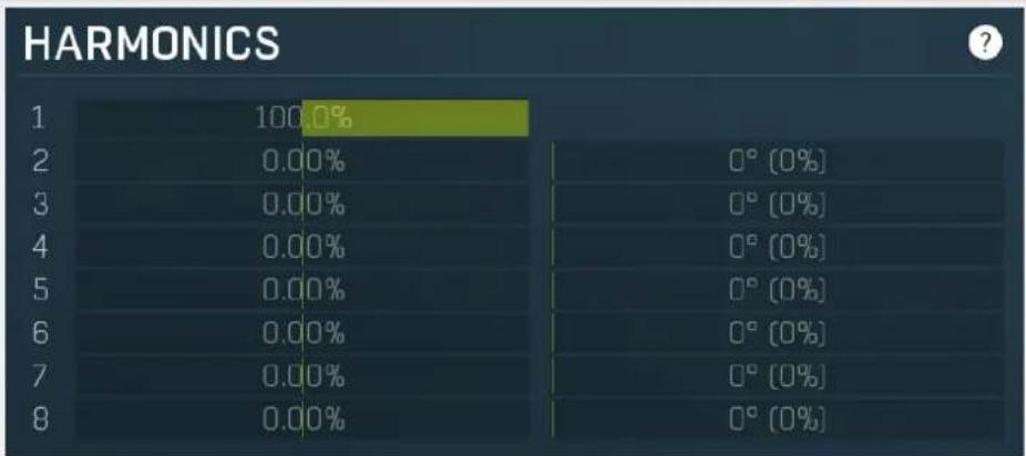
bar
HARMONICS | Category | Value (%) | |---|---| | 1 | 100.0 | | 2 | 0.00 | | 3 | 0.00 | | 4 | 0.00 | | 5 | 0.00 | | 6 | 0.00 | | 7 | 0.00 | | 8 | 0.00 |Harmonics panel lets you add separate harmonics of the original signal.
Post-processing panel
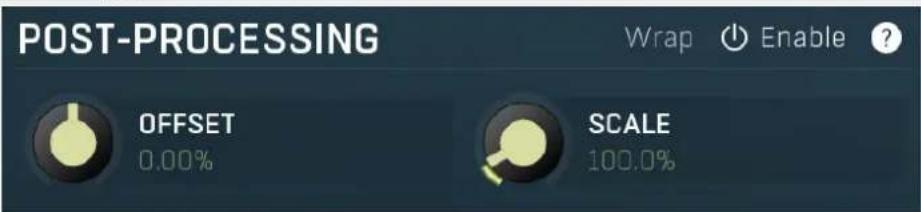
Post-processing panel lets you post-process the shape after all the previous generator items.
Transformations
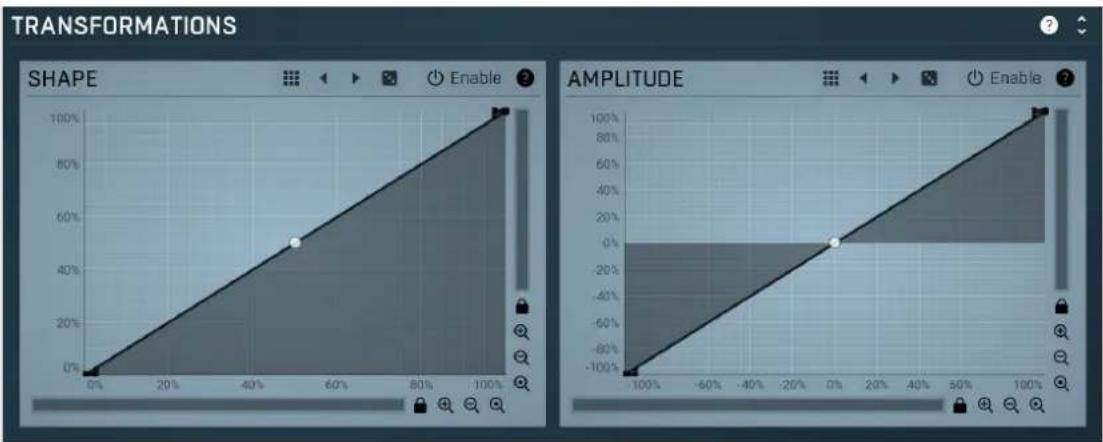
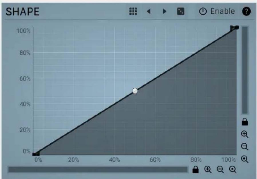
line
| X (%) | Y (%) | |-------|-------| | 0 | 0 | | 50 | 50 | | 100 | 100 |Shape transformation
graph
Shape transformation graph lets you perform arbitrary modification of the graph shape. Basically this graph lets you modify the shape "in time". The Y axis represents the position in the source signal related to the position in the target signal. The best way to check what it does is simply to try it.

Presets
Presets button displays a window where you can load and manage available presets. Hold Ctrl when clicking to load a random preset instead.

Left arrow
Left arrow button loads the previous preset.

Right arrow
Right arrow button loads the next preset.

Randomize
Randomize button loads a random preset.
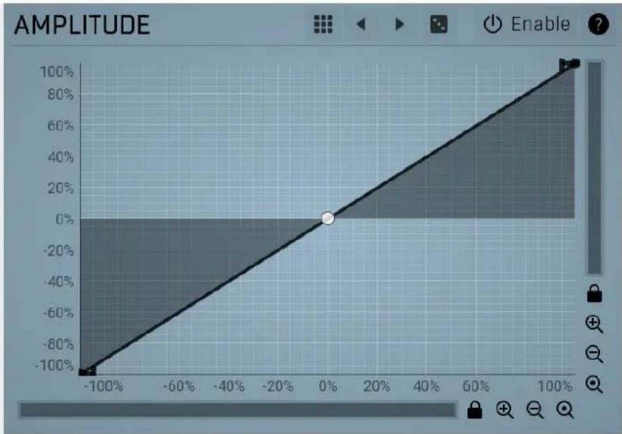
line
| X | Y | | ------ | ------ | | -100% | -100% | | 0% | 0% | | 100% | 100% |Amplitude
transformation graph
Amplitude transformation graph lets you perform arbitrary modification of the graph amplitude. Basically this graph lets you modify the shape's level, vertical axis. The X axis represents the original values, the Y axis defines the resulting values. The best way to check what it does is simply to try it.

Presets
Presets button displays a window where you can load and manage available presets. Hold Ctrl when clicking to load a random preset instead.

Left arrow
Left arrow button loads the previous preset.

Right arrow
Right arrow button loads the next preset.

Randomize
Randomize button loads a random preset.

Assignable advanced shape parameters
Assignable advanced shape parameters
Assignable advanced shape parameters allows you to assign advanced parameters such as step sequencer values to other subsystems such as multiparameters or modulators. By default it is disabled, which removes all the relevant parameters to save valuable resources.
Signal generator in Harmonics mode
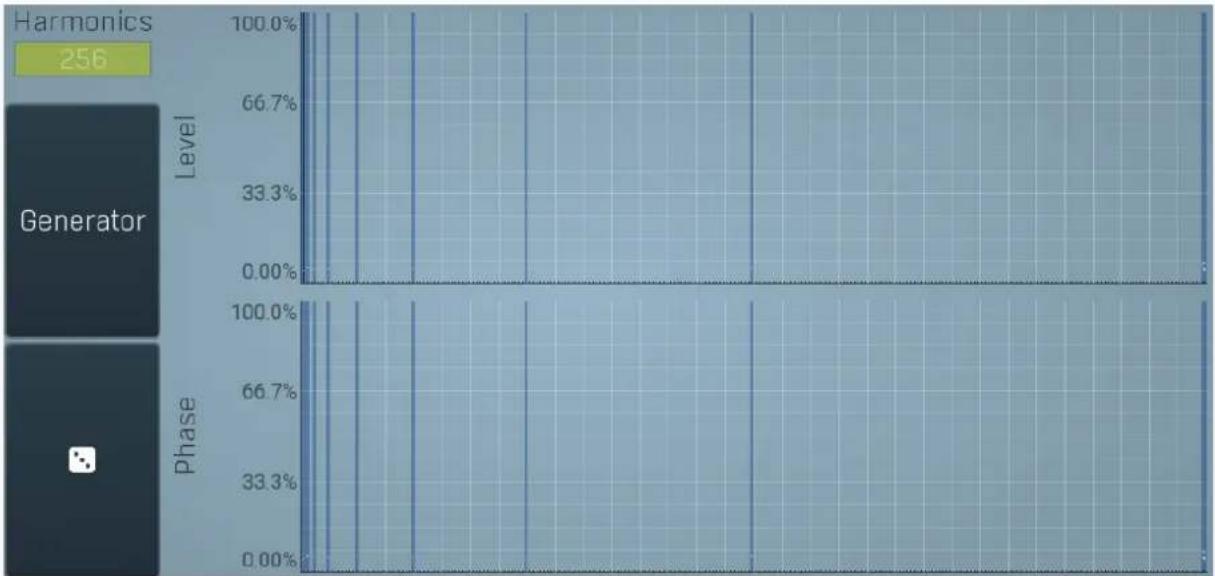
bar
| Level | Phase | |-------|-------| | 100.0% | 100.0% | | 66.7% | 66.7% | | 33.3% | 33.3% | | 0.00% | 0.00% |Signal generator in Harmonics mode works by generating the oscillator shape using individual harmonics. Essentially a harmonic is a sine wave. The first harmonic, known as the fundamental, fits once in the oscillator time period, hence it is the same as selecting sine wave in the Normal mode. The second harmonic fits twice, the third three times etc. In theory, any shape you create in normal mode can be converted into harmonics. However, this approach to signal generation needs an enormous number of harmonics, which is both inefficient to calculate and mostly hard to edit. Therefore, the harmonic mode can process up to 256 harmonics, which is enough for very complex spectrums, however it is still not enough to generate an accurate square wave for example. If your goal is to create basic shapes, it is better to use the normal mode.
It is nearly impossible to say how a particular curve will sound when used as a high-frequency oscillator in a synthesizer, just by looking at its shape. Harmonics mode, on the other hand, is directly related to human hearing and makes this process very simple. In general, the more harmonics you add, the richer the sound will be. The higher the harmonic, the higher the tone. Usually, one leaves the first harmonic enabled too, as this is the fundamental tone, however you may experiment with more dissonant sounds without it.
Editing harmonics can be time consuming unless you hear what you want, so a signal generator is also available. This great tool lets you generate a random spectrum by a single click. You can also open the Generator settings and edit its parameters, which basically control the audio properties in a more natural way - using parameters such as complexity, harmonicity etc.
Generator
Generator button shows a powerful harmonics generator, which can create unlimited number of various timbres and even analyze a sample and extract harmonics from it.
Harmonics generator
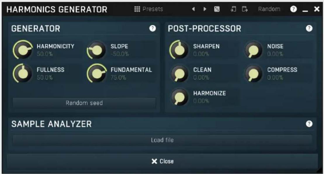
Harmonics generator is a powerful tool, that can generate various harmonics-based timbres and even analyze a sample file and extract harmonics from it.

Presets
Presets
Presets button displays a window where you can load and manage available presets. Hold Ctrl when clicking to load a random preset instead.

Left arrow
Left arrow button loads the previous preset.

Right arrow
Right arrow button loads the next preset.

Randomize
Randomize button loads a random preset.

Copy
Copy button copies the settings onto the system clipboard.

Paste
Paste button loads the settings from the system clipboard.
Random
Random button generates random settings using the existing presets.
Generator panel
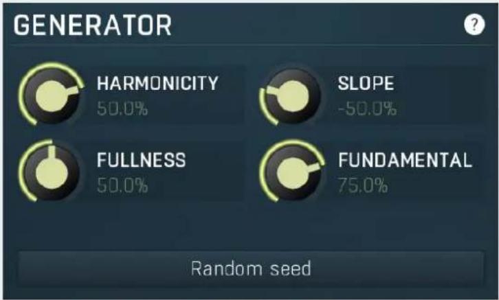
Generator panel contains parameters of the harmonics generator. By changing any of the parameters, the harmonics are changed, however only Random seed button changes the structure completely. The other parameters can be used to tweak the results.

HARMONICITY
50.0%
Harmonicity
Harmonicity controls the ratio between natural harmonics and those which sound disharmonic (despite the title "harmonics"). Assuming that the 1st harmonic is the fundamental, 2nd harmonic is 1 octave above, 4th is 2 octaves above, both can be considered very natural. 3rd harmonic is 1 octave and a 5th above the fundamental, and is still pretty harmonic, but less than the octaves. 5th harmonic is 2 octaves and a major 3rd above the fundamental. Such a tone may sound very disharmonic, in minor scales for example. Higher harmonics are often very disharmonic and produce typical ringing timbres.
When harmonicity parameter is set to 100%, only octaves are allowed. By lowering the value more and more disharmonics are created and with 0% all frequencies are allowed. For values below 0% disharmonics are preferred, hence you can expect more ringing timbres.

SLOPE
-50.0%
Slope
Slope defines the amount of higher harmonics compared to lower ones. When 0%, the higher harmonics have the same levels as lower ones. Typically you use values below 0%, which attenuates the higher harmonics making the resulting sound darker. Similarly values above 0% make the sound brighter.

FULLNESS
50.0%
Fullness
Fullness controls the number of generated harmonics. With values around 0% the resulting timbers will contain only a few harmonics making the sound clear. Higher values increase number of harmonics making the timbre rich.

FUNDAMENTAL
75.0%
Fundamental
Fundamental controls the minimum level of the fundamental (the 1st harmonic). Most sounds have a very strong fundamental as it carries the pitch.
Random seed
Random seed
Random seed button generates a new series of harmonics. Pressing this button will create a whole new timbre.
Post-processor panel
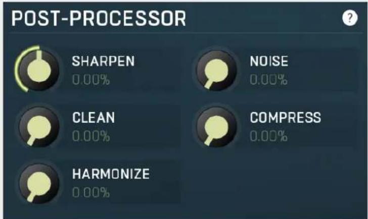
Post-processor panel contains parameters of the harmonics post-processor. The generator and sample analyzer first create a series of harmonics, the timbre. These harmonics are mixed depending on the Sample ratio parameter. After that the post-processor is engaged, which can further transform the harmonics in several ways.
SHARPEN
0.00%
Sharpen
Sharpen is a sort of soft compression/expanding unit. Values below 0% decrease the level of quiet harmonics, while values above 0% increase their level.

NOISE
0.00%
Noise
Noise defines amount of noise added to the timbre. Noise can make the results dirty providing much richer timbres.

CLEAN
0.00%
Clean
Clean controls the threshold of a gate. It basically attenuates or removes harmonics below this level making the output cleaner.

COMPRESS
0.00%
Compress
Compress reduces the dynamic range of the harmonics by increasing levels of the quiet ones, but keeping the levels of the loud ones.

HARMONIZE
0.00%
Harmonize
Harmonize creates additional higher harmonics from existing ones. This is especially useful to transform rich dirty disharmonic timbres into similarly rich but more harmonic timbres.
Sample analyzer panel
SAMPLE ANALYZER

Load file
Sample analyzer panel contains parameters of the sample analyzer. If there is no sample loaded, the sample analyzer is turned off. The analyzer takes the selected sample and a position within it, analyses one period of the signal waveform and produces the output set of harmonics. You can then combine these harmonics with the output of the generator using Sample ratio parameter.
The sample itself is not store with the plugin settings. Instead the path to the target sample file is stored along with the analyzed harmonics. If the sample file is not available, you cannot modify the analysis parameters and the last analyzed harmonics are used. This means that you actually don't need to have the sample file available on the computer on which you are using the settings.
Load file
Load file
Load file button lets you select a sample file to analyse.

natural_image
Solid dark blue background with a small white square containing three dots (no text or symbols)Randomize
Randomize button selects random parameters for the harmonics generator, so you can use it to get a random sound character instantly. Hold Ctrl to slightly modify existing generator settings instead of completely changing them.
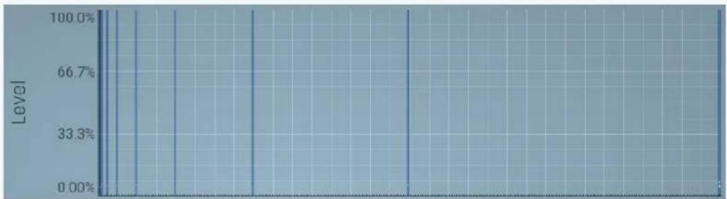
line
| Level | Value | |-------|-------| | 100.0% | 100.0% | | 66.7% | 100.0% | | 33.3% | 100.0% | | 0.00% | 100.0% |Magnitudes graph
Magnitudes graph contains the levels of the individual harmonics. The highlighted bars are octaves, thus the 1st, 2nd, 4th, 8th harmonic etc.
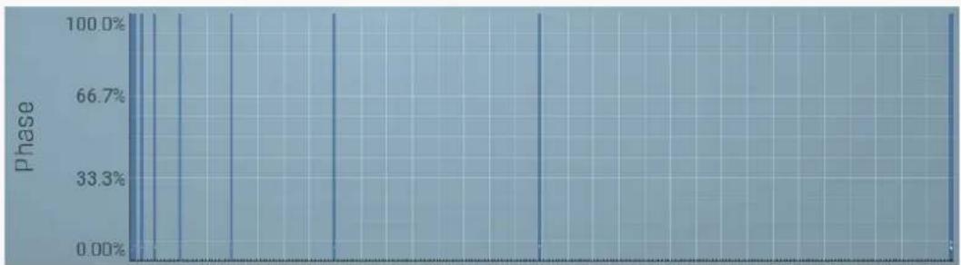
line
| Phase | Value (%) | |---|---| | 1 | 100.0 | | 2 | 66.7 | | 3 | 33.3 | | 4 | 0.00 | | 5 | 0.00 | | 6 | 0.00 | | 7 | 0.00 | | 8 | 0.00 | | 9 | 0.00 | | 10 | 0.00 | | 11 | 0.00 | | 12 | 0.00 | | 13 | 0.00 | | 14 | 0.00 | | 15 | 0.00 | | 16 | 0.00 | | 17 | 0.00 | | 18 | 0.00 | | 19 | 0.00 | | 20 | 0.00 | | 21 | 0.00 | | 22 | 0.00 | | 23 | 0.00 | | 24 | 0.00 | | 25 | 0.00 | | 26 | 0.00 | | 27 | 0.00 | | 28 | 0.00 | | 29 | 0.00 | | 30 | 0.00 | | 31 | 0.00 | | 32 | 0.00 | | 33 | 0.00 | | 34 | 0.00 | | 35 | 0.00 | | 36 | 0.00 | | 37 | 0.00 | | 38 | 0.00 | | 39 | 0.00 | | 40 | 0.00 | | 41 | 0.00 | | 42 | 0.00 | | 43 | 0.00 | | 44 | 0.00 | | 45 | 0.00 | | 46 | 0.00 | | 47 | 0.00 | | 48 | 0.00 | | 49 | 0.00 | | 50 | 0.00 | | 51 | 0.00 | | 52 | 0.00 | | 53 | 0.00 | | 54 | 0.00 | | 55 | 0.00 | | 56 | 0.00 | | 57 | 0.00 | | 58 | 0.00 | | 59 | 0.00 | | 60 | 0.00 | | 61 | 0.00 | | 62 | 0.00 | | 63 | 0.00 | | 64 | 0.00 | | 65 | 0.00 | | 66 | 0.00 | | 67 | 0.00 | | 68 | 0.00 | | 69 | 0.00 | | 70 | 0.00 | | 71 | 0.00 | | 72 | 0.00 | | 73 | 0.00 | | 74 | 0.00 | | 75 | 0.00 | | 76 | 0.00 | | 77 | 0.00 | | 78 | 0.00 | | 79 | 0.00 | | 80 | 133.3% (approx.) for the last two phases (Phase) in the chart, but the remaining three phases (Phase) are not explicitly labeled on the chart.Phases graph
Phases graph contains the phases of the individual harmonics. The highlighted bars are octaves, thus the 1st, 2nd, 4th, 8th harmonic etc.
Rate panel

bar
| Category | Value | | -------------- | --------- | | Frequency | 0.3467 Hz | | Sync group | Disabled | | Length | 1 / 4 | | Phase | 90° (25.0%) |Rate panel contains parameters controlling the speed of the LFO, whether the modulator is set to Normal mode or any other mode while the LFO modulation is used.
Sync
Sync
Sync switch turns the modulator into synced mode, where its speed is not defined by frequency, but it uses musical units instead.
Frequency
0.3467 Hz
Frequency
Frequency defines the modulation speed.
Sync group
Disabled
1
2
3
4
Sync group
Sync group lets you synchronize the modulators with each other and potentially with other parts of the plugin. It can be controlled only when to-host synchronization is disabled, otherwise it is overridden by synchronization from the host. By using the same synchronization group for all modulators you ensure they will always be in-sync even though no other synchronization is used. This can be useful, for example, when you want to modulate different parameters with different shapes or when using some more advanced method, such as using a follower. When the synchronization is enabled, it works on the 'first is the leader' basis, hence the first modulator controls the rest of the modulators in the same group.
Synchronization panel
| Length | 1 / 4 | ◀ ▶ | Type | Straight | ◀ ▶ | Set frequency |
| Phase | 90° (25.0%) | Count | 1 | |||
Synchronization panel contains parameters for the to-host synchronization.
Length
1/4

Length
Length defines the note length to be used.
Type
Straight

Type
Type defines the note type, such as straight notes or triplets, to be used. Together the Length and Type determine the actual time/delay.
Example: '1/4 Straight' at 120 bpm = a delay of 500 ms, '1/4 Triplet' at 160 bpm = a delay of 281.25 ms.
Phase
90°(25.0%)
Phase
Phase defines the phase offset of the to-host synchronization.
Range: 0° (0%) to 360° (100.0%), default 90° (25.0%)
Count

Count
Count defines the number of the units, hence multiplies of the sync length.
Range: 1 to 64, default 1
Set frequency
Set frequency
Set frequency button sets the Frequency parameter available for the frequency mode so that it matches the current synchronization. That way you can set the modulator's frequency to the current synchronization and then change it a little for example.
MIDI reset panel
MIDI RESET - (RE)TRIGGER

Enable


NOTE-10
nude enuun,
The quick brown fox jumps over the lazy dog.
[Unreadable due to severe distortion and noise]
Figure 3.1
(1) 2017年1月1日
The quick brown fox jumps over the lazy dog.
10.2.16
[Unreadable]
[Unreadable]
[Unreadable]
[Unreadable]
The quick brown fox jumps over the lazy dog.
- 2017年1月1日


MIDI reset panel configures the MIDI reset feature, which will reset the oscillator when a MIDI note is received or its MIDI reset parameter is a target of another modulator or multiparameter. This way you can make the oscillator perform "in-sync" with your playing. Please note that once you enable it, the oscillator will not be in phase-sync with the host.

Enable
Enable
Enable button enables or disables the feature.

11.4.2017年1月1日
Note-on
Note-on controls if the MIDI reset should occur when a note is pressed.

Note-off
Note-off controls if the MIDI reset should occur when a note is released.

Single shot
Single shot button activates the single shot mode in which the oscillator doesn't cycle around but instead only goes once from left to right, then stops until the MIDI reset occurs.

Note-on only first
Note-on only first controls if the MIDI reset should occur when a note is pressed only if it is the first note (thus no other note is being held).

Note-off only last
Note-off only last controls if the MIDI reset should occur when a note is released only if it is the last note (that is, no other note is being held afterwards).

Single shot reset
Single shot reset button defines if the phase should reset to 0 after a single shot period ends. For most waves such as sine it doesn't really matter since the value at 0 (the start of the cycle) is the same as value at 1 (the end of the cycle). But it might matter for saw wave for example.

Min velocity
Min velocity defines the minimum velocity that will reset the oscillator.

Max velocity
Max velocity defines the maximum velocity that will reset the oscillator.

Min note
Min note defines the minimum note that will reset the oscillator.

Max note
Max note defines the maximum note that will reset the oscillator.

Phase
Phase defines the initial oscillator phase after a reset.

Channel
Channel defines note MIDI channel to reset the oscillator.
Follower mode
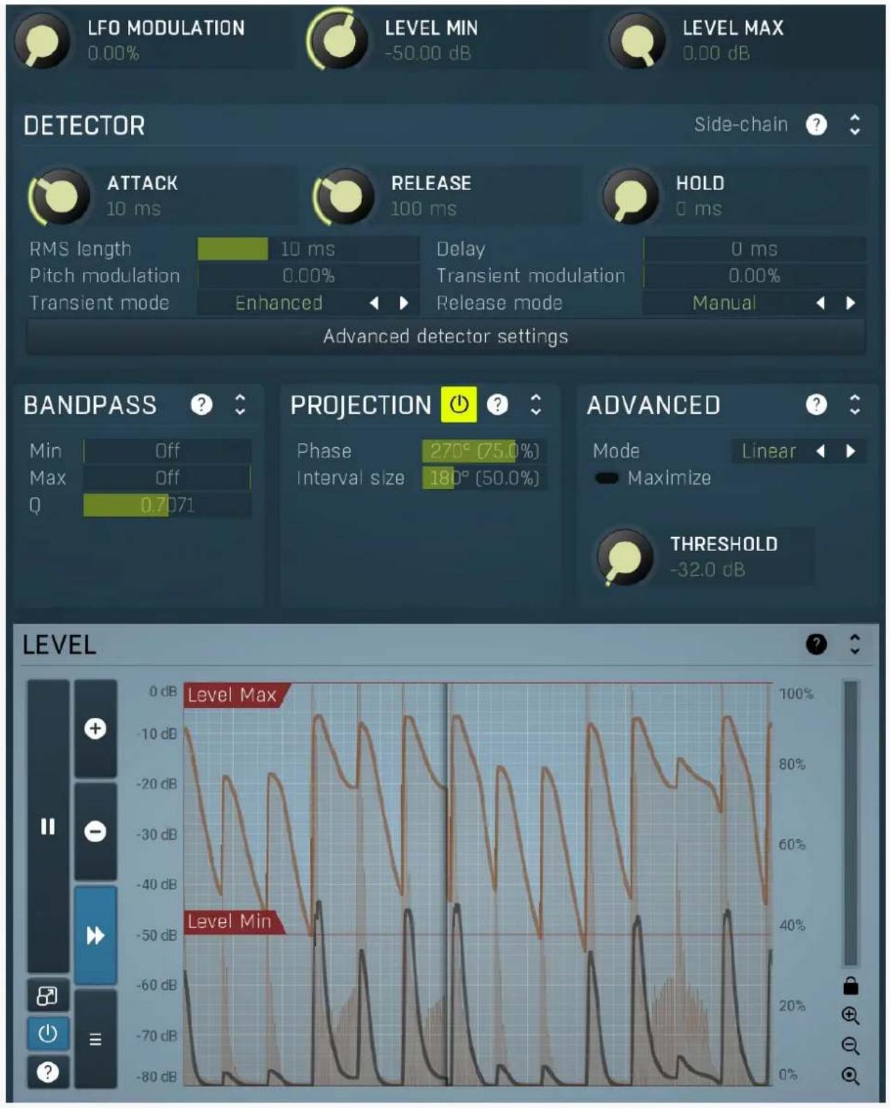
Follower mode makes the modulator follow the input signal level.

LFO MODULATION
0.00%
LFO modulation
LFO modulation defines the amount of LFO modulation to be applied in addition to the follower. With 0% the modulator uses only the follower; with 100% the modulator does the same job as if the modulator were in Normal mode. To set the LFO parameters switch to normal mode temporarily.
Range: 0.00% to 100.0%, default 0.00%

LEVEL MIN
-50.00 dB
Level min
Level min defines the minimum input level that is transformed into a modulator value of 0%. For example if you set the minimum / maximum levels to -50dB ... -20dB, then an input level of -50dB or lower results in a value of 0% and an input level at -20dB or above
results in 100%.
Range: -120.00 dB to 0.00 dB, default -50.00 dB

LEVEL MAX
0.00 dB
Level max
Level max defines the maximum input level that is transformed into a modulator value of 100%. For example if you set the minimum / maximum levels to -50dB ... -20dB, then an input level of -50dB or lower results in a value of 0% and an input level at -20dB or above results in 100%.
Range: -120.00 dB to 0.00 dB, default 0.00 dB
Detector panel
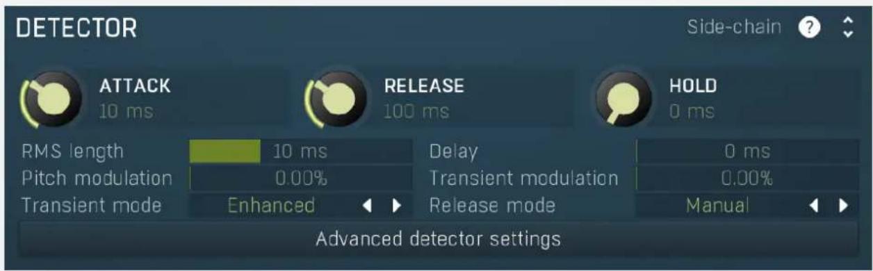
Detector panel contains the dynamic detector parameters, which control how the signal level is measured.
Side-chain
Side-chain input
Side-chain input makes the modulator analyze the side-chain input instead of the regular input.

ATTACK
10 ms
Attack
Attack defines the attack time, that is how quickly the level detector increases the measured input level. When the input peak level is higher than the current level measured by the detector, the detector moves into the attack mode, in which the measured level is increased depending on the input signal. The higher the input signal, or the shorter the attack time, the faster the measured level rises. Once the measured level exceeds the Threshold then the dynamics processing (compression, limiting, gating) will start.
There must be a reasonable balance between attack and release times. If the attack is too long compared to the release, the detector will tend to keep the measured level low, because the release would cause that level to fall too quickly. In most cases you may expect the attack time to be shorter than the release time.
To understand the working of a level detector, it is best to cover the typical cases:
In a compressor the attack time controls how quickly the measured level moves above the threshold and the processor begins compressing. As a result, a very short attack time will compress even the beginning transient of a snare drum for example, hence it would remove the punch. With a very long attack time the measured level may not even reach the threshold, so the compressor may not do anything.
In a limiter the attack becomes a very sensitive control, defining how much of the signal is limited and how much of it becomes saturated/clipped. If the attack time is very short, limiting starts very quickly and the limiter catches most peaks itself and reduces them, providing lower distortion, but can cause pumping. On the other hand, a higher attack setting (typically above 1ms) will let most peaks through the limiter to the subsequent in-built clipper or saturator, which causes more distortion of the initial transient, but less pumping.
In a gate the situation is similar to a compressor - the attack time controls how quickly the measured level can rise above the threshold at which point the gate opens. In this case you will usually need very low attack times, so that the gate reacts quickly enough. The inevitable distortion can then be avoided using look-ahead and hold parameters.
In a modulator, the detector is driving other parameters, a filter cut-off frequency for example, and the situation really depends on the target. If you want the detector to react quickly on the input level rising, use a shorter attack time; if you want it to follow the flow of the input signal slowly, use longer attack and release times.
Range: 0 ms to 1000 ms, default 10 ms

RELEASE
100 ms
Release
Release defines the release time, that is how quickly the level detector decreases the measured input level. The shorter the release time, the faster the response is. Once the attack stage has been completed, when the input peak level is lower than the current level measured by the detector, the detector moves into the release mode, in which the measured level is decreased depending on the input signal. The lower the input signal, or the shorter the release time, the faster the measured level drops. Once the measured level falls under the Threshold then the dynamics processing (compression, limiting, gating) will stop.
There must be a reasonable balance between attack and release times. If the attack is too long compared to release, the detector would tend to keep the level low, because release would cause the level to fall too quickly. Hence in most cases you may expect the attack time to be shorter than the release time.
To understand the working of a level detector, it is best to cover the typical cases:
In a compressor the release time controls how quickly the measured level falls below the threshold and the compression stops. As a result a very short release time makes the compressor stop quickly, for example, leaving the sustain of a snare drum intact. On the other hand, a very long release keeps the compression working longer, hence it is useful to stabilize the levels.
In a limiter the release time keeps the measured level above the limiter threshold causing the gain reduction. Having a very long release time in this case doesn't make sense as the limiter would be working continuously and the effect would be more or less the same as simply decreasing the input gain manually. However too short a release time lets the limiter stop too quickly, which usually causes distortion as the peaks through the limiter to the subsequent in-built clipper or saturator. Hence release time is used to avoid distortion at the expense of decreasing the output level.
In a gate the situation is similar to a compressor - the release time controls how quickly the measured level can fall below the threshold at which point the gate closes. Having a longer release time in a gate is a perfectly acceptable option. The release time will basically control how much of the sound's sustain will pass.
In a modulator, the detector is driving other parameters, a filter cut-off frequency for example, and the situation really depends on the target. If you want the detector to react quickly on the input level falling, use a shorter release time; if you want it to follow the flow of the input signal slowly, use longer attack and release times.
Range: 0 ms to 10000 ms, default 100 ms

HOLD
0 ms
Peak hold
Peak hold defines the time that signal level detector holds its maximum before the release stage is allowed to start. As an example, you can imagine that when an attack stage ends there can be an additional peak hold stage and the level is not yet falling, before the release stage starts. This is true only when true peak mode is enabled (check the advanced detector settings if available).
It is often used in gates to avoid the gated level falling below the threshold too quickly, while having short release times. If you want the gate to close quickly, you need a short release time. But in that case the ending may be too abrupt and even cause some distortion. So you use the peak hold to delay the release stage.
It is also used along with look-ahead to avoid distortion in limiters and compressors. If you need a very short attack, the attack stage may be too quick and cause distortions. In limiters this attack time is often 0ms, in which case it becomes a clipper. Setting look-ahead and peak hold to the same value will make the detector move ahead in time, so that it can react to attack stages before they actually occur and yet hold the levels for the actual signal to come.
Range: 0 ms to 10000 ms, default 0 ms
RMS length
10 ms
RMS length
RMS length smoothes out the values of the input levels (not the input itself), such that the level detector receives the pre-processed signal without so many fluctuations. When set to its minimum value the detector becomes a so-called "peak detector", otherwise it is an "RMS detector".
When you look at a typical waveform in any editor, you can see that the signal is constantly changing and contains various transient bursts and separate peaks. This is especially noticeable with rhythmical signals, such as drums. Trying to imagine how a typical attack/release detector works with such a wild signal may be complex, at least. RMS essentially takes the surrounding samples and averages them. The result is a much smoother signal with fewer individual peaks and short noise bursts.
RMS length controls how many samples are taken to calculate the average. It stabilizes the levels, but it also causes a slower response time. As such it is great for mastering, when you want to lower the dynamic range in a very subtle way without any instabilities. However, it is not really desirable for processing drums, for example, where the transient bursts may actually be individual drum hits, hence it is usually recommended to use peak detectors for percussive instruments.
Note that the RMS detector has 2 modes - a simplified approximation is used by default, and a true RMS is processor can be enabled from the advanced settings (if provided). Both respond differently, neither of them is better than the other, they are simply different.
Range: 0 ms to 1000 ms, default 10 ms
Delay
0 ms
Delay
Delay defines how much the follower output should be delayed. It is a powerful way to keep attacks intact for example.
Range: 0 ms to 10000 ms, default 0 ms
Pitch modulation
0.00%
Pitch modulation
Pitch modulation lets you employ the pitch detector (configurable from the Pitch tab) in the detector. This may sound odd at first, but thinking of the input signal, you may measure its level, but you can also measure other properties, such as its pitch, and use
them in exactly the same way. While an input level is usually understood as a value in decibels, pitch is a frequency in Hz, so the plugin smartly transforms the frequency to mimic the level axis. When you look at the detector graph afterwards, you can hardly tell the exact pitch in Hz, but that's not really relevant or necessary.
What is this for? Let's show it with an example. Let's say you have an instrument, say a bass, which is playing legato, and you want some kind of effect at the beginning of the note (in case of Follower mode) or you just want to restart some kind of filter at the beginning of each note (in case of Envelope mode). But since the performance is legato, meaning there are no gaps in between the notes, the level graph is just a steady horizontal line, which is pretty much useless for us. The pitch modulation lets you replace this horizontal line with something much more useful - the pitch. While the level isn't changing much at all, the pitch is changing. The plugin then takes the actual pitch as the input signal, so you can let the plugin follow it in some way, start envelopes when a certain pitch is exceeded, or using Transformation you can even let the plugin restart an envelope every time the pitch changes. By setting the pitch modulation half-way you can let the plugin react to both properties, the level and the pitch.
Range: 0.00% to 100.0%, default 0.00%
Transient modulation
0.00%
Transient modulation
Transient modulation lets you detect transients and blend that detection with the control signal. This way you may let the modulator be controlled not by level (alone or in combination with pitch for example), but also by transients detected in either of these properties - level or pitch.
Range: 0.00% to 100.0%, default 0.00%
Transient mode
Enhanced

Transient mode
Transient mode controls the way in which the transients are detected. These simply provide different results, so you should just try the alternative modes if the default one doesn't suit your audio material. Attack only modes ignore sustain transients - those moments when the level decreases.
Release mode
Manual

Release mode
Release mode defines how the plug-in performs when decreasing level. In manual mode this is based only on the release time, which is suitable for most cases when the signal has constant characteristics. Automatic release modes can adapt to signals with unstable characteristics.
Automatic and Automatic fast modes: the longer the level stays above the threshold, the longer the release time will be and thus, the longer it will take to move below the threshold and end the release stage. The idea is that if the input is loud for some time, it will most likely stay that way for some more time, hence it should be stabilized to avoid unnecessary temporary fluctuations, which could result in pumping.
Both automatic modes increase the release time when the input signal is above the threshold and vice versa. The speed of the increase depends on the Auto speed parameter. Automatic fast mode uses full speed immediately after crossing the threshold, automatic mode varies the speed according to the current signal level.
For example, when a guitarist plays softly, the level is low and fluctuates around the threshold and the release time gets slower. So the processor quickly responds to sudden changes. However, when the guitarist starts playing a solo, the level rises and, the longer the solo is, the longer the release time becomes, hence the response becomes slower avoiding unnecessary fluctuations (pumping) when the solo contains small silent sections.
Linear 1 and Linear 2 modes: the higher the level is, the longer the release. The idea is that if the input is very loud, it will probably stay that way for some time, so it is wise to keep the levels up too. This is similar to the automatic modes, however the main factor is not how long the level is high, but how high it is.
Below the threshold the release time is the same as the attack time, above the threshold the release time rises from the attack time up to the specified release time parameter. Linear 1 mode usually provides higher release times than does Linear 2.
Opto mode: the higher the level is, the shorter the release. So this is kind of the opposite of linear modes. The idea is, that you are expecting short transients, which you wish to deal with. Normally the higher the level would get in such a transient, the longer it would take to get the level below the threshold, so, when used in a compressor for example, these transients would cause unnecessary compression in the sustain stage. The opto detector lowers the level quickly, minimizing the amount of compression in the sustain stage.
For example, let's say you are compressing a full drumset, but there is a very dominant sharp and short hi-hat sound, so it is appropriate to have short release times. You would use Opto mode. But the rest of the drumset deserves a softer treatment, so you want to keep longer release times. Use one of the other modes.
Band-pass panel
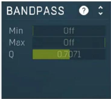
Band-pass panel contains parameters of the follower band-pass filter. Using this feature you can make the follower detect the level of just part of the spectrum instead of all frequencies. For example, when using band-pass from 20Hz to 100Hz the modulator will react mainly to a bass or bass-drum signal.
Min Off
Minimum
Minimum defines the high-pass filter cut-off frequency. The band-pass is disabled if both the minimum and maximum frequencies are set to their limits, thus from 20Hz to 20kHz.
Range: Off to 20.0 kHz, default Off
Max Off
Maximum
Maximum defines the low-pass filter cut-off frequency. The band-pass is disabled if both the minimum and maximum frequencies are set to their limits, thus from 20Hz to 20kHz.
Range: 20.00 Hz to Off, default Off
Q 0.7071 Q
Q defines the bandwidth for the high-pass and low-pass filters.
Range: 0.0500 to 10.0000, default 0.7071
Projection panel
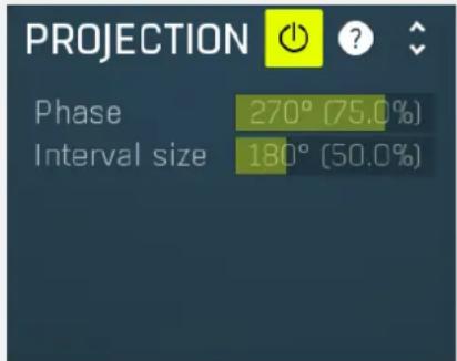
Projection panel contains parameters of projection onto the LFO oscillator shape, which takes the value generated by the modulator and puts it onto the LFO oscillator shape. This features is useful for several creative effects.

Enable
Enable button enables or disables the projection onto the LFO oscillator shape.
Phase 270° [75.0%]
Phase
Phase defines the offset from zero of the signal curve. By default it is 75%, because when you look at common oscillator shapes, such as a sine or triangle, at position 75% its value is minimal. Then when you look at the right side, the value is growing up to the 25%, where it becomes the maximum.
Range: 0 ^ (0%) to 360 ^ (100.0%), default 270 ^ (75.0%)
Interval size 180° (50.0%)
Interval
Interval defines the size of the interval from the oscillator shape in addition to Phase. As a result, phase defines where you start on the shape and interval specifies size of the window on the shape. Default value is 50% as for example sine grows from minimum to maximum in 50% of the period.
Range: 0 ^Â ° (0%) to 720 ^Â ° (200.0%), default 180 ^Â ° (50.0%)
Advanced panel
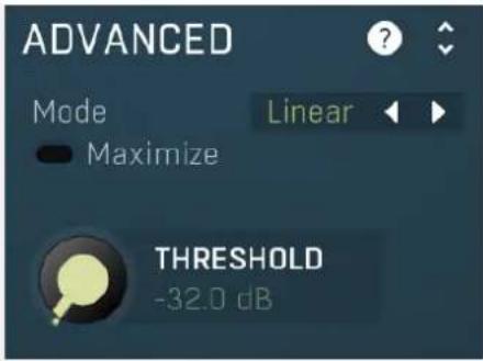
Advanced panel contains some more advanced features of the level follower.
Mode
Linear

Mode
Mode controls the way in which the audio level is treated. Linear mode takes the audio level and uses it directly. This often tends to result in very low modulator values. Squared mode treats the squared levels. This is a compromise between linear and logarithmic modes. Logarithmic mode is the most aggressive one and usually also the most natural as it emulates the logarithmic behaviour of our ears.
Direct mode is quite different as it doesn't really follow the level but instead takes the audio directly without any attack/release processing. It always takes the mid-range value, (minimum + maximum)/2, from each audio block. This is mostly useful for control signals.
For example, let's say your audio level is now -40dB. Then in linear mode it is treated as 1%, because the value of -40dB equals 0.01. In squared mode it becomes 10%. And finally in logarithmic mode it is 33%, because -40dB is 33% of the way from -60dB to 0dB.

THRESHOLD
-32.0 dB
Maximize
Maximize enables threshold-based maximization. Normally the input signal is used to drive the level follower. In this mode however each input sample is treated as 0 or 1, depending on whether it is below or above the threshold. As a result you can get very fast and sharp transitions.
Range: silence to 0.00 dB, default -32.0 dB
LEVEL
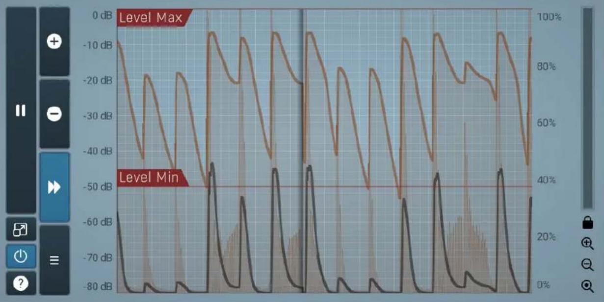
line
| Time | Level Max (dB) | Level Min (dB) | |------|----------------|----------------| | 0 | -10 | -60 | | 5 | -20 | -70 | | 10 | -30 | -80 | | 15 | -40 | -60 | | 20 | -50 | -70 | | 25 | -60 | -80 | | 30 | -70 | -60 | | 35 | -80 | -70 | | 40 | -90 | -80 | | 45 | -100 | -60 | | 50 | -110 | -70 | | 55 | -120 | -80 | | 60 | -130 | -60 | | 65 | -140 | -70 | | 70 | -150 | -80 | | 75 | -160 | -60 | | 80 | -170 | -70 | | 85 | -180 | -80 | | 90 | -190 | -60 | | 95 | -200 | -70 | | 100 | -210 | -80 | | 105 | -220 | -60 | | 110 | -230 | -70 | | 115 | -240 | -80 | | 120 | -250 | -60 | | 125 | -260 | -70 | | 130 | -270 | -80 | | 135 | -280 | -60 | | 140 | -290 | -70 | | 145 | -300 | -80 | | 150 | -310 | -60 | | 155 | -320 | -70 | | 160 | -330 | -80 | | 165 | -340 | -60 | | 170 | -350 | -70 | | 175 | -360 | -80 | | 180 | -370 | -60 | | 185 | -380 | -70 | | 190 | -390 | -80 | | 195 | -400 | -60 | | 200 | -410 | -70 | | 205 | -420 | -80 | | 210 | -430 | -60 | | 215 | -440 | -70 | | 220 | -450 | -80 | | 225 | -460 | -60 | | 230 | -470 | -70 | | 235 | -480 | -80 | | 240 | -490 | -60 | | 245 | -500 | -70 | | 250 | -510 | -80 | | 255 | -520 | -60 | | 260 | -530 | -70 | | 265 | -540 | -80 | | 270 | -550 | -60 | | 275 | -560 | -70 | | 280 | -570 | -80 | | 285 | -580 | -60 | | 290 | -590 | -70 | | 295 | -600 | -80 | | 300 | -610 | -60 | | 305 | -620 | -70 | | 310 | -630 | -80 | | 315 | -640 | -60 | | 320 | -650 | -70 | | 325 | -660 | -80 | | 330 | -670 | -60 | | 335 | -680 | -70 | | 340 | -690 | -80 | | 345 | -700 | -60 | | 350 | -710 | -70 | | 355 | -720 | -80 | | 360 | -730 | -60 | | 365 | -740 | -70 | | 370 | -750 | -80 | | 375 | -760 | -60 | | 380 | -770 | -70 | | 385 | -780 | -80 | | 390 | -790 | -60 | | 395 | -800 | -70 | | 400 | -810 | -80 | | 405 | -820 | -60 | | 410 | -830 | -70 | | 415 | -840 | -80 | | 420 | -850 | -60 | | 425 | -860 | -70 | | 430 | -870 | -80 | | 435 | -880 | -60 | | 440 | -890 | -70 | | 445 | -900 | -80 | | 450 | -910 | -60 | | 455 | -920 | -70 | | 460 | -930 | -80 | | 465 | -940 | -60 | | 470 | -950 | -70 | | 475 | -960 | -80 | | 480 | -970 | -60 | | 485 | -980 | -70 | | 490 | -990 | -80 | | 495 | -100+ | -6 | | >1 | + | + | Note: The chart displays a single line graph with two horizontal lines at different levels of 'Level Max' and 'Level Min'. The y-axis is labeled with values from 'dB' to 'dB'. The x-axis is labeled with 'Time' and 'Label' not explicitly shown.Level
panel
Level panel contains the metering system showing the follower level. It is indispensable when setting up the follower.
The orange graph displays the measured level, which depends on the detector parameters, such as Attack or Release. In most cases you will want to set the follower so that it responds well to the full range of the audio material. After the detector parameters the level range is the next most important and is available via Level min and Level max parameters (these can be also adjusted directly from the analyser). In most cases you will want the minimum level to lie just below the lowest signal peaks and maximum level just above the highest peaks.
The white graph displays the output modulator values. It includes all the processing that affects the modulator including LFO modulation and Project features.

Pause
Pause button pauses the processing.

Popup
Popup button shows a pop-up window and moves the whole metering / time-graph system into it. This is especially useful in cases where you cannot enlarge the meters within the main window or such a task is too complicated. The pop-up window can be arbitrarily resized. In metering mode it is useful for easier reading from a distance for example. In time-graph mode it is useful for getting higher accuracy and a longer time perspective.

Enable
Enable button enables or disables the metering system. You can disable it to save system resources.
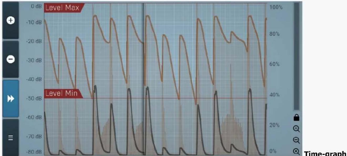
line
| Time - Level | Level Max (dB) | Level Min (dB) | | ------------ | -------------- | -------------- | | 0 | -10 | -60 | | 10 | -20 | -70 | | 20 | -30 | -80 | | 30 | -40 | -60 | | 40 | -50 | -70 | | 50 | -60 | -80 | | 60 | -70 | -60 | | 70 | -80 | -70 | | 80 | -90 | -80 | | 90 | -100 | -60 | | 100 | -110 | -70 | | 110 | -120 | -80 | | 120 | -130 | -60 | | 130 | -140 | -70 | | 140 | -150 | -80 | | 150 | -160 | -60 | | 160 | -170 | -70 | | 170 | -180 | -80 | | 180 | -190 | -60 | | 190 | -200 | -70 | | 200 | -210 | -80 | | 210 | -220 | -60 | | 220 | -230 | -70 | | 230 | -240 | -80 | | 240 | -250 | -60 | | 250 | -260 | -70 | | 260 | -270 | -80 | | 270 | -280 | -60 | | 280 | -290 | -70 | | 290 | -300 | -80 | | 300 | -310 | -60 | | 310 | -320 | -70 | | 320 | -330 | -80 | | 330 | -340 | -60 | | 340 | -350 | -70 | | 350 | -360 | -80 | | 360 | -370 | -60 | | 370 | -380 | -70 | | 380 | -390 | -80 | | 390 | -400 | -60 | | 400 | -410 | -70 | | 410 | -420 | -80 | | 420 | -430 | -60 | | 430 | -440 | -70 | | 440 | -450 | -80 | | 450 | -460 | -60 | | 460 | -470 | -70 | | 470 | -480 | -80 | | 480 | -490 | -60 | | 490 | -500 | -70 | | 500 | -510 | -80 | | 510 | -520 | -60 | | 520 | -530 | -70 | | 530 | -540 | -80 | | 540 | -550 | -60 | | 550 | -560 | -70 | | 560 | -570 | -80 | | 570 | -580 | -60 | | 580 | -590 | -70 | | 590 | -600 | -80 | | 600 | -610 | -60 | | 610 | -620 | -70 | | 620 | -630 | -80 | | 630 | -640 | -60 | | 640 | -650 | -70 | | 650 | -660 | -80 | | 660 | -670 | -60 | | 670 | -680 | -70 | | 680 | -690 | -80 | | 690 | -700 | -60 | | 700 | -710 | -70 | | 710 | -720 | -80 | | 720 | -730 | -60 | | 730 | -740 | -70 | | 740 | -750 | -80 | | 750 | -760 | -60 | | 760 | -770 | -70 | | 770 | -780 | -80 | | 780 | -790 | -60 | | 790 | -800 | -70 | | 80+ | ~-115 | ~-95% |view
Time-graph view shows the measurements over a period of time.
Plus
Plus button increases the time-graph speed (reduces the period that is displayed).

Minus
Minus button decreases the time-graph speed (increases the period that is displayed).

Rewind
Rewind button enables or disables the time-graph static mode. In static mode the graphs are fixed and the current position cycles from left to right; otherwise the graphs move from right to left and the current position is fixed (at the right-hand side).
Envelope mode
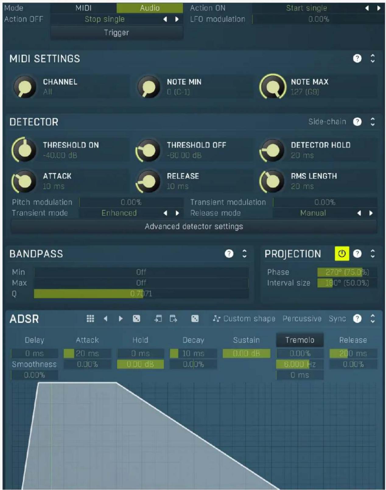
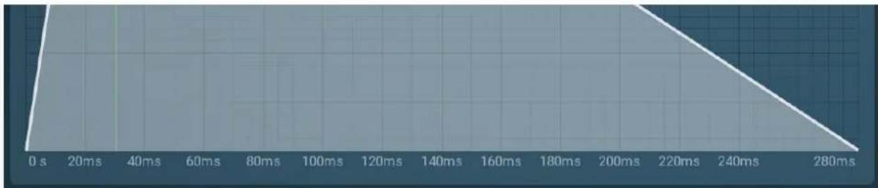
line
| Time (ms) | Value | | --------- | ----- | | 0 | 95 | | 20 | 90 | | 40 | 85 | | 60 | 80 | | 80 | 75 | | 100 | 70 | | 120 | 65 | | 140 | 60 | | 160 | 55 | | 180 | 50 | | 200 | 45 | | 220 | 40 | | 240 | 35 | | 280 | 30 |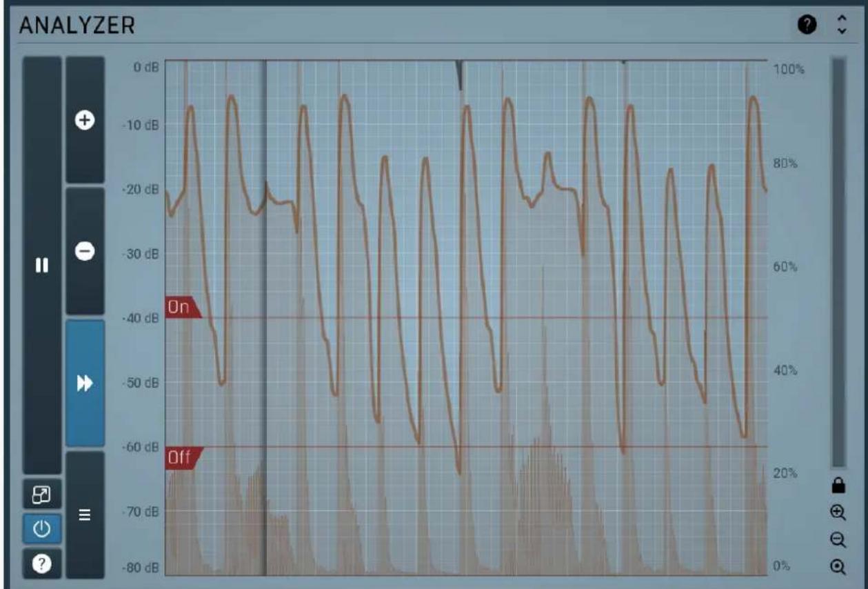
line
| Time | Amplitude (dB) | |------|----------------| | 0 | -25 | | 10 | -15 | | 20 | -30 | | 30 | -45 | | 40 | -60 | | 50 | -75 | | 60 | -90 | | 70 | -105 | | 80 | -120 | | 90 | -135 | | 100 | -150 | | 110 | -165 | | 120 | -180 | | 130 | -195 | | 140 | -210 | | 150 | -225 | | 160 | -240 | | 170 | -255 | | 180 | -270 | | 190 | -285 | | 200 | -300 | | 210 | -315 | | 220 | -330 | | 230 | -345 | | 240 | -360 | | 250 | -375 | | 260 | -390 | | 270 | -405 | | 280 | -420 | | 290 | -435 | | 300 | -450 | | 310 | -465 | | 320 | -480 | | 330 | -495 | | 340 | -510 | | 350 | -525 | | 360 | -540 | | 370 | -555 | | 380 | -570 | | 390 | -585 | | 400 | -600 | | 410 | -615 | | 420 | -630 | | 430 | -645 | | 440 | -660 | | 450 | -675 | | 460 | -690 | | 470 | -705 | | 480 | -720 | | 490 | -735 | | 500 | -750 | | 510 | -765 | | 520 | -780 | | 530 | -795 | | 540 | -810 | | 550 | -825 | | 560 | -840 | | 570 | -855 | | 580 | -870 | | 590 | -885 | | 600 | -900 | | 610 | -915 | | 620 | -930 | | 630 | -945 | | 640 | -960 | | 650 | -975 | | 660 | -990 | | 670 | -1010 | | 680 | -1025 | | 690 | -1040 | | 700 | -1055 | | 710 | -1070 | | 720 | -1085 | | 730 | -1100 | | 740 | -1115 | | 750 | -1130 | | 760 | -1145 | | 770 | -1160 | | 780 | -1175 | | 790 | -1190 | | 800 | -1210 | | 810 | -1225 | | 820 | -1240 | | 830 | -1255 | | 840 | -1270 | | 850 | -1285 | | 860 | -1300 | | 870 | -1315 | | 880 | -1330 | | 890 | -1345 | | 900 | -1360 | | 910 | -1375 | | 920 | -1390 | | 930 | -1410 | | 940 | -1425 | | 950 | -1440 | | 960 | -1455 | | 970 | -1470 | | 980 | -1485 | | 990 | -1500 | | 100+ | ~-88 |Envelope mode makes the modulator generate arbitrary envelopes from input MIDI or by analyzing the audio input level. When using MIDI the modulator responds to input note-on and note-off messages. When using an audio input (if available), the modulator detects the input level and when it exceeds the Threshold On, it behaves like a note-on MIDI event. Afterwards when the level drops down below Threshold Off, it behaves like a note-off MIDI event. Each event can result in just about any action. By default note-on starts the envelope and note-off initiates the release stage, but a different behaviour is also possible depending on Action ON and Action OFF parameters.
Mode MIDI Audio Mode
Mode controls if the envelope is triggered by audio or by MIDI input.
Action ON Start single Action ON
Action ON controls what happens when a note-on event occurs (either via audio or MIDI).
Start single action, which is the default, means that the envelope will start on the note-on event, but only once, it won't start again until you release all of the keys that are relevant for MIDI triggering only. With audio triggering it works the same as Start mode.
Start makes the envelope start every time you press a key, whether another key is already pressed or not. The envelope will seamlessly jump to the attack stage avoiding any abrupt changes.
Start forced is similar, but lets the envelope start from the very beginning every time. So for example if the envelope is currently in a long release stage and the new modulator value is 0.5, then the Start action jumps to a location in the attack stage where there is a value of 0.5 as well, hence avoiding abrupt changes. Start forced action on the other hand starts the whole envelope over from the beginning of the attack stage, where the value is most likely 0.
Start legato is in a way an opposite of the Start single in that it starts only if there is at least one other note already playing. As such it can only be used with MIDI triggering. With audio triggering it works the same as Start mode.
Ignore action simply ignores this event.
The remaining actions are rather creative and let you do the opposite - initiate release stage and stop the envelope when you press a key.
Action OFF Stop single Action OFF
Action OFF controls what happens when a note-off event occurs (either via audio or MIDI).
Stop single action, which is default, means that the envelope will enter the release stage on the note-off event, but only once, at the moment you release the last key (if you were holding more than one) it is relevant for MIDI triggering only.
Stop makes the envelope enter the release stage every time you release a key, whether another key is already pressed or not.
Ignore action simply ignores this event.
The remaining actions are rather creative and let you do the opposite - start the envelope when you release a key.
LFO modulation 0.00% LFO modulation
LFO modulation defines the amount of LFO modulation applied in addition to the envelope. With 0% the modulator uses only the envelope; with 100% the modulator does the same job as if the modulator were in Normal mode. To set the LFO parameters switch to normal mode temporarily.
Range: 0.00% to 100.0%, default 0.00%
Trigger
Trigger
Trigger button servers for manual triggering. It can be associated to other modulators as well for example, so it enables you to trigger the envelope pretty much any way.
MIDI panel
MIDI SETTINGS

CHANNEL
All

NOTE MIN
0 [C-1]

NOTE MAX
127 [G9]
MIDI panel contains parameters of the MIDI event detector.
Detector panel
DETECTOR

THRESHOLD ON
-40.00 dB

THRESHOLD OFF
-60.00 dB

DETECTOR HOLD
20 ms

ATTACK
10ms

RELEASE
10 ms

RMS LENGTH
20 ms
Pitch modulation
Transient mode
0.00%
Enhanced

Transient modulation
Release mode
0.00%
Manual

Advanced detector settings
Detector panel contains parameters of the audio event detector.
Side-chain
Side-chain input
Side-chain input makes the modulator analyze the side-chain input instead of the regular input.

THRESHOLD ON
-40.00 dB
Threshold On
Threshold On defines the note-on level. When the input level rises above it the envelope is started. Then it stays into the sustain stage until the level falls below Threshold Off and the release stage is initiated.
Range: -80.00 dB to 0.00 dB, default -40.00 dB

THRESHOLD OFF
-60.00 dB
Threshold Off
Threshold Off defines the note off level. When the input level rises above Threshold On, the envelope is started. Then it stays into the sustain stage until the level falls below this threshold off and the release stage is initiated.
Range: -80.00 dB to 0.00 dB, default -60.00 dB

DETECTOR HOLD
20ms
Peak hold
Peak hold defines the time that signal level detector holds its maximum before the release stage is allowed to start. As an example, you can imagine that when an attack stage ends there can be an additional peak hold stage and the level is not yet falling, before the release stage starts. This is true only when true peak mode is enabled (check the advanced detector settings if available).
It is often used in gates to avoid the gated level falling below the threshold too quickly, while having short release times. If you want the gate to close quickly, you need a short release time. But in that case the ending may be too abrupt and even cause some distortion. So you use the peak hold to delay the release stage.
It is also used along with look-ahead to avoid distortion in limiters and compressors. If you need a very short attack, the attack stage may be too quick and cause distortions. In limiters this attack time is often 0ms, in which case it becomes a clipper. Setting look-ahead and peak hold to the same value will make the detector move ahead in time, so that it can react to attack stages before they actually occur and yet hold the levels for the actual signal to come.
Range: 0 ms to 10000 ms, default 20 ms

ATTACK
10 ms
Attack
Attack defines the attack time, that is how quickly the level detector increases the measured input level. When the input peak level is higher than the current level measured by the detector, the detector moves into the attack mode, in which the measured level is increased depending on the input signal. The higher the input signal, or the shorter the attack time, the faster the measured level rises. Once the measured level exceeds the Threshold then the dynamics processing (compression, limiting, gating) will start.
There must be a reasonable balance between attack and release times. If the attack is too long compared to the release, the detector will tend to keep the measured level low, because the release would cause that level to fall too quickly. In most cases you may expect the attack time to be shorter than the release time.
To understand the working of a level detector, it is best to cover the typical cases:
In a compressor the attack time controls how quickly the measured level moves above the threshold and the processor begins compressing. As a result, a very short attack time will compress even the beginning transient of a snare drum for example, hence it would remove the punch. With a very long attack time the measured level may not even reach the threshold, so the compressor may not do anything.
In a limiter the attack becomes a very sensitive control, defining how much of the signal is limited and how much of it becomes saturated/clipped. If the attack time is very short, limiting starts very quickly and the limiter catches most peaks itself and reduces them, providing lower distortion, but can cause pumping. On the other hand, a higher attack setting (typically above 1ms) will let most peaks through the limiter to the subsequent in-built clipper or saturator, which causes more distortion of the initial transient, but less pumping.
In a gate the situation is similar to a compressor - the attack time controls how quickly the measured level can rise above the threshold at which point the gate opens. In this case you will usually need very low attack times, so that the gate reacts quickly enough. The inevitable distortion can then be avoided using look-ahead and hold parameters.
In a modulator, the detector is driving other parameters, a filter cut-off frequency for example, and the situation really depends on the target. If you want the detector to react quickly on the input level rising, use a shorter attack time; if you want it to follow the flow of the input signal slowly, use longer attack and release times.
Range: 0 ms to 1000 ms, default 10 ms

RELEASE
10 ms
Release
Release defines the release time, that is how quickly the level detector decreases the measured input level. The shorter the release time, the faster the response is. Once the attack stage has been completed, when the input peak level is lower than the current level measured by the detector, the detector moves into the release mode, in which the measured level is decreased depending on the input signal. The lower the input signal, or the shorter the release time, the faster the measured level drops. Once the measured level falls under the Threshold then the dynamics processing (compression, limiting, gating) will stop.
There must be a reasonable balance between attack and release times. If the attack is too long compared to release, the detector would tend to keep the level low, because release would cause the level to fall too quickly. Hence in most cases you may expect the attack time to be shorter than the release time.
To understand the working of a level detector, it is best to cover the typical cases:
In a compressor the release time controls how quickly the measured level falls below the threshold and the compression stops. As a result a very short release time makes the compressor stop quickly, for example, leaving the sustain of a snare drum intact. On the other hand, a very long release keeps the compression working longer, hence it is useful to stabilize the levels.
In a limiter the release time keeps the measured level above the limiter threshold causing the gain reduction. Having a very long release time in this case doesn't make sense as the limiter would be working continuously and the effect would be more or less the same as simply decreasing the input gain manually. However too short a release time lets the limiter stop too quickly, which usually causes distortion as the peaks through the limiter to the subsequent in-built clipper or saturator. Hence release time is used to avoid distortion at the expense of decreasing the output level.
In a gate the situation is similar to a compressor - the release time controls how quickly the measured level can fall below the threshold at which point the gate closes. Having a longer release time in a gate is a perfectly acceptable option. The release time
will basically control how much of the sound's sustain will pass.
In a modulator, the detector is driving other parameters, a filter cut-off frequency for example, and the situation really depends on the target. If you want the detector to react quickly on the input level falling, use a shorter release time; if you want it to follow the flow of the input signal slowly, use longer attack and release times.
Range: 0 ms to 10000 ms, default 10.0 ms

RMS LENGTH
20 ms
RMS length
RMS length defines the window length used for smoothing the input. In most cases the input waveform contains lots of separate peaks and short transients. All of them would generate note-on events and the spaces between them would similarly cause note-offs. RMS is used to smooth the input. The longer the window, the longer interval it takes and the longer delay it exhibits. If it is too short, unpredictable behaviour can be expected.
Range: 0 ms to 1000 ms, default 20 ms
Pitch modulation
0.00%
Pitch modulation
Pitch modulation lets you employ the pitch detector (configurable from the Pitch tab) in the detector. This may sound odd at first, but thinking of the input signal, you may measure its level, but you can also measure other properties, such as its pitch, and use them in exactly the same way. While an input level is usually understood as a value in decibels, pitch is a frequency in Hz, so the plugin smartly transforms the frequency to mimic the level axis. When you look at the detector graph afterwards, you can hardly tell the exact pitch in Hz, but that's not really relevant or necessary.
What is this for? Let's show it with an example. Let's say you have an instrument, say a bass, which is playing legato, and you want some kind of effect at the beginning of the note (in case of Follower mode) or you just want to restart some kind of filter at the beginning of each note (in case of Envelope mode). But since the performance is legato, meaning there are no gaps in between the notes, the level graph is just a steady horizontal line, which is pretty much useless for us. The pitch modulation lets you replace this horizontal line with something much more useful - the pitch. While the level isn't changing much at all, the pitch is changing. The plugin then takes the actual pitch as the input signal, so you can let the plugin follow it in some way, start envelopes when a certain pitch is exceeded, or using Transformation you can even let the plugin restart an envelope every time the pitch changes. By setting the pitch modulation half-way you can let the plugin react to both properties, the level and the pitch.
Range: 0.00% to 100.0%, default 0.00%
Transient modulation
0.00%
Transient modulation
Transient modulation lets you detect transients and blend that detection with the control signal. This way you may let the modulator be controlled not by level (alone or in combination with pitch for example), but also by transients detected in either of these properties - level or pitch.
Range: 0.00% to 100.0%, default 0.00%
Transient mode
Enhanced

Transient mode
Transient mode controls the way in which the transients are detected. These simply provide different results, so you should just try the alternative modes if the default one doesn't suit your audio material. Attack only modes ignore sustain transients - those moments when the level decreases.
Release mode
Manual

Release mode
Release mode defines how the plug-in performs when decreasing level. In manual mode this is based only on the release time, which is suitable for most cases when the signal has constant characteristics. Automatic release modes can adapt to signals with unstable characteristics.
Automatic and Automatic fast modes: the longer the level stays above the threshold, the longer the release time will be and thus, the longer it will take to move below the threshold and end the release stage. The idea is that if the input is loud for some time, it will most likely stay that way for some more time, hence it should be stabilized to avoid unnecessary temporary fluctuations, which could result in pumping.
Both automatic modes increase the release time when the input signal is above the threshold and vice versa. The speed of the increase depends on the Auto speed parameter. Automatic fast mode uses full speed immediately after crossing the threshold, automatic mode varies the speed according to the current signal level.
For example, when a guitarist plays softly, the level is low and fluctuates around the threshold and the release time gets slower. So the processor quickly responds to sudden changes. However, when the guitarist starts playing a solo, the level rises and, the longer the solo is, the longer the release time becomes, hence the response becomes slower avoiding unnecessary fluctuations (pumping) when the solo contains small silent sections.
Linear 1 and Linear 2 modes: the higher the level is, the longer the release. The idea is that if the input is very loud, it will probably stay that way for some time, so it is wise to keep the levels up too. This is similar to the automatic modes, however the main factor is not how long the level is high, but how high it is.
Below the threshold the release time is the same as the attack time, above the threshold the release time rises from the attack time up to the specified release time parameter. Linear 1 mode usually provides higher release times than does Linear 2.
Opto mode: the higher the level is, the shorter the release. So this is kind of the opposite of linear modes. The idea is, that you are expecting short transients, which you wish to deal with. Normally the higher the level would get in such a transient, the longer it would take to get the level below the threshold, so, when used in a compressor for example, these transients would cause unnecessary compression in the sustain stage. The opto detector lowers the level quickly, minimizing the amount of compression in the sustain stage.
For example, let's say you are compressing a full drumset, but there is a very dominant sharp and short hi-hat sound, so it is
appropriate to have short release times. You would use Opto mode. But the rest of the drumset deserves a softer treatment, so you want to keep longer release times. Use one of the other modes.
Band-pass panel
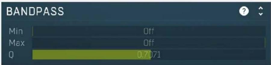
Band-pass panel contains parameters of the envelope detector band-pass. Using this feature you can make the enveloper detect level of just part of the spectrum instead of all frequencies. For example, when using a band-pass from 20Hz to 100Hz the modulator will react mainly to a bass or bass-drum.
Min Off Minimum
Minimum defines the high-pass filter cut-off frequency. The bandpass is disabled if both frequencies are set to their limits, thus from 20Hz to 20kHz.
Range: Off to 20.0 kHz, default Off
Max Off Maximum
Maximum defines the low-pass filter cut-off frequency. The bandpass is disabled if both frequencies are set to their limits, thus from 20Hz to 20kHz.
Range: 20.00 Hz to Off, default Off
Q 0.7071 Q
Q defines the bandwidth for the high-pass and low-pass filters.
Range: 0.0500 to 10.0000, default 0.7071
Projection panel
![PROJECTION Phase 270° [75.0%] Interval size 180° [50.0%]](/content/2026/05/983866/images/5e01d5e2691b48a136fa5056539ab5b56ac744777e2e459f9731de72903e650e.jpg)
Projection panel contains parameters of projection onto the LFO oscillator shape, which takes the value generated by the modulator and puts it onto the LFO oscillator shape. This features is useful for several creative effects.
Enable
Enable button enables or disables the projection onto the LFO oscillator shape.
Phase 270° (75.0%) Phase
Phase defines the offset from zero of the signal curve. By default it is 75%, because when you look at common oscillator shapes, such as a sine or triangle, at position 75% its value is minimal. Then when you look at the right side, the value is growing up to the 25%, where it becomes the maximum.
Range: 0 ^ (0%) to 360 ^ (100.0%), default 270 ^ (75.0%)
Interval size 180° (50.0%) Interval
Interval defines the size of the interval from the oscillator shape in addition to Phase. As a result, phase defines where you start on the shape and interval specifies size of the window on the shape. Default value is 50% as for example sine grows from minimum to maximum in 50% of the period.
Range: 0 ^ (0%) to 720 ^ (200.0%), default 180 ^ (50.0%)

Presets
Presets button displays a window where you can load and manage available presets. Hold Ctrl when clicking to load a random preset instead.

Left arrow
Left arrow button loads the previous preset.

Right arrow
Right arrow button loads the next preset.

Randomize
Randomize button loads a random preset.

Copy
Copy button copies the settings onto the system clipboard.

Paste
Paste button loads the settings from the system clipboard.

Random
Random button generates random settings using the existing presets.

Custom shape
Custom shape
Custom shape button enables custom shape mode, which lets you draw your own attack and release stages using the envelope system. Both stages are then automatically connected to form the resulting envelope.
Percussive
Percussive
Percussive button activates the immediate release mode in which case the note-off causes an immediate switch to the release stage. If this is disabled, the release stage does not occur until the whole attack/decay stage finishes.
Sync
Sync
Sync button controls the ADSR tempo sync feature. By default this is disabled and means that all times are followed exactly, meaning that if Attack is say 100ms, then it will be 100ms indeed. Tempo sync lets the plugin adjust the times to ensure it will be always in sync with the host tempo. In this case 100ms may become say 125ms if the tempo is 120bpm, because 125ms is the length of a 16th note. This makes it extremely simple to convert any envelope to a tempo-synced one. The plugin always chooses the nearest longer note, in other words it always round up.
Straight and Triplets modes automatically find 'nice' values.
For example, if a 16th note takes 100ms, the attack time is 550ms, and the sync mode is straight, then the plugin checks for 100ms, find out that it is too low, so it checks 8th note, being 200ms, still too low, then continues with quarter note, which takes 400ms, and still not enough, finally 800ms corresponding to a half note is the one, so the resulting time will be 800ms. Triplet cases are more complex, but the principle is the same.
1/16, 1/8 and 1/4 modes choose the nearest higher multiply of the base note length. For example, if a 16th note takes 100ms, the attack time is 550ms, and the sync mode is 1/16, the resulting time will be 600ms.
Tremolo
Tremolo
Tremolo button displays additional tremolo settings, containing tremolo behaviour and shape.
Tremolo settings
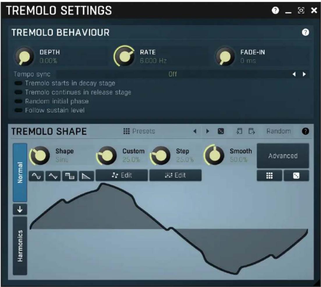
Tremolo behaviour
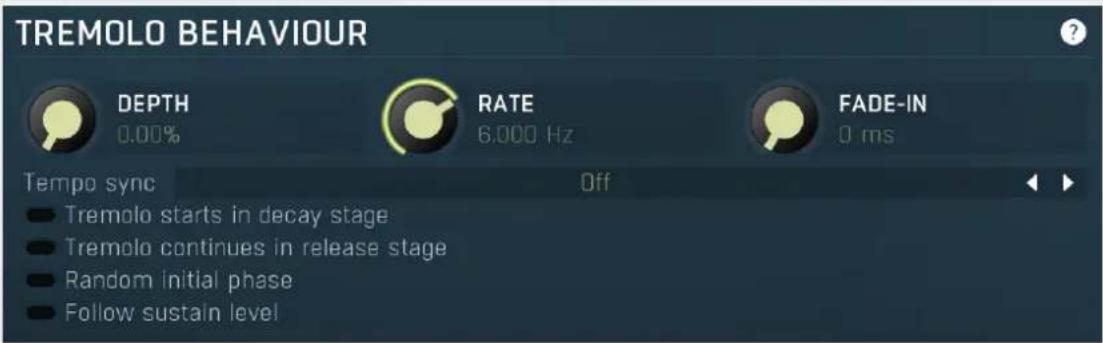

DEPTH
0.00%
Depth
Depth controls the amount of tremolo mixed in the sustain stage (or potentially before).

RATE
6.000 Hz
Rate
Rate controls the tremolo rate and is relevant only if tempo sync is not used.

FADE-IN
0 ms
Fade-in
Fade-in controls the length of the tremolo fade-in. It is especially useful when you want to use the random initial phase feature to avoid the initial discontinuity when the tremolo kicks in.
Tempo sync Off Tempo
sync
Tempo sync lets you synchronize the tremolo to the host's tempo.
Tremolo starts in decay stage
Tremolo
starts in decay stage
Tremolo starts in decay stage makes the tremolo start during the decay stage. By default this is disabled and the tremolo starts in the sustain stage. When it is enabled you will most likely have a longer decay and also a longer tremolo fade-in, so that the tremolo slowly comes in as the envelope is decaying.
Tremolo continues in release stage
Tremolo
continues in release stage
Tremolo continues in release stage makes the tremolo continue with the tremolo during the release stage. By default this is disabled and the tremolo stops as soon as the release stage starts.
Random initial phase
Random
initial phase
Random initial phase makes the tremolo start with a random phase. By default this is disabled and the tremolo starts always starts in the 0 phase, which ensures the tremolo always starts in the same way. However if you play multiple notes at once, the tremolo will be exactly the same, while you may want it to be different for each note and make it sound more 'human'. Enabling this option also activates a short tremolo fade-in to avoid initial discontinuity.
Follow sustain level
Follow
sustain level
Follow sustain level makes the tremolo level based on sustain level. When this is disabled, the tremolo rarely reaches up to 100% level. However if the sustain level is say -20dB, then the tremolo actually cannot exceed 1% (which is -20dB), so it is clipped. It can however go upwards to 100%. This naturally changes the actual tremolo shape. If you want to avoid that and make sine really be a sine for example, enable this option, and in the case above the tremolo will really go up/down -20dB if set to 100%.

Presets
Presets
Presets button displays a window where you can load and manage available presets. Hold Ctrl when clicking to load a random preset instead.

Left arrow
Left arrow button loads the previous preset.

Right arrow
Right arrow button loads the next preset.

Randomize
Randomize button loads a random preset.

Copy
Copy button copies the settings onto the system clipboard.

Paste
Paste button loads the settings from the system clipboard.
Random
Random
Random button generates random settings using the existing presets.
Normal
Normal
Normal button switches the generator into the normal mode, which lets you edit the shape of the oscillator. This is especially advantageous for low-frequency oscillators, where the shape matters even though it doesn't have any physical meaning.

Convert
Convert button converts the current shape into harmonic-based representation. Please note that since the number of harmonics is limited, the result will not perfectly resemble the original shape.
Harmonics
Harmonics button switches the generator into the harmonics mode, which lets you edit the levels and phases of individual harmonics. This is especially advantageous for high-frequency oscillators, hence sound generators.
Signal generator in Normal mode
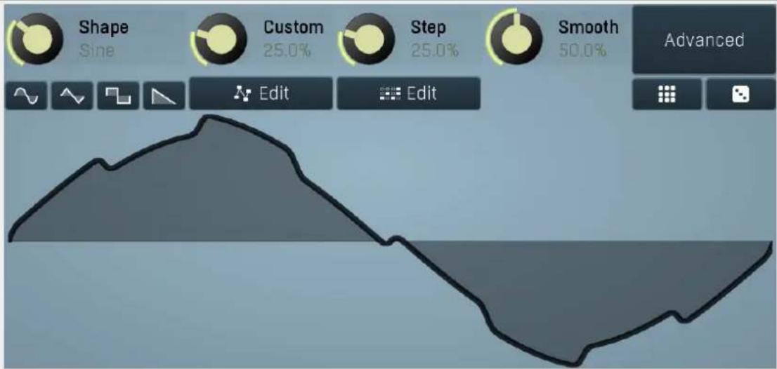
Signal generator in Normal mode works by generating the oscillator shape using a combination of several curves - a predefined set of standard curves, custom shape, step sequencer and custom sample. It also post-processes the shape using several filters including smoothing to custom transformations. This is especially useful when using the oscillator as an LFO (low-frequency-oscillator), where the harmonic contents does not really matter, but the shape does.
Shape
Sine
Shape
Shape controls the main shape used by the signal generator. There are several predefined shapes: exponential, triangle, sine power 8, sine power 4, sine square, sine, harmonics, more harmonics, disharmonics, sine square root, sine 4 root, rectangle, rect-saw, saw, noise and mess. You can choose any of them or interpolate between any 2 adjacent shapes using this control.
Custom
25.0%
Custom
Custom controls the amount of the custom shape that is blended into the main shape.

Edit
Edit
Edit button shows the custom shape editor.
Step
25.0%
Step
Step controls the amount of the step sequencer shape that is blended into the main shape (which has already been blended with the custom shape).
Edit
Edit
Edit button shows the step sequencer editor.
Smooth
50.0%
Smooth
Smooth controls the amount of smoothing. Many shapes, especially those produced by the step sequencer, have rough jagged edges, which may be advantageous, but when used to modulate certain parameters, the output may be clicking or causing other artifacts. Smoothness helps it by smoothing the whole signal shape out and removing these rough edges.
Advanced
Advanced
Advanced button displays an additional window with more advanced settings for post-processing the signal shape, such as harmonics or custom transformations.
Signal generator in Harmonics mode
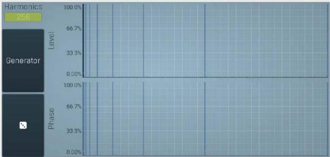
bar
| Level | Phase | |-------|-------| | 1 | 33.3% | | 2 | 66.7% | | 3 | 66.7% | | 4 | 100.0% | | 5 | 0.00% |Signal generator in Harmonics mode works by generating the oscillator shape using individual harmonics. Essentially a harmonic is a sine wave. The first harmonic, known as the fundamental, fits once in the oscillator time period, hence it is the same as selecting sine wave in the Normal mode. The second harmonic fits twice, the third three times etc. In theory, any shape you create in normal mode can be converted into harmonics. However, this approach to signal generation needs an enormous number of harmonics, which is both inefficient to calculate and mostly hard to edit. Therefore, the harmonic mode can process up to 256 harmonics, which is enough for very complex spectrums, however it is still not enough to generate an accurate square wave for example. If your goal is to create basic shapes, it is better to use the normal mode.
It is nearly impossible to say how a particular curve will sound when used as a high-frequency oscillator in a synthesizer, just by looking at its shape. Harmonics mode, on the other hand, is directly related to human hearing and makes this process very simple. In general, the more harmonics you add, the richer the sound will be. The higher the harmonic, the higher the tone. Usually, one leaves the first harmonic enabled too, as this is the fundamental tone, however you may experiment with more dissonant sounds without it.
Editing harmonics can be time consuming unless you hear what you want, so a signal generator is also available. This great tool lets you generate a random spectrum by a single click. You can also open the Generator settings and edit its parameters, which basically control the audio properties in a more natural way - using parameters such as complexity, harmonicity etc.
Generator
Generator
Generator button shows a powerful harmonics generator, which can create unlimited number of various timbres and even analyze a sample and extract harmonics from it.

Randomize
Randomize button selects random parameters for the harmonics generator, so you can use it to get a random sound character instantly. Hold Ctrl to slightly modify existing generator settings instead of completely changing them.
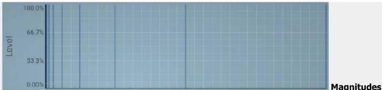
bar
| Level | Magnitudes (%) | |---|---| | 1 | 100.0 | | 2 | 66.7 | | 3 | 33.3 | | 4 | 0.00 | | 5 | 0.00 | | 6 | 0.00 | | 7 | 0.00 | | 8 | 0.00 | | 9 | 0.00 | | 10 | 0.00 | | 11 | 0.00 | | 12 | 0.00 | | 13 | 0.00 | | 14 | 0.00 | | 15 | 0.00 | | 16 | 0.00 | | 17 | 0.00 | | 18 | 0.00 | | 19 | 0.00 | | 20 | 0.00 | | 21 | 0.00 | | 22 | 0.00 | | 23 | 0.00 | | 24 | 0.00 | | 25 | 0.00 | | 26 | 0.00 | | 27 | 0.00 | | 28 | 0.00 | | 29 | 0.00 | | 30 | 0.00 | | 31 | 0.00 | | 32 | 0.00 | | 33 | 0.00 | | 34 | 0.00 | | 35 | 0.00 | | 36 | 0.00 | | 37 | 0.00 | | 38 | 0.00 | | 39 | 0.00 | | 40 | 0.00 | | 41 | 0.00 | | 42 | 0.00 | | 43 | 0.00 | | 44 | 0.00 | | 45 | 0.00 | | 46 | 0.00 | | 47 | 0.00 | | 48 | 0.00 | | 49 | 0.00 | | 50 | 0.00 | | 51 | 0.00 | | 52 | 0.00 | | 53 | 0.00 | | 54 | 0.00 | | 55 | 0.00 | | 56 | 0.00 | | 57 | 0.00 | | 58 | 0.00 | | 59 | 0.00 | | 60 | 0.00 | | 61 | 0.00 | | 62 | 0.00 | | 63 | 0.00 | | 64 | 0.00 | | 65 | 0.00 | | 66 | 0.00 | | 67 | 0.00 | | 68 | 0.00 | | 69 | 0.00 | | 70 | 0.00 | | 71 | 0.00 | | 72 | 0.00 | | 73 | 0.00 | | 74 | 0.00 | | 75 | 0.00 | | 76 | 0.00 | | 77 | 0.00 | | 78 | 0.00 | | 79 | 0.00 | | 80 | 0.00 | | 81 | 0.00 | | 82 | 0.00 | | 83 | 0.00 | | 84 | 0.00 | | 85 | 0.00 | | 86 | 0.00 | | 87 | 0.00 | | 88 | 0.00 | | 89 | 0.00 | | 90 | 0.00 | | 91 | 0.00 | | 92 | 0.00 | | 93 | 0.00 | | 94 | 0.00 | | 95 | 0.00 | | 96 | 0.00 | | 97 | 0.00 | | 98 | 0.00 | | 99 | 133.3% (approx.)graph
Magnitudes graph contains the levels of the individual harmonics. The highlighted bars are octaves, thus the 1st, 2nd, 4th, 8th harmonic etc.
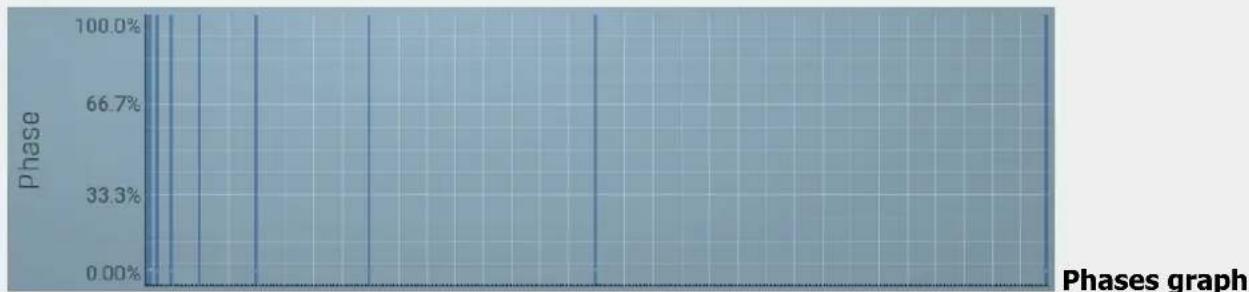
line
| Phase | Value | |-------|---------| | 1 | 100.0% | | 2 | 66.7% | | 3 | 33.3% | | 4 | 0.00% |Phases graph contains the phases of the individual harmonics. The highlighted bars are octaves, thus the 1st, 2nd, 4th, 8th harmonic etc.
0 ms
Delay
Delay lets you shift the entire envelope forwards in time. While this doesn't make much sense for a global instrument envelope for instance, it may be well useful to control characteristics of evolving sounds.
20 ms
Attack
Attack controls the length of the initial stage of the envelope. It is one of the most important parameters controlling how quick the initial transient is. For most instruments the length is quick short, but for pads and other slowly evolving sounds it is quite common to set this to several seconds.
0 ms
Hold
Hold specifies the time the level stays at maximum after the attack stage.
10 ms
Decay
Decay controls the time it takes for the level to drop from the maximum to the Sustain. If the sustain is 0dB, then this parameter has no effect, because in a way the sustain stage starts immediately after the attack.
0.00 dB
Sustain
Sustain controls the sustain level. For most sounds the initial attack transient is the highest point of the entire sound. Imagine playing a string instrument, such as a guitar, the initial hit to the strings is represented by the attack+hold+decay sections and is the most prominent. After that the level drops to the sustain stage, where it holds for most of the time.
0.00%
Tremolo
Tremolo defines the amount of the tremolo effect that is engaged in the sustain, or even in the decay section and continues until the envelope ends. While this is a rather unusual feature for an envelope to have, it is very handy for simulating various effects human players do when performing on real instruments, such as the tremolo or vibrato.
200 ms
Release
Release controls the length of the release section, which usually starts when a note is released.
0.00%
Attack shape
Attack shape controls the shape of the attack section and defines its sound character.
0.00 dB
Hold level
Hold level controls the level of the hold section. By default it equals maximum meaning that the hold section actually holds the maximum level. However by making it lower you can sort of simulate 2 separate decay sections, first going from maximum to hold level, second going from hold level to sustain.
0.00%
Decay shape
Decay shape controls the shape of the decay section and defines its sound character.
6.000 Hz
Tremolo rate
Tremolo rate controls the speed of the tremolo. In the tremolo settings it is possible to control additional characteristics including tempo sync.
0.00%
Release shape
Release shape controls the shape of the release section and defines its sound character.
0.00%
Smoothing
Smoothing lets you smoothen the entire envelope avoiding abrupt jumps. Note that in some cases involving short jumps the results may be a bit obscure.
0 ms
Tremolo fade-in
Tremolo fade-in defines the time for the tremolo to reach its full level. It is a natural behaviour of human players (on say a saxophone) that they don't start a full tremolo immediately and rather let the modulation rise to maximum over a period of time.
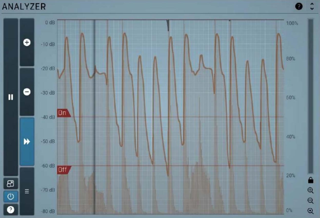
line
| Time (s) | Amplitude (dB) | | -------- | -------------- | | 0 | -25 | | 10 | -15 | | 20 | -30 | | 30 | -45 | | 40 | -60 | | 50 | -75 | | 60 | -90 | | 70 | -105 | | 80 | -120 | | 90 | -135 | | 100 | -150 | | 110 | -165 | | 120 | -180 | | 130 | -195 | | 140 | -210 | | 150 | -225 | | 160 | -240 | | 170 | -255 | | 180 | -270 | | 190 | -285 | | 200 | -300 | | 210 | -315 | | 220 | -330 | | 230 | -345 | | 240 | -360 | | 250 | -375 | | 260 | -390 | | 270 | -405 | | 280 | -420 | | 290 | -435 | | 300 | -450 | | 310 | -465 | | 320 | -480 | | 330 | -495 | | 340 | -510 | | 350 | -525 | | 360 | -540 | | 370 | -555 | | 380 | -570 | | 390 | -585 | | 400 | -600 | | 410 | -615 | | 420 | -630 | | 430 | -645 | | 440 | -660 | | 450 | -675 | | 460 | -690 | | 470 | -705 | | 480 | -720 | | 490 | -735 | | 500 | -750 | | 510 | -765 | | 520 | -780 | | 530 | -795 | | 540 | -810 | | 550 | -825 | | 560 | -840 | | 570 | -855 | | 580 | -870 | | 590 | -885 | | 600 | -900 | | 610 | -915 | | 620 | -930 | | 630 | -945 | | 640 | -960 | | 650 | -975 | | 660 | -990 | | 670 | -1010 | | 680 | -1025 | | 690 | -1040 | | 700 | -1055 | | 710 | -1070 | | 720 | -1085 | | 730 | -1100 | | 740 | -1115 | | 750 | -1130 | | 760 | -1145 | | 770 | -1160 | | 780 | -1175 | | 790 | -1190 | | 800 | -1210 | | 810 | -1225 | | 820 | -1240 | | 830 | -1255 | | 840 | -1270 | | 850 | -1285 | | 860 | -1300 | | 870 | -1315 | | 880 | -1330 | | 890 | -1345 | | 900 | -1360 | | 910 | -1375 | | 920 | -1390 | | 930 | -1410 | | 940 | -1425 | | 950 | -1440 | | 960 | -1455 | | 970 | -1470 | | 980 | -1485 | | 990 | -1500 | | 100 | -1515 |Analyzer panel
Analyzer panel contains the metering system showing the envelope level. It is indispensable when setting up the envelope. The orange graph (assuming the default color) displays the measured level, which depends on the detector parameters, such as RMS length. Its purpose is to smooth the input and to avoid extremely fast fluctuations. The main goal will be to set the Threshold On and Threshold Off properly, so that the events are well detected and there are no false events. Both parameters can be adjusted directly from the graph. In most cases the threshold on will be placed above the threshold off.
The white graph (assuming the default color) displays the modulator values. It includes all the processing that affects the modulator including LFO modulation and Project features.

natural_image
Vertical dark blue gradient bar with a single white double vertical line on the right side (no text or symbols)Pause
Pause button pauses the processing.

Popup
Popup button shows a pop-up window and moves the whole metering / time-graph system into it. This is especially useful in cases where you cannot enlarge the meters within the main window or such a task is too complicated. The pop-up window can be arbitrarily resized. In metering mode it is useful for easier reading from a distance for example. In time-graph mode it is useful for getting higher accuracy and a longer time perspective.

Enable
Enable button enables or disables the metering system. You can disable it to save system resources.
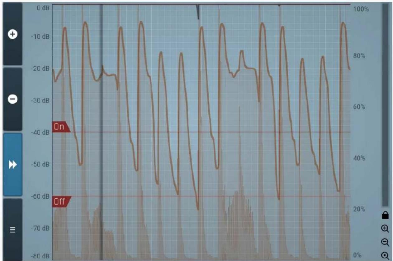
line
| Time | Value (dB) | |------|------------| | 0 | -25 | | 10 | -10 | | 20 | -30 | | 30 | -50 | | 40 | -70 | | 50 | -90 | | 60 | -110 | | 70 | -130 | | 80 | -150 | | 90 | -170 | | 100 | -190 | | 110 | -210 | | 120 | -230 | | 130 | -250 | | 140 | -270 | | 150 | -290 | | 160 | -310 | | 170 | -330 | | 180 | -350 | | 190 | -370 | | 200 | -390 | | 210 | -410 | | 220 | -430 | | 230 | -450 | | 240 | -470 | | 250 | -490 | | 260 | -510 | | 270 | -530 | | 280 | -550 | | 290 | -570 | | 300 | -590 | | 310 | -610 | | 320 | -630 | | 330 | -650 | | 340 | -670 | | 350 | -690 | | 360 | -710 | | 370 | -730 | | 380 | -750 | | 390 | -770 | | 400 | -790 | | 410 | -810 | | 420 | -830 | | 430 | -850 | | 440 | -870 | | 450 | -890 | | 460 | -910 | | 470 | -930 | | 480 | -950 | | 490 | -970 | | 500 | -990 | | 510 | -1010 | | 520 | -1030 | | 530 | -1050 | | 540 | -1070 | | 550 | -1090 | | 560 | -1110 | | 570 | -1130 | | 580 | -1150 | | 590 | -1170 | | 600 | -1190 | | 610 | -1210 | | 620 | -1230 | | 630 | -1250 | | 640 | -1270 | | 650 | -1290 | | 660 | -1310 | | 670 | -1330 | | 680 | -1350 | | 690 | -1370 | | 700 | -1390 | | 710 | -1410 | | 720 | -1430 | | 730 | -1450 | | 740 | -1470 | | 750 | -1490 | | 760 | -1510 | | 770 | -1530 | | 780 | -1550 | | 790 | -1570 | | 800 | -1590 | | 810 | -1610 | | 820 | -1630 | | 830 | -1650 | | 840 | -1670 | | 850 | -1690 | | 860 | -1710 | | 870 | -1730 | | 880 | -1750 | | 890 | -1770 | | 900 | -1790 | | 910 | -1810 | | 920 | -1830 | | 930 | -1850 | | 940 | -1870 | | 950 | -1890 | | 960 | -1910 | | 970 | -1930 | | 980 | -1950 | | 990 | -1970 | | 100+ | -21 |Time-graph view
Time-graph view shows the measurements over a period of time.

Plus
Plus button increases the time-graph speed (reduces the period that is displayed).

Minus
Minus button decreases the time-graph speed (increases the period that is displayed).

Rewind
Rewind button enables or disables the time-graph static mode. In static mode the graphs are fixed and the current position cycles from left to right; otherwise the graphs move from right to left and the current position is fixed (at the right-hand side).

Menu
Menu button displays the time-graph settings. In this window you can control which graphs are displayed, the speed and other relevant parameters.
Random mode
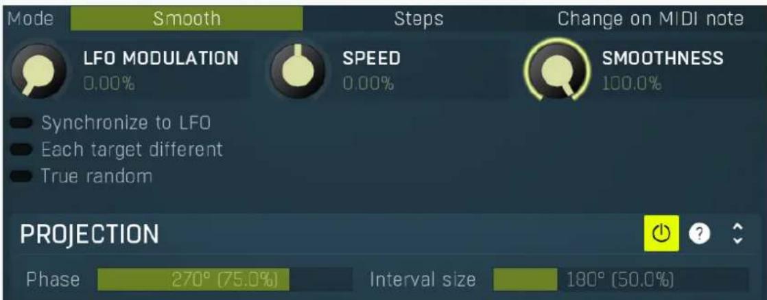
Random mode makes the modulator generate a pseudorandom sequence. Please note that despite its name, it is created so that it generates the same sequence every time. However the generator is linked to the Speed parameter, so if you change it, the whole sequence changes.
Mode Smooth Steps Change on MIDI note Mode
Mode defines the behaviour of the randomizer.
Smooth produces a continuous random modulation. Smoothness then controls how smooth it will be, where 0% means it will connect distinct values by straight lines, 100% means the modulation will be a completely smooth curve walking through these random points. Steps produces a step change every particular time interval. It can also granularize it to s specified number of possible values according to Smoothness value. 100% disables the granularization. Otherwise the number of steps is the number of percentage values, so 3%
means there will be 3 possible values, equally distributed over the range, let's call them 0%, 50% and 100%. Since it doesn't make sense to have 0 or 1 steps, the minimum is always 2. 2 steps essentially means the modulator is randomly switching between the minimum and maximum values for all associated parameters.
Change on MIDI note generates a random value every time a MIDI note is received by the plugin.

LFO MODULATION
0.00%
LFO modulation
LFO modulation defines the amount of LFO modulation applied in addition to the random generator. With 0% the modulator uses only the randomizer; with 100% the modulator does the same job as if the modulator were in Normal mode. To set the LFO parameters switch to normal mode temporarily.
Range: 0.00% to 100.0%, default 0.00%
SPEED
0.00%
Speed
Speed defines the speed of the random changes proportional to the current tempo. 0% means that the speed is the same as your song's tempo.
Range: -1000.0% to 1000.0%, default 0.00%

SMOOTHNESS
100.0%
Smoothness
Smoothness defines the amount of smoothing of the randomizer curve in order to minimize abrupt edges.
Range: 0.00% to 100.0%, default 100.0%
Synchronize to LFO
Synchronize to
LFO
Synchronize to LFO lets you synchronize the speed of the random sequence to LFO (Normal mode), hence also to your host. Speed is still applicable and, for example, +100% means 2x speed, +200% means 4x the speed etc.
Each target different
Each target
different
Each target different transforms value for each target, so that you can easily produce lots of different random values.
True random
True random
True random makes the modulator produce a true pseudo-random sequence independent of the current position within the project. By default this is disabled, so that every time you play your project, it sounds the same. But you might want to enable this option, for live performances for example.
Projection panel
PROJECTION
Phase
270° [75.0%]
Interval size
180° (50.0%)
Projection panel contains parameters of projection onto the LFO oscillator shape, which takes the value generated by the modulator and puts it onto the LFO oscillator shape. This features is useful for several creative effects.

Enable
Enable button enables or disables the projection onto the LFO oscillator shape.
Phase
270° [75.0%]
Phase
Phase defines the offset from zero of the signal curve. By default it is 75%, because when you look at common oscillator shapes, such as a sine or triangle, at position 75% its value is minimal. Then when you look at the right side, the value is growing up to the 25%, where it becomes the maximum.
Range: 0 ^ (0%) to 360 ^ (100.0%), default 270 ^ (75.0%)
Interval size
180° (50.0%)
Interval
Interval defines the size of the interval from the oscillator shape in addition to Phase. As a result, phase defines where you start on the shape and interval specifies size of the window on the shape. Default value is 50% as for example sine grows from minimum to maximum in 50% of the period.
Range: 0 ^ (0%) to 720 ^ (200.0%), default 180 ^ (50.0%)
Pitch mode
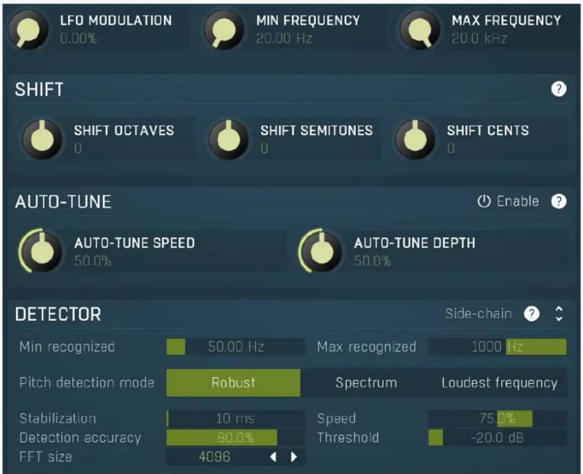
Pitch mode makes the modulator detect the input pitch.

LFO MODULATION
0.00%
LFO modulation
LFO modulation defines the amount of LFO modulation applied in addition to the pitch detector. With 0% the modulator uses only the pitch detector; with 100% the modulator does the same job as if the modulator were in Normal mode. To set the LFO parameters switch to normal mode temporarily.
Range: 0.00% to 100.0%, default 0.00%

MIN FREQUENCY
20.00 Hz
Min frequency
Min frequency defines the frequency, which will cause the modulated parameters to have their minimum values. This basically manipulates the range of the parameters, but it is based on the frequency rather than on parameter values.
Range: 20.00 Hz to 20.0 kHz, default 20.00 Hz

MAX FREQUENCY
20.0 kHz
Max frequency
Max frequency defines the frequency, which will cause the modulated parameters to have their maximum values. This basically manipulates the range of the parameters, but it is based on the frequency rather than on parameter values.
Range: 20.00 Hz to 20.0 kHz, default 20.0 kHz
Shift panel
SHIFT


SHIFT OCTAVES
0

SHIFT SEMITONES
B

SHIFT CENTS
0
Shift panel lets you shift the detected frequency by specified different amounts. All of its parameters do basically the same thing, but in different units.
SHIFT OCTAVES
0
Octaves
Octaves shifts the detected pitch by the specified number of octaves.
Range: -10 to +10, default 0
SHIFT SEMITONES
0
Semitones
Semitones shifts the detected pitch by the specified number of semitones.
Range: -24 to +24, default 0
SHIFT CENTS
0
Cents
Cents shifts the detected pitch by the specified number of cents of a semitone. The actual pitch change is the sum of these 3 control values.
Range: -100.0 to +100.0, default 0
Auto-tune panel
AUTO-TUNE

Enable


AUTO-TUNE SPEED
50.0%

AUTO-TUNE DEPTH
50.0%
Auto-tune panel contains the automatic tuner parameters. When the pitch detector computes the pitch of the input signal, it can further adjust this value in the same way as an automatic tuner plugin, such as MAutoPitch, works. Note that there are no modifications to the input signal, only the pitch is detected differently.

Enable
Enable
Enable button enables or disables the auto-tuner.

AUTO-TUNE SPEED
50.0%
Speed
Speed defines how quickly the plugin adjusts, when a note has been changed. Higher speed makes the results immediately in tune, but can cause less natural results.
Range: 0.00% to 100.0%, default 50.0%

AUTO-TUNE DEPTH
50.0%
Depth
Depth defines how accurate the output should be. With 100% depth the output of the detector shall be exactly in tune. With a lower depth the plugin tolerates more deviation.
Range: 0.00% to 100.0%, default 50.0%
Detector panel
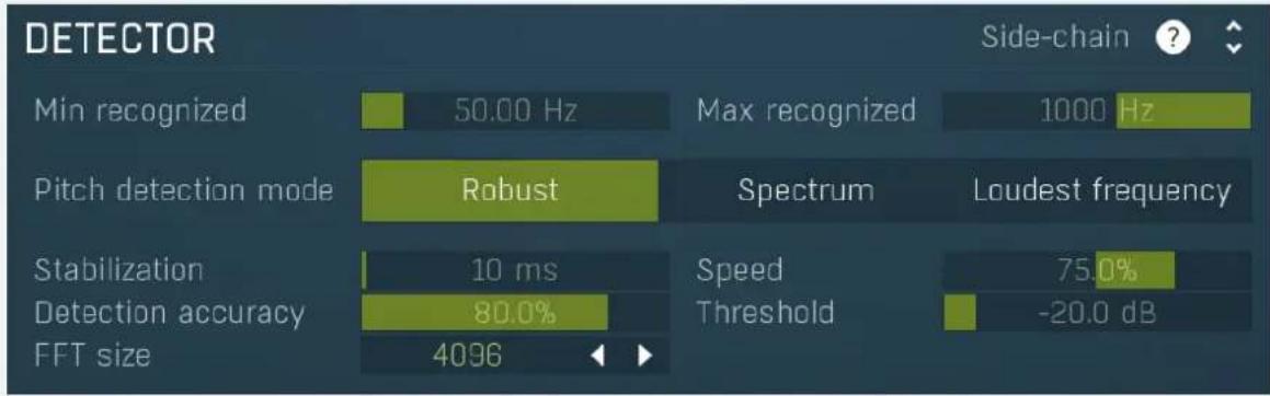
bar
| Category | Value | | --------------------- | --------- | | Min recognized | 50.00 Hz | | Pitch detection mode | Robust | | Stabilization | 10 ms | | Detection accuracy | 80.0% | | FFT size | 4096 |Detector panel contains parameters affecting the pitch detection. You can use them to make the detector work well with your audio material.
Side-chain
Side-chain input
Side-chain input makes the modulator analyze the side-chain input instead of the regular input.
Min recognized
50.00 Hz
Min frequency
Min frequency defines the minimum recognizable frequency. Any frequency below this value will be considered an error and ignored. For example the fundamental frequency of female vocals rarely goes below 100 Hz, so it may be useful to set this value to this limit to ensure that the detector won't pick up hum or vocal tract noises. Range: 20.00 Hz to 20.0 kHz, default 50.00 Hz
Max recognized
1000 Hz
Max frequency
Max frequency defines the maximum recognizable frequency. Any frequency above this value will be considered an error and ignored. For example the fundamental frequency of any vocal rarely goes above 1000 Hz, so it may be useful to set this value to this limit to ensure the detector won't pick harmonics as fundamental.
The pitch detector uses a smart search for fundamentals and avoids harmonics. However if you set this value higher than 2200Hz, it's technically impossible to avoid picking harmonics, so this smart search is disabled. This may be useful for scientific audio analysis, but is not desired for common audio processing.
Range: 20.00 Hz to 20.0 kHz, default 1000 Hz
Pitch detection mode
Robust
Spectrum
Loudest frequency
Pitch
detection mode
Pitch detection mode controls the way the pitch is detected. By default the Robust algorithm is used, which takes into account both spectrum and time properties of the audio signal. In most signals the fundamental frequency is related to the loudest harmonics as well, so normally the engine analyses these relations to find the most probable fundamental. However in some instruments such as bells, there may be lots of inharmonic content available and not so many harmonics, which may confuse the engine. In that case try some of the other modes to see which works the best.
Stabilization
10 ms
Stabilization
Stabilization specifies how quickly can the pitch make bigger changes. This can be useful for more complicated material, such as voice, which often contains short pieces of inharmonic material, which would normally make the detector jump too quickly. Range: 0 ms to 1000 ms, default 10 ms
Speed
75.0%
Speed
Speed specifies how quickly the pitch can change. By lowering this value the pitch won't be able to change so quickly, which can improve audio quality when modulating parameters, which are not handling abrupt changes well. It can also be used creatively. Range: 0.00% to 100.0%, default 75.0%
Detection accuracy
80.0%
Accuracy
Accuracy defines how quickly and accurately the detector will work at the expense of higher CPU usage. Range: 0.00% to 100.0%, default 80.0%
Threshold
-20.0 dB
Threshold
Threshold controls the minimum input level for the pitch to change. This is provided to minimize artifacts caused by the beginning and ending sections of vocals for example, where the pitch usually fluctuates a lot. It also makes the detector ignore noise in-between actual performances.
Range: silence to 0.00 dB, default -20.0 dB
FFT size
4096
◀ ▶
FFT size
FFT size defines the resolution of the pitch detector (for 44/48kHz sampling rates, automatically converted when needed). The higher it is, the more accurate the pitch will be, but its response will also be slower. Range: 256 to 16384, default 4096
MultiParameter editor
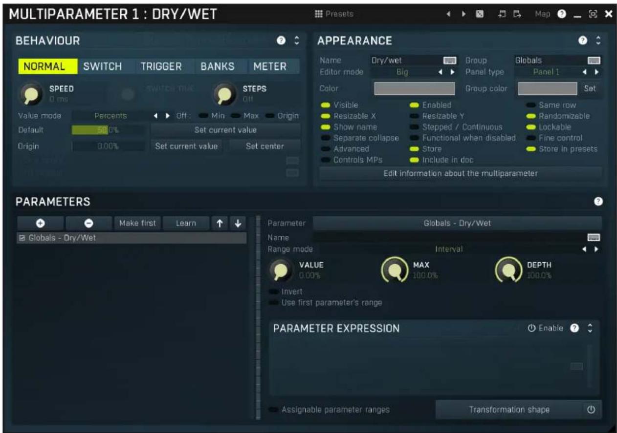
Multiparameter is a powerful structure, which can speed up your workflow significantly and even perform automatic tasks, often useful when performing in real-time for example. Essentially a multiparameter is a controller which controls other parameters, in fact, an unlimited number of them. Each parameter has limits and potentially a transformation curve for more advanced processing. By manually moving the multiparameter (or automating/modulating it) you can control all of the associated parameters at once.
This is just the beginning, but it is worth demonstrating how it could be used. We will show it on a vibrato effect. MVibratoMB (and partly MVibrato) is very good at simulating rotary speakers. A rotary speaker traditionally contains a speed switch, or in our case we will think of it as a speed knob - a control that alters the spin speed of the rotary. This would normally be the Rate parameter of the vibrato. However, when the rate is increased, the vibrato starts changing the pitch too much, sounding a little too "honky-tonk". We can compensate for this by lowering the Depth parameter. As it is not very convenient to control 2 parameters at once, we use a multiparameter to control both parameters with appropriate ranges (ascending for the Rate and descending for the Depth).
Besides this basic usage, multiparameters can also work as triggers and switches. Set a multiparameter's mode to Trigger or Switch and it stops being a slider and becomes a button. When you click the button, the multiparameter starts moving on its own - over the dialled-in switch time it will increase its value (and also the values of any associated parameters) to a maximum and, in the case of trigger mode, then decrease it back to a minimum. In switch mode clicking the button again, the multiparameter decreases back to the minimum value. To make the multiparameter into a simple switch, we can set the switch time to minimum, but in this case we want to extend the functionality in our rotary example.
As mentioned, rotary speakers often have a speed switch. Once switched on, the speed starts increasing until it reaches the "fast" setting, and when switched off, the speed starts decreasing to the original "slow" rate. All we need to do to replicate this functionality is to set the multiparameter's mode to 'switch'.
A real rotary actually has 2 speakers, one for low frequencies and the other for the higher ones. As you might expect, these do not have the same spin rate nor do they speed up or slow down equally either. Here is where we can start showing the true potential of multiparameters.
To simulate this, we have to use two bands of MVibratoMB, the first one will simulate the lower reproductor, and the second will be the higher. We use the first multiparameter to control the first band's rate in the same way as described in the example above. Similarly, we use the second multiparameter to control the second band's rate. Now we have 2 switches and can make each band speed-up or slow-down separately, but we want just one switch for both bands. To do this, we use a third multiparameter to control the first and second multiparameters, in switch mode again but with a 0ms switch time. Pressing the button of the 3rd multiparameter instantly activates the other 2 multiparameters, they both start speeding-up, over a different time period as we requested. Pressing the button again, releases it which also instantly releases the first 2 multiparameters and they start slowing down. Just like the real thing.
Now that we have shown you what is possible with multiparameters, it is worth mentioning that they are used extensively for building devices on the easy screens of most Melda plugins. Every multiparameter given a name in the Information panel will be shown on the Easy screen (if the plugin has one). Check our online video tutorials to get more information about multiparameters and building
devices.
It is also worth mentioning that you can access the multiparameter settings directly from easy screen by holding Ctrl+Alt and clicking on the target control. It may simplify building devices. Note that this may not work for some editor modes such as meters or bar graphs.

Presets
Presets
Presets button displays a window where you can load and manage available presets. Hold Ctrl when clicking to load a random preset instead.

Left arrow
Left arrow button loads the previous preset.

Right arrow
Right arrow button loads the next preset.

Randomize
Randomize button loads a random preset.

Copy
Copy button copies the settings onto the system clipboard.

Paste
Paste button loads the settings from the system clipboard.

Map
Map button displays all current mappings of modulators, multiparameters and MIDI (whichever subsystems the plugin provides).
Behaviour
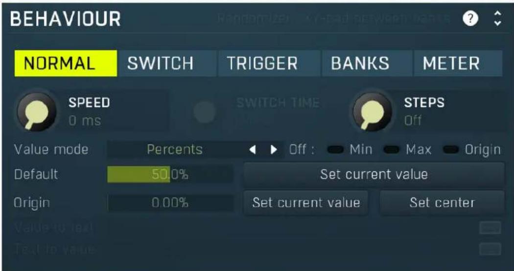
Randomizer
Randomizer switch is available only for Trigger mode and it makes the multiparameter produce random values for each associated parameters. This is useful to implement some sort of randomization feature, which covers a set of parameters. You usually want to set the Switch time to 0, so that the randomization is instant, but longer values may be useful for some creative effects.
K. T. 10. 15. 16. 17. 18. 19. 20. 21. 22. 23. 24. 25. 26. 27. 28. 29. 30. 31. 32. 33. 34. 35. 36. 37. 38. 39. 40. 41. 42. 43. 44. 45. 46. 47. 48. 49. 50. 51. 52. 53. 54. 55. 56. 57. 58. 59. 60. 61. 62. 63. 64. 65. 66. 67. 68. 69. 70. 71. 72. 73. 74. 75. 76. 77. 78. 79. 80. 81. 82. 83. 84. 85. 86. 87. 88. 89. 90. 91. 92. 93. 94. 95. 96. 97. 98. 99.
XY-pad between banks
XY-pad between banks switch is available only for Banks mode and it lets you create XY pads, that would interpolate between 3 or more banks that you specify. With 4 banks the engine creates a classic XY pad, where the 1st bank belongs to the left top corner, 2nd to the right top, 3rd to left bottom and 4th to the right bottom. With more banks the engine creates a circular pad with vertices associated to
individual banks.
Please note that in order for this to work, the multiparameter actual needs 2 multiparameters (X and Y values), hence must NOT be the last one and it occupies the next multiparameter as well. It is recommended to name the next multiparameter and associate it to some parameters, ideally the same ones, just to make sure the engine won't remove it. But in fact only the first multiparameter will actually be working.
NORMAL
SWITCH
TRIGGER
BANKS
METER
Mode
Mode controls the behaviour of the multiparameter.
Normal mode makes the multiparameter work like any other control.
Switch mode hides the slider and shows a button instead. The button has 2 states. By pushing the button, the multiparameter value starts rising from 0% to 100% over a specified time interval. By pushing it again the value starts falling back to 0%. You could do the same thing having the multiparameter in normal mode and moving the slider from left to right and then back, but mode this performs that automatically and maintains a constant time period.
Trigger mode is similar to switch mode, but the button has only a single state and when you push it, the value automatically goes from 0% to 100% and then back without any need to push the button again.
Banks mode is very different. A multiparameter in banks mode keeps several states (called banks) for all of the parameters, much like A-H presets, but only with a limited set of parameters. The multiparameter then morphs between the banks or can be set to switch directly between them (no interpolated values). This is a marvellous way to control many parameters with complex settings by using a single multiparameter.
Let's explain the banks mode in more detail. Say you switch a multiparameter to banks mode, learn a few parameters and set the number of banks to 4. Then bank 1 contains a value for all of the parameters. Similarly bank 2 contains a different value for each of them. And so on. If you set the multiparameter slider to 0% , the associated parameters will be set to values in bank 1. If you set the slider to 100% , bank 4 will be used. If you set the slider to 33.3% , bank 2 will be used. And what if you select 50% ? Then it will be halfway between bank 2 and bank 3.
You can have many banks, you can edit each of them, generate random settings etc. So let's say you want to create some complex movement. You use a multiparameter in banks mode, select a reasonable number of banks. You can edit each of them, but it is easier to use the randomization button to generate random settings for each of them. Then every time you move the multiparameter, all of the associated parameters will move, somewhere between the banks. You can then use a modulator or automation to slowly adjust the multiparameter.
Meter mode makes the multiparameter work as a meter. Instead of controlling other parameters it starts following the value of them. You can then use that to implement a simple meter on the easy screen (if the plugin has one).

Speed
Speed controls the interpolation time. When it is zero and you change the multiparameter value, the associated parameters are adjusted immediately. If this is non-zero however, the actual parameters won't change immediately but will interpolate over time. The speed value is actually the time needed to go from minimum to maximum or vice versa. So if this is 1 second and the current value is say 0% and you click 100%, it will take 1 second for the multiparameter to get there.
This feature is provided mainly because changing some parameter via MIDI or mouse may cause unnecessary zipper noise or inaccuracies due to low MIDI precision. Using the interpolation you can somewhat slow everything down, so that the artifacts become negligible. It can also be used creatively. The default value has been experimentally tested to avoid all artifacts for most parameters.

Switch time
Switch time defines the time needed to switch from the minimum value to the maximum one, or conversely. It is used only in switch and trigger modes.

Steps
Steps lets you create an arbitrary number of equi-distant steps for the multiparameter values. While this technically limits the possibilities of the multiparameter by limiting the number of accessible values, it is sometimes easier to choose from a predefined number of options than from the full range. If you want to use different ranges between the steps, use the Banks mode with Interpolate values disabled.
Percents

Value mode
Value mode defines the units displayed on the multiparameter.
Percents mode lets the multiparameter display percentages between 0% to 100%.
Percents (-100% to 100%) displays percentages between -100% to 100%.
By first parameter mode uses the current value of the first parameter that is controlled by the multiparameter. For example, if you want to control a plugin gain, but also in addition to the changed gain control other parameters, you may still want to call the multiparameter ("gain\" and the units should be decibels as usual, not percentages which do not make much sense for such a multiparameter."
By bank name displays the name of the nearest bank. In some controls, such as switchers, it is possible to display the set of the values as a menu. The menu is created automatically and it even creates groups for better clarity, based on the prefix of the bank names. You can use ' # ' (hashtag surrounded by spaces) to define the groups manually like this: "group # name". For example, you can name one bank "Main group # First bank" and another "Main group # Second bank", and these will be displayed in a single group in the menu. If you are going to use this method, make sure the ' # ' sequence is present in each bank's name.
By bank name interpolated considers name of all banks numbers. It then interpolates between them and displays the result as a number.
By bank name interpolated log is similar, but interpolates the values in logarithmic domain.considers name of all banks numbers. It's useful for units, which are naturally logarithmics, such as frequency.
By bank number shows the index of the nearest bank.
Expression lets you formulate the value -> text and back using mathematical expressions and can be used for some more complex MPs or if you need some custom units.
Default
50.0%
Default
Default controls the default value of the multiparameter. You can edit it directly or just set the MP into its reasonable default and click the Set current value. Most GUI components created for the multiparameter respond to right-click by setting the default value in the same way that other parameters do. It is essential for user experience when building your own devices.
Set current value
Set current value
Set current value stores the current value as the default one for the multiparameter.
Origin
0.00%
Origin
Origin informs the GUI engine of the origin of the value. For instance, a default value for panorama is in the center and it is logical that visual elements controlling panorama should somehow highlight the center position. If, for example, you are using a value button to edit the panorama, by default it displays the current value using a bar starting from the left side (being the origin defined as minimum) towards the actual value, but here it is better to display the bar from the center towards the current value, whether it is on the left or right of the center. Therefore the center should be the origin.
Set current value
Set current value
Set current value stores the current value as the origin for the multiparameter.
Set center
Set center
Set center sets the center (50%) as the origin for the multiparameter. This is often the case for parameters such as gain and panorama, so it deserves a dedicated button. It is supported only for knobs.
Value to text
Value to text is available only with Expression Value mode and lets you enter a text featuring mathematical expressions to produce the units. This can be used for more complex multiparameters. The text itself is just another text, but it can contain substrings of this structure:
{expression}
or
{expression;decimals}
where expression is the actual mathematical expression and decimals is the number of decimal places in the resulting value. Here is the list of variables available for each expression:
x = the multiparameter value in 0..1
sr = current sampling rate
Functions and features of the expressions are available below. Now let's see a few examples:
Test: {x} - produces "Test: 0.12" (with MP value 0.1234)
x (x*100;0%) - produces "0.12 (12%)" (with MP value 0.1234)
{ffrom01(x);1} Hz - produces say "215.56 Hz" ("20.0 Hz" for MP value 0 and "20000.0 Hz" for MP value 1)
{todb(sqr(x));4} dB - produces "-12.0412 dB" for 0.5. "sqr" is used to mimic the transformation used in pretty much every Volume parameter in MeldaProduction plugins.
Expression evaluator uses traditional C/C++ style formatting, which is natural for most people. It provides arithmetics, logical and conditional operators. Following terms are supported:
Constants: pi, e, sqrt2, ln2
Arithmetic operators:
-a inverts the sign, e.g. "-x" produces +2 for x=-2
a+b= addition
a-b = subtraction
a*b = multiplication
a/b = division
a%b = modulo, remainder after division
a^b = power, e.g. "2^3" produces 2*2*2 = 8
Arithmetic functions:
min(a,b) = minimum of both values
max(a,b) = maximum of both values
limit(a,min,max) = a limited into the interval min..max
to01(a,min,max) = converts "a" as min..max to 0..1
from01(a,min,max) = converts "a" as 0..1 to min..max
tom11(a,min,max) = converts "a" as min..max to -1..1
fromm11(a,min,max) = converts "a" as -1..1 to min..max
Basic mathematic functions: abs(x) = absolute value , e.g. abs(-3) = 3 sqr(x) = xx sqrt(x) = square root exp(x) = natural exponential e^x ln(x) = natural logarithm log10(x) = logarithm with base 10 log(x, base) = logarithm with specified base inv(x) = 1/x sgn(x) = sign of x, -1 or 0 or +1 depending on xx round(x) = rounding to the nearest value floor(x) = rounding to the nearest lower value, e.g. floor(-2.3) = -3 ceil(x) = rounding to the nearest higher value, e.g. ceil(-2.3) = -2 rand(x) = random value from 0 to x
Functions for specific units:
f01(a) = converts "a" as frequency from 20...20000 into log scale 0..1
ffrom01(a) = converts "a" as 0..1 (log scale) to frequency from 20...20000
todb(a) = converts "a" as multiplier to dB value by calculating "20*log10(a)"
fromdb(a) = converts "a" as dB value to multiplier by calculating "10^(a/20)"
Trigonometric functions: (x) , asin(x) , (x) , acos(x) , (x) , atan(x) , (x) , (x) , (x)
Logical operators:
a==b = comparison producing 1 if "a" and "b" are equal, 0 otherwise
a!=b = comparison producing 1 if "a" and "b" are NOT equal, 0 otherwise
a<b = comparison producing 1 if "a" is lower than "b", 0 otherwise
a<=b = comparison producing 1 if "a" is lower or equal to "b", 0 otherwise
a>b = comparison producing 1 if "a" is greater than "b", 0 otherwise
a>=b = comparison producing 1 if "a" is greater or equal to "b", 0 otherwise
!a = logical negation, 0 produces 1, 0 otherwise
a&&b = logical AND, produces 1 if both "a" and "b" are nonzero
a||b = logical OR, produces 1 if any of "a" and "b" are nonzero
a^^b = logical XOR, produces 1 if "a" and "b" are logically different
a ? b : c = if a is nonzero, then the result is b, otherwise it is c}}
Text to value
Text to value is available only with Expression Value mode and lets you convert a number user enters as a text input into the multiparameter value in 0..1. This can be used for more complex multiparameters. Unlike Value to text here you need to enter a single expression, no need for any other text. If the resulting value exceeds the 0..1 interval, it is automatically limited. Here is the list of variables available for the expression:
x = the value the user entered
sr = current sampling rate
Functions and features of the expressions are available below. Now let's see a few examples:
x - sets MP to 0.1234 if the user entered "0.1234"
x/100 - sets MP to 0.1234 if the user entered "12.34" (or "12.34%" for example)
fto01(x) - sets MP to the proper frequency in log scale, e.g. 20 is translated to 0, 20000 to 1
fromdb(sqrt(x)) - sets MP to 0.5 if the user entered "-12.0412" (or "-12.0412 dB" for example). "sqrt" is used to mimic the transformation used in pretty much every Volume parameter in MeldaProduction plugins.
Expression evaluator uses traditional C/C++ style formatting, which is natural for most people. It provides arithmetics, logical and conditional operators. Following terms are supported: Constants: pi, e, sqrt2, ln2
Arithmetic operators:
-a inverts the sign, e.g. "-x" produces +2 for x=-2
a+b = addition
a-b = subtraction
a*b = multiplication
a/b = division
a%b = modulo, remainder after division
a^b = power, e.g. "2^3" produces 2*2*2 = 8
Arithmetic functions:
min(a,b) = minimum of both values
max(a,b) = maximum of both values
limit(a,min,max) = a limited into the interval min..max
to01(a,min,max) = converts "a" as min..max to 0..1
from01(a,min,max) = converts "a" as 0..1 to min..max
tom11(a,min,max) = converts "a" as min..max to -1..1
fromm11(a,min,max) = converts "a" as -1..1 to min..max
Basic mathematic functions: ( \text{abs}(x) = \text{absolute value} ) , e.g. ( \text{abs}(-3) = 3 \text{ sqr}(x) = x*x \text{ sqrt}(x) = \text{square root exp}(x) = \text{natural exponential } e^{\wedge}x \text{ ln}(x) = \text{natural logarithm log10}(x) = \text{logarithm with base 10 log}(x, \text{base}) = \text{logarithm with specified base inv}(x) = 1/x \text{ sgn}(x) = \text{sign of } x, -1 \text{ or } 0 \text{ or } +1 \text{ depending on } x*x \text{ round}(x) = \text{rounding to the nearest value floor}(x) = \text{rounding to the nearest lower value, e.g. floor}(-2.3) = -3 \text{ ceil}(x) = \text{rounding to the nearest higher value, e.g. ceil}(-2.3) = -2 \text{ rand}(x) = \text{random value from 0 to
x
Functions for specific units:
f01(a) = converts "a" as frequency from 20...20000 into log scale 0..1
ffrom01(a) = converts "a" as 0..1 (log scale) to frequency from 20...20000
todb(a) = converts "a" as multiplier to dB value by calculating "20*log10(a)"
fromdb(a) = converts "a" as dB value to multiplier by calculating "10^(a/20)"
Trigonometric functions: (x) , asin(x) , (x) , acos(x) , (x) , atan(x) , (x) , (x) , (x)
Logical operators:
a==b = comparison producing 1 if "a" and "b" are equal, 0 otherwise
a!=b = comparison producing 1 if "a" and "b" are NOT equal, 0 otherwise
a<b = comparison producing 1 if "a" is lower than "b", 0 otherwise
a<=b = comparison producing 1 if "a" is lower or equal to "b", 0 otherwise
a>b = comparison producing 1 if "a" is greater than "b", 0 otherwise
a>=b = comparison producing 1 if "a" is greater or equal to "b", 0 otherwise
!a = logical negation, 0 produces 1, 0 otherwise
a&&b = logical AND, produces 1 if both "a" and "b" are nonzero
a||b = logical OR, produces 1 if any of "a" and "b" are nonzero
a^^b = logical XOR, produces 1 if "a" and "b" are logically different
a ? b : c = if a is nonzero, then the result is b, otherwise it is c}}
Appearance
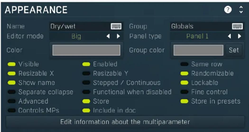
Name
Dry/wet

Name
Name specifies the name of the multiparameter, which is shown on the multiparameter button. The name is also used for devices - the multiparameter serves as a parameter for the device (on the Easy screen). If no name is specified or if the first character is an *, then the parameter is hidden. This is useful if you need some internal multiparameters which you don't want to show on the Easy screen for some reason.
Group
Globals

Group
Group can be used to put some multiparameters into the same group, which results in them being placed in the same panel on the Easy screen (the device editor). Additionally you can actually place the groups into tabs by setting group to "tabname#groupname". The name of the tab needs to be there only for the first parameter of the new group. This makes it possible to build a complex devices with dozens of parameters.
Editor mode
Big

Editor mode
Editor mode controls the way the multiparameter are to be displayed on the Easy screen.
Normal is the default mode and is represented by a small knob or button.
Big mode is similar, but uses a big knob or big button.
Button mode displays a value button, which is usually more compact than knobs.
Check-boxes makes the multiparameter displayed as a set of checkboxes (also called radio buttons). It is relevant only in Banks mode.
Check-boxes horiz & below is similar but displays the checkboxes in a single row, hence horizontally. Below mark makes the label underneath the actual checkbox.
Switcher and Selectors are useful for selecting a number of discrete values and similarly to check-boxes these are working only in
Banks mode.
Title button places the control into the title bar of the panel to which it belongs.
Title enable button places the control into the title bar of the panel to which it belongs and makes it a standard enable button (which also makes all controls within the panel unavailable if it is itself disabled).
XY pad creates a 2 dimensional XY pad control, that edits this multiparameter in the X axis and the next multiparameter in the Y axis.
There are multiple versions of this control, all of them differ only by size.
Spacer is a helper mode for device design, which doesn't display anything and only keeps empty space.
Meter creates a simple meter instead. You will probably want to set the multiparameter to Meter mode as well or attach it to a modulator. Meters don't really control anything and their purpose is purely to get a visual feedback. The meters can be horizontal or vertical and they can be up or down. Up is the usual choice useful for peak meters for example. Down is useful for gain reduction meters.
Bars start/end mode creates an editor, similar to step sequencer editor, where each parameter has its own bar. The Bars start starts the editor and all multiparameters are then added to it until a multiparameter with Bars end mode is found or until there are no remaining multiparameters. Note that this kind of editor doesn't show units and may have several other limitations.
Order is a very specific editor for Order modules available in modular systems such as MXXX. It lets you provide an processing order editor on the easy screen. To use it, attach the MP to Order parameter of the Order module and edit the MP information field, so that it contains all the items to be ordered, separated by ';'. The number of items must match the number of items in the Order module, otherwise the order won't work properly. You can also include colors for each item separated by # (hexa or one of the predefined set: Dynamics, Distortion, Modulation, Stereo, Spectral, Synthesis, Instrument, MDrummer, Reverb, Delay, EQ, Filter, Saturation, Limit, Time, Pitch, FX) and enable MP indices.
Example of the info: Compressor#Dynamics;EQ#EQ;Limiter#007F7F;Something
Panel type Panel 1
Panel type
Panel type defines the type of panel in which multiple controls of the same group are placed. These differ only in their graphics display.
Color
Color
Color defines colorization for the element on the Easy screen (if the plugin has one). The feature is disabled if the Alpha value of the color is 0. Using this feature often increases memory consumption of the plugin, so make sure you use it only if necessary and try to use as low a number of different colors as possible. It is recommended to use only the snapshot colors to make sure the same colors are used in most cases, reducing the memory consumption. It is also highly recommended to use colors with a value (lightness) of 128 (the middle value), which makes sure that the lightness of the elements won't be changed. This works best for most styles. Please note that the style may be configured to simply ignore this color, so there may be no change at all. If you use this feature, make sure that you test it with all styles.
For the sake of workflow the colors have predefined meanings. It's highly recommended to follow this standard:
Orange - dynamics
Green - equalization, filtering
Brown/yellow - reverb, delay
Blue - modulation
Red - limiting, saturation, distortion
Cyan/yellow - stereo
Purple/pink - time, pitch, unison...
Grey - utilities, tools
Group color
Set
Group color
Group color defines colorization for the group panel on the Easy screen (if the plugin has one) and is ignored for all multiparameters except for the first one in a group. The feature is disabled if the Alpha value of the color is 0. Using this feature often increases memory consumption of the plugin, so make sure you use it only if necessary and try to use as low number of different colors as possible. It is recommended to use only the snapshot colors to make sure the same colors are used in most cases, reducing the memory consumption. It is also highly recommended to use colors with a value (lightness) of 128 (the middle value), which makes sure that the lightness of the elements won't be changed. This works best for most styles. Please note that the style may be configured to simply ignore this color, so there may be no change at all. If you use this feature, make sure you test it with all styles.
For the sake of workflow the colors have predefined meanings. It's highly recommended to follow this standard:
Orange - dynamics
Green - equalization, filtering
Brown/yellow - reverb, delay
Blue - modulation
Red - limiting, saturation, distortion
Cyan/yellow - stereo
Purple/pink - time, pitch, unison...
Grey - utilities, tools
Set
Set
Set button sets the color and group color for all multiparameters in the same group. It is pretty sensible to do that as all controls should look similar within each group. This can also be done by editing each parameter, but this way is easier.

Visible
Visible
Visible checkbox controls if the parameter is visible on the Easy screen (if the plugin has one). Its effect is similar to the '*' prefix in the parameter name, but the multiparameter's name is also available to the plug-in host. This is useful when you wish to automate that multiparameter from the host but not show it on the Easy screen. This parameter can also be attached to another multiparameter for
example in order to change the GUI somehow.

Enabled
Enabled
Enabled switch enables/disables the multiparameter. If disabled, it is grayed on the easy screen.

Same row
Same row
Same row checkbox defines if the parameter should be displayed next to the previous one on the Easy screen. Otherwise it will placed on the next row. This setting serves as a hint and the plugin may ignore it, if it is impossible to do.

Resizable X
Resizable X
Resizable X switch lets you specify if the panel could be resized. It is on by default to make sure everything gets resized, however using multiple panels next to each other, it may be advantageous to disable resizing of some of them to save space. Otherwise e panel's size is proportional to number of controls it contains, which could make some of the panels larger than actually necessary

Resizable Y
Resizable Y
Resizable Y switch lets you specify if the panel could be resized vertically. It is off by default to make sure everything has the m size it requires, but for aesthetic reasons you may want to make all groups on the same row the same size even if the controls in them are not.

Randomizable
Randomizable
Randomizable option defines if the multiparameter can be randomized on the easy screen. You may want to disable this for input gain for example.

Show name
Show name
Show name option lets you show or hide the name of the multiparameter for some editor modes. The option has no effect for se editor modes.

Stepped / Continuous
Stepped / Continuous
Stepped / Continuous option tells the engine that the multiparameter can be in 2 modes, stepped or continuous. If so, it is assumed you either used Banks mode or Steps to produce some sort of predefined set of values for the stepped mode. By enabling this option you allow the engine to convert the multiparameter to continuous mode by either ignoring the steps or interpolating the bank value can be used when designing devices.

Lockable
Lockable
Lockable option creates a lock button next to the parameter on the Easy screen, allowing the user to browse through presets with this parameter changing. Please note that this feature is available only for some editor modes.
When the parameter is first locked on the Easy screen it is added to the set of lockable parameters (which are listed in the Global window).

Separate collapse
Separate collapse
Separate collapse checkbox makes the panel collapsable separately on the Easy screen. By default it is disabled and that makes engine find all panels on the same row and collapse all of then or none of them.

Functional when disabled
Functional when disabled
Functional when disabled switch makes the multiparameter work even when disabled. This may be useful in some complex sce where you need to make the MP control the target parameters and only use the Enabled flag to grey out the controls on the easy screen.

Fine control
Fine control
Fine control switch makes the multiparameter editor steps extra small, which is useful, when you need very high precision. This handy when using banks mode with many banks interpolating.

Advanced
Advanced
Advanced switch makes the multiparameter 'advanced', disabled by default. If such an multiparameter exists, the engine also creates a button to show/hide all advanced multiparameters. In effect this lets you create a simple GUI with optional advanced controls.

Store
Store
Store makes the multiparameter stored. Relevant when creating devices. In some rare cases you may want to disable this, e.g. if value is a meter or somehow it just doesn't need to be save at all.

Store in presets
Store in presets
Store in presets makes the multiparameter stored in presets. Relevant when creating devices. In some cases you may want to store value, but ignore it when browsing presets. For instance, input gain may be ignored if the user is supposed to set the gain to some predefined value and then browse the presets without changing that gain.

Controls MPs
Controls MPs
Controls MPs informs the engine that this MP is controlling other multiparameters. As such it shouldn't be 'invoked' unless it is touched by the user. This is relevant for example when it is used in a device with a device presets - loading a device preset involve relevant MPs, so that the state of the device is remembered properly, but invoking this one would actually make things incorrect

Include in doc
Include in doc
Include in doc makes the multiparameter's help included in the documentation / panel help. You may want to disable this if there are multiple 'identical' controls with the exact same help info, for all of them except for one.
Edit information about the multiparameter
Edit information
about the multiparameter
Edit information about the multiparameter lets you edit the information displayed as help for the multiparameter control on the easy screen. It can use a simplified HTML format, but in practice only following tags are likely to be useful:
= bold text
= italic text
For example:
When Order control is used, the first line of the information can contain additional info of ";" separated individual items in the following format:
name{#hexcolor}{*index of the enable MP} where {} denotes an optional item.
For example: Reverb;EQ#7F0000;Flanger#007F00*3
In this example, the order is probably used to control order of effects. When the order MP value is set to 0, Reverb is the first, with no specific color and no MP to enable/disable it. Flanger is next, the color is red, but no enable either. Finally Flanger is the third, it is green and MP3 is used to enable/disable it.
Parameters panel
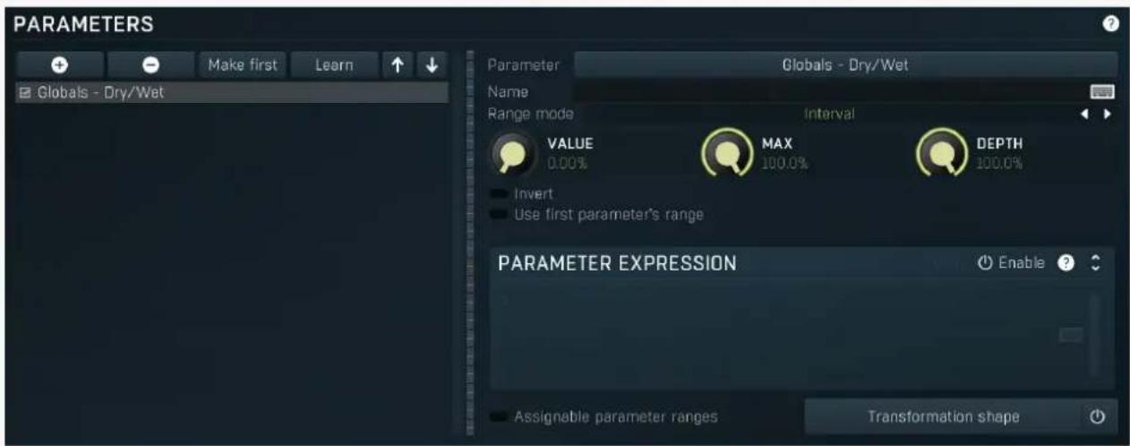
Parameters panel configures how the multiparameter assigns values to the target parameters.

Add
Add button adds a parameter to the list of controlled parameters. Alternatively you can use the learn feature available by right-clicking the multiparameter button.
Delete
Delete button deletes the selected parameter from the list of controlled parameters.
Make first
Make first
Make first button moves the selected parameter to the first item in the list. This is useful for sake of the By first parameter value mode, which makes the multiparameter show the units of the first parameter in the list. Please note that if you have some other multiparameter, modulator or another subsystem access the ranges of individual parameters, this function will reorder them, so these connections will no longer be correct.
Learn
Learn
Learn button starts or stops the learning. Click it, then move some parameters in the plugin, then click it again. Learning can also be accessed from the global multiparameter menu.

Up
Up button moves the selected parameter up one item, if possible. This may be useful when keeping things organized, but please note that if you have some other multiparameter, modulator or another subsystem access the ranges of individual parameters, this function will reorder them, so these connections will no longer be correct.

Down
Down button moves the selected parameter down one item, if possible. This may be useful when keeping things organized, but please note that if you have some other multiparameter, modulator or another subsystem access the ranges of individual parameters, this function will reorder them, so these connections will no longer be correct.
Parameter
Globals - Dry/Wet
Parameter
Parameter defines the target parameter which is being modulated. The set contains all automatable parameters.
Name

Name
Name lets you name the parameter somehow and may be helpful in situations, where there are many parameters being edited without obvious meanings.
Assignable parameter ranges
Assignable parameter ranges
Assignable parameter ranges allows you to assign parameter ranges of several first parameters to other subsystems such as multiparameters or modulators. By default it is disabled, which removes all the relevant parameters to save valuable resources. This feature is available only if automation compatibility mode for V10 is disabled.
Transformation shape

Transformation shape
Transformation shape button displays the graph editor, which lets you tweak the shape of the curve used to control the selected parameter. The X axis shows the original values, the Y axis defines the results. Please note that this takes some CPU, therefore you have to enable it using the enable button in the title bar.
Range mode
Interval

Range
mode
Range mode defines how the parameter range is selected. While sometimes it is better to specify minimum and maximum, other times it is better to use a nominal center and depth (\% of full scale). This control allows you to define which one it will be.
Up and down mode makes the values go above and below the selected Value, which is considered the center. The interval is made smaller if necessary.
Full range mode is similar, except the range is symmetrically constrained, so the selected Value may not be the center anymore.
Up/down only modes goes from the selected value up/down only.
Let's compare these 4 modes. Taking a value of -12dB value, with a depth of 75% and a scale of +/- 24dB. The nominal range is therefore = +/-24 dB * 75% = 36dB. With values of 0%, 50% and 100% the outputs are:
Up and down: -24, -12, 0 (range constrained to 12 dB either side)
Full range: -24, -6, 12 (range limited to minimum, but not constrained)
Up only: -12, 6, 24 (range not constrained = +/-24 dB * 75% = 36dB)
Down only: -12, -18, -24 (range limited to minimum)
Interval mode is the most simple one and goes from Value to Maximal value.

VALUE
0.00%
Value
Value defines the center of the target parameter's range or the minimum if the Range mode is set to Interval.

MAX
100.0%
Maximal value
Maximal value defines the upper limit of the target parameter's range. It is available only if the Range mode is set to Interval. This value can be lower than Value. 0% is always mapped to reference>Value and 100% to reference>Maximal value.
Depth defines size of the target parameter's range. It is used only if the Range mode is not set to Interval.
Invert
Invert
Invert checkbox inverts the target parameter's range, so that minimum becomes maximum and vice versa.
Use first parameter's range
Use first
parameter's range
Use first parameter's range makes the parameter display use the same range as the first parameter in the list. This is often useful if want to control the range in some way and apply the range to multiple parameters.
Parameter expression
PARAMETER EXPRESSION
Enable

Parameter expression panel lets you provide an algebraic expression for computing the final parameter value. Here are several predefined variables you can use in your expressions (# denotes a positive integer number):
x contains the current multiparameter value (in Meter mode it contains the parameter value);
p# contains the current value of the parameter number # in the parameter list (e.g. "p2+p3" computes the sum of values of parameters 2 and 3 in the parameter list);
mp# contains the current value of the multiparameter number #.
For example, an expression "(x+p2+mp5)/3.0" calculates the average of the values of the current multiparameter, parameter number 2 in the parameter list, and the multiparameter with index 5.

natural_image
Dark, low-resolution image with no discernible text, symbols, or identifiable objects.Post
Post button toggles whether the transform and min/max range are applied to the value x before evaluating the expression (Postprocessing mode, button on), or to the result of evaluating the expression (Preprocessing mode, button off, default).
Cyclic mode
Cyclic mode
Cyclic mode switches the multiparameter into so-called cyclic mode. If you have say 4 banks, called A, B, C and D, and gradually increase the multiparameter value, it starts with A, then interpolates to B, then to C and finally to D. But after that you cannot interpolate back to A, because D is the last one, the maximum value. In cyclic mode the multiparameter behaves as if there were a clone of A at the end, hence after D is reached, the multiparameter interpolates back to A and creates a full circle A->B->C->D->A. This is handy for example if you use a saw wave modulator to drive the multiparameter and want to repeat the sequence of the banks.

Interpolate values
Interpolate values
Interpolate values controls if the parameter value is to be interpolated between the bank values or if it will take the value from the nearest bank. For example, when bank A contains the value 0% for the parameter and bank B contains 100% and you set the multiparameter to 30%, then when interpolation is enabled, 30% is selected for that parameter, when the interpolation is disabled, the nearest value, 0%, is selected. If you want the parameter to step from one bank value to another then disable interpolate values.
Set interpolate to all parameters
Set interpolate to all parameters buttons
Set interpolate to all parameters buttons sets the interpolate values setting for all parameters controlled by that multiparameter.
Bank control panel
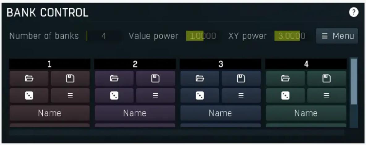
Bank control panel is available only in Banks mode and contains tools to define the banks between which the multiparameter is interpolating. The multiparameter stores parameter values for each bank. Here you can load and save these values.
Each bank has 5 buttons and a value for each controlled parameter. Click the load button to load the bank values into the plug-in. If you want to change say bank 3, you first click its load button, change whatever you need and resave the settings.
By clicking the save button you overwrite the bank's settings from those currently set in the plug-in. A typical approach to define the multiparameter's behaviour is to set the number of banks, then go to the plugin editor, set all associated parameters to the values you would like to have in bank 1 and click the save button for bank 1, then modify the parameters to whatever you want in bank 2 and click the save button for bank 2, etc.
You can also use the Random button to generate random values using the smart-randomization engine for each of the banks.
And the menu button enables you to re-order the banks
For each bank, the values for each parameter are shown and can be changed as desired.
Number of banks 4
Number of banks
Number of banks controls the number of settings that the multiparameter stores for all parameters. By changing the multiparameter value all associated parameters are then modified according to these settings. Please note that when you change the number of banks, the multiparameter will behave differently, because the multiparameter's range from 0% to 100% will now be distributed between a different number of presets. If you had automated the multiparameter value in your host for example you will almost certainly need to edit / rewrite the automation envelope.
Value power 1.0000
Value power
Value power lets you post-process values for each bank by specific power function. This either leads to higher values for low powers, or lower values for high powers. The same thing can be implemented using transforms, but this is much easier considering the potential number of parameters you may have there. It is especially useful for circular XY pads. Use trial-and-error approach to set this up to your liking.
XY power 3.0000
XY power
XY power is used only if XY-pad between banks is enabled and controls how the engine produces values for individual parameters. The higher the number is, the more will the engine separate them. Use trial-and-error approach to set this up to your liking.
≡ Menu
Menu
Menu button provides some additional features for processing the entire set of banks.
Sort banks (up) reorders the banks so that the values of the selected parameter are in increasing order.
Sort banks (down) reorders the banks so that the values of the selected parameter are in decreasing order.
Reverse reverses the order of banks, so that the first bank contains values of the previously last one and so on.
Interpolate lets you change the number of banks, but keeps the values as they are now by calculating values of parameter for all banks. It is usually useful when you want to provide 'banks in between current banks', without manually calculating the new values.
Auto-gain (if available) temporarily enables AGC and automatically sets up the main plugin gain to each bank so that all banks provide similar output loudness. To use it, ensure that the main gain parameter is attached to the multiparameter, start playback of your sound material and press this button. It will take several seconds to complete depending on the number of the banks.
Set names by values sets the names for each bank to the values of the selected parameter. It may be handy when replicating existing parameters for example.

Load
Load button loads the bank settings by setting all associated parameters to the values in the particular bank.

Save
Save button saves the current values of all associated parameters into the particular bank. So you can edit all those parameters in the plugin then click the save button to store them in the bank.

Randomize
Randomize button loads random settings to the bank using the smart randomization engine. Only parameters associated with the multiparameter are randomized.
Generally, randomization in plug-ins works by selecting random values for all parameters, but rarely achieves satisfactory results, as the more parameters that change the more likely one will cause an unwanted effect. Our plugins employ a smart randomization engine that learns which settings are suitable for randomization (using the existing presets) and so is much more likely to create successful changes.
In addition, there are some mouse modifiers that assist this process. The smart randomization engine is used by default if no modifier keys are held.
Holding Ctrl while clicking the button constrains the randomization engine so that parameters are only modified slightly rather than completely randomized. This is suitable to create small variations of existing interesting settings.
Holding Alt while clicking the button will force the engine to use full randomization, which sets random values for all reasonable automatable parameters. This can often result in "extreme" settings. Please note that some parameters cannot be randomized this way.
Hold Shift while clicking the button to undo the previous randomization.
Menu
Menu button provides some additional options related to the bank.

Name
Name button lets you rename the bank.
Name check
Name check button lets you rename the bank. This is a secondary name used for controls such as checkboxes and selectors if defined.
Parameter lock editor
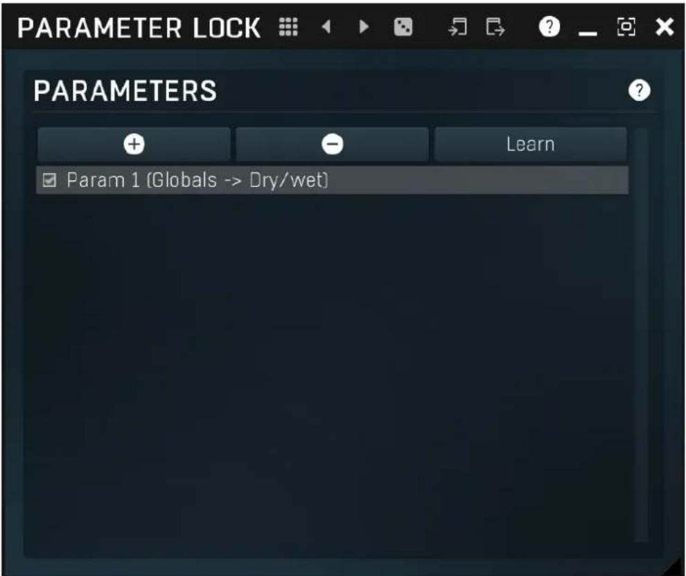
Lock provides a simple way to keep some parameters unchanged when using randomization or browsing presets. You can still change these locked parameters by adjusting the control directly. You simply use the learn feature (right click) in the same way you would with modulators or multiparameters, and touch every parameter you want to keep locked. You can also select them directly in the Parameter Lock window where you can also save them as presets, copy & paste etc. Learning mode is ended by clicking the button again. Please note that this list is not saved with global plugin presets for obvious reasons. The parameters can be locked or unlocked directly in the list or by clicking the lock button associated with the parameter on the Easy screen.

Presets
Presets button displays a window where you can load and manage available presets. Hold Ctrl when clicking to load a random preset instead.

Left arrow
Left arrow button loads the previous preset.

Right arrow
Right arrow button loads the next preset.

Randomize
Randomize button loads a random preset.

Copy
Copy button copies the settings onto the system clipboard.

Paste
Paste button loads the settings from the system clipboard.
Parameters panel
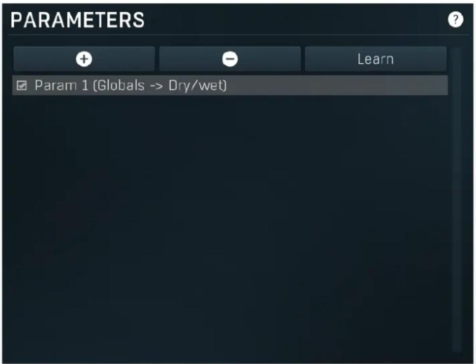
Parameters panel configures the list of the parameters which are locked.

Add
Add button adds a parameter to the list of locked parameters. Alternatively you can use the learn feature available by right-clicking the paramlock button for example.

Delete
Delete button deletes the selected parameter from the list of controlled parameters.

Learn
Learn button starts or stops the learning. Click it, then move some parameters in the plugin, then click it again. Learning can also be accessed from the global parameter lock menu.
MIDI editor
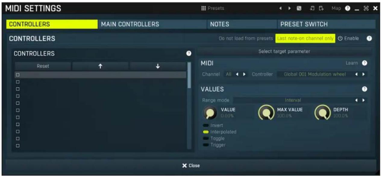
MIDI settings window lets you configure, how the plugin reacts to various MIDI messages. You can use MIDI controllers or MIDI notes and you can also configure a controller to switch between presets, which is especially useful for realtime performances.

Presets
Presets
Presets button displays a window where you can load and manage available presets. Hold Ctrl when clicking to load a random preset instead.

Left arrow
Left arrow button loads the previous preset.

Right arrow
Right arrow button loads the next preset.

Randomize
Randomize button loads a random preset.

Copy
Copy button copies the settings onto the system clipboard.

Paste
Paste button loads the settings from the system clipboard.

Map
Map button displays all current mappings of modulators, multiparameters and MIDI (whichever subsystems the plugin provides).
CONTROLLERS MAIN CONTROLLERS NOTES PRESET SWITCH Tab
selector
Tab selector switches between subsections.
Controllers panel
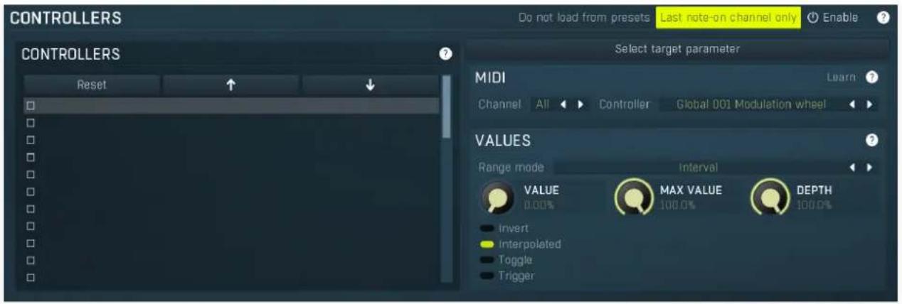
Controllers panel contains settings of MIDI controllers.
Do not load from presets
Do not load from presets
Do not load from presets button disables loading the controllers from presets. This may be handy if you have configured specific MIDI controllers with target parameters and you want to browse the presets without the need to configure them every time. Please note that some presets may rely on specific controllers though. For example, if a preset requires a velocity controller to provide velocity-dependent response, this option will avoid loading it, so the preset won't be complete, until you reconfigure it.
Last note-on channel only
Last note-on channel only
Last note-on channel only button makes the engine more suitable for voice-per-channel devices. These devices are able to send different controllers for each note you press, which however means that these could collide. This option makes the engine pass only the controllers that are related to the last note you pressed. For classic keyboards it is not relevant as you will usually use a single MIDI channel to transmit both the controllers and notes. Some more modern keyboard controllers will allow you to select one MIDI channel for the notes and a different one (or the same one) for the controllers.
Controllers
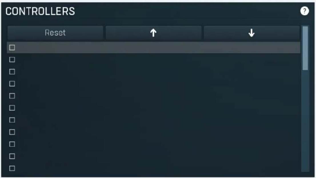
Reset
Reset
Reset button resets the selected controller to undefined state.

Up
Up button moves the selected controller up one item, if possible. This may be useful when keeping things organized, but please note that if you have some multiparameter, modulator or another subsystem access the ranges of individual controllers, this function will reorder them, so these connections will no longer be correct.

Down
Down button moves the selected controller down one item, if possible. This may be useful when keeping things organized, but please note that if you have some multiparameter, modulator or another subsystem access the ranges of individual controllers, this
function will reorder them, so these connections will no longer be correct.
Select target parameter
ParameterIndex
ParameterIndex button lets you choose the parameter being controlled. The set contains all automatable parameters.
MIDI

Learn
Learn
Learn enables or disables MIDI learn. When enabled, the plugin listens to both the MIDI CC messages from the controllers that you touch and the target parameters that you touch and associates the last-touched of each with the selected slot. You can perform several mappings by selecting another slot, adjusting a hardware controller. Then adjusting a target parameter, and repeating those steps for each mapping desired.
Channel
All
◀
Channel
Channel defines the controller MIDI channel.
Controller
Global
001 Modulation wheel

Controller
Controller defines the source controller.
Values
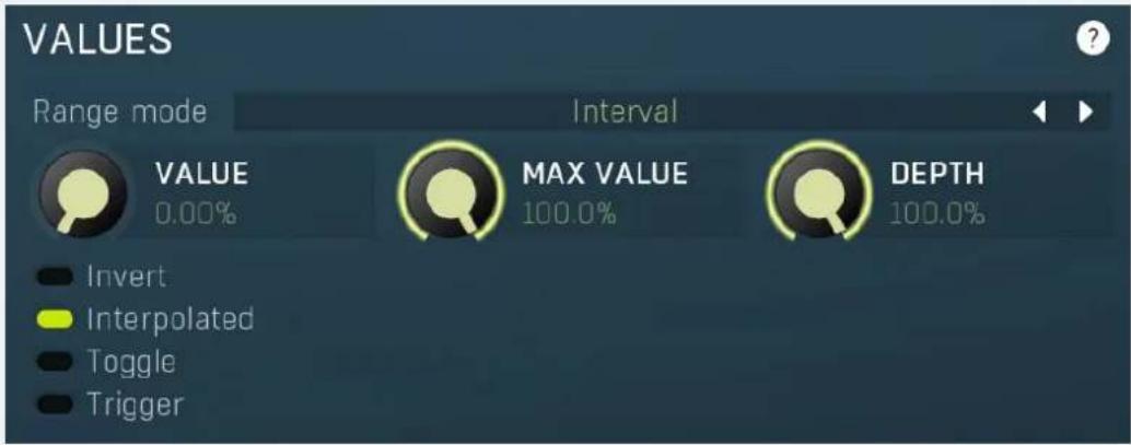
Range mode
Interval

Range mode
Range mode defines how the parameter range is selected. While sometimes it is better to specify minimum and maximum, other times it is better to use a nominal center and depth (% of full scale). This control allows you to define which one it will be.
Up and down mode makes the values go above and below the selected Value, which is considered the center. The interval is made smaller if necessary.
Full range mode is similar, except the range is symmetrically constrained, so the selected Value may not be the center anymore.
Up/down only modes goes from the selected value up/down only.
Let's compare these 4 modes. Taking a value of -12dB value, with a depth of 75% and a scale of +/- 24dB. The nominal range is therefore = +/-24 dB * 75% = 36dB. With values of 0%, 50% and 100% the outputs are:
Up and down: -24, -12, 0 (range constrained to 12 dB either side)
Full range: -24, -6, 12 (range limited to minimum, but not constrained)
Up only: -12, 6, 24 (range not constrained = +/-24 dB * 75% = 36dB)
Down only: -12, -18, -24 (range limited to minimum)
Interval mode is the most simple one and goes from Value to Maximal value.

VALUE
0.00%
Value
Value defines the center of the target parameter's range or the minimum if the Range mode is set to Interval.

MAX VALUE
100.0%
Maximal value
Maximal value defines the upper limit of the target parameter's range. It is available only if the Range mode is set to Interval. This value can be lower than Value. 0% is always mapped to reference>Value and 100% to reference>Maximal value.

DEPTH
100.0%
Depth
Depth defines size of the target parameter's range. It is used only if the Range mode is not set to Interval.

Invert
Invert
Invert checkbox inverts the controller shape, so the minimum becomes the maximum etc.

Interpolated
Interpolated
Interpolated makes the controller value interpolated over the time using the smart interpolation. This approach ensures there won't be abrupt changes, which could lead to clicks and pops. However sometimes you may want to apply these changes immediately - for example when changing ADSR based on the note velocity, in which case this parameter should be disabled.

Toggle
Toggle
Toggle mode makes the controller switch between the maximum and minimum of the target parameter whenever triggered. By default triggering it means going from values below 50% to above 50%. By enabling Trigger you can make it perform the trigger every time the value is changed.

Trigger
Trigger
Trigger mode makes the controller automatically produce maximum and the minimum right after it. It can be handy with some buggy MIDI controllers providing buttons, which however do not send value 0, and only repeat value 127. Trigger makes it behave like the minimum was actually sent by the MIDI controller a little bit after the original message.
Main controllers panel
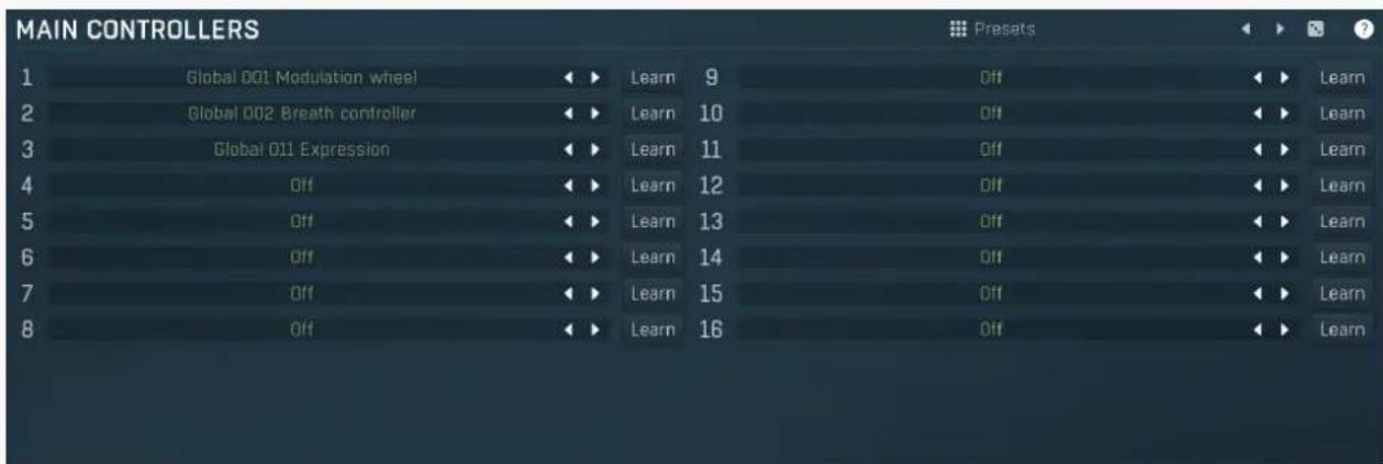
Main controllers panel lets you define the set of main MIDI controllers on your MIDI device. These are not stored with the presets, so using them lets you easily switch between MIDI controllers, create presets that will work for users of other MIDI controllers etc. Using the Main controllers is no different than using the standard MIDI controllers, but the extra 'layer' can make things simple when using multiple controllers and also in general situations where your MIDI device has several controllers with quite 'random' numbers.

Presets
Presets
Presets button displays a window where you can load and manage available presets. Hold Ctrl when clicking to load a random preset instead.

Left arrow
Left arrow button loads the previous preset.

Right arrow
Right arrow button loads the next preset.

Randomize
Randomize button loads a random preset.
Global 001 Modulation wheel

Controller
Controller defines the MIDI controller associated to this Main controller.
Learn
Learn
Learn enables or disables MIDI learn. When enabled, the plugin listens to the controllers you touch and associates them to the main controller.
Notes panel
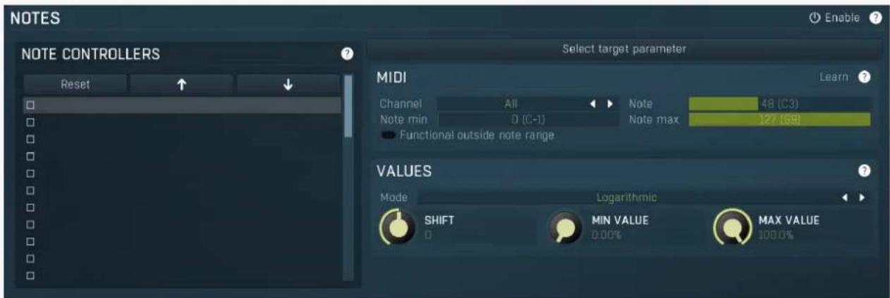
Notes panel contains settings of MIDI note controllers, if you want to control parameters using MIDI keys.
Note controllers
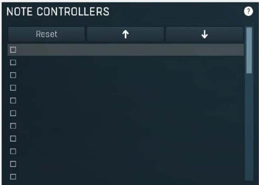
Reset
Reset
Reset button resets the selected controller to undefined state.

Up
Up button moves the selected controller up one item, if possible. This may be useful when keeping things organized, but please note that if you have some multiparameter, modulator or another subsystem access the ranges of individual controllers, this function will reorder them, so these connections will no longer be correct.

Down
Down button moves the selected controller down one item, if possible. This may be useful when keeping things organized, but please note that if you have some multiparameter, modulator or another subsystem access the ranges of individual controllers, this function will reorder them, so these connections will no longer be correct.
Select target parameter
Learn
Learn enables or disables MIDI learn. When enabled, the plugin listens to both the notes you touch and the parameters you touch and associates them with the selected slot.
MIDI
![MIDI Learn ? Channel All Note 48 [C3] Note min 0 (C-1) Note max 127 (G9) Functional outside note range](/content/2026/05/983866/images/552ed838a27f3d84a19a0c13376629ee277ffd8fae983504c11076fe991ba686.jpg)
Channel
All
◀ ▶
Channel
Channel defines the controller MIDI channel.
Note
48 [C3]
Note
Note defines the controller's target MIDI note. It is used only in On/off and Switch modes, which you can set using Mode parameter (in the Values panel).
Note min
0 (C-1)
Note min
Note min controls the lowest note to be used by a controller in Linear or Logarithmic mode. The minimum value of the target parameter will then be associated to this note.
If both Note min and Note max parameters are default, the plugin takes the actual frequency of each note, and transforms it into the range 20Hz to 20kHz, which is the range used by all equalizers and filters, so that you can literally play a parameter on a MIDI keyboard. If you change either of these 2 parameters however, the plugin takes the range of notes as the requested interval. This is useful for example if you have a small MIDI keyboard used for soloing and you want increase some parameter the higher you play. In the default mode it would be difficult, since the range of frequencies is much bigger than the range of your MIDI keyboard. Set the Note min and Note max to C0 and B0 respectively, the Mode to Logarithmic and select a suitable target parameter (Dry/Wet is fine). Send MIDI notes in the specified range to the plugin and you will see the target parameter increase (by 9.09% (= 100 / (12-1)) for a 100% range).
Note max
127 [G9]
Functional outside note range
Functional outside note range makes the note controller work even if the note isn't in the specified range, clamping the value to the minimum or maximum.
Values
VALUES
Mode

Logarithmic
SHIFT

MIN VALUE
0.00%

MAX VALUE
100.0%
Mode
Logarithmic
Mode
Mode controls how the controller works.
Key takes the note index and transforms it into 0..1, which is the output of any controller. This mode is useful for scale switches for example - if you want to use MIDI keys to change values linearly.
Key (in octave) is similar but it has only 12 values - one per each key and it doesn't matter which octave you press it in.
Linear converts the notes into frequencies and then transform them into the linear scale from 20Hz to 20kHz.
Logarithmic converts the notes into the frequencies and then into the logarithmic scale from (20) to (20000) . A typical use case is when you want to control an equalizer band using a MIDI keyboard. Since EQ frequencies work in logarithmic scale, this mode makes both things compatible and the EQ frequency will be set to the note frequency.
On/off modes react only to single notes and can be used for triggers. When the Note On is received the parameter is changed to its Max value and when the Note Off is received the parameter is changed to its Min value. So this mode can also be used to change between any 2 parameter values.
Switch modes are similar, but only recognize when a note is pressed. The Note Offs are ignored. Note Ons select the Max value and Min value alternately. In all octaves mode it doesn't matter which octave is used. For example, this is useful when you want to use any note C to switch something on and off.
Velocity modes do not actually follow the note number being pressed, but it's velocity instead. While you can do the same thing with normal MIDI controllers using the special Velocity controllers, this one allows you to select only some notes to follow.

SHIFT
0
Shift
Shift lets you shift the original note up or down by the specified number of semitones.

MIN VALUE
0.00%
Min value
Min value defines the minimum value for the target parameter.

MAX VALUE
100.0%
Max value
Max value defines the maximum value for the target parameter.
Enable MIDI program change
Enable
MIDI program change
Enable MIDI program change enables processing program change MIDI message.
Preset previous/next trigger panel

Preset previous/next trigger panel lets you select a MIDI controller, which will switch presets. It provides the same action as clicking the arrows next to the main preset button. When the controller value gets below 33%, the previous preset is loaded. When the controller value gets above 66%, the next preset is loaded.
Learn
Learn
Learn enables or disables MIDI learn.
Channel All
Channel
Channel defines the controller MIDI channel.
Controller Global 000 Bank select
Controller
Controller defines the source controller.
Simulate program change via controller panel

Simulate program change via controller panel lets you select a MIDI controller, that will work as program change, for convenience. You can use it then to switch between A-H presets or presets via panel below.

Learn
Learn enables or disables MIDI learn.

Channel
Channel defines the controller MIDI channel.

Controller
Controller defines the source controller.

Number of values
Number of values defines the number of programs to switch between. By default Program change MIDI standard offers 128 programs. However it may by too many and could be hard to actually control with the specific controller. Hence you can lower the number of actual programs.
Program change in presets panel

Program change in presets panel enables the MIDI program change processing. If disabled, the plugin follows Program Change messages by changing the A-H presets. The obvious disadvantage is that this way there are just 8 presets. By enabling this feature the plugin stops selecting A-H presets and rather loads different presets from the specified preset folder, including all sub-folders. The default folder is called "Programs". To use it, you simply need to create a preset folder called Programs and put the presets into it. Note that the order matters of course. And you can change the folder name at any time, so you can have several sets of selectable presets.

Folder
Folder defines the preset folder from which the presets for program-change MIDI messages are taken.

Channel
Channel defines the program change MIDI channel.
Used controls
Here we discuss the general properties of all application controls. As a most important rule you should note, that you can always use any question mark button or F1 (or Ctrl+F1 or Ctrl+H) key with the mouse cursor over a specified control to get detailed information about what it does and how to use it.
Value button
Volume
5.43 dB
Value button is an alternative to the knobs and its main advantage is that it is very small. In some cases the button simply serves as a clickable item and a menu is shown when clicked. However the mouse wheel and other controls still do work.
- Click and drag using the left mouse button to change the value.
- Right mouse button shows a menu with additional options. Hold ctrl/cmd to select the default value.
- Mouse wheel, arrow keys and vertical drag using middle mouse button or using left mouse button while holding Ctrl modifies the value more precisely.
- Home key configures the minimal possible value, conversely end key setups the maximal one.
- Esc or Backspace keys restore the original value when either one is pressed during dragging.
- Shift + left mouse button or double-click using left mouse button lets you edit the value as text. You can use the virtual keyboard or type on your computer keyboard. In some cases this shows a menu with all possible values instead.
- Alt + press then release measures the time between the press and the release and applies it as time/frequency tap. Usable only for certain values of course.
Edit
Algorithm ca[#an[a;fh;b[swap]]]
![MeldaProduction MTurboReverb - Algorithm ca[#an[a;fh;b[swap]]] - 1](/content/2026/05/983866/images/2e9d6cf4a447e52daaf6f29b10360bfef258884618f99c7a32e5a65c767c5417.jpg)
Edit control provides a standard way to specify any kind of text or numeric string. It can have a limited length or a limited set of allowed characters.
- Shift+arrows/Home/End modifies selection.
- Ctrl+C copies the selected text to the system clipboard.
- Ctrl+V pastes text from the system clipboard replacing the selected text or inserting it at the current cursor position.
- Ctrl+A selects the whole text.
- Ctrl+Tab inserts a tabulation character. This combination is provided because the Tab key alone moves the keyboard focus to the next control.
Switcher
Delay order
Random

Switcher is an alternative to a tracker or knob control, but it has a limited set of values.
- Left mouse button shows a menu with list of all possible values. This function might be unavailable in certain cases when the number of possible values is too high.
- Right mouse button shows a menu with additional options. Hold ctrl/cmd to select the default value.
- Up and Down arrow keys, buttons in the control and mouse-wheel increase or decrease the value.
Zoomer

Zoomer provides a simple way to zoom and move in an enlargeable view.
• Plus button zooms-in.
- Minus button zooms-out.
- Zoom default button zooms to the default ratio, which typically means full zoom-out.
- Lock button locks the zoom ratio.
Knob
DRY/WET
50.0%
Knob simulates physical knobs used to edit various values.
- Click and drag using the left mouse button to change the value.
- Right mouse button shows a menu with additional options. Hold ctrl/cmd to select the default value.
- Mouse wheel, arrow keys and vertical drag using middle mouse button or using left mouse button while holding Ctrl modifies the value more precisely.
- Home key configures the minimal possible value, conversely end key setups the maximal one.
- Esc or Backspace keys restore the original value when either one is pressed during dragging.
- Shift + left mouse button or double-click using left mouse button lets you edit the value as text. You can use the virtual keyboard or type on your computer keyboard. In some cases this shows a menu with all possible values instead.
- Alt + press then release measures the time between the press and the release and applies it as time/frequency tap. Usable only for certain values of course.
Graph editor
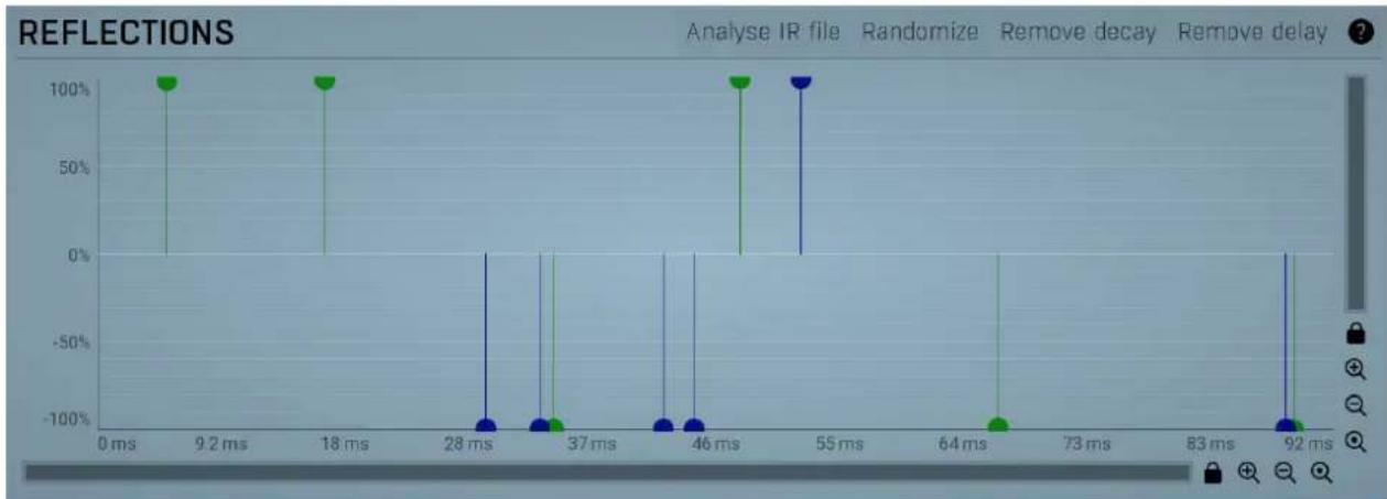
line
| Time (ms) | Reflection (%) | | --------- | -------------- | | 0 | 100 | | 9.2 | 100 | | 18 | 100 | | 28 | -100 | | 37 | -100 | | 46 | -100 | | 55 | 100 | | 64 | -100 | | 73 | -100 | | 83 | -100 | | 92 | -100 |Graph editor will show and edit one or more graphs.
- Zoomers below and on the right control the zoom amount and position of the view.
- Mouse wheel zooms in or out. Hold Shift to move the view horizontally instead, without zooming. Hold Ctrl to move the view vertically instead, without zooming. Alternatively you can zoom in using Alt + right button double click and out using Alt + left button double click. You can also use keyboard numbers 0 to 9 to quickly set the zoom level.
- Drag a rectangle using the left mouse button while holding Alt zooms into the selected rectangle if possible.
- Drag using the left mouse button while holding Alt and Ctrl to scroll the view. This is not possible when zoomed all the way out as there is nothing to scroll.
Tab-set
| ER 1 | ER 2 | ER 3 | ER 4 | LR 1 | LR 2 | LR 3 | LR 4 | LR 5 | LR 6 | DYNAMICS | EQ | EQ M/S |
Tab-set is typically used wherever there is too much to edit, but not enough space to display it all. It can be also used to switch between possible alternatives.
- Left mouse button selects a tab.
- Ctrl + Left mouse button or Right mouse button displays the whole tab in a pop-up window (this is not used for all sets of tabs). This comes handy when you want to have multiple tabs visible at the same time.
- Left and Right arrows select the neighbouring tab.
- Click on one of the buttons on the border to scroll the control and show tabs that are currently invisible.
Installation, activation, introduction to audio plugins
Installation
All MeldaProduction plugins are currently available for Windows and Mac OS X operating systems, both 32-bit and 64-bit versions. You can download all software directly from our website. Since the installation procedures for the two operating systems are quite different, we will cover each one separately.
The download files for the effects include all the effects plug-ins and MPowerSynth. During the installation process you can select which plug-ins or bundles to install. If you have not licensed all of the plugins in a bundle then you just need to activate each plugin separately.
If you have multiple user accounts on your computer, always install the software under your own account! If you install it under one account and run it under a different one, it may not have access to all the resources (presets for example) or may not even be able to start.
Installation on Windows
All plugins are available for VST, VST3 and AAX interfaces. The installer automatically installs both the 32-bit and 64-bit versions of the plugins.
Note: Always use 32-bit plugins in 32-bit hosts, or 64-bit plugins in 64-bit hosts. 64-bit plugins cannot work in 32-bit hosts even if the operating system is 64-bit. Conversely, never use 32-bit plugins in 64-bit hosts. Otherwise they would have to be 'bridged' and, in some hosts, can become highly unstable.
You can select the destination VST plugins paths on your system. The installer will try to detect your path, however you should check that the correct path has been selected and change it if necessary. In all cases it is highly recommended to use the current standard paths to avoid any installation issues:
32-bit Windows:
C:\Program files\VstPlugins
64-bit Windows:
C:\Program files (x86)\VstPlugins (for 32-bit plugins)
C:\Program files\VstPlugins (for 64-bit plugins)
If your host provides both VST and VST3 interfaces, VST3 is usually preferable. If a plugin cannot be opened in your host, ensure the plugin file exists in your VST plugin path and that if your host is 32-bit, the plugin is also 32-bit, and vice versa. If you experience any issues, contact our support via info@meldaproduction.com
Installation on Mac OS X
All plugins are available for VST, VST3, AU and AAX interfaces. Installers create both 32-bit and 64-bit versions of the plugins.
If your host provides multiple plugin interface options, VST3 is usually preferable. If you experience any issues, contact our support via info@meldaproduction.com
Most major hosts such as Cubase or Logic should work without problems. In some other hosts the keyboard input may be partly non-functional. In that case you need to use the virtual keyboard available for every text input field. You may also experience various minor graphical glitches, especially during resizing plugin windows. This unfortunately cannot be avoided since it is caused by disorder in Mac OS X.
Uninstallation on Windows
The Uninstaller is available from the Start menu and Control panel, in the same way as for other applications. If you don't have any of these for any reason, go to Program files / MeldaProduction / MAudioPlugins and run setup.exe.
Uninstallation on OSX
The Uninstaller is available from Applications / MeldaProduction / MAudioPlugins / setup.app.
Deleting all data, presets etc.
Even if you uninstall the plugins, some data will be left behind - because of potential crossdependencies or because these are your presets, settings, configurations etc. If you want to wipe out everything, please manually delete following folders:
Windows:
C:\ProgramData\MeldaProduction
Performance precautions
In order to maximize performance of your computer and minimize CPU usage it is necessary to follow a few precautions. The most important thing is to keep your buffer sizes (latency) as high as possible. There is generally no reason to use latency under 256 samples for 44kHz sampling rates (hence 512 for 96kHz etc.). Increasing buffer sizes (hence also latency) highly decreases required CPU power. In rare cases increasing buffer sizes may actually increase CPU power, in which case you can assume your audio interface driver is malfunctioning.
You should also consider using only necessary features. Usually the most CPU demanding features are oversampling and modulation of certain parameters. You can reduce modulation CPU usage at the cost of lower audio quality in Settings/Settings/Modulator protection.
Troubleshooting
The plugins are generally very stable, there are known problems however.
GPU compatibility
The software uses hardware acceleration to move some of the processing (mainly GUI related) from your CPU (processor) to your GPU (graphics processing unit). It is highly recommended to use a new GPU, as it will provide higher performance improvements, and update your GPU drivers. Older GPUs are slower and may not even provide required features, so the software will have to perform all calculations in the main CPU. We also have had extremely bad experiences with GPUs from ATI and despite the fact that software is now probably bulletproof, it is recommended to use NVidia GPUs as there has not been a single case of a problem with them.
If you experience problems with your GPU (crashing, blank/dysfunctional GUI), and that you cannot disable the GPU acceleration from the plugin's Settings window itself, download this file:
http://www.meldaproduction.com/download/GPU.zip
And place the GPU.xml included in the zip into
Windows: C:\Users{username}\AppData\Roaming\MeldaProduction
Mac OS X: \~/Library/Application support/MeldaProduction
Memory limits of 32-bit platform
Most hosts are now 64-bit ready, however some of them are not or users willingly choose 32-bit edition, because the required plugins are not 64-bit ready yet. All our software is 64-bit ready. Please note that you must NOT use the 64-bit plugins in 32-bit hosts, even if you have a bridge. If you are stuck with a 32-bit host for any reason, note that there is a memory limit (about 1.5 GB), which you may not exceed. This can happen if you load too many samples or different plugins for example. In that case the host may crash. There is no other solution than to use a 64-bit host.
Updating
You can use "Home/Check for updates" feature in any of the plugins. This will check online if there is a newer version available and open the download page if necessary.
To install a newer (or even older) version you simply need to download the newest installer and use it. There is no need to uninstall the previous version, the installer will do that if necessary. You also do not need to worry about your presets when using the installer. Of course, frequent backup of your work is recommended as usual.
Using touch-screen displays
Touch screen displays are supported on Windows 8 and newer and the GUI has been tweaked to provide a good workflow. Up to 16 connections/fingers/inputs are supported. Any input device such as touch-screens, mouse, tablets are supported. These are the main gestures used by the plugins:
- Tap = left click
- Double tap = double click
- Tap & hold and quickly tap next to it with another finger = right click. Tap & hold is a classic right-click gesture, however that doesn't provide a good workflow, so came up with this method, which is much faster and does not collide with functionality of some elements.
Purchasing and activation
You can purchase the plugin from our website or any reseller, however purchasing directly from our website is always the quickest and simplest option. The software is available online only, purchasing is automatic, easy and instant. After the purchase you will immediately receive a keyfile via email. If you do not receive an e-mail within a few minutes after your purchase, firstly check your spam folder and if the email is not present there, contact our support team using info@meldaproduction.com so we can send you the licence again.
To activate the software simply drag & drop the licence file onto the plugin. Unfortunately some hosts (especially on Mac OS X) either do not allow drag & drop, or make it just too clumsy, so you can use Home/Activate in any of the plugins and follow the instructions. For more information about activation please check the online video tutorial.
You are allowed to use the software on all your machines, but only you are allowed to operate the software. The licences are "to-person" as defined in the licence terms, therefore you can use the software on all your computers, but you are the only person allowed to operate them. MeldaProduction can provide a specialized licence for facilities such as schools with different licence terms.
Quick start with your host
In most cases your host will be able to recognize the plugin and be able to open it the same way as it opens other plugins. If it doesn't, ensure you did installation properly as described above and let your host rescan the plugins.
Cubase
Click on an empty slot (in mixer or in track inserts for example) and a menu with available plugins will be displayed. VST2 version is located in MeldaProduction subfolder. However VST3 version is recommended and is located in the correct folder along with Cubase's factory plugins. For example, dynamic processors are available from the "Dynamics" subfolder.
To route an audio to the plugin's side-chain (if it has one), you need to use the VST3 version. Enable the side-chain using the arrow button in the Cubase's plugin window title. Then you can route any set of tracks into the plugin's side-chain either by selecting the plugin as the track output or using sends.
To route MIDI to the plugin, simply create a new MIDI track and select the plugin as its output.
Logic
Choose an empty insert slot on one of your audio tracks (or instrument tracks for example) and select the plugin from the popup menu. You will find it in the Audio Units / MeldaProduction folder.
To route an audio to the plugin's side-chain (if it has one), a side-chain source should be available in the top of the plugin's window, so simply select the source track you want to send to the plugin's side-chain.
To route MIDI to the plugin, you need to create a new Instrument track, click on the instrument slot and select the plugin from AU MIDI-controlled Effects / MeldaProduction. The plugin will receive MIDI from that track. Then route the audio you want to process with the plugin to this track.
Studio One
Find the plugin in the Effects list and drag & drop it onto the track you would like to insert the plugin to.
To route an audio track to the plugin's side-chain (if it has one), first enable the side-chain using the "Side-chain" button in the Studio One's plugin window title. Then you can route any set of tracks into the plugin's side-chain from the mixer.
To route MIDI to the plugin, simply create a new MIDI track and select the plugin as its output.
Digital performer
In the Mixing Board, find an empty slot in the track you would like to insert the plugin to. Click on the field and select the plugin from the effects list.
To route an audio track to the plugin's side-chain (if it has one), choose the track you want to send using Side-chain menu, which appears at the top of the DP's plugin window.
To route MIDI to the plugin, simply create a new MIDI track in the Track view and select the plugin as its output.
Reaper
Click on an empty slot in the mixer and a window with available plugins will be displayed. Select the plugin you want to open by double clicking on it or using Ok button.
It is highly recommended to select all MeldaProduction plugins in the plugin window the first time you open it, click using your right mouse button and enable "Save minimal undo states". This will disable the problematic Undo feature, which could cause glitches whenever you change certain parameters.
To route an audio track to the plugin's side-chain (if it has one), click on I/O button of the side-chain source track in the mixer. Routing window will appear, there you click "Add new send" and select the track the plugin is on. In the created send slot select the channels (after the "=" mark) for the send, in stereo configuration 3/4 for example. Note that this way the whole track receives the side-chain signal and all plugins with it. It is possible to send it to a single plugin only, but it is more complicated, please check the Reaper's documentation about that.
To route MIDI to the plugin, create a new MIDI track and do the same thing as with side-chain, except you don't need to change output channels.
Live
In Session view, select the track you would like to insert the plugin to. At the left top of Ableton Live's interface, click on the Plug-in Device Browser icon (third icon from the top). From the plug-ins list choose the plugin (from MeldaProduction folder), double click on it or drag & drop it into the track.
The X/Y grid usually doesn't provide any parameters of the plugin. This is because the plugins have too many of them, so you have to select them manually. Check Live's documentation for more information.
To route an audio to the plugin's side-chain (if it has one), select the track you want to send to the side-chain and in the 'Audio To' menu, choose the audio track that has the plugin on it. Then in the box just below that select the plugin from the menu.
NOTE: Live does NOT support any interface correctly, it doesn't use the reported buses properly, hence it doesn't work with surround capable plugins. Therefore you need to use VST version, which reports only stereo capabilities by default.
To route MIDI to the plugin, create a new MIDI track and in the 'MIDI to' menu, choose the audio track that has the plugin on it. Note that in Live only the first plug-in on any track can receive MIDI.
ProTools
In the mixer click an empty slot to insert the plugin to and select the plugin from the tree. The plugin may be present multiple times, once for each channel configuration (mono->stereo etc.). As of now ProTools do not arrange them in the subfolders, which is a workflow dealbreaker, but we cannot do anything about it. The huge empty space on top of each plugin window, which occupies so much of the precious display area, is part of ProTools and every plugin window and again we cannot do anything about it. In some cases you may experience CPU overload messages, in which case please contact Avid for support. Note that ProTools 10 and newer is supported. RTAS compatibility for PT9 and older will never be added.
To route an audio to the plugin's side-chain (if it has one), open the plugin, click on the No key input button in the plugin title and select the bus you want the audio taken from. You might need to remember the bus number, unless your ProTools version supports bus renaming. ProTools doesn't support stereo (or surround) side-chains at all.
To route MIDI to the plugin, create a new MIDI track and in the mixer click the output field for that track and select the plugin, which should already be in the menu.
FL Studio
First make sure plugins are scanned, either a full scan through the Plugin Manager or an automatic fast scan when you open the Plugin Database section of the browser in FL. The scanned plugins will show up in the Plugin Database > Installed section of the FL browser. The Effects and Generators sections in the Plugin Database will show all "favorite" plugins. These can be checked and unchecked in the Plugin Manager or added in some other ways. These favorites also show up in the Add menu, the menu for the "+" button in the channel rack, when you right click an existing channel button to replace or insert, in the plugin slot menu in the mixer and in the plugin picker (F8). The menus with favorite plugins also have a "More" choice that will show all scanned plugins. The full explanation is in our help file, on the page Installing Plugins.
To route an audio to the plugin's side-chain, first set up the mixer: make sure the track you want to receive audio from is sent to the track the plugin as a sidechain (help). Then set up the plugin wrapper: choose the desired input on the Processing tab of the wrapper options.
To route MIDI notes to the plugin, first configure the sender: choose a MIDI port for the input device in the MIDI settings (for a hardware device), or an output port in the wrapper options (for a VST plugin that produces MIDI). For the receiving plugin, set the input port in the wrapper options to the same value you chose in step 1.
To route MIDI controllers, the procedure is different. The usual method in FL is to link CC messages to plugin parameters (help file). VST plugins will also have 128 CC parameters published (through the wrapper) that can be links this way. Those will send the specified CC MIDI message to the plugin, instead of changing a published parameter.
GUI styles, editor modes and colors
MeldaProduction plugins provide a state of the art styling engine, which lets you change the appearance to your liking. The first time you run the plugins a style wizard will appear and let you choose the style and other settings. It may not be available in ProTools and other problematic hosts.
By default each plugin has a certain color scheme, which differs based on what kind of plugin is that. Also, sections of some plugins are colorized differently, again, based on what kind of section is that (this can be disabled in global settings). Despite you can change the colors anyhow you want, it is advantageous to keep the defaults as these are standardized and have predefined meaning, so just by looking at a plugin's color you can immediately say what kind of plugin and section is that. Same rules apply when designing devices for easy screens. This is the current set of colors:
Dynamics = orange
Equalization, filtering = green
Reverb, delay = brown/yellow
Modulation = blue
Distortion, limiting = red
Stereo = cyan/yellow
Time, pitch, unison... = purple/pink
Tools = grey
Special colors:
Synchronization = grey
Detection = blue/green
Side-chain = green
Effects = red
Advanced stuff = grey

natural_image
Abstract orange triangle logo with white letter M (no text or symbols)MELDA production The only limit is your imagination
About MeldaProduction
The best sound on the market, incredible workflow and versatility beyond your imagination. We create the deepest and the most powerful audio plugins with unbelievable sound and tons of unique features you cannot find anywhere else.
Innovative Thinking
At MeldaProduction, we make the most advanced tools for music production and audio processing. We get inspired by the whole range of tools from the ancient analog gear to the newest digital creations, but we always push forward.
We've always felt the audio industry is extremely conservative, still relying on the prehistoric equipment making the job unnecessarily slow and complicated. That's why we invent new technologies, which make audio processing easier, faster, better sounding and more creative.
Sound Matters
In the world full of audiophiles you just need superb audio quality. And that's why we spend so much time perfecting audio algorithms until they sound unbeatable. Everything from dynamic filters to spectral dynamic processing. Our technologies just sound perfect.
Inspiring User Interface
Modern user interfaces must not only be easy and quick to use, but also versatile and the whole visual appearance should inspire you. MeldaProduction plugins provide the most advanced GUI engine on the market. It is still the first and only GUI engine, which is freely resizable and styable. Our plugins can look as an ancient vintage gear, if you are working on old-school rock music. Or as super-modern
Easy to Use, Yet Versatile
The only limit is your imagination. Our plugins are with absolutely no doubt the most powerful and versatile tools on the market. Yet we managed to make the plugins easy to use via the devices and smart randomization system. But when you are ready, you are one click away from the endless potential the plugins provide.
Never-Ending Improvements
Most companies create a plugin, sell it and abandon it. We improve our plugins, add features, optimize... until there is nothing left to improve and there are no more ideas. Unfortunately that hasn't happened yet :). And the best thing is that the updates are free-for-life!
MeldaProduction was founded in 2009 by Vojtech Meluzin and is based in Prague, Czech Republic.
www.meldaproduction.com
info@meldaproduction.com
MeldaProduction (c) 2017
- Overview
- Under the hood
- MTurboReverb vs. MTurboReverbLE
- Easy screen vs. Edit screen
- Presets
- Left arrow
- Right arrow
- Randomize
- Panic
- Settings
- WWW
- Sleep indicator
- Plugin toolbar
- Oversampling
- L+R
- Channel mode
- AGC
- Set
- Limiter
- A-H presets selector
- A/B
- 88
- Morph
- →
- Copy
- Paste
- Undo
- Redo
- WAV
- IR
- Collapse
- Reload
- Small spaces
- Device selector
- Comp
- Gate
- Pre
- Dynamics panel
- Focus
- RMS length
- Release
- Attack
- Comp ratio
- Gate ratio
- Type
- Treble
- High-cut
- High-cut mid
- Length
- Early/late
- Predelay
- Size
- Widening
- Bass
- Gain
- Saturation
- Low-cut side
- Low-cut
- Dry/Wet
- Diffusion
- Modulation
- Cross
- Hz
- Modulation rate
- Damp High
- Damp Low
- Complexity
- Time graph
- Pause
- Popup
- Enable
- Edit mode
- Random
- Mid
- Side
- Swap L/R
- Invert
- Parallel
- Gain compensation
- Analysis
- Impulse response analysis
- Load comparison
- Refresh
- Generate impulse
- OUTPUT
- Output gain
- VOLUME
- PANORAMA
- RIGHT DELAY
- selector
- Early panel
- ValRoom
- Monophonic
- Mode
- Decay
- Deform
- Volume 5.43 dB Volume
- 0.00%
- 50.0%
- Modulation panel
- Depth
- Rate
- High-pass panel
- Frequency
- Hz
- Q
- 0.71
- Low-pass panel
- Frequency 20.0 kHz Frequency
- Reflections editor
- Analyse IR file
- Remove decay
- Remove delay
- Late panel
- Living room
- Early
- Volume 5.57 dB Volume
- Panorama center
- Widening 0.00%
- Cross 50.0% Cross
- Input 0% prev, 100% dry
- Input
- Output 100% out, 100% prev
- Depth 0.00%
- Rate 0.2000 Hz
- Hz
- kHz
- Dampening Low panel
- Gain 0.00 dB Gain
- Frequency 100.2 Hz Frequency
- Q 0.40 Q
- Sparse 4 Sparse
- Dampening High panel
- Gain -3.00 dB Gain
- Frequency 8000 Hz Frequency
- Sparse 2 Sparse
- Randomize parameters
- Randomize algorithm
- Smart seed generator
- Stereo field, the biggest challenge in audio ever?
- What are the symptoms of a problematic stereo field?
- Ear fatigue
- How to balance the stereo field
- Stereo width
- What to minimize panel
- Set 0%
- Set 100%
- Parallel isolated LR generator
- Perform smart seed search
- Reset
- Calibrate
- Results
- Algorithm ca[#an[a;fh;b[swap]]
- Algorithm
- Introduction
- Syntax
- User parameters and expressions
- Need to know information about reverb design
- Helper modules
- PW / ParallelW (w1;w2...) [submodule1;submodule2;...]
- B / Bypass (probability) [submodule1;submodule2;...]
- L / Level (gain in dB)
- LC / LevelC (gain as multiplier)
- ST / SerialTap [submodule1;submodule2;...]
- STW / SerialTapW (w1;w2...)[submodule1;submodule2;...]
- Basic modules
- D / Delay (time)
- C / Comb (decay; time)
- CB / CombB (decay;time)
- X / XComb (decay;time) and XB / XCombB (decay;time)
- A / Allpass (decay;time)
- Filtering and modulation
- V | Vibrato (length; lfo frequency)
- FL / FilterL (frequency diff; Q diff)
- FH / FilterH (frequency diff; Q diff)
- FA / FilterA (frequency; Q)
- FAM / FilterAMod (modf;modq;modLFOFrequency;center frequency;center Q)
- F / Filter (frequency; type; Q; gain)
- Sat / Saturation (drywet;mode)
- Nested modules
- Complex modules
- XC / XCircularComb [outmodule1;...;outmoduleN;fbmodule1;..;fbmoduleN]
- CA / XCircularAllPass [outmodule1;...;outmoduleN;fbmodule1;..;fbmoduleN]
- FDN4 and FDN4D
- XFDN4 and XFDN4D
- FDN (size) [submodule1;submodule2...submoduleN]
- XFDN
- R / Reverb and RD / ReverbD
- RP / ReverbP [submodule1;submodule2...] and RPD / ReverbPD [submodule1;submodule2...]
- CROSS / Crossover (slope; frequency1; frequency2..) [band1; band2...]
- CROSSLP / CrossoverLP (slope;tapcount;frequency1;frequency2..) [band1;band2...]
- Multi-channel modules
- Swap
- Mono
- Widening (depth)
- LRtoMS and MStoLR
- Advanced modules
- Tremolo (depth; frequency)
- Autopan (depth; frequency)
- Pitch (fftsize; pitch shift; formant shift; keep formants)
- FreqShift (maximum; shift; override)
- Noise
- Mul (drywet) [submodule1;submodule2...]
- Spectral (fftsize;attack;hold)
- ConvoNoise (shape:length;hpshape;hpq;hpf;lpshape;lpq;lpf)
- Transient (attackdb; release; resolution; link)
- Seed
- Param 1
- 1.00
- Param 2
- Param 3
- Delay min
- 5.0%
- Delay max
- 18.6%
- Pitch shift
- 0
- Delay order
- ◀ ▶
- Delay focus
- -306.4%
- Delay width
- 100.0%
- Input order
- Input focus
- 400.0%
- Input width
- Output order
- Output focus
- Output width
- Channels unrelated
- Channel seeds unrelated
- Globals
- Side-chain
- Dry as side-chain
- Input gain
- Release mode
- Manual
- Peak hold
- ms
- Look-ahead
- Off
- Frequency min 20.00 Hz Frequency min
- Frequency max 20.0 kHz Frequency max
- Gate panel
- THRESHOLD
- RATIO
- Knee size 50.0%
- Knee size
- Processor 2 panel
- Range
- Level shape graph
- Meters
- Plus
- Minus
- Rewind
- Menu
- Time-graph settings
- Static mode
- Process hidden graphs
- RESOLUTION
- Graphs panel
- Envelope graph menu
- Snap to grid X
- X
- Snap to grid Y
- Insert points
- Step sequencer
- sequencer
- Export CSV
- Import CSV
- Expression evaluator
- Analyse audio
- Equalizer panel
- SHIFT
- Soft saturation
- Location
- Reverb
- Equalizer shape graph
- Analyzer
- Fill
- Analyzer Rainbow Colors
- Sonogram
- Analyzer settings
- Freeze
- Normalize
- OPACITY
- RAINBOW OPACITY
- SLOPE
- TIME RESOLUTION
- DEHARMONIZE
- Super-resolution mode
- Enable when hidden
- Global normalization
- Advanced panel
- Peak detection
- PEAK THRESHOLD
- Scientific settings
- Overlap
- Overlapping
- FFT size
- Window type
- Analytical smoothing
- Logarithmic averaging
- Average
- Copy analysis
- Analyzer Fill and Line Color - All Channels
- Analyzer Fill and Line Color - Left Channel
- Peaks
- Line opacity
- Micro-sonogram
- Line width
- Sonogram fill
- Fill opacity
- Average (infinite)
- Maximum
- Maximum (infinite)
- Maximum - Average (infinite)
- Comparison
- Paste analysis
- Sonogram panel
- Prefiltering panel
- Depth 100.0% Depth
- Envelope graph
- Band settings window
- General panel
- Invert gain
- Swap gains
- Channels
- Left
- Left + Right
- Right
- Advanced
- DYNAMICS
- Auto
- TRANSIENT
- 2.0ms
- ms
- silence
- Level gain
- dB
- Link channels
- Detector delay
- Filtered compensated
- Harmonics panel
- Linear
- Dynamics by fundamental
- HARMONICS
- SEMITONES
- MAXIMAL COUNT
- Harmonics grid
- Band advanced settings
- General settings panel
- GENERAL SETTINGS
- Shape Squared Shape
- Band-pass panel
- BAND-PASS
- Play
- Level transformation
- SCALE
- Link grid panel
- Utilities
- Lock
- Multiparameter
- Preset selector
- Backup
- Restore from backup
- Folders tree
- Auto-open
- Open all
- Close all
- Add
- Rename
- Delete
- Export
- Import
- Presets list
- Favourite
- Show
- Sort
- Previous
- Next
- Submit preset
- Download presets
- Replace
- Search
- Clear
- information
- Plugin settings
- Licence panel
- Licence manager
- Activate
- GUI & Style panel
- Style
- Random style
- Default style
- Select current style as default
- GPU acceleration
- Enabled
- Frames per second
- Enable high DPI support
- Enable high DPI / retina support
- Enable colorization
- Enable colorization for panels
- Allow default colors by plugin type
- Allow style changes if the editor is too big
- Clear window settings cache
- Plugin settings panel
- - Intelligent sleep on silence
- Intelligent sleep on silence
- Randomizer loudness compensation
- Smart bypass
- MIDI thru
- Sample-accurate event processing
- Latency reporting
- Custom GUI for devices
- Global system settings panel
- GLOBAL SYSTEM SETTINGS
- - Intelligent sleep on silence (global)
- Intelligent sleep on silence (global)
- Right click sets default value
- Tablet mode
- Enable keyboard input
- Collapse plugin toolbar
- Set default settings
- Reset default settings
- Advanced global settings panel
- Saturation antialiasing
- Forward unused keyboard input to DAW
- Silence when busy
- Store resampled files
- Show confirmations for destructive actions
- Online check for updates and tutorials
- Anonymous online platform reporting
- CPU benchmark
- System info
- Compatibility settings panel
- COMPATIBILITY SETTINGS
- Storage compatibility mode for V15
- Automation compatibility mode for V10
- Smart interpolation panel
- SMART INTERPOLATION
- Normal
- For rendering
- Modulator editor
- R
- W
- Map
- Parameters panel
- Parameter list
- Learn
- Up
- Down
- Parameter Settings
- Parameter Param 11 [Globals -> Saturation]
- Parameter
- Name
- Range mode Interval
- Range mode
- Value
- Maximal value
- Use first parameter's range
- Transformation shape
- Restore original values when disabled
- Restore original values when
- disabled
- Assignable parameter ranges
- FOLLOWER
- ENVELOPE
- PITCH
- Normal mode
- Signal generator
- Harmonics mode
- Signal generation fundamentals
- What happens above 20kHz?
- What you see is not always what you get!
- How can I generate non-harmonic frequencies?
- Convert
- Signal generator in Normal mode
- Shape
- Custom
- Edit
- Step
- Signal generator step sequencer editor
- Random values
- Random shapes
- Smooth
- Advanced settings
- Settings panel
- Enable crossfading
- Show position
- Interpolate between 1 and 0
- Custom sample panel
- Load sample
- Clear sample
- Shape panel
- Post-processing panel
- Transformations
- graph
- transformation graph
- Assignable advanced shape parameters
- Signal generator in Harmonics mode
- Generator
- Generator panel
- HARMONICITY
- FULLNESS
- FUNDAMENTAL
- Random seed
- Post-processor panel
- SHARPEN
- CLEAN
- COMPRESS
- HARMONIZE
- Sample analyzer panel
- SAMPLE ANALYZER
- Magnitudes graph
- Phases graph
- Rate panel
- Sync
- Sync group
- Synchronization panel
- Phase
- Count
- Set frequency
- MIDI reset panel
- Note-off
- Single shot
- Note-on only first
- Note-off only last
- Single shot reset
- Min velocity
- Max velocity
- Min note
- Max note
- Channel
- Follower mode
- LFO MODULATION
- LEVEL MIN
- LEVEL MAX
- Detector panel
- Side-chain input
- HOLD
- ms
- Delay
- Pitch modulation
- Transient modulation
- Transient mode
- Enhanced
- Min Off
- Minimum
- Max Off
- Q 0.7071 Q
- Projection panel
- Phase 270° [75.0%]
- Interval size 180° (50.0%)
- Interval
- Maximize
- LEVEL
- panel
- view
- Mode MIDI Audio Mode
- Action ON Start single Action ON
- Action OFF Stop single Action OFF
- LFO modulation 0.00% LFO modulation
- Trigger
- MIDI panel
- MIDI SETTINGS
- DETECTOR
- Threshold On
- Threshold Off
- Min Off Minimum
- Max Off Maximum
- Phase 270° (75.0%) Phase
- Interval size 180° (50.0%) Interval
- Custom shape
- Percussive
- Tremolo
- Tremolo settings
- Tremolo behaviour
- FADE-IN
- Tremolo starts in decay stage
- starts in decay stage
- Tremolo continues in release stage
- continues in release stage
- Random initial phase
- initial phase
- Follow sustain level
- Follow
- sustain level
- ms
- Sustain
- ms
- Attack shape
- Hold level
- Decay shape
- Hz
- Tremolo rate
- Release shape
- Smoothing
- Tremolo fade-in
- Analyzer panel
- Time-graph view
- Random mode
- Mode Smooth Steps Change on MIDI note Mode
- SPEED
- SMOOTHNESS
- Synchronize to LFO
- Synchronize to
- LFO
- Each target different
- Each target
- different
- True random
- PROJECTION
- Interval size
- Pitch mode
- MIN FREQUENCY
- MAX FREQUENCY
- Shift panel
- SHIFT OCTAVES
- SHIFT SEMITONES
- SHIFT CENTS
- Octaves
- Cents
- Auto-tune panel
- AUTO-TUNE
- AUTO-TUNE SPEED
- AUTO-TUNE DEPTH
- Min recognized
- Max recognized
- Pitch detection mode
- detection mode
- Stabilization
- Detection accuracy
- Accuracy
- MultiParameter editor
- devices.
- Behaviour
- Randomizer
- XY-pad between banks
- SWITCH
- BANKS
- METER
- Switch time
- Steps
- Percents
- Value mode
- Default
- Set current value
- Origin
- Set center
- Value to text
- Text to value
- Appearance
- Group
- Editor mode
- Banks mode.
- Panel type Panel 1
- Panel type
- Color
- Group color
- Visible
- Same row
- Resizable X
- Resizable Y
- Randomizable
- Show name
- Stepped / Continuous
- Lockable
- Separate collapse
- Functional when disabled
- Fine control
- Store
- Store in presets
- Controls MPs
- Include in doc
- Edit information about the multiparameter
- Edit information
- about the multiparameter
- Make first
- Globals - Dry/Wet
- MAX
- Use first
- parameter's range
- Parameter expression
- Post
- Cyclic mode
- Interpolate values
- Set interpolate to all parameters
- Set interpolate to all parameters buttons
- Bank control panel
- Number of banks 4
- Number of banks
- Value power 1.0000
- Value power
- XY power 3.0000
- XY power
- ≡ Menu
- Load
- Save
- Name check
- Parameter lock editor
- MIDI editor
- Controllers panel
- Do not load from presets
- Last note-on channel only
- Controllers
- Select target parameter
- ParameterIndex
- MIDI
- Values
- MAX VALUE
- Interpolated
- Toggle
- Main controllers panel
- Notes panel
- Note controllers
- Min value
- MIDI program change
- Preset previous/next trigger panel
- Controller
- Simulate program change via controller panel
- Number of values
- Program change in presets panel
- Folder
- Used controls
- Value button
- dB
- Algorithm ca[#an[a;fh;b[swap]]]
- Switcher
- Zoomer
- Knob
- Tab-set
- Installation, activation, introduction to audio plugins
- Installation
- Installation on Windows
- Installation on Mac OS X
- Uninstallation on Windows
- Uninstallation on OSX
- Deleting all data, presets etc.
- Performance precautions
- Troubleshooting
- GPU compatibility
- Memory limits of 32-bit platform
- Updating
- Using touch-screen displays
- Purchasing and activation
- Quick start with your host
- Cubase
- Logic
- Studio One
- Digital performer
- Reaper
- Live
- ProTools
- FL Studio
- GUI styles, editor modes and colors
- MELDA production The only limit is your imagination
- About MeldaProduction
- Innovative Thinking
- Sound Matters
- Inspiring User Interface
- Easy to Use, Yet Versatile
- Never-Ending Improvements
Brand : MeldaProduction
Model : MTurboReverb
Category : Audio software