
PSO-120 - Multimeter VOLTCRAFT - Free user manual and instructions
Find the device manual for free PSO-120 VOLTCRAFT in PDF.


| Product Type | PC-based Digital Storage Oscilloscope |
| Model | PSO-120 |
| Brand | VOLTCRAFT |
| Channels | 1 |
| Bandwidth | 20 MHz (-3 dB) |
| Maximum Real-Time Sample Rate | 96 MS/s |
| Memory Depth | 1 Mbyte per channel |
| Vertical Resolution | 8 bits |
| Vertical Sensitivity | 20 mV/div to 20 V/div |
| Timebase Range | 1 ns/div to 5000 s/div |
| Input Impedance | 1 MΩ |
| Maximum Input Voltage | 60 Vpk (DC + AC peak < 10 kHz) |
| Trigger Types | Edge (Rising/Falling), Auto/Normal/Single |
| Automatic Measurements | 20 (12 voltage, 8 time) |
| Math Functions | FFT (Rectangular, Hanning, Hamming, Blackman) |
| Interface | USB 2.0 |
| Power Supply | Bus-powered from USB, no external power required |
| PC Software | PSO2020 (supports Windows XP/Vista/7/8/10, 32/64-bit) |
| Dimensions | 230 x 40 x 20 mm |
| Weight | Approx. 200 g (estimated) |
| Accessories Included | PC software CD |
| Cleaning | Use a soft cloth dampened with water; avoid solvents |
| Safety Precautions | Use proper probe, observe voltage ratings, avoid wet/damp conditions |
Frequently Asked Questions - PSO-120 VOLTCRAFT
User questions about PSO-120 VOLTCRAFT
0 question about this device. Answer the ones you know or ask your own.
Ask a new question about this device
Download the instructions for your Multimeter in PDF format for free! Find your manual PSO-120 - VOLTCRAFT and take your electronic device back in hand. On this page are published all the documents necessary for the use of your device. PSO-120 by VOLTCRAFT.
USER MANUAL PSO-120 VOLTCRAFT
General Safety Summary ....1
Chapter 1 Getting Start....2
1.1 System Requirement .... 3
1.2 Install Software 4
1.3 Install Driver....7
1.4 General Features .... 10
1.5 General Check....11
1.6 Function Check....11
1.7 Self Calibration....12
1.8 Accessories....12
Chapter 2 Operating Basics....13
2.1 The User's Interface 14
2.2 Buttons description .... 15
2.3 The Menu System 16
2.4 The Vertical System 18
2.5 The Horizontal System 18
2.6 The Trigger System....19
2.7 Input Connectors....19
Chapter 3 Understanding Function....20
3.1 Set Oscilloscope 21
3.2 Set Vertical Systems....21
3.3 Set Horizontal System....25
3.4 Set Trigger System....26
3.5 Measure Signal....27
3.6 The Utility Function....31
3.7 The Display System 35
3.8 Save/Load Menu 39
3.9 Print....40
Chapter 4 Application Example....41
4.1 Simple Measurement 42
4.2 Capturing a Single-Shot Signal....43
4.3 Taking Cursor Measurements 44
Appendix 46
Appendix A: Specification 47
Appendix B: General Maintenance....49
General Safety Summary
Review the following safety precautions carefully before operate the device to avoid any personal injuries or damages to the device and any products connected to it. To avoid potential hazards use the device as specified by this user's guide only.
◆ To Avoid Fire or Personal Injury
◆ Use Proper Power Cord. Use only the power cord specified for this product and certified for the country of use.
◆ Connect and Disconnect Properly. Do not connect or disconnect probes or test leads while they are connected to a voltage source.
- Connect and Disconnect Properly. Connect the probe output to the measurement device before connecting the probe to the circuit under test. Disconnect the probe input and the probe reference lead from the circuit under test before disconnecting the probe from the measurement device.
- Observe All Terminal Ratings. To avoid fire or shock hazard, observe all ratings and markings on the product. Consult the product manual for further ratings information before making connections to the product.
◆ Use Proper Probe. To avoid shock hazard, use a properly rated probe for your measurement.
◆ Avoid Circuit or Wire Exposure. Do not touch exposed connections and components when power is on.
Do Not Operate With Suspected Failures. If suspected damage occurs with the device, have it inspected by qualified service personnel before further operations.
◆ Provide Proper Ventilation. Refer to the installation instructions for proper ventilation of the device.
◆ Do not operate in Wet/Damp Conditions.
◆ Do not operate in an Explosive Atmosphere.
◆ Keep Product Surfaces Clean and Dry.
Chapter 1 Getting Start
The oscilloscope is small, lightweight, no external power required, portable oscilloscopes! The oscilloscopes is ideal for production test, research and design and all of the applications involving analog circuits test and troubleshooting, as well as education and training.
In addition to the list of general features on the next page, this chapter describes how to do the following tasks:
◆ System Requirements
◆ Install software
◆ Install driver
◆ General Features
◆ General Check
◆ Functional Check
◆ self calibration
◆ Accessories
1.1 System Requirement
To run the oscilloscope software, the needs of computer configuration are as follows:
Minimum System Requirements
Operating System
Window XP /7/8/10/Vista 32bits and 64bits
Processor
Upwards of 1.00G processor
Memory
256M byte
Disk Space
500M disk free space
Screen resolution
800 × 600
Recommended Configuration
Windows XP SP2 System
2.4G Processor
512M Byte Memory
80G Disk Space
1024 x 768 or 1280 x 1024 resolution
DPI Setting: Normal Size (96DPI)
1.2 Install Software
Caution: You must install the software before using the oscilloscope.
- While in Windows, insert the installation CD into the CD-ROM drive.
- The installation should start up automatically. Otherwise in Windows Explorer, switch to the CD-ROM drive and run Setup.exe.
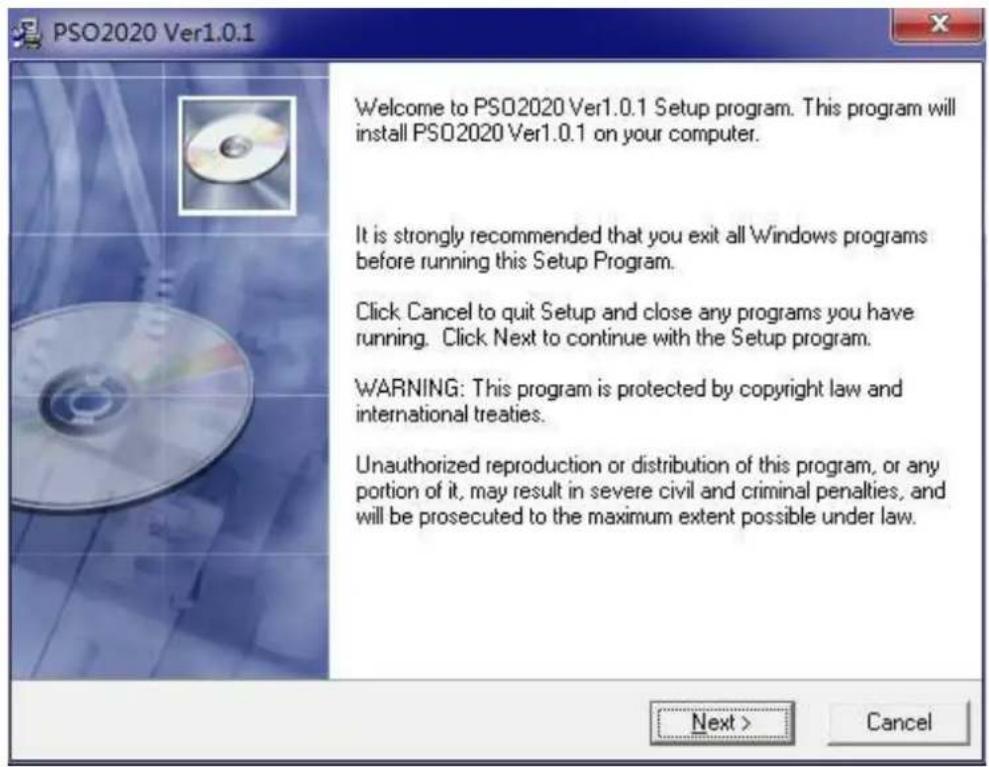
- The software Installation is started. Click 'Next' to continue.
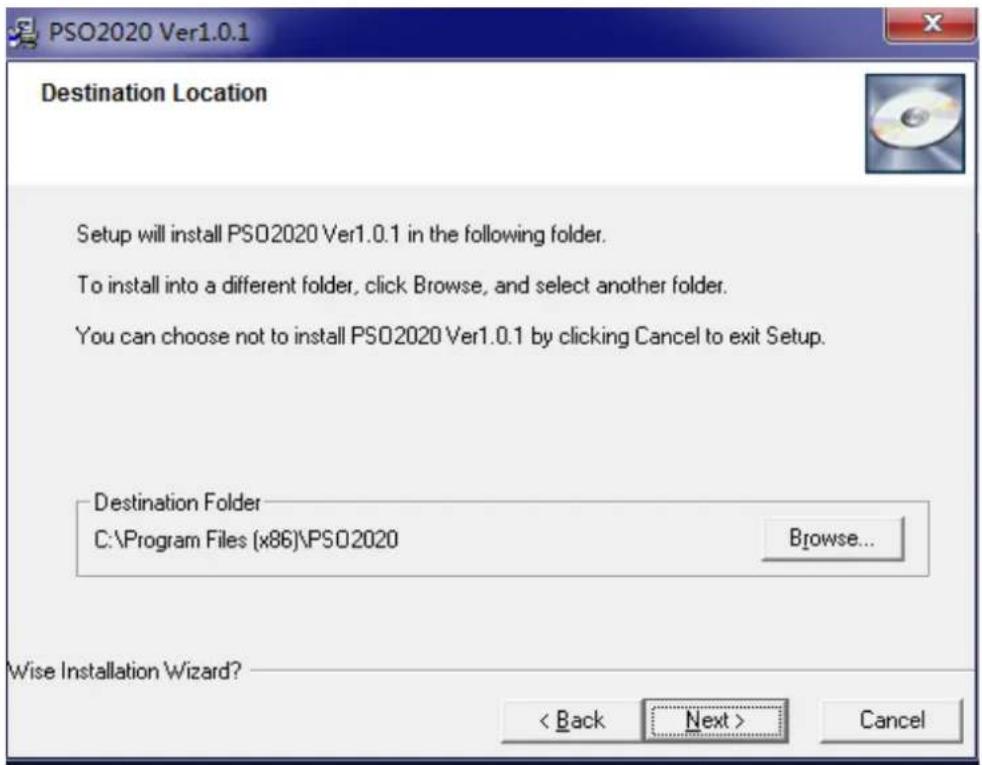
- Choose a destination directory. Click 'Next' to continue.
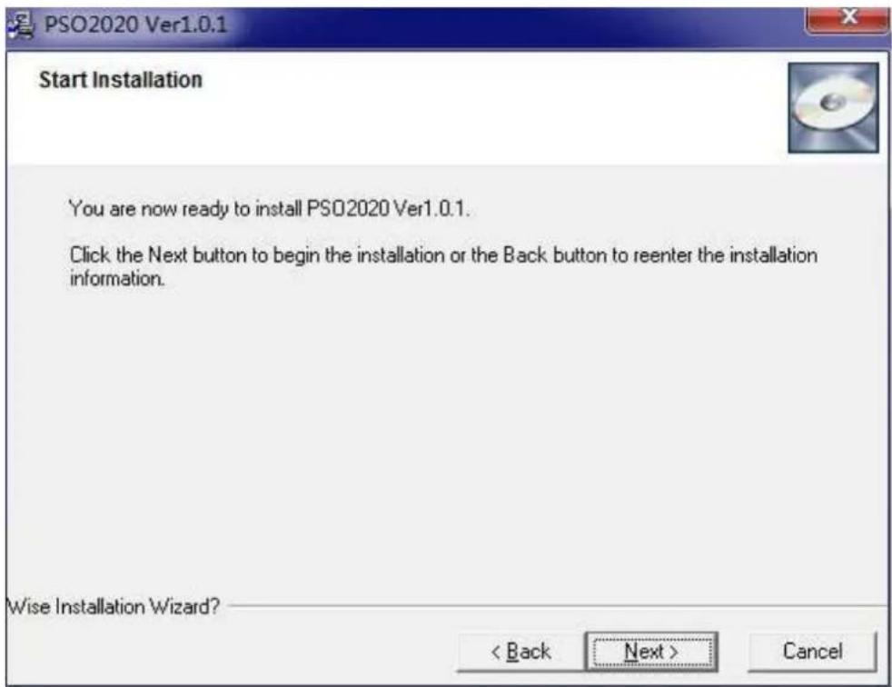
- Check the setup information. Click Next to start copying of files.
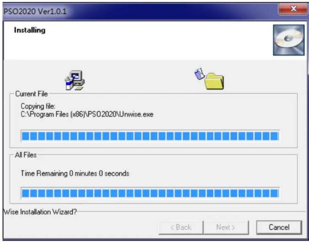
- This Status dialog is displayed during copying of files.
- Updating Your System Configuration.

Updating System Configuration, Please Wait...
- The installation is complete.
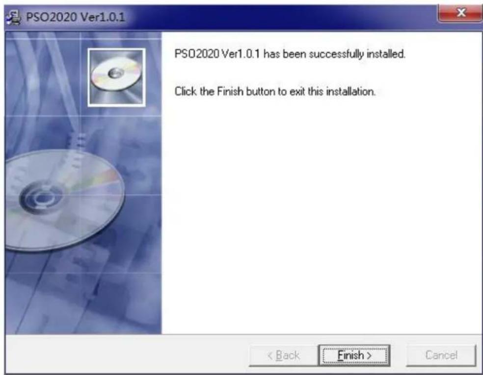
1.3 Install Driver
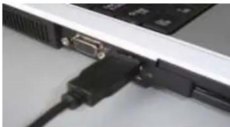
- Connect the A-Type Plug of USB cable to your PC'S USB port.
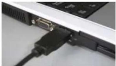
natural_image
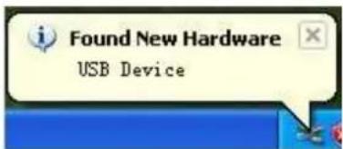
Close-up of a computer monitor with an attached black VGA port and adjacent cable (no visible text or symbols)- New hardware is found.
- New hardware search wizard starts.
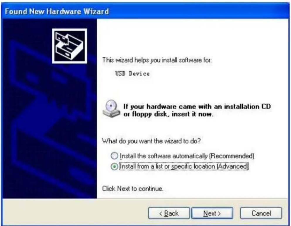
- New hardware search wizard starts to search the driver.
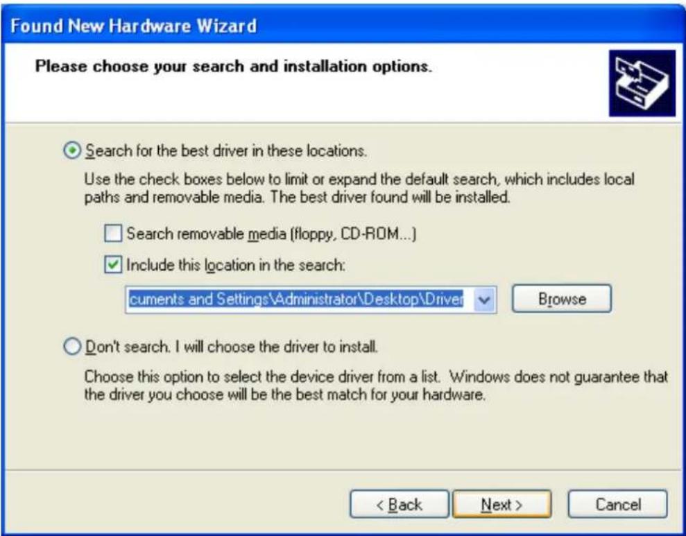
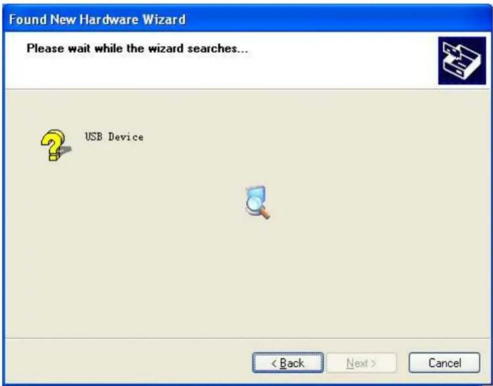
- New hardware wizard installs "DRIVER".
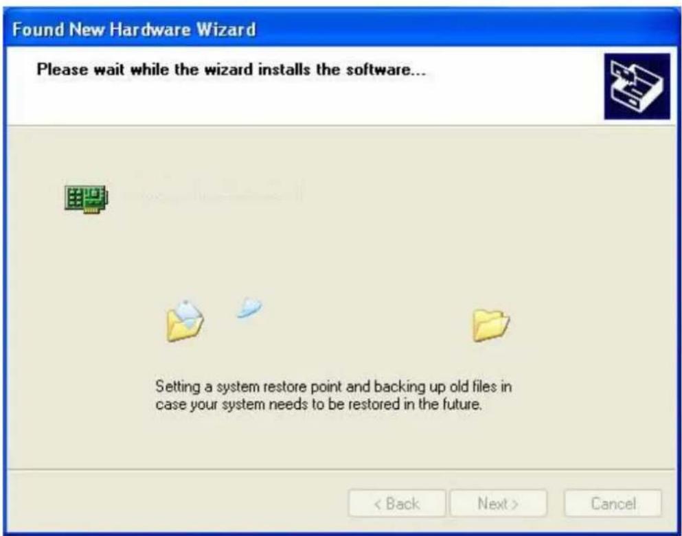
- The wizard has finished installing for "DRIVER".
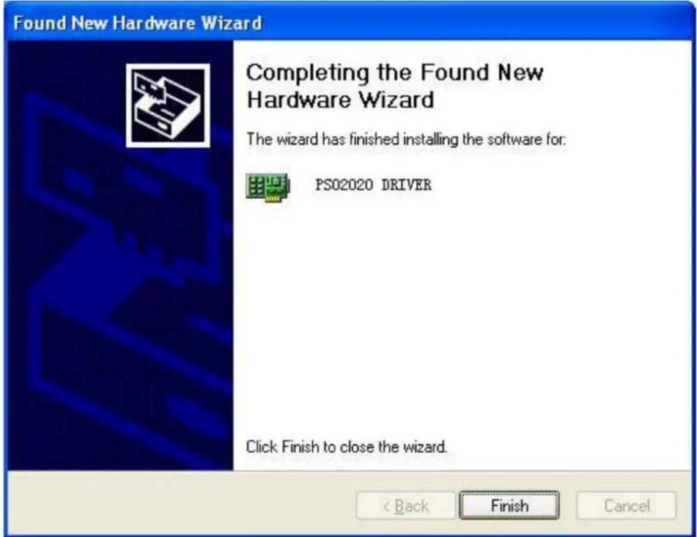
- Your new hardware is installed and ready to use.

1.4 General Features
◆ Maximum real-time sample rate: 96MSa/s
◆ Memory depth: 1Mbyte/channel
◆ Built-in Fast Fourier Transform function(FFT);
◆ 20 Automatic measurements;
◆ Automatic cursor tracking measurements;
◆ Waveform storage;
◆ User selectable fast offset calibration;
◆ User interface in several user-selectable languages;
◆ Adjustable waveform intensity, more effective waveform view;
1.5 General Check
Please check the instrument as following steps after receiving an oscilloscope:
◆ Check the shipping container for damage:
Keep the damaged shipping container or cushioning material until the contents of the shipment have been checked for completeness and the instrument has been checked mechanically and electrically.
◆ Check the accessories:
Accessories supplied with the instrument are listed in "Accessories" in this guide. If the contents are incomplete or damaged, please notify the franchiser.
◆ Check the instrument:
In case there is any mechanical damage or defect, or the instrument does not operate properly or fails performance tests, please notify the franchiser.
1.6 Function Check
Perform this functional check to verify that your oscilloscope is operating correctly.
◆ Connect the oscilloscope
You should connect the A-Type Plug of USB cable to your PC USB port and connect the probe with the signal source.
natural_image
Close-up of a black VGA connector inserted into a computer monitor (no visible text or symbols)◆ Input a signal to a channel of the oscilloscope
Please input signal in the following steps:
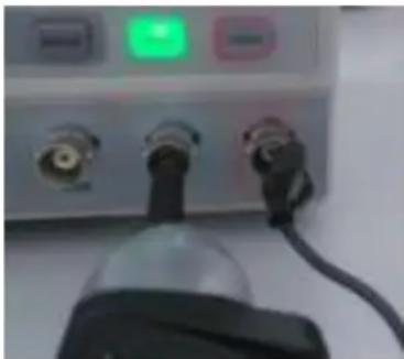
connect the probe with the signal source and ensure good grounding clip.
natural_image
Close-up of a medical device with two connectors and a black bulb, no visible text or symbols- Attach the tip of probe and ground nip to the Connector of Probe. A square wave will be displayed within a several seconds. (Approximately 1 kHz, 2V, peak-to-peak).
1.7 Self Calibration
The self calibration routine lets you optimize the oscilloscope signal path for maximum measurement accuracy. You can run the routine at any time but you should always run the routine if the ambient temperature changes by 5^ C or more. For accurate calibration, power on the oscilloscope and wait twenty minutes to ensure it is warmed up. To compensate the signal path, disconnect any probes or cables from the input connectors. Then, access the “Menu -> Utility -> Calibration” option and follow the directions on the screen. The self calibration routine takes about several minutes.
1.8 Accessories
All the accessories listed below are standard accessories for the oscilloscope:
◆ A PC software CD of the oscilloscope
Chapter 2 Operating Basics
◆ The User's Interface
◆ The Menu System
◆ The Vertical System
◆ The Horizontal System
◆ The Trigger System
◆ Input Connector
2.1 The User's Interface
Click the software icon on the desk after you finished the software setting and equipment connecting. Then a user interface will be showed as follows:
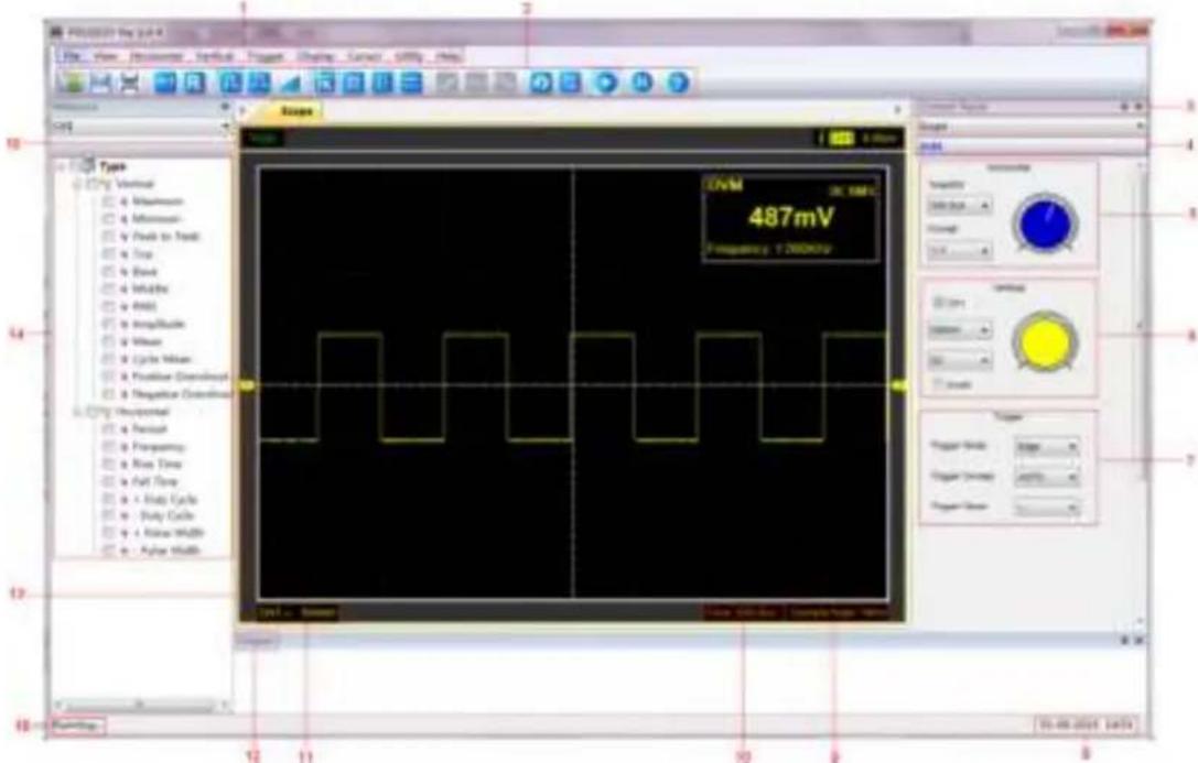
In addition to displaying waveforms, the display area is filled with many details about the waveform and the oscilloscope control settings.
1. The Main Menu
All settings can be found in the main menu.
2. The Toolbar
3. Control Panel
4. DVM
5. The Horizontal Panel
The user can change Time/Div, format in the panel.
6. The Vertical Panel
The user can turn on/off the CH1. Also the user can change the CH1 volt/div.
7. The Trigger Panel
In this panel, the user can change the trigger mode, sweep,slope.
8. Displays the system time.
9. Displays Sample Rate
10. Displays the main time base setting.
11. Displays the CH1 information
Readouts show the coupling of the channels.
Readouts show the vertical scale factors of the channels.
-
Output Window
-
The markers show the reference points of the displayed waveforms. If there is no marker, the channel is not displayed.
-
Measure Window.
-
Trige state
-
"Running": the program found the hardware and the hardware works normally. "Searching Device": not find the device and the program is searching the device.
2.2 Button description
The buttons with PSO2020 pen storage oscilloscope as follows:
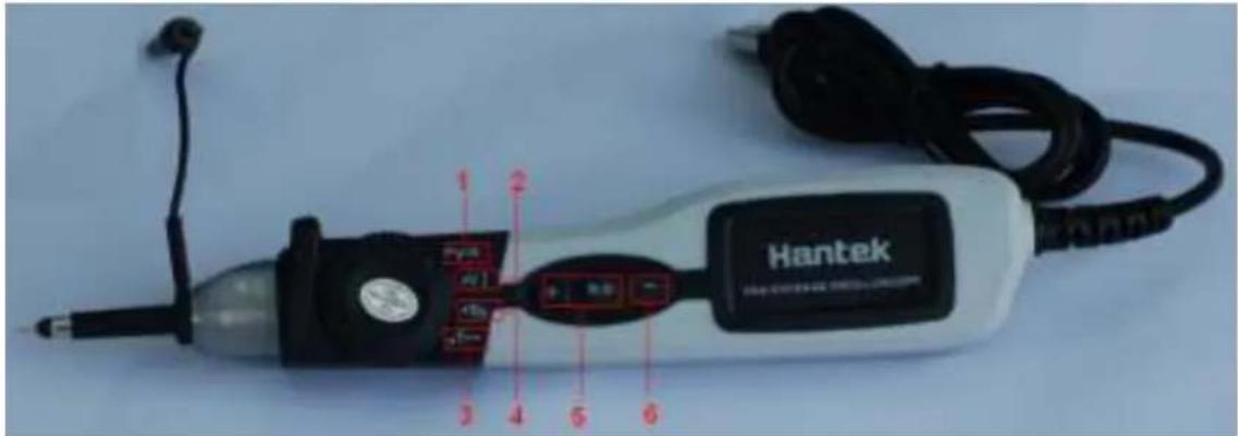
| 1、Voltage (V⊕) | “+” button | Single click: Voltage increaseKeep clicking: continuous increase with Voltage |
| “-” button | Single click: Voltage decreaseKeep clicking: continuous decrease with Voltage | |
| R/S button | Single click: RUN or STOPKeep clicking: AUTO SET | |
| 2、OFFSET (V↓) | “+” button | Single click: Waveform moves downKeep clicking: Waveform continuous downward movement |
| “-” button | Single click: Waveform move upwardKeep clicking: Waveform continuous upward movement | |
| R/S button | Single click: RUN or STOPKeep clicking: AUTO SET | |
| 3、POSITION (T←) | “+” button | Single click: left shiftKeep clicking: left shift continuous |
| “-” button | Single click: right shiftKeep clicking: right shift continuous | |
| R/S button | Single click: RUN or STOPKeep clicking: AUTO SET | |
| 4、TIME (T) | “+” button | Single click: Time increaseKeep clicking: continuous increase with Time |
| “-” button | Single click: Time decreaseKeep clicking: continuous decrease with Time | |
| R/S button | Single click: RUN or STOPKeep clicking: AUTO SET | |
| 5、combination button | “+” & “R/S” | Single click: LED lamp switch |
| 6、- | “-” | - |
2.3 The Menu System
The Main Menu
File View Horizontal Vertical Trigger Display Cursor Utility Help
- File: Load or Save data, setup
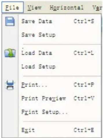
- View: Change the user interface
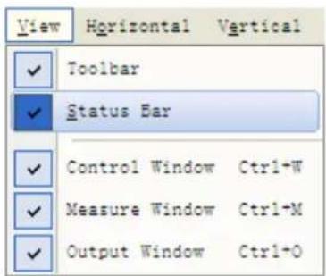
- Horizontal: Set the horizontal system
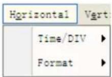
- Vertical: Set the vertical system
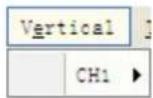
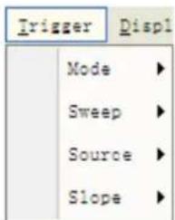
- Trigger: Set the trigger system
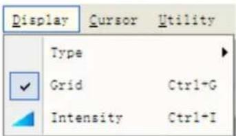
- Display: The waveform display setup
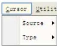
- Cursor: Cursor measure setup
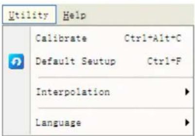
- Utility: Utility setting
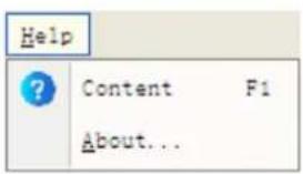
- Help: Turn on help file
2.4 The Vertical System
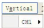
Click "Vertical" in main menu
The following figure shows the vertical system menu. It shows the vertical parameters setting.
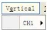
- CH1: Leads to the setting of the CH1 parameters
Use the left mouse button to dragging the channel icon to set the vertical position offset precisely.
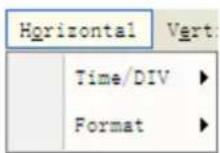
2.5 The Horizontal System
Click "Horizontal" in main menu
The following figure shows the Horizontal System window. It shows the horizontal parameters settings.
-
Time/DIV: leads the setting of the time base parameters
-
Format: leads the setting of the horizontal format parameters
The time base ranges of the oscilloscope is listed as follows. The horizontal scan speed is from 4ns/div to 1hour/div.
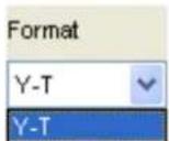
In the "Format" menu of the "Horizontal" menu, select the display mode to Y-T.
2.6 The Trigger System
Click "Trigger" in main menu.
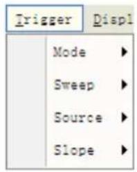
Mode: Sets the trigger mode to Edge trigger
Sweep: Selects the trigger sweep mode to AUTO, NORMAL or SINGLE
Source: Selects the trigger source to CH1.
Slope: Selects the edge trigger slope to Positive or Negative slope
The user can drag the trigger icon to adjust the trigger level and the trigger level will be displayed on the top right corner.
2.7 Input Connectors
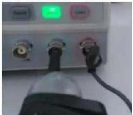
Input Connectors:
natural_image
Close-up of a medical or laboratory setup with two connectors and a green indicator light (no visible text or symbols)CH 1: Input connectors for waveform display.
GND.: a ground terminal
USB PORT: Connect the A-Type Plug of USB cable to your pc.
Chapter 3 Understanding Function
◆ Set Oscilloscope
◆ Set Vertical System
◆ Set Horizontal System
◆ Set Trigger System
◆ Measure Signal
◆ Utility Function
◆ The Display System
◆ Save/Load
◆ Print
3.1 Set Oscilloscope
Save Setup
The oscilloscope software saves the current setup before you close the oscilloscope software. The oscilloscope recalls this setup the next time you run the software. You can use the "Save Setup" menu to permanently save up to several different setups.
Load Setup
The oscilloscope can recall the last setup before the oscilloscope software was running, any saved setups, or the factory setup. You can use the "Load Setup" menu to permanently recall a setup.
Factory Setup
The oscilloscope software is set up for normal operation when it is shipped from the factory. This is the factory setup. To recall this setup, push the "Factory Setup" menu.
3.2 Set Vertical Systems
Click "Vertical" in main menu
The Vertical Menu function:
◆ Turn ON/Off: Turn on/off the channel
◆ Volt/DIV: Select the channel voltage/div
◆ Invert: Turns the displayed waveform 180 degrees
Change Volt/DIV
You can click "Volt/Div" in "CH1" Menu to select the voltage
You can also change "CH1" voltage in sidebar
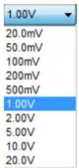
You can left click and drag the mouse on the green knob or the yellow knob to change the voltage.
Invert
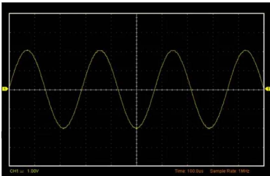
The invert function turns the displayed waveform 180 degrees, with respect to the ground level. When the oscilloscope is triggered on the inverted signal, the trigger is also inverted. Click "Invert" in vertical.
Turn off invert
Turn on invert
The following picture shows the waveform before inversion:
line
| Time (us) | Voltage (V) | | --------- | ----------- | | 0 | 0 | | 1 | 2 | | 2 | 0 | | 3 | -2 | | 4 | 0 | | 5 | 2 | | 6 | 0 | | 7 | -2 | | 8 | 0 | | 9 | 2 | | 10 | 0 | | 11 | -2 | | 12 | 0 | | 13 | 2 | | 14 | 0 | | 15 | -2 | | 16 | 0 | | 17 | 2 | | 18 | 0 | | 19 | -2 | | 20 | 0 | | 21 | 2 | | 22 | 0 | | 23 | -2 | | 24 | 0 | | 25 | 2 | | 26 | 0 | | 27 | -2 | | 28 | 0 | | 29 | 2 | | 30 | 0 | | 31 | -2 | | 32 | 0 | | 33 | 2 | | 34 | 0 | | 35 | -2 | | 36 | 0 | | 37 | 2 | | 38 | 0 | | 39 | -2 | | 40 | 0 | | 41 | 2 | | 42 | 0 | | 43 | -2 | | 44 | 0 | | 45 | 2 | | 46 | 0 | | 47 | -2 | | 48 | 0 | | 49 | 2 | | 50 | 0 | | 51 | -2 | | 52 | 0 | | 53 | 2 | | 54 | 0 | | 55 | -2 | | 56 | 0 | | 57 | 2 | | 58 | 0 | | 59 | -2 | | 60 | 0 | | 61 | 2 | | 62 | 0 | | 63 | -2 | | 64 | 0 | | 65 | 2 | | 66 | 0 | | 67 | -2 | | 68 | 0 | | 69 | 2 | | 70 | 0 | | 71 | -2 | | 72 | 0 | | 73 | 2 | | 74 | 0 | | 75 | -2 | | 76 | 0 | | 77 | 2 | | 78 | 0 | | 79 | -2 | | 80 | 0 | | 81 | 2 | | 82 | 0 | | 83 | -2 | | 84 | 0 | | 85 | 2 | | 86 | 0 | | 87 | -2 | | 88 | 0 | | 89 | 2 | | 90 | 0 | | 91 | -2 | | 92 | 0 | | 93 | 2 | | 94 | 0 | | 95 | -2 | | 96 | 0 | | 97 | 2 | | 98 | 0 | | 99 | -2 | | | |The following picture shows the waveform of inversion:
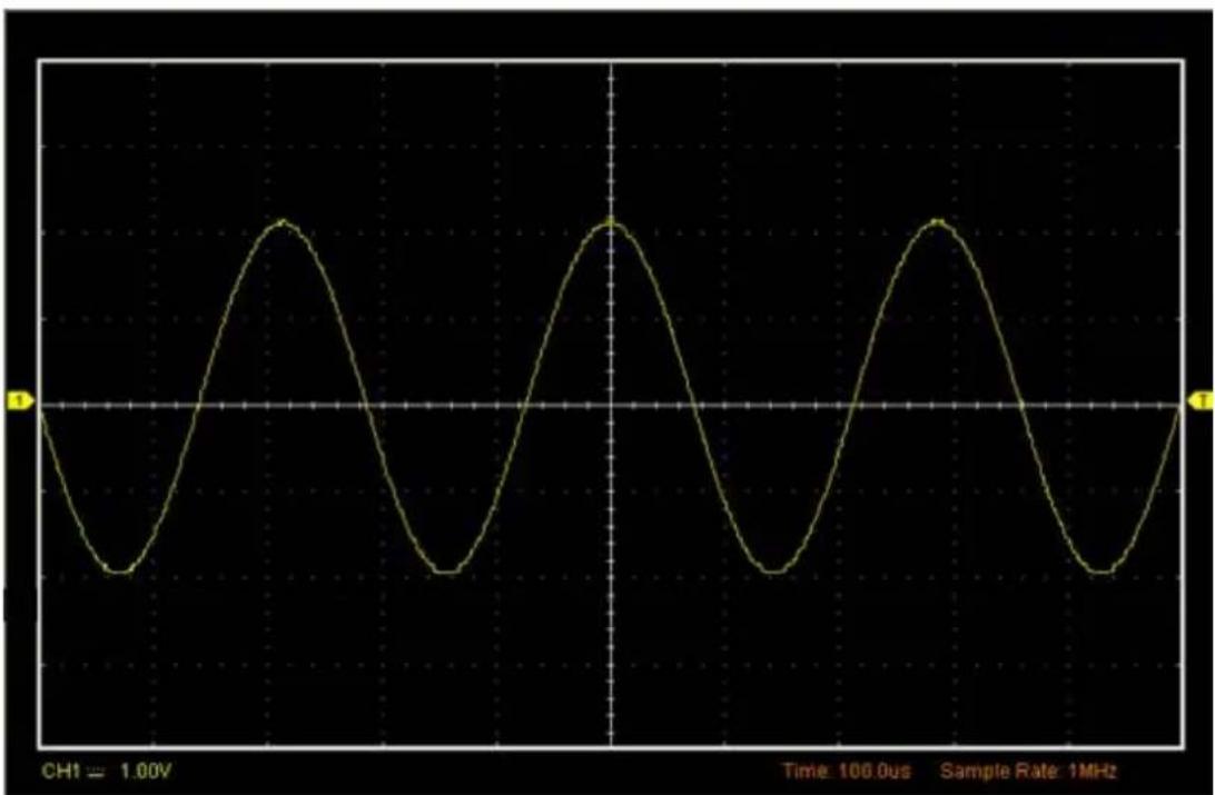
line
| Time (us) | Voltage | | --------- | ------- | | 0 | 0 | | 1 | -1 | | 2 | 0 | | 3 | 1 | | 4 | -1 | | 5 | 0 | | 6 | 1 | | 7 | -1 | | 8 | 0 | | 9 | 1 | | 10 | -1 | | 11 | 0 | | 12 | 1 | | 13 | -1 | | 14 | 0 | | 15 | 1 | | 16 | -1 | | 17 | 0 | | 18 | 1 | | 19 | -1 | | 20 | 0 | | 21 | 1 | | 22 | -1 | | 23 | 0 | | 24 | 1 | | 25 | -1 | | 26 | 0 | | 27 | 1 | | 28 | -1 | | 29 | 0 | | 30 | 1 | | 31 | -1 | | 32 | 0 | | 33 | 1 | | 34 | -1 | | 35 | 0 | | 36 | 1 | | 37 | -1 | | 38 | 0 | | 39 | 1 | | 40 | -1 | | 41 | 0 | | 42 | 1 | | 43 | -1 | | 44 | 0 | | 45 | 1 | | 46 | -1 | | 47 | 0 | | 48 | 1 | | 49 | -1 | | 50 | 0 | | 51 | 1 | | 52 | -1 | | 53 | 0 | | 54 | 1 | | 55 | -1 | | 56 | 0 | | 57 | 1 | | 58 | -1 | | 59 | 0 | | 60 | 1 | | 61 | -1 | | 62 | 0 | | 63 | 1 | | 64 | -1 | | 65 | 0 | | 66 | 1 | | 67 | -1 | | 68 | 0 | | 69 | 1 | | 70 | -1 | | 71 | 0 | | 72 | 1 | | 73 | -1 | | 74 | 0 | | 75 | 1 | | 76 | -1 | | 77 | 0 | | 78 | 1 | | 79 | -1 | | 80 | 0 | | 81 | 1 | | 82 | -1 | | 83 | 0 | | 84 | 1 | | 85 | -1 | | 86 | 0 | | 87 | 1 | | 88 | -1 | | 89 | 0 | | 90 | 1 | | 91 | -1 | | 92 | 0 | | 93 | 1 | | 94 | -1 | | 95 | 0 | | 96 | 1 | | 97 | -1 | | 98 | 0 | | 99 | 1 | | | |3.2.1 Set FFT
Fast Fourier Transform Function
To use the FFT mode, you need to click

in Toolbar to open the FFT setup window.
The FFT setup window:
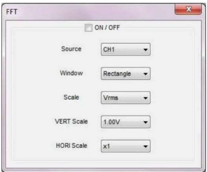
You can select the Source channel, Window algorithm, FFT number, and FFT Zoom factor. It displays only one FFT spectrum at a time.
Source:
Source

Selects the channel used as the FFT source
Window: Window Rectangle
Selects the FFT window type
Scale:
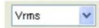
Selects the vertical scale units
Vert Scale: 1.00V
Selects the vertical scale
HORI Scale:
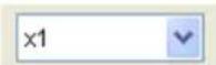
Selects the FFT zoom factor
Sets horizontal scale, If the information is more than the quantity displayed to the display window, more information is displayed by using scroll bar.
You can click the "ON/OFF" button to start FFT math, also you can click this button to stop FFT math.
3.2.2 Set Reference
Click "R" in Toolbar to set REF.
The Reference Channel Function:
◆ Turn On/Off: Turn on/off the reference channel.
◆ Volt/DIV: Channel the resolution of the reference channel.
◆ Time/DIV: leading the setting of the time base parameters.
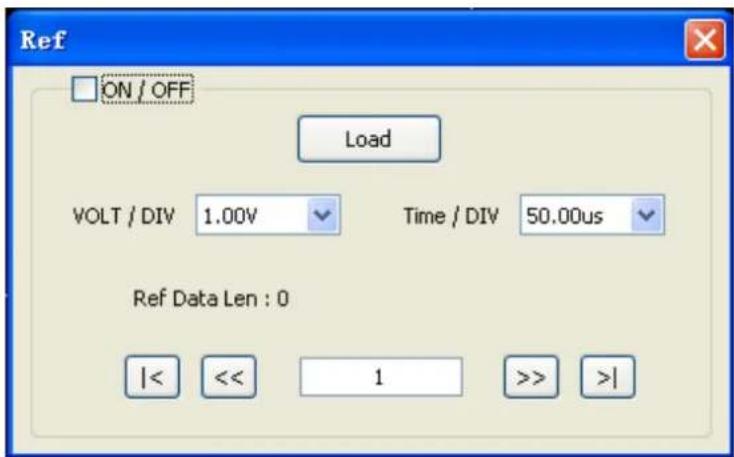
You can change the vertical scale of a waveform. The waveform display will contract or expand relative to the reference level.
The Reference Waveform Display Window:
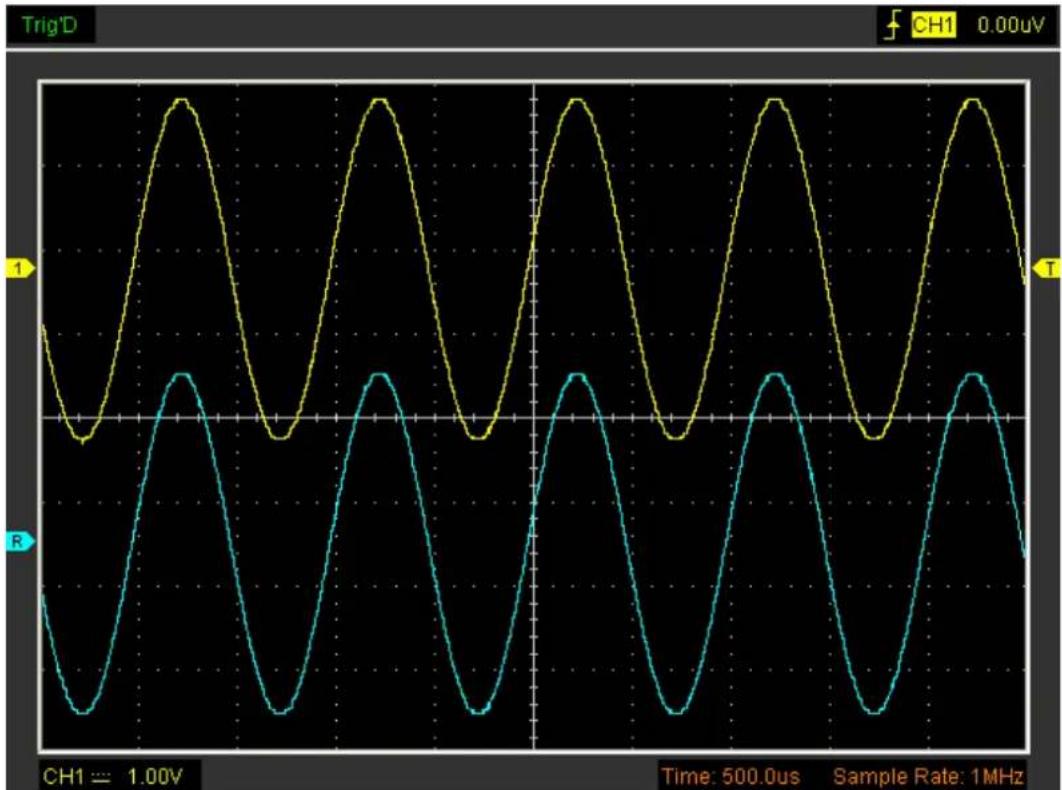
Note: If you turn on the "Reference" channel, the load file window will appear.
3.3 Set Horizontal System
The following figure shows the Horizontal System window. It shows the horizontal parameters settings.
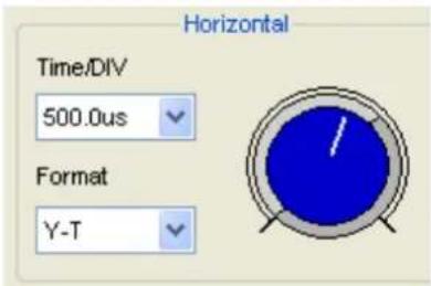
- Time/DIV: leads the setting of the time base parameters
- Format: leads the setting of the horizontal format parameters
The time base ranges of the oscilloscope is listed as follows. The horizontal scan speed is
from 4ns/div to 1hour/div.
In the "Format" menu of the "Horizontal" menu, select the display mode to Y-T.
3.4 Set Trigger System
Click "Trigger" in main menu.
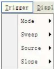
The trigger determines when the oscilloscope starts to acquire data and display a waveform. When a trigger is set up properly, it can convert unstable displays or blank screens into meaningful waveforms.
If the oscilloscope wants to acquire a waveform, it collects enough data so that it can draw the waveform to the left of the trigger point. The oscilloscope continues to acquire data while waiting for the trigger condition to occur. The oscilloscope continues to acquire enough data so that it can draw the waveform to the right of the trigger point after it detects a trigger.
The Edge trigger determines whether the oscilloscope finds the trigger point on the rising or the falling edge of a signal. Select Edge trigger mode to trigger on Rising edge or Falling edge.
Mode: Select the trigger mode.
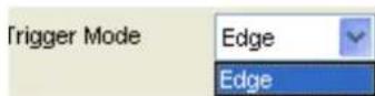
The oscilloscope only provides edge trigger mode.
Sweep: Set the sweep mode to Auto, Normal or Single.
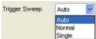
Auto: Acquire waveform even no trigger occurred
Normal: Acquire waveform when trigger occurred.
Single: Acquire waveform when trigger occurred then stop
Slope: Set the slope to Rising (+) or Falling (-).
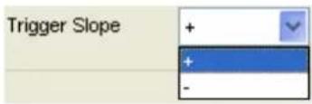
Rising: Trigger on rising edge
Falling: Trigger on falling edge
3.5 Measure Signal
3.5.1 Cursor
Click "Cursor" in main menu.
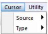
This method allows you to take measurements by moving the cursors
1. Source
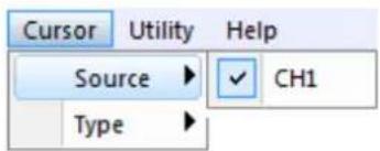
The user can set the source to CH1.
2. Type
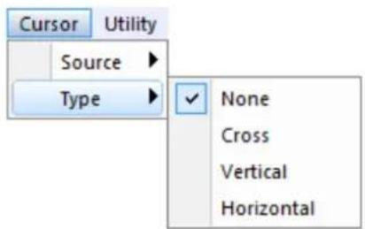
There are four types of cursors: Cross, Vertical and Horizontal.
1) Cross
The Cross cursors appear as cross lines on the display and measure the vertical and horizontal parameters.
The Cross cursor display window:
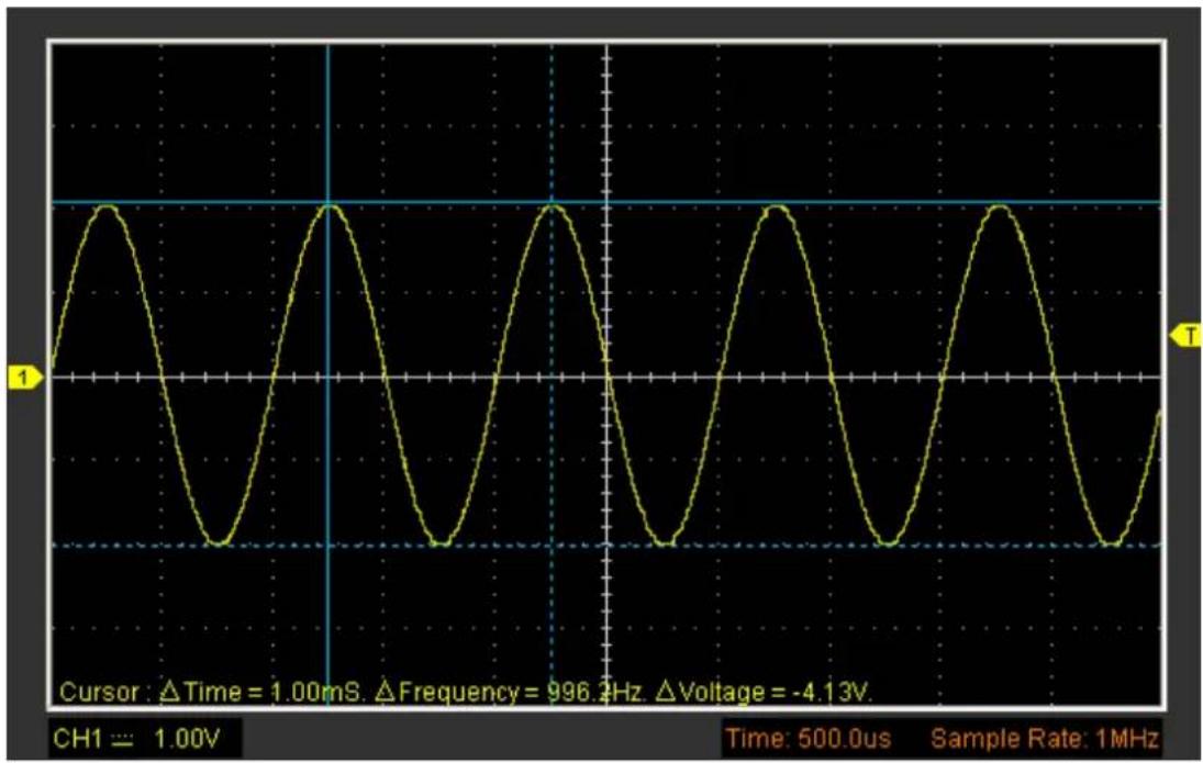
line
| Time (μs) | Voltage (V) | | --------- | ----------- | | 0 | -4.13 | | 500.0 | 996.2 |2) Vertical
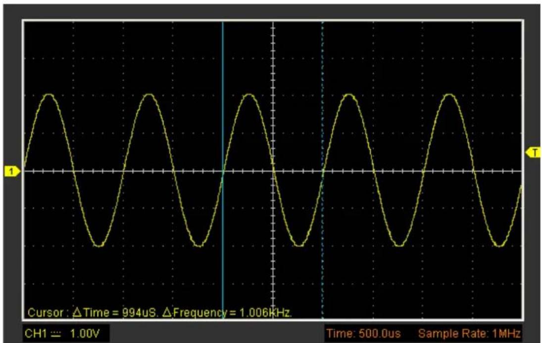
The Vertical cursors appear as vertical lines on the display and measure the vertical parameters.
The Vertical cursor display window:
line
| Time (μs) | Voltage | | --------- | ------- | | 0 | 1 | | 500.0 | 994 | | 1000.0 | 1 | | 1500.0 | 994 | | 2000.0 | 1 | | 2500.0 | 994 | | 3000.0 | 1 | | 3500.0 | 994 | | 4000.0 | 1 | | 4500.0 | 994 | | 5000.0 | 1 | | 5500.0 | 994 | | 6000.0 | 1 | | 6500.0 | 994 | | 7000.0 | 1 | | 7500.0 | 994 | | 8000.0 | 1 | | 8500.0 | 994 | | 9000.0 | 1 | | 9500.0 | 994 | | 10000.0 | 1 | | 10500.0 | 994 | | 11000.0 | 1 | | 11500.0 | 994 | | 12000.0 | 1 | | 12500.0 | 994 | | 13000.0 | 1 | | 13500.0 | 994 | | 14000.0 | 1 | | 14500.0 | 994 | | 15000.0 | 1 | | 15500.0 | 994 | | 16000.0 | 1 | | 16500.0 | 994 | | 17000.0 | 1 | | 17500.0 | 994 | | 18000.0 | 1 | | 18500.0 | 994 | | 19000.0 | 1 | | 19500.0 | 994 | | 20000.0 | 1 | | 20500.0 | 994 | | 21000.0 | 1 | | 21500.0 | 994 | | 22000.0 | 1 | | 22500.0 | 994 | | 23000.0 | 1 | | 23500.0 | 994 | | 24000.0 | 1 | | 24500.0 | 994 | | 25000.0 | 1 | | 25500.0 | 994 | | 26000.0 | 1 | | 26500.0 | 994 | | 27000.0 | 1 | | 27500.0 | 994 | | 28000.0 | 1 | | 28500.0 | 994 | | 29000.0 | 1 | | 29500.0 | 994 | | 30000.0 | 1 | | | |3) Horizontal
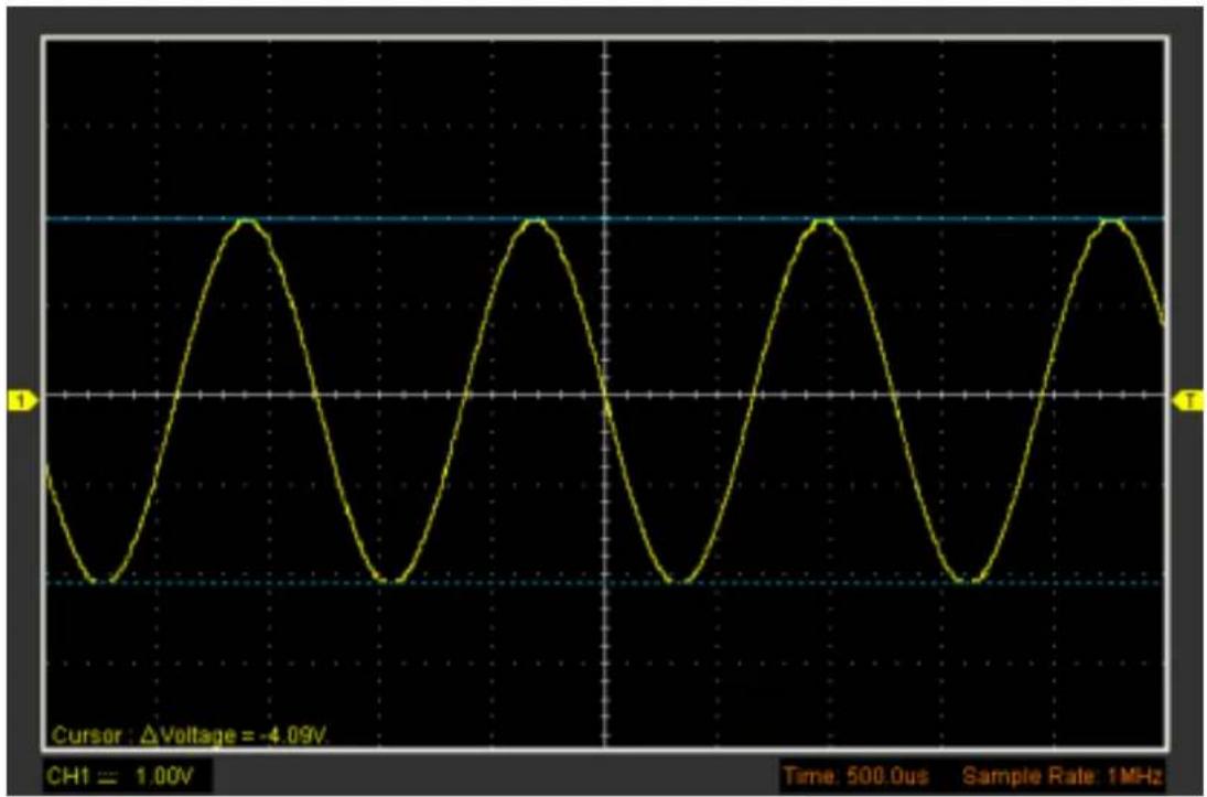
The Horizontal cursors appear as horizontal lines on the display and measure the horizontal parameters.
The Horizontal cursor display window:
line
| Time (ms) | Voltage (V) | | --------- | ----------- | | 0 | 1.00 | | 500 | 0.0 | | 1000 | ±4.09 | | 1500 | 0.0 | | 2000 | ±4.09 | | 2500 | 0.0 | | 3000 | ±4.09 | | 3500 | 0.0 | | 4000 | ±4.09 | | 4500 | 0.0 | | 500 | ±4.09 | | 550 | 0.0 | | 600 | ±4.09 | | 650 | 0.0 | | 700 | ±4.09 | | 750 | 0.0 | | 800 | ±4.09 | | 850 | 0.0 | | 900 | ±4.09 | | 950 | 0.0 | | 1000 | ±4.09 | | 1050 | 0.0 | | 1100 | ±4.09 | | 1150 | 0.0 | | 1200 | ±4.09 | | 1250 | 0.0 | | 1300 | ±4.09 | | 1350 | 0.0 | | 1400 | ±4.09 | | 1450 | 0.0 | | 1500 | ±4.09 | | 1550 | 0.0 | | 1600 | ±4.09 | | 1650 | 0.0 | | 1700 | ±4.09 | | 1750 | 0.0 | | 1800 | ±4.09 | | 1850 | 0.0 | | 1900 | ±4.09 | | 1950 | 0.0 | | 2000 | ±4.09 | | 2050 | 0.0 | | 2100 | ±4.09 | | 2150 | 0.0 | | 2200 | ±4.09 | | 2250 | 0.0 | | 2300 | ±4.09 | | 2350 | 0.0 | | 2400 | ±4.09 | | 2450 | 0.0 | | 2500 | ±4.09 | | 2550 | 0.0 | | 2600 | ±4.09 | | 2650 | 0.0 | | 2700 | ±4.09 | | 2750 | 0.0 | | 2800 | ±4.09 | | 2850 | 0.0 | | 2900 | ±4.09 | | 2950 | 0.0 | | 3000 | ±4.09 | | 3050 | 0.0 | | 3100 | ±4.09 | | 3150 | 0.0 | | 3200 | ±4.09 | | 3250 | 0.0 | | 3300 | ±4.09 | | 3350 | 0.0 | | 3400 | ±4.09 | | 3450 | 0.0 | | 3500 | ±4.09 | | 3550 | 0.0 | | 3600 | ±4.09 | | 3650 | 0.0 | | 3700 | ±4.09 | | 3750 | 0.0 | | 3800 | ±4.09 | | 3850 | 0.0 | | 3900 | ±4.09 | | 3950 | 0.0 | | 4000 | ±4.09 | | 4050 | 0.0 | | 4100 | ±4.09 | | 4150 | 0.0 | | 4200 | ±4.09 | | 4250 | 0.0 | | 4300 | ±4.09 | | 4350 | 0.0 | | 4400 | ±4.09 | | 4450 | 0.0 | | 4500 | ±4.09 | | 4550 | 0.0 | | 4600 | ±4.09 | | 4650 | 0.0 | | 4700 | ±4.09 | | 4750 | 0.0 | | 4800 | ±4.09 | | 4850 | 0.0 | | 4900 | ±4.09 | | 4950 | 0.0 | | 5₀₀₁₆ | ±4.⁰⁹ | | | |3.5.2 Measure
Click "Measure" in main menu.
The oscilloscope provides 20 parametric auto measurements (12 voltage and 8 time measurements).
1. Vertical
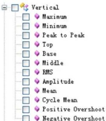
Maximum: Voltage of the absolute maximum level, Measured over the entire waveform
Minimum: Voltage of the absolute minimum level, Measured over the entire waveform
Peak To Peak: Peak-to-peak = Max - Min, Measured over the entire waveform
Top: Voltage of the statistical maximum level, Measured over the entire waveform
Base: Voltage of the statistical minimum level, Measured over the entire waveform
Middle: Voltage of the 50% level from base to top
RMS: The Root Mean Square voltage over the entire waveform
Amplitude: Amp = Base - Top, Measured over the entire waveform
Mean: The arithmetic mean over the entire waveform
Cycle Mean: The arithmetic mean over the first cycle in the waveform
Preshoot: Positive Overshoot = (Max - Top)/Amp x 100 %, Measured over the entire waveform
Overshoot: Negative Overshoot = (Base - Min)/Amp x 100 %, Measured over the entire waveform
2. Horizontal
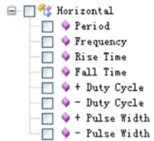
flowchart
graph TD
    A[" "] --> B["Horizontal"]
    B --> C["Period"]
    B --> D["Frequency"]
    B --> E["Rise Time"]
    B --> F["Fall Time"]
    B --> G["+ Duty Cycle"]
    B --> H["- Duty Cycle"]
    B --> I["+ Pulse Width"]
    B --> J["- Pulse Width"]
Period: Time to take for the first signal cycle to complete in the waveform
Frequency: Reciprocal of the period of the first cycle in the waveform
Rise Time: Time taken from lower threshold to upper threshold
Fall Time: Time taken from upper threshold to lower threshold
+Duty Cycle: Positive Duty Cycle = (Positive Pulse Width)/Period x 100%, Measured of the first cycle in waveform
-Duty Cycle: Negative Duty Cycle = (Negative Pulse Width)/Period x 100%, Measured of the first cycle in waveform
+Pulse Width: Measured of the first positive pulse in the waveform. The time between the 50% amplitude points
-Pulse Width: Measured of the first negative pulse in the waveform. The time between the 50% amplitude points
3. Clear Measure
Clear all measure items on display screen.
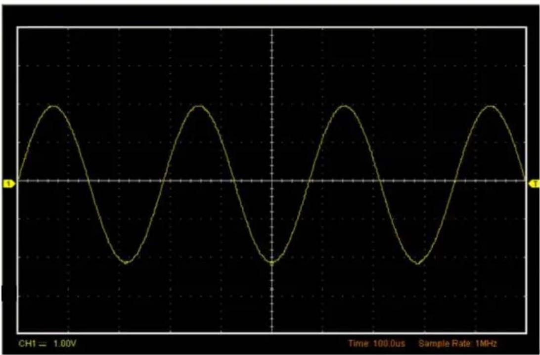
The Measure Display Window:
line
| Time (μs) | Voltage | | --------- | ------- | | 0 | 0 | | 1 | 2 | | 2 | 0 | | 3 | -2 | | 4 | 0 | | 5 | 2 | | 6 | 0 | | 7 | -2 | | 8 | 0 | | 9 | 2 | | 10 | 0 | | 11 | -2 | | 12 | 0 | | 13 | 2 | | 14 | 0 | | 15 | -2 | | 16 | 0 | | 17 | 2 | | 18 | 0 | | 19 | -2 | | 20 | 0 | | 21 | 2 | | 22 | 0 | | 23 | -2 | | 24 | 0 | | 25 | 2 | | 26 | 0 | | 27 | -2 | | 28 | 0 | | 29 | 2 | | 30 | 0 | | 31 | -2 | | 32 | 0 | | 33 | 2 | | 34 | 0 | | 35 | -2 | | 36 | 0 | | 37 | 2 | | 38 | 0 | | 39 | -2 | | 40 | 0 | | 41 | 2 | | 42 | 0 | | 43 | -2 | | 44 | 0 | | 45 | 2 | | 46 | 0 | | 47 | -2 | | 48 | 0 | | 49 | 2 | | 50 | 0 | | 51 | -2 | | 52 | 0 | | 53 | 2 | | 54 | 0 | | 55 | -2 | | 56 | 0 | | 57 | 2 | | 58 | 0 | | 59 | -2 | | 60 | 0 | | 61 | 2 | | 62 | 0 | | 63 | -2 | | 64 | 0 | | 65 | 2 | | 66 | 0 | | 67 | -2 | | 68 | 0 | | 69 | 2 | | 70 | 0 | | 71 | -2 | | 72 | 0 | | 73 | 2 | | 74 | 0 | | 75 | -2 | | 76 | 0 | | 77 | 2 | | 78 | 0 | | 79 | -2 | | 80 | 0 | | 81 | 2 | | 82 | 0 | | 83 | -2 | | 84 | 0 | | 85 | 2 | | 86 | 0 | | 87 | -2 | | 88 | 0 | | 89 | 2 | | 90 | 0 | | 91 | -2 | | 92 | 0 | | 93 | 2 | | 94 | 0 | | 95 | -2 | | 96 | 0 | | 97 | 2 | | 98 | 0 | | 99 | -2 | | | |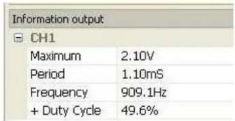
Note: The results of the automatic measurements will be displayed on the bottom of the screen. Maximum 8 results could be displayed at the same time. When there is no room, the next new measurement result will make the previous results moving left, out of screen.
3.6 The Utility Function
Click the "Menu -> Utility" to get into the "Utility" menu.
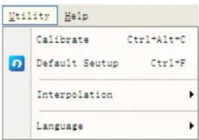
The "Utility" Functions:
◆ Default Setup
◆ Interpolation
Language
3.6.1 Default Setup
Click "Default Setup" in "Utility" menu to load default setups
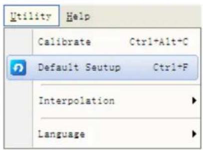
When you click the Default Setup in Utility menu, the oscilloscope displays the CH1 waveforms and removes all other waveforms.
The oscilloscope set up for normal operation when it is shipped from the factory and can be recalled at anytime by user.
The Factory Setup function does not reset the following settings:
◆ Language option
◆ Date and time
3.6.2 Language
Click "Language" in "Utility" menu.
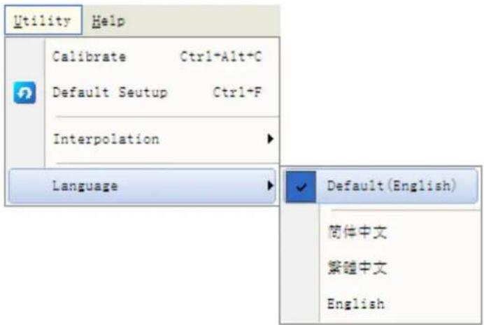
There are four languages in "Language" menu. The default language is English.
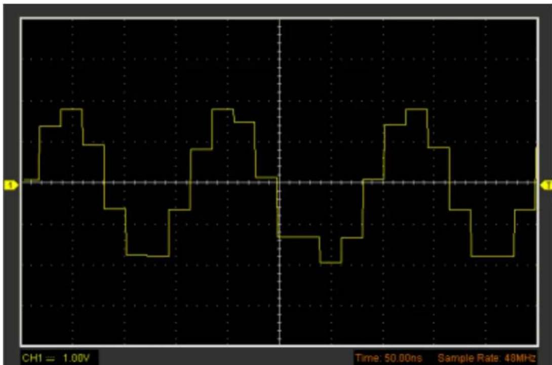
At the time base 40ns/div or faster, user can use the 3 different interpolation mode to get waveforms of different smoothness.
3.6.3 Interpolation
Click "Utility->Interpolation".
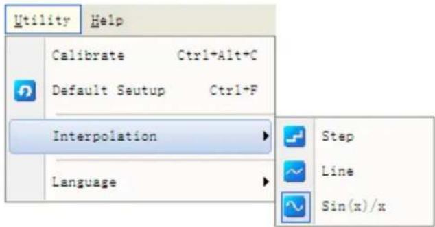
The Step Interpolation:
line
| Time (ns) | Voltage (V) | | --------- | ----------- | | 0 | 0 | | 50 | 1 | | 100 | -1 | | 150 | 2 | | 200 | -2 | | 250 | 3 | | 300 | -3 | | 350 | 4 | | 400 | -4 | | 450 | 5 | | 500 | -5 | | 550 | 6 | | 600 | -6 | | 650 | 7 | | 700 | -7 | | 750 | 8 | | 800 | -8 | | 850 | 9 | | 900 | -9 | | 950 | 10 | | 1000 | -10 | | 1050 | 11 | | 1100 | -11 | | 1150 | 12 | | 1200 | -12 | | 1250 | 13 | | 1300 | -13 | | 1350 | 14 | | 1400 | -14 | | 1450 | 15 | | 1500 | -15 | | 1550 | 16 | | 1600 | -16 | | 1650 | 17 | | 1700 | -17 | | 1750 | 18 | | 1800 | -18 | | 1850 | 19 | | 1900 | -19 | | 1950 | 20 | | 2000 | -20 | | 2050 | 21 | | 2100 | -21 | | 2150 | 22 | | 2200 | -22 | | 2250 | 23 | | 2300 | -23 | | 2350 | 24 | | 2400 | -24 | | 2450 | 25 | | 2500 | -25 | | 2550 | 26 | | 2600 | -26 | | 2650 | 27 | | 2700 | -27 | | 2750 | 28 | | 2800 | -28 | | 2850 | 29 | | 2900 | -29 | | 2950 | 30 | | 3000 | -30 | | 3050 | 31 | | 3100 | -31 | | 3150 | 32 | | 3200 | -32 | | 3250 | 33 | | 3300 | -33 | | 3350 | 34 | | 3400 | -34 | | 3450 | 35 | | 3500 | -35 | | 3550 | 36 | | 3600 | -36 | | 3650 | 37 | | 3700 | -37 | | 3750 | 38 | | 3800 | -38 | | 3850 | 39 | | 3900 | -39 | | 3950 | 40 | | 4000 | -40 | | 4050 | 41 | | 4100 | -41 | | 4150 | 42 | | 4200 | -42 | | 4250 | 43 | | 4300 | -43 | | 4350 | 44 | | 4400 | -44 | | 4450 | 45 | | 4500 | -45 | | 4550 | 46 | | 4600 | -46 | | 4650 | 47 | | 4700 | -47 | | 4750 | 48 | | 4800 | -48 | | 4850 | 49 | | 4900 | -49 | | 4950 | 50 | | 5000 | -50 | | ... | ... |The Linear Interpolation:
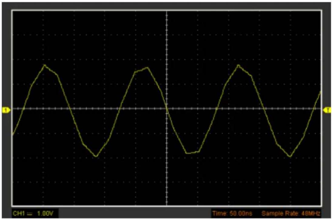
line
| Time (ns) | Voltage (V) | | --------- | ----------- | | 0 | 0 | | 1 | 1.0 | | 2 | 2.0 | | 3 | 3.0 | | 4 | 2.0 | | 5 | 1.0 | | 6 | 0 | | 7 | -1.0 | | 8 | -2.0 | | 9 | -3.0 | | 10 | -2.0 | | 11 | -1.0 | | 12 | 0 | | 13 | 1.0 | | 14 | 2.0 | | 15 | 3.0 | | 16 | 2.0 | | 17 | 1.0 | | 18 | 0 | | 19 | -1.0 | | 20 | -2.0 | | 21 | -3.0 | | 22 | -2.0 | | 23 | -1.0 | | 24 | 0 | | 25 | 1.0 | | 26 | 2.0 | | 27 | 3.0 | | 28 | 2.0 | | 29 | 1.0 | | 30 | 0 | | 31 | -1.0 | | 32 | -2.0 | | 33 | -3.0 | | 34 | -2.0 | | 35 | -1.0 | | 36 | 0 | | 37 | 1.0 | | 38 | 2.0 | | 39 | 3.0 | | 40 | 2.0 | | 41 | 1.0 | | 42 | 0 | | 43 | -1.0 | | 44 | -2.0 | | 45 | -3.0 | | 46 | -2.0 | | 47 | -1.0 | | 48 | 0 | | 49 | 1.0 | | 50 | 2.0 | | | |The Sin(x)/x Interpolation:
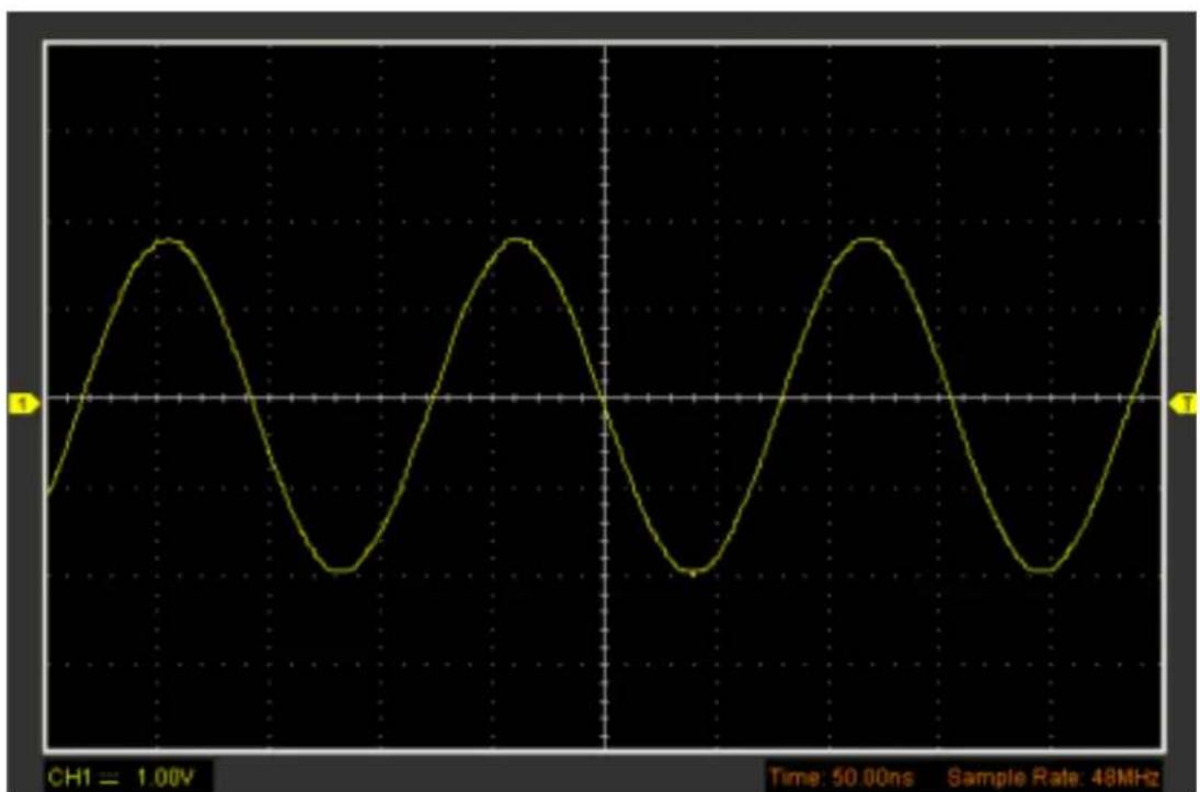
line
| Time (ns) | Voltage (V) | | --------- | ----------- | | 0 | 0 | | 50 | 3.5 | | 100 | 0 | | 150 | -3.5 | | 200 | 3.5 | | 250 | 0 | | 300 | -3.5 | | 350 | 3.5 | | 400 | 0 | | 450 | -3.5 | | 500 | 3.5 | | 550 | 0 | | 600 | -3.5 | | 650 | 3.5 | | 700 | 0 | | 750 | -3.5 | | 800 | 3.5 | | 850 | 0 | | 900 | -3.5 | | 950 | 3.5 | | 1000 | 0 | | 1050 | -3.5 | | 1100 | 3.5 | | 1150 | 0 | | 1200 | -3.5 | | 1250 | 3.5 | | 1300 | 0 | | 1350 | -3.5 | | 1400 | 3.5 | | 1450 | 0 | | 1500 | -3.5 | | 1550 | 3.5 | | 1600 | 0 | | 1650 | -3.5 | | 1700 | 3.5 | | 1750 | 0 | | 1800 | -3.5 | | 1850 | 3.5 | | 1900 | 0 | | 1950 | -3.5 | | 2000 | 3.5 | | 2050 | 0 | | 2100 | -3.5 | | 2150 | 3.5 | | 2200 | 0 | | 2250 | -3.5 | | 2300 | 3.5 | | 2350 | 0 | | 2400 | -3.5 | | 2450 | 3.5 | | 2500 | 0 | | 2550 | -3.5 | | 2600 | 3.5 | | 2650 | 0 | | 2700 | -3.5 | | 2750 | 3.5 | | 2800 | 0 | | 2850 | -3.5 | | 2900 | 3.5 | | 2950 | 0 | | 3000 | -3.5 | | 3050 | 3.5 | | 3100 | 0 | | 3150 | -3.5 | | 3200 | 3.5 | | 3250 | 0 | | 3300 | -3.5 | | 3350 | 3.5 | | 3400 | 0 | | 3450 | -3.5 | | 3500 | 3.5 | | 3550 | 0 | | 3600 | -3.5 | | 3650 | 3.5 | | 3700 | 0 | | 3750 | -3.5 | | 3800 | 3.5 | | 3850 | 0 | | 3900 | -3.5 | | 3950 | 3.5 | | 4000 | 0 | | 4050 | -3.5 | | 4100 | 3.5 | | 4150 | 0 | | 4200 | -3.5 | | 4250 | 3.5 | | 4300 | 0 | | 4350 | -3.5 | | 4400 | 3.5 | | 4450 | 0 | | 4500 | -3.5 | | 4550 | 3.5 | | 4600 | 0 | | 4650 | -3.5 | | 4700 | 3.5 | | 4750 | 0 | | 4800 | -3.5 | | 4850 | 3.5 | | 4900 | 0 | | 4950 | -3.5 | | 500 | |Note: The default interpolation mode is Sin(x)/x.
3.7 The Display System
Click "Display" in main menu.
The following figure shows the display system menu. Displays parameters setting.
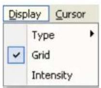
◆ Type
Grid
◆ Intensity
3.7.1 Type
Click "Type" in "Display" menu.
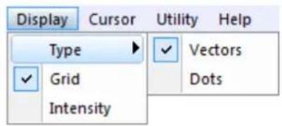
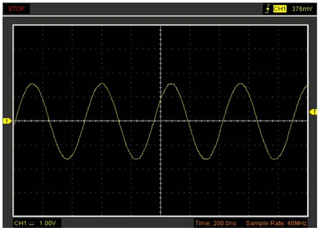
If the Vectors type mode is selected, the waveform will be displayed as following figure.
line
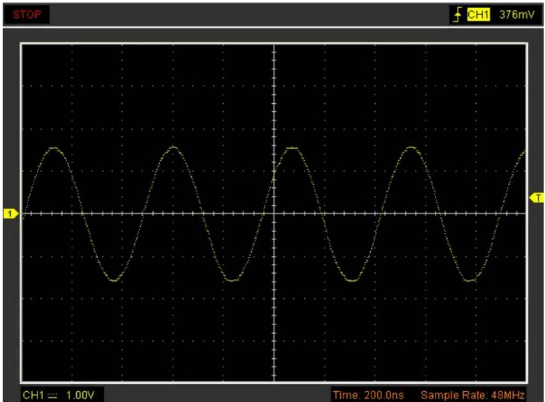
| Time (ns) | Voltage (mV) | | --------- | ------------ | | 0 | 0 | | 1 | 1.0 | | 2 | -1.0 | | 3 | 2.0 | | 4 | -2.0 | | 5 | 3.0 | | 6 | -3.0 | | 7 | 4.0 | | 8 | -4.0 | | 9 | 5.0 | | 10 | -5.0 | | 11 | 6.0 | | 12 | -6.0 | | 13 | 7.0 | | 14 | -7.0 | | 15 | 8.0 | | 16 | -8.0 | | 17 | 9.0 | | 18 | -9.0 | | 19 | 10.0 | | 20 | -10.0 | | 21 | 11.0 | | 22 | -11.0 | | 23 | 12.0 | | 24 | -12.0 | | 25 | 13.0 | | 26 | -13.0 | | 27 | 14.0 | | 28 | -14.0 | | 29 | 15.0 | | 30 | -15.0 | | 31 | 16.0 | | 32 | -16.0 | | 33 | 17.0 | | 34 | -17.0 | | 35 | 18.0 | | 36 | -18.0 | | 37 | 19.0 | | 38 | -19.0 | | 39 | 20.0 | | 40 | -20.0 | | 41 | 21.0 | | 42 | -21.0 | | 43 | 22.0 | | 44 | -22.0 | | 45 | 23.0 | | 46 | -23.0 | | 47 | 24.0 | | 48 | -24.0 | | 49 | 25.0 | | 50 | -25.0 | | 51 | 26.0 | | 52 | -26.0 | | 53 | 27.0 | | 54 | -27.0 | | 55 | 28.0 | | 56 | -28.0 | | 57 | 29.0 | | 58 | -29.0 | | 59 | 30.0 | | 60 | -30.0 | | 61 | 31.0 | | 62 | -31.0 | | 63 | 32.0 | | 64 | -32.0 | | 65 | 33.0 | | 66 | -33.0 | | 67 | 34.0 | | 68 | -34.0 | | 69 | 35.0 | | 70 | -35.0 | | 71 | 36.0 | | 72 | -36.0 | | 73 | 37.0 | | 74 | -37.0 | | 75 | 38.0 | | 76 | -38.0 | | 77 | 39.0 | | 78 | -39.0 | | 79 | 40.0 | | 80 | -40.0 | | 81 | 41.0 | | 82 | -41.0 | | 83 | 42.0 | | 84 | -42.0 | | 85 | 43.0 | | 86 | -43.0 | | 87 | 44.0 | | 88 | -44.0 | | 89 | 45.0 | | 90 | -45.0 | | 91 | 46.0 | | 92 | -46.0 | | 93 | 47.0 | | 94 | -47.0 | | 95 | 48.0 | | 96 | -48.0 | | 97 | 49.0 | | 98 | -49.0 | | 99 | 50.0 | | 100 | -50.0 |If the Dots type mode is selected, the waveform will be displayed as following figure.
line
| Time (ns) | Voltage (mV) | | --------- | ------------ | | 0 | 0 | | 100 | 200 | | 200 | 0 | | 300 | -200 | | 400 | 0 | | 500 | 200 | | 600 | 0 | | 700 | -200 | | 800 | 0 | | 900 | 200 | | 1000 | 0 | | 1100 | -200 | | 1200 | 0 | | 1300 | 200 | | 1400 | 0 | | 1500 | -200 | | 1600 | 0 | | 1700 | 200 | | 1800 | 0 | | 1900 | -200 | | 2000 | 0 | | 2100 | 200 | | 2200 | 0 | | 2300 | -200 | | 2400 | 0 | | 2500 | 200 | | 2600 | 0 | | 2700 | -200 | | 2800 | 0 | | 2900 | 200 | | 3000 | 0 | | 3100 | -200 | | 3200 | 0 | | 3300 | 200 | | 3400 | 0 | | 3500 | -200 | | 3600 | 0 | | 376 | 376 |3.7.2 Grid
Click "Display" in main menu.
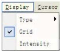
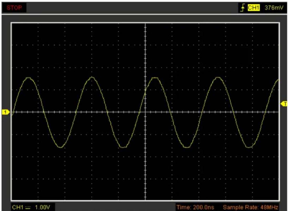
The grid shows:
line
| Time (ns) | Voltage (mV) | | --------- | ------------ | | 0 | 0 | | 100 | 2.5 | | 200 | 0 | | 300 | -2.5 | | 400 | 0 | | 500 | 2.5 | | 600 | 0 | | 700 | -2.5 | | 800 | 0 | | 900 | 2.5 | | 1000 | 0 | | 1100 | -2.5 | | 1200 | 0 | | 1300 | 2.5 | | 1400 | 0 | | 1500 | -2.5 | | 1600 | 0 | | 1700 | 2.5 | | 1800 | 0 | | 1900 | -2.5 | | 2000 | 0 | | 2100 | 2.5 | | 2200 | 0 | | 2300 | -2.5 | | 2400 | 0 | | 2500 | 2.5 | | 2600 | 0 | | 2700 | -2.5 | | 2800 | 0 | | 2900 | 2.5 | | 3000 | 0 | | 3100 | -2.5 | | 3200 | 0 | | 3300 | 2.5 | | 3400 | 0 | | 3500 | -2.5 | | 3600 | 0 | | 3700 | 2.5 | | 3800 | 0 | | 3900 | -2.5 | | 4000 | 0 | | 4100 | 2.5 | | 4200 | 0 | | 4300 | -2.5 | | 4400 | 0 | | 4500 | 2.5 | | 4600 | 0 | | 4700 | -2.5 | | 4800 | 0 | | 4900 | 2.5 | | 5000 | 0 | | 5100 | -2.5 | | 5200 | 0 | | 5300 | 2.5 | | 5400 | 0 | | 5500 | -2.5 | | 5600 | 0 | | 5700 | 2.5 | | 5800 | 0 | | 5900 | -2.5 | | 6000 | 0 | | 6100 | 2.5 | | 6200 | 0 | | 6300 | -2.5 | | 6400 | 0 | | 6500 | 2.5 | | 6600 | 0 | | 6700 | -2.5 | | 6800 | 0 | | 6900 | 2.5 | | 7000 | 0 | | 7100 | -2.5 | | 7200 | 0 | | 7300 | 2.5 | | 7400 | 0 | | 7500 | -2.5 | | 7600 | 0 | | 7700 | 2.5 | | 7800 | 0 | | 7900 | -2.5 | | 8000 | 0 | | 8100 | 2.5 | | 8200 | 0 | | 8300 | -2.5 | | 8400 | 0 | | 8500 | 2.5 | | 8600 | 0 | | 8700 | -2.5 | | 8800 | 0 | | 8900 | 2.5 | | 9000 | 0 | | 9100 | -2.5 | | 9200 | 0 | | 9300 | 2.5 | | 9400 | 0 | | 9500 | -2.5 | | 9600 | 0 | | 9700 | 2.5 | | 9800 | 0 | | 9900 | -2.5 | |1 | -1 |Without the grid show:
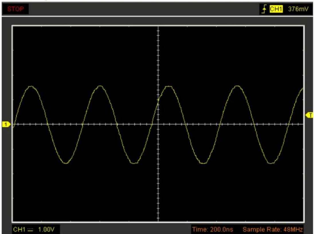
line
| Time (ns) | Voltage (mV) | | --------- | ------------ | | 0 | 0 | | 1 | 2.5 | | 2 | 5 | | 3 | 7.5 | | 4 | 10 | | 5 | 7.5 | | 6 | 5 | | 7 | 2.5 | | 8 | 0 | | 9 | -2.5 | | 10 | -5 | | 11 | -7.5 | | 12 | -10 | | 13 | -7.5 | | 14 | -5 | | 15 | -2.5 | | 16 | 0 | | 17 | 2.5 | | 18 | 5 | | 19 | 7.5 | | 20 | 10 | | 21 | 7.5 | | 22 | 5 | | 23 | 2.5 | | 24 | 0 | | 25 | -2.5 | | 26 | -5 | | 27 | -7.5 | | 28 | -10 | | 29 | -7.5 | | 30 | -5 | | 31 | -2.5 | | 32 | 0 | | 33 | 2.5 | | 34 | 5 | | 35 | 7.5 | | 36 | 10 | | 37 | 7.5 | | 38 | 5 | | 39 | 2.5 | | 40 | 0 | | 41 | -2.5 | | 42 | -5 | | 43 | -7.5 | | 44 | -10 | | 45 | -7.5 | | 46 | -5 | | 47 | -2.5 | | 48 | 0 | | 49 | 2.5 | | 50 | 5 | | 51 | 7.5 | | 52 | 10 | | 53 | 7.5 | | 54 | 5 | | 55 | 2.5 | | 56 | 0 | | 57 | -2.5 | | 58 | -5 | | 59 | -7.5 | | 60 | -10 | | 61 | -7.5 | | 62 | -5 | | 63 | -2.5 | | 64 | 0 | | 65 | 2.5 | | 66 | 5 | | 67 | 7.5 | | 68 | 10 | | 69 | 7.5 | | 70 | 5 | | 71 | 2.5 | | 72 | 0 | | 73 | -2.5 | | 74 | -5 | | 75 | -7.5 | | 76 | -10 | | 77 | -7.5 | | 78 | -5 | | 79 | -2.5 | | 80 | 0 | | 81 | 2.5 | | 82 | 5 | | 83 | 7.5 | | 84 | 10 | | 85 | 7.5 | | 86 | 5 | | 87 | 2.5 | | 88 | 0 | | 89 | -2.5 | | 90 | -5 | | 91 | -7.5 | | 92 | -10 | | 93 | -7.5 | | 94 | -5 | | 95 | -2.5 | | 96 | 0 | | 97 | 2.5 | | 98 | 5 | | 99 | 7.5 | | 100 | 10 |3.7.3 Intensity
Click "Display->Intensity" in main menu
The following figure shows the intensity dialog. It shows the display parameters setting.
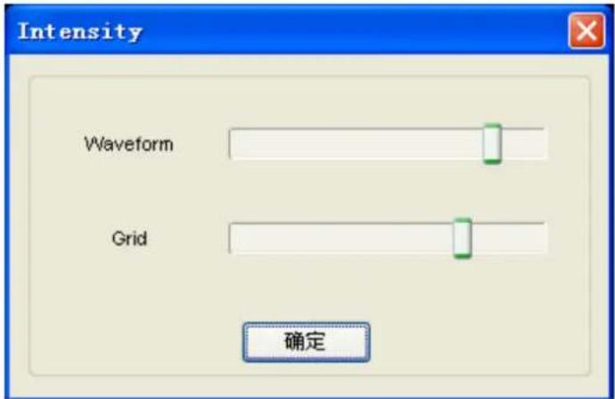
You can change the grid and waveform color intensity in this dialog.
3.8 Save/Load Menu
Click "File" in main menu to save waveform, setups and screen
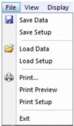
1. Save Data
Save waveform data
2. Save Setups
Save the current oscilloscope setups to file
Load Menu
Click "File" in main menu to recall saved waveform, setup
1. Load Data
Load the waveform
2. Load Setup
Load the instrument that had saved
3.9 Print
Click "Print" in File.
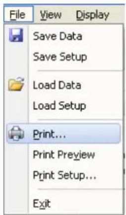
- Click "Print" in "File" menu to set the printer to print the current waveform.
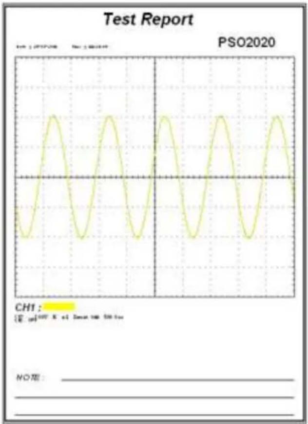
- Click the "PrintPreview" in "File" menu to get into the Preview window.
In "PrintPreview" window, use the + - button to change the size of the waveform graph. Click the "Close" button to turn this window off and click the "Print" button to print the report.
line
| Time (s) | Value | |----------|-------| | 0 | 0 | | 1 | 1 | | 2 | 0 | | 3 | -1 | | 4 | 0 | | 5 | 1 | | 6 | 0 | | 7 | -1 | | 8 | 0 | | 9 | 1 | | 10 | 0 | | 11 | -1 | | 12 | 0 | | 13 | 1 | | 14 | 0 | | 15 | -1 | | 16 | 0 | | 17 | 1 | | 18 | 0 | | 19 | -1 | | 20 | 0 | | 21 | 1 | | 22 | 0 | | 23 | -1 | | 24 | 0 | | 25 | 1 | | 26 | 0 | | 27 | -1 | | 28 | 0 | | 29 | 1 | | 30 | 0 | | 31 | -1 | | 32 | 0 | | 33 | 1 | | 34 | 0 | | 35 | -1 | | 36 | 0 | | 37 | 1 | | 38 | 0 | | 39 | -1 | | 40 | 0 | | 41 | 1 | | 42 | 0 | | 43 | -1 | | 44 | 0 | | 45 | 1 | | 46 | 0 | | 47 | -1 | | 48 | 0 | | 49 | 1 | | 50 | 0 | | 51 | -1 | | 52 | 0 | | 53 | 1 | | 54 | 0 | | 55 | -1 | | 56 | 0 | | 57 | 1 | | 58 | 0 | | 59 | -1 | | 60 | 0 | | 61 | 1 | | 62 | 0 | | 63 | -1 | | 64 | 0 | | 65 | 1 | | 66 | 0 | | 67 | -1 | | 68 | 0 | | 69 | 1 | | 70 | 0 | | 71 | -1 | | 72 | 0 | | 73 | 1 | | 74 | 0 | | 75 | -1 | | 76 | 0 | | 77 | 1 | | 78 | 0 | | 79 | -1 | | 80 | 0 | | 81 | 1 | | 82 | 0 | | 83 | -1 | | 84 | 0 | | 85 | 1 | | 86 | 0 | | 87 | -1 | | 88 | 0 | | 89 | 1 | | 90 | 0 | | 91 | -1 | | 92 | 0 | | 93 | 1 | | 94 | 0 | | 95 | -1 | | 96 | 0 | | 97 | 1 | | 98 | 0 | | 99 | -1 | | Note: The chart displays a single data series with values for CHI. The x-axis represents time in seconds (from left to right) and the y-axis represents signal amplitude. There is no label for the data series. The values are estimated based on the given code.Chapter 4 Application Example
◆ Simple Measurement
◆ Capturing a Single-Shot Signal
◆ Taking Cursor Measurement
4.1 Simple Measurement
To acquire and display a signal, please do the steps as follows:
Connect signal to CH1 by using probe
The oscilloscope set the vertical, horizontal, and triggers controls at the best status automatically. Also, you can adjust the controls to meet your measurement to optimize the waveform display.
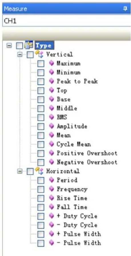
- To measure the frequency and "Vpp", you can do these steps as follows:
- Click the button, the frequency of the signal display on the bottom of the waveform interface.
- Click the ☑ Peak to Peak button, the "Vpp" of the signal will also display on the bottom of the waveform interface.
- To clear the measurement on the waveform interface, click the button.
line
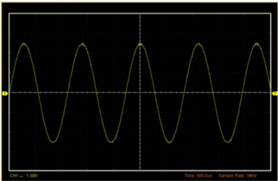
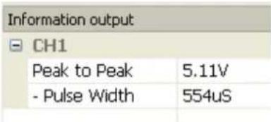
| Time (ms) | Voltage (V) | | --------- | ----------- | | 0 | 0 | | 1 | 1.0 | | 2 | 0 | | 3 | -1.0 | | 4 | 0 | | 5 | 1.0 | | 6 | 0 | | 7 | -1.0 | | 8 | 0 | | 9 | 1.0 | | 10 | 0 | | 11 | -1.0 | | 12 | 0 | | 13 | 1.0 | | 14 | 0 | | 15 | -1.0 | | 16 | 0 | | 17 | 1.0 | | 18 | 0 | | 19 | -1.0 | | 20 | 0 | | 21 | 1.0 | | 22 | 0 | | 23 | -1.0 | | 24 | 0 | | 25 | 1.0 | | 26 | 0 | | 27 | -1.0 | | 28 | 0 | | 29 | 1.0 | | 30 | 0 | | 31 | -1.0 | | 32 | 0 | | 33 | 1.0 | | 34 | 0 | | 35 | -1.0 | | 36 | 0 | | 37 | 1.0 | | 38 | 0 | | 39 | -1.0 | | 40 | 0 | | 41 | 1.0 | | 42 | 0 | | 43 | -1.0 | | 44 | 0 | | 45 | 1.0 | | 46 | 0 | | 47 | -1.0 | | 48 | 0 | | 49 | 1.0 | | 50 | 0 | | 51 | -1.0 | | 52 | 0 | | 53 | 1.0 | | 54 | 0 | | 55 | -1.0 | | 56 | 0 | | 57 | 1.0 | | 58 | 0 | | 59 | -1.0 | | 60 | 0 | | 61 | 1.0 | | 62 | 0 | | 63 | -1.0 | | 64 | 0 | | 65 | 1.0 | | 66 | 0 | | 67 | -1.0 | | 68 | 0 | | 69 | 1.0 | | 70 | 0 | | 71 | -1.0 | | 72 | 0 | | 73 | 1.0 | | 74 | 0 | | 75 | -1.0 | | 76 | 0 | | 77 | 1.0 | | 78 | 0 | | 79 | -1.0 | | 80 | 0 | | 81 | 1.0 | | 82 | 0 | | 83 | -1.0 | | 84 | 0 | | 85 | 1.0 | | 86 | 0 | | 87 | -1.0 | | 88 | 0 | | 89 | 1.0 | | 90 | 0 | | 91 | -1.0 | | 92 | 0 | | 93 | 1.0 | | 94 | 0 | | 95 | -1.0 | | 96 | 0 | | 97 | 1.0 | | 98 | 0 | | 99 | -1.0 | | | |The results of measure display in Information output.
4.2 Capturing a Single-Shot Signal
To capture a single event, it needs to gather some pre-test knowledge of the signal in order to set up the trigger level and slope correctly. For example, if the event is derived from 3.3V COMS logic, a trigger level of 1.2 or higher Volts should work on a rising edge.
Do these steps as follows:
- Set up the trigger in the Trigger Menu, or in the Trigger Setting window.
1) Adjust the Trigger Mode to Edge.
2) Set the Trigger Sweep to Single.
3) Set the Trigger Slope to "+" which means you select the rising edge.
4) Adjust the Volts/Div and the time base in a proper range for the signal.
5) Drag the trigger level sign on the waveform display screen to proper position. It's usually higher a little above the normal level.
6) When the trigger conditions are met, data appears on the display representing the data points that the oscilloscope obtained with one acquisition.
4.3 Taking Cursor Measurements
Use cursors to make time and amplitude measurements on a waveform quickly.
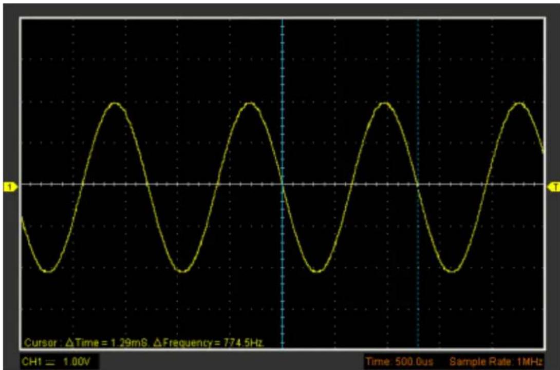
Measure the Peak Frequency or Time of the First Sine Waveform
Do these steps:
- Click "Cursor->Source", select CH1.
- Click "Cursor->Type", select Vertical.
- Push left mouse button, and the vertical lines appear.
- Drag the mouse button to the point you want to measure.
- Release the left mouse button, the frequency difference and time difference will be shown at the status bar.
line
| Time (us) | Voltage (mV) | | --------- | ------------ | | 0 | 0 | | 500 | 0 | | 1000 | 0 | | 1500 | 0 | | 2000 | 0 | | 2500 | 0 | | 3000 | 0 | | 3500 | 0 | | 4000 | 0 | | 4500 | 0 | | 5000 | 0 | | 5500 | 0 | | 6000 | 0 | | 6500 | 0 | | 7000 | 0 | | 7500 | 0 | | 8000 | 0 | | 8500 | 0 | | 9000 | 0 | | 9500 | 0 | | 10000 | 0 | | 10500 | 0 | | 11000 | 0 | | 11500 | 0 | | 12000 | 0 | | 12500 | 0 | | 13000 | 0 | | 13500 | 0 | | 14000 | 0 | | 14500 | 0 | | 15000 | 0 | | 15500 | 0 | | 16000 | 0 | | 16500 | 0 | | 17000 | 0 | | 17500 | 0 | | 18000 | 0 | | 18500 | 0 | | 19000 | 0 | | 19500 | 0 | | 20000 | 0 | | 20500 | 0 | | 21000 | 0 | | 21500 | 0 | | 22000 | 0 | | 22500 | 0 | | 23000 | 0 | | 23500 | 0 | | 24000 | 0 | | 24500 | 0 | | 25000 | 0 | | 25500 | 0 | | 26000 | 0 | | 26500 | 0 | | 27000 | 0 | | 27500 | 0 | | 28000 | 0 | | 28500 | 0 | | 29000 | 0 | | 29500 | 0 | | 30000 | 0 | | 30500 | 0 | | 31000 | 0 | | 31500 | 0 | | 32000 | 0 | | 32500 | 0 | | 33000 | 0 | | 33500 | 0 | | 34000 | 0 | | 34500 | 0 | | 35000 | 0 | | 35500 | 0 | | 36000 | 0 | | 36500 | 0 | | 37000 | 0 | | 37500 | 0 | | 38000 | 0 | | 38500 | 0 | | 39000 | 0 | | 39500 | 0 | | 40000 | 0 | | 4654 | -1 | | | |Measure the Amplitude of the First Waveform Peak of the Waveform
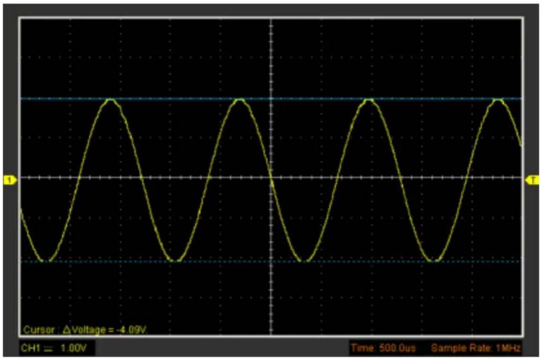
Do these steps:
- Click "Cursor->Source", select CH1.
- Click "Cursor->Type", select Horizontal.
- Push left mouse button, and the Horizontal lines appear.
-
Drag the mouse button to the point you want to measure.
-
Release the left mouse button, the voltage difference will be shown at the status bar.
line
| Time (μs) | Amplitude (V) | |-----------|---------------| | 0 | 0 | | 1 | 1 | | 2 | 0 | | 3 | -1 | | 4 | 0 | | 5 | 2 | | 6 | 0 | | 7 | -1 | | 8 | 0 | | 9 | 2 | | 10 | 0 | | 11 | -1 | | 12 | 0 | | 13 | 2 | | 14 | 0 | | 15 | -1 | | 16 | 0 | | 17 | 2 | | 18 | 0 | | 19 | -1 | | 20 | 0 | | 21 | 2 | | 22 | 0 | | 23 | -1 | | 24 | 0 | | 25 | 2 | | 26 | 0 | | 27 | -1 | | 28 | 0 | | 29 | 2 | | 30 | 0 | | 31 | -1 | | 32 | 0 | | 33 | 2 | | 34 | 0 | | 35 | -1 | | 36 | 0 | | 37 | 2 | | 38 | 0 | | 39 | -1 | | 40 | 0 | | 41 | 2 | | 42 | 0 | | 43 | -1 | | 44 | 0 | | 45 | 2 | | 46 | 0 | | 47 | -1 | | 48 | 0 | | 49 | 2 | | 50 | 0 | | 51 | -1 | | 52 | 0 | | 53 | 2 | | 54 | 0 | | 55 | -1 | | 56 | 0 | | 57 | 2 | | 58 | 0 | | 59 | -1 | | 60 | 0 | | 61 | 2 | | 62 | 0 | | 63 | -1 | | 64 | 0 | | 65 | 2 | | 66 | 0 | | 67 | -1 | | 68 | 0 | | 69 | 2 | | 70 | 0 | | 71 | -1 | | 72 | 0 | | 73 | 2 | | 74 | 0 | | 75 | -1 | | 76 | 0 | | 77 | 2 | | 78 | 0 | | 79 | -1 | | 80 | 0 | | 81 | 2 | | 82 | 0 | | 83 | -1 | | 84 | 0 | | 85 | 2 | | 86 | 0 | | 87 | -1 | | 88 | 0 | | 89 | 2 | | 90 | 0 | | 91 | -1 | | 92 | 0 | | 93 | 2 | | 94 | 0 | | 95 | -1 | | 96 | 0 | | 97 | 2 | | 98 | 0 | | 99 | -1 | | | |Note: Click "Cursor->Type", select "Cross", you can measure time and amplitude at one time.
Appendix
◆ Appendix A: Specifications
◆ Appendix B: General Maintenance
Appendix A: Specification
Specifications Table:
| Input | |
| Max. sample rate | Real-time sampling:96MS/s |
| Channels | 1 Channels |
| Bandwidth | 20MHz (-3dB) |
| Vertical resolution | 8 bits/channel |
| Gain range | 20mV~20V/div |
| Range | 8 divisions |
| Offset level | +/-4 divisions |
| Coupling | DC/AC/GND |
| Offset increments | 0.02 div |
| Impedance | 1M ohm |
| DC accuracy | +/-3% |
| Max. Input | 50V |
| Max. input voltage | 60Vpk(Without external attenuation DC + peak AC < 10kHz) |
| Display mode | Y-T |
| Timebase | |
| Timebase range | 1ns/div~5000s/div(1ns,2ns,5ns,10ns,20ns,50ns,100ns,200ns,500ns,1us,2us,5us,10us,20us,50us,100us,200us,500us,1ms,2ms,5ms,10ms,20ms,50ms,100ms,200ms,500ms,1s,2s,5s,10s,20s,50s,100s,200s,500s,1000s,2000s,5000s/div 1,2,5 sequence) |
| Range | 10 divisions |
| Buffer Size | MAX.1M samples |
| Trigger | |
| Type | Edge trigger: Rising edge, Falling edge |
| Mode | Auto, Normal and Single |
| Autoset | Yes(100Hz-20MHz) |
| Range | 8 divisions |
| Trigger level | +/-4 divisions |
| Settabillity | 0.02 div increments |
| Math | |
| Measurements | Vp-p, Vmax, Vmin, Vmean, Vrms, Vamp, Vtop, Vbase,Vmid,positive overshoot, negative overshoot, cycle mean, cycle RMS, period, frequency, positive pulse width, negative pulse width, rise time (10%~90%), fall time (10%~90%), positive duty cycle, negative duty cycle |
| Math | FFT |
| FFT | Rectangular, Hanning, Hamming, Blackman Window |
| Physical | |
| Interface | Universal Serial Bus(USB 2.0) |
| Power | No external power source required.Bus-powered from USB |
| Dimensions | 230x40x 20(mm) |
Appendix B: General Maintenance
General Care
Do not store or leave the oscilloscope where the device will be exposed to direct sunlight for long periods of time.
Caution
To avoid damages to the device or probes, do not expose them to sprays, liquids or solvents.
To avoid damages to the surface of the device or probes not use any abrasive or chemical cleaning agents.
Cleaning
Inspect the device and probes as often as operating conditions require. Make sure the device disconnect form all power sources.
To clean the exterior surface, perform the following steps:
- Remove loose dust on the outside of the oscilloscope and probes with a lint-free cloth. Use care to avoid scratching the clear glass display filter.
- Use a soft cloth dampened with water to clean the device.

- General Safety Summary ....1
- Chapter 1 Getting Start....2
- Chapter 2 Operating Basics....13
- Chapter 3 Understanding Function....20
- Chapter 4 Application Example....41
- Appendix 46
- General Safety Summary
- Chapter 1 Getting Start
- System Requirement
- Minimum System Requirements
- Operating System
- Processor
- Memory
- Disk Space
- Screen resolution
- Recommended Configuration
- Install Software
- Install Driver
- General Features
- General Check
- Function Check
- Self Calibration
- Accessories
- Chapter 2 Operating Basics
- The User's Interface
- The Main Menu
- The Toolbar
- Control Panel
- DVM
- The Horizontal Panel
- The Vertical Panel
- The Trigger Panel
- Displays the system time.
- Displays Sample Rate
- Displays the main time base setting.
- Displays the CH1 information
- Button description
- The Menu System
- The Vertical System
- The Horizontal System
- The Trigger System
- Input Connectors
- Input Connectors:
- Chapter 3 Understanding Function
- Set Oscilloscope
- Save Setup
- Load Setup
- Factory Setup
- Set Vertical Systems
- The Vertical Menu function:
- Change Volt/DIV
- Invert
- Set FFT
- Fast Fourier Transform Function
- Scale:
- HORI Scale:
- Set Reference
- Set Horizontal System
- Set Trigger System
- Measure Signal
- Cursor
- Source
- Type
- 1) Cross
- 2) Vertical
- 3) Horizontal
- Measure
- Vertical
- Horizontal
- Clear Measure
- The Utility Function
- Default Setup
- Language
- Interpolation
- The Display System
- Type
- Grid
- Intensity
- Save/Load Menu
- Save Data
- Save Setups
- Load Menu
- Load Data
- Load Setup
- Chapter 4 Application Example
- Simple Measurement
- Capturing a Single-Shot Signal
- Taking Cursor Measurements
- Measure the Peak Frequency or Time of the First Sine Waveform
- Measure the Amplitude of the First Waveform Peak of the Waveform
- Appendix
- Appendix A: Specification
- Appendix B: General Maintenance
- General Care
- Caution
- Cleaning
Brand : VOLTCRAFT
Model : PSO-120
Category : Multimeter