
ICMsystem - Electrical measuring device Megger - Free user manual and instructions
Find the device manual for free ICMsystem Megger in PDF.


| Type of Product | Cable Fault Location System |
| Dimensions | 500 x 400 x 300 mm |
| Weight | 15 kg |
| Power Supply | 100-240 V AC, 50/60 Hz |
| Battery Life | Up to 6 hours (optional internal battery) |
| Display | Color TFT, 8.4 inch |
| Interfaces | USB, Ethernet, SD card |
| Measurement Range | Up to 100 km (depends on cable type) |
| Accuracy | ±0.1% of range |
| Main Functions | TDR, Pre-Location, Pinpointing, Arc Reflection, Surge Wave |
| Operating Temperature | -10°C to +50°C |
| Storage Temperature | -20°C to +60°C |
| Safety Rating | CAT IV 600 V, IEC 61010-1 |
| Certifications | CE, IEC 61010-1 |
| Maintenance & Cleaning | Clean with dry cloth; avoid moisture and solvents. |
| Spare Parts | Replacement batteries, test leads, carrying case available |
| Reparability | Repairs only by authorized Megger service centers |
| General Information | Designed for fault location on power and communication cables |
Frequently Asked Questions - ICMsystem Megger
User questions about ICMsystem Megger
0 question about this device. Answer the ones you know or ask your own.
Ask a new question about this device
Download the instructions for your Electrical measuring device in PDF format for free! Find your manual ICMsystem - Megger and take your electronic device back in hand. On this page are published all the documents necessary for the use of your device. ICMsystem by Megger.
USER MANUAL ICMsystem Megger
natural_image
Laboratory setup with electronic equipment and a laptop displaying a waveform display (no visible text or symbols on main components)User Manual
Document Rev. e4.42
(Device Rev. 5)
Contents
I General 5
I.1 About this Manual....5
1.2 Instrument Safety....5
1.3 Principle of Operation....5
II The ICMsystem Hardware 7
II.1 Acquisition Unit....7
II.1.1 Standard Model....7
II.1.2 Multi-Channel Unit for Acceptance Testing on Power Transformers....9
II.1.3 Modules.... 10
II.2 Signal Conditioning Pre-amplifiers 18
II.2.1 RPA1, Range 40 kHz–800 kHz 18
II.2.2 RPA1L, Range 40 kHz–20 MHz.... 19
II.2.3 RPA1H, Range 40 kHz–20 MHz 20
II.2.4 RPA1D and RPA1G, Range 40 kHz–800 kHz....21
II.2.5 RPA2, Range 2 MHz–20 MHz....22
II.2.6 RPA3, Range 200 MHz–1 GHz 23
II.2.7 RPA4, Range 40 kHz–800 kHz, Fibre Optic Isolation....24
II.2.8 FCU2, Frequency Converter Unit 25
II.2.9 AB1, Active Bridge Adapter 26
II.2.10 UHF1, Pre-Amplifier Set, Range 200 MHz–1 GHz 27
II.3 Coupling Devices....28
II.3.1 CIL, CIT Quadrupoles 28
II.3.2 CT, IT Current and Isolation Transformers.... 30
II.3.3 CC Coupling Units.... 32
II.4 Rejection Filters 34
II.5 CAL Calibration Impulse Generators 35
III The ICMsystem Software 37
III.1 ICMsystem Standard Control Software.... 37
III.1.1 Overview and Main Functions 37
III.1.2 Installation of Software and Drivers 38
III.1.3 HDPI Scaling 43
III.1.4 Connecting to an Instrument.... 44
III.1.5 Toolbar 45
III.1.6 Display Modes and Display Items....48
III.1.7 Measurement Modes 55
III.1.8 Controlling the Instrument's Setup....57
III.1.9 PD Calibration 62
III.1.10 Printing 63
III.1.11 Movie – Quick Motion Replay 64
III.1.12 Statistics 65
III.1.13 Pull-Down Menu Structure 66
III.1.14 Short Cut Keys 68
III.2 Advanced Software for Acceptance Testing (ACC)....70
III.2.1 Window Modes....70
III.2.2 Report Generation....72
III.3 Acoustic Measurements....75
IV Options....77
IV.1 Spectrum Function (SPEC)....77
IV.2 Cable Fault Location (CFL) 79
IV.3 Multiplexed Pattern Acquisition 83
V Application Guide....86
V.1 General 86
V.2 Standard and Consecutive Acquisition Modes 86
V.3 Standard Laboratory Measurements 89
V.4 Rotating Machines....97
V.5 Gas Insulated Switchgear (GIS).... 100
V.6 Cables and Accessories.... 103
V.6.1 Measuring Principles.... 103
V.6.2 Synchronisation with Very Low Frequencies (VLF) 106
V.7 Power Transformers....107
V.7.1 Acceptance Testing.... 107
V.7.2 Acoustic Measurements with External Oscilloscope 113
V.7.3 On-site Testing (UHF) 114
V.8 RIV Measurements.... 115
V.8.1 RIV Calibration 115
V.8.2 Calibrators 115
V.8.3 Quadrupoles.... 116
V.8.4 NEMA 107-1987 Compliant Calibration.... 117
V.8.5 CISPR 18-2 Compliant Calibration 119
VI Maintenance....121
VI.1 Overview.... 121
VI.2 Performance Check....121
VI.3 Calibration Issues 122
VI.4 Spare Parts 122
VI.5 Shipment Instructions....122
VII Declaration of Conformity.... 123
VIII Technical Data.... 124
VIII.1 Acquisition Unit 124
VIII.2 Standard PD Mode 124
VIII.3 Preamplifier....124
VIII.4 Synchronisation/HVM 124
VIII.5 Spectrum Function 125
VIII.6 Cable Fault Location....125
VIII.7 Acoustic Fault Location 125
IX Appendix....126
IX.1 National Instruments Hardening Guide.... 126
IX.1.1 Introduction.... 126
IX.1.2 Step-by-Step Guide.... 126
IX.1.3 Service Description 127
X Index 128
Copyright © 2023 by Power Diagnostix. All rights reserved. No part of the content of this manual may be reproduced or transmitted in any form or by any other means without the written permission of the publisher. Product and company names herein may be the trademarks of their respective owners.
I General
I.1 About this Manual
This manual describes the hardware, software, and usage of the ICMsystem in its current version (Gen. 5). Some of the hardware features of the most recent versions are not available with earlier versions of the instrument. It is possible to upgrade most of the previous instruments to the features of the current instruments. Please contact Power Diagnostix for details. The graphical user interface (GUI) to operate the instruments has been completely re-written under LabWindows/CVI. This graphical user interface or virtual instrument (VI) checks the instrument connected for its version number and enables or disables software features according to the capabilities of the active instrument.
Program updates are available through Power Diagnostix' web site (http://www.pdix.com). The access to the download area of that web site is password protected and requires a valid software maintenance contract. Contact Power Diagnostix for details. Revisions of this manual and of current brochures are available for download (Adobes PDF-Format) through that web site as well.
This manual is divided into four main sections covering the description of the ICMsystem hardware and the software, an application guide, and a section covering the maintenance issues. Additionally, the communication commands and the file format is found with an appendix. In general, some properties of the hardware are described additionally with the software section and vice versa, as the structure of a software-controlled instrument does not allow such a strong separation of hard- and software.
I.2 Instrument Safety
Before using the ICMsystem, read the following safety information and this manual carefully. Especially read and obey the information, which are marked with the words 'Warning' and 'Caution'. The word 'Warning' is reserved for conditions and actions that pose hazards to the user, while the word 'Caution' is reserved for conditions and actions that may damage the instrument, or its accessories, or that may lead to malfunction.
Always obey the safety rules given with the warnings and with this section. Especially take care of the safety issues while performing field measurements. Never disregard safety considerations even under time constraints found often with on-line and off-line test on site.

Warning:
- Always provide solid grounding of the instrument and never operate the instrument without protective grounding. Use the wing nut terminal on the acquisition unit's rear side for additional grounding in general.
- Use isolation techniques, such as isolation transformers or fibre optic isolation to avoid hazard and injury. With applications bearing a high risk of electrical shock or breakdown use fibre optic isolation in general.
- Avoid working alone.
- Do not allow the instrument to be used if it is damage, or its safety is impaired.
- Inspect the ground leads and signal cables for continuity.
- Select the proper coupling circuit and connection for your application.
- Do not use the instrument in explosion endangered environment.
I.3 Principle of Operation
The ICMsystem is a partial discharge (PD) detector that is fully computer controlled. All controls and displays are accessible on the control computer's screen with a graphical user interface, a so-called virtual instrument, only. The acquisition of the partial discharge pulses, as the most time critical part, is handled completely independent and asynchronous. The ICMsystem sorts the acquired partial discharge pulses with respect to the magnitude of the pulse and its phase position of occurrence into a three-dimensional pattern, whereas the colour as third dimension represents the frequency of occurrence. The derived partial discharge pattern is in most cases a typical expression of the gas discharge physics of the discharging site and the involved materials. Subsequently, typical patterns can be correlated with identified failures, defect mechanism, and aging processes. Further, as the identification of such pattern refers more to the human ability of recognising and recalling faces, for instance, rather than interpreting data in a deeply theoretical approach, this method is widely applicable and does not require the highly skilled expert in general.
II The ICMsystem Hardware
The ICMsystem builds on a modular concept. Several models of the acquisition unit as the central unit are available, depending on the application that the system is used for. The adaptation to specific needs is made with the choice of the appropriate coupling circuits and pre-amplifiers or signal pre-processing devices. This section gives an overview regarding the properties of the different modules, units, and couplers. With the pre-amplifiers and coupling units the main application is discussed briefly.
II.1 Acquisition Unit
II.1.1 Standard Model
The standard ICMsystem Gen 5 acquisition unit, a small metal frame of 12 19" width, contains all necessary modules and circuits, such as amplifiers, A/D converters, micro controllers, and GPIB controller to take care of the pattern acquisition and the related measurements of frequency or voltage, for instance. The front panel of a standard acquisition unit, shown with figure II.1, bears the different signal input and output connectors for gating, partial discharge signals, synchronisation, and some LED indicators.
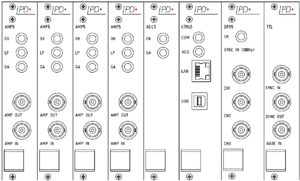
Fig. II.1: Front panel of the standard ICMsystem Gen 5 acquisition unit
It further contains the serial interface and may contain the connection of the telephone line to an optional built-in modem. The rear panel of the ICMsystem Gen 5, as shown with figure II.2, contains the mains supply connector, switch, and fuse. Furthermore, it bears the IEEE488 connector and the important wing nut terminal to safely tie the metal frame to ground. In general, observe the grounding of the ICMsystem carefully and familiarise yourself with the properties of the overall grounding system especially in case of field measurements. In case, safety reasons force you to introduce ground loops, you may use ferrite ring cores to reduce high frequency pick-up (feed one to few turns of the RG58 signal cable through the ring core). Regarding further isolation measures please refer to the sections covering the isolation transformer IT2 and the current transformers of the CT family. The isolation that is provided with the transformer type coupling units is of less efficiency. With applications of hazard of electrical shock or high risk of breakdown use fibre optic isolation in general. The RPA4 offers a battery-operated transmitter with fibre optic isolation and a signal behaviour similar to the RPA1. Consult Power Diagnostix regarding further equipment to provide fibre optic isolation.
8

Fig. II.2: Rear panel of the ICMsystem Gen 5 acquisition unit
II.1.2 Multi-Channel Unit for Acceptance Testing on Power Transformers
The version of the ICMsystem for partial discharge acceptance testing on power transformers builds on the acquisition core of the standard single-channel ICMsystem Gen 5 unit. It comes in a 19" metal enclosure. In order to have access to the partial discharge information and/or optionally to the RIV values of up to ten channels simultaneously, this instrument is equipped with up to ten parallel amplifier plug-ins. The unit further offers a multiplexed input for the synchronisation signal and the voltage measurement. Partial discharge pattern acquisition is offered in a semi-parallel mode, which allows an automated storage of consecutive files to analyse the history of a partial discharge pattern.

Fig. II.3: Front panel of the ICMsystem Gen 5 with nine channels

Warning!
Always provide solid grounding of the instrument and the coupling units. Use the rear side wing nut terminal for ground connection (see figure II.2). Never operate the instrument without protective grounding. Use isolation techniques, such as isolation transformers or fibre optic isolation to avoid hazard and injury. With applications bearing a high risk of electrical shock or breakdown use fibre optic isolation in general.
II.1.3 Modules
II.1.3.1 Built-in AC5 Power Supply Module
The AC5 module is the power supply of the instrument. The green LED on the front panel indicates that the power supply is on and that the output voltages are available. This power supply module offers a wide range of accepted mains voltages (95–264 V_AC ). Thus, all commonly used AC mains voltages are suitable.
OK Green LED indicates 'Power Good'
Specification: Temperature range: 10–40°C
Input voltage: 90–264 V _AC
Input frequency: 47–440 Hz
Power: \~ 110 VA max.
Fuse: 2 or 3.15 A
II.1.3.2 CTRL5 Controller

The controller module (figure II.4) contains the system- and communication controller. The standard unit comes with both the GPIB, and the USB, interface. The built-in modem is optional. Special controller units with fibre optic communication interfaces are available as well. The small system beeper can be set to act as a loudspeaker to make the PD signal or the gating signal audible with the yellow LED flashing accordingly. The upper green LED indicates ongoing communication, while the lower green LED indicates a running acquisition. The serial cable supplied is used to connect the instrument to a computer's USB port.
COM Green LED indicates ongoing communication
ACQ Bicolour LED; green indicates a running acquisition, yellow flashing accordingly with the internal beeper indicates system messages, PD activities, or gate activities
LAN LAN connector
USB USB connector
Options: Built-in modem 56.7 kbps
Fig. II.4
II.1.3.3 DPR5 Dual Port RAM
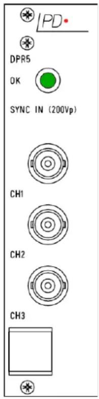
The module DPR5, contains the phase and time reference logic, the multi-channel memory and the voltage measurement circuits. The acquisition unit is caused by the ICMsystem software to sample the input voltage. Thus, the program can display the true shape of the high voltage signal. The unit is able to trigger either on the test voltage as it is picked up from an external synchronisation source (external trigger) or on the line signal (internal trigger). In case of external trigger chosen and no sync source connected, the unit switches to the TTL SYNC IN of the TTL module. The DPR5 unit contains a controller for the handling of the partial discharge pattern and the emulation of a Dual Port Ram to have the acquisition of the pattern and the communication completely asynchronous. The dwell time, i.e. the time the unit assigns a digitised pulse to a certain time channel or slot is calculated automatically or may be set by the control program.
OK Green LED indicates valid synchronisation
CH1-CH3 Isolated BNC connectors that supply the power for the pre-amplifiers for the delivery of the synchronisation signals
Specification: Memory array: 8 bits x 8 bits, 16 bits depth
Sync. frequency: 20–510 Hz (automatic.) / 0.02–510 Hz (manually)
Fig. II.5
II.1.3.4 ADC5 Peak A/D Converter

The ADC5, the pulse analogue to digital converter module, processes single impulses, it determines pulse magnitude and polarity, and it can handle various signal shapes, which can be encountered in practice. The appropriate setting of the A/D converter is a very critical parameter. These settings do have a strong impact on the measurement results. Thus, sufficient time should be spent to evaluate the influence of this module's features with the intended application of the instrument. The noise gate inhibits the transfer of the acquired pulse magnitude to the storage.
Trigger Mode,
The A/D-Converter has two basic trigger modes. Trigger on first peak and trigger in time window. The trigger on first peak may be set to act re-triggerable and non-re-triggerable. A more detailed explanation of these properties and their impact can be found with section V.
a) Trigger on first peak (non-re-triggerable)
With all modes a pulse conversion is started if a pulse exceeds the LLD threshold. In this mode the first peak of a signal is captured, held, and converted to its digital expression. Within the pre-set dead time no other pulse is accepted.
b) Trigger on first peak (re-triggerable)
In order to prevent multiple readings of oscillatory signals, another pulse occurring during the dead time automatically retriggers the dead time. Thus, the dead time is matched to the duration of the ringing. With high pulse repetition rates or with strongly oscillating signals this may cause excessive dead times and malfunction!
Fig. II.6
c) Trigger in time window
As with the other modes the conversion cycle is started with a pulse exceeding the LLD threshold. Other than with the trigger on first peak, the decision of the pulse polarity is taken at the end of the time window. I. e. both the positive and the negative peak is captured and held within the pre-set dead time, subsequently, the larger one is taken and transferred to the DPR5 module. It does not make sense to have the time window option re-triggerable.
Dead Time (DT)
Time during which a signal is converted, and which is reserved to a single pulse. The A/D converter does not convert or accept another signal during that time, so that another pulse occurring within the dead time is lost (first peak triggering). With the ADC5 set to trigger in time window, the dead time represents the time window during which both the positive and negative peak value is captured and held. Thus, only the pulse of the highest magnitude is assigned to the current trigger event, while the others are neglected. Although the internal dead time of the A/D converter is only 0.5 s leading to a high theoretical pulse repetition rate this value cannot be reached in practice. The bandwidth limit of the input amplifiers does not allow these high repetition rates without pulse pile-up. With respect to this effect, the dead time is limited to a minimum of 5 s. The dead time should be chosen as short as possible, but large enough to avoid multiple triggering. It is evident that an excessive dead time reduces the statistical reliability of a measurement.
Low Level Discriminator (LLD),
The LLD acts as threshold that a pulse must exceed to trigger the conversion cycle. The discriminator serves to reject continuous low-level noise or to reject high repetition rate small discharge pulses. An appropriate discriminator setting reduces dead time. In some cases, large pulses may be lost if they occur during the A/D conversion (dead time) of small pulses. This effect is reduced by choosing a higher discriminator-level or by means of the converter setting 'Trigger in Time Window'. The LLD acts symmetrically on positive or negative pulses. As the A/D converter saturates at ±5 V, 100% LLD means ±5 V. In the bipolar mode of the ICMsystem there is a basic resolution of 7 bits or 128 channels with each polarity. One channel is hence approximately 0.78%.

line
| Time Segment | Signal Value | |----------------------|--------------| | Start | 0 | | Peak | 1 | | Mid | -2 | | End | 0 |Fig. II.7 Triggering of the ADC5 module
Coding
As the basic resolution of the converter is 12 bits, a dynamic compression into 8 bits is done ( ± 11 bits into ± 7 bits). The choice of several coding procedures is offered, whereas unipolar offers the 8-bit resolution for the absolute value:
• Linear bipolar ( ±7 bits, the standard setting)
• Linear unipolar (8 bits)
The dynamic compression should only be used for a more efficient use of the display area while detecting low-level signals. The linear unipolar option is used for the analysis of unipolar signal sources of special detectors, or spectrum analyser outputs, or where the meaning of the polarity is invalidated due to excessive count rates or strong ringing, for instance.

| OK | Green LED to indicate check of main functions passed | |
| GA | Red LED to signalise gate action, ADC is locked by the gate impulse | |
| Specification: | Basic resolution | 12 bits or ±11 bits linearly compressed into 8 bits |
| Full range | ±5 V, over-ranging pulses are assigned to the ±5 V level | |
| Time window | 5 μs < window > 3 ms | |
| Dead time | 5 μs < window > 3 ms | |
| Threshold level | Bipolar symmetrical, range of 0–5 V | |
| Gating | Inhibition of conversion by internal signal from the AMP plug-in that is serving as gating module | |
| Real time rate | 200 kHz max. | |
| Signal input | Internally from the AMP5 module | |
Fig. II.8
II.1.3.5 AMP5 Main Amplifier
AMP Mode

Fig. II.9
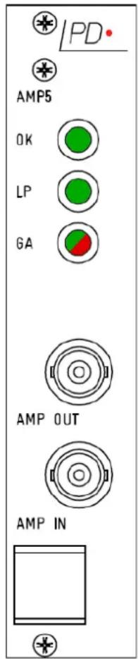
The AMP5 module contains the main or PD amplifier of the system with computer-programmable gain and band-pass filters as well as the power supply for the pre-amplifier RPA1. Further, it contains an analogue switch which opens the signal path when it is actuated by the noise gate, and a so-called pC meter with an A/D converter for the measurement of the apparent charge according to IEC 60270.
The PD signal should be connected preferably through an RPA pre-amplifier to the AMP IN connector (lower BNC plug). The RPA acts as impedance converter and line driver to isolate the (weak) PD source from the signal cable's capacitance and impedance, respectively. Furthermore, the active preamplifiers are designed to reduce the risk of electromagnetic hazards. The PD signal can be directly connected to the amplifier input as well. In case, please consider that the input impedance at the AMP IN connector is 50 Ω versus the 10 kΩ of the RPA1 and furthermore, that this BNC terminal carries the power supply voltage for the RPA pre-amplifiers, if it is not set to off. An RPA1 should be used even if a 50 Ω termination at the input is required with the RPA1's frequency range. The amplified PD signal is available at the AMP OUT terminal (upper BNC connector). Here, an oscilloscope may be connected using a BNC-T-connector to observe the signal. The lengths of the connecting cable must not exceed one meter.
| OK | Green LED to indicate check of main functions passed. | |
| LP | Green LED that is lit with an RPA pre-amplifier connected, activated, and ready to use. I.e., it indicates an established connection with the remote supply available and normal supply current drawn by the RPA. | |
| GA | Bipolar LED; red indicates gate action and AMP is locked by the gate impulse; green indicates that the module is used for gating (see page 16, GATE Mode) | |
| AMP IN | BNC connector. Connects to the remote pre-amplifier RPA for the PD signal. This input carries the supply and control voltage of the pre-amplifiers. May be used as direct signal input. 50 Ω input impedance. | |
| AMP OUT | BNC connector carrying the amplified and filtered PD signal. | |
| Caution: | The supply voltage for the pre-amplifiers may damage the output circuit of the signal source, such as receivers or spectrum analysers, if connected directly. Be sure to set the pre-gain to OFF prior connecting such devices. | |
| Specification: | Gain range: | 1, 2, 4, 8, 10, 20, ..., 200, 400, 800 |
| Coupling: | AC | |
| Input impedance: | 50 Ω | |
| Filter properties: | ||
| LF cut-off (-6 dB): | 40, 80, 100 kHz | |
| HF cut-off (-6 dB): | 250, 600, 800 kHz | |
| pC meter: | ||
| Charging time: | 500 ns (approx.) | |
| Resolution: | 12 bits | |
SPEC Mode

Fig. II.10
The optional spectrum function extends the AMP5 module to provide a spectrum analyser and an RIV (radio influence voltage) meter. This combination enables PD measurements even with large background noise e.g. in non-shielded test areas. Observing the frequency spectrum of a harsh distributed PD signal allows selecting frequency bands with fewer disturbances. Using this selected frequency for a PD acquisition gives a largely improved signal to noise ratio resulting in a clear pattern acquisition.
The spectrum option can be used either for PD detection with a bandwidth of 9 kHz or 300 kHz around the selected frequency or for RIV measurement with 9 kHz bandwidth around the selected frequency. Frequency bandwidth and centre frequency are fully controllable via the ICMsystem software, as well as the sweep time for a complete scan of the frequency spectrum. For frequencies above 1 MHz the usage of an RPA1L pre-amplifier instead of an RPA1 is inevitable.
| OK | Green LED to indicate check of main functions passed. | |
| LP | Green LED that is lit with an RPA pre-amplifier connected, activated, and ready to use. I. e., it indicates an established connection with the remote supply available and normal supply current drawn by the RPA. | |
| GA | Bipolar LED; red indicates gate action and AMP is locked by the gate impulse; green indicates that the module is used for gating (see page 16, GATE Mode) | |
| AMP IN | BNC connector. Connects to the remote pre-amplifier RPA for the PD signal. This input carries the supply and control voltage of the pre-amplifiers. May be used as direct signal input. 50 Ω input impedance. | |
| AMP OUT | BNC connector carrying the amplified and filtered PD signal. | |
| Caution: | The supply voltage for the pre-amplifiers may damage the output circuit of the signal source, such as receivers or spectrum analysers, if connected directly. Be sure to set the pre-gain to OFF prior connecting such devices. | |
| Specification: | Gain range: | 1, 2, 4, 8, 16, 32, 64, 128 |
| Coupling: | AC | |
| Input impedance: | 50 Ω | |
| Frequency: | 10 kHz–10 MHz (in steps of 10 kHz) | |
| Bandwidth: | 9 kHz or 270 kHz | |
GATE Mode
with an
oscilloscope.
Fig. II.11
When used as gate module the AMP5 plug-in board takes care of the triggering on noise pulses to avoid that these pulses contribute to the acquired partial discharge pattern. If an amplified noise signal exceeds a threshold or trigger level (0 to ±5 V equivalent to 0–100% trigger level) a TTL signal is internally send to the other AMP5 and ADC5 modules. If enabled by the control program, this TTL signal opens an analogue switch in the other AMP5 module and/or inhibits the further processing of a converted pulse magnitude by the ADC5.
The disturbance signal should be connected preferably through an RPA pre-amplifier to the AMP IN connector (lower BNC plug). The RPA acts as impedance converter and line driver to isolate the (weak) signal source from the signal cable's capacitance and impedance, respectively. Furthermore, the active preamplifiers are designed to reduce the risk of electromagnetic hazards. The disturbance signal can be directly connected to the amplifier input as well. In this case, please consider, that the input impedance at the AMP IN connector is 50 Ω versus the 10 kΩ of the RPA1 and, furthermore, that this BNC terminal carries the power supply voltage for the RPA pre-amplifiers, if it is not set to off. An RPA1 should be used even if a 50Ω termination at the input is required with the RPA1's frequency range. The TTL signal referring to the input pulses exceeding the threshold is available at the AMP OUT terminal (upper BNC connector). This signal is internally already connected to both AMP5 and ADC5 module. Thus, no further external connection is required. The AMP OUT connector may be used to observe the gating action
| OK | Green LED to indicate check of main functions passed. | |
| LP | Green LED that is lit with an RPA pre-amplifier connected, activated, and ready to use. i.e., it indicates an established connection with the remote supply available and normal supply current drawn by the RPA. | |
| GA | Bipolar LED; green indicates that the module is used for gating red LED indicates gate action and AMP is locked by the gate impulse; (see page 14 AMP Mode and page 15 SPEC Mode) | |
| AMP IN | BNC connector. Connects to the remote pre-amplifier RPA for the disturbance signal. This input carries the supply and control voltage of the pre-amplifiers. May be used as direct signal input. 50 Ω input impedance. | |
| AMP OUT | BNC connector carrying the TTL gating signal. May be used to gate pre-processing instruments. | |
| Caution: | The supply voltage for the pre-amplifiers may damage the output circuit of a signal source, such as receivers or spectrum analysers, if connected directly. Be sure to set the pre-gain to OFF prior connecting such devices. | |
| Specification: | Gain range: | 1, 2, 4, 8, 10, 20, ..., 200, 400, 800 |
| Coupling: | AC | |
| Input impedance: | 50 Ω | |
| Filter properties: | ||
| LF cut-off (-6 dB): | 40, 80, 100 kHz | |
| HF cut-off (-6 dB): | 250, 600, 800 kHz | |
| Gate pulse duration: | 10 μs fixed. With ADC gating used, the effective gating time refers to the dead time, i. e. may be chosen longer. | |
II.1.3.6 TTL Module
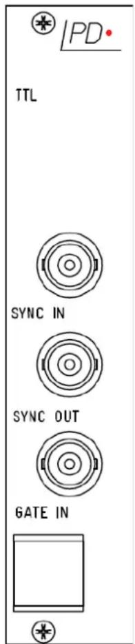
The TTL module offers input connectors for TTL signals used for synchronisation and gating.
If disturbances, like switching of a relay or thyristor firing, have a known source, it might be possible to get a TTL gating signal prior to the disturbance. This signal can be used to blind out the PD measurement path. For the time this input is logically high (5 V_DC ; TTL standard) no signal is taken from the AMP IN terminal i.e. no PD signal is recorded (see also section V.6.2 'Synchronisation with Very Low Frequencies (VLF)').
SYNC IN Input for a 5 V DC synchronisation signal supplied by the voltage source of the test-setup. This input is active only with manual frequency selection and the sync source set to external within the ICMsystem software.
SYNC OUT 5 V DC signal for synchronisation purposes.
GATE IN Input terminal for an external TTL gating signal.
Fig. II.12
II.2 Signal Conditioning Pre-amplifiers
The acquisition unit of the ICMsystem Gen 5, as described with the previous section, is used with all applications of the instrument and remains unchanged. The adaptation to the specific needs of a certain application requires the choice of the appropriate pre-amplifiers, signal conditioning modules, and coupling devices. This section describes the properties and main application of the available devices.
All external signal conditioning modules and pre-amplifiers are remote supplied and remote controlled through a simple coaxial signal cable (RG58). This technique allows placing these units close to the sensor or signal source. Furthermore, as these modules act as impedance converter and line driver, the weak signal source, such as voltage divider or coupling impedance, is not loaded by the cable capacitance or impedance, respectively. Additionally, an enhanced over-voltage protection becomes available by this technique.
The engraved arrows describe the signal flow direction on the pre-amplifiers. Caution: The signal direction must never be reversed to avoid malfunction or damage of the unit.
II.2.1 RPA1, Range 40 kHz–800 kHz
The RPA1 is the standard pre-amplifier for measurements in the low frequency range according to standards such as the IEC 60270.
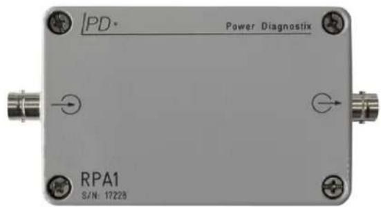
Fig. II.13
The RPA1 has with all other pre-amplifiers of the RPA range in common that it is able to drive a 50 Ω cable. The length of this signal cable may be as long as 50 m. Due to the low power requirements of the RPA1 an RG58 type of coaxial cable is sufficient for a length of up to 30–40 m. Use RG213 cable with applications exceeding the 40 m. The pass-band of the RPA1's filters is slightly wider than the widest bandwidth provided by the ICMsystem's AMP5 filters. This ensures that the acquisition unit's filters control the overall bandwidth, only. The input sensitivity in terms of [pC] depends on the efficiency of the coupling circuit and the noise situation. With a carefully designed setup this sensitivity may be even lower than 0.1 pC.

BNC input connector. To be connected to the signal source. To utilise the benefits of the relative high impedance of the RPA1's input, the connection cable to a quadrupole must be as short as possible. Use a BNC-BNC adapter or a very short BNC cable, preferably (RG58: 100 pF/m).
Warning:
The RPA's input is not able to carry the load current of a sample or coupling capacitor. A power separation filter or quadrupole is required in general!

BNC output connector. To be connected directly to the AMP IN of the AMP5 module. If not remote powered, this output has a high frequency connection to the input.
Caution:
Use AC coupling and high impedance input setting (1 MΩ//20 pF) if monitoring the RPA's output with an oscilloscope. Low impedance oscilloscope inputs may be damaged or cause malfunction, as the signal cable between RPA and ICMsystem carries the RPA's power supply and remote control.
Specification:
Input Impedance: 10 kΩ//50 pF
Bandwidth: 20 kHz–1.0 MHz (40–800 kHz or less with the ICMsystem)
Roll-Off: 40 dB/dec.
Gain steps: Off, 0, 20, 40 dB (remote controlled by the ICMsystem)
Input sensitivity: < 50 V_rms/0.03 pC
II.2.2 RPA1L, Range 40 kHz–20 MHz

The RPA1L is a pre-amplifier designed for measurements in a higher frequency range according to standards such as the IEC 60270.
The RPA1L offers a wider passband and lower input impedance than the RPA1 while the remaining key data stay the same. These differences to the RPA1 provide the possibility for PD and RIV measurements around centre frequencies above 1 MHz with high accuracy.
Fig. II.14

Warning:
BNC input connector. To be connected to the signal source. To utilise the benefits of the relative high impedance of the RPA1L's input, the connection cable to a quadrupole must be as short as possible. Use a BNC-BNC adapter or a very short BNC cable, preferably (RG58: 100 pF/m).

The RPA's input is not able to carry the load current of a sample or coupling capacitor. A power separation filter or quadrupole is required in general!
BNC output connector. To be connected directly to the AMP IN of the AMP5 module. If not remote powered, this output has a high frequency connection to the input.
Caution:
Use AC coupling and high impedance input setting (1 MΩ//20 pF) if monitoring the RPA's output with an oscilloscope. Low impedance oscilloscope inputs may be damaged or cause malfunction, as the signal cable between RPA and ICMsystem carries the RPA's power supply and remote control.
Specification:
Input impedance: 1 kΩ//50 pF
Bandwidth: 40 kHz–20 MHz
Roll-off: 40 dB/dec.
Gain steps: Off, 0, 20, 40 dB (remote controlled by the ICMsystem)
Input sensitivity: < 15 V_rms/0.02 pC
II.2.3 RPA1H, Range 40 kHz–20 MHz

The RPA1H covers the same frequency ranges as the RPA1L and, hence, the same application range, but with a lower input sensitivity because of a built-in attenuator with a ratio of 1:10.
Fig. II.15

BNC input connector. To be connected to the signal source. To utilise the benefits of the relative high impedance of the RPA1L's input, the connection cable to a quadrupole must be as short as possible. Use a BNC-BNC adapter or a very short BNC cable, preferably (RG58: 100 pF/m).
Warning: The RPA's input is not able to carry the load current of a sample or coupling capacitor. A power separation filter or quadrupole is required in general!

BNC output connector. To be connected directly to the AMP IN of the AMP5 module. If not remote powered, this output has a high frequency connection to the input.
Caution: Use AC coupling and high impedance input setting (1 MΩ//20 pF) if monitoring the RPA's output with an oscilloscope. Low impedance oscilloscope inputs may be damaged or cause malfunction, as the signal cable between RPA and ICMsystem carries the RPA's power supply and remote control.
Specification: Input impedance: 1 kΩ//50 pF Bandwidth: 40 kHz–20 MHz Roll-off: 40 dB/dec. Gain steps: Off, 0, 20, 40 dB (remote controlled by the ICMsystem) Input sensitivity: < 40 μV _rms /0.05 pC
II.2.4 RPA1D and RPA1G, Range 40 kHz–800 kHz

RPA1D and RPA1G are suited to connect directly to ultrasonic acoustic sensors with embedded pre-amplifiers. To simplify connection, they provide a selectable power supply for the sensor (15 V/28 V or Off/15 V/28 V, resp.).

Fig. II.16

BNC input connector. To be connected to the signal source. To utilise the benefits of the relative high impedance of the RPA1L's input, the connection cable to a quadrupole must be as short as possible. Use a BNC-BNC adapter or a very short BNC cable, preferably (RG58: 100 pF/m).
Warning:
The RPA's input is not able to carry the load current of a sample or coupling capacitor. A power separation filter or quadrupole is required in general!

BNC output connector. To be connected directly to the AMP IN of the AMP5 module. If not remote powered, this output has a high frequency connection to the input.
Caution:
Use AC coupling and high impedance input setting (1 MΩ//20 pF) if monitoring the RPA's output with an oscilloscope. Low impedance oscilloscope inputs may be damaged or cause malfunction, as the signal cable between RPA and ICMsystem carries the RPA's power supply and remote control.
Specification:
Input impedance: 10 kΩ//50 pF
Bandwidth: 40 kHz–800 kHz
Roll-off: 40 dB/dec.
Gain steps: Off, 0, 20, 40 dB (remote controlled by the ICMsystem)
Input sensitivity: < 50 V_rms/0.03 pC
II.2.5 RPA2, Range 2 MHz–20 MHz

Fig. II.17
The RPA2 module is a signal-conditioning amplifier that is designed to measure partial discharges in a frequency range higher than the range provided by the ICMsystem itself. Its basic function is to transfer the envelope of the high frequency signal found in the range of 2–20 MHz into a frequency range that can be acquired by the ICMsystem. Thus, the output signal reflects the frequency content between 100 kHz and 800 kHz of the envelope of the signals found between 2 MHz and 20 MHz. In principle the circuits behave as a broadband AM demodulator. The output signal is positive unipolar. The chosen frequency range of 2–20 MHz has proven a good match for the partial discharge signal spectra found with rotating
machines and capacitive sensors used to monitor cables and cable accessories. The 50 Ω input impedance of the RPA2 allows a connection of this unit between the ICMsystem's input multiplexer and the AMP input, as well.

BNC input connector. To be connected to the signal source. As the RPA2 has a matched 50 Ω input impedance, a certain length of RG58 cable between the sensor/coupler and this input does not affect the sensitivity in general.
Warning: The RPA's input is not able to carry the load current of a sample or coupling capacitor. A power separation filter or quadrupole is required in general!

BNC output connector. To be connected directly to the AMP IN of the AMP5 module.
Caution: Use AC coupling and high impedance input setting (1 MΩ//20 pF) if monitoring the RPA's output with an oscilloscope. Low impedance oscilloscope inputs may be damaged or cause malfunction, as the signal cable between RPA and ICMsystem carries the RPA's power supply and remote control.
| Specification: | Input impedance: | 50 Ω//50 pF |
| Bandwidth: | 2 MHz–20 MHz | |
| Roll-off: | 40 dB/dec. | |
| Output bandwidth: | 100 kHz–800 kHz | |
| Gain steps: | Off, 0, 20, 40 dB (remote controlled by the ICMsystem) | |
| Input sensitivity: | < 800 μVrms/1 pC |
II.2.6 RPA3, Range 200 MHz–1 GHz
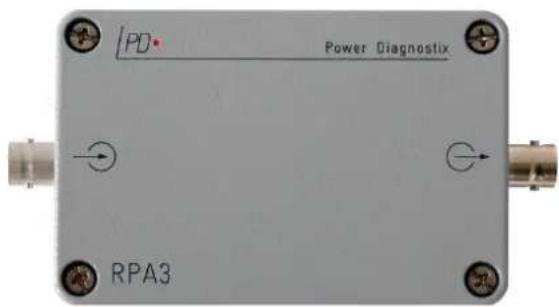
Fig. II.18
The RPA3 module is a signal-conditioning amplifier that is designed to measure partial discharges in a frequency range higher than the range provided by the ICMsystem itself. Its basic function is to transfer the envelope of the high frequency signal found in the range of 200 to 1000 MHz into a frequency range that can be acquired by the ICMsystem. Thus, the output signal reflects the frequency content between 100 kHz and 800 kHz of the envelope of the signals found between 200 MHz and 1 GHz. In principle the circuits behave as a broadband AM demodulator. The output signal is positive unipolar. The chosen frequency range of 200–1000 MHz has proven a good match for the partial discharge signal spectra found with sensors and antennae installed with gas insulated switchgear (GIS). The RPA3 must be placed close to the sensor, since the signal cable's attenuation with this frequency range is relative strong. Depending on the efficiency of the GIS sensor additional pre-amplification may be required.

BNC input connector. To be connected to the signal source. A short connection to the sensor is mandatory to avoid unwanted signal attenuation. Use low loss signal cable in case.
Warning:
The RPA's input is not able to carry the load current of a sample or coupling capacitor. With GIS sensors a limitation of VFT voltages is required.

BNC output connector. To be connected directly to the AMP IN of the AMP5 module.
Caution:
Use AC coupling and high impedance input setting (1 MΩ//20 pF) if monitoring the RPA's output with an oscilloscope. Low impedance oscilloscope inputs may be damaged or cause malfunction, as the signal cable between RPA and ICMsystem carries the RPA's power supply and remote control.
Specification:
Input impedance: 50 Ω//50 pF
Bandwidth: 200 MHz–1000 MHz
Roll-off: 40 dB/dec.
Output bandwidth: 100 kHz–800 kHz
Gain steps: Off, 0, 20, 40 dB (remote controlled by the ICMsystem)
Input sensitivity: < 2 μV
II.2.7 RPA4, Range 40 kHz–800 kHz, Fibre Optic Isolation
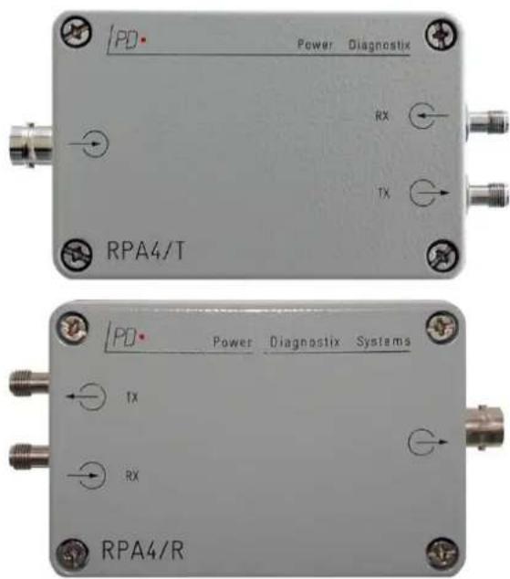
Fig. II.19
The RPA4 is a pre-amplifier set with fibre optical transmission offering outstanding isolation properties. Regarding the frequency response and other properties this amplifier set behaves similar to the RPA1. It consists of a battery-operated transmitter unit RPA4/T that is connected by two fibre optic cables to a receiver unit RPA4/R. The RPA4/R's output BNC connector is fed to the AMP IN of the ICMsystem. Again, with respect to the input and output BNC terminal there is, beside the isolation, no difference to the RPA1. The fibre optic cable used can isolate 100kV and more, if kept clean (refer to the next page, as well). The attenuation of the fibre optic cable responsible for the analogue transmission from the RPA4/T to the RPA4/R is compensated automatically. The second fibre transmits the gain control and the ON/OFF signal. While in standby (OFF), the transmitter consumes less than 50 μA, offering a standby period of several weeks. The use of the fibre optic isolation that is offered by this set is mandatory in case of field measurements bearing a high risk of breakdown, unreliable grounding, and hazard of electrical shock. Furthermore, it may be used for high side coupling, i.e., introducing a coupling unit into the high voltage feeding connection of a test setup. In conjunction
with the balancing bridge adapter AB1 high side balanced measurements become available. The standard length of the fibre optic cable is 20 m. Without any change of the modules this length may be extended up to 500 m.

BNC input connector. To be connected to the signal source. To utilise the benefits of the relative high impedance of the RPA4's input, the connection cable to a quadrupole must be as short as possible. Use a BNC-BNC adapter or a very short BNC cable, preferably (RG58: 100 pF/m).
Warning:
The RPA's input is not able to carry the load current of a sample or coupling capacitor. A power separation filter or quadrupole is required in general!

TX
FSMA connector bearing a fibre optic transmitter diode. To be connected to the RX terminal of the second module of the RPA4 set.

RX
FSMA connector bearing a fibre optic receiver diode. To be connected to the TX terminal of the second module of the RPA4 set.

BNC output connector. To be connected directly to the AMP IN of the AMP5 module.
Caution:
Use AC coupling and high impedance input setting (1 MΩ//20 pF) if monitoring the RPA's output with an oscilloscope. Low impedance oscilloscope inputs may be damaged or cause malfunction, as the signal cable between RPA and ICMsystem carries the RPA's power supply and remote control.
Specification:
Input impedance: 10 kΩ//50 pF
Bandwidth: 20 kHz–1 MHz (40–800 kHz or less with the ICMsystem)
Roll-off: 40 dB/dec.
Gain steps: Off, 0, 20, 40 dB (remote controlled by the ICMsystem)
Input sensitivity: < 50 V_rms/0.03 pC
Fiber optic cable: 20–500 m (110/125 μm/3 mm HCS with SMA connectors)
Battery operation: 10 h continuous, 3 weeks standby, NiMH battery
II.2.8 FCU2, Frequency Converter Unit

natural_image
Three black industrial electronic devices labeled with IPU2B and FCU2 connectors (no visible text or symbols on body)Fig. II.20
When capturing PD signals offering a larger dynamic range, a logarithmic scaling of the PD pulses is advantageous. The frequency converter unit FCU2 is a UHF matching and pre-processing unit mainly used for measurements at gas insulated switchgears (GIS). The output of this module is the envelope of the UHF signal down-converted into the HF range. The FCU2 is designed to withstand high voltage transients for most applications; however, in some cases it might be necessary to increase
the input protection by an IPU2. This input protection unit is designed to avoid damage of the FCU2 input stage under the presence of very strong transient signals. The FCU2 is placed directly at the output connector of the input protection unit in order to avoid long and lossy UHF cables. Mounting the FCU2 closely to the sensor's terminal generally ensures the highest sensitivity. Simple and inexpensive RG58/RG142 type coaxial cable connects the FCU2 to the input of the ICMsystem, as the FCU's output signal is of a frequency, which is not suffering from strong cable attenuation.
The FCU is available in two different housings offering different grades of environmental protection. The protection class IP65 offers extended protection for outdoor use, while the standard IP52 version is for indoor use, only.


Input connector of type N. To be connected to the input protection unit IPU2 or directly to the signal source. Keep the connection as short as possible to have all ranges utilised at its best.
BNC (IP52) or TNC (IP65) output connector. To be connected to the AMP IN of the AMP5 module.
Specification:
Input impedance: 50 Ω//50 pF
Bandwidth: 100 MHz–1800 MHz
Roll-off: 40 dB/dec.
Input sensitivity: < 200 μV (46 dBμV)
Output bandwidth: 40 kHz–2 MHz (approx., depends on input signal)
II.2.9 AB1, Active Bridge Adapter

Fig. II.21
The so-called active bridge adapter AB1 serves to balance the signal picked up by two RPA1 (or RPA4) to reduce the common mode noise or disturbance. This method is applicable in case two branches are available. These branches may be two samples or testing objects each equipped with a quadrupole and an RPA1, or one testing object and a coupling capacitor, for example. Additionally, introducing a quadrupole into the high voltage connection of a HV cable may pick up the first signal with the fibre optic pre-amplifier RPA4, while a coupling capacitor picks up the second signal. In general, the two required signals must bear the partial discharge signal in reversed polarity, while the disturbance signal must show up in common mode. A mismatch of the signal strength can be adjusted with the AB1's control knob. With the RPA1's of the two branches connected to the 'Pos' and 'Neg' input of the AB1 and the output connected to the AMP IN of the ICMsystem's AMP5 module, the control knob is used to minimise the common mode signal.
In case, use a calibrator to inject common mode signals, i.e., signals flowing through both branches. Afterwards, the system is calibrated by injecting charge pulses across the testing object.

Pos
BNC input connector. The signal received from the RPA1 connected to this terminal will show up non-inverted in the acquired pattern.

Neg
BNC input connector. The signal received from the RPA1 connected to this terminal will show up inverted in the acquired pattern.

Caution:
BNC output connector. To be connected directly to the AMP IN of the AMP5 module.
Use AC coupling and high impedance input setting (1 MΩ//20 pF) if monitoring the RPA's output with an oscilloscope. Low impedance oscilloscope inputs may be damaged or cause malfunction, as the signal cable between RPA and ICMsystem carries the RPA's power supply and remote control.
Specification:
Input impedance: 50 Ω//20 pF
Output impedance: 50 Ω
Adjustment range: 0.2–5
Power supply: The supply and remote-control signals from the ICMsystem to the RPAs are fed through.
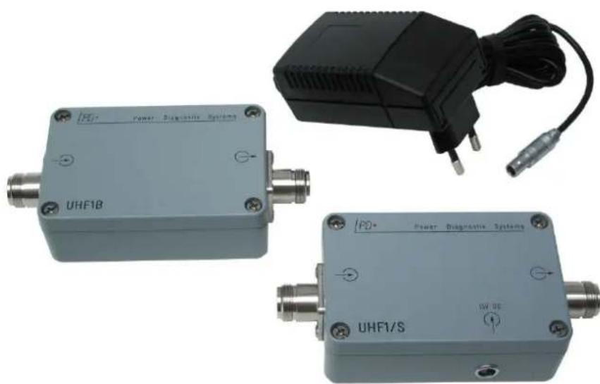
II.2.10 UHF1, Pre-Amplifier Set, Range 200 MHz–1 GHz
Often the signal strength derived from UHF sensors attached to gas insulated switchgear (GIS) is insufficient and requires additional amplification. Especially, sensors retrofitted externally may suffer from weak signals. Partly, integrated sensors showed up a disappointing efficiency, as well. The UHF1 offers an amplification of 27 dB in the range from 200 MHz to 1 GHz. The amplifier is remotely powered through the signal cable. The UHF1/S unit acts as so-called Bias-T. I. e., it provides the filter to feed the supply voltage into the signal cable, while maintaining the 50 Ω matched signal path. In order to avoid further reduction of the S/N ratio (signal to noise ratio), the UHF1 shall be placed close to the sensor or sensor terminal. The use of low loss 50 Ω cable is mandatory. At least, RG213 signal cable shall be used. Avoid the use of RG58 cable. RG58
natural_image
Three electronic devices labeled UHF1B, UHF1/S, and a black power diagnostic system with attached plug (no visible text or symbols on main components)cable is suitable for short patch cables, only. The 15 V _DC supply voltage to be fed into the UHF1/S can be taken from the 15 V connector at the ICMsystem's rear side.
Alternatively, the 15 V DC is derived from the small power block supplied with the UHF1 set. That power block accepts line voltages from 95 V to 250 V, and it comes with an exchangeable mains adapter (Euro, America, and others). The UHF output can be connected to the input of an RPA3 or a spectrum analyser's input.
Fig. II.22: UHF1, pre-amplifier set


15V DC

N input connector (UHF1B). The signal received from the GIS sensor is connected to this N terminal.
N output connector (UHF1B). This output connector carries the amplified signal and the remote supply voltage. Connect this terminal to the input of the UHF1/S (next item). The use of low loss coaxial cable is mandatory. Use at least RG213.
N input connector (UHF1/S). Connector to receive the amplified signal from the UHF1B. Further, it acts as output to remote supply the UHF1B.
N output connector (UHF1/S). To be connected directly or through the ICMsystem's UHF input multiplexer to the RPA3 or a spectrum analyser's input.
LEMO input connector. 15 V _DC to supply the UHF1. May be connected to the 15 V output connector of the ICMsystem or to the AC power block.
Specification:
Input impedance: 50 Ω
Output impedance: 50 Ω
Bandwidth: 200 MHz–1 GHz
Gain: 27 dB
Power supply: 15 V_DC
II.3 Coupling Devices
A variety of coupling devices allows adapting the ICMsystem to different measurement tasks. Beside the standard range of coupling units and devices further installation sets and sensor assemblies are available. These assemblies and sets are mostly engineering products and are built for customer needs.
II.3.1 CIL, CIT Quadrupoles
The CIL quadrupoles consist of an inductor in parallel with a damping resistor. This inductor and the resistor is calculated to form together with a high voltage coupling capacitor a second order high pass filter. Additionally, the CIL/V quadrupoles bear a capacitor acting as a divider together with the high voltage coupling capacitor. The CIT coupling units are transformer type units, where the RPA1's input resistance represents the required damping resistor. As these units offer a higher sensitivity than the CIL coupling units, their use is mandatory with applications suffering from signal attenuation, such as measurements on medium voltage cables.
CILXY Standard quadrupole with R//L circuit, spark gap, Banana input, BNC output.
X: [1-6] Coupling capacitor range
Y: [H, M, L] AC current range
The maximum voltage refers to the largest capacitor of the range given:
L: Low (125 kV @ 50 Hz)
M: Medium (500 kV @ 50 Hz)
H: High (1000 kV @ 50 Hz)

Fig. II.23
Available standard quadrupoles:
CIL4L: 600 pF-2.5 nF, 100 mA
CIL4M: 600 pF-2.5 nF, 400 mA
CIL4: 600 pF-2.5 nF, 1.1 A
CIL5L: 2–9 nF, 400 mA
CIL5M: 2–9 nF, 1.6 A
CIL5: 2–9 nF, 3.2 A
CIL6M: 6–25 nF, 4 A
CILXY/V
Standard quadrupole with R//L circuit, spark gap, banana input, additional voltage divider, BNC output for PD signal and voltage signal. Tailor made divider ratio available on request.
X: [1-6] Coupling capacitor range
Y: [H, M, L] AC current range
The maximum current depends on the divider ratio chosen, as the output voltage is limited 100 V_RMS .
L: Low (125 kV @ 50 Hz)
M: Medium (500 kV @ 50 Hz)
H: High (1000 kV @ 50 Hz)

Fig. II.24
Examples of standard quadrupoles:
CIL4M/V: 600 pF-2.5 nF, 400 mA*, 2 μF
CIL5M/V: 2 nF–9 nF, 1.6 A ^* , 4 F
CIL6M/V: 6 nF–25 nF, 4 A*, 10 μF
CITXY
Transformer type quadrupole. Isolated input (200 VAC, only) and impedance matching. Recommended for measurements at HV cables (increased sensitivity).

Fig. II.25
Available standard quadrupoles:
CIT4M: 600 pF-2.5 nF, 800 mA
CIT4: 600 pF-3.5 nF, 1.1 A
CIT5M: 2–12 nF, 1.4 A
CIT5: 2–12 nF, 3.8 A
CIT6M: 6–35 nF, 2.0 A
CIT6: 6–35 nF, 2.0 A
II.3.2 CT, IT Current and Isolation Transformers
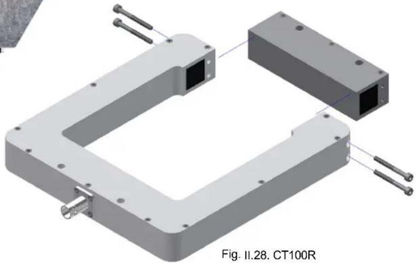
The current and isolation transformers serve to pick up partial discharge signals from the frequency range required with the IEC60270 up to the FM range. The CTs offer an installation of partial discharge pick-up devices with a very low impact, since there is no interruption of the power connection required. Such installation is even under on-line conditions possible, as the CT100 is a clip-on CT that can be opened (>100 mm) and clipped around a connecting cable, a ground lead, or even a feeding medium voltage cable with a high voltage motor installation (window: 100 mm).
CT1 Current Transformer (Fixed Type)
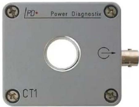
Specification:
Transfer ratio: 1:10 @ 50 Ω
Primary window: ∅ 15 mm
Bandwidth (-3 dB): 0.5 to ≥80 MHz
Bandwidth (-6 dB): 0.3 to ≥100 MHz
Fig. II.26
CT100(/R) Current Transformer (Clip-on or Split Type)

Specification:
Transfer ratio: 1:10 @ 50 Ω
Primary window: ∅ 100 mm (clamp-on) 110 x 100mm ² (split)
Bandwidth (-3 dB): 2 to ≥25 MHz
Bandwidth (-6 dB): 1.2 to ≥40 MHz
natural_image
3D mechanical assembly diagram showing two U-shaped components with mounting holes and metal rods (no text or symbols)IT2 HF-Isolation Transformer
The IT2 isolation transformer was designed to meet the requirements of monitoring high voltage cable joints assemblies in a multi-point configuration. Due to the operating or heating current and further, due to impulse voltages the screens of adjacent cables may severely deviate in their potentials. The design of the IT2 allows the isolation of a difference of 250 Volts between input and output permanently. It is tested to withstand potential difference of 10 kVac (50 Hz) for one minute in order to avoid damages due to such differential voltages (both AC and transients). Its high frequency behaviour is optimised for 50 Ω-systems and the use with multiplexer and RPA2.

Fig. II.29
Specification:
Transfer ratio: 1:1 @ 50 Ω
Connection: BNC-BNC
Isolation: 250 V AC permanent
Test voltage: 10 kV (50 Hz AC, 1 min)
Bandwidth (-3,0 dB): 500 kHz–30 MHz @ 50 Ω
Bandwidth (-6,0 dB): 300 kHz–80 MHz @ 50 Ω
II.3.3 CC Coupling Units
The standard coupling capacitors listed with this section are mainly suited for on-line and off-line measurements on rotating machines, as well as for smaller test setups. A wider range of coupling capacitors and assemblies with quadrupoles and pre-amplifiers is available on request. These tailor-made units are shipped with an individual data sheet and are thus not included with this manual.
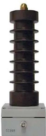
CC20B
natural_image
Exterior view of a black insulator with a gold pin, mounted on a gray base (no text or symbols visible)Fig. II.30
Coupling capacitor for permanent installation on rotating machines. The integrated termination circuit leaves a superimposed AC component for sync purpose. Mounted on a cast aluminium enclosure. Suited for line side coupling.
Specification:
Capacitance: 145 pF
Nom. voltage: 20 kV
Temp. range: -20^-+75^
HV connection: M10
GND connection: M5
PD output: BNC
CC25B

natural_image
Exterior view of an insulator with helical structure and control panel (no visible text or symbols)Fig. II.31
Coupling capacitor for temporary installation on rotating machines. The integrated termination circuit leaves a superimposed AC component for sync purpose. Mounted on a cast aluminium enclosure. Suited for line side and neutral coupling as well as for off-line tests. According to the CC25C/V (see next page) a /V version with voltage output is available (non-isolated BNC, only).
Specification:
Capacitance: 1 nF
Nom. voltage: 25 kV
Temp. range: -20^-+75^
HV connection: M8
GND connection: M5
PD output: BNC
33
CC25C/V

Fig. II.32
Coupling capacitor for temporary installation on rotating machines, transformers, or MV switchgears. Integrated HF current transformer CT1, termination circuit and a voltage divider for sync purpose. Mounted on a cast aluminium enclosure. Connecting a BNC cable to the quadrupole output terminal automatically opens the switch S1. Suited for line side and neutral coupling as well as for off-line tests. The BNC terminals are not isolated.
Specification:
Capacitance: 1 nF
Nom. voltage: 25 kV
Temp. range: -20^-+75^
HV connection: M8
GND connection: M5
PD and sync out: BNC
Divider ratio: 1:250
CC35B

natural_image
Exterior view of a high-voltage insulator with coil and mounting base (no visible text or symbols)Fig. II.33
Coupling capacitor for permanent or temporary installations on rotating machines, transformers, or MV switchgears. The integrated termination circuit leaves a superimposed AC component for sync purpose. Mounted on a cast aluminium enclosure. Suited for line side and neutral coupling as well as for off-line tests. There is /V version with voltage output available (non-isolated BNC, only).
Specification:
Capacitance: 145 pF
Nom. voltage: 35 kV
Temp. range: -20^-+75^
HV connection: M10
GND connection: M5
PD and sync output: BNC
Divider ratio: 1:350
II.4 Rejection Filters
Measuring RIV can be hampered by external radio frequency sources. Here, broadcasting signals, disturbance due to nearby machinery, or partial discharge of the setup itself may reduce the sensitivity or mask the signals totally.

natural_image
Exterior view of a gray electronic device labeled 'RF1/500' with ports and knobs (no readable text beyond labels)Fig. II.34: Tunable rejection filter according to CISPR 18-2
In case the RIV testing is made exclusively, a resonant filter tuned to the frequency used can be inserted into the high voltage connection between source, i. e. high voltage transformer, and test object. Power Diagnostix offers a variety of such tuneable rejection filters, which are just parallel LC resonant circuits.
Figure II.34 shows the RF1/500. This unit is adjustable between 450 kHz and 550 kHz which results in a available measuring range of 400–500 kHz. It comes with a variable air insulated capacitor. The capacitance is adjusted using the coarse and the fine drive of the centre control knob. The RF1/500 offers a maximum current of 1 A. Other currents and frequency ranges are offered as well, e.g. the rejection filter RF1/1000 offering a tuning frequency of 950–1050 kHz (measuring frequency: 900–1100 kHz) and a maximum current of 1 A.
The filter is placed in the high voltage connection of the test object. However, the unit as such does not provide any field shaping and, hence, must be put within a pair of toroids or other adequate shielding. Care must be taken to minimise the stray capacitance between input and output, as this shifts the resonant frequency.
In case of external disturbance, the rejection filter is simply tuned by observing and minimising the ICMsystem reading. Alternatively, the RIV calibrator is connected on the source side against ground using a higher magnitude (see section V.8.1 for further information on RIV calibration). Likewise, the filter is tuned to the minimum reading of the ICMsystem.
Warning: Always make sure that the high voltage test circuit is completely switched off and secured, before attempting any work on the rejection filter or the high voltage circuit. Be especially careful, when doing the fine-tuning of the rejection filter as well as the calibration, since here, the safety earthing has to be on the test transformer side.
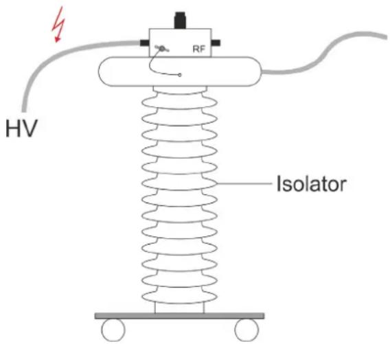
Fig. II.35: Typical installation
II.5 CAL Calibration Impulse Generators
There is a broad range of impulse generators offered by Power Diagnostix for different purposes. Table II.1 gives an overview of these calibrators. All calibrators allow the calibration of PD measurements according to IEC 60270/2000, except the CAL2B/C/D, since the CAL2B/C/D have left out the injection capacitor to enable calibration on GIS (gas insulated switchgear).
| Calibrator | Range | Injection capacitor (C) | 50Hz or 60Hz light | IEC60270 compliant | 2 pulses/cycle option | Connector | Remarks |
| CAL1A | 1, 2, 5, 10, 20, 50, 100 pC | <1pF | √ | √ | √ | BNC | Standard, laboratory use |
| CAL1B | 100, 200, 500 pC, 1, 2, 5, 10 nC | <100pF | √ | √ | √ | BNC | E. g. rotating machines & cable field tests |
| CAL1C | 1, 2, 5, 10, 20, 50, 100 pC* | V (50 Ω) | √ | √ | √ | BNC | Incl. ext. capacitor 100 pF; cable tests |
| CAL1D | 10, 20, 50, 100, 200, 500, 1000 pC | <10pF | √ | √ | √ | BNC | Standard, laboratory use, transformer tests |
| CAL1E | 0.5, 1, 2, 5, 10, 20, 50 nC | <500pF | √ | √ | √ | BNC | See CAL1B |
| CAL1F | 0.2, 0.5, 1, 2, 5, 10, 20 nC | <200pF | √ | √ | √ | BNC | |
| CAL1G | 0.02, 0.05, 0.1, 0.2, 0.5, 1, 2 nC | <20pF | √ | √ | √ | BNC | Transformer tests |
| CAL1J | 10, 20, 50, 100, 200, 500, 1000 pC*100, 200, 500, 1000, 2000, 5000, 10000 pC* | V (50 Ω) | √ | √ | √ | BNC | Incl. ext. capacitor 100 pF/1 nF, switchable; cable tests |
| CAL2B(/500) | 2, 5, 10, 20, 30, 40, 50 V (into RL=50 Ω) | V (50 Ω) | √ | √ | N | GIS & UHF | |
| CAL2C(/500) | 1, 2, 5, 7, 10, 12, 15, 17, 20 V (into RL=50 Ω) | V (50 Ω) | √ | √ | N | ||
| CAL2D(/500) | 5, 7.5, 10, 15, 20, 30, 40 V (into RL=50 Ω) | V (50 Ω) | √ | √ | N | ||
| CAL3A | 600 kHz to 1.35 MHz, 10 μV to 10 mV | V (50 Ω) | √ | BNC | RIV calibration, NEMA 107 compliant | ||
| CAL3B | 400 kHz to 1.9 MHz, 10 μV to 10 mV | V (50 Ω) | √ | BNC | RIV calibration, NEMA 107 compliant | ||
| CAL3D | 400 kHz to 1.9 MHz, 10 μV to 10 mV (into 300 Ω) | V(>20 kΩ) | √ | BNC | RIV calibration, CISPR 18-2 compliant |
Table II.1: Output and frequency ranges of PD calibrators
* with external high voltage capacitor
The generator is switched on with the pushbutton On/Off. Both amplitude (Range) and polarity (Pos/Neg) of the single charge pulse per cycle are displayed and can be adjusted by pressing of the two buttons. The instrument is synchronised to line frequency by a photo diode. In case of insufficient pick-up of power frequency light, it will automatically select the internal quartz oscillator (50 Hz- and 60 Hz-versions available). The button On/Off must be pressed for more than 1 s to switch the pulse generator off, while automatic switch-off occurs after 15 min, approximately.
Operation time of up to 200 hours are obtainable with the 9 V lithium battery due to an average supply current of approx. 5 mA (quiescent current is negligible). An alkaline battery resulting in approx. 90 hours of continuous operation may replace the lithium battery. A weak battery is indicated by the LO BAT sign of the LC display.
The charge pulse of all calibrators is generated, unlike commonly used instruments, by injecting a variable voltage step (correlated to an internal reference) via a fixed capacitor. The influence of the injection capacitor vs. the capacitance of the test object may be normally neglected, since the injection capacitor is relatively small (e.g. CAL1A: 0.8 pF, CAL1B: 82 pF, refer to IEC 60270). The pulse properties are meeting the requirements ( t_R ≤ 35 ns, t_D ≥ 100 s). The generator CAL1C is to be used with a permanently installed 100 pF high voltage injection capacitor.
Warning: While changing battery, be aware of internal parts carrying up to 125 V of DC potential!
We adjust the charge output of the calibrators according to the output of our reference calibrator, which has been calibrated at 'Physikalisch Technische Bundesanstalt' (PTB), the German authority of standards. By end of 2003, Power Diagnostix received the accreditation as calibration laboratory within the German Calibration Service (Deutscher Kalibrierdienst, DKD). The audit was held by PTB. In January 2012, Power Diagnostix passed over to the newly introduced German accreditation authority DAkkS (Deutsche Akkreditierungsstelle). The new accreditation is filed under D-K-15068-01-00. New charge calibrators are shipped with the calibration certificate to ensure the traceability of the calibration according to international standards.
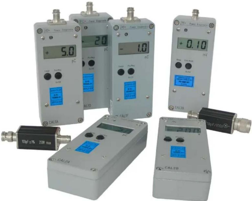
Fig. II.36: Different models of calibration impulse generators
III The ICMsystem Software
III.1 ICMsystem Standard Control Software
III.1.1 Overview and Main Functions
The ICMsystem is fully computer-controlled via communication interfaces such as LAN, an IEEE488 bus, built-in modem, USB, or fibre optic links. It contains no manual controls so that every setting is recorded and can be stored. Data formats and IEEE488 commands are open to the user allowing the programming of proprietary testing and evaluation routines. The ICMsystem software is created with National Instruments' programming language LabWindows/CVI. The software runs under Windows 7, Windows 8, and Windows 10.
Remark: If the application window appears very small when started on a PC with Windows 10, please refer to section III.1.3 "HDPI Scaling" on page 43.
The ICMsystem standard control software contains all functions necessary to control a 1-channel instrument, view and edit the setup parameters, acquire data and view the results. It also contains functions to re-load, store and export acquired data. A print routine for even complex jobs is integrated as well (see section III.1.10).
As with the adjustment of the low-level discriminator (LLD), most of the program functions are accessible through more than one control: Adjusting the red slider on the right-hand side of the main display modifies the value of the LLD. Further, this value may be chosen from a list (2, 5, 10, 20%) that comes up by double-clicking to the LLD entry, which is part of the subpanel Setup A. Finally, editing of the entry via the keyboard is offered by single-clicking to that entry. These different ways to obtain a function gives more flexibility and allows the user to find his most convenient way to control the instrument.

line
| Parameter | Value | | --------- | ----- | | Acc Time | 160.2 s | | Pos Counts | 21537 | | Neg Counts | 19650 | | Voltage [rms] | No Voltage | | Charge [IEC] | 7.54 pC | | R value | N/A | | NQS Value | 2.518 nA | | Frequency | 60.0 Hz [L] | | Amp In | No 1 | | Set Time | 300.0 s | | ADC LLD | 20.0 % | | Coding | LIN BIP | | Pre Gain | 100 | | Acq Mode vs Phase | 800 kHz | | Amp U Cutoff | AMP OUT | | Pattern Acq | -38 ° | | Phase Shift | Sync in | | Sync 4 | | | Input Mode | AMP | | Dead Time | 10.0 μs | | 2% | 20% | | 5% | 10% | | Wavelength | Sina | | Amp Main Gain | 8 | | Count Level | 10 pC | | Amp L Cutoff | 40 kHz | | Mem Erase | Auto | | Div Ratio | 1000.0 | | Sync + Line | - | | Setup G | MC Panel | | AT Panel | Load Save Search ExitFig. III.1 ICMsystem control software, different ways to adjust the low level discriminator (LLD)
Main functions of the program are controlled by a row of buttons at the lower end of the display. These buttons represent the computer's function keys F1 to F10 (an overview regarding the shortcut keys is given in section III.1.7). Both clicking to that button and pressing of the according function key will cause the action indicated by the button's label. These labels are correlated to the current operation mode of the program, the state of the instrument and the communication channel used. The button representing the function key F7 is labelled 'Offline' in case connected to an instrument. This key's label will change to 'Dial' with a modem found and to 'Discon' in case of an established modem connection.
The central display area shows the results of the current or of a re-loaded measurement. By means of the small icons in the middle of the tool bar this display can be switched to different modes. Beside the 'normal' ICMsystem-like coloured amplitude-phase-height-distribution, nine other display modes are available, among other a more traditional oscilloscope-like display and two different projection displays. The block at the right-hand side of the central display represents direct measurement results as voltage and frequency, for instance, as well as derived quantities. The display area at the main display's left-hand side indicates the status of the current measurement, communication channel and file loaded.
Four sub panels underneath the main display area control the instrument's setup. The function keys F1 is to toggle through these subpanels. The different setup entries are covering hardware-related entries, as filter settings, and display-related entries, as the colour distribution. Upon start-up, the program reloads the setup of the previous measurement. Further, the software checks the ports for a valid connection to an instrument. In case it transfers the re-loaded setup to the instrument found. Since all of the setup entries are stored along with the measurement data, re-loading of such *.DAT file resets the connected instrument precisely to its state, when this *.DAT file was stored.
III.1.2 Installation of Software and Drivers
Please install drivers and the ICMsystem software before connecting the instrument to the PC.
III.1.2.1 GPIB Driver
If you want to use a GPIB interface for communication instead of the standard USB interface, you need to install a GPIB driver. For a direct serial connection via USB the cable can be up to 5 m long, versus maximum 10 m for the standard GPIB cable. The installation of a GPIB interface card is independent of the installation of the program as explained afterwards.
To install the GPIB, please follow the steps below:
- Install the necessary GPIB driver before starting the hardware installation. Otherwise, Windows tries to find a driver, which usually causes problem.
- Shutdown your computer and insert the PCMCIA card into a free slot of your notebook computer.
- Insert the National Instruments CD-ROM into your CD-ROM drive.
- Reboot your system and install the GPIB drive from disk.
It is recommended to keep the GPIB card exclusively for the ICMsystem and to use no other device on the same GPIB bus. The software supports more than one GPIB board, so the ID number of the GPIB board is not relevant for the functionality.
III.1.2.2 Installer
The software comes with an installer and is suitable for Microsoft 7, Windows 8, and Windows 10. It is developed with National Instruments' LabWindows/CVI. Starting the program setup.exe, which is located on the provided CD-ROM, installs the software and the required CVI run time engine.
The installer will guide you through the installation process. The installation directory can be chosen individually, you may alter the locations of both the LabWindows/CVI runtime engine (if you install it the first time, only) and the ICMsystem software. In case you want to maintain access to different releases of the ICMsystem software you may place the software in a tree of subdirectories as C:\Program Files\Power Diagnostix\ICMsystem\icmstd.4\, for instance. Additional 'dll' files like i.e. cvirte.dll are copied to the Windows system folder. By pressing the 'Next' button, the program files are extracted, and a program folder is created. It is recommended to create a special data directory. Avoid placing the data directory as a subfolder into the program directory, as a de-installation of the program could lead to a loss of your data! Furthermore, Windows 7 (64 bit) and Windows 8 systems do not allow programs to save data into the 'Program Files' directory.

Fig. III.2 Install window with destination directories
III.1.2.3 USB Driver
Please install the USB driver before connecting the instrument to the PC.
A necessary driver for the standard USB interface for communication with the instrument comes with the ICMsystem software, and the installation process is automatically started after the software installation has successfully finished. Follow the instructions on the screen.
If you experience difficulties during the installation process of the USB interface, please try installing the driver manually. The installation file can be found in the sub directory 'USB_Driver' of the software's program directory. E. g. c:\Program Files\Power Diagnostix\ICMsystem\icmstd.463\USB_Driver\FTDI.
![Preferences Interface Settings LAN Settings Security Options Display and Graphs Miscellaneous Files Activation Codes Search for ICMSystem at Search GPIB ✓ Search COM ✓ COM1 (- No Information available - COM2 (- No Information available - COM3 (High-Speed PCI Serial Port COM4 (High-Speed PCI Serial Port COM5 (Silicon Labs CP210x USB) COM6 (Silicon Labs CP210x USB) COM7 (Silicon Labs CP210x USB) COM8 (Silicon Labs CP210x USB) COM9 (Belkin Serial On USB Port) COM10 (Silicon Labs CP210x USB) COM11 (Serial On USB Port) Interface Parameters. RS232 Search Timeout [s] 3.0 GPIB Search Timeout 1s RS232 Run Timeout [s] 20.0 Modam Run Timeout [s] 30.0 GPIB Run Timeout 10s Additional Modem Initialization Commands Additional Modem Disconnect Commands Search Device at Startup ✓ Connection Mode Manual Channel-ID Hardware-ID (G0.2-5S) Cancel Ok](/content/2026/05/1014079/images/ff5f3a1d521c3fb3244a7b3a3acdf212d4bbb452c3c4b392cb767a9c85ea5028.jpg)
Fig. III.3 Preferences: 'Interface Settings'
Since you must have administration rights to successfully install the driver, right click on the file 'CDM v2.12.04 WHQL Certified.exe' and chose 'Run as administrator' from the context menu. Then follow the installation instructions.
To activate USB support of the ICMsystem software, open the preferences using the 'Edit' menu. The 'Interface Settings' tab will show up. First select 'Search COM' then activate the ports which are needed for communication. If you have multiple ports available due to usage of multiple Power Diagnostix devices, you can either activate all of them or open the Windows Device Manager with only the ICMsystem connected to the computer to find the COM port of the instrument. The USB device should be listed (with its port name in brackets) as an item of 'Ports' (see figure III.4).

Fig. III.4 Windows Device Manager
Another part of this connection interface is the virtual channel management for multi-channel instruments. While deactivated per default this feature offers the possibility to choose eight independent sources for PD and voltage monitoring and eight separate sources for RIV monitoring. To activate virtual channel management switch 'Connection Mode' to 'Manual' (shown with figure III.3). When activated, each meter display in the panel represents one virtual channel, which consists of a PD source and a RIV source. Note that changing the connection mode will take effect the next time when connecting a device.
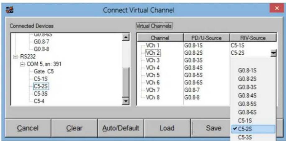
Fig. III.5 Connecting different sources for PD and RIV
The illustration above shows how a connection between a virtual channel and a real hardware 'AMP' or 'SPEC' card can be performed. This is done by a pull-down list or with an easy drag and drop function. The button 'Auto/Default' will automatically select the first eight boards as source of PD and RIV values, if possible.
III.1.2.3.1 Command Set of GPIB & Serial Communication
The ICMsystem is controlled through command strings sent by Power Diagnostix' PC program either via the GPIB interface or the serial interface. Power Diagnostix can supply a complete summary of these command strings on demand.
III.1.3 HDPI Scaling
On PCs running Windows 10 with the Creator's Update of 2017 the ICMsystem application window may appear very small on high resolution monitors. To enlarge the display size of the software, please take the following steps:
- Right-click on the application short cut on the desktop.
- Choose "Properties" from the context menu, which will open the Properties window.
- Enable "Override high DPI scaling behaviour" and set "Scaling performed by" to "System" on the "Compatibility" tab.
- If you have administrator rights, you can change the settings for all users by clicking the corresponding button.
- Approve the change by clicking "OK".
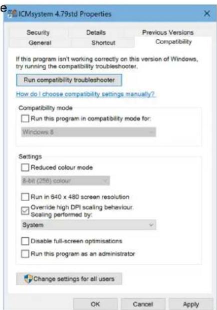
Fig. III.6: Properties window

Fig. III.7: Desktop before and after change of scaling behaviour
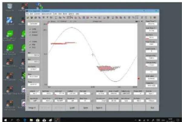
line
| Time (s) | Value | |---|---| | 0 | 10.0 | | 1 | 12.0 | | 2 | 14.0 | | 3 | 16.0 | | 4 | 18.0 | | 5 | 20.0 | | 6 | 22.0 | | 7 | 24.0 | | 8 | 26.0 | | 9 | 28.0 | | 10 | 30.0 | | 11 | 28.0 | | 12 | 26.0 | | 13 | 24.0 | | 14 | 22.0 | | 15 | 20.0 | | 16 | 18.0 | | 17 | 16.0 | | 18 | 14.0 | | 19 | 12.0 | | 20 | 10.0 | | 21 | 12.0 | | 22 | 14.0 | | 23 | 16.0 | | 24 | 18.0 | | 25 | 20.0 | | 26 | 22.0 | | 27 | 24.0 | | 28 | 26.0 | | 29 | 28.0 | | 30 | 30.0 | | 31 | 28.0 | | 32 | 26.0 | | 33 | 24.0 | | 34 | 22.0 | | 35 | 20.0 | | 36 | 18.0 | | 37 | 16.0 | | 38 | 14.0 | | 39 | 12.0 | | 40 | 10.0 | | 41 | 12.0 | | 42 | 14.0 | | 43 | 16.0 | | 44 | 18.0 | | 45 | 20.0 | | 46 | 22.0 | | 47 | 24.0 | | 48 | 26.0 | | 49 | 28.0 | | 50 | 30.0 | | 51 | 28.0 | | 52 | 26.0 | | 53 | 24.0 | | 54 | 22.0 | | 55 | 20.0 | | 56 | 18.0 | | 57 | 16.0 | | 58 | 14.0 | | 59 | 12.0 | | 60 | 10.0 | | 61 | 12.0 | | 62 | 14.0 | | 63 | 16.0 | | 64 | 18.0 | | 65 | 20.0 | | 66 | 22.0 | | 67 | 24.0 | | 68 | 26.0 | | 69 | 28.0 | | 70 | 30.0 | | 71 | 28.0 | | 72 | 26.0 | | 73 | 24.0 | | 74 | 22.0 | | 75 | 20.0 | | 76 | 18.0 | | 77 | 16.0 | | 78 | 14.0 | | 79 | 12.0 | | 80 | 10.0 | | 81 | 12.0 | | 82 | 14.0 | | 83 | 16.0 | | 84 | 18.0 | | 85 | 20.0 | | 86 | 22.0 | | 87 | 24.0 | | 88 | 26.0 | | 89 | 28.0 | | 90 | -30.0 | | ... (repeated) for visual display.III.1.4 Connecting to an Instrument
The ICMsystem program checks directly after start-up the GPIB interface for active instruments. It scans automatically through all possible GPIB addresses. The GPIB address of your instrument can be modified with the small rotary switch located on the front panel of the acquisition unit's CTRL5 plug-in. The instrument needs to be turned off and on again to accept the new address. In case more than one instrument was found connected to the GPIB bus, a selection box appears giving you the choice to which of the available instruments you want to connect. Furthermore, the ICMsystem software can be set to check serial ports for a modem assigned to this serial port. Figure III.8 shows the preferences to choose the serial port that will be scanned. This function can be disabled as well, since checking for a modem takes some time and will subsequently slow down system start-up. Further, with a modem found, the ICMsystem program sends a 'hang up' command upon exit of the software to make sure that there is no telephone connection left in standby. This procedure takes time as well. With no instrument found F6 remains labelled with 'Search'. With an instrument connected by the GPIB the communic transfer the current setup, any commands or change the peak charge, and the synchronisation frequency. function key F7 changes to 'Dial'. Clicking that key an entry will both select this entry and make it available for editing in the edit line at the top of this submenu. Once modified it may replace the selected entry (Replace,
while line 2 contains a default initialisation string (AT&FX3). This default initialisation works in most cases and will be used in case the second pair of brackets has been left empty. OK will close and dial the number selected. After establishing the connection with the built-in modem of the ICMsystem, the software will check the access code. With this check passed, the instrument is available for measurements. Beside the speed of data transfer, there is in principle no difference between the three communication modes (GPIB, serial, modem).
![Preferences Interface Settings LAN Settings Security Options Display and Graphs Miscellaneous Files Activation Codes Search for ICMSystem at: Search GPIB ✓ Search COM ✓ ✓ COM1 (High-Speed PCI Serial Port ✓ COM2 (High-Speed PCI Serial Port ✓ COM6 (Silicon Labs CP210x USB) ✓ COM10 (Prolific USB-to-Serial Com Interface Parameters: RS232 Search Timeout [s] 3.0 GPIB Search Timeout 1s RS232 Run Timeout [s] 20.0 Modem Run Timeout [s] 30.0 GPIB Run Timeout 10s Additional Modem Initialization Commands Additional Modem Disconnect Commands Search Device at Startup ✓ Connection Mode Automatic Channel-ID Hardware-ID (G0.2-5S) Cancel Qk](/content/2026/05/1014079/images/c42b925de1f74ca1c6fc30654eb531c958ff1407188c934612c19cdb4a3cae34.jpg)
Fig. III.8 Selecting the serial ports to be scanned
cation starts immediately: The ICMsystem software will be and will receive current measurements of the voltage, v. In case of a modem found and selected, the label of the activates the dial menu shown with figure III.9. Clicking to
![Select Dial Number Testnumber[18][AT &F M0 X3 &D0](*) sys1sn387[18][AT &F M1 X3 &D0](*) Testnumber[18][AT &F M0 X3 &D0](*) Testnumber[18][AT &F M0 X3 &D0](*) Cancel Insert Replace Delete Load OK](/content/2026/05/1014079/images/c88c80e18e85e71f4358ecd606a6294f285b56b997c81d9bd7b4b9c2903d6465.jpg)
III.1.5 Toolbar
Furthermore, the current software release offers a direct access to many frequently used functions via a toolbar. For each icon, a brief help description appears if the mouse cursor is kept above a specific icon of the toolbar. Alternatively, most of the functions or optional settings covered by these icons can be set via the menus or via the function buttons at the bottom of each main panel.

Clicking this icon opens a dialog box to select a data file with the file extension *.dat. This file contains one PD measurement consisting of a complete setup of one channel, a report concerning this measurement and the phase resolved PD pattern. Loading a file of this data type overwrites the settings of the currently activated channel and, if set, copies global values (!) to all other setups. A new optional setting, called 'Load/Save Mode' which can be found in 'Preferences', allows to load a consecutive number of files (automatic mode) if these files can be found on disc. Example: Loading a file named test1.dat starts searching for the consecutive files test2.dat, test3.dat, ..., test8.dat within the same directory, and, if found, these files are loaded to the setups of channel 1–8.

To save the last measurement to a 'dat' file, press this icon. In case 'Load/Save Mode' is set to automatic, eight files are created consisting of a setup of the corresponding channel, the report and the PD pattern. If the option 'Show report before saving data' in 'Preferences' is activated, a popup window appears before all data is saved to disc.

This function prints the PD pattern and the corresponding setup of the active channel on one page (A4 format recommended). The default printer is used.

Clicking this icon, the graph, visible on the main display, is copied to the clipboard. The content of a Windows clipboard can be inserted with most graphic or office applications.

To edit a brief report that is stored automatically as a 'dat' file, press this icon. Please note that this report is different from the kind of report that can be edited especially within the acceptance test panel (AT panel), because acceptance test reports are not saved as a 'dat' file but in several other file formats, which can be created with the export function of the acceptance test (AT) panel.

So-called templates can be handled after starting this function. Within a popup window, the setups of all channels are accessible. Loading and saving of templates is as well possible as editing new values or locking individual settings. The creation of templates helps to manage different setups for different test conditions. Please be aware, that the use of the same templates on different transformers with identical test conditions does not guarantee identical calibrations. Each PD test has to be calibrated separately. Please refer to section III.1.9 for detailed information about the calibration process.

All optional program settings are now consolidated under this popup window named 'Preferences'. These entries are stored after program shutdown to an initialisation file so that the settings remain unchanged on next start-up of the software. The preferences are divided into seven sections, 'Interface Settings', 'LAN Settings', 'Security Options', 'Display and Graphs', 'Miscellaneous', 'Files', and 'Activation Codes'. With former software releases, most of these settings were accessible in the menu 'Options'.

Pressing this icon changes the main display into meter and strip chart mode. On the left upper side, the current PD value and on the right upper side the current voltage value of this channel are updated continuously. Below these two meters, a strip chart is displayed, which can help to detect the inception voltage of a PD test object

The ellipse display is similar to the scope display. In this mode the phase positions from 0^ to 360^ are divided into two parts represented by two half sine waves. Every PD pulse is displayed as a double vertical line.
46

The ellipse display emulates the display of a traditional PD detector. It can be activated during a running acquisition without affecting it. With this display, the pulse differences between two data sets are shown as vertical bars at the phase angle where they occur.

The spectrum display shows the frequency spectrum in the lower half and provides the view of two small patterns above.

Use this icon to switch to the standard phase resolved pattern display.

The projections of a PD pattern versus phase are displayed when choosing this mode. The red line shows the positive count distribution of the discharges versus phase, the blue line shows the distribution of the negative discharges.

The projections of a PD pattern versus charge are displayed when choosing this mode. The red line shows the positive count distribution of the discharges versus charge, the blue line shows the distribution of the negative discharges.

The trending display shows the evolution of the calculated discharge current – the NQS value – versus time.

Clicking on this icon displays a three-dimensional view of the current PD pattern. The position, as well as the viewpoint and the scale of the display can be modified.

Oscilloscope display shows the PD signals in time domain similar to a digital storage oscilloscope. The view can be used for (acoustic) fault location.

This icon activates the display for cable fault location.

This function resets the strip chart of the meter display in the single channel (SC) panel or the strip chart within the acceptance test panel.

Toggling between all available measuring modes is done by this button, whose appearance is changing depending on the chosen measuring mode. The meanings of these modes are explained with the next section.

This icon enables the 'Offline Replay' function. With this function selected, the count distribution can be re-calculated for a reduced measurement time. This function is used to compare measurements that were taken with a different acquisition time.

This map converter offers the transfer of a coloured map into a black and white 128 x 80 pixels matrix. The converted map can be stored in a file format with the extension *.mon or *.cmp, which is compatible with files created by Power Diagnostix' PD acquisition units ICMcompact and ICMmonitor.

This icon sets the mode of the PD meter. The meter is updated once per reading cycle. Depending on the mode chosen, the magnitudes transferred from the instrument to the PC can differ. The 'Fast Mode' always reflects the biggest charge value since the most recent reading access. In 'Normal Mode' the meter acts similar but with an additional inertia as found with real-life analogue meters. The 'IEC Mode' considers the repetition rate of pulses according to the standard IEC 60270-2000. Pulses with a lower repetition rate are displayed with a lower PD level.

With the gating button the user can choose whether the gate should lock the amplifier ('AMP'), the A/D converter ('ADC'), both ('AMP&ADC'), or should be disabled. The setting 'AMP' opens an analogue switch in the AMP5 module, while 'ADC' inhibits the transfer of the converted pulse amplitude to the instrument's memory. Refer to section 0 for details. With an ICMsystem of the current hardware version the setting 'ADC' gives best results.

The calibration mode determines whether the calibration is valid for the currently activated channel only or for all channels of the instrument. For testing purposes, it is sufficient to calibrate just once, but for acceptance tests, this method should not be used. Different coupling conditions and variations of cables and pre-amplifiers, for instance, can result in unwanted deviations. Therefore, it is recommended to calibrate each channel separately.

The controller of the instrument has a built-in beeper. It gives a sound each time a PD pulse is acquired, when 'DT' is visible on the icon. Alternatively, if the icon shows 'GT', the sound refers to the triggering of the gating unit. The beeper sounds only for system messages if switched OFF.

The projection graph can be displayed with the Y-axis in logarithmic or linear scaling. Use this button to select the scaling mode.

Clicking this icon sets the count mode of the Y-axis of the projections. Choose 'N/s' to have the projections labelled with counts per second or choose 'N' for the absolute number of counts.

This icon activates the count level option. At the right side of the SC panel, two count displays are found. In case the count level option is enabled, these two entries show the total amount of PD pulses per map ('Total Counts') and the number of counts above a pre-set PD level (Level Counts). This count level can be set within 'Setup A' or using the blue slider. If disabled, these two displays are showing the positive counts and the negative counts of the PD activity.

Between 20 Hz and 400 Hz, the frequency is measured automatically by the instrument. In case of frequencies below 20 Hz, the line frequency must be set by the user.

The slider at the right-hand side of the main graph can have two different meanings. Depending on this icon, the LLD (red arrow) can be adjusted, or the count level (blue arrow) can be modified.

Pressing this button opens an additional window with the online help.

This 'Help About' icon opens a sub-window with additional information concerning Power Diagnostix, the version of the software and of the ICMsystem acquisition unit, in case connected to an instrument.
III.1.6 Display Modes and Display Items
The instrument has several measurement modes. The standard measurement mode is active directly after connection. While in this standard mode the software transfers setup data to the instrument and receives basic measurement data from the instrument. These basic measurements are the voltage at the SYNC IN input with respect to a divider ratio, the frequency of the chosen sync source, and the peak discharge value at the input of the pre-amplifier with respect to the calibration. This standard measurement mode serves to adjust the setup while viewing the influence of the modifications to the readings of the said measurement values. In order to have this optimisation process as fast as possible, we have put emphasis on the system response time in general. The display refresh cycle varies depending on the speed of the control computer's CPU and the communication channel used. It may be as fast as 15s^-1 and about 5s^-1 even in case of modem communication.
While in this standard display mode or idle mode, the central main display area shows the result of the measurement previously acquired or of a measurement re-loaded from file (Load, F4, or
• The map or partial discharge pattern
- Two more traditional oscilloscope-like displays
- Three different projection displays: count distribution versus phase, count distribution versus charge, and a 3D view of the current pattern
- Meter/strip chart
- Spectrum display
- Trending display
- Oscilloscope display
• CFL (cable fault location) display
The eleven small icons in the upper left corner (figure III.10) are used to choose the display type directly (The

Fig. III.10 Display icons
result of the peak A/D converter for this pulse. In case more than one pulse occurs at the same coordinates, the dot changes its colour to visualise the frequency of occurrence. This distribution is being built-up already
in the ICMsystem's memory (refer to the hardware section of this manual as well, section II.1.3): The DPR5 plug-in unit acts as a fast counter array. The counter memory size of this plug-in amounts to 1 Mbit = 8 bits x 8 bits x 16 bits (X: 256, Y: 256, Z: 65536) offering a detailed pattern of the partial discharge distribution. Figure III.11 shows an example of such a partial discharge pattern with the acquired shape of the high voltage super-imposed. The setup gives the choice of different ways to assign the three axes of the display. The coding of the Y-axis, which is the pulse amplitude calibrated in Coulomb,
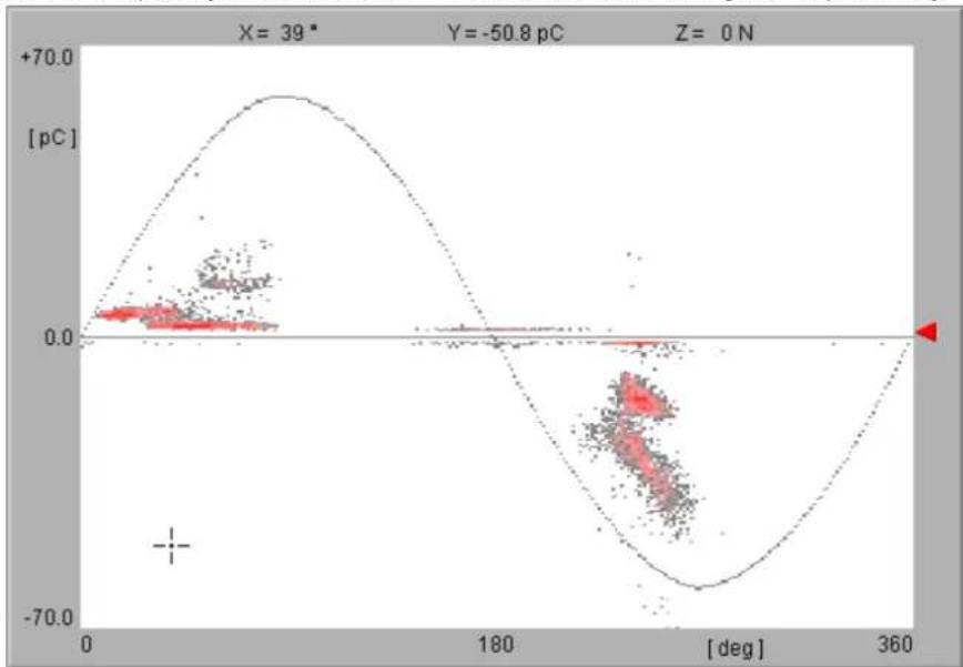
scatter
| X (deg) | Y (pC) | | ------- | ------ | | 39 | -50.8 |Fig. III.11 Partial discharge pattern
can be set to linear bipolar (as shown), linear unipolar, or logarithmic scaling, for instance (see ADC coding). The X-axis may represent the phase angle of the high voltage (as shown) or a pre-set time (in case of vs. time measurements), while the Z-axis (i. e. the distribution of the colour) may be coded linear or logarithmic, as well. Further, this colour distribution can be set to have discrete steps making it easier to compare different areas of the discharge pattern, or to have a continuous grading of the colour palette (requires a 'high-colour' or 'true-colour' display). The shape of the acquired sine wave of the high voltage can be displayed along with the partial discharge pattern not only to validate the phase relation between pattern and high voltage, but also to evaluate the influence of saturation effects or harmonics of the voltage on the pattern. Alternatively, a created sine wave can be displayed to give an impression of the phase position. With the acquired sine wave the partial discharge pattern can be shifted in its phase position, while the sine wave is shifted as well. With the created sine wave, you may choose whether the pattern or the sine wave is shifted. Most other available display modes are in principle sub-sets of this partial discharge pattern, which, again, is a direct display of the instrument's memory content.
The count distribution versus X-axis (counts vs. phase, or time) that is shown with figure III.12 can be set to display the distribution of the total number of counts of the current acquisition or to display this distribution with respect to the acquisition time passed (counts/s). The count-axis (Y-axis) may be scaled linear or logarithmic. The range is adjusted automatically. The logarithmic scaling can be activated/deactivated with the icon in the icon bar.
The second distribution display available is shown with figure III.13 . It displays the distribution of the counts versus amplitude . The Y-axis can be set to display the total or relative number of counts, as with the vs. phase distribution. Preferences like this scaling mode of the projections are saved automatically to an *.INI file within the ICMsystem software's home directory. Only few of these preferences, the ones closer related to the measurement, are stored with the individual *.DAT file, as the phase shift or the Z-axis coding of the map display, for example. As with the partial discharge pattern display, a cursor can be moved to a graph position of interest. The related values are shown at the top of the main display area. The icon 🧑 Fig. III.13 serves to enable/disable a cursor crosshair.

line
| X (pC) | Blue Line Value (N) | Red Line Value (N) | |--------|---------------------|--------------------| | 0.0 | 1.1E4 | 5.5E3 | | 13.3 | ~0.0 | ~0.0 | | 26.7 | ~0.0 | ~0.0 |Fig. III.12 Count distribution versus phase (counts per second, linear)
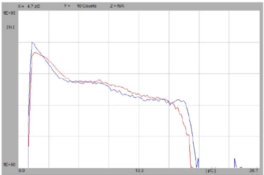
line
| X (pC) | Red Line Value [N] | Blue Line Value [N] | |--------|---------------------|----------------------| | 0.0 | ~1E+05 | ~1E+05 | | 13.3 | ~1E+04 | ~1E+04 | | 26.7 | ~1E+00 | ~1E+00 |Fig. III.13 Count distribution versus charge (counts per second, log.)
By means of the standard Windows copy function (
The fourth display mode available is the scope mode (figure III.15). This pseudo-analogue, oscilloscope-like display gives an impression similar to the display of older, oscilloscope based partial discharge detectors. With an acquisition running (see next section) it displays the partial discharge pulses that occurred during the current refresh cycle, only. The data for this display mode is derived by the calculation of the deviation between two consecutive memory contents transferred. Thus, the complete data of the entire acquisition is still maintained. With the acquisition ended or in case of a data set re-loaded from file, this scope display shows the envelope of the entire acquisition. This display mode is helpful to monitor changes in the occurrence of partial discharges while an acquisition is running. Mainly, however, this mode is used to correlate measurement results with the experience gained with this older type of instruments. All these display types are sub-sets of the amplitude-phase-height-distribution, the so-called partial discharge pattern.

scatter
| x [deg] | y [nC] | | ------- | ------ | | 0 | 0.0 | | 180 | 0.0 | | 360 | 0.0 |Fig. III.14 Screenshot sent to the Windows clipboard

line
| X (deg) | Y (pC) | | ------- | ------ | | 0 | 0.0 | | 136 | -39.3 | | 360 | 0.0 |Fig. III.15 Scope display mode (pseudo-analog display)
The fifth display available is called 'Oscilloscope' (see figure III.16). With the latest amplifier board generation, the ICMsystem can offer time-domain visualisation of the measured signals for all activated channels. Thus, the ICMsystem is capable of travel time analysis methods, which can be used for fault

line
| Parameter | Value | | ----------------- | --------- | | ΔRef - Ch.1 | 4.4 µs | | ΔRef - Ch.2 | 393.2 µs | | ΔRef - Ch.3 | 416.8 µs | | ΔRef - Ch.4 | 449.2 µs | | ΔRef - Ch.5 | | | ΔRef - Ch.6 | | | ΔRef - Ch.7 | | | ΔRef - Ch.8 | | | ΔRef - Ch.9 | | | ΔRef - Ch.10 | |Fig. III.16: Oscilloscope display
location using electric signals or for acoustic fault location in transformers. Here, the partial discharge signal serves as a reference point for travel time analysis of signals received by acoustic sensors. By using triangulation methods, the origin of the signal within the transformer tank can be identified. To each measurement curve belongs a vertical cursor that can be placed by moving the mouse above the curve and left clicking. The time gap between this cursor and the red reference cursor, whose position is usually identical to the position of the triggering signal, is automatically calculated and shown with the field 'Cursor' below the oscilloscope display. These data can be transmitted to an instance of Power Diagnostix' ICMacoustic software running in parallel by using the two 'Triangulation' function keys. There must be at least four active channels (including the trigger channel) to get sensible results with the ICMacoustic software. For more information on acoustic measurements please refer to section III.3 'Acoustic Measurements'.
For the sixth display 'Spectrum' see section IV.1 'Spectrum Function (SPEC)'.
The trending display shows the evolution of the measured discharge versus time. The time axis can be set to cover different time periods from 1 to 100,000 seconds. This selection is made with the 'Set Time' field in the SETUP A subpanel (see page 57).

line
| Parameter | Value | |-----------|-------| | G0.11-1S | 2.49 | | Time [ns] | 159.2 | | Voltage [ms] | 16.69 | | Charge [Fast] | 87.4 | | Frequency [E] | 50.0 | | Amp In | 0.00pC | | G0.11-1S | 0.3kV | | Sat Time | 0.0s | | ADC LLD | 0.0s | | ADC Mode | 1.1kV | | ADC Mode Input | 44.1s | | Coding Line | 1.2kV | | Pre Gain | 60.9s | | Acq Mode vs Phase | 1.2kV | | Amp U Cutoff | 1.2kV | | Pattern Acq. AMP OUT | 1.2kV | | Phase Shift | 1.2kV | | Sync In | 1.2kV | | Input Mode AMP | 100.0 μs | | Dead Time | 100.0 μs | | ADC Mode FP NRT | 100.0 μs | | Waveform Sine | 100.0 μs | | Amp Main Gain | 100.0 μs | | Count Level | 100.0 μs | | Amp L Cutoff | 100.0 μs | | Mem Erase Auto | 100.0 μs | | Div Ratio | 140.0 μs | | Sync + Extern | 140.0 μs | | Setup S | MC Panel, AT Panel, Load, Save, Offline, Stop, Cancel, ExitFig. III.17: Trending display
The blue graph in the lower panel shows the voltage versus time, while the red graph represents the partial discharge. To every graph belong two cursors with markers that show the measurement values for the current cursor positions. The position of the first red cursor indicates the last gain change (or the start of the acquisition if the gain has not been changed by the time), while the second red cursor shows the present values of the current measurement. The acquisition pattern for the period defined by the positions of the two cursors is shown in the panel on the upper right-hand side. The positions of the blue cursors are freely selectable but must lay within a period of constant gain settings. The acquisition pattern for the period defined by the positions of the blue cursors is shown in the panel on the upper left-hand side. If the user sets the cursors in a way that there is a gain change within the defined period, the cursor positions are automatically corrected by the software. If there's no ongoing pattern acquisition, the positions of the red cursors are also freely selectable.
Another display mode is for cable fault location (CFL). See section IV.2 for further information.
Beside the central display the instrument provides some additional measurements. Further, the ICMsystem software calculates some derived quantities. This information is presented with the two blocks at the right-hand and the left-hand edge of the main display. The right-hand block bears ten items (figure III.18). The first one is the cumulated dead time display. The dead time is the blanking time following an acquired pulse to avoid multiple triggering on pulse ringing, as described earlier (see the following section III.1.7 and the application guide, section V, for further details). The value displayed is the sum of all dead times within the acquisition time already passed. The relation of this cumulated dead time and the acquisition time is an important indicator of the statistical reliability of the whole measurement. Therefore, this display item has a combined indicator: The absolute value in seconds is shown in a numeric display, while the relation between cumulated dead time and acquisition time is indicated by a red bar underneath the numeric display. The next value displayed in the row is the cumulated gate time, i.e. the overall time the gate was active. This indicator is of the same combined numeric and bar graph type. As with the dead time, the relation between gate time and acquisition time is critical. Both numbers should be observed carefully, since they are indicating the amount of time whilst the instrument was 'blinded'. The third item shows the acquisition time. Again, a combined indicator, where the bar graph shows the relation between pre-set acquisition time and the amount of time passed already.
![Dead Time Σ 0.0 s Gate Time Σ 0.0 s Acq Time 60.0 s Pos Counts 290680 Neg Counts 0 Voltage [rms] 7.37 kV Charge [Fast] 1.00 pC RIV [off] N/A NQS Value 3.898 uA Frequency 50.0 Hz [L]](/content/2026/05/1014079/images/5c339374a9eac20b9529db9283d4dae4890c49784a7111b0cae163cc7492633c.jpg)
![Gate Time Σ 0.0 s Acq Time 151.0 s Total Counts 44311 Level Counts 0 Voltage [rms] 306.27 kV Charge (IEC) 0.02 pC PV off N/A Count Level [pC] 10.00 Cancel Pos/Neg OK](/content/2026/05/1014079/images/1d3a21337f92a79ef0cb070c4bc544005b00e6e08533196da41fc4a060f999a5.jpg)
Fig. III.19 Setting the count level
The following two entries are to display the number of positive and negative counts of the current acquisition. Double clicking to one of these items opens a sub-menu to modify the count level (figure III.19). Subsequently, the two labels change into 'Total Counts' and 'Level Counts', with level counts displaying the counts raising the level set. Alternatively, this level may be set by moving the blue arrow at the right-hand edge of the central display area after Fig. III.18
![Edit... Sync. Frequency [Hz] 0.10 Cancel Auto OK [ deg ] 360 Voltage [rms] 306.27 kV Charge [IEC] 0.02 pC R/V dtf N/A NOS Value 398.6 pA Frequency/ 0.1 Hz [M] Acq Mode Amp U Cutoff Pattern Acq Phase Shift Sync In vs Phase 800 kHz AMP OUT 0° Sync 1](/content/2026/05/1014079/images/3da4edac647af22827929e99cade0ba0871c1ffef300b7579d7bc63c51477ac1.jpg)
Fig. III.20 Low frequency synchronisation
switching to count level mode. The icon in the menu bar switches between count level (blue arrow) and low level discriminator mode of this slider (red arrow). The next item displays the value of the high voltage with respect to the divider ratio chosen. Double clicking to this entry calls a subpanel to edit the test voltage currently displayed. Changing the voltage causes the software to calculate the divider ratio on its own. This display is of the combined type as well: The bar graph indicates the utilisation with respect to the maximum input voltage at the sync input. The seventh item indicates the current peak charge measured with the peak A/D converter within the AMP5 plug-in unit. Again, the bar graph reads the utilisation. A click onto the entry calls a subpanel to change the calibration charge. The value entered will be assigned to the current position of the cursor. If the subpanel was called up with a double click onto the pattern display the value entered will be assigned to the position double clicked. Refer to section III.1.9 'PD Calibration' for details. If the selected AMP5 plug-in is used for gating, the seventh field shows the current signal level as utilisation in percent. This signal level displays serves to find the appropriate setting for the pre and main amplification and helps with the adjustment of the gate threshold. With earlier releases of the instrument, this function is not available (HW 2.00, 3.10). In case connected to such instrument, this indicator is dimmed. RIV measurement can be activated and deactivated
by clicking on the label 'RIV [off]'. The NQS value is a derived quantity. It is the average discharge current, calculated by dividing the sum of the charge of all discharge pulses acquired by the acquisition time.
The last item of this block is the frequency. It shows the frequency of the sync source currently chosen, with an 'L' in square brackets indicating line synchronisation. A double click to this entry opens a subpanel (figure III.20) to manually pre-set a sync frequency or to return to automatic calculation of the sync frequency. The (standard) automatic calculation is applicable for a range of 30 Hz to 400 Hz, while this manual mode is used for low frequency synchronisation beyond 30 Hz. Staying in manual mode is indicated by an 'M' in square brackets following the value of the frequency (0.1 Hz [M]).
Especially, the manual mode is used to synchronise to 0.1 Hz sources with cable measurements or LF tests on rotating machines utilising the SYNC input of the TTL module. This TTL synchronisation input is active only with the sync source set to external and no voltage source connected to the DPR5! With the sync source set to external and no sync signal available the frequency display reads 'No Sync' (in automatic mode, only).
Fig. III.21
The display block at the left-hand side of the central graph contains mainly status information regarding the current file or measurement and the communication channel used (figure III.21). In idle mode or while offline, the text box at the top of this block indicates whether the current measurement was calibrated or scaled. In acquisition mode this text box indicates the status of the acquisition running (see section III.1.7). The status of the communication interface used is shown with the six 'LED'-like indicators. The upper three are to indicate which of the possible interfaces is used or available (GPIB, USB, or modem). The next green one indicates an active connection (Online). In case of such an active connection, the upper red LED indicates ongoing transmission of data (commands and setup strings) to the instrument (TXD), while the lower red LED refers to a transmission of data (measurements) from the instrument (RXD). 'Total Time' is only visible in multi-channel consecutive measurement mode. It defines when scanning of the different channels stops. After measurement start it acts like a countdown. The 'Delay Time' indicator is visible only in the consecutive measurement mode. It is used to pre-set a delay time. With a consecutive measurement running, it indicates the remaining time until the next automatic start will take place. The next text display shows the file name of the current data set. In consecutive measurement mode this text display serves to enter the file prefix of the measurement files. The date and time shown with the two remaining displays
is referring to the moment when the acquisition of the current data set was started. Upon start of an acquisition a time stamp is taken and stored in binary format within the *.DAT file, i.e. these two displays do not reflect the time stamp of the file. The 'About' panel (Help/About) informs about the hardware release of the instrument connected, the software release, and our address.

Fig. III.22 About
III.1.7 Measurement Modes
The instrument, as the ICMsystem software controls it, has two different main measurement modes: The standard or idle mode and the acquisition mode. The standard mode, which exchanges only setup data and simple measurement results such as peak charge, voltage, and frequency with the acquisition unit, serves mainly to prepare the instrument for the acquisition. While in that mode all setup items are accessible and the effect of modifications of settings can be evaluated. An acquisition is started with the 'Start' button (F8,
| Setup O | MC Panel | AT Panel | Load | Save | Offline | Start | Reload | Exit |
Fig. III.23 Function keys while in idle mode (valid connection to an instrument)
idle mode (figure III.23) into the acquisition mode (figure III.24). The text of the status indicator, this text box at the upper left corner, changes from 'Calibrated' or 'Scaled' into 'Measuring'. Within the instrument, the counter array is reset, and the acquisition of the three-dimensional pulse-amplitude-phase-height-distribution
| Setup O | MC Panel | AT Panel | Load | Save | Offline | Stop | Cancel | Exit |
Fig. III.24 Function keys while in acquisition mode
is started. While in acquisition mode, the memory content of the instrument, i. e. the raw data of the partial discharge pattern is read and displayed in a continuous refresh cycle. The speed of this refresh cycle, as with the display refresh while in idle mode, depends on the speed of the control computer's CPU and the communication interface used. With a Pentium notebook and a PCMCIA-GPIB interface the refresh cycle takes less than two seconds. In case of serial transmission via USB or, especially, with a modem link, the refresh cycle depends further on the content of the partial discharge pattern: The compression algorithm used with the serial communication reduces consecutive zeros (i. e. the blank parts of the map) into a short expression. Thus, a map with a voluminous partial discharge pattern transmitted over a bad modem link may take up to 30 seconds. That compression routine works on the other hand efficiently with the transfer of more fragile discharge patterns, where the refresh cycle comes in the range of 2 to 5 seconds (modem). The acquisition stops automatically with the pre-set acquisition time ran out. While in the acquisition mode, the software checks with every cycle the acquisition status bit of the instrument. With the acquisition ended, the instrument's memory is read once more to make sure that the data of the entire acquisition period has been read. Since all the data is read sequentially, the cumulated dead time currently displayed belongs in principle to another point within the acquisition period than the partial discharge pattern currently displayed, for instance. This effect is illustrated with figure III.25 showing the acquisition of a broad noise signal. The memory was nearly empty with the start of the transfer (left-hand side) and got filled up during the further transfer, since the transmission runs independently from the acquisition. During a pattern acquisition the status indicator changes from 'Measuring' into 'Completing' before returning to the idle mode. An acquisition can be stopped manually by means of the 'Stop' or the 'Cancel' button. The 'Stop' button causes a process similar to the procedure described above. I. e. you derive a completed measurement, where all data is consistent and belongs to the same acquisition period. The 'Cancel' button is used to stop a faulty or unwanted acquisition as soon as possible to improve the setup entries, for example. In case you decide afterwards to save a cancelled acquisition, use the 'Reload' button in order to have a completed data set as discussed above. With some application it is wanted to have a consecutive set of acquisitions available to study the aging of material exposed to partial discharges, to study electrical treeing, or to evaluate the

heatmap
| [deg] | [pC] | |-------|----------| | 0 | -6.34 | | 180 | 0.0 | | 360 | +6.34 |Fig. III.25 Data transfer during a running acquisition
influence of an additional parameter as temperature, voltage, radiation, etc. Such measurements are made available by the ICMsystem software in consecutive measurement mode. Figure III.27 shows how to choose this mode. Once chosen, two additional display items labelled 'Total Time' and 'Delay Time' come up within the left block, as described in section III.1.5 already (figure III.21). Clicking the 'Start' button with the example given in figure III.26 causes the system to start an acquisition of 270 s duration (Set Time), store it under the name TEST001.DAT in the default directory (to be modified under 'File, Default Directory...' or F11), wait for 30 s, and start the next acquisition. The result of this second acquisition will be saved in the same directory under TEST0002.DAT. Subsequently, every 60 s a new acquisition is started and saved to disk until the process is stopped with the 'Stop' or 'Cancel' button. For the time between completing an acquisition and starting the next one, the status indicator displays 'Waiting' with the 'Delay Time' entry counting down the remaining seconds. Use preferably this waiting time for stopping, in order not to have a file of a different acquisition time. Be sure to have enough disk space available to leave such measurement unattended and to avoid losing valuable data. Keep in mind that Windows reserves during run-time disk space for swap files and may cause an 'out of disk space' message even with some space left. A quick motion replay of these consecutive files is provided by the 'Movie' function (see section III.1.11).
![Power Diagnostix - ICMsys Connect Measurement Tools View Panel Options Help Start Acquisition F8 Reload Map from Device F9 Acquisition Mode Single Channel (standard) Single Channel (consecutive) Multi Channel (standard) ✓ Multi Channel (consecutive) +2b.7 [ pC ]](/content/2026/05/1014079/images/57db8470ff49eb2c6dd37d4d44b77d902530ac8a2d75a2d0f65c10ed408e4611.jpg)
Fig. III.27 Activation of the consecutive measurement mode
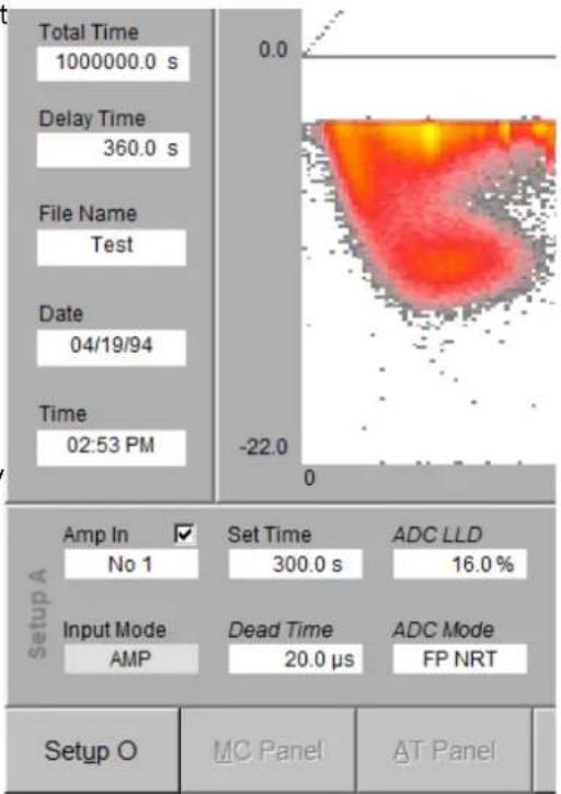
Fig. III.26 Preparing consecutive measurements
III.1.8 Controlling the Instrument's Setup
The ICMsystem is designed to meet the requirements of partial discharge measurements not only in a standard laboratory environment, but also in field application, where it is difficult or even impossible to control the measurement conditions. Thus, the ICMsystem and its control software do offer a huge variety of setup parameters to be modified in order to cope with such non-perfect measurement environments. The benefit of having all these possibilities of adjustment creates on the other hand the risk to operate the instrument not at its best performance available. Further, since there are no built-in precautions regarding inappropriate settings in general, it is possible to totally disable the instrument by its setup. Conducting partial discharge measurements in non-standard applications requires in general experience. Therefore, it is mandatory to study the meaning of each setup parameter carefully and to know about the capabilities of the hardware modules. Gaining experience takes time, and it is impossible to write everything down in such a manual. Try to have a small lab available, where you can evaluate the problems and solutions of your specific application.

Fig. III.28 Setup A
Several subpanels underneath the main display area control the ICMsystem's setup. Clicking the most left function key will toggle through the different subpanels. Upon start-up the setup displayed will reflect the setup that was active when the software was shut down the previous time (stored in the file ICMSYSXX.FIL). With every file reloaded the complete setup of that file is displayed and, in case of an instrument connected, sent to the acquisition unit as well. This makes sure, that the instrument is reset completely to the state it had, when the reloaded measurement was taken. On the other hand, take care to save your current setup to file before over-writing it by reloading a file. The subpanel 'Setup A' contains the following entries, as shown with figure III.28. Please refer to the hardware section (section II) for additional information on the hardware background of the items described.
Double clicking on field labels changes the mode of the corresponding values from local, i. e. valid for the currently selected channel only, to global, i. e. valid for all channels. The global mode is indicated by a label with italic letters.
| Amp In | This entry indicates the channel chosen for display. Clicking to that entry enables the selection of another channel and will recall the setup stored within the instrument. If a multi-channel instrument is used, only channels with a set checkmark are displayed. |
| Input Mode | This entry determines whether the selected channel is used for gating or as a measurement channel. Please be aware that pattern acquisition using the gating channel is only available for instruments of 2015 or newer. |
| Set Time | Entry to pre-set the acquisition time. Shortest time possible is 10 ms. In case of consecutive measurements, this time must be chosen shorter than the delay time With a GPIB connection few seconds difference is enough, consider at least 30 seconds difference for consecutive measurements via modem. However, with single measurements an acquisition may be stopped earlier by means of the 'Cancel' or 'Stop' button. Double clicking onto this field brings up a drop-down list with values of 10, 30, 60, 100, 500, and 1000 seconds. |
| Dead Time | Blanking time added after the acquisition of a pulse to avoid triggering on multiple under- and over-shots (ringing). The shortest dead time available is 5 μs, resulting in a theoretical repetition rate of 200 kHz. The dead time may be set to some milliseconds in case of acoustic sensors. Refer both to the hardware section (section II) and the application guide for further details (section 0). Double clicking onto this field brings up a drop-down list with values of 5, 10, 20, or 50 μs. |
ADC LLD
Low Level Discriminator. The LLD is the trigger threshold of the peak A/D converter (ADC5 plug-in). Every pulse higher than that level causes a conversion and contributes to the partial discharge pattern subsequently. This conversion is followed by a blanking time (dead time) to avoid multiple triggering on pulse ringing. Thus, adjusting the LLD too low (i.e. into the noise floor) causes many conversions tying up the A/D converter's time. See the application guide (section 0) for adjustment of LLD and Dead Time with respect to the ADC mode chosen. Single clicking to the entry offers keyboard editing of the value. Double clicking brings up a selection box (2, 5, 10, 20%). A convenient way to adjust the LLD to the top of the noise floor is provided by the red slider arrow at the right-hand edge of the central display area (figure III.1). Double clicking onto this field offers the choice of 2, 5, 10, or 20% as LLD.
If the AMP plug-in is used for gating, this entry is used to set the trigger threshold of the gate. The value may be further adjusted by means of moving the red bar graph underneath the numerical display. To find an appropriate adjustment, observe the gate level indicator and listen to the gate action tics (Preferences/Miscellaneous->Beeper Mode: 'Gate Time'). See the application guide (section 0) for further details of the gate's usage.
ADC Mode
Trigger mode of the A/D converter. The converter offers three different operation modes to cope with the properties of 'real life' partial discharge pulses. Click to the entry to choose from 'TW NRT' (Time Window Non-Re-triggerable), 'FP NRT' (First Peak Non-Re-triggerable), and 'FP RT' (First Peak Re-triggerable). The 'First Peak Non-Re-triggerable' mode gives in most cases good results. With the so-called -response, a pulse form that has a small first peak followed by a larger undershot (band pass response, dispersion, group delay), the Trigger in Time Window mode is mandatory (for details see section IV.2).
Coding
The A/D converter of the ADC5 module offers a 12-bit resolution, whereas the displayed partial discharge pattern has a Y-axis resolution of 8 bits only. An EPROM takes care of the conversion into the 8-bit expression. A conversion into logarithmic scale is possible as well, since the input data is of a higher precision. Clicking to the entry gives the choice of the available coding pages: 'LIN BIP', Linear Bipolar, which is the standard setting. 'LIN UNI', Linear Unipolar is chosen in applications, where the pulse polarity is invalidated by strongly ringing signals or with the use of a preprocessing that gives only unipolar output as the RPA2 or a spectrum analyser, for example. 'LOG BIP', Logarithmic Bipolar transfers the raw data into a logarithmic scale covering two decades ( ±1-100% ). The one-percent reading shows up the display pixel next to the zero line, while the ten-percent reading can be found in the middle of the display area for each polarity. 'LOG UNI' shows two decades as well, but unipolar. 'SIN' is coded according to sin x, while 'SQRT' follows the expression (sin x) ^1/2 .
Waveform
A sine wave may be superimposed on the partial discharge pattern to give an orientation regarding the phase position of the discharge pulses. In case the SYNC IN input is connected to a capacitive high voltage divider, a measured shape of the current voltage signal may serve to evaluate the influence of power frequency harmonics, for instance. The available options are 'Off', 'Sine', 'Shift. Sine', 'Acquired', '3 Sine', '3 Shift. Sine', 'Sine', and 'Shift. Sine'. With 'Sine' chosen a created (ideal) sine wave is superimposed. With a phase shift entered, this sine wave is kept at its origin, while the partial discharge pattern is shifted. 'Shift. Sine' will reverses this: The pattern stays at its position with respect to the sync source, but the sine wave is shifted (to express the known phase of the high voltage). 'Acquired' superimposes the shape of the high voltage measured. With that option both the pattern and acquired wave are shifted, since they are referring both to the same sync. '3 Sine' is used for easy identification of cross coupled PD. With a phase shift entered, these sine waves are kept at their origin, while the partial discharge pattern is shifted. '3 Shift. Sine' will reverses this: The pattern stays at its position with respect to the sync source, but the sine waves are shifted (to express the known
| phase of the high voltage). With ‘Sine 3’ it’s possible to compare the phase resolved shape of partial discharge with a sine wave to the power of three, and ‘Shift. Sine 3’ will show the sine wave shifted while the pattern stays at its position with respect to the sync source | |
| Pre Gain | Chooses the gain of the pre-amplifier. The supply voltage controls the gain of the pre-amplifiers RPA. A certain voltage fed to these pre-amplifiers cause their control circuits to switch to the amplification wanted. Clicking to this entry offers the choice from ‘Off’, ‘1’, ‘10’, ‘100’ and ‘UHF (LOG)’. The ‘Off’ setting should be used in case of direct connection (i. e. without an RPA) of the AMP IN to a spectrum analyser or any other pre-processing instrument in order to avoid damage of this instrument’s output by the DC supply voltage. Use the individual setting only in case you do not want to have the pre-set table of pre and main amplification offered by the [+] and [-] buttons. If the ICMsystem is connected to a frequency converter unit (FCU), ‘UHF (LOG)’ shall be used. |
| Amp Main Gain | Clicking to this entry brings up a list of the main amplification factors of the AMP5 unit (1, 2, 4, 8, 10, 20, 40, 80, 100, 200, 400, 800). Use the individual setting only in case you do not want to have the pre-set table of pre and main amplification offered by the [+] and [-] buttons. |
| + - | The plus and minus buttons serve to adjust the amplification of both pre and main amplification according to a table with optimised combinations of pre and main gain. Depending on your application you may need to choose a different combination. According to this table 10/40 expresses gain 400 and 100/8 expresses 800, for instance. Some application may require using 10/80 instead to avoid pre-amp saturation. Choosing this combination is a compromise between saturation and noise considerations in general. |
| Acq Mode | The X-axis of the partial discharge pattern can be chosen to express the phase (vs. Phase) or a pre-set time (vs. Time). The ‘vs. Phase’ mode is the standard mode of the ICMsystem for AC tests. The ‘vs. Time’ mode serves to monitor tests at DC voltage, to assess deviations of the discharge activity or to observe few AC cycles (E. g. acquisition time 100 ms). |
| Count Level | With some applications (especially DC testing) it is wanted to know the number of pulses exceeding a certain level. This entry serves to enter such level. Further, this entry reads the level adjusted by means of the blue slider arrow at the right-hand edge of the main display. The level counts and the total counts are displayed in the right-hand display block after choosing Options/Count Mode/Level Count. The count level can be set by double clicking to one of the count displays as well. |
| Amp U Cutoff | The AMP5 module contains filters to reduce the bandwidth given with the RPA1. The upper cut-off frequency can be chosen from ‘800 kHz’, ‘600 kHz’, and ‘250 kHz’. Regarding sensitivity the range 40 kHz–800 kHz would be best, while for pulse resolution 100 kHz–800 kHz may be better. Strong AM radio interference may require reducing the upper cut-off frequency. Choose with the pre-amps RPA2, RPA3, as well as with a spectrum analyser the setting 100 kHz–800 kHz. |
| Amp L Cutoff | The AMP5 module contains filters to reduce the bandwidth given with the RPA1. The lower cut-off frequency can be chosen from ‘40 kHz’, ‘80 kHz’, and ‘100 kHz’. Regarding sensitivity the range 40 kHz–800 kHz would be best, while for pulse resolution 100kHz–800kHz may be better. Choose with the pre-amps RPA2, RPA3, as well as with a spectrum analyser the setting 100 kHz–800 kHz. |
| Pattern Acq. | If the ICMsystem is equipped with the option for spectrum analysis, it’s possible to choose between the normal AMP path and SPEC path for pattern acquisition. While a pattern acquisition using the AMP path is limited to fixed cut-off frequencies, pattern acquisition using the spectrum path offers selection of a centre frequency up to 10 MHz with a bandwidth of 9 kHz or 300 kHz. |
60
| Mem Erase | Normally this entry is set to 'Auto' causing the instrument to clear its memory upon starting a new acquisition. In few cases it may be wanted to add a new acquisition to the one acquired previously (to continue a valuable experiment, for example). Thus, in that case the clear function must be disabled ('Off'). However, the acquisition time that will be stored, for instance, refers to the final acquisition started, only. |
| Phase Shift | In case the sync source used is not of the same phase as the high voltage causing the current discharge pattern, this entry serves to adjust the phase position by filling in a phase shift. Depending on the 'Waveform' setting, the discharge pattern and/or the superimposed sine wave is being shifted. Double clicking onto this field offers the choice of 0°, 60°, 120°, 180°, 240°, and 300° as value for phase shifting. |
| Div Ratio | Divider ratio. Clicking to that entry allows entering of the ratio of the high voltage divider used. Double clicking brings up the edit subpanel for the test voltage and subsequently causes the system to calculate the divider ratio on its own. |
| Sync In | Offers a drop-down list to choose the channel for synchronisation. |
| Sync | Determines the synchronisation source: '+ Line', '- Line', '+ Extern', '- Extern', and 'DC-Mode'. With 'Line' the positive or negative slope of the instrument's line voltage is taken for synchronisation. 'Extern' takes the positive or negative slope of the signal at the input for synchronisation. When set to 'Extern' the TTL sync input of the TTL module is taken.? |
| Setup O | Amp In No 1 | Trigger Level 15.0 % | Position 0.80 | Bandwidth 3 MHz | Pre Gain 100 + | Zoom 20 μs | Trigger Mode Automatic | Trigger Slope Unipolar |
| Trigger Ch CH 1 | Pre Trigger 2.00 μs | Cursor 0.00 μs | Sample Rate 50 Ms/s | Osc. Main Gain 10 - | Zoom Pos. 0 μs | Trigger Hold |
Fig. III.29: Setup O
| Amp In | This entry indicates the channel chosen for display. Clicking to that entry enables the selection of another channel and will recall the setup stored within the instrument. Only channels with a checkmark set are used in the oscilloscope display. |
| Trigger Ch | The trigger channel is chosen with this entry. With ‘Individual’ a trigger level for every channel is set separately. Please note, that the channels are not synchronised with this setting. |
| Trigger Level | If the signal of the trigger channel is exceeding the set value of this entry, the signals of all activated channels will be sampled and shown in the central display. |
| Pre Trigger | This entry determines the time on the DSO graph from zero position before the trigger event. |
| Position | Shows the current position of the active signal graph in units above and below the zero line. One unit is shown as vertical line in light grey. |
| Cursor | Shows the current cursor position of the active measurement channel. |
| Bandwidth | Sets the measurement bandwidth. Values between 1 and 30 MHz are possible. |
| Sample Rate | A high sample rate results in a better time resolution, while lower sample rates offer longer scan periods. 100, 50, 25, 10, 5, 2, and 1 Msample per second are possible. Higher sample rates are for research of electrical signals while the lower ones are more suitable for acoustic signals. |
| Pre Gain | Chooses the gain of the pre-amplifier. The supply voltage controls the gain of the pre-amplifiers RPA. A certain voltage fed to these pre-amplifiers causes their control circuits to switch to the amplification wanted. Clicking to this entry offers the choice from 'Off', '1', '10', '100', and UHF (LOG). The 'Off' setting should be used in case of direct connection (i. e. without an RPA) of the AMP IN to a spectrum analyser or any other pre-processing instrument in order to avoid damage of this instrument's output by the DC supply voltage. Use the individual setting only in case you do not want to have the pre-set table of pre and main amplification offered by the [+] and [-] buttons. If the ICMsystem is connected to a frequency converter unit (FCU), 'UHF (LOG)' shall be used. |
| Osc. Main Gain | Clicking to this entry brings up a list of the main amplification factors of the AMP5 unit (1, 2, 4, 8, 10, 20, 40, 80, 100, 200, 400, 800). Use the individual setting only in case you do not want to have the pre-set table of pre and main amplification offered by the [+] and [-] buttons. |
| + - | The plus and minus buttons serve to adjust the amplification of both pre and main amplification according to a table with optimised combinations of pre and main gain. Depending on your application you may need to choose a different combination. According to this table 10/40 expresses gain 400 and 100/8 expresses 800, for instance. Some application may require using 10/80 instead to avoid pre-amp saturation. Choosing this combination is a compromise between saturation and noise considerations in general. |
| Zoom | The Zoom value determines the size of the time interval, which is displayed. Possible values lie between 1 and 8000 μs and depend on the sample rate chosen. The zoom level can also be set by dragging the ends of the slider beneath the central display. |
| Zoom Pos. | Sets the starting point of the display. |
| Trigger Mode | Clicking to this entry brings up a list with possible trigger modes. 'Automatic' mode means, that sampling of the active channels will be started when the signal of the trigger channel is exceeding the set trigger value or after one second at the latest, even if the trigger level wasn't exceeded. In 'Normal' mode acquisition begins with the first signal exceeding the trigger level. The 'Single Shot' mode also starts sampling when the trigger level is exceeded but stops sampling after 16 events und changes the value of the Trigger field to 'Hold'. |
| Trigger | A click onto this field changes the mode from 'Running' to 'Hold' or vice versa. |
| Trigger Slope | This entry defines whether the slope of the electrical trigger is displayed as bipolar or unipolar. The standard is bipolar. |
| Averaging | Averaging is used to filter out noise by an algorithm. It assures that PD signals are not superimposed by background noise. Possible values are '4X', '8X', and '16X'. If this entry is set to 'OFF', no averaging is used. |
III.1.9 PD Calibration
Partial discharge measurements referring to the apparent charge are relative measurements. Thus, they do require a calibration in principle. Furthermore, the entire signal path from the discharging site to the instrument as well as some instrument properties as filters, for instance, are introducing an overall attenuation which is not precisely known. Thus, a pulse source injecting a known amount of charge is connected to the test object. Subsequently, the instrument is set to calculate correction factors causing the displays to read the charge amount injected. A suitable calibration source is connected to the test object according to the relevant standards. With the ICMsystem connected as described in the application guide, the gain of the instrument is adjusted by means of the [+] and [-] buttons of 'Setup A' to give a 50 to 80% reading at the charge meter (display block at the right-hand edge of the central display).

line
| Angle [deg] | Voltage [pC] | | ----------- | ------------ | | 0 | 0.0 | | 180 | +134 | | 360 | -134 |Fig. III.30 Calibration subpanel
Set the acquisition time to 100 seconds or more and start the acquisition by clicking to the 'Start' button (F8,
![X=180 ° Y= 65.8 pC Z= [ pC ] 132 Edit... Scaling Charge 1200 Cancel Ok [nC] Ok [pC]](/content/2026/05/1014079/images/3ce4681aa25fc808c99d93a830c49048b6fe15f76ec05775f32b8601724d0a74.jpg)
Fig. III.31 Scaling the charge axis
currently measured. In some cases, it is not possible to calibrate. The test object may be not accessible during the test, or may be inaccessible in principle, such as a discharging site within a cable joint, for instance. You may reload a calibration measurement performed previously, when the test object was accessible. In other cases, it's maybe required to scale the Y-axis, i. e. assign a value to the maximum point of the partial discharge pattern. To scale a data set previously acquired, double click to the positive numbering of the Y-axis in the upper left corner of the pattern display (i. e. the +132 with the example given in figure III.31). A sub panel similar to the calibration subpanel appears to edit the maximum value for both pattern display and peak charge meter. Subsequently, the status indicator changes to 'Scaled'. Scaling a
measurement, instead of calibrating it, results in assigning an identical correction factor to both the pattern and the peak charge meter. This may lead to a deviation of few percent between the two readings. Only with the so-called -response and the (inappropriate) setting 'Trigger on First Peak' chosen (Setup A, ADC mode), this deviation may be larger, since the pattern A/D converter takes the smaller first peak and the other one takes the maximum (i. e. the larger undershot).
With a multi-channel instrument each signal path can have different properties, so it is recommended to calibrate each channel separately. Saving the calibration of each channel to a separate file makes it possible to reload the calibration in case of a similar test configuration. Normally, the calibration takes place using the SC panel or MC panel, because they offer simultaneous calibration for the PD pattern and the PD meter.
III.1.10 Printing
For printing of measurement results the program's print utility is used. It offers printing of one, two, three, or four files per page. With one per page selected, the partial discharge pattern is printed along with the two projection graphs. Furthermore, the print program offers export to *.BMP format and printing of the report, i. e. the listing of the entire setup.
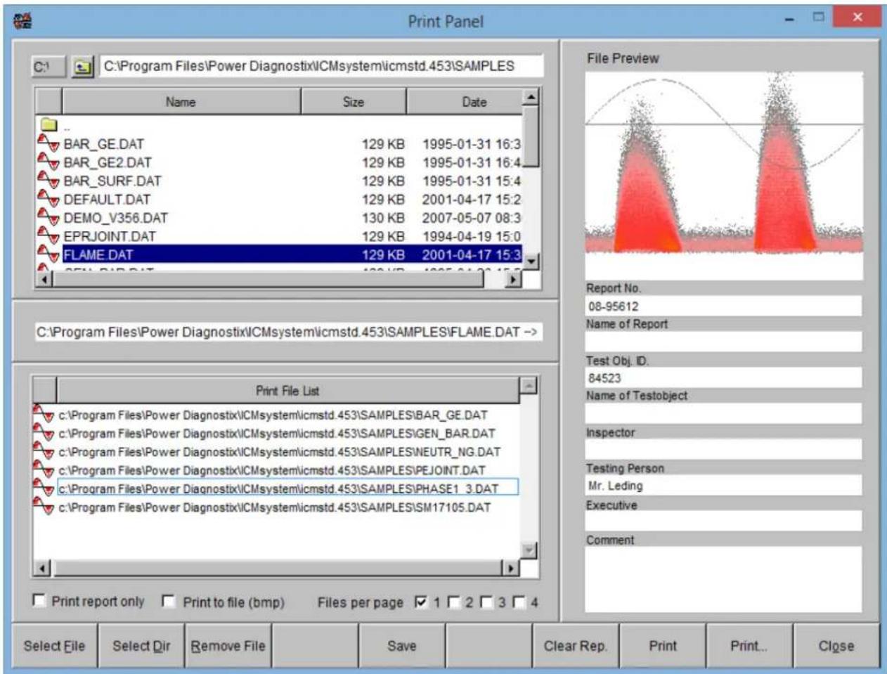
Fig. III.32 Panel of the ICMprint utility
The panel of the print utility (figure III.32) is divided into two areas. On the left-hand side is a load panel, offering the selection of more than one file. Click to the files you want to load in the desired order and press the 'Select File' button at the bottom of the panel. The software comes with a SAMPLE directory that includes several typical PD patterns. In order to print all files of a measurement session, 'Select Dir'. The latter will add the entire content of a directory to the 'Print File List'. The right-hand side of the print panel offers a preview of the selected file including pattern display and comment lines similar to the report header form
(see section III.1.5). The 'Save' button serves to store a file with modified comment entries, for instance, to the hard disk.
If the checkbox 'Print report only' is activated, only the corresponding report data will be printed. With the checkbox 'Print to file (bmp)' activated printing will create a *.BMP file of the active data set or of the files of an entire directory. The program uses the current directory to place the *.BMP files (TESTFILE.BMP belongs to TESTFILE.DAT, for example). Figure III.32 shows an example of such an exported *.BMP file. 'Print' starts the print process, while 'Close' leaves the print routine and closes the panel.
III.1.11 Movie – Quick Motion Replay
The ICMsystem program offers the so-called consecutive measurements, where several consecutive acquisitions are automatically taken and stored to disk (section III.1.7 'Measurement Modes'). The 'Movie' tool serves to replay the partial discharge patterns of these files. The panel of this program is shown with figure III.33. The 'Load' button calls a file load menu. Select the first file of the consecutive files to be loaded. Normally, this is the file bearing the name ????0001.DAT.
Subsequently, the program loads all files in a row, while stating 'Loading File...'. The files loaded are converted into a bitmap format and transferred to the computer's RAM in order to allow fast memory swapping. Depending on the computer's speed (CPU, bus, graphics), up to 30 pictures per second can be displayed. Adjust the speed of the memory swapping by means of the small slider at the right-hand side of the display. The 'Step' button is used to go stepwise through the files loaded. The maximum number of files the program is able to handle depends on the computer's memory size, only. Reaching the limit results in a jerky sequence of the pictures due to the usage of so-called virtual memory, i. e. memory swapping to the hard disk.

line
| Time | Speed | |------|-------| | Start | 0 | | End | 0 |Fig. III.33 Movie panel
III.1.12 Statistics
The ICMsystem software offers in-depth analysis of the measurement results via a statistics panel with six subpanels (figure III.34). The active subpanel is indicated by the darker grey of its frame. An information area beneath the panels shows several derived values. Similar to the software's main panel there's a row of function keys at the bottom of the window. They allow copying the content of the active subpanel to the computer's clipboard and exporting the loaded data set as an .HTM file.

Fig. III.34: Statistics window
III.1.13 Pull-Down Menu Structure

Fig. III.35 File menu
Beside the function keys and direct controls, the pull-down menus do offer an alternative way to revise and control the properties of the instrument and the ICMsystem software. The shortcut key of the menu items, if any, is listed with the entry as well. The commands of these pull-down menus are arranged in nine main groups named 'File', 'Edit', 'Connect', 'Measurement', 'Tools', 'View', 'Panel', 'Options', and 'Help'.
Figure III.35 shows the 'File' menu, a menu that does not branch into sub-menus. It offers loading of a *.DAT file as with the function key F4. Further, loading of the next and previous file (referring to the alphabetical order) is offered, while staying in a directory containing several *.DAT files. This function serves to browse quickly through the files of a directory. In order to avoid transferring the entire setup to the instrument with every new load process, the communication with the instrument may be interrupted (Options/Measuring Mode/Viewer). The same browse function is available by the Page Up and Page Down keys, as shown with figure III.35. Be sure to save your current setup before over-writing it by loading a *.DAT file. The 'Default Directory' is the location that has been entered with the previous 'Load' or 'Save' action. Use this command to determine (and create) the directory where the ICMsystem software places the files acquired in consecutive mode. 'Save' brings up a report form before saving a *.DAT file to disk in case this option has been set (Edit/Preferences/Security Options/Show report before saving data to disk). 'Save PD Pattern' offers saving of the PD pattern that is currently shown in the Map display as a .BMP OR .PNG file. 'Print' will give you a hardcopy of the current data set by use of the computer's standard printer. This printout contains the partial discharge pattern, the related measurements, and a listing of the entire setup. As this print function is intended to give a simple hardcopy only, one should use the program's print utility (Tools/Print Utility) for enhanced printing with options as directory printing, more than one pattern per page, printing of projections, etc.
The 'Edit' menu, as shown with figure III.36, contains the copy function of the current main display into the Windows clipboard (

Fig. III.36 Edit menu
Edit
| Copy to Clipboard | [copies the current display to the Windows clipboard] |
| Charge Unit | [calls the subpanel to alter the charge unit] |
| Clear | Active Map, All Maps |
| Copy Active Setup to Y Axis Scaling... | No 1, No 2, No 3, No 4, No 5, No 6, No 7, No 8, No 9, No 10, All [calls the subpanel to edit the scaling of the Y-axis] |
| Sync. Frequency... | [calls the subpanel to edit the frequency] |
| Voltage... | [calls the subpanel to edit the voltage] |
| Report... | [calls the report form] |
| Templates... | [calls the templates window] |
| Preferences... | [calls the preferences window] |
Fig. III.37 Submenus of the Edit menu
The pull-down menu 'Connect' allows searching for connected instruments and dialling a phone number for establishing a dial-up connection to an ICMsystem with built-in modem.
'Measurement' is shown with figure III.38. It allows starting an acquisition and reloading a map from device. The third menu entry is for choosing the acquisition mode 'Single Channel' (standard and consecutive) and, in case a multi-channel instrument is used, 'Multi Channel' (standard and consecutive). Please refer to section V.2 for detailed information concerning the different acquisition modes of the ICMsystem.

Fig. III.38 Measurement menu
The 'Tools' menu offers several utilities for handling the acquisition data, such as printing, statistics, and recalibrating, for instance.
The commands for toggling between the different setup panels and changing the display mode of the main panel can be found in the 'View' menu, which is shown with figure III.39. Additionally, the colour table for the coding of the Z-axis, can be shown and copied into the computer's clipboard. With the 'Offline Replay' command the function for re-calculating the count distribution can be switched on/off.

Fig. III.39: View menu
| View | |
| Setup Window | Setup A, Setup B, Setup O, Setup S |
| Main Window | Meter, Ellipse, Scope, Spectrum, Map (PD Pattern), Projections X, Projections Y, Trending, 3D Projections, Oscilloscope, Cable Fault Location |
| Color Table... | [calls the color table for the coding of the Z-axis] |
| Offline Replay | On, Off |
Fig. III.40: Sub menus of the View menu
The commands of the 'Panel' menu are active with multi-channel systems, only, or with single-channel instruments with multiplexer option. The first command toggles between the panels for single- and multi-channel pattern acquisition. 'Acceptance Test' brings up the panel for acceptance testing on power transformers.

Fig. III.41: Panel menu
'Options' is shown with figure III.42. It serves to set the program language and the auto gain adjustment for PD and RIV. The choices given by the different items of the pull-down menu are listed with figure III.43.
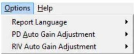
Fig. III.42 Options menu

Fig. III.43 Submenus of the Options menu
The item 'Device Config' of the 'Help' menu (see figure III.44) calls a subpanel to change the GPIB address of connected instruments and to update the firmware. The item 'About...' brings up the info panel as shown with figure III.22. This panel informs you about the hardware release of the instrument connected, the software release of your current ICMsystem software, and about Power Diagnostix' address.

Fig. III.44: Help menu
III.1.14 Short Cut Keys
The program is controlled by mouse clicks and certain keystrokes. This section gives a full listing of the keyboard controls.
Main functions of the program are accessible through short-cut keystrokes as well. Switching between the different display modes by means of the
| Function | Shortcut | Description |
| Setup (A, B, G, S, O) | Toggles between subpanel Setup A/B/G/S/O | |
| Load | Calls the Load panel | |
| Save | Calls the Save panel | |
| Search | Searches for instruments and modems | |
| Dial / Disconnect | Calls the Dial menu or terminates an existing modem connection | |
| Offline | Halts the communication | |
| Start/Stop | Starts or Stops an acquisition | |
| Reload | Reloads MAP data from the ICMsystem | |
| Cancel | Cancels a running acquisition | |
| Exit | Exits the program | |
| Load Next File | Loads next file in the current directory | |
| Load Previous File | Loads the previous file in the current directory | |
| Default Directory | Changes the default directory | |
| Copy | Copies the current display into the clipboard | |
| Prints MAP and data of the current data set | ||
| Meter display | Switches the main display to meter mode | |
| Ellipse Display | Switches the main display to ellipse mode | |
| Scope display | Switches the main display to scope mode | |
| Spectrum display | Switches the main display to spectrum mode | |
| Map display | Switches the main display to map mode | |
| Projections X display | Switches the main display to X-proj. mode | |
| Projections Y display | Switches the main display to Y-proj. mode | |
| Trending display | Switches the main display to trending mode | |
| 3D display | Switches the main display to 3D mode | |
| Oscilloscope display | Switches the main display to oscilloscope mode | |
| CFL display | Switches the main display to CLF mode | |
| Toggle trough displays | Toggles through the ten display modes | |
| Move cursor left | Moves the main display's cursor crosshair | |
| Move cursor right | Moves the main display's cursor crosshair | |
| Move cursor up | Moves the main display's cursor crosshair | |
| Move cursor down | Moves the main display's cursor crosshair | |
| Help index | Calls the 'About' window | |
| Escape | Exits a subpanel or an activated function |
Tab. III.1 Table of shortcut keys (main display)
While staying in a subpanel individual shortcut keystrokes to control the panel's buttons are active. With simple subpanels this is '
| Function | Shortcut | Description |
| Insert | + I | Inserts the edited entry ahead the selected one |
| Replace | + R | Replaces the selected by the edited entry |
| Delete | + D | Deletes the selected entry |
| Load | + L | Calls a menu to load a *.NUM file |
| Cancel | Exits the 'Dial' subpanel | |
| OK | + O | Starts dialling the selected number |
Tab. III.2 Table of shortcut keys (dial subpanel)
III.2 Advanced Software for Acceptance Testing (ACC)
III.2.1 Window Modes
The ICMsystem software version for acceptance tests offers three different window modes for acceptance tests:

Fig. III.45: Buttons for different views
- the table window showing the data measured via automatic or manual trigger
- a preconfigured graph view showing the voltage and PD values, which fits the needs of the most applications
- two live chart views, which can be freely configured to display every possible measured value.
The windows for live chart views can be configured via 'Config Live Chart', which is part of the 'Edit' menu.


Fig. III.46: Configuration of live chart view 1 and the corresponding window afterwards
The left part of figure III.46 shows the configuration popup for live chart view 1 configured to four rows and two columns. The right part of figure III.46 shows the corresponding window of the view displaying PD values on the left and some mixed values in the graphs on the right. The format and presentation of the measured values can be further adjusted via the 'Options' menu, that provides the following entries:
- Count Level: Switches the presentation of counts exceeding the 'Count Level' between absolute values and counts per second
• Display Mode: Switches between 'Table', 'Graph' and 'Live Chart View' 1 and 2 - Record Mode: Toggles between 'Auto Trigger' and manually triggered measurement
- PD Auto Gain Adjustment: If activated, the gain will be adjusted automatically by reference to the signal level of the PD source. Please note that the amplification will never exceed the amplification values during calibration.
-
Popup Pattern: Activates an automatic popup showing finished patterns recorded during an acceptance test
-
Report Language: Switches the language of the print outs of the ICMsystem software between English and French
- Report Time Format: Two Time formats are offered for acceptance tests: The real time of the triggered data set (e. g. 15:30:10, 15:30:40) and the time passed since starting the recording (e. g. 00:00:00, 00:00:30)
• RIV Unit: Switches between uV and logarithmic dBuV - RIV Auto Gain Adjustment: If activated, the gain will be adjusted automatically by the reference to the signal level of the RIV source. According to the configuration there are two different behaviours. If a card is used as PD and RIV source, only the Spec gain will be adjusted. So, the PD path will not be affected by 'RIV Auto Gain Adjustment'. If a board is used as a stand-alone RIV source for RIV measurement both the Pre-gain and the Spec gain will be adjusted automatically.
- Stripchart: Offers some options to alter the appearance of the strip charts like scaling and line-style. Additionally, it's possible to switch graph refresh between refresh with every trigger and refresh every second.
-
Table: Alters the sort order of the table values. Available orders are 'Normal', 'Sorted', and 'Cropped'.
-
'Normal': Channel-wise sorting: PD, counts, voltage and RIV value. Columns of not measured values are kept.
- 'Cropped': Channel-wise sorting: PD, counts, voltage and RIV value. Columns of not measured values are pruned.
- 'Sorted': Sorting according to the value type. At first all PD values, followed by counts, voltage and RIV values.

Fig. III.47: Options menu
III.2.2 Report Generation
There are two different kinds of reports to present the results of an acceptance test. The first one is accessible via the 'Export' button on the main panel and is designed to export the results in different file formats that allow easy integration into other documents. Three different file formats are available:
- 'TXT' : Standard ASCII file that can be edited with any text editor like e. g. Notepad
- 'HTML': Web page source code that can be displayed with any available browser like Internet Explorer, Mozilla, or Opera
• 'DOC' : Microsoft Office Word document
III.2.2.1 Customising the Report
The pre-defined report fields offer the most requested information. Additionally, the language can be toggled between English and French. Furthermore, it's possible to modify the report fields to adapt the displayed data to individual needs. By pressing the 'Config' button the configuration panel will appear. It offers the possibility to add, remove, and alter values, saving the modifications as report configuration files. It's also possible to load different report configurations ('Load Report') and to restore the default values ('Default').
It takes two steps to create and add a new field (see also figure 29):
- Creating the field and specifying its type: This task is carried out using the bottom right part of the window. The picture shows the creation of a field 'myValue' which will contain a text string.
- After creation the new field will appear in the middle of the window. Its position in the report is assigned by clicking the arrow buttons. The newly defined field can be moved to the left, right or bottom part of the acceptance test report window. Please note that some values have to be placed at the bottom of the window due to their size.
To remove an entry, select it, move it back to the 'Available Data' field and press 'Remove Item'. With 'Load / Save Report' you can save your modified report fields as a template. So, it's possible to use different report fields for different test types. The 'Clear Report' button will restore the default fields after installation of the ICMsystem software. Please note that changing the language of the reports only affects the default fields. Customised report fields have to be translated manually.


Fig. III.48: Default report fields
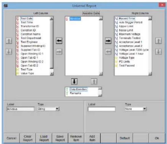
Fig. III.49: Creating a new report field (left) and positioning of its entry (right)
III.2.2.2 Printing the Report
The command 'Print Chart Report' is accessible via the 'Tools' menu. It offers a predefined page layout for fast and easy creation of print outs of the most significant values as tables and graphs. Additionally, tabs for the linearity test and the calibration matrices can be added as the first two tabs of this report window. In general, the shown data are defined by the checkmarks of the meter. Only the activated charge, voltage, and RIV values will be displayed.
To add or remove the page containing the calibration matrices use the button 'Add/Rem. Calmatrix' at the bottom of the window. The entries (including the logo on the upper left) of the header and the footer of the report can be edited by the corresponding 'Edit' button. The 'Lin. /Log. Scale' button toggles the scaling of the graphs at the end of the report between linear scaling with automatic range and logarithmic scaling from 1 to 10000. The order of the graphs is fixed: Graphs for the charge values first, then graphs displaying the number of counts exceeding the count level indicated through a blue line in the corresponding graph of the charge value. The last page contains the graphs of the RIV values if measured. On the bottom of every column the voltage graph of the first channel will be added. Please note that in logarithmic scaling the graph will be scaled to 100 kV by default until a different value in the nominal voltage field of the report header is entered.
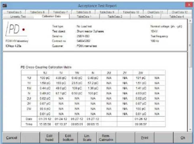
Fig. III.50: Calibration matrix
![Acceptance Test Report Linearity Test Calcibration Data TableData 1 TableData 2 TableData 3 TableData 4 TableData 5 TableData 6 TableData 7 TableData 8 TableData 9 TableData 10 OverData 11 OverData 12 /PD Test type No Load test Nominal voltage (ph - g/L) Test object Shunt reactor 3 phases 100kV Serial no 25874-653ipe Contract no 546845202ipe ICNps 4.22s Customer/PDXInternal test PD vs. Time [pC] Channel: 1U N = 100pC vs time Channel: 1U PD vs. Time [pC] Channel: 1V N = 100pC vs time Channel: 1V PD vs. Time [pC] Channel: 1V N = 100pC vs time Channel: 1V Cancel Edit head Edit bottom Lin. Scale Rom. Calmatrix Print Qk](/content/2026/05/1014079/images/ef8ea616f2a15954f5bd250c28b240d235ff54a9dafa9ddfb2a05ad79be5ac99.jpg)
Fig. III.51: Graph section of the report, PD and count values
![Acceptance Test Report Unstudy Test Calibration Data TableData 1 TableData 2 TableData 3 TableData 4 TableData 5 TableData 6 TableData 7 TableData 8 TableData 9 TableData 10 ChartData 11 ChartData 12 RV vs. Time [uV] Channel 2U RV vs. Time [uV] Channel 2V (% Voltage vs. Time) Channel 1U Tested by: Hiring Data: 00-01-09-12,Time: 17:18:21zano: Cancel Edit head Edit bottom Lin. Scale Rom. Calmatrix Print Qk](/content/2026/05/1014079/images/b0005492e0b52502148b63fc1e761163cfdbacc3fc4d8f8ebada30f1e3db36fc.jpg)
Fig. III.52: Graph section of the report, RIV values
Additionally, to the graphic display vs. time the measured voltage, charge, and RIV-values are presented in form of a table. The order within the tables is predefined. The first tables keep track of the PD values while the second ones keep track of the measured RIV values. Each table starts with the voltage values on the left and continues with the PD or RIV values of the activated channels.
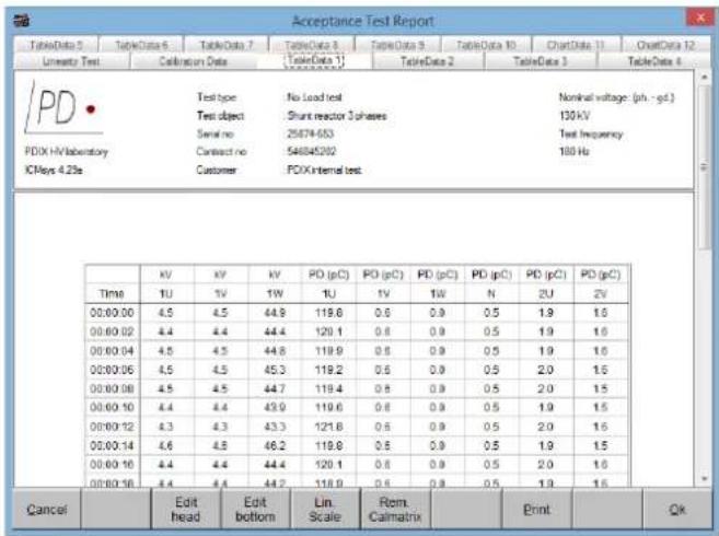
Fig. III.53: Table section of the report with PD values

Fig. III.54: Table section of the report with RIV values
III.3 Acoustic Measurements
The ICMsystem software offers acquisition of acoustic partial discharge signals in transformers for fault location with an iterative triangulation method. PD activity results in pulse-like acoustic emission, which travels well in the oil and in the tank wall of a liquid filled power transformer and can be detected by acoustic sensors. By using triangulation methods, the origin of the signal within the transformer tank can be identified.
The basic idea is to reduce the location to a “flat problem” by getting the horizontal position of a fault in a first step and to detect its vertical position in a second step. To do so, three sensors are arranged on a line to firstly get the horizontal position of the layer. The measured data can be transmitted to an instance of Power Diagnostix' ICMacoustic software running in parallel by using the two 'Triangulation' function keys. In a second step the sensors are placed on a vertical line, and their measurement results are transferred to the ICMacoustic software as well. There must be at least four active channels (including the trigger channel) to get sensible results with the ICMacoustic software.
For measurements the trigger channel must be set to the input channel which delivers the electrical trigger signal, e. g. by means of a quadrupole connected to a bushing tap. It is shown as the top trace within the display for the signal graphs (black graph in figure III.56). Assuming that the measurement is performed on a transformer which is approximately 2.50 m wide and considering the transmission velocities of the transformer liquid and of the transformer's steel tank a reasonable zoom factor for the display usually lies between 600 and 1000 μs. Averaging should be set to a value that allows the acoustic PD signal to be well

Fig. III.55: Setup for acoustic measurements
visible while the background noise of the transformer is filtered out by the algorithm. So usually '8x' or '16X' is a good choice. The trigger level and pre gain of the pre-amplifier RPA should be chosen in such a way that the signal graphs for all observed channels are clearly legible. That simplifies setting the cursors of the signal graphs to their appropriate positions corresponding to the arrival of the respective wave front. The time gap between each cursor and the red reference cursor indicating trigger signal is automatically calculated and shown with the field 'Cursor' in the 'Setup O' at the bottom of the software panel.

line
| Parameter | Value | | --------- | ----- | | Amplitude | 8.0 µs | | Position | 0.0 % | | Bandwidth | 3.51 | | 1 MHz | 1 MHz | | Pre Gain | 100 | | Zoom | 1000 µs | | Trigger Mode | Automatic | | Trigger Slope | Umpolar | | Trigger Ch | 2.0 µs | | Cursor | 98.7 µs | | Sample Rate | 10 Ms/s | | Osc Gain | 10 | | Zoom Fiss | 0 µs | | Trigger | Running | | Averaging | 4X | | Setup A | MC Panel | | AT Panel | Load | | Save | Search | | Triangulation (Hor.) | 46.8 µs | | Triangulation (Vert.) | 449.2 µs | | Edit | 4.4 µs |Fig. III.56: Oscilloscope display for acoustic measurements
If there are more than four acquisition channels of the ICMsystem active, the ICMacoustic software will take
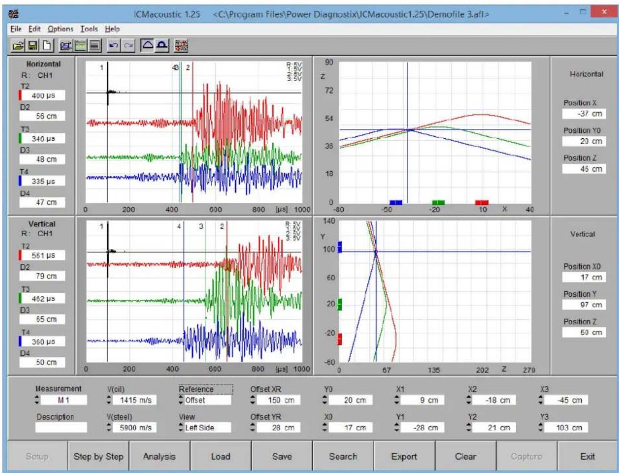
line
| Position | Value | |--------|-------| | -37 cm | 400 µs | | 20 cm | 346 µs | | 46 cm | 48 cm | | Vertical | 561 µs | | X0 | 17 cm | | Y7 | 97 cm | | Z | 50 cm |Fig. III.57: ICMacoustic software
the first three channels that are no trigger channel for fault location.
The ICMacoustic software shows the results of horizontal measurements in the upper left-hand screen and for vertical measurements in the lower left-hand screen. In the right-hand display area, the positions of the sensors are set either with reference to the lower left front corner of the transformer tank or a nearby point on the tank wall. Depending on the values being set for V(oil) and V(steel) in the lower section of the software panel, the distance that corresponds to the respective cursor position is displayed as a curve. The curves of all three censors should have one intercept point, which indicates the origin of the partial discharge.
Please refer to Power Diagnostix' separate user manual of the ICMacoustic software for more information.
IV Options
IV.1 Spectrum Function (SPEC)
The spectrum function is an optional hardware feature and extends the functionality of the AMP5 module to provide a spectrum analyser and an RIV (radio influence voltage) meter.
The software with SPEC function provides an additional panel for the usage of the AMP5 plug-in board for spectrum analysis. This display shows the frequency spectrum in the lower half and provides the view of two small patterns above. During pattern acquisition, spectrum analysis will be stopped and automatically continued when acquisition is finished.

line
| Parameter | Value | |-------------------------|-----------| | Dead Time Σ | 25.3 s | | Gate Time Σ | 0.0 s | | Acq Time | 159.2 s | | Pos Counts | 249625 | | Neg Counts | 0 | | Voltage [rms] | 16.69 kV | | Charge [Fast] | 87.4 pC | | RV [dB] | N/A | | NQS Value | 0.000 pA | | Frequency | 50.0 Hz [E]| | Amp In | G0.4-1S | | CF 1 | 330 kHz | | Sweep Time | 702 ms | | Start Freq. | 100 kHz | | Pre Gain | 10 | | Trace A | Maxhold | | Active Graph | CF 2 | | CF 2 | 1120 kHz | | Bandwidth | 300 kHz | | Stop Freq. | 5000 kHz | | Spec Main Gain | 32 | | Trace B | Clear Write| | Setup O | MC Panel | | AT Panel | Load | | Save | Offline | | Stop | Cancel | | Exit | G0.4-1S | | N/A | 5.0 s | | N/A | 6.0 s | | File Name | Date | | Time | 09:27:11 |Fig. IV.1: Spectrum display while recording a pattern
RIV measurement can be activated and deactivated by clicking on the label 'RIV [off]' on the right-hand side of the software window.
To activate pattern acquisition with the AMP5 board, switch pattern acquisition to SPEC OUT as shown in figure IV.2. If RIV measurement is turned on, there will be a popup to confirm switching to SPEC OUT for pattern acquisition, since this will turn off RIV measurement. Note that a spectrum board is only capable of recording unipolar pattern and that changing the 'Amp Main Gain' does not affect the 'Spec Main Gain'. So these options remain dimmed when using the SPEC OUT connection for pattern acquisition. The 'Spec Main Gain' can be changed by using 'Setup S' explained later on. Calibration of a SPEC OUT pattern is exactly the same as for a pattern recorded via the AMP OUT.

Fig. IV.2: Setup A switched to pattern acquisition using SPEC OUT
IV.1.1.1 Setup S
Below the spectrum graph the 'Setup S' is shown, providing the configuration settings for the spectrum board. If the active channel is equipped with a spectrum board, the 'Setup S' can be displayed by clicking the button in the bottom left-hand corner of the window. Each click changes to the next available setup display in the following order: 'Setup A', 'Setup S', 'Setup O'.
PD Measurement
| When using a spectrum board for PD measurement the following values and options can be set in 'Setup S': Amp In | Provides the option for channel selection (only for ICMsystem multi-channel devices). |
| Active Graph | Selects the centre frequency for pattern acquisition. If centre frequency 1 is chosen, the pattern will be shown in the upper left window. A pattern recorded for centre frequency 2 will be shown in the upper right window. |
| CF 1/CF 2 | Determines the middle frequency for pattern acquisition. The actual frequency range is determined by taking the bandwidth into account. For instance, the lower cut-off of the acquired pattern is calculated as follows: centre frequency - 12 bandwidth, and the upper cut-off is: centre frequency + 12 bandwidth. |
| Sweep Time | Specifies the time used for a complete spectrum scan from start frequency to stop frequency. |
| Bandwidth | Resolution bandwidth. 9 kHz and 300 kHz are selectable. |
| Start Freq. | Specifies the lowest frequency to begin spectrum analysis. Must be >10 kHz and dividable through 10. |
| Stop Freq. | Specifies the highest frequency. Must be < 10000 kHz and dividable through 10. |
| Pre Gain | Chooses the gain of the pre-amplifier. The supply voltage controls the gain of the pre-amplifiers RPA. A certain voltage fed to these pre-amplifiers cause their control circuits to switch to the amplification wanted. Clicking to this entry offers the choice from 'Off', '1', '10', '100', and UHF (LOG). The 'Off' setting should be used in case of direct connection (i. e. without an RPA) of the AMP IN to a spectrum analyser or any other pre-processing instrument in order to avoid damage of this instrument's output by the DC supply voltage. Use the individual setting only in case you do not want to have the pre-set table of pre and main amplification offered by the [+] and [-] buttons. If the ICMsystem is connected to a frequency converter unit (FCU), 'UHF (LOG)' shall be used. |
| Spec Main Gain | Sets the main amplification of the spectrum board.1, 2, 4, 8, 16, 32, 64 and 128 are available steps. Additionally, the + and - button can be used to increase and decrease the gain. |
Trace A/Trace B
Sets the graph mode for 'Trace A' (blue) and 'Trace B' (red). The modes are shown in figure IV.3.
Off: Hides the corresponding trace.
Clear Write: The trace shows the actual spectrum.
View: Freezes the trace.
Maxhold: Keeps the maxima of the succeeding spectrum scans.

Fig. IV.3
RIV Measurement
When taking RIV measurements, the settings of 'Setup S' will be limited to meet the industrial standards for RIV tests. So only 'Amp In', the centre frequency, and gain settings are available, while the other options will be dimmed. Note that the bandwidth of the radio influence voltage test is fixed to 9 kHz. Similar to PD measurement, the centre frequency determines the mid frequency used to measure, while the bandwidth determines the upper and the lower limit.

Fig. IV.4: Setup S when using the spectrum board for RIV measurement
When using the spectrum board for RIV measurement while the 'AMP OUT' connection is used for pattern acquisition, the software can automatically adjust the 'Spec Main Gain' according to the current signal level without affecting the 'Pre Gain' setting. This 'RIV Auto Gain Adjustment' option can be activated via the 'Options' menu.

Fig. IV.5: 'RIV Auto Gain Adjustment' option
IV.2 Cable Fault Location (CFL)
An ICMsystem with software integrated CFL option can perform PD fault location measurements on medium voltage cables by processing partial discharge signals by means of the time reflectometry. Single PD pulses can be triggered with a time resolution of 10 ns (100 Msamples/s) and a maximum display range of 320 μs corresponding to a theoretical maximum cable length of approximately 22 km for a cable with a pulse velocity of 140 m/μs.
To perform cable fault location, the length of the cable and/or the pulse velocity of the cable must be known in advance. The time domain reflectometry (TDR) is based on the travel time of pulses. Since a cable behaves as a wave conductor, the TDR principle can be used to locate sources of partial discharges along the full cable length.
A partial discharge pulse that is caused by an insulation imperfection travels to both ends of the cable if the cable has two open ends. With an open end means a cable hasn't its characteristic impedance at the end terminations. In this case, each partial discharge pulse occurring somewhere in the cable will be reflected to the opposite end, when reaching one of the cable end terminations. The distance of the PD source to the near and/or far end of the cable can be calculated using the time difference between the arrival times of pulses at a measuring impedance (coupling capacitor).
The principle of the time domain reflectometry is illustrated with figure IV.6. The travel paths of the first three reflections of the original partial discharge pulse that enters the coupling unit of the ICMsystem are displayed in three different colours.

Fig. IV.6: TDR principle

line
| Time (s) | Current (pC) | | -------- | ------------ | | 0.00 | 2.5 | | 0.15 | 2.8 | | 0.30 | 2.3 | | 0.45 | 2.5 | | 0.60 | 2.5 | | 0.75 | 2.5 | | 0.90 | 2.5 | | 1.05 | 2.5 | | 1.20 | 2.5 | | 1.35 | 2.5 | | 1.50 | 2.5 | | 1.65 | 2.5 | | 1.80 | 2.5 | | 1.95 | 2.5 | | 2.10 | 2.5 | | 2.25 | 2.5 | | 2.40 | 2.5 | | 2.55 | 2.5 | | 2.70 | 2.5 | | 2.85 | 2.5 | | 3.00 | 2.5 | | 3.15 | 2.5 | | 3.30 | 2.5 | | 3.45 | 2.5 | | 3.60 | 2.5 | | 3.75 | 2.5 | | 3.90 | 2.5 | | 4.05 | 2.5 | | 4.20 | 2.5 | | 4.35 | 2.5 | | 4.50 | 2.5 | | 4.65 | 2.5 | | 4.80 | 2.5 | | 4.95 | 2.5 | | 5.10 | 2.5 | | 5.25 | 2.5 | | 5.40 | 2.5 | | 5.55 | 2.5 | | 5.70 | 2.5 | | 5.85 | 2.5 | | 6.00 | 2.5 | | 6.15 | 2.5 | | 6.30 | 2.5 | | 6.45 | 2.5 | | 6.60 | 2.5 | | 6.75 | 2.5 | | 6.90 | 2.5 | | 7.05 | 2.5 | | 7.20 | 2.5 | | 7.35 | 2.5 | | 7.50 | 2.5 | | 7.65 | 2.5 | | 7.80 | 2.5 | | 7.95 | 2.5 | | 8.10 | 2.5 | | 8.25 | 2.5 | | 8.40 | 2.5 | | 8.55 | 2.5 | | 8.70 | 2.5 | | 8.85 | 2.5 | | 9.00 | 2.5 | | 9.15 | 2.5 | | 9.30 | 2.5 | | 9.45 | 2.5 | | 9.60 | 2.5 | | 9.75 | 2.5 | | 9.90 | 2.5 | | 10.05 | 2.5 | | 10.20 | 2.5 | | 10.35 | 2.5 | | 10.50 | 2.5 | | 10.65 | 2.5 | | 10.80 | 2.5 | | 10.95 | 2.5 | | 11.10 | 2.5 | | 11.25 | 2.5 | | 11.40 | 2.5 | | 11.55 | 2.5 | | 11.70 | 2.5 | | 11.85 | 2.5 | | 12.00 | 2.5 | | 12.15 | 2.5 | | 12.30 | 2.5 | | 12.45 | 2.5 | | 12.60 | 2.5 | | 12.75 | 2.5 | | 12.90 | 2.5 | | 13.05 | 2.5 | | 13.20 | 2.5 | | 13.35 | 2.5 | | 13.50 | 2.5 | | 13.65 | 2.5 | | 13.80 | 2.5 | | 13.95 | 2.5 | | 14.10 | 2.5 | | 14.25 | 2.5 | | 14.40 | 2.5 | | 14.55 | 2.5 | | 14.70 | 2.5 | | 14.85 | 2.5 | | 15.00 | 2.5 | | Note: The 'R' and 'T' labels are not present in the chart, but they are inferred from the plot area.Fig. IV.7: CFL graph
The reference pulse (R, red cursor) travelled directly from the pulse source to the coupling unit. The first reflection (1, green cursor) travelled first in the opposite direction of the coupler and then got reflected at the open end of the cable. This resulted in a time delay t_1 that indicates the distance of the PD source from the far end of the cable. Finally, the second reflection (2, grey cursor) shows the time delay between the reference pulse and its reflection at the far end. The time difference between the first and the second reflection results in a time delay t_2 representing the distance of the pulse source from the near end of the cable.
The CFL display shown with figure IV.8 can be activated with the icon in the icon bar. The panel on the upper left-hand side shows the summary of the measured reflections represented versus the position of the occurrence along the cable length, while the panel on the upper right-hand side displays continuously the PD activity in a 2-dimensional representation, accumulated of multiple refresh cycles vs. phase. Additionally, the current PD peak magnitude is shown in the upper left corner of this graph. The magnitude has to be calibrated (see section III.1.9 PD Calibration). The panel in the lower part of the display shows an oscilloscope graph with single PD pulses.
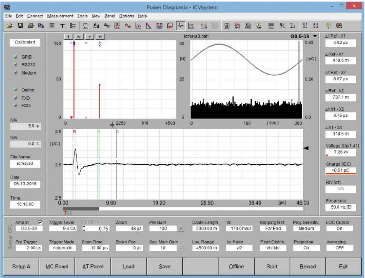
line
| Parameter | Value | | ----------------- | ----------- | | Δt Ref - X1 | 4.92 µs | | Δt Ref - X2 | 418.6 m | | Δt Ref - X2 | 8.67 µs | | Δt Ref - X2 | 737.1 m | | Δt X1 - X2 | 3.75 µs | | ΔX1 - X2 | 318.5 m | | Voltage [Up/1.41] | 7.26 kV | | Charge [EC] | >0.51 pC | | RIV [off] | N/A | | Frequency [E] | 50.0 Hz | | Setup CFL | Amp In | | | G0.5-3S | | | Trigger Level | | | 9.4 Os | | | Position | | | Zoom | | | Zoom | | | Pre Gain | | | Cable Length| | | 2000.00 m | | | Vc | | | 170.0 m/us | | | Far End | | | Medium | | | Proc. Sensitiv.| | | Medium | | | Medium | | | Proc. Sensitiv.| | | Proc. Sensitiv.| | | Proc. Sensitiv.| | | Proc. Sensitiv.| | | Proc. Sensitiv.| | | Proc. Sensitiv.| | | Proc. Sensitiv.| | | Proc. Sensitiv.| | | Proc. Sensitiv.| | | Proc. Sensitiv.| | | Proc. Sensitiv.| Setup A | MC Panel | | | AT Panel | | | Load | | | Save | | | Offline | | | Start | | | Reload | | | Exit |Fig. IV.8: Display for cable fault location
IV.2.1.1 Setup CFL
Below the CFL graph 'Setup CFL' is shown, providing the configuration settings for cable fault location. The 'Setup CFL' can be displayed by clicking the button in the bottom left-hand corner of the window. Each click

Fig. IV.9: Setup CFL
changes to the next available setup display in the following order: 'Setup A', 'Setup S', 'Setup CFL'. Note: 'Setup S is only available if the ICMsystem is equipped with the optional SPEC function.
| Pre Trigger | The entry determines the time on the DSO graph from zero position to the first trigger event. |
| Trigger Level | If the signal of the trigger channel is exceeding the set value of this entry, the signals of all activated channels will be sampled and shown in the central display. |
| Trigger Mode | This entry determines whether. |
| Position | Shows the current position of the active signal graph in units above and below the zero line. One unit is shown as vertical line in light grey. |
82
Zoom Zoomed area within the DSO graph. Zooming allows a more precise positioning of the cursors.
Zoom Pos. Zero position of the zoomed area.
Pre Gain Chooses the gain of the pre-amplifier. The supply voltage controls the gain of the pre-amplifiers RPA. A certain voltage fed to these pre-amplifiers cause their control circuits to switch to the amplification wanted. Clicking to this entry offers the choice from 'Off', '1', '10', '100', and UHF (LOG). The 'Off' setting should be used in case of direct connection (i.e. without an RPA) of the AMP IN to a spectrum analyser or any other pre-processing instrument in order to avoid damage of this instrument's output by the DC supply voltage. Use the individual setting only in case you do not want to have the pre-set table of pre and main amplification offered by the [+] and [-] buttons. If the ICMsystem is connected to a frequency converter unit (FCU), 'UHF (LOG)' shall be used.
Osc. Main Gain Clicking to this entry brings up a list of the main amplification factors of the AMP5 unit (1, 2, 4, 8, 10, 20, 40, 80, 100, 200, 400, 800). Use the individual setting only in case you do not want to have the pre-set table of pre and main amplification offered by the [+] and [-] buttons.
Cable Length Length of the cable under test. This length can be calculated during calibration or can be pre-set if the exact value is known.
Loc. Range Maximum set cable length in the location panel. Please make sure, that the real cable length fits with the location range.
Vc Pulse velocity factor for high frequency signals travelling along MV cables.
Vc Mode This entry indicates the pulse velocity factor mode, whether it is V or V/2. Please make sure, that the correct mode is set. A wrong value may result in faulty PD location.
Mapping Ref. This entry indicates the position of the PD decoupling unit. Please make sure, that the mapping reference is the same during measurement and cable length calibration. A fault location measurement can be performed to the near or the far end of the cable.
Peak Distrib. Enabling or disabling the display of PD peaks as blue Xs in the panel on the upper left-hand side. The peaks represent the PD value in pC at the given location.
Proj. Sensitiv. The projection sensitivity determines how measured cable faults are handled for display in the panel on the upper left-hand side. With a high sensitivity two fault locations are treated as identical, if their position is exactly the same in the DSO graph. If the sensitivity is set to medium, two fault locations may differ up to 13 samples in the DSO graph, while a low sensitivity allows differences of up to 23 samples.
Projection Enabling or disabling the display of cable fault locations, represented by thin red bars. The height of a bar indicates how often PD is located at this position.
LOC Cursor Enable or disabling the cable length cursors in the panel on the upper left-hand side.
Averaging If there's only a single position where PD occurs in the cable, an averaging of several DSO graphs can be activated to enhance the signal to noise ratio. With this entry the number of graphs used for averaging is set. Possible values are Off, 1, 2, 4, 8, 16, 32, 64, 128.
IV.3 Multiplexed Pattern Acquisition
The enhanced control software for multi-channel ICMsystems supports automatic multiplexed pattern acquisition.pattern acquisitionA channel is chosen and subsequently an acquisition is started. With this acquisition ended, the results are stored to disk, another channel is chosen, and the next acquisition is started manually. With some of the applications requiring multi-point access, such as measurements on power transformers, rotating machines or groups of cable joints, this procedure may be too time-consuming. Further, since the instrument is only able to take one acquisition at a time, valuable information of the other sites may get lost. In order to overcome these drawbacks with such applications, the ICMsystem software with multiplexer function was developed. This function offers a so-called semi-parallel measurement by cutting the pre-set acquisition time into small slices of sub-acquisitions. The instrument acquires three seconds on channel one, switches to the next channel, exchanges setup data, measures three seconds on that channel and continues with the next three seconds of channel one after having scanned through all activated channels. The different setups belonging to the different channels are maintained on the computer's side. The computer also takes care of the summing up of the sub-acquisitions to the data set of the full acquisition for each channel. Thus, other than with the standard program, the instrument looks only part-time to each channel, whereas further time is required for the transfer of the setup prior every sub-acquisition.

line
Power Diagnostix / Multi Channel Pattern Acquisition | Time (s) | Amplitude (pC) | | :--- | :--- | | 20.0 | Peak at 383 | | 10.4 | Peak at 192 | | 29.7 | Peak at 192 | | 71905 | Peak at 192 | | 0.0 | Peak at 192 | | 0.0 | Peak at 192 | | 0.0 | Peak at 192 | | 0.0 | Peak at 192 | | 0.0 | Peak at 192 | | 0.0 | Peak at 192 | | 0.0 | Peak at 192 | | 0.0 | Peak at 192 | | | 0.0 | Peak at 192 | | 0.0 | Peak at 192 | | 0.0 | Peak at 192 | | 0.0 | Peak at 192 | | 0.0 | Peak at 192 | | 0.0 | Peak at 192 | | 0.0 | Peak at 192 | | 0.0 | Peak at or below the peak of the waveform is reached by the G-code box.Fig. IV.10 Multi pattern display
The MUX display is activated with the 'MC Panel' function key at the bottom of the software's main window. The panel shows small displays of the ten channels at the left and the right-hand side of the main central display. The channels with their check box ticked will be scanned, only. The central display can be set to track with the scanning process through the channels or to stay with a specific channel of interest. Beneath the central display two additional entries can be found:
| Track Display | This entry determines whether the central display should follow the channel being currently active, or not. |
| Amp Mux | This entry indicates the channel chosen for display. Clicking to that entry enables the selection of another channel and will recall the setup stored within the instrument. The multiplexer is configured as 2-of-8-multiplexer. Avoid having both amplifier and gate looking at the same channel. In case, the remote supply of different pre-amplifier settings may interfere, or, with the multiplexer in front of the pre-amplifiers, the 50 Ω termination is invalidated. |
| Scan Period | This entry is only visible with the multi-channel standard mode. The scan period (lower left corner of the setup window) is a critical parameter. Setting this entry on a low value of one second, for instance, results in a relatively small cycle time where changes in the partial discharge behaviour show up quickly. As a drawback, the overall efficiency drops, since due to the frequent erase, send setup, start, and completing procedures the actual acquisition time amounts to less than 20% of the total time. With the scanning time set to ten seconds the efficiency is as high as 80%, but the cycle time will be about 100 s with all channels active bearing the risk of hiding a serious change in the discharge pattern of a channel for more than one minute. Depending on the number of channels in use and the application a scanning time between three and five seconds is a good compromise. |
The setup entries are the same as with the ICMsystem program but, Setup A is split into two parts (Setup A and Setup B), due to space constraints. Please refer to section III.1.8 for details on specific entries. The same applies to the displays of the additional meters and derived quantities, which are assembled at the top of the central display. Both these indicators and the setup entries belong to the channel being currently active. The small display area of a channel acts as control to select this channel and, eventually, bring up this channel's setup. This active channel is indicated with the darker grey of its frame (channel 1 with our example). In order to cope with the difficulty of maintaining up to ten different setups, an additional 'switch' was introduced. The label of each setup entry acts as control, whereas the label's font style indicates the status of this switch: Label with italic letters means global, while label with normal letters means local, only. It takes a little time to become familiar with this feature and the fact that with this software the instrument behaves as eight independent instruments in a time-sharing mode.
The scanning period (lower left corner of the setup area, multi-channel consecutive mode) is a critical parameter. Setting this entry on a low value of one second, for instance, results in a relatively small cycle time where changes in the partial discharge behaviour show up quickly. As a drawback, the overall efficiency drops, since due to the frequent erase, send setup, start, and completing procedures the actual acquisition time amounts to less than 20% of the total time. With the scanning time set to ten seconds the efficiency is as high as 80%, but the cycle time will be about 100 s with all channels active bearing the risk of hiding a serious change in the discharge pattern of a channel for more than one minute. Depending on the number of channels in use and the application a scanning time between three and five seconds is a good compromise. With the pre-set measurement time expired the data files of all active channels will be stored automatically in case 'Auto Save' in the lower left corner is set to 'Active'. Otherwise, the files may be stored manually by means of the 'Save' button (F5,
The 'Edit' menu (figure III.36) offers the feature 'Copy Active Setup to ▶'. This helpful feature allows copying the entire setup of the channel currently active to all other channels or to a selected one. 'Clear', the next pull-down menu item, is used to reset or clear a specific or all channels' display. Clearing all displays is offered as well with the shortcut '
V Application Guide
V.1 General
The ICMsystem covers a wide range of different applications. All these applications do have their different demands and objectives. In a production test area, your aim is mainly making sure that your products meet your test limits and identifying bad samples, while with a field measurement on VTs, for instance, your main objective is to identify discharge phenomena as indicator for a probably dangerous wear of that VT. With the latter application you mainly may care of the look of a discharge pattern, rather than looking on the last digit of the pico-coulomb-value. Thus, before choosing a signal conditioning procedure or special test setup, one should consider the purpose and requirements of a measurement task. Roughly, these measurements can be categorised as below:
• Research, Development (mainly laboratory):
Identification and understanding of discharge mechanism, material degradation, or aging processes, for instance, to gain knowledge about materials or to develop and improve high voltage equipment. Standards and acceptance limits are of minor (no) importance. Further, as the test environment mostly can be controlled, disturbance rejection is negligible.
- Acceptance Testing (off-line on-site or laboratory):
Standards or specifications define data acquisition and signal conditioning procedures and acceptance limits. Non-compliance has legal consequences. Thus, the choice of procedures is limited. The test is usually run in a laboratory or on-site using high voltage test equipment, such as test transformers or coupling capacitor. On-site testing requires disturbance rejection.
• Diagnostics (off-line):
The main purpose of the test is to reveal the condition of the test object, while the compliance to standards is of minor importance. The choice of procedures follows solely technical considerations. This test is done on site using high voltage test equipment. The test object is out of service. On-site testing requires disturbance rejection procedures.
• Diagnostics (on-line):
The same as off-line diagnostics, but the test is done with retrofit or integrated sensors. No high voltage test equipment is needed, as the test object remains in service. This test can be done using mobile instruments with an operator on-site, or, using permanently installed instruments, which are remotely controlled through a modem, for example. The interpretation is left to an expert. Testing is usually done periodically.
Thus, the importance of instrument properties, their drawbacks, and advantages, as well as the applicability of special methods varies with the different applications, in which the ICMsystem is used.
V.2 Standard and Consecutive Acquisition Modes
Depending on the application, one of the four available measurement modes is used. Each measurement mode has a different way to start and stop the individual acquisitions or to generate the file name and store the results. Thus, please carefully choose the measurement mode:
• Single-channel (SC) standard mode
• Single-channel consecutive mode
• Multi-channel (MC) standard mode
• Multi-channel consecutive mode
The measurement mode controls the way of acquiring partial discharge pattern within the SC panel or MC panel. The single-channel (SC) standard mode as shown in figure V.1 is used to acquire a PD pattern of a single channel for the pre-set value of 'Set Time'. The acquisition can be stopped manually by pressing the buttons 'Cancel', which stops the measurement immediately, or 'Stop', which completes the data of the current map. After having finished the acquisition, the data can be saved to a so-called 'dat' file. Use this mode for any single-channel measurement, such as calibration measurements, for instance.
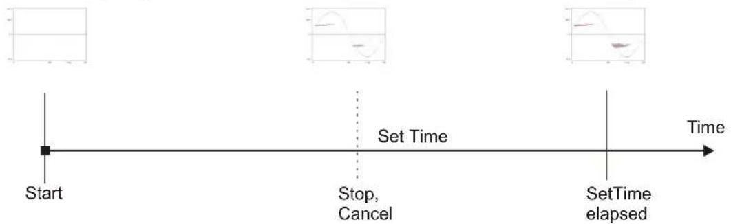
flowchart
graph LR
    A["Start"] --> B["Stop, Cancel"]
    B --> C["SetTime elapsed"]
    style A fill:#000,stroke:#fff,color:#fff
    style B fill:#f9f,stroke:#000,color:#fff
    style C fill:#f9f,stroke:#000,color:#fff
Fig. V.1: Single-channel standard mode
The single-channel consecutive mode (figure V.2) can be used to create a consecutive number of files with identical measurement times. After having started this mode, the software takes care of stopping the acquisition and re-starting the pattern acquisition automatically after the pre-set delay time between two starting points has passed. This mode is useful for long term measurements when trending information and new PD sources shall be detected. This mode can be stopped manually by pressing the buttons 'Stop' or 'Cancel'. The maximum number of files is limited to 9999. The user can choose a file prefix before starting the measurement. Each file name consists of this file prefix chosen and the number of the current file. The ICMmovie program offers a movie like replay of such consecutive files.
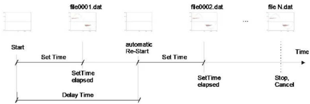
flowchart
graph LR
    A["Start"] --> B["Set Time"]
    B --> C["SetTime elapsed"]
    C --> D["Automatic Re-Start"]
    D --> E["Set Time"]
    E --> F["SetTime elapsed"]
    F --> G["Stop, Cancel"]
    G --> H["File N.dat"]
Fig. V.2: Single-channel consecutive mode
In case a multi-channel instrument is used, the software offers two additional acquisition modes: The multi-channel (MC) standard mode and the multi-channel consecutive mode. The difference to the single-channel mode is, that the software toggles to the next activated channel after having finished one PD pattern acquisition. In multi-channel standard mode (figure V.3) the PD pattern acquisition starts with channel one, if enabled, and takes a measurement of the pre-set 'Scan Period'. This 'Scan Period' has to be shorter than the 'Set Time' value. After this acquisition the software changes to the next enabled channel and starts a new pattern acquisition. At the end of one channel loop this procedure repeats as often as needed to get a full PD pattern of each channel for the pre-set 'Set Time'. The acquisition can be stopped at any time by pressing 'Stop' or 'Cancel'. One file for each channel is saved automatically after the measurement has been completed, if the 'Auto Save' option is enabled. Otherwise, it is necessary to save each file separately. The multi-channel standard mode is taken, when emphasis is placed on identifying the inception of a PD activity with a larger setup, such as with a commissioning test. Here, the 'Scan Period' is set to few seconds, only, in order to get a short cycle time. However, the history of the discharge activity is lost, since only one file per channel is created.

flowchart
graph LR
    A["Start"] --> B["Scan Period"]
    B --> C["file1.dat"]
    C --> D["file2.dat"]
    D --> E["..."]
    E --> F["file8.dat"]
    F --> G["file1.dat"]
    G --> H["file2.dat"]
    H --> I["..."]
    I --> J["Set Time of each channel completed"]
    J --> K["Time"]
Fig. V.3: Multi-channel standard mode
The difference between this standard mode and the consecutive mode is that in consecutive mode the data of one channel is not added up to one resulting PD pattern. Each cycle takes the 'Set Time' for each channel, and after having stopped automatically the data is stored to a file named e.g. 1file0001.dat (
Thus, for each channel a set of consecutive files is created. As with the single-channel consecutive mode, a movie-like replay is offered by the ICMmovie software. Using this mode, the full history of the PD activity is stored. However, to obtain a reasonably filled 'dat' file, usually, the 'Set Time' is 30 s or above per channel. Thus, the cycle time, i. e., the time the instrument needs to returns to the same channel, is relatively long. Therefore, this mode is less suitable when immediate action is required in case of the inception of partial discharge activity, for example.

flowchart
graph LR
    A["Start"] --> B["Set Time"]
    B --> C["Set Time"]
    C --> D["..."]
    D --> E["Set Time"]
    E --> F["Set Time"]
    F --> G["Set Time"]
    G --> H["Time"]
    H --> I["Total Time elapsed"]
    style A fill:#f9f,stroke:#333
    style I fill:#ccf,stroke:#333
Fig. V.4: Multi-channel consecutive mode
V.3 Standard Laboratory Measurements
With a standard laboratory application usually a high voltage source and a coupling capacitor is available. Often a shielded room is provided offering low levels of electromagnetic interference originating from external sources. The test setup follows in most cases given standards, such as the IEC 60270, for example. The circuit of such conventional test setup consists of the device under test (DUT) connected to the high voltage source and a coupling capacitor connected in parallel as shown with figure V.5. Into the ground lead of the coupling capacitor a quadrupole is inserted. This quadrupole serves to separate the high frequency current of the partial discharge signals from the power frequency current of the capacitor. Furthermore, this quadrupole may contain a suitable low voltage capacitor to form a voltage divider together with the coupling capacitor to provide the partial discharge detector with the synchronisation signal and to allow voltage measurements. In case the device under test or sample has a relative low capacitance, the quadrupole may be placed in the sample's ground lead, alternatively. However, a coupling capacitor is required in almost all cases in order to provide an adequate path for the high frequency signals and, subsequently, to derive a suitable signal strength while avoiding ringing of the PD pulses. Only in very few cases this required high frequency loop might be provided by the capacitance of the transformer's bushing.

flowchart
graph TD
    A["HV Transformer"] --> B["CAL"]
    B --> C["Sample, DUT"]
    C --> D["Quadrupole"]
    D --> E["PD"]
    D --> F["Sync"]
    G["Coupling Capacitor"] --> C
    G --> D
Fig. V.5 Standard test setup
It is mandatory in general to optimise the high frequency behaviour of the coupling circuit in order to derive an efficient coupling and to provide the instrument with clear, non-oscillatory pulses. Although the instrument is suited to cope with non-ideal conditions as found with field measurements, optimum performance of the ICMsystem is reached only by providing the instrument with such clear pulses with a steep front, no ringing, and a short duration. Optimising a test setup regarding its high frequency behaviour requires several measures:
- Choose the appropriate quadrupole that fits to your coupling capacitor (refer to section II.3 of the hardware section). Power Diagnostix may assist you in case you require a special tailor-made coupling unit.
- Keep all connection leads as short as possible. Avoid wrapping a high voltage connection cable on top of the coupling capacitor, for example: The additional inductance may lead to oscillatory pulses.
- Use test leads of larger diameter. For the ground leads copper mesh tapes are a good choice.
- Inject calibration pulses as shown with figure V.5 and monitor the PD output of the quadrupole with an oscilloscope to validate your measures. Alternatively, you may identify pulse ringing or the so-called -response (first peak smaller than the following undershot) by viewing the PD pattern of the ICMsystem, while modifying the dead time and the trigger mode of the ADC module.
Besides the high frequency considerations listed above, take care of proper handling of the high voltage, as well. Obey all safety regulations concerning your test setup. Consider all comments regarding safety given with this manual. Especially, provide a solid grounding of the coupling circuit and the instrument.
The basic circuit is shown with figure V.6 with respect to the ICMsystem modules needed. In general, an ICMsystem measurement configuration consists of:
- The signal coupler. With the standard laboratory application this is usually a coupling capacitor equipped with a matched quadrupole. In non-conventional applications this may be a part of the test object itself that is used for coupling purposes. A second coupler may be used to trigger a gate for rejecting unwanted pulses.
- The signal conditioning module which adapts the instrument to the signal coupler's properties. Subsequently, the pre-processed signal is transmitted to the acquisition unit.
• The acquisition unit. - A computer equipped with a GPIB or serial interface to control the instrument through the ICMsystem software.
With figure V.6 a coupling capacitor assembly with built-in quadrupole, the CC25B, is used. This CC25B stands for any matched combination coupling capacitor and quadrupole. Its output signal is fed to the RPA1's input. Subsequently, the RPA1's output is connected to the AMP IN terminal of the ICMsystem's AMP5 module. With this figure and the following a rectangular block showing the used connectors, only symbolises the ICMsystem. In case a quadrupole with voltage output is used, such as the CIL4M/V, the SYNC IN input of the ICMsystem is connected to the voltage terminal of the quadrupole. Coupling capacitor assemblies, such as the CC25B/V or the CC25C/V are equipped with a voltage output as well. Check in general the appropriate divider ratio for the maximum voltage you want to apply and consider the instrument's input range (200 V_peak max.).

flowchart
graph TD
    A["Test object"] --> B["High voltage cable"]
    B --> C["Capacitive PD coupler CC100B/V"]
    C --> D["Snchronization signal"]
    D --> E["RPA1"]
    E --> F["Laptop with waveform graph"]
    F --> G["Serial interface"]
    G --> H["RPA1"]
    H --> I["Noise coupling antenna or high frequency current transformer"]
    I --> J["(Used for gating)"]
Fig. V.6 Basic application circuit with ICMsystem (Gen. 5)
Optionally, a second RPA1 is connected to the AMP IN terminal of the AMP5 module that is used for gating. The input signal is derived from an antenna picking up the disturbance signal. Furthermore, a clip-on current transformer, such as the CT100, may be used to pick up disturbance signals by feeding the ground lead of a cabinet containing arcing relays, for instance, through the CT's window.
A notebook or PC is connected by means of a GPIB (IEEE488) interface or through a serial cable to the ICMsystem's rear-side GPIB connector or the serial connector on the front side, respectively. With the instrument energised, the ICMsystem program will recognise the acquisition unit during start-up. Refer to the section describing the software for the available modes of choosing different instruments on the GPIB bus, for instance. The partial discharge measurement is a relative measurement. Thus, prior to a PD test, a calibration of the instrument and the entire signal chain needs to be performed. A calibration impulse generator is connected as indicated with figure V.5. In most cases the CAL1A is best-suited (use the CAL1B or CAL1D in case charges of 100 pC and more are to be calibrated). Subsequently, with an acquisition started, a double click on the appearing pattern of the calibration pulse brings up the calibration edit panel.
The value injected by the calibrator is filled in. With clicking to the OK button, the correction factors are calculated according to the current configuration. Save this acquisition as the reference file for the current calibration. You may re-load this file in case you return to an identical configuration. Refer to section III.1.9 for more details regarding the calibration and to section II.4 for details on the calibration impulse generators available with Power Diagnostix.
The basic connection of the ICMsystem equipped with multiple channels is shown with figure V.7. Each input channel is connected by means of an individual high voltage capacitor, a quadrupole, and an RPA1. The cable between quadrupole and RPA1 must be as short as possible, since the RPA1's input sensitivity relies on its high input impedance of 10 kΩ//50 pF. With the use of an RPA2 having a 50 Ω input impedance the pre-amplifier may be placed between multiplexer and AMP IN. One of the quadrupoles may be equipped with a divider capacitor to synchronise the instrument and to measure the voltage signal.

flowchart
graph TD
    A["Test object"] --> B["High voltage capacitance"]
    B --> C["CIL4L"]
    C --> D["RPA1"]
    D --> E["ICM system"]
    F["Test object"] --> G["High voltage capacitance"]
    G --> H["CIL4L"]
    H --> I["RPA1"]
    I --> J["ICM system"]
    K["Test object"] --> L["High voltage capacitance"]
    L --> M["CIL4L"]
    M --> N["RPA1"]
    N --> O["ICM system"]
    P["ICM system"] --> Q["Sync. source"]
    Q --> R["Laptop with waveform display"]
    S["Noise coupling antenna"] --> T["RPA1"]
    T --> U["ICM system"]
Fig. V.7 Basic ICMsystem application circuit without gating
The instrument's setup needs to be adapted to the properties and requirements of the test to be conducted. The meaning of the setup entries and their effects are discussed in detail with the software section and, partly, with the hardware section of this manual.
Two groups of parameters of the instrument's setup require a more detailed attention, since both do severely affect the performance of the instrument and may lead to malfunction in case chosen inadequately. The first group is the combination of pre-amplification and main amplification with respect to the pre-amplifier chosen. The second one is the combination of dead time, low level discriminator, and ADC trigger mode.
The appropriate choice of the combination of pre and main amplification is mainly a compromise between noise and over-ranging considerations. The pre-amplifier RPA1 has an input sensitivity of better than 200 V_peak . Its output stage is able to drive a 50 load at a maximum signal level of 1.5 V_peak . The AMP IN terminal of the AMP5 module offers an input sensitivity of about 200 V_peak , if used as a direct input with the power supply of the RPA turned off (input impedance: 50 ). These limitations form the guidelines how to choose the combinations of pre-amplification and main amplification:
- Avoid choosing a main gain setting above 200 while using a pre-amplifier, as it causes an excessive amplification of input noise.
- Be aware of the 50 Ω input impedance of the AMP IN terminal if used without a pre-amplifier.
With respect to these limitations, the [+] and [-] buttons of the ICMsystem software select the combination of the two amplifications from a table that runs between a main gain of 8 to 40, i. e., 10/40 is followed by 100/8. This pre-set table is well suited for most of the cases. With the AMP5 module's filters set to 250 kHz, even the main gain of 8 might be too low, since the 1.5 V of the pre-amplifier is reduced to somewhat below 40% by the 250 kHz filter. With some applications the partial discharge pulse has a predominant high frequency content. In such cases similar effects may happen, since the RPA1 is able to process frequencies up to 2 MHz which may undergo signal clipping and subsequently may lead to a distorted pattern. Try in all situations, where you are in doubt, the alternative expression of the amplification, i. e. with 100/8 you may try 10/80. The latter may cause larger noise amplitudes, but over-ranging of the pre-amplifier does not hamper the measurement. Figure V.8 shows a table of the approximate full-scale RPA1 input amplitudes (in [mV]) to cause a full-scale signal of the pattern display. This table refers to a band-pass setting of 40–800 kHz. With the red coloured cells at the left-hand side an over-ranging of the RPA1's input stage may occur. Reduce the efficiency of your coupling circuit in case signal strength (input amplitudes in excess of 1 V_peak ) forces you to reach these combinations of settings. A simple way of such reduction of the efficiency is to load the PD signal with a 50 BNC termination resistor. The shading of the areas at the right-hand side symbolises that the noise floor with the pattern has raised the one percent level, while with the red coloured cells the noise floor is beyond of ten percent, i. e. the LLD needs to be set above ten percent, as well.
| Main Amp GainPre-Amp Gain | 4 | 8 | 10 | 20 | 40 | 80 | 100 | 200 | 400 | 800 |
| Off (R | = 50 Ω) | 1250 | 625 | 500 | 250 | 125 | 62.5 | 50 | 25 | 12.5 | 6.25 |
| 1 (R | = 10 kΩ) | 1250 | 625 | 500 | 250 | 125 | 62.5 | 50 | 25 | 12.5 | 6.25 |
| 10 (R | = 10 kΩ) | 125 | 62.5 | 50 | 25 | 12.5 | 6.25 | 5.0 | 2.5 | 1.25 | 0.625 |
| 100 (R | =10 kΩ) | 12.5 | 6.25 | 5.0 | 2.5 | 1.25 | 0.625 | 0.5 | 0.25 | 0.125 | 0.062 |
| 5.0 | Noise ≥ 1% | 0.5 | Noise ≥ 10% | |||||||
Fig. V.8 Input signal [mV] to cause a full-scale reading vs. the combinations of pre- and main gain
With the pre-set table of combinations, as shown with figure V.9, the critical settings at the corner points of the pre-amplification are avoided. However, no limitation exists regarding the settings with the remaining risk of pre-amplifier saturation (total gain of 1 or 2) and the noise at the high-gain end.
| Total gain | 4 | 8 | 10 | 20 | 40 | 80 | 100 | 200 | 400 |
| Pre Amp Gain | 1 | 1 | 1 | 1 | 1 | 10 | 10 | 10 | 10 |
| Main Amp Gain | 4 | 8 | 10 | 20 | 40 | 8 | 10 | 20 | 40 |
| Total gain | 800 | 1000 | 2000 | 4000 | 8000 | 10000 | 20000 | 40000 | 80000 |
| Pre Amp Gain | 100 | 100 | 100 | 100 | 100 | 100 | 100 | 100 | 100 |
| Main Amp Gain | 8 | 10 | 20 | 40 | 80 | 100 | 200 | 400 | 800 |
| 40 | Noise ≥ 1% | 200 | Noise ≥ 10% |
Fig. V.9 Pre-set table of the combinations of pre- and main gain
With the pre-amplifier switched off, the main gain is modified, only. As shown with figure V.8 no precautions regarding saturation or broadband noise are required. Consider the 50 Ω input impedance loading your signal source. Use this configuration (w/o RPA) only with pre-processing devices, such as spectrum analysers, ultra-sonic receivers, or photon multiplier devices, for instance. Further, make sure that the pre-amplifier gain is set to 'Off', as the supply voltage of the RPA carried by the AMP IN terminal may damage the output of your signal source. However, the use of the RPA1 is possible in such applications, as well. If required, use a 50 Ω BNC termination resistor at the RPA1's input. The use of an RPA with common high-voltage test setups is mandatory, since the RPA's input circuits offer an effective over-voltage protection, superseding the protection of the AMP IN terminal by far.
The second group of settings requiring an extended attention is the combination of low level discriminator (LLD), dead time, and ADC trigger mode with respect to the pulse properties of the input signal. The ICMsystem does not contain a continuously running A/D converter, where the peak value is derived by calculations. With the ICMsystem the pulse itself triggers a conversion. The LLD acts as a kind of trigger threshold for this conversion cycle. As soon as a pulse exceeds this threshold, an analogue peak detector tracks the signal of the current polarity or, depending on the trigger mode chosen, two peak detectors are used for tracking both polarities. Subsequently, the captured peak is converted and transferred to the pattern memory. With the dead time expired the circuit is re-armed to capture the next peak.
The instrument offers two different main trigger modes: Trigger in time window (TW NRT = time window non-re-triggerable) and trigger on first peak (FP (N)RT = First Peak (Non) Re-triggerable). Additionally, the trigger on first peak mode can be set to re-triggerable and to non-re-triggerable action.
The latter trigger on first peak mode (non-re-triggerable) is the standard mode, which gives best results with most of the applications. The pulse first exceeding the LLD threshold determines the polarity. Subsequently, the next peak value is captured and converted to its digital expression. This procedure takes about one microsecond. With the duration of the dead time no other peak is accepted. The dead time serves to avoid considering the under-shots or the ringing of a pulse as individual pulses. With respect to the properties of the entire signal chain acting as a band-pass of higher order, the minimum dead time was limited to five microseconds. The various effects of the low level discriminator's setting, the dead time chosen, and the shape of the pulse to be captured, are illustrated with the sketches shown with figure V.10. Several cases are listed with these simplified sketches. The main conclusions are that a dead time chosen too short causes multiple triggering on one single pulse, while a dead time chosen longer than required may result in the loss of pulses and in a reduction of the possible pulse repetition rate. In general, it is mandatory to set the LLD level slightly ahead the noise floor to avoid excessive cumulated dead times. With the LLD set too low the instrument is mainly busy converting all the small (noise) pulses with the effect of potentially losing the (few) larger true partial discharge pulses.
95

line
| Time Segment | Value | | ------------ | ----- | | dead time | 1 | | pd signal | -2 | | LLD | 0 |Dead time: correct
First peak detected correctly.

line
| Time Segment | Signal | | ------------ | ------ | | Dead Time | High | | LLD | Low |Dead time: too short
First peak and second positive overshoot detected.
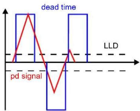
line
| Time Segment | Value | | ------------ | ----- | | Left Segment | 0 | | Peak | 1 | | Mid | -2 | | Right Segment | 0 |Dead time: much too short
Biggest peak detected. Negative undershot and positive overshot detected, as well.

line
| Time Segment | Signal Type | | ------------------ | --------------- | | Dead time | 1st day peak | | Dead time | 2nd day peak | | 1st day | 1st day peak | | 2nd day | 2nd day peak |Dead time: correct
Biggest first peak detected correctly. Due to high counterate detection of the negative undershot of the second pulse, only.

line
| Time | Value | |------|-------| | 0 | pd signal | | 1 | 0 | | 2 | -1 | | 3 | 0 | | 4 | -1 | | 5 | 0 |Dead time: correct
Due to -response biggest peak undetected.
Smaller first peak detected, only. Polarity swaps
if first peak drops under the LLD threshold.

line
| Time Segment | Signal Type | | ------------------ | --------------- | | 0 | dead time (blue box) | | 1 | dead time (blue box) | | 2 | dead time (blue box) | | 3 | dead time (blue box) | | 4 | dead time (blue box) | | 5 | dead time (blue box) | | 6 | dead time (blue box) | | 7 | dead time (blue box) | | 8 | dead time (blue box) | | 9 | dead time (blue box) | | 10 | dead time (blue box) | | 11 | dead time (blue box) | | 12 | dead time (blue box) | | 13 | dead time (blue box) | | 14 | dead time (blue box) | | 15 | dead time (blue box) | | 16 | dead time (blue box) | | 17 | dead time (blue box) | | 18 | dead time (blue box) | | 19 | dead time (blue box) | | 20 | dead time (blue box) | | 21 | dead time (blue box) | | 22 | dead time (blue box) | | 23 | dead time (blue box) | | 24 | dead time (blue box) | | 25 | dead time (blue box) | | 26 | dead time (blue box) | | 27 | dead time (blue box) | | 28 | dead time (blue box) | | 29 | dead time (blue box) | | 30 | dead time (blue box) | | 31 | dead time (blue box) | | 32 | dead time (blue box) | | 33 | dead time (blue box) | | 34 | dead time (blue box) | | 35 | dead time (blue box) | | 36 | dead time (blue box) | | 37 | dead time (blue box) | | 38 | dead time (blue box) | | 39 | dead time (blue box) | | 40 | dead time (blue box) | | 41 | dead time (blue box) | | 42 | dead time (blue box) | | 43 | dead time (blue box) | | 44 | dead time (blue box) | | 45 | dead time (blue box) | | 46 | dead time (blue box) | | 47 | dead time (blue box) | | 48 | dead time (blue box) | | 49 | dead time (blue box) | | 50 | dead time (blue box) | | 51 | dead time (blue box) | | 52 | dead time (blue box) | | 53 | dead time (blue box) | | 54 | dead time (blue box) | | 55 | dead time (blue box) | | 56 | dead time (blue box) | | 57 | dead time (blue box) | | 58 | dead time (blue box) | | 59 | dead time (blue box) | | 60 | dead time (blue box) | | 61 | dead time (blue box) | | 62 | dead time (blue box) | | 63 | dead time (blue box) | | 64 | dead time (blue box) | | 65 | dead time (blue box) | | 66 | dead time (blue box) | | 67 | dead time (blue box) | | 68 | dead time (blue box) | | 69 | dead time (blue box) | | 70 | dead time (blue box) | | 71 | dead time (blue box) | | 72 | dead time (blue box) | | 73 | dead time (blue box) | | 74 | dead time (blue box) | | 75 | dead time (blue box) | | 76 | dead time (blue box) | | 77 | dead time (blue box) | | 78 | dead time (blue box) | | 79 | dead time (blue box) | | 80 | dead time (blue box) | | 81 | dead time (blue box) | | 82 | dead time (blue box) | | 83 | dead time (blue box) | | 84 | dead time (blue box) | | 85 | dead time (blue box) | | 86 | dead time (blue box) | | 87 | dead time (blue box) | | 88 | dead time (blue box) | | 89 | dead time (blue box) | | 90 | dead time (blue box) | | 91 | dead time (blue box) | | 92 | dead time (blue box) | | 93 | dead time (blue box) | | 94 | dead time (blue box) | | 95 | dead time (blue box) | | 96 | dead time (blue box) | | 97 | dead time (blue box) | | 98 | dead time (blue box) | | 99 | dead time (blue box) | | 100 | dead time (red line)|Dead time: too long
Second pulse remains undetected.
Fig. V.10 Trigger on first peak, non-re-triggerable mode
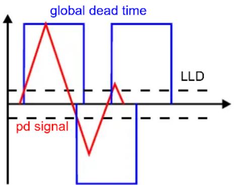
line
| Position | Value | | -------- | ----- | | Left | 0 | | Peak | 1 | | Mid | -2 | | Right | 0 |Multiple reading inhibited
Dead time increased to global dead time
Fig. V.11 Trigger on first peak, retriggerable

line
| Time Window | Peak Signal | | ----------- | ----------- | | Low | Low | | High | High |Fig. V.12 Trigger in time window
The re-triggerable option of the trigger on first peak mode offers an adaptation of the effective dead time. In order to prevent multiple readings of oscillatory signals, for instance, the dead time is automatically extended to the so-called global dead time by its original value if a further signal peak occurs during the initial dead time period (figure V.11). This option offers a convenient way to have the global dead automatically matched, but it bears with some applications the risk of excessive dead times. These excessive dead times, which can invalidate the whole measurement, may occur with high pulse repetition rates or with strongly oscillating signals. Especially, in case the LLD threshold was chosen too low, the global dead time might be extended ad infinitum and, subsequently, blind the instrument totally. Thus, this option should be used carefully, only.
Band-pass properties of the entire signal path from the discharging site to the A/D converter's input may cause the so-called -response with a smaller first peak leading a larger undershot, as mentioned earlier already. With such signal properties the use of the trigger in time window mode of the ADC module is required (figure V.12). With this mode the dead time acts as a time window within which the largest pulse is acquired, only. As with the previous mode, a signal exceeding the LLD threshold starts the pulse acquisition, but other than with the trigger on first peak mode, two peak detectors are used to capture both the positive and negative maximum pulse amplitude. With the expiration of the dead time both amplitudes are compared, and the decision of the polarity is made. Subsequently, the biggest pulse amplitude is converted to its digital expression and counted with the pattern memory. Again, with the trigger on first peak the first pulse higher than the LLD determines the pulse polarity, whereas with the trigger in time window this first pulse starts the pulse capturing, only. While using the trigger in time window, the setting of the LLD threshold is not that critical as it is with the trigger on first peak, since the predominant pulse magnitude within the window will be captured, even if that window was triggered by a smaller (noise) pulse. Thus, an inappropriate low LLD setting does not cause necessarily the loss of (all) large pulses.
With some applications all the measures provided by the instrument and described above does not allow revealing the correct polarity of the partial discharge pulses. This may happen with strongly ringing pulses or in cases where the pulse repetition rate is (temporarily) higher than the maximum rate of 200 kHz determined by the minimum dead time of five microseconds. In such cases, where the acquired polarity is meaningless, the ADC's coding page Linear bipolar is to be used.
V.4 Rotating Machines
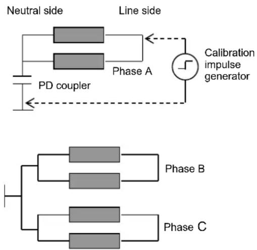
Fig. V.13 Off-line test, neutral bridge removed

Fig. V.14 Off-line test, neutral bridge
A stator winding of a rotating machine is relatively voluminous, it bears extended signal paths with various transfer properties causing a calibration being valid for the point of charge injection with respect to the coupling point and method, only. To determine the influence of the transfer function of the winding the signal strength of different points of charge injection needs to be compared.
With off-line tests the entire winding is energised with a conventional high voltage test set or with a resonant test set. In case the neutral connection is opened, each of the three phases can be tested individually. Depending on the accessibility, a coupling to the neutral side of the winding or to the line side may be chosen. The range of the 1 nF-couplers is a good choice. The CC25C/V offers a quadrupole connection and a high frequency current transformer output, as well as a voltage divider output for synchronisation and voltage measurement. Permanently installed couplers of the CC20B type may be utilised as well, as they offer a superimposed voltage signal for the synchronisation as well. Other types of couplers, such as the cable type couplers may be used with some restrictions regarding bandwidth and synchronisation.
With off-line tests the RPA1 is the standard pre-amplifier used, as this pre-amplifier operates in a frequency range offering a relative wide overview of the stator winding. Although this frequency range is hampered by external disturbances, such as thyristor firing pulses, it needs to be used with acceptance tests. The RPA2, operating in the frequency range of 2 to 20 MHz, covers a range where the commonly used quasi-integration of the pulses with a low-pass filter is not valid, in principle. But as the central function of the RPA2 is a rectification of the high frequency signal and a subsequent processing of the envelope of that rectified signal derived by low-pass filtering, a calibration in terms of pico-coulombs is roughly valid with this amplifier, as well. Nevertheless, a
validation of such calibration is required. To obtain this validation, the calibration impulse generator is connected to different points of the winding to evaluate the signal attenuation across the winding or parts of the winding. As a convention one may refer to a calibration with injection to the line side, i. e., to the part of the winding exposed to the highest voltage level, as shown with figures V.13 and V.14. As described in detail with the calibration section III.1.9, an acquisition is started for at least 100 s, giving you enough time for the required adjustments. The calibrator is connected to the line side terminal of the phase to be measured. The amplification is adjusted to give a utilisation of 50–90% of the meter's maximum reading. With the acquisition started a double-click to the map position, where the dot cluster or line of dots of the calibrator's signal appears, calls the calibration subpanel. Fill in the value of the calibrator's charge and confirm with OK. Both map and meter is now calibrated, i. e., the correction factors are calculated to the current setup's attenuation and related signal properties.
Subsequently, other accessible points to inject charge pulses are compared with this reference measurement to evaluate the signal distribution over the winding. As the RPA2 covers a frequency range where a machine winding still offers a relatively low attenuation and combined with the increasing effect of cross coupling and system resonance, the use of the RPA2 may sometimes result in a lower overall attenuation compared with the use of the RPA1. Nevertheless, these properties of the machine winding must be evaluated with every individual machine type. To avoid confusion with the results of such measurements, it is mandatory having one calibration file per phase with all measurements with this phase including the comparison measurements with other injection points referring to that calibration. Further, one should write detailed notes describing the measurement setup, the connections made, the coupling, and the calibration. Additionally, a clearly arranged structure of sub-directories is helpful in general.
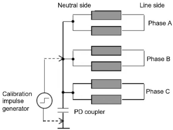
Fig. V.15 Off-line test, neutral connection
On-line tests are usually made with line-side couplers permanently installed. With no permanently installed couplers available, a connection similar to the circuit symbolised with figure V.15 may be chosen. This on-line neutral connection shown with figure V.18, as well, bypasses the neutral inductor, neutral transformer, or neutral resistor for high frequency signals. The line-side coupling requires three pieces of CC20B couplers installed to the terminals of the machine or to the bus bar. A calibration is made with the injection of the charge signal across the coupler. Subsequently, a comparison is made with injection to the neutral terminal, in case accessible. Furthermore, the cross coupling can be evaluated with injection of the charge pulses across the couplers of the other phases. The use of the RPA1 is in most cases hampered by noise interference originating from the excitation and control system. The ICMsystem's gating feature can be utilised to remove some of the interference signals. Especially, pulses of the excitation are promising candidates for gating. Nevertheless, the RPA2 is the best choice for on-line measurements.

flowchart
graph TD
    A["Neutral side"] --> B["Phase A"]
    A --> C["Phase B"]
    A --> D["Phase C"]
    B --> E["PD coupler"]
    C --> F["PD coupler"]
    D --> G["PD coupler"]
    H["Calibration impulse generator"] --> I["Ground"]
    style A fill:#f9f,stroke:#333
    style H fill:#ccf,stroke:#333
Fig. V.16 On-line test, calibration with line-side connection
Figure V.18 shows the neutral connection to a generator while on-line. In this case the neutral point is tied to ground. Thus, the neutral coupler cannot derive any synchronisation signal. Figure V.17 illustrates temporarily on-line coupling to the line side, for instance. In principle this coupling applies to any medium voltage equipment, whether on-line or off-line, unless the test voltage is higher than the 25 kV limit of the CC25x.

flowchart
graph TD
    A["Generator neutral"] --> B["ICM system"]
    B --> C["Sync. source"]
    B --> D["RPA1"]
    D --> E["Noise coupling antenna"]
    B --> F["RPA1"]
    F --> G["ICM system"]
    G --> H["Laptop with waveform graph"]
Fig. V.18 On-line PD measurement with neutral side coupling (external or line sync)

flowchart
graph TD
    A["Test object"] --> B["ICMsystem"]
    B --> C["RPA1"]
    C --> D["Noise coupling antenna"]
    C --> E["ICM System 1"]
    C --> F["ICM System 2"]
    C --> G["ICM System 3"]
    C --> H["ICM System 4"]
    C --> I["ICM System 5"]
    C --> J["ICM System 6"]
    C --> K["ICM System 7"]
    C --> L["ICM System 8"]
    C --> M["ICM System 9"]
    C --> N["ICM System 10"]
    C --> O["ICM System 11"]
    C --> P["ICM System 12"]
    C --> Q["ICM System 13"]
    C --> R["ICM System 14"]
    C --> S["ICM System 15"]
    C --> T["ICM System 16"]
    C --> U["ICM System 17"]
    C --> V["ICM System 18"]
    C --> W["ICM System 19"]
    C --> X["ICM System 20"]
    C --> Y["ICM System 21"]
    C --> Z["ICM System 22"]
    C --> AA["ICM System 23"]
    C --> AB["ICM System 24"]
    C --> AC["ICM System 25"]
    C --> AD["ICM System 26"]
    C --> AE["ICM System 27"]
    C --> AF["ICM System 28"]
    C --> AG["ICM System 29"]
    C --> AH["ICM System 30"]
    C --> AI["ICM System 31"]
    C --> AJ["ICM System 32"]
    C --> AK["ICM System 33"]
    C --> AL["ICM System 34"]
    C --> AM["ICM System 35"]
    C --> AN["ICM System 36"]
    C --> AO["ICM System 37"]
    C --> AP["ICM System 38"]
    C --> AQ["ICM System 39"]
    C --> AR["ICM System 40"]
    C --> AS["ICM System 41"]
    C --> AT["ICM System 42"]
    C --> AU["ICM System 43"]
    C --> AV["ICM System 44"]
    C --> AW["ICM System 45"]
    C --> AX["ICM System 46"]
    C --> AY["ICM System 47"]
    C --> AZ["ICM System 48"]
    C --> BA["ICM System 49"]
    C --> BB["ICM System 50"]
Fig. V.17 On-line PD measurement with line side coupling, sync signal derived from coupler
V.5 Gas Insulated Switchgear (GIS)
Partial discharge measurements on GIS equipment require special measures to effectively couple to the signals. Discharges occurring under SF_6 atmosphere are characterised by their extreme bandwidth up to the ultra-high frequency (UHF) range. As the materials used internally with gas-insulated switchgear allows the transmission of signals of such a bandwidth to a certain extent, as well, partial discharge measurements in the UHF range are possible in principle. However, utilisation of the inherent benefits of PD measurements at such high frequencies requires a careful design of the entire signal chain in order to maintain the available bandwidth.
The design of the GIS sensors, as the first link of the signal chain, used to pick up the pulse signals over such a wide frequency range requires special attention. The partial discharge impulses in SF _6 extend over a wide frequency range up to a couple of GHz. Discharges in GIS support insulators excite frequencies up to between 200 MHz and more than 1 GHz, depending on specific situations. It is thought that disturbances such as corona discharges in air on bushings or other disturbances do not enter into the GIS at frequencies higher than maybe 200 MHz. Our own studies show that in a few cases disturbances are found in the frequency range up to 2 GHz, as well. However, for on-line measurements and monitoring the UHF range appears to be best suited. A sensor for UHF monitoring is basically an antenna. We distinguish two types of sensors, a sensor that was integrated by the GIS manufacturer and the external retrofit sensor. The retrofit sensor is often less sensitive than the built-in, however the retrofit can be fitted to the GIS at marginal cost and whilst the equipment is on-line. The following retrofit sensors can be applied (figure V.19):
- External ring sensors, wrapped around non shielded support insulators (figure V.20).
- Window sensors, inserted into windows of disconnect switches, for example.
- Tapping of the ground connections of shield electrodes of current transformers, for instance.
- Tapping of embedded electrodes in support insulators (originally intended for electrical field shaping purposes).
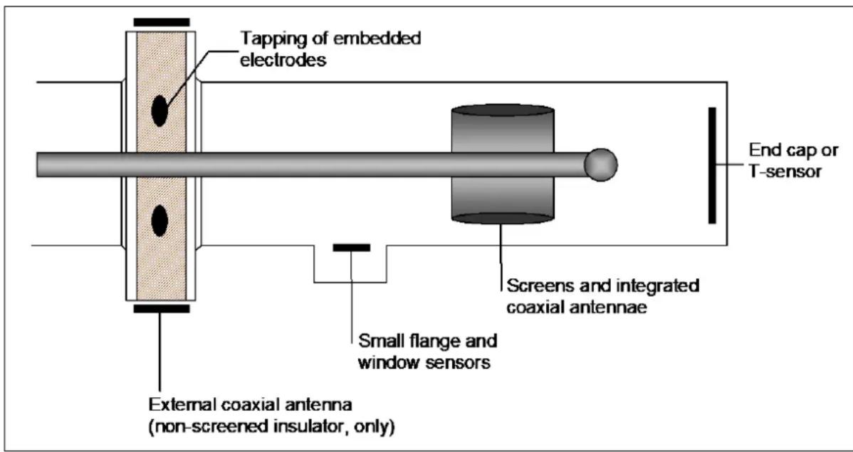
Fig. V.19 Possible sensor implementation with gas insulated switchgear (GIS)
The signals derived from these sensors are fed directly into the frequency converter unit FCU2 for signal processing. It may be necessary to protect the FCU2 against over-voltages causes by switching actions within the GIS by an input protection unit IPU2B. Alternatively, a spectrum analyser can provide appropriate signal pre-processing. The spectrum analyser is connected directly or via an UHF pre-amplifier, such as the UHF1, to the sensor. Subsequently, the analyser's output is connected via an RPA1 to the AMP IN terminal
of the ICMsystem's AMP5 module. First, the entire spectra is monitored with the analyser, areas of pulse activity are identified by comparison of the analysers average and peak-hold mode. The analyser's trigger must be set to free run, while viewing the entire spectra. Second, the analyser is tuned to a specific frequency of pulse activity with the span set to zero, the bandwidth usually set between 100 kHz and 3 MHz, and the reference level adjusted to have the pulses remaining within the analysers display area. Make sure, that the linear Y-axis mode is chosen. Now, the trigger option of the analyser may be set to line or external trigger, derived from the ICMsystem's trigger output, for instance.
Flexible ring sensors are available for all sizes of GIS. Keep in mind that this type of sensor is applicable with non-shielded support insulators, only. Such flexible ring sensors are tailor-made with respect to the dimensions of the GIS to be equipped. Required dimensions to be specified are the flange width (A), the insulator thickness (B), and the flange diameter (C), or the flange's circumference (figure V.20).

Fig. V.20 External flexible ring sensors for non-shielded spacers
External window sensors can be mounted to inspection windows, which are frequently found with older GIS. Here, the obtained results with sensitivity are comparable to embedded sensors if the window has a diameter of 80 mm or higher. In case well matched, such external window sensors offer a sensitivity of few pC.
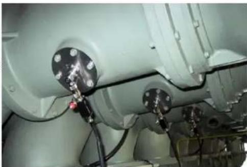
natural_image
Close-up of industrial machinery components with metallic fittings and wiring (no visible text or symbols)Fig. V.21: Windows sensor with FCU2

flowchart
graph TD
    A["Window sensor"] -->|IPU2B (opt.) & FCU2| B["ICMsystem"]
    C["DA2"] -->|50Ohm RG58/RG142 cables| B
    B --> D["Laptop with waveform display"]
Fig. V.23: Sample test setup for GIS measurements with FCU and optional IPU

flowchart
graph TD
    A["UHF1B"] -->|Low loss RG214 cable or others (UHF)| B["Spectrum analyzer"]
    B -->|VID OUT| C["ICMsystem"]
    C --> D["Laptop with waveform display"]
    E["DA2"] -->|RG58/142 cable| B
    F["Window sensor"] --> B
    G["Power supply"] --> B
    H["RPA1"] --> C
    style A fill:#f9f,stroke:#333
    style B fill:#ccf,stroke:#333
    style C fill:#cfc,stroke:#333
    style D fill:#fcc,stroke:#333
    style E fill:#cff,stroke:#333
    style F fill:#ffc,stroke:#333
    style G fill:#fcc,stroke:#333
    style H fill:#ffc,stroke:#333
Fig. V.22: Sample test setup for GIS measurements with UHF1 and spectrum analyzer
V.6 Cables and Accessories
V.6.1 Measuring Principles
Measurements on cables and accessories in a laboratory environment follow the strategies as described with the 'Standard Laboratory Measurements' section (0) of this section, i. e., the instrument is connected through a coupling capacitor to a conventional test setup. Recently, on-line PD monitoring and on-line after-laying PD tests of cables and accessories have found larger interest with the introduction of 400 kV polymer cables. However, the on-line after-laying test specifically for joints is worthwhile to be considered for MV cables, as well. This is possible if one integrates the so-called CCS into mainly cable joints. This technique has proven to be very effective for qualification tests of various joint and termination constructions in several applications. Long-term tests were conducted with ICMsystem multiplexer instruments equipped with LAN option for remote access. Partly, the instruments were equipped with fibre optic bus systems to safely chain up several units. Further, a specially suited version of the ICMmonitor offers a cost-effective monitoring of cable accessories under operation.
Such partial discharge detection is well suited for testing, diagnosis and monitoring of cable joints. It can be of interest to verify a joint's quality on-site when the cable is initially energised and, thus, supporting a decision whether a joint should be repaired or replaced before closing the excavation. All these measurements require an integrated sensor for effective coupling to the internal discharges. The central property of such sensor is that it must not affect the high voltage and insulation performance of the accessory or cable. Both effective coupling and the non-interference with the insulation system as the most critical objectives, is provided by the so-called coaxial cable sensor CCS. Figure V.24 shows the basic design of the CCS. A metal tape, foil, or metal mesh is applied on top of the outer semi-conductive layer acting as sensor connection. This sensor layer is connected to the inner conductor of a coaxial cable, such as RG58 or RG142 (a PTFE insulated cable). The sensor layer is isolated by means of wrapped tapes of adequate thermal stability. The shield of the signal cable is connected to another layer of metal foil or mesh applied on top of the wrapped insulation. Finally, the metal shield of the cable is (re-)

Fig. V.24 Coaxial cable sensor (CCS) applied to a power cable
applied. The capacitive divider formed by the metal tape layers determines the basic function of the CCS. This divider is loaded by the resistance of the cable's outer semi-conductive layer and, thus, introducing a high pass filter. The power frequency's ground is still provided by the semi-conductive layer leaving the insulation properties totally unaffected. Careful design of this sensor is required to derive high coupling efficiency and to maintain the integral noise suppression feature of this sensor. Assembly kits with readily connected PTFE signal cables are available to install such sensors to different types and sizes of cables and accessories. Power Diagnostix may assist with custom specific design.
The same basic principle is used in case parts of an accessory are used to act as sensing device. Main objective, again, is to avoid interference with the high voltage design of the accessory. Prominent candidates to be utilised as sensor or sensing part are those kept on the power frequency ground by resistive control, or those tied to ground by an individual connection. Further, a reliable method to connect the signal cable needs to be found. With most types of prefabricated joints, and accessories, such as outdoor terminations or GIS terminations, the stress cone can be utilised as sensor. The stress cone controls the shape of the electrical field when it enters the accessory. Thus, the quality of this field control and, especially, the mechanical quality of the lamination of this stress cone and the insulation material are very critical. In case the stress cone itself can be used as sensor, an excellent coupling is provided to signals originating from a delamination of the semi-conductive material, for instance.
Figure V.25 illustrates the coupling principle with a stress cone of a prefabricated adapter of a cable termination, for instance. Few layers of wrapped metal mesh (shown in orange) are applied to connect both the stress cone (grey coloured) and the outer semi-conductive layer (hatched) to a signal cable of 50 impedance. The signal cable's screen is connected to the power cable's shield or sheath, while leaving a certain part of the outer semi-conductive layer uncovered. This part of the layer forms a cylindrical resistor of the length S. Depending on the properties of that layer a length of few centimetres is enough to result in a resistance of 100 or more. Depending on the dimensions of the stress cone, the capacitance between the power cable's conductor and the sensing parts is in the range of several tens of Ohms and few hundred Ohms. The stray capacitance, i.e., the capacitance between sensor and ground, shall be kept as low as possible, as both capacitors form a divider limiting the coupling efficiency. The value of the cylindrical resistor

Fig. V.25 Connection to utilise an accessory's stress cone for sensing purposes
loading this high frequency capacitive divider is not critical in case it exceeds 50–100 Ω. Nevertheless, this resistor's value must not exceed several kilo-Ohms, as it carries the capacitive power-frequency current of the sensing parts. The value of that resistor can be easily measured at the sensor's external connector with the power cable de-energised. Further, with the cable energised, the capacitive current of the sensing parts is measurable. Thus, besides providing the high frequency coupling, this 'diagnostic connector' offers access to other parameters of interest. A sensitivity of about 1 pC can be achieved compared to conventional measurements according to standards such as the IEC 60270, for instance.
With cable joints the strategy is identical. An element of the joint construction, preferably a part of the field control system is utilised as sensor. This element is connected to a signal cable in a way suitable to carry high frequency signals, i. e., with short connections, avoiding non-shielded loops, and with a solid connection to the shield potential. Again, the main objective is to have these connections made on top of the semi-conductive layer and, thus, leaving the internal field distribution unaffected. With prefabricated joints being pre-moulded in one piece, the design of the sensor connection is often similar to the principle shown with figure V.25. With compression type joints using a pre-moulded adapter on each side, a pressure sleeve may be utilised to connect to the stress cone. Power Diagnostix may assist with the integration of sensors in existing accessory designs. Again, assembly kits with readily connected PTFE signal cables are available to install such sensors to different types and sizes of cables and accessories.
A sensor as described above is inherently de-coupled from the power frequency due to its high pass character. Another integral property of such sensor is that the signal cable's shield refers to the shield or sheath potential of the power cable. Subsequently, excessive voltage differences may be found between different sensors of a group of joints. Thus, this signal cable needs to be isolated from the ICMsystem's reference potential, while maintaining the high frequency signal to avoid damage due to excessive loop currents. For on-site installations the use of the IT2 is strictly mandatory to provide this isolation. The frequency range of the RPA2 is matched to the properties of the CCS and similar accessory sensors. With permanent installations and remote access, only, the IT2's isolation is sufficient, whereas operator controlled
on-line on-site measurements shall be made with fibre optic isolation provided by the RPA4 or other fibre optic signal transmission devices.

flowchart
ICM system architecture diagram showing sensor connections to ICM modules with synaptic source and output graphsFig. V.26 Connections for testing of power cable accessories
V.6.2 Synchronisation with Very Low Frequencies (VLF)
For synchronising under very low frequencies while testing e.g. high voltage cables the special synchronisation unit VLFS1 is available. This unit can be connected to a coupling capacitor's voltage output and converts an AC sine into a TTL logic signal for the TTL synchronisation input (SYNC IN). It recognises both the positive and negative half cycle and provides a high TTL level with the positive cycle and a low TTL level with the negative half of any AC sine wave.
For use of the VLFS1 the manual synchronisation has to be activated from the button bar of the ICMsystem software. The required synchronisation frequency should be entered in the upcoming pop-up window after a double click in the frequency field. For the synchronisation setting in the software, '+extern' must be selected (see explanation of 'Sync' field on page 60).

Fig. V.27: Connecting the VLFS1
Due to the unit's operational principle, the output signal of the VLFS1 has a frequency-dependent phase shift. Therefore, the correct phase position has to be verified with a partial discharge type that occurs at a fixed phase angle, e. g. a point plane discharge, starting in the negative half cycle's maximum (270°). The resulting phase position can be entered in the 'Phase shift' field of the subpanel 'Setup A' in the software (see explanation of 'Phase Shift' on page 60).
![Power Diagnostix - ICMystem File Edit Connect Measurement Tools View Panel Options Help Calibrated GPJB RS232 Modern Online TXD RXD N/A 5.0 s N/A 6.0 s File Name Spot. TE_2 Date 09-15-2014 Time 18:07:13 +651 [ pC ] 0.10 Edit... Sync. Frequency [Hz] 0.10 Cancel Auto OK Dead Time 1 0.0 s Gate Time 1 0.0 s Acq Time 7.4 s Total Counts 3793 Level Counts 3793 Voltage [ms] No Voltage Charge [Fatt] 40.6 pC RV [off] N/A NOB Value 26.54 nA Frequency 0.1 Hz [M] Amp In No 1 Set Time ADC LLD Coding Pre Gain Acq Mode Amp U Cutoff Pattern Acq Phase Shift Sync In 200.0 s 3.8% LR BIP 10 vs Phase 600 kHz AMP OUT 160° Sync 2 Input Mode Dead Time ADC Mode Waveform Amp Main Gain Count Level Amp L Cutoff Mem Erase Div Ratio Sync AMP TW NRT Sine 40 0 pC 100 kHz Auto 350.0 Extm Setup G MC Panel AT Panel Load Save Search Exit](/content/2026/05/1014079/images/3e7210053b32181a03708d16528845c1f0358d5893e090b78d5974a39d0fdc77.jpg)
Fig. V.28: Relevant settings for VLF synchronisation within the ICMsystem software
V.7 Power Transformers
V.7.1 Acceptance Testing
Typically, a multi-channel ICMsystem for acceptance testing on power transformers consists of the acquisition unit and a range of accessories as below:
- the multi-channel ICMsystem acquisition unit,
- one calibrator, type CAL1D (range 10 pC–1 nC) or CAL1B (range 100 pC–10 nC), 50 Hz or 60 Hz pulse repetition rate,
- 9 pre-amplifiers, type RPA1,
- 8 quadrupoles, type CIL4M/V0μ5/2μ0,
- 3 quadrupoles, type CIL5M/V4μ0,
- 3 high voltage filters T100/100.
Optional accessories such as coupling capacitors up to 100 kV, different quadrupole types, or tools for noise gating, for instance, are available to adapt the system to specific needs. Additionally, the instrument can be supplied with ready-to-use installed PCs or notebook computers.
The instrument should be placed close to the PC or laptop computer, which is normally used to run all tests within the test room. The power lead and the GPIB connector are located on the rear side of the instrument, whereas all signal input cables are connected at the front side of the unit.

Fig. V.29: Connection of CIL4M/V0μ5/2μ0 and RPA1
Always provide solid grounding of the instrument. Use the rear side wing nut terminal for ground connection. Never operate the instrument without protective grounding.
The quadrupole CIL4M/V0μ5/2μ0 should be connected to the tap of the transformer bushing (figure V.29). It is recommended to keep the connection cable to the pre-amplifier RPA1 as short as possible, as the capacitance of this cable adds to C2, which reduces the sensitivity. The quadrupole is designed for a bushing capacitance C1 in range of 200 pF to 2 nF, while the current is limited to 400 mA. The internal capacitance of the voltage divider is 2 μF. This quadrupole provides two output signals. The first one (PD) carries the partial discharge signal, which is subsequently amplified by the pre-amplifier. The second output (U) provides the ICMsystem with the synchronisation voltage signal. This voltage output can rise up to 140 V rms or 200 V peak . Both signals are transmitted to the acquisition unit using up to 50 m RG58 coaxial cables.
all three phases of transformer's high voltage winding. Depending on the test requirements, the activity of the three phases of the lower voltage side as well as on the neutral can be monitored. The system can use an individual synchronisation signal for each channel. However, often it is sufficient to use one synchronisation signal for each side.
Usually, the partial discharge activity is measured on
Please be careful when connecting the coaxial cables to the instrument and make sure that the voltage signal and the PD signal are not interchanged. As the voltage signal can rise up to 140 V_rms , the AMP IN input for the PD signal of the instrument can be damaged in case the wrong cable is connected.
When all accessories are installed and all cable connections are validated, the ICMsystem unit can be turned on. The instrument gives a short beep during start-up. The OK LED of each board is lit if the board was
initialised successfully. The pre-amplifier RPA1 is remote supplied by a superimposed DC voltage from the AMP IN input. If the connection between acquisition board AMP5 and pre-amplifier RPA1 is ok, the ICMsystem detects a current flow, and the LP LED of this channel will be turned on. This green LED should be checked each time before starting any measurements. The status of this LED is also displayed at the acceptance test panel of the software using the symbol:
V.7.1.1 PD Calibration
Every channel of a multi-channel ICMsystem should be calibrated separately (see section III.1.9). Saving the calibration of each channel to a separate file makes it possible to reload the calibration in case of a similar test configuration. Normally, the calibration takes place using the SC panel or MC panel, because they offer simultaneous calibration for the PD pattern and the PD meter.
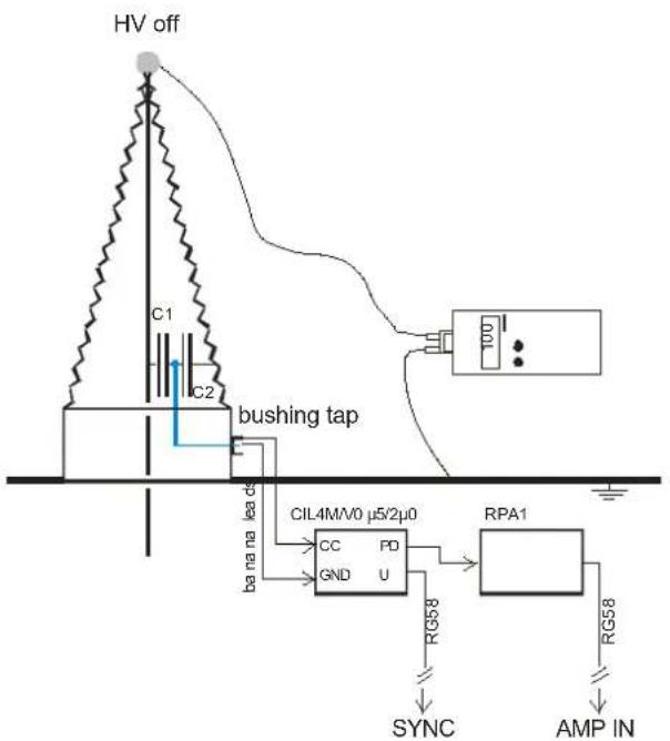

Fig. V.30: Connection of a pulse generator to the bushing tap
Please keep in mind that each channel has its own A/D converter and that the A/D converter for the pattern acquisition has its own calibration. Before starting a PD pattern acquisition the single-channel standard mode should be selected (see section III.1 and section 0). This makes sure to stay in the calibrated channel. Within the Acceptance test (AT) panel, it is also possible to calibrate the pC meter (AMP5). However, in this case the calibration factor for the PD pattern module (ADC5) is copied from the meter, only, and not precisely defined separately.
Before starting a calibration, the calibrator CAL1D, a charge impulse generator, is connected to the bushing of the channel to be calibrated as shown in figure V.31. The calibrator is set to a charge value in the range of the expected charge magnitude. The gain is adjusted using the 'UP' and 'DN' buttons for pre gain and main gain. The level of the meter signal should be between 60% and 80% of the full scale. Please refer to the red bar indicator underneath the pC value.

Fig. V.31: Calibration on bushings
Double clicking to this meter brings up a subpanel (figure V.32), where the charge value (pC or nC) has to be inserted into the field 'Cal Charge'. Pressing the button 'Cal pC' or 'Cal nC' applies this value to the A/D value currently read from the AMP module of this channel. The correction factor is stored automatically with the corresponding setup. Additionally, the cross-coupling levels of this charge to the other channels are stored. After having calibrated the next channel, this previously stored level is used to recalculate the corresponding pC value. The channel can be switched by selecting a different setting at the field 'Cal Channel'. Within the table, the active channel is marked by a green labelled text field. At the bottom of this table the date and time of the last calibration is displayed. Please use this entry to check if every channel has been calibrated. Pressing the button 'Clear' removes all data from the table and fills it with dashes. Thus, please be careful when using the 'Clear' button.
To copy the data to the Windows clipboard use the button 'Copy'. To prevent unintended modifications of an already calibrated channel it's possible to lock a channel by double-clicking the column header. This so-called cross coupling matrix table can show all values as absolute values in pC or nC or as relative values in percent. The cross-coupling matrix is helpful to estimate the location of PD sources within a transformer. In case, the cross coupling of the internal partial discharge activity is compared with the cross coupling of the calibration signal of the different phases.
![File Edit Connect Tools Panel Options Help VC 1 U 150 250 0 [pG] >418 p AMP 2 µV 200.5 H ✓ PD ✓ N ✓ U ✓ VC 2 V Calibration Panel Cross Coupling Calibration Matrix U V W X A B C D VCh9 VCh10 U 500 pC 538 pC 519 pC 20.9 nC 527 pC 490 pC 517 pC 493 pC 519 pC N/A V 170 pC 180 pC 179 pC 576 pC 175 pC 183 pC 172 pC 178 pC 175 pC N/A W 29.7 pC 29.2 pC 30.0 pC 336 pC 27.6 pC 27.6 pC 28.2 pC 27.2 pC 30.2 pC N/A X 68.7 pC 61.9 pC 61.2 pC 500 pC 68.1 pC 63.7 pC 64.9 pC 67.4 pC 63.5 pC N/A A 42.3 pC 39.2 pC 42.6 pC 403 pC 46.0 pC 42.2 pC 41.0 pC 42.0 pC 45.9 pC N/A B 59.4 pC 54.7 pC 57.5 pC 394 pC 59.0 pC 60.0 pC 56.0 pC 60.6 pC 56.6 pC N/A C 285 pC 274 pC 286 pC N/A 286 pC 279 pC 270 pC 305 pC 282 pC N/A D 108 pC 100 pC 112 pC N/A 109 pC 102 pC 101 pC 100 pC 103 pC N/A VCh9 N/A 44.3 pC 45.9 pC N/A 35.2 pC 36.2 pC 34.0 pC 33.9 pC 35.0 pC N/A VCh10 N/A N/A N/A N/A N/A N/A N/A N/A N/A Date 04-14-15 04-14-15 04-14-15 03-19-07 04-14-15 04-14-15 04-14-15 04-14-15 Time 14:41:30 14:41:51 14:42:14 14:45:14 14:42:42 14:43:02 14:43:14 14:43:23 14:43:33 Cal Channel Cal Charge Pre Gain Main Gain Charge Table G0.10-1S 500.0 100 800 >418 pC Absolute Clear Copy Print Linearity CAL pC CAL nC Close](/content/2026/05/1014079/images/547dbf4021fc170374c6883f53b75aeec0be3d74d253d692f36be387226f5415.jpg)
Fig. V.32: Calibration table (cross-coupling matrix)
V.7.1.2 Linearity Test
To verify the performed calibrations and the accuracy of the measurement for the whole expected value range the ICMsystem software offers a linearity test panel accessible via the 'Tools' menu or directly within the calibration matrices. This panel (shown in figure V.33) can be opened in parallel to one of the calibration matrices to easily verify the linearity of the current calibrated channel. Please note that only one calibration matrix can be opened at a time due to technical reasons. While the PD or RIV calibration value on the left column header is transferred from the corresponding calibration matrix to verify the quality of the actual calibration, the other two test values can be freely chosen by editing the corresponding header (see figure V.34). To capture a currently measured value, click into the corresponding table cell and press the 'Capture' button.
To perform linearity tests over a greater range of values with a reasonable signal level (50–80 % of full scale) it's possible to perform a linearity test are half and double of the injected calibration charge. Note that a channel is only displayed within the corresponding part of the table when it's activated to record the appropriate value. If a channel is deactivated the corresponding lines will be pruned. Figure V.33 shows the channel '2W', which is not activated for RIV measurement, while figure V.34 depicts a measurement of only three channels in total.
To save the results of the current linearity test close this panel using the 'Save' button, while 'Cancel' discards the changes made. The 'Print Test' option adds the linearity test to the print chart report described in section III.2.2.

Fig. V.33: Linearity test for channel 4 at 200 pC
change the gain settings within this panel. Typical values to

Fig. V.34: Setting the value of the first test charge for linearity test
V.7.1.3 RIV Calibration
Please refer to section V.8.1 on page 115 for information about RIV calibration.
V.7.1.4 Acceptance Test
A core aim of the development of the multi-channel ICMsystem for power transformer acceptance tests was to automate time consuming test procedures and to get standardised documents. A typical test sequence is shown in figure V.35. Starting such a test requires a valid calibration for the object to be tested. To reload calibration files later, it is recommended to save the calibration setups and the corresponding PD patterns to 'dat' files. Before starting an acceptance test, the cabling, all connections, and especially the ground leads must be checked for continuity. Further, make sure that the calibrator is at a safe place.

line
| Time | Voltage | | ------ | ------- | | 0 | 1.0 | | 1 | 1.05 | | 2 | 1.1 | | 3 | 1.15 | | 4 | 1.2 | | 5 | 1.5 | | 6 | 1.5 | | 7 | 1.7 | | 8 | 1.5 | | 9 | 1.5 | | 10 | 1.5 | | 11 | 1.5 | | 12 | 1.5 | | 13 | 1.5 | | 14 | 1.5 | | 15 | 1.5 | | 16 | 1.5 | | 17 | 1.5 | | 18 | 1.5 | | 19 | 1.5 | | 20 | 1.5 | | 21 | 1.5 | | 22 | 1.5 | | 23 | 1.5 | | 24 | 1.5 | | 25 | 1.5 | | 26 | 1.5 | | 27 | 1.5 | | 28 | 1.5 | | 29 | 1.5 | | 30 | 1.5 | | 31 | 1.5 | | 32 | 1.5 | | 33 | 1.5 | | 34 | 1.5 | | 35 | 1.5 | | 36 | 1.5 | | 37 | 1.5 | | 38 | 1.5 | | 39 | 1.5 | | 40 | 1.5 | | 41 | 1.5 | | 42 | 1.5 | | 43 | 1.5 | | 44 | 1.5 | | 45 | 1.5 | | 46 | 1.5 | | 47 | 1.5 | | 48 | 1.5 | | 49 | 1.5 | | 50 | 1.5 | | 51 | 1.5 | | 52 | 1.5 | | 53 | 1.5 | | 54 | 1.5 | | 55 | 1.5 | | 56 | 1.5 | | 57 | 1.5 | | 58 | 1.5 | | 59 | 1.5 | | 60 | 1.5 | | 61 | 1.5 | | 62 | 1.5 | | 63 | 1.5 | | 64 | 1.5 | | 65 | 1.5 | | 66 | 1.5 | | 67 | 1.5 | | 68 | 1.5 | | 69 | 1.5 | | 70 | 1.5 | | 71 | 1.5 | | 72 | 1.5 | | 73 | 1.5 | | 74 | 1.5 | | 75 | 1.5 | | 76 | 1.5 | | 77 | 1.5 | | 78 | 1.5 | | 79 | 1.5 | | 80 | 1.5 | | 81 | 1.5 | | 82 | 1.5 | | 83 | 1.5 | | 84 | 1.5 | | 85 | 1.5 | | 86 | 1.5 | | 87 | 1.5 | | 88 | 1.5 | | 89 | 1.5 | | 90 | 1.5 | | 91 | 1.5 | | 92 | 1.5 | | 93 | 1.5 | | 94 | 1.5 | | 95 | 1.5 | | 96 | 1.5 | | 97 | 1.5 | | 98 | 1.5 | | 99 | 1.5 | | 100 | - |Fig. V.35: Typical test sequence
Usually, the AT panel is activated and the table mode for the main graph is selected. The report of this test can be filled out before or after a recording was completed. It is important to set the recording time longer than the expected total time of the test sequence. Otherwise, it can happen that a recording stops with a timeout, although the test sequence was not finished completely.
![File Edit Connect Tools Panel Options Help Online RXD TXD Start Date Start Time D 02-16-2012 08:41:29 VC 1 1U 10.0 20.0 30.0 40.0 [ pC ] 55.2 AMP >55.2 pC N/A 50.0 Hz 26.0 KV ✓ PD ✓ N ✓ U ✓ Riv ✓ XC 2 1V 75 125 175 Exp Time 1U 1U 1U [pC] [pC] N [kV] [uV] X 08:41:32 72.75 0 0.0 - X 08:41:37 75.75 29 0.0 - X 08:41:42 72.75 57 0.0 - X 08:41:47 72.75 85 0.0 - X 08:41:52 75.00 112 0.0 - X 08:41:57 75.75 141 0.0 - X 08:42:02 73.25 168 0.0 -](/content/2026/05/1014079/images/a68e50d8f55e95e3085b25c526e2990a50b9f826c73caae0fe423bb33125027d.jpg)
Fig. V.36 Meter channel 1, over-ranged
During a running acquisition it is possible to toggle between automatic and manual trigger mode. With manual mode selected, the user can define when to take values to the recording list, whereas in automatic mode values are taken at a pre-defined interval ('Auto Trigger Time'). Additional to these auto-triggered values, the user can manually trigger values by pressing the button F1, whenever it is of interest. Each trigger stores the PD value, the voltage value, and the timestamp temporarily. Having finished a recording, these timestamps determine the data points shown in the report document.
During a running recording it is necessary to continuously check the level of all partial discharge meters. If a meter remains at full scale as shown in figure V.36, it is recommended to decrease the gain of this channel by pressing the button 'V' at the right-hand side of this meter. A correct calculation of the PD value can only be maintained if this level is not over-ranged.
In case of strong PD activity, acquiring a partial discharge pattern on this channel may be wanted without stopping the recording and without switching to the SC or MC panel. By clicking the pattern icon underneath the frequency display, a pattern acquisition is started for the 'Set Time' pre-set at 'Setup A'. The data of this pattern is not transferred to the PC until the acquisition is finished automatically. This guarantees that the data flow of the running recording is not interrupted. The data of this PD pattern is stored temporarily into 'dat' format and can be recalled or stored to different filenames after a test is completed. The acquired PD pattern is visible in the SC or MC panel.
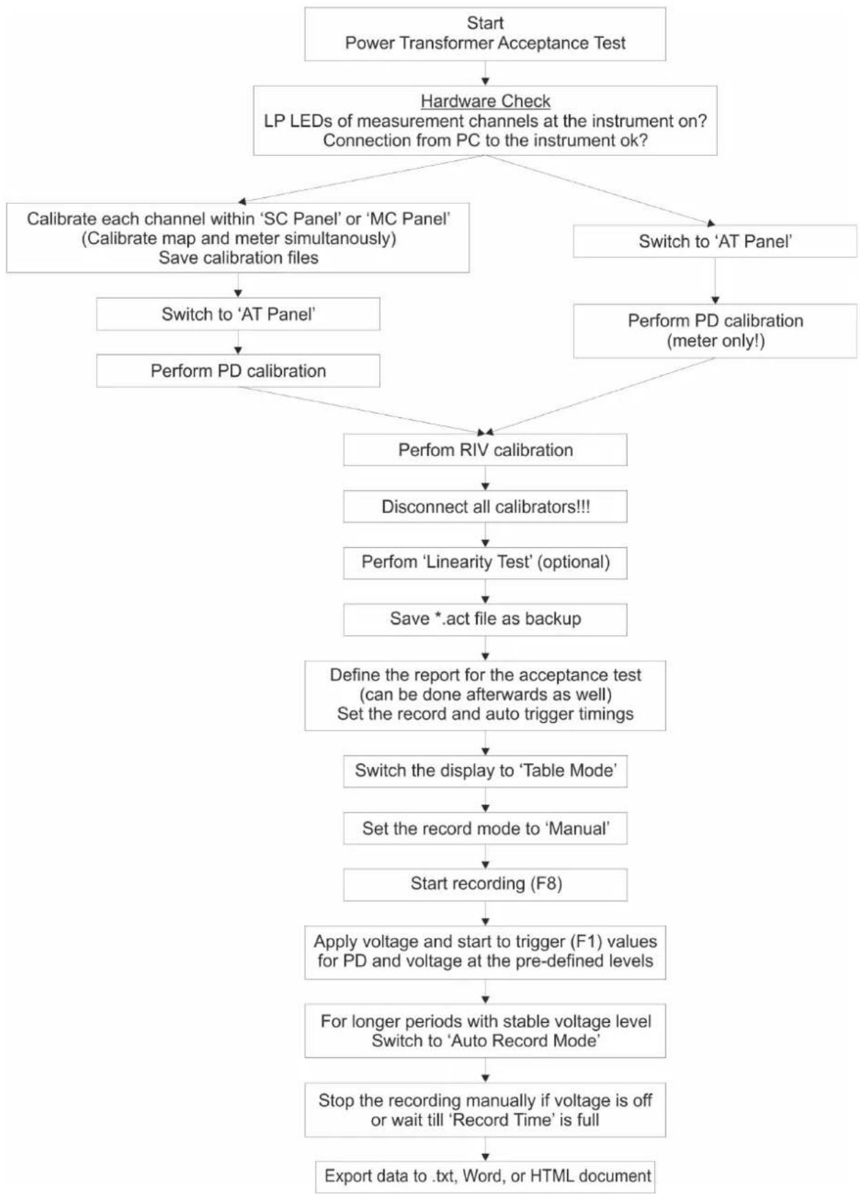
flowchart
graph TD
    A["Start Power Transformer Acceptance Test"] --> B["Hardware Check\nLP LEDs of measurement channels at the instrument on?\nConnection from PC to the instrument ok?"]
    B --> C["Calibrate each channel within 'SC Panel' or 'MC Panel'\n(Calibrate map and meter simultaneously)\nSave calibration files"]
    B --> D["Switch to 'AT Panel'"]
    B --> E["Switch to 'AT Panel'"]
    B --> F["Perform PD calibration"]
    D --> G["Perform PD calibration\n(meter only!)"]
    E --> G
    F --> H["Perform RIV calibration"]
    G --> H
    H --> I["Disconnect all calibrators!!!"]
    I --> J["Perform 'Linearity Test' (optional)"]
    J --> K["Save *.act file as backup"]
    K --> L["Define the report for the acceptance test\n(can be done afterwards as well)\nSet the record and auto trigger timings"]
    L --> M["Switch the display to 'Table Mode'"]
    M --> N["Set the record mode to 'Manual'"]
    N --> O["Start recording (F8)"]
    O --> P["Apply voltage and start to trigger (F1) values\nfor PD and voltage at the pre-defined levels"]
    P --> Q["For longer periods with stable voltage level\nSwitch to 'Auto Record Mode'"]
    Q --> R["Stop the recording manually if voltage is off\nor wait till 'Record Time' is full"]
    R --> S["Export data to .txt, Word, or HTML document"]
Fig. V.37: Flowchart of a PD acceptance test
V.7.2 Acoustic Measurements with External Oscilloscope

flowchart
graph TD
    subgraph_Cable["50Ohm RG58/BNC cable"]
        A["AC System"] --> B["ICM System"]
        B --> C["Standard oscilloscope"]
        C --> D["TRG"]
        E["RPA1D"] --> A
        F["RPA1D"] --> A
        G["AS75I & SFX2/50"] --> A
        H["AS75I & SFX2/50"] --> A
        I["AS75I & SFX2/50"] --> A
    end
    J["CIL4M/V2μ0"] --> K["RPA1"]
    K --> L["Standard oscilloscope"]
    style Cable fill:#f9f,stroke:#333
    style ICMsystem fill:#ccf,stroke:#333
    style Standardoscope fill:#dfd,stroke:#333
    style TRG fill:#dfd,stroke:#333
Fig. V.38: Example setup for acoustic measurements on power transformers (not to scale)
Remarks:
- The oscilloscope is triggered with the PD signal from the bushing tap (either on CH1 or connected to TRG).
- The oscilloscope must be set to 50 Ohm input impedance or a 50 Ohm resistor must be T-connected to each input. Additionally, the scope's input mode must be set to AC coupling.
- Alternatively, the AMP OUT signal from the ICMsystem can be used (Note: Here, the internal filter of the channel has to be set to 40 kHz L-cut-off and the scope input impedance has to be set to high impedance).
- Averaging on the scope reduces influence of noise.
– Time shift between electrical signal and acoustic signals can be used to calculate the fault position.
V.7.3 On-site Testing (UHF)

flowchart
graph TD
    A["TVS2"] --> B["CTB2 (for permanent installation only)"]
    B --> C["ICMsystem"]
    C --> D["Laptop with ICM system"]
    D --> E["Transformer tank"]
    style A fill:#f9f,stroke:#333
    style B fill:#ccf,stroke:#333
    style C fill:#cfc,stroke:#333
    style D fill:#fcc,stroke:#333
Fig. V.39: Example setup for onsite transformer testing with ICMsystem and transformer valve sensor (TVS2)
Caution: TVS2 must be properly installed. Please refer to the separate TVS2 installation guide.
V.8 RIV Measurements
If the ICMsystem is equipped with at least one AMP5 module with spectrum option, the instrument can be used as spectrum analyser and RIV meter. This combination enables PD measurements even with large background noise e.g. in non-shielded test areas. RIV measurement can be activated by clicking on the label 'RIV [off]' at the right-hand side of the software's single channel panel. The label will change to 'RIV [on]'. In the acceptance test panel RIV measurement is enabled by activating the checkbox beneath the corresponding channel window.
V.8.1 RIV Calibration
There are two standardised methods for RIV calibration: According to NEMA 107 and according to IEC CISPR 18-2. The calibration principle differs strongly between these two standards. According to NEMA 107, a calibrator with 50 Ω output impedance is used. This is typically the CAL3A or CLA3B. The calibrator is connected to the reference channel and the unit is adjusted. After this, the calibrator is connected to the test object and with the 'Calibrate' function the unit calculates the calibration factor k by comparing the (lowered) signal on the reference channel with the measurement channel.
With CISPR 18-2, the calibrator acts as current source, which causes a voltage drop across the 300 Ω measuring impedance. As here the test circuit does not load the calibrator, the complete calibration, i.e. determination of the circuit attenuation A and the network factor R can be done in one step without the use of a reference channel.
V.8.2 Calibrators
Power Diagnostix offers three different models of calibration impulse generators for RIV calibration: the CAL3A, CAL3B, and CAL3D.
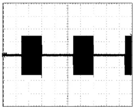
natural_image
Pure electrical circuit lines without any symbolsFig. V.41: Calibrator signal during burst mode
The calibrators are switched on with the pushbutton 'On/Off'. This button must be pressed for more than one second to switch the generator off, while automatic switch-off occurs after approximately 8 minutes. The same button allows to toggle between the continuous mode (Cont.) and the burst mode (Burst). The burst mode is indicated by a blinking '+' sign. During the burst mode, the calibration signal is turned on for about 8 ms each cycle (20 ms at 50 Hz version).
The 'Range' button sets the amplitude in
following steps for the CAL3A and CAL3B: 10 V, 20 V, 50 V, 100 V, 200 V, 500 V, 1 mV, 2 mV, 5 mV, 10 mV.

Fig. V.40: Calibrator
The rotary switch on the left side of the calibrator is used to select
the signal frequency. The top position '0' selects 600 kHz for the CAL3A. It is increased in steps of 50 kHz up to 1350 kHz. The standard frequency of 1 MHz is selected at lowest position '8'. The CAL3B and CAL3D offer a range of 400 kHz to 1900 kHz in steps of 100 kHz. The following table shows the position of the switch and the corresponding frequencies in kHz for all three types.
| Position | 0 | 2 | 4 | 6 | 8 | A | C | E | ||||||||
| CAL3A | 600 | 650 | 700 | 750 | 800 | 850 | 900 | 950 | 1000 | 1050 | 1100 | 1150 | 1200 | 1250 | 1300 | 1350 |
| CAL3B | 400 | 500 | 600 | 700 | 800 | 900 | 1000 | 1100 | 1200 | 1300 | 1400 | 1500 | 1600 | 1700 | 1800 | 1900 |
| CAL3D | 400 | 500 | 600 | 700 | 800 | 900 | 1000 | 1100 | 1200 | 1300 | 1400 | 1500 | 1600 | 1700 | 1800 | 1900 |
Table V.1: Calibrator frequencies
V.8.3 Quadrupoles
When a quadrupole and a coupling capacitor are used together as the coupling device, high voltage is applied both to a test object and to the coupling capacitor in parallel with the test object. A quadrupole (sometimes called also measuring impedance or power frequency separation filter) can then be placed in series with either the coupling capacitor or in series with the test object. CIL/V and CIT/V quadrupoles contain a capacitor acting as a voltage divider together with a high voltage coupling capacitor. This provides a low voltage copy of the applied high voltage wave that can be used to synchronise the PD detector and monitor the quality of the applied high voltage wave.
Optionally, a quadrupole can be supplied with a rotary switch to select the divider capacitor. Especially, when connected to the measurement tap of transformer bushings, the selectable capacitors expand the applicable voltage range. Standard quadrupoles, primarily designed for partial discharge testing, can be used with external matching resistors to achieve the measuring impedance of 150 Ω or 300 Ω, respectively, as specified by the standards. If the test setup is used exclusively for RIV testing, the basic circuits as listed with NEMA 107 (figure V.42) or CISPR 18-2 (figure V.43) can be used.

Fig. V.42: NEMA 107 1987 circuit (33%)

Fig. V.43: CISPR 18-2 circuit (8.3%)
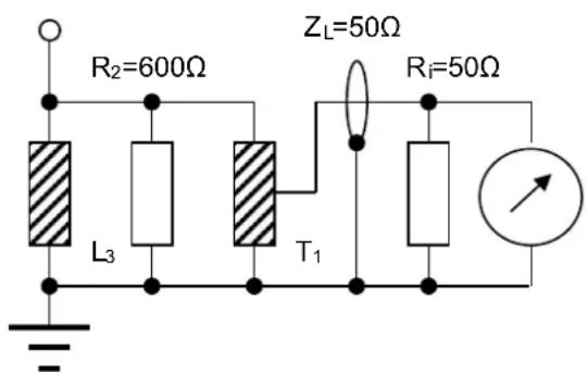
Fig. V.44: Improved NEMA 107 1987 circuit (50%)
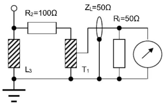
Fig. V.45: Improved CISPR 18-2 circuit (33%)
However, these circuits for use with a 50 Ω cable and meter with 50 Ω input impedance pose a strong attenuation, which hampers overall sensitivity. The CISPR circuit has an attenuation of 12 (21.6 dB), i.e. only 8.3% appear at the input. In order to have a more efficient circuit, RF transformer-based quadrupoles can be used. The CISPR circuit (fig. V.45) then attenuates by a factor of 3 and, hence gains sensitivity by a factor of 4 (12 dB), if compared with figure V.43.
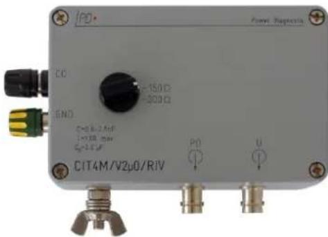
Both improved circuits are combined in a special RIV version of Power Diagnostix' CIT(IV) units. This quadrupole (figure V.46) comes with a switchable effective measuring impedance for RIV measurements according to NEMA 107-1987 (150 Ω) and CISPR 18-2 (300 Ω).
Fig. V.46: Quadrupole suiting both NEMA 107 and CISPR 18–2 impedance requirements
V.8.4 NEMA 107-1987 Compliant Calibration
The RIV calibration is a relative measurement. Before a calibration according to NEMA 107 the system has to be adjusted. This corrects any instrument drift and the impact of the signal path between the calibrator and the acquisition unit. For the adjustment routine the calibrator is connected to the input channel of the ICMsystem that is used as reference channel with a coaxial cable usually used with the measurements. The lead between the specimen and the calibrator has to be disconnected while a 50 Ω resistor is connected to the calibrator. This is mandatory in order to correct only the influence of the signal cable.

flowchart
graph TD
    A["HV off"] --> B["connected for calibration"]
    B --> C["disconnected during adjustment"]
    C --> D["bushing tap"]
    D --> E["CIL4M/V0μ5/2μ0/DC"]
    E --> F["CC PDA GND U"]
    E --> G["RPA1 or RPA1L"]
    G --> H["RPA1 or RPA1L"]
    H --> I["ICMsystem"]
    I --> J["PD-"]
    I --> K["PD-"]
    I --> L["PD-"]
    I --> M["PD-"]
    I --> N["PD-"]
    I --> O["PD-"]
    I --> P["PD-"]
    I --> Q["PD-"]
    I --> R["PD-"]
    I --> S["PD-"]
    I --> T["PD-"]
    I --> U["PD-"]
    I --> V["PD-"]
    I --> W["PD-"]
    I --> X["PD-"]
    I --> Y["PD-"]
    I --> Z["PD-"]
    I --> AA["PD-"]
    I --> AB["PD-"]
    I --> AC["PD-"]
    I --> AD["PD-"]
    I --> AE["PD-"]
    I --> AF["PD-"]
    I --> AG["PD-"]
    I --> AH["PD-"]
    I --> AI["PD-"]
    I --> AJ["PD-"]
    I --> AK["PD-"]
    I --> AL["PD-"]
    I --> AM["PD-"]
    I --> AN["PD-"]
    I --> AO["PD-"]
    I --> AP["PD-"]
    I --> AQ["PD-"]
    I --> AR["PD-"]
    I --> AS["PD-"]
    I --> AT["PD-"]
    I --> AU["PD-"]
    I --> AV["PD-"]
    I --> AW["PD-"]
Fig. V.47: Example test setup on a transformer bushing for adjustment and calibration with normal quadrupole and preamplifier according to NEMA 107
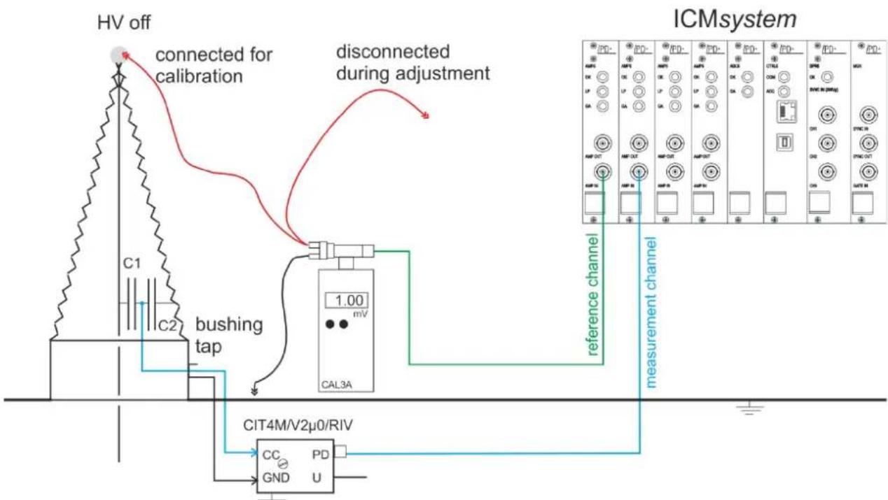
flowchart
graph TD
    A["HV off"] --> B["connected for calibration"]
    B --> C["disconnected during adjustment"]
    C --> D["bushing tap"]
    D --> E["1.00 mV CAL3A"]
    E --> F["CIT4M/V2μ0/RIV"]
    F --> G["CC PDA GND U"]
    G --> H["measurement channel"]
    H --> I["ICMsystem"]
    I --> J["PD- FD- FD- FD- FD- FD- FD- FD- FD- FD- FD- FD- FD- FD- FD- FD- FD- FD- FD- FD- FD- FD- FD- FD- FD- FD- FD- FD- FD- FD- FD- FD- FD- FD- FD- FD- FD- FD- FD- FD- FD- FD- FD- FD- FD- FD- FD- FD- FD- FD- FD- ND"]
    style A fill:#f9f,stroke:#333
    style B fill:#ccf,stroke:#333
    style C fill:#cfc,stroke:#333
    style D fill:#fcc,stroke:#333
    style E fill:#cff,stroke:#333
    style F fill:#ffc,stroke:#333
    style G fill:#cfc,stroke:#333
    style H fill:#fcc,stroke:#333
    style I fill:#fff,stroke:#333
Fig. V.48: Example test setup on a transformer bushing for adjustment and calibration with RIV quadrupole according to NEMA 107
As first step the ICMsystem must be adjusted. Double click on the numeric display showing the RIV value of the channel to be calibrated. The subpanel as shown in figure V.49 appears on top. In the left upper corner, the current value of the calibration channel and in the right upper corner the value of the reference channel are displayed. Firstly, the calibration mode must be set to 'NEMA'. Afterwards, the value of the reference channel has to be checked. If the shown value is not equal to the calibration value, displayed on the calibrator and set as value in the entry field on this panel, the centre frequency should be validated. If this frequency is the same as set on the calibrator then the gain should be adjusted. Choose a gain setting in such a way that the meter is in a range of 50% to 80% of full scale. By pressing the button 'Adjust' the reference channel should display the same value as the calibrator. This correction factor is used for all channels. The value is permanently stored until a new adjustment is done or the adjustment is removed at all by the 'RESET' button of the subpanel.
![RIV Calibration Panel Channel Ch25 [µV] 500 1500 2500 3500 4563 19 µV Channel Ch15 (References) [µV] 10 20 30 40 50 60 70 80 90 107 100 µV RIV Cross Coupling Calibration Matrix (Cal Factor) U V W X A B C D VCh9 VCh10 U 1.00 N/A N/A N/A N/A N/A N/A N/A N/A N/A N/A V N/A 0.11 N/A N/A N/A N/A N/A N/A N/A N/A N/A W N/A N/A 0.11 N/A N/A N/A N/A N/A N/A N/A N/A N/A X N/A N/A N/A 0.11 N/A N/A N/A N/A N/A N/A N/A A N/A N/A N/A N/A 0.11 N/A N/A N/A N/A N/A N/A B N/A N/A N/A N/A N/A 0.11 N/A N/A N/A N/A N/A C N/A N/A N/A N/A N/A N/A 0.11 N/A N/A N/A N/A D N/A N/A N/A N/A N/A N/A N/A 1.00 N/A N/A VCH9 N/A N/A N/A N/A N/A N/A N/A 0.90 N/A VCH10 N/A N/A N/A N/A N/A N/A N/A N/A 0.60 Time Date Channel Pre Amp Ch25 1 Frequency RIV Gain 1000 kHz 16 Cal Mode NEMA Ret Channel Pre Amp Ch1S 1 Frequency RIV Gain 1000 kHz 32 Cancel Calibrate Linearity Adjust Reset Ok](/content/2026/05/1014079/images/df9b332e63bfbc58864238b3c714405e1a00719162af0a7efac6309fc9a3c08d.jpg)
Fig. V.49: RIV calibration panel after adjustment
Then connect the calibrator to the test object and in parallel to the pre-amplifier of the reference channel. The calibrator should be connected as close as possible to the device under test avoiding unnecessary excess leads. Adjust the gain, 50% to 80% of full scale. Pushing the 'Calibrate' button starts a measurement on the reference input channel for about one second. Thereafter one measurement is done on the selected input channel. The unit calculates the correction factor (k) by comparing the (lowered) signal on the reference channel with the measurement channel. It is placed as a numeric value into the table (cross coupling matrix). However, if this factor is already known from a previous calibration, it can be entered manually in the corresponding field of the table.
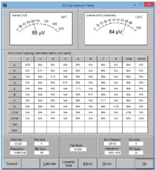
other
RIV Calibration Panel | Channel | Voltage (μV) | Frequency (kHz) | Channel | Reference | |---|---|---|---|---| | Channel Ch25 | 85 μV | 1000 | 20 | 40 | | Channel Ch25 | 85 μV | 160 | 30 | 40 | | Channel Ch25 | 85 μV | 215 | 30 | 40 | | Channel Ch1S (Reference) | 84 μV | 1000 kHz | 20 | 30 | | Channel Ch1S (Reference) | 84 μV | 160 | 30 | 40 | | Channel Ch1S (Reference) | 84 μV | 215 | 30 | 40 | | Channel Ch1S (Reference) [μV] | 84 μV | 1000 kHz | 20 | 30 | | Channel Ch1S (Reference) [μV] | 84 μV | 160 | 30 | 40 | | Channel Ch1S (Reference) [μV] | 84 μV | 215 | 30 | 40 | | Channel Ch1S (Reference) [μV] (Reference) VCH9: VCH10: VCH9: VCH10: VCH9: VCH10: VCH9: VCH10: VCH9: VCH10: VCH9: VCH10: VCH9: VCH10: VCH9: VCH10: VCH9: VCH10: VCH9: VCH10: VCH9: VCH10: VCH9: VCH10: W/ W/ W/ W/ W/ W/ W/ W/ W/ W/ W/ W/ W/ W/ W/ W/ W/ W/ W/ W/ W/ W/ W/ W/ W/ W/ W/ W/ W/ W/ W/ W/ W/ W/ W/ W/ W/ W/ W/ W/ W/ W/ W/ W/ W/ W/ W/ W/ W/ W/ W, Channel Ch25 Pre Amp Frequency RIV Gain Cal Mode NEMA Ret Channel Ch1S Frequency RIV Gain Cancel Calibrate Linearity Test Adjust Reset OkFig. V.50: RIV calibration panel after calibration
V.8.5 CISPR 18-2 Compliant Calibration
The CISPR 18-2 follows the idea of having a calibrator acting as current source, which causes a voltage drop of the desired calibration voltage across the specified resistor of 300 Ω. This requires that the source resistance of the calibrator is large against the measuring impedance. The standard specifies "at least 20 kΩ". The CAL3D comes with an internal source resistance of 30 kΩ. Additionally, this calibration principle requires that the high voltage source is not acting as RF bypass. Hence, a filter has to be inserted into the HV lead between device under test and source. This filter is a parallel resonant circuit. Here as well an impedance (at resonance) of >20 kΩ is specified.
If using off-shelf measurement receivers, the CISPR 18-2 standard specifies determining both the circuit attenuation A and the network attenuation factor R in dB. This result is then added to the receiver's reading taken in dBμV. However, the ICMsystem as a dedicated instrument allows automatic calculation of the combined correction factor and displays the corrected reading after calibration.
Figure V.51 shows a typical calibration setup according to CISPR 18-2
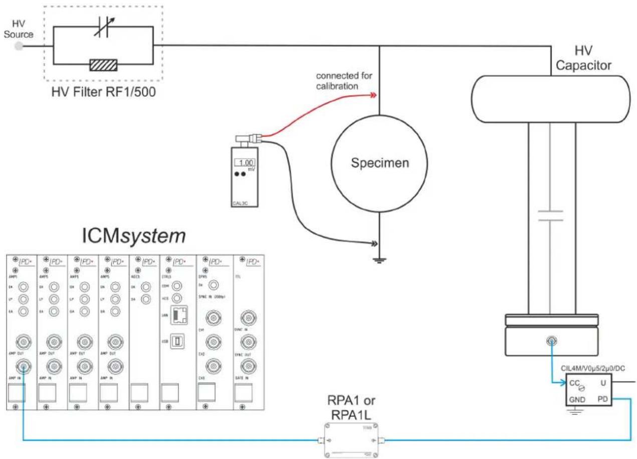
flowchart
graph TD
    A["HV Source"] --> B["HV Filter RF1/500"]
    B --> C["Specimen"]
    C --> D["HV Capacitor"]
    D --> E["CIL4M/V0μ5/2μ0/DC"]
    E --> F["RPA1 or RPA1L"]
    F --> G["ICMsystem"]
    G --> H["ICM System"]
    H --> I[" connected for calibration "]
    I --> J["1.00 mV CAL3C"]
Fig. V.51: Example test setup for calibration with normal quadrupole and preamplifier according to CISPR 18-2
Before starting the calibration, 'CISPR 18-2' has to be selected as 'Cal. Mode' in the calibration subpanel. Subsequently, all subpanel elements concerning a reference channel are hidden. Pushing the 'Calibrate' button starts the calibration process.
![RIV Calibration Panel Channel Ch19 [µV] 500 2500 3500 4653 19 µV RIV Cross Coupling Calibration Matrix (Cal Factor) U V W X A B C D VCM VCM10 U 1.00 N/A N/A N/A N/A N/A N/A N/A N/A N/A V N/A 0.11 N/A N/A N/A N/A N/A N/A N/A N/A W N/A N/A 0.11 N/A N/A N/A N/A N/A N/A N/A X N/A N/A N/A 0.11 N/A N/A N/A N/A N/A N/A N/A A N/A N/A N/A N/A 0.11 N/A N/A N/A N/A N/A N/A B N/A N/A N/A N/A N/A 0.11 N/A N/A N/A N/A N/A C N/A N/A N/A N/A N/A N/A 0.11 N/A N/A N/A N/A D N/A N/A N/A N/A N/A N/A N/A 1.00 N/A N/A VCH9 N/A N/A N/A N/A N/A N/A N/A 0.00 N/A VCH10 N/A N/A N/A N/A N/A N/A N/A 0.00 Time Date Channel Pre Amp Ch19 1 Frequency RIV Gain CISFR 18-2 1000 kHz 16 Cal Mode CISFR 18-2 Cancel Calibrate Linearity Test Adjust Reset Ok](/content/2026/05/1014079/images/e8d6dda93d50b401ea2b06eeaff4b8a78436429e038a2635fee37c6bb68ade0b.jpg)
Fig. V.52: RIV calibration panel in CISPR 18-2 mode
VI Maintenance
VI.1 Overview
The ICMsystem does not require any maintenance on a regular basis. Further, there is no fine adjustment on a regular basis required, as the partial discharge measurement is a relative measurement that is calibrated prior to a measurement with a reference source. The calibration impulse generator as the reference source, however, must be calibrated on an annual basis to ensure that its output signal still stays within the recommended boundaries. Each calibration impulse generator is shipped with a certificate stating the result of an individual calibration measurement. This certificate expires after one year. The calibrator needs to be returned to the factory for a performance check and re-calibration. Alternatively, an independent service organisation or your national authority of standards may perform this calibration.
VI.2 Performance Check
Although the ICMsystem does not require maintenance on a regular basis, a performance check shall be conducted from time to time. Especially, in case the instrument has seen severe breakdowns or over-voltages, or in case you are in doubt about the instrument's behaviour due to other reasons, such performance check is mandatory. This performance check is to make sure that the components and modules are operating correctly and that they are meeting their specification. This check starts with the communication between instrument and PC or notebook.
- Switch on the acquisition unit. The two micro controllers of the acquisition build up an internal communication upon start-up. They do check different registers, the controller periphery, their internal communication, and finally, determine if all modules are in place. With this boot sequence successfully passed a single beep is sound and the OK LED of the AMP5 module is lit. In case of severe malfunction this process is not completed. With peripheral failures detected a number of beeps sound indicating the defect detected. In both cases the acquisition unit needs to be returned to Power Diagnostix' factory. In case of built-in modem, the modem's detection is indicated few seconds after booting by a slightly deeper sounding beep.
- With the acquisition unit seemingly operating normally, the communication between the acquisition unit and the notebook or PC is tested. Connect the GPIB cable and start the ICMsystem program. Upon start-up this program checks for an instrument automatically. With an instrument found, the acquisition unit sounds another beep, and the communication starts immediately as described with the software section of this manual. In case the communication could not be established, try to use the GPIB interface with another application, check the GPIB cable and connectors, or try another GPIB interface. Further, you may try to connect by another computer. Additionally, the serial communication may be tested. Use the serial cable supplied and set the ICMsystem software to check the serial port used (Options, Port ...). In case the communication could not be established, and the instrument was identified as cause, it needs to be sent to Power Diagnostix.
- With the core of the measurement system running, the peripheral units and their continuity is checked. With the pre-amplifiers enabled, i.e. set not into off-state, check the OK LED of the DPR5 plug-in, and the OK LED of the AMP5 plug-ins for the RPA1 modules. A DC potential of 7.7 V for gain 1, 9.4 V for gain 10, and 11.0 V for gain 100 can be found on the RG58 cable running to the RPAs. If this voltage cannot be measured, the plug-in module may be defect. If the voltage is found with the RPA not connected, only, the pre-amplifier may be defect. In case, check the signal cable as well.
- The instrument is shipped with two test files, a file named RPA1_NOI.DAT and another file named RPA1_100.DAT. The first file contains a measurement taken with an RPA1 with open input and set to a very high gain, i.e. this measurement covers the input noise of the first amplifier stage within the RPA1. With the RPA1 connected re-load this file and start an acquisition. Subsequently, compare the results. The noise signal shall similarly cover the pattern as with the file provided. In case, this result proofs the integrity of the measurement chain. The second file was taken with the same configuration, but with a CAL1A connected directly to the RPA1s input. Connect your calibrator, re-load the file and start an acquisition. You should find the impulses of the calibrator at approximately the same horizontal location as with the file re-loaded. Allow a certain deviation due to the relative character of the measurement. Perform this check with all your RPA1s.
Identified defect modules shall be returned for repair. The instrument is relatively small and lightweight. Thus, it does not cause larger problems to ship the entire unit for a complete performance check with Power Diagnostix. With measurement systems normally used for field measurements at various locations, a regular factory performance check may be considered.
VI.3 Calibration Issues
Partial discharge measurements, as pointed out already, are relative measurements. Thus, only the reference source needs to be calibrated. With all other parts of the measurement chain a performance check regarding each module's specification, its continuity and integrity is sufficient. The calibrators may be re-adjusted at Power Diagnostix' laboratory. Such calibrators will be returned checked and repaired, if required, along with a new certificate stating the accuracy of the charge output. If this check or repair is not required, the calibration impulse generators may be calibrated with your national authority of standards or with a calibration laboratory that is approved for calibration of impulse charges.
VI.4 Spare Parts
The instrument follows a modular concept. Thus, solely the defect module may be exchanged in case of failure. Afterwards the performance check is made again. Since the instrument and its modules is relative lightweight, it not mandatory in general to have spare parts on stock with the user of the system. The units are designed to withstand the normal range of over-voltages and surges found with the common applications of such instrument. In case the system is used beyond the normal stress, one may consider having a spare PCMCIA-GPIB interface (at least the cable) and one piece of RPA1 as spare parts with the instrument.
VI.5 Shipment Instructions
In case a unit needs to be returned to the factory, make sure the acquisition unit is packed safely. As the units are relatively small, shipment by couriers, such as DHL, FedEx, or equivalent is the recommended mode of transportation. If possible, declare the instrument as 'used instruments for evaluation' at a relative low value. Consult Power Diagnostix for further details. Additionally, Power Diagnostix may provide you with a temporary replacement unit, in case of urgent needs.
VII Declaration of Conformity
Power Diagnostix Instruments GmbH
Vaalser Strasse 250
52074 Aachen
Germany

declares, that the instrument as specified below, meets the requirements of the standards and/or normative documents as listed below.
Product: ICMsystem
Description: Partial discharge detector
Guidelines: Low Voltage Directive 2014/35/EU
EMC Directive 2004/108/EG
RoHS Directive 2011/65/EU
Standards: EN 61010-1:2010,
EN 61326-1:2013
EN IEC 63000:2018
Date:
Dr. Mihai Huzmezan
(Managing director)
Remark: Since the measurement of partial discharge pulses is done in frequency bands partly occupied by radio transmission, and since further test leads may act as antennas, disturbance free measurements may require well shielded environments and/or additional filter techniques.
VIII Technical Data
VIII.1 Acquisition Unit
| Mains supply: 90–264 V | AC, 47–440 Hz (automatic) | |
| Line fuse: | 2 A (time-lag) | (ICMsystem with up to 4 channels) |
| 3.15 A (time-lag) | (ICMsystem with 5 to 10 channels) | |
| Power requirements: | Approx. 110 VA max. | |
| Operation: | Remote-controlled via ICMsystem software | |
| Operation temperature: | 0–40 °C (non-condensing) | |
| Input impedance (AMP IN): | 50 Ω || 50 pF | |
| A/D converter (PD): | 12 bits, compressed into 8 bits (unipolar) / ±7 bits (bipolar) | |
| Available | ||
| Communication Interfaces: | USB 2.0, GPIB, LAN | |
| Size: | 236 x 133 x 295 mm ^3 | (ICMsystem with up to 4 channels) |
| (W x H x D, excl. BNC conn.) | 450 x 133 x 295 mm ^3 | (ICMsystem with 5 to 10 channels) |
| Weight: | Approx. 6.9–9 kg | |
VIII.2 Standard PD Mode
| Lower cut-off (-6 dB): | 40, 80, or 100 kHz | (software-controlled) |
| Upper cut-off (-6 dB): | 250, 600, or 800 kHz | (software-controlled) |
| Input sensitivity: | < 500 μVrms/5pC | (without preamplifier) |
| Gain range: | 1, 2, 4, 8, 10, 20 ..., 200, 400, 800 | |
VIII.3 Preamplifiers
| Input impedance: | 10 kΩ || 50 pF | (RPA1 / RPA1D / RPA1G / RPA4) |
| 1 kΩ /|| 50 pF | (RPA1L / RPA1H) | |
| 50 Ω || 50 pF | (FCU2) | |
| Input sensitivity: | < 50 μVrms/0.03 pC | (RPA1 / RPA1D / RPA1G / RPA4) |
| < 15 μVrms/0.02 pC | (RPA1L) | |
| < 40 μVrms/0.05 pC | (RPA1H) | |
| < 800 μVrms/1 pC | (RPA2) | |
| < 2 μVrms | (RPA3) | |
| < 200 μVrms (46 dBμV) | (FCU2) | |
| Bandwidth: | 40–800 kHz | (RPA1 / RPA1D / RPA1G / RPA4) |
| 40 kHz–20 MHz | (RPA1L / RPA1H) | |
| 2–20 MHz | (RPA2) | |
| 200 MHz–1 GHz | (RPA3) | |
| 100 MHz–1800 MHz | (FCU2) |
VIII.4 Synchronisation/HVM
| Sync. frequency: | 20–510 Hz (automatically) / 0.02–510 Hz (manually) |
| Maximum voltage: | 200 V_peak (140 V_rms ), 100 V_rms nom. |
| Input impedance: | 10 MΩ |
| A/D converter: | ±15 bits |
| Precision: | Typ. < 1.5% |
VIII.5 Spectrum Function
| Input sensitivity | < 5 μVrms/0.5pC | (270 kHz bandwidth) |
| < 1 μVrms/2pC | (9 kHz bandwidth) |
| Gain range: | 1, 2, 4, 8, 16, 32, 64, 128 |
| Maximum input voltage: | 120 mV | (300 kHz bandwidth, SPEC mode) |
| 5 mV | (9 kHz bandwidth, SPEC mode) | |
| 2.5 mV | (RIV measurement) |
| Frequency range: | 10 kHz–10 MHz (in steps of 10 kHz) |
| Bandwidth: | 9 kHz or 270 kHz |
VIII.6 Cable Fault Location
| Trigger: | 0 to 100% of input signal (in steps of 3.125 %) |
| A/D Converter: | ±7 bits |
| Samples: | 100 Msamples/s ( T_sample = 10 ns) |
| Reduced sample rates: | 50 MS, 25 MS |
| Displayed time window: | 200 ... 8000 samples (2 ... 80 μs @ 100 MS / 8 ... 320 μs @ 25 MS) |
| Specimen cable length: | 10 to 5000 m, for 80 μs and v_c=140 m/μsCFL at cables > 3000 m not possible because of pulse attenuation |
| Localisation precision: | 1 m + 0.1% of the cable length |
VIII.7 Acoustic Fault Location
| Trigger: | 0 to 100% of input signal (in steps of 3.125 %) |
| A/D Converter: | ± 7 bits |
| Samples: | 100 MSamples/s ( T_sample = 10 ns) |
| Reduced sample rates: | 50 MS, 25 MS, 10 MS, 5 MS, 1 MS |
| Displayed time window: | 200 ... 8000 samples (2 ... 80 μs @ 100 MS / 200 ... 8000 μs @ 1 MS) |
| Localisation distance: | Max. 11.2 m, for 8000 μs and v_oil = 1400 m/s |
126
IX Appendix
IX.1 National Instruments Hardening Guide
IX.1.1 Introduction
This manual will guide you through the Power Diagnostix proposed cyber security operation system hardening after the installation of a National Instruments based software product. The configuration refers to the Power Diagnostix software products, only. If any other ^rd party National Instruments based software products are installed or required, the proposed configuration should be adjusted with the configuration of the responsible manufacturer.
This configuration guide will close three unnecessary National Instruments services. Furthermore, the local Port 3848 UDP and TCP opened by these services will be closed.
| ■ nidmsrv.exe | 3848 | TCPV6 | [0:0:0:0:0:0:0:1] | 49672 | [0:0:0:0:0:0:0:1] | 49673 | ESTABLISHED |
| ■ nidmsrv.exe | 3848 | TCPV6 | [0:0:0:0:0:0:0:1] | 49673 | [0:0:0:0:0:0:0:1] | 49672 | ESTABLISHED |
| ■ nidmsrv.exe | 3848 | TCP | DESKTOP-Q5NEF6E | 59111 | DESKTOP-Q5NE... | 0 | LISTENING |
| ■ nidmsrv.exe | 3848 | UDP | DESKTOP-Q5NEF6E | 5000 | * | * | |
| ■ nidmsrv.exe | 3848 | UDP | DESKTOP-Q5NEF6E | 6000 | * | * |
IX.1.2 Step-by-Step Guide
1.) Open the windows start menu and type "services.msc".

2.) Click onto the search result named "Services". The "Services" window will open.
3.) Locate these services in the service list:
• NI Domain Service
• NI PSP Service Locator
• NI Time Synchronisation
| NI Domain Service | Provides a domain server for NI Shared Variable se... | Running | Automatic | Local Syste... |
| NI PSP Service Locator | Locates servers at the request of network variable c... | Running | Automatic | Network S... |
| NI Time Synchronization | Allows this machine to keep its time synchronized ... | Running | Automatic | Local Syste... |
4.) Open the configuration popup by double click each service and change the "Startup type" to "Disabled".
5.) Save the changes with the button "OK".
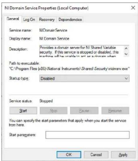
IX.1.3 Service Description
http://www.ni.com/product-documentation/14487/en/
NI Domain Service
Service: NIDomainService Process: nidmsrv.exe
Description: Provides a domain server for NI Shared Variable security.
If Disabled: If this service is stopped or disabled, this machine will be unable to act as a domain when configuring shared variable security.
NI PSP Service Locator
Service: IkClassAds Process: Ikads.exe
Description: Locates servers at the request of network variable clients and other proprietary NI network protocols.
If Disabled: If this service is stopped or disabled, network variables and network streams will stop working.
NI Time Synchronization
Service: IkTimeSync Process: Iktsrv.exe
Description: Allows this machine to keep its time synchronized with a master time server, or to act as a time server for other machines. This feature is configured with the Shared Variable Engine settings in LabVIEW.
If Disabled: If this service is stopped or disabled, this form of time synchronization will not be available.
X Index
A
A/D converter....7, 11
AB1 26
AC5 module 10
Acceptance test 70
Acceptance testing 107, 111
Acoustic measurement 113
Acoustic measurements ....75
ACQ....10
Acq Mode....59
Acquisition mode 55
Active bridge adapter....26
Active Graph 78
ADC LLD....58
ADC Mode 58
ADC5 module 11
Amp In....57, 60, 78
AMP IN....14, 15, 16
Amp L Cutoff....59
Amp Main Gain 59
AMP mode....14
Amp Mux....84
AMP OUT 14, 15, 16
Amp U Cutoff ....59
AMP5 module 14
Amplifier....7, 14
AT panel 111
Averaging....61, 82
B
Bandwidth 60,78
C
Cable fault location 79
Cable Length 82
Cable measurements....103
CAL 35
CAL1B....107
CAL1D 107
Calibration....108
Calibration charge....53
Calibrator 107
Calibrators 35, 115
CC....32
CF 1/CF 2....78
CFL display....81
CH1-CH3 11
Charge pulse 36
CIL 28
CISPR 18-2....116, 119
CIT 28,29
CIT4M/V....117
Coding....58
COM....10
COM ports.... 40
Connect menu.... 67
Consecutive measurement 56
Consecutive measurement mode 86
Copy unction....50
Correction factor 62, 97, 118, 119
Count distribution versus amplitude.... 49
Count distribution versus X-axis 49
Count level 53
Count Level 59
Counts.... 53
Coupling capacitor 32, 106
Coupling capacitors 97
Cross coupling matrix 109
CT 30
CTRL5 controller.... 10
Current transformer.... 30
Cursor 60
D
Dead time.... 12, 53, 93, 95
Dead Time 57
Delay time 54
Dial 44
Div Ratio 60
DPR5 module.... 11
E
Edit menu 66,70
Embedded electrode.... 100
F
Fault location....51,75
FCU2.... 25, 100
File menu 66
Frequency 54
Frequency converter unit 25, 100
Function keys.... 38, 55
G
GA....13, 14, 15, 16
Gas insulated switchgear.... 100
GATE IN.... 17
GATE mode 16
Gate threshold 53
Gate time 53
Gating 17
GIS 100
GIS sensors 100
GPIB....7,10
GPIB address.... 44
GPIB driver 38
GPIB installation 38
Graph view....70
H
HDPI scaling 43
Help menu 68
|
ICMacoustic software ....51, 75
Idle mode ....55
IEC 60270....36
IEEE488 commands....37
Input Mode....57
Input protection unit 100
IPU2B....100
Isolation transformer....31
IT2....31, 104
L
Laboratory measurements....89
LAN 10
Level counts....53
Line synchronisation....54
Linear bipolar....13
Linear unipolar....13
Linearity test ....110
Live chart 70
LLD 12,37
LO BAT 36
LOC Cursor....82
Loc. Range 82
Low level discriminator .....12, 37, 93
LP....14, 15, 16
M
Main amplification 93
Main gain 93
Map display....48
Mapping Ref. 82
MC panel 83
Measurement menu....67
Measuring impedances....116
Mem Erase 60
Modem....44
Movie tool 64
Multi pattern display....83
Multi-channel consecutive mode ....88
Multi-channel standard mode 88
Multiplexer function....83
MUX display....83
N
NEMA 107 ....116, 117
NQS value ....54
0
Off-line test 97
On/Off 36
On-line measurement 105
On-line test....98
Options menu.... 67, 70
Osc. Main Gain 61,82
Oscilloscope display 51
P
Panel menu....67
Partial discharge pattern 48
Pattern acquisition 55
PD calibration....62
Peak....95
Peak charge.... 53, 62
Peak Distribution....82
Performance check.... 121
Phase shift 60
Pos/Neg 36
Position 60,81
Pre gain....75
Pre Gain....59, 61, 78, 82
Pre Trigger 60, 81
Pre-amplification 93
Pre-amplifier.... 14, 18, 93, 107
Pre-amplifier set.... 27
Print utility 63
Proj. Sensitiv 82
Projection 82
Q
Quadrupole 28, 107, 116, 117
R
Range 36
Recording time.... 111
Reference pulse....80
Rejection filter.... 34
Report 72
Report printing 73
Resonant filter 34
RF1/1000 34
RF1/500 34
Ring sensor.... 100, 101
RIV [off] 54
RIV calibration.... 115, 117, 119
RIV measurement....79, 115
RIV meter.... 15, 77
Rotating machines 97
RPA....14
RPA1.... 14, 18, 97, 107
RPA1D 21
RPA1G 21
RPA1H 20
RPA1L.... 15, 19
RPA2.... 22, 97, 104
RPA3....23
RPA4....24,105
s
Safety....5
Sample Rate 60
Scan Period 84
Scanning period....84
Scope mode....50
Set Time....57
Setup A 57, 78, 84, 106
Setup B 84
Setup CFL....81
Setup O....60, 75
Setup S 78, 79
Shield electrode 100
Short cut keys....68
Signal level 53
Single-channel consecutive mode....87
Single-channel standard mode....87
Synchronisation frequency ....54
Software main panel....37
Spec Main Gain 78
SPEC mode....15
Spectrum analysis ....77
Spectrum display 77
Spectrum function....15
Standard display mode....48
Standard measurement mode 55, 86
Start Freq....78
Statistics......65
Stop Freq. 78
Sweep Time....78
Sync....60
Sync In....60
SYNC IN 17
SYNC OUT 17
Synchronisation ....17, 106
Synchronisation source ....54
T
Table window....70
TDR....79
TDR principle 80
Test voltage ....53
Time domain reflectometry 79
Time-domain visualisation....51
Tool menu....67
Toolbar 45
Total counts 53
Total time 54
Trace A/Trace B....79
Track Display 84
Transformer on-site testing.... 114
Transformer valve sensor 114
Travel time 79
Travel time analysis 51
Trending display.... 52
Trigger.... 11, 61, 75
Trigger Ch 60
Trigger channel 75
Trigger level 75
Trigger Level 60, 81
Trigger mode....93, 111
Trigger Mode.... 61, 81
Trigger Slope 61
TTL module.... 17
TTL synchronisation.... 54
TVS2 114
U
UHF1....27,100
USB....10
USB driver....40
V
Vc 82
Vc Mode 82
Very low frequency 106
View menu 67
Virtual channel management 42
VLF 106
VLFS1 106
W
Waveform....58
Window sensor 100, 101
Z
Zoom 61,82
Zoom Pos....61,82

- Contents
- I General 5
- II The ICMsystem Hardware 7
- III The ICMsystem Software 37
- I General
- I.1 About this Manual
- I.2 Instrument Safety
- Warning:
- I.3 Principle of Operation
- II The ICMsystem Hardware
- II.1 Acquisition Unit
- II.1.1 Standard Model
- II.1.2 Multi-Channel Unit for Acceptance Testing on Power Transformers
- Warning!
- II.1.3 Modules
- II.1.3.1 Built-in AC5 Power Supply Module
- II.1.3.2 CTRL5 Controller
- II.1.3.3 DPR5 Dual Port RAM
- II.1.3.4 ADC5 Peak A/D Converter
- Trigger Mode,
- c) Trigger in time window
- Dead Time (DT)
- Low Level Discriminator (LLD),
- Coding
- II.1.3.5 AMP5 Main Amplifier
- AMP Mode
- SPEC Mode
- GATE Mode
- II.1.3.6 TTL Module
- II.2 Signal Conditioning Pre-amplifiers
- II.2.1 RPA1, Range 40 kHz–800 kHz
- Caution:
- Specification:
- II.2.2 RPA1L, Range 40 kHz–20 MHz
- II.2.3 RPA1H, Range 40 kHz–20 MHz
- II.2.4 RPA1D and RPA1G, Range 40 kHz–800 kHz
- II.2.5 RPA2, Range 2 MHz–20 MHz
- II.2.6 RPA3, Range 200 MHz–1 GHz
- II.2.7 RPA4, Range 40 kHz–800 kHz, Fibre Optic Isolation
- II.2.8 FCU2, Frequency Converter Unit
- II.2.9 AB1, Active Bridge Adapter
- II.2.10 UHF1, Pre-Amplifier Set, Range 200 MHz–1 GHz
- II.3 Coupling Devices
- II.3.1 CIL, CIT Quadrupoles
- CILXY/V
- CITXY
- II.3.2 CT, IT Current and Isolation Transformers
- CT1 Current Transformer (Fixed Type)
- CT100(/R) Current Transformer (Clip-on or Split Type)
- IT2 HF-Isolation Transformer
- II.3.3 CC Coupling Units
- II.4 Rejection Filters
- II.5 CAL Calibration Impulse Generators
- III The ICMsystem Software
- III.1 ICMsystem Standard Control Software
- III.1.1 Overview and Main Functions
- III.1.2 Installation of Software and Drivers
- III.1.2.1 GPIB Driver
- III.1.2.2 Installer
- III.1.2.3 USB Driver
- III.1.2.3.1 Command Set of GPIB & Serial Communication
- III.1.3 HDPI Scaling
- III.1.4 Connecting to an Instrument
- III.1.5 Toolbar
- III.1.6 Display Modes and Display Items
- III.1.7 Measurement Modes
- III.1.8 Controlling the Instrument's Setup
- ADC LLD
- ADC Mode
- Waveform
- III.1.9 PD Calibration
- III.1.10 Printing
- III.1.11 Movie – Quick Motion Replay
- III.1.12 Statistics
- III.1.13 Pull-Down Menu Structure
- Edit
- III.1.14 Short Cut Keys
- III.2 Advanced Software for Acceptance Testing (ACC)
- III.2.1 Window Modes
- III.2.2 Report Generation
- III.2.2.1 Customising the Report
- III.2.2.2 Printing the Report
- III.3 Acoustic Measurements
- IV Options
- IV.1 Spectrum Function (SPEC)
- IV.1.1.1 Setup S
- Trace A/Trace B
- RIV Measurement
- IV.2 Cable Fault Location (CFL)
- IV.2.1.1 Setup CFL
- IV.3 Multiplexed Pattern Acquisition
- V Application Guide
- V.1 General
- V.2 Standard and Consecutive Acquisition Modes
- V.3 Standard Laboratory Measurements
- V.4 Rotating Machines
- V.5 Gas Insulated Switchgear (GIS)
- V.6 Cables and Accessories
- V.6.1 Measuring Principles
- V.6.2 Synchronisation with Very Low Frequencies (VLF)
- V.7 Power Transformers
- V.7.1 Acceptance Testing
- V.7.1.1 PD Calibration
- V.7.1.2 Linearity Test
- V.7.1.3 RIV Calibration
- V.7.1.4 Acceptance Test
- V.7.2 Acoustic Measurements with External Oscilloscope
- Remarks:
- V.8 RIV Measurements
- V.8.1 RIV Calibration
- V.8.2 Calibrators
- V.8.3 Quadrupoles
- V.8.4 NEMA 107-1987 Compliant Calibration
- V.8.5 CISPR 18-2 Compliant Calibration
- VI Maintenance
- VI.1 Overview
- VI.2 Performance Check
- VI.3 Calibration Issues
- VI.4 Spare Parts
- VI.5 Shipment Instructions
- VII Declaration of Conformity
- VIII Technical Data
- IX Appendix
- IX.1 National Instruments Hardening Guide
- IX.1.1 Introduction
- IX.1.2 Step-by-Step Guide
- IX.1.3 Service Description
- NI Domain Service
- NI PSP Service Locator
- NI Time Synchronization
- X Index
- A
- B
- C
- D
- E
- F
- G
- H
- |
- L
- M
- N
- 0
- P
- Q
- R
- s
- T
- U
- V
- W
- Z
Brand : Megger
Model : ICMsystem
Category : Electrical measuring device